Proceedings

12th International Symposium on Distributed Computing and Applications

to Business, Engineering & Science

DCABES 2013

Editor Souheil Khaddaj

Proceedings

12th International Symposium on Distributed Computing and Applications

to Business, Engineering & Science

DCABES 2013

Editor Souheil Khaddaj

2–4 September 2013 Kingston University — London

United Kingdom

Copyright © 2013 by The Institute of Electrical and Electronics Engineers, Inc. All rights reserved.

Copyright and Reprint Permissions: Abstracting is permitted with credit to the source. Libraries may photocopy beyond the limits of US copyright law, for private use of patrons, those articles in this volume that carry a code at the bottom of the first page, provided that the per-copy fee indicated in the code is paid through the Copyright Clearance Center, 222 Rosewood Drive, Danvers, MA 01923. Other copying, reprint, or republication requests should be addressed to: IEEE Copyrights Manager, IEEE Service Center, 445 Hoes Lane, P.O. Box 133, Piscataway, NJ 08855-1331. The papers in this book comprise the proceedings of the meeting mentioned on the cover and title page. They reflect the authors’ opinions and, in the interests of timely dissemination, are published as presented and without change. Their inclusion in this publication does not necessarily constitute endorsement by the editors, the IEEE Computer Society, or the Institute of Electrical and Electronics Engineers, Inc.

IEEE Computer Society Order Number P5060

ISBN-13: 978-0-7695-5060-2 BMS Part # CFP1320K-CDR

Additional copies may be ordered from:

IEEE Computer Society IEEE Service Center IEEE Computer Society Customer Service Center 445 Hoes Lane Asia/Pacific Office

10662 Los Vaqueros Circle P.O. Box 1331 Watanabe Bldg., 1-4-2 P.O. Box 3014 Piscataway, NJ 08855-1331 Minami-Aoyama

Los Alamitos, CA 90720-1314 Tel: + 1 732 981 0060 Minato-ku, Tokyo 107-0062 Tel: + 1 800 272 6657 Fax: + 1 732 981 9667 JAPAN Fax: + 1 714 821 4641 http://shop.ieee.org/store/ Tel: + 81 3 3408 3118

http://computer.org/cspress csbooks@computer.org

customer-service@ieee.org Fax: + 81 3 3408 3553 tokyo.ofc@computer.org

Individual paper REPRINTS may be ordered at: <reprints@computer.org>

Editorial production by Lisa O’Conner Cover art production by Zoey Vegas

IEEE Computer Society Conference Publishing Services (CPS)

http://www.computer.org/cps

2013 12th InternationalSymposium on Distributed

Computing and Applicationsto Business, Engineering &

Science

DCABES 2013Table of Contents

Preface..........................................................................................................................................................................ixCommittee Lists..........................................................................................................................................................x

Distributed/Parallel ApplicationsIterative Splitting Methods for Multiscale Problems ......................................................................................................3

Jürgen Geiser

Scalable Hybrid Deterministic/Monte Carlo Neutronics Simulations in Two SpaceDimensions .....................................................................................................................................................................7

Jeffrey Willert, C.T. Kelley, D.A. Knoll, and H. Park

Research on QoS Reliability Prediction in Web Service Composition ........................................................................11Lou Yuan-sheng, Jiang Man-fei, and Xu Hong-tao

Iterative Krylov Methods for Gravity Problems on Graphics Processing Unit ............................................................16Abal-Kassim Cheik Ahamed and Frédéric Magoulès

The DFrame: Parallel Programming Using a Distributed Framework Implementedin MPI ...........................................................................................................................................................................21

Tony Mclay, Andreas Hoppe, Darrel R. Greenhill, and Souheil Khaddaj

Model Size Challenge to Analysis Software ................................................................................................................26Peter Chow and Serban Georgescu

Aspect-Oriented Approach to Modeling Railway Cyber Physical Systems ................................................................29Lichen Zhang

Automatic Concurrent Program Generation from Petri Nets .......................................................................................34Weizhi Liao and Wenjing Li

Micro-scale Modelling Challenges in Electric Field Assisted Capillarity ...................................................................40C.E.H. Tonry, M.K. Patel, C. Bailey, M.P.Y. Desmuliez, and W. Yu

v

A Modelling and Analysis Tool for Systems with Probabilistic Behavior: ProbabilisticContinuous Petri Net ....................................................................................................................................................44

Weizhi Liao, Wenjing Li, and Zhenxiong Lan

Research on Petri Nets Parallelization the Functional Divided Conditions .................................................................50Wenjing Li, Shuang Li, Zhong-ming Lin, and Weizhi Liao

Swarm Intelligence Algorithms for Circles Packing Problem with EquilibriumConstraints ....................................................................................................................................................................55

Peng Wang, Shuai Huang, and Zhou-quan Zhu

A Beam-Tracing Domain Decomposition Method for Sound Holography in ChurchAcoustics ......................................................................................................................................................................61

Frédéric Magoulès, Rémi Cerise, and Patrick Callet

A Conceptual Approach for Assessing SOA Design Defects’ Impact on QualityAttributes ......................................................................................................................................................................66

Khaled Lh. S. Kh. Allanqawi and Souheil Khaddaj

Modeling Automotive Cyber Physical Systems ...........................................................................................................71Lichen Zhang

Survey of Research on Big Data Storage .....................................................................................................................76Xiaoxue Zhang and Feng Xu

Distributed/Parallel AlgorithmsA Domain-Specific Embedded Language for Programming Parallel Architectures ....................................................83

Jason McGuiness and Colin Egan

Study on Function Partition Strategy of Petri Nets Parallelization ..............................................................................89Wenjing Li, Shuang Li, Shuju Li, and Weizhi Liao

An Improved KM Algorithm for Computing Structural Index of DAE System ..........................................................95Yan Zeng, Xuesong Wu, and Jianwen Cao

Parallel ADI Smoothers for Multigrid ........................................................................................................................100Craig C. Douglas and Gundolf Haase

Schwarz Method with Two-Sided Transmission Conditions for the Gravity Equationson Graphics Processing Unit ......................................................................................................................................105

Abal-Kassim Cheik Ahamed and Frédéric Magoulès

The Changing Relevance of the TLB .........................................................................................................................110Jessica R. Jones, James H. Davenport, and Russell Bradford

On the Parallelization of a New Three Dimensional Hyperbolic Group Solverby Domain Decomposition Strategy ...........................................................................................................................115

Kew Lee Ming and Norhashidah Hj. Mohd. Ali

A Novel Binary Quantum-Behaved Particle Swarm Optimization Algorithm ..........................................................119Jing Zhao, Ming Li, Zhihong Wang, and Wenbo Xu

vi

Cloud/Grid ComputingSystem Performance in Cloud Services: Stability and Resource Allocation .............................................................127

Jay Kiruthika and Souheil Khaddaj

Study on Water Information Cloud of Nanjing Based on CloudStack .......................................................................132Qiuxiang Chen and Feng Xu

Cloud Service Monitoring System Based on SLA .....................................................................................................137Xuan Liu and Feng Xu

Cloud Computing: Resource Management and Service Allocation ...........................................................................142Eric Oppong, Souheil Khaddaj, and Haifa Elsidani Elasriss

Three-Layer MPI Fault-Tolerance Techniques ..........................................................................................................146Guo Yucheng, Wu Peng, Tang Xiaoyi, and Guo Qingping

E-Business/ScienceCDQ System Designing and Dual-Loop PID Tuning Method for Air SteamTemperature ................................................................................................................................................................153

Gao Jian and Chen Xianqiao

Application of VM-Based Computations to Speed Up the Web Crawling Processon Multi-core Processors ............................................................................................................................................157

Hussein Al-Bahadili and Hamzah Qtishat

The Application of the Combinatorial Relaxation Theory on the Structural IndexReduction of DAE ......................................................................................................................................................162

Xuesong Wu, Yan Zeng, and Jianwen Cao

A Multidisciplinary Scientific Data Sharing System for the Polar Region ................................................................167Cheng Wenfang, Zhang Jie, Zhang Beichen, and Yang Rui

A Service Selection Algorithm Based on the Trust of Data Provenance ...................................................................171Li Yang and Guoyan Xu

Research of Agricultural Information Service Platform Based on Internet of Things ...............................................176Ruifei Jiang and Yunfei Zhang

A Novel Distributed Multidimensional Management Approach for ModellingProactive Decision Making ........................................................................................................................................181

Masoud Pesaran Behbahani, Souheil Khaddaj, and Islam Choudhury

A Portfolio Pricing Model and Contract Design of the Green Supply Chain for HomeAppliances Industry Based on Manufacturer Collecting ............................................................................................186

Ai Xu and Shufeng Gao

The Training Design and Implementation of Stimulating Students’ LearningMotivation of University Novice Teachers Based on Web ........................................................................................191

Lina Sun, Linlin Wang, Ying Wang, and Yuanlin Chen

vii

Computer Networks and System ArchitecturesMulti-dimensional Analysis and Design Method for Aerospace Cyber-physicalSystems .......................................................................................................................................................................197

Lichen Zhang

Based on Rough Set and Support Vector Machine (SVM) in Jilin Province PowerDistribution Network Transformation Project Evaluation .........................................................................................202

Liu Min, Cong Li, Zhu Kai, and Du Qiushi

A Routing Protocol for Congestion Control in RFID Wireless Sensor Networks Basedon Stackelberg Game with Sleep Mechanism ............................................................................................................207

DuanFeng Xia and Qi Li

Confidential Communication Techniques for Virtual Private Social Networks ........................................................212Charles Clarke, Eckhard Pfluegel, and Dimitris Tsaptsinos

Space Angle Based Energy-Aware Routing Algorithm in Three Dimensional WirelessSensor Networks .........................................................................................................................................................217

Li Yaman, Wang Xingwei, and Huang Min

Coarse and Fine-Grained Crossover Free Search Based Handover Decision Schemewith ABC Supported ..................................................................................................................................................222

Wang Tong, Wang Xingwei, and Huang Min

Image ProcessingGeneralized Newton Method for Minimization of a Region-Based Active ContourModel ..........................................................................................................................................................................229

Haiping Xu, Meiqing Wang, and Choi-Hong Lai

Coarse Space Correction for Graphic Analysis ..........................................................................................................234Guillaume Gbikpi-Benissan and Frédéric Magoulès

Constrained-Based Region Growing Using Computerized Tomography-Based FiniteElement Analysis ........................................................................................................................................................239

Youwei Yuan, Yong Li, Lamei Yan, and Yanjun Yan

A Laplace Transform Method for the Image In-painting ...........................................................................................243N. Kokulan and C.H. Lai

Refined Adaptive Meshes from Scattered Point Clouds ............................................................................................247Lamei Yan, Youwei Yuan, Xiaohong Zeng, and M. Mat Deris

Author Index ............................................................................................................................................................250

viii

Preface

The DCABES is a community working in the area of Distributed Computing and Applications in Business, Engineering, and Sciences, and is responsible for organizing meetings and symposia related to the field. DCABES intends to bring together researchers and developers in the academic field and industry from around the world to share their research experience and to explore research collaboration in the areas of distributed parallel processing and applications. The annual DCABES conference is now becoming an important international event covering not only traditional high performance computing topics but also emerging fields such as service orientation and cloud computing. The Twelfth International Symposium on Distributed Computing and Applications to Business, Engineering and Science (DCABES2013) will be held at Kingston University – London, UK. DCABES2013 conference had received a large number of papers covering a wide range of topics, such as Parallel/Distributed Computing Applications and Algorithms, Cloud/Grid Computing, System Architecture, Network Technology and Information Security, Image Processing, E-Commerce and E-Business, Information Processing, Internet of Things, Swarm Intelligence, and so forth. All papers contained in this proceeding are peer-reviewed and carefully chosen by members of the scientific committee and external reviewers. The conference programme required the dedicated support and tireless effort of many people. Firstly, we are pleased to thank the authors, for creating and submitting their work whose papers are recorded here. Secondly, we are grateful to the programme committee members and the external reviewers for their time, expert and prompt reviewing. Thirdly, we thank the invited speakers for their participation and priceless contribution to the conference. Fourthly, we thank the workshop participants, chairs and the special session chairs for their contribution to the conference. Fifthly, special thanks to all the local and general organising committee, especially the organising chairs. Finally, we would like to thank the BCS - The Chartered Institute for IT and the LMS - The London Mathematical Society for their financial support. We wish you all a pleasant stay in Kingston and enjoyable and exiting conference. Souheil Khaddaj, Kingston University, United Kingdom DCABES 2013 Conference Chair Choi-Hong Lai, University of Greenwich, United Kingdom DCABES 2013 Conference Chair

ix

Committees

Chairs

Dr. S. Khaddaj , Kingston University, UK

Prof. C. H. Lai , University of Greenwich, UK

Organising Committee:

Dr. P. Dzwig, Concertant LLP, UK

Dr. A. Hoppe, Kingston University, UK

Dr. D. Greenhill, Kingston University, UK

Mr. Jason McGuiness, BCS, UK

Dr. S. Khaddaj, Kingston University, UK

Prof. C. H. Lai, University of Greenwich, UK

Prof. T. Kelley, North Carolina State University, USA

Dr. K. Danas, Kingston University, UK

Dr. B. Makoond, Cognizant Technology Solutions, UK Prof. F. Wray, Kingston University, UK

Steering Committee:

Members:

Prof. Q. P. Guo (Co-Chair), Wuhan University of Technology, Wuhan, China

Prof. C. H. Lai (Co-Chair), University of Greenwich, UK Prof. C. C. Douglas, University of Wyoming, USA

T. Thomas, Chinese University of Hong Kong, China Prof. W. Xu, Jiangnan University, Wuxi, China

x

Scientific Committee:

Prof. X.C. Cai, University of Colorado, Boulder, USA

Prof. J.W. Cao, Research and Development Centre for Parallel Algorithms and Software, Beijing, China Prof. X.B. Chi, Academia Sinica, Beijing, China

Prof. Craig C. Douglas, University of Wyoming, USA Prof. Q.P. Guo, Wuhan University of Technology, Wuhan, China Dr. H.W. He, Hohai University, Nanjing, China Dr. P. T. Ho, University of Hong Kong, Hong Kong, China Dr. Prof. C. Jesshope, University of Amsterdam, the Netherlands Prof. L.S. Kang, Wuhan University, China Prof. D.E. Keyes, Columbia University, USA Dr. S.A. Khaddaj, Kingston University, UK Prof. C.-H.Lai, University of Greenwich, UK Dr. John Lee, Hong Kong Polytechnic, Hong Kong, China Dr. H.X. Lin Delft University of Technology, Delft, the Netherlands

Prof. Ping Lin, University of Dundee, Old Hawhill Prof Michael Ng, Baptist University of Hong Kong, China Dr. Alfred Loo, Hong Kong Lingnan University, Hong Kong, China Prof. P.M.A. Sloot, University of Amsterdam, Amsterdam the Netherlands Prof. J. Sun, Academia Sinica, Beijing, China Prof. M.Q. Wang, Fuzhou University, Fuzhou, China Prof. W.B. Xu, Southern Yangtze University, Wuxi, China Prof. J. Zou, The Chinese University of Hong Kong, China

xi

Distributed/Parallel Applications

DCABES 2013

Iterative Splitting Methods for Multiscale ProblemsJurgen Geiser

Ernst-Moritz-Arntz University of GreifswaldInstitute of Physics

Felix-Hausdorff-Str. 6D-17489 Greifswald, Germany

Email: juergen.geiser@uni-greifswald.de

Abstract—One motivation to solve multiscale problems arisesfrom dynamical problems in fluids and plasmas. For numericalmethods to be suitable for such problems it is important thatone consider the coupling involved in the multiscale problems.We consider the coupling of two different scales, e.g., the micro-and macro-scales, and accelerate the standard splitting schemesvia novel schemes based on the idea of embedding the micro-scales into the macro-scale or by reconstructing the macro-scalewith partially micro-scale computations. We concentrate on arecent modification of a standard iterative splitting scheme withrespect to the micro–macro coupling (interpolation) and macro–micro coupling (restriction) and the equilibration of the scales.The convergence of the novel multiscale iterative splitting scheme(MISS) is discussed, as well as its algorithmical implementation.Applications of such splitting schemes in space and time are pre-sented, at first for simple fluid dynamic problems and stochasticproblems. At the end of the paper, we summarize our results andpresent some ideas for future research.

I. INTRODUCTION

In recent years, decomposition methods for multiphysicsand multiscale problems have begun to play an increasinglyimportant role in the numerical solution of spatial- and time-dependent partial differential equations, see [4], [5]. Decom-position strategies are particularly important for reducing theamount of computation in large scale and multidimensionalproblems. Based on the ideas of the conserved physicalquantities involved in the problems, the methods have takeninto account the numerical and physical errors of the problems.

Splitting schemes are important and, historically, weredevelopped to save computation time, see [7] and [8], bydecoupling the problem into simpler parts.

We will treat multiscale problems for which we can separatethe scales into two categories:

• Microscopic scale and an underlying microscopic equa-tion,

• Macroscopic scale and an underlying macroscopic equa-tion,

where both scales are coupled in the full equations. Weconcentrate on an iterative splitting scheme that allows sep-arating the overall system into microscopic and macroscopicparts, which are coupled together via the iterative steps. Theimportant coupling operators are given by

• Interpolation: Micro–macro coupling,• Restriction: Macro–micro coupling,

which are important for coupling the different scales. Oftenone can also rescale the different parts of the system of

equations and a further operator, the equilibration operatorsof the scales, is then used to balance the different scales, see[2]. We analyse the convergence of such a novel multiscaleiterative splitting scheme (MISS) and its algorithmical imple-mentation in different application cases. We obtain a higherorder scheme for linearized equations, in such a way that weattain a convergence order one higher in one iterative step, see[4].

The applications are given along with a benchmark exampleand an application to a stochastic problem. A simple fluiddynamics (CFD) problem is discussed.

The outline of the paper follows.Section II presents the multiscale problem with two differ-ent scales. Section III discusses the novel iterative splittingschemes, and their convergence analysis is presented in Sec-tion IV, where the iterative scheme is adapted to the multiscaleproblems. The applications are presented in Section V and wesummarize our results in Section VI.

II. MATHEMATICAL MODEL OF THE PROBLEM

We are motivated to study spatially discretized differentialequations, e.g., convection–diffusion–reaction equations [5]and stochastic differential equations, e.g., characteristics of thetransport equations in collision problems [1].

For the deterministic problems, we concentrate on spatiallydiscretized differential equations, given by

!c

!t= A(c(t)) +B(c(t)), in (0, T ) ,

c(0) = c0 (Initial-Condition) .

The unknown c(t) = (c1, . . . , cm)t is a vector of dimensionm and we assume A and B are known linear or nonlinearoperators. They are given as matrices, for example as spatially-discretized diffusion operators or as reaction operators of atransport–reaction process, see [4].

For the stochastic problems, we concentrate on stochasticdifferential equations, given by

dc = Ac dt+Bc dW (t), in (0, T ) ,

c(0) = c0 (Initial Condition) .

The unknown c(t) = (c1, . . . , cm)t is a vector of dimensionm and A and B are matrices. Furthermore, W is a one-dimensional Wiener process, see [6].

2013 12th International Symposium on Distributed Computing and Applications to Business, Engineering & Science

978-0-7695-5060-2/13 $26.00 © 2013 IEEEDOI 10.1109/DCABES.2013.7

3

III. MULTISCALE ITERATIVE SPLITTING SCHEME

The multiscale iterative splitting scheme is based on embed-ding the multiscale methods of coupling the micro and macroscales, see [4]. The iteration scheme is given with a coarsetime-step " and a fine time-step #" ! "/M , while M is thenumber of intermediate time-steps between the fine and coarsescale, see the illustration of the scheme in Figure 1. On themacroscopic time interval [tn, tn+1] we solve the followingtwo sub-problems, which are coupled by iterative steps:

• Initialisation: c0(tn) = cn , c!1 = 0 and cn is the knownsplit approximation at t = tn. We apply i = 0, 2, . . . , 2I+2 iterative steps in each cycle, over n = 1, . . . , N time-steps.

• One time-step (" ) in the macroscopic equation:

!ci(t)

!t= A(ci(t)) + R(B(ci!1(t)), (1)

with ci(tn) = cn, " = tn " tn!1, (2)

• M time-steps (#" ) in the microscopic equation:

!ci+1(t)

!t= I(A(ci(t))) + B(ci+1(t)), (3)

with ci(tn,m) = ci(t

n,m) , #" = tn,m " tn,m!1,

m = 1, . . . ,M,

• Restriction: Coupling operator B to the macroscale

R(B(cj)(tn+1)) =

1

M

M!

k=1

B(cj,k(tn+1)), (4)

where M is the number of the fine scale time-steps.• Interpolation: Coupling operator A to the microscale

I(A(ci)(t)) = A(c(tn))

+"

A(ci(tn+1))"A(c(tn))

# c(t)" c(tn)

ci(tn+1)" c(tn),(5)

We assume A is the macroscopic operator on the time-scale" and B is the microscopic operator on the time-scale #" .

Microscale equationt micro

Macroscale equationt macro

t!

(black microsteps are needed to reconstruct the macrostepand red microsteps are not necessary for the reconstruction.)

Multiscale Iterative Splitting Scheme

Interpolation

t"

Restriction

Fig. 1. Illustration of the Multiscale Scheme.

Remark III.1. For higher order schemes, we can also applyhigher order restriction operators or higher order interpola-tion operators, e.g., spline interpolations, see [3] and [4].

IV. ERROR ANALYSIS FOR THE MULTISCALE ITERATIVESPLITTING METHOD

The following algorithm is based on embedding the multi-scale problem into the splitting method. The iteration is witha fixed splitting discretisation step-size " of the macroscopicscale, while #" ! "/M is the microscopic scale. We con-centrate on the embedding into the macrosopic scale. Themicroscopic scale will be similar, mutatis mutandis.The time interval is [tn, tn+1] and we solve the following sub-problems consecutively for i = 0, 2, . . . 2m, see [4].

!ci(t)

!t= Aci(t) + RBci!1(t), (6)

with ci(tn) = cn

!ci+1(t)

!t= IAci(t) + Bci+1(t), (7)

with ci+1(tn) = cn ,

where c0(tn) = cn , c!1 = 0, and cn is the known splitapproximation at the time level t = tn. We assume A is themacroscopic discretised operator on the time-step " and B isthe microscopic discretised operator on the time-step #" .

The coupling operators are given as

Amacro"micro = I!""!A, (8)Bmicro"macro = R"!"!B, (9)

where I is the interpoation and R the restriction operator.

Theorem IV.1. Given the linearized operator equation (1),we treat the abstract Cauchy problem in a Banach space X

!tc(t) = Ac(t) +RBc(t), 0 < t ! T

c(0) = c0(10)

where A,RB,A + RB :X # X are given linear operatorswhich are generators of a C0-semigroup and c0 $ X is a givenelement. Then the iteration process (7)–(8) is convergent andthe rate of convergence is of higher order.

Proof. The ideas are given in [4]. Assuming that the genera-tors generate a uniformly continuous semi-group, the problem(10) has a unique solution c(t) = exp((A +RB)t)c0.We consider the macroscopic iteration (7)–(8) process on themacroscopic sub-interval [tn, tn+1]. For the local macroscopicerror function ei(t) = c(t)" ci(t), we have

!tei(t) = Aei(t) +RBei!1(t), t $ (tn, tn+1],

ei(tn) = 0,

(11)

and

!tei+1(t) = IAei(t) +Bei+1(t), t $ (tn, tn+1],

ei+1(tn) = 0,

(12)

for m = 0, 2, 4, . . . , with e0(0) = 0 and e!1(t) = c(t). Weemploy the notation X2 to mean the product space with thenorm %(u, v)% = max{%u%, %v%} (u, v $ X).

4

We iteratively define vectors Ei(t), Fi(t) $ X2 and thelinear operator A : X2 # X2 by

Ei(t) =$

ei(t)ei+1(t)

%

, Fi(t) =

$

RBei!1(t)0

%

,(13)

A =

$

A 0IA B

%

. (14)

We rewrite in the Cauchy problem in the form

!tEi(t) = AEi(t) + Fi(t), t $ (tn, tn+1],

Ei(tn) = 0.(15)

By assumption, A is a generator of the one-parameter C0

semi-group (expAt)t#0. We apply the variations of constantsformula and obtain

Ei(t) =& t

tnexp(A(t " s))Fi(s)ds, t $ [tn, tn+1]. (16)

We estimate with the maximum norm

%Ei%$ = supt%[tn,tn+1] %Ei(t)% , (17)

and we have

%Ei%(t) ! %Fi%$& t

tn%exp(A(t" s))%ds

= %B%%ei!1%& t

tn%exp(A(t" s))%ds, t $ [tn, tn+1].

(18)Because of our assumption that (A(t))t#0 is a semi-group, weapply the growth estimation:

% exp(At)% ! K exp($t), t & 0, (19)

holds for some numbers K & 0 and $ $ IR, see [4].We assume that (A(t))t#0 is a bounded or an exponentially

stable semi-group, and then we have the estimation:

% exp(At)% ! K, t & 0, (20)

holds, and hence, on the basis of (18), we have the relation

%Ei%(t) ! K%RB%"n%ei!1%, t $ [tn, tn+1]. (21)

The estimation is given by

%ei% = K%R%%B%"n%ei!1%+O("2n), (22)

where we apply the notation of the %Ei%$ operator. In thenext step we obtain a resolution one higher, given by

%ei+1% = K1"2n%ei!1%+O("3n), (23)

and we are done.

V. APPLCIATION

A. First test exampleIn the first test example, we test the improvement due to

the use of a finer partition on the microscopic scale. We treata test example, see also [3].

!u(t)

!t=

'

"%1 %2

%1 "%2

(

u (24)

with initial condition u0 = (1, 1) on the interval [0, 1] andthe analytical solutions is given, see also [?]. We deal withdifferent scales:Macroscale with %1 = 1 ' 1

!and

microscale with %2 = 104 ' 1"!

, where the scaling factor is104.

The macro- and micro-operators are

A =

'

"1 104

0 0

(

, B =

'

0 01 "104

(

, (25)

[A,B] =

'

104 "1081 "104

(

(26)

where the matrix norm of the commutator is given as||[A,B]||2 = 108, so we obtain a delicately coupled problemwith scale differences.

We apply different partitions of M to resolve the microscaleinto the macroscale. For a time-solver, we apply a third orderBDF (Backward differentiation formula), see [3].

TABLE INUMERICAL RESULTS FOR THE MULTISCALE ITERATIVE SPLITTING WITH

TIME DISCRETIZATION BDF3 AND TIME-STEP SIZE ! = 10!2 .

Iterative Number of err = ||unum ! uana||Steps time partitions M

"! =!

M

5 1 8.0230e+0025 10 1.5452e+000

10 1 3.6515e+00110 10 7.6975e-00420 1 1.1048e-00320 5 1.9442e-01020 10 2.6675e-011

We obtain the optimal results with at least M = 10 timepartitions at the finer scale and 10 " 15 iterative steps. Here,we could save computation time, while we did not resolve thefull M = 104 partitions. So higher order schemes and iterativesplitting can reduce the amount of computation.

B. Stochastic Differential EquationThe next problem is related to a stochastic problem, while

we deal with different deterministic and stochastic scales. Thedifferential equation is

dX = aXdt+ bXdW, in [0, 1], (27)X(0) = X0 = 1, (28)

where W is a Wiener process. We have the following scaledependencies: we apply a = "1, b = 10.0, which means we

5

use M = 10.The analytical solution is

X(t) = X(0) exp((a"b2

2)t+ b

(#t

M!

i=1

Ni), (29)

where Ni are independent Gaussian random numbers i =1, . . .M , with )Ni* = 0 and )N2

i * = #t = !t/M . Thedifferent scales areMacroscale with a = 1

!tand

microscale with b = 10 ' 1"t

, where the scaling factor is 104.In the following, the Euler–Maruyama scheme is used:

Xn+1 = Xn "Xn!t+Xn(Wtn+1"Wtn), (30)

where (Wtn+1"Wtn) = randn·

(!t, for n = 0, 1, . . . , N"1,

X0 = Xt0 . Furthermore, randn is a Gaussian random number.The splitting approach is carried out by decoupling the

micro- and macro-scales and coupling via a first iteration. Thesplitting method is

Xn = Xn!1 exp((a"b2

2)(!t)), (31)

Xn = Xn exp(b

)

!t

M

M!

i=1

Wi), (32)

where (Wi = randn ·(#t, i = 1, . . . ,M , and for the time-

steps n = 0, 1, . . . , N"1 with the initial condition X0 = Xt0 .We apply the splitting scheme with the improved method

of interpolating the microscale time-steps. Based on the sum-mative results of the smaller resolved time-partitions and theirembedding in the macroscale, we could improve the solutions,see Figure 2.

0 0.2 0.4 0.6 0.8 10.2

0.3

0.4

0.5

0.6

0.7

0.8

0.9

1

1.1

1.2

t

X

Ana EM

S

0 0.2 0.4 0.6 0.8 10.2

0.3

0.4

0.5

0.6

0.7

0.8

0.9

1

1.1

1.2

t

mea

n(X

N)

Ana

EM

S

Fig. 2. The left figures present the results of the EM-scheme and the splittingscheme. The right figures present the mean values (weak convergence) andthe variance of the schemes.

C. Diffusion equation with spatially and temporally dependentreactions

Consider the following diffusion equation with space- andtime-dependent reactions:

!tu(x, y, t) = Au+ f(x, y, t) (33)A = !xx + !yy, f = "4(1 + y2)e!tex+y2

, (34)u(x, y, 0) = ex+y2

in " = ["1, 1]+ ["1, 1], (35)u(x, y, t) = e!tex+y2

on !". (36)

The exact solution can be given, see [3]. We apply centralfinite difference schemes for the spatial discretization, with!x = 1/10, see [3], and apply BDF3 for the time dis-cretization. Based on the spatially and temporally dependentreaction part, given by exp(x+y2)|x%[!1,0],y%[!1,1] < exp(x+y2)|x%[0,1],y%[!1,1], with the scaling factor M ' 7.4, we havedifferent scales on the spatial domain and separate it into thefollowing operators:

A1 = A|"1+ f |"1

, A2 = A|"2+ f |"2

, (37)

where "1 = ["1, 0]+ ["1, 1], "2 = [0, 1]+ ["1, 1].We obtain more accurate results by carrying out more

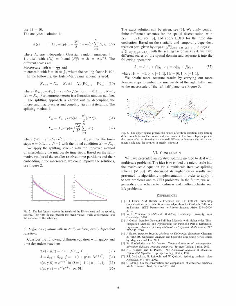
iterative steps to embed the microscale of the right half-planeto the macroscale of the left half-plane, see Figure 3.

Fig. 3. The upper figures present the results after three iteration steps (strongdifferences between the micro- and macro-scale). The lower figures presentthe results after ten iterative steps (small differences between the micro- andmacro-scale and the solution is nearly smooth.).

VI. CONCLUSION

We have presented an iterative splitting method to deal withmultiscale problems. The idea is to embed the micro-scale intothe macro-scale equation via a multiscale iterative splittingscheme (MISS). We discussed its higher order results andpresented its algorithmic implementation in order to apply itto test problems and to CFD problems. In the future, we willgeneralize our scheme to nonlinear and multi-stochastic reallife problems.

REFERENCES

[1] B.I. Cohen, A.M. Dimits, A. Friedman, and R.E. Caflisch. Time-StepConsiderations in Particle Simulation Algorithms for Coulomb Collisionsin Plasmas. IEEE Transactions on Plasma Science, 38(9): 2394–2406,2010.

[2] W. E. Principles of Multiscale Modelling. Cambridge University Press,Cambridge, 2010.

[3] J. Geiser. Iterative Operator-Splitting Methods with higher order Time-Integration Methods and Applications for Parabolic Partial DifferentialEquations. Journal of Computational and Applied Mathematics, 217,227–242, 2008.

[4] J. Geiser. Iterative Splitting Methods for Differential Equations. Chapman& Hall/CRC Numerical Analysis and Scientific Computing Series, editedby Magoules and Lai, 2011.

[5] W. Hundsdorfer and J.G. Verwer. Numerical solution of time-dependentadvection–diffusion–reaction equations, Springer-Verlag, Berlin, 2003.

[6] P.E. Kloeden and E. Platen. The Numerical Solution of StochasticDifferential Equations. Springer-Verlag, Berlin, 1992.

[7] R.I. McLachlan, G. Reinoult, and W. Quispel. Splitting methods. ActaNumerica, 341–434, 2002.

[8] G. Strang. On the construction and comparision of difference schemes.SIAM J. Numer. Anal., 5, 506–517, 1968.

6

Scalable Hybrid Deterministic/Monte Carlo Neutronics Simulations in Two SpaceDimensions

Jeffrey Willert !, C. T. Kelley!, D. A. Knoll †, H. Park †,!Department of Mathematics, North Carolina State University, Raleigh, NC 27695-8205

Email: jawiller@ncsu.edu, tim kelley@ncsu.edu† Theoretical Division, MS B216, Los Alamos National Laboratory, Los Alamos, NM 87545

Email: nol@lanl.gov, hkpark@lanl.gov

Abstract—In this paper we discuss a parallel hybrid de-terministic/Monte Carlo (MC) method for the solution of theneutron transport equation in two space dimensions. Thealgorithm uses an NDA formulation of the transport equation,with a MC solver for the high-order equation. The scalabilityarises from the concentration of work in the MC phase of thealgorithm, while the overall run-time is a consequence of thedeterministic phase.

Keywords-Neutron Transport, Jacobian-Free Newton-Krylov,NDA, Monte Carlo

I. INTRODUCTION

In this paper we report new scalability results for a hybriddeterministic/MC algorithm for the multigroup k-eigenvalueproblem in neutron transport in two space dimensions. Ourhybrid deterministic/MC solver [1], [2] is based on theNonlinear Diffusion Acceleration (NDA) formulation of theproblem [3]. The new features of the solver, as describedin [1], [2] are faster and more accurate Jacobian-vectorproducts and the use of MC simulation for the transportsweeps.

The equation is

! ·!!g(!,"r) + "t,g!g(!,"r)

= 14!

!Gg!=1 "

g!!gs #g!("r)

+ "g

4!keff

!Gg!=1 $"f,g!#g!("r),

(1)

with appropriate boundary conditions. This is a generalizedeigenvalue problem. We are interested in the dominant(largest) eigenvalue keff and corresponding eigenfunction.

In (1), "r " D # R3, !g is the group angular flux and #g ="

4! !gd! is the group scalar flux for groups g = 1, · · · , G."t,g , "g!!g

s , and "f,g are the total, inscattering and fissioncross-sections for group g. %g is the fission spectrum, and$ is the mean number of neutrons emitted per fission event.

There has been much recent work on Jacobian-freeNewton-Krylov and hybrid deterministic/MC algorithms forthe k-eigenvalue problem [1]–[8]. This paper is part of thatactivity.

Traditional methods for solving the neutron transport k-eigenvalue problem have been either purely deterministicor purely stochastic. Deterministic methods often sufferfrom noticeable discretization error in the spatial, angular

and energy variables, but can be designed to converge inrelatively few iterations. Stochastic, or Monte Carlo (MC),methods have the advantage that they are free troublesomediscretization error, but it can be prohibitively expensive toreduce the variance (and subsequently, the error) in the sim-ulation to the desired tolerance. For this reason, we considerthe intersection of these methods. Hybrid methods attempt toattain the fast convergence of deterministic methods withoutthe discretization error.

In the remainder of the paper we briefly describe thehybrid NDA formulation of the problem in § II. We referto [1]–[4], [6] for details and descriptions of discretizationsand boundary conditions. Our interest here is parallel per-formance, and in § III we report on new scalablity for aproblem in two space dimensions.

II. ALGORITHMS

The Nonlinear Diffusion Acceleration (NDA) algorithmreformulates the problem as a nonlinear equation for thegroup scalar fluxes [9]. In NDA, as with other nonlinearaccelerators, [9]–[13], we express the fixed point problem forthe flux into a “low-order” nonlinear diffusion equation. Thelow-order equation is coupled to the “high-order” transportequation to enforce consistency. The high-order equation isa fixed-source problem with no scattering, and is thereforeeasier to solve with a MC approach than the originaltransport equation [1], [2], [14]–[17].

As is standard, we will express (1) in operator notationas

L# = M#

S +1

keffF$

$. (2)

In (2), L = ! ·!+ "t, M = 14! , S = "s, and

F = %$"f .

# is the vector of group angular fluxes, and $ is the vectorof group scalar fluxes. A simple power method iteration canconverge very slowly. The NDA formulation will convergemore rapidly.

NDA splits the transport problem into a ”high-order”transport problem with no scattering in the right side ofthe equation and a ”low-order” diffusion equation. The

2013 12th International Symposium on Distributed Computing and Applications to Business, Engineering & Science

978-0-7695-5060-2/13 $26.00 © 2013 IEEEDOI 10.1109/DCABES.2013.8

7

resulting system of equations is nonlinear, but iterativemethods converge more rapidly for the NDA system thanfor the original problem [3], [9]. We will express the NDAformulation as a eigenvalue problem for the low-order flux$.

Given $ and keff , we compute a high-order angular flux#HO, scalar flux $HO, and current JHO by

#HO = L"1M%

S + 1keff

F&

$,

$HO ="

#HOd!, and "JHO ="

!#HOd!.

Define

Dg ="JHOg + 1

3!t,g!#HO

g

#HOg

. (3)

Note that D depends on $ through the high order flux andcurrent. The low-order eigenvalue problem is

!·%

$ 13!t,g

!#g + Dg#g&

+ ("t,g $ "g!gs )#g

=!

g! #=g "g!!gs #g! +

"g

keff

!Gg!=1 $"f,g!#g!

(4)

If the function $ and scalar keff we used to solve the high-order problem also solve the low-order problem, then wehave solved the k-eigenvalue problem.

We write (4) as

D$$ S$$ 1

keff%F$ = 0, (5)

where D is the differential operator and S the scatteringterms. The method proposed in [1]–[3] formulates the eigen-problem as nonlinear equation for $ by using

keff =

'

F$ dV

to obtain the equation

F ($) = D$$ S$$ %F$"

F$ dV= 0.

A. Hybrid NDAIn the results we report in § III, we use the hybrid

approach proposed in [1], where a MC simulation is usedto solve the scattering-free fixed source high order problem,and thereby compute D. We motivate this approach in thissection.

Traditional methods for computing the dominant eigen-value of neutron transport equation are deterministic; weemploy discretization in space, angle, and energy and solvethe eigenvalue problem in discrete space. The discretizationof each of these variables can lead to errors which may resultin non-physical solutions. Currently, we only concern our-selves with addressing the spatial and angular discretizationerrors.

The standard spatial discretizations, the diamond differ-ence method or the step-characteristics method, can both

be insufficient at times. The diamond difference method issecond-order accurate, however, if the mesh is too coarse,this differencing technique can lead to negative fluxes. Thestep-characteristics method guarantees positive solutions ev-erywhere in the domain, however is only first order accurate[18] The Sn angular discretization can yield “ray effects” orbiasing along the discrete angles in our quadrature set [18],[19]. These ray effects can only be remedied by increasingthe number of angles in the quadrature set, however this islimited as beyond a certain point the Sn quadrature containsnegative weights, leading to instability.

Each of these issues can be avoided entirely by opting touse the MC method. The MC method allows for a continuoustreatment of both the spatial and angular variables (andenergy, too). While MC simulations have stochastic noise,they have the potential to provide more physically accuratesolutions than deterministic methods. Furthermore, thesemethods are highly parallelizable and their implementationlends itself to emerging computing architectures.

In a pure MC k-eigenvalue calculation, one realizes thepower method by simulating a sequences of “batches” ofparticles. The computation begins with an approximationto the fission source, F#. Each batch takes as an input afission source distribution and outputs a new fission sourcedistribution. Once the eigenvector has begun to converge, webegin to average the fission source distributions from eachiteration to damp MC noise. The eigenvalue is the ratio ofthe number of particles born out of fission events from oneneutron generation to the next.

In the hybrid method, in which the MC simulation onlytakes place in order to approximate the inversion of L, weonly need to simulate the streaming of particles. All ab-sorption, scattering and fission events are controlled throughthe low-order system. This allows for a highly simplifiedimplementation of the MC algorithm. The logic is removedalmost entirely and particle histories are significantly shorterthan traditional MC particle histories.

III. RESULTS

We report results on the LRA-BWR test problem from [3],[20], [21]. This is a two group, six region problem with fivedifferent materials. The system is a 165cm square. We use1cm square cells in both directions. Figure 1 illustrates thegrid and the material distribution. The LRA-BWR problemis a standard benchmark in the field.

The lower-left corner of the domain has a reflectiveboundary, whereas the remaining boundaries are all vacuum.Our MC implementation uses Continuous Energy Deposition(CED) tallies [22], which we found to be very efficient in ourprevious studies [1], [14]. We solve the low-order equationwith at Newton iteration. This approach was refered to NDA-NCA in [1], [3], [14].

The code has Matlab and C++ components. The Matlabdriver takes the material and domain data and creates the

8

Figure 1.

x position

y p

osi

tio

n

Material Layout

20 40 60 80 100 120 140 160

20

40

60

80

100

120

140

160

1

5

4

2

3

NDA-NCA-MC initial iteration with enough power methoditerations to drive the eigen-residual for the lower-orderproblem to 10"3 (no more than five). At each NDA-NCA-MC iteration, the driver calls the C++ parallel MC codeto simulate particle histories. The C++ code tallies andaverages the scalar flux and current which are used to pro-vide a closure for the LO problem. The Matlab driver thenreads the scalar flux and current from text files, computesthe boundary conditions and builds the discrete low-orderproblem. At this point, the driver executes a single Newtoniteration to update the scalar flux for the next iteration.

The communication between the Matlab driver and theC++ MC code is via file I/O. The driver builds the sourceterm for the MC code from its computed scalar flux andwrites it and the domain parameters to a file. The C++ codereads the domain parameters and distributes these to eachnode. On each node, the source term is read in from thetext file and the source, domain parameters and number ofhistories per thread are distributed to each core via OpenMP.Each core stores an entire copy of the domain configurationand simulates its share of the neutron histories. Each coretallies a copy of the scalar flux and current before collapsingthis data to a total, on-node scalar flux and current. We thenuse a call to MPI Reduce to compute an average scalar fluxand current across cores. Finally, the C++ code writes thesedata to a file for the driver.

The computations were done on an HP DL585G7 Serverrunning CentOS 6.3 and gcc 4.7.2. Each node has four 1.9GHZ AMD 6168 twelve-core processors per node with a512KB cache and 64GB of memory.

In Table I we tabulate weak scaling results, where theproblem size increases proportionally to the number ofnodes, of a single transport sweep. This is an accuratesurrogate for the full eigensolve, for which the results withfewer nodes require an excessive amount of time.

Table IWEAK SCALAING OF GROUP 1 TRANSPORT SWEEP

nodes time (secs) speedup1 85.1665 100.00002 85.2150 99.94314 85.4985 99.61178 85.6725 99.4094

12 85.7175 99.357220 86.0830 98.9353

In Figure 2 we plot the results of a strong scaling studyfor the entire eigensolve, using 10 nodes as the base case.The plot clearly shows that the strong scaling is excellent.

Figure 2. Strong Scaling for Eigensolve

103

103

Number of Cores

Tim

e (m

inute

s)

Strong Scaling for Eigensolve

Observed Timings

Perfect Scaling

Finally, we plot the results of the solve in Figure 3.

IV. CONCLUSION

In this paper we describe a parallel nonlinear solver forthe NDA formulation of the k-eigenvalue problem in neutrontransport. The solver is a hybrid deterministic/MC method.We demonstrate the method’s good scalability properties fora two-dimensional benchmark problem.

ACKNOWLEDGMENT

This work was been partially supported by theConsortium for Advanced Simulation of Light Wa-ter Reactors (www.casl.gov), an Energy Innovation Hub(http://www.energy.gov/hubs) for Modeling and Simulationof Nuclear Reactors under U.S. Department of Energy Con-tract No. DE-AC05-00OR22725 and Los Alamos NationalLaboratory contract No. 172092-1.

9

Figure 3. Group Fluxes

x position

y p

osi

tio

n

Group 1 Scalar Flux

20 40 60 80 100 120 140 160

20

40

60

80

100

120

140

160

0.5

1

1.5

2

2.5

3

x 10!3

x position

y p

osi

tio

n

Group 2 Scalar Flux

20 40 60 80 100 120 140 160

20

40

60

80

100

120

140

160

2

4

6

8

10

12

x 10!4

REFERENCES

[1] J. Willert, C. T. Kelley, D. A. Knoll, and H. K. Park, “A hybridapproach to the neutron transport k-eigenvalue problem usingNDA-based algorithms,” 2013, to appear in Proceedings ofInternational Conference on Mathematics and ComputationalMethods Applied to Nuclear Science & Engineering.

[2] J. Willert and C. T. Kelley, “Efficient solutions to the nda-ncalow-order eigenvalue problem,” 2013, to appear in Proceed-ings of International Conference on Mathematics and Compu-tational Methods Applied to Nuclear Science & Engineering.

[3] H. Park, D. A. Knoll, and C. K. Neumann, “Nonlinear Ac-celeration of Transport Criticality Problems,” Nuclear Scienceand Engineering, vol. 171, pp. 1–14, 2012.

[4] ——, “Acceleration of k-Eigenvalue/Criticality CalculationsUsing the Jacobian-free Newton-Krylov Method,” NuclearScience and Engineering, vol. 167, pp. 133–140, 2011.

[5] D. Gill and Y. Azmy, “Newton’s method for solving k-eigenvalue problems in neutron diffusion theory,” NuclearScience and Engineering, vol. 167, pp. 141–153, 2011.

[6] D. Gill, Y. Azmy, J. Warsa, and J. Densmore, “Newton’sMethod for the Computation of k-Eigenvalues in SN Trans-port Applications,” Nuclear Science and Engineering, vol.168, pp. 37–58, 2011.

[7] M. T. Calef, E. D. Fichtl, J. Warsa, M. Berndt, and N. Carl-son, “A Nonlinear Krylov Accelerator for the Boltzmann k-Eigenvalue Problem,” Journal of Computational Physics, vol.238, pp. 188 – 209, 2013.

[8] E. Larsen and J. Yang, “A Functional Monte Carlo Method for$k$-Eigenvalue Problems,” Nuclear Science and Engineering,vol. 159, pp. 107–126, 2008.

[9] D. A. Knoll, H. Park, and K. Smith, “Application of theJacobian-free Newton-Krylov method to nonlinear accelera-tion of transport source iteration in slab geometry,” NuclearScience and Engineering, vol. 167, pp. 122–132, 2011.

[10] D. Y. Anistratov, “Nonlinear quasidiffusion accelerationmethods with independent discretization,” Nuclear Scienceand Engineering, vol. 95, pp. 553–555, 2006.

[11] W. A. Wieseiquist and D. Y. Anistratov, “The quasidiffusionmethod for transport problems in 2d cartesian geometry ongrids composed of arbitrary quadrilaterals,” Nuclear Scienceand Engineering, vol. 97, pp. 475–478, 2007.

[12] M. M. Miften and E. W. Larsen, “The quasi-diffusion methodfor solving transport problems in planar and spherical geome-tries,” Trans Th Stat Phys, vol. 22, pp. 165–186, 1993.

[13] V. Y. Gol’din, “A quasi-diffusion method for solving thekinetic equation,” USSR Comp. Math. and Math. Phys, vol. 4,pp. 136–149, 1967, original published in Russian in Zh. Vych.Mat. I Mat. Fiz. 4,1078(1964).

[14] J. Willert, C. T. Kelley, D. A. Knoll, and H. K. Park, “Hybriddeterministic/monte carlo neutronics,” 2012, to appear inSISC.

[15] J. Willert, X. Chen, and C. T. Kelley, “Newton’s method forMonte Carlo-based residuals,” 2013, submitted.

[16] J. Willert, C. T. Kelley, D. A. Knoll, H. Dong, M. Ravis-hankar, P. Sathre, M. Sullivan, and W. Taitano, “Hybrid Deter-ministic/Monte Carlo Neutronics using GPU Accelerators,” in2012 International Symposium on Distributed Computing andApplications to Business, Engineering and Science, Q. Guoand C. Douglas, Eds. Los Alamitos, CA: IEEE, 2012, pp.43—-47.

[17] J. Willert and C. T. Kelley, “Efficient solutions to the NDA-NCA low-order eigenvalue problem,” 2013, submitted toProceedings of International Conference on Mathematics andComputational Methods Applied to Nuclear Science & Engi-neering.

[18] E. E. Lewis and W. F. Miller, Computational Methods ofNeutron Transport. Grange Park, IL: Americal NuclearSociety, 1993.

[19] K. Lanthrop, “Spatial differencing of the transport equation:Positivity vs. accuracy,” Journal of Computational Physics,vol. 4, p. 475, 1969.

[20] K. S. Smith, “An analytic nodal method for solving the two-group, multidimensional static and transient neutron diffusionequations,” 1979, Masters Thesis, Massachusetts Institute ofTechnology.

[21] “Argonne code center: Benchmark problem book,” ArgonneNational Laboratory, Tech. Rep. ANL-7416, 1977, preparedby the Computational Benchmark Problems Committee ofthe Mathematics and Computational Division of the AmericalNuclear Society, Supplement 2.

[22] J. Fleck and J. Cummings, “Implicit Monte Carlo scheme forcalculating time and frequency dependent nonlinear radiationtransport,” Journal of Computational Physics, vol. 8, no. 3,pp. 313–342, 1971.

10

Research on QoS reliability Prediction in Web Service Composition

Lou Yuan-sheng, Jiang Man-fei College of Computer & Information

Hohai University Nan Jing, P.R.China, 210098

Wise.lou@163.com, dawei8013@126.com

Xu Hong-tao Data Management Center

Zheng zhou Human Resource and Social Security Bureau. Zheng Zhou, P.R.China, 450007

xhtl@ hazz.hrss.gov.cn

Abstract—Because of the flexibility of Web Services and dynamical network, QoS is difficult to be assured of reliability, often causing the Web Service selected and invoked by users are often not working properly, not result in high performance Web service composition. In the composition of services for service selection, in order to improve the reliability and performance of composite services need to consider the services of non-functional factors, the paper apply of knowledge of probability and statistics predicting Web service’s dynamic QoS property values, propose a objective evaluation of the credibility of Web Service and a improved K-MCSP QoS global optimization algorithm of service composition for improving the reliability of service composition.

Keywords: Global optimization method of QoS, QoS prediction, Service composition.

I. INTRODUCTION With the significant increase of Web services on the net

work, in the face of the same or similar functional Web services, previously based on "functional properties" service selection can not meet the needs of users, so also take into account the "non-functional properties", QoS (Quality of Service). However, some service providers for their own benefit provide false QoS information, or because of the aging hardware and the increasing number of user requests than the server processing capacity, so that the quality of services can not reach the extent of his previous release, therefore it is difficult to guarantee QoS Information released is real and reliable.

At present, many researchers focus on predicting a particular Web service QoS attributes, to predict the performance of one aspect of service as the basis of service selection, such as paper[1] predict the similarity of services, paper[2] predict availability, paper[3] predict the credibility of services, while there are some researchers in the academic community using mathematical model to predict QoS. However, due to too much service to predict in global optimization service selection, service composition QoS prediction algorithm is not efficient in performance and execution time.

In order to improve the performance of service composition, this paper gives three prediction methods of dynamic QoS information and a service credit evaluation mechanism, and proposed the based-on MCSP Web service composition QOS prediction algorithm K-MCSP, choose the

high quality service, get the best combination of services for solving path.

II. SINGLE WEB SERVICE QOS PREDICTION Web service QoS attributes describe the different

performance aspects of Web service, so different types of user groups have different needs, and focus on different QoS attributes. To address different user preferences for Web services, this article refers to the concept of key QoS properties.

Concept 1 Key QoS Property (KQP) is the most important QoS attributes focused by different user group in the service composition for different user groups. The key QoS properties in the different user groups are different.

This property presented by the user when the service request is given, or automatically set in service composition for special user group. The weight of KQP in all the QoS properties should be the maximum, set by user or automatically set the default value during the service composition, so as to ensure KQP importance. For example, the service WS, its failure rate is a key QoS property. Then the weight of the failure rate set between 0.25 and 0.5.

Service QoS prediction before service selection is very important. This paper predicts four basic services QoS properties-- running time, transfer time, failure rate and credibility.

A Running Time Prediction As the impact of software and hardware, running time of

service is fluctuations and dramatic, can not be constant. Exponential distribution has no memory, meaning that some components worked for a period of time, life distribution is the same as the original life distribution when it has been not working. So running time of service can be described by Exponential distribution. This article before the service composition predict the running time, distributed by exponential continuous probability distribution, the distribution density function:

e , 0( )0,

t tf tt o

!! "! >= " ## (1) Use Maximum likelihood estimation method to estimate

the parameters, get ! . Likelihood function is obtained:

1

1 1( ) ( , )

n

ii i

n n tt n

ii i

L f t e e!

!! ! ! ! ="

"

= =

$= = =$ $

(2) Logarithm on both sides of the equation ( it as running

2013 12th International Symposium on Distributed Computing and Applications to Business, Engineering & Science

978-0-7695-5060-2/13 $26.00 © 2013 IEEEDOI 10.1109/DCABES.2013.9

11

time in the past, n as number of collection services in the past), so the log-likelihood function is:

1( ) ( )

n

ii

InL nIn t n In t! ! ! ! !"

== " = "$

(3) Make 1( ) ( ) 0d InL n t

d!

! !"

= " =

So the maximum likelihood estimation of ! is:

1

n

ii

n

t!%

=

=$

(4) Therefore, the execution time distribution function is:

( ) 1 , 0tF t e t!"= " > (5) time is running time released by service provider, then the probability of the running time falling in the interval of [ , ]time x time x" + (x is the acceptable range radius of running time) is ( ) ( )F time x F time x+ " " .

B Transmission Time Prediction Due to network status transmission speed is changing,

affecting service request transmission time. Paper [4,5] shows that service data transmission time can be predicted according to the following formula:

0.7350.4 0.3i iws ws ipinglatency distance ws= + & (6)

0.51(0.02 1)i iws wsTranstime size pinglatency= & + & (7)

iwsdistance is the distance of Web Service iws , size is the size of the packet. C Failure Rate Prediction

Web services can use a Markov process to describe, and can be based on Markov methods to determine the services the state transition probability (Figure -1), forecasting service availability.

Figure-1 Station Transition Probability Graph

For Web services, on the one hand, if the current service is available, after t' time it will have ! t' probability to transfer to failure or have (1 )t!" ' probability to transfer to maintain available; In the other hand, if the current service is failure, after t' time it will have tµ' probability to transfer to be available or have (1 )tµ" ' probability to transfer to maintain failure[6].

So, Web service system for station transition matrix is:

Derivation of each component on the transition

probability matrix P can be drawn on the transfer rate, written in matrix from:

A!

µ"

= !µ" (8)

The paper[6], through the different equations to be solved on the availability of services, solve out the probability of the two station at someone time. If the initial station is available, the probability of availability at the moment of t is:

( )0( ) ( ) tA t P t e ! µµ !

! µ ! µ" += = +

+ + (9) If the initial station is failure, the probability of

availability at the moment of t is:

' ( )

0( ) ( ) tA t P t e ! µµ !! µ ! µ

" += = "+ + (10)

To be able to predict the final state of the system, also need to be steady-state distribution of availability, may be on the Limit of two formulas:

'lim ( ) lim ( )t t

A t A t µ! µ() ()

= =+ (11)

Steady-state availability of Web services is independent of the initial state. According to historical data we can use maximum likelihood estimation method to estimate the parameters ! and µ for the available time and the failure time distribution function of service.

Because of limited processing capacity and server request cache content of the services, under normal conditions in the server, the user's request may not be processed, resulting in a service request to fail. In paper [6], the user visits of server can be described as the number of random events per unit time, in line with the Poisson distribution parameter:

{ } , 0,1, 2,!

kep X k kk

!! "

= = = ! (11)

For different time to collect the data over each past time period we predict parameter values ! of the Poisson distribution , the maximum likelihood estimator of ! is user’s average visit amount for the unit time. Server's cache volume ( b ) and throughput (!) can be given when the service providers register the service. When the service visit amount is reached to b , the service cache is full; again the service can not be processed. By the queuing theory, we can draw the amount of saturated rate of service access:

11 , 0

11 , 0

1

ib

i

i bp

i bb

** ! µ*

! µ

+"! + # #% "%= "

% = # #% +# (12) Assuming !*

µ= ,

ip is the probability to have i requests in

the queue, when visit amount i reach to b , service cache is full, again denied the request to pay. So the probability of saturation for service visit is:

full bP p= . (13)

12

Combination of the above analysis, we can predict the overall failure rate out of service:

1 ( )failure full fullP A t P P!! µ

= " + = ++ (14)

D Reputation Evaluation Current evaluation of services is too subjective, can

only feel the performance of services from view of the user. Due to some network failure, and service composition in the poor performance of individual services, as well as poor performance service composition caused by fault of service composition engine, not truly reflect the performance of individual services, so performance of service composition can not evaluate the reputation of a single Web service.

In one hand the paper compare the execution time and the failure rate of each call-off services with the information distributed by service providers, in the other hand the performance of services response from a user perspective, both should multiply the corresponding right to the final reputation value, usually the right value to the former than the latter in order to ensure the objectivity of reputation, for example, 70% of the former, the user evaluation 30%.

By Standard & Poor's rating methodology, the reputation level from low to high order:

11 1 1 1 1[0, ],[ , ], ,[1 ,1 ],[1 ,1]

2 2 2 2 2L L L LT T T T TT T T "

" " " " "+ " " " "!

T is the threshold level of credibility, so the service below a sign does not advocate calling; L is the reputation level. Fall in different intervals, corresponding to different levels of reputation. The reputation of this method reflects the slow rise and rapid decline in reputation rating of poor performance characteristics. The credibility of new service had not previously called for is the average of the total reputation of service provider.

III. SERVICE COMPOSITION QOS PREDICTION Because the MCSP[7] algorithm is based on the

information released by service providers in the UDDI , can not guarantee the reliability of QoS information; Therefore, the paper propose improved global optimization algorithm of service composition QoS prediction-- K-MCSP, through objective reputation computing the real QoS property valuesof services, cycle operation select the maximum target function of the path, and predict each QoS attribute values for services in path, finally solve the optimal path of service composition.

A. Basic Ideas In this paper, service composition QoS prediction

algorithm K-MCSP, is based on the MCSP service selection algorithm to solve 01 multi-choice multidimensional knapsack problem. Idea of the algorithm is that the user selects a key QoS property, the selection strategy is divided into two stages:

1) In the first stage of service composition, due to the select service space is too much, this time predicting each Web service lower the efficiency of the service composition. Service QoS information is not reliable, but the reputation of the service objectively reflects the performance of the

service performance though compare the performance of services with released QoS information, it is truly and reliable. Therefore, key QoS property selected by user and reputation as the constraint of service selection, while using the true quality of service calculate the service objective function, apply MCSP algorithm, topological sort order to traverse each node of the Web service composition graph, in turn record the path of the maximum of the target utility function meeting the user's constraints from the source to each task node. if the task node reach the terminal node, indicating that the algorithm successfully found a best path of service composition, return the optimal path from the source to the end with constraints, circularly execute to generate the K best path of service composition;

2) In the second stage, as the first phase of the service selection is based on information released by service provider, the reliability of QoS calculated is not high. So the screening of candidates down the predicted QoS services, using upper prediction methods predict filtered candidate service. All the proposed prediction method to predict QoS attribute values of each web service in the k optimal path of service composition, re-computing QoS property values and objective utility function of path, and also meet the user's QoS constraints, solve the optimal path of service composition.

After user submits a request, QoS agent center of service composition manager selects one or more task nodes to compose scheme. Combination of all scheme together form a functional graph, then selection manager correspond all task nodes to the respective service group, finally connecting all possible candidate paths, and each path can execute the user's request. In the graph only considering the functional properties of each Web service, without taking into account QoS requirements, as shown in Figure -2, the arrows indicate the transfer process between the two services.

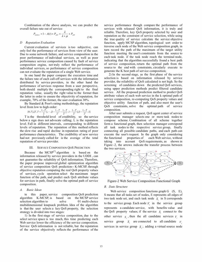
Figure-2 Web Service Composition Functional Graph

B. Date Structure Web service composition functions graph G (S, E),

S means that all tasks set of nodes, E represents all edges of two task node set, and each task node iS in S corresponds to the service group. Each node iV in the service group represents a candidate service, with benefits value and the QoS property values; if the service iS connect to the other service

jS , then the all candidate services iV in

service group iS are connected to all candidate jV

services in service group jS ; adding a virtual source node

13

sV without linking in and a virtual end source dV without linking out, their QoS attributes are always 0; C represents the user's QoS constraints ; Q, said the service quality vector of path; F is objective utility function of the path, the corresponding comprehensive quality of service composition path. In Figure -2, service selection problem of QoS global optimization in dynamic Web service composition can be converted to find the optimal path from source node to the destination node with constraints.

C. Implementation Based on QoS prediction the optimal path problem with

constraints can be formally described as: in the service composition function graph finding a path P from the source node to the end node, make the maximum utility objective function F, and satisfies the user's QoS property constraints.

In the first phase, in addition to credibility and transmission time, the main QoS information of Web service is distributed from service provider, but the service's QoS information is dynamic, QoS can not be guaranteed the reliability of information, not accurate know the performance to complete the requested service. Except the key QoS property, the paper use proposed method of the credibility evaluation, and use the user's credit rating to calculate real QoS property value of each candidate service. Type (4-4) is QoS property value through information directly released by the service provider:

1(1 )PD P

L LQ QL

" += " •

DQ is real QoS property value of service. PQ is QoS

property value of service released by service provider. L is the highest lever of reputation. PL is reputation lever of someone service.

Pseudo code K-MCSP selection algorithm for global optimization is: K-MCSP(G=(V,E),Vs,Vd,C):

{L(k) Kpath(G=(V,E),Vs,Vd,C) For (each Pi L(k)) { for(each Vj,P[i] V)

{Time=Time+ServiceTime(Vj) +TransmissionTime(Vj) F[i]=F[i] + Prediction(Vj Q) Q=Q + Vj QKOP } If ( Q>C) then F[i]=0 } Retrun Max(F) }

Kpath (G=(V,E),Vs,Vd,C) { While (n < = k )

{ for(each Si S) for(each Vi Si) { if (Vi= =Vs) then { Q Q(Vi) F F(Vi) } else {Q QD(Vi)+Q

F FD(Vi)+F }

if ( Q >CKOP) return else { if ( F < F(Si) ) return else remove P from P Si) } add Vi to P Si } if (Si = = Vd)

{ n ++ add p(Si) to L

P V =0 } return L

} }

IV. EXPERIMENT AND ANALYSIS Deployed in a lab environment Petium (R) 4 3.00GHz CPU, 1024M RMB's PC, the operating system using Windows XP, use development tools for the Eclipse3.2, java (jdk1.6). Because currently there is no relevant standard platforms and standard test data sets, experimental data were generated using simulations, and Web service QoS parameters within a certain range by random method, the range of parameters is, 0< priceq 100 0s< timeq 60s

0< failureq <1 0< transtimeq <60 0< eputationrq 10.

We compare the K-MCSP algorithm with prediction algorithm based-on average QoS information into the experiments, and global optimization of based-on average QoS information prediction algorithm select ACO for optimal path, the running time of two algorithms for solving the optimal service composition are as follows:

Figure -3 Running time for K-MCSP and average prediction Figure -3 shows compare of running time between the

algorithm of this paper and the average prediction algorithm. When the number of candidate service is round 5, and the task node is not much, running time of K-MCSP algorithm and the average prediction algorithms do not differ large, but the execution time with the task nodes increases, the iteration time and space is too large, the running time of K-MCSP is averagely superior to 20% than average prediction algorithm. In summary, processing data computation K-MCSP algorithm is more than average

14

prediction algorithm, but the running time of optimal path using K-MCSP is far below the average forecast of the ACO.

The purpose of the method predicts the service's ability. According to forecasted execution time of composition service and the actual measured value we assess the accuracy of prediction algorithms, the error rate can be predicted by the formula e a

a

V VV

- "=

. eV and

aV mean

respectively the predicted execution time and the actual measured value, then calculated the average prediction error rate:

1

n

ii

avg n

-- ==

$

If avg- is than 10%, the prediction is qualified. Table-1 Comparison of Running time

Using K-MCSP, the average prediction error was 7.6%, less than 10%, accurate prediction qualified, while the average prediction error rate is 16.8% on average. And based on actual data and a set of prediction data we can get compared map, as shown in Figure -4:

Figure-4 the comparison between prediction time and actual time Can be seen, our proposed service composition QoS

prediction algorithm can help to improve the performance of composition service.

V. CONCLUSIONS The K-MCSP algorithm is on the basis of global service

composition of services, within satisfying the user's

QoS constraints, choose the highest reliability service to compose service, predict the QoS of service composition based on MCSP, and solve the optimal service composition path. The first phase of the service composition we filter out most web service don’t satisfy the constraint and haven’t high credibility, leaving the k optimal service composition path. Although not very precise, but very effective QoS global optimization Service selection algorithm for reducing the burden and improve the efficiency of the entire service composition in the second phase of service composition. QoS of MCSP is released by service provider, so the reliability of QoS is difficult to ensure. Compared with the MCSP, K-MCSP prediction algorithm can accurately predict the QoS value of Web services, and QoS information of service composition is also reliable and effective, so the performance of service after composing is much higher than the MCSP algorithm, and have objective evaluation system of services, accurate evaluate Web services. Compared with similar global optimization algorithms, such as ACO, PSO and so on, K-MCSP algorithm computational efficiency and performance of global optimization, there is a great advantage, because K-MCSP before service selection have not a lot of Iteration time and space consumption, can quickly find the best service composition paths. Meanwhile we can accurately predict QoS of Web service, can greatly improved the reliability of service composition. Algorithm's time complexity can make use of algorithms to analyze the number of cycles, the algorithm calculated the total time in O (n2) or less.

REFERENCES [1] Ma Jian-wei, Shu Zhen, Guo De-ke, Chen Hong-hui. Survey on

service composition approach considering trustworthiness of QoS date. National University of Defense Technology.2010

[2] Hachem Moussa, Tong Gao, I-Ling Yen, Farokh Bastani, Jun-Jang Jeng. Toward effective service composition for real-time SOA-based systems. University of Texas.2010.

[3] Qi Xie, Kaigui Wu, Jie Xu, Pan le, and Min Chen. Personalized Context-Aware QoS Prediction for Web Services Based on Collaborative Filtering. College of Computer Science, Chongqing Universtiy.2010.

[4] Ye Y,Yen I-L,Xiao L, Thuraisingham B(2008) Secure, highly available, and high performance peer-to-peer storage systems. IEEE Int Conf High Assur Syst Eng.

[5] Zhang H,Goel A, Govindan R(2005) An empirical evaluation of internet latency expansion. ACM SIGCOMM Comput CommunRev.

[6] Huang Yang-qing. Research on the Problem of Web Service Failure. China University of Petroleum.2009

[7] Tao Yu, Kwei-Jay Lin. Service Selection Algorithms for Composing Complex Services with Multiple QoS Constraints. Dept of Electrical Engineering and Computer Science, University of Califonia.2005.

[8] Niko Thio, Shanika Karunasekera. Automatic Measurement of a QoS Metric for Web Service Recommendation. Department of Computer Science and Software Engineering, University of Melbourne.2005.

[9] Jiang Wu, Fangchun Yang. QoS Prediction for Composite Web Services with Transactions. Beijing University of Posts and Telecommunications.2007.

[10] Bang-Yu Wu, Chi-Hung Chi, Shi-Jie Xu, Ming Gu and Jia-Guang Sun. QoS Requirement Generation and Algorithm Selection for Composite Service Based on Reference Vector. Tsinghua University. November 18,2008

cases

K-MCSP prediction value

Average prediction value

Actual value

Error rate of K-MCSP

Error rate of average prediction

1 5.0 4.9 4.3 16% 14% 2 3.5 3.2 4.1 14% 22% 3 4.2 3.4 4 5% 15% 4 2.0 2.1 2.5 20% 16% 5 3.1 3.8 3.2 3% 19% 6 1.6 2.5 2 20% 25% 7 3.8 3.7 3.5 8% 6% 8 4.5 6.0 5.2 13% 15% 9 4.5 4.9 4.3 4% 14% 10 2.9 2.5 3.2 9% 22%

15

Iterative Krylov Methods for Gravity problems on Graphics Processing Unit

Abal-Kassim Cheik Ahamed, Frederic MagoulesEcole Centrale Paris, France

akcheik@gmail.com, frederic.magoules@hotmail.com

Abstract—This paper presents the performance of linearalgebra operations together with their uses within iterativeKrylov methods for solving the gravity equations on GraphicsProcessing Unit (GPU). Numerical experiments performed ona set of real gravity matrices arising from the Chicxulubcrater are exposed, showing the performance, robustness andefficiency of our algorithms, with a speed-up of up to thirty indouble precision arithmetics.

Keywords-Iterative Krylov methods; SpMV; Parallel comput-ing; GPU; CUDA; Gravity equations;

I. INTRODUCTION

Computers with high FLoating point Operations PerSecond (Flops), such as Graphics Processing Unit (GPU),are now common in the computing market. Historicaly,GPU, were used for calculations associated with graphicdisplay. After ten years from its apparition, General PurposeGPU computing (GPGPU) has undergone a revolution incomputational science with the use of graphics hardware.Over the past ten years, the high computing power hassignificantly evolved, allowing modern graphics processingunits to become more attractive for science and engineering.In order to allow researchers to exploit the computationalpower of GPU device, NVIDIA has proposed ComputeUnified Device Architecture (CUDA) [26], which offers ahigh level GPGPU-based programming language. In thispaper, we improve the implementation of Krylov methodson GPU architecture. To evaluate the performance we useAlinea [6], [5], our research group library, implementedin C++. Alinea is intended as a scalable framework forbuilding efficient linear algebra operations, together withmore advanced operations like iterative Krylov on both CPUand GPU clusters.

This paper is organized as follows. First, in Section II,we give a brief presentation of the idea of gravity modeling.Section III introduces briefly GPU computing for readersnot familar with GPU CUDA programming. Section IVpresents our algorithms and reports numerical results. De-tails of linear algebra operations needed in iterative Krylovmethods such as dot-product, addition of vectors, elementwise product and sparse matrix-product multiplication areanalyzed. Section VI presents numerical results on iterativeKrylov methods which clearly confirm the robustness, com-petitiveness and efficiency of the proposed implementationon GPU for solving the gravity equations.

II. GRAVITY EQUATIONS

See beneath the Earth or gaz investigation require thesolution of the gravity equation which refines geophysicalexploration. Gravity problem can be used for instance as acomplementary method to seismic imaging in geophyscialexploration. Gravity allows to more accurately define theunderground’s nature by determining density contrasts thatare then correlated with seismic speeds. By this way, we cananalyze for instance the gravity field in the Chicxulub craterarea located in between the Yucatan region and the Gulfof Mexico which represents strong magnetic and gravitymagnetic anomalies, which allow an evaluation of the impactof an asteroid 65 million years ago in the region. Thedensity of computation suits very well the huge computingpower of GPUs, making the parallel granularity of thealgorithm optimal. Unfortunately, to obtain high speed-up,several tuning and optimizations of the algorithms should becarrefully performed, such as data transferts between CPUand GPU, and data structure. Gravity method is a potentialmethod that improves velocity-density correlations whencoupled with seismic tomography or ultrasounds acousticmethods, and above all constrains the density distributionof the geological structures under study. The composant ofthe centrifugal force and the gravitational force describesthe gravity force. The gravitational potential of a sphericaldensity distribution is expressed as: !(r) = Gm/r, withm the mass of the object, r the distance to the object andG the universal gravity constant equal to G = 6.672 !10!11m3kg!1s!2. When we consider an arbitrary densitydistribution !, at a position x the gravitational potentialis equal to !(x) = G

!

(!(x")/||x " x"||)dx" where x" isone point position within the density distribution. Whetherthe effects related to the centrifugal force are neglected,only regional scale of the gravity equations is taken intoaccount. The gravitational potential ! of a density anomalydistribution "! is thus formulated as the solution of thePoisson equation "! = "4#G"!.

III. GENERAL PURPOSE GPU COMPUTING

This section introduces an overview of GPU programmingmodel and gives the considered features of the numericalexperiments considered.

Before 2000, most of numerical simulations were per-formed on Central processing Unit (CPU) cluster. In 2006

2013 12th International Symposium on Distributed Computing and Applications to Business, Engineering & Science

978-0-7695-5060-2/13 $26.00 © 2013 IEEEDOI 10.1109/DCABES.2013.10

16

the migration of GPGPU faces the era of CUDA program-ming that enables researchers to take advantages of highcomputational power of GPU architectures. GPGPU enablesto use graphics card with CPU orchestra to accelerategeneral-purpose scientific and engineering computing. Moreprecisely, GPGPU allows the use of the GPU to offloadthe CPU during portions of heavy calculations. Sequentialblocks of the code run on the CPU while parallel parts runon the GPU. The simplified architecture of a CPU processoris composed of several memories with multiple levels ofcache memories associated, a basic unit of computationand a more complex control unit. The idea behind thearchitecture of GPU is to have many small floating pointprocessors exploited on a large amount of data in parallel.Indeed, many GPU operations perform similar calculationson a large amount of independent data (Single InstructionMultiple Data); GPUs are in fact parallel devices of theSIMD architecture.

In a GPU, multiple processing elements, threads, carry outthe same operations on multiple data simultaneously, whichresults a gain in computing time. GPU architecture consistsof hundreds processor cores that work together to massivelyperform parallel computing data. This architecture rangesthe GPU as an excellent candidate to perform fast algebraoperations. GPU Computing is much significantly effectivefor large size problem compared to CPU. Manufacturershave developed API such as NVIDIA CUDA that enablesresearchers to easily make programs that could be run onGPU. In order to fully take advantages of this language,developers need to be close to the hardware, i.e. moreknowledge of the architecture of the GPU and its features.

Because a CPU accesses constantly the Random AccessMemory (RAM), it has a low latency at the detriment ofits raw throughput. On the other side, the memories havevery good rates and quick access to large amounts of dataon GPU. Unfortunately, their accesses are very slow. CUDAhave four main types of memory: global, local, constant andshared. A thread can be seen as the smallest unit of process-ing that can be scheduled by an operating system. Threadsare grouped into blocks and executed simultaneously inparallel. A GPU is associated with a grid, i.e all running orwaiting blocks in the running queue, and a kernel that willrun on many cores. A warp is the smallest executing unit ofthe GPU. Its number of threads are always executed together.Distribution of threads is not an automated process, i.e. thatthe developer chooses for each kernel the distribution of thethreads. The configuration of the GPU grid (gridification) ispointed out as follows: (i) threads are grouped into blocks;(ii) each block has three dimensions to classify threads; (iii)blocks are grouped together in a grid of two dimensions.The threads are then distributed to these levels and becomeeasily identifiable by their positions in the grid accordingto the block they belongs to and their spatial dimensions.CUDA processing flow. Reference [8] demonstrated that the

gridification, i.e. the grid features and organization, has astrong impact on the performances of the kernels.

In this paper, the workstation used for the experimentsconsists of an Intel Core i7 920 2.67GHz, which has 4physical cores and 4 logical cores, 5.8 GB RAM and twoNvidia GTX275 GPU equipped with 896 MB memory. Theworkstation is compatible with CUDA 4.0 and supportsdouble precision arithmetics. Depending on whether thecalculation is carried out, on the host (CPU) or on the device(GPU), the clock used is not the same. The native clock ofthe graphics card has an accuracy of a few nanosecondswhile the host has an accuracy of a few milliseconds. Toovercome this problem, the proposed benchmark consistsin performing the same operation several times, at least 10times and at least until the total measured time exceeds 100times the clock accuracy. For the sake of accuracy, in thispaper, we run 100 times each operation and the given timecorresponds to the average time.

IV. BASIC LINEAR ALGEBRA OPERATIONS

In this section, we briefly describe our algorithms andreport the experiments we have performed to evaluate thespeed-up of the GPU version compared to the CPU version.

Table I gives the double precision execution time of ourimplementation for the scale operation, where h correspondsto the size of the vector.

Table IDOUBLE PRECISION SCALE OF VECTORS

h cpu time (ms) gpu time (ms) cpu (Gflops) gpu (Gflops) ratio89056 0.364 0.058 0.244 1.5 6

181888 0.729 0.066 0.249 2.7 11450528 1.886 0.096 0.238 4.6 19848256 3.571 0.149 0.237 5.6 231587808 6.666 0.232 0.238 6.8 28

Double-precision real Alpha X Plus Y (Daxpy), i.e. y[i] =$!x[i]+y[i], is a level one (vector) operation between twovectors in the Basic Linear Algebra Subprograms (BLAS)package. The addition of the coefficients of each vectoris stored in a vector which overwrites the contents of thesecond vector, by a simple GPU kernel of the form:

global void Daxpy(double alpha, const double# d x,double# d y, int size ) {

unsigned int x = blockIdx .x # blockDim.x + threadIdx .x;unsigned int y = threadIdx .y + blockIdx .y # blockDim.y;int pitch = blockDim.x # gridDim.x;int idx = x + y # pitch ;if ( idx<size) {

d y[idx] = alpha#d x[idx] + d y[idx ];}

}

Table II shows the double precision execution time of ourimplementation for the Daxpy operation.

The scalar-vector multiplication or element wise product,i.e. y[i] = x[i] ! y[i], is inherently parallel making it an

17

Table IIDOUBLE PRECISION ADDITION OF VECTORS (DAXPY)

h cpu time (ms) gpu time (ms) cpu (Gflops) gpu (Gflops) ratio89056 0.735 0.058 0.363 4.5 12

181888 1.538 0.083 0.354 6.5 18450528 3.846 0.119 0.351 11.3 32848256 7.692 0.188 0.330 13.4 40

1587808 14.285 0.342 0.333 13.9 41

excellent candidate for implementation on GPU. The mul-tiplication result of the elements of both vectors overwritesthe contents of the first vector by a simple GPU kernel ofthe form:

global void ElementWiseProduct(double alpha, const double# d x,double# d y, int size ) {

unsigned int x = blockIdx .x # blockDim.x + threadIdx .x;unsigned int y = threadIdx .y + blockIdx .y # blockDim.y;int pitch = blockDim.x # gridDim.x;int idx = x + y # pitch ;if ( idx<size) {

d y[idx] = d x[idx] # d y[idx ];}

}

Table III shows the double precision execution time of ourimplementation for the Element wise product operation.

Table IIIDOUBLE PRECISION ELEMENT WISE PRODUCT

h cpu time (ms) gpu time (ms) cpu (Gflops) gpu (Gflops) ratio89056 0.680 0.060 0.130 1.4 11

181888 1.408 0.083 0.129 2.1 16450528 3.571 0.123 0.126 3.6 28848256 6.666 0.209 0.127 4.0 31

1587808 11.111 0.341 0.142 4.6 32

Dot product and norm evaluation can be very expensive onCPU for large size vectors. The basic dot product algorithmdesigned by a simple loop with simultaneous summationis not effective on GPU. To improve the efficiency of dotproduct algorithm, we compute it into two distinct tasks. Thefirst task consists in multiplying the elements of each vectorone by one and the second task consists in summing eachof these products to obtain the final result. On a sequentialprocessor, the summation operation would be implementedby writing a simple loop with a single accumulator variableto build the sum of all elements in the sequence. One elementof the input data is handled by a thread. The partial sum ofall elements of all threads of a block is stored into the firstthread (thread 0) of this block at the end of the reduction. Atthe end, the dot product is computed as a sum of all partialsums of all the blocks. In Table IV we compare the doubleprecision execution time of our implementation for the dotproduct on both CPU and GPU.

V. ADVANCED LINEAR ALGEBRA OPERATIONS

Table V sums a set of matrices from the gravity model.The density anomaly used are inherent from the Chicxulub

Table IVDOUBLE PRECISION DOT PRODUCT

h cpu time (ms) gpu time (ms) cpu (Gflops) gpu (Gflops) ratio89056 0.495 0.110 0.359 1.6 4

181888 1.041 0.124 0.349 2.9 8450528 2.564 0.150 0.351 6.0 17848256 5.263 0.204 0.322 8.3 251587808 9.090 0.335 0.349 9.4 27

crater in the Yucatan Peninsula in Mexico. It consists of 10km deep, 180 km diameter and was formed about 65 millionyears ago. The properties of these matrices are summarizedin Table V and a pattern example is given in Table VI wherethe quantity h, nz, density, bandwidth, max row, nz/hand nz/h stddev corresponds to the size of the matrix, thenumber of nonzero elements, the density, i.e. the number ofnonzero elements divided by the total number of elements,the upper bandwidth equals to the lower bandwidth for asymmetric matrix, the maximum row density, the mean rowdensity and the standard deviation of nz/h. Table VI gives

Table VSKETCHES OF THE MATRICES

h nz density bandwidth max row nz/h nz/h stddev89056 2010320 0.025 5675 27 22.573 8.805181888 4268192 0.013 9239 27 23.466 8.051450528 10972752 0.005 17099 27 24.355 7.119848256 21073920 0.003 26225 27 24.844 6.504

1587808 40077872 0.002 40019 27 25.241 5.930

the sparse matrix pattern in the second column and thedistribution of the nonzero elements in the third column.

Table VIEXAMPLE PATTERN OF GRAVITY MATRIX

gravi 1325848h=1325848nz = 33321792density = 0.002bandwidth = 33389max row = 27nz/h = 25.132nz/h stddev =

One of the most time consuming operation in sparsematrix computations is the Sparse matrix-vector product(SpMV). Finite element analysis generally involves ex-tremely large size sparse matrices, which consists of manyzero entries. Data structure, like the Compressed-SparseRow format (CSR) [4], [27], is a key point to store efficientlythe matrices on GPU memory. In addition, this paper usesadvanced gridification tuning techniques developped in [5],[6]. Table VII gives the double precision execution time ofour implementation when using the CSR format.

18

Table VIIDOUBLE PRECISION CSR MATRIX-VECTOR MULTIPLICATION

h cpu time (ms) gpu time (ms) cpu (Gflops) gpu (Gflops) ratio89056 13.750 0.523 0.292 7.6 26

181888 27.500 1.123 0.310 7.5 24450528 70.000 2.857 0.313 7.6 24848256 130.000 4.166 0.324 10.1 311587808 260.000 7.692 0.308 10.4 33

VI. KRYLOV METHODS

In order to solve gravity problems, iterative Krylov meth-ods [30], [2] can be considered. Iterative Krylov methodsperformance depends on the matrices conditioning, andeffective preconditioning techniques must be used to guar-antee fast convergence such as ILU factorization [1], [13],domain decomposition methods [31], [28], [20], hierarchicalpreconditioner, etc. A particular attention should be paid ondomain decomposition methods. These methods consist tosplit the global domain to solve into several sub-domains,each sub-domain beeing solved independently by sharinginformation along the interfaces between the neighboringsub-systems. These interface conditions [16] can be tunedfor the performance of the algorithm either with a continuousapproach [9], [12], [7], [19], [10], [18], [17], [15] or witha discrete approach [29], [24], [21], [11]. The condensedproblem on the interface is usually solved with an interativemethod, each iteration involving the solution of independentsub-problems in parallel [23], [22]. The solution of eachsub-problem is usually solved through a direct method oran iterative method, typically through the iterative Krylovmethods now considered.

Following the work of [14], [25], [3], [32], we now presentthe manner to implement iterative Krylov methods efficientlyon GPU device. The data transfer (sending and receiving)between host (CPU) and device (GPU) is one of the mostexpensive operations. In our Krylov algorithms, all inputdata are sent once from host (CPU) to device (GPU) beforestarting the iterative routine. Nevertheless, each iteration ofiterative Krylov algorithm requires more than one calculationof dot product (or norm) that implies data copy from deviceto host. The proposed iterative Krylov algorithm have beenperformed on the host but all computing steps (dot, norm,Daxpy, matrix-vector product) are performed on the device.Both CPU and GPU implementations are exactly the same.All experimental results of iterative Krylov methods pre-sented here are obtained from a residual tolerance threshold1!10!6 and an initial guess equals to zero. Table VIII repre-sents the execution time in seconds of the preconditioned (bythe diagonal) Conjugate Gradient, Bi-Conjugate GradientStabilized, Generalized Conjugate Residual for CSR format.The results clearly outline the robustness, performance andefficiency of GPU for double precision computation formatrices arising from gravity equations.

Table VIIICSR DOUBLE PRECISION

h #iter cpu time (s) gpu time (s) ratioCONJUGATE GRADIENT

89056 194 3.200 0.241 13181888 252 8.720 0.483 18450528 351 30.990 1.366 22848256 450 76.030 3.043 241587808 727 232.980 8.814 26

BICONJUGATE GRADIENT STABILIZED

89056 133 4.390 0.283 15181888 163 11.290 0.565 19544563 223 47.880 1.926 24848256 305 105.390 3.951 261587808 465 297.970 11.013 27

BICONJUGATE GRADIENT CONJUGATE RESIDUAL

89056 179 3.270 0.235 13181888 231 8.810 0.462 19450528 319 30.970 1.288 24848256 409 75.760 2.889 261587808 650 227.590 8.260 27

VII. CONCLUSION

This paper illustrates the performance evaluation andanalysis of our algorithms for linear algebra operationsperformed on Graphics Processing Unit. Several matricesarising from a gravity problem are used as a testbed. Afterexhibiting and analyzing a comparison of CPU/GPU linearalgebra operations, we consolidate our analyze by usingthem within iterative Krylov methods. The results clearlyshow the interest of the use of GPU technology to solve thegravity equations.

REFERENCES

[1] J.-I. Aliaga, M. Bollhofer, A. F. Martien, and E. S. Quintana-Orti, “Parallelization of multilevel ILU preconditioners ondistributed-memory multiprocessors,” in PARA (1), ser. Lec-ture Notes in Computer Science, K. Jnasson, Ed., vol. 7133.Springer, 2010, pp. 162–172.

[2] H. Anzt, V. Heuveline, and B. Rocker, “Mixed precisioniterative refinement methods for linear systems: Convergenceanalysis based on Krylov subspace methods.” in PARA (2),ser. Lecture Notes in Computer Science, K. Jnasson, Ed., vol.7134. Springer, 2010, pp. 237–247.

[3] J. M. Bahi, R. Couturier, and L. Z. Khodja, “Parallel gmresimplementation for solving sparse linear systems on gpuclusters,” in Proceedings of the 19th High PerformanceComputing Symposia. San Diego, CA, USA: Society forComputer Simulation International, 2011, pp. 12–19.

[4] N. Bell and M. Garland, “Implementing sparse matrix-vectormultiplication on throughput-oriented processors,” in Pro-ceedings of SC’09. New York, USA: ACM, 2009, pp. 1–11.

[5] A.-K. Cheik Ahamed and F. Magoules, “Fast sparse matrix-vector multiplication on graphics processing unit for finiteelement analysis,” in HPCC-ICESS. IEEE Computer Society,2012, pp. 1307–1314.

19

[6] ——, “Iterative methods for sparse linear systems on graphicsprocessing unit,” in HPCC-ICESS. IEEE Computer Society,2012, pp. 836–842.

[7] P. Chevalier and F. Nataf, “Symmetrized method with opti-mized second-order conditions for the Helmholtz equation,”in Domain decomposition methods, 10 (Boulder, CO, 1997).Providence, RI: Amer. Math. Soc., 1998, pp. 400–407.

[8] A. Davidson, Y. Zhang, and J. D. Owens, “An auto-tunedmethod for solving large tridiagonal systems on the gpu,”in Proceedings of the 25th IEEE International Parallel andDistributed Processing Symposium, IEEE. IEEE, May 2011.

[9] B. Despres, “Domain decomposition method and theHelmholtz problem.II,” in Second International Conferenceon Mathematical and Numerical Aspects of Wave Propagation(Newark, DE, 1993). Philadelphia, PA: SIAM, 1993, pp.197–206.

[10] M. Gander, L. Halpern, and F. Magoules, “An optimizedSchwarz method with two-sided Robin transmission condi-tions for the Helmholtz equation,” International Journal forNumerical Methods in Fluids, vol. 55, no. 2, pp. 163–175,2007.

[11] M. Gander, L. Halpern, F. Magoules, and F.-X. Roux, “Analy-sis of patch substructuring methods,” International Journal ofApplied Mathematics and Computer Science, vol. 17, no. 3,pp. 395–402, 2007.

[12] S. Ghanemi, “A domain decomposition method for Helmholtzscattering problems,” in Ninth International Conference onDomain Decomposition Methods, P. E. Bjørstad, M. Espedal,and D. Keyes, Eds. ddm.org, 1997, pp. 105–112.

[13] C. Janna, M. Ferronato, and G. Gambolati, “A block FSAI-ILU parallel preconditioner for symmetric positive definitelinear systems.” SIAM J. Scientific Computing, vol. 32, no. 5,pp. 2468–2484, 2010.

[14] R. Li and Y. Saad, “GPU-accelerated preconditioned iterativelinear solvers,” University of Minnesota, Minneapolis, MN,2010.

[15] Y. Maday and F. Magoules, “Non-overlapping additiveSchwarz methods tuned to highly heterogeneous media,”Comptes Rendus a l’Academie des Sciences, vol. 341, no. 11,pp. 701–705, 2005.

[16] ——, “Absorbing interface conditions for domain decompo-sition methods: a general presentation,” Computer Methodsin Applied Mechanics and Engineering, vol. 195, no. 29–32,pp. 3880–3900, 2006.

[17] ——, “Improved ad hoc interface conditions for Schwarzsolution procedure tuned to highly heterogeneous media,”Applied Mathematical Modelling, vol. 30, no. 8, pp. 731–743,2006.

[18] ——, “Optimized Schwarz methods without overlap forhighly heterogeneous media,” Computer Methods in AppliedMechanics and Engineering, vol. 196, no. 8, pp. 1541–1553,2007.

[19] F. Magoules, P. Ivanyi, and B. Topping, “Convergence analy-sis of Schwarz methods without overlap for the Helmholtzequation,” Computers and Structures, vol. 82, no. 22, pp.1835–1847, 2004.

[20] F. Magoules and F.-X. Roux, “Lagrangian formulation ofdomain decomposition methods: a unified theory,” AppliedMathematical Modelling, vol. 30, no. 7, pp. 593–615, 2006.

[21] F. Magoules, F.-X. Roux, and L. Series, “Algebraic wayto derive absorbing boundary conditions for the Helmholtzequation,” Journal of Computational Acoustics, vol. 13, no. 3,pp. 433–454, 2005.

[22] ——, “Algebraic approximation of Dirichlet-to-Neumannmaps for the equations of linear elasticity,” Computer Meth-ods in Applied Mechanics and Engineering, vol. 195, no. 29–32, pp. 3742–3759, 2006.

[23] ——, “Algebraic Dirichlet-to-Neumann mapping for linearelasticity problems with extreme contrasts in the coefficients,”Applied Mathematical Modelling, vol. 30, no. 8, pp. 702–713,2006.

[24] ——, “Algebraic approach to absorbing boundary conditionsfor the Helmholtz equation,” International Journal of Com-puter Mathematics, vol. 84, no. 2, pp. 231–240, 2007.

[25] K. K. Matam and K. Kothapalli, “Accelerating sparse matrixvector multiplication in iterative methods using GPU,” inICPP, G. R. Gao and Y.-C. Tseng, Eds. IEEE, 2011, pp.612–621.

[26] Nvidia Corporation, Nvidia - CUDA ToolkitReference Manual, 4th ed., available on line at:http://developer.nvidia.com/cuda-toolkit-40 (accessed onMarch 19, 2012).

[27] T. Oberhuber, A. Suzuki, and J. Vacata, “New row-groupedCSR format for storing the sparse matrices on GPU withimplementation in CUDA,” CoRR, vol. abs/1012.2270, 2010.

[28] A. Quarteroni and A. Valli, Domain Decomposition Methodsfor Partial Differential Equations. Oxford University Press,Oxford, UK, 1999.

[29] F.-X. Roux, F. Magoules, L. Series, and Y. Boubendir, “Ap-proximation of optimal interface boundary conditions for two-Lagrange multiplier FETI method,” in Proceedings of the 15thInternational Conference on Domain Decomposition Meth-ods, Berlin, Germany, July 21-15, 2003, ser. Lecture Notesin Computational Science and Engineering, R. Kornhuber,R. Hoppe, J. Periaux, O. Pironneau, O. Widlund, and J. Xu,Eds. Springer-Verlag, Haidelberg, 2005.

[30] Y. Saad, Iterative methods for sparse linear systems. SIAM,2003.

[31] B. Smith, P. Bjorstad, and W. Gropp, Domain Decomposition:Parallel Multilevel Methods for Elliptic Partial DifferentialEquations. Cambridge University Press, UK, 1996.

[32] A. H. E. Zein and A. P. Rendell, “Generating optimal CUDAsparse matrix-vector product implementations for evolvingGPU hardware,” Concurrency and Computation: Practice andExperience, vol. 24, no. 1, pp. 3–13, 2012.

20

!"#$%&'()#*$+('(,,#,$-'./'())01/$2301/$($4035'0625#4$7'()#8.'9$0)-,#)#15#4$01$:+;<

!"#$%&'()$*%+,-%.#/,0)1%2"330*%+,-%+),,0(%4%5,00#67((*%+,%8"9607(%:6)//);<)'9(=$%">%?"@39=7#A*%B#>",@)=7"#%8$1=0@1%)#/%&)=60@)=7'1*%:7#A1="#%C#7D0,17=$*%E"#/"#*%:!F%GHH*%C:

!"#$%&'$=>0/" $ ?.15#15 $ 5"'.2/"-25 $ 0)(/01/ $ 3@35#)3 $ )235$(--,@$50)#$?.132)01/$?.)-,#A$0)(/#$-'.?#3301/$(,/.'05")3$5.$)2,50-,# $ 60.B)#40?(, $ 0)(/# $ 35'#()3< $ !"#3# $ 3@35#)3 $ ('#$5@-0?(,,@$4#30/1#4$5.$23#$-('(,,#,$'#3.2'?#3$01$.'4#'$5.$(?"0#C#$'#32,53 $ 01 $ '#(3.1(6,# $ 50)# $ 3?(,#3< $ !"03 $ -(-#' $ -'#3#153 $ 5"#$4#30/1$.7$($4035'0625#4$7'()#8.'9$5"(5$-'.C04#3$3#-('(50.1$.7$5"#$,('/#,@$.'5"./.1(,$-('(,,#,03(50.1$7'.)$5"#$4.)(01$0)(/#$-'.?#3301/ $ (,/.'05") $ 4#C#,.-)#15< $ !"03 $ (,,.83 $ '#23# $ (14$-,2//(6,# $ #A5#130.1 $ .7 $ -('(,,#,0301/ $ -(55#'13D $ (3 $ 8#,, $ (3$-'.C0401/ $ 7.' $ #A5#13060,05@ $ .7 $ 4.)(01 $ 0)(/# $ -'.?#3301/<$!"#$%&'(%)

()*+,%-#.',/0,1)1$2 3 -4#$%4"5$)- 3 ',/05$4167 3 /047 3 4/&6) 30%,')##416

B- %BI!4J+C?!BJI

27A6 % '"#=0#= % =6,"9A639= % 7@)A7#A % 1$1=0@1 % )33($%)(A",7=6@1 % "> % 0D0, % 7#',0)17#A % '"@3(0K7=$ % )#/ % #9@L0, % ="%1=,0)@1%">%(),A0%G+%)#/%M+%7@)A0%/)=)10=1-%!6010%1$1=0@1%),0 % 7#60,0#=($ %3),)((0(* % =$37')(($ %)33($7#A %17@7(), %'"@3(0K%)#/%=7@0%'"#19@7#A%)(A",7=6@1%="%(),A0%#9@L0,1%">%7@)A01*%)#/%1"%')#%L0#0>7=%>,"@%3),)((0(%0K0'9=7"#-

N),)((0( % 3,"A,)@@7#A % ')# % L0 % /71=7#A97160/ % >,"@ % 7=O1%10,7)(%'"9#=0,3),=%7#%)=%(0)1=%=6,00%'",0%),0)1P%=60%',0)=7"#%)#/%1933",= %"> %3),)((0( % 0K0'9=7"#* % )# % 7#/9'0/ % ,0Q97,0@0#= % >",%'"@@9#7')=7"# % )#/ % 1$#'6,"#7R)=7"# % )@"#A1= % =60%'""30,)=7#A%3,"'01101* %)#/% =60 %6)#/(7#A%"> %3),=7)( % >)7(9,01%SFT- % B> %) % '"@39=)=7"#%')# %L0 %3),=7=7"#0/ % 7#=" % 7#/030#/0#=%19L=)1U1*%=60#%=6010%')#%L0%),,)#A0/%="%0K0'9=0%'"#'9,,0#=($%"#%@9(=73(0%3,"'011",1* % ="%)'670D0%)%,0/9'=7"#%7# %=60%="=)(%0K0'9=7"# % =7@0 % "> % =60 % '"@39=)=7"#* % =60 % 0110#'0 % "> %*+,* -./&01&2'3(/ - (12.4%+3, - !567)% - % !671 % 3),=7=7"#7#A % >",%3),)((0(71@ % ,019(=1 % 7# % =60 % #00/ % >", % '"@@9#7')=7"# % ="%/71=,7L9=0%=60%V",U*%'"((0'=%,019(=1%)#/%7@3(7'7=($%",%0K3(7'7=($%@)#)A0%/030#/0#'701%L0=V00#%=60%19L=)1U1-%B#%=60%>"(("V7#A%10'=7"#1 %V0 % A7D0 % ) % L,70> % ,0D70V % "> %@"/0(1* % 3)==0,#1 % )#/%>,)@0V",U1%=6)= %')#%)1171= %7#%@)#)A7#A%=60%'"@3(0K7=$%">%3),)((0(%3,"A,)@@7#A*%=60#%)%/01',73=7"#%">%"9,%/71=,7L9=0/%>,)@0V",U*%=01=%')101%)#/%,019(=1-%

BB- 4HE.!H+%WJ4:P%N.4.EEHE%N4J54.&&BI5%&J+HE8*%N.!!H4I8%.I+%<4.&HWJ4:8

"8 6'&'99/9-.&1,&'22+3,-21:/9$8

N),)((0( % 3,"A,)@@7#A %@"/0(1 % ,)#A0 % >,"@% ("V% =" %67A6%(0D0( %)L1=,)'=7"#1 % =6)= %'"@@"#($ % =,)/0 %0>>7'70#= %0K0'9=7"#%)A)7#1=%3,"/9'=7D7=$%)#/%3",=)L7(7=$-%J30#&N%71%=60%/0>)'="%1=)#/),/%("V%(0D0(%@"/0(%>",%16),0/%@0@",$%0K3(7'7=%3),)((0(%3,"A,)@@7#A % SGT- % .= % ) % 17@7(), % (0D0(* % B#=0( % !6,0)/7#A%X97(/7#A%X("'U1 %SMT% 3,"D7/01 %)#%JL;0'= %J,70#=0/% =0@3()=0%

L)10/%)33,")'6%="%@9(=7Y'",0%3),)((0(%3,"A,)@@7#A%Z0-A-%=60%=LLP3),)((0([>", % =0@3()=0 % >9#'=7"#\ % )#/ % 1933",= % >",%'"@3"17#A%3730(7#01%)#/%>("V%A,)361-%&NB%71%=60%)110@L($%()#A9)A0%>",%V,7=7#A%3",=)L(0%)#/%1')(0)L(0%)33(7')=7"#1%>",%/71=,7L9=0/ % @0@",$ % 1$1=0@1 % S]T- % .= % ) % 67A60, % (0D0( % ">%)L1=,)'=7"#*%@011)A0%3)117#A%10@)#=7'1%')#%L0%7@3"10/%"#%16),0/%@0@",$%1$1=0@1*%)%3"39(),%0K)@3(0%L07#A%=60%.'=",1%@"/0(%S^T%)#/%16),0/%@0@",$%10@)#=7'1%')#%L0%7@3(0@0#=0/%)',"11 % /71=,7L9=0/ %@0@",$ % 1$1=0@1 % )1 % 0K0@3(7>70/ % 7# % =60%N),=7=7"#0/ %5("L)( %.//,011 % 83)'0 % ZN5.8\ % ()#A9)A01 % S_T-%<9#'=7"#)( %3,"A,)@@7#A%3,"D7/01 %)#%0D0#%67A60, % (0D0( %">%)L1=,)'=7"#%L9=%6)1%6)/%(7@7=0/%19''011%7#%2N?%S`T-%.1%V0((*%6$L,7/%@"/0(1%),0%L0'"@7#A%7#',0)17#A($%'"@@"#%SaT-%J9,%'",0%/71=,7L9=0/%>,)@0V",U%71%)#%8N&+%D),7)#=%L97(= %)="3%&NB*%=),A0=7#A%&B&+%),'67=0'=9,01-%2$L,7/%@"/0(1%')#%L0%0)17($%7#=,"/9'0/%917#A%=60%3(9A7#%>9#'=7"#)(7=$-

;8 6'&'99/9-.&1,&'22+3,-.'%%/&3$-'3:-0&'2/<1&=$8-

.%3)==0,# % 0#'"@3)1101 % =60 % /01',73=7"# % "> % ) % ,0'9,,7#A%3,"L(0@%7#%1"@0%/"@)7#*%)%'"#=0K=%7#%V67'6%7=%71%,0(0D)#=*%)#/%)%U#"V#%3,"="=$37')(%1"(9=7"#%=6)=%6)1%V7/0%)''03=)#'0%)@"#A1= % =60 % /"@)7# % 0K30,=1* % )#/ % D),7"91 % 3),)((0(%3,"A,)@@7#A % 3)==0,# % ()#A9)A01 % SbT* %SFcT* %SFFT% )#/%=)K"#"@701%SFGT%6)D0%L00#%3,"3"10/-%8">=V),0%<,)@0V",U1%),0 % )# % "L;0'= % ",70#=0/ % ,0910 % =0'6#7Q90 % =6)= % '"@L7#01 % =60%'"#'03=%">%'"@3"#0#=1%)#/%3)==0,#1%SFMT-%.1%19'6*%=60$%),0%@",0%'"#',0=0%=6)#%3)==0,#1*%3,"D7/7#A%'"/0%=6)=%,0)(7101%=60%'",0 % 7#>,)1=,9'=9,0 % "> % )# % )33(7')=7"#* % 919)(($ % )1 % )L1=,)'=%'()1101* % )#/ % /0>7#7#A % =60 % 7#=0#/0/ % 7#=0,)'=7"# % "> % =6010%'()1101* % ", % '"#=,"( % >("V % "> % ) % 3,"A,)@ % =6)= % 9101 % =60%>,)@0V",U- % <,)@0V",U1 % ')# % L0 % ')=0A",710/ % )''",/7#A % ="%=607,%(0D0(%">%)L1=,)'=7"#-%.=%)%67A6%(0D0(%=60$%')#%'"@3(0=0($%1670(/ % =60 % 3,"A,)@@0, % >,"@ % =60 % '"@3(0K7=701 % "> % 3),)((0(%3,"A,)@@7#A*%L9=%L$%=60%1)@0%="U0#%')#%,0@"D0%)''011%="%3"=0#=7)(% ("V%(0D0(%@)'67#0%",%),'67=0'=9,0%130'7>7'%=9#7#A%0>>7'70#'701- % 20,0 % V0 % ,0D70V % ) % ,03,010#=)=7D0 % 1)@3(0 % ">%>,)@0V",U1 % =6)= % 103),)=0 % 3),)((0( % 3,"'0117#A % >,"@%)33(7')=7"#%/"@)7#%'"/0-

50#0,)( % @0=6"/1 % 0#)L(7#A % 1=,9'=9,0/ % 3),)((0(%3,"A,)@@7#A % 7#'(9/0 % .(A",7=6@7' % 8U0(0="# % <,)@0V",U1%Z.8U<\ % SF]T- % B#=,"/9'0/ % L$ %?"(0 % SF^T* % 1U0(0="#1 % 7@3"10%)//7=7"#)( % '"#1=,)7#=1 % =6)= % A97/0 % =60 % 910, % =" % ) % 197=)L(0%1"(9=7"#* % )#/ % /0=0,1 % 7#)33,"3,7)=0 % 7@3(0@0#=)=7"#1- %J=60,%A0#0,)( % )33,")'601 % 7#'(9/0 % >,)@0V",U1 % =6)= % )9="YA0#0,)=0%)33(7')=7"#1 % >,"@ % 3),)@0=0,7R0/ % /017A# % 3)==0,# % =0@3()=01%SF_T*%>,)@0V",U1%=6)=%0K3"10%/7>>0,0#=%/017A#%3)==0,#1%=6)=%),0 % =60# %3),)@0=0,7R0/ %V7=6 %3(9A7# %'"@3"#0#=1 % SF`T* %)#/%17@7(), % =0@3()=0 %L)10/ % >,)@0V",U1 % 19'6 % )1 % =60 % O80(0'=7D0%H@L0//0/*%d91=%B#%!7@0%130'7)(7R)=7"#O%Z8HdB!\%SFcT-%J=60,%>,)@0V",U1 % 7@3(0@0#= % ) % 130'7>7' % 3),)((0( % 3,"A,)@@7#A%

2013 12th International Symposium on Distributed Computing and Applications to Business, Engineering & Science

978-0-7695-5060-2/13 $26.00 © 2013 IEEEDOI 10.1109/DCABES.2013.11

21

3)==0,#-%HK)@3(01%7#'(9/0%&W%SFaT* %)%?ee%>,)@0V",U%=6)=%)(("V1 % )33(7')=7"#1 % =" % 3),)((0(7R0 % '"@39=)=7"#1 % 917#A % =60%9L7Q97="91 % @)1=0,YV",U0, % 3),)/7A@* % )#/ % =60 % 2)/""3%>,)@0V",U%SFbT*%)%3"39(),%"30#%1"9,'0%;)D)%7@3(0@0#=)=7"#%">%=60%@)3%,0/9'0%3,"A,)@@7#A%@"/0(%SGcT-

N),)((0( % 3,"A,)@@7#A % >,)@0V",U1 % ')# % )(1" % L0 % @",0%130'7>7'%="%)%/"@)7#%",%)33(7')=7"#*%3,"D7/7#A%"3=7@710/%'",0%3),)((0( % 3,"'0117#A % 7#>,)1=,9'=9,0 % )#/ % 1933",= % (7L,),701- % B#%7@)A0 %3,"'0117#A* % )# % 7#=0,01=7#A%)33,")'6 % SGFT % 7#=,"/9'01%=60%#"=7"#%">%.'&'99/9+>'#9/-.'%%/&3$%7#%",/0,%="%7#',0)10%'"/0%,0910* % )#/ % 7@3,"D0 % @)7#=)7#)L7(7=$- % B# % =671 % /)=) % 3),)((0(%7@)A0%3,"'0117#A%(7L,),$* %)%17#A(0%9#7>",@%)37% 71 %3,"D7/0/%)(=6"9A6%=60%9#/0,($7#A%7@3(0@0#=)=7"#%')#%L0%10Q90#=7)(%",%3),)((0(7R0/-%&",0"D0,*%7#%SGGT%/)=)%)#/%=)1U%3),)((0(71@%),0%L"=6%0K3("7=0/%="%$70(/%L0==0,%7@)A0%3,"'0117#A%30,>",@)#'0-%+)=) % 3),)((0(71@ % 9101 % )(A",7=6@7' % 1U0(0="#1 % >", % 7@)A0%"30,)=",1*%)#/%=)1U%3),)((0(71@%>",%'"@3"17=7"#%7#="%)#%7@)A0%)33(7')=7"#%=)1U%A,)36-

B#%=60%#0K=%10'=7"#*%)%D),7)#=%(7A6=V07A6=%>,)@0V",U%71%/01',7L0/* % V6"10 % ),'67=0'=9,0 % 7#'",3",)=01 % =60 % 0K=0#17L(0%3(9A7#%">%3),)((0(%3)==0,#1%)#/%/"@)7#%'"/0*%)#/%)(("V1%>",%17@3(0%0K=0#17"#%">% =60%>,)@0V",U%7=10(>- %!60%7@30=91 %>",%19'6%)% >,)@0V",U% 7#7=7)(($ %0@0,A0/%>,"@%'"#17/0,)=7"#%">%7@)A0%3,"'0117#A%)(A",7=6@1%)#/%)33(7')=7"#1*%)(=6"9A6%=60%>,)@0V",U%')#%L0%"=60,V710%A0#0,)(710/-

BBB- !2H%N4JNJ8H+%<4.&HWJ4:P%+<4.&H

!60%+<,)@0%71%/017A#0/%3,7@),7($%)1%)%/71=,7L9=0/%7@)A0%3,"'0117#A % >,)@0V",U- % B=O1 % 39,3"10 % 71 % =" % 103),)=0 % =60%",=6"A"#)(%3),)((0( %3,"'0117#A%>,"@%7@)A0%3,"'0117#A*%)#/%=691 % 1670(/ % )33(7')=7"# % /0D0("30,1 % >,"@ % =60 % 3),)((0(7R7#A%)130'=%">%/0D0("3@0#=-%!671%103),)=7"#%)(1"%)(("V1%3),)((0(%3,"A,)@@7#A % 0K30,=1 % =" % '"#'0#=,)=0 % "# % =60 % '",0 % 3),)((0(%3,"A,)@@7#A%0(0@0#=*%L07#A%)L(0%="%/0D0("3%3(9A7#%@"/0(1%7@3(0@0#=7#A % 3),)((0( % 3)==0,#1 % =6)= % )33(7')=7"# % /0D0("30,1%')#%=60#%9=7(7R0-%.1%V0((*%=60%+<,)@0%/017A#%)(("V1%>",%=60%'"@3"17=7"# % "> % 3),)((0(7R0/ % 0#=7=701* % 19'6 % =6)= % )# % 7@)A0%3,"'0117#A%3730(7#0%')#%L0%'"@3"10/%">%7#/7D7/9)(%0#=7=701%=6)= % ),0 % 0)'6 % 3),)((0(7R0/ % 917#A % =60 % +<,)@0- % B= % 71 % )(1"%7#=0#/0/ % =6)= % =60 % +<,)@0 % V7(( % L0 % )L(0 % =" % ,9# % =6010%3),)((0(7R0/%0#=7=701%'"#'9,,0#=($%Z670,),'67')(%3),)((0(71@\-

!60%>,)@0V",UO1%3),)((0(%3,"'0117#A%>0)=9,01%7#'(9/0P! .%@"/9(), % /017A# % =6)= % 1933",=1 % =60 % 3(9A7# % "> %@"/0(1%7@3(0@0#=7#A %3),)((0( % 3)==0,#1 % )#/ % >", %3(9A7# % 7@)A7#A%(7L,),701%)11"'7)=0/%V7=6%=60%3(9A7#%@"/0(1-

! N"7#=%="%3"7#=%)#/%'"((0'=7D0%&)1=0,YW",U0,%@"/0(1%),0%1933(70/* % =6)= % >)'7(7=)=0 % )/)3=7D0 % /71=,7L9=7"# % ">%3,"'0117#A%0#=7=701%L)10/%"#%0>>7'70#=%(")/%L)()#'7#A-

! B#1=,9@0#=)=7"#% =" %@"#7=", % =60 %30,>",@)#'0%"> %3),)((0(%3,"A,)@1* % )#/ % 3,"D7/0 % >00/L)'U % "# % "30,)=7"# % )#/%0>>7'70#'$-

! ?"#>7A9,)L(0 % /0L9AA7#A % ')3)L7(7=701 % =" % 60(3 % /0=0'=%/0)/("'U1* % 1$#'6,"#71)=7"# % 711901* % @0@",$ % (0)U1 % )#/%"=60,%3,"A,)@@7#A%0,,",1-

.1%V0((*%'",0%>0)=9,01%130'7>7'%="%7@)A7#A%),0%3,"D7/0/P! .# % 7@)A0 % >7(=0,7#A % (7L,),$* % ,03,010#=7#A % /$#)@7')(($%/71=,7L9=)L(0%0#=7=701%V7=67#%=60%>,)@0V",U-

! .#%7@)A0%BJ%(7L,),$%>",%(")/7#A%)#/%1=",7#A%=7>>%)#/%1=U%7@)A01-

! .#%7@)A7#A%(7L,),$%130'7>7' % ="%/71=,7L9=)L(0%,)$%=,)'7#A%)(A",7=6@1%)#/%)#'7((),$%7#>,)1=,9'=9,0-

!60%+<,)@0%3,"D7/01%)L1=,)'=7"#1%)=%D),7"91%(0D0(1-%.=%=60% ("V0, % (0D0( % =60 %+<,)@0%3,"D7/01 % =60 % 7#>,)1=,9'=9,0 % ="%@)#)A0%=60%3(9A7#%">%@"/0(1%7@3(0@0#=7#A%3),)((0(%3)==0,#1%)#/%)33(7')=7"#%@"/9(01%=6)=%910%=6"10%@"/0(1*%)#/%3,"D7/01%&NB%3"7#=%="%3"7#=%)#/%'"((0'=7D0%'"@@9#7')=7"#%10,D7'01*%V7=6 % =60 % /0'"#1=,9'=7"# % 3)'U7#A* % 10#/7#A* % ,0'07D7#A*%9#3)'U7#A % )#/ % ,0'"#1=,9'=7"# % "> % "L;0'=1 % L07#A % 30,>",@0/%=,)#13),0#=($%L$%=60%>,)@0V",U-%!60%+<,)@0%)(1"%3,"D7/01%)%'(70#=%7#=0,>)'0%0#)L(7#A%'(70#=1%="%7#=0,)'=%V7=6%=60%+<,)@0-%&"/0(1 % ),0 % =60# % 7@3(0@0#=0/ % =6)= %3(9A % 7#=" % )#/ %910 % =60%+<,)@0%10,D7'01%="%),,)#A0%>",%=60%/71=,7L9=7"#%">%/)=)%)#/%0K0'9=7"# % "> % )33(7')=7"# % '"/0 % =" % 0#19,0 % =6)= % 3),)((0(%,01"9,'01%),0%L07#A%910/%0>>7'70#=($-%

%<7A9,0%F-%!60%+<,)@0%CB%3,"="=$30*%L97(=%917#A%f!]%Z!,"((=0'6\

.#%)33(7')=7"#%'"/0%@"/9(0%'"@@9#7')=01%"#($%V7=6%7=1%)11"'7)=0/ % @"/0(* % 917#A % )# % )37 % /0>7#0/ % L$ % =60 % @"/0(-%803),)=0/%>,"@%)33(7')=7"#%'"/0*%)%@"/0(%=60#%9=7(7R01%=60%+<,)@0O1 % '"@@9#7')=7"# % 7#>,)1=,9'=9,0 % =" % 0>>0'= % 3),)((0(%0K0'9=7"# % )#/ % 7#=0,)'=7"#- % !60 % +<,)@0 % 3,"'01101%130'7>7')=7"#1 % =6)= % /0>7#0 % V67'6 % @"/0( % ", % @"/0( % A,"93%16"9(/ % L0 % ,9#* % ="A0=60, % V7=6 % 7#>",@)=7"# % "# % =60 % =),A0=%)33(7')=7"#%'"/0-%.%@"/0(%71%(")/0/%)#/%,9#*%V67'6%7#%=9,#%9101 % =60 % +<,)@0 % 7#>,)1=,9'=9,0 % =" % (")/ % )#/ % 0K0,'710 % =60%)33,"3,7)=0 % )33(7')=7"# % '"/0- % !60 % @"/9(0 % )#/ % /$#)@7'%O3(9A7#O%/017A#%)(("V1%>",%0K=0#17L7(7=$%)#/%,0910%">%/7>>0,0#=%3),)((0( %3,"A,)@@7#A%@"/0(1-%.%#"D0(%)==,7L9=0%71 %=6)= % =60%+<,)@0%')#%=60#%)9="@)=7')(($%)/;91=%)%@"/0(O1%3),)@0=0,1%)#/%)(1"%/0=0,@7#0%=60%@"1=%)33,"3,7)=0%@"/0(%>,"@%)%@"/0(%A,"93*%="%"3=7@710%0>>7'70#=%0K0'9=7"#-

22

.=%=60%67A601=%(0D0(*%@9(=73(0%=)1U%130'7>7')=7"#1%')#%L0%'"@3"10/%="%',0)=0%)%3730(7#0%">%3),)((0( %0#=7=701- %.%3,7",7%U#"V(0/A0%71%7#=,7#17')(($%7#'",3",)=0/%7#%=60%'"@3"17=7"#%">%=60 % 3730(7#0 % L$ % =60 % 910, % V67'6 % )9="@)=7')(($ % $70(/1%/030#/0#'701*%)L1"(D7#A%=60%910,%>,"@%>9,=60,%7#=0,D0#=7"#-%.%'",0 % )130'= % 71 % =6)= % =60 % >,)@0V",U % ')# % ',0)=0 % @9(=73(0%7#1=)#'01 % "> % =60 % 1)@0 % 3,"'0117#A % 0#=7=$ % "# % /0@)#/-%?"#'9,,0#'$ % 71 % =691 % 01=)L(7160/ % )#/ % @)#)A0/ % =6,"9A6%3,"'0117#A % 3),)((0( % 7#1=)#'01 % "> % /)=) % 1=,0)@1 % ", % /)=)%3),=7=7"#1- % +)=) % >("V % @)#)A0@0#= % 71 % 30,>",@0/ % 917#A%=0@3",)( % )#/ % 13)'7)( % 3),=7=7"#7#A % 1=,)=0A701* % =0@3",)(%3),=7=7"#7#A%="%3,"'011%@9(=73(0%7@)A01%17@9(=)#0"91($%)#/%13)'7)(%3),=7=7"#7#A%="%/7D7/0%)#%7#/7D7/9)(%7@)A0%7#="%19LYD"(9@01%=6)=%')#%L0%3,"'0110/%'"#'9,,0#=($-%<7A9,0%F%16"V1%=60%+<,)@0CB%910/%="%'"@3"10%3),)((0(%=)1U1-

Bg- !H8!%?.8H8%.I+%4H8CE!8

!60%>"(("V7#A%=01=1%910%'91="@%L0#'6@),U7#A%"#%#"#%1=)#/),/%M+%=01=%7@)A01%>,"@%'0((%/)=)%,010),'6*%="%)(7A#%V7=6%=60%7#=0#/0/%3,7@0%910%">%=60%>,)@0V",U-

"8 ?/$%-13-'..9@+3,-'-AB-'C/&',+3,-0+9%/&-%1-$9+(/$-10-13/-DB-+2',/E-<+%*-:+$%&+#4%+13-10-%*/-+2',/-$9+(/$8-

B#%=671%=01=%)%@)1=0,%3,"'011%(")/1%)%M+%7@)A0%>,"@%/71U*%)#/%/71=,7L9=01%)#%7@)A0%1(7'0%="%0)'6%V",U0,%3,"'011-%H)'6%V",U0,%=60#%3,"'01101%=6)=%7@)A0%1(7'0%Z7#%"9=%=01=1%V0%)33($%) % bKb % U0,#0( % >7(=0, % =" % 0)'6 % 7@)A0 % 1(7'0\* % ,019(=7#A % 7# % )#%93/)=0/%7@)A0%1(7'0%=6)=%71%=60#%,0=9,#0/%="%=60%@)1=0,-%!60%@)1=0,%,0'"@3"101%=60%1(7'01%7#="%)%,019(=)#=%M+%7@)A0%)#/%1=",01 %="%/71U-%!60%>"(("V7#A%A,)361%16"V%30,>",@)#'0%7#%=0,@1%">%=7@0%)#/%1300/%93*%>",%)#%7@)A0%'"#=)7#7#A%GF%1(7'01%!%/$% - +2',/F - GHGIJAKIAL - .+I/9$M - LGN#+%M - LOP;M - 0+9/ - $+>/ -LJALOGQJ-#@%/$)-

J#0%3,"'011*%=60%@)1=0,*%/"01%=60%,0)/7#A%)#/%V,7=7#A%">%=60%M+%7@)A0%Z)1%V"9(/%L0%=60%')10%"#%)%17#A(0%@)'67#0\-%.//7=7"#)( % "D0,60)/ % 71 % 7#'9,,0/ % 7# % /71=,7L9=7#A % =60%130'7>7')=7"#*%)#/%=60%19L10Q90#=%/71=,7L9=7"#%">%=60%7@)A0%1(7'01%="%V",U0,1%)#/%'"((0'=7"#%">%=60%,019(=)#=%7@)A0%1(7'01-%2"V0D0,*%=60%,019(=7#A%30,>",@)#'0%7@3,"D0@0#=1%),0%D0,$%0#'"9,)A7#A%Z100%>7A9,0%G\-%B#%=60%@)1=0,YV",U0,%@"/0(%910/%>",%=671%=01=*%7>%"#($%"#0%3,"'011%71%910/*%=60%@)1=0,%/"01%)(( %=60%V",U-%J=60,V710*%V60#%@",0%=6)#%"#0%3,"'011%71%/0>7#0/*%=60%@)1=0,%"#($%/71=,7L9=01%=60%V",U%)#/%'"((0'=1%=60%,019(=1*%)#/%/"01%#"=%3,"'011%)#%7@)A0%1(7'0%7=10(>-%J9,%1)@3(0%7@)A0%'"#=)7#0/ % GF % 7@)A0 % 1(7'01* % )#/ % 1" % =60 % >"(("V7#A %"3=7@)(%3),=7=7"#%'"#>7A9,)=7"#1%V0,0%=01=0/P

]%3,"'01101P%F%@)1=0,%e%M%V",U0,1%6)D7#A%`%=)1U1%0)'6-a%3,"'01101P%F%@)1=0,%e%`%V",U0,1%6)D7#A%M%=)1U1%0)'6-GG%3,"'01101P%F%@)1=0,%e%GF%V",U0,1%6)D7#A%F%=)1U%0)'6-

W0%6)D0%)(1"%19L10Q90#=($%)33(70/%)%O1')==0,YA)=60,O%@)1=0,%V",U0, % @"/0( % D),7)#= % =" % =671 % =01= % ')10* % 7# % V67'6 % )((%

3,"'011",1 % 0#A)A0 % 7# % &NB % 1')==0, % )#/ % A)=60, % '"((0'=7D0%"30,)=7"#1%="%/71=,7L9=0%7@)A0%1(7'01%)#/%,0=9,#%,019(=1-%B#%=671%@"/0(%D),7)#=%=60%@)1=0,%)(1"%/"01%V",U%3,"'0117#A%)#%7@)A0%1(7'0-%X,")/($%17@7(),%,019(=1%V0,0%"L10,D0/%Z917#A%"#0%(011%3,"'011",%7#%0)'6%=01=%)1%=60%@)1=0,%)(1"%)'=0/%)1%)%V",U0,\-%.#%",=6"A"#)(%19''011%V)1%=60%0)10%V7=6%V67'6%"#0%@"/0(%')#%L0%1V)330/%>",%)#"=60,%Z7-0-%L$%17@3($%93/)=7#A%)%(7#0%7#%=60%130'7>7')=7"#\- %!60% O1')==0,YA)=60,O%D),7)#=%">% =60%@"/0(%V",U1%V0((%7>%=60%'"@39=)=7"#)(%0>>",=%"#%0)'6%3,"'011",%71%7/0#=7')(*%)1%0)'6%3,"'011%,0'07D01%V",U%)#/%,0=9,#1%,019(=1%)1%) % '"((0'=7D0 %"30,)=7"# % )',"11 % )(( % 3,"'01101 % Z)#/ % =691 % =)U0%)/D)#=)A0 % "> % 0>>7'70#= % '"((0'=7D0 % 1')==0,YA)=60,%7@3(0@0#=)=7"#1\-

%

%<7A9,0%G-%N0,>",@)#'0%V7=6%0)'6%V",U0,%3,"'0117#A%"#0%7@)A0%1(7'0%">%)%

M+%7@)A0

;8 ?/$%$-13-'..9@+3,-'-DB-'C/&',+3,-0+9%/&-%1-2'3@-DB-+2',/$E-<+%*-:+$%&+#4%+13-10-+2',/-.'%*$F

<",%=671%=01=%')10*%V0%910%=60%@)1=0,YV",U0,%@"/0(%="%=01=%=60%/0A,00%">%1300/93%)==)7#)L(0%7#%)%67A6%'"#=0#=%=6,"9A639=%1'0#),7"- % !60% @)1=0, % @"/9(0 % '"/0 % 71 % 7@3(0@0#=0/ % ="%/71=,7L9=0%>7(0%3)=61%">%)%'"((0'=7"#%">%M+%7@)A01*%"#0%="%0)'6%

! " #! #" $! $"

!

"

#!

#"

$!

%&''()*&

+*,-'.)/0)1./2'%%/.%

! " #! #" $! $"

!

#!

$!

3!

4!

5/567)58,')9%'2/:(%;

+*,-'.)/0)1./2'%%/.%

23

V",U0,%3,"'011- %.1%=60%#9@L0,%">%V",U0,1%71%7#',0)10/*%=60%#9@L0,%">%7@)A01%3,"'0110/%71%)(1"%7#',0)10/%1"%=6)=%0)'6%V",U0,%0K0'9=01%)%,0)/Y3,"'011YV,7=0%V",U>("V%"#%"#0%M+%7@)A0 %Z'->- % =01=1 % =6)= % 3,"'011 % =60 % 1)@0 % 7@)A0 % "# % )#%7#',0)17#A%#9@L0,%">%3,"'011",1\-%H)'6%V",U0,%3,"'01101%)((%D"K0(1%">%)%/71=7#'=%M+%7@)A0%917#A%)%MKMKM%)D0,)A7#A%>7(=0,*%V7=6%)((%7@)A01%L07#A%=60%1)@0%17R0%!%/$%-+2',/F-GHGIJAKIAL-.+I/9$M-LGN#+%M-LOP;M-0+9/-$+>/-LJALOGQJ-#@%/$)-%B/0)(($*%)1%V0%)//%3,"'011",1%=60%="=)(%=7@0%="%0K0'9=0%16"9(/%,0@)7#%'"#1=)#=*%)1%0)'6%)//7=7"#)(%3,"'011",%V7((%3,"'011%7=O1%"V#%/71=7#'=%7@)A0-%2"V0D0,*%7#%3,)'=710%V0%V"9(/%0K30'=%="%100%1"@0%7@3)'= %"#%30,>",@)#'0%/90% ="%BJ%'"#=0#=7"#%)1% =60%(")/%"#%=60%1=",)A0%1$1=0@%,7101%Z1$1=0@%/030#/0#=\*%)#/%)(1"%7#',0)10/ % 7#=0,3,"'011", % '"@@9#7')=7"# % )1 % =60 % 3,"'011",%'"9#= % 71 % 7#',0)10/- %87#'0 %0)'6 %V",U0, %3,"'01101 %"#($%"#0%7@)A0 % 7# % =671 % =01=* % =60 % ="=)( % =7@0% ,0'",/0/ % =" % 0K0'9=0 % =60%3,"A,)@%V7((%L0%OV",1=%')10O*%V7=6%=60%="=)(%=7@0%,0>(0'=7#A%=60%O1("V01=O % V",U0,O1 % ,0)/Y3,"'011YV,7=0 %V",U>("V- % B= % 71 % )(1"%V",1=%')10%7#%=60%10#10%=6)=%0)'6%V",U0,%V7((%)==0@3=%="%,0)/%7=O1%7@)A0%)=%)L"9=%=60%1)@0%=7@0*%)#/%L0')910%3,"'0117#A%71%=60%1)@0%>",%)((%V",U0,1*%=60%V,7=01%V7((%)(1"%L0%)=%),"9#/%=60%1)@0 % =7@0* % V7=6 % 1"@0 % 7#',0)10/ % D),7)L7(7=$- %W0 % 7#10,=0/%>9,=60, % />,)@0 % =7@7#A % @0=,7'1 % =" % ')3=9,0 % 1"@0 % "> % =671%D),7)L7(7=$ % "> % 3,"'0117#A % )',"11 % =60 % 3,"'011",1* % ,0'",/7#A%0)'6%V",U0,O1%=7@0%="%,0)/*%3,"'011%)#/%V,7=0%7=O1%7@)A0-

I"=0%=6)=%V60#%=01=7#A%"#0%3,"'011*%"#0%=)1U%71%),,)#A0/%="%L0%,9#%("')(($%L$%=60%@)1=0,*%V67'6%=691%)'=1%)1%7=O1%"V#%V",U0,-%!"%')('9()=0%1300/%93*%V0%/7D7/0%=60%10,7)(%=7@0%7=%V"9(/%=)U0%="%3,"'011%#%7@)A01*%L$%=60%=01=0/%3),)((0(%=7@0%="%3,"'011%#%7@)A01%Z"#%#eF%3,"'011",1\-

!60%30,>",@)#'0%A,)361%Z100%>7A9,0%M\%16"V%=7@7#A1%)#/%=60%1300/93 %@)330/ % =" % =60 % #eF % 3,"'1 % 910/- %!60 % )11"'7)=0/%1300/%93%A,)36%3,010#=1%)%D70V%">%=60%)==)7#0/%30,>",@)#'0-%W67(1= %#"= % 7/0)(* % =6010 %3,0(7@7#),$ %,019(=1 %),0 %)A)7#%D0,$%0#'"9,)A7#A*%16"V7#A%'"#17/0,)L(0%1300/%93%7#%=671% OV",1=%')10O % =01=- %.1%)#=7'73)=0/* % =60% OV",U0, %0K0'9=0% =7@0O % %/"01%7#',0)10 %V7=6 % 7#',0)10/ %3,"'011", %'"9#=1* %L07#A %3,7@),7($%)==,7L9=0/% =" % 7#',0)10/ %BJ%'"#=0#=7"# %)1 %@",0% 7@)A01%),0%,0)/ % )#/ %V,7==0# % '"#'9,,0#=($* % )(=6"9A6 % 1"@0 % % 7#',0)10/%D),7)L7(7=$%7#%=60%=7@0%="%3,"'011%)#%7@)A0%"#'0%(")/0/%V)1%)(1"%"L10,D0/-%&",0%7#=0,01=7#A($%=6"9A6*%=671%)''"9#=1%>",%(011 % =6)#%6)(> % =60 %"L10,D0/%"D0,60)/ %0D7/0#=% 7# % =60 % O="=)(%=7@0O %A,)36-%!"%7#D01=7A)=0%>9,=60,* %V0%(7#U0/%7#%=60%&NH%)#)($171 % =""( % SGMT- % N0,6)31 % 9#19,3,717#A($* % =60 % )#)($171%,0D0)(0/ %=6)= % 7#7=7)(717#A %&NB%)''"9#=0/ %>", %)#%7#',0)17#A%>,)'=7"#%">%=60%="=)(%"D0,60)/%)1%3,"'011",%'"9#=1%7#',0)10/-%87#'0%=671% 7#7=7)(71)=7"#%71 %)% O"#0%">>O* % 7= %V7(( %L0%)@",=710/%V60#%7=%71%),,)#A0/%>",%0)'6%V",U0,%="%3,"'011%@",0%=6)#%"#0%7@)A0*%)#/%V0%16"9(/%100%7@3,"D0/%1300/93-

.1 % 7#=0,01=7#A* % =60 % )#)($171 % )(1" % ,0D0)(0/ % =6)= % 17A#7>7')#=%=7@0%V)1%130#=%)=%L),,70,1%7#10,=0/%7#="%=60%3,"A,)@-%8"@0%L),,70,1%V0,0%7#10,=0/%="%)(("V%,0)1"#7#A%">%3,"A,)@%>("V%)#/ % ),0 % "=60,V710 % ,0/9#/)#= % )#/ % V7(( % L0 % ,0@"D0/ % ="%7@3,"D0%1300/93-%2"V0D0,*%7=%71%1=7((%)#%),0)%">%'"#=7#90/%

7#D01=7A)=7"#%)1%="%V6$%3,"'01101%')#%,0@)7#%)=%)%L),,70,%>",%)%17A#7>7')#=%30,7"/%)>=0,%)((%3,"'01101%6)D0%),,7D0/%)=% =60%L),,70, % Z917#A % "30#@37 % F-]-G\- % H(10 % V710* % =60 % 7#=0,#"/0%Z@)1=0,YV",U0,\%'"@@1%71%'"@3),)=7D0($%D0,$%1@)((%)#/%/7/%#"=%17A#7>7')#=($%7@3)'=%30,>",@)#'0-%

%

%<7A9,0%M-%N0,>",@)#'0%V7=6%0)'6%V",U0,%3,"'0117#A%"#0%M+%7@)A0

g- ?JI?EC8BJI8

!60 % +<,)@0 % 71 % /017A#0/ % =" % 103),)=0 % "9= % 3),)((0(%7#>,)1=,9'=9,0*%@"/0(1%)#/%3)==0,#1%>,"@%)33(7')=7"#%'"/0*%1"%=6)= % 3,">7'70#= % 3),)((0( % 3,"A,)@@0,1 % ')# % '"#'0#=,)=0 % "#%/0D0("37#A % 3),)((0(717#A % '"/0* %V67(1= % /"@)7# % 0K30,=1 % ),0%(),A0($ % 1670(/0/ % >,"@ % =671 % )130'= % )#/ %')# %'"#'0#=,)=0 %"#%/0D0("37#A%)33(7')=7"#%'"/0-%!60%67A60,%(0D0(%)L1=,)'=7"#1%')#%7@3"10%)%=,)/0%">>%V7=6%30,>",@)#'0*%L9=%=60%3,010#=0/%3,0(7@7#),$ % ,019(=1 % ),0 % D0,$ % 3"17=7D0- %!671 % 103),)=7"# % ">%'"#'0,#1 % 71 % )(1" % "> % L0#0>7= %V60# % 7@3,"D7#A % =60 % 1$1=0@*%V60,0 % 0>>",= % =" % 7@3,"D0 % =60 %+<,)@0 %)#/ %@"/0(1 % ')# %L0%16),0/%)',"11%)((%)11"'7)=0/%@"/9(0%'"/0*%)#/%=60%@"/9(),%

! #! $! 3! 4! "! <! =!

!

"

#!

#"

$!

$"

3!

%&''()*&

+*,-'.)/0)1./2'%%/.%

! #! $! 3! 4! "! <! =!

!

"

#!

#"

$!

$"

>/.?'.)'@'2*5')58,'

5/567)58,')9%'2/:(%;

+*,-'.)/0)1./2'%%/.%

24

/017A#%V7((%0#'"9,)A0%7=1%910%)',"11%@)#$%7@)A0%3,"'0117#A%3,";0'=1%,0Q97,7#A%3),)((0(%3,"'0117#A%')3)L7(7=701-

N0,>",@)#'0%)#)($171%')#%60(3%7((9@7#)=0%=60%'6),)'=0,71=7'1%)#/ % L"9#/1 % "> % 1$1=0@ % 1=",)A0 % BJ* % 7#=0,3,"'011%'"@@9#7')=7"#* %@0@",$ % 670,),'6701 % )#/ % 3,"'011",1* % )#/%=607, % 7#=0,,0()=7"# % )#/ % 0>>0'= % "# % =60 % 30,>",@)#'0 % "> % =60%3,"L(0@%L07#A%1"(D0/*%)#/%@91=%L0%'"#17/0,0/%7#%'"#'0,=%V7=6 % =60 % % O16)30O % "> % =60 % 3,"L(0@ % L07#A % 1"(D0/-%B#1=,9@0#=)=7"#%V7=67#%=60%+<,)@0%71%@)/0%)D)7()L(0%)',"11%@"/0(1 % )#/ % @"/9(01* % =" % )7/ % 30,>",@)#'0 % )#)($171- % !60%)11011@0#= %"> % ,019(=1 %A97/01 % )#/ %/,7D01 % 7@3,"D0@0#=1 % ="%)(A",7=6@1 % =" % @)K7@710 % 30,>",@)#'0 % Z)#/ % ')# % 0D0#%67A6(7A6= %V67'6 %6),/V),0 % '"@3"#0#=1 % ')# %L0 % 7@3,"D0/\-%.#)($171 % "> % =60 % =01=1 % 6)1 % ,0D0)(0/ % V60,0 % @"/0(%7@3(0@0#=)=7"#1 % ')# % L0 % 7@3,"D0/ % Z1$#'6,"#71)=7"# % )#/%7#=0,'"@@1* % % ,0@"D7#A%L),,70,1%0='-\ %)#/% =6)= % 7= %@7A6=%L0%V",=6%>9,=60,%,010),'6%7#="%917#A%3),)((0(%BJ%Z1933",=0/%L$%&NBYG\ %)#/ %30,6)31 %/0/7')=7#A %) % 19L10= %"> %3,"'011",1 % ="%1=",)A0 % BJ % )#/ % =60# % =" % 910 % 7#=0,#"/0 % '"@@9#7')=7"# % ="%=,)#1>0, %/)=) % )L"9= % =60 %#0=V",U- %!671 % %@91= %L0 %L)()#'0/%)A)7#1=%7#',0)10/%3,"A,)@%'"@3(0K7=$-

gB- 4H<H4HI?H8

SFT%2-%H-%X)(*%d-%5-%8=07#0,%)#/%.-%8-%!)#0#L)9@*%hN,"A,)@@7#A%()#A9)A01%>",%/71=,7L9=0/%'"@39=7#A%1$1=0@1*h%"7P-712.4%8R4&C8E -D"(-%GF*%33-%G_FYMGG*%103*%Fbab-%

SGT%.-%4-%X-%J30#&N*%hJ30#&N%)33(7')=7"#%3,"A,)@%7#=0,>)'0*h%!0'6-%403-%g0,17"#%M-F*%GcFF-

SMT%d-%407#/0,1*%S3%/9-?*&/':+3,-;4+9:+3,-;91(=$8-80L)1="3"(*%?.*%C8.P%JO407(($%ij%.11"'7)=01*%B#'*%Gcc`-

S]T%C#7D0,17=$%">%!0##01100*%:#"KD7((0*%!0##01100-%P6SF-"-P/$$',/N6'$$+3,-S3%/&0'(/-R%'3:'&:-ZF-F1=%0/-\%Fbb^L-

S^T%N-%2)((0,%)#/%&-%J/0,1U$*%h.'=",1%=6)=%9#7>$%=6,0)/1%)#/%0D0#=1*h%7#%6&1(//:+3,$-10-%*/-H%*-S3%/&3'%+13'9-7130/&/3(/-13-711&:+3'%+13-P1:/9$-'3:-T'3,4',/$E-N)36"1*%?$3,91*%Gcc`*%33-%F`FYFbc-

S_T%&-%W07()#/*%7*'./9-E-U1&%&/$$-'3:-VLK-F-W1C/9-T'3,4',/$-01&-5678-C"H%2N?K%E=/*%Gcc`*-

S`T%+-%X-%8U7((7'",#%)#/%+-%!)(7)*%h&"/0(1%)#/%()#A9)A01%>",%3),)((0(%'"@39=)=7"#*h%"7P-712.4%8R4&C8E-D"(-%Mc*%33-%FGMYF_b*%Fbba-%

SaT%d-%+7)R*%?-%&9#"RY?),"%)#/%.-%I7#"*%h.%89,D0$%">%N),)((0(%N,"A,)@@7#A%&"/0(1%)#/%!""(1%7#%=60%&9(=7%)#/%&)#$Y?",0%H,)*h%SXXX-?&'3$8-6'&'99/9-B+$%&+#8-R@$%8E-D"(-%GM*%33-%FM_bYFMa_*%GcFG-%

SbT%!-%&)==1"#*%X-%8)#/0,1%)#/%X-%&)117#A7((*%6'%%/&3$-01&-6'&'99/9-6&1,&'22+3,8-.//71"#YW01(0$%N,">0117"#)(*%Gcc]-

SFcT%X-%?)=)#R),"%)#/%:-%:09=R0,*%hN),)((0(%'"@39=7#A%V7=6%3)==0,#1%)#/%>,)@0V",U1*h%V&:$E-D"(-%F`*%GcFc-%

SFFT%:HC!kH4*%:-%)#/%&.!!8JI*%!-*%*%.%N)==0,#%E)#A9)A0%>",%N),)((0(%N,"A,)@@7#A%D0,G-c-%.D)7()L(0P%6==3Pll3),()L-00'1-L0,U0(0$-0/9lV7U7l3)==0,#1l3)==0,#1-

SFGT%2-%km((7A6"D0#-%Y#Z/(%NY&+/3%/:-713$%&4(%+13-5'3:#11=-F-B/C/91.+3,-"..9+('%+13NY&+/3%/:-R10%<'&/-<+%*-%*/-?119$-j-P'%/&+'9$-"..&1'(*-Gcc]-

SFMT%4-%H-%d"6#1"#*%h<,)@0V",U1%n%Z'"@3"#0#=1%e%3)==0,#1\*h%712243-"7PE-D"(-%]c*%33-%MbY]G*%"'=*%Fbb`-%

SF]T%2-%5"#Ro(0RYgp(0R%)#/%&-%E0$="#*%h.%19,D0$%">%)(A",7=6@7'%1U0(0="#%>,)@0V",U1P%67A6Y(0D0(%1=,9'=9,0/%3),)((0(%3,"A,)@@7#A%0#)L(0,1*h%R10%<'&/F-6&'(%+(/-'3:-XI./&+/3(/E-D"(-%]c*%33-%FFM^YFF_c*%GcFc-%

SF^T%&-%?"(0*%"9,1&+%*2+(-R=/9/%13$F-R%&4(%4&/:-P'3',/2/3%-10-6'&'99/9-712.4%'%+138-?)@L,7/A0*%&.*%C8.P%&B!%N,011*%FbbF-

SF_T%8-%&)'+"#)(/*%d-%.#D7U*%8-%X,"@(7#A*%d-%8'6)0>>0,*%+-%8R)>,"#%)#/%:-%!)#*%h<,"@%3)==0,#1%="%>,)@0V",U1%="%3),)((0(%3,"A,)@1*h%6'&'99/9-712.4%8E-D"(-%Ga*%33-%F__MYF_aM*%/0'*%GccG-%

SF`T%:-%.1)#"D7'*%4-%X"/7U*%d-%+0@@0(*%!-%:0)D0#$*%:-%:09=R0,*%d-%+-%:9L7)="V7'R*%H-%.-%E00*%I-%&",A)#*%5-%I0'9()*%+-%.-%N)==0,1"#*%:-%80#*%d-%W)V,R$#0U*%+-%W0110(%)#/%:-%.-%q0(7'U*%h!60%3),)((0(%'"@39=7#A%()L",)=",$%)=%C-?-%L0,U0(0$P%.%,010),'6%)A0#/)%L)10/%"#%=60%L0,U0(0$%D70V*h%HH?8%+03),=@0#=*%C#7D0,17=$%">%?)(7>",#7)*%X0,U0(0$*%&),'6%GF-%Gcca-

SFaT%d-%5"9K*%8-%:9(U),#7*%&-%q"/0,%)#/%d-%E7#/0,"=6*%h.#%0#)L(7#A%>,)@0V",U%>",%@)1=0,YV",U0,%)33(7')=7"#1%"#%=60%'"@39=)=7"#)(%A,7/*h%7#%6&1(//:+3,$-10-%*/-H%*-SXXX-S3%/&3'%+13'9-R@2.1$+42-13-5+,*-6/&01&2'3(/-B+$%&+#4%/:-712.4%+3,E-Gccc*%33-%]M-

SFbT%?C!!BI5*%+-*%cMlFblGcFGY()1=%93/)=0*%W0('"@0%="%.3)'60r%2)/""3rs-%.D)7()L(0P%6==3Pll6)/""3-)3)'60-",Al%Sc_lF]lGcFGT%-

SGcT%d-%+0)#%)#/%8-%560@)V)=*%h&)340/9'0P%17@3(7>70/%/)=)%3,"'0117#A%"#%(),A0%'(91=0,1*h%712243-"7PE-D"(-%^F*%33-%Fc`YFFM*%;)#*%Gcca-%

SGFT%<-%d-%807#1=,)*%+-%:"0(@)%)#/%d-%&-%50910L,"0U*%h.%1">=V),0%),'67=0'=9,0%>",%910,%=,)#13),0#=%3),)((0(%7@)A0%3,"'0117#A*h%6'&'99/9-712.4%8E-D"(-%Ga*%33-%b_`YbbM*%)9A*%GccG-%

SGGT%?-%I7'"(01'9%)#/%N-%d"#U0,*%h.%/)=)%)#/%=)1U%3),)((0(%7@)A0%3,"'0117#A%0#D7,"#@0#=*h%6'&'99/9-712.4%8E-D"(-%Ga*%33-%b]^Yb_^*%)9A*%GccG-%

SGMT%?2.I*%.-*%54JNN*%W-%)#/%EC8:*%H-*%*%N0,>",@)#'0%g719)(7R)=7"#%>",%N),)((0(%N,"A,)@1-%.D)7()L(0P%6==3PllVVV-@'1-)#(-A"Dl,010),'6l3,";0'=1l30,>D71l%S@)$lb*%GcFMT-

25

Model size challenge to analysis software

Peter Chow Engineering Cloud Research

Fujitsu Laboratories of Europe Ltd Hayes Park Central, Hayes, Middlesex, UB4 8FE, UK

e-mail: Peter.Chow@uk.fujitsu.com

Serban Georgescu Engineering Cloud Research

Fujitsu Laboratories of Europe Ltd Hayes Park Central, Hayes, Middlesex, UB4 8FE, UK

e-mail: Serban.Georgescu@uk.fujitsu.com

Abstract—Existing analysis software, commonly used in scientific, engineering and business, is not designed for today and tomorrow’s model sizes. Most software has been developed decades before multi-threads, multi-cores, heterogeneous systems. In computer-aided engineering (CAE), some of the codes date back to the 50s and 60s aimed at model sizes of around 100 elements. They have been enhanced and developed for each generation of computing systems. Today, model sizes of million plus elements are common in business such as manufacturing. The need for accuracy and detail are driving model size from millions to billions to trillions and beyond. Can these analysis codes and supporting tools keep up with the progress or not? If not, what are the alternatives? In this presentation we investigate this challenge for software components as ‘Black-Box’ situation.

Keywords: Monolithic Software, Simulation Process, Computer-Aided Engineering

I. INTRODUCTION Today we are in the petascale computing (1015) era and

soon we will enter the exascale era (1018). The wealth and discoveries in the last 50+ years follow the exponential growth of computer processing power. This vast computing power means for human society that we can expect further advancements, from a better understanding of complex systems such as climate and environment to medical and brain studies, to social media and big data, and the inter-relationships and interactions with planet Earth. Together with mathematical modelling, simulation is used to study phenomena otherwise too expensive or impossible to observe in experiments. Current obstacles to continue the current rate of progress in computational processing are energy and the lack of software able to scale to future systems.

In the case of computer-aided engineering (CAE), some of the analysis codes in production use date back to the 50s and 60s, when model sizes were around 100 elements or cells. Today, these codes (enhanced and developed for each generation of computer systems), are addressing model sizes in the millions of elements. With accessible petascale computing, the need for accuracy and detailed models is driving model sizes from millions to billions to trillions and beyond. This begs the following question: can these analysis codes and supporting tools still be used? Obviously the best approach is to design and develop new software from scratch with these new requirements in mind. Naturally, such a development comes with challenges for instance accuracy,

stability, scalability, etc. in the algorithmic space, not to mention the software engineering complexity involved. This in turn requires significant investment and validation time. Such development frequently happens in academia, research trusts and government laboratories with government funding. For traditional matured applications this is usually not practical with the simulation infrastructure and environment that have taken years to develop as in manufacturing industries. For example, in applications targeting electronics design of products such as mobile phones and laptops, the design and development system typically consists of multiple software components from multiple vendors mixing with in-house codes and scripts in a tightly integrated simulation platform. These platforms cover multiple simulation disciplines (i.e. thermal cooling, structure mechanics and electromagnetic). While the key reason for using software from multiple vendors was that no one vendor could cover all the analysis fields – now some of the analysis tools have become industry standard or ‘de facto’ standard. For corporations, it was common to have separate departments for each field using different technologies and methods, for example finite-element for structure analysis and finite-volume for computational fluid dynamics. Supporting tools such as pre- and post-processing were frequently third party products. Thus we arrived at the multiple vendors’ situation where corporations have an integrated in-house CAE platform for product design and development.

With this challenge in mind we are investigating possible ways to address the model size question – can existing software components continue to be used or not? If you have access to the source code then can it be enhanced or redesigned. The answer is ‘Yes’ in such case, provided one can address the challenges highlighted above. However, the question that we focus on answering is the following: can we reuse existing components without modification?

In the sections below we present our preliminary concept and an example case of how tetrahedral mesh generation software, treated as a black-box, can generate anticipated mesh sizes on existing computer systems and beyond.

II. CONCEPT Software in CAE is designed to solve or handle one

“Monolithic” model. In finite element analysis this means one continuous mesh. Common models from computer-aided design (CAD) are meshed by mesh generation

2013 12th International Symposium on Distributed Computing and Applications to Business, Engineering & Science

978-0-7695-5060-2/13 $26.00 © 2013 IEEEDOI 10.1109/DCABES.2013.12

26

software before the solver stage. In the solver, the mesh of the model is partitioned into subdomain or sub-meshes for parallel processing by domain decomposition methods [1]. Figure 1 shows a common CAE simulation process chain where software components are commonly integrated. Changes to any component will impact others in the chain.

Figure 1. CAE simulation process chain.

On the other hand, CAD software handles entire models

such as electronic products and automobile by treating them as assemblies of parts as shown in Figure 2. This “Assembly” approach is naturally scalable to any model sizes where each part can be processed independently.

Figure 2. An assewmbly of parts of a vehicle model.

The idea is to take the assembly approach to address the

model size challenge in analysis software and tools without the need to access the source code. The strategy is a divide-and-conquer approach [2][3] with domain decomposition methods to bind the necessary elements [4][5]. In the next section we take the mesh generation example as the first feasibility case to assess the concept.

III. EXAMPLE

Figure 3. Stages needed from CAD model to a mesh model.

The processing stages to mesh a CAD model are shown

in Figure 3. There are two levels of parallelism in the proposed system: assembly-level and part-level. At part-level, the part can be partitioned into smaller sub-parts for decoupled parallel processing. The partition is achieved by CAD cutting with Boolean operations. In meshing no domain decomposition method is needed. Instead the cut surface mesh needs to be consistent between the sub-parts and a sub-assembly tree created for the partitioned part for processing and mesh reassembly. A job scheduler is used to manage the parallel processing tasks at various stages for performance. Any full 3D tetrahedral mesh generation software can be used, serial or parallel, for the part and sub-part meshing. The proposed system is capable to generate meshes of any size on any computer platforms; part partition makes it possible to generate large meshes on small memory platforms.

A full description of the meshing system and software

engineering can be found in a recent paper published by the authors [6].

IV. RESULTS The test case is a CAD assembly model of a laptop with

123 parts as shown in Figure 4. There is a large variation in part size, shape and complexity, common in these kinds of electronic products. Between the smallest and largest dimension there is more than two orders of magnitude difference.

Figure 4. A laptop computer model.

27

Table I shows the timing of mesh generation results

between the original Monolithic approach (no CAD cutting) and new proposed Assembly approach (last two rows). The meshing was conducted on a two nodes Intel cluster system. Each node with two Xeon X5670 CPUs at 2.93GHz, each CPU has 6 cores, and 24GB of RAM. The performance result attained for test model is modest, achieving a speedup of 3.2 for 1 node and 3.7 for 2 nodes. The CAD model disassembly is not included in the timing, at present this is a serial task same for both approaches. Similarly, the mesh reassembly is serial and included in the meshing time. Obviously, when these tasks are parallelized the performance would be better and increase scalability.

TABLE I. TABLE TYPE STYLES

Nodes Cores CAD cutting Meshing time (sec)

1 1 No 598

1 12 No 408

2 24 No 347

1 12 Yes 188

2 24 Yes 162

V. CONCLUSION In the case of mesh generation, the preliminary result

clearly shows the potential of the assembly approach to address the model size challenge. If we have one core per

part then for the monolithic approach the best time possible is the maximum time required for a part. Clearly, more computing resources will not make any difference to the time. The assembly approach on the other hand can utilize more computing resources when available by the divide-and-conquer strategy. From the study of these preliminary results we have identified several areas of improvement to increase scalability for mesh generation by assembly approach. Based on this research result we are encouraged to look at other software components in the simulation process chain. We anticipate that the hardest challenge will be the solver component. Based on previous research [4][5] domain decomposition methods will have a key part to play.

REFERENCES [1] Domain Decomposition Methods in Science and Engineering, Proc.

Int. conf. series Domain Decomposition Methods, Pub. DDM.org, URL: www.ddm.org

[2] G, Brassard, and P. Brately, “Fundamental of Algorithmics”, Prentice-Hall, 1996.

[3] T.H. Cormen, C.E. Leiserson, and R.L. Rivest, “Introduction to Algorithms”, MIT Press, 2000.

[4] P. Chow, and C-H. Lai, “Collaborating components in mesh-based electronic packaging”, Proc. DCABES 2002, Wuxi, China, Dec. 2002, pp.330-336.

[5] P. Chow, and C-H. Lai, “Electronic packaging and reduction in modelling time using domain decomposition methods”, Proc. DDM15, Berlin, Germany, Jul. 2003, pp.193-200.

[6] S. Georgescu, and P. Chow, “Software design for decoupled parallel meshing of CAD models”, 2013 Int. workshop Software Engineering for Computational Science and Engineering, San Francisco, USA, May 2013.

28

Aspect-Oriented Approach to Modeling Railway Cyber Physical Systems

Lichen Zhang

Faculty of Computer Science and Technology Guangdong University of Technology

Guangzhou 510090, China zhanglichen1962@163.com

Abstract—The development of railway cyber physical systems is a challenging process. Railway cyber physical systems involve interactions between train controllers, communication networks, and physical world. In railway cyber physical systems, the behavior of the physical world such as the velocity, flow and density are dynamic and continuous changing with time while the process of communication and calculation in railway cyber system is discrete. Non-functional requirements address important issues of quality and restrictions for railway cyber physical systems. The high need for quality is beyond dispute as human life may be endangered if a railway controller is malfunctioning. The struggle for high-quality software development methods is of highest importance in railway cyber physical area. Architecture Analysis and Design Language (AADL) is a standard architecture description language to design and evaluate software architectures for embedded systems already in use by a number of organizations around the world. In this paper we present our current effort to extend AADL to include new features for separation of concerns of railway cyber physical systems, we extend AADL in spatial aspect, dynamic continuous aspect, formal specification aspect. Finally, we illustrate the proposed method via an example of railway cyber physical system.

Keywords-Railway Cyber Physical Systems; Aspect-Oriented;

AADL; Dynamic continous;Non-Functional

I. INTRODUCTION The development of railway cyber physical systems

is a challenging process. On the one hand, the railway domain experts have to make the requirement analysis for the railway cyber physical systems in such a way that they are implementable. On the other hand, the software engineer has to understand these domain-specific requirements to be able to implement them correctly. The high need for product quality is beyond dispute as human life may be endangered if a railway controller is malfunctioning. The struggle for high-quality software development methods is of highest importance in railway cyber physical area. Railway cyber physical systems aim to reduce avoidable crashes that cause unnecessary deaths, injuries, and property damage.

The complexity of Railway cyber physical systems is expressing itself the issues of reliability, dependability and safety, as well as overall system performance. Non-functional requirements play very important role in railway cyber physical design process, and they must be considered during the system development whole life cycle.

Aspect-oriented programming (AOP) [1] is a new software development technique, which is based on the separation of concerns. Systems could be separated into different crosscutting concerns and designed independently by using AOP techniques. Every concern is called an “aspect”. Aspect-Oriented development method can decrease the complexity of models by separating its different concerns. In model-based development of railway cyber physical systems this separation of concerns is more important given the non-functional concerns addressed by railway cyber physical Systems. These concerns can include timeliness, safety, fault-tolerance, and security. AOP techniques can s increase comprehensibility, adaptability, and reusability of the system. AOSD model separates systems into tow parts: the core component and aspects.

The Architecture Analysis and Design Language (AADL) [2-3] is a standard architecture description language to design and evaluate software architectures for embedded systems. There are some works on the extension of AADL using aspect-oriented methods to deal with non-functional requirements [4-6].

In this paper, we propose an aspect-oriented modeling method based on AADL. In this paper we present our current effort to extend AADL to include new features for separation of concerns, we extend AADL in spatial aspect, dynamic continuous aspect, formal specification aspect. Finally, we illustrate aspect-oriented modeling via an example of railway cyber physical system.

II. ASPECTED-ORIENTED MODELING METHOD OF RAILWAY CYBER PHYSICAL SYSTEMS

AADL supports two main extension mechanisms:

property sets and annexes. Annexes and properties provide the addition of complex annotations to AADL models that

2013 12th International Symposium on Distributed Computing and Applications to Business, Engineering & Science

978-0-7695-5060-2/13 $26.00 © 2013 IEEEDOI 10.1109/DCABES.2013.13

29

accommodate the needs of multiple concerns. Thus, we can make the aspect-oriented extension base on AADL property sets and annexes. We can extend AADL with an aspect annex, aspects can be specified in a language other than AADL, and then integrated in AADL models as annexes. In this paper, we extend AADL by aspect-oriented method in following aspect:

Dynamic Continuous dynamics Aspect: Railway cyber physical systems are mixtures of continuous dynamic and discrete events. These continuous and discrete dynamics not only coexist, but interact and changes occur both in response to discrete, instantaneous, events and in response to dynamics as described differential or difference equations in time.

Formal Specification Aspect of Data: A formal specification aspect of data captures the static relation between the object and data. formal data aspect emphasizes the static structure of the system using objects, attributes, operations and relationships based on formal techniques..

Formal Specification aspect of Real-Time constraint aspect: In order to specify time constants strictly, we introduce a formal specification aspect that allows for formal specifications of timing constraints.

Spatial Aspect: The analysis and understanding of railway cyber physical systems spatial behavior – such as guiding, approaching, departing, or coordinating movements is very important. .

III. CASE STUDY: ASPECT ORIENTED SPECIFICATION OF RAILWAY CYBER PHYSICAL

SYTEMS

It is known that railway cyber physical system can be effectively split into four subsystems[7-10]: automatic train supervision subsystem (ATS), zone control subsystem, vehicle on-board subsystem and data communication subsystem. The ATS(ATP) subsystem, includes a series of servers for different purposes, printers, displays, many workstations and so on. Via the data communication subsystem, the ATS(ATP) subsystem gets respectively the information of databases, train position, wayside devices and movement authority from the database storage unit in data communication subsystem, vehicle on-board subsystem and zone control subsystem. After handling them, they are transferred to the correlated devices and subsystems. The vehicle on-board subsystem includes the VOBC (vehicle on-board controller), DMI (Driver Machine Interface) and so on. The subsystems accepts many different types of data in zone control subsystem and ATS(ATP) subsystem then calculates the train movement curve, measures the train speed and movement distance associating with the guide way databases to protect the safety of train movement. The zone control subsystem contains zone controller, computer interlocking(CI) devices, axle counter, signals, platform doors, switches and other wayside devices. This subsystem

gets and handles the useful data and statue information from other subsystems to generate the movement authority for the trains in control zones and update persistently as required. Then the subsystem transfers the movement authority to the vehicle on-board subsystem through the data communication subsystem in order to control the train movement. It also controls the switches, signals, and platform doors, and acknowledges the request of adjacent zone controller. The data communication subsystem mainly contains database storage unit, backbone fie-optical network, wayside access points, on-board wireless units and network switches. Data communication subsystem is the other subsystems communication bridge making normal communication between the subsystems and ensuring the safety of train operation. As shown in Fig..1, the communications between the subsystems are via the data communication subsystem.

Fig 1. the communication between the subsystems files structure

The above four subsystems can be expressed by the file structure as shown in Fig. 2.

Fig. 2. CBTC system's file structure

The components in the ATS (ATP) subsystem are shown in Fig. 3.

Fig.3. the components in the ATS subsystem

30

Dynamic Continuous dynamics Aspect can be expressed using the AADL extension on Device with differential equation. The dynamic continuous features of the train are specified by AADL annex as follows:

Device train

Features In_data :in data port; Out_data: out data port; Properties

Equation => { t300 0.284vF = !

02

t tv +CvW A B= + ;

i 1000 tanW "= ;

r

600WR

= ;

s s0.00013W L= ;

Wf=Wi+Wr+Ws;

W1=Wf*Lt;

B=M ;

0 1a=(1 )

F W W BM#

! ! !+

;

}; Const =>{M, !}; Const_value =>{M,!}; Var=>{vt,A,B,C,R,Ls,Lt, "};

End Train;

The spatial aspect can be expressed using the AADL extension on the behavior annex. We use Cellular Automaton( CA) [11] to specify spatial aspect, we transform CA into the behavior annex as follows: subprogram space features

dn: in parameter Types::float; dmin: in parameter Types::float; ltrain: in parameter Types::float; at: in parameter Types::float; bt: in parameter Types::float; vmax: in parameter Types::float; Xc: in parameter Types::float; Dgap: in parameter Types::float; vn: in parameter Types::float; xn: in parameter Types::float; vn: out parameter Types::float; xn: out parameter Types::float;

end space; subprogram implementation space.default

annex space_specification {** states

s1: initial state; s2:return state;

transitions normal: s1 -[ on accelerate]-> s2 {

if(isTrain){ if(dn-ltrain>dmin){ vn=min(vn+at,vmax);

}else if(dn-ltrain<dmin){ vn=max(vn-bt,0); }else{ vn=vn; } xn=xn+vn;

}else{ if( Dgap>Xc){ vn=min(vn+at,vmax);

}else if( Dgap>Xc){ vn=max(vn-bt,0); } else{ vn=vn; } xn=xn+vn;

} };

normal: s1 -[on decelerate ]-> s2 { if(isTrain){ vn=min(vn,dn-ltrain-1);

xn=xn+vn; }else{ vn=min(vn,Dgap);

xn=xn+vn; }

} ; **}; end space.default;

In this paper, we use ZIMOO [12] to specify data aspect. ZimOO is an extended subset of Object-Z allowing descriptions of discrete and continuous features of a system in a common formalism ZimOO supports three different kinds of classes: discrete as in Object-Z, continuous and hybrid classes. Thus, the system can be structured better and the well-known suitable formalisms can be applied to describe, analyze, and refine the different parts of the system. The bridge between the continuous and the discrete world is built by hybrid classes. We use clock theory to specify real-time constraint aspect formally. e time aspect of the system.

Clock theory [13] puts forward the possibility to describe the event in physical world by using a clock, and can analyze, records the event by clock. To use clock to specify Cyber Physical Systems, the time description is clearer to every event and can link continuous world with discrete world better, the definition and linking mechanism of clock theory is provided as below.

31

DEFINITION 1. A clock c is an increasing sequence of real numbers. We define its low and high rates by !(c) =df inf{(c[i + 1] " c[i])|i Nat} (c) =df sup{(c[i + 1] " c[i])|i Nat}

The train controller is formally specified as shown in Fig.4.

Fig. 4. Formal specification of train controller

Real-time aspect is specified as shown in Fig.5.

Fig.5 Real-time aspect

Rail crossing control is modeled as shown in Fig.6

Fig.6 Model of Railway Crossing Control

End to End flow latency analysis requires the

specifications of End to End flows. An End to End flow represents a logical flow of information from a source to destination passing through various system components. It is defined in the component implementation (typically in the top level component in the system hierarchy) and refers to the specifications of other flows in the system. The End to End flow specification consists of the flow specification of the contributing components connected through the AADL connector.

In ATS, the end to end data flow that is received from display interface workstations, are processed and then transferred to display output is specified as follows: device DisplayInterfaceWorkstations features DispDataInterface: out data port; … flows flow1:flow source DispDataInterface{ Latency => 20 Ms; };

end DisplayInterfaceWorkstations; process DisplayProcess features inInterface: in data port; outInterface: out data port; flows disp_flow:flow path inInterface->outInterface{ Latency => 20 Ms; }; end DisplayProcess; device Displayer features DispDataInterface: in data port; Power: requires bus access Tools::PowerSupply.Power;

32

flows flow2:flow sink DispDataInterface{ Latency => 20 Ms; }; end Displayer;

system implementation ATSys.Impl subcomponents

DispWorkstations: device DisplayInterfaceWorkstations; Disp: device Displayer; DispProcess: process DisplayProcess; …

connections DataPortAccessConn1: data port

DispWorkstations.DispDataInterface -> DispProcess.inInterface;

DataPortAccessConn2: data port DispProcess.outInterface -> Disp.DispDataInterface;

… flows

e2eflow:end to end flow DispWorkstations.flow1->DataPortAccessConn1->DispProcess.disp_flow ->DataPortAccessConn2->Disp.flow2{

Latency => 100 Ms; };

The end to end flow delay is predefined as 100ms, we make a flow analysis by the tool OSATE, and we obtained the delay 60 ms which is less than the delay 100ms. The test result is shown as Fig.7.

Fig.7. End to end flow analysis for ATS

IV. CONCLUSION In this paper we present our current effort to extend

AADL to include new features for separation of concerns of railway cyber physical systems, we extend AADL in spatial aspect, dynamic continuous aspect, formal specification aspect. Finally, we illustrate the proposed method via an example of railway cyber physical system.

Future works will focus the on integrating formal specification and verification techniques with AADL

ACKNOWLEDGMENT This work is partly supported by National Natural

Science Foundation of China under Grant No. 61173046 and Natural Science Foundation of Guangdong province under Grant No.S2011010004905.

REFERENCES [1] Kiczales, G., et al. Aspect-Oriented Programming. Proceedings of the

11th European Conference on Object-Oriented Programming, June 1997.

[2] Hudak J J, Feiler P H. Developing aadl models for control systems: A practitioner’s guide[J]. 2007.

[3] SAE AS-2C. Architecture Analysis & Design Language. SAE International Document AS5506B(2012) Revision 2.1 of the SAE AADL standard, Sept 2012.

[4] Dionisio de Niz and Peter H. Feiler. Aspects in the industry standard AADL. AOM '07 Proceedings of the 10th international workshop on Aspect-oriented modeling.P15 – 20

[5] Lydia Michotte, Thomas Vergnaud, Peter Feiler, Robert France.Aspect Oriented Modeling of Component Architectures Using AADL.Proceedings of the Second International Conference on New Technologies, Mobility and Security, Nov 5-7,2008, Tangier, Morocco..

[6] ]Sihem loukil, Slim Kallel, Bechir Zalila, and Mohamed Jmaiel.AO4AADL: an Aspect Oriented ADL for Embedded Systems.the 4th European Conference on Software Architecture (ECSA 2010),LNCS, Springer, Copenhagen, Dennmark

[7] Huawei Zhou. Design and Implementation of ATS Based on CBTC [D]. Chengdu China:Southwest Jiaotong University.(2010)

[8] Chan-Ho Cho,Dong-Hyuk Choi,Zhong-Hua Quan,Sun-Ah Choi,Gie-Soo Park and Myung-Seon Ryou. Modeling of CBTC Carborne ATO Functions using SCADE[J].11th International Conference on Control, Automation and Systems.(2011).1089-1094.

[9] Sehchan Oh, Yongki Yoon, Yongkyu Kim. Automatic Train Protection Simulation for Radio based

[10] Train Control System[J]. Information Science and Applications (ICISA).(2012).1-4.

[11] K Nagel,M Schreckenberg,A Cellular Automaton Model for Freeway Traffic[J] Phys.I France, 1992,2(12):2221-2229.

[12] Viktor Friesen. An Exercise in Hybrid System Specification Using an Extension of Z. citeseerx.ist.psu.edu/viewdoc/download?doi=10.1.1.30.2010&rep

[13] Jifeng He. A clock-based framework for constructions of hybrid systems. Key talk. In the Proceedings of ICTAC’2013,(2013)

33

Automatic concurrent Program Generation from Petri nets

Weizhi LIAO College of Mathematics Physics and Information

Engineering Jiaxing University

Jiaxing , China e-mail:weizhiliao2002@yahoo.com.cn

Wenjing LI College of Computer and Information Engineering

Guangxi Teachers Education University Nanning, China

e-mail:liwj@gxtc.edu.cn

Abstract—Automatic generation of code from Petri-Nets is an important topic. This paper presents a new approach to automatically translate Petri nets into concurrent program. In the proposed approach, place in Petri net is viewed as variable and transition as operating statement which change place marking according to enable and firing semantics. In order to conveniently translate Petri net to CC++ program code, sequence block and independent transition is defined and a graph called virtual Petri net is constructed. The translation rules of sequence structure, concurrent structure, select structure and loop structure of Petri nets are developed. According to these presented translation rules, an algorithm of concurrent program code generated automatically for Petri net was proposed. Finally, through case study, the effectiveness of the developed approach is illustrated.

Keywords- Petri nets; automatic; concurrent programming; CC++

I. INTRODUCTION Petri net is well known as a formalism for description and

modeling systems, but their use is largely limited to the earlier activities of software sys development. To extend the use Petri nets to the whole software development process, several researchers explored the code generation techniques for Petri nets, the selected target languages include XL/l [l], Ada83 [2] , OCCAM [3] and C++ [4]. Weili Yao and Xudong He present a new approach to translate Petri nets into CC++ (a general purpose concurrent object-oriented programming language) program skeletons [4]. However, reference [4] only focuses on the synchronization through share place, and programming code can’t generate automatically. Reference [5] presents an approach to translate hierarchical predicate transition nets into CC++ program skeletons. The approach consists of an overall translation architecture and a set of translation rules based on the syntax and semantics of hierarchical predicate transition nets, But automatic code generation from HPrTNs cannot be realized easily due to the general nature and complexity of constraints associated with transitions. E.A. Golenkov presents first steps in creating intellectual translator from Petri Net notation to C++, but could not provide how do translate in detail [6]. Stephan Philippi gives an overview of different -----------------------------------------------------------------------

* Supported by the National Natural Science Foundation of China (61163012), Guangxi Natural Science Foundation (2012GXNSFAA053218)

strategies to generate code from high-level Petri-Nets. One of these strategies is due to its characteristics investigated in more detail. Several improvements of the basic idea are introduced and also the impact of these enhancements in terms of efficient execution of generated code is illustrated with a benchmark [7] Recently, Dianxiang Xu presents a tool, ISTA (Integration and System Test Automation), for automated test generation and execution by using high-level Petri nets as finite state test models. ISTA has several unique features. It allows executable test code to be generated automatically from a MID (Model-Implementation Description) specification - including a high-level Petri net as the test model and a mapping from the Petri net elements to implementation constructs [8].

In this paper, we present a new approach to automatically translate Petri nets into CC++. In our approach, place in Petri net is viewed as variable and transition as operating statement which change place marking according to enable and firing semantics. In order to conveniently convert Petri net to CC++ programming code, sequence block and independent transition is defined and a graph called virtual Petri net is constructed. The conversion rules of sequence structure, concurrent structure, select structure and loop structure of Petri nets are developed. According to these presented conversion rules, an algorithm of concurrent programming code generated automatically for Petri net was proposed. Finally, we demonstrate our automatic generation approach with an example.

II. PETRI NET AND PAR CONSTRUCT OF CC++[4]

A. Petri net Definition 1 A Petri net is a five-tuple PN = (P, T, F, W,

M0) where • P is a finite set of places; • T is a finite set of transitions; • P!T=" and P#T$"; • F%(P&T)#(T&P) is a set of arcs; • W : F'{1,2,3, . . .} is a weight function; • M0: P'{0,1,2,3, . . .} is the initial marking. Markings are visually represented by black dots called tokens in corresponding places. The dynamic behavior, caused by marking changes, of a Petri net is defined as follows:

2013 12th International Symposium on Distributed Computing and Applications to Business, Engineering & Science

978-0-7695-5060-2/13 $26.00 © 2013 IEEEDOI 10.1109/DCABES.2013.14

34

• A transition t is said to be enabled under marking M if there is at least W(p,t) tokens for each place p in the pre-set of t (the pre-set as l of t is denoted •t). • An enabled transition t in marking M can fire and result in a new marking M* according to the following formula:

if p(•t#t•, then M*(p)=M(p) (1)

if p)•t*t•, then M*(p)=M(p)*W(p,t) (2)

if p)t•*•t, then M*(p)=M(p)+W(t,p) (3)

if p)t•!•t, then M*(p)=M(p)+W(t,p)-W(p,t) (4)

where t• denotes the post-set of t. Two enabled transitions can fire concurrently as long as

they are not in conflict (the firing of one of them disables the other).

B. Par Construct of CC++ CC++ is an extension to C++ for concurrent programming

which includes any valid C or C++ program. The detailed discussion of CC++ can be found in [9] and visited at http://www.compbio.caltech.edu/ccpp/. CC++ provides three concurrent constructs to model concurrency and logical parallelism, which are par, par for , and, spawn. In this section, we briefly introduce the par concurrent construct of C++, which will be used in our automatic translation. The par construct has the following general structure: S1 par{ S2;

Sm;

} Sm+1;

Where the statement S1, par{ }, and Sm+1 are executed sequentially, but statement S2, Sm in the par block are executed concurrently. The execution of the par block finishes when all statements in the par block finish their executions. Synchronization at the end of bar block is implicit.

III. AUTOMATIC CC++ PROGRAM GENERATION FROM PETRI NETS

A. Sequence Block and Independent Transition In this section, firstly, a sequence block and an

independent transition are defined, which will be used in our automatic conversion. Secondly, the algorithm of computing sequence block and independent transition is presented.

Definition 2 A sequence block SB is a subnet of Petri net, which satisfy the follows condition:

• The place set of SB is not null. • +t)SB, |•t| |t•|

Especially, the first place in SB is denoted by SB[f_p], and the last place in SB is denoted by SB[l_p].

Definition 3 If transition tj is not belong to any sequence structure of Petri net then transition tj is called an independent transition.

Algorithm 1 Computing sequence block and independent transition of Petri net

Input: Petri net Output: The set of sequence block (SBS) and the set of

independent transition (ITS) Step1 Initialization: SSP!{in};ITS!NULL;

SBS!NULL. Step2 If SSP=" then go to Step6 else go to Step3. Step3 Get a place pi from SS Step4 Construct sequence block Sk with pi as follows Insert place pi and its subsequent transition and place into

Sk until there exit its subsequent transition tj satisfy |tj

•|){0,2},or there exit its subsequent place pj satisfy |pj•|,2 or

|•pj|,2. Step5 ITS!{tj},SSP!{tj

•} {pj, pk},SBS!SBS{Sk},and go to Step2.

Step6 end. In order to conveniently translate Petri net to CC++

programming code, we construct a graph called virtual Petri net, which conclude all sequence blocks and independent transitions of Petri net. The constructing method as follows:

• The node set of virtual Petri net are consisted of sequence block and independent transition.

• For any sequence block Si: if Si(l_p)•)ITS then construct a arc from Si to Si(l_p)• in virtual Petri net.

• For any independent transition tj: if tj•=Si(f_p) then

construct a arc from tj to Si.

B. translation rule from Petri net to CC++ • sequence structure

If a subnet of Petri net is a sequence block, the structure of the subnet is called sequence structure. The translation rule of a sequence structure as follows:

if there is no any transition in sequence structure, the program code of the sequence structure is a null statement( i.e. “;”).

for any transition t in a sequence structure, the program code of t is: “if(p1>=W(p1,t)) {p1=p1-W(p1,t); p2=p2+W(t,p2);}”,where p1 is a marking variable for input place of t (i.e. p1) and p2 is a marking variable for output place of t(i.e. p2).

According to the definition 2, the subnet presented in Figure

1 is a sequence block. Thus, the structure of the subnet is

35

sequence structure, and the program code of the sequence block can be obtained as Table 1.

Table 1 code for Figure 1

(1) if(in>=1) (2) { (3) in--; (4) p1++; (5) }

(6) if(p1>=1) (7) { (8) p1--; (9) out++; (10) }

• parallel structure A parallel structure consists of two or more than enabled

transitions can fire concurrently as long as they are not in conflict. The structure presented in Figure 2 is a typical parallel structure. There are four sequence block(i.e. S1, S2, S3 ,S4) and two independent transitions(i.e. t1,t2) in this parallel structure. The conversion rule of parallel structure as follows: S1 t1 par{ S2;

S3; } t2 S4 Where the statement S1, t1, par, t2 and S4 are executed sequentially, but statement S2, S3 in the par block are executed concurrently. The program code of sequence block S1, S2, S3 and S4 can be obtained according to the translation rule of sequence structure.

For independent transition t in a parallel structure, if

•t={p1} and t•={pi1,pi2,…,pik},then the translation rule of t as follows:

if(p1>=W(p,t)) { p1=p1-W(p,t); pi1=pi1+W(t, pi1); pi2=pi2+W(t, pi2);

… pik=pik+W(t, pik);

} According to the translation rule, the program code of t1

in Figure 2 can be obtained (Table 2).

Table 2 code for t1 in Figure 2 (1) if(in>=1) (2) { (3) in--;

(4) p1++; (5) p1++ (6) }

Where in)•t1 and p1,p2)t1•. If an independent transition t has two or more places

the translation technique of MSPMRT(Multiple Shared Places with Multiple Required Tokens) in [4] will be used in our translation rule. Thus, the program code of independent transition t2 in Figure 2 can be obtained as follows (p3, p4)•t2)

atomic void MP(int *K, int label, in *wt) { If(*K>=label) { *K=*K label; *wt=0; } else *wt=1 }

atomic void MV(int *K, int label, in *wt, int sync *smph)

{ *K=*K+label; if(*wt==1) { *wt=0; smph=new int; } }

class MPV { public: atomic void MP(int K, int label, int *wt);

atomic void MV(int *K, int label, in *wt, int sync *smph);

}; void fire_t2()

{ MP(&p3, l, &wt1); if(wt1==1) { delete smph1; fire_t2(); } else { MP(&p4, 1, &wt2); if(wt2==1) { MV(&p3, 1, &wt1, &smph1);

delete smph2; fire_t2(); } }

36

} • select structure

In a Petri net, there is an actual conflict among transitions in a set {ti1, ti2, ,tik}, if at least one of them can’t be fired due to the other transitions in this set. The conflict resolution consists of choosing the transition which is fired when both are enabled. The way to tackle conflict resolution in this paper is priority rule, i.e., the higher priority of transition would be fired first. Thus, the program code of the higher priority of transition must be run first. According to the priority rule the program code of Petri net presented in Figure 3 is described in Table 3 Given the priority of t1 is higher than t2, and the output place of t1,t2,t3, and t4 is p1,p2,p3, and p4 ,respectively. .

Table 3 code for Figure 3 (1) if(in>=1) (2) { (3) in--; (4) p1++; (5) } (6) if(p1>=1) (7) { (8) p1--; (9) p3++; (10) }

(11) if(in>=1) (12) { (13) in--; (14) p2++; (15) } (16) if(p3>=1) (17) { (18) p3--; (19) out++; (20) }

(21) if(p2>=1)(22) { (23) p2--; (24) p4++; (25) } (26) if(p4>=1)(27) { (28) p4--; (29) out++; (30) }

• loop structure

Let {Si1, Si2, ,Sik} is the set of sequence block, it is said that there exits a loop structure in Petri net if Si1(l_p)=Si2(f_p)=Si3(l_p)= Sik(l_p)=Si1(f_p). The translation rule for a loop structure as follows:

Generate statement label “Li1” for the first statement of the program code for Si1;

The program code for Si1, Si2, ,Sik are generated sequentially by the translation rule for sequence structure;

Insert the statement “go to Li1” into the last statement of program code for Sik.

According to the translation rule for a loop structure we can obtain the program code of Petri net presented in Figure 4 as Table 4 Given the priority of t1 is higher than t3, and the output place of t2 is p1 .

C. automatic generation algorithm An algorithm designed to generate the concurrent

program for Petri net will be presented in this section. Firstly, algorithm 1 was applied to compute SBS and ITS. Secondly,

the virtual Petri net is constructed based on SBS and ITS. Finally, all nodes of the virtual Petri net are visited and were translated to CC++ program code with the translation rule of sequence structure, parallel structure, select structure and loop structure, respectively.

Algorithm 2 Automatic generation algorithm from Petri net to CC++ program

Input Petri net Output The program code of Petri net Step1 According to the algorithm 1, compute SBS, ITS.

Construct the virtual Petri net. Step2 Visit every nodes of the virtual Petri net from the

root node S0 and inserting it into the queue of SEQUENC. Let REFLECT_SET=".

Step3 for any place pi, generating the program code:{int pi=k;}. /*where k is initial marking of place pi */

Step4 if the queue of SEQUENC is NULL then go to Step6 else get the first element (node) of SEQUENC , and the following steps are operated

Step4.1 if node has only one child node (c_node), then generating the program code for c_node by the translation rule as mentioned. If the child node of c_node (c_c_node) is belong to REFLECT_SET then insert label “L” into the first statement of the program code for c_c_node, and insert the statement of “go to L” into the last statement of program code for c_node . Let REFLECT_SET=REFLECT_SET#{c_node}.

Table 4 code for Figure 4 (1) L1 if(in>=1) (2) { (3) in--; (4) p1++; (5) } (6) if(p1>=1) (7) { (8) p1--;

(9) in++; (10) } (11) go to L1; (12) if(p1>=1)(13) { (14) p1--; (15) out++; (16) }

Step4.2 if node is a sequence block then sequentially

generate program code for all child nodes of node based on the firing priority of the first transition in child node. If the ith child node of c_node(c_nodei) is belong to REFLECT_SET then insert label “Li” into the first statement of program code for c_nodei, and insert the statement of “go to Li” into the last statement of program code for c_node. Let REFLECT_SET= REFLECT_SET#{c_nodei}.

37

Step4.3: if node is an independent transition then generate program code for all child nodes of node according to the translation rule for parallel structure. If the ith child node of c_node(c_nodei) is belong to REFLECT_SET then insert label “Li” into the first statement of programming code for c_nodei, and insert the statement of “go to Li” into the last statement of programming code for c_node. Let REFLECT_SET= REFLECT_SET#{c_nodei}.

Step5: delete the element which has been translated from SEQUENC, go to Step4.

Step6:end.

IV. CASE STUDY In this section, an example was presented to show the

applicability of the proposed ways to generate concurrent program from Petri nets. The Petri net model presented in Figure 5 is considered. According to algorithm 1, there are 12 sequence blocks, where: S1: in"t1"p1; S2: p2"t3"p4; S3: p3"t4"p5; S4: p10"t6"out; S5: p6"t7"p7; S6: p8"t9"p9; S7: p11"t10"p12; S8: p13; S9: p14; S10: p15"t13"p16; S11: p17; S12: out; The set of independent transition is equal to {t2,t5,t8,t11,t12,t14,t15} and the virtual Petri net is illustrated in Figure 6.

Finally, we can apply automatic generation algorithm to obtain the main concurrent program code for Petri net as follows: int in=1; int p1=0; int p2=0; int p3=0; int p4=0; int p5=0; int p6=0; int p7=0; int p8=0; int p9=0; int p10=0; int p11=0; int p12=0; int p13=0; int p14=0; int p15=0; int p16=0; int p17=0; int out=0; if(in>=1){in--;p1++;} if(p1>=1) { p1--;p2++; p3++;} par {

{if(p2>=1){p2--;p4++;}}; {if(p3>=1){p3--;p5++;}}; }

void fire_t5() { MP(&p4, l, &wt1); if(wt1==1) {

delete smph1; fire_t5(); }

38

else { MP(&p5, 1, &wt2); if(wt2==1) { MV(&p4, 1, &wt1, &smph1);

delete smph2; fire_t5(); } }

} par{

{if(p10>=1){ p10--;out++;}}; {if(p6>=1){p6--;p7++;}}; }

if(p7>=1) { p7--;p8++; p11++;} par{

{if(p8>=1){p8--;p9++;}}; S7: {if(p11>=1){p11--;p12++;}}; }

if(p12>=1) { p12--;p13++; p14++;} void fire_t15()

{ MP(&p9, l, &wt1); if(wt1==1) { delete smph1; fire_t15(); } else { MP(&p17, 1, &wt2); if(wt2==1) { MV(&p9, 1, &wt1, &smph1);

delete smph2; fire_t15(); } }

} par{

{ ;}; { ;} }

if(p14>=1) { p14--;p11++; p15++;} par{

{ goto S7;}; { if(p15>=1){ p15--;p16++;};}

} void fire_t14()

{ MP(&p13, l, &wt1); if(wt1==1) { delete smph1; fire_t14(); } else {

MP(&p16, 1, &wt2); if(wt2==1) { MV(&p13, 1, &wt1, &smph1);

delete smph2; fire_t14(); } }

}

V. CONCLUSIONS In this paper, automated concurrent program code

generation from Petri net has been investigated. The concept of sequence block and independent transition were defined and a graph called virtual Petri net is constructed. The translation rules of sequence structure, concurrent structure, select structure and loop structure of Petri nets are developed too. Code generation from Petri net can be realized easily under the proposed methods. Another major advantage of our translation approach is its generality.

As demonstrated by case study, the translation approach has been successfully adapted to generate CC++ programs from Petri net. We can point out some directions for further work:

• Developing a translation system under the PC windows XP environment to implement the translation approach.

• Application of existed idea to continuous Petri net [10] and hybrid Petri net [11].

REFERENCES [1] R. Nelson, L. Haibt, P. Sheridan, Casting Petri nets into programs, IEEE

Trans. on Software Engineering SE-9(5) (1983) 590-602. [2] G. Bruno, G. Marchetto, Process-translatable Petri nets for the rapid

prototyping of process control systems, IEEE Trans. on Software Engineering SE-12(2) (1986) 346-357.

[3] D. Taubner, On the Implementation of Petri Nets; Advances in Petri Nets 1988, LNCS, vol. 340, Springer-Verlag, Berlin, 1988, pp. 418- 439.

[4] Weili Yao, Xudong He. Mapping Petri nets to concurrent programs in CC++. Information and Software Technology [J],1997,39 :485-495.

[5] Xudong He. Translating Hierarchical Predicate Transition Nets To CC++ Programs. Information and Software Technology 42 (2000) 475–488

[6] E.A. Golenkov, A.S. Sokolov, G.V. Tarasov, and D.I. Kharitonov. Experimental Version of Parallel Programs Translator from Petri Nets to C++. 2001,LNCS 2127: 226–231

[7] Stephan Philippi. Automatic Code Generation From High-Level Petri-Nets For Model Driven Systems Engineering. Journal of Systems and Software[J] ,2006,79 :1444–1455

[8] Dianxiang Xu. A Tool for Automated Test Code Generation from High-Level Petri Nets[J]. Applications and Theory of Petri Nets Lecture Notes in Computer Science, 2011, Volume 6709/2011, 308-317.

[9] I.Foster. Designing and Bulding Parallel Programs. Addison-Wesley, Reading, MA,1995.

[10] Weizhi Liao,Tianlong Gu. Optimization And Control Of Production Systems Based On Interval Speed Continuous Petri Nets[C]. IEEE International Conference on Systems, Man and Cybernetics, Hawaii, USA, 2005:1212-1217.

[11] F.Balduzzi, A.Giua and G.Menga. First-Order Hybrid Petri Nets: a Model for Optimitation and Control[J]. IEEE Transactions On Robotics And Automation, 2000, 16(14):382-399.

39

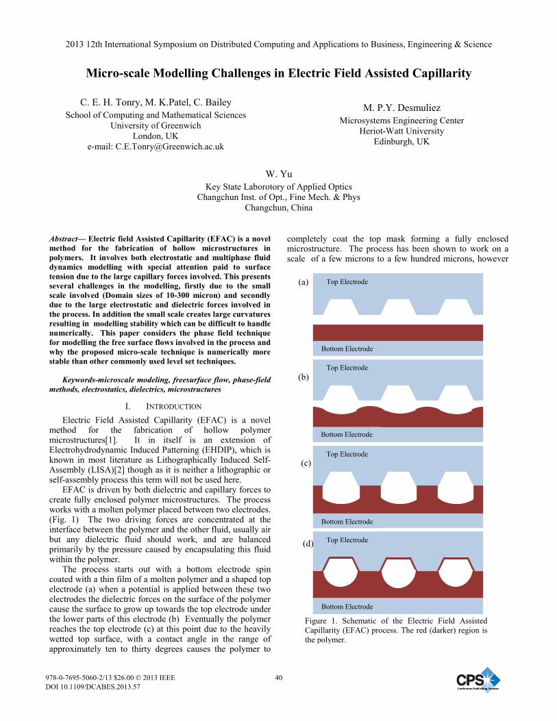
Micro-scale Modelling Challenges in Electric Field Assisted Capillarity

C. E. H. Tonry, M. K.Patel, C. Bailey School of Computing and Mathematical Sciences

University of Greenwich London, UK

e-mail: C.E.Tonry@Greenwich.ac.uk

M. P.Y. Desmuliez Microsystems Engineering Center

Heriot-Watt University Edinburgh, UK

W. Yu Key State Laborotory of Applied Optics

Changchun Inst. of Opt., Fine Mech. & Phys Changchun, China

Abstract— Electric field Assisted Capillarity (EFAC) is a novel method for the fabrication of hollow microstructures in polymers. It involves both electrostatic and multiphase fluid dynamics modelling with special attention paid to surface tension due to the large capillary forces involved. This presents several challenges in the modelling, firstly due to the small scale involved (Domain sizes of 10-300 micron) and secondly due to the large electrostatic and dielectric forces involved in the process. In addition the small scale creates large curvatures resulting in modelling stability which can be difficult to handle numerically. This paper considers the phase field technique for modelling the free surface flows involved in the process and why the proposed micro-scale technique is numerically more stable than other commonly used level set techniques.

Keywords-microscale modeling, freesurface flow, phase-field methods, electrostatics, dielectrics, microstructures

I. INTRODUCTION Electric Field Assisted Capillarity (EFAC) is a novel

method for the fabrication of hollow polymer microstructures[1]. It in itself is an extension of Electrohydrodynamic Induced Patterning (EHDIP), which is known in most literature as Lithographically Induced Self-Assembly (LISA)[2] though as it is neither a lithographic or self-assembly process this term will not be used here.

EFAC is driven by both dielectric and capillary forces to create fully enclosed polymer microstructures. The process works with a molten polymer placed between two electrodes. (Fig. 1) The two driving forces are concentrated at the interface between the polymer and the other fluid, usually air but any dielectric fluid should work, and are balanced primarily by the pressure caused by encapsulating this fluid within the polymer.

The process starts out with a bottom electrode spin coated with a thin film of a molten polymer and a shaped top electrode (a) when a potential is applied between these two electrodes the dielectric forces on the surface of the polymer cause the surface to grow up towards the top electrode under the lower parts of this electrode (b) Eventually the polymer reaches the top electrode (c) at this point due to the heavily wetted top surface, with a contact angle in the range of approximately ten to thirty degrees causes the polymer to

completely coat the top mask forming a fully enclosed microstructure. The process has been shown to work on a scale of a few microns to a few hundred microns, however

Figure 1. Schematic of the Electric Field Assisted Capillarity (EFAC) process. The red (darker) region is the polymer.

(a)

(b)

(c)

(d) Top Electrode

Top Electrode

Top Electrode

Top Electrode

Bottom Electrode

Bottom Electrode

Bottom Electrode

Bottom Electrode

2013 12th International Symposium on Distributed Computing and Applications to Business, Engineering & Science

978-0-7695-5060-2/13 $26.00 © 2013 IEEEDOI 10.1109/DCABES.2013.57

40

Flow Electric Field 1 Slip Wall Symmetry 2 No-Slip Wall 0V 3 Slip wall Symmetry 5 Slip wall 300V 6 Wetted Wall N/A 7 Wetted Wall N/A

12 Wetted Wall 300V 13 Wetted Wall 300V 15 Symmetry Symmetry 16 Symmetry Symmetry 17 Symmetry Symmetry 18 N/A 300V

Figure 2. Mesh, Geometry and Boundary Conditions

1

3 5

6 7 18

12

13 14

17

16

15

2

theoretically it should also work on a nanoscale provided that suitable masks can be produced.

II. GOVERNING EQUATIONS The initial driving force on the polymer is the dielectric

force at the interface between the two fluid. This force, which is concentrated at the interface between the two fluids, can be calculated from the equation for the force on a dielectric[3]:

۴ ൌ ۳ߩ െ ଵଶ ۳ ڄ ۳ ሺଵଶ ۳ ڄ ۳

డఢడఘ ሻ (1)ߩ

The first term in this equation is the electrostatic force due to a charge density ȡ¬f. The second term is due to inhomogeneities in the dielectric constant, as both fluids are considered to have a uniform dielectric constant this only has a value at the interface. The final term is the electrostriction force density this comes from changes in the materials mass density as both fluids are assumed to be incompressible this only has a value at the interface.

The polymer is assumed to be a perfect dielectric it therefore has zero free charge in the bulk material however there will be a charge at the interface due to the change in the dielectric, this can be calculated as[4]:

ߪ ൌ ሺ െ ͳሻ�۳ ȉ ෝ (2)ܖThis equation is a surface charge density and is therefore

an area density; ȡf is however a volume density and so to obtain this the gradient of the free surface variable can be used in place of the unit normal at the interface.

ߩ ൌ ሺ െ ͳሻ�۳ ȉ સ߶ (3) This gives the overall equation for the dielectric force

density at the interface as: ۴ ൌ ሺሺ െ ͳሻ�۳ ȉ સ߶ሻ۳ െ ଵ

ଶ ۳ ڄ ۳ ሺଵଶ ۳ ڄ ۳డఢడఘ ሻ (4)ߩ

The remainder of the governing equations are the defaults used in Comsol. Maxwell’s first equation is solved assuming zero charge to obtain the electric field, Lamina Navier-Stokes is solved for the motion of the fluid and a Phase field free surface method is used for the multiphase flow.

III. MODELING DIFICULTIES Comsol Multiphysics 4.2 has been used for all results

presented here. The model is two dimensional representing an infinitely long micro channel, the symmetry of the problem has also been exploited.

The Electrostatics and Incompressible Phase Field modules were used to model the physics. These were coupled together using the governing equation for the force at the interface listed previously. However there was an issue with implementing this equation directly as for some reason when used in a variable the components of the electric field evaluated to zero, therefore the spatial gradient of the voltage was used in its place.

The electrostatics module was used with zero free charge as both the air and the polymer were assumed to be perfect dielectrics. The Boundary conditions were a high voltage on the top mask, ground on the bottom mask and

41

Figure 4. Evolution of the polymer surface over time

(a) (b)

(c) (d)

symmetry (zero charge) at the sides of the mask these can be seen in Fig. 2.

Modelling two fluids on a microscale can be difficult this is due to the large curvatures caused by the small scales, this can cause conventional level set methods to become unstable. Often this leads to moving mesh being used in similar cases as they tend to be more stable, however this does not allow fluids to recombine which is required in this case. Therefore in this case it was decided to use a phase field method to track the polymer interface. The reason for this is that due to their nature phase field methods are more stable than level set methods for surface tension calculations. This is due to the fact that rather than using an artificial smoothing function such as those used in level set methods to smooth the interface a function is used that is based on the surface energy of the fluid. This surface energy therefore has a direct correlation to the surface tension in the material so the curvature of the material does not have to be calculated separately. This gives the phase field method a more stable calculation method for the surface tension.

In addition to this the electrostatic forces induced cause high velocities for the size of the problem this means that due to the CFL conditions there needs to be a small time step in order to achieve convergence. This can cause some issues as though increasing the viscosity decreases these velocities due to greater viscous drag the timescales involved increase to a greater degree making simulation times very long.

The boundary conditions here were a heavily wetted wall on the top mask, a no slip wall on the bottom mask and symmetry at the sides these can again be seen in Fig. 2.

A mapped mesh was used for the two Lower regions of the mask and a free triangular mesh used for the top part of the mask, this mesh can be seen in Fig. 2. This is the mesh for the geometry of the results presented here; other meshes have also been used to simulate different geometries of different shaped microchannels.

The material properties were that of Polydimethylsiloxane (PDMS) with the exception of the viscosity where an artificially lower viscosity was used to enable the simulation to run in a lower timescale. This was necessary as discussed earlier the CFL conditions mean the time step needed is very small thus the simulation time is too great with a larger viscosity. The properties used can be seen in Fig. 3.

The material properties used for air were the properties from the COMSOL materials library.

(a) (b)

(c) (d)

Figure 5 Evolution of the Electric field over time

Simulation Dynamic Viscosity

(Centipoise)

Specific Gravity (25Ԩ)

Dielectric Constant(100

Hz)

Surface Tension (mN/m)

1000 1.03 2.72 20 Figure 3. Material Properties of PDMS

42

IV. RESULTS The results for the geometry in Fig. 2 can be seen in Fig.

4. These is for a contact angle of 20 degrees on the wetted top mask. The force on the fluid is greater under the profusion of the mask due to the increased electric field, this causes the polymer to flow upwards at these points (a). When the polymer reaches the top mask (b) the surface tension becomes dominant, about an order of magnitude greater than the dielectric forces, this causes the fluid to flow up the mask reaching the corner (c) this continues reaching the middle of the channel and a steady state thus coating the mask (d). This is the general evolution of the flow for complete cases.

The evolution of the voltage (colour) and electric field (streamlines) for the same timesteps as Fig. 4 can be seen in Fig. 5. The higher electric field at the surface under the protrusion in the mask can be seen in these images. Also of note is the changing electric field

The surface is thinner in certain places and this could potentially cause problems. The electron micrograph image of the square capsules in Fig. 6 show similar thin areas though this is for a capsule rather than a channel these areas of thinness are where these capsules have ‘failed’ and have holes in them, both at the top and on the side.

V. CONCLUSIONS As discussed here there have been several modelling

challenges which needed to be overcome in order to produce a working model of the process. The first was the surface tension forces which in this case are very important as part of the process is driven by surface tension in the form of the capillary force. In addition the large electrostatic forces and the corresponding velocities mean that the CFL conditions caused problems with choosing a suitable time step for the problem.

Currently the model ignores the viscoelastic properties of the material involved however it is thought that this will not have a too great an effect on the final solutions. In addition the model as presented here is only two dimensional as the run time for the simulations is already large so a three dimensional version of the model would be very time consuming. It may be possible to develop this

further and include a viscoelastic model and three dimensional model to test whether this is the case.

The model appears to have an agreement with experiment, however there is currently a lack of quantitive experimental data available to compare with, though this is something that is being worked on in order to validate the model against experiments.

ACKNOWLEDGMENT The authors thank the EPSRC for their support in this

work

REFERENCES

[1] 1. H. Chen, W. Yu, S. Cargill, M. K. Patel, C. Bailey, C. Tonry and M. P. Y. Desmulliez, Self-encapsulated hollow microstructures formed by electric field-assisted capillarity, Microfluidics and Nanofluidics, Volume 13, Number 1, 75-82 (2012)

[2] 2. S. Y Chou and L. Zhuang, Lithographically induced self-assembly of periodic polymer micropillar arrays., Papers from the 43rd international conference on electron, ion, and photon beam technology and nanofabrication, Volume 17(6), 3197-3202, 1999

[3] 3. H. H. Woodson and J. R. Melcher, Electromechanical Dynamics, Vol 3: Elastic and Fluid Media; Wiley & Sons: New York, 1968

[4] 4. I.S. Grant and W.R. Philips, Electromagnetism (Second Edition), John Wiley & Sons(Sussex, 1990), pp. 50-70.

Figure 6 Electron Micrograph Image of a circular array of angled microchannels and

square capsules

43

A Modelling and Analysis Tool for Systems with Probabilistic Behavior: Probabilistic Continuous Petri Net

Weizhi LIAO College of Mathematics Physics and Information

Engineering Jiaxing University

Jiaxing , China e-mail:weizhiliao2002@aliyun.com

Wenjing LI, Zhenxiong LAN College of Computer and Information Engineering

Guangxi Teachers Education University Nanning, China

e-mail:liwj@gxtc.edu.cn

Abstract—So far, Continuous Petri nets (CPNs) have been a useful tool not only for approximating discrete-event system but also for modeling continuous processes. In applications there exist many continuous dynamic systems which have to deal with probabilistic behavior. However many CPNs as described in the literature are not able to model probabilistic continuous systems.. In this paper, the CPN is augmented with firing probability, and a noel continuous Petri net, i.e., the probabilistic continuous Petri nets (PCPNs) is defined. The enabling and firing semantics of transitions of the PCPN are investigated, and the calculation of IFSs and its firing probability are developed. Some polices and algorithms to undertake PCPN behavioral analysis are proposed. Also, a chemical process is illustrated.

Keywords- Continuous Petri nets; continuous dynamic systems; probability; instantaneous firing speed

I. INTRODUCTION Petri nets, as a graphical and mathematical tool, provides a

powerful and uniform environment for modeling, analysis, and design of discrete event systems [1]. One of the major advantages of using Petri nets is that the same methodology can be used for the modeling, qualitative and quantitative analysis, supervisory and coordinative control, planning and scheduling, and system design in system. In order to efficiently handle discrete event systems in which there exists considerable states and events, David and Halla defined a continuous Petri net(CPN)[2,3]. The main differences between the CPN and the classic Petri nets are nonnegative real number markings of places and continuous firing of transitions at some speed. Instantaneous firing speeds (IFSs) of transitions play an important role in the evolution of a CPN, which is specified uniquely by either a maximal constant speed or a maximal variable speed. Due to different ways of calculating IFS of transitions, various continuous Petri net models, such as the CCPN[3], the VCPN[4], and the ACPN[5] were developed. To approximate continuously the dynamics of time Perti nets, Interval speed CPN’s (ICPN’s) which constraints of maximal and minimal firing speed was defined and the semantics for

-----------------------------------------------------------------------

* Supported by the National Natural Science Foundation of China (61163012), Guangxi Natural Science Foundation (2012GXNSFAA053218)

transition’s enabling and firing were presented [6,7]. All these continuous Petri nets can be used to model situations where the underlying physical processes are continuous nature.

In order to model and analysis system with uncertainty behavior, related Petri nets were presented. Stochastic timed Petri nets associate to each transition, a probability distribution which represents the delay between the enabling and firing of the transition[8]. Fuzzy Petri nets are used to represent fuzzy rules between propositions [9]. Probabilistic Petri net is proposed to model and analysis vision-based systems which have to deal with ambiguities and inaccuracies in the lower-level detection and tracking systems [10]. However, the aforementioned versions of Petri nets are not suited to deal with those continuous dynamic systems with probabilistic behavior.

Owing to the fact that many continuous dynamic systems which have to deal with probabilistic behavior, the probabilistic continuous Perti net (PCPN) is proposed here. In a PCPN, the enabled transition would be fired with probability. Due to constraints on firing probability, the PCPN require more subtle and complicated semantics for firing transition. In order to analyze the dynamic behavior of PCPNs, the computation of IFSs and its firing probability are developed. In addition to that, as a novel tool for modeling and analyzing continuous systems, several illustrative examples are given.

The remainder of the paper is organized as follows: In Section 2, the formalism of PCPNs is presented and the semantics of enabling and firing are discussed. Section 3 deals with the computation of IFSs and its firing probability, conflict resolution policies, and related algorithms to undertake PCPN behavioral analysis are developed. The demonstrated example of a chemical process is given in Section 4. The paper concludes in Section 5.

II. FORMALISM OF PROBABILISTIC CONTINUOUS PETRI NET

In this section , we define a probabilistic continuous Petri

net as the tuple PCPN=(P, T, W, V, Fprob), where the common formalism and notion of CPNs and ICPNs are adopted.

2013 12th International Symposium on Distributed Computing and Applications to Business, Engineering & Science

978-0-7695-5060-2/13 $26.00 © 2013 IEEEDOI 10.1109/DCABES.2013.15

44

Definition 1 A Probabilistic Continuous Petri Net is a 5-tuple: PCPN=(P, T, W, V, Fprob), where

• P={ p1, p2, p3,…, pn } is a set of continuous places; • T={ t1, t2, t3,…, tm } is a set of continuous transitions; • P!T="; i.e. the sets P and T are disjointed; • W: (P# Td)$(Td #P) %Z+ is the weight mapping for

arc • V: T R+ is the maximum firing speed mapping. The

speed V(ti)=Vj corresponds to the maximum firing speed of transition ti.

• Fprob: T [0,1] is the firing probability mapping. The probability Fprob(tj)=fj corresponds to the firing probability of enabled transition tj.

The enabling of continuous transitions in PCPNs depends not only on the current marking, but also on the feeding flow of all its input place

Definition 2 A place pi&P is supplied or fed if and only if there is at least one of its input transitions tj&pi which is being fired at a positive speed v(tj)>0.

Property 1 Given •pi={1j

t ,…, 1njt } and the marking of

place pi is zero, then the supplied probability of place pi (denoted by Supplied_Prob(pi)) is equal to 1–

))t(Fprob( dnj

jd'(

=1

1

1,where )t(Fprob j1 ,…, )t(Fprob nj 1

is

the firing probability of transition 1j

t ,…,1njt respectively.

Definition 3 A transition tj&T is enabled at time ) if all input places pi&•tj satisfy that either mi())>0, or pi is supplied, otherwise, the transition is disabled.

Definition 4 A enabled transition tj&T is called as strongly enabled at time ) if all input places pi&•tj satisfy mi())>0.

Definition 5 A enabled transition tj&T is called as weakly enabled at time ) if at least one of its input places pi&•tj doesn’t satisfy mi())>0.

Property 2 Strongly enabled transition tj&T can be fired at the instantaneous firing speed v(tj)=Vj with the probability Fprob(tj).

Property 3 Weakly enabled transition tj&T can be fired at the instantaneous firing speed vj()) with the probability

Fprob(tj)· )P(obPr_Supplied dhk

nkd

2

1=( , where

•tj={1kp ,…,

1hkp ,1nkp ,…,

2hkp }, *pi1&{1kp ,…,

1hkp }

satisfy mi1())>0 and *pi&{1nkp ,…,

2hkp } satisfy mi())=0..

III. BEHAVIORAL ANALYSIS OF PCPNS

A. conflict resolution Definition 6 A conflict occurs when pi&P has at least two

transitions. We denote a conflict by K=<pi,t| t&pi•>. A conflict

is effective with the probability )t(Fprob jj

( (tj&pi•) if the

following conditions are met:

(1) mi())=0;

(2) For any transition tk&•pi, it satisfy that tk has the firing speed vk());

(3)0<! )+k

)(kv)ip,kt(W < jj

ji V)t,p(W! .

Property 4 An effective conflict K=<pi,t| t&pi•> can be

resolved by one of the following policies:

(1) Priority of policy:

vj())=min(Vj, ( ! )+k

)(kv)ip,kt(W – rjr

ri V)t,p(W!>

)), here r>j

corresponds to all transitions that are in pi• and have priority

over tj.

(2)Proportional policy:

vj())=min(Vj, (Vj·! )+k

)(kv)ip,kt(W / rr

ri V)t,p(W! )).

(3) Average policy:

vj())=min(Vj, ! )+k

)(kv)ip,kt(W /d), here is d equal to | pi•|.

Proposition 1 If there exist feasible IFSs for an effective K=<pi,t|& pi

•> by the priority policy, then

rr

ri v)t,p(W! ())!! )+k

)(kv)ip,kt(W , *tk&•pi *tr&pi•

Proposition 2 If there exist feasible IFSs for an effective K=<pi,t|& pi

•> by the proportional policy, then

0< rr

ri v)t,p(W! ())! rr

ri v)t,p(W! , *tk&•pi *tr&pi•

Proof. According to the proportional policy, any feasible instantaneous firing speeds vr()) for every tr&pi

• must satisfy

vr())!! )+k

)(kv)ip,kt(W / rr

ri V)t,p(W!

Thus

rr

ri v)t,p(W! ! jj

ji V)t,p(W! "! )+k

)(kv)ip,kt(W /

rr

ri V)t,p(W!

=! )+k

)(kv)ip,kt(W

By Definition 6, we have

45

0<! )+k

)(kv)ip,kt(W

Hence

rr

ri v)t,p(W! ())!! )+k

)(kv)ip,kt(W

If

Vr·! )+k

)(kv)ip,kt(W / rr

ri V)t,p(W! >0

Then

vr())>0 Thus

rr

ri v)t,p(W! >0

Let us consider the PCPN presented in Figure 1. A conflict situation can arise because place p1 have two output transitions i.e. t2 and t3. If m1>0, there is no effective conflict since transition t2 can be fired maximal speeds with the probability Fprob(t2), and t3 can be fired maximal speeds with the probability Fprob(t3). If m1=0, transition t1 supplies the place p1 with a quantity v1dt during dt (0<v1 !V1) with the probability Fprob(t1). If v1 is such that 0<v1<V2+V3, there is an effective conflict with the probability Fprob(t2)·Fprob(t3) since transitions t2 and t3 can not be fired with its maximal speed at same time. The behavior of the PCPN is such that v2!V2, v3!V3 and v2+v3= v1. According to the proposed solution policies, the firing speed is determined as follows: (1) Priority of policy: Given the priority of transition t2 is

higher than t3 , we have v2=min(V2, v1), v3= v1–min(V2, v1). (2) Proportional policy: In this case, we have v2=

v1·V2/(V2+V3), v3= v1·V3/(V2+V3).

(3) Average policy: Since | p1•|=2, thus v2=v3=v1/2.

B. Enabled Transition and Their IFS We could not know whether or not a transition is enabled from Definition 5. A feasible method to determine the set of enabled transitions would be considered in this section first. We use ai to denote whether or not a place pi is marked or supplied and ej to denote whether or not a transition tj is enabled. If a place pi is marked or supplied, ai=1, otherwise ai=0. If a transition tj is enabled, ej=1, otherwise ej=0. We finish up with a system of equations of the fixed point: ai is equal to1 if pi is supplied or marked, otherwise

ai=max{ej|tj&•pi}; ej is equal to 1 if •tj=", otherwise ej=min{ai|pi&•tj}. In order to calculate the set of enabled transitions, an algorithm is proposed as follows: Algorithm 1 Calculation of the enabled transitions for PCPN

Step1 Initialization: r=0,(a1r,…, an

r), (e1r,…, em

r). Step2 If pi is marked, then ai

r+1=1, else air+1=

max{ejr|tj&•pi}.

Step3 If •tj=", then ejr+1=1, else ej

r+1=min{air+1|pi&•tj}.

Step4 If (a1r+1,…, an

r+1)=(a1r,…, an

r) and (e1r+1,…, em

r+1)= (e1

r,…, emr), then r=r+1 and go to Step2.

Step5 End. Given the number )(r

kv is the value of speed kv obtained at the iteration step number r. At each step, the following calculation is performed, where kiW is an element of the incidence matrix:

(1) If *pi&•tj, there satisfy mi>0 then )1( +rjv =Vj;

(2) If pi•={ tj } and mi=0 then transition tj obtains the speed

from place pi at step r+1 is denoted by vji r+1 and vj

i r+1

=min{Vj, }vWus

uk)r(

kki!=

+1

, where •pi={tu1, , tus}

(3) If pi•={tj1, ,tjd} and mi=0 then transition tj obtains the

speed from place pi at step r+1 is calculated as following

(a) If !=

+us

uk

rkki vW

1

)( >=Vj1 + Vj2 +…+ Vjd, then

vj1i r+1 = Vj1 vj2

i r+1 = Vj2 … vjdi r+1 = Vjd

(b) If 0<!=

+us

uk

rkki vW

1

)( <Vj1 + Vj2 +…+ Vjd with the average

policy then

vj1i r+1 =min{Vj1, }/

1

)(!=

+us

uk

rkki dvW

vj2i r+1 =min{Vj2, }/

1

)(!=

+us

uk

rkki dvW

…

vjdi r+1 =min{Vjd, }/

1

)(!=

+us

uk

rkki dvW

(c) If 0< !=

+us

uk

rkki vW

1

)( <Vj1 + Vj2 +…+ Vjd with the

proportional policy then

vj1i r+1 =min{Vj1, }!

= !=

++us

uk d

kjk

j)r(kki

V

VvW

11

1

vj2i r+1 =min{Vj2, }!

= !=

++us

uk d

kjk

j)r(kki

V

VvW

11

2

…

Fprob(t3) Fprob(t2) m1 p1

t2 t3 V2 V3

t1 V1

Fig.1. A conflict situation

46

vjdi r+1 =min{Vjd, }!

= !=

++us

uk d

kjk

jd)r(kki

V

VvW

11

(d) If 0<!=

+us

uk

rkki vW

1

)( <Vj1 + Vj2 +…+ Vjd with the priority

policy then

vj1i r+1 =min{Vj1, }!

=+

us

uk)r(

kki vW1

vj2i r+1 =min{Vj2, })r(i

jus

uk)r(

kki vvW 111

+!=

'+

…

vjdi r+1 =min{Vjd, }!

'

=+!

='+

1

11

1

d

c)r(i

cus

uk)r(

kki vvW

where j1>j2>…>jd.

(e) If !=

+us

uk

rkki vW

1

)( =0 then

vj1i r+1 = vj2

i r+1 =,…,=vjdi r+1 = 0

Thus, we have

)1( +rjv =

"#

"$% >&*

+++

•

otherwise,v,,vmin{vm,tpifV

1)ih(rj

1)i2(rj

1)i1(rj

ijij

}!0

Where mi1=0, mi2=0, , mih=0 respectively.

Algorithm 2 Calculation of the IFS of enabled transitions Step1 Initialization v=0 and r=0. Step2 Calculation of vr+1 by formula (1). Step3 If vr+1 vr, then r=r+1 and go to Step2. Step4 End.

C. Behavioral Analysis The marking of a place in probabilistic continuous Petri net is a time continuous function. A characteristics quantity of the dynamic evolution of PCPNs is instantaneous firing speeds vector with probability, which remains constant in a invariant behavior (IB) state.

Definition 7 An invariant behavior state is defined as (M, V, prob, [!1,!2]), where M is the marking vector of all places, V is the instantaneous firing speeds vector of all transitions and prob is the firing probability with V, which remain unchanged in time interval [!1,!2].

Similarly to CPNs and ICPNs, the behavioral evolution of probabilistic continuous Petri net is driven by discrete events which a continuous place becomes empty. Thus the duration of time interval [!1,!2] in an invariant behavior state is determined by the first place whose marking become zero, i.e., #k=!k–!k-1 is given by

#k=i

min (mi(!k-

1)/ |)(v)t,p(W)(v)p,t(W|j j

kjikij! ! '' )+')+ 11 )

Since an enabled transition in PCPNs has the probabilistic behavior, there are many possible firing speed vectors at the same marking vector. In Algorithm 3, a method to calculate all

possible firing speed vectors and its firing probability were developed. Algorithm 3. (Behavioral Analysis of PCPN) Step1. Initialization: k=1, !k=0, Mk. Step2. If V(!k+1)=V(!k) then go to Step6. Otherwise, using

Algorithm 1 and Algorithm 2, calculate enabled transition set E and IFS vector V based on vector Mk.

Step3. Given E=(e1,…, em) and V=(v1,…, vk1, vk2,…,vm), where v1,…, vk1>0 and vk2=…=vm=0. Calculate all possible firing speed vectors and its firing probability based on Mk (denoted by IBS): IBS( 11 kx,,x ! )=[(v1

*, …, vk1*, vk2

*,…,vm*)(prob)]

Where 0,+'+! !j j

*jji

*jij v)t,p(Wv)p,t(W if mi=0, and

xj & {0,1},1!j!k1, v1*= 1x ·v1, …, vk1

*= 1kx ·vk1, vk2

*=…vm*=0, and prob is calculated as following:

Initialization: prob=1; For j=1 to m do If ej=2 and xj=1 then prob= prob"Fprob(tj);

If ej=2 and xj=0 then prob= prob"(1–Fprob(tj)); If ej=1 and vj can be obtained from (xj1·vj1, …, xjy·vjy) then

If xj=1 then prob= prob"Fprob(tj); If xj=0 then prob= prob"(1–Fprob(tj));

Where the value of vj is determined by vj1, …, vjy. Step4. Select the IBS which has the maximal firing probability

from all possible firing speed vectors and Calculate time interval based on the IBS

#k=i

min (mi(!k-

1)/ |)(v)t,p(W)(v)p,t(W|j j

kjikij! ! '' )+')+ 11 )

Step5. Calculate the marking vector at time !k+1 (Mk+1): mi(!+#k)=

mi(!)+( ! ! '' )+')+

j jkjikij )(v)t,p(W)(v)p,t(W 11 )·#

k, k=k+1 and go to Step2. Step6. End.

Let us consider the PCPN of Fig.2(a), there are two places i.e. p1, p2 and two transitions i.e. t1, t2, where m1=2, m2=1, V1=1, V1=1/3, Fprob(t1)=0.9 and Fprob(t2)=0.8.At initial time i.e. !0=0, since m1=2>0, m2=1>0(the initial marking vector of place is denoted by M0=(2,1)), thus transition t1 can be fired at maximal speed (i.e. 1) with probability 0.9, and t2 can be fired at maximal speed (i.e. 1/3) with probability 0.8. So t1 and t2 can be fired with maximal speed at the same time (!0=0) with probability 0.9"0.8, i.e. 0.72 under M0, denoted by IBS11=[(1,1/3)(0.72)]. Also, we have the others firing vectors including IBS00=[(0,0)(0.02)], IBS10=[(1,0)(0.18)] and IBS01=[(0,1/3)(0.08)] under the marking vector M0. In these firing vectors, we could find

that !=

1

0j,iijIBSprob )( =0.72+0.02+0.18+0.08=1 and IBS01 has

the maximal firing probability. Thus, the initial firing vectors [(1,1/3)(0.72)] is selected to be driven ,the evolution of the

47

markings of the two places is governed by the following equation system in time interval [0, !1):

#$%

'+=+''=+

d!)VV(!md!!md!)VV(!md!!m

2122

2111)()(

)()(

If m1(!)>0 and m2(!)>0, the two equations remain true. At time !1=m1(0)/(1–1/3)=3, place p1 becomes empty i.e. m1(3)=0. At time !1=3, we have M1=(0,3), since m2=3>0, t2 can be fired at maximal speed (i.e. 1/3) with probability 0.8. However, since m1=0, t1 can’t be fired at maximal speed (i.e. 1) with probability 0.9. In fact, t1 and t2 can be fired with the speed of 1/3 at the same time (!1=3) with probability 0.9"0.8, i.e. 0.72 under M1, denoted by IBS11=[(1/3,1/3)(0.72)]. Also, we have the others firing vectors including IBS00= [(0,0)(0.2)] and IBS01=[(0,1/3)(0.08)] based on M1. Since IBS11 has the maximal firing probability. Thus, the second firing vectors [(1/3,1/3)(0.72)] is driven, the evolution of the markings of the two places is governed by the following equation system in time interval [3, !2):

#$%

='+=+=''=+

)()()()()()(!md!)//(!md!!m

!md!)//(!md!!m222

1113131

3131

According to these equations, from time !1=3, we have v1= v2=1/3 and m1(!)=0 and m2(!)=3. The dynamic marking balance of any place is equal to 0. A steady state of the PCPNs is found to have been reached. Similarly to CPNs, the behavior of the PCPN can be represented by an evolution tree, given in Fig.2(b). In this tree, described in the form of PN, each node represents a constant instantaneous firing speeds vector (v1, v2) and firing probability of (v1, v2). Each transition is associated the marking whose occurrence produces a changeover from one instantaneous firing speeds vector to another. Thus the IFS vector (1,1/3) and firing probability (0.72) is associated with the initial marking. When marking vector M1 is reached, the IFS vector becomes (1/3,1/3) and firing probability becomes (0.72). The terminal node represents the steady IFS vector. According to the evolution tree, we can compute the probability of the steady IFS vector (1/3,1/3) which is reached. The probability is equal to 0.72"0.72, i.e. 0.5184.

IV. CHEMICAL PROCESS EXAMPLE

A chemical process with 4 units and 4 machines is shown in Figure 3(a). Two kinds of materials are processed in unit 1 and unit 2 respectively, and then fed to units 3. The feed flow from unit 1 to unit 3 through machine M1 (Operation with probability 0.9) is limited within [0,3], and the feed from unit 2 to unit 3 through machine M2 (Operation with probability 0.85) within [0,5]. Intermediate product is fed from unit 3 to unit 4 through machine M3 (Operation with probability 0.9) at a flow of [0,6]. There are two output flows of unit 4, one is the final product flow at speed of [0,4] through machine M4 (Operation with probability 1.0), and the other is the recycled flow to unit 3 through machine M5 (Operation with probability 0.8) at speed of [0,2]. The capacity of unit 3 is limited by 30, and its initial volume is 10. We assume that unit 1 and unit 2 have the sufficient materials for machine M1 and machine M2. This process can be modeled as the PCPN shown in Fig.3(b). From the PCPN model, we can analyze the dynamic as follows: At initial time, we have M0=(10,20,0), .i.e, m1(0)=10, m2(0)=20, m3(0)=0. Thus transition t1, t2 and t3 are strongly enabled transition, and t4, t5 are weakly enabled transition. All possible firing speed vectors and its firing probability based on M0 as follows: IBS00000=[(0,0,0,0,0)(0.0015)], IBS00110=[(0,0,6,4,0)(0.0027)], IBS00111=[(0,0,6,4,2)(0.0108)], IBS01000=[(0,5,0,0,0)(0.0085)], IBS01110=[(0,5,6,4,0)(0.0153)], IBS01111=[(0,5,6,4,2)(0.0612)], IBS10000=[(3,0,0,0,0)(0.0135)], IBS10110=[(3,0,6,4,0)(0.0243)], IBS10111=[(3,0,6,4,2)(0.0972)], IBS11000=[(3,5,0,0,0)(0.0765)], IBS11110=[(3,5,6,4,0)(0.1377)], IBS11111=[(3,5,6,4,2)(0.5508)].

Fprob(t1)=0.9

m2=1

Fprob(t2)=0.8

p2

m1=2 p1

t2

V1=1 t1

V2=1/3

Fig.2(a). A PCPN

!1=3 M1=(0,3)

(1/3,1/3) (0.72)

Fig.2(b). evolution tree

M0=(2,1) !0=0

(1,1/3) (0.72)

(0,0) (0.02) (1,0) (0.18)

(0,1/3) (0.08)

(0,0) (0.2) (0,1/3) (0.08)

48

Since the firing probability of IBS11111 is maximal, the PCPNs would be fired with the firing speed vector (3,5,6,4,2). In this case, from time !=0, the PCPN’s behavior is governed by the following equations

"#

"$

%

='=

+=

0420

410

3

2

1

)()()(

!m!!m!!m

At time !=5 we have M1=(30,0,0), i.e. m1(5)=30, m2(5)=0, m3(5)=0. Transition t3 is still strongly enabled, and the others transitions are weakly enabled. There exits an effective conflict K={p2, t1, t2 , t5}. In this example, the conflict solution is proportionally policy. All possible firing speed vectors and its firing probability based on M1 as follows: IBS00000=[(0,0,0,0,0)(0.1)], IBS00110=[(0,0,6,4,0)(0.0027)], IBS00111=[(0,0,6,4,1.2)(0.0108)], IBS01110=[(0,3,6,4,0)(0.0153)], IBS01111=[(0,3,6,4,1.2)(0.0612)], IBS10110=[(1.8,0,6,4,0)(0.0243)], IBS10111=[(1.8,0,6,4,1.2)(0.0972)], IBS11110=[(1.8,3,6,4,0)(0.1377)], IBS11111=[(1.8,3,6,4,1.2)(0.5508)]. Since the firing probability of IBS11111 is maximal, the PCPNs would be fired with the firing speed vector (1.8,3,6,4,1.2). In this case, from time !=5, the PCPN’s behavior is governed by the following equations

"#

"$

%

===

0030

3

2

1

)()()(

!m!m!m

It means that the dynamic marking balance of any place is equal to 0 and the steady state of process is reached, and we have an important conclusion that the probability of steady state (V=(1.8,3,6,4,1.2),M=(30,0,0)) which the chemical process reached is 0.3034.

V. CONCLUSION There has been extensive work in continuous Petri nets (CPNs) on the problem of modeling and analyzing discrete and continuous dynamic systems. Numerous CPNs have been developed. However, the proposed versions of Petri nets are not suited to deal with those continuous dynamic systems with probabilistic behavior. In this paper, the concept of a probabilistic continuous Petri nets is developed. Also, the behavioral analysis of PCPNs is investigated. As demonstrated by case study, the continuous dynamic system with probabilistic behavior has been efficiently modeled and analyzed by PCPNs.

Future work may focus on two important problems. First, more theoretical foundation regarding net dynamics and structural properties of PCPNs are needed to be established. Second, the control and optimization of continuous and hybrid processes with probability behavior via PCPNs is under way.

REFERENCES

[1] Murata, T. Petri nets: properties, analysis and applications. Proceedings of the IEEE, 77, pp.541-580, 1987.

[2] R.David, H.Alla. Continuous Petri Nets. Proceedings of the 8th Europeab Workshop on Application and Theory of Petri Nets(Saragossa, Spain), 1987, 275-294.

[3] H. Alla, R. David,A Modeling and Analysis Tool for Discrete Event Systems: Continuous Petri Nets, Performance Evaluation, (33),pp.175-199, 1998.

[4] R.David, H. Alla, Autonomous and Timed Continuous Petri Nets, Advances in Petri Nets 1993, G. Rozenberg Ed., Springer-Verlag, Berlin, 1993, pp. 71-90.

[5] J. LE Ball, H. Alla, R. David. Asymptotic Continuous Petri Nets. Discrete Event Dynamic Systems: Theory and Applications.1993, (2):235-263.

[6] Tianlong Gu, Rongsheng Dong, Yu-Chu Tian,Continuous Petri Nets Augmented with Maximal and Minimal Firing Speeds, International Conference on Systems ,Man and Cybernetics SMC2003,Vol.2,pp.1493-1498.

[7] Tianlong Gu, Rongsheng Dong. Novel Continuous Model to Approximate Time Petri Nets: Modeling And Analysis. Journal of Application Mathematic and Computer Science, 2005,15(1): 141-150.

[8] M. A.Marsan, G.Balbo, G.Chiola. An Introduction to Generalized Stochastic Nets. Microelectronics and Reliability,1991,31(4): 699-725.

[9] S.-M. Chen, J.-S. Ke, J.-F. Chang. Knowledge Using Fuzzy Petri Nets. IEEE Trans. Inf. Theory, 1990,2(3):311-319.

[10] M.Albance, R.Chellappa,V.S.Subrahmanian. A Constrained Probabilistic Petri Net Framework For Human Activity Detection Video. .IEEE Transition on Multmedia, 2008,10(8):1429-1443.

[0,3]

[0,4] [0,6]

[0,2]

[0,5]

1

2

3

4 M1

M2

M5

M3

M4

Fig.3 (a) A chemical process

p3

Fig.3 (b) The PCPN of chemical process

Fpro(t3)=0.9 Fpro(t1)=0.9

Fpro(t2)=0.85

V3=6 t3

t4 V4=4

Fpro(t4)=1

p2

p1

V1=3 t1

V5=2 t5 V2=5 t2 Fpro(t5)=0.8

202

10

49

Research on Petri nets parallelization the functional divided conditions

Wenjing LI, Shuang LI, Zhong-ming Lin College of Computer and Information Engineering

Guangxi Teachers Education University Nanning, China

e-mail:liwjgood@126.com

Weizhi LIAO College of Mathematics Physics and Information

Engineering Jiaxing University Jiaxing , China

e-mail:weizhiliao2002@yahoo.com.cn

Abstract— In order to solve the parallel algorithm for Petri nets system with concurrent function, to realize the parallel control and execution of the Petri nets, the Petri nets parallel subnets conditions were proposed, that provides the theory basis for judging P- invariant whether was the parallel subnet. Firstly, we according to the concurrent character of Petri net model, to analyze the parallelism of Petri net system, P- invariants the solving process and it's subnet division were given; Secondly, the Petri nets parallel subnets conditions were proposed, gives P- invariant constituted of Petri net parallel subnets decision theorem , and the theoretical proof and example verification; Finally, A Petri net parallel subnet division algorithm based on P- invariants were given. Theoretical validate and experimental result shows that Petri nets parallel subnets conditions set and divided algorithm were correct and effective.

Keywords-Petri nets; P-invariant; parallel subnet; divided condition; division algorithm

I. INTRODUCTION At present, different application areas established a

high-level Petri net, time Petri net, fuzzy and complicated with hybrid Petri net model in various forms, and the static analysis and the research on its structure, behavior, function etc. However, through the simulation, animation or parallel operation way for the realization of Petri net system behavior, function, dynamic performance test results lack. Therefore, research on the parallelization of the Petri net, has a very important significance. While the in Petri nets parallel process, division the parallel subnets conditions setting and determination P-invariants meets the parallelization condition is the key. When searching Petri nets parallel and its subnets division problem, the reference [1] provides a centralized method in P/T network, the method to scan each transition model, to check the transitions’ trigger, but it can't keep parallel model; reference [2] proposed decentralized approach in colored Petri nets. The method fully focus on the distributed execution, through the process to achieve each place and change, It maintains parallel models, but when the network scale becomes large, a large number of color sets of elements, its efficiency is very low, reference [3] proposed -------------------------------------------------------------------------

* Supported by the National Natural Science Foundation of China (61163012) ;Guangxi Natural Science Foundation (2012GXNSFAA053218); the University Scientific Research Project of Guangxi(2013YB147)

place invariant parallel technology, which applies to the subnet there is a positive place, but there are two deficiencies: Not given the subnets were all empty place parallelization conditions; and not give a solution to solve parallel problem when the Petri nets doesn’t exist place invariants. So, we search the parallel subnets division condition in process of parallelization Petri nets model, provide efficient partitioning strategy for design and implementation of parallel algorithms in Petri network.

II. PETRI NETS AND P-INVARIANTS PARALLEL ANALYSIS

A. The Petri nets concurrent analysis Petri nets model can be represented graphically, also

use algebra measures, the basic concept can reference literature [4 -5].

Used Petri nets model to system set up its model, can clearly be seen that the initial distribution and movement of system resources, and seen the various operations internal logic relationship within system. The behavior of the net system directly reflects the sequential relationship between the system transition and concurrent relationships, network’s elements (transition and place elements) constitute a partial order set, when in partial order set not two elements of sequential relationship is concurrently. Petri nets system concurrency including :( 1) Independent occurrence of P/T net transitional. If any transitional t in the net meet |·t|=|t·|=1, that is when the transition has only one input and one output place. The transitional is a local behavior or local action, it can occur independently.(2) Concurrent execution of P/T net transition. If any two translations of net t1and t2, There is a mark M, let M[t1>M1!M1[t2> and M[t2>M2!M2[t1>, The two transitional of t1 and t2 are concurrent, they do not influence each other.(3) Conflict place of P/T net. If the place of the net |p•|"2, that is more than two output transitions, so, that place is a conflict place. Conflict place is a shared resource of output transitional.(4) Conflict transition of P/T net. If any two translations of net t1 and t2, There is a mark M let M[t1>M1!M1[t2> and M[t2>M2!M2[t1>, the transition of t1and t2 in conflict the mark M. While two transitions have the conflict in one occurs, another transition will lose

2013 12th International Symposium on Distributed Computing and Applications to Business, Engineering & Science

978-0-7695-5060-2/13 $26.00 © 2013 IEEEDOI 10.1109/DCABES.2013.16

50

concession. The converse is also true. we can by applying an external control to solve the conflict problem, add the place pa and pb, Let pat1pbt to form a control loop, the conflict of t1and t2 would be eliminated[6][7].(5) Confusion transition of P/T net. If there is a transition occur in the network, it will make other two transition conflict, it is called P/T net confusion that the concurrency and conflict interaction.

B. P-invariants and Petri nets division P-invariant and its branch set of definitions and the

theorems of solving the P-invariants are as follows: Definition 1[1] Let N= (P,T;F) is a nets, |P|=m, |T|=n, D is a associated matrix of N. If exist a non-trivial m-

dimensional non-negative integer vector X satisfies DX=0, then X is an invariant place of the N net.

Definition 2[1] Take X is an invariant place of net N=(P,T;F),then ||X||={pi P|X(i)>0} is invariable place of branches set.

Theorem 1 If m-homogeneous linear equations DX = 0 have the zero solutions necessary and sufficient condition is rank r (D) <m.

Theorem 2 m-homogeneous linear equations DX = 0 only the zero solutions necessary and sufficient conditions is rank r (D) = m.

According to definition1, theorem1 and theorem2 the manually calculate P-invariants to steps as follows:

(1) According to the Petri net model get the initial output matrix D+=[dij

+] and input matrix D—=[dij-];

(2) According the formula D=D+ -D— to get the associated matrix of Petri nets model;

(3) Solution the homogeneous linear equations DX=0; (4) Calculate P-invariant and its branch sets. Example 1, Petri nets model ! show in Figure 1,

solving P-invariant and its invariant branch sets.

Fig.1 Petri net model !

Petri nets ! incidence matrix D1:

1D

! "# $# $= # $# $# $% &

-1 1 0 01 -1 1 -10 0 -1 10 0 -1 1

Solution the homogeneous linear equations D1X=0, X1=[1,1,0,0]T X2=[0,0,1,1]T X3=[1,1,1,1]T

X4=[0,0,0,0]T, their are conform the definition1,is P-invariant of ! network; By definition2 known ||X1||={p1,p2},||X2||={p3,p4},||X3||={p1,p2,p3,p4} all is P-invariant branch sets of ! network.

Subnets divided of Petri nets models. From the P-invariant defined and Example 1 have known four P-invariants, but only the P-invariant branch set X1 and X2 can divided Petri nets model into two subnets. Being subnet {||X1||, T1, M} contains the places and transitions {p1, p2, t1, t2}, subnet {||X2|| T2 M} contains the places and transitions { p3,p4,t2,t3,t4}, t2 is two subnets sharing transition. As a result, we can get the Petri nets system is divided into several subnets, subnets method which is based on the P-invariant Petri nets. Between subnet is divided them can execute concurrently, and can also be executed in parallel. Between the subnet different transition there is order, concurrency, conflict, parallelism, and other circumstances.

III. PETRI NET PARALLEL SUBNETS DIVISION CONDITION From the solving place invariants results can be seen

that maybe have several N net place invariants, and the net can constitute a collection !. But the basic division conditions which ! set elements of P-invariant maybe constitute to a Petri nets model, otherwise, will not become subnet. Otherwise, P-invariant will not become the subnet of Petri nets. Likes: ||X4||=#. While the P-invariant branch set whether constitute the individual functions process (subnet) of Petri nets, to solving the problem key is division conditions and principles, below we will discuss how divided the parallel subnets conditions of Petri nets.

A. The condition of P-invariant branch set transition into subnet

Assuming Petri net N= (P,T;F,K,W,M), where |P|=m|T|=n its P-invariants set is =!={ X1 X2 …, Xm} the branch set is !p={ X1 X2 …, Xr}, then the condition of P-invariant branch set transition into Petri nets subnet as follows:

(1) For any element Xi in branch set !p of P-invariant set, if ||Xi||$" or ||Xi||$P, then maybe is parallel subnets of Petri nets. That #Xi !p ,have ||Xi||$" or ||Xi||$P then maybe is parallel subnets;

(2) For any element Xi in branch set !p of P-invariant set, and ||Xi||$" or ||Xi||$P, it place pi ||Xi||={pi P|X(i)>0} must have the input and output transition, and the input and output arcs weights are equal to 1. Expressed as: #Xi !p

#pi ||Xi||,$(t,t") pi • % •pi and w(pi,t)= w(t’, pi)=1

(3) For any element Xi in branch set !p of P-invariant set, its subnet all place contains at least one token, otherwise, the Petri nets can’t run. That ( ) 1i

i iM p

p X' %

&;

(4) If !c is a subnet division which from branch set !p elements of Petri nets !p, then !c only contains all transition of the prototype network. Expressed as:

( ( ))1

cp p Tjji j Xi

'• •( =

= &! !

51

(5) In the sub division branch net not exist sharing place, that: #Xi Xj !c || Xi||%|| Xi||=".

B. The judgment theorem of Petri nets parallel subnet Based on the above analysis, the branch set of P-

invariant divided parallel subnet conditions can be obtained by theorem 3.

Theorem 3 If !p is a place invariant set in Petri net N= (P, T; F, K, W, M), o, in !p corresponding element of the subnet meet the following conditions, follow these subnets get the having individual functions parallel processes with Petri nets.

#Xi !p such that|| Xi||$" or || Xi||$P then Xi maybe the parallel subnet (2.1) #Xi !p #pi ||Xi||,$(t,t") pi

• % •pi and w(pi,t)= w(t’, pi)=1 (2.2)

( ) 1ii i

M pp X

' %&

(2.3)

#Xi Xj !c || Xi||%|| Xi||=" (2.4)

( ( ))1

cp p Tjji j Xi

'• •( =

= &! ! (2.5)

Proof: (1)If P- invariant branch only one element of net N. and

it satisfy the condition of (3.1) - (3.4), the corresponding element of the subnet can set a process;

(2)If P- invariant branch set !p of net N have n (limited) elements. Known that have n-1 elements corresponding subnet network is N's process, this n-1 elements meets the condition 2.1 - 2.4 , but it does not satisfy the condition (2.4). The N element also the satisfy the condition(3.1) - (3.3), by the condition (2.5) shows, n-1 elements and n elements constitute the P- invariant set !p of net N. They satisfy the condition (2.5).

Example 2: shows in Figure 2, according to theorem 3 divided Petri net model & parallel subnet (process). Solution: By the input matrix D-

2 and output matrix D+2 can

get the incidence matrix D2 of Petri nets &:

2

1 1 0 0 01 1 1 1 00 0 1 0 10 0 0 1 1

! ")# $) )# $

# $)# $# $)% &

D =

Obtained four P-invariants: X1=[1,1,0,0,0]T X2=[0,0,1,1,1]T X3=[1,1,1,1,1]T X4=[0,0,0,0,0]T According to definition 2, X1 X2 X3 is a P-invariant branch set. By theorem 3 formula (2.1) known, ||X3||=P can’t divide subnets. Therefore, only the|| X1||={p1,p2},|| X2||={p3,p4 p5} will the parallel network of & network. || X1|| and || X2|| satisfied the conditions (2.2) - (2.5) of theorem 3. So can be according to X1 X2 subnet to corresponding divided and create two parallel processes.

IV. BASED P-INVARIANT OF PETRI NETS PARALLEL SUBNETS DIVISION ALGORITHM

A. Solving the P-invariant According If Petri nets structure is relatively simple

and contain places and transitions less, use manual calculations linear equations DX=0 are relatively easy. However, if the Petri net model is more complex, the places and transitions number very large, it is difficult and error-prone when use the manually calculate and verify their meet to create a parallel process conditions. The following is through computer to solve P-invariant and several issues, the steps as follows:

(1) Input the initial data. The initial data includes output matrix D+=[dij

+], input matrix D—-=[dij-] and initial

marking M=(M(p1),M(p2),…,M(pm)) of the Petri nets model. After output matrix D+= [dij

+] and the input matrix D-= [dij

-] was determined, the incidence matrix D=D+ -D—- of the Petri net model can be automatically generated by a computer.

(2) Solving homogeneous linear equations group DX=0 and calculate the P-invariants of Petri nets. According to the structural characteristics of the Petri net model, it is assumed that | P | = m, | T | = n, then the associated matrix D is an n rows and m columns matrix. n and m denote the number of places and transitions of Petri nets; X is an m-dimensional vector, the required is solution the P-invariant, to indicate the state of the places in the network. There are three cases Petri net P-invariant homogeneous linear equations as follows:

The first case: When m>n, the number of Petri net place than translation, the number of uncertain variable than homogeneous linear equations;

The second case: When m=n, the number of place and translation is equation, the number of uncertain variable equation the homogeneous linear equations;

The third case: When m<n, the number of Petri net place less than translation, the number of uncertain variable less than the homogeneous linear equations;

From the theorem 1-2 we can know when before to solve equations DX=0, first obtained the rank r of incidence matrix D. When r<m, then for elementary transformation of matrix of homogeneous linear equations using basic solutions iterative method and orthogonal column action method to solved the non-zero solution of DX=0, these non-zero deconstruction became Petri nets P-invariant set. Then according definition 2.2 to judgment each vector in the set of P-invariant, solve and get the P-invariant branch set. When the rank r = m, DX = 0 only have the zero solution. By definition 1, DX = 0 there is no P-invariant. In this case, whether the Petri nets existence concurrent processes, need specific trips the Petri net model to determine.

52

(3) Judgment the P – invariant branch set collection elements whether meet the theorem 3 of parallel processes create conditions.

(a) One by one judgment branch set whether satisfy the condition of (2.2)-(2.3), as long as meet the conditions, that consider the branch set corresponding subnet may constitute a parallel process, otherwise, check the next branch set. When implementation it, first search for the input matrix (p,t) and the output matrix (t’,p) corresponding to the value of the element is equal to 1, if they are equal, then note precursor and successor translation of the place p, to generate a translation set Tp of branch set nonzero place (if the same translation take only one); If not equal, terminate the execution, return to check the next branch set. Based on the element values are equal to 1, if in the initial marking M= (M (p1), M (p2),…, M (pm)) computing the corresponding place marks and sum value than or equal to 1, then the branch set satisfy the first condition; Otherwise, search all the translation of branch set corresponding to the subnet, the initial sign of its subsequent place is greater than zero. If greater than zero, the branch set corresponding to subnet and successor place constitute the expansion of subnet possible to establish a parallel process; otherwise, go back check the next branch set. Search all branch set with corresponding subnet translation need two-step: step1 set Tp of translations for search the element value is equal 1 from the input matrix D-= [dij

-], but not belong to the place of non-zero place; step2, verify of these place flag initial value.

(b)In all branch set which satisfy the condition of formula (2.2) - (2.3), and pair wise comparisons according to the conditions of the formula (2.4). Specific relatively easy to achieve, as long as it is determined that the two branch set no common element, that is not shared place.

(c)The all branch set which haven been satisfy the condition of formula (2.2) - (2.3), their non-zero place precursor and subsequent translation (if the same translation takes just one) consisting of a collection of Tp+, if Tp+ T, corresponding to the set of these branched subnet can create a parallel process, output these P-invariant set branch vector; If Tp+$T, then output information of P-invariant will not meet the conditions.

B. Petri nets divided to parallel subnets algorithm According to the given Petri nets parallel sub netting

divided conditions and the process of solving P-invariant, we get Petri nets parallel sub netting divided algorithm based on the P-invariant. The steps are as follows:

Step1 Let non-P / T model of Petri nets converted into P / T net model, and let place to translation or translation to the place have arc weights of 1, not the vector arc weights is 0;

Step2: Input Petri net model output matrix D+=[dij+],

input matrix D-=[dij-] and the initial identification M= (M

(p1), M (p2),…, M (pm)) and other initial data;

Step3: By the formula D=D+ - D— solving correlation matrix D;

Step4: Solution the homogeneous linear equations DX = 0 and P-invariant set of Petri nets;

Step5: Each element of the P-invariant set, find the satisfy definition 2 P-invariant branch set collection;

Step6: Divided P/T network in accordance with the P-invariant set of branch set elements, get the corresponding subnet;

Step7: Verify all of elements in the P-invariant branch set collection corresponding to the subnet satisfy the conditions of Theorem 3 in (2.2) - (2.5). If the condition is true, then will obtained parallel processes and its subnet.

According to the specific application system with Petri net, determined by the algorithm to each of the parallel programming process can be simulated or running Petri net application system is to give the user satisfaction result.

V. EXPERIMENTAL RESULTS AND ANALYSIS Taking into account the actual Petri nets larger contains

places, transitions and complexity of the structure, it is quite difficult to manual calculate and parallelization. So, we write parallel C program base on P-invariant of Petri nets, the program consists of data input, P-invariant, verification of three functions. Where in the data input function is responsible for the output matrix D+=[dij

+], input matrix D-

=[dij-] and the initial identification M= (M (p1), M (p2),…, M

(pm)), etc. P-invariant function responsible for the solution of homogeneous linear equations, find the P-invariant and branch set; validation function is responsible for verifying the P-invariant branch set collection satisfy the conditions of theorem 3 in (2.1) - (2.5).

For example Petri net models in figures 3, experiment in VC++6.0 environment. The output of the input matrix is: D+[5][8] {{0,0,1,0,0,0,0,0} {0,1,0,0,1,0,0,0}{0,0,0,1,0,0,0,1} {0,0,0,1,0,1,0,0},{0,0,0,0,0,0,1,0}};Input matrices D—[5][8] {{1,1,0,0,0,0,0,0} {0,0,1,1,0,0,0,0}{0,0,0,0,0,1,1,0}{0,0,0,0,1,0,0,0},{0,0,0,0,0,0,0,1}},initial marking vector is: M0=(3,0,0,0,2,0,1,0). The experimental results are: P-invariant, respectively XT

1= 0,1,1,0,0,0,0,0 XT

2=(0,0,0,1,1,0,0,0) XT3=(0,0,0,0,0,0,1,1); X1 X2 X3

is branch set; X1 X2 X3 satisfy the conditions of theorem 3, are parallel processes.

The same as the experimental results with theoretical analysis in section 2.So, we proposed a Petri net system parallel subnets division based on P - invariant is feasible and effective, it is suitable for distributed parallel processing, specific discrete event, such as flexible manufacturing complex parallelization of Petri net system. According to this algorithm, divided into Petri net system of parallel process and its corresponding subnet, then each process is mapped to a different processor parallel platform, and behavior of each process, function and programming operation[8][9], Petri net system can run.

53

VI. CONCLUSIONS In this paper given the Petri parallel subnet division

condition, proposing a Petri nets parallel subnet division algorithm based on P - invariant, determine the Petri nets parallel subnet division and create the number of parallel processes. By theory and example to proof and verified parallel subnet divided condition and algorithm. Theoretical and experimental result shows that the algorithm is an effective method of Petri nets realize parallelization, however, the completeness of division conditions still insufficient, therefore, Petri nets parallel subnets division condition of completeness is us next step research work.

REFERENCES [1] M. Paludetto. Sur la commande de procedes

industriels:unemethodologie basee objets et reseaux de Petri. These de doctorat,Universite Paul Sabatier,Toulouse, France,1991 34-47.

[2] W.El Kaim and F.Kordon. An integrated framework for rapid system prototyping and automatic code distribution. In 5thIEEE International Workshop on Rapid System Prototyping,Grenoble,IEEE Comp.Soc.Press,1994:52-61.

[3] J.M.Colom and M.Silva. Convex geometry and semiflows in P/T nets. A comparative study of algorithms for computation of minimal P-semiflows. In Rozenberg,Advances in Petri Nets 1990,Volume 483 of Lecture Notes in Computer Science.Springer-Verlag,1991:79-112.

[4] WU Z H.Petri Nets Introduction[M]. Beijing: Mechanical industry publishing house.2006, pp.144-155.

[5] Girault C and Valk R.Petri Nets for Systems Engineering: A Guide to Modeling, Verification, and Applications [M].Springer-Verlag Berlin Heidelberg. 2003,pp.159-235.

[6] Wen-jing LI, Wen YANG, Shuang LI. Research on Methods of Transformation of Petri Nets Systems into the Place Transition Nets. 2012 Third Global Congress on Intelligent Systems,Publicshed by conference publishing services,2012:233-236.

[7] Hao Kegang, Ding Jianjie. Hierarchical Petri nets[J].Journal of Frontiers of Computer Science and Technology,2008, 2(2): 123-130.

[8] Suzuki, Murata T. A method for stepwise refinement and abstraction of Petri nets[J]. Journal of Computer and Sys-tem Science, 1983, 27(1): 51-76.

[9] Lee K H, Favrel J, Baptiste P. Generalized Petri net re-duction method[J]. IEEE Trans on Systems, Man and Cybernetics, 1987, 17(2): 297-303.

54

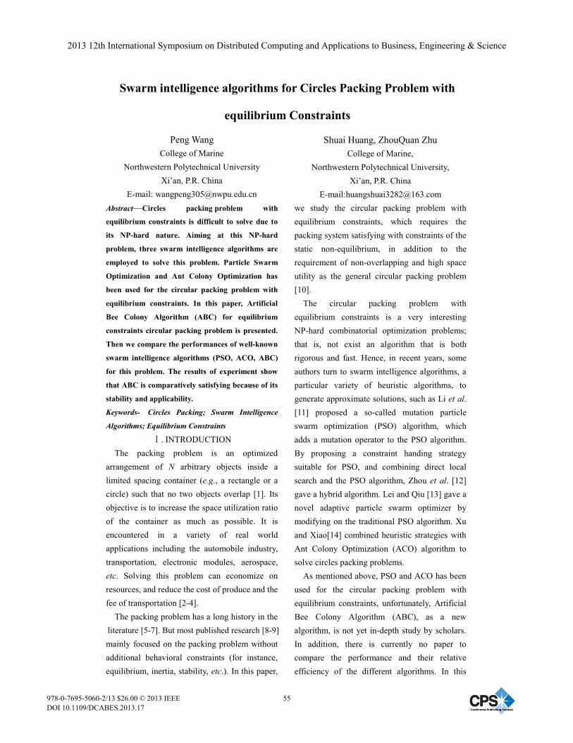
Swarm intelligence algorithms for Circles Packing Problem with

equilibrium Constraints

Peng Wang College of Marine

Northwestern Polytechnical University Xi’an, P.R. China

E-mail: wangpeng305@nwpu.edu.cn

Shuai Huang, ZhouQuan Zhu College of Marine,

Northwestern Polytechnical University, Xi’an, P.R. China

E-mail:huangshuai3282@163.com Abstract—Circles packing problem with equilibrium constraints is difficult to solve due to its NP-hard nature. Aiming at this NP-hard problem, three swarm intelligence algorithms are employed to solve this problem. Particle Swarm Optimization and Ant Colony Optimization has been used for the circular packing problem with equilibrium constraints. In this paper, Artificial Bee Colony Algorithm (ABC) for equilibrium constraints circular packing problem is presented. Then we compare the performances of well-known swarm intelligence algorithms (PSO, ACO, ABC) for this problem. The results of experiment show that ABC is comparatively satisfying because of its stability and applicability. Keywords- Circles Packing; Swarm Intelligence Algorithms; Equilibrium Constraints

. INTRODUCTION The packing problem is an optimized

arrangement of N arbitrary objects inside a limited spacing container (e.g., a rectangle or a circle) such that no two objects overlap [1]. Its objective is to increase the space utilization ratio of the container as much as possible. It is encountered in a variety of real world applications including the automobile industry, transportation, electronic modules, aerospace, etc. Solving this problem can economize on resources, and reduce the cost of produce and the fee of transportation [2-4].

The packing problem has a long history in the literature [5-7]. But most published research [8-9] mainly focused on the packing problem without additional behavioral constraints (for instance, equilibrium, inertia, stability, etc.). In this paper,

we study the circular packing problem with equilibrium constraints, which requires the packing system satisfying with constraints of the static non-equilibrium, in addition to the requirement of non-overlapping and high space utility as the general circular packing problem [10].

The circular packing problem with equilibrium constraints is a very interesting NP-hard combinatorial optimization problems; that is, not exist an algorithm that is both rigorous and fast. Hence, in recent years, some authors turn to swarm intelligence algorithms, a particular variety of heuristic algorithms, to generate approximate solutions, such as Li et al. [11] proposed a so-called mutation particle swarm optimization (PSO) algorithm, which adds a mutation operator to the PSO algorithm. By proposing a constraint handing strategy suitable for PSO, and combining direct local search and the PSO algorithm, Zhou et al. [12] gave a hybrid algorithm. Lei and Qiu [13] gave a novel adaptive particle swarm optimizer by modifying on the traditional PSO algorithm. Xu and Xiao[14] combined heuristic strategies with Ant Colony Optimization (ACO) algorithm to solve circles packing problems.

As mentioned above, PSO and ACO has been used for the circular packing problem with equilibrium constraints, unfortunately, Artificial Bee Colony Algorithm (ABC), as a new algorithm, is not yet in-depth study by scholars. In addition, there is currently no paper to compare the performance and their relative efficiency of the different algorithms. In this

2013 12th International Symposium on Distributed Computing and Applications to Business, Engineering & Science

978-0-7695-5060-2/13 $26.00 © 2013 IEEEDOI 10.1109/DCABES.2013.17

55

work, we overcome these drawbacks by a comprehensive comparative study on the performances of well-known swarm intelligence algorithms for equilibrium constraints circular packing problem.

. MATHEMATICAL FORMULATION OF THE PROBLEM

The circular packing problem with equilibrium constraints, based on the background of the man-made satellite module layout design, is in fact a layout optimization for the dishes installed on a rotating table. There is a rotating circular table with radius R0 and angle velocity ! and n circular objects Ci (i N={1, 2,. . . , n}), which are installed on the circular table such that all n circular objects tend to the center of the table as much as possible and satisfy the following constraints: 1) There is no interference (i.e., overlap) between any two different circular objects; 2) Each circular object does not extend outside the table; 3) The static non-equilibrium value of the packing system should not exceed a permissible value "J (>0).

Figure 1 The schematic diagram of packing of the

circular objects

Cartesian coordinate system is built as Fig. 1. Given n circular objects Ci with radii ri and masses mi (i N={1, 2,. . . , n}). Let the coordinates of the center of Ci be (xi, yi). We call X=(x1, y1, x2, y2,. . . , xn, yn) a solution of layout, i.e., a configuration. The circular packing problem with equilibrium constraints is in fact

how to pack all n circular objects into the circular container C0 without overlapping so that the radius of C0 is as small as possible. It is also the following constrained optimization problem:

{ }( ) ( )

2 20

2 2

2 20

2 2

1 1

R

, , ,

. . ,

i i ii N

i j i j i j

i i i

n n

i i i i Ji i

min max x y r

x x y y r r i j i j N

s t x y R r i N

J m x m y !

"

= =

= + +

!" # + # $ + % """

+ & # "#"" $ % $ %= + &" & ' & '( ) ( )*

+ +

where J denotes the static non-equilibrium value of the packing system. The physical implication of the static non-equilibrium constraints, i.e., J"J , is that the static non-equilibrium value J (or magnitude of non-equilibrium centrifugal force) induced by the masses of all circular objects that deviate from the center of the circular container (i.e., the spinning clapboard of satellite module) is within a permissible value. The smaller J is, the better the packing system satisfies the static equilibrium constraint. When J=0, the whole system is at a static balance.

. SWARM INTELLIGENCE ALGORITHMS A. Particle swarm optimization

Particle swarm optimization (PSO) is an algorithm that follows a collaborative population based search model. Each individual of the population, called a ‘particle’, flies around in a multidimensional search space looking for the optimal solution. Particles, then, may adjust their position according to their own and their neighboring particles experience, moving toward their best position or their neighbor’s best position. In order to achieve this, a particle keeps previously reached ‘best’ positions in a cognitive memory. PSO performance is measured according to a predefined fitness function (cost function of a problem). Balancing between global and local exploration abilities of the flying particles could be achieved through user defined parameters. PSO has many advantages over

56

TABLE 1 PSO ALGORITHM STEPS FOR CIRCLES PACKING PROBLEM WITH EQUILIBRIUM CONSTRAINTS

Step1(Initialization): For each particle i in the population:

Step1.1: Initialize PSO[i] randomly.

Step1.2: Initialize v[i] randomly.

Step1.3: Evaluate fitness[i].

Step1.4: Initialize Gbest with the index of the particle with the best fitness among the population.

Step 1.5: Initialize Pbest [i] with a copy of PSO[i].

Step 2: Repeat until a stopping criterion is satisfied

Step 2.1: Find such Gbest that fitness[Gbest]!Pbest_fitness[i].

Step 2.2: For each particle i: Pbest[i] = PSO[i] if fitness[i] Pbest_fitness[i].

Step 2.3: For each particle i: update v[i] and PSO[i].

Step 2.4: Evaluate fitness[i].

other heuristic techniques such that it can be implemented in a few lines of computer code, it requires only primitive mathematical operators, and it has great capability of escaping local optima. The flow chart of PSO algorithms for circles Packing Problem with equilibrium Constraints is shown in Table 1. B. Ant colony optimization

Ant colony optimization (ACO), which belongs to heuristic and bionic algorithm based on population, is presented by Italian scholar named Dorigo.M in the 1990s. It solves complex problems by simulating the behavior of ants searching for food together in the nature. The specialty of its probabilistic and random search enables the algorithm to acquire more opportunities to get the global optimal solution. In addition, it possesses three main advantages: (1) no requirements of the continuity, the differentiability and convexity of the objective function; (2) inherent parallelity of algorithm (its searching process is not starting from one point but multiple points, and its collaboration procedure is asynchronous and parallel); (3) making use of the positive feedback principle to accelerate the evolutionary procedure and search the best solution. Numerous research results indicate that ACO has stronger ability to find a optimal solution of problem. ACO algorithm Steps for Circles Packing Problem with equilibrium Constraints is shown in Table 2. C. Artificial bee colony

In Artificial bee colony (ABC) algorithm, the position of a food source represents a possible solution to the optimization problem and the nectar amount of a food source corresponds to the quality (fitness) of the associated solution. The number of the employed bees or the onlooker bees is equal to the number of solutions in the population. At the first step, the ABC generates a randomly distributed initial population P(C=0) of SN solutions (food source positions), where SN denotes the size of employed bees or onlooker bees. Each solution xi (i=1,2,3 SN) is a D-dimensional vector. Here, D is the number of optimization parameters. After initialization, the population of the positions (solutions) is subject to repeated cycles, C=1,2,3 MCN of the search processes of the employed bees, the onlooker bees and the scout bees. An employed bee produces a modification on the position (solution) in her memory depending on the local information (visual information) and tests the nectar amount (fitness value) of the new source (new solution). If the nectar amount of the new one is higher than that of the previous one, the bee memorizes the new position and forgets the old one. Otherwise she keeps the position of the previous one in her memory. After all employed bees complete the search process, they share the nectar information of the food sources and their position information with the onlooker bees. An onlooker bee evaluates the nectar information taken from

57

TABLE 2 ACO ALGORITHM STEPS FOR CIRCLES PACKING PROBLEM WITH EQUILIBRIUM CONSTRAINTS

step1. Initialize Population Size m, Positive Integer renewal, Maximum Iterative Times Ncmax; Initial search step of n circles are

"0; Set t=0 Nc=0 i=1 k=0

step2. Initialize the trail intensity T=[#ij]n$m;

Step3. Nc= Nc+1;

Step4. The number of ants k=k+1;

Step5. Each ant compute selection probabilistic, and chooses solution element j;

Step6. i=i+1, the new decision point;

Step7. If i = n, then Step8; Otherwise go to Step5;

Step8. If k< m, then Step4; Otherwise go to Step9;

Step9. Updating pheromone of each road;

Step10. If Nc!Ncmax, the iteration stops. Otherwise, go to Step2; Step11. Output the layout scheme of the best ant, and then algorithm terminates.

TABLE 3 ABC ALGORITHM STEPS FOR CIRCLES PACKING PROBLEM WITH EQUILIBRIUM CONSTRAINTS

Step1. Initialize the population of solutions xi, i=1, 2 SN; Evaluate the population;

Step2. Cycle=Cycle+1;

Step3. Produce new solutions vi for the employed bees and evaluate them;

Step4. Calculate the probability values Pi for the solutions xi;

Step5. Produce the new solutions vi for the onlookers from the solutions xi selected depending on Pi and evaluate them;

Step6. Determine the abandoned solution for the scout, if exists, and replace it with a new randomly produced solution xi;

Step7. Memorize the best solution achieved so far;

Step8. If Cycle MCN, then Step9; Otherwise, go to Step2;

Step9. Output the layout scheme of the best solution, and then algorithm terminates.

all employed bees and chooses a food source with a probability related to its nectar amount. As in the case of the employed bee, she produces a modification on the position in her memory and checks the nectar amount of the candidate source. If the nectar is higher than that of the previous one, the bee memorizes the new position and forgets the old one. ABC algorithm Steps for Circles Packing Problem with equilibrium Constraints is shown in Table 3.

. EXPERIMENT We test three examples which are usually used as benchmark for the circular packing problem with equilibrium behavioral constraints by the current literatures. Example 1 is a further simplified version of the recoverable satellite, including 7 cylinder objects (14 design variables). The size of the example is relatively small and the optimal solutions are known. In example 2 the theoretical optimal solutions are known, including 9 cylinder objects (18 design

variables). The size of the example 3 is relatively large, and its objective function and constraints are more complex and contain more objects (40 cylinders, about 80 design variables). It is studied for verifying whether and how well algorithms can deal with the complex engineering problems. The radii and masses of circular objects in examples are listed in Table 4.

We implement the ABC algorithm in Matlab language and run it on a PC with Intel Core 2 Duo, 3.33 GHz processor and 2.0 GB of RAM.

The comparison of the results obtained by three different algorithms for three test examples is shown in Table 5. ACO finds optimal radii of the circular container for example 1. For example 2, PSO finds smaller radii (which are shown in boldface) of the circular container than ACO and ABC. For example 3 with relatively large size, ABC finds optimal radii (which are shown in boldface) of the circular container. In addition, for each of the resulting configurations

58

TABLE 4 THE RADII AND MASSES OF THE CIRCULAR OBJECTS OF EXAMPLE 3

EXAMPLE DATA

EXAMPLE1

n=7

r={10,11,12,11.5,9.5,8.5,10.5}

m={100,121,144,132.25,90.25,72.25,110.25} EXAMPLE2

n=9

r={12.4264,12.4264,12.4264,12.4264,12.4264,30,30,30,30}

m={12.4264,12.4264,12.4264,12.4264,12.4264,30,30,30,30}

EXAMPLE3

n=40

r={106,112,98,105,93,103,82,93,117,81,89,92,109,104,115,110,114,89,82,120,108,86,93,100,102,106,111,107,

109,91,111,91,101,91,108,114,118,85,87,98}

m={11,12,9,11,8,10,6,8,13,6,7,8,11,10,13,12,12,7,6,14,11,7,8,10,10,11,12,11,11,8,12,8,10,8,11,12,13,7,7,9}

TABLE 5 THE COMPARISON OF THREE ALGORITHMS PERFORMANCE

Example Algorithm Radius of the out wrap

circle (mm) Static equilibrium

error (g.mm)

Interference

(mm)

1

PSO 32.308 8.95E-05 0

ACO 32.230 7.04E-05 0

ABC 32.264 0.02 0

2

PSO 72.688 0 0

ACO 72.861 0 0

ABC 72.993 0 0

3

PSO 812.311 0.005 0

ACO 811.806 0.002 0

ABC 810.935 0.02 0

(a) example 1

(b) example 2

(c) example 3

Figure 2 Geometric configurations of the optimal solutions obtained by ABC for three examples

of all three examples, the values of interference by three algorithms are zero. As for static equilibrium error, PSO finds optimal value(which are shown in boldface) for example 1, ACO for example 3. Conclusively, swarm intelligence algorithms are effective, realistic and practical for circles packing problem with equilibrium constraints. Fig. 2 illustrates the optimal layouts of the three test examples found by ABC.

. CONCLUSIONS The layout problem of circles is a class of layout optimization problems with behavior

constraints. Swarm Intelligence (SI) is a relatively new technology that takes its inspiration from the behavior of social insects and flocking animals. In this paper, we focus on three main SI algorithms: Particle Swarm Optimization (PSO), Ant Colony Optimization (ACO) and Artificial Bee Colony Algorithm (ABC), and their applications for circles packing problem with equilibrium constraints. In order to compare the performances of SI algorithms for equilibrium constraints circular packing problem, three experiment examples are presented. The results show that swarm intelligence algorithms

59

are effective, realistic and practical for circles packing problem with equilibrium constraints, especially ABC because of its stability and applicability.

REFERENCES [1] Dowaland K A;Dowaland W B. Packing

Problems.European Journal of Operational Research,

Vol.56(01), pp.2-14, 1992.

[2] Andrea Lodi, Silvano Martello. Two-dimensional packing

problems: A survey. European Journal of Operational

Research, Vol.141(2), pp.241-252, 2002.

[3] Birgin E G, Martinez J M, Ronconi D P. Optimizing the

packing of cylinders into a rectangular container: a nonlinear

approach. Eur J Oper Res, Vol.160, pp.19–33, 2005,

[4] Mhand Hifi, Rym M Hallah. A Literature Review on

Circle and Sphere Packing Problems: Models and

Methodologies. Advances in Operations Research, pp.1-22,

2009.

[5]Haessler. R.W. and Sweeney. P.E.: Cutting stock problems

and solution procedures. European Journal of Operational

Research, Vol.54(1), pp.141–150, 1991.

[6] G. R. Raidl, G. Kodydek: Genetic Algorithms for the

Multiple Container Packing Problem. in Proc. of the 5th Int.

Conference on Parallel Problem Solving from Nature V,

Amsterdam, The Netherlands, Springer LNCS, pp.875–884,

1998.

[7] D. Lubachevsky, R.L. Graham: Curved hexagonal

packing of equal disks in a circle. Discrete & Computational

Geometry (1997) pp.1 79–194

[8] Huang W Q, He K. A caving degree approach for the

single container loading problem. Eur J Oper Res, Vol.196,

pp.93–101, 2009.

[9] Wei L J, Zhang D F, Chen Q S. A least wasted first

heuristic algorithm for the rectangular packing problem.

Comput Oper Res, Vol.36, pp.1608–1614, 2009.

[10] Chen D B, Liu J F, Fu Y, et al. An efficient heuristic

algorithm for arbitrary shaped rectilinear block packing

problem. Comput Oper Res, Vol.37, pp.1068–1074, 2010.

[11] Li N, Liu F, Sun D B. A study on the particle swarm

optimization with mutation operator constrained layout

optimization.Chin J Comput, Vol.27, pp.897–903, 2004.

[12] Zhou C, Gao L, Gao H B. Particle swarm optimization

based algorithm for constrained layout optimization. Control

Decision, Vol.20, pp.36–40, 2005.

[13] Lei K Y, Qiu Y H. A study of constrained layout

optimization using adaptive particle swarm optimizer. J

Comput Res Develop, Vol.43, pp.1724–1731, 2006.

[14] Yi-Chun Xun, Ren-Bin Xiao. Ant colony algorithm for

layout optimization with equilibrium Constraints[J].

Controland Decision, Vol.23, pp.25-29, 2008.

60

A Beam-Tracing Domain Decomposition Method for Sound Holography in ChurchAcoustics

Frederic Magoules, Remi Cerise, Patrick CalletEcole Centrale Paris, France

frederic.magoules@hotmail.com

Abstract—In this paper, an original beam-tracing domaindecomposition method is proposed for church acoustics. Thisnew method allows to analyze large-scale acoustics problemsin a reasonnable time on parallel architectures. Numericalexperiments, for sound holography within the church of theRoyaumont abbey, illustrate the performance of the proposedbeam-tracing domain decomposition method on multi-coresand multi-processors architectures.

Keywords-Domain decomposition method; Beam-tracingmethod; Parallel computing; Acoustics; Church acoustics;

I. INTRODUCTION

Church acoustics is generally what manages the soundinside a church (the room itself, and objects within theroom). Church acoustics investigates what happens to thesound after it has been issued from the clergyman or themonks, to ensure that the people in the room (who aresupposed to hear the sound) actually get to hear it. Churchacoustics is the purpose to build space, dedicated to gettingthe right sound to the right person, from the right directionand at the right time, by removing echoes and additionalnoise. Despite it was not an easy task in middle age, i.e.without any simulation software, church acoustics was ofmajor importance, and we can surprisingly note the highquality acoustics propagation in middle age church. This isquite impressive indeed, because opposite to architecturalproject, church acoustics is not like most projects: it is doneonce in the life of the church, and can uneasily be changed.

Over the years, several churches have been destroyed inEurope, and it is not possible anymore to benefit from thefeeling of the song propagating within these churchs. Inorder to come up with effective solutions and virtual realityrendering, one must be able to simulate and to assess theeffect of architectural configurations. To do this, fast noisesimulation is an invaluable tool. However sound propagateseverywhere and is very sensitive to small scale details ofthe architecture, so simulations must be done with accuratearchitectural models, and well design methods are a keypoint to obtain fast simulations. Numerical methods, likeFinite Difference Methods (FDM) [5], [33], Finite ElementMethods (FEM) [13], [37], [12], Infinite Element Methods(IFEM) [6], [17], [4], [3], [2], and Boundary Element Meth-ods (BEM) [41], approximate the mathematical equations

of the acoustic problems. These very accurate methods re-quiere a lot of computational power and memory. Opposite,geometrical methods, like image-source methods [1], [31],ray-tracing methods [40] and beam-tracing methods [9],[16], assume that the sound propagates in straight lines.These methods, valid only for high frequencies relativelyto the size of the problem, requiere less memory andless computational resources. In this paper, a new domaindecomposition method based on beam-tracing is proposedfor fast church acoustics analysis.

The plan of this paper is the following. The motivation ofthis work is presented in Section II. In Section III, an originalmethod similar to domain decomposition techniques [36],[32], [38], [14], [24] is introduced to parallelize the beam-tracing method and allows us to solve large-scale acousticproblems. In Section IV, numerical experiments performedon Royaumont abbey illustrate the performance of this newparallel domain decomposition method for church acoustics.Finally, Section V concludes this paper.

II. ROYAUMONT ABBEY DIGITAL MODELLING

As already mentioned, the goal of this paper is todesign an efficient methodology for sound holography inchurch acoustics; the experiments beeing conducted in theRoyaumont abbey. The Royaumont abbey is located about35 kilometers north of Paris. This is a royal church andits construction was ordered by King Saint Louis and hismother, Blanche de Castille, in 1228 and accomplished in1235. During the reign of Saint Louis, the Royaumont abbeywas one of the most important Cistercian place in Europe,inhabited by a maximum of a 140 monks. After the deathof Saint Louis, the abbey lost its royal status and beganits progressive decline. Only a few douzen of monks stilllived in Royaumont at the end of the XVIIIth century.We do not know exactly the evolution of the architectureof the church during this period. Anyway, according tothe eighteenth-century naturalist Aubert-Louis Millin, manyrestorations have been done on the church to repair somedamages. For instance, the roof was restored a first time in1473 and 1761 after having been damaged by fires. Millinalso described a Gothic portal built around 1650. The lastabbot, M. de Balivire, ordered the construction of an abbeypalace in 1785, just before the French Revolution. After the

2013 12th International Symposium on Distributed Computing and Applications to Business, Engineering & Science

978-0-7695-5060-2/13 $26.00 © 2013 IEEEDOI 10.1109/DCABES.2013.18

61

Figure 1. Illustration of the CAD model of the Royaumont church (exteriorview of the architecture)

French Revolution, in 1792 the church was sold to industrywho transformed the abbey in a cotton manufacture. Thechurch was destroyed and its stones were reused to buildnew buildings . . . Other parts of the abbey were dramaticallymodified until 1869, where the site is returned to sisters of“Sainte-Famille de Bordeaux”. During the XXth the Gouinfamily restored some parts of the abbey after buying the sitein 1905, but no restoration concerned the church itself.

This is the reason why only a few elements of the originalbuilding of the church are still visible today, mainly thebasements, some columns, the northern wall of the aisleclosed to the cloister and a tower marking the end of thesouthern transept. With so few element, to build a virtualreality model of the church of Royaumont is not an easytask. Points cloud acquisition techniques [15], traditionallyused in cultural heritage cannot be considered in our case.Therefore, our modeling process required the correlationbetween two types of data: (i) results of the works ofarcheologists who can estimate the general aspect of thechurch from its remaining parts; (ii) results of the worksof historians who found several descriptions of the churchmade during past centuries in historical archives. The mostcomplete description of Royaumont abbey is described byMillin in [29] where a visit inside the church in late 1791is described; this book serves as the main source for today’shistorians, together with some engravings of the church andthe abbey. Based on these data and with close connectionswith historians and archeologists, we have created a three-dimensional model of the church of Royaumont abbey.Illustration of our CAD model is shown in Figure 1 withan exterior view of the architecture and in Figure 2 with aninterior view of the architecture.

Figure 2. Illustration of the CAD model of the Royaumont church (interiorview of the architecture)

III. PARALLEL GEOMETRICAL DOMAIN DECOMPOSITIONMETHODS

A. Geometrical acoustics methods

Geometrical acoustics methods, like the image-sourcemethod, the ray-tracing method, and the beam-tracingmethod, are commonly used to design three-dimensionalarchitectural environments. These methods mainly consistto compute the multiple paths of the sound from sources toreceivers, and then to collect the acoustic pressure at virtualmicrophones placed in the model at the points where thenoise level must be evaluated.

Within these methods, the image-source methods [1],[31] creates virtual sources for each reflection of a sourceby a surface of the model. For each virtual microphone,the image-source method computes the contribution of thesources by checking that the path between the source andthe virtual microphone is not blocked by an obstacle. Theray-tracing method [39], [30] divides the energy of eachsource between a huge numbers of elementary particles.Those particles propagate in straight lines and gradually

62

loose energy due to the damping of the air. The beam-tracingmethod [9], [35], instead of splitting the energy betweenparticles, splits the energy between beams. The energy isdistributed to a beam according to the power of the sourcein the direction of the beam. In this paper the beam-tracingmethod, because of its accuracy and its wide implementationin industrial acoustics software, is used.

B. Parallel computing

In order to simulate acoustics in a church in a reasonnabletime, parallel computing techniques could be applied tothe beam-tracing method. Several algorithms exist and havebeen efficiently used for beam-tracing methods in imageprocessing for video games for instance. Within these algo-rithms, we can mention work-sharing algorithms. The sim-plest idea, static partitioning algorithms, consists to staticallyassign some beams to some processes at the beginning of theprogram; each process receiving the same number of beams.A more complex idea, dynamic partitioning algorithms,consists to have a central process dispatching packets ofbeams on demand when the worker processes ask them.Another way to assign the work is to use work-stealingalgorithms. All beams are assigned at the beginning, butwhen a process has nearly finished its assigned beams, itcan steal some beams from other processes. Despite all thesealgorithms are parallel, the input, output and result gatheringare not. To be able to use a lot of processes efficiently, theinput, output and result gathering need to be made parallel.

C. Domain decomposition methods

Domain decomposition methods consist to split a globaldomain into several small sub-domains, allowing the load-ing, output and result gathering to be done in parallel; eachsub-domain beeing allocated to a different processor.

A basic idea, microphones partitioning, consists of simplysplitting the set of virtual microphones into multiple sets, oneper sub-domain. In each sub-domain the beams are shot inthe complete geometry. Each sub-domain is totally indepen-dent so the program can be run in parallel. If this method isused with traditional parallelism, some load balancing issuesmust be considered since the processing time of each sub-domain can vary a lot. Another idea, on demand geometryand microphones loading, consists to load sub-domains ondemand, i.e. that some hierarchical acceleration structure isrecomputed and only the first levels are loaded at the start.

The original method considered here [22], geometry andmicrophones partitioning, matches more closely domaindecomposition techniques [36], [32], [38], [14], [24]. Thesemethods consist to split the global domain to solve intoseveral sub-domains, each sub-domain beeing solved inde-pendently by sharing information along interface betweenneighboring sub-systems. These interface conditions [19]can be tuned for the performance of the algorithm eitherwith a continuous approach [8], [11], [7], [23], [10] or with a

discrete approach [34], [28], [25]. In this paper, the geometryof the model and the microphones are split into multiplesub-domains and the domain decomposition method [27],[26], [18], [21], [20] is considered, where the interfaceconditions simply consists of the continuity of the beamcharacteristics (i.e. direction, amplitude, angle, etc.) fromeach side of the interface, see [22]. Only the analysis of thebeams going through the interface between the sub-domainsis performed. For efficiency purpose, the beams are shot in amodified model where all the sub-domains except the currentone are replaced by a simplified version of themselve. Onedifference with a classical domain decomposition methodis that there is not a one to one correspondence betweenthe processes and the sub-domains. Indeed, if each processwas associated to one and only one sub-domain, the loadbalancing would be very bad. For instance, in the casewhere there is only one source. The sub-domain containingthe source would have the most work and the others a lotless, which would reduce the efficiency. This is why a morecomplex load-balancing scheme has to be used. The idea isthat each process starts with one sub-domain, but when it hasfew remaining beams to handle; it starts to load one or moresub-domains having a lot of beams remaining. Completedetails of efficient implementation can be found in [22].

IV. NUMERICAL EXPERIMENTS

The numerical experiments are conducted in order to sim-ulate the sound holography in the church of the Royaumontabbey. A total number of 60 sources are considered; eachsource located at 1,60 meters high at each monk’ chair. Eachsource is modelled with 1 million beams. The ComputerAided Design (CAD) model consists of 1.413.602 pointsand 2.632.344 polygons, and is shown in Figure 1 withan exterior view of the architecture and in Figure 2 withan interior view of the architecture. A total number of 20millions virtual microphones are placed in a regular gridin all the volume of the abbey, which corresponds to amicrophone every 10 centimeters in each of the three spatialdirections. The numerical experiments are run on a PCscluster composed of 20 nodes; each node is composed of twoquadricore processors, leading to a total number of cores of160. Figure 3 illustrates the noise level distribution obtainedfrom the simulation.

Table I collects the speedups obtained with our implemen-tation. Using the proposed domain decomposition methodallows a significant improvment of the performance. This isparticularly true for a large number of threads. With morethan 32 threads, the speedup becomes quite important. Be-sides, increasing the number of sub-domains still acceleratesthe execution of the method. As the first line represents thestandard case where the algorithm is applied without domaindecomposition method, but only with an MPI parallelizationapproach, we note that the equivalent performances with

63

Figure 3. Illustration of the sound holography in the church of Royaumontabbey (interior view)

16 32 64 128threads threads threads threads

1 sub-domain 14.5 22.8 27.4 21.04 sub-domains 14.6 26.6 46.1 49.28 sub-domains 14.7 26.4 47.9 75.9

Table ISPEED-UP OF THE WHOLE DDM PROGRAM (ETHERNET) WITH RESPECT

TO THE NUMBER OF THREADS AND SUB-DOMAINS.

eight sub-domains can be multiplied by a factor closed tofour in our tests.

V. CONCLUSION

In this paper, an original beam-tracing domain decom-position method has been proposed for church acoustics onparallel computers. This new method is based on domain de-composition method principles, where interface constraintsconsist to match the beam characteristics. A realistic testcase, namely the sound holography within the church ofthe Royaumont abbey has been presented which outlines

the performance and efficiency of the proposed method onmulti-cores architectures.

REFERENCES

[1] J. B. Allen and D. A. Berkley, “Image method for efficientlysimulating small-room acoustics,” Journal of the AcousticalSociety of America, vol. 65, no. 4, pp. 943–950, 1979.

[2] J.-C. Autrique and F. Magoules, “Numerical analysis of acoupled finite-infinite element method for exterior Helmholtzproblems,” Journal of Computational Acoustics, vol. 14,no. 1, pp. 21–43, 2006.

[3] ——, “Studies of an infinite element method for acousticalradiation,” Applied Mathematical Modelling, vol. 30, no. 7,pp. 641–655, 2006.

[4] ——, “Analysis of a conjugated infinite element method foracoustic scattering,” Computers and Structures, vol. 85, no. 9,pp. 518–525, 2007.

[5] D. Botteldooren, “Finite-difference time-domain simulationof low-frequency room acoustic problems,” Journal of theAcoustical Society of America, vol. 98, pp. 3302–3308, 1995.

[6] D. S. Burnett and R. L. Holford, “An ellipsoidal acousticinfinite element,” Computer Methods in Applied Mechanicsand Engineering, vol. 164, no. 1-2, pp. 49–76, 1998.

[7] P. Chevalier and F. Nataf, “Symmetrized method with opti-mized second-order conditions for the Helmholtz equation,”in Domain decomposition methods, 10 (Boulder, CO, 1997).Providence, RI: Amer. Math. Soc., 1998, pp. 400–407.

[8] B. Despres, “Domain decomposition method and theHelmholtz problem.II,” in Second International Conferenceon Mathematical and Numerical Aspects of Wave Propagation(Newark, DE, 1993). Philadelphia, PA: SIAM, 1993, pp.197–206.

[9] T. Funkhouser, N. Tsingos, I. Carlbom, G. Elko, M. Sondhi,J. E. West, G. Pingali, P. Min, and A. Ngan, “A beam tracingmethod for interactive architectural acoustics,” Journal of theAcoustical Society of America, vol. 115, no. 2, pp. 739–756,2004.

[10] M. Gander, L. Halpern, and F. Magoules, “An optimizedSchwarz method with two-sided Robin transmission condi-tions for the Helmholtz equation,” International Journal forNumerical Methods in Fluids, vol. 55, no. 2, pp. 163–175,2007.

[11] S. Ghanemi, “A domain decomposition method for Helmholtzscattering problems,” in Ninth International Conference onDomain Decomposition Methods, P. E. Bjørstad, M. Espedal,and D. Keyes, Eds. ddm.org, 1997, pp. 105–112.

[12] I. Harari and F. Magoules, “Numerical investigations ofstabilized finite element computations for acoustics,” WaveMotion, vol. 39, no. 4, pp. 339–349, 2004.

[13] F. Ihlenburg, Finite Element Analysis of Acoustic Scattering.Springer, 1998.

64

[14] J. Kruis, Domain Decomposition Methods for DistributedComputing. Saxe-Coburg Publications, 2007.

[15] S.-W. Kwon, F. Bosche, C. Kim, C. T. Haas, and K. A.Liapi, “Fitting range data to primitives for rapid local 3dmodeling using sparse range point clouds,” Department ofCivil Engineering, The University of Texas at Austin, Austin,TX 78712, USA, Tech. Rep., 2004.

[16] S. Laine, S. Siltanen, T. Lokki, and L. Savioja, “Acceleratedbeam tracing algorithm,” Applied Acoustics, vol. 70, no. 1,pp. 172–181, 2009.

[17] L.-X. Li, J.-S. Sun, and H. Sakamoto, “A generalized infiniteelement for acoustic radiation,” Journal of vibration andacoustics, vol. 127, no. 1, pp. 2–11, 2005.

[18] Y. Maday and F. Magoules, “Non-overlapping additiveSchwarz methods tuned to highly heterogeneous media,”Comptes Rendus a l’Academie des Sciences, vol. 341, no. 11,pp. 701–705, 2005.

[19] ——, “Absorbing interface conditions for domain decompo-sition methods: a general presentation,” Computer Methodsin Applied Mechanics and Engineering, vol. 195, no. 29–32,pp. 3880–3900, 2006.

[20] ——, “Improved ad hoc interface conditions for Schwarzsolution procedure tuned to highly heterogeneous media,”Applied Mathematical Modelling, vol. 30, no. 8, pp. 731–743,2006.

[21] ——, “Optimized Schwarz methods without overlap forhighly heterogeneous media,” Computer Methods in AppliedMechanics and Engineering, vol. 196, no. 8, pp. 1541–1553,2007.

[22] F. Magoules, “Decomposition de domaines pour le lancer derayons,” France Patent no. 1157329. 12 August 2011.

[23] F. Magoules, P. Ivanyi, and B. Topping, “Convergence analy-sis of Schwarz methods without overlap for the Helmholtzequation,” Computers and Structures, vol. 82, no. 22, pp.1835–1847, 2004.

[24] F. Magoules and F.-X. Roux, “Lagrangian formulation ofdomain decomposition methods: a unified theory,” AppliedMathematical Modelling, vol. 30, no. 7, pp. 593–615, 2006.

[25] F. Magoules, F.-X. Roux, and L. Series, “Algebraic wayto derive absorbing boundary conditions for the Helmholtzequation,” Journal of Computational Acoustics, vol. 13, no. 3,pp. 433–454, 2005.

[26] ——, “Algebraic approximation of Dirichlet-to-Neumannmaps for the equations of linear elasticity,” Computer Meth-ods in Applied Mechanics and Engineering, vol. 195, no. 29–32, pp. 3742–3759, 2006.

[27] ——, “Algebraic Dirichlet-to-Neumann mapping for linearelasticity problems with extreme contrasts in the coefficients,”Applied Mathematical Modelling, vol. 30, no. 8, pp. 702–713,2006.

[28] ——, “Algebraic approach to absorbing boundary conditionsfor the Helmholtz equation,” International Journal of Com-puter Mathematics, vol. 84, no. 2, pp. 231–240, 2007.

[29] A. Millin, Antiquites nationales, ou Recueil de monumentspour servir l’Histoire, 1791, vol. 2.

[30] T. Moller and B. Trumbore, “Fast, minimum storage ray/-triangle intersection,” in SIGGRAPH ’05: ACM SIGGRAPH2005 Courses. New York, NY, USA: ACM, 2005, p. 7.

[31] V. Pulkki, T. Lokki, and L. Savioja, “Implementation andvisualization of edge diffraction with image-source method,”in Proceedings of the 112th Audio Engineering Society Con-vention, 2002.

[32] A. Quarteroni and A. Valli, Domain Decomposition Methodsfor Partial Differential Equations. Oxford University Press,Oxford, UK, 1999.

[33] T. V. Renterghem and D. Botteldooren, “Prediction-stepstaggered-in-time FDTD: An efficient numerical scheme tosolve the linearised equations of fluid dynamics in outdoorsound propagation,” Applied Acoustics, vol. 68, no. 2, pp.201–216, 2007.

[34] F.-X. Roux, F. Magoules, L. Series, and Y. Boubendir, “Ap-proximation of optimal interface boundary conditions for two-Lagrange multiplier FETI method,” in Proceedings of the 15thInternational Conference on Domain Decomposition Meth-ods, Berlin, Germany, July 21-15, 2003, ser. Lecture Notesin Computational Science and Engineering, R. Kornhuber,R. Hoppe, J. Periaux, O. Pironneau, O. Widlund, and J. Xu,Eds. Springer-Verlag, Haidelberg, 2005.

[35] A. Schmitz, T. Rick, T. Karolski, L. Kobbelt, and T. Kuhlen,“Simulation of radio wave propagation by beam tracing,” inEurographics Symposium on Parallel Graphics and Visual-ization, 2009.

[36] B. Smith, P. Bjorstad, and W. Gropp, Domain Decomposition:Parallel Multilevel Methods for Elliptic Partial DifferentialEquations. Cambridge University Press, UK, 1996.

[37] L. L. Thompson, “A review of finite-element methods fortime-harmonic acoustics,” Journal of the Acoustical Societyof America, vol. 119, no. 3, pp. 1315–1330, 2006.

[38] A. Toselli and O. Widlund, Domain Decomposition methods:Algorithms and Theory. Springer, 2005.

[39] I. Wald and P. Slusallek, “State of the art in interactive raytracing,” in State of the Art Reports. EUROGRAPHICS,Manchester, UK, 2001, pp. 21–42.

[40] I. Wald, P. Slusallek, C. Benthin, and M. Wagner, “Interactiverendering with coherent ray tracing,” in Proceedings of EG2001, A. Chalmers and T.-M. Rhyne, Eds. BlackwellPublishing, 2001, vol. 20(3), pp. 153–164.

[41] J. Zhang, W. Zhao, and W. Zhang, “Research on acoustic-structure sensitivity using FEM and BEM,” Journal of Vibra-tion Engineering, vol. 18, no. 3, pp. 366–370, 2005.

65

A Conceptual Approach for Assessing SOA Design Defects' Impact on Quality

Attributes

Khaled Kh. S. Kh. Allanqawi Faculty of Science, Engineering and

Computing, Kingston University, London k0961606@kingston.ac.uk

Dr. Souheil Khaddaj Faculty of Science, Engineering and

Computing, Kingston University, London S. Khaddaj@kingston.ac.uk

Abstract—This research proposes an approach for assessing the impacts of SOA design defects on SOA quality attributes. Eleven items were selected to measure SOA Design Defects; fourteen items were selected to measure SOA Design Attributes; seventeen items were selected to measure SOA Quality Attributes and eleven items were selected to measure SOA Quality Metrics. This work is an integrated part to previous studies in the field. Index Terms— SOA Design Defects, SOA Design Attributes, SOA Design Attributes; SOA Quality Attributes, SOA Quality Metrics

I. INTRODUCTION It is difficult to define what a Service

Oriented Architecture (SOA) is. The term is being used in an increasing number of contexts with conflicting understandings of implicit terminology and components. For SOA services to be successful and reusable, it is important that the data they expose is of acceptable quality for all the consumers. Exposing quality data is necessary in any SOA initiative. Whether it is application services being exposed or a simple generated data query service, the resulting data must be accurate and appropriate to the business context to be of any value. The main objective of this research is to propose an approach that can be used to assess SOA design defects and its impact on quality attributes.

II. QUALITY OF SERVICE ORIENTED ARCHITECTURE

Quality is currently considered one of the main assets with which a firm can enhance its competitive global position. This is one reason "why quality has become essential for ensuring that a company’s products and processes meet customers’ needs" [1]. One of the most challenging aspects of building SOA applications is quality assurance. Developers must analyze every flow path, every condition, and every fault to ensure that processes are bullet-proof. A software quality attribute of a software system is

a characteristic, feature or property that describes part of the software system. Internal software quality attributes reflect structural properties of a software system [2].

A. Quality Attributes of SOA One of the most important quality models is

the quality model presented by Jim McCall et al., 1977 [3]. They presented a quality model focusing on a number of software quality factor that reflect both the users’ views and the developers’ priorities. The main quality factors were correctness, reliability, efficiency and integrity.

The second basic quality model is the quality

model presented by Boehm et al. 1978 [4]. Boehm's model is similar to the McCall quality model in that it also presents a hierarchical quality model consisted of 7 quality factors portability, reliability, efficiency, usability, testability, understandability and flexibility.

In 1998, The International Organization for Standardization (ISO) had defined a set of ISO and ISO/IEC standards related to software quality. The ISO/IEC 9126 is currently one of the most widespread quality standards. ISO 9126 indicated that component of the software quality must be described in terms of one or more of six characteristics defined as a set of attributes [5]: functionality, reliability, usability, efficiency, maintainability and portability.

Recently, Ortega et al. [1] designed a model prototype that reflects the essential attributes of quality. This model pinpointed three working areas based on McCall’s Quality model as follows: Product Operation, Product Revision and Product Transition. Pettersson [6] created a SOA Quality Evaluation Model that was applicable to SOA implementations. The model was based on two perspectives: Technical Perspective and Business Perspective. In 2007, O’Brien et al. [7] listed nine SOA quality

2013 12th International Symposium on Distributed Computing and Applications to Business, Engineering & Science

978-0-7695-5060-2/13 $26.00 © 2013 IEEEDOI 10.1109/DCABES.2013.19

66

attributes in their article: interoperability, performance, security, reliability, availability, modifiability, testability, usability, and scalability. Peng [8] studied the relationship between quality attributes and SOA and analyzed SOA impact on six quality attributes: availability, modifiability, performance, security, testability and usability. Erl [9] presented some SOA design patterns that can be used to satisfy the following quality attributes: reusability, performance, security, flexibility and modifiability.

More recently, in 2012 Montagud et al. [10]

classified quality attributes and measures for assessing the quality of software product lines. These quality attributes were reusability and efficiency. Galster et al. [11] suggested a framework for reference architecture design for variability-intensive service-based systems using the following quality attributes: variability, scalability, interoperability, performance, reliability, privacy and security. Marko [12] suggested a SOA prototype to evaluate the quality of the architecture resulting from the combination of EBI and SOA patterns. The quality is evaluated with respect to: efficiency, functionality, maintainability, portability, reliability and usability.

III. DESIGN DEFECTS Design defects are bad solutions to recurring

design problems in object-oriented programming. Most defect prediction studies are based on size and complexity metrics.

A. OA Design Attributes Perepletchikov et al. [13] provided a

comparative study on the impact of object orientation and service orientation on the structural attributes of size, complexity, coupling and cohesion. Whereas Shaik et al. [14] studied design components that were exclusive and defined the architecture of an object oriented design and listed the key terms in object oriented development environment: class, object, method, message instantiation, inheritance, polymorphism, encapsulation, cohesion, coupling, design size, hierarchies, abstraction and complexity. In 2011, Yaser and Suleiman [2] assessed software quality attributes of Service-Oriented Software Development Paradigms using four SOA design attribute: size, complexity, coupling and cohesion.

B. SOA Design Defects Developing code free of defects is a major

concern for the object-oriented software community. Basili et al. [15] classified design defects according User Interface (UI) to: omission, incorrect fact, inconsistency,

ambiguity and extraneous information. Whereas, Gueheneuc [16] classified design defects as: intra-class, inter-classes and behavioural defects. Tian [17] classified design defects as: interface capability, interface specification, interface description and missing design defects.

IV. QUALITY METRICS A Software Metric is an algorithm which

computes a numeric value from source code to measure properties of a software system. The purpose of software metrics is to make assessments throughout the software life cycle as to whether the software quality requirements are being met [5]. Software metrics are often used to assess the ability of software to achieve a predefined goal [18]. Many different metrics have been proposed for object-oriented systems. Several prior studies had used metrics to identify defects' impact on quality attributes, these metrics are [2], [14], [19 - 27].

• Size Metrics: they are used to evaluate the

ease of understanding of code by developers and maintainers. Size metrics is often measured using: Lines-Of-Code metric (LOC) and Weighted Methods per Class (WMC).

• Coupling Metrics: they are measure the relationships between entities. They are often measured using Depth of Inheritance Tree (DIT), Response set For a Class (RFC) and Coupling Between Object classes (CBO).

• Complexity Metrics: they are measure complexity in terms of control constructs and lexical tokens, respectively. They are often measured using Source Line of Code (SLOC), Weighted Methods per Class (WMC), Number Of Children (NOC), Cyclomatic Complexity (CC), Halstead’s Complexity (HC), Maintainability Index (MI) and Depth of Inheritance Tree (DIT)

• Cohesion Metrics: they are measure the relationships among the elements within a single module. They are often measured using Lack of Cohesion of Methods (LCOM).

• Inheritance Metrics: they are often measured using Method Inheritance Factor (MIF), Attribute Inheritance Factor (AIF), Number of Children (NOC) and Depth of Inheritance (DIT).

• Polymorphism Metrics: they are often measured using Polymorphism Factor (PF).

• Encapsulation Metrics: they are often measured using Method Hiding Factor (MHF) and Attribute Hiding Factor (AHF).

67

V. PRPOSED APPROACH The proposed approach is a comprehensive,

multidimensional framework of SOA defects detection. The measures used in this work were adapted primarily from previous researches; the components of proposed approach are shown in "Fig. 1". In reality, every study has interpreted and classified quality system metrics conform to its context, the proposed approach consists of eleven items to measure SOA Design Defects, fourteen items to measure SOA Design Attributes, seventeen items were selected to measure SOA Quality Attributes and eleven items to measure SOA Quality Metrics. The user can adapt the number of selected items according to the actual case.

Fig. 1. The proposed approach

A. Design Phase • Measures of SOA Design Defects: Eleven

items were selected to measure SOA Design Defects; these items were selected from the previous studies done by [15, 16 & 17].

• Measures of SOA Design Attributes: Fourteen items were selected to measure SOA Design Attributes; these items were selected from the previous studies done by [2, 13 & 14].

• Measures of SOA Quality Attributes: Seventeen items were selected to measure SOA Quality Attributes from the previous studies done by [1], [3-10].

• Measures of SOA Quality Metrics: Eleven items were selected to measure SOA Quality Metrics from the previous studies done by [2], [5], [14], [18 - 27].

B. Preparation Phase The intent of these measures is to measure customer satisfaction by assessing the design defects and its impacts on deign quality. The approach tool consists of four parts as shown in "Fig. 2":

• Part (I) represents SOA design attribute. Example (but not limited to): size, complexity, coupling, and cohesion.

• Part (II) represents metrics may be used to measure defects' impact on quality attributes. Example (but not limited to): LOC, CC, ECC, HC, MI, WMC, DIT, NOC, CBO, RFC & LCOM.

• Part (III) represents SOA design defects. Example (but not limited to): Algorithmic and Processing Defects, Control, Logic, and Sequence Defects, Data Defects and Functional Description Defects.

• Part (IV) represents SOA quality attributes. Example (but not limited to): Availability, Security, Performance, Modifiability, Scalability, Adaptability, Interoperability and Auditability.

Fig. 2. Approach Tool

C. Approach Implementation • The first step in implementing the proposed

approach is to define the most common design attributes (Part I).

• The second step is to define the suitable metrics used to describe the selected design attributes (Part II).

• The third step is to define the most common design defects (Part III).

• The fourth step is to matching between design attributes and design defects through the selected metrics.

• The fifth step is to define the most common quality attributes (Part IV).

68

• The sixth step is to matching between design defects and quality attributes.

• The last step is to assign the suitable metrics can be used to measure the impact of design defects on quality attributes.

VI. CONCLUSIONS AND FUTURE WORK This work summarizes many items the field

of SOA quality that may help the other researchers to build their own models. This work also proposes an approach for assessing the impacts of SOA design defects on SOA quality attributes. This work is an integrated part to previous studies in the field.

The next step of this work is to measure the validity of the proposed approach; actual case studies can be taken. The Fuzzy techniques can be used to assess the impacts of SOA design defects on SOA quality attributes.

REFERENCES [1] Ortega M., Pérez M., and Rojas T., (2003),

Construction of a Systemic Quality Model for evaluating a Software Product. Software Quality Journal, 11, 3: 219-242.

[2] Yaser I. Mansour, Suleiman H. Mustafa, (2011), "Assessing Internal Software Quality Attributes of the Object-Oriented and Service-Oriented Software Development Paradigms: A Comparative Study", Journal of Software Engineering and Applications, 4: 244-252.

[3] McCall, J., Richards, K., and Walters, F., "Factors in Software Quality", Nat'l Tech. Information Service, Vol. 1, 2 and 3, 1977.

[4] Boehm, B., Brown, R., Kaspar, H., Lipow, M., McLeod, G., and Merritt, M., (1978), "Characteristics of Software Quality", North Holland.

[5] ISO/IEC 9126-1.2. (1998), ISO/IEC 9126-1.2: Information Technology - Software Product Quality - Part 1: Quality Model, ISO/IEC JTC1/SC7/WG6

[6] Pettersson A., (2006), "Service-Oriented Architecture (SOA) quality attributes- A research model", MSc thesis, University of Lund.

[7] O’Brien, L., Paulo M. and Len B. (2007), “Quality Attributes for Service-Oriented Architectures”. In Proceedings of the International Workshop on Systems Development in SOA Environments. SDSOA ’07. Washington, DC, USA: IEEE Computer Society. ISBN: 0-7695-2960-7.

[8] Peng Q. (2008), "SOA and Quality", MSc. Thesis, Växjö University.

[9] Erl, T. (2009). SOA Design Patterns. Prentice Hall PTR.

[10] Montagud S., Abrahao S. and Insfran E., (2012), "A systematic review of quality attributes and measures for software product lines", Software Quality Journal, Vol. 20, I. 3-4: 425-486.

[11] Galster M., Avgeriou P., and Tofan D., (2013), "Constraints for the design of variability-intensive service-oriented reference architectures – An industrial case study", Information and Software Technology 55: 428–441.

[12] Marko M. (2013), "Using EBI Pattern in Conjunction with Service-Oriented Architectures", MSc. Thesis, University of Jyväskylä.

[13] Perepletchikov M., Ryan C. and Frampton K., (2005), “Comparing the Impact of Service-Oriented and Object-Oriented Paradigms on the Structural Properties of Software, ”Second International Workshop on Modeling Inter-Organizational Systems, Cyprus, Vol. 3762 : 431-441

[14] Shaik A., Reddy K., Manda B., Prakashini C, and Deepthi K., "An Empirical Validation of Object Oriented Design Metrics in Object Oriented Systems", Journal of Emerging Trends in Engineering and Applied Sciences (JETEAS) 1 (2), 2010, 216-224

[15] Basili, V., Green S., Laitenberger, O., Lanubile, F., Shull, F., Sorumgard, S., Zelkowitz, M. V., (1996), "The Empirical Investigation of Perspective-Based Reading", Empirical Software Engineering Journal, I: 133-164.

[16] Gueheneuc Y., Design defects: A taxonomy, Technical Report INFO-2001, Ecole des Mines de Nantes, 2001

[17] Tian, J., 2005. Software Quality Engineering, John Wiley and Sons

[18] Jaquith A., (2007), Security Metrics: Replacing Fear, Uncertainty, and Doubt. Upper Saddle River, NJ: Pearson Education Inc.

[19] Elish K. and Elish M., (2008), "Predicting Defect-prone Software Modules Using Support Vector Machines," The Journal of Systems & Software, vol. 81, 2008, pp. 649-660.

[20] Chowdhury I., (2009), "USING COMPLEXITY, COUPLING, AND COHESION METRICS AS EARLY INDICATORS OF VULNERABILITIES" MSc. Thesis, Queen’s University

[21] Graylin J., Joanne E., Randy K., David H., Nicholas A. and Charles W. (2009), "Cyclomatic Complexity and Lines of Code: Empirical Evidence of a Stable Linear Relationship", J. Software Engineering & Applications, 2: 137-143

[22] Sanjay D. and Ajay R., (2010), "A Comprehensive Assessment of Object-Oriented Software Systems Using Metrics Approach", (IJCSE) International Journal on Computer Science and Engineering Vol. 2, No. 8: 2726-2730

[23] Thapaliyal M. and Verma G., (2010), "Software Defects and Object Oriented Metrics – An Empirical Analysis", International Journal of Computer Applications (0975 – 8887) Vol. 9, No.5: 41-44.

69

[24] Gurdev S., Dilbag S. and Vikram S., (2011), "A Study of Software Metrics", IJCEM International Journal of Computational Engineering & Management, Vol. 11: 22-27.

[25] Kehan G., Taghi M., Huanjing W. and Naeem S., (2011), "Choosing software metrics for defect prediction: an investigation on feature selection techniques", Softw. Pract. Exper. 41:579–606

[26] Alahmari S., (2012), "A Design Framework for identifying Optimum services using Choreography and Model Transformation", PhD. Thesis, Faculty of Physical and Applied Science, University of Southampton.

[27] Agrawal D. and Mishra M., (2012), "An Integrated Approach to Measurement Software Defect using Software Matrices", International Journal of Computer & Organization Trends –Vol. 2, I. 4: 90-94.

70

Modeling Automotive Cyber Physical Systems

Lichen Zhang Faculty of Computer Science and Technology

Guangdong University of Technology Guangzhou 510090, China

zhanglichen1962@163.com Abstract—Automotive cyber physical systems (CPSs) involve interactions between software controllers, communication networks, and physical devices. These systems are among the most complex cyber physical systems being designed by humans. However, automotive cyber physical systems are not a loose combination of cyber system and physical system, but are a tight and comprehensive integration, and they are ubiquitous spatial-temporal and very large-scale complex systems. In automotive cyber physical systems, the behavior of the physical world such as the velocity, flow and density are dynamic and continuous changing with time while the process of communication and calculation in vehicular cyber system is discrete. In this paper, we extend the AADL to model the cyber world and physical world of automotive cyber physical system, and we propose a method to transform the rule of Cellular Automata to AADL model for modeling spatial-temporal requirements. We also propose an approach to transform the Modelica model to AADL model. The proposed method is illustrated by Vehicular Ad-hoc NETwork (VANET).

Keywords-VANET;CPS;AADL;Spatial-Temporal;Continuous Dynamic Features

I. INTRODUCTION There are a large number of challenges that must be

overcome for automotive cyber physical system (CPS) to reach their full potential [1-2]. These systems are software-intensive while being physical, that is, they are hybrid systems. Yet, they must be designed so that their physical and computational parts interoperate correctly. Automotive cyber physical systems, unlike the real-time systems as we currently think of them, are spatio-temporal systems that create computational environments [3]. These systems are spatio-temporal in the sense that correct behavior will be defined in terms of both space and time. Automotive cyber physical systems consist of three parts : the dynamics and control (DC) parts, the communication part and computation part. The DC part is that of a predominantly continuous-time system, which is modeled by means of differential (algebraic) equations, or by means of a set of trajectories. The evolution of a hybrid system in the continuous-time domain is considered as a set of piecewise continuous functions of time. The computation part is that of a predominantly discrete-event system.

In this paper, we extend the Architecture Analysis and Design Language (AADL) [5] to model the behavior characteristic, continuous dynamic features and spatial-

temporal requirements of automotive cyber physical systems. We propose a method to transform the rule of Cellular Automata [6] to AADL model for modeling spatial-temporal requirements and we propose an approach to transform the Modelica [7] model to AADL model. The proposed method is illustrated by Vehicular Ad-hoc NETwork [VANET] [8-9].

II. THE PROPOSED METHOD FOR SPECIFICATION AND MODELING OF AUTOMOTIVE

CYBER PHYSICAL SYSTEMS AADL [10-11] is an architecture description language

developed to describe embedded systems. AADL which is a modeling language that supports text and graphics, was approved as the industrial standard AS5506 in November 2004. Component is the most important concept in AADL. The main components in AADL are divided into three parts: software components, hardware components and composite components. Software components include data, thread, thread group, process and subprogram. Hardware components include processor, memory, bus and device. Composite components include system. AADL defines two main extension mechanisms [12]: property sets and sublanguages (known as annexes).Properties are label-value pairs used to annotate components. These properties can be grouped into named sets. These sets are then used in analysis tools that process AADL models to be able to verify characteristics of the modeled system. Sublanguages, on the other hand, enable the encoding of complex statements about components for which syntactic verification makes sense. The syntax of the language is defined inside the annex that implements the language. Annexes and properties allow the addition of complex annotations to AADL models that accommodate the needs of multiple concerns. . AADL cannot model the spatial-temporal features of automotive cyber physical systems, we must extend AADL in order to specify and model the spatial-temporal features. Cellular automata (CA) [13] are models that are discrete in space, time and state variables. The latter property distinguishes CA e.g. from discretised differential equations. Due to the discreteness, CA is extremely efficient in implementations on a computer. Cellular automata models are capable of explicitly representing individual vehicle interactions and relating these interactions to macroscopic

2013 12th International Symposium on Distributed Computing and Applications to Business, Engineering & Science

978-0-7695-5060-2/13 $26.00 © 2013 IEEEDOI 10.1109/DCABES.2013.20

71

traffic flow metrics, such as throughput, travel time, and vehicle speed. By allowing different vehicles to possess different driving behaviors (acceleration/deceleration, lane change rules, reaction times, etc.), CA models can more adequately capture the complexity of real traffic. In this paper, we build AADL Cellular automata model by the extension of AADL. The AADL Cellular automata model is expressed as follows:

class CA{ string Name string FullText int dimension Vector<string> states hash_map<string string> hm_state hash_map< hm_trans string> hm_trans …… public Parse() isTrans(String s); spitTrans(String s); spitState(String s); …… } CreateModels(string CAFile)// { CA ca =new CA;

string File=ReadFile(MoFile) Vector(string) Lines= ca.Parse (File) For_each(L in Lines) { If(isTrans(L))

{ Vector<string> s=spitTrans(L); For_each(string str in s)

{if(!find(str)) // Ca.states.insert(str);// }

} Else If(L) { Vector<string> s = spitState(L);

For_each(string str in s) {if(!find(state))

Ca.states.insert(); }

} Else

private Document dcmt; private Element roots; roots=new Element("CA"); dcmt= new Document(roots); roots.setAttribute(); TransformerFactory tranf=TransformerFactory.newInstance(); Transformer tsfm=tranf.newTransformer(); DOMSource ds =new DOMSource(dcmt); tsfm .setOutputProperty(OutputKeys.ENCODING,"gb

2312"); tsfm .setOutputProperty(OutputKeys.INDENT,"yes");

PrintWriter pw =new PrintWriter(NEW FileOutputStream(filename));

} }

Physical systems are often complex and span multiple

physical domains, whereas mostly these systems are computer controlled. Therefore, hierarchical models (i.e., models described as connected submodels) using properties of the physical domains involved should easily be described in physical modeling language.

Modelica [14]is a new language for hierarchical object oriented physical modeling which is developed through an international effort. Modelica is also an object-oriented equation based programming language, oriented towards computational applications with high complexity requiring high performance.

Integrating the descriptive power of AADL models with the analytic and computational power of Modelica models provides a capability that is significantly greater than provided by AADL or Modelica individually. AADL and Modelica are two complementary languages supported by two active communities. By integrating AADL and Modelica, we combine the very expressive, formal language for differential algebraic equations and discrete events of Modelica with the very expressive AADL constructs for requirements, structural decomposition, logical behavior and corresponding cross-cutting constructs. In addition, the two communities are expected to benefit from the exchange of multi-domain model libraries and the potential for improved and expanded commercial and open-source tool support.• The profile of integrating Modelica and AADL supports modeling with all Modelica constructs and properties i.e. restricted classes, equations, generics, variables, etc. Using Modelica and AADL,it is possible to describe most of the aspects of a system being designed and thus support system development process phases such as requirements analysis, design, implementation, verification, validation and integration. The profile of integrating Modelica and AADL supports mathematical modeling with equations since equations specify behavior of a system. Simulation diagrams are introduced to model and document simulation parameters and simulation results in a consistent and usable way.

The models of Modelica can be expressed as follows: M={Attribute, Extends, Variables, Imports, Components, Equations, Connects, Annotation }. We transform models of Modelica into AADL as follows:

class Model{ string Name string FullText string Attribute Vector(string) lmports

72

Vector(string) Extends Vector(string)Components Vector(string) equation

Vector(string) parameter string Annotation hash_map<string Model*> hm_Extends hash_map<string Component*>hm_Components hash_map(string Connect*>hm_Connects …… public Parse() // Parse1() // …… } CreateModels(string MoFile TreeNode* node) { string File=ReadFile(MoFile)

Vector(string) Lines= Split(File) CreateModel(Lines node) } CreateModel(Vector<string> &Lines,TreeNode* node) { string FullText=””;

for_each(L in Lines) {If(L)

{ node.add(newnode); Vector<string> Left=Lines. Erase(L); CreateModel(Left newNode)

} If(L) { Model m = new Model

m.FullText= FullText; } Else FullText+=L }

}

III. CASE STUDY: SPECIFICATION AND MODELING OF VANET USING THE PROPOSED

METHOD Fig.1 [15] shows the system architecture of Vehicular

Ad-hoc NETwork (VANET) [16-20] from the perspective of the different components and domains as well as their interactions. In general, the system architecture is composed of two domains: • The vehicle domain, which comprises the hardware and software for the vehicular subsystem • The infrastructure domain, comprising the subsystems relevant for the infrastructure services

The vehicles themselves are able to communicate with each other using dedicated short range communication technology based on IEEE 802.11p. Therefore, the vehicles are equipped with so-called ITS vehicle stations (IVSs),

which deploy the ITS applications on respective hardware. ITS roadside stations (IRSs) are also integrated in the vehicular network and thus able to communicate with the vehicles using IEEE 802.11p. An IRS can also be connected to traffic light switches in order to control traffic signs in urban scenarios. Moreover, the IRSs are connected to the infrastructure domain in order to provide connectivity from vehicles to backend services.

Fig.1. The Architecture of VANET

The VANET is expressed by AADL as follows: system carToXSys end carToXSys; system implementation carToXSys.Impl subcomponents

managementCenter:system ManagementCenter::MC.Impl; RoadStation:system RoadStationtem::RS.Impl; VehicleStation:system ExecutionUnit::VS.Impl; connections conn1:bus access ManagementCenter.Tosend->RoadStation.Receive; conn2:bus access RoadStation.Tosend ->VehicleStation.Receive; Conn3:bus access ManagementCenter.Tosend ->VehicleStation.Receive; Conn4:bus access VehicleStation.Tosend -> ManagementCenter.Receive; Conn5:bus access VehicleStation.Tosend ->VehicleStation.Receive; Conn6:bus access VehicleStation.Tosend -> ManagementCenter.Receive; properties ……

73

end carToXSys.Impl;

The AADL model of road station systems is shown in

Fig.2.

Fig.2. AADL model of road station systems

The above model is implemented by AADL as

follows: system implementation road_station.impl subcomponents the_light:device light; the_display :device display; the_vehi:device receptor1; the_Cen:device receptor2; the_tran1:device trans1; the_tran2:device trans2; PV:process process_vehicle; PC:process process_center; PL:process process_light; PD:process process_display; connections V2P: port group the_vehi.out_Data -> PV.inData; P2V: port group PV.outdata ->the_tran1.lt_Data; P2C: port group PC.outdata ->the_tran2.lt_Data; C2P: port group the_Cen.out_Data ->PC.inData; PL2L: port group PL.outdata ->the_light.in_Data; PD2D: port group PD.outdata ->the_display.in_Data; flows f_e2e: end to end flow the_vehi.Flow_R2C2R -> V2P->PV.FS1 -> P2V -> the_tran1.Flow_R{

Latency => 100 Ms; }; end road_station.impl;

The physical Modelica model of traffic lights is expressed as follows: Model traffic_light

Parameter real len=L; Parameter real G=W; Parameter real v=v0; Parameter real g’=g; Parameter real leni=I Real x1 Real f Real a Real t1 Real t

Equation

1x I L= +

Wf m a ag

= =

a gµ=

1 0( 0) /t v a= !

1 1 0/t t x v= + ;

End traffic_light; We transform the above Modelica model in to AADL

model as foolows:

Device traffic_light Features In_data in data port Properties

Equation => {

1x I L= +

Wf m a ag

= =

a gµ=

1 0( 0) /t v a= !

1 1 0/t t x v= + ;

74

Const =>{ len , G , v , g’, leni };

Const_value =>{L,W,v0,g,I};

Var=>{x1,f,a,t1,t}; End traffic_light;

IV. CONCLUSION Automotive cyber physical systems involve

interactions between software controllers, communication networks, and physical devices. In automotive cyber physical systems, the behavior of the physical world such as the velocity, flow and density are dynamic and continuous changing with time while the process of communication and calculation in vehicular cyber system is discrete. In this paper, we extended the AADL to model the cyber world and physical world of automotive cyber physical system, and we proposed a method to transform the rule of Cellular Automata to AADL model for modeling spatial-temporal requirements. We also propose an approach to transform the Modelica model to AADL model. The proposed method is illustrated by Vehicular Ad-hoc NETwork (VANET).

Future work focuses on the integration formal methods with AADL and Modelica

ACKNOWLEDGMENT This work is partly supported by National Natural

Science Foundation of China under Grant No. 61173046 and Natural Science Foundation of Guangdong province under Grant No.S2011010004905.

REFERENCES

[1] Grand Challenges for transportation Cyber-Physical Systems. www.ee.washington.edu/.../GregSullivan-20081014102113

[2] Steve Goddard and Jitender S. Deogun. Future Mobile Cyber-Physical Systems: spatio-temporal computational environments. varma.ece.cmu.edu/cps/Position-Papers/Goddard-2.pdf

[3] Jitender Deogun and Steve Goddard. Reasoning about Time and Space: A Cyber Physical Systems Perspective,”14th IEEE Real-Time and Embedded Technology and Application Symposium (RTAS’08), Work in Progress (WIP) Proceedings, pp. 1-4, St. Louis, Mo, April 2008.

[4] E. A. Lee and S. A. Seshia, Introduction to Embedded Systems – A Cyber-Physical Systems Approach, Berkeley, CA: LeeSeshia.org, 2011

[5] Feiler P H, Gluch D P, Hudak J J. The architecture analysis & design language (AADL): An introduction[R]. CARNEGIE-MELLON UNIV PITTSBURGH PA SOFTWARE ENGINEERING INST, 2006.

[6] K Nagel,M Schreckenberg,A Cellular Automaton Model for Freeway Traffic[J] Phys.I France, 1992,2(12):2221-2229.

[7] Mattsson, S.E., Elmqvist, H., Otter, M..Physical system modeling with Modelica. Control Engineering Practice, vol. 6, pp. 501-510, 1998

[8] Hannes Hartenstein and Kenneth P. Laberteaux.A Tutorial Survey on Vehicular Ad Hoc Networks. IEEE Communications Magazine • June 2008,p164-171

[9] Yousefi, S.;,Mousavi, M.S. and Fathy, M. Vehicular Ad Hoc Networks (VANETs): Challenges and Perspectives, Proceedings of 6th International Conference on ITS Telecommunications, 2006, p761 - 766

[10] Feiler P H, Lewis B, Vestal S, et al. An overview of the SAE architecture analysis & design language (AADL) standard: a basis for model-based architecture-driven embedded systems engineering[M].Architecture Description Languages. Springer US, 2005: 3-15.

[11] Hudak J J, Feiler P H. Developing aadl models for control systems: A practitioner’s guide[J]. 2007.

[12] Dionisio de Niz and Peter H. Feiler. Aspects in the industry standard AADL. AOM '07 Proceedings of the 10th international workshop on Aspect-oriented modeling.P15 – 20

[13] K.Culik,L.P.Hurd,Formal Languages and Global Cellular Automaton Behavior[J].Physical D,1990,45(13):396-403.

[14] Modelica Association. Modelica: A Unified Object- Oriented Language for Physical Systems Modeling: Language Specification Version 3.0, Sept 2007.www.modelica.org

[15] Hagen Stubing,Adam Opel Gmbh Marc Bechler.simTD: A Car-to-X System Architecture for Field Operational Tests[J]. IEEE Communications Magazine. 2010,48(5):148-154.

[16] CVIS. Cooperative Vehicle-Infrastructure Systems[EB/OL]. [ 2013-02-19]. http://www.cvisproject.org..

[17] A. Festag, H. F¨ussler, H. Hartenstein, A. Sarma, and R. Schmitz.FleetNet: Bringing Car-to-Car Communication into the Real World.//Proc of the 11th ITS World Congress and Exhibtion[C], Nagoya,Japan, 2004:1-8.

[18] R. J. Weiland and L. B. Purser. Intelligent Transportation Systems. Transportation Research, 1:40AM, 2009

[19] M. Rudack, M. Meincke, and M. Lott. On the Dyanamics of Ad Hoc Networks for Inter Vehicle Communications (IVC). In Proceedings of the International Conference on Wireless Networks (ICWN ’02), Las Vegas, NV, USA, 2002.

[20] Willlaim Milam “Automobiles as Cyber-Physical Systems” Workshop on Architectures for Cyber-Physical Sytems, Chicago IL, at CPSWeek2011.

75

Survey of Research on Big Data Storage

Xiaoxue Zhang College of Computer and Information

Hohai University Nanjing, China

zhang_zxx@163.com

Feng Xu College of Computer and Information

Hohai University Nanjing, China

njxufeng@163.com

Abstract—With the development of cloud computing and mobile Internet, the issues related to big data have been concerned by both academe and industry. Based on the analysis of the existed work, the research progress of how to use distributed file system to meet the challenge in storing big data is expatiated, including four key techniques: storage of small files, load balancing, copy consistency, and de-duplication. We also indicate some key issues need to concern in the future work.

Keywords-big data; storage;distributed file system

I. INTRODUCTION According to IDC (Internet Data Center), the global big

data will increase by 50 times in next decade. How to store these fast-growing, vast amounts of data? How to analysis and process these big data? A series of related problems become a common challenge faced by all enterprises, also become today's research focus. The reason why big data takes so much attention cab be summarized as follows: the network terminal changed from a single desktop to multi-terminal such as desktop, tablet PCs, book-reader PCs, mobile phones, television and so on, which greatly expands the content and scope of the network services, and improves the user's reliance on the Internet; the rapid growth of network users and the average time a user spends on the network, which makes a significant increase in the user network behavior data; the network services have changed from a single form of words to the multimedia form such as pictures, voice, video, leading to significant increase in the amount of data. All above lead to the increasing amount of data. Not just the Internet, the phenomenon of large data already exists in the fields of physics, biology, environmental ecology, automatic control and other scientific area. What’s more, big data also exist in military, communications, finance and other industries for some time. It is not a new problem, it is widespread. There is no in-depth study on it because of restricted by condition in the past. But now, with the hardware costs come down and more and more develop in science and technology, people can focus into the big data which implied the great value of.

II. THE CHARACTERISTICS OF BIG DATA The main sources of big data are data information within

the organization, sensory information in the Internet of things and interactive information in the Internet world. It is difficult to form a unified concept of big data. IDC defines it this way: Big data technologies describe a new generation of technologies and architectures, designed to economically extract value from very large volumes of a wide variety of data, by enabling high-velocity capture, discovery, and analysis [1]. This definition includes three main characteristics of big data .Two other characteristics seem relevant: value and complexity. Summarize as “4V+C”.

• Volume: The data volume is huge, especially the huge amounts of data generated by a variety of devices, the size of the data is very large, much larger than the flow of information on the Internet, PB level will be the norm. This implies the need for large storage space and computing power.

• Velocity: The data related to perception, transmission, decision making, control open loop have very high requirements on real-time data processing. The late result is of little value. It is essentially different with traditional data processing.

• Variety: Big data may be blogs, videos, pictures, location information, etc. Even with the same kind of data, encoding, data format or other aspects may be different.

• Value: Big Data having a high commercial value. It is the reason why more and more people are concerned about the big data. But the density of the value is low. Take the video for example, during uninterrupted monitoring process, useful data may only few seconds

• Complex: Big Data is not only complex and diverse in data types and representation. There is often a complex dynamic relationship between each data. The change of one data may have an impact to a lot of data.

III. BIG DATA STORAGE CHALLENGES With the expansion of the application scale, the amount

of data will show the trends of explosive growth. The conventional data storage system reaches a bottleneck,

2013 12th International Symposium on Distributed Computing and Applications to Business, Engineering & Science

978-0-7695-5060-2/13 $26.00 © 2013 IEEEDOI 10.1109/DCABES.2013.21

76

TABLE I. NEW CHALLENGES ON STORAGE

Characteristics Social networks Challenges

Large amount of data Large amount of data and growing rapidly Real-time

Intelligence Security

Reliability Integrity

Low consumption High concurrency High efficiency

Many kinds of data Unstructured

Semi-structured Structured

High potential value Social relationship

mining Personalized

recommendation Large fluctuations 7-8 times

unable to complete the operational task timely. Storage systems face the challenge of complex big data applications. Take social networks for example, as shown in the TABLE I.

• Because the fluctuation of load is high and uncertain, the storage system for big data needs to dynamically match the load characteristics.

• Because of the need of high real-time in big data applications, the delay and the length of IO path in data processing should be reduced.

• High accumulation of the amount of data, high concurrent user access and high data growth require the storage system large capacity, high aggregate bandwidth, high IOPS.

Currently, there are many storage technologies to deal with big data, such as distributed file system, new type of database based on MapReduce and so on. On one hand, the great value in big data promotes development on these technologies. On the other hand, these technologies provide technical support for big data storage and make big data becoming a research hotspot in recent years. Existing technology just can meet the demand of big data storage barely. So many improvements are needed and have high research value.

IV. DISTRIBUTED FILE SYSTEM File system is the foundation of upper layer application

[2]. With the continuous development of internet applications, data is growing rapidly. So the large-scale data storage became the arduous task of the companies and research focus. Because of the limit on the expansion of storage capacity, traditional storage system is difficult to meet the big data storage.

So have to use the distributed file system to transfer system load to multiple nodes. By grouping hard disks on multiple nodes into a global storage system, distributed file system provides polymeric storage capacity and I/O bandwidth, and easy to extension according to the system scale. Generally speaking, the mainstream distributed file systems, such as Lustre, GFS, HDFS, separately store metadata and application data because of the different characteristics of store and access. Divide and rule can improve the performance of the entire file system significantly. Despite these advantages, distributed file system still has many shortcomings when it faces explosive growth of data, complex variety of storage needs. Then these

shortcomings are paid more and more attention, and become the research focus today.

A. Small Files Problem The distributed file systems, such as GFS and HDFS, are

designed for larger files. But most of the data on the Internet represent by the high frequency of small files, and more storage access are for small files in the application.

TABLE II shows the problems of traditional distributed file system in the small file management aspect.

• Small file access frequency is higher, need to access the disk for many times, so the performance of the I/O is low;

• Small files will form a large amount of metadata, which can affect the management and retrieval performance of metadata server, and cause overall performance degradation.

• Because the file is relatively small, easy to form file fragmentation resulting in a waste of disk space;

• To create a link for each file can easily lead to network delays.

There are some common optimization methods [3-10] as the TABLE II shown. Of course, this is not comprehensive. In [11], the files belong to same directory will written into the same block as much as possible. This will help increase the task speed distributed by MapReduce in the future.

B. Load Balancing In order to make the multiple nodes can be a very good to

complete the task together , a variety of load balancing algorithm is proposed to eliminate or avoid unbalanced load, data traffic congestion and long reaction time.

The load balancing [10-12] can be done by two ways. One is to prevent. One is to prevent. The I/O request is equally distributed on each storage node by the right I/O scheduling policy, so each node can be a very good job, and the situation that a part of the nodes are overloaded, but another part of the nodes are light load will not be happened. Another way is to adjust after happened. When load imbalance phenomenon has emerged, it can be eliminated effectively by migration or copy. In general, load balancing algorithm through many years research has been relatively mature, usually divided into two types: static load balancing algorithm and dynamic load balancing algorithm.

Static load balancing algorithm has nothing to do with the current state of the system. It assigns the task by experience or pre-established strategy. This algorithm is easy, and spends little. But it does not consider the dynamic changes of the system status information, so it has blindness. It is mainly suitable for smaller and homogeneous service systems. Classical static load balancing algorithm includes polling algorithm, ratio algorithm, priority algorithm.

Dynamic load balancing algorithm assigns the I/O task or adjust the load between nodes according to the current load of the system. Classical load balancing algorithm includes minimum connection algorithm, weighted least connection algorithm, destination address hash algorithm, source address hash algorithm.

77

TABLE II. CLASSIFICATION AND ANALYSIS OF ALGORITHMS

method illustration advantage disadvantage

Metadata Management

Metadata compression reduces metadata size Improve space utilization

the metadata read performance was hurt due to extra steps of lookup file .

Performance Optimization

Utilizing prefetching and caching technologies to improve access efficiency e.g. Hot Files Caching, Metadata Caching

The improvement of the Cache hit ratio Just for particular application

Small file merging A set of correlated files is combined into a single large file to reduce the file count. An indexing mechanism has been built to access the individual files from the corresponding combined file.

Reduce the metadata Two indexes, affect the speed

sequence files Form by a series of binary, where key is the name of the file, the value of the file content.

Free access for small files, nor restrict how much users and files

Platform dependent

Way to store Small files stored separately in separate areas Reduce disk fragmentation Complexity of the movement

Dynamic load balancing algorithm can be divided into centralized and distributed strategy. TABLE III shows the advantages and disadvantages of them.

Load balancing algorithm in the distributed file system can also be divided into sender starting method and recipient starting method. Sender starting method starts load distribution activities by overload point, by which part of the load of the overloaded nodes is sent to light load nodes, is suitable for the system as a whole in light load condition, because of more light load nodes in system, light load node is easy to found, so frequent migration won’t happen. Recipient starting method starts load distribution activities by light load nodes which apply for part of the load of the overloaded nodes, is relatively effective when the system as a whole is in a state of overload, the reasons are similar to the above.

TABLE III. COMPARISON BETWEEN CENTRALIZED AND DISTRIBUTED STRATEGY

Principle

Centralized strategy Distributed strategy The function of the dynamic load balancing is concentrated in a special load management server. The server is responsible for the load information collection and maintenance of the whole system.

There is no specific load management server, so each node need to collect, record and manage the load information of the surrounding nodes.

Advantages

Simple and less communication cost; The best node for migration or copy can be found; Suitable for large system model

High reliability, easy to extend; There is no single point failure, paralysis of any host will not affect the normal work of the whole system.

Disadvantages

Low reliability, hard to extend; Once the load management server fails, the whole load balancing system will be paralyzed; The larger the size of the system, the more complex the management.

When the system is very large, the communication cost of load information collection will geometrically growth; Because each node only master a small amount of load information, and the load regulation is local, the result may be not satisfactory, and even have a chance to cause the load to move back.

Each type of load balancing strategy above has advantages and disadvantage, so some mix strategy emerged. In [12], keep three queues (light load, optimal load, overload) in master server, use priority algorithm among these queues, and weighting polling algorithm in the queues.

Because the centralized load balancing has the advantages of less communication overhead that is particularly important for the large data storage, so a lot of research enhances its reliability by changing the system structure. A more common way is to decompose complex load balancing management tasks by layering or grading and accomplished by multiple servers. In [13], a hierarchical dynamic load balancing strategy was proposed. An intermediate layer was added between the metadata server and the client, which was designed to collect load status information especially to reduce the load information acquisition cost, and by adding a backup server of load management to solve the problem of low reliability. In [14], a load balancing strategies of two-stage meta server cluster file system was proposed, using the idea that the high level manage the low level, the task allocation and task processing functions of the meta server were decentralized, which improves the parallel processing ability and extensibility of the system, and put forward a model of the heat reflecting accessing frequency of the storage node to determine the ideal location of the file to be saved.

The process of load balancing scheduling is complex, especially in dynamic equilibrium. In addition to the scheduling policy, there are many other factors, such as how to collect information, what information should be collected, when should migrate task, where the task should be migrated. More attention is paid to the related research of load evaluation index which is used to judge when to migrate. HDFS’s equilibrium strategies use the single evaluation index of disk usage, which has considerable limitations. In [15], the evaluation function is determined by multiple attributes and the server's load condition is determined by double threshold value.

However, the method above still can't solve the limitations of threshold. Usually thresholds are calculated and set in advance, if the thresholds are set too high, when the average system load is lighter, the phenomenon that part of the nodes are idle while the other part are busy may appear; If the threshold is set too low, when the average

78

system load is heavier, not only the phenomenon of frequent migration will appear, but also that a migration triggers a new migration will happen. That will cause the system instability. Dynamic threshold, which determines the threshold by the current system load situation, has the potential to become one of the ways to solve this problem and has very high research value.

C. Replica Consistency In distributed file system, replication technology is

widely used to improve the reliability and performance of system. Ensure the safety and reliability of the data and fault tolerance of the system by storing multiple copies, with that just using another copy can normally access the data when a copy is destroyed. In addition, when the system is larger, the use of replication technology on different servers to store a copy of the same file helps to achieve the load balancing of the system, thereby improving overall performance.

Nowadays the master - slave replica model is adopted by the most study of the Replica consistency, and it is the most original way for the salve replica to receive the update passively from the master replica. In [16] two consistency protocols based the tree are proposed: aggressive copy coherence and lazy copy coherence. With the root node regarded as the master copy, in the aggressive copy coherence, once the data of the root node update, the update will broadcast to each copy nodes, and the copy nodes will be updated; in the lazy copy coherence, the copy nodes are accessed by comparing timestamp to check their own data whether the latest version or not, if not, they will update. Therefore, though the aggressive copy coherence can guarantee update from the copy in a timely manner, in the big data environment, the system will be given a great deal of load pressure; while though the lazy copy coherence can reduce the network load, but will have access latency, and when the master copy is damaged it may not be restored from a copy of which has not been updated.

However, in the master - slave replica model, as the master copy is the only update source, the efficiency will by reduced and it will be the bottleneck of the system performance improvement. In [17] a non-centralized copy update consistency model based on the replica identification of timestamp was proposed, which effectively solves the bottleneck problem of the original model by substituting the master copy nodes to the slave copy nodes to trigger the update process. In addition, it also referred to a strategy of creating copy dynamically when a request exceeds the threshold, but no extra copies of deletion policy was referred, which makes a number of file copy used to be hot in the system resulting in a large number of redundant. In [18] the dynamic replication strategy was referred, dynamically changing the number of copies, including the creation and deletion.

In the actual application, load fluctuation of distributed file system of is very big, so if consistency detection can be done when the load is light, not only the data will be more reliable, but also the system resources will be fully used.

D. De-duplication Extensive redundancy exists in the distributed file

system, such as multi-user storing the same file, different versions of the unified file, similar file header of the same type file and so on. De-duplication is a very popular storage technology, effectively optimizing storage capacity. It deletes duplicate data in data set, leaving only one, thus eliminating redundant data.

The mainstream method to determine whether the data block is repeated is by the way of computing their hash value. If the hash value of the data block matches with a value from the hash index table, it indicates that data block is repeated, and substitute it with a pointer to the data storage. With the increase of the index, the memory performance will rapidly decline. So some researches focus on the approach by which more redundant data can be reduced, and some investigate how to do data de-duplication at high speed.

Another key technology is the division of the data. In file units to detect the speed will be very fast, but even if many of the same data exist in many different files, the duplicate data in the file can’t be deleted, so the file are needed to be divided, and are tested in block units. In [19], five representative chunking algorithms of data de-duplication are introduced and their performance on real data set is compared.

By de-duplication the rapid growth of data is effectively controlled, effective storage space is increased, storage efficiency is improved, and so on. However the reliability of data will be affected, and multiple files rely on the same data block, that is to say, multiple files are damaged, if the data block is damaged. Therefore, we can consider conducting the de-duplication firstly, and then backup appropriately for the data set with low access rate, by which storage space is saved, and the reliability of the data is ensured.

V. CONCLUSION Despite the big data is popular recently, the study of it is

not just started. There have been many countermeasures and related technologies to meet the challenge of big data. This paper summarizes and analyzes four technologies of distributed file system on big data storage, and gives some outlook for further study.

ACKNOWLEDGMENT This paper is supported by National Natural Science

Foundation of China: “Research on Trusted Technologies for The Terminals in The Distributed Network Environment” (Grant No. 60903018) and “Research on the Security Technologies for Cloud Computing Platform” (Grant No. 61272543).

REFERENCES [1] J. A. E. R. Gantz, "Extracting Value from Chaos," IDC’s Digital

Universe Study 2011. [2] X. Ci and X. Meng, "Big Data Management:Concepts,Techniques

and Challenges," journal of Computer Research and Development, 2013.

79

[3] X. Li, B. Dong, L. Xiao, L. Ruan, and Y. Ding, "Small files problem in parallel file system," in 2011 International Conference on Network Computing and Information Security, NCIS 2011, May 14, 2011 - May 15, 2011, Guilin, Guangxi, China, 2011, pp. 227-232.

[4] B. Dong, Q. Zheng, F. Tian, K. Chao, R. Ma, and R. Anane, "An optimized approach for storing and accessing small files on cloud storage," Journal of Network and Computer Applications, vol. 35, pp. 1847-1862, 2012.

[5] B. Dong, J. Qiu, Q. Zheng, X. Zhong, J. Li, and Y. Li, "A novel approach to improving the efficiency of storing and accessing small files on hadoop: A case study by PowerPoint files," in 2010 IEEE 7th International Conference on Services Computing, SCC 2010, July 5, 2010 - July 10, 2010, Miami, FL, United states, 2010, pp. 65-72.

[6] G. MacKey, S. Sehrish and J. Wang, "Improving metadata management for small files in HDFS," in 2009 IEEE International Conference on Cluster Computing and Workshops, CLUSTER '09, August 31, 2009 - September 4, 2009, New Orleans, LA, United states, 2009.

[7] S. Chandrasekar, R. Dakshinamurthy, P. G. Seshakumar, B. Prabavathy, and C. Babu, "A novel indexing scheme for efficient handling of small files in Hadoop Distributed File System," in 2013 3rd International Conference on Computer Communication and Informatics, ICCCI 2013, January 4, 2013 - January 6, 2013, Coimbatore, India, 2013, p. Gov. India, Dep. Sci. Technol., Minist. Sci. Technol.; Council for Scientific and Industrial Research (CSIR).

[8] Y. Zhang and D. Liu, "Improving the efficiency of storing for small files in hdfs," in 2012 International Conference on Computer Science and Service System, CSSS 2012, August 11, 2012 - August 13, 2012, Nanjing, China, 2012, pp. 2239-2242.

[9] [9] X. Li, B. Dong, L. Xiao, and L. Ruan, "Performance optimization of small file I/O with adaptive migration strategy in cluster file system," in 2nd International Conference on High-Performance Computing and Applications, HPCA 2009, August 10, 2009 - August 12, 2009, Shanghai, China, 2010, pp. 242-249.

[10] [10] N. Mohandas and S. M. Thampi, "Improving hadoop performance in handling small files," in 1st International Conference on Advances in Computing and Communications, ACC 2011, July 22, 2011 - July 24, 2011, Kochi, India, 2011, pp. 187-194.

[11] J. Liu, L. Bing and S. Meina, "The optimization of HDFS based on small files," in 2010 3rd IEEE International Conference on Broadband Network and Multimedia Technology, IC-BNMT2010, October 26, 2010 - October 28, 2010, Beijing, China, 2010, pp. 912-915.

[12] C. Zhang and J. Yin, "Dynamic Load Balancing Algorithm of Distributed File System," Journal of Chinese Computer Systems, vol. 32, pp. 1424-1426, 2011.

[13] W. Wu, "Research on mass storage metadata management,". vol. D: Huazhong University of Science and Technology, 2010.

[14] J. Tian, W. Song and H. Yu, "Load-Balance Policy in Two Level-cluster File System," Computer Engineering, vol. 33, pp. 77-79,82, 2007.

[15] F. Gu, "Research on Distributed File System Load Balancing in Cloud Environment,". vol. D: Beijing Jiaotong University, 2011.

[16] Y. Sun and Z. Xu, "Grid replication coherence protocol," in Proceedings - 18th International Parallel and Distributed Processing Symposium, IPDPS 2004 (Abstracts and CD-ROM), April 26, 2004 - April 30, 2004, Santa Fe, NM, United states, 2004, pp. 3197-3204.

[17] S. Zheng, M. Li and W. Sun, "DRCSM:a Novel Decentralized Replica Consistency Service Model," Journal of Chinese Computer Systems, vol. 32, pp. 1622-1627, 2011.

[18] S. Zheng, M. Li and W. Sun, "DRCSM:a Novel Decentralized Replica Consistency Service Model," Journal of Chinese Computer Systems, vol. 32, pp. 1622-1627, 2011.

[19] B. Cai, F. L. Zhang and C. Wang, "Research on chunking algorithms of data de-duplication," in International Conference on Communication, Electronics, and Automation Engineering, 2012, Xi'an, China, 2013, pp. 1019-1025.

80

Distributed/Parallel Algorithms

DCABES 2013

A Domain-Specific Embedded Language forProgramming Parallel Architectures

Jason McGuinessCount Zero LimitedLondon, U.K.dcabes2013@count-zero.ltd.uk

Colin EganCTCA, School of Computer ScienceUniversity of HertfordshireHatfield, U.K.

Abstract—The authors’ goal in this paper has been to definea minimal and orthogonal DSEL (Domain-Specific EmbeddedLanguage) that would add parallelism to an imperative language.It will be demonstrated that this DSEL will guarantee correct, ef-ficient schedules. The schedules will be shown to be deadlock- andracecondition-free. The efficiency of the schedules will be shownto add no worse than a poly-logarithmic order to the algorithmicrun-time of the program on a CREW-PRAM (Concurrent-Read,Exclusive-Write, Parallel Random-Access Machine[15]) or EREW-PRAM (Exclusive-Read EW-PRAM[15]) computation model. Fur-thermore the DSEL assists the user with regards to debugging.An implementation of the DSEL in C++ exists.

Keywords—DSEL; grammar; data-flow; data-parallel; library;parallel; concurrent; PRAM

I. INTRODUCTION

The current von Neumann model of super-scalar com-puter architectures has lead to increased penalties associ-ated with misses in the memory-subsystem, limiting ILP(Instruction-Level Parallelism), also increased design com-plexity and power consumption. Fetching instructions fromdifferent memory banks, i.e. introducing threads, would allowan increase in ILP.

Hence the increasing prevalence of computers with multiplecores, leading to a rise in the available parallelism to theprogramming community. This parallelism has been exposedvia various approaches: ranging from languages e.g. UPC,compilers e.g. HPF or libraries e.g. OpenMP or Cilk. Yet thecommon folklore in computer science has been that it is hardto program parallel algorithms correctly.

This paper presents an alternative library-based approach toexpose this parallelism by defining a minimal and orthogonalDSEL within the host language of the library. The DSELproposed differs from other approaches because it guaran-tees correct, efficient schedules with algorithmic run-timeguarantees and assists the user with debugging their parallelprograms. An implementation of the DSEL in C++ exists: see[9].

II. RELATED WORK

Summarizing [8]; with varying degrees of success the fol-lowing work has been done to assist in using this parallelism:• Auto-parallelizing compilers, via the data-flow com-

munity [13].

• Language support: such as Erlang [16] or UPC [4].• Library support: such as POSIX threads (pthreads),

OpenMP, Intel’s TBB [11] or Cilk [7]. Intel’s TBBlacks parallel algorithms, nor provided any correctnessguarantees. Also the API it has exposed suffers frommixing code relating to the parallel schedule and thebusiness logic, which would make testing more complex.

III. MOTIVATION

The compiler and language based approaches have beenthe only way to address both correctness or optimization. Ifprogrammers were to take advantage of these, they may haveto re-implement their programs, a hard change for businesses,limiting the adoption of new languages or novel compilers.

Amongst the criticisms raised regarding the use of libraries[8], [10] such as pthreads or OpenMP have been:• When used in object-orientated programming, they have

suffered from inheritance anomalies [2].• A related issue has been entangling the thread-safety,

thread scheduling and business logic. Each programbecomes bespoke, requiring re-testing for threading andbusiness logic issues.

• Debugging such code has been found to be very hardand an open area of research for some time.

Assuming that the language has to be immutable, a DSEL,defined within that language, by a library that supports thefollowing requirements will now be presented.

IV. THE DSEL TO ASSIST PARALLELISM

The DSEL should have the following properties:• Target general purpose threading, defined as scheduling

where conditionals or loop-bounds may not be computedat compile-time, nor memoized1.

• Support both data-flow and data-parallel constructs suc-cinctly and naturally within the host language.

• Provide guarantees regarding deadlocks and race-conditions.

• Provide guarantees regarding the algorithmic complexityof any parallel schedule implemented with it.

1A compile or run-time optimisation technique involving a space-timetradeoff. Re-computation of pure functions with the same arguments may beavoided by caching the result.

2013 12th International Symposium on Distributed Computing and Applications to Business, Engineering & Science

978-0-7695-5060-2/13 $26.00 © 2013 IEEEDOI 10.1109/DCABES.2013.22

83

• Assist in debugging any use of it.• Use an existing host language would avoid reimplement-

ation, so more likely to be used in business.First the grammar of the DSEL will be given together witha discussion of the properties. The theoretical results derivedfrom the grammar of the DSEL will follow then finally anexample of using the DSEL will be given.

A. Detailed Grammar of the DSELC++ was chosen to be the host language because it has been

considered hard to parallelize2 and has the ability to extend itstype system. Familiarity with its grammar, defined in AnnexA of the ISO C++ Standard [6], would assist the reader.

Clarifications of the notation used:• Has been based upon that used for context-free gram-

mars.• opt means that the keyword is optional.• def specifies the default value from the set of values for

the keyword.Initially the terminals, classified as types, then the rewrite rulesthat comprise the DSEL will be given in the following sections.

1) Types, or terminals: The primary types used within theDSEL should be obtained from the thread-pool-type.

1) Thread pools can be composed with various subtypesthat could be used to fundamentally affect the imple-mentation and performance of any client software:

thread-pool-type!thread_pool work-policy size-policy pool-adaptor

• A thread_pool would contain a collection ofthreads, which may differ from the number ofphysical cores. This could allow for implement-ations to virtualize the multiple cores. An imple-mentation may enforce how an instance of a poolshould be destroyed, synchronising the threadsto ensure they are destroyed and any work inthe process of mutation appropriately terminatedbefore the pool would be finally destroyed.

work-policy!worker_threads_get_work |one_thread_distributes

• The library should implement the classic work-stealing or master-slave work sharing algorithms.The specific choice could affect any internalqueues that would contain unprocessed work.For example a worker_threads_get_workqueue might be implemented such that the addi-tion and removal of work could be independent.

size-policy!fixed_size | tracks_to_max |infinite

• The size-policy combined with the threading-model could be used to optimize the implement-ation of the thread-pool-type.

2Chapter 30, “Thread Support Library” in the C++ Standard has notaddressed the properties of the DSEL described in this paper.

• tracks_to_max would implement some modelof the cost of maintaining threads. If threadshad low overheads to create & destroy, then aninfinite size might be a reasonable approx-imation, conversely opposite characteristics mightbe better implemented in a fixed_size pool.

pool-adaptor!joinability api-type threading-model priority-modeopt comparatoropt

joinability!joinable | nonjoinable

• The joinability type has been provided to al-low for optimizations of the thread-pool-type. Anonjoinable thread-pool-type could be moresimply implemented, but also faster in operation.

api-type!posix_pthreads | IBM_cyclops |... omitted for brevity

• posix_pthreads would be an implementationof the heavyweight_threading pthreadsAPI. IBM_cyclops would be an implementa-tion of the lightweight_threading IBMBlueGene/C Cyclops [1] API. The size-policy typemay also interact with this type.

threading-model!sequential_mode |heavyweight_threading |lightweight_threading

• This specifier provides a coarse representation ofthe various implementations of threading in themany architectures. For example pthreads wouldbe heavyweight_threading whereas Cyc-lops would be lightweight_threading.Separation of the threading model versus the APIallows multiple, different, threading APIs on thesame platform, for example if there were to bea GPU available, there could be two differentthreading models within the same program.

• The sequential_mode has been providedto ensure implementations removal all thread-ing aspects within the implementing library,which would ease the burden on the program-mer in identifying bugs within their code. Ifsequential_mode were specified then allthreading should be removed from the imple-menting library. All remaining bugs should residein the user-code, once debugged, could thenbe parallelized by changing this specifier andre-compiling. Then any further bugs introducedwould be due to bugs within the parallel aspectsof their code, or the implementing library. Weconsider this feature of paramount importance: itdirectly addresses the complex task of debuggingparallel software: the algorithm by which theparallelism should be implemented has been sep-arated from the code implementing the mutationson the data.

84

priority-mode!normal_fifodef |prioritized_queue

• The prioritized_queue would allow spe-cification of whether certain instances of work-to-be-mutated could be mutated before other in-stances according to the specified comparator.

comparator!std::lessdef

• A binary function-type that would be used tospecify a strict weak-ordering on the elementswithin the prioritized_queue.

2) Adapted collections should assist in providing thread-safety and specify the memory-access model of thecollection:

safe-colln!safe_colln collection-type lock-type

• This adaptor wraps the collection-type and lock-type in one object; also providing some thread-safe operations upon and access to the underlyingcollection. This access should be provided becauseof the inheritance anomalies described in [2]. Thisdesign decision has been chosen for simplicity.

• The adaptor also provides access to both read-lockand write-lock types, which may be the same, butallow the intent of the operations to be clearer.

lock-type!critical_section_lock_type| read_write |read_decaying_write

• A critical_section_lock_type wouldbe a single-reader, single-writer lock, a simulationof EREW semantics. Different architectures couldimplement this lock more optimally.

• A read_write lock would be a multi-readers,single-write lock, a simulation of CREW se-mantics.

• A read_decaying_write lock would be aspecialization of a read_write lock that alsoimplements atomic transformation of a write-lockinto a read-lock.

• The lock must be used to govern the operationson the collection, and not operations on the itemscontained within the collection.

• The lock-type would be used to specify ifEREW or CREW operations would be allowed.For example if EREW semantics have beenspecified then overlapped dereferences of theexecution_context resultant from parallel-algorithms operating upon the same instance of asafe-colln should be strictly ordered by an imple-mentation. Alternatively if CREW semantics werespecified then an implementation may allow read-operations upon the same instance of the safe-colln to occur in parallel, assuming they were notblocked by a write operation.

collection-type:A standard collection such as an STL-stylelist or vector, etc.

3) The thread-pool-type should define further sub-types (orterminals in the grammatical sense) for programmingconvenience:execution_context:

An opaque type of future that a transfer re-turns and a proxy to the result_type thatthe mutation creates. Access to the instance ofthe result_type implicitly causes the call-ing thread to wait until the mutation has beencompleted, a data-flow operation. Implement-ations of execution_context must spe-cifically prohibit: aliasing instances of thesetypes, copying instances of these types andassigning instances of these types. This wouldensure that the properties of the DSEL havebeen maintained.

joinable:A modifier for transferring work-to-be-mutated into an instance of thread-pool-type, a data-flow operation. If the work-to-be-mutated were transferred using this modifier,then the return result of the transfer must bean execution_context. This should beused to obtain the result of the mutation.

nonjoinable:Another modifier for transferring work-to-be-mutated into an instance of thread-pool-type, a data-flow operation. If the work-to-be-mutated were transferred using this modifier,then the return result of the transfer must benothing. The mutation could occur at someindeterminate time, the result of which could,for example, be detectable by side effects ofthe mutation within the result_type ofthe work-to-be-mutated.

2) Operators or rewrite rules on the thread-pool-type: Theseoperations tie together the types and express the restrictionsupon the generation of the CFG (Control Flow Graph) thatmay be created.

1) Transfer of work-to-be-mutated into an instance ofthread-pool-type has been defined as follows:

transfer-future!execution-context-resultoptthread-pool-type transfer-operation

execution-context-result!execution_context <<

• The token sequence “<<” defines the transferoperation, and also has been used in the definitionof the transfer-modifier-operation, amongst otherplaces.

• An execution_context should becreated only via a transfer of work-to-be-mutated with the joinable modifier into athread_pool defined with the joinable

85

joinability type. It must be an error to transferwork into a thread_pool that has beendefined using the nonjoinable type. Anexecution_context should not be creatablewithout transferring work, so guaranteed tocontain an instance of result_type of amutation, implying data-flow like operation.

transfer-operation!transfer-modifier-operationopt transfer-data-operation

transfer-modifier-operation!<< transfer-modifier

transfer-modifier!joinable | nonjoinable

transfer-data-operation!<< transfer-data

transfer-data!work-to-be-mutated | data-parallel-algorithm

3) The Data-Parallel Operations and Algorithms: This sec-tion will describe the various parallel algorithms defined withinthe DSEL.

1) The data-parallel-algorithms have been defined as fol-lows:

data-parallel-algorithm!accumulate | ...

• The style and arguments of the data-parallel-algorithms should be similar to those of the STLin [6]. Specifically they should all take a safe-collnas an argument to specify the range and functorsas specified within the STL. No explicit supporthas been made for loop-carried dependencies inthe functor argument.

• If the algorithms were to be implemented us-ing techniques described in [5] and [3] then thealgorithms would be optimal with O (log (p))complexity in distributing the work to thethread pool optimal algorithmic complexity ofO

!

np " 1 + log (p)

"

where n would be the num-ber of items to be computed and p would be thenumber of threads, ignoring the operation time ofthe mutations.

B. Properties of the DSELIn this section some results will be presented that derive

from the previous section, the first of which will show that theCFG should be a tree from which the other results will derive.

In all of the theorems presented, we shall assume that theuser should refrain from using any other threading-relateditems or atomic objects other than those defined in sectionIV-A and that the work they wish to mutate may not be aliasedby any other object.

Theorem 1. The CFG of any program must be an acyclicdirected graph comprising of at least one singly-rooted tree,but may contain multiple singly-rooted, independent, trees.

Proof: From the definitions of theexecution_context IV-A1.3.3, joinable IV-A1.3.3,transfer-future IV-A2.1.1 & execution-context-result IV-A2.1.1the transfer of work-to-be-mutated into the thread_poolmay be done only once, the result of which returns a singleexecution_context. This would imply that for a nodein the CFG, each transfer to the thread-pool-type represents asingle forward-edge connecting the execution_contextwith the child-node that contains the mutation. Each nodemay perform none, one or more transfers resulting innone, one or more child-nodes. A node with no childrenis a leaf-node, containing only a mutation. The back-edgefrom the mutation to the parent-node would be the edgeconnecting the result of the mutation with the dereference ofthe execution_context. Back-edges to multiple parentnodes cannot be created, because of definition IV-A1.3.3,so the execution_context and the dereference mustoccur in the same node. Therefore this sub-graph wouldbe acyclic moreover a tree. According to the definitions oftransfer-future and execution-context-result each child-nodewould either return via the back edge to the parent or generatea further sub-tree, to which the above properties apply. If theentry-point of the program were to be the single thread thatruns main(), i.e. the single root, this would be the root ofthe above tree, thus the whole CFG must be a tree. If therewere more entry-points, each one can only generate a treeper entry-point, as the execution_contexts cannot bealiased nor copied between nodes, by definition.

According to the above theorem, one may appreciate thata conforming implementation of the DSEL would implementdata-flow in software.

Theorem 2. The schedule of a CFG satisfying Theorem 1should be guaranteed to be free of race-conditions.

Proof: A race-condition in the CFG would be representedby a child node with two parent nodes, with forward-edgesconnecting the parents to the child. Note that the CFG mustan acyclic tree according to Theorem 1, then this sub-graphcannot be represented in a tree, so the schedule must be race-condition free.

Theorem 3. The schedule of a CFG satisfying Theorem 1should be guaranteed to be free of deadlocks.

Proof: To create a deadlock would require thatexecution_contexts C and D had been shared betweentwo threads. i.e. C had been passed from node Ato sibling node B, and vice-versa to D. But aliasingexecution_contexts has been explicitly forbidden bydefinition IV-A1.3.3.

Corollary 4. The schedule of a CFG satisfying Theorem1 should be guaranteed to be free of race-conditions anddeadlocks.

Proof: Given a CFG for which Theorem 1 held, it must beproven that the Theorems 2 and 3 should not be mutually ex-clusive. First suppose that a such CFG could exist that satisfiedTheorem 3 but not 2. Therefore multiple forward edges fromthe same execution_context would be allowed, but there

86

must be multiple back-edges, because of Theorem 1, causingTheorem 3 to not hold, a contradiction, therefore such a CFGcannot exist. Therefore any CFG for which Theorem 1 held,must also satisfy both Theorems 2 and 3.

Theorem 5. The schedule of a CFG satisfying Theorem 1should be executed with an algorithmic complexity of at leastO (log (p)) and at most O (n), in units of time to mutate thework, where n would be the number of work items to bemutated on p processors. The algorithmic order of the minimaltime would be poly-logarithmic, so within NC, therefore atleast optimal.

Proof: Given a tree with at most n leaf-nodes. It hasbeen proven in [5] that to distribute n items of work onto pprocessors may be performed with an algorithmic complexityof O (log (n)). The fastest computation time would be if theschedule were a balanced tree, where the computation timewould be the depth of the tree, i.e. O (log (n)) in the sameunits. If the n items of work were to be greater than the pprocessors, then O (log (p)) # O (log (n)), so the computationtime would be slower than O (log (p)). A node may take atmost O

!

np " 1 + log (p)

"

computations according to defini-tion IV-A3.1.1, if a data-parallel-algorithm were transferred.The slowest computation time would be if the tree werea chain, i.e. O (n) time. In those cases this implies that aconforming implementation should add at most a constantorder to the execution time of the schedule.

C. Some Example UsageTwo toy examples are given, based upon an example imple-

mentation in a library called PPD (Parallel Pixie Dust) [9].The first example shows the simple data-flow usage of the

DSEL.

Listing 1. Data-flow example of a Thread Pool and Future.s t r u c t r e s _ t { i n t i ; } ;s t r u c t work_type {

vo id p r o c e s s ( r e s _ t &) {}} ;t y p e d e f ppd : : t h r e a d _ p o o l <

p o o l _ t r a i t s : : w o r k e r _ t h r e a d s _ g e t _ w o r k , p o o l _ t r a i t s : : f i x e d _ s i z e ,p o o l _ a d a p t o r < g e n e r i c _ t r a i t s : : j o i n a b l e , p o s i x _ p t h r e a d s , h e a v y w e i g h t _ t h r e a d i n g >

> p o o l _ t y p e ;t y p e d e f p o o l _ t y p e : : j o i n a b l e j o i n a b l e ;p o o l _ t y p e poo l ( 2 ) ;a u t o c o n s t &c o n t e x t =pool << j o i n a b l e () < < work_type ( ) ;c o n t e x t!>i ;

The typedef for the thread-pool-type would be needed onceand could be held in a configuration trait in a header file.

The second example shows how a data-parallel version ofthe C++ accumulate algorithm might appear.

Listing 2. Example of a parallel version of an STL algorithm.t y p e d e f ppd : : t h r e a d _ p o o l <

p o o l _ t r a i t s : : w o r k e r _ t h r e a d s _ g e t _ w o r k , p o o l _ t r a i t s : : f i x e d _ s i z e ,p o o l _ a d a p t o r < g e n e r i c _ t r a i t s : : j o i n a b l e , p o s i x _ p t h r e a d s , h e a v y w e i g h t _ t h r e a d i n g >

> p o o l _ t y p e ;t y p e d e f ppd : : s a f e _ c o l l n <

v e c t o r < i n t > , l o c k _ t r a i t s : : c r i t i c a l _ s e c t i o n _ l o c k _ t y p e> v t r _ c o l l n _ t ;t y p e d e f p o o l _ t y p e : : j o i n a b l e j o i n a b l e ;v t r _ c o l l n _ t v ; v . push_back ( 1 ) ; v . push_back ( 2 ) ;a u t o c o n s t &c o n t e x t =pool << j o i n a b l e ( )

<< poo l . a c c u m u l a t e ( v , 1 , s t d : : p lu s < v t r _ c o l l n _ t : : v a l u e _ t y p e > ( ) ) ;a s s e r t (" c o n t e x t = = 4 ) ;

This example illustrates a map-reduce operation. An imple-mentation might:

1) take sub-ranges within the safe-colln, which would bedistributed within the thread_pool, within whichthe mutations would be performed sequentially, theirresults combined via the functor, without locking anyother thread,

2) these results would be combined, the implementationproviding suitable locking, computing the final result.

The accumulate algorithm produced the CFG in figure 1 ,

Figure 1. CFG for the accumulate data-parallel algorithm.main()

accumulate

v

distribute_root

s

distribute

h

distribute

v

distribute

h

distribute

v

distribute

v

distribute

v

distribute

h

distribute

v

distribute

v

distribute

v

distribute

v

distribute

v

distribute

v

distribute

v

the key is:• For the node-titles:

$ main(): the C++ entry-point for the program,$ accumulate & distribute_root: the root-

node of the transferred algorithm,$ distribute:

internally: distributed the input collection re-cursively within the graph,leaf nodes: performed the mutation upon thesub-range.

• The labels for the edges mean:$ s: sequential, shown for exposition purposes only,$ v: vertical, mutation performed by thread within

thread_pool.$ h: horizontal, mutation performed by a thread

spawned within an execution_context. En-sures that sufficient free threads available forfixed_size thread_pools.

The input collection has been distributed across eight threadsin the thread_pool and the CFG generated was a balanced,acyclic tree, satisfying Theorem 1, Corollary 4 and Theorem5.

V. CONCLUSIONS

A DSEL has been formulated:• targets general purpose threading using both data-flow

and data-parallel constructs within an existing host lan-guage,

• ensures there should be no deadlocks and race-conditions,

87

• provides guarantees regarding the algorithmic complex-ity, on a CREW-PRAM or EREW-PRAM computationmodel, of any schedule implemented

• and assists with debugging any use of it.Intuition suggests that this result should have come as no sur-prise considering the work done relating to auto-parallelizingcompilers, which work within the AST and CFGs of the parsedprogram[14].

Note that the DSEL presented in this paper may be hosted inany programming language, the choice of C++ was not special.

Further advantages of this DSEL are that programmerswould not need to learn an entirely new programming lan-guage, nor would they have to change to a novel compilerimplementing the host language, which may not be available,or if it were might be impossible to use for more prosaicbusiness reasons.

VI. FUTURE WORK

Investigation of the properties of [9] could be presented, byreimplementing SPEC2006 [12] and contrasting the perform-ance with the literature. The definition of safe-colln has notbeen an optimal design decision: a better approach would havebeen to define ranges that support locking upon the underlyingcollection, changing this would not invalidate the rest of thegrammar, as this would only affect the overloads to the data-parallel-algorithms. The DSEL may need to be extended toadmit memoization.

REFERENCES

[1] ALMASI, G., CASCAVAL, C., CASTANOS, J. G., DENNEAU, M.,LIEBER, D., MOREIRA, J. E., AND HENRY S. WARREN, J. DissectingCyclops: a detailed analysis of a multithreaded architecture. SIGARCHComput. Archit. News 31, 1 (2003), 26–38.

[2] BERGMANS, L. M. Composing Concurrent Objects. PhD thesis,Faculty of Electrical Engineering, Mathematics and Computer Science,University of Twente, CopyPrint 2000, Enschede, June 1994.

[3] CASANOVA, H., LEGRAND, A., AND ROBERT, Y. Parallel Algorithms.Chapman & Hall/CRC Press, 2008.

[4] EL-GHAZAWI, T. A., CARLSON, W. W., AND DRAPER, J. M. UPClanguage specifications v1.1.1. Tech. rep., 2003.

[5] GIBBONS, A., AND RYTTER, W. Efficient parallel algorithms. Cam-bridge University Press, New York, NY, USA, 1988.

[6] ISO. ISO/IEC 14882:2011 Information technology — Programminglanguages — C++. International Organization for Standardization,Geneva, Switzerland, Feb. 2012.

[7] LEISERSON, C. E. The Cilk++ concurrency platform. J. Supercomput.51, 3 (Mar. 2010), 244–257.

[8] MCGUINESS, J. M. Automatic Code-Generation Techniques for Micro-Threaded RISC Architectures. Master’s thesis, University of Hertford-shire, Hatfield, Hertfordshire, UK, July 2006.

[9] MCGUINESS, J. M. libjmmcg - implementing PPD. libjm-mcg.sourceforge.net, July 2009.

[10] MCGUINESS, J. M., EGAN, C., CHRISTIANSON, B., AND GAO, G.The Challenges of Efficient Code-Generation for Massively Parallel Ar-chitectures. In Asia-Pacific Computer Systems Architecture Conference(2006), pp. 416–422.

[11] PHEATT, C. Intel R!threading building blocks. J. Comput. Small Coll.23, 4 (2008), 298–298.

[12] REILLY, J. Evolve or Die: Making SPEC’s CPU Suite Relevant Todayand Tomorrow. In IISWC (2006), p. 119.

[13] SNELLING, D. F., AND EGAN, G. K. A Comparative Study of Data-Flow Architectures. Tech. Rep. UMCS-94-4-3, 1994.

[14] TANG, X. Compiling for Multithreaded Architectures. PhD thesis,University of Delaware, Delaware, USA, Fall 1999.

[15] TVRDIK, P. Topics in parallel computing - PRAM models.http://pages.cs.wisc.edu/ tvrdik/2/html/Section2.html, January 1999.

[16] VIRDING, R., WIKSTRÖM, C., AND WILLIAMS, M. Concurrentprogramming in ERLANG (2nd ed.). Prentice Hall International (UK)Ltd., Hertfordshire, UK, UK, 1996.

88

Study on Function Partition Strategy of Petri Nets Parallelization

Wenjing LI, Shuang LI,Shuju Li College of Computer and Information Engineering

Guangxi Teachers Education University Nanning, China

e-mail:liwj@gxtc.edu.cn

Weizhi LIAO College of Mathematics Physics and Information

Engineering Jiaxing University Jiaxing , China

e-mail:weizhiliao2002@yahoo.com.cn

Abstract—In order to solve the parallel algorithm for Petri net system with concurrent function to realize the parallel control and execution of Petri net, two different functional partition strategies based on P- invariant and T- graph are proposed for the parallel algorithm of Petri net system. Firstly, after the analysis of Petri net model and concurrent function, the basic idea of P/T network system function of parallel is proposed. Secondly, algebraic method of P- invariant and homogeneous linear equations are used to describe the P/T net parallel mathematical model and its formal process; the Petri net parallel function partition strategy based on P- invariants, model segmentation, conditions of creating process, and parallelization analysis are given with theoretical proof and example verification. Then the concept of T- graph is defined from the perspective of transition; the subnet partition principle, subnet partition conditions on Petri net model and parallelization analysis are put forward with theoretical proof and example verification. Finally, the natures of these two kinds of Petri net function partition strategy: the P- invariant and T- graph are compared; their advantages and disadvantages are evaluated. Hence, efficient partition strategy is provided for Petri nets parallelization.

Keywords-Petri net; parallelization; P- invariant; T- graph; partition strategy

I. INTRODUCTION Petri net is a kind of mathematical modeling and

graphical modeling of systems analysis tools. It is particularly suitable for modeling of discrete event systems with synchronous, concurrent, conflict, and is widely applied in the design and analysis of complex systems, such as distributed parallel processing, discrete event, flexible manufacturing. For the moment, the prototype Petri nets, colored Petri net, time Petri net and other system model are established, focusing on the static analysis and the study of its structure, behavior, function; The dynamic performance of the system's behavior and the function is reflected through system simulation, animation or operation. Petri network is the most direct, natural and precise representation tool of concurrent, synchronization, and mutual exclusion in the -------------------------------------------------------------------------

* Supported by the National Natural Science Foundation of China (61163012);Guangxi Natural Science Foundation (2012GXNSFAA053218); the University Scientific Research Project of Guangxi(2013YB147)

running process of the complex system. So, it is very important to study the parallel methods of Petri network system so as to provide effective parallelization method for the implementation and operation of practical Petri net system. In the research of Petri network system’ parallel, the literature of [1] provides centralized method in P/T network; the method can scan each transition model, check the transitions’ trigger, but it can't keep parallel model; Paper [2] proposes decentralized approach in colored Petri nets. The method fully focuses on the distributed execution, through the process to achieve each place and change; it maintains parallel models, but when the network scale becomes large, and there are a large number of color sets of elements, its efficiency is very low. Paper [3] provides divided conditions of place invariants, which is suitable for sub-netting in large-scale Petri networks, but lack of research and analysis of Petri network parallel partitioning strategy, lack of completeness divided conditions, and effect of parallel algorithm design and implementation of Petri network. Therefore, we study the functional partitioning strategy of Petri network parallelization from P (place) - invariant and T (transitional) – graph, with the hope of providing efficient partitioning strategy for the design and implementation of parallel algorithms in Petri network.

II. P/T NET MODEL AND FUNCTIONAL ANALYSIS There are two kinds of representation about Petri net

modes: one is graphic representation, and the other one is algebraic representation. In most cases, algebraic representation and graphical representation are equivalent. Therefore, we combine the two kinds of methods to analyze the structure and parallel function of Petri net model, in order to reveal the internal mechanism that Petri net can be parallelized.

A. P/T network and prototype Petri network In order to deeply analyze the P/T net model and its

function, we give the algebraic definition 1.1 of P/T network, other relevant the basic concept of Petri in literature [4-5].

Definition 1 A six -tuple N=(P,T;F,K,W,M) as a P/T net system, such that:

W:F {1,2,3,…}, which is called weight function

2013 12th International Symposium on Distributed Computing and Applications to Business, Engineering & Science

978-0-7695-5060-2/13 $26.00 © 2013 IEEEDOI 10.1109/DCABES.2013.23

89

(1) K:P {1,2,3,…}, which is called capacity function M:P {0,1,2,3,…},which Is a mark of the N ,

meeting the conditions!p P: M(p) K(p). (2) About the transition t T, t is enabled, remark it as

M[t> have condition is : !p •t: M(p) W(p,t) !p t•-•t: M(p)+W(t,p) K(p) !p t• •t: M(p)+W(t,p)- W(p,t) K(p)

(3) If we get a new mark M’ from M to t, then !p P: M(p)- W(p,t) if p •t- t•

M(p)+ W(t, p ) if p t•-•t (p)=

M(p)+W(t,p)- W(p,t) if p t• •t M(p) else

We note it M[t> M . Definition 2 A seven-tuple N=(P,T;F,C, K, W,M) as a

color Petri net, where (P,T;F) is a network, C is a finite color set {c1,c2,c3,…,cn}

W:F C, (1) K:P C,

M:P {0 C}, is an identity of N, to meet the conditions of !p P: M(p) K(p).

(2) About the transition t T, t is enabled, remark it as M[t> have condition is :

!p •t: M(p) W(p,t) (3) If from M into t get a new mark M , then !p P:

M(p)- W(p,t) if p •t- t•

M(p)+W(t, p ) if p t•-•t (p)=

M(p)+W(t,p)- W(p,t) if p t• •t M(p) else

We note it [t> . Definition 2 Let N=(P,T;F,C, K, W,M) is a Place /

transition (P/T) net system, the P/T network structure of N can be expressed as n rows and m columns of = + -

+=[dij+] =[dij

-]. Among them, dij dij+- dij

-; W(ti,pj) , if (ti ,pj) T P

dij+=

0, else

W(pj, t i) , if (pj,ti) P T dij

-= 0, else

i {1,2,…,n},j {1,2,…,m} Correlation matrix D is called P/T nets system N, + and is called the output matrix and input matrix.

From the Definition 1 we can know that the P/T network is based on the prototype Petri net, and it increases capacity function of Place and weight function on the set. Petri nets graph equivalent representation for: P is a set of components in all Places vertices; T is the set consisting of all transitional in the diagram. They constitute two different

types of vertices in Petri network; F is a directed edge (ARC) set, between the different types of vertex. W is a mapping edge on the set of weights, for every place contains nonnegative integer token; to any transitional- t is enabled. Then the Petri net is live. There are three difference main points between P/T network and Petri network, (1)Add the capacity function and weight function;(2)If transitional-t can occur under the indication M. and relationship with the before place and after place about transitional. The prototype network only has relationship with the former place; (3) after the occurrence of transitional, token changes quantity over and above the same as 1, and the amount of prototype network is only 1.

B. P/T nets function analysis The P/T net model place is regarded as system

conditions, location, resources and other passive state, but change is the system to perform active behavior, the execution of an event, action, sending, receiving and so on. P/T network system includes concurrent, conflict, confusion (confusion) and so on. The execution of a function is closely related to the case, the following analysis of P/T network function.

(1) Independent occurrence of P/T net transitional. If any transitional in the net meet | t|=|t |=1, that is when the transition has only one input and one output place, the transitional is a local behavior or local action. It can occur independently.

(2) Concurrent execution of P/T net transition. If any two changes of net t , there is a mark M let

. The two transitional of t1 and t2 are concurrent. They do not influence each other.

(3) Conflict place of P/T net. If the place of the net |p•|2, that is more than two output transitions, so, that place

is a conflict place. Conflict place is a shared resource of output transitional.

(4) Conflict transition of P/T net. If any two changes of net t , there is a mark M let

The transition of t in conflict the mark M. Two transitions in the conflict, when one occurs, another transition will lose concession. The converse is also true. We can solve the conflict problem by applying an external control, add the place pa and pb, Let pat1pbt to form a control loop. The conflict of t would be eliminated.

(5) Confusion transition of P/T net. If there is a transition occurs in the network, it will make other two transition conflicts. It is called P/T net confusion that the concurrency and conflict interact.

Petri network concurrent function must consider these transitions in different situation. (1) If the situation is the first case, transition behavior is a local behavior; its moves only have relationship with the input, output place. (2) If the situation is the second case, these transitions can be concurrently executed; they can be parallel executed; (3) If

90

the situation is the third case, the process cannot normal operation. Add two libraries so that they form a control loop, conflict between t disappeared, formation of two concurrent transitions. At this time, it can be classified into the second case. P/T net system can be divided into several function modules on the whole, some functional modules can be executed concurrently, and some modules can be sequential execution, multi transitions in the same function module can concurrently execute, and some sequential execution. The question now is how to divide the function module of P/T net, next we give the basic idea of P/T parallel and strategy of its function.

III. THE BASIC IDEA OF PARALLEL PETRI NET SYSTEM Running the simulation, animation demonstration of

Petri network, the most direct way is to use the characteristics of concurrency and synchronization to parallel Petri net. But the basic thoughts of parallel Petri net include: The first is to extract the P/T net model and formal; the second is to solve the transition subset or place subset of P/T net model in accordance with the place partition strategy or transition partitioning strategy; The third is to divide the P/T net as some subnet model (process); The fourth is the analysis of the parallelism between the subnet and subnet; The fifth is the design and implementation of parallel algorithms in Petri nets

Extraction of structure model from P/T net is different Petri net models into P/T models. Due to the application in different fields or solution of different practice problems, people use different Petri net models to describe the structure and behavior of the system. There are many kinds of Petri net models, including colored Petri net, time Petri net, hybrid Petri nets, fuzzy Petri nets and other high-level Petri net system. Although various types of model in the simulation of actual system operation ability, and can convert each other, but it is a problem that must be considered which kind of Petri net model is the most convenient, the most ideal about parallel of the system or division function. The literature [6] has conducted the research to this problem, said that the P/T net model is the ideal model of parallel and functional division. From literature [6] we can see the method of Petri net transformed into P/T net, this paper introduces the Petri net parallel functional partitioning strategy. The following is two different functional partition strategy of place-invariants and transition diagrams.

IV. FUNCTION PARTITIONING STRATEGY BASED ON P-INVARIANT

Function strategy division of P- invariant of P/T nets mainly include: Solving the P-invariants and invariant sets; setting the subnet conditions; determining the parallel process of P/T network (subnet).

A. Solving the P- invariants According to the following definition of place

invariants and solving homogeneous linear equations, we obtain the invariant solution.

Definition 3[1] Let N= (P, T; F) is a network, |P|=m|T|=n D is the incidence matrix N. If existence of nontrivial m dimensional negative integer vector = meets

=0, then is called invariants for a library network N. Definition 4[1] Let X be a place invariants of net N= (P,

T; F), then ||X||={pi P|X (I) >0} called a support to place-invariants X.

Theorem 2 m-homogeneous linear equations DX = 0 only the zero solutions necessary and sufficient conditions is rank r (D) = m.

If the Petri nets structure is relatively simple, places and transitions numbers are less, manual calculations of linear equations DX = 0 both easy which with solve and verify invariable of place. But, if Petri net model more complex, including the large number of places and transitions, manual calculation and verification is difficult and easy to make mistake. The follows are the methods and steps that using the computer to solve about invariable place problem.

(1) Input the initial data. The initial data includes Petri nets model output matrix +=[dij

+], input matrix =[dij-] and

Initial mark =(M(p1),M(p2),…,M(pm)).Definition the output matrix +=[dij

+] and input matrix -=[dij-], Petri nets model

of the incidence matrix = +- can automatically generated by a computer. (2) Get the incidence matrix D of rank r. According to the structural characteristics of the Petri net model, if |P|=m

|T|=n then associated matrix D is an n-row, m column matrix. n, m present transition and place numbers of Petri nets; X is an m-dimensional vector, which is the solution of the invariant place, it represents the place state of the network. When r = m homogeneous linear equations DX = 0 only the zero solution, Petri nets concurrent processes does not exist, so can’t be functional classification, this step stop; When r <m, turn to the next step; (3) Solve the homogeneous linear equations DX = 0, get the invariants place of Petri nets. We get the nonzero solution of algorithms which is use the elementary transformation of homogeneous linear equations of basic solutions iterative method and orthogonal column processing method, this non-zero solutions construction the invariable place sets ! of Petri nets.

(4) In accordance with the definition of 5, from the invariable place sets to solute the invariable place branch sets, generate invariable place branch sets !p.

Example 1: Petri net model shown in Figure 1, respectively solute the sets in invariable place and invariable place branch.

91

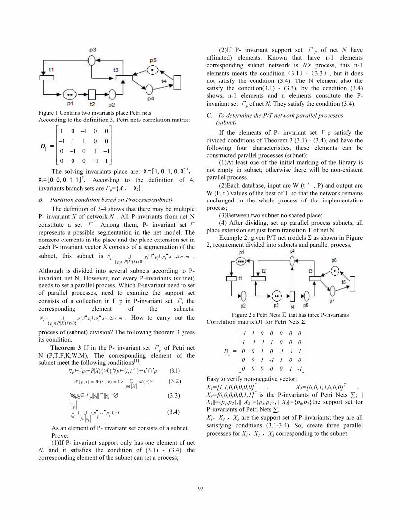
Figure 1 Contains two invariants place Petri nets According to the definition 3, Petri nets correlation matrix:

1 0 1 0 01 1 1 0 0

1 0 1 0 1 10 0 0 1 1

! ""# $"# $# $" "# $# $"% &

D =

The solving invariants place are: According to the definition of 4,

invariants branch sets are p={

B. Partition condition based on Processes(subnet) The definition of 3-4 shows that there may be multiple

P- invariant X of network-N . All P-invariants from net N constitute a set . Among them, P- invariant set represents a possible segmentation in the net model. The nonzero elements in the place and the place extension set in each P- invariant vector X consists of a segmentation of the subnet, this subnet is , 1,2, ,

{ | ( ) 0}N p p p i mi i i i

p P X ii

• •= =# >

! ! "! .

Although is divided into several subnets according to P- invariant net N, However, not every P-invariants (subnet) needs to set a parallel process. Which P-invariant need to set of parallel processes, need to examine the support set consists of a collection in ! p in P-invariant set , the corresponding element of the subnets:

, 1,2, ,{ | ( ) 0}

N p p p i mi i i ip P X ii

• •= =# >

! ! "! . How to carry out the

process of (subnet) division? The following theorem 3 gives its condition.

Theorem 3 If in the P- invariant set p of Petri net N=(P,T;F,K,W,M), The corresponding element of the subnet meet the following conditions[1]:

!p {pi P|X(i)>0},!p (t, t ) p• •p (3.1) '

( , ) ( , ) 1 ( ) 1W p t W t p M pp X

'= = $ %#

(3.2)

!s1,s2 p,||s1|| ||s2||=& (3.3)

( ( ))1

pp p Tjji j si

'• •( =

= #! ! (3.4)

As an element of P- invariant set consists of a subnet. Prove: (1)If P- invariant support only has one element of net

N. and it satisfies the condition of (3.1) - (3.4), the corresponding element of the subnet can set a process;

(2)If P- invariant support set p of net N have n(limited) elements. Known that have n-1 elements corresponding subnet network is N's process, this n-1 elements meets the condition 3.1 - 3.3 , but it does not satisfy the condition (3.4). The N element also the satisfy the condition(3.1) - (3.3), by the condition (3.4) shows, n-1 elements and n elements constitute the P- invariant set p of net N. They satisfy the condition (3.4).

C. To determine the P/T network parallel processes (subnet)

If the elements of P- invariant set p satisfy the divided conditions of Theorem 3 (3.1) - (3.4), and have the following four characteristics, these elements can be constructed parallel processes (subnet):

(1)At least one of the initial marking of the library is not empty in subnet; otherwise there will be non-existent parallel process.

(2)Each database, input arc W (t , P) and output arc W (P, t ) values of the best of 1, so that the network remains unchanged in the whole process of the implementation process;

(3)Between two subnet no shared place; (4) After dividing, set up parallel process subnets, all

place extension set just form transition T of net N. Example 2: given P/T net models " as shown in Figure

2, requirement divided into subnets and parallel process.

Figure 2 a Petri Nets that has three P-invariants Correlation matrix D1 for Petri Nets ":

1

-1 1 0 0 0 0 01 -1 -1 1 0 0 0

D 0 0 1 0 -1 -1 10 0 1 -1 1 0 00 0 0 0 0 1 -1

! "# $# $# $# $# $# $# $% &

=

Easy to verify non-negative vector: X1=[1,1,0,0,0,0,0]T X2=[0,0,1,1,0,0,0]T X3=[0,0,0,0,0,1,1]T is the P-invariants of Petri Nets #; || X1||={p1,p2},|| X2||={p3,p4},|| X3||={p6,p7}the support set for P-invariants of Petri Nets #. X1 X2 X3 are the support set of P-invariants; they are all satisfying conditions (3.1-3.4). So, create three parallel processes for X1 X2 X3 corresponding to the subnet.

92

V. PARTITION STRATEGY BASED ON T- DIAGRAM Petri Nets parallel partition strategy based on

transitional is: divided any two different transitional at different equivalence classes, it belongs to the before or after set in a place; the different transitional of equivalence class partition network conditions; determinant the Parallel processes (subnet).

A. A formal definition of T- diagram and basic principles The formal definition of divide subnet of T- diagram: Definition 5 !ti,tj T, )p P, let (ti

•p tj•p) (ti

p • tj p • ) (i"j and i, j {1,2,…,n}),then ti, tj is the equivalence class.

Definition 6 let #= P T F M is a Petri Nets, mark $:T {0,1}satisfy $ ti ==$ tj =1, if and only if !ti, tj T, )p P, let (ti

•p tj•p) (ti p • tj p • )

(i" j and i,j {1,2,…,n}); Otherwise $ t 0 !t T. Definition 7 [7-9] let # = (P, T; F, M0) is a Petri Nets,

P1 * P , !M$# R(M 0 ) ,then define 'p+p1M is a projection from M P to P1, satisfied !p # P1, 'p+p1M (p) = M (p).

Definition 8 let # = (P ,T ; F , M 0 ) is a Petri Nets, mark $:T {0,1}is a dynamic partition marked of transitional, if ,i = (Pi ,Ti ; Fi , M 0i ), (i$#{1, 2,..., k}) is the subnet of #.if and only if ,i satisfy:

(1) Ti = {!t # Ti $(t)= 0} Ti T;

(2) Pi$= {p # P )t #Ti , p# •t p# t •};

(3) Fi$ = {(Pi - Ti ) (Ti - Pi )} F ; (4) M 0i = 'S$+Si M 0 From the above four definitions we can get the basic

principle and steps of subnet based on T- diagram. First of all, by definition 6 to find the transitional of $(ti) t T; Secondly, analysis of marker $(ti), turn out mark of $(ti)=1 in the new set of A, and update marker $(ti) $(tj) ti T-A, tj A, until all the markers $(ti)=0 ti T-A; Secondly, repeat the above work for the new subnet set A, until all the markers $(tj)=0, tj A; Finally, constructing the of the dividing branch nets #i. by definitions 6, 7.

B. Condition of dividing branch nets for T- graph The condition gives by the following theorem 4. Theorem 4 let # = (P,T ; F , M 0 )is Petri Nets, If the

Net # can be divided, if and only if )t #T and $(t)=1. Proof: necessity Because the can be divided, it must have !ti, tj T,

)p P, Make (ti•p tj

•p) (ti p • tj p • ) (i" j i, j {1,2,…,n}), then by definition 2.1 we can see that there will be $(ti)=1, that is $(t)=1, necessity can be proved.

Sufficiency Because in the net )t #T and $ (t) =1, then by

definition 5 we can know, must satisfied !ti, tj T, )p P, make (ti

•p tj•p) (ti p • tj p • ) (i" j and i, j

{1,2,…,n}), can be derived from the original Net # can be divided, sufficiency can be proved.

Theorem 5 let # i= (Pi, Ti; Fi , M0i )is dividing branch nets of Petri Nets, Then the # i is a T- graph.

Proof: because # i= (Pi ,Ti ; Fi , M0i )is dividing branch nets of Petri Nets, then the # i is can't be divided, there is no !tk, tj Ti, )p Pi, make (tk

•p tj•p) (tk p • tj p • )

(k" j and k, j {1,2,…,n}), that is: !p P:| •p|=| p •|=1, according to the definition of T- graphs, theorem 6 can be proved.

C. To determine the T- graph process (subnet) Traverse of transitional set of Petri Nets, according to

definition 5 and definition 6, to determine if each transitional of phi (T) value is 1, according to the basic principle of dividing branch nets for T- graph, One by one divide into the net. The following example is parallel divided subnet of Petri Nets.

Ex.3: As the Petri Nets model shown in Figure 1, given the dividing branch nets based on.

By theorem 4 we can see that In the beginning, T={$(t1) 1 $(t2) 0 $(t3) 1 $(t4) 0}, then take the mark 1 in T t1 A, that is A {t1}; At this time, T-A{$(t2) 0 $(t3) 0 $(t4) 0},all of this transitional marks is 0 in T-A, and transitional marks also is 0 in A. Now T can be divided into A and T-A two subset, in which A = {t1}, T-A= {t2, t3, t4}. If let A A1 T-A A2, we can get two subnets#1 (P1 ,A1 ; F1 , M01) and #2 (P2 ,A2 ; F2, M02 ), it as shown in Figure 3 and Figure 4. By Theorem 5 we can know, figure 3, and figure 4 are T- diagram. According to the strategy and method of solving T- diagram, get? 1 and? 2 two T- diagram, the two T- diagram can constitute two subnets.

Figure 3 ,1 (P1 ,A1 ; F1 , M01 )

Figure 4 ,2 (P2 ,A2 ; F2, M02)

VI. ANALYSIS AND EVALUATION OF THE TWO PARTITION STRATEGY

By the two chapters described above, we research on the Petri Nets parallel partitioning strategy of functional from different points of view, get two different subnet

93

partition strategy. Below we will analyze and evaluate the two partition strategies in theory and practice.

A. Comparison and analysis of partition strategy The goal is the same with P- invariant function

partition strategy and T- graph partitioning strategy. In determining the process of the Petri Nets function partition and parallel process (subnet), they have certain commonality, such as: (1) to formalize the Petri net model by input, output and correlation matrix. (2) parallel processes (subnet) division must follow the principle and condition, only to satisfy division condition of Petri network can be divided into several subnets. But they have the essential difference, mainly in: (1) the P- invariant partition strategy is in accordance with the place of Petri net model and its change place to solve, but the T- graph partitioning strategy is based on the behavior of transitional and the state of changes in the classification; (2) to achieve the P- invariant partition strategy is through solving the correlation matrix for Petri Nets and homogeneous linear equations; the implementation of T- graph partitioning strategy is through traversing all the transitional of the Petri Nets. (3) on the basis of strict Theorem 3 mathematical theory as the P- invariant partition, partition results in higher precision, while also has the function as a conditions of T- graph partitioning but is relatively simple, accurate results in lower division.(4) for large Petri Nets, P- invariant partition strategy based on manual processing, is at such a high price, while automatic processing is fast; T- graph partition strategy using artificial treatment is much more convenient, but it takes a long time when the computer traversal process.

Case 1 in the fourth section and Case 3 in the fifth section are subnet in the same Petri Nets (Figure 1). Case 1 gets two P- invariant

that is According to the definition of 4, Place-

invariants branch set p={ satisfy the conditions of Theorem 3 subnet division, eventually Petri network into two subnet, each of them contains the places and transitions are Among them, is the common transition of two subnets, the two transition of classification is A1 {t1} ,A2={t2,t3,t4}.We can get two subnets #1 (P1 ,A1 ; F1 , M01)and #2 (P2 ,A2 ; F2, M02 ). Each of them contains the places and transitions are and

among them, is a common place of two subnets. From the classified results, Partition strategy of P- invariants is evenly distributed in division of the subnet can reflect the concurrency between transitions.

B. Evaluating the partitioning strategy After the comparison and analysis of the two kinds of

different partitioning strategies, two strategies can be subnet partition of Petri Nets system in accordance with the concurrent function. But from the perspective of Petri

network parallel, partitioning strategy based on P-invariant has the mathematical theories; The P- invariants also make the more accuracy of subnet division. Division of the subnet is more suitable for parallel processing. It is closer to the prototype of Petri Nets system. Therefore, for Petri parallel subnet partition strategy of function, P- invariant partition strategy is better than the T- graph partitioning strategy.

VII. CONCLUSIONS We study subnet of Petri Nets system, in order to realize

the parallel simulation or operation of the Petri network. In the research of Petri Nets partition strategy, through the method of correlation matrix and linear equations, solving the P- invariant, we can judge whether P- invariant can satisfy the functional condition of Petri Nets to determine the division of the subnet. Through traversing the transition of Petri Nets, we find out the classification of different transition, so as to determine the different subnet partition.Through the analysis and comparison of two different partition strategies, we can give the theoretical proof and example verification that the P- invariant partition strategy is better than the T- graph partitioning strategy, providing the effective and optimized subnet partition strategy for Petri net parallelization. Study of conditions of subnet division of the function for Petri Nets is our next major work.

REFERENCES [1] M. Paludetto. Sur la commande de procedes

industriels:unemethodologie basee objets et reseaux de Petri. These de doctorat,Universite Paul Sabatier,Toulouse, France,1991 34-47.

[2] W.El Kaim and F.Kordon. An integrated framework for rapid system prototyping and automatic code distribution. In 5thIEEE International Workshop on Rapid System Prototyping,Grenoble,IEEE Comp.Soc.Press,1994:52-61.

[3] J.M.Colom and M.Silva. Convex geometry and semiflows in P/T nets. A comparative study of algorithms for computation of minimal P-semiflows. In Rozenberg,Advances in Petri Nets 1990,Volume 483 of Lecture Notes in Computer Science.Springer-Verlag,1991:79-112.

[4] WU Z H.Petri Nets Introduction[M]. Beijing: Mechanical industry publishing house.2006, pp.144-155.

[5] Girault C and Valk R.Petri Nets for Systems Engineering: A Guide to Modeling, Verification, and Applications [M].Springer-Verlag Berlin Heidelberg. 2003,pp.159-235.

[6] Wen-jing LI, Wen YANG, Shuang LI. Research on Methods of Transformation of Petri Nets Systems into the Place Transition Nets. 2012 Third Global Congress on Intelligent Systems,Publicshed by conference publishing services,2012:233-236.

[7] Hao Kegang, Ding Jianjie. Hierarchical Petri nets[J].Journal of Frontiers of Computer Science and Technology,2008, 2(2): 123-130.

[8] Suzuki, Murata T. A method for stepwise refinement and abstraction of Petri nets[J]. Journal of Computer and Sys-tem Science, 1983, 27(1): 51-76.

[9] Lee K H, Favrel J, Baptiste P. Generalized Petri net re-duction method[J]. IEEE Trans on Systems, Man and Cybernetics, 1987, 17(2): 297-303.

94

Corresponding Author: Xuesong Wu

An Improved KM Algorithm for Computing Structural Index of DAE System

Yan Zeng1,2, Xuesong Wu 1, Jianwen Cao1 1. Laboratory of Parallel Software and Computational Science of Software, Institute of Software Chinese

Academy of Sciences, Beijing, 100190, China; 2. Graduate University of Chinese Academy of Sciences, Beijing, 100049, China.

Email: zengyan_616@yahoo.cn ; xuesongwu@msn.cn; caojianwen@gmail.com

Abstract: This paper proposes an improved KM algorithm to computing the structural index of linear time-invariant Differential Algebraic Equation (DAE) systems. The problem is of practical significance in index reduction based on structural index of DAE system and combinatorial relaxation theory. This improved KM algorithm combines greedy idea and classical KM algorithm. It first computes matches as much as possible using greedy technology, and then call KM algorithm to search the matches for the unmatched vertices during the step of greedy technology. The improved KM algorithm reduces the running time bound by a factor of , the

number of matches searched using greedy algorithm. Generally, the time complexity is , the optimal time is .

Keywords: DAE; Index Reduction; Structural Index; Bipartite Graph; Greedy; KM Algorithm

I. INTRODUCTION

Graph theory can be used to model many types of practical dynamical systems such as economic, electric networks, mechanical systems, etc. And graph theoretical methods are widely used in solving combinatorial optimization problem(such as assignment problem), determining the order of solving differential algebraic equation(DAE) and structural index reduction for high-index DAE[1].

High-index DAE systems describe these dynamic systems after multi-domain modeling and simulation, such as Modelica modeling[2]. For the high-index DAE, it is a difficult problem to solve it numerically at present[3]. It is desirable to transform the high-index DAE into an equivalent low-index DAE, which can be solved directly by numerical methods (such as Backward Difference method, Runge-Kutta method, etc[4]), through index reduction method.

Index reduction method based on structural index of DAE system (as Pentelides method[5]) is one of popular index reduction method, and combinatorial relaxation theory is widely used to check and correct the fail of structural index reduction[6]. Both in this index reduction method and combinatorial relaxation theory, the structural matrix is described as a bipartite graph

, where the vertex set stands the row set , the vertex set stands the column set ,

and the edge set corresponds to the set of nonzero entries of . Each edge is given a weight

, and the computing of structural index is converted to compute the maximum weighted matching of bipartite graph.

Kuhn and Munkres(KM) algorithm[7] is a classical combinatorial optimization algorithm to solve the maximum-weighted matching problem of bipartite graph. It is a prototype of a great number of algorithms in area such as network flows, matroids, and matching theory. Other combinatorial optimization algorithms, such as Ford-Fulkerson method[8], Edmons-Karp algorithm[9] developing from KM algorithm, also can solve this matching problem. They are based on searching for augmenting path and their time complexity is . But Ford-Fulkerson method is used in network flows and Edmonds-Karp is for the non-bipartite graph. So, this paper considers the KM algorithm.

For the linear time-invariant DAE system, there always have some rows in the structural matrix having different feasible matching columns with each other, so these rows have their unique matches which can be found via greedy method in times. This motivates us to propose an improved KM algorithm (called as Greedy_KM algorithm in this paper) to compute the structural index of DAE. It first computes matches as much as possible using

2013 12th International Symposium on Distributed Computing and Applications to Business, Engineering & Science

978-0-7695-5060-2/13 $26.00 © 2013 IEEEDOI 10.1109/DCABES.2013.24

95

greedy algorithm, and then call KM algorithm to search the matches for the unmatched vertices in the step of greedy technology. Greedy_KM algorithm reduces the number of vertices that need calling KM algorithm to search their matches via greedy algorithm and uses the classical KM algorithm to ensure the optimal solutions.

This paper is organized as follows: Section 2 simplify introduces the structure index and how to transform problem of computing structural index to the maximum weighted-matching problem of bipartite graph. For the maximum weighted- matching problem, it presents the classical KM algorithm and dwells on the improved KM algorithm in section 3. Some numerical experiments are provided to quantify the time performance of KM algorithm and Greedy_KM algorithm in section 4. And section 5 gives a conclusion.

II. STRUCTURAL INDEX

Given a linear time-invariant DAE system , in which is a nonsingular polynomial matrix in , is

the variable for the Laplace transformation corresponding to . According to the Cramer’s rule, the solution is as follows:

(1)

Assuming is the structural matrix of (1), the structural index of this DAE system can be defined as (2) [10]:

(2)

In which, of is a rational function in . The degree of a rational function (with and being polynomials) is defined by , so the structural index also can be defined as (3):

(3)

In fact, can be described as a flow network with as source and

as sink , and stand the row set and column set of separately. Vertex set , edge set , where

, ,

. The capacity set limits the flow of each edge, and the weight set

. Structural matrix describes the relationship between

equations and variables, and the relationship of with is a path in a graph[11]. For , it corresponds to a flow with as source and as sink in the flow network . In a flow network, a maximum flow[12] is a flow maximizes the value . And a max cost max flow is a flow has the maximum cost

among the maximum flows. The corresponds to the max cost max flow in , and its value is equal to the maximum cost of .

For the first term on the right side of (3), it corresponds to the maximum flow having the maximum cost among the

max cost max flows with source and sink . And its value

equals to the cost of , that is .

In fact, the max cost max flow in is the maximum weight in a bipartite graph

[13]. So, we can have , where

denotes the set of all the matching of size . For the second term on the right side of (3), there is

, according to above describes. So the structural index is equivalent to (4):

(4)

For the maximum weighted-matching of bipartite graph, this paper presents the classical KM algorithm and dwells on the Greedy_KM algorithm in next section.

III. MAXIMUM WEIGHTED MATCHING

ALGORITHM

KM algorithm is a classical algorithm in solving maximum weighted-matching problem of bipartite graph. Based on KM algorithm and greedy idea, this section introduces Greedy_KM algorithm. Compared with the classical KM algorithm, Greedy_KM algorithm has a significant improvement in time performance for the special matrices, which can be transformed to

96

main diagonally dominant positive matrices or diagonally dominant positive matrices by row/column transformations. Diagonally dominant matrix is widely applied in the mathematical model, such as DAE systems.

A. KM Algorithm

KM algorithm[7] is a combinatorial optimization algorithm. It solves the maximum weighted-matching problem of bipartite graph based on Hungarian method. The idea of KM algorithm: it converts the weight of edges to the value of feasible vertex labeling, and then calls the Hungarian method to find a perfect matching. If it finds a perfect matching , stop( is the maximum weighted matching); Otherwise, modify the value of feasible vertex labeling, increasing the feasible edges, and continue to call Hungarian method to find a perfect matching, repeat this process until it finds a perfect matching , then this matching is the maximum weighted matching.

B. Greedy_KM Algorithm

A greedy algorithm is an algorithm that follows the problem solving heuristic of making the locally choice at each stage with the hope of finding a global optimum. In some cases such a strategy is guaranteed to offer optimal solutions, but in some other cases it may just provide a compromise that produces approximate solutions. Its time complexity is . This paper takes advantage of its properties of high efficiency and approximate solution to propose a Greedy_KM algorithm.

For the maximum weighted-matching problem of bipartite graph , firstly, using greedy strategy to find a feasible matching vertex for all vertices

as much as possible. Feasible matching vertex has a maximum weight with and has not been matched by other vertices or if has been matched by . If there is such a feasible matching vertex , then mark being matched. After using the greedy strategy, call KM algorithm to find matches for the unmatched vertices in and . It works as follows (Algorithm3.1):

Algorithm 3.1: Greedy_KM Algorithm

In the step 2 of Algorithm 3.1, it will encounter three situations

that use greedy technology to search a feasible matching vertex for vertex , such as Graph 3, search a feasible matching vertex

for . Situation1: Vertex has not been matched by other vertices

and the weight is maximum for and , that is and

. Such as Graph 3.1a, it can find for and label . Situation2: Vertex has been matched by vertex and

, then mark vertex being not matched. Such as Graph 3.1b, the vertex has been matched by and

. Situation3: Vertex has been matched by vertex but

, then label and mark vertex being not matched, such as Graph 3.1c, vertex has been matched by , but , so label and mark being not matched.

For the situation 1 and situation 3, the match can be found in running times using greedy strategy. But for the situation 2,

as it cannot find a feasible matching vertex for vertex using greedy strategy, it must call KM algorithm to do this, and it needs

times. So using greedy strategy to search matches can

Input: Bipartite graph

Output: the maximum weighted-matching

Step 1: Make the bipartite graph to a complete weighted

bipartite graph by adding some edges of zero weight as necessary.

Step 2: Use greedy strategies to find a feasible matching vertex for all vertices as

much as possible, if all vertices in are matched, stop.

Otherwise, go to step 3. Step 3: For the unmatched vertices in , call KM algorithm to

find a perfect matching .

97

reduce the number of vertices, which should call KM algorithm to find their matches. At last, it can reduce the total time to compute the maximum weighted matching, especially for the special matrices, which can be transformed to main diagonally dominant positive matrices or diagonally dominant positive matrices by row/column transformations.

A diagonally dominant positive matrix is a special diagonally dominant matrix, satisfying and

, for all . So, we can have . And a main diagonally dominant positive matrix is a matrix which satisfies and , for all and .

Given a special matrix , supposing it can be transformed to a main diagonally dominant positive matrix or diagonally dominant positive matrix . The diagonal of matrix precisely corresponds to a term in the row of matrix . Therefore, the diagonal terms of are precisely the terms of , and

. So it is sure that there is a different feasible matching column for every row of . That is, if finding a feasible matching vertex in column set for the vertices in the row set , all will be found by using greedy technology, like as situation 1. Therefore, there is no vertex in

needing to call KM algorithm, and at last the time is for computing the maximum weighted-matching of

bipartite graph corresponding to the special matrix .

C. Comparison and Analysis

The classical KM algorithm calls Hungarian method to find a perfect matching and uses the feasible vertex labeling technologies. It uses DFS single-augmented method[14] to search augmenting paths. The time complexity of searching an augmenting path by DFS is and it at most needs times to search augmenting paths running KM algorithm, so the total time complexity is .

Greedy_KM algorithm takes advantage of the greedy algorithm’s properties of high efficiency and approximate solution, the time complexity of a greedy algorithm for computing maximum weighted-matching of bipartite graph is . Assuming there are matches computed by the greedy technology, then call KM algorithm to find matches for the unmatched vertices in , its time complexity is

. If , it has the optimal running time . The worst time is when , it may slightly

slower than classical KM algorithm. But in general, the time complexity is between and , when

. That is, Greedy_KM algorithm is better than the classical KM algorithm for the matrix , which has so many rows having different feasible matching column with each other. Such as diagonally dominant positive matrix, special matrix including a subdeterminant can be converted to the diagonally dominant positive form by row/column transformations.

IV. EXPERIMENT

For the linear time-invariant DAE system , this paper just considers (it is same to solve the DAE with

). According to the structure matrix of the DAE system, it can construct a bipartite graph , where

, . The vertex set corresponds to the row set of , the vertex set corresponds to the column set of , the edge set corresponds to the set of nonzero entries of , and each edge is given a weight

. In order to evaluate the time performance of the classical KM

algorithm and Greedy_KM algorithm, this paper run a set of numerical experiments on the Linux platform (Ubuntu SMP x86_64 GNU/Linux Kernel version2.6.35-32, Intel(R) Xeon(R) CPU X7550@2.00GHz, 512GB, GccVersion4.4.5), and the test data is randomly produced by programs. The weight of each edge

is randomly produced in range of as the degree of in DAE systems are mostly in this range. In the experiments, this paper compares special sparse ( ) and dense matrices (

), which can be transformed to main diagonally dominant positive matrices or diagonally dominant positive matrices by row/column transformations. The following tables show the results.

TABLE I: SPECIAL SPARSE MATRIX

Algorithms

Time (ms)

KM Greedy_KM

n=50 0.5 0.09

n=100 0.95 0.13

n=500 6.92 1.32

n=1000 16.2 4.8

n=5000 240 120

98

TABLE II: SPECIAL DENSE MATRIX

Algorithms

Time (ms)

KM Greedy_KM

n=50 0.56 0.1

n=100 1.17 0.18

n=500 8.85 2.77

n=1000 20 10

n=5000 820 670

“Table I” and “Table II” summarize the results of our random experiments for the special matrices, including sparse matrices and dense matrices. For the special matrices, the time performance of Greedy_KM algorithm is significantly improved. When the number of vertices , for the sparse matrices, its running time does not exceed of the classical KM algorithm, and its best running time is only about of classical KM algorithm. For the dense matrices, it does not exceed of classical KM algorithm. When , its running time does not exceed of the classical KM algorithm for sparse matrices.

V. CONCLUSION

Solving high-index DAE is often a difficult and challenging problem. Index reduction method based on the structural index of DAE system and the combinatorial relaxation theory, checking and correcting the fail of reducing the structural index, can solve this difficult problem. Both this index reduction method and combinatorial relaxation theory take advantages of graph theory to solve complex mathematical problems, they convert the problem of computing structural index to the maximum weighted-matching problem of bipartite graph. This paper presents the transformation in details and proposes an improved KM algorithm based on greedy idea and KM algorithm. The experiment results show that for the special matrices, which can be transformed to main diagonally dominant positive matrices or diagonally dominant positive matrices by row/column transformations, the time

performance of Greedy_KM algorithm is significantly improved. As the time performance is improved, the Greedy_KM algorithm is important for high performance computing. In the future, we will research how to computing the structural index of large-scale DAE systems by combining strongly connected component methods and the Greedy_KM algorithm.

ACKNOWLEGEMENTS

This research has been supported by National Natural Science Foundation (61170325) and National High Technology Research and Development Program of China (863 Program, 2009AA044501).

REFERENCE [1] Mikael Zebbelin Poulsen. Structural Analysis of DAEs. Denmark:

Informatics and Mathematical Modeling Technical University of Denmark, 2001.

[2] Fritzson P. Principles of Object-Oriented Modeling and Simulation with Modelica 2.1. New York: IEEE Press, 2003.

[3] Mizuyo Takamatsu, Saturu Iwata. Index Reduction for Differential-Algebraic Equations by Substitution Method, Linear Algebra and its Applications, 429, pp 2268-2277, 2008.

[4] Pawel Bujakiewicz. Maximum Weighted Matching for High Index Differential Algebraic Equations, Schiedam, 1994.

[5] Peter Kunkel, Volker Mehrmann. Differential-Algebraic Equations: Analysis and Numerical Solution, EMS Publishing House Zürich, 2006.

[6] Kazuo Murota. Combinatorial Relaxation Algorithm for the Maximum Degree of Subdeterminants: Computing Smith- McMillan Form at Infinity and Structural Indices in Kronecker Form, Applicable Algebra in Engineering, Communication and Computing, 6, pp 251-273, 1995.

[7] Kuhn, Harold W. Variants of the Hungarian method for assignment problems, Naval Research Logistics Quarterly, 3, pp 253-258, 1956.

[8] Ford, Lester R., and Delbert R. Fulkerson. Maximal flow through a network, Canadian Journal of Mathematics, 8, pp 399-404, 1956.

[9] J. Edmonds, Maximum matching and a polyhedron with 0 ! 1 vertices, Journal of Research of the National Bureau of Standards (B), 69, pp 125-130, 1965.

[10] Kazuo Murota. Matrices and Matroids for Systems Analysis, Springer Berlin Heidelberg, 2010.

[11] Rosen K.H. Discrete Mathematics and Its Applications, Beijing: China Machine Press, 2008.

[12] Andrew V.Goldberg, SagiHed, Haim Kaplan, Robert E.Tarjan, Renato F.Werneck. Maximum Flows by Incremental Breadth First Search, Algorithms-ESA, 2011.

[13] Thomas H.Cormen, Charles E.Leiserson, Ronald L.Rivest, Clifford Stein. Introduction to Algorithms, third edition. Beijing: China Machine Press, 2012.

[14] Yan Zeng, Xuesong Wu, Jianwen Cao. Analysis and Implementation for the Algorithm based on Combinatorial Relaxation for Computing the Structure Index of DAE, Springer System Simulation and Scientific Computing, pp 277-286, 2012.

99

Parallel ADI Smoothers for Multigrid

Craig C. Douglas

University of WyomingSchool of Energy Resources and Mathematics Department

Laramie, WY 82081-1000, USAEmail: craig.c.douglas@gmail.com

Gundolf Hasse

Karl-Franzens-University GrazInstitute for Mathematics and Scientific Computing

Heinrichstr. 36, Room 506A-8010 Graz, Austria/Europe

Email: gundolf.haase@uni-graz.at

Abstract—Alternating Direction Implicit (ADI) methods have been inuse since 1954 for the solution of both parabolic and elliptic partial differ-ential equations. The convergence of these methods can be dramaticallyaccelerated when good estimates of the eigenvalues of the operator areavailable, However, in the case of computation on parallel computers, thesolution of tridiagonal systems imposes an unreasonable overhead. Wediscuss methods to lower the overhead imposed by the solution of thecorresponding tridiagonal systems. The proposed method has the sameconvergence properties as a standard ADI method, but all of the solvesrun in approximately the same time as the “fast” direction. Hence, thisacts like a ”transpose-free” method while still maintaining the smoothingproperties of ADI. Algorithms are derived and convergence theory isprovided.

Keywords—Partial differential equations; Distributed/parallel comput-ing; Alternating direction implicit method; Iterative algorithms

I. INTRODUCTION

Consider the following elliptic boundary value problem:

Find !(x) such that

−∑!

"=1("(x)!#!(x))#! + #(x)!(x) = $(x), ∀x∈Ω,

!(x) = &(x), ∀x∈Γ,

(1)

where Ω is a rectangular domain in ℝ!, Γ = ∂Ω is the boundary,and " and # are positive and bounded real functions ∀x ∈ Ω.

In §II, we define several ways of distributing data in a parallelcomputing environment in order to minimize communication. In §III,we define a many properties of a model problem. In §IV, we definean approximate parallel ADI iteration that is inherently embarrassingparallel. In §V, some final conclusions are drawn.

II. PARALLEL DATA DISTRIBUTION

We begin by collecting some abstract results for non-overlappingelement data distribution [1], [2], [3]. Applications of this approachin biomedical simulations can be found in [4], [5]. We only considerparallel storage schemes for vectors and matrices that are dataconsistent on each processor, i.e., if any element is on more thanone processor, the value is the same on all processors. We denote thevectors by ! and " and the matrices by # and call them accumulatedvectors and matrices. The nodes can be grouped into three classes:inner nodes, edge nodes, and vertex nodes, with subscripts ( , ),

and * . This classification induces an appropriate block structure invectors and matrices.

As shown in [1], the operation # ⋅ ! can be performed withoutcommunication only for the following special structure:

# =

⎛

⎝#$ 0 0#%$ #% 0#&$ #&% #&

⎞

⎠ =⇒ ! = # ⋅", (2)

with block-diagonal matrices #& , #% , and #$ . In particular, thesubmatrices must not contain entries between nodes belonging todifferent sets of processors. The proof for (2) can be found in [2],[3].

The block-diagonality of #& and the correct block structureof #&% and #&$ are guaranteed by the data decomposition. How-ever, the mesh must fulfill the following two requirements in order toguarantee the correct block structure for the remaining three matrices:

R1: There is no connection between vertices belonging todifferent sets of subdomains. This guarantees the block-diagonality of #$ (often #$ is a diagonal matrix). Thereis no connection between vertices and opposite edges. Thisensures the admissible structure of #%$ (and #$ %).

R2: There is no connection between edge nodes belonging todifferent sets of subdomains. This guarantees the block-diagonality of #% .

Denote by + a diagonal matrix with elements +'' equal to thenumber of processors a node , belongs to. We introduce the booleanmatrix -" which maps a global vector to a local one, i.e., !" = -" ⋅!.Similarly, submatrices are notated by #" = -" ⋅# ⋅-(

" . If we makethe same assumptions on #& , #% , and #$ as in (2) and denotewith #), #* and #+ the strictly lower, upper and diagonal blockpart of #, then we can perform

" = # ⋅ ! := (#) +#+) ⋅ ! +,∑

"=1

-(" #*,"+

−1" ⋅ !" . (3)

The only difference between (3) and (2) is that the last term in (3)causes exactly one next neighbor communication.

2013 12th International Symposium on Distributed Computing and Applications to Business, Engineering & Science

978-0-7695-5060-2/13 $26.00 © 2013 IEEEDOI 10.1109/DCABES.2013.25

100

The inner product of two accumulated vectors requires the correctscaling of one vector to get the exact result, namely,

(!, +−1!

)

[1], [2]. Unfortunately, an inner product calculation requires globalsummation (e.g., a parallel reduction operation) of a scalar.

III. THE POISSON EQUATION AND ITS FINITE DIFFERENCE

DISCRETIZATION

Let us start with a simple, but at the same time very importantexample, namely the Dirichlet boundary value problem for the Pois-son equation in the rectanglular domain Ω = (0, 2) × (0, 1) withthe boundary Γ = ∂Ω. Given some real function $ in Ω and somereal function & on Γ, find a real function ! : Ω → ℝ defined onΩ := Ω ∪ Γ such that

"(x) = 1, , #(x) = 0, in (1) with & = 0 on Γ. (4)

For simplicity, we consider only homogeneous Dirichlet boundaryconditions, but more complicated boundary conditions are practical.The given functions as well as the solution are supposed to besufficiently smooth.

The Poisson equation (4) is certainly the most prominent repre-sentative of second-order elliptic partial differential equations (PDEs)not only from a practical point of view, but also as the most frequentlyused model problem for testing numerical algorithms.

The Poisson equation can be solved analytically in special cases,as in rectangular domains with just the right boundary conditions, e.g.,with homogeneous Dirichlet boundary conditions as imposed above.Due to the simple structure of the differential operator and the simpledomain in (4), a considerable body of analysis is known that can beused to derive or verify solution methods for Poisson’s equation andmore complicated ones.

If we split the intervals in both the / and 0 directions into 1#

and 1. subintervals of length ℎ each (i.e., 1# = 21.), then weobtain an appropriate grid (or mesh) of nodes. We define the set ofsubscripts for all nodes by 3ℎ := {(4, ,) : 4 = 0, 1#, , = 0, 1.}, theset of subscripts belonging to interior nodes by 3ℎ := {(4, ,) : 4 =1, 1# − 1, , = 1, 1. − 1}, and the corresponding set of boundarynodes by 5ℎ := 3ℎ ∖ 3ℎ. Furthermore, we set $",' = $(/", 0'), andwe denote the approximate values to the solution !(/", 0') of (4) atthe grid points (/", 0') := (4ℎ, ,ℎ) by the values !",' = !ℎ(/", 0')of some grid function !ℎ : 3ℎ → ℝ. Here and in the following weassociate the set of indices with the corresponding set of grid points,i.e., 3ℎ ∋ (4, ,)↔ (/", 0') ∈ Ωℎ. Replacing both second derivativesin (4) by second-order finite central differences at the grid points weimmediately arrive at the standard five point stencil finite differencescheme that represents the discrete approximation to (4) on the grid3ℎ: Find the values !",' of the grid function !ℎ : 3ℎ → ℝ at allinterior grid points (/", 0'), with boundary points (4, ,)∈3ℎ, suchthat

1ℎ2 (−!",'−1 − !"−1,' + 4!",' − !"+1,' − !",'+1) = $",' ,

!",' = 0.(5)

Arranging the interior (unknown) values !",' of the grid function!ℎ in a proper way in some vector !ℎ, e.g., along the vertical (orhorizontal) grid lines, and taking into account the boundary conditionson 5ℎ, we observe that the finite difference scheme (5) is equivalentto the following system of linear algebraic equations: Find !ℎ ∈ ℝ0 ,1 = (1# − 1) ⋅ (1. − 1), such that

6ℎ ⋅ !ℎ = $ℎ, (6)

where the 1×1 system matrix 6ℎ and the right-hand side vector$ℎ∈ℝ0 can be rewriten from (5) in an explicit form.

The (band as well as profile) structure of the matrix 6ℎ heavilydepends on the arrangement of the unkowns, i.e., on the numberingof the grid points. In our example, we prefer the numbering alongthe vertical grid lines because exactly this numbering gives us thesmallest band width in the matrix. To keep the band width as smallas possible is very importent for the efficiency of direct solvers.

We first look at further algebraic and analytic properties of thesystem matrix 6ℎ which may have some impact on the efficiency ofsolvers. More precisely, the dimension 1 of the system grows like7(ℎ−1), where 8 is the dimension of the computational domain Ω,i.e., 8 = 2 for our model problem (4). Fortunately, the matrix 6ℎ issparse since our matrix 6ℎ in (6) has at most 5 nonzero entries perrow and per column independent of the fineness of the discretization.This property is certainly the most important one with respect toefficiency of iterative solvers as well as direct solvers.

A smart discretization technique should preserve the inherentproperties of the differential operator involved in the BVP. The matrix6ℎ is symmetric (6 = 6( ) and positive definite ((6!, !) >0, ∀! ∕= 0). These properties result form the symmetry (formalself-adjointness) and uniform ellipticity of the Laplace operator.Symmetric and positive definite (SPD) matrices are regular, hence,invertible. Thus, our sytem of finite difference equations (5) has aunique solution.

Unfortunately, the matrix 6ℎ is badly conditioned. The spectralcondition number cond2(6ℎ) = :12#(6ℎ)/:1"3(6ℎ) defined bythe ratio of the maximal eigenvalue :12#(6ℎ) and the minimaleigenvalue :1"3(6ℎ) of the matrix 6ℎ behaves like 7(ℎ−2) ifℎ tends to 0. That behavior affects the convergence rate of allclassical iterative methods, and it can deteriorate the accuracy ofthe solution obtained by some direct method due to accumulatedround-off errors, especially on fine grids. These properties are notonly typical features of matrices arising from the finite differencediscretization but also characteristical for matrices arising from thefinite element discretization.

IV. ALTERNATING DIRECTION METHODS

Alternating Direction Implicit (ADI) methods are useful whena regular mesh is employed in two or more space dimensions. Thefirst paper that ever appeared with ADI in it was [6] rather thanthe commonly referenced [7]. The general ADI results for 1 spacevariables are found in [8]. The only paper ever written that showsconvergence without resorting to requiring commutativity of operatorswas written by Pearcy [9]. A collection of papers were writtenapplying ADI to finite element methods. An extensive treatment canbe found in [10]. Wachspress [11] has a very nice treatise on ADI.

The algorithm is dimension dependent, though the basic tech-niques are similar. The sparse matrix 6 is decomposed into a sum ofmatrices that can be permuted into tridiagonal form. The permutationnormally requires a data transpose that is painful to perform on aparallel computer with distributed memory.

In this section, we investigate ADI for two dimensional problemson a square domain with a uniform or tensor product mesh. Thetechniques used work equally well with general line relaxationiterative methods.

101

A. Sequential algorithm

Let us begin with the two dimensional model problem (4).Suppose that we have 6 = <+* , where < and * correspond to thediscretization in the horizontal and vertical directions only. Hence, <corresponds to the discretization of the term ∂25(#,.)

∂#2 in /-direction

and * corresponds to the discretization of the term ∂25(#,.)∂.2 in the

0-direction.

Choose !0

= := $ −6 ⋅ !0

> := >0 := (=, =)? := 0

while > > tolerance2 ⋅ >0 do(< + @6+1()!

6∗ = (@6+1( − * )!6 + $(* + @6+1()!

6+1 = (@6+1( −<)!6∗ + $= := $ −6 ⋅ !6+1

> := (=, =)? := ? + 1

end

Algorithm 1: Sequential ADI in two dimensions

The parameters @6 are acceleration parameters that are chosento speed up the convergence rate of ADI. For (4), we know theeigenvalues and eigenvectors for 6:

6A'1 = :'1A'1, where A'1 = sin(,B0) sin(8B//2).

We also know that

<A'1 = :1A'1 and * A'1 = :'A'1,

where :' + :1 = :'1.

It is also readily verified that < and * commute: <* = * < .This condition can be met in practice for all separable ellipticequations with an appropriate discretization of the problem. The erroriteration matrix C7 satisfies

C7A'1 =(:' − @)(:1 − @)(:' + @)(:1 + @)

A'1.

Suppose that0 < E ≤ :' , :1 ≤ F.

We can easily plot the eigenvalues and by inspection choose whicheigenvalues provide good or bad damping of the errors. This leadsus to note that at the extreme values of the eigenvalues there is notmuch damping, but there is an impressive amount at some point inbetween.

For a sequence of length 5 of acceleration parameters, we define

# = E/F, G = (√2− 1)2, and H = ⌈log8 #⌉+ 1.

Cyclically choose

@' = F#"−1#−1 , , = 1, . . . , H. (7)

Then the error every H iterations is reduced by a factor of G. For (4)with a (1# + 1)×(1. + 1) mesh, we have

E =1ℎ2

(2− 2 cos(Bℎ)) ≈ B2 and F =1ℎ2

(2 + 2 cos(Bℎ)) ≈ 4ℎ2

,

which, when substituted into (7), gives us

@' ≈4ℎ2

G'−1, , = 1, . . . , H.

B. Parallel algorithm

We illustrate the parallelization of the ADI method on the stripwise decomposition in Fig. 1. In this special case, we have onlyinterior nodes and edge nodes, but no cross points. Additionally, thereare no matrix connections between nodes from different edges. This

∙

∙

∙

∙

∙

∙

∙

∙

∙

∙

∙

∙

∙

∙

∙

∙

∙

∙∙

∙

∙

∙

∙

∙

∙

∙

∙

∙

∙

∙

∙

∙

∙

∙

∙

∙∙

∙

∙

∙

∙

∙

∙

∙

∙

∙

∙

∙

∙

∙

∙

∙

∙

∙∙

∙

∙

∙

∙

∙

∙

∙

∙

∙

∙

∙

∙

∙

∙

∙

∙

∙

Ω1

Ω2

Ω3

Ω4

["]

['] [6] [ℓ]

[1] [3] [:]

[;] [<]

Fig. 1: Decomposition in 4 strips, ∙ denotes an )dge node.

implies the following block structure of the stiffness matrix:

6 =

(6% 6%&

6&% 6&

),

where

6% =

⎛

⎜⎜⎜⎜⎝

6%01 0 0 0 00 6%12 0 0 00 0 6%23 0 00 0 0 6%34 00 0 0 0 6%40

⎞

⎟⎟⎟⎟⎠,

6&% =

⎛

⎜⎜⎝

6&1%01 6&1%12 0 0 00 6&2%12 6&2%23 0 00 0 6&3%23 6&3%34 00 0 0 6&4%34 6&4%40

⎞

⎟⎟⎠ ,

6%& =

⎛

⎜⎜⎜⎜⎝

6%01&1 0 0 06%12&1 6%12&2 0 0

0 6%23&2 6%23&3 00 0 6%34&3 6%34&4

0 0 0 6%40&4

⎞

⎟⎟⎟⎟⎠,

and

6& =

⎛

⎜⎜⎝

6&1 0 0 00 6&2 0 00 0 6&3 00 0 0 6&4

⎞

⎟⎟⎠ .

Hence, we need only one communication step in the matrix-vector multiplication. The great advantage of using an accumulatedmatrix in ADI is that we only need one storage scheme for all the

matrices in Alg. 1. The specialties of $ =

(%%,. %&%

%&% %&,.

)and

102

ℌ =

(%%,# 00 %&,#

)consist of a diagonal matrix %%,. and parallel

invertible matrices %%,#, %&,#, %&,. , '# := ℌ+@6+1ℑ. Therefore wecan write the whole parallel ADI algorithm in terms of accumulatedvectors and matrices.

Choose !0

) :=

⎛

⎝*%

− %% ⋅ !0% −,∑

"=1-(

" %%&," ⋅ !0&,"*&

− %&% ⋅ !0% − %& ⋅ !0&

⎞

⎠

> := >0 := (), +−1))? := 0

while > > tolerance2 ⋅ >0 do'# := ℌ+ @6+1ℑ

!6∗ =

⎛

⎜⎜⎜⎜⎝

'−1%,#

[*%

+ @6+1!6% −

%%,. ⋅ !6% −,∑

"=1-(

" %%&," ⋅ !6&,"]

'−1&,#

[*&

+ @6+1!6& −

%&% ⋅ !6% − %&,. ⋅ !6&]

⎞

⎟⎟⎟⎟⎠

'. := $+ @6+1ℑ

+ :=

(*%

+ @6+1!6∗% − %%,# ⋅ !6∗%

*&

+ @6+1!6∗& − %&,# ⋅ !6∗&

)

Solve '.!6+1 = +

) :=

⎛

⎝*%

− %% ⋅ !6+1% −

,∑"=1

-(" %%&," ⋅ !6+1

&,"

*&

− %&% ⋅ !6+1% − %& ⋅ !6+1

&

⎞

⎠

> := (), +−1))? := ? + 1

end

Algorithm 2: Parallel ADI in two dimensions: first try

Alg. 2 has the disadvantage of containing 2 communication stepsin the matrix-vector multiplications per iteration. This can be reducedto one communication step because the involved subvectors andsubmatrices are identical. We introduce the auxiliary vector , forthis purpose and rewrite the algorithm. Note that , contains parts ofthe residual ) and that is related to !6+1. Hence, , can be reusedin the next iteration to reduce the computational cost. The inversions'−1

%,# and '−1&,# in Alg. 2 and the inversion '−1

# in Alg. 3 only use asequential solver for tridiagonal band matrices along the lines in the/-direction. Hence, there is no communication at all.

On the other hand, a parallel solver for the tridiagonal system'.!

6+1 = + in the 0-direction is needed. For simplicity we use anadapted version of a parallel Gauss-Seidel-3-Jacobi algorithm [2] forthis purpose (see Alg. 4).

It is obvious that '.,% is a diagonal matrix and '.,& is equivalentto a block diagonal matrix with tridiagonal blocks. In this case, wecan solve systems with these matrices by means of a direct solver atlow costs. This changes

!ℓ+1% := !ℓ% + '−1

.,% ⋅(+%− '.,% ⋅ !ℓ% −

,∑

==1

-(= '.,%&,= ⋅ !ℓ&,=

)

from the strightforward Gauss-Seidel implementation into

!ℓ+1% := '−1

.,% ⋅(+%−

,∑

==1

-(= '.,%&,= ⋅ !ℓ&,=

)

and is applied in a block iteration for solving the system. Again weuse an auxiliary variable , to save communication steps.

Choose !0

, :=

⎛

⎝*%

−,∑

"=1-(

" %%&," ⋅ !0&,"*&

− %&% ⋅ !0%

⎞

⎠

) := ,−(%% 00 %&

)⋅ !0

> := >0 := (), +−1))? := 0

while > > tolerance2 ⋅ >0 do'# := ℌ+ @6+1ℑ

!6∗ := '−1# ⋅

[,+ @6+1!

6 −(%%,. 00 %&,.

)⋅ !6

]

'. := $+ @6+1ℑ

+ := *+ @6+1!6∗ −

(%%,# 00 %&,#

)⋅ !6∗

Solve '.!6+1 = +

, :=

⎛

⎝*%

−,∑

"=1-(

" %%&," ⋅ !6+1&,"

*&

− %&% ⋅ !6+1%

⎞

⎠

) := ,−(%% 00 %&

)⋅ !6+1

> := (), +−1))? := ? + 1

end

Algorithm 3: Parallel ADI in two dimensions: final version

!0 := !6∗ , ℓ := 0

,% := +%−

,∑==1

-(= '.,%&,= ⋅ !0&,=

while > > tolerance2 ⋅ >0 do!ℓ+1% := '−1

.,% ⋅ ,%,& := +

&− '.,&% ⋅ !ℓ+1

%

!ℓ+1& := '−1

.,& ⋅ ,&

,% := +%−

,∑==1

-(= '.,%&,= ⋅ !ℓ+1

&,=

) := ,−('.,% 00 '.,&

)⋅ !ℓ+1

> := (), +−1))ℓ := ℓ+ 1

end!6+1 := !ℓ

Algorithm 4: Gauss-Seidel iteration for solving '.!6+1 = +.

ADI is a smoother with many similarities to multigrid in moti-vation. In both cases corrections percolate across the entire grid veryquickly. However, ADI does not converge as quickly as multigriddoes. Using optimal parameters [12], ADI is an O(1JK&1 ) algorithmfor solving problems like (1).

For two level correction algorithms [13], [14], we can prove sharpconvergence estimates. In the two theorems, we refer to Alg. 1 as ADI

TABLE I. THEOREM 1 CONVERGENCE RATES

s ADI ADG(!, 1) ADG(!, 2) ADG(!, 3)1 0.1728 0.2422 0.1725 0.17152 0.0923 0.1039 0.0898 0.09203 0.0627 0.0677 0.0572 0.0602

103

TABLE II. THEOREM 2 CONVERGENCE RATES

s ADI ADG(!, 1) ADG(!, 2) ADG(!, 3)1 0.2089 0.3196 0.2084 0.20702 0.1017 0.1159 0.0987 0.10133 0.0669 0.0726 0.0607 0.0640

and Alg. 3 as ADG(@, 4), where we only allow one parameter @.

Theorem 1: For the model problem defined by (6), the two gridmethod using L smoothing steps of ADG(@, ?) at the finer levelconverges at the rates given in Table I. The optimum rates ofconvergence are achieved when @ =

√2 ⋅ 2

ℎ2 .

Using standard techniques (e.g., [13]), we can estimate multilevelconvergence rates for either a V or a W cycle based on the two levelrates in Theorem 1.

Theorem 2: For the model problem defined by (6), a , > 2 levelW cycle using L smoothing steps of ADG(@, ?) on all levels but thecoarsest one (which is solved directly), converges at the rates given inTable II. Once again, the optimum rates of convergence are achievedwhen @ =

√2 ⋅ 2

ℎ2 .

Proof: This is a direct application of Theorem 5 in [13].

The convergence rate for a V-cycle is bounded below by Theorem 1and above by Theorem 2 [13].

Theorems 1 and 2 show that only a very small number of Gauss-Seidel steps (one or two) are required to maintain the asymptotic rateof convergence for ADI as a smoother.

In fact, ? = 1 is sufficient and cost effective, which justifieschoosing only one parameter in the two theorems. Note that for aunilevel solution, multiple parameters are necessary to have goodconvergence rates. For (6), the number of parameters actually needed(10−12) in practice is a function of the floating point precision used.

V. CONCLUSIONS

We have investigated a novel ADI-like algorithm that has verynice properties for parallel computing. Unlike a standard ADI itera-tion, which runs fast in only one of the parallel updates per iteration,Alg. 3 runs fast in all directions.

While multigrid smoothers tend to be mostly variations of simplerelaxation methods like GauF-Seidel or line variants, ADI providesa very attractive convergence rate for model problems, such as thePoisson equation. A fast parallel ADI-like method is important forparallel multigrid since with new architectures (e.g., GP-GPUs andother many core CPUs), a renewed interest in what works best is nowopen to speculation and reexamination.

Our primary interest in considering parallel multigrid with anADI-like smoother is in modeling porous shape memory alloys(pSMA or SMA for nonporous SMAs) [15], [16] for delivering fragilecomponents to space [17], [18]. As part of future work we intendto provide numerical examples from the SMA arena demonstratinghow effective parallel multigrid with ADG smoothers is and comparethe convergence with model problems. Additionally, the code will beapplied to MPI-simulations of non-Newtonian fluid flows [19].

ACKNOWLEDGMENT

This research was supported in part by the National Science Foun-dation grant EPS-1135483, Air Force Office of Scientific Researchgrant FA9550-11-1-0341, and King Abdullah University of Science& Technology grant KUS-C1-016-04.

REFERENCES

[1] G. Haase, “Parallel incomplete Cholesky preconditioners based on thenon-overlapping data distribution,” Parallel Computing, vol. 24, pp.1685–1703, 1998.

[2] C. C. Douglas, G. Haase, and U. Langer, A Tutorial on Elliptic PartialDifferential Equations and Parallel Solution Methods. Philadelphia:SIAM, 2002.

[3] G. Haase, “A parallel AMG for overlapping and non-overlappingdomain decomposition,” Elec. Trans. Numer. Anal., vol. 10, pp. 41–55, 2000.

[4] A. Neic, M. Liebmann, G. Haase, and G. Plank, “Algebraic multigridsolvers on clusters of CPUs and GPUs,” in PARA (2), ser. Lecture Notesin Computer Science, K. Jonasson, Ed., vol. 7134. Springer, 2012, pp.389–398.

[5] A. Neic, M. Liebmann, E. Hotzl, L. Mitchell, E. Vigmond, G. Haase,and G. Plank, “Accelerating cardiac bidomain simulations using graph-ics processing units,” IEEE Transactions on Biomedical Engineering,vol. 59, no. 8, pp. 2281–2290, 2012.

[6] J. Douglas and D. W. Peaceman, “Numerical solution of two-dimensional heat flow problems,” American Institute of Chemical En-gineering Journal, vol. 1, pp. 505–512, 1955.

[7] D. W. Peaceman and H. H. Rachford, “The numerical solution ofparabolic and elliptic differential equations,” Journal of the Society forIndustrial and Applied Mathematics, vol. 3, pp. 28–41, 1955.

[8] J. Douglas, R. B. Kellogg, and R. S. Varga, “Alternating directioniteration methods for ! space variables,” Math. Comp., vol. 17, pp.279–282, 1963.

[9] C. M. Pearcy, “On convergence of alternating direction procedures,”Numerische Mathematik, vol. 4, pp. 172–176, 1962.

[10] J. Douglas and T. Dupont, “Alternating-direction Galerkin methods onrectangles,” in Numerical Solution of Partial Differential Equations II.New York: Academic Press, 1971, pp. 133–214.

[11] E. L. Wachspress, The ADI Model Problem. Windsor, CA: Wachspress,1995.

[12] ——, “Optimum alternating–direction–implicit iteration parameters fora model problem,” J. SIAM, vol. 10, pp. 339–350, 1962.

[13] R. E. Bank and C. C. Douglas, “Sharp estimates for multigrid rates ofconvergence with general smoothing and acceleration,” SIAM J. Numer.Anal., vol. 22, pp. 617–633, 1985.

[14] P. Wesseling, An Introduction to Multigrid Methods. Cos Cob, CT:http://www.MGNet.org, 2001, reprint of the 1992 edition.

[15] O. Kastner, First Principles of Modelling of Shape Memory Alloys.New York: Springer, 2012.

[16] D. C. Lagoudas, Shape Memory Alloys. New York: Springer, 2008.[17] C. C. Douglas, Y. Efendiev, P. Popov, and V. Calo, “An introduction to

a porous shape memory alloy dynamic data driven application system,”Procedia Comput. Sci., vol. 9, pp. 1081–1089, 2012.

[18] C. C. Douglas, V. Calo, D. Cerwinsky, L. Deng, and Y. Efendiev, “Usingshape memory alloys: a dynamic data driven approach,” ProcediaComput. Sci., vol. 18, pp. 1844–1850, 2013.

[19] D. Vasco, N. Moraga, A. Neic, and G. Haase, “OpenMP parallelacceleration of a 3D finite volume method based code for simulation ofnon-Newtonian fluid flows,” in Cuadernos de Mecanica Computacional,S. Gutierrez, D. Hurtado, and E. Saez, Eds. Concepcion, Chile:Sociedad Chilena de Mecanica Computacional, 2011, pp. 108–117.

[20] K. Jonasson, Ed., Applied Parallel and Scientific Computing - 10thInternational Conference, PARA 2010, Reykjavık, Iceland, June 6-9,2010, Revised Selected Papers, Part II, ser. Lecture Notes in ComputerScience, vol. 7134. Springer, 2012.

104

Schwarz Method with Two-sided Transmission Conditions for the Gravity Equationson Graphics Processing Unit

Abal-Kassim Cheik Ahamed, Frederic MagoulesEcole Centrale Paris, France

akcheik@gmail.com, frederic.magoules@hotmail.com

Abstract—In this paper, we solve the gravity equations onhybrid multi-CPU/GPU using high order finite elements. Do-main decomposition methods are inherently parallel algorithmsmaking them excellent candidates for implementation on hy-brid architectures. Here, we propose a new stochastic-basedoptimization procedure for the optimized Schwarz domaindecomposition method, which is implemented and tuned tographics processors unit. To obtain high speed-up, severalimplementation optimizations should be carrefully performed,such as data transfert between CPU and GPU, matrix data stor-age, etc. We investigate, describe and present the optimizationswe have developed for finite elements analysis, leading to betterefficiency. Numerical experiments carried out on a reallistic testcase, namely the Chicxulub crater, demonstrates the efficiencyand robustness of the proposed method on massive hybridmulti-CPU/GPU platforms.

Keywords-Domain decomposition methods; Schwarz method;parallel computing; hybrid CPU/GPU; gravity equations;

I. INTRODUCTION

Finite element analysis of gravimetry problem can beused as a complementary method to seismic imaging ingeophyscial exploration. By determining density contraststhat are correlated with seismic speeds, gravimetry enablesto define more accurately the underground’s nature. In thispaper, we analyze the gravity field in the Chicxulub craterarea located in between the Yucatan region and the Gulfof Mexico which presents strong magnetic and gravityanomalies. This area corresponds to the location of theimpact of an asteroid 65 million years ago. To solve thelinear system arrising from the finite element discretizationof the gravity equations, Schwarz domain decompositionmethods are here considered with new stochastic-basedoptimized transmission conditions. The principles of thesemethods consist: (i) to decompose the computational domaininto small subdomains, each subdomain beeing handled byone processor, i.e. a Central processing unit (CPU); (ii) toperform the iteration of the optimized Schwarz method, eachiteration involving the solution of independent subproblemsin parallel; (iii) to accelerate the computation of the solutionsof each subproblem on Graphics Processing Unit (GPU).

The plan of the paper is the following. In Section II,we briefly present the principles of gravimetry modeling.Section III introduces the optimized Schwarz method, fol-lowed in Section IV by a new idea of using a stochastic-

based algorithm to determine the optimized transmissionconditions. For readers not familiar with GPU programming,Section V describes an overview to the GPU programmingparadigm and hardware configuration suite is given. Sec-tion VI shows numerical experiments which clearly outlinethe robustness, competitiveness and efficiency of the pro-posed domain decomposition method on GPUs for solvingthe gravity equations.

II. GRAVITY EQUATIONS

The resultant of the gravitational force and the centrifugalforce descibes the gravity force. The gravitational potentialof a spherical density distribution is given by: !(r) =Gm/r, with m the mass of the object, r the distance tothe object and G the universal gravity constant equal toG = 6.672 ! 10!11m3kg!1s!2. At a given position x, byconsidering an arbitrary density distribution !, the gravita-tional potential is given by !(x) = G

!

(!(x")/||x"x"||)dx"where x" consists of one point position within the densitydistribution. The effects related to the centrifugal force isneglected and only regional scale of the gravity equations istaken into account in this paper. The gravitational potential! of a density anomaly distribution "! is thus given as thesolution of the Poisson equation "! = "4#G"!. Whenusing high order finite element, the discretization of thisproblem leads to a linear system which can be very large.

III. OPTIMIZED SCHWARZ METHOD

Domain decomposition methods [27], [30], [31], [22],[13] consist to partition a domain into several subdomains,and to solve independently the subproblems in parallel.Nevertheless, transmission conditions [18] between adjacentsubdomains must be carefully defined to ensure the conver-gence of the solution. The classical Schwarz algorithm havebeen propound by Schwarz more than a century ago [29]to demonstrate the existence and uniqueness of solutions toLaplace’s equation on irregular domains. The irregular do-main is divided into overlapping regular subdomains and aniteration scheme using only solutions on regular subdomainswas expressed to converge to a unique solution on the irregu-lar domain. The rate of convergence of the classical Schwarzmethod is proportional to the overlapping area between thesubdomains. For non-overlapping subdomains [14], [15],

2013 12th International Symposium on Distributed Computing and Applications to Business, Engineering & Science

978-0-7695-5060-2/13 $26.00 © 2013 IEEEDOI 10.1109/DCABES.2013.26

105

[16], this algorithm can be expressed by changing thetransmission conditions from Dirichlet to Robin [7], [6].These absorbing boundary transmission conditions definedon the interface between the non-overlapping subdomains,are the key ingredients to obtain a fast convergence ofthe iterative Schwarz algorithm. The “optimal” transmissionconditions consists of non local operators, which are noteasy to implement in a parallel computational environment.One way to overcome this difficulty consists in approxi-mating these continuous non local operators with partialdifferential operators [5], [11], [8] or in approximatingthe associated discrete non local operators with algebraicapproximation [28], [23], [25], [24], [26], [9].

In this paper we investigate an approximation based ona new stochastic optimization procedure. For the sake ofclarity and without lost of generality, the gravity equationsare considered in the domain # with homogeneous Dirich-let condition. The domain is decomposed into two non-overlapping subdomains #(1) and #(2) with an interface $.The Schwarz algorithm can be formulated as:

""!(1)n+1 = f, in #(1)

"

$!!(1)n+1 +A(1)!(1)

n+1

#

="

$!!(2)n +A(1)!(2)

n

#

, on $

""!(2)n+1 = f, in #(2)

"

$!!(2)n+1 "A(2)!(2)

n+1

#

="

$!!(1)n "A(2)!(1)

n

#

, on $

where n denotes the iteration number, and % the unit normalvector along $. The operators A(1) and A(2) are to be tunedfor best performance of the algorithm. Applying a Fouriertransform in # = R2 for the homogeneous problem f = 0,leads to the expression of the Fourier convergence rate,upon the quantities %(1) and %(2), which are the Fouriertransforms of A(1) and A(2) operators. Various techniqueshave been studied to approximate these non local operatorswith partial differential operators. One of these techniquesconsists in determining partial differential operators involv-ing a tangential derivative on the interface such as: A(s) :=p(s) + q(s)$2"2 , where s is the subdomain number, p(s), q(s)two coefficients, and & the unit tangential vector. The resultsshown in [6], [12] use a zero order Taylor expansion of thenon local operators to find p(s) and q(s). In [21], [8] forthe Helmholtz equation, in [5], [2] for Maxwell equation,in [11] for convection diffusion equations, and in [17], [19],[20] for heterogeneous media, a minimization procedurehas been used. The minimization function, i.e. the costfunction, is the maximum of the Fourier convergence ratefor the considered frequency ranges. This approach consistsin computing the free parameters p(s) and q(s) through anoptimization problem. The min-max problem for zeroth andsecond order approximation are respectively expressed asfollows for the one-sided formulation:

minp>0

( maxkmin<k<kmax

(|k| ! p)2

(|k| + p)2e!2|k|L

)

minp,q>0

( maxkmin<k<kmax

(|k| ! p ! qk2)2

(|k| + p + qk2)2e!2|k|L

)

and for the two-sided formulation:min

p1,p2>0( maxkmin<k<kmax

(!|k| + p1)(!|k| + p2)

(|k| + p1)(|k| + p2)e!2|k|L

)

p(1) q(1) p(2) q(2) !max

oo0 symmetric 0.185 0.000 0.183 0.000 0.682oo0 unsymmetric 1.219 0.000 0.047 0.000 0.446oo2 symmetric 0.047 0.705 0.047 0.705 0.214oo2 unsymmetric 0.095 1.386 0.024 0.329 0.110

Table IOPTIMIZED COEFFICIENTS OBTAINED FROM CMA-ES ALGORITHM.

minp1,q1,p2,q2>0

( maxkmin<k<kmax

(|k| ! p1 ! q1k2)(|k| ! p2 ! q2k2)

(|k| + p1 + q1k2)(|k| + p2 + q2k2)e!2|k|L

)

where L is the size of the overlap. Since the evaluation ofthe cost function is quite fast and the dimension of the searchspace reasonable, a more robust minimization techniquecould be considered, as described in the next section.

IV. STOCHASTIC-BASED OPTIMIZATION

The minimization procedure, we propose to use, namelythe Covariance Matrix Adaptation Evolution Strategy(CMA-ES), examines the whole space of solutions andgives the absolute minima. This algorithm clearly showsits robustness in [1] with good global search ability anddoes not require the computation of the derivatives of thecost function. The main idea behind the CMA-ES algorithmconsists in finding the minimum of the cost function byiteratively refining a search distribution. The distributionis described as a general multivariate normal distributiond(m,C). At the start, the distribution is given by the user.After that, at each iteration, ' samples are randomly chosenin this distribution and the evaluation of the cost functionat those points is used to calculate a new distribution.The center of the distribution m is considered as solutionwhen the variance of the distribution is small enough. Afteranalyzing the cost function for a new population, the samplesare sorted by cost and only the best µ are kept. The newdistribution center is calculted with a weighted mean. Themost complex step of the algorithm is to adapt (or update)the covariance matrix. While this could be done using onlythe current population, it would be unreliable especially witha small population size; thus the population of the previousiteration should also been taken into account. In this paper,we consider the following stopping criteria for the CMAESalgorithm: a maximum number of iterations equal to 7 200and a residu threshold equal to 5! 10!11.

Figure 1 represents the isolines of the convergence ratein the Fourier space of the Schwarz algorithm with zerothorder (left) and second order (right) transmission conditionsas issued from a stochastic-based optimization. Both one-sided and two-sided formulations are presented. Figure 1shows the obtained coefficients on the graph, and Table Igathers the exact values.

V. GPU PROGRAMMING PARADIGM

Ten years ago Graphics Processing Units (GPU) did notexist, and after an incredible expension GPU is now facing

106

Figure 1. Convergence rate’ isolines of the Schwarz algorithm withoptimized transmission conditions.

(a) CPU architecture (b) GPU architecture

Figure 2. Difference of CPU and GPU architectures.

the migration of the era of General-Purpose computation onGPU (GPGPU) technology (GPU Computing). With a CPU,GPU Computing uses a GPU to accelerate general-purposescientific and engineering computing. The peak performanceof CPUs and GPUs is significanlty different, due to theinherently different architectures between these processors.The simplified architecture of a CPU processor consistsof a more complex control unit, several memories withmultiple levels of caches and a basic unit of computationnamed Arithmetic and Logic Unit (ALU). The first ideabehind the architecture of GPU is to have many smallfloating points processors exploiting large amount of datain parallel. Figure 2 draws a comparison of these twoarchitectures. A specific characteristic of GPU comparedto CPU is the feature of memory used. Indeed, a CPU isconstantly accessing the RAM, therefore it has a low latencyat the detriment of its raw throughput. Opposite, on a GPU,the memories have very good rates and quick access to largeamounts of data, but unfortunately their access remain slow.On Compute Unified Device Architecture (CUDA) devices,for instance, four main types of memory exist: (i) Globalmemory is the memory that ensures the interaction with thehost (CPU), and is not only large in size and off-chip, butalso available to all threads, and is the slowest; (ii) Constantmemory is read only from the device, is generally cachedfor fast access, and provides interaction with the host; (iii)Shared memory is much faster than global memory and isaccessible by any thread of the block from which it was

Figure 3. Gridification of a GPU. Tthread, block, grid (left); GPUcomputing processing (right)

created; (iv) Local memory is specific to each computeunit and cannot be used to communicate. The multipleprocessing elements, threads, perform the same instructionson multiple data simultaneously, and a thread is the smallestunit of processing that can be scheduled by an operatingsystem. Threads are grouped into blocks and executed inparallel simultaneously as illustrated in Figure 3. A GPU isassociated with a grid, i.e., all running or waiting blocks inthe running queue and a kernel that will run on many cores.An ALU is associated with the thread which is currentlyprocessing. There is another type of thread grouping calledwarp, which is a group of 32 threads executed together.A warp consists of the smallest executing unit of the GPU.The notion of warp is close to the SIMD execution idea, andcorresponds to an execution of a same program on multipledata.

Threading is not an automated procedure. The developerchooses for each kernel the distribution of the threads, whichare organized (gridification process) as follows: (i) threadsare grouped into blocks; (ii) each block has three dimensionsto classify threads; (iii) blocks are grouped together in a gridof two dimensions. The threads are then distributed to theselevels and become easily identifiable by their positions inthe grid according to the block they belongs to and theirspatial dimensions. The kernel function must be called alsoproviding at least two special parameters: the dimension ofthe block, nBlocks, and the number of threads per block,nThreadsPerBlock. Figure 3 presents the CUDA processingflow. Data are first copied from the main memory to theGPU memory, (1). Then the host (CPU) instructs the device(GPU) to carry out calculations, (2). The kernel is thenexecuted by all threads in parallel on the device, (3). Finally,the device results are copied back (from GPU memory) tothe host (main memory), (4).

GPUs are inherently designed for single precision (32bits) computations [10]. Indeed, single precision is generallysufficient for graphics rendering, but numerical simulationgenerally requires double precision. Unfortunately, doubleprecision computation time is usually four to eight timeslonger than single precision. To cope with this difficulty the

107

implementation proposed in this paper uses some advancedtuning techniques developped by the authors, but the detailsare outside the scope of this paper, and the reader is refeeredto [4], [3] for the computer science aspects of this tuning.

VI. NUMERICAL ANALYSIS

We now report the experiments performed to evaluatethe speed-up of our implementation. The test case, i.e. theChicxulub impact crater, consists of 10 km deep, 180 kmdiameter and was formed about 65 million years ago. Theinternal structure of the Chicxulub crater has been imagedby using several geophysical data sets from land, marineand aerial measurements. In this paper we carry out a finiteelement analysis of the gravity equation using the charac-teristics of the region provided by measurements. The areaof investigation consists of a volume of 250! 250! 15 kmin each spatial direction, and is discretized with high orderfinite element with a total of 19 933 056 degrees of freedom.The finite element analysis involves the solution of largesize sparse matrices, which consists of many zero entries.In order to store the matrices more efficiently on memory,the Compressed-Sparse Row format (CSR) is considered [4],[3]. We carried out calculations using our CUDA-basedimplementation of the Schwarz method with stochastic-based optimization procedure. The workstation used for allthe experiments consists of 1 596 servers Bull NovascaleR422Intel Nehalem-based nodes. Each node is composedof 2 processors Intel Xeon 5570 quad-cores (2.93 GHz)and 24 GB of memory (3Go per cores). 96 CPU serversare interconnected with 48 compute Tesla S1070 serversNVIDIA (4 Tesla cards with 4GB of memory by server)and 960 processing units are available for each server. EachGPU has 4 GPUs of 240 cores. The diagonal preconditionedconjugate gradient method (PCG) is considered for solvingsubproblems and the coefficients of the submatrices arestored in CSR format. We fix a residual tolerance thresholdof ( = 10!10 for PCG.

Alinea [4], [3], our research group library, implementedin C++, is intended as a scalable framework for buildingefficient linear algebra operations on both CPU and GPUclusters. It offers CPU and GPU solvers for solving largelinear systems (sparse and dense). Alinea is intended toease the development of engineering and science problemson CPU and GPU by off-loading out most of the diffi-culties encountered when dealing with these architectues,mainly with GPUs. Furthermore, Alinea investigates thebest way to perform efficiently the algorithms on GPUby considering the hardware changes (dynamic tuning). Inthis paper, the GPU is used to accelerate the solution ofPCG algorithm. PCG algorithm required the computation ofaddition of vectors (Daxpy), dot product and sparse matrix-vector product. In GPU-implementation considered (Alinealibrary), the distribution of threads (gridication, differs withthese operations. The gridification of Daxpy, dot product

#subdomains #iter CPU GPU Speed-uptime (sec) time (sec)

32 41 11 240 1 600 7.0364 45 5 360 860 6.23

128 92 6 535 960 6.81

Table IICOMPARISON OF OUR METHOD ON CPU AND GPU

and sparse matrix-vector product correspond respectively to(nBlocks,nThreadsPerBlock) as follows:( (numb rows+numb th block-1)/(numb th block), 256 ),( (numb rows+numb th block-1)/(numb th block), 128 ),( ((numb rows!n th warp)+numb th block-1)/(numb th block), 256 ),where numb rows, n th warp and numb th block representrespectively the number of rows of the matrix, the numberof threads per warp and the thread block size. GPU isused only for solving the subproblems at each iteration.The distribution of processors is computed as follows:number of processors = 2 ! number of nodes, where 2corresponds to the number of GPU per node as available onour workstation. As a consequence, only two processors willshare the bandwidth, which strongly improve the commu-nications, especially the inter-subdomain communications.Table II gathers the results obtained with double precisionwith a residu threshold, i.e. stopping criterion equal to10!6, for several number of subdomains (one subdomainper processor).

VII. CONCLUSION

In this paper, we have proposed a stochastic-based op-timized Schwarz method for solving the gravity equationon hybrid multi-CPU/GPU platform. The effectiveness androbustness of our method are evaluated by numercial exper-iments carried out on a cluster composed of 1 596 serversBull Novascale R422Intel Nehalem-based nodes where 96CPU servers are interconnected with 48 compute TeslaS1070 servers NVIDIA. The presented results, ranging from32 up-to 128 subdomains, clearly show the interest of the useof GPU technologies on domain decomposition method forlarge size problems, and outline the robustness, performanceand efficiency of the Schwarz method with stochastic-basedoptimized transmission conditions.

REFERENCES

[1] A. Auger and N. Hansen, “Tutorial CMA-ES: evolutionstrategies and covariance matrix adaptation,” in GECCO(Companion), 2012, pp. 827–848.

[2] M. Bouajaji, V. Dolean, M. J. Gander, and S. Lanteri, “Com-parison of a one and two parameter family of transmissionconditions for Maxwell’s equations with damping,” 2012.

[3] A.-K. Cheik Ahamed and F. Magoules, “Fast sparse matrix-vector multiplication on graphics processing unit for finiteelement analysis,” in HPCC-ICESS. IEEE Computer Society,2012, pp. 1307–1314.

108

[4] ——, “Iterative methods for sparse linear systems on graphicsprocessing unit,” in HPCC-ICESS. IEEE Computer Society,2012, pp. 836–842.

[5] P. Chevalier and F. Nataf, “Symmetrized method with opti-mized second-order conditions for the Helmholtz equation,”Contemporary Mathematics, vol. 218, pp. 400–407, 1998.

[6] B. Despres, “Domain decomposition method and theHelmholtz problem.II,” in Second International Conferenceon Mathematical and Numerical Aspects of Wave Propagation(Newark, DE, 1993). Philadelphia, PA: SIAM, 1993, pp.197–206.

[7] B. Despres, P. Joly, and J. E. Roberts, “A domain decompo-sition method for harmonic Maxwell equations,” in Iterativemethods in linear algebra. Amsterdam: North-Holland,1992, pp. 475–484.

[8] M. Gander, L. Halpern, and F. Magoules, “An optimizedSchwarz method with two-sided Robin transmission condi-tions for the Helmholtz equation,” International Journal forNumerical Methods in Fluids, vol. 55, no. 2, pp. 163–175,2007.

[9] M. Gander, L. Halpern, F. Magoules, and F.-X. Roux, “Analy-sis of patch substructuring methods,” International Journal ofApplied Mathematics and Computer Science, vol. 17, no. 3,pp. 395–402, 2007.

[10] IEEE, “IEEE 754: Standard for binary floating-point arithmetic,” 2008, available on line at: http://grouper.ieee.org/groups/754 (accessed on May 26,2013).

[11] C. Japhet, F. Nataf, and F. Rogier, “The optimized order2 method. Application to convection-diffusion problems,”Future Generation Computer Systems, vol. 18, no. 1, pp. 17–30, 2001.

[12] J.D.Benamou and B. Despres, “A domain decompositionmethod for the Helmholtz equation and related optimal con-trol problems,” J. of Comp. Physics, vol. 136, pp. 68–82,1997.

[13] J. Kruis, Domain Decomposition Methods for DistributedComputing. Saxe-Coburg Publications, 2007.

[14] P.-L. Lions, “On the Schwarz alternating method. I.” inProceedings of the First International Symposium on DomainDecomposition Methods for Partial Differential Equations,1988, pp. 1–42.

[15] ——, “On the Schwarz alternating method. II. stochasticinterpretation and order properties,” in Proceedings of theSecond International Conference on Domain DecompositionMethods, 1989, pp. 47–70.

[16] ——, “On the Schwarz alternating method. III. a variant fornonoverlapping subdomains,” in Proceedings of the Third In-ternational Conference on Domain Decomposition Methods,1990, pp. 202–223.

[17] Y. Maday and F. Magoules, “Non-overlapping additiveSchwarz methods tuned to highly heterogeneous media,”Comptes Rendus a l’Academie des Sciences, vol. 341, no. 11,pp. 701–705, 2005.

[18] ——, “Absorbing interface conditions for domain decompo-sition methods: a general presentation,” Computer Methodsin Applied Mechanics and Engineering, vol. 195, no. 29–32,pp. 3880–3900, 2006.

[19] ——, “Improved ad hoc interface conditions for Schwarzsolution procedure tuned to highly heterogeneous media,”Applied Mathematical Modelling, vol. 30, no. 8, pp. 731–743,2006.

[20] ——, “Optimized schwarz methods without overlap forhighly heterogeneous media,” Computer Methods in AppliedMechanics and Engineering, vol. 196, no. 8, pp. 1541–1553,2007.

[21] F. Magoules, P. Ivanyi, and B. Topping, “Convergence anal-ysis of Schwarz methods without overlap for the helmholtzequation.” Computers & Structures, vol. 82, no. 22, pp. 1835–1847, 2004.

[22] F. Magoules and F.-X. Roux, “Lagrangian formulation ofdomain decomposition methods: a unified theory,” AppliedMathematical Modelling, vol. 30, no. 7, pp. 593–615, 2006.

[23] F. Magoules, F.-X. Roux, and L. Series, “Algebraic wayto derive absorbing boundary conditions for the Helmholtzequation,” Journal of Computational Acoustics, vol. 13, no. 3,pp. 433–454, 2005.

[24] ——, “Algebraic approximation of Dirichlet-to-Neumannmaps for the equations of linear elasticity,” Computer Meth-ods in Applied Mechanics and Engineering, vol. 195, no. 29–32, pp. 3742–3759, 2006.

[25] ——, “Algebraic Dirichlet-to-Neumann mapping for linearelasticity problems with extreme contrasts in the coefficients,”Applied Mathematical Modelling, vol. 30, no. 8, pp. 702–713,2006.

[26] ——, “Algebraic approach to absorbing boundary conditionsfor the Helmholtz equation,” International Journal of Com-puter Mathematics, vol. 84, no. 2, pp. 231–240, 2007.

[27] A. Quarteroni and A. Valli, Domain Decomposition Methodsfor Partial Differential Equations. Oxford University Press,Oxford, UK, 1999.

[28] F.-X. Roux, F. Magoules, L. Series, and Y. Boubendir, “Ap-proximation of optimal interface boundary conditions for two-Lagrange multiplier FETI method,” in Proceedings of the15th International Conference onf Domain DecompositionMethods, Berlin, Germany, July 21-15, 2003, ser. LectureNotes in Computational Science and Engineering (LNCSE),R. Kornhuber, R. Hoppe, J. Periaux, O. Pironneau, O. Wid-lund, and J. Xu, Eds. Springer-Verlag, Haidelberg, 2005.

[29] H. A. Schwarz, “ber einen grenzbergang durch alternieren-des verfahren,” Vierteljahrsschrift der NaturforschendenGesellschaft, vol. 15, pp. 272–286, 1870.

[30] B. Smith, P. Bjorstad, and W. Gropp, Domain Decomposition:Parallel Multilevel Methods for Elliptic Partial DifferentialEquations. Cambridge University Press, UK, 1996.

[31] A. Toselli and O. Widlund, Domain Decomposition methods:Algorithms and Theory. Springer, 2005.

109

The changing relevance of the TLBJessica R. Jones, James H. Davenport and Russell Bradford

University of BathBath, BA2 7AY, U.K.

Email: {J.R.Jones,J.H.Davenport,R.J.Bradford}@bath.ac.uk

Abstract—A little over a decade ago, Goto and van de Geijnwrote about the importance of the treatment of the translationlookaside buffer (TLB) on the performance of matrix multipli-cation [1]. Crucially, they did not say how important, nor didthey provide results that would allow the reader to make hisown judgement. In this paper, we revisit their work and lookat the effect on the performance of their algorithm when builtwith different assumed data TLB sizes. Results on three differentprocessors, one relatively modern, two contemporary with Gotoand van de Geijn’s writings ([1] and [2]), are examined andcompared within a real-world context. Our findings show that,although important when aiming for a place in the TOP500[3] list, these features have little practical effect, at least onthe architectures we have chosen. We conclude, then, that theimportance of the various factors, which must be taken intoaccount when tuning matrix multiplication (GEMM, the heartof the High Performance LINPACK benchmark, and hence ofthe TOP500 table), differ dramatically relative to one anotheron different processors.

Index Terms—BLAS, GEMM, performance, TLB, HPL, Lin-pack, HPC, high performance computing, optimisation, optimiza-tionBLAS, GEMM, performance, TLB, HPL, Linpack, HPC,high performance computing, optimisation, optimization.

I. INTRODUCTION

While memory hierarchies in modern processors are oftendiscussed, and every “fact sheet” will specify the sizes (evenif not other key factors) of the various levels of caches,much less attention is paid to the translation lookaside buffer(TLB). We refer the reader to [1, Figure 1 and discussion]for a good description of the TLB, though since this waspublished two-level TLBs and support for large pages havefurther complicated the situation beyond their “New Model”.

In 2002, Goto and van de Geijn wrote a report [1] statingthat the superior performance of their Basic Linear AlgebraSubprograms (BLAS) library over competing libraries was duein part to the way that their algorithm treated the TLB: Morespecifically

by casting the matrix multiplication in terms of aninner kernel that performs the operation C = AT B+C, where A fills most of memory addressable by theTLB table and C and B are computed a few columnsat a time [TLB miss effect is reduced].

We deduce from this that the size of A should be roughly thatof the memory addressable by the TLB, i.e.

(number of entries) · (space addressed by each). (1)

This was later repeated in another publication by the sameauthors in 2008 [2]. In neither paper was a context pro-vided, or the importance of the TLB quantified. Perhaps asa consequence of this, some in the community were skeptical,while many simply accepted the statement. After all, theGotoBLAS library delivered very good High PerformanceLINPACK (HPL) benchmark results on most systems at thetime, including the one at the University of Bath, and contin-ued to do so until work on the library stopped.

To investigate the continued relevance of this claim, andthe specific claim that having A filling most of the memoryaddressable by the TLB is important, we took a version ofGotoBLAS and a system that were contemporary with the laterpaper’s publication [2] (though post-dating [1]). On the latersystem the last published GotoBLAS2 was used to ensure thata BLAS kernel had been written for it. This is the last versionof the library to be written and maintained by Kazushige Goto.

We altered this software to assume a different data TLBsize to that on the target machine, overriding its deduction bythe build system and thus the tile sizes used in the GEMVBLAS kernels selected when the library was built. It shouldbe noted that the library builds on GEMV to produce GEMM,which is not an uncommon practice. The results of successiveHPL benchmark runs were plotted and compared, and theseare presented and discussed in this paper.

HPL was chosen due to its dependence on the GEMM al-gorithm. It was considered that if the changes to the treatmentof the TLB have as great an impact as is suggested by Gotoand van de Geijn, it should be visible in the results of thebenchmark.

Studies such as [4] use microbenchmarks that are very sim-ilar to the GEMV loop in GotoBLAS, and these are modifiedin a similar fashion in order to measure the performanceimpact of the data (or combined) TLB on a particular machine.One downside of these microbenchmarks is that they do notpresent a real world context to the reader and so make judgingthe effect on real programs difficult. In contrast, the HPLbenchmark demonstrates the value of Goto and van de Geijn’sapproach in a way that is familiar and easy to understand.

The production systems used were single, homogeneousnodes in clusters hosted at the Universities of Bath andSouthampton. The same tests were run on Intel R!Westmereprocessors, and also on Intel R!Harpertown (Penryn), a pro-cessor that was current when [2] was published. This allowedus to run a large number of similar tests, but still with problem

2013 12th International Symposium on Distributed Computing and Applications to Business, Engineering & Science

978-0-7695-5060-2/13 $26.00 © 2013 IEEEDOI 10.1109/DCABES.2013.27

110

sizes large enough to use the GEMM algorithm designed tooperate on matrix tiles within the processor cache.

We also would have liked to have compared the resultsfrom their AMD equivalents, but we do not have access to anAMD Barcelona system, and the more recent AMD Interlagosfamily of processors are not supported by GotoBLAS (or at thetime of the writing of this paper, by its successor, OpenBLAS[5]). It should be noted that Goto and van de Geijn used asingle-node Intel R! Northwood system for their experimentsin [1]. This chip is now a museum piece, but a family museumhas yielded one, and we have some results for it. Whilenot being the exact same chip that was used, it is of thesame microarchitecture and vintage, and should therefore showsimilar behaviour. Sadly, in [2] an Intel R! Prescott chip wasused, which, no longer being available, can only be speculatedabout here.

II. BACKGROUND

In 2007, the University of Bath purchased a modest (9TFLOPS) supercomputer. This machine is still in use today,and, as with most supercomputers of its size, this machine isa x86-based cluster running a variant of the Linux operatingsystem. During the acceptance testing, one of the benchmarkson which acceptance depended was the High PerformanceLINPACK (HPL) benchmark.

The HPL benchmark results are highly dependent on alibrary known as the Basic Linear Algebra Subprograms(BLAS). In particular, on one particular subroutine: DGEMM,responsible for double precision matrix multiplication. As HPLis so important in determining the results for the TOP500list [3] and also very commonly employed during acceptancetesting, a lot of effort has been put into the BLAS andparticularly into the DGEMM implementation.

For Bath’s acceptance testing, the engineer tasked withrunning the HPL benchmark chose to use GotoBLAS. It hadbeen stated that the cluster must achieve 80% of Rpeak whenHPL was run on it in order to pass that part of the acceptancetesting.

Unfortunately for the engineer, the version of GotoBLASinstalled on the Bath machine misidentified the processor asbeing from a different, older generation. The compute nodeson this machine all contain Intel R!Harpertown (Penryn) chips,but the library’s build system identified the processors asbeing Intel R!Prescott chips. The result was dramatic. Ratherthan the expected 80% of theoretical peak performance beingachieved, HPL only managed 50%, and no tweaking of theinput parameters would allow the engineer to achieve morethan a few percent improvement until the library was rebuiltfor the Penryn microarchitecture.

This massive change in performance piqued our interest,and in looking at this issue several of Goto and van de Geijn’spapers were examined for clues, in addition to the source code.

The two leading non-commercial BLAS libraries were, andstill are, GotoBLAS [2] (forked since into several versions,the most popular arguably being OpenBLAS [5]), written byKazushige Goto and Robert van de Geijn, and ATLAS [6],

a largely auto-tuning BLAS library authored mainly by R.Clint Whaley, who notably did not give the TLB more thana passing mention in his papers. Whaley instead states thatTLB problems are eliminated by careful structuring of thedata, which is done to ensure contiguous access and thuspromote good cache usage. This is a point mentioned alsoby Goto and van de Geijn, but which is accompanied byfrequent comments about the importance of and thought thatmust be given to the treatment of the TLB. Unfortunately thisimportance is neither quantified nor demonstrated in any oftheir publications, leaving the reader to decide for himself.

One of these comments stresses the importance of avoidinga TLB miss over a cache miss, since a TLB miss will causethe processor to stall while the required data is discoveredand the appropriate entry added, whereas a cache miss cansometimes be hidden by careful prefetching. Note also that,for every cache access (be it instruction or data), the TLBmust be accessed first, putting it in the critical path.

With no further information to go on than the publicationsof rival authors, it was necessary to do some testing of our ownto determine just how important the TLB is. As Goto and vande Geijn claimed that it is so essential, we decided to use theGotoBLAS library for these tests, since it seemed likely thatthis library would be affected, its authors having thought itnecessary to stress the point in their writing. Indeed, withinthe build system of GotoBLAS there are two variables that areset for each supported processor microarchitecture that referto the data TLB. These deal with the size of each entry in thedata TLB and the number of entries this data TLB holds intotal.

There is a curious interaction between the data TLB andthe HPL benchmark that does not seem to have been observedbefore. If we have differently-declared matrices, say

double a[1000][1000],*b,*c;b=calloc(1000*1000,sizeof(double));c=calloc(1000*1000,sizeof(double));

then accessing b after accessing a, or c after b, will needto access different addresses, and hence need new entries inthe TLB. However, if we free b before allocating c, it isconceivable that b and c will occupy the same addresses,and hence the same TLB entries. Experimental observationof the HPL benchmark shows that, although various differentmatrices are solved, they are in fact all at the same addresses.Hence the HPL benchmark is perhaps not as much an exerciseof TLBs as it might appear.

III. THE EXPERIMENTS

Full details of the machines involved, and the preciseHPL.DAT file used, are in the full paper [7]. Beginning withessentially the same toolkit as was used for the Bath bench-marking exercise (that is, HPL, GotoBLAS, OpenMPI [8]and GNU GCC [9]), the getarch.c file within the GotoBLASsource code was altered to provide several new processormicroarchitecture definitions based on those that would usuallybe used on the target machines. Each of these definitions wasessentially identical to the original, except for the value of

111

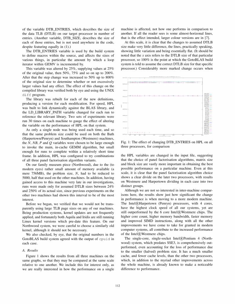
of the variable DTB ENTRIES, which describes the size ofthe data TLB (DTLB) on our target processor in number ofentries. (Another variable, DTB SIZE, describes the size ofeach of those entries, but is not used anywhere in the code,despite featuring equally in (1).)

The DTB ENTRIES variable is used by the build systemto define macros within the source, and affects the sizes ofvarious things, in particular the amount by which a loopiterator within GEMV is incremented by.

This variable was altered by 25%, supplying values at 25%of the original value, then 50%, 75% and so on up to 200%.After that the step change was increased to 50% up to 800%of the original size to determine whether or not excessivelylarger values had any effect. The effect of this change on thecompiled library was verified both by eye and using the UNIXdiff program.

The library was rebuilt for each of the new definitions,producing a version for each modification. For speed, HPLwas built to link dynamically against the BLAS library, andthe LD LIBRARY PATH variable changed for each run toreference the relevant library. Two sets of experiments wererun 30 times on each machine to gauge the effect of alteringthe variable on the performance of HPL on that system.

As only a single node was being used each time, and sothat the same problem size could be used on both the Bath(Harpertown/Penryn) and Southampton (Westmere) machines,the N, NB, P and Q variables were chosen to be large enoughto invoke the main, in-cache GEMM algorithm, but smallenough for runs to complete within a relatively short timeframe. In addition, HPL was configured to try combinationsof all three panel factorisation algorithm variants.

On our family museum piece (Northwood), due to the (tomodern eyes) rather small amount of memory available (amere 756MB), the problem size, N, had to be reduced to5000, half that used on the other machines. In addition, havinggained access to this machine very late in our investigations,runs were made only for assumed DTLB sizes between 24%and 250% of its actual size, since previous experiments on theother two machines had shown this interval to be of the mostinterest.

Before we began, we verified that we would not be trans-parently using large TLB page sizes on any of our machines.Being production systems, kernel updates are not frequentlyapplied, and fortunately both Aquila and Iridis are still runningLinux kernel versions which pre-date this feature. On ourNorthwood system, we were careful to choose a similarly oldkernel, although it should not be necessary.

We also checked, by eye, that the original numbers in theGotoBLAS build system agreed with the output of cpuid ineach case.

A. ResultsFigure 1 shows the results from all three machines on the

same graphs, so that they may be compared at the same scalerelative to one another. We include this for interest only, aswe are really interested in how the performance on a single

machine is affected, not how one performs in comparison toanother. If all the reader sees is some almost-horizonal lines,that is the effect intended, larger colour versions are in [7].

At this scale, it is clear that the changes to assumed DTLBsize make very little difference, the lines, practically speaking,showing little variation and being essentially flat. (It should benoted that the x axis refers to the DTLB size of that particularprocessor, so 100% is the point at which the GotoBLAS buildsystem is told to assume the correct DTLB size for that specificprocessor.) Considerably more marked change occurs when

Fig. 1: The effect of changing DTB ENTRIES on HPL on allthree processors, for comparison

the HPL variables are changed in the input file, suggestingthat the choice of panel factorisation algorithms, matrix sizeand block size are vastly more important in obtaining the bestpossible performance on a particular machine. Even at thisscale, it is clear that the panel factorisation algorithm choiceshows a clear divide on the later two processors, with resultson Westmere and Harpertown dividing in each case into twodistinct groups.

Although we are not so interested in inter-machine compar-isons here, the results show just how significant the changein performance is when moving to a more modern machine.The Intel R!Harpertown (Penryn) processors, with 4 cores,have the highest clock speed of all our systems, yet arestill outperformed by the 6 core Intel R!Westmere chips. Thehigher core count, higher memory bandwidth, faster memoryand improved SIMD instructions, along with all the otherimprovements we have come to take for granted in moderncomputer systems, all contribute to the increased performanceof the Intel R!Westmere chips.

The single-core, single-socket Intel R!Pentium 4 (North-wood) system, which predates SSE3, is comprehensively out-performed, even accounting for the loss of performance dueto the smaller (halved) problem size. It has a much smallercache, and fewer cache levels, than the other two processors,which, in addition to the myriad other improvements acrossthe whole machine, is already known to make a noticeabledifference to performance.

112

1) Intel R!Westmere: The Intel R!Westmere chip was thenewest that we were able to examine in this study. It sportsseveral improvements over the older two chips, including a12MB Intel R!Smart Cache, a dual QPI BUS and SSE4.2.This gives it a noticeable, and not unexpected, improvement inperformance over even the higher clocked Intel R!Harpertownprocessor. The 4-way DTLB on this processor supports 64entries for 4K pages, or 32 entries for 2M/4M pages.

The results show several interesting features. See figure2. The first observation is the similar shape to those forHarpertown (Penryn). Indeed, given the shape of the meaneven between the different HPL variations (C2C2, C2L4, etc),it seems unreasonable to presume that they might be causedby noise, and MATLAB’s ttest2 confirms that chance wouldbe an unlikely cause for the fluctuations in both these and theHarpertown (Penryn) results (P = 0.0002).

Of most interest is perhaps the section between 50% and150%, where there is a noticeable increase in performanceup to 100%, followed by a sudden drop in performance. Thechange in performance is relatively small, being in the order of0.3% of overall performance for this problem size, and is stillvastly dwarfed by the effect of panel factorisation algorithmchoice, not to mention other variables (particularly N and NB)that might have been chosen differently had our intention beento approach Rpeak.

Fig. 2: The effect of changing DTB ENTRIES on HPL onIntel R!Westmere

Unfortunately a small number of our runs on the Universityof Southampton machine, Iridis 3+, showed up nodes perform-ing at only 2/3rds the speed of their identically equipped peers.Their results have been discarded on the grounds of beingaffected by a probable hardware fault. Thus there are slightlyfewer than the intended 30 runs to be considered for this chip.

2) Intel R!Harpertown (Penryn): The results on this chip(see figure 3) show a strange dip when DTB ENTRIES wasaltered to be 50% of the actual DTLB size of 256 entriesfor 4K pages. Performance overall is relatively flat. Thesame repetition in fluctuations can be seen across the variousHPL tests, as we saw with Intel R!Westmere, and ttest2 again

confirmed our perception that these could not be attributed tosimple noise.

A further observation is that the choice of the two panelfactorisation algorithms affect performance differently onIntel R!Harpertown (Penryn) than on Intel R!Westmere, withright-looking approaches appearing to be a better choice onthis architecture.

Fig. 3: The effect of changing DTB ENTRIES on HPL onIntel R!Harpertown

3) Intel R!Pentium 4 (Northwood): Like Intel R!Westmere,this now obsolete processor sports 64 DTLB entries for 4Kpages. It supports SSE2, but none of the later improvements,and predates SMT. It is the only 32-bit processor in this paper.

Figure 4 is perhaps the most interesting, especially whencompared with figures 3 and 2. Unlike the results for the laterprocessors, there is very little difference between the differentchoices in panel factorisation algorithm.

Fig. 4: The effect of changing DTB ENTRIES on HPL onIntel R!Pentium 4

We speculate that this is due to the slightly differenttreatment of this processor. Since the version of the librarythat we are using post-dates [1], it seems highly likely that theauthors will have included any changes recommended by their

113

findings. In fact, on examining the source for the GotoBLASlibrary, it is clear that there are several places where the kernelsdiffer if built for the Intel R!Pentium 4 family.

B. Measuring DTLB misses

This has so far only been done on Intel R!Harpertown,and was accomplished using oprofile [10] to access the ownhardware counters built into the processor.

Fig. 5: Approximate DTLB misses on Intel R!Harpertown,running HPL with our modified GotoBLAS

As figure 5 shows, the change in the whole HPL run is onlyslight, and may be an artefact of the experimental error: see[7].

IV. CONCLUSION

The results show that any changes to the DTLB sizeassumed by Goto and van de Geijn’s build system result inperformance changes so small as to be, while statisticallysignificant, practically insignificant on the processors to whichwe had access, being almost indistinguishable from noise tothe unaided eye. Figure 5 shows that, even if TLB misseswere much more expensive, the change would still be slight.It is clear that changes to the HPL input values and thusthe problem shape and size affect performance considerablymore noticeably, as does the choice of panel factorisationalgorithms; an area we should like to investigate further.

However, in a situation where every advantage, howeversmall, is being exploited by national facilities and companiescompeting for a place in the TOP500 [3] list, the performanceeffected by their approach to the DTLB starts to becomemore interesting. We suspect that the importance of a specificcontext may help to explain why Goto and van de Geijn appearto disagree with others in the community.

Given the nature of the algorithm employed by Goto and vande Geijn, we suspect that the main reason for their improvedperformance over many of their competitors is due to thecache treatment, rather than their treatment of the DTLB.Their algorithms block for the largest cache level, usually thelevel 3 data cache on modern processors, and level 2 on older

processors such as Intel R!Harpertown (Penryn). In contrast,work on ATLAS has until recently focused on the level 1cache. Other work on cache design, such as [11], has indicatedthat it is the outermost cache level that has the greatest effecton overall memory I/O performance.

Other conclusions are that HPL is not a very good testof TLB performance, due to the aliasing effect mentioned insection II, and that GotoBLAS is even less portable than mightbe thought, due to the lack of use of DTB SIZE.

We anticipate continuing this work work by investigatingthe different relative performance of the various solvers ondifferent architectures, particularly on modern processors. Thiscould be better measured by looking at actual TLB miss rates,via hardware counters or similar, rather than the perhaps moredifficult to measure FLOP count. Work on this has begun, butis still ongoing.

Another area for further work would be to revisit the effectsof varying page sizes on benchmarks on modern architectures.Similar studies, such as that undertaken in [4] have been donein the past, using the SPEC benchmarks [12], as well as hand-written microbenchmarks. A similar approach could be usedhere, but extra care would have to be taken due to the effects ofthe aggressive energy saving functionality inherent in modernprocessor designs.

a) Acknowledgements: We are grateful to Ed White,David Stewart and Martin Brain for their comments andadvice, also to the reviewers for pointing out weaknesses inthe exposition.

REFERENCES

[1] K. Goto and R. van de Geijn, “On reducing TLB misses in matrixmultiplication,” Technical Report TR02-55, Department of ComputerSciences, U. of Texas at Austin, Tech. Rep., 2002. [Online]. Available:http://www.umiacs.umd.edu/ ramani/cmsc662/Goto vdGeijn.pdf

[2] ——, “Anatomy of high-performance matrix multipli-cation,” ACM Transactions on Mathematical Software (TOMS),vol. 34, no. 3, May 2008. [Online]. Available:http://portal.acm.org/citation.cfm?id=1356052.1356053

[3] H. Meuer, E. Strohmaier, J. Dongarra, and H. Simon, “TOP500supercomputer sites,” 1993. [Online]. Available: http://www.top500.org/

[4] J. B. Chen, A. Borg, and N. P. Jouppi, “A simulation based study ofTLB performance,” in ACM SIGARCH Computer Architecture News,ser. ISCA ’92. New York, NY, USA: ACM, 1992, pp. 114–123, ACMID: 139708.

[5] Z. Xianyi, W. Quian, Z. Chothia, C. Shaohu, L. Wen,S. Karpinski, and M. Nolta, “OpenBLAS,” 2012. [Online]. Available:http://xianyi.github.com/OpenBLAS/

[6] R. C. Whaley, J. J. Dongarra, and A. Petitet, “Automated empiricaloptimizations of software and the ATLAS project,” Parallel Computing,vol. 27, no. 1-2, pp. 3–35, Jan. 2001.

[7] J. R. Jones, J. H. Davenport, and R. Bradford, “The changing relevanceof the tlb (full paper).” [Online]. Available: http://opus.bath.ac.uk/35639

[8] E. Gabriel, G. E. Fagg, G. Bosilca, T. Angskun, J. J. Dongarra, J. M.Squyres, V. Sahay, P. Kambadur, B. Barrett, A. Lumsdaine, R. H.Castain, D. J. Daniel, R. L. Graham, and T. S. Woodall, “Open MPI:Goals, concept, and design of a next generation MPI implementation,”in Proceedings, 11th European PVM/MPI Users’ Group Meeting, Bu-dapest, Hungary, September 2004, pp. 97–104.

[9] “GNU compiler collection,” 1987. [Online]. Available: http://gcc.gnu.org[10] J. Levon and P. Elie, “OProfile — a system profiler for linux,” Aug.

2011. [Online]. Available: http://oprofile.sourceforge.net/[11] S. A. Pryzbylski, Cache and Memory Hierachy Design: A Performance

Directed Approach, 1990.[12] Standard Performance Evaluation Corporation, “SPEC benchmarks,”

1988. [Online]. Available: http://www.spec.org/

114

On the Parallelization of A New Three Dimensional Hyperbolic Group Solver by Domain Decomposition Strategy

Kew Lee Ming and Norhashidah Hj. Mohd. Ali School of Mathematical Sciences

Universiti Sains Malaysia 11800 Penang, Malaysia

e-mail: leeming_kew@hotmail.com; shidah@cs.usm.my

Abstract—In this paper, the parallel implementation of a new explicit group iterative scheme is proposed for the solution of a three dimensional second order telegraph partial differential equation. The explicit group (EG) method is derived from the standard centered seven-point finite difference discretisation formula. We utilize the domain decomposition technique on this group scheme to divide the tasks involved in solving the equation. The aim of this study is to describe the development of the parallel group iterative scheme under OpenMP programming environment as a way to reduce the computational costs of the solution processes using multiple-core technologies. Numerical experiments are conducted together with their detailed performance analysis. The results will be reported and discussed.

Keywords- Telegraph equation; explicit group method; domain decomposition algorithm; parallelization; multiple-core; OpenMP

I. INTRODUCTION Consider the three dimensional second order hyperbolic

equations (telegraph equation) defined in the region { }( , , , ) | 0 , , 1, 0x y z t x y z t! = < < > of the following form

2 2 2 22

2 2 2 22 ( , , , )U U U U UU F x y z t

t t x y z" #$ $ $ $ $+ + = + + +

$ $ $ $ $

(1)

where ( , , ) 0, ( , , ) 0.x y t x y t" #> % The initial condition consist of

1 2( , , , 0) ( , , ); ( , , , 0) ( , , )

tU x y z f x y z U x y z f x y z= =

and the boundary conditions consist of 1 2

3 4

5 6

(0, , , ) ( , , ); (1, , , ) ( , , )( , 0, , ) ( , , ); ( ,1, , ) ( , , )( , , 0, ) ( , , ); ( , ,1, ) ( , , )

U y z t g y z t U y z t g y z tU x z t g x z t U x z t g x z tU x y t g x y t U x y t g x y t

= == == =

This equation is commonly encountered in physics and engineering mathematics such as vibration of structures and signal analysis. In recent years, various numerical schemes have been developed for solving one-, two- and three- dimensional hyperbolic equation [1-10]. Ali and Kew [1] developed an unconditionally stable explicit group relaxation methods based on combination of rotated and centered five-point finite difference approximation on different grid spacing which solve the two dimensional

second order hyperbolic telegraph equation. The scheme is proven to require lesser execution time than the others explicit group methods [11]. As an extension to these works, Kew and Ali [12, 13] presented the utilization of domain decomposition techniques on explicit group methods and parallelized it using OpenMP programming environment. The parallel algorithms successfully save up of approximately 20% of the computational costs compared to their sequential algorithms. In year 2002, Mohanty [8] formulated the unconditionally stable Alternating Direction Implicit (ADI) difference scheme of second order accuracy in solving the three space dimensional hyperbolic equations. Mohanty [5] proposed another method of three level implicit operator splitting technique in solving the three dimensional hyperbolic telegraph equations (1). The method is unconditionally stable and applicable to singular problem.

In this paper, we present a new explicit group relaxation method derived from the standard seven-point difference approximation for the solution of (1). This explicit group method is developed using small fixed size group strategy which require lesser execution times than the classic point iterative method. The method is then parallelized using OpenMP environment with the utilization of domain decomposition technique.

In the next section, a brief overview will be given on the formulation of explicit group method for the three dimensional telegraph equations. The parallelization using domain decomposition technique under OpenMP programming environment will be discussed in Section 3. Section 4 presented the numerical experiments and the results. Finally, concluding remarks are given in Section 5.

II. FORMULATION OF THE GROUP METHOD In solving problem (1) using finite difference approximations, we let the spatial domain, ! be discretized uniformly in x-, y- and z- directions with a mesh size

1h x y z n= & = & = & = where n is an arbitrary positive integer. The grid points are given by ( , , , ) ( , , , )i j l mx y z t ih jh lh mk' where 1, 2, 3, ...m = and

0k > be the time steps. Let , ,

m

i j lU be the exact solution of the

2013 12th International Symposium on Distributed Computing and Applications to Business, Engineering & Science

978-0-7695-5060-2/13 $26.00 © 2013 IEEEDOI 10.1109/DCABES.2013.28

115

differential equation and , ,

m

i j lu be the computed solution of

the approximation method at the grid point. (1) can be approximated by various finite difference schemes. One commonly used formula is the standard seven-point difference approximation

( )( ) ( )( )( ) ( )( )( )( ) ( )( )( )( ) ( )

1, , , 1 1, , , 1 , , , 1

, 1, , 1 , 1, , 1 , , 1, 1 , , 1, 1

1, , , 1, , , , 1, , , 1, ,

, , 1, , , 1, , , ,

/ 2 1 3 / 2

/ 2 / 2

/ 2 / 2

/ 2 2 3 / 2

i j l m i j l m i j l m

i j l m i j l m i j l m i j l m

i j l m i j l m i j l m i j l m

i j l m i j l m i j l m

r u u r a b u

r u u r u u

r u u r u u

r u u r b u

+ + ( + +

+ + ( + + + ( +

+ ( + (

+ (

( + + + + +

( + ( +

= + + +

+ + + ( (

( ) 2

, , , 1 , , , 1/21

i j l m i j l ma u t F

( ++ ( + &

(2)

where 2 2 2 2 / ; ;r t h a t b t" #= & = & = & The iterations for this standard centered seven-point

difference scheme are generated at any time level on all grid point using (2) until convergence is achieved before proceeding to the next time level. The process continues until the desired time level is reached.

Consider the standard seven-point formula (2) which was derived from the centred finite difference discretisation. The mesh points are grouped in cubes of eight points (Fig. 1) and applying (2) to each of these points will produce the (8x8) systems of equations in the form

, , , 11 2 2 2

1, , , 12 1 2 2

1, 1, , 12 1 2 2

, 1, , 12 2 1 2

2 1 2 2 , , 1, 1

2 2 1 2

2 2 1 2

2 2 2 1

0 0 0 00 0 0 0

0 0 0 00 0 0 00 0 0 0

0 0 0 00 0 0 00 0 0 0

i j l m

i j l m

i j l m

i j l m

i j l m

i

uk k k kuk k k kuk k k kuk k k k

k k k k uk k k k u

k k k kk k k k

+

+ +

+ + +

+ +

+ +

( ( (( ( (

( ( (( ( (( ( (

( ( (( ( (

( ( (

! "# $# $# $# $# $# $# $% &

, ,

1, ,

1, 1,

, 1,

, , 1

1, , 1, 1 1, , 1

1, 1, 1, 1 1, 1, 1

, 1, 1, 1 , 1, 1

i j l

i j l

i j l

i j l

i j l

j l m i j l

i j l m i j l

i j l m i j l

rhsrhsrhsrhsrhsrhs

u rhsu rhs

+

+ +

+

+

+ + + + +

+ + + + + + +

+ + + + +

=

! " ! "# $ # $# $ # $# $ # $# $ # $# $ # $# $ # $# $ # $# $ # $% & % &

(3)

where 1 2 3 4

1 3 / 2; / 2; 2 3 / 2; 1k r a b k r k r b k a= + + + = = ( ( = (

, , 2 1, , , 1 , 1, , 1 , , 1, 1 1, , , 1, , , , 1, ,2

, 1, , , , 1, , , 1, 3 , , , 4 , , , 1 , , , 1/2

1, , 2 2 , , , 1 1, 1, , 1

()

(

i j l i j l m i j l m i j l m i j l m i j l m i j l m

i j l m i j l m i j l m i j l m i j l m i j l m

i j l i j l m i j l m

rhs k u u u u u uu u u k u k u t F

rhs k u u u

( + ( + ( + ( + (

+ ( + ( +

+ + + + ( +

= + + + + ++ + + + + +&

= + +1, , 1, 1 , , , 2 , , , 1, 1, ,

2

1, 1, , 1, , 1, 1, , 1, 3 1, , , 4 1, , , 1 1, , , 1/2

1, 1, 2 2 , 1, , 1 1, 2 , , 1 1, 1, 1, 1 ,

)(

i j l m i j l m i j l m i j l m

i j l m i j l m i j l m i j l m i j l m i j l m

i j l i j l m i j l m i j l m i j

u u uu u u k u k u t F

rhs k u u u u

+ ( + + + (

+ + + ( + + + + ( + +

+ + + + + + + + + + ( + +

+ + ++ + + + + +&

= + + +1, , 2 , 1, , 1, , ,

2

1, 2 , , 1, 1, 1, 1, 1, 1, 3 1, 1, , 4 1, 1, , 1 1, 1, , 1/2

, 1, 2 1, 1, , 1 , 2 , , 1 , 1, 1, 1 1, 1, , 1,

)(

l m i j l m i j l m

i j l m i j l m i j l m i j l m i j l m i j l m

i j l i j l m i j l m i j l m i j l m i

u uu u u k u k u t F

rhs k u u u u u

+ + +

+ + + + ( + + + + + + + ( + + +

+ ( + + + + + ( + ( + +

+ ++ + + + + +&

= + + + +1, , , , ,

2

, 2 , , , 1, 1, , 1, 1, 3 , 1, , 4 , 1, , 1 , 1, , 1/2

, , 1 2 1, , 1, 1 , 1, 1, 1 , , 2 , 1 1, , 1, 1, , 1, , 1, 1,

,

)(

j l m i j l m

i j l m i j l m i j l m i j l m i j l m i j l m

i j l i j l m i j l m i j l m i j l m i j l m i j l m

i j

uu u u k u k u t F

rhs k u u u u u uu

+

+ + ( + + + + ( + +

+ ( + + ( + + + + ( + + + ( +

++ + + + + +&

= + + + + ++ 2

1, 1, , , , , , 2 , 3 , , 1, 4 , , 1, 1 , , 1, 1/2

1, , 1 2 2 , , 1, 1 1, 1, 1, 1 1, , 2 , 1 , , 1, 2 , , 1, 1, , ,

1, 1, 1, 1, 1, 1

)(

l m i j l m i j l m i j l m i j l m i j l m

i j l i j l m i j l m i j l m i j l m i j l m i j l m

i j l m i j l

u u k u k u t Frhs k u u u u u u

u u

+ + + + + ( + +

+ + + + + + ( + + + + + + + + +

+ ( + + + +

+ + + + +&= + + + + +

+ + 2

, 1, , 2 , 3 1, , 1, 4 1, , 1, 1 1, , 1, 1/2

1, 1, 1 2 2 , 1, 1, 1 1, 2 , 1, 1 1, 1, 2 , 1 , 1, 1, 2 , 1, 1, 1, , 1,

1, 2 , 1, 1,

)(

m i j l m i j l m i j l m i j l m

i j l i j l m i j l m i j l m i j l m i j l m i j l m

i j l m i j

u k u k u t Frhs k u u u u u u

u u

+ + + + + + ( + + +

+ + + + + + + + + + + + + + + + + + + + + +

+ + + + +

+ + + +&= + + + + +

+ + 2

1, , 1, 1, 2 , 3 1, 1, 1, 4 1, 1, 1, 1 1, 1, 1, 1/2

, 1, 1 2 1, 1, 1, 1 , 2 , 1, 1 , 1, 2 , 1 1, 1, 1, 1, 1, 1, , , 1,

, 2 , 1, ,

)(

l m i j l m i j l m i j l m i j l m

i j l i j l m i j l m i j l m i j l m i j l m i j l m

i j l m i j

u k u k u t Frhs k u u u u u u

u u

+ + + + + + + + + ( + + + +

+ + ( + + + + + + + + + ( + + + + + +

+ + +

+ + + +&= + + + +

+ + 2

1, , , 1, 2 , 3 , 1, 1, 4 , 1, 1, 1 , 1, 1, 1/2)

l m i j l m i j l m i j l m i j l mu k u k u t F

+ + + + + + ( + + ++ + + +&

Figure1. Computational molecule for EG method This matrix (3) can be inverted to produce an eight points explicit group (EG) equation

, , , 11 2 3 2 2 3 4 3

1, , , 1 2 1 2 3 3 2 3 4

1, 1, , 1 3 2 1 2 4 3 2 3

, 1, , 1 2 3 2 1 3 4 3 2

2 3 4 3 1 2, , 1, 1

1, , 1, 1

1, 1, 1, 1

, 1, 1, 1

i j l m

i j l m

i j l m

i j l m

i j l m

i j l m

i j l m

i j l m

u m m m m m m m mu m m m m m m m mu m m m m m m m mu m m m m m m m mA m m m m m muuuu

+

+ +

+ + +

+ +

+ +

+ + +

+ + + +

+ + +

=

! "# $# $# $# $# $# $# $% &

, ,

1, ,

1, 1,

, 1,

3 2 , , 1

3 2 3 4 2 1 2 3 1, , 1

4 3 2 3 3 2 1 2 1, 1, 1

3 4 3 2 2 3 2 1, 1, 1

i j l

i j l

i j l

i j l

i j l

i j l

i j l

i j l

rhsrhsrhsrhs

m m rhsm m m m m m m m rhsm m m m m m m m rhsm m m m m m m m rhs

+

+ +

+

+

+ +

+ + +

+ +

! "! "# $# $# $# $# $# $# $# $# $# $# $# $# $% &% &

(4)

where 4 2 2 4

1 2 1 22 2

1 1 1 2 2 1 2 22 3

3 1

3

2 2

3

4

( 10 * * 9 * )7 * * ; * 3* ;

2 * * ; 6

/

*

1 k k k km k k k m k k km k k m

A

k

( += ( = (= =

=

The iterations are generated on these groups of eight

mesh points and it is treated explicitly similar to the way where the single point is treated in the point iterative method. Similarly, the process is repeated until the desired time level is achieved.

III. DOMAIN DECOMPOSITION TECHNIQUES Most domain decomposition methods (DDM) have been

developed for solving elliptic [14, 15] parabolic [16, 17] and hyperbolic problems [12, 13]. They have been considered as very efficient methods for solving partial differential equations on parallel computers [17]. They can be classified into two classes; overlapping and non-overlapping methods with respect to the decomposition of the domain. In [12, 13], Kew and Ali have demonstrated the use of DDM for the explicit group methods by using the overlapping sub-domain and Schwarz alternating procedure (SAP). This SAP operates between two overlapping sub-domains; solving the Dirichlet problem on one sub-domain in each iteration by taking the boundary conditions based on the most recent solution obtained from the other sub-domain. The details of the SAP can be obtained in [18]. In order to implement this domain decomposition algorithm, ordering strategies need to be considered for each finite difference discretization scheme due to the shared boundaries between sub-domains [12, 13].

116

The solution domain is decomposed into blocks as shown in Fig. 2. Referring to Fig. 2, when the point 1 in 1! is computing, points 2 – 7 at the same time level needs to be used if (3) is used. However, points 1 – 6 are from sub-domain 1! while point 7 is from sub-domain 2! . In the case of parallelization, the sub-domains 1! and 2! are computed concurrently. There is a possibility that the solutions at the points 7 is updating on the respective sub-domains when the point 1 are being computed. This may cause inaccuracy in the numerical results. Thus, we need to organize the ordering strategies to prevent any conflict on the usage of points among sub-domains. With this in mind, a red black group ordering strategy is introduced to this EG scheme. The black group points are set to be odd sub-domains and computed concurrently, followed by red group points, even sub-domains. The algorithm of this scheme is presented in Table I. The same concept of domain decomposition ordering strategy can also be implemented for the standard centered seven-point scheme.

Table II presents the syntax of implementing the program on multiple-core processor. It is observed that Steps 7 – 14 in Table I is the most expensive part of the algorithm and therefore stands to gain the most advantage from the parallelization process.

Figure 2 Explicit group scheme with domain decomposition

TABLE I. ALGORITHM FOR EXPLICIT GROUP SCHEME

USING RED BLACK GROUP ORDERING STRATEGY 1. Choose an initial guess u to the solution 2. For each time step: 3. Set Boundary Condition 4. Until convergence, Do (Global): 5. Identify the subdomain boundaries values 6. Until Convergence, Do (Local): 7. For each subdomain: 8. Solve at the black group points 9. EndDo 10. For each subdomain: 11. Solve at the red group points 12. EndDo 13. Check the local convergence test 14. EndDo 15. Check the global convergence test 16. EndDo 17. EndDo

TABLE II. SYNTAX FOR IMPLEMENTING THE PROGRAM ON MULTI-CORE PROCESSOR

#include <omp.h> void main() { int num_threads; omp_set_num_threads(omp_num_procs()); #pragma omp parallel for { Compute the points in each sub-domain } }

IV. NUMERICAL EXPERIMENTS AND RESULTS In order to demonstrate the viability of the proposed

method in solving the three dimensional second order hyperbolic equation (1), experiments were carried out on a quad core i7 CPU 2.0 GHz, 4GB of RAM with Window 7 operating system using Microsoft Visual Studio 2010. This experiment is to solve the hyperbolic problem (1) with the analytical solution [5]

2( , , , ) exp( ) sinh sinh sinh( , , , ) ( 2 2) exp( ) sinh sinh sinh

u x y z t t x y zf x y z t t x y z# "

= ( ) ) )= ( ( ) ) ) ) (5)

The boundary and initial conditions can be obtained from the analytical solution. The proposed group method is a three level scheme. The starting values of ( , , )u x y z at the first time level need to be obtained before any computation starts. The values may be obtained using the Taylor series expansion

( ) ( )( )1 0 0 2 0 3

, , , , , , , ,/ 2 ( )

i j l i j l t i j l tt i j lu u k u u k u u O k= + + + (6)

where u and tu are known explicitly at 0t = .The values of relaxation factor (Gauss Seidel relaxation scheme) for the various mesh sizes are set equal to 1.0. The convergence criteria used throughout the experiment was the l* norm with the local and global error tolerances were set equal to 610( and 710( , respectively. Throughout the computation, the values of 10.0" = and 5.0# = . The RMS errors are tabulated at 2T = for a fixed / 3.2k h+ = = for several mesh sizes of 16, 32, 64 and 128 and are listed in Table III. Table III also shows the comparison execution times obtained for the sequential algorithm (1 thread) and parallel algorithm (4 threads) for the point, and explicit group method. The speedup is used to measure the performance of the parallel algorithms compared to the corresponding sequential algorithms. The speedup formula used is in the form of

Execution time for a single threadSpeedup =Execution time using 4 threads

(7)

It can be observed that the computational results obtained from explicit group method maintained the same degree of accuracies with the standard point method. The EG method requires lesser computing times compared to point method due to its lower computational complexity. As shown in Table III, the execution times of the parallel EG can be saved up to about 34% compared to the sequential

1 2 3

4

5

6

7

1!

2!

117

EG and 39% for the standard centered seven-point method for the mesh size of 128. The percentages vary for difference schemes. This is due to the ordering strategies’ implementation which may cost overheads and thus affecting the execution timings.

V. CONCLUSION

In this paper, the parallel implementation of a new explicit group (EG) relaxation method, derived from the standard centered seven-point difference formula has been presented in solving the three dimensional telegraph equations. The parallel implementation utilizes the domain decomposition technique on the discretized solution domain using OpenMP programming environment. For comparison purposes, we also include the RMS error and the execution timings of the point-wise scheme; the standard centered seven-point method. The accuracy improves when the domain grid size for the iterative solution increases for both methods. It is observed that the accuracies of the proposed group method is as accurate as the standard point method even though the domain grid size for the iterative solution is doubled. It can also be observed that the parallel algorithms manage to save up approximately 35% of the computational costs compared to their sequential algorithms. Furthermore, better saving of computational costs are recorded when the grid size is finer. In conclusion, the explicit group relaxation method is able to take advantage from parallelism implemented on multi-core technology environment and the objective to reduce computational cost is achieved. Research on other explicit group method of the same class like the Explicit Decoupled Group (EDG) and its variants are under investigation and will be reported soon.

ACKNOWLEDGMENT Financial support provided by RU-PRGS Grant

#1001/PMATHS/845064 and the FRGS Grant #203/PMATHS/6711188 for the completion of this article are gratefully acknowledged.

REFERENCES [1] N.H.M. Ali and L.M. Kew, “New explicit group iterative methods in the solution of two dimensional hyperbolic equations,” Journal of Computational Physics 231, 2012, pp.6953–6968. [2] R.K. Mohanty, “New unconditionally stable difference scheme for the solution of multi-dimensional telegraphic equations,” International Journal of Computer Mathematics 86 (12), 2009, pp.2061–2071.

[3] M. Dehghan, A. Shokri, “A meshless method for numerical solution of a linear hyperbolic equation with variable coefficients in two space dimensions,” Numerical Methods for Partial Differential Equations 25, 2008, pp.494–506. [4] F. Gao, C. Chi, “Unconditionally stable difference schemes for a one-space-dimensional linear hyperbolic equation,” Applied Mathematics and Computation 187, 2007, pp.1272–1276. [5] R.K. Mohanty, “An operator splitting technique for an unconditionally stable difference method for a linear three space dimensional hyperbolic equation with variable coefficients,” Applied Mathematics and Computation 162, 2005, pp.549–557. [6] R.K. Mohanty, “An operator splitting method for an unconditionally stable difference scheme for a linear hyperbolic equation with variable coefficients in two space dimensions,” Applied Mathematics and Computation 152, 2004, pp.799–806. [7] R.K. Mohanty, “An unconditionally stable difference scheme for the one-space-dimensional linear hyperbolic equation,” Applied Mathematics Letters 17, 2004, pp.101–105. [8] R.K. Mohanty, M.K. Jain, U. Arora, “An unconditionally stable ADI method for the linear hyperbolic equation in three space dimensions,” International Journal of Computer Mathematics 79, 2002, pp.133–142. [9] D.J. Evans, UK Group Explicit Methods for the Numerical Solution of Partial Differential Equations. Loughborough University of Technology, Gordon and Breach Science Publisher, The Netherlands, 1997. [10] D.J. Evans, “Group explicit methods for the numerical solution of first-order hyperbolic problems in one dependent variable,” International Journal of Computer Mathematics 56 (3), 1995, pp.245–252. [11] L.M. Kew, N.H.M. Ali, “Explicit group iterative methods for the solution of telegraph equations,” in: The 2010 International Conference of Applied and Engineering Mathematics World Congress on Engineering 2010 (WCE 2010), 30 Jun–2 July, 2010, London, UK, Lecture Notes In Engineering and Computer Science, pp. 1770–1775. [12] L.M. Kew, N.H.M. Ali, “Parallel Explicit Group Domain Decomposition Methods for the Telegraph Equation,” in: International Conference on Applied Mathematics and Engineering Mathematics (WASET 2011), 21-23 December 2011 Phuket, Thailand, World Academy of Science, Engineering and Technology 60, 2011. [13] L.M. Kew, N.H.M. Ali, “OpenMP Technology In the Parallelization Of New Hyperbolic Group Solver,” in: 12th WSEAS International Conference on Applied Computer Science (WSEAS 2012), 11-13 May 2012, Singapore, Latest Advances in Information Science and Applications, pp. 136-141. [14] M. Dryja, and O.B. Widlund, Some Domain Decomposition Algorithms for Elliptic Problems, in: L. Hayes, D. Kincaid (Eds.), Iterative Methods for Large Linear Systems, Academic Press, San Diego, CA. 1989. [15] X.-C. Cai, and O.B. Widlund, “Domain Decomposition Algorithms for Indefinite Elliptic Problems,” SIAM J. Sci. Statist. Comput., 13, 1992, pp. 243–258. [16] Dawson, C.N., Du, Q., and Dupont, T.F. “A Finite Difference Domain Decomposition Algorithm for Numerical Solution of the Heat Equation.” Mathematics of Computation, 57(195), 1991, pp. 63-71. [17] Jun, Y. and Mai, T.Z., “IPIC Domain Decomposition Algorithm for Parabolic Problems,” Applied Mathematics and Computation, 177, 2006, pp. 352-364. [18] Saad, Y. Iterative Methods for Sparse Linear Systems. 2nd Edition. pp. 382-421.

TABLE III. EXPERIMENTAL RESULTS

Non Parallel (1 Thread) Parallel (4 Threads) h-1 Iter RMS Error Elapsed Time Iter RMS Error Elapsed Time Speed-up

Standard Point Method

16 44 6.570E-04 0.227 44 6.570E-04 0.223 1.018 32 67 3.180E-04 5.574 67 3.180E-04 4.683 1.190 64 88 1.580E-04 156.371 88 1.580E-04 118.445 1.320 128 100 8.350E-05 4539.633 100 8.350E-05 2771.018 1.638

Explicit Group Method

16 26 6.570E-04 0.142 26 6.570E-04 0.139 1.022 32 38 3.170E-04 2.951 38 3.170E-04 2.616 1.128 64 50 1.560E-04 77.823 50 1.560E-04 62.098 1.253 128 56 7.970E-05 1988.438 56 7.970E-05 1313.726 1.514

*Iter: Global iteration number at time T = 2.

118

A Novel Binary Quantum-behaved Particle Swarm Optimization Algorithm

Jing Zhao1 , Ming Li2, Zhihong Wang3, Wenbo Xu4 1School of Information, Qilu University of Technology, Jinan, China, zjstudent@126.com

2College of Science and Technology, Shandong University of Traditional Chinese Medicine, Jinan, China 3Shandong Yingcai University, Jinan, China

4School of Internet of Things Engineering, Jiangnan University, Wuxi, China

Abstract—To keep the balance between the global search and local search, a novel binary quantum-behaved particle swarm optimization algorithm with comprehensive learning and cooperative approach (CCBQPSO) is presented. In the proposed algorithm, all the particles’ personal best position can participate in updating the local attractor firstly. Then all the particles’ previous personal best position and swarm’s global best position are performed in each dimension of the solution vector. Five test functions are used to test the performance of CCBQPSO. The results of experiment show that the proposed technique can increase diversity of swarm and converge more rapidly than other binary algorithms.

Keywords-quantum-behaved particle swarm optimization; binary; comprehensive; cooperative

I. INTRODUCTION Particle swarm optimization (PSO) is an evolutionary

computation technique developed by Dr. Eberhart and Dr. Kennedy in 1995 [1]. Base on deep study of PSO and inspired by quantum mechanics, quantum-behaved PSO (QPSO) is proposed by Jun Sun [3,4,5]. QPSO has much fewer parameters without the velocity of particles and much stronger global search ability than PSO [6]. In 1997, Kennedy proposed the binary version of PSO (BPSO) [7], and Jun Sun proposed the binary version of QPSO (BQPSO) in 2007 [8].

This paper will focus on developing the binary version of QPSO with comprehensive learning and cooperative approach (CCBQPSO). The comprehensive strategy can keep the diversity of swarm, and the cooperative method can direct the algorithm into local search and converge to the optimum solution fleetly. In the proposed algorithm, all the particles’ personal best position can be participate in updating the local attractor firstly. Then each dimension of particle’s new solution vector replaces in turn the corresponding dimension of particle’s previous personal best position and swarm’s global best position to calculate the fitness value.

The rest part of the paper is arranged as follows. In section 2, a brief introduction of the BPSO is presented. The BQPSO is described in section 3. Next, the novel CCBQPSO is proposed in section 4. Then the experiment results are shown in section 5. And the conclusion is made in section 6.

II. BINARY PARTICLE SWARM OPTIMIZATION In PSO, the population with M particles is called a

swarm X in the D-dimensional space. The position vector and velocity vector of particle i at the generation t represented as ))(,),(),(()( 21 txtxtxtx iDiii != and

))(,),(),(()( 21 tvtvtvtv iDiii != .The particle moves according to the equations:

1 1

2 2

( 1) ( ) ( ( ))( ( ))

id id id id

d id

v t wv t c r pbest x tc r gbest x t

+ = + !+ !

(1)

( 1) ( ) ( 1)id id idx t x t v t+ = + + (2) Where DdMi ,,2,1;,,2,1 !! == , w is the inertia

weight. 1c and 2c are called the acceleration coefficients. 1r and 2r are random number uniformly distributed

in (0,1) .Vector 1 2( , , , )i i i iDpbest pbest pbest pbest= ! is the personal best position ( pbest ) of particle i, while the global best position ( gbest ), 1 2( , , , )Dgbest gbest gbest gbest= ! , is the best particle position among all the particles in the population.

In BPSO [6], Eq. (3) replaces Eq. (2): ( () ( )) 1 0id id idif then elserand S v x x< = = (3)

Where )(vS is a sigmoid function ()1(

1)( vevs !+

= ), and

()rand is a random number selected from a uniform distribution in (0,1) .

III. BINARY QUANTUM-BEHAVED PARTICLE SWARM OPTIMIZATION

In this section, BQPSO is depicted. Firstly the equations of QPSO algorithm are as follows:

1

1 M

d idi

mbest pbestM =

= ! (4) (1 )id id dp pbest gbest" "= # + ! # (5)

1( 1) ( ) *ln( )id id d idx t p mbest x tu

$+ = ± ! (6) Where " is a random number. mbest is mean best

position of the population. Parameter $ is called the Contraction-Expansion coefficient, which can be tuned to control the convergence speed of the algorithm.

2013 12th International Symposium on Distributed Computing and Applications to Business, Engineering & Science

978-0-7695-5060-2/13 $26.00 © 2013 IEEEDOI 10.1109/DCABES.2013.29

119

In BQPSO, the position of particle is represented as a binary string. Hamming distance is defined as the count of bits different between two binary strings. That is

( , )HX Y d X Y! = (7) The function ()Hd is to get the Hamming distance

between binary strings X and Y . The jth bit of the mbest is determined by the states of

the jth bits of all particles’ pbest in BQPSO. If more particles take on 1 at the jth bit of their own pbest , the jth bits of mbest will be 1; otherwise the bit will be 0. However, if half of the particles take on 1 at the jth bit of their pbest , the jth bit of mbest will be set randomly to be 1 or 0, with probability 0.5 for either state.

The point ip is obtained by one-point or multi-point crossover operation on ipbest and gbest . Firstly generate two offspring by crossover operation. Then randomly select one of the offspring and output it as the point iP .

Consider iterative Eq. (6) and transform it as

1( , ) ( , ) ln( )H i i H ib d x p d x mbestu

$= = # # (8) We can obtain the new string ix by the transformation

in which each bit in ip is mutated with the probability computed by

1 1

d

blc

bifl

"##= $# >#%

(9)

Where l is the length of the dth dimension of particle i . In the process of iteration, if () drand c< the corresponding bit in the position of particle i will be reversed, otherwise remains it.

With the above definition and modifications of iterative equations, BQPSO algorithm is described as the following procedure:

Step 1: Initialize an array of binary bits for all particles, pbest and gbest .

Step 2: For each particle, determine the mbest and ip . Step 3: For each dimension, compute the mutation

probability dc and update the particle’s new position ix . Step 4: Evaluate the objective function value of the

particle, and compare it with the objective function value of pbest and gbest . If the current objective function value is better than that of pbest and gbest , then update pbest and gbest .

Step 5: Repeat step 2~4 until the stopping criterion is satisfied or reaches the given maximal iteration.

IV. BINARY QUANTUM-BEHAVED PARTICLE SWARM OPTIMIZATION WITH COMPREHENSIVE LEARNING AND

COOPERATIVE APPROACH

A. Comprehensive Learning In comprehensive learning BQPSO (CLBQPSO), the

value of each dimension in the local attractor ip is randomly selected from corresponding dimension of an arbitrary particle’s personal best position [9]. For each particle i , learning probability iC is introduced to make the decision of which particle is adopted. For each dimension of particle i , if () irand C> , ip is taken from the current particle’s pbest itself. Otherwise, it should learn from other particles’ pbest use tournament selection.

B. Cooperative Approach For objective function ( )1 2( ) , , , Nf X f X X X= & '( )! , as

BQPSO described, each update step is also performed on a full D-dimensional solution vector. As long as the current objective function value is better than the former value, then update pbest and gbest . Then it may be appear the possibility that some dimension in the solution vector have moved closer to the global optimum, while others moved away from the global optimum. Whereas the objective function value of the solution vector is worse than the former value. Therefore, the current solution vector can be give up in next iteration and the valuable information of the solution vector is lost unknowingly. We present a cooperative method to avoid the undesirable behavior [10]. In the proposed method, each dimension of the new solution vector replaces in turn the corresponding dimension of pbest and gbest , and then compare the new objective

function value to decide whether to update pbest and gbest .The process is as follows:

Step 1: For each particle i , initialize cgbest gbest= , i icpbest pbest= .

Step 2: For each dimension of particle i , replace the dimension of cpbest and cgbest by the corresponding dimension of the particle.

Step 3: Evaluate the new objective function value of cpbest and cgbest , and compare it with the objective function value of pbest and gbest . If the current value is better than that of pbest and gbest , then update pbest and gbest .

Step 4: Repeat step 2~3 until all the dimension of the particle is compared.

C. CCBQPSO A novel hybrid algorithm, which is based on

comprehensive learning and cooperative approach BQPSO (CCBQPSO), is proposed in this section. The iteration process of CCBQPSO is described step-by-step.

Step 1: Initialize.

120

Step 2: For each particle, use comprehensive strategy to update the local attractor ip .

Step 3: Update the particle’s new position ix by BQPSO. Step 4: Evaluate the objective function value of the

particle, and compare it with pbest and gbest . If the current objective function value is better than that of pbest and gbest , then update pbest and gbest .

Step 5: Use cooperative approach to update pbest and gbest .

Step 6: Repeat step 2~5 until the stopping criterion is satisfied or reaches the given maximal iteration.

The proposed algorithm tries to improve convergence precision by comparing each dimension of the solution vector. It must extend the search space and then increase the time consumption. Two adaptive control methods are proposed.

(1) The cooperative strategy is adopted when the new objective function value is worse than the former.

(2) The cooperative strategy is performed when the bit of the particle is different from the corresponding bit of pbest and gbest .

V. EXPERIMENTS In this section, the performance of CCBQPSO algorithm

is tested on the following five different standard functions to be maximized[7]. Then the results are compared with BPSO, BQPSO and CLBQPSO.

32

11( ) 78.6 ( 5.12 5.12)i i

if X x x

== ! ! % %!

2 2 21 2 12( ) 3905.93 (100( ) (1 ) )

( 2.048 2.048)i

f X x x xx

= ! ! ! !! % %

1 2 3 4 53( ) 25 ( ), ( 5.12 5.12)i i

f X x x x x xx Z x= ! + + + +

& ! % % 30

4

14( ) 1248.2 ( 1.28 1.28)i i

if X x x

== ! ! % %!

25

2 61

1

15( ) 500 1 0.0021 ( )

32.0 16.0 0 16.0 32.032.0 16.0 0 16.0 32.0

( 65.536 65.536)

j i iji

i

f Xj x a

a

x

==

* +, -= ! +, -+ + !. /* += , -! !. /

! % %

! !

In the numerical experiments, the parameters setting of all the algorithms are described as follow: for BPSO, the acceleration coefficients are set to 1 2 2c c= = , and the inertia weight w is decreasing linearly from 0.9 to 0.4. In experiments for BQPSO, CLBQPSO and CCBQPSO, the value of $ is 1.4[11]. The parameters of learning probability are set as 0.5iC = . All experiments are run 50 independent times respectively with a population of 20, 40 and 80

particles. All the algorithms terminate when the number of iterations succeeds 200.

The best fitness value (BFV), maximum BFV, minimum BFV, mean BFV and the times of obtaining maximum BFV over 50 runs are recorded after all the algorithms terminate at each run. The mean BFV, minimum BFV and the times of obtaining maximum BFV of 50 trial runs are listed on Table 1-5. Fig.1 illustrates the convergence process of mean BFV of four algorithms over 50 runs with 40 particles on five test functions.

TABLE I. RESULTS OS 1f

Particles

BPSO BQPSO CLBQPSO CCBQPSO Mean Mean Mean MeanMIN MIN MIN MIN

(Max times) (Max times) (Max times) (Max times)

20 78.59986 78.59987 78.59967 78.6 78.5997 78.5997 78.5974 78.5999

(7) (12) (2) (48)

40 78.59985 78.59989 78.59986 78.6 78.5997 78.5997 78.5995 78.6

(2) (13) (9) (50)

80 78.59984 78.59992 78.59992 78.6 78.5997 78.5997 78.5997 78.6

(4) (20) (18) (50)

TABLE II. RESULTS OS 2f

Particles

BPSO BQPSO CLBQPSO CCBQPSO Mean Mean Mean MeanMIN MIN MIN MIN

(Max times) (Max times) (Max times) (Max times)

20 3905.9002 3905.9102 3905.928 3905.9289 3905.1536 3905.7815 3905.9116 3905.914

(9) (10) (4) (9)

40 3905.9242 3905.9235 3905.9293 3905.9298 3905.8418 3905.8312 3905.9247 3905.9292

(18) (13) (7) (11)

80 3905.9292 3905.9292 3905.9298 3905.9299 3905.9188 3905.9214 3905.9292 3905.9297

(15) (20) (10) (25)

TABLE III. RESULTS OS 3f

Particles

BPSO BQPSO CLBQPSO CCBQPSO Mean Mean Mean Mean MIN MIN MIN MIN

(Max times) (Max times) (Max times) (Max times)

20 54.86 54.96 54.66 54.96

54 54 54 54 (43) (48) (33) (48)

40 54.98 55 54.78 54.98

54 55 54 54 (49) (50) (40) (49)

80 55 55 54.94 55 55 55 55 55

(50) (50) (47) (50)

121

TABLE IV. RESULTS OS 4f

Particles

BPSO BQPSO CLBQPSO CCBQPSO Mean Mean Mean MeanMAX MAX MAX MAX MIN MIN MIN MIN

20 1250.7889 1253.5857 1252.4647 1261.469 1258.22 1261.7592 1259.2983 1268.48

1240.5389 1247.7543 1244.3038 1248.87

40 1251.7949 1252.9749 1252.0974 1262.1148 1263.1885 1262.126 1260.3056 1271.65 1241.2841 1245.6837 1247.5292 1253.4153

80 1251.851 1254.2206 1252.8175 1262.4969 1264.5341 1260.8333 1261.2899 1273.8849 1243.9959 1245.5395 1247.4616 1252.7685

TABLE V. RESULTS OS 5f

Particles

BPSO BQPSO CLBQPSO CCBQPSO Mean Mean Mean Mean MIN MIN MIN MIN

(Max times) (Max times) (Max times) (Max times)

20 498.71163 498.75278 499.2256 499.24135 497.76306 497.81977 498.7965 499.05711

(9) (11) (22) (31)

40 498.95986 498.97292 499.25785 499.26106 498.10809 497.62203 499.113 499. 159

(13) (7) (33) (38)

80 499.03857 498.94943 499.26989 499.2699 498.10906 498.10809 499.26975 499.26975

(19) (23) (46) (48) The optima of function 1f , whose fitness value is 78.6,

can be found out by all algorithms. As can be seen from Table 1, the mean BFV of CCBQPSO is best. And BQPSO outperforms BPSO and CLBQPSO. BPSO is better than CLBQPSO with 20 particles, but worse than CLBQPSO with 40 and 80 particles. However the minimum BFV of CLBQPSO is the worst in all algorithms. As of solution quality, the times of successful search of CCBQPSO is maximum. And BQPSO is second. CLBQPSO with 20 particles make 2 successful searches out of 50 trial runs, whereas BPSO find out the optima for 7 times. And the corresponding times is 9 and 2 respectively with 40 particles. When the population number is 80, the optima are found out for 18 and 4 times with CLBQPSO and BPSO.

The optima of function 2f , whose fitness value is 3905.93, can be found out by all algorithms. As can be seen from Table 2, the mean BFV of CCBQPSO is best. And CLBQPSO takes second place. BQPSO has the worst performance than other three algorithms with 40 particles. Note that the times of successful search of CLBQPSO is the worst. For other algorithms, the times of successful search are basically the same with 20 particles, and the best algorithm is BPSO with 40 particles. When the population number is 80, CCBQPSO is superior in times of successful search to BQPSO.

The optima of simple integer function 3f , whose fitness value is 55, can be found out by all algorithms. As

can be seen from Table 3, the mean BFV of BQPSO is best. CCBQPSO, BQPSO and BPSO with 80 particles hit the optima for 50 times out of 50 runs. CCBQPSO has better quality of solution than BPSO and CLBQPSO with 20 and 40 particles.

In order to measure the average fitness value over the entire population, Gaussian noise is introduced into 4f function. As can be seen from Table 4, in this function, the mean BFV of CCBQPSO is the maximum. The mean BFV of CLBQPSO is inferior to BQPSO but superior to BPSO. However the maximum BFV and minimum BFV of CLBQPSO with 80 particles are better than that of BQPSO. The same happens in minimum BFV with 40 particles.

The optima of function 5f , whose fitness value is 500. All the algorithms can found out the best value 499.26991. As can be seen from Table 5, the mean BFV and the successful searches of CCBQPSO are best. And CLBQPSO takes second place.

As is illustrated in Fig.1, we can see that the effectiveness of the proposed CCBQPSO. CCBQPSO can converge to the optimum more rapidly than other algorithms on function 2f and 4f . On function 1f and 3f , BQPSO converges rapidly than other algorithms at the early stage of running, but CCBQPSO exceeds BPSO soon and generates a slightly better solution. On function 5f , other algorithms converge more quickly but generate worse solution than CCBQPSO.

Compared with other algorithms, experimental results show the effectiveness of the proposed CCBQPSO. In summary, the comprehensive learning can keep the diversity of swarm and have better global search, and cooperative method can direct the algorithm into local search and converge to the optimum solution fleetly.

VI. CONCLUSIONS In this paper, a novel CCBQPSO is described. In the

proposed algorithm, all the particles’ pbest are used to update the local attractor for preventing the particles converge to local optima. And each dimension update of particle can feed back to pbest and gbest . The results of experiment have showed that CCBQPSO performs better global convergence than other algorithms. However with the increasing complexity of the problem, time wasting is the main deficiency of CCBQPSO.

REFERENCES

[1] J. Kennedy and R. Eberhart, “Particle Swarm Optimization”, Proc. IEEE International Conference on Neural Networks (ICNN 1995), IEEE Press, Nov. -Dec. 1995, pp. 1942-1948, doi: 10.1109/ICNN. 1995. 488968.

[2] F. Van den Bergh, “An Analysis of Particle Swarm Optimizers”, Ph.D. thesis, University of Pretoria, South Africa, 2002.

[3] J. Sun, B. Feng, and W. B. Xu, “Particle Swarm Optimization with Particles Having Quantum Behavior”, Proc. IEEE Congress on Evolutionary Computation (CEC 2004), IEEE Press, Jun. 2004, pp. 325-331, doi: 10.1109/CEC.2004.1330875.

122

[4] J. Sun, W. Fang, X. J. Wu, V. Palade, and W. B. Xu, “Quantum-behaved Particle Swarm Optimization: Analysis of Individual Particle Behavior and Parameter Selection”, Evolutionary Computation, vol. 20, Dec. 2012, pp. 349-393, doi: 10.1162/EVCO_a_ 00049.

[5] W. Fang, J. Sun, Y. R. Ding, X. J. Wu, and W. B. Xu, “A Review of Quantum-behaved Particle Swarm Optimization”, IETE Technical Review, vol. 27, Jul. 2010, pp. 336-348, doi: 10.4103/0256-4602. 64601.

[6] J. Sun, X. J. Wu, V. Palade, W. Fang, C. H. Lai, and W. B. Xu, “Convergence Analysis and Improvements of Quantum-behaved Particle Swarm Optimization”, Journal of Information Science, vol. 193, Jun. 2012, pp. 81-103, doi: 10.1016/j.ins.2012.01. 005.

[7] J. Kennedy and R. Eberhart, “A Discrete Binary Version of the Particles Swarm Algorithm”. Proc. IEEE International Conference on Systems, Man and Cybernetics (ICSMC 1997), IEEE Press, Oct. 1997, pp. 4104-4108, doi: 10.1109/ICSMC.1997.637339.

[8] J. Sun , W. B. Xu, W. Fang, and Z. L. Chai, “Quantum-behaved Particle Swarm Optimization with Binary Encoding”, Proc. International Conference on Adaptive and Natural Computing Algorithms (ICANNGA 2007), Springer Berlin Heidelberg, Apr. 2007, pp. 376-385, doi: 10.1007/978-3-540-71618-1_42 .

[9] W. Chen, Y. Fu, J. Sun, W. B. Xu, “Improved Binary Quantum-behaved Particle Swarm Optimization Clustering Algorithm”, Journal of Control and Decision, vol. 26, Oct. 2011, pp. 1463-1468. (in Chinese)

[10] F. Van den Bergh and A. P. Engelbrecht, “A Cooperative Approach to Particle Swarm Optimization”, IEEE Transactions on Evolutionary Computation, vol. 8, Jun. 2004, pp. 225-239, doi: 10.1109/TEVC. 2004. 826069.

[11] J. Sun, “Particle Swarm Optimization with Particles Having Quantum”, Ph.D. thesis, Jiangnan University, Wuxi, China, 2009. (in Chinese)

0 10 20 30 40 5077.6

77.8

78

78.2

78.4

78.6

iterations

Ave

rage

BF

V

function f1

BPSO

BQPSO

CLBQPSO

CCBQPSO

0 50 100 150 200

3905.76

3905.8

3905.84

3905.88

3905.92

iterations

Ave

rage

BF

V

function f2

BPSO

BQPSO

CLBQPSO

CCBQPSO

0 50 100 150 20050

51

52

53

54

55

iterations

Ave

rage

BF

V

function f3

BPSOBQPSOCLBQPSOCCBQPSO

0 50 100 150 200

1240

1245

1250

1255

1260

iterations

Ave

rage

BF

V

function f4

BPSO

BQPSO

CLBQPSO

CCBQPSO

0 10 20 30 40 50 60 70400

420

440

460

480

500

iterations

Ave

rage

BF

V

function f5

BPSO

BQPSOCLBQPSO

CCBQPSO

Figure 1. The convergence process of three algorithms with 40 particles.

123

Cloud/Grid Computing

DCABES 2013

System Performance in Cloud Services: Stability and Resource Allocation

Jay Kiruthika Dr.Souheil Khaddaj Kingston University Kingston University jay.kiruthika@gmail.com s.khaddaj@kingston.ac.uk

Abstract— Resources are allocated to web applications in large scale traditional servers depending on various factors like internal architecture, software support, hardware etc., resulting in under or over utilization of the resources. Valuable resources are allocated for the future continual business improvement which may or may not be utilized resulting in wastage. On the other hand cloud systems provide resources as needed, thereby maximizing resource utilization. Using cloud services increases productivity as it saves valuable time, cost and is portable in tablets and mobiles which are highly desirable for web businesses. These factors contribute to a high demand for system stability in cloud systems unlike other systems. Due to this dynamic internal cloud architecture, resource management has become a complex process. As a cloud service provider takes control of data and services, the resources can be allocated as a pay as you go service, forging resource management to fine tune the methods adopted to allocate them. This paper focuses on using one such method to allocate resources.

Keywords- Resource allocation; web cloud service allocation; Resource management in cloud services; Cloud Computing.

I. INTRODUCTION Cloud service providers have to work closely with the clients to provide the necessary resources and have a fool proof backup plans. They are attractive to businesses as they economize on resources, operating costs, capital costs, maintenance and service costs. The ability to optimize performance and the automatic system recovery with minimum to no interruption to day to day business due to system failures in cloud services is lucrative to industries. Companies rely on system stability to run businesses smoothly and as more business switch to cloud services to provide such stable and reliable architecture, the cloud resource management needs to be robust. In web-based cloud applications like an online book shop or Music store which rely on their web based e-mail marketing that

regularly sends out newsletters on events and books, system stability is crucial. When information on new music products or books are sent out via e-mail, if misused will utilize the whole system resources resulting in heavy web traffic bringing the whole business to its knees. These criteria should be carefully checked before allocating resources to applications. Underestimating them will result in risk of failure and overestimating it will result in under using the resources. A need for a balanced process is needed to achieve this. Moreover portability is highly desirable quality factor in cloud services, resulting in the need for a system to be highly stable that can be achieved by vigorous testing of resources. Security aspect of a business is one of the contention businesses have when upgrading from traditional services to cloud computing. A certain level of trust is needed between the cloud provider and the client for a seamless secure service. The cloud provider will be in charge of the data flow and the work flow which puts the providers in control of the business thereby the level of expectancy in secure services increase. Cloud services have solid backup systems so their services are very reliable. As data recovery systems and backup systems are part of the cloud packages the users have less worry of loss of data as they can be accessed anywhere 24-7. But outages do occur due to system failures and maintenance. A need for a continuous internet access in the client’s end is also required to ensure access to the available services. In this paper, system stability of a cloud architecture providing cloud based web services are discussed and the criteria for dynamic resource allocation to cloud services are also discussed in detail.

II. DESIRABLE FACTORS FOR SYSTEM STABILITY

Cloud services provided by Google, Amazon etc, calculate their resources carefully as cost per usage of services is involved. Methods like Black box, Gray box and analytical models are used to calculate the cost and resources [4] [5]. A cloud service provider supplying resources to cloud based web applications

2013 12th International Symposium on Distributed Computing and Applications to Business, Engineering & Science

978-0-7695-5060-2/13 $26.00 © 2013 IEEEDOI 10.1109/DCABES.2013.30

127

normally rely on key quality factors like performance and availability for its stability. They are given priority from a cloud service provider’s point of view to user’s requirement. Cloud service provider does not necessarily support or host web applications in a Virtualized environment. In a typical e-Commerce based cloud service platform, utilization of resources and their operating cost are based on the web usage and other quality factors [9]. Security of the system is a desired quality factor once it is launched on cloud as their e-shopping basket stores vital information like credit cards, personal details which needs encryption technology installed to safeguard the business. Reliability of the system is another desired quality for continuous supply of information. A Cloud System’s stability which supports e-Commerce businesses depend on some or all of the criteria listed below:

i. Expected web traffic on normal period ii. Expected web traffic on festive period or the

business period iii. Newsletters for events targeting regular users

or promotions iv. Increase in usage due to new web application

like eBooks reader v. Increase in web usage for a short period of

time due to new movie release vi. Increase in web usage as popular music is

downloaded vii. Increase in web usage due to new apps

launched

When allocating resources, a system’s resource manager has to take into account all of the above criteria before estimating an approximate level of usage and cost. The check points or the break points to look out for regularly are

• Hardware resources

o CPU usage and number of CPU cores allocated for the required applications if hosted in VM environment

o Memory usage used by applications o Virtual memory used by applications o Disk access used by applications o Storage space allocated to users o Number of applications run on the system

o I/O bandwidth • Speed of applications run on the system • Unexpected system resources allocated by

applications which eat up memory • Terminal services clients • Number of users given access should be limited

and restrictions imposed on what can be accessed

• Previous version of applications no longer in use should be deleted/archived to make way to new applications

• Changed or modified applications should be monitored for its memory usage and disk usage

• Systems using web email system to access and store email content

• Automated backups of system and applications is essential when traffic is low this can be midnight or early mornings.

• Introducing new changes like search mechanism or database expansion will eat up valuable resources, these need to be referred to load distribution. If needed increase in memory or disk capacity should be recommended to keep the system stable

By checking all the above aspects when allocating the resources, the system will be ready to handle any problems when issues arise and provide the much needed stability for a system. Figure 1 below illustrates the criteria for resource allocation.

Figure 1: Resources criteria Some of the properties and issues listed above are typically applicable in a system supporting web applications and it need not be the same in other systems. For example, the pay per use service, on demand service, dynamic scale up / down and virtualization are exclusively cloud computing related issues, marshalling SOAP message between client and server is exclusively a Web service related issue, while reusability of services is exclusively a SOA related issue. But, cloud computing expands scalability than

128

SOA by adding virtualization and grid computing concepts [1]. The cloud providers are expected to supply users with deployed applications which can be accessed from anywhere on demand basis, pushing the need to recalculate current resource baselines as of paramount importance.

III. DYNAMIC ALLOCATION OF RESOURCES The concept of dynamic programming is largely based on the principle of optimality due to Bellman. “An optimal policy has the property that whatever the initial state and initial decision are, the remaining decisions must constitute an optimal policy with regard to the state resulting from the first decision.”[10]. Simulation techniques and modeling can be used to estimate or predict the resource capacity in VM systems [2]. Numerous mathematical equations [8] and models can be applied to find a working combination of storage [6] [7] and resource allocation. It can be tuned for specific businesses.

Figure 2. Resource allocation by a Cloud Provider for cloud based eCommerce applications using

web usage Training data derived from a typical e-commerce web usage is tabulated in Table 1 below. This table is an approximate calculation of the resources by the resource manager in a cloud provider business. The pre existing crieteria to this allocation is the simple usage of web including web emails, requests and e-mail marketing traffic for standard applications. There are sufficient storage space available for the applications in all these VM servers and has room for expansion. They are regularly monitored for its web usage and performance. The system regularly backs up during off peak hours or silent hours during midnight and monthly once an overall maintenance is done in all the servers to weed

out applications which overuses resources due to fault in the software. The monthly maintenance also includes defragging the disks and applying any updates like SSL and removing expired SSL certificates. Due vigilance is carried out when granting out access to users restricting the information thereby ensuring the data is secure.

VM allocation Cores allocated

Web usage per month[approx]

Small 2 250,000 hits Medium 2-4 500,000-

1,00,000 Medium High 6 1,00,000

High 8 2,00,000-5,00,000

Table 1: Training data of resource allocation from a cloud provider for web based e-commerce applications. The Table 1 data is for standard usage of applications. As explained earlier certain e-Commerce web businesses tend to double their traffic during certain period which results in the need to increase the current resource allocation.

VM allocation Cores allocated

Web usage per month[approx]

Small 4 250,000 hits – 500,000

Medium 4-6 1,00,000 – 2,00,000

Medium High 8 2,00,000 – 4,00,000

High 8-10 2,00,000-5,00,000

Table 2: Training data of resource allocation from a cloud provider for web based e-commerce applications during festive periods. Taking this into account a new base line for resources are calculated and applying the same principle used to calculate for regular traffic in Table 1, the new baseline is calculated for the changed usage and listed in Table 2. Swapping the systems to a higher VM system is straightforward as the regular backups help to regurgitate the settings easily bringing down the down time when the services are switched over. It hardly took under 10 minutes to bring all the services up with the new configuaration. Extensive stress tests

129

and simulation tests were carried out to help estimate the resource allocation.

IV. ALLOCATING RESOURCES There are various models based on Linear regressions, multiple regression coded into resource management to allocate the system resources. The mathematical model used here is adopted from dynamic programming for linear problems. x = number of cores assigned to a business1 or an application and n-x be the number of cores used by a specific business/application, n being the maximum a VM system can support. 0 !x!n f(n) = Max[g(x1..j), h(y1..j)] where f(n) denote the total optimal cores and g(x1..j) denotes the initial number of cores for a business or an application allocated initially and h(y1..j) storage space a VM can support. Where x and y ranges from 1..j states/stages or baselines of resources used. An optimum value can be found by monitoring the usage of resources at various stages when the application is used. Now as the business demand rises consider number of cores and storage available to be n = a(x) , b(y) now for optimising resource usage, where a(x) and b(x) are the new values required by the application the VM supports can be calculated as f(n) = Max{g(x),h(y) + f[a(x) ,b(y)]}, y = n-x or in general f(n) = Max 0 !x!n{g(x),h(y) + f[a(x) ,b(y)]} y=n-x [3] By using this dynamic equation an optimum value to allocate the resources can be calculated. Below are some of the charecteristics of dynamic allocation and the stage metioned in the list denotes the change in the status of allocation by system expansion or changes to the infrastructure due to business expansion or client’s needs. Characteristics of Dynamic Allocation: a) The problem can be divided into stages with a

policy decision required at each stage

b) Decision at each stage converts the current state into state associated with the next state

c) When the current state of resources is known, an optimal policy for the remaining stages is independent policy of the previous ones.

d) By deriving the optimal policy at the end of each state of the last stage, the solution procedure starts

e) To identify the optimum policy for each state of the system a recursive equation is formulated with n stages remaining, given the optimal policy for each state with (n-1) stages remaining.

f) Using recursive approach each time the solution procedure moves backward stage by stage for obtaining the optimum policy for each state, until it attains the optimum policy beginning at the initial stage.

Forward and backward Recursive Approach: There is a need for forward and backward approach to free up unused resources. This can be obtained by using the recursive equation technique starting from the first stage f1 ! f2!…….. fN The computation involved is called the forward computational procedure. If the recursive equations are formulated in a different way so as to obtain the sequence fN ! fN-1 !……….. f1 The computation involved is called the backward computational procedure. For example divide c cores into n number of cores to obtain optimum utilization of resources Or using the dynamic programming to find the maximum value of y1 + y2 +…..+yn = c, Using the forward computational procedure x1 = c for stage 1 x2 = c for stages 1 and 2 x3 = c for stages 1,2 and 3

130

In general Xn = c for stages 1,2,….n The state xi of the system at stage j may be defined as the portion of c allocated to parts 1 through j, both inclusive. It implies that 0 !xj!c f(c) = max { x1 } x1 = c and fj(c) = max 0 !xj!c { xjfj-1 (c-xj)} For stage 1 or single business j =1 f1(c) = c for 2 businesses f2(c) = max 0 !x2!c { x2 f1 (c-x2)} and so on.. This dynamic resource allocation may not apply to other businesses as this mathematical model is applied to the e-commerce cloud based business only. More study and training data is required to test in other infrastructures.

V. CONCLUSIONS AND FUTURE WORK

As more and more companies move to cloud technology due to economic reasons the need to fine tune the resource allocation will always be there. The main advantage of using virtualization in cloud computing are the resource allocation, solid fool proof backups, quick system restoration from system failures, making them irresistable to businesses. Cloud technology is expanding at a rapid rate and the complications of using one is being addressed and solutions are sought earnestly. Governments, companies are forming a policy in regards to security, information property rights and legal boundaries of using data stored offshore. It is still a huge complex issue as nations need to agree unianimously in a unified policy.

Particularly in a cloud based e-Commerce business there are issues such as the physical location, time difference, software platform, hardware platform, web traffic are to be taken into account when designing storage and resource allocation. Due to the diversity of hardware platforms like virtualization, the system stability is heavily relied by the cloud providers for its seamless services. By regular monitoring of the usage of web, system stability for e-Commerce cloud based applications can be obtained. The model discussed in this paper not necessarily be applied to other cloud based services and applications.

REFERENCES [1] M. Balasingh Moses, V. Ramachandran, P. Lakshmi - 2011 - Cloud

Services for Power System Transient Stability Analysis - European Journal of Scientific Research - ISSN 1450-216X Vol.56 No.3 (2011), pp.301-310

[2] Jinsong Wang, Michael N.Huhns – 2012- Using simulations to assess the stability and capacity of cloud computing systems -ACM SE '10 proceedings of the 48th Annual Southeast Regional Article No. 74, ISBN:978-1-4503-0064-3

[3] N.P Agarwal, Sonia Agarwal - 2009 - Operations Research and Quantitative Techniques - ISBN:9788176114608.

[4] Sean Marston, Zhi Li, Subhajyoti Bandyopadhyay, Juheng Zhang, Anand Ghalsasi, 2011 – Cloud Computing – The Business Perspective – Science Direct - 0167-9236 doi:10.1016/j.dss.2010.12.006

[5] Iqbal, W.; Dailey, M.N.; Carrera, D. - 2011 -Cloud and Service Computing (CSC), 2011 International Conference on Black-box approach to capacity identification for multi-tier applications hosted on virtualized platforms - 10.1109/CSC.2011.6138506 - IEEE Conference Publications

[6] Jianfeng Zhao; Wenhua Zeng; Min Liu; Guangming Li; Min Liu - 2011- Multi-objective optimization model of virtual resources scheduling under cloud computing and it's solution - Cloud and Service Computing (CSC), 2011 International Conf. Digital Object Identifier: 10.1109/CSC.2011.6138518, Page(s): 185 - 190, IEEE Conference Publications.

[7] Zhen Xiao,Weijia Song,Qi Chen, 2012, Dynamic Resource Allocation using Virtual Machines for Cloud Computing Environment, DOI Bookmark: http://doi.ieeecomputersociety.org/10.1109/TPDS.2012.283 :ISSN: 1045-9219, 02 Oct. 2012. IEEE computer Society Digital Library.

[8] Wei Yin, Yogesh Simmhan, 2012- Viktor Prasanna Scalable Regression Tree Learning on Hadoop using Open Planet - Accessed on 03d October 2012, Computer department University of Southern California- http://ceng.usc.edu/~simmhan/pubs/yin-mapreduce-2012.pdf.

[9] Kiruthika J, Khaddaj S. and Horgan G, 2012- Quality measurement for Cloud based e-Commerce applications, Conference on Distributed Computer systems, DCABES 2012- Guilin, China

[10] S. Dreyfus, 2002 - 'Richard Bellman on the birth of dynamic programming' Operations Research 50 (1), pp. 48-51.

131

Study on Water Information Cloud of Nanjing Based on CloudStack

Qiuxiang Chen, Feng Xu College of Computer and Information

Hohai University Nanjing, China

e-mail: chenqiuxiang_1988@126.com e-mail:njxufeng@163.com

Abstract-At present, cloud computing technology and its layout have been increasingly improved, but its application in water resources informatization is just the beginning. Therefore, it is necessary to study on the construction of water information cloud. Taking the present situation of Nanjing water resources as the background, this paper proposes a four-layer architecture of Nanjing water information cloud which includes physical layer, infrastructure layer, service layer and presentation layer. The cloud computing platform is built using CloudStack, and three kinds of related service clusters are advanced according to the requirements of Nanjing water conservancy. Finally, we analyze the application prospects and development orientation of water information clouds.

Keywords-cloud computing; water information cloud; CloudStack; service cluster

I. INTRODUCTION Water is closely related to human survival, economic

development and social progress, and it has always been a great event for a country. In 21 Century, with the fast development of Internet technology and continued advance of government informatization construction, water informatization construction has achieved certain achievement. Reference [1] points out that, at present stage, a series of problems restricting its development has been exposed in the process of water conservancy informatization, such as the disunity of standard specifications for application software, resources division, sharing difficulty, low efficiency, repetitive construction, etc.

Since the concept of cloud computing was put forward, it has quickly gotten many attentions. It provides transparent service for users, and as long as the users put forward their demands, cloud computing providers can provide services as required. In the whole process, firstly users input demands through a simple interface, then the demands are automatically split into numerous smaller subroutines by the huge network and processing program, and then the subroutines are sent to the data center for processing, finally the results will be return to users. Service providers can process tens of millions or even billions messages in seconds, so that cloud computing can achieve the powerful performance of network services, as well as super computer [2]. In addition, some security techniques are well studied in [3-6].

At present, cloud computing technology and its layout have been increasingly improved, but the application of

cloud computing on water resources informatization is still relatively rare. The introduction of cloud computing to the construction of water resources informatization can solve the existing problems such as resource sharing, redundant construction, systems integration, business collaboration, and alternation between old and new system to some extent and it also can promote the development of water resources informatization.

II. BACKGROUND Nanjing is located in the lower reaches of the Yangtze

River, whose terrain is complex. There are a number of rivers and lakes in its territory, and along the river and lake the dyke is plain and the hinterland is hilly. In addition, precipitation and water resources are unevenly distributed in time and space. These factors make Nanjing a flood-prone area. In order to reduce the impacts of floods and droughts, Nanjing Water Conservancy Bureau has basically established the flood and drought control command system integrated by information collection, network communications, integrated database, and application service. It has also built wide area network between the city’s flood and drought protection offices and each county’s offices, and hydrological telemetry system to automatically collect and process hydrological information , and so on.

At present, Nanjing Water Conservancy Bureau owns ten servers to assume the operation of the existing application systems. An application system basically runs in a server to provide the corresponding service. However, due to the large scale of various systems, large amount of data and the obvious lack of some servers, the application system always takes long time to react. Specific problems are formulated as follows:

• Due to many reasons such as the scattered construction of flood and drought control system, the non-uniform standards of these systems and weak global consciousness etc., infrastructure resources are difficult to integrate and efficient utilization of these resources cannot be increased, performance of systems cannot be optimized. Eventually, these problems influent the results of flood control and drought control work.

• The development and application of flood and drought control application system are often lack of coordination between business systems, and can’t achieve the interconnection between related

2013 12th International Symposium on Distributed Computing and Applications to Business, Engineering & Science

978-0-7695-5060-2/13 $26.00 © 2013 IEEEDOI 10.1109/DCABES.2013.31

132

businesses. So that it is difficult to share information resources, and it cannot provide an "integration" approach to the designated users.

The past solution, replacing or adding servers, to a certain extent can improve the response speed of business systems, but it inevitably leads to the redundancy of the servers. The ability of some servers can’t be taken full advantage of, and it also fails to solve these issues like resource sharing and interconnection between related systems. In order to solve these problems, we can use cloud computing technology to integrate dispersed servers into one "server", and integrate the various business systems in the water information cloud platform, then all systems are scheduled as services.

III. SOLUTION

A. Structural Design The overall framework of Nanjing water information

cloud platform as shown in Fig.1 is a multi-tier architecture composed of the physical layer, infrastructure layer, service layer, and presentation layer.

Figure 1. Overall framework of Nanjing water information cloud Physical resources layer is in the bottom which provides

the physical resources of the entire platform, including servers, PC machines, computers, switches and other network facilities. In a word, this layer provides the physical carrier of the cloud platform. According to the different roles of servers in the platform, they are divided into two types of nodes: management nodes and compute nodes. The cloud platform management nodes deploy resource management services of cloud platform, and the cloud platform compute nodes provide the computing resources of the virtual machine.

Infrastructure layer is above the physical layer, which is used to process information in the Nanjing Water Information Cloud. In the cloud computing nodes, by using

the virtualization technology, the hardware resources can be divided into the virtual machine. A variety of services can be deployed on virtual machines. Through the portal, each service is managed in a uniform way.

Service layer mainly provides various service clusters. They are platform management services clusters, water-related service clusters, user management and authorization service cluster.

The presentation layer offers a variety of access methods for different service clusters. Users can access the services provided by the cloud platform through PCs, laptops, pads and smartphones.

B. Cloud Platform 1) CloudStack

In the water information cloud structure, the cloud platform which is used to process information is of great importance.

CloudStack, cloud system infrastructure, is open source software. With using a modular, portable design criterion, CloudStack is not only compatible with the existing infrastructure resources, but also easy to use, users can quickly install and configure. Modular design allows the user to customize the function of the system as needed, changed or replaced. In addition, CloudStack provides an API that's compatible with AWS EC2 and S3 for organizations that wish to deploy hybrid clouds.

The hardware resources are abstracted and separated into computing resources, storage resources and cyber sources by KVM [7], which are organized as virtual resources; CloudStack integrates and manages these virtual resources to build cloud platform, and provides transparent cloud services for users. It is responsible for the virtual resources mapping to hardware resources, and provides effective security isolation between users.

Logically, the deployment of CloudStack includes five parts as shown in Fig.2: host, cluster, pod, and availability zone and management server [8].

Figure 2. Components diagram of CloudStack

Host is a single computing node which has installed

CloudStack Agent and one of the hypervisors supported by the platform like VMware, KVM and XenServer. The hosts are where the actual cloud services run in the form of guest

PC PAD Phones

Water-related services Cloud platform management services

User Management services

Presentation layer

Service layer

VMs VMs VMs

KVM virtualization platform

Infrastructure layer

Physical resource layer Cloud platform computing node

Cloud platform management node

133

virtual machines. Cluster provides an approach to organize nodes. If many nodes are in the same cluster, they have the same hardware, hypervisor and subnet, and they can access to the shared primary memory. A Pod which is equivalent to a rack consists of one or more clusters and one or more primary memories. A zone is equivalent to a single data center which contains multiple pods and secondary storages. Its biggest advantage is to provide physical independence and redundancy.

CloudStack manages two types of storage. The primary storage connects to a cluster, and it is used to store the root disk image of the VMs and additional data volumes of running virtual machines. The secondary storage stores VMs templates, ISO images and disk snapshots. There must be a secondary storage per zone.

The CloudStack platform can manage three kinds of user roles: The root administrator that has the highest accessing level can manage the entire cloud, including the hosts, clusters, users, domains, service offerings, and templates; The domain administrator can perform administrative operations for users who belong to that domain, but it don’t have visibility into physical servers or other domains; The end users which are unprivileged can only manager their own virtual resources.

CloudStack helps users to manage their own cloud through a web interface and a RESTfull API. The web interface allows the complete access to the CloudStack administrators while end users are only allowed to manage their own virtual resource. Through RESTfull API, the third-party can manage the cloud platform.

2) Build Cloud Platform a) Preparation

Servers in the cloud platform are divided into two categories: management servers and hosts. Specific configuration is as follows:

TABLE I. THE CONFIGURATION TABLE

Host Name CloudManager Node

Hardware

CPU IntelG530 2.4GHz IntelG530 2.4GHz

RAM 2G DDR3 4G DDR3

Hard Disk 500G 500G

Network

IP 192.168.2.202 192.168.2.203

DNS 192.168.2.1 192.168.2.1

Gateway 192.168.2.1 192.168.2.1

Software

OS RHEL 6.2 64bit RHEL 6.2 64bit with KVM

software CloudStack

Management Server, MySQL

CloudStack Host Agent

Storage

Primary Storage NFS,60G

Second Storage NFS,40G

b) Management Server Installation Before installing CloudStack packages, system-related

services are configured first, including IP, host name, local yum source, and NTP (network time protocol) server. Then the CloudStack package and MySQL database are installed; At last, the NFS server is set up and the system virtual machine templates are prepared.

c) Hypervisor Installation First install RHEL 6.2 (64bit) with KVM in the host, then

install CloudStack Agent, and NTP should be installed and edited to ensure all hosts in a pod have the same time.

d) CloudStack Configuration After installing and running the Management Server

software, enter the CloudStack Web Console address http://192.168.1.200:8080/client in the browser, then input the username and password, you can log on the Nanjing city water cloud. The main page is shown in Fig.3, the logged user's situation is above the page, and the left is the basic control column, upper right is some conventional alarm, low right shows resources’ occupation and usage. To know more, you can find in [9].

Figure 3. The main page of Nanjing water cloud platform

When creating virtual machines, the user needs to use a

template or ISO file. The administrator can customize the mirror for the cloud platform to provide users virtualized instances. In the process of making mirrors, software and services can be customized. Namely, according to the specific needs of the development, install the corresponding development environment or open the related services in the virtual machine. When the customized mirror is instantiated, the user can directly use the perfect service platform. This approach avoids the tedious work to install the software and improve the work efficiency [10].

C. Water Information Cloud Servicse Cluster Nanjing water information cloud service clusters can be

divided into three main modules: cloud platform management service clusters, water-related service clusters, user management service clusters.

1) Cloud Platform Management Service Clusters

134

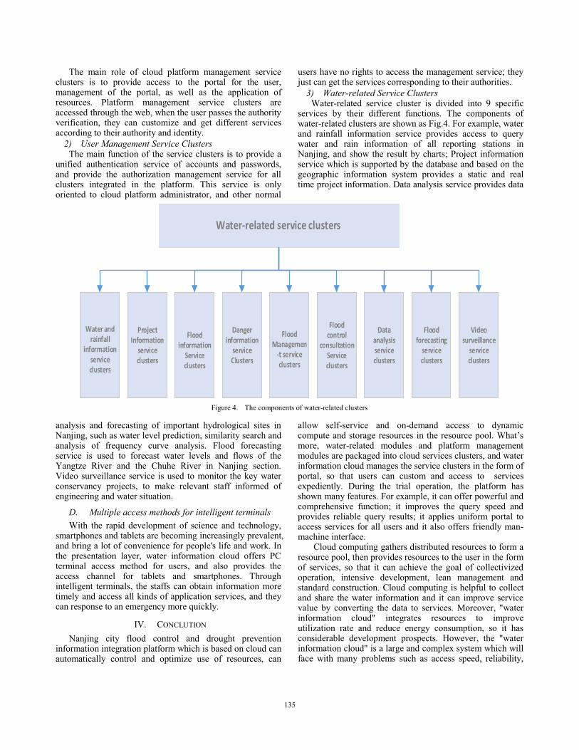
The main role of cloud platform management service clusters is to provide access to the portal for the user, management of the portal, as well as the application of resources. Platform management service clusters are accessed through the web, when the user passes the authority verification, they can customize and get different services according to their authority and identity.

2) User Management Service Clusters The main function of the service clusters is to provide a

unified authentication service of accounts and passwords, and provide the authorization management service for all clusters integrated in the platform. This service is only oriented to cloud platform administrator, and other normal

users have no rights to access the management service; they just can get the services corresponding to their authorities.

3) Water-related Service Clusters Water-related service cluster is divided into 9 specific

services by their different functions. The components of water-related clusters are shown as Fig.4. For example, water and rainfall information service provides access to query water and rain information of all reporting stations in Nanjing, and show the result by charts; Project information service which is supported by the database and based on the geographic information system provides a static and real time project information. Data analysis service provides data

Water-related service clusters

Project Information

service clusters

Water and rainfall

information service clusters

Flood information

Service clusters

Danger information

serviceClusters

Flood control

consultationService clusters

Data analysis service clusters

Flood forecasting

service clusters

Video surveillance

service clusters

Flood Managemen

-t service clusters

Figure 4. The components of water-related clusters

analysis and forecasting of important hydrological sites in Nanjing, such as water level prediction, similarity search and analysis of frequency curve analysis. Flood forecasting service is used to forecast water levels and flows of the Yangtze River and the Chuhe River in Nanjing section. Video surveillance service is used to monitor the key water conservancy projects, to make relevant staff informed of engineering and water situation.

D. Multiple access methods for intelligent terminals With the rapid development of science and technology,

smartphones and tablets are becoming increasingly prevalent, and bring a lot of convenience for people's life and work. In the presentation layer, water information cloud offers PC terminal access method for users, and also provides the access channel for tablets and smartphones. Through intelligent terminals, the staffs can obtain information more timely and access all kinds of application services, and they can response to an emergency more quickly.

IV. CONCLUTION Nanjing city flood control and drought prevention

information integration platform which is based on cloud can automatically control and optimize use of resources, can

allow self-service and on-demand access to dynamic compute and storage resources in the resource pool. What’s more, water-related modules and platform management modules are packaged into cloud services clusters, and water information cloud manages the service clusters in the form of portal, so that users can custom and access to services expediently. During the trial operation, the platform has shown many features. For example, it can offer powerful and comprehensive function; it improves the query speed and provides reliable query results; it applies uniform portal to access services for all users and it also offers friendly man-machine interface.

Cloud computing gathers distributed resources to form a resource pool, then provides resources to the user in the form of services, so that it can achieve the goal of collectivized operation, intensive development, lean management and standard construction. Cloud computing is helpful to collect and share the water information and it can improve service value by converting the data to services. Moreover, "water information cloud" integrates resources to improve utilization rate and reduce energy consumption, so it has considerable development prospects. However, the "water information cloud" is a large and complex system which will face with many problems such as access speed, reliability,

135

security and availability. In other words, there will be a lot of unpredictability in the future. So, we need deeper research on the operation mechanism and management means of the water information cloud in the future.

ACKNOWLEDGEMENT This paper is supported by National Natural Science

Foundation of China: “Research on Trusted Technologies for The Terminals in The Distributed Network Environment” (Grant No. 60903018) and “Research on the Security Technologies for Cloud Computing Platform” (Grant No. 61272543).

REFERENCES [1] Liu Lin, Liu Hengwei and Wang Zhe. “Discussion on the Application

of cloud computing in the construction of water conservation information”, Haihe Water Resources, vol.4, 2012, pp. 52-56. (In Chinese)

[2] LIU Qingtao, CUI Ruiling, GENG Dimgrui. “Discussion on Construction of Water Information Cloud”, Water Resources Informatization, no. 2, 2012, pp.5-9. (In Chinese)

[3] Feng X, Yuqi ZH, and Hongxu M, et al. Bilinear pairings-based threshold identity authentication scheme for Ad Hoc network. INTELLIGENT AUTOMATION AND SOFT COMPUTING, 2012, 18(5): 597-605.

[4] Feng X, Xin L, and Jia LK. A New Verifiable Threshold Decryption Scheme without Trusted Center. INTELLIGENT AUTOMATION AND SOFT COMPUTING, 2011, 17(5): 551-558.

[5] Xu F, Lv X, and Jiang RY. Online Public key cryptographic scheme for data security in bridge health monitoring. INTELLIGENT AUTOMATION AND SOFT COMPUTING, 2010, 16(5): 787-795.

[6] Feng X, Xin L, and Jia L. A new forward-secure threshold signature scheme for network agricultural trade. INTELLIGENT AUTOMATION AND SOFT COMPUTING, 2010, 16(6): 1231-1240.

[7] KVM: Kernel-based Virtualization Driver White Paper. [8] CloudStack3.0 Administration Guide. [9] CloudStack3.0 Advanced Installation Guide [10] Zhang Fan, Li Lei,Yang Chenghu and Chen Lizhen. “Constructing a

Private Cloud Computing Platform Based on Eucalyptus”, Telecommunications Science, no.11, vol.27,2011, pp.57-61. (In Chinese)

136

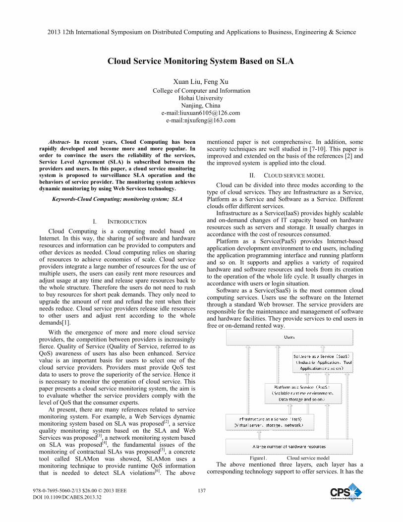
Cloud Service Monitoring System Based on SLA

Xuan Liu, Feng Xu College of Computer and Information

Hohai University Nanjing, China

e-mail:liuxuan6105@126.com e-mail:njxufeng@163.com

Abstract- In recent years, Cloud Computing has been

rapidly developed and become more and more popular. In order to convince the users the reliability of the services, Service Level Agreement (SLA) is subscribed between the providers and users. In this paper, a cloud service monitoring system is proposed to surveillance SLA operation and the behaviors of service provider. The monitoring system achieves dynamic monitoring by using Web Services technology.

Keywords-Cloud Computing; monitoring system; SLA

I. INTRODUCTION Cloud Computing is a computing model based on

Internet. In this way, the sharing of software and hardware resources and information can be provided to computers and other devices as needed. Cloud computing relies on sharing of resources to achieve economies of scale. Cloud service providers integrate a large number of resources for the use of multiple users, the users can easily rent more resources and adjust usage at any time and release spare resources back to the whole structure. Therefore the users do not need to rush to buy resources for short peak demands. They only need to upgrade the amount of rent and refund the rent when their needs reduce. Cloud service providers release idle resources to other users and adjust rent according to the whole demands[1].

With the emergence of more and more cloud service providers, the competition between providers is increasingly fierce. Quality of Service (Quality of Service, referred to as QoS) awareness of users has also been enhanced. Service value is an important basis for users to select one of the cloud service providers. Providers must provide QoS test data to users to prove the superiority of the service. Hence it is necessary to monitor the operation of cloud service. This paper presents a cloud service monitoring system, the aim is to evaluate whether the service providers comply with the level of QoS that the consumer experts.

At present, there are many references related to service monitoring system. For example, a Web Services dynamic monitoring system based on SLA was proposed[2], a service quality monitoring system based on the SLA and Web Services was proposed[3], a network monitoring system based on SLA was proposed[4], the fundamental issues of the monitoring of contractual SLAs was proposed[5], a concrete tool called SLAMon was showed, SLAMon uses a monitoring technique to provide runtime QoS information that is needed to detect SLA violations[6]. The above

mentioned paper is not comprehensive. In addition, some security techniques are well studied in [7-10]. This paper is improved and extended on the basis of the references [2] and the improved system is applied into the cloud.

II. CLOUD SERVICE MODEL Cloud can be divided into three modes according to the

type of cloud services. They are Infrastructure as a Service, Platform as a Service and Software as a Service. Different clouds offer different services.

Infrastructure as a Service(IaaS) provides highly scalable and on-demand changes of IT capacity based on hardware resources such as servers and storage. It usually charges in accordance with the cost of resources consumed.

Platform as a Service(PaaS) provides Internet-based application development environment to end users, including the application programming interface and running platform and so on. It supports and applies a variety of required hardware and software resources and tools from its creation to the operation of the whole life cycle. It usually charges in accordance with users or login situation.

Software as a Service(SaaS) is the most common cloud computing services. Users use the software on the Internet through a standard Web browser. The service providers are responsible for the maintenance and management of software and hardware facilities. They provide services to end users in free or on-demand rented way.

Figure1. Cloud service model

The above mentioned three layers, each layer has a corresponding technology support to offer services. It has the

2013 12th International Symposium on Distributed Computing and Applications to Business, Engineering & Science

978-0-7695-5060-2/13 $26.00 © 2013 IEEEDOI 10.1109/DCABES.2013.32

137

characteristics of the cloud computing. Each layer of cloud services can be independent clouds, and can also be based on the lower layer of cloud services. Each cloud can be directly available to end users, and can also be used to support the upper services[11].

III. SLA

A. SLA summary The SLA protocol is reached by the service sectors and

customers through consensus. Its content is the key service targets and responsibilities of both parties in service delivery and support process. SLA covers many aspects of the relationship between service providers and users, including service provide, services charge and service performance and so on. SLA not only allows users to clear their own needs, to help users claim compensation from service providers when they do not get the promised services, but also helps service providers understand the needs of users and service usage. So that they can optimize services and enhance competitiveness.

SLA generally includes some contents as follows: The regulation in all parties to provide services and

protocol of period of validity; The regulation of the number of users, the place and the appropriate hardware services; Fault reporting process description; Change request process description; The regulation of the service level objectives; The regulation of the service fees; The regulation of the responsibility of users; The description of solving different views on service-related process[12].

The focus of different cloud service model is different and their SLA contents are also different. Table 1 describes the corresponding SLA based on the different service types .

TABLE I The SLA of different cloud service model

Cloud service model SLA content

Infrastructure as a Service(IaaS)

The regulation of the virtual machine start-up time; The regulation of the virtual machine CPU speed; The regulation of virtual machine memory size; The regulation of the stored data memory size; The regulation of the IP quantity and throughput; The regulation of virtual machine expansion and reduced time.

Platform as a Service(PaaS)

The regulation of the electronic services and platform integration capabilities; The regulation of CPU time for application program; The regulation of the storage space for application program; The regulation of the network bandwidth available to application program.

Software as a Service(SaaS)

The regulation of the usability of the user interface; The regulation of response time from the user changed; The regulation of whether to support a variety of terminal access and use; The regulation for the programming interface integration capabilities.

B. Service quality parameter Service quality parameter is a service-related parameter.

A SLA should contain a lot of objectives and measurable parameters, service providers to the users to ensure that these parameters. Agreed service quality parameter should have a clear definition and be easy to reach a consensus between providers and users. At the same time it must have operative and accurate measuring methods for statistical analysis. Service quality parameter includes service usage rate, overload service usage rate and the service throughput of per unit time and so on.

C. SLA semantics SLA=<Provider,Consumer,Period,Obligation>represents

the four components of the SLA. Provider and Consumer are participants of SLA. They represent the cloud service providers and users. Period represents the valid time of the SLA.

Obligation=<Operation,SLO,Action,DataBase>represents the responsibility of the SLA.

Operation=<Schedule, Constants> Operation represents operation Schedule represents the interval and frequency of access to the original data. Constants define some constants in SLA.

SLO=<ValidTime, RDA, SLAParameters, Metric, Thresholds> defines the service level objectives, including the valid time of the service level objectives cloud service agent address for raw data service quality parameter the parameter Metric for calculation of SLAparameter and the Thresholds of users regulated. SLO can be calculated. When do not meet the conditions of conduct, the value of SLO is 0. On the other hand, the value of SLO is 1.

Action=<ActionCon, ActionGua> defines the mechanism behavior. When behavior conditions are met, behavior ActionGua is triggered. ActionCon is action condition. Generally it has four situations:

1)always: When SLO is 0, the action is triggered. 2)OnEntering: When SLO is 0, the action is triggered. On

the other hand, the state is reset to 0 times. 3) OnEnteringAndOnLeaving: When the value of SLO

changed, the action is triggered. 4) OnEveryEvaluation: the action is trigged without any

condition. DataBase=<TroubleReport,ServicePerfReport,Compress

Data>defines a database system. If the calculated quality parameters do not meet the requirements of users, then fault report TroubleReport is sent to the database system. When meet user requirements, service performance report ServicePerfReport is sent to the database system.

138

CompressData indicates that data in the database system should be regularly compressed.

IV. CLOUD SERVICE MONITORING SYSTEM STRUCTURE AND PROCESS

A. Cloud service monitoring system structure Different type of services correspond different type of

QoS data and the calculation processing of data is also different. Even though the same service, the user threshold requirements are also different. In order to meet the needs of different users, the SLA is combined with the Web Service technology for dynamic monitoring.

Cloud service monitoring system consists of the following five parts:

(1) SLA analyzer Analysis of the types of cloud services and cloud services

agent address. (2) Cloud service agent Record different users use the services of the raw data. (3) Cloud service monitoring process The process includes the raw data collection and

calculation process. 1) the raw data collection process: Access to raw data

from different cloud service agent.

2) the calculation process: The raw data collected always do not conform to the requirements of the user data. So we should calculate collected data according to the requirements of users.

(4) Cloud service quality assessment Calculated service quality parameter can be compared

with the threshold of the SLA and be analyzed whether meet user requirements. Then the appropriate treatments are be made depending on the different results.

(5) Database system Submit the results to the database system after the

assessment. If they meet user requirements, service performance report is sent to the database system. If do not conform to the requirements of users, the failure report is sent to the database system and the users are timely notified. To remind service providers check and remove troubles. The whole database system needs regular data compression.

The service agent in the cloud service monitoring process use Web Services technology to realize and WSDL describe management interface. It abstracts the monitoring process and divides process into multiple subservices. Analyze monitoring logic from the service level agreement. According to the logic combination monitoring process, we realize the dynamic monitoring system can meet the demands of a variety of services.

Figure2. Cloud service monitoring system structure

B. Cloud service monitoring system processes Firstly, SLA analyzer analyzes the input of SLA. To

analysis the various services and cloud service agent address. Then obtain the raw data from the cloud service agent. The raw data always does not conform to the required quality data of users. So we should calculate the raw data according to different services. Compare the calculated service quality parameter with the threshold. If more than the prescribed

threshold, the action is triggered and the failure report is sent to the database system. If do not meet the QoS requirements of users, the service performance report is sent to the database system.

139

V. THE INSTANCE

A. XML description of the monitoring system instance ProA offer email service, ConB is the consumer.

Specified in the SLA data transmission rate shall not be less than 1M. The threshold is 1M and the service quality parameter is transmission rate. If the transmission rate is less than 1M, the system will alarm.

<SLA name=“E-mail Service”> <Provider>ProA</Provider> <Consumer>ConB</Consumer> <Period> <Start>2013-3-17 09:00-20:00</Start> <End>2013-3-20 09:00-20:00</End> </Period> <Obligation > <Schedule>20s</Schedule> <SLAParameter name=“TransmissionRate”> <Metric>TransRateMetric TransTwoMetric

TransSubMetric TransDividMetric</Metric> </SLAParameter> <RDA> http://E-mailService/Agent/UtilityRequest

</RDA> <Thresholds>1M</Thresholds> </Obligation> </SLA>

B. Email service monitoring process Analyze SLA through SLA analyzer to get the contents

of the service and the service agent address. Put the raw data obtained from the service agent in TransData. TransTwoMetric means divide the collected raw data into two groups, function group() is called to realize. TransSubMetric means subtract two sets of data, function substract() is called to realize. TransDividedMetric means after reduction of data divided by 20, function divide() is called to realize. Compare the service quality parameter with the threshold 1M. If do not achieve 1M, function alarm() is called in the processing services. Then the failure report is sent to the database system and timely users are notified. If the transmission rate over 1M, the service performance report is sent to the database system.

Figure3. the process of the email service monitoring system

VI. CONCLUSION The paper presents a cloud service monitoring system

based on SLA. The aim is to provide more reliable services to users. The system is based on SLA and users can ensure the enjoyment of the service providers promised services based on cloud computing SLA. Cloud service providers according to cloud computing SLA to optimize allocation of resources and make their infrastructures could provide more high-quality services. Application of monitoring system Web Services technology makes the system have the characteristics of flexibility and cross-platform. System can be more scalability and reusable. The monitoring system guarantees quality of the services through the detection of violation situation. The next research focus is preventing the occurrence of violations.

ACKNOWLEDGMENT This paper is supported by National Natural Science

Foundation of China: “Research on Trusted Technologies for The Terminals in The Distributed Network Environment” (Grant No. 60903018) and “Research on the Security Technologies for Cloud Computing Platform” (Grant No. 61272543).

140

REFERENCES [1] Cloud computing.

http://zh.wikipedia.org/wiki/%E9%9B%B2%E7%AB%AF%E9%81%8B%E7%AE%97

[2] Xiangdong Yin, Xinlin Zhang. “A Web Services Dynamic Monitoring System Based on SLA”, Science and Technology Consulting Herald, no. 30, 2007, pp. 20-21. (In Chinese)

[3] Aihua Su, Guoqing Zhang. “ A Service Quality Monitoring System Based on the SLA and Web Services”. Computer Engineering and Applications, no. 11, 2006, pp.157-160. (In Chinese)

[4] Dan Liu, Bingxin Shi and Ling Zhou. “A Network Monitoring System Based on SLA”, Computer and Modernization,no. 4, 2005, pp.34-36. (In Chinese)

[5] Carlos Molina-Jimenez, Santosh Shrivastava, Jon Crowcroft and Panos Gevros. “On the Monitoring of Constractual Service Level Agreements”,First IEEE International Workshop on Electronic Contracting, 2004. pp. 1-8.

[6] David Ameller and Xavier Franch. “Service Level Agreement Monitor(SLAMon)”, Seventh International Conference on Composition-Based Software Systems, Madrid, Feb.25-29, 2008.pp.224-227.

[7] Feng X, Yuqi ZH, and Hongxu M, et al. “Bilinear pairings-based threshold identity authentication scheme for Ad Hoc network”,

INTELLIGENT AUTOMATION AND SOFT COMPUTING, vol. 18,no. 5, 2012, pp. 597-605.

[8] Feng X, Xin L, and Jia LK. “A New Verifiable Threshold Decryption Scheme without Trusted Center”, INTELLIGENT AUTOMATION AND SOFT COMPUTING, vol.17, no.5, 2011, pp.551-558.

[9] Xu F, Lv X, and Jiang RY. “Online Public key cryptographic scheme for data security in bridge health monitoring”, INTELLIGENT AUTOMATION AND SOFT COMPUTING, vol.16, no.5, 2010, pp.787-795.

[10] Feng X, Xin L, and Jia L. “A new forward-secure threshold signature scheme for network agricultural trade”, INTELLIGENT AUTOMATION AND SOFT COMPUTING,vol. 16, no.6, 2010, pp.1231-1240.

[11] Jinzhi Zhu. “The Wisdom of the Cloud Computing”, Publishing House of Electronics indusy, pp.59-64. (In Chinese)

[12] SLA.http://baike.baidu.com/view/3458408.htm [13] Liang Li, Meina Song and Xiaoqi Zhang. “An SLA Based Web

Service Quality Monitor System”, Pervasive Computing, Tamsui, Taipei, Dec.3-5, 2009.pp. 661-664.

[14] Nihita Goel, N V Narendra Kumar and R K Shyamasundar. “SLAMonitor: A System for Dynamic Monitoring Adaptive Web Services”, 2011 Ninth IEEE European Conference, Lugano, Sept.14-16, 2011.pp. 109-116.

141

Cloud Computing: Resource Management and Service Allocation

Eric Oppong, Souheil Khaddaj, Haifa Elsidani Elariss School of Computing, Information System and Mathematics Kingston University, Kingston upon Thames KT1 2EE, UK

K0212653@kingston.ac.uk, s.khaddaj@kinston.ac.uk, haifa.ariss@lau.edu.lb ABSTRACT The increase acceptance and adoption of cloud computing has seen many research projects focusing on tradition distributed computing issues such as resource allocation and performance. The scalability and dynamic heterogeneity of cloud computing presents a different challenge in deciding how resources are allocated to services. In this paper we identify the nature of cloud computing dynamics with virtualisation as a key part to resource allocation and meeting QoS needs. Service Level Agreement (SLA) mainly equates to actions taken when best effort falls and does not address the significant needs of meeting QoS demands as well as efficient utilisation of resources.

1. INTRODUCTION In cloud computing, virtualisation [1] of resources in important for providing a scalable and dynamic environment in meeting requirement. Cloud computing like many distributed computing paradigms, the focus of performance is driven by management of resources and allocation of Virtual machines. To maintain resource utilisation, VM migration from overloaded host to under-utilised host ensures certain form of utilisation as cloud computing demands can increase of decrease at any time. Cloud computing emerges from the utility computing paradigm, promising access to services at any time by consumers[2], there is the expectation that request are met without inquiring any additional cost, just as the providers manages the utilisation of resource to maintain efficiency. Migration of VM enables the re-allocation of resources to be relieved of the pressure and demands of request, consolidation and migration of VM improve utilisation, same way service consolidation and migration could add to the effective management of resources in cloud computing. Services consolidation utilises the full capacity of a VM and effectively minimising under-utilisation of resources and overloading. In this paper we identify the problem of resource under-use by VM in cloud computing and present an approach to reduce or in some cases eliminate the wastage improving utilisation and performance. The main contribution of this paper is identifying the need for service allocation in cloud computing to be The paper is arranged in the order as, section 2 related works, section 3 discussing service allocation in cloud and how improve to increase

performance, section 4 follows with results of experiments in a simulated cloud environment using Cloudsim toolkit and section 5 conclude with direction of future works.

2. RELATED WORK A number of algorithms are compared to identify the best algorithm that mixes best-effort and QoS needs to achieve optimal performance [3]. The scenarios created for the experiment were based on shared hosting environment using virtualisation. VM are crucial in delivery shared hosting resource allocation as used in their work, this relates to the core resource allocation as in many distributed computing environment where task allocation and scheduling is key to optimisation and performance. There are several research work on improving the scheduling of resource in a virtualised environment like the cloud using the many of the same algorithms but with differentiating how resources in cloud involve VM’s opposed to task, task in grid and distributed computing scheduling are mostly refined in granularity form to make it easy to execute with little amount of data association. Cloud computing emphasise on Vm’s which require much bigger data association and the allocation Vm’s require more intense algorithm to allocate resources. In most case VM migration mechanism aids the efficient allocation of resources in meeting QoS needs of consumers. By this trend, scheduling of resource in cloud computing is coupled with load balancing algorithms [4]. Basing their algorithm on traditional genetic algorithms ensuring Vm’s are effectively migrated where needed to relieve pressure on a host machine at any one time. Presenting optimisation algorithms for allocation of cloud services to resource, based on game-theoretic algorithm [5] using 3 refining algorithms process to analyse service dependencies. Service allocation in cloud can present complex problem in large scale environment which was considered hence the decision to calculate the completing times of dependent services in an approach to estimate optimised execution time. With the above and others scheduling proposed in cloud computing is that the focus is mainly on VM allocation and scheduling to meet subscribers and users QoS needs. We believe the approach should look into the allocation of service to VM which are

2013 12th International Symposium on Distributed Computing and Applications to Business, Engineering & Science

978-0-7695-5060-2/13 $26.00 © 2013 IEEEDOI 10.1109/DCABES.2013.33

142

in-turn allocated and scheduled on a host machine for execution. The problem we have identify is that when a number of services request are made, a VM’s takes the number that can be executed based on the capacity and the remainder is either allocated to another VM or wait for the current process to complete based on either on time or space shared allocation policy. In actual terms, sometimes the likelihood is that a VM might possible have extra capacity to accommodate a service partially, communication between VM’s can ensure that a service can be allocated to more than one VM at a time.

3. SERVICE ALLOCATION SCENARIO IN CLOUD COMPUTING

Many research papers and program focus on resource management, relating to service execution, however, the resource management fails to specifically manage the allocation of service and communication between services in-terms of VM creation and allocation. [6] Presents a case for the lack of communication management in cloud broker using the cloudsim simulation environment [6], hence broker management does not factor in other terms of communication i.e. VM communication and service communication to effectively identify datacentres based on QoS SLA. We assume that a datacentre host have a specific number of VM’s that can be executed based on the host, capacity. There is therefore a limitation on execution if service requests exceed the execution capacity of a host. The service is more likely to be migrated to a host that has enough capacity to meet the service needs, this create the following situation

1. Host1 is classified as not have sufficient

capacity to execute service and therefore is abandoned waiting for new request.

2. Host2 which meets the service request might be over-burden with services, this effectively affecting the performance of the datacentre.

With appropriate management broker, as we propose, the service can be executed on host1 and host2, effectively using the full capacity of host1 and the additional capacity from host2. We recognise that the objective of this paper must take in certain assumption and limit the problem to a single environment. Service Allocation Scenario in cloud computing

1. Service Request 2. Ack Request 3. Retrieve Service 4. Accept service 5. Create Datacenter Host 6. Create VM

7. If VM exceed Host Capacity, Migrate VM 8. Send output file to client 9. Ack Receipt

Proposed allocation Service allocation Hosts in datacentres are classified under 3 criteria based on Capacity (Memory, CPU and Bandwidth) low capacity (RAM < 10GB, CPU < 2GB, Bandwidth < 100MB), medium (RAM: 10>=100GB, CPU: 2>=4GB, Bandwidth: 100>=500MB) and high capacity (RAM: 10>=1000GB, CPU: 4>=8GB, Bandwidth :< 1000MB). The approach we are proposing assumes that a host has a capacity that allows for a certain number of VM to be created and hosted. If the services requested causes VM on a host to exceed it capacity then the host will not be used in this instances.

1. Service Request 2. Ack Request 3. Retrieve Service 4. Accept service 5. Create Datacenter Host 6. Create VM 7. If VM exceed Host Capacity, 8. Split Service (Create VM on another host

for service) 9. Re-group service output 10. Send output file to client 11. Ack Receipt

4. SERVICE ALLOCATIONS IN

CLOUD COMPUTING EXPERIMENT

We undertake an experiment using cloudsim [7], a simulator for creating experimental cloud-like environment to access the behaviour and execution on a single PC environment. Cloudsim is set-up to allow the user to create a cloud based environment with configurable datacentres and associated host machines as needed. In a simple cloudsim environment datacentres consist of host, cloudlet in cloudsim represents a service that is allocated to a VM running on a host. Also cloudsim offers scheduling based on time or space shared either in the allocation of services (cloudlet – CloudletTimeshare or Spaceshared) [8] and likewise for the VM, an instance can have a mix of timeshared police for services and spaceshared for VM’s Cloudsim only provides a simulation environment capable estimating a cloud-like environment for experimentation, however, in other to have a more realistic view of the allocation of services, we extended one example of cloudsim to include function call to methods the simulate execution of a

143

process. This effectively gives an estimated execution time used as the length of service to be allocated to a VM. We are able to measure the resource usage in this experiment first using the following allocation policies.

VM Ser VM Ser DC Host SS SS 5 10 2 2* TS TS 5 10 2 2 SS TS 5 10 2 2 TS SS 5 10 2 2

SS – SpaceShared, TS – TimeShared, DC – Datacentre, VM – Virtual Machine, Ser - Service VM Settings: MIPS =250, Image Size = 1MB, RAM = 2GB, No of CPU = 1, Bandwidth = 1000MB Service Setting: Filesize = 300, Outputsize=300 Host details: RAM = 16GB, Storage = 100GB, BW = 10MB Service ID

Start Time

Finish Time

Time Taken

VM ID

0 0 1.6 1.6 0 1 0 1.65 1.65 1 2 0 1.7 1.7 2 3 0 1.9 1.9 3

4 1.7 3.1 1.4 0

5 1.65 3.2 1.55 1

6 1.9 3.4 1.5 2

7 1.6 3.45 1.85 3

8 3.4 4.6 1.2 0

9 3.2 4.8 1.6 1 Table 1: allocation and execution of services

The results shows a predictable trend of service been allocated one at a time to each available VM, hence the first 5 services are allocated to the 5 VM specified, and then the process is repeated after completion of the services.

Fig 1: Service scheduling The other experiments did not yield an results using the same criteria, the broker in this instance failed to allocate VM to host as MIPS on host deemed inadequate. Out of the 4 experiments, only the experiments with both services and VM allocation policy set as spaceshared achieved a degree of allocation of service and VM to host. The others suffered from failure to allocate the VM’s to host due to lack of MIPS required.

Fig 2: Failure by policy This emphasis our approach to introduce a more reliable framework to minimise the failure rate, we envisage with the framework, a more stable allocation policy will factor in the capacity of the host and be able to create VM’s that would meet the requirement of the consumer.

144

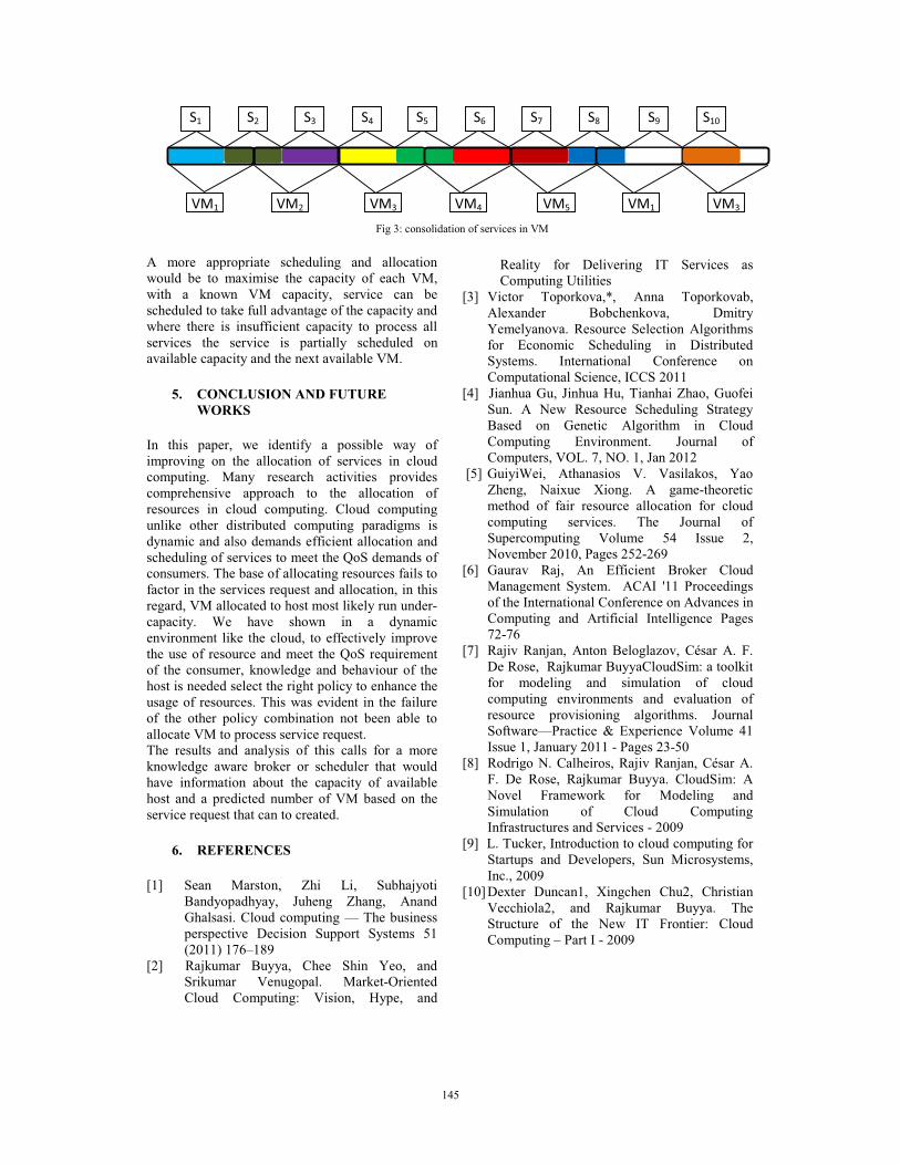
Fig 3: consolidation of services in VM A more appropriate scheduling and allocation would be to maximise the capacity of each VM, with a known VM capacity, service can be scheduled to take full advantage of the capacity and where there is insufficient capacity to process all services the service is partially scheduled on available capacity and the next available VM.

5. CONCLUSION AND FUTURE WORKS

In this paper, we identify a possible way of improving on the allocation of services in cloud computing. Many research activities provides comprehensive approach to the allocation of resources in cloud computing. Cloud computing unlike other distributed computing paradigms is dynamic and also demands efficient allocation and scheduling of services to meet the QoS demands of consumers. The base of allocating resources fails to factor in the services request and allocation, in this regard, VM allocated to host most likely run under-capacity. We have shown in a dynamic environment like the cloud, to effectively improve the use of resource and meet the QoS requirement of the consumer, knowledge and behaviour of the host is needed select the right policy to enhance the usage of resources. This was evident in the failure of the other policy combination not been able to allocate VM to process service request. The results and analysis of this calls for a more knowledge aware broker or scheduler that would have information about the capacity of available host and a predicted number of VM based on the service request that can to created.

6. REFERENCES [1] Sean Marston, Zhi Li, Subhajyoti

Bandyopadhyay, Juheng Zhang, Anand Ghalsasi. Cloud computing — The business perspective Decision Support Systems 51 (2011) 176–189

[2] Rajkumar Buyya, Chee Shin Yeo, and Srikumar Venugopal. Market-Oriented Cloud Computing: Vision, Hype, and

Reality for Delivering IT Services as Computing Utilities

[3] Victor Toporkova,*, Anna Toporkovab, Alexander Bobchenkova, Dmitry Yemelyanova. Resource Selection Algorithms for Economic Scheduling in Distributed Systems. International Conference on Computational Science, ICCS 2011

[4] Jianhua Gu, Jinhua Hu, Tianhai Zhao, Guofei Sun. A New Resource Scheduling Strategy Based on Genetic Algorithm in Cloud Computing Environment. Journal of Computers, VOL. 7, NO. 1, Jan 2012

[5] GuiyiWei, Athanasios V. Vasilakos, Yao Zheng, Naixue Xiong. A game-theoretic method of fair resource allocation for cloud computing services. The Journal of Supercomputing Volume 54 Issue 2, November 2010, Pages 252-269

[6] Gaurav Raj, An Efficient Broker Cloud Management System. ACAI '11 Proceedings of the International Conference on Advances in Computing and Artificial Intelligence Pages 72-76

[7] Rajiv Ranjan, Anton Beloglazov, César A. F. De Rose, Rajkumar BuyyaCloudSim: a toolkit for modeling and simulation of cloud computing environments and evaluation of resource provisioning algorithms. Journal Software—Practice & Experience Volume 41 Issue 1, January 2011 - Pages 23-50

[8] Rodrigo N. Calheiros, Rajiv Ranjan, César A. F. De Rose, Rajkumar Buyya. CloudSim: A Novel Framework for Modeling and Simulation of Cloud Computing Infrastructures and Services - 2009

[9] L. Tucker, Introduction to cloud computing for Startups and Developers, Sun Microsystems, Inc., 2009

[10] Dexter Duncan1, Xingchen Chu2, Christian Vecchiola2, and Rajkumar Buyya. The Structure of the New IT Frontier: Cloud Computing – Part I - 2009

VM1 VM2 VM3 VM4 VM5 VM1

S1 S2 S3 S4 S5 S6 S7 S8 S9 S10

VM3

145

!"#$$%&'($#)*+,)-'./0%!1/$#'23$)!$3"245.$6) !"#$%"&'()*+$,"$-()*+$./)*$01/#21+$!"#$31)*41)*$

5&'##6$#7$8#94":(;$5&1()&($/)<$.(&')#6#*2$,"'/)$=)1>(;?1:2$#7$.(&')#6#*2$

,"'/)+$@"A(1+$8'1)/$2&'()*B*C*9/16B&#9D$E4*"#CF'":B(<"B&)$

$$

!"#$%&'$7) !1) 8'9$) 0"$) *+,) ':';042<) 01) 0"$) :'0'%420$264=$)0'696>) 0"$)*+,)8.60)1?2);$#@$30) @'./0%01/$#'23$)3';'A4/404$6) 01)"'2:/$)$##1#6B)!"46);';$#);#1;16$6)')0"#$$%/'($#)@'./0%01/$#'23$)0$3"245.$) 0"'0) 3'2) '3"4$=$) 0"46) ;.#;16$) $C3$//$20/(B) !"$)*+,)0'69) :(2'843)84<#'0412) 0$3"245.$) ;#1;16$:) '2:) 48;/$8$20$:)A()1.#)&'A)"'6)#'#$/()6$$2)42)/40$#'0.#$6B))

D$(?1#:6%) -'./0%!1/$#'23$>) *+,>) E/1.:) E18;.042<>) !'69)F(2'843)*4<#'0412))

GB! $GH.IJK=8.GJH$$,1:'$ :'($ <(>(6#49():$ /)<$4;#*;(??$ #7$ &#94":(;$ ?&1()&($

/)<$:(&')#6#*2+$:'($<1?:;1A":(<$4/;/66(6$&#94":1)*$:(&')#6#*2$1?$ A(1)*$ /4461(<$ 1)$ (L:()<(<$ /;(/?+$ ?"&'$ /?$ :'($ !;1<$8#94":1)*$ /)<$ :'($ 86#"<$ 8#94":1)*B$ G)$ *()(;/6+$ :'($&#94":(;$ &6"?:(;$ A/?(<$ #)$ :'($ M(??/*($ -/??1)*$ G):(;7/&($NM-GO$ 1?$ :#$ /&'1(>($ :'($ >(;2$F/2$ #7$ :'($ <1?:;1A":(<$ 4/;/66(6$&#94":1)*B$ .'($ M-G$ 1?$ #7:()$ "?(<$ :#$ <(>(6#4$ 4/;/66(6$4;#*;/9?$ ;"))1)*$ #)$ :'($ &#94":(;$ &6"?:(;?$ /?$ F(66$ /?$ :'($?"4(;&#94":(;?$PQRB$$,'()$ M-G$ F/?$ 71;?:$ 1):;#<"&(<+$ 1:$ F/?$ <(?1*)(<$ /)<$

1946(9():(<$7#;$:'($?&1():171&$&#94":1)*+$?#$M-G$'/?$/$*##<$4(;7#;9/)&($ 1)$ :'($ &#94":(S1):()?1>($ :/?T?$F'16($ 1:$ &/)$ )#:$9((:$:'($4(;7#;9/)&($;(E"1;(9():?$#7$</:/S1):()?1>($:/?T?D$G)$7/&:+$:'($&";;():62$9#?:$4#4"6/;$<1?:;1A":(<$4/;/66(6$&#94":1)*$:(&')#6#*2+$ :'($ &6#"<$ &#94":1)*+$ 1?$ A#;)$ 7#;$ :'($ </:/S1):()?1>($&#94":1)*$PURB$$=?"/662$ :'($ M-G$ 1?$ )#:$ /4461(<$ :#$ </:/S1):()?1>($

&#94":1)*$ ?1)&($ :'($ M-G$ 1)'(;():$ <(?1*)$ &#)?:;/1):?B$ G)$ /$M-G$ V#A+$ /)2$ 4;#&(??$ 7/16";($ F166$ &/"?($ :'($ 91??1#)$ 7/16(<B$W<91::(<62+$ F'()$ :'($ &6"?:(;$ 1?$ (L(&":1)*$ /$ ?&1():171&$&#94":1)*$:/?T+$/)2$4;#&(??$/)#9/61(?$/;($9#?:$61T(62$:#$6(/<$:#$1)&#;;(&:$71)/6$;(?"6:?B$.'(;(7#;(+$:'($7(/:";(+$ :'/:$:'($M-G$&/))#:$ :#6(;/:($ :'($ 4;#&(??$ 7/16";(+$ &/)$ /</4:$ :#$ :'($&#94":1)*S1):()?1>($:/?T+$A":$6191:?$1:?$/4461&/:1#)$1)$:'($71(6<$#7$:'($</:/S1):()?1>($&#94":1)*B$.#$*(:$M-G$/</4:1)*$:#$:'($</:/S1):()?1>($:/?T+$M-G$9"?:$

#F)$ 4(;7(&:$ 7/"6:S:#6(;/)&($ &/4/A161:1(?$ :#$ '/)<6($ :'($ (;;#;?$N7#;$(L/946(+$ :'($4;#&(??$7/16";($(:&BOB$.'1?$4/4(;$4;#4#?(?$/$:';((S6/2(;$ 7/"6:S:#6(;/)&($ :(&')1E"(+$F'1&'$ &/)$ /&'1(>($ :'1?$4";4#?($(L&(66():62B$

GGB! M-G$XW=Y.S.JYZIWH8Z$.Z8@HG3=Z5$5#$7/;+$:'(;($/;($?#9($M-G$1946(9():/:1#)?+$?"&'$/?$X.S

M-G$ (:&B+$ F'1&'$ '/>($ /$ &(;:/1)$ <(*;(($ #7$ 7/"6:S:#6(;/)&($&/4/A161:1(?$/)<$&/)$:#6(;/:($:'($4;#&(??$7/16";($/)<$#:'(;$7/:/6$(;;#;?B$@#F(>(;+$:'($X.SM-G$'/?$)#:$A(()$"4</:(<$7#;$/$6#)*$:19(+$ /)<$ X.SM-G$ 9#<171(<$ :'($ ?(9/):1&?$ #7$ :'($ M-G$

?:/)</;<$P[RB$G)$:'($/?4(&:$#7$7/"6:S:#6(;/)&(+$M-G8@U$1?$#)($:'($9#?:$"?(7"6$1946(9():/:1#)?+$1)$F'1&'$:'($@2<;/$4;#&(??$9/)/*(9():$ ?2?:(9$ 4;#>1<(?$ &(;:/1)$ 7/"6:S:#6(;/)&($&/4/A161:2$ P\R+$'#F(>(;$1:?$/A161:2$#7$ 7/"6:S:#6(;/)&($1?$)#:$?#$*##<B$W66$ ;(?(/;&'$#7$ :'1?$4/4(;$ 1?$A/?(<$#)$M-G8@USQB\4Q+$F'1&'$ 1?$ /$ 4#4"6/;$ /)<$ 4#F(;7"6$M-G$ 1946(9():/:1#)$ 7;#9$:'($ W;*#))($ H/:1#)/6$ Y/A#;/:#;2D$ :'($ #4(;/:1)*$ ?2?:(9$ 1?$=A"):"$Q]BQ]$K(?T:#4$Z<1:1#)$N[USA1:OB$.'($ M-GSU$ ?:/)</;<$ <#&"9():$ <#(?$ )#:$ 4;#>1<($ /)2$

<(?&;14:1#)$#7$7/"6:S:#6(;/)&($(L&(4:$:'($(;;#;$'/)<6(;B$G)$7/&:+$/$ M-G$ /4461&/:1#)$ F'1&'$ "?(?$ :'($ (;;#;$ '/)<6(;$ 91*':$ )#:$:#6(;/:($ :'($ 4;#&(??$ 7/16";(+$ 7#;$ (L/946(+$ :'($ 594<$ 4;#&(??$9/)/*(9():$ ?2?:(9$ &/)$ )#:$ :#6(;/:($ :'1?$ 7/16";($ F'16($ :'($'2<;/$4;#&(??$9/)/*(9():$?2?:(9$1?$/A6($:#$:;(/:$ :'($7/16";($/?$ :'($ )#;9/6D$ G)$ *()(;/6+$ M-G8@U$ '/?$ A(()$ /A6($ :#$ &#4($F1:'$ :'($ A"77(;$ 1)&#)?1?:():$ 1)$ :'($ M-G+$ ?#$ :'($ (;;#;?$ :'($M-G8@U$;(/662$)((<$ :#$<(/6$F1:'$)#F$ 1?$ :'($4;#&(??$ 7/16";($P^RB$ .'($M-G8@U$ 4;#>1<(?$ &(;:/1)$ 7/"6:S:#6(;/):$ /A161:2$ A":$&/))#:$ ?/:1?72$ 7/"6:S:#6(;/):$ ;(E"1;(9():?$ 1)$ <(/61)*$ F1:'$</:/S1):()?1>($:/?T?$#)$:'($<1?:;1A":(<$46/:7#;9?B$$.241&/662+$ :'(;($ /;($ :F#$ &/"?/:1#)?+$ F'1&'$ &/"?($ :'($

4;#&(??$ 7/16";(_$ :'($ )#<($ 7/16";($ &/"?(<$ A2$ )(:F#;T$ 7/16";(?$/)<$ /&&1<():/6$ <(/:'$ #7$ M-G$ 4;#&(??(?B$ .'(;(7#;(+$ M-G$/4461&/:1#)?$F1:'$ :'($ 7/"6:S:#6(;/)&($ &/4/A161:2$9"?:$ A($ /A6($:#$ 4;#4(;62$ '/)<6($ :'($ :F#$ :24(?$ #7$ (;;#;?$ &/"?(<$ A2$ :'($4;#&(??$7/16";(B$52?:(9$9/67")&:1#)?$&/)$A($&6/??171(<$/?$:';(($&/?(?_$$QB$ H#<($ #;$ 4;#&(??$ 7/16";(?$ /:$ A(*1))1)*$ #7$ :'($ </:/$

4;#&(??1)*D$$UB$ H#<($ #;$ 4;#&(??$ 7/16";(?$ 1)$ :'($ 91<<6($ #7$ :'($ </:/$

4;#&(??1)*+$1)$F'1&'$/$6#:$#7$F#;T?$'/?$A(()$<#)($/6;(/<2B$$G)$ :'($ &/?($ U$ :'($ 7/16";($ &/)$ A($ 7";:'(;$ <1>1<(<$ /?$ :F#$

&/?(?_$$UBQB$.'($7/16";($)#<($#;$4;#&(??$&/)$A($;(?:/;:(<$"4D$$UBUB$.'($7/16";($)#<($#;$4;#&(??$&/)$)#:$A($;(?:/;:(<$"4B$$$W$:';((S6/2(;$7/"6:S:#6(;/):$?&'(9($'/?$A(()$4;#4#?(<$/)<$

1946(9():(<$1)$:'($4/4(;$7#;$/A#>($:';(($:241&/6$&/?(?+$F'1&'$&/)$?/:1?72$:'($7/"6:S:#6(;/):$;(E"1;(9():?$1)$M-GSA/?(<$&6#"<$&#94":1)*$46/:7#;9B$$

!"! #$%&'()*+&,-.%)&'-/,+0+1,%)-23%&+%3$2(4/%5&6%073$%8/,%&9:%3/+(12&&.'($ 71;?:$ 6/2(;$ 7/"6:S:#6(;/)&($ :(&')1E"(_$ I(S5&'(<"6($

ZL(&":1#)B$.'($?2?:(9$F166$;(<#$:'($V#A$199(<1/:(62$/7:(;$:'($7/16";($#7$/$M-G$:/?TB$,'16($:'($/>(;/*($:19($:'/:$/$M-G$:/?T$?4():$/)<$:'($/>(;/*($:19($:'/:$:'($?2?:(9$F/?$;(?:/;:(<+$A#:'$/;($;(6/:1>(62$?9/66+$#;$?#9($)#<($#;$4;#&(??$7/16";($'/44()(<$/:$:'($(/;61(;$?:/*($#7$;"):19(+$;(<#$:'($V#A$199(<1/:(62$/7:(;$1:?$ 7/16";($ 1?$ /$ *##<$ 7/"6:S:#6(;/)&($ ?#6":1#)$ 7#;$ /)$ (771&1():$

2013 12th International Symposium on Distributed Computing and Applications to Business, Engineering & Science

978-0-7695-5060-2/13 $26.00 © 2013 IEEEDOI 10.1109/DCABES.2013.34

146

M-G$ &6"?:(;$ ?2?:(9B$ .'($ &#;($ 4;1)&146($ #7$ :'1?$ :(&')1E"($ 1?$:19(62$ 71)<1)*$ :'($ 4;#&(??$ 7/16";(+$ :19(62$ ;(S?&'(<"61)*$ /)<$(L(&":1)*$:'($4;#*;/9$;(6/:(<$:#$:'($7/16";($4;#&(??B$JA>1#"?62$ :'($ 71;?:$ 6/2(;$ 7/"6:S:#6(;/):$ :(&')1E"($ &/))#:$

1)&;(/?($ :'($ ?2?:(9$ ;"):19($ (771&1()&2$ 7#;$ '(/>2$M-G$ :/?T?B$5#$ /)#:'(;$ :F#$ 7/"6:S:#6(;/):$ :(&')1E"(?$ /;($ 4;#4#?(<$ 7#;$)#<($ #;$ 4;#&(??$ 7/16";($ '/44()(<$ 1)$91<<6($ ;"):19($ 7#;$ :'($'(/>2$:/?T?B$

;"! #$%&*%3128&,-.%)&'-/,+0+1,%)-23%&+%3$2(4/%5&<$%3=>1(2+?6%*+-)+&&.'($ ?(&#)<$ 6/2(;$ 7/"6:S:#6(;/)&($ :(&')1E"(_$

8'(&T4#1):`I(?:/;:B$.'($M-G$4;#&(??(?$4(;1#<1&/662$<#$?:/:"?$8'(&T4#1):$#4(;/:1#)?B$.'($F'#6($V#Aa?$?:/:"?$1?$;(&#>(;(<$:#$:'($ 6/:(?:$ &'(&T4#1):$ /7:(;$ :'($ )#<($ #;$ 4;#&(??$ 7/16";(B$ $ G7$7/16";($'/44()(<$1)$:'($9/?:(;$)#<(+$:'()$:'($M-G$91??1#)$1?$;(?:/;:(<+$ :'($ ?2?:(9$ ;(?&'(<"6(?$ :'($M-G$ :/?T?+$ /)<$ F'#6($V#Aa?$?:/:"?$1?$;(&#>(;(<$:#$:'($6/:(?:$&'(&T4#1):+$:'()$91??1#)$&#):1)"(?$4(;7#;91)*D$G7$/$F#;T(;$1?$1)$7/16";($:'($?2?:(9$:;1(?$:#$ ;(?:/;:$ :'($ F#;T(;$ /)<$ ;(&#>(;$ 1:?$ :/?T$ :#$ :'($ 6/:(?:$&'(&T4#1):$ ?:/:"?$ /:$ :'($ 7/16(<$F#;T(;$ )#<(+$ /)<$ :'($F#;T(;$&#):1)"(?$4(;7#;91)*$:'($:/?TB$$.'($(??()&($#7$:'($?(&#)<$6/2(;$7/"6:S:#6(;/)&($:(&')1E"($

1?$ :#$ /66#F$M-G$ /4461&/:1#)?$ '/>1)*$ :'($ 8'(&T4#1):`I(?:/;:$&/4/&1:2B$ W9#)*$ 9/)2$ ?#7:F/;($ <(>(6#49():$ b1:?$ #7$8'(&T4#1):`I(?:/;:+$ ?"&'$ /?$ KM.8-+$ J4()cd+$ eY8I+$ :'($eY8I$7;#9$e(;T(6(2$Y/A$'/?$/$>(;2$*##<$4(;7#;9/)&(+$/)<$&/)$ ?(;>($ M-G$ 4(;7(&:62B$ 8";;():62$ #)$ :'($ Y1)"L$ #4(;/:1)*$?2?:(9$46/:7#;9+$F1:'$:'($'(64$#7$eY8I+$:'($M-G8@U$1?$/A6($:#$ *1>($M-G$ /4461&/:1#)?$ :'($8'(&T4#1):`I(?:/;:$ &/4/A161:1(?$:;/)?4/;():62$PfRPgRB$.'($ :';((S6/2(;$ 7/"6:S:#6(;/):$M-G$46/:7#;9$<(>(6#4(<$ 1)$

:'($K1?:;1A":(<$-/;/66(6$-;#&(??1)*$Y/A$#7$,"'/)$=)1>(;?1:2$#7$ .(&')#6#*2$ '/?$ 1):(*;/:(<$ :'($ 8'(&T4#1):`I(?:/;:$ #7$ :'($eY8IB$ 51)&($ :'($ ?(&#)<$ 6/2(;$ 7/"6:S:#6(;/)&($ :(&')1E"($ &/)$?/>($ :'($ 1):(;9(<1/:($ ;(?"6:?$ #7$ /$ ;"))1)*$ :/?T+$ 1:$ 9((:?$")1>(;?/6$ 7/"6:S:#6(;/)&($ ;(E"1;(9():?$ #7$ /$ >/;1(:2$ #7$ M-G$:/?T?B$

<"! #$%&+$()8&,-.%)&'-/,+0+1,%)-23%&+%3$2(4/%5&@.2-A(3&#-*=&B(C)-+(12&$.'($ :'1;<$ 6/2(;$ 7/"6:S:#6(;/)&($ :(&')1E"(_$K2)/91&$./?T$

M1*;/:1#)B$.'($ ?2?:(9$F166$ :/T($ :'($ 1)1:1/:1>($ :#$91*;/:($ :'($7/16(<$)#<(h?$:/?T$:#$/)#:'(;$)#;9/6$)#<(+$F'1&'$F166$&#):1)"($:#$(L(&":($:'($:/?T$1)$&/?($:'($?2?:(9$&/))#:$;(&#>(;$:'($:/?T$#)$ :'($ 7/16(<$F#;T(;$ )#<(B$ .'1?$ 4;#&(??$ <#(?$ )#:$ /77(&:$ :'($)#;9/6$)#<($F#;T1)*+$/?$?'#F)$1)$X1*";($USQB$5#$7/;+$ :'($M-G$1946(9():/:1#)?$)(1:'(;$4;#>1<($:'($:/?T$

91*;/:1#)$7(/:";($)#;$ :'($7(/:";(?$ :'/:$/$4;#&(??$ 7/16";($<#(?$)#:$ /77(&:$ #:'(;$ 4;#&(??(?B$ .'($ <2)/91&$ :/?T$ 91*;/:1#)$:(&')1E"($ 4;#4#?(<$ /)<$<(>(6#4(<$A2$ #";$ :(/9$ 1?$ /$ T1)<$ #7$/<>/)&(<$M-G$ 7/"6:S:#6(;/)&($ :(&')1E"(+$ F'1&'$ 1?$ /$ 4;#&(??$7/16";($ 7;(($ :(&')1E"($ :'/:$ <#(?$ )#:$ )((<$ :#$ ;(?:/;:$ :'($ V#A$&#94/;1)*$F1:'$:'($?(&#)<$6/2(;$7/"6:S:#6(;/)&($:(&')1E"(B$.'($ :'1;<$ 6/2(;$ 7/"6:S:#6(;/)&($ :(&')1E"($ ;(61(?$ #)$ :'($

(;;#;$'/)<6(;$#7$M-G+$F'1&'$:;(/:?$:'($&#99")1&/:1#)$7/16";($/?$ )#)S7/:/6$ (;;#;+$ /)<$ :'($ 7/"6:S:#6(;/)&($ &/4/&1:2$ 4;#>1<(<$A2$:'($@2<;/$4;#&(??$9/)/*(9():$?2?:(9+$F'1&'$4;#>1<(?$/)$/A161:2$ #7$ :'/:$ /$ 4;#&(??$ 7/16";($ <#(?$ )#:$ /77(&:$ #:'(;$

4;#&(??(?B$ .'($ M-G$ :/?T$ <2)/91&$ 91*;/:1#)$ :(&')1E"($4;#4#?(<$ /)<$ 1946(9():(<$ A2$ #";$ Y/A$ '/?$ ;/;(62$ ?(()$ 1)$61:(;/:";(?B$$$

X1*";($USQ$K2)/91&$./?T$M1*;/:1#)?$$

GGGB! .@Z$KZ5G!H$JX$.@Z$M-G$.@IZZSYW%ZI$XW=Y.S.JYZIWH8Z$-IJ.J.%-Z$5%5.ZM$

W?$ ?'#F)$ 1)$ X1*";($ [SQ+$ :'($ M-G$ :';((S6/2(;$ 7/"6:S:#6(;/)&($ 4;#:#:24($ ?2?:(9$ &#):/1)?$ 71>($ 4/;:?_$ i#AW<<+$i#A8#)+$ MV#ABM/?:(;+$ MZ2($ /)<$ MV#AB,#;T(;B$ i#AW<<$ 1?$:'($ V#A$ ?"A91??1#)$9#<"6(+$ i#A8#)$ 1?$ :'($ :/?T$9/)/*(9():$/)<$?&'(<"61)*$9#<"6(+$MZ2($1?$:'($9#)1:#;1)*$9#<"6(+$/)<$MV#A$1?$:'($M-G$:/?T$(L(&":1#)$9#<"6(B$MV#A$1?$<1>1<(<$1):#$:F#$4/;:?$#7$M/?:(;$/)<$,#;T(;+$M/?:(;$1?$:'($:/?T$9/)/*(;+$/)<$:'($,#;T(;$1?$:'($:/?T$(L(&":#;B$

$

X1*";($[SQ$.'($M-G$.';((S6/2(;$X/"6:S:#6(;/)&($-;#:#:24($52?:(9$!! i#AW<<$ 1?$ ;(?4#)?1A6($ 7#;$#A:/1)1)*$ V#A$ 1)7#;9/:1#)$

7;#9$ :'($ "?(;h?$ /A161:2+$ /)<$ ?()<1)*$ :'($ V#A$1)7#;9/:1#)$:#$i#A8#)B$

!! i#A8#)$1?$;(?4#)?1A6($7#;$*(::1)*$:'($V#A$1)7#;9/:1#)$7;#9$:'($V#A$?"A91??1#)$9#<"6(+$9/)/*1)*$:'($V#A$1)$:'($ 7#;9$ #7$ 9"6:146($ 4;1#;1:2$ E"("(?+$ /)<$ :'($ '1*'$4;1#;1:2$ V#A$ 1?$ :/T()$ #":$ 7;#9$ :'($ V#A$ E"("(?+$ /)<$:'()$<1?:;1A":(<$:#$MV#ABM/?:(;B$

147

!! W7:(;$ *(::1)*$ :'($ V#A$ 1)7#;9/:1#)$ <1?:;1A":(<$ 7;#9$i#A8#)+$MV#ABM/?:(;$)#:171(?$MZ2($ :#$*()(;/:($ :'($'#?:$61?:$716($F'1&'$1?$)((<(<$:#$?&'(<"6($/)<$(L(&":($:'($ M-G$ V#AD$ :'()$ A/?(<$ #)$ :'($ <2)/91&$ 4;#&(??$&;(/:1#)$ /)<$ 9/)/*(9():$ 9#<(6$ #7$ M-GSU+$MV#ABM/?:(;$ ?4/F)?$ :'($ MV#AB,#;T(;$ 4;#&(??(?$9((:1)*$ :'($ ;(E"1;(9():$#7$ :'($'#?:$ 61?:$ 716($F#;T(;B$e(?1<(?+$ :'($ M/?:(;$ <1?:;1A":(?$ :'($ :/?T?$ :#$ :'($,#;T(;$/)<$&#66(&:?$:'($1):(;9(<1/:($;(?"6:?$7;#9$:'($F#;T(;?S$9(;*(?$:'(?($1):(;9(<1/:($;(?"6:?$:#$*(:$:'($71)/6$;(?"6:$#7$:'($M-G$V#AB$

!! MV#AB,#;T(;$ 1?$ ;(?4#)?1A6($ 7#;$ :'($ :/?T?$<1?:;1A":(<$A2$MV#ABM/?:(;+$/)<$7((<$:'($1):(;9(<1/:($;(?"6:?$#7$:'($:/?T?$A/&T$:#$MV#ABM/?:(;B$.'($M-G$ 7/"6:?$ 1)$ :'($4;#:#:24($ ?2?:(9$ ?'#F)$ 1)$X1*";($

[SQ$9/2$#&&";$1)$:F#$46/&(?_$MV#ABM/?:(;$/)<$MV#AB,#;T(;B$G7$ :'($ 4;#:#:24($ ?2?:(9$ 1?$ )#:$ /4461(<$ :#$ :'($ &#;;(?4#)<1)*$7/"6:S:#6(;/)&($ :(&')1E"(?+$ 1:$ 9/2$ ;(?"6:$ 1)$ A#:'$ &/?(?_$ NQO$Mi#ABM/?:(;$ 7/16";(+$ /)<$ :'($ &#;;(?4#)<1)*$ 1):(;9(<1/:($;(?"6:?$ #7$ :'($ V#A$ /;($ 6#?:D$ NUO$Mi#AB,#;T(;$ 7/16";(+$ /)<$ :'($&#;;(?4#)<1)*$1):(;9(<1/:($;(?"6:?$#7$:'($:/?T$/;($6#?:B$G)$:'($71;?:$ &/?(+$ Mi#AB,#;T(;$ &/))#:$ &#):1)"($ :#$ F#;T$ 4;#4(;62$/7:(;$Mi#ABM/?:(;$ 7/16(<D$ 1)$ :'($ ?(&#)<$ &/?(+$F1:'$ :'($ 7/"6:S:#6(;/)&($ 7")&:1#)$ 4;#>1<(<$ A2$@2<;/+$ :'($ V#A$F166$ )#:$ 7/16B$.'(;(7#;(+$ :'($ ?(&#)<$ 7/"6:S:#6(;/)&($ :(&')1E"($ 1?$ "?(<$ :#$'/)<6($ :'($ Mi#ABM/?:(;$ 7/16";(D$ :'($ ?(&#)<$ /)<$ :'($ :'1;<$7/"6:S:#6(;/)&($:(&')1E"($/;($"?(<$:#$'/)<6($:'($Mi#AB,#;T(;$7/16";(B$K";1)*$ (L(&":1)*$ :'($ :/?T?+$ MV#ABM/?:(;$ /)<$

MV#AB,#;T(;$ <#$ :'($ 8'(&T4#1):$ #4(;/:1#)$ /&&#;<1)*$ :#$&(;:/1)$;"6(?B$,'()$MV#ABM/?:(;$7/16?+$:'($?2?:(9$"?($:'($71;?:$7/"6:S:#6(;/)&($ :(&')1E"($ :#$ ;(S?&'(<"6($/)<$ (L(&":($ :'($ V#A+$:'()$"?(?$ :'($?(&#)<$7/"6:S:#6(;/)&($ :(&')1E"($ :#$ ;(&#>(;$ :'($F'#6($ V#Ah?$ ?:/:"?$ :#$ :'($ 6/:(?:$ &'(&T4#1):B$ ,'()$ #)($MV#AB,#;T(;$ 7/16?+$ ?"44#?(<$ 1:$ #&&";?$ 1)$ :'($ )#<($ '#?:0+$MV#ABM/?:(;$ &/)$ T)#F$ :'1?$ (>():$ 199(<1/:(62+$ :'($ ?2?:(9$4;(?(;>(?$:'($)#;9/6$4;#&(??(?$1)$7/16";($F1:'$:'($'(64$#7$:'($7/"6:S:#6(;/)&($ 7")&:1#)$ #7$ @2<;/D$ /:$ :'($ ?/9($ :19(+$MV#ABM/?:(;$)#:171(?$MZ2($ :#$*()(;/:($ :'($'#?:$ 61?:$ 716(+$ :'($?2?:(9$ :;1(?$ :#$ ;(&#>(;$ MV#AB,#;T(;h?$ ?:/:"?$ :#$ :'($ 6/:(?:$&'(&T4#1):$ 1)$ :'($ )#<($ '#?:0$ 17$ '#?:0$ 1?$ 1)$ :'1?$ 61?:+$ #;$ :'($?2?:(9$"?(?$ :'($ :'1;<$ 7/"6:S:#6(;/)&($ :(&')1E"($ :#$'/)<6($ :'($:/?T$?:/:"?$#7$MV#AB,#;T(;$17$'#?:0$1?$)#:$1)$:'1?$61?:B$

GcB! .@Z$.Z5.$WHK$ZcWY=W.GJH$JX$.@Z$-IJ.J.%-Z$5%5.ZM$$

.(?:$ ()>1;#)9():$ ?(::1)*?_$ F1:'$ :'($ '(64$ #7$ :'($>1;:"/61j/:1#)$ :(&')#6#*2$ #7$cM,/;(fBQ+$ /$ &#94":(;$ ?(;>(;$F'#?($ &#)71*";/:1#)$ 1?$ kG):(6$ 0(#)$ 0Z^lU]$ mU$ n$ KKI[$Ql!e$n$5W.W$^]]!e$mU$n$,1)U]][IUo5-Uol\A1:k$?(;>(?$/?$7#";$&#99#)$&#94":(?$:'($&#)71*";/:1#)$#7$F'1&'$1?$kG):(6$U$&#;($$n$KKI$[g\Me$n$5W.W$^!e$n$=A"):"Q]BQ]o[UA1:k+$:'()$ "?($ M-G8@USQB\BQ4$ :#$ A"16<$ /$ M-G$ &6"?:(;$ A/?(<$ #)$:'(?($>1;:"/6$&#94":(; $.'($ M-G$ :';((S6/2(;$ 7/"6:S:#6(;/)&($ 4;#:#:24($ ?2?:(9$

?'#F)$ 1)$ X1*";($ [SQ_$ :'($ ?2?:(9$ ?:/;:$ :';(($ M-G$ 4;#&(??(?$N#)($9/?:(;$)#<(+$ :F#$F#;T(;$)#<(?$ ?4/F)(<$A2$ :'($9/?:(;$

)#<($ <2)/91&/662O$ (>(;2$ :19(+$ ?(/;&'$ 7#;$ :'($ ?4(&171&$ </:/$7;#9$ /$ ?(:$ #7$ </:/$ 716(?$ F'1&'$ &#):/1)$ /$ 6/;*($ )"9A(;$ #7$")?1*)(<$1):(*(;$)"9A(;+$/)<$:'($9/?:(;$#;$F#;T(;$4;#&(??$1?$T166(<$;/)<#962$F'()$:'($?2?:(9$1?$F#;T1)*+$1)$#;<(;$:#$:(?:$/)<$ (>/6"/:($ :'($ 7/"6:S:#6(;/)&($ &/4/&1:2$ #7$ :'($ 4;#:#:24($?2?:(9B$ 8";;():62+$ (>(;2$ </:/$ 716($ &#):/1)?$ \M$ )"9A(;?$F'#?($ :24($ 1?$ p")?1*)(<$ 1):q$ /)<$ F'1&'$ /;($ :19(S;(6/:(<D$'#F(>(;+$:'(;($/;($U]$</:/$716(?$F'#?($?1j($1?$[U]MeB$.'($:(?:$&#)?1?:?$#7$:';(($T1)<?+$:'($71;?:$1?$:'/:$:'($4;#&(??$

7/16?$ #)&($ F'()$ :'($ ?2?:(9$ 1?$ F#;T1)*+$ :'($ 71;?:$ 1?$ :'/:$ :'($4;#&(??$ 7/16?$ :F1&($ F'()$ :'($ ?2?:(9$ 1?$ F#;T1)*+$ :'($ 71;?:$ 1?$:'/:$:'($4;#&(??$7/16?$7#";$:19(?$F'()$:'($?2?:(9$1?$F#;T1)*B$.'(;($/;($:';(($T1)<?$#7$</:/$)((<(<$:#$A($;(&#;<(<$<";1)*$:'($:(?:_$ :'($ &#946(:($ :19($ #7$ V#A$ 1)$ )#;9/6$ (L(&":1#)+$ :'($&#946(:($ :19($#7$ V#A$ 1)$ ;(S?&'(<"61)*+$ :'($ &#946(:($ :19($#7$V#A$1)$7/"6:S:#6(;/)&(B$.'($:(?:h?$;(?"6:?$/;($?'#F)$1)$./A6($\SQ+$./A6($\SU+$./A6($

\S[$/)<$X1*";($\SQ+$:'($</:/$")1:$1?$?(&#)<B$$

./A6($\SQ$.(?:$J)($N:'($4;#&(??$7/16?$#)&(O$$ H#;9/6$ I(S5&'(<"6($ X/"6:S.#6(;/)&($

!;#"4BQ$ UfB[lf$ [UB[rf$ UgBQrl$!;#"4BU$ UlB^U^$ \[Bg][$ UfBUr^$!;#"4B[$ UfB]f^$ ^UBrUf$ UrBgQl$

$./A6($\SU$.(?:$.F#$N:'($4;#&(??$7/16?$:F1&(O$

$ H#;9/6$ I(S5&'(<"6($ X/"6:S.#6(;/)&($!;#"4BQ$ UfB[lf$ [rB\[$ UgBQ\f$!;#"4BU$ UlB^U^$ \^B[\\$ UgBf][$!;#"4B[$ UfB]f^$ ^fB[Ur$ UrBQ^Q$

$./A6($\S[$.(?:$.';(($N:'($4;#&(??$7/16?$\$:19(?O$$ H#;9/6$ I(S5&'(<"6($ X/"6:S.#6(;/)&($

!;#"4BQ$ UfB[lf$ [UB[Q$ UgB]\[$!;#"4BU$ UlB^U^$ ^]BUr$ UgB\Ur$!;#"4B[$ UfB]f^$ lQB]fQ$ UrBU]U$$X;#9$./A6($\SQ+$./A6($\SU+$./A6($\S[$/)<$X1*";($\SQ$F($

&/)$ ?(($ :'/:_$ :'($M-G$ 7/"6:S:#6(;/)&($ :(&')1E"(?$4;#4#?(<$ 1)$:'1?$ 4/4(;$ /;($ 1)<((<$ (77(&:1>($ :'/:$ :#6(;/):$ :'($ >/;2$ 7/"6:?$?"&'$ /?$ :'($M-G$ 4;#&(??(?$ 7/16";(+$ )#<($ 7/16";($ (:&BD$W?$ :'($:19(?$#7$ :'($4;#&(??$ 7/16";($ 1)&;(/?(?+$ :'($:19($&#)?"9(<$A2$:'($ ;(S?&'(<"61)*$F/2$F166$ A($ /$ ?1*)171&/):$ 1)&;(/?(+$ A":$ :'($:19($ 1?$)#$#A>1#"?$&'/)*($(??():1/662$F'1&'$ 1?$&#)?"9(<$A2$:'($M-G$:';((S6/2(;$7/"6:S:#6(;/)&($:(&')1E"(?B$

cB! $ 8JH8Y=5GJH$$.'1?$ 4/4(;$ <(?&;1A(?$ /$ :';((S6/2(;$ M-G$ 7/"6:S:#6(;/)&($

:(&')1E"(+$ F'1&'$ 1?$ <(>(6#4(<$ A2$ #";$ :(/9$ 7#;$ /$ 4;#V(&:$ :#$<(/6$ F1:'$ :'($ 4##;$ 7/"6:S:#6(;/)&($ &/4/&1:2$ #7$ :'($ M-GB$M#;(#>(;+$:'($6/::(;$:F#$7/"6:S:#6(;/)&($6/2(;?+$(?4(&1/662$:'($:'1;<$7/"6:S:#6(;/)&($6/2(;$/;($?(6<#9$9():1#)(<$1)$61:(;/:";(?+$F'1&'$/;($:'($#;1*1)/662$&;(/:1#)$#7$#";$:(/9B$

148

.'($&#;($#AV(&:1>($#7$ :'($M-G$ :';((S6/2(;$ 7/"6:S:#6(;/)&($:(&')1E"(?$1?$:#$194;#>($:'($7/"6:S:#6(;/)&($#7$M-G$4;#*;/9?+$!1>1)*$ M-G$ /4461&/:1#)?$ /$ &/4/A161:2$ :'/:$ :;(/:$ 7/"6:?$:;/)?4/;():62+$ 1)$ #;<(;$ :#$ /4462$ :'($ M-G$ )#:$ #)62$ :#$ :'($&#94":(S1):()?1>($V#A?$A":$/6?#$:#$</:/S1):()?1>($V#A?B$$

W8bHJ,YZK!MZH.$.'1?$ F#;T$ 1?$ ?"44#;:(<$ A2$ :'($ J4()$ I(?(/;&'$ X")<$ #7$

5:/:($ b(2$ Y/A#;/:#;2$ #7$ 8#94":(;$ 5&1()&(+$ :'($ G)?:1:":($ #7$5#7:F/;(+$ 8'1)(?($ W&/<(92$ #7$ 5&1()&(?$ NG58W5OB$ -;#V(&:$?(E"()&($)"9A(;_$5%5bXQ]]r$

$X1*";($\SQ$.'($.(?:$#7$:'($-;#:#:24($52?:(9$

$$

IZXZIZH8Z5$$

PQR! M-G_$ W$M(??/*(S-/??1)*$ G):(;7/&($ 5:/)</;<$ c(;?1#)$ UBUPIRB$M(??/*($-/??1)*$G):(;7/&(B$U]]rS]rS]\B$

PUR! 5:(4'()$eB$!##*6($ /)<$ :'($,1?<#9$ #7$ 86#"<?$ PdRB$ U]]fBQUB$'::4_``FFFBA"?1)(??F((TB&#9`9/*/j1)(`&#):():`]fo^U`A\]l\]\grU^g[lB':9$

P[R! X.SM-G$PZe`JYRB$PU]QUS]US]rRB$'::4_``1&6B&?B":TB(<"`7:941`$

P\R! WA#":$ M-G8@UPZe`JYRB$ PU]QUS]US]rRB$'::4_``FFFB9&?B/)6B*#>`;(?(/;&'`4;#V(&:?`941&'U`/A#":`1)<(LB4'4s?t/A#":$$

P^R! M-G_$ W$M(??/*(S-/??1)*$ G):(;7/&($ 5:/)</;<$ c(;?1#)$ UBUPIRB$M(??/*($-/??1)*$G):(;7/&(B$U]]rS]rS]\B$

PlR! W4461&/:1#)$ &'(&T4#1):1)*$ PZe`JYRB$ PU]QUS]US]rRB$'::4_``()BF1T14(<1/B#;*`F1T1`8'(&T4#1):o;(?:/;:$

PfR! i/?#)$ K"(66B$ .'($ K(?1*)$ /)<$ G946(9():/:1#)$ #7$ e(;T(6(2$Y/Aa?$ Y1)"L$ 8'(&T4#1):`I(?:/;:$ PdRB$ Y/F;()&($ e(;T(6(2$H/:1#)/6$Y/A#;/:#;2+$U]]^S]\S[]$

PgR! -/"6$ @$ @/;*;#>(+$ i/?#)$ 8$ K"(66B$ e(;T(6(2$ Y/A$8'(&T4#1):`I(?:/;:$NeY8IO$7#;$Y1)"L$86"?:(;?$PdRB$

$$$

B$

149

E-Business/Science

DCABES 2013

CDQ System Designing and Dual-loop PID Tuning Method for Air Steam Temperature

Gao Jian School of Automatization ,

Wuhan University of Technology. 430063 Wuhan, Hubei, P.R. China.

gaojianchenwenyuan@163.com

Chen Xianqiao School of Computer Science and Technology,

Wuhan University of Technology. 430063 Wuhan, Hubei, P.R. China.

Chenxq2499@sina.com

Abstract—In this paper, we mainly introduce the key technology of a steel plant’s CDQ(Coke Dry Quenching) control system design based on PLC (Programmable LogicController). The CDQ control system is divided into five systems which are as follows: the coke loading, CDQ Chamber, the CDQ boiler, coke fines collection and cold coke expelling. It is controlled by two important parts, the host computer and the hypogenous computer. Because the main steam temperature lags seriously for replenishing cold water in the temperature adjustment process, a new dual-loop PID (Proportion Integration Differentiation) adjustment method is suggested to achieve the effective control of the main steam temperature in this paper. Since the system was put into operation for more than one year, the practical application shows that the CDQ control system run reliably and meets the production demand. Because the excellent performs and the energy saving figures of the CDQ system in environment protecting, it has achieved remarkable economic benefits and social benefits.

Keywords-CDQ system; steam temperature control; Dual-loop PID Tuning; environment protecting

I. INTRODUCTION Saving energy and protecting environment are the two

major issues in metallurgical industry, which should be paid close attention to, and the green economy and circular economy derived from them are the trend of the development of enterprises. Because the CDQ technology has a number of advantages such as energy recovery, environmental protection and improving the quality of coke, it is widely used in the coke industry.

The Red coke, coming out from coal carbonization chamber, is up to 1000 , it must be cooled with some effective manner. Traditional wet quenching method is to reduce the temperature of the red coke by spraying water directly. The drawback of the method produce large amounts of poison gas which is not benefit to environmental protection and the thermal energy of the red coke are all wasted. Besides, the rapid cooling makes the coke cracks increase leading to the decline of the quality. The CDQ method is as follows: the low temperature inert gas and high-temperature coke are mixed in CDQ chamber. The coke moves down and the inert gas flows upward. After the exchange of energy the red coke becomes into 200 or less

cooled coke and discharges from the bottom of the CDQ Chamber. The high temperature inert gas getting the energy outflows from the CDQ Chamber and makes heat exchange with the deoxidizing and desalt de-chlorination water vapor in the CDQ boiler, and the hot steam will be sent to the CDQ gas to power stations to generate electricity, achieving the purpose of energy recovery. The use of new technology about catching Coke tank with precise positioning makes the dust easy to control, which is produced when the coke comes out from the coke oven and improves the production environment. The use of waste heat power generation of the red coke and heat recovery greatly reduces the energy consumption of coke. Coke in the stored section of the CDQ furnace has the effect of heat preservation, and its maturity is improved after the temperature uniformity and precipitation process of the residual volatile, basically eliminating the thermal coke. When the coke is moving in the CDQ chamber

the brittleness coke and thermal coke both become coke fines to be filtered out greatly improving the quality of coke. Because of the friction when the coke moves down in the CDQ chamber, the baked coke is uniform in size. The CDQ method is better than wet quenching method in the saving energy, saving water, protecting environment and improving coke quality.

II. THE CDQ CONTROL SYSTEM BASED ON CONTROL-LOGIX 5000 SERIES

There are upper monitor and lower machine used to control in the system. The upper monitor using the American Rockwell company's RSVIEW32 industry monitoring software monitors and manages the whole control process of the CDQ with the various on-site data collected by the lower machine. The lower machine uses the American Rockwell company's PLC controller of Control-Logix 5000 Series and its configuration software RsLogix5000 to achieve the on-site data collection and logic control of the five control systems which are the coke loading, CDQ chamber, the CDQ boiler, the coke fines collection and the cold coke discharge. It keeps the high-speed connection and control between the controller and I / O devices by the Control-Net network to achieve the desired control goals.

The Control-Logix system is the Rockwell company's latest control platform, which provides a single and integrated controlling architecture that can finish the task of dispersed, transmission, movement and process control.

2013 12th International Symposium on Distributed Computing and Applications to Business, Engineering & Science

978-0-7695-5060-2/13 $26.00 © 2013 IEEEDOI 10.1109/DCABES.2013.37

153

Using the Control-Logix controller as the core, together with the powerful RSLogix 5000 software and the network communication service software RSLinxs, the system structure is the three-tier network architecture that is (1) The network of the information layer, It use the Industrial Ethernet (Ether Net / IP) which is based on the TCP / IP communication protocol as the network medium in production scheduling layer (information layer). (2) The network of the control layer. (3) The network of the device layer, it is a kind of a field bus network for the transmission of the underlying device information and is used to connect the simple underlying industrial equipment. The RSNetWorx network configuration software are tools for configuration and planning, allowing the users to create a graphical interface for the network and to configure the corresponding parameters to define the network. According to the three-tier network architecture, there are three software: RSNetWorx for DeviceNet (for device network configuration), RSNetWorx for ControlNet (for control network configuration), RSNetWorx for EtherNet / IP (for Ethernet configuration).

III. THE UPPER MONITOR DESIGN OF THE CDQ MONITORING SYSTEM

RSView32 developed by the world's largest Rockwell Automation Co., Ltd. which is committed to the industrial automation and information is a industrial monitoring software based on Windows environment (supporting Windows 2000). It has a rich picture display function including powerful alarm, convenient communication system and abundant trend map. With the RSView32 it can widely establish communication links with different PLC and broad monitoring application.

1 The design of the upper monitor picture function According to the requirements the whole system screen is

divided into three categories that are operation monitoring screen, fault monitoring picture, The operation of the electric appliance picture.

2 Control model of the CDQ System In the heat exchange process, meet the first law of

thermodynamics. The total energy can be expressed as follows:

!=

+=n

iiiiisf dTVCQQ

1! (1)

Here, Qf, Qs, C, !, V and dT represent the system total heat generation rate, system heat loss, heat capacity, heat transfer media given density, volume and temperature variation

System heat loss Qs meets the following formula:

!=

"=n

iiiis TTAkQ

10 )( (2)

Here ki, Ai, Ti and T0 represent respectively, the coefficient of heat conduction, heat transfer area, medium temperature, ambient temperature.

Factors influencing total loss system volume Qs: system load power, three-way valve, relief valve, superheater,

vessels and piping. Most of the heat exchange between the steam superheater happened in two and the cooling water. Meet the following equation:

#$!#! dTTQCdTTqC efofipffwiwowww )()( "=" (3)

The subscript w, f analysis of cooling water and oil. To, Ti, e and QP respectively: exchanger external temperature, heat exchanger, heat exchange coefficient, the internal temperature of the steam flow.

Figure 1. the monitoring interface of the CDQ boiler

Figure 2. the interface of the PID Control

IV. THE DESIGN OF THE CDQ MAIN-STEAM TEMPERATURE CONTROL SYSTEM

The steam temperature control means to make the outlet steam of the CDQ boiler to maintain a constant temperature. The higher steam temperature will lead to the damage to the super-heater unit of the CDQ boiler, steam piping and steam turbines. The lower steam temperature will reduce the generating efficiency of the steam turbines resulting in the erosion to the turbine blades and could even affect the safe operation of steam turbines. Generally, the superheated steam temperature should be kept at 420 ° C ± 10 under the normal production of the CDQ boiler. In the system of the CDQ boiler the steam temperature mainly influenced by the steam flow D, desuperheating water flow A and air steam heat transfer V.

The main-steam temperature is adjusted in the method of spray desuperheating in the control technology of the CDQ. Because the change of the steam temperature has a large lag when using the desuperheating water to interfere with the cooling, the method of cascade control is used in the control structure. The principle of the main-steam cascade control system is shown in Figure 5.

Because T1 responses faster than T2 when the desuperheating water flow changes, T1 is used as the feedback quantity of the secondary regulator PID-2 while T2 as the feedback quantity of the primary controller(PID-1) and desuperheating water flow as the

154

output quantity of the control system. K1 is the feed-forward controller used to dampen the fluctuations of the temperature of the attemperator outlet steam. K2 is the feed-forward controller used to dampen the fluctuations of the temperature of the second superheater unit outlet steam. K3 is the main-steam temperature. T2 is the information signal amplitude. N

is the feedback factor of the desuperheating water flow. K F is a regulating valve used to adjust the desuperheating water flow.

Figure 3. the principle of the main-steam cascade control system

Figure 4. PID cascade control

The figure shows that the whole system consists of two closed-loop regulation loop: (1) The minor loop is made up of PID-2 adjustment unit, actuator, desuperheating water

flow regulating valve K F , desuperheating water flow feedback N, desuperheater outlet temperature feed forward K1 and the main steam flow feed forward K2. 2 The major loop is made up of PID-1 adjuster minor loop and the main steam temperature feedback K3.

Open the PID adjustment screen and the picture shown in Figure 6 will appear. Divide the picture into three regions. There are eight regulated quantity PV SP SOOUT[CV] Automatic / manual lock/unlock cascadesupplement and correct . Note: The regulated quantity is different with different regulating valve, slightly different. PV The actual feedback value SP the set value SOmanual control value OUT[CV] output value.

On the first region, the values of PV and SP are shown as histograms with the range shown beside and the corresponding value shown in the middle.

The second region is the input area to set values for the SP and SO. The input box is black text on a white background with relevant quantitative units. Note: input the value and press enter to confirm the data input or the data will be invalid. There are increment/decrement buttons of "+1" and "-1" beside. After pressing them, the original value will increase or decrease a value with the input confirmed at the same time.

The third region which is for the toggle button confirmation includes hand / auto selection and parameter setting. Note: Click the toggle button and the relevant text will show. Click the OK button and the text will turn green.

The system from the analysis of the above mathematical model in presence of large time delay problem, the conventional PID control model is very difficult to achieve the satisfactory control results. According to the factors of model analysis and actual effect analysis, system suitable for two PID cascade model to achieve the temperature regulation. The first level of main steam temperature by PID1 TS and actual detection TI temperature difference eT, calculate the OT temperature control theory; second level according to the temperature control of OT, combined load pressure PST, the main steam flow rate FST, the main steam desuperheating water temperature thermometer TST, TCT equivalent combination for warm water requirements set flow quantity FS is the second PID controller reduction. The water flow is FI minus the practical detection as desuperheating water output feedback, obtained by the PID2 regulation of desuperheating water control valve for opening OVO. In theory, the cascade PID control method can better approximate the steam boiler control model is true, but the cascade control model also increases the difficulty of choosing parameter in the practical application. On one hand, reduce the water flow requirements of ideal FS and each factor of OT, PST, FST, TST, TCT second PID in the function relationship between FS=f (OT, PST, FST, TST, TCT) is difficult to determine the optimal coefficient; on the other hand, the two PID control model of the proportional, integral, differential factor also it is difficult to get. CDQ boiler steam temperature control model of PID can be summarized as follows

" ++=t T

dTiTpT dtdeKdteKeKtO

0 111)( (4)

" ++=t F

dFiFpVO dtdeKdteKeKtO

0 222)( (5)

The formula in above control system model described in Figure 2, the optimal objective is when the load or the external environment is disturbed in main steam temperature output basic stability. However, (5) the accurate functional relationship model is difficult to determine, at the same time (1), (2) in two PID controller with a proportional, integral, differential coefficient optimization problems. In another essay the author presents with linear function approximation f (OT, PST, FST, TST, TCT), and through the analysis of the

155

on-site technical personnel manual adjustment of desuperheating water flow experience, optimization calculation of linear approximation coefficient function, good results have been achieved.

012345 CTCTCFCPCOCF CTSTSTSTTS +++++= (6) Set sampling time points:, accordingly, main steam

temperature, steam flow, desuperheating water flow, respectively: from (6) we can obtain

#$

#%

&

+++++=

+++++=

012345

011121314151

CTCTCFCPCOCF

CTCTCFCPCOCF

CTnSTnSTnSTnTnSn

CTSTSTSTTS

!! (7)

Equations (6) for the undetermined coefficient, generally n are far greater than the volume of 6, so the equation (7) can not find the analytical general solutions under. Therefore, the objective function is constructed as follows

=),,,( 510 CCCE !

!=

"+++++n

iSiCTiSTiSTiSTiTi FCTCTCFCPCOC

1

2012345 )(

The practical application shows that, in this paper, the basic algorithm is effective and feasible. However, in this paper the two PID control model of the proportional, integral, differential coefficient is given by experience, there is difficult to operate in practice, to further optimize and improve.

Equations (7) the main source of data sampling is of excellent field operations and technical personnel manual adjustment value, to be optimized coefficients are determined after the system into automatic control mode. But in equations (7) using the PID1 output OT, the data item depends on the ratio of PID1, integral, differential coefficient, into the automatic mode PID2 proportion, integral, differential coefficient will also affect the stability effect of system, system optimization problems further. Therefore, through the artificial experience value optimization of intermediate output basis, the introduction of fuzzy PID parameter self-tuning control strategy, so the system has better sensitivity, stability, accuracy in the main steam temperature output control.

Figure 5. PID Parameter tuning Structure

In Figure 5, R (T) is the set temperature value, y (T) is the actual temperature. Similar to the conventional PID method, the input is the temperature difference of E and its derivative EC. In order to obtain the appropriate dynamic control parameters Kp, Ki, Kd, adopts the following complex fuzzy logic rules.

V. CONCLUSION The coke is a kind of important fuel to the steelmaking,

and the quality of coke is directly related to the economic and technical indicators of steel products. As one of the very important part of the coking process, the CDQ has incomparable advantages over the traditional wet coke quenching in improving the quality of coke, recycling the energy and protecting the environment, so it is widely used in the domestic coking industry. The use of PID Regulation technology in the Xiangtan Steel CDQ system makes the main-steam temperature more stable and the work better. Considering the effect of one year running, Xiang Steel CDQ control system which is praised by many users and fully meets the production needs is safe and reliable.

REFERENCES [1] G. Eason, B. Noble, and I. N. Sneddon, “On certain integrals of

Lipschitz-Hankel type involving products of Bessel functions,” Phil. Trans. Roy. Soc. London, vol. A247, pp. 529–551, April 1955. (references)

[2] [1] Marcelo Risso Errera, Luiz Fernando Milanez, Thermodynamic analysis of a coke dry quenching unit, Energy Conversion and Management, Volume 41, Issue 2, January 2000:109-127.

[3] [2] Tarakanov A, A formal model of an artificial immune system[J]Biosystems 2000 55(9):15-18.

[4] [3] Nie J H Linkens D.A, Fast self-learning multivariable fuzzy controllers with a self- learning teacher [J], Int J. Control 2001:369-393.

[5] [4] K Bodeem, mathematical model for optimized operation and control in a CDQ-Boiler system[J] Coke and Chemical Processes2004 67(6):10-26.

[6] [5] KI Choi, A mathematical model for the estimation of flue temperature in a coke oven[C] Iron making Conference proceedings

Chicago 1997 56(1):107-213. [7] [6] Wang Y G Shao H H, Optimal tuning for PI controller[J],

Automatica 2000 36(1):147-152 [8] [7] R PADMA SREE M N SRINIVAS M CHIDAMBARAM, A

Simple Method of Tuning PID Controllers for Stable and Unstable FOPTD Systems[J], Computers and Chemical Engineering 200428(1):2201-2218

[9] [8] W Tan Horacio J Marque Z T W Chen, IMC design for unstable processes with time delays[J], Journal of Process Control2003 13:203-213

[10] [9] H T Toivonen K V Sandstrom R H Nystrom, Internal model control of nonlinear systems described by velocity-based linearization[J].Journal of Process Control 2003 13:215-224

[11] [10] DEEPAK SRINIVASAGUPTA HEINZ SCHATTLERBABU JOSEPH, An Algorithm for Contro1 of Processes with Random Delays[J], Computers and Chemical Engineering 2004(28):1337-1346

[12] [11] IBRAHIM KAYA, IMC Based Automatic Tuning Method for PID Controllers in a Smith Predictor Configuration[J], Computers and Chemical Engineering 2004 28(1):281-290

ACKNOWLEDGMENT This work is supported by the National Natural Science

Foundation of China (No. 51179146), the West Science Foundation of Chinese Transport Ministry (No.61263024, No. 2011328201110).

.

156

Application of VM-Based Computations to Speedup the Web Crawling Process on Multi-Core Processors

Hussein Al-Bahadili Faculty of Information Technology

University of Petra Amman, Jordan

Hamzah Qtishat Faculty of Information Technology

Middle East University Amman, Jordan

Abstract—A Web crawler is an important component of the Web search engine. It demands large amount of hardware resources to crawl data from the rapidly growing and changing Web. The crawling process should be performed continuously to maintain up-to-date data. This paper develops a new approach to speed up the crawling process on a multi-core processor by utilizing the concept of virtualization. In this approach, the multi-core processor is divided into a number of virtual-machines (VMs), which can concurrently perform different crawling tasks on different initial data. It presents a description, implementation, and evaluation of a VM-based distributed Web crawler. The speedup factor achieved by the VM-based crawler over no virtualization crawler, for crawling various numbers of documents, is estimated. Also, the effect of number of VMs on the speedup factor is investigated.

Keywords— Web search engine; Web crawler; virtualization; virtual machines; distributed crawling; multi-core processor; processor-farm methodology.

I. INTRODUCTION A Web search engine is an information retrieval system

designed to help finding information stored on the Web. It enables users to search the Web storage media for certain content in a form of text meeting specific criteria (typically those containing a given keywords or phrases) and retrieving a list of files that match those criteria [1, 2]. Web search engine consists of three main components: Web crawler, document analyzer and indexer, and search processor [3]. The Web crawler is one of the most important and time consuming component of the search engine [4]. It demands large amount of computing resources to crawl data from the rapidly growing and changing Web. The crawling process should be performed continuously to maintain highest updatability of it search outcomes. In spite of using high-speed computers and clever crawling software, the largest crawls cover only 30–40% of the Web, and refreshes take from few to several weeks to be done [2].

Two main approaches can be been identified to speed up the crawling process. The first approach is based on using high-performance computing resources. The second approach is based on using fast crawling computational architecture, algorithms, and models. Recently, an impressive gain in computing resources performance has been achieved due to the introduction of parallelism in the architecture of the processor, in a form of pipelining,

multitasking, and multithreading, and the introduction of a multi-core processor [5, 6]. A multi-core processor has two or more microprocessors (cores) each with its own memory cache on a single chip. The cores can operate in parallel and run programs much faster than a traditional single-core chip with a comparable processing power.

Due to its high speed, multi-core processors can play a big role in speeding up the crawling process, and can be used as a major building block in constructing cost-effective high speed crawling system. However, we strongly believe that a gap still exists between the OS capability and the multi-core processor hardware. As a result of that a significant percentage of the power of the multi-core processor is not fully utilized. There are many approaches that can be used to bridge the gap between the hardware and the software seeking optimum processing speed, such as by further improvement to the software (OS and application) or the technology and architecture of the hardware[7, 8].

In this paper, we develop a new approach to improve the multi-core processing power. The new approach utilizes the concept of virtualization, in which the multi-core processor is decomposed into a number of virtual machines (VMs) that can operate concurrently performing different tasks.

In order to evaluate the performance of the new approach, it is used to develop a VM-based distributed Web crawler. The methodology that is used in porting the sequential Web crawler to run efficiently on the VMs is the processor-farm methodology [9]. Extensive crawling experiments were carried-out to estimate the speedup factors for various numbers of crawled documents. Furthermore, the average crawling rate is computed, and the effect of the number of VMs on the speedup factor is investigated.

II. BACKGROUND This section provides a brief background on two of the

main topics underlined in this paper, namely, the Web crawler and the virtualization.

A. Web Crawler The Web search engine executes user search queries at

lightning speed and the search results are relevant most of the times, especially, if the user frames his search queries right. Fig. 1 outlines the architecture and main components of a standard Web search engine model [10].

2013 12th International Symposium on Distributed Computing and Applications to Business, Engineering & Science

978-0-7695-5060-2/13 $26.00 © 2013 IEEEDOI 10.1109/DCABES.2013.35

157

Fig. 1. Main components of standard search engine model [10].

Web search engines can be classified into generic and specialized Web search engines. Example of generic Web search engines include: Google, Yahoo, MSN, etc. There are many examples of specialized search engines, such as: Truveo and Blinkx TV for finding video content, Omgili for searching in discussions happening on public Internet forums and online mailing lists, Pipl for extracting personal information about any person from the Web, Ask Blog for searching content published on blogs, etc.

The Web search process can be broken up into three main sub processes as shown in Fig 2; these are [9]:

• Crawling process (CP), which runs on the crawling processor (CPR) (CP!CPR).

• Analysis and indexing process (AIP), which runs on the analysis and indexing processor (AIPR) (AIP!AIPR).

• Searching process (SP), which runs on the search processor (SPR) (SP!SPR).

Fig. 2. Web search process model [9].

The Web crawler is a software program usually used to find, download, parse content, and store pages in a repository. It also reads the Meta tags specified by the creator of the Website and index the information. A crawler needs a Web address as a starting point in order to index the

information about the Website. This address is called the URL. Then the crawler finds the hyperlink text and Meta tags in all the pages of the Website until the text finishes. Given a set of seed URLs, the crawler repeatedly removes one URL from the seeds, downloads the corresponding page, extracts all the URLs contained in it, and adds any previously unknown URLs to the seeds [9].

It is important to know at this stage that most of the Websites are very large so it takes long time to crawl and index all the data. Furthermore, some of the Websites change its content frequently, so is necessary to take care of this thing as when to revisit the page again in order to keep the database up-to-date. Further requirements for any crawling system may include: flexibility, high performance, fault tolerance, maintainability, configurability, etc.

Web crawlers are classified into specific and general-purpose (open source) crawlers. There are many examples of specific crawler, such as: Googlebot is the Google crawler, Yahoo! Slurp is the Yahoo crawler, Bingbot is the Microsoft's Bing crawler (It replaced MSNbot), etc. General-purpose crawlers include: Aspseek, DataparkSearch, GNU Wget, GRUB, Heritrix, HTTrack, ICDL, mnoGoSearch, Nutch, Open Search Server, ect.

B. Virtualization Virtualization is a technique for hiding the physical

characteristics of computing resources to simplify the way in which other systems, applications, or end users interact with those resources [11]. It lets a single physical resource (such as storage devices or servers) appear as multiple logical resources; or making multiple physical resources appear as a single logical resource. In addition, virtualization can be defined as the process of decomposing the computer hardware recourses into a number of VMs. A VM is a software implementation of a computing environment in which an OS or program can be installed and run. The VM typically emulates a physical computing environment by creation of a virtualization layer, which translates these requests to the underlying physical hardware, manages requests for CPU, memory, hard disk, network and other hardware resources.

Different forms of virtualization have been developed throughout the years; these are: guest OS-based, shared kernel, kernel-level, and hypervisor virtualization [11]. VMs can provide numerous advantages over the installation of OS's and software directly on physical hardware. Isolation ensures that applications and services that run within a VM cannot interfere with the host OS or other VMs. VMs can also be easily moved, copied, and reassigned between host servers to optimize hardware resource utilization [11].

III. LITERATURE REVIEW This section presents a review on most recent work

related to reducing the crawling processing time. The reviewed work is presented in chronological order from the old to the most recent.

Searching process (SP!SPR)

Analysis &indexing process (AIP!AIPR)

Crawling process (CP!CPR)

158

Chung & Clarke [12] proposed a topic-oriented approach, in which the Web is partitioned into general subject areas with a crawler assigned to each part to minimize the overlap between the activities of individual nodes. They examined design alternatives for their approach, including the creation of a Web page classifier for use in this context. They studied the feasibility of the approach and addressed the issues of communication overhead, duplicate content detection, and page quality.

Yan et la [5] proposed an architectural design and evaluation result of an efficient Web-crawling system. Their design involves a fully distributed architecture, a URL allocating algorithm, and a method to assure system scalability and dynamic configurability. Shkapenyuk & Suel [14] developed a distributed Web crawler that runs on a network of workstations. They described the software architecture, the performance bottlenecks, and efficient techniques for achieving high performance. The crawler scales to hundreds pages per second, resilient against system crashes and other events, and can be adapted to various crawling applications. They also reported experimental results based on a crawl of million pages on million hosts.

Takahashi et al [15] described a scalable Web crawler architecture that uses distributed resources. The architecture allows using loosely managed computing nodes (PCs connected to the Internet). They discussed why such architecture is necessary, point-out difficulties in designing such architecture, and described their design. They also reported experimental results to support the potential of their Web crawler design.

Loo et al [16] developed a distributed Web crawler, which harnesses the excess bandwidth and computing resources of clients to crawl the Web. Nodes participating in the crawl use a Distributed Hash Table (DHT) to coordinate and distribute work. They studied different crawl distribution strategies and investigated the trade-offs in communication overheads, crawl throughput, balancing load on the crawlers as well as crawl targets, and the ability to exploit network proximity. They developed a distributed crawler using PIER, a relational query processor that runs over the Bamboo DHT, and compared different crawl strategies on Planet-Lab querying live Web sources.

Hafri & Djeraba [17] developed a real-time distributed system of Web crawling running on a cluster of machines. The system crawls several thousands of pages every second, includes a high-performance fault manager, platform independent and transparently adaptable to a wide range of configurations without incurring additional hardware expenditure. They provided details of the system architecture and described the technical choices for very high performance crawling. Exposto et al [18] developed a scalable distributed crawler. The approach is based on the existence of multiple distributed crawlers each one is responsible for the pages belonging to one or more previously identified geographical zones.

Chau et al [19] developed a framework of parallel crawlers for online social networks, utilizing a centralized queue. The crawlers work independently, therefore, the failing of one crawler does not affect the others at all. The framework ensures that no redundant crawling would occur. Ibrahim et al [8] demonstrated the applicability of MapReduce on virtualized data center by conducting a series of experiments to measure and analyze the performance of Hadoop on VMs. The experiments were used as a basis for outlining several issues that will need to be considered when implementing MapReduce to fit completely in a virtual environment, such as the cloud.

Anbukodi & Manickam [20] addressed problems of crawling Internet traffic, I/O performance, network resources management, and OS limitations and proposed a system based on mobile crawlers using mobile agent. The proposed approach employs mobile agents to crawl the pages. These mobile crawlers identify the modified pages at the remote site without downloading them instead it downloads those pages only, which have actually been modified since last crawl. Hence it will reduce the Internet traffic and load on the remote site considerably. The proposed system implemented by the help of Java aglets.

IV. THE VM-BASED WEB CRAWLING MODEL

This section describes the VM-based Web crawling model. This model assumes that a multi-core processor is used as the main computing platform. The multi-core processor is divided into a number of VMs each acts as crawling processor. In particular, in this model, the crawling processor (CPR) is split into a number virtual crawling processors (vc), one of them acts a master crawling VM (MCVM), and the rest acts as slave crawling VMs (SCVMs), each of the SCVMs access the Internet independently retrieving HTML pages and passes them to the MCVM. In this model, the SCVMs can communicate with the MCVM and also with each other under the control of the master VM. Fig. 3 shows the architecture of the VM-based crawling model.

Fig. 3. The architecture of the VM-based Web crawling model.

Searching process (SP!SPR)

Analysis & indexing process (AIP!AIPR)

Master crawling virtual machine (CP!MCVM)

SCVM1 CP!SCVM1

SCVM2 CP!SCVM2

SCVMvc CP!SCVMvc

159

V. RESULTS AND DISCUSSIONS In order to evaluate the performance of the new model,

two types of crawlers are developed. The first one runs on a multi–core processor with no virtualization (i.e., no VMs are installed on), therefore, it is called no-virtualization crawler (NVMC). The second one runs on a multi-core processor with a number of VMs installed on each performing part of the crawling process; therefore, it is called distributed VM-based crawler (DVMC). The distributed methodology that is used in porting NVMC to run efficiently on VMs is the processor-farm methodology. Details of the implementation of NVMC and DVMC are given in [9].

The performance of the VM-based crawling model is evaluated by estimating the speed up factor (S) achieved due to the introduction of virtualization, where S is calculated as the ratio between the CPU time required to perform a specific crawling computation on a multi-core processor with no VMs installed on (Ts) and the CPU time required to perform the equivalent computation on the same processor with a number of VMs installed on (Td). So that S can be calculated as S=Ts/Td [9].

To obtain ultimate performance of a distributed system three points must be optimized these are: load balancing, data transfer rate, and system topology. Furthermore, it is well recognized that the document crawling time depends on the documents content and network performance, and it is increases with increasing number of crawled documents. Therefore, we have found it is necessary to estimate the average document crawling time (tavg), which is the average time required to crawl one document, and it can be expressed as tavg=Tx/Wa. Where Wa is the actual number of crawled documents, and Tx is the crawling time. Tx is taken as Ts for no VM-based crawling and Td for VM-based crawling.

The computer used in this work comprises a high-speed single multi-core processor, Intel® Core™ i5-2300 CPU @ 2.80 GHz, 8 GB memory, 1.5 TB hard drive, and Debian Squeeze (open source Linux-based OS).

Ts and Td for crawling different pre-specified number of Web documents (Wo) ranging from 10000 to 70000 in step of 10000, are estimated. The crawling process starts with the 30 URLs given in [9]. For each fetched URL, a number of Web documents will be retrieved. Since each Web document may contain a number of URLs. These URLs are extracted, parsed and added to the crawled database, i.e. updating the crawled database. The program(s) keeps records of both the actual number of crawled documents (Wa) and the actual number of fetched URLs (Ua). The crawling process is designed to continue until Wo documents are fetched (regardless of Ua). Since, the number of documents in any fetched URL cannot be predicted; in practice, the crawling process is continued until Wa"Wo.

Td is estimated using DVMC on the same computer described above with different number of VMs installed on. In particular, two different VM-based crawling systems are

configured. The first system has 3 VMs, while the second has 4 VMs. The VMs are configured in master-slave architecture, where one of the VMs is run as a master, while the other machines are run as slaves. Each VM starts with 30/(n-1) URLs. Having the values of Ts, Td, and Wa, the values of Tavg and S are then calculated. The values of Ts and Td for 3 and 4 VMs are shown in Fig. 4; the values of Tavg are shown in Fig. 5; and the estimated S is shown in Fig. 6.

Fig. 4. Variation of Ts and Td against Wo.

Fig. 5. Variation of Tavg against Wo.

Fig. 6. Variation of S against Wo

160

It can be seen in Fig. 4 that Td is less than Ts. Furthermore, the difference between Ts and Td increases as Wo increases. This demonstrates the potential of the concept of this work which provides better processor utilization through virtualization. The same is for Tavg as shown in Fig. 5. However, Td for 3 and 4 VMs are almost the same. This can be due to two main reasons:

1. On the same multi-core processor, as the number of VMs increases, the hardware resources allocated to each VM is reduced. This is because the resources of the processor are distributed between more VMs.

2. For the same value of Wo, when the number of VMs increases, the computation time is reduced, and the communication time is increased. As a result of that the total crawling time is almost unchanged.

Fig. 6 shows that S achieved by the VM-based crawling system increases with increasing Wo. The maximum (ideal) value for S is equivalent to the number of VMs. However, we expect to reach a steady state (saturated value) below the ideal value due to communication overhead.

VIII. CONCLUSIONS The main conclusions of this work can be summarized as:

1. For equivalent crawling task, a VM-based Web crawling system performs faster than the same system with no VMs installed on, i.e., reduces crawling CPU time and increases processor utilization.

2. Tavg and S increase as Wo increases. For example, Fig. 4 shows that S achieved by DVMC running on 3 VMs, increases from 1.01 for 10000 documents to 1.48 for 70000 documents. This demonstrates that for 70000 documents, Td is reduced by nearly 32%. This expects to be further increased as Wo increases.

3. A VM-based system crawling system shows smaller growth in the crawling CPU time as the data grows in size as compared to using the same system as a single processor (no virtualization).

4. The high-performance multi-core processors with VMs installed on can play a big role in developing cost-effective Web crawlers or can be used to enhance the performance of current Web crawlers at Google, Yahoo, and other Web search engines.

A number of recommendations that can be suggested as future work; these recommendations are:

1. Modify MVMC to assign crawling task to the master VM instead of being idle while waiting other slave VMs completing their crawling tasks, and then evaluate the performance of the modified tool and estimate the performance enhancement.

2. Extend the investigations for Wo>70000, and VM> 4. 3. Evaluate the performance of the new model on

various multi-core processors.

REFERENCES [1] B. Croft, D. Metzler, & T. Strohman, Search Engines:

Information Retrieval in Practice. Addison Wesley, 2009. [2] The Size of the World Wide Web. Retrieved from

http://www.worldwidewebsize.com on Jan. 30, 2013. [3] C. Olston and M. Najork. Web Crawling. Now Publishers Inc.

2010. [4] Q. Tan. Designing New Crawling and Indexing Techniques for

Web Search Engines. VDM Verlag. 2009. [5] T. L. Floyd. Digital Fundamentals. 10th Edition. Prentice Hall.

Upper Saddle River, NJ. 2009. [6] J. Laudon and L. Spracklen. The ComingWave of Multithreaded

Chip Microprocessors. Intl. Journal of Parallel Programming, Vol. 35, No. 3, pp. 299-330, 2007.!

[7] A. B. Silberschatz, G. Gagne, and P. B. Galvin. Operating System Concepts. 8th Edition. John Wiley & Sons, 2011.

[8] S. Ibrahim, H. Jin, L. Lu, L., Qi, S. Wu, and X. Shi. Evaluating MapReduce on Virtual Machines: The Hadoop Case. Lecture Notes in Computer Science, Vol. "#$%&!''( 519-528, 2009.!

[9] H. Al-Bahadili, H. Qtishat, & R. S. Naoum. Speeding up the Web Crawling Process on a Multi-Core Processor Using Virtualization. Intl. Journal on Web Service Computing (IJWSC), Vol. 4, No. 1, pp. 19-37, March 2013.

[10] H. Al-Bahadili and S. Al-Saab. Development of a Novel Compressed Index-Query Web Search Engine Model. Intl. Journal of Information Technology and Web Engineering (IJITWE), Vol. 6, No. 3, pp. 39-56, 2011.

[11] N. Smyth. Xen Virtualization Essentials. Payload Media. 2010. [12] C. Chung and C. L. A. Clarke. Topic-Oriented Collaborative

Crawling. Proc. of the ACM Conf. on Information and Knowledge Management (CIKM’02), McLean, Virginia, USA. Nov. 4–9. 2002.

[13] H. Yan, J. Wang, X. Li, & L. Guo. Architectural Design and Evaluation of an Efficient Web-Crawling System. Journal of System and Software, Vol. 60, Issue 3, pp.185-193, 2002.

[14] V. Shkapenyuk, and T. Suel. Design and Implementation of a High-Performance Distributed Web Crawler. Proc. of the 18th Intl. Conf. on Data Engineering, pp.357-368. San Jose, CA, USA. Feb. 26- Mar. 1, 2002.

[15] T. Takahashi, H. Soonsang, K. Taura, and A. Yonezawa. World Wide Web Crawler. Proc. of the 11th Intl. Conf. on World Wide Web (WWW’02). Honolulu, Hawaii, USA. May 7-11, 2002.

[16] B. T. Loo, O. Cooper, and S. Krishnamurthy. Distributed Web Crawling over DHTs. University of California, Berkeley. EECS Technical Report Identifier: CSD-04-1305. 2004.

[17] Y. Hafri and C. Djeraba. High Performance Crawling System. Proc. of the 6th ACM SIGMM Intl. Workshop on Multimedia Information Retrieval (MIR’04), pp. 299-306. New York, USA. Oct. 10-16, 2004.

[18] J. Exposto, J. Macedo, A. Pina, A. Alves, and J. Rufino. Geographical Partition for Distributed Web Crawling. Proc. of the 2nd Intl. ACM Workshop on Geographic Information Retrieval (GIR’05), ACM Press, pp. 55-60, Bremen, Germany. 2005.

[19] D. H. P. Chau, S. Pandit, S. Wang, and C. Faloutsos. Parallel Crawling for Online Social Networks. Proc. of the Intl. Conf. on World Wide Web (WWW’07), pp. 201-210. Banff, Alberta, Canada. May 8-12, 2007.

[20] S. Anbukodi amd K. M. Manickam. Reducing Web Crawler Overhead Using Mobile Crawler. Intl. Conf. on Emerging Trends in Electrical and Computer Technology (ICETECT’11). pp. 926-932. Nagercoil, India. Mar. 23-24, 2011.!

161

* This research is supported by National Natural Science Foundation (61170325) and National High Technology Research and Development Program of China (863 Program, 2009AA044501). Corresponding Author: Yan Zeng.

The Application of the Combinatorial Relaxation Theory on the Structural Index

Reduction of DA

Xuesong Wu1, Yan Zeng ,1,2, Jianwen Cao1 1. Laboratory of Parallel Software and Computat onal Science of Software, Institute of Software Chinese Academy

of Sciences, Beijing, 100190, China; 2. Graduate University of Chinese Academy of Sciences, Beijing, 100049, China.

Email: xuesongwu@msn.cn; zengyan_819@163.com; caojianwen@gmail.com

Abstract: Multi-domain unified modeling is an important development direction in the study of complex system. Modelica is a popular multi-modeling language. It describes complex systems by mathematical equations, solves the high-index of Differential algebraic equations (DAE) generated by modeling. But in this process, the index reduction based on structural index, which is a key step of solving high-index DAE, will fail with small probability. Based on the combinatorial optimization theory, it analyzes the incorrect problem leaded by the index reduction algorithm for solving the DAE, gives the algorithm of detecting and correcting the incorrect of structural index reduction for matrix pencils. It implements the algorithm of detecting and correcting, and apply the algorithm into solving first-order linear time-invariant DAE system. The experiment result shows that for first-order linear time-invariant DAE, the problem about the failure of structural index reduction can be solved by the combinatorial optimization theory.

Keywords: Complex system; Modelica; DAE; Index reduction; Combinatorial relaxation theory

I. INTRODUCTION

Mathematical modeling and simulation technology has become a key technology for testing and analyzing the technical performance of products. With the development of science, the structure and function of products are more and more complex and heterogeneous. In order to optimize the design of complex products, it needs to integrate subsystem models of different areas together to realize the collaborative simulation for the overall performance of complex products. The collaborative design and simulation platform based on

multi-domain unified modeling can efficiently achieve many functions, such as systems integration, resource reuse, collaborative development, etc. Modelica[1] is one of popular multi-domain physical system modeling language. It has many advantages, as high model reuse, modeling simple and convenient, without symbolic process and so on. At present, there are many modeling platforms based on Modelica, such as OpenModelica[2], Dymola[3],

MathModelica, etc. Modelica is often widely used in electrical, mechanical, biological, economic, vehicle design, aerospace and other fields[4, 5].

Modeling and simulation based on Modelica describes these subsystems of different fields with mathematical formulas, according to the physical laws and phenomena. It often leads to a high-index differential algebraic equation(DAE) systems, and then solve these DAE systems to achieve the model simulation.

Generally, it is difficult to solve high-index DAE numerically[6]. In order to solve the high-index DAE produced by Modelica modeling, it needs to transform the high-index DAE system to low-index DAE system by using index reduction technology, and then use numerical methods to solve the low-index DAE directly [6]. At present, index reduction method based on the structural index of DAE is a main-stream index reduction method, such as Pantelides[7], Dummy Derivatives[8] . But, in some time, the method may lead to incorrect solution when differential index is not equal to the structural index. So the structural index reduction method does not meet the Validation & Verification (V&V) and it has an effect on the stability of modeling and

2013 12th International Symposium on Distributed Computing and Applications to Business, Engineering & Science

978-0-7695-5060-2/13 $26.00 © 2013 IEEEDOI 10.1109/DCABES.2013.36

162

simulation platform. Checking and correcting this fails is very important to improve the robustness and reliability.

Combinatorial relaxation theory[9, 10, 11] is consist of matrix, matroid and combinatorial optimization, etc, it can effectively analyze and solve the fail of structural index reduction. For the first-order linear time-invariant DAE, it comes down the problem of checking the consistence between structural index and differential index to the maximum degree of matrix pencils and the problem of checking the matrix rank constraint rules. When the differential index is not equal to the structural index, it modifies the structural matrix so that the structural index is equal to the differential index, avoiding the fail of index reduction based on the structural index of DAE.

This paper is organized as: section 2 analyzes the fail of index reduction based on the structural index of DAE system. For the linear time-invariant DAE system, it introduces how to use combinatorial relaxation theory to check the fail of structural index reduction in section 3. For the first-order linear time-invariant DAE system, it presents how to make an association between modification of structural matrix and transformation of DAE system in section 4. Section 5 gives some numerical experiments. And the last section gives a conclusion and presents the research targets in the future.

II. ANALYSIS OF THE FAILURE OF STRUCTURAL INDEX

REDUCTION

For analyzing the failure of structural index reduction, we bring into some definitions about differential index and structural index in the follows and introduce the combinatorial relaxation theory.

Definition 1. Maximum degree !"#$% of & minor of rational function matrix.

Assuming $#'% ( $)*#'% is a + , - matrix, $)*#'% is a rational function about . in filed /, that is $)*#'% 0/1'2 (commonly, / is real number field) . So $#'% is called as rational function matrix, and the maximum degree of & , & minor of rational function matrix is defined as: !"#$% ( 3456789#78:$1;< =2%>>;> ( >=> ( &? < & ( @<A<B , where 789 is the degree of rational function[9].

Definition 2. Given a linear time-invariant DAE system:

$C DEFDGE H $CIJ DEKLFDGEKL H BH $J DFDG H $MN ( O#P%, (1.1)

where $) is a - , - constant matrix, Q ( @< A<B- . Transform the system (1.1) to the polynomial system $N ( R by Laplace transformation, in which S$ ( $#'% (#$)*#'%% is the coefficient matrix[9] corresponding to (1.1). If $ is a - , - non-singular polynomial matrix, then differential index[9] is : T#$% ( !CIJ#$% U !C#$% H A.

Definition 3. Structural Index[9] TVGW#$% ( !XCIJ#$% U!XC#$% H A. The definition about !X"#$% is as follows, the structural matrix $VGW corresponding to $ is: $VGW ( #$VGW%)* ( YP)*'789Z[\ < $)* ] @@< $)* ( @,

where P)* are independent variables, 789$)* stands for the degree of polynomial S$)* . Assuming TVGW#$% is the structural index of structural matrix S$VGW . About the relationship between S!"#$% and !X"#$%, there is a theorem in combinatorial relaxation theory:

Theorem 1.[9] Let $(x) be a rational function matrix, 1. !"#$% ^ !X"#$% 2. The equality holds generically, i.e., if the set of

nonzero leading coefficients $M ( #$)*M % ( 6_)*>_)* is the coefficient of the maximum term of $)*? is algebraically independent, then !"#$% ( !X"#$%.

3. We say that $#N% is upper tight if !"#$% ( !X"#$%. This theorem shows that the !X"#$% of structural

matrix is an upper bound to the !"#$% of coefficient matrix and !"#$% ( !X"#$% generically. The terms in the coefficient matrix $ may be algebraically dependent, so there is numerical elimination between these terms in some time. But for the structural matrix $VGW , these terms are algebraically independent with each other, so there is no numerical elimination. For this numerical elimination problem, there is an example as follows:

Example 1: NJ H N` H Nab U Na ( @Nb H Nc ( @NJ H Nab ( @Ncb ( P , (1.3)

After computing, we can have !c#$% ( d, !Xc#$% ( e, the structural index STVGW#$% ( A , and the differential index T#$% ( d. The reason of TVGW#$% ] T#$% is that there is

163

numerical eliminations when computing the differential index. Such as in the equation 78:$ ( ' , ' , #' U#' U A%% , the coefficients of 'a can be numerically eliminated, and then 789V78:$ ] 789V78:S#$VGW%.

III. CHECKING THE FAILURE OF STRUCTURAL INDEX

REDUCTION

In combinatorial relaxation theory[9, 10, 11], the problem with comparing the maximum degrees of & , & minors of the correlation matrix and structural matrix is transformed to a series of rank constraint rules. As long as all the rank constraint rules are satisfied, the structural index is equal to the differential index, !"#$% ( !X"#$%. If one is not satisfied, the structural index is not equal to the differential index, !"#$% ] !X"#$%, then the structural index reduction method will fail. In the follows, we give the method checking the fail of structural index reduction, according to the combinatorial relaxation theory.

Given a matrix $#'% with the row set f and the column set g , we construct a bipartite graph $h#$% (#f< g< i% with the vertex sets f and g. The edge set i corresponds to the degree of $)*, i.e., i ( 6j ( #Q< k%>Q 0f< k 0 g<l8m9n:Sop ( 789$)*?. For the linear programming problem1q2 in the following, if it has an optimal solution, O#&% is equal to the value of structural index . rst#&%u O#&% ( 3mv#wx) Hwy* U &P*0z)0{ %S '| P|SSx) H y* U P } op ( ~)*SSSS�#Q< k% 0 i�<S x) } @SS#Q 0 f%<y* } @SS#k 0 g%<

where ~)* ( 789$)*. The definitions about tight coefficient matrix are as follows:

Tight rows: f� ( 6Q 0 f>x) � @? the row set with x) � @ for the rst#&% problem. Tight columns: g� ( 6k 0 g>y* � @?, the column set

with y* � @. Weight set: g ( � ~)*< $)* ] @U�< $)* ( @| Weight set after reduction: g� ( �~�)* ( ~)* U x) U y* H P< ~)* ] U�<U�< �P�j�|

Tight edges: i� ( 6j 0 i>~�p ( @?. Tight coefficient matrix: $� ( #$)*M % ( �$)*M < #Q< k% 0 i�@< �:n8� . $� is from the leading coefficient matrix $M with letting

the coefficient as 0 when the edge does not belong to the tight edges i�.

Theorem 2.[9] Let #x< y% be an optimal dual solution for the rst#&%, !"#$% ( !X"#$% as long as the following four conditions are satisfied:

(r1) �4v�#$�1f< g2% } &, (r2) �4v�#$�1f�< g2% ( >f�>, (r3) �4v�#$�1f< g�2% ( >g�>, (r4) �4v�#$�1f�< g�2% } >f�> H >g�> U &. Example 2(continue Example 1): Consider the

correlation matrix:

� A A@ ' A @@ A' U A A@ @ ' @@ '� According to Theorem 1, we can have that:

(r1) �4v�#$�1f< g2% ( e � & ( �. The condition (r1) is not satisfied, so !c#$% ] !Xc#$%. At this time, it needs to make appropriate transformations for the original matrix $#N%.

IV. CORRECTING THE FAILURE OF STRUCTURAL INDEX

REDUCTION

The structural matrix of the first-order linear time-invariant DAE system is matrix pencils that each nonzero entry is of degree one or zero. For matrix pencils, Satoru Iwata[11] constructs a constant transformation matrix by using combinatorial relaxation theory. And then transforms the matrix pencils to tight coefficient matrix by multiplying the constant transformation to the correlation matrix, letting the structural index being equal to the differential index. Following, we present the modification strategies in details.

Partition R and C into f� ( 6Q>Q 0 f< x) ( �?S���S� (@<A<B < P< P H A and g� ( �k�k 0 g< y* ( ��S���S� (@<A<B < P< P H A. Set f� ( f U fM and g� ( g U gM. Test for (rl) and (r2):

164

! Put ;G�J ( fG�J , ;� ( � , and =� ( g� for � (@<A<B < P. Let t and � be the unit matrices whose rows/columns are indexed by f and g, respectively.

! For � ( @<A<B < P, do the following. " Put � ( P H A U �. " Compute rank t1;�< f�2$�1f�< g�2 by row transformations. " If rank t1;�< f�2$�1f�< g�2 � >;�>, then (r2) does not hold. Multiply a nonsingular matrix from left to t1;�< f�2 so that t1�< f�2$�1f�< g�2 ( @ for some � � ;� with >�> ( A, and halt. " Otherwise, replace =� by a column cobase of t1;�< f�2$�1f�< g�2 , and �1g�< g�2 by a nonsingular matrix such that t1;�< f�2$�1f�< g�2�1g�< =�2 ( @, Add ;� to ;�. " Find a row cobase ;�IJ � f�IJ of $�1f�IJ< g�2�1g�< =�2 by column transformations, and then replace t1f�IJ< f�IJ2 by a nonsingular matrix such that t1;�IJ< f�IJ2$�1f�IJ< g�2�1g�< =�2 ( @.

! Compute rank t1;M< fM2$�1fM< gG�J2 by row transformations.

! If rank t1;M< fM2$�1fM< gG�J2 � & H >;M> U +, then (r1) does not hold. Multiply a nonsingular matrix from left to t1;M< fM2 so that t1�< fM2$�1fM< gG�J2 ( @ for some � � ;M with >�> ( + U & H A, and halt. Lemma 1[11]. If the above test procedure for (rl) and

(r2) has terminated without detecting any violation, then both (rl) and (r2) hold.

Lemma 2[11]. If the above test procedure for (rl) and (r2) has detected that (rl) or (r2) does not hold, then $�#'% ( t$#'%� satisfies !X"�$�� � !X"#$%.

Similarly, we can test (r3) and (r4) by the method in [11].

Proposition 1[11]. For a matrix pencil $#'% and an integer & with & ^ �4v�S$, there exists a pair of constant matrices t and � such that $�#'% ( t$#'%� satisfies !X"�$�� ( �"�$�� ( �"#$%.

V. THE RELATION OF MATRIX TRANSFORMATION AND

DAE SYSTEM

Follows, we introduce the relationship between the DAE problem corresponding to the matrix $� and the DAE problem corresponding to the matrix $. There has: t$#'%��IJN ( $�#'%�IJN ( $�#'%Nb ( tR.

Multiplying the constant coefficient matrix to the left/right of $#'% and R corresponds to doing row/column transformations for the matrices. $#'% is the correlation matrix of the DAE after Laplace transformation, so doing row/column transformation on $#'% with the constant coefficient matrix corresponds to doing row/column transformation on the coefficient matrix and variables of the DAE. That is, t$J��IJNb H t$M��IJN ( tR.SLet � ( �IJN, there is, t$J�� H t$M�� ( tR. (1.3)S(1.3) is a DAE system which the differential index is equal to the structural index. So we can get the value of   by using structural index reduction method and numerical methods which can be used to solve DAE problems directly. Then we can have the solution for the original DAE problem through computing N ( ��.

VI. EXPERIMENT

For the DAE system (1.1), we have: xWJ ( @< xW` ( @< xWa ( @< xWc ( @<x¡J ( @< x¡` ( A< x¡a ( A< x¡c ( A<Sand P ( @ . So fM ( 6A<d<e<�? , fJ ( � , gM ( 6A? , gJ ( 6d<e<�?. Construct the constant matrix

t ( � A @UA A @ @@ @UA @@ @ A @@ A�, � ( �A @@ A @ @@ @@ @@ @ A @@ A�. Then the relation matrix of the original DAE system can be transform to

$�#'% ( t$#'%� ( � A AUA ' U A ' U A @U' H A A@ UA@ @ A @@ ' �. By computing !c�$�� ( !Xc�$�� ( e !a�$�� ( !Xa�$�� ( e. The original DAE system can be transform to

165

NJ H N` H Nab U Na ( @UNJ H Nb U N` U Nab H Na H Nc ( @UN` H Na ( @Ncb ( P , (1.4)

with initial value N ( #NJ< N`< Na< Nc% ( #@<@<@<@%. Solving the system (1.4) by structural index reduction and the direct solver(such as Sundials[12]), we have:

P ( @|A P ( @|d P ( @|e P ( @|� P ( @|¢ NJ 5.000e-3 2.000e-2 4.500e-2 8.000e-2 1.250e-1 N` -1.667e-4 -1.333e-3 -4.500e-3 -1.067e-2 -2.083e-2 Na -1.667e-4 -1.333e-3 -4.500e-3 -1.067e-2 -2.083e-2 Nc 5.000e-3 2.000e-2 4.500e-2 8.000e-2 1.250e-1

Compared with the analytic solution of (1.1) NJ ( Ad P`< N` ( UA£ Pa<Na ( UA£ Pa< Nc ( Ad P`| S P ( @|A P ( @|d P ( @|e P ( @|� P ( @|¢ NJ 5.000e-3 2.000e-2 4.500e-2 8.000e-2 1.250e-1 N` -1.667e-4 -1.333e-3 -4.500e-3 -1.067e-2 -2.083e-2 Na -1.667e-4 -1.333e-3 -4.500e-3 -1.067e-2 -2.083e-2 Nc 5.000e-3 2.000e-2 4.500e-2 8.000e-2 1.250e-1

From the example, we can draw the conclusion that the solution of (1.4) is equivalent to the solution of the original DAE system (1.1).

VII. CONCLUSION

Multi-domain unified modeling is an important development direction in the study of complex system. Modelica is a popular multi-modeling language. It describes the system by mathematical equations, and simulates the system by solving the high-index of Differential algebraic equations (DAE). The DAE system need be transform to numerical solvable DAE system by index reduction method because it is often high-index. The structural index reduction algorithm is one of the popular methods, but in special cases, it may fail. It does not meet the V&V and has an effect on the stability of modeling and simulation.

This paper analyzes the failure of structural index reduction method based on the combinatorial optimization theory, gives the algorithm of detecting and correcting the incorrect of structural index reduction for first-order linear

time-invariant DAE and testing examples. The result shows that for first-order linear time-invariant DAE, the problem about the failure of structural index reduction can be solved by the combinatorial optimization theory.

From describes in section 4, we can have that computing matrix rank is a key for combinatorial relaxation theory. Modelica modeling often entails a large-scale DAE system, so the corresponding structural matrix is also large scale. The structural matrix of DAE is always a specific type of sparse matrix, which has many nonzero elements on diagonals by row/column transformations. In order to check and correct the fail of structural index reduction using combinatorial relaxation theory, it needs to compute the rank of the corresponding matrix repeatedly. So computing the rank of the large-scale specific type matrix fast and efficiently is very important. SVD is a important methods to computing the rank in numerical computing and it is implemented in many software packages, such as Lapack, Scalapack, RedSVD, Eigen, ect. In the future, we will consider algorithms to compute the rank of the large-scale special matrix generated by modelica modeling fast and efficiently.

REFERENCE [1] Peter Fritzson. Introduction to Modeling and Simulation of

Technical and Physical Systems with Modelica. Hoboken: Wiley-IEEE Press, 2011.

[2] OpenModelica 1.9.0. https://openmodelica.org/. [3] Dymola. http://www.3ds.com/products/catia/portfolio/dymola/over

view/. [4] A.S.Chieh, P.Panciatici, J.Picard. Power system modeling in

Modelica for time-domain simulation. PowerTech, 2011 IEEE Trondheim, pp 1-8, 2011.

[5] F.Casella, A.Leva. Object-Oriented Modelling & Simulation of Power Plants with Modelica.CDC-ECC '05. 44th IEEE Conference, pp 7597-7602, 2005.

[6] C.W.Gear. Differential-Algebraic Equation Index Transformations. SIAM J.Sci.Stat.Comput, 9(1), pp 39-47, 1988.

[7] Pantelides C. The consistent Initialization of Differential-Algebraic Systems. SIAM J.Sci.Stat.Comput, 9(2), pp 213-231, 1988.

[8] Mattsson SE, Soderlind G. Index Reduction in Differential-Algrbraic Equations using dummy derivatives. SIAM J.Sci.Stat.Comput, 14(3), pp 677-692, 1993.

[9] Kazuo Murota. Matrices and Matroids for Systems Analysis. Berlin: Springer, 2009.

[10] Satoru Iwata, Kazuo Murota. Combinatorial relaxation algorithm for mixed polynomial matrices. Math. Program., Ser.A, 90, pp 353-371, 2001.

[11] Satoru Iwata. Computing the maximum degree of minors in matrix pencils via combinatorial relaxation. Algorithmica, 36(4), pp 331-341, 2003.

[12] Sundials 2.5.0. https://computation.llnl.gov/casc/sundials/main.html.

166

A Multidisciplinary Scientific data sharing system for the Polar Region

Wenfang ChengˈJie ZhangˈBeichen ZhangˈRui Yang Information dept.

Polar Research Institute of China Shanghai, Chinaˈ200136

e-mail: chengwenfang@pric.gov.cn

Abstract A polar scientific data sharing platform information system integrating a number of functions like data retrieval, data publishing, data application for approval and data applications based on Python in the paper, realizing effective management of polar scientific data. Now the system has begun to provide data service, becoming the first polar metadata platform of China opened and shared by both domestic and foreign users. The paper introduces the design and realization of the system by elaboration of key functional modules, and then demonstrate it’s by actual data and service.

Keywords Python; Antarctic and Arctic metadata; data management

I. INTRODUCTION Chinese National Arctic and Antarctic Data Center (and hereinafter referred to as CN-NADC) as a member of Joint Committee on Antarctic Data Management, has been devoted to establishing a Chinese Internet-based polar scientific data sharing platform in accordance with International Antarctic Data Management Framework so as to provide a relatively concentrated and complete essential data repository for foreign and domestic people engaged in polar scientific research[1]. Thinking of the important or scientific data[2], Ministry of Science and Technology (MOST) of the People’s Republic of China funded the establishment of China Polar Science Database System (project number: G99-A-02a) in 1999. In 2003, the system joined “Scientific Data Sharing Network for the Earth System of China” set by MOST, providing the scientific community and the public both at home and abroad with polar scientific data, information, research findings and other shared services for professional research, management decision-making and science education under the principles of Antarctic Treaty and Data Management Measures on Polar Scientific Expedition of China. After ten years of system running and service, the system was re-built in 2012, aiming at data individual application, providing better design and implementation of its response speed, dataset preview, data retrieval efficiency, data applications and data integration.

II. SYSTEM DESIGN

Data sharing platform of polar science (PolarDB) is built to implement retrieval, distribution, application and approval of Arctic and Antarctic expedition data. The system building adopts Python as the development language and open source plug-ins as the basis in combination with Ajax, JSON, and Lucence and other technologies to enable functions like release, browse, search, application, statistical analysis of polar science data. Python has an efficient high-level data structure, simple and effective for implementation of object-oriented programming and suitable for quick application development [3].

A. System structure For the reason the PolarDB loads 20 GB datasets, the web application server and file server are integrated within one hardware server considering the data growth and system access speed. The platform adopts Python as the development language, Django as the system framework and Oracle as the database in combination with Ajax asynchronous communication technology and JSON, XML data exchange format [4

ˈ7].Hardware and

software configurations are ˖ server machine HP580, operation system Redhat Linux Enterprise Server 6.0, web application server Apache2.4, Database Oracle RAC, Development tool Eclipse 2008, Development language Python2.5. The PolarDB system structure is shown in Figure 1.

2013 12th International Symposium on Distributed Computing and Applications to Business, Engineering & Science

978-0-7695-5060-2/13 $26.00 © 2013 IEEEDOI 10.1109/DCABES.2013.54

167

PolarDB

Physical data layer

Business layer

Browse client

Web Services

Internet

User layer

Database

Disk

Cache

Web server

Web application framework

Scheduled task

Data analysis Data statistics

Log processing

Index construction

System management

Metadata dataset

System data

Thematic data

Product results data

Parameter data

Logical data layer

Customized functions::data retrieval, publishing, application …

Internet

Other systems

Figure 1 System structure

On the business layer, business is divided into 4 smaller modules: Data mining module: Analyze data sharing and usage and improve the quality of thematic data. Provide thematic data e.g. sea ice monitoring data, voyage meteorological data, voyage temperature and salinity data, voyage GPS data; provide navigation data information for concerning researcher families and decision-making level through icebreaker Xuelong Online System (http://xuelong.chinare.cn/xuelong/index_en.php); provide conventional data analysis tools (such as the time zone converter, temperature converter, speed converter, latitude and longitude converter). Summarize and analyze data applications and relevant effects according to data sharing, data services and data quality. Cooperation and exchange module: Provide polar science knowledge popularization, media coverage, relevant domestic and foreign resources links, instant data-related messaging and other services to users[5]. Data application module: Provide data services e.g. publishing, retrieval, navigation and approval of resources application. Use My Science Data Space to record data applications and recommend data and relevant researchers’ activities. System management module: Keep system parameters, metadata parameters, dataset parameters under central management; provide system management functions e.g.

audit of registered users, quality audit of metadata publishing & datasets, public metadata filling templates and role cloning; work out public news of the platform; and support system backup and recovery.

B. Interfaces with other systems PolarDB is linked or affiliated with Gate to the Poles (Polar exploration information portal), Data Sharing Infrastructure of Earth System Science (GEODATA), National Science & Technology Infrastructure Center and Global Climate Change Master Directory (GCMD). The PolarDB platform system submits user information, metadata information and log information to GEODATA; submits resources data and services statistics to National Science & Technology Infrastructure Center [6]; shares news modules with Gate to the Poles enabling single signing-on, personalized definition of portlets, system role and permission authorization, sharing of public infrastructure data (e.g. institutions, personnel, papers and projects); shares metadata with GCMD. The PolarDB implementation structure is shown in Figure 2.

Figure 2 The Global Structure of system

III. IMPLEMENTATION OF KEY FUNCTIONS

System development involves configuration of development environment; data browsing, retrieval, publishing; metadata publishing approval, processing of query results, submitting of data-service logs, system management and so on.

A. Metadata standard Typical international geospatial metadata includes United States Geographic Information Council FGDC standards, CEOS IDN standards, EU standard CEN/TC211,

168

international ISO/TCC 211 etc. Different countries and organizations adopt different metadata standards according to their own data backgrounds, data features & emphasis and data management principles. For example, MMI focuses on marine monitoring, CODATA focuses on cross-study, OGC adopts ISO national standards, NASA adopts FGDC standards, and NSIDC adopts CEOS IDN standards. Australian Polar Data Center expands its standards to make them adapt to the international standard ISO19115/19139.PolarDB contains a large number of scientific data e.g. remote sensing images, maps and ecological environment monitoring data based on metadata exchange standards. During selection of the standards, the CEOS IDN geographic information metadata standard DIF V9.8 is adopted, of which the element attributes are adjusted according to features of domestic data leaving 36 elements retained. The constraints of elements are customer-defined and sub-elements are simplified, split, merged and pre-treated. The metadata standard adopts UML modeling, and then is mapped to XML for data storage and exchange. In order to ensure the quality of metadata and effectiveness of international exchange, core metadata is established on basis of metadata, of which the elements include: metadata identifications, metadata headers, parameters, ISO topic categories, abstracts, keywords, subject classification, data center, name of metadata standard, version of metadata standard. Metadata is stored in Oracle database in the dimensional relational data format, and converted to XML documents to be stored in the large field BLOB for automatic submission to GCMD.

Bˊ Metadata publishing

Reference to the metadata standards can ensure the metadata structure meets requirements of the standard but cannot ensure the correctness of metadata contents. Therefore, the paper proposes the audit & publishing flow of metadata to further check the metadata content by participation of industry experts and platform administrators. Metadata is published online by data collectors, authors and supports to ensure its integrity, correctness and objectivity of metadata description, reflecting the target data more real; online metadata sharing audit is done by platform data administrators. Only logging users who are users of Gate to the Poles can publish metadata online. Users after logging are identified and authorized by the website. Gate to the Poles adopts OAuth Protocol for authentication, which is an open standard and allows the user to provide a token rather than a user name and password to visit data stored at a specific service provider. Each token authorizes a specific application system to access specific resources within a specific time period. In this way, OAuth allows

users to authorize a third party website (such as PolarDB) to access some specific information stored by them on another service provider, and not all of the contents [8].

Cˊ Metadata retrieval

The system implementation adopts 4 retrieval modes i.e. metadata navigation, metadata retrieval, metadata map retrieval, Dataset retrieval. PolarDB is the first system for polar region in China which had been designed with the dataset retrieval function.

Under the data set retrieval mode, level-1 retrieval was done for the subject classification and file format, and thenlevel-2 retrieval was done for the keyword and publishing time.

Z = , i = 1, 2 In which: z1 and z2 are respectively the subject class and file format.Z1 includes polar oceanography, polar geophysics, polar atmospheric science, polar biology, polar environmental science, polar geography, polar geology, polar engineering, polar glaciology, Antarctica astronomy; z2 includes doc, xls, rar, txt, zip, csv, jpg, pdf, cdr, dat, xbt, xlsx, bmp and docx.

S = , K = , T =

In which f is the retrieval method for metadata titles, f' is the retrieval method for data set titles, zn is Chinese title retrieval factor, en is English title retrieval factor (zn and en are system translation of keywords); T is the retrieval result set for time intervalsthust1 is the starting time and t2 the ending time. The retrieval result set S may be a level-1 retrieval result set Z, or level-2 retrieval result set K ģ T, or result set of level-2 retrieval on a level-1 retrieval result. The paper also uses the data preview function to users to read retrieval results of datasets before download. The system designs data preview for 8 formats i.e. pdf, doc, jpg, bmp, xls, txt, zip, rar. Data in compressed formats has data list provided, data in doc is converted to a picture format at first and then offered for preview in a simplified picture way, pdf data is implemented realized by the third-party plug-in Reportlab of Django, xls is implemented by the third-party plug-ins xlrd, xlwt of Django. Test environment: HP Z400 Workstation, Intel Xeon CPU 3.07GHz,RAM 6GB, 64 Bit Windows 7 and only cost 0.02 seconds to load 425 pieces of metadata.

IV. CONCLUSION Till now the system building has been completed,

and advantages of polar scientific data sharing in terms of system responsiveness and efficiency are highlighted. The expected performance has been reached. It supports

169

IE5.0, IE7.0, IE8.0, IE9.0, Chrome, Firefox and Safari browser. Since the initiation, the system has published 502 pieces of metadata, 1,168 datasets, 8.6GB online dataset, with 1288 average daily hits, 4,437 total hit users and 30.4GB files download by users from 45 countries.

ACKNOWLEDGMENT Foundation Project: Platform for Basic Conditions of the

Ministry of Science and Technology (2005DKA32300), Youth Innovation Fund, State Oceanic Administration ˄2012621˅ , Foundation Project of Strategic Research of Polar Science of China ˄20120106˅.

REFERENCES [1] Zhang Xia, Zhu Jiangang, Ling Xiaoliang, et al. Management and

share of the data from China’s polar exploration [j]. Ocean Development and Management, 2004 (5): 50-53.

[2] Sun Shu. Earth Data is an Important Source for Earth Sciences Innovation—Discuss the viewpoint from Earth Science [J]. Advances in earth sciences, 2003, 18 (3): 334-337.

[3] Swaroop, C. H.(writer) and Shen Jieyuan (translator).Simple Tutorial of Python. Electronic document, 2005:2

[4] Qu Zhan, Li Chan. Application of JSON in Ajax Data Exchange [j]. Journal of Xi’an shiyou university(natural science), 2011, 26 (1): 95-98.

[5] Li Xin, Nan Zhuotong, Wu Lizong, et al. Environmental and Ecological Science Data Center for West China: Integration and Sharing of Environmental and Ecological Data[j]. Advances in Earth Science, 2008, 23 (6): 628-637.

[6] Zhu Yunqiang, Feng Min, Song jia, et al. Research on Earth System Scientific Data Sharing Platform Based on SOA[j]. Geo-Information Science, 2009, (11): 1-9.

[7] Introducing JSON [ EB /OL]. http: / /www. json. org /. [8] Zhu Yunqiang. Study on the Key Technology of Earth System

Scientific Data Sharing [d], Chinese Academy of Science, 2006.

170

A Service Selection Algorithm Based On The Trust Of Data Provenance

Li Yang College of Computer and Information

HoHai University Nan Jing, China

e-mail: 798651476@qq.com

Guoyan Xu College of Computer and Information

HoHai University Nan Jing, China

e-mail: Gy_xu@126.com

Abstract—The existing service selection methods consideration trust, basically consider the trust of QoS. In fact, the trust of service selection is not only about that of QoS, but the trust of the output data of Web service. However, the trust of the output data is related with the input data of Web service and the treating process of output data, that is to say, the trust of output data is related to the output data provenance. Therefore, a service selection algorithm based on the trust of data provenance is proposed in this paper, in which the trustworthiness computation tree is designed to calculate the trustworthiness of the output data treating process, and based on the trustworthiness of input data, the trustworthiness of output data is obtained, and then based on QoS and the trustworthiness of output data Web services are selected, improving the quality of service selection.

Keywords-service selection; trust; data provenance; the trustworthiness computation tree

I. INTRODUCTION With the rapid development of Internet technology, the

types and quantities of Web services on the Internet increase dramatically, at the same time, there are a lot of the same Web services. Therefore, it is a problem to be solved how to select trusted Web services from the numerous Web services with the same functions.

Currently, there are many papers of Web service selection methods based on QoS, and there have been some service selection methods conducting the trust of QoS data [1,2] . However, these studies are only in the view of the trust of QoS. In fact, in the process of service composition, service selection considers not only the trust of QoS, but also the trust of output data of services. While the trust of output data is related with the input data and the treating process of output data of Web services, that is to say, the trust of output data is related to the trust of output data provenance.

As a result, based on output data provenance (i.e. input data of service and treating process of output data), a service selection algorithm based on the trust of data provenance is proposed by this paper. Firstly, the trustworthiness computation tree is put forward to calculate the trustworthiness of Web service flow (i.e. the treating process of service output data); Secondly, based on the trustworthiness of input data, the trustworthiness of output data is obtained; Finally, based on QoS and the trustworthiness of output data services are selected, thus improving the quality of service selection.

II. RELATED WORK

A. W7 Model The W7 model [3,4] is a more recognized annotated

schema of data provenance, whose formal description is: Definition 1 (W7 Model): Data provenance is a n-tuple,

P = (WHAT, WHEN, WHERE, HOW, WHO, WHICH, WHY, OCCURS_AT, HAPPENS_IN, LEADS_TO, IS_INVOLVED_IN, IS_USED_IN, IS_BECAUSE_OF), where:

• WHAT describes a series of events effecting data; • WHEN records the time of events; • WHERE denotes the different locations or aspects of

events; • HOW records a sequence of actions resulting in

events; • WHO represents the related persons or agents with

events; • WHICH describes the application tools, software, or

parameters, etc. in events; • WHY denotes the causes of events; • OCCURS_AT is a set of (e, t), where ! " #$%&, ' " #$(), denoting some event happens at some

time; • HAPPENS_IN is a set of (e, l), where * " +,-., / " #$(0( , representing some event happens in

some location; • LEADS_TO is a set of (e, h), where ! " #$%& , 1 " $2# , describing some action leads to some

event; • IS_INVOLVED_IN is a set of (e, 3456 476 8 6 49:),

where 456;476 8 6 49 " ;#$2, denoting many agents are involved in an event;

• IS_USED_IN is a set of (e, 3<56 <76 8 6 <9:, where <56;<76 8 6 <9 " ;#$=>$ , denoting much data are used in an event;

• IS_BECAUSE_OF is a set of (e, y), where ;! "#$%& , ? " #$@ , denoting some event happens because of some cause;

WHICH, HOW, IS_USED_IN are mainly considered in this paper. And in the paper WHICH denotes the input data of Web services, and HOW represents Web service flows (i.e. the treating process of output data), and IS_USED_IN describes that the input data of Web service are used in the treating process of output data.

2013 12th International Symposium on Distributed Computing and Applications to Business, Engineering & Science

978-0-7695-5060-2/13 $26.00 © 2013 IEEEDOI 10.1109/DCABES.2013.38

171

B. The Computation Model of QoS In the service-oriented computing environment,

commonly, QoS (Quality of Service) is used to describe non-functional properties of Web services. QoS model is a scalable vector used to describe the quality of Web services, such as response time, reliability, service prices, throughput, availability, security and so on.

Before calculating each quality attribute, the data of quality attribute needs to be normalized. There are many QoS normalization methods, and the most common normalization method is that of [5], in which (1) is used to deal with negative attributes (the greater the value, the lower the quality, such as response time), and (2) is used for positive attributes (the larger the value, the higher the quality, such as availability).

AB C D EFGHIEJEFGHIEFJK ;;;6;;;;;LM;NOPQ R NOBS T UV;;;;;;;;6;;;;;;;;;;;;;;;;LM;NOPQ R NOBS C U (1)

AB C D EJIEFJKEFGHIEFJK ;;;6;;;;;LM;NOPQ R NOBS T UV;;;;;;;;6;;;;;;;;;;;;;;;;LM;NOPQ R NOBS C U (2)

In Equation (1) and (2),;NB and AB respectively denote the value of a quality attribute before and after normalization, while NOPQ and NOBS respectively denote the maximum and minimum value of all data of a quality attribute.

Web services selection methods based on QoS are aimed at finding out Web services meeting the requests of users. Thereby, the satisfaction is normally used to evaluating the quality of a Web service selection method, and the larger the satisfaction, the larger the accuracy of a Web service selection method, otherwise, the lower.

Definition 2 (Satisfaction): m is the number of QoS attributes of every service. In m, if the number of QoS attributes, x, is not less than that of QoS requests, the QoS satisfaction for the requests is x/m. For a service selection algorithm, sort the top-k services, and its QoS satisfaction for the requests is defined as SAT , W%& C 59XOY ZB9B[5 .

III. A SERVICE SELECTION ALGORITHM BASED ON THE TRUST OF DATA PROVENANCE

A. The Concept of Trust Three aspects of the concept of trust are involved in this

paper: the trust of the input data, the trust of Web service flow, and the trust of service output data.

Definition 3 (Trust of input data): The trust of the input data is the trustworthiness of input data provenance (i.e. metadata and treating process of the input data), used to measure the trust of the input data sources, with the input data trustworthiness &\ measuring the trust of input data.

Definition 4 (Trust of Web service flow): The trust of Web service flow is in the view of the trustworthiness such as availability, reliability, security of Web service output data treating process, with the trustworthiness of Web services &] measuring the trust of Web service.

Definition 5 (Trust of output data): The trust of the output data is the trustworthiness of Web service output data, related with the trust of input data and Web service flow, and is one of the aims of service selection, with the trustworthiness of Web service & measuring the trust of output data.

B. Service Selection Model The corresponding process of the service selection

method proposed in this paper is shown in Fig.1. The candidate set of Web services are a set of a series of Web services with the same function. At first, when the requests from users or service composition agents arrive, on one hand, QoS data are obtained by the method of the QoS calculation model [5], on the other hand, according to the trustworthiness of the input data and the Web service flow the trustworthiness of output data is calculated. At last, with the weighted sum of QoS data and the trustworthiness of output data, Web services are sorted by the service selection agent, and the optimal Web service returns to the requestor.

In the base of the service selection method in this paper, a Web service is described as follows:

Definition 6 (Web service): A Web service is a 3-tuple, that is # C 3=6 26 _:, where, = is the input of service, 2 is the output of service, and _ is the service flow. In addition, to such a Web service, a 3-tuple 3`aW6 &b6 &c: is used to evaluate the service quality:

• `aW is the non-functional attributes of Web services, such as respond time, throughput, availability;

• &b is the trustworthiness of service flow, and no matter whether Web service is invoked or not, &] always exists and never changes;

• &c is the trustworthiness of service output data, related with the trustworthiness of input data and &]. Only in a real process can &c make sense. For example, in a service composition, &c denotes the trustworthiness of the Web service in the particular composition, otherwise, &c has no meaning.

Figure 1. The process of service selection

172

Equation (3) is used to calculate the trustworthiness of Web service output data for service selection.

& C d&\ e fV R dg&b (3)

In Equation (3), &\[6] is the trustworthiness of input data, U h d h V.

C. Trustworthiness Calculation of Web Service Flow Web services are divided into basic services and

composite services. Trustworthiness calculation model is given for the two types in this paper.

• Basic services Basic services are the single-process Web services,

i.e. the existing or developed services, and they are transparent for other services or users [7]. For a basic service, the trustworthiness is a given value without calculation. • Composite services

Composite services refer to Web services combination of many basic services or composite services, and are available in the form of the interface to the users or other services [7]. For a composite service, its combination flow (i.e. the treating process of output data, recorded by “HOW” provenance) is a complex flowchart, whose trustworthiness depends on the combination flow and the trustworthiness of Web services involved. The combination flow of composite services is described

by sequence, parallel, fork and loop mode, shown in TABLE I.

An example of the combination flow of a composite service and its corresponding description is shown in Fig.2.

Figure 2. Combination flow description of a composite service

TABLE I. FLOW DESCRIPTION OF FOUR MODES

Sequence mode

Parallel mode

Fork mode Loop mode,

<flow> <sequence>

Process_A Process_B

</sequence> </flow>

<flow> <parallel>

Process_A Process_B

</parallel> </flow>

<flow> <switch>

<case con="C1"> Process_A

</case> <case con="C2">

Process_B </case>

</switch> </flow>

<flow> <while

con="C"> Process_A

</while> </flow>

As the trustworthiness can not be directly calculated by the combination flow of composite services, the trustworthiness computing tree algorithm is designed to solve that, shown as follows:

• Based on the idea of trees, the trustworthiness computing tree is proposed, turning the combination flow of a composite service into the trustworthiness computing tree.

• According to the idea of preorder traversal and the characteristics of trustworthiness computing trees, the preorder traversal value of the tree is obtained, i.e. the trustworthiness of Web service flow.

1) The Trustworthiness Computing Tree a) Definition

Definition 7 (Trustworthiness Computing Tree): The trustworthiness computing tree is a finite set T composed of n nodes, T={V E}, where V is the set of nodes, and E is the set of edges, and i C 3j6kLl6 m6 &bno " %6 p68q:( C 3h AB6 Ar s nAB6 Ar " i:.

b) Rules The core of the trustworthiness computing tree algorithm

is to apply four rules to the combination flow iteratively, eventually turning the combination flow into the trustworthiness computing tree.

Rule 1: The trustworthiness of the sequence mode, T, is the product of that of Process A and B, i.e. & C &t j &u, the subtree is shown in Fig.3(a).

Rule2: The trustworthiness of the parallel mode, T, is the minimum of that of Process A and B, i.e.;& C kLl;f&t6 &ug, the subtree is shown in Fig.3(b).

Rule 3: The trustworthiness of the fork mode, T, is the minimum of that of Process A and B, i.e., & C kLl;f&t6 &ug the subtree is shown in Fig.3(c).

Rule 4: The trustworthiness of the loop mode, T, is the n-th power of that of Process A, i.e. & C &tml, the subtree is shown in Fig.3(d).

(a) sequence (b) parallel (c) fork (d) loop

Figure 3. Subtrees description of four modes

<flow> <sequence> Process_A <while cond="con1"> <sequence> Process_B <switch> <case con="con2"> Process_C </case> <case con="con3"> Process_D </case> <case con="con4"> Process_E </case> </switch> Process_F </sequence> </while> Process_G

</sequence> </flow>

173

c) Algorithm According to above rules, the combination flow is turned

into the trustworthiness tree by the following algorithm, where p, pr are the pointers, and end is the matching string, while end+1 denotes the next string of end (omitting spaces).

• Algorithm of the trustworthiness computing tree

Input: “HOW” flow; trustworthiness computing tree R, R.root=null, p, pr->R.root, end=”<flow>”

Output The trustworthiness computing tree R

Process

while (end!=”</flow>”){ if(end==”<sequence>”)

Sequence-Algorithm(p,pr,end); else if(end==”<parallel>”)

Parallel-Algorithm(p,pr,end); else if(end==”<switch>”)

Fork-Algorithm(p,pr,end); else if(end==”<Loop>”)

Loop-Algorithm(p,pr,end,n); else end++; } return;

• Sequence-Algorithm Input: p, pr, end Output The trustworthiness computing subtree of sequence

mode

Process

Start-conduct(p,pr,*); while(end!=”</sequence>”){

if(p.key!=null){ build new child of pr; p->pr.child; }

if(end==”Process”){ add process name into p.key;

p->pr; } else if(end==”<parallel>”)

Parallel-Algorithm(pr,p,end); else if(end==”<switch>”)

Fork-Algorithm(pr,p,end); else if(end==”<while>”)

Loop-Algorithm(pr,p,end,n); else end++;} p->pr,pr->pr.parent; return;

• Parallel-Algorithm Input: p, pr, end Output The trustworthiness computing sub-tree of parallel

mode

Process

Start-conduct(p,pr,min); while(end!=”</parallel>”){ if(p.key!=null){ build new child of pr; p->pr.child; }

if(end==”Process”){ add process name into p.key;

p->pr; } else if(end==”<sequence>”)

Sequence-Algorithm(p,pr,end); else if(end==”<switch>”)

Fork-Algorithm(p,pr,end); else if(end==”<while>”)

Loop-Algorithm(p,pr,end,n);

else end++;} p->pr,pr->pr.parent; return;

• Fork-Algorithm Input: p, pr, endOutput The trustworthiness computing sub-tree of fork mode

Process

Start-conduct(p,pr,max); while(end!=”</switch>”){ if(p.key!=null){ build new child of pr; p->pr.child; }

if(end== Process ){ add process name into p.key

p->pr } else if(end==”</case>”&&p.key!=null){

build new child of pr; p->pr.child; }

else if(end==”<sequence>”) Sequence-Algorithm(p,pr,end);

else if(end==”<parallel>”) Parallel-Algorithm(p,pr,end);

else if(end==”<while>”) Loop-Algorithm(p,pr,end);

else end++; } if(p.key==null){ delete the node of p;

p->pr,pr->pr.parent; } return;

• Loop-Algorithm Input: p, pr, end

Output The trustworthiness computing sub-tree of loop mode

Process

Start-conduct(p,pr,^,n); while(end!=”</while>”){ if(p.key!=null){ build new child of pr; p->pr.child; }

if(end==”Process”){ add process name into p.key;

p->pr; } else if(end==”<sequence>”)

Sequence-Algorithm(p,pr,end); else if(end==”<parallel>”)

Parallel-Algorithm(p,pr,end); else if(end==”<switch>”)

Fork-Algorithm(p,pr,end); else end++; } build new child of pr;; pr->child.key=n; p->pr,pr->pr.parent; return;

• Start-conduct Input: p, pr, opeOutput null

Process

if(p.key!=null){ build new child of pr; p->pr.child;

p.key= ope; pr->r; build new child of pr;

174

p->pr.child; p.key=null; } else{ p.key= ope; pr->r; build new child of pr;

p->pr.child; }

2) The preorder traversal of the trustworthiness computing tree

Definition 8 (Preorder Traversal): The preorder traversal is also called as the first root traversal, and it firstly access the root node, and then traverses the subtrees from left to right. Traversing the subtrees from left to right, it still firstly access the root node, and then traverses the subtrees from left to right.

Fig.4 is the trustworthiness computing tree of the combination flow shown in Fig.2, whose preorder traversal is &v Cj f&t j fmf&uwxyf&z&{&|g&}glg&~g!

The leaf nodes of the trustworthiness computing tree indicate the trustworthiness of the middle Web services of combination flow. Therefore the preorder traversal value, in this paper, is the trustworthiness of the composite service flow, measuring the trust of the composite service flow.

IV. EXPERIMENTS AND CONCLUSIONS For the set of Web services, QWS, select 300 Web

services, and the combination flow (2-50) of 200 Web services of that are produced randomly. Suppose the trustworthiness of input data of Web services is a given value, i.e. 0.7. The request of the user is shown in TABLE II. For the five QoS parameters: respond time, availability, throughput, success-ability, reliability, comparing the Web service selection algorithm proposed by this paper with a service selection algorithm without considering the trust of data provenance, with random Web services, the satisfaction comparison is shown in Fig.5.

Figure 4. An example of the trustworthiness computing tree

TABLE II. THE REQUEST OF THE USER

Response Time

Availa-bility

Throu-ghput

Success-ability

Reliabi-lity

Request <100 85 9 95 70Weight 0.1 0.3 0.1 0.3 0.2

Figure 5. The satisfaction comparison

V.

SUMMARY

In this paper, based on the output data provenance (i.e. the input data and output data treating process of Web services), a service selection algorithm based on the trust of data provenance is proposed. In addition, the computation model is given to calculate Web service flow trustworthiness, and the trustworthiness computing tree algorithm is designed to solve the problem of the trust of the composite service combination flow, and based on the trustworthiness of input data, the trustworthiness of the service output data is obtained, with that and QoS services are selected. The result of experiments is proved that the proposed service selection algorithm based on the trust of data provenance effectively improve the quality of service selection.

ACKNOWLEDGMENT Without the environment provided by our university and

conduction from teachers, we can not do this paper successfully. We acknowledge who give us a hand.

REFERENCES [1] Li Yan, Zhou Minghui, Li Ruichao, Cao Donggang, Mei Hong, “A

service selection method considering QoS trust”, Journal of Software, 2008, Vol.19, No.10.

[2] Ma Jianwei, Shu Zhen, Guo Deke, Chen Honghui, “The study of service composition technology of QoS trust”, Application Research of Computers, 2010,Vol.27, No.5.

[3] Sudha Ram, Jun Liu, “Understanding the Semantics of Data Provenance to Support Active Conceptual Modeling”, Department of MIS[R], Eller School of Management, 2007.

[4] Sudha Ram, Jun Liu, Regi Thomas George, “PROMS: A System for Harvesting and Managing Data Provenance”, [ EB /OL ], http : //kartik. eller. arizona. edu /W ITS_DEMO_final, 2007.

[5] Ran S, “A model for Web services discovery with QoS”, ACM SIGEcom Exchanges, 2003,4(1):1 " 10.

[6] Luo Jianxiang, “The study of Web service match based on data provenance”, http://222.193.96.10/List.asp?lang=gb&DocGroupID=7.

[7] Gu Ning, Liu Jiamao, Chai Xiaolu, etc., “The theory and development practice of Web Services”, China Machine Press, Bei Jing, 2009.12.

[8] Eyhab Al-Masri, Qusay H. Mahmoud, “The QWS Dataset”, [EB/OL], http://www.datatang.com/data/42831.

20 30 40 50 60 70 800.5

0.55

0.6

0.65

0.7

0.75

0.8

0.85

0.9

the number of Web services

satis

fact

ion

A service selection algorithm without the trust of data provenanceA service selection algorithm based on the trust of data provenance

175

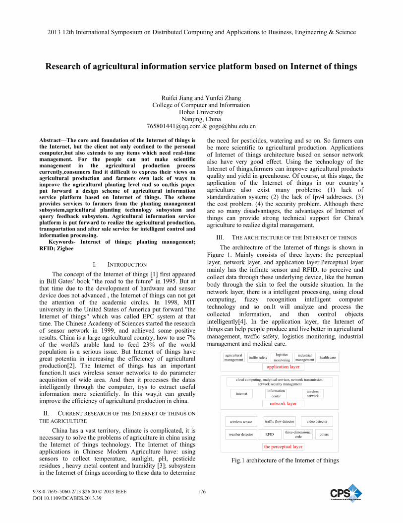
Research of agricultural information service platform based on Internet of things

Ruifei Jiang and Yunfei Zhang

College of Computer and Information Hohai University Nanjing, China

765801441@qq.com & gogo@hhu.edu.cn

Abstract—The core and foundation of the Internet of things is the Internet, but the client not only confined to the personal computer,but also extends to any items which need real-time management. For the people can not make scientific management in the agricultural production process currently,consumers find it difficult to express their views on agricultural production and farmers own lack of ways to improve the agricultural planting level and so on,this paper put forward a design scheme of agricultural information service platform based on Internet of things. The scheme provides services to farmers from the planting management subsystem,agricultural planting technology subsystem and query feedback subsystem. Agricultural information service platform is put forward to realize the agricultural production, transportation and after sale service for intelligent control and information processing.

Keywords- Internet of things; planting management; RFID; Zigbee

I. INTRODUCTION The concept of the Internet of things [1] first appeared

in Bill Gates’ book "the road to the future" in 1995. But at that time due to the development of hardware and sensor device does not advanced , the Internet of things can not get the attention of the academic circles. In 1998, MIT university in the United States of America put forward "the Internet of things" which was called EPC system at that time. The Chinese Academy of Sciences started the research of sensor network in 1999, and achieved some positive results. China is a large agricultural country, how to use 7% of the world's arable land to feed 23% of the world population is a serious issue. But Internet of things have great potentia in increasing the efficiency of agricultural production[2]. The Internet of things has an important function.It uses wireless sensor networks to do parameter acquisition of wide area. And then it processes the datas intelligently through the computer, trys to extract useful information more scientificly. In this way,it can greatly improve the efficiency of agricultural production in china.

II. CURRENT RESEARCH OF THE INTERNET OF THINGS ON THE AGRICULTURE

China has a vast territory, climate is complicated, it is necessary to solve the problems of agriculture in china using the Internet of things technology. The Internet of things applications in Chinese Modern Agriculture have: using sensors to collect temperature, sunlight, pH, pesticide residues , heavy metal content and humidity [3]; subsystem in the Internet of things according to these data to determine

the need for pesticides, watering and so on. So farmers can be more scientific to agricultural production. Applications of Internet of things architecture based on sensor network also have very good effect. Using the technology of the Internet of things,farmers can improve agricultural products quality and yield in greenhouse. Of course, at this stage, the application of the Internet of things in our country’s agriculture also exist many problems: (1) lack of standardization system; (2) the lack of Ipv4 addresses. (3) the cost problem. (4) the security problem. Although there are so many disadvantages, the advantages of Internet of things can provide strong technical support for China's agriculture to realize digital management.

III. THE ARCHITECTURE OF THE INTERNET OF THINGS The architecture of the Internet of things is shown in

Figure 1. Mainly consists of three layers: the perceptual layer, network layer, and application layer.Perceptual layer mainly has the infinite sensor and RFID, to perceive and collect data through these underlying device, like the human body through the skin to feel the outside situation. In the network layer, there is a intelligent processing, using cloud computing, fuzzy recognition intelligent computer technology and so on.It will analyze and process the collected information, and then control objects intelligently[4]. In the application layer, the Internet of things can help people produce and live better in agricultural management, traffic safety, logistics monitoring, industrial management and medical care.

traffic flow detector

cloud computing, analytical services, network transmission, network security management

agricultural management

application layer

RFID

network layer

the perceptual layer

logistics monitoring

traffic safety industrial management health care

information center

wireless networkinternet

wireless sensor video detector

weather detector three-dimensional code others

Fig.1 architecture of the Internet of things

2013 12th International Symposium on Distributed Computing and Applications to Business, Engineering & Science

978-0-7695-5060-2/13 $26.00 © 2013 IEEEDOI 10.1109/DCABES.2013.39

176

IV. SYSTEM DESIGN The agricultural information service platform system

based on the Internet of things consists of three subsystems.They are planting management subsystem, query feedback subsystem and agricultural planting technology subsystem. The design goal of this system is: make full use of the Internet of things technology and database technology, manage soil environment data like temperature, sunlight, pH, humidity and so on in the process of agricultural production, deploying production tools data, farmers’ work data,monitoring data in production process, query feedback data, agricultural planting technology data and so on.And then the system will manage these information intelligently by the computing advantages of computer itself.

In order to help farmers make production management better, the system uses various sensors to collect data in the planting management subsystem. And then transfer the data to the database, and process data in the computer with a decision support system, finally pass the results to the webpage where users can see. Query feedback subsystem is designed primarily for consumer to use.Consumers can feedback their own opinions to farmers. In addition, the system can save the results into the database, as historical data.The system can make judgments based on the historical data in the future. In this way,both sides can communicate, and it can provide market information for farmers' production. Because the farmers lack of agricultural technical guidance, in the agricultural planting technology system, it help farmers to study scientific knowledge from historical experience, farmers’ communicating with each other and experts’ guidance and so on.

The overall structure of agricultural information service platform system based on Internet of things is shown in figure 2.

agricultural information service system based on Internet of things

data acquisition

query feedback subsystem

agricultural planting technology subsystem

planting management subsystem

weather condition,outside

destruction, pests

seedersluice valve

work hours

number of workers

various sensors

monitor the production process

deploying production tools

farmer work

comparison of the average of sunlight yearly

comparison of the content of

pesticide yearly

comparison of the product price yearly

experienceagricultural experts online answers

farmers mutual communication

conventional planting model of agricultural expert

determine to increase

planting or not

comparison of the content of heavy

metal yearly

data base

consumer feedbackquery productionparameters

query production name ,production date

feedback according to the consumption

Fig. 2 the overall structure of system

The system mainly consists of 3 functional modules: (1) The planting management subsystem: it mainly responsible for using sensor to obtain data, sending the data

to the database, and then the data will be processed by the computer with the decision support system. It will decide the time of farmers work and the number of farmers according to the result, and decide whether to deploy the water valve, drill and other agricultural tools. This module is also responsible for monitoring the production process, for example, the weather is bad or not, the external damage and insect pests. (2) the query feedback subsystem: consumers can query the purchased agricultural products’ information, including its production date, production base, the processing place and pesticide residues. Then the consumers can put forward their comments according to their consumption feeling. So farmers can improve their planting mode according to the opinion, to improve the quality of agricultural products.So the products can meet the needs of the market better. (3) The agricultural planting technology subsystem: it mainly helps farmers improve planting skills through various channels. Farmers log on the system, and they can see the agricultural expert how to solve some conventional problems. There is an exchange platform between farmers. Farmers can share their own accumulation of experience so many years with everyone, which is called resource sharing. There is also agricultural experts online to answer questions.For the problems farmers really do not understand, they can consult a professional. In addition, the agricultural information service platform based on the Internet of things has its own historical data, such as the products price yearly, the pesticide content of some product yearly and so on. Farmers can sum up experience according to these data, judging whether to increase the planting next year.

V. KEY TECHNOLOGY

A. RFID Technology Simple RFID system is shown in figure 3. Composed

of three parts. (1) tag, the core of which is the radio frequency identification technology.It can read and write intelligently and make encrypted communication, and every label has an unique electronic code. (2) the reader, its main task is to make the radio frequency module emit read signal to the label and receive the response. (3) antenna, transmiting signals between tag and reader. [5]

177

Fig.3 RFID working principle diagram

B. EPC Technology EPC provides a unique identifier for a physical object.

The information which is stored in EPC encoding including embedded information and reference information. Then it use the Internet platform to construct a intelligence network which can share real-time information of global goods. The basic idea is to use the existing computer network and current information resources to store data[6]. EPC code length is divided into 64 bits, 96 bit and 256 bit. Coding is a string consisted of four field number, they are version number, domain name supervising, object classification and sequence number.EPC global and EPC management mechanism in different country manage the code sectionally[8]. EPC coding structure is shown in figure 4:

Fig.4 EPC code structure

C. ZigBee Technology ZigBee technology is a short-range, low-rate wireless

network technology. Wireless sensor network based on ZigBee has the characteristics of small volume of device, strong network self-healing ability.

VI. THE REALIZATION OF AGRICULTURAL INFORMATION SERVICE PLATFORM BASED ON INTERNET OF THINGS

A. The Flow Chart The flow chart of the system is shown in figure 5:

Fig.5 the flow chart of the system There are mainly 4 kinds of possibilities:

(a)The administrator logins, and goes into the planting management subsystem. And then the datas are edited and selected.After the administrator obtains the latest data,he will quit. (b) The farmer in ordinary users logins,and enters the agricultural planting technology subsystem. There are three services: expert advice, communicating with other farmers and past experience in the system.He will choose one of them. After service,he will quit. (c) The farmer in ordinary users logins, and browses one land environment on the website.He will formulate scientific planting scheme according to the datas,and then quit. (d) The consumer in ordinary users logins, and enters the query feedback subsystem. He can query some parameters about the product. After giving some advice according to his own consuming experience, he will quit.

B. Soil Environmental Report Figure 6 is a soil environmental report, it locates in the

various sensor collect datas of planting management part in the planting management subsystem.It records the soil situation from the location of the land, the soil temperature, sunlight is enough or not, pH value,humidity, soil fertility and soil color respectively. The administrator can also manage datas of one land through the information service platform, such as edite,delete and choose. Ordinary users do not have this authority.

Fig.6 a soil environmental report

C. The Editing State Figure 7 is the editing state of 3 land.Only

administrators can access this page, and ordinary users can only see the information on the page with no ability to edit. The administrator can change parameters like the name of the land, the soil temperature, sunlight, pH value, humidity and soil fertility etc. According to the data they obtaine, they can update the data in the database timely. So ordinary users to get accurate data timely, and they will manage their land scientificly. These data have effects on five aspects of planting management system: (1). In the aspect of planting

178

management, it can ensure the correctness of data various sensors collected and Database received. (2). In the aspect of farm management, it can help decision support system decide the number of work people and work time. (3). In the aspect of allocating production tools, the water valve can decide whether to water or not according to the humidity. Sowing machine can decide whether to sow or not according to some data of land environment. (4). In the aspect of monitoring the production process, the system can measure whether a plant have insect pests according to the data collected. (5). In the aspect of detecting the agricultural products, the system can judge whether agricultural products is harmful to the human body according to pesticide residue and heavy metal content.

Fig.7 the editing state of 3 land

D. Datas Six tables used in the system are Content, Manage,

Parameter, The login person, Query parameters and Historical data respectively. Database relation diagram is shown in figure 8. The left side of Figure 9 is some data of Parameter table in the agricultural information collection database. The right of Figure 9 is ER graphs of Parameter table.

Fig.8 Database diagram

Fig. 9

VII. IMPORTANT CODE a. the following code is to realize the planting management subsystem page. Admin/Product.xml

<siteRoot Id="root" url="~\Product.aspx" title="The Planting management subsystem" description="">

<siteMapNode url="" title="Planting management" description=""> <siteMapNode url="1.aspx" title="Various sensors collect datas" description="" /> <siteMapNode url="3.aspx" title="Database receives datas" description="" />// Put “variouse sensors collect datas” and “database receives datas”to”planting managerment” </siteMapNode> <siteMapNode url="" title="Farm management" description=""> <siteMapNode url="4.aspx" title="The number of working people" description="" /> <siteMapNode url="5.aspx" title="Working hours" description="" /> </siteMapNode> <siteMapNode url="" title="Allocate Production goods " description=""> <siteMapNode url="8.aspx" title="Hydrovalve needs to watering or not" description="" /> <siteMapNode url="9.aspx" title="Seeding machine needs to sow or not" description="" /> </siteMapNode> <siteMapNode url="" title="Monitoring the Production process" description=""> <siteMapNode url="14.aspx" title=" decides whether plant have diseases " description="" /> </siteMapNode> <siteMapNode url="" title="Detecting the agricultural products" description=""> <siteMapNode url="11.aspx" title="Detecting the content of pesticide" description="" /> <siteMapNode url="12.aspx" title="Detecting the content of heavy metal" description="" /> </siteMapNode>

179

<siteMapNode url="AdminOut.aspx" title="quit" description="administrators quit"> </siteMapNode> b. The following is part of the code which implements soil environmental report page. Pay attention to consistence: <Columns> <asp:BoundField DataField="LandID" HeaderText="LandID" InsertVisible="False" ReadOnly="True" SortExpression="LandID" /> <asp:BoundField DataField="LandName" HeaderText="LandName" SortExpression="LandName" /> <asp:BoundField DataField="Temperature" HeaderText="Temperature" SortExpression="Temperature" /> <asp:BoundField DataField="SunShine" HeaderText="SunShine" SortExpression="SunShine" /> <asp:BoundField DataField="PH" HeaderText="PH" SortExpression="PH" /> <asp:BoundField DataField="Water" HeaderText="Water" SortExpression="Water" /> <asp:BoundField DataField="soilfertility" HeaderText="soilfertility" SortExpression="soilfertility" /> <asp:BoundField DataField="soilcolour" HeaderText="soilcolour" SortExpression="soilcolour" />// The above is to add the columns <asp:CommandField ShowDeleteButton="True" ShowEditButton="True" ShowSelectButton="True" /> </Columns>

VIII. CONCLUSION The design scheme of agricultural information service platform based on Internet of things given in this paper,makes the Internet of things technology used in the agricultural production. From the acquisition of the data by the bottom sensor and detector device, to transfer the data to the computer system via the Internet.After intelligent processing like cloud computing ,the system will get valuable information, and the information is sent to the application layer, for people to use in agricultural production,agricultural transportation and other fields. For example, we can use IOT technology to improve agricultural productivity by achieving the best level of cultivation conditions in the greenhouse production. The service platform scheme can make Chinese agriculture

increase from the current inefficient state to a more digital management level.The competitiveness of Chinese agriculture can be greatly enhanced . With this information service platform, Chinese farmers can manage their lands more scientifically and make scientific decisions in time when some difficult situations appear. Thus, Chinese farmers will be able to benefit from scientific management and Chinese agriculture can make contributions to the world.

We can see from the advantages of the Internet of things, agriculture is an important domain of Internet of things.But application in actual production is still facing many problems to be solved such as data security, distribution and installation of sensors, system maintenance, power problems in remote environments etc. We should combine the characteristics of Chinese agriculture and national conditions, and strive to achieve breakthroughs and innovation of the key technology and common technology.

REFERENCES [1] Zhixiang Gan. Study on the origin and the development background

of the Internet of things [J] . modern economic information, 2010, (01): 158-157.

[2] Chunmeng Wang, Dapeng Zhang. Application of the Internet of things in agricultural production and food security [J]. agriculture network information, 2010, (12): 8-9.

[3] Liming Wen,Yalan Long.the IOT application in agriculture[J]. modern agricultural science and technology, 2010, (15): 54-56.

[4] Subin Shen, Quli Fan, Ping Zong, Yanqin Mao, Wei Huang. System structure of the Internet of things and related technology research [J]. Journal of Nanjing University of Posts and Telecommunications (NATURAL SCIENCE EDITION), 2009, (06): 1-11.

[5] Yifan Hu. radio frequency identification technology of RFID [J]. computer age, 2006, (12): 3-4.

[6] Zhiyu Ren, peiran Ren. Internet of things and EPC/RFID technology [J]. forest engineering, 2006, (01): 67-69.

[7] Ying Wang, Tiejun Zhou, Yang Li. The application prospect of IOT technology used in forestry informatization [J].Hubei Agricultural Sciences, 2010, (10): 2601-2604.

[8] Jing Wang [D]. Research and formulation of EPC key technologies and standards. Beijing University of Technology, 2006.

[9] Shanshan Liu, Shaowen Zhang. Exploitation conception of forest tree germplasm resource management information system based on RFID Technology [J]. forestry construction, 2008, (05): 27-31.

[10] Feng Liu, Junxiang Gao,Wenjun Yu, Xing Jin. AGIOT: A Model of the Internet of Things Used in Agriculture[J]. INFORMATION-AN INTERNATIONAL INTERDISCIPLINARY,2012,15(9): 3787-3792

[11] Yan-e Duan. Research on IOT Technology and IOT's Application in Urban Agriculture[J]. ADVANCED MATERIALS AND ENGINEERING MATERIALS, 2012, 457-458: 785-791

180

A Novel Distributed Multidimensional Management Approach For Modeling Proactive Decision Making

Masoud Pesaran Behbahni(1,2,3), Dr. Souheil Khaddaj2, Dr. Islam Choudhury2 1Azad University (IR) in Oxford, Oxford, UK

2School of Computing and Information Systems, Kingston University London, UK 3Azad University, Khorasgan Branch, Esfahan, Iran

e-mail: Masoud@Kingston.ac.uk

Abstract— The aim of this paper is to propose a new model for supporting proactive decision making in large enterprises. These organizations usually encounter enormous electronic transactions upon distributed infrastructures. The stockpiled data collections in these systems are the best source for providing necessary material for decision-making process to support managers and executives. The existing models for supporting decision-making, encounter practical problems while facing distributed databases. This paper introduces a new model that is designed to tackle the problem. The paper shows how the proposed model can be the best blueprint to increase the competitive advantage of an organization by intelligent use of the collections of data and synthesize useful knowledge. The proposed model is multidimensional because it is based on multidimensional data model concepts. It is also multilayer because it widely depends on multilayer mining theory concepts. The paper also presents the results of an empirical study to evaluate the model and the results of applying the model to real data collections.

Keywords- Decisin-making, distributed databases, Multidimensional Data Model, Data Mining, KDD

I. INTRODUCTION Regarding the importance of the decision support

systems, it is predictable to see that academics and practitioners have produced many models and frameworks for supporting decision-making using database intelligence and data mining techniques. A pioneer in this area is U. Fayyad who clearly defined a model for Knowledge Discovery in Database (KDD) process [1]. KDD as defined by who is the practice of using data mining methods to extract what is considered as knowledge according to the specification of measures and procedures. The KDD process is preceded by the development of an understanding of the application domain, the relevant prior knowledge and the goals of the end-user. His work successfully followed by researchers from SAS institute Inc. by introducing SEMMA. The acronym SEMMA stands for Sample, Explore, Modify, Model, and Assess. These phrases refer to the process phases required to conduct a data mining project. The problem with SEMMA is that it is configured to help the users of the SAS Enterprise Miner software. Another framework, CRISPDM, initially was conceived in 1996. The name stands for Cross Industry Standard Process for Data Mining. It is a non-proprietary, documented, and freely available data mining model. CRISP-DM organizes the data mining process into six phases: business understanding, data understanding, data

preparation, modeling, evaluation, and deployment [2] while generally, the sequence of the phases is not strict. A comparative study by Azevedo and Santos [3] comparing KDD, SEMMA, and CRISP-DM, illustrates that SEMMA and CRISP-DM can be viewed as implementations of the KDD framework. According to this study, five stages of the SEMMA process can be seen as a practical implementation of the five stages of the KDD process. Another useful analytical framework is the one developed by Lee Chung-Shing [4]. He introduced the framework primarily for evaluating ecommerce business models and strategies, though it is applicable in a wider range. In all the models, problems occur when the system uses distributed computing. The distributed databases, either homogenous or heterogeneous, may store fragmented data in large scales. This fragmentation makes the distributed database more efficient by keeping the tuples at the sites where they are used the most to minimize data transfer, but causes practical problems for the existing decision-support models.

This paper aims to introduce a new model that uses a novel strategy. The paper shows how the new strategy not only can tackle the mentioned problem, but also can be significantly effective in increasing the competitive advantage of any kind of organization by intelligent use of available data. This model basically tries to synthesize useful knowledge from collections of organized data. The model is multidimensional and multilayer. It is multidimensional because it focuses on multidimensional data model concepts. It is also multilayer because it uses multilayer mining structure based on the related theory, Multilayer Mining Theory, developed by Masoud P. Behbahani, Souheil Khaddaj, and Islam Choudhury [5] in Kingston University, London. These mining structures provide the platform for multilayer mining algorithms to maintain proactivity for the model, rather than just adjusting to situations and waiting for problems to happen. The paper primarily presents the outline of the new model. The proposed model is named Multidimensional Multilayer Mining Management Model (5M). The paper also presents results of evaluating the model by adapting it to the ebusiness discipline. This adaptation results in introducing EBAF, an EBusiness Analytic Framework.

II. OUTLINING OF THE NEW PROACTIVE FRAMEWORK The results of empirical study have already proved the

effectiveness of multilayer mining theory [6]. This theory encourages building layers of mining structures. Grounded

2013 12th International Symposium on Distributed Computing and Applications to Business, Engineering & Science

978-0-7695-5060-2/13 $26.00 © 2013 IEEEDOI 10.1109/DCABES.2013.40

181

on this theory, the new generic model, 5M is introduced. 5M is a model based on multidimensional data and multilayer mining structures designed to intelligently use available data collections in the organizational databases. This intelligent use of data makes the model a significant progress over the existing ones in many aspects. The final outline of the model mirrors the final results of a thoroughgoing empirical study. Though originally designed for distributed databases, 5M

serves as a generic model for all organizations wishing to capture database intelligence to significantly enhance their administrative behavior and gain profitable performance. It encourages best practices and offers organizations the structure needed to realize better, faster results from Database Intelligence. An overview of the model is shown in figure 1.

Figure 1. An Overview of 5M

A. Organization Understanding In order to understand which data should later be

analyzed, and how, it is vital to initially understand the business structure and objectives for which they are finding a solution. This phase perhaps is the most important stage of the model and involves several key steps that as are shown in figure 1.

B. Centralized Data Warehouse Development The next phase of model tries to tackle the problem of

organizing the collections of data. These collections may be dispersed or distributed in very different ways. In a

heterogeneous distributed database, different sites may use different schemas, and different database management system software with different format of data storage. In a homogenous distributed relational database, the relations can be vertically and/or horizontally fragmented. These fragments are usually stored in different geographical sites where they are more regularly accessed. Vertical fragmentation can be defined as a projection on the relation R. Each projected subset must include the primary key so the original relation can be reconstructed by taking the union of all fragments: R = R1 natural inner join R2 natural inner join · · · natural inner join Rn. A horizontal fragment can be defined as a selection on the relation R. Each tuple of

182

relation must belong to at least one of the fragments, so that the original relation can be reconstructed by taking the union of all fragments: R = R1 R2 · · · Rn.

Even in a centralized database this data also may be in different and not appropriate formats. This phase consists of identifying required data, collecting initial data, describing data, exploring data, Verifying data quality, designing data mart initial structure, identifying control flow tasks, identifying data flow tasks, cleaning data, reconstructing data, reformatting data, and carrying out aggregation calculations on data (Figure 1). In the final step, the process would be evaluated and reviewed and then data can be populated to data marts and a related report can be produced.

C. Analysis Engine Development The data marts that are developed in previous stage only

can store leaf-level values, i.e. the measure values that are in intersection of all of the dimensions of a data mart. To solve the problem, some or all of the possible data aggregates should be calculated ahead of time and stored within the multidimensional data structures. These multidimensional data structures are the best platform for building multilayer mining structures and applying proactive multilayer mining models. There are some distinct key steps in this phase that are summarized in figure 1. The figure shows that after defining data sources, measures and measure groups, dimensions and dimension hierarchies, Key Performance Indicators (KPI), partitions, mining structures are designed. Then some model validation tests run to validate the models against the measures of accuracy, reliability, and usefulness. The last steps in this phase include evaluating and reviewing the analysis process, deploying the cube design to analysis server, and then processing the multidimensional structure in the analysis server. The final step is producing an Analysis Engine Development Report.

D. Knowledge Delivery Platform Development Knowledge delivery platform stage in 5M primarily is

about choosing the end-users who are in charge of decision-making and designing appropriate reports for them. Knowledge delivery platform can contain a number of report projects, and each report project in turn can contain a number of reports. A report actually is a piece of art meant to convoy a message. This message changes based on the data that drives it. Each report internally contains two distinct sets of instructions that determine what the report will contain. The first set of instructions is data definition. Data definition controls where the data for the report comes from and what information is to be selected from that data. Data definition instruction set contains two distinct parts: the data source and the dataset. The data source instruction set is needed by the report to gain access to a data source that provides data for the report. When the report is compiled, it uses the data source instructions to gain access to the data source. It then extracts information from the data source into a new format that can be used by the report. This new format is called a dataset. The second set of instructions is the report layout, which specifies which field goes in which location on the screen or on paper. There are some basic steps in knowledge

delivery platform development phase that are summarized in figure 1. Identification of the end users, identification the purpose of each report, planning the authentication and authorization strategy, defining report data sources and data sets, choosing the data visualization methods, configuring reports layout, previewing and assessing the reports are main steps of this phase. It is also very important to have a plan for report maintenance. This stage includes identifying day-to-day activities that need constant monitoring and developing an efficient monitoring. A report of the process is produced at the end, including the list of components like data sources and dataset queries that can be reused.

III. EVALUATING THE NEW MODEL This section validates 5M by adapting it to a real

application as a case study and assessing the results in an empirical study. To validate the results, the model has been implemented and applied to EBusiness discipline and the results are evaluated.

A. Adapting the Model to Ebusiness Choosing ebusiness to apply the generic model is done

based on figures that showed a fast growing rate in the ebusiness branches specially in ecommerce domain. Ecommerce originally was identified as the facilitation of electronic commercial transactions, but in recent years, data mining, data warehousing and data integration modeling techniques [7], and Business Intelligence (BI) have become parts of its body. The term BI has been defined in different ways and in various contexts. Langit [8] defines it as effective storage and presentation of key enterprise data so that authorized users can quickly and easily access and interpret it. Knight et al. [9] consider it as a term that encompasses the process of getting data out of the disparate systems and into a unified model, so it can be used to analyze, report, and mine the data. The approach in this adaptation is more business-driven, rather than current software-driven ones [10]. Actually traditional views of business activities, like that of Kotler and Kelly [11] have mainly focused on the physical and human aspects of the organization. The information view of them started getting conceptualized with contributions from Holland and Naude [12], Jayachandran et al. [13] and Kumar Kar et al. [14] by emphasizing on marketing activities. The instance implementation of the new model is carried out for verification purposes by using Microsoft Visual Studio 2010 and SQL Server 2008. EBAF serves as a best practice blueprint for all kind of enterprises wishing to capture business intelligence and enhance their CRM. This all will be done through creating an architecture that not only provides useful information, but also provides organizational insight. A simplified overview of EBAF is provided by figure 2.

In the figure, a five-stage conversion model including awareness, contact, engagement, conversion and retention phases is proposed to help identify mid-level mining structures in business domain. The left side of the figure shows how EBAF classifies the people to six main state groups, target audience, aware target audience, unique

183

visitors, active unique visitors, actors, and finally the clients. The right side summarizes the influencers that affect awareness, Contact, Engagement, Conversion, and Retention

efficiency factors [15]. These influencers shape multilayer mining structures.

Figure 2. EBAF is the result of adapting 5M to Ebusiness discipline

EBAF evaluates and validates 5M by providing a roadmap to gain incredible competitive advantages in marketplace. EBAF offers the key ability to respond with more agility to changing business conditions using effective and corresponding actions. EBAF analysis core utilizes the EBAF Conversion Model constituents to create multilayer mining structures and finally enhances and optimizes the conversion model’s efficiency factors.

Figure 3. EBAF Analysis Core

Following the roadmap provided by 5M, results in EBAF Analysis Core in a shape of a trilateral BI supplier. It integrates enterprise multilayer KPI analysis, multilayer multidimensional analysis, and multilayer data mining analysis. Figure 3 provides an overview of characteristics of this core. EBAF multilayer enterprise KPI analysis offers a presentational business insight of critical measures. EBAF multidimensional cube analysis delivers an interactive, investigative and exploratory business perception. EBAF multilayer data mining analysis has a proactive role to provide discovery business vision.

B. Model Accuracy Testing and Validation Model accuracy testing and evaluation serves two

purposes. The first purpose is the prediction of how well the final model will work in the future or even whether it should be used at all. The second purpose is to find the best model that maintains EBAF objectives. The approach to model validation in this research is partitioning data into training and testing sets. This approach is an established method and is widely used by practitioners. In this approach, some portion of data from the training data set is reserved for testing. In figure 4, the lift chart graphically represents the improvement that the models provide when compared against a random guess for 24.75% population percentage.

184

Figure 4. Lift chart shows the significant improvement after using the

models

The yellow line in the chart is the result of the neural network model that does not have any effect on the prediction improvement. Therefore the line can also be considered as a blind guess. On the other hand, the blue line is for the ideal model. The red, green, and purple lines are correspondently related to EBAF Decision Tree MM1 and other specified models.

IV. CONCLUSION AND DISCUSSION A novel multidimensional multilayer model is presented

to significantly enhance decision-making process. The model also is capable to support distributed databases. The model is evaluated by adapting to ebusiness as a case study. The resulted ebusiness framework seems to be very successful in providing higher levels of business intelligence for the enterprises utilizing ecommerce as their main transactional model. There is also a debate about the expense of employing the model in enterprises. Though the model provides a solid insight for organization management, it can be costly due to data source providing for multilayer influencers and developing multilayer mining structures. Therefore a simplified version of the model can be used if there are not enough budgets for implementing 5M. This shortened version of the model can be called Multidimensional Mining Management Model (4M) and seems suitable for low-budget projects. The emphasis on building multilayer mining structures in 5M is not seen in 4M.

REFERENCES

[1] U Fayyad, G Piatetsky-Shapiro, and P Smyth, "From Data Mining to Knowledge Discovery in Database," American Association for Artificial Intelligence, vol. 17, no. 3, pp. 37-54, 1996.

[2] C Shearer, "The CRISP-DM Model: The New Blueprint for Data Mining," Journal of Data Warehousing, vol. 5, no. 4, pp. 13-22, 2000.

[3] A Azevedo and M F Santos, "KDD, SEMMA AND CRISP-DM: A PARALLEL OVERVIEW," in IADIS, 2008, pp. 182-185.

[4] L Chung-Shing, "An analytical framework for evaluating e-commerce business models and," Internet Research, vol. 11, no. 4, pp. 349 - 359, 2001.

[5] M Pesaran Behbahani, S Khaddaj, and I Choudhury, "Enhancing Organizational Performance through a new Proactive Multilayer Data Mining Methodology: An Ecommerce Case Study," International Journal of Innovation, Management and Technology, vol. 3, no. 5, pp. 600-607, October 2012.

[6] M Pesaran Behbahani, "A Business Intelligence Framework to Provide Performance Management through a Holistic Data Mining View," in UK Academy for Information System 17th Annual International Conference 2012, Oxford,UK, 2012.

[7] A D Giordano, Data Integration : blueprint and modeling techniques for a scalable and sustainable, 1st ed.: IBM Press, 2011.

[8] L Langit, Smart Business Intelligence Solutions with Microsoft SQL Server 2008.: Microsoft Press, 2009.

[9] B Knight, D Knight, A Jorgensen, P LeBlanc, and M Davis, Knight’s Microsoft Business Intelligence 24 Hour Trainer. Indianapolis, Indiana: Wiley Publishing, Inc., 2010.

[10] M T Fernandez, "Business Strategy Model," International Journal of Innovation, Management and Technology, vol. 2, no. 4, pp. 301-308, August 2011.

[11] P Kotler and K L Keller, Marketing Management. 12th Edition. New York: Prentice hall, 2006.

[12] P C Holland and P Naude, "The metamorphosis of marketing into an information-handling problem," The Journal of Business & Industrial Marketing 19(3), pp. 167-178, 2004.

[13] S Jayachandran, S Sharma, P Kaufan, and P Raman, "The Role of Relational Information Processes and Technology Use in Customer Relationship Management," Journal of Marketing, vol. 69, pp. 177-192, 2005.

[14] A Kumar Kar, A Kumar Pani, and S Kumar De, "A Study On Using Business Intelligence For Improving Marketing Efforts," Business Intelligence Journal, pp. 141-150, 2010.

[15] M Pesaran Behbahani, S Khaddaj, and I Choudhury, "A Multilayer Data Mining Approach to an Optimized Ebusiness Analytics Framework," in International Proceedings of Economics Development and Research, Dubai, UAE, 2011, pp. 66-71.

185

A Portfolio Pricing Model and Contract Design of the Green Supply Chain for Home Appliances Industry Based on Manufacturer Collecting

Ai Xu International Business Faculty

Beijing Normal University Zhuhai Zhuhai, China

e-mail: gdxuai@163.com

Shufeng Gao College of Computer Science & Technology

Beijing Institute of Technology Zhuhai Zhuhai, China

e-mail: gsfdl@163.com

Abstract—This paper examines the pricing issues of the green supply chain for home appliances industry by using game theory and contract coordination theory. Considering the influences of the effective recycle behavior of the used home appliances to the whole supply chain, the paper proposes a game model for the portfolio pricing for the wholesale, retail and recycle price based on manufacturer recycling model. Then a revenue and expense-sharing contract model is designed to improve the game effects, by allocating both total revenues and expenses related to the manufacturing, retailing and recycling operations in the green supply chain among all participating players, thus maximizing the profits and effectiveness of the supply chain as a whole.

Keywords-green supply chain; portfolio pricing decision-making; revenue and expense-sharing contract; home appliances industry; manufacturer collecting; game model

I. INTRODUCTION Nowadays, supply chain management has become an

important means to gain the competitive advantage. The pricing problems of supply chain management have been widely recognized in the literature and in practice. With the rise of green supply chain management, the pricing problems of supply chain management are facing new difficulties and challenges.

The urgency and importance of integrating home appliances industry with the green supply chain management has gained more attention all over the world, due to the fact that discarded used or recycled home appliances become hazardous substances and are harmful to the environment if disposing them by traditional means. How to take back used home appliances and improve the consumption of the green home appliances could be with great significance for the development of home appliances industry of China, which will depend on the price strategies to a large extent. Comparing with the traditional one, the pricing problems of the green supply chain for home appliances industry are more complicated due to its operational objectives and in consideration of its economic efficiency, social and environmental impact as well as its unique characteristics. Meanwhile, there are many difficulties about how to make pricing decisions in home appliances industry when considering the influences of the effective recycle behavior

of the used home appliances to the whole supply chain and the specific characteristics concerned with coordination.

II. LITERATURE REVIEW There are a growing number of research papers on green

supply chain management that use game theory to model pricing decisions. The present research results include some studies about the pricing problems for the green supply chain management itself and some studies about the pricing problems for the closed-loop supply chain with product remanufacturing focusing on the effective utilization of resources, with the latter as a majority. Savaskan et al [1] use game theory to present the optimal closed-loop supply chain structures and to study the pricing and recycle strategies based on three reverse channel formats. Ray et al [2] studied the optimal pricing and trade-in strategies for durable, remanufacturable products by focusing on the scenario where the replacement customers are only interested in trade-ins. Gu et al [3,4] have made an analysis about the price decision for reverse supply chain based on game theory. The research papers of Wang et al [5]-[8] from the year of 2006 to 2010 have systemically studied the pricing strategies of the closed-loop supply chain management and constructed a set of models by using game theory. Ge et al [9], Guo et al [10,11], Qiu and Huang [12], Huang et al [13] studied the pricing and coordination problems of the closed-loop supply chain management base on game theory too. Some scholars studied price-making decision and the coordination mechanism in the green supply chain, such as Jiao et al [14], Shen and Wang [15], Li [16], Liu and Ma [17], Zhu and Dou [18], Cao et al [19], etc. Xu and Zhou [20] proposed a portfolio pricing model for the Green Supply Chain of home appliances industry based on retailer collecting.

So far literatures about the pricing model of the green supply chain for home appliances industry is really limit. Therefore, considering the influences of the effective recycle behavior of the used home appliances to the whole supply chain, this paper will propose a game model for the portfolio pricing based on manufacturer colleting model to try to determine the optimal price decision about the wholesale price and the retail price for the green home appliances, and the recycle price for the used home appliances.

2013 12th International Symposium on Distributed Computing and Applications to Business, Engineering & Science

978-0-7695-5060-2/13 $26.00 © 2013 IEEEDOI 10.1109/DCABES.2013.53

186

III. MODEL NOTATIONS AND ASSUMPTIONS

A. Notations We use the following notation throughout the paper: Cm will denote the unit cost of manufacturing a new

green home appliance, Cr will denote the unit cost of remanufacturing a returned home appliance into a new one, and Cs will denote the unit cost of selling a new home appliance for the retailer. P is the retail price of the green home appliance and W is the unit wholesale price. Pc will denote the unit recycle price for the used home appliances from the consumer to the manufacturer. Sb will denote the unit subsidy or penalty that manufacturer obtained from governments. D(P) is the basic demand for the new green home appliance in the market as a function of retail price, and D’(Pc) is the derivative demand for the new green home appliance created by recycling used home appliance as a function of recycle price. j

i! will denote the profits function for channel member i in supply chain model j and * j

i! will denote the optimal profit correspondingly. The subscript i will take M, R and vacancy, which will denote the manufacturer, the retailer, and the centralized manufacturer, respectively. Superscript j will take values C and M, which will denote the centrally coordinated and manufacturer collecting models, respectively. P*j, W*j, Pc

*j and Pr*j will

denote the optimal prices, respectively.

B. Assumptions We consider the following scenario and make the

following modeling assumptions. Suppose that the manufacturer has incorporated a

remanufacturing process for used home appliances into her original production system, so that she can manufacture a new home appliance directly from raw materials, or remanufacture part or whole of a returned unit into a new product. We assume that the home appliances produced by using used products are the same as a new one by using raw materials in terms of quality and functions, and will be sold at the same wholesale price.

(1) We consider a two-echelon green supply chain and model a bilateral monopoly between a single manufacturer and a single retailer. It is the manufacturer who is responsible for collecting the used home appliances.

(2) While optimizing their objective functions, all supply chain members have access to the same information.

(3) We consider the manufacturer has sufficient channel power over the retailer to act as a Stackelberg leader. The Stackelberg structure for the solution of similar games has been widely used in the supply chain management literature [22].

(4) The pricing decisions are considered in a single-period setting.

(5) Producing a new green home appliance by using a used product is less costly than manufacturing a new one, and the cost saving is denoted by !, i.e., !=Cm-Cr.

(6) r denotes the fraction of the recycled used home appliance that will be put into remanufacturing and the other fraction 1-r will be put into other places, e.g., raw materials

regeneration, i.e. 0"r"1. We assume that the unit residual value of used home appliances is S S"! .

From Assumptions (5) and (6), the average unit revenue from recycling can be written as !'=r!+(1 r)S.

(7) We assume that the recycling quantity A is only dependent on the recycle price for used home appliances, i.e., A(Pc)=g+hPc, where g and h are parameters and both of them are greater than zero. Parameter g reflects the consumers’ awareness of environmental protection and h indicates the level of sensitivity of the consumers to Pc.

(8) We assume that part of recycling quantity will translate into new demand for the green home appliances particularly when taking some means and measures, such as cash incentives from government for older home appliances that are traded in for new green ones. We characterize the conversion rate by #, i.e., D'(Pc)=#(g+hPc) and 0!#!1. The conversion rate # can be influenced by appropriate subsidy from the governments to the consumers in practice. D'(Pc) is a derivative demand from the recycle of the used home appliances.

(9) We consider dedicated cost of recycling used home appliances is function of recycling quantity, i.e., C (Pc)=LA2(Pc) and L>0, where L is a parameter of recycling cost.

(10) We assume the basic demand function is D(P)= -P, with and being positive parameters. We assume a downward sloping linear demand function.

Lee and Staelin [23] have shown that the vertical interaction between the channel members and the optimality of the channel strategies depend on the convexity of the demand functions.

From Assumptions (8) and (10), the total demand for green home appliances are composed of the basic demand and the derivative demand from the recycle of the used home appliances: ( ) '( ) ( )c cD P D P P g hP" # $+ = % + + .

(11) We assume that fraction$1 of the unit manufacturing cost are those cost concerning to meet the requirements or standards of the green home appliances, and the other fraction 1-$1 are other kind of manufacturing cost, i.e., 0!$1!1. Similarly, we assume that fraction$2 of the unit retail cost are those cost concerning to the promotion of the green home appliances, and the other fraction 1-$1 are other kind of retail cost, i.e., 0!$2!1.

IV. A PORTFOLIO PRICING MODEL BASED ON MANUFACTURER COLLECTING

A. Centrally Coordinated Model (Model C) The centrally coordinated model provides a benchmark

scenario to compare the decentralized models with respect to the supply chain profits.

2

[ ( ) '( )] ( ) ( ) ( ' )[ ( )]( ) ( )( ' )

( )

Cc m s b c c

c m s b c c

c

D P D P P C C S A P P CP g hP P C C S g hP P

L g hP" # $

! = + & % % + + & ' % %= % + + % % + + + ' %% +

(1)

The simultaneous solution of the first-order conditions results and the profits are listed in Table . The optimal portfolio pricing strategies here is (P*C, Pc

*C).

187

TABLE I. EQUILIBRIUM RESULTS OF PORTFOLIO PRICING GAME MODELS UNDER MODEL C

Model C

* jP ( )

2m s bC C S A" # $

#+ + % +

* jcP 2 2

2 ( ' 2 ) [ ( ) ]4 (1 )

m s bh g Lgh h C C S gh Lh h

# $ " # $# $

' % % + % + % ++ %

A 22 ( ' ) [ ( )]

4 (1 )m s bh g h C C S

Lh h# $ " #

# $' + + % + %

+ %

D ( )2

m s bC C S A" # $% + % +

*! 2( ' )

2 4A h g B AB

h$#

' + ++

B. Decentralized Pricing Model Based on Manufacturer Collecting (Model M) In this model, the manufacturer is responsible for the

promotion and collection of used home appliances. The retailer decides the retail price P and the manufacturer decides the whole sale W for the new green home appliances and the recycle price Pc for the used home appliances.

The profits of the retailer, manufacturer and the total supply chain are given by following equations, respectively.

[ ][ ( ) '( )]( )

( ) ( )

MR c s

c s

D P D P P W CP g hP P W C" # $

! = + % %= % + + % %

(2)

[ ]2

[ ( ) '( )] ( ) ( ) ( ' )( ) ( )

( )( ' ) ( )

MM c m b c c

c m b

c c c

D P D P W C S A P P CP g hP W C S

g hP P L g hP" # $

! = + & % + + & ' % %= % + + % +

+ + ' % % +

(3)

2

[ ( )]( )( )( ' ) ( )

M M MR M c m s b

c c c

P g hP P C C Sg hP P L g hP

" # $! = ! + ! = % + + % % ++ + ' % % +

(4)

Because the objective function is concave in P, the best responses can be determined from the first-order conditions. And then given P R, the manufacturer will optimize her profits function. The best responses will be determined and the results are shown in Table . The optimal portfolio pricing strategies here is (W*M, P*M, Pc

*M).

TABLE II. EQUILIBRIUM RESULTS OF PORTFOLIO PRICING GAME MODELS UNDER MODEL M

Model M

* jW ( )2

m s b MC C S A" # $#

+ % % +

* jP 3 ( ) 3

4m s b MC C S A" # $

#+ + % +

* jcP

2 24 ( ' 2 ) [ ( ) ]

8 (1 )m s bh g Lgh h C C S g

h Lh h# $ " # $

# $' % % + % + % +

+ %

AM 24 ( ' ) [ ( )]

8 (1 )m s bh g h C C S

Lh h# $ " #

# $' + + % + %

+ %

D ( )4

m s b MC C S A" # $% + % +

*M! 2( ' )

2 8M MA h g B A B

h$#

' + ++

*R! 2( )

16MB A$

#+

*! 2 2 2( ' ) 3 4

2 16M M MA h g B A B A

h$ $

#' + + ++

It can be proved that the total supply chain profits of centrally coordinated model is less than the one of decentralized circumstance, which shows that there is

inefficiencies resulting from decentralization of decision making due to double marginalization in the channel. Therefore, it is very important to increase the profits of supply chain members so that the efficiency of the whole supply chain can be further improved. Appropriate contract can work in this circumstance.

V. A REVENUE AND EXPENSE-SHARING CONTRACT MODEL

We will design a revenue and expense-sharing contract model so as to improve the game effects of the pricing decision making.

In the existing research papers about recycle of the used products, it is usual that only sales revenue and fixed costs for collecting are allocated between the supply chain members. In this paper, considering the characteristics of the green supply chain for home appliances industry, all those revenues including not only sales but also subsidy from the governments, and all those costs including not only costs regarding the recycling but also the costs concerned with the green production and relevant promotion, will be allocated between the manufacturer and the retailer.

We assume that the manufacturer and the retailer sign a revenue and expense-sharing contract before the sale period. The manufacturer will sell home appliances to the retailer at a wholesale price lower than the unit manufacturer cost. At the end of sale period, sales revenue and subsidy from the governments will be allocated between the manufacturer and the retailer, with the retailer accounted for %1 (0!%1!1) percent and the manufacturer accounted for 1-%1. At the same time, costs will be allocated too, including the recycling costs and costs concerned with green production and relevant promotion, with the retailer accounted for %1 (0!%1!1) percent and the manufacturer accounted for 1-%1.

We characterize the superscript “-RES” to denote the optimal results. The profits are given by following equations, respectively.

[ ][ ]

1 1 2

2

( ) ( )( ) [ (1 ) ]

M RESR c m s b

c s

P g hP P C C SP g hP W C

( " # $ ) )" # $ )

%! = % + + % % +% % + + + %

(5)

[ ][ ]

1 1 2

1

2

(1 ) ( ) ( )( ) ( (1 ) ] ( )( ' )

( )

M RESM c m s b

c m c c

c

P g hP P C C SP g hP W C g hP P

L g hP

( " # $ ) )" # $ )

%! = % % + + % % ++ % + + % % + + ' %

% +

(6)

2

[ ( )]( )( )( ' ) ( )

M RES M RES M RESR M c m s b

c c c

P g hP P C C Sg hP P L g hP

" # $% % %! = ! + ! = % + + % % ++ + ' % % +

(7

) Because the objective function is concave in P, from the

first-order conditions, the best responses are determined by the following equation (8).

* 1 1 2 2

1

[ ( ) ( ) [ (1 ) ]2

M RES m s b c sC C S g hP W CP ( " # ) ) $ # )#(

% + + + + + + + %= (8)

In order to make the game result reach the efficiency of the centrally coordinated model, the condition P*M-RES= P*C and Pc

*M-RES= Pc*C must be satisfied, and we will get:

*1 1 1 2(1 ) (1 )(1 )M RES

m sW C C( ) ( )% = % % % % (9)

*2 2

2 ( ' 2 ) [ ( ) ]4 (1 )

M RES m s bc

h g Lgh h C C S gPh Lh h

# $ " # $# $

% ' % % + % + % +=+ %

(10)

188

It can be found that equation (8), (9) and (10) show the optimal portfolio pricing strategies under decentralized decision-making with the manufacturer responsible for collecting, i.e., (P*M-RES, W*M-RES ,Pc

*M-RES). In this circumstance, the optimal profits are given by the

following equations, respectively. 2

*1

2 2 2*

1

( )4

( ) ( ' )(1 )4 2 4

M RESR

M RESM

B A

B A A h g AB Ah

$(#

$ $ $(# #

%

%

+! =

+ ' + +! = % + %

(11)

2* ( ' )

2 4M RES A h g B AB

h$#

% ' + +! = + (12)

Form the above equation (11) and (12), it can be found that the profits of the supply chain members will depend on the value of %1. The conditions driving the manufacturer and the retailer to accept the contract are that the profits of the supply chain members will be as least not lower than the profits before signing the contract, i.e.,

* *

* *

M RES MR RM RES M

M M

%

%

! * !! * !

(13)

In general, the green supply chain can be coordinated by this revenue and expense-sharing contract. The gaming and decision process is as follows: the home appliances manufacturer determine the ratio %1 according to the constraint shown in equation (13), then the manufacturer determine the wholesale price W and the recycle price Pc from the consumers, and the retailer determine the retail price P. According to this portfolio pricing strategies, both the manufacturer and the retail will improve their profits and the total profits of the green supply chain can reach the optimal level of centrally coordinated system.

VI. A NUMERICAL EXAMPLE Here the models proposed in this paper will be analyzed

by numerical examples with specific data. The home appliance designated here is the Freon-free and inverter air-conditioner manufactured by Gree Electric Appliances, Inc. of Zhuhai. Assumption of the basic parameters for Gree Freon-free and inverter air-conditioner are list in Table .

TABLE III. ASSUMPTION OF THE BASIC PARAMETERS FOR GREE FREON-FREE AND INVERTER AIR-

CONDITIONER

Cm Cr r S "' Cs g

2400 1500 0.6 100 580 300 40

h # Sb L $ %

0.2 0.4 300 0.0005 4725 1.5

A. Equilibrium results of the portfolio pricing in Model C and Model M

TABLE IV. EQUILIBRIUM RESULTS OF THE PORTFOLIO PRICING FOR GREE FREON-FREE AND INVERTER AIR-CONDITIONER IN MODEL C AND MODEL M

Model C Model M

W*( RMB /unit) N/A 2486

P*( RMB /unit) 2787 2980

Pc*( RMB /unit) 267 229

A g+hPc (million unit) 93 86

D (million unit) 581 290 *M! (million RMB) N/A 142114 *R! (million RMB) N/A 55998 *! (million RMB) 254410 198112

Efficiency loss % -- 22.1

From Table , it can be seen that the retail price in Model M is greater than the one in Model C, which will result in a decline in the basic demand of the green home appliances. Meanwhile, the recycle price from the consumers Pc is lower than the one in Model C, which will affect the consumer’s decision to replace his or her used home appliance and result in a decline of the recycle quantity. As a result the quantity translated into the new demand will decrease too. From the perspective of social welfares, the decrease of the recycle price will reduce the enthusiasm of consumers to return their used products and affect the effective recycle of the used home appliances, which will decrease the environmental and social benefit.

As the result of the increased retail price and the decreased recycle price, the total demand for GREE freon-free and inverter air-conditioner is only a half of the demand in Model C, which is the main reason of the efficiency loss. It can be seen that the total profits of the supply chain is much less than the profits of centralized model, having lost 22.1 percent efficiency.

B. Improvements of the portfolio pricing by a revenue and expense-sharing contract Here we will observe the improvements of the portfolio

pricing by a revenue and expense-sharing contract with an assumption of &1=0.4 and &2=0.3. According to the equation (13), the value of '1 is between 0.249 and 0.499. Then according to the equation (11), we can calculate the profits of the retailer are 227067%1 and the profits of the manufacturer are 1-%1 227067+39285. Profits of the manufacturer and the retailer under different %1 are listed in Table .

TABLE V. PROFITS OF THE MANUFACTURER AND THE RETAILER UNDER DIFFERENT SHARING RATIO &1

!1 *M!

million RMB

*R!

million RMB

*! million RMB

0.25 198112 56298 254410

0.3 186852 67558 254410

0.35 175592 78818 254410

0.4 164332 90078 254410

0.45 153073 101337 254410

0.49 144065 110345 254410

It can be seen that the effects of the pricing game between the manufacturer and retailer have been improved by the revenue and expense-sharing contract. The total profits of the supply chain have reached the level of

189

centralized system and eliminated double marginalization. The exact allocation result of the profits will depend on the value of %1, which will be affected by the negotiation ability. The greater the %1 is, the more profits the retailer will gain and the less profits the manufacturer will gain, but profits level of both the retailer and the manufacturer have been improved compared with those without the contract.

VII. CONCLUSIONS In consideration of the impact of the recycle quantity of

the used home appliances on the demand for the green home appliances, a new demand function is proposed in this paper. A portfolio pricing model of the green supply chain for home appliances industry is presented based on the model that it is the manufacturer who is responsible for colleting the used home appliances, which is mainly about the decision-making of the portfolio pricing for the wholesale, retail price of the green home appliances and recycle price for used home appliances. As a benchmark case, the Centrally Coordinated Model is also analyzed to highlight inefficiencies resulting from decentralization of decision making, and is later used for deriving the channel coordinating pricing scheme. The analysis shows that there exists double marginalization and the pricing game effects should be further improved. Then a revenue and expense-sharing contract models is designed which will be able to allocate resources properly in accordance with the different cost factors such as green manufacture, retail and marketing expenses as well as cost of collecting and recycling, thus maximizing the profits and effectiveness of the supply chain as a whole. At last, using Gree Electric Appliances, Inc. of Zhuhai as a case, this paper applies its pricing models to one of its green products, namely, the freon-free and inverter air-conditioner, and has proved the rationality and feasibility.

Connecting the recycling of the used home appliances with the sale of the green home appliances and making a portfolio pricing strategies from the perspective of the whole supply chain, will be helpful to recycle the used home appliances effectively so as to relieve the pressure of the recycling for the used home appliances in China. At the same time, this can induce consumers to choose green home appliances when they return their used home appliances back, and reduce the bad influences of the home appliances to the environments during the usage as well as improve the environmental benefits.

This paper proposes an alternative model to solve the pricing problems of the complicated supply chain operations, especially the green supply chain management. The pricing models presented in this paper for the green supply chain of home appliances industry provides a practical and theoretical guidance for home appliances enterprises in making pricing decisions and supply chain contracts. It is also of significance in improving the effectiveness and efficiency of the whole supply chain.

REFERENCES [1] R. C. Savaskan, S. Bhattacharya, and L. N. VAN Wassenhove,

“Closed-loop supply chain models with product remanufacturing,” Management Science, vol. 50, Feb. 2004, pp. 239-252.

[2] S. RAY, T. BOYACI and N. ARAS, “Optimal prices and trade-in rebates for durable, remanufacturable products,” Manufacturing Service Operations Management, vol. 7, Mar. 2005, pp. 208-228.

[3] Q. L. Gu and J. H. Ji, “Price decision for reverse supply chain based on fuzzy recycling price,” Information and Control, vol. 35, Apr. 2006, pp. 417-422.

[4] Q. L. Gu, T. G. Gao and L. S. Shi, “Price decision analysis for reverse supply chain based on game theory,” Systems Engineering-theory & Practice, Mar.2005, pp. 20-25.

[5] Y. Y. Wang, “Closed-loop supply chain coordination under disruptions with revenue-sharing contract,” Chinese Journal of Management Science, vol. 17, Jun. 2009, pp. 78-83.

[6] Y. Y. Wang, “Closed-loop supply chain coordination under disruptions with buy back contract,” Operations Research Andmanagement Science, vol. 18, Jun. 2009, pp. 46-52.

[7] Y. Y. Wang, B. Y. Li and F. F. Le, “The Research on two price decision models of the closed-loop supply chain,” Forecasting, vol. 25, Jun. 2006, pp. 70-73.

[8] Y. Y. Wang, B. Y. Li and L. Shen, “The price decision model for the system of supply chain and reverse supply chain,” Chinese Journal of Management Science, vol. 14, Apr. 2006, pp. 40-45.

[9] J. Y. Ge, P. Q. Huang and Z. P. Wang, “Closed-loop supply chain coordination research based on game theory,” Journal of Systems & Management, vol. 16, May. 2007, pp. 549-552.

[10] Y. J. Guo, L. Q. Zhao and S. J. Li, “Revenue-and-expense sharing contract on the coordination of closed-loop supply chain under stochastic demand,” Operations Research and Management Science. vol. 16, Jun. 2007, pp. 15-20.

[11] Y. J. Guo, S. J. Li and L. Q. Zhao, “One coordination research for closed-loop supply chain based on the third part,” Industrial Engineering and Managemen, May. 2007, pp. 18-22.

[12] R. Z. Qiu and X. Y. Huang, “Coordination model for closed-loop supply chain with product recycling,” Journal of Northeastern University (Natural Science), vol. 28, Jun. 2007, pp. 883-886.

[13] Z. Q. Huang, R. H. Yi and Q. L. Da, “Study on the efficinecy of the closed-loop supply chain with remanufacturer based on third-party collecting,” Chinese Journal of Management Science, vol. 16, Mar. 2008, pp. 73-77.

[14] X. P. Jiao, J. P. Xu and J. S. Hu, “Research of price-making decision and coordination mechanism in a green supply chain,” Journal of Qingdao University (E & T), vol. 21, Jan. 2006, pp. 86-91.

[15] L. Shen and Y. Y. Wang, “To Analyse on Evolutionary Game of Green Supply Chain,” Value Engineering, May. 2007, pp. 65-69.

[16] W. N. Li, “Research on the coordinate mechanisms of node enterprises in green supply chain,” Guilin University of Electronic Technology, 2008.

[17] Q. Liu and J. R. Ma, “Research on the price coordination of supply chain under information sharing,” Logistics Technology, vol. 27, Dec. 2008, pp. 97-101.

[18] Q. H. Zhu and Y. J. Dou, “A game model for green supply chain management based on government subsidies,” Journal of Management Sciences in China, vol. 14, Jun. 2011, pp. 86-95.

[19] J. Cao, X. B. Wu and G. G. Zhou, “Coordination strategy of green supply chain based on product’s utility diversity,” Computer Integrated Manufacturing Systems, vol. 17, Jun. 2011, pp. 1279-1286.

[20] A. Xu, Z. Q. Zhou, “A Portfolio PricingModel and Contract Design of the Green Supply Chain for HomeAppliances Industry Based on Retailer Collecting”, The Twelfth Wuhan International Conference on E-Business. New York: Alfred University Press, May, 2011, pp. 822-832.

[21] E. Lee and R. Staelin, “Vertical strategic interaction: Implications for channel pricing,” Marketing Science, vol. 16, Mar. 1997, pp. 185-207.

[22] A. Xu, X. P. Hu and S. F. Gao, “Review of supply chain coordination with contracts,” The Tenth Wuhan International Conference on E-Business. New York: Alfred University Press, May, 2011, pp. 1219-1225.

190

The Traing Design and Implementation of Stimulating Students’ Learning Motivation of University Novice Teachers Based on Web

Lina Sun1, Linlin Wang1, Ying Wang1, Yuanlin Chen1

School of Computer and Information Technology Northeast Petroleum University

Daqing, China sunln912@126.com, wanglinlin0204@163.com, nepu_wy@163.com, ylchen80@163.com

Abstract—Most university teachers pay attention to stimulating the students’ learning motivation. Moreover, stimulating the students’ learning motivation is a capability of IBSTPI (the Internet Board of Standards for Training, Performance and Instruction). In this context, this research aims to design and implement a plan of training activity to enhance university novice teachers’ stimulating the students’ learning motivation skills through school-based training. Finally, according to the classification of teachers’ knowledge, we construct the training object and content system to design the activities based on the Network Platform of Moodle and Course review platform based on online video for university novice teachers.

Keywords-training; learning motivation; novice teachers; Moodle

I. TRAINING BACKGROUND This training is supported by the “The school-based

training study of improving university novice teachers’ teaching capability- taking Northeast Petroleum University as an example” ( “the study of teaching capability training” for short). In the phase of training design, the author has made a data analysis for international comparatively popular IBSTPI teacher competency standards and performance indicators system by Delphi method, and formed suitable objectives of school-based training for novice teachers of our university. According to the objects of the training, the study takes one of the objects “stimulating students’ learning motivation” as an example to design and implement the teachers’ training [1].

II. ESTABLISHMENT OF THE TRAINING OBJECT By talking with the top organizers of this program and

interviewing the related experts, the author takes the world-famous “IBSTPI teaching ability indicators” as the main basis of teaching ability indicators included in this training, and gives specific expectations of these indicators. At the same time, we get the importance level of subordinate indicators, which gives guidance of the following training activity design [2].

The subordinate indicators and their importance level are as follow [1]:

TABLE I. CURRENT STATUS AND “STIMULATING STUDENTS’ LEARNING MOTIVATION” INDICATORS OF NOVICE

TEACHERS

Ability indicators Current status

Importance level

Ability of stimulating students’ learning motivation

full score5

(1) The ability of attracting and maintaining the learners’ attention 4.5 1

(2) The ability of ensuring the learning objectives clearly 4.32 4

(3) The ability of establishing the learning motivation strategies 4.37 2

(4) The ability of providing the opportunities to participate in learning and

achieving success for students 4.37 2

III. CONSTRUCTION OF THE TRAINING CONTENT In the process of developing content system of school-

based training activity, this research references the research results of classification of teachers' knowledge and develops the classification and source of novice teachers’ knowledge [3]. Based on the classification of teachers’ knowledge, the author constructs three-layer logical structure “ability-performance indicator-teachers’ knowledge” and uses the specific teachers’ knowledge to construct the content of the training activity. It is shown as below:

Figure 1. Relationships between stimulating students’ learning motivation

and Teachers’ Knowledge

In the classroom teaching, it is very important to transform the students’ external motivation to internal motivation. The capability can not only stimulate the students’ learning interests, but also improve their learning

2013 12th International Symposium on Distributed Computing and Applications to Business, Engineering & Science

978-0-7695-5060-2/13 $26.00 © 2013 IEEEDOI 10.1109/DCABES.2013.41

191

effect. From the figure 1, we can see the corresponding teachers’ knowledge is mainly pedagogical knowledge.

IV. A DETAILED DESIGN PLAN OF TRAINING ACTIVITIES Stimulating and maintaining students’ learning

motivation is an interesting subject of many participating teachers, especially how to stimulate the students’ motivation in teaching practice.

Through looking up into the documents about learning motivation strategies home and abroad, the author finds that there are many ways to stimulate and maintain the students’ learning motivation, such as the ARCS model put forward by Keller in 1983 [4]. The ARCS model includes four factors: attention strategy (teaching should attract and maintain the learners' curiosity and interest), relevance strategy (teaching should be combined with the learners' needs, interests and motivation), confidence strategy (teaching should develop the students' positive expectations for success), and satisfaction strategy (provide the outer and the inner satisfaction). Wlodkowski analyzes motivation factors in the whole teaching process. There exist corresponding motivation factors from the beginning to the end [5].

Chinese scholar Zhao Liying references the TC motivation model and ARCS motivation design model, put the theory of motivation stimulating into the process of instructional design, and use teaching cases to verify that motivation theory has a direct relationship with teaching goals, teaching contents, teaching strategies, learning environment and teaching evaluation design [6].

Moreover, the author finds that a lot of scholars tend to change teaching methods and teaching modes to stimulate the students’ learning motivation, which both belong to the teaching strategy domain. Therefore, the training of this activity starts from the teaching methods and teaching modes that teachers usually use, such as classroom discussing method, scaffolding instruction mode, autonomous learning model based on WebQuest, group cooperative learning model and so on.

A. Activity Theme Activity theme is the training for stimulating and

maintaining students’ learning motivation.

B. Teachers’ Knowledge Teachers’ knowledge refers to teaching goals, learning

motivation strategies- those are pedagogical knowledge.

C. Some Ways Corresponding to Pedagogical Knowledge Daily communication with colleagues, Teachers’

experience and reflection, Observing excellent teaching case and Teachers’ professional training.

D. Activities Objects • Know the common learning motivation types of

college students. • Master several common methods of stimulating

students’ learning motivation.

E. Corresponding Capabilities The corresponding capabilities are to stimulate and

maintain the students’ learning motivation and to ask effective questions.

F. Organizational Forms of the Activities • Face-to-face lectures • Network learning platform based on Moodle • Course review platform based on online video

G. Activity Tools • Blog space • Scaffolding tools

H. Flow of the Training Activity According to the observation records of years of class

visiting, experts find that lots of teachers use discussion method and current relatively popular teaching mode, such as Scaffolding Instruction, independent learning based on WebQuest, group cooperative learning to stimulate the students’ learning motivation. In allusion to the characteristics of the contents and organizational form of the training activity, the training activity is as follows.

The activity begins with the theme “the application of discussion method and common teaching mode in classroom teaching”, and instructs participating teachers to design the plan of stimulating students’ learning motivation by their own reflections and scaffolding tools set up by assistants [7]. Experts and participating teachers watch teaching cases, discuss and modify the design plan of normal class through the course review platform based on network video. After the activities above, we can complete the training of expected contents, thus achieve the whole training goal of the project.

I. Activity Analysis Sub-activity1: Experts lecture face to face on "the

application of discussion method and common teaching mode in classroom teaching"

1) Activity steps First, experts have a lecture on the application of

discussion method and common teaching mode in classroom teaching by the case form. Then, experts point out the application mistakes teachers made in practical teaching, and discuss with participating teachers about how to solve these problems and stimulate students’ learning motivation efficiently. At last, participating teachers write their own reflections on Moodle network platform according to individual specific teaching situation.

2) Teaching method Case method and discussion method.

3) Activity environment Multi-media classroom and Moodle network learning

platform. 4) Activity tools

Blog space. Sub-activity2: participating teachers design the plan of

stimulating students’ learning motivation

192

1) Activity steps According to the experts’ face-to-face lectures on the

discussion method and application strategy of common teaching mode in classroom teaching, participating teachers design the plan of stimulating students’ learning motivation- taking one course in this session as the main content [8]. They can use the scaffolding tools that learning assistants set up in accordance with class discussion, scaffolding instruction and group cooperative learning, or design all by themselves. At last, participating teachers submit the design plan to the seminar in Moodle network learning platform.

2) Activity environment Moodle network learning platform

3) Activity tools: Scaffolding tools Scaffolding tool1: Discussion activity in class The preparation before activity contains five parts:

activity theme and goals, activity time, activity grouping, activity materials and activity evaluation.

The process of the activity contains teachers’ activity strategies and students’ activity strategies, such as exchanging roles in the activity timely, instructor, facilitator and audience, activity evaluation, group discussion and report and group summary and reflection after class.

Scaffolding tool2: Scaffolding instruction Because scaffolding instruction has relatively mature

teaching process, the assistants in this research reference the activity flow: putting up the scaffolding-entering the situation-independent exploration-cooperative learning-effectiveness evaluation.

Sub-activity3: Participating teachers watch cases and discuss the design of normal class.

1) Activity steps Participating teachers enter for the normal class recording

voluntarily; Assistants record and upload one lesson of stimulating students’ learning motivation that participating teachers designed; Experts gather participating teachers together to watch the case of normal class, and discuss about the design plan of stimulating students’ learning motivation; Participating teachers upload the modified design plan to the panel discussion module in Moodle network learning platform; Experts and assistants give participating teachers one-to-one instruction again [9].

2) Activity time: one week 3) Teaching method: discussion method 4) Activity environment: course review platform based

on network video and Moodle network learning platform 5) Activity tool: Moodle platform seminar 6) Activity feedback: Moodle mail integration

J. The summary of the Implementation of Training Activities The effectiveness analysis of this activity is mainly based

on the design of stimulating students’ learning motivation made by participating teachers.

From the Moodle log and the seminar we can see that participating teachers show great impassion in the design of stimulating students’ learning motivation, especially when it

is relative with their own curriculum. They would like to share their experience actively in how to stimulate students’ learning motivation in the normal class. By checking the design plan submitted in Moodle discussion forum, the author classified them as below [10]. ! Reference teaching models in expert lectures, such as:

class discussion, scaffolding instruction and group cooperative learning and so on.

! When the teachers assign homework to the student, give them the scope of the choice as far as possible and let the students choose proper titles according to their own interest.

! The teachers usually provide teaching feedback information to promote students to continue studying.

! After class, the teacher should often communicate with the students to understand their learning motivation.

! Teachers should use average grades as well as test score to evaluate students’ final grades, with the help of Average Grade and Attendance to supervise students’ learning in this course.

We can see that stimulating students’ motivation goes through the parts of before class, during class and after class, and participating teachers should draw attention in improving motivation by details things in teaching.

On the other hand, network video normal class recording activities take the teaching videos of participating teachers as the normal class cases for experts and participating teachers to watch and receive some participating teachers’ recognitions. We find that the expert comments on the learning motivation design plan of the participating teachers through class observation and points out the advantages and disadvantages of the plan. The author finds that the participating teachers can actively express personal views closely around the theme of the current discuss and reflect on their own design.

V. EFFECTIVENESS ANALYSIS OF THE TRAINING ACTIVITIES

The study is used Miss Zhu as an example to follow up “how to stimulate and maintain students’ learning motivation” in the Introduction to Mao Zedong thoughts and theoretical system of socialism with Chinese characteristics course.

Last term Miss Zhu taught the course named “Introduction to Mao Zedong thoughts and theoretical system of socialism with Chinese characteristics”, but she found that the teaching effect is not very ideal, especially the students often talked in class, their enthusiasm is not high and late arrival phenomenon is very serious. In a word, these are surface phenomenon that students perform in class. In fact, the main reason is that the students’ learning motivation in the course is not very intense.

According to the aforementioned analysis of Miss Zhu, she intended to stimulate students’ learning motivation using group cooperative learning in the process of teaching. Miss Zhu took the chapter Building a harmonious socialist society for the range of topics, and designed group cooperative learning activity step by step in accordance with the hints of

193

activity scaffolding. At the same time, Miss Zhu participated in the class recording of some group discussion activity in institute of resources and environment. Experts and other participating teachers commented on the group cooperative learning records and classroom videos that the group submitted.

Here is Miss Zhu’s group cooperative learning design plan.

A. Preparation Work before the Activity 1) Activity theme

Choose a topic from the chapter “Building a harmonious socialist society” and set a title by yourself.

2) Activity object To know the scientific connotation and significance of

building a harmonious socialist society and to learn about the main policies to build a harmonious socialist society are two activity objects.

3) Activity time Week of teaching: week 6 –week 11

4) Activity grouping Learning group can be divided by dormitory, interest or

combine freely. 5) Division of activity

Each group is suggested to clarify the division of tasks for everyone, such as materials collecting, speech draft writing, group report making etc.

6) Activity materials Activity materials are in the public e-mail.

7) Activity assessment The activity assessment consists of three parts: group

rating, the other groups rating and teacher rating. 8) Activity review

Group sends the theme and division of activity to the teacher’s e-mail a week in advance. If the activity gets approved, the group reporting time can be arranged.

B. Activity Organization Process 1) Teachers’ activity

The role of teachers in the activity is the organizer and audience. Meanwhile, the teachers organize reviews and ratings of the activity.

2) Students’ activity

There are three parts i.e. group reports, group summary and reflections, submit record of the group cooperative learning.

After group cooperative learning completed, Miss Zhu surveys the group cooperative learning method by using the questionnaire survey. It is widely believed that some improvement has achieved in learning initiative, learning ability, learning interest by students.

ACKNOWLEDGMENT This work is supported by the Higher Education

Comprehensive Reform Pilot Special Project Heilongjiang Province Education Office in 2012 #JGZ201201045: to enhance university novice teachers’ teaching capability through school-based training-taking Northeast Petroleum University as an example.

REFERENCES [1] Xiaoqing Gu, Teachers Ability Standard: face-to-face, online and

blended situations, East China Normal University Press, Shanghai, 2007.

[2] L. B. Yang, L. N. Sun, “The training program design of how to improve the teaching communication skills of young college teachers”, Proceeding of ICCSE2012 Conference, Melbourne, pp. 1884-1887, July 2012.

[3] Qinghua. Liu, “Research on Model Construction of Teacher Knowledge,” Southwest Normal University, 2004.

[4] Kaicheng. Yang, Xiulan. Li, “Building an online learning system based on ARCS motivation model”, E-education Research, pp. 46-49, June. 2001.

[5] Ling. Zhang, “The strategy of the motivation of learning of distance and open education under network environment”, Education and Examinations, pp. 89-93, May. 2008.

[6] Liying. Zhao, “A research on motivation theories-based instructional design strategies”, South China Normal University, 2004.

[7] Jiliang. Shen, Kairong. Wang, “On Teacher’s Teaching Abilities”, Journal of Beijing normal university(humanities and social science edition), pp. 64-71, January. 2000.

[8] Fugang. He, Li. Chen, “Design and Study of Learning Activity for Web-based Course”, Open Education Research, pp. 89-94, April. 2007.

[9] Li. Yang, Dongsheng. Zhao, “The Research on Blended Learning Which Based on Moodle”, Journal of Capital Normal University(Natural Science Edition), pp. 6-13, February. 2010.

[10] Feng. Liu, Yanhua. Wang, “Teachers’ Training Based on Moodle Platform”, Open education Research, pp. 91-94, October. 2008.

194

Computer Networks and SystemArchitectures

DCABES 2013

Multi-Dimensional Analysis and Design Method for Aerospace Cyber-Physical Systems

Lichen Zhang

Faculty of Computer Science and Technology Guangdong University of Technology

Guangzhou 510090, China zhanglichen1962@163.com

Abstract—In this paper, we propose a multi-dimensional

specification and modeling method of aerospace cyber-physical system. This method is proposed according to seven views of systems so that their physical and computational parts of aerospace cyber-physical system are modeled correctly. The physical world analysis is considered to be one fundamental stage of our proposed method. The proposed method is illustrated by the modeling of the lunar rover system, which involves a broad range of mechanical, electronic, control, communications, computing, mechanics, and physics. In this paper, we specify and model the lunar rover system by extending Modelica and AADL.

Keywords-CPS,LunarRover;Modelica;AADL;Spatial-Temporal Features;Dynamic Continuous Features

I. INTRODUCTION The integration of physical systems and processes with

wireless networked computing has led to the emergence of a new generation of engineered aerospace cyber physical systems. Such systems use computations and communication deeply embedded in and interacting with physical processes to add new capabilities to physical systems. These aerospace cyber-physical systems [1] range from spaceship to lunar rover [2] in which computation/information processing and physical processes are so tightly integrated that it is not possible to identify whether behavioral attributes are the result of computations (computer programs), physical laws, or both working together, functionality and salient system characteristics are emerging through the interaction of physical and computational objects, computers, wireless networks, devices and their environments in which they are embedded have interacting physical properties, consume resources, and contribute to the overall system behavior[3-6].

In order to meet the challenge of aerospace cyber-physical system design [7-10], we need to realign abstraction layers in design flows and develop semantic foundations for composing heterogeneous models and modeling languages describing different physics and logics. We need to develop new understanding of compositionality in heterogeneous systems that allows us to take into account both physical and computational properties. One of the

fundamental challenges in research related to aerospace cyber-physical system is accurate modeling and representation of these systems. The main difficulty lies in developing an integrated model that represents both cyber and physical aspects with high fidelity. Among existing techniques, an approach to integrate Modelica [11-14] with AADL [15-18] is a suitable choice, as it can encapsulate diverse attributes of aerospace cyber physical systems

In this paper, we propose a multi-dimensional approach to specify and model aerospace cyber physical systems. We specify and model the lunar rover system by extending Modelica and AADL. The extension of Modelica and AADL can model physical world, spatial-temporal features, dynamic continuous features, safety features.

II. THE PROPOSE METHOD FOR SPECIFICATION AND MODELING OF AEROSPACE CYBER

PHYSICAL SYSTEMS A number of methodologies and tools have been

proposed for the design of aerospace cyber-physical system. However, they are still evolving because systems and software engineers do not yet completely understand the aerospace cyber-physical system requirements analysis process, and the complex dynamic behavior of aerospace cyber-physical system is difficult to capture in a simple understandable representation. Consequently, development time for many of these systems extends beyond expectations. Furthermore, many methods are not tested properly, nor do they meet customer requirements or expectations. In our opinion, an acceptable aerospace cyber-physical system design methodology must synthesize the different views of systems, use a number of different methods, and consist of an orderly series of steps to assure that all aspects of the requirements and the design have been considered.

The most obvious difference between current methodologies and our approach is that we propose a methodology which explicitly avoids the use of a simple framework to design complex systems. Instead, this new methodology is proposed according to seven complementary views: physical word view, function view,

2013 12th International Symposium on Distributed Computing and Applications to Business, Engineering & Science

978-0-7695-5060-2/13 $26.00 © 2013 IEEEDOI 10.1109/DCABES.2013.42

197

static view, behavior view, spatial-temporal view, non-functional view and hardware view.

Unfortunately, the methodologies and tools developed for analysis of real-time systems do not adequately address these specification issues because they do not allow for the description of complex dynamic external environments. The current methodologies confuse the analysis of behavior of the physical world with the internal behavior of the system. The above facts explain why we propose a view of “physical world of system and a stage of the system environment analysis. We use Modelica [19-21] to make an environment analysis for physical world of aerospace cyber-physical system. Modelica is an object-oriented modeling language that facilitates the physical modeling paradigm. It supports a declarative (non-causal) model description, which permits better reuse of the models. Modelica is intended to serve as a standard format so that models arising in different domains can be exchanged between tools and users. Modelica supports multi-domain modeling and several formalisms, such as ODE, DAE, bond graphs, finite state automata, DEVS and Petri nets.

Notice that the objective to construct a system lies in the realization of functionality that a user demands. Integrating the descriptive power of UML models with the analytic and computational power of Modelica models provides a capability that is significantly greater than provided by UML or Modelica individually. UML and Modelica are two complementary languages supported by two active communities. By integrating UML and Modelica, we combine the very expressive, formal language for differential algebraic equations and discrete events of Modelica with the very expressive UML constructs for requirements, structural decomposition, logical behavior and corresponding cross-cutting constructs. [22-25].

A static view captures the static relation between the object and data. Static view emphasizes the static structure of the system using objects, attributes, operations and relationships. We can use AADL and UML to model the static structure of the system. AADL (Architecture Analysis and Design Language), which is a modeling language that supports text and graphics, was approved as the industrial standard AS5506 in November 2004. Component is the most important concept in AADL. The main components in AADL are divided into three parts: software components, hardware components and composite components. Software components include data, thread, thread group, process and subprogram. Hardware components include processor, memory, bus and device. Composite components include system [26-30].

The changes of an internal behavior of system are caused by the changes of the behavior of the external environment of the physical world.. So we propose a behavioral view in order to help analyze the behavior of real-time systems. The behavioral view captures the dynamics of the system, i.e., the conditions under which the functionality is performed. We can use an approach to

integrate Modelica, AADL behavior Annex, UML, hybrid automata [31] and Differential dynamic logic (dL) [32]. Differential dynamic logic (dL) [33] is a logic for specifying and verifying hybrid systems.

A spatio-temporal view captures the spatio-temporal requirements of Cyber physical systems. Cyber physical systems are spatio-temporal. In the sense that correct behavior will be defined in terms of both space and time [5-6]. The motion is a key notion in our understanding of spatial- temporal relations, the question remains of how to describe motion, and more specifically the interaction between moving objects, adequately within a qualitative calculus. In this paper, we use AADL , Time Automata, Cellular automata (CA)[33-34] and Basic Qualitative Trajectory Calculus [35] to express and reasoning spatial-temporal requirements Cellular automata (CA)]are models that are discrete in space, time and state variables.

Non-functional View addresses important issues of quality and restrictions for cyber physical systems, although some of their particular characteristics make their specification and analysis difficult: firstly, non-functional requirements can be subjective, since they can be interpreted and evaluated differently by different people; secondly, Non-functional requirements can be relative, since their importance and description may vary depending on the particular domain being considered; thirdly, non-functional requirements can be interacting, since the satisfaction of a particular non-functional requirement can hurt or help the achievement of other non-functional requirement.

A hardware view aims at supporting fitting the specification on a particular target hardware environment. A developer must decide what hardware should be used and how it is to be used to implement the specification, so we propose a hardware view that helps improve the implementation.

III. CASE STUDY: SPECIFICATION AND MODELING OF THE LUNAR ROVER SYSTEM

A lunar rover or Moon rover [37-41] is a space

exploration vehicle designed to move across the surface of the Moon. A lunar rover is an autonomous system capable of traversing a terrain with natural l obstacles. Its chassis is equipped with wheels/tacks or legs and possibly a manipulator setup mounted on the chassis for handling of work pieces, tools or special devices. Various preplanned operations are executed based on a preprogrammed navigation strategy taking into account the current status of the environment. Locomotion is a process, which moves a rigid body. To increase the safety of the drive, the rover has hazard avoidance software which causes to stop and reevaluate its position every few seconds. In the paper, we concentrate the physical world view and static view specification and modeling of the lunar rover system. The

198

overall architecture of the robot of the lunar rover is modeled by Modelica as shown in Fig.1.

Fig.1. the overall architecture of the robot of the lunar rover

We take PathPlanning6 components as an example,

PathPlanning6 is modeled by Modelica as shown in Fig.2.

Fig.2. PathPlanning6 components

The variable curve of PathPlanning6 components by the simulation using Modelica is shown as Fig.3.

Fig.3. the variable curve of PathPlanning6 components

The lunar rover body structure model is specified by

Modelica as shown in Fig.4.

Fig.4. lunar rover body structure model

We use AADL to model the navigation system of the lunar rover. The navigation system of the lunar rover contains three parts: control system, execution unit and survey device. The file organization of navigation system of the lunar rover is shown as Fig.5.

Fig.5. lunar rover navigation system file structure

The navigation system of the lunar rover is specified by

AADL as follows:

199

system NavigationSys end NavigationSys; system implementation NavigationSys.Impl subcomponents SurveyDevice: system SurveyDevice::SurveyPlatform.Impl; ControlSys: system ControlSystem::Control.Impl; ExecUnit: system ExecutionUnit::Execution.Impl; connections conn1: bus access SurveyDevice.ToControl -> ControlSys.FromSurvey; conn2: bus access ControlSys.ToExecution -> ExecUnit.FromControl; properties Actual_Processor_Binding => reference surveydevice.attitudeprocessor applies to ControlSys.AC; Actual_Processor_Binding => reference surveydevice.headingprocessor applies to ControlSys.HC; Actual_Processor_Binding => reference surveydevice.locationprocessor applies to ControlSys.LC; end NavigationSys.Impl;

The components of the survey device are shown in Fig.6.

Fig.6. The components of the survey device

The components of the control system are shown in Fig.7.

Fig.7. The components of the control system

The components of the execution unit are shown in Fig.8

Fig.8. the components of the execution unit

IV. CONCLUSION

We have proposed a multi-dimensional specification and modeling method for aerospace cyber-physical system. This method was proposed according to seven views of systems so that their physical and computational parts of aerospace cyber-physical system are modeled correctly. The physical world analysis has been considered to be one fundamental stage of our proposed method. In this paper, we specified and modeled the lunar rover system by integrating Modelica and AADL.

Future work focuses on the integration formal methods with AADL and Modelica

ACKNOWLEDGMENT

This work is partly supported by National Natural

Science Foundation of China under Grant No. 61173046 and Natural Science Foundation of Guangdong province under Grant No.S2011010004905.

REFERENCES [1] Don Winter. Cyber Physical Systems – An Aerospace Industry

Perspective. www.ee.washington.edu/research/nsl/aar-cps/winterrev4.pdf

[2] Lunar Rover Vehicle.www.hq.nasa.gov/alsj/a17/A17_LunarRover2.pdf

[3] Ella M. Atkins. Cyber-physical Aerospace:Challenges and Future Directions in Transportation and Exploration Systems. varma.ece.cmu.edu/cps/Position-Papers/Ella-Atkins.pdf

[4] E. M. Atkins, I. Alonso-Portillo, and M. J. Strube, "Emergency Flight Planning applied to Total Loss of Thrust," Journal of Aircraft, American Institute of Aeronautics and Astronautics (AIAA), 43(4):1205-1216, Jul-Aug 2006.

[5] •M. Xue and E. M. Atkins, “Runway-Independent Aircraft Approach Design for the Baltimore-Washington Airport,” Journal of Aircraft, American Institute of Aeronautics and Astronautics (AIAA), 43(1):39-51, Jan-Feb 2006.

[6] S. Roderick, B. Roberts, E. Atkins, P. Churchill, and D. Akin, “Design and Validation of an Autonomous Software Safety System for a Dexterous Space Robot,” Journal of Aerospace Computing, Information, and Communication, American Institute of Aeronautics and Astronautics (AIAA), vol. 1, no. 12, pp. 564-579, Dec. 2004.

200

[7] Grand Challenges for transportation Cyber-Physical Systems. www.ee.washington.edu/.../GregSullivan-20081014102113

[8] Steve Goddard and Jitender S. Deogun. Future Mobile Cyber-Physical Systems: spatio-temporal computational environments. varma.ece.cmu.edu/cps/Position-Papers/Goddard-2.pdf

[9] Jitender Deogun and Steve Goddard. Reasoning about Time and Space: A Cyber Physical Systems Perspective,”14th IEEE Real-Time and Embedded Technology and Application Symposium (RTAS’08), Work in Progress (WIP) Proceedings, pp. 1-4, St. Louis, Mo, April 2008.

[10] E. A. Lee and S. A. Seshia, Introduction to Embedded Systems – A Cyber-Physical Systems Approach, Berkeley, CA: LeeSeshia.org, 2011

[11] Otter M., Elmqvist H., Mattsson S. E.: Multidomain Modeling with Modelica. Handbook of Dynamic System Modelling, editor Paul A. Fishwick, Chapman & Hall/CRC, chapter 36, pp. 36.1 - 36.27, 2007.

[12] Elmqvist, H., Mattsson, S. E., Otter, M.. Object-Oriented and Hybrid Modeling in Modelica. Journal Européen des systèmes automatisés, 35,1/2001, pp. 1 à X.

[13] Mattsson, S.E., Elmqvist, H., Otter, M..Physical system modeling with Modelica. Control Engineering Practice, vol. 6, pp. 501-510, 1998

[14] Elmqvist, H., Mattsson, S.E.: An Introduction to the Physical Modeling Language Modelica. ESS'97 European Simulation Symposium, Passau, Germany, October 19-22, 1997.

[15] Feiler P H, Gluch D P, Hudak J J. The architecture analysis & design language (AADL): An introduction[R]. CARNEGIE-MELLON UNIV PITTSBURGH PA SOFTWARE ENGINEERING INST, 2006.

[16] Feiler P H, Lewis B, Vestal S, et al. An overview of the SAE architecture analysis & design language (AADL) standard: a basis for model-based architecture-driven embedded systems engineering[M].Architecture Description Languages. Springer US, 2005: 3-15.

[17] Hudak J J, Feiler P H. Developing aadl models for control systems: A practitioner’s guide[J]. 2007.

[18] Dionisio de Niz and Peter H. Feiler. Aspects in the industry standard AADL. AOM '07 Proceedings of the 10th international workshop on Aspect-oriented modeling.P15 – 20

[19] M. OTTER, C. SCHLEGEL, and H. ELMQVIST. “Modeling and realtime simulation of an automatic gearbox using Modelica.” In Proceedings of the 1997 European Simulation Symposium (ESS’97), Passau, Germany, October 1997.

[20] Modelica - a uni!ed object-oriented language for physical systems modelling. Language speci!cation. Technical report, Modelica Association, 2002.

[21] Modelica Association. Modelica: A Unified Object- Oriented Language for Physical Systems Modeling: Language Specification Version 3.0, Sept 2007.www.modelica.org

[22] OMG. OMG Unified Modeling Language TM (OMG UML). Superstructure Version 2.2, February 2009.

[23] Adrian Pop, David Akhvlediani, Peter Fritzson. Towards Unified Systems Modeling with the ModelicaML UML Profile. International Workshop on Equation-Based Object- Oriented Languages and Tools. Berlin, Germany, Linköping University Electronic Press, www.ep.liu.se,2007

[24] ModelicaML.A UML Profile for Modelica.www.openmodelica.org/index.php/developer/tools/134

[25] Wladimir Schamai, Peter Fritzson, Chris Paredis, Adrian Pop. Towards Unified System Modeling and Simulation with ModelicaML: Modeling of Executable Behavior Using Graphical Notations. Proceedings of the 7th International Modelica Conference, Como, Italy. September 20-22, 2009

[26] Peter H. Feiler and David P. Gluch. Model-Based Engineering with AADL: An Introduction to the SAE Architecture Analysis & Design Language. Addison-Wesley Professional, 2012

[27] SAE AS-2C. Architecture Analysis & Design Language. SAE International Document AS5506B(2012) Revision 2.1 of the SAE AADL standard, Sept 2012.

[28] Julien Delange. Towards a Model-Driven Engineering Software Development Framework. (2012) In: The Third Analytic Virtual Integration of Cyber-Physical Systems Workshop. , 04 Dec 2012, Porto Rico.

[29] Feiler, Peter and Hugues, Jérôme and Sokolsky, Oleg Architecture-Driven Semantic Analysis of Embedded Systems (Eds) Dagstuhl Seminar 12272. (2012) Dagstuhl Report, vol. 2 (n° 7). pp. 30-55.

[30] Saqui-Sannes, Pierre de and Hugues, Jérôme Combining SysML and AADL for the design, validation and implementation of critical systems. (2012) In: ERTSS 2012 (Embedded Real Time Software and Systems), 01-03 Feb 2012, Toulouse, France

[31] T.A. Henzinger, P.W. Kopke, A. Puri, P. Varaiya. What's decidable about hybrid automata? In Proceedings of the 27th Annual Symposium on Theory of Computing, pp. 373{382. ACM Press, 1995

[32] A. Platzer .Logical Analysis of Hybrid Systems: Proving Theorems for Complex Dynamics. Springer, 2010.

[33] K Nagel,M Schreckenberg,A Cellular Automaton Model for Freeway Traffic[J] Phys.I France, 1992,2(12):2221-2229.

[34] K.Culik,L.P.Hurd,Formal Languages and Global Cellular Automaton Behavior[J].Physical D,1990,45(13):396-403.

[35] Nico Van de Weghe et al. A Qualitative Trajectory Calculus and the Composition of Its Relations. Lecture Notes in Computer Science Volume 3799, 2005, pp 60-76

[36] E. Gat, R. Desai, R. Ivlev, J. Loch, and D. Miller, Behavior Control for Robotic Exploration of Planetary Surfaces, IEEE Transactions on Robotics and Automation, 10(4):490-503,August 1994.

[37] L. Robert, M. Buffa, and M. Hebert. Weakly-Calibrated Stereo Perception for Rover Navigation. In Proc. ARPA Image Understanding Workshop, pp. 1317-1324,November 1994

[38] C. Proy, M. Lamboley, and L. Rastel. Autonomous navigation system for the Marsokhod rover project. In Proc. Third Intl. Symposium on Artificial Inteligence, Robotics, and Automation for Space, October 1994.

[39] E. Krotkov and R. Simmons, Perception, Planning, and Control for Autonomous Walking with the Ambler Planetary Rover. Intl. J. Robotics Research, 1995

[40] Peter Berkelman et al. Design of a Day/Night Lunar Rover.www.ri.cmu.edu/pub_files/.../berkelman_peter_1995_1.pdf

201

Based on Rough Set and Support Vector Machine (SVM) in Jilin Province Power Distribution Network Transformation Project Evaluation

Liu Min Electric Power Research Institute of Jilin Electric Power

Co., Ltd Changchun, China

E-mail: liumin6886@163.com

Cong Li Telemetric of Jilin Electric Power Co., Ltd

Changchun, China E-mail: congli8462@163.com

Zhu Kai North China Electric Power University

Baoding, China E-mail: zhukai0731@163.com

Du qiushi

Electric Power Research Institute of Jilin Electric Power Co., Ltd

Changchun, China E-mail: sgccdqs@126.com

Abstract—in this paper, according to the current status of Jilin province power network construction and transformation projects, established the evaluation index system of power distribution network transformation project. Aiming at the characteristics of the large number of index, proposed a model of evaluating the power distribution network transformation based on rough set and support vector machine (SVM), And uses the evaluate data of the power distribution network in Jilin province for the empirical analysis, shows that the method has higher classification accuracy. The results of the research show that the model has good effectiveness and the method is practical and feasible.

Keywords-component; power distribution network transformation; project evaluation; rough set; support vector machine (SVM)

I. INTRODUCTION Electric power industry as a result of our country on

the power distribute network construction and transformed project management, has been using extensive management for a long time, lacking rigorous and scientific project management evaluation program. When new project is coming, often it ignores social benefits and economic benefits. This paper introduces the comprehensive analysis and evaluation system to the evaluation of electric power project, so as to obtain a scientific and objective comprehensive evaluation conclusion.

Setting up scientific index system can help us to evaluate and determine the effect of the project comprehensively from the perspective of society, economy and benefit. Doing comprehensive after evaluation for such as power distribution network construction and transformation project this kind of engineering project that it’s basic industry with obvious public welfare which is of particular importance to have practical and innovative index system. Only in this way can we make scientific and accurate evaluate conclusions to the project, so as to provide important reference for management decision.

This paper constructs the evaluate index system of Jilin power network construction and retrofit project, and put forwards the evaluation model of distribution network transformation project which based on rough set attribute reduction and support vector machine (SVM) classification. Using rough set to make up for the deficiency that support vector machine (SVM) in the aspect of reducing redundant information, and using support vector machine (SVM) to make up for the inadequacy of rough set theory in terms of generalization ability. On the basis of using the principle of rough set and support vector machine (SVM), making the second classification research for credit risk assessment. In order to verify the effectiveness of the proposed method, using the actual data to do empirical research, which proved that the method have higher classification accuracy.

II. POWER DISTRIBUTION NETWORK TRANSFORMATION PROJECT EVALUATION INDEX SYSTEM

Building a scientific and perfect evaluation index system is the most important premise to realize accurate assessment of distribution network transformation project, and it is also the basis of doing the comprehensive evaluation. According to the characteristics of the distribution network construction and renovation project in Jilin province, through analysis of various influencing factors of distribution network construction and retrofit, this article builds the index system including grid performance, regional economic, social benefit and enterprise financial (table 1).

TABLE I. EVALUATION INDEX SYSTEM

Grid performance

indexes

line loss rate grid power factor

grid security user terminal voltage

percent of pass power grid layout

2013 12th International Symposium on Distributed Computing and Applications to Business, Engineering & Science

978-0-7695-5060-2/13 $26.00 © 2013 IEEEDOI 10.1109/DCABES.2013.43

202

capacity-load ratio power supply

reliability

Regional economic

indexes

the first industrial output value

the second industry output value

the third industry output value

the second and third industry output value

proportion investment

environment improvement

Social benefit

indexes

alleviate burden amount on Per capita residents' satisfaction

domestic power consumption on Per

capita government's satisfaction

Living environment improvement

Enterprise financial

indexes

internal rate of return payback period of

investment financial net present

value

III. BASED ON ROUGH SET THEORY AND ATTRIBUTE REDUCTION

A. Knowledge expression system

Rough set is to abstract the sample set as a decision-making system ( ,{ }, )aS U V a= , in the formula U is a non-empty finite set, called universe of discourse; A is a non-empty finite set, called attribute set; { }aV is the domain of attribute a A! : aa U V" is a injection, which makes any element in the discourse U get attribute a having a unique value in aV . If A was composed by condition attribute set C and decision attribute set D, C and D meet ,C D A C D= = #! " , then we call S the decision system[2].

B. Attribute reduction In the various indicators that are selected, not all of the

indicators are very important, and some of them are redundant. Attribute reduction is in condition of keeping attribute classification conditions the same, to remove the

irrelevant or unimportant attributes. For a c$ ! if

( ) { } ( ) ( )( )c j j c jc apos D pos D pos D%= was called jD ’s

positive region, then consider a is redundant, and we call { }'c c a= % is a reduction of c.

C. Decision rule extraction

Assume that ( ,{ }, )aS U V a= is a knowledge expression system. a C D= & , C is a condition attribute set; D is a decision attribute set. The knowledge expression system which has condition attribute set and decision

attribute set is called the decision table. Make iX and iY respectively represent every equivalence class in /U C and

/U D , ( )ides X and ( )ides Y

indicate the description of

equivalence classes iX and iY , that are the particular

attribute values which equivalence class iX and iY correspond to. The decision rule is defined as

follows: ( ) ( ):ij i ir des X des Y". The certainty factor of

the rule ( ) ( ) ( ), /i i i i iX Y card Y X card Xµ =, in the

formula, ( )0 , 1i iX Yµ< '; when ( ), 1i iX Yµ =

, ijr is

certain; when ( )0 , 1i iX Yµ< <, ijr

is not certain. In a decision system, there is often some degree of

dependence or association between each condition attributes. Reduction can be understood as under the premise of without losing information, the simplest indication which shows the dependence and relevance between conclusions attribute of decision system and condition attributes set. Among them, the greater the attribute importance is, the greater the attribute puts an effect on the decision-making division, and the more important related to the decision attribute [3].

IV. PRINCIPLE AND ALGORITHM OF SUPPORT VECTOR MACHINE

Support vector machine is a universal type of feed forward network; the main idea is to establish a hyper plane as the decision surface, so that the both sides will more tend to the outside edge of interval line. This inductive principle is based on the fact that learning machine error rate on the testing data is bounded by training error rate and sum of VC dimension (Vapid Chervonenkis dimension) of items, under the mode of separable, support vector machine (SVM) for the former one has a value of zero, and minimize the second, on problems of mode classification, the support vector function provides good generalization ability, this is support vector machine a unique property. The basic idea can be described with the two-dimensional case illustrated in Figure

203

1.In figure , triangles and squares represent the two types of sample, we can use hyper plane H dividing them ,H1 and H2 for the two types of samples from the classification hyper plane recent sample and parallel to the separating hyper plane's two boundary hyper planes, the distance between them called classification interval (margin).So-called optimal separating hyper plane is the requirement hyper plane will not only be able to properly separate the two types of samples(training error rate of 0), but also make classification interval is the largest ]6][5[ .

Fig.1 Linear separating hyper planes for the separable

case

A. The linear case Assuming Linear separation get sample set is

( ), ,i ix y i = 1, , , dn x R!# category is represented by { }1, 1i ! + %y

.Linear equations are classified as: 0iw x b( + = normalization to it, satisfy: 1 2i = # n ,

in this case, the classification interval equal to w/2 to make classification interval maximization is that makes

2w minimum. Classification of surface that meet the

above conditions and makes the 2w minimize becomes

the optimal classification plane training sample point on the H1, H2 is called a support vector. Solving the problem of the optimal classification plane can be expressed as make follows function minimization:

1( )2

Tw w w) = 1

Satisfy the following constraints: ( ) 1i iy x w b( + * 1 2i = # n 2

The quadratic programming problem can be converted into its dual problem Namely:

Looking for maximization of the objective function:

1 1 1

1( )2

n n nT

i i j i j i ji i j

Q a a a y y x x+= = =

= %! !!

3

Is the Lagrange coefficient of { } 1n

i i+ =Satisfy the

constraints?

10

n

i ii

a y=

=! 0i+ * 1 2 ni = # 4

Where 0i+ * is for solving the introduced Lagrange coefficients .This is a secondary function optimization problem that under inequality constraint, there is a unique solution. It proved that solutions only part of the Lagrange coefficient is not zero, the corresponding sample is support vector. Suppose i+ ,

express optimal LaGrange coefficient's the optimal weight vector expressed as:

1

n

i i ii

w y x+, ,

==! 5

Optimum offset is expressed as:

1

nT

j j i i ji

b y y x x+, ,

== %! 6

Optimal classification function can be obtained as follows:

( )( )* *

( ) sgn

sgn i i i

f x w x b

a y x x b

, ," #= +$ %" #= ( +$ %!

$

7

b, Is classification threshold, you can use any of a support vector obtained or taking the middle value obtained by any one pairs support vector in two classes.

B. The nonlinear case To nonlinear separable problem can translate into a

linear problem in high dimensional space by nonlinear transformation, seek the optimal classification hyper plane in transform space. In the solution process, the use of inner product kernel function X that appropriate satisfy Mercer conditions, then linear classification can be achieved after a nonlinear transformation. At this point the problem to be solved becomes to search for the maximization of the objective function:

1 1 1

1( ) ( , )2

n n n

i i j i j i ji i j

Q y y K x x+ + ++= = =

= %! !! 8

Its langrage coefficients { } 1n

i i+ =.Solving the function that

satisfies the constraints gets classification function:

1( ) sgn ( , )

n

i i i ji

f x y K x x b+ , ,

=

& '= +( )* +! 9

It’s the support vector machine (SVM). The kernel function used of this paper is RBF kernel function

204

2

2( , ) exp2

ii

x xK x x

-" #%, -= %, -$ %

10

V. EMPIRICAL STUDY

A. Data Acquisition Description The data of this paper from Jilin Electric Power

Company and other related power industry. For the qualitative evaluation indexes, this paper adopts the expert scoring method. Respectively distribute evaluation form to the power grid company, the electric power research institute and electric power design institute’s relevant experts, ask them to make an objective scoring. For each index can take any value between 0-1.Electricity industry review level of credit evaluation index {poor, poor, fair, good, very good}, corresponding evaluation score values {(0-0.2) (0.2-0.4) (0.4-0, 6) (0.6-0.8), (0.8-1)}; for the quantitative index, using the actual data, and then proceed to the normalization process. Received 20 groups of experimental data.

B. Rough Set Attribute Reduction Because rough sets can only deal with discrete data, in

this paper, using Frequency division algorithm (Equal Frequency) for data discrimination. Other frequency allocation algorithm is based on user-given parameters k put m objects divide into k segments, each segment has m / k objects. Assuming maximum attribute value of a property

maxx , minimum attribute value of minx , the user to set the parameters for the k, then the value of this property in all instances you need to be ranked from small to large , and then averaged into k segments that get break point set. The number of property values between every two adjacent breakpoints is equal. In this paper, using the Algorithm of Johnson 's Algorithm to attribute reduction of decision table, get the reduction set {line loss rate, voltage qualification rate of the client, the power supply reliability rate, the second industry output value proportion of the second and tertiary industries, the amount of per capita burdens, the satisfaction of residents, per capita living electricity consumption, the improvement of the living environment, the internal rate of return, payback period, NPV}.The reduction properties as input to support vector machines, training and testing.

TABLE II. INDEX VALUE AFTER REDUCTION

After

transformi

ng

Before

the

modificat

ion

Before

the

modificat

ion

After

transfor

ming

1 0.91 0.7 0.84 0.92 4 0.94 0.82 0.78 0.89 7 0.82 0.83 0.79 0.81 9 0.93 0.85 0.84 0.74

11 0.91 0.82 0.86 0.93 13 0.96 0.46 0.52 0.99 14 0.91 0.52 0.54 0.86 15 0.94 0.79 0.83 0.93 17 0.94 0.92 0.95 0.98 18 0.96 0.93 0.92 0.97 19 0.92 0.92 0.93 0.94 20 0.93 0.9 0.92 0.94

Policy- decision

1 -1 -1 1

C. Support Vector Machine Classification 1. Training set and test set selection The training samples and the selection of training

samples can be seen from the above results. In order to investigate whether the support vector machine can effective classification the sample data, 8 groups of training samples were selected, each different from the proportion of the total sample of the number of training samples, each group of the remaining samples as test samples.

This article divides Jilin distribution network construction and transformation project evaluation into two categories: satisfaction and disappointment. "Satisfaction" indicates the effect of power grids in Jilin Province with good distribution network has made great progress and development; "disappointment" means distribution power grids did not achieve the desired effect, with no significant change in the situation of the grid. In support vector machine method, a +1 represents distribution network transformation project in Jilin Province was evaluated as "satisfaction", with -1 represents "disappointment ".

2. SVM training Use Smear software training samples of each group SVM

classifier training. Parameter C& gender each set of training samples of the different select different values. The training sample of 30% of total sample example case, 8 sets of data selected as the training samples for training input smear and choose C = 97.9826, g = 0.6826 as the model parameter. Training samples in each group are used to calculate the radial basis kernel function.

Using support vector machine method corresponding proportion of test samples in each group classification. Results are shown below:

TABLE III. CLASSIFICATION ACCURACY OF SVM

The proportion of the

total sample of training samples

Training sample

classification accuracy

Test sample classification accuracy

Total sample average correct

classification rate

20% 0.8635 0.8735 0.853130% 0.8543 0.8887 0.872940% 0.9122 0.9432 0.908550% 0.9426 0.9072 0.917

205

60% 0.9123 0.8536 0.888570% 0.9359 0.8829 0.904480% 0.9907 0.8827 0.9054

3. Analysis As can be seen from the above results, the training and

testing samples of the correct classification rate has reached a higher rate. The test sample classification rate will reach the maximum when the number of training samples about 30% of the total sample and the classification accuracy of test samples will show a downward trend when the proportion of training samples increases. Test samples in each group classification accuracy rate reached more than 70%; the average correct classification rate has reached 85%. This shows that the support vector machine in Jilin distribution network construction and transformation project evaluation in a better classification results. Moreover, also found in the actual operation, Software has a fast training speed for training samples, using small samples to predict the unknown sample which has a good effect that this method has a strong practical application.

VI. CONCLUSION In this paper, Rough Sets and Support Vector Machine

model are applied to Jilin distribution network construction and transformation project evaluation, on the " satisfaction" and " disappointment" by the effect of power grids in Jilin Province with the classification, the expert evaluation of empirical research data to prove this method has a better classification results, the actual distribution of power grids assessments can play a good role in guiding.

The empirical results show that, in order to rough sets and support vector machines for the model will be applied to Jilin distribution network construction and transformation project evaluation, according to the limited training samples to establish a nonlinear relationship, to solve the problem of dimensionality, and the kind of algorithm is simple, the advantages of high accuracy to meet the needs of practical application for the distribution grid construction and transformation project evaluation provides an effective tool. The evaluation method for the small data sample and requiring high precision evaluation has certain significance.

REFERENCES [1] Ma Guofeng, You Jianxin, Du Xuemei. Project schedule constraints

factor management [M] Beijing: Tsinghua University Press, 2007:186.

[2] Ziarko W, Introduction to the special issue on rough sets and knowledge discovery [J]. Computational Intelligence,1995,11(2) .

[3] Zhang Wenxiu, Wu Weichi, Liang Ji-Ye, Rough set theory and method [M]. Beijing: Science Press, 2001.

[4] V.Vapnik, The Nature of Statistical Learning Theory [M].New York:Springer-Verlag.

[5] Li Jian-Ping, Xu Wei-xuan, Liu Jing-li, The Study of Support Vector Machine in Consumer Credit Assessment. Systems Engineering. 2004.10.

[6] Wang Qiang, Shen Yongping, Chen Ying-wu, Multi-Attribute Decision Support Vector Machine Model and Algorithm [J]. Control and Decision, 2006,21 (12) :1338-1342.

[7] Zhu Yong-sheng, Zhang You-yun. The Study on Some Problems of Support Vector Classifier. Computer Engineering and Applications. 2003.13

206

A Routing Protocol for Congestion Control in RFID Wireless sensor networks Based on Stackelberg Game with Sleep Mechanism

DuanFeng Xia School of Computer Science and Technology

Hubei Normal University Huangshi, China

E-mail: aimixia@163.com

Qi Li* School of Computer Science and Technology

Hubei Normal University Huangshi, China

E-mail: 540016692@qq.com Abstract—RFID wireless sensor networks may produce a large number of data in some applications; congestion should be taken into account in some wireless sensor networks applications. A routing protocol based on Stackelberg game is proposed to reduce network congestion in this paper. It puts forward the network Stackelberg model and proves the existence of Nash equilibrium. The transmission rate is adjusted dynamically with Sleep mechanism. The experiments prove that the proposed protocol can increase the network throughput and balance the data transmission rate.

Keywords-wireless sensor networks;routing protocol; congestion; Stackelberg game; Sleep mechanism

I. INTRODUCTION

A. Congestion in wireless sensor networks IoT (Internet of Things, IoT) is widely discussed in

recent years. It will generate and transfer much a lot of multimedia data. The key point to IoT is the technology of RFID (Radio Frequency Identification, RFID) and wireless sensor networks. Wireless sensor networks are made up of a lot of sensor nodes. Different kind of sensor nodes collects different kind of information [1, 2]. In some applications of wireless sensor networks, sensor nodes are equipped with cameras in order to collect dynamic information. So, wireless sensor networks need to transfer multimedia data such as video, voice and pictures.

Wireless sensor networks face the problem of restricted resource, unbalanced flow and dynamic network changes. In actual application, it has many resource limits such as energy, bandwidth, capacity, buffer and the ability to deal with data [3]. It will generate a lot of multimedia data while sensor nodes work, the network must guarantee the data to transfer timely in order to avoid congestion in wireless sensor networks [4]. In order to meet the requirements of wireless sensor networks application, reasonable protocol must be designed to avoid congestion.

*corresponding author: Qi Li

B. Game Theory Game theory is a mathematical method which is used to

solve the cooperation or antagonism problem between rational decision-makers. Everyone in the game is selfish so that he can maximize his own profit. A good strategy is to make biggest gain in the whole game. It is widely used in economics and many scholars used game theory to study the related problem in computer network in recent years. In fact, game theory is more suitable for computer research. In economic transactions, the participants are irrational sometimes. While the computer is a perfectly rational actor, it has precise calculation ability and plays game with the principle strictly. Game theory is appropriate to solve the problem of energy, forwarding packets, bandwidth with allocation and quality of service, etc.

In wireless sensor networks, sensor nodes send the collected real-time multimedia to the sink node at a certain rate. Sensor node hopes that the rate of transferring data to sink node is fast, so that it can transfer the collected data to the sink node without delay [5]. However, as described above, in wireless sensor networks, the cache space and energy resources are limited. In network, it needs to guarantee the load balance, it can’t meet the requirements that every sensor node prefers to transfer multimedia data at a high rate. It can use game theory to mediate the contradiction and achieve optimum state and let each node in the network transfer information neck and neck.

C. The structure of this paper

The rest of this paper is organized as follows. Section 2 introduces the methods adopted by other scholars while solving the problem of wireless sensor networks congestion currently. Section 3 puts forward the network Stackelberg model, and proves the existence of the Nash equilibrium optimal solution. Section 4 discusses the dynamic strategy with Sleep Mechanism is presented and it introduces the algorithm. Section 5 carries on the numerical experiments and shows the rationality of the method. Finally, the paper is concluded in Section 6.

2013 12th International Symposium on Distributed Computing and Applications to Business, Engineering & Science

978-0-7695-5060-2/13 $26.00 © 2013 IEEEDOI 10.1109/DCABES.2013.44

207

II. RELATED WORK Congestion control is an important mechanism in the

process of data transmission. In recent years, the routing protocol with QoS mechanism is used to solve the problem of real-time information transmission in wireless sensor networks to avoid network congestion. Two forms of congestion exist in wireless sensor networks [6]. One form is that the sending nodes send data with a high speed and the receiver can not receive data at a corresponding rate; it results in congestion because of the accumulated information gathered in the small cache, this kind of congestion mainly occurred between the routers. Another kind of congestion is caused by a common wireless channel. Protocols select optimization path through different ways to increase the network lifetime, decrease the time delay of data transmission to avoid and deal with congestion in wireless sensor networks. A.Mahapatra put forward multipath QoS routing protocol to reduce congestion and increased the network lifetime [7]. In this protocol, each sensor node establishes a routing table which recorded the information exchanged with neighbor nodes. The sensor node queries routing table to find the optimal path when it needs to send message to a sink node. Adaptive Real-time Routing Protocol is proposed by H.Peng to solve the energy problem of real-time transmission of information in wireless sensor networks. It controls the sending rate to make the communicate smooth and save energy [8].

It is a research hotspot in recent years to use game theory in wireless sensor networks; game theory is used in routing protocol in order to save energy and increase the network lifetime. Sang-Seon proposed cooperative game theory to solve the energy control problem in wireless sensor networks whose energy is limited [9]. Haksub proposed energy MAC algorithm which is based on non-cooperative game theory, aimed at rational utilization of energy [10].Game theory is widely used in wireless sensor networks research.

Some researchers used sleeping mechanism to prolong the lifetime and improve the condition of energy distribution in wireless sensor networks.Zhu Jinghua proposed a novel data-driven sleeping scheduling mechanism to prolong lifetime and save energy [11]. Yang Jian proposed a regulating duty-cycle mechanism and makes up the nodes in time to predict the conflict on the data transmission to reduce the interference of conflict [12].

In the wireless sensor networks routing protocol, there is contradiction about sending rate, energy resource between each node. So we can use game method to study congestion control problem in wireless sensor networks. It needs to design a reasonable routing protocol in order to control the congestion problem in wireless sensor networks.

III. NETWORK MODEL Stackelberg game theory is a master-slave model. There

are leaders and followers in the model [13]. Leaders appoint strategy first; followers select strategy according the strategy appointed by leaders to make their own effectiveness maximization.

A. Stackelberg network model In wireless sensor networks, sink nodes are leaders,

sensor nodes are followers, they constitute a Stackelberg model. Sink node which is called leader receives the information from sensor nodes, it specifies the traffic price

ip for sensor nodes, and leaders receive profit. Sensor node, called followers, sends data for their own profit. Meanwhile, it needs to follow the traffic price appointed by leaders, also needs to consider the cost of other factors.

The utility function of leader and follower is represented as followed:

!=

=n

iii pxL

1 (1)

)()()( YCxpxuxF iiiiiii ""= (2) L also represents the network throughput. Where, ix

represents the sensor node’s sending data rate, ip represents the traffic price appointed by sink node, )(YCi represents the cost. When the number of sensor node is large, it does not consider the cost. That is, the utility function of follower is as follows:

iiiiii xpxuxF "= )()( (3) According to the definitions in the literate [14] and

improves it. iiiiii xpxxF "+= )1log()( ! (4)

ip represents the price in Stackelberg model. There many factors affecting the price in wireless sensor networks, such as the residual energy, the size of the buffer. Network environment will also influence the sink node, such as network time delay, network life cycle, the network throughput. In this paper, it chooses the residual energy and the buffer size. For the sink node, when its buffer size is limited, the ability for transmission is limited. So it will make higher price. The residual energy will also influence the price. When its energy is limited, the energy for transmission is limited. So it will make higher price.

In the Stackelberg model, sink node appoints the price as follows:

energybufferapi #

= (5)

Where, buffer represents the residual buffer size of the sink node; energy represents the residual energy in sink node; a is a constant.

B. Nash equilibrium 1) The existence of Nash equilibrium For (4), the first order partial derivatives

ii

i

i

iii p

xxxFxg "

+=

$$

=1

)()(1!

(6)

208

The second order partial derivatives

22

2 )1())(()(

i

i

i

ii xx

xgxg+

"=$

$=

!

(7) Due to 0)(2 <ixg is constant, )(1 ixg is a monotone

decreasing function. When ix is negative, )( ii xF is a strictly concave

function. So, Nash equilibrium exists. While 0=ix , 0)(1 >ixg

01

>"+ i

i

i px

!that is iip !<

2)The optimal solution of Nash equilibrium " represents the expectation of data packet size when

the network is unblocked.

While "=*ix , the network runs best .

While ),( ii px is ),( **ii px , master and slave will not

change strategy, the network reaches the Nash equilibrium.

IV. DYNAMIC INDUCTION STRATEGY ALGORITHM

A. Induction strategy with Sleep Mechanism If the data transmission rate is higher than the best

transmission rate, it needs to adjust the rate according to the induction strategy. Accordingly, if the data transmission rate is lower than the best transmission rate, it needs to improve is so that the network resource can be made full use of. The rate at step n has certain relation with the rate at step n-1.

At step n, suppose the rate of sending data is )(nxi . At step n-1, suppose the rate of sending data is

)1( "nxi .

While *)1( ii xnx <" , the active routers will be slept, it uses fewer routers to transfer data in order to save energy and resources.

)0(),1()( * >"+= bnxbxnx iii

While *)1( ii xnx >" the sleeping routers will be waked up, they begin to transfer data, so that data in the network will be transferred timely.

)0(,)1()( * <""= mmxnxnx iii B. Algorithm

The algorithm is presented in the following. STEP1 In the initialization, the network is in general

condition

STEP2 At step n, according to the current information, the follower adjust depending on the induction strategy if it does not reach the optimal state.

STEP3 While ** , iiii ppxx == ,it reaches the best state

STEP4 Otherwise, go to STEP2.

V. EXPERIMENTAL SIMULATION

A. Network model The network topology is organized as Fig.1.In the

topology, the Sink node is the leader, and three sensor nodes are followers. And there are also five routers. Meanwhile, there are two routers R11, R12 in the network. They may be waked u or slept depending on the network. According to the Stackelberg model, the leader appoints strategy first; followers select strategy according the strategy appointed by leaders to make their own effectiveness maximization.

Fig.1 The network topology

In the experiment, the utility function of the leader is as

follows: !=

=n

iii pxL

1

Set 101=i! ,the utility function of the follower is as

follows: iiiii xpxxF "+= )1log(101)(

Where, ip represents the traffic price appointed

by sink node, assume 2* == "ix , "

!+

=1

* iip .

Then, the induction strategy is presented as

follows.

209

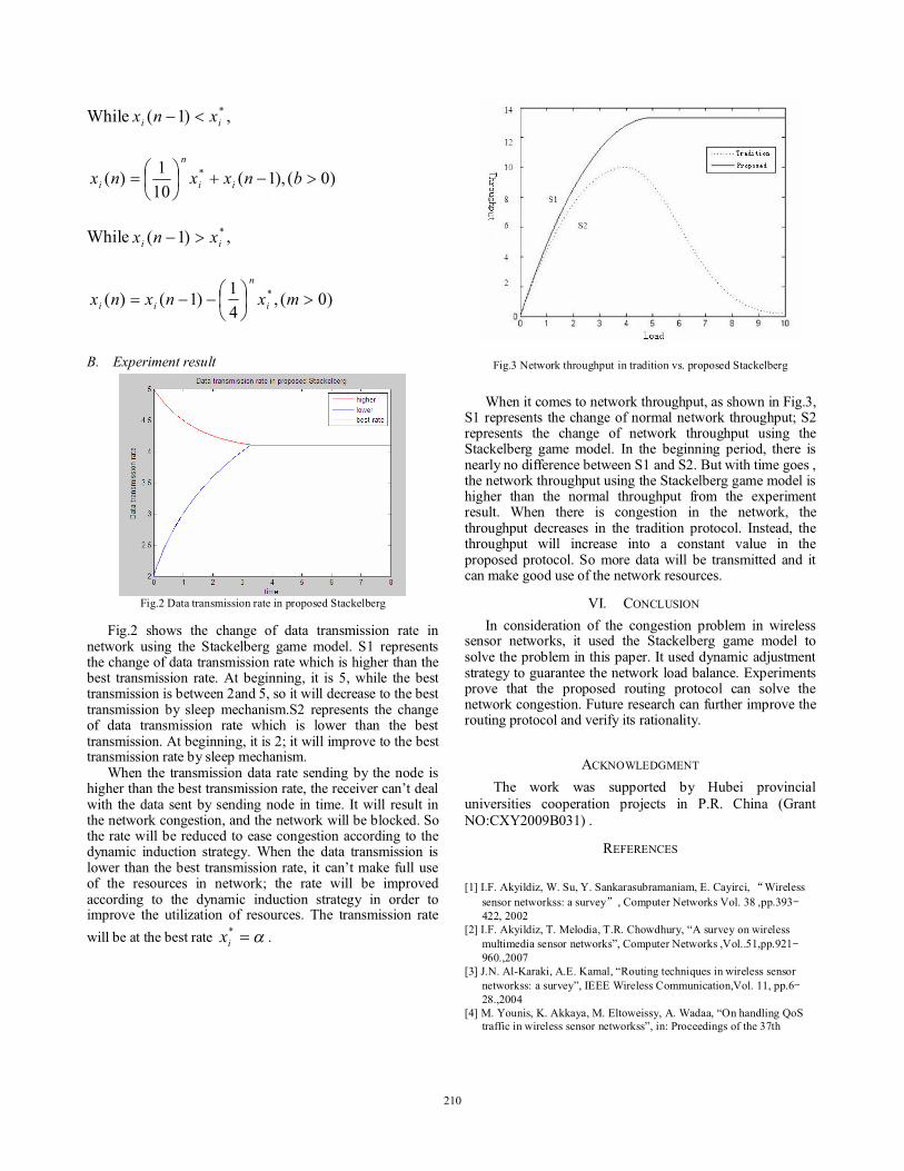
While *)1( ii xnx <" ,

)0(),1(101)( * >"+%&'(

)*= bnxxnx ii

n

i

While *)1( ii xnx >" ,

)0(,41)1()( * >%&'(

)*""= mxnxnx i

n

ii

B. Experiment result

Fig.2 Data transmission rate in proposed Stackelberg

Fig.2 shows the change of data transmission rate in network using the Stackelberg game model. S1 represents the change of data transmission rate which is higher than the best transmission rate. At beginning, it is 5, while the best transmission is between 2and 5, so it will decrease to the best transmission by sleep mechanism.S2 represents the change of data transmission rate which is lower than the best transmission. At beginning, it is 2; it will improve to the best transmission rate by sleep mechanism.

When the transmission data rate sending by the node is higher than the best transmission rate, the receiver can’t deal with the data sent by sending node in time. It will result in the network congestion, and the network will be blocked. So the rate will be reduced to ease congestion according to the dynamic induction strategy. When the data transmission is lower than the best transmission rate, it can’t make full use of the resources in network; the rate will be improved according to the dynamic induction strategy in order to improve the utilization of resources. The transmission rate will be at the best rate "=*

ix .

Fig.3 Network throughput in tradition vs. proposed Stackelberg

When it comes to network throughput, as shown in Fig.3,

S1 represents the change of normal network throughput; S2 represents the change of network throughput using the Stackelberg game model. In the beginning period, there is nearly no difference between S1 and S2. But with time goes , the network throughput using the Stackelberg game model is higher than the normal throughput from the experiment result. When there is congestion in the network, the throughput decreases in the tradition protocol. Instead, the throughput will increase into a constant value in the proposed protocol. So more data will be transmitted and it can make good use of the network resources.

VI. CONCLUSION In consideration of the congestion problem in wireless

sensor networks, it used the Stackelberg game model to solve the problem in this paper. It used dynamic adjustment strategy to guarantee the network load balance. Experiments prove that the proposed routing protocol can solve the network congestion. Future research can further improve the routing protocol and verify its rationality.

ACKNOWLEDGMENT The work was supported by Hubei provincial

universities cooperation projects in P.R. China (Grant NO:CXY2009B031) .

REFERENCES [1] I.F. Akyildiz, W. Su, Y. Sankarasubramaniam, E. Cayirci, Wireless

sensor networkss: a survey , Computer Networks Vol. 38 ,pp.393422, 2002

[2] I.F. Akyildiz, T. Melodia, T.R. Chowdhury, “A survey on wireless multimedia sensor networks”, Computer Networks ,Vol..51,pp.921960.,2007

[3] J.N. Al-Karaki, A.E. Kamal, “Routing techniques in wireless sensor networkss: a survey”, IEEE Wireless Communication,Vol. 11, pp.628.,2004

[4] M. Younis, K. Akkaya, M. Eltoweissy, A. Wadaa, “On handling QoS traffic in wireless sensor networkss”, in: Proceedings of the 37th

210

Annual Hawaii International Conference on System Sciences, 2004 January 5 8, Big Island, USA.

[5.] Kazemeyni, F. Johnsen, E. Owe, O. Balasingham, I, “Group Selection by Nodes in Wireless sensor networkss Using Coalitional Game Theory”. In Proceedings of 2011 16th IEEE International Conference on Engineering of Complex Computer Systems (ICECCS 2011), Las Vegas, NV, USA, 27–29 April 2011

[6] C.-T. Ee, R. Bajcsy, “Congestion control and fairness for many-to one routing in sensor networks”, in: Proceedings of ACM Sensys, November 2004.

[7] A. Mahapatra, K. Anand, D.P. Agrawal, “QoS and energy aware routing for real-time traffic in wireless sensor networkss”, Computer Communications Journal ,Vol.29,pp. 437 445, 2005

[8] H. Peng, Z. Xi, C.X. Ying, G. Chuanshan, “An adaptive real-time routing scheme for wireless sensor networkss”, The 21st International Conference on Advanced Information Networking and Applications Workshop, 2007 May 21 23, Ontario, Canada.

[9] Byun, S.-S.; Balasingham, I. “ Power control for mission critical wireless sensor networkss using repeated coalitional games”. In Proceedings of 2008 IEEE Military Communications Conference, San Diego, CA, USA, 17–19 November 2008.

[10] Haksub, K.; Hyungkeuk, L.; Sanghoon, L. “A cross-layer optimization for energy-efficient MAC protocol with delay and rate constraints”. In Proceedings of 2011 IEEE International Conference on Acoustics, Speech and Signal Processing, Prague, Czech Republic, 22–27 May 2011.

[11]Zhu Jinghua,Li jianzhong,Liu Yong,”Data-Driven Sleeping Scheduling mechanism in Sensor Networks”,Journal of Computer Research and Development,Vol45,pp:172-179,2008.

[12]YANG Jian,LI Jin-Bao,GUO Long-Jiang,ZHANG De-Sheng,”Sleep-Wake Scheduling Mechanism in Dual-RadioWireless sensor networkss”,Journal of Software,Vol 22,pp:62-72,2011.

[13]LIASAR T,OLSDER G J “Dynamic non-cooperative game theory[M] ”.London Academic Press 1982.

[14] TAMER B, SRIKANT R. “Revenue-maximizing pricing and capacity expansion in a many-users regime”. Proceedings of IEEE Information Communications Conference (INFOCOM 2002). New York, USA,2002.294-301.

211

Confidential Communication Techniques for Virtual Private Social Networks

Charles Clarke Faculty of SEC, Kingston University

Kingston upon Thames, UK Charles.Clarke@kingston.ac.uk

Eckhard Pfluegel Faculty of SEC, Kingston University

Kingston upon Thames, UK E.Pfluegel@kingston.ac.uk

Dimitris Tsaptsinos Faculty of SEC, Kingston University

Kingston upon Thames, UK D.Tsaptsinos@kingston.ac.uk

Abstract— In this paper, we are concerned with techniques for establishing confidentiality of user-generated content (UGC), shared in centralised and untrusted online social networks (OSNs). We describe how the concepts of secret sharing and steganography can be combined to result in a technique for sending confidential messages, as part of a proposed architecture for a virtual private social network (VPSN). We consider the types of UGC confidentiality threats that the VPSN can mitigate, based on those of a decentralised online social network (DOSN). We also postulate the concept of a virtual distributed online social network (VDOSN) in which a VPSN is established across multiple centralised OSNs.

Keywords-Virtual Private Social Network; Online Social Network; Decentralised Online Social Network; Data Confidentiality; Secret Sharing; Steganography; Trust;

I. INTRODUCTION By June 2012, [12] estimated that there were 2.4 billion

users online. More individuals are engaged in publishing and sharing data online, than at any other time in history. Much of this data is shared via centralised online social networks (OSNs), in the form of text, image, audio and video content. Examples of high profile OSNs include Facebook, Google+, and LinkedIn. They each host vast quantities of user-generated content (UGC) that is actively shared between peers. This has given rise to an escalation in incidents in which the confidentiality of UGC has been compromised.

A confidentiality breach of UGC can have detrimental consequences for all concerned. Examples include the propagation of insult, conflict, embarrassment, reputation damage, reputation suicide, broken relationships, lost jobs and in some cases, even the tragic loss of life as reported in [29]. The sheer scale of OSN use as indicated in [8] emphasises the potential magnitude of the problem.

In this research, we specifically consider confidentiality threats to shared content, published by members of a secret interest group (SIG). We define a SIG as an OSN group whose members want to exploit the convenience of using an OSN, to network disparate users. SIG members ultimately want to share uncensored, accurate, and often private content, in an innocuous manner that is ideally adverse to confidentiality threats.

Unlike a conventional “friendship” group that may be an organically large hub for linking families and friends, the content shared by SIG members may be perceived as sensitive, provocative, or taboo if exposed to an unintended

recipient. Content published by SIGs may even be subject to adversarial scrutiny. Examples of such groups include oppressed political or social groups operating within a suspicious regime, disparate counselling, and support services for victims of abuse or specialist teams from disparate organisations, collaborating on a classified project.

We further characterise SIGs as having small and restricted membership numbers whose members are likely to suffer a notable consequence in the event of a confidentiality breach of the content they share. To this end, we denote that SIGs prioritise confidentiality over convenience, unlike general friendship groups that conventionally prioritise convenience over confidentiality.

A potential solution for imposing UGC confidentiality in SIGs is to establish a Virtual Private Social Network (VPSN), first conceptualised in [6] and [15]. A VPSN is a framework that can leverage the mechanism of an OSN for providing anonymous, authenticated, and confidential access to data shared within a network of peers. The approach in [6] and [15] focuses on providing anonymity through obscuring the origin of published information. Whilst this provides an essential property of a VPSN, content is still published in an unprotected form leaving it exposed to confidentiality threats.

The main objective of this paper is to focus on the issue of establishing UGC confidentiality, within a VPSN framework. Encrypting UGC would appear to be an obvious answer. However, encrypted content poses several problems in our centralised OSN scenario as obfuscated data raises suspicion and may therefore be sanitised as an unacceptable format within the OSN platform.

In this paper, we present the following novel conceptual contribution: a framework for establishing confidentiality in a VPSN, which does not raise suspicion. Our approach protects information based on the concept of distributing it to several parties. In addition, we make use of a classical cryptographic technique of information hiding. Hence, we achieve confidentiality through invisibility.

This paper is organised as follows: in Section II, we discuss the security goals that are relevant in the context of OSNs and point out the dichotomy between provider and user security interests. Section III introduces our approach to UGC confidentiality in a VPSN. We acknowledge related work in Section IV, followed by a discussion in Section V and our conclusions are presented in Section VI.

2013 12th International Symposium on Distributed Computing and Applications to Business, Engineering & Science

978-0-7695-5060-2/13 $26.00 © 2013 IEEEDOI 10.1109/DCABES.2013.45

212

II. ASPECTS OF OSN SECURITY In this section, we outline security threats to OSN data

and delineate a conflict in security goals between an OSN and its users.

In [17], computer security is characterised as being concerned with implementing the requirements of confidentiality, integrity, and availability of computer-based systems, applications, and networks. Those parts of the system that need protection are referred to as assets (i.e. belonging to categories such as software, hardware, data, or people). We define threats as a scenario that has the potential to compromise data. As such, computer security studies the design, implementation, and deployment of controls to counter threats. In [5] controls are defined as a solution that can mitigate risks that arise from a match between threats and vulnerabilities of a system.

We apply this terminology in order to outline the security goals of OSNs and their users. OSN platforms are complex and as web-based systems are posed with extensive security threats. OSNs may seek to protect their assets through general security practices as well as more specialised web-application security practices. However, the security goals of an OSN and its users may conflict to create a dichotomy of security goals.

A. Security Goals – OSN A core security goal for OSNs is to achieve data

confidentiality of user data assets. Amongst many approaches, this might include steps to mitigate risks of false account registrations, identity masquerading (as expressed in [3]), account compromising (e.g. hacking as outlined in [16]), and threats from malware. Another security concern is the use of their platforms for illegal purposes. OSNs may attempt to counter this by monitoring and responding to suspicious user account activity.

OSNs may also encourage due diligence on the part of users with respect to managing their account. For example, this might include advice on password choices or guidance for applying appropriate privacy settings to protect against data leaks, summarised in [31] as a circumstance in which UGC is accessible beyond an intended group based on the weakest privacy settings of group members.

B. Security Goals – Users Ideally, users want to use trusted OSNs that implement

the security goals of confidentiality, integrity, and availability to UGC. However, some OSN terms of use and security practices actually pose confidentiality threats to UGC, effectively classifying the OSN as untrusted. To this end, we refer to three distinct threats to UGC characterised in [7] that originate from an OSN.

1) UGC Exploitation - An OSN may impose the right to use UGC for commercial or marketing purposes, without the need to consult, or compensate the user (see terms and conditions expressed in [9]). This includes content that a user may have deleted, but still exists as part of another users’ profile, as part of an OSN data backup or is in the possession of an OSN third party developer.

2) UGC Censorship - An OSN may impose the right to modify or remove UGC for reasons of censorship or violation of terms and conditions.

3) UGC Sanitisation - OSNs may sanitise UGC at the point of publication, in order to protect themselves and other users from malware.

III. OUR APPROACH In this section, we present and discuss our technique for

establishing VPSN confidentiality. The scenario we will examine is that of a user of the VPSN wanting to send a confidential message m to another member of the VPSN. In practice, this will mean that m will either appear as an announcement (a post) on the sender’s homepage (e.g. his wall in a Facebook environment) or as a comment on the recipient’s homepage. However, we wish to hide its existence and content from the OSN. Note that due to the nature of OSN functionality, m might contain either textual or binary (image, video) information, and the technique that we will present will work for either format although with different qualities or limitations.

A. Notation and Terminology We shall introduce some additional notation and

terminology: we denote as v the number of users of the VPSN, and let n and k be additional integer parameters satisfying 2 ! k ! n ! v. Here, the parameter n controls the security of our scheme, and the value n-k relates to its robustness. Our approach is based on combining two fundamental cryptographic techniques: secret sharing described in [18] and steganography described in [13].

The idea of secret sharing is to divide given data (the secret s) into n parts (the shares) in such a way that knowing at least k shares allows for reconstructing s. In an ideal secret sharing scheme, knowledge of less than k shares will not reveal any information on s. A secret sharing scheme with parameters k and n satisfying the aforementioned properties is also called a (k, n) threshold scheme.

Steganography achieves security through obscurity. The secret data (payload) is hidden in a carrier-medium by exploiting redundancy inherent to the underlying format or protocol. The resulting stego-medium is sent covertly through a communication channel. Steganalysis as denoted in [13] is the application of methods and techniques for detecting the presence of a stego-medium and recovering a payload.

B. Core Concept The basic architecture of our approach is presented in a

generic manner, without specifying any particular secret sharing or steganography technique. We will extend this architecture in the next section in order to strengthen the security of our scheme.

We first apply a (k, n) secret sharing scheme to the plaintext in order to split it into n shares. We then use steganography to hide the individual shares in a suitably crafted carrier-medium, thus creating a stego-medium. The

213

stego-medium (which to the OSN and non-VPSN members takes the form of generic and ordinary UGC) is shared with n VPSN members. Members access the original message by retrieving a subset of k messages from other members, extracting the shares from the stego-medium, and combining them in order to reconstruct m.

C. Security In order to analyse the security of our scheme, we

highlight the actions an OSN needs to undertake in order to intercept the message m. Let us assume that an OSN could identify VPSN members, steganalysis would be required to detect individual stego-medium. In addition, the correct combination of shares would have to be found using brute-force, searching across different users and different messages per user. Finally, the particular secret sharing scheme would have to be known in order to reconstruct the secret message m from the shares. These tasks seem intractable when considering the potential number of user/message and steganography/secret sharing scheme combinations.

D. The Use of Secret Sharing with a Private Channel The basic scheme that we have presented so far has some

shortcomings. We shall discuss these in the sequel and give solutions by identifying a suitable specialised secret sharing technique, and distributing our architecture across several OSNs.

The issue we address in this section is the need for small share sizes due to the limited capacity of steganographic techniques, especially those based on text. In standard secret sharing (following Shamir’s approach in [19] and Blakely’s approach in [1]), all shares have the same size as the secret. Note the fact that shares normally need to be sent in a manner that provides confidentiality and integrity, otherwise, they can be intercepted by attackers who could hence determine the secret, or modify the shares and consequently corrupt the scheme. A closer look at specific secret sharing schemes reveals that not all the information contained in a share needs to be confidential. For example, when using Shamir’s approach, a share consists of a pair (xi, f(xi)) where the xi 0 are pair-wise distinct integers, and f is a polynomial of degree k-1 satisfying f(0) = s (the secret). Hence, f can be reconstructed from k shares using interpolation. Note that the xi can be published openly, as long as each player can determine his index value i. Provided f(xi) is sent in a confidential and integrity preserving manner, and the value xi cannot be tampered with, the scheme will still work.

Online multi-secret sharing systematically splits the secret into public data P and private data Q for confidential sharing. The main interest is a favourable redistribution of data, mostly aiming at reducing the size of the private data. In the previous example, Shamir’s scheme, we have |P| = |Q| = n·|p| if f is evaluated as an element of Zp[x] where p > s is a prime number. Most online multi-secret sharing schemes however achieve |Q| < |s| and usually |P| |s|. For an overview of methods that have been published in the past, we refer to [4], [24], and [25]. The method in [2] separates the splitting into private/public data before the actual share

creation, and furthermore leads to a particular small share size, which would make it particularly apt for textual UGC.

Our approach can be extended in order to use an online multi-secret sharing scheme as follows: after splitting the message m into public and private values P and Q, we store P on an external server. We assume that this server grants integrity – but we do not have to be concerned about confidentiality. For example, a link to a document on Dropbox or Google Docs could be used for publishing P. The rest of the scheme works as previously, where we use Q rather than m. Compared to the basic scheme of the previous Section, we can identify two advantages: first of all, the share size is smaller as we have |Q| < |s|. This makes it easier to hide the data using steganography. Secondly, the scheme is more secure as the OSN would also have to access external data in order to carry out an attack. Note that we could also iterate the first stage of the splitting into public and private data, by applying this to Q. In this way, public data would grow and private data would be as small as desired. Small and scalable private data is a useful property for use in steganography, particularly when using a carrier-medium with limited capacity (e.g. text).

IV. RELATED WORK Previous research into imposing UGC confidentiality in

OSNs has featured various approaches. Our review focused on VPN inspired techniques that appeared to be most apt for addressing the research problem described in Section I.

As previously noted in Section I, [6] and [15] conceptualise the notion of a VPSN in which the entities of a traditional Virtual Private Network (VPN) are mapped to elements of an OSN. The OSN is deemed analogous to a public infrastructure and the users are analogous to network devices. The objective is to implement a means of communication between users that delivers the security goals of a VPN, hence VPSN. The research in [6] and [15] addresses a central problem of how to make the public facing elements of a Facebook user profile, private to all but intended friendship groups. The solution relies on users creating Facebook accounts, with fake user profile credentials. By default, the publicly accessible profile information will then display the fake credentials. True profile values are revealed to legitimate VPSN members via privately shared XML lookup tables that render dynamically when the user profile is visited. The proposed method is primarily designed to protect identity and not mitigate confidentiality threats to UGC. Therefore, content published via a pseudo-identity still relies on the OSN for confidentiality.

Both [11] and [14] promote the concept of Social VPNs. The term describes the integration of an overlay network (i.e. VPN) with an OSN (i.e. Facebook). This is achieved using a Facebook API. The overlay VPN establishes encrypted network links between social networking users based on their OSN social connections. Whilst aptly protecting UGC content, notable performance degradation is an acknowledged overhead due to the use of “on-the-fly” encryption. Further to this, an OSN may viably consider the

214

use of the proposed API as a threat to its business model, as activity tracking, and data mining might be impaired.

A cryptographic protocol for establishing a SIG and maintaining group membership in a secure manner has been presented in [20]. This approach could be used in conjunction with leveraging the communication platform of an OSN. During execution of the protocol, cryptographic keys are established that allow encrypted messages to be shared within the OSN. If live encryption were a practical option, this solution would meet the criteria of achieving UGC confidentiality.

V. DISCUSSION In this section, we outline the mitigation scope of a

decentralised online social network (DOSN) in the context of UGC and consider the mitigation scope of the proposed VPSN based on those of a DOSN. We also consider the conceptual functionality of a VPSN client application.

A. DOSN and VPSN Mitigation Scope In [7] a DOSN is described as an online social network

distributed over a network of trusted servers or a peer-to-peer infrastructure. DOSNs aim to mitigate numerous privacy and confidentiality problems that are associated with a centralised OSN architecture. In addition to mitigating the UGC confidentiality threats described in Section II, a DOSN has additional UGC security goals. They include: • Mitigating risks of centralised vulnerability to malware,

activity tracking and data mining • Giving users complete confidentiality control over the

content that they publish. • Mitigating risks of a centralised authority making

sudden and unexpected changes to terms and conditions of use that may generate new security risks to UGC.

The VPSN proposed in this research exhibits some of the mitigation scope of a DOSN. For example, the VPSN can effectively mitigate data exploitation, as confidential UGC is not stored on the OSN infrastructure. Data censorship and sanitisation are mitigated through invisibility, as any OSN content published by a user should be innocuous and not raise suspicion. Perhaps the most significant similarity is the facility of providing a user with control over the content that they publish which the VPSN facilitates through the Dropbox infrastructure.

The key differences between the mitigation scope of a VPSN and DOSN are derived from the differences in architectures. A VPSN would still be subject to central malware vulnerabilities. However, it is assumed that it is in the best interest of the OSN to strive to mitigate these problems. As part of a centralised model, VPSN members would also still be subject to activity tracking, data mining, and targeted advertising. However, with “real” content stored outside of the OSN the effectiveness of data mining outcomes may be skewed. Finally, the risks of sudden and unexpected changes to terms and conditions would also remain, although we anticipate that risks to UGC confidentiality would not necessarily be increased.

B. Application Overview VPSN members have to be users of the OSN, and need to

have the necessary access rights to share content. For example, they would be termed "friends" in the Facebook OSN. The application needs to know the OSN identities of the VPSN members and would have to accommodate new members joining the VPSN, removing existing users from the VPSN and recovering a VPSN user whose OSN profile had been deleted.

From a user perspective, an application deployed as a browser plug-in could be a convenient architecture. Secret sharing and methods of steganography can be implemented in JavaScript and access to the VPSN members’ walls is possible using API calls. The plug-in should be able adjust secrecy and robustness thresholds as well as distribute hidden shares by sending them to the different VPSN members. Similarly, it should be able to read from a wall (prompted by user action), retrieve the stego-medium, and extract its content. It should read meta-information from a share and hence find other cover-media located at additional walls, extract shares and reconstruct a secret message.

Whilst the proposed use of Dropbox as a private channel is currently conceptual, the Dropbox APIs described at [23] would appear to offer the technical scope to implement a private channel as part of the VPSN architecture. In addition to standardised routines for syncing shared folders between users, the Dropbox Sync API can write locally, sync globally and could support a private channel that works offline and syncs automatically when back online. According to the Dropbox website, the Core API allows low-level access to the Dropbox building blocks, including authentication routines.

Taking the idea of using an external server further (i.e. Dropbox) we can systematically distribute hidden shares across several OSNs. VPSN members would have to be users of all the OSNs involved, effectively establishing a virtual decentralised online social network (VDOSN).

We acknowledge that collation and analysis of Dropbox performance data would be a fundamental requirement to ratify the VPSN architecture that we propose.

VI. CONCLUSION In this paper, we have described a technique for

communicating a confidential message within a VPSN framework. The proposed technique combines secret sharing and steganography and is optimised to deliver relatively small secret shares in exchange for a secure but larger residual body of data that is stored outside of the OSN.

The framework exploits the infrastructure of a centralised OSN whilst providing some properties and qualities of a DOSN. For example, a core principle of a DOSN is to give individual users exclusive confidentiality controls of all the UGC that they publish. The proposed VPSN architecture achieved this in a manner that is invisible to the OSN and non-VPSN members.

Some OSNs may perceive the concept of such a VPSN as a threat to their business models, as it is plausible that a VPSN could affect the quality of data acquired via user

215

activity tracking, thus having a detrimental impact on advertising revenues. This requires further study. Use of a VPSN for criminal purposes could also prove to be a significant problem. Alternatively, the formal adoption of a VPSN by some OSNs could prove to be a competitive advantage by appealing to users (e.g. SIGs) who are particularly concerned with UGC confidentiality issues.

Further aims of our work include a robust implementation and evaluation of the techniques described in this paper. Additionally, an investigation into extending the architecture of a VPSN to that of a VDOSN will be another future step of our research.

REFERENCES [1] G. Blakley, "Safeguarding cryptographic keys." In

Proceedings of the national computer conference, vol. 48, pp. 313-317. 1979.

[2] E. Pfluegel, E. Panaousis, C. Politis, “A Probabilistic Algorithm for Secret Matrix Share Size Reduction,” in European Wireless Conference 2013, Guildford, UK, 2013.

[3] A. Beach, M. Gartrell, and R. Han, “Solutions to Security and Privacy Issues in Mobile Social Networking,” Computational Science and Engineering, 2009. CSE ’09. International Conference on, vol. 4, pp. 1036–1042, Aug. 2009.

[4] D. Stinson, "An explication of secret sharing schemes." Designs, Codes and Cryptography 2, no. 4 (1992): 357-390.

[5] CERT, “OCTAVE® Information Security Risk Evaluation,” CERT - Software Engineering Institute. 2008.

[6] M. Conti, A. Hasani, and B. Crispo, “Virtual private social networks,” in Proceedings of the first ACM conference on Data and application security and privacy, 2011, pp. 39–50.

[7] A. Datta, S. Buchegger, and L. Vu, “Decentralized online social networks,” Handbook of Social Network Technologies and Applications. Springer US, 2010. 349-378.

[8] E. Eldon, “ComScore 2011 Social Report: Facebook Leading, Microblogging Growing, World Connecting | TechCrunch,” techcrunch.com, 2011. [Online]. Available: http://techcrunch.com/2011/12/21/comscoresocial2011/. [Accessed: 05-Dec-2012].

[9] Facebook.“Facebook. Statement of Rights and Responsibilities”. [Online]. http://www.facebook.com/legal/ terms [Accessed: 14-Nov-2012].

[10] P. Ferguson and G. Huston, “What Is a VPN? - Part I - The Internet Protocol Journal - Volume 1, No. 1 - Cisco Systems,” The Internet Protocol Journal - Cisco, vol. 1, no. 1, Nov. 2012.

[11] R. J. Figueiredo, P. O. Boykin, P. S. Juste, and D. Wolinsky, “Integrating Overlay and Social Networks for Seamless P2P Networking,” Workshop on Enabling Technologies: Infrastructure for Collaborative Enterprises, 2008. WETICE ’08. IEEE 17th, pp. 93–98.

[12] Internet World Stats, “World Internet Users Statistics Usage and World Population Stats,” Internet World Stats - Usage and Population Statistics. Nov-2012.

[13] Jessica Fridrich, Steganography IN DIGITAL MEDIA Principles, Algorithms, and Applications, First. New York, NY, USA: Cambridge University Press, 2010.

[14] P. St. Juste, D. Wolinsky, P. Oscar Boykin, M. J. Covington, and R. J. Figueiredo, “SocialVPN: Enabling wide-area collaboration with integrated social and overlay networks,” P2P Technologies for Emerging Wide-Area Collaborative Services and Applications, vol. 54, no. 12, pp. 1926–1938, Aug. 2010.

[15] M. Conti, A. Hasani, and B. Crispo, “Virtual Private Social Networks and a Facebook Implementation,” math.unipd.it.

[16] D. Mills, “Analysis of a social engineering threat to information security exacerbated by vulnerabilities exposed through the inherent nature of social networking websites,” in 2009 Information Security Curriculum Development Conference, 2009, pp. 139–141.

[17] C. P. Pfleeger and S. L. Pleeger, Security in computing, 4th ed. Prentice Hall of India, 2008.

[18] B. Schneier and W. Diffe, Applied cryptography : protocols, algorithms, and source code in C, 2nd ed. chichester, New York: Wiley, 1996.

[19] A. Shamir, “How to share a secret,” Commun. ACM, vol. 22, no. 11, pp. 612–613, Nov. 1979.

[20] A. Sorniotti and R. Molva, “Secret interest groups (SIGs) in social networks with an implementation on Facebook,” in Proceedings of the 2010 ACM Symposium on Applied Computing - SAC ’10, 2010, p. 621.

[21] N. Wolf(guardian.co.uk), “Amanda Todd’s suicide and social media's sexualisation of youth culture | Naomi Wolf | Comment is free | guardian.co.uk,” The Guardian, 2012. [Online].Available: http://www.guardian.co.uk/commentisfree/2012/oct/26/amanda-todd-suicide-social-media-sexualisation. [Accessed: 08-Mar-2013].

[22] E. Zheleva and L. Getoor, “To join or not to join: the illusion of privacy in social networks with mixed public and private user profiles,” in Proceedings of the 18th international conference on World wide web, 2009, pp. 531–540.

[23] Dropbox, “Developers,” Dropbox, 2012. [Online]. Available: https://www.dropbox.com/developers. [Accessed: 15-May-2013].

[24] A. Beimel, “Secret-Sharing Schemes: A Survey,” in Coding and Cryptology, vol. 6639, Y. Chee, Z. Guo, S. Ling, F. Shao, Y. Tang, H. Wang, and C. Xing, Eds. Springer Berlin Heidelberg, 2011, pp. 11–46.

[25] G. J. Simmons, An introduction to shared secret and/or shared control schemes and their application, in Contemporary Cryptology: The Science of Information Integrity, G. J. Simmons, ed., IEEE Press, 1991, pp. 441-497.

216

Space Angle Based Energy-Aware Routing Algorithm in Three Dimensional

Wireless Sensor Networks

Li Yaman College of Information Science and

Engineering Northeastern University

Shenyang, Liaoning province, China

liyaman@sohu.com

Wang Xingwei College of Information Science and

Engineering Northeastern University

Shenyang, Liaoning province, China

wangxw@mail.neu.edu.cn

Huang Min College of Information Science and

Engineering Northeastern University

Shenyang, Liaoning province, China

mhuang@neu.edu.cn

Abstract—Most of the existing routing algorithms are based on two dimension, and the results can’t be directly applied to the three dimensional wireless sensor networks, the Space Angle Based Energy-Aware Routing algorithm in three dimensional wireless sensor networks is designed in this paper. Firstly, the Iterative Split Clustering Algorithm for dividing the network nodes is proposed. Secondly, we design the Space Angel Energy Routing algorithm to transfer data within the clusters and between the clusters respectively, achieving the goal of less energy consumption and extending the network lifetime. We simulate and implement the algorithm and evaluate the performance based on topologies with different scales, and get a conclusion that by comparing with the typical algorithm, the routing algorithms proposed in this paper are able to reduce the network energy consumption effectively and extend the network lifetime.

Keywords-three dimensional wireless sensor networks; clustering; routing algorithm; energy saving

I. INTRODUCTION Wireless sensor networks (WSNs) are multi-hop self-

organize networks composed of a large number of sensor nodes which are deployed in monitoring area. With the development of the Internet of things, the applications of WSNs become more and more extensive. As the basis of WSNs and the core technology of the network layer, the routing algorithm has become a hot issue for WSNs.

The research of 2D WSNs routing algorithms has been mature, but in the practical 3D network environment such as underwater, underground and space network, 2D routing algorithm is difficult to be used directly. Therefore, the research of 3D WSNs routing algorithm can meet the actual demand.

Considering the limited energy of sensor node, the routing algorithm for 3D WSNs is designed in this paper. Firstly, according to the energy and position coordinates of the node, the Iterative Split Clustering Algorithm (ISCA) based on the theory of the optimal number of cluster head is proposed. Secondly, the Space Angel Energy Routing (SAER) algorithm with the goal of saving energy is proposed. Finally, combining the clustering algorithm with the routing algorithm, we propose the Space Angle Based Energy-Aware Routing (SAEAR).

II. RELATED WORK Many researchers put forward corresponding solutions

for the problems of 3D WSNs routing algorithm. The efficient subminimal Ellipsoid geographical Greedy-Face 3D Routing (EGF3D) based on Greedy Routing and Face Routing in Smart Space improved packet delivery ratio, reduced the end-to-end latency and communication cost. But the assumption of the algorithm was very strict and it didn’t take the node’s mobility into account in 3D space [1].

In order to solve the local minimum in 3D WSNs, Shao Tao, Ananda A.L. and Mun Choon Chan designed the Spherical Coordinate Routing (SCR). It used the BACK mode to deal with the local minimum phenomenon in 3D environment [2]. The Included Angles Iteration Routing (3DIAIR) was put forward to solve the problem of loop in 3D WSNs routing. This algorithm chose the next hop based on the angle and direction vector to avoid planar loop. And it used actual distance to avoid space loop [3]. M. Huang et al. put forward the Energy-Efficient Restricted 3D Greedy Routing (ERGrd). This algorithm made use of Energy Mileage and Restricted Region to avoid loop and save the energy, but it might lead to local minimum [4].

III. PROBLEM STATEMENT Considering the characteristics of 3D WSNs, the routing

algorithm in this paper is based on the following assumptions:

• Each sensor node has a unique ID. • Once the node is deployed, its position remains

unchanged or the moving distance can be neglected compared with sensing radius or communication radius.

• The initial energy of the sensor nodes is limited so most of the nodes cannot communicate with the base station directly (but the nodes near to the base station can communicate with the base station directly).

• The base station has sufficient energy. • In order to simplify the design we assume that the

sensing radius equals to communication radius.

A. Energy Model The energy consumption of 3D WSNs includes the

energy consumed by perception, calculation and

2013 12th International Symposium on Distributed Computing and Applications to Business, Engineering & Science

978-0-7695-5060-2/13 $26.00 © 2013 IEEEDOI 10.1109/DCABES.2013.46

217

communication. The former two are very small compared with the communication energy consumption [5, 6] and they have little to do with the design of routing, so we only take the third one into account. According to the model of wireless communication shown in Fig1 [7], the node’s energy consumption includes the energy cost by data transmission and receiving.

Figure 1. Energy consumption model of wireless communication

The energy consumption of transmission message ETx(k,d) includes the energy consumed by transmitting electronics ETx-elec(k,d) and amplifier ETx-amp(k,d). According to this model ETx(k,d) can be expressed as the following formula.

20

40

( , ) ( , ) ( , )

* * *

* * * ,* * * ,

Tx Tx elec Tx amp

elec mp

elec fs

elec mp

E k d E k d E k d

E k k d

E k k d d dE k k d d d

!!"

""

# #= +

= +

! + <"= # + $"$

(1)

Where k is the size of the message and d is the transmission distance, Eelec is the energy consumed by transmitting electronics, amp" is the energy required by power amplifier. If d is less than the threshold d0, the power amplifier uses free-space model and amp fs" "= , 2! = , otherwise it uses the multi-path fading model while

amp mp" "= , 4! = . The energy consumption of receiving data ERx(k) only

includes the energy consumed by receiving electronic. When receiving a K-bit message ERx(k) can be expressed:

( ) ( ) *Rx Tx elec elecE k E k k E#= = (2)

B. Theory of Optimal Number of Cluster Head Clustering Routing algorithm divides the nodes into

cluster member node and cluster head node. The network is divided into several connected regions called cluster which is composed of cluster head and cluster members.

The theoretical research shows that there is an optimal number of cluster heads K can make the whole network consume the least energy. Suppose that N nodes distribute in the cube whose edge length is M randomly and uniformly, all the sensor nodes are divided into K clusters, the number of nodes in each cluster is about N/K, which contains a cluster head node and N/K-1 cluster member nodes.

IV. NODE CLUSTERING ALGORITHM M.J. Handy, M. Hasse and D. Timmermann designed the

clustering routing algorithm called Low-energy Adaptive Clustering Hierarchy (LEACH) [8]. However, this algorithm and some improved algorithms have many deficiencies. So we should improve the LEACH algorithm or find a more reasonable clustering method.

A. Iteravive Split Clustering Algorithm This paper proposes the Iterative Split Clustering

Algorithm (ISCA) based on the theory of optimal number of cluster heads. The basic idea is: Firstly, all nodes are divided into two clusters according to nodes’ position coordinates and initial energy. Secondly, estimate the quantity of nodes in each cluster and compare it with N/K. If it’s bigger go on clustering; otherwise stop clustering. The rest rounds don’t need re-clustering. The new cluster head is selected according to the node’s position and remaining energy.

The process of clustering is described as follows: 1) The first round of clustering

Step1: Calculate the average energy of all nodes called E. Then compare every node’s energy with E. If it’s bigger than E, the node is added to the temporary cluster head set.

Step2: Choose two nodes which are far away from each other as the temporary cluster heads from the temporary cluster head set. The rest nodes select the nearer one from the two as their cluster head. All of the nodes are divided into two temporary clusters.

Step3: Estimate the quantity of the nodes in the current cluster, if it’s not more than N/K this cluster is optimal and stop clustering. Otherwise, go to Step2.

2) The election of cluster head in the rest round The rest rounds only need to re-elect the cluster head

according to the nodes’ residual energy and position coordinates. Before starting a new round compare the remaining energy of the cluster members with the threshold, if it’s bigger, the node can compete for the cluster head. Then calculate the value of CH for these nodes. The node whose value of CH is the largest becomes the cluster head. The value of CH is calculated as follows:

2 21 2

1,( * ) * 1 1/ ( )

n

cur i BSi i m

CH W E W d d= %

% &= + # + (3)' (

) *+

Where Ecur represents node’s remaining energy, di and dBS are the distance of node m to other nodes and base station respectively, and n is the quantity of cluster members, W1 and W2 are the weight factors and could be adjusted according to the network environment. Their sum is 1.

Based on the analysis above we can choose the node with more residual energy , closer to the cluster center and base station as the new cluster head. If the current cluster head has the maximum value of CH, it remains to be the cluster head of a new round. If several nodes have the same value of CH we can randomly select one as the new cluster head.

218

V. THE DESIGN OF SPACE ANGLE BASED ENERGY-AWARE ROUTING

A. Space Angle Energy Routing Energy saving is the key of 3D WSNs, and this paper

proposes the Space Angel Energy Routing (SAER) based on this goal. The basic idea of this algorithm is: Firstly, select the nodes that meet bandwidth requirements from neighbors within the sensing radius. Then choose the next hop according to the ratio of the distance from current node to neighbors and the energy consumption of sending message to neighbors while taking the space angle composed of the current node, destination node and neighbors into account. SAER mainly includes the following seven parts:

1) Determine the set of candidate node Select the node within current node’s sensing radius or

communication radius that meets user’s requirement as the candidate node of next hop. And all of the candidate nodes compose the set of candidate node.

2) Determine the space angle The current node, neighbor node and destination node

compose the space angle & . Calculate the cosine of & then use the inverse cosine function to compute the value of & .

3) Compute node’s transmission energy consumption Calculate the energy TXE according to the formula 1.

4) Determine the node of next hop The energy consumption of the node includes the energy

consumed by sending and receiving message. And the former accounts for a large proportion. The node of next hop should use the least energy to transmit as far as possible. The next hop should compose the minimum value of space angle & to make the deviation from the destination node as small as possible. Consider the two factors above and set different weight factors W1 and W2 to them. And their sum is 1. The selection of next hop is according to the formula 4.

1 2* / *1/TXNT W d E W &= + (4)

Here d is the distance between current node and destination node. According to the above, choose the node that has the maximum value of NT as next hop.

5) Forming path The node of next hop that has been selected is

sequentially stored in the set of path. We use a set of selected node to prevent loop. Each node can only be selected once when finding a way. In addition, if the current node cannot find the next hop that meets the requirements, it will be removed from the set of path, then reselect the node whose value of NT is the second-largest as the next hop, and mark the current node with the formula state=0 and it will no longer be chosen in the rest rounds.

6) Update the residual energy of the node Use the following formula to calculate and update node’s

residual energy ER. R TX RXE E E E= # # (5)

Here E represents node’s current energy, ETX and ERX are calculated according to the formula 1 and formula 2.

7) Data fusion The data collected in the WSNs may be redundant

therefore the data needs to be fused to save energy. The rate of data fusion is about 70% [9]. The variable D and Dafter are the sizes of the packet before and after data fusion. The calculation formula is as follows:

70%afterD D= ' (6)

B. Space Angle Based Energy-Aware Routing Algorithm Based on the clustering algorithm and routing algorithm

above, the Space Angle Based Energy-Aware Routing (SAEAR) is designed in this paper. The algorithm is composed of three stages: the establishment of cluster, intra-cluster communication and inter-cluster routing. When establishing the cluster ISCA is used. After clustering, different Time Division Multiple Access (TDMA) time slot is assigned for each member. During the intra-cluster communication, every member sends the collected data to the cluster head node within its communication slot, and other time the node keeps dormant to save energy and prevent the conflict. When transferring data, if the transmission distance is less than the communication radius the member can directly send the data, otherwise using SAER to find out the path to the cluster head. When inter-cluster routing the cluster head node fuses the data and uses SAER to find out the path to the base station. The specific steps of SAEAR are described as follows:

Step0: Define variables i and n to represent the number of cluster head nodes and the quantity of nodes to control the routing of intra-cluster and inter-cluster. Define NumofClu and Ci to represent the total number of cluster head nodes and the node in each cluster.

Step1: Input the topology of the network. Step2: Cluster the whole nodes of network according the

first round clustering of ISC. Put the cluster head nodes into the set of cluster head node called head_vec.

Step3: Intra-cluster routing, finding out the path to the cluster head.

Step3.1: If the energy of the cluster member does not equal 0 and meets the conditions: i< NumofClu and n< Ci then go to Step3.2, otherwise go to Step4.

Step3.2: Identify the set of candidate neighbor node for the current node; calculate the space angle and compute the energy consumption of transmission according to formula 1.

Step 3.3: Select the node that has the maximum value of NT as next-hop, and send the data to the cluster head node.

Step3.4: Put the selected node into the set of path named Rout1 and the collection of selected nodes called Selectednodes1.

Step3.5: Calculate and update the residual energy according to formula5.

Step3.6 n=n+1, if n<Ci then go to Step3.1, otherwise go to Step4.

Step4: Fuse the received packets according to formula 6. Setp5: Inter-cluster routing, finding out the way to base

station.

219

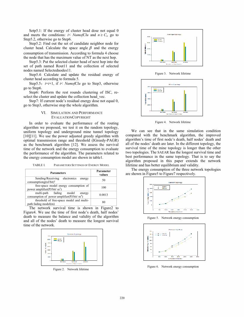
Setp5.1: If the energy of cluster head dose not equal 0 and meets the conditions: i< NumofClu and n $ Ci, go to Step5.2, otherwise go to Step6.

Step5.2: Find out the set of candidate neighbor node for cluster head. Calculate the space angle & and the energy consumption of transmission. According to formula 4 choose the node that has the maximum value of NT as the next hop.

Step5.3: Put the selected cluster head of next hop into the set of path named Rout11 and the collection of selected nodes named Selectednodes11.

Step5.4: Calculate and update the residual energy of cluster head according to formula 5.

Step5.5 i=i+1, if i< NumofClu go to Step3, otherwise go to Step6.

Step6: Perform the rest rounds clustering of ISC, re-select the cluster and update the collection head_vec.

Step7: If current node’s residual energy dose not equal 0, go to Step3, otherwise stop the whole algorithm.

VI. SIMULATION AND PERFORMANCE EVALUATIONCOPYRIGHT

In order to evaluate the performance of the routing algorithm we proposed, we test it on the random topology, uniform topology and underground mine tunnel topology [10][11]. We use the power adjusted greedy algorithm with optimal transmission range and threshold (IGreedy-PAGR) as the benchmark algorithm [12]. We assess the survival time of the network and the energy consumption to evaluate the performance of the algorithm. The parameters related to the energy consumption model are shown in table1.

TABLE I. PARAMETERS SETTINGS OF ENERGY MODEL

Parameters Parameter values

Sending/Receiving electronics energy consumptiong(nJ/bit)a 50

free-space model energy consumption of power amplifier(PJ/bit/ m2) 100

multi-path fading model energy consumption of power amplifier(PJ/bit/ m4) 0.0013

threshold of free-space model and multi-path fading model(m) 80

The network survival time is shown in Figure2 to Figure4. We use the time of first node’s death, half nodes’ death to measure the balance and validity of the algorithm and all of the nodes’ death to measure the longest survival time of the network.

Figure 2. Network lifetime

Figure 3. Network lifetime

Figure 4. Network lifetime

We can see that in the same simulation condition compared with the benchmark algorithm, the improved algorithm’s time of first node’s death, half nodes’ death and all of the nodes’ death are later. In the different topology, the survival time of the mine topology is longer than the other two topologies. The SAEAR has the longest survival time and best performance in the same topology. That is to say the algorithm proposed in this paper extends the network lifetime and has better equilibrium and validity.

The energy consumption of the three network topologies are shown in Figure5 to Figure7 respectively.

Figure 5. Network energy consumption

Figure 6. Network energy consumption

220

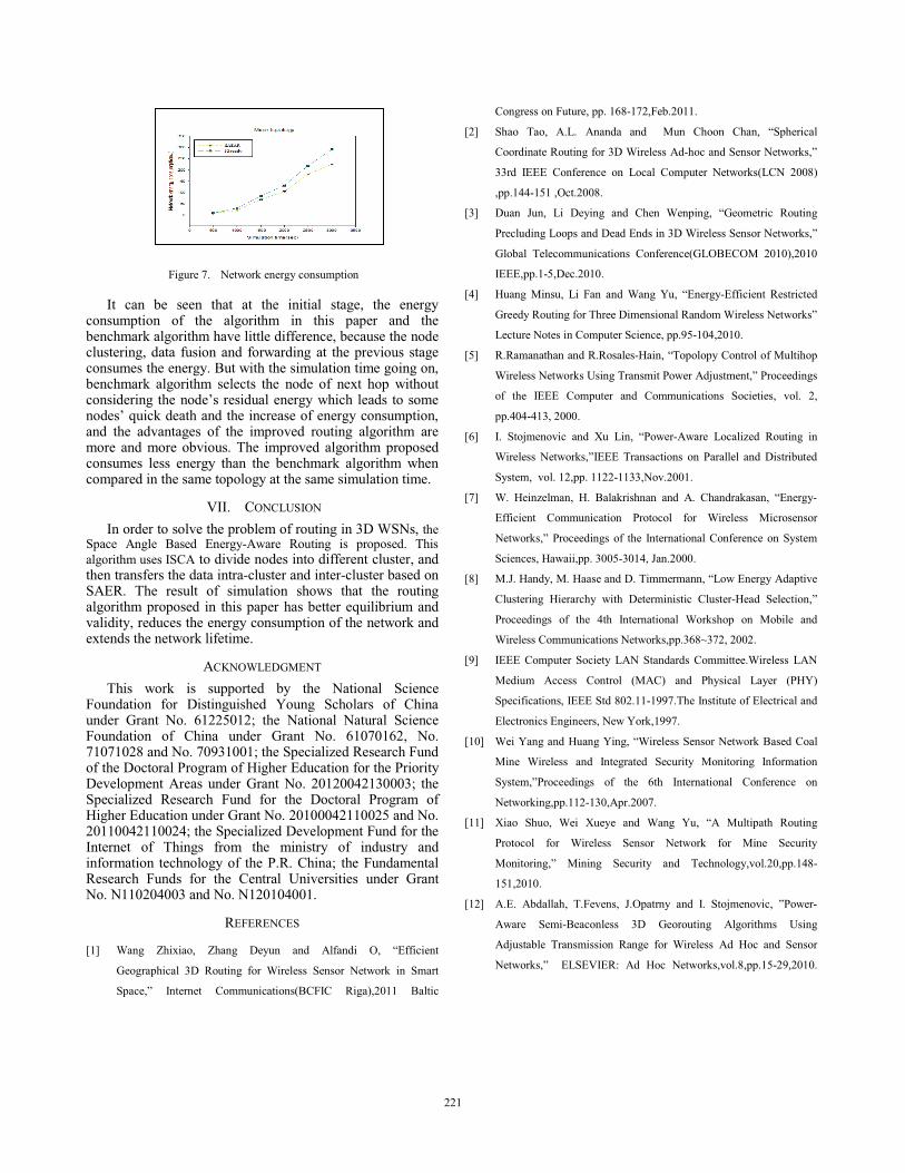
Figure 7. Network energy consumption

It can be seen that at the initial stage, the energy consumption of the algorithm in this paper and the benchmark algorithm have little difference, because the node clustering, data fusion and forwarding at the previous stage consumes the energy. But with the simulation time going on, benchmark algorithm selects the node of next hop without considering the node’s residual energy which leads to some nodes’ quick death and the increase of energy consumption, and the advantages of the improved routing algorithm are more and more obvious. The improved algorithm proposed consumes less energy than the benchmark algorithm when compared in the same topology at the same simulation time.

VII. CONCLUSION In order to solve the problem of routing in 3D WSNs, the

Space Angle Based Energy-Aware Routing is proposed. This algorithm uses ISCA to divide nodes into different cluster, and then transfers the data intra-cluster and inter-cluster based on SAER. The result of simulation shows that the routing algorithm proposed in this paper has better equilibrium and validity, reduces the energy consumption of the network and extends the network lifetime.

ACKNOWLEDGMENT This work is supported by the National Science

Foundation for Distinguished Young Scholars of China under Grant No. 61225012; the National Natural Science Foundation of China under Grant No. 61070162, No. 71071028 and No. 70931001; the Specialized Research Fund of the Doctoral Program of Higher Education for the Priority Development Areas under Grant No. 20120042130003; the Specialized Research Fund for the Doctoral Program of Higher Education under Grant No. 20100042110025 and No. 20110042110024; the Specialized Development Fund for the Internet of Things from the ministry of industry and information technology of the P.R. China; the Fundamental Research Funds for the Central Universities under Grant No. N110204003 and No. N120104001.

REFERENCES

[1] Wang Zhixiao, Zhang Deyun and Alfandi O, “Efficient

Geographical 3D Routing for Wireless Sensor Network in Smart

Space,” Internet Communications(BCFIC Riga),2011 Baltic

Congress on Future, pp. 168-172,Feb.2011.

[2] Shao Tao, A.L. Ananda and Mun Choon Chan, “Spherical

Coordinate Routing for 3D Wireless Ad-hoc and Sensor Networks,”

33rd IEEE Conference on Local Computer Networks(LCN 2008)

,pp.144-151 ,Oct.2008.

[3] Duan Jun, Li Deying and Chen Wenping, “Geometric Routing

Precluding Loops and Dead Ends in 3D Wireless Sensor Networks,”

Global Telecommunications Conference(GLOBECOM 2010),2010

IEEE,pp.1-5,Dec.2010.

[4] Huang Minsu, Li Fan and Wang Yu, “Energy-Efficient Restricted

Greedy Routing for Three Dimensional Random Wireless Networks”

Lecture Notes in Computer Science, pp.95-104,2010.

[5] R.Ramanathan and R.Rosales-Hain, “Topolopy Control of Multihop

Wireless Networks Using Transmit Power Adjustment,” Proceedings

of the IEEE Computer and Communications Societies, vol. 2,

pp.404-413, 2000.

[6] I. Stojmenovic and Xu Lin, “Power-Aware Localized Routing in

Wireless Networks,”IEEE Transactions on Parallel and Distributed

System, vol. 12,pp. 1122-1133,Nov.2001.

[7] W. Heinzelman, H. Balakrishnan and A. Chandrakasan, “Energy-

Efficient Communication Protocol for Wireless Microsensor

Networks,” Proceedings of the International Conference on System

Sciences, Hawaii,pp. 3005-3014, Jan.2000.

[8] M.J. Handy, M. Haase and D. Timmermann, “Low Energy Adaptive

Clustering Hierarchy with Deterministic Cluster-Head Selection,”

Proceedings of the 4th International Workshop on Mobile and

Wireless Communications Networks,pp.368~372, 2002.

[9] IEEE Computer Society LAN Standards Committee.Wireless LAN

Medium Access Control (MAC) and Physical Layer (PHY)

Specifications, IEEE Std 802.11-1997.The Institute of Electrical and

Electronics Engineers, New York,1997.

[10] Wei Yang and Huang Ying, “Wireless Sensor Network Based Coal

Mine Wireless and Integrated Security Monitoring Information

System,”Proceedings of the 6th International Conference on

Networking,pp.112-130,Apr.2007.

[11] Xiao Shuo, Wei Xueye and Wang Yu, “A Multipath Routing

Protocol for Wireless Sensor Network for Mine Security

Monitoring,” Mining Security and Technology,vol.20,pp.148-

151,2010.

[12] A.E. Abdallah, T.Fevens, J.Opatrny and I. Stojmenovic, ”Power-

Aware Semi-Beaconless 3D Georouting Algorithms Using

Adjustable Transmission Range for Wireless Ad Hoc and Sensor

Networks,” ELSEVIER: Ad Hoc Networks,vol.8,pp.15-29,2010.

221

Coarse and Fine-grained Crossover Free Search based Handover Decision Scheme with ABC Supported

WANG Tong College of Information Science and

Engineering Northeastern University

WANG Xing-wei College of Information Science and

Engineering Northeastern University

HUANG Min College of Information Science and

Engineering Northeastern University

Shenyang, Liaoning Province, China

wangtongneu@sohu.com

Shenyang, Liaoning Province, China

wangxw@mail.neu.edu.cn

Shenyang, Liaoning Province, China

mhuang@neu.edu.cn

Abstract—To find an optimal handover solution of terminal users under heterogeneous wireless networks, Pareto optimum under Nash equilibrium of users’ utility and network provider utility is achieved or approached for the found solution. QoS (quality of service) requirements, user preferences to access network coding schemes, user preferences to access network providers, user handoff history record, costs user willing to pay and the profit of suppliers are considered comprehensively in this paper. With introducing the knowledge of fuzzy mathematics and microeconomics, access networks and terminals are described. With the help of gaming analysis, an intelligent handover decision scheme with ABC (always best connected) supported is proposed by using coarse-grained and fine-grained crossover free search based intelligent optimization algorithm. After carrying out simulation and performance evaluation, the results show that the mechanism proposed in this paper is feasible and effective.

Keywords-NGI (next generation Internet); QoS (quality of service); ABC (always best connected); handover decision; intelligent optimization algorithm; search based on coarse-grained and fine-grained crossover

I. INTRODUCTION The next generation Internet NGI (next generation

Internet) is a kind of multi-level heterogeneous networks and wireless access is its main access way. With different types of access network existing, we need to support users for NGI with ABC (always best connected) [1] and guarantee for mobile terminal users with stable and high quality service.

According to the different access ways of users, ABC scheme guarantee the user’s handover done among networks under the heterogeneous network environment of NGI. Handover includes horizontal and vertical handover [2]. When triggering handover process, necessary information from each access network is collected, then the best access network for users is selected. Finally, handover is implemented and terminal completes handover process from current access network to the best access network.

The significance of ABC is the allowed connection between user terminal and NGI always through the best access network. In users’ view, QoS [3] requirements, user preferences to access network coding schemes, user preferences to access network providers, user handover history record, costs user willing to pay and access network

status are considered. From the perspective of network, the profit of suppliers [4] and other factors are considered to maximize the use of existing network resource and ensure the handover couldn’t happen frequently to avoid the “Ping-Pong Effect” [5]. Literature [6] presented a method based on RSS (received signal strength) vertical handover decision scheme. With bandwidth introduced, the average value of RSS was used in the algorithm. In [7], a vertical handover decision method based on fuzzy parameters was presented and the method effectively reduced the "Pingf-Pong Effect” in the handover process. In [8], it presented a handover decision method based on QoS requirements and considered the minimum bit rate, delay, delay jitter, error rate, user preferences and other factors. In [9], it presented a users’ network association scheme based on group game theory to problems of load balanced for heterogeneous wireless networks. In [10], it presented an intelligent handover algorithm to determine the vertical handover time effectively.

An optimal handover solution of terminal users is found by using free search intelligent algorithm based on coarse-grained and fine-grained crossover [11].

II. MODEL DESIGN Based on literature [12], the following handover models

are designed.

A. Application type and QoS parameter weight Suppose that there are I types of NGI based on

differentiated services [13] model, },...,,{ 21 IATATATATS = . Different application types have different QoS parameters on demand. To the application type iAT ( Ii !!1 ), consider four QoS parameters, bandwidth, delay, delay jitter and error rate. Then weight becomes T

EJDBW ],,,[ """"= .

B. Access network model Assume that the number of access network is M . To

access network j ( Mj !!1 ), the parameters are: The provider identifier of access network j is

PISPI j # . Type identifier of access network j is TISTI j # . The set of coding schemes supported by access

2013 12th International Symposium on Distributed Computing and Applications to Business, Engineering & Science

978-0-7695-5060-2/13 $26.00 © 2013 IEEEDOI 10.1109/DCABES.2013.47

222

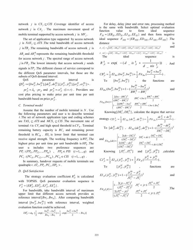
network j is CISCS j $ .Coverage identifier of access network j is jCA . The maximum movement speed of mobile terminal supported by access network j is jMV .

The set of application type supported by access network j is ATSNAS j $ .The total bandwidth of access network j is jTB .The remaining bandwidth of access network j is

jAB and thjAB represents the remaining bandwidth threshold

for access network j . The spectral range of access network j is jFR .The lowest intensity that access network j sends

signals is jTP .The different classes of service correspond to the different QoS parameter intervals, but those are the subsets of QoS demand interval.

QoS parameter interval is>=< ],[],,[],,[],,[ kh

jiklji

khji

klji

khji

klji

khji

klji

kji ererjtjtdedebwbwQS .

jikkji prpr %= & and )1(0 rctpr k

jiji +%= . Providers use cost plus pricing to make price per unit time per unit bandwidth based on price 0

jipr .

C. Terminal model Assume that the number of mobile terminal is N . Use

the following parameters and user u to describe terminal t .The set of network application type and coding schemes are ATSTASt $ and CISMCSt $ .The movement rate of terminal t is tCV and high speed threshold is hCV . Terminal remaining battery capacity is tRC and remaining power threshold is thRC . tRS is lower limit that terminal can receive signal strength. The working frequency is tWF .The highest price per unit time per unit bandwidth is tiHP .The user u includes two preference sequences are

),...,,(: 21 tqttt PPPPPPPP , ),...,1( qiPISPPti =# and ),...,,(: 21 tqttt PCPCPCPC , ),...,1( qiCISPCti =# .

In summary, handover requests of mobile terminals use quadruple >< titti HPPCPPAT ,,, .

D. QoS Satisfaction

The strategy evaluation coefficient kjiR is calculated

with TOPSIS. QoS parameter evaluation sequence is},,,{ k

jikji

kji

kji

kji EEEJEDEBF = .

For bandwidth, take bandwidth interval of maximum upper limit that different access network provides as reference interval ],[ hl BwBw . After comparing bandwidth interval ],[ kh

jiklji bwbw with reference interval, weighted

evaluation function could be achieved.

)]2

exp(21)exp(

21[ h

khji

klji

lh

klji

khji

Bkji Bw

bwbwBwBwbwbw

EB '+

%+''

'%%= "

For delay, delay jitter and error rate, processing method is the same with bandwidth. Select optimal evaluation function value to form ideal sequence

},,,{ ISISISISIS EEEJEDEBF = and then form negative ideal sequence },,,{ NISNISNISNISNIS EEEJEDEBF = .The distance is

2222 )()()()(_ ISkjiIS

kjiIS

kjiIS

kji

kji EEEEEJEJEDEDEBEBisd '+'+'+'= and

2222 )()()()(_ NISkjiNIS

kjiNIS

kjiNIS

kji

kji EEEEEJEJEDEDEBEBnisd '+'+'+'= .

The ideal sequence is

))_

1_(exp( kji

kji

kji nisd

isdR +'= . And

)2

(21),(

21 kh

jiklji

Bwkhji

kljiBw

kji

bwbwFitbwbwEICB

++= .

To ],[ khji

klji bwbw , the functions are

2)(1),( li

hi

klji

khjikh

jikljiBw BWBW

bwbwbwbwEI

'

''= and

!!"

!!#

$

!<+'

''

+!<'

'

=hi

li

hi

li

hi

hi

li

hil

ili

hi

li

Bw

BwbwBWBWBWBW

bwBW

BWBWbwBWBWBWBWbw

bwFit

2)()(21

2)()(2

)(

2

2

2

2

.

Knowing ],[ hi

li DEDE , calculate the degree that service

strategy. )2

(21),(

21 kh

jiklji

Dekhji

kljiDe

kji

dedeFitdedeEICD

++= .

To ],[ khji

klji dede , 2)(1),( l

ihi

klji

khjikh

jikljiDe DEDE

dedededeEI

'

''=

and

!!"

!!#

$

!<+'

'

+!<'''

=hi

li

hi

li

hi

hi

li

hil

ili

hi

li

De

DEdeDEDEDEDE

deDE

DEDEdeDEDEDEDEde

deFit

2)()(2

2)()(21

)(

2

2

2

2

.

Knowing ],[ hi

li JTJT and ],[ kh

jiklji jtjt ,calculate

)2

(21),(

21 kh

jiklji

Jtkhji

kljiJt

kji

jtjtFitjtjtEICJ

++= .

To ],[ khji

klji jtjt , functions are

2)(1),( li

hi

klji

khjikh

jikljiJt JTJT

jtjtjijiEI

'

''= and

!!"

!!#

$

!<+'

'

+!<'''

=h

i

li

hi

li

hi

hi

li

hil

ili

hi

li

JtJTjtJTJT

JTJTjtJT

JTJTjtJTJTJTJTjt

jtFit

2)()(2

2)()(21

)(

2

2

2

2

.The

223

same with above 2)(1),( li

hi

klji

khjikh

jikljiEr ERER

ererererEI

'

''=

and

!!"

!!#

$

!<+'

'

+!<'''

=hi

li

hi

li

hi

hi

li

hil

ili

hi

li

ErERerERER

ERERerER

ERERerERERERERer

erFit

2)()(2

2)()(21

)(

2

2

2

2

.

The total QoS fitness is:

kjiE

kjiJ

kjiD

kjiB

kji CECJCDCBCQ %+%+%+%= """"

. Then calculate total QoS fitness and its definition is

shown as kji

kji

kji CQRSQ %= .

E. Other satisfactions The price satisfaction of user to access network is

!"

!#

$

!<('

>=

tikji

ti

kji

tikji

tj HPprHPpr

HPprSP

0211

0 .The access network

provider preference satisfaction degree is

!"

!#

$%%&

'(()

* '+=

others0

sequence preferencein provider 1R

2

qxq

S tj.

The satisfaction of user preferences to access network

coding schemes is!"

!#

$%%&

'(()

* '+=

othersq

xqSCtj

0

sequence preferencein 12

.

Movement speed fitness is

!!"

!!#

$

<

!!'+<<

=

tj

jth

jtht

tj

CVMV

MVCVCVq

xqMVCVCVCV

SV

0

)1(

&1.

Battery fitness is !"

!#$ !'+

=others

RCRCq

xqSY tht

tj1

)1( .

The load evaluation function is

!"

!#$ <<>''=

othersABABABSL

thjjjji

tj 1,)2/)(exp( min

02

0 ))*)) .

F. Gaming analysis and Utility Calculations The two sides are mobile terminal and access network.

++,

-

.

./

0

'%''

=0)(0

kjiti

kjiti

prHPvprHP

TG and

++,

-

.

./

0 '%''=00

)( kji

kji

kji

kji ctprvctprNG .If ),( ** ji ba

satisfies!"

!#$

++

jiji

ijjiNGNG

TGTG***

***, it will achieve Nash equilibrium

of parties income.

The user utility is

ti

kjiti

tjSLtjSYtjSV

tjSPtjSCtjSRkjiSQjt

HPprHP

SLwSYwSVw

SPwSCwSRwSQwuui

'%%+%+%+

%+%+%+%%,%-=

]

[ .Netwo

rk utility kji

kji

kji

tjSLtjSYtjSV

tjSPtjSCtjSRkjiSQjt

prctpr

SLwSYwSVw

SPwSCwSRwSQwnui

'%%+%+%+

%+%+%+%%,%-=

]

[ .

G. Mathematical model

The objective are maximizing jt juu , jti

nu , 1=

n

tjti

uu1

,

1=

n

tjti

nu1

and 11= =

+N

t

M

jjtjt ii

nuuu1 1

.

III. ALGORITHM DESIGN Free search algorithm based on coarse-grained and fine-

grained crossover improves standard free search optimization algorithm.

A. Feasible solution and fitness function )(

qtANt NASTAS $ . )( ,/0 iAN MCSCSqt

.

)( tAN CVMVqt

+ . )(qtANt FRWF $ . )( tAN RSTP

qt+ .

)( tik

iAN HPprqt

! . )( minqtqtqt AN

khiANAN ABbwAB +' .The

fitness function is

!!"

!!#

$

1'

+= 1=

solution feasiblet isn',

solution feasible is,)11(

1

)(1

q

qN

t ANtANt

x

x

nuuuxfMaximize

qtiqti

.

B. Algorithm description Step 1: The },...,,{ 0

20

100

SxxxX = is generated randomly.qtAN and qtsl is assigned as integer selected from ]1,0[ 'M

and ]1||,0[ 'SL arbitrarily. 10 =qP and 1maxmin == qq PP .Set the population size S , upper limit of searching iterations K , searching steps SV = , crossover probability cp , individual neighborhood radius qR .

Step 2 : Complete initialization of population. Step 3: Select multiple individuals randomly in

population kX according to crossover probability cp . Individuals perform coarse-grained crossover in the group.

Step 4: Calculate fitness function value. Step 5: 1+= tt . If Nt < , turn to step 4. Otherwise, qx

is a feasible solution. Step 6: Reset remaining bandwidth of each access

network to judge the feasibility of offspring individuals. Step 7: The game factor - is updated. Step 8: Calculate fitness function value. Replace parent

individuals accordingly.

224

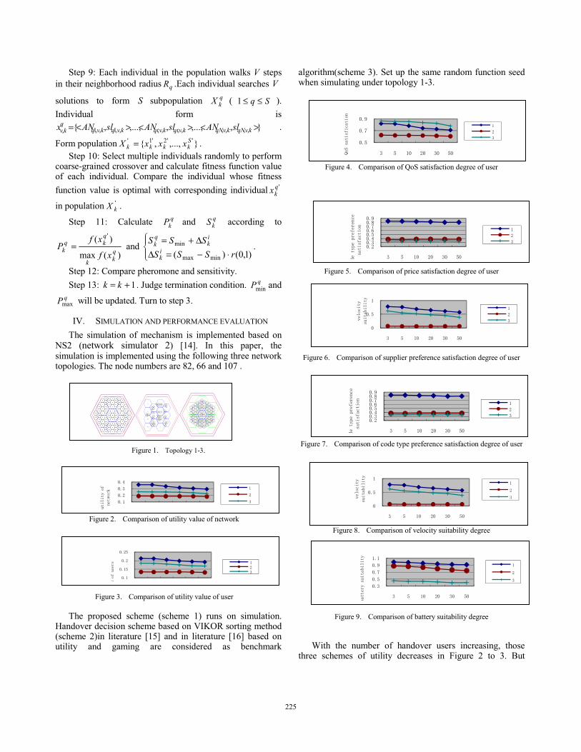
Step 9: Each individual in the population walks V steps in their neighborhood radius qR .Each individual searches V

solutions to form S subpopulation qkX ( Sq !!1 ).

Individual form is },,...,,,...,,{ ,,,,,,,,,,1,,1, ><><><= kvqNkvqNkvqtkvqtkvqkvq

qkv slANslANslANx .

Form population },...,,{ ''2'1' Skkkk xxxX = .

Step 10: Select multiple individuals randomly to perform coarse-grained crossover and calculate fitness function value of each individual. Compare the individual whose fitness function value is optimal with corresponding individual 'q

kx in population '

kX . Step 11: Calculate q

kP and qkS according to

)(max)( '

qkk

qkq

k xfxf

P = and !"

!#$

%'=22+=

)1,0()( minmax

min

rSSSSSS

ik

ik

qk .

Step 12: Compare pheromone and sensitivity. Step 13: 1+= kk . Judge termination condition. qPmin and

qPmax will be updated. Turn to step 3.

IV. SIMULATION AND PERFORMANCE EVALUATION The simulation of mechanism is implemented based on

NS2 (network simulator 2) [14]. In this paper, the simulation is implemented using the following three network topologies. The node numbers are 82, 66 and 107 .

Figure 1. Topology 1-3.

Figure 2. Comparison of utility value of network

Figure 3. Comparison of utility value of user

The proposed scheme (scheme 1) runs on simulation. Handover decision scheme based on VIKOR sorting method (scheme 2)in literature [15] and in literature [16] based on utility and gaming are considered as benchmark

algorithm(scheme 3). Set up the same random function seed when simulating under topology 1-3.

Figure 4. Comparison of QoS satisfaction degree of user

Figure 5. Comparison of price satisfaction degree of user

Figure 6. Comparison of supplier preference satisfaction degree of user

Figure 7. Comparison of code type preference satisfaction degree of user

Figure 8. Comparison of velocity suitability degree

Figure 9. Comparison of battery suitability degree

With the number of handover users increasing, those

three schemes of utility decreases in Figure 2 to 3. But

225

scheme 1 is higher than scheme 2 and 3 in utility of user and network. But both scheme 2 and 3 lack of users’ preferences consideration. From Figure 4 to 10, scheme 1 is better than scheme 2 and 3 in addition to QoS satisfaction degree and price satisfaction degree. Scheme 1 considers effect of utility for user and network when gaming between user and network provider Nash equilibrium can be reached in the course of finding the optimal solution. Scheme 1 is slightly lower than scheme 3 but far higher than scheme 2 in QoS satisfaction degree. Scheme 1 considers comprehensively various factors rather than only considering QoS. Scheme 3 pursuits QoS utility maximization and scheme 2 does not consider QoS.

Figure 10. Comparison of system running time

Scheme 1 is slightly lower than scheme 2 but far higher than scheme 3 in QoS price satisfaction degree. The selections of scheme 3 are mostly service strategies that provide high QoS and price. Scheme 2 selects the lowest level of the cheapest service strategy. Scheme 1 considers comprehensively various factors.

V. CONCLUSION This paper designs intelligent handover decision scheme

with ABC supported. Simulation and performance evaluation based on NS2 are carried and results show that: It has good performance

ACKNOWLEDGMENT This work is supported by the National Science

Foundation for Distinguished Young Scholars of China under Grant No. 61225012; the National Natural Science Foundation of China under Grant No. 61070162, No. 71071028 and No. 70931001; the Specialized Research Fund of the Doctoral Program of Higher Education for the Priority Development Areas under Grant No. 20120042130003; the Specialized Research Fund for the Doctoral Program of Higher Education under Grant No. 20100042110025 and No. 20110042110024; the Specialized Development Fund for the Internet of Things from the ministry of industry and information technology of the P.R. China; the Fundamental Research Funds for the Central Universities under Grant No. N110204003.

REFERENCES [1] Gábor Fodor, Anders Eriksson, and Aimo Tuoriniemi.,“Providing

quality of service in always best connected networks,” IEEE

Communications Magazine,vol.41.pp.154-163,Jul 2003,doi:10.1109/MCOM.2003.1215652

[2] Nidal Nasser, Ahmed Hasswa, and Hossam Hassanein, “Handoffs in fourth generation heterogeneous networks,” IEEE Communications Magazine, vol. 44, pp. 96–103, Oct 2006,doi: 10.1109/MCOM.2006.1710420.

[3] Liu Ji-ren, Wang Xing-wei, and Zhang Ying-hui, “Discussions on communication platforms and some related techniques in distributed multimedia systems,” Acta Electronica Sinica, vol. 25.pp.54-59,Nov 1997.

[4] Jun-seok Hwang, Jürn Altmann, Huw Olive, and Alfonso Suarez ,“Enabling dynamic market-managed QoS interconnection in the next generation internet by a modified BGP mechanism,” IEEE International Conference on Communications, vol.4.pp.2667-2671,Apr 2002,doi: 10.1109/ICC.2002.997325 .

[5] Shupeng Li, FangChen Cheng, Yifei Yuan, and Teck Hu, “Adaptive Frame Switching for UMTS UL-EDCH-Ping-Pong Avoidance ,” IEEE Vehicular Technology 63rd Conference, vol.5.pp.2469-2473, 2006,doi: 10.1109/VETECS.2006.1683301 .

[6] Sanjay Dhar Roy, Anup Sadhukhan, “Received Signal Strength Based Vertical Handoff Algorithm in 3G Cellular Network,” International Conference on Signal Processing, Communication and Computing, vol. 2, pp. 326–330, August 2012,doi: 10.1109/ICSPCC.2012.6335659

[7] Anita Singhrova, Nupiur Prakas, “Vertical handoff decision algorithm for improved quality of service in heterogeneous wireless networks,” IET Communications, vol.6,pp.211-223, Feb 2012,doi: 10.1049/iet-com.2010.0820

[8] Carlos Ramirez-Perez, Victor M. Ramos R, “A QoS hierarchical decision scheme for vertical handoff,” International Caribbean Conference on Devices, Circuits and Systems, pp.1-4, 2012,doi: 10.1109/ICCDCS.2012.6188942

[9] Jiang Yong, Hu Bo, and Chen Shan-zhi, “User-Network Association Optization in Hetergeneous Wireless Networks: A Population Game-Based Approach,” Chinese Journal of Computers, vol.35, pp.1249-1261, 2012

[10] Safdar Rizvi, Asif Aziz, and N.M. Saad, “An Overview of Vertical Handoff Decision Policies for Next Generation Wireless Networks,” Asia Pacific Conference on Circuits and Systems, pp.88-91, 2010,doi: 10.1109/APCCAS.2010.5775065

[11] Zhou Hui, Li Dan-mei, Xu Chen, Shao Shi-huang, and Yuan Cong-ming, "Free search algorithm based on coarse-grained and fine-grained crossover," Control and Decision, vol.23, pp.1068-1072, Sep 2008

[12] Wang Xing-wei, Guo Lei, Qin Pei-yu, and Huang Min, "Access Network selection Scheme with ABC Supported," http://www.paper.edu.cn/paper.p hp? serial_number=200909-109, Sep 2009

[13] Blake S, “ An architecture for differentiated services,” IETF2475, Dec, 1998

[14] Fang Lu-ping, “NS-2 Network simulation and Application,” Beijing, May 2008, National Defence Industry Press

[15] Gallardo-Medina J R, Pineda-Rico U, and Stevens-Navarro E, VIKOR Method for Vertical Handoff Decision in Beyond 3G

Wireless Networks, International Conference on Electrical Engineering, Computing Science and Automatic Control(CCE), 2009, pp.1-5,doi: 10.1109/ICEEE.2009.5393320 .

[16] Chung-Ju J. Chang, Tsung-Li Tsai, and Yung-Han H. Chen, “Utility and Game-Theory Based Network Selection Scheme in Heterogeneous Wireless Networks,” IEEE Wireless Communications and Networking Conference(WCNC 2009), 2009, pp.1-5,doi: 10.1109/WCNC.2009.4918016.

226

Image Processing

DCABES 2013

Generalized Newton Method for Minimization of A Region-based Active Contour Model

Haiping Xu, Meiqing Wang College of Mathematics and Computer Science

Fuzhou University Fuzhou, Fujian, China

e-mail: haipingcassie@gmail.com, mqwang@fzu.edu.cn

Choi-Hong Lai School of Computing and Mathematical Sciences

University of Greenwich London, UK

e-mail: c.h.lai@gre.ac.uk

Abstract—PED-based image segmentation based on the active contour model attracts many researchers due to the high precision of edge detection and the continuity of boundaries. Its basic idea is to define an energy functional on a dynamic curve which achieves its minimum when the curve conforms to the boundary of the objects. The most widely used optimization method is the gradient-descent method. However, the convergence of the gradient-descent method is very poor. In this paper, the effectiveness of the generalized Newton method is investigated by using it to minimize the energy functional of the RSF&CV model, which is a simple combination of the CV model and the RSF model. The experimental results show the accuracy and efficiency with robustness in noise.

Keywords-generalized newton; region-based active contour; image segmentation

I. INTRODUCTION PED-based image segmentation is one of the state-of-the-

art methods due to the high precision of edge detection and the continuity of boundaries. One of which is the active contour model, known as “Snake”, first introduced in 1988 by Kass et al.[1]. There are two classes of active contour models: edge-based models [1][2][3] and region-based models [4][5][6][7]. Generally speaking, the region-based models are more robust than edge-based models. Region-based models use the image statistical information to construct constraints, and have better performance for the images with weak boundaries. Moreover, they are less sensitive to the initial curves.

The Chan-Vese (CV) [4] model is one of the most popular region-based models, which uses global information of images to segment homogeneous images. Li et al. proposed the region-scalable fitting (RSF) model [7] to overcome the difficulty caused by intensity inhomogeneity, which relies on the local intensity information. The RSF model has been successfully applied in medical images. Due to these advantages, many researchers followed the original CV model and the RSF model, and put forward further improvements, such as the LBF&CV_B model [8] and the LGIF model [9].

The basic idea of segmentation methods based on the active contour model is to define an energy functional on a

dynamic curve which achieves its minimum when the curve conforms to the boundary of the objects. Thus, the image segmentation problem is transformed to minimize the energy functional. In general, the gradient-descent method is used to minimize an energy functional. The descent direction is calculated by the negative gradient of the functional in which the gradient is depended on the L2 inner product.

Recently, many researchers introduced generalized gradient-descent approaches in image processing via the definition of different inner product [10][11]. They revealed that the choice of the inner product could be seen as a priori information. Inspired by the above-mentioned generalized gradient-descent methods, Leah and Guillermo [12] extended the Newton methods with more general inner product, proposed the generalized Newton method and demonstrated that the “optimal” inner product for an energy functional can ease the sensitivity of noise and obtain a smooth curve.

In this paper, we adapt and extend the wok of Leah and Guillermo to a region-based active contour model to validate the accuracy and efficiency of the generalized Newton method. The region-based model is called RSF&CV model, which is a simple combination of the CV model and RSF model. Due to the Newton quadratic convergence, the re-initialization can be omitted. The experimental results show the accuracy and efficiency with robustness in noise.

The rest of this paper is organized as follows. In section 2, the CV model, the RSF model and generalized newton are briefly introduced. Application of generalized newton method to a region-based model is described in detail in section 3. The experimental results of proposed models are given in section 4. Section 5 concludes this paper.

II. BACKGROUND

A. CV Model The CV model [4] proposed by Chan and Vese is a

simplification of the Mumford-Shah model [5]. Let 2! " # be the image domain, and ( ) :I x ! $ # be a given gray level image. The CV model implements segmentation by minimizing the following energy functional:

2013 12th International Symposium on Distributed Computing and Applications to Business, Engineering & Science

978-0-7695-5060-2/13 $26.00 © 2013 IEEEDOI 10.1109/DCABES.2013.48

229

21 2 1 1( )

22 2( )

( , , )

( )

CVinside C

outside C

F C c c I c dx

I c dx

Length C

%

%

µ

= &

+ &

+ '

!! . (1)

where ( )inside C and ( )outside C represent the regions inside and outside the curve C , respectively. 1 2, ,µ % % are positive constants. 1c and 2c are two constants that approximate the image intensities in ( )inside C and ( )outside C .

The first and second terms of the CV model are called global energy, which utilizes global information to describe objects and backgrounds. The CV model is much less sensitive to the initialization. However, the CV model can only be used for simple homogeneous image segmentation. It is poor to segment out the images with multi-objects in different intensities.

B. RSF Model In order to deal with intensity inhomogeneity, Li et al.

used the local intensity information to definite the RSF model [7]. They used two local fitting functions 1f and 2f in substitution for 1c and 2c of the CV model. The level set formula of their energy functional is:

21 2 1 1

( )

22 2

( )

2

( , , ) ( ( ) | ( ) ( ) | ( ) )

( ( ) | ( ) ( ) | (1 ( )) )

1( ) ( ) ( ( ) 1)2

RSF

inside C

outside C

F f f K x y I y f x H dy dx

K x y I y f x H dy dx

x dx x dx

(

(

) * )

* )

+ , ) ) µ )

= & &

+ & & &

+ - + - &

! !

! !

! !

(2) where ) is the level set function, 1 2, , ,* * + µ are four positive

constants. H is the Heaviside function. ( ) ( )dx H xdx

, = is the

Dirac function. K( is a Gaussian kernel with the standard

deviation 0( > , which is defined as: 2 2| | /22

1( )2

xK x e (( .(

&= .

The first and second terms of RSF model are considered as local energy, which uses two fitting functions to approximate the intensities of the region. Though RSF model gets better performance in image with intensity inhomogeneity, the segmentation result is more dependent on the initialization of curves. The RSF model always fails for the images containing overlap regions or multi-object areas.

C. Generalized Newton method The energy functional defined for image segmentation,

such as (1) and (2), is usually minimized by using the gradient decent method. Due to its poor convergence, Leah and Guillermo [12] proposed the generalized Newton method and demonstrate its effectiveness by using to minimize the CV model.

It is known to all that the second order Taylor expansion of the energy functional induces the newton’s method. Consider the following energy functional

( ) : ( , ( ), ( ))F f I x f x f x dx!

= -! (3)

where 2( )I C/ # , 1( )f C/ ! . Let f be the estimation of the minimizer of this functional. Let 0 denote the functional variation in the domain ! . The second order Taylor approximation ˆ( )F f 0+ of F with the trust-region constraint [12] is given by

2 2

ˆ1ˆ ˆ ˆ( ) ( ) ( ) | | , . .2

L Lf fF f F f F f s t0 0 0 0 0+ = + - + 1 2! ! !H (4)

where : ( , , )Tx y0 0 0 0=! , 2 ˆ( )L

f F f- indicates the L2 directional

derivative with respect to f , 2

ˆLfH designates the L2

directional Hessian, and 2 denotes the trust-region radius. The notation |' ' stands for the L2 inner product such that:

2

2

( ) |Lg g g!

= . The minimum of (4) yields the newton step direction 0 as the solution to the equation

ˆ1 ˆ( ) ( ), . .2

S Sff F f s t0 0= & - 1 2H (5)

where 1

ˆ( ) : ( )i xi

NSf f x f

iF f I I

=- = & 3"

and ˆ1 1 , 1

( ) : ( )( )x x x x ji i i j

N N NS

ff i ff ff i i f f xfi i i j

I x I I x x I0 0= = =

= & 3 + 3 & 3 3" " "" "H .

The newton step direction 0 declines the functional ˆ( )F f 0+ towards the relative minimum. The above process

is classical newton method. In [12], the authors extend the above formulation to more general inner product structure:

| |u v u v=LL . Where 2 2: L L$L is a symmetric positive

definite linear operator. Moreover, they used the Gaussian kernel function h( of variance ( as smoothing operator sL , so : *

su v h u v(=

L.

Then equation (4) can be written as

2 2

ˆ1ˆ ˆ( ) : ( ) ( ) | | , . .2 ss s

L Lf fF f F f s t0 0 0 0 0= + - + 1 2! ! !

LL LM H

(6)

where 2 |s s0 0 0=L

L . At the same time the partial differential equation (5) is

converted to the following equation

ˆ ˆˆ( ( )) ( ( )) ( ( )), . .

s

S S Ss s s ff f F f s t0 0 0+ = & - 1 2

LH L L H L (7)

230

III. GENERALIZED NEWTON METHOD FOR THE RSF&CV MODEL

In this paper, we investigate the effectiveness of the generalized Newton method in more general case. In order to segment more general images, combinations of the CV model and the RSF models are common used, for examples, the LGIF model [9] and the LBF&CV_B model [8] . In this paper, a simplified version of the LGIF model, called RSF&CV model, is used to test.

The energy functional of the RSF&CV model is considered as following:

21 2 1 2 1 1( )

22 2( )

21 1

( )

22 2

( )

( , , , , ) ( ( ))

(1 ( ( ))

( ( ) | ( ) ( ) | ( ( )) )

( ( ) | ( ) ( ) | (1 ( ( ))) )

( ) ( )

inside C

outside C

inside C

outside C

F c c f f I c H x dx

I c H x dx

K x y I y f x H y dy dx

K x y I y f x H y dy dx

x dx

(

(

) % )

% )

* )

* )

+ , ) )

= &

+ & &

+ & &

+ & & &

+ -

!!! !

! !

!(8)

where the first two terms are global energy induce by the CV model, the third and fourth terms are the local energy induced by the RSF model, the last one is a length term used to maintain the smoothness and continuity of the evolution curve. Because the generalized Newton method has quadric convergence and the number of iterations usually needs several times, the re-initialization term common used in gradient decent methods is neglected here.

Then the generalized newton method is used to minimize the functional above. The functional (8) is alternately minimized among 1 2 1 2, , ,c c f f and ) . Then 1 2 1 2, , ,c c f f and ) can be achieved as follows, respectively:

( ) ( ) ( )( ) ( )( ) ( )( )

( )( ) ( )( )( ) ( )

( ) ( )( )

1 2

1

2

( ) (1 ( )), ,

( ) (1 ( ))

*,

1

1

H dx H dxc c

H dx H dx

K x H x I xf x

K x H x

K x H x I xf x

K x H x

(

(

(

(

µ ) µ )) )

))

)

)

! !

! !

&= =

&

# $% &=4

# $4 &% &=# $4 &% &

! !! !

The L2 directional derivative ( )F) )- is

( ) ( ) ( )( ) ( ) ( )

2 21 1 2 2

21 1

22 2

( ) ( )[ ( ) ( ) ( )]

( ( ))

( ( ))

F u c u c g

K x y I y f x y dy

K x y I y f x y dy

)

(

(

)) , ) * *)

% , )

% , )

-- = & & & & - '-

+ & &

& & &

!!

The L2 directional )H Hessian is given by

( ) ( ) ( )( ) ( ) ( )

1

21 1 2

21 2

' 2 21 1 2 2

' '2 ' 21 1

2 '2 2

2'

3/2 3/2

2'2

3/2

( )[ ( ) ( ) ( )]

( ) ( )( ( ))

( ( ))

( )( ) ( )

( )( )( )

x

x

x x

x x x

x xx

u c u c g

g gK x y I y f x y dy

K x y I y f x y dy

gg g

ggg

5 5(

(

55 5)

555

), ) * *)

, ) ) , ) )% , )) )

% , )

, ) ), ) ) , ) ) )) ) )

, ) ), ) ) ), ) )) )

-& & & &-'-

+ & &- -

& & &

&=

- - -

&- -

!!

H

3/2)

' () *) *) *) *) *) *) *) *) *) *) *) *) *-) *) *) *) *+ ,

The above L2 directional derivative and Hessian are used in equation (7) to provide Newton step. Due to intrinsic noise in real data, Leah used smoothing operator sL to smooth level set function and reduce high perturbation.

IV. NUMERICAL RESULTS

In order to evaluate the performances of the generalized newton method, three synthetic and two real images were used for testing. All the experiments were implemented by MATLAB 7.1 on Win 7 system.

A. Comparison of Different Optimization Methods on Synthetic Image In this test the efficiency of different optimization

methods are compared. Fig.1 shows the segmentation results of the RSF&CV model on three complex-shape images (cross, s and helix). To make a fair comparison, the gradient-descent method was also performed with the smoothing operator. Fig.1(a) are the original images with an initial curve; Fig.1(b) are the segmentation results by using the generalized Newton method; Fig.1(c) are the results by using gradient-descent method and Fig.1(d) are the results by using gradient-descent with the smoothing operator. From Figure 1 and Table 1, one can see that the generalized Newton method can get good segmentation results. And compared with the gradient decent method, the generalized Newton method is computationally efficient with faster convergence. B. Comparison of Different Models on Real Image

This test is to demonstrate that RSF&CV model could segment images with homogeneous and inhomogeneous regions and smoothing norm did make a difference in the segmentation results. Fig. 2(a) are the original images with an initial curve; Fig.2(b) are the segmentation results by using RSF&CV model; Fig.2(c) are the results by using CV model and Fig.2(d) are the results by using RSF model.

From Figure 2 and Table 2, using generalized newton method could obtain right segmentation result and only needed 11 iterations. Though CV model could get right segmentation result in airplane image, the number of iterations required 2500. For noisy image, CV model also failed. The energy functional is minimized along remarkable gradient. Due to the high gradients caused by the noise, the level set function is polluted. RSF model couldn’t get right segmentation results for these images, for lack of global

231

energy. The RSF&CV model succeeded to get the promising segmentation result, because the selection of the inner product structure contained some prior knowledge of the image’s characteristic. For noisy image, choosing an “optimal” norm would alleviate the sensitivity of the noisy.

TABLE I. RUNNING TIME (SECONDS) OF THE RSF&CV MODEL WITH DIFFERENT OPTIMIZATION METHODS FOR COMPLEX-SHAPE IMAGE

Image Generalized Newton Method

Gradient-descent Method

Generalized Gradient-

descent Method

Cross(132x122) 0.49 3.91 3.34 S(332x331) 3.43 9.24 9.15

Helix(334x332) 3.11 10.48 10.48

TABLE II. RUNNING TIME (SECONDS) AND ITERATIONS OF THE DIFFERENT MODELS FOR REAL WORD IMAGE

Image RSF&CV model

CV model RSF model

Hawk 3.36(11) 143.09(2500) 412.27(2500) Noisy hawk 7.08(11) 174.55(2500) 547.61(2500) Plane 3.33(11) 180.91(2500) 506.47(2500) Noisy plane 7.74(11) 212.05(2500) 991.07(2500)

V. CONCLUSIONG The applications of the generalized Newton method

make RSF&CV model much more efficient and accuracy than CV model and RSF model. RSF&CV model doesn’t need re-initialization. In addition high convergence rate, the curve is smooth and insensitive to the noise. The selection of the “optimal” inner product can be considered as a prior knowledge of image’s information. The numerical results show the pros of the generalized Newton method in computational efficiency. RSF&CV model mainly segment images with approximate homogeneous background. The generalized newton method is an optimization technique, which cannot help the RSF&CV model segment the image

with complex background. However, the generalized newton provides a promising though for future research. In the future, one might first analyze the energy functional for image with complex background, and design an appropriate inner product structure.

ACKNOWLEDGMENT This work was supported by NSFC under Grant No.

11071270.

REFERENCES [1] M. Kass, A. Witkin, D. Terzopoulos, “Snakes: active contour

models”, Int. J. Comput. Vis. 1(4), 1988, 321-331. [2] V. Caselles, R. Kimmel, G. Sapriro, “Geodesic active contours”, Int.

J. Gomput. Vis. 22(1), 1997, 61-79. [3] C. Xu., J. L. Prince, “Snakes, shapes, and gradient vector flow”, IEEE

Trans. Image Process, March 1998, 59-369. [4] T. F. Chan, L. A. Vese, “Active contours without edges”, IEEE

Trans. Image process, 10(2) 2001, 266-277. [5] D. Mumford, J. Shah.” Optimal approximations by piecewise smooth

functions and associated variational problems”, Comm. Pure Appl. Math. 42,1989,577-685.

[6] L. A. Vese, T. F. Chan, “A multiphase level set framework for image segmentation using the Mumford and Shah model”, Int. J. Comput. Vis. 50(3), 2002, 271-293.

[7] C. Li, C. Kao, J. C. Gore, Z. Ding, “Minimization of region-scalable fitting energy for image segmentation”, IEEE Trans. Image Process, 17(10),2008, 1940-1949.

[8] Y. Jiang, “PDE Image Segmentation Based on Semi-local Region Information”, [D], College of Mathematics and Computer Science, Fuzhou University, 2012.

[9] L. Wang, C. Li, Q. Sun, D. Xia, C. Kao, “Active contours driven by local and global intensity fitting energy with application to brain MR image segmentation”, J. Comput. Med, Imaageing Graph, 33(7), 2009,520-531.

[10] G. Charpiat, P. Maurel, J. P. Pons, R. Keriven, O. Faugeras, “Generalized gradients: Priors on minimization flow”, Int. J. Comput. Vision, 73, 2007, 325-344.

[11] G. Sundaramoorthi, A. Yezzi, A. C. Mennucci, “Sobolev active contours”, Int. J. Comput. Vision, 73,2007, 345-366.

[12] L. Bar, G. Sapiro, “Generalized Newton-type methods for energy formulations in image processing”, SIAM Journal on Image Sciences, Vol.2, No.2, 2009, 508-531.

232

(a) (b) (c) (d)

Figure 1. The segmentation results of RSF&CV model: (a) original image and initial cure, (b) the results by using generalized newton method, (c) the results by using gradient-descent method,(d) the results by using gradient-descent with the smoothing norm.

(a) (b) (c) (d)

Figure 2. The segmentation results of different models: (a) original image and initial cure, (b) the segmentation result of RSF&CV model, (c) the segmentation result of CV model,(d) the segmentation result of RSF model .The second and the forth row are noisy image.

233

Coarse Space Correction for Graphic Analysis

Guillaume Gbikpi-Benissan, Frederic MagoulesEcole Centrale Paris, France

Email: frederic.magoules@hotmail.com

Abstract—In this paper we present an effective coarse spacecorrection addressed to accelerate the solution of an algebraiclinear system. The system arises from the formulation of theproblem of interpolating scattered data by means of RadialBasis Functions. Radial Basis Functions are commonly used forinterpolating scattered data during the image reconstructionprocess in graphic analysis. This requires to solve a linearsystem of equations for each color component and this processrepresents the most time-consuming operation. Several basisfunctions like trigonometric, exponential, Gaussian, polynomialare here investigated to construct a suitable coarse space cor-rection to speed-up the solution of the linear system. Numericalexperiments outline the superiority of some functions for thefast iterative solution of the image reconstruction problem.

Keywords-coarse space; preconditioning technique; iterativemethod; radial basis function; image reconstruction

I. INTRODUCTION

Interpolation of scattered data is a main issue in imagereconstruction theory. The use of Radial Basis Functions(RBFs) for this purpose was introduced in [33] and [37].From these papers it appears that solving the System ofLinear Algebraic Equations (SLAE) induced by this methodcomes out to be the most time consuming operation ofthe whole reconstruction process. Indeed, interpolation ofan image by RBF involves performing O(N3) arithmeticoperations, where N denotes the number of data points.Therefore, the computation becomes impractical over severalthousands of points.

In spite of this extreme computational cost, RBFs havebeen widely adopted because of the good results theygenerally provide, even in many other areas [7], [10]. Severaladvances have been made, allowing to address quite largerdata sets, like the use of Compactly-Supported Radial BasisFunctions (CSRBFs) proposed by Wendland in [39], fromwhich the resulting SLAE becomes sparse. With this newproperty, Morse et al. carried out the reconstruction of im-plicit surfaces from sets of several thousands of points [27].

While direct methods used in these approaches allowedto afford less than forty thousands points, iterative methodshave been successfully applied for even larger data sets [5],[3], [29]. Recently, the main attention has been centered onpartition of unity method where small solutions are stickledtogether as proposed by Wendland [40]. Ohtake et al. [28]have developped multilevel partition of unity implicit. Ifthe density of the points is not uniform, iterative inclusionof new centers is used to estimate the small solutions.

Adaptive iterative inclusion has also been proposed by Honet al. [11] for solving large RBF collocation problems butits convergence behavior needs improvement by precon-ditioning techniques. Hybrid iterative-direct methods, suchas domain decomposition methods [34], [30], [36], [21]have been widely used to solve large scale linear systems.Additional preconditioning techniques based on transmissionconditions [16]–optimized with a continuous approach [6],[19], [20], [8] or with an algebraic approach [31], [22],[23], [24], [9]–or on coarse space techniques [41], [26] haveshown strong efficiency and robustness. Magoules et al. in[17], [18] propose an efficient algorithm to solve the SLAEresulting from the formulation of the problem of imagereconstruction from scattered data by means of CSRBF;but the authors did not present a suitable choice of coarsespace basis. In this paper we investigate several originalcoarse space basis functions and compare their respectiveefficiencies.

The paper is organized as follows. In section II theformulation of the CSRBF-based interpolation problem isintroduced. The coarse space correction is described insection III together with the iterative method considered inthis paper. Various coarse space basis functions are proposedand compared in section IV. Finally, section V contains theconclusions.

II. COMPACTLY SUPPORTED RADIAL BASIS FUNCTIONS

In a generalized form, the interpolation problem con-sists in reconstructing a function from a finite set of lin-ear measurements [13], [14]. This reconstructed functioncan be obtained by a linear combination of basis func-tions, such as in [35], [15], [38], [1], [12]. The presentstudy considers Compactly-Supported Radial Basis Func-tions (CSRBFs) [39], represented by the formula

s(x) = p(x) +N!

i=1

!i"(!x" xi!),

where s denotes the CSRBF, p, a polynomial of degreeone, ", a radially symmetric function (called basis function),!i’s, the CSRBF coefficients, xi’s, the centers of the basisfunction and the symbol !·!, the Euclidean norm of a vector.Defining an interpolating CSRBF consists to determine thecoefficients !i and the polynomial p such that, given a set

2013 12th International Symposium on Distributed Computing and Applications to Business, Engineering & Science

978-0-7695-5060-2/13 $26.00 © 2013 IEEEDOI 10.1109/DCABES.2013.49

234

of N points xi and values fi, s satisfies

s(xi) = fi, i = 1, 2, . . . N (1)

If {p1, . . . , pl} is a monomial basis for polynomials of thedegree of p, and c = (c1, . . . , cl)T the coefficients of p(x)in this basis, then the interpolation conditions Equation (1)can be expressed as a System of Linear Algebraic Equations(SLAE) in the form

"

! P

PT 0

#"

!c

#

=

"

f

0

#

,

where !i,j = "(!xi " xj!), i = 1, . . . , N , j = 1, . . . , N ,Pi,j = pj(xi), i = 1, . . . , N , j = 1, . . . , l which can besimplified to

A# = b (2)

where # = (!, c)T is the solution of the SLAE and b =(f , 0)T the values to be interpolated, padded with zeros.

III. ITERATIVE SOLUTION OF CSRBF INTERPOLATION

As mentionned previously, solving the linear system (2),is the main time consuming part of the image reconstructionprocess. Direct methods, similar to the one used in [33], [37],[27], [40], usually fail when the size of input data exceedsa few thousands of points.

With iterative methods [3], [4], [5], [29], [28], [11], largedata sets can be addressed, although convergence is oftendifficult to reach, due to the conditioning of the system.An efficient way to get rid of this limitation is to increasethe robustness of the algorithm by means of preconditioningtechniques [3], [11], [32].

Hybrid methods, like the non-overlapping Schwarz do-main decomposition method [1] and the multigrid meth-ods [2] have also been used. These algorithms offer powerfultools for the efficient solution of the interpolation problem,apart from the fact that their implementation in existingsoftware requires a quite high degree of skills.

In the following a simple iterative method with acoarse space correction issued from domain decompositionmethods is proposed to solve the linear system (2). Thisapproach consists of a coarse space correction [26], [41]applied to the solution of the interface problem arisingfrom the domain decomposition method. In references [17],[18] for graphic analysis this approach is applied directly tothe solution of the linear system (2). Each iteration of thealgorithm involves a projection of the residual on a coarsespace basis. With a suitable coarse space, this projectionaccelerates the convergence of the iterative method.

The GCR (Generalized Conjugate Residual) algorithm ishere considered. Not only does the GCR present similar con-vergence properties than the GMRES (Generalized MinimalRESidual) but it is also easier to implement in an existingsoftware, albeit that adds some extra computation. The GCR

algorithm for solving the system A# = b can be written as:

1: Initialize

r0 = b"A#0; w0 = r0

2: Iterate k = 0, 1, 2, ... until convergence

$k = (rk,Awk)(Awk,Awk)

#k+1 = #k + $k wk

rk+1 = rk " $k Awk

%ik = " (Ark+1,Awi)(Awi,Awi)

, for i = 0, 1, . . . , k

wk+1 = rk+1 +$k

i=0 %ik wi

where k denotes the iteration number, #k the approximatesolution, rk = b " A#k the residual vector, and wk thesearch direction.

As it is clear from this algorithm, each iteration requires amatrix-vector product, dot products and linear combinationof vectors; the matrix-vector product representing the mostexpensive task.

The proposed method consists in projecting at each iter-ation, the system (2) onto a proper coarse space, this pro-jection involving the solution of a small additional problem.Let rk denotes the k-th GCR residual, that is

rk = b"A#k (3)

The GCR algorithm can converge faster if, at each iteration,rk is made orthogonal to a subspace represented by a matrixQ, that is

QTrk = 0 (4)

Indeed, if A is symmetric, then this weighted weak formof rk = 0 will reduce the error rk and thus accelerate theconvergence. For instance, a matrix Q with N + 4 linearlyindependent columns makes the GCR method equipped witha coarse space correction converge in one iteration. Yet,it might be reminded that the subspace represented by thematrix Q should be coarse enough. Otherwise, the processof enforcing QT rk = 0 introduces a high unnecessaryoverhead. Enforcing QT rk = 0 at each GCR iteration canbe achieved by means of a vector of the form µ = Q&,where & is a vector of additional unknowns. Precisely, thevector #k of a GCR iteration will be replaced by a vector#k as follows

#k = #k + µk = #k +Q&k (5)

Then, the correction term µk = Q&k enforces exactly at eachiteration k the optional admissible constraint QT rk = 0.Substituting Equation (5) into Equation (3) and Equation (4)shows out a projection of the initial problem Equation (2)

235

onto the subspace represented by Q; this new problem called“second-level” CSRBF interpolation problem is given by:

QTAQ&k = Q

T (b"A#k) (6)

From Equation (5) and Equation (6), it follows that #k canbe computed as

#k = #0 + P#k (7)

where P is the projector given by P = I "Q(QTAQ)!1QTA and #0 is the initial vector given by#0 = Q(QTAQ)!1QTb Finally, by substituting # inEquation (7) by # in Equation (2) and multiplying theresult by PT , we replace the original CSRBF interpolationproblem by the alternative problem PTAP# = PTb Thewhole process is summarized in the following algorithm,where matrix-vector products surrounded by parentheses aresimple vector variables and not actual computation. If so,only one projection of the form Ps and one matrix-vectorproduct are performed per iteration.

1: Initialize#0 = Q[QTAQ]!1QTb

r0 = b"A#0; y0 = Pr0

w0 = y0, (Aw)0 = Aw0

2: Iterate k = 1, 2, ... until convergence

'k = ((Aw)k!1,rk!1)((Aw)k!1,(Aw)k!1)

#k = #k!1 + 'k wk!1

rk = rk!1 " 'k (Aw)k!1

yk = Prk

(Ay)k = Ayk

wk = yk "$i=k!1

i=0((Aw)i,(Ay)k)((Aw)i,(Aw)i)

wi

(Aw)k = (Ay)k "$i=k!1

i=0((Aw)i,(Ay)k)((Aw)i,(Aw)i)

(Aw)i

IV. COARSE SPACE CONSTRUCTION

In [26], Mandel and Sousedık explain the principles ofthe design of a coarse space in a simplified way. In [41],Widlund shows a historically complete presentation aboutthe development of coarse spaces for domain decompositionalgorithms. The efficiency of the coarse space correctionis closely related to its key ingredient: the choice of anappropriate coarse space. Our goal here is to build such acoarse space in the context of image interpolation problemwith CSRBF.

The first tentative of coarse space correction to solveCSRBF interpolation problem has been presented in [17].Choosing as a coarse space basis the eigenvectors of theCSRBF interpolation problem definitely improves the con-vergence of the iterative method. Only few eigenvectorsassociated with clustered eigenvalues are enough to acceler-ate the convergence of the algorithm. Unfortunately, such

Figure 1. Lena image (512! 512) used for the test case.

a choice can not be done in practice since these exacteigenvectors are too expensive to compute. Thus, a first ideais to approximate these eigenvectors numerically. An anotheridea presented in [18] consists of choosing as a coarsespace basis some particular RBF. These RBF are chosenupon the RBF as the minimum set of functions required toreconstruct some basic black and white images. This choiceleads to a better convergence of the iterative algorithm withthe coarse space correction. A more efficient preconditioningfor the CSRBF interpolation problem was also presentedin [18]. The authors reconstructed simple images consideringas coarse space basis functions square waveforms withdifferent frequencies and some radial basis functions witha bigger radius joined to the basis of the linear polynomialp(x). For more complex images, Daubechies wavelet basis(D4) was used. However, as the authors noted, neither theeigenvectors associated to non-clustered eigenvalues of theRBF interpolation problem, neither radial basis functionsseems to be efficient, and the choice of a “good” coarsespace is still an open issue.

In the following, several basis functions includingtrigonometric, exponentials and polynomials are investigatedfor CSRBF-based image reconstruction.

The Lena image with 262.144 pixels, displayed Figure 1,is used to compare the efficiency of the coarse space basis.Former experiments applied to acoustic scattering prob-lem [25] have shown the good convergence properties of thealgorithm with a coarse space composed with trigonometricfunctions. Besides by the fourier analysis they can representthe dominant frequencies very accurately in the solution,and thus improve the convergence of the algorithm. Table Ishows the number of iterations requiered by the GCR withcoarse space correction based on such trigonometric func-tions for two different stopping criteria. The best results withthe trigonometric functions are obtained with the sinc andexp functions. As explained previously, the iterative methodwith coarse space correction converges quickly when com-posed of orthogonal search direction vectors. For this reason,Gaussian functions and Tchebychev functions are consideredand the results reported in Table I. Despite evaluating these

236

# coarse Initial start # iterations (103) # iterations (106)COSINE BASIS

0 1 88 174

2 0.7627 84 169

4 0.7307 83 168

8 0.3172 82 167

16 0.2613 78 160

SINE BASIS0 1 88 174

2 0.7138 88 173

4 0.7123 84 165

8 0.7096 82 161

16 0.7022 80 158

TANGENT BASIS0 1 88 174

4 0.9832 87 174

4 0.9432 87 173

8 0.9306 83 170

16 0.7716 78 152

SINC BASIS0 1 88 174

2 0.7300 84 168

4 0.7016 82 164

8 0.2901 79 154

16 0.2565 77 148

EXPONENTIAL BASIS0 1 88 174

2 0.7679 85 172

4 0.7581 83 166

8 0.6348 80 158

16 0.2625 74 135

GAUSSIAN BASIS0 1 88 174

2 0.8286 86 169

4 0.8187 86 165

8 0.6348 80 155

16 0.4757 75 148

CHEBYSHEV BASIS0 1 88 174

2 0.7088 84 170

4 0.4642 82 169

8 0.2652 79 152

16 0.1642 69 121

Table ICOARSE SPACE CORRECTION

functions represents almost the same computational costthan the trigonometric functions, these coarse space basisfunctions outperform the later one.

V. CONCLUSIONS

In this paper, a coarse space correction is presented tosolve iteratively the Radial Basis Functions interpolationproblem. The method consists of an iterative method in-volving at each iteration a projection of the residual ontoa suitable coarse space. Numerical results illustrate theconvergence properties of the proposed method for differentcoarse space basis for image reconstruction.

REFERENCES

[1] M. Arigovindan, M. Suhling, P. Hunziker, and M. Unser,“Multigrid image reconstruction from arbitrarily spaced sam-

ples,” in Proc. IEEE Int. Conf. on Image Processing, vol. III,2002, pp. 381–384.

[2] O. Axelsson and M. Neytcheva, “Algebraic multilevel iter-ation method for stieltjes matrices,” Numer. Linear AlgebraAppl., vol. 1, no. 3, pp. 216–236, 1994.

[3] R. Beatson, J. Cherrie, and C. Mouat, “Fast fitting of radialbasis functions: Methods based on preconditioned GMRESiteration,” Advances in Computational Mathematics, no. 11,pp. 253–270, 1999.

[4] R. Beatson, W. Light, and S. Billings, “Fast solution ofthe radial basis function interpolation equations: Domaindecomposition methods,” SIAM J. Sci.Comput., vol. 22, no. 5,pp. 1717–1740, 2000.

[5] J. Carr, R. Beatson, J. Cherrie, T. Mitchell, W. Fright, B. Mc-Callum, and T. Evans, “Reconstruction and representationof 3D objects with radial basis functions,” in ComputerGraphics, ser. Annual Conference Series, ACM SIGGRAPH.IEEE Computer Society Press, May 2001, pp. 67–76.

[6] P. Chevalier and F. Nataf, “Symmetrized method with opti-mized second-order conditions for the Helmholtz equation,”Contemporary Mathematics, vol. 218, pp. 400–407, 1998.

[7] J. Duchon, “Splines minimizing rotation-invariant semi-normsin Sobolev spaces,” in Constructive Theory of Functions ofSeveral Variables, W. Schempp and K. Zeller, Eds. Springer,1977, pp. 85–100.

[8] M. Gander, L. Halpern, and F. Magoules, “An optimizedSchwarz method with two-sided Robin transmission condi-tions for the Helmholtz equation,” International Journal forNumerical Methods in Fluids, vol. 55, no. 2, pp. 163–175,2007.

[9] M. Gander, L. Halpern, F. Magoules, and F.-X. Roux, “Analy-sis of patch substructuring methods,” International Journal ofApplied Mathematics and Computer Science, vol. 17, no. 3,pp. 395–402, 2007.

[10] R. Hardy, “Theory and applications of the multiquadric-biharmonic method.” Computers and Mathematics with Ap-plications, vol. 19, pp. 163–208, 1990.

[11] Y. Hon, R. Schaback, and X. Zhou, “Adaptive greedy algo-rithm for solving large rbf collocation problems,” NumericalAlgorithms, no. 32, pp. 13–25, 2003.

[12] K. Ichige, T. Blu, and M. Unser, “Multiwavelet-like basesfor high quality image interpolation,” in SPIE Conferenceon Mathematical Imaging: Wavelet Applications in Signaland Image Processing X, August 2003. [Online]. Available:http://bigwww.epfl.ch/preprints/ichige0302p.html

[13] J. Kybic, T. Blu, and M. Unser, “Generalized Sampling: AVariational Approach—Part I: Theory,” IEEE Trans. on SignalProcessing, vol. 50, no. 8, pp. 1965–1976, 2002.

[14] ——, “Generalized Sampling: A Variational Approach—PartII:Applications,” IEEE Trans. on Signal Processing, vol. 50,no. 8, pp. 1977–1985, 2002.

237

[15] S. Lee, G. Wolberg, and S. Shin, “Scattered data interpolationwith multilevel B-splines,” IEEE Trans. on Visualization andComputer Graphics, vol. 3, no. 3, pp. 1–17, 1997.

[16] Y. Maday and F. Magoules, “Absorbing interface conditionsfor domain decomposition methods: a general presentation,”Computer Methods in Applied Mechanics and Engineering,vol. 195, no. 29–32, pp. 3880–3900, 2006.

[17] F. Magoules, L. Diago, and I. Hagiwara, “A two-level iterativemethod for image reconstruction with radial basis functions,”JSME International Journal, vol. 48, no. 2, pp. 149–159,2005.

[18] ——, “Efficient preconditioning for image reconstructionwith radial basis function,” Advances in Engineering Soft-ware, vol. 38, no. 5, pp. 320–327, 2007.

[19] F. Magoules, P. Ivanyi, and B. Topping, “Convergence anal-ysis of Schwarz methods without overlap for the Helmholtzequation,” Computers & Structures, vol. 82, no. 22, pp. 1835–1847, 2004.

[20] F. Magoules, P. Ivanyi, and B. Topping, “Non-overlappingSchwarz methods with optimized transmission conditionsfor the Helmholtz equation,” Computer Methods in AppliedMechanics and Engineering, vol. 193, no. 45-47, pp. 4797–4818, 2004.

[21] F. Magoules and F.-X. Roux, “Lagrangian formulation ofdomain decomposition methods: a unified theory,” AppliedMathematical Modelling, vol. 30, no. 7, pp. 593–615, 2006.

[22] F. Magoules, F.-X. Roux, and L. Series, “Algebraic wayto derive absorbing boundary conditions for the Helmholtzequation,” Journal of Computational Acoustics, vol. 13, no. 3,pp. 433–454, 2005.

[23] ——, “Algebraic approximation of Dirichlet-to-Neumannmaps for the equations of linear elasticity,” Computer Meth-ods in Applied Mechanics and Engineering, vol. 195, no. 29–32, pp. 3742–3759, 2006.

[24] ——, “Algebraic Dirichlet-to-Neumann mapping for linearelasticity problems with extreme contrasts in the coefficients,”Applied Mathematical Modelling, vol. 30, no. 8, pp. 702–713,2006.

[25] ——, “Algebraic approach to absorbing boundary conditionsfor the Helmholtz equation,” International Journal of Com-puter Mathematics, vol. 84, no. 2, pp. 231–240, 2007.

[26] J. Mandel and B. Sousedık, “Coarse spaces over the ages,”ArXiv e-prints, Nov. 2009.

[27] B. Morse, T. Yoo, P. Rheingans, D. Chen, and K. Subrama-nian, “Interpolating implicit surfaces from scattered surfacedata using compactly supported radial basis functions,” inShape Modeling International. IEEE Computer SocietyPress, May 2001, pp. 89–98.

[28] Y. Ohtake, A. Belyaev, M. Alexa, G. Turk, and H. Seidel,“Multi-level partition of unity implicits,” in Computer Graph-ics, ser. Annual Conference Series, ACM SIGGRAPH. IEEEComputer Society Press, 2003, pp. 27–31.

[29] Y. Ohtake, A. Belyaev, and H. Seidel, “Multi-scale approachto 3D scattered data interpolation with compactly supportedbasis functions,” in Shape Modeling International. IEEEComputer Society Press, May 2003.

[30] A. Quarteroni and A. Valli, Domain Decomposition Methodsfor Partial Differential Equations. Oxford University Press,Oxford, UK, 1999.

[31] F.-X. Roux, F. Magoules, L. Series, and Y. Boubendir, “Ap-proximation of optimal interface boundary conditions for two-Lagrange multiplier FETI method,” in Proceedings of the15th International Conference onf Domain DecompositionMethods, Berlin, Germany, July 21-15, 2003, ser. LectureNotes in Computational Science and Engineering (LNCSE),R. Kornhuber, R. Hoppe, J. Periaux, O. Pironneau, O. Wid-lund, and J. Xu, Eds. Springer-Verlag, Haidelberg, 2005.

[32] Y. Saad and J. Zhang, “Enhanced multi-level block ILUpreconditioning strategies for general sparse linear systems,”J. Comp. Appl. Math., no. 130, pp. 99–118, 2001.

[33] V. Savchenko, A. Pasko, O. Okunev, and T. Kunii, “Functionrepresentation of solids reconstructed from scattered surfacepoints and contours.” Computer Graphics Forum, vol. 14,no. 4, pp. 181–188, May 1995.

[34] B. Smith, P. Bjorstad, and W. Gropp, Domain Decomposition:Parallel Multilevel Methods for Elliptic Partial DifferentialEquations. Cambridge University Press, UK, 1996.

[35] T. Strohmer, “Computationally attractive reconstruction ofbandlimited images from irregular samples,” IEEE Trans. onImage Processing, vol. 6, no. 4, pp. 540–548, 1997.

[36] A. Toselli and O. Widlund, Domain Decomposition methods:Algorithms and Theory. Springer, 2005.

[37] G. Turk and J. F. O’Brien, “Shape transformation usingvariational implicit functions,” Computer Graphics, vol. 33,pp. 335–342, 1999.

[38] C. Vazquez, E. Dubois, and J. Konrad, “Reconstructionof irregularly-sampled images by regularization in splinespaces,” in Proc. IEEE Int. Conf. on Image Processing, Sept2002, pp. 405–408.

[39] H. Wendland, “Piecewise polynomial, positive definite andcompactly supported radial functions of minimal degree.”Advances in Computational Mathematics, no. 4, pp. 389–396,1995.

[40] ——, “Fast evaluation of radial basis functions: Methodsbased on partition of unity.” in Approximation Theory X:Wavelets, Splines and Applications, C. K. Chui, L. L. Schu-maker, and J. Stockler, Eds. Vanderbilt University Press,2002, pp. 473–483.

[41] O. Widlund., “The development of coarse spaces for domaindecomposition algorithms.” in Eighteenth International Con-ference on Domain Decompo- sition, Springer-Verlag, Ed.,2008, pp. 8–pages.

238

!"#$%&'(#)*+,'$)*-.)/("#-0&"1(#/-2$(#/-!"345%)&(6)*-7"3"/&'489+,'$)*-:(#(%)-;<)3)#%-=#'<9$($-

!

"#$%&'!"$()*!"#)+!,'*!,(-&'!"().!/01##2!#3!4#-5$6&7!/0'&)0&!()8!9&01)#2#+:!

;()+<1#$!='()<'!>)'?&7@'6:!;()+<1#$*!ABCCBD*41')(!

::%E18$F&8$F0)!

"()G$)!"()!"':()+!H)+')&&7')+!4#-5():!

"':()+*IBACCC*41')(!:G:()BADEBJAF0#-

!!

!"#$%&'$>78($- 4'4)&- 4&)$)#%$- %"4"<"/(?'<- '#'<9$($- "@-/)#)&'%(#/- $)/3)#%)*- A5'<(%9- 3)$8)$- %8&"5/8- ?"#$%&'(#)*+,'$)*- &)/("#- /&"1(#/B- C#- %8)- '</"&(%83-1)- @(&$%- ?'<?5<'%)- %8)-'D)&'/)- "@- %8)- 3'&E)&$F- ?""&*(#'%("#- %"- /)%- %8)- $))*- 4"(#%B-78)#-%8)-#"D)<-3)%8"*-@"&-?'<?5<'%(#/- %8)-*(@@)&)#?)-,)%1))#-%8)-#)(/8,"5&$-'#*-%8)-'D)&'/)-(#%)#$(%9-"@-%8)-$))*-4"(#%$-'$-1)<<- '$- 5$(#/- %8)- 3"*(@(?'%("#- "@- %8)- ;5?<(*)'#- *($%'#?)B-:(#'<<9- %8)- 3)%8"*- (%)&'%)$- ,)%1))#- &)/("#- /&"1(#/- '#*-$5&@'?)- @(%%(#/- %"- 3'G(3(6)- %8)- <'&/)&- #53,)&- "@- ?"##)?%)*-D)&%(?)$- '44&"G(3'%)*- ,9- '- $(#/<)- 5#*)&<9(#/- $5&@'?)B- 78)$)-$%)4$-D)&(@9-'<<-%8)-/"'<$-"@-)@@)?%(D)#)$$-"#-&)'<-*'%'-$)%$-@&"3-?"345%)&(6)*-%"3"/&'489-(3'/)$B-

()*+,%-#./0)12,3/1%,+2314/5,678$)%29)-/:,6,1%&7;*<5:=4/>232$)/)?)6)3$/&3&?*#2#<>@!=//

KF! !KL9MN=>49KNL!91&! -#@6! 5#5$2(7! 0#-5$6(6'#)(2! '-52&-&)6(6'#)@! 3#7!

O#)&! 7&-#8&2')+! -&61#8@! (7&! O(@&8! #)! 3')'6&! &2&-&)6!-&61#8@PQHR!%1'01! 0()! O&! 8&@07'O&8!O:! 61&! @$O8'?'@'#)!#3!0#-52&S! @1(5&@! ')6#! @-(22! 3')'6&! &2&-&)6@!%1'01! 0#)@6'6$6&!61&! -&@1! @1(5&F! ;(76! PBTDTR! 57#5#@&8! ()! (557#S'-(6&!@#2$6'#)@!6#!@67(')@!()8!@67&@@&@!0()!O&!@#2?&8!(6!():!5#')6!#3!@67$06$7&!%'61! 61&!(00$7(0:!#3! 61&! @#2$6'#)@!-&61#8@!O:! 61&!-&@1! 7&3')&-&)6UBV! F! W552'0(6'#)! #3! 3')'6&! &2&-&)6! PQHR!-&61#8!1(@!O&&)!-#7&!()8!-#7&!7&0#+)'<&8!(@!(!$@&3$2!6##2!3#7! 7&@&(701')+! 61&! -&01()'0(2! O&1(?'#7! #3! O'#2#+'0(2!@67$06$7&@! PPX7&)8&7+(@6! BTTYR! %1'01! '-52&-&)6&8! 61&!')6&7)(2!O#)&! 7&-#8&2')+!')!()! '6&7(6'?&!)$-&7'0(2!(557#(01!6#! &?(2$(6&! @67(')! ()8! @67&@@!8'@67'O$6'#)@!O#61! ')! 61&! 3&-$7!()8! ')! 61&! @6&-*! 61&! @1&(7! @67(')! 3#7! (7O'67(7:! +&#-&67'&@!O&6%&&)!61&!@6&-!()8!3&-#7(2!O#)&!()8!61&!@67&@@!@1'&28')+F!91&! @67(')@! %&7&! (552'&8! 8! 6#! 87'?&! 01()+&@! ')! 2#(8')+!+&#-&67:!()8!-(6&7'(2!57#5&76'&@!UZVF!!!

L#%(8(:@*!0#-5$6&7'<&8! 6#-#+7(51:!P49R!8(6(!57#?'8&!')3#7-(6'#)! 3#7! @$OG&06! @5&0'3'0! QH! -#8&2')+*! %1'01! '@!O&0#-')+! ()! ')07&(@&8! $@&8! 6##2! 3#7! 61&! @'-$2(6'#)!)$-&7'0(2! ()(2:@'@! #3! 61&!O'#-&01()'0(2! O&1(?'#$7! #3! O#)&!@67$06$7&FUAV! ! 91&! -(')! ('-! #3! 61'@! @6$8:! '@! 6#! 57&@&)6@!6#5#2#+'0(2!()(2:@'@!#3!+&)&7(6')+!@&+-&)6&8![$(2'6:!-&@1&@!617#$+1!0#)@67(')&8\O(@&8!7&+'#)!+7#%')+UI\JV!F!

KKF! W!XMNXN/H=!4NL/9MWKLH=\]W/H=!MH^KNL!^MN_KL^!`H9;N=!>/KL^!49\]W/H=!QHW!

!"! #$%$&'()*'+'%&(,-.'*$%/(012'.(34(51&1(91&! 3')'6&! &2&-&)6! 8(6(*! '-5#76&8! `'-'0@! ?FBaFC!

P-(6&7'(2'@&*! ,&$?&)*! ]&2+'$-R! %(@! &-52#:&8! 6#! 07&(6&! (!67'()+2&\O(@&8!@$73(0&!-#8&2!#3!61&!O#)&!3&-$7F!!W!@&7'&@!#3!@6(6'0!3')'6&!&2&-&)6!()(2:@&@!%&7&!5&73#7-&8!$@')+!O#$)8(7:!0#)8'6'#)@! 0#)@'@6&)6! O(@&8! #)! 49! @0()&8! 8(6(F!='@52(0&-&)6@! #3! @&2&06&8! )#8&@! (6! 61&! 67#01()6&7! @$73(0&!%&7&! @$55#@&8! 6#! <&7#! (2#)+! 61&! <\8'7&06'#)F! W! @'-$2(6&8!3#70&!O#$)8(7:!0#)8'6'#)!%(@!(552'&8!')!BCC!L!')07&-&)6@!6#!61&!3&-#7(2!@$73(0&F!W!$)'3#7-!617&@1#28!?(2$&!%(@!$@&8! 6#!@&+-&)6! 61&! 57#S'-(2! 3&-$7! 37#-! &(01! 49! '-(+&! ()8!()(2:@&! @&-'\-()$(22:! 3'22&8! ():! 8'@0#)6')$#$@! &8+&@F! 91&!'-(+&@!%&7&!7&\@(-52&8!')6#!Z\--!0$O'0!?#S&2@*!()8!61&!QH!-&@1!%(@!0#)@67$06&8!O:!0#)?&76')+!&(01!?#S&2!')6#!(!0$O&!@1(5&8*! 3#$7\)#8&8! O7'0b! &2&-&)6F! W! 3')'6&! &2&-&)6!G$@6'3'0(6'#)! 3#7! @1(5&! [$(2'6:! -&(@$7&@! 3#7! 67'()+2&@! ()8!6&67(1&87(!%'22!O&!@6$8'&8!()8!(@!(!7&@$26!(!)&%!@1(5&![$(2'6:!-&(@$7&!3#7!6&67(1&87(2!1(@!O&&)!7&(2'<&8F!!

91&!+#?&7)')+!3')'6&!&2&-&)6!&[$(6'#)@!(7&!8'@07&6'<&8!#)!(!67'()+$2(7!#7!6&67(!H$2&7!#7!L/!-&@1!-#6'?(6')+!(!^(2&7b')!-&61#8!O(@&8!#)!49!'-(+&!8(6(!(@!3#22#%')+!UYVc!

d e P R * !#)! f!6 6 6 6 % 6 67 8 8 9 8 /= ! " = #" !!-!!!!!PBR!

d e P R * C!#)! !f6 6 6 6 % 69$ $ $% = ! " = #" !!!!!!!!!PZR!

_1&7&! P R69 " !7&57&@&)6! ! (! 3')'6&\8'-&)@'#)(2! 3$)06'#)!@5(0&!#)!" *!()8!%!8&)#6&!61&!8'-&)@'#)!#3!61&!@5(0&F!91&!3')'6&! &2&-&)6! 57#O2&-! 0()! O&! @#2?&8! ! 6 68 7! @$01! 61(6!

6 6$& !% c!

c P R6 6 68 . :.' $ ( $" "" "=! ! ! !!!!!!!!!!!!!!!!!!!!!!!!!!PAR!

`&@1! 1'+1! \7&@#2$6'#)! %'22! O&! [$'6&! (8&[$(6&! 6#! 7&@#2?&!3&(6$7&@! #3! 61&! &2(@6'0! @#2$6'#)*! 61&) 69 '@! 7&+(78&8! (@! 61&!@5(0&!#3! 3$)06'#)@! 2')&(7!#)! 61&(&2&-&)6@!#3! 61&!-&@1*!()8!%&! 1(?&! P R c P R6 68' $ ( '@! 0#)@6()6! #)! 61&! &2&-&)6@*!@'-52'3:')+!'-52&-&)6(6'#)!+7&(62:F!

2013 12th International Symposium on Distributed Computing and Applications to Business, Engineering & Science

978-0-7695-5060-2/13 $26.00 © 2013 IEEEDOI 10.1109/DCABES.2013.50

239

0"! 3-+;8&1&$-%(-:(<8=:1>'(?-=+1*2(1%.(38=@1&8='(A'/$-%(B=-C$%/(

M&+'#)! +7#%')+! )&&8! 6#! &S67(06! (! 7&+'#)! #3! 61&! '-(+&!O(@&8!#)!@#-&!57&8&3')&8!07'6&7'(!%1'01!7&[$'7&@!6#!0(20$2(6&!61&! 0(20$2(6&! 61&!8'33&7&)0&!O&6%&&)! 61&!)&'+1O#$7@!()8! 61&!(?&7(+&! ')6&)@'6:! #3! 61&! @&&8! 5#')6@UDVF! ,&6! ()! ')'6'(2! @&&8!5#')6!5'!()8!(22!)&'+1O#7@!2'@6!3#7!(!0$77&)6!7&+'#)!M0F!!!

W)!&8+&!O&6%&&)!@&&8!5#')6!X'!()8!'6@!)&'+1O#7!XG!0()!O&!3#7-$2(6&8!(@c!

@1*$.gPZ ZP 0#@ R P RD $ D .$E E E E)' '* + , *! R!!!!!!!!PIR!

_1&7&! )' ()8! .' 7&57&@&)6!-(S'-$-!()+$2(7!()8!2&)+61!6#2&7()0&@!*7&@5&06'?&2:F!

W6! &?&7:! 5'S&2! (2#)+! '6@! '-(+&! (S&@*! %&! 0(20$2(6&! 61&!')6&)@'6:!8'33&7&)0&!O&6%&&)! 61&! 6%#!5'S&2@!8'@6()0&!,! 37#-!5'S&2! (2#)+! 61&! @(-&! (S'@! ()8! 61&! ')6&)@'6:! 8'33&7&)0&!O&6%&&)!6%#!5'S&2@!@&5(7(6&8!O:!Z,!5'S&2@!()8!5$6!61&!7&@$26!6#!61&!5'S&2!X!0&)6&7&8!O&6%&&)!61#@&!6%#!5'S&2@F!%&!@&2&06&8!,!g!DC!5'S&2@F!

K)! 7&+'#)! +7#%')+! 57#0&@@! *6%#! 5#')6@! 8&3')&8! 6#! O&!@5(6'(22:! O&! (@! 02#@&! (@! 61&! -(G#7'6:! #3! 61&! 5#')6@! 61(6! (7&!02#@&! 6#! 61&'7! )&'+1O#71##8F! H$02'8'()! ='@6()0&! PH=R! 6#!0#-5$6&! 61&!5#')6! 6#!5#')6!8'@6()0&F!91&!0##78')(6&@!#3! 61&!@&&8!5#')6!(7&!0#-5$6&8!(@!61&!')'6'(2!0&)67#'8!#3!61&!+7#%')+!7&+'#)UTVF!

_&!0#-5$6&!61&!2#0(2!@$73(0&!)#7-(2!%$!3#7!5#')6(E$!(@!61&!%&'+16&8! (?&7(+&! #3! 61&! 52()&! )#7-(2@! #3! 61&! 3(0&@!@$77#$)8')+! E$F! >@')+! 61&! 07#@@! 57#8$06! O&6%&&)! 61&!8'33&7&)0&! ?&06#7@! #3! 61&! O#$)8')+! ?&76'0&@! 6#! 0#-5$6&! 61&!3(0&!)#7-(2*!()8!01##@')+!61&!%&'+16@!6#!O&!57#5#76'#)(2!6#!61&! (7&(! #3! 67'()+2&@*! 7&-#?&@! 61&! )&&8! #3! )#7-(2'<')+! 61&!3(0&!)#7-(2@!O&3#7&1()8F!91$@*!%&!0()!#O6(')!)'!!(@UBC\BZVc!

!!)$!!g* * * *C

* * * *C

P R P R

P R P R

4

$

?D 1 D F D 1 D >D

?D 1 D F D 1 D >D

; ; ; ;

; ; ; ;=

=

, - ,

, - ,

""

!!!!!!!!!!!PaR!

_1&7&!XDG1*XDGF!()8!XDG>!3#7-!67'()+2&(DF!

H)@(#(%("#-IB!,&6! %+

B!()8! %+

Z!(7&!61&!6%#!$)'6!)#7-(2@!3#7!61&!$&6!5#')6FH <. O&!(!3')'6&!@&6!#3!!5#')6@!%1'01!0#)6(')@!(22!0#)&!5#')6@*! 61&!@$73&2@!@&6!/!()8!O#$)8(7:!5#')6@! @&6!0('F&F < 0/ %'61!61&!2#%&@6!0 C!?(2$&!(@!61&!@&&8!5#')6!E$(#3!61&! 0$77&)6! 7&+'#)! A>F! ;&)0&! 61&! @(-&! 57#0&@@! #3! 7&+'#)!+7#%')+!%'22!O&!0#)6')$&8!$)6'2! < 0/ !'@!&-56:F!

H)@(#(%("#- JB! ! ,&6! 5#')6! 02#$8! Egd;$f*! @&6! #3! )#7-(2@(

?gd %+

$f*!@&6!#3!0$7?(6$7&!?(2$&@!d( P(;$Rf*!'3!()+2&!617&@1#28!) 'G!O&6%&&)!@&&8!5#')6!E$(()8!'6@!)&'+1O#7!ED(h!(2@#!ED($2($%(E(&6'%( $%2'=&(ED( $%&-(>8=='%&(='/$-%(A>(1%.(>8=='%&(2''.(;-$%&(<>("(;&)0'(2-=&!61&!-&7+&8!7&+'#)@!(@!61&!3')(2!@&+-&)6F!

3"! <61=;(I+1/'()2&$+1&$-%(]&! 6(b')+!(8?()6(+&!#3! 61&!#7'+')(2!@1(75!'-(+&*!%&!$@&!

@$O\5'S&2! &8+&!8&6&06'#)! 3#7!O2')8!57&8'06'#)! ()8!@$O\5'S&2!0#7)&7!8&6&06'#)! 3#7! )#)O2')8! 57&8'06'#)! FN$7!-&61#8! '@! 6#!+7#$5! &(01! @67#)+&7! &8+&!%'61! &8+&!%'61! '6@!%&(b&7! +1#@6!&8+&@! $@')+! 0#)6#$7! -(601')+F! W36&7! 61&! +1#@6! &8+&@! (7&!

'8&)6'3'&8*!@1(75!&8+&!57&8'06'#)!#)2:!3#7!61&!57'-(7:!&8+&@!%'22!O&!5&73#7-&8F!/1(75!&8+&@!37#-!5#6&)6'(2!@&&8!7&+'#)@!%'22!O&!&S02$8&8!8$7')+!61&!7&+'#)\+7#%')+!51(@&UBAV!F!!

91&! )&'+1O#71##8! @'<&! 3#7! (! ?&76&S! J$! 0()! O&! 0#-5$6&8!37#-!61&!(?&7(+&!2&)+61!#3!61&!&8+&@!')0'8&)6!6#!'6c!!

*(?+*'gP R

BD $

D ? $J J

? !

," !!!!!!!!!!!!!!!!!!!!!!!!!!!!!!!!!!!!!!PJR!

%1&7&! ?K$L( 0#)6(')@! 61&! ?( ')8'0&@! #3! ?&76'0&@!6#5#2#+'0(22:!(8G(0&)6!6#(J$(F!

*(?+! '@! 61&! (?&7(+&! 2&)+61F! 91&! @1(5&! &8+&! 0()! O&!8&6&7-')&8c!

*-(S*

B BCeb e 1@/ $

$

*<

!!!!!!!!!!!!!!!!!!!!!!!!!!!!!!!!!!!!!!!!!!!!!!!!PYR!_1&7&! 61&!@-(22&@6! 7(8'$@!#3!-&@1!0$7?(6$7&!BieM-(Se!(6!(!

?&76&S! 8&)#6&! 61&! @0(2&! #3! (! 3&(6$7&! ()8! 61&! (?&7(+&! &8+&!2&)+61!*(?+!37#-!&[$(6'#)!'@!61&!@(-52')+!8&)@'6:F!

!

5"! 46'(!*/-=$&6+(1='(3-+;8&'.(12(&6'(#-**-C$%/(3-%2&=1$%'.NF12'.(A'/$-%(B=-C$%/(

!W2+#7'61-!ZFB!4#)@67(')&8\O(@&8!M&+'#)!^7#%')+!

C#45%K-!!A=!8(6(@&6@!37#-!49!K-(+&@!L5%45%K-!!/#76!61&!-&7+&8!7&+'#)@!!!!!MgdM0f !2'@6!#3!7&+'#)@!A)123/

!!!!,&6! ()! ')'6'(2! @&&8! 5#')6!;$! ()8! (22! )&'+1O#7@! 2'@6! 3#7! (!0$77&)6! 7&+'#)!A>*! 61&)! (88! (! )&'+1O#7!ED( 6#!A3! ()8!61&!0$77&)6!@&&8!5#')6!2'@6!<>"!#-=('1>1!@2'0&!5-(

!!!!!!!!!!(I:( A>( $2( *'22( &61%( 1( +$%$+8+( %8+F'=! KA+$%L( -:(;-$%&2! *%&!@&2&06!(!@&&8!5#')6! 3#7!61&!)&S6!7&+'#)!')!E(61(6!1(@!61&!2&(@6!( P;RF!

!!!%1'2&!%-(1..'.(;-$%&2(&-(&6'(2'/+'%&1&$-%(='/$-%((((5-(!!!!!!4(20$2(6&!()+2&!617&@1#28) 'G!O&6%&&)!E$(()8!ED"!!!!!!(#-=('1>6(;$J'*($%(F-8%.1=O(

5-(!!!!!!!!!!!4(20$2(6&! 61&! 8'33&7&)0&! ')! ')6&)@'6:! O&6%&&)! 61&!

)&'+1O#7@!()8!(?&7(+&F!!!!!!!((I:(+$%$+8+(.$::'='%>'(P46='26-*.Q(((((((((5-(

((((((((((((((41&0b!+7(8'&)6!()8!H=!8'@6()0&!617&@1#28F!!!!!!!!!!!!!!(I:(&6'()5(.$2&1%>'!j!.$2&1%>'(&6='26-*.!

(((((((()%.(:-=(!!!!!!!!I:(ED($2($%(E(&6'%($%2'=&(ED($%&-(A>(1%.(<>"(!!!!!()%.(:-=(!(()%.(C6$*'()%.(:-=(

@3-/B,-8?)/

240

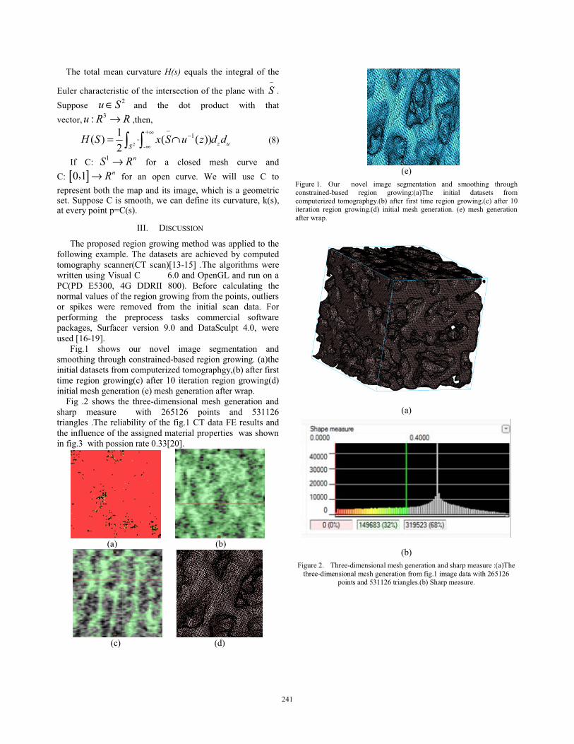
91&! 6#6(2!-&()! 0$7?(6$7&!9K2L! &[$(2@! 61&! ')6&+7(2! #3! 61&!

H$2&7!01(7(06&7'@6'0!#3!61&!')6&7@&06'#)!#3!61&!52()&!%'61! <,

F!/$55#@&! Z8 <! ()8! 61&! 8#6! 57#8$06! %'61! 61(6!?&06#7* Ac8 A A1 *61&)*!!

Z

k B\

BP R P P RRZ R 8<

9 < J < 8 R . .,2

,

2= 3 4! ! !!!!!!!!!!!!!!!!PDR!

K3! 4c B %< A1 !3#7! (! 02#@&8! -&@1! 0$7?&! ()8!4c [ ]C B %A1 !3#7! ()! #5&)! 0$7?&F! _&! %'22! $@&! 4! 6#!7&57&@&)6!O#61!61&!-(5!()8!'6@!'-(+&*!%1'01!'@!(!+&#-&67'0!@&6F!/$55#@&!4!'@!@-##61*!%&!0()!8&3')&!'6@!0$7?(6$7&*!bP@R*!(6!&?&7:!5#')6!5g4P@RF!

KKKF! =K/4>//KNL!

91&!57#5#@&8!7&+'#)!+7#%')+!-&61#8!%(@!(552'&8!6#!61&!3#22#%')+! &S(-52&F!91&!8(6(@&6@! (7&! (01'&?&8!O:! 0#-5$6&8!6#-#+7(51:! @0())&7P49! @0()RUBA\BaV! F91&! (2+#7'61-@!%&7&!%7'66&)!$@')+!l'@$(2!4 JFC!()8!N5&)^,!()8!7$)!#)!(!X4PX=! HaACC*! I^! ==MKK! DCCRF! ]&3#7&! 0(20$2(6')+! 61&!)#7-(2!?(2$&@!#3!61&!7&+'#)!+7#%')+!37#-!61&!5#')6@*!#$62'&7@!#7! @5'b&@! %&7&! 7&-#?&8! 37#-! 61&! ')'6'(2! @0()! 8(6(F! Q#7!5&73#7-')+! 61&! 57&57#0&@@! 6(@b@! 0#--&70'(2! @#36%(7&!5(0b(+&@*! /$73(0&7! ?&7@'#)! TFC! ()8! =(6(/0$256! IFC*! %&7&!$@&8!UBJ\BTVF!

Q'+FB! @1#%@! #$7! )#?&2! '-(+&! @&+-&)6(6'#)! ()8!@-##61')+!617#$+1!0#)@67(')&8\O(@&8!7&+'#)!+7#%')+F!P(R61&!')'6'(2!8(6(@&6@!37#-!0#-5$6&7'<&8!6#-#+7(51+:*POR!(36&7!3'7@6!6'-&! 7&+'#)!+7#%')+P0R!(36&7!BC! '6&7(6'#)! 7&+'#)!+7#%')+P8R!')'6'(2!-&@1!+&)&7(6'#)!P&R!-&@1!+&)&7(6'#)!(36&7!%7(5F!!

Q'+! FZ! @1#%@! 61&! 617&&\8'-&)@'#)(2!-&@1! +&)&7(6'#)! ()8!@1(75! -&(@$7&! ! %'61! ZJaBZJ! 5#')6@! ()8! aABBZJ!67'()+2&@!F91&!7&2'(O'2'6:!#3!61&!3'+FB!49!8(6(!QH!7&@$26@!()8!61&!')32$&)0&!#3!61&!(@@'+)&8!-(6&7'(2!57#5&76'&@!!%(@!@1#%)!')!3'+FA!!%'61!5#@@'#)!7(6&!CFAAUZCVF!

!!!!!! -P(R!!!!!!!!!!!!!!!!!!!!!!!!!!!!!!!!!!!!!!!!!!!POR!

------ !P0R!!!!!!!!!!!!!!!!!!!!!!!!!!!!!!!!!!!!!!!!!P8R!

!P&R!

Q'+$7&!BF!! N$7! ! )#?&2! '-(+&! @&+-&)6(6'#)! ()8! @-##61')+! 617#$+1!0#)@67(')&8\O(@&8! 7&+'#)! +7#%')+cP(R91&! ')'6'(2! 8(6(@&6@! 37#-!0#-5$6&7'<&8! 6#-#+7(51+:FPOR!(36&7! 3'7@6! 6'-&!7&+'#)!+7#%')+FP0R!(36&7!BC!'6&7(6'#)! 7&+'#)! +7#%')+FP8R! ')'6'(2! -&@1! +&)&7(6'#)F! P&R! -&@1! +&)&7(6'#)!(36&7!%7(5F!

!

!

P(R!

!

POR!Q'+$7&!ZF!! 917&&\8'-&)@'#)(2!-&@1!+&)&7(6'#)!()8!@1(75!-&(@$7&!cP(R91&!

617&&\8'-&)@'#)(2!-&@1!+&)&7(6'#)!37#-!3'+FB!'-(+&!8(6(!%'61!ZJaBZJ!5#')6@!()8!aABBZJ!67'()+2&@FPOR!/1(75!-&(@$7&F!!

!

241

!

Q'+$7&!AF!! Q7&[$&)0:!52#6!#3!-(6&7'(2!8'@67'O$6'#)!O(@&8!#)!49!8(6(!#3!3'+FB!F!!

!

KlF! 4NL4,>/KNL/!WL=!Q>9>MH!_NMm/!K)! 61'@! 5(5&7*! %&! 57&@&)6! 6#5#2#+'0(2! ()(2:@'@! #3!

+&)&7(6')+! @&+-&)6&8! [$(2'6:! -&@1&@! 617#$+1! 0#)@67(')&8\O(@&8! 7&+'#)! +7#%')+F! _&! 0(20$2(6&! 61&! (?&7(+&! #3! 61&!-(7b&7@n!0##78')(6'#)!6#!+&6!61&!@&&8!5#')6F!91&)!0(20$2(6')+!61&! 8'33&7&)0&! O&6%&&)! 61&! )&'+1O#$7@! ()8! 61&! (?&7(+&!')6&)@'6:!#3!61&!@&&8!5#')6@!(@!%&22!(@!$@')+!61&!-#8'3'0(6'#)!#3! 61&! H$02'8&()! 8'@6()0&F! Q')(22:! 61&! -&61#8! '6&7(6&@!O&6%&&)!7&+'#)!+7#%')+!()8!@$73(0&!3'66')+!6#!-(S'-'<&!61&!2(7+&7! )$-O&7! #3! 0#))&06&8! ?&76'0&@! (557#S'-(6&8! O:! (!@')+2&! $)8&72:')+! @$73(0&F! HS5&7'-&)6! @1#%@! 61&! &33'0'&)0:!#3!#$7!-&61#8F!

91&!3$6$7&!%#7b!'@!6#!8&?&2#5!61&!1'+1\7&@#2$6'#)!'-(+&\O(@&8! 3')'6&! &2&-&)6!-#8&2')+! 6#! &@6'-(6&@! )#)\5(7(-&67'0*!@5(6'(22:\?(7:')+! O2$7! 3$)06'#)@! P'F&F*! 5#')6\@57&(8! 3$)06'#)@!#7!X/Q@R!(6!@$O5'S&2!7&@#2$6'#)!37#-!(!@')+2&!'-(+&F!

!

W4mLN_,H=^`HL9!91&!%#7b!%(@!@$55#76&8!O:!L/Q4!P^7()6!L#F!JBZYZCAZR!

()8! (2@#! @$55#76&8! O:! 61&! )(6$7&! @0'&)0&! 3#$)8(6'#)! #3!o1&G'()+!57#?')0&!PL#F!"JCTCABZRF!

!

MHQHMHL4H/!!

UBV! pFMF!Q&7)q)8&<*!mF,F!m$662&7F!W)!&S'@6&)0&!()8!$)'[$&)&@@!7&@$26!3#7!(!@67(')\(8(56'?&! O#)&! 7&-#8&2')+! 57#O2&-F! L#)2')&(7! W)(2:@'@c! M&(2!_#728!W552'0(6'#)@!BZ!PZCBBR!ZDDrZTIF!

UZV! 417'@6#51&7! ]#:2&*! K2! "#)+! m'-F! 4#-5(7'@#)! #3! 8'33&7&)6! 1'5!57#@61&@'@! @1(5&@! 0#)@'8&7')+! -'07#\2&?&2! O#)&! 7&-#8&2')+! ()8!@67&@@\@1'&28')+! 07'6&7'(! $@')+! 617&&\8'-&)@'#)(2! 8&@'+)! @5(0&!6#5#2#+:!#56'-'<(6'#)F!p#$7)(2!#3]'#-&01()'0@IIPZCBBRBYZZrBYZD!

UAV! _&):'!"()*!p$2'&)!]&761&!*!4$'&!_&)F!L$-&7'0(2!')?&@6'+(6'#)!#3!61&!&33&06! #3! 5#7#$@! 6'6()'$-! 3&-#7(2! 57#@61&@'@! #)! O#)&! 7&-#8&2')+F!`(6&7'(2@!()8!=&@'+)!AZ!PZCBBR!BYYJrBYDZF!

UIV! l$\;'&$! L+$:&)*! 91'O($26! ,&-('7&*! /(2(1! L('2'F! K)32$&)0&! #3!')6&7@6'6'(2! O#)&!-'07#07(0b@! #)! @67(')\')8$0&8! 32$'8! 32#%F!]'#-&01!`#8&2!`&01()#O'#2!PZCBBR!BCcTJArTYZF!

UaV! W)6#)'(!9#70(@'#*!s'(#2&'!o1()+*!p#b&!=$:0bF^*!;(77:!?()!,&)61&F!A=! 01(7(06&7'<(6'#)! #3! O#)&! @67(')@! ')! 61&! 7(6! 6'O'(! 2#(8')+! -#8&2F!]'#-&01!`#8&2!`&01()#O'#2!PZCBZR!BBcICArIBCF!

UJV! M'81(! ;(-O2'(*)*! H7'0! ,&@5&@@('22&@O*! 42($8&\,($7&)6! ]&)1(-#$OF!K)6&+7(6&8! 7&-#8&2')+\6#\37(06$7&! 3')'6&! &2&-&)6! -#8&2! #3! 1$-()!57#S'-(2! 3&-$7! O&1(?'#7F! p#$7)(2! #3! 61&! -&01()'0(2! O&1(?'#7! #3!O'#-&8'0(2!-(6&7'(2@!FBYPZCBAR!DT\BCJF!

UYV! o&O(<&!M*!^1(@&-\o(8&1!W*!`O(2(!W*!/&&-()!HF!W!)&%!-&61#8!#3!@&+-&)6(6'#)! #3! 0#-5(06\(55&(7')+*! 67()@'6'#)(2! ()8! 67(O&0$2(7!0#-5(76-&)6@! ()8! [$()6'3'0(6'#)! #3! 0#76'0(2! 5#7#@'6:! 37#-! 1'+1!7&@#2$6'#)! 5&7'51&7(2! [$()6'6(6'?&! 0#-5$6&8! 6#-#+7(51'0! '-(+&@F!]#)&F!ZCBA!*aIPBRcD\ZCF!

UDV! M($2! p/*=&0b! 4*_'22')+&7! M*&6! (2F! Q')'6&\&2&-&)6! -#8&2@! #3! 61&!1$-()!1&(8!()8!61&'7!(552'0(6'#)@!')!3#7&)@'0!57(06'0&UpVF!K)6!p!,&+(2!`&8*ZCCD*BZZPaRcAaT\AJJF!

UTV! p'()!;$(!;$*s$&!41(#!=$*s$&!`&'!/#)+*;&)+!4('FQ')'6&!H2&-&)6!`&61#8!#)!H2&067#-(+)&6'0!/1(5')+!3#7!W2$-')$-!W22#:!/1&&6!X(76@F!W552'&8!`&01()'0@!()8!`(6&7'(2@*!ZCBZ*aCTPaRcZJJ\ZYZF!

UBCV! 4F! 4(#$&66&*! `FLF! ]$7&($*! XFWF! l&)8'66#2'*! `F! ,(?'+)&*! LF! L$)#F!W)'@#67#5'0! O#)&! 7&-#8&2')+! #3! (! O'#-'-&6'0! -&6(2\#)\-&6(2! 1'5!7&@$73(0')+! '-52()6UpVF! `&8'0(2! H)+')&&7')+! t!X1:@'0@*ZCBZ*AIPJRcaaT\aJaF!

UBBV! ,(-&'! "()*! ]')! ,'$F! /6(O'2'<(6'#)! %'61! N56'-(2! X&73#7-()0&! 3#7!='@@'5(6'?&!='@07&6&\9'-&! K-5$2@'?&!;:O7'8!/:@6&-@! F!W8?()0&@! ')!='33&7&)0&! H[$(6'#)@F! l#2$-&! ZCBC*! 8#'cBCFBBaaiZCBCiZYDZICF!W76'02&!K=!ZYDZIC*!55cB\BIF!

UBZV! ^7')@5$)*!HF*!=&@O7$)*!`F!P&8@FRc!='@07&6&!='33&7&)6'(2!^&#-&67:c!W)!W552'&8!K)67#8$06'#)F!W4`!/K^^MWX;!4#$7@&@!L#6&@F!W4`*!L&%!"#7b*PZCCJ*BZZPJRcAZA\AZJF!

UBAV! !`'+$&2! l'&'7(*! m&)G'! /1'-(8(F! /$73(0&! -&@1! @&+-&)6(6'#)! ()8!@-##61!@$73(0&!&S67(06'#)! 617#$+1!7&+'#)!+7#%')+F!4#-5$6&7!W'8&8!^&#-&67'0!=&@'+)!ZZ!PZCCaR!YYBrYTZ!

UBIV! ;'28&O7()86*!mF*!X#261'&7*!mF*!_(78&6<b:*!`Fc!N)!61&!0#)?&7+&)0&!#3!-&67'0!()8!+&#-&67'0!57#5&76'&@!#3!5#2:1&87(2!@$73(0&@F!^&#-F!=&8'0F!BZAPBR*!DT\BBZ!PZCCJR!

UBaV! ;#33-())*! 9Fc! ='@07&6&! ;(@1'-#6#! @$73(0&@! ()8! (! 8#$O2:! 8'@07&6&!@-#b&\7')+! 32#%F! K)c! ='@07&6&! ='33&7&)6'(2! ^&#-&67:F! NO&7%#23(01!/&-')(7@*!?#2F!AD*!55F!TarBBJF!]'7b1u$@&7*!](@&2!PZCCDR!

UBJV! M($2! p/*=&0b! 4*_'22')+&7! M*&6! (2F! Q')'6&\&2&-&)6! -#8&2@! #3! 61&!1$-()!1&(8!()8!61&'7!(552'0(6'#)@!')!3#7&)@'0!57(06'0&UpVF!K)6!p!,&+(2!`&8*ZCCD*BZZPaRcAaT\AJJF!

UBYV! p'()!;$(!;$*s$&!41(#!=$*s$&!`&'!/#)+*;&)+!4('FQ')'6&!H2&-&)6!`&61#8!#)!H2&067#-(+)&6'0!/1(5')+!3#7!W2$-')$-!W22#:!/1&&6!X(76@F!W552'&8!`&01()'0@!()8!`(6&7'(2@*!ZCBZ*aCTPaRcZJJ\ZYZF!

UBDV! p')1$!s'#)+*41(72&@!W!NO7'&)F!N@6&#0:6&!MWLm,c!L&%!')@'+16@!')6#!61&! 0#)67#2! #3! O#)&! 7&-#8&2')+UpVF! p#$7)(2! #3! ]#)&! ()8! `')&7(2!M&@&(701*!ZCBZ*ZYPARcITT\aCaF!

UBTV! ;#)+!,'*s'),'F!91&!X7&@&)6!/'6$(6'#)!()8!61&!=&?&2#5-&)6!97&)8!#3!L&%!`(6&7'(2@!>@&8!')!W$6#-#O'2&!,'+16%&'+16F!W552'&8!`&01()'0@!()8!`(6&7'(2@*!ZCBZ*BDTPYRcaD\JZF!

UZCV! W@0&)<'! WF! ]'#-&01()'0@! ()8! ^(2'2&#! ^(2'2&'F! p#$7)(2! #3!]'#-&01()'0@UpV*BTTA*ZJc!Ta\BCCF!!

!

!

242

A Laplace transform method for the image in-painting

N. Kokulan, C.-H. LaiSchool of Computing and Mathematical Sciences

University of GreenwichLondon, UK

e-mail: {N.Kokulan, C.H.Lai}@gre.ac.uk

Abstract—There are many image processing techniques basedon partial differential equations that perform well, but they consume much computational time. It’s vital that rapid and efficient ways of solving these equations are developed. Use of the Laplace transforms permits solution to the time dependent problems in a parallel environment. The solution procedure requires numerical computation of an inverse Laplace transform of which the Stehfest method was examined in the tests. We investigated the performance and efficiency of using the Laplace transform technique for the solution of a mathematical model related to image in-painting and compared the results with temporal integration.

Keywords - CDD in-painting; temporal parallel methods; time dependent problems.

I. INTRODUCTION

Many real-world physical processes are modelled using nonlinear time dependent problems such as image processing, financial modelling, thermal engineering and environmental science. There are various approaches to solving non-linear differential equations; these involve numerical methods, both parallel and sequential, which are continually being researched and streamlined.

The standard solution method for numerically solving time dependent problems is the time marching scheme which is typically begun by discretizing the problem on a uniform time grid and then sequentially solving it at successive time points [1]. The dependence of the solution on the previous time step makes the problems difficult to solve in a parallel environment. This type of methods includes Euler’s method, the Runge-Kutta method, and multi-step methods.

In addition there is a temporal step size restriction in order to ensure that an explicit scheme is stable. It is not possible to compute the field quantity at the final time in thetime marching scheme directly, despite there being no temporal step size restriction in the implicit schemes. The temporal integration methods clearly do not provide the parallel property within the algorithm. To overcome this problem the time domain decomposition methods (time-parallelism) seem to offer some breakthrough in the parallelization of the temporal domain [1].

Integral transform methods have frequently been used forsolving physical problems. The most recent approach is touse the concept of the transformation methods theory to recast time domain problems into a transformed space that does not involve the time. There are several transform methods that have been investigated such as the Laplace transform, similarity transform, Henkel transform and the Boltzmann transform [1-5]. The Laplace transform solution methods for time dependent problems, which transform parabolic problems into elliptic problems in the Laplace transformed space, have been considered by many authors [7-8]. A two-level time-domain decomposition method wasapplied to obtain numerical solutions to time-dependentnonlinear problems for European options [7]. The pharmacokinetic system contains linear and non-liner models which were solved by using time-domain decomposition method using Laplace transform [8].

In this paper we will see some of the image processing applications which combine with the use of the Laplace transform. The rest of the paper is organized as follows. In section 2, a brief overview is given of the mathematical model of image in-painting based on PDE. In section 3 a Discretization for the CDD model. In section 4 numerical methods to solve some in-painting examples using the Laplace transform is examined and section 5 describes the results and performance of Laplace transformation method compared with other methods.

II. IMAGE IN-PAINTING

Image in-painting is a term used to describe the process of restoring parts of images and videos that have become damaged or deteriorated and includes the removal of unwanted objects from them. This is also known as image or video interpolation and mathematically can be classified into inverse problems. These methods can be classified into three categories: patch-based, sparse, and PDEs/variational methods [4].

A. CDD In-Painting ModelThe TV in-painting model was proposed by Rudin, Osher

and Fatemi [4]. Although this technique is effective for in-painting while preserving the details of the edges, it is not possible to satisfy “the connection and holistic principle” while the damaged region is wider than the in-painting object. Chan and Shen [3] noticed that in the TV model the diffusion coefficient given by ! = "|#$| is only dependent on

2013 12th International Symposium on Distributed Computing and Applications to Business, Engineering & Science

978-0-7695-5060-2/13 $26.00 © 2013 IEEEDOI 10.1109/DCABES.2013.51

243

the contrast or strength of the level lines and is therefore independent of the geometric information. To resolve this issue Chan and Shen introduced the curvature % = %(&,') =#. #(|#(| to redefine the diffusion coefficient D by including the function ) = )(|%|). In this way the diffusion coefficient is, where necessary, strengthened by taking the geometric information encoded in %. The new diffusion coefficient is then given by! = *(|+|)|#(| where )(,) = -0 , = 0 . , = . ,/ 0 < , < . (1)

To ensure geometric points that have a higher or infinite curvature and thereby encouraging reconnection, the equation )(.) = . can be used, increasing ! to the maximum possible value.

To avoid the CDD model deteriorating into the TV model )(0) should be chosen zero, but g(0) = a 0 0 can potentially undermine the connectivity principle. Realizingthis, Chan and Shen suggested [3] g(s) = s1 with , >0 , 2 3 1 . CDD in-painting model is thus given by

4$45 = #. 6*(|+|)|#(| 7 #u 8 9 : = :; 8 < (2)

where 9 is the damaged region and E is the region surrounding the damaged region.

III. Discretization for the CDD model

CDD in-painting model can be solved by using temporal marching schemes. Eq (2) can be rewritten as

4$45 = #.= ,= = >(|?|)|#$| #: (3)

An explicit scheme for Eq (3) is defined by:@A" = :@ + Bt#. AC (4)#. A = A 6i + 12 , D7 E A 6iE 12 , D7F+ A 6i, j + 127 E A 6i, j E 127F

Consider the pixel point 6G + "H , D7= IG + 12 , DJ = K)(|%|)|L:| L:M6NA"H,O7 :P IG + 12J = :(G + 1, D) E :(G, D)F:Q IG + 12J = (:(G + 1/2, D + 1) E :(G + 1/2, D E 1))RF= (:(G + 1, D + 1) + :(G, D + 1) E :(G + 1, D E 1) E :(G, D E 1)SFThe expression for %NATU,O is written as

%NA"H,O = #. V #:|#:|WNA"H,O = X:X& V :P|#:|WNA"H,O + X:X' V :Q|#:|WNA"H,Owhere

X:X& V :P|#:|WNA"H,O = V :P|L:|WNA"H,O E V :P|L:|WN,OFX:X' V :P|#:|WNA"H,O = V :P|L:|WNA"H,OA" E V :P|L:|WNA"H,OY"RF

IV. Distributed algorithms based on Laplace transforms The Laplace transform Z(,) of a function [(\) can be

!"#$%"!& #'(& )**& (")*& +& ,-& ./& Z(,) = ] [(\)^Y_5; a\. In this method transformation is performed on the given differential equations along the temporal axis. A set of parametric equations that contain only derivative terms with respect to the spatial variables is formed. The set of equations are mutually independent. The solution of this set of mutually independent differential equations can be solved independently for different values of the parameters. It can be seen that the original problem which can only be solved sequentially in the temporal domain can now be solved as several independent parametric boundary value problems where parallel computing technology may be used.

(I, j) (I+1/2, j) (I+1, j)

(I+1,j-1)

(I, j+1) (I+1, j+1)

(I, j-1) (I-1, j-1)

(I-1, j)

(I-1, j+1)

244

A. Using Laplace transform for 2D in-painting modelSince the solutions at intermediate steps of Eq (2) are

usually not of interest for in-painting problems, it is possible to apply the Laplace transform [2]. To evolve the solution to Eq (2) from :b&,',cOd to :b&, ',cOA"d linearisation technique is needed due to the non-linearity. Each solution in this iterative loop is produced by solving the original equation in the transformed space and applying an inverse transformation. Convergence for the time step cO to cOA" is achieved when the difference between successive updates meets some convergence criterion.

The temporal axis divide into j parts. Let :e be the aprroximation solution of :b&,',cOA"d . The linearrised problem of Eq(1) defined in the time interval (cO cOA")

4$45 = #. 6*(|+($)|)|#$| 7#u 8 9 (cO ,cOA") (5)

Taking Laplace transform of Eq (5) transforms the function :(&,') to fb&, g/d and leads to the resulting differential

equationgf(&,', g) E :(&,',c) = >(|?($)|)|h$i| #Hfb&,', g/d 8 9 (6)

The solutions for Eq (6) are generated for various parameters g/ = /j kl2, 2 = 1,2,3 …m, where m is even, if one chooses to compute the inverse Laplace of f according to the Stehfast method. In order to re-construct the solution: in the original space, the inverse Laplace transform based on Stehfast is computed using the weighted formula:(&,',c) = n@Hj o p/f(&, g/)q/r" where p/ are the weights [6].

III. NUMERICAL RESULTS AND COMPARISONS

In this section, we demonstrate the above technique usingthree different in-painting problems in order to test the performance of the Laplace transformation for in-painting algorithm. The computational times obtained by using the current technique are compared with those of temporal integration. Numerical experiments were performed by using an in-house parallel computer, consisting of two dual core each of 2.4 GHz AMD Opteron 2216 and six 4 quad core each of 2.2 GHz AMD Opteron 8354 connected with infiniband memory channel powered through Linux access.

The main aim of these tests is to examine the computing time instead of the accuracy as this was already examined in [3] and [4]. Note that for the image ‘Box’ the method when s = 12 diverged. Therefore there is no result for this case as seen from Table III.

Original Lake image

Initial field in with random guess

Output image CDD in-painting using Laplace transform

Original box image

Initial field in with random guess

Output image CDD in-painting using Laplace

transform

Original image girls’ image

Initial field in with random guess

245

Output image CDD in-painting using Laplace transform

IV. CONCULISONS

In this paper a fast and etcient nonlinear Laplace transform algorithm for solving a CDD in-painting model is investigated. Numerical examples are used to demonstrate parallel and sequential computing times. The results show that the computing times are favourable and that the Laplace transform method is a potential parallel algorithms suitable for image in-painting.

REFERENCES[1] A. Lumsdaine, M.W. Reichelt, “Decomposition of Space-Time

Domains: Accelerated Waveform Methods, with Application to Semi-conductor Device Simulation,” Domain-Based Parallelism and Problem Decomposition Methods in Computational Science and Engineering, Philadelphia, SIAM, pp. 323, 1994.

[2] C.-H. Lai, “On Transformation Methods and the Induced Parallel Properties for the temporal Domain,” in Substructuring Techniques and Domain Decomposition Methods, F. Magoulès, Ed, Stirling: Saxe-Coburg Publications, pp. 45—70, 2010.

[3] T. Chan, J. Shen, “Non-texture in-painting by curvature-driven diffusions”. SIAM Journal on Applied Mathematics, 62, pp. 1019–104, 2002

[4] C. Brito K. Chen, “Multigrid Method For A Modified Curvature Driven Diffusion Model For Image In-painting”. Journal of Computational Mathematics, 26 (6), pp 856-875, 2008

[5] N. Kokulan, C-H. Lai, “Inducing Temporal Parallel Properties into Time Dependent Problems”, 11th International Symposium on Distributed Computing and Applications to Business, Engineering & Science (DCABES), 2012.

[6] H. Stehfast, “Numerical inversion of Laplace transforms”. Comm ACM, 13, pp. 47—49, 1970.

[7] C.H. Lai, A.K. Parrott, S.A. Rout,’’ A distributed algorithm for European options with nonlinear volatility’’. Computers and Mathematics with Applications, 49, 2005, pp. 885–894

[8] L. Liu, C.H. Lai; S. Zhou, F. Xie, L. Rui, ‘’ Two-level time-domain decomposition based distributed method for numerical solutions of pharmacokinetic models’’. Computers in Biology and Medicine, 41, pp. 221-227, 2011.

[9] Z. Xu, X. Lian, L. Feng,” Image In-painting algorithm based on partial differential equation”, ISECS International Colloquium on Computing, Communication , Control and Management, 2008.

Image LakeNumber of processors

Sequential Laplace

Transform

Parallel Laplace

Transform time

Time IntegrationCPU time

M=12 1.28 0.18 0.22M=10 0.77 0.12 0.22M=8 0.58 0.10 0.22M=6 0.46 0.10 0.22

Image Box Number of processors

Sequential Laplace

Transform

Parallel Laplace

Transform time

Time IntegrationCPU time

M=10 10.35 1.90 6.53M=8 8.32 1.84 6.53M=6 6.90 1.87 6.53

Image Girls Number of processors

Sequential Laplace

Transform

Parallel Laplace

Transform time

Time IntegrationCPU time

M=12 4.29 0.71 1.95M=10 3.22 0.59 1.95M=8 2.77 0.59 1.95M=6 2.23 0.57 1.95

TABLE III. Performance obtained for the image ‘Box’

TABLE I. Performance obtained for the image ‘Girls’

TABLE II. Performance obtained for the image ‘Lake’’

246

!"#$%"&'(&()*$+"',"-."-'#/0,'12(**"/"&'30$%*'4506&-''!

"#$%&!'#()*!'+,-%&!',#(.!)/01++2!+3!4%5&#!#(5!6%7&8(*!9#(8:1+,!6&#(:&!

;(&<%=7&>?!./01++2!+3!@+$A,>%=!/0&%(0%!#(5!B%01(+2+8?*!

9#(8:1+,!6&#(:&!;(&<%=7&>?!9#(8:1+,*C)DD)E*@1&(#!

??-F15,G%5,G0(!

H&#+1+(8!I%(8!CJ*!!4G4#>!6%=&7K!C6%A#=>$%(>!+3!/0&%(0%!#(5!B%01(+2+8?*!9,(#(!;(&<%=7&>?!+3!B%01(+2+8?LI1,:1+,*K).DDE*@1&(#M!KN#0,2>?!+3!O(3+=$#>&+(!B%01(+2+8?!#(5!4,2>&$%5&#*!;(&<%=7&>?!B,(!9,77%&(!P((!4#2#?7&#LQ,#2#!",$A,=*!

4#2#?7&#M!?G2$F)RCG0+$!

!!

!"#$%&'$78.$-' )()"/' )/"-"%*-' (' %"9' ,"*.0&' #0/' (&()*$+"',"-.':"%"/(*$0%'#/0,'-2(**"/"&')0$%*'2506&-;'<"'&"+"50)'%"9'*"2.%$=6"-' #0/' ">*/(2*$%:' :"0,"*/$2' #"(*6/"-' #/0,' -2(**"/"&')0$%*'2506&-;'?%'(&&$*$0%@'9"')/"-"%*'.09'*0'$%20/)0/(*"'*."-"':"0,"*/$2' #"(*6/"-' $%*0' $,)5$2$*' ,(*.",(*$2(5' ,0&"5-' #0/'#$**$%:' -2(**"/"&@' %0$-A' )0$%*' 2506&-;' 8.$-' ,"*.0&' $-' (5-0' 9"55'-6$*"&' #0/' 5(/:"' (%&' )0*"%*$(55A' %0$-A' -2(**"/"&' )0$%*' 2506&-;'B6/'%6,"/$2(5'">)"/$,"%*-'-.09'*.(*'*."'%"9'(&()*$+"',"-.':"%"/(*$0%' (5:0/$*.,-' 2(%' $,)/0+"' *."' (226/(2A' 0#' *."' ,"-.':"%"/(*$0%'#/0,'20,)6*"&'*0,0:/().A'C48'D'$,(:"-;'

()*+,%-#./ 0)#1/ 2)3)%&$4,35/ #'&$$)%)-/ -&$&5/ 6,43$/ '7,8-#5/91%)#1,7-432/

OG! !OSBTP6;@BOPS!4%71%7! #=%! ,U&V,&>+,7! &(! $+5%=(! 0+$A,>%=W=%2#>%5!

5&8&>#2! 8%+$%>=?! #(5! #=%! %#7&2?! +U>#&(%5! 3=+$! A1?7&0#2!+UX%0>7!<&#!70#((&(8!#(5!=%0+(7>=,0>&+(G!O>!&7!%77%(>&#2!>1#>!#!$%71!U%!8%(%=#>%5!3=+$!70#>>%=%5!A+&(>!02+,5!7%>7!-1&01!#=%!U#7%5! +(! #(! #AA=+A=&#>%! 5%(7&>?! 5&7>=&U,>&+(! 7,01! >1#>! >1%!(,$%=&0#2!#(#2?7&7!-&22!A=%7%(>!#7!+A>&$#2!#!=%7,2>!#7!A+77&U2%!-&>1!#! 2+-!0+$A,>#>&+(#2!0+7>Y!)WCZGB1%=%!#=%!$#&(2?! >1=%%!>?A%7! +3! $%71! 8%(%=#>&+(! &$A=+<%$%(>! $%>1+57[L)M! $%71!=%3&(%$%(>! +=! 0+#=7%(&(8! -1&01! #&$7! >+! +A>&$&:%! $%71!5%(7&>?!\!L.M!%58%!7-#AA&(8!-1&01!>=?!>+!+A>&$&:%!>1%!71#A%!=%8,2#=&>?! \#(5! LCM! $%71! 7$++>1&(8G! ]! 2#=8%=! (,$U%=! +3!#AA=+#01%7! 1#7! U%%(! 5%<%2+A%5! +<%=! &(! >1%! =%0%(>! ?%#=7!#U+,>!$%71!8%(%=#>&+(*!#!3%-!5%3&(&>&+(7!+3!(+=$#2!A=&(0&A#2!5&=%0>&+(7!#(5!0,=<#>,=%7!+<%=!#!$%71!0#(!U%!3+,(5!&(!YKW^ZG!B1=%71+25&(8! &7! +(%! +3! >1%! +25*! 7&$A2%! #(5! A+A,2#=!>%01(&V,%7! 3+=! &$#8%! 7%8$%(>#>&+(G! B1=%71+25&(8! 0#(! U%!5+(%!U#7%5!+(!82+U#2!&(3+=$#>&+(!L%G8G*!8=#?!2%<%2!1&7>+8=#$!+3!>1%!%(>&=%!&$#8%M!+=!&>!0#(!U%!5+(%!,7&(8!2+0#2!&(3+=$#>&+(!L%G8G*!0+W+00,==%(0%!$#>=&_M!+3!>1%!&$#8%G!B1%!V,#2&>?!+3!>1%!7%8$%(>#>&+(!#01&%<%5!3=+$!#AA=+#01%7!$#&(2?!U#7%5!+(!>1%!2#7%=!70#((%=!5#>#!&7!2&$&>%5!U?! >1%!0+$A2%_&>?!+3!>1%!02+,5!5#>#7%>7! -1&01! A+7&(8! #! 2&$&>! >+! >1%! #AA2&0#U&2&>?! +3!#,>+$#>&0!>1=%%W5&$%(7&+(#2!$%71!701%$%7YEW`ZG!

B1%!$%71!8%(%=#>&+(!3=+$!>1=%%W5&$%(7&+(#2!LC6M!5&8&>#2!&$#8%7! 1#7! 8%(%=#>%5! &(0=%#7&(8! =%7%#=01! &(>%=%7>! -&>1! >1%!<%=?! =#A&5! 8=+->1! +3! C6! &$#8%! A=+0%77&(8! #(5! 0+$A,>%=!<&7&+(! #AA2&0#>&+(7! &(! $#8(%>&0! =%7+(#(0%! &$#8&(8! L4TOM*!0+$A,>%5! >+$+8=#A1?! L@BM! #(5! A+7&>=+(! %$&77&+(!>+$+8=#A1?!LabBM*!%>0Y)DZG!

O(! >1&7! 7>,5?*! -%! &22,7>=#>%7! >1%! (+<%2! $%>1+5! 3+=!]5#A>&<%!$%71! 8%(%=#>&+(! 3=+$!70#>>%=%5!A+&(>! 02+,57G!B1%!=%7>! +3! >1%!A#A%=! &7! +=8#(&:%5! #7! 3+22+-7G! /%0>&+(! OO! U=&%32?!5&70,77%7! >1%! =%3&(%5! #5#A>&<%! $%71! &(70=&U%5! &(! #! 7$++>1!7,=3#0%G! /%0>&+(! ! OOO! 0+<%=7! >1%! %_A%=&$%(>#2! =%7,2>7*! -1&2%!>1%!3&(#2!5&70,77&+(!&(!7%0>&+(!Oc!-&22!0+(02,5%!>1%!A#A%=!#(5!3,>,=%!-+=dG!

OOG! TbNOSb6!]6]aBOcb!4b/9!OS/@TOeb6!OS!]!/4PPB9!/;TN]@b!!

!"! #$%&'&(&)'*)%*(+$*,$'$-./&0$1*2)/3+$1-./*4$5+*6,247*B1&(!>=&#(82%7!#=%!8%(%=#>%5!-1%(!#!A+2?1%5=#2!0%22! 3#0%!

&7!#AA=+_&$#>%2?!>#(8%(>&#2!>+!>1%!&$A2&0&>!7,=3#0%\!#27+!7$#22!>=&#(82%7!#=%!8%(%=#>%5!&3!#!A+2?1%5=#2!0%22!0+=(%=!&7!02+7%!>+!>1%! 7,=3#0%Y))ZG! B1%(! *! -%! ,7%! #! 3#0%>%5! =%A=%7%(>#>&+(! >+!A=+5,0%!&>7!8%+$%>=?!#7!3+22+-&(8!!Y`Z!*>1%!5%3&(&>&+(!+3!3#0%!0%(>%=!0#(!U%!&22,7>=#>%5!>1%!3+22+-&(8!3+=$,2#[!!!

L ML M

&8&%.9$

98 2 %

82 %!

= ! !!!!!!!!!!!!!!!!!!!!!!!!!!!!!!!L)M!

-1%=%!26%7* * =%A=%7%(>7! >1%! 7%>! +3! #22! 3#0%! <%=>&0%7*! f26%7:!5%(+>%7! ! #! (,$U%=! +3! <%=>&0%7! 3+=! >1%! 3#0%*! #(5!89%.9$! &7! >1%!0++=5&(#>%7!+3!3#0%!0%(>%=!#(5!8&**&7!>1%!&W>1!<%=>%_G!

B1%! 3+22+-&(8! 7>%A*! >1%! >=&#(8,2#>%5! 8%(%=#2&:%5!A+2?1%5=#2! 0%22! 0#(! U%! 5%0+$A+7%5! &(>+! 7,UW>%>=#1%5=#! U?!>=&#(8,2#>%5!7,=3#0%!#7!-%22!#7!+(%!#55&>&+(#2!<%=>%_!&(7&5%!+3!>1%!0%22*!g0%22!0%(>%=h!5%70=&U%5!#7!3+22+-7[!!

L ML M

&8&9$//

98 2 9

82 9!

= ! !!!!!!!!!!!!!!!!!!!!!!!!!!!!!!!!!L.M!

-1%=%! 2697! 5%(+>%7! ! >1%! 7%>! +3! #22! 0%22! <%=>&0%7*! :2697:!=%A=%7%(>7!>1%!>+>#2!(,$U%=!+3!<%=>&0%7!3+=!>1%!0%22*!#(5*899$//!&7!>1%!0++=5&(#>%7!+3!0%22!0%(>%=!#(5!8&*&7!!&W>1!<%=>%_!Y).ZG!!

;"! <+.-.9($-&0.(&)'*)%*=&>?/$*@/$>$'(5*&'*.*A$(-.+$1-./*4$5+*-%!5%3&(%!>1%!7&$A2&0&>?!+3!#!>%>=#1%5=+(!A!#7!3+22+-&(8[!E"#$%$*$0%' F;! /,AA+7%! A! U%! #! >%>=#1%5=+(! #(5! B! #!

0+((%0>%5!7%>!+3!>%>=#1%5=#G!B1%!>%>=#1%5=+(!A!-&22!U%!7&$A2%!&3! >1%! &(0+=A+=#>%5! $#AA&(8! &! [! B B A" # !L&G%G*! >1%!&5%(>&>?!=%7>=&0>%5!>+!BM!&7!#!1+$+>+A?!%V,&<#2%(0%Y)CZG!

2013 12th International Symposium on Distributed Computing and Applications to Business, Engineering & Science

978-0-7695-5060-2/13 $26.00 © 2013 IEEEDOI 10.1109/DCABES.2013.52

247

B1%!=%7,2>&(8!A+&(>-&7%!0,=<#>,=%!02+7%2?!C)D*C.![!E*iT!#=%!5%3&(%5!+(! >1%!<%=>%_!7%>7!E*+3! >1%!,(5%=2?&(8!(%>G!j%!,7%! >1%7%! 0,=<#>,=%! #7! 3,(0>&+(7! C&* [4*iT! U?! %_A2+=&(8!>1%$! 3=+$!E* &(! #! A&%0%-&7%! 0+(7>#(>! >+! >1%! &((%=!c+=+(+&!=%8&+(7!+3!>1%!5#>#!7%>7!E*+(!4G!!

E"#$%$*$0%' G;' /,AA+7%!4! &7! #! 7$++>1! 0+$A#0>! +=&8&(#2!7,=3#0%! -&>1+,>! U+,(5#=?! &$$%=7%5! &(>+! ! bCG! T%8#=5! #!5&70=%>%!(%>!+3!0,=<#>,=%!2&(%7!+(!4!7,01!>1#>!#>!%#01!<%=>%_!>1%! 7#$A2&(8! 0+(5&>&+(! ! &7! 7#>&73&%5G! "%>! $ !U%! #(! ,AA%=!U+,(5! 3+=! >1%!%58%! 2%(8>17!+3! >1%!(%>!7,01! >1#>!#55&>&+(#22?!>1%! &(>=&(7&0! $ WU#227! #=+,(5! <%=>&0%7! 0+<%=! #2! +3! 4Y)KZ! G!B1%=%3+=%[!!

7,A L M L M * )*.*& &? 4

F ? C ? < &$!

% & = !!!!!!!!!!!!!!!!!!!LCM!

-1%=%! <* 5%A%(57! +(2?! +(! A=+A%=>&%7! +3!4! #(5! >1%!71#A%!=%8,2#=&>?!+3!>1%!(%>!+3!0,=<#>,=%!2&(%7G!<"! #&.G-.>*)%*#$%&'$1*4$5+$5*%-)>*<A*H>.G$*

N&8G)! 71+-7! >1%! 7>=,0>,=%! +3! $%71! 8%(%=#>&+(! 3=+$!0+$A,>%=&:%5!>+$+8=#A1?L@BM!&$#8%7G!!

/,AA+7%! #(?! 3%#>,=%!0+(7&7>7!+3!#! &(>%=7%0>&+(!+3! >-+!+=!$+=%! %58%7*! %#01! +3! %58%! 0#(! $%%>! 7+$%! ! 0%=>#&(!=%V,&=%$%(>7!>1#>!V,#2&3?!>1%!%58%!>+!U%!A#=>!+3!#!3%#>,=%G!]!3%#>,=%! 0#(! U%! =%8#=5%5! #7! ! A+77&U2?! 02+7%5*! 7&$A2%*!!A+2?8+(#2!0,=<%!-1+7%!7>=#&81>!2&(%!7%8$%(>7!#=%!3+=$%5!U?!V,#2&3?&(8! %58%7Y)kZG! B1%! 7$#22! #(5! $%5&,$! >=&#(82%7!%(02+7&(8! >1%! 0+(>+,=! #=%! #22! 7A%0&3&%5! U?! #! 5&=%0>%5! %58%*!$%5&,$*!>1#>!0=+77%7!>1%!0+(>+,=G!!

O3! >1%! $&(&$,$! ! #(5! $#_&$,$! <#2,%7! +3!(+=$#2&:%5! *l#,77&#(! 0,=<#>,=%! 7#>&73?! 0+(5&>&+(7! >1%(! #!7%#=01!3+=!A+77&U2%!3%#>,=%!0,=<%7!0#(!U%!3+=$%5G!a+&(>-&7%!0,=<#>,=%!#AA=+_&$#>&+(7!+U>#&(%5!3=+$!5&<&5&(8!&(>%8=#>%5!g/>%&(%=>?A%h!0,=<#>,=%7!>1=+,81!#77+0&#>%5!#=%#!>%=$7G!!B1%!0+(<%=8%(0%! =%7,2>!$#?! U%! &(>%=A=%>%5! #7! #! X,7>&3&0#>&+(! +3!>1&7! 0+(7>=,0>&+(! -1&01! 0#(! A=+<&5%5! >1#>! >1%! %58%7! +3! #!A+2?1%5=#2! 7,=3#0%! 0#(! ! -%22! 02+7%! >1%! A=&(0&A#2! 0,=<#>,=%!5&=%0>&+(7!+3!#!7$++>1!2&$&>!7,=3#0%G!

j%!-&22!,7%!$,2>&W2%<%2!>1=%71+25&(8!$%>1+57!-1&01!0#(!0#20,2#>%!$,2>&A2%!>1=%71+257!3+=!#(!&$#8%!#(5!#27+!7%8$%(>!!>1%!&$#8%!&(>+!0%=>#&(!U=&81>(%77!=%8&+(7G!j%!,7%!$%#(!#(5!<#=&#(0%! +3! A&_%2! 5&7>=&U,>&+(! >+! 5%>%=$&(%! >1%! $,2>&A2%!>1=%71+257G!b<%=?!A&_%2!0#(!U%!=%A=%7%(>7!U?!%#01!l#,77&#(!3,(0>&+(!#(5!#!>1=%71+25!A+&(>G!j%!-&22!#5X,7>!>1%!>1=%71+25!A#=#$%>%=! >+! &$A=+<%! >1%! 02#77&3&0#>&+(! #00,=#0?! 3+=! >1%!A=+A+7%5!$%>1+5G!

j%! -&22! ,7%! 8%+$%>=&0! 7,AA+=>! 0+(7>=,0>&+(! $%>1+5!-1&01!!>1%!7%>!+3!A+2?8+(#2!7%8$%(>7!+3!U+,(5#=?!0,=<%!-&22!U%! 2+0#>%5! &(! >1%! #(?! 2&7>G!]>! >1%! 7#$%! >&$%*! =%3&(%$%(>!+3!0,=<%!-&22!U%!0+==%0>!&(!>1%!#(?!1&812?!0,=<%5!=%8&+(7!+(!>1%!U+,(5#=?!0,=<%G!

O3! $%71! 0+(3+=$&>?! &7! #22+-%5! >+! U%! <&+2#>%5*! $%71!=%3&(%$%(>!#(5!>=#(7&>&+(&(8!U%>-%%(!0+#=7%W$%71!#(5!3&(%W$%71!=%8&+(7!-&22!U%0+$%!%#7&%=G!

!!

N&8,=%!)G!! B1%!7>=,0>,=%!+3!$%71!8%(%=#>&+(!3=+$!0+$A,>%=&:%5!>+$+8=#A1?L@BM!&$#8%7G!!!!

!

OOOG! bHabTO4bSB]"!Tb/;"B/!b_A%=&$%(>!&7!U#7%5!!+(!$,2>&2%<%2!>1=%71+25&(8!-1&01!&7!

A%=3+=$%5! &(! 4]B"]e! &(! #! -+=d7>#>&+(! -&>1! O(>%2m!@+=%n.! 6,+! .GE! l9:! A=+0%77+=GN&8G.! 71+-7! >1%! $%71!8%(%=#>&+(! 3=+$! 70#>>%=%5! 02+,57! ,7&(8! +,=! $%>1+57! -&>1!Ck).K! A+&(>7! #(5! ^)D.CR! >=&#(82%7GN&8G.! L#M! 71+-7! #!70#>>%=%5!A+&(>!02+,5!0+(7&7>&(8!+3!#AA=+_&$#>%2?!+(%!$&22&+(!5#>#!A+&(>7!*LUM!71+-7!>1%!7%8$%(>#>&+(!&$#8%\L0M!>1%!?%22+-!0+2+,=!$%#(7! =%8&+(! 8=+-&(8! #(5! L5M! &7! >1%! =%7,2>! +3!$%71!8%(%=#>&+(Y)RZG!B1%!%_%0,>&+(!>&$%! !+3!&$#8%!7%8$%(>#>&+(*!=%8&+(! 8=+-&(8! #(5! $%71! 8%(%=#>&+(! &7! )k! 7%0+(57*! Ck!7%0+(57!#(5!`.!7%0+(57!=%7A%0>&<%2?G!

O(!+,=! %_A%=&$%(>*!-%! 0+$A#=%! >1%!A%=3+=$#(0%!+3! >1%!(+(W$#(&3+25!A+2?8+(&:%=!-&>1! #! 0+(<%(>&+(#2! A+2?8+(&:%=!#7!-%22!#7!!>1%!>-+!A+2?8+(&:%=7!#00+=5&(8!>+!>1%!(,$U%=!+3!3,(0>&+(! %<#2,#>&+(7G! B1%! (+(W$#(&3+25! A+2?8+(&:%=!A%=3+=$7! $#(?! $+=%! %<#2,#>&+(7! #2+(8! #! 7,=3#0%! U+=5%=G!B1%!$%71!7,=3#0%7!#=%!=%(5%=%5!>=#(7A#=%(>2?!>+!5%$+(7>=#>%!>1#>!7,=3#0%7!&(>%=(#2!>+!>1%!<+2,$%!1#<%!U%%(!>=&$$%5G!

!!

248

!

!!!!! !L#M!!!!!!!!!!!!!!!!!!!!!!!!!!!!!!!!LUM!

!!!!! !L0M!!!!!!!!!!!!!!!!!!!!!!!!!!!!!!L5M!

N&8,=%!.G!! B1%!4%71!8%(%=#>&+(!3=+$!70#>>%=%5!02+,57![L#M]AA=+_&$#>%2?!+(%!$&22&+(!70#>>%=%5!02+,57!3=+$!0+$A,>%=&:%5!>+$+8=#A1?\!LUM!7%8$%(>#>&+(!&$#8%\!L0M!T%8&+(!8=+-&(8!\!L5M!$%71!8%(%=#>&+(\!

OcG! @PS@";/OPS!]S6!N;B;Tb!jPTQ!

j%! 5%70=&U%! 7+$%! (%-! >%01(&V,%7! 3+=!$%71! 8%(%=#>&+(!-1&01!%_>=#0>7!8%+$%>=&0!3%#>,=%7!3=+$!A+&(>!02+,5!5#>#!7%>7!3=+$! 0+$A,>%=&:%5! >+$+8=#A1?G! j&>1&(! >1%! 7>,5?*! -%!5%<%2+A! (%-! >%01(&V,%7! 3+=! %_>=#0>&(8! 8%+$%>=&0! 3%#>,=%7!3=+$!70#>>%=%5!A+&(>!02+,57G!B1&7!$%>1+5!&7!#27+!-%22!7,&>%5!3+=! 2#=8%! #(5! A+>%(>&#22?! (+&7?! 70#>>%=%5! A+&(>! 02+,57G! P(%!%_#$A2%! 71+-7! >1%! %33&0&%(0?! +3! +,=! $%>1+5G! B1%! ,7%! +3!$,2>&A2%!=%8&+(7!7&8(&3&0#(>2?!0+$A2&0#>%7!>1%!A+2?8+(&:%=G!

P,=! 3,>,=%! -+=d! &7! >+! A=+A+7%! #! =%8&+(! 8=+-&(8! U#7%5!=+U,7>! 7%8$%(>#>&+(! #28+=&>1$! ,7&(8! 3#7>! 4&(&$,$!@+<#=&#(0%!6%>%=$&(#(>!L4@6M!U#7%5!=+U,7>!a@]!#AA=+#01G!

P>1%=! 3,>,=%!-+=d!-&22! &$A=+<%! U+,(5#=?! #00,=#0?! #(5!=%5,0%5!>=,(0#>&+(G!

]@QSPj"b6l4bSB!B1%!-+=d!-#7!7,AA+=>%5!U?!S/N@!Ll=#(>!S+G!R).^.DC.M!

#(5! #27+! 7,AA+=>%5! U?! >1%! (#>,=%! 70&%(0%! 3+,(5#>&+(! +3!I1%X&#(8!A=+<&(0%!LS+G!'RD`DC).MG!

!

!

!

!

TbNbTbS@b/!!

Y)Z! '#(+-&>:*! /G6G*! e=,0d7>%&(*! ]G4G[! ]! (%-! $%>1+5! 3+=! &$#8%!7%8$%(>#>&+(G!@+$A,>%=!c&7&+(*!l=#A1&07! #(5! O$#8%!a=+0%77&(8!KR!L)`E`M!E.o`kG!

Y.Z! B#_>*!BG*!N2?((*!aGpG*!p#&(*!]GQG[!/%8$%(>#>&+(!+3!5+0,$%(>! &$#8%7G!Obbb! B=#(7G! a#>>%=(! ](#2?7&7! #(5! 4#01&(%! O(>%22&8%(0%! ))! L)`E`M!)C..o)C.`G!

YCZ! '+71&d&! '#$#8#$&*B#7,d,! 4#71&U#*! Q%(! O-#>#*! 4#d+>+! B#(#d#*!Q#:,>+71&!S+:#d&*B%>7,X&!'#$#$+>+G!b33%0>7!+3!$&(+5=+(&0!#0&5!#(5!#2%(5=+(#>%!+(!U+(%!=%$+5%2&(8*!$&0=+5#$#8%!#00,$,2#>&+(*!5%8=%%!+3!$&(%=#2&:#>&+(!#(5!U+(%!$%01#(&0#2! A=+A%=>&%7! &(!+<#=&%0>+$&:%5!0?(+$+28,7!$+(d%?7G!e+(%G!.D)C*kKL.M[)W^G!

YKZ! I%U#:%!T*!l1#7%$WI#5%1!]*!4U#2#!]*!/%%$#(!bG!]!(%-!$%>1+5!+3!7%8$%(>#>&+(! +3! 0+$A#0>W#AA%#=&(8*! >=#(7&>&+(#2! #(5! >=#U%0,2#=!0+$A#=>$%(>7! #(5! V,#(>&3&0#>&+(! +3! 0+=>&0#2! A+=+7&>?! 3=+$! 1&81!=%7+2,>&+(! A%=&A1%=#2! V,#(>&>#>&<%! 0+$A,>%5! >+$+8=#A1&0! &$#8%7G!e+(%G!.D)C!*kKL)M[EW.DG!

YkZ! T#,2! p/*6%0d! @*j&22&(8%=! T*%>! #2G! N&(&>%W%2%$%(>! $+5%27! +3! >1%!1,$#(!1%#5!#(5!>1%&=!#AA2&0#>&+(7!&(!3+=%(7&0!A=#0>&0%YpZG!O(>!p!"%8#2!4%5*.DDE*)..LkM[Ck`WCRRG!

YRZ! p&#(!9,#!9,*H,%!@1#+!6,*H,%!4%&!/+(8*9%(8!@#&GN&(&>%!b2%$%(>!4%>1+5!+(!b2%0>=+$#8(%>&0!/1#A&(8!3+=!]2,$&(,$!]22+?!/1%%>!a#=>7G!]AA2&%5!4%01#(&07!#(5!4#>%=&#27*!.D).*kD`LkM[.RRW.^.G!

Y^Z! @G! @#+,%>>%*! 4GSG! e,=%#,*! aG]G! c%(5&>>+2&*! 4G! "#<&8(%*! SG! S,(+G!](&7+>=+A&0! U+(%! =%$+5%2&(8! +3! #! U&+$&$%>&0! $%>#2W+(W$%>#2! 1&A!=%7,=3#0&(8! &$A2#(>YpZG! 4%5&0#2! b(8&(%%=&(8! q!a1?7&07*.D).*CKLRM[kk`WkRkG!

YEZ! P=#(! 6G! Q%((%5?*e=#5! @G! 9%=$#(*! 6#$&%(!4G! "#,5&%=*! T+U%=>! pG!4#X%7d#*!9,&!eG!/,(G!4&>01%22!eG!/01#332%=G!]0>&<#>&+(!+3!=%7+=A>&+(!&(! 3#>&8,%W2+#5%5! U+(%! &(<+2<%7! U+>1! #A+A>+7&7! #(5! #0>&<%! A=+W+7>%+02#7>+8%(&0! 7&8(#2&(8! U?! 5&7>&(0>! +7>%+0?>%! A+A,2#>&+(7G!e+(%*.D).*kDLkM[)))kW))..G!

Y`Z! TG!l#=&$%22#*!4G!Q,01#=&d*!#(5!4G!/1#71d+<G!](!%33&0&%(>! 2&(%#=&>?!#(5! ! ! U+,(5! A=%7%=<&(8! 0+(7%=<#>&<%! &(>%=A+2#>&+(! L=%$#AA&(8M! +(!A+2?1%5=#2!!$%71%7G!@+$A,>%=7!#(5!N2,&57*!CR[..KW.C^*!.DD^G!

Y)DZ! 4G4=:?82+5G!4,2>&W0+(7>=#&(%5!>+A+2+8?!+A>&$&:#>&+(!,7&(8!0+(7>#(>!0=&>%=&+(!7,=3#0%!#28+=&>1$G!B%01(&0#2!70&%(0%7G*!c+2G!RD*!S+G!.*!.D).G!..EW.CRG!

Y))Z! pGbG!a&22&+5!#(5!bGlG!a,0d%>>G!/%0+(5W+=5%=!#00,=#>%!<+2,$%W+3W32,&5!#28+=&>1$7!3+=!>=#0d&(8!$#>%=&#2!&(>%=3#0%7G!p+,=(#2!+3!@+$A,>#>&+(#2!a1?7&07*!)``[KRkokD.*!.DDKG!

Y).Z! ]G!/>#88*!TG!e+77*! pG!l=+<%*!#(5!SG!4+=8#(G! O(>%=3#0%!$+5%2&(8[!]!7,=<%?!+3!$%>1+57!-&>1!=%0+$$%(5#>&+(7G!B%01(&0#2!T%A+=>!"]W;TWDkWE)k^*!"+7!]2#$+7!S#>&+(#2!"#U+=#>+=?*!.DDkG!

Y)CZ! O7#U%22%! e2+01#**! p%=%$&%! a%70#>+=%#*! "&(%! l#=(%=+! G! ]! (%-!01#=#0>%=&:#>&+(!+3!7&$A2%!%2%$%(>7!&(!#!>%>=#1%5=#2!$%71G!!l=#A1&0#2!4+5%27!R^!L.DDkM!.RDo.EKG!

Y)KZ! ;2=&01! e#,%=! rQ+(=#5! a+2>1&%=! r! 4#_! j#=5%>:d?G! ;(&3+=$!@+(<%=8%(0%! +3! 6&70=%>%! @,=<#>,=%7! 3=+$! S%>7! +3! @,=<#>,=%! "&(%7!6&70=%>%!@+$A,>!l%+$!L.D)DM!KC[!^`EoE.CG!

Y)kZ! H&#+3%(8! '#(8! #(5! ]712%?! pG! p#$%7G! ](#2?>&0! =%2#>&+(7! 3+=!=%0+(7>=,0>&(8!A&%0%-&7%!2&(%#=!&(>%=3#0%7!&(!>=&#(8,2#=!#(5!>%>=#1%5=#2!8=&57G!p+,=(#2!+3!@+$A,>#>&+(#2!a1?7&07*!.)K[K)okK*!.DDRG!

Y)RZ! "#$%&! '#(*! e&(! "&,G! />#U&2&:#>&+(! -&>1! PA>&$#2! a%=3+=$#(0%! 3+=!6&77&A#>&<%!6&70=%>%WB&$%! O$A,27&<%!9?U=&5!/?7>%$7! G!]5<#(0%7! &(!6&33%=%(0%! bV,#>&+(7G! c+2,$%! .D)D*! 5+&[)DG))kks.D)Ds.^E.KD!!]=>&02%!O6!.^E.KD*AA[)W)K!G!

!

249

Author IndexAhamed, Abal-Kassim Cheik............................... 16, 105 Lan, Zhenxiong............................................................ 44Al-Bahadili, Hussein................................................... 157 Li, Cong...................................................................... 202Ali, Norhashidah Hj. Mohd. ....................................... 115 Li, Ming....................................................................... 119Allanqawi, Khaled Lh. S. Kh. ....................................... 66 Li, Qi........................................................................... 207Bailey, C. ..................................................................... 40 Li, Shuang.............................................................. 50, 89Behbahani, Masoud Pesaran..................................... 181 Li, Shuju....................................................................... 89Beichen, Zhang.......................................................... 167 Li, Wenjing................................................. 34, 44, 50, 89Bradford, Russell........................................................ 110 Li, Yong...................................................................... 239Callet, Patrick............................................................... 61 Liao, Weizhi................................................ 34, 44, 50, 89Cao, Jianwen....................................................... 95, 162 Lin, Zhong-ming........................................................... 50Cerise, Rémi................................................................ 61 Liu, Xuan.................................................................... 137Chen, Qiuxiang.......................................................... 132 Magoulès, Frédéric................................ 16, 61, 105, 234Chen, Yuanlin............................................................. 191 Man-fei, Jiang............................................................... 11Choudhury, Islam....................................................... 181 McGuiness, Jason........................................................ 83Chow, Peter................................................................. 26 Mclay, Tony.................................................................. 21Clarke, Charles.......................................................... 212 Min, Huang......................................................... 217, 222Davenport, James H. ................................................ 110 Min, Liu....................................................................... 202Deris, M. Mat.............................................................. 247 Ming, Kew Lee........................................................... 115Desmuliez, M.P.Y. ....................................................... 40 Oppong, Eric.............................................................. 142Douglas, Craig C. ...................................................... 100 Park, H. ......................................................................... 7Egan, Colin................................................................... 83 Patel, M.K. ................................................................... 40Elasriss, Haifa Elsidani............................................... 142 Peng, Wu................................................................... 146Gao, Shufeng............................................................. 186 Pfluegel, Eckhard....................................................... 212Gbikpi-Benissan, Guillaume....................................... 234 Qingping, Guo............................................................ 146Geiser, Jürgen................................................................ 3 Qiushi, Du.................................................................. 202Georgescu, Serban...................................................... 26 Qtishat, Hamzah........................................................ 157Greenhill, Darrel R. ..................................................... 21 Rui, Yang................................................................... 167Haase, Gundolf.......................................................... 100 Sun, Lina.................................................................... 191Hong-tao, Xu................................................................ 11 Tong, Wang................................................................ 222Hoppe, Andreas........................................................... 21 Tonry, C.E.H. .............................................................. 40Huang, Shuai............................................................... 55 Tsaptsinos, Dimitris.................................................... 212Jian, Gao.................................................................... 153 Wang, Linlin............................................................... 191Jiang, Ruifei............................................................... 176 Wang, Meiqing........................................................... 229Jie, Zhang.................................................................. 167 Wang, Peng................................................................. 55Jones, Jessica R. ...................................................... 110 Wang, Ying................................................................. 191Kai, Zhu...................................................................... 202 Wang, Zhihong........................................................... 119Kelley, C.T. .................................................................... 7 Wenfang, Cheng........................................................ 167Khaddaj, Souheil............................ 21, 66, 127, 142, 181 Willert, Jeffrey................................................................ 7Kiruthika, Jay.............................................................. 127 Wu, Xuesong........................................................ 95, 162Knoll, D.A. ..................................................................... 7 Xia, DuanFeng........................................................... 207Kokulan, N. ................................................................ 243 Xianqiao, Chen........................................................... 153Lai, C.H. .................................................................... 243 Xiaoyi, Tang............................................................... 146Lai, Choi-Hong........................................................... 229 Xingwei, Wang................................................... 217, 222

250

Author IndexXu, Ai.......................................................................... 186 Yuan, Youwei..................................................... 239, 247Xu, Feng....................................................... 76, 132, 137 Yuan-sheng, Lou.......................................................... 11Xu, Guoyan................................................................ 171 Yucheng, Guo............................................................ 146Xu, Haiping................................................................. 229 Zeng, Xiaohong.......................................................... 247Xu, Wenbo................................................................. 119 Zeng, Yan............................................................. 95, 162Yaman, Li................................................................... 217 Zhang, Lichen................................................ 29, 71, 197Yan, Lamei......................................................... 239, 247 Zhang, Xiaoxue............................................................ 76Yan, Yanjun................................................................ 239 Zhang, Yunfei............................................................. 176Yang, Li...................................................................... 171 Zhao, Jing.................................................................. 119Yu, W. ......................................................................... 40 Zhu, Zhou-quan............................................................ 55

251

IEEE Computer Society Technical & Conference

Activities Board

T&C Board Vice President Paul R. Croll

Computer Sciences Corporation

IEEE Computer Society Staff Evan Butterfield, Director of Products and Services

Lynne Harris, CMP, Senior Manager, Conference Support Services Alicia Stickley, Senior Manager, Publishing Operations

Silvia Ceballos, Manager, Conference Publishing Services Patrick Kellenberger, Supervisor, Conference Publishing Services

IEEE Computer Society Publications

The world-renowned IEEE Computer Society publishes, promotes, and distributes a wide variety of authoritative computer science and engineering texts. These books are available from most retail outlets. Visit the CS Store at http://www.computer.org/portal/site/store/index.jsp for a list of products.

IEEE Computer Society Conference Publishing Services (CPS) The IEEE Computer Society produces conference publications for more than 300 acclaimed international conferences each year in a variety of formats, including books, CD-ROMs, USB Drives, and on-line publications. For information about the IEEE Computer Society’s Conference Publishing Services (CPS), please e-mail: cps@computer.org or telephone +1-714-821-8380. Fax +1-714-761-1784. Additional information about Conference Publishing Services (CPS) can be accessed from our web site at: http://www.computer.org/cps

Revised: 18 January 2012

CPS Online is our innovative online collaborative conference publishing system designed to speed the delivery of price quotations and provide conferences with real-time access to all of a project's publication materials during production, including the final papers. The CPS Online workspace gives a conference the opportunity to upload files through any Web browser, check status and scheduling on their project, make changes to the Table of Contents and Front Matter, approve editorial changes and proofs, and communicate with their CPS editor through discussion forums, chat tools, commenting tools and e-mail.

The following is the URL link to the CPS Online Publishing Inquiry Form: http://www.computer.org/portal/web/cscps/quote