Copyright

by

Kenneth Joseph Dayman

2015

The Dissertation Committee for Kenneth Joseph Dayman certifies that this is the

approved version of the following dissertation:

Determination of Independent and Cumulative FissionProduct Yields with Gamma Spectrometry

Committee:

Steven Biegalski, Supervisor

Derek Haas

Sheldon Landsberger

Justin Lowrey

Erich Schneider

Determination of Independent and Cumulative FissionProduct Yields with Gamma Spectrometry

by

Kenneth Joseph Dayman, B.S.; M.S.E.

Dissertation

Presented to the Faculty of the Graduate School of

The University of Texas at Austin

in Partial Fulfillment

of the Requirements

for the Degree of

Doctor of Philosophy

The University of Texas at Austin

August 2015

Dedication

To everyone who was there

Acknowledgments

There are numerous people that have helped during the course of this research.

First and foremost, I’d like to thank my adviser Steven Biegalski, whose patience al-

lowed me to wander and learn, even when it seemed without end or purpose, and whose

guidance ensured that I found my way.

Second, I’d like to thank Erich Schneider and Sheldon Landsberger from UT. You not

only taught me the skills I needed to complete this research, but also inspired me to believe

that I could.

Thank you to scientists at PNNL, including Derek Haas, Amanda Prinke, and Sean

Stave, who performed the 14 MeV irradiations and provided the data for my analysis.

This material is based upon work supported by the U.S. Department of Homeland Se-

curity under Grant Award Number, 2012-DN-130-NF0001-02. The views and conclusions

contained in this document are those of the authors and should not be interpreted as repre-

senting the official policies, either expressed or implied, of the U.S. Department of Home-

land Security.

v

Determination of Independent and Cumulative Fission

Product Yields with Gamma Spectrometry

Kenneth Joseph Dayman, Ph.D.

The University of Texas at Austin, 2015

Supervisor: Steven Biegalski

Fission product yields are vital to nuclear forensics and safeguards missions, especially

active interrogation technologies and post-event forensic response. However, there have

been limited experimental measurements performed to date, and the majority of the existing

data is based on nuclear models. Updates to the nuclear data such as branching ratios have

been made over time, the need for new measurements has come to light as datasets are no

longer self-consistent and there are significant discrepancies between datasets.

A method has been developed to determine independent and cumulative fission prod-

uct yields using Bayesian inference. The methodology combines gamma-ray spectrome-

try, nuclide transmutation and burnup modeling, numerical optimization, and Monte Carlo

sampling. The developed convex optimization was solved using three solvers: the Nelder-

Mead Simplex direct search, the Levenberg-Marquardt algorithm, and Newton’s Method.

Sources of uncertainty were treated using sensitivity coefficient estimation with perturba-

tion analysis as well as Monte Carlo sampling to determine uncertainty in the estimated

values for fission product yields and produce uncertainty budgets.

vi

Each part of the analysis method was verified using controlled data analysis exper-

iments with known results and then validated with two experiments. The Levenberg-

Marquardt algorithm is the fastest and most reliable approach to optimization of three al-

gorithms tested, and Monte Carlo sampling better treated uncertainty by explicitly treating

correlations between input parameters, accounting for higher-order effects neglected by

first-order sensitivity coefficients, and providing entire probability distributions for results.

Thermal irradiations were performed at The University of Texas to produce fission

products by bombarding naturally enriched U3O8 in a thermal neutron field provided by

the 1.1 MW TRIGA reactor’s thermal pneumatic transfer irradiation facility. Eleven long-

lived fission products were identified and quantified using a series of gamma-ray spectra

collected of the sample after the end of irradiation. Molybdenum-99 was used as an inter-

nal standard to estimate the time-averaged neutron flux incident on the sample, resulting

in a value of (2.26 ± 0.24) × 1010 cm−2s−1, which agrees with prior operator experience.

Fission product yields for the other ten identified radionuclides were estimated. The results

agreed reasonably with literature values. Biases relative to literature values are positive and

negative with an average bias of 6.3%, and the absolute relative error is 9.7%, suggesting

that no systematic biases or major sources of untreated error were present in the analysis.

Scientists at Pacific Northwest National Laboratory irradiated a 220 mg 235U foil with

greater than 99% enrichment in a 14.1 MeV neutron field using a neutron generator and

collected list-mode gamma-ray counting data. These data were parsed at The University of

Texas to create sets of twenty-minute and twelve-hour gamma-ray spectra that were used

to identify and quantify short- and long-lived fission products, respectively. In total, nine-

teen fission products with half-lives ranging from 3.2 minutes to 64.0 days were studied.

The neutron flux of (2.36 ± 0.11) × 108 cm−2s−1was estimated using 99Mo as an internal

standard, and the determined value was used to calculate fission product yields of the re-

maining fission products. Determined values differ greatly from literature values; however,

vii

literature values for 14.1 MeV neutrons are less studied, especially for short-lived nuclides,

and gamma-ray measurements of long-lived fission products are unreliable due to the small

number of fissions that occurred during irradiation.

Despite the limitations of the data, the results of the analyses are positive and confirm

the viability of the developed methodology for further fission product yield analysis, as well

as other nuclear data measurements, and application to nuclear forensics and safeguards

inverse problems.

viii

Table of Contents

Acknowledgments v

List of Figures xiii

List of Tables xv

1 Introduction 11.1 Motivation . . . . . . . . . . . . . . . . . . . . . . . . . . . . . . . . . . . 11.2 Previous Work . . . . . . . . . . . . . . . . . . . . . . . . . . . . . . . . . 5

1.2.1 Cumulative Yield Measurements . . . . . . . . . . . . . . . . . . . 51.2.2 Independent Yield Estimation . . . . . . . . . . . . . . . . . . . . 8

1.3 Goals . . . . . . . . . . . . . . . . . . . . . . . . . . . . . . . . . . . . . 10

2 Theory 112.1 Analysis Overview . . . . . . . . . . . . . . . . . . . . . . . . . . . . . . 132.2 Experimental Analysis of Fission Products . . . . . . . . . . . . . . . . . . 14

2.2.1 Nuclide Identification . . . . . . . . . . . . . . . . . . . . . . . . . 142.2.2 Activity Quantification . . . . . . . . . . . . . . . . . . . . . . . . 20

2.3 Parameter Estimation . . . . . . . . . . . . . . . . . . . . . . . . . . . . . 312.3.1 Bayesian Inference . . . . . . . . . . . . . . . . . . . . . . . . . . 312.3.2 Likelihood Model Development . . . . . . . . . . . . . . . . . . . 36

2.4 Solution of Optimization Problem . . . . . . . . . . . . . . . . . . . . . . 462.4.1 Final Optimization Problem . . . . . . . . . . . . . . . . . . . . . 462.4.2 Solution Methods . . . . . . . . . . . . . . . . . . . . . . . . . . . 482.4.3 Estimation of Uncertainty . . . . . . . . . . . . . . . . . . . . . . 54

3 Verification 633.1 Spectral Analysis . . . . . . . . . . . . . . . . . . . . . . . . . . . . . . . 633.2 Nuclide Evolution Modeling . . . . . . . . . . . . . . . . . . . . . . . . . 70

3.2.1 Comparisons to Analytic Solutions . . . . . . . . . . . . . . . . . 703.2.2 Comparisons to ORIGEN-ARP . . . . . . . . . . . . . . . . . . . . 81

3.3 Self-Shielding and Self-Attenuation . . . . . . . . . . . . . . . . . . . . . 843.4 Solution Methods . . . . . . . . . . . . . . . . . . . . . . . . . . . . . . . 873.5 Sensitivity to Prior Distribution . . . . . . . . . . . . . . . . . . . . . . . . 903.6 Self-Consistency . . . . . . . . . . . . . . . . . . . . . . . . . . . . . . . 92

3.6.1 27Al (n,γ) Cross Section . . . . . . . . . . . . . . . . . . . . . . . 93

ix

3.6.2 Neutron Flux with 99Mo Standard . . . . . . . . . . . . . . . . . . 99

4 Thermal Neutron Irradiation:P0687 Experiment 1004.1 Experiment . . . . . . . . . . . . . . . . . . . . . . . . . . . . . . . . . . 100

4.1.1 Sample Preparation . . . . . . . . . . . . . . . . . . . . . . . . . . 1004.1.2 Irradiation . . . . . . . . . . . . . . . . . . . . . . . . . . . . . . . 1014.1.3 Collection of Gamma-ray Spectra . . . . . . . . . . . . . . . . . . 105

4.2 Data Analysis . . . . . . . . . . . . . . . . . . . . . . . . . . . . . . . . . 1074.2.1 Radionuclide Analysis . . . . . . . . . . . . . . . . . . . . . . . . 1084.2.2 Neutron Flux and FPY Determination . . . . . . . . . . . . . . . . 111

5 14.1 MeV Neutrons:Run 2 Experiment 1225.1 Experiment . . . . . . . . . . . . . . . . . . . . . . . . . . . . . . . . . . 1225.2 Data Analysis . . . . . . . . . . . . . . . . . . . . . . . . . . . . . . . . . 126

5.2.1 Data Processing & Calibration . . . . . . . . . . . . . . . . . . . . 1265.2.2 FPY Estimation . . . . . . . . . . . . . . . . . . . . . . . . . . . . 127

6 Conclusions 1436.1 Summary . . . . . . . . . . . . . . . . . . . . . . . . . . . . . . . . . . . 1436.2 Fulfillment of Goals . . . . . . . . . . . . . . . . . . . . . . . . . . . . . . 1456.3 Further Work . . . . . . . . . . . . . . . . . . . . . . . . . . . . . . . . . 147

6.3.1 Refinement of Experiments . . . . . . . . . . . . . . . . . . . . . . 1476.3.2 Further FPY Measurements . . . . . . . . . . . . . . . . . . . . . 1496.3.3 Additional Mathematical Investigations . . . . . . . . . . . . . . . 1496.3.4 Applications of FRACTURE . . . . . . . . . . . . . . . . . . . . . 152

Appendix A Analysis Procedure Checklist 155

Appendix B FRACTURE User Manual 157B.1 FRACTURE Overview . . . . . . . . . . . . . . . . . . . . . . . . . . . . . 157B.2 Nuclide Identification, NID . . . . . . . . . . . . . . . . . . . . . . . . . . 159B.3 Activity Calculation, ACT . . . . . . . . . . . . . . . . . . . . . . . . . . 162B.4 Parameter Estimation . . . . . . . . . . . . . . . . . . . . . . . . . . . . . 163

Appendix C Code Listing 170C.1 Nuclide Identification . . . . . . . . . . . . . . . . . . . . . . . . . . . . . 170C.2 Activity Calculation . . . . . . . . . . . . . . . . . . . . . . . . . . . . . . 187C.3 BATEMAN . . . . . . . . . . . . . . . . . . . . . . . . . . . . . . . . . . . 195C.4 Inverse Analysis . . . . . . . . . . . . . . . . . . . . . . . . . . . . . . . . 205

Index 232

x

References 235

xi

List of Figures

1.1 Cumulative fission product yields for thermal neutron-induced fission on235U and 239Pu . . . . . . . . . . . . . . . . . . . . . . . . . . . . . . . . . 3

1.2 A diagram of the multi-target fission chamber used by Laurec et al . . . . . 7

2.1 Gamma-ray spectrum collected of an irradiated uranium foil . . . . . . . . 152.2 Multiplet peak fitting in complex gamma-ray spectra . . . . . . . . . . . . 172.3 Visual representation of the basic peak search algorithm . . . . . . . . . . . 192.4 Illustration of simultaneous decay-chain solution . . . . . . . . . . . . . . 222.5 Gamma-ray self-attenuation function evaluated using the mass attenuation

coefficient for uranium and five values for effective thickness . . . . . . . . 292.6 Photon mass attenuation coefficient curve provided by NIST . . . . . . . . 302.7 Values for the cumulative yield of 140Ba and the independent yield of 140La 372.8 Diagram showing a general system of coupled fission products . . . . . . . 392.9 Several solutions of a three-nuclide system of coupled radionuclides using

several sets of perturbed input values . . . . . . . . . . . . . . . . . . . . . 442.10 Several solutions of a three-nuclide system of coupled radionuclides using

several sets of perturbed input values . . . . . . . . . . . . . . . . . . . . . 452.11 Transformation operations used in the NMS search . . . . . . . . . . . . . 502.12 Example showing additional information given in multivariate posterior

distributions . . . . . . . . . . . . . . . . . . . . . . . . . . . . . . . . . . 61

3.1 Excerpt from nuclide identification algorithm output . . . . . . . . . . . . 663.2 Optimal mixture of radionuclides identified by nuclide identification algo-

rithm . . . . . . . . . . . . . . . . . . . . . . . . . . . . . . . . . . . . . . 673.3 The residual between the numerical and analytical solutions for 140Ba/140La

verification case . . . . . . . . . . . . . . . . . . . . . . . . . . . . . . . . 753.4 The residual between the numerical and analytical solutions for 140Ba/140La

using a coarse time mesh . . . . . . . . . . . . . . . . . . . . . . . . . . . 763.5 The residual between the numerical and analytical solutions for Case 2 . . . 773.6 The residual between the numerical and analytical solutions for Case 3 . . . 783.7 The residual between the numerical and analytical solutions for Case 4 . . . 793.8 ORIGEN-ARP/BATEMAN benchmark results . . . . . . . . . . . . . . . . 833.9 MCNPX model geometry used to assess neutron shielding due to sample

packaging and within sample self-shielding effects . . . . . . . . . . . . . 853.10 Neutron spectrum produced by geometric attenuation and downscattering

in sample packaging . . . . . . . . . . . . . . . . . . . . . . . . . . . . . 86

xii

3.11 Expected fission reaction rate as a function of position within U3O8 sample. 873.12 The estimated values for the iFPY of 140La and associated uncertainty ob-

tained from a series of inverse calculations used to study the sensitivity ofthe problem to the prior distribution . . . . . . . . . . . . . . . . . . . . . 91

3.13 Approximate posterior distribution for time-averaged neutron flux incidenton the first 27Al verification sample . . . . . . . . . . . . . . . . . . . . . . 95

4.1 The encapsulation of U3O8 samples . . . . . . . . . . . . . . . . . . . . . 1024.2 Compton-suppressed gamma-ray spectrometer used to collect spectra of

fission products after irradiation of U3O8 samples . . . . . . . . . . . . . . 1064.3 Gamma-ray spectrum collected of P0687 sample . . . . . . . . . . . . . . 1084.4 Approximate posterior distribution for the time-averaged one-group neu-

tron flux in P0687 experiment . . . . . . . . . . . . . . . . . . . . . . . . 1124.5 Estimation of sensitivity coefficient between estimated neutron flux and

fission cross section . . . . . . . . . . . . . . . . . . . . . . . . . . . . . . 1144.6 Approximate two-dimensional posterior distribution for the iFPY of 140La

and cFPY of 140Ba . . . . . . . . . . . . . . . . . . . . . . . . . . . . . . 117

5.1 The 235U foil irradiated with neutron generator to measure 14.1 MeV neutron-induced fission FPY . . . . . . . . . . . . . . . . . . . . . . . . . . . . . . 123

5.2 Neutron generator used to irradiate the 235U shown in Figure 5.1 . . . . . . 1245.3 The broad-energy HPGe detector used to collect gamma-ray counting data

following the irradiation of 235U foil . . . . . . . . . . . . . . . . . . . . . 1255.4 Peak detetector efficiency, self-attenuation, and effective efficiency curves

for the 14.1 MeV PNNL dataset . . . . . . . . . . . . . . . . . . . . . . . 1285.5 Absolute relative difference between the determined FPY and the literature

values . . . . . . . . . . . . . . . . . . . . . . . . . . . . . . . . . . . . . 135

B.1 Visual representation of the basic peak search algorithm . . . . . . . . . . . 160

xiii

List of Tables

1.1 Discrepancies and uncertainties in FPY between ENDF and JEFF data li-braries . . . . . . . . . . . . . . . . . . . . . . . . . . . . . . . . . . . . . 4

2.1 List of mathematical notation used throughout this document . . . . . . . . 122.2 Uncertain parameters considered in an analysis . . . . . . . . . . . . . . . 55

3.1 Certification of multi-gamma standard used to validate nuclide identifica-tion and activity calculation capabilities . . . . . . . . . . . . . . . . . . . 68

3.2 Data obtained from gamma-ray spectrum collected of multi-gamma standard 693.3 Comparison of nuclide activities calculated manually and with developed

code . . . . . . . . . . . . . . . . . . . . . . . . . . . . . . . . . . . . . . 693.4 Input parameter values for solutions whose residuals are shown in Fig-

ure 3.3. TA and TB are the half-lives of nuclides A and B, respectively. . . . 753.5 Input parameters for Case 2. . . . . . . . . . . . . . . . . . . . . . . . . . 773.6 Input parameters for Case 3. . . . . . . . . . . . . . . . . . . . . . . . . . 803.7 Input parameters for Case 4. . . . . . . . . . . . . . . . . . . . . . . . . . 803.8 Difference measure as defined in Equation (3.19) for four test cases, each

with restricted time domains. . . . . . . . . . . . . . . . . . . . . . . . . . 813.9 Summary of ORIGEN-ARP benchmark . . . . . . . . . . . . . . . . . . . 823.10 Expected fission reaction rates with and without polyethylene sample vials

and spacers . . . . . . . . . . . . . . . . . . . . . . . . . . . . . . . . . . 853.11 Neutron flux in 14.1 MeV experiment determined using three solvers . . . . 893.12 Uncertainty in neutron flux estimated using sensitivity coefficient estimates

and Monte Carlo sampling and summary statistics . . . . . . . . . . . . . . 903.13 Experimental parameters used irradiating and counting 27Al standard to test

inverse analysis capability . . . . . . . . . . . . . . . . . . . . . . . . . . 943.14 Results of analysis of 28Al with gamma-ray spectrometry . . . . . . . . . . 973.15 Results of validation experimental analysis of 27Al . . . . . . . . . . . . . 98

4.1 Nuclide composition of P0687 U3O8 (BNL-129A) sample . . . . . . . . . 1014.2 Summary of irradiation parameters used in the P0687 experiment . . . . . . 1044.3 The available fission yield data, the desired energy limits, the actual energy

limits, the macroscopic group constants, and the group fluxes . . . . . . . . 1054.4 Summary of the counting parameters used in the P0687 experiment . . . . 1074.5 Activities of the nuclides studied in the P0687 experiment used for estima-

tion of FPY . . . . . . . . . . . . . . . . . . . . . . . . . . . . . . . . . . 110

xiv

4.6 Measured activities, experimental data, and nuclear parameters used to es-timate the average neutron flux . . . . . . . . . . . . . . . . . . . . . . . . 112

4.7 Uncertainty budget for neutron flux estimation in P0687 experiment . . . . 1134.8 FPY prior distribution statistics used in P0687 experiment . . . . . . . . . 1164.9 FPY determined for long-lived FP observed in P0687 experiment . . . . . . 1204.10 Percent bias in long-lived FPY determined in P0687 experiment . . . . . . 121

5.1 Measured activities of long-lived FP produced during 14.1 MeV neutronirradiation of 235U foil . . . . . . . . . . . . . . . . . . . . . . . . . . . . 138

5.2 Measured activities of short-lived FP produced during 14.1 MeV neutronirradiation of 235U foil . . . . . . . . . . . . . . . . . . . . . . . . . . . . 139

5.3 Measured activities, experimental data, and nuclear parameters used to es-timate the average neutron flux . . . . . . . . . . . . . . . . . . . . . . . . 140

5.4 Uncertainty budget for neutron flux estimation in 14.1 MeV FPY experiment1405.5 FPY determined for FP produced following 14.1 MeV neutron irradiation . 1415.6 Bias in FPY determined for FP produced following 14.1 MeV neutron ir-

radiation . . . . . . . . . . . . . . . . . . . . . . . . . . . . . . . . . . . . 142

6.1 Families of conjugate distributions relevant to three regimes of radiationcounting . . . . . . . . . . . . . . . . . . . . . . . . . . . . . . . . . . . . 151

xv

1 | Introduction

This chapter justifies the presented research. Section 1.1 discusses the importance of

fission product yields (FPY) and the shortcomings of the current data. Section 1.2 summa-

rizes previous work on the determination of independent fission product yields and cumu-

lative fission product yields undertaken in the last 50 years, and the primary goals of the

presented research are enumerated in Section 1.3

1.1 Motivation

The composition of fission products (FP) in a material is governed by probability dis-

tributions, termed fission product yields (FPY), which are unique to fissionable material

and incident neutron energy. Since the yields differ between incident neutron energy and

fissionable material, accurate knowledge of these distributions allow forensic signatures to

be derived based on fission product composition. To this end, accurate FPY are integral in

inverse device modeling, forward modeling used in fuel cycle analysis, active interrogation

technologies, and next-generation reactor design which must take material properties and

system stresses posed by the buildup of fission products.

We aim to make measurements of independent fission product yields (iFPY) and cu-

mulative fission product yields (cFPY) for nuclides with short half-lives. These data will

either confirm the values that have been developed to date and possibly reduce the uncer-

tainty in the reported values, or the data will differ from existing values and suggest that

modifications to these curves are needed to capture additional physics that has not yet been

1

treated.

For example, Table 1.1 shows the iFPY for a portion of the 131 mass chain as reported

in the ENDF/B-VII and JEFF data repositories [1, 2]. The fission yields for 131mXe and 131I

reported in the JEFF library are larger than those reported in ENDF by a factor of 3.01 and

4.10, respectively. There are shortcomings in the data presented: there are large differences

in the values reported by the two datasets, the reported uncertainties do not capture the ap-

parently limited state of knowledge as the uncertainties do not span the difference between

the mean values, and uncertainties are the same for most of the values, which suggests they

are not based on the actual values and measurements.

Another motivating example for this work is shown in Figure 1.1, which shows the

cumulative fission product yield curves for thermal neutron-induced fission on 235U and

239Pu. The data for the highest-yield nuclide at each mass number are shown. The curve is

very irregular near the two peaks. The fission yields for radioxenon are located at the left

side of the higher-mass peak. As can be seen, there are large differences in the fission yields

for 133Xe, 134Xe, and 135Xe, making them excellent candidate nuclides for differentiating

fissile materials [3], and it has been shown elsewhere that short-lived fission products may

be useful in differentiating between fissioning nuclides [4, 5, 6, 7, 8]. Due to the current

limited knowledge of FPY (especially iFPY), it may be argued the irregularities in the

curve are representative of reality or features of the inadequacy of the data. Experimental

measurements of these data would bolster confidence in the irregular features shown in

Figure 1.1.

The next section will summarize some of the existing work that has been performed

to measure FPY in order to place the proposed research into context and justify why it is

novel with respect to the existing body of work.

2

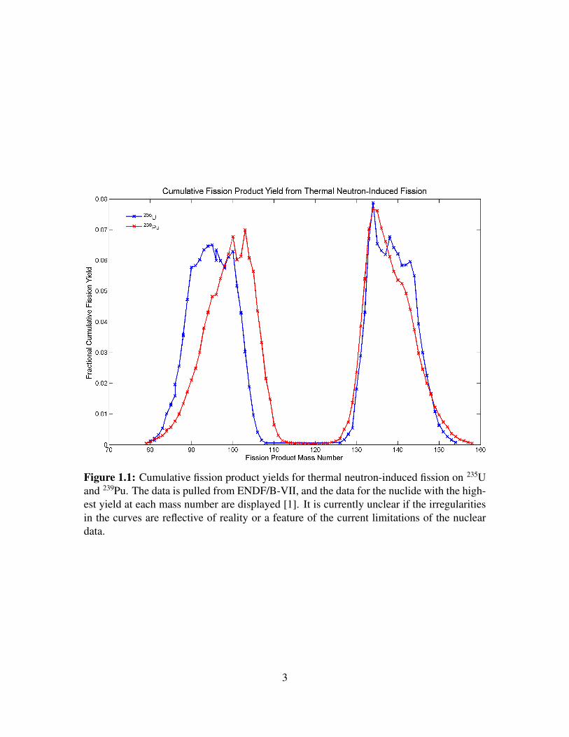
Figure 1.1: Cumulative fission product yields for thermal neutron-induced fission on 235Uand 239Pu. The data is pulled from ENDF/B-VII, and the data for the nuclide with the high-est yield at each mass number are displayed [1]. It is currently unclear if the irregularitiesin the curves are reflective of reality or a feature of the current limitations of the nucleardata.

3

Tabl

e1.

1:D

escr

epen

cies

and

unce

rtai

ntie

sin

FPY

betw

een

EN

DF

and

JEFF

data

libra

ries

.T

heiF

PYfo

rth

e13

1m

ass

chai

nas

repo

rted

inE

ND

F/B

-VII

and

JEFF

data

libra

ries

are

show

n.D

ata

for

131m

Xe

and

131 I

are

diff

eren

tby

afa

ctor

of3.

0an

d4.

1,re

spec

tivel

y.

EN

DF/

B-V

IIJE

FF

Nuc

lide

Yie

ld[%

]R

elat

ive

Unc

erta

inty

[%]

Yie

ld[%

]R

elat

ive

Unc

erta

inty

[%]

Rel

ativ

eD

iffer

ence†

131m

Xe

2.41±

1.54×

10−

964

7.43±

2.81×

10−

938

3.01

131 I

1.08±

6.92×

10−

564

4.43±

1.67×

10−

538

4.10

131m

Te2.

24±

1.43×

10−

364

3.80±

1.24×

10−

333

1.70

131 Te

7.54±

4.83×

10−

464

1.38±

0.44×

10−

333

1.83

131 Sb

1.50±

0.34×

10−

223

2.34±

0.25×

10−

211

1.56

131 Sn

6.93±

4.44×

10−

364

1.32±

0.43×

10−

333

0.19

† Thi

sfa

ctor

was

com

pute

dby

divi

ding

the

yiel

das

repo

rted

inth

eJE

FFlib

rary

byth

eco

rres

pond

ing

EN

DF

valu

e.

4

1.2 Previous Work

To date, long-lived FP have been measured using chemical separations and destructive

analysis, and FPY curves have been fit to this data using functional forms suggested by

physics. The following section will summarize major measurement efforts determining

cumulative fission product yields of nuclides at the end of decay chains. A summary of the

work to estimate iFPY follows.

1.2.1 Cumulative Yield Measurements

Possibly the largest effort to measure FPY for fission spectrum and thermal (reactor

spectrum) neutrons was performed at Los Alamos National Laboratory (LANL) in the

1970’s as a part of the Inter-laboratory Liquid Metal Fast Breed Reactor (LMFBR) Re-

action Rate (ILRR) collaboration [9, 10, 11]. This effort included research groups from

multiple institutions, led by scientists at the National Institute of Standards and Technology

(NIST). The campaign was primarily aimed at performing high-confidence (within 2.5%

uncertainty) measurements of fission yields for nuclides typically used as burnup moni-

tors, e.g., 95Zr, 99Mo, 137Cs, 140Ba, 141,143,144Ce, and 147Nd, in order to support fast reactor

development.

Fission spectrum measurements were performed using the LANL BIG TEN critical as-

sembly, thermal measurements were done using the Omega West water cooled reactor, and

14 MeV irradiations were conducted at the LANL Cockcroft-Walton accelerator facility

using a tritium target. The fissionable targets examined included 235U, 238U, and 239Pu.

The scientists at LANL utilized techniques initially developed during the Manhattan

Project. The number of fissions were directly measured using fission chambers developed

by scientists at NIST, and fission products were quantified using beta counting performed

5

after radiochemical separation. During irradiation, a fission chamber with small, thin tar-

gets (microfoils) of fissionable material was placed alongside a larger target (macrofoil) of

the same material. The fission chamber included two independent microfoils to provide

redundant measurements of the number of fissions during irradiation, and the macrofoil

produced enough FP for analysis.

In order to quantify fission products and determine the yields, analysts used a technique

of developing successive ratios, called K, R, and Q factors. K factors relate the number

of fissions, determined using the fission chamber during irradiation, to detector response

when counting a particular fission product, isolated using radiochemical separations. R

factors relate the K factor for a fission product relative to a reference fission product such

as 99Mo, produced from a standard target in a standard neutron spectrum. Finally, the Q

factor is a ratio of the R factor at a given neutron energy and fissionable target relative to a

reference energy and target.

In these experiments, 99Mo was used as the reference fission product due to its low

variability with incident neutron energy and fissionable material. Only cFPY of long-lived

nuclides were examined due to the lengthy time required to perform the necessary radio-

chemical separations.

Another measurement campaign was undertaken in the 1970’s by the Commissariat a

l’Energie Atomique (CEA) in France [12]. Cumulative fission yields were estimated for

several fission products following the irradiation of 233U, 235U, 238U, and 239Pu by thermal,

fission, and 14 MeV neutrons.

Scientists utilized fission chambers to quantify the number of fissions. These chambers

used a microfoil for monitoring the number of fissions, and FP were produced in a macro-

foil and analyzed with gamma-ray spectrometry measurements performed after the end of

irradiation. Activation foils were included in the chamber to determine the approximate

neutron spectrum incident on the macrofoil sample. A diagram of the fission chamber is

6

provided by the authors and given in Figure 1.2.

Figure 1.2: The fission chamber (1) used by Laurec et al. A microfoil (5) was used tomonitor the number of fissions occuring during irradiation, while a larger macrofoil (4)produced enough fission products suitable for gamma-ray counting after irradiation. Acti-vation foils (3) were also included to approxiamte the neutron spectrum [12].

The authors detail their analysis method for quantifying the cumulative fission yields

for long-lived nuclides. They account for decay of the nuclides during irradiation and

prior to counting. In addition, they account for changes in flux, e.g., cyclic irradiation or

non-constant fluxes, and two-nuclide parent/daughter relations; however, they neglect in-

dependent fission yields of the daughter product† and only cumulative FPY are considered.

In addition, the range of fission products reported is somewhat limited: 95Zr, 97Zr, 99Mo,

103Ru, 105Rh, 131I, 132Te, 140Ba, 141Ce, 143Ce, and 147Nd.

More recently, scientists at Idaho National Laboratory (INL) have made measurements

of cumulative fission product yields for stable fission products at the end of fission decay

chains [13]. Citing other researchers’ success applying inductively-coupled plasma mass-

spectrometry (ICP-MS) for fission product measurements [14, 15, 16], Glagolenk et al.

†In the case of long-lived fission products that reside near or at the end of decay chains, independentfission yields are on the order of a thousandth of a percent.

7

measured stable fission products in 44 - 58 % enriched uranium test fuel samples irradiated

in the Advanced Test Reactor (ATR) during a Reduced Enrichment for Research and Test

Reactors (RERTR) research program at INL and 78 % enriched uranium metallic fuel irra-

diatied in the Experimental Breeder Reactor (EBR-II). Thermal cFPY were determined for

fuels irradiated in ATR and fast neutron-induced fission yields in the fuels taken from EBR-

II. In both cases, the samples were used for fuel testing, and irradiations were very long

(burnup at discharge were approximately 15.1 % and 3.9 % in the ATR and EBR-II exper-

iments, respectively). As a result, the authors cite neutron capture reactions as significant

interferences in the analysis. Other sources of uncertainty include dissolution and fission

fragment migration problems associated with the radiochemical preprocessing required for

ICP-MS.

In 2009, Metz et al. published their results from initial work in measuring fission yields

for short-lived fission products [17, 18]. Researchers prepared high purity (≤ 3 % contami-

nant) targets of 233U, 235U, 238U, 237Np, 239Pu, and 241Am in quantities sufficient to produce

approximately 108 fissions following a $ 2 reactor pulse at the Washington State University

1 MW TRIGA research reactor. The samples were counted multiple times following the

end of irradiation on three different HPGe-based gamma-ray spectrometers. Nuclides were

quantified in multiple spectra when appropriate and cumulative fission yields were quan-

tified. Activities were decay-corrected to the end-of-irradiation time, yielding consistent

fission product activity per fission.

1.2.2 Independent Yield Estimation

Cumulative fission product yields give the total number of nuclei of a particular FP be-

ing produced following some number of fissions in a particular configuration, i.e., particle,

target and energy. To date, iFPY have been found using semi-empirical models to find dis-

8

tributions of FP in terms of mass, charge, and isomeric state, e.g., metastable states. The

product of these three marginal distributions gives the total iFPY, the amount of a particular

FP expected to be produced directly from the fission of target nuclei such as 235U [19].

Wahl has developed these models since the 1960’s. His initial ZP (A) describes the

distribution of charge (proton number) for a nucleus of mass A that is normally distributed

about ZP with a width parameter σ [20]. These semi-empirical distributions were used to

calculated iFPY and normalized to give sums over FP decay chains that are consistent with

the measured values for cFPY.

Further research showed regular variation of σ with proton and neutron numbers as well

as over- and under-estimations in the predicted yield values based on lighter versus heavier

FP. This effect was later termed the even-odd effect and Wahl updated his model to include

these effects [21, 22].

While these theoretical values have proved useful to date, measurements of iFPY are

needed to either confirm the validity of the models and/or reduce uncertainty in the reported

values, or suggest that models must be updated to capture additional physics if measured

values repeatedly differ from those in the literature. Referring to the fidelity of the ZP

model, Wahl acknowledges the need for further measurements of cFPY for low-yield FP

and direct measurements of iFPY:

Uncertainties in experimental yields, and in σ [the width of the symmetric

charge distribution about the central value] are reflected as uncertainties in the

empirical ZP values. Of course, errors may be larger if the assumed charge

distribution curve is not applicable, and it should be remembered that the curve

is derived from data for only a few mass numbers with high fission yields.

Curves for mass numbers with low yield might well be different in width or

lack symmetry, and yields of fission products or fragments whose compositions

9

are close to nuclear shell edges might well deviate in yield from a smooth

curve [20].

1.3 Goals

The three main goals of the presented research are as follows:

1. Measure the activity of fission products with half lives ranging from minutes to days

using gamma-ray spectrometry,

2. Assess math methods for determining the cumulative and/or independent fission

yields for the measured radionuclides, and

3. Evaluate different methods for estimating the uncertainty in the determined values.

10

2 | Theory

This chapter explains the theoretical basis of the presented research and details the ma-

jor results, methods, and algorithms used to produce fission products, collect gamma-ray

spectra of the irradiated material, identify gamma-emitting radionuclides, calculate activi-

ties of fission products in decay chains, and estimate fission product yields. Table 2.1 gives

the mathematical notation used throughout this document.

11

Table 2.1: List of mathematical notation used throughout this document.

Symbol Meaning

NX(t) or N(X) number density of XAX(t) activity of X at time tσf microscopy fission cross sectionΣf macroscopic fission cross sectionσa microscopic absorption cross sectionσ(n,2n) microscopic cross for (n,2n) reactionσγ microscopic radiative capture cross sectionσ(n,p) microscopic cross section for (n,p) reactionφ(t) neutron cross section at time tχ

(i)X independent fission yield of Xχ

(c)X cumulative fission yield of XλX decay constant of Xγ gamma-ray intensity/yieldε(E) peak detector efficiency at energy Eu(·) standard uncertaintyθ parameters to be estimatedθ0 known parameters〈·〉 time-averaged value‖ · ‖p p vector normR the set of real numbersR+ the set of non-negative real numbersR++ the set of positive real numbersP[A|B] probability of A given BN (x|µ,Σ) multivariate normal distribution· mean value/best-estimateE[·] expectation

12

2.1 Analysis Overview

Our process for determining fission product yields involves four primary steps, de-

scribed below.

Produce Fission Products: The first step to measuring fission product yields is to pro-

duce fission products in a controlled, well-defined experiment. This includes sample

preparation, where the isotopic composition, mass, and density are recorded. This

target is then bombarded in a neutron field to produce fission products.

Identify Fission Products: Following the end of irradiation, gamma-ray spectra are col-

lected of the irradiated material. We choose to collect these spectra in list-mode using

digital spectroscopy equipment and process the data into sets of “time-sliced” spectra

offline. Time windows are chosen based on analytes’ half-lives in order to compro-

mise between statistics and informative activity time series that appreciably change

between spectra. Patterns of characteristic gamma-rays are compared between the

nuclear data and gamma-ray spectra to identify the observed FP.

Quantify Fission Products: Following identification, the activity of each FP is calcu-

lated using detector efficiency, peak areas, and nuclear data. Samples are sufficiently

dense to significantly attenuate photons emitted from within the irradiated targets.

Using the target, e.g., 235U, as an internal standard, the effective thickness of mate-

rial the photons traversed on average is estimated, and this result is used to create a

self-attenuation correction function. The activity of decay chains of FP are solved

simultaneously in order to account for radioactive decay sources and losses during

counting. This is done for each spectrum, giving activities of FP’s over time follow-

ing the end of irradiation.

13

Inverse Analysis: Using FP activity time series, FPY are estimated using a Bayesian in-

ference framework. A model of the buildup and decay of FP during irradiation and

during counting is used to predict activities which are compared to measured results,

and best-fit values for all unknown parameters are calculated with numerical opti-

mization. Finally, uncertainties from all inputs are propagated to the final results.

2.2 Experimental Analysis of Fission Products

This section describes the methods used to analyze gamma-ray spectra collected of ir-

radiated fissionable materials. Section 2.2.1 discusses attribution of observed photopeaks

to gamma-emitting radionuclides within the sample, and Section 2.2.2 describes the simul-

taneous solution method to calculate the activity of entire FP decay chains at the beginning

of counting for each identified radionuclide.

2.2.1 Nuclide Identification

Figure 2.1 shows a typical fission product gamma-ray spectrum. A highly-enriched

uranium foil was irradiated for five minutes in a 14.1 MeV neutron flux of approximately

2.5 × 108 cm−2s−1and allowed to decay for about six minutes prior to measurement. The

data shown was collected over a period of twenty minutes. More detail on the sample and

experiment are given in Chapter 5 on page 122. The spectrum shows the complexity ex-

pected in fission product gamma-ray spectroscopy: there are over 352 significant peaks,

considerable peak overlap (see Figure 2.2 on page 17), and large background continuum,

especially in the range of the 235U peaks that reside in the 110 - 225 keV range. Large

Compton continua increase the baseline/background upon which photopeaks lie and com-

plicate peak location algorithms (see the 150 - 250 keV region of the spectrum shown

in Figure 2.1 which features a large baseline arising from 235U). In addition, small peaks

14

may be obscured by nearby large peaks that alter the statistics used by peak-finding al-

gorithms. Many commercially available spectral analysis packages fail with such spectra

due to the large number of peaks, requiring a potentially massive data library for nuclide

identification, and large number of spectral interferences. This leads to a high-dimensional

problem that is largely intractable with existing techniques, especially for cases featuring

poor counting statistics.

Figure 2.1: Gamma-ray spectrum collected of an irradiated uranium foil. The foil wasirradiated for approximately five minutes, allowed to decay for six minutes, and measuredfor twenty minutes. There are over 352 significant peaks.

Each gamma-emitting radionuclide emits one or more characteristic gamma-rays at a

known energy and yield, i.e., how often a decay of a particular nuclide leads to emission

of the gamma-ray of specified energy. A match between the centroid energy of a measured

photopeak to the nuclear data associated with a particular gamma-emitting radionuclide in-

dicates the presence of that nuclide in the measured sample; however, many radionuclides

15

emit gamma-rays of similar energies that create spectral interferences †. Additional char-

acteristic gamma-rays are used to differentiate nuclides with spectral interferences. Ideally,

all the gamma-rays of a nuclide would be observed in a spectrum at the ratio given by the

yields reported in the nuclear data (adjusted for the detector efficiency); however, some

gamma-rays may be obscured by other peaks in the spectrum or be emitted at insufficient

abundance to be observed above the background. These complications make radionuclide

identification a difficult pattern matching task better suited to machines than humans.

Figure 2.2 shows the overlapping peaks and multiplet fitting in the 450-470 keV region

of the spectrum shown in Figure 2.1. The multiplet fitting was performed manually with

Genie-PC by interactive application of the Interactive Peak Fitting tool [23]. Considerable

effort is needed on the part of the analyst to ensure multiplets are fit correctly. Extract-

ing peaks from multiplet regions may lead to skewed estimates of centroid energies and

peak areas, which complicates nuclide identification and activity calculations. In addition,

peaks are assumed to be Gaussian in Genie-PC, and this assumption is not valid for FP

with low yields, specific activity, or gamma-ray yield. As will be described below, our

method treats overlapping peaks as a single peak and neglects exact multiplet fitting in

favor of more complex spectral interferences, which are then resolved using our convex

optimization framework.

Spectral interference resolution is inherently coupled to nuclide identification: deter-

mining if a peak measured in the spectrum is a valid signal from a nuclide or an interference

from a different nuclide. Assuming the analyst can confidently identify all radionuclides

contributing to the spectrum, the next step is to resolve spectral interferences. The con-

tribution of a interfering peak may be calculated using a secondary, interference-free peak

and the nuclear data, multiplied in a ratio as shown below, and subtracting this contribution

†The notion of similar energy is dependent on the energy resolution of the detector used.

16

Figure 2.2: Multiplet peak fitting in the 450-470 keV energy range of the spectrum shownin Figure 2.1. Multiplet fitting was manually performing using Genie-PC.

from the interfering peak’s area.

C2 = C1

(γ2ε2γ1ε1

)(2.1)

Here Ci, γi, and εi are the counts, yield, and detector efficiency for the ith peak in the spec-

trum. This technique has several shortcomings: (1) it requires that the analyst know the

nuclides that are contributing to the peak (recall the resolution of spectral interferences is

coupled with radionuclide identification), (2) it requires peaks that are free from interfer-

ences to calculate the contribution to the interference, and (3) it increases uncertainty in the

peak areas. If interference-free peaks are not observed, a sequential process of interference

resolution may be pursued†, but uncertainties will typically compound. Large peak area

uncertainties increase the overall uncertainty in the determined activities.

A product of this research is a code module to aid in gamma-ray spectra analysis.

†In this method, an interference-free peak belonging to nuclide 1 is used to remove an interference withnuclide 2, and the result is used to calculate the contribution of nuclide 2 to a peak interfering with nuclide 3.This inductive process may be extended as far as necessary, but each step increases uncertainties.

17

Genie-PC by Canberra Industries is utilized to perform peak fitting and determine detector

efficiency correction factors. This analysis gives a list of peak energies, areas, efficiencies,

and associated standard uncertainties, which is used as input to our code. First, a peak

search produces a list of gamma-emitting radionculdies hypothesized to be in the sample

and set up an optimization problem to find the most likely mixture of radionuclides that

explains the observed pattern of photopeaks in the spectrum. The remainder of this section

summarizes these steps.

Peak Search

First, the area of each identified peak is corrected by the associated efficiency and

loaded in the spectrum vector s (see Figure 2.3a). For each peak energy, a database created

using data extracted from the ENSDF library is queried and all nuclides that emit a gamma-

ray within ∆ of the observed energy is saved into a list of hypothesized nuclides. During

this step, peaks within the spectrum that have energies within ∆ are pooled together and

the average energy is used to query the database (see Figure 2.3b).

Next, for each hypothesized nuclide, the intensities of its characteristic photons are

loaded into a response matrix R as shown in Figure 2.3c. Care is taken to preserve the

ordering of the gamma-rays and nuclides. Combining peaks during the peak search lessen

the reliance on correct multiplet fitting for spectral interference resolution in favor of res-

olution by implicit pattern matching and optimization. A small value δ is placed in s for

any gamma-ray in R not observed in the spectrum. Use of nonzero values for δ relaxes the

mismatch criteria in case low-intensity peaks from a hypothesized nuclide are not observed

above background, Compton continuum, and interferences in the spectrum. A reasonable

value for δ is the average counts per channel in the background (or the uncertainty in this

value) times the average width of peaks in number of channels.

18

(a) Loading the efficiency-corrected peak areasinto the initial spectrum vector s.

(b) Peak energies are compared to a databaseand overlapping peaks are combined.

(c) For each hypothesized nuclide, intensitiesof characteristic photons are loaded into the re-sponse matrix R.

(d) Small values δ are inserted into s to matchwith gamma-rays inR not observed in the spec-trum.

Figure 2.3: Visual representation of the basic peak search algorithm that populates theinitial list of hypothesized nuclides, vector representation of the spectrum, and responsematrix.

19

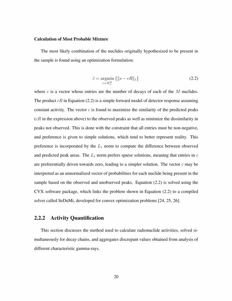
Calculation of Most Probable Mixture

The most likely combination of the nuclides originally hypothesized to be present in

the sample is found using an optimization formulation:

c = argminc∈RM+

{‖s− cR‖1} (2.2)

where c is a vector whose entries are the number of decays of each of the M nuclides.

The product cR in Equation (2.2) is a simple forward model of detector response assuming

constant activity. The vector c is found to maximize the similarity of the predicted peaks

(cR in the expression above) to the observed peaks as well as minimize the dissimilarity in

peaks not observed. This is done with the constraint that all entries must be non-negative,

and preference is given to simple solutions, which tend to better represent reality. This

preference is incorporated by the L1 norm to compute the difference between observed

and predicted peak areas. The L1 norm prefers sparse solutions, meaning that entries in c

are preferentially driven towards zero, leading to a simpler solution. The vector c may be

interpreted as an unnormalized vector of probabilities for each nuclide being present in the

sample based on the observed and unobserved peaks. Equation (2.2) is solved using the

CVX software package, which links the problem shown in Equation (2.2) to a compiled

solver called SeDuMi, developed for convex optimization problems [24, 25, 26].

2.2.2 Activity Quantification

This section discusses the method used to calculate radionuclide activities, solved si-

multaneously for decay chains, and aggregates discrepant values obtained from analysis of

different characteristic gamma-rays.

20

Simultaneous Decay Chain Solution

Many FP are short-lived and form large decay chains of radionuclides. FP are neutron-

rich and typically decay along an isobar by β− emission; however, some nuclides may also

decay by other modes such as neutron emission that couple isobars in the decay chain. As

radionuclides decay, activities vary during spectral acquisition, and the activity at a single

point in time is calculated. In this research, the activity at the beginning of counting is used.

Nuclide decay must be explicitly treated to calculate the correct activity at the begin-

ning of counting, especially when the half-life is similar to the counting time and activities

change drastically during counting. If there is considerable in-growth of a daughter nuclide

from the decay of a parent nuclide, the activities of both nuclides must be solved simul-

taneously in order to avoid an overestimation of the daughter nuclide’s initial activity. In

the case of short- and medium-lived FP in a decay chain, this argument is extended and the

entire decay chain must be solved simultaneously.

Figure 2.4 illustrates the situation. If three nuclides are coupled in a decay chain (left in

Figure 2.4), but solved separately, each nuclide is assumed to have the typical exponential

decay behavior in time,

A(t) = A0e−λt, (2.3)

shown in the right panel of Figure 2.4. This solution neglects the positive term from the

decay of the parent nuclide. Both sets of solutions have the same integral, i.e., would lead

to the same number of measured counts; however, the activity at the beginning of counting

is different for the daughter and granddaughter nuclides (red and yellow in Figure 2.4).

The approach for simultaneous solution of a chain of two nuclides is shown below.

AλA−−→ B

λB−−→ C (2.4)

21

Figure 2.4: Illustration of simultaneous decay-chain solution. The solution for activityat the beginning of counting is different when nuclides are treated as a decay chain (left)rather than solving for each nuclide’s activity separately and adjusting for decay duringcounting (right).

First, the time evolution of the concentration of each nuclide in this decay chain is found

using a system of ODEs, shown below in Equation (2.5).

ddt

(NA) = −λANA

ddt

(NB) = λANA − λBNB

(2.5)

These ODE’s are solved and multiplied by the appropriate decay constants to find the nu-

clides’ activities.

AA(t) = A(0)A e−λAt

AB(t) =1

λA − λB

(e−λBt

(A

(0)A λB + A

(0)B (λA − λB)

)− A(0)

A λBe−λAt

) (2.6)

Note, for clarity, the activities at time t = 0 of nuclides A and B are now denoted A(0)A

and A(B)B , respectively. Assuming a peak at energy Ei and a peak at energy Ej are used to

22

find the activities of nuclide A and B, respectively, the expressions shown in Equation (2.6)

are integrated as shown in Equation (2.7). Finally, these equations are solved to give the

activities of each nuclide in the decay chain. These solutions are shown in Equation (2.8).

CA(Ei) = γiε(Ei)

∫ tc

0

A(0)A e−λAsds

CB(Ej) = γjε(Ej)

∫ tc

0

e−λBs(A

(0)A λB + A

(0)B (λA − λB)

)− A(0)

A λBe−λAs

λA − λB

ds

(2.7)

A(0)A (Ei) =

CA(Ei)λAγiε(Ei)

(1− e−λAtc

)−1

A(0)B (Ei, Ej) =

((CB(Ej)

γjε(Ej)− A

(0)A (Ei)λB(e−λAtc−1)

λA(λA−λB)

)(λB(λA−λB)

1−e−λBtc

)− A(0)

A (Ei)λB

)λA − λB

(2.8)

Equation (2.8) is applied for each combination of characteristic photons observed in

the spectrum,i.e., values of i and j, to obtain a set of N pairs of values. The uncertainty in

the calculated activities, u(A(0)A ) and u(A

(0)B ), are found using conventional propagation of

uncertainty,

u(y)2 =∑k

(∂y

∂xk

)2

u(xk)2, (2.9)

where y denotes the calculated activity, A(0)A and A(0)

B , and xk are the uncertain inputs in

Equation (2.8).

23

Aggregating Multiple Results

Statistical variation and uncertainty are reduced by calculating nuclide activities with

multiple photopeaks and aggregating the results. A statistically robust approach† that ac-

counts for the inhomogeneous uncertainty associated with each value is used to calculate a

value to report. Many FP analyzed in this research are anticipated to have low count rates,

leading to poor counting statistics, and the statistical variation between activities deter-

mined with different characteristic gamma-rays leads to outliers. Additional outliers may

arise from spectral interferences that are not identified and removed.

The arithmetic (common) mean and weighted arithmetic mean are common aggregate

measures; however the mean is not robust to outliers and the weighted mean can overes-

timate the influence of a single datapoint with small absolute uncertainty‡ [29]. A more

robust statistical measure of the center of a set of datapoints is the median, which is less

sensitive to outliers; however, the standard median calculation, shown in Equation (2.10)

for a set of N datapoints {xi}Ni=1, does not consider the uncertainty associated with each

input observation, nor does it give an immediate output uncertainty.

x =

x(N+1)/2 N odd

1

2

(xN/2 + x1+N/2

)N even

(2.10)

Combining a bootstrapping procedure with the median as suggested by Helene [28]

remedies both of these shortcomings. The bootstrap median estimator is computed as

follows:

†Here the term “robust” refers to a method or measure’s resilience to outliers and other extreme data—that is, the presence of an outlier should minimally affect a value determined using a robust measure [27, 28].

‡The maximum likelihood estimation for weights is the inverse squared standard uncertainty, which leadsto small-uncertainty observations dominating the aggregate value. This effect may be somewhat mitigatedusing heuristic methods to engineer the weights to limit the influence of a single observation as discussed byRajput [29].

24

1. For each input datapoint with associated uncertainty, {(xi, u(xi))}Ni=1, sample M

points from the normal distribution N (x|xi, u(xi)2) and save the N ×M values,

2. DrawA bootstrap sets (with replacement) ofB values from theN×M pool of values

and compute the median for each bootstrap set,

3. Compute the mean and standard deviation for the A medians, i.e., fit a normal distri-

bution to the collection of median values.

The activities of daughter nuclides, e.g., nuclide B in Equation (2.8), are correlated with

the calculated activities of parent nuclides. Thus, the bootstrap median processing must be

applied to all nuclides in the decay chain simultaneously. In order to account for the corre-

lation between the activities for parent and daughter nuclides, the normal distribution used

to generate new samples is extended to a multivariate normal distribution with nontrivial

covariance. To construct the covariance matrix, we use the definition of covariance for two

variables xi and xj ,

Σij = E[(xi − xi)(xj − xj)], (2.11)

where E[·] denotes the expectation and the bar denotes the mean value. If the value of xi

changes, the covariance Σij gives the expected change in xj . Since xj is a function of xi,

the expected change is found using the partial derivative. If xi − xi = ∆, the value of xj

may be predicted as xj = xj +(xjxi

)∆. Thus,

Σij = E[(xi − xi)(xj − xj)] = ∆

(∂xj∂xi

)∆. (2.12)

Since we are free to choose a step size, choose ∆ = u(xi).

Σij = u(xi)2

(∂xj∂xi

)(2.13)

25

Now it remains to check that this definition leads to the desired properties of covariance.

1. Say xi − xi = 0. Then xi = xi and xj is xj by definition. Here ∆ is zero, which

suggests xj − xj = 0, which is consistent with our expectations.

2. The diagonal of the covariance matrix should be the variance of the random variable.

Using Equation (2.13), Σii = u(xi)2(∂xi∂xi

)= u(xi)

2, which is the variance of the

random variable by our assumption.

3. Finally, we check for symmetry. First, assume a value for u(xi). Using the propaga-

tion of errors, u(xj)2 =

(∂xj∂xi

)2

u(xi)2. Plugging the definition of the uncertainty in

xj and multiplying through by one shows the equivalence.

Σij = u(xi)2

(∂xj∂xi

)= u(xi)

2

(∂xj∂xi

)(∂xj∂xi

)(∂xi∂xj

)= u(xj)

2

(∂xi∂xj

)= Σji.

�

The generalized bootstrap median procedure for aggregating decay-chain activities is

given below.

1. For N sets of calculated values for a two-nuclide chain with uncertainties calculated

using propagation of errors (see Equation (2.9)),{

(A(0)A,k, u(A

(0)A,k), A

(0)B,k, u(A

(0)B,k))

}Nk=1

,

26

assemble the vector of mean values,

µ =

A(0)A,1 A

(0)B,1

A(0)A,2 A

(0)B,2

......

A(0)A,N A

(0)B,N

, (2.14)

and N 2× 2 covariance matrices,

Σ(k)ij =

(∂B∂A

)|k u(A

(0)A,k)

2 i 6= j

u(A(0)A,k)

2 or u(A(0)B,k)

2 i = j, (2.15)

2. For each set of observations indexed by k, sample M new points from multivariate

normal distributions N (x|µk,Σ(k)) and save the N ×M values,

3. DrawA bootstrap sets (with replacement) ofB values from theN×M pool of values

and compute the median for each bootstrap set,

4. Compute the mean and standard deviation for the A medians, i.e., fit a normal distri-

bution to the collection of median values.

Correcting Self-Attenuation

In high-density samples, gamma-rays born within a sample are attenuated as they tra-

verse the sample matrix, and self-attenuation must be accounted for in order to correctly

calculate nuclide activities given count rates of low- and medium-energy gamma-rays. We

suggest two methods for determining self-attenuation correction factors.

Case 1: Known Internal Standard

27

If there is a known gamma-emitting radionuclide present in the sample, as is the case

with a well-characterized actinide target used for FP production and FPY measurement,

the known nuclide may be used as an internal standard. Given a mass m of this internal

standard with molecular weight MW that emits a gamma-ray of energy E with intensity

γ, the expected count rate, Cr, may be calculated:

Cr =m

MWNAvλγε(E). (2.16)

We may define the effective thickness, xeff , of the sample to be the average distance a

photon born within the sample travels given it is eventually incident on the detector. With

this definition we may calculate the observed count rate by multiplying Equation (2.16) by

an attenuation factor e−µ(E)x averaged over distance traveled through the matrix, shown in

Equation (2.17).

Cr =m

MWNAvλγε(E)

(∫ x0e−µ(E)sds∫ x0

ds

)=

m

MWNAvλγε(E)

(1− e−µ(E)xeff

µ(E)xeff

)(2.17)

Equation (2.17) is solved transcendentally for the effective thickness and used to calculate

the attenuation function across the entire energy range of the analysis:

α(E) =1− e−µ(E)xeff

µ(E)xeff. (2.18)

Figure 2.5 shows Equation 2.18 evaluated for five effective thicknesses of uranium, calcu-

lated using NIST-evaluated mass attenuation coefficient functions [30]. The mass attenua-

tion function is shown in Figure 2.6. The attenuation function is multiplied by the peak

detector efficiency, ε(E), to form the effective efficiency function,

εeff (E) = ε(E)× α(E), (2.19)

28

Figure 2.5: Gamma-ray self-attenuation function evaluated using the mass attenuationcoefficient µ for uranium and five values for effective thickness ranging from 0.1 mm to 2mm.

29

Figure 2.6: Photon mass attenuation coefficient curve, µ(E)/ρ, provided by NIST [30].

30

which is used for all activities calculations (see Equations (2.8) and (2.9)).

Case 2: No Standard Available

Without an internal standard, the effective thickness and attenuation function may be

calculated by finding the relative difference in attenuation between two gamma-rays of

different energies. The ratio of count rates is given by

Cr,1Cr,2

=

(γ1ε(E1)

γ2ε(E2)

)(1− e−µ(E1)xeff

µ(E1)

)(µ(E2)

1− e−µ(E2)xeff

), (2.20)

which is solved transcendentally for xeff and used to compute the attenuation function and

effective efficiency using Equations (2.18) and (2.19), respectively.

2.3 Parameter Estimation

This section presents a summary of Bayesian inference as it pertains to parameter esti-

mation, develops the associated likelihood model and solves for the particular case of FPY

measurements. Solution methods to this problem and estimation of uncertainty are given

in Section 2.4 on page 46.

2.3.1 Bayesian Inference

Given a set of measurements, y, and a model that predicts the measurement response

depending on a vector of input parameters, θ, we aim to estimate the parameters θ by

finding the values that are best associated with the measurements. In Bayesian inference,

the best values for θ are defined as those with the greatest probability given the observed

measurements:

θ = argmaxθ

{P[θ|y]} = argmaxθ

{P[y|θ]P[θ]} , (2.21)

31

where the second equality follows from Bayes’s theorem. Note, the denominator is a nor-

malization constant and is invariant with respect to the maximization. The first term on

the right-hand side is the likelihood function†, which describes the likelihood of making

the observed measurements given a set of values for θ, and the second term is the prior

distribution for θ, which captures the prior knowledge (if any) about the parameters’ val-

ues. If there is no prior knowledge, then Equation (2.21) reduces to maximum likelihood

estimation (MLE). Implicitly, the left-hand side of Equation (2.21) is also a probability

distribution for θ. This is called the posterior distribution for θ, which captures the state of

knowledge about θ once the measurements y are combined with the prior.

To describe the likelihood of observing particular values following a measurement, we

develop a model for radiation counting. This model depends on the parameters in the vector

θ as well as the independent variable time, t,

yi = f(ti|θ) + εi, i = 1, 2 . . . , N, (2.22)

where εi is the error/noise on the ith measurement, yi.

Assuming each of the N observations/measurements and M parameters is identically

and independently distributed, the joint probability distribution is the product of each indi-

vidual distribution.

θ = argmaxθ{P[y|θ]P[θ]} = argmax

θ

{N∏i=1

M∏j=1

P[yi|θ]P[θj]

}(2.23)

Taking the logarithm of the objective function gives

†Note, the term P[y|θ] in Equation (2.21) is the likelihood distribution evaluated at θ, i.e., integratedabout θ.

32

θ = argmaxθ

{log

N∏i=1

P[yi|θ]M∏j=1

P[θj]

}

= argmaxθ

{N∑i=1

logP[yi|θ]M∑j=1

logP[θj]

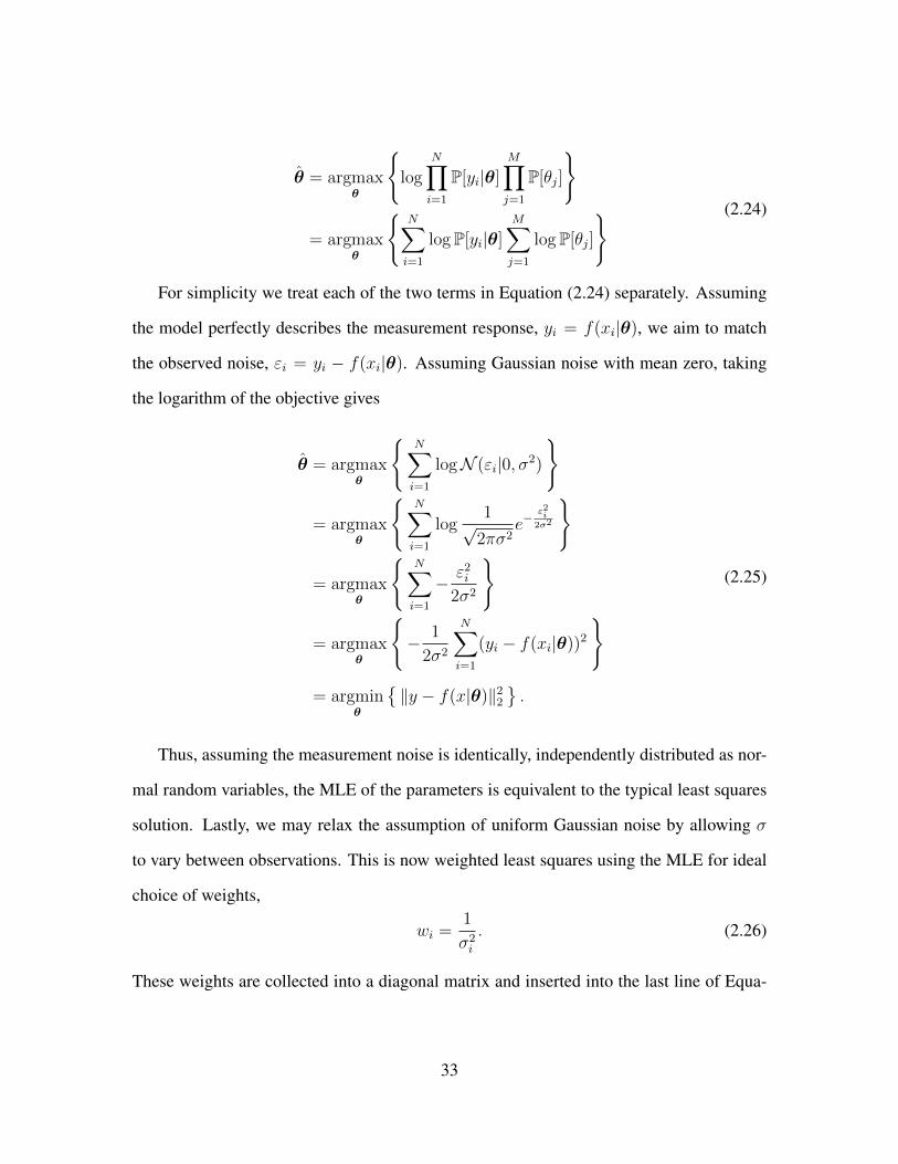
} (2.24)

For simplicity we treat each of the two terms in Equation (2.24) separately. Assuming

the model perfectly describes the measurement response, yi = f(xi|θ), we aim to match

the observed noise, εi = yi − f(xi|θ). Assuming Gaussian noise with mean zero, taking

the logarithm of the objective gives

θ = argmaxθ

{N∑i=1

logN (εi|0, σ2)

}

= argmaxθ

{N∑i=1

log1√

2πσ2e−

ε2i2σ2

}

= argmaxθ

{N∑i=1

− ε2i

2σ2

}

= argmaxθ

{− 1

2σ2

N∑i=1

(yi − f(xi|θ))2

}

= argminθ

{‖y − f(x|θ)‖2

2

}.

(2.25)

Thus, assuming the measurement noise is identically, independently distributed as nor-

mal random variables, the MLE of the parameters is equivalent to the typical least squares

solution. Lastly, we may relax the assumption of uniform Gaussian noise by allowing σ

to vary between observations. This is now weighted least squares using the MLE for ideal

choice of weights,

wi =1

σ2i

. (2.26)

These weights are collected into a diagonal matrix and inserted into the last line of Equa-

33

tion (2.25):

argminθ

{‖W (y − f(x|θ))‖2

2

}(2.27)

Prior Distribution

A challenge in Bayesian inference is the choice of prior distribution. There are numer-

ous methods to choosing a prior, e.g., specifying a parametric function and fitting the pa-

rameters to prior measurements or empirically determining a probability distribution func-

tion by binning prior observations into a histogram [31]. Here we describe the approach

we have followed.

Let the continuous distribution for θ be π(θ) and assume that some properties of π are

known:

Eπ[gk(θ)] = ωk, k = 1, 2, . . . , K, (2.28)

where Eπ denotes the expectation under the distribution π, and gkθ is a function such as

mean, variance, or indicator. In a physical system, the entropy describes the number of pos-

sible configurations. In 1948, Shannon used the concept of entropy to describe information

and uncertainty in signals [32]. Jaynes developed the application of maximum entropy prior

distributions as a way to incorporate prior information into Bayesian statistics in the least

restrictive way possible [33, 34]. For a continuous distribution π(θ), the entropy is

E(π) = Eπ[logπ(θ)

π0(θ)] =

∫log

π(θ)

π0(θ)π0(θ) dθ, (2.29)

where π0 is a reference measure needed for normalization† [31]. The choice of π(θ) con-

sistent with the constraints shown in Equation (2.28) that maximizes entropy contributes

the least information while still incorporating the known data. The ideal choice of prior

†A common reference measure is the Lebesgue measure on R, i.e., length [31].

34

distribution for θ is given by the following constrained optimization problem:

π?(θ) = argmax E(θ)

subject to Eπ[gk(θ)] = ωk, k = 1, 2, . . . , K.

(2.30)

This problem has been solved for some scenarios. When no constraints are known, π(θ)

is uniform and Equation (2.21) reduces to MLE. When the mean and variance/standard

deviation are known, π?(θ) is the normal distribution.

The prior for each parameter will be taken from the nuclear data and assumed to be

normally distributed, i.e.,

θj ∼ N (θ | θj, u(θj)2). (2.31)

Expanding the prior distribution,

M∑k=1

logN (θk|θk, u(θk)2) =

M∑k=1

log

(1√

2πu(θk)2e− (θk−θk)2

2u(θk)2

)

=M∑k=1

(− log(2π)

2− log (u(θk))−

(θk − θk)2

2u(θk)2

),

(2.32)

inserting this expansion into Equation (2.21), disregarding the constants, and exchanging

the maximum for minimum by inserting a negative gives the function shown in Equa-

tion (2.33).

θ = argminθ

{‖W (y − f(x|θ))‖2

2 +M∑k=1

(θk − θk)2

2u(θk)2

}(2.33)

As shown in Table 1.1 on page 4, there are significant differences in some FPY val-

ues reported in different data libraries. To construct a normal prior distribution, we must

assess the state of the data and determine a mean value to assign to µ and a value that re-

flects the uncertainty in the true value to assign to σ. In this research, we have used three

data libraries to construct prior distributions for FPY: ENDF/B-VII [1], JEFF3.1[2], and

35

JENDL [35]. Letting these three values be denoted (xi± u(xi)), we assign values to µ and

σ with Equations (2.34) and (2.35), respectively.

µ =1

3

3∑i=1

xi (2.34)

σ = 3×max{u(x1), u(x2), u(x3)} (2.35)

Using the maximum reported uncertainty has several rationale:

1. The largest value for uncertainty is the most conservative estimate,

2. Propagating the uncertainty through Equation (2.34) actually reduces the reported

uncertainty, which is inappropriate given the apparent uncertainty in the value (see

Table 1.1 on page 4),

3. Using a scaled value of the maximum reported uncertainty ensures that the normal

distribution covers the distribution implied by the values reported by the three data

sources.

Figure 2.7 illustrates these points. When the uncertainty is taken from propagation of un-

certainty (yellow), the distribution is too narrow and does not sufficiently cover the range

in values the FPY could taken. Note, the variation in values shown are small, and the prob-

lem is greater with less studied FP. The scalar value of 3 was determined from a sensitivity

study (see Section 3.5 on page 90).

2.3.2 Likelihood Model Development

In this section, we develop the likelihood function,

‖W (y − f(x|θ)‖22, (2.36)

36

Figure 2.7: Values for the cumulative yield of 140Ba and the independent yield of 140La.Normal distributions are shown for the values taken from the ENDF, JEFF, and JENDL datalibraries. The mean values are computed and distributions are illustrated for these valuesusing uncertainties obtained through propagation of uncertainty as well as the maximumreported uncertianty value.

37

introduced in the previous section. This function relates the probability of observing the

measured detector response, given assumed values of unknown parameters, θ (see Sec-

tion 2.3.1 on page 31). When Gaussian noise is assumed, maximizing this probability is

equivalent to minimizing the difference between measured and predicted values in the L2-

norm sense. We discuss the three terms, y and f(x|θ) and W , in the remainder of this

section.

Measured Values: y

Using the methods discussed in Section 2.2.2 on page 20, the activities of FP identified

from a set of gamma-ray spectra collected of irradiated material are calculated simultane-

ously for entire decay chains along with the associated uncertainties. It may not be possible

to determine the activity of each analyzed radionuclide in each spectra, i.e., at each time

step in the time series, therefore we index the activities time series of each nuclide with

index j for each nuclide separately, as shown below.

{Aj(ti)± u(Aj(ti))}i∈Ij (2.37)

Predicted Nuclide Activities: f(y|θ)

To describe the activities of FP during measurement, we have developed a flexible

solver capable of calculating the time evolution of the coupled set of FP shown in Fig-

ure 2.8. There are several possible source and loss terms for any particular nuclide, AZX:

fission, decay loss, decay source (from the decay of a parent nuclide), neutron absorption

loss, source from radiative capture (reaction A-1ZX(n,γ)A

ZX), source from (n,2n) reactions

from nuclide A+1ZX, and source from (n,p) reactions from nuclide A

Z+1X. Coupling of iso-

bars by neutron emission could be modeled; however, this feature is currently not modeled

because decay by neutron emission has not been observed in the FP studied to date (see

38

Chapters 4 and 5)†. As shown, the cFPY are used for the first nuclide in each decay chain

and the iFPY are applied for each subsequent daughter nuclide. Note, the loss terms from

neutron absorption are not shown in Figure 2.8.

A

Stable

B

T1/2 =TB

C

T1/2 =TC

D

T1/2 =TD

F

T1/2 =TF

G

T1/2 =TG

H

T1/2 =TH

J

T1/2 =TJ

K

T1/2 =TK

σγ σγ

σγ σγ

σγ σγ

σ(n,p)

σ(n,p)

σ(n,p)

σ(n,p)

σ(n,p)

σ(n,p)

σ(n,2n) σ(n,2n)

σ(n,2n) σ(n,2n)

σ(n,2n) σ(n,2n)

λD λF λG

λH λJ λK

λB λC

σa

σa

σa

χ(i)A χ

(i)B χ

(i)C

χ(i)D χ

(i)F χ

(i)G

χ(c)H χ

(c)J χ

(c)K

Figure 2.8: Nuclide diagram showing the general system of coupled fission products. Inthis example, all possible couplings are displayed and nuclide A is shown as stable forillustration. Given the included nuclides, the displayed system is most appropriate forstudying the independent fission yields of nuclides B and F, as well as the cumulativefission yield of nuclide J.

The system shown in Figure 2.8 is described by a system of coupled first-order differ-

ential equations (ODE), which are shown in Equation (2.38).

ddt

(N ) = f(N , t |θ,θ0) (2.38)

Here the vector of unknown parameters, e.g., neutron flux or FPY, are differentiated from

†This extension could easily be added by adding the line dN(i) = dN(i) + BR*dcy(i+4); tothe loop on lines 237-261 in Bateman.m.

39

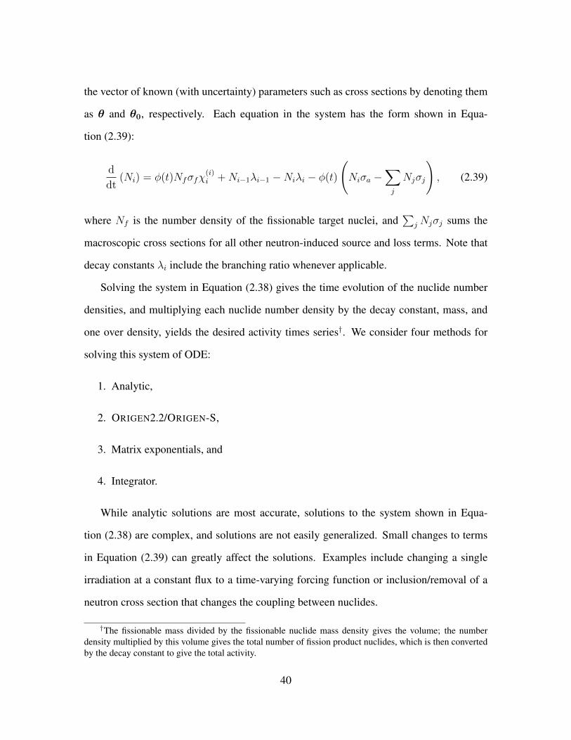
the vector of known (with uncertainty) parameters such as cross sections by denoting them

as θ and θ0, respectively. Each equation in the system has the form shown in Equa-

tion (2.39):

d

dt(Ni) = φ(t)Nfσfχ

(i)i +Ni−1λi−1 −Niλi − φ(t)

(Niσa −

∑j

Njσj

), (2.39)

where Nf is the number density of the fissionable target nuclei, and∑

j Njσj sums the

macroscopic cross sections for all other neutron-induced source and loss terms. Note that

decay constants λi include the branching ratio whenever applicable.

Solving the system in Equation (2.38) gives the time evolution of the nuclide number

densities, and multiplying each nuclide number density by the decay constant, mass, and

one over density, yields the desired activity times series†. We consider four methods for

solving this system of ODE:

1. Analytic,

2. ORIGEN2.2/ORIGEN-S,

3. Matrix exponentials, and

4. Integrator.

While analytic solutions are most accurate, solutions to the system shown in Equa-

tion (2.38) are complex, and solutions are not easily generalized. Small changes to terms

in Equation (2.39) can greatly affect the solutions. Examples include changing a single

irradiation at a constant flux to a time-varying forcing function or inclusion/removal of a

neutron cross section that changes the coupling between nuclides.

†The fissionable mass divided by the fissionable nuclide mass density gives the volume; the numberdensity multiplied by this volume gives the total number of fission product nuclides, which is then convertedby the decay constant to give the total activity.

40

Since most optimization solution algorithms are iterative [25], ORIGEN carries too

much overhead to be used effectively [36]. At each iteration, a text input file must be

generated and passed to the code, a text output file is generated by the code, and an ex-

ternal parser must process the file and pass the results to the optimization solver. If the

neutron flux varies in time, input/output file complexity and computation time increases.

In addition, we require complete control in specifying all parameters in Equation (2.39)

in order to best match the known nuclear parameters to values that reflect the experiment,

e.g., cross sections computed with the appropriate neutron spectrum. Furthermore, greater

control over parameter specification allows increased flexibility in which values may be

treated as unknown values to be estimated.

By implementing a custom solver using the method of matrix exponentials [37], the

overhead of writing input files and parsing output files may be avoided and parameter con-

trol is increased. Matrix exponentials are only applicable for constant equations. As shown

in Equation (2.39), the neutron flux, φ(t), is a time-varying forcing function. In order to

apply the method of matrix exponentials, the time domain must be partitioned such that

the neutron flux is constant in each time region. The system of equations is solved in each

time region and boundary conditions must be applied to ensure continuous solutions. Ex-

periments with complex neutron flux behavior such as cyclic irradiations or pulses make

matrix exponential solutions exceedingly complex.

To achieve maximum user control, flexibility, and speed, we have implemented a solver

using a Runge-Kutta integrator, which solves the system shown in Equation (2.38) through

direct, numerical integration as shown in Equation (2.40) [37].

N (t) =

∫ T

t0

(dNdt

)dt =

∫ T

t0

(f(N , t |θ,θ0)) dt (2.40)

Runge-Kutta algorithms give numerical approximations for the functions, N (t), by dis-

41

cretizing the above integral [37]. The simplest version of such a solution method is the

Euler method, where the trajectory is solved by updating the current function values using

the defined differential:

N (tn+1) = N (tn) + hdN

dt

∣∣∣∣t=tn

, (2.41)

where h is the time step. This uses the value for the derivative at the left side of the time

interval. This method may be improved using additional values of the derivative.

The classic fourth-order Runge-Kutta algorithm uses four values of the derivative for

each time step:

1. the beginning of the time interval,

2. the midpoint of the time interval,

3. the midpoint of the time interval using an updated estimate based on (2), and

4. the end of the interval.

These four above values are combined to produce the best estimate for N (tn+1) using

quadrature weights.

The Runge-Kutta integrator produces an adaptive time mesh, {ti}i∈Imesh , and the nu-

clide trajectories are evaluated at each time step.

{Rθ,j(ti)}i∈Imesh j = 1, 2, . . . . (2.42)

The solution depends on the parameter values θ, and the dependency is signified by the

subscript. The time mesh created for the numerical solution by Runge-Kutta integration is

different than the time steps at which nuclide activities are measured, and linear interpola-

42

tion is used to obtain predicted values for nuclide activities at the same time values as the

measured values†.

Uncertainty in Differences: W

There are two sources of uncertainty that appear in the likelihood function (see Equa-

tion (2.36)): the measured values and the predicted values produced by the Runge-Kutta

solver.

The uncertainty in the measured values are calculated as shown in Equation (2.9) in

Section 2.2.2 on page 20, but the uncertainty in the Runge-Kutta values {Rθ(ti)}Imesh

must be calculated. We have performed perturbation studies to determine how solutions

are affected by changes in the inputs. Two examples are shown below. Figure 2.9 shows

solutions for a three-nuclide system with mean input values (solid line),±1σ values for the

decay constant of the first daughter product (dashed line), and ±2σ values (dotted line).

Figure 2.10 shows the results of a similar study; however both the decay constant and

fission yield of the first daughter product are perturbed. Further studies were performed,

and the results are consistent with those shown in Figure 2.9 and 2.10.

In all cases, the nuclide trajectories produced with perturbed inputs were linearly related

to the trajectories produced with mean-value inputs, so we estimate the uncertainty in the

Runge-Kutta solutions as shown in Equation (2.43).

u(Rθ,j}i∈Imesh) = αj {Rθ,j(ti)}i∈Imesh j = 1, 2, . . . (2.43)

It remains to calculate the appropriate scalar, αj , for each nuclide in the system. We have

solved a simplified system, i.e., single irradiation with constant neutron flux, and explicitly

propagated all input uncertainties using conventional propagation of uncertainty (see Equa-

†The Runge-Kutta time mesh is sufficiently fine to ensure that linear interpolation is locally accurate.

43

Figure 2.9: Several solutions of a three-nuclide system of coupled radionuclides (desig-nated by colors) using several sets of perturbed values (designated by line style) for thedecay constant of the first daughter product, λF (see Figure 2.8 on page 39).

44

Figure 2.10: Several solutions of a three-nuclide system of coupled radionuclides (desig-nated by colors) using several sets of perturbed values (desiginated by line stile) for thedecay constant and fission yield of the first daughter product, λF and χ(i)

F (see Figure 2.8on page 39).

45

tion (2.9)) and calculated αj . This calculation is done offline and then αj values are used as

inputs to the calculation so the uncertainty in Runge-Kutta solutions are quickly calculated

at run time.

Finally, we construct the weights matrix W . Each entry of the likelihood function is

the difference between {Aj(ti)}i∈Ij and the corresponding predicted results, {Rθj(ti)}i∈Ij

(recall, the values given directly by the Runge-Kutta solver are used to interpolate and find

predicted values at the same time values as those obtained from experimental measure-

ments). The uncertainty in each difference is the sum of the individual uncertainties added

in quadrature. The time series for each nuclide are concatenated to make a single column

vector. Thus, W is defined as shown below in Equation (2.44).

W = diag

(1

u(A1(t1))2 + α21Rθ1(t1)2

,1

u(A1(t2))2 + α21Rθ1(t2)2

, · · ·)

(2.44)

2.4 Solution of Optimization Problem

This section discusses the final optimization problem developed for the determination

of FPY or other parameters in the Bateman equations as well as the challenges to solving

this problem. Three tested solution methods are presented in Section 2.4.2 on page 48 and

two methods for uncertainty estimation are presented in Section 2.4.3 on page 54.

2.4.1 Final Optimization Problem

Using the developments of the previous section, the final optimization objective used to

determine FPY is given in Equation (2.45).

θ = argminθ∈R++

∑j

∑i∈Ij

W (Aj(ti)−Rθj(ti))2 +

∑k

((θk − θk)2

2u(θk)2

) (2.45)

46

Note the domain has been explicitly constrained to the positive real numbers.

The domain is a subset of R, and is a convex set [25]. The objective function defined

over this domain is a sum of two terms: the L2 norm of the weighted difference between

measured and predicted activities and the sum of scaled quadratic differences between

the estimated and literature values of parameters. First, any p-norm is convex. Second,

quadratic functions such as (θk − θk)2 are convex and so is the scaled sum of such terms.

Sums of convex functions are convex; thus the prior distribution term is convex. In conclu-

sion, since the objective function and the domain over which it is defined are both convex,

the entire optimization problem is convex [25].

The convexity of Equation (2.45) admits many solution methods, some of which were

tested in this research and will be discussed in Section 2.4.2 on the next page. Convexity

also guarantees that a global optimum exists and is solvable. However, the problem shown

in Equation (2.45) presents challenges. Uncertainty and biases in activity estimates make

the objective function non-smooth. The irregular topology leads to difficulties estimating

gradients as local behavior of the function is not always reflective of the function’s global

behavior. In addition, small changes to θmay not cause a discernible change in the function

value, potentially causing iterative solvers to stop updating even though an optimum has

not been found.

Optimization of noisy functions is difficult, although some solvers are more robust to

noise than other algorithms (see the follow section). A possible remedy is to use large step

sizes when numerically estimating derivatives. A restart method may be used to improve

solver performance. Using a restart method, the solver is run multiple times using random

starting points, and the optimal result is found from direct examination of the pool of results

generated by restart.

47

2.4.2 Solution Methods

This section describes three solvers applied to the problem in Equation (2.45): the

Nelder-Mead Simplex Direct Search (NMS) [38, 39], Newton’s Method (NM) [40, 41],

and the Levenbgerg-Marquardt (LM) algorithm [42]. These methods range from a global,

derivative-free method (NMS), to a localized method that uses gradients and Hessian (cur-

vature) to accelerate local convergence (NM). The LM algorithm is an intermediate method

that limits the need for derivative estimation and moves between global and local methods

at each iteration.

Nelder-Mead Simplex Direct Search

The NMS is a heuristic algorithm for nonlinear optimization that is applicable when

derivatives of the objective function are not available [38]. To optimize a multivariate

function, f , over a k-dimensional space, a k-simplex† is initialized and transformed based

on a set of rules. Through transformations, the simplex traverses the function space {x ∈

Rk+1} ∪ {f(x ∈ Rk+1)} until a convergence criterion is met. Following the description

given in [43, 39, 44], the algorithm proceeds as follows:.

1. Initialize A k + 1-dimension simplex is initialized and the objective is evaluated at

each vertex, f(xi), i = 1, 2, . . . , k + 1.

2. Order The vertices are ordered according to their objective values: f(x1) ≤ f(x2) ≤

· · · ≤ f(xk+1), and the center of mass x0, of all but the worst point is found.

3. Reflect The worst vertex, i.e., the vertex with the largest objective value xk+1, is

reflected across x0 and labeled xr. If f(x1) ≤ f(xr) < f(xk), set xk+1 = xr and go

to step 2.

†A k simplex is the k + 1-dimensional convex hull of k + 1 points.

48

4. Expand If f(xr) < f(x1), define xe by expansion. If f(xe) < f(xr), set xk+1 = xe

and go to step 2. If not, set xk+1 = xr and go to step 2.

5. Contract If f(xr) ≥ f(xk), define xc by contraction. If f(xc) < f(xk1), set xk+1 =

xc and go to step 2.

6. Shrink Move all vertices except the worst towards x1 and go to step 2.

These steps are repeated until one or more of the following convergence criteria are met:

1. The points in the domain get sufficiently close together, e.g., d(xi, xj) ≤ εd ∀ i, j,

where d(·, ·) is a metric,

2. The objective values get sufficiently close together, e.g., |f(xi)− f(xj)| ≤ εf ∀ i, j,

3. A maximum number of iterations or computation time is exceeded.

Figure 2.11 show the reflection, expansion, contraction, and shrinkage transforms for a 2-

simplex. The NMS algorithm is implemented within Matlab using the optimization func-

tion “fminsearch.”

Unlike Newton’s method, the NMS solver does not require derivatives of the objec-

tive function, and the solver avoids errors from numerically estimating the gradient of the

objective function. However, there is no guarantee of the solver converging to a global op-

timum [44], and many iterations are typically required. One solution to the solver getting

stuck in local optima is to run the algorithm multiple times starting with different initial

simplexes (see the discussion of the restart method in Section 2.4 on page 46). After mul-

tiple iterations, the solution with the smallest objective value may be chosen as the best

estimate. Another option is to report a weighted sum of the solutions, using the squared

inverse of the objective/penalty value for each proposed solution as the weighted factor.

In our implementation, we have chosen to use the solution, θ, with the smallest objective

value.

49

(a) Reflection transform (b) Expansion transform

(c) Contraction transform (d) Reduction transform

Figure 2.11: Transformation operations used in the NMS search. In this figure, the centerof mass point is labeled c, x1 is labeled xl, and xk+1 is labeled xh. Taken from [43].

50

Newton’s Method

Newton’s method is a well-understood root-finding method with faster convergence

than other typical methods, e.g., gradient descent [40, 25]† Typically, Newton’s method

will converge within tens of iterations, as opposed to other algorithms which require hun-

dreds or thousands of iterations. This is a favorable property as the number of required

forward calculations required to estimate the various derivatives to populate the gradient

and Hessian matrices for the system could lead to a large computational burden.

To find a minimum or maximum of the objective function shown in Equation (2.45),

g(A,Rθ), we employ Newton’s method to find a zero of the gradient of this function:

∇g(A,Rθ) = 0. (2.46)

Implicitly, the values in θ are the independent variables.

After initializing the algorithm with initial values for the parameters, denoted θ1 to

avoid confusion with the known parameters in the ODE system (see Equation (2.38)),

Newton’s method proceeds with the following rule for successive iterations until a specified

number of iterations are performed or a convergence criterion is met:

θn+1 = θn − γH−1(g(A,Rθn))∇g(A,Rθn). (2.47)

Here H(g(A,Rθn)) denotes the Hessian matrix evaluated at θn, H−1 denotes the inverse

of this matrix, and γ is a weighting factor in the interval (0, 1]. When γ = 1, the classical

Newton’s method algorithm results; however, a smaller nonzero value may be chosen to

†In fact, for any local extremum x0 ∈ RN , there is a neighborhood around x0 such that Newton’s methodwill converge quadratically as long as the algorithm is started within the neighborhood, the Hessian matrix isinvertible, i.e., the steps in the algorithm may be computed, and the objective function is Lipschitz continuouseverywhere in the neighborhood [40].

51

increase stability, and other procedures may be followed to ensure the step results in a

descent, i.e., smaller value for g(A,Rθ) with each iteration; however this step comes at the

price of additional complexity [40].

An example convergence criterion is given by Boyd [25]:

∇g(A,Rθn)TH(g(A,Rθn))∇g(A,Rθn) ≤ ε, (2.48)

i.e., the step prescribed by Newton’s method becomes sufficiently small.

Rather than explicitly compute the inverse of the Hessian, the following system is

solved numerically:

Hp = ∇g(A,Rθ), (2.49)

such that p approximates the desired matrix product. This formulation requires the gradient

and Hessian of the objective.

The gradient is the vector of first derivatives of the objective with respect to each inde-

pendent variable, i.e., the components of the unknown parameter vector θ:

∇g(A,Rθ) =

(∂g(A,Rθ)

∂θ1

,∂g(A,Rθ)

∂θ2

, . . . ,∂g(A,Rθ)

∂θN

)T

, (2.50)

and each partial derivative is estimated with a central difference:

∂g(A,Rθ)

∂θi≈ g(A,Rθ, θi + h)− g(A,Rθ, θi − h)

2h. (2.51)

The Hessian is the matrix of all second partial derivatives, and it is also numerically esti-

mated using second order central differences.

∂2g(A,Rθ)

∂θ2i

≈ g(A,Rθ, θi + h)− 2g(A,Rθ)− g(A,Rθ, θi − h)

h2, (2.52)

52

The mixed partials are computed as two nested central difference first derivative approxi-

mations:

∂2g(A,Rθ)

∂θiθj≈ ∂

∂θi

(g(A,Rθ, θj + h)− g(A,Rθ, θj − h)

2h

)≈ g(A,Rθ, θj + h, θi + h)− g(A,Rθ, θj − h, θi + h)

4h2− · · ·

− g(A,Rθ, θj + h, θi − h) + g(A,Rθ, θj − h, thetai − h)

4h2.

(2.53)

The primary advantage of Newton’s method is the speed of execution. For many prob-

lems, Newton’s method converges within tens of iterations. This reduces the number of

times the ODE solver is executed. In addition,the evaluation of the required numerical

partial derivatives required to form the gradient and Hessian lends itself to a parallel imple-

mentation.

Levenberg-Marquardt

The LM algorithm is developed from the NM algorithm. The Hessian in the updating

rule (see Equation(2.47)) may be written as a sum-of-squares of the residuals (the difference

between the measured and predicted activities, see Equation (2.45) on page 46†), rj:

H(g(A,Rθ)) = ∇rT∇r +∑j

rj∇2rj. (2.54)

If the second derivatives are ignored, the resulting approximation for the Hessian may be

used to give the Gauss-Newton algorithm,

θn+1 = θn −(∇rT∇r

)−1∇rTr. (2.55)

†The first term in Equation (2.45) is clearly a sum-of-squares term with r =√W (Aj(ti) − Rθj(ti)).

The prior distribution terms are rewritten as 1√2

(θk−θk)u(θk) are appended to the end of the residuals vector, r.

This form of r gives the objective in Equation (2.45) when squared, rTr.

53

It is possible that the matrix ∇rT∇r is not semi-positive definite and thus not invertible.

Adding a scaled identity matrix, In, ensures the inverse exists.

θn+1 = θn −(∇rT∇r + νIn

)−1∇rTr (2.56)

As the value ν goes to 0, the Gauss-Newton algorithm results, and as ν increases, the

method of gradient descent results [40, 25].

Like NM, the Gauss-Newton method is expected to converge well for overdetermined

systems when the current point is near the optimum being sought [42]. On the other hand,

the method of gradient descent always improves with each iteration by definition; however,

convergence is slower than NM. By altering the value of ν at each iteration, the algorithm

improves overall reliability by starting near gradient descent, decreasing ν if the improve-

ment at each iteration is above a threshold, and decreasing ν to move back towards gradient

descent if objective function values worsen.

2.4.3 Estimation of Uncertainty

The attribution of uncertainty to fission yields determined using the techniques de-

scribed in the previous section is of equal importance to the value itself. The uncertainty

communicates the analyst’s confidence in the reported value and suggests the spread in the

underlying probability distribution describing the parameter’s true value.

Table 2.2 lists the input parameters with uncertainty. The time-averaged flux(es)†, fis-

sion cross section, mass and density of the fissionable material/target, decay constant for

each unstable modeled nuclide, and the measurements of activity are considered.

Typically, the uncertainty from input parameters and/or measurements are translated

†If the time behavior of a neutron pulse or cyclic irradiation scenario is considered, multiple flux valuesand irradiation times are needed.

54

Table 2.2: Uncertain parameters considered in an analysis.

Uncertain Parameter Considered

〈φ〉 Time-averaged fluxσf One-group fission cross sectionm Mass of fissionable materialρ Density of fissionable materialtirr Irradiation timeλi Decay constant of each nuclideσij Cross sections{Aj(ti)}i∈Ij Measurements of each nuclide at multiple time points

into an uncertainty on the derived value using propagation of errors. For a linear measure-

ment, i.e., one where the derived value is linearly related to the input values, the uncertainty

in the input value directly scales to the uncertainty in the derived value. Most measurements

are nonlinear, so the expression for the derived value is linearized and estimated using a

first-order Taylor expansion. For small uncertainty values on the input values, this approx-

imation is good; however, the error on this expansion will become significant for larger

uncertainty values.

There are no closed-form analytical solutions to Equation (2.45) on page 46, and the

typical method for propagation of errors is not directly applicable. However, the sensitivity

coefficients† of the system may be numerically estimated and the Taylor expansion may

be approximated. This method will be discussed in the following section. An alternative

method using Monte Carlo sampling was also used. There are differences in the statistical

interpretation of the results provided by these two different methods and the type of output

they provide.

†The sensitivity coefficients are the partial derivatives of the objective with respect to each uncertaintyinput parameter evaluated at the mean values.

55

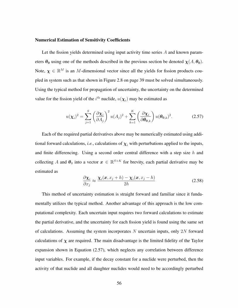
Numerical Estimation of Sensitivity Coefficients

Let the fission yields determined using input activity time series A and known param-

eters θ0 using one of the methods described in the previous section be denoted χ(A,θ0).

Note, χ ∈ RM is an M -dimensional vector since all the yields for fission products cou-

pled in system such as that shown in Figure 2.8 on page 39 must be solved simultaneously.

Using the typical method for propagation of uncertainty, the uncertainty on the determined

value for the fission yield of the ith nuclide, u(χi) may be estimated as

u(χi)2 =

S∑j=1

(∂χi∂Aj

)2

u(Aj)2 +

K∑k=1

(∂χi∂θ0,k

)u(θ0,k)

2. (2.57)

Each of the required partial derivatives above may be numerically estimated using addi-

tional forward calculations, i.e., calculations of χi with perturbations applied to the inputs,

and finite differencing. Using a second order central difference with a step size h and

collecting A and θ0 into a vector x ∈ RS+K for brevity, each partial derivative may be

estimated as∂χi∂xj≈ χi(x, xj + h)− χi(x, xj − h)

2h(2.58)

This method of uncertainty estimation is straight forward and familiar since it funda-

mentally utilizes the typical method. Another advantage of this approach is the low com-

putational complexity. Each uncertain input requires two forward calculations to estimate

the partial derivative, and the uncertainty for each fission yield is found using the same set

of calculations. Assuming the system incorporates N uncertain inputs, only 2N forward

calculations of χ are required. The main disadvantage is the limited fidelity of the Taylor

expansion shown in Equation (2.57), which neglects any correlation between difference

input variables. For example, if the decay constant for a nuclide were perturbed, then the

activity of that nuclide and all daughter nuclides would need to be accordingly perturbed

56

in order to capture the activity’s dependence on the decay constant (see Equation (2.8) on

page 23). In addition, the expansion is truncated after first-order terms, and truncation error

will grow with increasing uncertainty on input values.

When there is little prior knowledge of the values of θ and an uniformative prior dis-

tribution such as the uniform distribution over R++ is used, the objective function shown

in Equation (2.45) (see page 46) reduces to MLE†. The combination of this objective with

the approximate Taylor expansion propagation of uncertainty is a frequentist approach to

parameter estimation [31].

When an informative prior distribution is used (clearly moving into a Bayesian objec-

tive function) and combined with the perturbation basis of uncertainty estimation, the result

is one possible frequentist approximation of the Bayesian result. In Bayesian statistics, the

estimates of the most likely value for θ are given by probability distribution functions.

Two frequentist approximations/reductions are the maximum value of the posterior distri-

bution, called the maximum a posteriori (MAP) (MAP) and the expected value. The MAP

may be directly computed by solving Equation (2.45); however, computing the expected

value requires the entire distribution. In this research, the MAP was used as a frequentist

approximation of Bayesian results.

Monte Carlo Sampling of Uncertain Inputs

An alternative method to estimating the uncertainty is by generating a pool of results

using Monte Carlo sampling and examining the spread in results. The collection of uncer-

tain parameters (see Table 2.2 on page 55) makes the input space. A multivariate normal

distribution is ascribed to describe the input space. At each iteration of the Monte Carlo

algorithm, this distribution is sampled to obtain a set of values for all the uncertain param-

†The uniform distribution over the positive real numbers is not strictly uninformative as it ensures theresult is greater than zero.

57

eters, and θ is found by solving Equation (2.45). This process is repeated, and the pool of

results are binned to form an unnormalized approximation of the posterior distribution for

θ.

As shown in Equation (2.39) on page 40, the neutron flux and FPY are not independent

because the two terms only appear together in each equation. As a result, neutron flux and

FPY may not be determined simultaneously. A two-stage approach is used. First, a well-

studied, long-lived, fission product such as 99Mo is used to determine the neutron flux and

associated uncertainty†. In this initial stage of the analysis, the standard’s cFPY is treated

as uncertain parameter (see θ0 in Equation (2.38) on page 39) and θ is the time-averaged

neutron flux, 〈φ〉. The determined value for neutron flux and associated uncertainty is used

as an uncertain input for all subsequent analyses corresponding to the same experiment,

and all subsequent determined FPY are essentially normalized to the FPY of the standard

FP utilized.

The multistage analysis gives rise to correlations between input parameters: Fissionable

material mass, density, and fission cross section are used when determining the neutron flux

as well as FPY. Therefore, the neutron flux is correlated with m, ρ, and σf , and tirr (see

Table 2.2 on page 55). In addition, decay constants are used in the calculation of nuclide

activity time series as well as directly into the parameter estimation. These correlations

are needed in order to correctly construct and sample the input space. Equation (2.13) on

page 25 is used to estimate the covariance between variables.

The uncertainty in half-lives for all nuclides studied to date is small. Therefore, u(λ)2

makes the covariance negligible, therefore the input space used for flux estimation is uncor-

related. After finishing the Monte Carlo sampling, the sampled values for 〈φ〉 are regressed

†In all results presented in this research, a single, constant-power irradiation was used, and the time-averaged neutron flux is determined. If a time-varying flux is used, e.g., a neutron pulse, the relative timebehavior is programmed by the user and a scaling factor to obtain the corrected integrated fluence is deter-mined in the first stage of the analysis.

58

against corresponding values for tirr, m, ρ, and σf , and the derivative in Equation (2.13) is

estimated using ordinary least squares to fit a linear function.

This technique for numerical estimation of the sensitivity coefficients between the result

and uncertain input parameter may also be used in order to obtain the uncertainty budget,

which quantifies the relative contribution of each source of uncertainty to the result [45].

Each entry is calculated using Equation (2.59).

ηi(χ) =

(∂χ∂θi

)2

u(θi)2∑

j

(∂χ∂θj

)2

u(θj)2

× 100 (2.59)

The most obvious way to process the posterior distribution given by Monte Carlo sam-

pling and obtain summary statistics is to do so individually, i.e., statistics such as the mean

and standard deviation are computed for each estimated parameter separately, using the

expressions shown in Equation (2.60) for a collection of N samples, indexed by j. This

implicitly assumes that the entries of θ are independent of each other. Since FPY for all

nuclides in a decay chain are calculated simultaneously, results are clearly not independent.

θi =1

N

N∑j=1

θ(j)i ∀ i

u(θi) =1

N − 1

N∑j=1

√(θ

(j)i − θi

)2

∀ i

(2.60)

Monte Carlo sampling produces the entire posterior distribution and is a fully Bayesian

approach to parameter estimation. Retaining the posterior distribution gives several advan-

tages:

1. Correlation between uncertain inputs are explicitly treated by off-diagonal terms in

Σ when the input space is sampled,

59

2. Higher-order effect that are neglected by the truncated Taylor expansion in Equa-

tion (2.57) are retained,

3. Covariances between the entries of θ may be computed using Equation (2.61), and

4. Additional information is gained by treating θ with a multivariate probability distri-

bution function (see Figure 2.12).

Without the assumption of independent variables, the summary statistics are still com-

puted with the expressions in Equation (2.60); however, the multivariate posterior distri-

bution gives additional information about the true values for θ. Figure 2.12 illustrates the

situation. The marginal distributions for θ1 and θ2 are the same in Figures 2.12a and 2.12b;

however, in Figure 2.12a, no covariance is reported and the variables are assumed inde-

pendent as suggested by the two-dimensional joint distribution shown. In Figure 2.12b,

a correlation of 0.85 is reported, and the correct two-dimensional normal posterior distri-

bution is shown. When the off-diagonal term is considered (Figure 2.12b), the posterior

distribution occupies less volume in R2 than when it is neglected (Figure 2.12a). This

decrease in volume amounts to an increase in reported information as the space of likely

values for θ is smaller.

For N samples, the covariance between the jth and kth determined parameters, qjk, is

estimated using the sample covariance.

qjk =1

N − 1

N∑i=1

(θ

(i)j − θj

)(θ

(i)k − θk

)(2.61)

A more informative metric of the relation between two determined values is the corre-

lation, which is the covariance scaled by the uncertainty in each variable as shown in

Equation (2.62). Like the covariance estimated by sample covariance, the correlation is

computed using the unbiased estimation of sample covariance and sample standard devia-

60

(a) When summary statistics are computed forθi independently, a posterior with diagonal co-variance, i.e., symmetric, is implied.

(b) Given the same marginal distributionsshown below and to the right, reporting themultivariate posterior with nonzero correlationreduces the range of values θ may take.

Figure 2.12: Two-dimensional example showing additional information given in multi-variate posterior distribution given identical marginal distributions for each estimated pa-rameter. While the mean values and standard uncertainties, computed with Equation (2.60)are identical in the left and right panels, the actual correlated posterior distribution forθ = (θ1 θ2) occupies less volume in R2 than the assumed uncorrelated distribution im-plied by the summary statistics (without covariance) alone.

61

tion.

rjk =

∑Ni=1

(θ

(i)j − θj

)(θ

(i)k − θk

)√∑N

i=1

(θ

(i)j − θj

)2∑Ni=1

(θ

(i)k − θk

)2(2.62)

It is possible that the posterior distribution may not be normal at all. In this case,

reporting the entire posterior distribution for θ is necessary as summary statistics may fail

to capture the state of knowledge.

62

3 | Verification

The methods for nuclide identification and quantification from gamma-ray spectrome-

try and flexible modeling and parameter estimation described in Chapter 2 was prototyped

and implemented in Matlab. The primary functions, data input and output infrastructure,

and necessary subroutines, were collected into a package called FRACTURE (Flexible Ra-

dionuclide Analysis parameTeR Estimation).

This chapter presents data analysis experiments used to verify the fidelity of the meth-

ods and validate the end results produced by FRACTURE. Sections 3.1 through 3.5 exam-

ine individual modules of the analysis: nuclide identification, activity calculation, nuclide

buildup/decay modeling, solving the optimization problem in Equation (2.45) and finding

associated uncertainty, and assessing the evaluated solution’s sensitivity to the prior distri-

bution. Section 3.6 presents two experiments validating the entire process on inverse prob-

lems with known solutions. In addition to demonstrating the efficacy of the methodology,

these experiments serve as opportunities to study the performance of different implemented

options such as optimization solvers and approaches to uncertainty estimation.

3.1 Spectral Analysis

To test the nuclide identification and activity quantification abilities of the methods and

associated code implementation described Section 2.2 on page 14, a gamma-ray spectrum

was collected of a sample containing known amounts of radionuclides and analyzed using

the developed code. The process and results of this experiment are presented below.

63

A multi-gamma standard source was obtained from Eckert & Ziegler Analytics. The

sample contains ten gamma-emitting radionuclides that emit twelve strong characteristic

gamma-rays at certified rates. The data from the sample certification are reproduced in

Table 3.1. The sample was counted using a HPGe gamma-ray spectrometer (see Figure 4.2

on page 106) for twelve hours. The long count time gave high quality statistics with average

uncertainty in peak counts of approximately 0.6%. Spectral processing was simple and

peak fitting as well as efficiency evaluation was performed using Genie-PC [23].

The list of peak energies, peak areas, and peak detector efficiency values were fed into

the nuclide identification algorithm described in Section 2.2.1 and Equation 2.2 was solved.

Figure 3.1 gives an excerpt of the output file generated by the code. The input settings are

given at the top and a portion of the initial list of hypothesized radionuclides is shown.

Thirty-three radionuclides were identified by the peak search as being possible sources of

the observed gamma-rays. For each of the thirty-three hypothesized nuclides, an entry

for each characteristic gamma-ray was added to the response matrix. After populating

the response matrix, a total of 158 peaks were considered. The gamma-rays added to

the response matrix account for photopeaks not observed in the spectrum (they were not

already in the response matrix after converting the spectral data to vector form) but would

be observed in the gamma-ray spectrum if all the hypothesized radionuclides were present

in the sample.

The results of the analysis are shown in Figure 3.2. The numerical values for c have

units of Bq·s; however, the values have not been verified. The values may be interpreted

as unnormalized probabilities and radionuclides with larger values are more likely to be in

the sample. All nuclides present in the sample were identified by the algorithm; however,

additional nuclides were also identified. Some nuclides decay to the same daughter product

and have the same gamma-ray signature as the nuclides shown in Table 3.1: 109mAg, 109Pd,

60Cu, 139Ba, 88Rb, and 57Mn. Nuclides that decay to identical daughter products are indis-

64

tinguishable using a single spectrum. Using multiple spectra and checking for the correct

time behavior (within the optimization formulation) would improve these results.

The counting data for the characteristic gamma-rays of the radionuclides in the sample

is given in Table 3.2. This data was used to verify the operation of the activity calculation

methods described in Chapter 2.

This dataset contains neither short-lived radionuclides nor decay-chains of radionu-

clides. Thus, the activity at the beginning of counting is easily computed by assuming each

nuclide has constant activity during counting, no decay sources or losses are present, and

calculating the average activity as shown in Equation (3.1).

A =Ciγiεitc

(3.1)

The activity of each nuclide shown in Table 3.1 was computed using the data in Table 3.2

and Equation (3.1). These values were compared to values computed using the method of

Section 2.2.2 on page 20, and the analysis is summarized in Table 3.3. The relative bias was

computed assuming the manual analysis’s results are true to reality, and all uncertainties

are written as percents relative to the reported value as in Table 3.2.

There is excellent agreement between the results calculated using a manual spectral

analysis and Equation (3.1) and the developed code discussed in Chapter 2. The new

method produces marginally larger activity estimates due to correction for decay during

counting, but this effect is minimal as all radionuclides in the multi-gamma standard are

long-lived. The difference in the results produced by the two methods are at least a factor

of ten smaller than the uncertainty in the calculated activities, and results were obtained in

a single step with less possibility of error than multi-step manual analysis. Thus, the newly

developed method/implementation is valid.

65

%%%%%%%%%%%%%%%%%%%%%%%%%%%%%%%%%%%%%%%%%%%%%%%%%%%%%%%%%%% NUCLIDE IDENTIFIER %% Kenneth Dayman %% University of Texas at Austin %% November 2012 %%%%%%%%%%%%%%%%%%%%%%%%%%%%%%%%%%%%%%%%%%%%%%%%%%%%%%%%%%%

Spectrum Name: BatemanValidateion-NID-MultiGamma-Jan2015-EnergyRecal

Time of Analysis: 13:20, 1/14/2015

Minimum energy [keV]: 46 Maximum energy [keV]: 1850Minimum gamma intensity [%]: 3Energy tolerance used in peak search [+/- keV]: 1.000000e-01Epsilon value used for unobserved peaks [Bq*s]: 650Number of peaks used in analysis: 158Number of peaks observed in spectrum: 12Number of peaks added to analysis (unobserved): 146Optimization Method: NNLSQ

%%%%%%%%%%%%%%%%%%%%%%%%%%%%%%%%%%%%%%%%%%%%%%%%%%%%%%%%%%% RESULTS OF NID ANALYSIS %%%%%%%%%%%%%%%%%%%%%%%%%%%%%%%%%%%%%%%%%%%%%%%%%%%%%%%%%%%

Tentative NID Analysis======================

Peak Energy [keV] Area Possible Nuclide(s)----------------- ---- -------------------

4.64600e+01 2.49505e+07 Pb210Re183Ta183W183m

5.95400e+01 1.68627e+07 Am241Pu237Tm161U237

8.80000e+01 9.83723e+06 Ag109mCd109Ce133mPd109Ru113Tm155Tm155m

1.22090e+02 2.71823e+06 Co57Mn57

1.36480e+02 3.60241e+05 Co57W174

Figure 3.1: Excerpt from nuclide identification algorithm output.

66

Interference-Corrected NID Analysis====================================

Nuclide Activity-Time [Bq*s]------- --------------------

Pb210 5.8705e+08Ag109m 9.4734e+07Cd109 9.4734e+07Pd109 7.8237e+07Am241 4.5768e+07Co60 2.5694e+07Pu237 1.3099e+07Cs137 9.7676e+06Ba137m 9.6760e+06Cu60 4.2857e+06Co57 3.1744e+06Fr206m 3.0975e+06Ba139 1.6841e+06Rb88 1.0462e+06Y88 9.3499e+05Sn113 5.2554e+05Ce139 5.1067e+05Tm161 1.2671e+04Mn57 1.1818e+04Tm155m 1.0870e+04W174 7.8645e+03Re183 0000Ta183 0000W183m 0000U237 0000Ce133m 0000Ru113 0000Tm155 0000Er159 0000Ho159m 0000Kr88 0000Lu165 0000Cd125m 0000

Figure 3.2: Optimal mixture of radionuclides identified by nuclide identification algo-rithm.

67

Tabl

e3.

1:C

ertifi

catio

nof

mul

ti-ga

mm

ast

anda

rdco

unte

dan

dus

edto

valid

ate

nucl

ide

iden

tifica

tion

and

activ

ityca

lcul

atio

nca

pabi

litie

sof

deve

lope

dm

etho

dsan

dco

de.

Unc

erta

inty

Type

Nuc

lide

Gam

ma-

ray

Ene

rgy

[keV

]H

alf-

Lif

e[d

]γ/s

uA

uB

UC

alib

ratio

nM

etho

d210Pb

46.5

8.10

9×

103

6.02

7×

102

0.1

2.1

4.1

4πL

S241A

m59

.51.

580×

105

3.95

0×

102

0.1

1.7

3.5

4πL

S109C

d88

.04.

626×

102

5.70

8×

102

0.5

2.3

4.7

HPG

e57C

o12

2.1

2.71

8×

102

3.12

4×

102

0.4

2.0

4.1

HPG

e139C

e16

5.9

1.37

6×

102

4.40

7×

102

0.4

1.9

3.9

HPG

e203H

g27

9.2

4.66

1×

101

9.34

9×

102

0.3

1.9

3.8

HPG

e113Sn

391.

71.

151×

102

6.12

2×

102

0.4

1.9

3.9

HPG

e137C

s66

1.7

1.09

8×

104

4.03

5×

102

0.7

1.9

4.0

HPG

e88Y

898.

01.

066×

102

1.47

2×

103

0.5

1.9

3.9

HPG

e60C

o11

73.2

1.92

5×

103

7.41

2×

102

0.6

1.9

4.0

HPG

e60C

o13

32.5

1.92

5×

103

7.41

3×

102

0.7

1.9

4.0

HPG

e88Y

1836

.11.

066×

102

1.55

9×

103

0.7

1.9

4.0

HPG

e

68

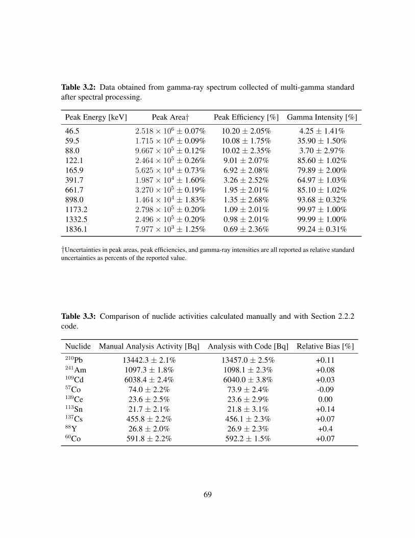
Table 3.2: Data obtained from gamma-ray spectrum collected of multi-gamma standardafter spectral processing.

Peak Energy [keV] Peak Area† Peak Efficiency [%] Gamma Intensity [%]

46.5 2.518× 106 ± 0.07% 10.20 ± 2.05% 4.25 ± 1.41%59.5 1.715× 106 ± 0.09% 10.08 ± 1.75% 35.90 ± 1.50%88.0 9.667× 105 ± 0.12% 10.02 ± 2.35% 3.70 ± 2.97%122.1 2.464× 105 ± 0.26% 9.01 ± 2.07% 85.60 ± 1.02%165.9 5.625× 104 ± 0.73% 6.92 ± 2.08% 79.89 ± 2.00%391.7 1.987× 104 ± 1.60% 3.26 ± 2.52% 64.97 ± 1.03%661.7 3.270× 105 ± 0.19% 1.95 ± 2.01% 85.10 ± 1.02%898.0 1.464× 104 ± 1.83% 1.35 ± 2.68% 93.68 ± 0.32%1173.2 2.798× 105 ± 0.20% 1.09 ± 2.01% 99.97 ± 1.00%1332.5 2.496× 105 ± 0.20% 0.98 ± 2.01% 99.99 ± 1.00%1836.1 7.977× 103 ± 1.25% 0.69 ± 2.36% 99.24 ± 0.31%

†Uncertainties in peak areas, peak efficiencies, and gamma-ray intensities are all reported as relative standarduncertainties as percents of the reported value.

Table 3.3: Comparison of nuclide activities calculated manually and with Section 2.2.2code.

Nuclide Manual Analysis Activity [Bq] Analysis with Code [Bq] Relative Bias [%]210Pb 13442.3 ± 2.1% 13457.0 ± 2.5% +0.11241Am 1097.3 ± 1.8% 1098.1 ± 2.3% +0.08109Cd 6038.4 ± 2.4% 6040.0 ± 3.8% +0.0357Co 74.0 ± 2.2% 73.9 ± 2.4% -0.09139Ce 23.6 ± 2.5% 23.6 ± 2.9% 0.00113Sn 21.7 ± 2.1% 21.8 ± 3.1% +0.14137Cs 455.8 ± 2.2% 456.1 ± 2.3% +0.0788Y 26.8 ± 2.0% 26.9 ± 2.3% +0.460Co 591.8 ± 2.2% 592.2 ± 1.5% +0.07

69

3.2 Nuclide Evolution Modeling

As described in Chapter 2, the time evolution of a FP decay chain during and after irra-

diation (or in a cyclic irradiation scheme) is calculated using a Runge-Kutta integrator. This

solver is integrated into a Matlab code called BATEMAN, which handles data preprocess-

ing, calculation of the requisite derivatives, i.e., the right-hand side of the system shown in

Equation 2.38, plotting, and data post-processing and output.

Six simulations were executed to test the results of the nuclide time evolution model

described in Section 2.3.2 on page 36 called BATEMAN. The first four compare BATEMAN

against analytical solutions, and the next two simulations compare BATEMAN to ORIGEN-

ARP. These tests and results are described in Sections 3.2.1 and 3.2.2, respectively.

3.2.1 Comparisons to Analytic Solutions

Nuclide evolution (concentration or activity) through time is exactly described by the

system of ODE shown in Equations (2.38) and (2.39). The equations admit exact analytic

solutions; however, the forms for the solutions are specific to the set of parameters used

and are inflexible in a general sense. Analytic solutions solve the system exactly with-

out approximation or numerical error, which makes analytic solutions ideal for verifying

BATEMAN.

To validate the nuclide trajectories produced by BATEMAN against analytic solutions,

Equation (2.38) is solved for four specific cases to obtain exact solutions for nuclide activ-

ity through time ΛN (t), the same system is solved using BATEMAN, and the results are

compared.

70

During Irradiation

Consider a system of two fission products in a parent/daughter configuration:

AλA−−→ B

λB−−→ , (3.2)

where the fission sources are not shown. Assuming there are no significant neutron-induced

reactions such as (n,2n) or (n,p) reactions to couple the decay chain with another isobar,

and assuming there are no alternative decay paths, the equations describing the situation

during irradiation are shown below in Equation (3.3).

dNA

dt= φΣfχ

(c)A −NAλA

dNB

dt= φΣfχ

(i)B +NAλA −NBλB,

(3.3)

The solution for the number density of nuclide A, NA(t), is

NA(t) = c1e−λAt +

φΣfχ(c)A

λA. (3.4)

Given an initial condition, NA(t = 0) = 0,

NA(t = 0) = c1 +φΣfχ

(c)A

λA= 0,

=⇒ c1 = −φΣfχ(c)A

λA,

(3.5)

the final solution is

NA(t) = −φΣfχ(c)A

λAe−λAt +

φΣfχ(c)A

λA

NA(t) =φΣfχ

(c)A

λA

(1− e−λAt

).

(3.6)

Multiplying through by λA gives the behavior of nuclide A during irradiation in terms of

71

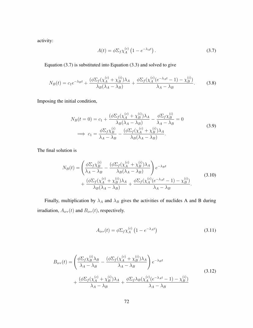
activity:

A(t) = φΣfχ(c)A

(1− e−λAt

). (3.7)

Equation (3.7) is substituted into Equation (3.3) and solved to give

NB(t) = c1e−λBt +

(φΣf (χ(c)A + χ

(i)B )λA

λB(λA − λB)+φΣf (χ

(c)A (e−λAt − 1)− χ(i)

B )

λA − λB. (3.8)

Imposing the initial condition,

NB(t = 0) = c1 +(φΣf (χ

(c)A + χ

(i)B )λA

λB(λA − λB)− φΣfχ

(i)B

λA − λB= 0

=⇒ c1 =φΣfχ

(i)B

λA − λB− (φΣf (χ

(c)A + χ

(i)B )λA

λB(λA − λB).

(3.9)

The final solution is

NB(t) =

(φΣfχ

(i)B

λA − λB− (φΣf (χ

(c)A + χ

(i)B )λA

λB(λA − λB)

)e−λBt

+(φΣf (χ

(c)A + χ

(i)B )λA

λB(λA − λB)+φΣf (χ

(c)A (e−λAt − 1)− χ(i)

B )

λA − λB.

(3.10)

Finally, multiplication by λA and λB gives the activities of nuclides A and B during

irradiation, Airr(t) and Birr(t), respectively.

Airr(t) = φΣfχ(c)A

(1− e−λAt

)(3.11)

Birr(t) =

(φΣfχ

(i)B λB

λA − λB− (φΣf (χ

(c)A + χ

(i)B )λA

λA − λB

)e−λBt

+(φΣf (χ

(c)A + χ

(i)B )λA

λA − λB+φΣfλB(χ

(c)A (e−λAt − 1)− χ(i)

B )

λA − λB

(3.12)

72

After Irradiation

After irradiation is ended, the neutron flux is removed and the system in Equation (3.3)

reduces to the equations shown in Equation (3.13).

dNA

dt= −NAλA

dNB

dt= NAλA −NBλB

(3.13)

The first solution is

Adcy(td) = Airr(tirr)e−λAtd (3.14)

The general solution to the second equation in the system shown in Equation (3.13) is

NB(t) = c1e−λBt − N0

AλAe−λAt

λA − λB. (3.15)

Imposing continuity of atom density between the end of the first time regime (irradiation,

when the number densities of nuclides A and B areN0A andN0

B, respectively) and beginning

of the second time regime (decay) gives the following initial condition for the general

solution shown above:

NB(t = 0) = c1 −N0AλA

λA − λB= N0

B

=⇒ c1 =N0AλA

λA − λB+N0

B.

(3.16)

The solution for the atom density of the daughter nuclide and the activity is

NB(td) =

(N0AλA

λA − λB+N0

B

)e−λBt − N0

AλAe−λAt

λA − λB

B(td) =

(N0AλAλB

λA − λB+B0

)e−λBt − N0

AλAλBe−λAt

λA − λB.

(3.17)

The last expression in Equation (3.17) may be simplified by noting that N0A = A0λ

−1A .

73

Additionally, the initial conditions for this solution may be written in terms of the solutions

in Equations (3.7) and (3.11):

B(td) =

(Airr(tirr)λBλA − λB

+Birr(tirr)

)e−λBtd − Airr(tirr)λBe

−λAtd

λA − λB, (3.18)

where Airr(t) is the activity of nuclide A during irradiation (given by Equation (3.7)),

occurring in the time interval t ∈ [0, tirr], Birr(t) is the activity of the daughter nuclide B

during the interval [0, tirr], and td is the decay time, i.e., the time since the end of irradiation

td = t− tirr.

Comparison to BATEMAN

To quantify the accuracy of the numerical solution (denoted An(t) and Bn(t)) relative

to the analytical solutions developed in the previous section (Aa(t) and Ba(t)), a difference

measure is defined. The measure is shown for the parent nuclide in Equation (3.19).

d(A) = 100×∫ T

0|An(t)− Aa(t)| dt∫ T

0Aa(t) dt

(3.19)

Here T is the maximum time considered in the simulation/solution, and multiplying by a

factor 100 converts to a percent error over the time domain. The numerator is the integrated

residual between the two solutions. Four cases are presented below.

Case 1 (140Ba/140La) The first case is representative of the common FP parent/daughter

pair 140Ba and 140La. The input parameters needed for characterizing the problem are

shown in Table 3.4, and the residuals between the solutions is plotted in Figure 3.3.

The residuals display an oscillating behavior, which likely stem from the need to in-

terpolate from the time mesh used by the numerical solver onto the regularly-spaced mesh

used to evaluate and display the analytical solution (see Section 2.3.2 on page 36). The reg-

74

Table 3.4: Input parameter values for solutions whose residuals are shown in Figure 3.3.TA and TB are the half-lives of nuclides A and B, respectively.

Parameter Value Unit

Σf 0.0105 cm−1

φ 1× 1012 cm−2s−1

χ(c)A 6.21 %χ

(i)B 5.20× 10−3 %TA 1.1× 106 sTB 1.4× 105 stirr 120 s

Figure 3.3: The residual between the numerical and analytical solutions for 140Ba/140Laverification case. Throughout the entire time domain, the residual does not exceed 0.01%.

ular mesh for the analytical mesh is also used to compute the residual, {An(ti)− Aa(ti)}iinIa .

Figure 3.4 shows the solution for the same system generated using a coarser time mesh for

the analytical solution. The observed oscillating behavior is similar to that seen in the orig-

inal solution; however, the frequency of variation is lower, which supports the hypothesis

on the source of the oscillation.

75

Figure 3.4: The residual between the numerical and analytical solutions for 140Ba/140Lausing a coarse time mesh for the analytical solution. An oscillating behavior similar to thatshown in Figure 3.3 is observed, albeit with a lower frequency.

Case 2 For the second case, a system with shorter-lived nuclides is examined. As with

the first case, the daughter nuclide has a shorter half-life than the parent. The parameters

are summarized in Table 3.5.

When the daughter nuclide activity drops below approximately 1× 10−8 Bq, the resid-

uals exceed 0.1% and continues to rise as the activity continues to decrease. The thresh-

old occurs at approximately 50 half-lives of the parent nuclide and 150 half-lives of the

daughter nuclide. At these activities, empirical measurement is no longer possible, and the

numerical solutions in this extreme of the time regime are not needed.

Case 3 The third verification case features daughter nuclides with longer half-lives than

the parent. Table 3.6 summarizes the input values for Case 3, and the residuals between the

numerical and analytical solutions are shown in Figure 3.6.

76

Table 3.5: Input parameters for Case 2.

Parameter Value Unit

Σf 0.0105 cm−1

φ 1× 1012 cm−2s−1

χ(c)A 6.21 %χ

(i)B 5.20× 10−3 %TA 1.1× 103 sTB 3.6× 102 stirr 120 s

Figure 3.5: The residual between the numerical and analytical solutions for Case 2. Inthis example, the residual increases as the activity decreases. The residual exceeds 0.1%(shown in the black dashed line) when the activity drops to the level of nano-Becquerels.

Case 4 The final verification case examines the situation where the daughter product is

much longer-lived than the parent nuclide. As shown in Table 3.7, the half-life of the

daughter nuclide is 15 times larger than that of the parent nuclide. Consistent with results

in the first three cases, numerical solutions produced by BATEMAN agree very well with

analytic solutions.

77

Figure 3.6: The residual between the numerical and analytical solutions for Case 3. As inthe case of Case 2, the residual is less than 0.1% at all times before the activity drops belowunmeasurable levels. In this case, the residual of the parent nuclide becomes unacceptablylarge for use in inverse problem solving when the activity falls below 10−5 Bq.

78

Figure 3.7: The residual between the numerical and analytical solutions for Case 4. As inthe previous cases, the residual is less than 0.1% at all times before the activity drops belowunmeasurable levels. In this case, the residual of the parent nuclide becomes unacceptablylarge for use in inverse problem solving when the activity falls below 10−8 Bq.

79

Table 3.6: Input parameters for Case 3.

Parameter Value Unit

Σf 0.0105 cm−1

φ 5× 1012 cm−2s−1

χ(c)A 4.0 %χ

(i)B 1.0 %TA 1.2× 103 sTB 3.6× 103 stirr 60 s

Table 3.7: Input parameters for Case 4.

Parameter Value Unit

Σf 0.0105 cm−1

φ 2× 1012 cm−2s−1

χ(c)A 4.75 %χ

(i)B 0.5 %TA 1.2× 102 sTB 1.8× 103 stirr 60 s

Summary of Cases In these and other cases not shown, the residual between the nu-

merical and analytic solutions is at acceptable levels, 0.1%, as long as the activities are

above approximately 10−5 Bq†. This minimum activity is well below the level that is ap-

propriate for measurement and quantification with gamma-ray spectrometry. Therefore,

the numerical solver within BATEMAN is sufficiently accurate for the range of anticipated

applications.

In other cases, accuracy of the numerical solution was examined during the irradiation

period. Residuals in excess of 0.1% were observed at the beginning of irradiation. Inac-

†It is possible that the observed error is a compounding error that accumulates over large number of timesteps; however, the distinction between compounding error associated with large number of time steps anderror associated with small-value solutions is not important for modeling and measurement of FP.

80

curacies at the beginning of irradiation are likely due to changes in the differential as a

function of time and imperfections in the time mesh refinement used in the Runge-Kutta

solver. The residual decreased and was below the 0.1% threshold past a threshold time

within the irradiation period. The cutoff time showed some dependence on input parame-

ters; however, since no activity measurements are made during the irradiation period, these

errors do not affect the analysis and the complete characterization of this cutoff time was

not pursued.

To summarize the accuracy of the numerical solver in these four cases, the time domain

was restricted to [0, T ], where T = min{T1, T2}, where T1 and T2 are the times when the

parent and daughter nuclide activities fall to 1 Bq. Any activity below this level is consid-

ered unfeasible for measurement and would not be used in fission product analysis. Using

these restricted time domains, the integrated measure of error shown in Equation (3.19)

was quantified, and these values are shown in Table 3.8.

Table 3.8: Difference measure as defined in Equation (3.19) for four test cases, each withrestricted time domains.

Case Parent Difference [%] Daughter Difference [%]

1 6.4× 10−4 8.3× 10−4

2 5.6× 10−4 1.0× 10−3

3 5.8× 10−4 8.5× 10−4

4 7.0× 10−4 1.1× 10−3

3.2.2 Comparisons to ORIGEN-ARP

A benchmarking simulation was performed using ORIGEN-ARP and BATEMAN. This

test featured a cyclic irradiation pattern expected in the use of a neutron generator, where

fluxes are relatively low and a series of irradiation and decay cases are performed. The

81

nuclides 135Sb, 135Te, and 135I were simulated through four different irradiations. Table 3.9

summarizes the parameters used, and the results are shown in Figure 3.8.

Table 3.9: Summary of ORIGEN-ARP benchmark, where 135Sb, 135Te, and 135I were sim-ulated.

Parameter Value Units

Fission Yieldsχ

(i)I 2.93 %χ

(i)Te 3.22 %χ

(c)Sb 1.46× 10−1 %

Decay ConstantsλI 2.9306× 10−5 s−1

λTe 3.6481× 10−2 s−1

λSb 4.1259× 10−1 s−1

Cross Sectionsσf (235U) 245 b

Irradiation 1Irradiation Time 5 sFlux (φ) 1× 106 cm−2s−1

Decay Time 30 sIrradiation 2

Irradiation Time 5 sFlux (φ) 1× 106 cm−2s−1

Decay Time 20 sIrradiation 3

Irradiation Time 5 sFlux (φ) 2× 106 cm−2s−1

Decay Time 10 sIrradiation 4

Irradiation Time 5 sFlux (φ) 3× 106 cm−2s−1

Simulation Time 1 hr

Predicted concentrations were within 20% of each other. Maximum differences in pre-

dictions of 135I and 135Te concentrations made by BATEMAN and ORIGEN-ARP were ap-

proximately -16% and -20%, respectively. Numerical results from BATEMAN compared

82

(a) Solution calculated by ORIGEN-ARP

(b) Solution calculated by BATEMAN

Figure 3.8: Nuclide evolution computed using ORIGEN-ARP and BATEMAN, where 135Sb,135Te, and 135I during cyclic irradiation were simulated.

83

favorably to analytic solutions presented in the previous section. Thus, we attribute the

observed differences between BATEMAN and ORIGEN-ARP to differences in the neutron

spectrum used to compute one-group cross sections. The spectrum used in ORIGEN corre-

sponds to a commercial boiling water reactor, which has a larger high-energy component

than the spectrum in the tPNT of the UT TRIGA that was used in BATEMAN. The harder

spectrum used in ORIGEN leads to differences in the one-group cross sections and fission

yields. Accordingly, the one-group flux specified in each code are inherently different since

one-group flux values are tied to the cross sections.

3.3 Self-Shielding and Self-Attenuation

As shown in Figure 4.1 on page 102, U3O8 samples were tripled encapsulated in polyethy-

lene prior to irradiation at NETL. In this section, we detail the calculations performed to

ensure no significant changes to the neutron spectrum were caused by this relatively large

amount of sample packaging. Additional calculations were performed to verify that self-

attenuation was not an issue, i.e., the entire sample was evenly irradiated. To do this,

models were built in MCNP to examine the neutron spectrum and flux profile in the U3O8

volume samples.

A model of the sample geometry shown in Figure 4.1 was built in MCNPX 2.7.0, and

the flux in the sample with and without the polyethylene vials and spacers was tallied in

order to assess any neutron shielding effects that may require consideration during data

analysis. The model geometry is shown in Figure 3.9. The central red region is the U3O8

sample at 2.7 g/cm3†, the polyethylene vials and spacers are shown in green at 0.97 g/cm3,

and the blue regions are air at STP.

†The simulation is based on thermal irradiations performed at UT, and the density was calculated usingthe measured mass of the powdered oxide and the volume of sample vial used for irradiations.

84

Figure 3.9: MCNPX model geometry used to assess neutron shielding due to sample pack-aging and within sample self-shielding effects.

The results are shown in Figure 3.10, which shows the incident neutron spectrum pro-

vided by the tPNT facility (blue), the flux on sample without polyethylene present (red),

which is reduced due to geometric attenuation, and the flux on sample with polyethylene

(green). The degree of neutron shielding in the polyethylene is minimal; however, there

is some downscattering. This slight softening of the spectrum increases the probability of

fission, and the expected fission reaction rate (normalized to atom density) increases when

polyethylene is present. These results are summarized in Table 3.10.

Table 3.10: Expected fission reaction rates with and without polyethylene sample vials andspacers.

Case Reaction Rate (Normalized to atom density, ×1024) [s−1]

With polyethylene 6.39Without polyethylene 6.87Ratio 1.07

85

Figure 3.10: Neutron spectrum in the tPNT calculated by MCNP (red) and the downscat-tered flux produced by the polyethylene sample packaging (green).

In a second simulation, the sample container (red in Figure 3.9) was segmented into

concentric cylinders and the flux tallied in each in order to assess the fission reaction rate

in each region. A depression in the flux would signify self-shielding. The multi-group flux

estimated in each region was used to estimate the fission reaction rate, normalized to the

maximum rate found in the outermost region and plotted in Figure 3.11. The flux is not

monotonically decreasing towards the center of the sample, suggesting the irregularity is

due to statistical uncertainty; however, the results are sufficiently converged to demonstrate

that no significant self-shielding occurred. The neutron flux in the center of the sample is

approximately 1.5% less than at the outer edge, but the estimate for incident neutron flux

made using 99Mo as an internal standard (see Section 4.2 on page 107) implicitly accounts

for the flux depression by calculating a value consistent with the number of fissions that

have occurred and number of 99Mo nuclei produced.

86

Figure 3.11: Expected fission reaction rate as a function of position within U3O8 sample.

3.4 Solution Methods

There were two primary motivations for implementing multiple optimization solvers.

1. If results calculated using different solvers that rely on different fundamental solu-

tion methods agree with each other, it may be confidently asserted that the tabulated

results are representative of reality as opposed to an artifact of the mathematics or

software implementation†.

2. Explore the performance characteristics of different solution methods to the con-

strained optimization problem developed in Chapter 2 and shown in Equation (2.45)

in order to determine the best approach in terms of reliability, speed, accuracy, and

precision.

†Note, this assertion assumes that the mathematical model in Equations (2.38) and (2.39) accuratelymodels the true behavior of FP.

87

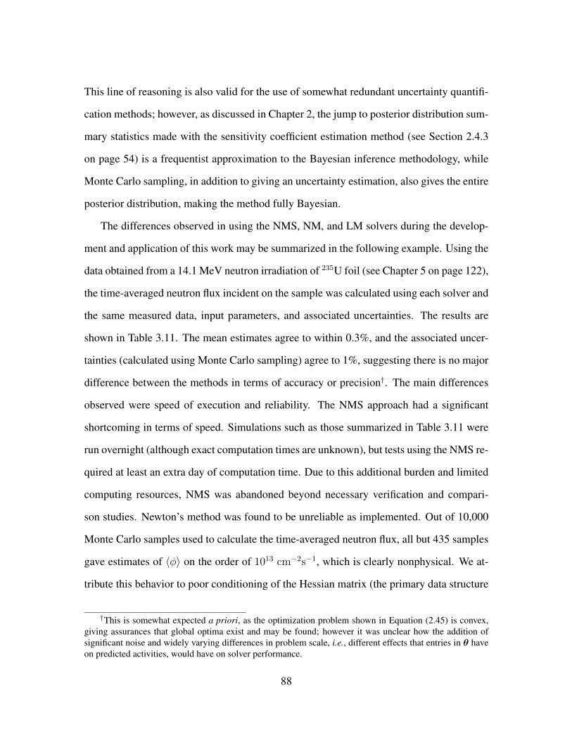
This line of reasoning is also valid for the use of somewhat redundant uncertainty quantifi-

cation methods; however, as discussed in Chapter 2, the jump to posterior distribution sum-

mary statistics made with the sensitivity coefficient estimation method (see Section 2.4.3

on page 54) is a frequentist approximation to the Bayesian inference methodology, while

Monte Carlo sampling, in addition to giving an uncertainty estimation, also gives the entire

posterior distribution, making the method fully Bayesian.

The differences observed in using the NMS, NM, and LM solvers during the develop-

ment and application of this work may be summarized in the following example. Using the

data obtained from a 14.1 MeV neutron irradiation of 235U foil (see Chapter 5 on page 122),

the time-averaged neutron flux incident on the sample was calculated using each solver and

the same measured data, input parameters, and associated uncertainties. The results are

shown in Table 3.11. The mean estimates agree to within 0.3%, and the associated uncer-

tainties (calculated using Monte Carlo sampling) agree to 1%, suggesting there is no major

difference between the methods in terms of accuracy or precision†. The main differences

observed were speed of execution and reliability. The NMS approach had a significant

shortcoming in terms of speed. Simulations such as those summarized in Table 3.11 were

run overnight (although exact computation times are unknown), but tests using the NMS re-

quired at least an extra day of computation time. Due to this additional burden and limited

computing resources, NMS was abandoned beyond necessary verification and compari-

son studies. Newton’s method was found to be unreliable as implemented. Out of 10,000

Monte Carlo samples used to calculate the time-averaged neutron flux, all but 435 samples

gave estimates of 〈φ〉 on the order of 1013 cm−2s−1, which is clearly nonphysical. We at-

tribute this behavior to poor conditioning of the Hessian matrix (the primary data structure

†This is somewhat expected a priori, as the optimization problem shown in Equation (2.45) is convex,giving assurances that global optima exist and may be found; however it was unclear how the addition ofsignificant noise and widely varying differences in problem scale, i.e., different effects that entries in θ haveon predicted activities, would have on solver performance.

88

not used in the other two solvers). Poor matrix conditioning leads to stiff problems, i.e.,

x may vary widely as b is minutely perturbed in problems of the form Ax = b, which is

solved at every Newton updating step. Poor conditioning of the Hessian matrix may arise

from poor estimates of partial derivatives made by finite differencing (recall, the objective

function is noisy with respect to θ and y, which makes estimation of global behavior of the

objective function difficult to estimate with a local technique such as finite differencing).

The LM algorithm avoids estimation of all second derivatives that use two nested sets of

finite differencing. Another possible cause of the poor conditioning of the Hessian is the

difference in sensitivity of the predicted activities (and accordingly the determined values

of θ) to different inputs. For example, predicted activities of 140La will depend much more

strongly on the cumulative yield of 140Ba than the independent yield of 140La. As a result

of this unreliable behavior, the results for NM shown in Table 3.11 only use the reliable

435 samples.

Table 3.11: Time-averaged neutron flux incident on sample in 14.1 MeV experiment. Theflux was determined using all three solvers to investigate any possible effects on results.Posterior distributions were estimated with Monte Carlo sampling and summary statisticswere computed using the sample mean and standard deviation.

Optimization Solver Flux Estimate [cm−2s−1]

Levenberg-Marquardt (2.3565± 0.1113)× 108

Newton’s Method† (2.3606± 0.1101)× 108

Nelder Mead Simplex (2.3538± 0.1109)× 108

†Large outliers (> 1 × 1013) were made with Newton’s method due to instability in the iterative updatingprocess stemming from poor conditioning of the Hessian matrix. Outliers were removed, leaving 435 samplesto compute the reported summary statistics.

Using the LM algorithm, the uncertainty in the determined time-averaged flux was

assessed using the sensitivity coefficient approach and compared to the value determined

using Monte Carlo sampling. These results are shown in Table 3.12. Both values agree to

two decimal places, approximately 3%; however, it should be noted that the input space for

89

a flux measurement is uncorrelated, the effect of neglecting correlation between inputs is

not examined.

Table 3.12: Uncertainty in neutron flux estimated using sensitivity coefficient estimatesand Monte Carlo sampling and summary statistics. The Levenberg-Marquardt method wasused in both cases.

Uncertainty Method Flux Estimate [cm−2s−1]

Sensitivity Coefficient (2.3492± 0.1149)× 108

Monte Carlo Sampling (2.3565± 0.1113)× 108

3.5 Sensitivity to Prior Distribution

A series of inverse calculations were performed using the experimental data collected

following a thermal irradiation performed at UT (see Chapter 4) to assess the developed

methodology’s sensitivity to the strength of the prior distribution, i.e., the effect the value

of the uncertainty in the prior distribution (u(θk) in Equation (2.45)) has on the calculated

result, θ. This was done by performing a series of calculations using different input param-

eters and estimating the cFPY and iFPY of 140Ba and 140La, respectively. First, a “baseline

prior” was made by setting µ = 1/3∑3

i=1 xi, where i indexes over the three data libraries

ENDF, JEFF, and JENDL, and assigning the shaping parameter to quantify the uncertainty

in the prior value, σ = max{u(x1), u(x2), u(x3)}. In each calculation, the value of µ was

kept constant, and the strength of the prior term in Equation (2.45) was varied by applying

a scalar to value of σ in the baseline prior. This scalar varied from 0.02 to∞, i.e., the MLE.

Figure 3.12 shows the estimated value and associated standard uncertainty for the iFPY

of 140La as a function of the scalar applied to the baseline prior distribution. From left

to right along the abscissa, the strength of the prior decreases. As the scalars increase,

the values for χ(i)La140 (blue) and standard uncertainty (red) move asymptotically towards

90

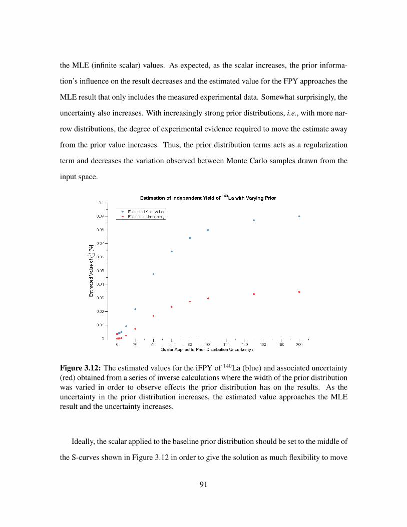
the MLE (infinite scalar) values. As expected, as the scalar increases, the prior informa-

tion’s influence on the result decreases and the estimated value for the FPY approaches the

MLE result that only includes the measured experimental data. Somewhat surprisingly, the

uncertainty also increases. With increasingly strong prior distributions, i.e., with more nar-

row distributions, the degree of experimental evidence required to move the estimate away

from the prior value increases. Thus, the prior distribution terms acts as a regularization

term and decreases the variation observed between Monte Carlo samples drawn from the

input space.

Figure 3.12: The estimated values for the iFPY of 140La (blue) and associated uncertainty(red) obtained from a series of inverse calculations where the width of the prior distributionwas varied in order to observe effects the prior distribution has on the results. As theuncertainty in the prior distribution increases, the estimated value approaches the MLEresult and the uncertainty increases.

Ideally, the scalar applied to the baseline prior distribution should be set to the middle of

the S-curves shown in Figure 3.12 in order to give the solution as much flexibility to move

91

between the prior value and the prior-free experimental value (the value determined using

the uninformative prior—the asymptote in Figure 3.12). However, the value of this scalar

depends on the number of experimentally measured activities, their relative uncertainty,

the value of σ in each of the prior distributions, and the magnitude of the coupling between

the parent and daughter nuclides in the FP decay chain†. Further investigation of these

dependencies and developing a way to determine the ideal value of the scalar (and even

refining the notion of the ideal value) is a study unto itself. Therefore, a value of 3 as

estimated in the examination of the 140Ba/140La parent-daughter pair was used throughout

this research.

3.6 Self-Consistency

After verifying the performance of each step of the analysis process and associated

code module, two experiments were performed to validate the implemented code. In the

first experiment, samples of 27Al were irradiated in the TRIGA reactor to produce short-

lived 28Al (2.24 m) by the 27Al(n,γ)28Al reaction, the time-averaged incident neutron flux

was estimated using one sample and the known radiative capture cross section, and this

cross section was estimated using gamma-ray spectra collected of a second sample. The

second experiment was performed during the analysis of the 14.1 MeV dataset described

in Chapter 5. After estimating the neutron flux incident on the target using 99Mo as an

internal standard, the data were used to recover the fission product yield of 99Mo. These

experiments are further described below.

†To clarify this last point: the sensitivity of a daughter nuclide’s activity to a parent FP parameter, e.g.,FPY, leads to a dependence of the scalar factor (abscissa in Figure 3.12) on the activity measurements, base-line prior, etc. of the parent nuclide.

92

3.6.1 27Al (n,γ) Cross Section

Two samples of 27Al were prepared using certified natural Al in solution prepared by

Inorganic Ventures. The solution has a certified concentration of 100.07 ± 0.19 µg ·mL−1

in 2% HNO3. To prepare each sample, 500 µL of the solution was pipetted onto ChemWipe

in a 2/5 dram polyethylene vial. These vials were heat sealed, placed with spacers into a 2

dram vial, and the outer vial was heat sealed. The 27Al content of each sample was 0.05 ±

0.2%.

Each sample was irradiated in the tPNT irradiation facility in the TRIGA reactor at

full power (950 kW). The first sample was irradiated for 60.0 ± 1.4 s†. The sample was

transferred to a clean vial, allowed to decay for 151 seconds, and then counted on the HPGe

gamma-ray spectrometer shown in Figure 4.2 on page 106. Counts were recorded until the

uncertainty in the characteristic 1778.9 keV photopeak of 28Al fell below 1%. Additional

spectra were collected until the 28Al activity was approximately zero (approximately 6

half-lives). The second sample was treated similarly; however, the irradiation time was

reduced to 30.0 ± 1.4 seconds to reduce the sample activity (initial detector dead time)

and the required decay time between the end of irradiation and counting. The experimental

parameters followed for the irradiation of each sample are given in Tables 3.13.

The nuclide identification algorithm was used to trivially identify the primary gamma-

emitting radionuclide in the sample as 28Al, and the activity at the beginning of collection

of each spectrum was calculated using the method of Section 2.2.2. Only spectra with

detector dead time less than 10% were considered. The results are shown in Table 3.14.

To estimate the neutron flux incident on the sample, the one-group radiative capture

cross section, σγ was calculated using a 63-group neutron spectrum in the tPNT as weights

†The output timers in the counting laboratory signaled an elapsed time of 61.4 seconds, so the irradiationtime was assumed to be 60.0 ± 1.4 seconds.

93

Table 3.13: Summary of experimental parameters used irradiating and counting 27Al stan-dard to test inverse analysis capability. Each spectrum was collected until the 1778.9 keVpeak of 28Al had better than 1% precision.

Parameter First Sample Second Sample

Irradiation Facility tPNT tPNTIrradiation Time 60 s 30 sDecay Time 151 s 70 sReactor Power 950 kW 950 kWNumber of Spectra 13 11

to collapse the group constants found in the CINDER90 library:

σγ =

∑g φgσg∑j φj

, (3.20)

and

u(σγ)2 =

∑i

(σiΦ

)2

u(φi)2 + u(Φ)2

(∑j

σjφj

)2

, (3.21)

where Φ =∑

i φi and u(Φ)2 =∑

i u(φi)2. This group collapse gave an estimate of

σγ ≈ 0.1101 ± 0.0050 barns. This value was treated as the known, true value of the

27Al(n,γ)28Al cross section.

The known cross section and sample 1 (S1) activity time series was used to estimate

the time-averaged neutron flux. The LM algorithm and Monte Carlo sampling were used

to solve Equation (2.45) and treat uncertainty, respectively. An uninformative prior, uni-

form over R++, was used. The resulting approximate posterior distribution is shown in

Figure 3.13, and the summary statistics, computed with Equation (2.60), were estimated as

(1.3338 ± 0.0764) × 1012 cm−2s−1. This value agrees well with prior operational experi-

ence.

The flux estimated using S1 was used as an uncertain input along with the activity

series measured of sample 2 (S2) to estimate the one-group radiative capture cross section

94

Figure 3.13: Approximate posterior distribution for time-averaged neutron flux incident onthe first 27Al verification sample, calculated using the LM algorithm and an uniformativeprior distribution.

95

and associated uncertainty. The result was 0.1151 ± 0.0088 barns, which is within 4.5%

of the true value. Finally, S1 data was used to recover σγ and ensure there is no systematic

bias. The resulting estimate is σγ = 0.1011 ± 0.0065 barns, which aligns perfectly with

the true value. The results of 27Al analysis are summarized in Table 3.15.

96

Tabl

e3.

14:R

esul

tsof

anal

ysis

of28A

lwith

gam

ma-

ray

spec

trom

etry

.

Sam

ple

One

Sam

ple

Two

Tim

eA

fter

Irra

diat

ion

[s]

Cou

ntTi

me

[s]

Act

ivity

[Bq]

Tim

eA

fter

Irra

diat

ion

[s]

Cou

ntTi

me

[s]

Act

ivity

[Bq]

408

37.1

6.53±

0.06×

104

297

40.5

6.06±

0.07×

104

459

49.5

5.02±

0.06×

104

348

53.5

4.72±

0.06×

104

519

69.5

3.80±

0.05×

104

413

87.6

3.42±

0.04×

104

602

121.

02.

41±

0.03×

104

512

171.

62.

01±

0.02×

104

735

118.

61.

26±

0.02×

104

697

274.

98.

01±

0.11×

103

864

272.

46.

34±

0.09×

103

––

–

97

Table 3.15: Results of validation experimental analysis of 27Al.

Parameter Value

True 27Al cross section, σγ 0.1011 ± 0.0050 [b]φ estimated with S1 and σγ (1.3338± 0.0764)× 1012 [cm−2s−1]σγ estimated with S2 and φ 0.1151 ± 0.0088 [b]σγ recovered with S1 and φ 0.1011 ± 0.0065 [b]

98

3.6.2 Neutron Flux with 99Mo Standard

During the analysis of the 14.1 MeV irradiation performed at Pacific Northwest Na-

tional Laboratory (PNNL), a second validation experiment was performed. Following the

neutron flux estimation with 99Mo as internal standard, the cFPY of 99Mo was estimated

using the neutron flux as an uncertain input. Similar to the experiment described in the

previous section, this exercise was performed to identify any possible systematic bias in

the estimation of FPY (as opposed to cross sections that appear in different parts of the

Bateman equations).

The FPY value used to calculate the neutron flux was 5.1713 ± 0.0063 %, and the

estimate made using the 99Mo data was 5.1773 ± 0.2809 %, which agrees well with the

literature value.

99

4 | Thermal Neutron Irradiation:

P0687 Experiment

In addition to the verification experiments described in Chapter 3 on page 63, two ther-

mal irradiations were conducted using the TRIGA reactor at NETL at UT. These irradi-

ations provided long-lived FP data to further test the methods described in Chapter 2 on

page 11. This chapter presents the second of these experiments, called the “P0687 Ex-

periment” in accordance with the sample tracking number used. Section 4.1 describes the

methods used to prepare samples, perform irradiations and produce FP, and collect gamma-

ray spectra. Section 4.2 on page 107 outlines the process and presents the results of data

analysis, including nuclide identification, nuclide activity quantification, and FPY determi-

nation.

4.1 Experiment

This section describes the experimental process of preparing a target, irradiating the

material to produce FP, and collecting gamma-ray spectra. These topics are addressed in

the following three subsections.

4.1.1 Sample Preparation

First, a sample containing 235U was prepared for irradiation. Natural U3O8 powder

(BNL 129-A) was used due to low cost and ease of use. A standard lab balance was used to

100

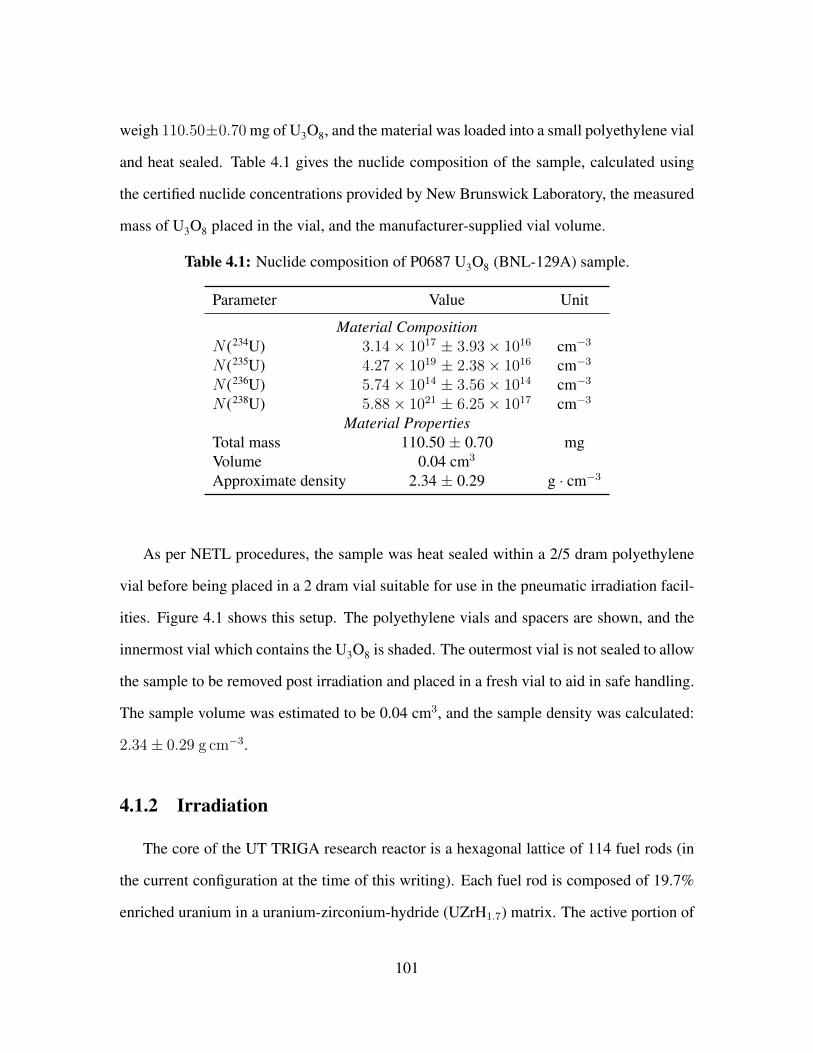
weigh 110.50±0.70 mg of U3O8, and the material was loaded into a small polyethylene vial

and heat sealed. Table 4.1 gives the nuclide composition of the sample, calculated using

the certified nuclide concentrations provided by New Brunswick Laboratory, the measured

mass of U3O8 placed in the vial, and the manufacturer-supplied vial volume.

Table 4.1: Nuclide composition of P0687 U3O8 (BNL-129A) sample.

Parameter Value Unit

Material CompositionN (234U) 3.14× 1017 ± 3.93× 1016 cm−3

N (235U) 4.27× 1019 ± 2.38× 1016 cm−3

N (236U) 5.74× 1014 ± 3.56× 1014 cm−3

N (238U) 5.88× 1021 ± 6.25× 1017 cm−3

Material PropertiesTotal mass 110.50 ± 0.70 mgVolume 0.04 cm3

Approximate density 2.34 ± 0.29 g · cm−3

As per NETL procedures, the sample was heat sealed within a 2/5 dram polyethylene

vial before being placed in a 2 dram vial suitable for use in the pneumatic irradiation facil-

ities. Figure 4.1 shows this setup. The polyethylene vials and spacers are shown, and the

innermost vial which contains the U3O8 is shaded. The outermost vial is not sealed to allow

the sample to be removed post irradiation and placed in a fresh vial to aid in safe handling.

The sample volume was estimated to be 0.04 cm3, and the sample density was calculated:

2.34± 0.29 g cm−3.

4.1.2 Irradiation

The core of the UT TRIGA research reactor is a hexagonal lattice of 114 fuel rods (in

the current configuration at the time of this writing). Each fuel rod is composed of 19.7%

enriched uranium in a uranium-zirconium-hydride (UZrH1.7) matrix. The active portion of

101

Figure 4.1: The encapsulation of U3O8 samples.

102

the rod, i.e., the section containing uranium, is approximately 15 inches long, and graphite

reflectors are placed within the rod above and below the uranium-bearing region. The rod

is enclosed in 304 stainless steel cladding. At steady-state, the core produces 1.1 MW of

thermal power†, which corresponds to a total neutron flux of approximately 1013 cm−2s−1at

the center of the core. During a reactor pulse, a peak power of 1600 MW and neutron flux

of 1016 cm−2s−1is achieved on a time scale of milliseconds.

The pneumatic transfer facility (PNT) allows the experimenter to pneumatically intro-

duce and retrieve a small (one the order of a few grams) sample from the TRIGA reactor

while at power. The polyethylene transfer line transports a sample from a loading station

in a counting laboratory to an aluminum terminus that is placed in a vacant location in

the outer ring of the reactor’s fuel lattice with a transfer time of approximately seven sec-

onds. The system uses an optical sensor to determine when the sample enters and leaves

the reactor core, and this information is used to perform irradiations of a user-specified

time duration. If the terminus is left unlined, a full thermal reactor spectrum is provided

for irradiation; however, an optional cadmium liner may be used in the terminus to remove

neutrons below approximately 1 eV. These configurations are termed the thermal pneumatic

transfer facility (tPNT) and epithermal pneumatic transfer facility (ePNT), respectively.

The U3O8 sample was irradiated using the tPNT irradiation facility for two minutes. A

long irradiation time was chosen to reduce the relative uncertainty in the irradiation time,

and a low power level, i.e., small neutron flux, was chosen to balance the long irradia-

tion time and ensure that activity of the FP at discharge would be suitable for gamma-ray

counting. Table 4.2 summarizes the procedure for irradiation of the P0687 sample.

†950 kW is taken to be full power in order to avoid SCRAM-ing the reactor from excessive flux/powerduring typical flux variation.

103

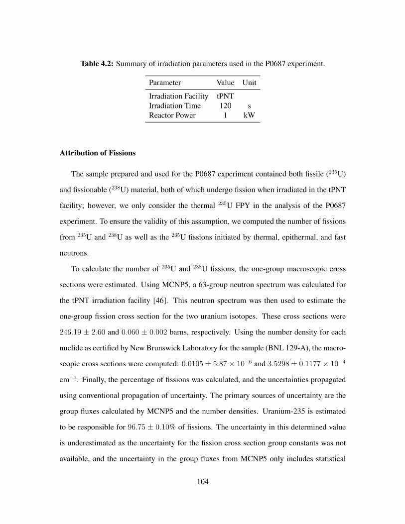
Table 4.2: Summary of irradiation parameters used in the P0687 experiment.

Parameter Value Unit

Irradiation Facility tPNTIrradiation Time 120 sReactor Power 1 kW

Attribution of Fissions

The sample prepared and used for the P0687 experiment contained both fissile (235U)

and fissionable (238U) material, both of which undergo fission when irradiated in the tPNT

facility; however, we only consider the thermal 235U FPY in the analysis of the P0687

experiment. To ensure the validity of this assumption, we computed the number of fissions

from 235U and 238U as well as the 235U fissions initiated by thermal, epithermal, and fast

neutrons.

To calculate the number of 235U and 238U fissions, the one-group macroscopic cross

sections were estimated. Using MCNP5, a 63-group neutron spectrum was calculated for

the tPNT irradiation facility [46]. This neutron spectrum was then used to estimate the

one-group fission cross section for the two uranium isotopes. These cross sections were

246.19 ± 2.60 and 0.060 ± 0.002 barns, respectively. Using the number density for each

nuclide as certified by New Brunswick Laboratory for the sample (BNL 129-A), the macro-

scopic cross sections were computed: 0.0105 ± 5.87 × 10−6 and 3.5298 ± 0.1177 × 10−4

cm−1. Finally, the percentage of fissions was calculated, and the uncertainties propagated

using conventional propagation of uncertainty. The primary sources of uncertainty are the

group fluxes calculated by MCNP5 and the number densities. Uranium-235 is estimated

to be responsible for 96.75 ± 0.10% of fissions. The uncertainty in this determined value

is underestimated as the uncertainty for the fission cross section group constants was not

available, and the uncertainty in the group fluxes from MCNP5 only includes statistical

104

uncertainty and neglects any systematic bias.

Given the majority of fissions are from 235U, the breakdown of incident neutron energy

leading to fission was then estimated by computing the macroscopic group cross sections.

The limits on energy for the thermal, epithermal, and fast bins were chosen to coincide (as

nearly as possible given the group structure used to compute the tPNT neutron spectrum)

with the available fission yields. Table 4.3 summarizes the available fission yield data,

the desired energy limits, the actual energy limits, the macroscopic group constants, and

the group fluxes. Note, the reported group fluxes are normalized to fission as per MCNP

KCODE.

Table 4.3: The available fission yield data, the desired energy limits, the actual energylimits, the microscopic group constants, and the group fluxes (normalized to fission).

Available Fission Yields Desired Energy Limits Actual Energy Limits σf,i [b] φi [cm−2s−1]

0.0253 eV [0, 10 eV] [0, 13.7 eV] 415.62± 4.45 1.85± 0.02× 10−4

500 keV [10 eV, 1 MeV] [13.7 eV, 1.11 MeV] 9.14± 0.25 9.72± 0.14× 10−5

14 MeV [1 MeV, 25 MeV] [1.11 MeV, 25 MeV] 1.24± 0.03 3.39± 0.08× 10−5

The reaction rates in each group were computed. It is estimated that 98.80 %, 1.14

%, and 0.05 % of the fissions were initiated by thermal, epithermal, and fast neutrons,

respectively. Finally, these values were used to weight the 0.0253 eV, 500 keV, and 14

MeV cumulative fission yields for 140Ba and 132Te. The ratio of these weighted average

yields to the 0.0253 eV values are 99.94 % and 100.10 %, respectively. Thus, the 0.0253

eV literature values are valid for comparison to FPY determined following analysis of FP

produced in the TRIGA reactor.

4.1.3 Collection of Gamma-ray Spectra

A Compton-suppressed gamma-ray spectrometer using a high-purity germanium (HPGe)

solid state detector was used to collect normal (Compton suppression mode not utilized)

105

gamma-ray spectra of the irradiated uranium samples. Figure 4.2 shows the gamma-ray

spectrometer along with a close-up view of source-detector geometry.

(a) Gamma-ray spectrometer (b) Source-detector geometry

Figure 4.2: Compton-suppressed gamma-ray spectrometer used to collect spectra of fissionproducts after irradiation of U3O8 samples.

In order to accurately determine the energy of the observed photopeaks and quantify the

activity of the decaying radionuclides, the detector must be energy calibrated and efficiency

calibrated across the complete energy range to be used in subsequent analysis. To span the

energy range and match the U3O8 sample matrix, a custom multi-gamma sand source from

Eckert and Ziegler Analytics containing 210Pb (46.5 keV), 241Am (59.5 keV), 109Cd (88.0

keV), 57Co (122.1 keV), 139Ce (165.9 keV), 203Hg (279.2 keV), 113Sn (391.7 keV), 137Cs

(661.7 keV), 88Y (898.0 and 1836.1 keV), and 60Co (1173.2 and 1332.5 keV) was used for

calibration. The sample was counted in two source-detector geometries used for counting

fission products. The peak locations and characteristic energies from the nuclear data were

106

used to perform an energy calibration with Genie-PC spectral analysis software, and the

peak areas and certified gamma-ray output were used to perform an efficiency calibration.

The efficiency was fitted using the following functional form:

log(ε(E)) =N∑n=0

an log(E)n. (4.1)

Following the end of irradiation, the sample was counted using the HPGe detector

shown in Figure 4.2 several times over three weeks as detector availability allowed. Count-

ing times were determined for each collection based on sample activity, and times ranged

from 3 to 24 hours. Table 4.4 gives the time since end of irradiation (decay time), counting

time, and source-detector distance for each gamma-ray spectrum.

Table 4.4: Summary of the counting parameters used in the P0687 experiment.

Spectrum Decay Time [s] Counting Time [s] Source-Detector Geometry [cm]

1 3630 600 92 9990 1200 93 13710 1800 94 18450 3600 95 194010 10800 96 1224270 18000 17 1306590 64800 18 1471830 72000 19 1813050 72000 110 1987050 86400 111 2167110 86400 1

4.2 Data Analysis

The previous section described the process used to obtain gamma-ray spectra collected

of FP decaying over time following the end of irradiation. These gamma-ray spectra were

107

analyzed to identify FP signatures, calculate the activities of the identified radionuclides at

the beginning of spectral acquisition, and determine FPY in a two-stage analysis: find the

time-averaged neutron flux using 99Mo as an internal standard and then estimate FPY for

all other identified FP using the determined neutron flux and associated uncertainty. This

section concludes with a discussion of the results.

4.2.1 Radionuclide Analysis

Figure 4.3 shows an example spectrum collected of the P0687 sample two days after

the end of irradiation (see Spectrum 5 in Table 4.4). A VMS peak search performed with

Genie-PC found 129 significant peaks in the spectrum.

Figure 4.3: Gamma-ray spectrum collected of P0687 sample two days after end of irradia-tion. The spectrum was counted for three hours, and there are at least 129 significant peaks.An inset figure shows the 0 to 225 keV portion of the spectrum. Counts below 35 keV areremoved by the low-level discriminator.

108

The following nuclides were identified in the spectra collected of the P0687 sample:

95Zr, 95Nb, 99Mo, 132Te, 132I, 133I, 135I, 140Ba, 140La, 141Ce, and 143Ce. Not all nuclides were

observed in each spectrum; however, in every spectrum in which a nuclide’s characteristic

photopeaks were observed, the activity at the beginning of counting was calculated using

the method of Section 2.2.2 on page 20. Spectral interferences were observed between the

162.7 keV and 163.3 keV photons of 140Ba and 235U, as well the 765.8 keV and 766 keV

photons of 95Nb and 234mPa. These interferences were resolved using the 185.7 keV and

1001 keV photons of 235U and 234mPa (second daughter of 238U), respectively. Table 4.5

gives the final estimates for the activities of each nuclide in each spectrum in which char-

acteristic photopeaks were observed.

109

Tabl

e4.

5:A

ctiv

ities

ofth

enu

clid

esst

udie

din

the

P068

7ex

peri

men

tuse

dfo

res

timat

ion

ofFP

Y.N

egat

ive

activ

ities

prod

uced

from

inte

rfer

ence

corr

ectio

nor

pare

nt-d

augh

tera

ctiv

ityca

lcul

atio

nsw

ere

roun

ded

toze

ro.

Nuc

lide

Act

ivity

[Bq]

Spec

trum

4Sp

ectr

um5

Spec

trum

6Sp

ectr

um7

Spec

trum

8Sp

ectr

um9

Spec

trum

10Sp

ectr

um11

95Z

r–

–10

.15±

0.22

9.84±

0.12

10.2

9±

0.12

9.27±

0.11

9.60±

0.10

8.52±

0.10

95N

b–

–1.

41±

1.13

2.61±

0.12

2.98±

0.12

3.52±

0.12

3.70±

0.12

4.10±

0.12

99M

o–

132.

50±

5.78

7.68±

0.41

4.88±

0.14

3.70±

0.19

––

–13

2 Te–

23.6

1±

4.92

9.17±

0.15

13.6

5±

0.16

4.35±

0.09

3.65±

0.06

2.83±

0.05

1.46±

0.04

132 I

–11

7.67±

5.41

6.06±

1.01

0.00±

47.0

02.

39±

18.3

40.

00±

21.3

90.

00±

25.8

50.

00±

13.7

413

3 I–

158.

18±

5.29

––

––

––

135 I

1.37±

0.04×

103

––

––

––

–14

0 Ba

–46

.22±

1.89

19.6

2±

0.48

16.9

8±

0.39

15.1

9±

0.32

13.2

3±

0.29

11.8

6±

0.27

11.0

0±

0.28

140 L

a–

27.4

2±

0.75

23.6

4±

0.17

24.1

8±

0.23

21.4

1±

0.21

17.1

8±

0.18

16.0

7±

0.23

14.3

8±

0.24

141 C

e–

11.7

6±

1.06

9.49±

0.15

9.09±

0.09

9.14±

0.09

8.38±

0.08

8.02±

0.08

7.68±

0.07

143 C

e35

6.66±

9.36

135.

77±

3.08

––

––

––

110

4.2.2 Neutron Flux and FPY Determination

As discussed in Section 2.4.3, 99Mo was used as an internal standard to determine the

time-averaged neutron flux, 〈φ〉. In this stage of the analysis, the cFPY of 99Mo, χ(c)Mo99, was

treated as an uncertain input parameter and 〈φ〉 was the single parameter to be estimated.

The value for χ(c)Mo99, 6.1087± 0.0855, was taken from the ENDF database [1].

Table 4.6 gives the ten input values and associated uncertainties used in the determi-

nation of 〈φ〉. These ten variables were combined to form a ten-dimensional multivariate

Gaussian distribution, N (x|µ,Σ), with µ set to the mean values and Σ diagonal with en-

tries given by the squared standard uncertainties, Σii = u(θ0i)2 ∀ i. The only correlated

values (off-diagonal terms in Σ) are the measured activities and decay constants; however,

the uncertainty in the decay constant of 99Mo is sufficiently small such that the calculated

covariance terms were neglected. As discussed by Tarantola, the use of a diagonal covari-

ance matrix, i.e., neglecting the off-diagonal terms, is warranted and conservative because

a diagonal covariance matrix conveys less information and covers a larger portion of the

input space [47]. Even though there is considerable prior knowledge of the neutron flux in

tPNT facility, an uninformatve (uniform) prior distribution was used to allow the value for

〈φ〉 to freely vary in the domain, R++.

After drawing 10,000 samples from the input space and calculating the associated value

of 〈φ〉 using the LM algorithm, a reasonable approximation for the posterior distribution of

the time-averaged one-group neutron flux was obtained. This approximate distribution is

shown in Figure 4.4. The final flux estimate is 2.2576×1010 ± 2.4040×109 cm−2s−1, which

is commensurate with the reactor operators’ prior experience. The agreement between the

estimate of neutron flux with prior research and measurements suggests that there is no

apparent bias or unaccounted source of error in the determined 〈φ〉. This flux estimate was

used as an uncertain input for all subsequent data analysis.

111

Table 4.6: Measured activities, experimental data, and nuclear parameters used to estimatethe average neutron flux. Mean values, standard uncertainties, and relative uncertaintiesare shown.The reported times for each activity measurement are the elapsed time betweenthe end of irradiation and the beginning of gamma-ray counting.

Parameter Mean Value Relative Uncertainty99Mo Activity (t = 2.3 d) 132.50 Bq 4.4%99Mo Activity (t = 14.2 d) 7.68 Bq 5.3%99Mo Activity (t = 15.1 d) 4.88 Bq 2.9%99Mo Activity (t = 17.0 d) 3.70 Bq 5.1%Irradiation time 120 s 4.2%99Mo Decay constant 2.92× 10−6 s−1 0.02%99Mo Cumulative yield 6.11% 1.4%235U Fission cross section 245 b 5.0%235U Mass 6.67× 10−4 g 1.0%235U Density 1.67× 10−2 g cm−3 10.2%

Figure 4.4: Approximate posterior distribution for the time-averaged one-group neutronflux obtained after 10,000 samples of the ten-dimensional input parameter space.

Figure 4.5 shows a plot of calculated 〈φ〉 values versus sampled values for σf . A linear

function was fit to this data using ordinary least squares to give an estimate of the sensitivity

112

Table 4.7: Uncertainty budget for neutron flux estimation in P0687 experiment. The sen-sitivity coefficient for each input value was estimated by applying a linear regression fluxestimates onto sampled input values drawn during the Monte Carlo routine.The reportedtimes for each activity measurement are the elapsed time between the end of irradiationand the beginning of gamma-ray counting.

Parameter Contribution to Uncertainty [%]99Mo Activity (t = 2.3 d) 9.2799Mo Activity (t = 14.2 d) 4.9399Mo Activity (t = 15.1 d) 0.0199Mo Activity (t = 17.0 d) 2.71Irradiation time 26.4599Mo Decay constant 0.0699Mo Cumulative yield 3.45235U Fission cross section 50.99235U Mass 2.01235U Density 0.13

coefficient, i.e., first-order partial derivative ∂〈φ〉/∂σf , centered on the mean value σf = 245

barns. This procedure was used to calculate the sensitivity coefficient between the flux

and the irradiation time, fission cross section, fissionable material mass, and fissionable

material density. Using these values and Equation (2.13), the covariance matrix, Σ, was

constructed and used in subsequent FPY analyses. In addition, estimated sensitivity coef-

ficients were used with Equation (2.59) to calculate the uncertainty budget for the neutron

flux measurement, shown in Table 4.7.

Approximately 75% of the total uncertainty in the calculated time-averaged neutron

flux comes from uncertainties in the microscopic one-group fission cross section of 235U,

σf , and the irradiation time. A relative uncertainty of 5% was ascribed to the irradiation

time to be conservative; however, it is likely that the true variation in irradiation times is

smaller when the pneumatic transfer system is used. The fission cross section was calcu-

lated using a 63-group neutron spectrum for the tPNT facility calculated using MCNP5 as

a weighting function to collapse the 235U fission cross section from the CINDER90 cross

113

Figure 4.5: Estimation of sensitivity coefficient between estimated neutron flux and fissioncross section in P0687 experiment. A linear function (red) was fit to sampled data (blue) toestimate the first-order partial derivative. This value was used to evaluate covariance, Σ, indeveloping input space distribution for FPY evaluation with Monte Carlo sampling.

114

section file [48]. CINDER90 does not provide uncertainties on the group constants, and the

uncertainty in the calculated one-group cross section only includes uncertainty in the entries

of the weighting function (neutron group fluxes) provided by MCNP. These uncertainties

only include statistical variation and neglect the uncertainty in all the material properties,

nuclear data, and geometric parameters used in the model to generate the neutron group

fluxes. While additional simulation time could reduce the statistical variation in each neu-

tron group constant, the true uncertainty has a lower limit due to untreated uncertainties†.

Accordingly, the 5% relative uncertainty ascribed to σf (12.25 b) is appropriate.

Sensitivity coefficient estimation with least squares after Monte Carlo sampling as de-

scribing is only possible because the input space is independent‡. If the variables are not

independent (as is the case in subsequent FPY analyses), trends between θ and an input

may be incorrectly observed when no true sensitivity is present due to a correlation with a

more sensitive variable.

Using Equations (2.34) and (2.35), the prior distributions for FPY of the identified nu-

clides (excluding 99Mo) were developed. The resulting values are given in Table 4.8. Using

the LM solver and Monte Carlo sampling, the posterior distribution for FPY was approxi-

mated for each FP observed in the gamma-ray spectra collected of the P0687 sample and

shown in Table 4.5 on page 110. In each case, 10,000 samples were drawn from the multi-

variate normal distributions (input space) and used to approximate the posterior distribution

of θ. Figure 4.6 shows the approximate two-dimensional posterior distribution for the cu-

†Recently, a new code called SAMPLER has been developed at Oak Ridge National Laboratory to facil-itate perturbations on cross sections (and possibly other) input parameters used in KENO radiation transportsimulations and ORIGEN point depletion calculations. The result is a Monte Carlo procedure to sample valuesand generate transport models, each of which are then simulated using Monte Carlo radiation transport, andthe net effect is a result that includes statistical variation arising from the simulation methodology as well asthe previously untreated uncertainties in the nuclear data and physical specifications of the model. To date,it unknown if this method has been applied to such a problem in order to assess the magnitude of effect ongroup fluxes of the aforementioned untreated uncertainties, and it is unlikely as such as computation wouldlikely require significant computational resources.

‡Recall, this is due to the small uncertainty in λ, making the term ∂Ai/∂λu(λ)2 small.

115

mulative yield of 140Ba and independent yield of 140La, which were treated as a two-nuclide

decay chain coupled by radioactive decay and solved simultaneously. Equation (2.62) on

page 62 was used to calculate a correlation of +0.60 between χ(c)Ba140 and χ(i)

La140.

Table 4.8: FPY prior distribution statistics used in P0687 experiment.

Nuclide Ind./Cum. Yield Prior Statistics [%] Relative Unc. in Prior [%]95Nb (35.0 d) I 4.27× 10−5 ± 1.94× 10−5 45.495Zr (64.0 d) C 6.50 ± 0.27 4.2132I (2.3 h) I 0.01 ± 0.02 191.4132Te (3.2 d) C 4.29 ± 0.18 4.2140La (1.7 d) I 3.60× 10−3 ± 9.90× 10−3 275.0140Ba (12.8 d) C 6.24 ± 0.28 4.5133I (20.8 h) C 6.65 ± 12.86 193.5135I (6.6 h) C 6.31 ± 0.66 10.4141Ce (32.5 d) C 5.85 ± 0.44 7.5143Ce (33.0 h) C 5.95 ± 0.25 4.2

It is unclear why the FPY of 140Ba and 140La are more strongly correlated than the other

parent/daughter pairs. Three possible causes are addressed below.

Half-Lives: The half-lives of 140Ba and 140La fall between those of 132Te/132I and 95Zr/95Nb.

This same relationship is true for the ratio of parent nuclide and daughter nuclide

half-lives.

Uncertainty in Prior Distributions: The relative uncertainty in the prior distributions

used for each nuclide’s FPY dictate the strength of the prior term that competes with

the experimental evidence encoded in the likelihood function affects the result (see

Section 3.5). The relative uncertainty in the prior for χ(i)La140 is greater than any other

FP examined.

116

Figure 4.6: Approximate two-dimensional posterior distribution for the iFPY of 140La andcFPY of 140Ba. There is a clear positive correlation between the FPY; Equation (2.62) onpage 62 was used to calculate a correlation value of +0.60.

117

Uncertainty in Measured Activities: Examining the values in Table 4.5 on page 110, the

average relative uncertainty in the measured activities is smallest for 140Ba and 140La

at 2.6% and 1.4%, respectively.

The expressions given in Equation (2.60) were used to compute the mean reported value

and the associated standard uncertainty for each estimated value. The results are summa-

rized in Table 4.9. For pairs of nuclides coupled into a decay chain and FPY solved simul-

taneously, the correlation between the estimated values, calculated with Equation (2.62), is

given.

Table 4.10 shows the percent bias in the determined values. These values assume that

the literature/prior values are correct to reality, which is not assured (see the discussion in

Section 1.1 on page 1). The bias values were calculated as

100×

(θ

θ− 1

). (4.2)

The average bias is +6.3%, indicating a good agreement with existing literature values.

The overall relative difference in the values is 9.7%. The determined values for χ(c)I135 and

χ(c)Ce141 are lower than the values found in the literature, while the rest of the values are

greater than the literature values. The presence of positive and negative biases relative

to literature values suggests that no systematic bias are present. The average bias is less

than the absolute relative difference (+6.3% and 9.7%, respectively), which supports this

conclusion. The largest differences between determined and literature values are in the

estimated FPY for 95Zr, 133I, and 140La. We attribute the difference in the value for 140La to

the small contribution to the total 140La inventory made directly from fission, i.e., from the

iFPY. The additional 140La expected beyond the contribution from the decay of the parent

140Ba is small enough to reside primarily in the noise of the experimental measurements.

The results presented in Table 4.9 on page 120 agree well with the existing values,

118

and all determined FPY are within the expected range of values, i.e., they are realistic and

physical. While it possible to reduce uncertainty by refining the value for irradiation time

(see Table 4.7 on page 113) and collecting additional gamma-ray spectra (there are limited

measurements of 133I, 135I, and 143Ce as shown in Table 4.5 on page 110), the experiment

outcome is positive as it demonstrates the viability of the methodology described in Chap-

ter 2.

119

Tabl

e4.

9:Su

mm

ary

ofFP

Yde

term

ined

forl

ong-

lived

FPob

serv

edin

P068

7ex

peri

men

t.

Nuc

lide

Ind.

/Cum

.Yie

ldPr

iorS

tatis

tics

[%]

Cal

cula

ted

Val

ue[%

]C

orre

latio

nr jk

95N

b(3

5.0

d)†

I4.

27×

10−

5±

1.94×

10−

54.

27×

10−

5±

3.56×

10−

8+0

.09

95Z

r(64

.0d)

C6.

50×

100±

2.10×

10−

17.

53×

100±

3.45×

10−

1+0

.09

132I(

2.3

h)I

1.00×

10−

2±

2.00×

10−

21.

05×

10−

2±

1.20×

10−

4-0

.02

132Te

(3.2

d)C

4.29×

100±

1.80×

10−

24.

39×

100±

1.34×

10−

1-0

.02

140L

a(1

.7d)

I3.

60×

10−

3±

9.90×

10−

34.

19×

10−

3±

2.90×

10−

4+0

.60

140B

a(1

2.8

d)C

6.24×

100±

2.80×

10−

16.

35×

100±

3.42×

10−

1+0

.60

133I(

20.8

h)C

6.65×

100±

12.8

6×

100

9.13×

100±

7.51×

10−

1–

135I(

6.6

h)C

6.31×

100±

6.60×

10−

16.

30×

100±

5.53×

10−

4–

141C

e(3

2.5

d)C

5.85×

100±

4.40×

10−

14.

86×

100±

3.07×

10−

1–

143C

e(3

3.0

h)C

5.95×

100±

2.50×

10−

16.

02×

100±

1.15×

10−

1–

†Im

plic

itly

norm

aliz

edto

cFPY

of99M

oby

two-

stag

ean

alys

is.

120

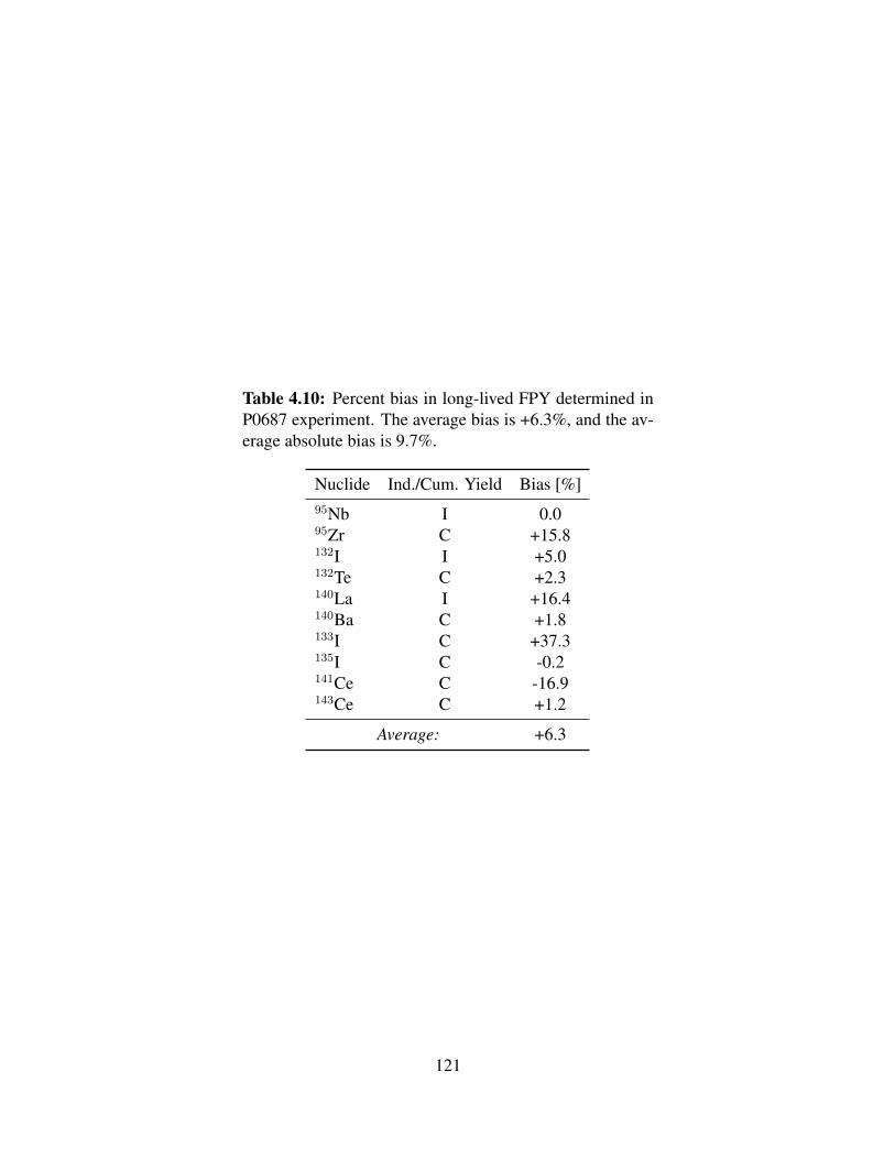
Table 4.10: Percent bias in long-lived FPY determined inP0687 experiment. The average bias is +6.3%, and the av-erage absolute bias is 9.7%.

Nuclide Ind./Cum. Yield Bias [%]95Nb I 0.095Zr C +15.8132I I +5.0132Te C +2.3140La I +16.4140Ba C +1.8133I C +37.3135I C -0.2141Ce C -16.9143Ce C +1.2

Average: +6.3

121

5 | 14.1 MeV Neutrons:

Run 2 Experiment

A measurement of FPY from 14.1 MeV neutron-induced fission was conducted in con-

junction with scientists at PNNL. Collaborators at PNNL prepared an isotopically pure 235U

sample, irradiated the target using a 14.1 MeV neutron generator, and collected gamma-ray

counting data using an HPGe detector and digital spectroscopy data collection.

At UT, these list-mode (time- and energy-stamped) data were parsed to form “time

slices” of the counting data. Differently sized time slices were used to target radionuclides

with different half-lives, and these time-sliced spectra were used to identify and quantify FP.

The activity times series for each decay chain of FP were used as inputs for FPY analysis

using the methodology of Chapter 2.

5.1 Experiment

Collaborators at PNNL produced an isotopically pure 235U foil and verified the purity

at greater than 99%. A portion of the sample was cut and the mass was determined using a

standard lab balance. The mass of the foil is 220 ± 0.5 mg and then packaged in a plastic

bag to prevent contamination during handling as shown in Figure 5.1.

The sample was placed inside an aluminum rabbit and pneumatically transferred to a

commercial neutron generator for irradiation, shown in Figure 5.2. Scientists estimated a

maximum neutron flux of 1 × 109 cm−2s−1; however, the flux on target is expected to be

122

Figure 5.1: The 235U foil irradiated with neutron generator to measure 14.1 MeV neutron-induced fission FPY.

smaller due to geometric attenuation. The sample was irradiated for 5:33.

After then end of irradiation, the sample was returned to experimenters using the pneu-

matic transfer line and surveyed by radiation protection personnel prior to analysis. The

sample was then placed in a sample holder inside of a detector align jig and counted us-

ing a Canberra BE6530 broad energy HPGe with carbon window, shown in Figure 5.3.

In characterization studies, the detector energy range and resolution were measured as 13

keV - 2.2 MeV and between 1 and 2 keV FWHM, respectively. The measured resolution

was confirmed in subsequent analysis described in Section 5.2.1. The spectral data was

processed and recorded in list-mode using a Lynx multichannel analyzer.

123

Figure 5.2: Neutron generator used to irradiate the 235U shown in Figure 5.1.

124

Figure 5.3: The broad-energy HPGe detector used to collect gamma-ray counting datafollowing the irradiation of 235U foil and determine 14.1 MeV neutron-induced fission FPY.

125

5.2 Data Analysis

5.2.1 Data Processing & Calibration

A text-parsing code called “lynxparse” was implemented in Fortan90 to perform the

“time slicing” and produce sets of gamma-ray spectra from the list-mode data. The user

specifies a beginning time and the desired length of for each spectrum. The code then reads

each event (count) in the file, checks the time stamp, and then bins the energy of the event if

the time stamp falls into the desired time window. A second code called “lynxparsedt” was

developed to perform the same procedure; however, the differential dead time† is used to

adjust the bin increment value when each event is recorded and correct for the time-varying

detector dead time.

Parsing the list-mode data gave sets of gamma-ray spectra in *.n42 format, which were

then converted to *.chn files suitable for analysis in Genie-PC. The primary peaks of 235U

(109.2 keV, 143.8 keV, 163.3 keV, 185.7 keV, 205.3 keV, and 279.5 keV) were observed

well above background and the majority of the fission product signal. These uranium peaks

were used for energy calibration. After this initial calibration, several peaks from the well-

studied FP 140Ba and 140La were analyzed to refine the energy calibration, ensuring accurate

determined peak energies and reduce the energy uncertainty in the nuclide identification

algorithm (∆ in Figure 2.3b).

The density of the sample (approximately 19 g · cm−3 for U metal) leads to self-

attenuation of gamma-rays born in the sample as the photons traverse the metal towards

to detector. The attenuation factor, averaged over the (unknown) thickness of the foil was

†The differential dead time is calculated by computing the ratio between the live time and real time thatare given by the Lynx system. Incrementing the bin value by the inverse fractional dead time corrects thecounts in the spectrum by the current dead time, which may vary greatly between the beginning and end ofspectrum collection as short-lived nuclides decay.

126

computed with Equation (2.18). Since the foil is over 99% pure 235U, the mass attenuation

coefficient for pure uranium was taken from NIST [30], and is shown in Figure 2.6.

The peak detector efficiency of the HPGe detector (see Figure 5.3) was computed using

the data described in the previous section. Given the efficiency and the sample data, the

count rate of the primary 235U peaks expected in the last 12-hour spectrum were computed,

and the ratio of the actual count rate to the expected value gives point-wise attenuation

factors, {α(Ei)}i. The effective thickness was then computed using each datapoint, and

the results were aggregated to find a best estimate of xeff . Equation (2.18) was then used

to extrapolate the attenuation coefficient across the energy range of the analysis: approx-

imately 50 keV (above the L1-edge) to 2.25 MeV. Finally, this curve was multiplied with

the point-wise peak detector efficiency (see Equation (2.19)), and the resulting data were

used to fit a curve using the log-log functional form shown in Equation (4.1) on page 107.

The results are given in Figure 5.4.

5.2.2 FPY Estimation

The following gamma-emitting radionuclides were identified using 12-hour cuts of the

dataset collected following irradiation by 14.1 MeV neutrons: 95Zr/95Nb, 99Mo, 127Sb, 131I,

140Ba/140La, and 147Nd. Half-lives in this subset range from 1.7 days (140La) to 64.0 days

(95Zr).

Count rates were extremely low for the majority of the radionuclides shown in Ta-

ble 5.1. For example, integral counts for the strongest gamma-ray from 140Ba and 140La in

the first spectrum analyzed, 12 hours after end of irradiation† were 1830 ± 214 and 388

± 55, respectively. These peak areas correspond to count rates of approximately 0.04 and

0.01 counts per second, respectively. In additional, the (software) multi-channel analyzer

†The first spectrum extracted from the list-mode data was not used for analysis of long-lived FP in orderto reduce interferences and noise from shorter-lived nuclides.

127

Figure 5.4: Peak detetector efficiency, self-attenuation, and effective efficiency curves forthe HPGe detector used in the analysis of 14.1 MeV PNNL dataset. The peak detectorefficiency curve is shown in blue, the extrapolated attenuation factors calculated using theestimated effective thickness, xeff , and NIST attneuation coefficients is shown in red, andthe effective efficiency curve is shown in greens. The large dip in the red and green curvesat 115 keV is due to the K-absorption shell of 235U.

128

within the Lynx data acquisition system used only 4096 channels, which reduces the ability

of the analyst to differentiate between peaks and resolve spectral interferences; however,

increasing the number of channels would further degrade counting statistics. It is likely

that the number of fissions was relatively low (this is confirmed below), and steps should

be taken to increase the number of fissions in future analysis of 14.1 MeV FPY for long-

and medium-lived FP.

The following nuclides were identified using 20-minute cuts of the dataset: 89Kr/89Rb,

94Y, 104Tc, 130Sb, 134Te/134I, 138Xe/138Cs, 146Ce/146Pr. The half-lives in this subset ranged

from 3.2 minutes (89Kr) to 52.5 minutes (134I). Some nuclides were initially identified with

gamma-gamma coincidence spectroscopy; however, the conditional gamma-ray intensities

were not available for activity calculations using the coincidence spectra. All nuclides were

quantified using singles spectra. The FP gases Kr and Xe were observed in the coincidence

spectra. Recent research has shown that FP noble gases are retained in materials [49]. In

addition, the sample was sealed in plastic, and the metal target was not damaged by the

small neutron fluence. Therefore, we believe the FP gasses were correctly analyzed.

Counting statistics for photopeaks and associated determined activities for the nuclides

shown in Table 5.2 were much better than the long-lived FP shown in Table 5.1 due to

shorter half-lives and greater specific activities.

As with the thermal irradiations performed at UT, the time-averaged neutron flux in-

cident on the sample was determined using the measurements of 99Mo. The value of the

cFPY of 99Mo from 14.1 MeV neutrons was determined by aggregating the values reported

in the ENDF, JEFF, and JENDL data libraries using the (one dimensional) bootstrap me-

dian algorithm. The 235U fission cross section was determined by interpolating on the

values given in the CINDER90 cross section library to obtain the value at 14.1 MeV (pure

D-T source). The uncertainty in σf was estimated by examining the relative difference be-

tween the cross sections reported by ENDF and JENDL. The inputs and associated relative

129

uncertainties are given in Table 5.3. For brevity, only a summary of relative uncertainty is

given for the measured 99Mo activities is given; the full results are given in Table 5.1.

An uninformative prior distribution, LM algorithm, and Monte Carlo sampling were

used to determine the posterior distribution for the flux. The final estimate of neutron flux

is (2.36 ± 0.11) ×108 cm−2s−1. This flux value, along with the sample parameters and

235U 14.1 MeV fission cross section was used to calculate the number of fissions. The

expected number is approximately 9.22 × 107 fissions, confirming the hypothesis that the

experiment produced a small number of FP.

The uncertainty budget was computed and is shown in Table 5.4. The three primary

sources of uncertainty in the analysis are the measured activities, cFPY for 99Mo, and the

235U fission cross section. The values for the FPY and σf were determined directly from

the nuclear data, e.g., no group collapse was performed, so the uncertainty in the values

are irreducible without significant effort, i.e., nuclear data measurement campaign. The

uncertainty in the measured activity of 99Mo may be reduced by increasing the count rate

and/or signal-to-noise ratio. There are several ways to achieve this:

1. Increase the number of fissions by using a more massive target,

2. Increase the irradiation time to increase the number of fissions,

3. Increase the efficiency of the detector by reducing source-detector distance,

4. Use larger detector(s) to increase the solid angle subtended by the detector,

5. Use additional detectors and sum the signals, or

6. Use cyclic irradiations (for short-lived nuclides).

The estimated neutron flux was used as an uncertain input in all subsequent short-

and long-lived nuclides FPY analyses. For each calculation, the input space was sampled

130

10,000 times, and the LM solver was used to determine θ. Finally, summary statistics were

computed and are given in Table 5.5.

The cFPY and iFPY of 89Kr and 89Rb were solved simultaneously, and measured re-

sults are within 3.9% and 46.7% of the literature values, respectively. Short half-lives and

corresponding high activities of these two nuclides led to good counting statistics. There

is considerable uncertainty in the true value of the iFPY of 89Rb—the literature-derived

uncertainty is 50.6%. While this research does not constitute a complete nuclear data mea-

surement campaign and is primarily intended as a proof of concept for the Bayesian inver-

sion method for FPY determination, the results of the present measurement may indicate

that an update to the iFPY of 89Rb value is warranted.

The measured value for the cFPY of 94Y is approximately 24% smaller than the prior

value. The average uncertainty in the activity measurements is 5%. No clear source of

bias is evident; however, due to the short half-live of the radionuclide, it is unlikely that the

literature values are based on measurements (it is too short-lived to be observed in historic

measurements using radiochemical separations). The literature value is likely computed

using model-derived independent yields of parent nuclides and summed down the decay

chain, and it is possible that relevant branching ratios have been updated since the original

determination and the literature value is no longer valid.

The cFPY and iFPY of 95Zr and 95Nb were solved simultaneously, and measured results

differ from literature values by 133.1% and 3900.0%, respectively. Average uncertainty in

the activity measurements are 15.5% and 7.4% for Zr and Nb, respectively. We attributed

the errant result in the value corresponding to Nb to an unresolved spectral interference and

associated overestimation of activity and the very small expected value of the iFPY. The

additional contribution from fission is much smaller than the product of Nb coming from

the decay of Zr, fed by zirconium’s cFPY, and the additional activity that would indicate

the iFPY is easily lost in the measurement uncertainty and error. Given these facts, it

131

should be noted that the actual bias value is only 0.039%. The large overestimation in the

determined value for the cFPY of 95Zr is attributed to the coupling with Nb, which was

grossly overestimated.

The determined values for the cFPY of 104Tc, 127Sb, and 130Sb agree with literature val-

ues. Counting statistics for these three measurements were good and average uncertainties

are less than 3.1% for each nuclide. The absolute biases for these values are -0.6, -0.51,

and -0.61 percentage points, respectively. These results are fairly commensurate with prior

values obtained from the literature.

The measured value for the cFPY of 131I was obtained with good counting statistics as

average uncertainty in the activity measurements is 5.3%. The overestimation of the yield

is attributable to an unresolved spectral interference increasing the measurement activity

values.

Due to the short half-lives and large specific activities, the average precision of the

measured activities of the two-nuclide chain of 134Te and 134I are less than 1% for both

nuclides. The determined values are commensurate with the value obtained from the liter-

ature, differing by 0.01 and 1.06 percentage points, respectively.

The average uncertainty in the activity measurements of 138Xe is 23.9%; however, the

difference between the measured and literature values for the cFPY of 138Xe is not insignif-

icant, -0.53 percentage points. This difference is smaller than the uncertainty in the prior

value, 0.96 percentage points. The measured value for the iFPY 138Cs is 1.36 percentage

points greater than the prior value; however, the uncertainty in the prior value is significant,

0.43 percentage points. The overestimation is attributed to the underestimation of the cFPY

of the parent nuclide, which is balanced by an overestimation of the iFPY of the daughter.

The measured values for the yields of 140Ba and 140La exhibit similar behavior to 138Xe

and 138Cs. The measured yield of the parent 140Ba is less than the prior value, and this

underestimation is apparently balanced by an overestimation of the iFPY of the daughter

132

140La. It is possible that the activity of La was overestimated due to a spectral interference,

but this is unlikely as La emits numerous characteristics photons that were observed in

the gamma-ray spectra. The expected value of the iFPY of La is very small, and the signal

attributable to the iFPY rather than the cFPY of the decaying parent nuclide is small relative

to the measurement uncertainty.

The measured values for 146Ce and 146Pr are commensurate with prior values, differing

by 0.36 and 0.17 percentage points, respectively. As in previous cases, an underestima-

tion in the FPY of the parent nuclide coincides with an overestimation in the FPY of the

daughter nuclide†.

Lastly, the measured value of the cFPY of 147Nd differs significantly from the prior

value, differing by 7.77 percentage points. The average uncertainty in the measured activi-

ties of Nd is 39.9% (the uncertainty ranges from 1.6% to 91.0%). The large overestimation

of the FPY is attributed to overestimation of activities, stemming from poor counting statis-

tics and likely unresolved spectral interferences.

The bias in each determined FPY (assuming the mean value assembled from the liter-

ature and used in the prior distribution, see Section 2.3.1, is the true value) was calculated

and shown in Table 5.6. The average bias is +361.4% and the average absolute bias is

379.2%, and the absolute error being greater than the bias suggests that there is no system-

atic bias in the analysis.

In general, the FPY values determined experimentally differ greatly from the literature

values, and these differences are greater for the 14.1 MeV experiment than the thermal

irradiations performed at UT. The greater disparity between experimentally determined and

literature values may be attributed to several possible factors. Yields for FP following 14.1

MeV neutron-induced fission are less well-understood than values for thermal neutrons,

†It should be noted that this correlation is not necessarily causation. A separate factor, such as spectralinterference, could drive an overestimation of a poorly measured and/or poorly understood daughter nuclideand the FPY of the parent is adjusted during the simultaneous solution.

133

and it is possible that the experimental values are better representative of reality. The

overall quality of the measurements in this experiment is suspect, primarily due to the small

number of fissions that occurred. Counting statistics for long-lived FP were very poor, and

this trend is reflected in the data. The average bias in determined FPY of long-lived FP

with half-lives greater than one day is 860% (137% excluding 95Nb and 140La), while the

average bias of FPY determined for short-lived FP is 73%. Shorter-lived FP with half-

lives on the order of minutes have much larger specific activity and led to better counting

statistics.

Additionally, there are larger differences between the experimental and literature values

in the independent yields, which we attribute to smaller expected values. In the case of

small iFPY, the number of nuclei produced directly from fission are much less than the

number produced from the decay of parent nuclides, i.e., from the cumulative yield of

the parent nuclide. The net signal indicative of the iFPY is easily lost in the noise and

uncertainty of the measurement. Figure 5.5 illustrates the situation. In Figure 5.5a shows

the absolute bias versus the literature values cFPY, and Figure 5.5b shows the data for

nuclides for which iFPY was determined. No distinct trend is visible in Figure 5.5a, but the

results for two nuclides stand out. The cFPY of 147Nb differed greatly from the literature

value, and we attribute this overestimation to an unresolved spectral interference. There

is a large difference in the cFPY determined for 95Zr, which may stem from the coupling

between 95Zr and 95Nb, for which the largest difference between the measured and literature

values; however, it is unclear if the error comes from the parent and propagates the daughter

or if the opposite. There is a clear negative trend between the absolute bias (assuming the

literature values are true) and the literature value for iFPY as shown in Figure 5.5b.

Normalizing the bias to the central values used in the prior distributions potentially

gives an overly pessimistic view of the results. Figures 5.6a and 5.6b show the measured

versus prior values for the cumulative and independent FPY determined for 14.1 MeV

134

(a) Cumulative fission product yields.

(b) Independent fission product yields.

Figure 5.5: Absolute relative difference between the determined FPY and the literaturevalues

135

neutron-induced fission, respectively.

Figure 5.6a shows the measured values for cFPY are close to agreement with the prior

values to within uncertainty; however the results for cFPY of 147Nd and 95Nb are errant,

clearly disagreeing with the prior value and are greater than 7%, indicating these results are

not reasonable. There is a possibility of a small negative systematic bias in the measured

cFPY, and underestimated cFPY values are correlated with overestimated values of iFPY

as shown in Figure 5.6b.

136

(a) Measured versus prior values for cumulative FPY following 14.1 MeV neutron-induced fission.

(b) Measured versus prior values for independent FPY following 14.1 MeV neutron-induced fission.

Figure 5.6: Measured versus prior values for FPY determined after irradiation in 14.1 MeVneutron field.

137

Tabl

e5.

1:M

easu

red

activ

ities

oflo

ng-l

ived

FPpr

oduc

eddu

ring

14.1

MeV

neut

ron

irra

diat

ion

of235U

foil.

Twel

ve-h

our

cuts

ofth

elis

t-m

ode

data

colle

cted

usin

gan

HPG

ede

tect

orfo

llow

ing

the

end

ofir

radi

atio

nw

ere

used

tode

term

ine

radi

onuc

lide

activ

ities

.

Nuc

lide

Act

ivity

[Bq]

Spec

trum

1Sp

ectr

um2

Spec

trum

3Sp

ectr

um4

Spec

trum

5Sp

ectr

um6

Spec

trum

7Sp

ectr

um8

Spec

trum

9Sp

ectr

um10

Spec

trum

11Sp

ectr

um12

95Z

r3.

64±

2.69

1.35±

0.03

0.66±

0.00

0.74±

0.01

0.71±

0.01

0.66±

0.01

22.1

0±

20.9

51.

00±

0.01

0.83±

0.01

0.53±

0.01

1.00±

0.04

0.79±

0.01

95N

b–

–1.

47±

0.01

––

0.10±

0.00

0.10±

0.00

0.10±

0.00

0.17±

0.00

0.21±

0.00

0.09±

0.00

0.14±

0.00

99M

o–

10.5

6±

0.65

9.57±

0.66

8.87±

0.69

8.18±

0.66

5.78±

0.54

5.21±

0.59

6.61±

0.86

4.81±

0.95

3.12±

0.67

2.66±

1.40

2.92±

0.89

131I

8.33±

0.13

5.48±

0.11

3.28±

0.10

4.02±

0.10

3.80±

0.09

3.79±

0.10

3.33±

0.09

3.17±

0.08

6.95±

2.46

3.80±

0.09

3.55±

0.14

4.85±

0.14

127Sb

3.01±

0.02

2.46±

0.03

1.88±

0.03

2.23±

0.02

1.80±

0.01

1.47±

0.02

1.90±

0.02

2.73±

0.70

2.01±

0.03

0.85±

0.02

1.24±

0.01

1.27±

0.02

140B

a3.

59±

0.01

2.86±

0.34

3.00±

0.01

5.66±

0.38

2.39±

0.01

2.23±

0.01

1.68±

0.01

2.09±

0.01

2.37±

0.01

2.49±

0.01

1.64±

0.01

1.96±

0.01

140L

a0.

50±

0.01

0.96±

0.01

1.02±

0.01

1.12±

0.01

1.50±

0.02

1.86±

0.01

1.96±

0.01

1.72±

0.01

2.66±

0.04

1.97±

0.01

2.05±

0.01

1.92±

0.01

147N

d68

.08±

5.19

20.8

7±

19.0

041

.51±

3.66

14.6

1±

12.7

420

.36±

1.88

7.62±

5.67

7.58±

2.14

8.08±

6.74

6.96±

5.74

16.5

6±

0.34

14.5

6±

0.33

13.8

5±

0.22

138

Tabl

e5.

2:M

easu

red

activ

ities

ofsh

ort-

lived

FPpr

oduc

eddu

ring

14.1

MeV

neut

ron

irra

diat

ion

of235U

foil.

Twen

ty-m

inut

ecu

tsof

the

list-

mod

eda

taco

llect

edus

ing

anH

PGe

dete

ctor

follo

win

gth

een

dof

irra

diat

ion

wer

eus

edto

dete

rmin

era

dion

uclid

eac

tiviti

es.

Nuc

lide

Act

ivity

[Bq]

Spec

trum

1Sp

ectr

um2

Spec

trum

3Sp

ectr

um4

Spec

trum

5Sp

ectr

um6

Spec

trum

789K

r19

32.2

2±

13.1

0–

––

––

–89R

b19

49.4

5±

24.2

791

5.93±

3.32

379.

19±

1.64

151.

40±

1.03

72.9

4±

0.71

43.9

6±

0.64

–94Y

1505

.22±

9.89

880.

03±

8.70

484.

54±

4.86

225.

83±

13.5

412

8.51±

8.97

52.7

2±

5.32

32.8

3±

4.69

104T

c91

8.60±

5.30

456.

76±

4.73

253.

35±

7.48

102.

22±

1.52

38.9

0±

1.18

––

130Sb

345.

78±

1.28

114.

52±

0.41

57.1

7±

0.25

38.0

0±

0.23

25.4

9±

0.13

20.7

1±

0.19

18.5

1±

0.15

134Te

623.

74±

1.78

471.

12±

1.14

313.

91±

0.49

212.

02±

0.58

150.

26±

0.21

107.

62±

0.39

76.5

5±

0.32

134I

459.

50±

1.42

466.

51±

1.20

366.

65±

0.89

352.

90±

0.60

286.

68±

0.52

253.

22±

0.51

213.

57±

0.31

138X

e16

60.0±

7.80

689.

40±

14.4

832

1.23±

1.54

114.

28±

0.28

100.

02±

54.9

448

.31±

29.1

842

.14±

20.5

6138C

s67

2.00±

3.49

778.

39±

2.45

604.

23±

2.85

491.

12±

1.24

320.

87±

0.93

219.

15±

0.48

156.

22±

0.92

146C

e11

62.0

2±

3.86

337.

45±

0.75

153.

10±

0.37

85.4

1±

0.55

––

–146Pr

182.

51±

5.04

415.

09±

2.06

231.

18±

1.50

193.

74±

1.34

––

–

139

Table 5.3: Measured activities, experimental data, and nuclear parameters used to estimatethe average neutron flux. Mean values, standard uncertainties, and relative uncertaintiesare shown.

Parameter Mean Value Relative Uncertainty

Measured activities (11 points) – 16.99%†Irradiation time 120 s 4.2%99Mo Decay constant 2.92× 10−6 s−1 0.02%99Mo Cumulative yield 6.11% 1.4%235U Fission cross section 245 b 5.0%235U Mass 6.67× 10−4 g 1.0%235U Density 1.67× 10−2 g cm−3 10.2%

†The average relative uncertainty in the 11 measured activities is reported for brevity.

Table 5.4: Uncertainty budget for neutron flux estimation. The sensitivity coefficient foreach input value was estimated by applying a linear regression of each flux estimate tosampled values performed in the Monte Carlo routine. The reported times for each activitymeasurement are the elapsed time between the end of irradiation and the beginning ofgamma-ray counting.

Parameter Percent of Uncertainty [%]99Mo Activity (t = 1.0 d) 5.7399Mo Activity (t = 1.5 d) 6.3699Mo Activity (t = 2.0 d) 6.3599Mo Activity (t = 2.5 d) 6.2999Mo Activity (t = 3.0 d) 5.5299Mo Activity (t = 3.5 d) 4.6499Mo Activity (t = 4.0 d) 2.3399Mo Activity (t = 4.5 d) 1.6199Mo Activity (t = 5.0 d) 2.8099Mo Activity (t = 5.5 d) 0.4699Mo Activity (t = 6.0 d) 0.89Irradiation time 0.5899Mo Decay constant 0.0099Mo Cumulative yield 30.29235U Fission cross section 17.37235U Mass 0.78235U Density 0.00

140

Tabl

e5.

5:Su

mm

ary

ofFP

Yde

term

ined

forF

Ppr

oduc

edfo

llow

ing

14.1

MeV

neut

ron

irra

diat

ion.

Nuc

lide

Ind.

/Cum

.Yie

ldPr

iorS

tatis

tics

[%]

Cal

cula

ted

Val

ue[%

]C

orre

latio

nr jk

89K

r(3.

2m

)C

3.32±

0.39

3.19±

0.15

+0.9

389R

b(1

5.2

m)

I0.

75±

1.14

1.10±

0.05

+0.9

394Y

(18.

7m

)C

5.05±

2.81

3.82±

0.17

–95Z

r(64

.0d)

C5.

14±

0.56

11.9

8±

0.51

-0.9

495N

b(3

5.0

d)I

0.00

1±

0.00

20.

04±

0.00

1-0

.94

104T

c(1

8.3

m)

C2.

47±

1.71

1.87±

0.08

–127Sb

(3.9

d)C

2.08±

0.95

1.57±

0.07

–130Sb

(39.

5m

)C

1.45±

3.14

0.84±

0.04

–131I(

8.0

d)C

4.11±

0.49

6.00±

0.27

–134Te

(41.

8m

)C

2.37±

1.66

2.38±

0.10

+0.9

9134I(

52.5

m)

I1.

06±

1.05

2.12±

0.09

+0.9

9138X

e(1

4.1

m)

C3.

40±

2.87

2.83±

0.12

+0.9

5138C

s(3

3.4

m)

I0.

47±

1.28

1.83±

0.08

+0.9

5140B

a(1

2.8

d)C

4.49±

0.38

4.18±

0.74

-0.7

8140L

a(1

.7d)

I0.

03±

0.06

0.46±

0.46

-0.7

8146C

e(1

3.5

m)

C2.

17±

2.03

1.81±

0.08

+0.5

2146Pr

(24.

2m

)I

0.07±

0.16

0.24±

0.02

+0.5

2147N

d(1

1.0

d)C

1.64±

0.14

9.41±

0.11

–

141

Table 5.6: Relative bias in FPY determined following 14.1 MeV neutron irradiation. Theaverage bias is +361.4% and the average absolute bias is 379.2%.

Nuclide Ind./Cum. Yield Bias [%]89Kr (3.2 m) C -3.989Rb (15.2 m) I +46.794Y (18.7 m) C -24.495Zr (64.0 d) C +133.195Nb (35.0 d) I +3900.0104Tc (18.3 m) C -24.3127Sb (3.9 d) C -24.5130Sb (39.5 m) C -42.1131I (8.0 d) C +46.0134Te (41.8 m) C 0.4134I (52.5 m) I +100.0138Xe (14.1 m) C -16.8138Cs (33.4 m) I +289.4140Ba (12.8 d) C -6.9140La (1.7 d) I +1433.3146Ce (13.5 m) C -16.6146Pr (24.2 m) I +242.9147Nd (11.0 d) C +473.8

142

6 | Conclusions

In this chapter, the work completed to date is summarized, the fulfillment of the goals

for the work discussed in Section 1.3 are addressed, and opportunities for further work are

then presented.

6.1 Summary

To date, limited FPY have been experimentally determined, and primary efforts have

focused on the cFPY of long-lived FP at the end of decay chains, typically measured using

radiochemical separation and/or destructive analysis. Independent FPY have been esti-

mated using nuclear models such as the ZP (A) model of Wahl, which was developed in

the early sixties and refined over the next twenty years. Despite these efforts, there is still

considerable uncertainty in the true values which is not adequately reflected in the three

major nuclide data libraries ENDF, JEFF, and JENDL.

During the course of this research, a flexible method to perform parameter estimation

in a framework of Bayesian inference was developed, and ancillary methods to perform

reliable and accurate gamma-ray spectrometry, i.e., radionuclide identification and activity

quantification, of complex FP gamma-ray spectra were also developed. All the functions

used to perform the analysis, import data, and produce output visualizations were proto-

typed and implemented in Matlab in a package called FRACTURE.

The accuracy of each module within FRACTURE (nuclide identification, activity calcu-

lation for coupled decay chains, nuclide transmutation modeling during and after neutron

143

irradiation, optimization, and uncertainty quantification) was verified in a series of con-

trolled, isolated experiments, and the ability of the complete package to perform the de-

sired inverse analyses was validated. During the course of these verification and validation

exercises, the best methodology among the options studied, e.g., optimization solver, were

examined.

Experiments were performed at UT to produce FP using thermal neutrons and deter-

mine iFPY and cFPY for long-lived FP. Samples of naturally-enriched U3O8 were prepared

and irradiated in the 1.1 MW TRIGA reactor at NETL, and a series of gamma-ray spectra

were collected of the sample post irradiation using an HPGe-based spectrometer. Long-

lived FP were identified in the sample: 95Zr, 95Nb, 99Mo, 132Te, 132I, 133I, 135I, 140Ba, 140La,

141Ce, and 143Ce. The activity at the beginning of counting was calculated for each nuclide

and spectrum to form activity time series of each radionuclide. The time series for 99Mo

and nuclear data and associated uncertainties were used to determine the neutron flux inci-

dent on the sample, and the time series for the remainder of the observed FP were used to

determine thermal FPY using the developed Bayesian framework.

Collaborating scientists at PNNL produced isotopically pure 235U metal foil, and bom-

barded a foil with 14.1 MeV neutrons produced with a D-T neutron generator. An HPGe

detector was used to count gamma-rays for 166 hours and collect list-mode data. The data

was parsed offline to produce time-sliced cuts of the total dataset. These sets of spec-

tra were analyzed to produce activity time series of FP. Twelve-hour cuts were used to

analyze long-lived FP (95Zr/95Nb, 99Mo, 127Sb, 131I, 140Ba/140La, and 147Nd), and twenty-

minute cuts were used to analyze shorter-lived FP (89Kr/89Rb, 94Y, 104Tc, 130Sb, 134Te/134I,

138Xe/138Cs, 146Ce/146Pr). The last twelve-hour cut was used to determine self-attenuation

correction factors using the 235U as a basis for correction. The gamma-emitting radionu-

clide 99Mo was used to determine the neutron flux incident on the sample, and the FPY for

all remaining nuclides were estimated.

144

The differences between the determined values for FPY and the prior values assembled

from the literature, and in the case of the data taken from the 14.1 MeV irradiations per-

formed at PNNL, are significant. Average biases are smaller than the average absolute error,

suggesting that there are no significant sources of systematic bias. The final results of these

two experiments are positive, but they are not suitable for updating the nuclear data, nor is

this recommended. From analysis of the data and positive results of verification and vali-

dation studies, the majority of the difference/error in the experimentally determined values

for FPY found in this research may be attributed to measurements made with gamma-ray

spectrometry. The most likely causes are errors in gamma-ray intensities (especially in less

studied short-lived nuclides), poor signal-to-noise arising from a small number of fissions

or very low yields (for example, the independent yields of FP near the end of decay chains,

e.g., 140La), or unresolved spectral interferences. In summary, the developed methodology

and code, FRACTURE, appear to be suitable for the determination of iFPY and cFPY using

gamma-ray spectrometry using Bayesian inference.

6.2 Fulfillment of Goals

We now address each of the goals presented in Section 1.3.

Measure the activity of fission products with half-lives ranging from minutes to days

using gamma-ray spectrometry: As described in Sections 4.1.3, 4.2.1, and 5.2.1, FP

were successfully identified and their activities quantified. Activities for 95Zr/95Nb, 99Mo,

127Sb, 131I, 140Ba/140La, 147Nd, 89Kr/89Rb, 94Y, 104Tc, 130Sb, 134Te/134I, 138Xe/138Cs, and

146Ce/146Pr were determined following thermal and/or 14.1 MeV neutron irradiation. Half-

lives of the analyzed radionuclides range from 3.2 minutes (89Kr) to 64 days (95Zr).

145

Assess math methods for determining the cumulative and/or independent fission yields

for the measured radionuclides: Methods of Bayesian inference and inverse problems

as applied to parameter estimation problems were researched and tailored to FPY mea-

surement experiments. Newton’s method, the Levenberg-Marquardt algorithm, and the

Nelder-Mead simplex direct search were implemented and used for solving the developed

optimization problem. A flexible Runge-Kutta solver was implemented to rapidly solve

generalized Bateman equations with minimal overhead and easy control of all inputs. The

fidelity of this solver was tested against against analytic solutions, and ORIGEN-ARP. After

embedding this solver into the optimization problem, the performance of the three solution

methods was studied and compared. Ultimately, it was found that the Nelder-Mead direct

search was too slow due to a large number of required iterations to settle on an optimal

solution, and Newton’s method was observed to be inherently unstable due to poor condi-

tioning of the Hessian matrix used in calculating variable updates (Newton steps) at each

iteration. The Levenberg-Marquardt algorithm was found to be the ideal solution algorithm

of the three tested.

Evaluate different methods for estimating the uncertainty in the determined values:

Two approaches to uncertainty quantification, representing different approaches to Bayesian

inference were examined. Using perturbations to uncertain input parameters, sensitivity co-

efficients were estimated with finite differencing and used to propagate uncertainty to the

final estimate of neutron flux and FPY. This approach to uncertainty quantification may be

interpreted as directly computing the summary statistics of the posterior distribution gen-

erated in Bayesian inference and is one possible frequentist approximation of the Bayesian

method. In a fully Bayesian method, Monte Carlo sampling was used to draw values for

uncertain inputs from a correlated, multivariate normal distribution representing the input

space, find the most likely value for estimated parameters (θ), and collect the results into

146

an approximation of the posterior distribution. Both methods gave similar estimates of

uncertainty, although the fully Bayesian approaches carries more information such as the

correlation between the estimated parameters, which reduces the volume in RN that the

likely values of θ occupy.

6.3 Further Work

This section summarizes avenues for further work based on the research presented in

this disseration. First, possibilities for improvement upon the experiments described in

Chapters 4 and 5 are presented, followed by possibilities of further FPY measurements

using the developed methodology. Possible direct and extended applications of FRACTURE

are then described.

6.3.1 Refinement of Experiments

Several steps may be taken to improve upon the experiments described in Chapter 4

and 5. The first major improvement is to increase the number of fissions, which would in-

crease the number of each FP produced and the measured signal relative to the background

produced naturally, in the laboratory, and by the sample matrix, e.g., uranium in the sam-

ple. To increase the number of fissions, the neutron flux could be increased either by raising

the reactor power in the case of thermal irradiations in the TRIGA or obtaining a neutron

generator capable of producing a more intense source of 14.1 MeV neutrons or placing

the target closer to the location of the D-T reaction. Using larger targets or increasing the

irradiation time would also give more fissions. Increasing the number of fissions would in-

crease the overall activity of the sample, which would require care to adjust source-detector

geometries in order to ensure the gamma-ray data could be reliably collected, e.g., ensure

147

the dead time of the detector was at a level such that the detector response was still linear

with respect to the rate of incident photon interaction in the detector crystal.

A second possibility for improvement is to increase gamma-ray count rates. Such an

increase would improve signal-to-noise ratios, improve counting statistics, and decrease the

uncertainty in the determined FP activities. This is especially important for nucldies with

small FPY, where the contribution of the iFPY is easily overwhelmed by the contribution of

the cFPY and decay of the parent nuclide. In this case, the concentration of the analyte FP

produced directly from fission is lost in the uncertainty of the activity measurement. The

count rates could be increased by improving the peak detector efficiency via reduction of

source-detector distance or using larger detectors. A further improvement could be realized

through the use of multiple detectors and summing in the signals, i.e., a clover detector,

thereby increasing the solid angle subtended by detector(s).

Lastly, more advanced gamma-ray spectrometry methods could be utilized to improve

the quality of the experimental activity measurements. The simplest improvement is to

collect all data digitally in list-mode, which allows the user to parse the data to obtain var-

ious time slices and ultimately obtain more spectra with which to determine activities of

FP. With this improvement, the approach to time slicing could be studied and optimized,

e.g., determine the ideal size of time slice, start times, and end time, for each analyzed FP

based on half-life and interfering radionuclides. If additional detectors were used, Comp-

ton suppression and gamma-gamma coincidence methods could be implemented. For FP

with limited gamma-ray output, Compton suppression can effectively reduce background

and improve signal-to-noise. Gamma-gamma coincidence spectroscopy does reduce the

overall efficiency of the measurement but gives high selectivity in the analysis, possibly

eliminating background and sources of interference completely; however, activity calcu-

lation using coincidence spectroscopy is hindered by the availability of the conditional

gamma-ray intensities required to transform detector response to activities.

148

6.3.2 Further FPY Measurements

There are several possible avenues for further FPY measurements that should be un-

dertaken. These include further experiments and replicate measurements, which would

improve the statistics, reduce biases in measurements (presumably repeated measurements

would present as many negative biases as positive, resulting in an overall reduction of bias)

and increase the strength of the experimental evidence term in the optimization objective

(see Equation (2.45) on page 46 in Chapter 2). In addition, demonstrating reproducibility

of results would bolster confidence in results.

In addition, more complete spectral analysis of measurements could improve results.

Due to the complexity of FP gamma-ray spectra, not every peak was successfully attributed

to source nuclides. Unresolved spectral interferences would lead to overestimation of FP

activity.

Lastly, different fissionable materials such as 239Pu or 237Np should be analyzed in order

to form a more complete dataset that could be compared to the existing literature values.

Data from such a complete campaign could lead to updates of the nuclear data or at least

further verification and validation of the methodology presented in this dissertation.

6.3.3 Additional Mathematical Investigations

There are three primary components of the mathematical analysis developed and im-

plemented in FRACTURE: the use of the bootstrap median algorithm for aggregating of

multiple measurements and the development of and effects of the prior distributions to de-

scribe the state of knowledge of variables, i.e., neutron flux and FPY, prior to conducting

measurements, and the form of the likelihood function, f(y|θ).

149

Aggregating Discrepant Data

In this research, discrepant FP activities calculated using different characteristic pho-

tons were aggregated using the bootstrap median algorithm and the generalized multidi-

mensional version. Alternative formulations such as the use of a different distribution in

the parameterized bootstrap, e.g., use a Poisson in the sampling of each activity calcula-

tion†.

In addition, alternative algorithms are worth investigating. As described in Chapter 2,

conventional methods such as the arithmetic mean and weighted mean are not ideal due

to their treatment of uncertainties—the mean does not account for input uncertainty and

the weighted mean is too heavily influenced by observations with small uncertainty. Rajput

summarizes several heuristic methods that seek to adjust the weights used in the calculation

of the weighted mean in order to limit the influence any individual observation has on the

aggregate result [29]. Finally, an alternative resampling method (as opposed to the boot-

strap) such as the “jackknife” could be combined either with the mean or the median [50].

Forming Prior Distributions

Bayesian inference relies on two components: the likelihood function quantifying the

degree of experimental evidence encouraging updating of values, θ, and the prior distribu-

tion, which captures the state of knowledge regarding the values of θ prior to an experiment.

Further investigation to methods of developing prior distributions for FPY from the litera-

ture and their effects is warranted in future work.

Jefferys proposed a method for developing prior distributions based on Fisher informa-

†Radionuclide activity is a linear function of the underlying counting data. If the counting data is properlydescribed by the Poisson or binomial distribution, then these distributions should be applied to the resultingactivity.

150

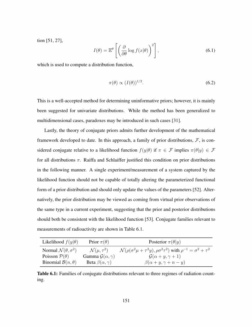
tion [51, 27],

I(θ) = Eθ[(

∂

∂θlog f(x|θ)

)2], (6.1)

which is used to compute a distribution function,

π(θ) ∝ (I(θ))1/2. (6.2)

This is a well-accepted method for determining uninformative priors; however, it is mainly

been suggested for univariate distributions. While the method has been generalized to

multidimensional cases, paradoxes may be introduced in such cases [31].

Lastly, the theory of conjugate priors admits further development of the mathematical

framework developed to date. In this approach, a family of prior distributions, F , is con-

sidered conjugate relative to a likelihood function f(y|θ) if π ∈ F implies π(θ|y) ∈ F

for all distributions π. Raiffa and Schlaiffer justified this condition on prior distributions

in the following manner. A single experiment/measurement of a system captured by the

likelihood function should not be capable of totally altering the parameterized functional

form of a prior distribution and should only update the values of the parameters [52]. Alter-

natively, the prior distribution may be viewed as coming from virtual prior observations of

the same type in a current experiment, suggesting that the prior and posterior distributions

should both be consistent with the likelihood function [53]. Conjugate families relevant to

measurements of radioactivity are shown in Table 6.1.

Likelihood f(y|θ) Prior π(θ) Posterior π(θ|y)

Normal N (θ, σ2) N (µ, τ 2) N (ρ(σ2µ+ τ 2y), ρσ2τ 2) with ρ−1 = σ2 + τ 2

Poisson P(θ) Gamma G(α, γ) G(α + y, γ + 1)Binomial B(n, θ) Beta β(α, γ) β(α + y, γ + n− y)

Table 6.1: Families of conjugate distributions relevant to three regimes of radiation count-ing.

151

Likelihood Function

In this research, all activity measurements were assumed to be drawn from normal

distributions. In radiation counting experiments with sufficient statistics (10,000 counts

per peak is a typical rule of thumb), this assumption is valid; however, this condition is not

always true, as was observed in the analysis of the PNNL 14.1 MeV data, which featured

low count rates in FP with half-lives longer than 1 day. Low counting statistic scenarios

may be directly treated by substituting the Poisson or binomial distributions for the normal

distribution in εi term in Equation (2.22) on page 32.

6.3.4 Applications of FRACTURE

During the implementation of the methodology developed in Chapter 2, an emphasis

was placed on flexibility. For example, any term that appears in the Bateman equations

(see Equation (2.39) on page 40) may be set as an unknown quantity to be estimated. In

addition, the embedded Runge-Kutta solver Bateman is capable of modeling nuclides with

any cross section, nuclear data, and the forcing term φ(t) is completely arbitrary. This

allows cyclic irradiations, pulses and power/flux changes to be simulated and/or used in

inverse problems. Therefore, further applications of the existing capabilities of FRACTURE

are expected and encouraged. Some possibilities include the determination of:

1. Branching ratios that are implicitly included in the decay constants in Equation (2.39),

2. Relative abundance/rate of population to metastable states,

3. Half-lives,

4. One-group cross sections,

5. Neutron flux, and

152

6. Initial nuclide concentrations.

The last two items warrant further discussion.

It is possible that the determination of neutron flux and initial nuclide concentrations

could be applied to nuclear forensics and safeguards applications. Using known FPY and

measured activities of FP, it may be possible to determine the neutron fluence, number

of fissions, or yield of a nuclear weapon. Alternatively, it may be possible to determine

neutron fluence and use the value as a surrogate for burnup in safeguards applications.

In addition, FPY are multivariate patterns that are unique to the fissionable material and

incident neutron energy. It may be possible to use the FP inventory, determined by gamma-

ray spectrometry in this case, to determine the initial isotopics of the fissionable target/fuel

by considering the inverse problem solved by FRACTURE as a basis pursuit problem [27].

In this framework, the fission source term in Equation (2.24) is expanded to include more

than one fissionable material,

Nfσf →∑j

Nfjσfjχ(i)ij , (6.3)

and the values of Nfj are optimized to give the best-fit behavior in the Bayesian sense.

Furthermore, upon examination of Equation (2.39), it is apparent that the behavior of FP

and activation products (AP) are relatively independent, as the FPY for expected AP, such

as Co, Ca, and Fe, is very small, while the nuclide concentrations of FP are small enough

such that expected rates of neutron-induced reactions are negligible for most nuclides. Ma-

jor exceptions would include Xe and Gd, which have cross sections on the order of tens or

hundreds of thousands of barns. The loose couple between FP and AP production may al-

low analysis to implicitly distinguish AP from FP and calculate initial concentrations of AP

precursors. If the solver were to attempt to increase neutron flux φ(t) in order to produce

the desired amount of an AP nuclide through fission, there would be a large over prediction

153

of FP activities.

In all of the above scenarios, the simultaneous solution method used by the optimization

formulation may make these approaches robust to tampering, corrupted measurements,

missing data, or outliers.

Improvements to FRACTURE

There are several ways in which the current implementation of FRACTURE could be

improved during further development. These include:

1. Expanding data structures within BATEMAN to allow for larger decay chains,

2. Change the activity calculation formulation to a matrix method,

3. Include subroutines to detect low-statistics measurements and account for these situ-

ations in the formulation of the likelihood function by applying Poisson or binomial

error distributions as appropriate,

4. Re-implement the code in a compiled language to accelerate performance, and

5. Implement an intelligent sampling method such Metropolis-Hastings [31] or Differ-

ential Evolution Adaptive Metropolis [54] to accelerate Monte Carlo sampling.

154

A | Analysis Procedure Checklist

This appendix provides procedural checklists for FPY analyis using the methods of

Chapters 2 and 4. Steps regarding sample preparation are specific to the thermal irradiations

at UT/NETL.

1. Measure approximately 100 mg of naturally-enriched U3O8 (contains 0.67 mg of

235U)

2. Pack U3O8 into 1539-LG high density polyethylene vial

3. Heat seal the vial by melting

4. Pack vial into 2/5 dram vial along with spacers made of half 2/5 dram vials (see

Figure 4.1 on page 102)

5. Heat seal 2/5 dram vial by melting

6. Pack vial into 2 dram vial along with spacers and cap. Make sure to use vial that

successfully passes through pneumatic transfer jig

7. Using the thermal pneumatic transfer irradiation facility (tPNT), irradiate the sample

for 60 seconds at a reactor power of 1 kW

8. Remove the sample from the outermost vial, place in a new 2 dram vial along with

spacers, and cap

9. Place sample on HPGe detector using a long sample geometry, approximately 10 cm

source-to-detector distance

155

10. Once detector dead time has somewhat subsided (below approximately 20%), start

collecting spectra

11. Collect multiple spectra over time as detector availability allows—ensure that spec-

tra are collected long enough to gain adequate counting statistics (see Table 4.4 on

page 107)

12. In each spectrum, identify fission products, resolve interferences, and calculate ac-

tivities at the beginning of counting

13. Using a well-known FP such as 99Mo or 147Nd, perform an inverse analysis with

uniform prior to estimate the posterior distribution for the time-averaged neutron

flux (see Appendix B on the following page) and compute summary statistics

14. Estimate sensitivity coefficients and calculation off-diagonal covariance terms

15. For each FP decay chain with measured activities, compile a prior distribution for

FPY

16. Perform an inverse analysis for each decay chain to obtain posterior distributions for

FPY

156

B | FRACTURE User Manual

This chapter gives a short introduction to the use of the code FRACTURE. All functions

included in the package are commented for explanation of all variables and options to

possible future developers; however, this manual will explain the usage of FRACTURE

to an end-user and examples of parameter estimation of the kind studied and suggested

in this dissertation. Sections of the code not explicitly needed for parameter estimations

problems but possibly useful to future researchers, e.g., generation of synthetic data and

testing scripts, will be pointed out, but the usage left to code headers and comments.

B.1 FRACTURE Overview

FRACTURE includes three main sections or modules:

1. NID: Nuclide identification using L1 minimization and linear model of detector re-

sponse,

2. ACT: Activity and associated uncertainty calculation for decay series of up to three

radionuclides using the bootstrap median to aggregate discrepant results,

3. Parameter Estimation: Estimation of parameters within the Bateman equations using

Bayesian inference and optimization.

The FPY analyses presented in this dissertation proceeded as follows:

1. Prepare a sample of fissionable material,

157

2. Irradiate the sample for a known amount of time (with uncertainty), tirr ± u(tirr),

3. Allow a short decay period, td, to allow for sample transfer and the sample activity

to fall to a level appropriate for gamma-ray counting (depending on the spectrometer

and geometry used),

4. Collect gamma-ray spectra and calculate their time since end of irradiation including

td,

5. Using Genie†, detect peaks and calculate their net counts (areas) and associated un-

certainty,

6. Using Genie, calculate peak detector efficiency at each peak energy found in the

previous step,

7. Save the peak areas, efficiencies, and uncertainties in a four-column text file (an

example is shown in the next section),

8. For each spectrum,

(a) Input text file into NID to identify most likely gamma-emitting radionuclides in

the sample‡.

(b) For each decay chain of gamma-emitting radionuclides, e.g., 140Ba and 140La,

input the counts, efficiency, gamma intensity, and counting time into ACT to

determine the activity at the beginning of counting and associated uncertainty

(c) Collected activities for all radionuclides as a function of time, where time is the

total time between the end of irradiation and beginning of spectral collection†Any spectum analysis software would work, but any specifics herein refer to Genie-PC.‡As explained in Chapter 2, the values returned by the NID code may be thought of as an unnormal-

ized probability of each gamma-emitting radionuclide being present in the sample; however these values areconflated with the gamma intensities and peak detector efficiencies. This confusion will be rectified in afuture update of the code and reworking of the primary objective function formulation by combining nuclideidentification and activity calculation. See [55].

158

9. Form prior distributions for each variable/parameter to be estimated, e.g., fission

product yield,

10. Run the parameter estimation code—the Levenberg Marquardt method with Monte

Carlo sampling is recommended (the use the Monte Carlo procedure, the covariance

matrix of all known uncertain inputs must be calculated),

11. Remove gross outliers,

12. Calculate summary statistics and plot results.

B.2 Nuclide Identification, NID

The approach for nuclide identification implemented in NID is described in detail in

Section 2.2.1. Figure B.1 visually shows the algorithm. Main features of the code are the

library data, peak search ∆, and mismatch/unobserved peak value δ (called epsilon in the

NID functions). The library data is stored in the ~/NID/data/ directory. The value

of ∆ is used to identify when a library gamma-ray energy is considered a match with the

value observed in the spectrum. The value of ∆ is reflective of the quality of the energy

calibration (variations in the energy calibration during counting, e.g., due to lab temperature

changes, should be associated with larger ∆ values), as well as the amount of peak overlap.

If many of the peaks are overlapping and combined into a perfect overlap, a larger ∆ value

should be used to ensure all possible library gamma-ray contributions are reflected in the

formation of the response matrix, R.

If a peak is not observed in the spectrum, it’s possible the corresponding gamma-

emitting radionuclide is not present, or it is not observed above the background/baseline

in the spectrum. A reasonable value of δ (again, called epsilon in the NID functions) is

related to the background/baseline counts in the spectrum multiplied by the number of

159

channels of a prototypical peak. For example, if the baseline counts is approximately 500

counts per channel, the typical peak is 2 keV wide, and the energy calibration is 0.25 keV

per channel, then a reasonable value is 500× 2/0.25 = 4000.

(a) Loading the efficiency-corrected peak areasinto the initial spectrum vector s.

(b) Peak energies are compared to a databaseand overlapping peaks are combined.

(c) For each hypothesized nuclide, intensitiesof characteristic photons are loaded into the re-sponse matrix R.

(d) Small values δ are inserted into s to matchwith gamma-rays inR not observed in the spec-trum.

Figure B.1: Visual representation of the basic peak search algorithm that populates theinitial list of hypothesized nuclides, vector representation of the spectrum, and responsematrix.

Additional variables are the minimum gamma intensity considered, i.e., a gamma-ray

with 0.1% intensity is not expected to be observed in a typical spectrum, and the minimum

and maximum energy values seen in the spectrum. For this research, a minimum value of

160

40 keV (above the low-energy discriminator and the x-ray region) and maximum value of

about 2200 keV was used.

NID solves the following problem:

c = argminc∈RM+

{‖s− cR‖1} . (B.1)

Additional options in NID include forced inclusion of a radionuclide despite the peak

search results, exclusion of nuclides that peak search may identify, and heuristic identifica-

tion of possible sum and escape peaks. These options are designed for use in iterative exe-

cutions of the NID code and are triggered by additional optional arguments in the NIDrun

call (see source code in Section C).

Assume the following inputs:

1. The text file is called TestSpectrum.txt

2. The file TestSpectrum.txt is located in the same directory as NID

3. The value for ∆ is 0.4 keV

4. The spectrum covers energies from 15 to 2500 keV, but we want to ignore x-rays

5. Based on counting procedures, i.e., we did not pursue low-level counting experimen-

tal practices, so the minimum intensity will be 2.5%

6. The value for δ = 3000

7. Based on counting procedures, we believe that a radionuclide that decays less than

1000 times during counting will not be observed

8. We want to save the output as TestOutput

The general format for NID is shown below.

161

NIDrun(file, path, pathFlag, tol, E_min, E_max, I_min, eps, ...

opt, minDflag, minDis, verb,outputname,varargin)

The function call for the example described above is

NIDrun(’TestSpectrum’, [], 0, 0.4, 40, 2500, 2.5, 3000, ...

’NNLSQ’, 1, 1000, 1, ’TestOutput’)

B.3 Activity Calculation, ACT

In comparison to NID, the ACT module is very simple to use. Each radionuclide in the

decay chain is put in its own cell with four matrices and a string: a N × 2 matrix with each

row corresponding to a photopeak, the first column is the number of counts and the second

column the associated standard uncertainty, aN×2 matrix of efficiencies and uncertainties,

a 1×1 matrix of nuclide half-life and uncertainty, a N ×2 matrix of gamma-ray intensities

and uncertainties, and a string giveing the unit of the half-life. Possible half-life strings are

• ’a’: years,

• ’d’: days,

• ’h’: hours,

• ’m’: minutes, and

• ’s’: seconds.

In addition, the count time in seconds is also passed as the first argument before the cells.

Results are given as cells to be unpacked, and the results are printed in an eye-readable

format to the command window.

The general function call for two nuclides is

162

a = ACT(t, {[c u(c)], [e u(e)], [t u(t)], [g u(g)], ’Tunit’},...

{<nuclide2>},...);

Note, at present, the multivariate bootstrap median used to aggregate results from the cal-

culation of activities with different characteristic photons is limited to decay chains of one

or two nuclides; however, the calculation is easily generalizable to more dimensions.

B.4 Parameter Estimation

The parameter estimation problem solved with embedded Bateman equation solver

(BATEMAN) is discussed at length in Chapter 2, so it is not presented here. After test-

ing, the recommended method for Bayesian parameter estimation is to use a diagonal input

space to estimate the neutron flux and sensitivity coefficients for flux and irradiation time,

flux and fission cross section, flux and fissionable material mass, and flux and fissionable

material density. The sensitivity coefficient between activities of members of a decay chain

at a single time point are obtained from the function dB/dA in the ACT code package

(~/Fracture/ACT/helpers/dBdA.m and the sensitivity between mass and density

of the fissionable material is a simple linear function, ∂ρ/∂m = 1/V , where V is the

sample volume, assumed to be known exactly. The sensitivity coefficients found following

incident neutron flux calculation for an experiment are used to form the covariance matrix

for the input space (see Equation (2.13)) of all parameter estimation calculations performed

for the experiment. Following parameter estimation, outliers may be detected and removed,

then plotted.

There are many inputs needed. They are listed and described below.

data: The time points and measured activities of the nine-nuclide system of coupled fis-

sion products shown in Figure 2.8. Data is a matrix of column vectors comprising

163

the measured data for each nuclide. data(:,1) are the time points and data(:,j) are the

time series for the j-1 nuclide. If the j-1 nuclide was not measured at the ith time step

listed in data(:,1), then data(i,j) = NaN. NaN values are skipped in the calculation of

the objective function at each iteration of the optimization solver. For N time points,

the dimension is N × 10.

uData: Uncertainty in each measured activity. There is one less column because time

values are assumed to be known with certainty. For N time points, the dimension is

N × 9.

XS: Column vector with each known parameter used to define the system of equations

d

dt(Ni) = φ(t)Nfσfχ

(i)i +Ni−1λi−1 −Niλi − φ(t)

(Niσa −

∑j

Njσj

), (B.2)

and these values are inputs as a 70 + ×1 vector. Each entry, the indices in XS it

populates, and definition are given below.

1. IV = 01 - 09 : initial values of each nuclides. Set to zero for fission on fresh

targets

2. tmx = 10: maximum simulation time in seconds; can be any value greater than

the last time point in ‘data’

3. tir = 11: irradiation time in seconds

4. dcy = 12 - 20: decay constants in s−1

5. sga = 21 - 29: absorption cross section in barns

6. ng = 30 - 38: (n,γ) cross section in barns

7. n2n = 39 - 47: (n,2n) cross section in barns

8. np = 48 - 56: (n,p) cross section in barns

164

9. yld = 57 - 65: fission yields in %

10. trgt = 66 - 68: three-vector of fission cross section in barns, fissionable material

mass in grams, and fissionable material density in g cm3

11. plt = 69: flag to plot at each execution of BATEMAN

12. flx = 70 - end: neutron flux in cm−2s−1. If cyclic irradiation is used, this will

be a vector. See comments in BATEMAN.m for more information

optidx: Indices of variables in XS to be estimated with Bayesian inference

obj: Type of objective. Either ’MLE’ to neglect prior distribution(s) or ’MAP’ to include

prior distributions.

prior: M × 2 matrix with the µ and σ values for the prior distribution(s)

rkunc: Percent uncertainty values in the Runge-Kutta solutions (α values) for the results

produced by BATEMAN given as a N × 1 vector.

slv: Optimization solver to be used. Recommended is ’lmf’ for Levenberg-Marquardt

method

uXS: Vector with same dimension as ’XS’ giving the uncertainty in each value in ’XS’

h: Step size used for computing numerical derivatives with finite differencing. May be

specified for numerical studies or skipped to use optimal values determined in previ-

ous tuning/optimizing studies

sig: Covariance matrix for input space

cnt: Currently unused—planned to be used in automatic calculation of covariance matrix

entries for activities of parent/daughter nuclides

165

N: Number of Monte Carlo samples to draw

There are several outputs generated. The three important ones are Srcs (which lists

the values of ’XS’ that have uncertainty and are accordingly sources of uncertainty in the

estimated variables), P (which gives the values of the parameters for each of the N Monte

Carlo samples), and S (the sampled values drawn in Monte Carlo routine). The values

in P are used to calculate the summary statistics, and the values in P and S are used to

compute sensitivity coefficients and uncertainty budgets. Everything is pretty well docu-

mented excepted for the variable robust, which increases the number of restarts used for

the optimization of the noisy objective function. The robust mode is typically turned

off except for when the Jacobian uncertainty estimation is used by calling the function

slvBtmn_jac.

The function call is

[FPY, hist, Srcs, conv, P,S] = slvBtmn_mc(data,uData,XS,...

optidx,obj,prior,rkunc,slv,uXS,h,sig,cnt,N)

Example Execution An example execution of the inverse analysis is given below using

the 134Te/134I data collected following the 14.1 MeV irradiation performed at PNNL. The

nuclides 134Te and 134I form a two-nuclide decay chain with no significant coupling be-

tween isobars, e.g., there are no significant (n,2n) or (n,p) reactions. The parent nuclide,

134Te, is assigned to index 5, and the daughter, 134I, is assigned to index 2 (refer to Fig-

ure 2.8 for help assessing nuclide indices). This assignment could be changed to indices 4

& 1, 9 & 6, etc.

166

% --------------- %% Te/I-134 YIELD %% --------------- %

cd ~/Desktop/Sherlock/’Parameter Estimation’/Bateman/addpath helpers

% Initialize XSIV = zeros(9,1);tir = 333;tmx = 8000;dcy = zeros(9,1);ng = zeros(9,1);n2n = zeros(9,1);sga = zeros(9,1);np = zeros(9,1);yld = zeros(9,1);sgf = 2.0839;m = 220/100;p = 19;flx = 2.3565e8;trgt = [sgf;m;p];

% #2 is La-140, #5 is Ba-140dcy(5) = 2.7637-4;dcy(2) = 2.2005e-4;yld(2) = 1/10;yld(5) = 5;XS = [IV; tmx; tir; dcy; sga; ng; n2n; np; yld; trgt; 0; flx];

% set parameter uncertaintiesuXS = zeros(70,1);% tiruXS(11) = 1;% lambdauXS(13) = 8.3827e-7;uXS(16) = 5.2895e-6;% fission XSuXS(66) = 0.0417;% fissionable massuXS(67) = 1/1000;% fissionable densityuXS(68) = 0.3;uXS(70) = 0.1113e8;

167

% experimental datanTimePoints = 7;data = zeros(nTimePoints,10);uData = zeros(nTimePoints,9);data(:,1) = [297 1497 2697 3897 5097 6297 7497];data(:,3) = [459.4978 466.5078 366.6456 352.8965 286.6768...

253.2177 213.5744 ];uData(:,2) = [1.4165 1.2017 0.8873 0.5967 0.5187 0.5109 0.3059];data(:,6) = [623.7401 472.1208 313.9091 212.0222 150.2561...

107.6191 76.5491];uData(:,5) = [1.7815 1.1405 0.4889 0.5787 0.2131 0.3906 0.3238];

% covariance matrix% recall, the covariance matrix is strictly diagonal for flux% determinations this allows for estimation of sensitivity% coefficients for subsequent analysesmA = sum(uData~=0);sig = diag(0.5.*[uData(uData~=0).^2; uXS(uXS~=0).^2]);sig(mA + 1, end) = -7.1187e5;sig((end - 3),end) = -1.9320e5;sig((end - 2),end) = -974.9414;sig((end - 1),end) = -4.5542e3;sig = sig + sig’;

% Runge-Kutta uncertaintyalpha = zeros(9,1);alpha(2) = 5.4/100;alpha(5) = 5.8/100;

% prior% no prior is used in the MLE calculation of average fluxprior = [1.0621 1.0488; 2.3672 1.6572];

% solver optionsoptidx = [58 61];obj = ’map’;slv = ’lmf’;h = 0;cnt = [];N = 2500;

% execution and results[FPY,~,~,~,P,S] = slvBtmn_mc(data,uData,XS,optidx,obj,prior,...

alpha,slv,uXS,h,sig,cnt,N);cd Results

168

cd MARCsave(’MARC_TeI134_1.mat’);

Note, there are functions for generating synthetic data in the

~/Parameter Estimation/ directory.

Outlier removal is performed by the function postMC.m and plotting is done with

pltMC.m.

Some functions in the package were used in developing the code (such as generating

synthetic data, or runSlvBtmn) which are not used in the recommended typical code

flow.

Lastly, I’ve tried to ensure that all functions are documented in the headers—feel free

to explore!

169

C | Code Listing

This chapter gives a listing of main code written to support the presented research.

Scripts for setting up and running specific tests and generating specific plots that are un-

likely to have significant reuse have been omitted.

C.1 Nuclide Identification

ENSDF Parsing

import globimport pdbimport numpy as np

##################### HELPER FUNCTIONS #####################def getHalfLife(input):

halfLife = input.split()[0]unit = input.split()[1]if unit.lower() == ’ms’:

scalar = 1e-3halfLife = float(halfLife)*scalarunit = ’S’halfLife = ’%.4e’ % halfLife

elif unit.lower() == ’us’:scalar = 1e-6halfLife = float(halfLife)*scalarunit = ’S’halfLife = ’%.4e’ % halfLife

elif unit.lower() == ’ns’:scalar = 1e-9halfLife = float(halfLife)*scalarunit = ’S’halfLife = ’%.4e’ % halfLife

elif unit.lower() == ’ps’:scalar = 1e-12halfLife = float(halfLife)*scalarunit = ’S’halfLife = ’%.4e’ % halfLife

elif unit.lower() == ’fs’:scalar = 1e-15halfLife = float(halfLife)*scalarunit = ’S’halfLife = ’%.4e’ % halfLife

elif unit.lower() == ’as’:scalar = 1e-18halfLife = float(halfLife)*scalarunit = ’S’halfLife = ’%.4e’ % halfLife

HL = [halfLife, unit]return HL

def isNumber(n):’’’

170

Given a string character, returns True is the character is a number; otherwise returnsFalse.’’’try:

float(n)return True

except ValueError:return False

def findNumbers(s):’’’Finds non-numeric characters in a string, then returns the numeric and alpha parts’’’k = 0while isNumber(s[k]) or s[k] == ’.’:

k = k + 1return s[0:k]

def convertUncExp(nF, unc):’’’This function converts the usual uncertainty expression shorthand touseful standard notation, e.g., 12.5 22 -> 12.5 +/- 2.2.’’’nDigits = len(nF)decPos = nF.find(’.’)if decPos == -1:

return uncnumDec = nDigits-decPos-1if (numDec - len(unc)) > 0:

newUnc = ’0.’for i in range(numDec - len(unc)):

newUnc = newUnc + ’0’newUnc = newUnc + unc

elif (numDec - len(unc)) == 0:newUnc = ’0.’ + unc

else:newUnc = unc[len(unc):len(unc)-numDec-1:-1] + ’.’ + unc[::-1][numDec:len(unc)]newUnc = newUnc[::-1]

return newUnc

def processFile(filename):’’’This helper function reads in an ENSDF file, retrieving all the includednuclides, daughters, half-lives, photon energies, and photon intensities withassociated standard uncertainties.’’’

# exceptionNuclides = [’252CF’]exceptionNuclides = [’Hello’]blankLine = ’ \n’nonNumericVals = [’LT’,’GT’,’LE’,’GE’,’AP’,’CA’,’SY’]counter = 0

# pdb.set_trace()

# open the file and initialize the read-permitted file object, f.with open(filename,’r’) as f:

lines = f.readlines()

# temp quick find for the parent lines# for i in range(len(lines)):# if " P " in lines[i]:# print i,lines[i]

# loop over all the lines in the filefor i in range(len(lines)):

# the parent keyword indicates the start of a decay data blockif " P " in lines[i][0:10]:

# print lines[i][0:5]if (len(lines[i][39:49].split()) == 0) or (lines[i][39:49].split()[0] == ’?’):

continue

# print i,lines[i]currentNuclideName =lines[i][0:5].split()[0]# skip over any spontaneous fission parents/decaysif currentNuclideName in exceptionNuclides:

#print ’Found exception nuclide! Skipping this parentnuclide and continuing search to next parent nuclide in the current file %s\n\n’ % filenamecontinue

# record the energy of the state. If non-zero, then append an m to designate a metastable statestateEnergy = lines[i].split()[2]if stateEnergy != ’0.0’ and stateEnergy != ’0’:

currentNuclideName = currentNuclideName + ’m’currentDaughter = lines[i-1][0:5].split()[0]

171

# read through the unknown-length half-life numeric; read until a space is# found

HL = getHalfLife(lines[i][39:49])halfLife = HL[0]halfLifeUnit = HL[1]

# search nearby for the normalization line (if present), extract normalization# factor and branching ratio, and combine them with uncertaintyn = i -5while n < len(lines):

if ’ N ’ in lines[n]:if lines[n] == blankLine:

breaknFactorLine = lines[n][9:21].split()if len(nFactorLine) == 0:

nFactor = ’1.0’unc_nFactor = ’0.0’

elif len(nFactorLine) == 1:if isNumber(nFactorLine[0]):

nFactor = nFactorLine[0]else:

nFactor = findNumbers(nFactorLine[0])unc_nFactor = ’0.0’

else:if isNumber(nFactorLine[0]):

nFactor = nFactorLine[0]else:

nFactor = findNumbers(nFactorLine[0])if isNumber(nFactorLine[1]):

unc_nFactor = convertUncExp(nFactor, nFactorLine[1])else:

temp = float(nFactor)/5.0unc_nFactor = ’%.4e’ % temp

# debug line# print nFactor, unc_nFactor

branchData = lines[n][31:41].split()if len(branchData) == 0:

BR = ’1.0’unc_BR = ’0.0’

elif len(branchData) == 1:if isNumber(branchData[0]):

BR = branchData[0]else:

BR = findNumbers(branchData[0])unc_BR = ’0.0’

else:if isNumber(branchData[0]):

BR = branchData[0]else:

BR = findNumbers(branchData[0])if isNumber(branchData[1]):

unc_BR = convertUncExp(BR, branchData[1])else:

unc_BR = float(BR)/5.0unc_BR = ’%.4e’ % unc_BR

# debug line# print BR, unc_BR

nFactor = float(nFactor)*float(BR)nFactor = ’%.4e’ % nFactorunc_nFactor = np.sqrt(float(nFactor)**2 * float(unc_BR)**2 + float(unc_nFactor)**2 * float(BR)**2)unc_nFactor = ’%.4e’ % unc_nFactorbreak

n = n + 1

# read in photon information for current nuclidej = i + 1doneReadingPhotons = FalsephotonEnergies = []EnergyUnc = []photonIntensities = []IntensityUnc = []

while (doneReadingPhotons == False) and (j <= len(lines)):# print j

# found a gamma-data lineif " G " in lines[j][0:10]:

# read in fixed-length fields, separate based on spaces, convert# the uncertainty shortand, then append to the photon energy,# intensity, and associated uncertainty listsgammaData = lines[j][9:21].split()# print lines[j]if len(gammaData) != 0:

if len(gammaData) == 1:

172

if isNumber(gammaData[0]):photonEnergies.append(gammaData[0])

else:photonEnergies.append(findNumbers(gammaData[0]))

EnergyUnc.append(’0’)else:

if isNumber(gammaData[0]):photonEnergies.append(gammaData[0])

else:photonEnergies.append(findNumbers(gammaData[0]))

if isNumber(gammaData[1]):EnergyUnc.append(convertUncExp(photonEnergies[-1], gammaData[1]))

else:EnergyUnc.append(convertUncExp(photonEnergies[-1], findNumbers(gammaData[1])))

if isNumber(photonEnergies[-1])==False:del photonEnergies[-1]del EnergyUnc[-1]j += 1continue

intensityData = lines[j][21:31].split()if len(intensityData) == 0:

# if there is no intensity data, we need to remove the last# entry to the energy and energy uncertainty structuresdel photonEnergies[-1]del EnergyUnc[-1]

elif len(intensityData) == 1:if isNumber(intensityData[0]):

photonIntensities.append(intensityData[0])tempUncVal = float(intensityData[0])tempUncVal = tempUncVal/5.0IntensityUnc.append(’%.4e’ % tempUncVal)

else:photonIntensities.append(findNumbers(intensityData[0]))if isNumber(photonIntensities[-1]) == False:

del photonEnergies[-1]del EnergyUnc[-1]del photonIntensities[-1]j += 1continue

tempUncVal = float(findNumbers(intensityData[0]))tempUncVal = tempUncVal/5.0IntensityUnc.append(’%.4e’ % tempUncVal)

else:photonIntensities.append(intensityData[0])if intensityData[1] in nonNumericVals:

tempUncVal = float(intensityData[0])tempUncVal = tempUncVal/5.0IntensityUnc.append(’%.4e’ % tempUncVal)

else:if isNumber(intensityData[1]):

IntensityUnc.append(convertUncExp(intensityData[0], intensityData[1]))else:

IntensityUnc.append(convertUncExp(intensityData[0], findNumbers(intensityData[1])))

# ensure that all entries are corrected populated before incrementing# and going to next gamma-data line#if any([len(photonEnergies[-1])==0,len(EnergyUnc[-1])==0,len(photonIntensities[-1])==0,len(IntensityUnc[-1])==0]):# del photonEnergies[-1]# del EnergyUnc[-1]# del photonIntensities[-1]# del IntensityUnc[-1]

j += 1# is a parent line is found, then we’ve gotten to the next nuclide# and escape the while loop reading through gamma linesif (" P " in lines[j]) or (lines[j] == blankLine):

doneReadingPhotons = True

# apply the normalization/branching-ratio factor and prop. uncertainties;# convert to floats to calculate, then reformat back as string for storage# and printingif len(photonEnergies) != 0:

g = 0while g < len(photonEnergies):

if any([isNumber(photonEnergies[g]) == False,isNumber(EnergyUnc[g]) == False,isNumber(photonIntensities[g]) == False,isNumber(IntensityUnc[g]) == False]):del photonEnergies[g]del EnergyUnc[g]del photonIntensities[g]del IntensityUnc[g]g = g - 1

g = g + 1

173

if len(photonEnergies) != 0:for g in range(len(photonEnergies)):

tempGammaUnc = float(IntensityUnc[g])**2*float(nFactor)**2 +float(photonIntensities[g])**2*float(unc_nFactor)**2IntensityUnc[g] = ’%.4e’ % np.sqrt(tempGammaUnc)tempGamma = float(photonIntensities[g])*float(nFactor)photonIntensities[g] = ’%.4e’ % tempGamma

# renormalize to ensure that everything is in percentages# note the change to floats for computation and casting back to strings# this would be fast if the conversion to strings in lines 160 - 162 were# held offmaxIntensity = float(max(photonIntensities,key=float))if maxIntensity > 100:

renormFactor = 100.0/float(maxIntensity)photonIntensities = [float(x) for x in photonIntensities]photonIntensities = [x*renormFactor for x in photonIntensities]photonIntensities = [’%.4e’ % x for x in photonIntensities]IntensityUnc = [float(x) for x in IntensityUnc]IntensityUnc = [x*renormFactor for x in IntensityUnc]IntensityUnc = [’%.4e’ % x for x in IntensityUnc]

# sort the gamma data before writing to filephotonEnergies = [float(x) for x in photonEnergies]tempTuples = zip(photonEnergies, EnergyUnc, photonIntensities, IntensityUnc)sortedTuples = sorted(tempTuples)photonEnergies = [x[0] for x in sortedTuples]EnergyUnc = [x[1] for x in sortedTuples]photonIntensities = [x[2] for x in sortedTuples]IntensityUnc = [x[3] for x in sortedTuples]photonEnergies = [’%.4e’ % x for x in photonEnergies]

# write the current nuclide data to a new text file; if this is a secondary# decay for the parent nuclide, the data is appended to the existing *.dat# fileoutputFileName = currentNuclideName + ’.dat’fileList = glob.glob(’./*.dat’)testString = ’./’ + outputFileNameif testString in fileList:

repeatFileCount = 2appendedString = ’%d’ % repeatFileCountnewName = currentNuclideName + appendedString + ’.dat’newTestString = ’./’ + newNamewhile newTestString in fileList:

repeatFileCount += 1appendedString = ’%d’ % repeatFileCountnewName = currentNuclideName + appendedString + ’.dat’newTestString = ’./’ + newName

g = open(newName,’w’)else:

g = open(outputFileName,’w’)g.write(’Nuclide Data\n’)g.write(’------------\n’)g.write(’Nuclide Name: ’ + currentNuclideName + ’\n’)g.write(’Daughter Product: ’ + currentDaughter + ’\n’)g.write(’Half-Life: ’ + halfLife + ’ ’ + halfLifeUnit + ’\n’)g.write(’Branching Ratio: ’ + BR + ’\n’)if len(photonEnergies) != 0:

g.write(’\nGamma Data\n’)g.write(’----------\n’)g.write(’Energy [keV]’.ljust(13) + ’ ’ + ’StdUnc [keV]’.center(13) + ’ ’ +’Intensity [%]’.center(13) + ’ ’ + ’StdUnc [%]’.center(13) + ’\n’)for k in range(len(photonEnergies)):

g.write(photonEnergies[k].ljust(13) + ’ ’)g.write(EnergyUnc[k].center(13) + ’ ’)g.write(photonIntensities[k].center(13) + ’ ’)g.write(IntensityUnc[k].center(13) + ’\n’)

g.close()counter += 1

return counter

############## MAIN BODY ##############

def mkNIDdir(name,flag):if flag == ’file’:

numFilesDone = processFile(name)print ’Done processing file ’ + name + ’. ’ + str(numFilesDone) + ’ nuclides/decays processed.’

elif flag == ’dir’:totalFiles = 0for x in glob.glob(’./*.ens’):

numFilesDone = processFile(x)totalFiles = totalFiles + numFilesDoneprint ’Done processing file ’ + x + ’. ’ + str(numFilesDone) + ’ nuclides/decays processed.’

print ’All done! A total of ’ + str(totalFiles) + ’ nuclides have been generated into the NID directory.’

174

mkNIDdir(’./108.ens’,’dir’)

Original NID Algorithm

% Kenneth Dayman -- University of Texas -- 2013%% This function is appropriate for running the NID algorithm from the% Matlab command line. Using this entry, the optional commands may be% accessed.%% Function Call:% NIDrun(file, path, pathFlag, tol, E_min, E_max, I_min, eps, opt,...% minDflag, minDis, verb, outputname,varargin)%% Notes:% (i) The verbosity argument is not used, but is left in the function% call until an update can rectify the dependencies% (ii) The file name is given enclosed in tic marks without *.txt% extension% (iii) The path name is given enclosed in tic marks% Example: The full path is "~/NID/spectra/<folder>/<file>.txt;% and the user enters ’<folder>’% (iv) The minimum intensity (I_min) is given in percentages, i.e.,% ranges in [0, 100]% (v) Opt is a string and enclosed in tick marks% (vi) Optional arguments are collected in varargin. Keywords and% associated arguments are shown bewow.% ’include’% ’exclude’% ’keep’% ’peakRemove’

function NIDrun(file, path, pathFlag, tol, E_min, E_max, I_min, eps, opt, minDflag, minDis, verb,outputname,varargin)verb = 1;addpath helpers data spectra results

% convert text optimization strategy into a numericif strcmpi(opt,’LSQ’)

optn = 0;gamma = 0;

elseif strcmpi(opt,’NNLSQ’)optn = 1;gamma = 0;

elseif strcmpi(opt,’WLSQ’)optn = 2;gamma = 0;

elseif strcmpi(opt,’WNNLSQ’)optn = 3;gamma = 0;

elseif strcmpi(opt,’WNNLSQ-REG’)optn = 4;

elseerror(’Unrecognized optimization strategy’)

end

% set up problem given data library, spectrum file, and user optionsif pathFlag % path is specified

[e,a,u_a] = readSpectrum(file,path);else

[e,a,u_a] = readSpectrum(file);end

% run idSum and idEscape to identify possible sum, single-, and% double-escape peaks. This data is passed to printOutput, and the% user may review it and run the code iteratively, removing% undesirable peakssp = idSum(e,a,tol);ep = idEscape(e,a,tol);

I_min = I_min/100; % convert intensity to decimal% check for optional arguments, then call to NIDexclude and NIDinclude% based on keywords (varargin{1} & varargin{3})if nargin > 13

if nargin == 15

for i = 1:2:length(varargin)-1strcmpi(varargin{i},’peakRemove’);[e,a,u_a,list] = peakRemove(e,a,u_a,ep,sp,varargin{i+1});

175

[N,Nr,data] = peakSearch(e,tol,E_min,E_max,I_min);end

elseif nargin == 17

for i = 1:2:length(varargin)-3strcmpi(varargin{i},’peakRemove’);[e,a,u_a,list] = peakRemove(e,a,u_a,ep,sp,varargin{i+1});

end

[N,Nr,data] = peakSearch(e,tol,E_min,E_max,I_min,varargin{3},varargin{4});

elseif nargin == 19

for i = 1:2:length(varargin)-5strcmpi(varargin{i},’peakRemove’);[e,a,u_a,list] = peakRemove(e,a,u_a,ep,sp,varargin{i+1});

end

[N,Nr,data] = peakSearch(e,tol,E_min,E_max,I_min,varargin{3},varargin{4},varargin{5},varargin{6});

elseif nargin == 21

for i = 1:2:length(varargin)-5strcmpi(varargin{i},’peakRemove’);[e,a,u_a,list] = peakRemove(e,a,u_a,ep,sp,varargin{i+1});

end

[N,Nr,data] = peakSearch(e,tol,E_min,E_max,I_min,varargin{3},varargin{4},varargin{5},varargin{6},varargin{7},varargin{8});else

error(’Bad call to peakSearch’)end

else% no optional arguments are used. Default call to peakRemove to% initiate ’list’ data structure. Default call to peakSearch with% no optional arguments, e.g., NIDexclude.[e,a,u_a,list] = peakRemove(e,a,u_a,ep,sp,[]);[N,Nr,data] = peakSearch(e,tol,E_min,E_max,I_min);

end

[s,se,R,coord,su] = formatData(N,Nr,e,a,tol,data,eps,u_a);

temp1 = cell(250,1);

for i = 1:length(varargin)if strcmpi(varargin{i},’keep’)

% append ’.txt’ to each nuclide (cell item)temp1 = varargin{i+1};for j = 1:length(temp1)

temp2 = cell(1,1);temp2{:} = strcat(temp1{j},’.txt’);temp1(j) = temp2;

endend

end

for k = 1:length(varargin)if strcmpi(varargin{k},’keep’)

i = 1;while i <= length(Nr)

remove = 1;for j = 1:length(temp1)

if strcmpi(temp1{j},Nr{i})remove = 0;break;

endendif remove

Nr(i) = [];R(:,i) = [];i = i-1;

endi = i+1;

endend

end

% prediction of concentrations via some optimization strategy using CVXn = length(Nr); %#ok<NASGU> % size of optimized vectorcvx_precision(’best’)switch optn

case 0 % LSQcvx_begin

variable c(n)minimize( norm(s - R*c) ) %#ok<NODEF>

cvx_endcase 1 % NNLSQ

176

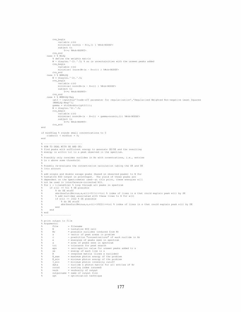
cvx_beginvariable c(n)minimize( norm(s - R*c,1) ) %#ok<NODEF>subject to

0<=c %#ok<NOPRT>cvx_end

case 2 % WLSQ% define the weights matrixW = diag(su.^-2).^.5; % su is uncertainities with the unseen peaks addedcvx_begin

variable c(n)minimize( (norm(W*(s - R*c))) ) %#ok<NODEF>

cvx_endcase 3 % WNNLSQ

W = diag(su.^-2).^.5;cvx_begin

variable c(n)minimize( norm(W*(s - R*c)) ) %#ok<NODEF>subject to

0<=c %#ok<NOPRT>cvx_end

case 4 % WNNLSQ-Regipt2 = inputdlg(’Trade-off paramater for regularization’,’Regularized Weighted Non-negative Least Squares(WNNLSQ-Reg)’);gamma = str2double(ipt2{1});W = diag(su.^2).^.5;cvx_begin

variable c(n)minimize( norm(W*(s - R*c)) + gamma*norm(c,1)) %#ok<NODEF>subject to

0<=c %#ok<NOPRT>cvx_end

end

if minDflag % rounds small concentrations to 0c(abs(c) < minDis) = 0;

end

% ---------------------------% HOW TO DEAL WITH SE AND DE:% find peaks with sufficient energy to generate SE/DE and the resulting% energy is within tol to a peak observed in the spectrum.%% Possibly only consider nuclides in Nr with cocentrations, i.e., entries% in c above some threshold.%% Possbly re-evaluate the concentration calculation taking the SE and DE% into account%% add single and double escape peaks (based on observed peaks) to N for% tentative NID output in printOuput. The yield of these peaks are% dependent on the spectrometer used--at this point, these energies will% not be used in interference-corrected NID.% for i = 1:length(e) % loop through all peaks in spectrum% if e(i) >= 511 % SE possible% % do SE stuff% abs(bsxfun(@minus,e,e(i)+511))<=tol % index of lines in e that could explain peak e(i) by SE% % add nuclides associated with these lines to N for e(i)% if e(i) >= 1022 % DE possible% % do DE stuff% abs(bsxfun(@minus,e,e(i)+1022))<=tol % index of lines in e that could explain peak e(i) by DE% end% end% end% -------------------

% print output to file% Arguments:% file = filename% N = tentative NID cell% Nr = possible nuclides (reduced from N)% s = vector of peak areas in problem% c = prediction "concentrations" of each nuclide in Nr% e = energies of peaks seen in spectrum% a = area of peaks seen in spectrum% tol = tolerance for peak search% eps = zero-epsilon value for unseen peaks added to s% se = energy of each line in s% R = response matrix (lines x nuclides)% E_max = maximum photon energy of the problem% E_min = minimum photon energy of the problem% I_min = minimum photon intensity cutoff% data = nuclide x photon matrix for all entries of Nr% coord = sorting index (unused)% verb = verbosity of output% outputname = name of output file% opt = optimization technique

177

% gamma = tradeoff parameter if regularized regression is usedprintOutput(file,N,Nr,s,c,e,a,tol,eps,se,R,E_max,E_min,I_min,data,coord,verb,outputname,opt,gamma,ep,sp,list);clear R a c coord data e eps file ipt outputname prompt s se title tol u_a verb Nr N I_min E_min E_max gammaminDflag minDis n opt optn su temp

end

% Kenneth Dayman -- University of Texas -- Nov. 2012%% This function reads the output from a peak area determination w/% efficiency correction from GENIE2K and outputs the list of peak energies,% areas (corrected for eff.), and uncertainities in the areas.%% Input:% f = filename (located in ’spectra’ folder within NID)% Output:% e = vector of peak energies% a = vectors of peak areas, corrected for efficiency% u_a = uncertainty in peak areas

function [e,a,u_a] = readSpectrum(varargin)%change directoryif nargin == 1

cd spectraf = varargin{1};depth = 1;

elseif nargin == 2% change directory when a path is specifieddname = strcat(’spectra’,’/’,varargin{2});f = varargin{1};depth = length(regexp(dname,’/’)) + 1;if strcmpi(dname(length(dname)),’/’)

depth = depth - 1;endcd(dname)

elseerror(’Too many inputs in readSpectrum’)

end

% read filefilename = sprintf(’%s%s’,f,’.txt’);fid = fopen(filename);temp = textscan(fid,’%s %f %f %f %f %f %f’,’HeaderLines’, 12);e = temp{2};area = temp{3};u_a = temp{4};eff = temp{5};u_e = temp{6};fclose(fid);for i = 1:depth

cd ..end

% change the efficiency values from percentages to fractional valueseff = eff./100;u_e = u_e./100;

% efficiency correctiona = area./eff;u_a = (((u_a./eff).^2+(area./eff./eff.*u_e).^2).^.5)./a; % expressed as fraction of area

end

% Edit 1: 1-13-15:% Added lines 47 - 49 to change the unit of the efficiency data from% percent to fractional values

% Kenneth Dayman -- University of Texas -- Sept. 2012%% This function compares the peak energies in a spectrum file to a data% library and returns a list of possible nuclides present in the spectrum%% Input:% e = list of peak energies% tol = tolerance for peak search% Emin = minimum energy to inlcude in the data% Emax = maximum energy to inlcude in the data% Imin = minimum gamma intensity to include% varargin = used to specify possible nuclides used in concentration% calculation using keywords "exclude" and "include"% Output:% Nr = reduced nuclide list for use in interference handling% N = list of nuclides possibly in the spectrum

178

% N is sorted to give the tentative NID for each line% data = contains the peak energies and associated intensities of the% nuclides in Nr. data(i,j,1) is the energy of the jth line of the% ith nuclide in Nr, and data(i,j,2) is the associated gamma% intensitiy, written in decimal units

function [N,Nr,data] = peakSearch(e,tol,Emin,Emax,Imin,varargin)

% initializenumPeak = length(e);

% read in data files% get name of filescd datad = dir;cd ..nF = length(d)-2; % number of filesnames = cell(nF,1); % names of nuclidesfor i = 3:length(d)

names{i-2} = d(i).name;end

% get matrix of all lines in the dataE = zeros(nF,500);for i = 1:nF

fid = fopen(names{i},’r’);temp = textscan(fid,’%f %f’);tempE = temp{1};tempI = temp{2};fclose(fid);%impose limits on intensity and peak energytempE = tempE(tempI >= Imin);% logical ANDs done via multiplication of the 0/1 logic vectorstempE = tempE(logical((tempE >= Emin).*(tempE <= Emax)));% sort the data to ensure energies are monotonically increasingtempE = sort(tempE);% load the filtered and sorted energies into EE(i,1:length(tempE))=tempE;

end% delete unused space in EmaxNumLines = max(sum(E>0,2));E(:,maxNumLines+1:500) = [];

% Form list of possible nuclides(tentative NID) and max energy% different between library values and each peak in the spectrum (if% there is fit)N = cell(numPeak,1);deltaE = zeros(numPeak,1);for i = 1:numPeak

temp = abs(bsxfun(@minus,E,e(i))); % abs of E diffif sum(sum(temp <= tol)) > 0 % there are fits in lib

N{i,1} = names(logical(sum(temp<=tol,2))); % all nucl that fitdeltaE(i) = max(temp(temp<=tol)); % max. difference less than tol.

endend

% Reduce N into single list of candidates% Loop through each line’s contribution to N, check if it’s in Nr, if% not, then add it to NrNr = cell(250,1);t = 0;for i = 1:numPeak

for j = 1:length(N{i})present = 0;temp = N{i};for k = 1:t

if strcmpi(temp(j),Nr{k})present = 1;break

endendif present==0

t = t + 1;Nr{t} = temp(j);

endend

end

% Remove or add nuclides to Nr based on "exclude" and "include"% keywords, or changes Nr to a particular cell array based on% "keep" keywordif nargin > 5

for i = 6-5:2:nargin-5% append ’.txt’ to each nuclide (cell item) before passing to% include/exclude functionstemp1 = varargin{i+1};for j = 1:length(temp1)

179

temp2 = cell(1,1);temp2{:} = strcat(temp1{j},’.txt’);temp1(j) = temp2;

end% call to NIDinclude/NIDexclude/keepif strcmpi(varargin{i},’exclude’)

[N, Nr] = NIDexclude(Nr,temp1,N);elseif strcmpi(varargin{i},’include’)

Nr = NIDinclude(Nr,temp1);elseif strcmpi(varargin{i},’keep’)

breakelse

error(’Error in peakSearch: unknown keyword in call to peakSearch.m’)end

endend

% Clear unused Nrt = length(Nr) - sum(cellfun(’isempty’,Nr));Nr(t+1:length(Nr)) = [];

% Read through data files of the Nr nuclides and form peak data% structure: (i,j,1) = energy of jth line of ith nuclide in Nr% (i,j,2) = intensity of line j from nuclide i.data = zeros(length(Nr), maxNumLines,2);cd datafor i = 1:length(Nr)

% open file and read datatemp = Nr{i};fid = fopen(temp{1},’r’);temp = textscan(fid,’%f %f’);tempE = temp{1};tempI = temp{2};fclose(fid);

%impose limits on intensity and peak energytempE = tempE(tempI >= Imin);tempI = tempI(tempI >= Imin);% logical ANDs done via multiplication of the 0/1 logic vectorstempI = tempI(logical((tempE >= Emin).*(tempE <= Emax)));tempE = tempE(logical((tempE >= Emin).*(tempE <= Emax)));% sort the data to ensure energies are monotonically increasing[tempE, idx] = sort(tempE);tempI = tempI(idx);% loads energy and intensities into one ’data’ structuretry

data(i,1:length(tempE),1) = tempE;data(i,1:length(tempE),2) = tempI;

catchdisplay(’Error in peakSearch in entry ’)display(Nr{i})display(’\n’)display(’Size of tempE: ’)display(size(tempE,1))display(’ x ’)display(size(tempE,2))display(’\n’)display(’Size of tempI: ’)display(size(tempI,1))display(’ x ’)display(size(tempI,2))display(’\nMax number of lines: ’)display(maxNumLines)

endendcd ..

end

% Kenneth Dayman -- University of Texas -- Nov. 2012%% This function takes the list of peak energies & areas, the results of the% peak search, and the peak data structure, and forms the spectrum vector s% and response matrix R that reproduces s given a concentration vector c%% Input:% N = cell of possible nuclides associated with each peak% Nr = reduced list of possible nuclides% e = peak energies observed in the spectrum% eps = epsilon (near zero) value used as the area of non-observed% peaks% Output:% s = spectrum vector, each entry is a peak area% se = energy of each peak represented in s% R = response matrix for the LSQ problem

180

function [s,se,R,coord,su] = formatData(N,Nr,e,a,tol,data,eps,u_a)

% initializes = zeros(1000,1);se = zeros(1000,1);R = zeros(length(Nr),5000);su = zeros(1000,1);u_a_u = .01; % uncertainty for unseen peaks

% Process peaks observed in spectrumfor i = 1:length(e) % num peaks in spectrum

se(i) = e(i);s(i) = a(i);su(i) = u_a(i);posNucl = N{i};for j = 1:length(posNucl)

% Nr(pos) = posNucl(j)pos = 1;while ~strcmpi(posNucl(j),Nr{pos})

pos = pos + 1;end% kth line of Nr(pos) nuclide matches the ith peak in spectrumk = 1;while abs(data(pos,k,1)-e(i)) > tol

k = k + 1;endR(pos,i) = data(pos,k,2);data(pos,k,2) = 0;

endend

% Process peaks not oberserved in spectra, putting epsilon in s,% updating se, and finding all peaks that should contribute to within% tol of the unobserved peak

% Sort all the energies in the data, and make a reference vector with% the locations of the data associate with each energy within ’data’energy_unsorted = zeros(size(data,1)*size(data,2),1);coord_unsorted = zeros(length(energy_unsorted),2);t = 0;for i = 1:size(data,1)

for j = 1:size(data,2)if data(i,j,1)~=0&&data(i,j,2)~=0

t = t +1;energy_unsorted(t) = data(i,j,1);coord_unsorted(t,:) = [i,j];

endend

end% remove empty entries of energy_unsortedcoord_unsorted = coord_unsorted(energy_unsorted~=0,:);energy_unsorted = energy_unsorted(energy_unsorted~=0);[e_sorted,idx] = sort(energy_unsorted); % e_sorted is all nonzerocoord = coord_unsorted(idx,:); % coord maps entries of e_sorted to data(i,j,1/2)

% proceed through each peak in e_sortedt = 1; % counts in e_sortedz = length(e); % where s and se are currently filled to; z counts in s/sewhile t <= length(e_sorted)

% look for energies above e_i within tolerancek = 0;if t+1 > length(e_sorted) % e_t is the last entry

z = z + 1;se(z) = e_sorted(t);s(z) = eps;su(z) = u_a_u;R(coord(t,1),z) = R(coord(t,1),z) + data(coord(t,1),coord(t,2),2);t = t + 1; % have to increment so the while loop finishes

elseif e_sorted(t+1)-e_sorted(t) <= tol

while e_sorted(t+k+1)-e_sorted(t) <= tolk = k+1;if t+k+1>length(e_sorted)

breakend

end% e_(t+k) is highest energy within tol of e_t

% look for energies that e_(t+1:t+k) are closer to than e_tif t+k+1 <= length(e_sorted)

while (e_sorted(t+k+1)-e_sorted(t+k) < e_sorted(t+k)-e_sorted(t))&&(k > 0)k = k - 1;

endend

elsek = 0;

181

end% proper k is foundz = z+1;se(z) = mean(e_sorted(t:t+k)); % add an entry to se as the mean of the grouped unseen peakssu(z) = u_a_u;s(z) = eps; % add an entry to se to account for the new unseen peak% fill in the zth column of R with the intensities for all% nuclides/lines that contribute to the new unseen peak% an addition rather than assignment construction is used in case a% nuclide has two lines that are grouped together by the algorithm% coord(w,1) is the nuclide index; coord(w,2) is the line index% for the coord(w,1)th nuclide (as ordered in Nr & data)for w = t:t+k % loop through the nuclides/lines that contribute

R(coord(w,1),z) = R(coord(w,1),z) + data(coord(w,1),coord(w,2),2);endt = t + k +1;

endend% clear unused parts of s, se, and R. Transpose R for use in lsqnonnegs(z+1:length(s)) = [];se(z+1:length(se)) = [];su(z+1:length(su)) = [];R(:,z+1:size(R,2)) = [];R = R’;

end

% Clinton Peterson -- University of Texas -- March 2013%% This function takes the list of peak energies and areas and checks for% any possible escape peaks, which will be stored in the matrix sp% Input:% e = peak energies observed in the spectrum% a = peak areas observed in the spectrum% eps = epsilon (near-zero) value used as uncertainty% Output:% ep = matrix containing escape peak low and high values, and% whether it is a single-escape or double-escape peak (0 for SE, 1% for DE)

function ep = idEscape(e,a, eps)

ep = zeros(length(e),3);

m = find(e>=1022);b = 0;

for k = m:length(e)b = b+1;for j = 1:k

if (abs(e(k) - (e(j) - 511)) <= 2*eps) && a(j) > a(k) && e(j) >= 1022ep(b,:) = [e(k) e(j) 0];

endif (abs(e(k) - (e(j) - 1022)) <= 2*eps) && a(j) > a(k) && e(j) >= 1022

ep(b,:) = [e(k) e(j) 1];end

endend

ep(ep(:,1) == 0, :) = [];

end

% Clinton Peterson -- University of Texas -- March 2013%% This function takes the list of peak energies and areas and checks for% any possible sum peaks, which will be stored in the matrix sp% Input:% e = peak energies observed in the spectrum% a = peak areas observed in the spectrum% eps = energy uncertainty in peakSearch% Output:% sp = matrix containing sum-peak "ingredients" (columns 1 and 2)% and the sum peak (column 3)

function sp = idSum(e,a,eps)

sp = zeros(length(e),3);

for k = 1:length(e)for j = 1:(k-1)

for i = 1:(k-1)

182

% checks if the difference between possible escape peak and% the sum of 2 possible "ingredient" peaks is lower than% 2 * epsilon. If it is, it gets added to the output matrix.% Also makes sure the area of the sum peak is less than the% second "ingredient" peak and is below 1.if abs(e(i) + e(j) - e(k) ) <= 2 * eps && a(k) < a(j) && a(k) < a(i)

sp(k,:) = [e(i) e(j) e(k)];end

endend

end

sp(sp(:,1) == 0, :) = [];

end

% Kenneth Dayman -- University of Texas -- Jan. 2013%% This function removes specified nuclides to Nr and N%% Input:% Nr = list of nuclides used in NID analysis% n = nuclides to be removed from Nr% Output:% Nr = nuclide list without removed nuclides

function [N, Nr] = NIDexclude(Nr,n,N)% number of nuclides in NrnumNucl = length(Nr) - sum(cellfun(’isempty’,Nr));

for i = 1:length(n)% remove from Nrj = 1;while j <= numNucl

if strcmpi(Nr{j},n{i})Nr(j) = [];numNucl = numNucl - 1; % break

elsej = j + 1;

endend% remove from Nfor j = 1:length(N)

temp = N{j};k = 1;while k <= length(temp)

if strcmpi(temp{k},n{i})temp(k)=[];N{j}=temp;

elsek = k + 1;

endend

endend

end

% Kenneth Dayman -- University of Texas -- Jan. 2013%% This function adds nuclides to Nr%% Input:% Nr = list of nuclides used in NID analysis% n = nuclides to be added to Nr% Output:% Nr = nuclide list with added nuclides

function Nr = NIDinclude(Nr, n)

numNucl = length(Nr) - sum(cellfun(’isempty’,Nr));Nr{numNucl+1:numNucl+length(n),1} = n;display(’done’)

end

% Clinton Peterson -- University of Texas -- April 2013%% This function takes the list of peak energies, areas, and area% uncertainties and removes values from the lists according to a

183

% user-specifed command. If the input is the string ’all’ then peakRemove% will remove all sum peaks and escape peaks. If the input is a vector of% energies, peakRemove will remove all these energies and their associated% areas and area uncertainties from the original matrix.% Input:% e = peak energies observed in the spectrum% a = peak areas observed in the spectrum% u_a = peak area uncertainties observed in the spectrum% ep = matrix containing escape peak values% sp = matrix containing sum peak values% list= matrix containing custom user-specified energy values to% remove from the observed spectrum, or string ’all’ to remove all% sum peaks and escape peaks% Output:% e = filtered peak energies% a = filtered peak areas% u_a = filtered area uncertainty values

function [e,a,u_a,list1] = peakRemove(e,a,u_a, ep, sp, list)if isempty(list)

list1 = list;elseif isnumeric(list) == 0

if strcmpi(list,’all’)

%defines variables v and c as vectors containing all lower%escape peak energies and sum peak energies respectivelyd = ep(:,1);c = sp(:,3);list1 = [d’,c’];

%removes values from e,a,u_a that match lower-energy escape%peaksfor i = 1:length(d)

[r,idx] = min(abs(d(i)-e));if r<.6

e(idx) = [];a(idx) = [];u_a(idx) = [];

elseerror(’Error in peakRemove: Change tolerance level to remove all escape peaks’)

endend

%removes values from e,a,u_a that match sum peaksfor i = 1:length(c)

[r,idx] = min(abs(c(i)-e));if r<.6

e(idx) = [];a(idx) = [];u_a(idx) = [];

elseerror(’Error in peakRemove: Change tolerance level to remove all sum peaks’)

endend

elseif iscell(list)list1 = [];

elseerror(’Error in peakRemove: Please type "all" to remove all peaks or a matrix of energies to remove,or insert a vector of energies to be removed’);

endelse

%removes values from e and corresponding values from a and u_a that%match user-specified energy values from vector "list"for i = 1:length(list)

[v,idx] = min(abs(list(i)- e));if v > 1

error(’Error in peakRemove: No peaks found within 1 keV’);else

list1(i) = e(idx);e(idx)=[];a(idx)=[];u_a(idx)=[];

endend

endend

% Kenneth Dayman -- University of Texas -- September 2012

% Prints output file of NID analysis%% N = tentative nuclide identification (all nuclides for each line)% Nr = reduced NID w/ interference handling% s = spectrum vector

184

% c = predicted concentrations% E = peak energies% A = peak areas% tol= tolerance used in peak search%

function printOutput(file,N,Nr,s,c,e,a,tol,eps,se,R,E_max,E_min,I_min,data,coord,verb,outputname,opt,gamma,ep,sp,list)% initialize and save as *.mat fileoutputmat = sprintf(’%s%s’,outputname,’.mat’);cd resultsmkdir(outputname)cd(outputname)save(outputmat,’N’,’Nr’,’s’,’c’,’e’,’a’,’tol’,’eps’,’se’,’R’);

% PRINT HEADERfilename = sprintf(’%s%s’,outputname,’.nid’);fid = fopen(filename,’w’);fprintf(fid,’%%%%%%%%%%%%%%%%%%%%%%%%%%%%%%%%%%%%%%%%%%%%%%%%%%%%%%%%%%%%%%%%%%%%%%%%%%%%%%%%%%%%%%%%%%%%%%%%%%%%%%%%%%\n’);fprintf(fid,’%% NUCLIDE IDENTIFIER %%\n’);fprintf(fid,’%% Kenneth Dayman %%\n’);fprintf(fid,’%% University of Texas at Austin %%\n’);fprintf(fid,’%% November 2012 %%\n’);fprintf(fid,’%%%%%%%%%%%%%%%%%%%%%%%%%%%%%%%%%%%%%%%%%%%%%%%%%%%%%%%%%%%%%%%%%%%%%%%%%%%%%%%%%%%%%%%%%%%%%%%%%%%%%%%%%%\n\n’);fprintf(fid,sprintf(’%s%s’,’Spectrum Name: ’,file));fprintf(fid,’\n\n’);% print date and time of runtime = clock;fprintf(fid,’Time of Analysis: %2.0d:%2.0d, %02.0d/%02.0d/%4.0d’,time(4),time(5),time(2),time(3),time(1));fprintf(fid,’\n\n’);fprintf(fid,’Minimum energy [keV]: ’);fprintf(fid,’%d’,E_min);fprintf(fid,’ Maxmum energy [keV]: ’);fprintf(fid,’%d’,E_max);fprintf(fid,’\n’);fprintf(fid,’Minimum gamma intensity [%%]: ’);fprintf(fid,’%d’,I_min*100);fprintf(fid,’\n’);fprintf(fid,’Energy tolerence used in peak search [+/- keV]: ’);fprintf(fid,’%d’,tol);fprintf(fid,’\n’);fprintf(fid,’Epsilon value used for unobserved peaks [Bq*s]: ’);fprintf(fid,’%d’,eps);fprintf(fid,’\n’);fprintf(fid,’Number of peaks used in analysis: ’);fprintf(fid,’%d’,length(se));fprintf(fid,’\n’);fprintf(fid,’Number of peaks observed in spectrum: ’);fprintf(fid,’%d’,length(e));fprintf(fid,’\n’);fprintf(fid,’Number of peaks added to analysis (unobserved): ’);fprintf(fid,’%d’,length(se)-length(e));fprintf(fid,’\n’);fprintf(fid,’Optimization Strategy: %s’,opt);if strcmpi(opt,’WNNLSQ-Reg’)

fprintf(fid,’\n\tTrade-off Parameter: %f’,gamma);endfprintf(fid,’\n\n’);

% PRINT RESULTSfprintf(fid,’%%%%%%%%%%%%%%%%%%%%%%%%%%%%%%%%%%%%%%%%%%%%%%%%%%%%%%%%%%%%%%%%%%%%%%%%%%%%%%%%%%%%%%%%%%%%%%%%%%%%%%%%%%\n’);fprintf(fid,’%% RESULTS OF NID ANALYSIS %%\n’);fprintf(fid,’%%%%%%%%%%%%%%%%%%%%%%%%%%%%%%%%%%%%%%%%%%%%%%%%%%%%%%%%%%%%%%%%%%%%%%%%%%%%%%%%%%%%%%%%%%%%%%%%%%%%%%%%%%\n\n’);fprintf(fid,’ Tentative NID Analysis\n’);fprintf(fid,’ ======================\n\n’);fprintf(fid,’Peak Energy [keV]\t\tArea\t\t\tPossible Nuclide(s)\n’);fprintf(fid,’-----------------\t\t----\t\t\t-------------------\n’);mtCell = cellfun(’isempty’, N);% go through each peak, then print the area and possible nuclidesfor i = 1:length(e)

fprintf(fid,’\n’);fprintf(fid,’%0.5e’,e(i));fprintf(fid,’\t\t\t’);fprintf(fid,’%0.5e’,a(i));fprintf(fid,’\t\t’);if mtCell(i)==1 % no possible nuclides

fprintf(fid,’\t\t-----’);else

temp = N{i};temp2 = regexp(temp(1),’\.’,’split’);temp3 = temp2{1};fprintf(fid,’\t\t%s’,temp3{1});for j = 2:length(temp)

fprintf(fid,’\n\t\t\t\t\t\t\t\t\t\t\t’);temp2 = regexp(temp(j),’\.’,’split’);temp3 = temp2{1};fprintf(fid,’%s’,temp3{1});

end

185

endend% optionally print gamma-ray data for each nuclide in Nr% intensity would need to be multiplied by 100 to get into units of% percentif verb==1

R = R’;fprintf(fid,’\n\n’);fprintf(fid,’ \t\t\t\t\t\t\t\t\t\tGamma-Ray Data\n’);fprintf(fid,’ \t\t\t\t\t\t\t\t\t\t==============\n’);fprintf(fid,’Nuclide\t\tEnergy (true) [keV]\t\tObserved in Spectrum [Y/N]\t\tEnergy (Approx., used in Calc.) [keV]\t\tIntensity [%%]\n’);fprintf(fid,’-------\t\t-------------------\t\t--------------------------\t\t-------------------------------------\t\t-------------\n’);for i = 1:length(Nr)

numLines = sum(data(i,:,1)~=0);% FIRST LINE% print nametemp = Nr{i};temp2 = regexp(temp{1},’\.’,’split’);temp3 = temp2{1};fprintf(fid,’%s\t\t\t’,temp3);% print peak energy (from data)fprintf(fid,’%5.4d\t\t\t\t’,data(i,1,1));% print 0/1 if observed in spectrum (placement in se/R_col)inSpec = sum(abs(bsxfun(@minus,e,data(i,1,1)))<=tol);fprintf(fid,’%d\t\t\t\t\t\t’,inSpec);% if a unseen peak, print the entry (from se)if inSpec == 0

[~,loc] = min(bsxfun(@minus,se,data(i,1,1)));fprintf(fid,’\t%d\t\t\t\t\t\t\t’,se(loc));

elsefprintf(fid,’\t-----\t\t\t\t\t\t\t’);

end% print intensity (from R)fprintf(fid,’\t\t\t%7.2d\n’,data(i,1,2)*100);% LOOPS THROUGH 2:LAST LINEfor j = 2:numLines

fprintf(fid,’\t\t\t\t’);% print peak energy (from data)fprintf(fid,’%5.4d\t\t\t\t’,data(i,j,1));% print 0/1 if observed in spectrum (placement in se/R_col)inSpec = sum(abs(bsxfun(@minus,e,data(i,j,1)))<=tol);fprintf(fid,’%d\t\t\t\t\t\t\t’,inSpec);% if a unseen peak, print the entry (from se)if inSpec == 0

[~,loc] = min(abs(bsxfun(@minus,se,data(i,j,1))));fprintf(fid,’%0.4d\t\t\t\t\t\t\t’,se(loc));

elsefprintf(fid,’-----\t\t\t\t\t\t\t’);

end% print intensity (from R)fprintf(fid,’\t\t%7.2d\n’,data(i,j,2)*100);

endendR = R’;

end

% print the interference-corrected resultsfprintf(fid,’\n\n’);fprintf(fid,’ Interference-Corrected NID Analysis\n’);fprintf(fid,’ ====================================\n\n’);fprintf(fid,’\t\t\tNuclide\t\tActivity-Time [Bq*s]\n’);fprintf(fid,’\t\t\t-------\t\t--------------------\n\n\t\t\t’);% sort the results based on number disintegrations, which is a% surrogate for confidence in the identification[c, idx] = sort(c,’descend’);Nr = Nr(idx);for i = 1:length(Nr)

temp = Nr{i};temp2 = regexp(temp{1},’\.’,’split’);temp3 = temp2{1};fprintf(fid,’%s’,temp3);fprintf(fid,’\t\t\t’);fprintf(fid,’%7.4d’,c(i));fprintf(fid,’\n\t\t\t’);

end

% print the possible sum peaksfprintf(fid,’\n\n’);fprintf(fid,’ Possible sum peaks\n’);fprintf(fid,’ ====================================\n\n’);fprintf(fid,’\t\t\tPeak 1\t\tPeak2\t\tSum Peak\t\tSum Peak - (Peak 1 + Peak 1)\n’);fprintf(fid,’\t\t\t-------\t\t-------\t\t-------\t\t-------------------\n\n\t\t\t’);for i = 1:size(sp,1)

fprintf(fid,’%0.2f\t\t%0.2f\t\t%0.2f\t\t%0.2f\n\t\t\t’, sp(i,1), sp(i,2), sp(i,3), abs(sp(i,3)-sp(i,1)-sp(i,2)));end

% print the possible escape peaks

186

for i = 1:size(ep,1)if ep(i,3) == 0

clintemp{i} = ’SE’;else

clintemp{i} = ’DE’;end

endfprintf(fid,’\n’);fprintf(fid,’ Possible escape peaks\n’);fprintf(fid,’ ====================================\n\n’);fprintf(fid,’\t\t\tHigh Peak\t\tLow Peak\t\tSE/DE\t\tDifference in peaks\n’);fprintf(fid,’\t\t\t--------\t\t--------\t\t---------\t\t------\n’);for i = 1:size(ep,1)

fprintf(fid,’\t\t\t%0.2f\t\t\t%0.2f\t\t\t\t%s\t\t\t%0.2f’, ep(i,2), ep(i,1), clintemp{i}, (ep(i,2)-ep(i,1)));fprintf(fid,’\n’);

end

%print peaks removedfprintf(fid,’\n’);fprintf(fid,’ Peaks Removed:\n’);fprintf(fid,’ ==============\n\n’);for i = 1:length(list)

fprintf(fid,’\t\t\t%0.2f’, list(i));fprintf(fid,’\n’);

endfclose(fid);

cd ..cd ..

end

C.2 Activity Calculation

% Kenneth Dayman - March 2013 - University of Texas%% This function finds the activities at the beginning of counting of% nuclide(s) with parent daughter relationships%% Version 1.0% The code can handle single nuclides and 2-nuclide parent-daughter pairs% and single photons per nuclide%% Version 1.1 Updates:% 1) Handling different time units% 2) Using multiple photons per nuclide% to average out statistical error%% Future Version Features:% 1) Handling branching ratios% 2) Handling 3-nuclide systems%% Inputs:% t = count time [s]% varargin = Each nuclide receives a cell array (4 elements) of piars:% C & u(C) = counts in spectra% E & u(E) = efficiency [%]% T & u(T) = half life of nuclide [s]% G & u(G) = gamma intensities of the photon [%]% and each is input in the order of the decay series into a% cell array%% Outputs:% activities = a cell of pairs of the form (A, u(A)) in the order of% input%% Example Call (2 nuclides):% a = ACT(t, {[c u(c)], [e u(e)], [t u(t)], [g u(g)], ’Tunit’}, {<nuclide2>},...);

function a = ACT(t, varargin)

addpath helpers

if size(t,1) == 2output = 0;t = t(1);

elseoutput = 1;

end

187

switch nargincase 1

error(’Unsupported number of nuclides: No nuclides entered’)case 2

% first cell in varargin is nuclide 1 informationN1 = varargin{1};% Each element of the cell N1 is a 1x2 matrix with a value and% uncertaintyC = N1{1};E = N1{2}./100;T = N1{3};G = N1{4}./100;

% Check for time unit specification and convert to secondsif length(N1) == 5

u = N1{5};T = [Tconvert(T(1),u) Tconvert(T(2),u)];

end

% check for multi-photon modeif size(C,1)>1

if output == 0a = findA1_multi(C,E,T,G,t,0);

elsea = findA1_multi(C,E,T,G,t);

endelse

a = findA1(C(1),C(2),E(1),E(2),T(1),T(2),G(1),G(2),t);end

case 3N1 = varargin{1};N2 = varargin{2};CA = N1{1};EA = N1{2}./100;TA = N1{3};GA = N1{4}./100;CB = N2{1};EB = N2{2}./100;TB = N2{3};GB = N2{4}./100;

% Check for time unit specification for nuclide A and convert% to secondsif length(N1) == 5

u = N1{5};TA = [Tconvert(TA(1),u) Tconvert(TA(2),u)];

end

% Check for time unit specification for nuclide B and convert% to secondsif length(N2) == 5

u = N2{5};TB = [Tconvert(TB(1),u) Tconvert(TB(2),u)];

end

% check for multi-photon modeif (size(CA,1) > 1) || (size(CB,1) > 1)

a = findA2_multi(CA,EA,TA,GA,CB,EB,TB,GB,t);else

a = findA2(CA(1),CA(2),EA(1),EA(2),TA(1),TA(2),GA(1),GA(2),...CB(1),CB(2),EB(1),EB(2),TB(1),TB(2),GB(1),GB(2),t);

end

otherwiseerror(’Unsupported number of nuclides: Too many nuclides’)

endend

% Kenneth Dayman -- University of Texas -- Nov 2014%% bootstrapMedian.m%% This function determines a recommended aggregate value based on a set of% discrepent data with uncertainty. Follows the method described and% recommended in J. Chen et al./Applied Radiation and Isotopes 69 (2001)% 1064-1069. Summary of conclusions of this paper are given at the bottom.%% Inputs:%% data: input data/measurements

188

% stdunc: standard uncertainty for each measurement% plt: flag to choose whether to plot the distribution of medians%% Ouputs:%% val: recommended aggregate value% unc: recommended uncertainty in the recommended value% points: all the generated points from all the normal distribution% attributed to each input data point% medians: the median for each subset. these are plotted in the optional% histogram.

function [val, unc, points, medians] = bootstrapMedian(data, stdunc, plt)

% parametersnumSubsets = 5e4;numPoints = 1e4;maxPoints = numPoints * length(data);sizeSubset = round(0.05 * maxPoints);

% compute data points for each input datapointpoints = zeros(maxPoints,1);for i = 1:length(data)

points((i-1)*numPoints + 1 : i*numPoints ,1) = data(i).*ones(numPoints,1) + stdunc(i).*randn(numPoints,1);end

% parpool

% find median of subsetsmedians = zeros(numSubsets,1);for i = 1:numSubsets

% fprintf(’%d/%d\n’,i,numSubsets)medians(i) = median(randsample(points,sizeSubset,true));

end

% delete(gcp)

% compute summary statistics of the median distributionval = mean(medians);unc = std(medians);

% plot the resultsif plt

drk = 0.20;f = figure();hist(medians, round(length(medians)/750),’color’,linspecer(1));hPatch = findobj(gca,’Type’,’patch’);set(hPatch,’FaceColor’,linspecer(1),’EdgeColor’,linspecer(1).*0.75);hx = xlabel(’Activity Estimate [Bq]’);hy = ylabel(’Number of Occurances’);htit = title(’Multiple Photon Activity Estimate Aggregated with Bootstrap Median’);

% formatting block% resize the figureset(f,’units’,’inches’,’position’,[1 1 9 6])

set(gca, ...’TickDir’ , ’out’ , ...’TickLength’ , [.015 .015] , ...’XMinorTick’ , ’on’ , ...’YMinorTick’ , ’on’ , ...’XColor’ , [drk drk drk], ...’YColor’ , [drk drk drk],...’XAxisLocation’,’bottom’,...’YAxisLocation’,’left’);set(gcf, ’PaperPositionMode’, ’auto’);

% fontsset([htit, hx, hy],...’FontName’, ’AvantGarde’);set([hx, hy],...’FontSize’, 14);set(htit, ...’FontSize’, 16, ...’FontWeight’ ,’bold’);set([gca], ...’FontSize’, 12);

end

end

% Notes on Reference:%% The median is less sensitive to outliers than the mean, which is used% by other data combining techniques: unweighted mean, weighted mean,% limitation of relative statistical weights (LWM), normalized residuals

189

% (NRM), and Rajeval technique. These amount to identifying and removing% discrepent data, adjusting weights, and then calculating a weighted% mean.% The median does not taken into account uncertainties on the input data% points, nor does it have an esily-computable uncertainty, and it is% typically forced to be equal to one of the input values. These% limitations are overcome by using a Bootstrap method.% Chen observes that the Bootstrap median method and Mendel-Paule method% are less sensitive to the inclusion or exclusion of the very precise% measurement. The uncertainty give by the M-P method are unrealistically% high (2.75, 18.33, and 7.86 times larger than the unweighted mean,% weighted mean, and Bootstrap median methods, respectively).% Thus, Chen recommends the Bootstrap median method’s results.

% Kenneth Dayman -- University of Texas -- March 2015%% bootstrapMedian2D.m%% Inputs:% Mu = N x 2 matrix of mean values% C = N x 1 cell array of 2 x 2 covariance matrices% C_ii = u(A_i)^2% C_ij = dBdA * u(A)^2 = dBdA * C(1,1)^2% plt = plotting flag%% Output:% est = 2 x 2 matrix of estimated values (:,1) and std unc (:,2)% p = all bootstrap points; M x 2% m = medians from all bags; P x 2

function [est, p, m] = bootstrapMedian2D(Mu, C, plt)

% parametersnumSubsets = 5e4;numPoints = 1e4;maxPoints = numPoints * size(Mu,1);sizeSubset = round(0.05 * maxPoints);

% generate pool of samplesp = zeros(maxPoints,2);for i = 1:size(Mu,1)

p((i-1)*numPoints + 1 : i*numPoints ,:) = mvnrnd(Mu(i,:),C{i},numPoints);end

% generate bootstrap subsets and compute median value for each% parpoolm = zeros(numSubsets,2);%parfor i = 1:numSubsetsidx = 1:size(p,1);for i = 1:numSubsets

subidx = randsample(idx,sizeSubset,true);m(i,:) = median(p(subidx,:));

end%delete(gcp)

% compute summary statisticsv = mean(m);u = std(m);est = cell(2,1);est{1} = [v(1) u(1)];est{2} = [v(2) u(2)];

if pltfigure()[N,bins] = hist3(m, ones(1,2).*round(length(m)/750));imagesc(bins{1},bins{2},N)colormap(cbrewer(’seq’,’Blues’,9))colorbarhx = xlabel(’Activity of Parent [Bq]’);hy = ylabel(’Activity of Daughter [Bq]’);htit = title(’Multiple Photon Activity Estimate Aggregated with Bootstrap Median’);

endend

% Kenneth Dayman - March 2013 - University of Texas%% Calculates the activity and uncertainty of a single nuclide determined

190

% by gamma spectroscopy%% Inputs:% C = counts in spectra (net area)% uC = uncertainty in counts% E = efficiency% uE = uncertainty in efficiency% T = half life [seconds]% uT = uncertainty in half life% G = gamma intensity% uG = uncertainty in gamma intensity% t = count time [s]%% Output:% a = activity and uncertainty%

function a = findA1(C,uC,E,uE,T,uT,G,uG,t)

% find lambdaL = log(2)/T;uL = log(2)*uT/T/T;

% compute activitya(1) = L * C / E / G / (1 - exp(-L * t));% compute uncertaintya(2) = sqrt((uC)^2*dAdC(L,E,G,t)^2 + (uE)^2*dAdE(C,L,E,G,t)^2 + (uL)^2*dAdL(C,L,E,G,t)^2 + (uG)^2*dAdG(C,L,E,G,t)^2);

end

% Kenneth Dayman - April 2013 - University of Texas%% Calculates the activity and uncertainty of a single nuclide determined% by gamma spectroscopy using 2 or more photons%% Inputs:% C = counts in spectra (net area)% E = efficiency% T = half life [seconds]% G = gamma intensity% t = count time [s]%% Output:% a = activity and uncertainty%

function a = findA1_multi(C,E,T,G,t,varargin)

% set option to plot following bootstrap medianplt = 1;

% check to make sure number of entries for C, E, G all matchif (size(C,1) == size(E,1))&&(size(E,1) == size(G,1))else

error(’Bad call to ’’findA1_multi.m’’: Number of counts, efficiencies, and intensities do not match.’)endN = size(C,1);

% collect raw results for each photonr = zeros(N,2);for i = 1:N

temp = findA1(C(i,1),C(i,2),E(i,1),E(i,2),T(1),T(2),G(i,1),G(i,2),t);r(i,:) = temp’;

if nargin == 5% print the results of computing the activity and associated% uncertainty of the nuclide with each individual photonif i == 1

fprintf(’\n------------------------------------------------------------------’)fprintf(’\n Activity of Nuclide 1 at beginning of counting with single photons:\nPhoton 1: %4.4f +/- %4.4f\n’,temp(1),temp(2))

elsefprintf(’ Photon %d: %4.4f +/- %4.4f\n’,i,temp(1),temp(2))

endendend

% Find mean results and propagated uncertaintya = zeros(2,1);

% old straight average: a(1) = sum(r(:,1))/N;% prop of error on straight average a(2) = sqrt(sum(r(:,2).^2))/N;

% weighted average% a(1) = sum(r(:,2).^(-2).*r(:,1))/sum(r(:,2).^(-2));

191

% u = sum(r(:,2).^(-2));% a(2) = sqrt(sum(ones(N,1)./(r(:,2).^2.*u^2)));

% bootstrap median[a(1), a(2), ~, ~] = bootstrapMedian(r(:,1), r(:,2),plt);

if nargin == 5% print aggregated results

fprintf(’\n\nMulti-Photon Aggregate Results:\n Using Bootstrap Median, the aggregate activity estimate is %4.2f+/- %4.2f\n\nEnd of Output\n’,a(1),a(2))

fprintf(’------------------------------------------------------------------\n\n’)end

end

% Kenneth Dayman - March 2013 - University of Texas%% Calculates the activity and uncertainty of a two-nuclide nuclide system% determined by gamma spectroscopy%% Inputs:% ( Done twice, first for A, second for B )% C = counts in spectra (net area)% uC = uncertainty in counts% E = efficiency% uE = uncertainty in efficiency% T = half life [seconds]% uT = uncertainty in half life% G = gamma intensity% uG = uncertainty in gamma intensity% t = count time [s]%% Output:% a = activity and uncertainties, each stores in 1x2 matrix, loaded into% a two-element cell array%

function a = findA2(CA,uCA,EA,uEA,TA,uTA,GA,uGA,CB,uCB,EB,uEB,TB,uTB,GB,uGB,t)

% compute decay constantsL = log(2)/TA;uL = log(2)/TA/TA*uTA;R = log(2)/TB;uR = log(2)/TB/TB*uTB;

% compute activity of AA = zeros(2,1);A(1) = L * CA / EA / GA / (1 - exp(-L * t));% compute uncertaintyA(2) = sqrt((uCA)^2*dAdC(L,EA,GA,t)^2 + (uEA)^2*dAdE(CA,L,EA,GA,t)^2 + ...

(uL)^2*dAdL(CA,L,EA,GA,t)^2 + (uGA)^2*dAdG(CA,L,EA,GA,t)^2);

% compute activity of BB = zeros(2,1);B(1) = (CB/GB/EB-A(1)/(L^2-L*R)*(R*(exp(-L*t)-1)+L*(1-exp(-R*t))))*(R/(1-exp(-R*t)));B(2) = sqrt(uCB^2*dBdC(R,EB,GB,t)^2 + uEB^2*dBdE(CB,R,EB,GB,t)^2 + uR^2*dBdR(CB,GB,EB,L,R,A(1),t)^2 +uL^2*dBdL(A(1),L,R,t)^2 + uGB^2*dBdG(CB,R,GB,EB,t)^2 + A(2)^2*dBdA(L,R,t)^2);

% load output into cella = cell(2,1);a{1} = A;a{2} = B;

end

% Kenneth Dayman - March 2013 - University of Texas%% Calculates the activity and uncertainty of a two-nuclide nuclide system% determined by gamma spectroscopy%% Inputs:% ( Done twice, first for A, second for B )% C = counts in spectra (net area)% E = efficiency% T = half life [seconds]% G = gamma intensity% t = count time [s]%% Output:% a = activity and uncertainties, each stores in 1x2 matrix, loaded into% a two-element cell array%

192

function a = findA2_multi(CA,EA,TA,GA,CB,EB,TB,GB,t)

% set option to plot following bootstrap medianplt = 1;

% check to make sure number of entries for C, E, G all match% nuclide Aif (size(CA,1) == size(EA,1))&&(size(EA,1) == size(GA,1))else

error(’Bad call to ’’findA2_multi.m’’: Number of counts, efficiencies, and intensities do not match for parent nuclide.’)endN = size(CA,1);

% nuclide Bif (size(CB,1) == size(EB,1))&&(size(EB,1) == size(GB,1))else

error(’Bad call to ’’findA2_multi.m’’: Number of counts, efficiencies, and intensities do not match for daughter nuclide.’)endM = size(CB,1);

% find raw results for each combination of photonsr = zeros(N*M,4);w = 0;for i = 1:N

for j = 1:Mw = w + 1;s = findA2(CA(i,1),CA(i,2),EA(i,1),EA(i,2),TA(1),TA(2),GA(i,1),...

GA(i,2),CB(j,1),CB(j,2),EB(j,1),EB(j,2),TB(1),TB(2),GB(j,1),GB(j,2),t);r(w,:) = [s{1}’ s{2}’];

%%% begin new lines %%%% print the results of computing the activity and associated% uncertainty of the nuclide with each individual photonif w == 1

fprintf(’\n------------------------------------------------------------------’)fprintf(’\n Activity of Parent/Daughter Nuclides at beginning of counting with single photons:\nPhotons 1 & 1: %4.4f +/- %4.4f, %4.4f +/- %4.4f\n’,r(1,1), r(1,2), r(1,3), r(1,4))

elsefprintf(’ Photons %d & %d: %4.4f +/- %4.4f, %4.4f +/- %4.4f\n’, i, j, r(w,1), r(w,2), r(w,3), r(w,4))

end%%% end of new lines %%%

endend

% average results and propagate uncertainty% N = N*M;

A = zeros(2,1);B = zeros(2,1);

% A(1) = sum(r(:,1))/N;% A(2) = sqrt(sum(r(:,2).^2))/N;% B(1) = sum(r(:,3))/N;% B(2) = sqrt(sum(r(:,4).^2))/N;

% UNCOMMENT THIS BLOCK TO RESTORE WEIGHTED AVERAGE% %%% weighted averaging and prop of uncertainty %%%% A(1,1) = sum(r(:,2).^(-2).*r(:,1))/sum(r(:,2).^(-2));% u1 = sum(r(:,2).^(-2));% A(2,1) = sqrt(sum(ones(w,1)./(r(:,2).^2.*u1^2)));% B(1,1) = sum(r(:,4).^(-2).*r(:,3))/sum(r(:,4).^(-2));% u2 = sum(r(:,4).^(-2));% B(2,1) = sqrt(sum(ones(w,1)./(r(:,4).^2.*u2^2)));% a = {A, B};% END OF BLOCK

% bootstrap medianMu = [r(:,1) r(:,3)];L = log(2)/TA(1);R = log(2)/TB(1);C = cell(size(r,1),1);for i = 1:size(r,1)

Cov = zeros(2,2);Cov(1,1) = r(i,2)^2;Cov(2,2) = r(i,4)^2;Cov(1,2) = dBdA(L,R,t)*r(i,2)^2;Cov(2,1) = Cov(1,2);C{i,1} = Cov;

end[est, ~, ~] = bootstrapMedian2D(Mu, C, plt);A(:,1) = est{1}’;B(:,1) = est{2}’;a = {A, B};

% print aggregated resultsfprintf(’\n\nMulti-Photon Aggregate Results:\n Using Bootstrap Median, the aggregate activity estimate is \n%4.4f +/- %4.4f and %4.4f +/- %4.4f\n\nEnd of Output\n’,A(1,1),A(2,1),B(1,1),B(2,1))fprintf(’\n------------------------------------------------------------------\n\n’)

%%% end new lines %%%

193

end

% Kenneth Dayman - April 2013 - University of Texas%% Converts the time value into seconds%

function T = Tconvert(T,u)

if strcmpi(u,’a’)T = T.*365.25*86400;

elseif strcmpi(u,’m’)T = T.*60;

elseif strcmpi(u,’d’)T = T.*86400;

elseif strcmpi(u,’s’)elseif strcmpi(u,’h’)

T = T.*3600;else

error(’Unrecognized time unit’)end

end

% Kenneth Dayman - March 2013 - University of Texas%% Finds the partial derivative of A_a wrt counts of A in spectrum%

function d = dAdC(L,E,G,t)

d = L / E / G / (1 - exp(-L * t));

end

% Kenneth Dayman - March 2013 - University of Texas%% Finds the partial derivative of A_a wrt efficiency of the photon%

function d = dAdE(C,L,E,G,t)

d = -C * L / (1 - exp(-L * t)) / E / E /G;

end

% Kenneth Dayman - March 2013 - University of Texas%% Finds the partial derivative of A_a wrt intensity of the photon%

function d = dAdG(C,L,E,G,t)

d = -C * L / (1 - exp(-L * t)) / E / G / G;

end

% Kenneth Dayman - March 2013 - University of Texas%% Finds the partial derivative of A_a wrt decay constant of A%

function d = dAdL(C,L,E,G,t)

d = C * exp(L * t) * (-L * t + exp(L * t) - 1) / E / G / ((exp(L * t) - 1)^2);

end

% Kenneth Dayman - March 2013 - University of Texas%% Finds the partial derivative of A_b wrt A_a%

function d = dBdA(L,R,t)

d = -R * (-L * exp(-R * t)+R * (exp(-L * t)-1)+L) / ((L^2-L * R) * (1 - exp(-R * t)));

end

% Kenneth Dayman - March 2013 - University of Texas

194

%% Finds the partial derivative of A_b wrt counts of B in the spectrum%

function d = dBdC(R,E,G,t)

d = R / (E * G * (1 - exp(-R * t)));

end

% Kenneth Dayman - March 2013 - University of Texas%% Finds the partial derivative of A_b wrt gamma intensity%

function d = dBdG(C,R,G,E,t)

d = C * R / (G * G * (E - E * exp(-R * t)));

end

C.3 BATEMAN

% Kenneth Dayman -- University of Texas -- August 2013.%% Bateman.m%% Version 1.0%% Some experimentation with a Bateman system with activation and decay terms.% This code will be used to generate synthetic data of generalized Bateman% systems; however, it may used to make a generalized function for% evaluating the RHS of the Bateman systems for use in the R-K ODE solvers.%% We aim to simulate a system of 9 nuclides, coupled by activation and decay% terms.%% A ---> B ---> C --->% \ \% D ---> F ---> G --->% \ \ \% H ---> J ---> K --->%%% Here we model nine nuclides: A, B, C, D, F, G, H, J, and K, shown loosely% above. For the purposes of concisely encapsulating the way in which each% nuclide in couopled to the others, this representation can be changed to% a matrix rather than the offset view above typical of the table of% nuclides.%% 1 ---> 2 ---> 3 --->% | | |% 4 ---> x ---> 6 --->% | | |% 7 ---> 8 ---> 9 --->%% Each nuclide can have several possible terms associated with them:%% (i) Decay (Loss) x --> 2 Assumes x is below the line of stability. In% general, reflection over the line of stability will produce% the above configuration for nuclides proton-rich nuclei.% Requires decay constant of x%% (ii) Decay (Source) 8 --> x% Requires decay constant of 9%% (iii) Abs (Loss) x --> (arbitrary loss, destination not tracked)% Requires absorption cross section of x and flux%% (iv) (n,g) (Source) 4 --> x% Requires radiative capture cross section of 4 and flux%% (v) fission (Source) U --> x% Requires the ind./cum. yield, macro. fission cross section% of the fissile material, and the flux%% (vi) (n,2n) (Source) 6 --> x

195

% Requires (n,2n) cross section of 6 and flux%% (vii) (n,p) (Source) 2 --> x **CHECK THIS ONE***% Requires (n,p) cross section of 1 and flux%% For this generator, each of these terms will be tracked for each nuclide% in the system (A - K) in a seperate data structure, i.e., 7 vectors of length 9.% By defining the nuclide coupled to x for each nuclide, is given for the% reactor, i.e., reaction type, no organization/storage of the coupling (as% in an adjacency matrix or something similiar) is needed.%% In the future, this could be changed to a N x M (N, M odd) matrix for each% tracked nuclide, where each entry contains the sum of the terms% corresponding to all the reactions that would couple the center nuclide.% For example, in the (A - K) system above, the coupling terms of x could% be stored in a 3 x 3 matrix, X, where X(1,1) would contain the decay% loss term from x: N_x * lambda_x.%% If length(tir) > 1 --> Cyclic Irradiation Mode% Length(flx) must equal length(tir) -1) / 2 + 1, and be an odd number%% Inputs:% IV = 9 x 1 vector of initial values for A - K [1/cc]% tmx = maximum time for solution [s]% tir = irradiation time (max. time when flux is nonzero) [s]% flx = scalar flux [1/cm2/s]% --> if length(tir) = length(flx) > 1, then cyclic mode is engaged% dcy = decay terms [1/s]% sga = absorption cross section for each species [b]% ng = radiative capture cross section for each nuclide [b]% n2n = cross section for the (n,2n) reaction [b]% np = cross section for the (n,p) reaction [b]% yld = fission yield for each nuclide (ind. or cum.) [%]% trgt = 3-vector of target data: [sgf_, m, p]% sgf_ = microscopic 1-group fission cross section [b]% m = mass of the target [g]% p = density of the target -nuclide- [g/cc]% (careful with these in mixed-targets, e.g., nat. U as we need% u235 sgf_, m, p for thermal system)% plot = flag for plotting; 1 --> plot activity, 2 --> plot number% densities%% Outputs: No outputs at this time. Produces a plot of the numerical% solution for the specified system of equations% Sample Call:% [t,A] = Bateman(IV, tmx, tir, flx, dcy, sga, ng, n2n, np, yld, trgt, plt)

function [t,A] = Bateman(IV, tmx, tir, flx, dcy, sga, ng, n2n, np, yld, trgt, plt)

% This function constructs the time vector and employs the Runge-Kutta% ODE solver to find the nuclide concentration vector at each time step

% check if in cyclic irradiation mode (cyc)if length(tir) > 1

cyc = 1;% do some checks on the tir and flx vectorsif length(flx) ~= (length(tir)+1)/2

error(’Incorrect number of flux and irradiation time entries’)end

for l = 1:length(tir)-1if tir(l+1) <= tir(l)

error(’Irradiation times must be monotonically increasing’)end

end

if tir(length(tir)) > tmxerror(’Final irradiation cycle exceeds maximum simulation time’)

endelse

cyc = 0;end

% set some options for ODE solver% first option requires that solutions are non-negative at all time% stepsoptions = odeset(’NonNegative’,ones(9,1),’RelTol’,2e-7,’Refine’,12);

% compute macroscopic fission XS, sgf assuming target has mass MW. For% typical thermal uranium irradiations, MW = 235 as most fissions occur% in uranium-235MW = 235;sgf_ = trgt(1);m = trgt(2);p = trgt(3);sgf = p/MW*6.022e23*sgf_*1e-24;

196

% solve the system with ode45/ode23s% system is solved with resolution of 1/2 half life of short-lived% nuclide being modeled% deltaT = min(log(2)/max(dcy)/2,20);% tspan = [0:deltaT/20:tir tir+deltaT:deltaT:tmx];tspan = [0 tmx];[t, N] = ode45(@dN_Btmn,tspan,IV,options);% [t, N] = ode23s(@dN_Btmn,tspan,IV);% ode45(@dN_Btmn,tspan,IV,options);

% convert to nuclide activities% old expression% A = bsxfun(@times,N’,dcy);% new expression (see page 141 of lab notebook 2)A = zeros(size(N));for k = 1:length(dcy) % number of nuclides

A(:,k) = N(:,k).*dcy(k).*(m/p);end

if (plt == 1)||(plt == 2)% plot the fluxx = zeros(2*length(tir) + 2, 1);x(1) = 0;for s = 1:length(tir)

x(2*s) = tir(s);x(2*s+1) = tir(s);

end

x(length(x)) = tmx;

y = zeros(length(x),1);

for s = 1:length(flx)y(4*s-3) = flx(s);y(4*s-2) = flx(s);y(4*s-1) = 0;y(4*s) = 0;

end

hold onplot(x,y,’r-’)if plt == 1

% plot the solution (A)plot(t,A)legend(’Nuclide A’,’Nuclide B’,’Nuclide C’,’Nuclide D’,...

’Nuclide F’,’Nuclide G’,’Nuclide H’,’Nuclide J’,...’Nuclide K’);

title(’Numerical Solution of Bateman System (During Irradiation)’)xlabel(’Time [s]’)ylabel(’Nuclide Activity [Bq]’)

endif plt == 2

% plot the solution (N)plot(t,N)legend(’Flux’,’Nuclide A’,’Nuclide B’,’Nuclide C’,’Nuclide D’,...

’Nuclide F’,’Nuclide G’,’Nuclide H’,’Nuclide J’,...’Nuclide K’);

title(’Numerical Solution of Bateman System (During Irradiation)’)xlabel(’Time [s]’)ylabel(’Nuclide Concentration [1/cc]’)

hold offend

endfunction dN = dN_Btmn(t, N)

% This function evaluates the RHS of the defined Bateman ODE system% It is defined as nested function within Bateman in order to have% access to global parameters passed to Bateman

% Initialize LHS vector, 1 entry per nuclidedN = zeros(length(N),1);

% Setting flux according to timing and irradiation mode% IF CYC = 0 --> Single Irradiation% if t is past tir, irradiation is halted and flux is set to zeroif cyc == 0

if t > tirflx_ = 0;

elseflx_ = flx;

end% IF CYC = 1 --> Cyclic Irradiationelseif cyc == 1

tir_ = [0 tir];flx_ = 0;for w = 1:2:length(tir_)-1

197

if t >= tir_(w) && t <= tir_(w+1)flx_ = flx((w + 1) / 2);break;

endend

end

% Loop through dN vector and evaluate RHS expressionsfor i = 1:length(dN)

% all nuclides have decay loss, neutron absorption loss, and% fission source terms (sgf already converted to 1/cm)dN(i) = -N(i)*dcy(i) - N(i)*flx_*sga(i)*1e-24 + sgf*flx_*yld(i)/100;

% if not on bottom row, add decay sourceif i <= 6

dN(i) = dN(i) + N(i+3)*dcy(i+3);end

% if not on left column, add (n,g) sourceif (i~=1) && (i~=4) && (i~=7)

dN(i) = dN(i) + N(i-1)*flx_*ng(i-1)*1e-24;end

% if not in right column, add (n,2n) sourceif (i~=3) && (i~=6) && (i~=9)

dN(i) = dN(i) + N(i+1)*flx_*n2n(i+1)*1e-24;end

% if not on top row, add (n,p) sourceif i >= 4

dN(i) = dN(i) + N(i-3)*flx_*np(i-3)*1e-24;end

endend

end

% Kenneth Dayman -- Sept. 2013 -- University of Texas%% Simple script to generate some data of two coupled nuclides to test the slvBtmn function%% Nuclide 1 is the parent%% Inputs:% tir = irradiation time [s]% tmx = max sim time [s]% yld = fission yield [%]% dcy = decay constants [1/s]% n = number of time steps% n2 = number of time steps per state variable after data is% removed randomly% s = determines the noise on the data. The uncertainty on each% data point is taken to be the square root of the value (from% Poisson counting statistics). The noise applied to each% data point is sampled from a mean zero Normal distribution% with sigma is s*u(x), where u(x) is the uncertainty on the% data value.% name = name for *.mat file%% Example Call: BtmnGenData(tir, tmx, yld, dcy, n,s,name, trgt, flx)

function BtmnGenData(tir, tmx, yld, dcy, n,s,name, trgt, flx)

% after irradiation, IV gives the nuclide number density% compute macroscopic fission XS, sgfyld = yld./100;sgf_ = trgt(1);m = trgt(2);p = trgt(3);sgf = p/235*6.022e23*sgf_*1e-24;IV = zeros(2,1);IV(1) = flx*sgf*yld(1)/dcy(1)*(1-exp(-dcy(1)*tir));IV(2) = flx*sgf*(yld(1)+yld(2))/dcy(2) + flx*sgf*yld(1)*exp(-dcy(1)*tir)/(dcy(1)-dcy(2)) +exp(-dcy(2)*tir)/(dcy(2)*(dcy(1)-dcy(2)))*(flx*sgf*yld(2)*(dcy(2)-dcy(1))-flx*sgf*yld(1)*dcy(1));

% generate some time points during decay to calculated the nuclide% number densities% generate observation timesh = (tmx-tir)/n;t = (tir + h):h:tmx;

% generate true values at each of these time pointsN = zeros(2,length(t));for i = 1:length(t)

N(1,i) = IV(1)*exp(-dcy(1)*(t(i)-tir));N(2,i) = (IV(1)*dcy(1) + IV(2)*(dcy(1)-dcy(2)))/(dcy(1)-dcy(2))*exp(-dcy(2)*(t(i)-tir)) -IV(1)*dcy(1)*exp(-dcy(1)*(t(i)-tir))/(dcy(1)-dcy(2));

198

end

Ntrue = N;

% add noise, sampled from Normal distributions with mu = 0, sigma =% s*sqrt(value)for i = 1:size(N,2)

N(1,i) = N(1,i) + s*sqrt(N(1,i))*randn();N(2,i) = N(2,i) + s*sqrt(N(2,i))*randn();

end

uN = 5e4.*sqrt(abs(N));%uN = 2e4.*sqrt(abs(N)).*randn(size(N));

% covert to activitiesA = zeros(size(N));uA = zeros(size(uN));Atrue = zeros(size(Ntrue));for k = 1:length(dcy) % number of nuclides

A(k,:) = p/m.*N(k,:).*dcy(k);Atrue(k,:) = p/m.*Ntrue(k,:).*dcy(k);uA(k,:) = p/m.*uN(k,:).*dcy(k);

end

% save data in *.mat filet = t’;cd datasetssave(strcat(name,’.mat’),’t’, ’tir’, ’tmx’, ’N’, ’Ntrue’, ’A’, ’Atrue’, ’uA’, ’uN’)cd ..

% plot data with absolute uncertaintiessubplot(2,2,1)hold onerrorbar(t,A(1,:),uA(1,:),’bx’)errorbar(t,A(2,:),uA(2,:),’rx’)title(sprintf(’Generated data: yld(1) = %d, yld(2) = %d, s = %d’,yld(1),yld(2),s))xlabel(’Time [s]’)ylabel(’Nuclide Activity as Measured [Bq]’)drawnowbox on

% xlim([0 20.1])legend(’Parent’, ’Daughter’)

% plot with relative error (nonphysical)subplot(2,2,2)hold onerrorbar(t,A(1,:),uA(1,:)./A(1,:).*100,’bx’)errorbar(t,A(2,:),uA(2,:)./A(2,:).*100,’rx’)hold offylabel(’Nuclide Activities as Measured [Bq]’)box onxlabel(’Time [s]’)legend(’Parent’, ’Daughter’)

% xlim([0 20.1])title(’Plot with Relative Errors Shown’)

% plot with true data given in lines to help visualize the errorssubplot(2,2,3)hold onerrorbar(t,A(1,:),uA(1,:),’bx’)errorbar(t,A(2,:),uA(2,:),’rx’)plot(t,Atrue(1,:),’b-’,t,Atrue(2,:),’r-’)xlabel(’Time [s]’)ylabel(’Nuclide Activity [Bq]’)drawnow

% xlim([0 20.1])legend(’Parent’, ’Daughter’)box onclear

end

% Kenneth Dayman -- June 2014 -- University of Texas at Austin%% pltBtmn.m%% Plots the measured data and the best-fit numerical solutions for a% "Bateman" problem.

function pltBtmn(data,uData,XS, optidx,fpy,varargin)

% find number of nuclides modeling/measured in the system, get% colors, and index vector for the active entries in "data"tmp = sum(data ~= 0,1) ~= 0;nNuc = sum(tmp) - 1;clrOff = 0;clrs = linspecer(nNuc + clrOff);

199

tmp = find(tmp ~= 0);idx = tmp(2:length(tmp));% darkness of the X- and Y-axis labels and lines: 0 --> black & 1 -->% whitedrk = 0.20;

if nargin > 5nucNames = varargin{1};

end

% run Bateman to get the numerical solutions using the estimation% parameter(s)XS(optidx) = fpy(:,1);IV = XS(1:9);tmx = XS(10);tir = XS(11);dcy = XS(12:20);sga = XS(21:29);ng = XS(30:38);n2n = XS(39:47);np = XS(48:56);yld = XS(57:65);trgt = XS(66:68);flx = XS(70:length(XS));[tsol,ysol] = Bateman(IV,tmx,tir,flx,dcy,sga,ng,n2n,np,yld,trgt,0);

% determine the time unit for plottingt = data(:,1);if tmx <= 600

sclr = 1;elseif tmx <= 86400

sclr = 60;elseif tmx <= 864000

sclr = 3600;else

sclr = 86400;end

f = figure();hold onh = zeros(nNuc*2,1);for i = 1:nNuc

h(2*i-1) = errorbar(t./sclr,data(:,idx(i)),uData(:,idx(i)-1),’Color’,clrs(i + clrOff,:),’linestyle’,’none’,’Marker’,’o’,’MarkerSize’,4,’MarkerFaceColor’,clrs(i + clrOff,:));h(2*i) = plot(tsol./sclr,ysol(:,idx(i)-1),’Color’,clrs(i + clrOff,:),’linestyle’,’-.’);set(h(2*i),’LineWidth’,2);

endhold offif sclr == 1

hXLabel = xlabel(’Time [s]’);elseif sclr == 60

hXLabel = xlabel(’Time [m]’);elseif sclr == 3600

hXLabel = xlabel(’Time [h]’);else

hXLabel = xlabel(’Time [d]’);endhYLabel = ylabel(’Nuclide Activity [Bq]’);hTitle = title(’Numerical Solution Using Estimated Parameters and Measured Data’);% set(findall(gcf,’type’,’text’),’fontSize’,14)% set(findall(gcf,’type’,’axes’),’fontsize’,14)

% make the legends = [];if nargin == 5

for i = 1:length(idx)switch idx(i)

case 2s = [s; ’Nuclide A’];

case 3s = [s; ’Nuclide B’];

case 4s = [s; ’Nuclide C’];

case 5s = [s; ’Nuclide D’];

case 6s = [s; ’Nuclide F’];

case 7s = [s; ’Nuclide G’];

case 8s = [s; ’Nuclide H’];

case 9s = [s; ’Nuclide J’];

case 10s = [s; ’Nuclide K’];

endend

200

elses = nucNames;

end

sFinal = cell(nNuc*2,1);for i = 1:nNuc

sFinal{2*i - 1} = sprintf(’%s Measured Data’,s{i});sFinal{2*i} = sprintf(’Predictive Model of %s Activity’,s{i});

end

hLegend = legend(h,sFinal);

% resize the figureset(f,’units’,’inches’,’position’,[1 1 9 6])

set(gca, ...’TickDir’ , ’out’ , ...’TickLength’ , [.015 .015] , ...’XMinorTick’ , ’on’ , ...’YMinorTick’ , ’on’ , ...’XColor’ , [drk drk drk], ...’YColor’ , [drk drk drk],...’XAxisLocation’,’bottom’,...’YAxisLocation’,’left’);set(gcf, ’PaperPositionMode’, ’auto’);%’LineWidth’ , 1 );%’YTick’ , 0:500:2500, ...

% fontsset([hTitle, hXLabel, hYLabel],...’FontName’, ’AvantGarde’);set([hXLabel, hYLabel],...’FontSize’, 14);set(hTitle, ...’FontSize’, 16, ...’FontWeight’ ,’bold’);set([hLegend, gca], ...’FontSize’, 12);

% tweak axis label positionsset(hXLabel, ’Position’, get(hXLabel,’Position’) - [0 0.2 0]);set(hYLabel, ’Position’, get(hYLabel,’Position’) - [0.2 0 0]);

% optinally save the figuresvFlg = input(’Save this plot? (y/n): ’,’s’);if strcmpi(svFlg,’y’)

temp = clock;name = [datestr(date) ’-’ num2str(temp(4)) ’-’ num2str(temp(5))];saveas(gcf,sprintf(’%s.png’,name),’png’);saveas(gcf,sprintf(’%s.eps’,name),’eps2c’);fprintf(sprintf(’\nFigure saved as %s.png and %s.eps in current working directory.\n’,name,name))

endend

% Script to evaluate the MLE or MAP objectives along a mesh suitable for% plotting.

% CHECK INPUTS (TAKEN FROM ’runSlvBtmn.m’)

% Check for required inputs, setting defaults if not found. When defaults% are used, a message is printed to the command line and will be noted in% the output file.

% initializedatSpec = 0;udatSpec = 0;ivSpec = 0;tmxSpec = 0;tirSpec = 0;dcySpec = 0;sgaSpec = 0;ngSpec = 0;n2nSpec = 0;npSpec = 0;yldSpec = 0;sgfSpec = 0;mSpec = 0;pSpec = 0;flxSpec = 0;optidxSpec = 0;nameSpec = 0;objSpec = 0;slvSpec = 0;uncSpec = 0;pltSpec = 0;priorSpec = 0;

201

% check for ’data’ structureif exist(’data’,’var’)datSpec = 1;

numTimeSteps = size(data,1);if size(data,2) ~= 10

error(’Error in problem input: Not all nuclides specified (’’data’’ does not have 10 columns,with first being the time points)’)

endelse

error(’Error in problem input: measured data not defined (’’data’’)’)end

% check for ’uData’ structureif exist(’uData’,’var’)udatSpec = 1;if size(uData,2) ~= 9error(’Error in problem input: measurement uncertainty not given for all nuclides (’’uData’’ does not have 9 columns)’)endif size(uData,1) ~= numTimeStepserror(’Error in problem input: incorrect number of time points in measurement uncertainties(the number of rows in ’’uData’’ not equal to ’’data’’)’)endelseerror(’Error in problem input: measured data uncertainties not input (’’uData’’)’)end

% check for initial values structureif exist(’IV’,’var’)ivSpec = 1;elsefprintf(’Initial values not specified: Default values (zero concentration prior to irradiation for all modeledfission products) will be used\n\n’)IV = zeros(9,1);end

% check for irradiation timeif exist(’tir’,’var’)tirSpec = 1;elseerror(’Error in problem input: irradiation time not specified’)end

% check for maximum simulation timeif exist(’tmx’,’var’)tmxSpec = 1;elsefprintf(’End of simulation time not specified: last time point specified in measured data will be used\n\n’)tmx = 1.1*max(data(1,:));end

% check for decay constantsif exist(’dcy’,’var’)dcySpec = 1;elseerror(’Error in problem input: nuclide decay constants not specified’)end

% check for absorption XSif exist(’sga’,’var’)sgaSpec = 1;elsefprintf(’Absorption cross sections not specified. Default values (all zero) will be used\n\n’)sga = zeros(9,1);end

% check for radiation capture XSif exist(’ng’,’var’)ngSpec = 1;elsefprintf(’Radiative capture cross sections not specified. Default values (all zero) will be used\n\n’)ng = zeros(9,1);end

% check for (n,2n) XSif exist(’n2n’,’var’)n2nSpec = 1;elsefprintf(’Cross sections for (n,2n) reactions not specified. Default values (all zero) will be used\n\n’)n2n = zeros(9,1);end

% check for (n,p) XSif exist(’np’,’var’)npSpec = 1;elsefprintf(’Cross sections for (n,p) reactions not specified. Default values (all zero) will be used\n\n’)np = zeros(9,1);

202

end

% check for fission yieldsif exist(’yld’,’var’)yldSpec = 1;elsefprintf(’Fission yields not specified. Default values (all zero) will be used\n\n’)yld = zeros(9,1);end

% check for fission cross sectionif exist(’sgf’,’var’)sgfSpec = 1;elseerror(’Error in problem input: microscopic fission cross section not specified’)end

% check for fissionable massif exist(’m’,’var’)mSpec = 1;elseerror(’Error in problem input: fissionable mass not specified’)end

% check for fissionable densityif exist(’p’,’var’)pSpec =1;elseerror(’Error in problem input: mass of fissionable material not specified’)end

% check for flux specification (Does not look at non-constant irradiations just yet)if exist(’flx’,’var’)flxSpec =1;elseerror(’Error in problem input: flux not specified (If running an inverse problem to estimate the flux, input a dummy value for "flx")’)end

% check for variables to be estimatedif exist(’optidx’,’var’)optidxSpec = 1;if max(optidx) > (69 + length(flx))error(’Error in specification of variable(s) to be estimated: index out of bounds)’)endelseerror(’Error in problem input: Variables to be estimated not specified’)end

% check for objectiveif exist(’obj’,’var’)objSpec = 1;if strcmpi(obj,’map’)||strcmpi(obj,’mle’)if strcmpi(obj,’map’)obj = ’map’;elseif strcmpi(obj,’mle’)obj = ’mle’;endelseerror(’Error in objective function specification: Unrecognized objective function designation (mle or map)’)endelseerror(’Error in problem input: objective function (MLE/MAP) not specified’)

end

% if MAP is used, check for prior distribution inputif strcmpi(obj,’map’)

if exist(’prior’,’var’)if size(prior,1)~=length(optidx)

error(’Error in problem input: The number of prior distributions specified does not match the number of parametersto be estimated’)

endelse

error(’Error in problem input: The MAP objective has been chosen, but the prior distributions for the parametersto be estimated has been designated in "prior"’)

endelse

prior = NaN;end

% check for optimization solverif exist(’slv’,’var’)slvSpec = 1;if strcmpi(slv,’nldr’)slv = ’nldr’;if exist(’constr’,’var’)if (constr == 1) || (constr == 2)else

203

error(’Error in Nelder-Mead constraint: Unrecognized option (1 --> max. value and non-negativity or 2 --> non-negativity only)’)endelseerror(’Problem in specification of a Nelder-Mead problem: You need to choose to constrain the estimated variables to greater than 0and less than 25 (constr = 1) or just non-negativity (constr = 2, used for flux estimations)’)

endelseif strcmpi(slv,’nm’)slv = ’nm’;elseerror(’Error in optimization solver specification: Unrecognized optimization solver designation (nldr/nm)’)

endelse

error(’Error in problem input: Optimization solver not specified (Nelder-Mead (nldr)/Newton’’s Method (nm))’)end

% check for uncertainty methodif exist(’unc’,’var’)uncSpec = 1;if strcmpi(unc,’jacobian’)unc = ’jacobian’;elseif strcmpi(unc,’mc’)unc = ’mc’;elseerror(’Error in uncertainty method designation: Unrecognized designation (jacobian/MC)’)endelseerror(’Error in problem input: Uncertainty estimation method not specified’)end

% check for plottingif exist(’plt’,’var’)pltSpec = 1;elsefprintf(’Plotting option not specified, default (off) used\n\n’)plt = 0;

end

% check for Runge Kutta uncertaintyif exist(’alpha’,’var’)

numNuclides = sum(dcy~=0);if (length(alpha) == 1) && (numNuclides > 1)

error(’Error in problem input: You have not specified enough RK uncertainty factors’)elseif (length(alpha) ~= 9) && (numNuclides >1)

error(’Error in problem input: When more than one nuclide is modeled, RK uncertainty factors (alpha)must have length 9 with zeros for non-modeled nuclides’)

end

if (sum(alpha ~= 0) ~= numNuclides) && (sum(alpha ~= 0) ~= 0)error(’Error in problem input: Relative uncertainty in Runge Kutta uncertainties not specified for each modeled nuclide(length of alpha not equal to number of non-zero entries in dcy)’)

endelse

error(’Error in problem input: Runge Kutta relativel uncertainty not specified (Run dat MathCad!)’)end

% name designationif exist(’name’,’var’)nameSpec = 1;elsefprintf(’No experiment name designated. Date/Time name will be used\n\n’)

temp = clock;name = [datestr(date) ’-’ num2str(temp(4)) ’-’ num2str(temp(5))];

end

% SET UP DATA

% collapse data into XS data structuretrgt = [sgf; m; p];prtFlg = 0;

t = data(:,1);y = data(:,2:10);if isempty(uData)uy = ones(size(y));

elseuy = uData;

endrkunc = alpha;yld_parent = linspace(1,10,150);yld_daughter = linspace(1e-4,1,2500);S = zeros(length(yld_parent),length(yld_daughter));total_runs = length(yld_parent)*length(yld_daughter);

% RUN BATEMAN SOLVER AND COMPUTE THE OBJECTIVE VALUEq = 0;for i = 1:length(yld_parent)

for j = 1:length(yld_daughter)

204

q = q + 1;fprintf(sprintf(’Run %d of %d\n’,q, total_runs))yld(2) = yld_daughter(j);yld(5) = yld_parent(i);% calls the Bateman ODE solver with the arguments unpacked from XS% don’t plot within Bateman (=> last arg is 0)[tsol,ysol] = Bateman(IV, tmx, tir, flx, dcy, sga, ng, n2n, np, yld, trgt, 0);

% finds the predicted activities of each nuclide at each of the% measured time steps via (linear) interpolationypred = interp1(tsol,ysol,t);

% --------------- %% MLE COMPUTATION %% --------------- %% when available, the weighted function needs to be changed to do a prop. of error for% the sum of standard errors in RK solution and measurements (not relative error).% recall, ypred is the RK solution, y and uy are the empirical% measurements. Should check that the RKuncertainty scalar factor is% correctly applied to the numerical solutions here and in the MAP% computation

if strcmpi(obj,’mle’)% HERE %w = 1./((bsxfun(@times, ypred, rkunc’)).^2 + uy.^2); % compute the weighting termtmp = ((y-ypred).^2).*w; % compute the objective termsS(i,j) = sum(sum(tmp(isnan(tmp)==0))); % remove NaN’s and sum

end

% --------------- %% MAP COMPUTATION %% --------------- %if strcmpi(obj,’map’)

P = [yld(2);yld(5)];w = 1./((bsxfun(@times, ypred, rkunc’)).^2 + uy.^2); % compute the weighting termtmp = ((y-ypred).^2).*w; % compute the objective termsS(i,j) = sum(sum(tmp(isnan(tmp)==0))); % remove NaN’s and sum% adds the prior dist. term(s) to the MLE termS(i,j) = S(i,j) + sum((0.5).*((P-prior(:,1)).^2)./(prior(:,2).^2));

endend

end

C.4 Inverse Analysis

% Kenneth Dayman -- May 2014 -- University of Texas%% slvBtmn_nm%% This function solves a parameter estimation using a generalized system of% 9-coupled equations describing the production and decay of fission% products measured at arbitrary times following an arbitrary number of% irradiations at arbitrary flux values. The user specifies input parameters,% e.g., decay constants and flux values, measured data, and parameters to% be estimated. Predictive modeling of nuclide activity(s) are done% "Bateman.m," and the results are compared to the observed data. The "best-% fit" parameter values are determined using either the Maximum Likelihood% Estimator (MLE) or Maximum A Posteriori (MAP) objective functions. The% specified objective is solved using Newton’s Method (for an alternative% solver, use the Nelder Mead Simplex by "slvBtmn_nldr"). Partial% derivatives of these functions are estimated using finite differencing.%% Inputs:%% data: matrix of column vectors comprising the measured data for each% nuclide. data(:,1) are the time points and data(:,j) are the% time series for the j-1 nuclide. If the j-1 nuclide was not% measured at the ith time step listed in data(:,1), then% data(i,j) = NaN.%% uData: matrix of column vectors giving the (absolute) uncertainty of% each of the data points in data (except for the time vector).% It is assumed that time is known exactly, so size(uData,2) =% size(data, 2) - 1 as one less column is needed. If% uncertainties are entirely unknown, then uData is left empty% ([]) and the code populates equal weights.%

205

% XS: column vector with all of the required parameters (known and% unknown) that are used in the problem. These are given in a% particular order to aid in separating them before passing them% to the ODE solver. The order and indices are given below:%% IV = 01 - 09% tmx = 10% tir = 11% dcy = 12 - 20% sga = 21 - 29% ng = 30 - 38% n2n = 39 - 47% np = 48 - 56% yld = 57 - 65% trgt = 66 - 68% plt = 69% flx = 70 - end%% optidx: an index vector of the entries of XS that are considered% unknown and will be optimized over. length(optidx) = number of% parameters to be optimized over. max(optidx) <= length(XS)%% obj: specifies the objective function to be used. Two options:% ’mle’ and ’map’. If the MAP (’map’) objective is used, the% prior distribution for each of the parameters to be estimated% (specified by optidx by the index in XS) must be specified.%% prior: matrix of 2-vectors specifying the mean and standard uncertainty% for each of the parameters to be estimated (see optidx). The% prior for each parameter is assumed Gaussian.%% rkunc: values for averaged relative error throughout the simulation% time for the Runge-Kutta solutions for nuclide activity. If% only one nuclide is modeled, this value is a scaler. If more% than one nuclide is modeled, size(rkunc) = 9x1 with the values% placed in the appropriate spots (see documentation in "Bateman.m").%% Outputs:%% Pbest: Vector of length N with the estimate(s) for the N parameters to be% estimated, specified in optidx%% Obj: Final objective function value corresponding to P%% Call: [Pbest, Obj] = slvBtmn_nldr(data,uData,XS,optidx,obj,prior,rkunc,h,<P or []>)

function [pBest, objBest] = slvBtmn_nm(data, uData, XS, optidx, obj, prior, rkunc,h,P)

global robust

% set h if it isn’t passed to solverif h == 0

if strcmpi(obj,’mle’)h = 1.707;

elseh = 1.874;

endend

% if no starting value, P, is passed, run the algorithm N times with% random initial starting points, then find the result that minimizes the% objective value and return as best estimateif isempty(P)

% number of re-runsif robust

N = 21;else

N = 7;endPCollection = zeros(length(optidx),N);ObjCollection = zeros(N,1);for i = 1:N

% if a value for the starting value(s) for the variables to optimized% is not passed to slvBtmn_nm (in P), randomly generate starting% value(s)

% initial guess for the unknown parametersP = abs(ones(length(optidx),1) + 2*randn(length(optidx),1));

% scale up the initialized values if flux is being determinedP(optidx > 69) = P(optidx > 69) * 1e10;

[PCollection(:,i), ObjCollection(i)] = slvBtmn_nm_(data, uData, XS, optidx, obj, prior, rkunc,h,P);end

% find best result by minimizing over the objective function values

206

[pBest, objBest] = softConstraint(optidx, PCollection, ObjCollection);

else[pBest,objBest] = slvBtmn_nm_(data, uData, XS, optidx, obj, prior, rkunc,h,P);

endend

% Kenneth Dayman -- May 2014 -- University of Texas%% getGrad.m%% This function estimates the gradient of either the MLE or MAP objective% functions via finite differencing%% Note: h is specified as a percent of the value it’s acting on, e.g., when% computing df/dx with h = 0.5, the actual step size used in the% finite difference is (0.5/100)*x. This allows for specifying in h% with some notion of sensitivity that is consistent for values with% greatly differing magnitudes

function grad = getGrad(data,uData,XS,optidx,obj,prior,rkunc,h,P)

% initialize gradient column vectorN = length(optidx);grad = zeros(N, 1);

% for each parameter to be estimated, a partial derivative is computedfor i = 1:N

% translate relative step size to absolutestep = (h/100)*XS(optidx(i));

% compute "plus" perturbationXS(optidx(i)) = XS(optidx(i)) + step;

fp = getObj(data,uData,XS,obj,prior,rkunc,P);

% compute the "minus" perturbationXS(optidx(i)) = XS(optidx(i)) - 2 * step;fm = getObj(data,uData,XS,obj,prior,rkunc,P);

grad(i) = (fp - fm) / (2 * step);XS(optidx(i)) = XS(optidx(i)) + step;endend

% Kenneth Dayman -- May 2014 -- University of Texas%% getHessian.m%% This function estimates the Hessian of either the MLE or MAP objective% functions via finite differencing%% Note: h is specified as a percent of the value it’s acting on, e.g., when% computing df/dx with h = 0.5, the actual step size used in the% finite difference is (0.5/100)*x. This allows for specifying in h% with some notion of sensitivity that is consistent for values with% greatly differing magnitudes

function H = getHessian(data,uData,XS,optidx,obj,prior,rkunc,h,f,P)

% initialize Hessain matrixN = length(optidx);H = zeros(N,N);

for i = 1:Nfor j = 1:N

% use a simpler formula if on the diagonal, which requires only% two objective computations instead of four

if i == j

% translate h to absolute valuestep = (h/100) * XS(optidx(i));

% compute the "plus" perturbationXS(optidx(i)) = XS(optidx(i)) + step;

fp = getObj(data,uData,XS,obj,prior,rkunc,P);

% compute the "minus" perturbationXS(optidx(i)) = XS(optidx(i)) - 2 * step;fm = getObj(data,uData,XS,obj,prior,rkunc,P);

% combine to form the 2nd derivativeH(i,j) = (fp - 2*f + fm) / (step ^ 2);

% reset XSXS(optidx(i)) = XS(optidx(i)) + step;

207

else

% translate h to absolute valuesstepi = (h/100) * XS(optidx(i));stepj = (h/100) * XS(optidx(j));

% compute the "plus,plus"XS(optidx(i)) = XS(optidx(i)) + stepi;XS(optidx(j)) = XS(optidx(j)) + stepj;fpp = getObj(data,uData,XS,obj,prior,rkunc,P);

% compute the "plus,minus"XS(optidx(j)) = XS(optidx(j)) - 2*stepj;fpm = getObj(data,uData,XS,obj,prior,rkunc,P);

% compute the "minus,plus"XS(optidx(i)) = XS(optidx(i)) - 2*stepi;XS(optidx(j)) = XS(optidx(j)) + 2*stepj;fmp = getObj(data,uData,XS,obj,prior,rkunc,P);

% compute the "minus,minus"XS(optidx(j)) = XS(optidx(j)) - 2*stepj;fmm = getObj(data,uData,XS,obj,prior,rkunc,P);

% compute the derivativeH(i,j) = (fpp - fpm - fmp + fmm) / (4 * stepi * stepj);

% reset XSXS(optidx(i)) = XS(optidx(i)) + stepi;XS(optidx(j)) = XS(optidx(j)) + stepj;end

endendend

% Kenneth Dayman -- May 2014 -- University of Texas%% slvBtmn_lmf% Solves the Btmn inverse problem using the% Levenberg-Marquardt-Fletcher (LMF) algorithm. This is a modification% of the LMFsolve function written by M. Balda (ref at bottom of file).%% Inputs:%% FUN: should be ’getResVector’ in order to pass option passing%% X0: intial value(s) for parameter(s) to be optimized. If empty,% the starting position is randomly generated%% data: matrix of column vectors comprising the measured data for each% nuclide. data(:,1) are the time points and data(:,j) are the% time series for the j-1 nuclide. If the j-1 nuclide was not% measured at the ith time step listed in data(:,1), then% data(i,j) = NaN.%% uData: matrix of column vectors giving the (absolute) uncertainty of% each of the data points in data (except for the time vector).% It is assumed that time is known exactly, so size(uData,2) =% size(data, 2) - 1 as one less column is needed. If% uncertainties are entirely unknown, then uData is left empty% ([]) and the code populates equal weights.%% XS: column vector with all of the required parameters (known and% unknown) that are used in the problem. These are given in a% particular order to aid in separating them before passing them% to the ODE solver. The order and indices are given below:%% IV = 01 - 09% tmx = 10% tir = 11% dcy = 12 - 20% sga = 21 - 29% ng = 30 - 38% n2n = 39 - 47% np = 48 - 56% yld = 57 - 65% trgt = 66 - 68% plt = 69% flx = 70 - end%% optidx: an index vector of the entries of XS that are considered% unknown and will be optimized over. length(optidx) = number of% parameters to be optimized over. max(optidx) <= length(XS)%% obj: specifies the objective function to be used. Two options:% ’mle’ and ’map’. If the MAP (’map’) objective is used, the

208

% prior distribution for each of the parameters to be estimated% (specified by optidx by the index in XS) must be specified.%% prior: matrix of 2-vectors specifying the mean and standard uncertainty% for each of the parameters to be estimated (see optidx). The% prior for each parameter is assumed Gaussian.%% rkunc: values for averaged relative error throughout the simulation% time for the Runge-Kutta solutions for nuclide activity. If% only one nuclide is modeled, this value is a scaler. If more% than one nuclide is modeled, size(rkunc) = 9x1 with the values% placed in the appropriate spots (see documentation in% "Bateman.m").%% h: step size used for finite difference approximation of the% Jacobian for the residual. If an empty argument is passed,% the default values for the MLE or MAP objectives are set.%% Optns: options specified in (name, value) pairs. Reverts to% defaults as needed%% Output:%% pBest: final solution approximation%% objBest: sum of squares of residuals%% Example Call:% [xf, Sf, cnt] = slvBtmn_lmf(’FUN’,X0, data, uData, XS, optidx, obj, prior rkunc, h, OPTIONS)% ’FUN’ is an arbitray (unused) string and OPTIONS is optional% arguments passed as keyword/value pairs. If X0 is not specified, it% is randomly generated.

function [pBest,objBest] = slvBtmn_lmf(fun,x0,data,uData,XS,optidx,obj,prior,rkunc,h)

% robust modeglobal robust

% number of re-runs to get around noisy objectiveif robust

N = 21;else

N = 7;end

% if starting iterate is not passed, run multiple times with randomly% generated starting pointsif isempty(x0)

% initialize loop variables and run LMF solver multiple timesxfCollection = zeros(length(optidx),N);objCollection = zeros(N,1);for i = 1:N

% the LMF solver is called without specifying x0, so the% starting point will be randomly generated[xfCollection(:,i),objCollection(i),~] = slvBtmn_lmf_(fun,[],data,uData,XS,optidx,obj,prior,rkunc,h);

end

% find the solution with minimal objective value[pBest, objBest] = softConstraint(optidx, xfCollection, objCollection);

% if a starting point is specified, run once from that value and return% resultselse

[pBest,objBest,~] = slvBtmn_lmf_(fun,x0,data,uData,XS,optidx,obj,prior,rkunc,h);end

end

% actual LMF solver, set as a subfunction in order to make the optional% repeated callings easier to handle in the above functionfunction [xf, Sf, cnt] = slvBtmn_lmf_(varargin)

% ----------- %% SET OPTIONS %% ----------- %

% Default Optionsif nargin==1 && strcmpi(’default’,varargin(1))

% no print of iterationsxf.Display = 0;% maximum number of iterations allowedxf.MaxIter = 100;% automatic scaling by D = diag(diag(J’*J))xf.ScaleD = [];% tolerace for final function value

209

xf.FunTol = 1e-7;% tolerance on difference of x-solutions (min size of step)xf.XTol = 1e-4;return

% Updating Optionselseif isstruct(varargin{1}) % Options=LMFsolve(Options,’Name’,’Value’,...)

if ~isfield(varargin{1},’Display’)error(’Options Structure not correct for LMFsolve.’)

endxf=varargin{1}; % Optionsfor i=2:2:nargin-1

name=varargin{i}; % Option to be updatedif ~ischar(name)

error(’Parameter Names Must be Strings.’)endname=lower(name(isletter(name)));value=varargin{i+1}; % value of the optionif strncmp(name,’d’,1), xf.Display = value;elseif strncmp(name,’f’,1), xf.FunTol = value(1);elseif strncmp(name,’x’,1), xf.XTol = value(1);elseif strncmp(name,’m’,1), xf.MaxIter = value(1);elseif strncmp(name,’s’,1), xf.ScaleD = value;else disp([’Unknown Parameter Name --> ’ name])end

endreturn

% Pairs of Optionselseif ischar(varargin{1}) % check for Options=LMFSOLVE(’Name’,Value,...)

Pnames=char(’display’,’funtol’,’xtol’,’maxiter’,’scaled’);if strncmpi(varargin{1},Pnames,length(varargin{1}))

xf=LMFsolve(’default’); % get default valuesxf=LMFsolve(xf,varargin{:});return

endend

% if optional arguments are passed, parse the (keyword, value) pairsif nargin > 10

if isstruct(varargin{11})options=varargin{11};

elseif ~exist(’options’,’var’)

options = LMFsolve(’default’);endfor i = 11:2:size(varargin,2)-1

options = LMFsolve(options, varargin{i},varargin{i+1});end

endelse

if ~exist(’options’,’var’)options = LMFsolve(’default’);

endend

% -------------------- %% INITIALIZE ALGORITHM %% -------------------- %

% strip out the passed in parameters for Bateman solving.data = varargin{3};uData = varargin{4};XS = varargin{5};optidx = varargin{6};obj = varargin{7};prior = varargin{8};rkunc = varargin{9};h = varargin{10};

% set finite differencing step size to default objective values if it% isn’t passedif h == 0

if strcmpi(obj,’mle’)h = 4.329;

elseh = 4.329;

endend

% Options for LFM updatingRlo = 0.25;Rhi = 0.75;

% initial value for interpolation parameterl = 1;lc = .75;

210

is = 0;

% initialize itartion countercnt = 0;

% step size for the initial iteration; used to get into the while loopd = options.XTol;

% maximum number of iteations through the LFM solvermaxit = options.MaxIter;

if isempty(varargin{2})% initial value(s) for optimizing parameter(s)xc = abs(ones(length(optidx),1) + 2*randn(length(optidx),1));

% scale up the initialized values if flux is being determinedxc(optidx > 69) = xc(optidx > 69) * 1e10;

elsexc = varargin{2};

end

% set the current value of x to the initial values, xcx = xc(:);

% number of variables to be optimizedlx = length(x);

% compute the initial residuals and Jacobian using the input initial% values. Combinations of these structures used for updating are% assigned to A and v for clean computation of trial solution and% predicited objective reduction[r, J] = getResVector(data,uData,XS,obj,prior,rkunc,optidx,h,x);S = r’*r;epsx = options.XTol(:);epsf = options.FunTol(:);A = J.’*J;v = J.’*r;

% compute the dampening/interpolation matrixD = diag(diag(A));for i = 1:lx

if D(i,i) == 0D(i,i) = 1;

endend

% -------------- %% LFM ITERATIONS %% -------------- %

while (cnt < maxit) && (any(abs(d) >= epsx)) && (any(abs(r) >= epsf))

% computes the solution increment, d, for the new trial solutiond = (A + l*D)\v;

% computes the trial solution by incrementing the current solutionxd = x-d;

% computes the residual and Jacobian for the trial solution[rd, ~] = getResVector(data,uData,XS,obj,prior,rkunc,optidx,h,xd);

% compute the penalty for trial solutiona and prediction reductionSd = rd.’*rd;dS = d.’*(2*v-A*d);

% ratio of actual to predicted reduction in the penaltyR = (S-Sd)/dS;

% Update LMF parameters according to convergence progression% Reduce lambda (towards Gauss-Newton) if R too largeif R > Rhi

l = l/2;if l < lc

l=0;end

% compute nu if R too lowelseif R < Rlo

nu = (Sd - S) / (d.’*v) + 2;if nu < 2

nu = 2;elseif nu > 10

nu = 10;end% if lambda is zero, reset it to a new critical valueif l == 0

lc = 1/max(abs(diag(inv(A))));l = lc;

211

nu = nu/2;endl = nu*l;

end

% increment the iteration countercnt = cnt+1;

% if there is an improvement to the objective, accept the trial% solution; otherwise, recompute a new trial solution using the% updated LMF parametersif Sd < S

S = Sd;x = xd;r = rd;[~, J] = getResVector(data,uData,XS,obj,prior,rkunc,optidx,h,x);A = J’*J;v = J’*r;

endend

% ------------ %% FINAL OUTPUT %% ------------ %xf = x; % final solutionif cnt == maxit

cnt = -cnt;end % maxit reached[rd, ~] = getResVector(data,uData,XS,obj,prior,rkunc,optidx,h,xf);Sf = rd.’*rd;

end

% Reference for original code:%% Fletcher, R., (1971): A Modified Marquardt Subroutine for Nonlinear Least% Squares. Rpt. AERE-R 6799, Harwell

% Kenneth Dayman -- May 2014 -- University of Texas%% getObj.m%% This function, given input measured data and nuclear data parameters,% computs either the MLE or MAP objective functions.

function S = getObj(data,uData,XS,obj,prior,rkunc,P)

% unpack the XS data into form appropriate for calling "Bateman.m"t = data(:,1);

y = data(:,2:10);if isempty(uData)uy = ones(size(y));

elseuy = uData;

endIV = XS(1:9);tmx = XS(10);tir = XS(11);dcy = XS(12:20);sga = XS(21:29);ng = XS(30:38);n2n = XS(39:47);np = XS(48:56);yld = XS(57:65);trgt = XS(66:68);plt = XS(69);flx = XS(70:length(XS));

% Call "Bateman" to produce the predicted activities for modeled% nuclides.[tsol,ysol] = Bateman(IV,tmx,tir,flx,dcy,sga,ng,n2n,np,yld,trgt,plt);

% Interpolate on the numerical solutions produced by the RK solver to% time steps suitable for comparison to numerical data

ypred = interp1(tsol,ysol,t);

% Compute either the MLE or MAP objective values% MLE Objectiveif strcmpi(obj,’mle’)

% compute the weighting termw = 1./((bsxfun(@times, ypred, rkunc’)).^2 + uy.^2);

% compute the objective termstmp = ((y-ypred).^2).*w;

% remove NaN’s and sumS = sum(sum(tmp(isnan(tmp)==0)));

end

212

% MAP Objectiveif strcmpi(obj,’map’)% compute the weighting term

w = 1./((bsxfun(@times, ypred, rkunc’)).^2 + uy.^2);

% compute the objective termstmp = ((y-ypred).^2).*w;

% remove NaN’s and sumS = sum(sum(tmp(isnan(tmp)==0)));

% adds the prior dist. term(s) to the MLE termS = S + sum((0.5).*((P-prior(:,1)).^2)./(prior(:,2).^2));

endend

% Kenneth Dayman -- May 2014 -- University of Texas%% getResVector.m%% Helper function for the Levenberg-Marquardt method. Computes the residual% (col) vector for the MLE/MAP objectives and the associated Jacobian for% that residual vector. The ith column of Jac the first derivative of each% residual (row) with respect to the ith element of optimized parameters,% indexed by optidx(i).

function [R, Jac] = getResVector(data,uData,XS,obj,prior,rkunc,optidx,h,P)

% load the values of XS with the current parameter valuesXS(optidx) = P;

% compute the residual vectorR = getRVector(data,uData,XS,obj,prior,rkunc,P);

% compute the Jacobain matrix via 2nd order central difference.Jac = zeros(length(R),length(optidx));for i = 1:length(optidx)

% compute absolute step sizestep = (h/100)*XS(optidx(i));

% compute "plus" perturbation column vectorXS(optidx(i)) = XS(optidx(i)) + step;

% update the current parameter value for computing the MAP termsP(i) = P(i) + step;

fp = getRVector(data,uData,XS,obj,prior,rkunc,P);

% compute the "minus" perturbation column vectorXS(optidx(i)) = XS(optidx(i)) - 2 * step;P(i) = P(i) - 2 * step;

fm = getRVector(data,uData,XS,obj,prior,rkunc,P);

Jac(:,i) = (fp - fm)./(2 * step);

XS(optidx(i)) = XS(optidx(i)) + step;P(i) = P(i) + step;

endif strcmpi(obj,’map’)

if sum(sum((Jac(size(Jac,1)-(length(optidx)-1):size(Jac,1),:) < 0))) > 0error(’Error in Jacobian caluclation in getResVector: negative value(s) for partial of prior term(s)’)

endend

end

function R = getRVector(data,uData,XS,obj,prior,rkunc,P)

% should return a column vector

% unpack the XS data into form appropriate for calling "Bateman.m"t = data(:,1);

y = data(:,2:10);if isempty(uData)uy = ones(size(y));

elseuy = uData;

endIV = XS(1:9);tmx = XS(10);tir = XS(11);dcy = XS(12:20);sga = XS(21:29);ng = XS(30:38);n2n = XS(39:47);np = XS(48:56);yld = XS(57:65);trgt = XS(66:68);

213

flx = XS(70:length(XS));

% Call "Bateman" to produce the predicted activities for modeled nuclides.% Hardcoded 0 argument bypasses plotting

[tsol,ysol] = Bateman(IV, tmx, tir, flx, dcy, sga, ng, n2n, np, yld, trgt, 0);

% Interpolate on the numerical solutions produced by the RK solver to% time steps suitable for comparison to numerical data

ypred = interp1(tsol,ysol,t);

% Compute either the MLE or MAP objective values% MLE Objectiveif strcmpi(obj,’mle’)

% compute the weighting termw = 1./((bsxfun(@times, ypred, rkunc’)).^2 + uy.^2);

% compute the objective termstmp = ((y-ypred)).*sqrt(w);

R = tmp(isnan(tmp)==0);end

% MAP Objectiveif strcmpi(obj,’map’)% compute the weighting term

w = 1./((bsxfun(@times, ypred, rkunc’)).^2 + uy.^2);

% compute the objective termstmp = ((y-ypred)).*sqrt(w);

R = [tmp(isnan(tmp)==0);(1/sqrt(2)).*((P-prior(:,1)))./(prior(:,2))];end

end

% Kenneth Dayman -- Sept 2013 -- University of Texas%% This function uses the Nelder-Mead Simplex Direct Search to find the% (locally) optimal parameters for a Bateman-type system of coupled ODE% describing the building and decay of fission products from a fissioning% system.%% This functionality will be primarily used to find the independent fission% yields of short-lived fission products by comparing numerical solutions% of the Bateman system to measured data. The objective/penality function% will initially be a weighted least squares comparision between measured% and predicted data (this objective comes from the MLE with iid Gaussian noise).% The weights will be the relative uncertainty of the% measurements (need to justify this decision).%% There are 2 main nested operations/functions in this process:%% (0) slvBtmn_nldr: Uses Nelder-Mead to solve the MLE or MAP (not yet implemented)% fission product yield inverse analysis.%% (i) slvBtmn: imports measured data, sets up and executes the N-M% optimization procedure, as well as outputs the resulting optimal% parameter(s). Includes a subfunction ’objBtmn’ that compares% the measured data to the ODE solution and computes a penalty% function.%% (ii) Bateman: sets up the numerical ODE solver and executes using% ode23s or ode45. Has ’dN_Btmn’ within to compute the RHS of the% ODE system.%% Inputs:%% data: matrix of column vectors comprising the measured data for each% nuclide. data(:,1) are the time points and data(:,j) are the% time series for the j-1 nuclide. If the j-1 nuclide was not% measured at the ith time step listed in data(:,1), then% data(i,j) = NaN.%% uData: matrix of column vectors giving the (absolute) uncertainty of% each of the data points in data (except for the time vector).% It is assumed that time is known exactly, so size(uData,2) =% size(data, 2) - 1 as one less column is needed. If% uncertainties are entirely unknown, then uData is left empty% ([]) and the code populates equal weights.%% XS_: column vector with all of the required parameters (known and% unknown) that are used in the problem. These are given in a% particular order to aid in separating them before passing them% to the ODE solver. The order and indices are given below:% IV = 01 - 09% tmx = 10% tir = 11% dcy = 12 - 20

214

% sga = 21 - 29% ng = 30 - 38% n2n = 39 - 47% np = 48 - 56% yld = 57 - 65% trgt = 66 - 68% plt = 69% flx = 70 - end%% optidx_:an index vector of the entries of XS that are considered% unknown and will be optimized over. length(optidx) = number of% parameters to be optimized over. max(optidx) <= length(XS_)%% prtFlg: a flag if a perturbation is needed for the initial estimates% of the parameters to be optimized. This flag is incremented% every time the N-M algorithm fails to converge to a satisfactory% solution, i.e., one that visually agress with the measured% data.%% Outputs:%% Pbest: the optimal parameters found by N-M optimization%% ObjVal: the (local) optimal objective value%% If plt == true, the input data, numerical solution(s), and flux are all% plotted%% Input Dimensions:% data = N x M where N is number of total time points [s & Bq]% and M is number of nuclides + 1% uData = N x (M-1)%% XS_ = P x 1 col vector of all required parameters (theta_0 and% theta). For n nuclides, P = 7*n + 6 + F, where F is% number of entries in flx%% optidx_ = O x 1 where O is dim(theta). max(optidx_) <= P%% pertFlag = 1 x 1%% constr = 1/2 for constraints on the domain for NM solutions; 1 -->% non-negative and less than 25 (for yields); 2 --> non-neg.% only (for flux estimations)%% obj_ = chooses wich objective function is to be solved, ’mle’/’map’%% prior_ = specifies the prior distributin for parameters to be% estimated (designated in optidx_). Each entry (row)% requires two values (columns): the mean and standard% uncertainty, which specifies the normal distribution% N(mu, u^2) for the corresponding estimated parameter.%% rkunc_ = relative uncertainty for each of the nuclides to be modeled.% Should be 9 x 1.%%% Notes:%% The Nelder-Mead direct search used for optimization over theta does not% have global convergence guarentees. Therefore, the optimization is% executed multiple times (nmItr), then the resulting% parameters that give the smallest value for the objective function is% taken to be correct and output.%% Call: [Pbest, ObjVal, flag, output] = slvBtmn(data,uData,XS_,optidx_,obj_,prior_,rkunc_)

function [pBest, objBest] = slvBtmn_nldr(data,uData,XS_,optidx_,obj_,prior_,rkunc_)

% Wrapper to perform the optimization procedure a number (nmItr) times, and% the best solution is taken to be the values to give the lowest value for% the penalty function.

global robust

% number of re-runs with different initial simplexes. Used to combat getting stuck in% local optima

if robustnmItr = 31;

elsenmItr = 15;

endp = zeros(nmItr,length(optidx_));obj = zeros(nmItr,1);

% run solver multiple times with different randomly-generated starting% points

215

for i = 1:nmItr[p(i,:), obj(i), ~, ~] = slvBtmn_nldr_(data,uData,XS_,optidx_,obj_,prior_,rkunc_);

end

% aggregate the results from multiple runs[pBest, objBest] = softConstraint(optidx_, p, obj);

end

function [Pbest, ObjVal, flag, output] = slvBtmn_nldr_(data,uData,XS_,optidx_,obj_,prior_,rkunc_)

% start-up checksif max(optidx_) > length(XS_)

error(’Error in slvBtmn_nldr: Theta reference out of bounds of parameter vector’)end

if size(uData,1) ~= size(data,1)error(’Error in slvBtmn_nldr: Number of time points in data and uncertainty do not match’)

end

if size(uData,2) ~= (size(data,2)-1)error(’Error in slvBtmn_nldr: Number of nuclides in data and uncertainty do not match’)

end

if sum(isnan(data(:,1))) ~= 0error(’Error in slvBtmn_nldr: Time point in data is NaN’)

end

% unpack and initialize all variablesglobal t y uy XS optidx...

IV tmx tir flx dcy sga ng n2n np yld trgt plt prior obj rkunc% measured time values and nuclide activitiesprior = prior_;rkunc = rkunc_;obj = obj_;XS = XS_;optidx = optidx_;t = data(:,1);y = data(:,2:10);if isempty(uData)uy = ones(size(y));

elseuy = uData;

end

% initial guess for the unknown parametersP = abs(ones(length(optidx),1) + 2*randn(length(optidx),1));% scale up the initialized values if flux is being determinedP(optidx > 69) = P(optidx > 69) * 1e10;

% % if the current optimized parameters does not lead to a satisfactory% % solution, the optimization procedure is run again with perturbed% % initial estimates for the parameters% if pertFlag ~= 0% P = abs(P + pertFlag*randn(1,length(P)));% display(sprintf(’New starting values for iteration %d’,pertFlag + 1))% end

% run N-M optimization algorithmoptions = optimset(’MaxFunEvals’, 3500, ’MaxIter’, 3500,’TolFun’,5e-4,’TolX’,5e-4);[Pbest, ObjVal, flag, output] = fminsearch(@funBtmn, P, options);

% % manual convergence check. If the output plot looks like the NM% % algorithm got caught in a local optimum or other similiar numerical% % artifact, the initial guess for the initial gues for the unknown% % parameters are perturbed and the algorithm is run again.% converge = input(’Converged solution> (y/n):’,’s’);% if strcmpi(converge,’n’)% [Pbest, ObjVal, flag, output] = slvTy2([t y(:,1) y(:,2)],[uy(:,1) uy(:,2)],pertFlag + 1);% end

end

function S = funBtmn(P)

% declare the global variables in order to have access to themglobal t y uy XS optidx...

IV tmx tir flx dcy sga ng n2n np yld trgt plt obj prior rkunc

% set up the data variables used for the ODE solver using the parameter% values passed to ’funBateman’ by the N-M algorithm% first, put the values from P (the optimizing parameters) into the XS% data vectorXS(optidx) = P;

% optional section to print the current guess for parameter value(s)% % Show the values of the optimization parameter% for k = 1:length(optidx)

216

% fprintf(sprintf(’Current value for P(%d): %f\n’,k,P(k)))% end

% separate XS into the data used in the ODE solverIV = XS(1:9);tmx = XS(10);tir = XS(11);dcy = XS(12:20);sga = XS(21:29);ng = XS(30:38);n2n = XS(39:47);np = XS(48:56);yld = XS(57:65);trgt = XS(66:68);plt = XS(69);flx = XS(70:length(XS));

% calls the Bateman ODE solver with the arguments unpacked from XS% don’t plot within Bateman (=> last arg is 0)[tsol,ysol] = Bateman(IV, tmx, tir, flx, dcy, sga, ng, n2n, np, yld, trgt, 0);

% finds the predicted activities of each nuclide at each of the% measured time steps via (linear) interpolationypred = interp1(tsol,ysol,t);

% --------------- %% MLE COMPUTATION %% --------------- %if strcmpi(obj,’mle’)

% compute the weighting termw = 1./((bsxfun(@times, ypred, rkunc’)).^2 + uy.^2);

% compute the objective termstmp = ((y-ypred).^2).*w;

% remove NaN’s and sumS = sum(sum(tmp(isnan(tmp)==0)));

end

% --------------- %% MAP COMPUTATION %% --------------- %if strcmpi(obj,’map’)% compute the weighting term

w = 1./((bsxfun(@times, ypred, rkunc’)).^2 + uy.^2);

% compute the objective termstmp = ((y-ypred).^2).*w;

% remove NaN’s and sumS = sum(sum(tmp(isnan(tmp)==0)));

% adds the prior dist. term(s) to the MLE termS = S + sum((0.5).*((P-prior(:,1)).^2)./(prior(:,2).^2));

end

% PLOTTINGif plt

% plot numerical solution with error bars of each measurement after% each iteration of the solver% dataclrs = [0.7834 0.4665 1.0000;

0.1953 0.8828 0.1953;1.0000 0.7047 0.3050;0.4357 0.1842 0.7232;0.1172 0.5664 0.1172;0.9453 0.5352 0.1250;0.2500 0.0352 0.5000;0.0352 0.4180 0.0352;0.7756 0.3878 0];

% loop through all the nuclides, if not all zero, i.e., is modeled,% plot the measured data and the numerical solution

% Plot the fluxxflx = zeros(2*length(tir) + 2, 1);xflx(1) = 0;for s = 1:length(tir)

xflx(2*s) = tir(s);xflx(2*s+1) = tir(s);

end

xflx(length(xflx)) = tmx;

yflx = zeros(length(xflx),1);

for s = 1:length(flx)

217

yflx(4*s-3) = flx(s);yflx(4*s-2) = flx(s);yflx(4*s-1) = 0;yflx(4*s) = 0;

end

plot(xflx,yflx,’r--’)hold on% plot data and numerical solutionfor i = 1:9

% if measurements of ith nuclide are given, plot the measured% data and numerical solutionif sum(y(:,i)) ~= 0

h = errorbar(t, y(:,i), uy(:,i));set(h,’Color’,clrs(i,:));set(h,’LineStyle’,’none’)h = plot(tsol,ysol(:,i));set(h,’Color’,clrs(i,:));

endendtitle(’Numerical Solution with Near-Optimal Parameters’)xlabel(’Time [s]’)ylabel(’Nuclide Acitivity [Bq]’)hold off

endend

% Kenneth Dayman -- June 2014 -- University of Texas%% softConstraint.m%% Aggregates results from repeated runs of an optimization solver, applying% one of two different constraints:%% nz: result(s) must be non-zero% nzmx: result(s) must be non-zero and below a hard-coded maximum value%% The minimizer of the objective value is taken if it satisfies the% constraint. If it doesn’t, all results that do satisfy are combine via a% weighted-average ysubg the squared inverse of the associated objective% values.

function [pBest, objBest] = softConstraint(optidx, p, obj)

% parameters for generality and tuning; mx is the max value constraint% on the estimate parameter(s)totNuc = 9;mx = 15;

% make sure the parameters are rows and the repeated trials are columnsif size(p,1) == length(optidx)elseif size(p,2) == length(optidx)

p = p’;else

error(’Error in softConstraint: The dimensions of the estimate paramter(s) data array does not match the numberof estimated parameter(s) as specified by optidx’)

end

% determine constraintif (length(optidx) == 1)&&(optidx >= (7*totNuc +7))

% used for flux determinationsconstr = ’nz’;

else% used for other valuesconstr = ’nzmx’;

end

% find the minimizer of the objective value[~,idx] = min(obj);

% impose the "soft constraint"if strcmpi(constr,’nz’)

if (sum(p(:,idx) <= 0) == 0)pBest = p(:,idx);objBest = obj(idx);

else% solution with minimum objective value is out-of-domain% find solutions that are within the domainidx = sum((p <= 0),1) == 0;% perform the weighted averageweights = obj(idx).^(-2);pBest = sum(bsxfun(@times,p(idx,:),weights’),2)./sum(weights);obj = NaN;

endelseif strcmpi(constr,’nzmx’)

if (sum(p(:,idx) <= 0) == 0) && (sum(p(:,idx) > mx) == 0)pBest = p(:,idx);

218

objBest = obj(idx);else

% solution with minimum objective value is out-of-domain% find solutions that are within the domainidx = sum((p <= 0) + (p > mx), 1) == 0;% perform the weighted averageweights = obj(idx).^(-2);pBest = sum(bsxfun(@times,p(:,idx),weights’),2)./sum(weights);objBest = NaN;

endelse

error(’Error in softConstraint: Unknown soft constraint’)end

end

% Kenneth Dayman -- May 2014 -- University of Texas%% slvBtmn_jac.m%% This function is a wrapper that solves a Bateman system for a parameter% (specified by optidx) using either the MLE or MAP objective (specified% in obj) using the Nelder-Mead Simplex (nldr), Newton’s Method (nm), or% Levenberg-Marquardt (lmf) solvers. The uncertainty in the determined% value is estimated using a first order Taylor expansion (conventional% propagation of ucnertianty) using a 2nd-order finite difference estimate% for each of the sensitivity coefficients.%% Inputs:%% data: matrix of column vectors comprising the measured data for each% nuclide. data(:,1) are the time points and data(:,j) are the% time series for the j-1 nuclide. If the j-1 nuclide was not% measured at the ith time step listed in data(:,1), then% data(i,j) = NaN.%% uData: matrix of column vectors giving the (absolute) uncertainty of% each of the data points in data (except for the time vector).% It is assumed that time is known exactly, so size(uData,2) =% size(data, 2) - 1 as one less column is needed. If% uncertainties are entirely unknown, then uData is left empty% ([]) and the code populates equal weights.%% XS: column vector with all of the required parameters (known and% unknown) that are used in the problem. These are given in a% particular order to aid in separating them before passing them% to the ODE solver. The order and indices are given below:%% IV = 01 - 09% tmx = 10% tir = 11% dcy = 12 - 20% sga = 21 - 29% ng = 30 - 38% n2n = 39 - 47% np = 48 - 56% yld = 57 - 65% trgt = 66 - 68% plt = 69% flx = 70 - end%% optidx: an index vector of the entries of XS that are considered% unknown and will be optimized over. length(optidx) = number of% parameters to be optimized over. max(optidx) <= length(XS)%% obj: specifies the objective function to be used. Two options:% ’mle’ and ’map’. If the MAP (’map’) objective is used, the% prior distribution for each of the parameters to be estimated% (specified by optidx by the index in XS) must be specified.%% prior: matrix of 2-vectors specifying the mean and standard% uncertainty for each of the parameters to be estimated (see% optidx). The prior for each parameter is assumed Gaussian.%% rkunc: values for averaged relative error throughout the simulation% time for the Runge-Kutta solutions for nuclide activity. If% only one nuclide is modeled, this value is a scaler. If more% than one nuclide is modeled, size(rkunc) = 9x1 with the values% placed in the appropriate spots (see documentation in% "Bateman.m").%% h: step size used for finite difference estimates of partial% derivatives. Specified as a percentage of the value to be% perturbed.%% slv: string designator for the solver to be used:% ’nldr’ = Nelder-Mead Simplex% ’nm’ = Newton’s Method

219

% ’lmf’ = Levenberg-Marquardt-Fletcher%% uXS: vector of uncertainties on each of the entries in XS. If% uXS(i) = 0, then either there is no uncertainty on XS(i) or% it is ignored.%% Outputs:%% FPY: N x 2 matrix of N determined fission product yields and% associated uncertainty%% Srcs: M x 3 cell with the names of the M (mA + mX) sources of% uncertainty (column one strings), assumed uncertainty (column% 3 floats), and the entry of the uncertainty budget written as% a percent (column 3)%% Example Call: [FPY, Srcs] = slvBtmn_jac(data,uData,XS,optidx,obj,prior,rkunc,h,slv,uXS)

function [FPY, Srcs] = slvBtmn_jac(data, uData, XS, optidx, obj, prior, rkunc, h, slv, uXS)

global robustrobust = 1;

% clear the command window prior to printing status updatesclc

% ------------------------ %% READ DATA AND INITIALIZE %% ------------------------ %

% progress messagetextprogressbar(’Calculating: ’)

% step size for the perturbations made on the activities or data,% expressed as a percentage of the value) for estimating sensitivity% coefficients (the h that is passed into the function call is used for% the Newton’s method or LMF solvers)hjac = 0.25;

% look for NaN entries in data, and remove corresponding entries in% uData by setting the uncertainty to 0.uData(isnan(data(:,2:end))) = 0;

% reads through uXS, creating a vector of sources of uncertainty in the% data (SrcsX) and activities (SrcsA), which is converted to strings% using external function call that accepts a logical index vectorSrcsX = getUncSrcNms(uXS ~= 0);SrcsA = getActSrcNms((uData ~= 0).*(~isnan(uData)));

% initialize the Srcs cell based on the size of SrcsX and SrcsA, then% load the names gathered above into the first column of the cellmX = length(SrcsX);mA = length(SrcsA);Srcs = cell(mA+mX, 3);Srcs(1:mA,1) = SrcsA;Srcs(mA+1 : mA+mX, 1) = SrcsX;

% load the specified uncertainties into the cell column 2tmp = uData(uData ~= 0);for i = 1:mA

Srcs{i,2} = tmp(i);endtmp = uXS(uXS ~= 0);for i = 1:mX

Srcs{i + mA,2} = tmp(i);end

% determine the number of nuclides empirically measured by looked for% columns in data with non-zero entriesnT = size(data,1);

% ------------------ %% GET MEAN SOLUTIONS %% ------------------ %

% set constraint and perturbation flags for the Nelder-Mead solver to% zero. These are then determined within the solver functionprtFlg = 0;constr = 0;

% determine solver and callif strcmpi(slv,’nldr’)

% call Nelder-Mead[Pmean, ~] = slvBtmn_nldr(data,uData,XS,optidx,obj,prior,rkunc);

elseif strcmpi(slv,’nm’)% call Newton’s Method

220

[Pmean, ~] = slvBtmn_nm(data, uData, XS, optidx, obj, prior, rkunc,h,[]);

else% call Levenberg-Marquardt-Fletcher[Pmean, ~] = slvBtmn_lmf(’getResVector’,[],data,uData,XS,optidx,obj,prior,rkunc,h);

end

textprogressbar(1/(mX+mA+1)*100)

% --------------------------------- %% ESTIMATE SENSITIVITY COEFFICIENTS %% --------------------------------- %

% initialize matrix to hold the sensitivity vectorsjac = zeros(length(Pmean), mA + mX);

% create linear indices for the modeled activities using uData% and number of time pointsActIdx = find(uData~=0);

% loop over the activitiesfor i = 1:mA

textprogressbar((i+1)/(mX+mA+1)*100)% fprintf(sprintf(’Progress: %d/%d\n’,i,mA+mX))

% if the ith measured data point is NaN, skip it, and the ith entry% of the jacobian will be 0if isnan(data(ActIdx(i) + nT))

continueend

% compute the step size, set to 0.25 percent of valuestep = (hjac/100)*data(ActIdx(i) + nT);

% compute "plus" perturbation by perturbing the ith measured% activity; the corresponding uncertainty is left untoucheddata(ActIdx(i) + nT) = data(ActIdx(i) + nT) + step;

% determine solver and callif strcmpi(slv,’nldr’)

% call Nelder-Mead[pls, ~] = slvBtmn_nldr(data,uData,XS,optidx,obj,prior,rkunc);

elseif strcmpi(slv,’nm’)% call Newton’s Method[pls, ~] = slvBtmn_nm(data, uData, XS, optidx, obj, prior, rkunc,h,[]);

else% call Levenberg-Marquardt-Fletcher

[pls, ~] = slvBtmn_lmf(’getResVector’,[],data,uData,XS,optidx,obj,prior,rkunc,h);end

% compute "minus" perturbation by perturbing the ith measured% activity; the corresponding uncertainty is left untoucheddata(ActIdx(i) + nT) = data(ActIdx(i) + nT) - 2*step;

% determine solver and callif strcmpi(slv,’nldr’)

[mns, ~] = slvBtmn_nldr(data,uData,XS,optidx,obj,prior,rkunc);elseif strcmpi(slv,’nm’)

[mns, ~] = slvBtmn_nm(data, uData, XS, optidx, obj, prior, rkunc,h,[]);else

[mns, ~] = slvBtmn_lmf(’getResVector’,[],data,uData,XS,optidx,obj,prior,rkunc,h);end

% compute the numerical partial derivative with a second-order% central differencejac(:,i) = (1/(2*step)).*(pls - mns);

% fix value of datadata(ActIdx(i) + nT) = data(ActIdx(i) + nT) + step;

end

% loop over the parametersXidx = find(uXS ~= 0);

for i = 1:mX

textprogressbar((i+1+mA)/(mX+mA+1)*100)% fprintf(sprintf(’Progress: %d/%d\n’,i + mA,mA+mX))

% compute step size, 0.25 percent of valuestep = (hjac/100)*XS(Xidx(i));

% compute the "plus" perturbationXS(Xidx(i)) = XS(Xidx(i)) + step;

221

% determine solver and callif strcmpi(slv,’nldr’)

[pls, ~] = slvBtmn_nldr(data,uData,XS,optidx,obj,prior,rkunc);elseif strcmpi(slv,’nm’)

[pls, ~] = slvBtmn_nm(data, uData, XS, optidx, obj, prior, rkunc,h,[]);else

[pls, ~] = slvBtmn_lmf(’getResVector’,[],data,uData,XS,optidx,obj,prior,rkunc,h);end

% compute the "minus" perturbationXS(Xidx(i)) = XS(Xidx(i)) - 2*step;

% determine solver and callif strcmpi(slv,’nldr’)

[mns, ~] = slvBtmn_nldr(data,uData,XS,optidx,obj,prior,rkunc);elseif strcmpi(slv,’nm’)

[mns, ~] = slvBtmn_nm(data, uData, XS, optidx, obj, prior, rkunc,h,[]);else

[mns, ~] = slvBtmn_lmf(’getResVector’,[],data,uData,XS,optidx,obj,prior,rkunc,h);end

% compute the numerical partial derivative using second-order% central differencejac(:,i + mA) = (1/(2*step)).*(pls - mns);

% fix the perturbed data in the XS data structureXS(Xidx(i)) = XS(Xidx(i)) + step;

end

% --------------------- %% COMPUTE UNCERTAINTIES %% --------------------- %

u = zeros(size(jac,1),1);

for i = 1:mAu = u + jac(:,i).^2.*uData(ActIdx(i)).^2;

end

for i = 1:mXu = u + jac(:,i + mA).^2.*uXS(Xidx(i)).^2;

end

if size(Pmean,1) < size(Pmean,2)Pmean = Pmean’;

end

if size(u,1) < size(u,2)u = u’;

end

FPY = [Pmean sqrt(u)];

% -------------------------- %% COMPUTE UNCERTAINTY BUDGET %% -------------------------- %

uBudg = zeros(size(jac));for j = 1:size(uBudg,2)

for i = 1:size(uBudg,1)% first mA columns of jac are from uData and the next mX% are from uXS. ActIdx and xIdx allow to retrieve the% appropriate non-zero entries of uData and uXS using the% iterator j for entries in uBudg (maps index in uBudg to index% in the other data) and u(i) is the squared uncertainty for% the ith nuclideif j <= mA

uBudg(i,j) = jac(i,j)^2 * uData(ActIdx(j))^2 / u(i)*100;else

uBudg(i,j) = jac(i,j)^2 * uXS(Xidx(j-mA))^2 / u(i)*100;end

endend

% average over all estimated parameters to get a single UB representative of% the experiemnt as a wholeif size(uBudg,1) > 1

uBudgAvg = mean(uBudg);else

uBudgAvg = uBudg;end

% load the UB row vector into the third column of the Srcs cell for% outputfor i = 1:(mX+mA)

Srcs{i,3} = uBudgAvg(i);end

222

end

% Kenneth Dayman -- May 2014 -- Unversity of Texas%% slvBtmn_mc.m%% This function estimates uncertainties in determined FPY from Bateman% systems using Monte Carlo sampling. The uncertain input data, including% nuclear data and emperical measurements of FP activities over time, are% each modeled as normal random variables with mean given by the reporting% value and variance by the squared standard uncertainty. These are then% combined into a single multivariate Gaussian. The covariance operator is% computed, then the multivariate distribution is sampled, FPY calculated% given these sampled values, and recorded.%% Inputs:%% data: matrix of column vectors comprising the measured data for each% nuclide. data(:,1) are the time points and data(:,j) are the% time series for the j-1 nuclide. If the j-1 nuclide was not% measured at the ith time step listed in data(:,1), then% data(i,j) = NaN.%% uData: matrix of column vectors giving the (absolute) uncertainty of% each of the data points in data (except for the time vector).% It is assumed that time is known exactly, so size(uData,2) =% size(data, 2) - 1 as one less column is needed. If% uncertainties are entirely unknown, then uData is left empty% ([]) and the code populates equal weights.%% XS: column vector with all of the required parameters (known and% unknown) that are used in the problem. These are given in a% particular order to aid in separating them before passing them% to the ODE solver. The order and indices are given below:%% IV = 01 - 09% tmx = 10% tir = 11% dcy = 12 - 20% sga = 21 - 29% ng = 30 - 38% n2n = 39 - 47% np = 48 - 56% yld = 57 - 65% trgt = 66 - 68% plt = 69% flx = 70 - end%% optidx: an index vector of the entries of XS that are considered% unknown and will be optimized over. length(optidx) = number of% parameters to be optimized over. max(optidx) <= length(XS)%% obj: specifies the objective function to be used. Two options:% ’mle’ and ’map’. If the MAP (’map’) objective is used, the% prior distribution for each of the parameters to be estimated% (specified by optidx by the index in XS) must be specified.%% prior: matrix of 2-vectors specifying the mean and standard% uncertainty for each of the parameters to be estimated (see% optidx). The prior for each parameter is assumed Gaussian.%% rkunc: values for averaged fractional relative error throughout the simulation% time for the Runge-Kutta solutions for nuclide activity. If% only one nuclide is modeled, this value is a scaler. If more% than one nuclide is modeled, size(rkunc) = 9x1 with the values% placed in the appropriate spots (see documentation in% "Bateman.m").%% slv: string designator for the solver to be used:% ’nldr’ = Nelder-Mead Simplex% ’nm’ = Newton’s Method% ’lmf’ = Levenberg-Marquardt-Fletcher%% uXS: vector of uncertainties on each of the entries in XS. If% uXS(i) = 0, then either there is no uncertainty on XS(i) or% it is ignored.%% sig: covariance matrix with diagonals being the squared standard% uncertainty of things in uData and uXS. Off-diagonals are the% covariance terms. If empty, the calcSig function is called.%% cnt: structure of counting parameters used in computing the% required derivatives for assembling the covariance matrix of% uncertain inputs.%% N: number of samples to compute%

223

% Outputs:%% FPY: N x 2 vector of mean values and standard uncertainty% estimations%% Hist: FPY as computed as additional samples are made and computed%% Srcs: M x 2 cell with names of considered uncertainties and their% values%% Conv: Convergence boolean. Using simple test of relative difference% between mean results from Monte Carlo sampling and the result% using the mean input values are within an epsilon value for% all estimated parameters.%% P: All the results from the N histories. Dimension% length(optidx) x N%% S: Matrix of M x N samples used for sensitivity studies and% estimating the dependence between variables and calculation% of covariance terms%% [FPY, Hist, Srcs, Conv, P] = slvBtmn_mc(data,uData,XS,optidx,obj,prior,rkunc,slv,uXS,h,sig,cnt,N)

function [FPY, hist, Srcs, conv, P,S] = slvBtmn_mc(data,uData,XS,optidx,obj,prior,rkunc,slv,uXS,h,sig,cnt,N)

global robustrobust = 0;

% clear the command window to make way for any outputcls

% ------------------------ %% SET ALGORITHM PARAMETERS %% ------------------------ %

% parameter for checking covergenceeps = 1e-3;M = 2;

% look for NaN entries in data, and remove corresponding entries in% uData by setting the uncertainty to 0.uData(isnan(data(:,2:end))) = 0;

% reads through uXS, creating a vector of sources of uncertainty in the% data (SrcsX) and activities (SrcsA), which is converted to strings% using external function call that accepts a logical index vectorSrcsX = getUncSrcNms(uXS ~= 0);SrcsA = getActSrcNms(uData ~= 0);

% initialize the Srcs cell based on the size of SrcsX and SrcsA, then% load the names gathered above into the first column of the cellmX = length(SrcsX);mA = length(SrcsA);nT = size(data,1);Srcs = cell(mA+mX, 3);Srcs(1:mA,1) = SrcsA;Srcs(mA+1 : mA+mX, 1) = SrcsX;

% load the specified uncertainties into the cell column 2tmp = uData(uData ~= 0);for i = 1:mA

Srcs{i,2} = tmp(i);endtmp = uXS(uXS ~= 0);for i = 1:mX

Srcs{i + mA,2} = tmp(i);end

% initilize the sources matrixS = zeros(N, (mA+mX));

% ---------------------------- %% SET UP MULTIVARIATE GAUSSIAN %% ---------------------------- %

% compute mean column vector, mu. the order wil be all the activities, in nuclide% then time step order, then the XS parameters, in the order they% appear in XS/uXS.nVar = mA + mX;nPar = length(optidx);mu = zeros(nVar,1);aIdx = bsxfun(@plus,find(uData~=0),nT);% aIdx(isnan(data(aIdx))) = [];mu(1:mA,1) = data(aIdx);mu(mA + 1:mA + mX,1) = XS(uXS ~= 0);

224

% compute covariance matrix if it isn’t passed as an argumentif isempty(sig)

sig = calcSig_new(uData,XS,uXS,nVar,optidx,cnt);end

% ---------------------------------- %% COMPUTE MEAN VALUES FOR PARAMETERS %% ---------------------------------- %

% determine solver and callif strcmpi(slv,’nldr’)

% call Nelder-Mead[Pmean, ~] = slvBtmn_nldr(data,uData,XS,optidx,obj,prior,rkunc);

elseif strcmpi(slv,’nm’)% call Newton’s Method[Pmean, ~] = slvBtmn_nm(data, uData, XS, optidx, obj, prior, rkunc,h,[]);

else% call Levenberg-Marquardt-Fletcher[Pmean, ~] = slvBtmn_lmf(’getResVector’,[],data,uData,XS,optidx,obj,prior,rkunc,h);

end

% ---------------------------- %% PERFORM MONTE CARLO SAMPLING %% ---------------------------- %

% initialize structures to store values for each sampleP = nan(nPar,N);

% indices for activities and XS data for loading sampled data into the% data and XS structuresxIdx = find(uXS ~= 0);

% textprogressbar(’Performing Monte Carlo Sampling: ’)parpoolparfor i = 1:N% for i = 1:N

% update progress bar% textprogressbar(i/N*100)

% check for a bad result and resample if true% currently only NaN’s are considered bad results (softConstraint% is applied within the solvers so numeric results should be% within the domain of the problem)while any(isnan(P(:,i)))

% copy the original datadata_ = data;XS_ = XS;

% sample the multivariate distribution to get parameter values% and save them to the sources structuredat = mvnrnd(mu,sig);S(i,:) = dat;

% load the sampled values into the appropriate data structures for% calling to solversdata_(aIdx) = dat(1:mA);XS_(xIdx) = dat(mA+1:length(dat));

% determine solver and callif strcmpi(slv,’nldr’)

[P(:,i), ~] = slvBtmn_nldr(data_,uData,XS_,optidx,obj,prior,rkunc);elseif strcmpi(slv,’nm’)

[P(:,i), ~] = slvBtmn_nm(data_, uData, XS_, optidx, obj, prior, rkunc,h,[]);else

[P(:,i), ~] = slvBtmn_lmf(’getResVector’,[],data_,uData,XS_,optidx,obj,prior,rkunc,h);end

endend

% textprogressbar(’Done.’)

% ------ %% OUTPUT %% ------ %

% compute final output statisticsfinalP = mean(P,2);finalU = std(P,0,2);

% compute history structure, giving the statistics after each history% and the final outputhMean = zeros(nPar,N);hStd = zeros(nPar,N);

225

hist = zeros(2*nPar,N);parfor i = 1:N

hMean(:,i) = mean(P(:,1:i),2);hStd(:,i) = std(P(:,1:i),0,2);

endfor i = 1:nPar

hist(2*i-1,:) = hMean(i,:);hist(2*i,:) = hStd(i,:);

endif any(hMean(:,N) ~= finalP) || any(finalU ~= hStd(:,N))

error(’Error in slvBtmn_mc: Problem computing output statistics’)end

% do a convergence checkif any(abs(100 - mean(P(:,1:(N-M)),2)./mean(P(:,1:N),2).*100) > eps)

conv = 0;fprintf(sprintf(’\nWarning: results may not have converged using M = %d and epsilon = %f, and further samplingis recommended\n’,M,eps))

elseconv = 1;

end

FPY = [Pmean finalU];

delete(gcp)end

function [c,B] = getSensitivities(P,S)

% ensure each variable is a column in Sif size(S,2) > size(S,1)

S = S’;end

nV = size(S,2);nS = size(S,1);B = zeros(nV,2);

for i = 1:nVX = [ones(nS,1) S(:,i)];B(i,:) = (X’*X)\(X’*P’);

end

c = B(:,2);

end

% Kenneth Dayman - University of Texas - August 2014%% Use samples from a (diagonal) slvBtmn_mc run to estimate an uncertainty% budget%% Call: uncBudg_mc(P,S,sig)

function uBudg = uncBudg_mc(P,S,sig)

nNuc = size(P,1);nPar = size(S,2);

% do a postMC run to ensure that the outliers are removed from P and% these changes are reflected in SnSig = 5;newP = cell(nNuc,1);newS = cell(nNuc,1);

for i = 1:nNucStemp = S;dat = P(i,:);mu = mean(dat);dev = std(dat);

while any(abs(dat - mu) > nSig*dev)Stemp(abs(dat - mu) > nSig*dev) = [];dat(abs(dat - mu) > nSig*dev) = [];mu = mean(dat);dev = std(dat);

end

newP{i,1} = dat;newS{i,1} = Stemp;

end

% for each nuclide, compute the sensitivity coefficients via linear OLSsens = cell{nNuc,1};

for i = 1:nNuc

226

sensTemp = zeros(nPar,1);

for j = 1:nPar

% OLSx = [ones(size(S,1),1) S(:,j)];y = (newP{i,1})’;beta = (x’*x)\(x’*y);sensTemp(j,1) = beta(2);

end

sens{i,1} = sensTemp;

end

% compute the uncertainty budget for each nuclideuBudg = zeros(nNuc, nPar);

for i = 1:nNucsens_ = sens{i,1};for j = 1:nPar

uBudg(i,j) = sens_(j)^2*sig(j,j);end

endsums = sum(uBudg,2);uBudg = bsxfun(@times,uBudg,1./sums);

end

% Kenneth Dayman -- May 2014 -- University of Texas%% getActSrcNms.m%% Takes an index vector and returns a cell array of strings with the names% of nuclide activity uncertainties in a human-readable format corresponding% to the index

function Srcs = getActSrcNms(idx)

if isempty(idx)Srcs = [];return

end

% find NaN entries in the measured data and remove the entry from idx,% preventing it from populating into Srcs.% idx_nan = isnan(data(:,2:end)) == 0;% idx = idx.*idx_nan;

% gets the indices where nuclide activity measurement uncertainties are% specified: row number identigies the time point and the column% identifies the nuclide[time, nuclide] = find(idx == 1);

% intialize the cell of strings to be madenP = sum(sum(idx == 1));Srcs = cell(nP,1);

for i = 1:nP

% determines the letter designator for the nuclide whoses% measurement uncertainty is at the current indexswitch nuclide(i)

case 1nuc = ’A’;

case 2nuc = ’B’;

case 3nuc = ’C’;

case 4nuc = ’D’;

case 5nuc = ’F’;

case 6nuc = ’G’;

case 7nuc = ’H’;

case 8nuc = ’J’;

case 9nuc = ’K’;

end

string = sprintf(’u(A_%s(t_%d))’,nuc,time(i));Srcs{i} = string;

endend

227

% Kenneth Dayman -- May 2014 -- University of Texas%% getUncSrcNms.m%% Takes an index vector and returns a cell array of strings with the names% corresponding to the index

function Srcs = getUncSrcNms(idx)

if length(idx) > 70error(’Error in ’’getUncSrcNms’’: length of the index vector longer than 70 (cyclic irradiation not yet supportedin some parameter estimation functionality); length of idx as passed is %d’,length(idx))

end

% make the cell array of possible namespossibleNames = cell(70,1);possibleNames{1} = ’Initial Value of Nuclide A’;possibleNames{2} = ’Initial Value of Nuclide B’;possibleNames{3} = ’Initial Value of Nuclide C’;possibleNames{4} = ’Initial Value of Nuclide D’;possibleNames{5} = ’Initial Value of Nuclide F’;possibleNames{6} = ’Initial Value of Nuclide G’;possibleNames{7} = ’Initial Value of Nuclide H’;possibleNames{8} = ’Initial Value of Nuclide J’;possibleNames{9} = ’Initial Value of Nuclide K’;possibleNames{10} = ’Maximum Simulation Time’;possibleNames{11} = ’Irradiation Time’;possibleNames{12} = ’Decay Constant of Nuclide A’;possibleNames{13} = ’Decay Constant of Nuclide B’;possibleNames{14} = ’Decay Constant of Nuclide C’;possibleNames{15} = ’Decay Constant of Nuclide D’;possibleNames{16} = ’Decay Constant of Nuclide F’;possibleNames{17} = ’Decay Constant of Nuclide G’;possibleNames{18} = ’Decay Constant of Nuclide H’;possibleNames{19} = ’Decay Constant of Nuclide J’;possibleNames{20} = ’Decay Constant of Nuclide K’;possibleNames{21} = ’Absorption Cross Section of Nuclide A’;possibleNames{22} = ’Absorption Cross Section of Nuclide B’;possibleNames{23} = ’Absorption Cross Section of Nuclide C’;possibleNames{24} = ’Absorption Cross Section of Nuclide D’;possibleNames{25} = ’Absorption Cross Section of Nuclide F’;possibleNames{26} = ’Absorption Cross Section of Nuclide G’;possibleNames{27} = ’Absorption Cross Section of Nuclide H’;possibleNames{28} = ’Absorption Cross Section of Nuclide J’;possibleNames{29} = ’Absorption Cross Section of Nuclide K’;possibleNames{30} = ’Radiative Capture Section of Nuclide A’;possibleNames{31} = ’Radiative Capture Section of Nuclide B’;possibleNames{32} = ’Radiative Capture Section of Nuclide C’;possibleNames{33} = ’Radiative Capture Section of Nuclide D’;possibleNames{34} = ’Radiative Capture Section of Nuclide F’;possibleNames{35} = ’Radiative Capture Section of Nuclide G’;possibleNames{36} = ’Radiative Capture Section of Nuclide H’;possibleNames{37} = ’Radiative Capture Section of Nuclide J’;possibleNames{38} = ’Radiative Capture Section of Nuclide K’;possibleNames{39} = ’(n,2n) Cross Section of Nuclide A’;possibleNames{40} = ’(n,2n) Cross Section of Nuclide B’;possibleNames{41} = ’(n,2n) Cross Section of Nuclide C’;possibleNames{42} = ’(n,2n) Cross Section of Nuclide D’;possibleNames{43} = ’(n,2n) Cross Section of Nuclide F’;possibleNames{44} = ’(n,2n) Cross Section of Nuclide G’;possibleNames{45} = ’(n,2n) Cross Section of Nuclide H’;possibleNames{46} = ’(n,2n) Cross Section of Nuclide J’;possibleNames{47} = ’(n,2n) Cross Section of Nuclide K’;possibleNames{48} = ’(n,p) Cross Section of Nuclide A’;possibleNames{49} = ’(n,p) Cross Section of Nuclide B’;possibleNames{50} = ’(n,p) Cross Section of Nuclide C’;possibleNames{51} = ’(n,p) Cross Section of Nuclide D’;possibleNames{52} = ’(n,p) Cross Section of Nuclide F’;possibleNames{53} = ’(n,p) Cross Section of Nuclide G’;possibleNames{54} = ’(n,p) Cross Section of Nuclide H’;possibleNames{55} = ’(n,p) Cross Section of Nuclide J’;possibleNames{56} = ’(n,p) Cross Section of Nuclide K’;possibleNames{57} = ’Fission Prodct Yield for Nuclide A’;possibleNames{58} = ’Fission Prodct Yield for Nuclide B’;possibleNames{59} = ’Fission Prodct Yield for Nuclide C’;possibleNames{60} = ’Fission Prodct Yield for Nuclide D’;possibleNames{61} = ’Fission Prodct Yield for Nuclide F’;possibleNames{62} = ’Fission Prodct Yield for Nuclide G’;possibleNames{63} = ’Fission Prodct Yield for Nuclide H’;possibleNames{64} = ’Fission Prodct Yield for Nuclide J’;possibleNames{65} = ’Fission Prodct Yield for Nuclide K’;possibleNames{66} = ’Microscopic Fission Cross Section’;possibleNames{67} = ’Fissionable Material Mass’;possibleNames{68} = ’Fissionable Material Density’;possibleNames{69} = ’Plotting’;possibleNames{70} = ’Time-Averaged Neutron Flux’;

228

% initialize new cell andSrcs = cell(sum(idx),1);

% load the correct names into Srcs and returnSrcs(:,1) = possibleNames(idx);

end

% Kenneth Dayman -- Juen 2014 -- University of Texas at Austin%% pltMC.m%% Plots the results and statistics for the Monte Carlo sampling%% Call: pltMC(P,h,FPY,varargin), where optional input is names for the% parameter(s) estimated and displayed in the legend(s)

function pltMC(P,h,FPY,varargin)

nVar = size(P,1);nBins = 150;clrs = linspecer(2*nVar);drk = 0.20;blck = 0.5*ones(1,3);

if nargin > 3nucNames = varargin{1};

elsenucNames = [];

end

f = figure();for i = 1:nVar

% plot the histogram with the fitted Guassian on top.subplot(2,nVar,2*i-1)hold on

if iscell(P)tempP = P{i};

elsetempP = P(i,:);

end

N = length(tempP);

if isempty(h)avg = mean(tempP);sig = std(tempP);

elseavg = h(2*i-1,end);sig = h(2*i,end);

end

idx_high = tempP <= (avg + 3*sig);idx_low = tempP >= (avg - 3*sig);idx = logical(idx_high.*idx_low);binHeights = hist(tempP(idx),nBins,’color’,clrs(2*i-1,:));hist(tempP(idx),nBins,’color’,clrs(2*i-1,:));hPatch = findobj(gca,’Type’,’patch’);set(hPatch,’FaceColor’,clrs(2*i-1,:),’EdgeColor’,clrs(2*i-1,:).*0.75)x = linspace(avg - 3*sig, avg + 3*sig,500);y = pdf(’Normal’,x,avg,sig);sclr = max(binHeights)/max(y);plot(x,sclr.*y,’LineStyle’,’-.’,’Color’,clrs(2*i-1,:));hold offhx = xlabel(’Yield Value [%]’);hy = ylabel(’Number of Occurances’);hleg = legend(’Histogram of Evaluated Yields’,’Gaussian Fitted to Output’,’Location’,’Best’);%legend(’boxoff’)

if ~isempty(nucNames)htit = title(sprintf(’Results for %d Samples of Uncertain Inputs (%s Yield)’,N,nucNames{i}));

elsehtit = title(sprintf(’Results for %d Samples of Uncertain Inputs’,N));

end

% formatting block% resize the figureset(f,’units’,’inches’,’position’,[1 1 9 6])

set(gca, ...’TickDir’ , ’out’ , ...’TickLength’ , [.015 .015] , ...’XMinorTick’ , ’on’ , ...’YMinorTick’ , ’on’ , ...

229

’XColor’ , [drk drk drk], ...’YColor’ , [drk drk drk],...’XAxisLocation’,’bottom’,...’YAxisLocation’,’left’);set(gcf, ’PaperPositionMode’, ’auto’);

% fontsset([htit, hx, hy],...’FontName’, ’AvantGarde’);set([hx, hy],...’FontSize’, 14);set(htit, ...’FontSize’, 16, ...’FontWeight’ ,’bold’);set([hleg, gca], ...’FontSize’, 12);

% tweak axis label positions% set(hx, ’Position’, get(hx,’Position’) - [0 0.2 0]);% set(hy, ’Position’, get(hy,’Position’) - [0.2 0 0]);

% plot the mean and standard deviation computed after each historysubplot(2,nVar,2*i)hold on

if isempty(h)temp = mkhist(tempP);N = length(tempP);plot(1:N,temp(1,:),’LineStyle’,’-.’,’Color’,clrs(2*i-1,:));plot(1:N,temp(2,:),’LineStyle’,’-.’,’Color’,clrs(2*i,:));

elseplot(1:N,h(2*i-1,:),’LineStyle’,’-.’,’Color’,clrs(2*i-1,:));plot(1:N,h(2*i,:),’LineStyle’,’-.’,’Color’,clrs(2*i,:));

endif ~isempty(FPY)

plot([1 N],[FPY(i,1) FPY(i,1)],’LineStyle’,’:’,’Color’,blck);else

if isempty(h)plot([1 N],[mean(tempP) mean(tempP)],’LineStyle’,’:’,’Color’,blck);

elseplot([1 N],[h(2*i-1,end) h(2*i-1,end)],’LineStyle’,’:’,’Color’,blck);

endendhold offhtit = title(’Mean Value and Standard Uncertainty After Each Sample’);hy = ylabel(’Value after Number of Samples’);hx = xlabel(’Number of Samples’);if ~isempty(FPY)

hleg = legend(’Mean Value’,’Standard Uncertainty’,’Value Computed Using Mean-Value Inputs’,’Location’,’Best’);else

hleg = legend(’Mean Value’,’Standard Uncertainty’,sprintf(’Mean Value after %d Samples’,N),’Location’,’Best’);end% formatting block% resize the figure% set(f,’units’,’inches’,’position’,[1 1 9 6])

set(gca, ...’TickDir’ , ’out’ , ...’TickLength’ , [.015 .015] , ...’XMinorTick’ , ’on’ , ...’YMinorTick’ , ’on’ , ...’XColor’ , [drk drk drk], ...’YColor’ , [drk drk drk],...’XAxisLocation’,’bottom’,...’YAxisLocation’,’left’);set(gcf, ’PaperPositionMode’, ’auto’);

% fontsset([htit, hx, hy],...’FontName’, ’AvantGarde’);set([hx, hy],...’FontSize’, 14);set(htit, ...’FontSize’, 16, ...’FontWeight’ ,’bold’);set([hleg, gca], ...’FontSize’, 12);

end

svFlg = input(’Save this plot? (y/n): ’,’s’);if strcmpi(svFlg,’y’)

temp = clock;name = [datestr(date) ’-’ num2str(temp(4)) ’-’ num2str(temp(5))];saveas(gcf,sprintf(’%s.png’,name),’png’);saveas(gcf,sprintf(’%s.eps’,name),’eps2c’);fprintf(sprintf(’\nFigure saved as %s.png and %s.eps in current working directory.\n’,name,name))

end

230

if size(P,1)<size(P,2)P = P’;

endif size(P,2) == 2

% make 2-d plot of 2-d posterior distributionf = figure();[N, bins] = hist3(P, [60,60]);imagesc(bins{2},bins{1},N);colormap(cbrewer(’seq’,’Blues’,9))if nargin > 3

hx = xlabel(nucNames{2});hy = ylabel(nucNames{1});

elsehx = xlabel(’Yield of Parent [%]’);hy = ylabel(’Yield of Daughter [%]’);

end

% compute statisticsmu = mean(P);sig = std(P);covariance = cov(P);correlation = covariance(1,2)/(sig(1)*sig(2));statStr = sprintf(’ Variable 1 = %.2e %s %.2e\n Variable 2 = %.2e %s %.2e\n Correlation = %.2f’,mu(1),char(177),sig(1),mu(2),char(177),sig(2),correlation)

% mTextBox = uicontrol(’style’,’text’);% set(mTextBox,’String’,statStr);% set(mTextBox,’Position’,[100 100 100 100])% set(mTextBox,’BackgroundColor’,[1 1 1])

set(gca,’ydir’,’normal’)htit = title(’Two-Dimensional Posterior Distribution’);set(gca, ...’TickDir’ , ’out’ , ...’TickLength’ , [.015 .015] , ...’XMinorTick’ , ’on’ , ...’YMinorTick’ , ’on’ , ...’XColor’ , [drk drk drk], ...’YColor’ , [drk drk drk],...’XAxisLocation’,’bottom’,...’YAxisLocation’,’left’);set(gcf, ’PaperPositionMode’, ’auto’);

% fontsset([htit, hx, hy],...’FontName’, ’AvantGarde’);set([hx, hy],...’FontSize’, 14);set(htit, ...’FontSize’, 16, ...’FontWeight’ ,’bold’);

svFlg = input(’Save this plot? (y/n): ’,’s’);if strcmpi(svFlg,’y’)

temp = clock;name = [datestr(date) ’-’ num2str(temp(4)) ’-’ num2str(temp(5))];saveas(gcf,sprintf(’%s.png’,name),’png’);saveas(gcf,sprintf(’%s.eps’,name),’eps2c’);fprintf(sprintf(’\nFigure saved as %s.png and %s.eps in current working directory.\n’,name,name))

endend

end

% Kenneth Dayman -- June 2014 -- University of Texas%% postMC.m%% Post-processes the results from Monte Carlo sampling to remove outliers%% Output:%% newP: cell array with the new P vectors and hist vectors; (:,1) is% the new P vector and (:,2) is the 2-vector of mean and dev% over time%% Call: newP = postMC(P)

function newP = postMC(P)

nSig = 5;newP = cell(size(P,1),2);

% loop through the rows of P, which each hold data for a parameterfor i = 1:size(P,1)

dat = P(i,:);mu = mean(dat);dev = std(dat);

231

while any(abs(dat - mu) > nSig*dev)dat(abs(dat - mu) > nSig*dev) = [];mu = mean(dat);dev = std(dat);

end

newP{i,1} = dat;

% process a new "hist" data structure showing the progress of mean% and deviation as more samples are drawnh = zeros(2,length(dat));h(1,1) = dat(1,1);

for j = 2:length(dat)h(1,j) = mean(dat(1:j));h(2,j) = std(dat(1:j));

end

newP{i,2} = h;

endend

232

Index

Abstract, vi

Acknowledgments, v

Appendices, 154

Bootstrap median, 24

Multivariate source code, 190

source code, 188

Covariance

constructing for correlated inputs, 25

of output estimates, θ, 60

Dedication, iv

Hessian matrix, 48, 51, 53

poor conditioning, 88

Irradiation

14.1 MeV neutron generator, 123

pneumatic transfer facility (PNT), 93

Levenberg-Marquardt, 48, 53, 94

stability, 89

Maximum a posteriori (MAP), 57

Maximum likelihood estimation (MLE), 32,

57

Nelder-Mead simplex, 48

Newton’s method, 48, 51

Nuclide identification, 20, 65, 109, 127

Example code execution, 162

source code, 175

Parameter estimation

example code execution, 166

of fission product yields, 115

of neutron flux, 58, 111

Posterior distribution, 115

finite approximation, 58

Prior distribution, 34, 57

as regularization, 91

determining, 35

in P0687 experiment, 115

maximum entropy, 34

sensitivity, 90

uninformative, 57, 94, 151

References, 235

Restart method, 47, 49

Runge-Kutta, 41, 146

233

Self-attenuation, 27, 127

Spectral interference, 17

Uncertainty

budget, 59, 113, 140

in measured activities, 24, 38

in Runge-Kutta solutions, 43

Validation, 92

234

References

[1] M. Chadwick, M. Herman, and et al., “ENDF/B-VII.1: Nuclear data for science and

technology: Cross sections, covariances, fission product yields and decay data,” Nucl.

Data Sheets, vol. 112, 2011.

[2] A. Koning, C. Dean, U. Fischer, and R. Mills, “Validation of the JEFF-3.1 Nuclear

Data Library: JEFF Report 23,” Tech. Rep. Technical Report 7079, Nuclear Energy

Agency, 2013.

[3] P. Saey, “Ultra-Low-Level Measurements of Argon, Krypton and Radioxenon for

Treaty Verification Purposes,” ESARDA Bulletin, vol. 36, pp. 42–56, 2007.

[4] R. Marrs, E. Norman, and et al., “Fission-product gamma-ray line pairs sensitive to

fissile material and neutron energy,” Nucl. Instr. and Meth., vol. A 592, pp. 463–471,

2008.

[5] E. Norman and et al., “Signatures of fissile material: High-energy γ rays following

fission,” Nucl. Instr. and Meth., vol. A 521, no. 2-3, pp. 608–610, 2004.

[6] H. Miley, R. Arthur, and et al., “Evaluation of ffission product isotopes for field or

laboratory detection,” J. Radioanal. Nucl. Chem., vol. 248, no. 3, pp. 651–656, 2001.

[7] D. Beddingfield and F. Cecil, “Identification of fissile material from fission product

gamma-ray spectra,” Nucl. Instr. and Meth., vol. A 417, no. 2-3, pp. 405–412, 1998.

235

[8] C. Hollas, D. Close, and C. Moss, “Analysis of fissfission material using delayed

gamma rays from photofission,” Nucl. Instr. and Meth., vol. B 24, no. 1, pp. 503–505,

1987.

[9] H. Selby, M. MacInnes, D. Barr, and et al., “Fission Product Data Measured at Los

Alamos for Fission Spectrum and Thermal Neutrons on 239Pu, 235U, 238U,” Nucl,

vol. 111, pp. 2891–2922, 2010.

[10] M. MacInnes, M. Chadwick, and T. Kawano, “Fission Product Yields for 14 MeV

Neutrons on 235U, 238U, and 239Pu,” Nucl. Data Sheets, vol. 112, pp. 3135–3152,

2011.

[11] M. Chadwick, T. Kawano, D. Barr, and et al., “Fission Product Yields fro Fission

Spectrum n+239Pu for ENDF/B-VII.1,” Nucl. Data Sheets, vol. 111, pp. 2923–2964,

2010.

[12] J. Laurec, A. Adam, T. de Bruyne, and et al., “Fission Product Yields of 233U, 235U,

238U and 239Pu in Fields of Thermal Neutrons, Fission Neutrons and 14.7-MeV Neu-

trons,” Nucl. Data Sheets, vol. 111, pp. 2965–2980, 2010.

[13] I. Glagolenk, B. Hilton, and et al., “Fission yield measurements by inductively cou-

pled plasma mass-spectrometry,” J. Radioanal. Nucl. Chem., vol. 282, pp. 651–655,

2009.

[14] S. Wolf, D. Bowers, and et al., “Analysis of high burnup spent nuclear fuel by ICP-

MS,” J. Radioanal. Nucl. Chem., vol. 263, no. 3, pp. 581–586, 2005.

[15] H. Zwicky, J. Low, and et al., “Isotopic analysis of irradiated fuel samples in the

Studsvik hotcell laboratory,” in Proceedings of the 2004 International Meeting on

LWR Fuel Performance, pp. 19–22, 2004.

236

[16] V. Sullivan and D. Bowers, “Determination of actinide and fission-product isotopes

in very-high-burnup spent nuclear fuel,” J. Radioanal. Nucl. Chem., vol. 277, no. 1,

pp. 59–64, 2008.

[17] L. Metz, R. Payne, and et al., “Experimental measurements of short-lived fission

products from uranium, neptunium, plutonium and americium,” J. Radioanal. Nucl.

Chem., vol. 282, pp. 373–377, 2009.

[18] E. Finn, L. Metz, and et al., “Short-lived fission product measurements from > 0.1

MeV neutron-induced fission using boron carbide,” J. Radioanal. Nucl. Chem., 2012.

[19] R. Mills, Fission Produt Yield Evaluation. PhD thesis, University of Birmingham,

1995.

[20] A. Wahl, R. Ferguson, and et al., “Nuclear-Charge Distribution in Low-Energy Fis-

sion,” Phys. Review, vol. 126, no. 3, pp. 1112–1127, 1962.

[21] A. Wahl, “Systematics of Nuclear Charge Distribution in Fission: The ZP Model,” J.

Radioanal. Nucl. Chem., vol. 55, no. 1, 1980.

[22] A. Wahl, “Nuclear-charge distribution and delayed-neutron yields for thermal-

neutron-induced fission of 235U, 238U, and 239Pu and for spontaneous fission of 252Cf,”

Atomic Data and Nucl. Data Tables, vol. 39, no. 1, pp. 1–156, 1988.

[23] M. Koskelo and M. Mercier, “Verification of gamma spectroscopy programs: Multi-

plet area problems and solutions,” J. Radioanal. Nucl. Chem., 1995.

[24] M. Grant, S. Boyd, and Y. Ye, CVX: Matlab software for disciplined convex program-

ming, 2008.

[25] S. Boyd and L. Vandenberghe, Convex Optimization. Cambridge University Press,

2004.

237

[26] J. Sturm, “Using SeDuMi 1.02, A Matlab toolbox for ooptimization over symmetric

cones,” Optimization Methods and Software, vol. 11, pp. 625–653, 1999.

[27] T. Hastie, R. Tibshirani, and J. Friedman, The Elements of Statistical Learning: Data

Mining, Inference, and Prediction. Springer, 2011.

[28] O. Helene and V. Vanin, “Analysis of Discrepant Data Using a Bootstrap Procedure,”

Nucl. Instr. and Meth., vol. A 481, pp. 626–631, 2002.

[29] M. Rajput and T. M. Mahon, “Techniques for Evaluating Discrepant Data,” Nucl.

Instr. and Meth., vol. A 312, pp. 289–295, 1992.

[30] J. Hubbell and S. Seltzer, “Tables of X-Ray Mass Attenuation Coefficients and Mass

Energy-Absorption Coefficients from 1 keV to 20 MeV for Elements Z=1 to 92 and

48 Additional Substances of Dosimetric Interest,” Tech. Rep. 5632, National Institute

of Science and Technology, 2004.

[31] C. Robert, The Bayesian Choice: From Decision-Theoretic Foundations to Computa-

tional Implementation. Springer, 2nd ed., 2007.

[32] C. Shannon, “A Mathematical Theory of Communication,” Bell System Tech., vol. 27,

pp. 379–423 and 623–656, 1948.

[33] E. Jaynes, Bayesian Analysis in Econometrics and Statistics, ch. Marginalization and

Prior Probabilities. North-Holland, 1980.

[34] E. Jaynes, Papers on Probability, Statistics and Statistical Physics. Reidel, 1983.

[35] J. Katakura, “JENDL FP Decay Data File 2011 and Fission Yields Data File 2011,”

tech. rep., Japan Atomic Energy Agency, 2012.

238

[36] I. Gauld, S. Bowman, and J. Horwedel, “Origen-Arp: Automatic Rapid Processing for

Spent Fuel Depletion, Decay, and Source Term Analysis,” tech. rep., ORNL Nuclear

Science and Technology Division, 2009.

[37] W. E. Boyce and R. C. DiPrima, Elementary Different Equations and Boundary Value

Problems. John Wiley & Sons, 8 ed., 2005.

[38] J. A. Nelder and R. Mead, “A simplex method for function minimization,” The Com-

puter Journal, vol. 7, 1965.

[39] M. H. Wright, “Direct Search Methods: Once Scorned, Now Respectable,” in Pro-

ceedings of the 1995 Dundee Biennial Conference in Numerical Analysis (D. F. Grif-

fiths and G. A. Watson, eds.), (Hawlow, UK), pp. 191–208, Addison Wesley Long-

man, 1996.

[40] E. K. Chong and S. H. Zak, An Introduction to Optimization. John Wiley & Sons,

4th ed., 2013.

[41] R. Aster, B. Borchers, and C. Thurber, Parameter Estimation and Inverse Problems.

Boston: Academic, 2012.

[42] C. Kelley, Iterative Methods for Optimization. Philadelphia: Society for Industrial

and Applied Mathematics, 1999.

[43] S. Singer and J. Nelder, “Nelder-Mead Algorithm,” Scholarpedia, vol. 4, p. 2928,

2009.

[44] J. C. Lagarias, J. A. Reeds, M. H. Wright, and P. E. Wright, “Covergence Properties

of the Nelder-Mead Simplex Method in Low Dimensions,” SIAM J. Optim., vol. 9,

no. 1, pp. 112–147, 1998.

239

[45] BIPM, IEC, ISO IFCC, and IUPAP IUPAC, “OIML 2008 Evaulation of Measurement

Data–Guide to the Expression of Uncertainty in Measurement,” tech. rep., Bureau

International des Poids et Mesures, 1995.

[46] F. Brown, B. Kiedrowski, and J. Bull, “MCNP5-1.60 Release Notes,” Tech. Rep. LA-

UR-I0-06235, Los Alamos National Laboratory, 2010.

[47] A. Tarantola, Inverse Problem Theory anad Methods for Model Parameter Estimation.

Society for Industrial and Applied Mathematics, 2005.

[48] W. Wilson, T. England, D. George, D. Muir, and P. Young, “Recent development of

the CINDER’90 transmutation code and data library for actinide transmutation stud-

ies,” tech. rep., Los Alamos National Lab., NM (United States). Funding organisation:

USDOE, Washington, DC (United States), 1995.

[49] S. Biegalski, “Radioxenon availability for transport after fission,” in Transactions of

the American Nuclear Society, vol. 111, (Anaheim, CA), pp. 537–538, 2014.

[50] B. Efron and B. Efron, The jackknife, the bootstrap and other resampling plans,

vol. 38. Society of Industrial and Applied Mathematics, 1982.

[51] H. Jeffereys, Theory of Probability. Oxford University, 1961.

[52] H. Raiffa and R. Schlaifer, Applied Statistical Decision Theory. Division of Research,

Graduate School of Business Administration, Harvard University, 1961.

[53] B. de Finetti, Theory of Probability, Volume 1. Wiley, 1974.

[54] J. Vrugt, C. ter Braak, C. Diks, and B. Robinson, “Accelerating Markov Chain Monte

Carlo Simulation by Differential Evolution with Self-Adaptive Randomized Subspace

Sampling,” Int Nonlin Sci Num, vol. 10, pp. 273–290, 2009.

240

[55] K. Dayman and S. Biegalski, “Automatic Identification and Quantification of Ra-

dionuclides in Gamma Spectra using Numerical Optimization,” J Radioanal Nucl

Chemistry, submitted 2015.

241