Data Warehousing and Mining - PTU (Punjab Technical University)

Self Learning Material

Data Warehousing and Mining

(MSIT- 404)

Course: Masters of Science [IT]

Semester- IV

Distance Education Programme

I. K. Gujral Punjab Technical University

Jalandhar

Syllabus

I. K. G. Punjab Technical University

MSIT404 Data Warehousing and Data Mining

Section A: Review of Data Warehouse: Need for data warehouse, Big data, Data Pre-

Processing, Three tier architecture; MDDM and its schemas, Introduction to Spatial Data

warehouse, Architecture of Spatial Systems, Spatial: Objects, data types, reference

systems; Topological Relationships, Conceptual Models for Spatial Data, Implementation

Models for Spatial Data, Spatial Levels, Hierarchies and Measures Spatial Fact

Relationships.

Section B: Introduction to temporal Data warehouse: General Concepts, Temporality Data

Types, Synchronization and Relationships, Temporal Extension of the Multi Dimensional

Model, Temporal Support for Levels, Temporal Hierarchies, Fact Relationships, Measures,

Conceptual Models for Temporal Data W arehouses : Logical Representation and Temporal

Granularity

Section C: Introduction to Data Mining functionalities, Mining different kind of data,

Pattern/Context based Data Mining, Bayesian Classification: Bayes theorem, Bayesian

belief networks Naive Bayesian classification, Introduction to classification by Back

propagation and its algorithm, Other classification methods: k-Nearest Neighbor, case

based reasoning, Genetic algorithms, rough set approach, Fuzzy set approach

Section- D: Introduction to prediction: linear and multiple regression, Clustering: types of

data in cluster analysis: interval scaled variables, Binary variables, Nominal, ordinal, and

Ratio-scaled variables; Major Clustering Methods: Partitioning Methods: K-Mean and K-

Mediods, Hierarichal methods: Agglomerative, Density based methods: DBSCAN

References:

1. Data Mining: Concepts and Techniques By J.Han and M. Kamber Publisher

Morgan Kaufmann Publishers

2. Advanced Data warehouse Design (from conventional to spatial and temporal

applications) by Elzbieta Malinowski and Esteban Zimányi Publisher Springer

3. Modern Data W arehousing , Mining and Visualization By George M Marakas, Publisher

Pearson

Table of Contents

ChapterNo. Title Written By Page No.

1 Data Warehouse: An overview Ms. Rajinder Vir Kaur, DAVIET,

Jalandhar

2 Data warehouse: Three tier

architecture

Ms. Rajinder Vir Kaur, DAVIET,

Jalandhar

3 Multidimensional data models Ms. Rajinder Vir Kaur, DAVIET,

Jalandhar

4 Spatial Data Warehouse Ms. Rajinder Vir Kaur, DAVIET,

Jalandhar

5 Temporal Data Warehouses- 1 Ms. Seema Gupta, AP, Mayur

College, Kapurthala.

6 Temporal Data Warehouses- 2 Ms. Seema Gupta, AP, Mayur


7 Introduction to data mining Ms. Seema Gupta, AP, Mayur


8 Classification Techniques- 1 Ms. Seema Gupta, AP, Mayur


9 Classification Techniques- 2 Mr. Tarun Kumar, Lecturer, St. Joseph

School, Barnala

10 Prediction Mr. Tarun Kumar, Lecturer, St. Joseph

School, Barnala

11 Introduction to clustering Mr. Tarun Kumar, Lecturer, St. Joseph

School, Barnala

12 Clustering Methods Mr. Tarun Kumar, Lecturer, St. Joseph

School, Barnala

Reviewed By:

Mr. Gagan Kumar

DAVIET, Kabir Nagar, Jalandhar,

Punjab, 144001

©I K Gujral Punjab Technical University Jalandhar

All rights reserved with I K Gujral Punjab

Lesson- 1 Data Warehouse: An overview

Structure

1.0 Objective

1.1 Introduction

1.2 Data Warehouse

1.2.1 Need of data warehouse

1.2.2 Difference between operational and Informational data stores

1.3 Big data

1.4 Data preprocessing

1.4.1 Steps in Data Pre-processing

1.5 Summary

1.6 Glossary

1.7 Answers to check your progress/self assessment questions

1.8 References/ Suggested Readings

1.9 Model Questions

1.0 Objective

After Studying this lesson, students will be able to:

1. Define data warehouse.

2. Discuss the need of data warehouse.

3. Describe the notion of big data.

4. Explain the need of data preprocessing.

1.1 Introduction

Every enterprise is involved in managing large data for its applications. It is difficult for any business

to survive without the database management systems. Initially the enterprises were only interested to

manage the transactional data, i.e. to record all day to day transactions. But in this competitive age,

companies need quick access to strategic information for improved decision making. Transactional

data stores failed to provide this support. Extraction of interesting data from the transactional stores

that is according to end-user requirements and aggregation of the same are key to building strategic

information.

Data warehousing is a solution to this problem. Data warehousing has been around for more than 2

decades now. Data warehouse is an integrated central repository of data extracted from heterogeneous

data sources of an enterprise. It is important to get to the roots of as to why an enterprise really needs

data warehouse. It is critically important to understand the significance of data warehouse need. It is

lack of this factor that kills motivation and leads to the failure of so many data warehousing projects.

1.2 Data Warehouse

Data warehouse systems are probably the most popular among all the DSS’s. Data warehouse may be

defined as Collection of data that supports decision-making processes and it provides the following

features:

It is subject-oriented.

It is integrated and consistent.

It is time variant

It is non-volatile.

Data warehouses are subject-oriented as they pivot on enterprise-specific concepts. Transactional

databases on the other hand pivot around enterprise-specific applications like payroll, inventory, and

invoice.Data warehouses extract data from variety of sources. A data warehouse should provide an

integrated view of data. Data warehouse systems also add some degree of new information, but are

predominantly used for rearranging of existing information. Operational data covers transactions

involving the latest data, i.e. for a very short period of time. Data warehouse records all historical data

and lets you analyze the past data as well. Data is kept in the warehouse foreverand regular and

periodical updates are made to it from operational data stores.

Concept of the data warehousing is simple. The need for strategic information gave birth to it. The

new concept of data warehouse does not generate new data. The already existing data is transformed

into forms suitable for providingstrategic information. The data warehouse facilitates direct access to

data for business users, a single unified edition of the performance indicators, accurate historical

records, and ability to analyze the data from many different perspectives.

Figure 1.1:Mapping between operational and information data stores

1.2.1 Need of data warehouse

You need to a data warehouse to fulfill the following requirements:

1. Data Integration: Managers are always keen to find answers to Key Performance Indicators. And

the manager wishes to analyze it across all products by location, time and channel. Data in different

operational data stores is not integrated and hence cannot be used directly for analysis task.

2. Advanced Reporting & Analysis: Data warehouse:The data warehouse supports viewing of data

from multiple dimensions and support querying, reporting and analysis tasks. Multidimensional

models as data cubes are used to facilitate viewing of data from multiple dimensions.

3. Knowledge Discovery and Decision Support: Data in a warehouse is maintained at different

levels of abstractions using latest data structures, and hence it supports knowledge discovery and

helps in decision making.

4. Performance: Optimizing the query response time make the case for a data warehouse. The

transactional systems are meant to perform transactions efficiently and are designed to optimize

frequent database reads and writes operations. The data warehouseis designed to optimize frequent

complex querying and analysis. There is need to separate operational database from informational

database. Ad-hoc queries and interactive analysis take a heavy toll on transactional systems and drag

their performance down. Querying can be performed using data warehouse without interrupting the

transactional database. Data warehouse can also hold on to historical data generated by transactional

systems for longer period of time, hence letting the transactional database to do with the historical

data and focus on the current data.

Check your progress/ Self assessment questions- 1

Q1. List 4 features of data warehouse.

___________________________________________________________________________

__________________________________________________________________________

____________________________________________________________________________

Q2. Multidimensional models as _____________ are used to facilitate viewing of data from multiple

dimensions.

1.2.2 Difference between operational and Informational data stores

Operational data stores Informational data stores

Large number of users. Relatively small number of users.

Read, update and delete operations are

performed.

Only read operation is performed.

Objective is to Record and manage day to

day transactions.

It is objective is to provide decision-

making support.

Model used is application-based Model used is subject-based

Only current data is stored. It stores both current and historical data

The data is updated continuously. The data is updated periodically.

Database is highly Normalized. De-normalized, multidimensional data

structure for optimization of complex

queries.

Response time is minimal. Response time can range between

seconds, minutes to hours.

It involves predicted and repetitive queries. It involves Ad-hoc, random or heuristic

queries.

1.3 Big data

Data over the last decade has grown exponentially. It became impossible for the current database

management systems to handle this humongous data. What is big data or how much data is

considered to big data? No rule of thumb is defined for it. Big data may be defined as the data that

exceeds the processing capacity of conventional database systems. The data gets so large that it

becomes impossible to process it, migrate it, or even store it. It becomes necessary to deploy advanced

tools to process big data.

Big data may be characterized using volume, velocity and variability of massive data. Within this data

lie valuable patterns and information. Today’s commodity hardware, cloud architectures and open

source software bring big data processing into the reach of the less well-resourced. Big data enables

an enterprise to conduct effective data analysisor even develop new products. Ability to process each

and every item in big data over a reasonable time promotes an investigative approach to data. There is

no need to create sampling of the large data.

Figure 1.2 Big Data

Source: www.shineinfotect.com.au

Big data became the best option for new start ups, especially in the field of web services. Facebook is

a big example of big data. It has successfully highly personalized user experience and created a new

kind of advertising business. Some of the prominent users of big data are Google, Yahoo, Amazon

and Facebook. Big data can be very vague. Input to big data systems arebanking transactions, social

networks, web server logs, satellite imagery, the content of web pages, etc. How to characterize big

data or how to differentiate between big data and manageable data? Three Vs (volume, velocity and

variety) are used to characterize big data.

Volume: Ability to process large amounts of information led to the big data analytics. Ability to

forecast considering100 factors rather than 5 is surely going to result better prediction of demand.

Volume presents the most immediate challenge to conventional IT database systems. Large volume of

data needs highly scalable storage and a distributed approach to querying. Companies over the years

have stored historical data in form of archived data. The archived data is maintained in the form of

logs that cannot be processed. This choice is based on variety feature of big data.Data warehousing

approach involvesuse of predetermined schemas, whereas Apache does not placeany conditions on the

structure of the data it can process.

Hadoop is a platform for distributing computing problems across a number of servers. It implements

the MapReduce approach initiated by Google in compiling its search indexes. Hadoop’s MapReduce

involves distributing a dataset among multiple servers and operating on the data.

Velocity: It refers to the rate of increase in the data flows into an organization. An organization

currently may not have massive data volumes, but its velocity may be too high that is eventually

going to result in massive volumes of data. Finance industry with the help of big data tools is able to

take advantage of this fast moving data. Internet and mobile era has changed the way products and

services are delivered and consumed. Online retailers are able to compile large histories of customers

with every click and interaction. Even if no transaction happens, the data is generated on the basis of

browsing done by the customers. It helps the online retailers to recommend additional purchases or

make discounted offers. Fast-moving data can be streamed into bulk storage for later batch

processing, key lies in the speed of the feedback loop, i.e. taking data from input through to decision.

Velocity is also subject to system’s output. Tighter or shorter the feedback loop, better the competitive

advantage.

Variety: Input data is highly un-structured. It is not ready for processing in its current state.Source

data is diverse and obtained from a variety of sources such as operational databases, external sources,

etc. All input data is not in the form of relational structures. It may also be in the form of text from

various social networks or raw feed directly from a sensor source. The input data from the sources

lacks integration.

Transformation of un-structured data into structured data is one application of big data. Processing is

done on the unstructured data to extract ordered meaning, for consumption either by humans or as a

structured input to an application. Extraction involves picking up only the useful information and

throwing away additional information. Certain data types suit certain classes of database better.

Documents encoded as XML can be stored better using MarkLogic and Neo4J. These are best suited

to store the social network relations that represent graph databases.

Relational databases are not suitable with agileenvironment in which the computations evolve with

the detection and extraction of more signals. Semi-structured NoSQL databases meet this need for

flexibility. It provides enough structure to organize data, but do not require the exact schema of the

data before storing it.


Q3. _______________ data stores involves Ad-hoc, random or heuristic queries.

Q4. Big data may be defined as the data that exceeds the ___________ capacity of conventional

database systems.

Q5. Big data may be characterized using _________, ________ and ___________ of massive data.

1.4 Data preprocessing

Rules and standards followed to maintain transactional databases vary from region to region. Also the

transactional databases suffer from various anomalies which make them susceptible for the analysis

task. It is important that all such problems like inconsistency and other issues are resolved before the

data is loaded into a data ware house. Analysis performed on data that in inconsistent and is not

integrated is going to result into in accurate analysis results, which in turn will result into bad

decisions. Following are the key factors that make data preprocessing must:

Incomplete Data: Often an analyst asks, as to why the information related to some dynamic was not

recorded. The most common answer to it is, it was not considered to be important. Vision of people

involved in designing relational model for transactional data stores is entirely different from people

involved in analysis. Transactional data store are optimized to record all live transactions even if it has

to compromise on some optional attributes.

Inconsistent Data: There are many possible reasons for it like, use of faulty data entry hardware

equipment, human errors during data entry, data transmission errors while backing up. Incorrect data

may also be the result of inconsistencies in naming conventions, or inconsistent format for attributes.

Descriptive data summarization helps us to know the general characteristics of the data. These

characteristics then help to identify the presence of noise or outliers in data. Presence of outliners and

noise in data should be handled at the very first stage.

1.4.1Steps in Data Pre-processing

You need to perform data preprocessing before the data from operational stores is archived in a data

warehouse.

1. Data Cleaning

Following are some of the data cleansing operations.

Missing Values: In case some values are missing, you can take following actions:

a. Ignore the tuple.

b. Manually fill the missing value

c. Global constant be used to fill the missing value.

d. Fill the missing value as attribute mean.

e. Predicting most probable value.

2. Handling Noisy Data

Noise is an error or variance in a measured variable, mostly worked upon in numeric variables. Some

of the techniques are:

a. Binning

b. Regression

c. Clustering

3. Data Integration

Merging of data from multiple heterogeneous data stores is referred to as data integration. The data is

then transformed into formats appropriate for end-user analysis. The data analysis task in Data

Warehouse involves data integration. It means keeping the data in consistent state in data warehouse.

Schema integration refers to entity identification problem. Best example is use of different attribute

names to save the same information on different platforms.

Redundancy is another important issue. If you can derive one attribute from some other attribute, it is

considered to be redundant attribute.

4. Data Transformation

The data needs to be transformed or consolidated into formats appropriatefor end-user analysis. Data

transformation involves:

Smoothing: Techniques such as binning, regression, and clustering are used to remove noise from the

data.

Aggregation: Aggregation operations are applied to data. For example, performing the aggregate

operation on sales to get monthly, quarterly or annual sales.

5. Data Reduction

If you are preparing for data analysis, the data set from a data warehouse is likely to be huge. Data

reduction helps to reduce the data size and hence reduce the mining time. It does not affect the

integrity of original meaning. Reduced data set allows efficient mining on small, reduced data.


Q6. List three actions that can be taken to overcome the problem of missing values during data

cleaning process.

___________________________________________________________________________

__________________________________________________________________________

____________________________________________________________________________

Q7. Binning is an example of handling __________ data problem.

___________________________________________________________________________

__________________________________________________________________________

____________________________________________________________________________

Q8. Merging of data from multiple heterogeneous data stores is referred to as data___________.

Q9. Which of the following is not a feature of data warehouse?

a. Subject oriented

b. Integrated

c. Volatile

d. Time variant

Q10. Which is the following are features of big data?

a. Volume

b. Velocity

c. Variety

d. All the above.

Q11. Which of the following is not a feature of data pre-processing?

a. Data cleansing.

b. Data production.

c. Data reduction.

d. Data transformation.

1.5 Summary

Data warehouse may be defined as collection of data that supports decision-making processes.

Operational data stores are used to record and manage day to day transactions; its model is

application-based; only current data is stored; and database is highly normalized whereas,

informational data stores are used to decision-making support; its model used is subject-based; it

stores both current and historical data; and database is de-normalized. Data over the last decade has

grown exponentially. It became impossible for the current database management systems to handle

this humongous data. Big data may be defined as the data that exceeds the processing capacity of

conventional database systems. Volume presents the most immediate challenge to conventional IT

database systems. Large volume of data needs highly scalable storage and a distributed approach to

querying. Velocity refers to the rate of increase in the data flows into an organization. An

organization currently may not have massive data volumes, but its velocity may be too high that is

eventually going to result in massive volumes of data. Transformation of un-structured data into

structured data is one application of big data. Processing is done on the unstructured data to extract

ordered meaning, for consumption either by humans or as a structured input to an application. It is

important that all problems like inconsistency and other issues in various sources are resolved before

the data is loaded into a data ware house.

1.6 Glossary

Data warehouse- Data warehouse is a collection of data that supports decision-making processes.

Operational store- Used to record day to day transactions.

Normalization- Model that is used to optimize the transactional databases.

De-Normalization- Model that is used to optimize the database query response time.

Data granularity- It refers to the level of detail at which each subject or fact is stored.

Big Data- Big data may be defined as the data that exceeds the processing capacity of conventional

database systems. The data gets so large that it becomes impossible to process it, migrate it, or even

store it.


1. Four features of data warehouse are subject-oriented, integrated, time variant and non-volatile.

2. Data cubes.

3. Informational

4. Processing.

5. Volume, velocity, variability.

6. In case some values are missing, you can take following actions:

a. Ignore the tuple.

b. Manually fill the missing value

c. Global constant be used to fill the missing value.

7. Noisy.

8. Integration

9. c.

10. d.

11. b.


1. Data Mining: Concepts and Techniques by J. Han and M. Kamber Publisher


2. Advanced Data warehouse Design (from conventional to spatial and temporal applications) by

Elzbieta Malinowski and Esteban Zimányi Publisher Springer

3. Modern Data Warehousing, Mining and Visualization by George M Marakas,

Publisher Pearson.

1.9 Model Questions

1. List various needs of data warehouse.


3. Differentiate between operational and informational data stores.

4. What is big data? Explain the 3 V's of big data.

5. What is the need of data pre-processing?

6. List various steps in data pre-processing.

Lesson- 2 Data warehouse: Three tier architecture

Structure

2.0 Objective

2.1 Introduction

2.2 Data warehouse three-tier architecture

2.2.1 Data Sources

2.2.2 ETL

2.2.3 Bottom Tier

2.2.3.1 Data Mart

2.2.4 Middle tier

2.2.4.1 OLAP servers

2.2.5 Top Tier

2.2.5.1 Front-End Reporting Tool

2.3 Summary

2.4 Glossary



2.7 Model Questions

2.0 Objective



3. Discuss the need of data warehouse.

4. Describe the notion of big data.

5. Explain the need of data preprocessing.

2.1 Introduction

Now that you are familiar with data warehouse, in this lesson you will learn the three tier architecture

of data warehouse. Data goes through lot of phases before it is ready for analysis. Data must be

processed before it is considered fit for analysis. Also there is a need to represent the data using a

model fit for quick response to queries. Overall the architecture of data warehouse is divided into

three tiers. In this lesson you will learn about each and every tier in detail.

2.2 Data warehouse three-tier architecture

Data warehouse can also be implemented as single tier and two tier architecture. But the two fail to

distinguish between the activities performed in data warehouse architecture. Single-tier architecture

is like no data warehouse. Actual data source acts as the only layer. All data warehouse activities are

performed at the data source site only. Only the virtual existence of data warehouse is there. Main

drawback of single tier architecture is that it fails to separate analytical and transactional

processing. End-user queries are submitted to the source database only. It also effects the

performance of the transactional database, i.e. the source database.

Two-tier architecture provides one additional layer than the single-tier architecture and that

is the actual physical data warehouse. So there is a clear separation between the source data

and the data for analysis. The source data is placed into staging area where it is extracted,

cleansed to remove inconsistencies, and integrated to one common schema using advanced

ETL tools. Information is then stored to one logically centralized repository called data

warehouse and this central repository through analysis layer interacts with end-users. Still,

the two-tier architecture did not support multidimensional server to speed up query

processing.

Following is the structure of three tier architecture. It provides additional layer to store the data using

the model fit for carrying out analysis task is effective manner.

Figure 2.1: Three-tier architecture of data warehouse

Source: http://slideplayer.com/slide/2493383/

2.2.1 Data Sources

Before you are introduced to the three tiers of the data warehouse architecture, you need to understand

the sources from where the data is brought into the data warehouse.

Production Data: operational or transaction data stores result in production data. Not all data is

imported from the operational data stores. Only the data useful for analysis is extracted from the

operation data stores.

Internal Data: Internal data refers to data stored in the private spreadsheets, documents, customer

profiles, etc. Internal data of an enterprise has nothing to do with operational data stores.

Archived Data: Operational systems focus only on the current business data requirements. Historical

snapshots of data can be obtained from archived files, where it is stored in the form of logs.

External Data: High percentage of information used by executives depends on data from external

sources. External data includes market share data of competitors, data released by various government

agencies and various standard financial indicators to check on their performance.

2.2.2 ETL

Once you have identified various storage components, it is time to prepare the data before it is stored

in the data warehouse. Data from several dissimilar sources is full of inconsistencies. Also the data

lacks integration. There is a need to transform the data in a format suitable for querying and analysis.

Data extracted from source components is transformed and then loaded into the data staging

component of the data warehouse. Data staging comprises of temporary storage area and a set of

functions to clean, change, combine, convert, and prepare source data for storage and use in the data

warehouse. Overall ETL activity can be expressed as follows:

Data Extraction: Data extraction deals with numerous data sources and each data source requires use

of relevant and appropriate technique for it. Data sources do employ different models to store data.

Part of data may be stored using relational database systems, legacy network and hierarchical data

models, flat files, private spreadsheets and local departmental data sets, etc.

Data Transformation: Transformation is an important function considering the heterogeneous nature

of source data components. When you implement database system in an enterprise for the first time,

data is inputted manuallyfrom the prior system records, or by extracting data from a file system and

saved to relational database system. In either case, there is need for transforming the data format from

the prior systems. Similarly the data extracted from various dissimilar data store components must to

be transformed into a centralized format acceptable for querying and analyzing of data.

Data Loading: When the data warehouse goes live for the first time, the initial load moves large

volumes of data using up substantial amounts of time. As the data warehouse kicks off and initial

loading has been done with, continuous extraction, transformation of the changes to the source data

are fed as incremental data revisions on an ongoing basis. All operations that lead to loading of

data into data warehouse are performed by the load manager.


Q1. Main drawback of single tier architecture is that it fails to separate ____________ and

________________ processing.

Q2. List difference sources of data.

__________________________________________________________________________

__________________________________________________________________________

Q3. What is the need of data transformation?

__________________________________________________________________________

__________________________________________________________________________

2.2.3 Bottom Tier

Bottom tier of data warehouse architecture stores the data after performing adequate transformation.

The model used to store data in bottom tier is mostly relational data model. Data from various sources

is inserted into the bottom tier using back-end tools. The data is initially loaded into the staging area.

Data may either be stored in a single central repository or maintained in smaller sub-sets of data

warehouse called data marts. Data at the bottom tier is free of in-consistency and integration

problems.

Components/Roles of bottom tier of Data warehouse architecture:

1. Warehouse Monitoring

DM is responsible for the monitoring of data at bottom tier. DM may also be assigned the

responsibility for the overall management of the data warehouse. Responsibilities of data manager

include creating of indexes, deciding on level of denormalization, generating pre-computed

summaries or aggregations and archiving of data. The warehouse manager also does query profiling.

2. Detailed Data

It is important to maintain detailed data in data warehouse. All of it may not be useful and it is not

directly used for analysis purpose. It is basically used to generate aggregated data.

3. Lightly and Highly Summarized Data

Summarized data is key to providing fast response to ad-hoc queries. Summaries are saved in the

bottom tier separately. The data keeps on changing depending upon the nature of query profiles or

change in demand of end user. Query profiles are done to ascertain the general nature of queries in the

past.

4. Archive and back-up data

Back-up of the detailed data is maintained in the form of archives in the bottom tier itself. Archives

are saved as logs and hence takes much lesser space than the actual data.

5. Meta Data

It refers to data about data. It is generally maintained for each activity performed in data warehouse. It

helps to understand the flow of data in warehouse. Meta data is maintained for extraction, loading,

transformation processes. It helps to understand the type of cleansing and transformation performed

on data. It gives an insight into the type of inconsistencies that existed in the source data. Meta data

is also useful in automating the summary generation from detailed data.

2.2.3.1 Data Mart

A data mart is department level data warehouse. It includes information relevant to a particular

business area, department, or category of users. Data marts are designed to satisfy the decision

support needs of specific department or a functional unit. For example, Sales Department, Marketing

department, Accounts department, all have their own data marts. Some data marts are dependent on

other data marts to get their information. The data marts populated (using top-down approach) from a

primary data warehouse are mostly dependent. Data marts very useful for data warehouse systems in

large enterprises as they are used for incrementally developing data warehouses. Data marts are used

to mark out the information required by a category of users to solve queries and it can deliver better

performance as they are smaller in size than primary data warehouses.

Data marts have emerged as key concept along with the rapid growth of data warehouses. Data marts

are similar to data warehouses, but the scope is much smaller (department level). Rather than focusing

on all business activities of an enterprise, data mart focuses on only a single subject.

Data mart can extract data either from the centralized data warehouse or it can extract data directly

from the operational and other sources. Data marts are preferred when the size of the data warehouse

grows to an unmanageable proportion.


Q4. Summarized data is key to providing fast response to _______ queries.

Q5. Query __________ are done to ascertain the general nature of queries in the past.

Q6._______________ refers to data about data.

Q7. Data mart refers to a department level data warehouse. ( TRUE / FALSE ).

_____________________________________________________________

2.2.4 Middle tier

The middle tier of 3-teir architecture is an extension of relational model. Relational model as such is

not fit for analysis. In this layer the data is transformed into a model that is fit for analysis.

2.2.4.1 OLAP servers

OLAP is a relatively new technology, and it comes with several varieties. OLAP servers provide

multidimensional view of data to the managers. Following are the different OLAP servers based on

their implementation:

1. Relational OLAP (ROLAP) servers (Star Schema based): These are the intermediate servers

that provide interface between a relational back-end server and front-end client tools. ROLAP uses an

extended relation DBMS to store data. ROLAP servers include optimization for back-end DBMS,

implementation of aggregation logic, and additional tools and services. ROLAP technology tends to

provide greater scalability than some of the other OLAP servers.

2. Multidimensional OLAP (MOLAP) servers (Cube based): It support multidimensional view of

data using array-based multidimensional storage engines. Data cubes are used to map the

multidimensional view. The data cube allows fast indexing to pre-computed summarized data. With

multidimensional data stores, the storage utilization is significantly low if the data set is sparse. In

such cases, sparse matrix compression techniques should be looked at. MOLAP servers often adopt a

two-level storage representation to handle sparse and dense data sets: the dense sub-cubes are

identified and stored as array structures, while the sparse sub-cubes use compression technology for

efficient storage utilization.

3. Hybrid OLAP (HOLAP) servers: Both the ROLAP and MOLAP comes with their own set of

advantages and disadvantages. The hybrid OLAP approach is the combination of both the ROLAP

and MOLAP technology. It inherits the high scalability of ROLAP and the faster computation of

MOLAP. HOLAP server allows large volumes of detailed data to be stored in a ROLAP relational

database, while aggregations are kept in a separate MOLAP store.

4. Specialized SQL servers: In order meet the ever growing demand of OLAP processing in

relational databases, many relational and data warehousing firms implement specialized SQL servers

that offer advanced query language and query processing support for queries over star and snowflake

schemas in a read-only environment.


Q8. ROLAP provides higher scalability than MOLAP.

a. TRUE

b. FALSE

Q9._____________ allows fast indexing to pre-computed summarized data.

Q10. Data mart is:

a. Enterprise wide data warehouse.

b. Department wide data warehouse.

c. Not a data warehouse.

d. Replication of data warehouse.

Q11. R in ROLAP stands for:

a. Reduced

b. Rational

c. Relational

d. Re

2.2.5 Top Tier

The top tier acts as front end reporting tool to the analysts. The analysts submit their queries using

this front end reporting tool. The front end reporting tool can be an interactive GUI based on

navigation. The end user with little or no knowledge of query languages can also operate it. For

analysts that are well versed with query languages, can type their own queries using a command based

reporting tool. The results are displayed using a variety of visualization tools. The top tier takes the

services of aQuery Manager. End-user queries are managed by the query manager. Front End tools are

used to manage it. Front end tools can also be third party software.

2.2.5.1 Front-End Reporting Tool

Ultimately all rests with the worth of reporting tools to be provided to end-user. Depending upon the

extent of features to be used, a proper investigation of alternative of building or purchasing a reporting

tool must be done. It involves evaluating the cost of building a custom reporting (and OLAP) tool

with the purchase price of a third-party tool. Reporting-tools also have drill-down capabilities; many

of the services can be realized through the use of basic software services like Pivot Table Service of

Microsoft Excel 2000. If the reporting requires more services than what Excel can offer, there is a

need to develop or buy a full fledge OLAP tool.

It is sometimes advisable to buy a third party reporting tool like Microsoft Data Analyzer before

jumping into the development process of developing your own software because reinventing the

wheel is not always beneficial or affordable. Building OLAP tools is not a trivial exercise by any

means.


Q12. The top tier acts as front end ____________ tool to the analysts.

13._____________ is an example of third party reporting tool.

Q14. Analyst must have complete knowledge of query language in order to use front end reporting

tools. ( TRUE / FALSE )

_____________________________________________________

2.3 Summary

Single-tier architecture is like no data warehouse. All data warehouse activities are performed at the

data source site only. End-user queries are submitted to the source database only. It also effects the

performance of the transactional database, i.e. the source database. Two-tier architecture provides

one additional layer than the single-tier architecture and that is the actual physical data

warehouse.Data extracted from source components is transformed and then loaded into the data

staging component of the data warehouse.Data from various sources is inserted into the bottom tier

using back-end tools.Data marts very useful for data warehouse systems in large enterprises as they

are used for incrementally developing data warehouses.The middle tier of 3-teir architecture is an

extension of relational model. OLAP servers provide multidimensional view of data to the managers.

The top tier acts as front end reporting tool to the analysts. The analysts submit their queries using this

front end reporting tool. End-user queries are managed by the query manager.Microsoft Data Analyzer

is a popular third party front end reporting tool.

2.4 Glossary

Data warehouse- Data warehouse is a collection of data that supports decision-making processes.

Data mart- A data mart is department level data warehouse. Data marts are designed to satisfy the

decision support needs of specific department or a functional unit.

ETL tool- That facilitates extraction, transformation and loading of source data into a data warehouse.

Staging area- Temporary storage area where the data is initially loaded before it is fed into data

warehouse.

ROLAP- It refers to intermediate servers that provide interface between a relational back-end

server and front-end client tools. ROLAP servers include optimization for back-end DBMS,

implementation of aggregation logic, and additional tools and services.

MOLAP- It support multidimensional view of data using array-based multidimensional storage

engines. Data cubes are used to map the multidimensional view.


1. Analytical, transactional.

2. Different sources of data are:

Production data

Internal data

External data

Archived data

3. Data sources do employ different models to store data. Transformation is an important function

considering the heterogeneous nature of source data components.

4. ad-hoc

5. Profiles.

6. Meta data.

7. TRUE.

8. a.

9. Data cube.

10. b.

11. c.

12. Reporting

13. Microsoft Data Analyzer

14. FALSE.


1. Data Mining: Concepts and Techniques by J. Han and M. Kamber PublisherMorgan Kaufmann

Publishers



3. Modern Data Warehousing, Mining and Visualization by George M Marakas, Publisher Pearson.

2.7 Model Questions

1. Explain in detail the use of ETL tools.

2. What is a data mart? List various advantages of creating a data mart over data warehouse.

3. List various sources of data.

4. What is Meta data? What is the advantage of maintaining meta data?

5. Explain ROLAP and MOLAP.

6. What is a front end reporting tool?

Lesson- 3 Multidimensional data models

Structure

3.0 Objective

3.1 Introduction

3.2 Data model for OLTP

3.3 Multidimensional data model

3.3.1 Schemas for multi-dimensional data

3.3.2 Designing a dimensional model

3.3.3 Dimension Table

3.3.4 Fact Table

3.3.5 Star schema

3.3.5.1 Additivity of facts

3.3.5.2 Surrogate Keys

3.3.6 Snowflake Schema

3.3.7 Difference between Star schema and Snow-flake schema

3.3.8Fact Constellation

3.4 Summary

3.5 Glossary



3.8 Model Questions

3.0 Objective


1. Define denormalization.

2. Describe the fact table and dimension table used in multidimensional model.

3. Explain the various schemas used in multidimensional data model.

4. Differentiate between star and snowflake schemas.

3.1 Introduction

Objective of creating a data warehouse is entirely different from creating a transactional data store.

Hence, the data model needed to maintain the data warehouse is also different from transactional data

stores. You need to design a data model that support faster retrieval of data. In this lesson you will

learn the basic data models used in OLAP and other terminologies used with it.

3.2 Data model for OLTP

OLTP systems are based on normalized relational database models are used to manage the basic

transactional operations. Transactional operation include insertion, deletion and updation. Selection or

retrieval is also performed, but the queries used are predictable in nature and it involves small data.

OLTP is optimized to perform large number of transactions per seconds and the frequency of

transactions is very large. The response time is very low.

Figure 3.1: Data model for OLTP https://functionalmetrics.wordpress.com/tag/relational-

model/

The OLTP systems are based on the ER-model. An ER model is an abstract way of relating to

a database. The data stored in tables using a relational database, often points to data stored in other

tables. The ER model describes each attribute or table as an entity, and the relationship between them.

The ER-model is based on the concept of normalized databases, or we can say the database model

used for representing ER-MODEL is called normalized database. Normalized model for database is a

way of organizing the attributes and tables of a relational database to minimize redundancy. Data

initially is in un-normalized for, i.e. all related attributes of a database are stored within a single table.

Normalized data model typically involves breaking large table into smaller tables, which are less

redundant and defining relationships between them. This type of data isolation helps in speeding up

the data transactional processing. For example, additions, deletions, and modifications to a field can

be made in a single table and then propagated through the rest of the database using the defined

relationships.

Let us consider an example of un-normalized database and how it can be normalized to various levels

of database normalization that supports OLTP systems.

Name address Books issued Stream

Jitesh CHD OS, OB IT, Management

Sachin JAL Communication Skills, POM English, Management

Kunal PHG ACA IT

Table 3.1: Un-normalized database.

The books issued and stream columns have multiple values. To overcome this problem, we move to

1st Normal Form. In 1st normal form each table cell must contain single value and each record needs to

be unique.

Name Address Movies rented Category

Jitesh CHD OS IT

Jitesh CHD OB Management

Sachin JAL Communication Skills English

Sachin JAL POM Management

Kunal PHG ACA IT

Table 3.2: First normal form

Discussing all normalizations is beyond the scope of this lesson. Next you will learn the core topic of

this lesson and that is multidimensional model used to maintain data in data warehouse.

3.3 Multidimensional data model

Multidimensional data model are best suited for data analysis purpose. Multi dimensional data model

is entirely different from relational model. It lets you view data from multiple dimensions. Data cube

structure is used to view data from 3 dimensions.

Figure 3.2: Multidimensional cube

Data using data cube is defined by dimensions and facts. Each dimension in the data cube is assigned

a dimension table. Dimension table is discussed later in this lesson.Each dimension table is connected

to one central fact table (also discussed later in this lesson). A number of operations can be performed

on the data cube in order to provide better viewing of data and viewing of data from specified

dimensions.

It is easy and fast to perform pre-computation using data cubes. A number of multi-dimensional

schemas based on this MDDM can be generated. These schemas are different from the schemas used

to represent the relational model.It is easy for the analysts to identify interesting measures, dimensions

and attributes that make is easy and effective be organize data into levels and hierarchies. MDDM is

based on de-normalization and it is the process of adding back small degree of redundancy in

normalized database. Normalized database may be useful to speed up the recording of transactions,

but it certainly limits the processing speed of responding to various ad-hoc queries. De-normalized

tables for large databases are stored on different disks and even on different sites occasionally. Trying

to fetch data from all these databases in response to a join query can result in large response time.

Data warehouses are based on providing fasterresponse to queries. De-normalization results in need of

large repository. De-normalization optimises the query responsiveness of a database by adding

redundant data back to the normalized database. Not all attributes of normalized databases are joined

together, but only the attributes that are part of the join queries are added back.


Q1. Define ER model.

___________________________________________________________________________

__________________________________________________________________________

____________________________________________________________________________

Q2. Data using multidimensional model can be viewed as _________________.

Q3. What is the objective of denormalization?

___________________________________________________________________________

__________________________________________________________________________

____________________________________________________________________________

3.3.1 Schemas for multi-dimensional data

You already know that ER model is used to implement the relational model in OLTP systems. Also,

that multidimensional model is the most popular model for data warehouses.Dimensionalmodelling

schema is to represent a set of business measurements using an easy to understand framework for the

end users.A fact table in dimensional model contains measurements of the business. A fact table

consists of foreign keys or dimensions that join to their respective dimension tables. A fact depends

upon its dimensions stored in the dimension tables. A dimension table consists of a primary key that

provides referential integrity with the foreign key of fact table.

3.3.2 Designing a dimensional model

Following factors must be kept in mind while designing a dimensional model.

1. Selection of Business Process

It is important to identify the business process that needs to be modelled.

2. Granularity

It is key to future analysis process.Results of data analysis are based on level of granularity you

choose. It refers to level of detail in a fact table. High level of granularity helps to analyze the data

better. Surely it will increase the storage overhead, but if you do not store detailed data to begin with;

there is no way to generate the same in future.

3. Choice of Dimensions

It is directly linked to the granularity. Dimensions must be carefully selected to begin with and no

dimension should be left out. Addition of dimensions at later stage can be of little or no use.

4. Identification of the Facts

It is linked to selection of the business process. The central fact table is a direct representation of

business activity. Identifying fact tables involve examining of the business to identify the transactions

of interest.

3.3.3 Dimension Table

A dimension table is used to represent one dimension of the MDDM. Dimension table model is used

to represent the business dimensions. Each dimension table consists of a key attribute that is used to

connect with the central fact table. Generally a dimension table consists of a large number of

attributes. Depending on the schema in use, all attributes can be kept in a single dimensions table or

the same can be normalized and broken into number of dimension tables. All dimension tables are

connected to the central fact table, and no two dimensions represented using different key attributes

can be joined together.

3.3.4 Fact Table

There is only a single fact table for a business activity. This single fact table is connected to all

dimension tables in the MDDM. The central fact table does not consist of a key attribute. All keys in

the fact table are connected to the key attribute of the dimension tables surrounding it. One must keep

high level of granularity for the fact table, i.e. more and more attributes should be saved for a fact

table. Additivity of fact table is a key feature. The dimensions of a fact table can either be fully

additive, semi additive or non- additive. Additivity of a fact is a measure that defines the ability of the

fact to be aggregated across all dimensions and their hierarchy without changing the original meaning

of the fact.

3.3.5 Star schema

Star schema is the basic MDDM schema. In star schema, a central fact table is directly connected to

each dimension table in the MDDM. No dimension is normalized or split to form multiple dimension

tables. Each dimension table consists of large number of attributes. The pictorial representation of star

schema takes the form of a star. Cube or hypercube is used to represent a star schema.

Figure 3.3: Star schema.

3.3.5.1 Additivity of facts

A fact table in star schema based on additivity, can be categorized into following three.

Additive: Additive facts are the ones that can be summed up through all of the dimensions in the fact

table.

Semi-Additive: Semi-additive facts ones that can be summed up for some of the dimensions in the

fact table, but not the others.

Non-Additive: Non-additive facts are ones that cannot be summed up for any of the dimensions

present in the fact table.


Q4. Define star schema.

___________________________________________________________________________

__________________________________________________________________________

____________________________________________________________________________

Q5. __________facts are the ones that can be summed up through all of the dimensions in the fact

table.

3.3.5.2 Surrogate Keys

Dimension tables can be connected to fact table using Surrogate keys. It is possible that a single key is

being used by different instances of the same entity across different OLTP systems. Surrogate keys

helps to identify such keys inside of a dimension table.

cust_id customer_name

1 Jitesh

2 Ravi

3 Sachin

Table 3.3: Relational database1

cust_id customer_name

1 Ram

2 Harry

3 Karan

Table 3.4: Relational database2

It is clearly visible that the cust_id attribute with key “1” is being used for 2 different customers

across 2 operational systems. It is a major problem faced by the data warehouse designers. Some of

the scenarios when such a problem is faced by the DW designers are as follows:

1. When consolidating information from various source systems.

2. When a company acquires some other company and is trying to create/modify data warehouses of

two companies.

3. Systems developed independently might not be using the same keys.

4. When the value of the key in the source system gets changed in the middle of a year.

It is not guaranteed that the primary key for a dimension table is unique due to this problem.

Sometimes few entities become obsolete and their keys are assigned to new entities in the operational

systems and we are using such keys as the primary keys for dimension tables. Now you are faced with

the problem where a key relates to the data for the newer entity and also to the data of the old entity.

Use of production system keys as primary keys for dimension tables should be avoided.

A surrogate key is capable of uniquely identifying each entity in the dimension table, irrespective of

its original source key. Surrogate key generates a simple integer value or sequence number for every

new entity. They do not have any built-in meanings and are used to map to the production system

keys of the source systems.

3.3.6 Snowflake Schema

With star schema, it can get very difficult to manage the dimension tables with extremely large

number of rows. To manage large dimension tables, it is must to break them down to number of small

tables. Snowflake schema is an extension of Star schema. Snowflake schema normalizes the

dimension tables of Star schema. Normalizing the dimension tables helps to reduce the size of the

dimension table and also helps in reducing the disk space required for the dimension table.

Snowflaking results in removing low cardinality attributes from dimension tables and shifting them in

secondary or next level dimension tables. Snowflaking comes with its own disadvantages.

Normalization leads to high number of complex joins between the dimensions.

Figure 3.4: Snowflake schema

Snowflake model stores the dimensions in normalized form to reduce redundancies. Such dimension

tables are easy to maintain and save a lot of storage space. The snowflake structure results in slower

execution of a query sue to large number of joins. Snowflake schema is not a popular option with data

warehouse experts, but due to bad data warehouse design or inability to handle large dimension tables,

we are left with no other option then to convert the star schema to snowflake schema.

The snowflake schema has the most complex structure and consists of far more number of tables then

the star schema representation. It requires multi-table joins to satisfy queries and is often more time

consuming then a star schema. The starflake schema has a slightly more complex structure than the

star. However, while it has redundancy within each table, redundancy between the dimensions is

eliminated.


Q6. Define surrogate keys.

___________________________________________________________________________

__________________________________________________________________________

____________________________________________________________________________

Q7. Define snowflake schema.

___________________________________________________________________________

__________________________________________________________________________

____________________________________________________________________________

3.3.7 Difference between Star schema and Snow-flake schema

Star Schema Snow-flake Schema

The fact table is at the center and is connected

to all dimension tables.

The dimension tables are completely in

denormalized structure.

Performance of SQL queries is good as there

are less number joins involved.

Data redundancy is high.

Preferred when dimension table is of relatively

low size and contains less number of rows.

It is an extension of star schema where the

dimension tables are further connected to one

or more dimensions. The fact table is only

connected to first level of dimension tables.

The dimensional tables are partially in

denormalized structure.

Performance of SQL queries is not as good as

that of star schema, as there is higher number

of joins involved.

Data redundancy is low.

Preferred when dimension table is of big size

and contains high number of rows.

3.3.8 Fact Constellation

As its name implies, it is shaped like a collection of stars (i.e., star schemas). Contrary to star schema,

it consists of more than one fact table and dimension tables are shared amongst the multiple fact

tables. This Schema is mainly used to aggregate fact tables, or where you want to split a fact table for

better understanding.

Figure 3.5: Fact constellation schema


Q8. Which of the following is an example of MDDM?

a. Star schema

b. Snow-flake schema

c. Fact-constellation schema.

d. All the above

Q9. Fact constellation schema comes with

a. No fact table

b. 1 fact table

c. Multiple fact tables

d. No dimension table

3.4 Summary

OLTP systems are based on normalized relational database model or ER model. An ER model is an

abstract way of relating to a database. Multidimensional data model is based on dimension relations.

Single dimension table is associated to each dimension in the data cube. There is a central fact table in

multidimensional data model connected to each dimension table or dimension. Denormalization is the

process of attempting to optimise the query responsiveness of a database by adding some redundant

data back to the normalized database. Star schema consists of a single fact table and all dimension

tables are connected directly to it and no 2 dimension tables are connected to each other directly. It

forms the shape of a star. A surrogate key is capable of uniquely identifying each entity in the

dimension table, irrespective of its original source key. Snowflake schema normalizes the dimension

tables of Star schema removing low cardinality attributes from dimension tables and shifting them in

secondary or next level dimension tables. Fact constellation schema has more than one fact table and

dimension tables are shared between the fact tables.

3.5 Glossary

Dimension table- A dimension table is associated to each dimension in the data cube.

Fact table- It is connected to each dimension table or dimension of data cube and it represent a

subject.

Star schema- It consists of a single fact table and all dimension tables are connected directly to it.

Snowflake schema- It normalizes the dimension tables of Star schema removing low cardinality

attributes from dimension tables and shifting them in secondary or next level dimension tables.

Fact constellation schema- Extension of star schema having more than one fact table and dimension

tables are shared between the fact tables.


1. An ER model is an abstract way of relating to a database. The ER model describes each attribute or

table as an entity, and the relationship between them. The ER-model is based on the concept of

normalized databases.

2. Data cubes.

3. Denormalization is the process of attempting to optimise the query responsiveness of a database by

adding some redundant data back to the normalized database. 4. Star schema consists of a central fact

table surrounded by dimension tables. It consists of a single fact table and all dimension tables are

connected directly to it and no 2 dimension tables are connected to each other directly. It forms the

shape of a star.

5. Additive.

6. A surrogate key is capable of uniquely identifying each entity in the dimension table, irrespective

of its original source key. Surrogate key generates a simple integer value or sequence number for

every new entity.

7. Snowflake schema normalizes the dimension tables of Star schema and reduce the size of the

dimension table. Snowflaking results in removing low cardinality attributes from dimension tables

and shifting them in secondary or next level dimension tables.

8. d.

9. c.



Publishers




3.8 Model Questions

1. Explain star schema with the help of an example.

2. Differentiate between the star schema and snowflake schema.

3. Define denormalization and how it helps to speed up data retrieval.

4. Define data cube.

5. List various properties of fact table and dimension table.

Lesson- 4 Spatial Data Warehouse

Structure

4.0 Objective

4.1 Introduction

4.2 Spatial Objects

4.3 Spatial Data Types

4.4 Reference Systems

4.5 Topological Relationships

4.6 Conceptual Models for Spatial Data

4.7 Implementation Models for Spatial Data

4.8 Architecture of Spatial Systems

4.9 Spatial Levels

4.10 Spatial Hierarchies

4.11 Spatial Fact Relationships

4.12 Spatial Measures

4.13 Summary

4.14 Glossary



4.17 Model Questions

4.0 Objective


1. Define various spatial objects and data types.

2. Discuss the concept of topological relationships in spatial data.

3. Describe various spatial levels and hierarchies.

4. Explain spatial fact relationships and measures.

5. Explain different types of architectures for spatial systems.

4.1 Introduction

Spatial data warehouse is a combination of the spatial database and data warehouse technologies. Data

warehouses provide OLAP capabilities for analyzing data using different perspectives. Whereas,

spatial databases provide sophisticated management of spatial data, including spatial index structures,

storage management, and dynamic query formulation. Spatial data warehouses lets you exploit the

capabilities of both types of systems for improving data analysis, visualization, and manipulation.

4.2 Spatial Objects

A spatial object is used by an application to store the spatial characteristics corresponding to a real-

world entity. Spatial objects consist of both the conventional and spatial components. Basic data types

like integer, date, string are used to represent the conventional components of the spatial object.

Conventional components contain the general characteristics of the spatial object, such an employee

object is described by components like name, designation, department, data of joining, etc. whereas,

the spatial component includes the geometry, which can be of various spatial data types, such as point,

line, or surface.

4.3 Spatial Data Types

Spatial data types are used to represent the spatial extent of real-world objects. Conceptual

spatiotemporal model MADS defined number of spatial data types. Each data has an Icon associated

with it. Following are some of the spatial data types defined by conceptual spatiotemporal model

MADS:

Figure 4.1 Spatial data types

Reference: " Advanced Data Warehouse Design: From Conventional to Spatial and Temporal

Applications"

Point- It is used to represent a zero-dimensional geometries that denotes a single location in space,

such as a school in a city.

Line- It is used to represent a one-dimensional geometries that denotes a series of connected points. A

linear equation can be used to define a line. Route from one city to another is an example of line.

OrientedLine- It is used to represent lines with semantics of a start point and an end point. It also

called a directed line from start to end. A river can be represented using an orientedline

Surface- It is used to represent a two-dimensional geometries denoting a series of connected points

that lie inside a boundary formed by one or more disjoint closed lines.

SimpleSurface- It is used to represent surfaces without holes, such as a river without any island.

SimpleGeo- It is a generalization of spatial types Point, Line, and Surface.

SimpleGeo can be instantiated by specifying which of its subtypes characterizes the new element.

Following are some of the spatial data types used to describe spatially homogeneous sets:

PointSet- It is used to represent sets of points, such as houses in a colony.

LineSet- It is used to represent the represent sets of lines, such as a road network.

OrientedLineSet- It is used to represent a set of oriented lines, such as river and its branches.

SurfaceSet- It is used to represent sets of surfaces with holes.

SimpleSurfaceSet- It is used to represent sets of surfaces without holes.

ComplexGeo- It is used to represent any heterogeneous set of geometries that may include sets of

points, sets of lines, and sets of surfaces, such as water system consisting of rivers, lakes, and

reservoirs. Subsets of ComplexGeo consist of PointSet, LineSet, OrientedLineSet, SurfaceSet, and

SimpleSurfaceSet

Geo- It is the most generic spatial data type. It is the generalization of spatial the types SimpleGeo and

ComplexGeo. Geo can be used to represent the regions that may be either a Surface or a SurfaceSet.


Q1. Spatial data warehouse is a combination of the ___________ database and

________________________ technologies.

Q2. Spatial objects consist of both the ___________ and spatial components.

Q3. ______________ is used to represent surfaces without holes

4.4 Reference Systems

Spatial reference system is used to represent some co-ordinates of a plane that define the locations in a

given geometry. It is a function that associates real locations in space with geometries of coordinate’s

defined in mathematical space. For instance, projected coordinate systems give Cartesian coordinates

that result from mapping a point on the Earth’s surface to a plane. Number of spatial reference

systems are available that can be used in practice.

4.5 Topological Relationships

Relationship between the two spatial values is represented using topological relationships.

Topological relationships are extremely used in practical spatial applications. For example,

topological relationships can be used to find if the two countries share a common border, or to find if

a national highway crosses a state, or to find if a city is located within a state or not . Definitions of

the boundaries, the interior, and the exterior of spatial values are key to the definition of the

topological relationships.

Exterior of a spatial value is composed of all the points of the underlying space that do not belong to

the spatial value.

Interior of a spatial value is composed of all its points that do not belong to the boundary.

Definition of the boundary depends on the spatial data type.

Interior refers to a single point has an empty or no boundary.

The boundary of a line refers to set of all successive points given by its extreme points.

The boundary of a surface is given by the enclosing closed line and the closed lines defining the holes.

The boundary of a ComplexGeo is defined using a recursive function for the spatial union of:

The boundaries of its components that do not intersect other components.

The intersecting boundaries that do not lie in the interior of their union.

Figure 4.2: Topological relationship Icons


Applications"

Following is the list of some of the topological relationships given in figure above:

1. meets- It refers to a topological relationship where two geometries intersect but their interiors do

not. It is possible that the two geometries may intersect in a point and not meet.

2. contains/inside: Consider the predicate: X contains Y if and only if Y inside X. It is an example of

symmetric predicate. It suggests that a geometry contains another one if the inner of an object is

contained in the interior of another object and the two objects to not intersect.

3. Equals: Two geometries are considered to be equal only if they share exactly the same set of points.

4. Crosses: One geometry crosses another if they intersect and the dimension of this intersection is

less than the greatest dimension of the geometries.

5. disjoint/intersects: It is an example of inverse predicate, i.e. when one applies, the other does not.

Two geometries are disjoint if the interior and the boundary one object intersects only the exterior of

another object.

6. covers/coveredBy: Again consider the predicate: X covers Y if and only if Y coveredBy X. It is

also an example of symmetric predicate. A geometry covers another one if it includes all points of the

other.

7. Disjoint- Two geometries are disjoint if they do not intersect or meet.


Q4. Spatial reference system is used to represent some co-ordinates of a plane that define the locations

in a given geometry. (TRUE / FALSE)

___________________________________________________________________

Q5. Relationship between the two _____________ values is represented using topological

relationships.

Q6. The topological relationship in which two geometries intersect but their interiors do not, is called

________.

4.6 Conceptual Models for Spatial Data

A number of conceptual models have been proposed in the literature for representing spatial and

spatiotemporal data. These models are extensions of conceptual models to meet the requirements of

spatial data. Some of the examples of extended conceptual models are ER model and UML model.

Still, these conceptual models vary significantly and it is not easy to extend these to meet the needs of

spatial data, and even if you succeed in doing so, the cost can be enormous. None of these conceptual

models have yet been widely adopted in practice or by the research communities.

4.7 Implementation Models for Spatial Data

Spatial data at an abstract level can be represented using object-based and field-based data models.

Raster and vector data models are used to represent these abstractions of space at the implementation

level. The raster data model is structured as an array of cells representing the value of an attribute for

a real-world location. A cell is addressed or indexed by its position in the array. Usually cells

represent square areas of the grounds. The raster data model can be used to represent spatial objects

like, point for a single cell, line as a sequence of adjoining cells, surface as a collection of contiguous

cells. However, storage of spatial data using raster model is very inefficient for large uniform area.

For a vector data model, objects are created using points and lines as primitives. A point is used to

represent a pair of coordinates, whereas more complex linear and surface objects uses lists, sets, or

arrays, based on the point representation. The vector data representation is inherently more efficient in

its use of computer storage than the raster data representation. However, vector model fails to

represent phenomena for which clear boundaries do not necessarily exist. One such example is

temperature.

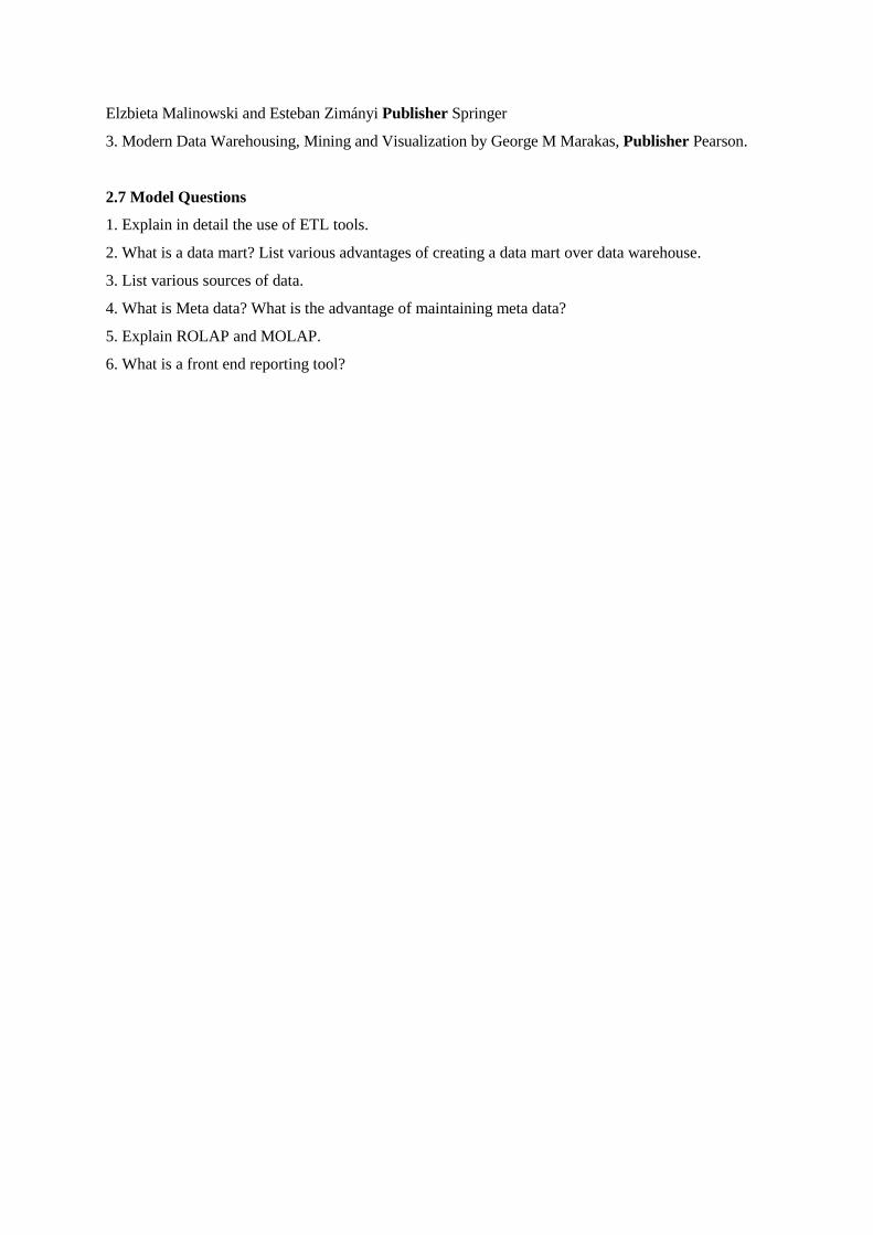
4.8 Architecture of Spatial Systems

Collection of spatial objects (using vector representation) can be stored using the following models

1. Spaghetti model,

2. Network model, and

3. Topological models.

Irrespective of which structure is selected for storing collection of spatial objects, two different

computer architectures can be used for spatial systems, called dual and integrated. Dual architecture is

based on separate management systems for spatial and non spatial data and integrated architecture is

an extension of existing database management systems with spatial data types and functions.

Geographic information systems or GISs make use of dual architecture system. GIS requires

heterogeneous data models to represent spatial and non-spatial data. Spatial data is generally

represented using proprietary data structures, which implies difficulties in modelling, use, and

integration.

Whereas, integrated architectures or extended DBMSs provide support for storing, retrieving,

querying, and updating spatial objects while preserving other DBMS functionalities, like recovery

techniques and optimization. The integrated architecture lets you define an attribute of a table as being

of spatial data type. It can be extremely useful in speeding up spatial queries using spatial indexes by

retrieving topological relationships between spatial objects using spatial operators and spatial

functions.

Oracle Spatial and IBM DB2 Spatial Extender are two examples of widely used DBMSs that support

the management of spatial data.

4.9 Spatial Levels

Spatial level may be defined as a level for which the application needs to store spatial characteristics.

It is captured by its geometry represented using one of the spatial data types defined earlier in this

lesson. For example, Point, Line, OrientedLine, Surface, etc. A spatial attribute refers to an attribute

that has a spatial data type as its domain. Multi Dimensional model represents spatial level using the

icon of its associated spatial type with the level name. Consider the figure below:

Figure 4.3 Spatial levels


Applications"

SurfaceSet icon represents the geometry of State members. A level may be spatial independently of

the fact that it has spatial attributes. For example, a level such as State may be spatial and have spatial

attributes such as Capital location.


Q7.Spaghetti model is used to store the collection of spatial objects. (TRUE / FALSE)

Q8. ________ and ___________ computer architectures can be used for spatial systems

Q9. Dual architecture is an extension of existing database management systems with spatial data

types and functions. (TRUE / FALSE)

____________________________________________________________________________

4.10 Spatial Hierarchies

Hierarchy Classification

A spatial hierarchy is composed of several related levels, of which at least one is spatial. If two related

levels in a hierarchy are spatial, a pictogram indicating the topological relationship between them

should be placed on the Link between the levels. If this symbol is omitted, the coveredBy

topologicalrelationship is assumed by default. Following are the different types of spatial hierarchies.

Simple Spatial Hierarchies

Simple spatial hierarchies are those hierarchies where, if all its component parent-child relationships

are one-to-many, the relationship between their members can be represented as a tree. Simple spatial

hierarchies can be further categorized s:

Balanced spatial hierarchies at schema level, have only one path, where all levels are mandatory. At

the instance level, the members form a tree where all the branches have the same length.

Unbalanced spatial hierarchies have only one path at the schema level but, as implied by the

cardinalities, some lower levels of the hierarchy are not mandatory. At instance level, the members

represent an unbalanced tree, with branches of the tree having different lengths

Generalized spatial hierarchies contain multiple exclusive paths sharing some. All these paths

represent one hierarchy and account for the same analysis criterion. At the instance level, each

member of the hierarchy belongs to only one part. The symbol ⊗ is used to indicate that for every

member, the paths are exclusive.

Non-Strict Spatial Hierarchies

Simple spatial hierarchy is used to represent one-to-many parent child relationship, i.e. a child

member can be related to a maximum of a one parent member, but a parent member can be related to

number of child members. But, in practice there may exist many-to-many relationship between the

parent-child members. Non-strict spatial hierarchy has at least one many-to-many relationship. Strict

spatial hierarchy has all one-to-many relationships. Graph is used to represent the members of a non-

strict hierarchy.

Alternative Spatial Hierarchies

Alternative spatial hierarchies have in them several nonexclusive simple spatial hierarchies sharing

some levels. However, all these hierarchies account for the same analysis criterion. Graph is used to

represent these hierarchies at instance level, because a child member can be associated with more than

one parent member belonging to different levels. It is called alternative spatial hierarchies because it is

not semantically correct to simultaneously traverse different component hierarchies, and you must

choose one of the alternative aggregation paths for analysis.

Parallel Spatial Hierarchies

Parallel spatial hierarchies are used when a dimension is associated with several spatial hierarchies

accounting for different analysis criteria. Such hierarchies can be independent or dependent. Various

hierarchies in a parallel independent spatial hierarchies do not share levels or represent non

overlapping sets of hierarchies. Whereas, various hierarchies in parallel dependent spatial hierarchies

share some levels.

4.11 Spatial Fact Relationships

Fact relationship is used to relate the leaf members from all its participating dimensions into a

relationship. For non-spatial dimensions, this relationship corresponds to a relational join operator.

For spatial dimensions, spatial join based on a topological relationship is needed to represent the

relationships. Spatial data warehouses include a feature called n-ary topological relationships.

Topological relationships in spatial databases are generally binary relationships, whereas, topological

relationships in spatial data warehouses relates more than two spatial dimensions.

4.12 Spatial Measures

Spatial measures can be represented by a geometry. Current OLAP systems require aggregation

functions for numeric attributes during the roll-up and drill-down operations. By default, the sum is

applied. Distributive functions reuse aggregates for a lower level of a hierarchy in order to calculate

aggregates for a higher level. Algebraic functions require additional manipulation to reuse values.

Whereas, holistic functions, such as the median, and rank require complete recalculation using data

from the leaf level.

Spatial measures also require the specification of a spatial aggregation function. Several different

aggregation functions for spatial data are defined, such as:

1. Spatial distributive functions including convex hull, spatial union, and spatial intersection.

2. Spatial algebraic functions including center of n points and the center of gravity.

3. Spatial holistic functions are the equipartition and the nearest-neighbor index


Q10.Non-strict spatial hierarchy has at least one many-to-many relationship. (TRUE / FALSE)

____________________________________________________________________________

Q11. _________ is used to represent the alternate spatial hierarchies at instance level.

Q12Topological relationships in spatial data warehouses are binary relationships (TRUE / FALSE)

____________________________________________________________________________

4.13 Summary

Spatial objects consist of both the conventional and spatial components. Conceptual spatiotemporal

model MADS defined number of spatial data types that were discussed in this lesson. Spatial

reference system is used to represent some co-ordinates of a plane that define the locations in a given

geometry. Relationship between the two spatial values is represented using topological relationships.

Conceptualmodels for spatial data are extensions of conceptual models to meet the requirements of

spatial data. Spatial objects can be stored using the spaghetti model, network model, and topological

models. Two different computer architectures are used for spatial systems, called dual and integrated.

A separate management system is created for dual architecture to manage spatial and non-spatialdata,

whereas, integrated architecture is an extension of existing database management systems with spatial

data types and functions. Multi Dimensional model represents spatial level using the icon of its

associated spatial type with the level name. Several related levels are used to represent spatial

hierarchies. Spatial measures can be represented by a geometry. Current OLAP systems require

aggregation functions for numeric attributes during the roll-up and drill-down operations. Spatial

measures also require the specification of a spatial aggregation function.

4.14 Glossary

Spatial data warehouse- It refers to the combination of both the data warehouse and spatial

database technologies.

Spatial object- A spatial stores the spatial characteristics corresponding to a real-world entity and it

consists of both the conventional and spatial components.

Spatial reference system- It is used to represent some co-ordinates of a plane that define the locations

in a given geometry.

Topological Relationship- Relationship between the two spatial values is represented using

topological relationships.

Spatial measure- It can be represented by a geometry. Spatial measures require specification of a

spatial aggregation function during the roll-up and drill-down operations.


1. Spatial, data warehouse.

2. Conventional.

3. SimpleSurface.

4. TRUE.

5. Spatial.

6. Meets.

7. TRUE.

8. Dual, integrated.

9. FALSE.

10. TRUE.

11. Graph.

12. FALSE.


"1. Data Mining: Concepts and Techniques by J. Han and M. Kamber Publisher





Publisher Pearson."


1. List different spatial data types used in spatial databases.

2. List some of the topological relationships used in spatial databases.

3. Define interior, exterior and boundary in topological relationships.

4. What is the difference between dual and integrated architectures of spatial systems?

5. Explain different types of spatial hierarchies.

6. What do you mean by spatial data warehouse?

Lesson- 5 Temporal Data Warehouses- 1

Structure

5.0 Objective

5.1 Introduction

5.2 Temporal Databases: General Concepts

5.2.1 Temporality Types

5.2.2 Temporal Data Types

5.2.3 Synchronization Relationships

5.2.4 Conceptual and Logical Models for Temporal Databases

5.3 Temporal Extension of the MultiDimensional Model

5.3.1 Support for temporality types

5.3.2 Overview of the Model

5.4 Summary

5.5 Glossary



5.8 Model Questions

5.0 Objective


1. Describe the need of temporal database.

2. Discuss the basic concepts of temporal databases.

3. Explain the challenges associated with extension of a MultiDim model to temporal model.

4. List the support provided by source systems for various temporality types.

5.1 Introduction

It is very important to represent the information that varies with time. Conceptual databases do not

save historical data. Temporal databases is a solution to store information that varies with time. Also

the MultiDim models fails to provide support for data that varies with time. This lesson focuses on the

basic concepts of temporal databases and how a MultiDim model can be extended to support

Temporal data model.

5.2 Temporal Databases: General Concepts

Temporal databases are used to represent information that varies over time. Conventional databases

generally store current data, whereas temporal databases store the historical and future data along with

the times at which the changes have happened and are expected to happen. Discrete model is used to

represent the time in a temporal database. The timeline is then represented as a sequence of

consecutive time intervals of same duration called chronons. Groups of consecutive chronons is

calledgranules that may represent time in terms of units like seconds, minutes or even hours.


Following are some of the temporality types:

1. Valid time (VT): It is used to specify the time period for which a fact is true in the modelled reality.

For example, it can be identified as to how many tickets were booked by a customer in a given period

of time. The time period must be supplied by the customer itself.

2. Transaction time (TT): It is used to specify the time period in which a fact is current in the

database and it starts when the fact is inserted or updated, and ends when the fact is deleted or

updated.

3. Bitemporaltime (BT): It is combination of both the VT and TT, and is used to specify the time

period for which the fact is true in reality and it is current in the database.

4. Lifespan (LS): It is used to specify the time period during which an object exists. For example, a

life span can be used to specify the time period for which an individual was member of an association.

5.2.2 Temporal Data Types

Temporal data types are used to specify the temporal extent of real-world phenomena and are defined

using the spatiotemporal conceptual model MADS,

Figure 5.1 Temporal data types


Applications"

1. Instant: It does not represent a time period, instead it represents a single point of time based on

some specified granularity.

2. Interval: It may be thought of a time period. It refers to set of all successive instants between two

points of instants.

3. SimpleTime: It refers to the generalization of both the Instant and the Interval. It is must to specify

the values for Instant and Interval every time value for SimpleTime is created.

4. InstantSet: It is used to represent a set of single points of time or Intervals. For example, InstantSet

can be used to represent the Instants at which the goals happened during a football match.

5. IntervalSet: Also known as temporal element, it is used to specify simple intervals that is capable of

representing discontinuous duration like duration of matches played in a single tournament.

6. Complex Time: It is used to represent dissimilar set of temporal values, i.e. the set may contain

both the Interval and Instant values.

7. Time: It is the most generic or abstract temporal data type. It can be used to represent the lifespan

of a tournament.

5.2.3 Synchronization Relationships

Relationship between two temporal extents can be represented using synchronization relationships.

Synchronization relationships helps to identify if two events have occurred simultaneously or one

after the other. Synchronization relationships for temporal data are also used to correspond to the

topological relationships for spatial data. Synchronization relationships can also be defined on the

basis of the boundary, interior, and exterior.

Exterior of a temporal value refers to all instants that do not belong to temporal value.

Interior of a temporal value refers to all instants that do not belong to boundary.

Boundary for different temporal data types is different. Because an Instant refers to a single point of

time, it does not have a boundary. As Intervalrefers to set of all successive instants between two

points of instants. First and last Instant forms the boundary of an Interval. Boundary for

ComplexTime is defined as the union of the boundaries of its components that do not intersect with

other components.

Figure 5.2 Icons for Synchronization relationships


Applications"

Following are some of the commonly used synchronization relationships

1. Meets: It refers to the relationship when two temporal values intersect in an instant but their

interiors do not.

2. Overlaps: It refers to the relationship when interiors of two temporal values intersect and their

intersection is not equal to either of them.

3. contains/inside: Consider the predicate: X contains Y if and only if Y inside X. It is an example of

symmetric predicate. It suggests that a temporal value contains another one if the interior of the

former contains all instants of the latter.

4. covers/coveredBy: Again consider the predicate: X covers Y if and only if Y coveredBy X. It is

also an example of symmetric predicate. A temporal value covers another one if the former includes

all instants of the latter.

5. disjoint/intersects: It is an example of inverse predicate, i.e. disjoint and intersects are inverse

temporal predicates. It means that two temporal values are disjoint if they do not share any instant, i.e.

when one applies, the other does not.

6. Equals: Two temporal values are considered to be equal if and only if every instant of one value

belongs to the second and conversely.

7. starts/finishes: A temporal value starts/finishes another if the first/last instants of the two temporal

values are equal, respectively

8. precedes/succeeds: A temporal value precedes/succeeds another if the last/first instant of the former

is before/later the first/last instant of the latter, respectively.


Q1. Temporal databases are used to represent information that _______ over time.

Q2. List various temporality types.

____________________________________________________________________________

____________________________________________________________________________

Q3. Define Instant.

____________________________________________________________________________

____________________________________________________________________________

Q4. Define SimpleTime.

____________________________________________________________________________

____________________________________________________________________________

Q5. Synchronization relationships helps to identify if two events have occurred simultaneously.

(TRUE / FALSE)

____________________________________________________________________________

5.2.4 Conceptual and Logical Models for Temporal Databases

Number of conceptual models have been extended to support the time-varying temporal models in

databases. Some of the conceptual models for which this extension can be provided are ER model

UML model. Extension means to introduce all new construct or to change or modify the existing

construct of a conceptual model. Easy it may sound, it is not easy to implement and may not be cost

effective. Temporal database once created, must be translated into a logical schema for

implementation in a DBMS. Till date, little support is provided by SQL to incorporate support for

time-varying temporal models.

Eventually the lack of support for time-varying temporal models in conceptual models led to the

research in the field of temporal databases. Effective mapping of temporal conceptual models into the

conceptual model, like relational model is still a lot to be desired. Another approach to logical-level

design for temporal databases is to use temporal normal forms, which again is a difficult task to

achieve. As a database student, you already know that normalizing a database in conceptual models in

itself is a very difficult task.

The relational representation of temporal data leads to large number of tables, which causes

performance problems due tomultiple join operations needed for retrieving this information. Also the

model suffers from manyintegrity constraints that encode the underlying semantics of time-

varyingdata. Object-relational model can be used to group together the related temporal data into a

single table, and hence providing a partial solution tofirst problem. Still, integrity constraints must be

added toobject-relational schema. Object-relational model suffers from performance issues when it

comes to managing the time-varying data.

5.3 Temporal Extension of the MultiDimensional Model

In this section, you will learn the fundamental concepts related to the temporal extension of Multi

Dimensional Model.

5.3.1 Support for temporality types

The Multi Dimensional model do provide support the following temporality types discussed earlier in

this lesson:

1. Valid time (VT),

2. Transactiontime (TT),

3. Lifespan(LS).

However, these temporality types should exist in the source systems and these cannot be introduced

by users or generated by DBMS. Following is the list of temporal support provided by different types

of source systems:

1. Snapshot: Data is obtained by dumping the entire source system and changes are found by

comparing current data withprevious snapshots.

Support provided for (VT), (LS)temporality types.

2. Queryable: Data is extracted using a query interface provided by the source system. Changes can

be found by periodic polling of data.Queryable provide direct access to source data.

Support provided for (VT), (LS)temporality types.

3. Logged: Log files are used to record each and every data modification. Periodic polling is done to

find data changes, if any have occurred. Transaction time can be retrieved from log files and valid

time and/or lifespan may be included in thesystem.

Support provided for TT, (VT), and (LS)temporality types.

4. Callback and internal actions: Triggersor a programming environment is provided by the source

system to detect changes and notify those to the user. Changes in data with the time of change are

detected without any delay.

Support provided for TT, (VT), and (LS)temporality types.

5. Replicated: Changed are detected by analyzing the messages sent by the replication system. This

analysis can happen periodically, or even manually.

Support provided for (TT), (VT), and (LS)temporality types.

6. Bitemporal: The source systems itself are temporal databases that include valid time, and/or

lifespan, as well as transaction time.

Support provided for TT, VT, LS temporality types.

Some of the temporality types are enclosed within parentheses that suggests the possibility of their

existence in the source system.Support for temporality types is for the following reasons:

1 Temporalitytypes in developing procedures for correct measure aggregation during roll-up

operations. Roll up operation is one the basic operations that can be performed on OLAP data.

2. Also the transaction time is useful for traceability applications, like for fraud detection.

In addition to temporality types discussed above, loading time(LT) was proposed by the authors of

"Advanced Data Warehouse Design: From Conventional to Spatial and Temporal Applications". LT

is used to specify the time since thedata is current in a data warehouse. It is not necessarily same as

transaction time. There may be a delay in integrated the change into atemporal data warehouse.

Loading time helps to identify the time since a data item has been available in a data warehouse for

analysispurposes.


Q6. It is not possible to extend a conceptual models to support the time-varying temporal

models in databases. (TRUE / FALSE)

____________________________________________________________________________

Q7.What do you refer to Queryable support?

____________________________________________________________________________

____________________________________________________________________________

Q8. Loading time can be different from the transaction time. (TRUE / FALSE)

____________________________________________________________________________

5.3.2 Overview of the Model

It is not mandatory to store data related to an application over time. Symbols corresponding to the

temporality types are maintained in the schema to determine which temporal data might be needed in

time.

Figure 5.3 Conceptual schema (Temporal Data Warehouse)


Applications"

Changes in the values of measures for data related toproducts and stores are important for analysis

purposes, and hence temporality types are included in the schema for them. Depending on the type of

requirement, appropriate temporality type is mentioned.

MultiDimensional model allows and maintains for both temporal and nontemporal attributes, levels,

parent-child relationships,hierarchies, and dimensions. Temporal level refers to a level for which the

applicationneeds to store the time frame associated with its members. Schema in figure above

includes 4 temporal levels. Non-Temporal levels are calledconventionallevels. In the figure above,

client is an example of conventional level. It also maintains the time at which those changes took

place. Valid time support for the Size and Distributor attributes in the Product level is used to indicate

that the history of changes in the two attributes will be kept.

Atemporal parent-child relationship is used to keep track of time frameassociated with the links. LS

type in the relationship linkingof ProductandCategory is used to store the evolution in time of

assignments of products to categories. Cardinality for temporal support for parent-child relationships

can be interpretations as follows:

1. Instant cardinality: It is valid at every time instant.Symbols for the temporality type can be used to

represent the instant cardinality. For example, LS.

2. Lifespan cardinality: It is valid over the entire member’s lifespan. Symbol's of LS temporality type

surrounded by ellipse is used to represent the lifespan cardinality

Storeand Sales Districtlevels is one-to-many, while the lifespancardinality is many-to-many. It is used

to specify that at any time instant, a store can belong to 1 sales district, but over a lifespan, it may

belong tomany sales districts. Take another example, where both the Instant and Lifespan cardinality

betweenProduct andCategory are one-to-many.It is used to specify that that products belong to one

category over their lifespan that also include instant.

Temporal hierarchy includes at least onetemporal level. Also, a temporal dimensionhas at least one

temporal hierarchy.The non-temporal dimensions and hierarchies are calledconventionaldimensions

andhierarchies. Synchronization relationship refers to two related temporal levels in a hierarchy.

Product and Category is an example of overlap synchronization relationship, and is used to indicate

that lifespan of each product overlaps the lifespan of its corresponding category. In other words, you

can say that each valid product belongs to a valid category.

Temporal join between two or more temporal levels is used to represent the temporal fact relationship.

In the last figure, temporal fact relationshipSalesrelates two temporallevels: Product

andStore.Theoverlapssynchronization icon in the relationship is used to indicate that the users focus

their analysis on products whose lifespanoverlaps the lifespan of their related store. For instance, user

may wish to analyze whether the exclusion of some products from Stores will affect the Sales.

Temporal multidimensional model must provide temporal support for different elements of the model,

such as levels, hierarchies,and measures. Measures and attributes in fact relationships are considered

to be same, and hence support for measures must be provide similar to the support for attributes.

Temporality types of the MultiDimensional model may include levels, attributes, measures and

Parent-child relationships. If you consider the conceptual model given in the last figure, lifespan

support is provided for levels and parent-child relationships. Valid time support is provided for

attributes and measures.

5.4 Summary

Temporal databases are used to represent information that varies over time. Conventional databases

generally store current data, whereas temporal databases store the historical and future data along with

the times at which the changes have happened and are expected to happen. Discrete model is used to

represent the time in a temporal database.Relationship between two temporal extents can be

represented using synchronization relationships. Synchronization relationships helps to identify if two

events have occurred simultaneously. Common synchronization relationships are meets, overlaps,

contains/inside, covers/coveredBy, disjoint/intersects, equals, starts/finishes, precedes/succeeds. Some

of the conceptual models for which this extension can be provided are ER model UML model.

Extension means to introduce all new construct or to change or modify the existing construct of a

conceptual model. It is possible to provide extend MultiDim model to support temporal data models.

5.5 Glossary

Temporal databases- Databases that are used to represent information that varies over time.

Instant-It represents a single point of time based on some specified granularity.

Interval- It refers to set of all successive instants between two points of instants.

SimpleTime- It refers to the generalization of both the Instant and the Interval.

InstantSet- It is used to represent a set of single points of time or Intervals.

IntervalSet-It is used to specify simple intervals that is capable of representing discontinuous duration.

Complex Time- It is used to represent dissimilar set of temporal values.

Synchronization relationships- It is used to identify if two events have occurred simultaneously or one

after the other.


1. Varies.

2. Following are the temporality types:

Valid time (VT)

Transaction time (TT)

Bitemporaltime (BT)

Lifespan (LS)

3. Instantrepresents a single point of time based on some specified granularity.

4. SimpleTime refers to the generalization of both the Instant and the Interval. It is must so specify the

values for Instant and Interval every time value for SimpleTime is created.

5. TRUE.

6. FALSE.

7. It provides a query interface to extract data from the source system, i.e. it provide direct access to

source data. Support is provided for (VT), (LS)temporality types.

8. True.







Publisher Pearson."

5.8 Model Questions

1. Explain various temporality types used in temporal databases.

2. Explain various temporal data types.

3. What do you mean by synchronization relationships? Explain with the help of an example.

4. Explain different temporal support provided by different types of source systems:

5. What do you mean by instant cardinality?

6. What do you mean by load time?

Lesson- 6 Temporal Data Warehouses- 2

Structure

6.0 Objective

6.1 Introduction

6.2 Temporal Support for Levels

6.3 Temporal Hierarchies

6.3.1 Non-temporal Relationships between Temporal Levels

6.3.2 Temporal Relationships between Non-temporal Levels

6.3.3 Temporal Relationships between Temporal Levels

6.3.4 Instant and Lifespan Cardinalities

6.4 Temporal Fact Relationships

6.5 Temporal Measures

6.5.1 Temporal Support for Measures

6.6 Temporal Granularity

6.7 Logical Representation of Temporal Data Warehouses


6.7.2 Levels with Temporal Support

6.7.3 Parent-Child Relationships

6.7.4 Fact Relationships and Temporal Measures

6.8 Summary

6.9 Glossary




6.0 Objective


1. Describe the concept of temporal support in temporal data warehouse.

2. Discuss the representation of hierarchies in Multi Dimensional model.

3. Explain the representation of temporal facts and temporal measures.

4. Define the notion of temporal granularity.

5. List various rules for logical representation of Temporal Data Warehouse.

6.1 Introduction

In the last lesson you learned the basic concepts related to the temporal databases and how the Multi

Dimensional models can be extended to provide temporal support. In this lesson you will study

various rules that should be followed when creating a conceptual temporal data warehouse. Also, the

lesson discusses in detail the technicalities associated with the mapping of conventional model to a

temporal model.

6.2 Temporal Support for Levels

Two types of changes can happen in a level:

1. It can either occur at the member level, i.e. inserting or deleting an entire row.

2. Or, it can occur at the level of attribute values, i.e. changing the value of an attribute.

Temporal data warehouse must represent these changes for analysis purpose. For example, you want

know the effect of change in the MRP a product, on the sales of that product. It is possible to

associate times frames with the members of a level, only if it provides for the temporal support.

Representing the temporal support for a level is easy, and it can be represented using a symbol for the

temporality type next to the level name. Lifespan support is used to specify the time of existence of

the members in the modelled reality. Transaction time and loading time are used to specify the time

since the members are current in a source system and in a temporal data warehouse, respectively. It is

possible that the transaction time is not the same as loading time. It can happen due to delay in

recording the changes in a temporal data warehouse. Temporal support for attributes is used to specify

the changes in their values and the times when these changes occurred. Temporal support for

attributes can be represented by including the symbol for the corresponding temporality type next to

the attribute name. Transaction time, valid time, loading time, or combination of these can be used as

temporal support for attributes. Some of the classical temporal models impose certain constraints on

temporal attributes and the lifespan of their corresponding entity types.

6.3 Temporal Hierarchies

The Multi Dimensional model is capable of representing hierarchies that contain several related

levels. Given two related levels in a hierarchy, following three situations can be encountered:

6.3.1 Non-temporal Relationships between Temporal Levels

It is possible to associate temporal levels with non-temporal relationships. Consider the following

example:

Figure 6.1 Temporal levels with non-temporal relationships


Applications"

Relationship are used to store only the current links between Products and Categories. It means that a

product can only be related with a category, if the two are currently valid. Also, the lifespans of a

child member and its associated parent member must overlap, which can be specified using icon of

the synchronization relationship with the temporal link.

6.3.2 Temporal Relationships between Non-temporal Levels

Temporal relationships also allow you to keep track of the evolution in time of links between parent

and child members. This type of temporal relationship can be represented by inserting the temporality

symbol on the link between the hierarchy levels as shown in the figure below:

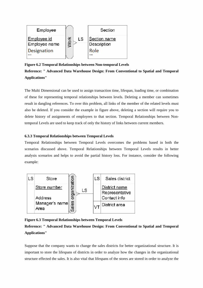
Figure 6.2 Temporal Relationships between Non-temporal Levels


Applications"

The Multi Dimensional can be used to assign transaction time, lifespan, loading time, or combination

of these for representing temporal relationships between levels. Deleting a member can sometimes

result in dangling references. To over this problem, all links of the member of the related levels must

also be deleted. If you consider the example in figure above, deleting a section will require you to

delete history of assignments of employees to that section. Temporal Relationships between Non-

temporal Levels are used to keep track of only the history of links between current members.

6.3.3 Temporal Relationships between Temporal Levels

Temporal Relationships between Temporal Levels overcomes the problems based in both the

scenarios discussed above. Temporal Relationships between Temporal Levels results in better

analysis scenarios and helps to avoid the partial history loss. For instance, consider the following

example:

Figure 6.3 Temporal Relationships between Temporal Levels


Applications"

Suppose that the company wants to change the sales districts for better organizational structure. It is

important to store the lifespans of districts in order to analyze how the changes in the organizational

structure effected the sales. It is also vital that lifespans of the stores are stored in order to analyze the

impact of staring a new store or closing an existing store. Also, it will be possible to keep track of the

evolution in time of work assigned of stores to sales districts. It means that the store and the sales

district exist throughout the lifespan of the relationship linking them.

6.3.4 Instant and Lifespan Cardinalities

In conventional or non-temporal model, cardinality is used to define the number of members in a level

related to number of members in another level. Whereas in case of temporal model, considered may

be defined in terms of Instant (instantcardinality), or lifespan (lifespan cardinality).

Figure 6.4 Instant and lifespan cardinalities.


Applications"

Generally it is assumed that the instant cardinality is equal to the lifespan cardinality. In case the two

are different, the lifespan cardinality is represented using an additional line with the LS symbol

surrounded by an ellipse.

For the example in the figure above, instant and lifespan cardinalities are same for work hierarchy, but

different for affiliation hierarchy. Both the cardinalities for Work hierarchy are many-to-many, which

means that an employee can work in different sections at any given instant or during its lifespan.

Whereas, the instant cardinality for affiliation hierarchy is one-to-many and lifespan cardinality is

many-to-many. It means that an employee can be affiliated to one section only at any given instant,

but the same employee can get affiliated to multiple sections during its lifespan.


Q1. _________Relationships Between Temporal Levels results in better analysis scenarios.

Q2. It is possible to associate times frames with the members of a level. (TRUE / FALSE)

____________________________________________________________________________

____________________________________________________________________________

Q3. In conventional model, ____________ is used to define the number of members in a level related

to number of members in another level.

6.4 Temporal Fact Relationships

Fact relationship instance is used to relate the leaf members from all its participating dimensions. If

some of these members are temporal, they have an associated lifespan. Covering the valid time of

measures by the intersection of lifespans of the related temporal members helps in ensuring correct

aggregation. This type of constrain ensures that the lifespan of an instance of a parent-child

relationship is covered by the intersection of the lifespan of the participating objects. This constraint is

similar to the constraint imposed on Temporal Relationships between Temporal Levels.

For instance, consider the following example:

Figure 6.5 Schema for Insurance Company


Applications"

The schema above is useful for an Insurance company if it wants to analyze the amount of

compensation paid against different types of risks covered. The indemnity amount is determined by

the measure in the fact relationship determines. Constraint for the schema above indicates that for the

instance of a fact relationship, valid time of Amount measure is covered by the lifespans of the related

members: Insurance policy and Repair work. Temporal join on different synchronization relationships

is needed when two or more temporal levels participate in a fact relationship. For the schema above,

synchronization relationship in the fact relationship states that the lifespans of the 3 members

(Insurance Policy, Repair Work, and Event) must have a nonempty intersection in order to relate

them.

6.5 Temporal Measures

6.5.1 Temporal Support for Measures

Support for only the valid time for measures is provided by the current Multi Dimensional models. In

this section you will see few cases where you can provide loading time and transaction time support

for measures. Let us consider some of the cases that show the benefits of providing different temporal

supports for the measures. It may not be possible to discuss all the situations in this section.

Non-Temporal Sources, Data Warehouse with LT

Generally the source systems do not provide temporal support, or it may be provided in an ad hoc

manner which not sufficient and also difficult to obtain. Also the integration of temporal support in

the source systems into a data ware house is extremely costly. Checking the time consistency

between different source systems is a perfect example for it. In order to obtain the history of how the

source data evolved in time, measure values can be timestamped with the loading time to indicate the

time at which the data was loaded into the warehouse.

Source Systems and Data Warehouse with VT

Support for the valid time, if provided by the source systems is needed in the temporal data warehouse

as well. Valid time in source systems are used to represent the events or states. For example, you can

design an event model to analyze the banking transactions and a state model to analyze the salary of

the employees. Generally the difference between an event model and a state model is not explicit in

the graphical notation, but the same can be stated in its textual representation. Different types of

queries are designed for such a schema. Events model for the banking transaction schema can be used

to analyze the total amount withdrawn from the ATM, maximum or minimum withdrawal, frequency

with which the clients use ATMs during holidays and working days, etc. States model for employee’s

salary can be used to analyze the evolution in time of the salaries paid to employees according to

different criteria, such as changes in professional skills or participation in various training programs,

etc.

A number of other situation exist that can be used to analyze the benefits of providing different

temporal supports for the measures


Q4. Integration of temporal support in the source systems into a data ware house is extremely costly.

(TRUE / FALSE)

____________________________________________________________________________

Q5. ___________________time in source systems are used to represent the events or states.

6.6 Temporal Granularity

Temporal data warehouses must deal with different temporal granularities for measures and for

dimensions. Temporal granularity of measures in the source systems is much finer than in the

temporal data warehouse.

Regular and irregular mappings are used for conversion between different temporal granularities. For

regular mapping, one granule is a partitioning of another granule. For example, an integer granule can

be converted by using a simple divide or multiply strategy. Conversion between seconds and minutes,

minutes and hours, is a perfect example of regular mapping. Granules using irregular mapping cannot

be converted using simple operations like divide or multiply. For example, conversion between days

and months is not easy as number of days in different months are not same.

Also, temporal databases do not allow for the mappings between certain different granularities. For

example, temporal databases to do not allow mapping between weeks and months, as it is possible

that a week days are spread over two months. However, data warehouse supports forced granularities

that are not easy to map or are not mapped in temporal databases.

6.7 Logical Representation of Temporal Data Warehouses


Mapping of the Multi Dimensional model into an ER model requires additional attributes to keep

track of the temporal support in the Multi Dimensional model. Also the mapping of temporal elements

depends on whether they represent events or states. Instant or a set of instants are used to represent the

events in an ER model. Whereas, interval or a set of intervals are used to represent the states in an ER

model.

Multi Dimensional model provides support for various temporality types like transaction time, valid

time, loading time and lifespan. Events and states can both be represented using the valid time and

lifespan temporality types. Interval or a set of intervals are used to represent the transaction time.

Whereas, an instant is used to represent the loading time as it indicates the point of time instant at

which data was loaded into a temporal data warehouse. Mapping of temporality types from Multi

Dimensional model to ER model can be achieved using either of the following rule:

Rule 1:

Monovalued attribute is used to represent an instant.

Multivalued attribute is used to represent a set of instants.

Composite attribute consisting of two attributes are used to specify the start and end of the

interval.

Multivalued composite attribute is used to represent a set of intervals.

6.7.2 Levels with Temporal Support

Following rules are used to provide transformation of levels and their attributes into the ER model:

Rule 2: Entitytype in an ER model is used to represent a Non-Temporal level.

Rule 3: Entitytype in an ER model for temporal level can be represented using additional attribute for

each of its associated temporality types. Mapping can then be achieved using rule 1.

Rule 4: A monovalued attribute in an ER model is used to represent the non-temporal attribute

Rule 5: Multivalued composite attribute in an ER model is used to represent the temporal attribute.

Mapping can then be achieved using rule 1.

6.7.3 Parent-Child Relationships

Mapping of parent-child relationships can be categorized into following:

Non-Temporal Relationships

The transformation of non-temporal relationships between levels to the ERmodel is based on the

following rule:

Rule 6: Binary relationship without attributes in the ER model is used to represent the non-temporal

parent-child relationship.

Temporal Relationships

The following rule is used for mapping temporal relationships:

Rule 7: Binary relationship with an additional attribute in the ER model us used to represent the

temporal parent-child relationship. The additional attribute keeps track of each of the associated

temporality types of temporal parent-child relationship. Mapping can then be achieved using rule 1.

6.7.4 Fact Relationships and Temporal Measures

Following rules are used for mapping fact relationship and temporal measures:

Rule 8: N-ary relationship in ER model is used to represent the fact relationship

Rule 9: Multivalued composite attribute in an ER model is used to represent the measure of a fact.

Mapping can then be achieved using rule 1.


Q6. Conversion between seconds and minutes is an example of _____________ mapping.

Q7. _____________ relationship in ER model is used to represent the fact relationship

Q8. It is not possible to map a Multi Dimensional model into an ER model. (TRUE / FALSE).

__________________________________________________________________________

6.8 Summary

Changes can occur in a level either at the member level, i.e. inserting or deleting an entire row, or it

can occur at the level of attribute values, i.e. changing the value of an attribute. Temporal data

warehouse must represent these changes for analysis purpose. Temporal Relationships between

Temporal Levels results in better analysis scenarios and helps to avoid the partial history loss.

Cardinality is used to define the number of members in a level related to number of members in

another level. Whereas in case of temporal model, considered may be defined in terms of Instant

(instant cardinality), or lifespan (lifespan cardinality). Support for only the valid time for measures is

provided by the current Multi Dimensional models. The integration of temporal support in the source

systems into a data ware house is extremely costly. Conversion between seconds and minutes,

minutes and hours, is an example of regular mapping. Conversion between days and months is an

example of irregular mapping as number of days in different months are not same. Temporal

databases to do not allow mapping between weeks and months, as it is possible that a week days are

spread over two months.

6.9 Glossary

Temporal databases- Databases that are used to represent information that varies over time.

Instant- It represents a single point of time based on some specified granularity.

Interval- It refers to set of all successive instants between two points of instants.

InstantSet- It is used to represent a set of single points of time or Intervals.

IntervalSet- It is used to specify simple intervals that is capable of representing discontinuous

duration.

Synchronization relationships- It is used to identify if two events have occurred simultaneously or one

after the other.


1. Temporal

2. TRUE.

3. Cardinality

4. TRUE.

5. Valid.

6. Regular.

7. N-ary.

8. FALSE.







Publisher Pearson."


1. Explain in detail the concept of representing temporal hierarchies in Multi Dimensional model.

2. Define cardinality for non-temporal models.

3. Explain the concept of temporal support for measures with the help of an example.

4. What do you mean by regular mapping and irregular mapping in context of temporal granularity?

5. Write the rule using which the mapping of temporality types from Multi Dimensional model to ER

model can be achieved.

Lesson- 7 Introduction to data mining

Structure

7.0 Objective

7.1 Introduction

7.2 Data Mining

7.3 Steps in Data Mining

7.4 Types of Data mining

7.5 Mining various Data types

7.6 Data mining issues

7.7 Pattern/context based mining

7.8 Summary

7.9 Glossary



7.12 Model questions

7.0 Objective

After studying this lesson, students will be able to:

1. Define data mining.

2. List the steps involved in data mining process.

3. Explain different data mining techniques.

4. Discuss various data types on which data mining can be performed.

5. Describe pattern/context based data mining.

7.1 Introduction

Information Technology has grown leaps and bounces in the field of database and its functionalities.

The database life cycle goes through various operations and phases like data collection, data creation,

data management, data analysis and data understanding. Businesses over time like to study the

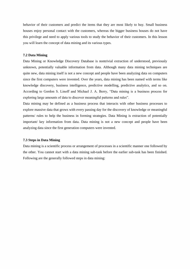
behavior of their customers and predict the items that they are most likely to buy. Small business

houses enjoy personal contact with the customers, whereas the bigger business houses do not have

this privilege and need to apply various tools to study the behavior of their customers. In this lesson

you will learn the concept of data mining and its various types.

7.2 Data Mining

Data Mining or Knowledge Discovery Database is nontrivial extraction of understood, previously

unknown, potentially valuable information from data. Although many data mining techniques are

quite new, data mining itself is not a new concept and people have been analyzing data on computers

since the first computers were invented. Over the years, data mining has been named with terms like

knowledge discovery, business intelligence, predictive modelling, predictive analytics, and so on.

According to Gordon S. Linoff and Michael J. A. Berry, “Data mining is a business process for

exploring large amounts of data to discover meaningful patterns and rules”.

Data mining may be defined as a business process that interacts with other business processes to

explore massive data that grows with every passing day for the discovery of knowledge or meaningful

patterns/ rules to help the business in forming strategies. Data Mining is extraction of potentially

important/ key information from data. Data mining is not a new concept and people have been

analyzing data since the first generation computers were invented.

7.3 Steps in Data Mining

Data mining is a scientific process or arrangement of processes in a scientific manner one followed by

the other. You cannot start with a data mining sub-task before the earlier sub-task has been finished.

Following are the generally followed steps in data mining:

Figure 7.1: Steps in data mining

1. Data Cleaning and Integration- Integrating the data from multiple heterogeneous data sources and

removal of error prone and inconsistent data.

2. Data Selection and Preprocessing-The extraction of data from previous stage and making it

consistent for analysis.

3. Data Transformation-It is data extracted from previous stage into data form appropriate for mining.

4. Data Mining- Discovery of intelligent patterns and rules from data.

5. Pattern Evaluation- It means Identification of patterns/ rules that are of interest depending upon the

problem in hand.

Once the patterns have been identified, visualization techniques are used to present the mined

knowledge to the end user or client (which is mainly top level management).

7.4 Types of Data mining

Data mining is performed by different business houses for their special requirements. Like a retail

chain might do it to identify which products are in demand and which products are bought together.

Production house may want to know the model of a particular product which is in demand or any

product sold by competitors that they don't produce, etc. Depending on the nature of use, data mining

can be classified as follows:

Figure 7.2: Types of data mining

Predictive

1. Regression is a statistical tool helps to predict value of dependent variable from the independent

variables. It uses the relation between the numeric variables (both dependent and independent).

Regression analysis can be simple linear, multiple linear, curvilinear, and multiple curvilinear

regression model.

2. Prediction consists of class that is a continuous. Prediction model is used to find numerical value of

the target attribute for objects from real life scenarios and live data.

3. Classification is based on pre-defined classes. It is used to assign a newly presented object to a set

of predefined classes. The classification task is characterized by a well-defined definition of the

classes, and a model set consisting of pre-classified examples. The class label is a discrete qualitative

identifier; forexample, large, medium, or small.

4. Time series analysis is used to store the time related data. It represents sequences of values

changing over time. Data is recorded at regular intervals of time. Some of the applications of time

series analysis are financial applications, scientific applications, etc.

Descriptive

1. Clustering is used to organize information about variables to form homogeneous groups or clusters.

These clusters are based on self similarities between variables.

2. Association Rules are statements about the relationships between attributes of a known set of

entities. It enable the system to predict the aspects of other entities that are not in the group, but

possess the same attributes.

3. Data Summarization is done at the early stages and is used as initial exploratory data analysis. It is

used to find potential hypotheses byunderstanding the behavior of data and exploring hidden

information in that data.


Q1. Define data mining.

___________________________________________________________________________

___________________________________________________________________________

___________________________________________________________________________

Q2. The extraction of data from previous stage and making it consistent for analysis is called

_____________________ .

Q3. Which data mining step comes after preprocessing?

________________________________________________________________________

Q4. Data mining may be broadly classified into _______________ and ______________ data mining.

Q5. _________________ are statements about the relationships between attributes of a known set of

entities.

7.5 Mining various Data types

Data mining is not specific to one type data and is applicable to any kind of data repository. Mining

algorithms vary depending on the types of data to be mined. Here are some examples of data types

that can be mined:

1. Flat files: Data is also available in the form of files. These files contain data in the form of text or

binary format with a structure already known by the data mining algorithm to be applied.

2. Relational Databases: Relational database is a set of tables containing values of entity attributes.

Table is represented as a 2-D matrix in which columns are used to represent the attributes and rows

are used to represent tuples. Data mining algorithms for relational databases are more versatile since

they can take advantage of the structure inherent to relational databases.

3. Data Warehouses: A data warehouse is a repository of data collected from multiple heterogeneous

data sources. Data warehouse is set up to generate a central integrated repository of data. Data from

multiple heterogeneous sources is preprocessed to remove all kinds of inconsistencies and integrity

problems from it. Multi-dimensional data models are used to maintain data in Data warehouses to

support decision making.

4. Transaction Databases: A transaction database represents transactional records each with a time

stamp, an identifier and a set of items. Transactions are stored in flat files or in normalized transaction

tables.

5. Multimedia Databases: Multimedia databases include various media types like video, images,

audio, etc. stored on extended object-relational or object-oriented databases.

6. Spatial Databases: Spatial databases store geographical information like maps, and global or

regional positioning along with normal data.

7. Time-Series Databases: Time-series databases contain time related data such as stock market data

or logged activities. It contains data stored at regular intervals. Data mining in such databases

includes the study of trends and correlations between evolutions of different variables.

8. World Wide Web: Data in the World Wide Web is organized in inter-connected documents that

have text, audio, video, and even applications. The World Wide Web is comprised of content of the

Web (Documents), the structure of the Web (Hyperlinks), and the usage of the web (Resource

accessibility).


Q6. A data warehouse is a repository of data collected from multiple heterogeneous data sources.

a. TRUE

b. FALSE

Q7. Data mining cannot be performed on multimedia databases.

a. TRUE

b. FALSE

Q8. Which of the following is not a type of predictive data mining technique?

a. Regression

b. Classification

c. Clustering

d. Prediction

Q9. _____________ databases store geographical information like maps, and global or regional

positioning along with normal data.

7.6 Data mining issues

1. Security issues: Data meant for decision taking purpose must be secured from unauthorized access

and manipulation. Data collected for customer profiling includes sensitive and private information

about individuals or companies.

2. End-user interface issues: The knowledge discovered should be interesting and understandable by

the end-user. Good data visualization helps to achieve this objective. End-user should be able to

visualize data from different dimensions in order to discover meaningful knowledge from it.

3. Methodology issues: Data for mining is extracted from variety of heterogeneous sources. Ensuring

the consistency and integrity of data is vital. Data mining techniques should be able to handle noise in

data or incomplete information. The size of the search space is crucial. The search grows

exponentially with the increase in dimensions. All methodology related issues must be handled

promptly.

4. Performance issues: Data is growing exponentially. Scalability and efficiency of data mining

methods is a challenge when it comes to processing such massive amount of data. To overcome these

issues, sampling of data sets was used for data mining. Now-a-days big data tools are used to manage

massive amount of data and it helps to process the data in much more effective manner.

7.7 Pattern/context based mining

Pattern mining consists of using/developing data mining algorithms to discover interesting,

unexpected and useful patterns in databases. Pattern mining algorithms can be designed to discover

various types of patterns: subgraphs, associations, indirect associations, trends, periodic patterns,

rules, lattices, sequential patterns, etc. Apriori algorithm is a popular frequent itemset mining

algorithm and a number of variations to it have also been designed. Frequent itemset mining or

frequent patterns are fast growing mining technique. It leads to the discovery of interesting patterns

such as association rules, correlations, sequences, classifiers and clusters among distinct items in large

point-of-sale or transactional data sets. The mining of association rules is one of the most critical and

widely accepted problems. Frequent patterns may be defined as patterns that appear frequently in a

data set. For example, if items like watch, sun-glasses, shoes appear in the same order and that too

frequently may be class frequent itemset. And if the tree items are bought one after the other, the same

may be called a frequent sequential pattern.

Measuring the strength of association rule: The association rules technique should be capable of

separating the strong patterns from the weak patterns. The three important methods for measuring the

strength of an association rule are support, confidence, and lift. Support measures the proportion of

transactions that contain all the items in the rule. Confidence is used to measure the predictive

strength of the rule. Confidence is a measure that tells you; how good a rule is at predicting the right

side of the rule. Sometimes the rules may be so obvious, that confidence is of little or no use. Lift is

used to measure the power of the rule by comparing the full rule to randomly guess the right side.

Association rule mining somehow fails to generate the rules that represent true correlation relationship

between the objects. Association rules may or may not be interesting from mining perspective.

Increasing the value for support threshold is not an efficient solution, as it might lead to missing of

many important association rules. So we need a mechanism using which we can separate important

association rules from unimportant association rules. Correlation analysis is the method capable of

revealing as to which association rules not only satisfy the minimum threshhold criteria, but are also

interesting and useful. Statistics based judgment from behind the data, can be much more effective in

leaving out uninteresting rules out of the total rules discovered.

Classification model is also known as classifier. The model is then used to classify new objects or

unseen objects in the real world. For example, after starting a credit policy, an enterprise may wish to

classify employee’s performance and label then accordingly to pre-classified labels such as

"excellent", "good", "ok" and "need improvement". Classifier begins by describing a predetermined

set of data classes. This is also called the learning or training step, where an algorithm is used to build

the classifier. It does so by learning from a training set made up of database tuples and their associated

class labels. X = (x1, x2, …., xn) represents a tuple X. Each tuple implicitly belong to a predefined

class as determined by class label attribute. The class label attribute is categorical and not continuous,

for example, outstanding, good, average and bad. Each tuple of training set is referred by training

tuple and is selected from the database under analysis.

Clustering is also used to find the similar patterns or more popularly known as pattern recognition.

Being able to identify patterns and make scientific reasoning for the same helps in better decision

making. Time series analysis is used to store the time related data. It represents sequences of values

changing over time. Data is recorded at regular intervals of time. Some of the applications of time

series analysis are financial applications, scientific applications, etc.


Q10. What are frequent patterns?

___________________________________________________________________________

___________________________________________________________________________

___________________________________________________________________________

Q11. ______________ analysis is used to find which association rules satisfy the minimum thresh

hold criteria and are also interesting and useful.

Q12. Define classifier.

___________________________________________________________________________

___________________________________________________________________________

___________________________________________________________________________

7.8 Summary

According to Gordon S. Linoff and Michael J. A. Berry, “Data mining is a business process for

exploring large amounts of data to discover meaningful patterns and rules”. Data mining process goes

through following 5 steps:

1. Data Cleaning and Integration

2. Data Selection and Preprocessing

3. Data Transformation

4. Data Mining

5. Pattern Evaluation

Data mining is broadly classified into predictive and descriptive data mining. Predictive data mining

may be further classified as regression, prediction, classification and time series analysis. Descriptive

analysis may be further classified as clustering, association rules, and data summarization. Data

mining can be applied on flat files, relational databases, data warehouses, operational databases,

multimedia databases, spatial databases, timer-series databases and WWW. Frequent itemset mining

algorithm and a number of variations to it have also been designed. Frequent itemset mining or

frequent patterns leads to the discovery of interesting patterns such as association rules, correlations,

sequences, classifiers and clusters among distinct items in large point-of-sale or transactional data

sets. Correlation analysis is the method capable of revealing as to which association rules not only

satisfy the minimum thresh hold criteria, but are also interesting and useful. Classification model is

also known as classifier. The model is then used to classify new objects or unseen objects in the real

world. Clustering is also used to find the similar patterns or more popularly known as pattern

recognition.

7.9 Glossary

Data mining- Data mining is a business process for exploring large amounts of data to discover

meaningful patterns and rules.

Regression- It is a statistical tool helps to predict value of dependent variable from the independent

variables.

Classification- It is used to assign a newly presented object to a set of predefined classes.

Clustering- It is used to organize information about variables to form homogeneous groups or clusters.

Association Rules- These are statements about the relationships between attributes of a known set of

entities.

Relational databases- Relational database is a set of tables containing values of entity attributes.

Tables have columns and rows, where columns represent attributes and rows represent tuples.

Data warehouse- A data warehouse is a central integrated repository of data collected from multiple

heterogeneous data sources.


1. Data mining may be defined as exploration of massive data for the discovery of knowledge or

meaningful patterns/rules to help the business in forming strategies.

2. Data selection and preprocessing.

3. Transformation.

4. Predictive, descriptive.

5. Association Rules.

6. a.

7. b.

8. c.

9. Spatial.

10. Frequent patterns may be defined as patterns that appear frequently in a data set.

11. Correlation.

12. Classifier model is then used to classify new objects or unseen objects in the real world into a set

of predefined classes.


"1. Data Mining: Concepts and Techniques by J. Han and M. Kamber Publisher Morgan Kaufmann

Publishers




4. Data Warehousing, Data Mining, & Olap by Alex Berson and Stephen J smith, Tata McGraw-Hill

Education.

5. Data Mining and Data Warehousing by Bharat Bhushan Agarwal and Sumit Prakash Tayal,

University Science Press.

6. Data Mining: Technologies, Techniques, tools and Trends by Bhavani Thuraisingham."


1. Explain the process of data mining.

2. Explain different types of data mining.

3. List various types of data types on which data mining can be performed.

4. What do you mean by pattern based mining?

5. What is the benefit of correlation analysis?

Lesson- 8 Classification Techniques- 1

Structure

8.0 Objective

8.1 Introduction

8.2 Classification

8.3 Bayesian Classifier

8.4 Bayes’ Theorem

8.5 Naive Bayesian Classification

8.6 Bayesian Belief Networks

8.7 Summary

8.8 Glossary




8.0 Objective


1. Define the concept of classification in data mining.

2. List different techniques used for implementing classification.

3. Describe the use of Bayesian classifier.

4. State the Bayes' Theorem.

5. Differentiate between Bayesian classifier and Bayesian belief networks.

8.1 Introduction

Classification is key data mining technique that is implemented in various applications. Now a days

you need to identify the characteristics or label your customers based on available attributes. Mobile

service providers, banks, insurance companies, ecommerce companies, all use classification for better

outcome. In this lesson you will learn a basic classification statistical tool called the Bayesian

classifier.

8.2 Classification

Classification is used to predict categorical labels. Classification analysis helps to organize the data in

predefined classes. Classification is also known as supervised learning. For example, depending on

the yearly sales figure or increase in sales, performance of salesman can be classified into predefined

classes such as outstanding, good, average and poor. All objects of training set are associated with

pre-classified class labels. The classification algorithm builds a model by learning from the training

set. Classification model is also known as classifier. The model is then used to classify new objects or

unseen objects in the real world. For example, after starting a credit policy, an enterprise may wish to

classify customers and label then accordingly to pre-classified labels such as "safe", "risky" and "very

risky".

Following techniques can be used with classification model of data mining:

1- Decision Trees.

2- Artificial Neural Networks.

3- Genetics Algorithm.

4- K-Nearest Neighbour.

5- Memory Based Reasoning;

6- Naive Bayesian classifier.

As already discussed earlier, classifier describes a predetermined set of data classes. This is also

called the learning or training step, where an algorithm is used to build the classifier. It does so by

learning from a training set made up of database tuples and their associated class labels. X = (x1, x2,

…., xn) represents a tuple X. Each tuple implicitly belong to a predefined class as determined by class

label attribute. The class label attribute is categorical and not continuous, for example, outstanding,

good, average and bad. Each tuple of training set is referred by training tuple and is selected from the

database under analysis.

Then it time to estimate the predictive accuracy of classifier. You can use either the training set or test

set to measure classifier's accuracy. The estimate value for predicting the accuracy of the classifier is

assumed to be rather high in case we are using the training set. The classifier tends to overfit the data.

Rather, the test set randomly selected from the general data set and its associated class labels should

be used. Test set is mostly free from any anomalies. Accuracy of a classifier is the percentage of

correctly classified test set or training set tuples. Accuracy of a classifier based on test set is expected

to be more than the accuracy of a classifier based on training set.

Figure 8.1: Classification process


Q1. Classification is an example of supervised learning. (TRUE / FALSE).

____________________________________________________________________________

Q2. Classification analysis helps to organize the data in _______________ classes.

Q3. List some of the classification techniques used in data mining.

____________________________________________________________________________

____________________________________________________________________________

____________________________________________________________________________

8.3 Bayesian Classifier

Bayesian classifiers are popular statistical classifiers. Bayesian classifier is used to predict the

probability that a given tuple belongs to a particular class. It is a classification tool. It is based on

Bayes’ theorem discussed later in this lesson. A simple Bayesian classifier called naiveBayesian

classifier is very good in terms of performance when compared with other classification algorithms.

Studies have also revealed that Bayesian classifiers result in high accuracy and speed when applied to

large databases.

Naive Bayesian classifier is based on an assumption that the effect of an attribute value on a given

class is independent of the values of the other attributes known as class conditional independence.

Bayesian belief networks are popular graphical models that represent of dependencies among subsets

of attributes. Bayesian belief networks can also be used for classification and are discussed later in

this lesson.

8.4 Bayes’ Theorem

What is Bayes’ theorem all about? A data tuple X is considered as evidence in Bayesian terms. Let

H be some hypothesis stating that data tuple X belongs to a pre-defined class C. The classification

problem is used to determine the probability P(H | X), stating that the hypothesis H holds given the

evidence X.

P(H | X) iscalled the posterior probabilityof H conditioned onX. For instance, suppose that the data

tuples in our database are confined to customers described by attributesage and income. Let the

evidence X be a 25 year customer in age with an income of Rs. 55,000/-. Let H be the Hypothesis that

the customer will purchase a smartphone. It means that P(H | X) reflects the probability that a

customer will purchase a smartphone in case the customer’s age and income is25 and 55,000

respectively. Other attributes such as gender, occupation, marital status does not matter.

Also, P(H) is called prior probability of H. No evidence is considered in prior probability and it is

assumed that a given customer will purchase smartphone irrespective of any attribute like age,

income, occupation, gender, or any other information. The probabilityP(H | X) is the posterior

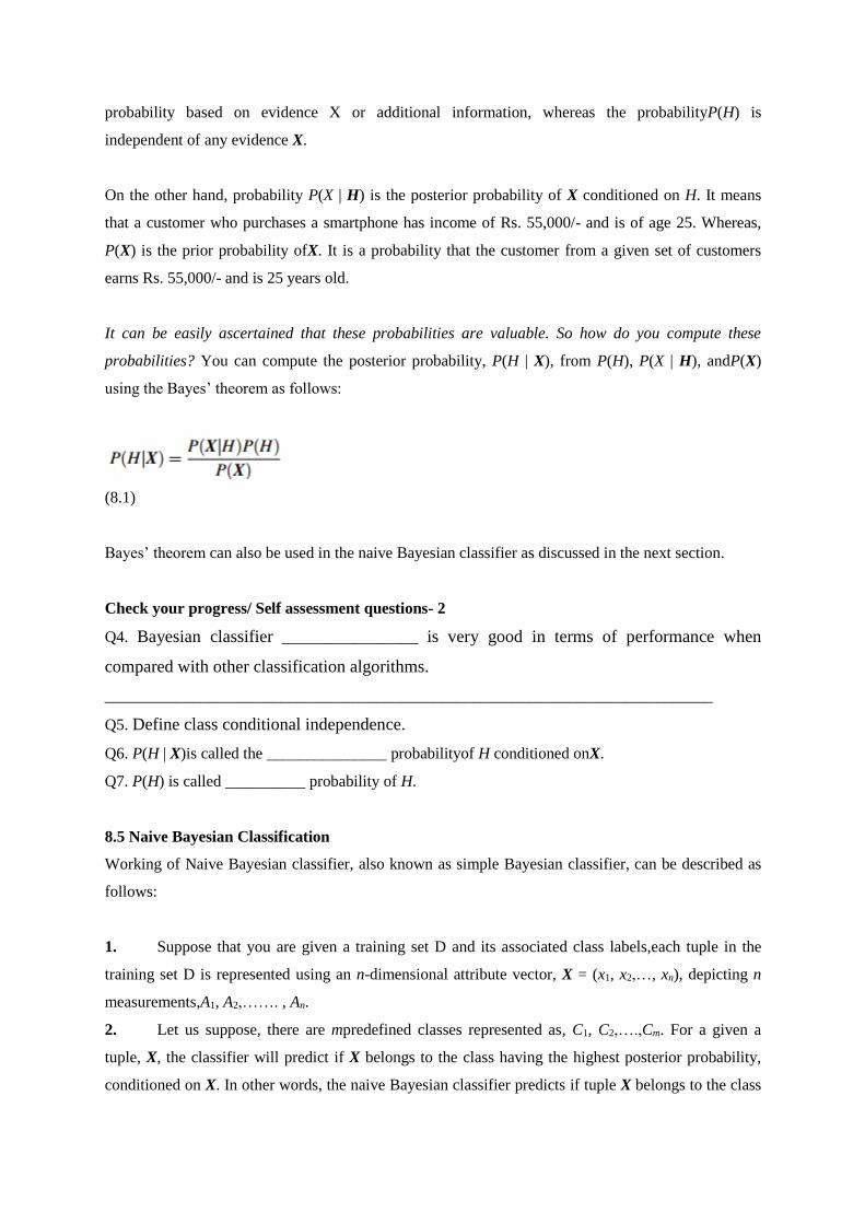
probability based on evidence X or additional information, whereas the probabilityP(H) is

independent of any evidence X.

On the other hand, probability P(X | H) is the posterior probability of X conditioned on H. It means

that a customer who purchases a smartphone has income of Rs. 55,000/- and is of age 25. Whereas,

P(X) is the prior probability ofX. It is a probability that the customer from a given set of customers

earns Rs. 55,000/- and is 25 years old.

It can be easily ascertained that these probabilities are valuable. So how do you compute these

probabilities? You can compute the posterior probability, P(H | X), from P(H), P(X | H), andP(X)

using the Bayes’ theorem as follows:

(8.1)

Bayes’ theorem can also be used in the naive Bayesian classifier as discussed in the next section.


Q4. Bayesian classifier _________________ is very good in terms of performance when

compared with other classification algorithms.

____________________________________________________________________________

Q5. Define class conditional independence.

Q6. P(H | X)is called the _______________ probabilityof H conditioned onX.

Q7. P(H) is called __________ probability of H.

8.5 Naive Bayesian Classification

Working of Naive Bayesian classifier, also known as simple Bayesian classifier, can be described as

follows:

1. Suppose that you are given a training set D and its associated class labels,each tuple in the

training set D is represented using an n-dimensional attribute vector, X = (x1, x2,…, xn), depicting n

measurements,A1, A2,……. , An.

2. Let us suppose, there are mpredefined classes represented as, C1, C2,….,Cm. For a given a

tuple, X, the classifier will predict if X belongs to the class having the highest posterior probability,

conditioned on X. In other words, the naive Bayesian classifier predicts if tuple X belongs to the class

Ci if and only if

P(Ci | X)> P(Cj| X)for1<= j<= m; j !=i

Idea is to maximize P(Ci | X). The class Ci for which the probability P(Ci | X) is maximized is called

the maximum posteriori hypothesis. By Bayes’ theorem,

(8.2)

3. P(X) in equation 8.2 is constant for all classes. Hence, there is need to maximize P(X |

Ci)P(Ci) in order to maximize P(Ci | X). Class prior probabilities are assumed to be equally likely in

case they are absent, i.e. P(C1) = P(C2) = … = P(Cm). In that case, there is need to maximize only the

P(X | Ci). You can compute the class prior probabilities by P(Ci)= |Ci,D | / |D |, where |Ci,D | represent

the number of training tuples of class Ci in training set D.

4. Compute P(X| Ci) for data sets with large attributes can be very expensive. In order to reduce

the computation cost, naive assumption of class conditional independence is made. Hence, it is

assumed that the attribute values are conditionally independent of each another for a given class label

of the tuple. Thus,

(8.3)

It is rather easy to estimate the probabilities P(x1 | Ci), P(x2 | Ci), …, P(xn | Ci) from the training tuples

asxk refers to the attribute valueAk for tuple X. P(X | Ci) can be computed for both categorical and

continuous-value attributes as follows:

(a) For categorical attribute, P(xk | Ci) refers to the number of tuples of class Ci in D having

value xk for Ak, divided by the number of tuples of classCi in D represented by |Ci,D|.

(b) For continuous-valued attributes, calculations are easy, but are little costly as compared to

calculations for categorical attributes. A continuous-valued attribute is defined by:

(8.4)

Such that

(8.5)

µCirefers to means for class Ciand σCi refers to standard deviation for class Ci, respectively, of the

values of attribute Ak for training tuples of class Ci. These two values are then used with attribute xk,

in equation 8.4 to estimate P(xk | Ci).

5. P(X | Ci)P(Ci) is computes for each class Ci to predict the class label of X. The classifier predicts

that the class label of tuple X is the class Ci if and only if:

P(X | Ci)P(Ci) > P(X | Cj)P(Cj) for1 <= j <= m, j != i

It means that the predicted class label is the class Ci for which P(X | Ci)P(Ci) is the maximum.

In theory, the Bayesian classifiers have minimum error rate in comparison to other classifiers such as

decision tree and neural network classifiers, however, in practice it is not always the case, due to

inaccuracies in the assumptions made for its use like the class conditional independence, and due to

missing probability data.

8.6 Bayesian Belief Networks

Computation cost for the naive Bayesian classifier can be reduced by making the assumption that

there exists class conditional independence. Class conditional independence means that the values of

the attributes on a given class is independent of the values of the other attributes. Theoretically the

naive Bayesian classifier may be most accurate as compared with other classifiers, but however,

dependencies do exist between variables. Bayesian belief networks specify joint conditional

probability distributions. It allows class conditional independencies to be defined between subsets of

variables. It provides a graphical model of causal relationships, on which learning can be performed.

A Bayesian belief network or belief network is defined by two components—a directed acyclic graph

and a set of conditional probability tables. A directed acyclic graph is one that does not involve

cycles, i.e. there is no path from one node to itself. Each node in the directed acyclic graph for belief

network represents a random variable. The variables can be discrete or continuous-valued. The

attributes used to represent nodes can be actual attributes or “hidden variables” believed to form a

relationship. Each directed arc in the graph represents a probabilistic dependence between the

variables. An arc from a node A to node B means that Ais immediate predecessor of B, and B is a

descendant of Y. Each variable is conditionally independent of its non-descendants in the graph.

Figure 8.2: Belief Network

The belief network in the figure above represents a casual model using directed acyclic graph and

conditional probability table for variable Blood pressure and all combinations with parent nodes

Family history and spicy food. The belief network involves 6 Boolean variables. Each arc is used to

represent causal knowledge. For instance, blood pressure problem is influenced by both the family

history of the patient and whether the patient like to eat spicy and oily food. Once the value for a

variable is evaluated, then the value for parent variables do not provide any additional information

regarding descendant variables of that variable. For instance, once it is established that the patient is

suffering from blood pressure, variables FamilyHistory and Spicy food do not provide additional

information regarding Hypertension.

Also the directed arcs of acyclic graph for belief network represented in figure 8.2 shows that variable

BloodPressure is conditionally independent of Cholesterol, given its parents, FamilyHistoryand

SpicyOilyFood.

One conditional probability table for each variable is included in belief network. Which means you

can create 6 CPT's for the belief network represented in figure 8.1. CPT for a variable Xindicates the

conditional distribution P( X | Parents( X )), where Parents( X ) represent the immediate predecessor

variable X. Figure 8.1(b) shows only a single CPT and that for the variable BloodPressure. The

conditional probability for each known value for variable BloodPressure is given for each possible

combination of values of its parents.

P(BloodPressure = yes | FamilyHistory = yes, SpicyOilyFood = yes) = 0.8

P(BloodPressure = no | FamilyHistory = yes, SpicyOilyFood = yes) = 0.2

P(BloodPressure = yes | FamilyHistory = yes, SpicyOilyFood = no) = 0.5

P(BloodPressure = no | FamilyHistory = yes, SpicyOilyFood = no) = 0.5

P(BloodPressure = yes | FamilyHistory = no, SpicyOilyFood = yes) = 0.7

P(BloodPressure = no | FamilyHistory = no, SpicyOilyFood = yes) = 0.3

P(BloodPressure = yes | FamilyHistory = no, SpicyOilyFood = no) = 0.1

P(BloodPressure = no j FamilyHistory = no, SpicyOilyFood = no) = 0.9

Total of each column is 1.

Let X = (x1, … , xn) be a data tuple described by the variables or attributes Y1, …. , Yn,respectively.

A network can provide a complete representation of the existing joint probability distribution with the

following equation:

(8.6)

Where P(x1, … , xn) refers to the probability of a particular combination of values of X, and values

for P(xi | Parents( Yi )) correspond to the entries in the CPT for Yi.

A class label attribute can be represented by selecting any node within the network as an “output”

node. It is possible for the belief network to have more than one output node. It is also possible to

apply various learningalgorithms to the network. In that case, the classifier can return a probability

distribution that gives the probability of each class.


Q8. The naive Bayesian classifier is used to predictifa ______________ belongs to class.

Q9. What happens when the class prior probabilities are absent or missing.

___________________________________________________________________________

Q10. Why the naive Bayesian classifier is difficult to use practically?

___________________________________________________________________________

___________________________________________________________________________

8.7 Summary

Classification is used to predict categorical label.The classification algorithm builds a model by

learning from the training set. Some of the examples of classification techniques are Decision Trees,

Artificial Neural Networks, Genetics Algorithm, K-Nearest Neighbour, Memory Based Reasoning,

Naive Bayesian classifier, etc. A simple Bayesian classifier called naive Bayesian classifier is very

good in terms of performance when compared with other classification algorithms. Naive Bayesian

classifier is based on an assumption that there exists class conditional independence. The

classification problem using Bayes' theorem is used to determine the probability P(H | X), stating that

the hypothesis H holds given the evidence or tuple X. The probability P(H | X)is the posterior

probability based on evidence X or additional information , whereas the probability P(H) is

independent of any evidence X. Bayesian classifier is based on the assumption that their exists class

conditional independence, but however, dependencies do exist between variables practically.

Bayesian belief networks try to overcome this problem by specifying joint conditional probability

distributions. A Bayesian belief network consists of a directed acyclic graphthat does not involve

cycles, i.e. there is no path from one node to itself, and a set of conditional probability tables (one for

each variable)

8.8 Glossary

Classifier- It is used to predict categorical labels for classes. Classifier helps to organize the data in

predefined classes.

Directed acyclic graph- A directed acyclic graph is one that does not involve cycles, i.e. there is no

path from one node to itself.

Conditional Probability table- CPT for a variable X indicates the conditional distribution P( X |

Parents( X )), where Parents( X ) represent the immediate predecessor variable X.

Probability-

Bayesian belief network- It is a popular graphical models that represent of dependencies among

subsets of attributes.

Naive Bayesian classification- It is used to determine the probability P(H | X), stating that the

hypothesis H holds given the evidence X.


1. TRUE.

2. Predefined

3. Following are some of the classification techniques used in data mining:

Decision Trees.

Artificial Neural Networks.

Genetics Algorithm.

K-Nearest Neighbour.

Memory Based Reasoning;

Naive Bayesian classifier.

4. NaiveBayesian classifier.

5. It means that the attribute values are conditionally independent of each another.

6. Posterior,

7. Prior.

8. Tuple.

9. In that case, class prior probabilities are assumed to be equally likely, i.e. P(C1) = P(C2) = … =

P(Cm).

10. It is based on the assumption that there exists class conditional independence, but however,

dependencies do exist between variables practically.







Publisher Pearson."


1. Define classification model of data mining. Give an example.

2. Explain the Bayes' theorem.

3. Explain the working of Naïve Bayesian Classification.

4. Draw a Bayesian Belief Network by taking any example.

Lesson- 9Classification Techniques- 2

Structure

9.0 Objective

9.1 Introduction

9.2 k-Nearest-Neighbor Classifiers

9.3 Case-Based Reasoning

9.4 Genetic Algorithms

9.5 Rough Set Approach

9.6 Fuzzy Set Approaches

9.7 Classification by Backpropagation

9.8 Summary

9.9 Glossary




9.0 Objective


1. Explain the working of k-nearest-neighbor classifier.

2. Discuss the usage of case-based reasoning.

3. Describe the steps involved in genetic algorithms.

4. State the benefits of using Rough set approach to classification.

5. Justify how fuzzy set approach is better than rule based classification.

6. Write the algorithm for backpropagation.

9.1 Introduction

In the last lesson you got an idea of what is classification in data mining. Also you learned about a

probability theory based classification method called Bayesian classification. A number of other

classification techniques exist that can be used for predicting the class labels of continuous values

with lesser error rate. This lesson discusses some of these methods.

9.2 k-Nearest-Neighbor Classifiers

Pattern recognition is one example where k-nearest neighbor classifier is used. Nearest-neighbor

classifiers are designed to learn by comparing a given test tuple with training tuples similar to it. The

training tuples are described by n attributes. Each tuple represents a point in an n-dimensional space

and all training tuples are stored in an n-dimensional pattern space. The k-nearest-neighbor classifier

works by searching entire pattern space for the k training tuples that are closest to a given unknown

tuple. Thek training tuples that are closest to the given unknown tuple are called k “nearest neighbors”

of the unknown tuple.

How do you define Closeness? It can be defined in terms of the distance metric computed using

Euclidean distance. The Euclidean distance refers to the distance between 2 points or tuples, say, X1 =

(x11, x12, …..,x1n) andX2= (x21,x22,….,x2n), is

(9.1)

For each numeric attribute, the difference between the corresponding values for that attribute in tuple

X1 and X2 is computed, then the difference is squared, and accumulated. Finally the square root for the

total accumulated distance is evaluated. It is useful to normalize the attributes to prevent attributes

with large ranges from outweighing attributes with smaller ranges. Example of attributes with large

ranges can be income and attributes with small ranges can be Makes_Investement or some binary

attribute. Min-max normalization can be used to convert a value vfor a numeric attribute A to v' in the

range [0, 1]:

(9.2)

WhereminA and maxArefers to minimum and maximum numeric values of attribute A.

It is also possible to compute the distance for categorical values. If the corresponding values for an

attribute in tuple X1 and X2 are identical, the difference between the 2 is taken as 0.If the

corresponding values for an attribute in tuple X1 and X2 are not identical, the difference is considered

to be 1.

It may also be possible that corresponding values for a given attributeAis missing intuple X1 and/or in

tuple X2. In such a case, maximum possible difference is assumed. Suppose that each of the attributes

have been mapped to the range [0, 1].

In case of categorical attributes, the difference is assumed to be 1, if the corresponding value is

missing in one or both the tuples. For numeric attributes, the difference is assumed to be 1, if the

corresponding value is missing in both the tuples. In case, only one of the corresponding value is

missing, the difference can either be |1 - v1| or |0 - v0|, whichever is greater.

What should be the value of k for k-nearest neighbour classifier?It can be computed iteratively.

Compute the error rate of the classifier for a test set with k = 1. Increment the value of k and compute

the error rate of the classifier for a test set again. Repeat the process for a large value of k. Select the

value of k that gives the minimum error rate. In general, the value of k depends on the size of the

training tuples.

For training database D, of |D| tuples and k = 1, O(|D|) comparisons are needed to classify a given test

tuple. It is possible to reduce the number of comparisons to O(log(|D|) by pre-sorting and arranging

the stored tuples into search trees. Also, the parallel implementation can be used to reduce the running

time to almost a constant O(1).

9.3 Case-Based Reasoning (CBR)

Database containing solutions to various problems is used by CBR classifier to solvenew problems.

The tuples or “cases” for problem solving using CBR are saved as complex symbolic descriptions.

Customer service help desks, answers to frequently asked questions, are popular examples of CBR

classifiers.CBR is also used in medical education.

For every new case, CBR classifier first searches for a matching training case. Solution ofatraining

case is returnedif it found to be identical to the new case. In case no identical match is found, CBR

searches for training cases with components similar to those of the new case. These training cases

may be considered as neighbors of the new case. In case incompatibilities arise with the individual

solutions, you can backtrack to search for other solutions. Graph is the best data structure that can be

used to logically maintain training cases for CBR classifier.

CBR is based on searching for a good similarity metric.Indexing of training cases and the

development of efficient indexing techniques is key to success of CBR classifier


Q1. The k-nearest neighbor classifier is not used for Pattern recognition.

a. TRUE

b. FALSE.

____________________________________________________________________________

Q2. ____________________containing solutions to various problems is used by CBR classifier

to solvenew problems.

Q3. C in CBR stands for

a. Categorical

b. Class

c. Case

d. Classifier

9.4 Genetic Algorithms

Genetic algorithmsis based on natural evolution. It works as follows:

You need to create an initial populationconsisting of randomly generated rules. String of bits are used

to represent each rule. Suppose that samples in a given training set are described using Boolean

attributes Is_Consistent and Not_Consistent, and there are two classes, Likely_to_pass and

Not_Likely_to_pass. The rule “IFIs_Consistent THENLikely_to_pass” can be encoded using string of

bits “11”, where the leftmost bit represent attribute Is_Consistent, and rightmost bit represents class

Likely_to_pass. ‘k’ bits are needed to encode the attribute’s values,incase an attribute has k>2values.

Then a new population is formed that consists of fittest rules in the current population along with the

offspring of these rules. It is based on the rule “survival of the fittest”. The crossover and mutation,

two genetic operators are used to create the offspring. In crossover, Swapping of substrings from a

given pairs of rules to form new pairs of rules is called crossover, whereas mutation refers to

randomly selected bits in a rule’s string are inverted.

The process of forming new population and offspring based on prior populations of rules continues

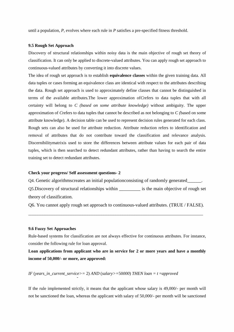
until a population, P, evolves where each rule in P satisfies a pre-specified fitness threshold.

9.5 Rough Set Approach

Discovery of structural relationships within noisy data is the main objective of rough set theory of

classification. It can only be applied to discrete-valued attributes. You can apply rough set approach to

continuous-valued attributes by converting it into discrete values.

The idea of rough set approach is to establish equivalence classes within the given training data. All

data tuples or cases forming an equivalence class are identical with respect to the attributes describing

the data. Rough set approach is used to approximately define classes that cannot be distinguished in

terms of the available attributes.The lower approximation ofCrefers to data tuples that with all

certainty will belong to C (based on some attribute knowledge) without ambiguity. The upper

approximation of Crefers to data tuples that cannot be described as not belonging to C (based on some

attribute knowledge). A decision table can be used to represent decision rules generated for each class.

Rough sets can also be used for attribute reduction. Attribute reduction refers to identification and

removal of attributes that do not contribute toward the classification and relevance analysis.

Discernibilitymatrixis used to store the differences between attribute values for each pair of data

tuples, which is then searched to detect redundant attributes, rather than having to search the entire

training set to detect redundant attributes.


Q4. Genetic algorithmscreates an initial populationconsisting of randomly generated______.

Q5.Discovery of structural relationships within _________ is the main objective of rough set

theory of classification.

Q6. You cannot apply rough set approach to continuous-valued attributes. (TRUE / FALSE).

__________________________________________________________________________

9.6 Fuzzy Set Approaches

Rule-based systems for classification are not always effective for continuous attributes. For instance,

consider the following rule for loan approval.

Loan applications from applicant who are in service for 2 or more years and have a monthly

income of 50,000/- or more, are approved:

IF (years_in_current_service>= 2) AND (salary>=50000) THEN loan = t =approved

If the rule implemented strictly, it means that the applicant whose salary is 49,000/- per month will

not be sanctioned the loan, whereas the applicant with salary of 50,000/- per month will be sanctioned

the loan, no matter even if his/her years in service are much lesser than the first applicant. It is unfair

and lacks sensibility.

It will be better to discretize salary into categories such as {low_salary, medium_salary, high_salary

}, and then let “fuzzy” thresholds or boundaries to be defined for each category.Fuzzy logic uses truth

values between 0:0 and 1:0, instead of exact cutoff between categorise to represent the degree of

membership a given value has in a given category. A fuzzy set is then used to represent each category.

How does the fuzzy logic, then makes out for 49,000/- per month? The fuzzy logic states that salary

of 49,000/- per month is more or less, high, even though it is not as high as 50,000/-. It provides a

graphical tool that helps in converting attribute values to fuzzy truth values.

Fuzzy set theory is also called possibility theory. It lets you work at a high level of abstraction and

offers a means for dealing with inexact measurement of data. What is inexact? For example, if

50,000/- is high, what about 49,000/-? It surely cannot be medium. In fuzzy set theory, elements may

belong to more than one fuzzy set. If you take the same example again, 49,000/- may belong to

medium and high fuzzy sets. Consider the following fuzzy set notion:

mmedium_salary(49000) =0:20 and mhigh_salary(49000) =0:90,

Wheremis a membership function operating on the fuzzy sets of medium_salary andhigh_salary,

respectively. In fuzzy set theory,

Fuzzy set theory is particularly useful for rule-based classification task. It is possible to provide

operations for combining fuzzy measurements. For example, fuzzy sets for salary can be combined

with fuzzy sets junior_employee and senior_employee for the attribute years_in_current_service.

More than 1 fuzzy rule may be applied to classify a tuple. Each applicable rule

contributesavoteformembership in thecategories. A number of methods exist for translating the

resulting fuzzy output into a defuzzified value that is returned by the system.

9.7 Classification by Backpropagation

It is an example of neural network learning algorithm. Neural networkis a set of connected

input/output units, and each connection has a weightassociated to it. Neural network learns by

adjusting the value of the weights. It does so to predict the correct class label of the input tuples.

Neural networks are highly tolerant to noisy data. Also the neural networks are good at classifying the

patterns on which they are trained, also known as unseen patterns. Neural networks are best or

continuous-valued inputs and outputs. Some of the applications of neural networks are character

recognition, robot designing etc. Amongst many of the neural network algorithms, it is themost

popular neural network algorithm. Backpropagation algorithm can be implemented on multilayer

feed-forward networks,

A multilayer feed-forward neural network consists of an input layer, hiddenlayers, and an output

layer.

Figure 9.1 Multilayer feed-forward neural network

Multilayer feed-forward neural network may consist of number of multiple hidden layers. Each layer

in multilayer feed-forward neural network is made up of units. Attributes for each training tuple forms

the inputs to the network. Input units are then weighted and fed to first hidden layer. Output from a

hidden layer units are passed to second hidden layer, and soon. The last hidden layer passes the

weighted outputs to outputlayerthat produces the prediction of the class label for given tuples. Input

layer units are called input units, hidden layer and output layer units are called neurodes.

Figure 9.2: A multilayer feed-forward neural network with weights.

Multilayer feed forward is also fully connected, as output of each unit at one layer provides input to

each unit in the next forward layer.

Each unit accepts as input, a weighted sum of outputs from all units in the previous layer.A nonlinear

(activation) function is then applied to the weighted input. Multilayer feed-forward networks should

be supplied large hidden units and large training samples, so it can closely approximate any function.

Backpropagation processing adata set of training tuples iteratively, comparing the prediction made by

the network for each tuple with the actual known target value. The target value can either be known

class label or continuous value. The weights for each training tuple are modified to minimize the

mean squared error between the network’s prediction and the actual target value. These modifications

are made in the “backwards” direction. The steps in the algorithm are expressed in terms of inputs,

outputs, and errors.


Q7. Fuzzy set approach to classification is better than rule-based classification. (TRUE/

FALSE).

__________________________________________________________________________

Q8. Neural networks are highly tolerant to noisy data. (TRUE / FALSE).

__________________________________________________________________________

Algorithm: Backpropagation.

1. Initialize the weighted links. Typically the weights are initialized to a small random number.

2. Then, for each training example in the testing set:

Input the training data to the input nodes, then calculate Ok, which is the output of node k. This is

done for each node in the hidden layer(s) and output layer.

3. Then calculate δk for the each output node, wheretkis the targetof the node:

δk←Ok(1 – Ok)(tk– Ok)

4. Now calculate δk for the each hidden node,

δk←Ok(1 – Ok) ∑wh,k • δk

5. Finally adjust weights of all the links, where xiis the activation and ηis the learning rate:

Wi,j← Wi,j+ ηδjxi

Neural network is trained at many iterations of the training set to find an acceptable

approximation of the function it is being trained on.

9.8 Summary

The k-nearest-neighbor classifierworks by searching entirepattern space for the k training tuples that

are closest to a given unknown tuple. The k training tuples that are closest to the given unknown tuple

are called k “nearest neighbors” of the unknown tuple. Database containing solutions to various

problems is used by CBR classifier to solvenew problems. For every new case, CBR classifier first

searches for a matching training case. Solution ofatraining case is returnedif it found to be identical to

the new case. Customer service help desks, answers to frequently asked questions, are popular

examples of CBR classifiers.CBR is also used in medical education. Genetic algorithmsis based on

natural evolution. It works as follows. You need to create an initial populationconsisting of randomly

generated rules. String of bits are used to represent each rule. Then a new population is formed that

consists of fittestalong with the offspring of these rules. The crossover and mutation, two genetic

operators are used to create the offspring. In crossover, Swapping of substrings from a given pairs of

rules to form new pairs of rules is called crossover, whereas mutation refers to randomly selected bits

in a rule’s string are inverted. Discovery of structural relationships within noisy data is the main

objective of rough set theory of classification. It can only be applied to discrete-valued attributes. You

can apply rough set approach to continuous-valued attributes by converting it into discrete values. The

idea of rough set approach is to establish equivalence classes within the given training data. Rough

set approach is used to approximately define classes that cannot be distinguished in terms of the

available attributes. Neural networks are highly tolerant to noisy data. Also the neural networks are

good at classifying the patterns on which they are trained, also known as unseen patterns. Neural

networks are best or continuous-valued inputs and outputs. Some of the applications of neural

networks are character recognition, robot designing etc.

9.9 Glossary

Classification- Classification is also known as supervised learning. Classification is used to predict

categorical labels. The classification algorithm builds a model by learning from the training set.

Rough set approach- Rough set approach is used to approximately define classes that cannot be

distinguished in terms of the available attributes.

Multilayer feed-forward neural network- In it the output from a previous layer is fed as input to the

next layer and output from one layer is not connected back to itself or some previous layer.

Fuzzy set- It refers to a thresholds or boundaries defined for discretize values for an attribute. For

example, salary can categorized into fuzzy set {low_salary, medium_salary, high_salary}

Rough set approach- Rough set approach is used to approximately define classes that cannot be

distinguished in terms of the available attributes.


1. b.

2. Database

3. c.

4. Rules

5. Noisy data

6. FALSE.

7. TRUE.

8. TRUE.







Publisher Pearson."


1. What is a multilayer feed-forward neural network?

2. Write the backpropagation algorithm for classification.

3. Explain the process of genetic algorithm.

4. How fuzzy set approach is better than rule-based classification. Give an example.

5. Explain k-nearest-neighbor approach to classification.

Lesson- 10 Prediction

Structure

10.0 Objective

10.1 Introduction

10.2 Prediction Model

10.3 Regression analysis

10.3.1 Linear regression

10.3.2 Nonlinear Regression

10.4 Summary

10.5 Glossary




10.0 Objective

After studying this lesson, students will be able to:

1. Define the prediction model of data mining

2. Discuss the use of regression analysis in prediction model.

3. Describe the two types of regression analysis.

4. Explain the need to study the predictors or classifiers accuracy

10.1 Introduction

Classification is used to classify the data into predefined classes based on some categorical data. In

this lesson you will study another data mining technique called prediction used to predict continuous

values for a given input. Prediction is a very popular tool of data mining and is used mainly in retail

chains to predict the buying patterns of customers over a period of time. In this lesson regression

analysis as a tool of prediction is discussed. Linear and Non-linear regression techniques are discussed

with the help of suitable examples. In the end, the lesson discusses the need to study the accuracy of

these prediction tools. Ultimately the benefit of using any prediction tools greatly depends upon the

accuracy of such tools.

10.2 Prediction Model

In the last lesson you studied classification task of data mining and decision tree as a tool to classify

data. Classification using decision tree is used to classify categorical data that defines data ranges.

Predicting continuous values for a given set of input is called numeric prediction. Suppose that

marketing manager of any retail shop wants to predict purchasing that will be done by a particular

customer during a sale at his/ her shop. It is a perfect example of numeric prediction. Such a model is

called a predictor. The most popular and widely used approach to numeric prediction is a statistical

methodology called regression. Some classification techniques can also be customized for numeric

prediction such as, back propagation, k-nearest-neighbor classifiers, or support vector machines.

The attribute is referred to as the predicted attribute rather than calling it class label attribute. For

example, instead of predicting if it would be safe to sanction a loan to particular customer, rather the

numerical prediction model is used to predict the amount that is considered to be safe for advancing to

a particular customer by the bank. Whereas the classification model is more concerned with labeling

the attributes to some pre-defined categorical classes. Simply change class label attribute

(loan_decision) that is used to classify if it is safe to advance the loan with continuous-valued

attribute (loan_amount) that is used to predict the amount considered safe for advancing.

Prediction may be defined as a function, y= f (X), where X refers to the input and y refers to the output

which is acontinuous valued attribute. In other words you predict the value of y in respect to input

value X. For example, details of loan applicant can be input to prediction model and loan amount can

be output of that model. Rather than using a separate test set to evaluate the accuracy for a classifier,

accuracy for a predictor is easy to compute. You can define error as the difference between the value

predicted by the model and the known value for that output variable y.

10.3 Regression analysis

Regression analysis is a statistical technique used for predicting relationships among variables for

each tuple. The variables under consideration are called independent and dependent variables.

Regression analysis is used to study the relationship between the dependant and independent

variables. Regression analysis shows the change in the value of dependent variable in respect to

change in the value of independent variable keeping value of all other variables fixed. The prediction

target is a function of independent variables called the regression function.

The output variable is also known as response variable. Predictor variables (class labels in classifiers)

are the attributes of interest that describe the tuple. Prediction for the value of response variable is

done in respect to the value of known predictor variables.

Regression analysis does well when all predictor variables are also continuous-valued or ordered.

Most of data mining problems can be solved using linear regression, and most of nonlinear problems

can also be transformed and converted to a linear one.


Q1. What is the difference between classification and prediction?

___________________________________________________________________________

__________________________________________________________________________

____________________________________________________________________________

Q2. Define regression analysis.

___________________________________________________________________________

__________________________________________________________________________

____________________________________________________________________________

Q3. Regression analysis does well when all predictor variables are _________________ or

_________.

10.3.1 Linear regression

Linear regression develops a linear equation that explains the relationship between 2 variables for

some data set D. Of the two variables, one is called the predictor variable whose value is known and

the other is called response variable whose value is to be predicted. You can construct a regression

model for fitness, i.e. to predict the weight of based on the height of an individual. You often find

such data in hospitals or gyms. Height in this example is predictor variable and weight is response

variable and both are continuous ordered variables. It is extremely important to determine if there

exists a relationship between two variables of interest before you attempt to fit a linear model to

observed data set D. A tool called scatterplot is used to determine the relationship strength between

two variables.

A linear regression line can be specified as Y = a + bX,

Where X refers to an independent variable and Y refers to a dependent variable. Both b and a are

called regression coefficients, b refers to the slope the regression line and a refers to intercept or value

of y when x = 0.

Figure 10.1: Regression line

Least-squares method is a simple technique for fitting a regression line. It minimizes the sum of

squares of vertical deviations from each data point to the regression line. Vertical deviations are also

called errors. The vertical deviation for a point that lies exactly on the fitted line is 0.

http://www.stat.yale.edu/Courses/1997-98/101/scatter.htm

Figure 10.2: Regression line using Least-Squares method.

Least-squares method tries to best fit the data set by adjusting the regression coefficients a and b of a

model function. A data set D or n data pairs , for i = 1, 2 ..., n. The model function has the

form , where m adjustable parameters are held in the vector , and it tries to find the

parameter values that "best" fits the data. The least squares method results in the best fit when the sum

(s), of squared deviations is minimum.

Deviation or residual is defined as the error or the difference between the actual value of

dependant (response) variable and the predicted value for the same.

.

You can compute the value for regression coefficients (a and b) to find the line of best fit

“graphically” by using curve-fitting program, e.g. Excel’s Trendline. Excel in essence calculates a and

b using these formulae:

refers to mean of x values and refers to mean of y values, and point ( ; ) always lies on the

line of best fit. In other words, y’ = ax + b, where y’ is the average of yi’s and x is the average of xi’s.

Let us consider the following example,

Compute the best fit equation:

X 8 2 11 6 5 4 12 9 6 1

Y 3 10 3 6 8 12 1 4 9 14

Calculate the means of the x-values and the y-values.

= ( 8 + 2 + 11 + 6 + 5 + 4 + 12 + 9 + 6 + 1 ) / 10 = 6.4

= ( 3 + 10 + 3 + 6 + 8 + 12 + 1 + 4 + 9 + 14 ) / 10 = 7

Now calculate , , , and for each i.

i xi yi xi - yi - (xi - ) (yi - ) (xi - )2

1 8 3 1.6 -4 - 6.4 2.56

2 2 10 - 4.4 4 - 13.2 19.36

3 11 3 4.6 -4 - 18.4 21.16

4 6 6 - 0.4 -4 0.4 0.16

5 5 8 - 1.4 1 - 1.4 1.96

6 4 12 - 2.4 5 - 12 5.76

7 12 1 5.6 - 6 - 33.6 31.36

8 9 4 2.6 - 3 - 7.8 6.76

9 6 9 - 0.4 2 - 0.8 0.16

10 1 14 - 5.4 7 - 37.8 29.16

Calculate the slope.

Calculate the y-intercept.

Use the formula to compute the y-intercept.

Use the slope and y-intercept to form the equation of the line of best fit.

The slope of the line is –1.1 and the y -intercept is 14.0.

Therefore, the equation is y = –1.1 x + 14.0.

Draw the line on the scatter plot.

Figure 10.3: regression line. http://hotmath.com/hotmath_help/topics/line-of-best-fit.html


Q4.Define linear regression.

___________________________________________________________________________

__________________________________________________________________________

____________________________________________________________________________

Q5. A tool called ______________ is used to determine the relationship strength between two

variables.

Q6.Define linear regression line.

___________________________________________________________________________

__________________________________________________________________________

____________________________________________________________________________

Q7. Classification is used to classify:

a. Continuous valued variables.

b. Categorical valued variables.

c. Both a and b.

d. None of the above.

Q8. Which method is widely used for linear regression?

a. Best square

b. Least square

c. Most square.

d. None of the above.

10.3.2 Nonlinear Regression

The linear regression is used to fit a straight line to a set of data points. The response variable, y in

case of linear regression is modeled as a linear function of a single predictor variable, x.The best or

most accurate relationship is not always straight, but a curved one. To represent a curved relationship

between two variables, you can use nonlinear regression. For example, if the growth in dependent

variable is exponential to independent variable, the relationship between the two is a curve. Non-

linear regression is best suited when the relationship between response variable and predictor

variable may be modeled using a polynomial function. You can make linear least-squares method

adapts to it. The method creates new variables that are nonlinear functions of variables in your data.

New variables or data points results in a curved function of the original variables.

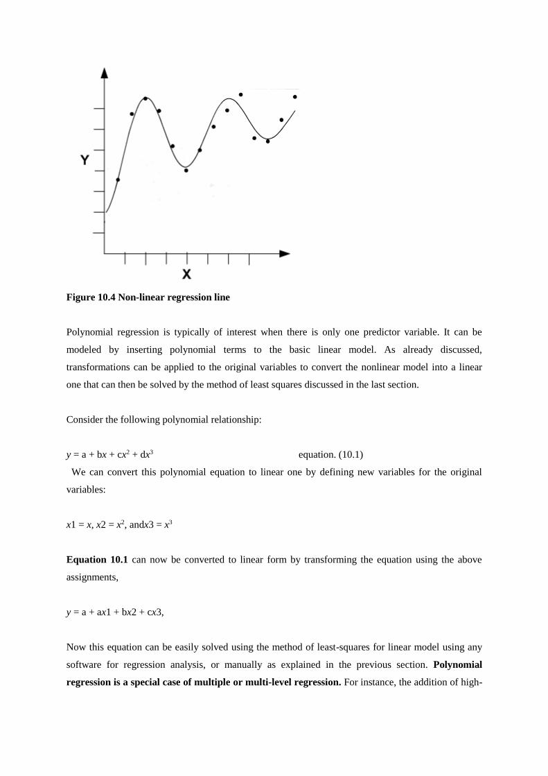
Figure 10.4 Non-linear regression line

Polynomial regression is typically of interest when there is only one predictor variable. It can be

modeled by inserting polynomial terms to the basic linear model. As already discussed,

transformations can be applied to the original variables to convert the nonlinear model into a linear

one that can then be solved by the method of least squares discussed in the last section.

Consider the following polynomial relationship:

y = a + bx + cx2 + dx3 equation. (10.1)

We can convert this polynomial equation to linear one by defining new variables for the original

variables:

x1 = x, x2 = x2, andx3 = x3

Equation 10.1 can now be converted to linear form by transforming the equation using the above

assignments,

y = a + ax1 + bx2 + cx3,

Now this equation can be easily solved using the method of least-squares for linear model using any

software for regression analysis, or manually as explained in the previous section. Polynomial

regression is a special case of multiple or multi-level regression. For instance, the addition of high-

order variables x2, x3, and so on, are simple functions of the single variable x, and can be considered

equivalent to adding new independent variables.

Some nonlinear models are inflexible and cannot be converted into equivalent linear form. It is only

possible to obtain least square estimates through extensive calculations on more complex formulae.

Typically, a regression analysis is extremely accurate for prediction, except when the data contain

outliers. Having outliners is the problem with the data and not with the analysis technique. Outliers

are data points that are highly inconsistent as compared to remaining data.

Figure 10.5 outliners in data set.

Outlier detection is a topic that needs separate and special mention. But applying such technique to

detect and remove outliners, must take care that we don’t remove any meaningful data point from the

data set.


Q9. When you use nonlinear regression analysis? Also give an example.

___________________________________________________________________________

__________________________________________________________________________

____________________________________________________________________________

Q10. Some nonlinear models are __________________ and cannot be converted into equivalent

linear form.

Q11. What is an outlier?

___________________________________________________________________________

___________________________________________________________________________

Q12. Prediction accuracy using regression analysis suffers when the data contain____________.

10.4 Summary

Classification is used to classify the data into predefined classes based on some categorical

data.Classification using decision tree is used to classify categorical data that defines data ranges.

Predicting continuous values for a given set of input is called numeric prediction. The most popular

and widely used approach to numeric prediction is a statistical methodology called regression.

Prediction may be defined as a function, y= f (X), where X refers to the input and y refers to the output

which is acontinuous valued attribute. Regression analysis is a statistical technique used for predicting

relationships among variables for each tuple. Regression analysis does well when all predictor

variables are also continuous-valued or ordered. Linear regression develops a linear equation that

explains the relationship between 2 variables for some data set D. A linear regression line can be

specified as Y = a + bX, where X refers to an independent variable and Y refers to a dependent

variable. Both b and a are called regression coefficients, b refers to the slope the regression line and

a refers to intercept or value of y when x = 0. To represent a curved relationship between two

variables, you can use nonlinear regression. Non-linear regression is best suited when the relationship

between response variable and predictor variable may be modeled using a polynomial

function.Polynomial regression is a special case of multiple or multi-level regression.Some nonlinear

models are inflexible and cannot be converted into equivalent linear form.Typically, a regression

analysis is extremely accurate for prediction, except when the data contain outliers.Outliers are data

points that are highly inconsistent as compared to remaining data.

10.5 Glossary

Prediction- Model used to predict continuous or ordered values for a given set of input.

Regression analysis - Statistical technique used for predicting relationships between the dependant

and independent variables.

Scatterplot- A tool used to determine the relationship strength between two variables.

Outlier- Outlier is a data point that is highly inconsistent as compared to remaining data points.

Classification- Classification is used to classify the data into predefined classes based on some

categorical data.

Scatterplot- Scatterplot is a tool used to determine the relationship strength between two variables.

Least square method- It is a simple technique for fitting a regression line. It minimizes the sum of

squares of vertical deviations from each data point to the regression line.




1. Classification is used to classify data into predefined categorical classes, whereas numeric

prediction model is used to predict continuous values for a given set of input.

2. Regression analysis is a statistical technique used for predicting relationships between the

dependant and independent variables. Regression analysis shows the change in the value of dependent

variable in respect to change in the value of independent variable keeping value of all other variables

fixed.

3. continuous-valued, ordered.

4. Linear regression develops a linear equation that explains the relationship between 2 variables for

some data set D. Of the two variables, one is called the predictor variable whose value is known and

the other is called response variable whose value is to be predicted.

5. Scatterplot.

6. A linear regression line can be specified as Y = a + bX, where X refers to an independent variable

and Y refers to a dependent variable. Both b and a are called regression coefficients, b refers to the

slope the regression line and a refers to intercept or value of y when x = 0.

7. c.

8. b.

9. Sometimes the best line fit is not the straight line, but a curved one. A curved relationship between

two variables can be represented using nonlinear regression. For example, if the growth in dependent

variable is exponential to independent variable, the relationship between the two is a curve.

10. Inflexible.

11. Outliers are data points that are highly inconsistent as compared to remaining data.

12. Outliers.



Publishers




4. Data Warehousing, Data Mining, & Olap by Alex Berson and Stephen J smith, Tata McGraw-Hill

Education.

5. Data Mining and Data Warehousing by Bharat Bhushan Agarwal and Sumit Prakash Tayal,

University Science Press.

6. Data Mining: Technologies, Techniques, tools and Trends by Bhavani Thuraisingham.



1. Define numeric prediction model.

2. Define linear regression.

3. Why do we need nonlinear regression?

4. Give an example of outlier.

5. Can you always convert a nonlinear model into equivalent linear form?

6. Explain least square method.

Lesson- 11 Introduction to clustering

Structure

11.0 Objective

11.1 Introduction

11.2 Clustering

11.3 Cluster Types

11.4 Types of Data in Cluster Analysis

11.4.1 Interval-Scaled Variables

11.4.2 Binary Variables

11.4.3 Categorical Variables

11.4.4 Ordinal Variables

11.4.5 Ratio-Scaled Variables

11.5 Summary

11.6 Glossary




11.0 Objective


1. Define the concept of clustering.

2. Differentiate between clustering and classification.

3. Describe various cluster types.

4. Explain different type of data used in cluster analysis.

11.1 Introduction

Clustering is another important type of analysis method used in data mining. It is widely in data

mining applications. Some of the applications where clustering is used include market research,

pattern recognition, data analysis, and image processing, biology, processing of documents on web,

etc. The next two lessons focus on what you mean by clustering and various techniques to clustering.

11.2 Clustering

Cluster analysis is used to group together objects based their relationships. It results into clear

separation of objects that are not similar to each other. Clustering comes under undirected data

mining. The process of undirected data mining is both different and similar to the process for directed

data mining. Both directed and undirected mining works with applications that require exploration

and understanding of the data. Both techniques are improved by including intelligent variables into

the data that identify different aspects of the business. Undirected data mining differs from data

mining by not having a target variable, and it poses following challenges:

As there is no target variable, the human interpretation is very important. Hence, the process

of undirected data mining cannot be fully automated.

The measures for clustering are more qualitative than the ones associated with directed

techniques. There are no simple statistical measures such as the CCR or the R2 value for summarizing

the goodness of the results. Instead, undirected mining uses descriptive statistics and visualization for

summarizing the results.

Clustering is different from classification in the sense that clustering leads to classification.

Classification is preferred when the classes are pre-defined or known in advance, where as in

clustering, we derive classes on the basis of similarity between objects. Objects in one class are

dissimilar to the objects in another class.

Some of the applications or uses of clustering technique in data mining are as follows:

1. Clustering is used widely in applications such as market research. Understanding the

customer behaviour in order to improve the customer base and provide better facilities are the prime

objectives. Sometimes it is even used to study the time patters at which there is great amount of rush

as compared to other time slots.

2. Clustering is also used to find the similar patterns or more popularly known as pattern

recognition. Being able to identify patterns and make scientific reasoning for the same helps in better

decision making.

3. Clustering is also useful in classification of documents on the web. It is particularly useful in

designing of search engines and search engine optimization.

4. Clustering is frequently used by the bankers to identify clusters that are most likely to be

fraudulent. It is particularly useful in case of predicting credit card frauds.

5. Clustering in data mining acts as a tool to gain insight into the distribution of data to observe

characteristics of each cluster.

Initially the data points or objects in the database belong to one cluster. Or you can say that they all

are one, but still don't have any similarities. The initial data points can be viewed as:

As you can see in the figure above, all data points are shown using the same symbol. Already, a

simple look at these points is enough to identify the similarities and the dissimilarities between the

data points.

The most basic type of clustering would be to divide the data points into two clusters. One consisting

of all data points on the left side and the other consisting of all data points on the right side.

Last figure shows data points as members of two clusters. Again, as sub-cluster can be further divided

into sub-clusters on the basic of similarity or relationship among the data points. As you can see, that

both the left and right clusters can be further divided into 2 clusters each. Four data points on the

lower side of cluster on left side and four data points on the upper side of cluster on right side are

dissimilar to other data points in the same cluster and hence can be assigned to a separate cluster as

shown in the figure below,

Careful analysis of the clusters in the figure above can lead to formation of 2 more clusters. 2 clusters,

one on the left and other on the right consisting of 8 data points each can be divided into 2 clusters

each as shown in the figure below:

Observe the figure above, it is not just the shape of data elements, but also the density or difference

with other data points in same cluster and other clusters that makes the clusters feel quite obvious.

The definition of a cluster or how well we can divide a given data set into clusters, not only depend

upon the clustering algorithm, but also on the fact that how well the data points are related or

unrelated to each other. Once the data points have been partitioned into groups or clusters based on

data

Assign of labels to newly formed clusters is the next step. It is far better and less expensive technique

as compared to the classification technique. Also, the clustering technique is much more adaptive to

changes.


Q1. What is the difference between classification and clustering?

____________________________________________________________________

____________________________________________________________________

Q2. Clustering is an example of directed data mining. (TRUE / FALSE ).

____________________________________________________________________

____________________________________________________________________

Q3. Clustering is used in the field of pattern recognition. (TRUE / FALSE ).

____________________________________________________________________

11.3 Cluster Types

1. Well-Separated Cluster: It consists of objects or set of points such that, one object or point in a

cluster is nearer to other objects in the same cluster as compared to any other object from other

clusters.

2. Center-based Cluster: In this type of clustering method, a set of randomly selected points or

objects are considered to be the center of each cluster. Each point is assigned to the cluster whose

center is closest to that point as compared to the center of other clusters.

3. Nearest-neighbour based Cluster: A cluster in which each point is similar to at least one other

point in the same cluster and it allows a point to be close to a minimum of one point in the same

cluster.

4. Density-based Cluster: A density base cluster is one in which all clusters with dense regions of

points are separated by low-density point. This definition is used when the data points are highly

inconsistent and there exist a number of outliners. So a well-separated cluster cannot be defined for it.

11.4 Types of Data in Cluster Analysis

Now it is time to study the types of data used in cluster analysis and how it is used for analysis. Data

to be clustered may represent income, sales, documents, countries, and so on. Typical clustering

algorithms operate on either of the following two data types.


Q4. A ______________________ consists of objects where one object in a cluster is nearer to other

objects in the same cluster as compared to any other object from other clusters.

Q5. A density based cluster is one in which each point is similar to at least one other point in the same

cluster. (TRUE / FALSE ).

____________________________________________________________________

11.4.1 Interval-Scaled Variables

Interval-scaled variables refer to continuous measurements of a roughly linear scale. Some of the

examples of interval-scales variables are height and weight, latitude and longitude coordinates, marks,

etc. Change in measurement unit can affect the results of clustering analysis. For instance, changing

measurement units from absolute marks to grades, or from Celsius to Fahrenheit for temperature, may

lead to a very different clustering structure. Changing to smaller units generally lead to a larger range

of values for that variable, and thus a larger effect on the resulting clustering structure.

Standardization is used to avoid dependence on the choice of measurement units. It attempts to give

all variables an equal weight. Sometimes there may be a need to give more weight to a certain set of

variables as compared to others. For example, if you are selecting players for spot number 5 and 6 in

20-20 cricket, you may prefer to give more weight to the strike rate than the average of the batsman.

How do you achieve standardization for a variable?The idea is to convert the original

measurements to unit-less variables. Given measurements for a variable f, this can be performed as

follows.

1. Calculate the mean absolute deviation,sf:

(11.1)

Where x1f , …, xn f are n measurements of f, and mf is the mean value of f, i.e.

2. Calculate the standardized measurement, or z-score:

(11.2)

The mean absolute deviation, sf, handles outliers much better than the standard deviation, σf. For mean

absolute deviation, the deviations from the mean (i.e., |xi f -mf |) are not squared. It helps to reduce the

effect of outliers. Advantage of mean absolute deviation over other measures is that the z-scores of

outliers do not become too small and the outliers remain detectable.

Standardization is not useful for all application types and the choice of standardization should be left

to the user, i.e. whether to implement it or not. Standardization is also known as normalization.

Dissimilarity or similarity between the objects described by interval-scaled variables is computed

based on the distance between each pair of objects. One example for distance measure is Euclidean

distance, which is defined as

(11.3)

Where i = (xi1, xi2, …., xin) and j = (xj1, xj2, …, xjn) are two n-dimensional data objects.

Euclidean distance satisfies the following mathematic requirements of a distance function:

1. d(i, j) >= 0: Which means the distance is a nonnegative number.

2. d(i,i) = 0: Which means the distance of an object to itself is 0.

3. d(i, j) = d( j,i): Which means the distance is a symmetric function.

4. d(i, j)<= d(i, h) + d(h, j): Triangular inequality.

11.4.2 Binary Variables

A binary variable is used to represent two constant states: 0 or 1, where 0 means absent, and 1 means

present. For example, given a variable married, 1 means that the person is married and 0 means the

person is not married. Binary variables cannot be treated as interval-scaled variables as it can lead to

misleading clustering results.

Computing the dissimilarity using binary variables involve computing a dissimilarity matrix from the

given binary data. A 2-by-2 contingency table can be used to represent the dissimilarity matrix, where

q refers to the number of variables = 1 for both i and j, r refers to the number of variables = 1 for i and

0 for j, s refers to the number of variables = 0 for i and 1 for j, and t refers to the number of variables

= 0 for both objects i and j. The total number of variables is p, where p = q + r + s +t.

A binary variable is symmetric if both of its states are equally valuable and carry the same weight.

For example, gender variable during registration is a symmetric binary variable. Dissimilarity that is

based on symmetric binary variables is called symmetric binary dissimilarity. Its dissimilarity can be

used to assess the dissimilarity between objects i and j.

(11.4)

A binary variable is asymmetric if the outcomes of the two states are not equally important, such as

the positive and negative outcomes of a disease test. You should code the most important outcome,

which is usually the rarest one. For example 1 means the test is positive and 0 means the test is

negative. For two asymmetric binary variables, the agreement of two 1s (a positive match) is then

considered more significant than that of two 0s (a negative match). The dissimilarity based on such

variables is called asymmetric binary dissimilarity, where the number of negative matches, t, is

considered unimportant and thus is ignored in the computation,

(11.5)


Q6. List some of the examples of interval-scaled variables.

____________________________________________________________________

____________________________________________________________________

Q7. _____________ is used to avoid dependence on the choice of measurement units in case of

interval-scaled variables.

Q8. Distance between each pair of objects can be computed using a distance measure

called__________________.

Q9. Which of the following is a type of cluster?

a. Well-separated cluster

b. Centre based cluster

c. Density based cluster

d. All the above

Q10. Which type of variable refers to continuous measurements of a roughly linear scale?

a. Categorical variable

b. Ordinal variable

c. Inter scaled variable

d. Binary variable

11.4.3 Categorical Variables

Categorical variable is also known as nominal variable and it is a generalization of the binary variable

as it can take on more than two states. For example, grade variable can be used to represent states

like A, B, C, D and F.

Let M be the number of states for a categorical variable. Letters, symbols, or integers can be used to

represent the states. The dissimilarity between two objects using categorical variables can be

computed based on the ratio of mismatches:

(11.6)

Where i and j refer to 2 objects, m represents the number of matches and p represents the total number

of variables. A match means that objects i and j represent same state for a variable. Weights are used

to increase the effect of m or to assign greater weight to the matches in variables with larger number

of states.

11.4.4 Ordinal Variables

An ordinal variable is similar to a categorical variable, except that the M states of ordinal value are

ordered in a sequence. For example, designations can be represented using sequential order, such as

Registrar, Deputy Registrar, Assistant Registrar, etc. A continuous ordinal variableis like a set of

continuous data of an unknown scale. Ordinal variables can also be obtained by performing

discretization of interval-scaled quantities by splitting the value range into a finite number of classes.

The values of an ordinal variable can be mapped to ranks.

Computing the dissimilarity between objects for ordinal variables is similar to that of interval-scaled

variables. The computation of dissimilarity with respect to variable finvolves:

1. The value of f for the ith object is xi f, and f has Mf ordered states, representing the ranking 1, …, Mf.

2. Map the range of each variable onto [0.0,1.0] so that each variable has equal weight. It can be

achieved by replacing the value of ri f by:

(11.7)

3. Compute the dissimilarity using the Euclidean distance measure for interval-scaled variables,

using zi f to represent the f value for the ith object.

11.4.5 Ratio-Scaled Variables

A ratio-scaled variable makes a positive measurement on a nonlinear scale, such as an exponential

scale, approximately following the formula:

PeQt or Pe-Qt

(11.8)

Where P and Q are positive constants, and t represents time. Some of the examples can be decay of

deadly virus like EBOALA or the growth of a bacteria population

Computation of dissimilarity between objects for ratio-scaled variables can be achieved using wither

of the three methods:

Treat ratio-scaled variables like interval-scaled variables.

With the help of logarithmic transformation to a ratio-scaled variable f having value xi f for

object i by using the formula yif = log(xif). The yif values can be treated as interval-values.

Treat xi f as continuous ordinal data and treat their ranks as interval-valued.

11.5 Summary

Cluster analysis is used to group together objects based their relationships. Clustering comes under

undirected data mining. Classification is preferred when the classes are pre-defined or known in

advance, where as in clustering, we derive classes on the basis of similarity between objects. Some of

the applications where clustering is used include market research, pattern recognition, data analysis,

and image processing, biology, processing of documents on web, etc. some of cluster types include

well separated clusters, center based clusters. Nearest neighbour based clusters, density based clusters,

etc. Interval-scaled variables refer to continuous measurements of a roughly linear scale. Some of the

examples of interval-scales variables are height and weight, latitude and longitude coordinates, marks,

etc. A binary variable is used to represent two constant states: 0 or 1, where 0 means absent, and 1

means present. Computing the dissimilarity using binary variables involve computing a dissimilarity

matrix from the given binary data. Categorical variable is also known as nominal variable and it is

ageneralization of the binary variable as it can take on more than two states. An ordinal variable is

similar to a categorical variable, except that the M states of ordinal value are ordered in a sequence. A

ratio-scaled variable makes a positive measurement on a nonlinear scale, such as an exponential scale.

11.6 Glossary

Clustering- Clustering is used to group together objects based on the intra-cluster similarities and

inter-cluster dissimilarities between the objects.

Classification- It refers to assignment of objects to one of the pre-defined classes.

Standardization- Also known as normalization is used to avoid dependence on the choice of

measurement units in case of interval-scaled variables.

Euclidean distance- It refers to a distance measure andis used to compute the distance between each

pair of objects.


1. Classification is preferred when the classes are pre-defined or known in advance, where as in

clustering is used to derive classes on the basis of similarity between objects.

2. FALSE.

3. TRUE.

4. Well-Separated Cluster.

5. FALSE.

6. Some of the examples of interval-scales variables are height and weight, latitude and longitude

coordinates, marks, etc.

7. Standardization.

8. Euclidean distance.

9. d.

10. c.







Publisher Pearson.


1. Explain different cluster types along with figures.

2. Define cluster and list some of the applications of clusters.

3. What is the difference between clustering and classification?

4. Define standardization.

5. What are categorical or nominal variables? How can you compute the dissimilarity between objects

using categorical variables?

Lesson- 12 Clustering Methods

Structure

12.0 Objective

12.1 Introduction

12.2 Partitioned Clustering

12.2.1 K-means clustering

12.2.2 K-medoid clustering

12.3 Hierarchical clustering

12.3.1 Agglomerative clustering

12.4 Density-Based Methods

12.4.1 DBSCAN

12.5 Summary

12.6 Glossary




12.0 Objective


1. Explain different methods of clustering.

2. Describe k-mean and k-medoid partitioning methods of clustering.

3. Explain hierarchical methods of clustering called agglomerative clustering.

4. Discuss the density based clustering method called DBSCAN.

5. Write algorithms for all 3 types of clustering methods.

12.1 Introduction

Now that you are aware of what clustering is and types of data used in cluster analysis, in this lesson

you will learn the major clustering methods used in data mining. Clustering methods are based on

type of clustering approach followed. Major clustering methods are based on type of clustering used,

like partitioning based methods, hierarchical clustering methods and density based methods. The

lesson contains brief explanations for each of the methods along with the algorithms. I am sure you

will enjoy reading this lesson

12.2 Partitioned Clustering

Let us suppose you want to form k clusters for a given data set consisting of n data points or objects; a

partitioning algorithm arranges the data points into k partitions or less then K partitions in case, k >n).

One partition means one cluster. The partition clusters are formed on the basis of threshold value that

defines the similarity or dissimilarity between the data points of one cluster with data points of other

clusters, i.e. it classifies the data into k groups, which together satisfy the following requirements:

1. Each group must contain at least one object.

2. Each object must belong to exactly one group.

A partitioning method creates an initial k partitioning and with each iteration it attempts toimprove

the partitioning by moving objects from one group to another. Grouping of objects in name cluster is

based on how close or related the objects are to each other.

In this section we will discuss the most basic and most popular data partitioning technique based on

centroid of cluster called K-means clustering.

12.2.1 K-means clustering

K-mean clustering is based on the idea that a center (centroid) can represent a cluster. Centroid is

computed as a mean/ median of points within a cluster. Cluster similarity is measured in regard to the

mean value of the objects in a cluster, which can be viewed as the cluster’s centroid or center of

gravity. A centroid doesn’t need to correspond to an actual data point. New data points for each

cluster have high intra-cluster similarity and low inter-cluster similarity. The k-means algorithm

proceeds by randomly selectingk objects, each of which initially represents a cluster mean or center.

The remaining objectsare assigned to the cluster based on the shortest distance between the object and

the cluster mean. It then computes the new mean for each cluster.

For example, consider the following image with circles representing the data points and cross

representing two initial randomly chosen centroids.

Each data point should be assigned to the centroid that is nearest to it. The devision of the data points

can be better viewed as follows:

Visually it seems that it is not the best classifictation. Compute the average of data points in two

clusters and compute the new centroids for two clusters. The new clentroids are as follows:

The figure also shows the assignment of data points to the centroid nearest to each data point.

Recompute the two centroids again and assign the data points to each centroid. The final clustering or

classification will look like:

Why did I call it final classification. Because if you compte the mean of data points from both

clusters, the mean expected is same.

K-means Clustering Algorithm

1. Select any K points to form initial centroids.

2. Assign each data point to centroid nearest to it.

3. Re-compute mean centroid for all clusters using the data points for each cluster.

4. Jump to step 2, if there is a change in the centroids.

12.2.2 K-medoid clustering

The k-means algorithm is prone to or sensitive to outliers as objects with extremely large value may

substantially distort the distribution of data. Instead of taking the mean value of the objects in a

cluster as a reference point, you may pick actual objects to represent the clusters. Each remaining

object is clustered with the representative object to which it is the most similar. The partitioning

method is then performed based on the principle of minimizing the sum of the dissimilarities between

each object and its corresponding reference point.In this section, you will learn an algorithm that

diminishes such sensitivity. Rather than considering the mean value of the data points as a centroid,

actual data point is picked to represent the cluster. The representative points for all clusters are called

medoids. The remaining non-selected data points are then clustered using representative data point to

which it is the most similar.

K-medoid Clustering Algorithm

1. K candidate points are initial selected as medoids that are expected to be the best central points for

a cluster.

2. Assign each non-selected data point to the medoid closest to it.

3. Distance of non-selected points from the closest candidate medoid is computed. Sum up the

computed distance over all points. The one with the lowest cost is selected as the new configuration.

If there is change between old and new configurations, jump to step 2.

4) End.

A change in the medoid leads to reassignment of data points. The data points may be reassigned to

new medoid, or to some other medoid with current minimum distance, or no reassignment at all. Let

us consider few cases of reassignment. DPj is the representative point or medoid to which point P is

currently assigned. Dpi is another medoid and DPrandom is the non-selected data point that will

replace DPj as representative point or medoid.

Initially DPj and DPi are two medoids, and a data point P which is closer to DPj and hence is assigned

to DPj. Now, if we replace the medoid DPj with DPrandom, the distance of P with Dpi is less than the

new medoid DPrandom, hence, the data point P will be reassigned to DPi.

In this case, the data point P after replacement is closer to new medoid DPrandom rather than old

medoid DPi, and hence will be assigned to DPrandom.

Initially in this case, the data point P is closer to DPi and is assigned to DPi. After replacement of DPj

with DP random, the data point P is closer to DPrandom instead of DPi. So it will be reassigned to

new medoid DPrandom instead of DPi.

There is one more case in which there will be no reassignment. I wish if the readers could

themselves draw that case.


Q1. Partitioning algorithm classifies the data into k groups that satisfies the following requirements:

___________________________________________________________________________

___________________________________________________________________________

Q2. In case of k-mean clustering, the centroid is computed as a ___________ of points within a

cluster.

Q3. Centroid in k-mean clustering corresponds to an actual data point.

a. TRUE

b. FALSE

Q4. What is the difference between k-mean and k-medoid clustering methods?

___________________________________________________________________________

___________________________________________________________________________

12.3 Hierarchical clustering

A hierarchical method creates a hierarchical decomposition ofthe given set of data objects. Data

points are grouped together into a tree like structure of clusters. The clusters of individual points at the

bottom of the tree structure are all-inclusive to cluster points at the top. There are two techniques to

form this cluster hierarchy known as agglomerative or divisive based on how the hierarchical

decomposition is formed.

a) Agglomerative: It is a bottom-up strategy that starts by taking data objects as atomic clusters. It

successively merges the objects or groups that are close to one another, until all of the groups are

merged into one (the topmost level of the hierarchy), or until a termination condition holds.

b) Divisive: It is a top-down strategy that starts by taking one all-inclusive cluster and all objects

belonging to the same cluster. In each successive iteration, a cluster is split up into smaller clusters,

until eventually each object is in one cluster, or until a termination condition holds.

Hierarchical method suffers in term of flexibility. Once a step (merge or split) is done, it can never be

undone. There are two approaches to improving the quality of hierarchical clustering:

(1) Perform careful analysis of object “linkages” at each hierarchical partitioning.

(2) Integrate hierarchical agglomeration and other approaches by first using a hierarchical

agglomerative algorithm to group objects into microclusters, and then performing macroclusteringon

the microclusters using another clustering method such as iterative relocation.

12.3.1 Agglomerative clustering

Initial data points or atomic clusters

Join the clusters with minimum distance, in this example the clusters with minimum distance are A

and B.

Then we proceed further to join clusters with minimum distance

We continue with this process until we reach single all-inclusive cluster.

Figure 12.1 Hierarchical view of this data clustering process

Agglomerative based Hierarchical Clustering Algorithm

1) Compute the proximity graph.

2) Merge 2 clusters with minimum distance.

3) Proximity matrix should be updated to replicate the proximity between newly formed cluster and

remaining clusters.

4) If more than one cluster remains, go to step 3.

The divisive strategy is absolutely the opposite of it, and you can achieve single atomic clusters by

just reversing the order that we discussed in the last example.

Divisive hierarchical clustering algorithm

1. Compute the proximity graph first and then the minimum spanning tree for the same.

2. Create a new cluster by removing the link corresponding to largest distance.

3. Jump to step 2 until a single atomic clusters remain.


Q5. In case of hierarchical clustering, data points are grouped together into a ________ like structure

of clusters.

Q6. Two techniques to form cluster hierarchy are known as ______________ and____________.

Q7. Agglomerative clustering is a top-down strategy that starts by taking one all-inclusive cluster and

all objects belonging to the same cluster.

a. TRUE

b. FALSE

12.4 Density-Based Methods

Density-based clustering methods are good to discovering clusters with arbitrary shapes. Density-

based clustering methods consider clusters as dense regions of objects in the data space that are

separated by regions of low density. DBSCAN is one popular method of clustering based on density.

It grows clusters according to a density-based connectivity analysis. OPTICS extends DBSCAN to

produce a cluster ordering obtained from a wide range of parameter settings.

12.4.1 DBSCAN

It stands for Density-Based Spatial Clustering of Applications with Noise and is a density-

based clustering algorithm. The algorithm is used to discover clusters of arbitrary shape in

spatial databases with noise by growing regions with sufficiently high density into clusters. A

cluster using DBSCAN may be defined as a maximal set of density-connected points.

Consider the following definitions:

The neighbourhood within a radius ε of a given object is called the ε-neighbourhood of the object.

The object is called a core objectif the ε-neighbourhood of an object contains at least a minimum

number, MinPts, of objects.

Density reachability is the transitive closure of direct density reachability, and this relationship is

asymmetric. Only core objects are mutually density reachable. Density connectivity, however, is a

symmetric relation.

Given a set of objects, D, we say that an object p is directly density-reachable from object q if p is

within the ε-neighbourhood of q, and q is a core object.

An object p is density-reachable from object q with respect to ε and MinPts in a set of objects, D, if

there is a chain of objects p1, …, pn, where p1 = q and pn = p such that pi+1is directly density-reachable

from piwith respect toεandMinPts, for1i n, pi2D.

An object p is density-connected to object q with respect to ε and MinPts in a set of objects, D, if

there is an object o 2 D such that both p and q are density-reachable from o with respect to ε and

MinPts.

A density-based cluster is a set of density-connected objects that is maximal with respect to density-

reachability. DBSCAN searches for clusters by checking theε-neighbourhood of each point in the

database. If the ε-neighbourhood of a point p contains more than MinPts, a new cluster with p as a

core object is created. DBSCAN then iteratively collects directly density-reachable objects from these

core objects, which may involve the merge of a few density-reachable clusters. The process

terminates when no new point can be added to any cluster.

Figure 12.2: Density reachability and density connectivity in density-based clustering.


Q8. ____________________is one popular method of clustering based on density.

Q9. Density-based clustering methods are good to discovering clusters with arbitrary shapes. ( TRUE

/ FALSE ).

___________________________________________________________________________

Q10. DBSCANstands for:

___________________________________________________________________________

12.5 Summary

Toform k clusters for a given data set consisting of n data points or objects, a partitioning algorithm

arranges the data points into k partitions or less then K partitions in case, k >n).The partition clusters

are formed on the basis of threshold value that defines the similarity or dissimilarity between the data

points of one cluster with data points of other clusters. A partitioning method creates an initial k

partitioning and with each iteration it attempts toimprove the partitioning by moving objects from one

group to another. Centroid in k-mean clustering is computed as a mean/ median of points within a

cluster.A centroid doesn’t need to correspond to an actual data point. New data points for each cluster

have high intra-cluster similarity and low inter-cluster similarity.The k-means algorithm is prone to or

sensitive to outliers. K-medoid clustering does consider the mean value of the data points as a

centroid, instead actual data point is picked to represent the cluster. The representative points for all

clusters are called medoids. The remaining non-selected data points are then clustered using

representative data point to which it is the most similar.Data points in hierarchical clustering are

grouped together into a tree like structure of clusters.Agglomerative clustering is a bottom-up strategy

that starts by taking data objects as atomic clusters and then these objects are merged together to form

different clusters based on their similarities. Divisive clusteringis a top-down strategy that starts by

taking one all-inclusive cluster and all objects belonging to the one cluster. Clusters are then split into

smaller clusters. Density-based clustering methods are good to discovering clusters with arbitrary

shapes.DBSCAN is one popular method of clustering based on density.The algorithm is used to

discover clusters of arbitrary shape in spatial databases with noise by growing regions with

sufficiently high density into clusters.

12.6 Glossary

DBSCAN- DBSCAN algorithm is used to discover clusters of arbitrary shape in spatial databases

with noise by growing regions with sufficiently high density into clusters.

Centroid- Centroid is called the center of gravity for a given cluster. All objects in a cluster are based

on the similarity with the centroid object.

Mean- It refers to average sum of all objects or elements in a cluster.

Median- It refers to an element or object lying at the midpoint of a frequency distribution of observed

values or quantities.

Tree- A tree data structure is used to simulate the hierarchical relationship between the objects.

Object on top of tree is called ROOT and objects at the bottom of the tree are called LEAFS.


1.

a. Each group must contain at least one object.

b. Each object must belong to exactly one group.

2. Mean/ median.

3. b.

4. K-mean clustering takes the mean/ median value of the objects in a cluster as the centroid, whereas

in case of k-medoid clustering actual objects are selected as medoids to represent the clusters.

5. Tree

6. Agglomerative, divisive.

7. b.

8. DBSCAN

9. TRUE.

10. Density-Based Spatial Clustering of Applications with Noise







Publisher Pearson.


1. Write the algorithm for agglomerative based hierarchical clustering.

2. What is the difference between k-mean and k-medoid clustering?

3. Explain the working of k-mean clustering with the help of an example.

4. Write the algorithm for k-medoid clustering.

5. Define the concept of density reachability.

6. Define centroid.

7. What is the termination condition of k-mean clustering method?

8. What is the difference between agglomerative and divisive clustering methods?

Data Warehousing and Mining - PTU (Punjab Technical University)

Documents

Transcript of Data Warehousing and Mining - PTU (Punjab Technical University)