Cycles of cooperation and free-riding in social

systems

Yiping Ma(a)∗, Sebastian Goncalves(a)†, Sylvain Mignot(a),Jean-Pierre Nadal(b,c) and Mirta B. Gordon(a)‡

(a)Laboratoire TIMC-IMAG, UMR 5525 CNRS-UJF-INPGUniversite Joseph Fourier, Grenoble

(b)Centre d’Analyse et Mathematique Sociales (UMR 8557 CNRS-EHESS),Ecole des Hautes Etudes en Sciences Sociales, Paris

(c)Laboratoire de Physique Statistique (UMR 8550 CNRS-ENS-Paris 6-Paris 7),Ecole Normale Superieure, Paris

January 2, 2009

Abstract

Basic evidences on non-profit making and other forms of benevolent-based or-ganizations reveal a rough partition of members between some pure consumers ofthe public good (free-riders) and benevolent individuals (cooperators). We studythe relationship between the community size and the level of cooperation in a sim-ple model where the utility of joining the community is proportional to its size.We assume an idiosyncratic willingness to join the community ; cooperation bearsa fixed cost while free-riding bears a (moral) idiosyncratic cost proportional to thefraction of cooperators. We show that the system presents two types of equilibria:fixed points (Nash equilibria) with a mixture of cooperators and free-riders andcycles where the size of the community, as well as the proportion of cooperatorsand free-riders, vary periodically.

Key-Words: Collective Systems, Complex Adaptive Systems, Social Interac-tions, Cycles.

1 Introduction

The aim of this paper is to study the relationship between the growth ofa group - or community - and the quality of cooperation within this group.This concerns cooperative organizations, usually studied by anthropologists,volunteer organizations like non-profit associations and charities, informal∗Present address: Department of Physics, University of California, Berkeley, California

94720 USA†Permanent address: Instituto de Fisica, UFRGS, Porto Alegre, Brazil‡Corresponding author: mirta.gordon@imag.fr

1

hal-0

0349

642,

ver

sion

1 -

3 Ja

n 20

09

groups in the internet such as knowledge communities, open-source softwarecommunities, and many others.

Generally, contributing to the aim of the community bears some cost.But free-riding on the cooperators’ efforts may also be a burden becausesuch behavior is contrary to the social norms generally accepted in suchcommunities and may be felt as a failure of personal morality. Thus, evenif membership is voluntary, the members of such associations face a socialdilemma, because they may benefit of their participation without contribut-ing to the social good (or the common cause). Actually, a polymorphicconfiguration where cooperators and free riders coexist seems to be a stableform of organization. Clearly, if all the individuals shirk, everybody getsworse and the community may even disappear.

There is a vast literature on social dilemmas. Olson [1] and early work onthe Prisoner Dilemma, a game theoretical formulation of this type of prob-lems, predicted that selfish individuals have no interest to cooperate in theproduction of a public good, and as a result, at equilibrium all the playersshould be free-riders. However, many experimental economic studies (see[2] for an extensive survey) do not support this claim. Although a stablecooperation is rarely attained in finitely repeated public good games, thereis substantial cooperation on the average, at least in the first periods. Moregenerally, reciprocity, reputation-based altruism and sanctions are mecha-nisms that may help high and stable cooperation levels to emerge amongselfish individuals. They give raise to social norms, which are standards ofbehaviors based on shared beliefs of how individuals ought to behave. In-dividuals may value approval from their peers to a generous contributionfrom their part. They may also value negatively their own free-riding be-havior when peers contribute. All these mechanisms have proved efficientin increasing the cooperation level in experiments. Altruistic enforcementmay be provided by the players after each period [3] or by external (thirdparty) players [4]. In finitely repeated games [5], they generally contributeto increase the cooperation rates but do not succeed to achieve complete co-operation. Although these experiments do not explain why some individualsare willing to bear the cost of punishing, they show that such individualsexist.

The experimental results are usually presented as averages of the in-dividuals’ behaviors over several groups playing under similar experimen-tal conditions. However, this average may hide quite complex individualbehaviors. In a public goods experiment Hichri and Kirman [6] showedthat, despite very smooth trends of average contributions, individual groupsbehaviors may have a very large volatility, with oscillations that becomecompletely smeared-out after averaging. Thus, the actual behavior of in-dividuals in public goods games may be much more complex than usuallydescribed. Another evidence is the indirect reciprocity game [7], where thereis an asymmetry in the social connexions built-in by the oriented ring of in-

2

hal-0

0349

642,

ver

sion

1 -

3 Ja

n 20

09

teractions. Although the aggregate behavior seems almost monotonic alongthe periods (besides the break at which the protocol of the game –the deci-sion dynamics– changes from parallel to sequential), the individual behavior(the amount invested at each decision conditional to the received amount)is indeed highly oscillatory. However, little attention has been paid to theseoscillatory phenomena in the literature of public goods so far.

Theoretically, besides some simple games, which present cycles clearlyrelated to their payoffs structures (like Rock, Paper and Scissors and similargames [8]) there are few examples of oscillatory behavior in large systemsin the literature. Huberman and Glance [9] have shown that in a pub-lic goods problem with large populations, cycles and even chaos may bethe asymptotic behavior of the system when individuals adopt particulardecision strategies. In particular, if there are opportunistic individuals hav-ing a non-monotonic probability of cooperation (cooperate when there arefew cooperators but free-ride if the fraction of cooperators increases above athreshold) cycles in the fraction of cooperators may exist. More recently [10]it has been shown that finite populations may oscillate between three typesof strategies when playing the prisonner’s dilemma. These are cycles in thestrategy space, but do not necessarily give raise to cycles in the decisions oractual payoffs of the players. However, such cycles disappear in the limit ofvery large systems. In fact, large systems of interacting agents with the usualbest response dynamics may present a cyclic behavior at equilibrium when-ever the interactions are non-symmetric. Iori and Koulovassilopoulos [11]have shown that a simple model of consumers with social interactions similarto the one proposed by Durlauf [12] present oscillations in the consumptionlevel provided that the interactions are sufficiently asymmetric. This gen-eralizes well known results in the statistical physics literature, where it isknown that the attractors of systems with completely asymmetrical interac-tions (i.e. the influence of individual i on individual j and that of j on i haveopposite signs) may be cycles of order 2 or 4, depending on the decisionsdynamics. Moreover, even with symmetric interactions, if all the individu-als make their decisions at the same time (parallel dynamics) cycles of ordertwo cannot be excluded (although they are seldom observed in computersimulations).

In this paper we raise the question of the types of equilibria that mayappear in the case of heterogeneous populations, when the heterogeneity isrelated to both the willingness to join the community, and the strength ofthe moral burden felt by free-riders. Besides the possible fixed point Nashequilibria, we also look for the possible existence of oscillatory behavior,i.e. cycles. More specifically, intuition suggests that a community is morelikely to be stable if the amount of cooperation within the group is high.However, the conditions under which a polymorphic community with bothfree-riders and cooperators may exist in equilibrium, is still an open question.In particular, is there some threshold of cooperation level beyond which

3

hal-0

0349

642,

ver

sion

1 -

3 Ja

n 20

09

such a community may be stabilized? Another question is whether, from acollective point of view, it is better to have a large community with a largeproportion of free-riders or a relatively small one but with a majority ofcooperators.

We consider the model proposed in [13], which is an extension of thebasic economic model of binary choices with externality [12, 14, 15, 16]. Itconsiders a population of interacting individuals with idiosyncratic prefer-ences that have to decide whether to join a peers organization and cooperate,whether to join it without cooperating (free-riding) or whether not to joinit at all. Cooperators bear a fixed cost, but free-riding has an idiosyncraticcost due to the social disapproval [5] experienced by a free-rider when facingcooperators.

The paper is organized as follows: section 2 summarizes the details of themodel. Section 3 is devoted to the study of the different possible equilibriain the limit of an infinite population under parallel and random sequentialdynamics. In section 4 the results are applied to a particularly interestingcase. We show that beyond the usual Nash equilibria, that correspond tofixed points, cycles are also expected. The theoretical analysis is comparedwith computer simulations, showing that cycles persist in finite size systems.The results are discussed in section 6, and we conclude in section 7.

2 The model of choice with social interactions

We consider a population of N agents in which each individual i must chooseone among the following three possibilities:

• to join the community and cooperate (si = 1)

• to join the community and free-ride (si = −1)

• not to join the community (si = 0)

In the following, we denote ηc and ηf the population fraction of cooper-ators and of free-riders respectively,

ηc =1N

N∑k=1

δsk,1 (1a)

ηf =1N

N∑k=1

δsk,−1, (1b)

where δs,s′ denotes the Kronecker delta (= 1 if s = s′, 0 otherwise). Thetotal fraction of individuals in the population that belong to the organizationis ηc + ηf .

We assume that each agent i has a private estimate Hi of the value of thecommunity, that determines his idiosyncratic willingness to join (IWJ) it.

4

hal-0

0349

642,

ver

sion

1 -

3 Ja

n 20

09

Besides, the community value depends on its social composition, increasingproportionally to the fraction of individuals that join it. We assume thatthis social component takes the simple form of a badwagon effect, given by(J + G)ηc + Jηf with J ≥ 0 and G ≥ 0. The term (J + G)ηc means thatthe social benefit produced by each cooperator is (J + G)/N , while it isonly J/N per free-rider. With these hypothesis, free-riders also help makingthe community attractive, although to a lesser extent than cooperators.Therefore, the value of the community for an individual i is Hi + (J +G)ηc + Jηf .

Cooperators bear a fixed cost C ≥ 0 that we assume constant, the samefor everyone. Free-riders in contrast support a cost proportional to thenumber of cooperators, weighted by an idiosyncratic factor Xi ≥ 0. Thiscost may be interpreted as a moral burden: Xi reflects the importance givenby i to the disapproval of cooperating peers.

The utility or surplus Ui of individual i depends on his own choice aswell as on the choices of the others:

Ui(si = +1|ηc, ηf ) = Hi + (J +G)ηc + Jηf − C, (2a)Ui(si = −1|ηc, ηf ) = Hi + (J +G)ηc + Jηf −Xiηc, (2b)Ui(si = 0|ηc, ηf ) = 0. (2c)

We assume that individuals have a myopic behavior, i.e. at each time stepevery agent makes the choice which maximizes his utility, estimated fromthe current observed values of the fractions of cooperators and free-riders.

This model is different from the usual games considered in experimentaleconomics of public goods. In the latter, an amount proportional to theindividual contributions (Cη in our model) is equally distributed among themembers. Such models are suited for explaining cooperation in small groupswhose members are remunerated according to the collective output. Here weconsider large organizations whose value is strongly related to their collectiveaction, but whose production is not redistributed among the members. Thisis the case of non-profit organizations and other kinds of communities citedin the introduction. The value of the community is not related to the costsbore by its members, but to their number: larger communities are moreattractive.

It is convenient to write the surplus of i as follows:

Ui (si |s−i ) = (Ai +Bi) δsi,1 + Ai δsi,−1 (3)

where s−i represents the choices of the other agents. Ai is the surplus ofjoining the community being free-rider, and Bi is the bonus for cooperating:

Ai = Hi + (J +G−Xi)ηc + Jηf , (4)Bi = Xiηc − C. (5)

5

hal-0

0349

642,

ver

sion

1 -

3 Ja

n 20

09

Then, the best response of agent i given the choices of the other agents maybe written as follows:

si = 1⇐⇒ Ai +Bi > 0 and Bi > 0; (6a)si = −1⇐⇒ Ai > 0 and Bi < 0; (6b)si = 0 otherwise (6c)

Notice that, by eq. (6a) we may have Ai < 0 compensated by a positiveBi, making thus profitable for i to join the community provided that hecooperates. This may be the case for highly moral individuals, i.e. havinglarge weights Xi.

One can note that in this model the social interactions are not symmet-ric because of the idiosyncratic weights Xi. More precisely, the interactionbetween cooperators is symmetric: if i and j are both cooperators, theycontribute equally to their respective utilities, by (J + G)/N . But when-ever one free-rider at least is involved, interactions are non-symmetric. Forexample, if i cooperates and j free-rides, the contribution of i to j’s utilityis (J + G − Xj)/N while the contribution of j to i’s utility is J/N . Dueto this dissymmetry there is no general result ensuring that the dynamicsconverges to fixed point solutions. These are guaranteed only for symmetricinteractions (see [11] for a discussion in a case of social systems). Thus,cyclic attractors and even chaos may exist. Notice also that some agentsmay have Xi < J + G, and others Xi > J + G: that is, there may bea mixture of positive and negative influences. In this case, reminiscent ofspin-glass systems in physics, there may be a very large number of equilibriafor some range of parameters. Although multiple equilibria do appear as thegeneric situation in our model, we will see that their number remains small,at least for the particular case of global interactions considered here.

In our analysis we assume that the idiosyncratic terms Hi and Xi arerandomly distributed among the population, with averages H and X andvariances σH and σX respectively. For the analysis it is convenient to workwith dimensionless variables. To this end we divide all the parameters en-tering the utility by a quantity that plays the role of unit of measurement1,that we denote β. Thus we write

Hi = β(h+ yi) (7)

where H ≡ βh stands for the population’s average willingness-to-join thecommunity. Thus, yi is a dimensionless random variable; its probabilitydensity function (pdf) fY (y) has zero mean and variance σH/β. We denotethe parameters of the model in units of β with small characters:

h =H

β, j =

J

β, g =

G

β, c =

C

β, xi =

Xi

β, (8)

1We may choose any convenient unit, like H, σH , homogeneous to a utility.

6

hal-0

0349

642,

ver

sion

1 -

3 Ja

n 20

09

and correspondingly, ai = Ai/β, bi = Bi/β.Hereafter we consider the equilibria corresponding to an iterative best

response dynamics: starting from an arbitrary initial condition each agentchooses the strategy that maximizes his surplus. Agents may either maketheir decisions simultaneously (parallel dynamics) or one after the other inan arbitrary order (random sequential dynamics).

y = x η c - h - ( j + g ) η c - j η f

d o n o t j o i n( a i < 0 ; a i + b i < 0 )

f r e e - r i d e( a i > 0 ; b i < 0 )

y

x

c o o p e r a t e( b i > 0 ; a i + b i > 0 )

x = c / η c

y = c - h - ( j + g ) η c - j η f

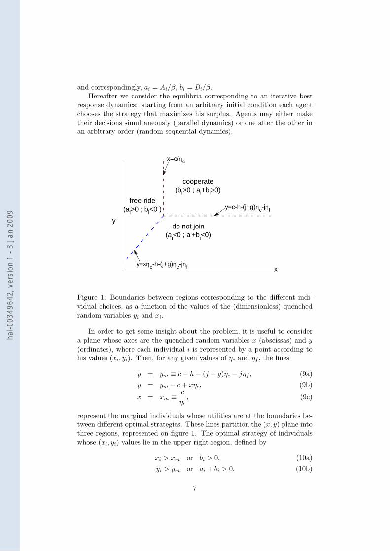
Figure 1: Boundaries between regions corresponding to the different indi-vidual choices, as a function of the values of the (dimensionless) quenchedrandom variables yi and xi.

In order to get some insight about the problem, it is useful to considera plane whose axes are the quenched random variables x (abscissas) and y(ordinates), where each individual i is represented by a point according tohis values (xi, yi). Then, for any given values of ηc and ηf , the lines

y = ym ≡ c− h− (j + g)ηc − jηf , (9a)y = ym − c+ xηc, (9b)

x = xm ≡c

ηc, (9c)

represent the marginal individuals whose utilities are at the boundaries be-tween different optimal strategies. These lines partition the (x, y) plane intothree regions, represented on figure 1. The optimal strategy of individualswhose (xi, yi) values lie in the upper-right region, defined by

xi > xm or bi > 0, (10a)yi > ym or ai + bi > 0, (10b)

7

hal-0

0349

642,

ver

sion

1 -

3 Ja

n 20

09

is to cooperate. The best strategy for those whose (xi, yi) satisfy

xi < xm or bi < 0, (11a)yi > ym − c+ xiηc or ai > 0, (11b)

is to free-ride. Individuals with (xi, yi) in the lower-right region do not jointhe community.

3 Mean field dynamics

We are interested in the temporal evolution of the system within an iteratedgame setting, in which individuals have to choose their best strategies si(t)based on the available information. We assume that each time an agent hasto make a decision, he has the exact information of the global proportions ofcooperators and free-riders at the preceding outcome, ηc(t−1) and ηf (t−1),and uses these quantities to estimate his surplus (2). Such a dynamics iscalled Cournot best reply in economics literature. In simulations, startingfrom initial guesses ηc(0) and ηf (0), the updating is said to be in parallelif all the individuals in the population first determine their best strategiesbased on the preceding outcome, and make their decisions simultaneouslyafterwards. At the opposite, in random sequential updating, a single indi-vidual selected at random is asked to make his decision at each time step.The latter dynamics simulates systems where the individuals make theirdecisions without any temporal correlation. In order to compare the timescales of both dynamics, it is usual to consider that N sequential time stepsare equivalent to one parallel update. Intermediate updating schemes maybe implemented, but here we only consider these two extreme cases, thatare standard in economics and in statistical physics.

Referring back to figure 1, since the boundary lines depend on the valuesof ηc(t) and ηf (t), they will shift in the course of updating according tothe perceived proportions of cooperators and free-riders. Individuals whosevalues of yi and xi lie close to the boundaries are susceptible to small changesof ηc and ηf : their strategies may change with time, and in turn inducechanges in those of the others.

Hereafter we study how the system reaches its stable states upon suc-cessive updates, that is, the path followed by a point representative of thesystem’s state in the plane (ηc, ηf ). Such paths should either end up in astable fixed point or get trapped in other types of attractors if they exist.In the following we consider separately the parallel and sequential updatingschemes, since the corresponding dynamic equations are different.

Let us introduce the complementary cumulative functions defined by:

Gχ(ζ) ≡ 1− Fχ(ζ) =∫ ∞ζ

fχ(ξ)dξ, (12)

8

hal-0

0349

642,

ver

sion

1 -

3 Ja

n 20

09

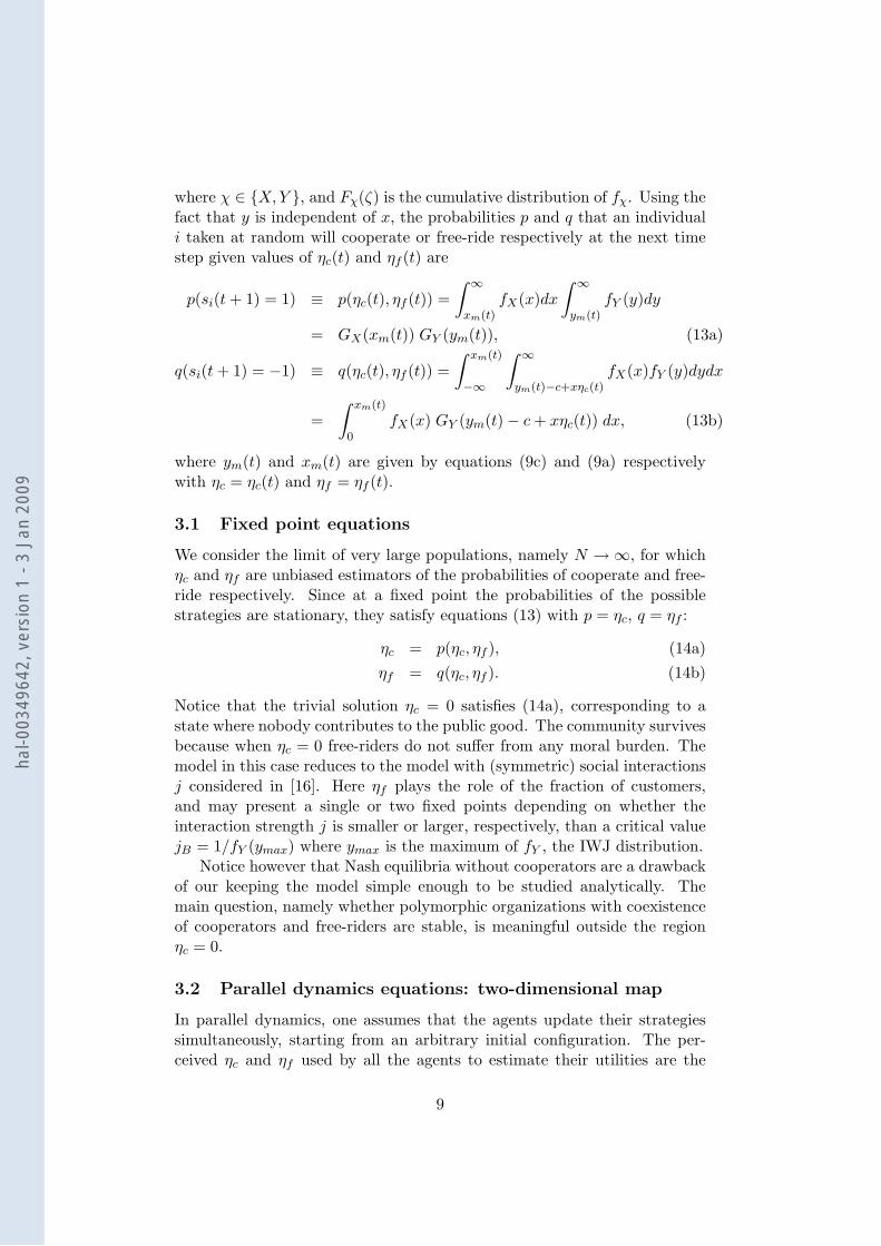
where χ ∈ X,Y , and Fχ(ζ) is the cumulative distribution of fχ. Using thefact that y is independent of x, the probabilities p and q that an individuali taken at random will cooperate or free-ride respectively at the next timestep given values of ηc(t) and ηf (t) are

p(si(t+ 1) = 1) ≡ p(ηc(t), ηf (t)) =∫ ∞xm(t)

fX(x)dx∫ ∞ym(t)

fY (y)dy

= GX(xm(t)) GY (ym(t)), (13a)

q(si(t+ 1) = −1) ≡ q(ηc(t), ηf (t)) =∫ xm(t)

−∞

∫ ∞ym(t)−c+xηc(t)

fX(x)fY (y)dydx

=∫ xm(t)

0fX(x) GY (ym(t)− c+ xηc(t)) dx, (13b)

where ym(t) and xm(t) are given by equations (9c) and (9a) respectivelywith ηc = ηc(t) and ηf = ηf (t).

3.1 Fixed point equations

We consider the limit of very large populations, namely N →∞, for whichηc and ηf are unbiased estimators of the probabilities of cooperate and free-ride respectively. Since at a fixed point the probabilities of the possiblestrategies are stationary, they satisfy equations (13) with p = ηc, q = ηf :

ηc = p(ηc, ηf ), (14a)ηf = q(ηc, ηf ). (14b)

Notice that the trivial solution ηc = 0 satisfies (14a), corresponding to astate where nobody contributes to the public good. The community survivesbecause when ηc = 0 free-riders do not suffer from any moral burden. Themodel in this case reduces to the model with (symmetric) social interactionsj considered in [16]. Here ηf plays the role of the fraction of customers,and may present a single or two fixed points depending on whether theinteraction strength j is smaller or larger, respectively, than a critical valuejB = 1/fY (ymax) where ymax is the maximum of fY , the IWJ distribution.

Notice however that Nash equilibria without cooperators are a drawbackof our keeping the model simple enough to be studied analytically. Themain question, namely whether polymorphic organizations with coexistenceof cooperators and free-riders are stable, is meaningful outside the regionηc = 0.

3.2 Parallel dynamics equations: two-dimensional map

In parallel dynamics, one assumes that the agents update their strategiessimultaneously, starting from an arbitrary initial configuration. The per-ceived ηc and ηf used by all the agents to estimate their utilities are the

9

hal-0

0349

642,

ver

sion

1 -

3 Ja

n 20

09

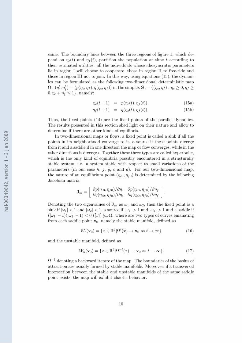
same. The boundary lines between the three regions of figure 1, which de-pend on ηc(t) and ηf (t), partition the population at time t according totheir estimated utilities: all the individuals whose idiosyncratic parameterslie in region I will choose to cooperate, those in region II to free-ride andthose in region III not to join. In this way, using equations (13), the dynam-ics can be formulated as the following two-dimensional deterministic mapΩ : (η′c, η

′f ) = (p(ηc, ηf ), q(ηc, ηf )) in the simplex S := (ηc, ηf ) : ηc ≥ 0, ηf ≥

0, ηc + ηf ≤ 1, namely:

ηc(t+ 1) = p(ηc(t), ηf (t)), (15a)ηf (t+ 1) = q(ηc(t), ηf (t)). (15b)

Thus, the fixed points (14) are the fixed points of the parallel dynamics.The results presented in this section shed light on their nature and allow todetermine if there are other kinds of equilibria.

In two-dimensional maps or flows, a fixed point is called a sink if all thepoints in its neighborhood converge to it, a source if these points divergefrom it and a saddle if in one direction the map or flow converges, while in theother directions it diverges. Together these three types are called hyperbolic,which is the only kind of equilibria possibly encountered in a structurallystable system, i.e. a system stable with respect to small variations of theparameters (in our case h, j, g, c and d). For our two-dimensional map,the nature of an equilibrium point (ηc0, ηf0) is determined by the followingJacobian matrix

Jm =[∂p(ηc0, ηf0)/∂ηc ∂p(ηc0, ηf0)/∂ηf∂q(ηc0, ηf0)/∂ηc ∂q(ηc0, ηf0)/∂ηf

].

Denoting the two eigenvalues of Jm as ω1 and ω2, then the fixed point is asink if |ω1| < 1 and |ω2| < 1, a source if |ω1| > 1 and |ω2| > 1 and a saddle if(|ω1| − 1)(|ω2| − 1) < 0 ([17] §1.4). There are two types of curves emanatingfrom each saddle point x0, namely the stable manifold, defined as

Ws(x0) = x ∈ R2|Ωt(x)→ x0 as t→∞ (16)

and the unstable manifold, defined as

Wu(x0) = x ∈ R2|Ω−t(x)→ x0 as t→∞ (17)

Ω−1 denoting a backward iterate of the map. The boundaries of the basins ofattraction are usually formed by stable manifolds. Moreover, if a transversalintersection between the stable and unstable manifolds of the same saddlepoint exists, the map will exhibit chaotic behavior.

10

hal-0

0349

642,

ver

sion

1 -

3 Ja

n 20

09

3.3 Random sequential dynamics equations: two-dimensionalflow

In sequential dynamics, one updates one agent chosen at random in eachtime step. It is usual to consider N (the number of agents in the system)successive updates (called one Monte-Carlo step) as being comparable toone step of parallel updating, i.e., the time step between two successiveindividual updatings is τ = 1/N .

In each individual update, the expected displacement of the pair (ηc, ηf )is

ηc(t+ τ) = ηc(t) + (1/N)(p(ηc(t), ηf (t))− ηc(t)), (18a)ηf (t+ τ) = ηf (t) + (1/N)(q(ηc(t), ηf (t))− ηf (t)), (18b)

where p and q are defined in (13), and the factor 1/N is the probability ofselecting the agent that is updated. Taking the continuous limit N → ∞,we have the following set of differential equations:

dηcdt

= p(ηc, ηf )− ηc, (19a)

dηfdt

= q(ηc, ηf )− ηf , (19b)

with the time unit being one Monte-Carlo step. Now the system evolves asan autonomous system in a planar phase space, i.e. as a two-dimensionalflow in S. Clearly, the fixed points of the sequential dynamics are the sameas the equilibria (14).

The three generic types of equilibria, namely source, sink and saddleexist in a structurally stable two-dimensional flow as well. The nature ofan equilibrium point (ηc0, ηf0) is now determined by the Jacobian matrix ofthe flow

Jf =[∂p(ηc0, ηf0)/∂ηc − 1 ∂p(ηc0, ηf0)/∂ηf∂q(ηc0, ηf0)/∂ηc ∂q(ηc0, ηf0)/∂ηf − 1

].

Denoting the eigenvalues of Jf as ω′1 and ω′2, then the point is a sink if ω′1 < 0and ω′2 < 0, a source if ω′1 > 0 and ω′2 > 0 and a saddle if ω′1ω

′2 < 0 ([17]

§1.2∼1.3). Note that the condition for an equilibrium to be a saddle gives thesame inequality as in the parallel case. Therefore, the set of saddle points insequential updating coincides with that in parallel updating. However, theset of sinks or sources are not necessarily the same in both cases, since thegoverning inequalities are quite different. The definitions of the stable andunstable manifolds are analog to those in the two-dimensional map with thediscrete time step replaced by the continuous time variable t. According tothe Poincare-Bendixson Theorem ([17] Theorem 1.8.1), the two-dimensionalflow system will never go into chaos.

11

hal-0

0349

642,

ver

sion

1 -

3 Ja

n 20

09

4 Equilibria for particular distributions fX and fY

To go further with the analysis of the preceding section we need to specifythe pdfs of the idiosyncratic parameters. In this paper we present the mostinteresting of the cases we have studied, in which the xi follow a uniformdistribution of finite width d:

fX(x) =1d

for 0 ≤ x ≤ d, (20a)

fX(x) = 0 otherwise. (20b)

and the yi are distributed according to:

fY (y) =1

4 cosh2(y/2). (21)

The cumulative function corresponding to (21) is the logistic distribution.The complementary functions (12) are:

GX(z) = (1− z)Θ(1− z), (22a)GY (z) = 1/[1 + exp(z)], (22b)

where Θ is the Heaviside function.

Fixed points

The fixed point equations (14) may be written as follows:

ηc = (1− ρ

ηc)Θ(1− ρ

ηc) GY (c− Z) (23a)

ηf =ρ

cηclog[1 + (ec − 1)GY (c− Z)], (23b)

where ρ ≡ c/d and Z ≡ h + j(ηc + ηf ) + gηc. Since fX has a boundedsupport, equation (23a) vanishes if 0 ≤ ηc(t) ≤ ρ. Thus, if ηc(0) ≤ ρ, thesystem evolves towards the trivial equilibrium without cooperators. In par-allel dynamics, equation (15a) gives ηc(1) = 0: the state with no cooperatorsis reached after a single parallel update. Afterwards, on the axis ηc = 0, ηfevolves according to equation (15b),

ηf (t+ 1) = GY (−h− jηf (t)). (24)

The equilibrium value of ηf is given by (14b), obtained by replacing ηf (t)and ηf (t + 1) by ηf in the above equation. As already mentioned (see[16]) there is a critical value of j, jB, such that for j < jB, there is asingle equilibrium. In that case all the points ηc(0) < ρ will eventually bemapped to it. If j > jB (14b) has three solutions. One of them, ηfu, isan unstable fixed point separating the basin of attraction of the two others,

12

hal-0

0349

642,

ver

sion

1 -

3 Ja

n 20

09

that are stable. To summarize, when ηc(0) < ρ, after a first time stepthe system is mapped to the axis ηc = 0 and then evolves, following (24),either to one fixed point (if j < jB) or to one of two fixed points (if j >jB) depending on whether ηf (0) > ηfu or ηf (0) < ηfu. In the case ofthe logistic distribution fY considered here, jB = 4 [15]. Under randomsequential updating, since p(ηc(0), ηf (0)) = 0 for 0 ≤ ηc(0) ≤ ρ, equation(19a) shows that ηc vanishes exponentially fast, the fixed points being thesame as for the parallel dynamics. These solutions have been described herefor completeness since, as already stated, they are not within the scope ofthe questions addressed by the model

Notice that there are no fixed points with ηf = 0: since GY ≥ 0, theright hand side of (23b) vanishes only if c = 0, i.e. full cooperation mayexist only if cooperation is costless.

When ηc(0) > ρ, calling G the value taken by GY (c−Z), equation (23a)gives ηc = (1− ρ

ηc) G, which can be solved for non-vanishing ηc in terms of

G:ηc = η±c [G] ≡ 1

2G 1± [1− 4ρ

G]1/2 (25)

Later we shall see that both the + and the − branches may give stableequilibria, though the parameter range for which a stable equilibrium existsfor the − branch is much narrower than for the + branch. From (25) onegets that the Nash equilibria with cooperators satisfy ηc ≥ 2ρ (equality canoccur when j = g = 0): the fraction of cooperators is larger than a thresholdgiven by the cooperation cost relative to the average weight (x = d/2) ofthe social disapproval for free-riding.

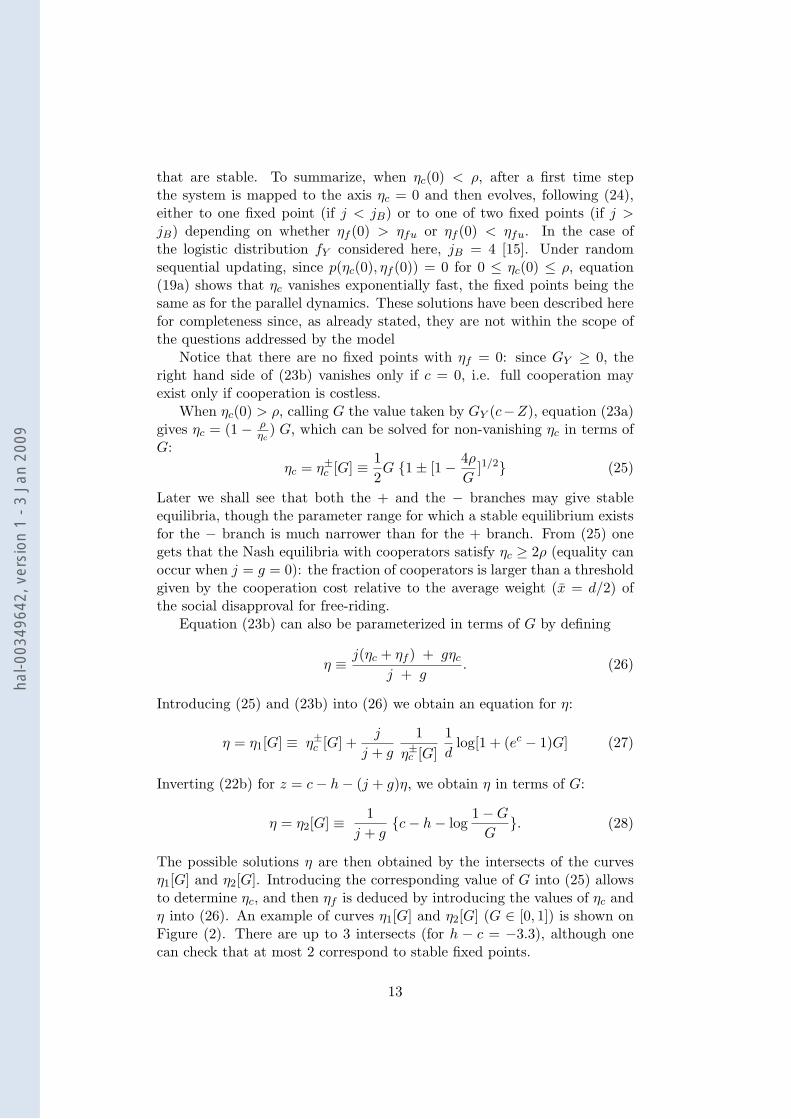
Equation (23b) can also be parameterized in terms of G by defining

η ≡j(ηc + ηf ) + gηc

j + g. (26)

Introducing (25) and (23b) into (26) we obtain an equation for η:

η = η1[G] ≡ η±c [G] +j

j + g

1η±c [G]

1d

log[1 + (ec − 1)G] (27)

Inverting (22b) for z = c− h− (j + g)η, we obtain η in terms of G:

η = η2[G] ≡ 1j + g

c− h− log1−GG. (28)

The possible solutions η are then obtained by the intersects of the curvesη1[G] and η2[G]. Introducing the corresponding value of G into (25) allowsto determine ηc, and then ηf is deduced by introducing the values of ηc andη into (26). An example of curves η1[G] and η2[G] (G ∈ [0, 1]) is shown onFigure (2). There are up to 3 intersects (for h − c = −3.3), although onecan check that at most 2 correspond to stable fixed points.

13

hal-0

0349

642,

ver

sion

1 -

3 Ja

n 20

09

0 . 0 0 . 2 0 . 4 0 . 6 0 . 8 1 . 00 . 0

0 . 2

0 . 4

0 . 6

0 . 8

1 . 0

η 2

η 1 -

η[G]

G

h - c = - 3 . 7 h - c = - 3 . 3 h - c = - 3 . 1

η 1 +

j = 5g = 1c = 4 . 5d = 7 2

2 ρ

Figure 2: Fixed points. Solution by curve intersection for distributions fX and fY

given by equations (20) and (21).

- 4 . 0 - 3 . 5 - 3 . 0

- 4 . 0 - 3 . 5 - 3 . 0

r a n d o m s e q u e n t i a l d y n a m i c s

µ4

t r i v i a lf i x e d p o i n t ( s )

λ 6λ 5λ 4λ 2

f i x e d p o i n tO +

limit c

ycle

fixed p

oint

O’ +p a r a l l e l d y n a m i c s

µ2 µ5

j = 5g = 1c = 4 . 5d = 7 2

f i x e d p o i n tO ’ +

h - c

t r i v i a lf i x e d p o i n t ( s )

f i x e d p o i n tO +

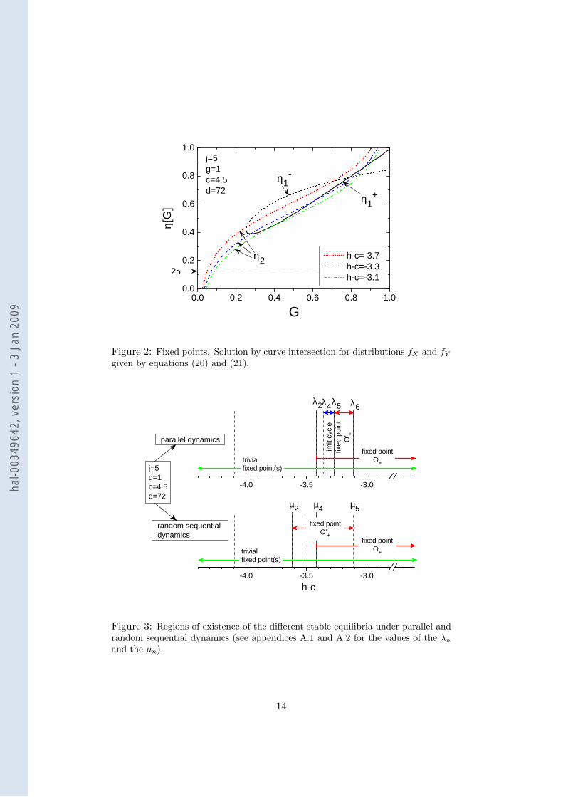
Figure 3: Regions of existence of the different stable equilibria under parallel andrandom sequential dynamics (see appendices A.1 and A.2 for the values of the λn

and the µn).

14

hal-0

0349

642,

ver

sion

1 -

3 Ja

n 20

09

Equilibria with parallel dynamics.

Notice that the above analysis allows to determine the fixed points of thesystem, but doesn’t give any hint about the existence of cycles. We havethus numerically computed the stable and unstable manifolds for each saddlepoint, with the same set of values for j, g, c and d as in figure 2, whilechanging h− c from −4 to −3 in steps of 0.02. We summarize here the mainresults, leaving the details to appendix A.1.

Besides the trivial fixed point(s) with ηc = 0, for any h − c ≥ −3.4201there is a fixed point O+ corresponding to a relatively large organizationhaving a proportion of cooperators larger than the proportion of free-riders.This occurs for cooperation costs relatively large compared to the averagewillingness to join (h − c is negative). The value of j considered is largeenough to compensate negative values of hi − c on a large fraction of thepopulation, producing a bandwagon effect. For −3.3504 < h− c < −3.1146,this fixed point O+ coexists with another non-trivial attractors (see figure 3).For −3.3504 < h− c < −3.2726, the attractor is a limit cycle CS . It shrinks(at h − c = −3.2726) to a second fixed point O′+ which corresponds to anorganization with qualitatively similar proportions of cooperators and freeriders, and with fewer members than at the equilibrium O+. This secondfixed point O′+ exists for −3.2726 < h − c < −3.1146. For larger values(h− c > −3.1146) it disappears, leaving only the fixed point O+ with a verylarge basin of attraction.

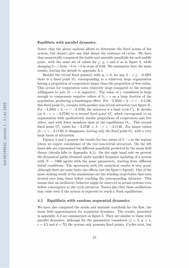
Figures 4 and 5 present the results for two values of h− c in the regionswhere we expect coexistence of the two non-trivial attractors. On the lefthand side are represented the different manifolds predicted by the mean fieldtheory (details lefts to Appendix A.1). On the right hand side we presentthe dynamical paths obtained under parallel dynamics updating of a systemwith N = 1000 agents with the same parameters, starting from differentinitial conditions. The agreement with the analytical results is very good,although there are some finite size effects (see the figure’s legend). One of themost striking result of the simulations are the winding trajectories that turnaround over long times before reaching the corresponding attractor. Thismeans that an oscillatory behavior might be observed in actual systems evenbefore convergence to the cycle attractor. Notice also that these oscillationsmay exist even if the system is expected to reach a Nash equilibrium.

4.1 Equilibria with random sequential dynamics

We have also computed the stable and unstable manifolds for the flow, themean field approximation for sequential dynamics. The results, presentedin appendix A.2 are summarized on figure 3. They are similar to those withparallel dynamics, although for the parameters considered (j = 5, g = 1,c = 4.5 and d = 72) the system only presents fixed points. Cycles exist, but

15

hal-0

0349

642,

ver

sion

1 -

3 Ja

n 20

09

0 0.2 0.4 0.6 0.8 10

0.2

0.4

0.6

0.8

1

!c

!f

"

H−

X+

O+H+

Cs

h − c = −3.3j = 5g = 1c = 4.5d = 72

0 . 0 0 . 2 0 . 4 0 . 6 0 . 8 1 . 00 . 0

0 . 2

0 . 4

0 . 6

0 . 8

1 . 0

h - c = - 3 . 3j = 5g = 1c = 4 . 5d = 7 2

η f

η c

Figure 4: Left. Stable and unstable manifolds of the theoretical saddle points inthe plane (ηc, ηf ) for the same parameter values as in figure 3, with h− c = −3.3.The non trivial attractors are a stable cycle Cs (its basin of attraction is limited bythe dashed line corresponding to the stable manifold of H+, with its two ends atthe line ηf = 0). The point O+ is a fixed point. Its basin of attraction is the regionbounded by the stable manifold of H− between the lines ηc + ηf = 1 and ηf = 0,excluding the basin of attraction of Cs.Right. Trajectories of the simulated system for four different initial conditions,that converge respectively to a trivial fixed point (squares), to a cycle of length41 (empty triangles), to a fixed point (full circles) not predicted by the mean fieldequations (due to finite size effects) and to the non-trivial fixed point O+ (emptycircles).

0 0.2 0.4 0.6 0.8 10

0.2

0.4

0.6

0.8

1

!c

!f

"

H−

O+’

O+H+

h − c = −3.2j = 5g = 1c = 4.5d = 72

0 . 0 0 . 2 0 . 4 0 . 6 0 . 8 1 . 00 . 0

0 . 2

0 . 4

0 . 6

0 . 8

1 . 0

η f

η c

h - c = - 3 . 2j = 5g = 1c = 4 . 5d = 7 2

Figure 5: Left. Theoretical equilibria for the map in the plane (ηc, ηf ), for thesame parameter values as in figure 3, with h− c = −3.2. The stable limit cycle Cs

has merged with the source X+ through a Hopf bifurcation to become a sink O′+,whose basin of attraction is the stable manifold of the saddle H+.Right. Trajectories of the simulated system (parallel dynamics) for five differentinitial conditions. One of them converges to a trivial fixed point (squares), one(circles) to a cycle of length 13 (instead of the predicted non-trivial fixed pointO′+), the three others (triangles) converge to the non-trivial fixed point O+, whichhas a large basin of attraction.

16

hal-0

0349

642,

ver

sion

1 -

3 Ja

n 20

09

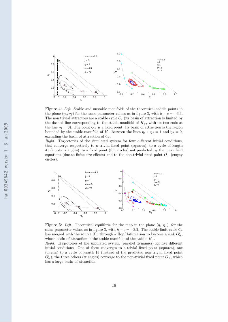
for other parameter values, as discussed in the appendix.Figure 6 presents an example of evolution of the same system under

parallel and sequential dynamics, showing the dramatic difference betweenboth types of updating rules.

Figure 6: Examples of trajectories for parallel and random sequential dynamicsstarting from the same initial conditions, for a system with the same parametervalues as in figure 3, and h− c = −3.3.

5 Simulations results and phase diagrams

The theoretical results of the preceding sections predict the behavior of aninfinite system. On figure 7 we present the phase portrait obtained throughparallel dynamics with systems of different sizes, for h − c = −3.3 andthe same set of parameters as in figure 4. Starting from different initialconditions, we determined the attractors in the phase space (ηc, ηf ). As Ndecreases, more and more fixed points invade the region where cycles exist,and many different cycles appear. This multiplicity of attractors is due tomissing values of the IWJ in the finite population. However, the mean fieldpredictions, and in particular the existence of cycles, remain qualitativelycorrect.

In order to get deeper insight on the phase diagram of the model, westudied the attractors of large systems as a function of the different param-eters. Results as a function of h − c, summarized on figure 8, are in verygood agreement with the mean field predictions, as may be seen through theposition of the theoretical boundaries λn.

Figures 9 present separately the ηc values at the fixed points and at thecycles for systems of different sizes, ranging from N = 1 000 to N = 100 000,as a function of h − c. Consistently with the above results, the size effectsare important, but do not modify qualitatively the phase diagram.

As may be seen on figure 10 (left), the fraction of the phase space that

17

hal-0

0349

642,

ver

sion

1 -

3 Ja

n 20

09

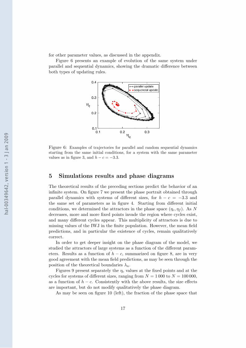
Figure 7: Attractors and their basins of attraction for different system sizes, ob-tained by starting from all the possible initial conditions (with a mesh of 0.01).Parameters are: j = 5, g = 1, d = 72, h = 1.2. The white region is the basin ofattraction of the cycles.

Figure 8: Attractors for parallel dynamics with N = 100 000, for 20 simulatedsystems, with the same parameters as in the preceding figures, i.e. j = 5, g = 1,c = 4.5 and d = 72. The points in this and the following figures are obtained asfollows: we draw 20 systems at random with probabilities fX and fY . The pointsin the figures correspond to the final states obtained for each system, starting fromeach possible initial point in the plane ηc, ηf laying on a grid of mesh 0.1 satisfyingthe condition ηc + ηf ≤ 1. That corresponds to 45 different initial conditions foreach of the 20 systems, i.e. a total of 900 simulations.

18

hal-0

0349

642,

ver

sion

1 -

3 Ja

n 20

09

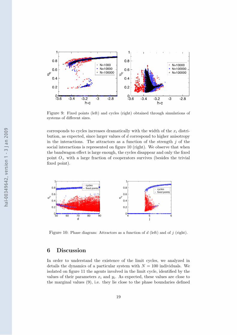
Figure 9: Fixed points (left) and cycles (right) obtained through simulations ofsystems of different sizes.

corresponds to cycles increases dramatically with the width of the xi distri-bution, as expected, since larger values of d correspond to higher anisotropyin the interactions. The attractors as a function of the strength j of thesocial interactions is represented on figure 10 (right). We observe that whenthe bandwagon effect is large enough, the cycles disappear and only the fixedpoint O+ with a large fraction of cooperators survives (besides the trivialfixed point).

50 60 70 80 90d

0

0.2

0.4

0.6

0.8

1

η c

cyclesfixed points

4 5 6j

0

0.2

0.4

0.6

0.8

1

η c

cyclesfixed points

Figure 10: Phase diagram: Attractors as a function of d (left) and of j (right).

6 Discussion

In order to understand the existence of the limit cycles, we analyzed indetails the dynamics of a particular system with N = 100 individuals. Weisolated on figure 11 the agents involved in the limit cycle, identified by thevalues of their parameters xi and yi. As expected, these values are close tothe marginal values (9), i.e. they lie close to the phase boundaries defined

19

hal-0

0349

642,

ver

sion

1 -

3 Ja

n 20

09

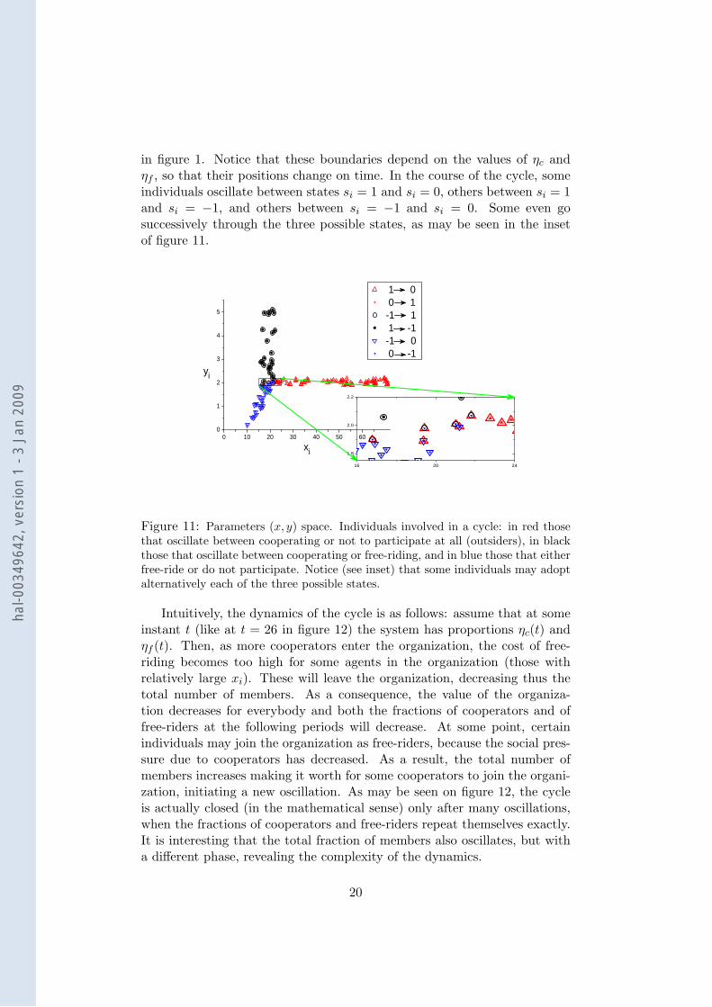
in figure 1. Notice that these boundaries depend on the values of ηc andηf , so that their positions change on time. In the course of the cycle, someindividuals oscillate between states si = 1 and si = 0, others between si = 1and si = −1, and others between si = −1 and si = 0. Some even gosuccessively through the three possible states, as may be seen in the insetof figure 11.

0 1 0 2 0 3 0 4 0 5 0 6 00

1

2

3

4

5

y i

x i

1 0 0 1- 1 1 1 - 1- 1 0 0 - 1

1 6 2 0 2 4

1 . 8

2 . 0

2 . 2

Figure 11: Parameters (x, y) space. Individuals involved in a cycle: in red thosethat oscillate between cooperating or not to participate at all (outsiders), in blackthose that oscillate between cooperating or free-riding, and in blue those that eitherfree-ride or do not participate. Notice (see inset) that some individuals may adoptalternatively each of the three possible states.

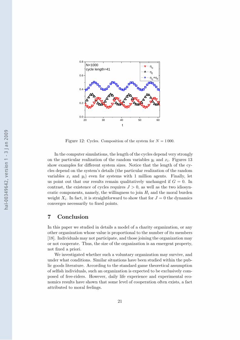
Intuitively, the dynamics of the cycle is as follows: assume that at someinstant t (like at t = 26 in figure 12) the system has proportions ηc(t) andηf (t). Then, as more cooperators enter the organization, the cost of free-riding becomes too high for some agents in the organization (those withrelatively large xi). These will leave the organization, decreasing thus thetotal number of members. As a consequence, the value of the organiza-tion decreases for everybody and both the fractions of cooperators and offree-riders at the following periods will decrease. At some point, certainindividuals may join the organization as free-riders, because the social pres-sure due to cooperators has decreased. As a result, the total number ofmembers increases making it worth for some cooperators to join the organi-zation, initiating a new oscillation. As may be seen on figure 12, the cycleis actually closed (in the mathematical sense) only after many oscillations,when the fractions of cooperators and free-riders repeat themselves exactly.It is interesting that the total fraction of members also oscillates, but witha different phase, revealing the complexity of the dynamics.

20

hal-0

0349

642,

ver

sion

1 -

3 Ja

n 20

09

2 0 3 0 4 0 5 0 6 00 . 0

0 . 2

0 . 4

0 . 6

0 . 8

N = 1 0 0 0c y c l e l e n g t h = 4 1

t

η c η f η c + η f

Figure 12: Cycles. Composition of the system for N = 1 000.

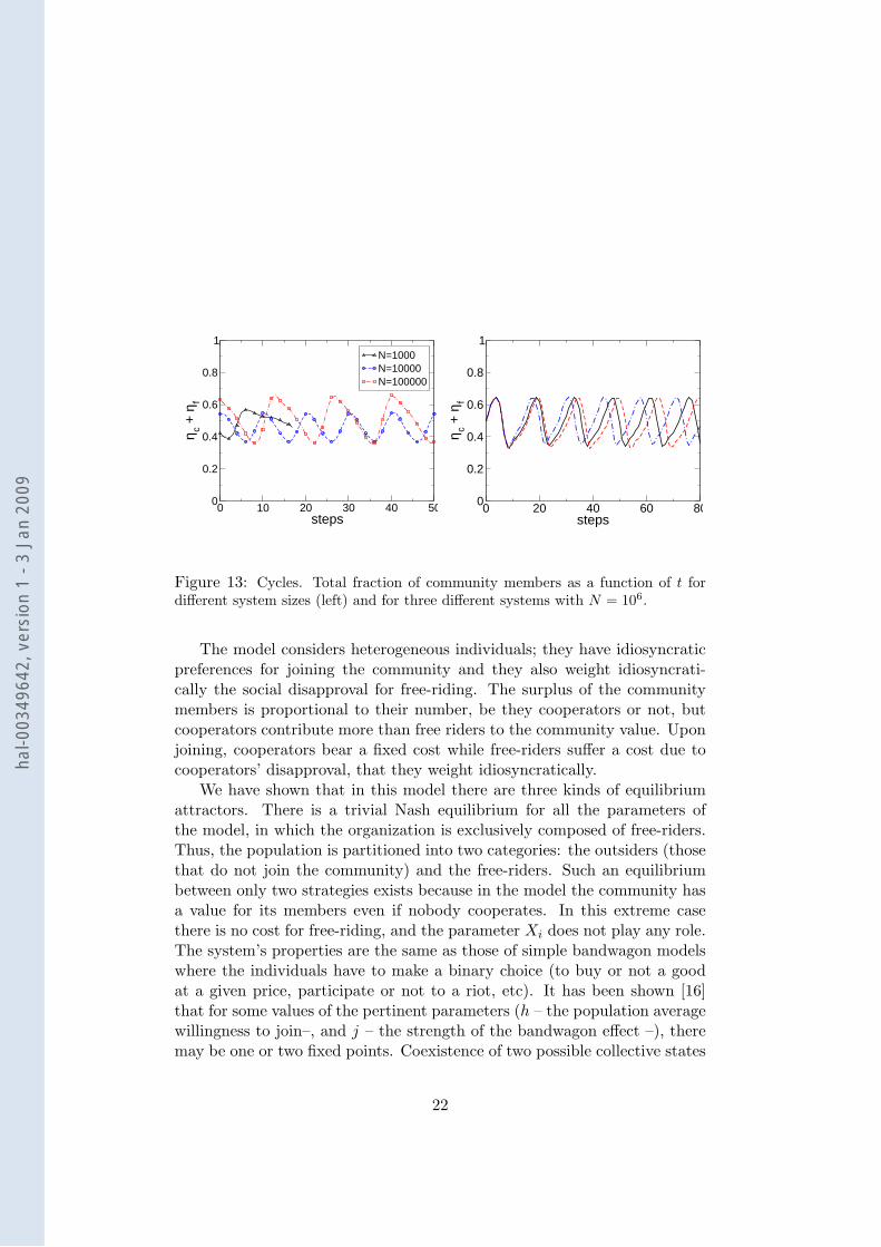
In the computer simulations, the length of the cycles depend very stronglyon the particular realization of the random variables yi and xi. Figures 13show examples for different system sizes. Notice that the length of the cy-cles depend on the system’s details (the particular realization of the randomvariables xi and yi) even for systems with 1 million agents. Finally, letus point out that our results remain qualitatively unchanged if G = 0. Incontrast, the existence of cycles requires J > 0, as well as the two idiosyn-cratic components, namely, the willingness to join Hi and the moral burdenweight Xi. In fact, it is straightforward to show that for J = 0 the dynamicsconverges necessarily to fixed points.

7 Conclusion

In this paper we studied in details a model of a charity organization, or anyother organization whose value is proportional to the number of its members[18]. Individuals may not participate, and those joining the organization mayor not cooperate. Thus, the size of the organization is an emergent property,not fixed a priori.

We investigated whether such a voluntary organization may survive, andunder what conditions. Similar situations have been studied within the pub-lic goods literature. According to the standard game theoretical assumptionof selfish individuals, such an organization is expected to be exclusively com-posed of free-riders. However, daily life experience and experimental eco-nomics results have shown that some level of cooperation often exists, a factattributed to moral feelings.

21

hal-0

0349

642,

ver

sion

1 -

3 Ja

n 20

09

0 10 20 30 40 50steps

0

0.2

0.4

0.6

0.8

1

η c + η

f

N=1000N=10000N=100000

0 20 40 60 80steps

0

0.2

0.4

0.6

0.8

1

η c + η

f

Figure 13: Cycles. Total fraction of community members as a function of t fordifferent system sizes (left) and for three different systems with N = 106.

The model considers heterogeneous individuals; they have idiosyncraticpreferences for joining the community and they also weight idiosyncrati-cally the social disapproval for free-riding. The surplus of the communitymembers is proportional to their number, be they cooperators or not, butcooperators contribute more than free riders to the community value. Uponjoining, cooperators bear a fixed cost while free-riders suffer a cost due tocooperators’ disapproval, that they weight idiosyncratically.

We have shown that in this model there are three kinds of equilibriumattractors. There is a trivial Nash equilibrium for all the parameters ofthe model, in which the organization is exclusively composed of free-riders.Thus, the population is partitioned into two categories: the outsiders (thosethat do not join the community) and the free-riders. Such an equilibriumbetween only two strategies exists because in the model the community hasa value for its members even if nobody cooperates. In this extreme casethere is no cost for free-riding, and the parameter Xi does not play any role.The system’s properties are the same as those of simple bandwagon modelswhere the individuals have to make a binary choice (to buy or not a goodat a given price, participate or not to a riot, etc). It has been shown [16]that for some values of the pertinent parameters (h – the population averagewillingness to join–, and j – the strength of the bandwagon effect –), theremay be one or two fixed points. Coexistence of two possible collective states

22

hal-0

0349

642,

ver

sion

1 -

3 Ja

n 20

09

(Nash equilibria), having either a large or a small fraction of free-riders, arisefor values of h smaller than, and j larger than, threshold values that dependon the distribution of the idiosyncratic component Hi. Besides this trivialequilibrium, the model considered here presents one or two Nash equilibriawith finite fractions of cooperators and free-riders.

An interesting result of this model is that besides the Nash equilib-ria, it exhibits limit cycles with corresponding fractions of cooperators, offree-riders (and their sum —the fraction of the population that joins theorganization—) oscillating through time. This phenomenon has its root inthe strong asymmetry of the interaction between agents, introduced by theidiosyncratic weights that free-riders attach to social disapproval. Althoughwe studied in details the case where these weights Xi are uniformly dis-tributed, we verified that the same kind of oscillations exist in the case of abimodal distribution2. The fixed points in this case may be found analyti-cally.

We studied in details the dynamics of the cycles under parallel and ran-dom sequential updating both analytically and numerically. Assuming aglobal neighborhood (i.e. every agent’s surplus depends on the fractions ofcooperators and free-riders in the whole population), we obtained resultswhich are exact in the asymptotic limit N → ∞. The two-dimensional dy-namical maps and flows have been studied for a large range of parameters.Although qualitatively similar, the phase diagrams of maps and flows cor-responding to the same parameters are not identical. The fact that a richclass of bifurcations can occur within a narrow parameter region is in itselftruly remarkable. A natural question to ask is what happens in intermedi-ate regimes, where subsets of agents make decisions simultaneously, whileothers make them at independent times.

Numerical simulations of finite size systems with parallel dynamics qual-itatively agree with the analytical results. The dynamical behaviour of thesimulated systems show winding trajectories in very large regions of thephase diagram. Oscillations in the fraction of cooperators and free-ridersare thus expected in such systems before the onset of the cycle and evenwhen the attractor is a fixed point. We are currently performing simulationswith sequential dynamics, where the notion of cycle is not well defined, dueto the randomness in the order in which the agents’ decisions are updated.Preliminary results also exhibit the above mentionned oscillatory behavior,but the analysis of the data is much more cumbersome.

Future work should focus on the dynamics for interactions restrictedto closer neighborhoods, which probably requires more sophisticated tech-niques from the theory of dynamical systems. Another interesting question

2Note added in proof: A similar model for an asset market with two kinds of agents,that corresponds to a bimodal distribution of the Xi, restricted to binary decisions [19]was shown to present cycles.

23

hal-0

0349

642,

ver

sion

1 -

3 Ja

n 20

09

is how the phase diagram is modified in the case where the agents learn frompast actions and can form expectancies.

Acknowledgements

M.B.G. and J-P.N. are members of CNRS. S.G. thanks support from FAPERGSand CNPq (Brazil) and also from CNRS during his stay in Grenoble.

References

[1] Mancur Olson. The Logic of Collective Action : Public Goods and theTheory of Groups. Harvard University Press, 1965.

[2] John O. Ledyard. Public goods: A survey of experimental research.In Roth and Kagel, editors, The Handbook of Experimental Economics,pages 111–194. Princeton University Press, 1995.

[3] E. Fehr and S. Gaechter. Altruistic punishment in humans. Nature,415:137–140, (2002).

[4] Ernst Fehr and Urs Fischbacher. Social norms and human cooperation.Trends in Cognitive Sciences, 8(4):185–190, 2004.

[5] S. Gaechter and E. Fehr. Collective action as a social exchange. Journalof Economic Behavior and Organization, 39:341–369, (1999).

[6] W. Hichri and A. Kirman. The emergence of coordination in publicgood games. The European Physical Journal B, 55:149–159, 2007.

[7] Ben Greiner and M. Vittoria Levati. Indirect reciprocity in cyclicalnetworks. an experimental study. Journal of Economic Psychology,26:711–731, 2005.

[8] Herbert Gintis. Game Theory Evolving. Princeton University Press,2000.

[9] B. Huberman and N. Glance. Beliefs and cooperation. In Peter Daniel-son, editor, Modelling Rational and Moral Agents, pages 210–235. Ox-ford University PressUniversity Press, (1996).

[10] L. A. Imhof, D. Fudenberg, and M. A. Nowak. Evolutionary cycles ofcooperation and defection. PNAS, 102:10797–10800, (2005).

[11] G. Iori and V. Koulovassilopoulos. Patterns of consumption in a dis-crete choice model with asymmetric interactions. In W. Barnett, Ch.Deissenberg, and G. Feichtinger, editors, Economic Complexity: Non-linear Dynamics, Multi-agents Economies, and Learning, page ISETEVol 14. Elsevier, Amsterdam, (2004).

24

hal-0

0349

642,

ver

sion

1 -

3 Ja

n 20

09

[12] S. N. Durlauf. Statistical mechanics approaches to socioeconomic be-havior. In B. Arthur, S. N. Durlauf, and D. Lane, editors, The Economyas an Evolving Complex System II, pages 81–104. Santa Fe InstituteStudies in the Sciences of Complexity, Volume XVII, Addison-WesleyPub. Co, (1997).

[13] M. B. Gordon, D. Phan, R. Waldeck, and J.-P. Nadal. Cooperationand free-riding with moral cost. In Kokinov Boicho, editor, Advancesin Cognitive Economics, Proceedings of International Conference onCognitive Economics (ICCE), Sofia, Bulgaria, August 5-8, pages 294–304. Sofia, NBU Press, (2005).

[14] S. N. Durlauf. How can statistical mechanics contribute to social sci-ence? Proceedings of the National Academy of Sciences, 96:10582–10584, (1999).

[15] J.-P. Nadal, D. Phan, M. B. Gordon, and J. Vannimenus. Multipleequilibria in a monopoly market with heterogeneous agents and exter-nalities. Quantitative Finance, 5(6):557–568, (2006). Presented at the8th Annual Workshop on Economics with Heterogeneous InteractingAgents (WEHIA 2003).

[16] Mirta B. Gordon, Jean-Pierre Nadal, Denis Phan, and ViktoriyaSemeshenko. Discrete choices under social influence: Generic prop-erties. Mathematical Models and Methods in Applied Sciences (M3AS),2009. Working paper (2007).

[17] J. Guckenheimer and P. Holmes. Nonlinear oscillations, dynamical sys-tems, and bifurcations of vector fields. Springer Verlag, 1990.

[18] Denis Phan, Roger Waldeck, Mirta B. Gordon, and Jean-Pierre Nadal.Adoption and cooperation in communities: mixed equilibrium in poly-morphic populations. In Annual Workshop on Economics with Hetero-geneous Interacting Agents - WEHIA 2005, June 13-15, University ofEssex, UK, (2005).

[19] V. Belitsky, A. L. Pereira, and F. P. de A. Prado. Stability analysiswith applications of a two-dimensional dynamical system arising from astochastic model for an asset market. Presented at ECCS08 (Jerusalem,november 2008), 2008.

[20] J. P. England, B. Krauskopf, and H. M. Osinga. Computing one-dimensional stable manifolds and stable sets of planar maps withoutthe inverse. SIAM J. APPLIED DYNAMICAL SYSTEMS, 3(2):161–190, 2004.

[21] K. Alligood, T. Sauer, and J.A. Yorke. Chaos: An Introduction toDynamical Systems. Springer Verlag, 1997.

25

hal-0

0349

642,

ver

sion

1 -

3 Ja

n 20

09

A Appendix

A.1 Phase structure of the maps

0 0.2 0.4 0.6 0.8 10

0.2

0.4

0.6

0.8

1

!c

!f

"

H−

X−

h − c = −3.7j = 5g = 1c = 4.5d = 72

0 0.2 0.4 0.6 0.8 10

0.2

0.4

0.6

0.8

1

!c!

f

"

H−

X+

O+H+

Cs

h − c = −3.3j = 5g = 1c = 4.5d = 72

0 0.2 0.4 0.6 0.8 10

0.2

0.4

0.6

0.8

1

!c

!f

"

H−

X+

O+H+

h − c = −3.4j = 5g = 1c = 4.5d = 72

0 0.2 0.4 0.6 0.8 10

0.2

0.4

0.6

0.8

1

!c

!f

"

H−

O+’

O+H+

h − c = −3.2j = 5g = 1c = 4.5d = 72

0 0.2 0.4 0.6 0.8 10

0.2

0.4

0.6

0.8

1

!c

!f

"

H−

X+

O+H+

h − c = −3.36j = 5g = 1c = 4.5d = 72

0 0.2 0.4 0.6 0.8 10

0.2

0.4

0.6

0.8

1

!c

!f

"

H−

O+

h − c = −3.1j = 5g = 1c = 4.5d = 72

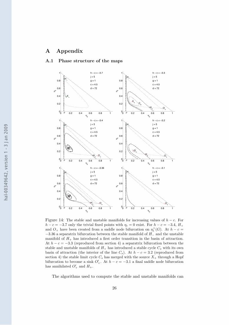
Figure 14: The stable and unstable manifolds for increasing values of h − c. Forh− c = −3.7 only the trivial fixed points with ηc = 0 exist. For h− c = −3.4, H+

and O+ have been created from a saddle node bifurcation on η+1 (G). At h − c =

−3.36 a separatrix bifurcation between the stable manifold of H− and the unstablemanifold of H+ has introduced a first order transition in the basin of attraction.At h− c = −3.3 (reproduced from section 4) a separatrix bifurcation between thestable and unstable manifolds of H+ has introduced a stable cycle Cs with its ownbasin of attraction (the interior of the line Cs). At h − c = 3.2 (reproduced fromsection 4) the stable limit cycle Cs has merged with the source X+ through a Hopfbifurcation to become a sink O′+. At h − c = −3.1 a final saddle node bifurcationhas annihilated O′+ and H+.

The algorithms used to compute the stable and unstable manifolds can

26

hal-0

0349

642,

ver

sion

1 -

3 Ja

n 20

09

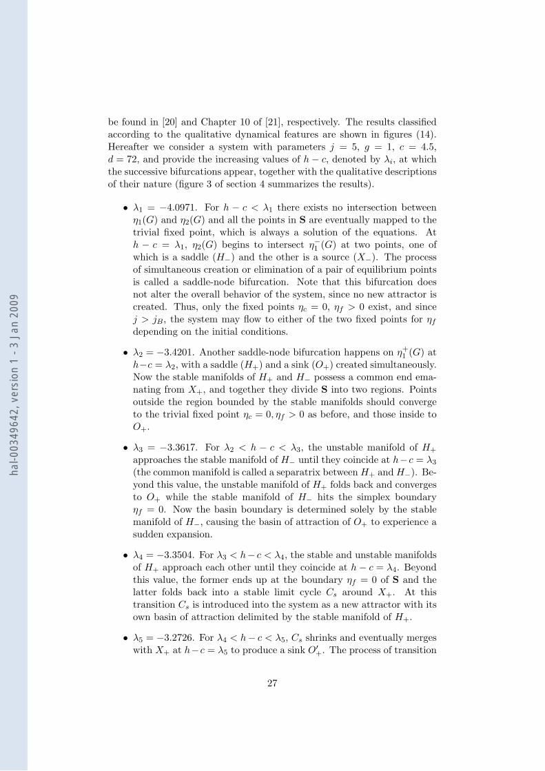
be found in [20] and Chapter 10 of [21], respectively. The results classifiedaccording to the qualitative dynamical features are shown in figures (14).Hereafter we consider a system with parameters j = 5, g = 1, c = 4.5,d = 72, and provide the increasing values of h− c, denoted by λi, at whichthe successive bifurcations appear, together with the qualitative descriptionsof their nature (figure 3 of section 4 summarizes the results).

• λ1 = −4.0971. For h − c < λ1 there exists no intersection betweenη1(G) and η2(G) and all the points in S are eventually mapped to thetrivial fixed point, which is always a solution of the equations. Ath − c = λ1, η2(G) begins to intersect η−1 (G) at two points, one ofwhich is a saddle (H−) and the other is a source (X−). The processof simultaneous creation or elimination of a pair of equilibrium pointsis called a saddle-node bifurcation. Note that this bifurcation doesnot alter the overall behavior of the system, since no new attractor iscreated. Thus, only the fixed points ηc = 0, ηf > 0 exist, and sincej > jB, the system may flow to either of the two fixed points for ηfdepending on the initial conditions.

• λ2 = −3.4201. Another saddle-node bifurcation happens on η+1 (G) at

h−c = λ2, with a saddle (H+) and a sink (O+) created simultaneously.Now the stable manifolds of H+ and H− possess a common end ema-nating from X+, and together they divide S into two regions. Pointsoutside the region bounded by the stable manifolds should convergeto the trivial fixed point ηc = 0, ηf > 0 as before, and those inside toO+.

• λ3 = −3.3617. For λ2 < h − c < λ3, the unstable manifold of H+

approaches the stable manifold of H− until they coincide at h−c = λ3

(the common manifold is called a separatrix between H+ and H−). Be-yond this value, the unstable manifold of H+ folds back and convergesto O+ while the stable manifold of H− hits the simplex boundaryηf = 0. Now the basin boundary is determined solely by the stablemanifold of H−, causing the basin of attraction of O+ to experience asudden expansion.

• λ4 = −3.3504. For λ3 < h− c < λ4, the stable and unstable manifoldsof H+ approach each other until they coincide at h− c = λ4. Beyondthis value, the former ends up at the boundary ηf = 0 of S and thelatter folds back into a stable limit cycle Cs around X+. At thistransition Cs is introduced into the system as a new attractor with itsown basin of attraction delimited by the stable manifold of H+.

• λ5 = −3.2726. For λ4 < h− c < λ5, Cs shrinks and eventually mergeswith X+ at h−c = λ5 to produce a sink O′+. The process of transition

27

hal-0

0349

642,

ver

sion

1 -

3 Ja

n 20

09

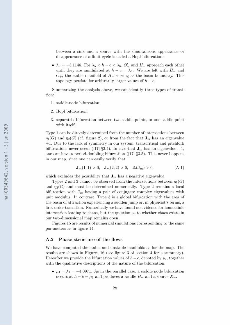
between a sink and a source with the simultaneous appearance ordisappearance of a limit cycle is called a Hopf bifurcation.

• λ6 = −3.1146. For λ5 < h− c < λ6, O′+ and H+ approach each otheruntil they are annihilated at h − c = λ6. We are left with H− andO+, the stable manifold of H− serving as the basin boundary. Thistopology persists for arbitrarily larger values of h− c.

Summarizing the analysis above, we can identify three types of transi-tion:

1. saddle-node bifurcation;

2. Hopf bifurcation;

3. separatrix bifurcation between two saddle points, or one saddle pointwith itself.

Type 1 can be directly determined from the number of intersections betweenη1(G) and η2(G) (cf. figure 2), or from the fact that Jm has an eigenvalue+1. Due to the lack of symmetry in our system, transcritical and pitchforkbifurcations never occur ([17] §3.4). In case that Jm has an eigenvalue −1,one can have a period-doubling bifurcation ([17] §3.5). This never happensin our map, since one can easily verify that

Jm(1, 1) > 0, Jm(2, 2) > 0, ∆(Jm) > 0, (A-1)

which excludes the possibility that Jm has a negative eigenvalue.Types 2 and 3 cannot be observed from the intersections between η1(G)

and η2(G) and must be determined numerically. Type 2 remains a localbifurcation with Jm having a pair of conjugate complex eigenvalues withunit modulus. In contrast, Type 3 is a global bifurcation with the area ofthe basin of attraction experiencing a sudden jump or, in physicist’s terms, afirst-order transition. Numerically we have found no evidence for homoclinicintersection leading to chaos, but the question as to whether chaos exists inour two-dimensional map remains open.

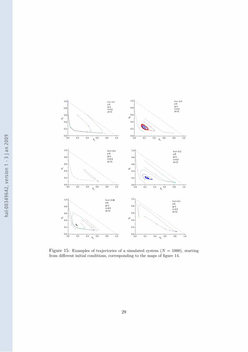
Figures 15 are results of numerical simulations corresponding to the sameparameters as in figure 14.

A.2 Phase structure of the flows

We have computed the stable and unstable manifolds as for the map. Theresults are shown in Figures 16 (see figure 3 of section 4 for a summary).Hereafter we provide the bifurcation values of h− c, denoted by µi, togetherwith the qualitative descriptions of the nature of the bifurcation:

• µ1 = λ1 = −4.0971. As in the parallel case, a saddle node bifurcationoccurs at h− c = µ1 and produces a saddle H− and a source X−.

28

hal-0

0349

642,

ver

sion

1 -

3 Ja

n 20

09

0 , 0 0 , 2 0 , 4 0 , 6 0 , 8 1 , 00 , 0

0 , 2

0 , 4

0 , 6

0 , 8

1 , 0 h - c = - 3 . 7j = 5g = 1c = 4 . 5d = 7 2

η f

η c0 , 0 0 , 2 0 , 4 0 , 6 0 , 8 1 , 0

0 , 0

0 , 2

0 , 4

0 , 6

0 , 8

1 , 0 h - c = - 3 . 3j = 5g = 1c = 4 . 5d = 7 2

η f

η c

0 , 0 0 , 2 0 , 4 0 , 6 0 , 8 1 , 00 , 0

0 , 2

0 , 4

0 , 6

0 , 8

1 , 0 h - c = - 3 . 4j = 5g = 1c = 4 . 5d = 7 2

η f

η c0 , 0 0 , 2 0 , 4 0 , 6 0 , 8 1 , 0

0 , 0

0 , 2

0 , 4

0 , 6

0 , 8

1 , 0

η f

η c

h - c = - 3 . 2j = 5g = 1c = 4 . 5d = 7 2

0 , 0 0 , 2 0 , 4 0 , 6 0 , 8 1 , 00 , 0

0 , 2

0 , 4

0 , 6

0 , 8

1 , 0 h - c = - 3 . 3 6j = 5g = 1c = 4 . 5d = 7 2

η f

η c0 , 0 0 , 2 0 , 4 0 , 6 0 , 8 1 , 0

0 , 0

0 , 2

0 , 4

0 , 6

0 , 8

1 , 0

η f

η c

h - c = - 3 . 1j = 5g = 1c = 4 . 5d = 7 2

Figure 15: Examples of trajectories of a simulated system (N = 1000), startingfrom different initial conditions, corresponding to the maps of figure 14.

29

hal-0

0349

642,

ver

sion

1 -

3 Ja

n 20

09

0 0.2 0.4 0.6 0.8 10

0.2

0.4

0.6

0.8

1

!c

!f

"

H−

X−

h − c = −3.7j = 5g = 1c = 4.5d = 72

0 0.2 0.4 0.6 0.8 10

0.2

0.4

0.6

0.8

1

!c

!f

"

H−

O+’

O+H+

h − c = −3.3j = 5g = 1c = 4.5d = 72

0 0.2 0.4 0.6 0.8 10

0.2

0.4

0.6

0.8

1

!c

!f

"

H−

O−# $Cu

h − c = −3.6j = 5g = 1c = 4.5d = 72

0 0.2 0.4 0.6 0.8 10

0.2

0.4

0.6

0.8

1

!c

!f

"

H−

O+

h − c = −3.1j = 5g = 1c = 4.5d = 72

0 0.2 0.4 0.6 0.8 10

0.2

0.4

0.6

0.8

1

!c

!f

"

H−

O+’

h − c = −3.46j = 5g = 1c = 4.5d = 72

0 0.2 0.4 0.6 0.8 10

0.2

0.4

0.6

0.8

1

!c

!f

"

H−

X+ Cs

h − c = −3.423j = 5g = 1c = 3.2d = 28

Figure 16: The stable and unstable manifolds for the flow for h−c = 3.7 (Comparewith figure 14 with the same value of h− c). At h− c = −3.6, a sink O− togetherwith an unstable limit cycle Cu have emerged from the source X− through a Hopfbifurcation. At h − c = −3.46 a separatrix bifurcation has eliminated Cu andexpanded the basin of attraction of the sink. At h − c = −3.3, H+ and O+ havebeen created from a saddle node bifurcation on η+

1 (G) (Compare with figure 14for the same value of h − c). For h − c = −3.1 a final saddle node bifurcationhas annihilated O′+ and H+ (compare with Figure 14 for the same value of h− c).Notice that the figure on the bottom (right) shows a cycle that arises for otherparameters c and d.

30

hal-0

0349

642,

ver

sion

1 -

3 Ja

n 20

09

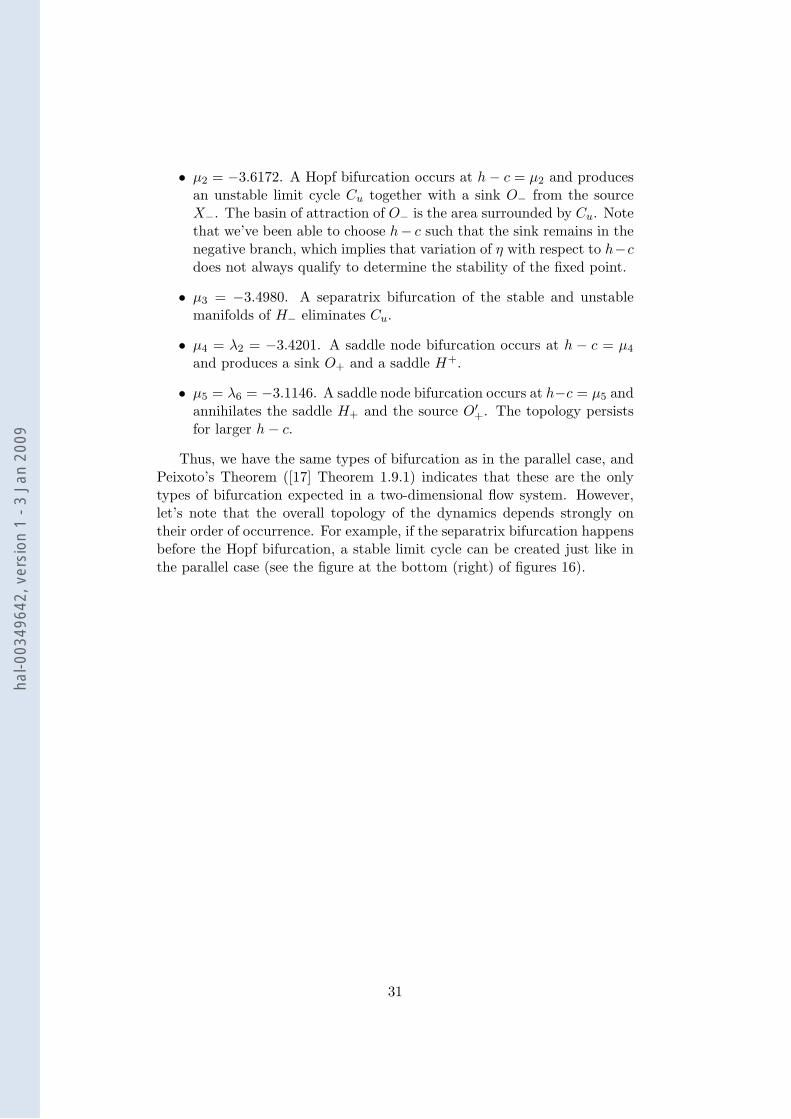
• µ2 = −3.6172. A Hopf bifurcation occurs at h− c = µ2 and producesan unstable limit cycle Cu together with a sink O− from the sourceX−. The basin of attraction of O− is the area surrounded by Cu. Notethat we’ve been able to choose h− c such that the sink remains in thenegative branch, which implies that variation of η with respect to h−cdoes not always qualify to determine the stability of the fixed point.

• µ3 = −3.4980. A separatrix bifurcation of the stable and unstablemanifolds of H− eliminates Cu.

• µ4 = λ2 = −3.4201. A saddle node bifurcation occurs at h − c = µ4

and produces a sink O+ and a saddle H+.

• µ5 = λ6 = −3.1146. A saddle node bifurcation occurs at h−c = µ5 andannihilates the saddle H+ and the source O′+. The topology persistsfor larger h− c.

Thus, we have the same types of bifurcation as in the parallel case, andPeixoto’s Theorem ([17] Theorem 1.9.1) indicates that these are the onlytypes of bifurcation expected in a two-dimensional flow system. However,let’s note that the overall topology of the dynamics depends strongly ontheir order of occurrence. For example, if the separatrix bifurcation happensbefore the Hopf bifurcation, a stable limit cycle can be created just like inthe parallel case (see the figure at the bottom (right) of figures 16).

31

hal-0

0349

642,

ver

sion

1 -

3 Ja

n 20

09