1

CVC: The Contourlet Video Compression algorithm for real-time applications Stamos Katsigiannis, Georgios Papaioannou, and Dimitris Maroulis

S. Katsigiannis and D. Maroulis are with the Real-time Systems and Image Analysis Group, Department of Informatics and Telecommunications, National and Kapodistrian University of Athens, Panepistimioupolis, Ilisia, 15703 Athens, Greece. G. Papaioannou is with the Computer Graphics Group, Department of Informatics, Athens University of Economics and Business, 76 Patission Str., 10434, Athens, Greece.

Abstract. Nowadays, real-time video communication over the internet through video conferencing

applications has become an invaluable tool in everyone’s professional and personal life. This trend

underlines the need for video coding algorithms that provide acceptable quality on low bitrates and

can support various resolutions inside the same stream in order to cope with limitations on

computational resources and network bandwidth. In this work, a novel scalable video coding

algorithm based on the contourlet transform is presented. The algorithm utilizes both lossy and

lossless methods in order to achieve compression. One of its most notable features is that due to

the transform utilised, it does not suffer from blocking artifacts that occur with many widely

adopted compression algorithms. The proposed algorithm takes advantage of the vast

computational capabilities of modern GPUs, in order to achieve real-time performance and provide

satisfactory encoding and decoding times at relatively low cost, making it suitable for applications

like video conferencing. Experiments show that the proposed algorithm performs satisfactorily in

terms of compression ratio and speed, while it outperforms standard methods in terms of

perceptual quality on lower bitrates.

Keywords: real-time video encoding, GPU computing, video conferencing,

surveillance video, contourlet transform

2

1 Introduction

Real-time video communications over computer networks are being

extensively utilised in order to provide video conferencing and other video

streaming applications. Transmitting and receiving video data over the internet

and other heterogeneous IP networks is a challenging task due to limitations on

bandwidth and computational power, as well as caching inefficiency. The

increased cost of computational and network resources underlines the need for

highly efficient video coding algorithms that could be successfully utilised under

the limited resources of casual users, i.e. commodity devices with limited

bandwidth.

The most desirable characteristic of such an algorithm would be the ability

to maintain satisfactory visual quality while achieving enough compression in

order to meet the low bandwidth requirement. Low computational complexity and

real-time performance would also be an advantage since it would allow the

algorithm to be used in a wide variety of less powerful devices. Especially in the

case of video conferencing, real-time encoding and decoding is necessary. Taking

into consideration the diversity of available hardware and bandwidth among users,

the algorithm should also have the ability to adapt to the network’s end-to-end

bandwidth and transmitter/receiver resources.

State of the art video compression algorithms that are commonly utilised

for stored video content cannot achieve both optimal compression and real-time

performance without the use of dedicated hardware, due to their high

computational complexity. Moreover, they depend on multipass statistical and

structural analysis of the whole video content in order to achieve optimal quality

and compression. This procedure is acceptable for stored video content but cannot

be performed in cases of live video stream generation as in the case of video

conferencing. Another disadvantage of popular Discrete Cosine Transform

(DCT)-based algorithms like H.264 [1], VP8 [2], other algorithms belonging to

the MPEG family, etc. is that at low bitrates they introduce visible block artifacts

that distract the viewers and degrade the communication experience. In order to

cope with this problem, deblocking filters are utilised either as an optional post

processing step or as part of the compression algorithm. Nevertheless, in both

cases this constitutes a separate processing layer that increases the computational

complexity.

3

Most state of the art video and image encoding algorithms require the

transformation of visual information from the spatial (pixel) intensity to the

frequency domain before any further manipulation (e.g. JPEG [3], JPEG2000 [4],

MPEG1&2 [5][6], H.264 [1], VP8 [2]). Frequency domain methods like the

Fourier Transform, the Discrete Cosine Transform (DCT), and the Wavelet

Transform (WT) have been extensively exploited in image and video encoding, as

they offer advantages such as reversibility, compact representations, efficient

coding, capturing of structural characteristics, etc [7].

In this work, we extend the proof-of-concept contourlet-based video

compression algorithm that was introduced in [8], and propose CVC, a complete

algorithm that is able to achieve increased compression efficiency while

minimizing the loss of visual quality. The proposed algorithm is based on the

Contourlet Transform (CT) [9], a reversible transform that offers multiscale and

directional decomposition, providing anisotropy and directionality [9], features

missing from traditional transforms like the DCT and WT. The CT has been

utilised in a variety of image analysis applications, including denoising [10][11],

medical and natural image classification [12], image fusion [13], image

enhancement [14], etc. An important aspect of the CT is its efficient parallel

implementation. Despite its computational complexity, by taking advantage of the

fast parallel calculations performed on modern graphics processing units (GPUs),

a GPU-based encoder is able to provide all the CT’s benefits, while achieving

real-time performance in commodity hardware.

The proof-of-concept algorithm performed real-time video encoding,

targeting content obtained from low resolution sources like web cameras,

surveillance cameras, etc. and experiments showed promising results. Although it

provided satisfactory visual quality, it lacked some basic elements that would

provide sufficient compression efficiency. The most important observation is that

the previous version performed the CT on the luminance channel and only

subsampled the chrominance channels. This handling of the chrominance

channels was insufficient for high frame quality at low bitrates, however. In this

paper, the revised compression scheme (CVC) performs the CT decomposition on

all channels and combines this with chrominance subsampling. Additionally, the

lack of a variable-length entropy encoding scheme did not allow it to compete in

terms of compression with current state-of-the-art algorithms, a problem solved in

4

the proposed version by the utilization of the DEFLATE algorithm. Combined

with an additional lossless filtering step that enhances the compressibility of the

data and a mechanism for producing scalable or non-scalable transmission

streams, CVC can achieve increased versatility and efficiency in terms of

compression. Moreover, CVC introduces a new quantization strategy for the

components of the video stream in order to address the limitations of the previous

scheme that only supported three quality levels by utilising custom quantization

matrices targeting low, medium and high visual quality. Finally, temporal

redundancy is now addressed using motion estimation techniques and CVC’s

performance is evaluated against other video compression algorithms.

The rest of this paper is organised in four sections. Section 2 provides

some important background knowledge, while the proposed algorithm is

presented in detail in Section 3. The experimental study for its evaluation is

provided in Section 4 and finally conclusions are drawn in Section 5.

2 Background

2.1 The Contourlet Transform

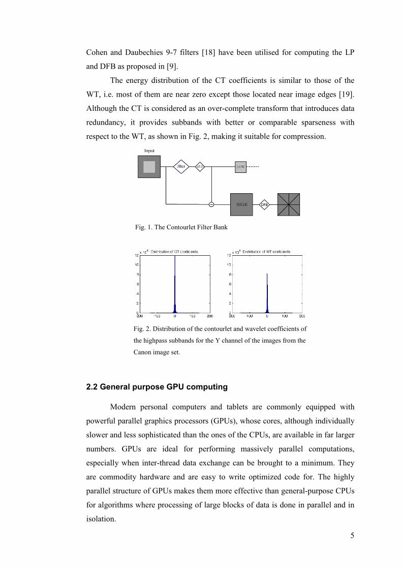
The Contourlet Transform (CT) [9] is a multiscale image representation

scheme that provides directionality and anisotropy, and is effective in representing

smooth contours in different directions on an image. The method is realized as a

double filter bank consisting of first, the Laplacian Pyramid (LP) [15] and

subsequently, the Directional Filter Bank (DFB) [16]. The DFB is a 2D

directional filter bank that can achieve perfect reconstruction and the simplified

DFB used for the CT decomposes the image into 2l subbands with wedge-shaped

frequency partitioning [17], with l being the level of decomposition. In each LP

level, the image is decomposed into a downsampled lowpass version of the

original image and a more detailed image, containing the supplementary high

frequencies, which is fed into a DFB in order to capture the directional

information. The combined result is a double iterated filter bank that decomposes

images into directional subbands at multiple scales and is called the Contourlet

Filter Bank (Fig. 1). This scheme can be iterated continuously in the lowpass

image and provides a way to obtain multiscale decomposition. In this work, the

5

Cohen and Daubechies 9-7 filters [18] have been utilised for computing the LP

and DFB as proposed in [9].

The energy distribution of the CT coefficients is similar to those of the

WT, i.e. most of them are near zero except those located near image edges [19].

Although the CT is considered as an over-complete transform that introduces data

redundancy, it provides subbands with better or comparable sparseness with

respect to the WT, as shown in Fig. 2, making it suitable for compression.

Fig. 1. The Contourlet Filter Bank

Fig. 2. Distribution of the contourlet and wavelet coefficients of

the highpass subbands for the Y channel of the images from the

Canon image set.

2.2 General purpose GPU computing

Modern personal computers and tablets are commonly equipped with

powerful parallel graphics processors (GPUs), whose cores, although individually

slower and less sophisticated than the ones of the CPUs, are available in far larger

numbers. GPUs are ideal for performing massively parallel computations,

especially when inter-thread data exchange can be brought to a minimum. They

are commodity hardware and are easy to write optimized code for. The highly

parallel structure of GPUs makes them more effective than general-purpose CPUs

for algorithms where processing of large blocks of data is done in parallel and in

isolation.

6

In this paper, the most computationally intensive steps of the proposed

algorithm are processed on the GPU. For our GPU implementation, the NVIDIA

Compute Unified Device Architecture (CUDA) [20] has been selected due to the

extensive capabilities and optimized API it provides.

2.3 The YCoCg colour space

The RGB-to-YCoCg transform decomposes a colour image into luminance

(Y), orange chrominance (Co) and green chrominance (Cg) components. It was

developed primarily to address some limitations of the different YCbCr colour

spaces and has been shown to exhibit better decorrelation properties than YCbCr

and similar transforms [21]. The YCoCg colour space has been utilised in various

applications like the H264 compression algorithm, on a real-time RGB frame

buffer compression scheme using chrominance subsampling [22], etc. The

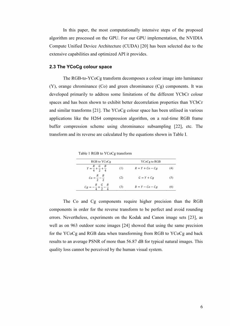
transform and its reverse are calculated by the equations shown in Table I.

Table 1 RGB to YCoCg transform

RGB to YCoCg YCoCg to RGB

𝑌 =𝑅4

+𝐺2

+𝐵4

(1) 𝑅 = 𝑌 + 𝐶𝐶 − 𝐶𝐶 (4)

𝐶𝐶 =𝑅2−𝐵2

(2) 𝐺 = 𝑌 + 𝐶𝐶 (5)

𝐶𝐶 = −𝑅4

+𝐺2−𝐵4

(3) 𝐵 = 𝑌 − 𝐶𝐶 − 𝐶𝐶 (6)

The Co and Cg components require higher precision than the RGB

components in order for the reverse transform to be perfect and avoid rounding

errors. Nevertheless, experiments on the Kodak and Canon image sets [23], as

well as on 963 outdoor scene images [24] showed that using the same precision

for the YCoCg and RGB data when transforming from RGB to YCoCg and back

results to an average PSNR of more than 56.87 dB for typical natural images. This

quality loss cannot be perceived by the human visual system.

7

3 Algorithm overview

3.1 RGB to YCoCg transform and Chroma subsampling

Assuming that input frames are encoded in the RGB colour space with 8

bit colour depth for each chrominance channel, the first step of the algorithm is

the conversion from RGB to YCoCg colour space.

The next step is the subsampling of the chrominance channels. It is well

established in literature that the human visual system is significantly more

sensitive to variations of luminance compared to variations of chrominance.

Exploiting this fact, the encoding of the luminance channel of an image with

higher accuracy than the chrominance channels provides a low complexity

compression scheme that achieves satisfactory visual quality, while offering

significant compression. This technique, commonly referred to as chroma

subsampling, is utilised by various image and video compression algorithms. In

this work, the chrominance channels are subsampled by a user-defined factor N

that directly affects the output’s visual quality and compression.

Then, the Co and Cg channels are normalized to the range [0, 255]. Since

the range of values for the Co and Cg channels is [-127 , 127] for images with 8

bit depth colour per channel in the RGB colour space, as can be derived by the

equations 2-3, normalization is performed very fast by adding 127 to every

element. For the reconstruction of the chrominance channels at the decoding

stage, the Co and Cg channels are normalized to their original range of values by

subtracting 127 from each element and the missing chrominance values are

replaced by using bilinear interpolation from the four neighboring pixels.

3.2 Motion estimation

Motion estimation is performed on the luminance channel of the video in

order to exploit the temporal redundancy between consecutive frames. The

luminance channel is divided into blocks of size 16x16 and a full search block-

matching algorithm is utilised in order to calculate the motion vectors between the

current and the previous frame. The maximum displacement between a block and

a target block is set as W pixels, leading to (2W+1)2 possible blocks including the

original block, with W being user defined. The Mean Squared Error (MSE) is used

as the similarity measure for comparing blocks. Although the full search

8

algorithm is an exhaustive search algorithm that significantly increases the

computational complexity, it can be efficiently computed in parallel using the

capabilities of the GPU and thus is selected due to its simplicity. Contrary to

traditional video coding algorithms, the motion-compensated prediction is not

applied on the spatial domain (i.e. the raw frame) at this step, but on the contourlet

domain, as explained on Section 3.7.

3.3 Contourlet Transform decomposition

At this step, all channels are decomposed using the CT. Decomposing into

multiple levels using the LP provides the means to separately store different scales

of the input that can be in turn individually decoded, thus providing the desirable

scalability feature of the algorithm, i.e. multiple resolutions inside the same video

stream. At each level, CT decomposition provides a lowpass image of half the

resolution of the previous scale and the directional subbands containing the

supplementary high frequencies. For example, decomposition of 2 levels of a

VGA (640x480) video provides a video stream containing the VGA, QVGA

(320x240) and QQVGA (160x120) resolutions. The final result contains the

lowpass image of the coarsest scale and the directional subbands of each scale.

This property allows CVC to adapt to the network’s end-to-end bandwidth and

transmitter/receiver resources. The quality for each receiver can be adjusted by

just dropping the encoded information referring to higher resolution than

requested, without the need to re-encode the video frames at the source.

Moreover, due to the downsampling of the lowpass component at each scale, it

provides enhanced compression.

3.4 Normalization of lowpass component

The lowpass component provided by the CT decomposition is

subsequently normalized to the range [0 , 255] in order for its values to fit to 8 bit

variables. Experiments on a large number of images from various datasets showed

that precision loss due to this normalization is negligible or non-existent

depending on the method utilised. It must be noted that during the decoding

phase, the lowpass component has to be restored to its correct range.

9

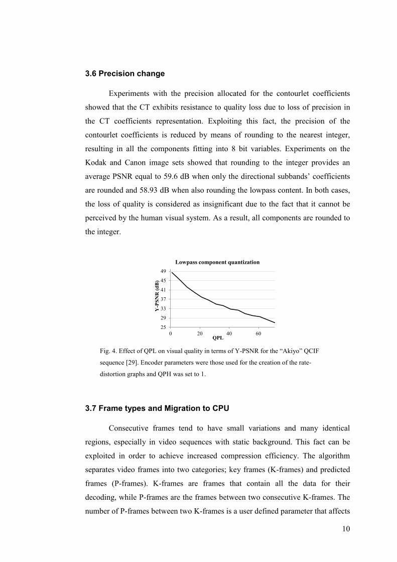
3.5 CT coefficients reduction

In order to compress and transmit/store only perceptually significant

information and therefore decrease the bandwidth demands further, the number of

different values for the CT coefficients of the directional subbands, as well as for

the elements of the lowpass component, is reduced by means of quantization.

Quantization is achieved through dividing each element by a user-defined

parameter and then rounding to the integer, as explained on the next step of the

algorithm. Two separate quantization parameters are used: QPH for the

directional subbands and QPL for the lowpass component. QPH takes values in

the range [1 , 181]. A QPH of 1 means that no element of the directional subbands

is altered, while when QPH=181, all the directional subband elements are reduced

to zero. Intermediate values determine the range of the quantized values that can

be assigned to CT coefficients. QPL takes values in the range of [1 , 71], with a

QPL of 1 meaning that no element of the lowpass component is altered. Although

QPL values higher than 71 are possible, the visual quality degradation is severe,

as shown in Fig. 4. As a result, the value 71 has been selected as the maximum

QPL value. The maximum QPH was selected through experimental evaluation.

This quantization step reduces the number of distinct values an element

inside the video stream can take, effectively increasing the compressibility of the

data. Higher valued quantization parameters provide higher compression and

worse visual quality, while lower valued parameters provide the opposite result.

The effect of the quantization procedure in terms of quality is shown in Fig. 3 and

4.

Fig. 3. Effect of QPH on visual quality in terms of Y-PSNR for the “Akiyo” QCIF

sequence [29]. Encoder parameters were those used for the creation of the rate-distortion

graphs and QPL was set to 1.

30

34

38

42

46

50

0 50 100 150

Y-P

SNR

(dB

)

QPH

Directional subbands quantization

10

3.6 Precision change

Experiments with the precision allocated for the contourlet coefficients

showed that the CT exhibits resistance to quality loss due to loss of precision in

the CT coefficients representation. Exploiting this fact, the precision of the

contourlet coefficients is reduced by means of rounding to the nearest integer,

resulting in all the components fitting into 8 bit variables. Experiments on the

Kodak and Canon image sets showed that rounding to the integer provides an

average PSNR equal to 59.6 dB when only the directional subbands’ coefficients

are rounded and 58.93 dB when also rounding the lowpass content. In both cases,

the loss of quality is considered as insignificant due to the fact that it cannot be

perceived by the human visual system. As a result, all components are rounded to

the integer.

Fig. 4. Effect of QPL on visual quality in terms of Y-PSNR for the “Akiyo” QCIF

sequence [29]. Encoder parameters were those used for the creation of the rate-

distortion graphs and QPH was set to 1.

3.7 Frame types and Migration to CPU

Consecutive frames tend to have small variations and many identical

regions, especially in video sequences with static background. This fact can be

exploited in order to achieve increased compression efficiency. The algorithm

separates video frames into two categories; key frames (K-frames) and predicted

frames (P-frames). K-frames are frames that contain all the data for their

decoding, while P-frames are the frames between two consecutive K-frames. The

number of P-frames between two K-frames is a user defined parameter that affects

25

29

33

37

41

45

49

0 20 40 60

Y-P

SNR

(dB

)

QPL

Lowpass component quantization

11

the total number of K-frames inside a video stream. P-frames are encoded

similarly to K-frames up to this step.

For the K-frames, a simple lossless filtering method is applied in order to

enhance the compressibility of the lowpass component. At each lowpass

component’s column, each element’s value is calculated by subtracting the value

of the element above. Neighboring elements tend to have close values. As a result,

a filtered column will have elements with values clustered near zero, providing

more compressible data due to the large number of zero-valued sequences of bits

inside the bit stream. Filtering is performed across the columns. An example of

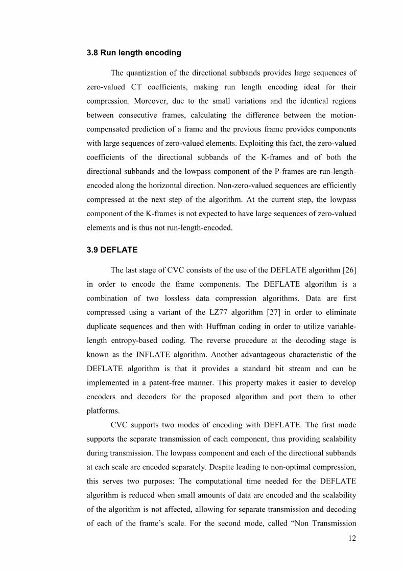
gain in compression is shown in Fig. 5.

If a frame is identified as a P-frame, all its components are calculated as

the difference between the motion-compensated prediction of the components of

the current frame and the respective components of the previous frame. Motion-

compensated prediction is applied on the CT components of the frame in order to

avoid the emergence of artifacts during the CT reconstruction process at the

decoding stage. If the prediction is applied on the raw frame, the calculation of the

difference provides artificial edges in the image that produce CT coefficients of

significant magnitude. Lowering the precision of these coefficients leads to the

emergence of artifacts that significantly distort the output image, especially at

higher compression levels. Since the CT coefficients are spatially related [25], this

problem is avoided by applying the CT on the original frame and then performing

the motion-compensated prediction on each CT component by mapping the

motion vectors to the corresponding scale and range for each component.

After performing the frame-type-specific operations, all components are

passed from the GPU memory to the main memory. Computations up to this point

are all performed on the GPU, avoiding unnecessary memory transfers from the

main memory to the GPU memory and vice versa. The input frame is passed to

the GPU at the beginning of the encoding process and at this step the encoded

components are returned to the main memory. Computations from this point on

are executed on the CPU, since they are inherently serial (run-length encoding,

DEFLATE). Processing those steps on the GPU would provide worse

performance than on the host CPU.

12

3.8 Run length encoding

The quantization of the directional subbands provides large sequences of

zero-valued CT coefficients, making run length encoding ideal for their

compression. Moreover, due to the small variations and the identical regions

between consecutive frames, calculating the difference between the motion-

compensated prediction of a frame and the previous frame provides components

with large sequences of zero-valued elements. Exploiting this fact, the zero-valued

coefficients of the directional subbands of the K-frames and of both the

directional subbands and the lowpass component of the P-frames are run-length-

encoded along the horizontal direction. Non-zero-valued sequences are efficiently

compressed at the next step of the algorithm. At the current step, the lowpass

component of the K-frames is not expected to have large sequences of zero-valued

elements and is thus not run-length-encoded.

3.9 DEFLATE

The last stage of CVC consists of the use of the DEFLATE algorithm [26]

in order to encode the frame components. The DEFLATE algorithm is a

combination of two lossless data compression algorithms. Data are first

compressed using a variant of the LZ77 algorithm [27] in order to eliminate

duplicate sequences and then with Huffman coding in order to utilize variable-

length entropy-based coding. The reverse procedure at the decoding stage is

known as the INFLATE algorithm. Another advantageous characteristic of the

DEFLATE algorithm is that it provides a standard bit stream and can be

implemented in a patent-free manner. This property makes it easier to develop

encoders and decoders for the proposed algorithm and port them to other

platforms.

CVC supports two modes of encoding with DEFLATE. The first mode

supports the separate transmission of each component, thus providing scalability

during transmission. The lowpass component and each of the directional subbands

at each scale are encoded separately. Despite leading to non-optimal compression,

this serves two purposes: The computational time needed for the DEFLATE

algorithm is reduced when small amounts of data are encoded and the scalability

of the algorithm is not affected, allowing for separate transmission and decoding

of each of the frame’s scale. For the second mode, called “Non Transmission

13

Scalable CVC” (CVC-NTS), all the components of a frame are encoded together

using DEFLATE. CVC-NTS does not allow the independent transmission of

separate scales of the video stream but each scale can still be decoded separately,

thus providing scalability at the decoding stage.

Fig. 5. Rate-distortion graph for the “Akiyo” QCIF sequence when lowpass component

filtering is applied (F) and when not applied (NF).

3.10 GPU implementation

In order to encode a video frame using CVC, the raw frame’s data are first

transferred to the GPU memory. Then the next steps of the algorithm are

computed on the GPU up to the run-length encoding step, where the encoded

components of the frame are transferred to the main memory. Run-length

encoding and DEFLATE are inherently serial algorithms and cannot be

effectively parallelized. For the GPU implementation of the algorithm, all its steps

are mapped to their respective parallel equivalents and can be grouped into four

main categories: 1) Operations applied to each element of a 2D array

independently, 2) Operations applied to specific chunks of a 2D array, e.g. for

every column or row of the array, 3) Operations specific to the Fast Fourier

Transform (FFT) calculations needed for computing a 2D convolution, and 4)

Operations referring to the motion estimation and motion compensation steps.

Resource allocation is done according to the CUDA guidelines in order to exploit

the advantages of the CUDA scalable programming model [28].

23

27

31

35

39

43

47

0 10 20 30 40

Y-P

SNR

(dB

)

Bit rate (kbit/frame)

Lowpass component filtering

CVC (F)

CVC (NF)

14

4 Quality and performance analysis

4.1 Compression and visual quality

In order to evaluate the performance of CVC, three publicly available

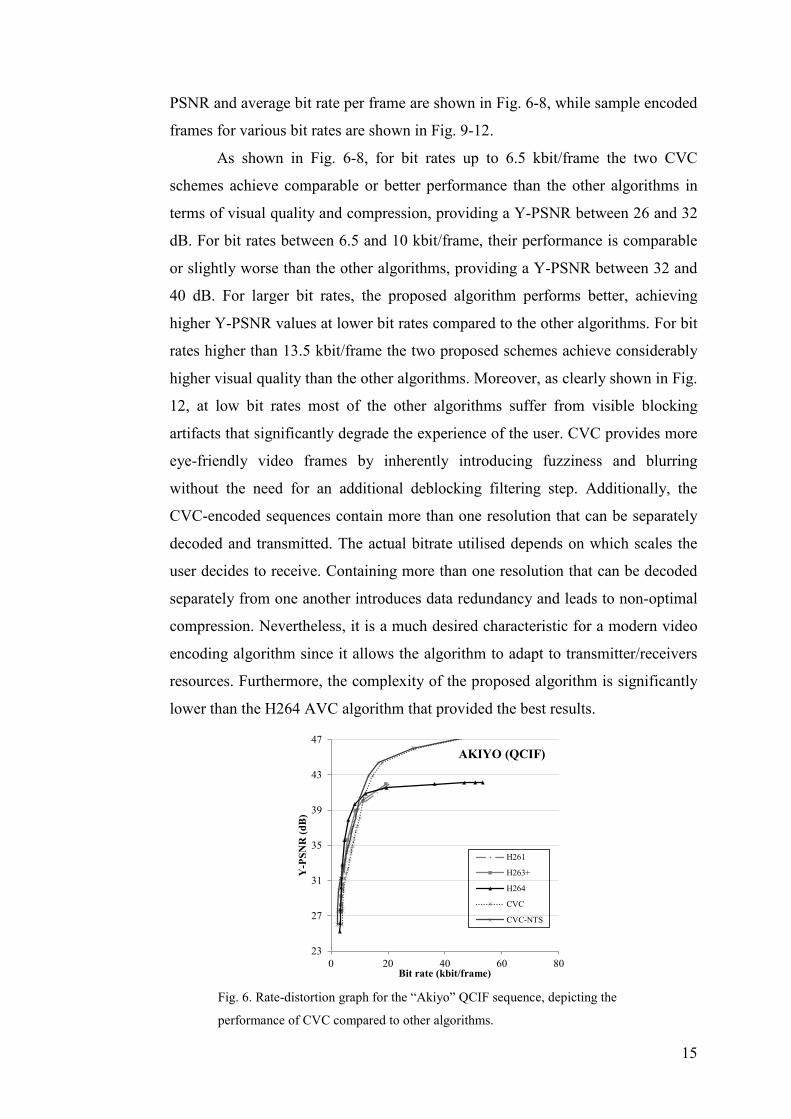
video sequences [29], commonly used in video encoding experiments, were

encoded. The first two videos (Akiyo, Claire) depict the upper part of the human

body and static background in order to resemble video conferencing sequences.

The third video (Hall monitor) depicts a hall area with static background and

occasional movement of people, resembling a video surveillance sequence. The

resolution of the video sequences was QCIF and their frame rate 15 fps.

Rate-distortion graphs for each video sequence reporting the average Y-

PSNR and average bit rate per frame are shown in Fig. 6-8. The chrominance

channels of the video samples were downsampled by a factor of N=4 before being

decomposed using the CT and the video stream contained the original, as well as

half that resolution. The W parameter for motion estimation was set to 8 pixels

and the contourlet coefficients of both the luminance and chrominance channels

were quantized using the whole range of QPH supported by CVC. For each

encoding, QPL was set to QPH/14 in order to balance lowpass and highpass

content degradation. Τhe interval between the K-frames was set to 10 frames.

Videos were encoded using both the scalable CVC and CVC-NTS schemes.

The video sequences were also encoded using widely adopted video

compression algorithms in order to evaluate the performance of the CVC. The

compression algorithms tested were the H261 [30], H263+ [31], and H264 AVC

[1]. The libraries included into the FFmpeg framework [32] were utilised for the

encoding with the first two algorithms and the x264 encoder [33] was used for

H264 AVC. In order to simulate the application scenarios targeted by CVC, i.e.

live video creation like video conferencing, all the encoders were set to one-pass

encoding, with the same interval between key frames (intra frames) as selected for

the CVC, i.e. 10. Additionally, the baseline profile was selected for H264 AVC,

without using CABAC [34] due to the real-time restriction. In order to provide

comparable results, quantization-based encoding was selected and multiple

quantization parameters were tested: the lowest, the highest and intermediate

samples. Rate-distortion graphs for each video sample reporting the average Y-

15

PSNR and average bit rate per frame are shown in Fig. 6-8, while sample encoded

frames for various bit rates are shown in Fig. 9-12.

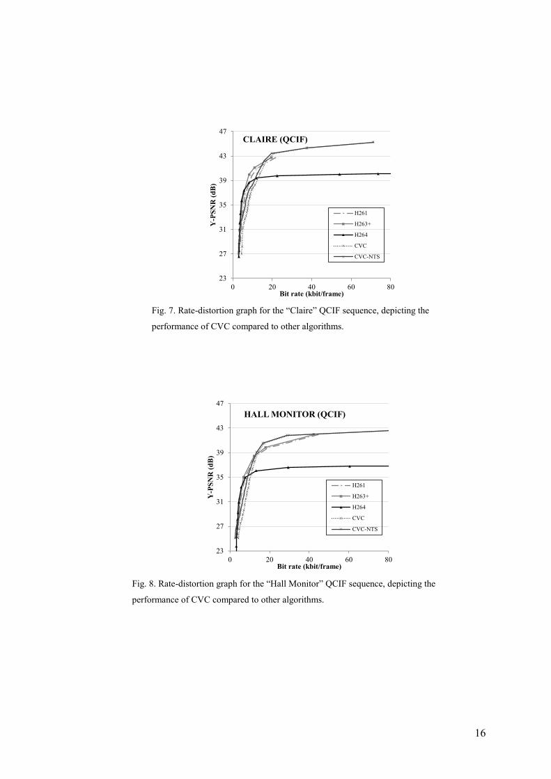
As shown in Fig. 6-8, for bit rates up to 6.5 kbit/frame the two CVC

schemes achieve comparable or better performance than the other algorithms in

terms of visual quality and compression, providing a Y-PSNR between 26 and 32

dB. For bit rates between 6.5 and 10 kbit/frame, their performance is comparable

or slightly worse than the other algorithms, providing a Y-PSNR between 32 and

40 dB. For larger bit rates, the proposed algorithm performs better, achieving

higher Y-PSNR values at lower bit rates compared to the other algorithms. For bit

rates higher than 13.5 kbit/frame the two proposed schemes achieve considerably

higher visual quality than the other algorithms. Moreover, as clearly shown in Fig.

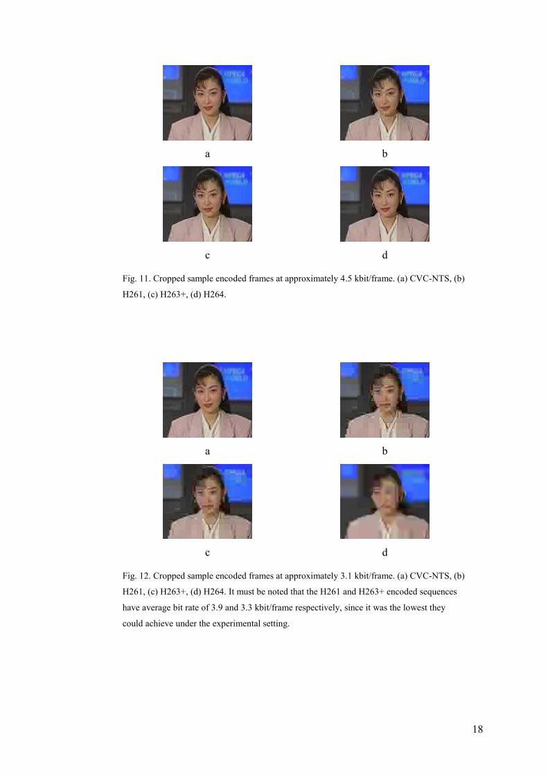
12, at low bit rates most of the other algorithms suffer from visible blocking

artifacts that significantly degrade the experience of the user. CVC provides more

eye-friendly video frames by inherently introducing fuzziness and blurring

without the need for an additional deblocking filtering step. Additionally, the

CVC-encoded sequences contain more than one resolution that can be separately

decoded and transmitted. The actual bitrate utilised depends on which scales the

user decides to receive. Containing more than one resolution that can be decoded

separately from one another introduces data redundancy and leads to non-optimal

compression. Nevertheless, it is a much desired characteristic for a modern video

encoding algorithm since it allows the algorithm to adapt to transmitter/receivers

resources. Furthermore, the complexity of the proposed algorithm is significantly

lower than the H264 AVC algorithm that provided the best results.

Fig. 6. Rate-distortion graph for the “Akiyo” QCIF sequence, depicting the

performance of CVC compared to other algorithms.

23

27

31

35

39

43

47

0 20 40 60 80

Y-P

SNR

(dB

)

Bit rate (kbit/frame)

AKIYO (QCIF)

H261

H263+

H264

CVC

CVC-NTS

16

Fig. 7. Rate-distortion graph for the “Claire” QCIF sequence, depicting the

performance of CVC compared to other algorithms.

Fig. 8. Rate-distortion graph for the “Hall Monitor” QCIF sequence, depicting the

performance of CVC compared to other algorithms.

23

27

31

35

39

43

47

0 20 40 60 80

Y-P

SNR

(dB

)

Bit rate (kbit/frame)

CLAIRE (QCIF)

H261

H263+

H264

CVC

CVC-NTS

23

27

31

35

39

43

47

0 20 40 60 80

Y-P

SNR

(dB

)

Bit rate (kbit/frame)

HALL MONITOR (QCIF)

H261

H263+

H264

CVC

CVC-NTS

17

a b

c d

Fig. 9. Cropped sample encoded frames at approximately 20 kbit/frame. (a) CVC-NTS, (b)

H261, (c) H263+, (d) H264.

a b

c d

Fig. 10. Cropped sample encoded frames at approximately 11 kbit/frame. (a) CVC-NTS, (b)

H261, (c) H263+, (d) H264.

18

a b

c d

Fig. 11. Cropped sample encoded frames at approximately 4.5 kbit/frame. (a) CVC-NTS, (b)

H261, (c) H263+, (d) H264.

a b

c d

Fig. 12. Cropped sample encoded frames at approximately 3.1 kbit/frame. (a) CVC-NTS, (b)

H261, (c) H263+, (d) H264. It must be noted that the H261 and H263+ encoded sequences

have average bit rate of 3.9 and 3.3 kbit/frame respectively, since it was the lowest they

could achieve under the experimental setting.

19

4.2 Execution times

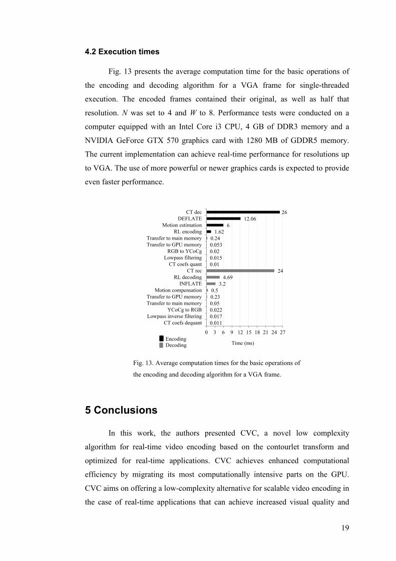
Fig. 13 presents the average computation time for the basic operations of

the encoding and decoding algorithm for a VGA frame for single-threaded

execution. The encoded frames contained their original, as well as half that

resolution. N was set to 4 and W to 8. Performance tests were conducted on a

computer equipped with an Intel Core i3 CPU, 4 GB of DDR3 memory and a

NVIDIA GeForce GTX 570 graphics card with 1280 MB of GDDR5 memory.

The current implementation can achieve real-time performance for resolutions up

to VGA. The use of more powerful or newer graphics cards is expected to provide

even faster performance.

Fig. 13. Average computation times for the basic operations of

the encoding and decoding algorithm for a VGA frame.

5 Conclusions

In this work, the authors presented CVC, a novel low complexity

algorithm for real-time video encoding based on the contourlet transform and

optimized for real-time applications. CVC achieves enhanced computational

efficiency by migrating its most computationally intensive parts on the GPU.

CVC aims on offering a low-complexity alternative for scalable video encoding in

the case of real-time applications that can achieve increased visual quality and

0.0110.0170.0220.050.230.5

3.24.69

240.010.0150.020.0530.24

1.626

12.0626

0 3 6 9 12 15 18 21 24 27

CT coefs dequantLowpass inverse filtering

YCoCg to RGBTransfer to main memoryTransfer to GPU memory

Motion compensationINFLATE

RL decodingCT rec

CT coefs quantLowpass filtering

RGB to YCoCgTransfer to GPU memoryTransfer to main memory

RL encodingMotion estimation

DEFLATECT dec

Time (ms)EncodingDecoding

20

satisfactory compression, while harnessing the underutilized computational power

of modern personal computers.

The incorporation of the DEFLATE algorithm, the CT decomposition of

the chrominance channels, the motion estimation, the quantization of CT

coefficients and the filtering of the lowpass component provided increased

compression efficiency and enhanced visual quality compared to the preliminary

version of the algorithm [8]. Furthermore, the new quantization scheme offers

support for a wide range of compression and visual quality levels, providing the

requisite flexibility for a modern video compression algorithm. The scalable video

compression scheme, inherently achieved through the CT decomposition, is ideal

for video conferencing content and can support scalability for decoding and

transmission, depending on the scheme selected.

CVC achieves comparable performance with the algorithms examined in

the case of lower visual quality and higher compression, while achieving

comparable or slightly worse performance at medium levels of compression and

quality. Nevertheless, it outperforms the examined algorithms in the case of

higher visual quality. Moreover, in cases of higher compression, the algorithm

does not suffer from blocking artifacts and the visual quality degradation is much

more eye-friendly than with other well-established video compression methods, as

it introduces fuzziness and blurring, providing smoother images.

References

[1] ITU-T Recommendation H.264: Advanced video coding for generic audiovisual services,

(2012)

[2] RFC 6386: VP8 Data format and decoding guide, (2011)

[3] ISO/IEC 10918-1:1994:, Digital compression and coding of continuous-tone still images:

Requirements and guidelines, (1994).

[4] ISO/IEC 15444-1:2004: JPEG 2000 image coding system: Core coding system, (2004)

[5] ISO/IEC 11172-1:1993: Coding of moving pictures and associated audio for digital

storage media at up to about 1,5 Mbit/s -- Part 1: Systems (1993)

[6] ISO/IEC 13818-1:2007: Generic coding of moving pictures and associated audio

information: Systems, (2007)

[7] Jindal, N., Singh, K.: Image and video processing using discrete fractional transforms.

Springer Journal of Signal, Image and Video Processing (2012). DOI 10.1007/s11760-

012-0391-4

21

[8] Katsigiannis, S., Papaioannou, G., Maroulis, D.: A contourlet transform based algorithm

for real-time video encoding. In: Proc. SPIE 8437, (2012)

[9] Do, M.N., Vetterli, M.: The contourlet transform: an efficient directional multiresolution

image representation. IEEE Trans. Image Processing 14(12):2091-2106 (2005)

[10] Zhou, Z.-F., Shui, P.-L.: Contourlet-based image denoising algorithm using directional

windows. Electronics Letters 43(2):92-93 (2007)

[11] Tian, X., Jiao, L., Zhang, X.: Despeckling SAR images based on a new probabilistic

model in nonsubsampled contourlet transform domain. Springer Journal of Signal, Image

and Video Processing (2012). DOI 10.1007/s11760-012-0379-0

[12] Katsigiannis, S., Keramidas, E., Maroulis, D.: A contourlet transform feature extraction

scheme for ultrasound thyroid texture classification. Engineering Intelligent Systems

18(3/4) (2010)

[13] Yang, B., Li, S. Sun, F.: Image fusion using nonsubsampled contourlet transform. In:

Proc. ICIG, 719-724 (2007)

[14] Asmare, M.H., Asirvadam, V.S., Hani, A.F.M.: Image enhancement based on contourlet

transform. Springer Journal of Signal, Image and Video Processing (2014). DOI

10.1007/s11760-014-0626-7

[15] Burt, P.J., Adelson, E.H.: The laplacian pyramid as a compact image code. IEEE Trans.

Communications 31(4): 532-540 (1983)

[16] Bamberger, R.H., Smith, M.J.T.: A filter bank for the directional decomposition of

images: Theory and design. IEEE Trans. Signal Processing 40(4): 882-893 (1992)

[17] Shapiro, J.M.: Embedded image coding using zerotrees of wavelet coefficients. IEEE

Trans. Signal Processing 41(12):3445-3462 (1993)

[18] Cohen, A., Daubechies, I., Feauveau, J.C.: Biorthogonal bases of compactly supported

wavelets. Communications on Pure and Applied Mathematics 45(5): 485-560 (1992)

[19] Yifan, Z. Liangzheng, X.: Contourlet-based feature extraction on texture images. In: Proc.

CSSE, 221-224 (2008)

[20] NVIDIA Corporation: NVIDIA's Next Generation CUDA Compute Architecture: Fermi”,

Whitepaper, (2009)

[21] Malvar, H., Sullivan, G.: YCoCg-R: A Color space with RGB reversibility and low

dynamic range. Joint Video Team (JVT) of ISO/IEC MPEG & ITU-T VCEG, Document

No. JVTI014r3, (2003)

[22] Mavridis, P., Papaioannou, G.: The compact YCoCg frame Buffer. Journal of Computer

Graphics Techniques 1(1):19-35 (2012)

[23] Rensselaer Polytechnic Institute: CIPR Still Images, Center for Image Processing

Research (CIPR). [Online]. Available: http://www.cipr.rpi.edu/resource/stills/index.

[24] University of Washington: Object and Concept Recognition for Content-Based Image

Retrieval Groundtruth Database. [Online]. Available:

http://www.cs.washington.edu/research/imagedatabase/groundtruth/

[25] Po, D.D.Y. Do, M.N.: Directional multiscale modeling of images using the contourlet

transform. IEEE Trans. on Image Processing 15(6):1610 - 1620 (2006)

22

[26] RFC 1951: DEFLATE Compressed Data Format Specification, (1996)

[27] Ziv, J., Lempel, A.: Compression of individual sequences via variable-rate coding. IEEE

Trans. on Information Theory 24(5):530-536 (1978)

[28] NVIDIA Corporation: NVIDIA CUDA programming guide”, version 4.2., (2013)

[29] Arizona State University: YUV Video Sequences. [Online]. Available:

http://trace.eas.asu.edu/yuv/

[30] ITU-T Recommendation H.261: Video codec for audiovisual services at p x 64 kbits,

(1993)

[31] ITU-T Recommendation H.263: Video coding for low bit rate communication, (2005)

[32] FFmpeg framework. [Online]. Available: http://www.ffmpeg.org.

[33] x264 encoder. [Online]. Available: http://x264.nl/.

[34] Marpe, D., Schwarz, H., Wiegand, T.: Context-Based Adaptive Binary Arithmetic

Coding in the H.264/AVC Video Compression Standard. IEEE Trans. Circuits and

Systems for Video Technology 13(7): 620-636 (2003)