Customer Recognition and Mobile Geo-Targeting Irina Baye ...

No 285

Customer Recognition and Mobile Geo-Targeting Irina Baye, Tim Reiz, Geza Sapi

March 2018

IMPRINT DICE DISCUSSION PAPER Published by düsseldorf university press (dup) on behalf of Heinrich‐Heine‐Universität Düsseldorf, Faculty of Economics, Düsseldorf Institute for Competition Economics (DICE), Universitätsstraße 1, 40225 Düsseldorf, Germany www.dice.hhu.de

Editor: Prof. Dr. Hans‐Theo Normann Düsseldorf Institute for Competition Economics (DICE) Phone: +49(0) 211‐81‐15125, e‐mail: [email protected] DICE DISCUSSION PAPER All rights reserved. Düsseldorf, Germany, 2018 ISSN 2190‐9938 (online) – ISBN 978‐3‐86304‐284‐4 The working papers published in the Series constitute work in progress circulated to stimulate discussion and critical comments. Views expressed represent exclusively the authors’ own opinions and do not necessarily reflect those of the editor.

Customer Recognition and Mobile Geo-Targeting

Irina Baye� Tim Reizy Geza Sapiz

March 2018

Abstract

We focus on four important features of mobile targeting. First, consumers�real-time loca-

tions are known to sellers. Second, location is not the only factor determining how responsive

consumers are to discounts. Other factors such as age, income and occupation play a role,

which are imperfectly observable to marketers. Third, sellers may infer consumer responsive-

ness from their past purchases. Fourth, �rms can deliver personalized o¤ers to consumers

through mobile devices based on both their real-time locations and previous purchase be-

havior. We derive conditions that determine how combining behavior-based marketing with

mobile geo-targeting in�uences pro�ts and welfare in a competitive environment. Our setting

nests some earlier models of behavior-based price discrimination as special cases and yields

additional insights. For instance, di¤erent from previous studies we show that pro�t and

welfare e¤ects of behavioral targeting may depend on �rm discount factor.

JEL-Classi�cation: D43; L13; L15; M37.

Keywords: Mobile Marketing, Location Targeting, Price Discrimination, Customer Data.

�Corresponding Author: Düsseldorf Institute for Competition Economics (DICE), Heinrich Heine Universityof Düsseldorf. E-mail: [email protected].

yDüsseldorf Institute for Competition Economics (DICE), Heinrich Heine University of Düsseldorf. E-mail:[email protected].

zEuropean Commission DG COMP - Chief Economist Team and Düsseldorf Institute for Competition Eco-nomics (DICE), Heinrich Heine University of Düsseldorf. E-mail: [email protected]. The views ex-pressed in this article are solely those of the authors and may not, under any circumstances, be regarded asrepresenting an o¢ cial position of the European Commission.

1

1 Introduction

The widespread use of smartphones revolutionized marketing by providing an advertising means

that allows delivering personalized commercial messages depending on a wide range of customer

characteristics. One of the most pro�table and novel marketing opportunities opened up by

mobile devices is geo-targeting. Various apps installed on a device read the GPS signals of users

and share these with a¢ liated advertisers and retailers who can in turn send messages with

commercial o¤ers to users. Geo-targeted mobile advertising is booming. BIA Kelsey (2015)

projects location-based mobile ad revenues in the U.S. to nearly triple within four years from $6.8

billion in 2015 to $18.2 billion in 2019. Mobile phone users di¤er also in other characteristics than

location. Clearly, age, demographics, income, profession and many other factors in�uence how

users respond to commercial o¤ers and discounts. Mobile marketers routinely complement geo-

location data with behavioral information on customers, which can signal their responsiveness

to discounts (Thumbvista, 2015).

A prominent example recognizing both geo-location and behavioral data is the highly suc-

cessful mobile marketing campaign of Dunkin�Donuts. In the �rst quarter of 2014, Dunkin�

Donuts rolled out a campaign with discounts sent to phone users �around competitors�locations

coupled with behavioral targeting to deliver coupons on mobile devices�(Tode, 2014).1 The cam-

paign proved highly lucrative, with a signi�cant share of discount recipients showing interest

and redeeming the coupon.

In our paper we focus on four important features of mobile targeting, which distinguish it

from traditional targeting. First, consumers�real-time locations are known to sellers. Second,

location is not the only factor determining how responsive consumers are to discounts. Other

factors such as age, income and occupation play a role, which are imperfectly observable to

marketers. Third, sellers may infer responsiveness from observing previous purchase behavior.

Finally, �rms can deliver personalized o¤ers through mobile devices to individually address-

able consumers. These features of mobile technology allow �rms to engage in a new form of

price discrimination by charging consumers di¤erent prices depending on both their real-time

locations and previous purchase behavior. Our aim is to investigate how behavioral targeting

1Dunkin�Donuts complemented geo-location data with external data on behavioral pro�les, obtained frombillions of impressions gathered through mobile devices to identify anonymous Android and Apple device IDs.The campaign delivered banner ads to targeted devices that ran in the recipient�s favorite apps or on mobile websites. These ads featured o¤ers such as a $1 discount on a cup of co¤ee and $2 discount on a co¤ee plus sandwichmeal.

2

combined with perfect location-based marketing a¤ects pro�ts and welfare in a modeling setup

that matches the main features of today�s mobile marketing environment. We consider a model,

where consumers di¤er along two dimensions: their locations and �exibility. We interpret lo-

cation in a physical sense, as the focus of our paper is on mobile geo-targeting.2 Flexibility is

understood as the responsiveness of consumers to discounts. There are two �rms, each selling a

di¤erent brand of the same product and competing over two periods. We take as a starting point

that consumer geo-locations are known to the �rms. Additionally they can obtain behavioral

information on the �exibility of customers by observing their purchases in the �rst period. To

concentrate on the strategic e¤ects of customer data, we assume that consumers are myopic

while �rms are forward-looking.

Our main results are as follows. First, we show that combining behavioral data with geo-

targeting can in�uence second-period pro�ts in three di¤erent ways, depending on how strongly

consumers di¤er in their preferences. With weakly di¤erentiated consumers, �rms always gain

from additional customer data and pro�ts of the second period are the highest when this data is

most precise. With moderately di¤erentiated consumers, pro�ts respond di¤erently to behavioral

data (depending on its quality) and �rms are better o¤ only if data is su¢ ciently accurate.

Finally, when consumers are strongly di¤erentiated among each other, �rms are always worse

o¤ in the second period with behavioral data of any quality. The intuition reaches back to the

standard insight in the price discrimination literature distinguishing between rent-extraction and

competition e¤ects of additional customer data. More data potentially allows �rms to extract

more rents from consumers, but targeting may also strengthen the intensity of price competition.

When consumers are weakly di¤erentiated, each �rm wants to serve most consumers close-

by. This, however, induces the rival to price aggressively even absent behavioral data. Firms

therefore experience only the rent-extraction e¤ect of additional data and their pro�ts rise. When

consumers are strongly di¤erentiated, without behavioral data �rms avoid tough competition by

targeting consumers of di¤erent �exibility at each location. Precisely, each �rm serves only the

less �exible consumers among those located closer to it. Additional customer data intensi�es

competition because �rms compete for each group previously served by only one �rm, which

makes both of them worse o¤. Finally, when consumers are moderately di¤erentiated, the

pro�t e¤ect of behavioral data in the second period depends on the interplay between the rent-

2Our results would apply equally if location were interpreted in preference space, as is often done with spatialmodels of product di¤erentiation.

3

extraction and competition e¤ects. In this case �rms are better o¤ only if data is su¢ ciently

precise.

Second, we �nd that �rms strategically in�uence the quality of the (revealed) behavioral

data by choosing the respective �rst-period prices. This is due to the fact that data quality

is interlinked with the distribution of �rm market shares in the �rst period and data is most

precise when on a given location �rms can distinguish between two consumer groups of equal

size. In addition, the value of behavioral data to the �rms depends on the strength of consumer

heterogeneity. When consumers are relatively homogeneous, the value of additional �exibility

data is low. In this case every �rm serves all consumers close-by in the initial period, such that

no data about their �exibility is revealed in equilibrium. With more di¤erentiated consumers,

behavioral data boosts pro�ts in the second period and its quality in equilibrium is higher when

�rms value future pro�ts more. In contrast, with strongly di¤erentiated consumers �exibility

data intensi�es competition in the second period. Consequently, �rms end up with less precise

information when they discount future pro�ts less. Overall, �rms in�uence the quality of the

revealed behavioral data in a way that allows them to realize the highest pro�ts over two periods.

Precisely, when they expect the rent-extraction e¤ect to dominate, they make sure to gather

more precise information about customers. When data intensi�es competition, �rms strategically

distort its quality downwards.

Third, we compare the overall pro�ts with the situation where �rms cannot collect behavioral

data for some exogenous reasons. We �rst isolate cases where the pro�t e¤ect of data can be

assessed in a quite simple manner, as it is driven purely by the level of consumer di¤erentiation.

In particular, if consumers are relatively homogeneous, the value of behavioral data is low and

�rms do not collect it in equilibrium, such that the ability to observe consumers�past purchases

does not in�uence pro�ts. In contrast to conventional wisdom, �rms are worse o¤when they can

collect behavioral data on consumers if these are very di¤erent. In turn, behavioral data boosts

the overall pro�ts if consumers are moderately di¤erentiated, because in this case additional data

does not intensify competition dramatically. Finally, if consumer di¤erentiation is in between

these pure cases the e¤ect of behavioral data on pro�ts depends on the discount factor and

is likely to be positive when �rms value future pro�ts more. In this case �rms have stronger

incentives to adjust their price choices in the initial period, which increases the overall pro�ts.

We also show that consumers�and �rms�interests are not necessarily opposed. If consumers are

4

moderately di¤erentiated, both consumer surplus and pro�ts can increase when �rms are able

to observe customers�past purchases leading to a higher social welfare.

2 Related Literature

Our paper contributes to two main strands of literature. The �rst strand analyzes the com-

petition and welfare e¤ects of �rms�ability to recognize past customers and price discriminate

between them and the rival�s customers in the subsequent periods.3 The second relatively new

and actively developing strand analyzes competition between mobile marketers who can observe

geo-locations of consumers and target them with personalized o¤ers.

In the literature on behavior-based targeting �rms adjust their prices in the �rst period

taking into account the impact of behavioral data on their future pro�ts. Corts (1998) proposes

an elegant way how to predict the price and pro�t e¤ects of �rms�ability to discriminate among

two customer groups. He distinguishes between two types of markets. If for a given uniform

price of the rival both �rms optimally charge a higher price to the same consumer group, then

according to Corts such market is characterized by best-response symmetry. In all other cases

best-response asymmetry applies. Corts shows that with best-response asymmetry targeted

prices to both consumer groups change in the same direction relative to the uniform price.

This change may be either positive or negative leading to higher or lower discrimination pro�ts,

respectively. Thisse and Vives (1988) were the �rst to demonstrate the negative e¤ect of price

discrimination on prices and pro�ts leading to a prisoners� dilemma situation.4 More recent

literature showed that �rms may be better o¤ with price discrimination under best-response

asymmetry.5

The seminal article by Fudenberg and Tirole (2000) considers a dynamic Hotelling-type

duopoly model with horizontally di¤erentiated consumer preferences and a market showing best-

response asymmetry. In the initial period �rms quote uniform prices, while in the subsequent

period they can o¤er di¤erent prices to the former customers of each other. Under uniformly

distributed consumer preferences second-period pro�ts always remain below the level without

3Fudenberg and Villas-Boas (2006) provide a review of this literature.4For a similar result see Sha¤er and Zhang (1995), Bester and Petrakis (1996) and Liu and Serfes (2004).5Precisely, the positive pro�t e¤ect is demonstrated in articles starting with an asymmetric (more advantageous

to one of the �rms) situation (see Sha¤er and Zhang, 2000 and 2002; Carroni, 2016) and in articles which assumeimperfect customer data (as in Chen et al., 2001; Liu and Shuai, 2016; Baye and Sapi, 2017).

5

price discrimination.6 This is so because customer data intensi�es competition: A consumer�s

purchase at a respective �rm in the �rst period reveals her (relative) preference for that �rm�s

product making the rival compete aggressively for such consumers, which creates a downward

pressure for this �rm�s pro�ts. Interestingly, Fudenberg and Tirole �nd that second-period

considerations do not in�uence the �rst-period equilibrium, as a result �rms end up with the

lowest second-period pro�ts possible and are worse o¤ being able to recognize own customers.7,8

Esteves (2010) adopts a discrete distribution of customer preferences. In her model there

are two consumer groups who prefer the product of a given �rm if its price does not exceed

that of the rival by more than a given amount (referred to as �the degree of consumer loyalty�).

Esteves investigates both the static and dynamic (two-period) games for an equilibrium in mixed

strategies and considers myopic consumers. Similar to Fudenberg and Tirole (2000), in Esteves

�rms are also better o¤ in the second period when they cannot engage in behavioral price

discrimination. However, second-period pro�t considerations do in�uence the prices of the �rst

period. Firms price to soften future competition and consequently the probability of an outcome

where they learn consumer preferences decreases when �rms become more patient.

Chen and Zhang (2009) consider a market with three consumer segments, two of which are

price-insensitive consumers who always purchase from the preferred �rm. The third segment

consists of switchers who buy from the �rm with a lower price. The authors solve the model

for an equilibrium in mixed strategies and assume that both �rms and consumers are forward-

looking. Surprisingly, pro�ts when �rms are unable to collect behavioral data are equal to

those with automatic customer recognition. However, �rms are better o¤ if they must actively

gather customer data. The reason is that a �rm which is able to recognize its loyal consumers

bene�ts from the rent-extraction in the second period. As a result, each �rm charges a relatively

high price in the �rst period to separate its loyal consumers from switchers, thereby softening

competition.9

6Fudenberg and Villas-Boas (2006) provide a detailed analysis of the uniform case of Fudenberg and Tirole(2000).

7This result is driven by the fact that the pro�ts of the second period get their minimum at equal marketshares, such that the optimal prices following from the �rst-order conditions in a one-period and dynamic modelscoincide.

8 In related articles Villas-Boas (1999) and Colombo (2016) also show that �rms are worse o¤ with the abilityto recognize consumers. Villas-Boas derives this result in a model with in�nitely lived �rms and overlappinggenerations of consumers, while Colombo assumes that �rms can recognize only a share of their previous customers.

9 In Chen and Zhang (2009) customer data is fully revealed in equilibrium. Precisely, the �rm with a higherprice in the �rst period identi�es all of its loyal consumers, because none of them foregoes a purchase to pretend

6

The model proposed in this paper nests the setups of Fudenberg and Tirole (2000), Esteves

(2010) and Chen and Zhang (2009) as special cases. In particular, we obtain the results of

Fudenberg and Tirole and Esteves when consumers are strongly di¤erentiated. Firms are then

worse o¤ with additional customer data irrespective of the discount factor. In Esteves, with

customer data �rms can discriminate between two groups of consumers loyal to one of the �rms.

In contrast, in our analysis customer data allows to distinguish at any geo-location among two

groups with di¤erent �exibility within the loyal consumers of a �rm.10 It follows that compared

to our model, the level of consumer di¤erentiation considered by Esteves is higher.11 Also similar

to Esteves, we show that with strongly di¤erentiated consumers �rms choose �rst-period prices

so as to minimize the quality of the revealed customer data.

We also get the result of Chen and Zhang (2009) where �rms are better o¤ with behavioral

targeting irrespective of the discount factor when we consider weakly di¤erentiated consumers.

The reason is that in Chen and Zhang �rms compete for price-sensitive switchers who always

buy at a �rm with a lower price and are, hence, fully homogeneous in their preferences. We

conclude that the level of consumer di¤erentiation in preferences can serve as a reliable tool

for predicting pro�t e¤ects of targeted pricing based on customer behavioral data.12 A further

novelty of our paper compared to the previous studies is to demonstrate that this e¤ect may also

depend on the discount factor and behavioral targeting is more likely to boost pro�ts if �rms

value future pro�ts more. All previous articles on behavior-based price discrimination known to

us found that it increases or reduces pro�ts, irrespective of the discount factor.

We also contribute to the rapidly growing literature on oligopolistic mobile geo-targeting.

Chen et al. (2017) consider a duopoly model with consumers located at one of the two �rms�

addresses as well as some consumers situated in the middle between the �rms. The authors

assume that consumers are di¤erentiated along two dimensions: locations and brand preferences.

Furthermore, some consumers are aware of available o¤ers at di¤erent locations and choose

to be a switcher.10 In our analysis, consumers are loyal to a �rm if they buy from it when both �rms charge equal prices.11Slightly di¤erent from Esteves (2010), in Fudenberg and Tirole (2000) with behavioral data �rms can identify

two consumer groups, which are only on average more loyal to one of them. However, this also implies a highlevel of consumer heterogeneity than in our analysis.12Our result that behavior-based targeting is more likely to be pro�table if consumers are less di¤erentiated,

depends on the symmetry of customer data available to the �rms. Shin and Sudhir (2010) show that it can bereversed when customer data is asymmetric. Precisely, in their analysis every �rm can distinguish between theown low- and high-demand customers of the previous period, while the rival only knows that these consumersbought from the other �rm.

7

among these, but incur travel costs. Chen et al. show that mobile targeting can increase pro�ts

compared to the uniform pricing, even in the case where traditional targeting (where consumers

do not seek for the best mobile o¤er) does not. Unlike in Chen et al., in our model �rms start

out with mobile geo-targeting (�traditional targeting,�according to Chen et al.) and we analyze

how the ability to collect additional behavioral data in�uences pro�ts. Di¤erent from Chen et

al., we also vary the level of consumer heterogeneity in preferences and show that it is crucial

for predicting the pro�t and welfare e¤ects of combining behavior-based pricing with mobile

geo-targeting.13

Dubé et al. (2017) conduct a �eld experiment to analyze the pro�tability of di¤erent mo-

bile marketing strategies in a competitive environment. In their analysis two �rms can target

consumers based on both their locations and previous behavior. They show that in equilibrium

�rms choose to discriminate only based on consumer behavior, in which case pro�ts increase

above those with uniform prices. However, pro�ts would be even higher if �rms applied �ner

targeting, which relies on both behavioral and location data. Our paper di¤ers from Dubé et

al. in two important ways. First, we show that customer targeting based on both location

and behavioral data does not necessarily increase pro�ts and can harm �rms if consumers are

su¢ ciently di¤erentiated.14 Second, in our model behavioral data is generated endogenously in

a dynamic setting, where �rms strategically in�uence its quality. For instance, when consumers

are rather homogeneous, in equilibrium �rms do not collect any behavioral data unless they are

quite patient, although they would bene�t from such data in the second period.15

Finally, Baye and Sapi (2017) also consider today�s mobile marketing data landscape, where

�rms can use near-perfect customer location data for targeted pricing. They analyze how �rms�

incentives to acquire (costlessly) data on other consumer attributes being (imperfect) signals

of their �exibility depend on its quality. In our model �rms collect additional data through

observing consumers�purchase histories, which is not costless, because �rms have to sacri�ce

13To keep our analysis tractable we do not allow consumers to strategically change their locations (to get thebest mobile o¤er) and assume that they are targeted at their home locations. We also �nd this level of consumersophistication realistic in markets where our analysis applies most.14 Interestingly, when commenting why geo-targeting is more pro�table than behavioral targeting, Dubé et

al. (2017) explain it through the di¤erence in the levels of consumer heterogeneity over locations and purchasebehavior (recency).15Dubé et al. (2017) also recognize that in a dynamic setting customer segmentation (derived from the accu-

mulated customer data) is determined endogenously. They argue that �an interesting direction for future researchwould be to explore how dynamics a¤ect equilibrium targeting and whether �rms would continue to pro�t frombehavioral targeting.�

8

some of their �rst-period pro�ts to gain customer data of a better (worse) quality. As a result,

compared to our paper, Baye and Sapi overestimate both the bene�t of additional customer

data to �rms and its damage to consumers in mobile marketing.

3 The Model

There are two �rms, A and B, that produce two brands of the same product at zero marginal

costs and compete in prices. They are situated at the ends of a unit Hotelling line: Firm A

is located at xA = 0 and �rm B at xB = 1. There is a unit mass of consumers each with an

address x 2 [0; 1] on the line, which describes her real physical location, as transmitted by GPS

signals to retailers in mobile marketing. If a consumer does not buy at her location, she incurs

linear transport costs proportional to the distance to the �rm. We follow Jentzsch et al. (2013)

and Baye and Sapi (2017) to assume that consumers di¤er not only in their locations, but also

in transport costs per unit distance (�exibility), t 2�t; t�, where t > t � 0.16,17 Transport costs

are higher if t is larger. Each consumer is uniquely characterized by a pair (x; t). We assume

that x and t are uniformly and independently distributed giving rise to the following density

functions: ft = 1=(t � t), fx = 1 and ft;x = 1=(t � t). The utility of a consumer (x; t) from

buying at �rm i = fA;Bg is

Ui(pi(x); t; x) = � � t jx� xij � pi(x). (1)

In equation (1) � > 0 denotes the basic utility, which is assumed high enough such that the

market is always covered in equilibrium. A consumer buys from the �rm whose product yields

higher utility.18 Without loss of generality, we normalize t = 1 and measure the level of consumer

heterogeneity by the ratio of the largest to the lowest transport cost parameter: l := t=t = 1=t,

16Di¤erent from Jentzsch et al. (2013) and Baye and Sapi (2017), data on consumer �exibility is generatedendogenously in our model and, as we show below, �rms in�uence strategically the quality of the revealed customerdata.17Esteves (2009), Liu and Shuai (2013 and 2016), Won (2017) and Chen et al. (2017) also consider a market,

where consumer preferences are di¤erentiated along two dimensions. However, in their analysis the strengththereof (�exibility) is the same among all consumers. In Borenstein (1985) and Armstrong (2006) consumersalso di¤er in their transport cost parameters. Both show that �rms may bene�t from discrimination along thisdimension of consumer preferences. In our analysis where �rms are endowed with the ability to target consumersbased on their locations, the pro�t e¤ect of behavioral data on consumer �exibility depends on the level of theoverall consumer heterogeneity and �rm discount factor.18We follow the tie-breaking rule of Thisse and Vives (1988) and assume that if a consumer is indi¤erent, she

buys from the closer �rm. If x = 1=2, then in the case of indi¤erence a consumer buys from �rm A.

9

with l 2 (1;1). As we show below, parameter l plays a crucial role in our analysis. To consumers

with x < 1=2 (x > 1=2) located closer to �rm A (�rm B) we refer as the turf of �rm A (B). We

also distinguish among consumers at the same location. Precisely, we refer to consumers with

lower (higher) transport cost parameters as more (less) �exible ones.

We assume that �rms observe with perfect precision the physical locations of all consumers

in the market. There are two periods in the game. In the �rst period location is the only

dimension by which �rms can distinguish consumers. They issue targeted o¤ers at the same

time to all consumers, depending on their locations. Consumers at the same location will

receive the same targeted o¤er. In the second period �rms again send simultaneously targeted

o¤ers to consumers. However, this time they are able to distinguish among consumers that

visited them in the �rst period and those that did not.19 As a result, in the second period �rms

can charge (up to) two di¤erent prices at each location: one to the own past customers and

the other one to those of the rival. Table 1 summarizes the three types of information �rms

can obtain in our model. We analyze how this information translates into pricing decisions in a

dynamic competitive environment. We assume that �rms are forward-looking while consumers

are myopic, which allows us to concentrate on the strategic e¤ects of customer data.20 We solve

for a subgame-perfect Nash equilibrium and concentrate on equilibria in pure strategies.

Type of customer data Time obtained Quality

Geo-location Real-time in each period Perfect

Own/rival�s past customer Inferred from 1-st period purchasing decisions Perfect

Flexibility Inferred from 1-st period purchasing decisions Imperfect

Table 1: Customer data available to the �rms

19Danaher et al. (2015) show in a �eld experiment, where all consumers got coupons with the same discount,that both the consumer�s distance to the store and her previous behavior (redemption history) determine theprobability that a coupon will be redeemed by a customer. It is then consistent with these results that in ourmodel where �rms can target consumers with personalized coupons, they use the information on both customerlocations and their purchase history to design coupons. Similarly, Luo et al. (2017) show in a recent �eldexperiment that depending on consumer locations di¤erent temporal targeting strategies are needed to maximizeconsumer responses to mobile promotions. This also speaks for a necessity to target consumers individuallydepending on location.20See Esteves (2010) for a similar assumption.

10

4 Equilibrium Analysis

We start from the second period, where �rms can discriminate depending on both consumer

locations and their behavior.

Equilibrium analysis of the second period. As �rms are symmetric, it is su¢ cient to

analyze a single location for instance on �rm A�s turf. Consider an arbitrary x < 1=2. Let

t� denote the transport cost parameter such that consumers with t � t� visited �rm A in the

previous period, while consumers with t < t� purchased at �rm B.21 If the share of consumers

at x who bought from �rm B in the �rst period is � 2 [0; 1], then t� := � + t (1� �). We

will refer to consumers with t < t� as segment � and to those with t � t� as segment 1 � �.

Segment � includes the relatively �exible consumers who purchased in the �rst period from the

�rm located further away. We denote the prices of the second period to consumers on segments

� and 1 � � as p�i and p1��i , with i = A;B, respectively. Firms choose the prices so as to

maximize their pro�ts on each segment separately. Figure 1 depicts both segments at location

x.

Figure 1: Segments � and 1� � at some location x < 1=2

Consider segment �. On its own turf �rm A can attract consumers with su¢ ciently high

21A standard revealed-preference argument implies that if a consumer on x < 1=2 with t = et bought from �rmA (B) in the �rst period, then all consumers with t > et (t < et) made the same choice.

11

transport cost parameters, such that

UA(p�A(x); t; x) � UB(p�B(x); t; x) implies t � t�c (p�A(x); p�B(x)) :=

p�A(x)�p�B(x)1�2x .

Firms choose prices p�A(x) and p�B(x) to maximize their expected pro�ts:

maxp�A(x)

[t��t�c (�)]p�A(x)1�t and max

p�B(x)

[t�c (�)�t]p�B(x)1�t .

The mechanism is analogous on segment 1��. The following lemma describes the equilibria on

each segment at a given location x < 1=2 depending on market shares of the �rst period.22

Lemma 1. Consider an arbitrary x on the turf of �rm A. The equilibrium on each segment at

this location depends on the asymmetry between �rst-period market shares.

i) If in the �rst period �rm B�s market share at this location was low, � � 1= (l � 1), then it

attracts no consumer on segment � in the second period, where �rm A charges the price p�A(x) =

t (1� 2x) and the price of �rm B is zero. Otherwise, �rm B serves the more �exible consumers

on segment �, with t < t [� (l � 1) + 2] =3 at the price p�B(x) = t (1� 2x) [� (l � 1)� 1] =3, while

the price of �rm A is p�A(x) = t (1� 2x) [2� (l � 1) + 1] =3.

ii) If in the �rst period �rm B�s market share at this location was high, � � (l � 2) = [2 (l � 1)],

then it attracts no consumer on segment 1 � �, where �rm A charges the price p1��A (x) =

t� (1� 2x) and the price of �rm B is zero. Otherwise, �rm B serves the more �exible con-

sumers on segment 1 � �, with t < t [l + 1 + � (l � 1)] =3, and �rms charge prices p1��A (x) =

t (1� 2x) [2l � 1� � (l � 1)] =3 and p1��B (x) = t (1� 2x) [l � 2� 2� (l � 1)] =3.

Remember that � denotes the share of consumers at location x that bought from �rm B

in the previous period. If � is small, then consumers on segment � are relatively similar in

�exibility, such that �rm A can attract them all without having to signi�cantly reduce the price

targeted at the least �exible consumer (with t = t�). As a result, the monopoly equilibrium

emerges on segment � where �rm A serves all consumers and �rm B cannot do better than

charging zero. Analogously, if � is large then the complementary segment 1 � � is relatively

small, such that in equilibrium �rm A serves all consumers there. In contrast, with large �,

consumers are quite di¤erent in their preferences on segment �. In this case �rm A prefers to

extract rents from the less �exible consumers there and lets the rival attract the more �exible

22All the omitted proofs are contained in Appendix.

12

ones. The following lemma characterizes the equilibria at any location x < 1=2 depending on

the heterogeneity parameter, l, and the �rst-period market share of �rm B, �.

Lemma 2. Consider an arbitrary x on the turf of �rm A. The equilibrium at this location

depends on the asymmetry between �rst-period market shares and consumer heterogeneity in

�exibility.

i) If l � 2, then �rm A attracts all consumers at x irrespective of �.

ii) If 2 < l < 4, then �rm A attracts all consumers at x provided �rm B�s �rst-period market

share at this location was intermediate, i.e., 1= (l � 1) � � � (l � 2) = [2 (l � 1)]. Otherwise, �rm

A loses consumers on one of the segments.

iii) If l � 4, then irrespective of � �rm A loses some consumers at x. However, it can

monopolize segment � ( 1 � �) provided �rm B served in the �rst period relatively few (many)

consumers at that location, with � � 1= (l � 1) (� � (l � 2) = [2 (l � 1)]). For intermediate

values of �, 1= (l � 1) < � < (l � 2) = [2 (l � 1)], both �rms serve consumers on both segments.

If l � 2, then independently of �rm B�s �rst-period market share consumers on both segments

are quite similar in their preferences, such that in equilibrium �rm A serves all consumers at x

for any �. When consumers become more di¤erentiated, with 2 < l < 4, the optimal strategy

of �rm A depends on the market share of �rm B in the �rst period. Precisely, if � takes

intermediate values, then consumers have similar �exibility on each segment yielding again

monopoly equilibria on both segments. Finally, for l � 4 irrespective of � on each segment

�rm A faces very di¤erent consumers and always loses some of them in equilibrium. Figure 2

provides two examples of the second-period equilibrium at some x < 1=2 depending on l and �

and shows each �rm�s demand regions on both segments.

We next analyze how total pro�ts in the second period change with �. We assume that every

�rm served the share � of customers at any location on the rival�s turf in the �rst period.23 The

following proposition summarizes our results.

Proposition 1. Assume that in the �rst period each �rm served the share � of consumers at

any location on the rival�s turf. A �rm�s second-period pro�ts as a function of � depend on how

strongly consumers di¤er in their preferences.

23We make this assumption to derive each �rm�s total pro�ts (at all locations together) in the second period inorder to compare them with the similar pro�ts from the other relevant studies mentioned above. Moreover, wedemonstrate below that the �rst-period market share of each �rm, �, in equilibrium is indeed the same at anylocation on the rival�s turf.

13

i) If l � 2:38, pro�ts are an inverted U-shaped function of �. Moreover, for any � 2 (0; 1)

pro�ts are higher than at � = 0 (� = 1). The highest pro�t level is attained at � = 1=2.

ii) If 2:38 < l < 8, pro�ts are given by di¤erent non-monotonic functions of l, sharing the

following common features: First, there exists b�(l), such that pro�ts are lower than at � = 0

(� = 1) if � < b�(l) and are higher otherwise. Moreover, @b�(l)=@l > 0. Second, the highest

pro�t level is attained at � = 1=2 if l < 2:8 and at � = (9l � 16) = [8 (l � 1)] otherwise.

iii) If l � 8, pro�ts are a U-shaped function of �. Moreover, for any � 2 (0; 1) pro�ts are lower

than at � = 0 (� = 1). The lowest pro�t level is attained at � = (2l � 3) = [5 (l � 1)].

Figure 2: Demand regions at some x < 1=2 in the second period for l = 3 and � = 0:2 (left)

and l = 10 and � = 0:4 (right)

The impact of combining behavioral data with geo-targeting on pro�ts of the second period

is driven by two e¤ects: rent-extraction and competition. Precisely, with behavioral data every

�rm can recognize its past customers and distinguish between these and the more �exible ones

who bough from the rival. It then charges higher prices to the former, which describes the rent-

extraction e¤ect. In contrast, the rival targets more aggressively exactly these consumers, to

which we refer as the competition e¤ect. The overall e¤ect of additional data on pro�ts depends

on the interplay between these two opposing e¤ects and is driven by the ratio l and the quality

of the gained data. In the extreme cases of � = 0 or � = 1, �exibility data does not provide

any additional information on customer preferences, because all consumers at a given location

bought from the same �rm in the �rst period. In contrast, the highest level of data accuracy is

14

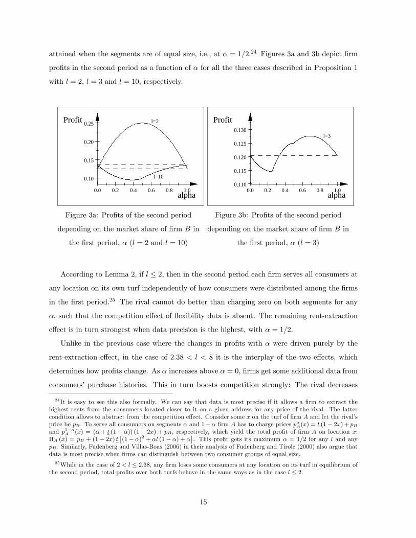
attained when the segments are of equal size, i.e., at � = 1=2.24 Figures 3a and 3b depict �rm

pro�ts in the second period as a function of � for all the three cases described in Proposition 1

with l = 2, l = 3 and l = 10, respectively.

0.0 0.2 0.4 0.6 0.8 1.0

0.10

0.15

0.20

0.25

alpha

Profit l=2

l=10

Figure 3a: Pro�ts of the second period

depending on the market share of �rm B in

the �rst period, � (l = 2 and l = 10)

0.0 0.2 0.4 0.6 0.8 1.00.110

0.115

0.120

0.125

0.130

alpha

Profit

l=3

Figure 3b: Pro�ts of the second period

depending on the market share of �rm B in

the �rst period, � (l = 3)

According to Lemma 2, if l � 2, then in the second period each �rm serves all consumers at

any location on its own turf independently of how consumers were distributed among the �rms

in the �rst period.25 The rival cannot do better than charging zero on both segments for any

�, such that the competition e¤ect of �exibility data is absent. The remaining rent-extraction

e¤ect is in turn strongest when data precision is the highest, with � = 1=2.

Unlike in the previous case where the changes in pro�ts with � were driven purely by the

rent-extraction e¤ect, in the case of 2:38 < l < 8 it is the interplay of the two e¤ects, which

determines how pro�ts change. As � increases above � = 0, �rms get some additional data from

consumers�purchase histories. This in turn boosts competition strongly: The rival decreases

24 It is easy to see this also formally. We can say that data is most precise if it allows a �rm to extract thehighest rents from the consumers located closer to it on a given address for any price of the rival. The lattercondition allows to abstract from the competition e¤ect. Consider some x on the turf of �rm A and let the rival�sprice be pB . To serve all consumers on segments � and 1�� rm A has to charge prices p�A(x) = t (1� 2x) + pBand p1��A (x) = (�+ t (1� �)) (1� 2x) + pB , respectively, which yield the total pro�t of �rm A on location x:�A (x) = pB + (1� 2x) t

�(1� �)2 + �l (1� �) + �

�. This pro�t gets its maximum � = 1=2 for any l and any

pB . Similarly, Fudenberg and Villas-Boas (2006) in their analysis of Fudenberg and Tirole (2000) also argue thatdata is most precise when �rms can distinguish between two consumer groups of equal size.25While in the case of 2 < l � 2:38, any �rm loses some consumers at any location on its turf in equilibrium of

the second period, total pro�ts over both turfs behave in the same ways as in the case l � 2.

15

its prices on both segments, eroding pro�ts. When data quality improves further, the rent-

extraction e¤ect starts to take over and pro�ts increase. Overall, pro�ts are the highest when

data is more accurate, i.e., � takes intermediate values (close to � = 1=2). With a further

increase in �, behavioral data becomes less and less precise about the consumers who bought

from the rival in the initial period decreasing its overall predictive power and pro�ts altogether.

However, pro�ts then always remain above the level without �exibility data (at � = 1 or � = 0).

If l � 8, pro�ts drop rapidly as � becomes strictly positive. As a result, although pro�ts

start recovering when � increases above a certain threshold, they never exceed the level without

behavioral data (at � = 1 or � = 0). Interestingly, in this case pro�ts are the lowest when data is

most precise (� takes intermediate values), because competition is most intense then. The case

l � 8 is similar to the result obtained by Fudenberg and Tirole (2000) for the uniformly distrib-

uted consumer preferences. This similarity is driven by the fact that their model corresponds

to the case of very high l in our analysis. Indeed, behavioral customer data in Fudenberg and

Tirole allows to distinguish among two consumer groups loyal (on average) to di¤erent �rms,

while in our setting at each location in the second period �rms can discriminate among two

consumer groups loyal to the same �rm. We now turn to the analysis of the �rst period.

Equilibrium analysis of the �rst period. In this subsection we analyze competition in the

�rst period where �rms can discriminate only based on consumer locations and charge prices

to maximize their discounted pro�ts over two periods. Similar to Fudenberg and Villas-Boas

(2006) we concentrate only on equilibria in pure strategies in the �rst period.26 The proposition

below summarizes our results.27

Proposition 2. Consider an arbitrary location x on the turf of �rm i = A;B. The subgame-

perfect Nash equilibrium (in pure strategies) takes the following form:

i) First period. In equilibrium �rm i monopolizes location x only if consumers are relatively

homogeneous, i.e., l � h1 (�), with h1 (0) = 2, h1 (1) = 1:5 and @h1 (�) =@� < 0. Otherwise, in

the �rst period �rms share consumers at x, such that the more �exible of them buy at the more

distant �rm.

26 If 2 < l < 2; 89 or 5 < l < 14; 13 there are some values of �rm discount factor, for which the equilibriumin pure strategies in the �rst period does not exist or two equilibria in pure strategies exist. In Proposition 2we consider only those constellations of parameters l and �, which yield the unique equilibrium prediction inpure strategies in the �rst period. This becomes more likely when �rms are less patient because in that case thedynamic maximization function is close to the static one.27 In Proposition 2, �h�stays for the critical levels of consumer heterogeneity.

16

ii) Second period. In equilibrium �rm i monopolizes location x if consumers are weakly dif-

ferentiated, i.e., l � h2 (�), with h2 (0) = 2, @h2 (�) =@� > 0 and h2 (�) > h1 (�) for any

� > 0. In equilibrium �rm i serves all consumers on segment �, while the more �exible con-

sumers on segment 1 � � buy at the rival provided consumers are moderately di¤erentiated,

i.e., h3 (�) � l � min fh4 (�) ; h5 (�)g, with h3 (0) = 2, hn (0) = 5, @hn (�) =@� > 0 and

hn (�) > h3 (�) for any �, n = 4; 5. Finally, if consumers are strongly di¤erentiated, i.e.,

l � max fh4 (�) ; h5 (�)g, then �rm i serves the less �exible consumers on both segments, while

the more �exible consumers buy at the rival, with max fh4 (1) ; h5 (1)g = 14:13.

The subgame-perfect Nash equilibrium in pure strategies is driven by both the level of

consumer di¤erentiation and �rm discount factor. Although the relationship is intertwined,

there are parameter ranges that allow unambiguous insights. In particular, if l � 1:5, then

in equilibrium each �rm serves all customers at any location on its turf in both periods. If

2:89 � l � 5, then in equilibrium each �rm attracts only the less �exible consumers close by in

the �rst period, while in the following period all of them as well as the more �exible consumers on

segment 1�� buy at that �rm. Finally, if l � 14:13, then in equilibrium each �rm loses the more

�exible consumers in the �rst period and also on any segment in the second period. Proposition

2 states that for other values of consumer di¤erentiation in �exibility, the equilibrium depends

on how strongly �rms value future pro�ts. In this case a su¢ ciently high discount factor leads

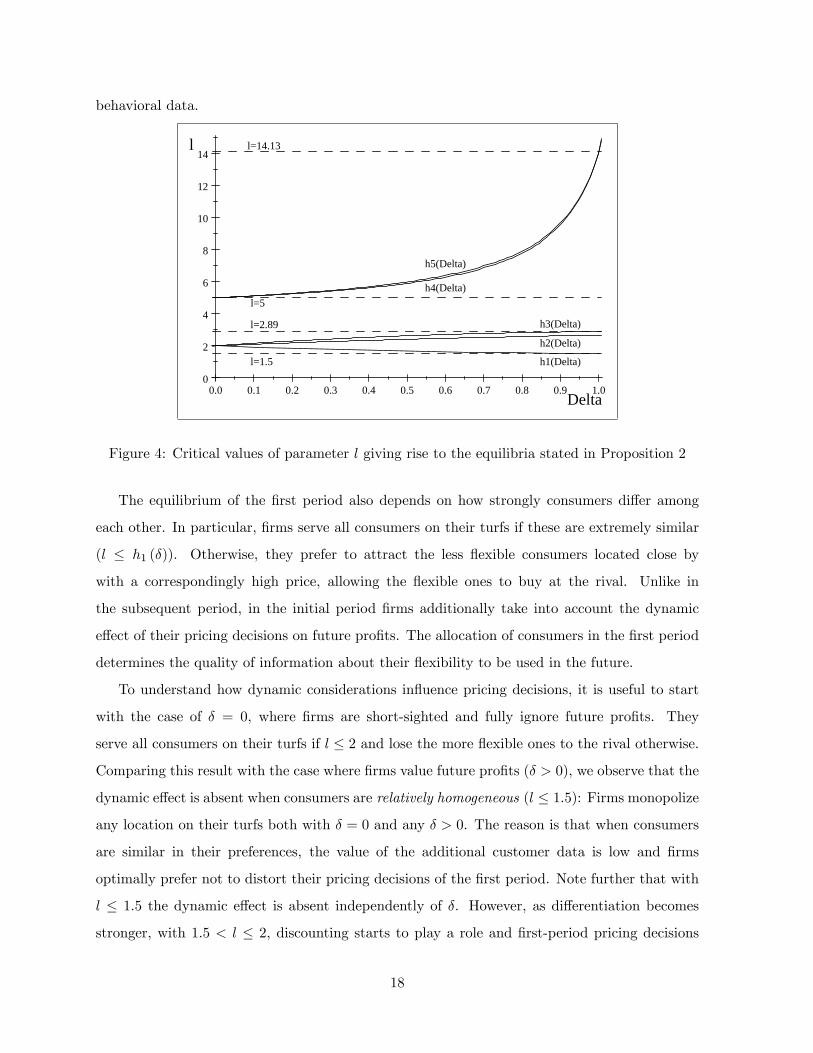
to the monopoly outcome in the second period (on one or both segments). Figure 4 depicts the

critical values of l (as a function of �), which give rise to the equilibria stated in Proposition 2.

We observe from Proposition 2 that with increasing consumer heterogeneity (l gets larger),

the equilibrium where �rms lose some of the close-by consumers becomes more likely in the

second period. This conclusion allows us to qualify the results of Lemma 2, which yields multiple

equilibrium predictions for l > 2 depending on �. Precisely, it establishes that in equilibrium of

the second period a �rm serves all consumers on segment 1� � at any location on its turf and

at the same time loses some consumers on the complementary segment if the share � is large

enough. As Proposition 2 shows, this outcome never emerges on the equilibrium path. It is

useful to recall that segment � includes those consumers at some location on a �rm�s turf who

bought from the rival in the previous period. As none of the �rms loses in the equilibrium of

the initial period more than half of the consumers on its turf, this segment is relatively small,

which makes it easy for a �rm to monopolize it in the subsequent period relying on the acquired

17

behavioral data.

0.0 0.1 0.2 0.3 0.4 0.5 0.6 0.7 0.8 0.9 1.00

2

4

6

8

10

12

14

Delta

l

h1(Delta)

h2(Delta)

h3(Delta)

h4(Delta)

h5(Delta)

l=1.5

l=2.89

l=5

l=14.13

Figure 4: Critical values of parameter l giving rise to the equilibria stated in Proposition 2

The equilibrium of the �rst period also depends on how strongly consumers di¤er among

each other. In particular, �rms serve all consumers on their turfs if these are extremely similar

(l � h1 (�)). Otherwise, they prefer to attract the less �exible consumers located close by

with a correspondingly high price, allowing the �exible ones to buy at the rival. Unlike in

the subsequent period, in the initial period �rms additionally take into account the dynamic

e¤ect of their pricing decisions on future pro�ts. The allocation of consumers in the �rst period

determines the quality of information about their �exibility to be used in the future.

To understand how dynamic considerations in�uence pricing decisions, it is useful to start

with the case of � = 0, where �rms are short-sighted and fully ignore future pro�ts. They

serve all consumers on their turfs if l � 2 and lose the more �exible ones to the rival otherwise.

Comparing this result with the case where �rms value future pro�ts (� > 0), we observe that the

dynamic e¤ect is absent when consumers are relatively homogeneous (l � 1:5): Firms monopolize

any location on their turfs both with � = 0 and any � > 0. The reason is that when consumers

are similar in their preferences, the value of the additional customer data is low and �rms

optimally prefer not to distort their pricing decisions of the �rst period. Note further that with

l � 1:5 the dynamic e¤ect is absent independently of �. However, as di¤erentiation becomes

stronger, with 1:5 < l � 2, discounting starts to play a role and �rst-period pricing decisions

18

remain undistorted by future pro�ts considerations only if � is su¢ ciently small. Otherwise,

�rms sacri�ce some of the short-run pro�ts to be able to extract higher rents in the future:

They lose some consumers at any location on their turfs in order to gain additional data about

their preferences. Overall, the dynamic considerations play a role if consumer di¤erentiation is

su¢ ciently strong and enough weight is put on second-period pro�ts in discounting.

If l > 2, the sharing equilibrium prevails in the �rst period with any � � 0, such that �rms

always gain some behavioral customer data. To understand how dynamic considerations drive

pricing decisions in this case, we analyze how the distribution of consumers at a given location

depends on the discount factor. We focus on the derivative of �� (�), the market share of the

rival at some location on a �rm�s turf in the �rst period, with respect to �. If @�� (�) =@� > 0,

we conclude that more (better) customer data is revealed in the �rst period when �rms become

more patient. Since the share �� (�) always includes less than half of consumers at any location,

a larger �� (�) implies a more symmetric distribution of consumers between the �rms and, hence,

more information gained about their preferences. The following corollary summarizes our results.

Corollary 1 (Revelation of customer �exibility data). Consider an arbitrary location x

on the turf of �rm i. The quality of the additionally revealed customer information in the �rst

period depends on how strongly consumers di¤er in their preferences and �rm discount factor.

i) If consumers are relatively homogeneous, l � h1 (�), no additional information is revealed in

the �rst period independently of the discount factor, such that �� (�) = 0 for any �.

ii) In all other cases �rms obtain additional customer information on �exibility. How a higher

discount factor in�uences its quality, depends on the intensity of consumer di¤erentiation: If

l / 2:64, then @�� (�) =@� > 0 and the sign is opposite if l ' 2:67. Finally, if 2:64 < l < 2:67,

then @�� (�) =@� < 0 when �rms are relatively impatient and the sign is opposite otherwise.

Corollary 1 shows that the e¤ect of a larger discount factor on the quality of the revealed

customer data can be threefold. In particular, if l and/or � are small so that consumers are

relatively homogeneous (l � h1 (�)), then this e¤ect is absent and �rms charge the same prices

yielding the same market shares as if there were no second period. As explained above, this

happens because the value of customer data is low when consumers are similar and/or when

�rms discount away future pro�ts. When consumers are more di¤erentiated and/or �rms put

su¢ cient weight on future pro�ts, dynamic considerations matter for �rst-period prices and

market shares. Whether in this case the distribution of consumers in the �rst period becomes

19

more symmetric and, hence, customer data of a better quality is revealed, depends on how

future pro�ts respond to �rms holding more precise data. As we showed in Proposition 1, the

e¤ect of better customer data (measured by �) on second-period pro�ts tends to be positive

when consumers are more similar in their preferences and negative otherwise. In the former

case �rms prefer more accurate customer data when the discount factor becomes larger, so that

�� (�) =@� > 0 holds if h1 (�) < l / 2:64 (or if 2:64 < l < 2:67 and the discount factor is

large). In the latter case �rms prefer less precise information, so that �� (�) =@� < 0 if l ' 2:67.

However, in both cases �rms acquire at least some customer data even if this reduces their

second-period pro�ts. This is because with su¢ cient heterogeneity in �exibility (l > h1 (�))

serving all consumers on a �rm�s turf in the �rst period would require setting excessively low

prices.

An important result of Esteves (2010) is that �rms may avoid learning consumer prefer-

ences to prevent tense competition in the subsequent period. In particular, she shows that the

probability of the sharing outcome in the �rst period under which consumer types are fully

revealed decreases when �rms become more patient. We �nd an analogous result with l ' 2:67,

in which case less precise customer data is revealed when �rms value future pro�ts more. How-

ever, our model generates also the opposite result for h1 (�) < l / 2:64, because more accurate

behavior-based targeting is likely to increase pro�ts in this case.

We conclude that by in�uencing the precision of revealed customer information in the �rst

period, �rms are able to strengthen the positive and dampen the negative e¤ect of this infor-

mation on second-period pro�ts. We now turn to the question of how overall pro�ts change

compared to the case where �rms are (for some exogenous reasons) not able to collect behav-

ioral data and therefore can only discriminate along consumer locations in the second period.

The following corollary summarizes our results, where we compare the discounted sum of pro�ts

in the subgame-perfect Nash equilibrium (in pure strategies) in both cases.

Corollary 2 (The pro�t e¤ect of behavioral targeting). The pro�t e¤ect of combining

mobile geo-targeting with behavior-based price discrimination is:

i) neutral irrespective of the discount factor if l � 1:5,

ii) positive provided the discount factor is large enough and neutral otherwise if 1:5 < l < 2,

iii) positive irrespective of the discount factor if 2 � l / 3:07,

iv) (weakly) positive if the discount factor is large enough and negative otherwise if 3:07 < l / 4,

20

v) negative irrespective of the discount factor if l > 4.

Our results demonstrate that there are pure cases where the pro�t e¤ect of targeted pric-

ing based on consumer purchase histories depends only on their heterogeneity in preferences.

Precisely, if l � 1:5, the ability of �rms to engage in behavioral targeting is neutral for their

discounted pro�ts. When consumers do not di¤er a lot among each other, the value of additional

customer data is small and no �exibility data is revealed in equilibrium making behavioral tar-

geting irrelevant for pro�ts. This result is in sharp contrast with Baye and Sapi (2017), where

�rms are strictly better o¤ with additional customer data when consumers are quite homoge-

neous in their preferences. The reason is that in Baye and Sapi additional data is costless, while

in our model �rms have to sacri�ce some of their �rst-period pro�ts to gain it. When consumer

di¤erentiation is only modest, the value of this data to the �rms is low, such that they prefer

not to distort their optimal prices of the �rst period. As a result, Baye and Sapi overestimate

the positive e¤ect of additional data on pro�ts.

If 2 � l / 3:07 (l > 4), the ability of �rms to collect behavioral data is bene�cial (detrimental)

for their discounted pro�ts. These results are consistent with the e¤ect of �exibility data on

second-period pro�ts, as described in Proposition 1. Precisely, we showed there that pro�ts

are more likely to increase above the level without �exibility information if consumers are more

homogeneous. In that case price competition is intensive even without behavioral data, so that

additional customer data has mainly a positive rent-extraction e¤ect as competition cannot

increase much.

If the level of consumer di¤erentiation takes intermediate values (not covered by the pure

cases), then the sign of the pro�t e¤ect of behavioral targeting is convoluted by the discount

factor. Precisely, a higher weight on future pro�ts makes this form of price discrimination

pro�table. This result is also driven by the e¤ect of �exibility data on second-period pro�ts

as stated in Proposition 1. We showed there that when consumer di¤erentiation is moderate,

the e¤ect of additional �exibility data on pro�ts is related to the share �� (�), which in turn

depends on �rm discount factor. This result is novel in the literature. Previous studies attributed

unambiguous pro�t e¤ects to price discrimination based on purchase histories independent of

the discount factor (see Fudenberg and Tirole, 2000; Chen and Zhang, 2009; Esteves, 2010).28

28To make the results of Chen and Zhang (2009) comparable with ours, we need to set consumer discount factorto zero in their model. In this case �rms are always better o¤ with targeted pricing based on consumer purchasehistories, irrespective of the �rm discount factor (see Proposition 1).

21

We qualify these strict e¤ects by allowing for di¤erent levels of consumer di¤erentiation. This in

turn in�uences the interplay between the rent-extraction and competition e¤ects. When neither

of these e¤ects is strong enough, then the discount factor becomes the determining factor. We

now turn to the analysis of how �rms�ability to combine behavior-based price discrimination

with geo-targeting in�uences consumer surplus and social welfare.29

Corollary 3 (The welfare e¤ect of behavioral targeting). The e¤ect of combining mobile

geo-targeting with behavior-based price discrimination on social welfare (consumer surplus) is:

i) neutral irrespective of the discount factor if l � 1:5,

ii) negative if the discount factor is large enough and neutral otherwise if 1:5 < l < 2,

iii) negative irrespective of the discount factor if 2 � l < 2:28 ( 2 � l < 2:61),

iv) negative if the discount factor is large enough and positive otherwise if 2:28 / l / 2:67

( 2:61 / l / 2:67),

v) positive irrespective of the discount factor if l > 2:67.

Comparing the impact of the �rm ability to engage in behavioral targeting on their pro�ts and

welfare, we conclude the following. If consumers are very similar in their preferences (l � 1:5),

both �rms serve all customers located closer to them in the �rst period and no �exibility data

is revealed. As a result, both pro�ts and welfare do not depend on whether �rms can target

consumers based on their behavior. When �rms do gain �exibility data in equilibrium (l > 1:5),

�rms�and social welfare�s interests are likely to be opposed. Additional customer data renders

the second-period distribution of consumers more e¢ cient, because more consumers buy from

the �rm located closer. This reduces transport costs and improves social welfare. However, with

more homogeneous consumers (l is relatively small), �rms distort �rst-period prices in order to

obtain more �exibility data leading to a higher misalignment of consumers between the �rms:

The more �exible of them purchase from the �rm located farther away. In this case �rms bene�t

from behavioral data but social welfare reduces. This result is reversed when consumers become

more di¤erentiated (l is relatively large), because behavioral data in that case harms �rms. They

therefore consciously weaken information revelation in the �rst period making the distribution

of consumers more e¢ cient, because less customers buy from a farther �rm. A similar pattern

follows from the comparison of a change in pro�ts and consumer surplus. From Corollaries 2 and

29To keep the exposition as simple as possible, we do not mention in the corollary a very special case of2:28 / l < 2:29 (2:61 / l < 2:62), where social welfare (consumer surplus) increases when the discount factortakes intermediate values and decreases otherwise.

22

3 we can also conclude that �rm and consumer interests are not necessarily opposed. Precisely,

if 2:67 < l / 3:07, then pro�ts as well as consumer surplus (social welfare) increase by adding

behavioral price discrimination to geo-targeting.

As in the case of the pro�t e¤ect of behavior-based price discrimination, the way how the

latter in�uences social welfare and consumer surplus also depends on �rm discount factor when

consumers di¤er moderately in their preferences. Precisely, consumers (and the overall welfare)

are more likely to gain from �rms combining behavioral pricing with mobile geo-targeting when

the latter discount future pro�ts more and are, hence, more likely to be worse o¤.

5 Conclusion

This paper analyzes a model taking into account four important features of a modern mobile

targeting environment. First, sellers can observe consumers�real-time locations. Second, apart

from location, there are other factors in�uencing the responsiveness of a consumer to discounts,

such as age, income and occupation. Di¤erent from location, these are imperfectly observable

by marketers. Third, sellers may infer consumer responsiveness (�exibility) from the observed

previous purchasing behavior of a customer. Fourth, �rms can deliver personalized o¤ers through

mobile devices in a private manner based on both consumer locations and their �exibility inferred

from the previous purchase decisions. Our results show that �rms bene�t from the ability

to collect behavioral data and use it for personalized pricing in mobile geo-targeting when

consumers di¤er moderately in their preferences. With less di¤erentiated consumers behavior-

based price discrimination is neutral for pro�ts, while with strongly di¤erentiated consumers

it intensi�es competition and reduces pro�ts. Di¤erent from the previous studies, our results

also highlight the importance of the discount factor for the pro�t e¤ect of behavioral targeting,

which is likely to be positive when �rms are more patient. We also �nd that consumer and �rm

interests are not necessarily opposed. In particular, when customers di¤er modestly in their

preferences both consumer surplus and pro�ts can increase with behavioral targeting leading

to a higher social welfare. Finally, we show that �rms strategically in�uence the quality of the

(revealed) consumer behavioral data so as to enable higher rents extraction in case the data

allows them to do so, and reduce the pro�t loss if data intensi�es competition.

Our results are relevant for managers and policy alike. The main managerial implication

of our results is that combining behavioral marketing with geo-targeting needs very careful

23

consideration of the market environment. We highlight the role of consumer heterogeneity

and �rm discount factor and derive precise conditions under which such a campaign may be

pro�table in a competitive landscape. The main policy message relates to consumer and privacy

policy: Combining behavioral price discrimination with geo-targeting can be both bene�cial

and harmful for consumers. While geo-targeting has been argued to typically foster competition

(e.g., Thisse and Vives, 1988), combining it with behavioral price discrimination can turn around

this e¤ect, giving scope for a careful consumer policy. For example, restricting �rms in their

collection of types of data, such as age and demographics, that relate to their �exibility may

improve consumer outcomes when these do not di¤er strongly among each other. Similarly,

decreasing the data retention period (a proxy for the discount factor in our model) may also

bene�t consumers when these are moderately di¤erentiated.

Appendix

Proof of Lemma 1. As �rms are symmetric, we will restrict attention to the turf of �rm

A. Consider some x < 1=2 and segment �. Maximizing the expected pro�t of �rm A yields

the best-response function, which depends on the ratio t�=t. If t�=t � 2 (� � 1= (l � 1)), then

p�A(x; p�B) = p�B + t (1� 2x), such that �rm A optimally serves all consumers on segment �

irrespective of �rm B�s price. Then in equilibrium �rm B charges p�B (x) = 0, because it would

have an incentive to deviate from any positive price. Hence, p�A(x) = t (1� 2x). If t�=t > 2,

then the best response of �rm A takes the form:

p�A(x; p�B) =

8<: p�B + t (1� 2x) if p�B � (t� � 2t) (1� 2x)p�B+t

�(1�2x)2 if p�B < (t

� � 2t) (1� 2x) ,(2)

such that �rm A serves all consumers on segment � only if the rival�s price is relatively high.

Maximization of the expected pro�t of �rm B yields the best-response function:

p�B(x; p�A) =

8>>><>>>:any p�B if p�A � t (1� 2x)

p�A�t(1�2x)2 if t (1� 2x) < p�A < (2t� � t) (1� 2x)

p�A � t� (1� 2x) if p�A � (2t� � t) (1� 2x) .

(3)

24

Inspecting (2), we conclude that �rm B cannot serve all consumers in equilibrium. It is straight-

forward to show that there are no such prices, which constitute the equilibrium, where �rm A

serves all consumers. Hence, only the equilibrium can exist, where both �rms serves consumers.

Solving (2) and (3) simultaneously, we get the prices: p�A(x) = t (1� 2x) [2� (l � 1) + 1] =3 and

p�B(x) = t (1� 2x) [� (l � 1)� 1] =3. For this equilibrium to exist, it must hold that t�=t > 2.

In a similar way one can derive the equilibrium on the segment 1 � �. Precisely, if 1=t� � 2

(� � (l � 2) = [2 (l � 1)]), then in the monopoly equilibrium �rm A serves all consumers, where

�rms charge prices: p1��A (x) = t [1 + � (l � 1)] (1� 2x) and p1��B (x) = 0. If 1=t� > 2, then

the sharing equilibrium emerges with the prices: p�A(x) = t (1� 2x) [2l � 1� � (l � 1)] =3 and

p�B(x) = t (1� 2x) [l � 2� 2� (l � 1)] =3. Q.E.D.

Proof of Lemma 2. Lemma 2 follow directly from Lemma 1 given the following results:

1= (l � 1) > (l � 2) = [2 (l � 1)] if l < 4, (l � 2) = [2 (l � 1)] > 0 if l > 2, 1= (l � 1) > 1 if l < 2,

with the opposite sign otherwise. Note that 1= (l � 1) > 0 and (l � 2) = [2 (l � 1)] < 1 hold for

any l. Q.E.D.

Proof of Proposition 1. Consider �rst some x on the turf of �rm A. We start with deriving

�rms�pro�ts on each segment depending on �. Consider �rst segment �. If � � 1= (l � 1), then

�rm A serves all consumers and pro�ts are

��A(xjx<1=2)t(1�2x) = ��;1A (l;�) := t��t

1�t = � and

��B(xjx<1=2)t(1�2x) = ��;1B (l;�) := 0.

If � > 1= (l � 1), then �rm A serves consumers with t � t [� (l � 1) + 2] =3 and pro�ts are

��A(xjx<1=2)t(1�2x) = ��;2A (l;�) :=

ht� � t(�(l�1)+2)

3

i[2�(l�1)+1]3(1�t) = [2�(l�1)+1]2

9(l�1) and

��B(xjx<1=2)t(1�2x) = ��;2B (l;�) :=

ht(�(l�1)+2)

3 � ti[�(l�1)�1]3(1�t) = [�(l�1)�1]2

9(l�1) .

Consider now segment 1��. If � � (l � 2) = [2 (l � 1)], then �rm A gains all consumers and

�rms realize pro�ts:

�1��A (xjx<1=2)t(1�2x) = �1��;1A (l;�) := (1�t�)t�

(1�t)t = (1� �) [1 + � (l � 1)] and�1��B (xjx<1=2)

t(1�2x) = �1��;1B (l;�) := 0.

25

If � < (l � 2) = [2 (l � 1)], then �rm A serves consumers with t � t [l + 1 + � (l � 1)] =3 and �rms

realize pro�ts:

�1��A (xjx<1=2)t(1�2x) = �1��;2A (l;�) :=

h1� t[l+1+�(l�1)]

3

i[2l�1��(l�1)]

3(1�t) = [2l�1��(l�1)]29(l�1) and

�1��B (xjx<1=2)t(1�2x) = �1��;2B (l;�) :=

ht[l+1+�(l�1)]

3 � t�i[l�2�2�(l�1)]

3(1�t) = [l�2�2�(l�1)]29(l�1) .

The pro�ts on some x on the turf of �rm B can be derived in a similar way. Note now thatR 1=20 (1� 2x) dx =

R 11=2 (2x� 1) dx = 1=4. Using the above results, we can write down the total

pro�ts depending on l and � under the assumption that on any x on its turf in the �rst period

every �rm served consumers with t � t�.

Consider �rst l � 2. The total pro�ts of �rm i = A;B on both turfs are

4�i(l;�)t = ��;1A (�) + �1��;1A (�) = f1 (l;�) := �+ (1� �) [1 + � (l � 1)] .

Taking the derivative of f1 (l;�) with respect to � we get

@f1(l;�)@� = (1� 2�) (l � 1) ,

such f1 (l;�) is given by the inverted U-shaped function of �, which gets its maximum at � = 1=2.

Consider now 2 < l < 4 and � � (l � 2) = [2 (l � 1)], then the total pro�ts of �rm i on both

turfs are

4�i(l;�)t = ��;1A (�) + �1��;2A (�) + �1��;2B (�) = f2 (l;�) := �+ [2l�1��(l�1)]2

9(l�1) + [l�2�2�(l�1)]29(l�1) .


@f2(l;�)@� = 10�(l�1)�8l+19

9 > 0 if � > �2 := 8l�1910(l�1) .

Note that �2 � 0 if l � 19=8 � 2:38 and �2 < (l � 2) = [2 (l � 1)] if l < 3. Hence, if 2 < l � 19=8,

then f2 (l;�) increases in �. If 19=8 < l < 3, then f2 (l;�) decreases till � = �2 and increases

afterwards. Finally, if 3 � l < 4, then f2 (l;�) decreases in �.

26

If (l � 2) = [2 (l � 1)] < � < 1= (l � 1), then the total pro�ts of �rm i on both turfs are

4�i(l;�)t = ��;1A (�) + �1��;1A (�) = f3 (l;�) := �+ (1� �) [1 + � (l � 1)] .


@f3(l;�)@� = (1� 2�) (l � 1) > 0 if � < 1

2 .

Note that (l � 2) = [2 (l � 1)] < 1=2 for any l and 1= (l � 1) < 1=2 if l > 3. Hence, if 2 < l � 3,

then on (l � 2) = [2 (l � 1)] < � < 1= (l � 1), f3 (l;�) increases in � till � = 1=2 and decreases

afterwards. If 3 < l < 4, then f3 (l;�) increases in � on (l � 2) = [2 (l � 1)] < � < 1= (l � 1).

If � � 1= (l � 1), then the total pro�ts of �rm i on both turfs are

4�i(l;�)t = ��;2A (�) + ��;2B (�) + �1��;1A (�)

= f4 (l;�) :=[2�(l�1)+1]2

9(l�1) + [�(l�1)�1]29(l�1) + (1� �) [1 + � (l � 1)] .


@f4(l;�)@� = 9l�8�(l�1)�16

9 > 0 if � < �4 := 9l�168(l�1) .

Note that �4 < 1= (l � 1) if l < 24=9 � 2:67 and �4 < 1 for any 2 < l < 4. Hence, if 2 < l < 24=9,

then f4 (l;�) decreases in �. If 24=9 � l < 4, then f4 (l;�) increases till � = �4 and decreases

afterwards.

Consider �nally l � 4. If � � 1= (l � 1), then the total pro�ts of �rm i on both turfs are

4�i(l;�)t = ��;1A (�) + �1��;2A (�) + �1��;2B (�)

= f5 (l;�) := �+[2l�1��(l�1)]2

9(l�1) + [l�2�2�(l�1)]29(l�1) .


@f5(l;�)@� = 10�(l�1)�8l+19

9 > 0 if � > �5 := 8l�1910(l�1) .

Note that for any l � 4 it holds that �5 > 1= (l � 1). Hence, f5 (l;�) decreases in �.

27

If 1= (l � 1) < � < (l � 2) = [2 (l � 1)], then the total pro�ts of �rm i on both turfs are

4�i(l;�)t = ��;2A (�) + ��;2B (�) + �1��;2A (�) + �1��;2B (�)

= f6 (l;�) :=[2�(l�1)+1]2

9(l�1) + [�(l�1)�1]29(l�1) + [2l�1��(l�1)]2

9(l�1) + [l�2�2�(l�1)]29(l�1) .


@f6(l;�)@� = 20�(l�1)�4(2l�3)

9 > 0 if � > �6 := 2l�35(l�1) .

Note that for any l � 4 it holds that 1= (l � 1) � �6 � (l � 2) = [2 (l � 1)]. Hence, f6 (l;�)

decreases till � = �6 and increases afterwards.

If � � (l � 2) = [2 (l � 1)], then the total pro�ts of �rm i on both turfs are

4�i(l;�)t = ��;2A (�) + ��;2B (�) + �1��;1A (�)

= f7 (l;�) :=[2�(l�1)+1]2

9(l�1) + [�(l�1)�1]29(l�1) + (1� �) [1 + � (l � 1)] .


@f7(l;�)@� = 9l�16�8�(l�1)

9 > 0 if � < �7 := 9l�168(l�1) .

Note that for any l � 4 it holds that �7 > (l � 2) = [2 (l � 1)]. Moreover, �7 > 1 if l > 8, with

an opposite inequality otherwise. Hence, if 4 � l � 8, then f7 (l;�) increases till � = �7 and

decreases afterwards. If l > 8, then f7 (l;�) increases in �.

We can now summarize the results on the behavior of the total pro�ts in � depending on l.

i) If l � 2:38, then total pro�ts are given by the inverted U-shaped function of �, which gets its

maximum at � = 1=2.

ii) If 2:38 < l < 2:67, then total pro�ts are given by a non-monotonic function, which gets a

(local) minimum at � = (8l � 19) = (10l � 10) and a (local) maximum at � = 1=2. This function

decreases on the intervals: [0; (8l � 19) = (10l � 10)] and [1=2; 1], and increases on the remaining

intervals. Note that

4�i

�l;12

�t = f3

�l; 12�= l+3

4 > 4�i(l;0)t = f2 (l; 0) =

5l2�8l+59(l�1) , for any 2:38 < l < 2:67,

28

such that �i (l; k) gets a global maximum at � = 1=2. From this and the fact that �i (l; k) is a

continuous function of �, we conclude that there exists (8l � 19) = (10l � 10) < b�(l) < 1=2, suchthat �i (l;�) � �i (l; 0) if � � b�(l), with an opposite inequality otherwise. b�(l) is implicitlygiven either by the equation:

f2 (l; 0) =5l2�8l+59(l�1) = f2 (l; b�(l)) = b�+ [2l�1�b�(l�1)]2

9(l�1) + [l�2�2b�(l�1)]29(l�1) , (4)

or by the equation:

f2 (l; 0) =5l2�8l+59(l�1) = f3 (l; b�(l)) = b�+ (1� b�) [1 + b� (l � 1)] . (5)

In the former case we get that

@b�(l)@l = �(5��8)

8l�19�10�(l�1) > 0

and in the latter case we get

@b�(l)@l =

�2(9l2�18l+9)+�(�9l2+18l�9)+5l2�10l+39(1�2�)(l�1)3 > 0,

because if 2:38 < l < 2:67, then �2�9l2 � 18l + 9

�+ �

��9l2 + 18l � 9

�+ 5l2 � 10l + 3 > 0 for

any �.

iii) If 2:67 < l < 3, then the function �i (l; k) decreases on: [0; (8l � 19) = (10l � 10)],

[1=2; 1= (l � 1)] and [(9l � 16) = (8l � 8) ; 1]. The comparisons show that

4�i(l; 12)t = f3

�l; 12�= l+3

4 �4�i

�l; 9l�168(l�1)

�t = f4

�l; 9l�168(l�1)

�= 9l2�16l+16

16(l�1) if 2:67 < l � 2:8,4�i(l; 1

l�1)t = f3

�l; 1l�1

�= f4

�l; 1l�1

�= 2l�3

l�1 > f2 (l; 0) = f4 (l; 1) =5l2�8l+59(l�1) if 2:67 < l < 3.

We make two conclusions. First, �i (l;�) gets the global maximum at � = 1=2 if l � 2:8 and at

� = (9l � 16) = [8 (l � 1)] otherwise. Second, using the fact that �i (l;�) is a continuos function of

�, we conclude that there exists (8l � 19) = (10l � 10) < b�(l) < 1=2, such that �i (l;�) � �i (l; 0)if � � b�(l), with an opposite inequality otherwise. As in the previous case, b�(l) is given byeither (4) or (5). As we showed above, in both cases @b�(l)=@l > 0 holds.

iv) If 3 < l � 4, then �i (l;�) decreases on: [0; (l � 2) = (2l � 2)] and [(9l � 16) = (8l � 8) ; 1],

29

while increases on the remaining interval. Note that

f2 (l; 0) = f4 (l; 1) =5l2�8l+59(l�1) < f4

�l; 9l�168(l�1)

�= 9l2�16l+16

16(l�1) for any l, (6)

such that �i (l;�) has a global maximum at � = (9l � 16) = (8l � 8). As �i (l;�) is a continuous

function of �, we conclude that there exists (l � 2) = (2l � 2) < b�(l) < (9l � 16) = (8l � 8), suchthat �i (l;�) � �i (l; 0) if � � b�(l), with an opposite inequality otherwise. As in the previouscase, b�(l) is given by either (4) or (5). As we showed above, in both cases @b�(l)=@l > 0 holds.

v) If 4 < l < 8, then �i (l;�) decreases on: [0; (2l � 3) = (5l � 5)] and [(9l � 16) = (8l � 8) ; 1],

while increases on the remaining interval. Due to (6), �i (l;�) has a global maximum at � =

(9l � 16) = (8l � 8). As �i (l;�) is a continuous function of �, we conclude that there exists

(2l � 3) = (5l � 5) < b�(l) < (9l � 16) = (8l � 8), such that �i (l;�) � �i (l; 0) if � � b�(l), with anopposite inequality otherwise. b�(l) is implicitly given either by the equation:f5 (l; 0) =

5l2�8l+59(l�1) = f6 (l; b�(l)) = [2b�(l�1)+1]2

9(l�1) + [b�(l�1)�1]29(l�1) + [2l�1�b�(l�1)]2

9(l�1) + [l�2�2b�(l�1)]29(l�1) ,

or by the equation:

f5 (l; 0) =5l2�8l+59(l�1) = f7 (l; b�(l)) = [2b�(l�1)+1]2

9(l�1) + [b�(l�1)�1]29(l�1) + (1� b�) [1 + b� (l � 1)] .

In the former case we get that

@b�(l)@l = �(�5l

2+10l�5)[��1(l)][��2(l)]2(l�1)2[2l�3��(5l�5)] , where

�1 (l) =�(4l2�8l+4)+2(l�1)

p4l2�8l+9

2(�5l2+10l�5) and �2 (l) =�(4l2�8l+4)�2(l�1)

p4l2�8l+9

2(�5l2+10l�5) .

Note that as f6 (l;�) is de�ned on 1= (l � 1) < � < (l � 2) = [2 (l � 1)], while �1 (l) < 1= (l � 1)

and �2 (l) > (l � 2) = [2 (l � 1)] for any 4 < l < 8, then � � �1 (l) > 0 and � � �2 (l) < 0.

Finally, as �5l2 + 10l � 5 < 0 for any 4 < l < 8 and b�(l) > (2l � 3) = (5l � 5), we conclude that@b�(l)=@l > 0. In the latter case we get

@b�(l)@l = � 4(��1)(�� 5

4)8�(l�1)�(9l�16) > 0 as b�(l) < 9l�16

8�(l�1) .

vi) If l � 8, then �i (l;�) is a U�shaped function, which gets its (global) minimum at � =

30

(2l � 3) = (5l � 5). Q.E.D.

Proof of Proposition 2. Consider some x on the turf of �rm A. Using the results of Lemma

2 and the notation from the proof of Proposition 1, we can write down second-period pro�ts at

x depending on l and �. If l � 2, then �rm A gains all consumers at x independently of �, such

that pro�ts of �rm i = A;B at x, �i (xjx < 1=2), are

�A(xjx<1=2)t(1�2x) = ��;1A (l;�) + �1��;1A (l;�) = �+ (1� �) [1 + � (l � 1)] , (7)

�B(xjx<1=2)t(1�2x) = ��;1B (l;�) + �1��;1B (l;�) = 0.

Consider now 2 < l < 4, in which case second-period pro�ts at x depend on �. If � �

(l � 2) = [2 (l � 1)], then �rm A gains all consumers on � and loses some consumers on 1 � �,

such that pro�ts are

�A(xjx<1=2)t(1�2x) = ��;1A (l;�) + �1��;2A (l;�) = �+ [2l�1��(l�1)]2

9(l�1) , (8)

�B(xjx<1=2)t(1�2x) = ��;1B (l;�) + �1��;2B (l;�) = [l�2�2�(l�1)]2

9(l�1) .

If (l � 2) = [2 (l � 1)] � � < 1= (l � 1), then �rm A serves all consumers on both segments, and

pro�ts are given by (7). If � � 1= (l � 1), then �rm A loses consumers on �, and pro�ts are

�A(xjx<1=2)t(1�2x) = ��;2A (l;�) + �1��;1A (l;�) = [2�(l�1)+1]2

9(l�1) + (1� �) [1 + � (l � 1)] , (9)

�B(xjx<1=2)t(1�2x) = ��;2B (l;�) + �1��;1B (l;�) = [�(l�1)�1]2

9(l�1) .

Consider �nally l � 4. If � � 1= (l � 1), then �rm A loses consumers on 1 � �, and pro�ts

are given by (8). If 1= (l � 1) < � < (l � 2) = [2 (l � 1)], then �rm A loses consumers on both

segments, and �rms realize pro�ts:

�A(xjx<1=2)t(1�2x) = ��;2A (l;�) + �1��;2A (l;�) = [2�(l�1)+1]2

9(l�1) + [2l�1��(l�1)]29(l�1) , (10)

�B(xjx<1=2)t(1�2x) = ��;2B (l;�) + �1��;2B (l;�) = [�(l�1)�1]2

9(l�1) + [l�2�2�(l�1)]29(l�1) .

If � � (l � 2) = [2 (l � 1)], then �rm A loses consumers on �, and pro�ts are given by (9).

31

We introduce now a new notation for the (adjusted) price of �rm i = A;B on some x < 1=2:

pxi :=pA(x)(1�2x)t .

At any x < 1=2 those consumers buy at �rm A who have relatively high transport costs:

t � t� (pA (x) ; pB (x)) = �+ t (1� �) , where (11)

t� (�) = pA(x)�pB(x)1�2x = (pxA � pxB) t,

from where we can derive � as follows

� = pA(x)�pB(x)(1�2x)t(l�1) �

1l�1 =

pxA�pxB�1l�1 . (12)

Note next that if t � t� (�) � 1, then the pro�t of �rm A at x < 1=2 in the �rst period is

h1� pA(x)�pB(x)

1�2x

ipA(x)1�t = t (1� 2x)

hl � pA(x)�pB(x)

(1�2x)t

ipA(x)

t(1�2x)(l�1)

=t(1�2x)(l�pxA+pxB)pxA

l�1 .

Similarly, the pro�t of �rm B at x < 1=2 in the �rst period is

hpA(x)�pB(x)

1�2x � tipB(x)1�t =

t(1�2x)(pxA�pxB�1)pxB(l�1) .

To derive the optimal prices of the �rst period, we will consider the discounted sum of each

�rm�s pro�ts over two periods, multiplied by (l � 1) and divided by t (1� 2x).

Part 1. Consider �rst l � 2, in which case �rm A chooses pxA to maximize the pro�ts:

(l � pxA + pxB) pxA + � (l � 1) [�+ (1� �) (1 + � (l � 1))] (13)

= (l � pxA + pxB) pxA + � [pxA � pxB � 1 + (l � pxA + pxB) (pxA � pxB)] .

Firm B chooses pxB to maximize the pro�ts:

(pxA � pxB � 1) pxB. (14)

32

Solving �rms��rst-order conditions we arrive at the prices:

px�A = 2l(1+�)�12�+3 and px�B = l�2��(1�l)

2�+3 . (15)

Note that second-order conditions are also ful�lled. For the prices (15) to constitute the equi-

librium, it must hold that t < t� ((1� 2x) tpx�A ; (1� 2x) tpx�B ) � 1, which yields the condition:

11+l <

1+�3+2� �

l1+l . (16)

Note that l= (1 + l) > 0:5 for any l and (1 + �) = (3 + 2�) � 0:4 for any �, such that the

right-hand side of (16) is ful�lled for any � and any l. The left-hand side of (16) is ful�lled if

l > l1 (�) :=2+�1+� . (17)

It holds that 1:5 � l1 (�) � 2 for any � and @l (�) =@� < 0. Note �nally that if (17) holds, then

px�A > 0 and px�B > 0.

If l � l1 (�), then the monopoly equilibrium emerges, where �rm A serves all consumers at

x. In this equilibrium �rm A charges the highest price at which it can gain all consumers:

pA (x; pB (x)) = pB (x) + t (1� 2x) . (18)

It follows from (18) that p�B (x) = 0, because �rm B would have an incentive to deviate down-

wards from any positive price. Hence,

px�A (x) = 1 and px�B (x) = 0. (19)

For the prices (19) to constitute the equilibrium, none of the �rms should have an incentive to

deviate. Precisely, �rm A should not have an incentive to increase its price: the derivative of

(13) evaluated at pxA = 1 and pxB = 0 must be non-positive, which yields the condition l � l1 (�),

which is the opposite of (17).

Part 2. Consider now 2 � l � 4, in which case second-period pro�ts are given by di¤erent

functions depending on �.

i) Consider �rst � � (l � 2) = [2 (l � 1)]. The pro�ts of the second period are then given by

33

(8). Firm A chooses pxA to maximize the pro�ts:

(l � pxA + pxB) pxA + �9

h9� (l � 1) + (2l � 1� � (l � 1))2

i(20)

= (l � pxA + pxB) pxA + �9

h9 (pxA � pxB � 1) + (2l � pxA + pxB)

2i.


(pxA � pxB � 1) pxB +�[l�2�2�(l�1)]2

9 = (pxA � pxB � 1) pxB +�(l�2pxA+2pxB)

2

9 . (21)

We �rst show that no monopoly equilibrium (where �rm A serves all consumers at x) in the

�rst period exists. Assume that there is such an equilibrium. In this equilibrium �rm A will

charge the price pxA = pxB + 1. Indeed, at a higher price �rm A does not serve all consumers

at x and at any lower price �rm A realizes lower pro�ts (�rst-period pro�ts decrease, while

second-period pro�ts do not change). Firm B does not have an incentive to increase its price,

because both the �rst-period and second-period pro�ts do not change. However, one has to

exclude the incentive of �rm B to decrease its price. Similarly, one has to exclude the incentive

of �rm A to increase its price. Taking the derivatives of (20) and (21) with respect to pxA and

pxB and evaluating them at pxA = pxB + 1, yields the following inequalities, respectively:

l + 119 � �

49 l� � 2 � p

xB and

49 l� �

89� � p

xB. (22)

There exists pxB, which satis�es both inequalities in (22), only if

l � 18�19�9�8� . (23)

Note that for any � and any l � 2 (except for � = 0 and l = 2, which is covered by l � l1 (�) in

Part 1 ), (23) does not hold, which proves that in the �rst period only the sharing equilibrium

can exist.

In the sharing equilibrium �rst-order conditions have to be ful�lled. Solving them simulta-

neously, we arrive at the prices:

px�A = 54l+60��36l��24�2+8l�2�2781�30� , (24)

px�B = 27l+33��12l��24�2+8l�2�5481�30� , which yield

34

� (px�A ; px�B ) =

9l+19��8l��18(l�1)(27�10�) . (25)

Note that second-order conditions are ful�lled, and for any � and any l � 2 it holds that

� (px�A ; px�B ) � 0. Imposing � (px�A ; px�B ) � (l � 2) = [2 (l � 1)], we arrive at

l � l2 (�) := 6(1+�)3+2� .

Note that @l2 (�) =@� > 0, l2 (0) = 2 and l2 (1) = 2:4. Note that px�A � 0 stated in (24) requires

l � f1(�) := 24�2�60�+272(4�2�18�+27)

,

which is true for any � and any l, because for any � it holds that f1(�) < 1. Finally, px�B � 0

stated in (24) requires

l � f2(�) := 24�2�33�+548�2�12�+27 ,

which is true for any � and any l � 2, because for any � it holds that f2(�) � 2.

ii) Consider now (l � 2) = [2 (l � 1)] � � < 1= (l � 1). In this case the (adjusted) pro�ts over

two periods are given by (13) and (14), which yields the equilibrium prices (15) and the share

of �rm B in the �rst period:

� (px�A ; px�B ) =

px�A �px�B �1l�1 = l(1+�)�(2+�)

(3+2�)(l�1) .

The condition � (px�A ; px�B ) < 1= (l � 1) requires l < (5 + 3�) = (1 + �), which is ful�lled for any �,

because (5 + 3�) = (1 + �) � 4 for any �. The condition � (px�A ; px�B ) � (l � 2) = [2 (l � 1)] requires

l � l3 (�) := 2 (1 + �). Note that @l3 (�) =@� > 0, l3 (0) = 2 and l3 (1) = 4. Note �nally that for

any 2 � l � 4 and any �, it holds that px�A > 0 and px�B � 0.

iii) Consider �nally � � 1= (l � 1), in which case the pro�ts of the second period are given

by (9). Then �rm A chooses pxA to maximize the pro�ts:

(l � pxA + pxB) pxA +�[2�(l�1)+1]2

9 + � (1� �) (l � 1) [1 + � (l � 1)] (26)

= (l � pxA + pxB) pxA +�(2pxA�2pxB�1)

2

9 + � (l � pxA + pxB) (pxA � pxB) .

35


(pxA � pxB � 1) pxB +�[�(l�1)�1]2

9 (27)

= (pxA � pxB � 1) pxB +�(pxA�pxB�2)

2

9 .

Solving simultaneously �rst-order conditions of the �rms, we arrive at the prices:

px�A = ��54l+42��48l��16�2+6l�2+2724�+81 , (28)

px�B = ��27l+18��21l��16�2+6l�2+5424�+81 ,

which yield the share of �rm B in the �rst period:

� (px�A ; px�B ) =

px�A �px�B �1l�1 = 9l(1+�)�16��18

(27+8�)(l�1) . (29)

Note that for any l � 2 and �, px�A > 0 and px�B � 0 hold. The condition � (�) � 1= (l � 1)

requires that

l � l4 (�) := 15+8�3(1+�) .

Note that @l4 (�) =@� < 0 and l4 (�) � 4 if � � 0:75. The condition � (�) � 1 requires that

l � 9�8�18�� . (30)

Since the the right-hand side of (30) is for any � smaller than 1, then � (�) � 1 holds for any �

and any l � 2. Finally, it can be checked that second-order conditions are ful�lled.

Combining the results from the analysis of the cases i), ii) and iii), we conclude that de-

pending on l and � we have either one, two or three candidate equilibria. At the next step we

have to �nd the equilibrium for any l and �.

1) Consider �rst l2 (�) � l � min�l3 (�) ; l4 (�)

, which yield two candidate equilibria, (15)

and (24).

1.a) Consider �rst the candidate equilibrium (24). It is straightforward that none of the

�rms has an incentive to deviate on � (�) � (l � 2) = [2 (l � 1)]. We consider two other deviations

by each of the �rms.

Deviation on (l � 2) = [2 (l � 1)] � � (�) � 1= (l � 1).

36

i) The incentives of �rm A. If �rm A deviates, then it realizes the pro�ts (13). Maximizing

(13) with respect to pxA and keeping pxB at p

x�B given in (24), yields the deviation price:

px;devA (px�B ) =108l+6�+93l�+12�2�48�3�46l�2+16l�3�54

�60�2+102�+162 , (31)

and the market share of �rm B in the �rst period:

��px;devA (px�B ) ; p

x�B

�= �54��54l�63l��54�2+38l�2+108

6(l�1)(27�10�)(1+�) .

Note that px;devA (px�B ) > 0 for any � and any l. Imposing the requirement that


x�B

�� l�2

2(l�1) , (32)

we arrive at the constraint:

l � 48��6�2+548�2�12�+27 . (33)

Note that for any � it holds that

48��6�2+54�12�+8�2+27 > min

�l3 (�) ; l4 (�)

,

such that for any l with l2 (�) � l � min�l3 (�) ; l4 (�)

, (33) holds and, hence, (32) is ful�lled.

Imposing the requirement


x�B

�� 1

l�1 (34)

we arrive at the constraint:

l � 156��114�2+27063��38�2+54 . (35)

Note that for any � it holds that

156��114�2+27063��38�2+54 > min

�l3 (�) ; l4 (�)

,

such that for any l with l2 (�) � l � min�l3 (�) ; l4 (�)

, (35) holds and, hence, (34) is ful�lled. It

follows that the price (31) is indeed the optimal deviation price of �rm A on (l � 2) = [2 (l � 1)] �

37

� (�) � 1= (l � 1). The di¤erence between �rm A�s equilibrium and deviation pro�ts is

f1 (l; �) :=�[l2(�100�3+372�2+531�+2268)�l(�120�3+276�2+6552�+6156)�360�3+2520�2+6120�+3240]

36(�+1)(10��27)2 .

The function f1 (l; �) opens upwards for any � and has two roots:

l1 (�) : =�120�3+276�2+6552�+6156�36(27�10�)(1+�)

p(�+1)(9��)

2(�100�3+372�2+531�+2268)and (36)

l2 (�) : =�120�3+276�2+6552�+6156+36(27�10�)(1+�)

p(�+1)(9��)

2(�100�3+372�2+531�+2268).

For any � it holds: l1 (�) < l2 (�) and l2 (�) � l2 (�) � min�l3 (�) ; l4 (�)

. Hence, for any l

with l2 (�) � l � min�l3 (�) ; l4 (�)

we have that f1 (l; �) � 0 if l � l2 (�), while f1 (l; �) < 0 if

l < l2 (�). In the former case �rm A does not have an incentive to deviate from px�A in (24) and

does in the latter.

ii) The incentives of �rm B. If �rm B deviates, then its pro�ts are given by (14). Maximizing

(14) with respect to pxB and keeping pxA at p

x�A in (24), yields the deviation price:

px;devB (px�A ) =27l+45��18l��12�2+4l�2�54

81�30� ,

and the market share of �rm B in the �rst period:

��px�A ; p

x;devB (px�A )

�= 27l+45��18l��12�2+4l�2�54

(l�1)(81�30�) .

Note that for any � and any l � 2 it holds that px;devB (px�A ) � 0. The comparison shows that

��px�A ; p

x;devB (px�A )

�� l�2

2(l�1) =(9�4�)(6��3l�2l�+6)6(27�10�)(l�1) . (37)

The right-hand side of (37) is non-negative if

l � l2 (�) = 6(1+�)3+2� . (38)

As we consider l � l2 (�), the optimal deviation price of �rmB follows from ��px�A ; p

x;devB (px�A )

�=

(l � 2) = [2 (l � 1)]. Then from the continuity of �rm B�s pro�ts we conclude that it does not

have an incentive to deviate.

38

Deviation on � (�) � 1= (l � 1).

i) The incentives of �rm A. If �rm A deviates, then its pro�t is given by (26). Keeping pxB

at px�B in (24) and taking the derivative of (26) with respect to pxA yields the deviation price of

�rm A:

px;devA (px�B ) = �567��972l�621l��234�2+240�3+318l�2�80l�3+486�300�2+270�+1458 . (39)

Note that for any � and l � 2 it holds that px;devA (px�B ) > 0. The prices px;devA (px�B ) and p

x�B yield

the market share of �rm B in the �rst period:


x�B

�= 297��162l�189l��212�2+114l�2+324

(100�2�90��486)(l�1).

Note that for any � and any l � 2 it holds that ��px;devA (px�B ) ; p

x�B

�< 1. The other comparison

shows that


x�B

�� 1

l�1 = �3(129��54l�63l��104�2+38l�2+270)

2(l�1)(�50�2+45�+243). (40)


l � l5 (�) := 129��104�2+27063��38�2+54 . (41)

Solving l5 (�) = l3 (�), we arrive at � � 0:89. If � < 0:89, then l5 (�) > min�l3 (�) ; l4 (�)

, such

that (41) does not hold and ��px;devA (px�B ) ; p

x�B

�< 1= (l � 1).

Consider �rst � < 0:89 and � � 0:89 with l � l5 (�). The optimal deviation price of �rm A

follows from ��px;devA (px�B ) ; p

x�B

�= 1= (l � 1), which yields

px;devA (px�B ) =27��27l+12l�+24�2�8l�2�108

30��81 .

Note that for any l and any �, it holds that px;devA (px�B ) > 0. Then the di¤erence between the

equilibrium and deviation pro�ts of �rm A is

l2(112�3�480�2+513�+243)�l(712�3�2874�2+2322�+2430)+1053�3�3807�2+1215�+60753(10��27)2 . (42)

The numerator of (42) is a quadratic function with respect to l with a non-positive discriminant

(for any �), such that it does not have roots. As this function opens upwards (for any �), it

takes only positive values. Hence, �rm A does not have an incentive to deviate if � < 0:89 or if

39

� � 0:89 with l � l5 (�) hold.

Consider now � � 0:89 with l5 (�) < l < min�l3 (�) ; l4 (�)

, in which case (41) holds and (39)

is the optimal deviation price of �rm A. The di¤erence between the equilibrium and deviation

pro�ts of �rm A is

�[�l2(2092�3�8796�2+6615��2916)+l(9472�3�36876�2+10530�+11664)�11388�3+42264�2+5805��43740]12(5�+9)(10��27)2 . (43)

The function in the parentheses of (43) is quadratic in l, opens upwards for any � and has two

roots, one of which is negative for any �, while the other root is smaller than l5 (�) for any �.

Hence, for any l5 (�) < l < min�l3 (�) ; l4 (�)

and � � 0:89, the function in the parentheses in

(43) is positive, such that �rm A does not have an incentive to deviate.

ii) The incentives of �rm B. Given the rival�s price, px�A in (24), there exists px;devB � 0,

which yields the share of �rm B in the �rst period satisfying � (�) � 1= (l � 1) only if

l � l5 (�) := �120�+24�2+189�36�+8�2+54 . (44)

In the following we will restrict attention to l satisfying (44), because only in that case �rm

B can deviate. Keeping pxA at px�A in (24) and taking the derivative of (27) with respect to pxB

yields the deviation price of �rm B:

px;devB (px�A ) =243l+594��216l��228�2+24�3+72l�2�8l�3�486

30�2�351�+729 .

Note that px;devB (px�A ) > 0 for any � and l > 2. The prices px;devB (px�A ) and p

x�A yield the market

share of �rm B in the �rst period:

��px�A ; p

x;devB (px�A )

�=

px�A �px;devB (px�A )�1l�1 = 81l+108��54l��26�2+12l�2�162

(l�1)(10�2�117�+243). (45)

Note that for any l and � it holds that ��px�A ; p

x;devB (px�A )

�< 1. The other comparison shows

that

��px�A ; p

x;devB (px�A )

�� 1

l�1 =3(27l+75��18l��12�2+4l�2�135)

(l�1)(10�2�117�+243). (46)


l � 135�75�+12�227�18�+4�2 . (47)

40

Note that the right-hand side of (47) is for any � larger than 4, such that (47) does not hold

and ��px�A ; p

x;devB (px�A )

�< 1= (l � 1) stated in (45). Hence, the optimal deviation price of �rm

B is such that � (�) = 1= (l � 1), which yields

px;devB (px�A ) =54l+120��36l��24�2+8l�2�189

81�30� . (48)

Note that for any l > l5 (�), px;devB (px�A ) > 0. Then the optimal deviation price of �rm B is given

by (48) and the di¤erence between the equilibrium and deviation pro�ts is

� l2(52�3�204�2+297��243)�l(352�3�1608�2+2862��2430)+588�3�3123�2+6642��60753(10��27)2 . (49)

Note that the numerator of (49) is a quadratic function with respect to l, which opens downwards

(for any �). As its discriminant is non-positive (for any �), for any � and l it takes only negative

values, such that the whole term in (49) is positive for any � and l and �rm B does not have an

incentive to deviate.

Conclusion from 1.a). We conclude that on l2 (�) � l � min�l3 (�) ; l4 (�)

the equilibrium (24)

exists if l � l2 (�), with

l2 (�) =�120�3+276�2+6552�+6156+36(27�10�)(1+�)

p(�+1)(9��)

2(�100�3+372�2+531�+2268).

1.b) Consider now the equilibrium (15).

Deviation on � � (l � 2) = [2 (l � 1)].

i) The incentives of �rm A. If �rm A deviates, then its pro�ts are given by (20). Maximizing

(20) with respect to pxA and keeping pxB at p

x�B in (15) yields the deviation price of �rm A:

px;devA (px�B ) =36l+22�+13l�+20�2�10l�2�18

�4�2+30�+54 , (50)

such that the market share of �rm B in the �rst period is


x�B

�=

px;devA (px�B )�px�B �1l�1 = 18l+6��3l�+22�2�8l�2�36

(l�1)(54�4�2+30�).

41

Note that for any l and any �, px;devA (px�B ) in (50) is positive. The comparison shows that


x�B

�� l�2

2(l�1) =3(12��3l�6l�+6�2�2l�2+6)2(l�1)(�2�2+15�+27)

. (51)

Note that for any l � l2 (�) it holds that

l > 12�+6�2+66�+2�2+3

, (52)

such that the right-hand side of (51) is negative. Note next that ��px;devA (px�B ) ; p

x�B

�� 0 if

l � 36�6��22�218�3��8�2 . (53)

As any l � 2 also satis�es (53), ��px;devA (px�B ) ; p

x�B

�� 0 holds. We conclude that (50) is the

optimal deviation price of �rm A.

Given (50), the di¤erence between the equilibrium and the deviation pro�ts of �rm A is

� �f2(l;�)

4(9��)(2�+3)2 , with

f2 (l; �) : = l2�4�3 + 24�2 + 49� + 28

�� l�24�3 + 124�2 + 176� + 76

�+40�3 + 120�2 + 120� + 40.

The function f2 (l; �) opens upwards (for any �) and has two roots:

l3 (�) : =24�3+124�2+176�+76�4(�+1)(2�+3)

p(�+1)(9��)

2(4�3+24�2+49�+28), (54)

l4 (�) : =24�3+124�2+176�+76+4(�+1)(2�+3)

p(�+1)(9��)

2(4�3+24�2+49�+28).

For any � it holds that l3 (�) < 2 and l2 (�) � l4 (�) � min�l3 (�) ; l4 (�)

. It then follows that

for any l such that l2 (�) � l � min�l3 (�) ; l4 (�)

, �rm A does not have an incentive to deviate

if l � l4 (�) and deviates otherwise.

ii) The incentives of �rm B. If �rm B deviates, then its pro�ts are given by (21). Maximizing

(21) with respect to pxB and keeping pxA at p

x�A in (15), yields the deviation price of �rm B:

px;devB (px�A ) = �5��9l�7l�+4l�2+18�8�2+6�+27 .

42

Note that px;devB (px�A ) � 0 for any � and any l � 2. This deviation price yields the market share

of �rm B in the �rst period:

��px�A ; p

x;devB (px�A )

�=

px�A �px;devB (px�A )�1l�1 = 9l+3�+3l�+8�2�4l�2�18

(l�1)(�8�2+6�+27).

The comparison shows that

��px�A ; p

x;devB (px�A )

�� l�2

2(l�1) =9(2��l+2)

2(l�1)(�8�2+6�+27). (55)

The right-hand side of (55) is non-positive if l � l3 (�) = 2 (1 + �). Hence, for any l2 (�) � l �

min�l3 (�) ; l4 (�)

, the optimal deviation price of �rm B follows from � (�) = (l � 2) = [2 (l � 1)].

Then from the continuity of �rm B�s pro�ts we conclude that for any l and � �rm B does not


Deviation on � � 1= (l � 1).

i) The incentives of �rm A. If �rm A deviates, it realizes the pro�t (26). Keeping pxB at px�B

in (15) and taking the derivative of (26) with respect to pxA yields the deviation price of �rm A:

px;devA (px�B ) = �41��36l�64l�+18�2�28l�2+1820�2+66�+54

, (56)

which is non-negative if

l � 41�+18�2+1864�+28�2+36

. (57)

Note that for any � the right-hand side of (57) is smaller than 1, such that (57) is ful�lled as

strict inequality for any � and l. The price (56) yields the market share of �rm B in the �rst

period:


x�B

�=

px;devA (px�B )�px�B �1l�1 = �69��18l�36l�+28�2�18l�2+36

(l�1)(20�2+66�+54). (58)



x�B

�� 1

l�1 = �3(45��6l�12l�+16�2�6l�2+30)

2(l�1)(10�2+33�+27). (59)


l � 45�+16�2+3012�+6�2+6

. (60)

43

We showed above that on l2 (�) � l � min�l3 (�) ; l4 (�)

, the equilibrium (15) exists if l � l4 (�),

the latter being stated in (54). The comparison shows that for any �, the right-hand side of

(60) is larger than l4 (�), such that (60) is not ful�lled for any � and the right-hand side of (59)

is negative. Hence, the optimal deviation price of �rm A follows from ��px;devA (px�B ) ; p

x�B

�=

1= (l � 1). Then from the continuity of �rm A�s pro�ts, we conclude that �rm A does not have

an incentive to deviate.

ii) The incentives of �rm B. Keeping pxA at px�A in (15) and requiring that � � 1= (l � 1)

yields the restriction on �rm B�s deviation price:

px;devB � �4��2l�2l�+72�+3 . (61)

There exists px;devB � 0, which satis�es (61) if l � (4� + 7) = (2� + 2). We showed above that on

l2 (�) � l � min�l3 (�) ; l4 (�)

, the equilibrium (15) exists if l � l4 (�). Note that for any � it

holds that (4� + 7) = (2� + 2) > l4 (�), which implies that �rm B cannot deviate.

Conclusion from 1.b). We conclude that on l2 (�) � l � min�l3 (�) ; l4 (�)

, the equilibrium (15)

exists if l � l4 (�), with

l4 (�) =24�3+124�2+176�+76+4(�+1)(2�+3)

p(�+1)(9��)

2(4�3+24�2+49�+28).

2) Consider now 2 � l � l2 (�), which yields the unique candidate equilibrium (15).

Deviation on � � (l � 2) = [2 (l � 1)].

i) The incentives of �rm A. Refer to the analysis in 1.b). For any � it holds that

2 � 12�+6�2+66�+2�2+3

� l2 (�) .

For any

12�+6�2+66�+2�2+3

� l � l2 (�)

the analysis in 1.b) applies, such that �rm A does not have an incentive to deviate. Consider

now

2 � l � 12�+6�2+66�+2�2+3

,

44

in which case the optimal deviation price of �rm A follows from


x�B

�= l�2

2(l�1) .

Then from the continuity of �rm A�s pro�ts, we conclude that �rm A does not have an incentive

to deviate either.

ii) The incentives of �rm B. The analysis in 1.b) allows us to conclude that �rm B does

not have an incentive to deviate.

Deviation on � � 1= (l � 1). The analysis in 1.b) allows us to conclude that neither �rm A,

nor �rm B have an incentive to deviate.

Conclusion from 2). We conclude that on 2 � l � l2 (�) the unique equilibrium is (15).

3) Consider now l3 (�) � l � min�4; l4 (�)

, which yields the unique candidate equilibrium

(24).

Deviation on (l � 2) = [2 (l � 1)] � � (�) � 1= (l � 1).

i) The incentives of �rm A. We introduce a new notation:

l6 (�) :=48��6�2+548�2�12�+27 .

Consider �rst l3 (�) � l � min�l6 (�) ; l4 (�)

. From the analysis in 1.a) it follows that �rm A

does not have an incentive to deviate. Consider now l6 (�) � l � min�l4 (�) ; 4

. From the analy-

sis in 1.a) we conclude that the optimal deviation price of �rmA follows from (l � 2) = [2 (l � 1)] =


x�B

�. As �rm A�s pro�ts are continuous, we conclude that �rm A does not have


ii) The incentives of �rm B. From the analysis in 1.a) we conclude that �rm B does not


Deviation on � (�) � 1= (l � 1).

i) The incentives of �rm A. We �rst consider l3 (�) � l � min�l5 (�) ; 4

, with l5 (�) being

de�ned in (41). From the analysis in 1.a) it follows that �rm A does not have an incentive to

deviate. Consider now l5 (�) � l � min�l4 (�) ; 4

. From the analysis in 1.a) it follows that �rm

A does not have an incentive to deviate either.

45

ii) The incentives of �rm B. From the analysis in 1.a) it follows that �rm B does not have


Conclusion from 3). We conclude that on l3 (�) � l � min�4; l4 (�)

the unique equilibrium is

(24).

4) Consider now max�l3 (�) ; l4 (�)

� l � 4, which yields two candidate equilibria, (24) and

(28).

4.a) Consider �rst the candidate equilibrium (24).

Deviation on � (�) � 1= (l � 1).

i) The incentives of �rm A. If �rm A deviates, its pro�t is given by (26). Keeping pxB at px�B


px;devA (px�B ) = ��l(80�3�318�2+621�+972)+240�3�234�2+567�+486

270��300�2+1458 , (62)


l � 567��234�2+240�3+486621��318�2+80�3+972 . (63)

Since the right-hand side of (63) is smaller than 1 for any �, then (63) holds for any l. Using

px�B in (24) and px;devA (px�B ) in (62) we calculate the market share of �rm B in the �rst period:


x�B

�= �297��162l�189l��212�2+114l�2+324

(l�1)(486�100�2+90�).

The comparison shows that ��px;devA (px�B ) ; p

x�B

�� 1= (l � 1) if

l � 129��104�2+27063��38�2+54 ,

which is ful�lled for any � and any max�l3 (�) ; l4 (�)

� l � 4. The other comparison shows

that ��px;devA (px�B ) ; p

x�B

�� 1 if

l � �207�+112�2+162�99�+14�2+324 . (64)

Since the right-hand side of (64) is smaller than 1 for any �, then (64) holds for any l and any

�. Hence, (62) is the optimal deviation price of �rm A, which yields the following di¤erence

46

between the equilibrium and the deviation pro�ts:

�[�l2(2092�3�8796�2+6615��2916)+l(9472�3�36876�2+10530�+11664)�11388�3+42264�2+5805��43740]12(5�+9)(10��27)2 . (65)

The function in the brackets in (65) is quadratic in l. It opens upwards (for any �) and has two

roots:

�(9472�3�36 876�2+10 530�+11 664)+4(27�10�)q�(3485�4�16 032�3+801�2+42 930��55 404)

�2(2092�3�8796�2+6615��2916),

�(9472�3�36 876�2+10 530�+11 664)�4(27�10�)q�(3485�4�16 032�3+801�2+42 930��55 404)

�2(2092�3�8796�2+6615��2916).

Both of these roots are smaller than max�l3 (�) ; l4 (�)

for any �. Hence, for any � and any

max�l3 (�) ; l4 (�)

� l � 4, the expression in (65) is non-negative, such that �rm A does not


ii) The incentives of �rm B. If �rm B deviates, then its pro�t is given by (27). Keeping pxA

at px�A in (24) and taking the derivative of (27) with respect to pxB yields the deviation price of

�rm B:

px;devB (px�A ) =243l+594��216l��228�2+24�3+72l�2�8l�3�486

30�2�351�+729 , (66)

which is non-negative for any

l � 594��228�2+24�3�486216��72�2+8�3�243 . (67)

Since the right-hand side of (67) is for any � not lager than 2, then (67) holds for any � and any

l � 2. Using px;devB (px�A ) in (66), we can calculate the market share of �rm B in the �rst period:

��px�A ; p

x;devB (px�A )

�= 81l+108��54l��26�2+12l�2�162

(l�1)(10�2�117�+243).


��px�A ; p

x;devB (px�A )

�� 1

l�1 =3(27l+75��18l��12�2+4l�2�135)

(l�1)(10�2�117�+243). (68)


l � �75�+12�2+135�18�+4�2+27 . (69)

47

Since the right-hand side of (69) is not smaller than 5 for any �, (69) does not hold for any �

and any max�l3 (�) ; l4 (�)

� l � 4. Hence, the optimal deviation price of �rm B follows from

��px�A ; p

x;devB (px�A )

�= 1

l�1

and is given by

px;devB (px�A ) =54l+120��36l��24�2+8l�2�189

81�30� , (70)


l � �120�+24�2+189�36�+8�2+54 . (71)

The right-hand side of (71) is for any � smaller than max�l3 (�) ; l4 (�)

, such that (71) holds for

any � and any max�l3 (�) ; l4 (�)

� l � 4. Hence, px;devB (px�A ) in (70) is the optimal deviation

price of �rm B. Using the latter we calculate the di¤erence between the equilibrium and the

deviation pro�ts of �rm B:

� l2(52�3�204�2+297��243)�l(352�3�1608�2+2862��2430)+588�3�3123�2+6642��60753(10��27)2 . (72)

The numerator of (72) is a quadratic function of l, which opens downwards and has a non-

positive discriminant (for any �). It follows that for any � and any l the expression in (72) is

non-negative, such that �rm B does not have an incentive to deviate.

Deviation on (l � 2) = [2 (l � 1)] � � (�) � 1= (l � 1).

i) The incentives of �rm A. If �rm A deviates, then its pro�t is given by (13). Keeping pxB

at px�B in (24) and taking the derivative of (13) with respect to pxA yields the deviation price of

�rm A:

px;devA (px�B ) =108l+6�+93l�+12�2�48�3�46l�2+16l�3�54

�60�2+102�+162 , (73)


l � � 6�+12�2�48�3�5493��46�2+16�3+108 . (74)

As the right-hand side of (74) is for any � smaller than 1, (74) holds for any � and any l. Using

(73), we calculate the market share of �rm B in the �rst period:


x�B

�= �54��54l�63l��54�2+38l�2+108

(l�1)(162�60�2+102�).

48



x�B

�� 1

l�1 = �(156��54l�63l��114�2+38l�2+270)

6(l�1)(�10�2+17�+27). (75)

The right-hand side of (75) is non-positive if

l � l7 (�) := 156��114�2+27063��38�2+54 . (76)

The other comparison shows that


x�B

�� l�2

2(l�1) =48��27l+12l��6�2�8l�2+546(l�1)(�10�2+17�+27)

,


l � l8 (�) := 48��6�2+54�12�+8�2+27 . (77)

Note that if � =�24� 3

p7�=19 � 0:85, then l7 (�) = l8 (�) = 4. Consider max

�l8 (�) ; l4 (�)

�

l � 4, in which case (77) does not hold and px;devA (px�B ) follows from ��px;devA (px�B ) ; p

x�B

�=

(l � 2) = [2(l � 1)]. As �rm A�s pro�t is continuous, we conclude that �rm A does not have

an incentive to deviate. Consider now max�l7 (�) ; l3 (�)

� l � 4, in which case (76) does

not hold and px;devA (px�B ) follows from ��px;devA (px�B ) ; p

x�B

�= 1=(l � 1). As �rm A�s pro�t is

continuous, we conclude that �rm A does not have an incentive to deviate. Consider �nally

max�l3 (�) ; l4 (�)

� l � min fl7 (�) ; l8 (�)g, in which case both (76) and (77) are ful�lled and

the optimal deviation price of �rm A is given by (73). Using the latter price we calculate the

di¤erence between the equilibrium and the deviation pro�ts of �rm A:

�[l2(�100�3+372�2+531�+2268)�l(�120�3+276�2+6552�+6156)�360�3+2520�2+6120�+3240]36(�+1)(10��27)2 . (78)

For any �, the function in the brackets in (78) is quadratic in l, looks upwards and has two roots

both of which are smaller than max�l3 (�) ; l4 (�)

. Hence, the expression in (78) is non-negative

for any � and any max�l3 (�) ; l4 (�)

� l � min fl7 (�) ; l8 (�)g, such that �rm A does not have


i) The incentives of �rm B. If �rm B deviates, then its pro�ts are given by (14). Keeping

pxA at px�A in (24) and taking the derivative of (14) with respect to pxB yields the deviation price

49

of �rm B:

px;devB (px�A ) =27l+45��18l��12�2+4l�2�54

81�30� , (79)


l � �45�+12�2+54�18�+4�2+27 . (80)

Since the right-hand side of (80) is for any � not larger than 2, then (80) holds for any � and

any l � 2. Using (79) we can calculate the equilibrium share of �rm B in the �rst period:

��px�A ; p

x;devB (px�A )

�= 27l+45��18l��12�2+4l�2�54

(l�1)(81�30�) .


��px�A ; p

x;devB (px�A )

�� l�2

2(l�1) =(9�4�)(6��3l�2l�+6)6(27�10�)(l�1) . (81)


l � l2 (�) = 6(1+�)2�+3 . (82)

Note that for any � and any max�l3 (�) ; l4 (�)

� l � 4, (82) does not hold, such that the

optimal deviation price of �rm B follows from ��px�A ; p

x;devB (px�A )

�= (l � 2) = [2 (l � 1)]. As �rm

B�s pro�ts are continuous, we conclude that it does not have an incentive to deviate.

Conclusion from 4.a) We conclude that for any � and any max�l3 (�) ; l4 (�)

� l � 4 there

exists the equilibrium (24).

4.b) Consider now the candidate equilibrium (28).

Deviation on � (�) � (l � 2) = [2 (l � 1)].

i) The incentives of �rm A. If �rm A deviates, its pro�t is given by (20). Keeping pxB at px�B


px;devA (px�B ) =l(12�3�192�2+27�+972)�32�3+396�2+675��486

�48�2+270�+1458 . (83)

The price px;devA (px�B ) is non-negative if

l � �675�+396�2�32�3�48627��192�2+12�3+972 . (84)

50

The right-hand side of (84) is for any � smaller than 1, such that (84) holds for any � and any

l and px;devA (px�B ) � 0. Using px;devA (px�B ) in (83) we can calculate the market share of �rm B in

the �rst period:


x�B

�= ��l(14�2+99��162)+40�2+207��324

�(l�1)(�16�2+90�+486). (85)

The numerator of (85) is non-negative if

l � 207�+40�2�32499�+14�2�162 . (86)

The right-hand side of (86) is for any � smaller or equal to 2, such that (86) is ful�lled for any

� and any l � 2. The denominator of (86) is negative for any � and any l. It then follows that

for any � and any l � 2, ��px;devA (px�B ) ; p

x�B

�� 0 holds.



x�B

�� l�2

2(l�1) =3[�l(2�2+48�+27)+8�2+99�+54]

2(l�1)(�8�2+45�+243). (87)


l � 99�+8�2+5448�+2�2+27

. (88)

The right-hand side of (88) is for any � smaller than max�l3 (�) ; l4 (�)

. Hence, for any � and

any max�l3 (�) ; l4 (�)

� l � 4, (88) holds. We conclude that px;devA (px�B ) in (83) is the optimal

deviation price of �rm A. Using the latter price we can calculate the di¤erence between the

equilibrium and the deviation pro�ts of �rm A:

�[�264l2�3+1116l2�2�2619l2��2916l2+1184l�3�2676l�2+2754l��11 664l�1472�3+1200�2+9585�+43 740]12(9��)(8�+27)2 . (89)

The expression in the brackets in the numerator of (89) is a quadratic function with respect to

l, which opens downwards (for any �) and has two roots, one of which is negative for any � and

51

the other one is smaller than max�l3 (�) ; l4 (�)

for any �:

�(1184�3�2676�2+2754��11 664)+4(8�+27)p�149�4+2472�3�12 033�2+10 530�+55 404

�2(264�3�1116�2+2619�+2916), (90)

�(1184�3�2676�2+2754��11 664)�4(8�+27)p�149�4+2472�3�12 033�2+10 530�+55 404

�2(264�3�1116�2+2619�+2916).

It then follows that for any � and any max�l3 (�) ; l4 (�)

� l � 4 the expression in the brackets

in (89) is negative, which implies that �rm A has an incentive to deviate.

Conclusion from 4.b) We conclude that for any � and any max�l3 (�) ; l4 (�)

� l � 4 there

does not exist the equilibrium (28).

Conclusion from 4). We conclude that for any � and any max�l3 (�) ; l4 (�)

� l � 4 there

exists the unique equilibrium (24).

5) Consider �nally l4 (�) � l � l3 (�), which yields three candidate equilibria, (15), (24) and

(28).


Deviation on � (�) � (l � 2) = [2 (l � 1)].

i) The incentives of �rm A. Note that the right-hand side of (88) is for any � smaller than

l4 (�). Note also that the second expression in (90) is for any � smaller than l4 (�). Then similar

to the analysis in 4.b) we conclude that for any � and any l4 (�) � l � l3 (�), �rm A has an


Conclusion from 5.a). We conclude that for any � and any l4 (�) � l � l3 (�), the equilibrium

(28) does not exist.

5.b) We consider now the candidate equilibrium (15).

Deviation on � � (l � 2) = [2 (l � 1)].

i) The incentives of �rm A. From the analysis in 1.b) it follows that for any � and any

l4 (�) � l � l3 (�), �rm A has an incentive to deviate.

Conclusion from 5.b). We conclude that for any � and any l4 (�) � l � l3 (�), the equilibrium

(15) does not exist.

5.c) We consider �nally the candidate equilibrium (24).

52

i) The incentives of �rm B. We can use the results of the analysis in 1.a) to conclude that

�rm B does not have an incentive to deviate on (l � 2) = [2 (l � 1)] � � (�) � 1= (l � 1). Note

also that for any � it holds that l5 (�) < l4 (�), with l5 (�) being de�ned in (44). Then we can use

the results of the analysis in 1.a) to conclude that �rm B does not have an incentive to deviate

on � (�) � 1= (l � 1) either.

ii) The incentives of �rm A.

Deviation on � (�) � 1= (l � 1). Note that for any � it holds that l5 (�) � l4 (�), with l5 (�)

being de�ned in (41). Based on this result we conclude from the analysis in 1.a) that for any �

and any l4 (�) � l � l3 (�), �rm A does not have an incentive to deviate.

Deviation on (l � 2) = [2 (l � 1)] � � (�) � 1= (l � 1). We �rst note that the right-hand side of

(33) is for any � not smaller than l3 (�). Consider �rst � and l, for which (35) holds. We can

then use the results of the analysis in 1.a) to conclude that for any � and any l4 (�) � l � l3 (�),

�rm A does not have an incentive to deviate. Consider next � and l, for which (35) does not

hold, such that px;devA (px�B ) follows from ��px;devA (px�B ) ; p

x�B

�= 1= (l � 1). We showed, however,

above that �rm A does not have an incentive to deviate on � (�) � 1= (l � 1) for any � and any

l4 (�) � l � l3 (�).

Conclusion from 5.c). We conclude that for any � and any l4 (�) � l � l3 (�), the equilibrium

(24) exists.

Conclusion from 5. We conclude that for any � and any l4 (�) � l � l3 (�), the unique

equilibrium is (24).

Part 3. Consider �nally l � 4, in which case second-period pro�ts are given by di¤erent

functions depending on �.

i) Consider �rst � � 1= (l � 1). The pro�ts of the second period are given by (8). Firm A

chooses pxA to maximize the pro�t (20). Firm B chooses pxB to maximize the pro�t (21). Solving

simultaneously �rms��rst-order conditions yields the equilibrium prices (24), both of which are

positive for any � and any l � 4. These prices yield the market share of �rm B in the �rst period

given by (25), which is positive for any � and any l � 4. The comparison shows that

� (px�A ; px�B )� 1

l�1 =9l+29��8l��45(27�10�)(l�1) . (91)

53


l � l6 (�) := 45�29�9�8� . (92)

We conclude that for any � the equilibrium (24) can only exist if l � l6 (�).

ii) Consider now 1= (l � 1) < � < (l � 2) = [2 (l � 1)]. In this case second-period pro�ts are

given by (10). Then �rm A chooses pxA to maximize the pro�ts:

(l � pxA + pxB) pxA + �9

h(2� (l � 1) + 1)2 + (2l � 1� � (l � 1))2

i(93)

= (l � pxA + pxB) pxA + �9

h(2pxA � 2pxB � 1)

2 + (2l � pxA + pxB)2i.


(pxA � pxB � 1) pxB + �9

h(� (l � 1)� 1)2 + (l � 2� 2� (l � 1))2

i(94)

= (pxA � pxB � 1) pxB + �9

h(pxA � pxB � 2)

2 + (l � 2pxA + 2pxB)2i.

Solving simultaneously �rms��rst-order conditions yields the prices:

px�A = l(18�14�)+6��927�20� and px�B = l(9�6�)+14��18

27�20� . (95)

Note that px�A � 0 if

l � 9�6�18�14� . (96)

Since for any � the right-hand side of (96) is smaller than 1, px�A � 0 holds for any � and any

l � 4. Note also that px�B � 0 if

l � 18�14�9�6� . (97)

Since for any � the right-hand side of (97) is not larger than 2, px�B � 0 holds for any � and any

l � 4. Using the prices (95) we can calculate the market share of �rm B in the �rst period:

� (px�A ; px�B ) =

9l+12��8l��18(l�1)(27�20�) .

54


� (px�A ; px�B )� l�2

2(l�1) = �l(9�4�)+16��182(27�20�)(l�1) . (98)


l � 18�16�9�4� . (99)

Since the right-hand side of (99) is for any � not larger than 2, (99) holds for any � and any

l � 4. The other comparison shows that

� (px�A ; px�B )� 1

l�1 =l(9�8�)+32��45(27�20�)(l�1) . (100)


l � l8 (�) := 45�32�9�8� .

We conclude that for any �, equilibrium (95) can only exist if l � l8 (�).

iii) Consider �nally � � (l � 2) = [2 (l � 1)]. The pro�ts of the second period are given by

(9). Firm A chooses pxA to maximize the pro�ts (26). Firm B chooses pxB to maximize the

pro�ts (27). Solving simultaneously �rms��rst-order conditions yields the equilibrium prices

(28). These prices yield the market share of �rm B in the �rst period (29). As follows from

(30), for any � and any l � 4 it holds that � (px�A ; px�B ) � 1. The other comparison shows that

� (px�A ; px�B )� l�2

2(l�1) = ��l(10��9)+16��182(8�+27)(l�1) . (101)

If � < 0:9, then the right-hand side of (101) is non-negative if

l � l7 (�) := 18�16�9�10� . (102)

If � > 0:9, then the opposite to (102) inequality should hold. Finally, if � = 0:9, then the

right-hand side of (101) is positive for any l. Note now that l7 (0:75) = 4 and for any � < 0:75

it holds that l7 (�) < 4, such that there is no l � 4, which satis�es (102) in that case. Note also

that if � > 0:9, then l7 (�) < 0. We conclude that the equilibrium with � � (l � 2) = [2 (l � 1)]

55

does not exist for any l if � < 0:75, can exist for l � l7 (�) if 0:75 � � < 0:9 and can exist for

any l if � � 0:9.

In the following we analyze in turn every candidate equilibrium.


i) The incentives of �rm A.

Deviation on 1= (l � 1) � � (�) � (l � 2) = [2 (l � 1)]. If �rm A deviates, it realizes the pro�t

(93). Keeping pxB at px�B in (28) and taking the derivative of (93) with respect to pxA yields the

deviation price of �rm A:

pxdevA (px�B ) =�l(�60�3+360�2+189��972)�160�3+228�2+54��486

�240�2�378�+1458 . (103)

This price is non-negative if

l � 54�+228�2�160�3�486189�+360�2�60�3�972 . (104)

Since the right-hand side of (104) is for any � smaller than 1, then (104) holds for any l. Using

the price (103) we can calculate the market share of �rm B in the �rst period:

��pxdevA (px�B ) ; p

x�B

�= �99l��72��162l+14l�2+324

(l�1)(�80�2�126�+486).



x�B

�� l�2

2(l�1) =81l+54�+36l�+80�2�26l�2�162

2(l�1)(40�2+63��243). (105)


l � �54�+80�2�16236��26�2+81 . (106)

Since the right-hand side of (106) is for any � not larger than 2, then (106) holds for any � and

any l � 2. The other comparison shows that


x�B

�� 1

l�1 =162l+198��99l�+80�2�14l�2�810

2(l�1)(�40�2�63�+243). (107)

56


l � 198�+80�2�81099�+14�2�162 . (108)

We �rst consider the case (108), such that the optimal deviation price of �rm A is given by

(103). Then the di¤erence between the equilibrium and the deviation pro�ts is equal to

�[l2(�3176�3+6372�2+8991��20412)�l(�12160�3+19152�2+43092��55404)�12800�3+5760�2+35640��29160]36(9�5�)(8�+27)2 .

(109)

The function in the brackets of the numerator of (109) is quadratic in l, opens downwards for

any � and has two roots, both of which are not larger than 2. Hence, for any � and any l � 2,

it takes non-positive values. We conclude that for any � and any l, which satisfy (108), �rm A

has an incentive to deviate. Consider now the other case with

l < 198�+80�2�81099�+14�2�162 . (110)

Then the deviation price of �rm A follows from ��pxdevA (px�B ) ; p

x�B

�= 1= (l � 1) and is given by

pxdevA (px�B ) =l(�6�2+21�+27)+16�2+30�+108

24�+81 , (111)

which is positive for any � and any l. Using the price (111), we can calculate the di¤erence

between the equilibrium and the deviation pro�ts of �rm A:

�l2(�149�3+189�2+1053��729)+l(�496�3+1134�2+3726��7290)+320�3�1296�2+405�+182259(8�+27)2

. (112)

Remember that the equilibrium (93) can exist only if � � 0:75. For any � � 0:75, the quadratic

function in the numerator of (112) opens downwards and has two roots:

l9 (�) =�(�496�3+1134�2+3726��7290)+6(8�+27)

q3�(8�3�70�2+51�+270)

�2(�149�3+189�2+1053��729),

l10 (�) =�(�496�3+1134�2+3726��7290)�6(8�+27)

q3�(8�3�70�2+51�+270)

�2(�149�3+189�2+1053��729).

Note that l9 (�) < 0 for any � � 0:75. For any � � 0:75 it also holds that l10 (�) � 4 and l10 (�)

satis�es (110). Finally, for any 0:75 � � < 0:9 it holds that l10 (�) � l7 (�). We conclude that

57

for any � � 0:75, �rm A does not have an incentive to deviate if 4 � l � l10 (�).

Deviation on � (�) � 1= (l � 1). If �rm A deviates, then its pro�t is (20). Keeping pxB at px�B

in (28) and taking the derivative of (20) with respect to pxA yields the price:

pxdevA (px�B ) =972l+675�+27l�+396�2�32�3�192l�2+12l�3�486

�48�2+270�+1458 . (113)

This price is non-negative if

l � �675�+396�2�32�3�48627��192�2+12�3+972 . (114)

Note that for any �, the right-hand side of (114) is smaller than 1, such that (114) holds for any

� and any l. Using the price (113) we calculate the market share of �rm B in the �rst period:


x�B

�=

�l(14�2+99��162)+40�2+207��324(�16�2+90�+486)(l�1)

. (115)

The numerator in (115) is non-negative if

l � 207�+40�2�32499�+14�2�162 . (116)

The right-hand side of (116) is for any � not larger than 2, such that (116) holds for any �

and any l � 2. The denominator of (115) is negative for any � and any l. We conclude that


x�B

�� 0 holds for any � and any l � 2. The other comparison shows that


x�B

�� 1

l�1 =162l+117��99l�+56�2�14l�2�810

2(l�1)(�8�2+45�+243). (117)

The numerator in (117) is non-positive if

l � 117�+56�2�81099�+14�2�162 . (118)

In the following we will restrict attention to the case (118) only, because it includes 4 � l � l10 (�),

where �rmA does not have an incentive to deviate, as we showed above. Under (118), the optimal

deviation price of �rm A is given by (113). Using (113), we calculate the di¤erence between the

equilibrium and the deviation pro�ts of �rm A:

�[�l2(264�3�1116�2+2619�+2916)+l(1184�3�2676�2+2754��11 664)�1472�3+1200�2+9585�+43740]12(9��)(8�+27)2 . (119)

58

The function in the brackets in the numerator of (119) is quadratic in l, opens downwards and

has two roots both of which are smaller than 4 for any �. It then follows that for any � and any

4 � l � l10 (�), the term in (119) is non-positive, such that �rm A has an incentive to deviate.

Conclusion from 6.a) We conclude that for any l � 4 the equilibrium (28) does not exist.

6.b) Consider now the candidate equilibrium (24).

Deviation on 1= (l � 1) � � (�) � (l � 2) = [2 (l � 1)].

i) The incentives of �rm A. If �rm A deviates, then its pro�t is (93). Keeping pxB at px�B in

(24) and taking the derivative of (93) with respect to pxA yields the deviation price of �rm A:

pxdevA (px�B ) =972l+513��972l��426�2+240�3+312l�2�80l�3�486

300�2�1350�+1458 . (120)


l � 513��426�2+240�3�486972��312�2+80�3�972 . (121)


l. Using (120) we calculate the market share of �rm B in the �rst period:


x�B

�= 162l+243��162l�+12�2+16l�2�324

(l�1)(100�2�450�+486).



x�B

�� l�2

2(l�1) = �81l+207��63l��112�2+34l�2�162

2(l�1)(50�2�225�+243). (122)


l � �207�+112�2+162�63�+34�2+81 . (123)

The right-hand side of (123) is for any � not larger than 2, such that (123) holds for any � and



x�B

�� 1

l�1 =162l+693��162l��88�2+16l�2�810

2(l�1)(50�2�225�+243). (124)

59


l � �693�+88�2+810�162�+16�2+162 . (125)

We showed above that the equilibrium (24) can only exist if l � l6 (�), with l6 (�) being de�ned

in (92). The comparison shows that

l6 (�)� �693�+88�2+810�162�+16�2+162 =

3(27�10�)�2(8�2�81�+81)

� 0 for any �.

Consider �rst

l � �693�+88�2+810�162�+16�2+162 , (126)

in which case the optimal deviation price of �rm A follows from ��pxdevA (px�B ) ; p

x�B

�= 1= (l � 1).

As the pro�ts of �rm A are continuous, we conclude that �rm A does not have an incentive to

deviate when (126) holds.

We consider now the other case and assume that (125) holds, such that (120) is the optimal

deviation price of �rm A. Using this price we calculate the di¤erence between the equilibrium

and the deviation pro�ts of �rm A:

�[l2(1024�3�11520�2+22032��11664)�l(6464�3�74376�2+155844��90396)+9076�3�111888�2+253935��160380]36(9�5�)(10��27)2 .

(127)

The function in the brackets in the numerator of (127) is quadratic in l, opens downwards for

any � and has two roots, one of which does not ful�ll (125). The other root does and is given by

l9 (�) :=(6464�3�74376�2+155844��90396)�12(80�2�306�+243)

p5�2�54�+81

2(1024�3�11520�2+22032��11664).

For any � it holds that l9 (�) � l6 (�). We conclude then that �rm A deviates for any � if

l9 (�) < l � l6 (�) and does not deviate if

�693�+88�2+810�162�+16�2+162 < l � l9 (�) .

Conclusion from i). We conclude that for any � �rm A deviates if l9 (�) < l � l6 (�) and

does not deviate if 4 � l � l9 (�).

ii) The incentives of �rm B. If �rm B deviates, then its pro�t is (94). Keeping pxA at px�A in

60

(24) and taking the derivative of (94) with respect to pxB yields the deviation price of �rm B:

pxdevB (px�A ) =�l(40�3�156�2+270��243)+120�3�468�2+702��486

150�2�675�+729 . (128)


l � 702��468�2+120�3�486270��156�2+40�3�243 . (129)

For any �, the right-hand side of (129) is not larger than 2, such that (129) holds for any � and

any l � 2. Using (128) we calculate the share of �rm B in the �rst period:

��px�A ; p

xdevB (px�A )

�= 81l+216��108l��66�2+32l�2�162

(l�1)(50�2�225�+243).


��px�A ; p

xdevB (px�A )

�� l�2

2(l�1) = ��l(14�2+9��81)+32�2+18��162

2(l�1)(50�2�225�+243). (130)


l � 18�+32�2�1629�+14�2�81 . (131)

For any � the right-hand side of (131) is not larger than 2, such that (131) holds for any � and


��px�A ; p

xdevB (px�A )

�� 1

l�1 =(9�4�)(9l+29��8l��45)(l�1)(50�2�225�+243)

. (132)


l � l6 (�) = 45�29�9�8� . (133)

We showed above that the equilibrium (24) can exist only if l � l6 (�). It follows then from (133)

that the optimal deviation price of �rm B is given by ��px�A ; p

xdevB (px�A )

�= 1= (l � 1). From the

fact that the pro�ts of �rm B are continuous, we conclude then that �rm B does not have an


61

Conclusion from ii). We conclude that for any � and l � 4 �rm B does not have an incentive

to deviate.

Deviation on � (�) � (l � 2) = [2 (l � 1)].


(24) and taking the derivative of (26) with respect to pxA yields the optimal deviation price of

�rm A:

pxdevA (px�B ) = ��l(80�3�318�2+621�+972)+240�3�234�2+567�+486

�300�2+270�+1458 . (134)


l � 567��234�2+240�3+486621��318�2+80�3+972 . (135)


l. Using (134) we calculate the market share of �rm B in the �rst period:


x�B

�= 297��162l�189l��212�2+114l�2+324

(l�1)(100�2�90��486).



x�B

�� 1 = � l(14�2�99�+324)�112�2+207��162

2(l�1)(�50�2+45�+243). (136)


l � �207�+112�2+162�99�+14�2+324 . (137)


l. The other comparison shows that


x�B

�� l�2

2(l�1) = �l(64�2�144�+81)�112�2+207��162

2(l�1)(�50�2+45�+243). (138)

The right-hand of (138) is non-negative if

l � l11 (�) := �207�+112�2+162�144�+64�2+81 . (139)

62

Consider �rst max f4; l11 (�)g � l � l9 (�), in which case (139) does not hold and the optimal

deviation price of �rm A follows from ��pxdevA (px�B ) ; p

x�B

�= (l � 2) = [2 (l � 1)] and is given by

pxdevA (px�B ) =l(16�2�54�+135)�48�2+66��108

162�60� . (140)

The numerator of (140) is non-negative if

l � �66�+48�2+108�54�+16�2+135 . (141)


l. Using (140) we calculate the di¤erence between the equilibrium and the deviation pro�ts of

�rm A:

� l2(436�3�2376�2+2025��729)�l(2816�3�15 444�2+14 418��2916)+4324�3�23 868�2+23 652��291636(10��27)2 . (142)

The numerator of (142) is a quadratic function of l, which opens downwards for any � and has

two roots:

(2816�3�15 444�2+14 418��2916)+6(27�10�)q3�(36�3�200�2+195�+108)

2(436�3�2376�2+2025��729),

(2816�3�15 444�2+14 418��2916)�6(27�10�)q3�(36�3�200�2+195�+108)

2(436�3�2376�2+2025��729).

Since for any � both roots are smaller than 4, the numerator of (142) is negative for any � and

any max f4; l11 (�)g � l � l9 (�), such that �rm A does not have an incentive to deviate.

Consider now 4 � l � min�l11 (�) ; l9 (�)

, in which case (139) holds and (134) is the optimal

deviation price of �rm A. Then the di¤erence between the equilibrium and the deviation pro�ts

of �rm A is

�[�l2(2092�3�8796�2+6615��2916)+l(9472�3�36876�2+10530�+11664)�11 388�3+42 264�2+5805��43 740]12(5�+9)(10��27)2 . (143)

The function in the numerator of (143) is quadratic in l, opens upwards for any � and has two

63

roots:

�(9472�3�36 876�2+10 530�+11 664)+4(27�10�)q�(3485�4�16 032�3+801�2+42 930��55 404)

�2(2092�3�8796�2+6615��2916),

�(9472�3�36 876�2+10 530�+11 664)�4(27�10�)q�(3485�4�16 032�3+801�2+42 930��55 404)

�2(2092�3�8796�2+6615��2916),

both of which are for any � smaller than 4, such that the numerator of (143) is non-negative for

any � and any 4 � l � min�l11 (�) ; l9 (�)

and �rm A does not have an incentive to deviate.

Conclusion from i). We conclude that for any � and 4 � l � l9 (�) �rm A does not have an


ii) The incentives of �rm B. If �rm B deviates, then it realizes the pro�t (27). Keeping pxA


�rm B:

pxdevB (px�A ) =�l(8�3�72�2+216��243)+24�3�228�2+594��486

30�2�351�+729 . (144)


l � 594��228�2+24�3�486216��72�2+8�3�243 . (145)


any l � 2. Using (144) we calculate the market share of �rm B in the �rst period:

��px�A ; p

xdevB (px�A )

�= 81l+108��54l��26�2+12l�2�162

(l�1)(10�2�117�+243).


��px�A ; p

xdevB (px�A )

�� 1 = ��l(2�2+63��162)+16�2+9��81

(l�1)(10�2�117�+243). (146)


l � 9�+16�2�8163�+2�2�162 . (147)


64

l. The other comparison shows that

��px�A ; p

xdevB (px�A )

�� l�2

2(l�1) = ��l(14�2+9��81)+32�2+18��162

2(l�1)(10�2�117�+243). (148)


l � 18�+32�2�1629�+14�2�81 . (149)

The right-hand side of (149) is for any � not larger than 2, such that (149) does not hold for

any � and any l > 2. Hence, pxdevB (px�A ) follows from � (�) = (l � 2) = [2 (l � 1)] and is given by

pxdevB (px�A ) =l(16�2�42�+27)�48�2+120��54

162�60� . (150)


l � �120�+48�2+54�42�+16�2+27 . (151)


any l � 2. Hence, (150) is the optimal deviation price of �rm B. Using (150) we calculate the

di¤erence between the equilibrium and the deviation pro�ts of �rm B:

� l2(244�3�432�2+81��729)�l(1664�3�4104�2+2268��2916)+2896�3�8964�2+7128��291636(10��27)2 . (152)

The numerator of (152) is a quadratic function of l, which opens downwards for any � and has

two roots:

1664�3�4104�2+2268��2916�12(81�10�2�3�)p�(9�4�)

2(244�3�432�2+81��729),1664�3�4104�2+2268��2916+12(81�10�2�3�)

p�(9�4�)

2(244�3�432�2+81��729),

both of which are for any � smaller than 4. Hence, for any � and any 4 � l � l9 (�) the numerator

of (152) is non-positive, such that �rm B does not have an incentive to deviate.

Conclusion from ii). We conclude that for any � and any 4 � l � l9 (�) �rm B does not have


Conclusion from 6.b). We conclude that equilibrium (24) exists for any � and any 4 � l �

65

l9 (�).

6.c) Consider �nally the candidate equilibrium (95).

Deviation on � (�) � 1= (l � 1).



pxdevA (px�B ) =l(92�2�360�+324)�208�2+405��162

40�2�414�+486 . (153)


l � �405�+208�2+162�360�+92�2+324 . (154)

Since the right-hand side of (154) is for any � smaller than 1, (154) holds for any � and l. Using

(153) we calculate the market share of �rm B in the �rst period:


x�B

�=

l(80�2�234�+162)�220�2+531��324(l�1)(40�2�414�+486)

. (155)


l � �531�+220�2+324�234�+80�2+162 . (156)

For any � the right-hand side of (156) is not larger than 2, such that (156) holds for any � and



x�B

�� 1

l�1 =l(80�2�234�+162)�260�2+945��810

2(l�1)(20�2�207�+243). (157)


l � l12 (�) := �945�+260�2+810�234�+80�2+162 .

We showed above that the equilibrium (95) can only exist if l � l8 (�). The comparison shows

that

l12 (�)� l8 (�) = 3�(27�20�)2(40�2�117�+81)

� 0 for any �.

66

We next analyze two cases. Consider �rst l � l12 (�), in which case the optimal deviation price

of �rm A follows from ��pxdevA (px�B ) ; p

x�B

�= 1= (l � 1). As �rm A�s pro�ts are continuous, we

conclude that �rm A does not have an incentive to deviate.

Consider next l8 (�) � l � l12 (�), in which case the optimal deviation price of �rm A is given

by (153). Then the di¤erence between the equilibrium and the deviation pro�ts of �rm A is

� �[l2(5120�3�20 736�2+27 216��11 664)�l(31 360�3�136 368�2+194 076��90 396)+a(�)]36(9��)(20��27)2 , with (158)

a (�) := 47120�3 � 212616�2 + 319869� � 160380.

The function in the brackets of (158) is quadratic in l, opens downwards for any � and has two

roots:

(31 360�3�136 368�2+194 076��90 396)+12(160�2�396�+243)p5�2�54�+81

2(5120�3�20 736�2+27 216��11 664),

l10 (�) : =(31 360�3�136 368�2+194 076��90 396)�12(160�2�396�+243)

p5�2�54�+81

2(5120�3�20 736�2+27 216��11 664).

The �rst root is for any � smaller than l8 (�), while the other root for any � ful�lls l8 (�) � l10 (�) <

l12 (�). Hence, on the interval l8 (�) � l < l12 (�), �rm A does not deviate if l10 (�) � l < l12 (�)

and deviates otherwise.

Conclusion from i). Combining the results from both cases we conclude that �rm A does

not deviate if l � l10 (�) and deviates if l8 (�) � l < l10 (�).

ii) The incentives of �rm B. If �rm B deviates, then its pro�t is given by (21). Keeping pxA


�rm B:

pxdevB (px�A ) =l(16�2�81�+81)�24�2+153��162

80�2�288�+243 . (159)


l � �153�+24�2+162�81�+16�2+81 . (160)


67

l � 4. Using (159) we calculate the market share of �rm B in the �rst period:

��px�A ; p

xdevB (px�A )

�=

l(40�2�117�+81)�80�2+225��162(l�1)(80�2�288�+243)

. (161)


l � �225�+80�2+162�117�+40�2+81 . (162)

Note that for any � and any l � l8 (�), the inequality (162) holds. The other comparison shows

that

��px�A ; p

xdevB (px�A )

�� 1

l�1 =(9�5�)(9l+32��8l��45)(l�1)(80�2�288�+243)

. (163)

The right-hand side of (163) is non-positive if l � l8 (�) holds. Since the equilibrium (95) can

only exist if l � l8 (�), the optimal deviation price of �rm B follows from � (�) = 1= (l � 1). As

the pro�ts of �rm B are continuous, we conclude that �rm B does not have an incentive to

deviate.

Conclusion from ii). We conclude that for any � and any l � l8 (�), �rm B does not have an


Deviation on � (�) � (l � 2) = [2 (l � 1)].



pxdevA (px�B ) =�l(�240�2+99�+324)�220�2+162�+162

200�2+90��486 , (164)


l � 162��220�2+16299��240�2+324 . (165)

Since for any � the right-hand side of (165) is smaller than 1, then (165) holds for any � and

any l. Using (164) we calculate the market share of �rm B in the �rst period:


x�B

�= �144��162l�117l��280�2+180l�2+324

2(l�1)(�100�2�45�+243).

68



x�B

�� 1 = l(20�2+207��324)+80�2�234�+162

2(l�1)(�100�2�45�+243). (166)


l � ��234�+80�2+162207�+20�2�324 . (167)

Since for any � the right-hand side of (167) is smaller than 1, (167) holds for any � and any l.

The other comparison shows that


x�B

�� l�2

2(l�1) =(9�8�)(9l+10��10l��18)2(l�1)(100�2+45��243)

. (168)


�l (10� � 9) + 10� � 18 � 0 (169)

holds. We have to distinguish between the cases: a) if � < 0:9, then (169) holds for l �

(18� 10�) = (9� 10�) and b) if � � 0:9, then (169) holds for any l. Remember that the equi-

librium (95) exists if l � l8 (�). Note next that if � = 0:75, then l8 (�) = (18� 10�) = (9� 10�).

If � < 0:75, then for any l � l8 (�) (169) does not hold. Similarly, if 0:75 � � < 0:9 and

l > (18� 10�) = (9� 10�), then (169) does not hold either, in which case the optimal deviation

price of �rm A follows from � (�) = (l � 2) = [2 (l � 1)]. Hence, in these cases �rm A does not

have an incentive to deviate because its pro�ts are continuous.

Consider the remaining two cases: c) 0:75 � � < 0:9 and l8 (�) � l � (18� 10�) = (9� 10�),

d) � � 0:9 and l � l8 (�). In these cases (169) is ful�lled and (164) is the optimal deviation price

of �rm A. Using (164) we calculate the di¤erence between the equilibrium and the deviation

pro�ts of �rm A:

� �[l2(6800�3�27720�2+39933��20412)�l(16000�3�74160�2+112428��55404)+12800�3�51840�2+68040��29160]36(5�+9)(20��27)2 .

(170)

The function in the brackets in (170) is quadratic in l, opens downwards and has two roots both

of which are for any � smaller than 4. Hence, the expression in (170) is non-negative for any �

69

and any l � 4, which implies that �rm A does not have an incentive to deviate.

Conclusion from i). We conclude that �rm A does not have an incentive to deviate.

ii) The incentives of �rm B. If �rm B deviates, then its pro�t is (27). Keeping pxA at px�A in

(95) and taking the derivative of (27) with respect to pxB yields the deviation price of �rm B:

pxdevB (px�A ) =l(14�2�81�+81)�46�2+180��162

20�2�207�+243 , (171)


l � �180�+46�2+162�81�+14�2+81 . (172)


any l � 2. Using (171) we calculate the market share of �rm B in the �rst period:

��px�A ; p

xdevB (px�A )

�= 81l+90��63l�+20�2�162

(l�1)(20�2�207�+243).


��px�A ; p

xdevB (px�A )

�� l�2

2(l�1) = �(9�5�)(9l+16��4l��18)2(l�1)(20�2�207�+243)

,


l � 18�16�9�4� . (173)

The right-hand side of (173) is for any � not larger than 2, such that (173) does not hold

for any � and any l > 2. Hence, the optimal deviation price of �rm B follows from � (�) =

(l � 2) = [2 (l � 1)], which together with the fact that the pro�ts of �rm B are continuous, implies

that �rm B does not have an incentive to deviate.

Conclusion from ii). We conclude that �rm B does not have an incentive to deviate.

Conclusion from 6.c) We conclude that the equilibrium (95) exists for any � and any l �

l10 (�).

70

In Proposition 2 we use the following new notation:

h1 (�) : = l1 (�) =2+�1+� ,

h2 (�) : = l4 (�) =24�3+124�2+176�+76+4(�+1)(2�+3)

p(�+1)(9��)

2(4�3+24�2+49�+28),

h3 (�) : = l2 (�) =�120�3+276�2+6552�+6156+36(27�10�)(1+�)

p(�+1)(9��)

2(�100�3+372�2+531�+2268),

h4 (�) : = l9 (�) =(6464�3�74376�2+155844��90396)�12(80�2�306�+243)

p5�2�54�+81

2(1024�3�11520�2+22032��11664),

h5 (�) : = l10 (�) =(31 360�3�136 368�2+194 076��90 396)�12(160�2�396�+243)

p5�2�54�+81

2(5120�3�20 736�2+27 216��11 664).

We can now summarize our results as follows. If l � h1 (�), then in equilibrium in the �rst

period �rms charge prices (19) and realize pro�ts (13) and (14). If h1 (�) < l � h2 (�), then

�rms realize the same pro�ts but charge the prices (15). If h3 (�) � l � min fh4 (�) ; h5 (�)g,

then in equilibrium �rms charge prices (24) and realize pro�ts (20) and (21). Finally, if l �

max fh4 (�) ; h5 (�)g, then in equilibrium �rms charge prices (95) and realize pro�ts (93) and

(94).

Note �nally that if � . 0:98, then min fh4 (�) ; h5 (�)g = h4 (�) and the other way around if

� > 0:98. Our results show that if h2 (�) < l < h3 (�) and h4 (�) < l < h5 (�), then no equilibrium

in pure strategies in the �rst period exists. If h5 (�) < l < h4 (�), then two equilibria exist, where

in the �rst period �rms charge prices (24) or (95). Q.E.D.

Proof of Corollary 1. We use the results on the equilibrium market share of �rm B de-

rived in the proof of Proposition 2. If l � h1 (�), then �� (�; l) = 0. If h1 (�) < l � h2 (�),

then �� (�; l) = [l (1 + �)� 2� �] = [(2� + 3) (l � 1)]. If h3 (�) � l � min fh4 (�) ; h5 (�)g, then

�� (�; l) = [l (9� 8�) + 19� � 18] = [(l � 1) (27� 10�)]. Finally, if l � max fh4 (�) ; h5 (�)g, then

�� (�; l) = [l (9� 8�) + 6 (2� � 3)] = [(l � 1) (27� 20�)]. Taking the derivatives of these market

shares yields the results stated in the corollary. Q.E.D.

Proof of Corollary 2. To prove the corollary we will use the results stated in the proof of

Proposition 2. In that proof we derived the equilibrium adjusted pro�ts (divided by t (1� 2x)

and multiplied by (l � 1)) of each �rm on a given location on �rm A�s turf. Note that these

pro�ts do not depend on the location and �rms are symmetric. Hence, to analyze how the ability

to collect additional �exibility data in�uences pro�ts it is su¢ cient to compare the sum of both

�rms�adjusted equilibrium pro�ts on some location. Precisely, for the case without additional

71

customer data we evaluate the respective pro�ts at � = 0 and then multiply them with 1 + � to

get the discounted sum of pro�ts over two periods. In the following we derive �rst the pro�ts

without additional customer data.

Consider l � 2. Evaluating the sum of (13) and (14) at (19) and � = 0 and then multiplying

with 1 + � yields

(1 + �) (l � 1) . (174)

Consider 2 < l � 5. Evaluating the sum of (20) and (21) at (24) and � = 0 and then multiplying

with 1 + � yields(1+�)(5l2�8l+5)

9 . (175)

Consider �nally l > 5. Evaluating the sum of (93) and (94) at (95) and � = 0 and then

multiplying with 1 + � yields again (175).

We now compare a �rms� equilibrium discounted pro�ts with and without the additional

customer data. If l � h1 (�), then �� (�; l) = 0, such that no additional data is revealed in

equilibrium and pro�ts do not depend on �rms�ability to collect it. Consider h1 (�) < l � 2.

The di¤erence between the sum of (13) and (14) evaluated at (15) and (174) is equal to

l2(�3+6�2+10�+5)�l(2�3+14�2+28�+17)+�3+8�2+19�+14(2�+3)2

. (176)

The nominator of (176) is a quadratic function with respect to l, which opens upwards (for any �)

and has two roots: r1 (�) :=��2 + 6� + 7

�=��2 + 5� + 5

�and r2 (�) := h1 (�) = (2 + �) = (1 + �).

Note that for any �, r1 (�) < h1 (�) holds, such that for any l > h1 (�) the nominator of (176) is

positive and �rms are better-o¤ when they can obtain additional customer data.

Consider 2 < l � h2 (�). The di¤erence between the sum of (13) and (14) evaluated at (15)

and (175) is equal to

� �[l2(11�2+26�+15)�l(50�2+146�+105)+47�2+152�+123]9(2�+3)2

. (177)

The function in the brackets in (177) is quadratic in l, opens upwards (for any �) and has two

72

roots:

r3 (�) =(50�2+146�+105)�3(2�+3)

p3(2�+3)(2�+5)

2(11�2+26�+15),

r4 (�) =(50�2+146�+105)+3(2�+3)

p3(2�+3)(2�+5)

2(11�2+26�+15).

For any � it holds r3 (�) < 2 and r4 (�) > h2 (�), such that for any � > 0 and 2 < l � h2 (�),

the function in the brackets in (177) is negative and �rms are better o¤ when they can collect

additional customer data.

Consider h3 (�) � l � min fh4 (�) ; h5 (�)g. The di¤erence between the sum of (20) and (21)

evaluated at (24) and (175) is equal to

� �[l2(560�2�2380�+2079)�l(2480�2�10864�+9855)+2525�2�11452�+10665]9(10��27)2 . (178)


roots:

r5 (�) =(2480�2�10 864�+9855)�(27�10�)

q3(1648�2�5084�+3855)

2(560�2�2380�+2079),

h6 (�) : = r6 (�) =(2480�2�10 864�+9855)+(27�10�)

q3(1648�2�5084�+3855)

2(560�2�2380�+2079).

For any � it holds that r5 (�) < h3 (�) and h3 (�) < r6 (�) < min fh4 (�) ; h5 (�)g. Hence, for

any � > 0 �rms are (weakly) better o¤ with the ability to collect additional customer data if

h3 (�) � l � h6 (�) and are worse o¤ otherwise. Note that @h6 (�) =@� > 0 for any �.

Consider �nally l � max fh4 (�) ; h5 (�)g. The di¤erence between the sum of (93) and (94)

evaluated at (95) and (175) is equal to

�8�[l2(80�2�209�+135)�l(240�2�662�+459)+80�2�209�+135]9(20��27)2 . (179)

The function in the brackets of (179) is quadratic in l, opens upwards (for any �) and has two

roots:

r7 (�) =(240�2�662�+459)�(27�20�)

p80�2�244�+189

2(80�2�209�+135)and

r8 (�) =(240�2�662�+459)+(27�20�)

p80�2�244�+189

2(80�2�209�+135).

73

Note that for any � it holds that rn (�) < min fh4 (�) ; h5 (�)g, with n = 7; 8. Hence, for any

� > 0 and any l � min fh4 (�) ; h5 (�)g, the nominator of (179) is positive and �rms are worse

o¤ with the ability to collect additional customer data.

We �nally summarize our results (for � > 0). Note that h1 (1) = 1:5. Hence, for any l � 1:5,

irrespective of �, pro�ts do not depend on whether �rms can collect additional customer data.

For any 1:5 < l < 2 pro�ts are larger when �rms can collect data if � > h�11 (l) and are same

otherwise. Remember next that for any � it holds that @hn (�) =@� > 0, with n = 2; :::; 6. It

also holds that h3 (1) � 2:89 < h6 (0) � 3:07. Hence, for any 2 � l � 3:07 �rms are better o¤

with the ability to collect additional data irrespective of the discount factor. Note next that

h6 (1) � 4. Hence, for 3:07 < l � 4 �rms are better of if � > h�16 (l) and are (weakly) worse o¤

otherwise. Finally, if l > 4, then �rms are worse o¤ with the ability to collect additional data

irrespective of the discount factor. Q.E.D.

Proof of Corollary 3. For any l and � we �rst calculate the equilibrium discounted social

welfare over two periods and then subtract equilibrium pro�ts to dirive consumer surplus. We

then analyze how social welfare and consumer surplus change when �rms are able to recognize

consumers.

Part 1. i) If l � h1 (�), then each �rm serves all consumers on any location on its turf in

both periods, such that social welfare is

SW 1+21 (l; �) = v (1 + �)� 2(1+�)

1�t

1Rt

1=2R0

(tx) dxdt = v (1 + �)� (1+�)(l+1)t8 .

The discounted pro�ts of a �rm over two periods are given by the sum of (13) and (14) evaluated

at (19), multiplied by t (1� 2x) = (l � 1)) and integrated over x 2 [0; 1=2], which yields the dis-

counted pro�ts of both �rms over two periods: �1+21 (l; �) = (1 + �) t=2. The di¤erence between

SW 1+21 (l; �) and �1+21 (l; �) yields consumer surplus: CS1+21 (l; �) = v (1 + �)�(1 + �) (l + 5) t=8.

ii) If h1 (�) < l � h2 (�), then the discounted pro�ts of a �rm over two periods are given by

the sum of (13) and (14) evaluated at (15), multiplied by t (1� 2x) = (l � 1) and integrated over

x 2 [0; 1=2], which yields the discounted pro�ts of both �rms over two periods:

�1+22 (l; �) =t[l2(�3+6�2+10�+5)�l(�2�3�2�2+7�+8)�3�3�8�2�2�+5]

2(2�+3)2(l�1) .

We calculate now social welfare. On each location on its turf a �rm serves consumers with

74

t � t� (�) = t (1 + �) (l + 1) = (2� + 3) (we used (11) to compute t� (�)) in the �rst period and

all consumers in the second period, which yields the discounted social welfare over two periods,

SW 1+22 (l; �) =

v (1 + �)� 21�t

1Rt(1+�)(l+1)

2�+3

1=2R0

(tx) dxdt� 21�t

t(1+�)(l+1)2�+3Rt

1=2R0

[t (1� x)] dxdt� 2�1�t

1Rt

1=2R0

(tx) dxdt

= v (1 + �)� t[l2(4�3+18�2+25�+11)+l(4�2+8�+4)�4�3�22�2�41��25]8(l�1)(2�+3)2 .

Subtracting �1+22 (l; �) from SW 1+22 (l; �) we get the discounted consumer surplus over two pe-

riods:

CS1+22 (l; �) = v (1 + �) +t[�l2(8�3+42�2+65�+31)+l(�8�3�12�2+20�+28)+16�3+54�2+49�+5]

8(2�+3)2(l�1) .

iii) If h3 (�) � l � min fh4 (�) ; h5 (�)g, then the discounted pro�ts of a �rm over two periods

are given by the sum of (20) and (21) evaluated at the prices (24) multiplied by t (1� 2x) = (l � 1)

and integrated over x 2 [0; 1=2], which yields the discounted pro�ts of both �rms over two

periods:

�1+23 (l; �) = � t[l2(20�3�60�2+378��1215)�l(560�3�2448�2+2781��1944)+675�3�3084�2+3240��1215]6(10��27)2(l�1) .

We calculate now social welfare. On each location on its turf a �rm serves in the �rst period

consumers with t � t� (�) = t [l (9� 8�) + 9 (1 + �)] = (27� 10�) and in the second period all con-

sumers on segment � and those with t � t [l + 1 + � (l � 1)] =3 = 3 (4l + � � 2l� + 1) t= (27� 10�)

on segment 1� � (we used (12) to compute �), which yields the discounted social welfare over

75

two periods, SW 1+23 (l; �) =

= v (1 + �)� 21�t

1Rt[l(9�8�)+9(1+�)]

27�10�

1=2R0

(tx) dxdt� 21�t

t[l(9�8�)+9(1+�)]27�10�Rt

1=2R0

[t (1� x)] dxdt

� 2�1�t

t[l(9�8�)+9(1+�)]27�10�Rt

1=2R0

(tx) dxdt� 2�1�t

3(4l+��2l�+1)t27�10�R

t[l(9�8�)+9(1+�)]27�10�

1=2R0

[t (1� x)] dxdt

� 2�1�t

1R3(4l+��2l�+1)t

27�10�

1=2R0

(tx) dxdt

= v (1 + �)� t[l2(44�3�312�2+27�+891)�l(�216�3+252�2+144��324)�244�3+114�2+1071��2025]8(l�1)(10��27)2 .


riods, CS1+23 (l; �) =

= v (1 + �) +t[l2(�52�3+696�2+1431��7533)�l(2888�3�10 548�2+10 692��6804)+3432�3�12 678�2+9747�+1215]

24(10��27)2(l�1) .

iv) If l > max fh4 (�) ; h5 (�)g, then the discounted pro�ts of a �rm are given by the sum of

(93) and (94) evaluated at (95), multiplied by t (1� 2x) = (l � 1) and integrated over x 2 [0; 1=2],

which yields the discounted pro�ts of both �rms over two periods:

�1+24 (l; �) = � t[l2(�1360�3+1728�2+2835��3645)�l(�1280�3+144�2+6480��5832)�1360�3+1728�2+2835��3645]18(20��27)2(l�1) .

We now compute social welfare. On each location on its turf a �rm serves in the �rst period

consumers with t � t� (�) = t [(9� 8�) (l + 1)] = (27� 20�). In the second period a �rm serves

consumers with t (36� 28� + 9l � 8l�) = (81� 60�) � t � t� (�) on segment � and consumers

with t (9� 8� + 36l � 28l�) = (81� 60�) � t � 1 on segment 1 � �, which yields the discounted

76

social welfare over two periods, SW 1+24 (l; �) =

v (1 + �)� 21�t

1Rt[(9�8�)(l+1)]

27�20�

1=2R0

(tx) dxdt� 21�t

t[(9�8�)(l+1)]27�20�Rt

1=2R0

[t (1� x)] dxdt

� 2�1�t

t[(9�8�)(l+1)]27�20�R

t[36�28�+9l�8l�]81�60�

1=2R0

(tx) dxdt� 2�1�t

1Rt[9�8�+36l�28l�]

81�60�

1=2R0

(tx) dxdt

� 2�1�t

t[36�28�+9l�8l�]81�60�Rt

1=2R0

[t (1� x)] dxdt� 2�1�t

t[9�8�+36l�28l�]81�60�R

t[(9�8�)(l+1)]27�20�

1=2R0

[t (1� x)] dxdt = v (1 + �)

� t[�l2(�4144�3+6696�2+4455��8019)�l(512�3�3168�2+5508��2916)�10256�3+17 784�2+8181��18225]72(27�20�)2(l�1) .


riods, CS1+24 (l; �) = v (1 + �)+

+t[l2(�9584�3+13608�2+15795��22599)�l(�5632�3+3744�2+20412��20412)+4816�3�10872�2+3159�+3645]

72(20��27)2(l�1) .

In the following we analyze how social welfare and consumer surplus change when �rms

become able to target consumers based on their behavior.

Part 2. i) If l � h1 (�), then social welfare and consumer surplus do not change with

behavior-based targeting.

ii) If h1 (�) < l < 2, the comparison of social welfare shows that

SW 1+22 (l; �)� (1 + �)SW 1+2

1 (l; 0) = � t[l2(�2+2�+1)+l(2�2+4�+2)�3�2�10��8]4(2�+3)2(l�1) . (180)

The function in the brackets in the nominator of (180) is quadratic in l, opens upwards (for any

�) and has two roots, h1 (�) and the negative one (for any �), such that for any l > h1 (�) and �

the right-hand side of (180) is negative. The other comparison shows that

CS1+22 (l; �)� (1 + �)CS1+21 (l; 0) = � t[l2(2�3+13�2+22�+11)�l(4�3+26�2+52�+32)+2�3+13�2+28�+20]4(2�+3)2(l�1) .

(181)

The function in the brackets in the nominator of (181) is quadratic in l, opens upwards (for

any �) and has two roots, h1 (�) and the other smaller than 1 (for any �), such that for any

l > h1 (�) and � the right-hand side of (181) is negative. We conclude that both social welfare

77

and consumer surplus decrease when �rms can recognize consumers.

iii) If 2 � l � h2 (�), the comparison of social welfare shows that

SW 1+22 (l; �)� (1 + �)SW 1+2

3 (l; 0) =t�[l2(4�2+7�+3)+l(8�2+14�+6)�32�2�101��78]

36(2�+3)2(l�1) . (182)


roots, one of which is negative an the other one is larger than h2 (�) for any �. We conclude that

for any 2 � l � h2 (�) and any � > 0 social welfare is smaller with behavioral targeting. The

other comparison shows that

CS1+22 (l; �)� (1 + �)CS1+23 (l; 0) =t�[l2(26�2+59�+33)�l(92�2+278�+204)+62�2+203�+168]

36(2�+3)2(l�1) . (183)

The function in the brackets of the nominator of (183) is quadratic in l, opens upwards (for

any �) and has two roots, one of which is smaller than 1 and the other one is larger than h2 (�)

for any �. It follows that for any 2 � l � h2 (�) and any � > 0 consumers are worse o¤ with

behavioral targeting.

iv) If h3 (�) � l < 5, the comparison of social welfare shows that

SW 1+23 (l; �)� (1 + �)SW 1+2

3 (l; 0) =�t[l2(352�2�1016�+918)+l(�772�2+254�+1026)�152�2+4987��7182]

36(10��27)2(l�1) .

(184)

The function in the brackets of (184) is quadratic in l, opens upwards (for any �) and has two

roots, one of which is negative (for any �) and the other one is

l13 (�) :=�(�772�2+254�+1026)+6(27�10�)

p225�2�1016�+1045

2(352�2�1016�+918).

Note that @l13 (�) =@� < 0. It also holds that l13 (�) = h3 (�) � 2:28 if � � 0:19, l13 (�) > h3 (�) if

� < 0:19, with an opposite sign otherwise. Hence, if � > 0:19, then social welfare increases for any

� and any h3 (�) � l < 5. If � � 0:19, then social welfare increases if l13 (�) < l < 5 and (weakly)

decreases otherwise. The other comparison shows that CS1+23 (l; �)� (1 + �)CS1+23 (l; 0) =

=�t[l2(1472�2�5776�+5076)�l(5732�2�21982�+18684)+4898�2�17917�+14148]

36(10��27)2(l�1) . (185)


78

roots one of which is smaller than h3 (�) (for any �) and the other is

l14 (�) :=(5732�2�21982�+18684)+2(27�10�)

q3(3347�2�9712�+7068)

2(1472�2�5776�+5076).

Note that @l14 (�) =@� < 0. It also holds that l14 (�) = h3 (�) � 2:61 if � � 0:48, l14 (�) > h3 (�) if

� < 0:48, with an opposite sign otherwise. Hence, if � > 0:48, then consumer surplus increases

for any � and any h3 (�) � l < 5. If � � 0:48, then consumer surplus increases if l14 (�) < l < 5

and (weakly) decreases otherwise.

v) If 5 � l � min fh4 (�) ; h5 (�)g, the comparison of social welfare shows that

SW 1+23 (l; �)� (1 + �)SW 1+2

4 (l; 0) =�t[l2(352�2�1016�+918)+l(�772�2+254�+1026)�152�2+4987��7182]

36(10��27)2(l�1) .

(186)


any �) and has two roots both of which are smaller than 5 (for any �). It follows that for any

5 � l � min fh4 (�) ; h5 (�)g and any � > 0 social welfare is larger with behavioral targeting.

The other comparison shows that CS1+23 (l; �)� (1 + �)CS1+24 (l; 0) =

=t�[l2(1472�2�5776�+5076)�l(5732�2�21982�+18684)+4898�2�17917�+14148]

36(10��27)2(l�1) . (187)


any �) and has two roots both of which are smaller than 5 (for any �). It follows that for any

5 � l � min fh4 (�) ; h5 (�)g and any � > 0 consumer surplus is larger with behavioral targeting.

vi) If l � max fh4 (�) ; h5 (�)g, the comparison of social welfare shows that

SW 1+24 (l; �)� (1 + �)SW 1+2

4 (l; 0) =t�[l2(128�2�392�+297)+l(1056�2�2944�+2052)+128�2�392�+297]

36(20��27)2(l�1) .

(188)


any �) and has two roots both of which are negative (for any �), such that for any l �

max fh4 (�) ; h5 (�)g and any � > 0 social welfare is larger with behavioral targeting. The other

comparison shows that

CS1+24 (l; �)�(1 + �)CS1+24 (l; 0) =t�[l2(1408�2�3736�+2457)�l(2784�2�7648�+5292)+1408�2�3736�+2457]

36(20��27)2(l�1) .

(189)

79


any �) and has two roots both of which are smaller than 5 (for any �), such that for any

l � max fh4 (�) ; h5 (�)g and any � > 0 consumer surplus is larger with behavioral targeting.

We now summarize our results for � > 0. We �rst combine the results from cases i) and ii).

Note that h1 (1) = 1:5. If l � 1:5, both social welfare and consumer surplus do not change with

targeted pricing. If 1:5 < l < 2, they decrease for � > h�11 (�) and do not change otherwise.

We now combine the results from cases iii) and iv). Note that @h2 (�) =@� > 0, h2 (0) = 2 and

h2 (1) � 2:67. Hence, if 2 � l < 2:28 (2 � l < 2:61), then social welfare (consumer surplus)

decreases with behavioral targeting for any l and �. If 2:28 / l < 2:29 (2:61 / l < 2:62), then

social welfare (consumer surplus) (weakly) decrease for � � l�113 (�) (� � l�114 (�)), decrease for

� � h�12 (�) and increases otherwise. Finally, if 2:29 / l / 2:67 (2:62 / l / 2:67), then social

welfare and consumer surplus increase for � � h�13 (�) and decrease for � � h�12 (�). From cases

v) and vi) it follows that for any l > 2:67 both social welfare and consumer surplus increase for

any � > 0. Q.E.D.

References

1. Armstrong M. (2006) Recent Developments in the Economics of Price Discrimination.

In: Blundell, R. and Newey, W.K. and Persson, T., (eds.) Advances in Economics and

Econometrics: Theory and Applications: Ninth World Congress: volume II. (pp. 97-141).

Cambridge University Press: Cambridge, UK.

2. Baye I., Sapi G. (2017) Should Mobile Marketers Collect Other Data Than Geo-Location?

Forthcoming in Scandinavian Journal of Economics, DOI: 10.1111/sjoe.12275.

3. Bester H., Petrakis E. (1996) Coupons and Oligopolistic Price Discrimination. Interna-

tional Journal of Industrial Organization; 14; pp. 227-242.

4. BIA Kelsey (2015) Mobile Will Grab 11.5% of Total Local Media Revenues by 2019.

http://www.biakelsey.com/mobile-will-grab-11-5-of-total-local-media-revenues-

by-2019/.

5. Borenstein S. (1985) Price Discrimination in Free-Entry Markets. RAND Journal of Eco-

nomics; 16; pp. 380-397.

80

6. Carroni, E. (2016) Competitive Customer Poaching with Symmetric Firms. International

Journal of Industrial Organization; 48; pp. 173-206.

7. Chen Y., Li X., Sun M. (2017) Competitive Mobile Geo Targeting. Marketing Science; 36;

pp. 666-682.

8. Chen Y., Narasimhan C., Zhang Z. J. (2001) Individual Marketing with Imperfect Tar-

getability. Marketing Science; 20; pp. 23-41.

9. Chen Y., Zhang Z. J. (2009) Dynamic Targeted Pricing with Strategic Consumers. Inter-

national Journal of Industrial Organization; 27; pp. 43-50.

10. Colombo, S. (2016) Imperfect Behavior-Based Price Discrimination. Journal of Economics

& Management Strategy; 25; pp. 563-583.

11. Corts K. S. (1998) Third-Degree Price Discrimination in Oligopoly: All-Out Competition

and Strategic Commitment. RAND Journal of Economics; 29; pp. 306-323.

12. Danaher P. J., Smith M. S., Ranasinghe K., Danaher T. S. (2015) Where, When, and

How Long: Factors Than In�uence the Redemption of Mobile Phone Coupons. Journal of

Marketing Research; 52; pp. 710-725.

13. Dubé J.-P., Fang Z., Fong N., Luo X. (2017) Competitive Price Targeting with Smartphone

Coupons. Forthcoming in Marketing Science, https://doi.org/10.1287

/mksc.2017.1042.

14. Esteves R.-B. (2009) Price Discrimination with Partial Information: Does it Pay o¤?

Economics Letters; 105; pp. 28-31.

15. Esteves R.-B. (2010) Pricing with Customer Recognition. International Journal of Indus-

trial Organization; 28; pp. 669-681.

16. Fudenberg D., Tirole J. (2000) Customer Poaching and Brand Switching. RAND Journal

of Economics; 31; pp. 634-657.

17. Fudenberg D., Villas-Boas J.M. (2006), Behavior-Based Price Discrimination and Cus-

tomer Recognition, pp. 377-433, in: T. Hendershott (eds.), Handbook in Information

Systems, Vol. 1, Emerald Group Publishing Limited, UK.

81

18. Jentzsch N., Sapi G., Suleymanova I. (2013) Targeted Pricing and Customer Data Sharing

Among Rivals. International Journal of Industrial Organization; 31; pp. 131-144.

19. Liu Q., Serfes K. (2004) Quality of Information and Oligopolistic Price Discrimination.

Journal of Economics & Management Strategy; 13; pp. 671-702.

20. Liu Q., Shuai J. (2013) Multi-dimensional Price Discrimination. International Journal of

Industrial Organization; 31; pp. 417-428.

21. Liu Q., Shuai, J. (2016) Price Discrimination with Varying Qualities of Information. B.E.

Journal of Economic Analysis and Policy; 16; pp. 1093-1121.

22. Luo X., Andrews M., Fang Z., Phang C. W. (2017) Mobile Targeting. Management Science;

60; pp. 1738-1756.

23. Sha¤er G., Zhang Z. J. (1995) Competitive Coupon Targeting. Marketing Science; 14; pp.

395-416.

24. Sha¤er G., Zhang Z. J. (2000) Pay to Switch or Pay to Stay: Preference-Based Price

Discrimination in Markets with Switching Costs. Journal of Economics and Management

Strategy; 9; pp. 397-424.

25. Sha¤er G., Zhang Z. J. (2002) Competitive One-to-One Promotions. Management Science;

48; pp. 1143-1160.

26. Shin J., Sudhir K. (2010) A Customer Management Dilemma: When Is It Pro�table to

Reward One�s Own Customers? Marketing Science; 29; pp. 671-689.

27. Thisse J.-F., Vives X. (1988) On the Strategic Choice of Spatial Price Policy. American

Economic Review; 78; pp. 122-137.

28. Thumbvista (2015) Behavioral Targeting � Using Consumer Behavior For Advertising.

https://thumbvista.com/2015/04/mobile-advertising-using-consumer-location-

behavioral-targeting/.

29. Tode C. (2014) Dunkin�Donuts�Winning Mobile Triple Play: Geofencing, Behavioral

Targeting and Coupons. Mobile Commerce Daily. http://www.retaildive.com/ex/

mobilecom-mercedaily/dunkin-donuts-winning-mobile-triple-play-geofencing-

behavioral-targeting-and-coupons.

82

30. Villas-Boas J. M. (1999) Dynamic Competition with Customer Recognition. RAND Jour-

nal of Economics; 30; pp. 604-631.

31. Won, S. B. (2017). Two-Dimensional Price Discrimination With Uncertainty About

Willingness-To-Pay. Annals of Regional Science; 58; pp. 513-541.

83

PREVIOUS DISCUSSION PAPERS

285 Baye, Irina, Reiz, Tim and Sapi, Geza, Customer Recognition and Mobile Geo-Targeting, March 2018.

284 Schaefer, Maximilian, Sapi, Geza and Lorincz, Szabolcs, The Effect of Big Data on Recommendation Quality. The Example of Internet Search, March 2018.

283 Fischer, Christian and Normann, Hans-Theo, Collusion and Bargaining in Asymmetric Cournot Duopoly – An Experiment, March 2018.

282 Friese, Maria, Heimeshoff, Ulrich and Klein, Gordon, Property Rights and Transaction Costs – The Role of Ownership and Organization in German Public Service Provision, February 2018.

281 Hunold, Matthias and Shekhar, Shiva, Supply Chain Innovations and Partial Ownership, February 2018.

280 Rickert, Dennis, Schain, Jan Philip and Stiebale, Joel, Local Market Structure and Consumer Prices: Evidence from a Retail Merger, January 2018.

279 Dertwinkel-Kalt, Markus and Wenzel, Tobias, Focusing and Framing of Risky Alternatives, December 2017. Forthcoming in: Journal of Economic Behavior and Organization.

278 Hunold, Matthias, Kesler, Reinhold, Laitenberger, Ulrich and Schlütter, Frank, Evaluation of Best Price Clauses in Online Hotel Booking, December 2017 (First Version October 2016). Forthcoming in: Journal of Industrial Organization.

277 Haucap, Justus, Thomas, Tobias and Wohlrabe, Klaus, Publication Performance vs. Influence: On the Questionable Value of Quality Weighted Publication Rankings, December 2017.

276 Haucap, Justus, The Rule of Law and the Emergence of Market Exchange: A New Institutional Economic Perspective, December 2017. Published in: von Alemann, U., D. Briesen & L. Q. Khanh (eds.), The State of Law: Comparative Perspectives on the Rule of Law, Düsseldorf University Press: Düsseldorf 2017, pp. 143-172.

275 Neyer, Ulrike and Sterzel, André, Capital Requirements for Government Bonds – Implications for Bank Behaviour and Financial Stability, December 2017.

274 Deckers, Thomas, Falk, Armin, Kosse, Fabian, Pinger, Pia and Schildberg-Hörisch, Hannah, Socio-Economic Status and Inequalities in Children’s IQ and Economic Preferences, November 2017.

273 Defever, Fabrice, Fischer, Christian and Suedekum, Jens, Supplier Search and Re-matching in Global Sourcing – Theory and Evidence from China, November 2017.

272 Thomas, Tobias, Heß, Moritz and Wagner, Gert G., Reluctant to Reform? A Note on Risk-Loving Politicians and Bureaucrats, October 2017. Published in: Review of Economics, 68 (2017), pp. 167-179.

271 Caprice, Stéphane and Shekhar, Shiva, Negative Consumer Value and Loss Leading, October 2017.

270 Emch, Eric, Jeitschko, Thomas D. and Zhou, Arthur, What Past U.S. Agency Actions Say About Complexity in Merger Remedies, With an Application to Generic Drug Divestitures, October 2017.

269 Goeddeke, Anna, Haucap, Justus, Herr, Annika and Wey, Christian, Flexibility in Wage Setting Under the Threat of Relocation, September 2017. Published in: Labour: Review of Labour Economics and Industrial Relations, 32 (2018), pp. 1-22.

268 Haucap, Justus, Merger Effects on Innovation: A Rationale for Stricter Merger Control?, September 2017. Published in: Concurrences: Competition Law Review, 4 (2017), pp.16-21.

267 Brunner, Daniel, Heiss, Florian, Romahn, André and Weiser, Constantin, Reliable Estimation of Random Coefficient Logit Demand Models, September 2017.

266 Kosse, Fabian, Deckers, Thomas, Schildberg-Hörisch, Hannah and Falk, Armin, The Formation of Prosociality: Causal Evidence on the Role of Social Environment, July 2017.

265 Friehe, Tim and Schildberg-Hörisch, Hannah, Predicting Norm Enforcement: The Individual and Joint Predictive Power of Economic Preferences, Personality, and Self-Control, July 2017. Published in: European Journal of Law and Economics, 45 (2018), pp. 127-146.

264 Friehe, Tim and Schildberg-Hörisch, Hannah, Self-Control and Crime Revisited: Disentangling the Effect of Self-Control on Risk Taking and Antisocial Behavior, July 2017. Published in: European Journal of Law and Economics, 45 (2018), pp. 127-146.

263 Golsteyn, Bart and Schildberg-Hörisch, Hannah, Challenges in Research on Preferences and Personality Traits: Measurement, Stability, and Inference, July 2017. Published in: Journal of Economic Psychology, 60 (2017), pp. 1-6.

262 Lange, Mirjam R.J., Tariff Diversity and Competition Policy – Drivers for Broadband Adoption in the European Union, July 2017. Published in: Journal of Regulatory Economics, 52 (2017), pp. 285-312.

261 Reisinger, Markus and Thomes, Tim Paul, Manufacturer Collusion: Strategic Implications of the Channel Structure, July 2017.

260 Shekhar, Shiva and Wey, Christian, Uncertain Merger Synergies, Passive Partial Ownership, and Merger Control, July 2017.

259 Link, Thomas and Neyer, Ulrike, Friction-Induced Interbank Rate Volatility under Alternative Interest Corridor Systems, July 2017.

258 Diermeier, Matthias, Goecke, Henry, Niehues, Judith and Thomas, Tobias, Impact of Inequality-Related Media Coverage on the Concerns of the Citizens, July 2017.

257 Stiebale, Joel and Wößner, Nicole, M&As, Investment and Financing Constraints, July 2017.

256 Wellmann, Nicolas, OTT-Messaging and Mobile Telecommunication: A Joint Market? – An Empirical Approach, July 2017.

255 Ciani, Andrea and Imbruno, Michele, Microeconomic Mechanisms Behind Export Spillovers from FDI: Evidence from Bulgaria, June 2017. Published in: Review of World Economics, 153 (2017), pp. 704-734.

254 Hunold, Matthias and Muthers, Johannes, Capacity Constraints, Price Discrimination, Inefficient Competition and Subcontracting, June 2017.

253 Dertwinkel-Kalt, Markus and Köster, Mats, Salient Compromises in the Newsvendor Game, June 2017. Published in: Journal of Economic Behavior and Organization, 141 (2017), pp. 301-315.

252 Siekmann, Manuel, Characteristics, Causes, and Price Effects: Empirical Evidence of Intraday Edgeworth Cycles, May, 2017.

251 Benndorf, Volker, Moellers, Claudia and Normann, Hans-Theo, Experienced vs. Inexperienced Participants in the Lab: Do they Behave Differently?, May 2017. Published in: Journal of the Economic Science Association, 3 (2017), pp.12-25.

250 Hunold, Matthias, Backward Ownership, Uniform Pricing and Entry Deterrence, May 2017.

249 Kreickemeier, Udo and Wrona, Jens, Industrialisation and the Big Push in a Global Economy, May 2017.

248 Dertwinkel-Kalt, Markus and Köster, Mats, Local Thinking and Skewness Preferences, April 2017.

247 Shekhar, Shiva, Homing Choice and Platform Pricing Strategy, March 2017.

246 Manasakis, Constantine, Mitrokostas, Evangelos and Petrakis, Emmanuel, Strategic Corporate Social Responsibility by a Multinational Firm, March 2017.

245 Ciani, Andrea, Income Inequality and the Quality of Imports, March 2017.

244 Bonnet, Céline and Schain, Jan Philip, An Empirical Analysis of Mergers: Efficiency Gains and Impact on Consumer Prices, February 2017.

243 Benndorf, Volker and Martinez-Martinez, Ismael, Perturbed Best Response Dynamics in a Hawk-Dove Game, January 2017. Published in: Economics Letters, 153 (2017), pp. 61-64.

242 Dauth, Wolfgang, Findeisen, Sebastian and Suedekum, Jens, Trade and Manufacturing Jobs in Germany, January 2017. Published in: American Economic Review, Papers & Proceedings, 107 (2017), pp. 337-342.

241 Borrs, Linda and Knauth, Florian, The Impact of Trade and Technology on Wage Components, December 2016.

240 Haucap, Justus, Heimeshoff, Ulrich and Siekmann, Manuel, Selling Gasoline as a By-Product: The Impact of Market Structure on Local Prices, December 2016.

239 Herr, Annika and Normann, Hans-Theo, How Much Priority Bonus Should be Given to Registered Organ Donors? An Experimental Analysis, November 2016.

238 Steffen, Nico, Optimal Tariffs and Firm Technology Choice: An Environmental Approach, November 2016.

237 Behrens, Kristian, Mion, Giordano, Murata, Yasusada and Suedekum, Jens, Distorted Monopolistic Competition, November 2016.

236 Beckmann, Klaus, Dewenter, Ralf and Thomas, Tobias, Can News Draw Blood? The Impact of Media Coverage on the Number and Severity of Terror Attacks, November 2016. Published in: Peace Economics, Peace Science and Public Policy, 23 (1) 2017, pp. 1-16.

235 Dewenter, Ralf, Dulleck, Uwe and Thomas, Tobias, Does the 4th Estate Deliver? Towars a More Direct Measure of Political Media Bias, November 2016.

234 Egger, Hartmut, Kreickemeier, Udo, Moser, Christoph and Wrona, Jens, Offshoring and Job Polarisation Between Firms, November 2016.

233 Moellers, Claudia, Stühmeier, Torben and Wenzel, Tobias, Search Costs in Concentrated Markets – An Experimental Analysis, October 2016.

232 Moellers, Claudia, Reputation and Foreclosure with Vertical Integration – Experimental Evidence, October 2016.

231 Alipranti, Maria, Mitrokostas, Evangelos and Petrakis, Emmanuel, Non-comparative and Comparative Advertising in Oligopolistic Markets, October 2016. Forthcoming in: The Manchester School.

230 Jeitschko, Thomas D., Liu, Ting and Wang, Tao, Information Acquisition, Signaling and Learning in Duopoly, October 2016.

229 Stiebale, Joel and Vencappa, Dev, Acquisitions, Markups, Efficiency, and Product Quality: Evidence from India, October 2016. Forthcoming in: Journal of International Economics.

228 Dewenter, Ralf and Heimeshoff, Ulrich, Predicting Advertising Volumes: A Structural Time Series Approach, October 2016. Published in: Economics Bulletin, 37 (2017), Volume 3.

227 Wagner, Valentin, Seeking Risk or Answering Smart? Framing in Elementary Schools, October 2016.

226 Moellers, Claudia, Normann, Hans-Theo and Snyder, Christopher M., Communication in Vertical Markets: Experimental Evidence, July 2016. Published in: International Journal of Industrial Organization, 50 (2017), pp. 214-258.

225 Argentesi, Elena, Buccirossi, Paolo, Cervone, Roberto, Duso, Tomaso and Marrazzo, Alessia, The Effect of Retail Mergers on Prices and Variety: An Ex-post Evaluation, June 2016.

224 Aghadadashli, Hamid, Dertwinkel-Kalt, Markus and Wey, Christian, The Nash Bargaining Solution in Vertical Relations With Linear Input Prices, June 2016. Published in: Economics Letters, 145 (2016), pp. 291-294.

223 Fan, Ying, Kühn, Kai-Uwe and Lafontaine, Francine, Financial Constraints and Moral Hazard: The Case of Franchising, June 2016. Published in: Journal of Political Economy, 125 (2017), pp. 2082-2125.

222 Benndorf, Volker, Martinez-Martinez, Ismael and Normann, Hans-Theo, Equilibrium Selection with Coupled Populations in Hawk-Dove Games: Theory and Experiment in Continuous Time, June 2016. Published in: Journal of Economic Theory, 165 (2016), pp. 472-486.

221 Lange, Mirjam R. J. and Saric, Amela, Substitution between Fixed, Mobile, and Voice over IP Telephony – Evidence from the European Union, May 2016. Published in: Telecommunications Policy, 40 (2016), pp. 1007-1019.

220 Dewenter, Ralf, Heimeshoff, Ulrich and Lüth, Hendrik, The Impact of the Market Transparency Unit for Fuels on Gasoline Prices in Germany, May 2016. Published in: Applied Economics Letters, 24 (2017), pp. 302-305.

219 Schain, Jan Philip and Stiebale, Joel, Innovation, Institutional Ownership, and Financial Constraints, April 2016.

218 Haucap, Justus and Stiebale, Joel, How Mergers Affect Innovation: Theory and Evidence from the Pharmaceutical Industry, April 2016.

217 Dertwinkel-Kalt, Markus and Wey, Christian, Evidence Production in Merger Control: The Role of Remedies, March 2016.

216 Dertwinkel-Kalt, Markus, Köhler, Katrin, Lange, Mirjam R. J. and Wenzel, Tobias, Demand Shifts Due to Salience Effects: Experimental Evidence, March 2016. Published in: Journal of the European Economic Association, 15 (2017), pp. 626-653.

215 Dewenter, Ralf, Heimeshoff, Ulrich and Thomas, Tobias, Media Coverage and Car Manufacturers’ Sales, March 2016. Published in: Economics Bulletin, 36 (2016), pp. 976-982.

214 Dertwinkel-Kalt, Markus and Riener, Gerhard, A First Test of Focusing Theory, February 2016.

213 Heinz, Matthias, Normann, Hans-Theo and Rau, Holger A., How Competitiveness May Cause a Gender Wage Gap: Experimental Evidence, February 2016. Forthcoming in: European Economic Review, 90 (2016), pp. 336-349.

212 Fudickar, Roman, Hottenrott, Hanna and Lawson, Cornelia, What’s the Price of Consulting? Effects of Public and Private Sector Consulting on Academic Research, February 2016. Forthcoming in: Industrial and Corporate Change.

211 Stühmeier, Torben, Competition and Corporate Control in Partial Ownership Acquisitions, February 2016. Published in: Journal of Industry, Competition and Trade, 16 (2016), pp. 297-308.

210 Muck, Johannes, Tariff-Mediated Network Effects with Incompletely Informed Consumers, January 2016.

209 Dertwinkel-Kalt, Markus and Wey, Christian, Structural Remedies as a Signalling Device, January 2016. Published in: Information Economics and Policy, 35 (2016), pp. 1-6.

208 Herr, Annika and Hottenrott, Hanna, Higher Prices, Higher Quality? Evidence From German Nursing Homes, January 2016. Published in: Health Policy, 120 (2016), pp. 179-189.

207 Gaudin, Germain and Mantzari, Despoina, Margin Squeeze: An Above-Cost Predatory Pricing Approach, January 2016. Published in: Journal of Competition Law & Economics, 12 (2016), pp. 151-179.

206 Hottenrott, Hanna, Rexhäuser, Sascha and Veugelers, Reinhilde, Organisational Change and the Productivity Effects of Green Technology Adoption, January 2016. Published in: Energy and Ressource Economics, 43 (2016), pp. 172–194.

205 Dauth, Wolfgang, Findeisen, Sebastian and Suedekum, Jens, Adjusting to Globa-lization – Evidence from Worker-Establishment Matches in Germany, January 2016.

Older discussion papers can be found online at: http://ideas.repec.org/s/zbw/dicedp.html

ISSN 2190-9938 (online) ISBN 978-3-86304-284-4

Customer Recognition and Mobile Geo-Targeting Irina Baye ...

Documents

Transcript of Customer Recognition and Mobile Geo-Targeting Irina Baye ...