Title: Geo-Engineering Modeling through INternet Informatics (GEMINI) Type of Report: Final Reporting Period Start Date: September25, 2000 Reporting Period End Date: September 30, 2003 Principal Authors: W. Lynn Watney

John H. Doveton (Project Manager) Date Report was Issued: May 13, 2004 Cooperative Agreement No.: DE-FC26-00BC15310 Contractor Name and Address: The University of Kansas Center for Research Inc. 2385 Irving Hill Road Youngberg Hall The University of Kansas Lawrence, KS 66045-7563 Attn: Barbara Armbrister DOE Cost of Project: $ 877,271 (Budget Period 10/01/00 – 09/30/03) Project Manager: Daniel J. Ferguson, NPTO Tulsa, Oklahoma Kansas Geological Survey Staff Involved with GEMINI Project: W. Lynn Watney, PI, petroleum geology John H. Doveton, Co-PI, Project Manager, Log Petrophysics John R. Victorine, Lead Programmer Geoffrey C. Bohling, Co-PI, Mathematical Geologist & Programmer Saibal Bhattacharya, Co-PI, Petroleum Engineer Alan P. Byrnes, Rock Petrophysicist Timothy R. Carr, Co-PI, Petroleum Geologist Martin K. Dubois, Petroleum Geologist Glen Gagnon, Programmer Willard J. Guy, Log Petrophysicist Kurt Look, Co-PI, Systems Programmer Mike Magnuson, Analyst for Rock Petrophysics Lab Melissa Moore, Data Manager Jayprakash Pakalapadi, Programmer Ken Stalder, Web programmer, geologist Participating Companies and corresponding staff members: Mr. Henry DeWitt, Anadarko Petroleum Corporation, 17001 Northchase, Houston, TX 77060 Mr. Richard P. Dixon, (MC 3.414), Post Office Box 3092, BP, Houston, TX Mr. Philip Van De Verg, Phillips Petroleum Company, 249B Geoscience Building, Bartlesville, OK 74004 Mr. Mark Shreve, Mull Drilling Company, Inc., 221 N. Main, Suite 300, Wichita, KS 67202 Mr. Scott Robinson, Murfin Drilling Company, Inc., 250 N. Water, Suite 300, Wichita, KS 67202 Mr. Louis Goldstein, Pioneer Resources Company, 5205 N. O'Connor Blvd., Suite 1400, Irving, TX 75039-3746

i

DISCLAIMER

This report was prepared as an account of work sponsored by an agency of the United States Government. Neither the United States Government nor any agency thereof, nor any of their employees, makes any warranty, express or implied, or assumes any legal liability or responsibility for the accuracy, completeness, or usefulness of any information, apparatus, product, or process disclosed, or represents that its use would not infringe privately owned rights. Reference herein to any specific commercial product, process, or service by trade name, trademark, manufacturer, or otherwise does not necessarily constitute or imply its endorsement, recommendation, or favoring by the United States Government or any agency thereof. The views and opinions of authors expressed herein do not necessarily state or reflect those of the United States Government or any agency thereof.

ii

ABSTRACT

GEMINI (Geo-Engineering Modeling through INternet Informatics) is a public-domain web application

focused on analysis and modeling of petroleum reservoirs and plays (http://www.kgs.ukans.edu/Gemini/index.html).

GEMINI creates a virtual project by “on-the-fly” assembly and analysis of on-line data either from the Kansas

Geological Survey or uploaded from the user. GEMINI’s suite of geological and engineering web applications for

reservoir analysis include: 1) petrofacies-based core and log modeling using an interactive relational rock catalog

and log analysis modules; 3) a well profile module; 4) interactive cross sections to display “marked” wireline logs;

5) deterministic gridding and mapping of petrophysical data; 6) calculation and mapping of layer volumetrics; 7)

material balance calculations; 8) PVT calculator; 9) DST analyst, 10) automated hydrocarbon association navigator

(KHAN) for database mining, and 11) tutorial and help functions. The Kansas Hydrocarbon Association Navigator

(KHAN) utilizes petrophysical databases to estimate hydrocarbon pay or other constituent at a play- or field-scale.

Databases analyzed and displayed include digital logs, core analysis and photos, DST, and production

data. GEMINI accommodates distant collaborations using secure password protection and authorized access.

Assembled data, analyses, charts, and maps can readily be moved to other applications. GEMINI’s target audience

includes small independents and consultants seeking to find, quantitatively characterize, and develop subtle and

bypassed pays by leveraging the growing base of digital data resources.

Participating companies involved in the testing and evaluation of GEMINI included Anadarko, BP,

Conoco-Phillips, Lario, Mull, Murfin, and Pioneer Resources.

iii

TABLE OF CONTENTS

TITLE PAGE.......................................................................................................................................i DISCLAIMER ...................................................................................................................................ii ABSTRACT ..................................................................................................................................... iii TABLE OF CONTENTS ..................................................................................................................1 LIST OF FIGURES...........................................................................................................................3

INTRODUCTION ...........................................................................................................................11 Project Description ................................................................................................................11

Background .....................................................................................................................11 Work Performed.............................................................................................................12

GEMINI Schedule..................................................................................................................13 EXECUTIVE SUMMARY .............................................................................................................14 EXPERIMENTAL...........................................................................................................................15 Petrofacies Analysis and Scale- and Data-Integrated Reservoir Modeling Realized in GEMINI ..........................................................................19 Project Design ........................................................................................................................20 Program Considerations .......................................................................................................31 RESULTS AND DISCUSSION .....................................................................................................34 Task 1. Design Project Interface .........................................................................................34

Subtask 1.1 Evaluate needs of user and define software options................................34 Subtask 1.2. Implement a phased development strategy and schedule .....................35 1.2.1. User/Project Module Development ..............................................................35

1.2.2. Project Workflow...........................................................................................37 Task 2. Reservoir Characterization .....................................................................................39

Subtask 2.1. Parameter Definition ................................................................................39 2.1.1. Well Profile Module.......................................................................................39

Subtask 2.2. Petrophysical Modeling ............................................................................41 2.2.1. PfEFFER Log Analysis Module ...................................................................50 2.2.2. GEMINI Rock Catalog..................................................................................59 2.2.3. Synthetic Seismogram .................................................................................68

Subtask 2.3. Geomodel Development ............................................................................71 2.3.1. Cross Section ..................................................................................................71 2.3.2. KHAN (Kansas Hydrocarbon Association Navigator ................................79

Task 3. Geo-Engineering Modeling.......................................................................................89 Subtask 3.1. Volumetrics Module..................................................................................89

3.1.1. Production Plotting and Mapping .............................................................100 Subtask 3.2. Material Balance Module........................................................................102 Subtask 3.3. Parameterization for Reservoir Simulation ..........................................108

3.3.1. PVT Calculator ............................................................................................108 3.3.2. DST Analyst .................................................................................................109

Task 4. Technology Transfer..............................................................................................112 Subtask 4.1. Project Application and Testing ............................................................112

4.1.1. Technology Transfer Activities...................................................................112 4.1.2. Industry partners affiliated with GEMINI................................................112 4.1.3. Case Studies..................................................................................................113

4.1.3.1. Medicine Lodge North Field, Barber County, Kansas – Resolving Complex Mississippian (Osage) Chert Reservoir with Cross Section, Log Analysis, and Volumetric Analyses, Integrated Geologic and Engineering Mapping......................................113 4.1.3.2. Minneola field complex, Clark County, Kansas – Correlation, Log Analysis, Volumetrics, and Integrated Geologic and Engineering Mapping to Resolve Reservoir Heterogeneity in Morrow Sandstone Deposited in Incised Valley ................................130

Subtask 4.2. Concepts and Tutorial ...........................................................................153

1

CONCLUSIONS...........................................................................................................................157 Deployment of GEMINI.......................................................................................................157 Bridge to XML and Distributed Databases ........................................................................159 Growth of GEMINI User Base ............................................................................................164 Summary ...............................................................................................................................165 GEMINI Project Synopsis....................................................................................................166

SELECTED REFERENCES....................................................................................................... 189

2

List of Figures Figure 1. List of deliverables as presented in September 24, 2003 workshop. ...................................12 Figure 2. GEMINI schedule as proposed...............................................................................................12 Figure 3. Reservoir characterization and modeling incorporates observations ranging in

scale of at least 9 orders of magnitude. .........................................................................................16 Figure 4. Well data stream utilized in GEMINI. ..................................................................................18 Figure 5. Types of data residing on the KGS Oracle relational database at the time

that GEMINI was officially released............................................................................................. 19 Figure 6. Database mapping of stratigraphic mnemonics found in database tables of

stratigraphic tops and producing formations. ............................................................................20 Figure 7. Database mapping of log mnemonics. ..................................................................................21 Figure 8. Software tools such as ESRI’s ARC IMS MapServer help to assemble and

display information available in public-domain databases such as at the KGS........................22 Figure 9. The basic software framework for GEMINI software and data exchange

between the server, database, and user/client. .............................................................................22 Figure 10. Modular software development in GEMINI showing groups of modules organized

by well and field level accompanied by rock and fluid catalogs and PVT calculator for a total of 14 modules. ........................................................................................................................ 23

Figure 11. Documentation of each version is available through the GEMINI website. ....................24 Figure 12. Java source code is organized into a centrally organized web-based format. ................24 Figure 13. Password protection of a database in GEMINI. ................................................................25 Figure 14. Access of Java-based production charting tool next to data, running outside of an integrated GEMINI project. ................................................................................................26 Figure 15. GEMINI production plot launched from web browser next

to the production data. User is able to manipulate the chart using the interactive dialog. .....26 Figure 16. Applet dialog for user to choose particular module. Modules are organized by well

level analyses, field level analyses, and catalogs and calculators. Blue color indicates completed module, green represents nearly completed for release, and red indicates work in progress. ...........................................................................................................................27

Figure 17. Opening browser dialog. User clicks on <Log on to GEMINI> button to begin a session. Browser can be used to negotiate GEMINI or examine reports and developments in GEMINI. .....................................................................................................................................28

Figure 18. Example of the documentation directory for the KHAN module in GEMINI.................29 Figure 1.1. Map interface showing wells in Stanton County that reside on the Oracle

database at the Kansas Geological. ...............................................................................................32 Figure 1.2. Example of data uploaded into a GEMINI project. .........................................................33 Figure 1.3. Dialog showing project for Minneola Field demonstration. ............................................33 Figure 1.4. Example of GEMINI notes. ................................................................................................34 Figure 1.5. Workflow and summary buttons are located along the left margin of the project

dialog and are used to review the project tasks and parameters used and obtained in the process. ...........................................................................................................................................34

Figure 1.6. The project summary list shown for the PfEFFER well log analysis includes the name of the zone or reservoir subdivision analyzed and the input parameters and results obtained. .........................................................................................................................................35

Figure 1.7. When user logs into GEMINI, a possible workflow path is included along the right side of the web page to help the user visualize which path they might take to analyze the reservoir. .........................................................................................................................................35

Figure 2.1. Dialog used in Well Profile that is used to select depth interval, depth scale, curve type and tracks, formation tops database, core data to display, and provide quick look log analysis (saturation parameters such as Sw using PfEFFER). ....................................36 Figure 2.2. Screen capture of dialog showing Well Profile including core data plotted as small Circles and location of core images along right margin. .............................................................37

3

Figure 2.3. When mouse is clicked in an active log window in the Well Profile module, a pop-up windows appears that is used to add formation tops, set intervals for PfEFFER (log analysis), and establish perforated and DST intervals. ......................................................37 Figure 2.4. Example of well profile from a well in Minneola Field where Pennsylvanian cycles overlying Mississippian (Ste. Gennevieve Limestone). ...................................................38 Figure 2.5. Super Pickett crossplot. ......................................................................................................39 Figure 2.6. Pay cut-offs applied to a Super Pickett crossplot. ............................................................40 Figure 2.7. Variation in BVW and pore type as discerned from Super Pickett crossplot. ................41 Figure 2.8. Clustering of points in Super Pickett crossplot suggesting interval of water-free hydrocarbon production. .............................................................................................................42 Figure 2.9. Common trends of points on Super Pickett crossplot. ......................................................43 Figure 2.10. Combined cut-offs of BVW (phi x Sw), phi, and Sw as used to define hydrocarbon pay. ..........................................................................................................................43 Figure 2.11. Illustration of the use of the Timur equation to estimate permeability. ......................45 Figure 2.12. Opening dialog of the PfEFFER manual, which allows the user to re-examine the well profile, view and revise the regions or zones of the reservoir to analyze, or simply launch the PfEFFER program.........................................................................................47 Figure 2.13. Once PfEFFER is launched for a particular well, the user is able to access all the zones being examined and analyze them. .............................................................................48 Figure 2.14. PfEFFER dialog containing Archie Equation Parameters and Pay Cut-Offs. ............48 Figure 2.15. Computation dialog for LansingJ. ...................................................................................50 Figure 2.16. Small function buttons with icons are found across the top of the PfEFFER dialog..............................................................................................................................................50 Figure 2.17. Depth plot of results from well log analysis. Resistivity, porosity with bulk volume water to show separation where pay may be located, and the 3rd track is apparent m, water saturation, Vsh, and Pay. ............................................................................51 Figure 2.18. Super Pickett crossplot with contours of water saturation in blue and bulk water volume shown in red. Points are color coded by depth as shown on legend. Corresponding well log shown in right with arrow identifying the zone of interest, the J zone. .....................................................................................................................................52 Figure 2.19. Well information and well parameter dialogs including key information about well and reservoir. .............................................................................................................53 Figure 2.20. Rhomma-Umma crossplot for Pennsylvanian cyclic mixed clastic-carbonate interval in Minneola Field, Clark County, Kansas. ..................................................................54 Figure 2.21. Combined Well Profile of cyclic mixed clastic-carbonate interval in Minneola Field and depth profile of lithology solution from Rhomma-Umma crossplot. ......................54 Figure 2.22. Depth-constrained clustering on right half compared to well profile showing cycles including pay interval highlighted in red. .......................................................................55 Figure 2.23. Upper most figure shows set of Super Pickett crossplots for multiple zones in a single well and the lower portion of the figure illustrates a well profile displaying the reservoir zones within a stacked sandstone that are displayed in the overlying Super Pickett crossplot. ...........................................................................................................................56 Figure 2.24. Upper dialog from Rock Catalog Module shows a cross plot between the porosity and permeability for two lithologies. ...........................................................................57 Figure 2.25. Opening dialog in Rock Catalog used to identify core data that is to be analyzed. ......58 Figure 2.26. A key feature in the cross plotting is the ability to overlay and compare various data on the same chart. User selects the data and the symbol to be used. ...............................59 Figure 2.27. The symbols and colors that can be used to delineate samples/layers that are compared are shown in this applet window ...............................................................................59 Figure 2.28. Queries used to select data for an overlay are shown along with a description of the data in this Title applet window. ......................................................................................60 Figure 2.29. A depth profile of the core data and well logs can also be launched in Rock Catalog. The Well Profile allows user to integrate log response, core, stratigraphic, test, and perforations. ..................................................................................................................60

4

Figure 2.30. Example of the main Well Profile dialog showing how core data is accessed and assembled to create the depth plot. Track 5 is a quick look PfEFFER log analysis to also show preliminary results to further compare to the core data. .....................61 Figure 2.31. Crossplots of the core data are fundamental to analyzing core analyses. This charting function addresses anticipated options for this display. ............................................61 Figure 2.32. User can construct a series of crossplots to analyze the available core data. ..............62 Figure 2.33. Example of crossplots generated from Rock Catalog. ....................................................62 Figure 2.34. Histogram tabbed area of Rock Catalog is used to great simple histograms to examine the families of information in an attempt to delineate coherent petrofacies. ......63 Figure 2.35. Core images can also be accessed through the Rock Catalog or through the Well Profile alongside the depth............................................................................................63 Figure 2.36. Rock Catalog has a Print Report button that when activated generates web page of charts and images corresponding to what was analyzed. ....................................................64 Figure 2.37. Future of Rock Catalog Module........................................................................................65 Figure 2.38. Map of Comanche County, Kansas showing the distribution of oil and gas fields, highlighting three fields including Box Ranch Field in southwestern Comanche County that contains Middle Ordovician Viola Limestone, the focus of the synthetic seismic example. ............................................................................................................................66 Figure 2.39. Series of Java applets showing the well profile in upper left, identifying the Viola Limestone interval and potential pay interval highlighted by the red arrow. ..............67 Figure 2.40. Showing how the synthetic output can be linked to a well profile of an equivalent interval. .......................................................................................................................67 Figure 2.41. Dominant frequency can be altered to help user correlate the synthetic to the actual seismic data. .......................................................................................................................68 Figure 2.42. Cross Section module is used to generate images from the digital well logs that are part of a GEMINI project..............................................................................................69 Figure 2.43. Close-up of dialog boxes for an example with many formation tops that are read from the database and displayed on the cross section. ..............................................70 Figure 2.44. Cross section showing various components of a project including study of Marm B and St. Louis “C” reservoirs. User can cut and paste graphics to suite needs to convey findings. ............................................................................................................................70 Figure 2.45. Same wells but different datums to convey underlying structural control on location of an incised valley. Upper section datumed above incised valley shows location of valley in structural low.............................................................................................................71 Figure 2.46. Index map for Comanche County located in south-central Kansas. Cross section index line show for subsequent cross sections that span a 40 mile long transect between southwest Comanche County to the northeastern corner. ........................................72 Figure 2.47 showing the regional cross section extending across Comanche County. ......................73 Figure 2.48. Shows a “close-up” of cross section in Figure ff in northern Comanche County where the Osage ”Chat “ reservoir undergoes significant thinning against regional subcrop...........................................................................................................................................74 Figure 2.49. Local structural variation shown in structural cross section extending west to east across Bird Field in Comanche County Kansas. ................................................................74 Figure 2.50. Production plot of leases in Bird Field and well log showing pay in Viola Limestone. .....................................................................................................................................75 Figure 2.51. Detailed well log profile and Super Pickett crossplot of the Viola pay zone. ...............75 Figure 2.52. Additional analyses done in PfEFFER for the Viola pay zone in Bird Field including lithology solution. ........................................................................................................76 Figure 2.53. Java applet dialog running alongside production plot in new standalone production plot applet. .................................................................................................................76 Figure 2.54. Depiction of shingled block lattice used in the CMAC discretization scheme of KHAN and KIPLING. ............................................................................................................77 Figure 2.55. (upper) Data distribution vs Rhomma-Umma plot. (lower) CMAC histograms based on the data set (upper) that is used to build themodel from which predictions are made. .......................................................................................................................................79 Figure 2.56. Examples of dialogs for KHAN that are used in training to develop a model. ............80

5

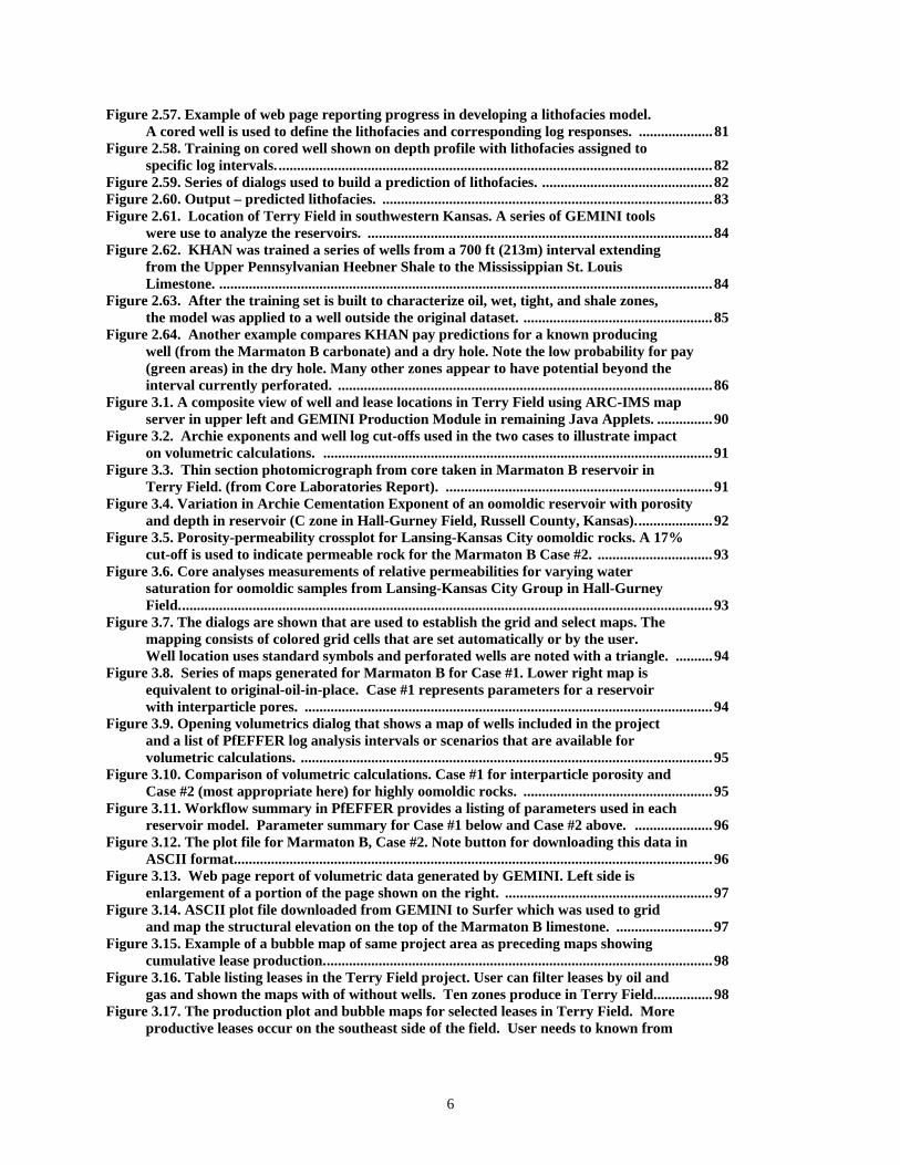
Figure 2.57. Example of web page reporting progress in developing a lithofacies model. A cored well is used to define the lithofacies and corresponding log responses. ....................81 Figure 2.58. Training on cored well shown on depth profile with lithofacies assigned to specific log intervals. ..................................................................................................................... 82 Figure 2.59. Series of dialogs used to build a prediction of lithofacies. ..............................................82 Figure 2.60. Output – predicted lithofacies. .........................................................................................83 Figure 2.61. Location of Terry Field in southwestern Kansas. A series of GEMINI tools were use to analyze the reservoirs. .............................................................................................84 Figure 2.62. KHAN was trained a series of wells from a 700 ft (213m) interval extending from the Upper Pennsylvanian Heebner Shale to the Mississippian St. Louis Limestone. .....................................................................................................................................84 Figure 2.63. After the training set is built to characterize oil, wet, tight, and shale zones, the model was applied to a well outside the original dataset. ...................................................85 Figure 2.64. Another example compares KHAN pay predictions for a known producing well (from the Marmaton B carbonate) and a dry hole. Note the low probability for pay (green areas) in the dry hole. Many other zones appear to have potential beyond the interval currently perforated. .....................................................................................................86 Figure 3.1. A composite view of well and lease locations in Terry Field using ARC-IMS map server in upper left and GEMINI Production Module in remaining Java Applets. ...............90 Figure 3.2. Archie exponents and well log cut-offs used in the two cases to illustrate impact on volumetric calculations. .........................................................................................................91 Figure 3.3. Thin section photomicrograph from core taken in Marmaton B reservoir in Terry Field. (from Core Laboratories Report). ........................................................................91 Figure 3.4. Variation in Archie Cementation Exponent of an oomoldic reservoir with porosity and depth in reservoir (C zone in Hall-Gurney Field, Russell County, Kansas).....................92 Figure 3.5. Porosity-permeability crossplot for Lansing-Kansas City oomoldic rocks. A 17% cut-off is used to indicate permeable rock for the Marmaton B Case #2. ...............................93 Figure 3.6. Core analyses measurements of relative permeabilities for varying water saturation for oomoldic samples from Lansing-Kansas City Group in Hall-Gurney Field................................................................................................................................................93 Figure 3.7. The dialogs are shown that are used to establish the grid and select maps. The mapping consists of colored grid cells that are set automatically or by the user. Well location uses standard symbols and perforated wells are noted with a triangle. ..........94 Figure 3.8. Series of maps generated for Marmaton B for Case #1. Lower right map is equivalent to original-oil-in-place. Case #1 represents parameters for a reservoir with interparticle pores. ..............................................................................................................94 Figure 3.9. Opening volumetrics dialog that shows a map of wells included in the project and a list of PfEFFER log analysis intervals or scenarios that are available for volumetric calculations. ...............................................................................................................95 Figure 3.10. Comparison of volumetric calculations. Case #1 for interparticle porosity and Case #2 (most appropriate here) for highly oomoldic rocks. ...................................................95 Figure 3.11. Workflow summary in PfEFFER provides a listing of parameters used in each reservoir model. Parameter summary for Case #1 below and Case #2 above. .....................96 Figure 3.12. The plot file for Marmaton B, Case #2. Note button for downloading this data in ASCII format.................................................................................................................................96 Figure 3.13. Web page report of volumetric data generated by GEMINI. Left side is enlargement of a portion of the page shown on the right. ........................................................97 Figure 3.14. ASCII plot file downloaded from GEMINI to Surfer which was used to grid and map the structural elevation on the top of the Marmaton B limestone. ..........................97 Figure 3.15. Example of a bubble map of same project area as preceding maps showing cumulative lease production.........................................................................................................98 Figure 3.16. Table listing leases in the Terry Field project. User can filter leases by oil and gas and shown the maps with of without wells. Ten zones produce in Terry Field................98 Figure 3.17. The production plot and bubble maps for selected leases in Terry Field. More productive leases occur on the southeast side of the field. User needs to known from

6

which zones that the leases produce from in order to access how these results can be compared to the volumetrics. ..................................................................................................99 Figure 3.18. The production curve can also be accessed from a standalone Java applet that is available from the lease and field production web pages. User is in ‘real-time” control of modifying the chart. ...................................................................................................99 Figure 3.19. Simplified material balance equation and relevance of performing

analysis in engineering reservoir modeling. .......................................................................... 104 Figure 3.20. Summary of features of Material Balance used when have an ideal data set, i.e., required data available is complete. ............................................................................ 104 Figure 3.21. Procedures to use in material balance when data set is incomplete. .......................... 105 Figure 3.22. Opening Java Application Window using Web Start that is launched and runs on the user’s PC without a link to the Internet................................................................ 105 Figure 3.23. Example dialogs from the PVT Module. ........................................................................ 106 Figure 3.24. Available modules in PVT Calculator. ........................................................................... 107 Figure 3.25. Overview of components included in DST module. ...................................................... 107 Figure 3.26. Calculation sequence in DST Analyst ............................................................................. 108 Figure 3.27. Opening dialog in Drill Stem Test Analyst allows the user to look up a digital DST test from the public-domain database. The series of tabs on the top are the main sheets while the bottom............................................................................................................... 108 Figure 3.28. The calculation worksheet tab opens the worksheet of time and pressure data. This sheet is active so a user can type in the time and pressure data if it is not available in digital form. Other dialogs are also shown in this figure including the Horner graph with a sliding bar to fit a curve and the first part of the calculation sheet. ........................... 109 Figure 3.29. The last dialog of the DST Analyst is shown where the calculations are made for the transmissibility, effect permeability, and skin. .................................................................. 109 Figure 4.1. Lineaments are added manually based on visual inspection paralleling trends recognized from previous work that indicates deep-seated basement heterogeneity reflected in Paleozoic structure and magnetic and gravity mapping (Watney et al., 2001). Many of these field produce oil and gas from the Mississippian “chat”. Map is generated from ARC-IMS map server (http://www.kgs.ku.edu/PRS/petroMaps.html). ..................................................................... 112 Figure 4.2. County production for Barber County showing cumulative and annual production. .................................................................................................................................. 113 Figure 4.3. Lineaments based on surface drainage bound Medicine Lodge North Field. Map is generated from ARC-IMS map server (http://www.kgs.ku.edu/PRS/petroMaps.html). ..................................................................... 113 Figure 4.4. Type log of cored well in Medicine Lodge North Field shows lithofacies and stratigraphic subdivisions of “chat” reservoir. Note that the nodular zones have slightly higher porosity and than the zones of breccia. ....................................................................... 114 Figure 4.5. Comparision between core plug porosity and porosity calculated from conversion of neutron counts. ....................................................................................................................... 115 Figure 4.6. Northwest-southeast structural log cross section highlighting chat2 reservoir interval with blue bar. The potential southwest “A” infill location is identified. ................. 116 Figure 4.7. Northwest-southeast structural log cross section through center of field and identifying another potential infill location. ............................................................................ 117 Figure 4.8. Northwest-southeast structural log cross section identifying another potential infill location. Note local thinning and truncation of the uppermost “chat” reservoir along the basal Pennsylvanian unconformity and local thickening of overlying Pennsylvanian conglomerate some correspondence to areas of underlying truncation of “chat”....................................................................................................................................... 117 Figure 4.9. Map depicting both current reservoir pressure in color with contours of overlying structure on top of the “chat” reservoir. Crest of structure and lower pressure closely coincide. ........................................................................................................... 118 Figure 4.10. Southwest potential infill location “A” showing Super Pickett crossplots in chat2 reservoir of surrounding wells. Red vertical lines in crossplot are BVW contours.

7

Points farther to right suggest coarser pores. Southwest side has higher Sw and BVW (less desireable properties) vs. lower Sw and BVW in southeast side of location “A”. ........ 119 Figure 4.11. Prospective infill location “B” in northwest part of field where reservoir pressure and rock properties are moderately high. Better reservoir quality (lower Sw and BVW) are in southeast side of this infill site, closer to structural crest and depleted reservoir pressure. ...................................................................................................................... 119 Figure 4.12. Eastern infill location “C” with surrounding wells exhibiting Super Pickett crossplots indicating lower BVW and Sw. .............................................................................. 120 Figure 4.13. The dialogs in GEMINI showing the main project list (upper left) and well list in the introductory dialog going to the volumetric module. ................................................... 121 Figure 4.14. Volumetric dialog for Medicine Lodge North showing various zones and models that were part of the experiment to define the optimum volumetric model for assessing infill drilling locations. ............................................................................................................... 121 Figure 4.15. Dialog where parameters are set to grid and map volumetric data in GEMINI. ....... 122 Figure 4.16. Color grid map (220 ft [67 m]cells) for average porosity in pay from chat2 reservoir in Medicine Lodge North Field. Prospective locations have moderate porosity and border highly porous and productive central areas of the field. ....................................................... 122 Figure 4.17. Average water saturation in pay of chat2 reservoir in Medicine Lodge Field. Note lower Sw in central producing area of field. Super Pickett crossplots of wells surrounding prospective infill drilling locations show similar patterns of Sw distribution. ................................................................................................................................ 123 Figure 4.18. Net pay thickness for chat2 reservoir in Medicine Lodge North Field. Indications are that location B has noticeably higher net pay that other prospective infill sites. ................................................................................................................................... 123 Figure 4.19. ASCII plotfile of volumetric data downloaded from GEMINI. Reservoir data were extrapolated to wells that have no logs, an example of a well shown by the red arrow. ........................................................................................................................ 124 Figure 4.20. Net pay map of chat2 reservoir using final cut-offs generated using Kriging for grid generation in Surfer using plotfile from GEMINI. This map and GEMINI’s net pay (Figure 4.18) are essentially the same. ........................................................................ 124 Figure 4.21. Map of average Vsh for pay interval in the chat2 reservoir. Arrows locate prospective infill drilling locations. .......................................................................................... 125 Figure 4.22. OOIP calculation dialog for Medicine Lodge North Field............................................ 125 Figure 4.23. Map of OOIP for Medicine Lodge Field with 200 ft (61 m) grid cell. ......................... 126 Figure 4.24. Core measurements of m, the Archie cementation exponent vs. depth indicate that m varies between 1.9 and 3.3. ............................................................................................ 126 Figure 4.25. Variation of core (General Atlantic A-1 Tjaden) measured m vs depth in Spivey-Grabs Field located 15 miles (24 km) northeast of Medicine Lodge North Field. ... 127 Figure 4.26. West central Midcontinent showing location of Minneola field complex ................... 128 Figure 4.27. Index map showing location of cross section H-H’ on right and production plot of Norcan Field on left. ...................................................................................................... 128 Figure 4.28. Regional SW-NE cross section Lower to Middle Pennsylvanian from Youle (1992) ................................................................................................................................ 129 Figure 4.29. East to west stratigraphic cross section through Minneola field complex (from Youle, 1992). ............................................................................................................................... 130 Figure 4.30. Base map of the Minneola field complex ....................................................................... 131 Figure 4.31. Composite well log plot with stratigraphic units and core description with Pe curve for Patton 1-3. ................................................................................................................... 133 Figure 4.32. Full Morrow interval highlighted by blue bar extending to the top of the Mississippian (Ste. Genevieve). ................................................................................................. 133 Figure 4.33. Core well Statton 2-12 with reservoir sandstone. ......................................................... 134 Figure 4.34. Porosity-permeability crossplot for Statton 2-12 and Patton 1-3 cores. ..................... 134 Figure 4.35. Porosity-permeability relationships for Morrow sandstones in southwestern Kansas. ......................................................................................................................................... 135

8

Figure 4.36. Structure maps (sealevel datum) for the datum at the top and base of the Morrow.................................................................................................................................. 136 Figure 4.37. Index map for cross sections shown in Figure mm. ...................................................... 136 Figure 4.38. Structure cross sections focused on the Morrow interval showing the S1, S2, and S3 cycles. .............................................................................................................................. 137 Figure 4.39. Depth profile of S2 cycle showing sandstone pay. To right is production plot of Schlicting 1-2 lease. ........................................................................................................ 138 Figure 4.40. Super Pickett crossplot of Schlicting #1-2 well. Low BVW (high phi and low Sw) combine to describe a good hydrocarbon pay zone. ................................................. 138 Figure 4.41. Well profile of Latzke #1 showing pay in lower portion of S2 sandstone. .................. 139 Figure 4.42. Super Pickett crossplot of Latzke #1 well, a marginal well with high BVW and relatively high Sw. ...................................................................................................................... 139 Figure 4.43. Cumulative BOE in 1000’s bbls for Norcan East Field. Two areas of high productivity. Blue circles denote leases with multiple wells. ................................................... 140 Figure 4.44. Average BVW for S2 sandstone overlain with total BOE contours. ........................... 140 Figure 4.45. Average Vsh for S2 sandstone overlain with total BOW contours. ............................ 141 Figure 4.46. Portion of map of Norcan East Field showing well profiles and well status and performance information ................................................................................................... 141 Figure 4.47. Plotfile for volumetrics of S2 cycle sandstone reservoir. .............................................. 142 Figure 4.48. Volumtric gridding dialog showing grid set for all mapping. ...................................... 142 Figure 4.49. Gross thickness, net pay, and average porosity for S2 cycle sandstone. ..................... 143 Figure 4.50. Average water saturation and OOIP for S2 cycle sandstone in Norcan East Field.... 144 Figure 4.51. Volumetric calculation dialog and report for S2 cycle sand in Norcan East Field. ... 145 Figure 4.52. Comparisons of total BOE and So*phi*ft and elevation base of S2 cycle. .................. 146 Figure 4.53. Comparison of plots and maps of BVW and Vsh illustrating trends. ......................... 147 Figure 4.54. Plot of Vsh and BVW vs. total BOE. ............................................................................. 148 Figure 4.55. Composite of the log, core, Pe curve and stratigraphic subdivisions within the S2 sedimentary cycle................................................................................................................... 149 Figure 4.56. Diagramatic Holocene Quaternary transgressive system (transgressive parasequences) along a valley fill profile modeled after the Texas Gulf Coast (from Thomas and Anderson, 1994). .................................................................................................. 149 Figure 4.57. Quaternary-Holocene transgressive systems tract for Texas Gulf Coast (Thomas and Anderson, 1994). .................................................................................................150 Figure 4.58. Clastic deposits on Texas Gulf Coast related to Quaternary lowstand and transgressive conditions (from Thomas and Anderson, 1994). .............................................. 150 Figure 4.59. A portion of the Help dialog in GEMINI showing active buttons used to access concepts and step-by-step tutorial of each module. ................................................................ 151 Figure 4.60. Portion of PfEFFER Concepts web page outlining topics. .......................................... 151 Figure 4.61. Web page from section on Pay Determination from PfEFFER Concepts Web Page in GEMINI Help. ............................................................................................................. 152 Figure 4.62. FAQ on GEMINI is available to the user. ..................................................................... 153 Figure 4.63. Access to Project Workflow is available through left margin of project dialogs. ...... 153 Figure 4.64. Summary of Volumetrics parameters for each well obtained when user accesses the Project Workflow, in this case, for Volumetrics. ................................................ 154 Figure 4.65. Dialogs showing that application is processing while user waits. Wait time for all of the GEMINI applications in minimal. ................................................................................. 154 Figure 4.66. Documentation of GEMINI releases available on the GEMINI website. .................... 155 Figure 4.67. Introductory page to KGS showing access point of GEMINI under software............ 155 Figure 4.68. LAS log viewer is a standalone adaptation of the Well Profile in GEMINI. The module runs on the server and logs accesses can be viewed, printed, and downloaded. ..... 156 Figure 4.69. Access to Standalone production module through KGS website provides automated plot and dialog to modify the plot. ......................................................................... 156 Figure 4.70. Web page to access standalone and downloadable Web Start applications. ............... 157 Figure 4.71. Example of a possible XML Read process. ................................................................... 158 Figure 4.72. Example of a possible XML Read process. ................................................................... 159

9

Figure 4.73. Example of possible XML framework for distributed database version of GEMINI. ..................................................................................................................................... 159 Figure 4.74. Data type XML File Formats. ......................................................................................... 160 Figure 4.75. Example of a possible Data Portal to access a server, view, and select data to assemble a GEMINI project “on-the-fly”. ............................................................................... 161 Figure 4.76. Web visits to GEMINI in February 2004 has grown to over 12,000. 40% of visits are from commercial addresses. ............................................................................................... 162

10

1. INTRODUCTION

Project Description Background

Utilization of improved recovery technologies could add significantly to the U.S. energy supply. In reservoir management, consistent, quantitative characterization and modeling of reservoirs are essential to make decisions on application of the most appropriate technology. Implementing this type of modeling is often not practical because of limitation of software, staff, expertise, and time. GEMINI (Geo-Engineering Modeling through Internet Informatics) has brought together existing geologic and engineering expertise and resources of the Kansas Geological Survey to provide efficient, interactive access to data and a suite of web-based software geologic and engineering modeling tools to apply to data when and wherever it is needed. GEMINI integrates extensive petroleum and petrophysical databases associated with the DOE-funded Northern Mid-Continent Digital Petroleum Atlas (DPA) (http://crude2.kgs.ku.edu/DPA/dpaHome.html). GEMINI is built on experience gained in software development provided through the DOE-funded PfEFFER (Petrofacies Evaluation of Formations for Engineering Reservoirs) software (http://crude2.kgs.ku.edu/PRS/software/pfeffer1.html. GEMINI also incorporates this successful log analysis software into the new web application. GEMINI offers a dozen different modules to:

• resolve reservoir parameters that control well performance via integrated log analysis,

drill stem test analysis, and a PVT calculator; • characterize subtle reservoir properties important in understanding and modeling

hydrocarbon pore volume and fluid flow through integrated, interactive rock catalog, display of core data in a well profile, precise pay delineation and spatial analysis via interactive spreadsheet-based log analysis, interactive cross sections and well plots annotated with perforation and DST data;

• expedite recognition of bypassed, subtle, and complex oil and gas reservoirs at regional and local scale using spatial analysis tools, detailed well profiles, and volumetric analysis;

• differentiate commingled reservoirs using integrated tools to analyze and view petrophysics of well profile alongside perforations and drill stem tests;

• build integrated geologic and engineering models based on real-time, iterative solutions to evaluate reservoir management options for improved recovery including volumetric and material balance models for comparison and iterative testing and refinement with map gridding structured for ease of use in a reservoir simulator;

11

• provide an integrated set of practical tools to assist the geoscientist, engineer, and petroleum operator in making their tasks more efficient and effective;

• enable evaluations to be made at different scales, ranging from individual well, through lease, field, to play and region (scalable information infrastructure) leveraging the public domain datasets;

• provide training and technology transfer via web-based tutorial and examples to enhance capabilities of the client;

• provide tracking of project workflow to facilitate review and updating among collaborators; and

• give the user the option to export data and results to other applications further add value to the analyses, e.g., reservoir simulation, geostatistical analysis, or to utilize more enhanced mapping software.

Work Performed

The program, for development and methodologies, was a 3-year interdisciplinary effort to develop an interactive, integrated Internet Website named GEMINI (Geo-Engineering Modeling through Internet Informatics) that builds real-time geo-engineering reservoir models for the Internet using the Java-based Web applications (www.kgs.ku.edu/Gemini). The client is able to retrieve databases from the KGS website, upload their own information, and run software interactively using the intelligent interfaces that efficiently assemble in real-time a project based on the definition of a three-dimensional data volume, be it a reservoir or larger-scale endeavor. Software procedures are described to provide linkage of GEMINI software applications to other public-domain servers allowing users can work through their website and database of primary interest and be able to use GEMINI tools to analyze their information as made possible by the latest technological advances. Additional options are presented to run certain modules as standalone applications on the user’s PC. After download, the application can be run without an Internet connection. Analytical software operating on the assembled data and results are delivered to the client through the web pages. System informatics, consisting of the network, software, data, and tutorial components, permit the client to develop any number of projects. Analytical components of GEMINI include assembling fluid and rock parameters, basic and enhanced wireline log interpretation, spatial analysis and visualization, volumetrics, material balance, and specific parameterization and formatting of these results suited for input into reservoir simulation software. A tutorial module instructs clients on the theory, application of analytical tools, and operation of GEMINI. Participating major and independent companies provided information and expertise to test modules, provide feedback during the development process to help make GEMINI relevant to the needs of the clientele.

12

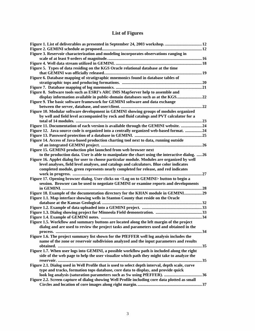
GEMINI-Deliverables

An internet web-site

Rock and Fluid CatalogsAccess through the Gemini User/Project Module

Web-based analytical software tools.Well Level Modules (Well Profile, PfEFFER, DST, Synthetic Seismogram, KHAN)Field Level Modules (Cross Section, Volumetric, Production, Material Balance, ASCII Output for Reservoir Simulation, PVT Calculator)Access through the Gemini User/Project Module

Tutorial module including theory, application of analytical tools and operation of GEMINI.

Reports, Seminars, Conferences and Workshops will be provided as records of technology transfer activities.

– http://www.kgs.ukans.edu/Gemini/index.html

–http://www.kgs.ukans.edu/Gemini/R1.0/GeminiUserProjectModule.html

–

–

–http://www.kgs.ukans.edu/Gemini/R1.0/GeminiUserProjectModule.html

– http://www.kgs.ukans.edu/Gemini/gemini-help.html

Figure 1. List of deliverables as presented in September 24, 2003 workshop. GEMINI Schedule The schedule for the GEMINI Project as proposed is divided into five tasks as described in Figure 2. Figure 2. GEMINI schedule as proposed.

13

EXECUTIVE SUMMARY

GEMINI (Geo-Engineering Modeling through Internet Informatics) is an interdisciplinary effort that has developed an interactive, integrated Internet Website used to build real-time, on-line geo-engineering reservoir models. The client is able to retrieve databases, upload information, and run software interactively using intelligent interfaces that efficiently assemble a project based on the definition of a three-dimensional data volume. Analytical software operating on the assembled data were developed in modular form and include:

Well Profile Module – View LAS files that are part of a project, annotated with formation tops from database and reservoir intervals established for log analysis; interactive interface to label additional formation tops, perforations, and DST intervals. PfEFFER Log Analysis Module – Module utilizes a spreadsheet appearance and incorporates a modified Pickett crossplot to analyze well logs and define net reservoir pay for use in volumetric module. Module includes standard water saturation equations, lithology interpretation, secondary porosity, and depth-constrained cluster analysis. Rock Catalog Module – A comprehensive module develops correlations between core petrophysics, lithofacies, and pore types. Module can also be used to look up core analyses in database. Synthetic Seismogram Module – This module provides the means to generate a synthetic seismogram from a sonic log to facilitate linking these petrophysical results with seismic information. Cross Section Module - Module is used to interactively build an annotated wireline log cross section. Sections include up to five wells, datums can be selected interactively, stratigraphic datums and designated reservoir intervals common to wells are automatically correlated and emphasized in color. KHAN Module – Kansas Hydrocarbon Association Navigator (KHAN) Module is used for statistical modeling of petrophysical core and log data to derive meaningful patterns such as use in scanning LAS file for hydrocarbon pay and classifying lithofacies. Models can be shared with other users to allow use with their data. Volumetrics Module – Pay calculations obtained from the log analysis module, including average water saturation and porosity, net and gross pay thickness, are shared with volumetics module to calculate and map original and remaining hydrocarbon in place. Information can be downloaded as ASCII files for use in other software. Material Balance Module – Module calculates original-oil-in-place (OOIP) for a waster-driven reservoir above the bubble point. Results are used to compare with volumetric-derived OOIP PVT Calculator - The PVT calculator estimates formation volume factors, viscosity, and compressibilities used in calculations involving DST, volumetric, and material balance modules. Well Production Module – Module generates time-series changes in oil and gas production in a project area by generated a time-lapse movie of bubble maps. Bubble map is useful to compare with volumetric results. Module also generates a standard semi-log production-time plot for leases that are part of project. DST Analyst – DST Analyst uses Horner analysis to calculate permeability, skin, and drainage radius from manually entered and digital DST information.

14

Fluid Catalog – Module is a browser interface to look up fluid composition and resistivities. ASCII Output for Reservoir Simulation – Grid files of key reservoir parameters generated in volumetrics are assembled for a simulator such as BOAST. GEMINI results are delivered to the client through web pages, Java dialogs, and ASCII

files. System informatics, consisting of the network, software, data, and tutorial components, permit the client to develop any number of projects. The tutorial module instructs clients on theory and concepts, application of analytical tools, and operation of GEMINI. A separate workflow provides new and returning users the means to review progress and facilitate distant collaborations.

The development of GEMINI proceeded through series of tasks, each performed in

collaboration with different team members and under the supervision of the project manager including: design of the project interface and design and building of the modules in reservoir characterization and geo-engineering modeling. Technology transfer was implemented throughout the project via workshops, presentations, and publications utilizing case studies and operator feedback. Project deliverables to USDOE include: an internet web-site that is able to build petroleum projects, rock and fluid catalogs, analytical software tools, tutorial module, and reports.

EXPERIMENTAL

GEMINI (Geo-Engineering Modeling through INternet Informatics) is a public–domain, interactive, integrated Internet web application that provides a suite of user-friendly geologic and engineering software, calculators, and utility programs designed to facilitate real-time geologic and engineering petroleum reservoir modeling. Digital data obtained from the Kansas Geological Survey and the user is assembled “on the fly”. Compilation of data, calculations, and models are maintained as a project on the Internet server where reports and data files can be downloaded at any time and location with an Internet connection. Projects and data uploaded into the project are password protected. The project provides a proof-of-concept to use an extensive set of public-domain petroleum reservoir analysis applications that run on the Internet for use in seamless analysis of a public-domain database and user-uploaded information. The use of the Java development platform makes the GEMINI operable on any client platform and operating system, provided they are able to load on their workstation or PC a Java plug-in from Sun Microsystems (http://java.sun.com/products/plugin/) and are able to allow Java applets to be sent to their computer.

GEMINI was developed by the Kansas Geological Survey (KGS)

(http://www.kgs.ku.edu/Gemini/index.html), over a 3-year period between September 2000- September 2003, funded by the U.S. Department of Energy (Contract No.DE-FG26-00BC15310). Six companies are providing data and expertise to test and evaluate the software including: Anadarko Production Corporation, BP-Amoco, Conoco-Phillips, Lario Petroleum, Mull Drilling Company, Murfin Drilling Company, and Pioneer Resources.

Current prototype modules in GEMINI perform many functions useful in everyday petroleum reservoir characterization and modeling including software to view, annotate, and

15

analyze digital well logs. GEMINI provides an integrated solution of effective pay utilizing core, well log, and test data. In particular, the integration with rock, log, and test data permit ease in developing refined interactive solutions. The need for input and exporting of data is minimized in the process. The goal is to provide users, particularly small operators, an option to build a simple petrophysical model of a project, quickly obtain volumetric calculation, and be able to check results against a material balance calculation to determine accuracy of the geomodel. Such analysis available at the fingertips of the small operator permits them to make more informed decisions in evaluating their properties.

Geo-engineering modeling as used in GEMINI involves a methodology comprised of integration of log, core, and well test analyses followed by iteratively solving volumetric and material balance calculations (Bhattacharya et al., 1999). The approach facilitates application of the concept of petrofacies analysis where lithofacies as described are associated with particular pore types and petrophysics, and, in turn, characteristic reservoir parameters that are used to define reservoir pay (Watney et al., 1999). Petrofacies analysis is closely analogous to pore-type classification of Choquette and Pray (1970) and Lucia (1983, 1999). Petrofacies relationships are realized by a close integration of core and log petrophysics used to establish families of related reservoirs, e.g., moldic, vuggy, interparticle, microporous, and fracture porosity. Previous studies indicate that lithofacies modified by diagenesis and structure lead to preferred pore types, e.g., the commonality between moldic pore types in Midcontinent Paleozoic carbonate reservoirs -- Cambro-Ordovician dolomite, Mississippian (Osage) chert, and Pennsylvanian oomoldic carbonate systems (Byrnes, et al., 2003).

Calculators and catalogs are provided to obtain reservoir and fluid parameters needed in

modeling. The goals of GEMINI are to: 1) provide real-time, interactive analyses of the petroleum reservoir, 2) quantitatively model reservoir heterogeneity, 3) estimate recoverable hydrocarbons, 4) target locations in the reservoir best suited for further development, 5) provide reliable quantitative information for more informed reservoir management, 6) obtain reservoir and fluid parameters for subsequent reservoir fluid flow simulation, and 7) screen wells for subtle, overlooked or bypassed pay from both exploration and development perspective. Answers in GEMINI are delivered to the user interactively via the Internet where application tools and data reside in projects developed on the Internet. GEMINI can rapidly establish a project, assemble information, and develop simple geo-engineering models to determine appropriate methods and technologies to improve oil and gas recovery. As an exploration application, GEMINI can process and model large amounts of digital log data to target prospective reservoirs suited for further evaluation. Once pay is established, the KHAN module, for example, can be used to train and predict on pay zone to screen digital LAS log files. The small independent operators are the key clients identified for this technology, providing software tools to them that are similar to those used by large independents and major oil companies.

The reservoir model is closely calibrated to the reservoir’s petrofacies defined as a

combination of lithofacies and pore type with characteristic and constrained variations in petrophysical properties (Bhattacharya, et al., 1999). Evaluation of the pore type and distribution and related fluid saturation is increasingly essential to reevaluate mature oil and gas fields where the objective is to develop underproduced and bypassed reserves. Smaller and often subtle pays remain due to reservoir complexities that caused them to be overlooked initially due to primary

16

flush production from more clearly defined pays. A relational rock catalog in GEMINI provides unprecedented access to core data to facilitate rapid access, analysis. and integration of results with wireline log interpretation to efficiently establish correlations between rock petrofacies and log petrophysical response. The net result is to improve accuracy of hydrocarbon volume and resulting economic decisions. Recent studies conducted by the project team illustrate this critical need to integrate quantitative core and log data into reservoir analyses to develop more robust results (Dubois et al., 2001; Watney et al., 2001; Bohling and Dubois, 2003; Byrnes, et al., 2003; Dubois et al., 2003a,b)

Limited volumes of the reservoir are typically targeted in redevelopment of mature oil

and gas fields, e.g., isolating bypassed and underproduced zones. Thus, complex quantitative modeling of the reservoir may be at first impractical and uneconomic (Bhattacharya et al., 1999; Watney et al. 1999; Doveton et al 2000). Simple, petrophysically-based models are best suited for small reservoir systems and are believed to be quite adequate for reservoir management, particularly when these simple petrophysical models, volumetric analysis, and material balance calculations can be integrated and accessed interactively and collaboratively on the web. Having access to the tools to conduct the analyses is better than the alternative without tools and no analyses. The job will not get done and the opportunity will be lost eventually through a sale of the field to someone who will take on the challenge.

Activities in development of fields and exploration plays can both benefit from

application of simple, efficient approaches to geologic and engineering modeling. Access to simple modeling that is web-based and linked to the public-domain data sources are well suited to this task to permit rapid screening for decision making or more in-depth investigation. Data assembly and integration with software tools are provided seamlessly to the user though GEMINI, specifically tailored to help the small oil and gas operators and consultants. The ultimate goal of the project is to allow an operator to reach beyond standard approaches in evaluation of borehole data, serving as a component to maintain a viable petroleum economy and infrastructure in mature oil and gas producing areas.

Targeted users are companies and consultants who seek to develop remaining oil and gas reserves in mature oil and gas provinces like Kansas. Cost-effective, efficient, and reliable means are essential to rapidly assemble and analyze well, lease, field, and reservoir play information. Integrated information handling and software tools are used to resolve, correlate, and map reservoir pay. Help and tutorial functions and Project Workflow assist the user in operation of GEMINI. This coupled with means to easily export results facilitate continued collaborative solutions as part of a stepwise process to evaluate, refine, and apply knowledge.

GEMINI was developed to address opportunities to facilitate quantitative reservoir evaluation in smaller, mature oil and gas fields in the domestic U.S. (Table 1 and 2).

17

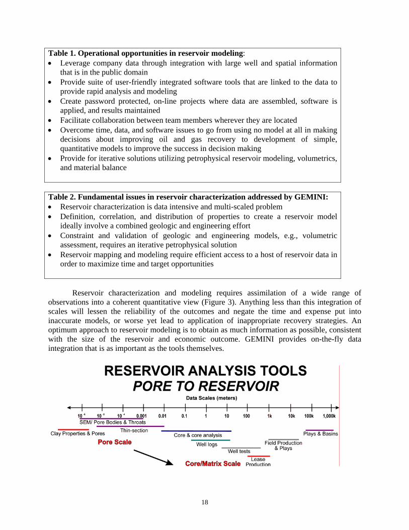
Table 1. Operational opportunities in reservoir modeling: • Leverage company data through integration with large well and spatial information

that is in the public domain • Provide suite of user-friendly integrated software tools that are linked to the data to

provide rapid analysis and modeling • Create password protected, on-line projects where data are assembled, software is

applied, and results maintained • Facilitate collaboration between team members wherever they are located • Overcome time, data, and software issues to go from using no model at all in making

decisions about improving oil and gas recovery to development of simple, quantitative models to improve the success in decision making

• Provide for iterative solutions utilizing petrophysical reservoir modeling, volumetrics, and material balance

Table 2. Fundamental issues in reservoir characterization addressed by GEMINI: • Reservoir characterization is data intensive and multi-scaled problem • Definition, correlation, and distribution of properties to create a reservoir model

ideally involve a combined geologic and engineering effort • Constraint and validation of geologic and engineering models, e.g., volumetric

assessment, requires an iterative petrophysical solution • Reservoir mapping and modeling require efficient access to a host of reservoir data in

order to maximize time and target opportunities

Reservoir characterization and modeling requires assimilation of a wide range of

observations into a coherent quantitative view (Figure 3). Anything less than this integration of scales will lessen the reliability of the outcomes and negate the time and expense put into inaccurate models, or worse yet lead to application of inappropriate recovery strategies. An optimum approach to reservoir modeling is to obtain as much information as possible, consistent with the size of the reservoir and economic outcome. GEMINI provides on-the-fly data integration that is as important as the tools themselves.

18

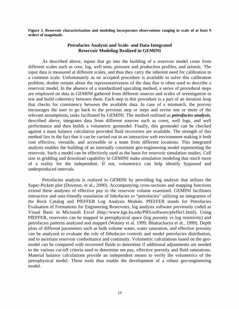
Figure 3. Reservoir characterization and modeling incorporates observations ranging in scale of at least 9 orders of magnitude.

Petrofacies Analysis and Scale- and Data-Integrated Reservoir Modeling Realized in GEMINI

As described above, inputs that go into the building of a reservoir model come from

different scales such as core, log, well tests, pressure and production profiles, and seismic. The input data is measured at different scales, and thus they carry the inherent need for calibration to a common scale. Unfortunately as no accepted procedure is available to solve this calibration problem, doubts remain about the representativeness of the data that is often used to describe a reservoir model. In the absence of a standardized upscaling method, a series of procedural steps are employed on data in GEMINI gathered from different sources and scales of investigation to test and build coherency between them. Each step in this procedure is a part of an iteration loop that checks for consistency between the available data. In case of a mismatch, the process encourages the user to go back to the previous step or steps and revise one or more of the relevant assumptions, tasks facilitated by GEMINI. The method outlined as petrofacies analysis, described above, integrates data from different sources such as cores, well logs, and well performance and then builds a volumetric geomodel. Finally, this geomodel can be checked against a mass balance calculation provided fluid recoveries are available. The strength of this method lies in the fact that it can be carried out in an interactive web environment making it both cost effective, versatile, and accessible to a team from different locations. This integrated analysis enables the building of an internally consistent geo-engineering model representing the reservoir. Such a model can be effectively used as the basis for reservoir simulation studies. Cell size in gridding and download capability in GEMINI make simulation modeling that much more of a reality for the independent. If not, volumetrics can help identify bypassed and underproduced intervals.

Petrofacies analysis is realized in GEMINI by providing log analysis that utilizes the Super-Pickett plot (Doveton, et al., 2000). Accompanying cross-sections and mapping functions extend these analyses of effective pay to the reservoir volume examined. GEMINI facilitates interactive and user-friendly translation of lithofacies to “petrofacies” utilizing an integration of the Rock Catalog and PfEFFER Log Analysis Module. PfEFFER stands for Petrofacies Evaluation of Formations for Engineering Reservoirs, log analysis software previously coded as Visual Basic in Microsoft Excel (http://www.kgs.ku.edu/PRS/software/pfeffer1.html). Using PfEFFER, reservoirs can be mapped in petrophysical space (log porosity vs log resistivity) and petrofacies patterns analyzed and mapped (Watney et al. 1999; Bhattacharya et al., 1999). Depth plots of different parameters such as bulk volume water, water saturation, and effective porosity can be analyzed to evaluate the role of lithofacies controls and model petrofacies distribution, and to ascertain reservoir conformance and continuity. Volumetric calculations based on the geo-model can be compared with recovered fluids to determine if additional adjustments are needed to the various cut-off criteria used to determine net pay, effective porosity and fluid saturations. Material balance calculations provide an independent means to verify the volumetrics of the petrophysical model. These tools thus enable the development of a robust geo-engineering model.

19

Reservoir geomodels are typically based on limited subsurface information and require classification of core and log data and their extrapolation between wells utilizing latest geological concepts, models, and analogs. Depositional sequence analysis is a popular methodology to classify strata and provides a means to characterize surfaces and define continuity and coherency of stratal elements so important to correlation. Substantiation of sequences includes understanding regional reservoir frameworks and incorporating knowledge gained from analogs. In addition to stratigraphic constraints, reservoir geometry is subject to interpretations of depositional environment, diagenesis, and structure, e.g., delta or estuary sandstones, oolite bars vs. spillover lobes. After these fundamental classifications and correlations are made, the next step is to analyze the petrophysical information and fill the reservoir volume. The procedure itself can lead to refining the geomodel, e.g., recognizing and substantiating flow units with more coherent physical properties. Iterations are needed along the way to develop the best fit between the petrophysical data and the geomodel. Ideally, this is a team effort between the geologist and engineer. As the complexity of a reservoir models grows, so can the uncertainty. In mature fields, often limited data and time compel a simple solution, at least initially. GEMINI provides a practical rapid solution to assemble, build, and verify these simple models before going to more complex ones.

Inexpensive spreadsheet software (Doveton et al., 2000), and now integrated, platform-

independent, web-based software as GEMINI provide the opportunity for cost-effective translation of geomodels to geo-engineering models and its associated testing and validation. GEMINI also facilitates the necessary collaboration between geoscientists and engineers and leveraging the on-line public domain databases.

The steps in petrofacies analysis provided by GEMINI include analysis of core data,

creation of Super-Pickett crossplots of well log data, volumetric calculations based on the reservoir petrophysics, and material balance calculations originating from the fluids produced. Material balance calculations are independent of the petrophysical data and results are used to verify the volumetrics. Moreover, material balance enables the identification of the reservoir drive mechanism (an important component of the reservoir model). The comparison between the volumetric and the mass balance calculations integrates the production, pressure and PVT data with the petrophysics of the geomodel. These tasks can all be carried out in this web application, thus facilitating iterative solutions to develop simple, but optimized geo-engineering models.

Project Design The project interface in GEMINI has changed over the three years of development reflecting new modules and enhancements made to them. The flow has also been modified to make negotiation of GEMINI more user-friendly directed toward compiling well data and running software modules in the context of wells assembled into a defined project. Access to projects is password-protected. A user might establish a project for analysis, becoming the project owner, and, in turn, share it as read-only or permit full read and write capability. The data, analyses, and results that are maintained in a GEMINI project can be updated or retrieved and downloaded as web browser pages, ASCII files, images, and charts. The semicolon-delimited ASCII files permit further analysis using other software.

20

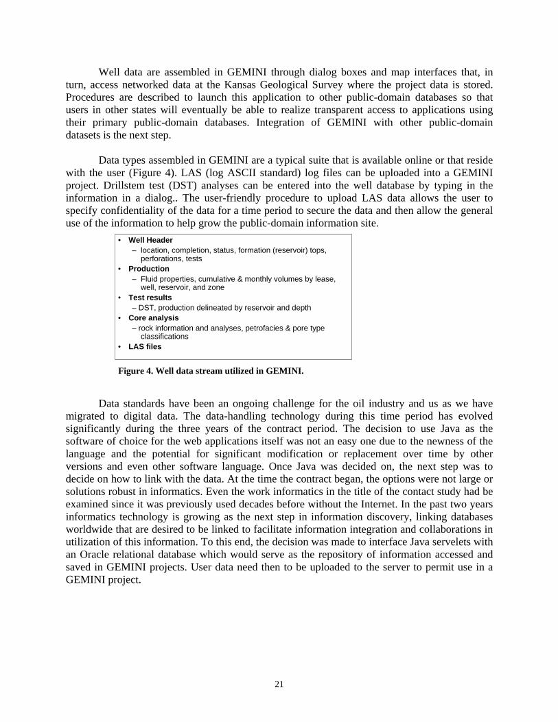
Well data are assembled in GEMINI through dialog boxes and map interfaces that, in turn, access networked data at the Kansas Geological Survey where the project data is stored. Procedures are described to launch this application to other public-domain databases so that users in other states will eventually be able to realize transparent access to applications using their primary public-domain databases. Integration of GEMINI with other public-domain datasets is the next step.

Data types assembled in GEMINI are a typical suite that is available online or that reside

with the user (Figure 4). LAS (log ASCII standard) log files can be uploaded into a GEMINI project. Drillstem test (DST) analyses can be entered into the well database by typing in the information in a dialog.. The user-friendly procedure to upload LAS data allows the user to specify confidentiality of the data for a time period to secure the data and then allow the general use of the information to help grow the public-domain information site.

• Well Header

– location, completion, status, formation (reservoir) tops, perforations, tests

• Production– Fluid properties, cumulative & monthly volumes by lease,

well, reservoir, and zone• Test results

– DST, production delineated by reservoir and depth• Core analysis

– rock information and analyses, petrofacies & pore type classifications

• LAS files

Figure 4. Well data stream utilized in GEMINI.

Data standards have been an ongoing challenge for the oil industry and us as we have migrated to digital data. The data-handling technology during this time period has evolved significantly during the three years of the contract period. The decision to use Java as the software of choice for the web applications itself was not an easy one due to the newness of the language and the potential for significant modification or replacement over time by other versions and even other software language. Once Java was decided on, the next step was to decide on how to link with the data. At the time the contract began, the options were not large or solutions robust in informatics. Even the work informatics in the title of the contact study had be examined since it was previously used decades before without the Internet. In the past two years informatics technology is growing as the next step in information discovery, linking databases worldwide that are desired to be linked to facilitate information integration and collaborations in utilization of this information. To this end, the decision was made to interface Java servelets with an Oracle relational database which would serve as the repository of information accessed and saved in GEMINI projects. User data need then to be uploaded to the server to permit use in a GEMINI project.

21

Figure 5. Types of data residing on the KGS Oracle relational database

Counts of various data types in the KGS database September 2003 395,932 Wells (QUALIFIED.WELL_HEADERS) 73,527 Leases (NOMENCLATURE.LEASES) 6,831 LAS files (LAS.WELL_HEADERS) 166,535 Elogs for 93,362 wells (ELOG.LOG_HEADERS) 10,708 scanned elogs for 6,107 wells that are available for download (ELOG.SCAN_URLS) 2,451 DSTs (DST.DSTS) 1,822,393 tops for 154,787 wells (QUALIFIED.WELL_TOPS) 3,800 core samples analyzed -- for 21 wells – available in the database now (CORE_LIBRARY.CORE_DATA_AND_DESCRIPTIONS) 7,800 core samples analyzed -- for 200 wells – data are being prepared for addition to the existing data 400 core samples analyzed -- from the Arbuckle -- for 20-30 wells – data are being prepared for addition to the existing data This is a longer-term project because there is still a few days of laboratory work that must be finished. 137 Crude oil samples analyzed for 136 wells (FLUID_CATALOG.CRUDE_OIL_SAMPLES) 1811 Gas Compositions analyzed for 1626 wells (FLUID_CATALOG.GAS_COMPOSITIONS)

Brine analyses from over 3500 wells

at the time that GEMINI was officially released.

Data types and file structures vary significantly among public-domain and individual

users. Vendors strive to provide digital data that meet certain standards, if not internally being consistent. File types generated and maintained in ASCII, such as well log LAS, have provided straight forward reading and parsing into data frameworks. ASCII has dominated data types used in GEMINI. In contrast, digital DST records written in binary are in need of standardization so they can be read from the original files.

Standardization of table formats are usually not maintained between servers or in files

created by individual users. Also, nomenclature of variable names and mnemonics used vary widely from area to area and database to database, e.g., stratigraphic names and well log types (Figures 5 and 6). The metadata issues include variations in nomenclature and variable completeness of data types needed to be solved before linking numbers of public-domain databases. The Java tool development was accordingly focused to interact with a single server with fixed data format. Steps were taken along with way to investigate options to extend the

22

applications to other servers once the technology was available to facilitate linkage with minimal overhead in time and resources for systems administrators of other public-domain servers.

The database mapping of subsurface stratigraphic names shown in Figure 6 shows the

mnemonics that occur in the formation database and a correlation with stratigraphic nomenclature arranged by age and formation rank. Attempts to filter results and spatially map stratigraphic information require this database mapping.

Mapping Subsurface Stratigraphic Names

Figure 6. Database mapping of stratigraphic mnemonics found in database tables of stratigraphic tops and producing formations.

Well log mnemonics are similarly in need of database mapping so that log curves can be

properly accessed and output (Figure 7). Occurrences of various log types are each correlated to a hierarchical family of logs. The classification is built around other standard classifications that are in the public domain such as the Society of Professional Well Log Analysts (SPWLA) (http://www.spwla.org/library_info/mnemonics/mnemonics.htm), POSC, a not for profit organization working on petroleum industry data standards also provides information to help map the log mnemonics (http://www.posc.org/technical/PWLS/pwls_20.htm). The Canadian Well Logging Society, which provided the LAS standard, also has software to certify LAS files before they are uploaded to the server (http://www.cwls.org/las_info.htm).

23

Mapping LAS Mnemonics

Figure 7. Database mapping of log mnemonics.

In the past three years access and display of public-domain data has grown significantly as software visualization tools have become available such as at the KGS (Figure 8).

•Dynamic Mapping of Kansas Oil and Gas Data with Spatial Data Engines and Internet Map Server

Victory Fieldlease productiondeline curvesFrom ProductionModule

Thickness of Lansing-Kansas City Groups

Hugoton Field Area

Hugoton wells shown

Figure 8. Software tools such as ESRI’s ARC IMS MapServer help to assemble and display information available in public-domain databases such as at the KGS.

24

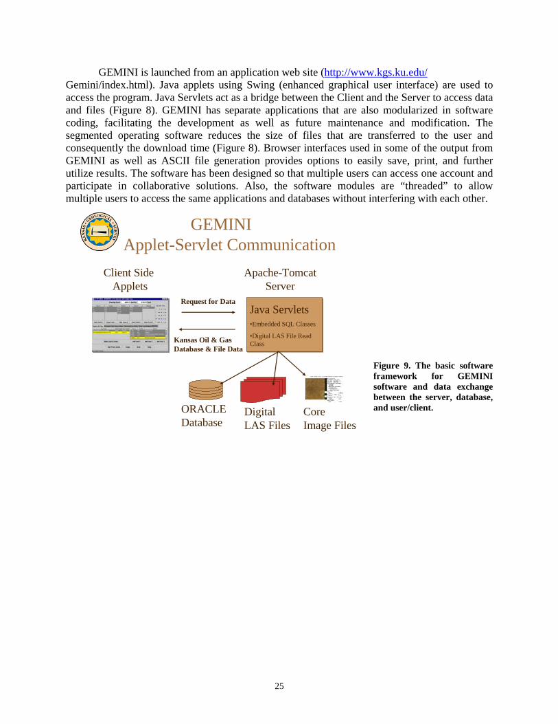
GEMINI is launched from an application web site (http://www.kgs.ku.edu/Gemini/index.html). Java applets using Swing (enhanced graphical user interface) are used to access the program. Java Servlets act as a bridge between the Client and the Server to access data and files (Figure 8). GEMINI has separate applications that are also modularized in software coding, facilitating the development as well as future maintenance and modification. The segmented operating software reduces the size of files that are transferred to the user and consequently the download time (Figure 8). Browser interfaces used in some of the output from GEMINI as well as ASCII file generation provides options to easily save, print, and further utilize results. The software has been designed so that multiple users can access one account and participate in collaborative solutions. Also, the software modules are “threaded” to allow multiple users to access the same applications and databases without interfering with each other.

GEMINI

Applet-Servlet CommunicationClient Side

AppletsApache-Tomcat

Server

Java Servlets•Embedded SQL Classes

•Digital LAS File Read Class

ORACLE Database

Digital LAS Files

Core Image Files

Request for Data

Kansas Oil & GasDatabase & File Data

Figure 9. The basic software framework for GEMINI software and data exchange between the server, database, and user/client.

25

Figure 10. Modular software development in GEMINI showing groups of modules organized by well and field level accompanied by rock and fluid catalogs and PVT calculator for a total of 14 modules. Modules operate as part of an integrated workflow allowing information and results to be passed between modules within a user-defined project. Certain modules can also be used as standalone basis, e.g., DST, synthetic seismic, Rock Catalog, and PVT. The LAS viewer in Well Profile and the production plot from Well Production module are also standalone activities that run against single wells and leases, respectively, in the database.

A penultimate GEMINI Version 3.6 was issued on July 31st, 2003, which was extensively tested. The final version of GEMINI was released on September 30, 2003 containing 908 Java Source Files, Applets, Servlets, Plot Classes, Math Model Classes, Java Swing Frames, Panels and Table Classes in 284,772 lines of Java code (see modules in Figure 10). Descriptions of versions are available on the GEMINI website (Figure 9). Level 2 compliant code and documentation is utilized to insure that code can be easily understood by other programmers for maintenance and modification (Figure 10). Code listing is available through the web browser to facilitate updating and review by programming team. Program organization is suited to facilitate open programming environment to permit other Java code to be easily added to those already present. This open environment may be an added incentive for participation by other public-domain sites to tailor new software to meet their particular needs as well as assisting the needs of other public domain sites to better serve their clients.

26

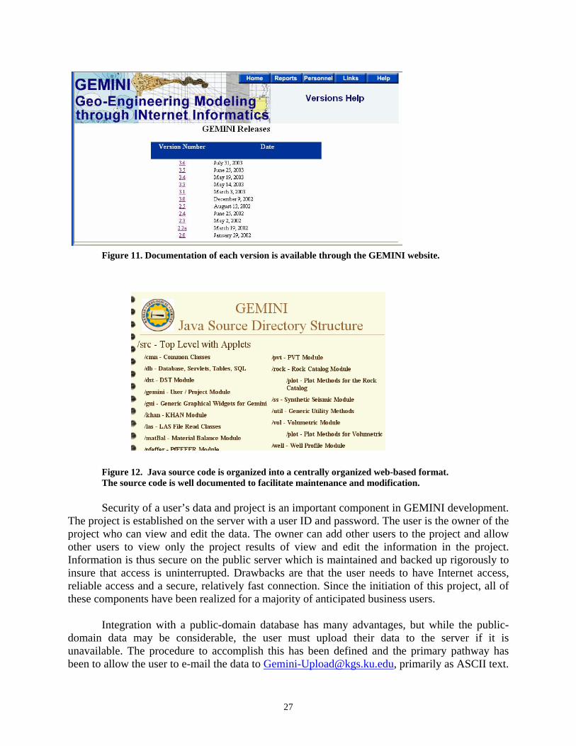
Figure 11. Documentation of each version is available through the GEMINI website. Figure 12. Java source code is organized into a centrally organized web-based format. The source code is well documented to facilitate maintenance and modification. Security of a user’s data and project is an important component in GEMINI development.

The project is established on the server with a user ID and password. The user is the owner of the project who can view and edit the data. The owner can add other users to the project and allow other users to view only the project results of view and edit the information in the project. Information is thus secure on the public server which is maintained and backed up rigorously to insure that access is uninterrupted. Drawbacks are that the user needs to have Internet access, reliable access and a secure, relatively fast connection. Since the initiation of this project, all of these components have been realized for a majority of anticipated business users.

Integration with a public-domain database has many advantages, but while the public-

domain data may be considerable, the user must upload their data to the server if it is unavailable. The procedure to accomplish this has been defined and the primary pathway has been to allow the user to e-mail the data to Gemini-Upload@kgs.ku.edu, primarily as ASCII text.

27

The other security issue is that some data within a project may be secure to certain members of the team. These data can have additional password protection to allow certain users access (Figure 13).

GEMINIValidate if user has access to data

Table: GeoUserName TypeKID N (10)USER_NAME V(80)COMPANY V(80)EMAIL_ADDRESS V(80)ACCOUNT_NAME V(30)PASSWORD V(30)CREATE_DATE DLAST_DATE_USED D

Table: Upload_DataName Type

KID N (10)USER_KID N(10)WELL_HEADER_KID N(10)DATA_TYPE N(2)TABLE_KID N(10)DATA _SOURCE V(60)CREATE_ DATE DUNTIL_ DATE D

Figure 13. Password protection of a database in GEMINI.

The project framework offers a unique collaborative environment where a project team

can be located anywhere the Internet is available. The project provides an integrated environment to apply the software modules to realize the development of a geo-engineering model of the reservoirs when one may not have been forthcoming from the available tools. It can not be overemphasized that the results can be downloaded and transferred to other software tools to achieve additional insights into the reservoir being analyzed.

While the specified deliverable in this contract was an integrated project, several software

functions, namely the PVT Calculator, LAS Viewer, Production Plotting, Gridding and Mapping, and Material Balance have been adapted at the close of the project to Java Web Start standalone applications that are run from the user’s computer, http://www.kgs.ku.edu/Gemini/Tools/Tools.html, and as web applications that run alongside data in a browser next to the data that accessed (Figures 14 and 15). The versatility of the software is readily apparent providing options for use with other public-domain database and websites.

28

Figure 14. Access of Java-based production charting tool next to data, running outside of an integrated GEMINI project.

Figure 15. GEMINI production plot launched from web browser next to the production data. User is able to manipulate the chart using the interactive dialog.

29

In the course of development, the primary interface has evolved and been refined. The interface includes icons for all modules, catalogs, and calculators that are color-coded by status (Figure 16).

Figure 16. Applet dialog for user to choose particular module. Modules are organized by well level analyses, field level analyses, and catalogs and calculators.

The GEMINI website at http://www.kgs.ku.edu/Gemini/index.html provides the entry point for users. This GEMINI requires a Java 2, v 1.4.2 (J2SE) plug-in installed on the client’s computer. The plug-in is obtained free from the Sun Microsystems website (http://java.sun.com/j2se/1.4.2/download.html) as provided in a link in the GEMINI opening page.

Fourteen software modules in GEMINI are grouped into three categories: geological,

engineering, and utilities (Figure 16). The geological modules include: Well Profile (viewing LAS logs), Rock Catalog, PfEFFER log analysis, Synthetic Seismogram, Correlative Modeling (cross section), and KHAN. The later is a non parametric statistical software used to predict categorical information, such as hydrocarbon pay, from well log response. The Engineering modules include Volumetrics (including mapping), DST Analyst, PVT calculator, Production (bubble map movies and time plots), Material Balance, and ASCII output to a simulator. The web pages that accompany Java applet dialogs guide the user through the use of GEMINI (e.g., Figure 17). The opening web page provides updates on reports, personnel, links, and access to tutorial and help functions. A “Log on to GEMINI” button is used to launch GEMINI.

30

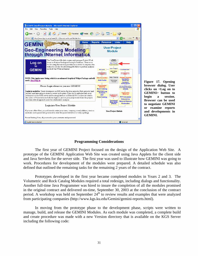
Figure 17. Opening browser dialog. User clicks on <Log on to GEMINI> button to begin a session. Browser can be used to negotiate GEMINI or examine reports and developments in GEMINI.

Programming Considerations The first year of GEMINI Project focused on the design of the Application Web Site. A prototype of the GEMINI Application Web Site was created using Java Applets for the client side and Java Servlets for the server side. The first year was used to illustrate how GEMINI was going to work. Procedures for development of the modules were prepared. A detailed schedule was also defined that outlined the remaining tasks for the remaining 2 years of the contract. Prototypes developed in the first year became completed modules in Years 2 and 3. The Volumetric and Rock Catalog Modules required a total redesign, including dialogs and functionality. Another full-time Java Programmer was hired to insure the completion of all the modules promised in the original contract and delivered on-time, September 30, 2003 at the conclusion of the contract period. A workshop was held on September 24th to review results and examples that were analyzed from participating companies (http://www.kgs.ku.edu/Gemini/gemini-reports.html). In moving from the prototype phase to the development phase, scripts were written to manage, build, and release the GEMINI Modules. As each module was completed, a complete build and create procedure was made with a new Version directory that is available on the KGS Server including the following code:

31

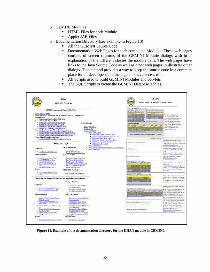
o GEMINI Modules HTML Files for each Module Applet JAR Files

o Documentation Directory (see example in Figure 18) All the GEMINI Source Code Documentation Web Pages for each completed Module – These web pages

consists of screen captures of the GEMINI Module dialogs with brief explanation of the different classes the module calls. The web pages have links to the Java Source Code as well as other web pages to illustrate other dialogs. This method provides a way to keep the source code in a common place for all developers and managers to have access to it.

All Scripts used to build GEMINI Modules and Servlets The SQL Scripts to create the GEMINI Database Tables.

Figure 18. Example of the documentation directory for the KHAN module in GEMINI.

32

The goals at the time of the Official Release were to provide a fully tested version of GEMINI that met the deliverables are stated in the original proposal and to demonstrate the practical application of the software using examples and expert feedback provided by eight participating companies. The concept of integrated web-based software tools and proof of methodologies including use of Java servelets, applets, Web Start, and XML-based data handling were developed and demonstrated for use with public-domain database and website. Additional support is needed to implement the software among the public domain database.

GEMINI deliverables are listed in the following table.

An internet web-site

Rock and Fluid CatalogsAccess through the Gemini User/Project Module

Web-based analytical software tools.Well Level Modules (Well Profile, PfEFFER, DST, Synthetic Seismogram, KHAN)Field Level Modules (Cross Section, Volumetric, Production, Material Balance, ASCII Output for Reservoir Simulation, PVT Calculator)Access through the Gemini User/Project Module

Tutorial module including theory, application of analytical tools and operation of GEMINI.

Reports, Seminars, Conferences and Workshops will be provided as records of technology transfer activities.

– http://www.kgs.ukans.edu/Gemini/index.html

–http://www.kgs.ukans.edu/Gemini/R1.0/GeminiUserProjectModule.html

––

–http://www.kgs.ukans.edu/Gemini/R1.0/GeminiUserProjectModule.html

– http://www.kgs.ukans.edu/Gemini/gemini-help.html

33

RESULTS AND DISCUSSION Task 1. Design Project Interface

Subtask 1.1. Evaluate Needs of User and Define Software Options A key task was to define the user’s needs for improved reservoir modeling via web applications. A series of workshops, presentations, demonstrations, and posters were conducted over the course of the project involving annual meetings with representatives of the eight company participants; technical meetings of the Kansas Geological Society, Tulsa Geological Society, and the Panhandle Geological Society; annual seminars with the Kansas Independent Oil and Gas Association in conjunction with PTTC; and annual meetings of the AAPG. In addition a series of evolving examples of regional, field, and lease applications were developed to demonstrate use. Information was posted on the GEMINI website to encourage interest.

It was learned that many small operators conduct some form of reservoir modeling including basic log analysis and pay identification. The mapping of net pay in conjunction with standard reservoir descriptors such as structure and isopachs is also done when a lease or field reached a critical juncture, e.g., when property was sold or when EOR was being considered. The tasks are carried out by the geologist or engineer, either one who may be a consultant working with the operator. Partnering companies also tend to employ their own models and compare results. Thus, the concept of conducting the task of integrated reservoir geo-engineering modeling collaboratively on the web in real-time where everyone is works on the same model is non traditional. The Internet technology at the outset of the project in 2000 was pointed toward Java as the best vehicle to deliver the product since it is platform independent and developed around the concept of a versatile web interface. Access to the Internet and higher speed Internet service was being realized for small independent operators. The petroleum operator was increasingly more knowledgeable and savvy with the computing environment improving their abilities and potential to interact with a web-based computer reservoir modeling program. The availability of public-domain, web-based data was also in a discovery stage as was the general availability of digital data to the small petroleum operator obtained directly from the field. Finally, the precise software and methodology to link software to other public-domain databases to accommodate varying database systems and levels of support and variable data types offered uncertainty for future implementation once GEMINI applications were in place on one server, i.e., the KGS side. Since then, Java has matured and expanded its capabilities and features offering new utilities that make the programming language more efficient and offer solutions that can make implementation of GEMINI software tools on a national level at reality. An example is the major revision of Java in 2003 (version 1.4.2, also called J2SE) that greatly facilitates implementing new options to adapt server-based applications such as GEMINI to run on the user’s PC with or without an internet connection (Web Start, http://java.sun.com/products/javawebstart/). Importantly, GEMINI was readily adapted to the new version of Java. In addition, the Java programming environment has embraced the interaction with XML databases, and as demonstrated this contract we have demonstrated its use at the vehicle to extend GEMINI to other distributed databases nationwide, namely other public-domain petroleum databases. It is clear that future development of GEMINI involves combinations server-based software, Java

34

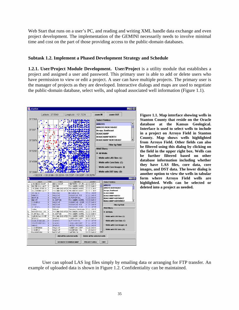
Web Start that runs on a user’s PC, and reading and writing XML handle data exchange and even project development. The implementation of the GEMINI necessarily needs to involve minimal time and cost on the part of those providing access to the public-domain databases. Subtask 1.2. Implement a Phased Development Strategy and Schedule 1.2.1. User/Project Module Development. User/Project is a utility module that establishes a project and assigned a user and password. This primary user is able to add or delete users who have permission to view or edit a project. A user can have multiple projects. The primary user is the manager of projects as they are developed. Interactive dialogs and maps are used to negotiate the public-domain database, select wells, and upload associated well information (Figure 1.1).

Figure 1.1. Map interface showing wells in Stanton County that reside on the Oracle database at the Kansas Geological. Interface is used to select wells to include in a project on Arroyo Field in Stanton County. Map shows wells highlighted from Arroyo Field. Other fields can also be filtered using this dialog by clicking on the field in the upper right box. Wells can be further filtered based on other database information including whether they have LAS files, core data, core images, and DST data. The lower dialog is another option to view the wells in tabular form where Arroyo Field wells are highlighted. Wells can be selected or deleted into a project as needed.

User can upload LAS log files simply by emailing data or arranging for FTP transfer. An

example of uploaded data is shown in Figure 1.2. Confidentiality can be maintained.

35

Figure 1.2. Example of data uploaded into a GEMINI project.

The user adds wells residing on the public-domain database using the User/Project dialog (Figure 1.3). The user is able to manage the data and access modules from this entry point.

Figure 1.3. Dialog showing project for Minneola Field demonstration. The users who share the project are listed along with the list of wells included in the project. The user can add or remove wells and enter petrophysics and multi-well analyses from this dialog.

Once the user establishes a project, they can use a notes feature to establish a running dialog about the project, describing the main features and tasks to be done or those accomplished to assist collaborations from remote locations or simply remind the user (Figure 1.4).

36

Figure 1.4. Example of GEMINI notes.

1.2.2. Project Workflow. Project Workflow tracks the progress of GEMINI project including activities completed and parameters obtained. The user can rapidly determine the status of the tasks performed and evaluate specific parameters used in the analysis (Figures 1.5 and 1.6).

Project Workflow

Figure 1.5. Workflow and summary buttons are located along the left margin of the project dialog and are used to review the project tasks and parameters used and obtained in the process. User is also reminded what information is input and results that are obtained as output in the particular activity.

37

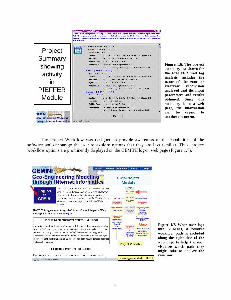
Project Summaryshowing activity

in PfEFFERModule

Figure 1.6. The project summary list shown for the PfEFFER well log analysis includes the name of the zone or reservoir subdivision analyzed and the input parameters and results obtained. Since this summary is in a web page, the information can be copied to another document.

The Project Workflow was designed to provide awareness of the capabilities of the software and encourage the user to explore options that they are less familiar. Thus, project workflow options are prominently displayed on the GEMINI log-in web page (Figure 1.7).

Project Workflow

www.kgs.ku.edu/GEMINI

Figure 1.7. When user logs into GEMINI, a possible workflow path is included along the right side of the web page to help the user visualize which path they might take to analyze the reservoir.

38

Task 2. Reservoir Characterization Subtask 2.1. Parameter Definition 2.1.1. Well Profile Module. The Well Profile Module is used to view LAS (Log ASCII Standard) wireline log files and interactively annotate logs with formation tops, pay/flow units for log analysis, perforations, and DST intervals; print logs to scale, or export image files to other applications. The primary well profile dialog is used to select the depth interval, the vertical scale, the log curves and tracks, curve colors and scale, core data to be included, and computation of quick-look log analysis, e.g., water saturation (Figure 2.1). The result is a screen image of the logs such as in Figure 2.2 or a jpeg file that can saved to the user’s computer and printed to scale. The onscreen version of the well log can be interactively used to select new formation tops in addition to those incorporated from the database and used to define intervals of the reservoir that may proxy as flow units. Also, the user can set the drill stem and perforation intervals to be shown later in cross section displays (Figure 2.3). This annotated or marked log developed in Well Profile is saved for use in other modules, in particular, log analysis and cross section. These marked logs can be modified as needed, as the reservoir model is refined. As described above, digital logs can be uploaded into a project as they are obtained by the user and viewed, marked, and shared with other users who are collaborating.

Figure 2.4 illustrates the use of the quick look pay feature in the Well Profile Module that

can be used to target zones of interest. Detailed log analysis is accomplished in the PfEFFER log analysis module, built around principles of petrofacies analysis as described in the next section.

39

Figure 2.1. Dialog used in Well Profile that is used to select depth interval, depth scale, curve type and tracks, formation tops database, core data to display, and provide quick look log analysis (saturation parameters such as Sw using PfEFFER). User sets plot limits which include scales in tracks and color of curves.

Figure 2.2. Screen capture of dialog showing Well Profile including core data plotted as small Circles and location of core images along right margin.

Figure 2.3. When mouse is clicked in an active log window in the Well Profile module, a pop-up windows appears that is used to add formation tops, set intervals for PfEFFER (log analysis), and establish perforated and DST intervals.

40

Figure 2.4. Example of well profile from a well in Minneola Field where Pennsylvanian cycles overlying Mississippian (Ste. Gennevieve Limestone). Identified as S1, S2, and S3. Cycle S2 contains a thin sandstone reservoir. Quick look pay indicator in Well Profile provides indication of pay in cycle S2. Small dot on depth track shows perforated interval.

Subtask 2.2. Petrophysical Modeling Well data – integrating log and core data with production performance

Data collected from electric logs and cores serve as major building blocks in construction of the geological model of a reservoir. In turn, log analysis needs to be fully integrated with the process of building the geo-engineering models. Upscaling core and log data to that of reservoir scale of grid cells, at times measuring to several hundred square feet, requires close integration of reservoir geology, rock characteristics and their horizontal and vertical extent and also their correspondence with the associated production data. This is ideally an iterative process where the user can return to the log analysis to adjust the parameters, such as after comparing volumetric and material balance results (Bhattacharya et al., 1999).

The petrophysical data finally attributed to the reservoir grids must be able to support the production performance of the reservoir. This match between field performance and rock attributes not only validates the geomodel of the reservoir, but sets the stage to conduct a reservoir simulation study. A powerful technique to analyze wireline log data is a graphical

41

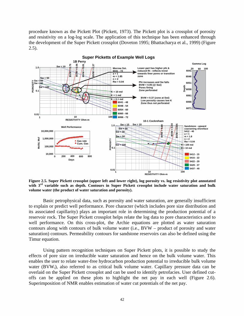
procedure known as the Pickett Plot (Pickett, 1973). The Pickett plot is a crossplot of porosity and resistivity on a log-log scale. The application of this technique has been enhanced through the development of the Super Pickett crossplot (Doveton 1995; Bhattacharya et al., 1999) (Figure 2.5).

RESISTIVITY Ohm-m

RESISTIVITY Ohm-m

POR

OSI

TY

POR

OSI

TY

Morrow Sst.6041 - 72a = 1m = 1.85n = 2Rw = 0.04

Sandstone - upward coarsening shoreface5412 - 40a = 1m = 1.8n = 2Rw = 0.04

6041 - 48

5412 - 15

6048 - 54

5415 - 22

6054 - 60

5422 - 29

6060 - 66

5429 - 37

6066 - 72

5437 - 40

1 10 1000.01

0.1

1.0

Super Picketts of Example Well Logs

K = 10 mdK = 1 mdK = 0.1 md

Sw = 100Sw = 80Sw = 60

Sw = 50

Sw = 10

BVW

= 0

.37

BVW

= 0

.05

BVW

= 0

.06

BVW

= 0

.75

1B Perry

20 60 1006041

6046

6051

6058

6061

6066

6071

Dep

th

Gamma Log

BVW = 0.37 (zone at Swi)Low porosity causes low KZone thus not perforated

Phi increases and Sw fallsBVW = 0.05 (@ Swi)Pores finingZone perforated

Lower part has higher phi &reduced Rt - reflects trendtowards finer pores or transition zone

K = 100 mdK = 10 md

10-1 Cockreham

0.01

0.1

1.0

100101

Sw = 100

Sw = 50

Sw = 30Sw = 20

Sw = 15 Sw = 10

BVW

= 0

.025

BVW

= 0

.03

BVW

= 0

.04

Gas rateCum. Gas

Mcf

/d, M

cf

Days

Well Performance

10,000

100,000

1,000,000

10,000,000

0 200 400 600 800

Figure 2.5. Super Pickett crossplot (upper left and lower right), log porosity vs. log resistivity plot annotated with 3rd variable such as depth. Contours in Super Pickett crossplot include water saturation and bulk volume water (the product of water saturation and porosity).

Basic petrophysical data, such as porosity and water saturation, are generally insufficient to explain or predict well performance. Pore character (which includes pore size distribution and its associated capillarity) plays an important role in determining the production potential of a reservoir rock. The Super Pickett crossplot helps relate the log data to pore characteristics and to well performance. On this cross-plot, the Archie equations are plotted as water saturation contours along with contours of bulk volume water (i.e., BVW – product of porosity and water saturation) contours. Permeability contours for sandstone reservoirs can also be defined using the Timur equation.

Using pattern recognition techniques on Super Pickett plots, it is possible to study the effects of pore size on irreducible water saturation and hence on the bulk volume water. This enables the user to relate water-free hydrocarbon production potential to irreducible bulk volume water (BVWi), also referred to as critical bulk volume water. Capillary pressure data can be overlaid on the Super Pickett crossplot and can be used to identify petrofacies. User defined cut-offs can be applied on these plots to highlight the net pay in each well (Figure 2.6). Superimposition of NMR enables estimation of water cut potentials of the net pay.

42

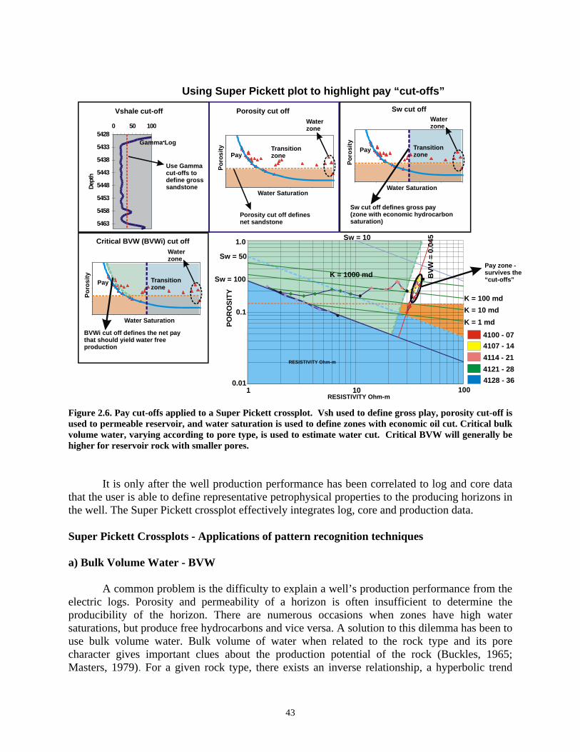
Using Super Pickett plot to highlight pay “cut-offs”

Gamma Log5428

5433

5438

5443

5448

5453

5458

5463

0 50 100

Dept

h

Use Gammacut-offs todefine grosssandstone

Vshale cut-off Porosity cut off

Water Saturation

Waterzone

TransitionzonePay

Porosity cut off defines net sandstone

Poro

sity

Water Saturation

Waterzone

Transitionzone

Pay

Poro

sity

Sw cut off defines gross pay(zone with economic hydrocarbonsaturation)

Sw cut off

Water Saturation

Waterzone

Transitionzone

Pay

Poro

sity

Critical BVW (BVWi) cut off

BVWi cut off defines the net paythat should yield water freeproduction

RESISTIVITY Ohm-m

POR

OSI

TY

4100 - 074107 - 144114 - 214121 - 284128 - 36

1 10 1000.01

0.1

1.0

Sw = 100

Sw = 50

Sw = 10

BVW

= 0

.045

K = 1 mdK = 10 mdK = 100 md

K = 1000 mdPay zone -survives the“cut-offs”

RESISTIVITY Ohm-m

Figure 2.6. Pay cut-offs applied to a Super Pickett crossplot. Vsh used to define gross play, porosity cut-off is used to permeable reservoir, and water saturation is used to define zones with economic oil cut. Critical bulk volume water, varying according to pore type, is used to estimate water cut. Critical BVW will generally be higher for reservoir rock with smaller pores.

It is only after the well production performance has been correlated to log and core data

that the user is able to define representative petrophysical properties to the producing horizons in the well. The Super Pickett crossplot effectively integrates log, core and production data.

Super Pickett Crossplots - Applications of pattern recognition techniques a) Bulk Volume Water - BVW

A common problem is the difficulty to explain a well’s production performance from the electric logs. Porosity and permeability of a horizon is often insufficient to determine the producibility of the horizon. There are numerous occasions when zones have high water saturations, but produce free hydrocarbons and vice versa. A solution to this dilemma has been to use bulk volume water. Bulk volume of water when related to the rock type and its pore character gives important clues about the production potential of the rock (Buckles, 1965; Masters, 1979). For a given rock type, there exists an inverse relationship, a hyperbolic trend

43

(Buckles, 1965) between the irreducible water saturation, Swi, and its porosity, also noted by several early authors including Archie (Archie 1952) (Bhattacharya et al., 1999).

iwi BVWS =×φ As the pore characteristics change between rock types, so does the value of the

irreducible bulk volume of water. Thus, each hyperbolic trend represents a characteristic signature for a particular pore size distribution in a rock body. This characteristic signature exists because the Swi value is dependent on the factors, such as capillary pressure and the surface tension on the internal rock surfaces, which are dependent on the pore characteristics. A BVW plot (Figure 2.7) of a moderately homogenous rock body will show zones at Swi to lie on the characteristic BVWi curve for that rock while zones with water saturation values greater than the Swi will lie above this BVWi curve. Thus, the plotting of BVW lines on a porosity-resistivity crossplot, such as the Super Pickett, is an effective way to incorporate pore characteristics with the log characteristics. The advantage of plotting the BVW lines on a log-log crossplot is that the above equation appears as a straight line (Doveton, 1995). Pay zones with water saturations at Swi will produce water free hydrocarbons while those with higher water saturations (and located in the transition zone) will show a water cut. The extent of the water cut can even be estimated from the relative position of the producing horizon within the transition zone.

PO

RO

SITY

POR

OS

ITY

KC Sniabar Lmst.4643 - 4682a = 1m = 2.0n = 2Rw = 0.04

Iatan & Stanton Lmst.4091 - 4174a = 1m = 2.0n = 2Rw = 0.04

4091 - 98

4643 - 46

4098 - 09

4646 - 54

4109 - 20

4654 - 62

4120 - 32

4662 - 69

4132 - 76

4669 - 761

1

10

10

100

1000.01

0.01

0.1

0.1

1.0

1.0

Sw = 50

Sw = 100

Sw = 10

Sw = 20Sw = 30

Super Pickett Interpretation of Field Examples

RESISTIVITY Ohm-m

RESISTIVITY Ohm-m

1- 33 Long

1- 31 Thunderbird

BVW

= 0

.03

BVW

= 0

.04

BVW

= 0

.05 1-33 Long

Gamma Log10 35 60

Dep

th4643

4648

4653

4658

4663

4668

4673

4678

Possibly good paySw = 13%, BVW = 0.035

Production potential linked to type of lmst. - lithology

Low ooliclastic porosity(less weathering of oolites)

4 humps - 4 depositional sequences

Phi & Sw appear attractiveBut high BVW for oolitic lmst.(BVW fine for bioclastic lmst.)

(2nd & 3rd humps - pays of decreasing quality)

Sw = 100Sw = 80

Sw = 60Sw = 50

Sw = 20

Sw = 10

BVW

= 0

.09

BVW

= 0

.07

BVW

= 0

.06

BVW

= 0

.04

BVW

= 0

.035

Signature of oolitic lmst.High phi - secondary phi(phi inside the oolites)BVW = 0.04, Sw 11 - 20%Vertical profile (@ Swi)Offsets - produce little/no wtr.

Signature of Bioclastic lmst.Higher BVW (0.07)Intergranular phiSw > 50%Offsets - produce with water

Requires different m, n,and Rw values

Figure 2.7. Variation in BVW and pore type as discerned from Super Pickett crossplot.

44

Typically a low BVWi value represents a distribution of relatively larger pore sizes as the Swi value is smaller for such a rock. For distributions of finer (smaller) pore sizes the internal area of the rock increases and this results in a higher Swi value which in turn leads to a higher characteristic BVWi value (Figure 2.7, 2.8, and 2.9). Different rock types have different pore size distributions and thus they will end up having different BVWi values. The BVWi value for a particular rock is not only dependent on its pore size distribution but also on the height of the oil/gas column. For rocks with similar pore size distributions, the value of BVWi is smaller for taller hydrocarbon columns. The increased buoyancy in a thick hydrocarbon column is able to overcome a higher capillary pressure value and thus it reduces the Swi. The BVWi value for a particular rock type corresponds to the BVW contour associated with data points which have produced and tested water free hydrocarbons. Water free hydrocarbon producing zones are generally found to cluster around the BVWi line on the Super Pickett crossplot (Figure 2.8). For cases where the critical water saturation, Swcrit (i.e., Krw = 0), is different from Swi, critical BVW (BVWcrit) takes a value greater than BVWi. However, one must be cautioned that BVWi or BVWcrit defined via the Super Pickett plot can be considered to be representative of the rock body only when the rock body is assumed to have a similar pore size distribution as that of the zone producing water free hydrocarbons.

Figure 2.8. Clustering of points in Super Pickett crossplot suggesting interval of water-free hydrocarbon production.

G

G

a

a

m

m

m

m

a

a

L

L

o

o

g

g

5428

5433

5438

5443

5448

5453

5458

5463

0 50 100

D

D

e

e

p

p

t

t

h

h

RESISTIVITY Ohm-m

RESISTIVITY Ohm-m

POR

OSI

TY

POR

OSI

TY

23-1 Kendrick

2A - Tjaden

Miss. Chat4270-4331a = 1m = 2.0n = 2Rw = 0.055

Morrow Sst.5428- 5465a = 1m = 1.8n = 2Rw = 0.04

5428 - 36

4270 - 82

5436- 44

4282 - 98

5444 - 52

4298 - 05

5452 - 62

4305 - 13

5462 - 65

4313 - 31

1

0.1 1.0 10

10 1000.01

0.01

0.1

0.1

1.0

1.0

Sw = 100

Sw = 100

Sw = 80Sw = 60 Sw = 10

Sw = 50Sw = 40

Sw = 50Sw = 40Sw = 30 Sw = 20

Sw = 10

BVW

= 0

.025

BVW

= 0

.03

BVW

= 0

.04

BVW

= 0

.05

BVW

= 0

.06

BVW

= 0

.07

Zone at Swir

Upper shaleIncreasing phi & BVWFiner pores

Transition zone

Super Pickett Interpretation of Field Examples

4270

4280

4290

4300

4310

4320

4330

10 35 60

BVW

= 0

.1

BVW

= 0

.15

BVW

= 0

.2

BVW

= 0

.3

Lower zone - tripolitic chertBVW 0.26 to 0.4Sw 60 to 100%High BVW and Sw - due togreater micro-porosityProductive in offset wells

Cherty- limestoneseparates upper & lowerzones

Upper zone - tripolitic chertBVW 0.13 to 0.2Sw around 50%Productive in offset wells

45

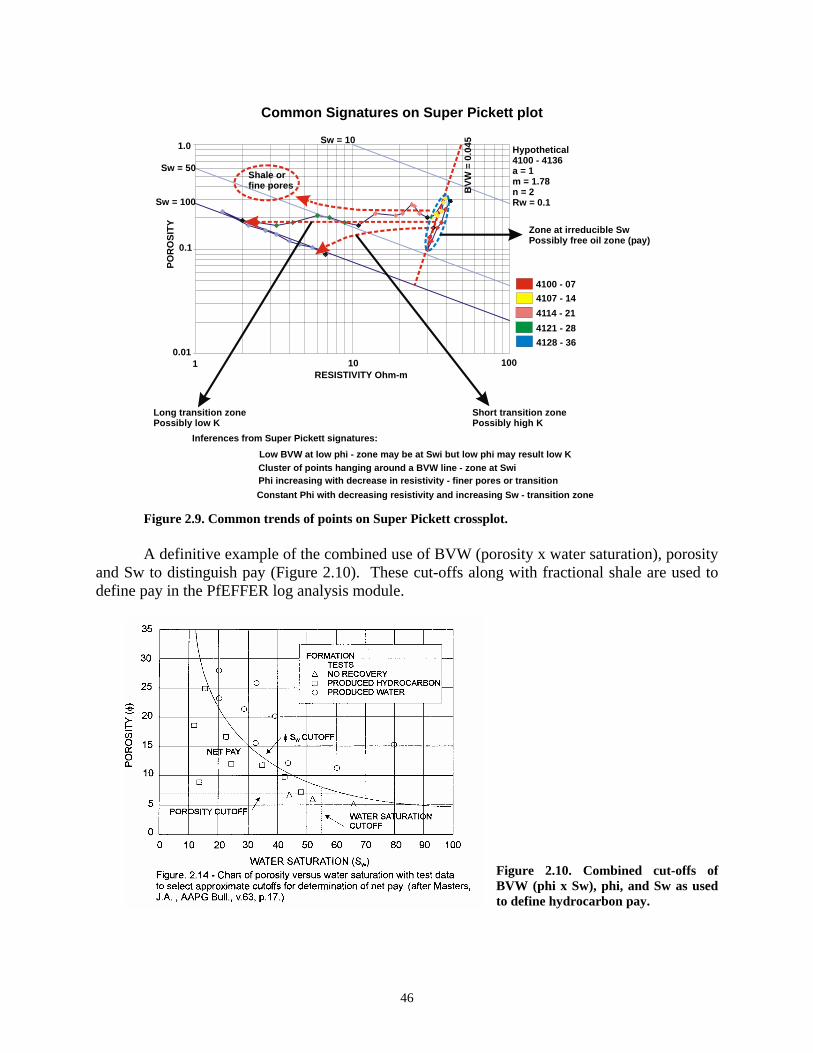
Inferences from Super Pickett signatures:Low BVW at low phi - zone may be at Swi but low phi may result low KCluster of points hanging around a BVW line - zone at SwiPhi increasing with decrease in resistivity - finer pores or transitionConstant Phi with decreasing resistivity and increasing Sw - transition zone

RESISTIVITY Ohm-m

POR

OSI

TY

Hypothetical4100 - 4136a = 1m = 1.78n = 2Rw = 0.1

4100 - 074107 - 144114 - 214121 - 284128 - 36

1 10 1000.01

0.1

1.0

Common Signatures on Super Pickett plot

Sw = 100

Sw = 50

Sw = 10

BVW

= 0

.045

Shale orfine pores

Zone at irreducible SwPossibly free oil zone (pay)

Short transition zonePossibly high K

Long transition zonePossibly low K

Figure 2.9. Common trends of points on Super Pickett crossplot. A definitive example of the combined use of BVW (porosity x water saturation), porosity

and Sw to distinguish pay (Figure 2.10). These cut-offs along with fractional shale are used to define pay in the PfEFFER log analysis module.

Figure 2.10. Combined cut-offs of BVW (phi x Sw), phi, and Sw as used to define hydrocarbon pay.

46

b) Permeability Contours The Super Pickett crossplot also includes application of permeability contours. One

common quantitative method to predict permeability from logs is to use an empirical equation of the form:

φ×= BAK where A and B are constants that are determined from the correlation developed from

core measurements between permeability and porosity. It adds to the accuracy of the correlation when the core porosities are correlated with the log porosities during the determination of the above constants. The above predictive equation has worked with acceptable errors as a screening tool when such an equation is specifically developed for a particular producing horizon in an individual field. However, the use of the equation, applicable only to sandstones, can result in large errors, while when used for carbonates the errors often range across orders of magnitude. Thus, it is prudent to use permeability contours with caution. One of the reasons for the discrepancy in permeability prediction by equations of the above form is that permeability is not solely dependent on the pore volume of the rock. It is controlled by many other factors such as the internal surface area, tortuosity in the pore network, pore throat geometry etc. For sandstones, different equations such as Kozeny Carmen and Wyllie-Rose have been proposed to include effects of specific surface area and Swi. The Wyllie-Rose equation has been further modified by several authors such as Tixier, Timur, Coates-Dumanoir, Coates etc. Of these the Timur equation, shown below, is perhaps the most widely used equation for sandstones relating the permeability K (md) as a function of porosity and irreducible water saturation.

wi

25.25.0

S100

Kφ×=

Porosity and saturation in the above equation are expressed in fractional units.

Permeability contours, expressed in terms of porosity and Swi, further enhance the production prediction capability of the Super Pickett plot. The Timur equation is recommended for use in drawing permeability contours on the crossplots. The user may however use a different correlation to generate permeability contours by simply changing the coefficients.

Timur’s equation correlates the permeability with the porosity at irreducible water

saturation. Thus, the permeability contours can be directly used to obtain permeability for points located in the hydrocarbon reservoir where the water saturation has been reduced to Swi. For points located in the transition zone (i.e., where Sw > Swi), the permeability contours can be utilized only when it is assumed that the rock type and the pore character remain similar to that in the reservoir. These points in the transition zone, are displaced horizontally (i.e., maintaining the porosity constant) to the BVWi line (where Sw = Swi) and then the corresponding permeability is determined. Figure 2.11 exemplifies the technique of using Timur permeability contours on the Super Pickett crossplot for sandstone reservoirs.

47

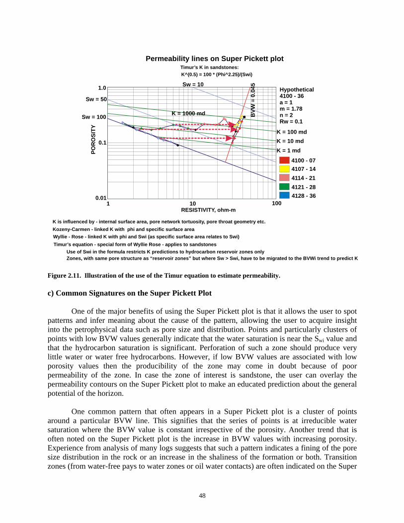
RESISTIVITY Ohm-m

POR

OSI

TYHypothetical4100 - 36a = 1m = 1.78n = 2Rw = 0.1

4100 - 074107 - 144114 - 214121 - 284128 - 36

1 10 1000.01

0.1

1.0

Permeability lines on Super Pickett plot

Sw = 100

Sw = 50

Sw = 10

BVW

= 0

.045

K = 1 mdK = 10 mdK = 100 md

K = 1000 md

Timur’s K in sandstones:K^(0.5) = 100 * (Phi^2.25)/(Swi)

K is influenced by - internal surface area, pore network tortuosity, pore throat geometry etc.Kozeny-Carmen - linked K with phi and specific surface areaWyllie - Rose - linked K with phi and Swi (as specific surface area relates to Swi) Timur’s equation - special form of Wyllie Rose - applies to sandstones

Use of Swi in the formula restricts K predictions to hydrocarbon reservoir zones onlyZones, with same pore structure as “reservoir zones” but where Sw > Swi, have to be migrated to the BVWi trend to predict K

RESISTIVITY, ohm-m

Figure 2.11. Illustration of the use of the Timur equation to estimate permeability. c) Common Signatures on the Super Pickett Plot

One of the major benefits of using the Super Pickett plot is that it allows the user to spot

patterns and infer meaning about the cause of the pattern, allowing the user to acquire insight into the petrophysical data such as pore size and distribution. Points and particularly clusters of points with low BVW values generally indicate that the water saturation is near the Swi value and that the hydrocarbon saturation is significant. Perforation of such a zone should produce very little water or water free hydrocarbons. However, if low BVW values are associated with low porosity values then the producibility of the zone may come in doubt because of poor permeability of the zone. In case the zone of interest is sandstone, the user can overlay the permeability contours on the Super Pickett plot to make an educated prediction about the general potential of the horizon.

One common pattern that often appears in a Super Pickett plot is a cluster of points

around a particular BVW line. This signifies that the series of points is at irreducible water saturation where the BVW value is constant irrespective of the porosity. Another trend that is often noted on the Super Pickett plot is the increase in BVW values with increasing porosity. Experience from analysis of many logs suggests that such a pattern indicates a fining of the pore size distribution in the rock or an increase in the shaliness of the formation or both. Transition zones (from water-free pays to water zones or oil water contacts) are often indicated on the Super

48

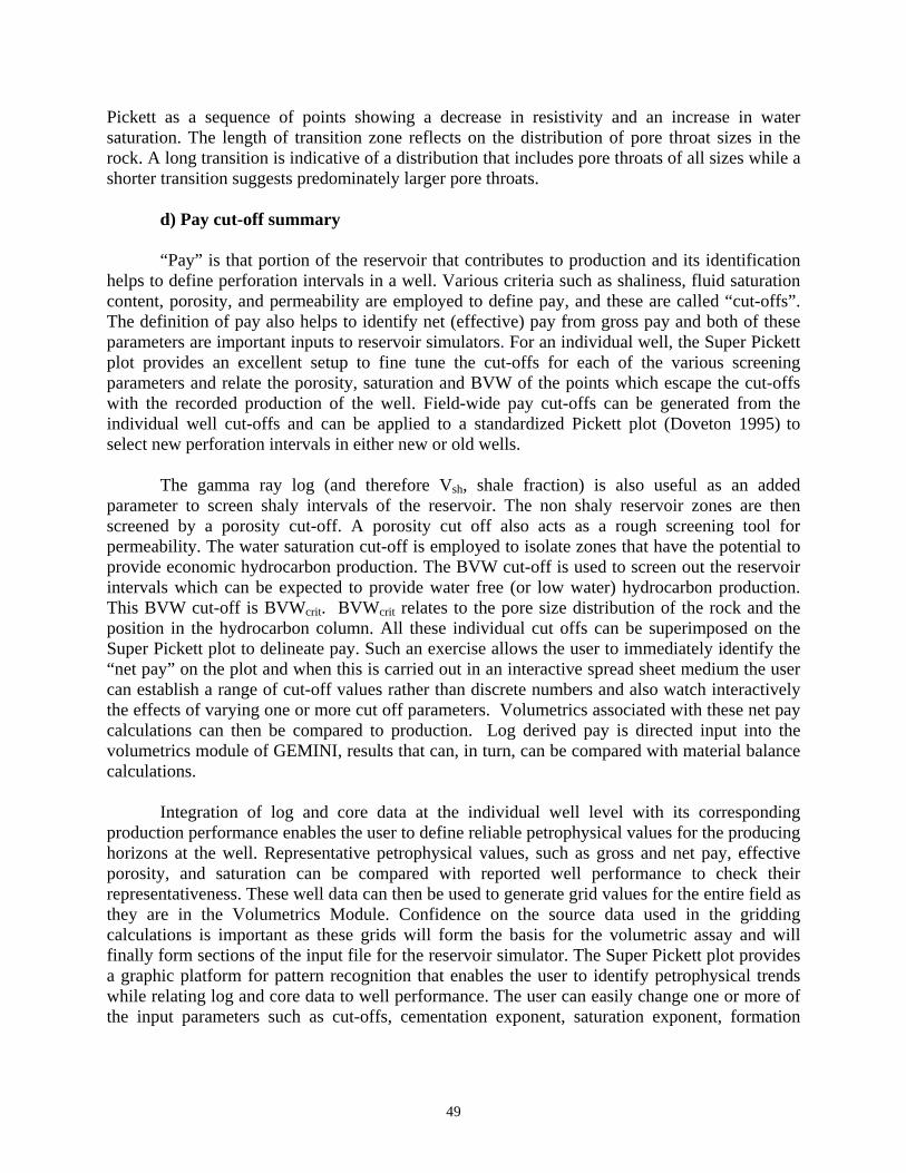
Pickett as a sequence of points showing a decrease in resistivity and an increase in water saturation. The length of transition zone reflects on the distribution of pore throat sizes in the rock. A long transition is indicative of a distribution that includes pore throats of all sizes while a shorter transition suggests predominately larger pore throats.

d) Pay cut-off summary “Pay” is that portion of the reservoir that contributes to production and its identification

helps to define perforation intervals in a well. Various criteria such as shaliness, fluid saturation content, porosity, and permeability are employed to define pay, and these are called “cut-offs”. The definition of pay also helps to identify net (effective) pay from gross pay and both of these parameters are important inputs to reservoir simulators. For an individual well, the Super Pickett plot provides an excellent setup to fine tune the cut-offs for each of the various screening parameters and relate the porosity, saturation and BVW of the points which escape the cut-offs with the recorded production of the well. Field-wide pay cut-offs can be generated from the individual well cut-offs and can be applied to a standardized Pickett plot (Doveton 1995) to select new perforation intervals in either new or old wells.

The gamma ray log (and therefore Vsh, shale fraction) is also useful as an added

parameter to screen shaly intervals of the reservoir. The non shaly reservoir zones are then screened by a porosity cut-off. A porosity cut off also acts as a rough screening tool for permeability. The water saturation cut-off is employed to isolate zones that have the potential to provide economic hydrocarbon production. The BVW cut-off is used to screen out the reservoir intervals which can be expected to provide water free (or low water) hydrocarbon production. This BVW cut-off is BVWcrit. BVWcrit relates to the pore size distribution of the rock and the position in the hydrocarbon column. All these individual cut offs can be superimposed on the Super Pickett plot to delineate pay. Such an exercise allows the user to immediately identify the “net pay” on the plot and when this is carried out in an interactive spread sheet medium the user can establish a range of cut-off values rather than discrete numbers and also watch interactively the effects of varying one or more cut off parameters. Volumetrics associated with these net pay calculations can then be compared to production. Log derived pay is directed input into the volumetrics module of GEMINI, results that can, in turn, can be compared with material balance calculations.

Integration of log and core data at the individual well level with its corresponding

production performance enables the user to define reliable petrophysical values for the producing horizons at the well. Representative petrophysical values, such as gross and net pay, effective porosity, and saturation can be compared with reported well performance to check their representativeness. These well data can then be used to generate grid values for the entire field as they are in the Volumetrics Module. Confidence on the source data used in the gridding calculations is important as these grids will form the basis for the volumetric assay and will finally form sections of the input file for the reservoir simulator. The Super Pickett plot provides a graphic platform for pattern recognition that enables the user to identify petrophysical trends while relating log and core data to well performance. The user can easily change one or more of the input parameters such as cut-offs, cementation exponent, saturation exponent, formation

49

water resistivity etc. An unacceptable match will prompt the user to redefine one or more of the input parameters and also may be the underlying assumptions of the geological model.

2.2.1. PfEFFER Log Analysis Module

The log analysis module is PfEFFER referring to “Petrofacies Evaluation of Formations for Engineering Reservoirs”. The Java coding in GEMINI is a rewrite of the successful Visual Basic/Excel version (http://www.kgs.ku.edu/PRS/software/pfeffer1.html). PfEFFER operates using digital log data, LAS format. The module allows the user to perform log analysis on each region or zone defined consisting of a depth range. The reservoir layers delineated in correlation allow the user to establish consistency in correlations. The user can define the zones or regions in the Well Profile Module, on a cross section, or in the opening page of the PfEFFER Module (Figures 2.12 and 2.13).

Figure 2.12. Opening dialog of the PfEFFER manual, which allows the user to re-examine the well profile, view and revise the regions or zones of the reservoir to analyze, or simply launch the PfEFFER program.

50

Figure 2.13. Once PfEFFER is launched for a particular well, the user is able to access all the zones being examined and analyze them.

The example shown in Figure 2.13 includes a series of tabs near the base, one being

highlighted, the LansingJ. The right column indicates the depth range and the reservoir parameters of the LansingJ derived from the log analysis. These results are available to the Volumetrics Module. A second dialog box for the LansingJ zone is shown in Figure 2.14 accessed by clicking on the Parameters Tab. The Archie Equation Parameters and pay cut-offs are set in this dialog. The goal is to use the cut-offs as a trial and error basis constrained by nonproductive and productive wells. Experience has shown that the cut-offs work together and pay in some wells may be limited by one cut-off over another.

Figure 2.14. PfEFFER dialog containing Archie Equation Parameters and Pay Cut-Offs.

51

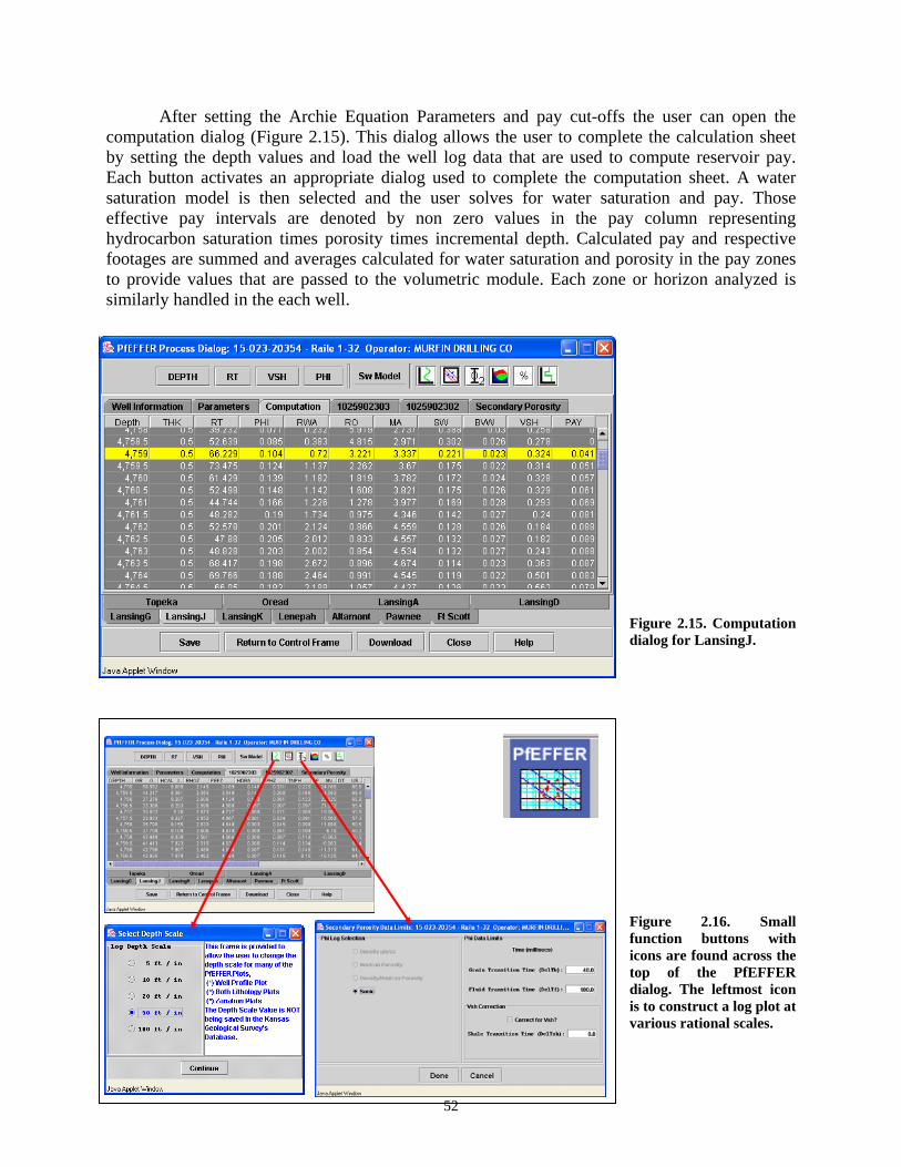
After setting the Archie Equation Parameters and pay cut-offs the user can open the computation dialog (Figure 2.15). This dialog allows the user to complete the calculation sheet by setting the depth values and load the well log data that are used to compute reservoir pay. Each button activates an appropriate dialog used to complete the computation sheet. A water saturation model is then selected and the user solves for water saturation and pay. Those effective pay intervals are denoted by non zero values in the pay column representing hydrocarbon saturation times porosity times incremental depth. Calculated pay and respective footages are summed and averages calculated for water saturation and porosity in the pay zones to provide values that are passed to the volumetric module. Each zone or horizon analyzed is similarly handled in the each well.

Figure 2.15. Computation dialog for LansingJ.

52

Figure 2.16. Small function buttons with icons are found across the top of the PfEFFER dialog. The leftmost icon is to construct a log plot at various rational scales.

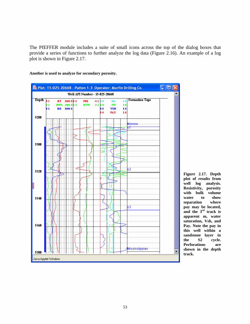
The PfEFFER module includes a suite of small icons across the top of the dialog boxes that provide a series of functions to further analyze the log data (Figure 2.16). An example of a log plot is shown in Figure 2.17. Another is used to analyze for secondary porosity.

Figure 2.17. Depth plot of results from well log analysis. Resistivity, porosity with bulk volume water to show separation where pay may be located, and the 3rd track is apparent m, water saturation, Vsh, and Pay. Note the pay in this well within a sandstone layer in the S2 cycle. Perforations are shown in the depth track.

53

PfEFFER log analysis incorporates conventional log analysis to define pay cut-offs using water models and Super Pickett crossplots annotated with BVW (bulk volume water) and Sw contours (Figure 2.17). The data points are connected by depth and, in this example, the points are color-coded by depth through the sandstone reservoir. Patterns produced reflect pore type and relative fluid saturations, the later related to the capillarity of the pore and fluid system and the elevation above the hydrocarbon:water contact. Correlating the clusters and patterns of points on the Pickett crossplot with data from core descriptions and analyses is used to establish the reservoir’s petrofacies, a distinctive family of the lithofacies and pore type. Clusters of points, often paralleling BVW contours suggests the reservoir is at irreducible water saturation. Also, succession of points that form a linear trend paralleling porosity suggest a transition zone while those that parallel water saturation lines possibly indicate changes in pore type, with smaller pores toward higher values of BVW. Points that lie

J

K

G

J Zone 20 BW + Tr W

IP 20 BO + Tr W

Figure 2.18. Super Pickett crossplot with contours of water saturation in blue and bulk water volume shown in red. Points are color coded by depth as shown on legend. Corresponding well log shown in right with arrow identifying the zone of interest, the J zone. Blue vertical lines in depth column indicated separate carbonate reservoir analyzed in PfEFFER project. Red vertical lines with horizontal bars represent drill stem test intervals. Small red circles in depth tract represent perforated interval.

54

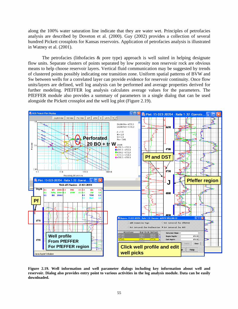
along the 100% water saturation line indicate that they are water wet. Principles of petrofacies analysis are described by Doveton et al. (2000). Guy (2002) provides a collection of several hundred Pickett crossplots for Kansas reservoirs. Application of petrofacies analysis is illustrated in Watney et al. (2001).

The petrofacies (lithofacies & pore type) approach is well suited in helping designate flow units. Separate clusters of points separated by low porosity non reservoir rock are obvious means to help choose reservoir layers. Vertical fluid communication may be suggested by trends of clustered points possibly indicating one transition zone. Uniform spatial patterns of BVW and Sw between wells for a correlated layer can provide evidence for reservoir continuity. Once flow units/layers are defined, well log analysis can be performed and average properties derived for further modeling. PfEFFER log analysis calculates average values for the parameters. The PfEFFER module also provides a summary of parameters in a single dialog that can be used alongside the Pickett crossplot and the well log plot (Figure 2.19).

DST 4736-4773

J

Perforated20 BO + tr W

Pf

Pf and DST

Pfeffer region

Click well profile and editwell picks

Well profileFrom PfEFFERFor PfEFFER region

Figure 2.19. Well information and well parameter dialogs including key information about well and reservoir. Dialog also provides entry point to various activities in the log analysis module. Data can be easily downloaded.

55

Complex lithologies such as Pennsylvanian marine and estuarine mixed clastic-carbonate cycles can be readily analyzed with Pe, neutron-density logs and the PfEFFER log analysis module. PfEFFER provides standard Rhomaa-Umaa plots that can be tailored to the dominant lithologies (Figures 2.20 and 2.21).

Figure 2.20. Rhomma-Umma crossplot for Pennsylvanian cyclic mixed clastic-carbonate interval in Minneola Field, Clark County, Kansas.

Figure 2.21. Combined Well Profile of cyclic mixed clastic-carbonate interval in Minneola Field and depth profile of lithology solution from Rhomma-Umaa crossplot.

56

Depth-constrained cluster analysis is a practical tool in PfEFFER that can quickly

identify zonation on a reservoir (Figure 2.22). In this example below, the Pennsylvanian cyclic mixed clastic-carbonate sedimentary succession was subdivided into ten units based on cluster analysis using the gamma ray, neutron and density porosity, and induction log. These layers are compared with the three cycles, S1, S2 and S3, that were identified from cored lithofacies and log correlation using sequence stratigraphic concepts. Thin red horizontal lines are drawn to highlight the cycle boundaries. S1 is carbonate-dominated and forms one major cluster while the S2 and S3 are clastic dominated. Further clustering identifies the various beds of sandstone, shale, and carbonate including the bed that is the perforated reservoir-bearing unit (as highlighted with the arrow on the illustration.

Figure 2.22. Depth-constrained clustering on right half compared to well profile showing cycles including pay interval highlighted in red.

Comparison of the petrophysical character of reservoir layers can be accomplished by compilation of a set of Pickett crossplots of each layer or displaying Pickett plots for a number of wells from a reservoir zone (Figure 2.23). The Lower Pennsylvanian Morrow sandstone reservoir in the example below is divided into five layers as shown in the underlying depth plot of a well from the project. All of the layers in this well lie above the oil:water contact and are near irreducible hydrocarbon saturation, thus the various clustering of points are believed to reflect variations in pore type. In turn, the changes in BVW are believed to reflect changes in pore type with the larger pores corresponding to lower values of BVW.

57

\

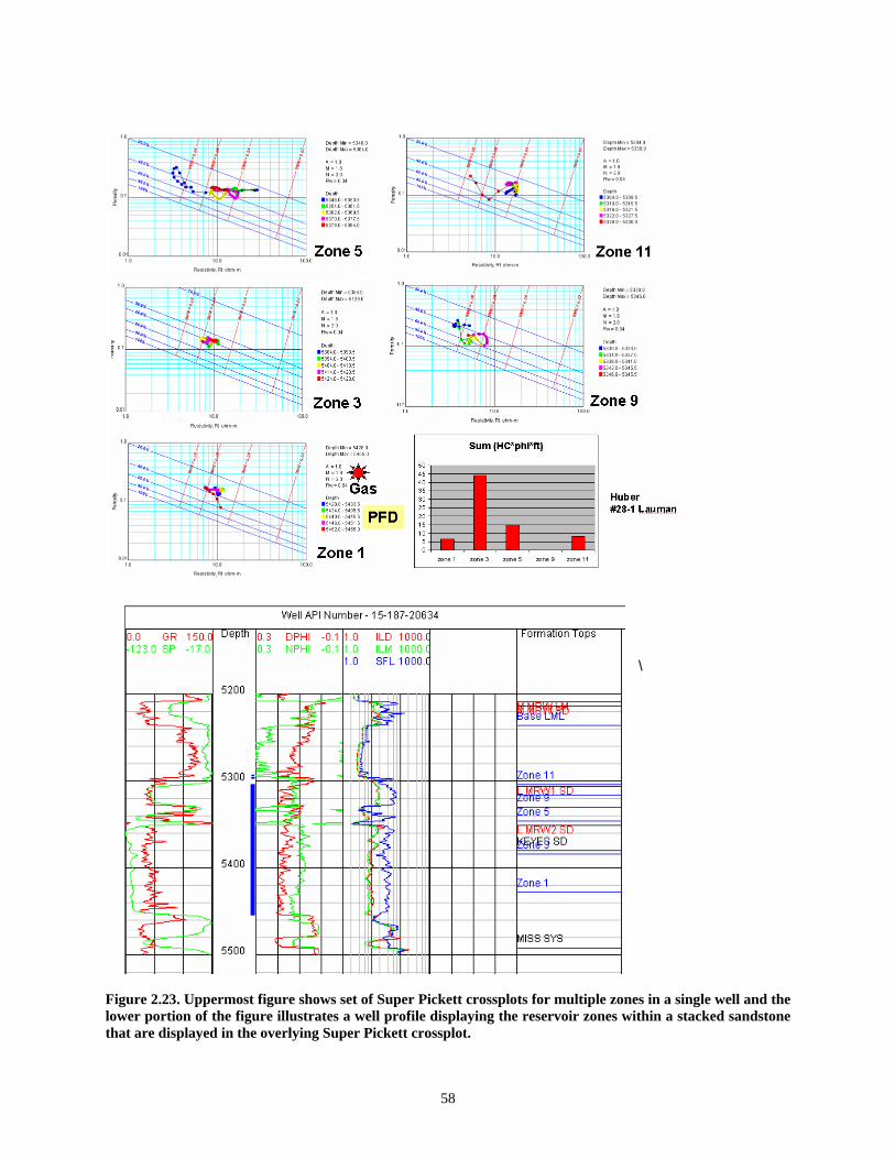
Figure 2.23. Uppermost figure shows set of Super Pickett crossplots for multiple zones in a single well and the lower portion of the figure illustrates a well profile displaying the reservoir zones within a stacked sandstone that are displayed in the overlying Super Pickett crossplot.

58

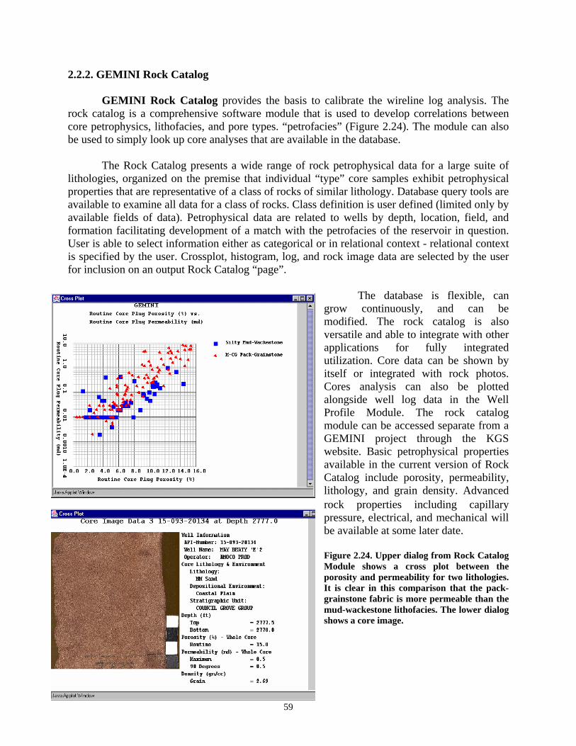
2.2.2. GEMINI Rock Catalog

GEMINI Rock Catalog provides the basis to calibrate the wireline log analysis. The rock catalog is a comprehensive software module that is used to develop correlations between core petrophysics, lithofacies, and pore types. “petrofacies” (Figure 2.24). The module can also be used to simply look up core analyses that are available in the database.

The Rock Catalog presents a wide range of rock petrophysical data for a large suite of

lithologies, organized on the premise that individual “type” core samples exhibit petrophysical properties that are representative of a class of rocks of similar lithology. Database query tools are available to examine all data for a class of rocks. Class definition is user defined (limited only by available fields of data). Petrophysical data are related to wells by depth, location, field, and formation facilitating development of a match with the petrofacies of the reservoir in question. User is able to select information either as categorical or in relational context - relational context is specified by the user. Crossplot, histogram, log, and rock image data are selected by the user for inclusion on an output Rock Catalog “page”.

The database is flexible, can grow continuously, and can be modified. The rock catalog is also versatile and able to integrate with other applications for fully integrated utilization. Core data can be shown by itself or integrated with rock photos. Cores analysis can also be plotted alongside well log data in the Well Profile Module. The rock catalog module can be accessed separate from a GEMINI project through the KGS website. Basic petrophysical properties available in the current version of Rock Catalog include porosity, permeability, lithology, and grain density. Advanced rock properties including capillary pressure, electrical, and mechanical will be available at some later date. Figure 2.24. Upper dialog from Rock Catalog Module shows a cross plot between the porosity and permeability for two lithologies. It is clear in this comparison that the pack-grainstone fabric is more permeable than the mud-wackestone lithofacies. The lower dialog shows a core image.

59

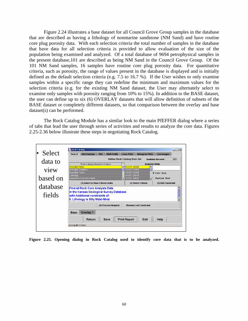
Figure 2.24 illustrates a base dataset for all Council Grove Group samples in the database that are described as having a lithology of nonmarine sandstone (NM Sand) and have routine core plug porosity data. With each selection criteria the total number of samples in the database that have data for all selection criteria is provided to allow evaluation of the size of the population being examined and analyzed. Of a total database of 9694 petrophysical samples in the present database,101 are described as being NM Sand in the Council Grove Group. Of the 101 NM Sand samples, 16 samples have routine core plug porosity data. For quantitative criteria, such as porosity, the range of values present in the database is displayed and is initially defined as the default selection criteria (e.g. 7.5 to 16.7 %). If the User wishes to only examine samples within a specific range they can redefine the minimum and maximum values for the selection criteria (e.g. for the existing NM Sand dataset, the User may alternately select to examine only samples with porosity ranging from 10% to 15%). In addition to the BASE dataset, the user can define up to six (6) OVERLAY datasets that will allow definition of subsets of the BASE dataset or completely different datasets, so that comparison between the overlay and base dataset(s) can be performed. The Rock Catalog Module has a similar look to the main PfEFFER dialog where a series of tabs that lead the user through series of activities and results to analyze the core data. Figures 2.25-2.36 below illustrate these steps in negotiating Rock Catalog.

• Select data to view

based on database

fields

Figure 2.25. Opening dialog in Rock Catalog used to identify core data that is to be analyzed.

60

•

Relational comparison

can be evaluated

using overlays

Figure 2.26. A key feature in the cross plotting is the ability to overlay and compare various data on the same chart. User selects the data and the symbol to be used.

• Overlay graphic control

Figure 2.27. The symbols and colors that can be used to delineate samples/layers that are compared are shown in this applet window

61

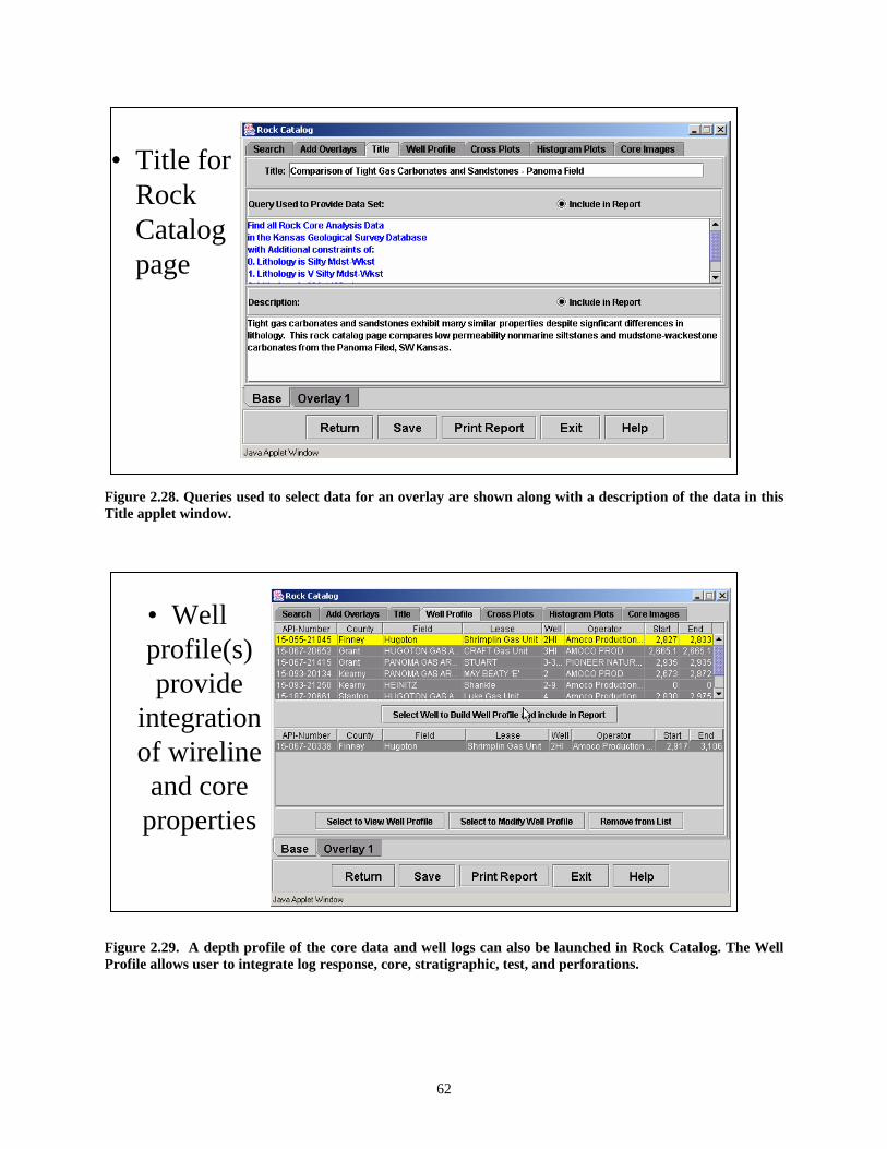
• Title for Rock Catalog page

Figure 2.28. Queries used to select data for an overlay are shown along with a description of the data in this Title applet window.

• Well profile(s) provide

integration of wireline and core

properties

Figure 2.29. A depth profile of the core data and well logs can also be launched in Rock Catalog. The Well Profile allows user to integrate log response, core, stratigraphic, test, and perforations.

62

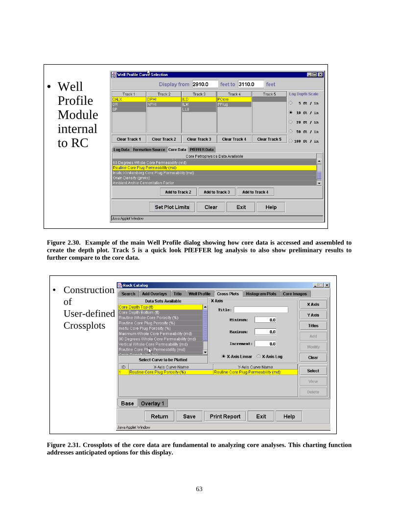
• Well Profile Module internal to RC

Figure 2.30. Example of the main Well Profile dialog showing how core data is accessed and assembled to create the depth plot. Track 5 is a quick look PfEFFER log analysis to also show preliminary results to further compare to the core data.

• Construction of User-defined Crossplots

Figure 2.31. Crossplots of the core data are fundamental to analyzing core analyses. This charting function addresses anticipated options for this display.

63

• Construct Crossplots

Figure 2.32. User can construct a series of crossplots to analyze the available core data.

• Crossplotsfor Rock Catalog page

Figure 2.33. Example of crossplots generated from Rock Catalog.

64

• Histograms for any variable

Figure 2.34. Histogram tabbed area of Rock Catalog is used to great simple histograms to examine the families of information in an attempt to delineate coherent petrofacies.

• View and select

available images

Figure 2.35. Core images can also be accessed through the Rock Catalog or through the Well Profile alongside the depth

65

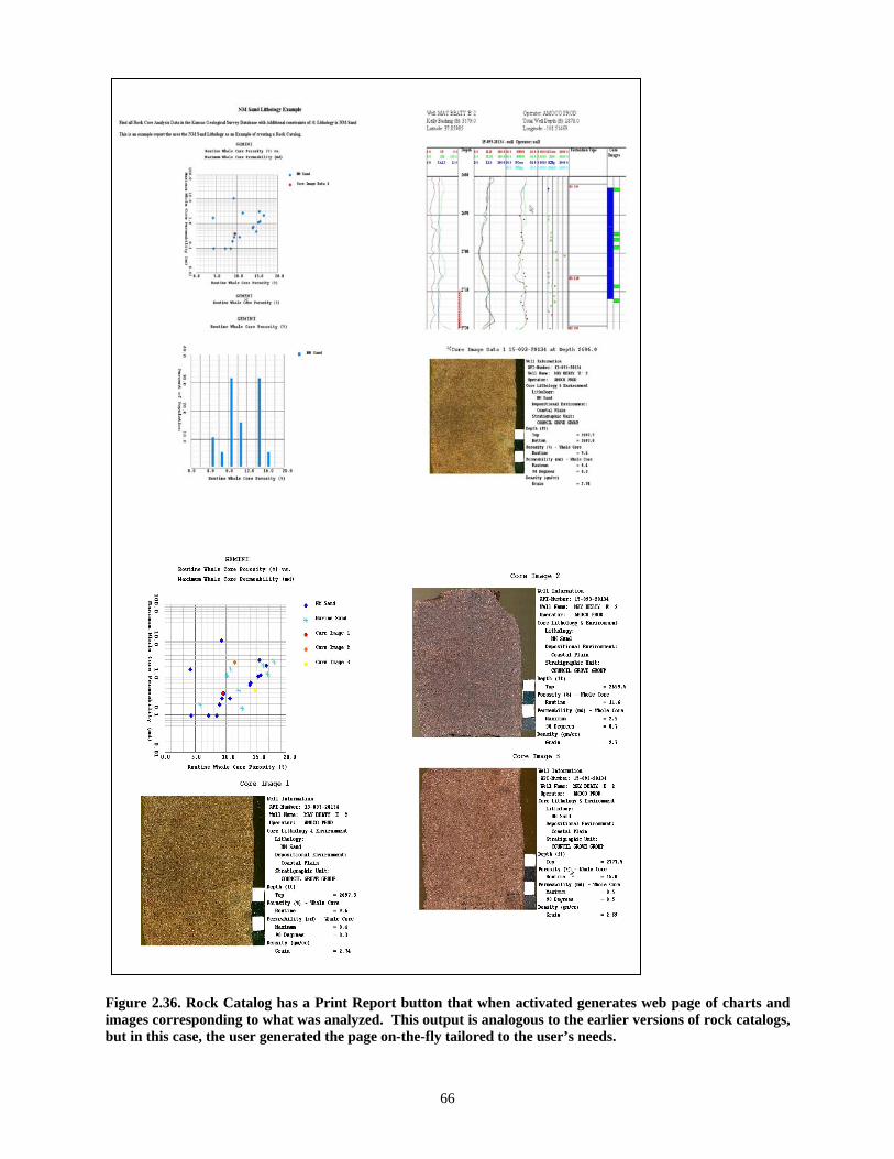
Figure 2.36. Rock Catalog has a Print Report button that when activated generates web page of charts and images corresponding to what was analyzed. This output is analogous to the earlier versions of rock catalogs, but in this case, the user generated the page on-the-fly tailored to the user’s needs.

66

In the GEMINI release workshop of September 24, 2003, the immediate future of the Rock Catalog module was described as shown in Figure 2.37 below.

Rock Catalog Module

• Ongoing and Future Developments– New additions to Kansas Database

• 200 wells – 9,500 analyses– Construct XML to access/share with other

databases– Expand Versatility of Crossplot

• Allow multi-database plots and mixing of data types by User-input from different databases (User can create plots with different data types on same plot allowing cross-referencing data that are similar but not exactly the same)

– Complete Advanced Rock Properties Tabs• Relative Permeability• Capillary Pressure• Electrical/Magnetic Properties• Fluid Sensitivity• Utilize Crossplot source code but change structure to provide

query to data tables that contain tabular data and not single values

– Extend rock properties functions in PfEFFER Module• Effective permeability module and addition to Pay criteria –

designate pay/nonpay based on effective flow, calculate cumulative keoh, φeoh

• Capillary pressure module– Variable Transform Utility

• Provide utilities to translate petrophysical variables (e.g. Capillary pressure to height above free water or pore throat diameter

Figure 2.37. Future of the Rock Catalog Module.

67

2.2.3. Synthetic Seismogram The synthetic seismogram module provides the means to generate a synthetic seismogram from a sonic log to facilitate linking these petrophysical results with seismic information. Operators can inventory the sonic logs available on the public-domain database and select this application to build a seismic synthetic using a simple Ricker Wavelet. The user has liberty to change the dominant frequency of the Ricker Wavelet, clip the interval, and add formation tops and depths to annotate the synthetic that is generated. Figures 2.38 through 2.41.

Glick Field(“Chat”)

Bird Field(Viola example)

Box Ranch Field

Glick Field(“Chat”)

Bird Field(Viola example)

Box Ranch Field

Figure 2.38. Map of Comanche County, Kansas showing the distribution of oil and gas fields, highlighting three fields including Box Ranch Field in southwestern Comanche County that contains Middle Ordovician Viola Limestone, the focus of the synthetic seismic example.

SYNTHETIC SEISMOGRAM

The GEMINI synthetic seismogram module is in the planning and development stage. The algorithm that drives the module will convolve reflection coefficients with a first order Ricker wavelet whose frequency is chosen by the User. This method is widely used in commercial synthetic seismogram software packages.

The steps in the procedure are:1. Input a sonic log or pseudo-sonic log2. Integrate the sonic log to rescale from depth in feet to two-way travel time in millisecond increments.3. Compute the train of reflection coefficients from the time-scaled velocity log.4. Compute a first-order Ricker wavelet as a digital filter with elements at two millisecond increments of two-way

travel time, using a frequency in Hertz stipulated by the User.5. Convolve the reflection coefficient sequence with the Ricker wavelet to generate the amplitudes of the synthetc

seismogram.

In the GEMINI version, the two major simplifying features will be that:there is no attenuation of the wavelet with depth andthe seismogram does not model multiple reflections

However, these simplifications are minor and do not adversely affect the ability of reflection events on the synthetic to be matched easily with a field seismic record as demonstrated by the following case-study example, using the algorithm described implemented by KOALA (a Kansas Geological Survey software package).

68

Box RanchField

Figure 2.39. Series of Java applets showing the well profile in upper left, identifying the Viola Limestone interval and potential pay interval highlighted by the red arrow. The synthetic is in the upper right and subsequent dialogs are shown to annotate strata on the time plots. Another dialog is used to look up wells making the module little dependent on other applications.

Box Ranch, 1-3 Roberts and Murphy Figure 2.40. Showing how the synthetic output can be linked to a well profile of an equivalent interval.

69

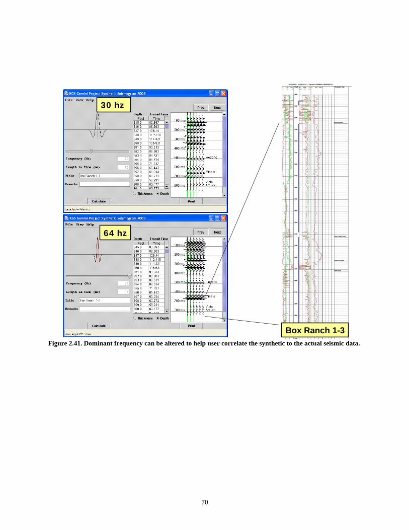
30 hz

64 hz

Box Ranch 1-3Figure 2.41. Dominant frequency can be altered to help user correlate the synthetic to the actual seismic data.

70

Subtask 2.3. Geomodel Development 2.3.1. Cross Section

The Cross Section Module is used to interactively build an annotated wireline log cross section (Figure 2.42). A map interface permits selection of wells from a project to include in the cross section. Up to five wells can be selected at one time, intentionally limited by the processing time and attempt to avoid exceeding the video memory of smaller PC’s of users. The interface from the Well Profile Module is used to establish the logging curves and scales. Well logs within the cross section can be annotated with flow units/zones, tops, perforations, and DST intervals. Correlation lines between formation tops are drawn automatically. Layers defined in the PfEFFER log analysis are also correlated between wells and color coded with color scheme defined by the user. The user can toggle between structural and stratigraphic datums, while the cross section is automatically refreshed to the new datum. Cross sections can be saved as a JPEG image files and reopened in a graphics program in order to print the section to a plotter or other device.

Touch log andEdit database

Cross sectionDialog

NW-SE Structural Datum

Marmaton B (Altamont) Terry Field

Marmaton B

40 ft

Figure 2.42. Cross Section module is used to generate images from the digital well logs that are part of a GEMINI project. The upper right image is the actual dialog box where the cross section is initially viewed. The user can interact with the logs on the section y clicking on the log and editing tops, log analysis intervals. The user has several options to datum the ection including with sea level by tops of log analysis regions, by tops of formations that are part of the dadetermines the dept interval shown and the vertical scale. Cross section ndex map shown in this Figure.right side of Figure.

b s

tabase. User selects the wells, the logs to be shown, and scale. Horizontal distance between wells is fixed, i.e., no Also, image of full cross section is shown in the upper

h i

71

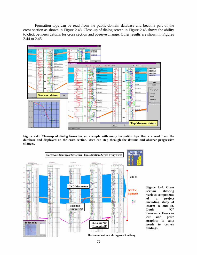
Formation tops can be read from the public-domain database and become part of the cross section as shown in Figure 2.43. Close-up of dialog screen in Figure 2.43 shows the ability to click between datums for cross section and observe change. Other results are shown in Figures 2.44 to 2.45.

Sea level datum

Top Morrow datum

Figure 2.43. Close-up of dialog boxes for an example with many formation tops that are read from the database and displayed on the cross section. User can step through the datums and observe progressive changes.

LKC-Marmaton

Marm B(Example #2)

St. Louis “C”(Example #1)

Northwest-Southeast Structural Cross Section Across Terry Field

200 ft

Horizontal not to scale; approx 5 mi long

Figure 2.44. Cross section showing various components of a project including study of Marm B and St. Louis “C” reservoirs. User can cut and paste graphics to suite needs to convey findings.

KHANExample

Index map

72

Figure 2.45. Same wells but different datums to convey underlying structural control on location of an incised valley. Upper section datumed above incised valley shows location of valley in structural low.

73

Comanche County Kansas is located in south-central Kansas on the western flank of the

Pratt Anticline (Figure 2.46). The distance across the county is some 40 miles (64 km). The cross section module is used to examine two significant pay zones in the area, the Mississippi “Chat” in Glick Field in the far northeastern section of the county and Viola Limestone reservoir that produces in Bird Field in the west-central part of the county.

Glick Field(“Chat”)

Bird Field(Viola example)

Box Ranch Field

Glick Field(“Chat”)

Bird Field(Viola example)

Box Ranch Field

Figure 2.46. Index map for Comanche County located in south-central Kansas. Cross section index line show for subsequent cross sections that span a 40 mile long transect between the southwest and northeastern corners of Comanche County.

74

The cross section in Figure 2.47 runs southwest to northeast with a sea level datum depicting the interval from the Upper Pennsylvanian Oread Limestone to the uppermost part of the Lower Ordovician Arbuckle Group. The yellow interval is the Mississippian Osage Stage and includes the “Chat” oil and gas reservoir, a heavily weathered porous and locally permeable chert dolomite. The reservoir is truncated to the northeast approaching the edge of the Pratt Anticline. The Viola Limestone in lime green thins and toward the northeast, eventually pinching out. Figures 2.48 and 2.49 show close-up cross sections of the northeastern region, highlighting the Mississippian “Chat” (shown by the boxed area in Figure 2.47) and locally the thinning Viola Limestone in Bird Field where the Viola is noted for prolific production.

SW-NE Regional Sealevel datumUpper Penn. Oread to Cambro-Ordovician ArbuckleComanche County, Ks

Viola

Figure 2.47 showing the regional cross section extending across Comanche County.

75

Figure 2.48. Shows a “close-up” of cross section in Figure ff in northern Comanche County where the Osage ”Chat “ reservoir undergoes significant thinning against regional subcrop. The “Chat” is equivalent downdip to the Cowely Facies a cherty dolomite, an unweathered unit deposited along the shelf margin (Watney et al., 2001). Note porosity increase in the updip direction. Hydrocarbon traps are combination structural & stratigraphic.

Glick FieldProlific MissChat Field

OsageCowley Facies

Osage“Chat”

Viola Limestone

West-East Sealevel DatumBird Field AreaOread to Arbuckle

Rich C-4 Rich C-7

Glick Field(“Chat”)

Bird Field(Viola example)

Box Ranch Field

Glick Field(“Chat”)

Bird Field(Viola example)

Box Ranch Field

Viola

Bird Field area

Pay

Figure 2.49. Local structural variation shown in structural cross section extending west-to-east across Bird Field in Comanche County Kansas. Pay in Viola Limestone in two wells named with blue stars along thinning of the interval against regional subcrop.

76

The user is quickly able to access the other GEMINI modules to further analyze the logs and production from Bird Field. Figure 2.50 shows the lease production from Bird Field alongside a well log annotated with the pay zone in the Viola Limestone. Figure 2.51 and 2.52 uses the PfEFFER module to examine a detailed log profile and a Super Pickett crossplot of the pay.

Bird Field Area Lease Production Plot

Rich C-4

Viola Ls.

Pay

Rich C-4

Figure 2.50. Production plot of leases in Bird Field and well log showing pay in Viola Limestone.

Rich C-4 Sweet Spot

Figure 2.51. Detailed well log profile and Super Pickett crossplot of the Viola pay zone.

77

Viola Rich C-4

Figure 2.52. Additional analyses done in PfEFFER for the Viola pay zone in Bird Field including lithology solution.

A standalone Java applet runs alongside access to the production database that can quickly show the viewer lease and field production and allow them to easily interact and modify the production plot (Figure 2.53). In this case, a recent rapid decline is noted. Producer can track these data at will and use GEMINI tools to get on top of the problems and opportunities.

Figure 2.53. Java applet dialog running alongside production plot in standalone production plot applet.

78

2.3.2. KHAN (Kansas Hydrocarbon Association Navigator) KHAN is designed to conduct statistical modeling (continuous variable prediction,

discriminant analysis, and clustering) of large databases to derive meaningful patterns including assessing pay in multiple LAS files. The module accomplishes data mining via statistical analysis of well log and core information. The process is semi-automated directed to reveal meaningful patterns in large volumes of log and core data. For example, the parameters that define hydrocarbon pay vary as the pore type/lithofacies change so a single set of cut-offs are not possible. KHAN allows the user to “train” on the log and core analyses from known producing zones and use this predict similar pay zones. Multiple pore types can be included in the training and used to assess their presence in the form of probabilities in unclassified datasets. The user can select an LAS file of interest, such one from a new well, and use a pay model to determine if zones are present in the well that resemble pay zones from other wells in the area. The larger the training set and the more intervals involved in training, the more robust the predictions. Systematic classification of pay in a field, region, or basin has considerable potential to classify hydrocarbon shows in a quantitative, mappable manner. Systematizing pay at the field level can also help to develop reservoirs by identifying priority areas and intervals, e.g., indications of bypassed pay and underproduced zones.

The predecessor of KHAN called KIPLING demonstrated the ability to be able to predict discrete and continuous variables such as lithofacies and permeability using wireline logs (http://www.kgs.ku.edu/software/Kipling/Kipling1.html). KHAN fits in the family of applications that include classical and localized regression, smoothing splines and kernel functions, neural networks, and CMAC (Cerebellar Model Arithmetic Computer). Hagens and Doveton (1991) adapted the CMAC algorithm for use in representing a general function of multiple variables and applied the algorithm to mapping of a geological surface. The software developed for this work was a predecessor to the Kipling software. Applications of Kipling to prediction of facies sequences are described in Bohling, Doveton, and Watney (1996) and Bohling, Doveton, and Hoth (1997).

Supervised classification methods include classical

discriminant analysis, kernel density estimates, nearest neighbor, neural networks, CMAC, decision trees, and expert systems. Unsupervised classification (clustering) includes a wide variety of clustering techniques. KHAN will incorporate the functionality of both supervised and unsupervised classification. Figure 2.54. Depiction of shingled block lattice used in the CMAC discretization scheme of KHAN and KIPLING.

79

The CMAC's discretization of variable space is quite similar to that employed in the averaged shifted histogram (ASH) proposed by Scott (1992) (Figure 2.54). In fact, Scott's algorithm is somewhat more elaborate, in that the shifting of averaging bins along each axis is specified independently of that along other axes, rather than occurring in lockstep along all axes, as in the CMAC. The simpler CMAC discretization scheme results in a more efficient implementation, both in terms of execution speed and in terms of the amount of information that needs to be stored. The algorithm implemented in Kipling can be considered a hybrid, combining the traditional Albus CMAC discretization scheme with the bin-wise averaging employed in the ASH.

KHAN is based on Kipling.xla, an add-in Visual Basic program for Excel. Kipling.xla uses the CMAC algorithm (similar to neural net) and accommodates discrete variable prediction and supervised classification. The prototype is a stand-alone application and can read data from local files. A flexible, intuitive interface selects data volume and variables to analyze. Then KHAN is integrated with GEMINI where computed results, e.g., zonation from depth constrained cluster analysis in the PfEFFER module of GEMINI can be used as inputs to KHAN. KHAN results are displayed in a depth-based well profile of probabilities of classifying variables that were trained for in the model. KHAN is structured such as models developed can be shared at large with other GEMINI users or within a password-protected project.

In addition to hydrocarbon pay, KHAN can be used to predict “electrofacies”, discrete geometric units that ideally are correlatable and correspond to significant, rationale geologic rock bodies. In other words, the petrophysical classification resulting from this “electrofacies” analysis might be based on a “training set” consisting of petrofacies (lithofacies+pore types) or genetic stratigraphic units such as flooding units, condensed sections, and paleosols.

Dialogs lead the user through specifying training variables and the well logs or cores

from which training sets will be built. Predictions will be made and the model will be matched to the dataset variables. A 2D example below illustrates how KHAN transforms the data to a model (Figure 2.55). The two variables are crossplotted showing some correlation between them. The computation creates a histogram that bins and counts the data. The data counts provide an estimate of the relative prevalence of each variable to be used in prediction in any particular region of the two dimensional variable space defined by independent training variables Rhomaa and Umma. The lower illustration in Figure 2.55 shows resulting histogram counts used to describe the data from which the model is built. Using this information, KHAN computes a set of electrofacies membership probabilities associated with a vector of measured log values. After training is complete, the model can be used to predict these variables from other sets of Rhomaa and Umma data. Plots of the membership probabilities or facies indicators versus depth can then be constructed.

80

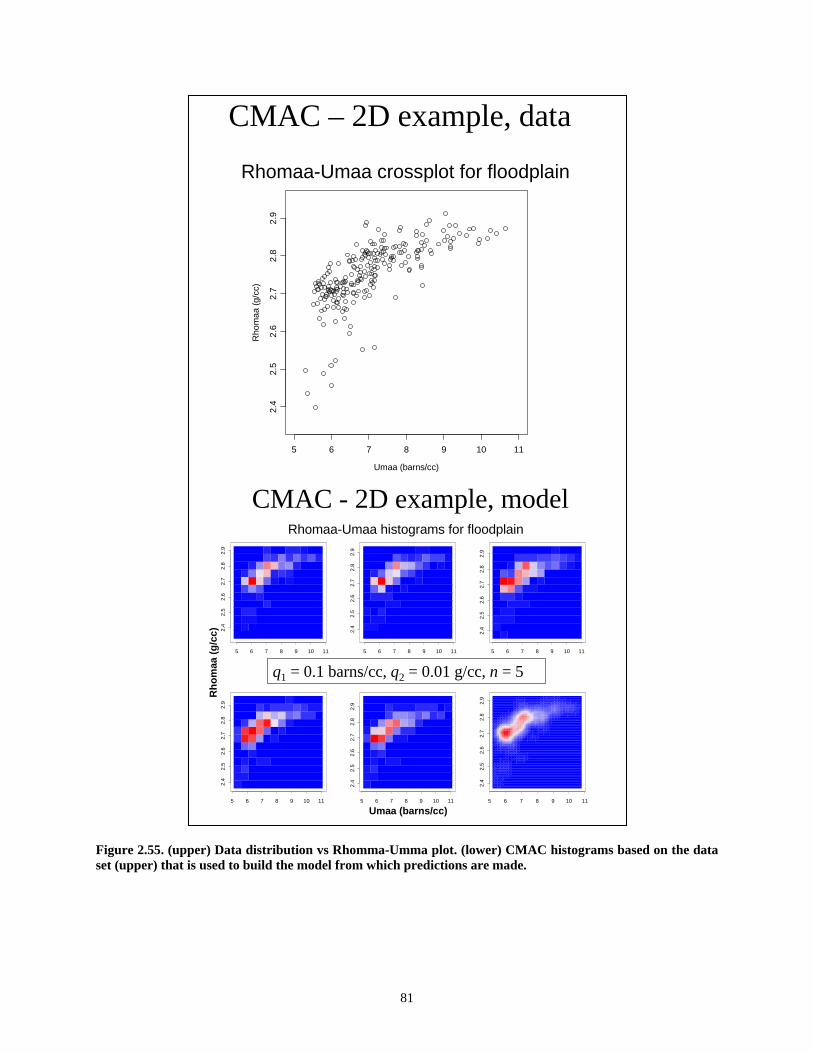
CMAC – 2D example, data

Umaa (barns/cc)

Rho

maa

(g/c

c)

5 6 7 8 9 10 11

2.4

2.5

2.6

2.7

2.8

2.9

Rhomaa-Umaa crossplot for floodplain

CMAC - 2D example, model

5 6 7 8 9 10 11

2.4

2.5

2.6

2.7

2.8

2.9

5 6 7 8 9 10 11

2.4

2.5

2.6

2.7

2.8

2.9

5 6 7 8 9 10 11

2.4

2.5

2.6

2.7

2.8

2.9

5 6 7 8 9 10 11

2.4

2.5

2.6

2.7

2.8

2.9

5 6 7 8 9 10 11

2.4

2.5

2.6

2.7

2.8

2.9

5 6 7 8 9 10 11

2.4

2.5

2.6

2.7

2.8

2.9

Umaa (barns/cc)

Rho

maa

(g/c

c)

Rhomaa-Umaa histograms for floodplain

q1 = 0.1 barns/cc, q2 = 0.01 g/cc, n = 5

Figure 2.55. (upper) Data distribution vs Rhomma-Umma plot. (lower) CMAC histograms based on the data set (upper) that is used to build the model from which predictions are made.

81

The dialogs used in KHAN lead the user through the training and modeling (Figure 2.56). Workflow is shown on the left margin of the dialogs to help the user track their progress. User has the option to use core or log data in the training. In using core data, lithofacies are define and corresponding well log response is used to build a model to predict lithofacies in other wells. Log suites must be the same in training and prediction. The KHAN interface checks available log curves for wells identified for training to assist the user in selecting those wells that have the correct log suite. This function saves considerable time when many wells are involved in establishing the training set.

Figure 2.56. Examples of dialogs for KHAN that are used in training to develop a model. The user may use multiple sessions to build a training set. To accommodate this extended activity, reports can be generated as web pages to review what has been accomplished (Figure 2.57). These reports contain variables, well logs, wells used, and provide links to web pages created along the way.

82

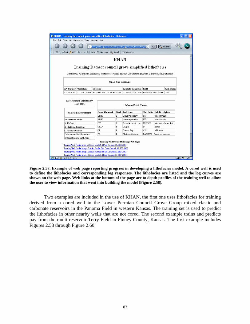
Figure 2.57. Example of web page reporting progress in developing a lithofacies model. A cored well is used to define the lithofacies and corresponding log responses. The lithofacies are listed and the log curves are shown on the web page. Web links at the bottom of the page are to depth profiles of the training well to allow the user to view information that went into building the model (Figure 2.58). Two examples are included in the use of KHAN, the first one uses lithofacies for training derived from a cored well in the Lower Permian Council Grove Group mixed clastic and carbonate reservoirs in the Panoma Field in western Kansas. The training set is used to predict the lithofacies in other nearby wells that are not cored. The second example trains and predicts pay from the multi-reservoir Terry Field in Finney County, Kansas. The first example includes Figures 2.58 through Figure 2.60.

83

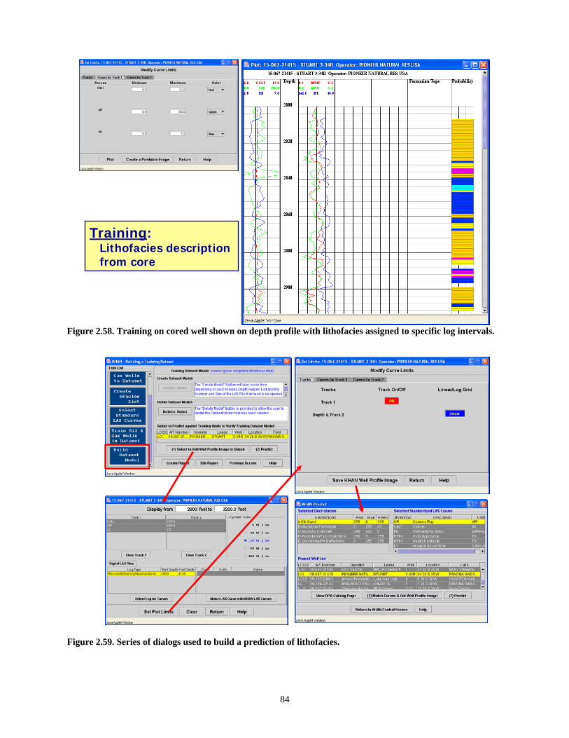
Training: Lithofacies description from core

Figure 2.58. Training on cored well shown on depth profile with lithofacies assigned to specific log intervals. Figure 2.59. Series of dialogs used to build a prediction of lithofacies. B ildi d l di i

84

Figure 2.60. Output – predicted lithofacies. Terry Field is located in Finney County in southwestern Kansas (Figure 2.61). It has been a prolific field that has cumulative production nearing 5 million barrels originating from a series of 10 Pennsylvanian and Mississippian carbonate and clastic reservoirs. Oomoldic pore type dominates the Pennsylvanian carbonate reservoirs while interparticle oolitic pay is present in the Mississippian St. Louis Limestone. Also, Pennsylvanian sandstone reservoirs are present with predominant interparticle porosity. Bypassed pay in the field is a possibility. In addition, the concentration of pay zones with these varied pore types may serve as a good training set to predict pay in other wells, potentially bypassed and offering opportunities for recompletion or washdown. Considerable amounts of data have been assembled on the field to document the pay including an excellent suite of well logs, core, DST, geology reports with good sample descriptions, and production data. Figures 2.61- 2.63 describe the results in application of KHAN to define pay in these clastic and carbonate reservoirs.

85

after Gerlach (1997)

Terry Field, Finney County

Target:• Complex stacked carbonate oil reservoirs• Field scale

Data:• Core, DST, well logs, perfs & IP, production history

Oil propertiesTools:

Rock catalog, production & DST analyst, PVT, log analysis, well profile (marked log), cross section, mapping-volumetric analysis,KHAN (Kansas Hydrocarbon Association Navigator)

Figure 2.61. Location of Terry Field in southwestern Kansas. A series of GEMINI tools were use to analyze the reservoirs. Well Profile showing portion of 700 ft interval for training and prediction

Training KHAN to recognize:--Oil, Wet, Tight, Shale

Reservoirs with varying:• Lithology (although not in this example)• Pore geometry• Pore type• Archie m, n• Log cutoffs

PfEFFER Paycalculation usingsingle set of cutoffs (blue curve)

entire LKC-Marmaton

Figure 2.62. KHAN was trained a series of wells from a 700 ft (213 m) interval extending from the Upper Pennsylvanian Heebner Shale to the Mississippian St. Louis Limestone. Perforated zones from a series of wells were input into the training exercise to capture the stratigraphic range of pay in the field. Also, intervals that produced water from DST results were selected as wet/water zones for training. Obvious tight, low

86

porosity zones were classified as tight and shale intervals were classified as shale. In this figure, a Super Pickett cross plot is used to show demonstrate the vast amount of petrophysical variation on this interval being analyzed and choosing pay is not simple. The depth plot on the left from the Well Profile module includes a quick look pay calculation highlighted with the red arrow that uses a single set of Archie parameters and log cut-offs. The possible pay zones indicated by this approach are considerable, but the question is raised that due to the considerable variations in pore type, it is not possible to apply a single set of Archie parameter and cut-offs to obtain reliable indicators of pay. KHAN was called upon to help refine the search for pay.

From wellProfile

Pay Prediction

Figure 2.63. After the training set is built to characterize oil, wet, tight, and shale zones, the model was applied to a well outside the original dataset. User selects the model and applies it to a well. User must select the log curves that match those curves used in training and then KHAN predict the probability of pay, which is presented in a depth column. The well profile at the right shows a thick highly probable (almost certain) oil section in a Morrow sandstone. The completion records indicate that this zone was perforated for production and lease records indicate 41000 bbls of oil produced in just over one year. The other shallower zones remain untested.

87

Marm BMarm B

Producing Well Dry Hole

HighProbabiltyfor oil pay

Currentperforations KHAN

Predictions

-Build training setsand share models

-Use as quick lookto search throughLAS files

Prediction:Oil, Wet, Tight, Shale

St. Louis “C”

Figure 2.64. Another example compares KHAN pay predictions for a known producing well (from the Marmaton B carbonate) and a dry hole. Note the low probability for pay (green areas) in the dry hole. Many other zones appear to have potential beyond the interval currently perforated.

88

Task 3. Geo-Engineering Modeling Subtask 3.1. Volumetrics Module Volumetric calculations

An important application of the reservoir geomodel is in the initial evaluation of reserves and also in the estimation of the volume of recoverable hydrocarbons. The knowledge about the volume of the asset in place and an approximation about the recoverable fraction serve as the basis for reservoir development and management. Also, the volumetric calculations lend an economic face to the rigor and technical detail that goes into the construction of the geomodel. Most modern mapping tools including GEMINI enable the display of grid cells values, used to construct geologic maps of gross and net thickness, average porosity and water saturation. This provides an opportunity to carry out volumetric calculations on a grid cell by grid cell basis. Volumetrics is a logical extension of core and log analysis, especially when effort is made to petrophysically define pay. Volumetric mapping is an important step to compare spatial distribution of key reservoir parameters and relate them to oil or gas production. This is an iterative process and requires trail and error due to uncertainties in establishing pay cut-offs and assessing reservoir layering, continuity, and vertical conformance. Inputs to volumetric calculations

The inputs to the volumetric calculations include three petrophysical parameters: net hydrocarbon bearing thickness, effective porosity and water saturation. These values are obtained from the Super Pickett analysis in GEMINI and they vary spatially across the reservoir as interpolated in the GEMINI volumetric module. Subdivision of the reservoir into grid cells followed by volumetric calculations on each grid cell helps to manage and assess the effects of variations in the petrophysical properties. The general rule is to have at least five grid cells between wells to best represent the variation in the reservoir. The standard formulas used in the volumetric calculations of oil and gas reserves are: a) oil reservoir

∑=n

1 o

rowgrnp

BE)S-(1Vh N φ

b) gas reservoir

∑=n

1 g

rgwgrnp

BE)S-(1Vh G φ

where n is the number if grid cells, Np and Gp are oil and gas reserves at surface conditions, Ero and Erg are recovery factors for oil and gas reservoirs, hn is the net pay at

89

each grid, φ is the effective grid porosity and Sw is the water saturation in each grid cell. Bo and Bg are formation volume factors for oil and gas and they can also vary spatially. a) Net pay: Definition of net pay from within the gross reservoir pay is a difficult task

and yet it has very important consequences in the calculation of the reservoir volume. Normally within the reservoir rock heterogeneities such as intercalation of shales, streaks of low porosity and permeability, or zones with high mobile water saturation may exist. In order to obtain a realistic value for net pay the cumulative thickness of these non productive intervals had to be subtracted from the gross pay. Log analysis in the PfEFFER module utilizing the Super Pickett crossplot provides a convenient way to define cut-offs to eliminate non productive intervals from the reservoir interval. PfEFFER automatically sums net pay thickness and corresponding average water saturation and porosity within the pay interval. Information is passed to the Volumetrics module in GEMINI to perform the gridding, mapping, and OOIP calculations.

b) Effective porosity: The average porosity at each well is the thickness weighted mean

of the porosities derived from logs. c) Water saturation: The water saturation in a reservoir is dependent on the height

above the free water level and the distribution of the pore throat sizes. The average water saturation at each well is calculated by taking the volume weighted mean across only those intervals that have been included within the net pay. This value is automatically calculated for each zone in each well within the PfEFFER log analysis module. The formula below is used to calculate the average water saturation. The

number of productive layers included in the net pay identified in the well is m and Sw,k, φk, and hn,k are the corresponding saturation, effective porosity and height of the each productive layer in the well. The average well porosity is represented by φw and hn,w is the average net pay at the well.

wn,w

m

1kkn,kkw,

ww,h

hSS

φ

φ∑==

d) Formation volume factors: The formation factor for oil, Bo, and especially that for gas, Bg, does not vary much within most reservoirs. Laboratory measured values on oil and gas samples are generally adequate for use in volumetric calculations. In absence of measured values, standard correlations can be used to generate them. The PVT module in GEMINI provides quick access to these correlations. In very thick oil reservoirs, gravity segregation may lead to thicker oil settling at the bottom and this may result in Bo varying with depth.

e) Recovery factor: The estimation of a recovery factor (Er) is a difficult and uncertain

aspect of reserve evaluation by the volumetric method. Er depends on a number of interrelated factors such as reservoir drive mechanism, reservoir heterogeneity, number of wells and their distribution, production schedule, and status of

90

implementation of secondary and enhanced recovery schemes. Thus, the Er value will be a unique value for every field and it can be calculated with confidence only after the field has reached its economic limit. Er values from analogous reservoirs, preferably in the same sedimentary basin and with same drive mechanism, can be used in the volumetric calculations. Another option is using the recovery factors correlations published by API which are based on final recoveries recorded in reservoirs with known drive mechanism, petrophysical and hydrocarbon properties.

Net pay, effective porosity, and average saturation values obtained at each well

are used to calculate the corresponding attribute values for the grid cells between adjacent wells. Volumetrics for reservoirs with production history

For reservoirs with significant production history, the volumetric study can be used to cross check if the petrophysical properties of the reservoir, such as net pay, porosity, and saturation can support the reported field production. Hydrocarbon production is attributed to individual wells of the field. Thus to obtain the production obtained from a grid cell, the well production has to distributed amongst the grid cells in the drainage area of the well. In the absence of a more accurate method at this initial stage of a reservoir characterization, cumulative oil production from each well can be distributed among the grid cells present in the drainage area of the well. If discrepancies are noted between cumulative production and volumetric OOIP, the user can easily return to the PfEFFER to make adjustments to the pay cut-offs, Archie equation parameters, or even reservoir layering and correlations.

If production information is available for a field, material balance calculations can

be used to independently estimate hydrocarbon recovery. The Material Balance module in GEMINI serves this function. If the volumetric and material balance results are vary more than10%, the volumetric model should be modified. The material balance results indicate communicating volume in the reservoir, while is it not known if the reservoir described by the volumetric model is actually continuous and communicating. Errors in this reservoir volume will cause serious problems during the reservoir simulation. Example Using the Volumetric Module

Volumetric study carried out during the construction of a reservoir geomodel offers an opportunity to get a feel for the total production potential of the reservoir based on the petrophysical properties defined at each wells. If production data is available then this potential can be related to the cumulative production already recorded. Any major discrepancies that are spotted will need to be resolved by either correcting the production data or by revising the data obtained from analysis of well logs, cores and individual well performances. For fields that have some recorded pressure and production history and PVT data, this sets the stage for a material balance study.

91

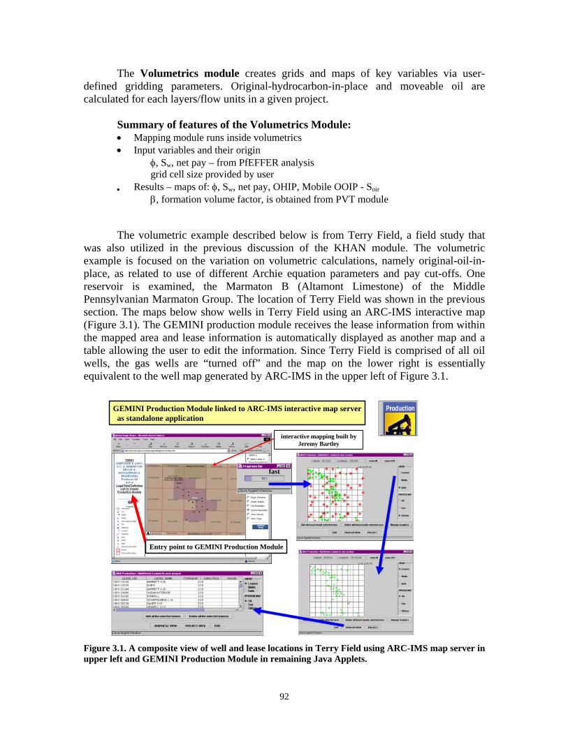
The Volumetrics module creates grids and maps of key variables via user-defined gridding parameters. Original-hydrocarbon-in-place and moveable oil are calculated for each layers/flow units in a given project.

Summary of features of the Volumetrics Module: • Mapping module runs inside volumetrics • Input variables and their origin

φ, Sw, net pay – from PfEFFER analysis grid cell size provided by user

• Results – maps of: φ, Sw, net pay, OHIP, Mobile OOIP - Soir

β, formation volume factor, is obtained from PVT module

The volumetric example described below is from Terry Field, a field study that was also utilized in the previous discussion of the KHAN module. The volumetric example is focused on the variation on volumetric calculations, namely original-oil-in-place, as related to use of different Archie equation parameters and pay cut-offs. One reservoir is examined, the Marmaton B (Altamont Limestone) of the Middle Pennsylvanian Marmaton Group. The location of Terry Field was shown in the previous section. The maps below show wells in Terry Field using an ARC-IMS interactive map (Figure 3.1). The GEMINI production module receives the lease information from within the mapped area and lease information is automatically displayed as another map and a table allowing the user to edit the information. Since Terry Field is comprised of all oil wells, the gas wells are “turned off” and the map on the lower right is essentially equivalent to the well map generated by ARC-IMS in the upper left of Figure 3.1.

interactive mapping built by Jeremy Bartley

GEMINI Production Module linked to ARC-IMS interactive map serveras standalone application

Entry point to GEMINI Production Module

fast

Figure 3.1. A composite view of well and lease locations in Terry Field using ARC-IMS map server in upper left and GEMINI Production Module in remaining Java Applets.

92

The two cases for the volumetric analysis are presented in Figure 3.2. The need to for this comparison originates from what parameters are needed to evaluate this oomoldic carbonate reservoir.

VolumetricsMarmaton BTerry FieldFinney County, Kansas

Oomoldic Reservoir

Compare impact of twosets of cutoffs

Marmaton BInitial log cutoffs

Archie Exponentsm=2, n=2

Well Log CutoffsPhi =.15Sw = .25Vsh = .3BVW = .04

Marmaton B

Log calibration utilizing

core analysisof highly

oomoldic LKClimestones from

CKU

Archie Exponentsm=3.5, n=2

Well Log CutoffsPhi =.17Sw = .55Vsh = .3

BVW = .097

Case #1

Case #2 Figure 3.2. Archie exponents and well log cut-offs used in the two cases to illustrate impact on volumetric calculations. The Marmaton B carbonate reservoir appears to be an extreme oomoldic end member with abundant molds connected by touching vugs creating by dissolution and crushing. The original interparticle porosity was filled by early finely crystalline equant calcite cement (Figure 3.3). Oomoldic Lithofacies:

Terry Field, McCoy Six M Farms “A” 3-22 Marmaton B (Altamont Ls.)4288.5 ft, thin section photomicrograph40x transmitted light; core analysis: 25.6% porosity, 28.8 md

0.5 mm

Figure 3.3. Thin section photomicrograph from core taken in Marmaton B reservoir in Terry Field. (from Core Laboratories Report).

93

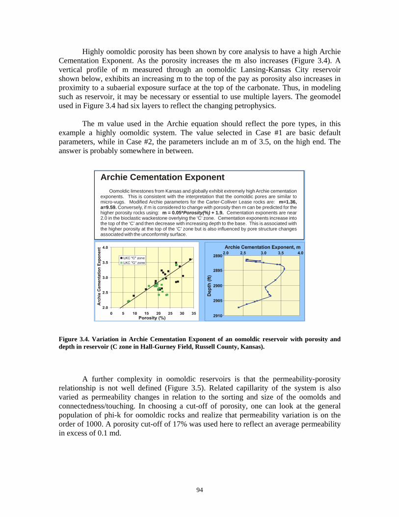
Highly oomoldic porosity has been shown by core analysis to have a high Archie Cementation Exponent. As the porosity increases the m also increases (Figure 3.4). A vertical profile of m measured through an oomoldic Lansing-Kansas City reservoir shown below, exhibits an increasing m to the top of the pay as porosity also increases in proximity to a subaerial exposure surface at the top of the carbonate. Thus, in modeling such as reservoir, it may be necessary or essential to use multiple layers. The geomodel used in Figure 3.4 had six layers to reflect the changing petrophysics. The m value used in the Archie equation should reflect the pore types, in this example a highly oomoldic system. The value selected in Case #1 are basic default parameters, while in Case #2, the parameters include an m of 3.5, on the high end. The answer is probably somewhere in between. Archie Cementation Exponent

Oomoldic limestones from Kansas and globally exhibit extremely high Archie cementation exponents. This is consistent with the interpretation that the oomoldic pores are similar to micro-vugs. Modified Archie parameters for the Carter-Colliver Lease rocks are:

Conversely, if m is considered to change with porosity then m can be predicted for the higher porosity rocks using: Cementation exponents are near 2.0 in the bioclastic wackestone overlying the ‘C’ zone. Cementation exponents increase into the top of the ‘C’ and then decrease with increasing depth to the base. This is associated with the higher porosity at the top of the ‘C’ zone but is also influenced by pore structure changes associated with the unconformity surface.

m=1.36, a=9.59.

m = 0.05* + 1.9. Porosity(%)

Figure 3.4. Variation in Archie Cementation Exponent of an oomoldic reservoir with porosity and depth in reservoir (C zone in Hall-Gurney Field, Russell County, Kansas).

A further complexity in oomoldic reservoirs is that the permeability-porosity relationship is not well defined (Figure 3.5). Related capillarity of the system is also varied as permeability changes in relation to the sorting and size of the oomolds and connectedness/touching. In choosing a cut-off of porosity, one can look at the general population of phi-k for oomoldic rocks and realize that permeability variation is on the order of 1000. A porosity cut-off of 17% was used here to reflect an average permeability in excess of 0.1 md.

94

Lansing-Kansas City Oomoldic Ls

0.001

0.01

0.1

1

10

100

1000

10 12 14 16 18 20 22 24 26 28 30 32Porosity (%)

Insi

tu P

erm

eabi

lity

(md)

CoxBoundsDrew sDorrWittOberleA17WBoxbergerLeurmanTremblyVopatGordonEE TobiasHaffermanMichaelisSoekenSellens 2Sellens 1OeserPrincTiepermanColliver 1C-C CO2I CC-C CO2IGC-C CO2IC WCColliver #16Colliver #16 WC CColliver #16 WC GColliver #16 90~Upper Limit~Low er Limit

17% Porosity cutoff Figure 3.5. Porosity-permeability crossplot for Lansing-Kansas City oomoldic rocks. A 17% cut-off is used to indicate permeable rock for the Marmaton B Case #2. The water saturation cut-off is defined by economics, the relative amount of oil and water produced, the oil cut. A 4% oil cut is used as the economic limit and according to relative permeability measurements in these oomoldic systems, the corresponding water saturation is approximately 55% (Figure 3.6). Figure 3.6. Core analyses measurements of relative permeabilities for varying water saturation for oomoldic samples from Lansing-Kansas City Group in Hall-Gurney Field.

Oomoldic Ls Sw Cut-off Criteria• Dependent on:

– Kr curve & Sorw– LOE & economic

oil/water ratio• Assuming

~2BO/50BW limit then:

– krow/krw = 0.04– Swcutoff @ 0.04 =

0.55 for rock with kr curve shown and Sorw = 0.35

0.0001

0.001

0.01

0.1

1

10

100

1000

0.0 0.1 0.2 0.3 0.4 0.5 0.6 0.7 0.8 0.9 1.0Water Saturation Sw

Kro

w//K

rw

2893V1 SetMarmatonmodel 1model2model3

Econlimit

Swcut

95

PfEFFER is used define the pay for the Marmaton B reservoir in Terry Field. When the Volumetrics module is launched, the parameters used to compute the volumetrics are accessed. The initial step is to grid the data. The user is able to set the grid parameters and after doing so is able to map them (Figure 3.7 and 3.8).

Marmaton B – Case #1

Triangle show perfed wells

Figure 3.7. The dialogs are shown that are used to establish the grid and select maps. The mapping consists of colored grid cells that are set automatically or by the user. Well location uses standard symbols and perforated wells are noted with a triangle.

Marmaton BCase #1

m=2, n=2

CutoffsPhi =.15Sw = .25Vsh = .3BVW = .04

Gross Thickness Net Pay Average Phi

Average Sw Sum (So*phi*ft)

Figure 3.8. Series of maps generated for Marmaton B for Case #1. Lower right map is equivalent to original-oil-in-place. Case #1 represents parameters for a reservoir with interparticle pores.

96

Marmaton B Case #2 consists to using another set of Archie equation exponents and well log cut-offs to reflect values suggested by core analysis for highly oomoldic rocks (Figure 3.9). A separate set of PfEFFER analyses were used to develop the new volumetric calculations.

Marmaton BAlternative Volumetrics

Marmaton B

Log calibration as defined by

core analysisof highly

oomoldic LKClimestones from

CKU area

Archie Exponentsm=3.5, n=2

Well Log CutoffsPhi =.17Sw = .55Vsh = .3

BVW = .097

Case #2

Figure 3.9. Opening volumetrics dialog that shows a map of wells included in the project and a list of PfEFFER log analysis intervals or scenarios that are available for volumetric calculations. Marmaton Case #1 and #2 volumetrics are compared in Figure 3.10. The OOIP is 40% less in Case #2, which is probably more realistic since the parameters are likely more appropriate for this highly oomoldic reservoir. .

Marmaton B

Case #2Archie Exponents

m=3.5, n=2

Well Log CutoffsPhi =.17Sw = .55Vsh = .3

BVW = .097

4.2 MM Bbls OOIP (40% less than Case #1)9.7 MM Bbls OOIP

Marmaton BCase #1

Archie Exponentsm=2, n=2

Well Log CutoffsPhi =.15Sw = .25Vsh = .3

BVW = .04

OOIPOOIP

Figure 3.10. Comparison of volumetric calculations. Case #1 for interparticle porosity and Case #2 (most appropriate here) for highly oomoldic rocks.

The user can view the cut-offs and Archie parameters used in the volumetric analysis by examining workflow summaries PfEFFER as shown in Figure 3.11. The

97

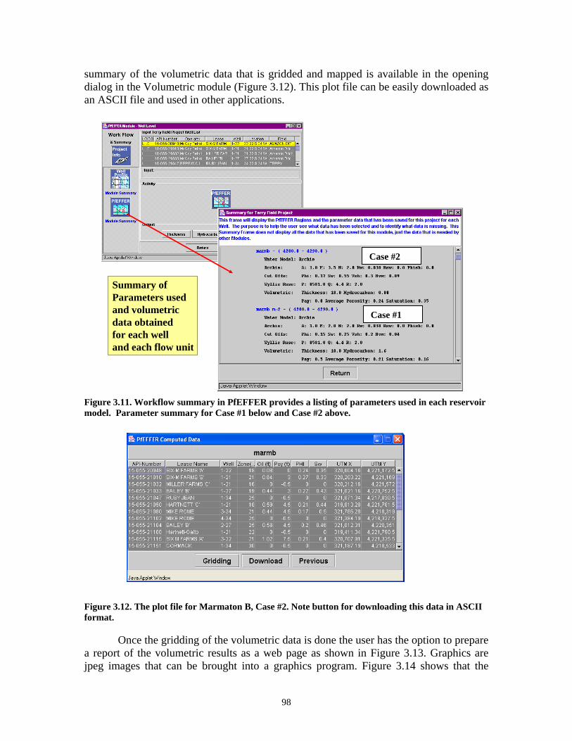
summary of the volumetric data that is gridded and mapped is available in the opening dialog in the Volumetric module (Figure 3.12). This plot file can be easily downloaded as an ASCII file and used in other applications.

Summary of Parameters used and volumetric data obtained for each welland each flow unit

Case #2

Case #1

Figure 3.11. Workflow summary in PfEFFER provides a listing of parameters used in each reservoir model. Parameter summary for Case #1 below and Case #2 above. Figure 3.12. The plot file for Marmaton B, Case #2. Note button for downloading this data in ASCII format. Once the gridding of the volumetric data is done the user has the option to prepare a report of the volumetric results as a web page as shown in Figure 3.13. Graphics are jpeg images that can be brought into a graphics program. Figure 3.14 shows that the

98

downloaded ASCII data can be brought into other mapping program for enhanced gridding and mapping or can be used as input in a reservoir simulator.

Output of Volumetrics to web browser and ASCii file download

Figure 3.13. Web page report of volumetric data generated by GEMINI. Left side is enlargement of a portion of the page shown on the right.

4000 6000 8000 10000 120004000

6000

8000

10000

12000

14000

16000

18000

20000

-1350-1348-1346-1344-1342-1340-1338-1336-1334-1332-1330-1328-1326-1324-1322-1320-1318-1316-1314-1312-1310-1308-1306-1304

4000 6000 8000 10000 120004000

6000

8000

10000

12000

14000

16000

18000

20000

4000 6000 8000 10000 120004000

6000

8000

10000

12000

14000

16000

18000

20000

4000 6000 8000 10000 120004000

6000

8000

10000

12000

14000

16000

18000

20000

Versions of Surfer structure map on top of Marmaton B (Altamont Limestone) -- (feet scale)Map uses same gridding type and parameters as GEMINI volumetrics.Plot file cut and paste from GEMINI Volumetric Report web page.

4000 6000 8000 10000 120004000

6000

8000

10000

12000

14000

16000

18000

20000

-1350-1348-1346-1344-1342-1340-1338-1336-1334-1332-1330-1328-1326-1324-1322-1320-1318-1316-1314-1312-1310-1308-1306-1304

4000 6000 8000 10000 120004000

6000

8000

10000

12000

14000

16000

18000

20000

4000 6000 8000 10000 120004000

6000

8000

10000

12000

14000

16000

18000

20000

4000 6000 8000 10000 120004000

6000

8000

10000

12000

14000

16000

18000

20000

Versions of Surfer structure map on top of Marmaton B (Altamont Limestone) -- (feet scale)Map uses same gridding type and parameters as GEMINI volumetrics.Plot file cut and paste from GEMINI Volumetric Report web page.

Figure 3.14. ASCII plot file downloaded from GEMINI to Surfer which was used to grid and map the structural elevation on the top of the Marmaton B limestone.

99

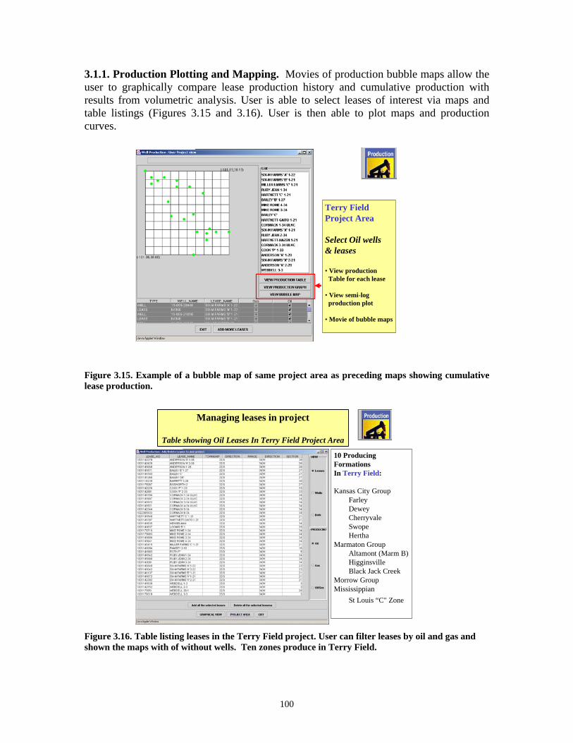
3.1.1. Production Plotting and Mapping. Movies of production bubble maps allow the user to graphically compare lease production history and cumulative production with results from volumetric analysis. User is able to select leases of interest via maps and table listings (Figures 3.15 and 3.16). User is then able to plot maps and production curves.

Terry Field Project Area

Select Oil wells & leases

• View productionTable for each lease

• View semi-logproduction plot

• Movie of bubble maps

Figure 3.15. Example of a bubble map of same project area as preceding maps showing cumulative lease production.

Managing leases in project

Table showing Oil Leases In Terry Field Project Area

10 Producing FormationsIn Terry Field:

Kansas City Group Farley Dewey Cherryvale Swope Hertha

Marmaton Group Altamont (Marm B)Higginsville Black Jack Creek

Morrow Group Mississippian

St Louis “C" Zone

Figure 3.16. Table listing leases in the Terry Field project. User can filter leases by oil and gas and shown the maps with of without wells. Ten zones produce in Terry Field.

100

The production plot and bubble maps can have color of curves and bubbles coordinated. In both cases wells are listed alongside the graphics (Figure 3.17). User also has access to a standalone production plotting routine that is accessed outside of GEMINI the field and lease production web page (Figure 3.18).

Semi-Log Plot of Oil Productionfor Selected Leases

Oil Production Bubble Map Movie of Selected Leases Paused at Year 2003)

Figure 3.17. The production plot and bubble maps for selected leases in Terry Field. More productive leases occur on the southeast side of the field. User needs to known from which zones that the leases produce from in order to access how these results can be compared to the volumetrics.

igure 3.18. The production curve n also be accessed from a andalone Java applet that is vailable from the lease and field roduction web pages. ser is in ‘real-time” control of odifying the chart (see upper right).

FcastapUm

101

Subtask 3.2. Material Balance Module Material Balance Calculations

lation of OOIP based on the geomodel defined y log and core data obtained from individual wells. Uncertainty exists as to the degree of

del to the real reservoir. The question arises as to the level of

ulation, r for t

nce between the volumetric OOIP and the effectiv

ysical description of the reservoir geomodel. An acceptable atch

Volumetric studies result in calcubrepresentativeness of this geomo

certainty required and the effort and data needed to obtain the required accuracy and precision. Causes for this uncertainty in part result from differences in scales of measurement between different logs and that between the log and core data and this provides a need to cross check the volumetric calculations if possible. This check is often not done before proceeding to reservoir simulation and may make the development of a predictive geo-engineering model difficult, if not impossible.

Material balance calculations corroborate volumetric OOIP independent of any geologic volume description. This is an underutilized methodology that provides a owerful means to check the petrophysical model before moving to reservoir simp

o hat matter, making decisions on a basic reservoir geomodel. The issue with many mature older fields is having sufficient production data to perform material balance calculations. Having good production data can not be overemphasized for these engineering analyses.

The input required for material balance calculations include the production and

pressure histories and PVT parameters of the hydrocarbons and water. Material balance calculates the effective OOIP. The differe

e OOIP is the measure of the reservoir heterogeneity that affects the production performance of the reservoir. Also, the material balance calculations help to identify the reservoir drive mechanism. For water driven reservoirs it helps to define the average aquifer properties and to calculate the water influx. In case of a reservoir with a gas cap it enables sizing the initial gas cap volume. When pressure and production data are recorded meticulously through the life of the field, advanced material balance calculations can be employed in versatile ways. Such endeavors result in generation of full field pseudo relative permeability curves and for gas cap driven reservoirs in determination of the critical gas saturation and recovery efficiencies at specified abandonment pressures.

Material balance calculations provide a means to develop and check input data for a reservoir simulation because it affords an opportunity to match the pressure-production-

VT data to the petrophPm between the volumetric calculation and the material balance investigation indicates that the well level data (i.e., petrophysical parameters chosen to represent the pay zones in each well) and the interpolation (gridding) procedure conform to the field level performance. Such a match confirms the representativeness of the data chosen to represent the pay horizons irrespective of the problems inherent to upscaling. It has been noted (Dake, 1994) that reservoir simulation can not provide additional clarity when the material balance calculation shows a mismatch with volumetrics. In case of a mismatch,

102

it is prudent to revise the geomodel and its associated petrophysics rather than proceeding to the simulation study. Geomodel development, volumetrics, and material balance can all be carried out in GEMINI permitting and facilitating iterative solutions to produce an optimized solution.

Generalized material balance equation and its application

The basis for the construction of the material balance equation rests on the fact

that the recor lume of the servoir fluids in response to the pressure history. Thus the volume of underground

withdra

gas, Eg

reduction in pore volume, and W stands for the reservoir volume of water that influxed from the aquifer. Also, the in rvoir is defined as N and m

thought to be operating in the reservoir. Thus the first ep in material balance calculations is identification of the reservoir drive mechanism,

i.e. dec

where

plified material balance equation thus appears as a straight line, with a unit slope, when F/E is plotted against W axis intercept (i.e. N) of this line stimates the OOIP. This estimate of the OOIP should be comparable with that obtained

from t

ded volume of field production is equal to the change in vore

wal is balanced against the change in volume of the system and its contents and the volume of water influx into the system. Havlena and Odeh (1963) expressed the fully expanded material balance equation in a more useable form and it is stated below:

In the above equation, the underground withdrawn of fluids from the reservoir is represented by F, Eo represents the change in volume of the oil and the dissolved

denotes the gas cap expansion, Efw stands for the connate water expansion and the

represents the ratio of the pore volume occupied by the gas cap and the oil column at the onset of production of the field.

The generalized material balance equation can be tailored according to the nature of drive mechanism operating or

efwgo W)EmEE(NF +++=

eitial volume of oil in the rese

stiding whether the reservoir owes its energy to volumetric depletion or gas cap

expansion or water drive or formation compaction or any combination of the above. In most cases, educated assumptions are initially employed to describe the reservoir drive mechanism and this helps to simplify the generalized material balance equation. For a reservoir with no gas cap but being charged by an aquifer, the material balance equation takes the form of:

E

WNEF e

+=

fwo EEE +=

The sime/E and the Y-

ehe volumetric study if correct assumptions have been made about the drive

mechanism and the aquifer water influx. The material balance OOIP is considered to be the “active” (Dake, 1994) or “effective” initial oil in place in the reservoir, i.e., it represents the oil volume that contributes to the production and pressure history of the

103

field. The volumetric OOIP is generally higher than that from material balance calculations because it includes immobile oil trapped in the reservoir heterogeneity. An acceptable tolerance for this difference is less than 10% (Dake, 1994). The need to re-evaluate the reservoir dimensions and its petrophysical properties may arise if the material balance OOIP exceeds that from volumetrics and there is confidence about the assumptions made in the mass balance calculations. The ratio of the material balance to volumetric estimate helps to refine the petrophysical cut-offs applied on well level data.

Water influx calculations are based on the geological and petrophysical assumptions about the aquifer. Incorrect choices of aquifer parameters will result in eviation of the data from the straight line when F/E is plotted against We/E.

Modifi

through a process of trial and error. However, most often tisfactory aquifer models are not unique. Problems regarding the data not falling along

the exp

ost servoirs the pore compressibility is small and remains constant during the life of the

reservo

where GI is the surface volume of ation volume factor of the injected gas. It would be difficult to obtain a material balance match between the right

dcations of the aquifer parameters through the process of “aquifer fitting” enables

matching the observed pressure and production data to the geomodel describing the reservoir and the aquifer. Aquifer fitting assumes importance because most often very little is known about the aquifer geometry and petrophysics because wells are not planned to be drilled into the aquifer. Alternatively, if something is known about the aquifer it is important to integrate the information in the mass balance calculations. Water influx from very small aquifers can be calculated by time independent material balance equations. However, for large reservoirs the aquifer boundary takes a finite time to respond to reservoir pressure changes and thus time dependent models such as Hurst and van Everdingen, Fetkovitch, Carter and Tracy or Allerd and Chen are used to calculate the water influx, We.

An aquifer model that matches the reservoir pressure and production data is generally determinedsa

ected straight line may persist despite all efforts at aquifer fitting in case of incorrect identification of the reservoir drive mechanism. Initial assumptions about the reservoir drive mechanism are indirect. They are based on the pressure and production performance profiles of the reservoir and thus they carry room for revisions. Identification of reservoir drive mechanism is very important because it helps to refine the aquifer description and definition and also estimate the size of the initial gas cap.

The degree of reservoir compaction is indicated by the constancy of the F/E value and this indicates whether the pore compressibility is unaffected by pressure. In mre

ir. However for reservoirs under compaction drive, pore compressibility is significant and varies with time. Compaction of the reservoir rock often leads to surface subsidence. This becomes an important factor in the design of surface facilities especially in offshore fields. The simplified material balance equation for a reservoir believed to be operating under volumetric depletion and supplemented by gas reinjection, is:

gIIfwo BG)EE(NF ++=

injected gas and BgI is the form

104

and the left sides of the above equation if a small constant compressibility (Efw) input was used, particularly when significant reservoir compaction is occurring. Such a disparity

etween the sides of the equation would be easily visible in material balance calculations

cording of reservoir pressure at each well forms the basis of aterial balance calculations.

band indicate that pore compressibility was variable and increasing with time. However, owing to the many degrees of freedom available in a reservoir simulator, a match could be obtained with the production and pressure history of the field without discovering the possibility of irregular compaction or subsidence being active in the reservoir. Some of the many options available in a simulator for history matching include changing the petrophysical properties of the reservoir, or modifying the reservoir boundaries, or altering the PVT properties or any combination of the above. Invalid simulation matches have little predictive power and are unable to forewarn the operator to initiate preventive steps, like timely implementation of pressure maintenance schemes, to avoid or reduce complications arising out of irregular compaction of reservoir rock. Thus material balance calculations often display discrepancies in the geomodel which may not visible during the simulation study.

Material balance calculations require adequate field pressure and production profiles along with the PVT data of reservoir fluids. One method to determine the average field pressure is by volume weighting the shut in pressures within the drainage area of each well. Regular rem

105

The Material Balance methodology is summarized in Figures 3.18 through 3.19. The later two figures describe procedures in handling ideal data sets and incomplete data sets. Both options are handled in the GEMINI’s Material Balance module. Material Balance

Simplified equation & Relevance

Water driven reservoir - above bubble pointwater influx - Carter Tracy Aquifer modelsimplified eq. - F/E = N + We/E

E

*

* Formation volume factors from PVT module

= Eo+Efw

Bw = 1

Why do Material balance?Validate OOIP calculated volumetrically

confirm reservoir model

identify drive mechanismaquifer fitting

Figure 3.19. Simplified material balance equation and relevance of performing analysis in engineering reservoir modeling.

Material BalanceModule Overview & Ideal data set

System modeledEdge water driven under-saturated reservoirs

Formulations usedAquifer fitting - Havlena-Odeh methodWater influx - van Everdingen and Hurst modelFranchi’s regression equations

dimensionless CTR solution of diffusivity equation Complete Input data set

Cumulative field oil or gas production with timeCumulative field water production with timeAverage reservoir pressure history - starting with PiPVT data of reservoir properties & avg. aquifer properties

ProcedurePlot F/E vs. We/EIterate Aquifer model - till straight line is achieved

Figure 3.20. Summary of features of Material Balance when dataset is complete.

106

Material BalanceIncomplete data set

Commonly real-life data setCumulative field oil or gas production with timeCumulative field water production with timePiPVT data of reservoir properties & average aquifer properties

ObjectivesAssume volumetric OOIP is correctReconstruct avg. reservoir pressure history

Compare with available pressure data - DST & shut-in fluid levelsProcedure

Iterate avg. reservoir pressure at each time stepcalculated OOIP is within 10% of volumetric OOIP

Resultsrecreate avg. reservoir pressure historydesignate representative petrophysical properties for aquifer

Figure 3.21. Procedures to use in material balance when data set is incomplete. The Material Balance Module is also available to download and run as a standalone module on the user’s desktop (Figure 3.21). The downloadable version is available on a separate web page (http://www.kgs.ku.edu/Gemini/Tools/Tools.html). Once downloaded and installed as a Java Web Start application, the user does not have to be connected to the Internet to run the application. Figure 3.22. Opening Java Application Window using Web Start that is launched and runs on the user’s PC without a link to the Internet.

107

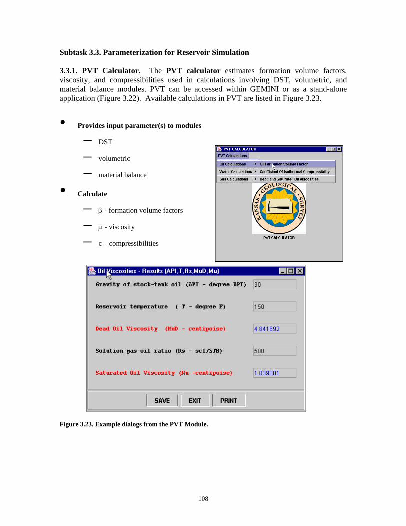
Subtask 3.3. Parameterization for Reservoir Simulation 3.3.1. PVT Calculator. The PVT calculator estimates formation volume factors, viscosity, and compressibilities used in calculations involving DST, volumetric, and material balance modules. PVT can be accessed within GEMINI or as a stand-alone application (Figure 3.22). Available calculations in PVT are listed in Figure 3.23.

• Provides input parameter(s) to modules

– DST

– volumetric

– material balance

• Calculate

– β - formation volume factors

– µ - viscosity

– c – compressibilities Figure 3.23. Example dialogs from the PVT Module.

108

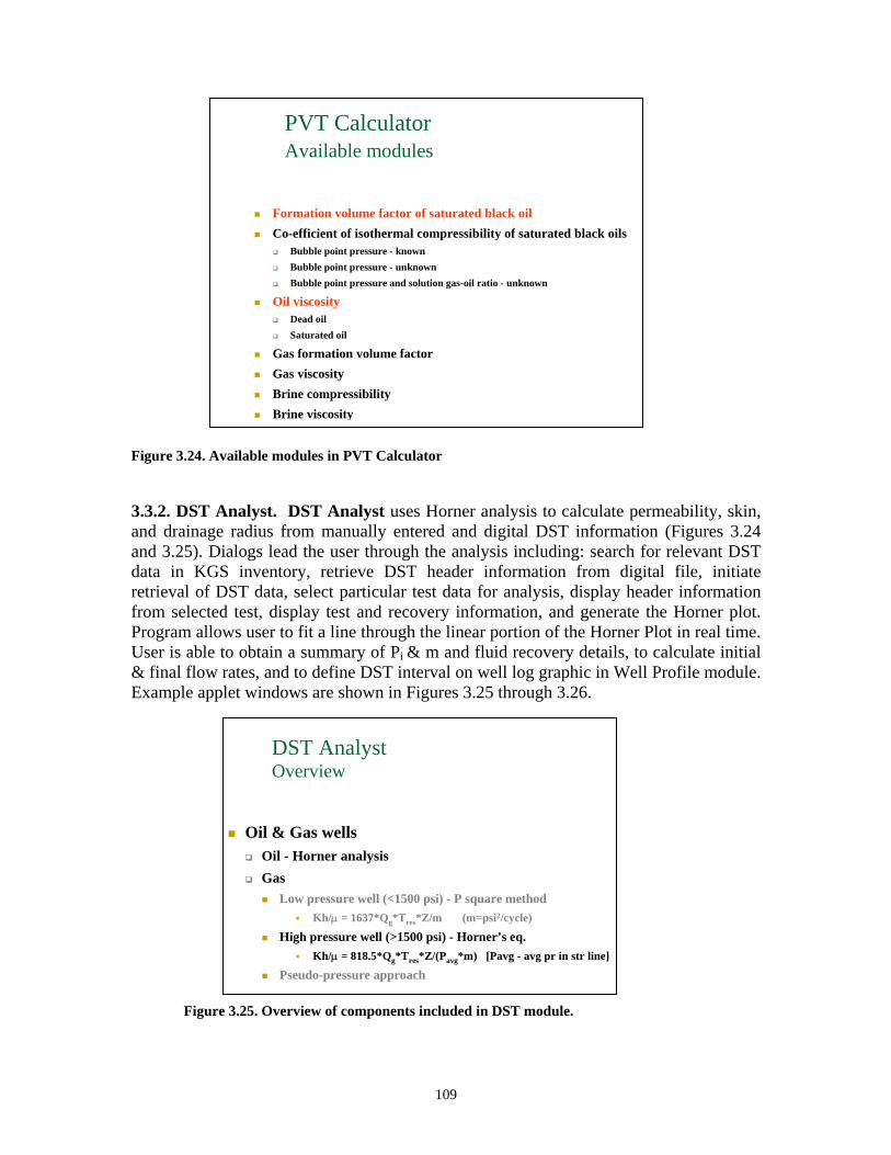
Figure 3.24. Available modules in PVT Calculator

.3.2. DST Analyst. DST Analyst uses Horner analysis to calculate permeability, skin,

igur

rated black oilsBubble point pressure - knownBubble point pressure - unknownBubble point pressure and solution gas-oil ratio - unknown

Oil viscosity

Saturated oil

Gas formation volume factorGas viscosityBrine compressibilityBrine viscosit

PVT CalculatorAvailable modules

Formation volume factor of saturated black oilCo-efficient of isothermal compressibility of satu

Dead oil

3and drainage radius from manually entered and digital DST information (Figures 3.24 and 3.25). Dialogs lead the user through the analysis including: search for relevant DST data in KGS inventory, retrieve DST header information from digital file, initiate retrieval of DST data, select particular test data for analysis, display header information from selected test, display test and recovery information, and generate the Horner plot. Program allows user to fit a line through the linear portion of the Horner Plot in real time. User is able to obtain a summary of Pi & m and fluid recovery details, to calculate initial & final flow rates, and to define DST interval on well log graphic in Well Profile module. Example applet windows are shown in Figures 3.25 through 3.26.

y

DST AnalystOverview

Oil & Gas wellsOil - Horner analysisGas

Low pressure well (<1500 psi) - P square methodKh/µ = 1637*Qg*Tres*Z/m (m=psi2/cycle)

High pressure well (>1500 psi) - Horner’s eq.Kh/µ = 818.5*Qg*Tres*Z/(Pavg*m) [Pavg - avg pr in str line]

Pseudo-pressure approach

F e 3.25. Overview of components included in DST module.

109

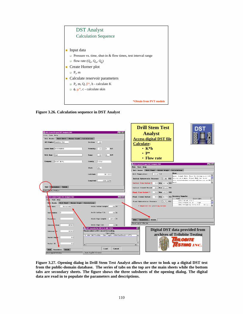
DST AnalystCalculation Sequence

Input dataPressure vs. time, shut-in & flow times, test interval rangeflow rate (Qo, Qw, Qg)

Create Horner plotPi, m

Calculate reservoir parametersPi, m, Q, β*, h - calculate Kφ, µ*, c -

calculate skin

*Obtain from PVT module

Figure 3.26. Calculation sequence in DST Analyst

Figure 3 . Opening dialog in Drill Stem Test Analyst allows the user to look up a digital DST test from the public-domain database. The series of tabs on the top are the main sheets while the bottom tabs are secondary sheets. The figure shows the three subsheets of the opening dialog. The digital data are read in to populate the parameters and descriptions.

Digital DST data provided from archives of Trilobite Testing

Drill Stem TestAnalyst

Access digital DST fileCalculate:

• K*h• P*• Flow rate

.27

110

DST Analysis

• K*h• P*• Flow rate

Data can be enteredmanually in this “spreadsheet”if digital data are not available

Sliding bar to fit curve

Figure 3.28. The calculation worksheet tab opens the worksheet of time and pressure data. This sheet is active so a user can type in the time and pressure data if it is not available in digital form. Other dialogs are also shown in this figure including the Horner graph with a sliding bar to fit a curve and the first part of the calculation sheet.

111

–Calculators for oil•Permeability

•Skin

Fluid parametersFormation volume factor

Figure 3.29. The last dialog of the DST Analyst is shown where the calculations are made for the

ansmissibility, effect permeability, and skin. tr

Task 4. Technology Transfer

ubtask 4.1. Project Application and Testing

.1.1. Technology Transfer Activities. The final year of the contract involved extensive

ensive final testing and finalizing the modules consumed most of the time between May-September, 2003 to ensure that user’s would not experience unexpected crashes and could negotiate the software successfully. The web-based tutorial and concepts were completed as scheduled. Analyses of datasets were done in the course of testing and results placed on website and use in oral presentations. Presentations during the last year included a seminar at the Kansas Independent Oil and Gas Association Annual Meeting in Wichita, August 18, a talk in a session at the AAPG Mid-Continent Meeting in Tulsa on October 13th, a DOE-Industry Project Review Workshop in Lawrence, September 24, coinciding with the official release of the software, and a talk on GEMINI at a geoinformatics session at the Geological Society of America Annual Meeting in Seattle on November 2nd. Three opportunities followed to obtain new funding for GEMINI related web application development – February DOE solicitation, cost extension to existing contract, and industry consortium 4.1.2. Industry partners affiliated with GEMINI. Well and production data were obtained from several partnering companies to test and evaluate the prototype software and to obtain feedback on how the software can be improved. Company representatives from BP, Lario Petroleum, Mull Drilling Company, Murfin Drilling Company, and Pioneer Resources participated in the evaluation process. Test examples were also drawn from well and lease databases available on the Kansas Geological Survey website (www.kgs.ku.edu), and Digital Petroleum Atlas (www.kgs.ku.edu/DPA/dpaHome.html), including several DOE-sponsored field demonstration projects. Examples include field studies and regional pay assessment with results available on the GEMINI website: http://www.kgs.ku.edu/Gemini/gemini-reports.html.

Previous annual reports describe results from field and regional (exploration) applications of GEMINI including Arroyo Field and regional evaluation of Haskell County Lansing-Kansas City. Also other studies conducted have results reported in previous sections of this report. In this final report, two field demonstration projects are presented as case studies that were undertaken after the full suite of software applications were officially tested and released on September 30, 2003. These two case studies address outstanding reservoir modeling problems, one currently being funded by DOE and industry.

• Medicine Lodge North Field in Barber County, Kansas, DOE contract with Woolsey petroleum, “Optimizing Fracture Stimulation in North Medicine Lodge Field” (current DOE Technology Development with Independents, K.D. Newell, PI)

• Minneola Field (Norcan East) in Clark County, Kansas with previous data and financial support by Murfin Drilling Company, Wichita, Kansas

S 4testing and implementation of software code, building examples and tutorial, documentation, and website design. Ext

112

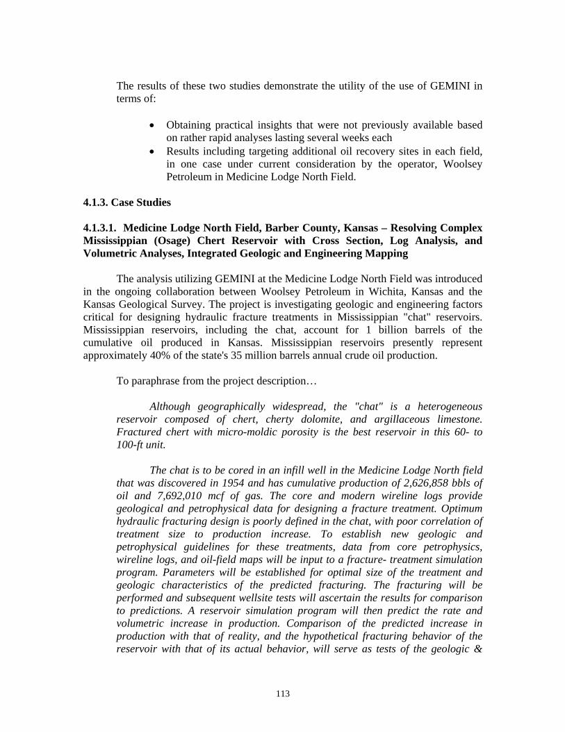
The results of these two studies demonstrate the utility of the use of GEMINI in

gineering factors

logs, and oil-field maps will be input to a fracture- treatment simulation

perto pvolumetric increase in production. Comparison of the predicted increase in

terms of:

• Obtaining practical insights that were not previously available based on rather rapid analyses lasting several weeks each

• Results including targeting additional oil recovery sites in each field, in one case under current consideration by the operator, Woolsey Petroleum in Medicine Lodge North Field.

4.1.3. Case Studies 4.1.3.1. Medicine Lodge North Field, Barber County, Kansas – Resolving Complex Mississippian (Osage) Chert Reservoir with Cross Section, Log Analysis, and Volumetric Analyses, Integrated Geologic and Engineering Mapping The analysis utilizing GEMINI at the Medicine Lodge North Field was introduced in the ongoing collaboration between Woolsey Petroleum in Wichita, Kansas and the

ansas Geological Survey. The project is investigating geologic and enKcritical for designing hydraulic fracture treatments in Mississippian "chat" reservoirs. Mississippian reservoirs, including the chat, account for 1 billion barrels of the cumulative oil produced in Kansas. Mississippian reservoirs presently represent approximately 40% of the state's 35 million barrels annual crude oil production.

To paraphrase from the project description…

Although geographically widespread, the "chat" is a heterogeneous reservoir composed of chert, cherty dolomite, and argillaceous limestone. Fractured chert with micro-moldic porosity is the best reservoir in this 60- to

00-ft unit. 1

The chat is to be cored in an infill well in the Medicine Lodge North field that was discovered in 1954 and has cumulative production of 2,626,858 bbls of oil and 7,692,010 mcf of gas. The core and modern wireline logs provide geological and petrophysical data for designing a fracture treatment. Optimum hydraulic fracturing design is poorly defined in the chat, with poor correlation of treatment size to production increase. To establish new geologic and petrophysical guidelines for these treatments, data from core petrophysics, wirelineprogram. Parameters will be established for optimal size of the treatment and geologic characteristics of the predicted fracturing. The fracturing will be

formed and subsequent wellsite tests will ascertain the results for comparison redictions. A reservoir simulation program will then predict the rate and

production with that of reality, and the hypothetical fracturing behavior of the reservoir with that of its actual behavior, will serve as tests of the geologic &

113

petrophysical characterization of the oil field. After this feedback, a second well

stics determined to be critical for designing cost-effective fracture eatments. (K.D. Newell, KGS, PI)

The ob twithin the Mississreservoir attributes del was then compared to

il recoveries from leases and the current reservoir pressure in lieu of more extensive g ue to lack of detailed fluid and pressure history in the field. Core

ses were used to establish Archie Equation parameters and well log cut-offs for the

ct that has been resented to the operator. The site will be shared with other interested parties at some

Figure 4Figure 4from pstructurand ga(http://w

will be cored and logged, and the procedure will be repeated to test characteritr

jec ive of using GEMINI was to re-evaluate the establishment of pay ippian “chat” reservoir and map its volumetric parameters and other throughout the field. This petrophysical mo

oengineering modelin danalychert reservoir. Previous work with these reservoirs alerted us to the complexities at many scales in the “chat” (Watney et al., 2001). The Well Profile, Cross Section, PfEFFER, and Volumetric modules were used to build a web-based projeppoint after the company exercises its option to drill a well. Figure 4.1 provides field distribution map in Barber County, Kansas.

.1. Location of Medicine Lodge North Field in Barber County in south-central Kansas. .1. Lineaments are added manually based on visual inspection paralleling trends recognized

revious work that indicates deep-seated basement heterogeneity reflected in Paleozoic e and magnetic and gravity mapping (Watney et al., 2001). Many of these fields produce oil s from the Mississippian “chat”. Map is generated from ARC-IMS map server ww.kgs.ku.edu/PRS/petroMaps.html).

Figure 4.2 is an oil production plot for Barber County generated using the I production applet that is linked to on the county production web page

GEMIN

Medicine Lodge North

Spivey-GrabsGlick

114

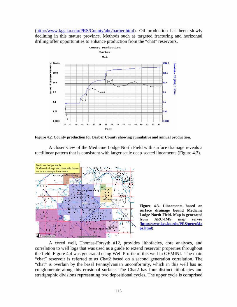
(http://www.kgs.ku.edu/PRS/County/abc/barber.html). Oil production has been slowly g in this mature province. Methods such as targeted fracturing and horizontal

offer opportunities to enhance production from the “chat” reservoirs. declinindrilling

A closer view of the Medicine Lodge North Field with surface drainage reveals a ctilinear pattern that is consistent with larger scale deep-seated lineaments (Figure 4.3).

Figure 4.3. Lineaments based on surface drainage bound Medicine Lodge North Field. Map is generated from ARC-IMS map server (http://www.kgs.ku.edu/PRS/petroMa

Figure 4.2. County production for Barber County showing cumulative and annual production. re

ps.html).

ration correlation. The hat”

A cored well, Thomas-Forsyth #12, provides lithofacies, core analyses, and correlation to well logs that was used as a guide to extend reservoir properties throughout the field. Figure 4.4 was generated using Well Profile of this well in GEMINI. The main chat” reservoir is referred to as Chat2 based on a second gene

Medicine Lodge Northace drainage and manually drawnace drainage lineaments

Surfsurf

Medicine Lodge Northace drainage and manually drawnace drainage lineaments

Surfsurf

““c is overlain by the basal Pennsylvanian unconformity, which in this well has no conglomerate along this erosional surface. The Chat2 has four distinct lithofacies and stratigraphic divisions representing two depositional cycles. The upper cycle is comprised

115

of the 1st nodular and 1st breccia and the lower cycle consists of the 2nd breccia and 2nd nodular. The upper beds of breccia are more heavily weathered and broken “chat” and the lower nodular are more intact lithofacies exhibiting transitions in pore types. These

thofa portant to distinguish in efining reservoir pay. The lower “chat” is non permeable chert and the underlying owley Formation is a cherty dolomitic limestone that comprises a regional lithofacies elieved to have been deposited along an extensive basin margin residing along southern ansas and northern Oklahoma. Downdip from the Mississippian subcrop on uplifts such

s that on which this field resides, the “chat” beds grade laterally to Cowley Formation thofacies. This is seen locally off the flanks of the Medicine Lodge North Field.

isubdivisions of “chat” reservoir. Note that the nodular zones hthe zones of breccia.

As previously mentioned, production data is sparse including on well level

li cies also exhibit different petrophysics which is imdCbKali Figure 4.4. Type log of cored well in Medicine Lodge North F

No Conglomerate

Lower Chat

Cowley Fm.

Chat2

eld shows lithofacies and stratigraphic ave slightly higher porosity and than

production data. However, static reservoir pressure data is available for most well, obtained in 1998. The effective permeability was obtained from build-up tests indicating that the matrix permeability is very low. Examples of calculated K (md) from DST data are 1.08, 0.051, 0.056, 0.272, 0.174, 0.116, and 0.56, all decidedly low, thus, the consideration to fracture the reservoir in order to enhance oil production.

The reservoir drive mechanism based on available data is a solution as drive with little water production. Current production from the Thomas-Forsyth lease (13 wells) is

116

10 bopd, 45.5 bwpd, and 110 mcfd. Only one well is classified as gas well, the Warwick #3. Gas production data from individual wells is not available. It is assumed that the reservoir produces under solution-gas drive.

Majority of the wells do not have a modern porosity log so porosity was estimated from old neutron logs (API counts) using exponential scaling with low porosity = 3% and high porosity = 33%. The core from Thomas-Forsyth #12 had porosities measured on core-plugs that were compared to porosity estimated from neutron counts. The match between core porosity and porosity calculated from neutron counts is quite good (Figure 4.5). Available petrophysical logs at each well were analyzed within GEMINI using the

uper-Pickett technique with Rw = 0.04 and m = n = 2.

igure 4.5. Co of eutron counts.

Pay cut-offs were applied by trail and error. Water saturation was initially set at .6, the value estimated for “chat” reservoirs that only produce water. The minimum orosity was set at 0.12 to reflect those intervals that can flow oil. A maximum BVW w x phi) of 0.12 was established for this chat reservoir, below which the chat would

potential in effective pay was estimated by summing [porosity * (1-w)]. These cut-offs were used to derive reservoir volumetrics. The validation of this OIP was not possible using material balance since production data was not available.

Rather

S

Medicine Lodge North

0

10

20

30

40

4380 4400 4420 4440 4460 4480 4500 4520

Depth, ft

Poro

sity

Phi - fr neu count core plug phi

F mparison between core plug porosity and porosity calculated from conversion n 0p(Sproduce hydrocarbon. The relatively high BVW is due to an abundance of fine pores and high bound water. These cut-offs were used to isolate effective pay within the chat interval. The reserveSO

a correlation was sought between initial estimated reserves from volumetrics and wells that produced significant volumes of hydrocarbons.

117

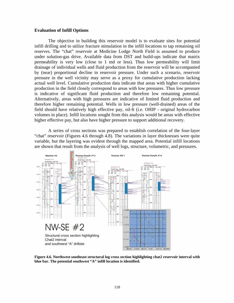
Evaluation of Infill Options

The objective in building this reservoir model is to evaluate sites for potential fill drilling and to utilize fracture stimulation in the infill locations to tap remaining oil

reserve

at areas with higher cumulative roduction in the field closely correspond to areas with low pressures. Thus low pressure indicativelternatively, areas with high pressures are indicative of limited fluid production and erefore higher remaining potential. Wells in low pressure (well-drained) areas of the eld should have relatively high effective pay, oil-ft (i.e. OHIP - original hydrocarbon olumes in place). Infill locations sought from this analysis would be areas with effective igher effective pay, but also have higher pressure to support additional recovery.

A series of cross sections was prepared to establish correlation of the four-layer chat” reservoir (Figures 4.6 through 4.8). The variations in layer thicknesses were quite ariable, but the layering was evident through the mapped area. Potential infill locations re shown that result from the analysis of well logs, structure, volumetric, and pressures.

Figure 4.6. Northwest-southeast structural log cross section highlighting chat2 reservoir interval with blue bar. The potential southwest “A” infill location is identified.

ins. The “chat” reservoir at Medicine Lodge North Field is assumed to produce

under solution-gas drive. Available data from DST and build-ups indicate that matrix permeability is very low (close to 1 md or less). Thus low permeability will limit drainage of individual wells and fluid production from the reservoir will be accompanied by (near) proportional decline in reservoir pressure. Under such a scenario, reservoir pressure in the well vicinity may serve as a proxy for cumulative production lacking actual well level. Cumulative production data indicate thpis of significant fluid production and therefore low remaining potential. Athfivh “va

Warwick #4 Thomas Forsyth #13 Thomas #G-1 Thomas Forsyth #14

Southwt “A

”

and southwest “A” drillsite

es

NW-SE #2Structural cross section highlighting Chat2 interval

118

“chat” reservoir along the basal ennsylvanian unconformity and local thickening of overlying Pennsylvanian conglomerate some rrespondence to areas of underlying truncation of “chat”.

Gulf Warwick #1 Graves Warwick #

Figure 4.7. Northwest-southeast structural log cross section through center of field and identifying another potential infill location.

1 T-F #5 T-F #8 Pickrell Tedrow #1

Northw

est “B”

NW-SE #5Structural cross section highlighting Chat2 intervaland northwest “B” drillsite

Figure 4.8. Northwest-southeast structural log cross section identifying another potential infill

cation. Note local thinning and truncation of the uppermost

Warwick #3 T-F #1 T-F #15 T-F #3 Tedrow #2Ea

ster

n “C

”

NW-SE #7Structural cross section highlighting Chat2 and eastern “C”drillsite

loPco

119

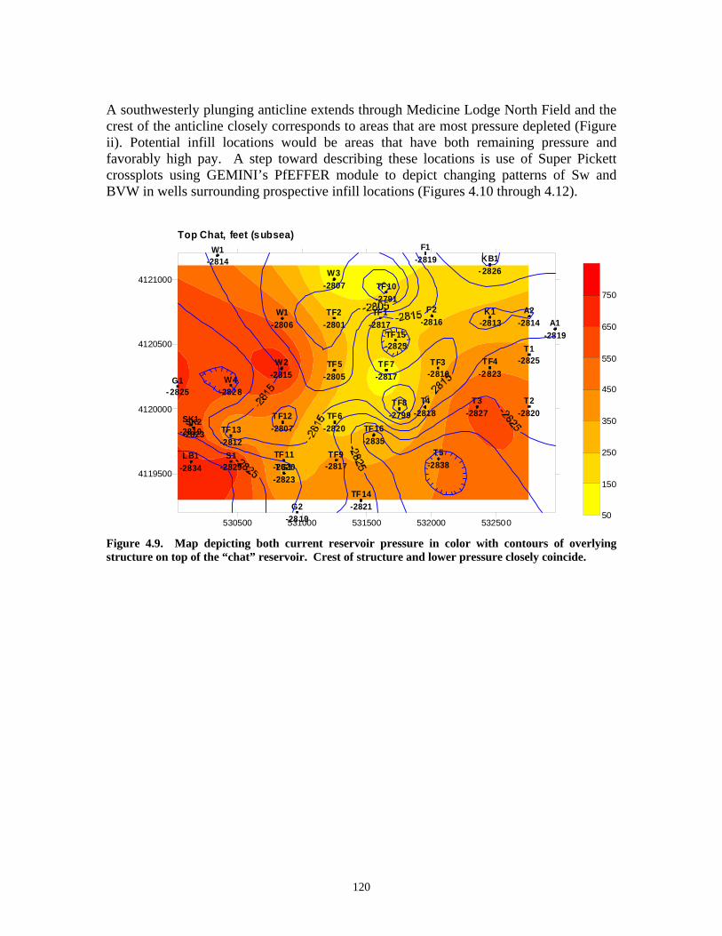
A southwesterly plunging anticline extends through Medicine Lodge North Field and the crest of the anticline closely corresponds to areas that are most pressure depleted (Figureii). Potential infill locations woul

e areas that have both remaining pressur

favorably high pay. A step toward describing these locations is use of Super Pickett crossplots using GEMINI’s PfEFFER module to depict changing patterns of Sw and BVW in wells surrounding prospective infill locations (Figures 4.10 through 4.12).

Fi overlying

e

d b e and

530500 531000 531500 532000 532500

4119500

4120000

4120500

4121000

W1

T1

F1

TG1

KB1

A1TF1 F2

T2

TF2W1

TF3

K1

TF4TF5

T3

TF7W2

A2

TF6

T4TF8

TF9

W3TF10

T5TF11

TF12

gure 4.9. Map depicting both current reservoir pressure in color with contours of structure on top of the “chat” reservoir. Crest of structure and lower pressure closely coincid .

S1

SK1SK2TF13

W4

TF14G2

TF15

G1

LB1

TF16

-2814

-2825

-2819

-2823

- 2826

-2819-2817 -2816

-2820

-2801-2806

-2810

-2813

-2823-2805

-2827

-2817-2815

-2814

-2820

-2818-2799

-2817

-2807-2791

-2838-2820

-2807

-2829

-2819-2823-2812

- 2825

-2834

-2828

-2821-28 19

-2825

-2835

50

150

250

450

550

650

750

Top Chat, feet (subsea)

350

120

Southwest “A” Location

530500 531000 531500 532000 532500

4119500

4120000

4120500

4121000

W1

T1

F1

Fre

iguservoir of surrounding wells. Red vertical lines in crossplot are BVW contours. Points farther to ght suggest coarser pores. Southwest side has higher Sw and BVW (less desirable properties) vs. wer Sw and BVW in southeast side of location “A”.

igure 4.11. Prospective infill location “B” in northwest part of field where reservoir pressure and ck properties are moderately high. Better reservoir quality (lower Sw and BVW) are in southeast

de of this infill site, closer to structural crest and depleted reservoir pressure.

re 4.10. Southwest potential infill location “A” showing Super Pickett crossplots in chat2

rilo Frosi

TG1

KB1

A1TF1 F2

T2

TF2W1

TF3

K1

TF4TF5

T3

TF7W2

A2

TF6

T4TF8

TF9

W 3TF10

T5TF11

TF12

S1

SK1SK2TF13

G1

LB1

W4

TF14G2

TF15

TF16

-2825

-2819-2814

-2823

-2826

-2819-2817 -2816

-2820

-2801-2806

-2810

-2813

-2 823-2805

-2827

-2817-2815

-2814

-2820

-2818-2799

-2817

-2807-2791

-2838-2820

-2807

-2829

-2819-2823-2812

- 2825

-2834

-282 8

-2821-28 19

-2825

-2835

50

150

250

350

450

550

650

750

Top Chat, feet (subsea)

Higher Sw and BVW Lower Sw and BVW

Northwest “B” Location

530500 531000 531500 532000 532500

4119500

4120000

4120500

4121000

W1

T1

F1

TG1

KB1

A1TF1 F2

T2

TF2W1

TF3

K1

TF4TF5

T3

TF7W2

A2

TF6

T4TF8

TF9

W3TF10

T5TF11

TF12

S1

SK1SK2TF13

G1

LB1

W4

TF14G2

TF15

TF16

-2814

-2825

-2819

-2823

- 2826

-2819-2817 -2816

-2820

-2801-2806

-2810

-2813

-2823-2805

-2827

-2817-2815

-2814

-2820

-2818-2799

-2817

-2807-2791

-2838-2820

-2807

-2829

-2819-2823-2812

- 2825

-2834

-2828

-2821-28 19

-2825

-2835

50

150

250

350

450

550

650

750

Top Chat, feet (subsea)

Lower Sw and BVW

121

Eastern “C” Location

530500 531000 531500 532000 532500

4119500

4120000

4120500

4121000

W1

T1

F1

TG1

KB1

A1TF1 F2

T2

TF2W1

TF3

K1

TF4TF5

T3

TF7W2

A2

TF6

T4TF8

TF9

W3TF10

T5TF11

TF12

S1

SK1SK2TF13

G1

LB1

W4

TF14G2

TF15

TF16

-2814

-2825

-2819

-2823

- 2826

-2819-2817 -2816

-2820

-2801-2806

-2810

-2813

-2823-2805

-2827

-2817-2815

-2814

-2820

-2818-2799

-2817

-2807-2791

-2838-2820

-2807

-2829

-2819-2823-2812

-2825

-2834

-2828

-2821-2819

-2825

-2835

50

150

250

350

450

550

650

750

Top Chat, feet (subsea)

Figure 4.12. Eastern infill location “C” with surrounding wells exhibiting Super Pickett crossplots

Several iterations of log analysis and volumetrics were done to “tune” the eomodel to the well performance or lack thereof. A key parameter to delimit pay in the g analysis phase was to apply a fractional shale, Vsh, cut-off of 0.3. GEMINI was used roughout the process to conduct this fine tuning (Figures 4.13 and 4.14).

indicating lower BVW and Sw. gloth

122

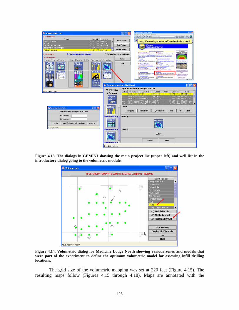
http://www.kgs.ku.edu/Gemini/index.html

igure 4.13. The dialogs in GEMF INI showing the main project list (upper left) and well list in the

Figure 4.14. Volumetric dialog for Medicine Lodge North showing various zones and models that were part of the experiment to define the optimum volumetric model for assessing infill drilling locations. The grid size of the volumetric mapping was set at 220 feet (Figure 4.15). The resulting maps follow (Figures 4.15 through 4.18). Maps are annotated with the

introductory dialog going to the volumetric module.

123

prospective infill locations. Porosity is moderately high in the prospective sites (Fig4.16). Water saturation is moderately low, but higher than the core producing area where the pressure has been depleted (Figure 4.17). Net pay is also at moderate levels based on the use of log cut-offs employed in the final optimized model.

ure

igure 4.15. Dialog where parameters are set to grid and map volumetric data in GEMINI.

odge North Field. Prospective locations have moderate porosity and border highly orous and productive central areas of the field.

F Figure 4.16. Color grid map (220 ft cells) for average porosity in pay from chat2 reservoir in Medicine L

GEMINI Volumetric Module

Location B

Location A Location C

p

124

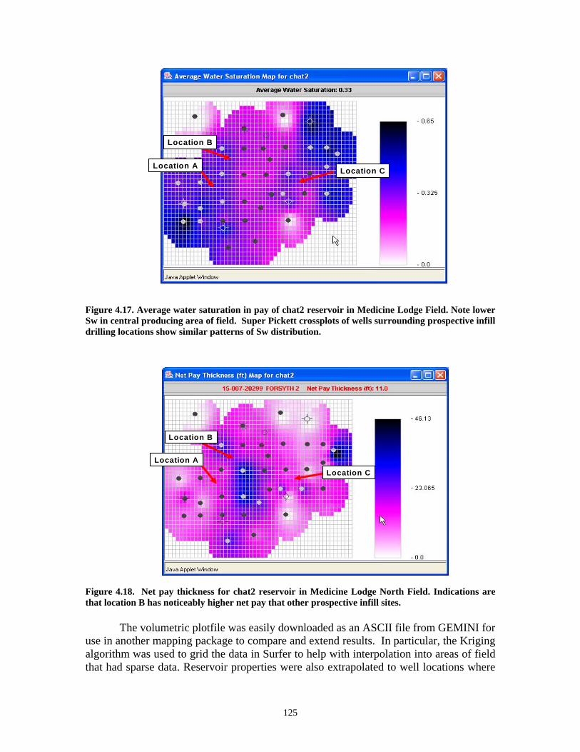
Figure 4.17. Average Note lower

w in central producing area of field. Super Pickett crossplots of wells surrounding prospective infill rilling locations show similar patterns of Sw distribution.

igure 4.18. dications are at location B has noticeably higher net pay that other prospective infill sites.

algorithm was used to grid the data in Surfer to help with interpolation into areas of field that had sparse data. Reservoir properties were also extrapolated to well locations where

water saturation in pay of chat2 reservoir in Medicine Lodge Field.

Location B

Location A Location C

Location B

Location ALocation C

Sd F Net pay thickness for chat2 reservoir in Medicine Lodge North Field. Inth

The volumetric plotfile was easily downloaded as an ASCII file from GEMINI for use in another mapping package to compare and extend results. In particular, the Kriging

125

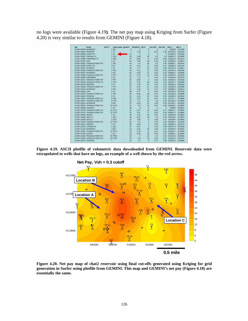
no logs were er (Figure .20) is very similar to results from GEMINI (Figure 4.18).

igure 4.19. ASCII plotfile of volumetric data downloaded from GEMINI. Reservoir data were trapolated to wells that have no logs, an example of a well shown by the red arrow.

igure 4.generati

available (Figure 4.19). The net pay map using Kriging from Surf4

api lease well # map name gross h So*phi*h net h ave phi ave Sw utm x utm y15-007-00208 WARWICK 1 W1 0 0 0 0 0 530343 412118615-007-00616 TEDROW 1 T1 7 1.32 7 0.27 0.38 532753.8 412041915-007-00620 FORSYTH 1 F1 11 0 0 0 0 531952.9 412120315-007-20002 THOMAS 'G' 1 TG1 23 1.68 16 0.2 0.5 530857.4 411950215-007-20008 KIRKBRIDE 'B' 1 KB1 27 0.06 0 0.16 0.58 532452.6 412111315-007-20287 ASH 1 A1 50 7.08 48 0.26 0.45 532956.8 412061715-007-20291 THOMAS-FORSYTH 1 TF1 24 4.3 16 0.3 0.26 531600.1 412070215-007-20299 FORSYTH 2 F2 15 2.43 11 0.28 0.27 532002.8 412071815-007-20322 TEDROW 2 T2 34 1.77 14 0.22 0.48 532755.4 412001715-007-20336 THOMAS-FORSYTH 2 TF2 19 4.21 17 0.33 0.29 531246.2 412070015-007-20357 WARWICK 1 W1 34 4.39 27 0.25 0.39 530844.2 412069915-007-20358 THOMAS-FORSYTH 3 TF3 25 2.13 12 0.26 0.38 532050.3 412031615-007-20390 KIRKBRIDE 1 K1 27 0.1 7 0.22 0.42 532453.6 412071015-007-20417 THOMAS-FORSYTH 4 TF4 20 0.85 3 0.31 0.31 532452.4 412031815-007-20418 THOMAS-FORSYTH 5 TF5 42 9.78 36 0.34 0.22 531247.7 412029915-007-20419 TEDROW 3 T3 32 7.28 24 0.37 0.22 532353.3 412001515-007-20443 THOMAS-FORSYTH 7 TF7 21 5.63 21 0.33 0.24 531650.4 412030015-007-20444 WARWICK 2 W2 24 2.48 13 0.27 0.37 530838.9 412031215-007-20462 ASH 2 A2 48 0.77 8 0.18 0.54 532755.4 412071515-007-20479 THOMAS-FORSYTH 6 TF6 38 8.66 36 0.31 0.26 531249.9 411989615-007-20482 TEDROW 4 T4 31 4.25 25 0.24 0.33 531950.6 412001415-007-20514 THOMAS-FORSYTH 8 TF8 22 3.23 14 0.31 0.31 531751.7 411999915-007-20527 THOMAS-FORSYTH 9 TF9 25 5.1 22 0.3 0.28 531260.4 411960315-007-20614 WARWICK 3 W3 32 2.83 12 0.29 0.26 531245.1 412100215-007-20621 THOMAS-FORSYTH 10 TF10 21 3.9 14 0.27 0.28 531648.1 412090215-007-20646 TEDROW 5 T5 26 0 0 0 0 532053 411961315-007-20708 THOMAS-FORSYTH 11 TF11 32 5.27 20 0.34 0.27 530857.1 411960115-007-20744 THOMAS-FORSYTH 12 TF12 32 2.97 17 0.26 0.38 530847.2 411989415-007-20845 SEARS 1 S1 19 2.23 10 0.31 0.34 530446.9 411959415-007-20960 SKELLY 1 SK1 24 4.81 23 0.3 0.34 530136.6 411987515-007-21000 SKELLY 2 SK2 23 1.68 8 0.29 0.37 530158.9 411985415-007-21016 THOMAS-FORSYTH 13 TF13 34 0.6 4 0.22 0.46 530446.2 411979315-007-21017 GIBSON 1 G1 38 0.65 3 0.25 0.34 530035.3 412017515-007-21070 LONKER 'B' 1 LB1 37 0.52 9 0.15 0.68 530137.6 4119592

0 0.27 0.38 532053.9 4119899

15-007-21133 WARWICK 4 W4 24 2.34 13 0.26 0.37 530444.8 4120181

15-007-21687 THOMAS-FORSYTH 14 TF14 23 3.33 11 0.37 0.26 531453.1 411929315-007-22100 GLENN 2 G2 26 5.38 26 0.28 0.31 530960.1 411920015-007-22158 THOMAS-FORSYTH 15 TF15 16 4 15 0.3 0.25 531722.6 412053115-007-22330 THOMAS-FORSYTH 16 TF16 22 5.8 24 0.31 0.27 531551.4 411979715-007-30372 TEDROW 1 34 1.3

Fex

Net Pay, Vsh = 0.3 cutoff

530500 531000 531500 532000 532500

4119500

4120000

4120500

4121000

0

7

0

16

0

4816 11

14

1727

12

7

336

24

2113

8

36

2514

22

1214

020

17

10

2384

3

9

13

1126

15

240

W1

T1

F1

TG1

KB1

A1TF1 F2

T2

TF2W1

TF3

K1

TF4TF5

T3

TF7W2

A2

TF6

T4TF8

TF9

W3TF10

T5TF11

TF12

S1

SK1SK2TF13

G1

LB1

W4

TF14G2

TF15

TF16

0

4

8

12

16

20

24

28

32

36

40

44

48

Location B

Location A

Location C

0.5 mile F 20. Net pay map of chat2 reservoir using final cut-offs generated using Kriging for grid

on in Surfer using plotfile from GEMINI. This map and GEMINI’s net pay (Figure 4.18) are essentially the same.

126

A map of the average Vsh for the chat2 reservoir clearly outlines the areas of cleaner “chat” reservoir rock and is comparable to the field pressure map (Figure 4.21).

he northwe

igure 4.21. Ma ospective fill drilling locations.

The resulting original oil in place calculation is 25 million barrels. This value is milar to that derived from other estimates for the field (Figures 4.22 and 4.23). The OIP is highest at infill location “B” in northwest sector of Medicine Lodge North Field

).

T stern most prospective infill location has the cleanest “chat” interval.

4119500

4120000

4120500

4121000

W1

T1

F1

TG1

KB1

A1TF1 F2

T2

TF2W1

TF3

K1

TF4TF5

T3

TF7W2

A2

TF6

T4TF8

TF9

W3TF10

T5TF11

TF12

S1

SK1SK2TF13

G1

LB1

W4

TF14G2

TF15

TF16

0.05

530500 531000 531500 532000 532500 F p of average Vsh for pay interval in the chat2 reservoir. Arrows locate prin siO(Figure 4.23 Figure 4.22. OOIP calculation dialog for Medicine Lodge North Field.

0.1

0.15

0.2

0.25

0.3

0.35

0.4

0.45

0.5

Vsh (new cutoff at 0.3)

Use interpolated values of reservoir parameters from Kridged mapping of Surfer software for input into GEMINI volumetric calculator

127

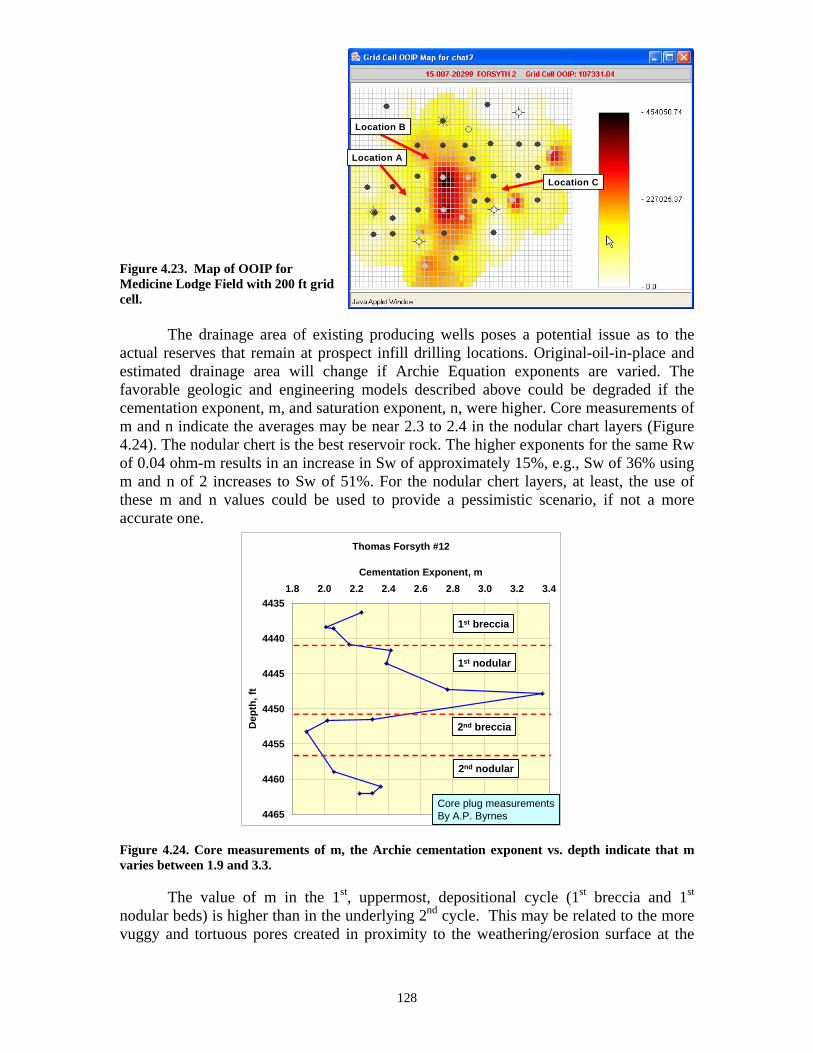
Figure 4.2

edicine Lodge Field with 200 ft grid ll.

The drainage area of existing producing wells poses a potential issue as to the

ctual reserves that remain at prospect infill drilling locations. Original-oil-in-place and stimated drainage area will change if Archie Equation exponents are varied. The vorable geologic and engineering models described above could be degraded if the

ementation exponent, m, and saturation exponent, n, were higher. Core measurements of and n indicate the averages may be near 2.3 to 2.4 in the nodular chart layers (Figure

.24). The nodular chert is the best reservoir rock. The higher exponents for the same Rw f 0.04 ohm-m results in an increase in Sw of approximately 15%, e.g., Sw of 36% using and n of 2 increases to Sw of 51%. For the nodular chert layers, at least, the use of ese m and n values could be used to provide a pessimistic scenario, if not a more

ccurate one.

igure 4.24. Core measurements

The value of m in the 1st, uppermost, depositional cycle (1st breccia and 1st odular beds) is higher than in the underlying 2nd cycle. This may be related to the more uggy and tortuous pores created in proximity to the weathering/erosion surface at the

Location B

3. Map of OOIP for

Location A

Location C

Mce aefacm4omtha Thomas Forsyth #12

4435

4440

1.8 2.0 2.2 2.4 2.6 2.8 3.0 3.2 3.4

4445

4450

4455

4460

4465

Cementation Exponent, m

Dep

th, f

t

Core plug measurementsBy A.P. Byrnes

1st breccia

1st nodular

2nd breccia

2nd nodular

F of m, the Archie cementation exponent vs. depth indicate that mvaries between 1.9 and 3.3.

nv

128

base of the Pennsylvanian (Wnalogous “chat” cycles in Spivey-Grabs Field, located 15 miles (24 km) northeast of edicine Lodge North Field. In that reservoir, higher m’s were measured in core

pproaching the tops of subaerially exposed cycle boundaries (Figure 4.25). However in ontrast, nodular cherts in Spivey Grabs Field have lower m and n values than in the recciated chert layers.

igure 4.25. Variati . depth in Spivey-Grabs ield located 15 miles (24 km) northeast of Medicine Lodge North Field.

ummary in GEMINI Application to Medicine Lodge North Field

Expeditious construction of a reservoir model of Medicine Lodge North has relied n the ability to integrate various analytical steps from core and log analysis to mapping nd volumetric evaluation. Seamless iteration among these analytical tools has helped to chieve an optimized solution. Moreover, web collaboration environment leverages the ublic-domain data, helps achieve an interdisciplinary solution in spite of distance etween collaborators, and provides the ability to share the model and data with artnering companies and eventually the public as part of technology transfer. The option export results for further modeling has enhanced results. In total, the integrated

atney et al., 2001). Clear depth trends were also observed in aMacb F on of core (General Atlantic A-1 Tjaden) measured m vsF S oaapbptosoftware makes possible collaborative, interdisciplinary quantitative reservoir modeling in a timely manner.

129

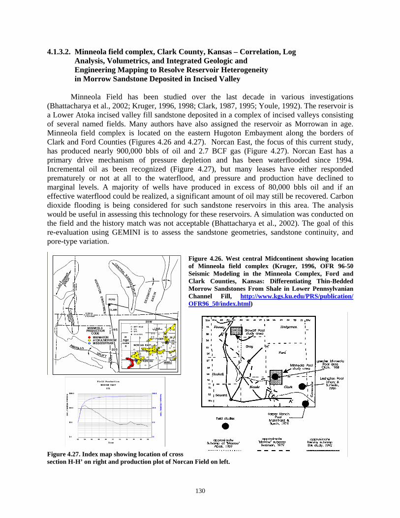
4.1.3.2. Minneola field complex, Clark County, Kansas – Correlation, Log Analysis, Volumetrics, and Integrated Geologic and Engineering Mapping to Resolve Reservoir Heterogeneity in Morrow Sandstone Deposited in Incised Valley Minneola Field has been studied over the last decade in various investigations (Bhattacharya et al., 2002; Kruger, 1996, 1998; Clark, 1987, 1995; Youle, 1992). The reservoir is a Lower Atoka incised valley fill sandstone deposited in a complex of incised valleys consisting of several named fields. Many authors have also assigned the reservoir as Morrowan in age. Minneola field complex is located on the eastern Hugoton Embayment along the borders of Clark and Ford Counties (Figures 4.26 and 4.27). Norcan East, the focus of this current study, has produced nearly 900,000 bbls of oil and 2.7 BCF gas (Figure 4.27). Norcan East has a primary drive mechanism of pressure depletion and has been waterflooded since 1994. Incremental oil as been recognized (Figure 4.27), but many leases have either responded prematurely or not at all to the waterflood, and pressure and production have declined to marginal levels. A majority of wells have produced in excess of 80,000 bbls oil and if an effective waterflood could be realized, a significant amount of oil may still be recovered. Carbon dioxide flooding is being considered for such sandstone reservoirs in this area. The analysis would be useful in assessing this technology for these reservoirs. A simulation was conducted on the field and the history match was not acceptable (Bhattacharya et al., 2002). The goal of this re-evaluation using GEMINI is to assess the sandstone geometries, sandstone continuity, and pore-type variation.

Figure 4.26. West central Midcontinent showing location of Minneola field complex (Kruger, 1996, OFR 96-50 Seismic Modeling in the Minneola Complex, Ford and Clark Counties, Kansas: Differentiating Thin-Bedded Morrow Sandstones From Shale in Lower Pennsylvanian Channel Fill, http://www.kgs.ku.edu/PRS/publication/ OFR96_50/index.html)

Figure 4.27. Index map showing location of cross section H-H’ on right and production plot of Norcan Field on left.

130

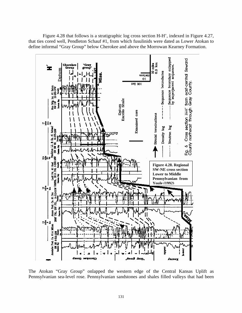
Figure 4.28 that follows is a stratigraphic log cross section H-H’, indexed in Figure 4.27, that ties cored well, Pendleton Schauf #1, from which fusulinids were dated as Lower Atokan to define informal “Gray Group” below Cherokee and above the Morrowan Kearney Formation.

Figure 4.28. Regional SW-NE cross section Lower to Middle Pennsylvanian from Youle (1992)

The Atokan “Gray Group” onlapped the western edge of the Central Kansas Uplift as Pennsylvanian sea-level rose. Pennsylvanian sandstones and shales filled valleys that had been

131

incised into the underlying Mississippian surface. Figure 4.29 is a detailed cross section through the Minneola field complex close to the axis of the incised valley. Based on cores from the field, regional cycles I, J, and K were identified to comprise the valley fill at Norcan East in the Minneola field complex (Youle, 1992). The basal cycle is discontinuous, while the middle cycle contains the main reservoir sandstone. The uppermost cycle, Cycle I, is comprised of mainly limestone. Also, carbonates begin to dominate all the cycles on the west side of the field, indicative of the marine influence.

Figure 4.29. East to west stratigraphic cross section through Minneola field complex (from Youle, 1992).

132

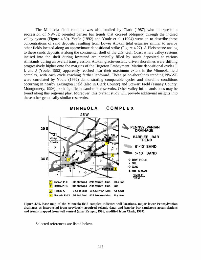
The Minneola field complex was also studied by Clark (1987) who interpreted a succession of NW-SE oriented barrier bar trends that crossed obliquely through the incised valley system (Figure 4.30). Youle (1992) and Youle et al. (1994) went on to describe these concentrations of sand deposits resulting from Lower Atokan tidal estuaries similar to nearby other fields located along an approximate depositional strike (Figure 4.27). A Pleistocene analog to these sands deposits is along the continental shelf of the U.S. Gulf Coast where valley systems incised into the shelf during lowstand are partically filled by sands deposited at various stillstands during an overall transgression. Atokan glacio-eustatic driven shorelines were shifting progressively higher onto the margins of the Hugoton Embayment. Marine depositional cycles I, J, and J (Youle, 1992) apparently reached near their maximum extent in the Minneola field complex, with each cycle reaching farther landward. These paleo-shorelines trending NW-SE were correlated by Youle (1992) demonstrating comparable cycles and shoreline conditions occurring in nearby Lexington Field (also in Clark County) and Stewart Field (Finney County, Montgomery, 1996), both significant sandstone reservoirs. Other valley-infill sandstones may be found along this regional play. Moreover, this current study will provide additional insights into these other genetically similar reservoirs. Figure 4.30. Base map of the Minneola field complex indicates well locations, major lower Pennsylvanian drainages as interpreted from previously acquired seismic data, and barrier bar sandstone accumulations and trends mapped from well control (after Kruger, 1996, modified from Clark, 1987). Selected references are listed below.

133

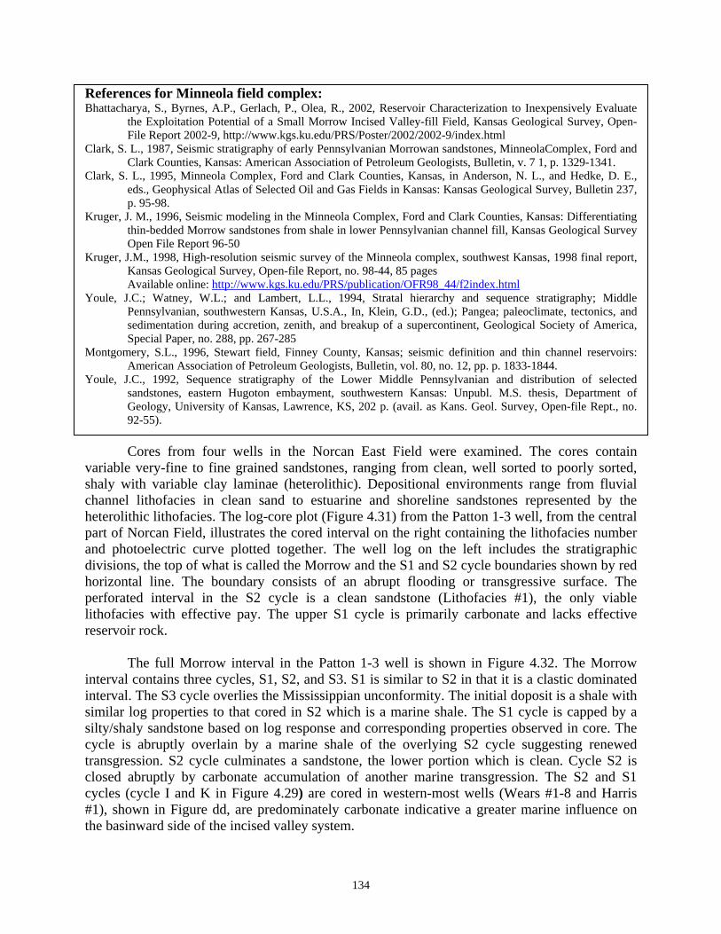
References for Minneola field complex: Bhattacharya, S., Byrnes, A.P., Gerlach, P., Olea, R., 2002, Reservoir Characterization to Inexpensively Evaluate

the Exploitation Potential of a Small Morrow Incised Valley-fill Field, Kansas Geological Survey, Open-File Report 2002-9, http://www.kgs.ku.edu/PRS/Poster/2002/2002-9/index.html

Clark, S. L., 1987, Seismic stratigraphy of early Pennsylvanian Morrowan sandstones, MinneolaComplex, Ford and Clark Counties, Kansas: American Association of Petroleum Geologists, Bulletin, v. 7 1, p. 1329-1341.

Clark, S. L., 1995, Minneola Complex, Ford and Clark Counties, Kansas, in Anderson, N. L., and Hedke, D. E., eds., Geophysical Atlas of Selected Oil and Gas Fields in Kansas: Kansas Geological Survey, Bulletin 237, p. 95-98.

Kruger, J. M., 1996, Seismic modeling in the Minneola Complex, Ford and Clark Counties, Kansas: Differentiating thin-bedded Morrow sandstones from shale in lower Pennsylvanian channel fill, Kansas Geological Survey Open File Report 96-50

Kruger, J.M., 1998, High-resolution seismic survey of the Minneola complex, southwest Kansas, 1998 final report, Kansas Geological Survey, Open-file Report, no. 98-44, 85 pages Available online: http://www.kgs.ku.edu/PRS/publication/OFR98_44/f2index.html

Youle, J.C.; Watney, W.L.; and Lambert, L.L., 1994, Stratal hierarchy and sequence stratigraphy; Middle Pennsylvanian, southwestern Kansas, U.S.A., In, Klein, G.D., (ed.); Pangea; paleoclimate, tectonics, and sedimentation during accretion, zenith, and breakup of a supercontinent, Geological Society of America, Special Paper, no. 288, pp. 267-285

Montgomery, S.L., 1996, Stewart field, Finney County, Kansas; seismic definition and thin channel reservoirs: American Association of Petroleum Geologists, Bulletin, vol. 80, no. 12, pp. p. 1833-1844.

Youle, J.C., 1992, Sequence stratigraphy of the Lower Middle Pennsylvanian and distribution of selected sandstones, eastern Hugoton embayment, southwestern Kansas: Unpubl. M.S. thesis, Department of Geology, University of Kansas, Lawrence, KS, 202 p. (avail. as Kans. Geol. Survey, Open-file Rept., no. 92-55).

Cores from four wells in the Norcan East Field were examined. The cores contain variable very-fine to fine grained sandstones, ranging from clean, well sorted to poorly sorted, shaly with variable clay laminae (heterolithic). Depositional environments range from fluvial channel lithofacies in clean sand to estuarine and shoreline sandstones represented by the heterolithic lithofacies. The log-core plot (Figure 4.31) from the Patton 1-3 well, from the central part of Norcan Field, illustrates the cored interval on the right containing the lithofacies number and photoelectric curve plotted together. The well log on the left includes the stratigraphic divisions, the top of what is called the Morrow and the S1 and S2 cycle boundaries shown by red horizontal line. The boundary consists of an abrupt flooding or transgressive surface. The perforated interval in the S2 cycle is a clean sandstone (Lithofacies #1), the only viable lithofacies with effective pay. The upper S1 cycle is primarily carbonate and lacks effective reservoir rock.

The full Morrow interval in the Patton 1-3 well is shown in Figure 4.32. The Morrow interval contains three cycles, S1, S2, and S3. S1 is similar to S2 in that it is a clastic dominated interval. The S3 cycle overlies the Mississippian unconformity. The initial doposit is a shale with similar log properties to that cored in S2 which is a marine shale. The S1 cycle is capped by a silty/shaly sandstone based on log response and corresponding properties observed in core. The cycle is abruptly overlain by a marine shale of the overlying S2 cycle suggesting renewed transgression. S2 cycle culminates a sandstone, the lower portion which is clean. Cycle S2 is closed abruptly by carbonate accumulation of another marine transgression. The S2 and S1 cycles (cycle I and K in Figure 4.29) are cored in western-most wells (Wears #1-8 and Harris #1), shown in Figure dd, are predominately carbonate indicative a greater marine influence on the basinward side of the incised valley system.

134

lith no. lithology1 ss, f gr, clean2 ss, vfg, w/lam. shale3 shale, calc4 ls, brn, dense5 ls, dk.gr-blk

5295

5300

5305

5310

5315

5320

5325

5330

1 2 3 4 5

Litho no. PEF .NONE

Figure 4.31. Composite well log plot with stratigraphic units and core description with Pe curve for Patton 1-3.

Figure 4.32. Full Morrow interval highlighted by blue bar extending to the top of the Mississippian (Ste. Genevieve).

135

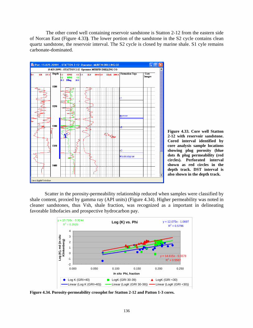
The other cored well containing reservoir sandstone is Statton 2-12 from the eastern side of Norcan East (Figure 4.33). The lower portion of the sandstone in the S2 cycle contains clean quartz sandstone, the reservoir interval. The S2 cycle is closed by marine shale. S1 cyle remains carbonate-dominated.

Figure 4.33. Core well Statton 2-12 with reservoir sandstone. Cored interval identified by core analysis sample locations showing plug porosity (blue dots & plug permeability (red circles). Perforated interval shown as red circles in the depth track. DST interval is also shown in the depth track.

Scatter in the porosity-permeability relationship reduced when samples were classified by

shale content, proxied by gamma ray (API units) (Figure 4.34). Higher permeability was noted in cleaner sandstones, thus Vsh, shale fraction, was recognized as a important in delineating favorable lithofacies and prospective hydrocarbon pay. Figure 4.34. Porosity-permeability crossplot for Statton 2-12 and Patton 1-3 cores.

Log (K) vs. Phi y = 12.075x - 1.0697R2 = 0.5796

y = 13.716x - 0.9244R2 = 0.2929

y = 14.615x - 0.5578R2 = 0.5567

-2

-1

0

1

2

3

4

0.000 0.050 0.100 0.150 0.200 0.250

In situ Phi, fraction

Log

(K),

md

(in s

itu

Klin

kenb

erg)

Log K (GRI>40) LogK (GRI 30-39) LogK (GRI <30)Linear (Log K (GRI>40)) Linear (LogK (GRI 30-39)) Linear (LogK (GRI <30))

136

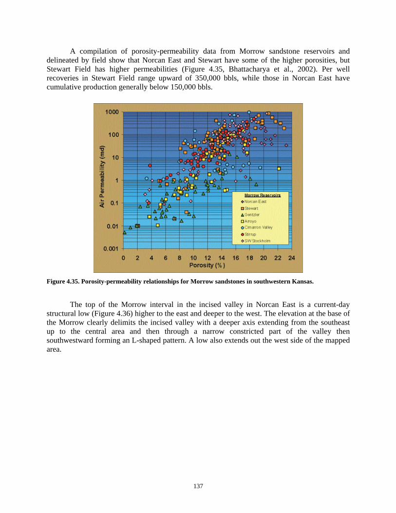
A compilation of porosity-permeability data from Morrow sandstone reservoirs and delineated by field show that Norcan East and Stewart have some of the higher porosities, but Stewart Field has higher permeabilities (Figure 4.35, Bhattacharya et al., 2002). Per well recoveries in Stewart Field range upward of 350,000 bbls, while those in Norcan East have cumulative production generally below 150,000 bbls. Figure 4.35. Porosity-permeability relationships for Morrow sandstones in southwestern Kansas. The top of the Morrow interval in the incised valley in Norcan East is a current-day structural low (Figure 4.36) higher to the east and deeper to the west. The elevation at the base of the Morrow clearly delimits the incised valley with a deeper axis extending from the southeast up to the central area and then through a narrow constricted part of the valley then southwestward forming an L-shaped pattern. A low also extends out the west side of the mapped area.

137

406000 406500 407000 407500 408000 408500 409000 409500 410000 410500 411000 411500

4146000

4147000

t ed1

patt1

latz1

goell1-4

h arris1-3

ted1-10

fager1-3

hind1-3

patt1- 3

ted2-10

fag2-3

no rt1

pat t2-3

t ed 2- 10

bo uch1-3A f ag 1- 3

ro on1-11

sch li1-2t ed 4- 10

t ed 3-10

1

hall2-2

go el1-4p at t2-3

statt1-12

mcgee1-1

nort1-4

ted1-10

alle1- 9

roo1-2

roo1 stat t2-12

-2720

-2710

-2700

-2690

-2680

-2670

-2660

Top Morrow

406000 406500 407000 407500 408000 408500 409000 409500 410000 410500 411000 411500

4146000

4147000

ted1

patt1

lat z1

goell1- 4

harris1-3

ted1-10

fager1- 3

hind1-3

p at t1-3

ted2-10

fag 2-3

nort1

patt2-3

ted2-10

bouch1-3A f ag 1-3

roon 1-11

schli1-2ted4-10

ted3-10

1

hall2-2

goel1-4patt2-3

statt1-12

mcgee1-1

nort1-4

ted1-10

alle1-9

ro o1-2

roo 1 st at t2-12

-2810

-2800

-2790

-2780

-2770

-2760

-2750

-2740

-2730

-2720

-2710

Base Morrow

Figure 4.36. Structure maps (sealevel datum) for the top and base of the Morrow.

A series of three cross sections follow, a southwest-northeast cross section through the western limits of Norcan East, a south-north cross section in the central portion of the field, and a west-to-east cross section that resides in the southeastern portion of the field (Figure 4.38). Index maps for each cross section are found in Figure 4.37. Western-most section (top) shows lateral facies change from carbonate on west to sandstone toward northeast. Central section shows cleaner sands toward north (central illustration), and lower section shows cleaner sand toward east. Together these changes suggest different sand bodies. Figure 4.37 Index map for cross sections shown in Figure 4.38.

138

Figure 4.38. Structure cross sections focused on the Morrow interval showing the S1, S2, and S3 cycles. Yellow bar in depth track highlights the porous sandstone reservoir in the S2 cycle that is the focus of this current study. Upper, western section, shows small lob of sand in west surrounded by carbonate, near basinward margin of sandstone. In central section, sandstone properties deteriorate to north. In lower section, similar decline in reservoir properties is noted from east to west.

139

Log analysis was conducted on the S2 sandstone reservoir to define effective pay. The Schlicting 1-2 lease produced a billion cubic feet of gas. The S2 sandstone is thick and clean. Well profile shows lobe of sand with Vsh curve and high porosity. Well perforations are also shown. Alongside the log profile is the lease production history showing annual and cumulative (Figure 4.39). Cut-offs include Vsh = 30%, Phi = 12%, Sw = 50%, and BVW = 0.12. Archie equation parameters were measured from core including: A = 1.8, M = 1.74, N = 2, with an Rw = 0.04. Figure 4.39. Depth profile of S2 cycle showing sandstone pay. To right is production plot of Schlicting 1-2 lease. Super Pickett crossplot of S2 cycle in Schlicting 1-2 well from east side of Norcan East Field shows low BVW (.55 minimum), low Sw, and high porosity equivalent to the hydrocarbon pay. (Figure 4.40). Figure 4.40. Super Pickett crossplot of Schlicting #1-2 well. Low BVW (high phi and low Sw) combine to describe a good hydrocarbon pay zone.

140

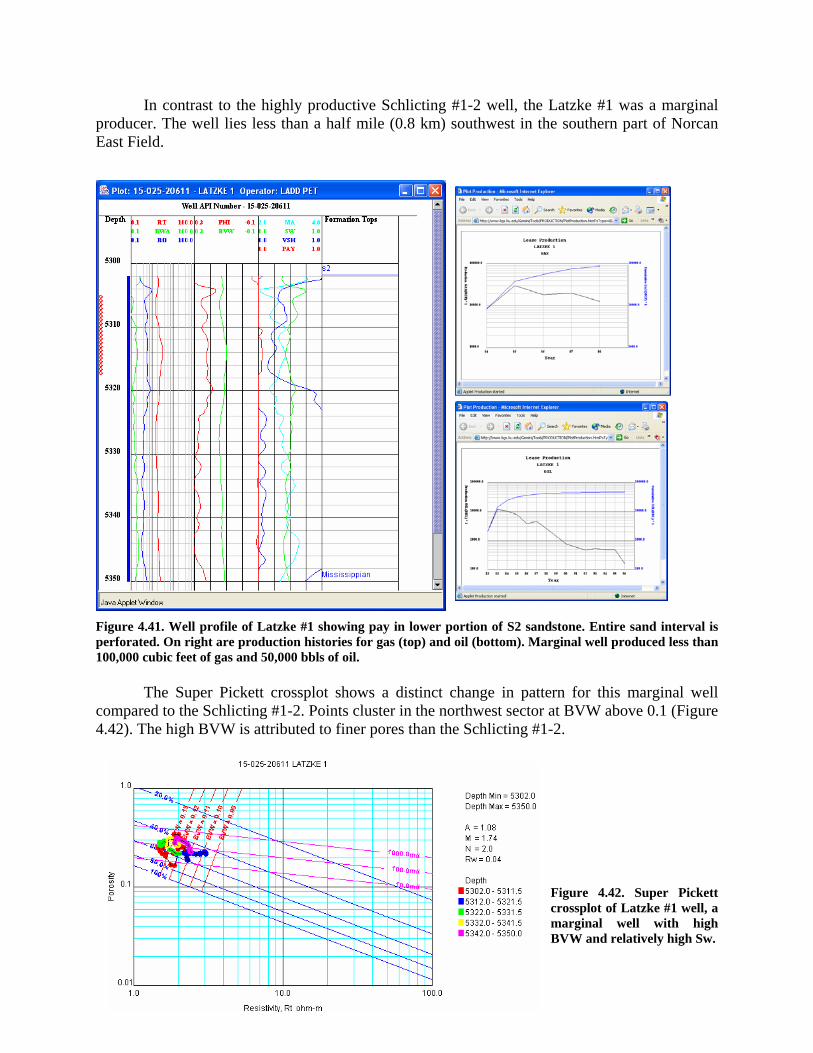
In contrast to the highly productive Schlicting #1-2 well, the Latzke #1 was a marginal producer. The well lies less than a half mile (0.8 km) southwest in the southern part of Norcan East Field.

Figure 4.41. Well profile of Latzke #1 showing pay in lower portion of S2 sandstone. Entire sand interval is perforated. On right are production histories for gas (top) and oil (bottom). Marginal well produced less than 100,000 cubic feet of gas and 50,000 bbls of oil. The Super Pickett crossplot shows a distinct change in pattern for this marginal well compared to the Schlicting #1-2. Points cluster in the northwest sector at BVW above 0.1 (Figure 4.42). The high BVW is attributed to finer pores than the Schlicting #1-2.

141

Figure 4.42. Super Pickett crossplot of Latzke #1 well, a marginal well with high BVW and relatively high Sw.

The total barrels of oil equivalent (BOE) was mapped for Norcan East (Figure 4.43) showing two areas of high BOE, one on the east side (mainly gas production) and the other in the central region. The sand on the far west side has limited production. 406000 406500 407000 407500 408000 408500 409000 409500 410000 410500 411000 411500

4146000

4147000

2.504

26.04

68.5

3

Figure 4.43. Cumulative BOE in 1000’s bbls for Norcan East Field. Two areas of high productivity. Blue circles denote leases with multiple wells. The average BVW is shown in Figure 4.44 with total BOE contours. The lower the BVW, the coarser the pores. Note low BVW in central region forming a north-south pattern. Also note southerly gradient of increasing BVW for central zone.

igure 4.44. Average BVW for S2 sandstone overlain with total BOE contours.

Cumulative BVW is also plotted against average Vsh and reveals similar pattern to BVW igure 4.45). The central lobe is cleanest (low Vsh) in north and gradually falls to the uthwest. Similarly, the Vsh in the eastern area forms a lobe shaped feature where Vsh declines the north. Locus of highly productive areas closely corresponds to these lobes of cleaner ndstone and it is inferred that the lobes reflect depositional features, low Vsh closest to the urce of the sand. Based on comparison of productive and dry wells, the Vsh cut-off was

onfirmed to be 0.3. The inverse relation between gamma ray and permeability is consistent with is observation.

F (Fsotosasocth

Cumulative BOE

406000 406500 407000 407500 408000 408500 409000 409500 410000 410500 411000 411500

4146000

4147000

0.071

0.074

0.1

0.05

0.079

0.063

0.044

0.085

0.087

0.04

0.055

0.087

0.069

0.0620.041

0.071

0.046

0.06

0.092

0.063 0.065

ted1

patt1

latz1

goell1-4

harris1-3

ted1-10

fager1-3

hind1-3

patt1-3

ted2-10

fag2-3

nort1

patt2-3

ted2-10

bouch1-3A fag1-3

roon1-11

schli1-2ted4-10

ted3-10

1

hall2-2

goel1-4patt2-3

statt1-12

mcgee1-1

nort1-4

ted1-10

alle1-9

roo1-2

roo1statt2-12

S2 Average BVW (color)

0.04

0.05

0.06

0.07

0.08

0.09

0.1

3.47

105.2

37.46

0

78.04

53.15

5.726

73.62

0

132.9

0

0 0

0

193.8150

0

0

39.80

90

2 925.

6

0

0

46.87 228.9

186.1

187.5

ted1

patt1

latz1

goell1-4

harris1-3

ted1-10

fager1-3

hind1-3

patt1-3

ted2-10

fag2-3

nort1

patt2-3

ted2-10

bouch1-3A fag1-3

roon1-11

schli1-2ted4-10

ted3-10

1

hall2-2

goel1-4

patt2-3

statt1-12

mcgee1-1

nort1-4

ted1-10

alle1-9

roo1-2

roo1 statt2-12Statt C

Patton C

Tedford C

Cumulative BOE

142

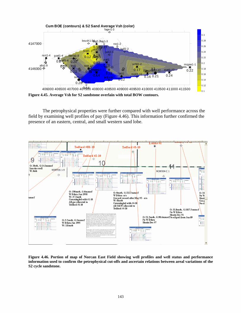
Figure 4.45. Average Vsh for S2 sandstone overlain with total BOW contours. The petrophysical properties were further compared with well performance across the field by examining well profiles of pay (Figure 4.46). This information further confirmed the presence of an eastern, central, and small western sand lobe.

Figure 4.46. Portion of map of Norcan East Field showing well profiles and well status and performance information used to confirm the petrophysical cut-offs and ascertain relations between areal variations of the S2 cycle sandstone.

406000 406500 407000 407500 408000 408500 409000 409500 410000 410500 411000 411500

41460000.23

0.26

0.22

0.170.21

0.19

0.12

0.12

0.64

41470000.12

0.19

0.64

0.27

0.170.19

0.2

0.240.22

0.28

0.16 0.21

ted1

patt1

latz1

goell1-4

harr is1-3

fager1-3

hind1-3

ted1-10

patt1-3

ted2-10

fag2-3

nor t1

patt2-3

bouch1-3A fag1-3roo1-2

hall2-2

ted2-10

roon1-11

schli1 -2ted4-10

ted3-10

1goel1 -4

patt2-3nort1-4

statt1-12

mcgee1-1

ted1-10

alle1-9

roo1statt2-12

Cum BOE (contours) & S2 Sand Average Vsh (color)

0. 1

0. 12

0. 14

0. 16

0. 18

0. 2

0. 22

0. 24

0. 26

0. 28

0. 3

143

The volumetrics were calculated for the S2 cycle sandstone (Figure 4.47). The results further support two sandstone lobes that account for the observed reservoir volume.

om

igure 4.48. Volumtric gridding dialog showing grid set for all mapping.

Figure 4.47. Plotfile for volumetrics of S2 cycle sandstone reservoir. Reservoir parameters derived frPfEFFER log analysis module. Plotfile is also available for ASCII download. Volumetric gridding was by inverse distance squared and the grid spacing was set at 200 feet (Figure 4.48). F

144

Results of Volumetric gridding in GEMINI. Mapping supports two distinct areas of better quality reservoir rock (Figure 4.49). Gross thickness is the total thickness of the S2 cycle, so it

cludes a shale zone underlying the sandstone. The net pay clearly shows two lobes of with higher

igure 4.49 ties for net sand nly.

insandstone. The average porosity map indicates that thicker net sand is also associatedaverage porosity.

F . Gross thickness, net pay, and average porosity for S2 cycle sandstone. Propero

145

The average water saturation is not as clearly interpretable (upper diagram in Figure 4.50). On the other hand, the original-oil-in-place shows two distinctive lobes. The injection well, also the cored well, Patton #1-3 (denoted by blue arrow) is located in the middle of the field. But the location of the injector is not optimum in terms of sand quality or hydrocarbon pore volume. Any realignment of the waterflood would include reversing the low pressure regime

rough large water volume needed just to fill up the pore space and regain elevated pressures. lso, los ill block oil ovement from some areas and make incremental oil recovery expensive and difficult. eservoir simulation will utilize the new volumetric parameters to examine further options for proving oil recovery.

igure 4.50. Average water saturation and OOIP for S2 cycle sandstone in Norcan East Field.

Calculated OOIP for study area is 7.8 million barrels (Figure 4.51). Total BOE recovered 1.682 million bbls using a 5.7 mcf/bbl conversion factor for gas to oil. Current recovery

thA s of solution gas pressure and occupancy of free gas in the pore space wmRim F isamounts to 22%, which is ok for primary and secondary in a solution gas drive oil reservoir.

146

Figure 4.51. Volumetric calculation dialog and report for S2 cycle sand in Norcan East Field.

147

Comparison of maps of total BOE and hydrocarbon*porosity* ft. with elevation of the levation of the base of S2 cycle suggests that the sand in the southeastern portion of Norcan ast Field was deposited in the valley (Figure 4.52). Similarly, most of the sand in the central be was confined to the valley, but the northern side shows sand high on the valley wall. A

ossible source of the sand supplying the central lobe of sandstone appears to have been from the orth where the reservoir properties are better. The source of the southeastern lobe of sand ppears to originate from the southeast. Lithofacies suggests fluvial channel sand modified by arine and tidal influence more distal from the source. A stillstand in sealevel or prolonged

ccupancy of the shoreline at this location led to sand accumulation in a partially filled incised alley system (as also indicated as barrier sands of Clark, 1986). As in Stewart Field to the orthwest along strike with this field, the quartz sand closely resembles the sandy matrix of the nderlying Mississippian Ste. Genevieve Limestone into which the incised valley was eveloped. The sealevel stillstand may also have been responsible for transported products of the eathered limestone, i.e., sandstone, to sites of lower energy such as local fall lines in bays and

stuaries such as the valley would provide. This limited sand accumulation is suggestive of local nd supply, rather than a large tributary drainage system. Moreover, the western limit of the S2

ycle sand in Norcan East Field grades to limestone confirmed in cores obtained within a mile uthwest of the field (Wears #1 in Section 8-30S-25W and Harris #1 in Section 9-30S-25W).

his suggests that marine shelf equivalents to the clastics are carbonate deposits.

Figure 4.52. Comparisons of total BOE and So*phi*ft and elevation base of S2 cycle.

eElopnamovnudwesacsoT

406000 406500 407000 407500 408000 408500 409000 409500 410000 410500 411000 411500

4146000

4147000

ted1

patt1

latz1

goel l1-4

harris1-3

ted1-10

fager1-3

hind1-3

patt1-3

ted2-10

fag2-3

nort1

patt2-3

ted2-10

bouch1-3A fag1-3

roon1-11

schli1-2ted4-10

ted3-10

1

hall2-2

goel1-4patt2-3

statt1-12

m cgee1-1

nor t1-4

ted1-10

alle1-9

roo1-2

roo1statt2-12Statt C

Patton C

Tedford C

2.504

26.04

68.5

33.47

105.2

37.46

0

78.04

53.15

5.726

73.62

0

132.9

0

0 0

0

193.8150

0

0

0

39.890

25.92

6

0

0

46.87 228.9

186.1

187.5

-2785

-2770

-2755

-2740

-2725

-2710

Cumulative BOE (contours) & structure base of S2

406000 406500 407000 407500 408000 408500 409000 409500 410000 410500 411000 411500

4146000

4147000

ted 1

pat t1g oell1- 4

harris1-3

t ed1- 10

f ager1- 3

h ind1- 3

pat t1- 3

t ed2- 10

lat z1

fag 2-3

no rt 1

p att2- 3

ted 2-10

bo uch 1-3A fag 1-3

ro on1- 11

schli1- 2t ed4- 10

ted3- 10

1

h all2-2

goe l1-4

pat t2-3

st att 1-12

m cgee1- 1

n ort 1-4

t ed1- 10

alle1-9

roo 1-2

ro o1 stat t2-12

0.2

0.4

0.6

1

1.2

1.4

1.6

1.8

2

S2 sum of hydrocarbon*porosity*ft

0.8

148

A plot of the average BVW and Vsh distinguishing the east and western lobes shows a positive correlation between increasing BVW and Vsh (Figure 4.53). Links to maps of BVW and Vsh support the relationship between improved reservoir properties in proximal positions within the lobes of sand, i.e., closer to the sources of the sand as previously discussed above.

406000 406500 407000 407500 408000 408500 409000 409500 410000 410500 411000 411500

4146000

4147000

0.071

0.074

0.1

0.05

0.079

0.063

0.044

0.085

0.087

0.04

0.055

0.087

0.069

0.0620.041

0.071

0.046

0.06

0.092

0.063 0.065

ted1

patt1

latz1

goell1-4

harris1-3

ted1-10

fager1-3

hind1-3

patt1-3

ted2-10

fag2-3

nort1

patt2-3

ted2-10

bouch1-3A fag1-3

roon1-11

schli1-2ted4-10

ted3-10

1

hall2-2

goel1-4patt2-3

statt1-12

mcgee1-1

nort1-4

ted1-10

alle1-9

roo1-2

roo1statt2-12

S2 Average BVW

0.04

0.05

0.06

0.07

0.08

0.09

0.1

Figure 4.53. Comparison of plots and maps of BVW and Vsh illustrating trends.

406000 406500 407000 407500 408000 408500 409000 409500 410000 410500 411000 411500

4146000

4147000

0.23

0.26

0.22

0.170.21

0.19

0.12

0.12

0.64

0.12

0.19

0.64

0.27

0.170.19

0.2

0.240.22

0.28

0.16 0.21

ted1

patt1

latz1

goell1-4

harris1-3

ted1-10

fager1-3

hind1-3

patt1-3

ted2-10

fag2-3

nort1

patt2-3

ted2-10

bouch1-3A fag1-3

roon1-11

schli1-2ted4-10

ted3-10

1

hall2-2

goel1-4patt2-3

statt1-12

mcgee1-1

nort1-4

ted1-10

alle1-9

roo1-2

roo1statt2-12

0.1

0.12

0.14

0.16

0.18

0.2

0.22

0.24

0.26

0.28

0.3

S2 Average Vsh

Minneola

0.000

0.020

0.040

0.060

0.080

0.100

0.120

0.000 0.100 0.200 0.300 0.400 0.500 0.600 0.700

Vsh

BVW

ave BVW(E) ave BVW(W) ave BVW©

Harris 2-3(no log,marginal well. Wtr.breakthrough)

Vsh shift

149

Correlation between average Vsh and BVW also extends to total BOE as might be anticipated since Vsh and BVW correlate with critical reservoir properties (Figure 4.54).

igure 4.54. Plot of Vsh and BVW vs. total BOE.

Additional inferences made about the stratigraphic succession within S2 cycle sandstone an be related to closely to a Pleistocene analog on the Gulf Coast. A portion of the Patton 1-3 ored interval is divided into stratigraphic units A, B, C, and D. Units B, C, and D create a ipartite division of the sandstone, a very common attribute to estarine valley fill deposits igure 4.55). Unit D is the clean, dominantly fluvial channel to estuarine facies that serves as e petroleum reservoir in Norcan East Field. Unit D reflects lower sealevel and nonmarine fluence in most of the field area except on the far west which maintain marine carbonate

eposition. The overlying Unit C is a marine/estuarine shale and probably represents quieter ner bay deposition. Unit B may be the shoreline barrier sand, a calcareous, silty, quartz sand ith shale laminae. Unit B is a sand on the far west reaches of the field in contrast to carbonate elow suggesting westward progradation and improved sorting of the sand body to where local ay is indicated. This is a separate reservoir from the eastern lobes of sandstone. Unit A at the p of the Cycle S2 is dense carbonate and reflecting marine transgression and the end of cycle 2 accumulation. Cycle 1 above represents higher sea level conditions where the shoreline oved farther eastward as indicated by Youle (1992) and Youle et al. (1994). The same tripartite

tratigraphic division is seen in the reservoir in Stewart Field where sand was deposited in all ree phases of the succession (Youle, 1992; Montgomery, 1996). This increased sand content ay be due to greater sediment supply or more prolonged conditions. Since the sedimentary

ycles may be equivalent between the areas, the increased sand content is more likely due to reater sediment supply.

Minneola Field

0.00

0.05

0.10

0.1

0.2

0.25

0.30

0.0 50.0 100.0 150.0 200.0 250.0

Total BOE

Ave

. Vsh

& B

VW

5

0 ave Vshave BVWLinear (ave Vsh)Lin e BVear (av W)

F cctr(Fthni

dinwbptoSmsthmcg

150

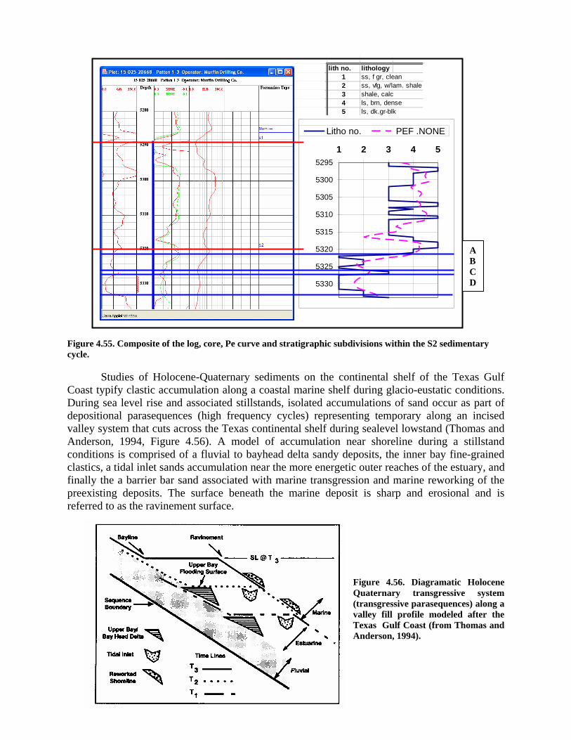
igure 4.55. Composite of the log, core, Pe curve and stratigraphic subdivisions within the S2 sedimentary ycle.

Studies of Holocene-Quaternary sediments on the continental shelf of the Texas Gulf oast typify clastic accumulation along a coastal marine shelf during glacio-eustatic conditions. uring sea level rise and associated stillstands, isolated accumulations of sand occur as part of epositional parasequences (high frequency cycles) representing temporary along an incised alley system that cuts across the Texas continental shelf during sealevel lowstand (Thomas and nderson, 1994, Figure 4.56). A model of accumulation near shoreline during a stillstand

onditions is comprised of a fluvial to bayhead delta sandy deposits, the inner bay fine-grained lastics, a tidal inlet sands accumulation near the more energetic outer reaches of the estuary, and nally the a barrier bar sand associated with marine transgression and marine reworking of the reexisting deposits. The surface beneath the marine deposit is sharp and erosional and is eferred to as the ravinement surface.

lith no. lithology

5 ls, dk.gr-blk

1 ss, f gr, clean2 ss, vfg, w/lam. shale3 shale, calc4 ls, brn, dense

5295

5300

5305

5310

5315

5320

5325

5330

1 2 3 4 5

Litho no. PEF .NONE

ABCD

Fc CDdvAccfipr

Figure 4.56. Diagramatic Holocene Quaternary transgressive system (transgressive parasequences) along a valley fill profile modeled after the Texas Gulf Coast (from Thomas and Anderson, 1994).

151

A Holocene-Quaternary depositional cycle developed along an incised valley system of the Texas Gulf Coast consists of the low-stand fluvial deposits deposited along the erosional sequence boundary. Staggered glacial eustatic rise in sealevel leads to localized accumulations of sand, i.e., local progradation, as part of the valley fill process. The components include the bayhead delta, inner estuarine fine grained clastics, and the tidal bar at the mouth of the estuary (Figure 4.57). Locally, these sands are partially eroded (ravinement) and reworked to form barrier islands as expressed today by Galveston Island. Variations in sediment supply and length of sealevel stillstands will affect the extent of these deposits (Figure 4.58). Conditions during the Pennsylvanian transgression were believed to have been similar.

Figure on,

994). 4.57. Quaternary-Holocene transgressive systems tract for Texas Gulf Coast (Thomas and Anders

1 Figure 4.58. Clastic deposits on Texas Gulf Coast related to Quaternary lowstand and transgressive conditions (from Thomas and Anderson, 1994).

152

Subtask 4.2. Concepts and Tutorial The concepts and tutorial are available in GEMINI Help (http://www.kgs.ku.edu/Gemini/ gemini-help.html) (Figure 4.59). Help is presented as a set of indexed web pages. Help concepts and tutorial are also linked directly to m

153

odules as they are accessed. The on-line tutorial provides step-by-step negotiation of the GEMINI functions. The user is provided with background

ation of the modules.

step-by-step tutorial of each module.

PfEFFER (log analysis) concepts is an example of the organization of these help web pages (Figure 4.60). The topics are further described through additional links (Figure 4.61).

Figure 4.60. Portion of PfEFFER Concepts web page outlining topics.

information and fundamental concepts that educate the user in the applic

Figure 4.59. A portion of the Help dialog in GEMINI showing active buttons used to access concepts and

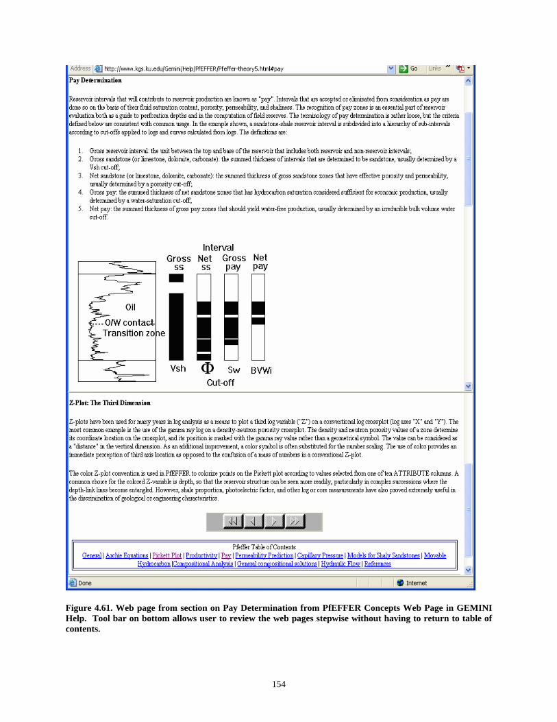
igure 4.61 n GEMINI elp. Tool bar on bottom allows user to review the web pages stepwise without having to return to table of

F . Web page from section on Pay Determination from PfEFFER Concepts Web Page iHcontents.

154

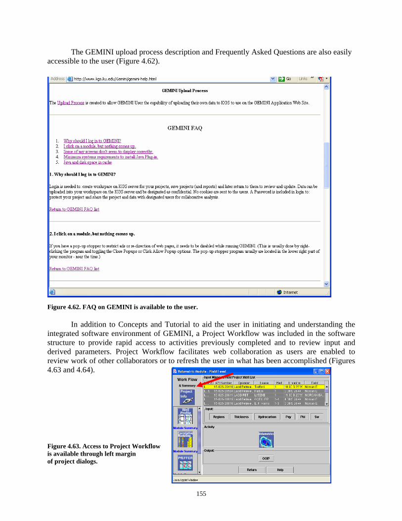
The GEMINI upload process description and Frequently Asked Questions are also easily ccessible to the user (Figure 4.62).

derived parameters. Project Workflow facilitates web collaboration as users are enabled to review work of other collaborators or to refresh the user in what has been accomplished (Figures 4.63 and 4.64). Figure 4.63. Access to Project Workflow is available through left margin of project dialogs.

a

Figure 4.62. FAQ on GEMINI is available to the user.

In addition to Concepts and Tutorial to aid the user in initiating and understanding the integrated software environment of GEMINI, a Project Workflow was included in the software structure to provide rapid access to activities previously completed and to review input and

155

Figure 4.64. SummaryVolumetrics parameterseach well obtained when accesses the Project Workflin this case, for Volumetrics

of for user ow, .

Dialogs are provided to show that the activity is running since some operations take a few

econds to complete. Visual cues to the user of active GEMINI processing (Figure 4.65) are an portant feature for smooth interaction in the work flow.

igure 4.65. Dialogs showing that application is processing while user waits. Wait time for all of the GEMINI pplications minimal.

sim Fa

156

CONCLUSIONS

Deployment of GEMINI

ber 30,

all

ins a new phenomenon, but it is surmised that lication service providers (ASP) and other web

ervice

All GEMINI modules were completed by July 31, 2003 (Figure 4.66). Intensive testing

was initiated in May 2003 and GEMINI was officially reviewed and released on Septem2003. Figure 4.66. Documentation of GEMINI releases available on the GEMINI website.

Speed in access and operation of modules in GEMINI is no longer an issue with common broadband connections to the Internet that are now available in many variations for smbusinesses. Internet access can be arranged from most locations when potential user’s are traveling. Set-up procedures are increasingly straight forward and the use of the Internet is becoming an increasingly essential activity to conduct the petroleum business enterprise. At the outset of this project in 2000, dial-up access to the Internet and e-mail service were issues for potential users, but these are no longer impediments to potential clients. Actual running of programs on the web for business purposes rema

is impediment will also be soon removed. Appths s such as auto-updating of software are increasingly more commonplace.

Primary access to GEMINI is currently

through the KGS site at www.kgs.ku.edu under the Software title (Figure 4.67). In addition, individual modules are available alongside the data on which they perforcomputations or display, e.g., LAS viewer

m

ww.kgs.ku.edu/Gemini/LAS.html?sA(http://wPI=15-025-20635&sKID=1021084922)

(Figure 4.68) and Production viewer is shown in Figure 4.69. Figure 4.67. Introductory page to KGS showing access point of GEMINI under software.

157

Figure 4 8. LAS log viewer is a standalone adaptation of the Well Profile in GEMINI. The module runs on the serv logs accesses can be viewed, printed, and downloaded.

Figure 4.69. Access to Standalone production module through KGS website provides automated plot and dialog to modify the plot.

.6er and

158

In addition to the GEMINI integrated project modules and standalone modules that run

on the server as described above, J d to deliver the application to the user’s PC so that the application can run without access to Internet. User accesses a web page from th

nt a new generation of web application utilized XML data handling protocol. Web Start pplications communicate with th

from the user’s PC. Additional individualized standalone modules are anticipated.

i GEMINI data access was created around Kan example of access to a large relational databdesigned used to access the KGS Database. The GGUI, Dialogs, Panels, and Tables are dependant o& Core Image File data are hard coded in theApplication configuration is also centered aroundto read that database and files for 13 Modules.

It was realized in 2002 that in order to attain a practical, efficient, cost-effective, and low maintenance implementation of GEMINI with the

ava Web Start is being use

e KGS site to download these applications, including PVT calculator, Material Balance, and Gridding and Mapping (Figure 4.70). The Web Start and server standalone programs represea e server to acquire data needed in the operation as well asuploading data

Figure 4.70. Web page to access standalone and downloadable Web Start applications.

stributed Databases

ansas Geological Survey’s (KGS) Database as ase residing on a server. Java Servlets were EMINI Application Graphical User Interfaces, n KGS Database Tables. The location of LAS

GEMINI Application. The present GEMINI Java Servlets. Some 75 Java Servlets are used

Bridge to XML and D

public-domain data sites that XML was

159

preferred protocol to accommodate variations in server type, data structure, expertise of systems anagers, and m t this linkage. These overriding factors led to is focus on XML as the optimum solution to realize GEMINI access to distributed public-

omain database nationwide and beyond. Although it is possible to replicate the current structure with other databases, as originally intended, it would involve significant effort on behalf of the data source and the GEMINI team that was not funded in the current contract. XML data protocol provides the means to allow GEMINI’s utilization nationwide.

tilization of XML means replacing the primary Java Servlet Layer with a Java-XML I/O Layer. While the present GEMINI Modules use KGS Database to save user data, an XML File Database System is used for user saved data. This allows the user to save data directly to their PC. To share projects the user is allowed to save their data to a server that has accessed to the outside world. The user is also given the ability to copy Project XML files to and from PC and Server. Data is retrieved in the same way no matter the source.

ML replaces the dependency of having to compile GEMINI Code for every new public omain Data Source. Rather, the Servlet location is hard-coded into a Java Class File. An Access ML File will identify a URL and File Paths for the Data Access Software for each public-omain site. For example, if the user selects data from the KGS, the Access XML File will give

n example is where KHAN, Rock Catalog and Well Profile Modules user interface is

dynam . KHAN and Well Profile Modules use LAS Curve information stored in KGS database for each LAS File. In this case, a standardized LAS Curve XML File would be created and an interpre r software would help user identify units directly from the LAS File being read. Data would also be read as XML (Figure 4.72). Without XML, data formatting becomes a very large issue and consumes considerable resources that could be focused instead on processing and analysis of value-added activities.

igure 4.71. Example of

GEMINI Read XML Process

m inimize the workload to implementhd

U

X

dXdthe URL of the Servlet to retrieve the data.

Adesigned around measured core data in the KGS database. The revised modules would read the Database Structure of Core Data from XML File (Figure 4.71). Access to the database is

ic

te

Applet or Application

Gemini IO Processing

Package

Gemini IO Processing

Package

JAVA-XML IO Processing

Package

JAVA-XML IO Processing

Package

•Read XML Input Sstream

•Parse XML to Linked List

•Write XML Output Stream

•Parse Linked List to XML F

•Read Comma Delimited Data

•Write Comma Delimited Data

Request for Data

Data Structure

Request for DataURL or File

Linked List with Parsed XML Data

GEMINI Processing XML File

User Project Processing XML File

Server

Database

•Cold Fusion

•ORALCE PL/SQL

•Java Servlets

LAS & CoreImage Files

Request for XML Data

XMLFile

XML Files

User’s PC

•Date Type DTD File

•Available Sources URLs

•Well API

•URL Location Of Data

a possible XML Read process.

•Data Type •Data Type

XMLFile

Request for XML Data

160

L version of GEMINI would be to identify , the base URL address for the

Figure 4.72. Example of a possible XML Read process. The procedure followed by a user in this XMthe public-domain server, the name of host organization of the sitedatabase, e.g., http://www.kgs.ukans.edu. Once the site isavailable data from this host database. Basic information iden

chosen the user would identify the ti ld include: Well Header

Information, Formation Top, Digital LAS Files, DST, Core Analysis, Core Images, and Production. The user would then identify the module use to use the Data Type and software would help define Data Types Requested, Format of data, Input Variables needed to retrieve data, URL to retrieve the XML, Output Stream, and Programming Application used to generate XML Stream such as Cold Fusion. Hypothetical framework is shown in Figure 4.73.

f GEMINI.

GEMINI Write XML Process

fied wou

Figure 4.73. Example of possible XML framework for distributed database version o

Applet or Application

Gemini IO Processing

Package

Gemini IO Processing

Package

JAVA-XML IO Processing

Package

JAVA-XML IO Processing

Package

•Read XML Input Stream

•Parse XML to ked List

•Write XML Ou ream

•Parse Linked L to XML

•Read Comma limited Data

•Write Comma limited Data

Lin

tput St

ist

De

De

Save Data

Errors Linked List withSave Data for XML File.

Errors

GEMINI Processing XML File

User Project Processing XML File

Server •Cold Fusion

•ORALCE PL/SQL

•Java Servlets

Users ProjectXML Files

User Save XML Data

User’s PC

•Data Type

•Date Type DTD File

•Available Sources URLs

•Data Type

•Well API

•URL Location Of Data

User Save XML Data

Users ProjectXML Files

Oil & Gas Data Source

Server

ORACLEDatabase

•Cold Fusion

•ORALCE PL/SQL

•Java Servlets

LAS & CoreImage Files

Oil & Gas Database Data Tables:•Well Header Information

•Digital LAS Files

•Formation Tops

Kansas Geological Survey

•Measured Core Data

•Core Image Files

•DST

•Lease Production

•Field Production

Server

Database

•Cold Fusion

LAS Files

Oil & Gas Database Data Tables:•Well Header Information

•Digital LAS Files

•M

Public-Domain db

easured Core Data

•Lease Production

Comma Delimited

Files

User’s PC

LAS Files

User Oil & Gas Data Files:•Digital LAS Files

•Measured Core Data

161

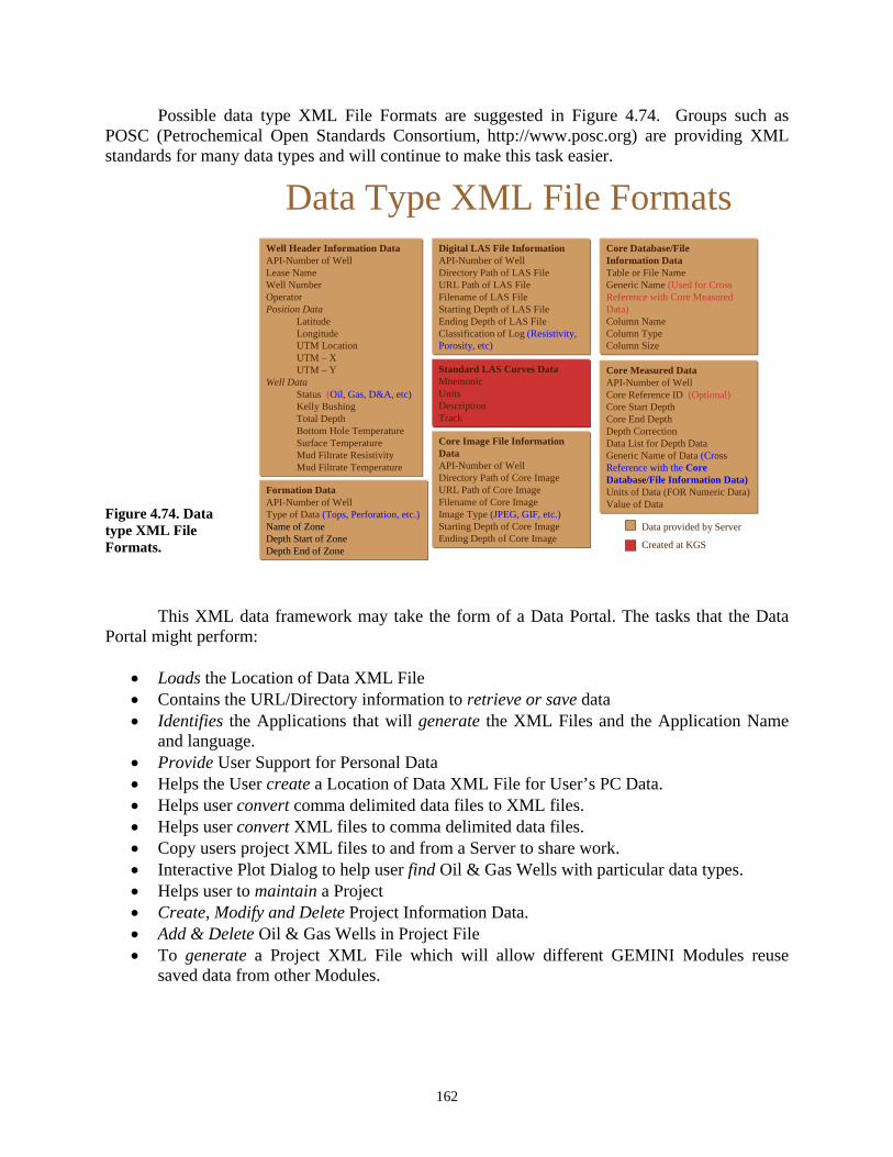
16

XML files to comd from

lls with ata type

& Gas Wells in Project File XML F low diff EMIN

• Provide User Support for Personal Data e User create a Location of Data XML File for User’s PC Data.

• Helps user convert comma delimited data files to XML files. • Helps user convert ma delimited data files. • Copy users project XML files to an a Server to share work. • Interactive Plot Dialog to help user find Oil & Gas We particular d s. • Helps user to maintain a Project • Create, Modify and Delete Project Information Data. • Add & Delete Oil • To generate a Project ile which will al erent G I Modules reuse

saved data from other Modules.

Possible data type XML File Formats are suggested in Figure 4.74. Groups such as POSC (Petrochemical Open Standards Consortium, http://www.posc.org) are providing XML standards for many data types and will continue to make this task easier.

Data Type XML File FormatsWell Header Information DataAPI-Number of WellLease NameWell Number

Digital LAS File InformationAPI-Number of WellDirectory Path of LAS FileURL Path of LAS File

Core Database/File Information DataTablGe

e or File Nameneric Name (Used for Cross

Reference with Core Measured Operator Filename of LAS FilePosition Data

LatitudeLongitudeUTM LocationUTM – XUTM – Y

Well DataStatus (Oil, Gas, D&A, etc)Kelly BushingTotal DepthBottom Hole Temperature

Starting Depth of LAS FileEnding Depth of LAS FileClassification of Log (Resistivity, Porosity, etc)

Standard LAS Curves DataMnemonicUnitsDescriptionTrack

Data)Column NameColumn TypeColumn Size

Core Measured DataAPI-Number of WellCore Reference ID (Optional)Core Start Depth

Core End Depth Depth Correction

Core Image File Information

Ending Depth of Core Image

Surface TemperatureMud Filtrate ResistivityMud Filtrate Temperature

Data List for Depth DataGeneric Name of Data (Cross Reference with the Core Database/File Information Data)Units of Data (FOR Numeric Data)Value of Data

Data provided by Server

DataAPI-Number of WellDirectory Path of Core ImageURL Path of Core ImageFilename of Core ImageImage Type (JPEG, GIF, etc.)Starting Depth of Core Image

Figure 4.74. Data type XML File

ormats.

Formation DataAPI-Number of WellType of Data (Tops, Perforation, etc.) Name of ZoneDepth Start of ZoneDepth End of ZoneF

Created at KGS

This XML data framework may take the form of a Data Portal. The tasks that the Data Portal might perform:

• Loads the Location of Data XML File • Contains the URL/Directory information to retrieve or save data • Identifies the Applications that will generate the XML Files and the Application Name

and language.

• Helps th

2

Obviously, the handlinmain sites will be a major task prior to actually analyzing the data with the Java

ftware tools. An example of the data portal is shown in Figure 4.75.

igure 4.75. Example of a possible Data Portal to access a server, view, and select data to assemble a GEMINI roject “on-the-fly”.

To make GEMINI Modules useful, a standard I/O process will nee created to llow data access from any source. XML is the data handling ol to best accomplish this. his will entail modification of the GEMINI Module GUI to reflect different data sources

help the user assemble and maintain their mat that GEMINI can understand. This could be accomplished with a GEMINI Data scribed a

g of many and varied and sometimes complex data types among many public-doso

User Project Processing XML File

•Project Information

•Oil & Gas Well List

•URL/Directory Location Of Data

Fp

d to be protoc

bove.

aTdynamically. A process would need to be created to

rdata in a fo dePortal as

163

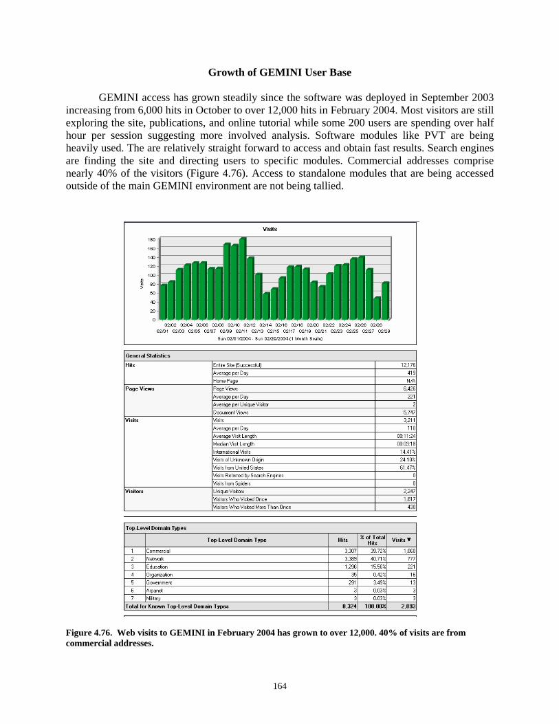
Growth of GEMINI User Base GEMINI access has grown steadily since the software was deployed in September 2003

creasing from 6,000 hits in October to over 12,000 hits in February 2004. Most visitors are still xploring the site, p alf our per session suggesting more involved analysis. Software modules like PVT are being eavily used. The are relatively straight forward to access and obtain fast results. Search engines re finding the site a prise early 40% of the visi modul eing accessed utside of the main GEMINI environment are not being tallied.

Figure 4.76. Web visits to GEMINI in February 2004 has grown to over 12,000. 40% of visits are from commercial addresses.

ine ublications, and online tutorial while some 200 users are spending over hhha nd directing users to specific modules. Commercial addresses com

tors (Figure 4.76). Access to standalone es that are bno

164

Increased utilization of GEMINI by users on a national level by industry, academia, and

education is an ultimate goal. Several strategies to help with deployment include: 1. Develop efficient software procedures to connect the integrated GEMINI

modules, the “spinoff” standalone server software, and the new Web Start downloaded applications via “XML-based Data Portal” to provide access of the Java software to other public-domain databases.

e practical

ized

ness

ore a sts of data vendors has also heightened substantially, both commercially and ation programming environment has also improved includin ML EMINI. With these successes, the expectations and sophisticat ent b aller independent companies that depend on the public-domain databases, has grown rapidly in the past few years.

hey have developed technical prowess coupled with an urgency to maintain competitiveness for eir investors as the search for oil and gas is increasingly focused on the hard to find remaining sources. It is anticipated beyond any doubt that businesses and academia will expect public-

omain websites that serve data to be capable of providing: 1. quick geospatial viewing of the data to refine a search and compare trends and

patterns, 2. rapid access to many data types and large volumes of data for use in tailored

applications, 3. utilization of web-based technical applications to “dig deeper into/mine” the

database by analyzing the information in real-time as it is accessed, 4. assembly of data into projects founded on the public-domain data and

integrated with their own to perform essential analytical procedures in such a manner as to enable distant collaborations and decision making, and

5. seamless integration of these results with commercial softwares to further analyze results and improve models to minimize risks and maintain competitiveness.

2. Encourage links to the GEMINI software to bring familiarity to new user group. 3. Include web links to DOE and PTTC. 4. Publish case studies in national journals and post on website. 5. Present workshops and short courses on use of GEMINI in practical applications. 6. Obtain published reviews of software from 3rd parties. 7. Continue to track usage to learn how to better design. 8. Enhance modules to help user more easily apply the software to solv

problems and find oil and gas. 9. Obtain testimonies as to experience in use and relate successes. 10. Maintain security of projects and data. 11. Work with commercial software vendors to ensure that bridges are optim

between softwares.

Summary Subsurface, petroleum-related public-domain databases continue to improve in rich

of types and volume of information. Over the past four years, improving and standardization of web servers and data-handling procedures have allowed web-based data to be much mccessible to outside clients. The knowledge and intere

public-domain. The web-applicg Java and X being used in Gion of the cli ase, particularly sm

Tthred

165

Web-based computing has advanced from a curiosity and a “bleeding edge” technology

the mainstream and is now a fully functional, basic computing environment that provides liable, value-added results for businesses and research. The National Science Foundation is

ully committed to this endeavor with their Informatics initiatives, eg., Geoinformatics, as are ommercial application service providers (ASP). It is anticipated that web-applications will be an ssential technology for petroleum clients to help “mine” the public-domain data and tailor it to eir needs. Those who best manage the information will be competitive. The more direct and

ach other. The web-based informatics environment with greatly expanding capability in rocessing speed and storage capacity is greatly improving opportunities for web-based, eoscien t needs and

capabil

GEMINI Project Synopsis

The GEMINI web-application is summarized through a series of images that complete is report to help further convey the capabilities of the software and the ability it has to offer

solutions to practical problems. r captioned and are not logged to the List of Figures following the Table of Contents.)

torefceth“seamless” the software applications are linked to the public-domain data, the more the tools will be used and the greater the need for rich datasets. The two assets will drive the development of epg ce software applications in a public-domain setting. Close linkage of clien

ities of the public domain host will be beneficial to each. The overall success of the client base in the oil and gas producing provinces will support the petroleum industry enterprise and sustain or enhance local economies that are dependent on them. Serving data and applications will help regions stay competitive.

th

(These figures are not numbered oin

Well Production

Module

Well Profile

Module

Well Profile

Module

PfEFFER

Module

PfEFFER

Module

DST

Module

DST

Module

Cross Section

Module

Cross Section

Module

Volumetric

Module

Volumetric

Module

W

Material Balance

Module

ell Production

Module

Material Balance

Module

Rock Catalog

Module

Rock Catalog

Module

Module

Fluid CatalogFluid Catalog

Integrated Reservoir Modeling

Module

166

GEMINIProject Workflow

User/Project Module

Enter Project Information:(Name, Location, Field, Description)

Well Level Analysis Field or Multi-Well Analysis

Data Compilation

Well Profile ModuleDis ay and annotate well logs with tops, layCo

Help ModuleTutorial - Step-by-step

Concepts

Test ing, Case Studies, Progress Reports, Workshops, Short Courses,

Geological Modeling

Correlative Modeling Module

Synthetic Seismogram Module

Cross Section Utilize marked logs, on-the-fly editing, output

Intervals, core data, quick look well log analysis

ng Modeling

Production Module

es - Oil, gas and water properties

original oil and gas in place, field recovery ions, output results urther analysis

volumetric, aquifer fitting

Production bubble map Time-rate plots

aracteristics)

II output file for mapping and analysis software and simulators including DOE’s ED

Project Workflow

Ro atalo

PfEFFE g An

Correlate rock trophylocation, field, formationlithofacies/depositional

Basic Log An s -

Enhanced Lo alysis

Wapay cutoffs, ef e pay

clustering, flo defini

Calculate res r pres

Brine catalog Rw C

T Mo

Fl atal

Develop WellModel

DevelopGeo-Engineering Model

plers/zones, perforations DST intervals, re data, quick look well log analysis

Technology Transfer to raster file and print

Publ ications, Web-based Compliations

Petr physical Modeling

Engineeriw unit tion, lithology

PVPVT Properti

ervoi sure & permeabilty T Calculator Module DS dule

Volumetrics ModuleMapping of reservoir variables, calculate

and alculationOutput

Material Balance ModuleIdentify drive mechanism, confirm reservoir

Parametrics for Simulation Model Module)

ASC

efficiency, residual saturatas ascii files and grids for f

Kansas Hydrocarbon Association Navigator (KHAN Module)

Continuous and discrete variable prediction and supervised classification (e.g. Predict pay, lithofacies, reservoir ch

ck C g Module pe sics by depth,

, environment

Boast

Assist efforts in project management and collaborative

o

R Lo alysis Modulealysi ter saturation models,

g An - fectiv by reservoir layers

Depth-constrained

uid C og Module Synthesis and

User/Project ModuleUser(s) setupAdd/Delete Wells

Wells by county/fieldWells by Interactive MapAssemble data from online db & upload: Formation tops, production, perforations, dri ll stem test, Core data, LAS files

GEMINIProject Workflow

User/Project Module

Enter Project Information:(Name, Location, Field, Description)

Well Level Analysis Field or Multi-Well Analysis

Data Compilation

Well Profile ModuleDis ay and annotate well logs with tops, layCo

Help ModuleTutorial - Step-by-step

Concepts

Test ing, Case Studies, Progress Reports, Workshops, Short Courses,

Geological Modeling

Correlative Modeling Module

Synthetic Seismogram Module

Cross Section Utilize marked logs, on-the-fly editing, output

Intervals, core data, quick look well log analysis

ng Modeling

Production Module

es - Oil, gas and water properties

original oil and gas in place, field recovery ions, output results urther analysis

volumetric, aquifer fitting

Production bubble map Time-rate plots

aracteristics)

II output file for mapping and analysis software and simulators including DOE’s ED

Project Workflow

Ro atalo

PfEFFE g An

Correlate rock trophylocation, field, formationlithofacies/depositional

Basic Log An s -

Enhanced Lo alysis

Wapay cutoffs, ef e pay

clustering, flo defini

Calculate res r pres

Brine catalog Rw C

T Mo

Fl atal

Develop WellModel

DevelopGeo-Engineering Model

plers/zones, perforations DST intervals, re data, quick look well log analysis

Technology Transfer to raster file and print

Publ ications, Web-based Compliations

Petr physical ModelingKansas Hydrocarbon Association

Navigator (KHAN Module)

Continuous and discrete variable prediction and supervised classification (e.g. Predict pay, lithofacies, reservoir ch

ck C g Module pe sics by depth,

, environment

Engineeriw unit tion, lithology

PVPVT Properti

ervoi sure & permeabilty T Calculator Module DS dule

Volumetrics ModuleMapping of reservoir variables, calculate

and alculationOutput

Material Balance ModuleIdentify drive mechanism, confirm reservoir

Parametrics for Simulation Model Module)

ASC

efficiency, residual saturatas ascii files and grids for f

Boast

Assist efforts in project management and collaborative

o

R Lo alysis Modulealysi ter saturation models,

g An - fectiv by reservoir layers

Depth-constrained

uid C og Module Synthesis and

User/Project ModuleUser(s) setupAdd/Delete Wells

Wells by county/fieldWells by Interactive MapAssemble data from online db & upload: Formation tops, production, perforations, dri ll stem test, Core data, LAS files

167

168

User/Project

Module

User/Project

ModuleWell Profile

Module

Well Profile

Module

PfEFFER

Module

PfEFFER

Module

DST

Module

DST

Mod

SyntheSeismog

Modul

ule

tic ram

e

SyntheSeismogr

Modu

tic am

le

KHAN

Module

KHAN

Module

Cross Section

Module

Cross Section

Module

Volumetric

Module

Volumetric

Module

Well Production

Module

Well Production

Module

Module

Material BalanceMaterial Balance

Module

ASCII Output for Reservoir Simulation

Module

ASCII Output for Reservoir Simulation

Module

PVT

Module

PVTRock Catalog

ModuleModule

Rock CatalogFluid Catalog

ModuleModule

Fluid Catalog

Module

ck & Fluid Characteristics Java Applets

Field Level Analysis

Java Applets

Well Level Analysis

Java Applets

Ro

KGS Server

Apache - Tomcat

Java ServletsKGS Database & Files

Integrated Web-based Petroleum Reservoir Modeling

ld GEMINI Releases.• Source Code is Doc e web for peer

review.

Home page: http://www.kgs.ku.edu/Gemini/

Engineering Modules

GEMINISteps in Development

• GEMINI Java Code Standards created before developers write any code.– http://www.kgs.ukans.edu/Gemini/R1.0/Documentation/JavaCodeConve

ntions21November2000.doc• Design of the Modules are worked out with geologist, engineer, and

peer review.• Source Code is accessible to all developers.

– Java Source Code.– SQL Scripts to build GEMINI Database Tables– DOS Scripts to bui

umented and displayed on th

– Developers write html with screen captures and links to the javasource code.

GEMINI Rock Catalog

Council Grove Comparison of Lithofacies

Find all Rock Core Analysis Data in the Kansas Geological Survey's Database with Additional constraints of: 0. Lithology is Silty Mdst-Wkst

Well: ALEXANDER 'D' 2 Operator: CITIES SERVICE CO Kelly Bushing (ft): 3100.0 Total Well Depth (ft): 3150.0 Latitude: 37.67467 Longitude: -101.16757

Html output onBrower page

Rock Properties

GEMINIApplet-Servlet Communication

Client Side Applets

Apache-Tomcat Server

Java Servlets•Embedded SQL Classes

•Digital LAS File Read Class

ORACLE Database

Digital LAS Files

Core Image Files

Request for Data

Kansas Oil & GasDatabase & File Data

169

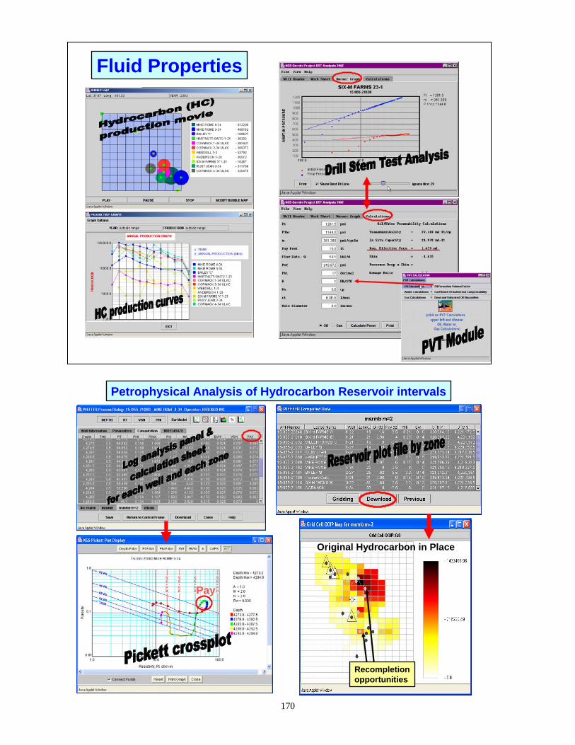
Fluid Properties

Original Hydrocarbon in Place

Pay

Recompletionopportunities

Petrophysical Analysis of Hydrocarbon Reservoir intervals

170

Marmaton BCase #1

m=2, n=2

CutoffsPhi =.15Sw = .25Vsh = .3BVW = .04

Gross Thickness Net Pay Average Phi

Average Sw Sum (So*phi*ft)

Marm BMarm B

Producing Well Dry Hole

HighProbabiltyfor oil pay

Currentperforations

Kansas HydrocarbonAssociation Navigator

-Build training setsand share models

-Use to findattribute that hasdiagnostic petrophysicalresponse.

Prediction:Oil, Wet, Impermeable, Shale

St. Louis “C”

171

Project Workflow and Summary

“Real Time” Immediate Interaction• Option to launch software modules as data is accessed • Option to download modules as Java Web Start applications • Move to XML database I/O for distributed db access

Java desktop application

Java applet

172

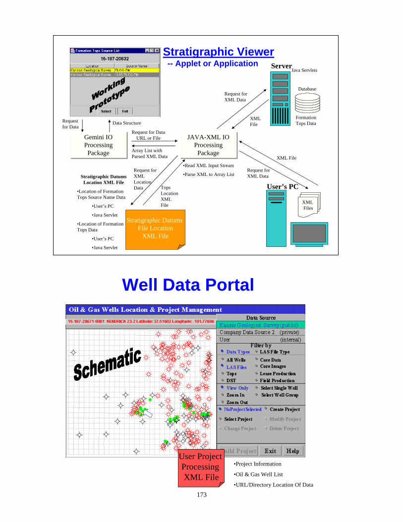
Stratigraphic Viewer-- Applet or Application

Gemini IO Processing

Package

Gemini IO Processing

Package

JAVA-XML IO Processing

Package

JAVA-XML IO Processing

Package

•Read XML Input Stream

•Parse XML to Array List

Request for Data

Data Structure

Request for DataURL or File

Array List with Parsed XML Data

Stratigraphic DatumsFile Location

XML File

Server

Database

Java Servlets

Request for XML Data

XMLFile

XML Files

User’s PCStratigraphic Datums

Location XML File

•Location of Formation Tops Source Name Data

•User’s PC

•Java Servlet

•Location of Formation Tops Data

•User’s PC

•Java Servlet

XML File

Request for XML Data

Request for XML Location Data Tops

Location XMLFile

Formation Tops Data

Well Data Portal

User Project Processing XML File

•Project Information

•Oil & Gas Well List

•URL/Directory Location Of Data

173

174

GEMINI (Geo-Engineering Modeling through INternet Informatics)

• GEMINI is a public–domain, interactive, integrated Internet web application.

• 14 user-friendly software modules, calculators, and utility programs.

• Construct geologic/engineering petroleum reservoir models.

• Common data types -- digital well logs; core analyses, descriptions, and images; stratigraphic information; drill stem tests; completion information; monthly and annual production.

• Data assembled “on the fly” into projects built and accessed by collaborators.

• Reports and data files generated from the analyses can be downloaded for use in other applications.

• Projects and data uploaded into the project are password protected.

Mineral Management Services

Linking to Distributed DataNetwork

F u tu re• C re a te a p p le ts a n d W e b S ta rt

a p p lic a tio n s o f s o ftw a re m o d u le s

• A c c e s s d is tr ib u te d d a ta b a s e s

• In te g ra te s o ftw a re to o ls th ro u g h X M L d a ta b a s e s

175

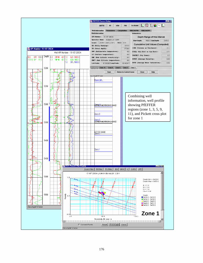
176

Combining well information, well profile showing PfEFFER regions (zone 1, 3, 5, 9, 11), and Pickett cross plot for zone 1

Zone 1Zone 1

Succession of Super-Pickett Cross Plots by stratigraphic order broken out as PfEFFER Regions or divisions of the Morrow sandstone reservoir

Zone 1

Gas

PFD

Zone 1Zone 1

GasGas

PFD

Zone 9Zone 9

Zone 5Zone 5

Zone 3Zone 3

177

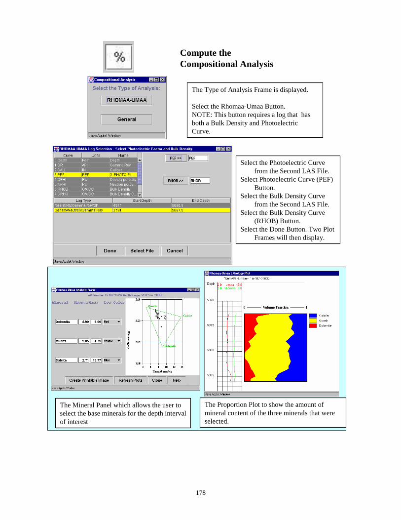
Compute the Compositional Analysis

The Type of Analysis Frame is displayed.

Select the Rhomaa-Umaa Button.NOTE: This button requires a log that has both a Bulk Density and Photoelectric Curve.

Select the Photoelectric Curve from the Second LAS File.

Select Photoelectric Curve (PEF) Button.

Select the Bulk Density Curve from the Second LAS File.

Select the Bulk Density Curve (RHOB) Button.

Select the Done Button. Two PlotFrames will then display.

The Mineral Panel which allows the user to select the base minerals for the depth interval of interest

The Proportion Plot to show the amount of mineral content of the three minerals that were selected.

178

Second well of cross section has been added and user clicks on one of five reservoir layers to obtain color dialog to use in selecting color to use forlayerthroughout the cross section.

All five layershave been colored in this illustration.

179

NW-SE Structural Cross Section-- Jpeg file

• Antiform and subcrop in Mississippian• Lower sandstone (1, 3, 5) onlap• Upper sandstone (9, 11) overstep• Carbonate thickening over antiform

13

59

11

NW-SE Stratigraphic Cross Section• Antiform and subcrop of Mississippian

on paleohigh• Lower sandstone onlap

• Upper sandstone overstep

• Carbonate thickening over antiform

Datum

180

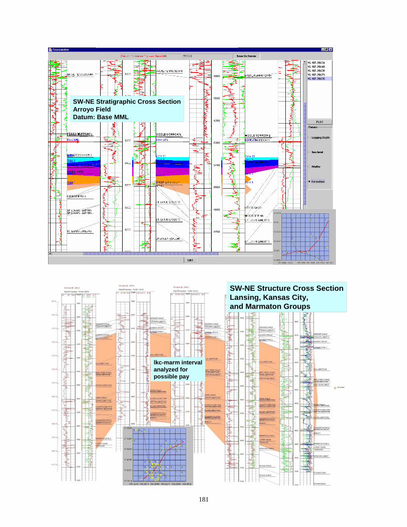
SW-NE Stratigraphic Cross SectionArroyo FieldDatum: Base MML

SW-NE Structure Cross SectionLansing, Kansas City, and Marmaton Groups

lkc-marm intervalanalyzed for possible pay

181

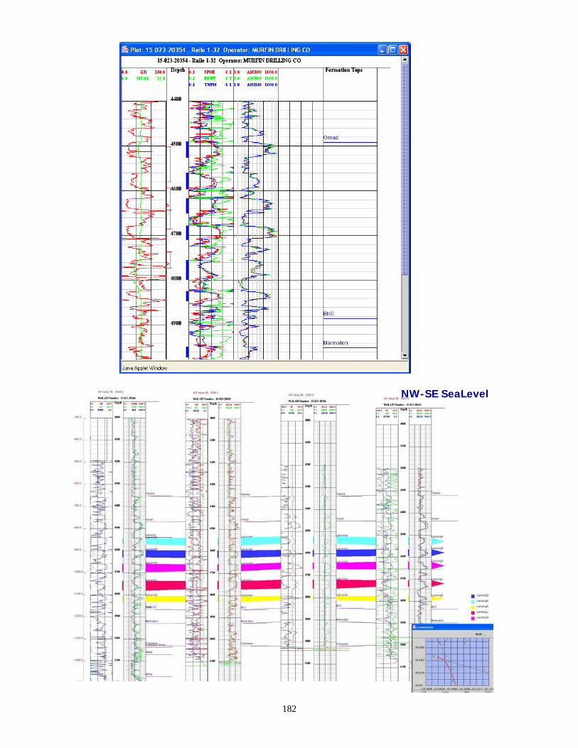
182

NW-SE SeaLevel

Pay

107.6 BO + 32 BW

Subzonation suggested By Depth ConstrainedCluster Analysis (using 10 zones)

183

184

Cumula

Location B

Location A

Location C

0.04

0.05

0.06

0.07

0.08

0.09

0.1

tive BOE

406000 0 411500406500 407000 407500 408000 408500 409000 409500 410000 410500 41100

4146000

4147000

0.071

0.074

0.1

0.05

0.079

0.063

0.044

0.085

0.087

0.04

0.055

0.087

0.069

0.0620.041

0.071

0.046

0.06

0.092

0.063 0.065

ted1

patt1

latz1

goell1-4

harris1-3

ted1-10

fager1-3

hind1-3

patt1-3

ted2-10

fag2-3

nort1

patt2-3

ted2-10

bouch1-3A fag1-3

roon1-11

schli1-2ted4-10

ted3-10

1

hall2-2

goel1-4patt2-3

sta tt1-12

mcgee1-1

nort1-4

alle1-9

ted1-10

roo1-2

roo1statt2-12

S2 Average BVW (color)

Originalcore description

Predicted reservoir lithofaciesfrom the Council Grove (center colored box) compared to core description on right column.

185

186

STANDARD NAME STND. UNITS UNITS DESCRIP. PWLS MNEM1 UNITS1Depth FT feet DEPTH. DEPTH FBit size IN inches ? BS INCaliper IN inches CAL. CALI INBorehole volume FT3 cubic feet BH.VOL. BHV FT3Tension LB pounds TENS. TENSION POUNDSLogging time SEC seconds TIME. TIME STemperature DEGF degrees Fahrenheit TEMP. TEMP DEGGamma Ray API API units GR. GR GAPIGamma Ray Minus Uranium API API units GR.KTH. CGR APIThorium Concentration PPM parts per million ELE.TH. THOR PPMUranium Concentration PPM parts per million ELE.U. URAN PPMPotassium Concentration % or FRAC percent or fraction ELE.K. POTA PERCBulk Density GM/CC grams per cc DEN. RHOB G/C3Density porosity PU porosity units DEN.POR.APP. DPHI V/VBulk Density Correction GM/CC grams per cc DEN.CRN. DRHO G/C3Photoelectric factor BARNS/E barns per electron PEF. PE BARNNeutron counts COUNTS counts NEU.CTS. NEUT APINeutron porosity PU porosity units NEU.POR.APP. NPHI V/VAcoustic transit time USEC/FT microseconds per foot AC.TIME. DT US/FSonic porosity PU porosity units AC.POR.APP. SPHI DECPSpontaneous Potential MV millivolts SP. SP MVConductivity MMHO/M millimhos per meter CON. COND MMHO/MDeep Induction Conductivity MMHO/M millimhos per meter CON.DEP.IND. CILD MMHO/MMedium Induction Conductivity MMHO/M millimhos per meter CON.MED.IND. CILM MMHO/MResistivity OHM-M ohm-meters RES. RES OHM-MShallow Resistivi ty OHM-M ohm-meters RES.SHA. RSHAL OHM-MDeep Resistivity OHM-M ohm-meters RES.MED. RMED OHM-MMedium Resistivity OHM-M ohm-meters RES.DEP. RDEP OHM-MDeep Induction Resistivity OHM-M ohm-meters RES.DEP.IND ILD OHMMMedium Induction Resistivity OHM-M ohm-meters RES.MED.IND. ILM OHMMArray Induction Resistivity OHM-M ohm-meters RES.ARR.IND. AHT* OHMMShallow Laterolog Resistivity OHM-M ohm-meters RES.SHA.LAT. LL8 OHMMShallow Normal Resistivity OHM-M ohm-meters RES.SHA.NOR. SN OHMMLong Normal Resistivity OHM-M ohm-meters ? LN OHMMSpherically Focused Resistivity OHM-M ohm-meters RES.SHA.SPH. SFL OHMMDeep Laterolog Resistivity OHM-M ohm-meters RES.DEP.LAT LL OHMMMicro Inverse Resistivity OHM-M ohm-meters RES.MIC.INV. MINV OHMMMicro Laterolog Resistivity OHM-M ohm-meters RES.MIC.LAT. MLL OHMMMicro Normal Resistivity OHM-M ohm-meters RES.MIC.NOR. MNOR OHMMMicro Spherically Focused Resis OHM-M ohm-meters RES.MIC.SPH. MSFL OHMM Apparent Water Resistivity OHM-M ohm-meters WAT.RES.APP. RWA OHMMRxo/Rt ratio RATIO ratio ? RXRT V/VElectromagnetic Attenuation Rat DB/M decibels per meter ELM.ATT. EATT DB/MCalcite Volume Fraction FRAC proportion VF.MIN.CALC. V1M3 V/VQuartz Volume Fraction FRAC proportion VF.MIN.QRTZ. V2M3 V/VDolomite Volume Fraction FRAC proportion VF.MIN.DOLM. V3M3 V/V

Core elements of KML(Kansas Mnemonic Lexicon

Predicted genetic unitsapplied to wells in training set

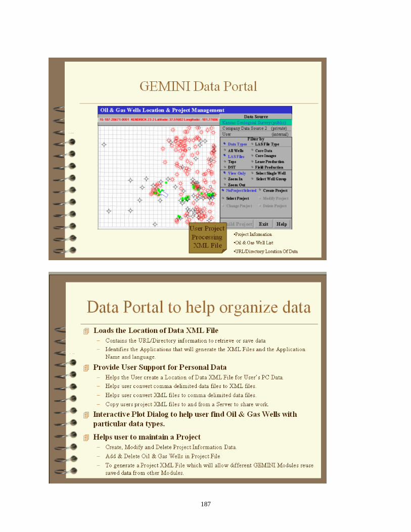
187

GEMINI Geo-Engineering Modeling through Internet Informatics

Kansas Geological SurveyThe University of Kansas

Project funded by

US Department of EnergyCooperative Agreement No. DE-FC26-00BC15310

188

SELECTED REFERENCES

rchie, G. E., 1952, Classification of reservoir rocks and petrophysical considerations: AAPG Bulletin, v. 36, no. 2, p. 278-298.

hattacharya, S., Byrnes, A.P., Gerlach, P. R., 2002, Reservoir Characterization to Inexpensively Evaluate the Exploitation Potential of a Small Morrow Incised Valley-fill Field, Kansas Geological Survey, Open-File Report 2002-9, http://w S/Poster/2002/2002-9/index.html

hattacharya, S., Watney, W.L., Do J., Bohling, G., 1999, From geomodels to engineering models – Opportunities put ulf Coast Section Society SEPM, Advanced Reservoir

r tio e y, Nineteenth Annual Bob F. Perkins Research Conference, Gulf o o n, TX. , p. 179-193.

ohlin . ton, and ey, 1996, Sy identification of sequenc raphic units m wir raphi tilizin vanced Geophysical, Wirelin Borehole

Technology Fo oleu io ion r ulf Co ection SEPM 17th Annual Rese nference, p.

ohling, G. C., J. H. Dove th, 19 Pro ilistic classification and prediction of facies types in a mid-continent cretaceou arine sequence from petrophysical log descriptors using a CMAC procedure, in Proceedings of the Thir ual Conference of the IAMG, CIMNE, Barcelona, p. 242-247.

ohling, G.C., and Dubois, M.K., 2003, An Integrated Application of Neural Network and Markov Chain Techniques to Prediction of Lithofacies from Well Logs: Kansas Geological Survey, Open-File Report 2003-50, http://www.kgs.ku.edu/PRS/publication/2003/ofr2003-50.pdf

A

B , Olea,

ww.kgs.ku.edu/PRveton, J.H., Guy, W.

for spreadsheet com ing: GCha acteriza n for th Twenty-First CenturCoast Section, SEMP F undation, H ustog, G C., J. H. Dove W. L. Watn stematic e stratigfro eline logs, in Stratig c Analysis U g Ad e and

r Petr m Explorat n and Product , Pape s presented at the G ast Sarch Co 29-37.

ton, and P. Ho 97, babs deltaic-m

d Ann

B

B

B

B

. uckles, R.S., 1965, Correlating and averaging connate water saturation data: Journal of Canadian Petroleum

Technology, p. 42-52. yrnes, A.P., Franseen, E.K., Watney, W.L., and Dubois, M.K., 2003, The Role of Moldic Porosity in Paleozoic

Kansas Reservoirs and the Association of Original Depositional Facies and Early Diagenesis With Reservoir Properties by Petroleum Research Section, Kansas Geological Survey The Jules Braunstein Memorial Award for the best AAPG poster at the 2003 Annual Convention in Salt Lake City, Utah, http://www.kgs.ku.edu/PRS/publication/2003/ofr2003-32/index.html

B

B

. ex, Ford and 1341. edke, D. E., lletin 237, p.

sedimentary

w subsurface nd Ross, W., ition, Kansas

ications in

og analysis of illiams, C.P. id-continent

n platform he southern

aracterization File Report,

Clark, S. L., 1987, Seismic stratigraphy of early Pennsylvanian Morrowan sandstones, MinneolaComplClark Counties, Kansas: American Association of Petroleum Geologists, Bulletin, v. 7 1, p. 1329-

Clark, S. L., 1995, Minneola Complex, Ford and Clark Counties, Kansas, in Anderson, N. L., and Heds., Geophysical Atlas of Selected Oil and Gas Fields in Kansas: Kansas Geological Survey, Bu95-98.

Choquette, P.W., and Pray, L.C., 1970, Geologic nomenclature and classification of porosity incarbonates: American Association of Petroleum Geologists, Bulletin, v. 54, no. 2, p. 207-244.

Doveton, J.H., 1991, Lithofacies and geochemical facies profiles from nuclear wire-line logs; netemplates for sedimentary modeling, in, Franseen, E.K., Watney, W.L., Kendall, C.G.St.C., aeds.: Sedimentary modeling; computer simulations and methods for improving parameter definGeological Survey, Bulletin, No. 233, p. 100-110.

Doveton, J.H., 1994, Geological Log Analysis Using Computer Methods: AAPG Computer ApplGeology, No. 2, AAPG,Tulsa, 169 pp.

Doveton, J.H., Guy, W., Watney, W.L., Bohling, G.C., Ullah, S., and Adkins-Heljeson, D.,1995, Lpetrofacies and flow-units with microcomputer spreadsheet software, in, Swindler, D.L.; and W(compls.): Technology Transfer - Crossroads to the Future Transactions of the 1995 AAPG msection meeting, , Tulsa, Oklahoma, p. 224-233.

Doveton, J.H., Watney, W.L., and Guy, W.J., 2000, Integrated analysis of reservoir petrofacies icarbonates of Kansas: techniques and case studies, in Johnson, K.S., ed., Platform carbonates in tMidcontinent, 1996 symposium: Oklahoma Geological Survey Circular 101, p. 223-225.

Dubois, M.K., Byrnes, A.P., and Watney, W.L., 2003, Field Development and Renewed Reservoir Chfor CO2 Flooding of the Hall-Gurney Field, Central Kansas: Kansas Geological Survey, Open-2001-38, http://www.kgs.ku.edu/PRS/publication/OFR2001-38/toc1.html.

Dubois, M.K., Byrnes, A.P., and Bhattacharya, S., 2003a, Understanding Mississippi Dolomite Central Kansas: Kansas Geological Survey Open-File Report,http://www.kgs.ku.edu/PRS/publication/2003/ofr2003-73/OFR-2003-73.pdf.

Dubois, M.K., Byrnes, A.P., Bohling, G.C., Seals, S.C., and Doveton, J.H., 2003b, Statistically-based Lithofacies Predictions for 3-D Reservoir Modeling: An Example from the Panoma (Council Grove) Field, Hugoton

Reservoirs in 2003-73

189

190

30, Embayment, Southwest Kansas: Kansas Geological Survey, Open-File Report, 2003-http://www.kgs.ku.edu/PRS/publication/2003/ofr2003-30/index.html.

, W.J., 2002, A practical Log Analysis Guide to the Oil and Gas Fields of Kansas, PTTC Workshop, Octo18th, Lawrence, KS.

ns, A., and J. H. Doveton, 1991, Application of a simple cerebellar model to geologic surface maComputers & Geosciences, Vol. 17, No. 4, p. 561-567.

uger, J. M., 1996, Seismic modeling in the Minneola Complex, Ford and Clark Counties, Kansas: Differentiatthin-bedded Morrow sandstones from shale in lower Pennsylvanian channel fill, Kansas Geological SurvOpen File Report 96-50

uger, J.M., 1998, High-resolution seismic survey of the Minneola complex, southwest Kansas, 1998 final repoKansas Geological Survey, Open-file Report, no. 98-44, 85 pages

ailable online: http://www.kgs.ku.edu/PRS/publication/OFR98_44/f2index.html

Guy ber

Hage pping,

Kr ing ey

Kr rt,

AvLucia, F.J., 1983, Petrophysical parameters estimated from visual descriptions of carbonate rocks: A field

classification of carbonate pore space: Journal of Petroleum Technology: v. 35, p. 629-637. a, F.J., 1999, Carbonate Reservoir Characterization, Springer, Berlin, 226 p.

Masters, J.A., 1979, Deep Basin Gas Trap, Western Canada: American Association of Petroleum GeologBulletin, v. 63, no. 2, p. 152-181.

ontgomery, S.L., 1996, Stewart field, Finney County, Kansas; seismic definition and thin channel reservoiAmerican Association of Petroleum Geologists, Bulletin, vol. 80, no. 12, pp. p. 1833-1844.

ett, G.R., 1973, Pattern recognition as a means of formation evaluation: The Log Analyst, v. 14, no. 4, p. 3-11tt, D. W., 1992, Multivariate Density Estimation: Theory, Practice, and Visualization, John Wiley & Sons, In

New York, 317 pp. omas, M.A., and Anderson, J.B., 1994, Incised valley systems: origin and sedimentary sequences, in Dalrym

R.., Boyd, R., and Zaitlin, B.A., eds., Incised-Valley Systems: Origin and Sedimentary Sequences: Society of Economics and Paleontologists and Mineralogists, Special Publication No. 51, p. 63-82.

Watney, W.L., W.J. Guy, J.H. Doveton, S. Bhattacharya, P. M. Gerlach, G. C. Bohling, T. R. Carr, 19Petrofacies Analysis - A petrophysical tool for geologic/engineering reservoir characterization: Proceediof the Fourth International Reservoir Characterization Technical Conference, American Association of Petroleum Geologists Memoir 71, p. 73-90.

Watney, W.L., Guy, W.J., and Byrnes, A.P., 2001, Characterization of the Mississippian Osage Chat in Central Kansas: American Association of Petroleum Geologists Bulletin, v. 85, p. 85-114.

le, J.C.; Watney, W.L.; and Lambert, L.L., 1994, Stratal hierarchy and sequence stratigraphy; MiddPennsylvanian, southwestern Kansas, U.S.A., In, Klein, G.D., (ed.); Pangea; paleoclimate, tectonics, sedimentation during accretion, zenith, and breakup of a supercontinent, Geological Society of America,Special Paper, no. 288, pp. 267-285

ule, J.C., 1992, Sequence stratigraphy of the Lower Middle Pennsylvanian and distribution of sandstones, eastern Hugoton embayment, southwestern Kansas: Unpubl. M.S. thesis, Department of GeoloUniversity of Kansas, Lawrence, KS, 202 p. (avail. as Kans. Geol. Survey, Open-file Rept., no. 92-55).

Luciists,

M rs:

Pick . Sco c.,

Th ple,

99, ngs

South-

You le and

Yo selected gy,