IDAMAP 2006 - International Medical Informatics Association

IDAMAP 2006

INTELLIGENT DATA ANALYSIS IN

BIOMEDICINE AND PHARMACOLOGY

Niels Peek and Carlo Combi (chairs)

August 25-26, 2006

Department of Computer Science, University of Verona, Italy Organized in collaboration with:

International Medical Informatics Association Intelligent Data Analysis and Data Mining Workgroup

American Medical Informatics Association Knowledge Discovery & Data Mining SIG

University of Verona Department of Computer

Science Faculty of Science

IDAMAP 2006 – Verona i

IDAMAP 2006 – Verona ii

IDAMAP 2006 Intelligent Data Analysis in bioMedicine And Pharmacology

Niels Peek and Carlo Combi (chairs)

1. Introduction Welcome to IDAMAP-2006, the eleventh workshop on intelligent data analysis in biomedicine and pharmacology, hosted by the Department of Computer Science of the University of Verona, Verona, Italy. This is the first IDAMAP workshop, to last more than one day: IDAMAP-2006 consists of one afternoon (on Friday, August 25) and one full day (on Saturday, August 26). The IDAMAP workshop series is devoted to computational methods for data analysis in medicine, biology and pharmacology that present results of analysis in the form communicable to domain experts and that somehow exploit knowledge of the problem domain. Such knowledge may be available at different stages of the data-analysis and model-building process. Typical methods include data visualization, data exploration, machine learning, and data mining. This year's IDAMAP will spend specific, although not exclusive, attention to methods for handling temporal data. Gathering in an informal setting, participants have the opportunity to meet and discuss selected technical topics in a deep way: indeed, ample time is allotted for informal discussion among the participants. All participants are invited to join the workshop dinner on Friday, August 25. 2. Program The scientific program of the workshop consists of presentations of accepted scientific papers, two invited presentations, a panel, and demonstrations of data analysis tools. More particularly, we will have 11 long presentations, 5 short presentations, and a long presentation within a panel. 5 demos enrich the workshop with a more application-oriented focus. We have also two invited talks. We are happy to have Amar Das from Stanford University and Xiaohui Liu from Brunel University accepting to act as invited speakers. 3. Program Committee − Ameen Abu-Hanna, Academic Medical Center,

Amsterdam, The Netherlands − Riccardo Bellazzi, University of Pavia, Italy − Carlo Combi, University of Verona, Italy − Janez Demsar, University of Ljubljana, Slovenia − Michel Dojat, Universite Joseph Fourier, Grenoble,

France − Dragan Gamberger, Rudjer Boskovic Institute,

Croatia

− Werner Horn, Medical University of Vienna, Austria − John H. Holmes, University of Pennsylvania School

of Medicine, USA − Jim Hunter, University of Aberdeen, UK − Elpida Keravnou-Papaeliou, University of Cyprus,

Cyprus − Matjaz Kukar, University of Ljubljana, Slovenia − Pedro Larranaga, University of the Basque Country,

San Sebastian, Spain − Nada Lavrac, J. Stefan Institute, Slovenia − Xiaohui Liu, Brunel University, UK − Peter Lucas, Radboud University Nijmegen, The

Netherlands − Silvia Miksch, Vienna University of Technology,

Austria − Lucila Ohno-Machado, Harvard Medical School and

M.I.T., Boston, USA − Niels Peek, Academic Medical Center, Amsterdam,

The Netherlands − Paola Sebastiani, Boston University School of Public

Health, USA − Marco Ramoni, Harvard Medical School, Boston,

USA − Yuval Shahar, Ben-Gurion University of the Negev,

Israel − Stephen Swift, Brunel University, UK − Allan Tucker, Brunel University, UK − Adam B. Wilcox, University of Utah, USA − Blaz Zupan, University of Ljubljana, Slovenia 4. Organization Committee − Carlo Combi, University of Verona, Italy − Barbara Oliboni, University of Verona, Italy

5. Acknowledgements We would like to thank the invited speakers, the authors of papers and demos, the members of the program committee, Barbara Oliboni and all the people helping in the organization of the workshop. Finally, we are grateful to the Department of Computer Science and to the Faculty of Science, University of Verona, and to AMIA for their financial support and sponsorship of IDAMAP 2006.

IDAMAP 2006 – Verona iii


Schedule

Friday, August 25, 2006

2:00 pm Opening of IDAMAP Workshop

Niels Peek and Carlo Combi

2:15 pm Invited presentation

Amar Das Knowledge-Driven Querying of Time-Oriented Biomedical Data

Page 3

3:00 pm Paper session: Temporal Data Mining

*** F Guil, JM Juarez, R Marin Mining Possibilistic Temporal Constraint Networks: A Case Study in Diagnostic Evolution at Intensive Care Units

Page 7

*** L Sacchi, M Verduijn, N Peek, E de Jonge, B de Mol, R Bellazzi Describing and Modeling Time Series based on Qualitative Temporal Abstraction

Page 13

*** S Badaloni, M Falda Mining Temporal Characterization of Ill-known Diseases

Page 17

4:15 pm Break (including demos)

4:45 pm Paper session: Signal and Image Processing

*** U Castellani, M Cristani, P Marzola, V Murino, E Rossato, A Sbarbati Cancer Area Characterization by Non-Parametric Clustering

Page 25

*** M Verduijn, N Peek, E de Jonge, B de Mol A Procedure for Automated Filtering of ICU Monitoring Data using Basic Smoothing Techniques and Clinical Judgement

Page 31

* N Brümmer, J Baumeister, D Riewenherm, F Puppe, J Broscheit Visual Development of Temporal Patterns for Medical Data Abstraction

Page 37

5:45 pm End of Day 1

8:00 pm Dinner

IDAMAP 2006 – Verona iv

IDAMAP 2006 – Verona v


Schedule

Saturday, August 26, 2006

9:00 am Invited presentation

Xiaohui Liu Intelligent Data Analysis for Biomedicine: What have we learned?

Page 41

9:45 pm Paper session: Bioinformatics

*** T Curk, U Petrovic, G Shaulsky, B Zupan, Rule-based Clustering for Gene Regulation Pattern Discovery

Page 45

*** G Santafé, J A Lozano, P Larrañaga Population substructure determination by means of Bayesian model averaging for Clustering

Page 51

* F Ferrazzi, P Sebastiani, R Bellazzi, I S Kohane, M F Ramoni Identification of Feedback Structures from Gene Expression Time Series

Page 57

* K Kulovesi, J Muhonen, I Lappalainen, P T Riikonen, M Vihinen, H Toivonen, T A Pasanen Visualisation of Associations Between Nucleotides in SNP Neighbourhoods

1

11:00 am Break (including demos)

11:30 pm Paper session: Markov Models

*** M A J van Gerven, F J Díez, B G Taal, P J F Lucas Prognosis of High-grade Carcinoid Tumor Patients using Dynamic Limited-Memory Influence Diagrams

Page 65

*** T Charitos, S Visscher, L C van der Gaag, P Lucas, K Schurink A Dynamic Model for Therapy Selection in ICU Patients with VAP

Page 71

*** L Peelen, N Peek, R J Bosman Describing Scenarios for Disease Episodes and Estimating Their Probability: a new Approach with an Application in Intensive Care

Page 77

12:45 am Lunch

2:30 pm Panel discussion: An infrastructure for collaboration in time series analysis

*** J Hunter TSNet – A Distributed Architecture for Time Series Analysis

Page 85

3:30 pm Paper session: Information Retrieval, Data Mining

*** T B Røst, Øystein Nytrø, A Grimsmo Investigating the Value of Diagnosis Codes in the Primary Care Patient Record

Page 93

* O Edsberg, S J Nordbø, Øystein Nytrø, A Grimsmo Event Chart Explorer: A Prototype for Visualizing and Querying Collections of Patient Histories

Page 99

* A Shillabeer, J F Roddick, D de Vries On the Arguments Against the Application of Data Mining to Medical Data Analysis

Page 101

4:15 pm Closing


Schedule

During the breaks there will be demos of various intelligent data analysis tools and systems.

Demos (during breaks)

N Brümmer, J Baumeister, D Riewenherm, F Puppe, J Broscheit Visual Development of Temporal Patterns for Medical Data Abstraction

Page 37

K Kulovesi, J Muhonen, I Lappalainen, P T Riikonen, M Vihinen, H Toivonen, T A Pasanen Visualisation of Associations Between Nucleotides in SNP Neighbourhoods

Page 61

J Hunter TSNet – A Distributed Architecture for Time Series Analysis

Page 85

O Edsberg, S J Nordbø, Øystein Nytrø, A Grimsmo Event Chart Explorer: A Prototype for Visualizing and Querying Collections of Patient Histories

Page 99

E Burattini, M Chilosi, C Conti, P Ferraris, F Malvezzi Campeggi, F Monti, G Tosi, A Zamò Application of a Commercial Software to the Analysis of Infrared Spectral Images on Lymph Node Tissues: A Preliminary Study

Page 105

Timing of presentations:

Invited talks: 35 minutes + 10 minutes discussion Long presentations (***): 20+5 minutes Short presentation (*): 8+2 minutes

IDAMAP 2006 – Verona vi

IDAMAP 2006 – Verona vii

Invited presentation

IDAMAP 2006 Page 1 of 106

Knowledge-Driven Querying of Time-Oriented Biomedical Data

Amar K. Das

Departments of Medicine and of Psychiatry and Behavioral Sciences Stanford University School of Medicine

Querying and abstracting time-stamped data are frequently undertaken steps in biomedical data analysis and require extensive use of domain knowledge that is difficult to support at the database level. Prior knowledge-based methods for biomedical data analysis have not adequately addressed the temporal limitations of underlying database technologies. Thus, there is a need for principled methods that can resolve the disconnect between the representation of temporal data in biomedical databases and the specification of domain-relevant concepts used in data analysis. In this talk, I present my group’s work on methods for knowledge-level querying of time-oriented data that permit knowledge generated from query results to be tied to the data and, if necessary, used for further inference. We use the Semantic Web ontology and rule languages, OWL and SWRL, respectively, to specify a temporal ontology that can integrate the domain knowledge with the database content. We have created a general bridge-based software architecture to process knowledge-driven queries efficiently using existing time-oriented databases. I demonstrate the applicability of our approach for the discovery of drug resistance patterns in the Stanford HIV Database.


Paper session: Temporal Data Mining


Mining Possibilistic Temporal Constraint Networks: A Case Study inDiagnostic Evolution at Intensive Care Units

Francisco GuilDept. Languages and Computer Science

University of Almeria04120 - Almeria, [email protected]

Jose M. Juarez and Roque MarinDept. Information and Comm. Engineering

University of Murcia30100 - Murcia, Spain

jmjuarez, [email protected]

Abstract

It is commonly accepted that the large numberof temporal associations extracted in the tempo-ral data mining step makes the knowledge dis-covery process practically unmanageable for hu-man experts. This is the typical second-orderdata mining problem, where the vast amount ofsimple sequences or patterns needs to be summa-rized further. In this paper we propose a methodfor building possibilistic temporal constraint net-works that better summarizes the huge set ofmined timed-stamped sequences from a temporaldata mining process. This method is based on theTheory of Evidence of Shafer as a mathematicaltool for obtaining the fuzzy measures involved inthe temporal network. This work also presentsa practical example describing an application ofthis proposal in the Intensive Care Unit domain.

1 IntroductionTemporal data mining can be defined as the activity of loo-king for interesting correlations (or patterns) in large setsof temporal data accumulated for other purposes. It hasthe capability of mining activity, inferring associations ofcontextual and temporal proximity, that could also indicatea cause-effect association. This important kind of know-ledge can be overlooked when the temporal componentis ignored or treated as a simple numeric attribute [Rod-dick and Spiliopoulou, 2002]. In non-temporal data mi-ning techniques, there are usually two different tasks: thedescription of the characteristics of the database (or analy-sis of the data), and the prediction of the evolution of thepopulation. However, in temporal data mining this distinc-tion is less appropriate, because the evolution of the popu-lation is already incorporated in the temporal properties ofthe analyzed data.

In [Guil et al., 2004] we presented an algorithm, namedTSET , based on the inter-transactional framework formining frequent sequences from several kind of datasets,mainly transactional and relational datasets. The improve-ment of the proposed solution was the use of a uniquestructure to store all frequent sequences. The data struc-ture used is the well-known set-enumeration tree, widelyused in the data mining area, in which the temporal seman-tic is incorporated. The result is a set of frequent sequences

describing partially the dataset. This set forms a potentialbase of temporal information that, after the experts analy-sis, can be very useful to obtain valuable knowledge. Ho-wever, the overwhelming number of discovered frequentsequences may make such task absolutely impossible inpractice. This problem can be viewed as a second-orderdata mining problem, which consists in the necessity of ob-taining a more understandable and useful sort of knowledgefrom a huge volume of temporal associations resulting afterthe data mining process.

In this paper, we propose an extension of a previous work[Guil and Marın, 2006], which consists on the descriptionof the building of a special model of temporal networkformed by a set of uncertain relations amongst temporalpoints. The temporal model, proposed by HadjAli, Duboisand Prade in [HadjAli et al., 2004], is based on the Possi-bility Theory as expressive tool for the representation andmanagement of uncertainty in point-based temporal rela-tions. The uncertainty is represented by a vector describingthree possibility values, expressing the relative plausibilityof the three basic relations between two temporal points,that is, ”before”, ”at the same time” and ”after”. Thus, theauthors define the basic operations (inversion, composition,combination and negation) that allow to infer new temporalinformation and to propagate uncertainty in a possibilisticway.

Once the sequences base is obtained (characterized by afrequency distribution), we propose a Shafer Theory-basedtechnique which: firstly divides the sequence base into aset of nested subsets and then it normalizes the frequenciesof each nested subset so they add to 1. Secondly, for eachnested subset, it builds a temporal constraint network calcu-lating, for each pair of temporal points or events, the possi-bility degrees of the three basic temporal relations. The re-sult is an enumeration of temporal constraint networks thatbetter summarizes the temporal information existing in thedataset. In other words, they permit the qualitative repre-sentation of uncertain temporal relations and they are basedon formal sound theory for reasoning with uncertainty.

The remainder of the paper is organized as follows. Sec-tion 2 describes briefly the TSET algorithm and gives aformal description of the problem of mining frequent se-quences from datasets. Section 3 describes briefly the re-presentation aspects of the possibilistic temporal model. InSection 4 we describe the approach for obtaining the un-certain vectors associated with the basic temporal relations


from the divided sequences base. Section 5 presents a prac-tical experience at Intensive Care Unit (hereinafter ICU)that illustrates the proposed approach. Conclusions and fu-ture work are finally drawn in Section 6.

2 The TSET algorithmTSET is an algorithm designed for mining frequent se-quences (or frequent temporal pattern) from large rela-tional datasets. It is based on the 1-dimensional inter-transactional framework [Lu et al., 2000], and therefore,the aim is to find associations of events amongst differentrecords (or transactions), and not only the associations ofevents within records. The main improvement of TSETis that it uses a unique tree-based structure to store all fre-quent sequences. The data structure used is the well knownset-enumeration tree, in which the temporal semantic is in-corporated.

The algorithm follows the same basic principles as mostapriori-based algorithms [Agrawal et al., 1993]. Frequentsequence mining is an iterative process, and the focus ison a level-wise pattern generation. Firstly, all frequent 1-sequences (frequent events) are found, these are used togenerate frequent 2-sequences, then 3-sequences are foundusing frequent 2-sequences, and so on. In other words,(k+1)-sequences are generated only after all k-sequenceshave been generated. On each cycle, the downward closureproperty is used to prune the search space. This property,also called anti-monotonicity property, indicates that if asequence is infrequent, then all super-sequence must alsobe infrequent.

In the sequel, we will introduce the terminologies andthe definitions necessary to establish the problem of miningfrequent sequences from large datasets.

2.1 Concepts and terminologiesDefinition 1 A dataset D is an ordered sequence of recordsD[0], D[1],...,D[r−1] where each D[i] can have c columnsor attributes, A[0], ..., A[c − 1]. The 0-attribute will be thedimensional attribute, the temporal data associated withthe record, expressed in temporal units. The rest of attri-butes can be quantitative or categorical.

We assume that the domain of each attribute is a finitesubset of non-negative integers, and we also assume thatthe structure of time is discrete and linear. Due to eve-ry event registered has its absolute date identified, we re-present the time for events with an absolute dating system[Pani, 2001].

In order to simplify the calculations, we transform theoriginal dataset subtracting the date of each record fromthe date of the first record, i.e. the time origin.

Definition 2 An event e is a 3-tuple (A[i], v, t), where0 < i < c, v ∈ domA[i], and t ∈ domA[0], that is,t ∈ N. Events are ”things that happen”, and they usuallyrepresent the dynamic aspect of the world [Pani, 2001].

In our case, an event is related to the fact that a value vis assigned to a certain attribute A[i] with the occurrencetime t. The set of all distinct pairs (A[i],v) can be alsocalled event types. We will use the notation e.a, e.v, ande.t to set and get the attribute, value, and time variables

related to the event e, and e.type to get the event type asso-ciated with it.

Definition 3 Given two events e1 and e2, we define the ≤relation as follows:

1. e1 = e2 iff (e1.t = e2.t) ∧ (e1.a = e2.a) ∧ (e1.v =e2.v)

2. e1 < e2 iff (e1.t < e2.t) ∨ ((e1.t = e2.t) ∧ (e1.a <e2.a))

3. e1 ≤ e2 iff (e1 < e2) ∨ (e1 = e2)We assume that a lexicographic ordering exists among thepairs (attribute, value), the events types, in the dataset.

Definition 4 A sequence (or event sequence) is an orderedset of events S = e0, e1, ..., ek−1, where for all i < j,ei < ej .

Obviously, |S| = k. Note that different events with thesame temporal unit can belong to the same sequence. Fur-thermore, the same events with different temporal unit asso-ciated can belong to the same sequence. Nevertheless, inany case will exist two or more pairs (attribute, value) asso-ciated to the same temporal unit. So, an attribute cannottake two different values in the same instant.

Definition 5 Let Utmin be the minimal dimensional valueassociated to the sequence S. In other words, Utmin =minei.t, for ei ∈ S. If Utmin = 0, we say that S isa normalized sequence. Note that any non-normalized se-quence can be transformed into a normalized one througha normalization function.

Let Utmax be the maximal dimensional value associatedto the sequence S. This value indicates the maximum dis-tance amongst the events belonging to the normalized se-quence S. In other words, Utmax = ek.t, where |S| = k.From both, confidence and complexity points of view [Lu etal., 2000], this value will be always less than or equal to auser-defined parameter called maxspan, denoted by ω.

Definition 6 The support (frequency) of a sequence is de-fined as:

support(S) =fr(S)|D| ,

where fr(S) denotes the number of occurrences of the se-quence S in the dataset, and |D| is the number of recordsin the dataset D, in other words, r.

Definition 7 A frequent sequence is a normalized se-quence whose support is greater than or equal to a user-specified threshold called minimum support. We denote thisuser-defined parameter as minsup, or simply σ.

Definition 8 A sequence is a frequent maximal sequenceif and only if it is frequent and no proper super-sequence(superset) of it is frequent.

Given a dataset D and the user-defined parameters ω andσ, the goal of sequence mining is to determine in the datasetthe set SD,σ,ω

f , formed by all the frequent sequences whosesupport are greater than or equal to σ, that is,

SD,σ,ωf = Si|support(Si) ≥ σ.

This set, formed by a large number of time-stamped se-quences, is the goal of the temporal data mining algorithm


and the input of the method proposed in this paper for ob-taining a temporal constraint network. Basically, the ideais to divide it into a set of nested subsets and, for each sub-set, obtain a temporal constraint model which summarizebetter the existing temporal information in the sequences.

3 Representation of Uncertain TemporalRelations

In literature can be found a large amount of work trying tohandle uncertainty in temporal reasoning. However, veryfew work deal with time points as ontological primitivesfor expressing temporal elements. Basically, two tempo-ral point-based approaches have been recently proposedfor representing and managing uncertain relations betweenevents, the probabilistic model done by Ryabov and Puu-ronen [Ryabov and Puuronen, 2001], and the possibilisticmodel proposed by HadjAli, Dubois, and Prade [HadjAli etal., 2004]. In this paper, the authors argued the main diffe-rences between these two approaches. Mainly, there aretwo main differences. First, the possibilistic modeling canbe purely qualitative, avoiding the necessity of quantifyinguncertainty if information is poor. Second, their proposal iscapable of modeling ignorance in a non-biased way. In ourcase, the selection of the possibilistic model is reinforcedby the fact that we need a model which make the fusion ofmined and expert knowledge easier [Dubois et al., 1999].

The selected model is based on possibility theory[Dubois and Prade, 1988] for the representation and ma-nagement of uncertainty in temporal relations between twopoint-based events. Uncertainty is represented as a vec-tor involving three possibility values expressing the rela-tive plausibility of the three basic relations (” < ”, ” =”, and ” > ”) that can hold between these points. Also,they describe the inference rules (that form the basis ofthe reasoning method) defining a set of operations: inver-sion, composition, combination, and negation, the opera-tions that govern the uncertainty propagation in the infer-ence process. The authors show that the whole reasoningprocess can actually be handled in possibilistic logic.

Three basic relations can hold between two temporalpoints, ”before (<)”, ”at the same time (=)”, and ”after(>)”. An uncertain relation between temporal points is ex-pressed as any possible disjunction of basic relations:

≤ ⇐⇒ < or =≥ ⇐⇒ > or == ⇐⇒ < or >? ⇐⇒ <, =, or >

The last case represents total ignorance, that is, anyof the three basic relations is possible. The representa-tion is extended using the Possibility Theory for mode-ling the plausibility degree of each basic relation. Giventwo temporal points, a and b, an uncertain relation rab be-tween them is represented by a normalized vector Πab =(Π<

ab, Π=ab, Π

>ab), such that max(Π<

ab, Π=ab, Π

>ab) = 1,

where Π<ab (respectively, Π=

ab, Π>ab) is the possibility of

a < b (respectively a = b, a > b).From the uncertain vector (Π<

ab, Π=ab, Π

>ab), and using the

duality between possibility and necessity, namely

N(A) = 1 − Π(Ac), where Ac is the complement of A

we can derive the possibility and necessity degree of eachbasic relation and their disjunctions.

As,Π≤

ab = max(Π<ab, Π

=ab)

Π≥ab = max(Π=

ab, Π>ab)

Π=ab = max(Π<

ab, Π>ab),

we can obtain the necessity degrees of the basic relations,

N<ab = N(a < b) = 1 − Π≥

ab

N=ab = N(a = b) = 1 − Π=

ab

N>ab = N(a > b) = 1 − Π≤

ab.

In a similar way, we can also obtain

N≥ab = N(a ≥ b) = 1 − Π<

ab

N =ab = N(a = b) = 1 − Π=

ab

N≤ab = N(a ≤ b) = 1 − Π>

ab.

Moreover, the authors defined the rules that enable usto infer new temporal information and to propagate uncer-tainty in a possibilistic way. The reasoning tool relies onfour operations expressing:

inversion ⇐⇒ rab = rba

composition ⇐⇒ rac = rab ⊗ rbc

combination ⇐⇒ rab = r1ab⊕ r2ab

negation ⇐⇒ ¬These rules complete the definition of a model for re-

presenting and reasoning with uncertain temporal relationsthat uses the Possibility Theory as an expressive tool fordealing with uncertainty in temporal reasoning.

4 Extracting Uncertain Temporal RelationsIn this section, we propose a technique for extract the un-certain temporal relation between each pair of event typesfrom the sequences base. The uncertain temporal relation isrepresented by an uncertain vector formed by three possibi-lity values, expressing the plausibility degree for each basictemporal relation. We propose the use of Shafer Theory ofEvidence [Shafer, 1976] to obtain the plausibility degreesfrom the frequencies values associated with the set of se-quences. The result will be a set of temporal constraint net-works, which belong to a a suitable model for representingand reasoning with temporal informationwhere uncertaintyis presented.

4.1 Shafer’s Theory of EvidenceThe Shafer Theory of Evidence, also known as Dempster-Shafer Theory, is a theory of uncertainty developed spe-cially for modelling complex systems. It is based on a spe-cial fuzzy measure called belief measure. Beliefs can beassigned to propositions to express the uncertainty associ-ated to them being discerned. Given a finite universal set U ,the frame of discernment, the beliefs are usually computedbased on a density function m : 2U → [0, 1] called basicprobability assignment (bpa):

m(∅) = 0, and∑A⊆U

m(A) = 1.


m(A) represents the belief exactly committed to the set A.If m(A) > 0, then A is called a focal element. The set offocal elements constitute a core:

F = A ⊆ U : m(A) > 0The core and its associated bpa define a body of evidence,from where a belief function Bel : 2U → [0, 1] is defined:

Bel(A) =∑

B|B⊆A

m(B)

For any given measure Bel, a dual measure, Pl : 2U →[0, 1] can be defined:

Pl(A) = 1 − Bel(A).

So, this measure called plausibility measure, can be alsodefined:

Pl(A) =∑

B|B∩A =∅m(B).

It can be verified [Shafer, 1976] that the functions Bel andPl are, respectively, a possibility (or necessity) measure ifand only if the focal elements form a nested or consonantset, that is, if it can be ordered in such a way that each iscontained within the next. In that case, the associated beliefand plausibility measures posses the following properties:For all A, B ∈ 2U ,

Bel(A ∩ B) = N(A ∩ B) = min[Bel(A), Bel(B)]

Pl(A ∪ B) = Π(A ∪ B) = max[Pl(A), P l(B)]

4.2 Calculating the possibility measures oftemporal relations

In our proposal, the sequences base is formed by a set oflinked nested set, each one corresponding to a frequentmaximal sequence and its subsequences. From an algo-rithm point of view, each nested set corresponds with abranch of the tree. So the proposed method build the tem-poral constraint networks in a linear time, just with a depth-first traversal of the tree.

Following the notation of Shafer’s Theory, our core iseach set of nested sequences NS ⊆ BSD,σ,ω which isformed by a set of focal elements or sequences. We nor-malize the frequencies of each nested subset so they add to1.

Let Ω be the set of event types presented in the dataset,that is,

Ω = (A[i], v)|v ∈ dom(A[i]) .

Taking into account the maxspan constraint, the set ofevents is defined as an extension of the Ω set in this way:

Ωω = (A[i], v, t)|v ∈ dom(A[i]) ∧ 0 ≤ t ≤ w)This set is our frame of discernment, that is, Ωω = U . So,the set of focal elements, the nested sequences base, is de-fined:

NS = Si ⊆ Ωω|m(Si) > 0 ,

where m is the bpa function derived from the frequenciesof the sequences, such that m : 2Ωω → [0, 1],

m(∅) = 0,∑

i

m(Si) = 1

We will denote a temporal relation between two eventse1, e2 as e1Θe2. Since we are only interested in the basictemporal relations,

Θ ∈ <, =, > .

For each pair of event types presented in the nested set,we need to obtain the possibility degree of each basic tem-poral relation between them. In order to compute the possi-bility of a temporal relation, it is necessary to consider allfocal elements, that is, all sequences which make the tem-poral relation possible. However, from complexity point ofview, we will obtain the possibility degrees from the ne-cessity ones, calculated over the complement of the basictemporal relation, that is,

Θc ∈ >=, <>, <= .

Proposition 1 Let suppose the qualitative temporal rela-tion e1Θce2. This relation induces a parameterized set:

Xe1Θce2 = (eiej) ,

where ei, ej ∈ Ωω, ei.type = e1, ej .type = e2, andei.tΘcej.t.

Proposition 2 In order to obtain the set of sequences in-volved in the temporal relation, we introduce the assess-ment operator Γ, defined as:

Γ(Xe1Θce2) = Si|Si ⊆ Xe1Θce2 ,

where Si ∈ NS.

Proposition 3 The possibility degree of the temporal rela-tion e1Θe2 is defined as:

Π(e1Θe2) = 1 − N(e1Θce2) = 1 −∑

Si∈Γ(Xe1Θe2 )

m(Si)

5 A practical experience at Intensive CareUnit

The Intensive Care Unit (ICU) is a medical service to pro-vide critical attention of medically recoverable patients.One of the fundamental characteristics of this domain isthat patients require a permanent availability of monito-ring equipment and specialist care. Thus, clinicians workin shifts in order to provide a 24 hours service. In thissense, the temporal evolution of patients is permanentlyrecorded. Physicians at ICU are daily required to providereports, describing the different diagnosis hypotheses thatthey assume and the posterior actions (tests, treatments, orrequiring new laboratory analysis). In our particular case,the ICU service has a Health Information System (HIS) thatstores this information and generates the reports.

Due to the amount of information (different medical a-reas implied), and the importance of the temporal dimen-sion (implicitly and explicitly analysed in patients’ evolu-tion), we consider that the ICU is a suitable domain to applyour second-order temporal data mining proposal.

5.1 Practical ApplicationIn ICU domains, as well as the final diagnosis (like otherhospital services), there are evolutive diagnoses that statethe diagnostic hypotheses. These hypotheses are daily


made by physicians during patient’s stay at the ICU service.Furthermore, they can be considered high-level medical in-formation since it is obtained from physician’s knowledgeand medical observations (like EKGs, tests, or nursing caredata).

Despite the importance of other clinical informationwithin the health record, such as treatments or demographicdata, we consider in our experiment that the evolutionof these diagnosis are a good representation of patientproblems and the discovery of temporal pattern diagnosiscould be useful in many AI systems for temporal diagnosisor prognosis.

In our experiment, each patient is represented in thedatabase by a temporal sequence of diagnoses (temporalpoints) and the data mining process results are frequenttemporal patterns (or frequent sequences) of diagnosis evo-lution. In the analysis of this data, different parametershave been empirically stated (maxspan = 24 , and supportvalue = 3, 5, 9) depending of the dataset of 144 patients.

Supp Patient Patt Tot Patt3 N= 936 Max=5 N=379374 Max=125 N=122 Max=3 N=115810 Max=119 N= 49 Max=1 N=20837 Max=9

Table 1: Practical experiments considering independent pa-tients and complete data. Supp = data mining parameterof minimum support. N = number of sequences obtained.Max = maximum size of the sequences.

In Table 1 is shown a summary of some of the resultsobtained from the proposed data mining process. In orderto count the frequency of possible patterns, two alternativestrategies have been adopted. Firstly, if medical data is in-terpreted, the patterns discovery could be more relevant,considering only the repetitions of the occurrences of diag-nosis hypotheses on different patients (Patient Patt columnin Table 1). Secondly, considering all possible occurrenceswithout any kind of semantics (see Tot Patt column in Ta-ble 1). At present, there is not fully medical evaluation ofthe patterns obtained yet. However, it must be consideredthat the current state of the practical part of this research isin an initial step.

5.2 Evolutive Diagnosis Pattern ExampleIn order to explain the results obtained, this section descri-bes a particular example of the patterns obtained from thecomplete temporal data mining process applied on tempo-ral diagnosis evolution.

The following maximal sequence (and their subse-quences) has been obtained from the ICU database:

Id Sequence Frequences4 (d6, 0), (d7, 0), (d169, 0), (d′169, 3) 3s3 (d6, 0), (d7, 0), (d169, 0) 4s2 (d6, 0), (d7, 0) 6s1 (d6, 0) 10

Table 2: Sequences and frequency. (di, t) diagnosis i atday t

d6

d7

d169

d169’r6,169’

r7,169

r169,169’

r6,7

r6,169

r7,169’

Figure 1: Pattern described by a Possibilistic TemporalConstraint Network

The maximal sequence (s4 in Table2) describes patientsto whom physicians diagnosed at income day:d6 (AcuteMiocardial Infarction of the Pared Inferior -ICD 10 l211),d7 (haemorrhage complications), and d169 (Acute Miocar-dial Infarction -ICD 10 l252). But also d169 again the thirdday of stay at the ICU.

Thus, a basic assignment (m) can be defined consideringEvidence Theory of Shafer and normalizing the sequence’sfrequency.

m(s1) = 10/23 = 0.434.. (1)

m(s2) = 6/23 = 0.260.. (2)

m(s3) = 4/23 = 0.173.. (3)

m(s4) = 3/23 = 0.130.. (4)

Note that sequences describe a nested set (s1 ⊆ s2 ⊆s3 ⊆ s4) and therefore Shafer Theory can be applied forobtaining the possibilistic values of relations between sin-gleton sets as follows:

Πdi<dj = 1 − Ndi≥dj = 1 − Beldi≥dj (5)

Πdi=dj = 1 − Ndi<>dj = 1 − Beldi<>dj (6)

Πdi>dj = 1 − Ndi≤dj = 1 − Beldi≤dj (7)

For example, in the particular case of d6 and d7:

Πd6<d7 = 1 −∑

d6≥d7⊆B

m(B) = 1 − 13/23 = 10/23 (8)

Πd6=d7 = 1 −∑

d6<>d7⊆B

m(B) = 1 − 0 = 1 (9)

Πd6>d7 = 1 −∑

d6≤d7⊆B

m(B) = 1 − 13/23 = 10/23 (10)

These formulae state the possibilistic values of thethree temporal relations between d6 and d7, describ-ing one of the temporal constraints of the pattern((Πd6<d7 , Πd6=d7 , Πd6>d7)). The relations between d6 −d169, d7−d169 ,and d169−d′169 can be obtained in the sameway (see Figure 1).

Note that the inverse of these relations are easily ob-tained by the use of the inverse operator defined by Hadjali,Dubois, and Prade temporal model. Thus, the final set ofpossibilistic temporal constraints is shown in table 3:

Combination of PatternsThis model partially solves the second order problem ofdata mining, providing a simple representation of the pa-


d6 d7 d169 d’169d6 (1,1,1) (.44,1,.44) (.7,1,.7) (1,.87,.87)d7 (.44,1,.44) (1,1,1) (.7,1,.7) (1,.87,.87)

d169 (.7,1,.7) (.7,1,.7) (1,1,1) (1,.87,.87)d’169 (.87,.87,1) (.87,.87,1) (.87,.87,1) (1,1,1)

Table 3: All Possibilistic Temporal Constraints of the Net-work from ICU data

tterns obtained. Thus, one of the advantages of this re-presentation is the capability of combination between di-fferent patterns. This is useful when some kind of reason-ing is required to infer new potential patterns.

Let consider again two patterns obtained given the fol-lowing maximal sequences from the ICU database:

Id Sequence Frequences4 (d6, 0), (d7, 0), (d169, 0), (d′169, 3) 3s5 (d6, 0), (d95, 0), (d169, 0), (d′95, 2) 4

Table 4: Maximal Sequences.

The possibilistic temporal constraint networks are ob-tained as shown in previous section. In order todo this combination, we suggest to use the Mini-mum Rule. Then, for each relation present in bothpatterns (e.g. rd6−d169 in our case), the new rela-tion of the combined pattern is the minimum of both:min(rd6d169 , r

′d6d169

) = ((min(Πd6<d169 , Π′d6<d169

)),(min(Πd6=d169 , Π′

d6=d169)), (min(Πd6>d169 , Π′

d6>d169)))

In case that one of the relations is not present in both (e.g.rd6d95 ), the same calculus is done with the trivial relation(1, 1, 1).

6 Conclusions and future workIn this paper, we propose an initial approach for buil-ding qualitative temporal constraint networks from a set ofmined frequent sequences with the aim of obtaining a moreunderstandable, useful, and manageable sort of knowledge.The selected temporal model is the proposed by HadjAli,Dubois, and Prade, which uses the Possibility Theory asan expressive tool for representing and reasoning with un-certain temporal relations between point-based events. Wepropose a Shafer’s Theory-based technique to obtain thesepossibility degrees involved in the network from the fre-quencies of the sequences.

In order to demonstrate the viability of this proposal wehave applied it to the temporal evolution of diagnosis hy-potheses at a ICU service. Despite that the clinical valida-tion is not yet performed, the presented results points outthe simplicity of representation and the advantage for ex-pert’s comprehension.

In future work, we intend to analyze in depth the net-works obtained from the set of mined frequent sequences.We also propose to extend the model of temporal networkin order to represent not only qualitative but also quanti-tative temporal relations, taking advantage of the temporalinformation presented in the time-stamped sequences ex-tracted by TSET .

AcknowledgmentsThis work is supported in part by MEC TIC2003-09400-C04 and the FPU national plan (grant ref. AP2003-4476).

References[Agrawal et al., 1993] R. Agrawal, T. Imielinski, and

A. N. Swami. Mining association rules between sets ofitems in large databases. In P. Buneman and S. Jajodia,editors, Proc. of the ACM SIGMOD Int. Conf. on Man-agement of Data, Washington, D.C., May 26-28, 1993,pages 207–216. ACM Press, 1993.

[Dubois and Prade, 1988] D. Dubois and H. Prade. Possi-bility Theory. Plenum Press, 1988.

[Dubois et al., 1999] D. Dubois, H. Prade, and G. Yager.Merging fuzzy information. In Fuzzy Sets in Approxi-mate Reasoning and Information Systems, pages 335–401. Kluwer Academic Publishers, 1999.

[Guil and Marın, 2006] F. Guil and R. Marın. Extractinguncertain temporal relations from mined frequent se-quences. In Proc. of the 13th Int. Symposium on Tem-poral Representation and Reasoning (TIME 2006), ac-cepted, 2006.

[Guil et al., 2004] F. Guil, A. Bosch, and R. Marın. TSET:An algorithm for mining frequent temporal patterns. InProc. of the First Int. Workshop on Knowledge Discov-ery in Data Streams, in conjunction with ECML/PKDD2004, pages 65–74, 2004.

[HadjAli et al., 2004] A. HadjAli, D. Dubois, andH. Prade. A possibility theory-based approach forhandling of uncertain relations between temporalpoints. In 11th International Symposium on TemporalRepresentation and Reasoning (TIME 2004), pages36–43. IEEE Computer Society, 2004.

[Lu et al., 2000] H. Lu, L. Feng, and J. Han. Be-yond intra-transaction association analysis: Miningmulti-dimensional inter-transaction association rules.ACM Transactions on Information Systems (TOIS),18(4):423–454, 2000.

[Pani, 2001] A. K. Pani. Temporal representation and rea-soning in artificial intelligence: A review. Mathematicaland Computer Modelling, 34:55–80, 2001.

[Roddick and Spiliopoulou, 2002] J. F. Roddick andM. Spiliopoulou. A survey of temporal knowledgediscovery paradigms and methods. IEEE Transactionson Knowledge and Data Engineering, 14(4):750–767,2002.

[Ryabov and Puuronen, 2001] V. Ryabov and S. Puuro-nen. Probabilistic reasoning about uncertain relationsbetween temporal points. In 8th International Sym-posium on Temporal Representation and Reasoning(TIME 2001), pages 1530–1511. IEEE Computer Soci-ety, 2001.

[Shafer, 1976] G. Shafer. A Mathematical Theory of Ev-idence. Princenton University Press, Princenton, NJ,1976.


Describing and modeling time series based on qualitative temporal abstraction

Lucia Sacchi1, Marion Verduijn2,5, Niels Peek2, Evert de Jonge3, Bas de Mol4,5, Riccardo Bellazzi11Laboratory for Medical Informatics, University of Pavia, Pavia, Italy, [email protected]

2Dept. of Medical Informatics, Academic Medical Center (AMC), Amsterdam, The Netherlands 3 Dept. of Intensive Care Medicine, AMC, Amsterdam, The Netherlands 4 Dept. of Cardio-thoracic Surgery, AMC, Amsterdam, The Netherlands

5 Dept. of Biomedical Engineering, University of Technology, Eindhoven, The Netherlands

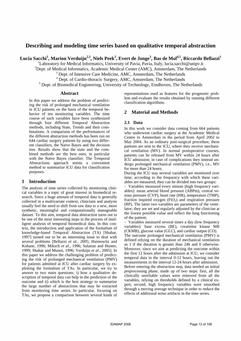
Abstract In this paper we address the problem of predict-ing the risk of prolonged mechanical ventilation in ICU patients on the basis of the temporal be-havior of ten monitoring variables. The time course of such variables have been synthesized through four different Temporal Abstraction methods, including State, Trends and their com-binations. A comparison of the performances of the different abstraction methods has been run on 644 cardiac surgery patients by using two differ-ent classifiers, the Naïve Bayes and the decision tree. Results show that the state and the com-bined methods are the best ones, in particular with the Naïve Bayes classifier. The Temporal Abstractions approach seems a convenient method to summarize ICU data for classification purposes.

1 Introduction The analysis of time series collected by monitoring clini-cal variables is a topic of great interest in biomedical re-search. Since a huge amount of temporal data is generally collected in a multivariate context, clinicians and analysts usually feel the need to shift from raw data to a new, more synthetic, meaningful and computationally manageable dataset. To this aim, temporal data abstraction turns out to be one of the most interesting steps in the process of intel-ligent analysis of temporal biomedical data. In this con-text, the introduction and application of the formalism of knowledge-based Temporal Abstraction (TA) [Shahar, 1997] turned out to be an interesting issue to deal with several problems [Bellazzi et al., 2005; Haimowitz and Kohane, 1996; Miksch et al., 1996; Salatian and Hunter, 1999; Shahar and Musen, 1996; Verduijn et al., 2005]. In this paper we address the challenging problem of predict-ing the risk of prolonged mechanical ventilation (PMV) for patients admitted at ICU after cardiac surgery by ex-ploiting the formalism of TAs. In particular, we try to answer to two main questions: i) how a qualitative de-scription of temporal data can help in the prediction of the outcome and ii) which is the best strategy to summarize the large number of abstractions that may be extracted from monitoring time series. In particular, focusing on TAs, we propose a comparison between several kinds of

representations used as features for the prognostic prob-lem and evaluate the results obtained by running different classification algorithms.

2 Material and Methods

2.1 Data In this work we consider data coming from 664 patients who underwent cardiac surgery at the Academic Medical Centre in Amsterdam in the period from April 2002 to May 2004. As an ordinary post-surgical procedure, these patients are sent to the ICU, where they receive mechani-cal ventilation (MV). In normal postoperative courses, patients can be released from MV within 24 hours after ICU admission; in case of complications they instead un-dergo prolonged mechanical ventilation (PMV), i.e., MV for more than 24 hours. During the ICU stay several variables are monitored over time; according to the frequency with which these vari-ables are measured, they can be divided into two groups: - Variables measured every minute (high frequency vari-ables): mean arterial blood pressure (ABPm), central ve-nous pressure (CVP), heart rate (HR), temperature (TMP), fraction inspired oxygen (FiO2) and respiration pressure (RP). The latter two variables are parameters of the venti-lator; they are set and regularly adjusted by the clinician at the lowest possible value and reflect the lung functioning of the patient; - Variables measured several times a day (low frequency variables): base excess (BE), creatinine kinase MB (CKMB), glucose value (GLC), and cardiac output (CO). The outcome prolonged mechanical ventilation (PMV) is defined relying on the duration of mechanical ventilation as 1 if the duration is greater than 24h and 0 otherwise. Moreover, since we aim at predicting the outcome within the first 12 hours after the admission at ICU, we consider temporal data in the interval 0-12 hours, leaving out the measurements in the interval 12-24 hours after admission. Before entering the abstraction step, data needed an initial preprocessing phase, made up of two steps: first, all the clinically unreliable values were removed from all the variables, relying on thresholds defined by a clinical ex-pert; second, high frequency variables were smoothed through a moving average technique in order to reduce the effects of additional noise artifacts in the time series.


For the qualitative representation of the time series we chose to resort to the formalism of knowledge-based TA.

2.2 Knowledge-based Temporal Abstractions Temporal Abstractions represent a convenient AI tech-nique to extract compact and meaningful descriptions from temporal data; the most interesting feature of such representation is the shift from a time-point (quantitative) to an interval-based qualitative representation of the time series, aimed at extracting specific patterns which are verified in the data. Within TAs, we can distinguish be-tween basic and complex abstractions. Basic TAs are used to extract simple patterns, and can be specified into Trend TAs, to capture increasing, decreasing or stationary courses in a numerical time series, and State TAs, to de-tect qualitative patterns corresponding to low, high or normal values in a numerical or symbolic time series. Complex TAs, on the other hand, correspond to intervals in which specific temporal relationships between basic or other complex TAs hold. Such temporal relationships are usually identified with the ones defined in Allen algebra [Allen, 1984].

2.3 Comparison between different TA represen-tations

As already mentioned in the introduction, in this paper we address the problem of the representation of temporal variables recorded during an ICU stay through TAs, aim-ing at evaluating their capability in predicting the outcome and at establishing a comparison of different descriptions of the variables. In more detail, by exploiting TAs in sev-eral ways, we propose the four representations introduced in the following sections.

Representation through State TAs Through this representation we aim at assigning an ab-straction reflecting information on the level of each vari-able (i.e., low, normal, high) over intervals specified over the time series. In particular, for high frequency variables we aim at defining a label over the four 3-hours intervals: 0-3, 3-6, 6-9, 9-12 hours, while for the low frequency variables the labels are detected over the two 6-hours in-tervals 0-6 and 6-12 hours after admission at the ICU. To extract such labels, each numerical value of the time se-ries is first replaced by a qualitative label of the kind ‘low’, ‘normal’, or ‘high’, where the thresholds for defin-ing the levels are detected through an automatic 10-fold cross validation procedure. As a second step, the propor-tion of labels of different type found over each interval is evaluated, in order to establish a label valid over all the period. If a label is found to be significantly overrepre-sented over a period (p-value of a chi-squared Pearson’s statistic <0.05), that label is then assigned to the corre-sponding interval. If no majority label can be detected, the interval is labeled with a ‘varying’ TA. According to this strategy, a total number of 32 features for the classifica-tion problem is obtained; we have in fact one label for each of the 4 three-hour periods for the 6 high frequency variables and one label for each of the 2 six-hour periods for the 4 low frequency variables.

Representation through trend TAs Through this representation we aim at assigning an ab-straction reflecting information on the temporal trend of each variable (i.e. increasing, decreasing, stationary) over specific intervals. For what concerns the high frequency variables ABPm, CVP, HR and TMP, the same 3-hours intervals identified for the state abstractions are consid-ered. As a first step, trend detection is performed over each of the considered periods, relying on a piecewise linear segmentation of the time series carried out through a sliding window algorithm [Keogh et al, 2003]. A trend label reflecting the information on the slope is used to label each segment of the approximating curve. The pro-cedure for trend detection develops then in a similar way as for state abstractions: if more than one type of trend is detected over the three-hour period, a chi-squared Pear-son’s statistic is computed to determine if one trend label can be assigned as a global label to that specific period (p-value<0.05). If that is not the case, the global label ‘vary-ing’ is assigned to the trend pattern. Because of the long steady periods and the little number of measurements respectively, the variables FiO2 and RP and the four low frequency variables were all considered over the whole twelve-hour period; according to this pro-cedure, one global trend label is assigned to these time series relying on the slope of the regression line obtained over the whole period. According to this strategy, a total number of 22 features for the classification problem is obtained; we have in fact one label for each of the 4 three-hour periods for ABPm, CVP, HR and TMP plus one label for FiO2, RP and the 4 low frequency variables.

Combining State and Trend Abstractions With this representation, features are defined by merging the information coming from both the trend and the state descriptions extracted as described in the previous para-graphs. In particular, state and trend labels are combined over each period defined for each variable, replicating the trend label where necessary (e.g., the state labels of each three-hour period for the variables FiO2 and RP are com-bined with the trend label of the twelve hour period of these variables, which is ‘spread’ over every subperiod). As in the case of the State TA representation, the total number of features for the classification problem is of 32.

Clustering State and trend TAs To reduce the high number of features (22 for the trend representation and 32 for the state description) obtained by representing time series through trend and state TAs we performed a clustering of the available labels and used the information on both the clustering trends and states as features for the classification problem. The general proce-dure to cluster the qualitative variables develops in a way which is similar both for trend and state TAs. In particu-lar, when the variable is evaluated on different periods, the labels are first pasted together to form a pattern of trend or state changes. Time series that present similar labels are then clustered together according to an heuristic criterion. The following tables show the clusters that have been defined for each variable.


STATE TAs Classification

Algorithm CA Sensitivity Specificity AUC

NB 0.7803 0.8589 0.5939 0.8163 CT 0.7244 0.8739 0.3703 0.6777

Table 1. Labels for the clustered State TAs

STATE Tas Variables Clusters ABPm, CVP, HR, and TMP

‘high at least for six consecutive hours’ ‘low at least for six consecutive hours’ ‘normal for the last nine hours or for the whole twelve-hour period’, ‘normal for the last six hours’ ‘normal at least six consecutive hours not at the end’ ‘varying’

FiO2 and RP ‘high at least for the six last hours’ ‘normal all twelve hours or low at least for six consecutive hours’ ‘normal at least for the six last hours ‘varying’

BE, CI, CKMB, and GLC

‘high at least for the six last hours’ ‘low at least for the six last hours’ ‘normal all twelve hours’ ‘normal at least for the six last hours’ ‘varying’

Table 2. Labels for the clustered Trend TAs As it is clear from the previous tables, the clusters are not mutually exclusive: for example, a variable which is nor-mal in the last nine hours is also normal in the last six hours. To overcome this ambiguity, the variables are as-signed to the most specific group (e.g. normal in the last nine hours).

2.4 Prognostic modeling Once the TA-based features for each representation have been derived, both Naïve Bayes and classification trees were tested on the task of predicting the risk of PMV. The performances of the two classifiers were evaluated through 3-fold cross validation. The analysis were per-formed in Orange, a data mining environment which is based on visual programming [Demsar et al., 2004].

3 Results In this Section we will present the results obtained by running Naïve Bayes and classification trees on the prob-lem of predicting the risk of PMV from ICU monitoring temporal variables. For each of the TA representations presented in Section 2 a table is reported. As a reference, also the results for the majority classifier are shown. Classification accuracy (CA), sensitivity, specificity and area under ROC curve (AUC) are shown for a complete evaluation of the performances of the classifiers.

Table 3. Results for the default classifier, which classifies all the examples according to the majority class in the training set.

Table 4. Results for the State TA representation. (NB = Naïve Bayes, CT = Classification Tree)

TREND TAs Classification


NB 0.6958 0.6378 0.5013 0.6502 CT 0.6494 0.6579 0.5846 0.5785

Table 5. Results for the Trend TA representation. (NB = Naïve Bayes, CT = Classification Tree)

MERGED TAs Classification


NB 0.7623 0.8589 0.5324 0.8023 CT 0.7231 0.8547 0.4104 0.6603

TREND Tas Variables Clusters ABPm, CVP, HR, and TMP

‘decreasing at least for six consecutive hours’, ‘increasing at least for six consecutive hours’, and ‘varying’

Table 6. Results for the Merged State and Trend TA representa-tion. (NB = Naïve Bayes, CT = Classification Tree)

Table 7. Results for the Clustered State and Trend TA represen-tation. (NB = Naïve Bayes, CT = Classification Tree)

CLUSTERED TAs Classification


NB 0.7517 0.8632 0.4680 0.7737 CT 0.7073 0.8377 0.3972 0.6201

By comparing the results obtained using different kinds of TA representations, we can point out some interesting observations: first of all, the trend representation as it is seems to be not informative for the prediction of the out-come. The reason for such a behaviour may be that con-sidering only the information about the trend (i.e. without any hint on the level of the variable) might not be enough to describe causes that may lead to a PMV. The observa-tion that, on the other hand, the state representation results in better performances with both the classifiers supports the hypothesis just introduced. The merging of state and trend TAs into a single label, that can be seen as a complex TA, performs in a way that is comparable to the state representation. From a clinical point of view this description might anyway be more in-formative that the mere use of state TAs, since it allows a more complete description of the variables, including both level and trend information. A similar comment can be made also for what concerns the representation through clustered variables; with such a description we have in fact the possibility of synthesizing both the trend and the state features with an improvement in interpretability and clarity of the results for the clini-cians. Classification


Majority 0.7048 1 - 0.5000 4 Discussion and conclusions In this paper we have analyzed how a qualitative represen-tation of time series through knowledge-based TAs can be exploited for the task of predicting the risk of prolonged


mechanical ventilation in patients recovered at the ICU after cardiac surgery. We have introduced four descriptions of temporal data derived by exploiting temporal abstractions in several ways. One of the main advantages of introducing such a representation of time series is of course the fact that it results in a more intuitive and clear interpretation of the results by the clinicians. The descriptions of the variables obtained in terms of TAs are in fact self-explanatory and don’t need to be interpreted by an algorithm-expert. Another issue that we have explored in this paper is the effect of combining different abstractions (representation through merged and clustered TAs) in terms of predictive capability and to reduce the number of features of the problem. From the results it turns out that the best performances are obtained when introducing the information on the level of the variables into the problem features. Trend information by itself results in fact in poor performances of both the considered classifiers. The two methods for coupling both trend and state descriptions result rather satisfactory in terms of performances and in terms of synthesis of the information in a lower number of features in terms of in-terpretability of the results. Further work can be made on both on the improving of the description through trend TAs, in particular by consider-ing also the information about the rate (e.g. ‘slightly in-creasing’ or ‘fast decreasing’) and also on the improving on sensitivity which results rather low in all the cases.

References [Allen, 1984] James F. Allen. Towards a general theory of

action and time. Artificial Intelligence, 23:123-154, 1984.

[Bellazzi et al., 2005] Riccardo Bellazzi, Cristiana Lariz-za, Paolo Magni, and Roberto Bellazzi. 2005. Tempo-ral data mining for the quality assessment of hemodi-alysis services. Artificial Intelligence in Medicine, 34(1):25-39, 2005.

[Demsar et al., 2004] Janez Demsar, Blaz Zupan, Gregor Leban. Orange: From Experimental Machine Learning to Interactive Data Mining. White Paper (www.ailab.si/orange). Faculty of Computer and In-formation Science. University of Ljubljana, 2004.

[Haimowitz and Kohane, 1996] Ira J. Haimowitz, Isaac S. Kohane. Managing temporal worlds for medical trend diagnosis. Artificial Intelligence in Medicine, 8: 299-321, 1996.

[Keogh et al., 2003] Eamonn Keogh, Selina Chu, David Hart, Michael Pazzani. Segmenting time series: A sur-vey and novel approach. In: M. Last, A. Kandel, H. Bunke (Eds.), Data Mining in Time Series Databases, World Scientfic Publishing Company, pp. 1-22, 2003.

[Miksch et al., 1996] Silvia Miksch, Werner Horn, Chris-tian Popow, Franz Paky. Utilizing temporal data ab-straction for data validation and therapy planning for artificially ventilated newborn infants Artificial Intelli-gence in Medicine, 8: 543-576, 1996.

[Salatian and Hunter, 1999] Apkar Salatian, Jim Hunter. Deriving trends in historical and real time continu-ously sampled medical data. Journal of Intelligent In-formation Systems, 13: 47-71, 1999.

[Shahar and Musen, 1996] Yuval Shahar and Mark A. Musen. Knowledge-based temporal abstraction in clinical domains. Artificial Intelligence in Medicine 8(3):267-98, 1996.

[Shahar, 1997] Yuval Shahar. A framework for knowl-edge-based temporal abstraction. Artificial Intelligence, 90:79-133, 1997. [Verduijn et al., 2005] Marion Verduijn, Arianna Dagliati,

Lucia Sacchi, Niels Peek, Riccardo Bellazzi, Evert de Jonge, Bas de Mol. IC prediction from patient monitoring data: a comparison of two temporal abstraction procedures. In Proceedings of the AMIA 2005 Annual Symposium,2005.


Temporal Characterization of Ill-known Diseases

Silvana Badaloni and Marco FaldaUniversity of Padova via Gradenigo 6, 35100 Padova, Italy

[email protected], [email protected]

AbstractIn the identification of unknown diseases thetemporal evolution is one of the most importantaspects. Very often information about a new dis-ease is imprecise and vague, due to the fact thatthe disease itself is hardly recognized by study-ing the symptoms of the patients. To this aim,we have applied a Fuzzy Temporal Reasoningsystem we have developed to the case of SevereAcute Respiratory Syndrome (SARS). The sys-tem is able to handle both qualitative and met-ric temporal knowledge affected by vaguenessand uncertainty. In this preliminary work, weshow how the fuzzy temporal framework allowsus to represent temporal evolutions of symptomsin different patients thus making possible to de-duce characteristic periods of an unknown dis-ease such as SARS was.

1 IntroductionUnpurified drinking water, improper use of antibiotics, lo-cal warfare, massive refugee migration and changing socialand environmental conditions around the world have fos-tered the spread of new and potentially devastating virusesand diseases and have made surveillance for infectiousdiseases a public health need [Berkelman et al., 1994;Berkelman et al., 1996].

Medical examiners and coroners certify approximately20% of all deaths that occur within the United States andcan be a key source of information regarding infectiousdisease deaths [Wolfe et al., 2004]. A computer-assistedsearch tool could detect infectious disease deaths from amedical examiner database, thereby reducing the time andresources required to perform such surveillance manually.

Medical diagnosis is a field in which imprecise informa-tion about symptoms and events can appear; for examplethis happens when the physician must interpret the descrip-tion of a patient, or when a new disease appears and typicalpatterns have to be discovered. Human reasoning aboutuncertainty is often poorly coherent, while an automatedsystem can guarantee an homogeneous treatment of vaguedata.

The framework of Fuzzy Sets can be regarded as themost suitable formalism to deal with imprecision intrin-sic to many medical problems [Steimann, 2001] especially

when epidemiological studies cannot be developed sincestatistical data are lacking or insufficient. Therefore, fuzzy-set based approaches allow one the ease of expression of-fered by symbolic models avoiding the unwieldiness of an-alytical alternatives, bridging the gap between the discreteworld of reasoning and the continuity of reality [Steimann,2001].

The most common use of fuzzy temporal reasoning inmedical diagnosis is for representing the temporal evolu-tion of the manifestations of patient diseases in order to rec-ognize the typical temporal evolution of a specific disease,and then make a diagnosis. In [Wainer and Rezende, 1997;Wainer and Sandri, 1999] it has been shown how diag-nostic reasoning can be fundamental to detect infectiousdiseases on the basis of temporal information. For exam-ple, Staphylococcus aureus and short therm Bacillus cereusare the only possible bacterial causes for nausea and vom-iting within 1-6 h from ingestion of contaminated matterwhile a patient with botulism will only have those symp-toms only 18-36 h after ingestion. In [Badaloni and Falda,2005] we have addressed the problem of recognizing an ex-anthematic disease starting from the approximated knowl-edge of the temporal sequence of its symptoms and fromthe imprecise data coming from a patient’s description. Inexanthematic diseases the temporal evolution and the du-ration of the symptoms are sufficient to discriminate them,therefore the diagnosis can be based on the identification oftypical temporal structures.

In this preliminary work, we address the problem of di-agnostic reasoning from a different point of view. We startfrom a set of data concerning the temporal evolution ofsymptoms of different patients affected by an unknown orill-known disease. It should be noticed that, at the mo-ment, we don’t treat data extracted from laboratory tests ortemporal biomedical patterns that would require the use ofadvanced methodologies to deal with [Sacchi et al., 2005]but, more simply, we treat temporal data relative to com-mon symptoms of a limited group of patients. Once repre-sented such data in a fuzzy constraint temporal network, wepropose a method for abstracting general temporal featurescharacterizing the disease, if they exist (e.g. the incubationperiod). To this aim we utilize a model [Badaloni et al.,2004] based on Fuzzy Temporal Constraint Networks. Theconstraint based system allows one to manage in a unifiedframework temporal information of different types. In fact,temporal information coming from the domain may be both


qualitative such as “the interval I1 with fever precedes theinterval I2 with cough” or metric such as “fever lasts oneday” or mixed such as “symptom m2 follows symptom m1and starts at 8pm”.

In this paper, we present an application of our temporalreasoning system in a case study: the Severe Acute Respi-ratory Syndrome (SARS). It is organized as follows: Sec-tion 2 describes our approach to integrate temporal infor-mation in presence of vagueness and uncertainty, Section 3defines the medical problem under study, Section 4 reportsthe considered temporal data and shows how the problemcan be modeled. Finally, the results are discussed in Sec-tion 5.

2 Qualitative and quantitative fuzzytemporal constraints

Let’s first describe the different components of our integra-tion model. To deal with qualitative temporal informationthe most famous approach is the Allen’s Interval Algebra[Allen, 1983]; in this algebra each constraint is a binaryrelation between a pair of intervals, represented by a dis-junction of atomic relations:

I1 (rel1, . . . , relm) I2

where each rel i is one of the 13 mutually exclusiveatomic relations that may exist between two intervals (suchas equal, before, meets etc.).

Allen’s Interval Algebra has been extended in [Badaloniand Giacomin, 2006] with the Possibility Theory [Duboiset al., 1996] by assigning to every atomic relation rel i a de-gree αi, which indicates the preference degree of the corre-sponding assignment among the others

I1 R I2 with R = (rel1[α1], . . . , rel13[α13])

where αi is the preference degree of rel i (i = 1, . . . , 13);preferences can be defined in the interval [0, 1]. If we takethe set 0, 1 the classic approach is obtained.

Intervals are interpreted as ordered pairs (x, y) : x ≤ yof <2, and soft constraints between them as fuzzy subsetsof <2×<2 in such a way that the pairs of intervals that arein relation relk have membership degree αk.

If temporal entities are points, the Point Algebra [Vilainet al., 1989] and its fuzzy extension [Badaloni and Gia-comin, 2006] have been considered. In the classical case,i.e. when temporal information is not affected by uncer-tainty and vagueness, a Qualitative Algebra QA that in-cludes all the combinations that can occur between tem-poral points and intervals is defined in [Meiri, 1996], con-taining all the algebras: the Point Algebra PA , the Inter-val Algebra IA, the Point-Interval and Interval-Point Alge-bras PI and IP , referring to point-point, interval-interval,point-interval, interval-point relations. In order to buildthe fuzzy Qualitative Algebra QAfuz , we have consid-ered the corresponding fuzzy extensions PAfuz and IAfuz

[Badaloni and Giacomin, 2002; Badaloni and Giacomin,2006], PIfuz and IP fuz [Badaloni et al., 2004].

Dealing with temporal metric information, tradi-tional Temporal Constraint Satisfaction Problems (TCSPs)[Dechter et al., 1991] have been extended to the fuzzy case[Marın et al., 1997; Godo and Vila, 2001]. In most cases

trapezoidal distributions have been used, since they seemenough expressive and computationally less expensive. Wetoo adopt trapezoidal distributions: each trapezoid is rep-resented by a 4-tuple of values describing its four charac-teristic points plus a degree of consistency αi denoting itsheight.

Tk = ak, bk, ck, dk [αk]with ak, bk ∈ <∪−∞, ck, dk ∈ <∪+∞, αk ∈ (0, 1], is either ( or [ and is either ) or ].

The points bk and ck determine the interval of those tem-poral values which are likely, whereas ak and dk determinethe interval out of which the values are absolutely impossi-ble.

As an example, let’s consider the following sentence:“Patient P1 had fever on February 27; within ap-proximately 5 days he developed cough.”

By setting the origin of time on February 27 and assum-ing an imprecision of one day, we can model this sentenceas

P1 : (4, 4.5, 5.5, 6)

in Figure 1 its graphical representation is shown.

Figure 1: Example of trapezoidal possibility distribution

In our approach the following trapezoids can be mod-eled:

open triangle:(ai, ai, ai, di)[αi]open trapezoid:(−∞,−∞, ci, di)[αi]

closed left semiaxis:(−∞,−∞, di, di][αi]in this way the expressiveness of the language is in-

creased with respect to e.g. [Barro et al., 1994]. Be-sides, these trapezoids allow us to integrate qualitative con-straints.

As far as operations between metric constraints areconcerned, the usual operations i.e. inversion, conjunc-tive combination, disjunctive combination and compositionhave been defined.

2.1 About the integrationFuzzy qualitative constraints and fuzzy metric constraintshave been integrated together in a single framework[Badaloni et al., 2004] defining two transformation func-tions QUANfuz and QUALfuz that allow to switch fromthe qualitative to the metric plane and vice versa. In theconversion from the metric to the qualitative plane a lot ofinformation is lost, due to the fact that for example any met-ric constraint that represents a positive distance betweentemporal events is transformed into the “before” qualitativeconstraint; nothing instead is lost in the inverse conversion.For this reason, when the constraints to be represented are


of different nature the operations between qualitative andmetric constraints are made, as far as possible, in the met-ric plane, in order to loose as less information as possible;therefore we always try to transform the qualitative con-straints into metric constraints. There is a case howeverwhere it is not possible to remain in the metric plane; thishappens when the composition operation involves a mixedqualitative relation. In this case it is necessary to transformthe metric operand and to operate in the qualitative plane.Once the operations have been extended to the fuzzy caseusual algorithms to solve CSPs can be easily generalized.

This way, we can manage temporal networks wherenodes can represent both points and intervals, and whereedges are accordingly labeled by qualitative and quantita-tive fuzzy temporal constraints. A more detailed descrip-tion of our approach can be found in [Badaloni et al., 2004].

2.2 AlgorithmsThe notions of local consistency have been extended too.In particular, local consistency has been expressed as thedegree of satisfaction which denotes the acceptability ofan assignment with respect to the soft constraints involvedin the relative sub-network. According to [Dubois et al.,1996], this degree of satisfaction corresponds to the leastsatisfied constraint.

Moreover, Path-Consistency and Branch & Bound algo-rithms have been generalized to the fuzzy case adding somerelevant refinements that improve their efficiency. Path-consistency allows to prune significantly the search spacewhile having a polynomial computing time.

In our integrated system embedding both qualitative andmetric constraints composition and conjunction operationsused in the algorithms depend on the type of operands,therefore they change according to the kind of constraintsto be processed (qualitative or metric).

3 The SARS caseIn the following we will consider the case of SARS, a kindof pneumonia spread from Far East in 2003. We take as ref-erence one of the first articles written in that period [Pouta-nen et al., 2003]; it is about the cases in Toronto. We willstudy only four patients of ten (Patients 1, 2, 7 and 8), be-cause they are better described from the temporal point ofview. In this initial study the scenario has been simplified,but it is sufficient to show the flexibility of the constraintsthat can be used to model a problem, but the system couldbe applied to tens of patients thus outperforming a humananalysis in terms of coherence and consistency.

3.1 Description of the outbreakThe Toronto index case (Patient 1) and her husband trav-eled to Hong Kong to visit relatives from February 13through February 23, 2003. They returned to their apart-ment in Toronto on February 23, 2003. Patient 1, a 78-year-old woman, had fever, anorexia, myalgias, a sore throat,and mild nonproductive cough two days after returninghome. Two days later, she noted the development of in-creasing cough with dyspnea. She died three days later, onMarch 5, at home, nine days after the onset of her illness.

The index patient’s 43-year-old son (Patient 2), had feverand diaphoresis on February 27. Within approximately five

days he became afebrile, but concurrently, a nonproductivecough, chest pain, and dyspnea developed. Because of per-sistent symptoms, 4 days later he was assessed at a hospitaland noted to have a fever (temperature, 39.8C) and an oxy-gen saturation of 82 percent while breathing room air. De-spite intensive physiological support, multiorgan dysfunc-tion syndrome developed, and he died on March 13, 2003,6 days after admission, and 15 days after becoming ill.

As a result of media attention, three additional cases ofSARS were identified. The first case was in a previouslyhealthy 37-year-old female family physician of Asian de-scent (Patient 7) who saw Patient 2 and his wife on March6, when they were both symptomatic. Patient 7 had a severeheadache on March 9, followed by fevers (temperaturesof up to 40C), myalgias, and malaise. Four days later, anonproductive cough developed, and she was noted to havefever (temperature, 38.5C) and tachypnea with an oxygensaturation of 100 percent on room air.

The second additional identified case was in a 76-year-old man of non-Asian descent (Patient 8). Patient 8 was as-sessed in the emergency department on March 7 for atrialfibrillation and observed overnight on a gurney separatedby a cotton curtain 1 to 2 m from Patient 2. Patient 8was discharged home on March 8, and two days later hehad fever (temperatures of up to 40C), diaphoresis, andfatigue. Despite receiving broad-spectrum antibiotics, os-eltamivir, intravenous ribavirin, and intensive support, hedied on March 21, 5 days after admission and 12 days afterthe onset of his illness.

4 Modelling the scenariosThe four patients were suspected to have SARS because thelived in the same apartment in Toronto and the symptomswere similar to those reported in Hong Kong, where Patient1 spent a week before returning home.

Our aim is to characterize the incubation period, that isthe period between the contagion and the first symptoms.To do this, we take into account the period during which thedisease could have been got, the fever (as initial symptom),the cough, the contagion and the death.

For example the following temporal evolution can be ab-stracted from the previous observations about Patient 1:

• in travel from February 13 to February 23;• 2 days later, fever;• 2 days later, cough;• 3 days later, death.

These temporal descriptions allow to build timetables foreach patient in exam, as depicted in Figure 3. Note thatmetric information need to be specified as relative distancesbetween temporal events, since this is the semantics of met-ric constraints.

Four distinct networks have been build for each patientstarting from the previous data. In a preliminary phase thesymptoms common to all patients have been identified bythe physicians. There are seven significant points plus aninterval (V6) that represents the period during which thedisease could be got, in the following called I .

The seven points become the network vertices and areidentical in each network (Figure 3):


15

13 23 25 27 2 6 7 8 9 10 13 14 15

13 23 25 27 2 6 7 8 9 10 13 14 15

13 23 25 27 2 6 7 8 9 10 13 14 15

H R F D

V F C

HCF D

13 23 25 27 2 6 8 9 10 13 14

T CF D T: travel D: deathF: fever V: visitC: cough R: dischargeH: hospital

Figure 2: Timelines for the patient’s data

1. V0: t0, the “origin of time”;2. V1: begin of I;3. V2: end of I;4. V3: fever;5. V4: cough;6. V5: death;8. V7: contagion.

The “origin of time” has been set on February 23, thatis the day in which Patient 1 returned home and infectedher family. The end of period I coincides respectively withthe death, the admission to hospital, the discharge to homeand the one-day medical visit. The constraints that referto a patient have been defined as in the following example,where we assume an uncertainty of half a day:

• about -10 days from V0 to V1:

V0[−11,−10.5,−10,−9.5]V1

• 0 days from V0 to V2

V0=V2

• about 2 days from V2 to V3

V2[1, 1.5, 2.5, 3]V3


V3[1, 1.5, 2.5, 3]V4

Figure 3: Graph of the problem


V4[2, 2.5, 3.5, 4]V5

Additionally in all four cases there are the following con-straints that model the facts that the contagion must be be-fore the first symptom and that the I period is characterizedby a begin and an end, and that the contagion must be con-tained in period I .

V7<V3

V6siV1

V6fiV2

V7d, s, fV6

In this example all qualitative constraints have a degreeof preference equal to 1, because here they are used onlyto link qualitative intervals with metric points. Metric con-straints instead present, as said before, a trapezoidal possi-bility distribution (that is the set of all preference degrees inthe domain) that sets the maximal plausibility to the assign-ments in the core between b and c, and states as impossiblethe values outside the range (a, d).

5 ResultsThe previous networks are then coded as XML files basedon a XML schema designed to represent Fuzzy TemporalNetworks, and then passed to the solver.

A consistency analysis of the temporal data gave thefollowing incubation estimates in terms of constraints be-tween the contagion V7 and the fever V3, being Pi the pa-tients

P1 : V3(−13.5,−12.5,−1.5,−1.0)V7

P2 : V3(−4.5,−4.0, 0.0, 0.0]V7

P7 : V3(−4.5,−3.5,−2.0,−1.0)V7

P8 : V3(−5.0,−3.5,−1.5,−1.0)V7


That can be interpreted as:

P1: approximately from 1 to 12 days;



P8: approximately from 1 to 4 days.

The output of the solver is still a valid XML file thatcould be possibly modified and processed again. In thisprototype version the application has a command line in-terface, but since it works with XML the output could beeasy formatted to be shown on a Web interface using XMLstylesheets.

In Figures 4, 5, 6 and 7 the period I is represented as ahatched rectangle and the incubation period as an intervalbetween the begin of the period I and the onset of the firstsymptoms.

Figure 4: Evolution in Patient 1



In this paper to merge information coming from differ-ent sources the intersection operations has been considered:therefore real incubation period is the intersection of thefour estimated periods, that is about 2-4 days. In this casethe deduction has been not too difficult, but in a more re-alistic scenario with a lot of temporal data to analyze anautomated reasoning system could be very helpful for aphysician that has to figure out the temporal evolution ofthe symptoms of a new disease. Besides, a more robusttechnique should take into account the weight of data com-ing from different sources in order to reduce the influenceof less common cases (possibly wrong).

6 ConclusionsIn this paper we have shown an application of our tempo-ral constraint solver in a medical domain; this applicationcould support the physician to characterize temporally an


unknown disease by aid him to deduce its temporal evo-lution. Our solver extends the classic temporal constraintsby allowing to specify uncertainty and vagueness; this isfundamental in the context of unknown illnesses.

In order to make the system more useful a first enhance-ment will be the management of constraint classes; in thisway, it will be possible to merge automatically the deduceddurations in order to identify the most plausible.

Moreover, as in [Wainer and Sandri, 1999; Keravnou,2002], a real diagnosis expert system should consider alsoatemporal aspects of diseases. As future work we intend toenrich our system by addressing also these aspects.

References[Allen, 1983] J. F. Allen. Maintaining knowledge about

temporal intervals. Communications of the ACM,26(1):832–843, 1983.

[Badaloni and Falda, 2005] S. Badaloni and M. Falda.Discriminating exanthematic diseases from temporalpatterns of patient symptoms. In LNAI 3581, pages 33–42, Springer, Germany, 2005.

[Badaloni and Giacomin, 2002] S. Badaloni and M. Gia-comin. Fuzzy extension of interval-based temporal sub-algebras. In Proc. of IPMU 2002, pages 1119–1126,Annecy, France, 2002.

[Badaloni and Giacomin, 2006] S. Badaloni and M. Gia-comin. The algebra IAfuz: a framework for qualita-tive fuzzy temporal reasoning. Artificial Intelligence,170(10):872–908, 2006.

[Badaloni et al., 2004] S. Badaloni, M. Falda, and M. Gi-acomin. Integrating quantitative and qualitative con-straints in fuzzy temporal networks. AI Communica-tions, 17(4):183–272, 2004.

[Barro et al., 1994] S. Barro, R. Marın, J. Mira, and A. Pa-ton. A model and a language for the fuzzy representationand handling of time. Fuzzy Sets and Systems, 175:61–153, 1994.

[Berkelman et al., 1994] R. L. Berkelman, R. T. Bryan,M. T. Osterholm, J. W. LeDuc, and J. M. Hughes. In-fectious disease surveillance: a crumbling foundation.Science, 264:368–370, 1994.

[Berkelman et al., 1996] R. L. Berkelman, R. W. Pinner,and J. M. Hughes. Addressing emerging microbialthreats in the united states. JAMA, 275:315–317, 1996.

[Dechter et al., 1991] R. Dechter, I. Meiri, and J. Pearl.Temporal constraint networks. Artificial Intelligence,49:61–95, 1991.

[Dubois et al., 1996] D. Dubois, H. Fargier, and H. Prade.Possibility theory in constraint satisfaction problems:


Handling priority, preference and uncertainty. AppliedIntelligence, 6:287–309, 1996.

[Godo and Vila, 2001] L. Godo and L. Vila. Possibilistictemporal reasoning based on fuzzy temporal constraints.In Proc. of IJCAI95, pages 1916–1922, 2001.

[Keravnou, 2002] E. T. Keravnou. Temporal constraintsin clinical diagnosis. Journal of Intelligent and FuzzySystems, 12(1):49–67, 2002.

[Marın et al., 1997] R. Marın, M. A. Cardenas, M. Balsa,and J. L. Sanchez. Obtaining solutions in fuzzy con-straint network. International Journal of ApproximateReasoning, 16:261–288, 1997.

[Meiri, 1996] I. Meiri. Combining qualitative and quanti-tative constraints in temporal reasoning. Artificial Intel-ligence, 87:343–385, 1996.

[Poutanen et al., 2003] Susan M. Poutanen, Donald E.Low, Bonnie Henry, Sandy Finkelstein, David Rose,Karen Green, Raymond Tellier, Ryan Draker, DenaAdachi, Melissa Ayers, Adrienne K. Chan, Danuta M.Skowronski, Irving Salit, Andrew E. Simor, Arthur S.Slutsky, Patrick W. Doyle, Mel Krajden, Martin Petric,Robert C. Brunham, and Allison J. McGeer. Identifica-tion of severe acute respiratory syndrome in canada. TheNew England Journal of Medicine, 348(20):1995–2005,2003.

[Sacchi et al., 2005] L. Sacchi, R. Bellazzi, C. Larizza,R. Porreca, and P. Magni. Learning rules with complextemporal patterns in biomedical domains. In LNAI 3581,pages 23–32, Springer, Germany, 2005.

[Steimann, 2001] F. Steimann. On the use and usefulnessof fuzzy sets in medical AI. Artificial Intelligence inMedicine, 21:131–137, 2001.

[Vilain et al., 1989] M. Vilain, H. Kautz, and P. van Beek.Constraint propagation algorithms for temporal reason-ing: a revised report. In J. de Kleer D. S. Weld, editor,Readings in Qualitative Reasoning about Physical Sys-tems, pages 373–381, San Mateo, CA, 1989. MorganKaufmann.

[Wainer and Rezende, 1997] J. Wainer and A. Rezende. Atemporal extension to the parsimonious covering theory.Artificial Intelligence in Medicine, 10:235255, 1997.

[Wainer and Sandri, 1999] J. Wainer and S. Sandri. Fuzzytemporal/categorical information in diagnosis. Journalof Intelligent Information Systems, 11:9–26, 1999.

[Wolfe et al., 2004] M Wolfe, K. B. Nolte, and Yoon S.S. Fatal infectious disease surveillance and the medicalexaminer database. Emerg. Infect. Dis., 2004.


Paper session: Signal and Image Processing


Cancer area characterization by non-parametric clustering

U. Castellani, M. Cristani, P. Marzola, V. Murino, E. Rossato∗, A. Sbarbati†

Abstract

The application of machine learning techniquesto open problems in different medical researchfields appears to be stimulating and fruitful, es-pecially in the last decade. In this paper, a newmethod for MRI data segmentation is proposed,which aims at improving the support of medicalresearchers in the context of cancer therapy. Inparticular, our effort is focused on the process-ing of raw output obtained by Dynamic Contrast-Enhanced MRI (DCE-MRI) techniques. Here,morphological and functional parameters are ex-tracted, which seem indicate the local develop-ment of cancer. Our contribute consists in or-ganizing automatically these output, separatingMRI slice areas with different meaning, in a his-tological sense. The technique adopted is basedon the Mean-Shift paradigm, and it has recentlyshown to be robust and useful for different andheterogeneous segmentation tasks. Moreover,the technique appears to be predisposed to nu-merous extensions and medical-driven optimiza-tions.

1 IntroductionSegmentation is a vast and complex domain, both in termsof problem formulation and resolution techniques. It con-sists in formally translating the delicate visual notions ofhomogeneity and similarity, and defining criteria which al-low their efficient implementation[Petitjean, 2002]. Thegoal is to partition the source data into meaningful pieces,i.e. those parts corresponding to the different entities, inthe physical and semantical sense of the application en-visioned. Roughly speaking, the segmentation methodscan be categorized into two main classes:edge-basedand

∗U. Castellani, M. Cristani, V. Murino and E. Rossato are withthe Dipartimento di Informatica, University of Verona, Strada leGrazie 15, 37134 Verona (Italy). Contacts: U. Castellani, [email protected] .

†P. Marzola and A. Sbarbati are with the Department of Mor-phological and Biomedical Sciences, Anatomy and HistologySection, University of Verona, P.le Scuro 10 - Policlinico B.goRoma - 37134 Verona (Italy). Contacts: P. Marzola, [email protected] .

region-based[Petitjean, 2002]. In the former, features cor-responding to part boundaries are first detected and thenregions are built, each one formed by sets of points de-limited by the same boundary. In the latter, points shar-ing the same similarity property are grouped together. Inparticular, three are the most popular approaches to region-based segmentation:split-and-mergemethods, identifiedby a top-down paradigm;region-growingmethods, thatadopt a bottom-up paradigm, andclustering-basedmeth-ods, based on the projection of the points onto a higherdimensional space where the clusters (i.e., segments) arerecovered by defining some particular distance functions[Jainet al., 1999a].

In this paper, we apply a recently proposed clustering-based technique for the analysis of data, which considersas leading framework the Mean Shift (MS) clustering para-digm, proposed in[Comaniciu and Meer, 2002]. The mainunderlying idea of such non parametric approach is that thedata space is regarded as an empirical probability densityfunction to estimate. The MS procedure operates by shift-ing a fixed size estimation window, i.e.,the kernel, fromeach data point towards a local mode, denoted, roughlyspeaking, as a high concentration of points. The pointsconverging to the same mode are considered as belongingto the same region.

Although MS has shown to be a powerful technique forseveral research fields such as image and video segmenta-tion, tracking, clustering and data mining[Comaniciu andMeer, 2002; Collins, 2003; Georgescuet al., 2003], veryfew work has been derived from it in the context of med-ical multidimensional data segmentation.

In this paper, the MS paradigm is applied to performsegmentation of multidimensional data, obtained using Dy-namic Contrast-Enhanced Magnetic Resonance Imaging(DCE-MRI). Briefly speaking, DCE-MRI techniques rep-resent non-invasive ways to discover symptoms of local tu-mor growth, based on a manually-driven feature extractionstep that operates on the MRI imagery.

As explained in the following, our method bring twoadvantages to the current state of the DCE-MRI analysis.First, it permits a more accurate feature extraction step, thathere operates in anautomaticfashion. Second, it permitsto fasten the analysis itself, ensuring a higher throughput,that turns out to be useful in the case of massive analysis.

The rest of the paper is organized as follow. In Section2, an overview of the previous work done in the context


of medical data segmentation is provided; subsequently, inSection 3, the necessary medical background is provided,considering the classical DCE-MRI experimental method-ology, in the contest of the tumor development monitoring.This section will elucidate the nature of the data managed;moreover, here it will be possible to deeply understand theadvantages brought by our method. In Section 4, the MeanShift procedure is explained, connecting it with a classicalpattern recognition procedure, i.e. the Parzen Windows es-timation method. In Section 5, the technical details of theproposed method are reported. Results are shown in Sec-tion 6, also compared with a state of the art method, and,finally, Section 7 concludes the paper.

2 Previous Works

In the realm of medical data segmentation, several workshave been introduced, especially for MRI clustering andclassification[Windishbergeret al., 2003; Dimitriadouetal., 2004; Zhang and Chen, 2004; Wismulleret al., 2006;Arulmurgan et al., 2005; Wei and Yang, 2005; Jainetal., 1999b; Scarthet al., 1995; Castellaniet al., 2005].Most proposed methods are based on theK-Means al-gorithm [McQueen, 1967; Han and Kamber, 2000]. In[Windishbergeret al., 2003; Zhang and Chen, 2004], avariant of the K-Means has been implemented, calledfuzzyC-Means(FCM) [Scarthet al., 1995; Jainet al., 1999b;Dimitriadouet al., 2004]. Such variant takes advantages offuzzy logic algorithms to enhance clustering performance.In particular, the FCM algorithm assigns pixels to fuzzyclusters without labels. Unlike the hard clustering methodswhich force pixels to belong exclusively to one class, FCMallows pixels to belong to multiple clusters with varying de-grees of memberships. In[Windishbergeret al., 2003] theclustering of MRI time series have been performed for theidentification and separation of artifacts as well as quan-tification of expected novel information on brain activi-ties. In[Zhang and Chen, 2004] the authors focused on themethodological aspect of thefuzzy C-Meansby introduc-ing a kernel-induced distance metric and a spatial penaltyon the membership functions. The proposed approach hasproved to be more robust to noise and other artifacts withrespect to standard algorithms. In[Castellaniet al., 2005]the authors proposed a DCE-MRI clustering approach, cou-pled with a Information Visualization module, in which aBayesian development of the K-Means was applied. Herethe add-on is that the number of the clusters is automati-cally computed; the algorithm is similar in spirit to the X-Means algorithm proposed by[Pelleg and Moore, 2000].In [Dimitriadouet al., 2004], a quantitative comparison ofMRI cluster analysis has been reported.With respect to the proposed evaluation, the results clearlyshow that approaches based on k-means algorithm performsignificantly better than all the other methods.More complex techniques have been proposed in[Wis-mulleret al., 2006; Arulmurganet al., 2005; Wei and Yang,2005] which are based on neural networks or genetic algo-rithms[Jainet al., 1999b; Han and Kamber, 2000], but theyare time consuming and therefore are not suitable for inter-active applications.

3 The DCE-MRI analysisThe main purpose of DCE-MRI analysis is to accuratelymonitor the local development of cancer, eventually sub-ject to different treatments.The traditional criteria to assess the tumor response to treat-ment is based on the local measurement of tumor sizechange. This phenomenon is due to the localangiogenesis,i.e., the process of growth of new vessels which provide thetumor tissue with nutrients. In consequence, various angio-genesis inhibitors have been developed to target vascularendothelial cells and to block tumor angiogenesis.

Recently, a different and more appealing indicativesymptom of the cancer development has been analyzed, i.e.the tissue vascularization[Marzolaet al., 2004]. Roughlyspeaking, vascular effect may precede, by a remarkablylong time interval, the effect on tumor growth. For thesereasons, the assessment of antiangiogenic compounds re-quires imaging methods that can detect early vascular al-terations.

DCE-MRI techniques play a relevant role in this field[Marzolaet al., 2004]. The final aim is to provide quan-titative measures that indicate the level of vascularizationin the cancer tissue, eventually treated with antiangiogeniccompounds, in anon-invasiveway.Roughly speaking, the DCE-MRI analysis can be dividedin the following steps (see Fig.1)1: 1) injecting macromole-cular contrast agents in the tissue being analyzed; 2) pro-ducing MRI image sets of different slices of the tissue; 3)extracting morphological and functional parameters suchas fractional plasma volume(fPV) and transendothelialpermeability(kPS), that model the tissue vascularization;in practice, to each point of the MRI image is associated apair consisting offPV andkPS values; 4) manually select-ing a Region Of Interest on the MRI slices, in order to iso-late the highly vascularized local tumoral area; usually thisarea is ring-shaped and separates a necrotic area (that liesin the center of the ring) from the external healthy portionof the tissue; 5) averaging the values offPV andkPS insuch ring-shaped area, obtaining for each slice a couple offPV andkPS mean values, that indicate the overall levelof vascularization. This process has been recently testedusing a well-known anti-cancer treatment[Marzolaet al.,2005], evidencing that thefPV andkPS parameters welldescribe the effectiveness of the treatment, as checked byadditional histological analysis; as we see in the following,we take as experimental data-set the one coming from thisresearch.

In this paper, we strongly improve the process above,providing an automatic method of data segmentation; theproposed technique is applied to this particular kind ofanalysis, but we suppose it can be also applied in general inthe DCE-MRI context. In detail, we focus on steps 3), 4)and 5); our method takes as input the functional parametersfPV andkPS obtained in step 3); in an automatic fashion,it is able to segment areas that experimentally correspondsto the tumoral area extracted by hands in step 4); note thatoriginally this step was driven by histological and physio-

1The procedure listed above comes from the investigation de-tailed in [Marzola et al., 2005], that in turn presents additionalsimilar researches


necroticarea

high vascularized area

healthy area

fPV, kPS

1)

2)

3)

4)

5)

Figure 1: DEC-MRI analysis: example of DEC-MRIanalysys procedure; 1) contrast agent injection; 2) MRI im-age acquisition 3)kPS,fPV extraction; for clarity, here thebright zone highlights the tumor4) ring shape ROI drawingby hand; 5) meankPS,fPV values computation

logical a-priori considerations, being the ring-shaped zonesegmented by hand by an human operator.

The advantage brought by the proposed approach istwofold: firstly and mostly important is that, given a DCE-MRI slice, we provide a region of points composed by anensemble offPV andkPS values that individuate separategroups; note that the partition is histologically meaning-ful, and not relies on a-priori manual settings. Secondly,such a segmentation is produced automatically and quickly( 5 seconds, versus the 4-5 minutes needed for an accu-rate manual setting), thus fasting the analysis process listenabove.

4 Mean ShiftThe Mean Shift procedure is a dated non-parametricdensity estimation technique [Fukunaga, 1990;Comaniciu and Meer, 2002]. The main underlyingidea is that the data feature space is regarded as an em-pirical probability density function to estimate: therefore,a big concentration of points that fall near the locationxindicates a big density nearx.

The theoretical framework of the mean shift arises fromthe Parzen Windows[Dudaet al., 2001] basic expression,i.e. the kernel density estimator, that is

f(x) =1n

n∑

i=1

KH(x− xi) (1)

wheref(x) represents the approximated density calculatedin thed-dimensional locationx, n is the number of avail-able points and

KH(x) = |H|−1/2K(H−1/2x). (2)

Here above,KH can be imagined as a weighted windowused to estimate the density, dependent on the kernelKand the symmetric positive definited×d bandwidth matrixH. The functionK is a bounded function with compactsupport (for full details, see[Comaniciu and Meer, 2002]);

the bandwidth matrix codifies the uncertainty associated tothe whole feature space.

In the case of particular radial symmetric kernels (see[Comaniciu and Meer, 2002]), K can be specified usingonly a 1-dimensional function, theprofile k(·), equal foreach dimension. Moreover, if we assume independenceamong the feature dimensions and equal uncertainty overthem, the bandwidth matrix can be rewritten as propor-tional to the identity matrixH = h2I. Under such hy-potheses, Eq. 2 can be rewritten as:

fh,k(x) =ck,d

nhd

n∑

i=1

k

(∣∣∣∣∣∣∣∣x− xi

h

∣∣∣∣∣∣∣∣2)

(3)

whereck,d is a normalizing constant,n is the number ofpoints available, andk(·) is the kernel profile; in Eq.(3) itis easy to note thatk(·) models how strongly the points aretaken into account for the estimation, in dependence withtheir distanceh to x.

Mean Shift extends this “static” expression, differentiat-ing (3) and obtaining the gradient of the density, i.e.:

∇fh,k(x) =

2ck,d

nhd

[n∑

i=1

g

(∣∣∣∣∣∣∣∣xi − x

h

∣∣∣∣∣∣∣∣2)]

∑n

i=1 xig(∣∣∣∣xi−x

h

∣∣∣∣2)

∑ni=1 g

(∣∣∣∣xi−xh

∣∣∣∣2) −x

(4)

whereg(x) = k′(x). In the above equation, the first termin square brackets isproportional to the normalized den-sity gradient, and the second term is theMean Shiftvector,that is guaranteed to point towards the direction of maxi-mum increase in the density[Comaniciu and Meer, 2002].Therefore, starting from a pointxi in the feature space, themean shift produces iteratively a trajectory that convergesin a stationary pointyi, representing a mode of the wholefeature space.

5 The proposed methodOur segmentation method can be thought as a clusteringprocess, derived from the approach proposed in[Comani-ciu and Meer, 2002]. Briefly speaking, the first step of suchprocess is made by applying the Mean Shift procedure toall the pointsxi, producing several convergency pointsyi. A consistent number of close convergency locations,yil, indicates a modeµl. The labeling consists in mark-ing the corresponding pointsxil that produces the setyil with the labell. This happens for all the convergencylocationl = 1, 2, . . . , L.

In this paper, we consider each point of the MRI as ad-dimensional entity, living in ajoint domain. In specific,eachxi is composed by the pairxs ∈ R2 of spatial coordi-nates relative to thex,y image axes (theforming the spatialsub-domain) and the pairxc ∈ R2 of fPV andkPS co-efficients (forming thecoefficients sub-domain). For eachsub-domain we assume Euclidian metric.In order to explore the joint domain, a multivariate kernel isused[Comaniciu and Meer, 2002; Wanget al., 2004], thathas the form

Khs,hc(xi) =

C

h2sh

2c

k

(∣∣∣∣∣∣∣∣xi,s

hs

∣∣∣∣∣∣∣∣2)k

(∣∣∣∣∣∣∣∣xi,c

hc

∣∣∣∣∣∣∣∣2)

(5)


wherexi,s indicates the spatial coordinates of thei−thpoint and so on forxi,c; C is a normalization constant,andhs,hc are the kernel bandwidths for each sub-domain.These values give to each feature domain the intuitive con-cept of “importance”: strictly speaking, the bigger the re-lated kernel bandwidth, the less important that feature. Inother words, a big amplitude of the kernel tends to agglom-erate points in few convergence locations, while a smallkernel highlights better local modes, encouraging clusterseparations.In this paper, we use the Epanechnikov kernel[Comaniciuand Meer, 2002], that can be described by the profile

k(x) =

1− x if 0 ≤ x ≤ 10 otherwise (6)

that differentiated leads to the uniform kernel, i.e. ad-dimensional unit sphere.

6 ExperimentsThe experiments performed in this paper are related to aseries of investigations on the effects of a particular tumortreatment, using DCE-MRI techniques. Here, human mam-mary carcinoma fragments (13762 MAT B III) were subcu-taneously injected in the right flank of 42 female rats at thelevel of the median-lateral. The details about the experi-ment outstand the scope of the paper (see[Marzolaet al.,2005] for details); anyway, the interesting aspects are thefollowing: 1) after the injection of a contrast compound inthe animals, MRI images were acquired for tumor local-ization and good visualization of extratumoral tissues. Thedynamic evolution of the Signal Intensity in MR images isanalyzed using a two compartments tissue model in whichthe contrast agent can freely diffuse between plasma andinterstitial space. The kPS and fPV values are obtainedpixel by pixel by fitting the theoretical expression to exper-imental data. After that, data were transferred on a PC foranalysis. Images were analyzed on a ring-like region-of in-terest (ROI) basis to obtain the average value ofkPS andfPV within it: in each animal, the central 5 slices of the3D data set were analyzed.

In our case, we select a reasonable section of the MRIslice, (Fig.2 (a); in principle, the analysis can be applied tothe entire slice); in this area, we calculate the relatedkPSandfPV coefficients (Fig.2 (b) and (c)) and we performMS segmentation using a uniform kernel for each subdo-main.

After the normalization of the data, that brought allthe values between 0 and 1, the kernel bandwidth widthshave been easily chosen. In particular, after some (lessthan 10) trials the bandwidth values have been set to[0.3, 0.3, 0.03, 0.06] for the spatial (first pair of values), andthe coefficient sub-domain (second pair of values), respec-tively.

The current implementation of the proposed method isworking under the Matlab 7 environment. The segmenta-tion process takes∼ 5 sec. each for each MRI slice.

A result obtained for the slice shown in Fig.2 is shownin Fig.3 (b).As comparative test, we perform the same analysis usingthe approach based on the Bayesian development of the K-Means, presented in[Castellaniet al., 2005]; the result is

(a)

(b)

(c)

Figure 2: DEC-MRI: (a) example of MRI slice, where acontrast agent has been introduced into the tissue beforethe image acquisition; a rough section of the tissue was se-lected in order to apply our algorithm, highlighted by thedotted circle; (b) intensity image representing thefPV val-ues; (c) intensity image representing thekPS values; in b)and c), the higher the values of the parameters, the brighterthe color of the correspondent pixels.

shown in Fig.3 (a). As one can see, our approach iden-tify two clusters: both of them have a different histolog-ical meaning; the darker cluster, roughly forming a ring,indicates effectively the zone of the tumor more affectedby vascularization. This zone corresponds to the one seg-mented by hand at steps 4) and 5) of the DCE-MRI analy-sis discussed in Sect.3. The second cluster, that spreadsover the center, indicates another different zone, affectedby high permeability with respect to the contrast agent. Theresult obtained using the X-Means based approach showsslightly only the circular high vascularized ring.

With the same experimental setup, we perform anothertwo tests on the same DCE-MRI data set. As shown inFig.4 (b) and (d), in both the cases the resulting segmen-tations show 2 clusters, i.e., an external high vascularized


(a) (b)

Figure 3: Comparative results: (a) the segmentation ob-tained using the X-means method; (b) our approach

ring and a central necrotic spread zone, with precise histo-logical meanings, as written above.

(a) (b)

(c) (d)

Figure 4: DCE-MRI results: on the left, the MRI imagesrelated to two different experiments, with the tumoral zonehighlighted. On the right, the resulting segmentations

7 ConclusionsIn this paper, we introduce a multidimensional segmenta-tion technique derived by the Mean Shift (MS) procedure,aimed at improving the analysis and the characterization oftumor tissues. Briefly speaking, the multidimensional out-put obtained by a recent and non invasive tissue analysis,

namely, the Dynamic Contrast-Enhanced MRI (DCE-MRI)technique is considered; the output of this technique, com-posed by spatial, morphological and functional tumor pa-rameters is projected in a joint space, where anautomaticclustering-based segmentation is performed; this processresults in a histologically meaningful partition, that indi-viduates tissue zones differently involved with the devel-opment of the tumor. The goals of the proposed methodare two: 1) we permit an analysis of the tissue more preciseand 2) fast than the manual analysis currently performed;these two results assess that the non-parametric paradigmderived from the MS strategy well behaves with medicalsegmentation issues, related to the DCE-MRI context. Fur-ther research is currently under study, specially devoted tomake automatic the phase of kernel selection.

References[Arulmurganet al., 2005] S. Arulmurgan, T. Selvi, and

S. Alagappan. Mri image segmentation using unsuper-vised clustering techniques. InProceedings of Inter-national Conference on Computational Intelligence andMultimedia Applications, pages 105–110, 2005.

[Castellaniet al., 2005] U. Castellani, C. Combi, P. Mar-zola, V. Murino, A. Sbarbati, and M Zampieri. Towardsinformation visualization and clustering techniques formri data sets. InConference on Artificial Intellicence inMedicine, pages 315–319, 2005.

[Collins, 2003] R.T. Collins. Mean-shift blob trackingthrough scale space. InCVPR (2), pages 234–240, 2003.

[Comaniciu and Meer, 2002] D. Comaniciu and P. Meer.Mean shift: A robust approach toward feature spaceanalysis. IEEE Trans. Pattern Anal. Mach. Intell.,24(5):603–619, 2002.

[Dimitriadouet al., 2004] E. Dimitriadou, M. Barth,C. Windshberger, K. Hornik, and E. Moser. A quantita-tive comparison of funtional mri.Artificial Intelligencein Medicine, 31:57–71, 2004.

[Dudaet al., 2001] R.O. Duda, P.E. Hart, and D.G. Stork.Pattern Classification. John Wiley and Sons, second edi-tion, 2001.

[Fukunaga, 1990] K. Fukunaga.Statistical Pattern Recog-nition. Academic Press, second edition, 1990.

[Georgescuet al., 2003] B. Georgescu, I. Shimshoni, andP. Meer. Mean shift based clustering in high dimensions:A texture classification example. InICCV ’03: Pro-ceedings of the Ninth IEEE International Conference onComputer Vision, pages 456–463, 2003.

[Han and Kamber, 2000] J. Han and M. Kamber. DataMining: Concepts and Techniques. Morgan Kaufmann.August 2000.

[Jainet al., 1999a] A. K. Jain, M. N. Murty, and P. J.Flynn. Data clustering: a review.ACM Comput. Surv.,31(3):264–323, 1999.

[Jainet al., 1999b] A. K. Jain, M. N. Murty, and P. J.Flynn. Data clustering: a review.ACM Comput. Surv.,31(3):264–323, 1999.


[Marzolaet al., 2004] P. Marzola, A. Degrassi,L. Calderan, P. Farace, C. Crescimanno, E. Nico-lato, A. Giusti, E. Pesenti, A. Terron, A. Sbarbati,T. Abrams, L. Murray, and F. Osculati. In vivo as-sessment of antiangiogenic activity of su6668 in anexperimental colon carcinoma model.Clin. CancerRes., 2(10):739–50., 2004.

[Marzolaet al., 2005] P. Marzola, S. Ramponi, E. Nico-lato, E. Lovati, M. Sandri, L. Calderan, C. Crescimanno,F. Merigo, A. Sbarbati, A. Grotti, S. Vultaggio, F. Cav-agna, V Lo Russo, and F. Osculati. Effect of tamoxifenin an experimental model of breast tumor studied by dy-namic contrast-enhanced magnetic resonance imagingand different contrast agents.Investigative radiology,40(7):421–429., 2005.

[McQueen, 1967] J. B. McQueen. Some methods of clas-sification and analysis of multivariate observations. InL. M. Le Cam and J. Neyman, editors,Proceedings ofFifth Berkeley Symposium on Mathematical Statisticsand Probability, pages 281–297, 1967.

[Pelleg and Moore, 2000] Dan Pelleg and Andrew Moore.X-means: ExtendingK-means with efficient estimationof the number of clusters. InProc. 17th InternationalConf. on Machine Learning, pages 727–734. MorganKaufmann, San Francisco, CA, 2000.

[Petitjean, 2002] Sylvain Petitjean. A survey of methodsfor recovering quadrics in triangle meshes.ACM Com-put. Surv., 34(2):211–262, 2002.

[Scarthet al., 1995] G. Scarth, M. McIntyre, B. Wowk,and R. L. Somorjai. Detection of novelty in functionalimages using fuzzy clustering. InThird Scientific Meet-ing of the International Society for Magnetic Resonancein Medicine, pages 238–245, 1995.

[Wanget al., 2004] J. Wang, B. Thiesson, Y. Xu, andM. Cohen. Image and video segmentation by anisotropickernel mean shift. InECCV (2), pages 238–249, 2004.

[Wei and Yang, 2005] L. Wei and Y. Yang. A study on sev-eral machine-learning methods for classification of ma-lignant and benign clustered microcalcifications.IEEETransaction on Medical Imaging, 24(3):371–380, 2005.

[Windishbergeret al., 2003] C. Windishberger, M. Barth,C. Lamm, L. Shroeder, H. Bauer, R. Gur, and E. Moser.Fuzzy cluster analysis of high-field functional mri data.Artificial Intelligence in Medicine, 29:203–223, 2003.

[Wismulleret al., 2006] A. Wismuller, A. M. Baese,O. Lange, M. F. Reiser, and G. Leinsinger. Clusteranalysis of dynamic cerebral contrast-enhanced perfu-sion mri time-series. IEEE Transaction on MedicalImaging, 25(1):62–73, 2006.

[Zhang and Chen, 2004] D. Q. Zhang and S. C. Chen. Anovel kernelize fuzzy c-means algorithm with applica-tion in medical image segmentation.Artificial Intelli-gence in Medicine, 32:37–50, 2004.


A procedure for automated filtering of ICU monitoring datausing basic smoothing techniques and clinical judgement

Marion Verduijn 1,4, Niels Peek1, Evert de Jonge2, Bas de Mol31Dept. of Medical Informatics,2Dept. of Intensive Care Medicine,3Dept. of Cardio-thoracic Surgery,

Academic Medical Center, University of Amsterdam, P.O. Box 22700, 1100 DE Amsterdam, The Netherlands4Dept. of Biomedical Engineering, University of Technology, Eindhoven, The Netherlands

[email protected]

Abstract

This paper presents the first results from a studyon automated filtering of monitoring data thatare automatically recorded in information sys-tems. Monitoring data often contain erroneousmeasurements and artifacts. In practice, experi-enced clinicians ignore particular measurementsthat they consider as unreliable when inspect-ing and using monitoring data. In this study,we investigate to what extent this clinical filter-ing of monitoring data can be imitated by basicsmoothing techniques. We developed a proce-dure for automated filtering of monitoring datain which smoothing is used to classify measure-ments as artifacts and non-artifacts. In the pro-cedure, clinical judgement of monitoring data isused as gold standard. The procedure is appliedto ICU monitoring data, and evaluated for threedifferent smoothing techniques.

1 IntroductionThe intensive care unit (ICU) is one of the most data in-tensive environments in medicine. The treatment aims tokeep a close watch to a patient’s physiological conditionand to intervene immediately when needed. Therefore, au-tomated monitoring systems measure many physiologicalvariables with high frequency to continuously check the pa-tient’s status. In modernly equipped ICUs, these measure-ments are automatically recorded in an ICU informationsystem, a replacement of the paper-based patient record: itprovides an comprehensive overview of the patient’s condi-tion and recent medical history, and is regularly inspectedby the ICU physician to adjust treatment and instruct thenursing staff. ICU information systems are increasinglyequipped with computerized medical assistants for support-ing these tasks[Miksch et al., 1996; Michelet al., 2003;Charbonnier, 2005].

A necessary condition for optimal functioning of theseinformation systems is that reliable patient data be recordedin these systems. Monitoring data, however, often containinaccurate and erroneous measurements, also calledarti-facts. These measurements can, for instance, be due tomovements of the patient, or to equipment malfunction.These measurements hamper clinical interpretation of thedata. In practice, experienced clinicians ignore particular

measurements that they consider as unreliable when in-specting and using monitoring data. Computerized medi-cal assistants as implemented in information systems do notdiscern artifacts in monitoring data, though, and may there-fore provide inaccurate support based on these measure-ments. Therefore, the monitoring data should be cleanedfrom artifacts and measurement errors prior to data usage.

Except for measurements that take theoretically impossi-ble values (e.g., negative blood pressures), it is often not ev-ident which measurements are artifacts. Although the gen-eral course of monitoring data is a smooth pattern withoutlarge changes within short periods of time, sudden changescannot be considered as artifacts by definition. Suddenchanges may reflect actual clinical events and may there-fore contain information of patient’s health state.

This paper presents the first results from a study on au-tomated, retrospective filtering of monitoring data. In thisstudy, we investigate to what extent basic smoothing tech-niques can be used to imitate filtering of monitoring data byexperienced clinicians, without taking account of contextinformation and domain knowledge. We develop a proce-dure for automated filtering of monitoring data in whicha smoothing technique is used. The intended applicationof this procedure is prior to periodical consultations of thedata in the ICU information system by ICU physicians,nursing staff, and computerized medical assistants. In theprocedure, clinical judgement of monitoring data is usedas gold standard: time series that are manually filtered byphysicians are used to tune the procedure for particulartypes of physiological variable.

The paper is organized as follows. In Section 2, somepreliminaries of the automated data filtering procedure aredescribed. In Section 3, we introduce the monitoring datathat is used in this study. Subsequently, the procedure ofmanual filtering by the ICU physicians and the procedurefor automated filtering are described. Section 4 describesthe results of manually filtering, and the results of applyingthe automated filtering procedure to the monitoring data.We conclude the paper with a discussion and conclusionsin Section 5.

2 PreliminariesArtifact data are often recognizable by their large devia-tion from the average level of the variable in question. Acommon approach to detect such data points is thereforeto compare point-based values to averages of a series over


time. The main difficulty with this approach is that alsomean values may change over time, and that such changesare sometimes rapid and sometimes slow. The estimatorof the series average should therefore have the flexibilityto adapt to the data. However, it should not be so flexiblethat it adapts to artifacts, as it is then no longer possible todetect them.

In practice, (time-dependent) averages are usually esti-mated by flexible regression techniques that originate fromthe field of data visualization and smoothing. These tech-niques are based on least-squares regression and obtainflexibility by utilizing a notion of locality (in time). In thisstudy, we applied three conventional smoothing techniquesfor filtering time series data: kernel smoothing, local re-gression, and smoothing splines. We briefly describe thesetechniques in this section.

Let x = (x1, . . . , xn) be a series of successive measure-ments, andt = (t1, . . . , tn) be the associated measurementtimes, i.e.,ti < ti+1, i = 1, . . . , n − 1. A smoothing es-timateof x is a vectorf(t) = (f(t1), . . . , f(tn)) that is‘close’ to x (i.e., the difference betweenxi and f(ti) isgenerally small), but varies less thanx (i.e., the differencebetweenf(ti) and f(ti+1) is generally smaller than thatbetweenxi andxi+1).

Kernel smoothingandlocal regressionare different gen-eralizations of the simple moving average[Cleveland andLoader, 1996]. In the simple moving average, the smoothedseriesf(t1), . . . , f(tn) is composed of local averages ofthe time series. That is, for each measurementxi, a lo-cal average is calculated based on the measurement itselfand its neighborhood measurements. Increasing the neigh-borhood size tends to increase the smoothness of the seriesf(t1), . . . , f(tn).

In kernel smoothing, the neighborhood measurements ofxi are weighed using akernel functionto obtain a locallyweighted average. The kernel function gives higher weightto the measurements in the neighborhood that are closerto ti and lesser weight to those that are further away. Inlocal regression, a polynomial regression function is fittedfor each measurementxi based on its neighborhood mea-surements. The polynomial degree of these functions canbe zero (i.e., local linear regression), or higher.

Smoothing splinesare regression functions of piece-wisepolynomials that minimize a compromise between the datafit and the degree of smoothness by calculating the penal-ized residual sum of squares:

RSS(f, λ) =n∑

i=1

xi − f(ti)2 + λ

∫f ′′(ti)2dt

whereλ is a smoothing parameter. The first part of theequation measures the closeness of functionf to the data,and the second part penalizes its curvature based on thesecond derivative of the function;λ establishes a tradeoffbetween the two parts[Hastieet al., 2001].

In this study, we applied these three smoothing tech-niques as implemented in the S-plus statistical softwarepackage. For each smoothing technique, some parame-ters can be chosen. We optimized the complexity of eachsmoothing function for only one parameter: the number ofdegrees of freedom for smoothing splines, and the neigh-borhood size for kernel smoothing and local regression.

Common settings were used for the other parameters ofthese latter two techniques, namely the gaussian kernelfunction for kernel smoothing, and a polynomial degreeof two for local regression. Compared to the neighbor-hood size, the choice of these parameters are less important[Wand and Jones, 1995].

3 Data and methods

3.1 Monitoring data

In this study, monitoring data were used of the departmentof Intensive Care Medicine of the Academic Medical Cen-ter in Amsterdam, the Netherlands. At this department, thecritically ill patients are monitored by Philips monitoringsystems. During patient care, these monitoring data aresampled with a frequency of one measurement per minuteto be recorded in the Metavision ICU information systemdeveloped by iMDsoft1.

Our study is restricted to three physiological variablesthat concern the cardiovascular system: mean arterial bloodpressure (ABPm), central venous pressure (CVP), andheart rate (HR). These variables are recorded in the ICUinformation system with equal frequency, but they differgreatly in their variability. For instance, arterial pressureand heart frequency are much more amenable to suddenchanges than venous pressure.

The study population consisted of 367 patients who un-derwent cardiac surgery at the AMC in the period of April2002 to June 2003. All available values for the three car-diovascular variables were retrieved from the ICU infor-mation system, yielding time series of several thousandsof measurements for each patient. Using visual inspectionof these data, 30 subseries with a relatively rough coursewere selected for our experiment. Each of these subseriesincluded several hundreds of measurements (a duration oftwo to five hours); they originated from 18 different pa-tients. Overall, 10 ABPm, 13 CVP, and 7 HR subserieswere selected, with a total length of 2693, 3145, and 2005minutes, respectively.

3.2 Manual filtering procedure

Four senior ICU physicians from the Academic MedicalCenter (where the data were recorded) were asked to in-spect the 30 time series and point out individual data pointsthat should be removed. The results of this manual filteringwere used as gold standard during tuning and evaluatingof the automated filtering procedure. The manual filteringprocedure was carried out in two steps.

First, all four physicians were provided with paper ver-sions of the 30 time series, and asked individually to markdata points they judged to be ‘questionable’. The formalrule was to mark data points that they suspected to not re-flect the actual health status of the patient at the time ofmeasurement, and that they would therefore neglect in clin-ical practice. Removal of these points would therefore notresult in a loss of information with respect to the patient’shealth status, but rather clean the data from disturbancesthat would be ignored by clinicians anyway. During this

1www.imdsoft.com


Time (minutes)

mean A

rterial B

lood P

ress

ure

(m

mH

g)

100 150 200 250 300

60

80

100

120

140

160

180

111

1

4

11

3

1

3

3

2

1

3

2

4

Time (minutes)

mean A

rterial B

lood P

ress

ure

(m

mH

g)

100 150 200 250 300

60

80

100

120

140

160

180

x

x

x

x

x

x

a b

Figure 1: Results of the manual filtering procedure on a series of 200 mean arterial blood pressure measurements. Shadedcircles represent data points that were judged to not reflect the actual health status of the patient, (a) by the four ICUphysicians individually, where the associated numbers correspond to the number of physicians having that judgement, and(b) after reaching agreement during the consensus meeting.

task the physicians were provided with context informa-tion of the time series to be judged, such as measurementsof other physiological variables that were recorded simulta-neously on the same patient, and data of concurrent therapy(e.g., medication) and fluid administration.

Second, a consensus meeting was organized in whichthe four ICU physicians involved were asked to harmonizetheir individual judgements. During this meeting, two ad-ditional researchers (MV, NP) were present to guard con-sistency in the consensus judgements. Again, context in-formation was provided, as well as the initial judgementsof all four physicians.

3.3 Automated filtering procedureIn the automated filtering procedure, the measurements inthe time series were classified as artifacts and non-artifactsby their deviance from the time-dependent average level ofthe variable. For that purpose, a smoothing technique wasapplied to the time series to obtain smoothed estimates ofthe measurements, and the deviance of the measurementswas quantified in terms of the squared residuals. Based onthese residuals, we examined to what extent measurementswith a large deviance are judged as artifacts by physicians.

We use the following notation to describe the procedurein more detail. Let each time series of variable typev(i.e., ABPm, CVP, HR in this study) again be denoted byx = (x1, . . . , xn), and the associated measurement timesby t = (t1, . . . , tn). Furthermore, lety = (y1, . . . , yn)denote a binary variable with the associated clinical judge-ment of the time series as obtained in the manual filteringprocedure;1 is used to encode the artifacts and0 to encodethe non-artifacts.

The procedure was tuned and evaluated in five steps.In the first step, we obtained smoothed estimates of thetime series of variablev, and calculated the corresponding

squared residuals. These analyses were performed at thelevel of time series. So, we analyzed each of the time se-ries of variablev as follows. We applied a given smoothingtechnique to the time series for a large number of parame-ter settings (i.e., the neighborhood size in kernel smoothingand local regression, and the number of degrees of freedomin smoothing splines in our study), and obtained a vectorf(t) = (f(t1), . . . , f(tn)) with smoothed estimates foreach parameter setting. For each measurementxi in thetime series, we defined the squared residual as

r2i = (xi − f(ti))2,

and obtained a vectorr2 = (r21, . . . , r

2n) with residuals for

each parameter setting.The analysis was subsequently continued at the level of

variablev. For that purpose, these vectors with residualsand the associated clinical judgement of all time series ofvariablev were combined in a single data set, and the re-sulting set was randomly split into a training and test sam-ple.

In the third step of the analysis, the optimal smoothingparameter was chosen based on the training sample. Foreach parameter setting, the probability of being judged asartifact in the manual procedure was estimated for eachresidualr2

j with a logistic regression function:

P (yj = 1|r2j ) =

eβ0+β1r2j

1 + eβ0+β1r2j

,

whereβ0 andβ1 were optimized on the training sample.Based on the estimated probabilities, the log likelihood ofthe residuals of each parameter setting with respect to theclinical judgement of the time series was calculated. Weapplied this in a 10-fold cross validation procedure. Theparameter setting with maximal cross validated log like-lihood was selected as optimal parameter setting for the


Time (minutes)

Centr

al V

enous

Pre

ssure

(m

mH

g)

200 250 300 350 400

010

20

30

x

x

x

Time (minutes)

Square

d r

esi

duals

200 250 300 350 400

050

100

150

200

x

x

x

a b

Figure 2: Results of the automated filtering procedure on a series of 200 central venous pressure using smoothing splines:(a) shows the time series, the smoothed function (in bold), and the data points considered as artifacts by the manual filteringprocedure (shaded circles) and by the automated procedure (large circles); (b) shows the corresponding residuals and theclassification threshold.

given smoothing technique as applied to the time series ofthe variablev.

Subsequently, the optimal threshold value to classifymeasurements as artifacts and non-artifacts was chosen onthe training sample. For each squared residualr2

j in thetraining sample, we defined

cj =

1, if r2j ≥ τv,

0, otherwise.

Thresholdτv was chosen by minimizing the classificationerror of cj with respect toyj . We assigned equal weightto the two different types of error, false positives (i.e., non-artifacts incorrectly classified as artifacts) and false neg-atives (i.e., artifacts incorrectly classified as non-artifacts).In case of a tie, the classification threshold was chosen con-servatively (i.e., the highest threshold value). This amountsto assigning additional weight to the false positive errors tominimize the risk of classifying non-artifacts in future timeseries as artifacts and removing them incorrectly from theseries.

Finally, after tuning of this procedure on the trainingsample, the procedure was applied and evaluated on the testsample; in practice, these will be new monitoring data.

3.4 Experiments and evaluationWe applied our procedure for automated filtering to the 10ABPm, 13 CVP, and 7 HR time series. The procedure wasapplied to these variables using kernel smoothing, local re-gression, and smoothing splines as smoothing techniquewith the aim to compare the performance of the procedurefor these different smoothing techniques. So, we performednine experiments.

To make optimal use of the available data, we evaluatedthe performance of the procedure in each experiment using10-fold cross validation. We used the clinical judgement of

the measurements as obtained in the manual filtering proce-dure as gold standard, and we quantified the performancein terms of the sensitivity (i.e., the proportion of artifactsthat have been classified as such by the automated filter-ing procedure) and the positive predictive value (i.e., theproportion of measurements that have been classified as ar-tifacts by the automated procedure that are artifacts accord-ing to clinical judgement). As the non-artifacts were over-represented in the time series (> 97%), we do not reportthe specificity and negative predictive value; the number ofincorrectly classified non-artifacts can be derived from thereported positive predictive value.

4 ResultsIn this section, we describe the results of filtering of the30 time series by the ICU physicians. Subsequently, theresults of applying the automated filtering procedure to thetime series are described.

4.1 Manual filtering procedureThe four ICU physicians judged respectively 12, 57, 46,and 49 of the 2693 measurements that compose the 10ABPm time series as ‘questionable’, 18, 18, 51, and 73 ofthe 3145 measurements in the 13 CVP time series, and 46,58, 42, and 16 of the 2005 measurements in the 7 HR timeseries. In the consensus meeting, the individual judgementswere harmonized to a consensus judgement, and 22 mea-surements (0.8%) in the ABPm time series were judged asartifacts, 22 measurements (0.7%) in the CVP time series,and 46 measurements (2.3%) in the HR time series.

Figure 1 illustrates the results of the manual filtering pro-cedure for a mean arterial blood pressure series. In Fig-ure 1a, the shaded circles represent data points that one ormore ICU physicians considered as ‘questionable’; the as-sociated numbers correspond to the number of physicians


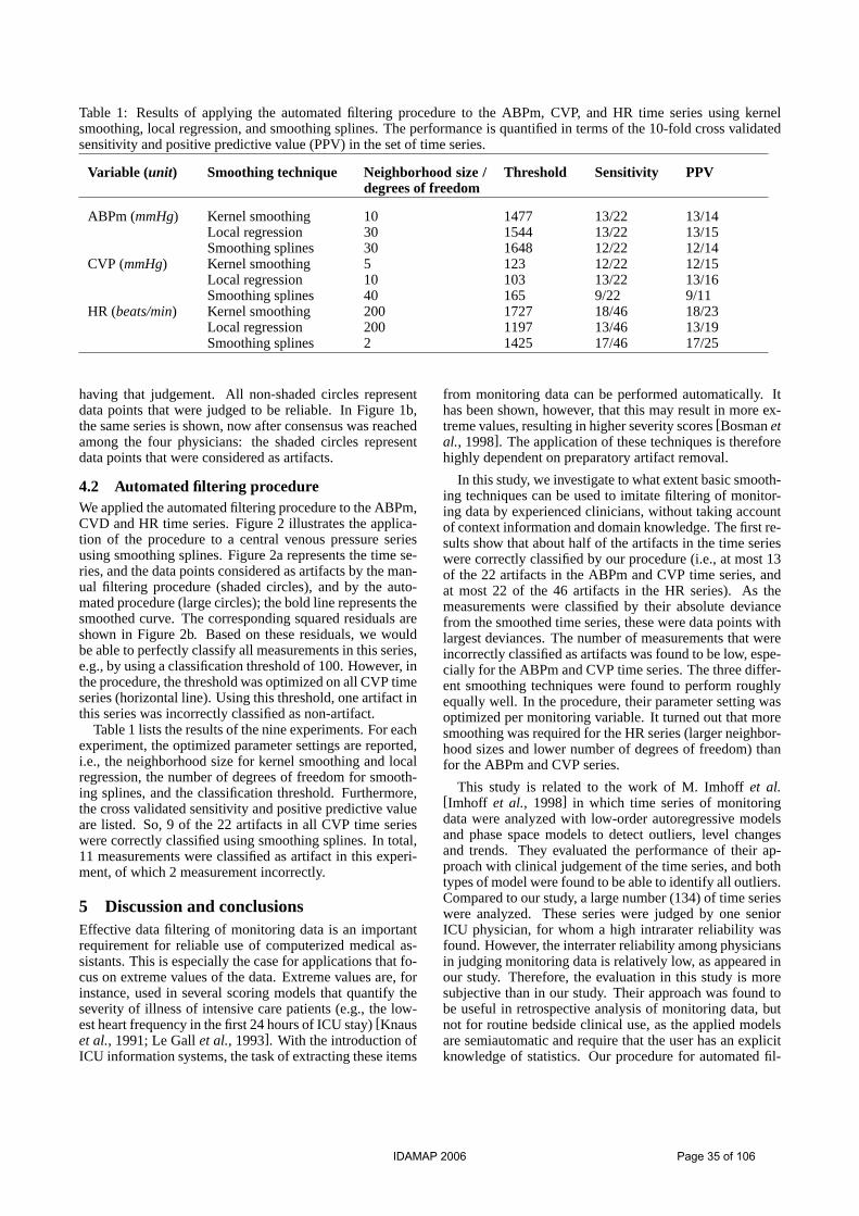
Table 1: Results of applying the automated filtering procedure to the ABPm, CVP, and HR time series using kernelsmoothing, local regression, and smoothing splines. The performance is quantified in terms of the 10-fold cross validatedsensitivity and positive predictive value (PPV) in the set of time series.

Variable (unit) Smoothing technique Neighborhood size /degrees of freedom

Threshold Sensitivity PPV

ABPm (mmHg) Kernel smoothing 10 1477 13/22 13/14Local regression 30 1544 13/22 13/15Smoothing splines 30 1648 12/22 12/14

CVP (mmHg) Kernel smoothing 5 123 12/22 12/15Local regression 10 103 13/22 13/16Smoothing splines 40 165 9/22 9/11

HR (beats/min) Kernel smoothing 200 1727 18/46 18/23Local regression 200 1197 13/46 13/19Smoothing splines 2 1425 17/46 17/25

having that judgement. All non-shaded circles representdata points that were judged to be reliable. In Figure 1b,the same series is shown, now after consensus was reachedamong the four physicians: the shaded circles representdata points that were considered as artifacts.

4.2 Automated filtering procedureWe applied the automated filtering procedure to the ABPm,CVD and HR time series. Figure 2 illustrates the applica-tion of the procedure to a central venous pressure seriesusing smoothing splines. Figure 2a represents the time se-ries, and the data points considered as artifacts by the man-ual filtering procedure (shaded circles), and by the auto-mated procedure (large circles); the bold line represents thesmoothed curve. The corresponding squared residuals areshown in Figure 2b. Based on these residuals, we wouldbe able to perfectly classify all measurements in this series,e.g., by using a classification threshold of 100. However, inthe procedure, the threshold was optimized on all CVP timeseries (horizontal line). Using this threshold, one artifact inthis series was incorrectly classified as non-artifact.

Table 1 lists the results of the nine experiments. For eachexperiment, the optimized parameter settings are reported,i.e., the neighborhood size for kernel smoothing and localregression, the number of degrees of freedom for smooth-ing splines, and the classification threshold. Furthermore,the cross validated sensitivity and positive predictive valueare listed. So, 9 of the 22 artifacts in all CVP time serieswere correctly classified using smoothing splines. In total,11 measurements were classified as artifact in this experi-ment, of which 2 measurement incorrectly.

5 Discussion and conclusionsEffective data filtering of monitoring data is an importantrequirement for reliable use of computerized medical as-sistants. This is especially the case for applications that fo-cus on extreme values of the data. Extreme values are, forinstance, used in several scoring models that quantify theseverity of illness of intensive care patients (e.g., the low-est heart frequency in the first 24 hours of ICU stay)[Knauset al., 1991; Le Gallet al., 1993]. With the introduction ofICU information systems, the task of extracting these items

from monitoring data can be performed automatically. Ithas been shown, however, that this may result in more ex-treme values, resulting in higher severity scores[Bosmanetal., 1998]. The application of these techniques is thereforehighly dependent on preparatory artifact removal.

In this study, we investigate to what extent basic smooth-ing techniques can be used to imitate filtering of monitor-ing data by experienced clinicians, without taking accountof context information and domain knowledge. The first re-sults show that about half of the artifacts in the time serieswere correctly classified by our procedure (i.e., at most 13of the 22 artifacts in the ABPm and CVP time series, andat most 22 of the 46 artifacts in the HR series). As themeasurements were classified by their absolute deviancefrom the smoothed time series, these were data points withlargest deviances. The number of measurements that wereincorrectly classified as artifacts was found to be low, espe-cially for the ABPm and CVP time series. The three differ-ent smoothing techniques were found to perform roughlyequally well. In the procedure, their parameter setting wasoptimized per monitoring variable. It turned out that moresmoothing was required for the HR series (larger neighbor-hood sizes and lower number of degrees of freedom) thanfor the ABPm and CVP series.

This study is related to the work of M. Imhoffet al.[Imhoff et al., 1998] in which time series of monitoringdata were analyzed with low-order autoregressive modelsand phase space models to detect outliers, level changesand trends. They evaluated the performance of their ap-proach with clinical judgement of the time series, and bothtypes of model were found to be able to identify all outliers.Compared to our study, a large number (134) of time serieswere analyzed. These series were judged by one seniorICU physician, for whom a high intrarater reliability wasfound. However, the interrater reliability among physiciansin judging monitoring data is relatively low, as appeared inour study. Therefore, the evaluation in this study is moresubjective than in our study. Their approach was found tobe useful in retrospective analysis of monitoring data, butnot for routine bedside clinical use, as the applied modelsare semiautomatic and require that the user has an explicitknowledge of statistics. Our procedure for automated fil-


tering using simple smoothing techniques does not sufferfrom these disadvantages, and is expected to be easily im-plemented in an ICU information system.

In the patient monitoring and therapy planning systemVIEVENT [Miksch et al., 1996], an extensive procedurefor data validation is implemented to detect and repair er-roneous measurements[Horn et al., 1997]. The procedureemploys data filtering in a hybrid approach using (clinical)knowledge of the (course of the) variables and their interre-lation in addition to statistical methods. Manually filteredtime series are sufficient for tuning our procedure, and thereis no further necessity to make knowledge of the variablesexplicit.

A general problem in studies on artifact detection is thatthe concept of ‘artifact’ is vague and hard to define. Thisexplains the low interrater reliability that we found amongthe physicians’ judgements and has motivated harmoniza-tion of the judgements through a consensus meeting. Yetthe resulting consensus judgement is at best an intersub-jective, and not an objective, standard. We note howeverthat (inter)subjective standards may be equally well repro-ducible by automated filtering techniques, and that is pre-cisely what this study aims at.

One may suggest that the procedure will improve by ap-plying the smoothing techniques in a leave-one-out designto avoid that data artifacts attract the smoothing function.In a leave-one out design, for each measurement in thetime series, the smoothing technique is applied to the timeseries of which this measurement is excluded from, andthe resulting function was subsequently applied to obtaina smoothed estimate of the particular measurement. Wealso performed our experiments in a leave-one-out design,but did not found an improvement of the performance ofthe filtering procedure, though.

In our procedure, the stability of the time series wasnot explicitly taken into account. The variance over timecontains important additional information for data filter-ing, though, as physicians generally judge sudden smallchanges in stable parts of the series as artifacts with morecertainty, than sudden larger changes in unstable patterns.Therefore, in the future part of this study, we will deriveconfidence intervals around the time series from bootstrapsamples, and perform filtering based on these intervals.

The time series that were used in this study were selectedfor their relatively rough course, and stable time series wereunderrepresented. Because of the aforementioned featureof the current procedure, the sensitivity of the proceduremay therefore be overestimated in our experiments. To de-termine the performance of the procedure for automated fil-tering of monitoring data in general, the procedure shouldbe applied to randomly selected time series.

To conclude, the procedure for automated data filteringusing basic smoothing techniques and based on theresulting residuals turned out to be highly predictive, butmoderately sensitive, and will therefore be refined in thefuture part of this study.

Acknowledgments

We would like to thank Marcus Schultz, Erik-Jan vanLieshout and Anne-Cornelie de Pont, senior ICU physi-

cians at the Academic Medical Center, Amsterdam, TheNetherlands, for scoring the temporal patterns.

Niels Peek receives a grant from the Netherlands Organi-zation of Scientific Research (NWO) under project number634.000.020.

References[Bosmanet al., 1998] R. J. Bosman, H. M. Oudemans van

Straaten, and D. F. Zandstra. The use of intensive careinformation systems alters outcome prediction.Inten-sive Care Medicine, 24:953–958, 1998.

[Charbonnier, 2005] S. Charbonnier. On line extraction oftemporal episodes from ICU high-frequency data: a vi-sual support for signal interpretation.Computer Meth-ods and Programs in Biomedicine, 78:115–132, 2005.

[Cleveland and Loader, 1996] W. S. Cleveland andC. Loader. Smoothing by local regression: Principlesand methods. In W. Haerdle and M. G. Schimek,editors,Statistical Theory and Computational Aspectsof Smoothing, pages 10–49. Springer, New York, 1996.

[Hastieet al., 2001] T. Hastie, R. Tibshirani, and J. Fried-man. The Elements of Statistical Learning. Springer,Berlin, 2001.

[Hornet al., 1997] W. Horn, S. Miksch, G. Egghart,C. Popow, and F. Paky. Effective data validation of high-frequency data: time-point-, time-interval-, and trend-based methods.Computer in Biology and Medicine,Special Issue: Time-Oriented Systems in Medicine,27:389–409, 1997.

[Imhoff et al., 1998] M. Imhoff, M. Bauer, U. Gather, andD. Lohlein. Statistical pattern detection in univariatetime series of intensive care on-line monitoring data.In-tensive Care Medicine, 24:1305–1314, 1998.

[Knauset al., 1991] W. A. Knaus, D. P. Wagner, E. A.Draper, J. E. Zimmerman, M. Berger, P. G. Bastos,C. A. Sirio, D. J. Murphy, T. Lotring, and A. Damiano.The APACHE III prognostic system: risk prediction ofhospital mortality for critically ill hospitalized adults.Chest, 100(6):1619–36, 1991.

[Le Gallet al., 1993] J. Le Gall, S. Lemeshow, andF. Saulnier. A new Simplified Acute Physiology Score(SAPS II) based on a European/North American multi-center study.Journal of the American Medical Associa-tion, 270:2957–2963, 1993.

[Michel et al., 2003] A. Michel, A. Junger, M. Benson,D. G. Brammen, G. Hempelmann, J. Dudeck, andK. Marquardt. A data model for managing drug ther-apy within a patient data management system for inten-sive care units. Computer Methods and Programs inBiomedicine, 70:71–79, 2003.

[Mikschet al., 1996] S. Miksch, W. Horn, C. Popow, andF. Paky. Utilizing temporal data abstraction for data val-idation and therapy planning for artificially ventilatednewborn infants. Artificial Intelligence in Medicine,8:543–576, 1996.

[Wand and Jones, 1995] M.P. Wand and M.C. Jones.Ker-nel Smoothing. Chapman & Hall, London, 1995.


Visual Development of Temporal Patterns for Medical Data Abstraction

Norman Brummer∗, Joachim Baumeister∗, Daniel Riewenherm†, Frank Puppe∗, Jens Broscheit†∗Department of Computer Science, University of Wuerzburg, Am Hubland, 97074 Wuerzburg

bruemmer,baumeister,[email protected]†Department of Anesthesiology, University of Wuerzburg, Josef-Schneider-Str. 2, 97080 Wuerzburg

riewenhermd,[email protected]

Abstract

In this paper we present a visual representationof temporal patterns in abstractions of numericaland timestamped data. We provide a curve-likeacquisition tool which supports domain special-ists to develop and refine temporal knowledge inan intuitive and effective manner. The resultingpatterns can be used to detect artifacts as well asmore complex phenomena, e.g., in order to de-rive intelligent alarms.

1 IntroductionThe temporal development of numerical data and its inter-pretation, respectively, is of prime importance when moni-toring patients in the medical domain, e.g., during surgeriesor in the context of an ICU. Here, the automatic abstractionand interpretation of these continuously received parametervalues can support the medical staff, e.g., anesthetists, withthe tracking of the patient’s status.

Furthermore, the interpretation of parameter values andtheir development is often difficult because they are super-imposed by artifacts, e.g., an accidently dropped pulse sen-sor. In consequence, the validation of received parametervalues preceding the actual interpretation is a crucial issue.

In this paper we present an approach for a visual repre-sentation of temporal abstraction and validation knowledgeallowing for an intuitive and precise formalization. The ap-plied visual patterns were adopted from knowledge engi-neering interviews taken with the domain specialists andwere refined in order to allow for a formal and precise in-terpretation of the modeled temporal knowledge.

The visually acquired patterns will be translated to a tex-tual representation in order to be integrated into a rule-based formalism. This enables a combination of temporalpatterns and non-temporal rule conditions including con-junctions, such asand, or andnot expressions.

The context of our work is an intelligent monitoring andalarm system to be used during surgeries or in IC units,there supporting the work of anesthetists.

The paper focuses on the development of high–level ab-stractions, i.e., deriving meaningful alarms or artifacts, al-though the handling of basic abstractions derived from rawdata streams is also an important task.

The derivation of intelligent alarms is two-folded in oursystem: In the first step we try to detect defined states of ar-

tifacts within previously abstracted data streams and anno-tate the data with possibly found artifacts (thus enabling fora high-level data validation). In the second step we inves-tigate the annotated data streams for defined alarm states,e.g. insufficient anesthesiaandhypovolemia.

2 A Visual Representation for High-LevelAbstractions

The manual definition of complex patterns of the particularparameter changes over time is a difficult and error–pronetask. For this reason we introduce an intuitive and visualrepresentation for describing such patterns, i.e.,AbstractTemporal Curves (ATC), which can be interpreted as con-ditions for temporal rules for deriving high-level abstrac-tions, i.e. artifacts and alarms. The representation offers acurve-like description of the temporal behavior of parame-ters, thus describing certain phenomena.

2.1 Abstract Temporal Curves

In the following, we introduce simple graphical elementsthat enable a description of basic events occurring in ab-stract parameter courses. Thereafter, we define temporalconstraints that can be applied to events in order to describethe temporal behavior. A more complex temporal patternis described by a set of events, attached constraints and amaximum duration restricting the entire pattern.

The modeling basis of an ATC contains layers for eachinvolved parameter (Figure 1). Horizontal lines denote thecorresponding abstract parameter values. There exist twobasic elements that can be combined in different ways inorder to describe the possible events.

Edges are horizontal lines describing a persistent value thespecified parameter may take. Parallel edges of thesame parameter define alternative and possible valuesfor the parameter.

Nodes are markers placed on edges at arbitrary positions.They define changes of parameter values and thus ba-sically declare temporal constraints.

Changes in the specified parameter behavior must beseparated by nodes. Additionally, further nodes can beplaced at any position, as it has been done with the first de-fined node in Figure 1. Here the decrease of the abstractedparameter valueAP (arterial blood pressure) is specified


AP

critical

normal

low

high

EdgeNode

Figure 1:Edges and nodes in a parameter sequence in an ATC.Nodes can be defined at arbitrary positions on edges. They denoteevents expressing value changes and value persistence.

starting with valuecritical then falling to eitherhighor nor-mal and finally decreasing to the valuelow.

We extend the notation bytemporal constraintsbetweenthe nodes. A temporal constraint consists of a pair of nodesconnected by a period. It denotes that the enclosed eventsneed to occur within the specified time range. There arethree alternatives to connect nodes by temporal constraints;Figure 2 depicts different types of constraints: Asequence(c) defines a time span for a certain event flow, occurringon a single parameter. It is required to occur within thegiven period. A second alternative for a definition of tem-poral constraints areintervals (a). An interval connects twonodes of different parameter courses, which means that thecorresponding events need to occur in the given time span.With the third alternative, i.e., thepoint-interval (b), wedirectly connect nodes in order to express that the corre-sponding events are required to occur simultaneously. The

APhigh

normallow

Tmax

[5,10]s

HRhigh

normallow

[10,15]s (c) sequence

(a) interval

(b) point- interval

Figure 2: An ATC with temporal constraints defined betweensome nodes on the courses of the parametersAP (arterial bloodpressure) andHR (heart rate).

additional global constraintTmax on top of the pattern de-scription implies that the duration of the entire scenario isrestricted to the time-interval(0, Tmax].

2.2 Translation of ATCs to Temporal RulesThe presented visual notation allows for an intuitive de-scription of temporal events. These events will be compiledto a textual representation consisting of temporal eventsand expressions. The resulting temporal patterns can becombined with non-temporal rule conditions. Thus, theycan be integrated into a rule-based formalism. For exam-

ple, the rule framework ofd3web[Baumeister, 2004] al-lows for a definition of complex rule conditions built up bynon-terminal constructs, e.g.and, or andnot. This enablesthe intuitive definiton of complex temporal patterns.

3 Results and DiscussionThe presented work was implemented in the context of amedical project aiming for an intelligent detection of ar-tifacts and alarms during surgeries. Two medical expertswere involved with the formalization and refinement of thetemporal knowledge including a variety of typical artifactand alarms. It turned out that the domain specialists got fa-miliar very quickly with the meaning of the visual knowl-edge representation. This was not surprising since the rep-resentation was adopted from the observations made dur-ing knowledge acquisition interviews conducted with thedomain specialists. In fact, similar curves were drawn onpaper during the interview sessions to explain the partic-ular events. Consequently, almost no training phase wasrequired and the initial model was discussed and imple-mented in about 5 minutes for each pattern. However, themain effort consisted in testing and refining the collectedpatterns. The most complex task was the appropriate defin-ition and refinement of temporal constraints included in thepatterns. These adaptations required frequent testing cy-cles. For simple patterns, e.g., mostly artifacts, the refine-ment phase took about 10 minutes, whereas more complexpatterns required more than 30 minutes for adaptation andtesting.In the literature, representations for high-level abstractionsare mostly graph-based. A related approach to our visualrepresentation can be found in[Chittaro and Combi, 2003].There, three alternative visual vocabularies representing in-tervals and their relations (as subset of Allen-Relations),based on objects from the physical world, are presented.But, explicit temporal periods (e.g.[10s, 30s]) can not bemodeled, as it is possible in our approach.In the future we are planning to integrate a fuzzy definitionof abstraction thresholds and temporal expressions, sincean exact definition turned out to be one of the most diffi-cult tasks. Visualizations of temporal uncertainty has beenaccomplished e.g. in[Kosara and Miksch, 1999]. Further-more, we consider the semi-automation of the refinementprocess of the patterns by adapting discovery algorithmsfor this task.

References[Baumeister, 2004] Joachim Baumeister.Agile Develop-

ment of Diagnostic Knowledge Systems. AKA Verlag,DISKI 284, 2004.

[Chittaro and Combi, 2003] Luca Chittaro and CarloCombi. Visualizing Queries on Databases of TemporalHistories: New Metaphors and Their Evaluation.Dataand Knowledge Engineering, 44(2):239 – 264, 2003.

[Kosara and Miksch, 1999] Robert Kosara and SilviaMiksch. Visualization Techniques for Time-Oriented,Skeletal Plans in Medical Therapy Planning.JointEuropean Conference on Artificial Intelligence inMedicine and Medical Decision Making (AIMDM’99),pages 291–300, 1999.


Invited presentation


Intelligent Data Analysis for Biomedicine:

What have we learned?

Xiaohui Liu Intelligent Data Analysis Group

School of Information Systems, Computing and Mathematics Brunel University, London

www.ida-research.net

Intelligent Data Analysis (IDA) is the interdisciplinary study concerned with the effective analysis of data. The ever increasing and variety of data in biomedicine have provided one of the most fertile grounds for testing existing analysis techniques and providing great motivations for investigating new IDA methods. For over ten years, the IDA group at Brunel have been working on the interface between artificial intelligence, dynamic systems, image and signal processing, pattern recognition and statistics, and have been applying this research to challenging problems in biology and medicine, e.g. microarray data analysis, managing glaucoma and muscular dystrophy. In this talk, I shall introduce some of our work in this area, particularly those involving temporal data analysis. Key research issues covered will include data quality control, multivariate time series analysis, and biomedical evaluations. Finally some useful lessons we have learnt will be discussed.


http://www.ida-research.net/

Paper session: Bioinformatics


Abstract Sequence and structure of gene regulatory pro-moter regions determine the genetic response programs of cells according to their internal state and environment. Computational inference of the relation between structure of promoter regions and gene expression can help us to understand the underlying genetic programs and can greatly assist in experiment planning. It most often relies on a large data base of regulatory elements (i.e. putative or known transcription factor binding sites) and then infers rules that relate promoter structure and gene expression. The principal ob-stacle it faces is combinatorial explosion of rules to test. We developed a rule-based clustering method that uses gene expression distance to guide rule inference and searches only the most promising part of the vast and expressively rich rule-space. We also developed a set of effective visualizations to present and explore the shared structural promoter features of discovered gene clusters. Cross-validation confirms the ability of the proposed rule-based clustering method to find rules with good predictive power.

1 Introduction Regulation of gene expression is a complex key mecha-nism in the biology of eukaryotic cells. Cells carry their function and respond to the environment by an orchestra-tion of signaling molecules and transcription factors that influence gene expression. Resulting products regulate expression of other genes thus forming diverse set of regulatory pathways. To better understand gene functions and gene interactions we need to discover and analyze the programs of gene regulation. Computational analysis of gene regulatory regions can greatly speed-up and to a cer-tain extent automate the normally tedious discovery proc-ess performed by geneticists.

Gene’s regulatory (promoter) region is defined as a stretch of DNA, normally located upstream of the gene’s coding region. Transcription factors are special proteins that can bind to sequence-specific binding sites in regula-tory regions, and by doing so inhibit or excite gene ex-pression of their target genes. Regulation by binding of transcription factors is just one of the many mechanisms

of gene expression regulation. Expression is also deter-mined by chromatin structure, epigenetic effects, post-transcriptional, translational, post-translational and other forms of regulation [Wasserman and Sandelin, 2004]. Because there is a lack of these kinds of data, most current studies focus on inference of relations between gene regu-latory content and their expression as measured using mi-croarray technology.

Determining the regulatory region and putative binding sites are the first crucial steps in such analyses. Regula-tory regions differ from coding regions in nucleotide and codon frequency. This fact is successfully used by many prediction algorithms [Bajic et al., 2004]. Genome pro-moter sequences are readily available for download for most organisms (for yeast see www.yeastgenome.org).

The next more important and well studied step is to de-termine transcription factors’ putative binding sites in promoter regions. These are 4 to 20 nucleotide long DNA sequences [Wasserman and Sandelin, 2004] which are highly conserved (with low sequence variation) in the promoter regions of regulated genes. A matrix representa-tion of binding sites is normally used in computational analysis. The matrix defines the frequency of the four nucleotides (A, T, G, C) at each position in the binding site (see Table 1 and Figure 2 for example). The binding site is often also presented as a single consensus line (see Table 1), or graphically as a logo (see Figure 2). Experi-mentally confirmed and computationally inferred putative binding sites are now available in data bases such the TRANSFAC data base [Wingender et al., 1996]. When analyzing genes with unknown regulators, one can find candidate binding sites using local sequence alignment programs such as the MEME program [Bailey and Elkan, 1994] that can identify short, frequent sequences. A de-tailed description and evaluation of such tools is presented in [Tompa et al., 2005].

Most of contemporary methods to relate gene structure and expression start with gene expression clustering. Next, they determine cluster-specific binding sites. The success of such approach is heavily dependent on number (usually a parameter to clustering method) and composi-tion of gene clusters. A slight change in initial conditions or parameter values for clustering can lead to different groupings with substantially different sets of binding sites. Another problem with such approach is its inability to discover overlapping subgroups; it is biologically known

Rule-based clustering for gene regulation pattern discovery

Tomaz Curk,a Uros Petrovic,b Gad Shaulsky,c Blaz Zupana,c a) University of Ljubljana, Faculty of Computer and Information Science, Ljubljana, Slovenia b) J. Stefan Institute, Department of Biochemistry and Molecular Biology, Ljubljana, Slovenia

c) Baylor College of Medicine, Department of Molecular and Human Genetics, Houston, TX [email protected], [email protected], [email protected], [email protected]


position 0 1 2 3 4 5 6 7 8 9 10 11

A 0 0 0 0.2 0.1 0 0 0 0 0.1 0.6 0.1C 0 0 0 0 0 0 0 0 0 0 0 0 G 0 0.5 0 0.4 0.4 0.1 0 0.8 0.4 0.8 0 0.6T 1.0 0.5 1.0 0.4 0.5 0.9 1.0 0.2 0.6 0.1 0.4 0.3

single line

consensus T K T K K T T G K G A K

Table 1. Matrix presentation of an example putative binding site. A single line consensus sequence presentation, giving the most frequent nucleotide at each position, is also used (coded with standard FASTA codes, e.g. K indicates G or T).

Figure 2. Logo representation of the putative binding site from Table 1. Information of nucleotides at each position is given.

that same gene can respond in many different ways and perform various functions. An alternative to above is to start with information about binding sites and search for descriptions shared be-tween similarly expressed genes. An example is the ap-proach proposed by [Chiang et al., 2001] where for each binding site and corresponding set of genes their method calculates the correlation of gene expression profiles. This correlation is then statistically compared with the one ob-tained from the same-sized randomly drawn set of genes. If the observed difference is statistically significant, the method reports on the rule for the particular binding site. The method fails to model combinations of two, three or more putative binding sites. This could be regarded as a major deficiency as it is biologically known that regula-tion of gene expression can be highly combinatorial and requires the coordinated presence of many bound tran-scription factors. More advanced methods try to infer rules that describe the structure of regulatory regions with more than one, but rarely more than two putative binding sites [Pilpel et al., 2001; Beer and Tavazoie, 2004]. The principal bottle-neck is the complexity of exhaustive combinatorial search that these methods employ, which quickly becomes prohibitive when exploring combina-tions of binding sites. For example, the number of all pos-sible combinations of three binding sites, from a base of thousand binding sites available for modeling, quickly grows into hundreds of millions. Transcription is also affected by absolute or relative orientation and distance between binding sites and other landmarks in the pro-moter region (i.e. the translation start ATG), making ex-haustive search that would include such models unpracti-cal. To overcome these limitations we have developed a heuristic rule search method that is able to efficiently identify complex structural descriptions of gene regula-tory regions. The proposed rule-based clustering method is guided by the information on the similarity of gene ex-pression and explores only the most promising (coherent) subgroups of genes with similar regulatory content.

2 Rule-based clustering method We devised a rule-based clustering approach with the goal to find potentially complex rules that describe the shared regulatory structure of genes with similar expression pro-files. Similarity in gene expression is assessed using Pear-

son correlation, but other distance measures could be used instead. Rules are of the form “IF structure THEN expres-sion profile”, where structure is an assertion over the binding sites in the gene promoter sequence and uses a description language defined below, and expression pro-file is a average profile of genes that match the structure.

2.1 Descriptive language and rule search We have defined a rich descriptive language which, be-sides being able to describe presence of a binding site, can be used to define conditions on the distance of putative binding sites from transcription and translation start site (ATG) and other landmarks, the distance between putative binding sites and their relative and absolute orientation relative to a given reference point (see Figure 3).

+s1−s2

d1

d2

+s1−s2

d1

d2 Figure 3. The descriptive language for gene’s structure can in-clude conditions on distance (d2) between two binding sites (s1 and s2), distance from ATG (d1) and orientation of binding sites in the sense (+s1) or non-sense reading direction (-s2). We based our heuristic rule search method on the ap-proach of clustering trees developed by [Blockeel et al., 1998]. We developed a general rule search method that is guided by the information on example distance (gene dis-tance in our applications) and only the most promising parts of the vast rule-space are searched. Every next step in the group (or cluster) discovery process is selected based on the correlation of gene expression in currently discovered groups. Further refinements of rules are per-formed on only those rules describing the most promising groups.

The method requires a “target” set of genes for which we want to find rules describing their promoter regions and cluster them into subgroups. The target set can be the full genome or can be a set of differentially expressed genes in one or many experimental conditions (mutation of a gene, outside chemical, temperature or other influ-ence) measured with DNA microarrays. The algorithm starts with the set of all genes, which is represented by the conditional part of the initial rule “True.” The algorithm then tries to refine the current rule set B by adding condi-tional parts. For example, the conditional part of rule


“M1” requiring only the presence of binding site M1 can be refined into “M1+” requiring the orientation of M1 to be in sense direction. The initial condition “M1” can be refined to require binding site M1 to be at a distance −100 to −80 nucleotides relative to ATG, which is stated by the rule’s condition “M1@−100..−80(ref:ATG).” Another binding site (e.g. M2) can be used as a reference point, which we write as “M1@−100..−80(ref:M2).” The initial rule can also be refined into “M1 and M2” requiring both binding sites to be present in the promoter region.

Every refined rule has to cover fewer genes than the original but at least N target genes (parameter N is set by user). If not, it is completely discarded from further con-sideration. Also, the similarity in gene expression within the newly refined group must significantly increase com-pared to the similarity in the original group. The signifi-cance in decrease of variance is tested using F-test. Rules that pass this test are added into set B and used for further refinements (size of set B is limited to L best rules, pa-rameter L set by user. Set B is usually referred as “beam”.) Otherwise the rule is scored based on the group average intra-distance, which must be lower than parame-ter D (parameter set by user), and moved into the final set of rules R where only K best rules are kept and returned as result of the rule-based clustering algorithm (parameter K set by user). For the basic step of the search algorithm see Figure 4, for the algorithm see Algorithm 5.

Note that because the algorithm starts with the entire genome, the discovered rules can cover genes outside the target set. The method can be applied to search for genes that were initially left out of a target set but should have been included based on their regulatory content and gene expression.

The proposed rule-inference method differs from clas-sic rule-coverage algorithms (e.g. CN2 described by [Clark and Niblett, 1989]) because it allows the discovery of overlapping groups of genes. The basic CN2 algorithm has a relatively small beam (size of beam set B in our al-gorithm is bigger) and iteratively removes examples (genes in our case) that can be described by the best rule discovered in current iteration. The procedure is then re-peated on the reduced set until no examples are left to cover. Our proposed method uses a larger beam and searches for rules until refinements are possible. No actual gene coverage is considered in these steps. After the search is completed, all discovered rules are sorted by their score. We then traverse the ordered list and check the average cumulative gene group coverage of each rule. If average cumulative coverage is less than parameter M (set by user) then the rule is selected and the genes’ cumula-tive coverage updated accordingly, otherwise the rule is discarded. This procedure selects the final set of best rules that are presented to the user.

Exhaustive search of even relatively simple rules can quickly grow into a prohibitively hard problem due to combinatorial explosion. The main distinctive feature of our method is its ability to efficiently derive rules describ-ing a higher combinatorial regulation involving three or more binding sites by starting from a base set of thou-sands putative binding sites. We give an example of the number of rules search by our heuristic method and com-

pare it with the number of all possible combinations that would be inspected by exhaustive search.

True

P1 P2 PM…

True

P1 P2 PM…

True

P1 P2 PM…

True

R1 R2 RM…

a) b)True

R1 R2 RM…

a) True

R1 R2 RM…

a) b)b)

Figure 4. a) Rule refinement is the basic step of the search algo-rithm. b) The intra-group gene expression similarity of genes covered by the refined rule (bottom nodes) must increase sig-nificantly compared to the group described by the original rule (top node). Different refinements of same rule lead to differently homogeneous groups (check mark indicates a significant in-crease in the group intra-similarity, cross represents a not sig-nificant increase compared to expression of original group). 1 beam B is a set of maximum L best rules for

further refinement: B = True 2 R = is a set of K best discovered rules 3 WHILE B ≠ 4 take best rule Rb from set B 5 FOR EACH k IN 1..number of binding sites 6 refine Rb by using binding site Mk,

create new rule Rn 7 IF rule Rn acceptable AND significant

increase between Rb in Rn THEN 8 Add Rn into B (keep best L rules in B). 9 add rule Rb into R if among K best 10 return K best discovered rules in set R Algorithm 5. The search algorithm. Rule Rb is refined into Rn (line 6) by adding conditions on presence, orientation and dis-tance of a new binding site (Mk) relative to binding sites already described in other terms of rule Rb.

2.2. Visualization of results The rich descriptive language and the method’s ability to discover overlapping gene groups can result in a large number of discovered rules. We implemented three graph-based visualizations that facilitate a better insight into the common structural features of discovered rules and gene groups (see Figure 6). Gene network graph is the simplest way to visualize the discovered groups (Figure 6a). Nodes represent genes and we connect two nodes if the two genes are covered by same rule. Presence of many over-lapping groups can quickly render this visualization satu-rated. The next level of abstraction is group graph (Figure 6b). Nodes represent groups of genes (that can be de-scribed by one or more rules) and we connect two nodes (groups) if they share an arbitrary number of genes (pa-rameter set by user). This visualization is useful for explo-ration of regulatory or functional overlaps in discovered subgroups of genes. By varying the threshold one can observe how the initial grouping of genes breaks into less connected subgroups. The last level of abstraction is motif graph (Figure 6c). Nodes represent terms (parts of rules requiring specific characteristics for a binding site; bind-ing site is also called “motif,” hence the graph name) and two nodes are connected if they appear in same rule. This can be used to identify common and rule-specific binding sites appearing in discovered rules indicating potential general and group-specific regulators respectively.


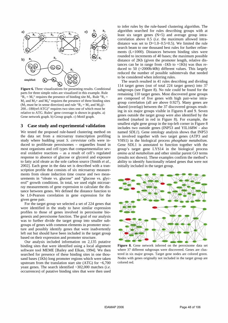
G4 G6

G5 G7

G1 G3

G2

R2

G1 G2

G3

G3 G4

G4 G6

G5 G7

R1

R3

R1R2

R3

simplified:

a)

b)

M1M2

M3 M4

M5

c) R2R1

R3

R2R1R3

G4 G6

G5 G7

G1 G3

G2

G4 G6

G5 G7

G1 G3

G2

G4 G6

G5 G7

G1 G3

G2

R2

G1 G2

G3

G1 G2

G3

G3 G4G3 G4

G4 G6

G5 G7

G4 G6

G5 G7

R1

R3

R1R2

R3

R1R2

R3

simplified:

a)

b)

M1M2

M3 M4

M5

c)M1

M2

M3 M4

M5

M1M2

M3 M4

M5

c) R2R1

R3

R2R1R3

Figure 6. Three visualizations for presenting results. Conditional parts for three simple rules are visualized in this example. Rule “R1 = M1“ requires the presence of binding site M1. Rule “R2 = M2 and M3+ and M4” requires the presence of three binding sites (M3 must be in sense direction) and rule “R3 = M3 and [email protected](ref:ATG)” requires two sites one of which must be relative to ATG. Rules’ gene coverage is shown in graphs. a) Gene network graph. b) Group graph. c) Motif graph.

3 Case study and experimental validation We tested the proposed rule-based clustering method on the data set from a microarray transcription profiling study where budding yeast S. cerevisiae cells were in-duced to proliferate peroxisomes – organelles found in most organisms and cell types that compartmentalize sev-eral oxidative reactions – as a result of cell’s regulated response to absence of glucose or glycerol and exposure to fatty acid oleate as the sole carbon source [Smith et al., 2002]. Each gene in the data set is described with a tran-scription profile that consists of six microarray measure-ments from oleate induction time course and two meas-urements in “oleate vs. glucose” and “glucose vs. glyc-erol” growth conditions. In total, we used eight microar-ray measurements of gene expression to calculate the dis-tance between genes. We defined the distance function to be 1.0-Pearson correlation in gene expression for the given gene pair.

For the target group we selected a set of 224 genes that were identified in the study to have similar expression profiles to those of genes involved in peroxisome bio-genesis and peroxisome function. The goal of our analysis was to further divide the target group into smaller sub-groups of genes with common elements in promoter struc-ture and possibly identify genes that were inadvertently left out but should have been included in the target group based on their expression and promoter structure.

Our analysis included information on 2,135 putative binding sites that were identified using a local alignment software tool MEME [Bailey and Elkan, 1994]. We then searched for presence of these binding sites in one thou-sand bases (1Kb) long promoter regions which were taken upstream from the translation start site (ATG) for ~6,700 yeast genes. The search identified ~302,000 matches (i.e. occurrences) of putative binding sites that were then used

to infer rules by the rule-based clustering algorithm. The algorithm searched for rules describing groups with at least six target genes (N=5) and average group intra-correlation above 0.5 (i.e. the maximum allowed intra-distance was set to D=1.0−0.5=0.5). We limited the rule search beam to one thousand best rules for further refine-ments (L=1000). Distances between binding sites were rounded to increments of 40 bases; the maximum possible distance of 2Kb (given the promoter length, relative dis-tances can be in range from -1Kb to +1Kb) was thus re-duced to 50 (=2000b/40b) different values. This largely reduced the number of possible subintervals that needed to be considered when inferring rules.

The search resulted in 41 rules describing and dividing 114 target genes (out of total 224 target genes) into 37 subgroups (see Figure 8). No rule could be found for the remaining 110 target genes. Most discovered gene groups are composed of five genes with high pair-wise intra-group correlation (all are above 0.927). Many genes are shared (overlap) between the 37 discovered groups result-ing in six major groups visible in Figures 8 and 9. Seven genes outside the target group were also identified by the method (marked in red in Figure 8). For example, the smallest eight gene group in the top-left corner in Figure 8 includes two outside genes (INP53 and YIL168W - also named SDL1). Gene ontology analysis shows that INP53 is involved together with two target genes (ATP3 and VHS1) in the biological process phosphate metabolism. Gene SDL1 is annotated to function together with the group’s target gene LYS14 in the biological process amino acid metabolism and other similar parent GO terms (results not shown). These examples confirm the method’s ability to identify functionally related genes that were not initially included in the target group.

Figure 8. Gene network inferred on the peroxisome data set where 37 different subgroups were discovered. Genes are clus-tered in six major groups. Target gene nodes are colored green. Nodes with genes originally not included in the target group are colored red.


Figure 9. Group graph of discovered 37 subgroups that cluster 114 target and 7 outside genes into six major gene groups.

Figure 10. Distribution of distance in predicted and actual gene expression for matching rules. Red vertical line marks average distance 0.72 (average intra-correlation is 0.28).

Majority of discovered rules include conditions that are composed of three terms, each term describing a putative binding site’s orientation and distance relative to ATG or binding sites included in the rule. An exhaustive search for all possible rules composed of three binding sites with defined orientation (three possible values: positive, nega-tive, no preference) and distance (50 different values) would require checking a relatively huge number of rules:

153 1047.5503

32135⋅≈⋅⎟⎟

⎠

⎞⎜⎜⎝

⎛ ⋅

Our method checked 9102.11 ⋅ of the most promising rules, or less than 0.00004% of the entire three-part rule space. The search took 40 minutes on a Pentium 4, 3.4 GHz workstation.

3.1 Cross-validation of rule-based clustering To asses the predictive ability of the inferred rules we applied five-fold cross-validation using the same data and parameter values as described in the section above. The data was randomly divided into five folds. The split was stratified, i.e. each fold contained one fifth of the 224 tar-get genes and one fifth of the remaining ~6500 non-target genes. In each step of the cross-validation procedure the training part of the data was used to infer rules and iden-tify clusters of genes. Discovered rules were then tested on genes from the test set. If a rule matched the promoter region of a test gene then the average distance (in expres-sion) between the test gene and all training genes covered by the rule was calculated. These distances are plotted in the histogram in Figure 10. The achieved average distance is 0.72 (the average correlation is 1.0-0.72 = 0.28) which is a good indication of a good predictive quality of in-ferred rules.

4 Conclusion Experimental results show the ability of the proposed rule-based clustering method to efficiently identify groups of similarly expressed genes with similar structure of regulatory region. In contrast with other contemporary methods that mainly use information on presence of bind-

ing sites in promoter region, the principal novelty of our approach is the use of a rich language to describe the structure of regulatory elements and a heuristic approach to find associated rules. To summarize the findings of our analysis we have also implemented three different visuali-zations that can help in understanding and biological in-terpretation. We believe that the main application of our method is the search for additional evidence that genes from theoretically or experimentally defined group actu-ally share some common regulatory mechanisms or regu-lators. The biologist can then gain insight by looking at the presented evidence and can better decide which in-ferred hypotheses to test in the lab. We experimentally confirmed the ability of the pro-posed method to infer rules that describe a complex regu-latory structure and can reliably predict gene expression from regulatory content. We are currently implementing a web-based application allowing biologists to easily ana-lyze their own data using the proposed rule-based cluster-ing method.

Acknowledgments This work was supported in part by Program and Project grants from the Slovenian Research Agency and by a grant from the National Institute of Child Health and Hu-man Development, P01 HD39691.

References [Wasserman and Sandelin, 2004] Wasserman WW, San-

delin A. Applied bioinformatics for identification of regulatory elements. Nature Reviews Genetics, 5:276-87, 2004.

[Bajic et al., 2004] Bajic VB, Tan SL, Suzuki Y, Sugano S. Promoter prediction analysis on the whole human genome. Nature Biotechnology, 22:1467-73, 2004.

[Wingender et al., 1996] Wingender E, Dietze P, Karas H, Knuppel R. TRANSFAC: a database on transcription factors and their DNA binding sites. Nucleic Acids Research, 24(1):238-41, 1996.


[Bailey and Elkan, 1994] Bailey TL, Elkan C. Fitting a mixture model by expectation maximization to discover motifs in biopolymers. Proc Int Conf Intell Syst Mol Biol, 2: 28-36, 1994.

[Tompa et al., 2005] Tompa M, Li N, Bailey TL et al. Assessing computational tools for the discovery of transcription factor binding sites. Nature Biotechnol-ogy, 23:137-144, 2005.

[Chiang et al., 2001] Chiang DY, Brown PO, Eisen MB. Visualizing associations between genome sequences and gene expression data using genome-mean expres-sion profiles. Bioinformatics, 17(s1):S49-S55, 2001.

[Pilpel et al., 2001] Pilpel Y, Sundarsanam P, Church GM. Identifying regulatory networks by combinatorial analysis of promoter elements. Nature Genetics, 29(2):153-9, 2001.

[Beer and Tavazoie, 2004] Beer MA, Tavazoie S. Predict-ing gene expression from sequence. Cell, 117:185-198, 2004.

[Blockeel et al., 1998] Blockeel H, De Raedt L, Ramon J. Top-down induction of clustering trees. Machine Learning, Proceedings of the 15th International Con-ference, Morgan Kaufmann, 1998.

[Clark and Niblett, 1989] Clark P, Niblett T. The CN2 induction algorithm. Machine Learning, 3(4):261-83, 1989.

[Smith et al., 2002] Smith JJ, Marelli M, Christmas RH, Vizeacoumar FJ, Dilworth DJ, Ideker T, Galitski T, Dimitrov K, Rachubinski RA, Aitchison JD. Tran-scriptome profiling to identify genes involved in perox-isome assembly and function. The Journal of Cell Bi-ology, 158(2):259-71, 2002.


Population substructure determination by means of Bayesian model averagingfor Clustering

Guzman Santafe1, Jose A. Lozano1, Pedro Larranaga1 and Eleazar Eskin2

1Dept. of Computer Science and A.I. (University of the Basque Country, Spain)2Dept. of Computer Science and Engineering (University of California, San Diego)[email protected], [email protected], [email protected], [email protected]

Abstract

Bayesian statistical methods based mainly onMarkov chain models have recently proposed inthe literature and provide powerful tools to an-alyze population substructures on the basis ofmolecular markers such as SNPs. The SNPs se-quences are used to classify individuals into theirpopulation of origin. These SNPs sequences maycontain markers which are not relevant for thisclustering process and they may blur the cluster-ing assignation. In this paper we present the useof a powerful Bayesian model averaging algo-rithm for clustering which includes in the learn-ing process a kind of implicit Bayesian variableselection. Therefore the algorithm is able to dealwith irrelevant variables and then it is appropri-ated to analyze the population substructures. Onthe other hand, we also develop a two-step algo-rithm based on mutual information that can beused to obtain, from the clustering model, the setof SNPs which are considered relevant for clus-tering purposes. Hence, the proposed Bayesianapproach not only offers to retrieve the popula-tion substructure, but also to obtain the set of rel-evant SNPs to retrieve this population substruc-ture. The algorithm has been applied to both syn-thetic and real datasets, and the obtained resultsoutperform the commonly used Structure soft-ware.

1 Introduction

Most genetic variation among different people can becharacterized by single nucleotide polymorphisms (SNPs),which are single point mutations in the nucleotide sequencethat have occurred during human history and are inheritedamong generations. There are lots of these nucleotide mu-tations that exist in a few or only one individual. How-ever, it has been estimated that there are about 7 millioncommon SNPs (with minor allele frequency of at least5%) among the different human populations [Botstein andRisch, 2003].

Most studies of human variation begin by sampling indi-viduals from a certain population. This population is usu-ally defined in terms of subjective aspects such as religion,culture or geographical location, but these aspects do not

necessarily reflect underlying genetic relationships. Indi-viduals in the same population share certain genetic infor-mation that can be used to identify them. The problem ofrecovering the underlying group structure from a set of in-dividuals is know as population substructure problem andit is well-studied in population genetics [Rosenberg et al.,2002]. Apart from the evolutionary perspective, the es-timated group structure can provide a useful insight intomany applications such as correcting for population strat-ification in association studies [Sillanpaa et al., 2001]. Inaddition clinical trials can suffer from false positive of re-duction of power due to population substructure [Pritchardet al., 2000b].

From a purely machine learning approach, populationsubstructure problem can be seen as a clustering problemwhere each SNP in the DNA sequence represents a pre-dictive variable and the population substructure, the clus-ter variable that remains hidden. However, this clusteringproblem has certain special characteristics such as the oc-currence of independent random mutation across the se-quence and the presence of irrelevant variables (not allthe SNPs available in the sequence may be relevant to re-trieve the underlying group structure). This situation canmake the problem not very amenable for distance-basedclustering methods. Recently, Bayesian statistical meth-ods based on Markov chain models have shown to pro-vide powerful tools for the analysis of genetic popula-tion structure and to assign individuals or chromosomalsegments into clusters using multilocus molecular mark-ers [Pritchard et al., 2000a; Corander et al., 2004]. Otherrecently proposed techniques also include the use of mu-tual information-based metrics to obtain the best popula-tion partition [O’Rourke et al., 2005].

On the other hand, the special characteristics of theproblem make the application of other particular cluster-ing techniques very interesting. Specifically, the Bayesianmodel averaging of naive Bayes proposed in [Santafe et al.,2006] is a method which is suitable to be used in the pop-ulation substructure problem. This is a Bayesian clusteringmethod based on naive Bayes model, which is a kind ofBayesian network successfully used in many other biolog-ical problems [Barash and Friedman, 2002].

The naive Bayes model assumes that all the predictivevariable are conditionally independent given the clustervariable. However, the Bayesian model averaging of naiveBayes [Santafe et al., 2006] accounts for model uncertaintyby taking into consideration that each predictive variable


may or may not be relevant for clustering purposes. Sincein population substructure problem mutations in the se-quence are considered independent and not all SNPs maybe relevant to reveal the underlying group structure, thenaive Bayes model learned with this Bayesian model av-eraging algorithm is an appropriated method to tackle thisproblem. Moreover, the model averaging process incor-porates into the learned model a kind of implicit variableselection that can be used to decide which SNPs are morerelevant to cluster individuals into their populations of ori-gin. Therefore, in the same process in which we obtain theclustering structure of the data, we are able to obtain theset of relevant SNPs for this clustering process. In contrastto other SNPs selection methods such as the ones based onsupervised classification models, the proposed method is aclustering approach, which is not guided by a predefinedgroup structure. Clustering methods are supposed to bepreferred in population substructure problem because notalways the population assignation is known or, in the casewhere it is known, there may be unknown subpopulationsgroups inside the know groups or some individual, fromthe point of view of their genetic sequence, may be closerto other population than to the population that they havebeen assigned a priori.

The selection of a informative subset of SNPs that con-tains enough information to differentiate between popu-lations under study may be very useful not only to cor-rect population stratification in association studies or inadmixture-mapping studies [Patterson et al., 2004] but alsoto reduce the economical cost of sequencing samples forthis studies.

In this paper we propose the use of the Bayesianmodel averaging algorithm (EMA algorithm) introducedin [Santafe et al., 2006] to tackle population substructureproblem. Furthermore, we develop a two-step mutual in-formation test that allows the use of the model obtained bythe EMA algorithm to select those SNPs which are relevantto retrieve the underlying structure from the dataset.

The rest of the paper is organized as follows. Section 2overviews the theoretical aspects of the EMA algorithm inthe context of the population substructure problem. Thissection shows how to learn the clustering model from dataas well as how to use this model to select the most relevantSNPs or variables for clustering purposes. Section 3 teststhe behavior of the EMA algorithm in a toy example prob-lem and in a real problem with SNPs data. Finally, Section4 presents some conclusions yielded from the paper as wellas future work.

2 MethodologyThe target that we are aiming for is to obtain a cluster-ing model that provides a posterior distribution among thedataset and thus allows us to cluster the instances into dif-ferent partitions or populations. For this purpose we use theEMA algorithm [Santafe et al., 2006] which is a Bayesianmodel averaging approach to learn a naive Bayes model forclustering. The method obtains, in an efficient way, a naiveBayes model as a result of a Bayesian model averaging overall the possible selective naive Bayes (see Figure 1). Themethod itself is an adaptation of the well-known EM algo-rithm [Dempster et al., 1977] that allows us to extend effi-cient model averaging techniques for complete data [Dash

and Cooper, 2004] to clustering problems. The EMA al-gorithm is a greedy iterative algorithm that is comprised oftwo steps: expectation (E step) and model averaging (MAstep). This last step accounts for model uncertainty by anapproximation of the averaging over all the selective naiveBayes models.

X1 X2

C

X1 X2

C

X1 X2

C

X1 X2

C

Figure 1: Selective naive Bayes structures with two predic-tive variables: each predictive variable can be dependent onor independent of C. That is, each predictive variable canbe considered relevant or irrelevant for clustering purposes.

Let the predictive variables X = X1, . . . , Xn denotethe molecular marker loci, specifically SNPs in our case.The cluster variable, C, represents the population group-ing of the given h haploid sequences D = x(1), . . . , x(h)with x(l) the SNPs alleles of the l-th individual x(l) =x(l)

1 , . . . , x(l)n and l = 1, . . . , h. Note that the algorithm

assumes that the number of clusters is know, although itcan be varied across independent runs of the algorithm inorder to select the best number of population groups.

For each locus Xi, following the idea of model averagingover selective naive Bayes models, we consider two kind ofparameters: if the the locus is relevant for clustering pur-poses, we denote θijk as the unknown relative frequency ofthe allele k at the i-th locus in population j. On the otherhand, if the information of the i-th locus is irrelevant todecide the population to which a sequence belongs, the al-lele frequency does not depend on the population to whicheach sequence is assigned and therefore θ i−k denotes therelative frequency of allele k at locus Xi. This last relativeallele frequency can be calculated directly from the datasetD. Additionally, θC−j represents the unknown relative fre-quency of population j in the dataset D.

As was said before, the EMA is an iterative algorithm.At each iteration t, a naive Bayes model for clustering iscalculated by means of a Bayesian model averaging overselective naive Bayes where each naive Bayes structure is,a priori, equiprobable. That is, the θ

(t)ijk parameter of the

model at the t-th iteration is calculated taking into accountnot only the parameter θijk , but also θi−k .

In order to perform the model averaging calculations ef-ficiently, it is necessary to assume that the allele frequen-cies θijk and θi−k for any locus Xi and any population jand allele k are distributed following a Dirichlet distribu-tion with parameters αijk and αi−k respectively, and thatθijk , for any population j and allele k, is independent ofother θi′jk with i = i′. Similarly, θi−k is independent ofany other θi′−k. This is known as parameter independenceassumption. Moreover, it is assumed that there is no miss-ing values for the predictive variables X in the dataset.

The whole set of parameters for the model learned at it-eration t, θ

(t)ijk and θ

(t)C−j for any i, j and k, is denoted as

Θ(t). The EMA algorithm successively performs the E and


MA steps until the difference between parameter set of themodels calculated in two consecutive iterations is less thana given parameter, ε. The first parameter set, Θ(0), is usu-ally taken at random.

For a better understanding of the EMA algorithm, weattempt to give some intuition about the calculations per-formed at E and MA steps, at each iteration t, in the fol-lowing two sections.

2.1 E Step (Expectation)Intuitively, we can see this step as a probabilistic assig-nation of each individual to each population on the basisof the current model Θ(t). Actually, this step computes,given the current model Θ(t), the expected number of in-dividuals from a population j that present allele k at thei-th locus when the locus is considered relevant for clus-tering purposes, E(Nijk|Θ(t)), and the expected numberof individuals classified into population j, E(NC−j |Θ(t)).The number of individuals of the dataset that present allelek at locus Xi, Ni−k, is also necessary for model averag-ing calculations. This value does not depend on populationassignments, therefore, it is constant throughout the algo-rithm.

After the E step at each iteration t, we have some infor-mation about the population membership of each individ-ual. To distinguish between the dataset D and the datasetafter the E step where this information has been alreadycomputed, we refer to the dataset after the E step at itera-tion t as D(t).

2.2 MA Step (Model Averaging)In this step, the EMA algorithm calculates a new set ofparametes, Θ(t+1), for a naive Bayes model by averagingover all the selective naive Bayes models. These calcula-tions are given by the following equation:

p(cj, x|D(t)) =X

S

p(cj , x|D(t), S)p(S|D(t)) (1)

=X

S

Zp(cj , x|S, Θ) p(Θ|S, D(t))dΘ p(D(t)|S)P (S)

where S denotes a specific selective naive Bayes model thatsets which loci are considered relevant for clustering pur-pose and which are not. We abuse the notation by using c j

and x to denote the fact that the cluster variable C takes thej-th value and the molecular marker loci X take a specificSNP alleles x. For a more simple notation, when we writex, we assume that each SNP Xi takes its k-th allele value.

The general idea of an efficient model averaging over se-lective naive Bayes is that Equation 1 can be approximatedin terms that only depend on each locus (variable X i) or oneach locus and the population membership (X i and C).

On the one hand, the integral in Equation 1 can be ap-proximated by the maximum a posteriori (MAP) parameterconfiguration.

p( cj , x|D(t), S) ≈ αC−j + E(NC−j|Θ(t))

αC + h·

nYi=1

αijk + E(Nijk|Θ(t))

αij + E(Nij |Θ(t))= θS

C−j

nYi=1

θSijk (2)

where θSijk and θS

C−j denote the MAP parameter configu-ration for a selective naive Bayes structure S. Additionally,

αij =∑

k αijk and E(Nij |Θ(t)) =∑

k E(Nijk |Θ(t)),and similarly for values related to C, where αC−j repre-sents the Dirichlet parameter for θC−j . Note that S setsif a variable Xi is dependent on or independent of C.Therefore, if S sets that the locus Xi is independent ofC, we should use θS

i−k and Ni−k instead of the θSijk and

E(Nijk|Θ(t)) respectively in Equation 2, and substituteNi− for E(Nij |Θ(t)) with Ni− =

∑k Ni−k = h.

On the other hand, the marginal likelihood can also bewritten in terms that only depend on X i or on Xi andC. This is given by the well-known close formula forp(D|S) [Cooper and Herskovits, 1992] adapted to our spe-cific problem. Note that, while p(D|S) is resolvable inclosed form when the value of C is known (the dataset iscomplete), in our case D(t) is not a complete dataset, there-fore we are not able to calculate the sufficient statistics Nijk

and NC−j but only approximations given the current modelΘ(t). Hence, the adaptation of Cooper and Herskovits’ for-mula gives an approximation to p(D (t)|S).

p(D(t)|S)≈ Γ(αC)

Γ(αC + h)

Yj

Γ(αC−j + E(NC−j |Θ(t)))

Γ(αC−j)·

nYi=1

Yj

Γ(αij)

Γ(αij + E(Nij |Θ(t)))

Yk

Γ(αijk + E(Nijk|Θ(t)))

Γ(αijk)(3)

where Γ(·) represents the gamma function. Of course,again it is S which sets if we should use αi−k, Ni−j andNi− instead of the originals in Equation 3. The approxi-mation given by this equation in the model averaging pro-cess, have been compared to a Monte Carlo approximation,which is a more accurate and computationally expensivetechnique to approximate p(D|S), obtaining similar results[Santafe et al., 2006].

At this point, as a consequence of parameter indepen-dence assumption, we can state that if two different selec-tive naive Bayes structures set the same relationship be-tween locus Xi and C (in both structures Xi is relevant orirrelevant for clustering purposes) the calculations relatedto locus Xi in Equations 2 and 3 are the same for both struc-tures. This is essential for an efficient model averaging cal-culations since it allows to eliminate the dependence on Sin the model averaging calculations performed in Equation1. That is, using the approximations given by Equations2 and 3 in Equation 1, and grouping these calculations interms that depend on each variable X i, each one of thesegroups will contain only two kind of terms: the ones thatconsider Xi relevant for clustering, ρijk , and the ones thatconsider Xi irrelevant for clustering, ρi−k. Therefore, themodel averaging calculations from Equation 1 can be ap-proximated as follows:

p(cj , x|D(t)) ≈ ρC−j

nYi=1

(ρi−k + ρijk) (4)

where ρC−j is the term which groups the calculations re-lated only to the cluster variable. Thus, the new set of pa-rameters, Θ(t+1), can be calculated from ρC−j , ρi−k andρijk . The expression of terms ρC−j , ρi−k and ρijk is givenin Equation 5.


ρC−j ∝ θC−jΓ(αC)

Γ(αC + h)

Yj

Γ(αC−j + E(NC−j |Θ(t)))

Γ(αC−j)(5)

ρi−k ∝ θi−k

Yj

Γ(αi)

Γ(αi + h)

Yk

Γ(αi−k + Ni−k)

Γ(αi−k)

ρijk ∝ θijk

Yj

Γ(αij)

Γ(αij + E(Nij |Θ(t)))

Yk

Γ(αijk + E(Nijk|Θ(t)))

Γ(αijk)

where αi =∑

k αi−k . Therefore, the calculation of theparameters for the naive Bayes model at t+1 step are givenby:

θ(t+1)ijk = ρi−k + ρijk θ

(t+1)C−j = ρC−j

2.3 Multi-start EMAThe EMA is a greedy algorithm that is susceptible to betrapped in a local optima. The results obtained by the al-gorithm depend on the random initialization of the param-eters. Therefore, we propose the use of a multi-start algo-rithm where m different runs of the algorithm with differ-ent random initializations are performed. In [Santafe et al.,2006] different criteria to obtain the final model from themulti-start process are proposed.

In our case, we use the best choice multi-start EMA,where the best model, in terms of likelihood, among them models calculated by the multi-start process is selectedto be the final model. This is not a pure Bayesian approachto the model averaging process but, in practice, it works, atleast, as well as other more complicated criteria.

2.4 Selecting the most relevant SNPs forclustering

The model averaging process performed by the EMA al-gorithm can be seen as an implicit unsupervised variableselection that is incorporated in the final model. In fact,although the EMA algorithm obtains a naive Bayes modelwhere all the predictive variables (maker loci) are indepen-dent given the value of C (population assignation), the pa-rameters of the resultant naive Bayes model are calculatedby a model averaging over selective naive Bayes and thus,these parametes should reflect the significance of each lo-cus for clustering purposes.

In this section we propose a two-step test that can beused to obtain information about relevant locus that is im-plicitly contained in the final naive Bayes model calculatedby the EMA algorithm. This test is based on mutual in-formation. It is known [Cover and Thomas, 1991] that thestatistic 2NI(Xi, C) asymptotically follows a Chi-squareprobability distribution with (ri − 1)(rC − 1) degrees offreedom. In our case, ri is the number of alleles that a lo-cus Xi can present and rC the total number of populations.

The mutual information of a locus X i and the clustervariable, or the mutual information of two predictive vari-ables Xi′ and Xi′′ with i′ = i′′ can be calculated usingthe naive Bayes model obtained by the EMA algorithm.Thus, a Chi-square test can be performed to decide whichmarker loci are relevant for the clustering process. In thefirst step, we set a test threshold prel and use a Chi-square

test to filter out those predictive variables which are con-sidered not relevant for clustering purposes. This first stepselects the relevant SNPs but the set of selected SNPs maycontain redundant information. As a consequence, we de-velop a second step to filter out redundant SNPs by againusing a Chi-square test with a test threshold pred. In thissecond step we calculate the pairwise mutual informationof the variables selected in the first step and use this valueto decide whether or not two variables are redundant. Fig-ure 2 describes the two-step algorithm to obtain the set ofSNPs, Xrel, which are relevant to obtain the underlyinggroup structure.

Xrel = (X1, . . . , Xn)

– STEP 1 –

for i = 1 to nif 2NI(Xi, C) < χ2

(ri−1)(rC−1);1−prel

remove Xi from Xrel

end ifend for

– STEP 2 –

for all Xi′ , Xi′′ with Xi′ , Xi′′ ∈ Xrel and i′ = i′′

if 2NI(Xi′ , Xi′′) < χ2(ri′−1)(ri′′−1);1−pred

if I(Xi′ , C) < I(Xi′′ , C)remove Xi′ from Xrel

elseremove Xi′′ from Xrel

end ifend if

end for

Figure 2: Pseudo-code for SNPs selection.

The thresholds prel and pred can be used to control thenumber of selected variables. On the one hand, the biggerprel is, the less variables are selected as relevant for clus-tering. On the other hand, as pred decreases, the number ofvariables considered redundant increases and therefore, thefinal number of selected variables is smaller.

3 ResultsIn order to show how the characteristics of the EMA al-gorithm can fit properly to the population substructureproblem, we firstly use the toy example introduced in[O’Rourke et al., 2005]. The dataset for this toy exampleis composed of individuals represented by 50-character bit-strings. We generate three ancestral sequences with relativeHamming distances 2, 3 and 5. Each ancestral sequence isused to generate a set of 19 new clone individuals in whichrandom mutations may happen at each position of the stringwith a mutation rate 0.05. Thus, we obtain 60 individualsgrouped into three different populations with an expectedHamming distance of 2.5 between a mutant and its ances-tral sequence. The individuals from the three different pop-ulation are differentiated by 5 positions of the sequence andthe rest of the positions may only differ from one individ-ual to another because of random mutations. In fact, it isenough with only 2 of the 5 positions to differentiate be-tween individuals from the three populations because there


is redundant information.We use a multi-start EMA algorithm with ε = 0.01 and

m = 1000 runs in the multi-start process to cluster the60 individuals into 3 clusters. Since the EMA algorithmis not deterministic, we perform 10 runs of the multi-startalgorithm that, on average, classify 95% of the sequencesinto their original population with null standard deviation.Moreover, the naive Bayes model obtained by the multi-start EMA at each run is used to obtain the set of relevantpositions to decide the clustering membership. The test de-scribed in Section 2.4 with parameters prel = 0.01 andpred = 0.01 is used to obtain these relevant positions. Allthe 10 runs yield the selection of only two positions of thefive positions that diffentiate between the three populations.Thus, the algorithm correctly selects the minimum numberof positions to differentiate between populations.

Moreover, the Structure software [Pritchard et al.,2000a] with default parameters and 10, 000 models forthe burning period and also 10, 000 iterations to learn themodel is able to classify, on average over ten runs, only79.64% of the sequences into their population of originwith standard deviation 9.91%.

The proposed toy example shows that the EMA algo-rithm presents a good behavior for clustering sequencesfrom different populations and where random mutationacross the sequence positions may happen. In the followingsection we apply the EMA algorithm to a real dataset.

3.1 Human Population Substructure

For this experiment, we use the dataset of common SNPsreported in [Hinds et al., 2005]. This dataset contains about1.5 million SNPs uniformly distributed across the humangenome and which are common to, at least, individualsfrom the three human populations under study: European,African and Asian. The data came from the genotype of 71unrelated individuals: 24 European-American, 23 African-American and 24 Han-Chinese from the Los Angeles area.

Following the experimental description from [O’Rourkeet al., 2005], and in order to avoid linkage disequilibriumfrom proximity in the genome, we only use every thou-sandth SNP, leaving a total of 1, 520 marker loci. The EMAalgorithm, proposed in this paper to tackle the populationsubstructure problem, uses haploid data. Therefore, eachindividual gives rise to two haplotype sequences belongingto the same population. Hence, the dataset is made up of142 sequences with 1, 520 SNPs each. On the other hand,this dataset with 1, 520 SNPs contains information aboutSNPs from all over the human genome. However, in otherreal problems, not all this information is always available.Sometimes only SNPs from one or several chromosomalsegments are provided and then, the population substruc-ture is more difficult to retrieve. In order to simulate thesesituations, we split the dataset into 19 datasets with only 80SNPs. In the experiments we refer to the dataset that con-tains all the 1, 520 SNPs as dsSNPs. The smaller datasetswith 80 SNPs are denoted as ds1, . . . , ds19.

Table 1 shown the percentage of individuals, on aver-age over 10 independent runs, correctly assigned to theirpopulation of origin using both multi-start EMA and Struc-ture algorithms for each dataset. The parameters used forboth algorithms are the same as those used in the toy ex-ample. A Man-Withney test at 0.01 level is performed to

Structure EMADataset Mean Std Mean Stdds1 87.28 0.55 95.07 0.47ds2 88.27 1.35 93.24 0.36ds3 88.48 0.48 93.38 1.49ds4 91.27 0.34 95.77 0.00ds5 83.75 7.67 93.94 0.36ds6 84.53 0.51 86.13 0.48ds7 92.20 0.25 96.48 0.00ds8 74.79 2.66 82.75 2.11ds9 81.86 0.62 86.06 1.78ds10 85.28 0.74 89.08 1.11ds11 87.25 0.38 90.14 0.00ds12 89.59 0.35 91.55 0.00ds13 90.72 0.38 94.37 0.00ds14 89.41 0.26 95.99 0.48ds15 86.08 0.30 90.07 0.52ds16 84.96 0.84 93.45 0.48ds17 88.34 0.17 93.52 0.30ds18 81.16 0.53 86.55 2.92ds19 82.65 0.86 86.62 0.00Mean over ds1-ds19

86.20 — 91.27 —

dsSNPs 96.78 0.09 100 0.00

Table 1: Percentage of correctly assigned individuals totheir population of origin (mean and standard deviationover 10 runs) using both EMA and Structure algorithms.

check if the difference between the two algorithms is sta-tistically significant. Those values which are significantlybetter are written in bold in Table 1. We can see that theresults obtained by the multi-start EMA algorithm outper-form the structure software, and the differences are statisti-cally significant for all the datasets.

The SSCC method proposed in [O’Rourke et al., 2005]also obtain 100% of correct classications for dsSNPsdataset. In the case of the dataset with only 80 SNPs, onlythe mean value over the 19 datasets is reported in the pa-per. The multi-start EMA algorithm obtains, on averageover the 19 datasets, 91.27% of correct classified individu-als. This figure is very close to the precision obtainded bythe SSCC, 91.80%

Another important characteristic of the EMA algorithmis its ability to select the set of relevant SNPs for clus-tering purposes. Using the dsSNPs dataset and settingprel = pred = 0.01, the 10 runs of the multi-start EMAalgorithm give rise to 10 sets of selected relevant SNPs.These datasets contain, on average, 277.1 relevant SNPsand 146 of them are common to the 10 sets. Note that eachset of relevant SNPs is selected on the basis of a differentnaive Bayes model learned with the multi-start EMA algo-rithm. Therefore, although two sets of relevant SNPs sharemany SNPs, some of them may be different. The fact thattwo sets of relevant SNPs contain different SNPs does notnecessarily mean that one set is better than the other be-cause they may contain different subsets of non-redundantSNPs. In order to evaluate the sets of relevant SNPs ob-tained by the multi-start EMA algorithm, we run the Struc-ture software with the same parameters on these datasets.The percentage of correctly classified individuals is, on av-erage over the 10 different sets of relevant SNPs, 94.98%with standard deviation 4.66%. Note that the reduction inthe number of SNPs in the dataset is very big while thepercentage of correctly classified individuals is similar.


4 DiscussionIn this paper we propose the use of the EMA algorithm,originally introduced in [Santafe et al., 2006], in popula-tion substructure problems. This algorithm learns a naiveBayes model for clustering by means of a Bayesian modelaveraging over selective naive Bayes models. That impliesthat the Bayesian model averaging includes in the learnedmodel a kind of implicit variable selection of relevant pre-dictive variables. This special characteristic make the algo-rithm appropriated for the considered problem. Moreover,in the same clustering process we are able to retrieve theunderlying population substructure and to obtain the set ofrelevant markers used to retrieve this population substruc-ture. In order to show this, we evaluate the algorithm in atoy example but also in a real problem. In the experimentsperformed in the paper the multi-start EMA algorithm out-performs other common used algorithms such as Structure.

In the literature, we can find some algorithms based onStructure that obtain quite good results [Rosenberg et al.,2002; Patterson et al., 2004]. By contrast, the EMA al-gorithm provides a probabilistic tool that can be used toidentify unknown genetically related subgroups of samplesand identify the set of SNPs that is providing most of therelevant genetic differences among the identified groups.

The current version of the EMA algorithm can not dealwith missing values in the predictive variables. This couldbe a problem for a general use of the EMA algorithm in thepopulation substructure problem since it is very commonthat not all the marker loci can be sequenced for all theindividuals from a study. However, this assumption can beeasily relaxed by modifying the E step.

On the other hand, the parameters of the EMA algorithmmay influence the obtained results. Specifically the selec-tion of the thresholds prel and pred affects the number ofselected SNPs. The aim of SNP selection is to select assmaller set of SNPs as possible but this subset of SNPsshould contain enough information to describe the obtainedclustering structure. It would be interesting an empiricalevaluation of the impact of these parameters on the per-formance of the SNPs selection. Other future work mayinclude the use of several runs of the algorithm with differ-ent number of clusters in order to evaluate how it is able todetect subpopulations in the dataset.

AcknowledgmentsThe authors are grateful to the anonymous reviewers forhelpful comments. This work was done when the sec-ond author was in the university of California (San Diego)under grant PR2006-0315. The work was supported bythe SAIOTEK-Autoinmune (II) 2006 and Etortek researchprojects from the Basque Government, by the Spanish Min-isterio de Educacion y Ciencia under grant TIN 2005-03824, and by the Government of Navarre under a PhDgrant.

References[Barash and Friedman, 2002] Y. Barash and N. Friedman.

Context-specific Bayesian clustering for gene expres-sion data. Journal of Computational Biology, 9:169–191, 2002.

[Botstein and Risch, 2003] D. Botstein and N. Risch. Dis-covering genotypes underlying human phenotypes: Pastsuccesses for Mendelian disease, future approaches forcomplex diseae. Nature Genetics, 33:228–237, 2003.

[Cooper and Herskovits, 1992] G. F. Cooper and E. Her-skovits. A Bayesian method for the induction of proba-bilistic networks from data. Machine Learning, 9:309–347, 1992.

[Corander et al., 2004] J. Corander, P. Waldmann, P. Mart-tinen, and M. J. Sillanpaa. BAPS 2: Enhanced possi-bities for the analysis of genetic population structure.Bioinformatics, 20(15):2363–2369, 2004.

[Cover and Thomas, 1991] T. M. Cover and J. A. Thomas.Elements of Information Theory. John Wiley & Sons,1991.

[Dash and Cooper, 2004] D. Dash and G. F. Cooper.Model averaging for prediction with discrete Bayesiannetworks. Journal of Machine Learning Research,5:1177–1203, 2004.

[Dempster et al., 1977] A. P. Dempster, N. M. Laird, andD. B. Rubin. Maximum likelihood from incomplete datavia the EM algorithm (with discussion). Journal of theRoyal Statistical Society B, 39:1–38, 1977.

[Hinds et al., 2005] D. A. Hinds, L. L. Stuve, G. B. Nilsen,E. Halperin, E. Eskin, D. G. Ballinger, K. A. Frazer,and D. R. Cox. Whole-genome patterns of commonDNA variation in three human populations. Science,307:1072–1079, 2005.

[O’Rourke et al., 2005] S. O’Rourke, G. Chechik, andE. Eskin. Separation of overlapping subpopulation bymutual information. In Proceedings of the NIPS Work-shop on Computational Biology and the Analysis of Het-erogeneous Data, 2005.

[Patterson et al., 2004] N. Patterson, N. Hattangadi,B. Lane, k: E: Lohmuller, D. A. Hafler, J. R. Oksenberg,S. L. Hauser, M. W. Simith, S. J. O’Brien, D. Altshuler,J. Daly, and D. Reich. Methods for high-densityadmixture mapping of disease genes. American Journalof Human Genetics, 74:1001–1013, 2004.

[Pritchard et al., 2000a] J. K. Pritchard, M. Stephens, andP. Donnelly. Inference of population structure us-ing multilocus genotype data. Genetics, 155:945–959,2000.

[Pritchard et al., 2000b] J.K. Pritchard, M. Stephens, N.A.Rosenberg, and P. Donnelly. Association mapping instructured populations. American Journal of Human Ge-netics, 67:170–181, 2000.

[Rosenberg et al., 2002] N. A. Rosenberg, J. K. Pritchard,J. L. Weber, H. M. Cann, K. K. Kidd, L. A. Zhivotovsky,and M. W. Feldman. Genetic structure of human popu-lation. Science, 298:2381–2385, 2002.

[Santafe et al., 2006] G. Santafe, J. A. Lozano, andP. Larranaga. Bayesian model averaging of naive Bayesfor clustering. IEEE Transactions on Systems, Man, andCybernetics–Part B, 2006. Accepted for publication.

[Sillanpaa et al., 2001] M. J. Sillanpaa, R. Kilpikari, S. Ri-pati, P. Onkamo, and P. Uimari. Bayesian associationmapping for quantitative traits in a mixture of two pop-ulations. Genetic Epidemiology, 21:S692–S699, 2001.


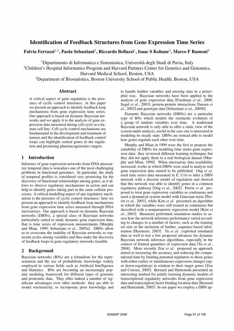
Identification of Feedback Structures from Gene Expression Time SeriesFulvia Ferrazzi1,2, Paola Sebastiani3, Riccardo Bellazzi1, Isaac S Kohane2, Marco F Ramoni2

1Dipartimento di Informatica e Sistemistica, Universita degli Studi di Pavia, Italy2Children’s Hospital Informatics Program and Harvard Partners Center for Genetics and Genomics,

Harvard Medical School, Boston, USA3Department of Biostatistics, Boston University School of Public Health, Boston, USA

AbstractA critical aspect of gene regulation is the pres-ence of cyclic control structures: in this paperwe present an approach to identify feedback loopmechanisms from gene expression time series.Our approach is based on dynamic Bayesian net-works and we apply it to the analysis of gene ex-pression data measured during cell cycle in a hu-man cell line. Cell cycle control mechanisms arefundamental in the development and treatment oftumors and the identification of feedback controlloops can highlight central genes in the regula-tion and promising pharmacogenomics targets.

1 IntroductionInference of gene expression networks from DNA microar-ray temporal data is nowadays one of the most challengingproblems in functional genomics. In particular, the studyof temporal profiles is considered very promising for thediscovery of functional relationships among genes, as it al-lows to observe regulatory mechanisms in action and canhelp to identify genes taking part in the same cellular pro-cesses. A critical modelling aspect of any regulatory mech-anism is the presence of cyclic control structures: here wepresent an approach to identify feedback loop mechanismsfrom gene expression time series measured through DNAmicroarrays. Our approach is based on dynamic Bayesiannetworks (DBNs), a special class of Bayesian networksparticularly suited to study dynamic gene expression data,that is time series of expression measurements [Murphyand Mian, 1999; Sebastiani et al., 2005a]. DBNs allowus to overcome the inability of Bayesian networks to rep-resent cycles among variables and thus make the discoveryof feedback loops in gene regulatory networks feasible.

2 BackgroundBayesian networks (BNs) are a formalism for the repre-sentation and the use of probabilistic knowledge widelyemployed in various fields such as Artificial Intelligenceand Statistics. BNs are becoming an increasingly pop-ular modeling framework for different types of genomicand proteomic data. They offer indeed a number of sig-nificant advantages over other methods: they are able tomodel stochasticity, to incorporate prior knowledge and

to handle hidden variables and missing data in a princi-pled way. Bayesian networks have been applied to theanalysis of gene expression data [Friedman et al., 2000;Segal et al., 2003], protein-protein interactions [Jansen etal., 2003] and genotype data [Sebastiani et al., 2005b].

Dynamic Bayesian networks (DBNs) are a particulartype of BNs which models the stochastic evolution ofa group of random variables over time. A traditionalBayesian network is only able to offer a static view of thesystem under analysis, useful in the case one is interested inmodeling its steady state. DBNs are instead able to modelhow genes regulate each other over time.

Murphy and Mian in 1999 were the first to propose thesuitability of DBNs for modeling time series gene expres-sion data: they reviewed different learning techniques butthey did not apply them to a real biological dataset [Mur-phy and Mian, 1999]. When microarray data availabilityincreased, works in which DBNs were used to analyze realgene expression data started to be published. Ong et al.used time series data measured in E. Coli to infer a DBNnetwork with a discrete model of regulation and showedthat this network was able to identify genes in a commonregulatory pathway [Ong et al., 2002]. Perrin et al. pro-posed to treat gene expression variables as continuous andused a dynamical system model with Gaussian noise [Per-rin et al., 2003], while Kim et al. presented an algorithmin which the variables were still treated as continuous butdescribed with a nonparametric regression model [Kim etal., 2003]. Husmeier performed simulation studies to as-sess how the network inference performance varied accord-ing to changes in a number of factors, such as the trainingset size or the inclusion of further, sequence-based infor-mation [Husmeier, 2003]. Yu et al. exploited simulateddata as well to test a few proposed advances for dynamicBayesian network inference algorithms, especially in thecontext of limited quantities of expression data [Yu et al.,2004]. More recently Zou et al. proposed an approachaimed at increasing the accuracy and reducing the compu-tational time by limiting potential regulators to those geneswith either earlier or simultaneous expression changes (up-or down-regulation) in relation to their target genes [Zouand Conzen, 2005]. Bernard and Hartemink presented aninteresting method for jointly learning dynamic models oftranscriptional regulatory networks from gene expressiondata and transcription factor binding location data [Bernardand Hartemink, 2005]. In our paper we employ a DBN ap-


proach based on Linear Gaussian models to describe generelationships. This approach, which is described in the fol-lowing Section, is very useful for a first level, genome-wideanalysis of high throughput dynamic data.

3 MethodA DBN is a directed acyclic graph that encodes a jointprobability distribution over a set of random variables:the nodes in the graph represent these stochastic variablesand directed arcs represent the dependencies among them,which are quantified by conditional probability distribu-tions.

Supposing expression values for n genes in p consecu-tive time points are available, it is possible to indicate withY (t) = Y1(t), Y2(t), . . . , Yn(t) the set of random vari-ables representing gene expression values at time t. Weassume that the process under study (the dynamics of geneexpression) is• Markovian, i.e. p(Y (t + 1)|Y (0), . . . , Y (t)) =

p(Y (t + 1)|Y (t)) and• stationary, i.e. the transition probability p(Y (t +

1)|Y (t)) is independent of t.Furthermore, we assume that a certain time lag is neces-sary for the expression of a gene to affect the expression ofother genes, so that no instantaneous relationship betweenthe expression levels of two genes is possible. Given thesethree assumptions, it is necessary to learn only the tran-sition network between expression values at time t and attime t + 1 [Friedman et al., 1998].

The use of DBNs allows us to overcome the inability ofBayesian networks to represent cycles among variables andthus makes the discovery of feedback loops in gene net-works feasible. Indeed, the necessary acyclic structure ofthe directed graph that encodes the dependencies betweenthe network variables is no longer a limitation in the frame-work of DBNs. Considering for example two genes A andB and indicating with the subscripts t and t + 1 their ex-pression values in two consecutive time points, if two linksAt → Bt+1 and Bt → At+1 are found through the learn-ing of a DBN, it is possible to say that there is a feedbackloop connecting these two genes, either directly or throughother genes.

As Bayesian networks, DBNs can be learned from thedata. To this aim, a probability model and a searchstrategy must be chosen. We assume that the variablesY1, . . . , Yn are all continuous, and that the conditional dis-tribution of each variable Yi given its parents Pa(yi) =(Yi1, . . . , Yip(i)) follows a Gaussian distribution with meanµi that is a linear function of the parent variables and con-ditional variance σ2

i[Sebastiani et al., 2005a]. The depen-

dency of each variable on its parents is thus represented bythe linear regression equation:

µi = βi0 +∑

j

βijyij (1)

that models the conditional mean of Yi at time t + 1 giventhe parent values yij , measured at time t.

In accordance with the Bayesian literature, we look forthe network associated with the maximum posterior prob-ability with respect to the data. As an exhaustive search

over the space of all possible networks encoding the proba-bilistic dependencies among the n analyzed variables is notfeasible, we exploit a finite horizon local search and we ex-plore the dependency of each variable on all the variablesat the previous time point [Cooper and Herskovitz, 1992;Sebastiani et al., 2005a].

4 Data analysis and discussionWe decided to focus our investigation on the cell cycle,a process of critical importance where feedback controlloops are expected to play a central regulatory role. Theanalysis of cell cycle regulation is indeed one of the mostimportant areas of research in the medical and biologicalcommunity, as an understanding of how cells divide andproliferate is crucial for the study of various diseases, mostnotably cancer. In this analysis, the discovery of feedbackloop mechanisms could be extremely useful in highlightinggenes which play a key role in cell cycle control and whichthus constitute potential targets for an effective cancer ther-apy.

For this purpose, we use a database of gene expres-sion data measured in a human epithelial cell line de-rived from a cervical carcinoma [Whitfield et al., 2002].This database, available from the web (http://genome-www.stanford.edu/Human-CellCycle/Hela/), includes datacoming from 5 different experiments. In particular, in oneof these, gene expression values were measured every hour,from 0 to 46 hs, using cDNA microarrays containing about40000 probes. This dataset currently represents one ofthe most extensive collections of gene expression tempo-ral data. Its abundant amount of samples (47 time points)constitutes a significant advantage for the inference of thenetwork. In fact, a problem often encountered in the learn-ing is that the number of variables (genes/probes) is nor-mally very high, while the available measurements (geneexpression values) are usually very few, thus often leadingto a low degree of sensitivity and specificity in the inferrednetworks [Husmeier, 2003].

We are currently analyzing a set of 1000 probes identi-fied as periodical in [Whitfield et al., 2002]: the authors,employing a Fourier transform and correlation to knowncell cycle yeast genes, calculated a periodicity score foreach of the probes and selected about 1000 probes whosescore exceeded a carefully chosen threshold. We analyzedtheir time profiles with the algorithm presented in the previ-ous Section. The inferred DBN is very parsimonious, witha number of parents for every node that ranges from 0 to 2.

Starting from this DBN, we reconstructed a gene regula-tory network, in which nodes referring to the same variableat consecutive time points (eg. At and At+1) were col-lapsed into a single node. This regulatory network is not aBayesian network anymore and can instead contain loops.Figure 1 presents an example of how a gene regulatory net-work is reconstructed from the transition network.

The reconstructed gene regulatory network is shown inFigure 2. The analysis of this network led us to concen-trate our attention on a group of 12 probes that appear to beinvolved in various feedback loops. Some of these probesmap to well characterized cell cycle genes, while othershighlight potential new key players in cell cycle regulation.


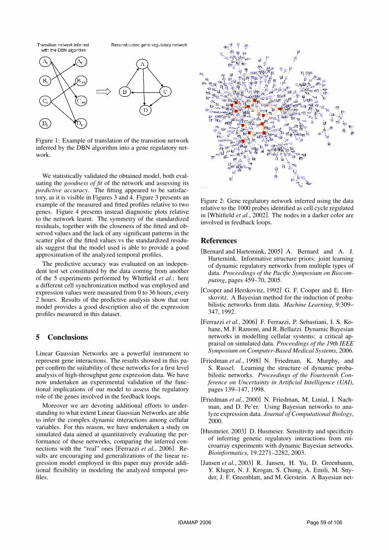
Figure 1: Example of translation of the transition networkinferred by the DBN algorithm into a gene regulatory net-work.

We statistically validated the obtained model, both eval-uating the goodness of fit of the network and assessing itspredictive accuracy. The fitting appeared to be satisfac-tory, as it is visible in Figures 3 and 4. Figure 3 presents anexample of the measured and fitted profiles relative to twogenes. Figure 4 presents instead diagnostic plots relativeto the network learnt. The symmetry of the standardizedresiduals, together with the closeness of the fitted and ob-served values and the lack of any significant patterns in thescatter plot of the fitted values vs the standardized residu-als suggest that the model used is able to provide a goodapproximation of the analyzed temporal profiles.

The predictive accuracy was evaluated on an indepen-dent test set constituted by the data coming from anotherof the 5 experiments performed by Whitfield et al.: herea different cell synchronization method was employed andexpression values were measured from 0 to 36 hours, every2 hours. Results of the predictive analysis show that ourmodel provides a good description also of the expressionprofiles measured in this dataset.

5 Conclusions

Linear Gaussian Networks are a powerful instrument torepresent gene interactions. The results showed in this pa-per confirm the suitability of these networks for a first levelanalysis of high-throughput gene expression data. We havenow undertaken an experimental validation of the func-tional implications of our model to assess the regulatoryrole of the genes involved in the feedback loops.

Moreover we are devoting additional efforts to under-standing to what extent Linear Gaussian Networks are ableto infer the complex dynamic interactions among cellularvariables. For this reason, we have undertaken a study onsimulated data aimed at quantitatively evaluating the per-formance of these networks, comparing the inferred con-nections with the “real” ones [Ferrazzi et al., 2006]. Re-sults are encouraging and generalizations of the linear re-gression model employed in this paper may provide addi-tional flexibility in modeling the analyzed temporal pro-files.

Figure 2: Gene regulatory network inferred using the datarelative to the 1000 probes identified as cell cycle regulatedin [Whitfield et al., 2002]. The nodes in a darker color areinvolved in feedback loops.

References[Bernard and Hartemink, 2005] A. Bernard and A. J.

Hartemink. Informative structure priors: joint learningof dynamic regulatory networks from multiple types ofdata. Proceedings of the Pacific Symposium on Biocom-puting, pages 459–70, 2005.

[Cooper and Herskovitz, 1992] G. F. Cooper and E. Her-skovitz. A Bayesian method for the induction of proba-bilistic networks from data. Machine Learning, 9:309–347, 1992.

[Ferrazzi et al., 2006] F. Ferrazzi, P. Sebastiani, I. S. Ko-hane, M. F. Ramoni, and R. Bellazzi. Dynamic Bayesiannetworks in modelling cellular systems: a critical ap-praisal on simulated data. Proceedings of the 19th IEEESymposium on Computer-Based Medical Systems, 2006.

[Friedman et al., 1998] N. Friedman, K. Murphy, andS. Russel. Learning the structure of dynamic proba-bilistic networks. Proceedings of the Fourteenth Con-ference on Uncertainty in Artificial Intelligence (UAI),pages 139–147, 1998.

[Friedman et al., 2000] N. Friedman, M. Linial, I. Nach-man, and D. Pe’er. Using Bayesian networks to ana-lyze expression data. Journal of Computational Biology,2000.

[Husmeier, 2003] D. Husmeier. Sensitivity and specificityof inferring genetic regulatory interactions from mi-croarray experiments with dynamic Bayesian networks.Bioinformatics, 19:2271–2282, 2003.

[Jansen et al., 2003] R. Jansen, H. Yu, D. Greenbaum,Y. Kluger, N. J. Krogan, S. Chung, A. Emili, M. Sny-der, J. F. Greenblatt, and M. Gerstein. A Bayesian net-


Figure 3: Measured and fitted profiles for two analyzedprobes.

works approach for predicting protein-protein interac-tions from genomic data. Science, 302:449–53, 2003.

[Kim et al., 2003] S. Kim, S. Imoto, and S. Miyano. In-ferring gene networks from time series microarray datausing dynamic Bayesian networks. Briefings in Bioin-formatics, 4:228–235, 2003.

[Murphy and Mian, 1999] K. Murphy and S. Mian. Mod-elling gene expression data using dynamic Bayesian net-works. Technical Report, Berkeley, CA Computer Sci-ence Division, University of California, 1999.

[Ong et al., 2002] I. M. Ong, J. D. Glasner, and D. Page.Modelling regulatory pathways in E. coli from timeseries expression profiles. Bioinformatics, 18 (Suppl1):S241–8, 2002.

[Perrin et al., 2003] B. E. Perrin, L. Ralaivola, A. Mazurie,S. Bottani, J. Mallet, and F. D’Alche-Buc. Genenetworks inference using dynamic Bayesian networks.Bioinformatics, 19 (Suppl 2):II138–II148, 2003.

[Sebastiani et al., 2005a] P. Sebastiani, M. Abad, and M.F.Ramoni. Bayesian networks for genomic analysis.

(a) Histogram of standardized residuals

(b) Fitted vs observed values (c) Fitted values vs standardized res.

Figure 4: Diagnostic plots for the network model learnt.

Genomic Signal Processing and Statistics. EURASIPBook Series on Signal Processing and Communications,2005.

[Sebastiani et al., 2005b] P. Sebastiani, M. F. Ramoni,V. Nolan, C. T. Baldwin, and M. H. Steinberg. Geneticdissection and prognostic modeling of overt stroke insickle cell anemia. Nature Genetics, 37:435–40, 2005.

[Segal et al., 2003] E. Segal, M. Shapira, A. Regev,D. Pe’er, D. Botstein, D. Koller, and N. Friedman. Mod-ule networks: identifying regulatory modules and theircondition-specific regulators from gene expression data.Nature Genetics, 34:166–176, 2003.

[Whitfield et al., 2002] M.L. Whitfield, G. Sherlock, A.J.Saldanha, J.I. Murray, C.A. Ball, K.E. Alexander, J.C.Matese, C.M. Perou, M.M. Hurt, P.O. Brown, andD. Botstein. Identification of genes periodically ex-pressed in the human cell cycle and their expressionin tumors. Molecular Biology of the Cell, 13(6):1977–2000, 2002.

[Yu et al., 2004] J. Yu, V. A. Smith, P. P. Wang, A. J.Hartemink, and E. D. Jarvis. Advances to Bayesiannetwork inference for generating causal networks fromobservational biological data. Bioinformatics, 20:3594–603, 2004.

[Zou and Conzen, 2005] M. Zou and S. D. Conzen. A newdynamic Bayesian network (DBN) approach for iden-tifying gene regulatory networks from time course mi-croarray data. Bioinformatics, 21:71–9, 2005.


Visualisation of AssociationsBetween Nucleotides in SNP Neighbourhoods

Kimmo Kulovesi∗,†, Juho Muhonen∗, Ilkka Lappalainen‡, Pentti T. Riikonen§,Mauno Vihinen¶ ,†, Hannu Toivonen∗

,

‖ and Tomi A. Pasanen∗

AbstractA large number of single nucleotide polymorph-isms have been mapped onto the human genome.Mutations are induced through endogenous andexogenous processes, and these procedures havebeen shown to be sequence-dependent. Associa-tion mining is a powerful tool for analyzing se-quence neighbourhoods; however, visualisationis essential for pattern recognition because of theabundance of resulting association rules.A software tool was developed to visualize posi-tion interdependencies within the sequence vari-ation data. The software is capable of interac-tive reorganization of the association rules, en-abling fast and easy exploration of the data us-ing a standard web browser. The software andits complete source code is freely available at:http://www.cs.helsinki.fi/group/bioalgss/asvis/

1 IntroductionA single nucleotide polymorphism (SNP) is a site in DNAwhere at least two different nucleotides occur in a specificpopulation, the less frequent nucleotide(s) occurring at afrequency of 1% or more. The nucleotide variation be-tween individuals forms the genetic background responsi-ble for biological and physical differences such as colourof hair, susceptibility to a disease or response to specifictreatment. The International HapMap project aims to char-acterise the common human sequence variations [Interna-tional HapMap Consortium, 2005]. The data is publiclyavailable in the dbSNP database [Wheeler et al., 2005].

New mutations arise by errors in endogenous processesinvolved in maintaining genomic stability, or are induced

∗Department of Computer Science, FI-00014 University ofHelsinki, Finland

†Institute of Medical Technology, FI-33014 University ofTampere, Finland

‡Department of Chemistry, Cambridge University, CB2 1EWCambridge, UK

§Department of Information Technology, FI-20520 Universityof Turku, Finland

¶Research Unit, Tampere University Hospital, FI-33520 Tam-pere, Finland

‖Department of Computer Science, University of Freiburg, D-79110 Freiburg, Germany

by various exogenous agents, such as UV radiation [Jiricny,1998]. The efficiency and specificity of these processes isDNA sequence dependent [Cooper and Krawczak, 1993].Data mining can be used to analyze the sequence neigh-bourhoods of neutral and disease-causing SNPs in orderto better understand the genetic differences that underliepathogenic conditions.

Association rules are suitable for this task. Discovery ofassociation rules is popular in data mining and it has a widevariety of applications. In principle, individual associationrules describing co-occurrences of sets of attributes in theinput data are straightforward to interpret. However, thevery large number of resulting association rules seriouslyhinders their analysis. General-purpose visualisation toolsare ill-suited for association rules, and the few available as-sociation visu-alisation tools are not suitable for position-dependent SNP neighbourhoods. Furthermore, the existingtools for visualizing SNP neighbouring-nucleotide biasesare not applicable to association rules (for example, [Zhangand Zhao, 2005]). Here we introduce a new, publicly avail-able visualisation tool with interactive controls for the se-lection and arrangement of association rules obtained fromSNP data. The tool has a novel position-dependent displayof association rules. It can also be used with other similardata, such as protein sequences. The tool provides simpleand legible graphical output.

2 System and MethodsFor demonstration in this paper, sequence variation datawas extracted from the dbSNP (build 124). Only true poly-morphisms that could be located within gene coding re-gions of the human genome (build 35) were used. We con-sider a sequence neighbourhood of each mutation site thatextends up to ten nucleotides on both sides. The mutationposition is numbered zero, while positive and negative po-sition numbers denote the distance of following and pre-ceding nucleotides, respectively.

Our software consists of two programs, Firm and AsVis.Firm is used for application-independent discovery of as-sociation rules. As an example, the rule 0:’C→T’ ←−+1:’G’ indicates that the substitution of cytosine (C) bythymine (T) is probable when the mutation site is immedi-ately followed by guanine (G) (see Figure 1). To rank theassociation rules, Firm yields a number of measures for thestrength and generality of each rule within the data. Sup-port is the number of records that fully match the rule. Con-


Figure 1: Example association rules (above) visualised by AsVis (below). No information is lost in the visualisation, butthe positional nature of the rules is immediately apparent.

fidence of a rule is the conditional probability of the con-sequent (e.g. 0: ’C→T’) given the condition (+1:’G’).Lift is simply the ratio of confidence over the relative fre-quency of the rule consequent, whereas J-measure [Smythand Goodman, 1992] is an information-theoretic measuredescribing the amount of information that the conditiongives about the consequent.

Association rules are suitable as such for exploratorydata analysis, and a large amount of them can be discoveredefficiently, without setting a strong focus on any particularattributes. Usually only support and confidence thresholdsare used to limit the number of rules, and algorithms suchas Apriori [Agrawal et al., 1996] produce all associationrules between any sets of attributes that exceed the thresh-olds. A rule can have any number of conditions and conse-quents, but with reasonable threshold values, our data didnot give any strong associations for complex dependencieswith more than one consequent.

To facilitate visual browsing and exploration of thou-sands of rules, an interactive web interface, AsVis, was de-veloped. AsVis graphically renders the rules into a formthat visually reflects the sequential nature of the data, tak-ing advantage of the relatively small number of dimen-sions (positions). The association rules are listed in a table,where each row represents a single rule, and each columncorresponds either to a position relative to the point of mu-tation or to a strength or generality measure for the rule (seeFigure 1). Consequents and conditions are colour-coded inthe positional columns.

The interface enables the user to explore the most in-teresting rules. Clicking on the column header of a mea-sure sorts the rules by that measure, with the best scoresat the top. Clicking on a positional column header limitsthe display to only those rules that have either a conditionor a consequent in that position, while keeping the currentsorting. This approach is somewhat similar to the TASAsystem [Klemettinen et al., 1999].

This simple approach enables quick visual scanning ofthe rules for an overview of dependencies between posi-tions. The measures for each rule are for closer inspection,providing the full scope of information discovered by thedata mining process.

AcknowledgementsThis research has been supported by Tekes (the NationalTechnology Agency of Finland), The Medical Reseach

Fund of Tampere University Hospital, and the Academyof Finland. We thank Adrian Nickson for valuable discus-sions.

References[Agrawal et al., 1996] Rakesh Agrawal, Heikki Mannila,

Ramakrishnan Srikant, Hannu Toivonen, and A. InkeriVerkamo. Fast discovery of association rules. pages307–328, 1996.

[Cooper and Krawczak, 1993] David N. Cooper andMichael Krawczak. Human Gene Mutation. 1993.

[International HapMap Consortium, 2005] The Interna-tional HapMap Consortium. A haplotype map of thehuman genome. Nature, 437(7063):1299–1320, 2005.

[Jiricny, 1998] J. Jiricny. Replication errors: cha(lle)ngingthe genome. 17(22):6427–6436, 1998.

[Klemettinen et al., 1999] M. Klemettinen, Heikki Man-nila, and Hannu Toivonen. Interactive exploration ofinteresting patterns in the telecommunication networkalarm sequence analyzer tasa. Information and SoftwareTechnology, 41:557–567, 1999.

[Smyth and Goodman, 1992] P. Smyth and R. M. Good-man. An information theoretic approach to rule induc-tion from databases. IEEE Transactions on Knowledgeand Data Engineering, 4(4):301–316, 1992.

[Wheeler et al., 2005] David L. Wheeler, Tanya Barrett,Dennis A. Benson, Stephen H. Bryant, Kathi Canese,Deanna M. Church, Michael DiCuccio, Ron Edgar,Scott Federhen, Wolfgang Helmberg, David L. Kenton,Oleg Khovayko, David J. Lipman, Thomas L. Mad-den, Donna R. Maglott, James Ostell, Joan U. Pon-tius, Kim D. Pruitt, Gregory D. Schuler, Lynn M.Schriml, Edwin Sequeira, Steven T. Sherry, KarlSirotkin, Grigory Starchenko, Tugba O. Suzek, RomanTatusov, Tatiana A. Tatusova, Lukas Wagner, and Eu-gene Yaschenko. Database resources of the NationalCenter for Biotechnology Information. Nucl. Acids Res.,33:D39–45, 2005.

[Zhang and Zhao, 2005] Fengkai Zhang and ZhongmingZhao. SNPNB: analyzing neighboring-nucleotidebiaseson single nucleotide polymorphisms (SNPs). Bioinfor-matics, 21(10):2517–2519, 2005.


Paper session: Markov Models


Prognosis of High-Grade Carcinoid Tumor Patients usingDynamic Limited-Memory Influence Diagrams∗

Marcel A.J. van Gerven1, Francisco J. Dıez2, Babs G. Taal3, Peter J.F. Lucas11Institute for Computing and Information Sciences, RadboudUniversity Nijmegen

Toernooiveld 1, 6525 ED Nijmegen, The NetherlandsE-mail: [email protected]

2Department of Artificial Intelligence, UNED, Madrid3Netherlands Cancer Institute/Antoni van Leeuwenhoek hospital, Amsterdam

AbstractDynamic limited-memory influence diagrams(DLIMIDs) have been developed as a frameworkfor decision-making under uncertainty over time.We show that DLIMIDs constructed from two-stage temporal LIMIDs can represent infinite-horizon decision processes. Given a treatmentstrategy supplied by the physician, DLIMIDsmay be used as prognostic models. The theoryis applied to determine the prognosis of patientsthat suffer from an aggressive type of neuroen-docrine tumor.

1 IntroductionAn important task in medicine is making an accurate prog-nosis for a particular patient given the patient’s history.Ac-curate prognosis facilitates patient feedback and allows thephysician to adjust the treatment strategy but is non-trivialin a world that is characterized by change and uncertainty.In our research, we have been engaged in the construc-tion of a prognostic model for high-grade carcinoid tumorsof the midgut, which are an aggressive type of neuroen-docrine tumor[Modlin et al., 2005]. The model has beenconstructed in collaboration with an expert physician of theNetherlands Cancer Institute (NKI).

The aim of this paper is to show how prognostic mod-els may be constructed using an approach that is based onlimited-memory influence diagrams(LIMIDs) [Lauritzenand Nilsson, 2001]. We extend the definition of LIM-IDs to dynamicLIMIDs, which explicitly take time intoaccount. We show that dynamic LIMIDs allow the han-dling of infinite-horizon and partially observable Markovdecision processes (POMDPs)[Astrom, 1965] wheneverthey are representable as a so-calledtwo-stage temporalLIMID (2TLIMID). Infinite-horizon POMDPs cannot bedealt with using standard (limited-memory) influence dia-grams, and contrary to POMDPs, the 2TLIMID represen-tation makes explicit a factorization of the state-space thatis defined by the variables in the domain1. This is advanta-geous, from a computational point of view, since it allows

∗This research was sponsored by the Dutch Institute Madridand by the Dutch Science Foundation under grant number612.066.201.

1Much recent POMDP research has been concerned with tak-ing advantage of such factorizations[Boutilier et al., 1996a].

for more efficient inference algorithms, and also from arepresentational point of view, since it allows us to describethe model in terms of the relations that hold between do-main variables (see e.g.[Peek, 1999]). Given the strategyof a decision maker, a 2TLIMID can be transformed intoa two-stage temporal Bayes network[Dean and Kanazawa,1989], and prognosis then proceeds by means of probabilis-tic inference using this Bayesian network.

In contrast to classical approaches to prognosis, such asCox’s proportional hazard model[Cox, 1972], we take amodel-basedapproach that aims to represent as accuratelyas possible the causal relations that hold between domainvariables. It has been argued that models which capturecause-effect relationships are more meaningful, accessibleand reliable than models which capture empirical associa-tions [Druzdzel, 1997]. Causal models are also richer inrepresentational power than non-causal models, since theyallow for reasoning under interventions[Pearl, 2000]. Inthe context of decision support in medicine, causal modelshave several advantages. They allow for capturing expertknowledge, which is a valuable commodity in itself, andare more easily modified when new knowledge becomesavailable (i.e. they are lessbrittle than models based onempirical associations). Furthermore, they facilitate the ex-planation of drawn conclusions, which may increase the ac-ceptance of decision-support systems in medicine[Teachand Shortliffe, 1984; Lacave and Dıez, 2002]. However,building causal models often proves to be non-trivial, as itis difficult to elicit the needed qualitative and quantitativeknowledge.

We proceed as follows. Section 2 describes requiredpreliminaries. Dynamic LIMIDs and 2TLIMIDs are intro-duced in Section 3. Section 4 presents a formalization ofprognosis, where we use 2TLIMIDs to represent prognos-tic models. Section 5 describes the prognostic model forhigh-grade carcinoids as an illustration of the theory. Sec-tion 6 describes some results concerning prognostic modelperformance. The paper is concluded in Section 7.

2 PreliminariesBayesian networks[Pearl, 1988] provide for a compact fac-torization of a joint probability distribution of a set of ran-dom variables by exploiting the notion ofconditional in-dependence. One way to represent conditional indepen-dence is by means of an acyclic directed graph (ADG)Gwhose nodesV (G) correspond to random variablesX and


the absence of arcs from the set of arcsA(G) representsconditional independence. Due to this one-to-one corre-spondence we will use nodesv ∈ V (G) and random vari-ablesX ∈ X interchangeably. ABayesian network(BN)is then defined as a pairB = (G, P ), such that the jointprobability distributionP is factorized according toG:

P (X) =∏

X∈X

P (X | πG(X))

whereπG(X) denotes theparentsof X : X ′ | (X ′, X) ∈A(G). We also say thatX is thechildof someX ′ ∈ π(X)where we drop the subscriptG when clear from context. Inthis paper, we say that a (random) variableX takes valuesx from a setΩX and usex to denote an element inΩX =×X∈X ΩX for a setX of (random) variables.

Limited-memory influence diagrams are models fordecision-making under uncertainty[Lauritzen and Nils-son, 2001]. They generalize standard influence-diagrams(IDs) by relaxing theno-forgettingassumption[Howardand Matheson, 1984]. This assumption states that, givena total ordering of the decisions, the information knownwhen making decisionD is also available when makingdecisionD′, if D precedesD′ in the ordering. Alimited-memory influence diagram(LIMID) is defined as a tupleL = (C,D,U, G, P ). Here,C is a set ofchance variables(graphically depicted by circles), which are random vari-ables as in a Bayesian network that represent the stochasticcomponent of the model.D is a set ofdecision variables(graphically depicted by squares), which take on a valuefrom a set of choicesΩD that represent the decisions thatmay be externally manipulated by a decision maker.U is aset ofutility functions(graphically depicted by diamonds),which represent the utility of being in a certain state as de-fined by configurations of chance and decision variables.Gis an ADG, where nodesV (G) correspond toC ∪ D ∪ U.Again, due to this correspondence, we will use nodes inV (G) and corresponding elements inC ∪ D ∪ U inter-changeably.P is a family of probability distributions thatspecifies for each configurationd ∈ ΩD a distribution:

P (C : d) =∏

C∈C

P (C | π(C))

that represents the distribution overC when the decisionmaker has setD = d [Cowell et al., 1999]. Hence,C isnot conditioned onD, but rather parameterized byD.

The meaning of an arc(X, Y ) ∈ A(G) is determinedby the type ofY . If Y ∈ C then the conditional proba-bility distribution associated withY is conditioned byX ,as in a Bayesian network. IfY ∈ D then the state ofX isavailable to the decision maker prior to deciding uponY . IfY ∈ U thenX takes part in the specification of the utilityfunctionY such thatY : Ωπ(Y ) → R. Utility nodes cannothave children and the joint utility functionU is assumed tobe additively decomposable such thatU =

∑U∈U U .

In contrast to standard influence diagrams, the order inwhich decisions are made in a LIMID should only be com-patible with the partial order induced byG, and making adecisionD is based solely on its direct parentsπ(D). Astochastic policyfor decisionsD ∈ D is defined as a dis-tributionPD(D | π(D)) that maps configurations ofπ(D)

C01

D01

C02

D02

U01

Ct-11

Dt-11

Ct-12

Dt-12

Ct

1

Dt

1

Ct

2

Dt

2

Ut

1

L0 Lt

Figure 1: Structure of a 2TLIMID.

to a distribution over alternatives forD. If PD is degener-ate (i.e. consisting of ones and zeros only) then we say thatthe policy is deterministic. LetV denoteC∪D. A strategyis a set of policies∆ = PD : D ∈ D which induces thefollowing joint distribution over the variables inV:

P∆(V) = P (C : D)∏

D∈D

PD(D | π(D)).

Using this distribution we can compute the expected utilityof a strategy∆ as

E∆(U) =∑v

P∆(v)U(v).

The aim of any rational decision maker is then to maxi-mize the expected utility by finding the optimal strategyarg max∆ E∆(U).

3 Dynamic LIMIDsIn this section we demonstrate how to use dynamic LIM-IDs that are constructed by means of a structure that weterm atwo-stage temporal LIMID(2TLIMID). When deal-ing with time, we useT ⊆ N to represent a set of timepoints, which we normally assume to be an intervalu |t ≤ u ≤ t′, t, u, t′ ⊂ N, also written ast : t′. Weassume that chance variables, decision variables and util-ity functions are indexed by a superscriptt ∈ T, and useCT, DT andUT to denote all chance variables, decisionvariables and utility functions at timest ∈ T, where weabbreviateCT ∪ DT with VT. If T = 0 : n, wheren ∈ 1, 2, . . . is the horizon, then we suppressT alto-gether, and we suppress indices for individual chance vari-ables, decision variables and utility functions when clearfrom context.

3.1 Constructing Dynamic LIMIDsA dynamic LIMID (DLIMID) is simply defined as aLIMID (C,D,U, G, P ) such that for all pairs of variablesXt, Y u ∈ V∪U it holds that ift < u thenY u cannot pre-cedeXt in the partial ordering that is induced byG. If thefirst-order Markov assumption holds that the future is con-ditionally independent of the past given the present, thenwe can define a DLIMID in terms of a two-stage temporalLIMID (Fig. 1).


Definition 3.1. A two-stage temporal LIMID(2TLIMID ) is a pair (L0,Lt) with prior model L0

= (C0,D0,U0, G0, P 0) and transition model Lt =(Ct−1:t,Dt−1:t,Ut, G, P ) such that chance and decisionvariablesV t−1

i in Vt−1 have no parents.

The prior model is used to represent the initial distribu-tion P 0(C0 : D0) and utility functionsU ∈ U0. The tran-sition model is not yet bound to any specifict, but if boundto somet ∈ 1 : n, then it is used to represent the con-ditional distributionP (Ct : Dt−1:t) and utility functionsU ∈ Ut where bothG andP do not depend ont. We definethe interfaceof the transition model as the setIt ⊆ Vt−1

such that(V t−1i , V t

j ) ∈ A(G) ⇔ V t−1i ∈ It.

Given a horizonn, we mayunroll a 2TLIMID for n time-slicesin order to obtain a DLIMID such that we obtain thefollowing joint distribution:

P (C,D) = P 0(C0 : D0)n∏

t=1

P (Ct : Dt−1:t). (1)

Let ∆t = PD(D | πG(D)) | D ∈ Dt be the strategy fortime t and∆ = ∆0 ∪ · · · ∪ ∆n. Given a strategy∆0, L0

defines the following distribution over variables inV0:

P∆0(V0) = P 0(C0 : D0)∏

D∈D0

PD(D | πG0(D)).

Likewise, given a strategy∆t with t > 0, Lt defines thefollowing conditional distribution over variables inVt:

P∆t(Vt | Vt-1) = P (Ct : Dt:t−1)∏

D∈Dt

PD(D | πG(D)).

Combining these equations, given a horizonn and strat-egy∆, a 2TLIMID induces the following distribution overvariables inV:

P∆(V) = P∆0(V0)n∏

t=1

P∆t(Vt | It). (2)

Let U0(V0) =∑

U∈U0 U(πG0(U)) stand for the jointutility for t = 0 and letU t(Vt−1:t) =

∑U∈Ut U(πG(U))

denote the joint utility for time-slicet > 0. We redefine thejoint utility function for a dynamic LIMID as

U(V) = U0(V0) +n∑

t=1

γtU t(Vt−1:t)

whereγ, with 0 ≤ γ < 1, is adiscount factor, representingthe notion that early rewards are worth more than the samerewards earned later in time.

3.2 Representing Observed HistoryIt is clear from Eq. 1 that DLIMIDs constructed from a2TLIMID take into accountat mostall chance and decisionvariables in two subsequent time-slices, sinceπ(D0

i ) ⊆ V0

andπ(Dti) ⊆ Vt−1:t. Observations made earlier in time

are not taken into account and as a result, states that arequalitatively different can appear the same to the decisionmaker, leading to suboptimal policies. This phenomenonis known asperceptual aliasing[Whitehead and Ballard,1991]. In this paper we usememory variablesto take into

Figure 2: Dealing with perceptual aliasing by introducingmemory variables (black circles). Memory variables areused instead of associated observed variables (shaded cir-cles) as the informational predecessor for a decision vari-able (squares).

account (part of) the observed historyv′ with V′ ⊆ V0:c

and current timec, as depicted in Fig. 2.Note that if we represent the full observed history, infer-

ence becomes intractable for long histories since the statesof a memory variableM ∈ C associated with a variableV ∈ V are given byΩn

M , whereΩj+1M = Ωj

M ∪(ΩjM ×ΩV )

andΩ0M = ΩV . However, by restricting the length of the

observed history and/or by usingaggregationtechniques[Boutilieret al., 1996a] that group states which are indistin-guishable from the point of view of the decision maker, wecan both use the limited-memory assumption of LIMIDsand deal with perceptual aliasing2. Examples of variablesthat fulfill the role of memory variable areBMDHIST andTREATHIST in Fig. 3, which maintain information regard-ing complications and previous treatments respectively. Anadditional advantage of the use of memory variables is thefact that we retain the first-order Markov assumption. Dueto this property DLIMIDs can take benefit from efficientalgorithms for probabilistic inference.

3.3 Inference using 2TLIMIDsTo perform inference with a LIMIDL = (C,D,U, G, P )given a strategy∆, we convertL into a Bayesian networkB = (G′, P ′) that is subsequently used for inference pur-poses. As has been remarked, a strategy∆ induces a dis-tribution over variablesV (viz. Eq. 2). Hence, given∆,we may convert decision variablesD into random variablesXD with parentsπG(D) such that

P ′(XD | πG′(XD)) = PD(D | πG(D)).

Additionally, it is possible to convert utility functionsUinto random variablesXU . Let πG′(XU ) = πG(U) whereΩXU

= 0, 1. We associateP ′(XU | π(XU )) with XU

by means of a transformation

P ′(XU =1 | x′) =U(x′) − minx U(x)

maxx U(x) − minx U(x)

with x,x′ ∈ Ωπ(U), as defined in[Cooper, 1988]. WeuseB(L, ∆) to denote this transformation. If the strat-egy is stationary for each time-slicet ∈ 1, . . . , n thenwe can apply the transformation to a 2TLIMID(L0,Lt),to obtain a so-calledtwo-stage temporal Bayes network

2In the context of POMDPs, methods that rely on the use of afinite history are common[Aberdeen, 2003].


GENDER

AGE

GHS

MASS

RESP

TREATHIST

CGA

CHEMO

BMDHIST

GENDER

AGE

GHS

MASS

RESP

TREATHIST

CHEMO

BMDHIST

GENDER

AGE

GHS

MASS

RESP

TREATHIST

BMD

CGA

CHEMO

BMDHIST

L0 Lt

Figure 3: The prognostic model, where shaded nodes are observed and rounded rectangles denote internal structure.

(TBN) (B0,Bt) that is often used to construct adynamicBayesian networkor DBN [Dean and Kanazawa, 1989;Boutilier et al., 1996a; Peek, 1999]. For online infer-ence, efficient algorithms exist that exploit the structureofa 2TBN. In our work, we have used theinterface algorithm[Murphy, 2002], which allows for online filtering, wherethe space and time taken to computeP (Xt | Xt−1) is in-dependent of the number of time-slices.

4 Prognosis with 2TLIMIDsInformally, we interpret prognosis asthe prediction of thefuture status of the patient given the patient history, con-ditional on a treatment strategy. This is a non-trivial tasksince the physician often has incomplete information uponwhich to base treatment and treatment itself can have un-certain effects. LetC andD be sets of chance and decisionvariables respectively. Leto0:c with Ot ⊆ Ct, t ∈ 0 : c,represent the observed evidence until thecurrent timecand letn denote the horizon. We use thequery variableQ ⊆ C ∪ D to denote the variable of interest, and defineprognosis given a 2TLIMID as follows:

Definition 4.1. A prognosis for a query variable Qand a horizonn is a conditional probability distributionP∆(Qc:n | o0:c) overQc:n.

In order to computeP∆(Qc:n | o0:c), we assume thatthe prognostic model is defined by

((L0,Lt), (∆0, ∆t)

),

where(L0,Lt) is a 2TLIMID and (∆0, ∆t) is a pair ofstrategies. Prognosis then proceeds as follows:

1. Define((L0,Lt), (∆0, ∆t)

).

2. Create(B0,Bt) =(B(L0, ∆0), B(Lt, ∆t)

).

3. Recursively computeP∆(Qc:n | o0:c) using(B0,Bt).

Although the processes we consider in medicine are fi-nite since they are bounded by patient’s life-span, we de-scribe them as infinite-horizon processes where the processhas some probability of terminating at each time-slice. In

computing the prognosis however we assume that the hori-zon n is finite. In the next section we develop the actualmodel for prognosis of high-grade carcinoid tumor patientsusing the theory developed so far.

5 The High-Grade Carcinoid Model

A carcinoid tumor is a type of neuroendocrine tumor thatis predominantly found in the midgut and is normally char-acterized by the production of excessive amounts of bio-chemically active substances, such as serotonin[Modlin etal., 2005]. In a small minority of cases, tumors are of high-grade histology which, although biochemically much lessactive than low-grade carcinoids, show much more rapidtumor progression. Therefore, aggressive chemotherapy inthe form of an etoposide and cisplatin-containing schemeis the only treatment option[Moertelet al., 1991]. In thissection we develop the prognostic model for high-gradecarcinoid tumors, consisting of a 2TLIMID(L0,Lt) anda strategy(∆0, ∆t), supplied by the physician. Patientsare admitted to the hospital at the initial timet = 0. Eachtime-slice represents the patient status at three-month inter-vals since patients return for follow-up every three months.Since the aim is not to improve upon the provided strategy,we omit utility nodes from the discussion.

The qualitative structure of the 2TLIMID that resultedfrom our modeling efforts is depicted in Fig. 3. The pa-tient’sgeneral health status(GHS) is of central importance.In oncology, one way to represent the general health sta-tus is by means of theperformance status[Oken et al.,1982]. We defineΩGHS = 0, . . . , 5 where GHS = 0stands for normal health status,GHS = 1 stands for mildcomplaints,GHS = 2 stands for impaired age-appropriateactivity, GHS = 3 stands for confinement to bed for morethan 50% of the time,GHS=4 stands for intensive care andGHS=5 stands for patient death. The general health statusdepends on patient properties such asAGE, GENDER andcurrent general health status. Furthermore,GHS is influ-enced by the tumor mass (MASS) and the treatment policy


Figure 4: Kaplan-Meier curve, showing the cumulative probability of survival for patients A (dashed line) and B (solidline) over a five year period, as predicted by the model (left), and the physician (right).

that is adopted. Chemotherapy (CHEMO), with ΩCHEMO =none, reduced, standard, is the only available treatment,where a reduced dose is at 75% of the standard dose.Chemotherapy can have both positive and negative effectson general health status; positive due to reductions in tumormass, and negative due to severe bone-marrow depression(BMD) and damage associated with prolonged chemother-apy. We useBMDHIST, with ΩBMDHIST = no-bmd, bmd,as a memory variable to represent whether or not the patienthas experiencedBMD in the past. SevereBMD is assumedto be fully observable since patients are always tested forit. We useTREATHIST, with ΩTREATHIST = 0, 1, 2, 3, asa memory variable to represent the patient’s relevant treat-ment history, such thatTREATHIST = i represents contin-ued chemotherapy over the past3 · i months. Reductionsin tumor mass due to chemotherapy are often described interms of tumor response (RESP).

The amount of tumor mass can be estimated by mea-suring the plasmachromogranin Alevel (CGA) since it isstrongly correlated with tumor burden[Nobelset al., 1998].SinceCGA levels are always measured we need not includethe decision variable whether or not to determineCGAlevels (i.e., the associated policy isblind). Severe bone-marrow depression may cause patient death due to associ-ated sepsis and/or internal bleeding[Moertelet al., 1991].AGE andGENDER are risk factors that may lead to patientdeath due to causes other than the disease.MASS andGHSin Fig. 3 are compact representations of a Bayesian net-work fragment. This representation has the advantage ofpreventing unnecessary clutter in the graphical represen-tation of a Bayesian network and provides a way to repre-sentcontext-specific independence[Boutilier et al., 1996b].Due to space restrictions, we will not discuss the internalstructure of these fragments.

To complete the model, we have to choose a treatmentstrategy and assess the probabilities that parameterize themodel. We mention only the chosen treatment strategy. InL0, π(CHEMO0) = GHS0, whereas inLt, π(CHEMOt) =TREATHISTt, BMDt, GHSt. The policy for chemotherapyin ∆0 is to apply standard chemotherapy only if the gen-

eral health status is good enough (GHS0 ≤ 3); otherwiseno chemotherapy is applied. The policy used in∆t is asfollows:

(TREATHISTt =0 ∧ GHSt≤3 ∧ BMDHISTt =x)∨(TREATHISTt =1 ∧ GHSt <3 ∧ BMDHISTt =x)→ CHEMOt =y

wherex = no-bmd⇔ y = standardandx = bmd⇔ y =reduced. In all other cases, we do not give chemotherapy.

6 Experimental ResultsIn this section we use the prognostic model to answer thefollowing query:

What is the probability of patient survival overthe next five years?

We assume that the current timec = 0 and compare theprognosis for the following two patients. Patient A is a 75year old male of poor general health status (GHS0 =2) andan initially extremeCGA level. Patient B is a 50 year oldfemale of average general health status (GHS0 = 0) and aninitially elevatedCGA level.

In order to compute the probability of patient survival(Q) over the next five years, we assume thatQ ∈ C withΩQ = alive, dead , whereGHS is a parent ofQ, such thatP (Qt =alive | GHSt = x) is one ifx 6= 5 and zero other-wise for0 ≤ t ≤ n. We have compared the prognosis madeby the model with the prognosis made by the physician, asis shown in Fig. 5.

The physician felt that model predictions where some-what too positive for patient A, whereas they where some-what too negative for patient B. Of course, it is difficultto decide how the model would perform in clinical prac-tice, since the physician’s opinion is not necessarily thegold standard with which to compare performance. Fur-thermore, according to the physician, the predictions madeby the model do make sense from a qualitative point ofview in that it reflects a much worse prognosis for patient Athan for patient B. The evaluation and possible calibrationof the model in a clinical setting deserves further attention.


7 ConclusionWe have defined DLIMIDs constructed from 2TLIMIDsas a framework for decision-making under uncertainty andused them as the basis for a prognostic model for high-grade carcinoid patients. Although the repetitive struc-ture of a 2TLIMID has been used implicitly in[Lauritzenand Nilsson, 2001], the explicit use of a 2TLIMID and itstransformation to a 2TBN allows for the representation ofinfinite-horizon POMDPs. This benefit comes at the ex-pense of using policies that may suffer from perceptualaliasing. This is resolved by means of memory variableswhich represent the observed history that is considered rel-evant by the physician. This approach is particularly usefulwhenever the policy depends on a small subset of the ob-served history, as is for instance dictated by a treatmentprotocol. In general, we would also like to use 2TLIMIDsin order to improve strategies for infinite-horizon partially-observable Markov decision processes, which is a researchtopic we are currently pursuing. The advocated model-based approach allows for a computationally efficient prog-nostic model that facilitates interpretation by the physician,while the experimental results demonstrate the feasibilityof our approach to prognosis in medicine.

References[Aberdeen, 2003] D. Aberdeen. A (revised) survey of

approximate methods for solving partially observablemarkov decision processes. Technical report, NationalICT Australia, Canberra, Austalia, 2003.

[Astrom, 1965] K.J. Astrom. Optimal control of Markovdecision processes with incomplete state estimation.Journal of Mathematical Analysis and Applications,10:174–205, 1965.

[Boutilier et al., 1996a] C. Boutilier, T. Dean, andS. Hanks. Planning under uncertainty: structuralassumptions and computational leverage. In M. Ghallaband A. Milani, editors,New Directions in AI Planning,pages 157–171. IOS Press, Amsterdam, 1996.

[Boutilier et al., 1996b] C. Boutilier, N. Friedman,M. Goldszmidt, and D. Koller. Context-specific in-dependence in Bayesian networks. InProceedingsof the 12th Conference on Uncertainty in ArtificialIntelligence, pages 115–123, San Francisco, CA, 1996.Morgan Kaufmann Publishers.

[Cooper, 1988] G.F. Cooper. A method for using beliefnetworks as influence diagrams. InProceedings of the4th Workshop on Uncertainty in AI, pages 55–63, Uni-versity of Minnesota, Minneapolis, 1988.

[Cowellet al., 1999] R. Cowell, A. P. Dawid, S. L. Lau-ritzen, and D. Spiegelhalter.Probabilistic Networks andExpert Systems. Springer, 1999.

[Cox, 1972] D.R. Cox. Regression models and life tables(with discussion).Journal of the Royal Statistical Soci-ety, Series B, 34:197–220, 1972.

[Dean and Kanazawa, 1989] T. Dean and K. Kanazawa. Amodel for reasoning about persistence and causation.Computational Intelligence, 5(3):142–150, 1989.

[Druzdzel, 1997] M.J. Druzdzel. Five useful properties ofprobabilistic knowledge representations from the pointof view of intelligent systems.Fundamenta Informati-cae, 30(3–4):241–254, 1997.

[Howard and Matheson, 1984] R.A. Howard and J.E.Matheson. Influence diagrams. In R.A. Howard andJ.E. Matheson, editors,Readings in the Principles andApplications of Decision Analysis. Strategic DecisionsGroup, Menlo Park, CA, 1984.

[Lacave and Dıez, 2002] C. Lacave and F.J. Dıez. A re-view of explanation methods for Bayesian networks.Knowledge Engineering Review, 17(2):107–127, 2002.

[Lauritzen and Nilsson, 2001] S.L. Lauritzen and D. Nils-son. Representing and solving decision problems withlimited information.Management Science, 47(9):1235–1251, 2001.

[Modlin et al., 2005] I.M. Modlin, M. Kidd, I. Latich,M.N. Zikusoka, and M.D. Shapiro. Current sta-tus of gastrointestinal carcinoids.Gastroenterology,128:1717–1751, 2005.

[Moertelet al., 1991] C.G. Moertel, L.K. Kvols, M.J.O’Connell, and J. Rubin. Treatment of neuroendocrinecarcinomas with combined etoposide and cisplatin. Evi-dence of major therapeutic activity in the anaplastic vari-ants of these neoplasms.Cancer, 68(2):227–232, 1991.

[Murphy, 2002] K.P. Murphy. Dynamic Bayesian Net-works. PhD thesis, UC Berkely, 2002.

[Nobelset al., 1998] F.R.E. Nobels, D.J. Kwekkeboom,R. Bouillon, and S.W.J. Lamberts. Chromogranin A:Its clinical values as marker of endocrine tumours.Eu-ropean Journal of Clinical Investigation, 28:431–440,1998.

[Okenet al., 1982] M.M. Oken, R.H. Creech, D.C.Tormey, J. Horton, T.E. Davis, E.T. McFadden, and P.P.Carbone. Toxicity and response criteria of the easterncooperative oncology group.American Journal of Clin-ical Oncology, 5:649–655, 1982.

[Pearl, 1988] J. Pearl. Probabilistic Reasoning in Intelli-gent Systems: Networks of Plausible Inference. MorganKaufmann Publishers, 2 edition, 1988.

[Pearl, 2000] J. Pearl.Causality: Models, Reasoning andInference. Cambridge University Press, New York, NY,2000.

[Peek, 1999] N.B. Peek. Explicit temporal models fordecision-theoretic planning of clinical management.Ar-tificial Intelligence in Medicine, 15:135–154, 1999.

[Teach and Shortliffe, 1984] R.L. Teach and E.H. Short-liffe. An analysis of physicians’ attitudes. In B.G.Buchanan and E.H. Shortliffe, editors,Rule-Based Ex-pert Systems: The MYCIN Experiments of the Stan-ford Heuristic Programming Project. Addison-Wesley,Reading, Mass, 1984.

[Whitehead and Ballard, 1991] S.D. Whitehead and D.H.Ballard. Learning to perceive and act by trial and error.Machine Learning, 7:45–83, 1991.


A Dynamic Model for Therapy Selection in ICU Patients with VAP

Theodore Charitos1, Stefan Visscher2,Linda C. van der Gaag1, Peter Lucas3, andKarin Schurink 2

1 Dept. of Inform. and Comp. Sciences, Utrecht University,The Netherlands2 Dept. of Internal Medic. and Infect. Diseases, University Medical Center Utrecht, The Netherlands3 Inst. for Comp. and Inform. Sciences, Radboud University, Nijmegen, The Netherlands

Abstract

Treating ventilator-associated pneumonia in me-chanically ventilated patients in intensive careunits is seen as a clinical challenge. In this pa-per, we develop a dynamic-decision model thatexplicitly captures the development of the dis-ease over time. To represent the dependenciesbetween the variables involved in a compact waywe use a dynamic Bayesian network and com-bine it with the framework of partially observ-able Markov decision processes to choose opti-mal antimicrobial therapy for respiratory tract in-fections. We discuss implementation issues andmodelling advantages of our model and demon-strate its use for a number of real patients.

1 IntroductionMany patients admitted to an intensive care unit (ICU) needrespiratory support by a mechanical ventilator, which pro-motes the development of ventilator-associated pneumonia(VAP) in these patients. Effective and fast treatment of VAPis seen as an issue of major significance. The difficulty indiagnosing VAP is in the lack of an accurate, non-invasive(that is, patient-friendly) gold standard; VAP is thereforediagnosed by taking a number of different clinical featuresinto account[9; 14].

A prominent role in the development of VAP is playedby two stochastic processes:colonisationof the laryngotra-cheobronchial tree by pathogens and the onset and develop-ment ofpneumonia. A dynamic Bayesian network, calleddVAP was developed that explicitly captures the temporalrelationships between the variables involved[5]. This net-work takes into account the patient’s characteristics fromearlier days when performing diagnosis. The numericalpart of the network was constructed from estimations byinfectious-disease experts and from the literature. In a laterstage these probabilities were updated through machinelearning using collected patient data, which resulted in abetter diagnostic performance of the model.

The treatment of VAP is seen as a significant problemby ICU doctors. Firstly, many of the patients sufferingfrom VAP are severely ill. Secondly, the presence of multi-resistant bacteria in clinical wards, in particular the ICU,makes prescription of antibiotics with a spectrum as narrow

as possible essential; the description of broad-spectrum an-tibiotics promotes the development of antimicrobial resis-tance, and should therefore be avoided when possible. Inthis paper, we address optimal therapy selection using thedVAP model. For this purpose, we focus on the frame-work of partially observable Markov decision processes(POMDPs)[1; 7; 12; 15] for sequential decision making.

Although the standard POMDP framework in essence al-lows us to capture the main elements of choosing a therapyof VAP, it cannot be used directly, mainly because: (1) thenumber of parameters required can be huge, and (2) ex-act methods for solving the problem are computationallyvery demanding and only small problems can be solved ex-actly. In view of these considerations, we extend the dVAPnetwork and construct a dynamic-decision model that in-corporates the uncertainty included in the treatment proce-dure. We then use the Perseus algorithm for its evaluation[16]. Perseus is a point-based approximate value-iterationalgorithm for POMDPs that achieves competitive perfor-mance both in terms of solution and speed comparing toalternative (and more complex) algorithms in the literature[3]. Perseus can moreover be easily implemented in prac-tice [13]. Perseus, however, is designed for problems with-out any structure among the variables representing the stateof the process. We enhance the applicability of Perseus forour structured domain to take advantage of the factorisa-tions and independencies among the variables included inthe dVAP model.

We tested the resulting model on a group of patientsdrawn from the files of the ICU of the University MedicalCenter Utrecht in the Netherlands. The solutions obtainedindicate that our dynamic-decision model provides a use-ful framework for solving and analysing complex decisionproblems. Our results in fact advocate further applicationof Perseus in structured domains of other medical therapyproblems.

The remainder of this paper is organised as follows. InSection 2, we describe the dVAP network for the diagnosisof VAP. In Section 3 we describe the basics of the POMDPframework and of the Perseus algorithm; in Section 4 wediscuss modelling and computational issues related to ap-plying Perseus to decision making for patients with VAP.Section 5 presents and discusses the results from an evalu-ation study. Finally, the paper ends with our conclusions inSection 6.


2 Diagnosing VAPWe begin by discussing the pathophysiology of VAP andthen describe the dVAP model that captures the develop-ment of VAP.

2.1 Pathophysiology of VAPVentilator-associated pneumonia is, when looking at a dailylevel, a low-prevalence disease occurring in mechanically-ventilated patients in critical care and involves infection ofthe lower respiratory tract[2]. In contrast to infections ofmore frequently involved organs (such as the urinary tract),for which mortality is low, ranging from 1 to 4%, the mor-tality rate for VAP ranges from 24 to 50% and can reach76% for some high-risk pathogens. Variables that changedue to the development of VAP, among others, are an in-creasedbody temperature, an abnormal amount of colouredsputum, signson the chest X-ray, the duration ofmechani-cal ventilation, and an abnormal number ofleukocytes.

The relationship between thecolonisationby pathogensand the development ofpneumoniais captured as follows.Periodically, a sample of the patient’s sputum is culturedat the laboratory. When the culture shows a number ofcolonies of a particular bacterium that is above a partic-ular threshold, the patient is said to be colonised by thisbacterium. The seven groups of microorganisms that occurmost frequently in critically ill patients and cause colonisa-tion, are modelled in thediagnostic partof the network.Information about which bacterium or bacteria are cur-rently present in a patient and the current signs and symp-toms constitute the basis for choosing optimal antimicro-bial treatment.

2.2 A dynamic model for diagnosisA dynamic Bayesian network(DBN) is a graphical modelthat encodes a joint probability distribution on a set ofstochastic variables, explicitly capturing the temporal re-lationships between them. More formally, letVn =(V 1

n , . . . , V mn ), m ≥ 1, denote the set of variables at time

n. Then, a dynamic Bayesian network is a tuple(B1, B2),whereB1 is a Bayesian network that represents the priordistribution for the variables in the first time sliceV1, andB2 defines the transitional relationships between the vari-ables for two consecutive time slices, so that for everyn≥2

p(Vn | Vn−1) =m∏

i=1

p(V in | π(V i

n))

whereπ(V in) denotes the set of parents ofV i

n, for i =1, . . . ,m.

DBNs are usually assumed to be time invariant, whichmeans that the topology and the parameters of the networkper time slice and across time slices do not change. More-over, the Markov property for transitional dependence isassumed, which means thatπ(V i

n) can include variables ei-ther from the same time slicen or from the previous slicen − 1, but not from earlier time slices[10]. Then, by un-rolling B2 for N time slices, a joint probability distributionp(V1, . . . ,VN ) is defined for which the following decom-position property holds:

p(V1, . . . ,VN ) =N∏

n=1

m∏

i=1

p(V in | π(V i

n))

Figure 1: The dVAP network for the diagnosis of VAP;clear variables are hidden, shaded variables are observable.The dashed boxes indicate the hidden processes.

Monitoring in a DBN is the task of computing the proba-bility distribution for a set of variables of interestXn ⊂ Vn

at timen given the observations that are available up to andincluding timen.

2.3 Modelling and computational issuesAn overview of the structure of the dynamic network con-structed for the diagnosis of VAP[5] is depicted in Figure 1.The dVAP network includes two interacting dynamic hid-den processes, modelled by the compound variablescoloni-sation(7 variables) andpneumonia(8 variables). The pro-cess of colonisation is influenced by three input variables:hospitalisation, mechanical ventilationand previous an-tibiotics, and one hidden variableaspirationthat in essencecontrols its dynamics. We note that the variableshospital-isation andmechanical ventilationare observed for a pe-riod that is longer than the transition interval of the model.The variables thus are modelled as affecting adjacent timeslices. The variableprevious antibioticsrepresents the ef-fect of previous medication to the patient on the process ofcolonisation. The symptoms and signs of pneumonia aredepicted in Figure 2. These variables are included in thediagnostic partof the network.

The practicability of the dVAP network depends to alarge extent on the computational burden of inference withthe network. For diagnosing patients with VAP, monitor-ing is performed at each time. For this purpose, theinter-face algorithmcan be applied[10]. This algorithm is anextension of thejunction-tree algorithmfor inference withBayesian networks in general[6] and efficiently exploitsthe forward interface of a dynamic network. Recall that theforward interface is the set of variables at time slicen thataffect some variables at time slicen + 1 directly. Note thatthe interface algorithm is linear in the total number of timeslices and for large time scopes, the computation time canprove to be prohibitive in practice.

Recent results show that, in case consecutive similar ob-servations are obtained, the probability distribution of thehidden process converges to a limit distribution within agiven level of accuracy[4]. After some number of timeslices, therefore, there is no need for further inference aslong as similar observations are obtained. The phenomenonof consecutive similar observations was evident for severalpatients in the ICU files. For example, for these patients


Figure 2: Symptoms and signs of pneumonia.

it was found that the same combination of values was ob-served for all or almost all of the observable variables for anumber of consecutive days. On a set of ICU patients, testresults indicated that representing time explicitly and tak-ing into consideration the history of the patient increaseddiagnostic performance[5].

3 Therapy planningIn this section we describe our approach to solving thedynamic-decision model for patients with VAP. We beginwith the theoretical background of POMDPs.

3.1 Basics of POMDPsPartially Observable Markov Decision Processes(POMDPs) constitute a common framework for deci-sion making about complex dynamic processes where thestate of the process cannot be fully observed[1; 7; 15;16]. A POMDP more specifically describes a stochasticprocess of which the states are hidden and for whichdecisions can only be based on observations seen and pastactions performed.

Formally, a POMDP is a 6-tuple(S, Θ, A, P, O,R)whereS is a finite set of states of the hidden process;Θis a finite set of observations (findings, results of diagnostictests);A is a finite set of actions;P : S × A × S → [0, 1]is a set ofMarkovian transition models, one for each actionα, such thatpα(s′ | s) represents the probability of goingfrom states to s′ with actionα; O : S×A×Θ → [0, 1] is aset ofobservation models, one for each actionα, such thatpα(o | s′) represents the probability of making observationo after taking actionα and transitioning to states′; andRis a reward functionR : S × A × S × Θ → R, such thatR(s, α) represents the expected reward received in statesafter taking actionα.

Given a POMDP, the goal is to construct acontrol policythat maximizes anobjective (value) function. The objec-tive function combines rewards over multiple time slices,and typically is the expectation of the cumulative sum ofrewardsrn at each timen over afinite-horizonof N slices,that isE(

∑Nn=1 rn), or over adiscounted infinite-horizon,

that isE(∑∞

n=1 γnrn), where0 < γ < 1 is a discount rate.In this paper we focus on the discounted infinite-horizonmodel as in previous applications of POMDPs in medicine[7].

A belief stateb assigns a probabilityb(s) to every possi-ble states ∈ S. There thus are an infinite number of possi-

ble belief states over S. An optimal policy forb has avaluefunctionthat satisfies the Bellman optimality equation

V ∗(b)=maxα∈A

[r(b, α) + γ

∑

o∈Θ

p(o | b, α)V ∗(τ(b, α, o))]

(1)where

• r(b, α) =∑

s∈S b(s)R(s, α);• p(o |b, α)=

∑s′∈S p(o |s′, α)

∑s∈S p(s′ |s, α)b(s);

• τ(b, α, o)∝p(o |s, α)∑

s′∈S p(s |s′, α)b(s′);

in whichr(b, α) represents the expected reward for a beliefstateb and current actionα, p(o | b, α) represents the prob-ability of making observationo one time slice ahead undercurrent actionα for a belief stateb, andτ(b, α, o) is theupdate of the belief state given a previous belief stateb andactionα, and a current observationo. The optimal policyµ∗ : b → A now selects the value-maximizing action

µ∗(b)=argmaxα∈A

[r(b, α)+γ

∑

o∈Θ

p(o | b, α)V ∗(τ(b, α, o))]

In order to compute the value functionV ∗(b) in equation(1) we can use thevalue iteration algorithm[15], whichguarantees that the sequence of value function approxima-tionsVi defined as

Vi(b)=maxα∈A

[r(b, a)+γ

∑

o∈Θ

p(o |b, α)Vi−1(τ(b, α, o))]

(2)converges to the optimal solution. An important prop-erty of this approximation sequence is that the value func-tionsVi(b) in equation (2) are piecewise linear and convex,which allows for computing the update in finite time for thecomplete belief space[1]. However, the computational costof doing so is high for all but trivial problems, and thus sev-eral methods have been proposed in the literature that try toapproximate the optimal value functionV ∗ [8].

3.2 The Perseus algorithmPerseus is an efficient point based approximate value itera-tion algorithm for POMDPs[16]. The main idea is to usea set of reachable belief statesB that are sampled fromthe belief simplex to perform value function updates, en-suring that in each iteration the new value function is anupper bound to the previous value function, as estimatedon the sampled set of belief states. The intuition behindthis approach is that in most practical problems the beliefsimplex is sparse, in the sense that only a limited number ofbelief states can ever be reached by letting the hidden pro-cess interact with its environment. The algorithm performsvalue function updates, making sure that in each step thenew value function estimateVi+1(b) is an upper bound forVi(b) for all b ∈ B. The major advantage of Perseus is thatin each iterationi it uses only a (random) subset of statesin B until the valueVi(b) of everyb ∈ B has improved orremained the same. This property makes the algorithm effi-cient even in problem domains with large state spaces com-pared to other approximate methods[8]. We note, however,that the Perseus algorithm has been designed for POMDPs


Figure 3: The dynamic-decision network for therapy selec-tion of VAP. Action choice is represented as a rectangle andthe reward function as a diamond. The observable variablesare excluded for clarity.

with flat belief state, that is, for states without any type ofinternal structure. To incorporate Perseus into our approachto solving the dynamic-decision model for VAP, we have toenhance its applicability to more structured domains. Wediscuss such modifications in the next section.

4 Decision making for VAPThe aim of our dynamic-decision model is to aid cliniciansin dealing with patients with suspected VAP. Optimal an-timicrobial therapy for VAP is selected by balancing theexpected efficacy of treatment, which is related to the num-ber of pathogens causing the infection, against the spec-trum of antimicrobial treatment. Each of the seven mod-elled groups of pathogens are susceptible to particular an-tibiotics. Some of these pathogens are easy to cover. Forthese pathogens, a narrow or even very narrow antimicro-bial spectrum is sufficient. Some pathogens, however, aremore difficult to eradicate. Here, we need broader spec-trum antibiotics. The problem of prescribing unnecessarilybroad-spectrum antibiotics is the occurrence of antibioticresistance, which means that pathogens are no longer sus-ceptible to a particular antibiotic. Antibiotic resistance isa well-known problem in health-care[2]. Our dynamic-decision model now incorporates the idea of prescribingantibiotic spectra as narrow as possible. The narrowerthe spectrum, the higher the preference. How well thepathogen is covered by an antibiotic times the preference ofthe broadness of its spectrum gives the final utility of pre-scribing this antibiotic[9]. The prescribed treatment thusis a trade-off between maximising coverage and narrowingbroadness of spectrum.

To incorporate for decision making in the dVAP model,we add a decision-theoretic part that represents the effect ofselected therapy on the probability distribution of VAP. Fig-ure 3 depicts the resulting model. The dynamic-decisionmodel includes the hidden compound variablesusceptibil-ity (8 variables) that represents the susceptibility of the sus-pected pathogens to particular antibiotics. A causal in-dependence model, known as the noisy-AND gate[9], isused to model the conjunctive effect of antibiotics on thesusceptibility of pathogens. The model thus includes 24 bi-

nary hidden variables with224 possible configurations. Thetherapyvariable includes 26 different antibiotics or combi-nations of antibiotics and the value ”none” indicating thatthe clinician does not prescribe any antibiotic to the patient.These antibiotics have been further classified into four dif-ferent groups from very narrow to very broad, according totheir spectrum. The reward function is thus based on thesefour spectrum groups and has been assessed by a domainexpert[14]. Insight into the potential efficacy of treatmentcan be obtained by entering symptoms and signs of a pa-tient. In total, the model contains 13 observable variableswith 1382400 possible configurations.

At first sight, it seems impossible for Perseus or for anyother algorithm to solve our model since both|S| and|Θ|are extremely large. However, an important feature of ourmodel is that its state and observation sets are not flat, butstructured in a factored way. More specifically, the statesand the observations of the model are not represented enu-meratively but via hidden and observation variables respec-tively. We further note that although the hidden state of ourmodel consists of 24 variables, only the variables pneumo-nia and susceptibility are important for decision making.Now, to make efficient use of the Perseus algorithm, wecompute the joint probability distribution of just these twovariables, which can be done in a similar manner to moni-toring in the dVAP model. Our implementation of Perseusin addition takes into account that some variables in theforward interface are observable. Since, for example,im-munological statusis always observed andcolonisationcanbe observed for some days, the belief state is modelled asa hybrid state with an observed and a hidden component[7]. Finally, we observe from Figure 2 that we have to con-sider just six observable variables that are probabilisticallyaffected by pneumonia.

To decrease the computational burden of applyingPerseus, we further do not take all observable variables intoaccount when computing the summation in equation (2).That is, upon applying Perseus we sample belief states re-flecting realistic data settings only. For example, VAP bydefinition may be initiated after a patient has been venti-lated for more than two days. The state of the mechanicalventilation variable can thus be selected in every iterationof equation (2), from among just the states in which theduration of the ventilation is greater than two days.

As a result of the above modifications, the setΘ in-cludes to 768 possible combinations, and thus is smallerin size than the original set by a factor 1800. The afore-mentioned considerations were used initially to create a setof reachable belief statesB and then to apply Perseus withγ = 0.95. In our experiments on a 2.4 GHz Intel(R) Pen-tium computer, creatingB took1.5 seconds per belief state,while computing an optimal policy took approximately oneminute using a total of10000 sampled belief states.

5 EvaluationWe examined the performance of our dynamic-decisionmodel on5 patients diagnosed with VAP randomly selectedfrom a prospectively collected database of ICU patients.Using the dVAP network we monitored these patients andcomputed their belief state per day for a total of10 days.


day p(VAP) + colon.path. antibiotic

2 0.2295- none- meropenem (b)

3 0.0049Enterobacteria2 cotrimoxazol (n)

- none

4 0.0052- cotrimoxazol (n)- none


6 0.3401- none- cotrimoxazol (n)

7 0.0363- none- erythromycin (vn)

8 0.0017P.aeruginosa cotrimoxazol (n)

Enterobacteria2 none

9 0.0012P.aeruginosa cotrimoxazol (n)

Enterobacteria2 none


(a) patient A

day p(VAP) + colon.path. antibiotic



4 0.1905Enterobacteria2 cotrimoxazol (n)

S.aureus erythromycin (vn)

5 0.5929- cotrimoxazol (n)- erythromycin (vn)



8 0.9791Acinetobacter ceftazidim (i)

- aztreonam (i)

9 0.9459Acinetobacter cotrimoxazol (n)

S.aureus, S.pneumoniae meropenem (b)

10 0.9918- cotrimoxazol (n)- meropenem (b)

(b) patient B

Table 1: The best two recommendations (and their spectrum in parenthesis) at each time slice for two patients. Abbrevia-tions for antibiotic spectrum: vn=very narrow; n=narrow; i=intermediate; b=broad.

Contrary to an earlier evaluation of the diagnostic perfor-mance of the dVAP network[5], we took into account thesparse colonisation data that existed in the datasets of somepatients. In contrast to the data for the observable variablesthat were readily available, the colonisation data were pro-vided by the laboratory from sputum cultures and took onaverage 48 hours to become available. Also, these data con-cerned only a (small) subset of colonisation pathogens andwere observed for a few days (maximum 3). To process thecolonisation data, we assumed that whenever there was apositive culture for a specific pathogen on a specific day,then the values of the other non-observed pathogens wereset to negative. We are aware that this assumption shouldbe used with care. More specifically, the transition matricesestimated by the expert[5] suggested that, under particularconditions, if a pathogen is positive (negative) on one daythen it cannot be negative (positive) on the next day. Forone patient for example, we noticed upon processing theavailable data, that on day 8 we assumed the presence ofS.aureus and S.pneumoniae to be negative while these twopathogens were actually observed to be positive on day 9.To resolve this issue, we made no assumption about thesetwo pathogens on day 8 and left their value as unobserved.

We compared the recommended decisions from themodel with an expert opinion as to the most appropriateantibiotics to cover the likely pathogens. The results werenot entirely satisfactory in the opinion of the expert. Forone patient, for whom no colonisation data were available,we found that the decisions recommended by the modelwere acceptable; for two patients the model recommendedtoo broad a spectrum antibiotics, while for the other twopatients the recommended antibiotics did not cover the ob-served pathogens. A possible explanation of this subop-timal performance of the model is that its decisions arestrongly affected by the probability of VAP at each time

and less by the colonising pathogens; that is, the prescrip-tion of antibiotics is heavily dominated byp(VAP), whileless weight is given to the presence of colonisation data.For example, if on a specific day a patient has a very smallp(VAP) but a positive colonising pathogen, then the modelwill abstain from prescribing antibiotics and will not usea narrow spectrum antibiotics as would be expected. An-other reason is that the influence of the colonisation dataon the recommended decision diminished with time ac-cording to the specification of the model. More precisely,since colonisation data are sparsely observed, a colonisa-tion pathogen found to be positive on one day will haveminor effect on the decision taken two days later becauseof the Markov assumption underlying the dVAP network.

In view of the above considerations, we enhanced ourdecision model to incorporate the influence of the colonisa-tion data on the recommended decision in a more appropri-ate fashion. For each colonisation (group of) pathogen(s)found to be positive on a given day, we force the model toprescribe antibiotics to cover this pathogen. In this wayour model considers a conglomeration of different deci-sion plans that are influenced by the presence of positivepathogens in the patient’s dataset. To cope with the spar-sity of the colonisation data, we use the enhanced modelfor the following two days as well. As a result, the clin-ician is presented with a therapy plan that aims to coverpositive observed pathogens for at least three days. For theremaining days for which no colonisation data were avail-able, the original decision model was used. The evalua-tion now showed now that the new recommendations bettercomply with the expert’s recommendations.

We discuss the results for two patients in order to conveyhow our dynamic-decision model might be employed clin-ically, and to point out some of its limitations. For patientA, the dVAP network assigns a small probability to VAP


for almost all the days. As a consequence, the decisionnot to prescribe any antibiotic is always recommended bythe model. However, positive cultures of pathogens are ob-served for the days 3, 8 and 9. For these days (and for thenext two days) the antibiotic cotrimoxazol (narrow spec-trum) is recommended first. This recommendation reflectsthe ability of the model to prescribe an antibiotic even if theprobability of VAP is very small. We note, however, thaton day 2, the model suggests the antibiotic meropenem.This recommendation is far too broad for this patient, andraises the question whether alternative utility models mightalleviate this problem. For patient B, the dVAP networkassigns quite early (day 5) a relatively high probability toVAP which even further increases in the following days.In addition, positive cultures of pathogens are observed forthe days 4, 8 and 9. Our dynamic-decision model takes intoaccount both the high probability of VAP and the positivecultures to recommend appropriate antibiotics that belongto a narrow spectrum whenever possible. This is evident inthe recommendations for days 4 to 7, while for days 8 to 10ther recommendation belongs to the intermediate or broadspectrum. The predictions made and the therapy suggestedby the model for both patients are shown in Table 1.

6 ConclusionsWe have described the development of a dynamic-decisionmodel that is able to assist clinicians in the clinical man-agement of ventilator-associated pneumonia. For the pur-pose of computing appropriate decisions from the model,we applied the framework of partially observable Markovdecision processes for modelling the action-outcome un-certainty and partial observability. The application and po-tential of the POMDP framework to medical planning hasbeen discussed in[12] and successfully explored in[7]; inthe latter work, a hierarchical Bayesian network was usedto represent the disease dynamics and to decrease the com-putational burden involved. Since exact computation ina POMDP is intractable, we discussed the application ofthe Perseus algorithm to our problem, in which the beliefstate of the hidden process is structured. The solutions ob-tained for a small set of patients from an initial evaluationof our model showed that POMDPs could provide a usefulframework for solving complex decision problems. We feelthat the promising results justify further refinement and ex-tension of our current model as well as application of ourframework to other complex structured decision problems[11].

AcknowledgementsThis research was (partly) supported by the NetherlandsOrganization for Scientific Research (NWO). The first au-thor would like to thank Matthijs Spaan and Nikos Vlassisfor their help in implementing Perseus.

References[1] J. Astrom (1965). Optimal control of Markov decision

processes with incomplete state estimation.Journalof Mathematical Analysis and Applications, 10:174-205.

[2] M.J.M. Bonten (2004). Prevention of infection in theintensive care unit.Current Opinion in Critical Care,10(5):364-368.

[3] R. Brafman (2006). Personal communication.

[4] T. Charitos, P. de Waal, and L.C. van der Gaag (2005).Speeding up inference in Markovian models.Pro-ceedings of the 18th International FLAIRS confer-ence, pp. 785-790.

[5] T. Charitos, L.C. van der Gaag, S. Visscher, K.Schurink, and P. Lucas (2005). A dynamic Bayesiannetwork for diagnosing ventilator-associated pneu-monia in ICU patients. Working notes of the 10thIDAMAP Workshop, pp. 32-37.

[6] R.G. Cowell, A.P. Dawid, S.L. Lauritzen, and D.J.Spiegelhalter (1999).Probabilistic Networks and Ex-pert Systems. Springer.

[7] M. Hauskrecht and H.S.F. Fraser (2000). Planningtreatment of ischemic heart disease with partially ob-servable Markov decision processes.Artificial Intelli-gence in Medicine, 18(3):221-244.

[8] M. Hauskrecht (2000). Value-Function Approxima-tions for Partially Observable Markov Decision Pro-cesses.Journal of Artificial Intelligence Research, 13:33-94.

[9] P.J.F. Lucas, N.C de Bruijn, C.A.M Schurink, and A.Hoepelman (2000). A probabilistic and decision the-oretic approach to the management of infectious dis-ease at the ICU.Artificial Intelligence in Medicine,19(3):251-279.

[10] K. Murphy (2002). Dynamic Bayesian networks:Representation, Inference and Learning. Ph.D. thesis,University of California Berkeley.

[11] P. Poupart (2005).Exploiting Structure to EfficientlySolve Large Scale Partially Observable Markov De-cision Processes. Ph.D. thesis, University of Toronto.

[12] N.B. Peek (1999). Explicit temporal models fordecision-theoretic planning of clinical management.Artificial Intelligence in Medicine, 15(2): 135-154.

[13] Perseus: URL: http://www.science.uva.nl/ mtjs-paan/pomdp.

[14] C.A.M. Schurink (2003).Ventilator Associated Pneu-monia: a Diagnostic Challenge. Ph.D. thesis, UtrechtUniversity.

[15] E.J. Sondik (1978). The optimal control of partiallyobservable Markov decision processes over the infi-nite horizon: Discounted costs.Operations Research,26:282-304.

[16] M.T.J. Spaan and N. Vlassis (2005). Perseus: Ran-domized Point-based Value Iteration for POMDPs.Journal of Artificial Intelligence Research, 24:195-220.


Describing scenarios for disease episodes and estimating their probability:a new approach with an application in Intensive Care

Linda Peelena, Niels Peeka, Robert J Bosmanba Department of Medical Informatics, Academic Medical Center - University of Amsterdam

PO Box 22700 1100 DE Amsterdam The Netherlands. Email:l.m.peelen, n.b.peek @ amc.uva.nlb Department of Intensive Care, Onze Lieve Vrouwe Gasthuis, Amsterdam, The Netherlands

Abstract

In medical reasoning, disease scenarios are of-ten expressed in abstract terms, e.g., ‘multipleorgan failure during ICU stay’. In estimating theprobability of this type of scenarios from clini-cal data two problems arise. First, the data areexpressed in terms of clinical observations, i.e.,low-level data attached to specific time points,whereas scenarios are expressed in terms of high-level concepts, related to time intervals. Second,the amount of data is often too small to directlyestimate the probabilities from the data.This paper provides solutions for these problems.First, the paper introduces a symbolic languageto describe multivariate, discrete data measuredat a low frequency, and to define abstract sce-narios based on these descriptions. Second, thepaper proposes a model-based approach to arriveat reliable estimates for the probabilities, using aMarkov model and Monte Carlo simulations.Theapproach is illustrated with an example from thearea of Intensive Care.

1 IntroductionTime is an important concept in medicine. The dynamicsof a disease, i.e., changes that occur over time in the con-dition of a patient, give an indication of the progression ofthe disease. If the condition of a patient worsens, a negativeoutcome of the disease becomes more likely. Physicianstherefore closely monitor changes that occur over time, asthese changes may reveal a necessity of changes in treat-ment or additional examinations of the patient.

The condition of a patient is often described by a combi-nation of variables. Together, the values of these variablesat a given time point describe thestateof a patient’s condi-tion, and subsequent states form thescenarioof the disease.

Because of the tight relationship between changes in thecondition of a patient, treatment, and outcome, physiciansare interested in the scenarios that are likely to occur, in thepatient population in general or in a specific patient group.In medical reasoning the focus is often not on the low-leveldata observed at specific time points, but on high-level con-cepts that are related to events during a time interval. E.g.,a physician at the Intensive Care Unit (ICU) may not be

directly interested in patients who experienced liver failureon the second day of their ICU stay and renal failure on thethird, but moreover in patients who suffered from liver fai-lure early in their ICU stay and developed subsequent renalfailure.

Providing physicians with estimates of the probabilityof this type of ‘abstract scenarios’ poses two problems.First, the low-level data is to be abstracted to a more gen-eral level. Most of the temporal abstraction methods thathave been developed through the years focus on univari-ate, high-frequency measurement of continuous data. If thestate of the patient is jointly described by multiple, discretevariables, measured at a low frequency, a different type oftemporal abstraction is required. Second, when directly es-timating the probability of a complex scenario, which con-sists of a combination of high-level concepts, from data, alarge amount of data is necessary, which is often not avai-lable in real practice.

This paper provides a solution for these problems. Weintroduce a symbolic language (based on set-theory) whichallows for the construction of high-level concepts by ab-stracting from multiple, discrete variables, which describethe changes in the condition of a patient. Using this lan-guage the knowledge of clinical experts (expressed at ahigh-level) can be related to clinical observations expressedin terms of low-level data and vice versa. To arrive atreliable estimates of the probability of a specific scenariowe propose a relatively simple model-based approach, byconstructing a Markov model and subsequently performingMonte Carlo simulations.

Both the language and the approach are illustrated us-ing an example from Intensive Care medicine, an area ofmedicine in which insight into changes in the state of a pa-tient plays a crucial role and can literally be life-saving.

The paper is organized as follows: Section 2 explains thenotation to describe data of this particular type. Section 3describes the approach to arrive at reliable estimates. InSection 4 we present the case-study that was undertakenusing this method in the area of Intensive Care. We discussour approach and relate it to other work in Section 5.

2 Describing scenariosIn this section we introduce a notation to describe the con-dition of a patient, and changes therein, both in concreteand abstract terms. The notation is applicable in situationsin which the condition of a patient is described by multiple


discrete variables, measured at a low frequency at equidis-tant time points.

State and time Let X = x1, . . . , xm be a set of dis-crete random variables, each with a finite value domain.For convenience, we will assume thatxi ∈ 0, 1 for each1 ≤ i ≤ m, but the theory is easily adapted to more generaldiscrete variables. Formally speaking, the variables in thesetX are used to jointly describe the state of a stochasticdynamic system; in our application, this “system” is a pa-tient, and the variablesxi ∈ X describe different aspectsof his or her health condition. To describe temporal pro-gression, we also assume that a discrete and ordered setTof time points is given. It defines the time points wherethe state of the system is observed; for convenience we willassume thatT = 1, . . . , N, N ∈ N+.

We note that as the length of the care process varies frompatient to patient,T will also vary per patient. The valueof N however is equal for all patients. This implies thatfor a patient who has been observed at timet > N , onlythe values observed at timest, . . . , N are considered. IfN is chosen sufficiently large though, most patients willnot reach timet = N . In the domain of intensive care forexample, if we chooseN = 65 (days), less than 1 out of500 patients stays longer, in reality.

To capture the fact that most patients depart from the careprocess before time pointt = N is reached, we require thatthe setX contains a designated variable, calledexit , toindicate that the patient leaves the process. There is at mostone time pointt ∈ T whereexit = 1; after that point, allvariables from the setX become meaningless. In our ap-plication,exit = 1 at the day of ICU discharge.

Scenarios To describe state changes of the system overtime, we further extend our notation. Afact is an ex-pression of the formxi(t) = c, and it denotes that variablexi ∈ X takes valuec ∈ 0, 1 at time pointt ∈ T . A sce-nario is a set of facts that are mutually consistent. That is,two facts in a given scenario cannot refer to the same vari-ablexi ∈ X at the same pointt ∈ T , otherwise these twofacts would contradict each other. We useΦ to denote theset of all possible scenarios. Scenarios can be very general,for instance when they contain just a single fact, or veryspecific, when they involve a large number of facts. We saythat a given scenarioϕ ∈ Φ permitsscenarioψ ∈ Φ, andwrite ϕ Ã ψ, whenϕ ∪ ψ is also a possible scenario (i.e.,when the elements ofϕ andψ do not contradict each other).Thus, the empty scenario,∅, is the most general scenarioand permits all scenarios.

As noted before, patients may depart from the care pro-cess before the final time pointt ∈ N is reached, and thisis indicated by the variableexit . Thus far, the definitionof our languageΦ allows for improper assignments to thisvariable. We therefore impose restrictions onΦ.

First, we defineopenandclosedscenarios. A scenariothat contains a factexit(t) = 1 is said to be closed;all other scenarios are called open. Now, letmaxobs(ϕ)be the largest time pointt covered by scenarioϕ, otherthan through the exit variable. So, scenarioϕ contains in-formation on the patient’s clinical state up to timet, but

not thereafter. We distinguishproper scenarios fromim-proper ones, by definingϕ to be a proper scenario when(i) there exists at most one time pointt such thatϕ con-tainsexit(t) = 1, and (ii) if so, thenmaxobs(ϕ) ≤ t.In words, we require that the exit time is unique and ex-ceeds all observation times. We useΦ∗ ⊆ Φ to denote theset of all proper scenarios. Note that all open scenarios areproper by definition.

We finally distinguish scenarios that describe all state in-formation up to the patient’s exit time from those who donot. Letϕ ∈ Φ∗ be a proper scenario. Nowϕ is completewhen either (i)ϕ is closed at time pointt and contains a factfor each variablexi ∈ X at each time pointt′ ≤ t, or (ii)ϕ is open, and contains a fact for each variablexi ∈ X ateach time pointt′′ ∈ T . In the second case, the patient leftthe care process after timet = N , but we have completestate information at each of the moments inT .

Abstract scenarios Whereas complete scenarios refer toentire disease histories of individual patients, partial sce-narios are more general and may permit many completions.They are therefore associated with groups of patients in-stead of with individuals. Yet, the languageΦ∗ still forcesus to be highly specific on the facts that constitute partialscenarios: we must specify the exact values and time pointsthat are involved. In a data analysis, however, we are ratherinterested in identifying groups of patients that share moregeneral characteristics; for instance, our attention could befocused on all ICU patients that experienced multiple organfailure at some time during their stay. This type of circum-stance cannot be expressed in our language.

We therefore now introduce the notion of anabstractscenario. An abstract scenarioσ is a set of (concrete)proper scenarios, each of which is considered a possiblerealization of the disease process. The elements ofσ maybe both partial and complete scenarios fromΦ∗, and theymay, but need not, be mutually exclusive.

As an example, consider the abstract scenario

σ = xi(1) = c, . . . , xi(N) = c. (1)

The elements ofσ are concrete, single-fact scenarios wherevariablexi has valuec, but each of them refers to a differentpoint in time. We may therefore summarize this scenario as“there was a point in time wherexi = c occurred”.

The notion of permittance is easily generalized to ab-stract scenarios. We say that an abstract scenarioσ permitsconcrete scenarioψ (written σ Ã ψ) when there exists atleast oneϕ ∈ σ that permitsψ.

Time and state abstractors To construct abstract scenar-ios, we will make use of two additional types of variables,time abstractorsandstate abstractors. A time abstractor isa variablet that ranges over the setT of all time points, andcan be arbitrarily instantiated with elements from that set.For instance,xi(t) = c covers all concrete scenarios ofthe formxi(t) = c, t ∈ T , and is therefore a shorthandnation for the abstract scenarioσ of Eq. 1.

A state abstractor is a variable that summarizes particu-lar aspects of the patient’s condition, captured by multiplestate variables from the setX, and independent of time.


We will often use a time abstractor to express that the stateabstraction holds at all time points. For instance, whenx1, . . . , xm represent distinct injuries, we may introducea state abstractory that indicates that two or more injuriesoccur simultaneously. That is, we then define thaty(t) = 1if and only if the abstract scenarioxi(t) = 1, xj(t) = 1 | 1 ≤ i, j ≤ m, i 6= j (2)

holds. Again this is merely a shorthand notation for com-plex expressions. So, we can now write

y(t) = 1, xi(t) = 0 (3)to define the abstract scenario where, at some point in time,multiple injuries occur simultaneously, but not involvingthe one described byxi.

We finally extend our language with basic arithmetic andcomparison operators for time abstractors. In abstract sce-narios we allow for the inclusion of additional facts thatexpress relations between time abstractors, using one of theoperators ‘=’, ‘ >’, ‘≤’, ‘ <’, and ‘≤’. For instance,y1(t1) = 1, y2(t1) = 0, y2(t2) = 1, t2 > t1 (4)

expresses that both abstract statesy1 andy2 occur, and thatthe former precedes the latter.

3 Estimating the probability of scenariosLet D = ψz|z = 1, . . . , n, be a random sample ofcomplete, proper scenarios, and letσ be an abstract sce-nario. The setD could describe, for instance, a retrospec-tive sample of completed disease histories from patientswith a given diagnosis, andσ could describe a particulartype of malign disease progression for such patients. Thenwe can estimate the marginal probability ofσ in D as

P (σ | D) =1n

n∑z=1

I(σ Ã ψz), (5)

where I is the identity function. That is, we estimateP (σ | D) by counting the number of complete scenariosin D that are permitted byσ. Similarly, we can estimatethe conditional probability thatσ occurs, given that a sec-ond scenarioσ′ applies:

P (σ | σ′,D) =∑n

z=1 I(σ Ã ψz) I(σ′ Ã ψz)∑nz=1 I(σ′ Ã ψz)

(6)

For instance, we could be interested in the frequency withwhichσ occurs among those who die from the disease, andcompare it to the frequency where this happens among thesurvivors.

However, this approach of estimating probabilities di-rectly from the data is not feasible when the second sce-nario,σ′, is rare. In that case, there may be no scenariosin D that are both permitted byσ andσ′; and even if theyexist, the numbers will be too small to make reliable esti-mates. In summary, a nonparametric estimation approach isfeasible for simple, general scenarios that occur often, butnot for more complex scenarios with a lower prevalence.

To alleviate this problem, we propose amodel-basedap-proach for estimating marginal and conditional probabil-ities of abstract scenarios. The approach consists of twosteps: (1) describe the underlying stochastic dynamic sys-tem as a Markov model, and (2) derive the probabilities ofinterest by drawing inferences on this model. Both stepsare now described in more detail.

Markov model Let SX = 0, 1m denote the set of allpossiblestatesof the system described byX, i.e. theset of all 2m possible value assignments tox1, . . . , xm.A transition probability functionfor X is a functionf : SX × SX → [0, 1] where, for each states ∈ SX , wehave that

∑s′∈SX

f(s, s′) = 1.

A Markov modelis now defined as a pairM = (T, f),wheref is a transition probability function forX. It as-sumes that, at each time pointt ∈ T , t > 1, the system’sstate is conditionally independent of all earlier states, giventhe state at time pointt− 1. The functionf describes theconditional probability distribution of state changes at sub-sequent time points, and is estimated from the datasetD;in principle, it has22m parameters (one for each pair ofstates). As the function itself is independent of time, theunderlying Markov process is assumed to be stationary.

In a multivariate Markov model, such as described here,the joint transition probability functionf can be describedby separate functionsf1, . . . fm for each of state variables.Reductions in the number of parameters that need to beestimated can subsequently be obtained by (i) assumingconditional independence among the state variables, and(ii) using a parametric form for these functions. In Sec-tion 4 we illustrate this approach by using logistic regres-sion equations forf1, . . . , fm.

Inference Once the Markov model has been constructed,we can use it to infer probabilities of interest such as thosein Eqs. 5 and 6. Roughly speaking, there are two optionsfor doing this. The first one is to describe the multivari-ate Markov model as a dynamic Bayesian network, and touse methods for exact probabilistic inference on such net-works (e.g., the unrolled junction tree algorithm[Kjærulff,1995]). However, this would require all state and time ab-stractors to be modelled explicitly within the network. Thecomplexity of the model and the associated computationswould quickly increase when more abstractors are defined.

The second option, which is chosen here, is to use MonteCarlo simulations of the model to randomly generate sce-narios, and estimate the probabilities of interest from theresulting simulated data[Robert and Casella, 2004]. Whenthe modelM fits well to the original datasetD, the esti-mated probabilities will approximate the true probabilitiesthat generatedD. The procedure to generate scenarios issummarized as follows:

1. sample values forx1(1), . . . , xm(1), and sett = 1

2. determine the probability distribution overx1(t + 1),. . . , xm(t + 1) usingf

3. sample values forx1(t + 1), . . . , xm(t + 1) based onthis distribution, and incrementt by one

4. repeat steps 2 and 3 untilexit(t) = 1 or t = N .

We note that steps 2 and 3 can be repeated for a large num-ber of times. At each iteration we test whether the sys-tem occupies an exit state, and if the maximum time pointt = N is reached. The procedure thus generates scenar-ios that are both proper and complete. If we chooseN tobe large, most of of the scenarios will also be closed (i.e.,exit(t) = 1 beforet > N ).


Two options exist to choose the starting values of a sim-ulated scenario. They can be randomly sampled from sce-narios in the original datasetD. This option is used to an-swer questions of the form ‘Which scenarios do frequentlyoccur within the given patient population?’. A second pos-sibility is to use a predefined set of starting values foreach simulation. In this case the question that is answeredamounts to the form: ‘Given that a patient arrives in thisparticular condition, which scenarios are likely to occur?’.

The entire procedure is repeated a large number of times,n, resulting in a datasetD∗ which contains a large numberof generated scenarios. For each scenario inD∗ the relevanttime and state abstractors are computed. Based on this datathe probabilities described in Eqs. 5 and 6 are calculated.

4 Case-study in intensive care

We have applied this approach in the area of intensive careto investigate changes in organ failure. In this section wefirst briefly introduce the role of organ failure in the ICU.Then we describe how we applied the approach in this spe-cific situation and the results of these experiments.

4.1 Organ failure at the intensive care unit

A major goal of treatment at the ICU is to stabilize the func-tioning of organ systems and if necessary to temporarilytake over organ function using machinery and medication.Changes in the functioning of specific organ systems are animportant indicator of progress of the disease. The devel-opment of failure in more than one organ system (multipleorgan failure, MOF) requires specific attention, as it is amajor cause for mortality and morbidity in ICU patients[Boneet al. , 1992].

In the ICU organ failure is described on a day-to-day ba-sis using the Sequential Organ Failure Assessment (SOFA)scoring system[Vincentet al., 1998], which consists of sixscores that indicate the function of six major organ systems:circulation, respiration, kidney function, central nervoussystem, the liver and coagulation. For each organ systemthe degree of organ failure is quantified by an integer valuebetween 0 and 4 (with 0 indicating normal organ functionand 4 referring to complete failure). These scores are basedon the values of one or two (mostly physiological) vari-ables related to the particular organ system. For example,the score for the hepatic system is determined by the levelof bilirubin in the blood. The SOFA scores are measureddaily based on the preceding 24 hours of ICU stay.

Although the importance of MOF is well recognized andthe SOFA score is routinely collected in more and moreICUs, physicians do not explicitly know which sequencesor combinations of organ failure occur more often than oth-ers. In this study we use the SOFA score as a basis to dis-cover scenarios of organ failure. We focus on scenarios thatdescribe the relation between MOF and outcome.

4.2 Data

This section gives a brief description of the dataset andindicates which states, abstractor variables and scenarioswere used.

Characteristics of the dataset The experiments de-scribed in this paper are based on data collected in the ICUof the Onze Lieve Vrouwe Gasthuis (OLVG), an 18 bedmixed medical-surgical ICU in a teaching hospital in Ams-terdam. We used data from patients admitted between Jan-uary 1st, 2002 and December 31st, 2004. We excluded pa-tients admitted after cardiac surgery. For patients who werereadmitted to the ICU within the same hospital stay we onlyused data on their first ICU admission. The dataset con-tained information on 1508 patients of which 248 (16.4%)died in the ICU. The median length of stay was 2 days, 587patients were discharged or died after 1 day of ICU stay. Intotal 6845 records on SOFA scores were available.

States Each of these records describes the state ofa particular patient at a given day. The clini-cal condition of a patient is described by six vari-ables,coag, hepa, circ, neuro, renal, resp, describingthe functioning of the coagulation, hepatic, circulatory,neurological, renal and respiratory system respectively. Inthe original data the SOFA scores were measured on a scaleranging from 0 to 4, we dichotomized these values based onthe distribution of the scores in the dataset.

Next to these variables which describe theclinical aspectof the state of a patient, we use three additional variablesthat serve as the status indicator: theexit variable indi-cates whether the patient has departed from the care pro-cess. To explicitly distinguish between patients who died atthe ICU and those who were discharged from the ICU alive,we introduce the variablesICU death andICU dischargerespectively. Ifexit = 0, these variables equal zero; incaseexit = 1 exactly one of these variables equals 1.

The nine variables together describe the state of the pa-tient. In total 66 different states are distinguished:26 dif-ferent states whenexit = 0 and 2 additional states whenexit = 1 (eitherICU death = 1 or ICU discharge = 1).

Abstractors and scenarios Based on these variables wedefine a number of time and state abstractors and scenariosrelated to MOF and outcome. The state abstractorMOF2(t)expresses whether the patient experienced organ failure inat least 2 organ systems at any time point during ICU stay.In analogy with Eq. 2,MOF2(t) = 1 if the following sce-nario holds:

xi(t) = 1, xj(t) = 1|, i 6= j, (7)

wherexi, xj ∈ coag, hepa, circ, neuro, renal, resp.In a similar fashion we defineMOF3(t), MOF4(t), MOF5(t),MOF6(t) which evaluate to 1 if the patient experienced or-gan failure in at least three, four, five, or in all organ sys-tems respectively. To express the exact amount of organfailure, we combine these abstractors as follows:

MOFexact2(t) = 1 ⇔ MOF2(t) = 1, MOF3(t) = 0. (8)

To arrive at scenarios of interest we can combine scenar-ios based on these abstractors with concrete scenarios. Forexample,

MOFexact2(t) = 1, hepa(1) = 1 (9)


expresses the scenario in which the patient was admittedwith liver failure and experienced failure in exactly two or-gan systems at a given day during the ICU stay.

To investigate the relation between MOF and outcome,we define the following scenarios:

died : ICU death(t) = 1, and (10)

MOF2exit : MOF2(t1), exit(t2)|t2 = t1 + 1 (11)

which indicate respectively the scenario in which the pa-tient died at the ICU and the scenario in which the patientsuffered from MOF at the day before leaving the ICU.

Finally, the abstract scenarioMOFmaxexit refers to thescenario in which the maximum number of failing organsystems was reached at the day before ICU discharge orICU death. For brevity we do not provide the definitionof MOFmaxexit here, we will however use this scenario inour experiments.

4.3 Estimating probabilitiesThis section describes the transition probability functionwe used and the resulting probabilities associated with par-ticular scenarios based on these abstractions.

Transition probability function The number of possi-ble states clearly shows the need for a parametric transitionprobability function. We chose to describe the transitionprobabilities using regression equations. The regressionequations express the probability that the value of the de-pendent variable at time pointt equals1, given the valuesof the covariates at time pointt− 1. As covariates we onlyuse the six variables that relate to the clinical condition ofthe patient. The status indicator variables do not form partof the covariates, as this would result in an improper sce-nario once the the status indicator variable evaluates to 1.The variablesICU death andICU discharge do howeverserve as dependent variables. The combination of the re-gression equations for these two variables makes a separateequation usingexit as dependent variable redundant. Soin total eight regression equations are developed.

We note that we assume the variables at timet to be inde-pendent of each other, given the values for the covariates attime t − 1. Therefore we estimate the parameters in theseequations independently for all dependent variables usingnormal regression procedures. As the variables in our dataare all binary, we used logistic regression analysis. A moreextensive description of the procedure we applied and theresulting coefficients are given in[Peelenet al., 2006]. Theresulting Markov model is depicted in Figure 1.

Probability of scenarios Based on this Markov modelwe generated 10,000 scenarios using Monte Carlo simula-tion. The values forx1(1), . . . , xm(1) were sampled basedon the distribution in the original data. For bothD∗ (gen-erated data) andD (OLVG data) the aforementioned ab-stractors were calculated. Together with the time-indexedvariables these were used to estimate the probability of anumber of scenarios. To enable a comparison, these esti-mates were based onD and onD∗.

renal renal

resp resp

hepa hepa

neuro neuro

circ circ

coag coag

ICU discharge

ICU death

t t + 1

Figure 1: The resulting Markov model

Results Table 1 shows the results for four of these sce-narios. Comparing estimates based onD andD∗, we notethat for simple scenarios both datasets yield similar results,which indicates that our model is able to correctly repre-sent the basic underlying processes in organ failure. Oncethe scenarios get more complicated however, a differencebetween the estimates occurs. The estimates based onDare unreliable as they are based on few patients only (26 inthe fourth scenario). For the more complex scenarios wetherefore use the results based onD∗.

5 DiscussionThis paper describes an approach to estimate the probabi-lity of particular scenarios for a disease. The approach hasbeen illustrated with a case-study in the area of intensivecare. Temporal abstraction (TA) plays an important role inour work. TA is often applied in the situation in which alarge time series describes the changes in a single variableover time. Based on such a time series, TA results in adescription of subsequentstatesof a variable, andtrends,i.e. changes in these states over time[Bellazziet al., 2000].These abstractions can be purely based on statistics of thedata (e.g. by using the distribution of the data), or medi-cal knowledge can serve as input in the TA process (e.g., indefining state boundaries)[Verduijnet al., 2005].

In contrast to most of the work on TA, our approach ap-plies to situations in which the condition of the patient isdescribed by multiple, discrete variables, sampled at a lowfrequency. In these situationsknowledge-basedtemporalabstraction is more appropriate. In our approach medicalknowledge is explicitly incorporated in the specification ofthe time and state abstractors, and in the variables that areincluded in the Markov model. Our time and state abstrac-tors relate to the concepts of horizontal and vertical infer-ence, respectively, as introduced by[Shahar and Musen,1996].

Another aspect at which our approach differs from mostof the work on TA lies within theuseof the abstractions.In other work TAs often provide a ‘summary’ of the timeseries and serve as input for further modeling or reasoning.In our approach TAs are defined apart from the data, andwe subsequently use the data to estimate the frequency atwhich these TAs (or combinations thereof) occur.


Scenario D (n = 1508) D∗ (n = 10000)P (died) 0.164 (248/1508) 0.173 (1727/10000)P (hepa(1) = 1|died) 0.214 (53/248) 0.213 (368/1727)P (hepa(1) = 1, renal(t) = 1|died) 0.105 (26/248) 0.063 (108/1727)P (MOFmaxexit|hepa(1) = 1, renal(t) = 1, died) 0.462 (12/26) 0.676 (73/108)

Table 1: Probability of scenarios estimated based on original and simulated data

Markov models have been used in health care for var-ious purposes since the 1970s[Beck and Pauker, 1983].They have been implemented using Causal ProbabilisticNetworks, e.g. by[Riva and Bellazzi, 1996; Andreassenetal., 1999]. [Charitoset al., 2005; Kayaalpet al., 2001] useddynamic Bayesian networks to model changes in the con-dition of patients admitted to the ICU. In the latter study,changes in SOFA scores were used, among other variables,to predict ICU survival. They reduced the parameter spaceby replacing a series of scores by a binary variable indicat-ing whether a particular pattern was present. Conceptuallythis relates to our abstract scenarios. However, our abstractscenarios do not restrict to one particular variable.

We are aware that our approach has its limitations. Animportant determinant of the success of the approach is theMarkov model. The first-order Markov assumption may betoo strict for many clinical applications. The assumption ofstationarity can be questioned for some disease areas andmight disturb the model’s fit to the data. It therefore seemsuseful to somewhat relax these assumptions. Finally, theparametric form chosen forf1, . . . , fm (in our applicationlogistic regression) should be appropriate. Therefore eval-uation of the transition probability function is an importantaspect in the application of this approach.

We have chosen to estimate the probability of scenariosusing Monte Carlo simulations, instead of using methodsfor explicit probabilistic inference. This saves us from thenecessity to model all abstractors explicitly. Furthermore,adding abstractors would rapidly increase the complexityof a dynamic Bayesian network, whereas the complexity ofperforming Monte Carlo simulations increases in a linearfashion. We do however realize that in the case of rarelyoccurring scenarios, the number of simulations that is to begenerated also requires a large number of computations.

In our experiments on ICU data we assumed a very sim-ple Markov model. In future work we will improve themodel by adding factors that are known to influence thetransition probabilities, such as admission type (medical orsurgical) and pre-existing chronic organ dysfunction (e.g.,cirrhosis), and by adding “memory variables” that copy orsummarize information from earlier states. Another impor-tant direction of future work lies within the developmentof appropriate evaluation measures. Finally, until now wehave estimated the probabilities of scenarios that were de-fined in advance. In future investigations we will apply datamining techniques onD∗ to discover frequently occurringscenarios.

AcknowledgmentsNiels Peek receives a grant from NWO (Netherlands Orga-nization for Scientific Research) under no. 634.000.020.

References[Andreassenet al., 1999] S Andreassen, C Riekehr,

B Kristensen, et al. Using probabilistic and decision-theoretic methods in treatment and prognosis modeling.Artif Intell Med, 15:121–134, 1999.

[Beck and Pauker, 1983] JR Beck and SG Pauker. TheMarkov process in medical prognosis.Medical Deci-sion Making, 3(4):419–458, 1983.

[Bellazziet al., 2000] R Bellazzi, C Larizza, P Magni,et al. Intelligent analysis of clinical time series: an appli-cation in the diabetes mellitus domain.Artif Intell Med,20:37–57, 2000.

[Boneet al. , 1992] R.C. Bone and other members of theACCP/SCCM Consensus Conference Committee. Con-census conference: Definitions for sepsis and organ fai-lure. Crit Care Med, 20(6):864–874, 1992.

[Charitoset al., 2005] T Charitos, LC Van der Gaag,S Visscher, et al. A dynamic Bayesian network for diag-nosing ventilator-associated pneumonia in icu patients.In Working notes of IDAMAP, 2005.

[Kayaalpet al., 2001] MS Kayaalp, GF Cooper, andG Clermont. Predicting with variables constructed fromtemporal sequences. InProc 8th Int WS on ArtificialIntelligence and Statistics, pages 220–225, 2001.

[Kjærulff, 1995] U Kjærulff. dHugin: a computationalsystem for dynamic time-sliced Bayesian networks.In-ternational Journal of Forecasting, 11:89–111, 1995.

[Peelenet al., 2006] L Peelen, N Peek, NF De Keizer,et al. Discovering scenarios for organ failure in theintensive care unit.Proc. Medical Informatics Europe(MIE), 2006.To appear.

[Riva and Bellazzi, 1996] A Riva and R Bellazzi. Learn-ing temporal probabilistic causal models from longitu-dinal data.Artif Intell Med, 8:217–234, 1996.

[Robert and Casella, 2004] CP Robert and G Casella.Monte Carlo Statistical Methods. Springer, 2004.

[Shahar and Musen, 1996] Y Shahar and MA Musen.Knowledge-based temporal abstraction in clinical do-mains.Artif Intell Med, 8:267–298, 1996.

[Verduijnet al., 2005] M Verduijn, A Dagliati, L Sacchi,et al. Comparison of two temporal abstraction proce-dures: a case study in prediction from monitoring data.In Proc AMIA annual symposium, 2005.

[Vincentet al., 1998] J-L Vincent, A De Mendonca,F Cantraine, et al. Use of the SOFA score to assess theincidence of organ dysfunction/failure in intensive careunits. Crit Care Med, 26(11):1793–1800, 1998.


Panel discussion: An infrastructure for collaboration in

time series analysis


Abstract Abstraction of complex time-series data is a nec-essary precursor to other higher-level activities; this is particularly true in the Intensive Care Unit. If we are to obtain a consensus as to the best ways to achieve these abstractions, different re-search groups need to be able to experiment with data acquired from a variety of sources, and to apply algorithms developed elsewhere. This pa-per sets out an infrastructure which has been de-veloped to allow collaborative working of this kind.

1 Introduction Imaging apart, the Intensive Care Unit (ICU) is arguably the clinical environment that generates the largest volume of data. The greatest contribution to this comes from the measurement of up to ten physiological variables often as frequently as every second, 24 hours a day (i.e. almost a million measurements per day). In addition there will be a number of data items which are entered sporadically – laboratory results, blood gases, medication, equipment settings, patient observations, etc. These data can be processed for a number of purposes including:

• the application of clinical guidelines and other deci-sion support activities;

• generation of textual summaries;

• clinical audit;

• data mining.

All of these activities share the same requirement as far as the raw data are concerned – namely that the volume of the data be reduced in some way, i.e. that abstractions be generated. This process of abstraction may involve time series from only one numerical variable or from several; it may also involve the data which are entered sporadically. It will almost certainly involve the removal of low level artifact arising from patient movement, ambient noise and clinical intervention – e.g. [Cao et al., 1999]; higher level abstractions may involve segmentation e.g. [Keogh et al., 2001], trend detection, Markov modeling e.g. [Williams et al., 2006] and other sophisticated pattern matching tech-niques.

At present, most of the analysis of time series data from the ICU is carried out by individual research groups, who apply techniques developed in their own laboratories to data generated by their own clinical collaborators. There is little sharing of data nor comparison of the effectiveness of different techniques when applied to the same data. In part, I believe this to be due to the lack of a suitable infrastructure to enable this sharing of data and algorithms to take place. This paper presents such an infrastructure which allows sharing across the internet. Our vision is of a researcher in group A, being able to access data acquired by group B, and comparing a signal processing algorithm she has developed (say in MatLab) with algorithms devel-oped by groups C (written in Java) and D (written in Del-phi). She might even use a display technique written by group E. I believe such collaboration to be necessary because:

• the abstraction of complex ICU time series data is difficult; we do not know in advance which ap-proach(es) will bear fruit;

• people tend not to appreciate the advantages or dis-advantages of the algorithms developed by others until they have tried them themselves;

• it is dangerous to claim generality for a specific ap-proach until it has been tested on data from differ-ent sources.

The basic architecture we propose (called TSNet) is, unsurprisingly, based on the standard client/server model. Before we describe it in more detail, we need to define some terms.

2 Definitions 2.1 Channels A channel consists of a named data stream. The data may be the raw data, or may be the result of some form of processing. Channels have two main sub-classes – equi-sampled and interval. The data values in equi-sampled channels are (as the name implies) acquired at a regular, constant frequency. The data ‘values’ can be a variety of different types:

• numerical (floating point);

• Boolean;

• enumerated (in the Pascal sense – i.e. sequential in-tegers starting at 0);

TSNet – A Distributed Architecture for Time Series Analysis

Jim Hunter Department of Computing Science

University of Aberdeen King’s College, Aberdeen, UK

[email protected]


• a vector of floating point values – typically a fre-quency spectrum.

An interval channel consists of a set of temporal inter-vals, each defined by:

• start and end date/times;

• an attribute name;

• a value (of any type).

Intervals can be of zero length duration, known as events. Interval attributes can be organised into a tree structure, known as a descriptor tree. Irregularly sampled numerical channels can also be handled by an interval channel of events.

2.2 Filters Within TSNet, any module which has zero or more chan-nels as inputs and zero or more channels as outputs is known as a filter. A very simple example would be the family of moving window filters (mean, standard devia-tion, median, slope, etc.) which take in one equi-sampled numerical channel and output a channel of the same class. Special sub-classes of filter are:

• data sources, which have no inputs but whose out-put channels provide the raw data from a particular source; of course there are inputs in the forms of files or databases, but the function of the raw data source is to hide the details of the format of that data from the rest of the system;

• data sinks, which have one or more channels as in-puts but no output channels; again, of course, there are outputs - one type of data sink is the inverse of the raw data source, in that the input channels are written to a permanent medium.

The introduction of sinks and sources means that every channel is the output of some filter and acts as the input to one or more filters. Filters can carry out more complex operations such as segmentation, where the filter takes in an equi-sampled numerical channel and outputs an interval channel - the intervals representing the segments. Filters can even be complex rule-based pattern recognisers. One example is a filter that recognises the presence of a transcutaneous probe change [Hunter and McIntosh, 1999]. Another ex-ample is the Asbru Guideline Execution Engine which takes in a number of processed channels (e.g. with arte-facts removed) and outputs an interval channel containing the recommendations which result from the application of a particular guideline written in the Asbru language [Fuchsberger et al., 2005]. One barrier to collaboration between groups is that they may well use different programming languages and are reluctant to devote time to translating their algorithms into languages that other groups can easily use. By defining standards for channels and for the interfaces to filters, TSNet enables filters to be written in a variety of lan-guages including Java, Delphi, MatLab and CLIPS.

2.3 Plots The most common type of data sink is the plot, where input channels are converted to a visual representation; although plots are sub-classes of filters, they are suffi-ciently specialised that we will refer to them explicitly. The most common type of plot is that of the values of a variable against time, but different type of plot are appro-priate for representing interval channels, descriptor trees, spectra, etc.

2.4 Displays A display consists of a number of plots, laid out according to the wishes of the user.

2.5 Channel/Filter Networks An output channel of one filter can be an input to another thus enabling the construction of complex channel/filter networks. Filters specify the classes of channel that they input and output and any network must respect these type constraints. A display will specify the plots it requires, a plot specifies its channels, a channel specifies the filter it is derived from (which in turn will specify other channels and filters) – see Figure 1, with display D, plots P1 and P2, and filters F1 to F5; channels are shown by arrows.

2.6 Complex filters We can define a connected sub-graph of channel and filter classes as constituting a filter class in its own right; such a filter is said to be complex, in that it can be decomposed into further ‘hidden’ filters and channels. Figure 2 shows a complex filter has with two input channels, two output channels, three hidden filters and three hidden channels.

F1

F2

F3F4

F5

raw

data

source

P1

P2

D

Figure 1: Channel / Filter Network

F1F1

F2F2

F3F3F4F4

F5F5

raw

data

source

P1P1

P2P2

D

Figure 1: Channel / Filter Network

F1

F2

F3

Figure 2: Complex Filter

Equi-sampled numerical



Interval

F1F1

F2F2

F3F3

Figure 2: Complex Filter




Interval


2.7 Contexts TSNet is designed to be flexible and incremental. To this end, contexts are defined and organised hierarchically. Typically a context corresponds to a specific data source and/or project. Contexts provide an environment for the definition of channels, filters (especially raw data sources) plots and displays. All contexts inherit from the ROOT context. As is usual with inheritance hierarchies, the ad-vantage is that filters, channels etc. are inherited down the hierarchy. Filters which are used extensively (e.g. involv-ing moving windows or segmentation) can be defined in the ROOT context, whereas more specialised filters can be defined at an appropriate level. An example of a deep hierarchy is found in the Neonate project [Hunter et al., 2003a and b, Law et al., 2005]:

ROOT ICU Neonatal ICU Badger (the basic data collection system) Neonate (including observational channels) GraphVsText (a specific experiment)

2.8 Catalogues A catalogue is a list of time periods (called data periods) which the researcher wishes to study. Contexts can have as many catalogues defined for them as is desired. Nor-mally the catalogue is displayed to the user for her to se-lect a data period for display, but it is possible to arrange for the same processing to be applied to all of the ele-ments of a catalogue.

2.9 TSNetClasses The TSNet architecture makes explicit the classes which are available and which can be referred to – these are im-plementation independent. The base class is TSNetCom-ponent:

TSNetComponet Catalogue Channel Equisampled Numerical EquisampledNumerical EquisampledBoolean EquisampledEnumerated Interval Context Display Filter Plot

2.9 Parameters All TSNetComponents can have associated parameters with the following class structure:

String Memo DescriptorTree FileName URL DirectoryName Selection Integer Colour Float Boolean

For example, moving window filters need to know the width of the window, and the amount by which the win-dow is advanced.

3 TSNet Clients TSNet clients enable the user (i) to manage the cata-logues; (ii) to configure channels, filter classes, plots and displays; (iii) to display the data from a selected data pe-riod. Clients may implement filters internally or they may invoke external filters as TSNet services. At present only one serious client, the Time Series Workbench (TSW) has been implemented (in Delphi); however a prototype is also being written in Java to dem-onstrate that clients can be written in other languages. The TSW offers the following functionality.

3.1 Catalogues Within the TSW, the contents of the catalogue may be determined by:

• the structure of the raw data; if the data has been collected sporadically over an extended period, then the catalogue will represent those intervals over which data is available;

• some other temporal structure in the data; for exam-ple, in the Neonate project we were interested in those time periods where the baby was being manu-ally ventilated; these intervals were available as the result of observations and could be made available as a catalogue;

• intervals which someone (usually a clinical expert) has ‘marked up’ by hand while looking at other data; a good example would be where the expert has marked up the presence of artefact.

3.2 Plots A plot is a visual representation of one or more channels. The simplest plot is a graph of value against time (referred to as a temporal plot) but there are many other possibili-ties:

• the descriptor tree associated with a channel;


• interval plots can list the attributes and values of the intervals forming an interval channel;

• time slice plots show the values present in all chan-nels at a particular point in time.

Figure 3 shows a temporal plot, a descriptor tree and an interval plot.

3.3 Configuration The TSW allows interactive configuration of channels, plots and displays:

• Channel configuration includes the introduction of new raw data channels and channels derived from other filters, the deletion, copying and renaming of channels, the specification of the parameters of the channel and of the filter from which the channel is derived.

• In configuring a plot, the user specifies which chan-nels are to be displayed. Interval channels may be displayed in a number of ways – as a solid bar, as lines indicating the start and end points of the inter-val, as shading underneath numerical data, etc); the TSW allows these characteristics to be set interac-tively. As with channels, plots can be created, de-

leted, copied and renamed.

• Within the TSW, a display consists of a number (currently three) of separate areas; see Figure 3. Each area can contain as many plots on selectable tabs as are required. Configuring a display means allocating specific plots to specific areas on the dis-play.

3.4 Execution Execution consists of displaying the data specified by an individual catalogue entry. In order to improve efficiency, only those channels which are required for plotting are computed; this subset of all possible channels is derived by working backwards from the plots through the chan-nel/filter network. A vital parameter for any filter class is Execution at; this defines whether the filter is implemented internally within the client or externally. It makes sense to imple-ment some filters (especially simple ones which belong to the root context) within the client for the sake of effi-ciency.

Figure 3 TSW Client


4 TSNet Servers Servers make external filters available. Currently TSNet uses web service technology supported by Apache Tom-cat. The primary interface on the server side is a filter manager which locates the filter concerned and arranges for the channel data to be presented to and recovered from it. Special case has been taken to optimize the structure of the SOAP messages to ensure rapid transfer of large vol-umes of data.

5 Collaboration As we have said, the main aim of TSNet is to allow col-laboration between different sites (research groups). This means that channels, filter classes (including complex filters), plots and displays can be named and described by one group or individual in such a way that they can be used by others. This requires that mechanisms be found for managing name spaces and for exchanging definitions.

5.1 Name spaces Groups and individuals are organized in a hierarchy of originators. At the root of this hierarchy is a super-user called CORE. This user corresponds to the TSNet admin-istrator, and is responsible for those entities which are judged to be useful to all users. Such entities will belong to root context. Under CORE will be a number of sites and within each site a number of individuals. An entity is fully named by the following tuple:

• the context to which it belongs; • its originator; • its class; • a name which is unique within the space defined

by context/originator/class.

5.2 TSNetClass Definitions. The built-in TSNet classes were described in section 2.9; all of these classes belong to the ROOT context, are owned by the CORE originator and can not be altered. However subclasses of filter can be defined by other originators; for each subclass, the originator needs to pro-vide:

• the name of the class;

• an abbreviation;

• a list of the input channel classes;

• a list of the output channel classes;

• a list of the parameters which are applicable to this filter class (in addition to those defined for the generic filter) and default values;

• a textual description - this is the only place where the semantics of the operation of the filter are pro-vided; it is up to users to decide whether the filter provides functionality which is of use to them.

Whenever a new TSNet class is defined, it is tagged with the name of the originator. All of the TSNet classes available to a given client are described in a database associated with that client.

5.3 Instances of TSNetComponent Instances of channels, filters, plots, displays and studies as configured by the user are held in the same database as the TSNet classes. Each is tagged with the name of the origi-nator and the context to which it belongs.

5.4 Sharing The general architecture of TSNet is shown in Figure 4. Sharing of classes and instance takes place as follows. An individual user will have her own TSNet database. Initially this will contain those classes and instances which are built-in to her client plus those that she has de-veloped herself. Let us suppose that she has developed a new filter class. Once the class has been debugged, she copies the definition of the class to her site (server side) database and installs the class as a run time module on the site’s web server. Each site participating in the collaboration will main-tain a TSNet database containing those classes and in-stances which originate from that site. These site data-bases are visible (with password protection) to all other sites and users who are members of the collaboration. Either by regular browsing of the TSNet sites, or by email notification, other users become aware of the exis-tence of the filter and copy the definition into their own personal databases. Note that they are not importing the filter code, but only sufficient information for their client to refer to the filter and to configure it into channel/filter networks. The TSNet client should ensure that imported entities are read-only so that definitions of named entities are

Web server

Filters

Servers

Clients

Client

Database

Client

Database

Database ...

Web server

Filters

Client

Database

Client

Database

Database ...

Site A Site B

Figure 4 TSNet architecture

Web server

Filters

Servers

Clients

Client

Database

Client

DatabaseDatabase

Client

Database

Client

DatabaseDatabase

DatabaseDatabase ...

Web server

Filters

Client

Database

Client

DatabaseDatabase

Client

Database

Client

DatabaseDatabase

DatabaseDatabase ...

Site A Site B

Figure 4 TSNet architecture


unique within the system. It is always open to users to modify copies of imported definitions, but the user who makes the copy will become the originator of the copy. When this other user comes to execute the filter on a particular data period, his client recognizes that the filter is external, and has enough information to locate the rele-vant web-server. The client then interacts with that server, sending the data for the input channel(s) and recovering the output channel(s). Such an arrangement has the advantage that the origina-tor of the filter can make it available to the community without giving up ownership. We envisage that other lev-els of access could be made available, such as allowing the copying of the compiled code, or eventually of its source. It is possible for a site to expose the description of a complex filter (i.e. one composed of other filters) while retaining the knowledge about its internal workings. Thus an external user of such a complex filter exports the input channels to the site which ‘owns’ the filter. That site then takes responsibility for managing the passage of the data through the elements of the complex filter, even when this may involved exporting the data to a third site which owns filters which contribute to the operation of the com-plex filter. Confidentiality is important when it comes to exchang-ing medical data. TSNet assumes that all input data sets have been fully anonymised before being made available.

5 Discussion TSNet has much in common with the MEDIATOR archi-tecture [Wiederhold and Genesereth, 1997] and specialisa-tions thereof designed to handle time oriented data [Nguyen et al., 1997; Boaz and Shahar, 2005]. What dif-ferentiates TSNet from these systems is its emphasis on the processing of large volumes of rapidly sampled data. The consequences of this emphasis may be implementa-tional rather than conceptual, but they are none the less significant. TSNet represents a serious attempt to enable collaborat-ing research groups to work together in developing ways of analysing complex time series data. Issues of standard-ized schemas and vocabularies need to be addressed; however given that TSNet has been designed to foster collaborative research between a relatively small number of groups, this issue is perhaps less important than if it were attempting to offer a real-time service to a wider community. The system has been fully implemented and a demonstration will be provided – over the internet if suitable access facilities are available. It is hoped that it can be evaluated by an interested user group in the near future. Acknowledgements The author is grateful to all of those students who have contributed to the development of TSNet over the years, but in particular to Christian Fuchsberger, Steven McHardy, Mark Homer, Lazaros Mavridis, Paul McCue and Ying Gao. The NEONATE project was supported by

the UK PACCIT Programme run jointly by ESRC and EPSRC.

References [Boaz and Shahar, 2005] D Boaz and Y Shahar, “A Framework

for Distributed Mediation of Temporal-Abstraction Queries to Clinical Databases”, Artificial Intelligence in Medicine, 34(1), 2005.

[Cao et al., 1999] CG Cao, IS Kohane, N McIntosh and K Wang, “Artifact Detection in the PO2 and PCO2 Time Series Monitoring Data from Preterm Infants”, Journal of Clinical Monitoring and Computing, 15, pp 369-378, 1999.

[Fuchsberger et al., 2005] C Fuchsberger, JRW Hunter, P McCue, “Testing Asbru Guidelines and Protocols for Neona-tal Intensive Care”, AIME-05: Proceedings of the Tenth European Conference on Artificial Intelligence in Medicine, Springer Verlag, pp 101-110, 2005.

[Hunter and McIntosh, 1999] JRW Hunter and N McIntosh, “Knowledge-Based Event Detection in Complex Time Series Data”, AIMDM'99: Joint European Conference on Artificial Intelligence in Medicine and Medical Decision Making, Horn W et al. (Eds.), Springer Verlag, pp 271-280, 1999.

[Hunter et al., 2003a] JRW Hunter, Y Freer, G Ewing, R Logie, P McCue and N McIntosh, “NEONATE: Decision Support in the Neonatal Intensive Care Unit – A Preliminary Report”, AIME-03: Proceedings of the Ninth European Conference on Artificial Intelligence in Medicine, Springer Verlag, pp 41-45, 2003.

[Hunter et al., 2003b] JRW Hunter, L Ferguson, Y Freer, G Ewing, R Logie, P McCue and N McIntosh, “The NEONATE Database”, Workshop on Intelligent Data Analy-sis in Medicine and Pharmacology and Knowledge-Based Information Management in Anaesthesia and Intensive Care, AIME-03, pp 21-24, 2003.

[Keogh et al., 2001] E Keogh, S Chu S, D Hart D, M Pazzani, “An Online Algorithm for Segmenting Time Series”, Pro-ceedings of IEEE International Conference on Data Mining, pp 289-296, 2001.

[Law et al., 2005] A Law, Y Freer, JRW Hunter, RH Logie, N McIntosh, J Quinn, “A Comparison of Graphical and Textual Presentations of Time Series Data to Support Medical Deci-sion Making in the Neonatal Intensive Care Unit”, Journal of Clinical Monitoring and Computing, 19, pp 183-19, 2005.

[Nguyen et al., 1999] J Nguyen et al., “Integration of Temporal Reasoning and Temporal-Data Maintenance into a Reusable Database Mediator to Answer Abstract Time-Oriented Que-ries: The Tzolkin System”, J Int. Inf. Sys., 13, pp 121-145, 1999.

[Wiederhold and Genesereth, 1997] G Wiederhold and M Gene-sereth, “The Conceptual Basis of Mediation Services”, IEEE Expert, 12(5), pp 38-47, 1997.

[Williams et al., 2006] CKI Williams, J Quinn, N McIntosh, “Factorial Switching Kalman Filters for Condition Monitor-ing in Neonatal Intensive Care”, to appear in Advances in Neural Information Processing Systems 18, 2006.


Paper session: Information Retrieval, Data Mining


Investigating the Value of Diagnosis Codes in thePrimary Care Patient Record

Thomas Brox Røst, Øystein Nytrø, Anders GrimsmoDepartment of Computer and Information Science and The Norwegian EHR Research Center

Norwegian University of Science and TechnologyTrondheim, Norway

brox, [email protected], [email protected]

AbstractWe have used supervised document classificationto investigate whether or not the ICPC diagno-sis code used in the primary care patient recordcomplements the associated encounter note. Ourhypothesis is that diagnosis codes are set inde-pendently from the notes and that the code ac-cordingly provides additional information that isnot reflected in the note. To investigate this hy-pothesis we built a set of document classifiersusing data from a primary care practice and at-tempted to predict the correct diagnosis code foreach encounter note. At best we achieved a cor-rect prediction rate of 51.6 %. Given our resultswe discuss possible reasons behind misclassifi-cations and find some indicators that the diagno-sis code may add information that can not be in-ferred from the encounter note.

1 IntroductionIn this study we attempt to classify primary care clinicalencounter notes into their corresponding diagnosis groups.We do so by learning document classifiers from a manu-ally coded dataset collected from a Norwegian primary carecenter. While being able to infer diagnoses from writtentext may be a worthy goal in itself, e.g. for detecting incor-rect diagnoses and improving electronic patient record sys-tems, our main purpose is to explore if the diagnosis codecomplements the written encounter note; that is, whetheror not it adds information that is not explicitly stated in thewritten note. Research has shown that manual encodingof primary care encounter notes tend to be of high qual-ity [Nilsson et al., 2003]. Assuming that the diagnosis isa relevant descriptor of the encounter note, we seek to useclassification as an estimate of the amount of overlap be-tween the written note and the diagnosis. A lack of predic-tive power might indicate that the encounter note can notbe viewed as a stand-alone entity and that surrounding in-formation (diagnosis, prescriptions, etc) must also be takeninto account.

The electronic patient record (EPR) has gradually at-tained widespread usage in primary care. In Norway, morethan 90 % of primary care physicians are routinely usingcomputer-based patient-record systems [Bayegan, 2002]and many have been doing so for more than 15 years. A

typical feature of most commercial EPR systems in usetoday is that the encounter note, which is the main docu-mentation of the doctor-patient consultation, is written asfree-text narrative. There are perfectly practical reasonsfor this: Unstructured free-text is easy to write and repre-sents the traditional way of documenting patient treatment.However, this makes the information within less suitablefor automated processing and thereby keeps the EPR fromfulfilling its potential as a useful tool for both research andclinical practice. Attempts have been made to create EPRsthat impose varying degrees of structure on the clinical nar-rative, but with varying success so far.

To alleviate this problem, many researchers have turnedto the use of natural language processing (NLP), text clas-sification and text mining techniques on clinical narra-tive. Some NLP systems have proven very useful in anumber of clearly defined domains, such as detection ofbacterial pneumonia from chest X-ray reports [Fiszman etal., 2000], finding adverse drug events in outpatient med-ical records [Honigman et al., 2001] and discharge sum-maries [Melton and Hripcsak, 2005], and identifying sus-picious findings in mammogram reports [Jain and Fried-man, 1997]. A common feature of these systems is thatthey restrict themselves to a narrow clinical domain witha clearly defined vocabulary and a limited form of dis-course, such as one would find in specialized hospital re-ports. Our long-term goal is to draw on research from theseareas and explore the usefulness of similar techniques onthe primary care patient record. However, the lack of em-pirical knowledge on the content in primary care documen-tation raises the need for preliminary investigations on itsnarrative structure. The main motivation behind this ini-tial study is therefore to learn more about the informationalvalue and underlying documentational patterns in primarycare encounter notes.

2 BackgroundAmong the characteristic features of primary care en-counter notes are sparseness, brevity, heavy use of abbrevi-ations and many spelling mistakes. The notes are normallywritten during the consultation by the treating physician,this in contrast with hospital patient records which are usu-ally dictated by the physician and then transcribed by a sec-retary. A typical encounter note might look something likethis:


Table 1: ICPC chapter codes.

Chapter code Description

A General and unspecifiedB Blood, blood-forming organs and im-

mune mechanismD DigestiveF EyeH EarK CirculatoryL MusculoskeletalN NeurologicalP PsychologicalR RespiratoryS SkinT Endocrine, metabolic and nutritionalU UrologicalW Pregnancy, child-bearing, family

planningX Female genitalY Male genitalZ Social problems

Inflamed wounds over the entire body. Wastreated w/ apocillin and fucidin cream 1 mth.ago. Still using fucidin. Taking sample for bact.Beginning tmnt. with bactroban. Call in 1 weekfor test results1.

The encounter note will often follow the Subjective-Objective-Assessment-Plan (SOAP) structure, althoughnot necessarily in a strict manner [Nilsson et al., 2003].

To classify such notes we rely on the presence of manu-ally coded diagnosis codes. The use of clinical codes in pri-mary care is common in the United Kingdom, the Nether-lands, and Norway [Letrilliart et al., 2000]. The motivationfor coding is both for reimbursement and statistical pur-poses. In our experimental dataset the notes are coded ac-cording to the ICPC-2 coding system. ICPC-2 is the sec-ond edition of the International Classification of PrimaryCare, a coding system which purpose is to provide a clas-sification that reflects the particular needs and aspects ofprimary care. Using a single ICPC code, each health careencounter can be classified so that both the reasons for en-counter, diagnoses or problems, and process of care are ev-ident. Together, these elements make out the core parts ofthe health care encounter in primary care. Moreover, oneor more encounters associated with the same health prob-lem or disease form an episode of care [Hofmans-Okkesand Lamberts, 1996].

ICPC-2 follows a bi-axial structure with 17 chaptersalong one axis and 7 components along the other. Thechapters are single-letter representations of body systems(Table 1) while the components are two-digit numeric val-ues (Table 2). As an example, ”R02” is the ICPC code forshortness of breath.

There are several examples of attempts to automate thecoding of diagnoses [Franz et al., 2000; Larkey and Croft,

1Translated from the Norwegian.

Table 2: ICPC component codes.

Number Range Description

1 01-29 Complaint and symptomcomponent

2 30-49 Diagnostic, screening, andpreventive component

3 50-59 Medication, treatment, pro-cedures component

4 60-61 Test results component5 62-63 Administrative component6 64-69 Referrals and other reasons

for encounter7 70-99 Diagnosis/disease compo-

nent

1996; March et al., 2004; Satomura and do Amaral, 1992;Vale et al., 2003], all of which concern themselves with thealternative ICD code. ICD is a more complex code thanICPC and is more suited for specialized usage in hospitals.[March et al., 2004] describes the use of Bayesian learningto achieve automated ICD coding of discharge diagnoses.[Franz et al., 2000] compares coding methods with andwithout the use of an underlying lexicon and concludes thatlexicon-based methods perform no better than lexicon-freemethods, unless one adds conceptual knowledge. [Larkeyand Croft, 1996] found that using a combination of dif-ferent classifiers yielded improved automatic assignmentof ICD codes. There is a practical purpose to automatedICD coding: ICD is a more complex code than ICPC andaccordingly manual ICD encoding takes up a lot of time.There have also been other approaches towards automatedcoding of clinical text. [Hersh et al., 1998] attempted topredict trauma registry procedure codes from emergencyroom dictations. [Aronow et al., 1995] classified encounternotes in order to find acute exacerbations of asthma andradiology reports for certain findings, this through the useof Bayesian inference networks and the ID3 decision treealgorithm. Document classification and IR has been ap-plied in other medical domains as well, such as clusteringof medical paper abstracts [Makagonov et al., 2004].

Examples of automated ICPC coding are less common.[Letrilliart et al., 2000] describes a string matching systemthat assigns ICPC codes from free-text sentences contain-ing hospital referral reasons, based on a manually createdlook-up table. We have not found examples of similar at-tempts at automated ICPC classification in the literature.

As for classification techniques, this study uses supportvector machines (SVM). SVMs have proved useful andhave shown good general performance for text classifi-cation tasks [Joachims, 1998] when compared with othermethods. Our goal for this study is not to compare clas-sification methods; this will be explored further in futurework.

3 Methods and DataWe have collected a dataset from a medium-sized gen-eral practice office in Norway. The data consists of en-counter notes for a total of 10,859 patients in the period


Table 3: Number of ICPC codes per encounter.

Number of ICPC codes Number of encounters

1 235,8602 44,6513 6,037≥4 1,320

from 1992 to 2004. All in all, there are 482,902 uniqueencounters. The Norwegian Health Personnel Act [HealthPersonell Act, 2001] requires that caregivers provide “rele-vant and necessary information about the patient and aboutthe health care” in the patient record. In practice, this man-ifests itself as a combination of structured and unstructuredinformation about the encounter. Information such as per-sonal details about the patient, prescriptions, laboratory re-sults, medical certificates and diagnosis codes is typicallyavailable in structured format, while encounter notes, re-ferrals and discharge notes are in the form of unstructuredfree-text. For the purposes of this paper, we have only con-sidered the encounter notes and the accompanying ICPC-2diagnosis code.

A known source of noise is that a minority of the notesare likely to be written in Danish or nynorsk (literally “NewNorwegian”) rather than standard Norwegian (bokmal).There are also more than 20 different authors, so there maybe differences in documentational style as well. Internsfresh out of medical school may for example be inclinedto document more thoroughly than an experienced physi-cian.

The dataset has been automatically anonymized using acustom-built anonymization tool [Tveit et al., 2004]. Eachword or token is controlled against a database of wordsthat are known to be insensitive and a set of rules that dealwith alphanumeric patterns such as medication doses, dateranges, and laboratory test values. Sensitive tokens are re-placed with a general identifier or an identifier that showsthe type of token that was replaced.

Each encounter will typically consist of a written noteof highly variable length and zero or more accompanyingICPC codes. 287,868 of the available encounters have oneor more ICPC codes (Table 3).

There are some notable differences in terms of code usebetween hospital and primary care settings. [Larkey andCroft, 1996] describes a test set of discharge summarieswith a mean of 4.43 ICD-9 codes per document, while[Nilsson et al., 2003] notes that a set of Swedish generalpractice patient records has a mean of 1.1 ICD-10 codesper record. While there may be regional and cultural differ-ences with respect to coding practice, the latter correspondswith our findings of 1.2 ICPC-2 codes per note (Table 3).

Since we concern ourselves with the relation between theencounter note and the ICPC code, we discard all encoun-ters with more than one code in order to avoid ambiguity inthe training data. Of the 235,860 encounters that are left,175,167 have an accompanying encounter note.

The use of ICPC codes as classification bins for en-counter notes is essentially a multi-class classificationproblem. Since there are 726 distinct ICPC codes it be-

Table 4: Average note length and class frequencies.

Avg. St. ClassChapter words dev. Samples freq.

N (Neurological) 40 33.2 5,637 3.2 %D (Digestive) 39 30.0 11,386 6.5 %Z (Social) 36 35.1 570 0.3 %X (Female genital) 36 27.1 6,244 3.5 %P (Psychological) 32 35.6 9,939 5.6 %A (General) 32 28.9 12,052 6.8 %Y (Male genital) 31 24.9 1,993 1.1 %F (Eye) 31 23.5 4,998 2.8 %L (Musculoskeletal) 29 26.8 36,493 20.8 %R (Respiratory) 28 21.8 22,846 13.0 %K (Circulatory) 27 25.6 21,089 12.0 %H (Ear) 27 21.3 5,526 3.1 %W (Pregnancy) 26 24.5 5,614 3.2 %U (Urological) 26 25.2 4,502 2.5 %T (Endocrine) 26 22.4 5,498 3.1 %S (Skin) 26 20.3 18,432 10.5 %B (Blood) 22 23.3 2,348 1.3 %

comes practical to reduce the class dimensionality. Wechoose to group codes according to their chapter value,so that we are left with the 17 single-letter body codes asclasses.

When grouping encounter notes by their ICPC chaptervalue we note that there is a varying degree of verbosity.The use of sparse encounter notes is often common in pri-mary care, for instance when renewing recurring prescrip-tions. To determine average note verbosity for each ICPCchapter, all relevant encounter notes are tokenized. Af-ter removing stop words, whitespace and other noisy ele-ments, the average length and standard deviation is calcu-lated as shown in Table 4. The table also shows that theclass frequency distribution is highly skewed, with the topthree classes (L, R and K) covering 45.8 % of the selectedencounter notes.

We note that Larkey’s discharge summaries [Larkey andCroft, 1996] has a mean length of 633 words, which is morethan an order of magnitude higher than for the notes in ourdataset. Notwithstanding cultural and institutional differ-ences, this highlights how hospital discharge summariesusually provide a more self-contained description of the pa-tient. In the Norwegian health care system the patient willtypically use just one primary care physician who acts as agatekeeper for admittance to specialized hospital care. Thisimplies that the primary care physician is highly involvedin most phases of a patient’s contact with health services.The effect of this persistent doctor-patient relationship onprimary care documentation is that the information foundin a single encounter note will often just add to informationfound in previous encounter notes, thereby offering just asmall glimpse of the complete situation.

Since many classification techniques, including supportvector machines, are restricted to dealing with binary clas-sification tasks, we have to reduce our multi-class clas-sification task into a set of binary tasks. For each pair


Table 5: L versus D classifier, 20 most relevant features.

Original n-gram Appr. Eng. translation Comment

ve kne left knee Abbrbevegelighet movabilityceleston celestonhø kne right knee Abbrkne kneeankel anklekneet the kneefot footskulder shoulderhø skulder right shoulder Abbrkiropraktor chiropractorhofte hiplat lateral(?) Abbrnakke neckryggsmerter backachetraume traumastiv stifflar thighfalt fellhevelse swelling

of classes (i, j) : i, j ∈ A,B, . . . , Z where i, j =1 . . . c, j 6= i we create a two-class classifier < i, j >. Ifc is the number of classes, we end up with c(c− 1) binaryclassifiers, or 17 × 16 = 272 in this case. This techniqueis known as double round robin classification [Furnkranz,2002]. The classifier < i, j > will then solely consist oftraining examples from encounter notes with ICPC chaptercodes i and j. To determine the final predicted class of anygiven note we feed it through each classifier and record theresult. The class that receives the highest number of pre-dictions is chosen to be the most likely one. In case of tieswe choose the class with the highest number of occurrencesin the training set, or, as a last resort, pick one at random.To build and run the classifiers we used the SVM-Light2toolkit with the default parameter settings.

We use word and phrase frequencies as the base compo-nent when constructing feature vectors for the classifiers.If we were to rely on single words alone we would losesome contextual information [Hersh et al., 1998], so fre-quency counts are performed on all unigrams, bigrams andtrigrams in the encounter note, excluding stop words. Theoccurrence of an n-gram is recorded as a true value in thefeature vector. While n-grams may be a simplistic way ofrepresenting context, it still allows us to catch phrases andturns of words that may have discerning qualities.

As is common with word-based feature vectors, it is use-ful to apply some dimension-reducing technique to limitthe size of the vector. The challenge lies in pruning thosefeatures that are the most inconsequential to the classifier’spredictive qualities. For this experiment we adapt a tech-nique described in [Kruger et al., 2000]. For each classifierthe frequency of all unigrams, bigrams and trigrams occur-ring in all training notes for both classes are counted. If

2http://svmlight.joachims.org/

Table 6: Classification results.

Training examples Test examples Correct Accuracy

320 320 116 36.3 %3,145 3,145 1,458 46.4 %

36,846 10,000 5,162 51.6 %173,167 2,000 994 49.7 %

an n-gram occurs in more than 7.5 % of either the true orthe false class notes it is tagged as a likely candidate forinclusion. All candidates are then ranked according to theirtrue class frequency to false class frequency ratio. Finallythe top 100 candidates are chosen as the most relevant fea-tures.

Four different experiments were run, using train-ing/test ratios of 320/320, 3,145/3,145, 36,846/10,000 and173,167/2,000. The class frequency distribution for eachtraining and test data set was kept approximately consis-tent with the overall dataset frequency distribution.

4 ResultsTable 6 shows the prediction accuracy for all four experi-ments, while Table 7 shows the results for the experimentwith 36,846 training cases. As a comparison, guessing forthe most frequent chapter code (L) all the time will yield anaccuracy of 19.9 %.

5 Discussion and Future WorkIncreasing the amount of training data will to a certainextent improve the classifier. Our best results were with36,846 training examples, which yielded an accuracy of51.6 %. For this classifier we note that the accuracy ishighly variable for the individual chapters; from no cor-rect predictions at all (B, U, Y and Z) to 91.2 % in thebest case (L). The most notable feature is how the L (mus-culoskeletal) class appears to soak up the majority of themisclassified cases. The L class is the largest group in thetraining set, indicating that a certain bias towards this classshould be expected but not dramatically so. When attempt-ing to perform the same classification task without the Lcases the S group became the major misclassification bin,but in a less prominent fashion; the overall accuracy raterose to 57.5 %.

A possible explanation is that the notes with L-chapteredICPC codes deal with a broader range of bodily experi-ences; that is, they tend to cover more ground than the morespecialised chapters. Table 5 shows the 20 most relevantfeatures for one of the L-classifiers. We notice that the fea-tures associated with the L class describe several differentparts of the body (knee, ankle, foot, shoulder, hip, thigh,neck) and different kinds of pain experiences (swelling,trauma, backache). If some of these features are typicalfor other diagnosis types as well it would seem natural thatthe L class absorbs encounter notes that do not have unam-biguous, unique features.

Moreover, the L-related features may be terms that aretypically used to describe the patient’s subjective experi-ences. [Nilsson et al., 2003] notes that the subjective and


Table 7: Results of training with 36,846 notes and testing with 10,000.

Correct Predicted ICPC chapterICPC Percent

chapter A B D F H K L N P R S T U W X Y Z Sum correct

A 52 0 9 0 0 125 273 1 20 118 57 0 0 11 8 0 0 674 7.7 %B 1 0 4 0 0 9 73 0 3 6 5 0 0 34 0 0 0 135 0.0 %D 7 0 247 0 0 32 256 1 15 33 31 0 0 4 5 0 0 631 39.1 %F 1 0 1 50 0 11 127 1 5 9 61 0 0 0 0 0 0 266 18.7 %H 1 0 0 0 22 13 141 3 1 57 32 0 0 1 0 0 0 271 8.1 %K 5 0 6 0 0 924 243 3 8 14 28 0 0 1 2 0 0 1,234 74.8 %L 3 0 4 0 0 58 1,821 2 21 35 52 0 0 0 0 0 0 1,996 91.2 %N 4 0 2 0 0 72 189 25 8 14 21 0 0 0 4 0 0 339 7.3 %P 3 0 2 0 0 29 325 2 143 9 5 0 0 0 1 0 0 519 27.5 %R 8 0 4 0 0 30 291 0 16 849 28 0 0 0 0 0 0 1,226 69.2 %S 6 0 5 0 0 20 346 0 4 22 648 0 0 1 4 0 0 1,056 61.3 %T 3 0 1 1 0 70 133 1 24 1 7 5 0 7 3 0 0 256 1.9 %U 3 0 5 0 0 17 221 0 5 23 15 0 0 1 7 0 0 297 0.0 %W 2 0 3 0 0 53 224 0 7 7 13 0 0 184 27 0 0 520 35.3 %X 3 0 9 0 0 28 152 0 10 11 16 0 0 19 192 0 0 440 43.6 %Y 2 0 2 0 0 6 80 0 1 4 10 0 0 0 1 0 0 106 0.0 %Z 0 0 1 0 0 0 28 0 5 0 0 0 0 0 0 0 0 34 0.0 %

objective descriptions makes up the bulk of the encounternote. Again, when unable to find features that are charac-teristic for the other classes, the more general, subjectivefeatures will make the classifier default to L. This mightindicate that the diagnosis code does in fact add extra in-formation; in many cases the encounter note alone will notbe sufficient to give a complete picture of the encounter.This also corresponds with Nilsson’s findings, where theassessment (or diagnosis) part of the encounter note wasshown to be relatively small in comparison with the otherparts.

There are several other possible approaches to approv-ing the predictive quality of the classifier. We made noattempts to normalize the vocabulary in the training data.Techniques such as stemming or mapping terms to a com-mon controlled vocabulary would reduce the number of rel-evant features. This would also involve dealing with com-mon misspellings [Hersh et al., 1997] and dialect terms,both of which are quite common in our dataset. [Wilcoxand Hripcsak, 2003] notes that the use of expert knowledgecan provide a significant boost to medical text report clas-sifiers.

We made no efforts to control the amount of noise inthe classifiers or to screen the notes in the test data set.Very short notes and notes with non-standard language usewere not discarded. In the case of short notes, the diagno-sis code will nonetheless be the main information carrierfor the consultation. Also, we did not consider the num-ber and distribution of different writers on our dataset. Ashave been noted, there might be differences in documen-tational style; training and testing on notes written by thesame physician could have been attempted for the sake ofcomparison.

The a priori anonymization could also influence the re-sults. Since the anonymization tool only allows knownnon-sensitive words, it is likely that special and unusualwords are lost. Such words may have a higher predic-

tive effect than more common words. Comparing the clas-sifier on a non-anonymized dataset could possibly indi-cate how much of destructive effect that is incurred due toanonymization.

The choice of ICPC chapter codes as class indicatorsis not necessarily a natural choice. Alternatives includegrouping according to ICPC component codes or, as a nat-ural follow-up, attempting to classify into the full ICPCcodeset of 726 different codes. One could also considerclassifying into several classes rather than discarding noteswith more than one ICPC code as in this experiment.

The use of round-robin all-vs-all classification can beargued; a simpler one-vs-all scheme might work just aswell [Rifkin and Klautau, 2004] with the added bonus ofbeing less computationally expensive. Moreover, we madeno attempts to evaluate different feature selection mecha-nisms and classification methods; this is scheduled for fu-ture work.

Finally, we must bear in mind that the results are fromsingle test runs rather than using e.g. cross-validation tech-niques.

In general, our naive, largely domain-ignorant approachgranted results that are interesting enough to legitimate fur-ther work in this area. Given the findings it would be worthinvestigating if the use of accompanying information fromthe EPR, such as lab results and prescriptions, can help im-prove classification quality. Another possible approach isto view the encounter note in its longitudinal context byalso considering notes from previous (and following) en-counters related to the same episode of care.

Acknowledgments

Thanks go to Amund Tveit, Ole Edsberg, Inger DybdahlSørby and Gisle Bjørndal Tveit for comments and sugges-tions.


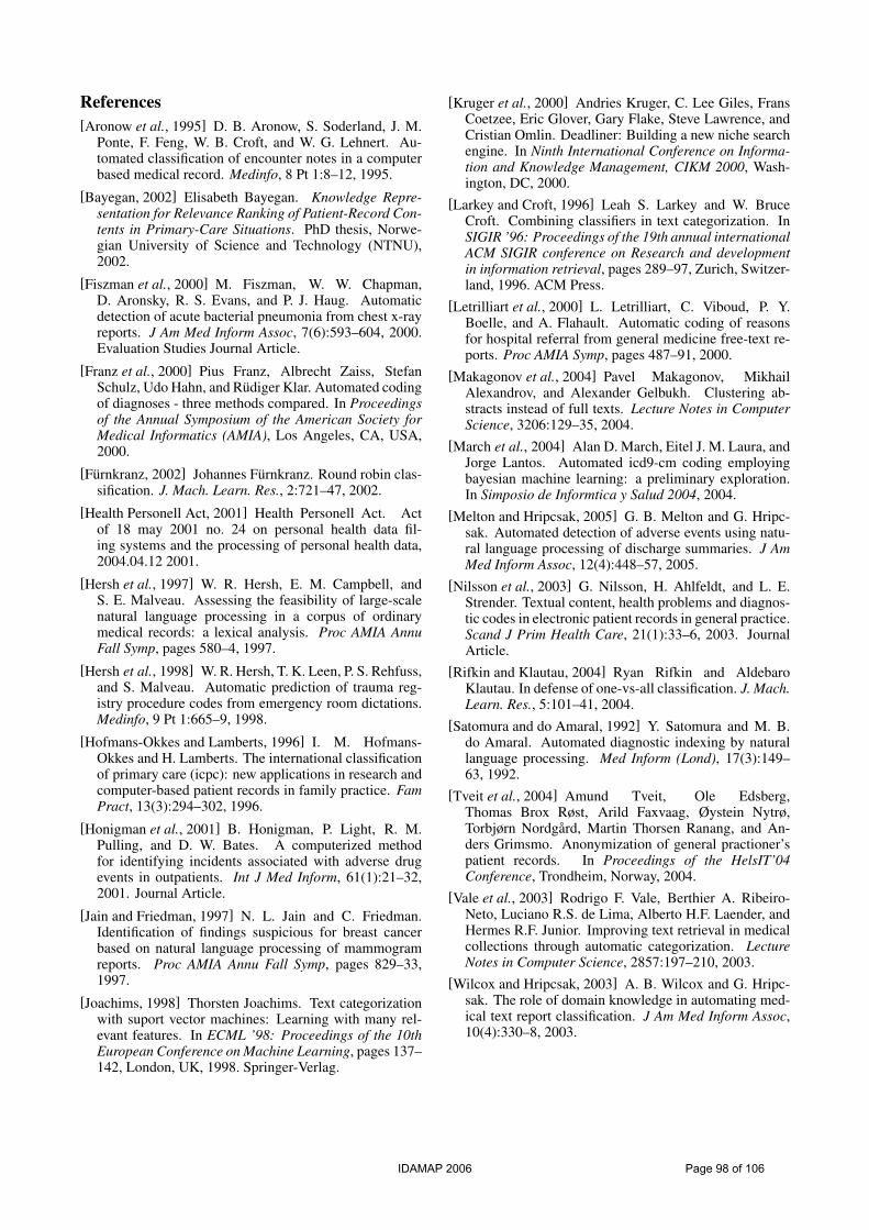
References[Aronow et al., 1995] D. B. Aronow, S. Soderland, J. M.

Ponte, F. Feng, W. B. Croft, and W. G. Lehnert. Au-tomated classification of encounter notes in a computerbased medical record. Medinfo, 8 Pt 1:8–12, 1995.

[Bayegan, 2002] Elisabeth Bayegan. Knowledge Repre-sentation for Relevance Ranking of Patient-Record Con-tents in Primary-Care Situations. PhD thesis, Norwe-gian University of Science and Technology (NTNU),2002.

[Fiszman et al., 2000] M. Fiszman, W. W. Chapman,D. Aronsky, R. S. Evans, and P. J. Haug. Automaticdetection of acute bacterial pneumonia from chest x-rayreports. J Am Med Inform Assoc, 7(6):593–604, 2000.Evaluation Studies Journal Article.

[Franz et al., 2000] Pius Franz, Albrecht Zaiss, StefanSchulz, Udo Hahn, and Rudiger Klar. Automated codingof diagnoses - three methods compared. In Proceedingsof the Annual Symposium of the American Society forMedical Informatics (AMIA), Los Angeles, CA, USA,2000.

[Furnkranz, 2002] Johannes Furnkranz. Round robin clas-sification. J. Mach. Learn. Res., 2:721–47, 2002.

[Health Personell Act, 2001] Health Personell Act. Actof 18 may 2001 no. 24 on personal health data fil-ing systems and the processing of personal health data,2004.04.12 2001.

[Hersh et al., 1997] W. R. Hersh, E. M. Campbell, andS. E. Malveau. Assessing the feasibility of large-scalenatural language processing in a corpus of ordinarymedical records: a lexical analysis. Proc AMIA AnnuFall Symp, pages 580–4, 1997.

[Hersh et al., 1998] W. R. Hersh, T. K. Leen, P. S. Rehfuss,and S. Malveau. Automatic prediction of trauma reg-istry procedure codes from emergency room dictations.Medinfo, 9 Pt 1:665–9, 1998.

[Hofmans-Okkes and Lamberts, 1996] I. M. Hofmans-Okkes and H. Lamberts. The international classificationof primary care (icpc): new applications in research andcomputer-based patient records in family practice. FamPract, 13(3):294–302, 1996.

[Honigman et al., 2001] B. Honigman, P. Light, R. M.Pulling, and D. W. Bates. A computerized methodfor identifying incidents associated with adverse drugevents in outpatients. Int J Med Inform, 61(1):21–32,2001. Journal Article.

[Jain and Friedman, 1997] N. L. Jain and C. Friedman.Identification of findings suspicious for breast cancerbased on natural language processing of mammogramreports. Proc AMIA Annu Fall Symp, pages 829–33,1997.

[Joachims, 1998] Thorsten Joachims. Text categorizationwith suport vector machines: Learning with many rel-evant features. In ECML ’98: Proceedings of the 10thEuropean Conference on Machine Learning, pages 137–142, London, UK, 1998. Springer-Verlag.

[Kruger et al., 2000] Andries Kruger, C. Lee Giles, FransCoetzee, Eric Glover, Gary Flake, Steve Lawrence, andCristian Omlin. Deadliner: Building a new niche searchengine. In Ninth International Conference on Informa-tion and Knowledge Management, CIKM 2000, Wash-ington, DC, 2000.

[Larkey and Croft, 1996] Leah S. Larkey and W. BruceCroft. Combining classifiers in text categorization. InSIGIR ’96: Proceedings of the 19th annual internationalACM SIGIR conference on Research and developmentin information retrieval, pages 289–97, Zurich, Switzer-land, 1996. ACM Press.

[Letrilliart et al., 2000] L. Letrilliart, C. Viboud, P. Y.Boelle, and A. Flahault. Automatic coding of reasonsfor hospital referral from general medicine free-text re-ports. Proc AMIA Symp, pages 487–91, 2000.

[Makagonov et al., 2004] Pavel Makagonov, MikhailAlexandrov, and Alexander Gelbukh. Clustering ab-stracts instead of full texts. Lecture Notes in ComputerScience, 3206:129–35, 2004.

[March et al., 2004] Alan D. March, Eitel J. M. Laura, andJorge Lantos. Automated icd9-cm coding employingbayesian machine learning: a preliminary exploration.In Simposio de Informtica y Salud 2004, 2004.

[Melton and Hripcsak, 2005] G. B. Melton and G. Hripc-sak. Automated detection of adverse events using natu-ral language processing of discharge summaries. J AmMed Inform Assoc, 12(4):448–57, 2005.

[Nilsson et al., 2003] G. Nilsson, H. Ahlfeldt, and L. E.Strender. Textual content, health problems and diagnos-tic codes in electronic patient records in general practice.Scand J Prim Health Care, 21(1):33–6, 2003. JournalArticle.

[Rifkin and Klautau, 2004] Ryan Rifkin and AldebaroKlautau. In defense of one-vs-all classification. J. Mach.Learn. Res., 5:101–41, 2004.

[Satomura and do Amaral, 1992] Y. Satomura and M. B.do Amaral. Automated diagnostic indexing by naturallanguage processing. Med Inform (Lond), 17(3):149–63, 1992.

[Tveit et al., 2004] Amund Tveit, Ole Edsberg,Thomas Brox Røst, Arild Faxvaag, Øystein Nytrø,Torbjørn Nordgard, Martin Thorsen Ranang, and An-ders Grimsmo. Anonymization of general practioner’spatient records. In Proceedings of the HelsIT’04Conference, Trondheim, Norway, 2004.

[Vale et al., 2003] Rodrigo F. Vale, Berthier A. Ribeiro-Neto, Luciano R.S. de Lima, Alberto H.F. Laender, andHermes R.F. Junior. Improving text retrieval in medicalcollections through automatic categorization. LectureNotes in Computer Science, 2857:197–210, 2003.

[Wilcox and Hripcsak, 2003] A. B. Wilcox and G. Hripc-sak. The role of domain knowledge in automating med-ical text report classification. J Am Med Inform Assoc,10(4):330–8, 2003.


Event Chart Explorer: A Prototype for Visualizing and Querying Collections ofPatient Histories

Ole Edsberg1),3)∗, Stein Jakob Nordbø1),3), Øystein Nytrø1),3) and Anders Grimsmo2),3)

1) Department of Computer and Information Science2) Department of Community Medicine and General Practice

3) Centre for EHR ResearchNorwegian University of Science and Technology, Trondheim, Norway

Abstract

We present our work in progress on a system forvisualizing and querying collections of patienthistories. The main features of the system are: 1)Compact LifeLines-like visualization of historiesas explorable and configurable time lines abovea common time axis, with any query hits outlined,and 2) Operations for search, selection, sortingand alignment of the histories based on temporalqueries.

1 IntroductionThe ability to query and visually explore collections of pa-tient histories is potentially useful in several types of tasks:When faced with a difficult clinical decision, one couldsearch for similar fragments from other histories in thedatabase and explore them to learn from what happened inother cases. In quality assurance of a clinical practice, onecould search for deviations from guidelines and explore theresult to see if the deviations were justified. In preparing re-search on clinical processes, one could search for relevanthistory fragments and explore them to improve one’s un-derstanding of the subject matter and get ideas for researchhypotheses and analysis methods.

The well-known LifeLines system [Plaisant et al., 1998]provides a time line visualization of the elements of a his-tory. Event charts [Lee et al., 2000] provide a static vi-sualization of a collection of histories as a set of stackedand possibly aligned lines above a common time axis, withevents represented by glyphs on the lines. The visualiza-tion part of our approach can be seen as an attempt to com-bine the information rich, interactive LifeLines visualiza-tion with the event charts’ ability to visualize many histo-ries. Related to the query part of our system, the literaturedescribes a query system based on the event calculus thatallows users to query collections of series of measurementsfor patterns of temporal abstractions [Combi and Chittaro,1999]. Our query language is mainly intended for search-ing for patterns in the categorical event and interval dataof the patient record, and it consequently contains a differ-ent set of constructs. We also have a different approach toresult visualization.

∗Contact email: [email protected]

2 The visualization and query systemOur data model contains point events for contacts, diag-noses and lab results, and interval events for prescriptions.(Our data source unfortunately often requires some guess-work in determining end points of prescriptions.) Figure1 shows and explains the main view of our system, leav-ing the query language and query-based operations for therest of this section. Applying a query to a history results ina set of matches, where a match is defined by its startingand ending points in time. The query language consists ofprimitive constructs matching data elements in themselvesand composite constructs specifying temporal constraintson their sub-queries. Recursively, a query may match:

• a point event, such as a diagnosis, lab test or prescrip-tion, or

• an interval of medication with a specified drug type,or the beginning or end of such an interval, or

• a sequence of the matches of two sub-queries, withpossible constraints on the time that can pass betweenthem, or

• the parallel or alternative occurrences of the matchesof two sub-queries, or

• a window of a specified length, within which a sub-query does, or does not, match, or

• a sub-query’s first match in the entire history.

Here is an informal description of an example query: Findall history fragments where the patient first has a one-yeartime window without at least three positive blood pres-sure measurements, and then is prescribed blood pressure-related medication for the first time in the history. (We omitthe syntax, since it is currently under revision.)

The prototype provides the following query-based op-erations: With the search operation, the user submits aquery, and red boxes are drawn around the matches of thequery. The user can cycle through the matches. With theselect operation, the user submits a query, and a newtab is opened, containing a visualization of only those his-tories that contained a match of the query. With the alignoperation, the user submits a query, and the histories aresynchronized so that the start points of the matches line upvertically. The time axis changes to shows the number oftime units relative to the alignment point. With the sortoperation, the user submits a query with a sequence as the


Figure 1: Screenshot of the main view in the prototype. Each of the horizontal bands corresponds to a history. The lowerleft panel contains a legend of the information types selected to be displayed, in this case specialized for hypertension.In the bands, tall, narrow rectangles indicate diagnoses, coloured subdivision of the background medication, and arrowsblood pressure measurements, with colour showing value category and orientation showing trend. The bottom panelshows the journal note and the upper left panel shows details about the events at the current position of the cursor. Thesearch operation has been used to mark the hits of the query informally described as Find all history fragments wherethe patient get his first hypertension diagnosis and then, sometime later, gets his first diagnosis for a hypertension-relatedcomplication. The select operation has been used to extract the 359 histories containing a hit of this query. Then, thealign operation has been used to synchronize the histories on the first part of the query. Finally, the sort operationhas been used to sort the histories according to the distance between first and second part of the query. Menus not shownprovide other possibilities, such as zooming, jumping to a journal-like view or changing the information types shown.

top-level construct, and the histories are sorted accordingto the distance between the matches of the sub-queries. Byusing these four operations, the visualization can be incre-mentally narrowed down and adapted to suit the problem athand. Figure 1 shows a screen shot from our application ofthe prototype to a data set of about 10000 patient records,in collaboration with a general practitioner wanting to in-vestigate the treatment of hypertension at his health centre.

3 Current workWe are currently working on 1) refining the query languageaccording to our improved understanding of the users’needs, 2) grounding its semantics in the event calculus, and3) creating a query editor that allows users to design queriesin a flowchart-like visual language.

References[Combi and Chittaro, 1999] Carlo Combi and Luca Chit-

taro. Abstraction on clinical data sequences: object-oriented data model and a query language based onthe event calculus. Artificial Intelligence in Medicine,17:271–301, 1999.

[Lee et al., 2000] J. Jack Lee, Kenneth R. Hess, andJoel A. Dubin. Extensions and applications of eventcharts. The American Statistician, 54(1):63–70, 2000.

[Plaisant et al., 1998] Catherine Plaisant, Richard Mush-lin, Aaron Snyder, Jia Li, Dan Heller, and Ben Shnei-derman. Lifelines: Using visualization to enhance nav-igation and analysis of patient records. In Proc AMIAAnnual Fall Symp., pages 76–80, 1998.


On the Arguments Against the Application of Data Mining toMedical Data Analysis

Anna Shillabeer, John F. Roddick and Denise de VriesSchool of Informatics and Engineering

Flinders University,PO Box 2100, Adelaide, South Australia 5001,

Email: anna.shillabeer, roddick, [email protected]

AbstractThere is a variety of criticisms of medical data min-ing which has led, in some cases, to the technologybeing overlooked as a tool. This paper presents adiscussion of six of the strongest arguments againstthe application of data mining to the complex fieldof human medicine. The aim of the paper is toraise the predominant issues and suggest solutionswhilst also opening the issues for further consider-ation by both medical and information technologycommunities.

The Arguments1. Data mining outcomes are seen as generalisations andnot verified for medical validity or accuracy. [Elwood andBurton, 2004; Milloy, 1995]

Medicine is a highly complex domain for which data min-ing processes were not designed. In many cases they orig-inated in response to changes in commerce or managementpractices and there was no real need to substantiate resultson the basis of protocols or domain knowledge. Medicinehas requirements which are outside of the original scope ofthe technology, and to be applicable to a science which isconcerned with critical decision making there is a need tomodify the technology to reflect this different environment.Whilst this first argument is a serious issue, it is often bornefrom misrepresentation of the results of data mining ratherthan from the process itself. There is a heightened need forcareful consideration of the language used when reporting re-sults [Raju, 2003; Maindonald, 1998]. It is possible for theresults to be specific but for the language of reporting to gen-eralise the message. For example, the MJA described a casewhere a mining outcome showed that smoking does not havea direct link with skin cancer [Elwood and Burton, 2004],however the resulting media story reported that smoking isnot linked with cancer generally. While a scientific data min-ing process was applied the language of information presen-tation was misleading and the resultant reporting was inaccu-rate and medically invalid. Medicine is especially sensitiveto this form of information distortion and the consequenceshave the potential to be life threatening, politically sensitive,costly and persistent which is rarely the case in other do-mains.

There is little to sustain this argument in light of recentwork in the field. By the application of suitable statisticalmethods, evaluation of all results and applying industry ac-cepted standards there is no reason to believe that data miningcannot provide effective validation and accuracy checkingprocesses [Shillabeer and Roddick, 2006; Gebski and Keech,

2003]. Three steps have been suggested to safeguard againstthis particular criticism [Smith and Ebrahim, 2002].

1. Results should not be published on the basis of correla-tion alone.

2. An explanation should be provided with the results toprovide clarification e.g. A definition of the uniquequality of the allergen that triggers the alleged immuneresponse.

3. Results should be replicated, confirmed and docu-mented prior to publication.

These steps are not part of standard data mining method-ologies but are required to be undertaken if the mining ofmedical data is to overcome criticism, be viewed as ‘goodscience’ and gain trust in the medical community.

2. Associations are not representative of other similar at-tributes and do not consider other potential contributors.[Milloy, 1995; Raju, 2003; Smith and Ebrahim, 2002]

In a medical context, relationships found between oneallergen and symptoms must be substantiated throughanalysis of similar allergens or the same allergen inother temporal, spacial or demographic instances. Ifthis cannot be shown it suggests that there is not aconclusive argument for cause and effect or that someother catalyst or cause has been missed [Raju, 2003;Smith and Ebrahim, 2002]. Again, data mining was notdesigned to do this however this should not be a preventive.Methods are available to achieve this where it is important todetermine the semantic closeness of results [Shillabeer andRoddick, 2006]. Criticism often focuses on data dredgerswho promote results as facts rather than being indicativeof a possible scenario requiring further investigation [Raju,2003]. Where an association is found it is important tocompare this with other associations or to apply a clusteringalgorithm to group semantically and determine where thereis similarity or otherwise to other attributes or rules.

3. P-values are set arbitrarily and therefore the resultscannot be trusted. [Milloy, 1995; Smith and Ebrahim, 2002]

The P-value is applied to the statistical testing of a nullhypothesis to gauge the probability of the result happeningby chance in a total population. Data mining provides asimilar function through the use of support and confidencevalues although these apply only to the data set being mined,where support is the percentage of the data transactionsunder analysis that hold true for the association, and con-fidence (a.k.a. conditional probability) is the percentage ofdata transactions containing a specific attribute value thatalso contain another specific attribute value. Support andconfidence values are thresholds set for reporting purposes


and are not p-values, although they are liable to attract thesame criticism. P-values, support and confidence may beapplied in two ways: to evaluate and discriminate the accept-ability of data analysis results for follow-up research and,as a guideline or tool for reducing the number of irrelevantoutcomes. Data mining can also be applied in divergentmodes; to show what the common patterns in data are, or toshow where common patterns are refuted in the data. It isimportant to always set heuristic thresholds in context of thespecific analysis being done and in fact a calculation appliedshould not be used alone [Shillabeer and Roddick, 2006;Gebski and Keech, 2003]. In the medical domain attributevalue relationships which occur frequently, and hence havehigh support and confidence, as well as a low p-value, arelikely to be known already and would generally be of little ifany interest. This is a major difference between traditionaldata mining applications, where generally the events whichoccur most frequently are of the greatest interest andhence have a similar support threshold, and applications inthe medical domain where frequency is not a conclusivedeterminant in defining the usefulness, validity or applicabil-ity of results and hence may require varying threshold values.

4. Associations between attributes are dependent uponthe data set being analysed and are not representative.[Raju, 2003; Smith and Ebrahim, 2002]

There is often a poor approach to the collection and de-scription of data sources and samples which is not consistentwith the process of data mining or other scientific method-ologies [Milloy, 1995; Maindonald, 1998]. For results to beaccepted the data source should be from an identifiable popu-lation with defined characteristics e.g. location, demograph-ics, and proportions [Smith and Ebrahim, 2002]. In a clinicalresearch setting this is overcome by the use of protocols andguidelines to ensure that results are representative and able tobe replicated. One such protocol is CONSORT which is usedglobally by medical researchers and is endorsed by a numberof prominent journals.

Data mining provides validation through the applicationof tools such as artificial intelligence and neural nets to theknowledge mining step to sample the data, provide outcomesthen automatically test them on the whole data source toshow that the outcome holds true for all available data notjust one small subset [Smith and Ebrahim, 2002]. Datamining is a highly intensive machine process which utiliseshuge processing power, memory and time. Data sampling isoften used as an initial step to reduce these constraints butcorrect utilisation may help to overcome this criticism also.

5. Data mining is simply a desperate search for some-thing interesting without knowing what to look for. [Mil-loy, 1995; Smith and Ebrahim, 2002]

Exploratory mining, which is not constrained by user ex-pectations, can uncover unexpected or unknown knowledgewith wide reaching benefit and can be utilised to review andextend current medical knowledge. With the wealth of databeing produced daily in the medical field the argument that itshould not be used in an exploratory fashion to at least noteimportant changes in data patterns demonstrates a misun-derstanding of the potential value held therein. It is arguedby some [Maindonald, 1998; Smith and Ebrahim, 2002;Shillabeer and Roddick, 2006] that it can be beneficial tolook simply for something interesting rather than make anassumption about what is present in the data as if we onlyever look for what is known we will potentially never findanything new and progress cannot be made. Provided this isa result of a scientific process then further mining or clinical

trials can be undertaken for evidence to substantiate theinitial findings. This criticism is only valid where the searchis for anything interesting even if only minimally and wherethere is little or no validation.

6. Data mining displaces research and testing andpresents results as facts requiring no further justification.[Milloy, 1995]

Contrary to the criticism, data mining in medicine is gen-erally viewed as an efficient tool for enhancing the work donein the field rather than as a replacement for it [Maindonald,1998]. Its value is seen as a process of automated serendip-ity that stimulates and supports testing rather than replaces it.When considering the use of mining outcomes there are twoquestions often asked; is this result representative of whathas been recorded over time?, and can the analysis outcomebe verified through real world application? [Raju, 2003;Smith and Ebrahim, 2002]. Whilst the first can be answeredwith some conviction by data mining the second requiresclinical input and hence the process of providing trustedknowledge from data requires a collaborative effort by auto-mated and clinical processes. When we consider that timefrom hypothesis to application of new knowledge is oftenmeasured in decades we should feel compelled to find newknowledge as quickly as possible and data mining offers theideal tool for this.

ConclusionThis paper has presented six common criticisms of medicaldata mining in an effort to demonstrate that as technologistswe need to be aware of the social environment in which wework and to give a suggestion of the importance of continu-ing to work on making the technology applicable to this com-plex domain. We should not be disheartened by the criticismwhich surrounds the field in which we work but should takethe criticisms on board, work with them and provide an out-come which is beyond reasonable reproach.

References[Elwood and Burton, 2004] J.M. Elwood and R.C. Burton.

Passive smoking and breast cancer: is the evidence forcause now convincing? Medical Journal of Australia,181(5):236–237, 2004.

[Gebski and Keech, 2003] V.J. Gebski and A.C. Keech. Sta-tistical methods in clinical trials. Medical Journal of Aus-tralia, 178(4):182–184, 2003.

[Maindonald, 1998] J. Maindonald. New approaches to us-ing scientific data- statistics, data mining and related tech-nologies in research and research training. Occasional pa-per, Australian National University, 1998.

[Milloy, 1995] Steven Milloy. Science without sense - Therisky business of public health. Cato Institute, WashingtonDC, 1995.

[Raju, 2003] S. Raju. Data flaws. Technical report, Ameri-can Council on Science and Health, 2003.

[Shillabeer and Roddick, 2006] Anna Shillabeer and John F.Roddick. Towards role-based hypothesis evaluation forhealth data mining. Electronic Journal of Health Infor-matics, 1(1):e6, 2006.

[Smith and Ebrahim, 2002] G.D. Smith and S. Ebrahim.Data dredging, bias or confounding. British Medical Jour-nal, 325(21-28 December 2002):1437–1438, 2002.


Software Demos


AbstractIn this work we present preliminary results ob-tained using a commercial software to analyzeinfrared spectra and infrared spectral imagescollected on lymph node tissues by using either asingle detector or a multielement Focal Plane Ar-ray detector (FPA). Our results indicate thatCluster Analysis and Principal ComponentAnalysis can allow to distinguish different com-partments in the sample, as well as to classifytumoral and non tumoral samples. The need totreat huge amounts of spectral data, especiallywhen the FPA is used for data acquisistion,would require to improve the software perform-ance.

1 IntroductionNon-Hodgkin lymphomas constitute about 4% of all hu-man malignancies. Morphological analysis coupled toimmunohistochemistry is the most widely used approachfor their classification, but these analyses are somehowprone to subjective interpretation. An automated tech-nique such as Fourier Transform Infrared (FTIR) micros-copy could bring the benefits of objective tissue evalua-tion, together with the possibility of using this techniqueas a first-line screening methodology to distinguish nor-mal versus neoplastic samples [Conti et al., 2003].As it is known, position and intensity of infrared absorp-tion bands, particularly in the midle infrared region (i.e. inthe wavenumber range from 4000 to 400 cm-1), carry in-formation on the biochemical status of organic samples,since they are related to the presence and amount of spe-cific molecular groups and to their chemical environment[Gunzler-Gremlich, 2002]. The use of the interferometrictechnique (FTIR) allows to acquire in a reasonable time(say from a few minutes to half an hour) well resolvedspectra with high signal to noise ratio from sample areasas small as about 10x10 µm2 . If the interferometer is cou-pled to a visible/IR microscope it is possible to obtain aspectral map by scanning a selected sample region. Re-cently, spectral images data can be obtained more rapidlyusing a multielement detector (Focal Plane Array, FPA)[Jackson et al., 2002], which allow to acquire simultane-ously up to 4096 spectra from a 180x180 µm2 sample area

(down to 3x3 µm2 spatial resolution). In this case, a hugeamount of spectral data has to be analysed: for each point,the instrument acquires an interferogram (thousands tomore than one hundred thousand data points, dependingon the desired spectral resolution) which has to be FourierTransformed to obtain the absorption spectrum (hundredsto thousands of data points, depending on the resolutionand on the extension of the spectral region of interest).File dimensions go from hundreds of Kb for a singlepoint spectrum up to tenths of Mb for a FPA acquisition.

2 Experimental and data analysisThis preliminary study included six samples from six dif-ferent patients: three neoplastic samples of follicular ly m-phoma, as classified by morphology and immunoisto-chemistry [Jaffe et al., 2001], and three non-neoplasticsamples of reactive lymph nodes. For each sample, ourattention was focussed on three tissue compartments: in-trafollicular zone, mantle and interfollicular zone. About 7µm thick sections were measured in transmission mode onBaF2 supports in the 4000-700 cm-1 spectral region with 4cm-1 resolution using a Bruker Vertex-70 spectrometercoupled to a Hyperion 3000 microscope and equippedwith a single element HgCdTe detector and with aHgCdTe FPA multidetector of 4096 elements. The Bruker5.5. OPUS software was utilized for data analysis.

2.1 Point by point spectraFor each compartment of each one of the six samples, tento twenty point by point absorption spectra (typically froma sample area of 50 x 50 µm2 or 25x 25 µm2) were ac-quired with the single element detector, as the ratio of thetransmitted to the incident photon intensity vs wavelength.Cluster Analysis (using Euclidian distance to calculatespectral distances and the Ward’s algorithm to determinethe degree of heterogeneity) and Principal ComponentAnalysis (PCA) applied on the spectra, by selecting vari-ous spectral regions and choosing different preprocessingmethods (such as straight line subtraction, vector normali-zation, first or second derivative), allowed to:- identify homogeneous groups of spectra (Figure 1) andexclude outliers before making an average to obtain arepresentative spectrum of each compartment of a sample.

APPLICATION OF A COMMERCIAL SOFTWARE TO THEANALYSIS OF INFRARED SPECTRAL IMAGES ON LYMPH NODE TISSUES:

A PRELIMINARY STUDY

Emilio Burattini1, Marco Chilosi2, Carla Conti3, Paolo Ferraris3,Flaminia Malvezzi Campeggi1, Francesca Monti1, Giorgio Tosi3, Alberto Zamò2

Department of 1Computer Science and Department of 2Pathology–Section of Pathological AnatomyUniversità di Verona - Verona, Italy

3Department of Material Science - Università Politecnica delle Marche - Ancona, Italy


The spectra representative of various sample regions canbe further analysed for a more detailed interpretation ofthe behaviour of the bands.- identify wider classes of spectra from different samples,such as “tumoral” and “non tumoral” (Figure. 2). In par-ticular, our data indicate that non tumoral samples show ahigher biological variability, as it is expected from pathol-ogy studies.

Figure 1: Spectra from mantle and intra-follicular zone of asample are well distinguished by Cluster Analysis through 1stderivative and vector normalization in the range 1800-900 cm-1.

Figure 2: Two classes can be identified by PCA on intra-follicular spectra after straight line subtraction in the range 980-1350 cm-1: in this score diagram blue, grey and red refer to pointspectra from three different tumoral samples; magenta, cyan andorange to three different non tumoral samples.

2.2 Hyperspectral images

Figure 3: Map of intrafollicular zone and mantle (6x7 grid of 20µm2 points): in this example integration was performed at the1080 cm-1 band. A typical spectrum is also shown in the center.

Hyperspectral images can be acquired either by mapping alimited selected region using the single detector or bymapping a wider region using the FPA multidetector.It is then possible to draw a map of the peak height or ofthe intensity, after integration, of a single band (Figure 3and Figure 4). As it can be seen, different compartmentsof the same sample can be clearly distinguished by FTIR.

Figure 4: Map of a whole follicle from an area of about 550x550µm2 obtained with a 3x3 FPA grid, at 12x12 µm2 spatial reso-lution. In this example integration was performed at the 1240cm-1 band.

3 ConclusionsPresent results are very promising as regards the use ofFTIR microscopy for objective tissue evaluation and first-line screening to distinguish non-neoplastic versus neo-plastic tissues. To this aim, an improved performance ofthe software would also be very useful: for example, toperform clustering directly on the acquired hyperspectralimage of the same sample, in order to draw a color map ofthe clusters; and to run PCA analysis directly on the hy-perspectral data from different samples to characterizetumoral and non tumoral classes.

AcknowledgmentsThis work was entirely supported by “FondazioneCariverona” in the framework of “Funds 2003 for Re-search Projects of Biomedical Interest”.

References[Conti et al., 2003] C. Conti, E. Giorgini, T. Pieramici, C.

Rubini, G. Tosi, J. Mol. Struct., 744-7, 187 (2005).];1st DASIM Workshop (Diagnostic Applications ofSynchrotron Infrared Microspectroscopy), DaresburyLab.s, Manchester, July 2005; RSC Faraday Division.Faraday Discussion 126, Nottingham (2003).

[Gunzler-Gremlich, 2002] H. Gunzler, H.U. Gremlich, IRSpectroscopy, An Introduction, Wiley-Vch, 2002

[Jackson et al., 2002] M. Jackson, H.H. Mantsch, Pathol-ogy by Infrared and Raman Spectroscopy, in Hand-book of Vibrational Spectrosc., J.M.Chalmes, P.R.Griffiths, Wiley, Chichester, 2002, Vol. 5, 3227-3245.

[Jaffe et al., 2001] E. Jaffe, N. Harris, H. Stein (editors):WHO classification of tumours: pathology and geneticsof tumours of haematopoietic and lymphoid tissues.Lyon, France, IARC Press, 2001

1ü

2ü

7ü

8ü

10 11

18 1 9 2 0 22 23

24 2 5ü

2 6ü

28 29

30 3 1ü

3 2ü

34 35

36 3 7 3 8 40 41

0.100

0.200

0.300

0.400

0.500

0.600

0.700

0.800

0.900

1.000

Absorbance Units

3500 3000 2500 2000 1500 1000Points

C:\Documents and Settings\flaminia\Desktop\misure_flami\single_spec_tessu\8877\mappa_follicolo_mantello_25micron.0 mappa_follicolo_mantello_25micron Instrument type and / or accessory

12/01/2006

Page 1/1


IDAMAP 2006 - International Medical Informatics Association

Documents

Transcript of IDAMAP 2006 - International Medical Informatics Association