Quality Technology & Quantitative Management Vol. 4, No. 1, pp. 17-34, 2007

QQTTQQMM © ICAQM 2007

Cumulative Damage Models for Failure with Several Accelerating Variables

Chanseok Park1 and W. J. Padgett1,2

1Department of Mathematical Sciences, Clemson University, Clemson 2Department of Statistics, University of South Carolina, Columbia

(Received April 2005, accepted December 2005)

______________________________________________________________________

Abstract: In this paper, we present a method for incorporating several accelerating variables into accelerated test models for failure of materials. We propose a hyper-cuboidal volume approach as an overall accelerating measure, which enables one to extend existing models for one accelerating variable to the case of several. In particular, we extend a general cumulative damage model and the power-law Weibull model for materials failure to the several accelerating variables case. A real-data example is presented, which illustrates the improvement of the proposed methods over existing models.

Keywords: Accelerated testing, cumulative damage, failure of materials, inverse Gaussian distribution, stochastic process, strength reduction function, tensile strength. ______________________________________________________________________

1. Introduction

he strength and lifetime properties of materials or products are of basic interest for most manufacturers. Materials strength is directly related to randomly occurring flaws

in the materials which might come from imperfections in the manufacturing process or handling. Due to this, it seems to be very difficult or impossible to find deterministic strength models such as the Hooke’s law in stress and strain models that fit observed data well. Thus, in practice, these properties must be modeled by statistical methods, which ideally would also consider the cost of testing.

T

Thanks to the modern manufacturing technology, many products that are made nowadays are stronger and more reliable than before. Thus, it takes more time and cost to study the strength properties of modern products. Since it may be very difficult to observe breakdown strength or lifetime measurements especially under normal-use conditions, strength tests under normal-use conditions can be costly. Thus, one needs to use time- and cost-saving experimental procedures. To this end, accelerated tests are widely used in many manufacturing industries to obtain the strength and lifetime properties more easily or in a more timely fashion.

Accelerated tests decrease the strength or time to failure and the cost of testing by exposing the test specimens to higher levels of stress conditions (increased sizes or levels of environmental variables) which cause earlier breakdowns and shorter lifetimes than the normal-use condition (see, for example, Nelson [13]). These environmental variables and levels of stress conditions are referred to as the “accelerating variables” in the statistics and reliability literature.

Statistical models incorporating accelerating variables related to “size” of test specimen are useful to predict strengths of materials. One of the commonly used models is

18 Park and Padgett

the power-law Weibull probability model [18, 25]. However, it is now widely understood that the Weibull-based models often do not provide good fits to tensile strength measurements of brittle materials such as carbon fibers. For examples, the reader is referred to Durham and Padgett [8] and Wolstenholme [30]. Thus, for better estimation of materials strength, other probability models are required that provide better fits to experimental strength observations. Based on cumulative damage models for failure, many authors have investigated this issue to some extent and several derived Birnbaum-Saunders-type or inverse Gaussian-type models incorporating an accelerating variable. Recent work includes Durham and Padgett [8], Onar and Padgett [14], Owen and Padgett [15, 16], Padgett et al. [18], Padgett and Tomlinson [19], Park and Padgett [21, 22], Stoner et al. [27], Taylor [28], and their references. The work by Park and Padgett [21] is the most general model among these obtained to date. However, all of the aforementioned models, including the power-law Weibull model, involved only one accelerating variable. With ever more advanced and sophisticated products, often more than one accelerating variable must be incorporated to better predict the strength or lifetime properties. Some specific acceleration models have been used for two or more accelerating variables, such as the Eyring or linear models, but are of limited use.

In this paper, we extend the models mentioned above in order to incorporate several accelerating variables. Section 2 presents the generalized cumulative damage models developed by Park and Padgett [21], and provides the method of incorporating several accelerating variables. In Section 3, we introduce the GLM-based model and extend the power-law Weibull model to the case of several accelerating variables. We also provide model selection procedures based on the mean square error (MSE) and the Akaike information criterion (AIC). Finally, an illustrative example using real tensile strength data is presented and discussed in Section 4. This example also shows that the model is improved by incorporating two accelerating variables, both “gauge length” and diameter of carbon fibers, to predict tensile strength, rather than only their gauge length as has been done in previous models.

2. Generalized Cumulative Damage Failure Models for Accelerated Tests

Here we review existing failure models with one accelerating variable and present the method for incorporating several accelerating variables. These models are all based on a cumulative damage approach.

2.1. Derivation of the Models

As in Park and Padgett [21,22], we consider a material specimen of size, or gauge length, L , with unknown theoretical strength, ψ , which is a fixed unknown quantity. In testing, the specimen is placed under stress or load which is steadily increased until failure. We make the following four assumptions which generalize those of Durham and Padgett [8]:

A1. The increasing stress is assumed to be incremented by small, discrete amounts until the specimen breaks, resulting in its observed breaking stress or strength.

A2. Each small increment of stress causes a non-negative amount of damage, , which is a random variable having a distribution function

D( )DF ⋅ with mean µ and variance

2σ .

A3. The initial damage to the specimen, before the stress is applied, is in the form of the most severe “flaw" existing in the specimen and is quantified by a random variable,

Cumulative Damage Models for Failure 19

0X , and results in a random initial strength that is a reduction of the theoretical strength, ψ .

A4. The strength reduction is given by a strictly increasing function denoted by ( )cH ⋅ which is subject to a damage accumulation function ( )c ⋅ described later. The difference of strength reduction functions, 0( ) ( )c cH H Xψ − , is almost surely greater than zero and the initial strength of the specimen, , is given by

. W

10( ( ) ( )c c cW H H H Xψ−= − )

As an example of the assumption A4, ( )cH u u= gives additive damage accumulation with 0W Xψ= − (linear reduction in initial strength) and ( ) logcH u = u gives multiplicative damage accumulation with 0W Xψ= / (geometric reduction in initial strength), which are the cases considered by Park and Padgett [22].

As the tensile load on the specimen is increased under the assumptions above, the cumulative damage after increments of stress (see Desmond [7], and Durham and Padgett [8]) is denoted by

1 ( )n n nX X D h X+ n= + ,

where for 0jD > 0 1 2 ...,j n= , , , are the independent and identically distributed damages to the specimen at each stress increment and the damage model function, , is positive for . Here,

( )h u0u > ( ) 1h u = gives an additive damage model, and ( )h u u= gives a multiplicative

damage model.

Following Park and Padgett [22], the cumulative damage model can be generalized to

1( ) ( ) ( )n n nc X c X D h X+ n= + ,

where is an increasing non-negative damage accumulation function. Using ( )c ⋅( ) ( ) ( )1n n nD c X c X h X+= − n , we can express the damage incurred to the specimen after

increments of stress as n

0

1 11

00 0

( ) ( ) ( )( ) (

( ) ( )n

n n Xi ii cX

i i i

c X c X c xD dx H

h X h x

′− −+

= =

−= ≅ = −∑ ∑ ∫ )n cX H X

for large , where n ( ) ( '( ) ( ))cH x c x h x d= ∫ x

)

.

Then, by the central limit theorem, 0( ) (c n cH X H X− has an approximate normal distribution with mean nµ and standard deviation nσ .

Let N be the number of increments of tensile stress applied to a specimen of strength ψ until failure. From the assumption A4, we have

1 1: ,..., nn

N sup n X Xψ ψ−= ≤ ≤

1 0 0

1 0 0

: ( ) ( ) ( ) ( ),.

( ) ( ) ( ) ( ) ,

c c c cn

c n c c c

sup n H X H X H H X

H X H X H H X

ψ

ψ−

= − ≤ −

− ≤ −

..,

)]

where if the set is empty. From the conditional probability, we have 1N =

0 0[ ( ) ( ) ( )] [ ( ) ( ) (c c c c n c cP N n H H X H w P H X H X H wψ> | − = = − ≤ ,

which results in

20 Park and Padgett

(1) [ ] ( ) ( )n WP N n F w dG wΩ> = ∫W

,

by the law of total probability. Here 0( ) [ ( ) ( ) ( )]n c n c cF w P H X H X H w= − ≤ and is the distribution function of initial strength satisfying

( )WG ⋅W 0( ) ( ) ( )c c cH W H H Xψ= − . From

the earlier argument,

0

( )( ) [ ( ) ( ) ( )] ( )c

n c n c cH w n

F w P H X H X H wn

µσ−

= − ≤ ≅ Φ , (2)

where denotes the cumulative distribution function (cdf) of the standard normal distribution.

( )Φ ⋅

For a specimen of size, or “gauge length,” L , let uY denote the damage due to inherent flaws at location ( 0u u L≤ ≤ ) along the length of the specimen. Let

denote the initial damage in terms of the most severe of the inherent flaws over the specimen. That is, L is the random strength reduction of the specimen due to the most severe inherent flaw present before stress is applied to the specimen of gauge length

max 0 L uM Y u= : ≤ ≤ LM

L . Thus, the initial strength becomes

1( ( ) ( ) )c c c LW H H H Mψ−= − .

Next, we derive the distribution of the initial strength W above. Since is strictly increasing, W is equivalent to

( )cH ⋅w≤ ( ) ( ) ( )c c L cH H M H wψ − ≤)

W∈Ω

]

, that is, . Thus, the cdf of is given by 1( ( ) ( )L c c c LM H H H Mψ−≥ − W

1( ) [ ( ( ) ( )) ]W c c c LG w P H H H M w wψ−= − ≤ |

1[ ( ( ) ( ))L c c c WP M H H H w wψ−= ≥ − | ∈Ω

11 ( ( ( ) ( )))

[0 ]LM c c c

L

F H H H w

P M

ψψ

−− −=

< <

11 ( ( ( ) ( )))

( ) (0)L

L L

M c c c

M M

F H H H w

F F

ψψ

−− −=

−,

where 1 ( ( ) ( )) 0W c c cw w H H H m m ψ ψ−Ω = : = − , < < . It is immediate from differentiating that the pdf of is ( )WG ⋅ W

1

1

( ( ( ) ( )))( )( )

( ( ( ) ( )))LM c c cc

Wc c c c

f H H H wH wg w

B H H H H w

ψ

ψ

−′

′ −

−= ⋅

−, (3)

where ( ) (0)L LM MB F Fψ= − and ( ) ( )c cH u dH u du′ = / .

Substituting (2) and (3) into (1), we obtain the approximate survival probability after a large number, , increments of stress as n

( ) ( )( ) ( ) ( ) [ (

W

c cW

H w n H W nP N n g w dw E

n n)]

µ µσ σΩ− −

> ≅ Φ = Φ∫ .

For convenience, let ( ( ) ) (cZ H W n n )µ σ= − / and ( )a E Z= . Using a two-term Taylor’s

Cumulative Damage Models for Failure 21

expansion of about , we have ( )ZΦ a

( ) ( ) ( )( )Z a a Z a′Φ ≈ Φ + Φ − .

Taking the expectation of the above with respect to W and using , we have ( )a E Z=( ) ( )E ZΦ = Φ a , that is,

( ) ( ( ))[ ( )] ( )c cH W n E H W n

En n

µ µσσ σ

−Φ ≅ Φ − ,

where the expectation of ( )cH W , denoted by ( )LθΛ ; , is given by

( ) ( ( )) ( ) ( )Wc c WL E H W H w g w dwθ ΩΛ ; = = ⋅ .∫ (4)

Note that this expectation can be considered as an acceleration function for the material strength with an unknown parameter (possibly a vector) and depends on the known specimen size, or gauge length, L (i.e., the accelerating variable) from (3).

Finally, letting be a continuous version of S N and using the symmetry of gives the strength distribution of the specimen as

( )Φ ⋅

( )( ) ( ) ( )s LS s

F s P S s µ θσ σ

Λ ;= ≤ = Φ − .

Reparameterizing as ( )L Lµ θ= Λ ; /µ and 2[ ( ) ]L Lλ θ σ= Λ ; / , we have

( ) ( ) [ ( 1)] [ ( )]L LS

L L L

s sF s P S s

s sλ λ

µ µ µ= ≤ = Φ − = Φ − Lµ

, (5)

which is an accelerated Birnbaum-Saunders-type distribution [4] that incorporates the specimen size, or gauge length, L . It should be noted that the difference between the inverse Gaussian and Birnbaum-Saunders distributions is negligible when L Lλ µ [3, 8, 20]. So Birnbaum-Saunders models can be approximated by the first term of an inverse Gaussian cdf when 1L Lξ λ µ= / which will be assumed to be the case here (and verified by the parameter estimates in the example of Section 4). The pdf for (5) is therefore approximated by an inverse Gaussian pdf with mean parameter Lµ and scale Lλ

2

3 2

( )( ) exp[ ] 0

2 2L L L

SL

sf s s

s s

λ λ µπ µ

−= − , > . (6)

The inverse Gaussian approximation for the Birnbaum-Saunders distribution is used for easier estimation. This inverse Gaussian approximation enables us to find good initial values for the parameters by using so-called “least squares method” proposed by Durham and Padgett [8].

2.2. pL - Norm Type Strength Reduction

Selecting various forms of the functions ( )c ⋅ and ( )h ⋅ generates several new models for material strength incorporating the size L as shown by Park and Padgett [21,22]. It should be noted that other models can also be obtained by using any reasonable distribution of the initial strengthW , not necessarily subject to . Using different such distributions, one can obtain existing models such as the

10( ( ) ( )c c cW H H H Xψ−= − )

22 Park and Padgett

“Gauss-Weibull additive model” [8] and the “Gauss-Gauss multiplicative model” [17]. Some models based on the choice of ( )h ⋅ with ( )c u u= are listed in Table1. Here, motivated by the power-law, we focus on the strength reduction function 1( ) p

c pH u u= with . As a special case for0p > 0p = , we obtain ( )h u u= which gives ( ) logcH u u= , a geometric strength reduction function. However, 0lim ( )p cH u→ is not . This discrepancy comes from the inability to interchange the limit and the integral of the function . As a special case for

log u

1 u/ 1p = , we obtain ( )cH u u= which gives a linear reduction in initial strength. For details of these linear and geometric models, the reader is referred to Park and Padgett [22]. The use of 1( ) p

c pH u u= ( ) gives 0p >1

0 ( 0 )p p pR Xψ /= − , and it is immediate that 10 0( )p p pR Xψ /= + . This implies that the

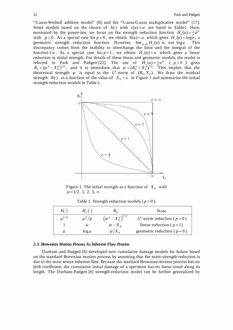
theoretical strength ψ is equal to the pL -norm of 0 0(R X ), . We draw the residual strength ( )R ⋅ as a function of the value of 0X x= in Figure 1 and summarize the initial strength reduction models in Table 1.

Figure 1. The initial strength as a function of with 0X

1 2, 1, 2, 3, p = ∞

Table 1. Strength reduction models ( ). 0p >

( )h ⋅ ( )cH ⋅ 0R Note 1 pµ − p pµ ( )1/

0

pp pXψ − pL -norm reduction ( ) 0p >1 µ 0Xψ − linear reduction ( ) 1p =µ log µ 0Xψ geometric reduction ( ) 0p =

2.3. Brownian Motion Process As Inherent Flaw Process

Durham and Padgett [8] developed new cumulative damage models for failure based on the standard Brownian motion process by assuming that the main strength reduction is due to the most severe inherent flaw. Because the standard Brownian motion process has no drift coefficient, the cumulative initial damage of a specimen has no linear trend along its length. The Durham-Padgett [8] strength-reduction model can be further generalized by

Cumulative Damage Models for Failure 23

allowing linear trend in the Brownian motion (see Park and Padgett [22]). Thus, here we use the Brownian motion process with drift coefficient α and diffusion 2β . Because the main strength reduction in this kind of model is due to the most severe inherent flaw, it is appropriate to assume small linear trend, if any, along the length of the specimen. That is, we assume that β α| |

L

. This will model increasingly (or decreasingly) severe flaws inherent over the specimen or system due to handling or manufacturing, for example.

Suppose that the inherent flaw process is a Brownian motion with small drift coefficient

0 uY u: ≤ ≤α and diffusion 2β . Then the random strength reduction of the

specimen is . We find the pdf of first and then we will obtain the pdf of

max 0 L uM Y u= : ≤ ≤ L LM1( )p p p

LW Mψ /= − .

Using the result of Shepp [24], we have the following joint pdf of and of a Brownian motion process:

LZ M=LX Y=

2 2

2 2 26 3

2(2 ) (2 )( ) exp( )exp( )

2 22

z x x L z xg z x

LL

α αβ β βπβ

− −, = − − ,

where and 0z > x z< . The pdf of is obtained by the marginal pdf of the above joint pdf so that we have

LM

2 2

2 2( ) ( ) ( )exp( )

LMz L z L z

f zL L L

2α α αφβ ββ β β

− += − Φ −

α.

The above pdf can be approximated by the first term on the right-hand side when β α| | , so that we have

2( ) ( )

LMz L

f zL L

αφβ β

−≅ .

Substituting the above into (3) with ( ) pcH u u= p , we have the pdf of , W

1 1

( 1)

2 (( ) ( )

( )

p p p p

W p p p p

w wg w

wB L L

ψ αφψβ β

− /

− /

− −= ,

−) L

where 2 ( ) 2 ( )L LL

B ψ α αβ− −= Φ − Φ

Lβ. It follows that

1/

0

2 1 ( )2( ( )) ( )

( 1)( )

p p p

c

p w LwE H W dw

p p p ppB L Lw

ψ ψ αφβ βψ

− − −= ∫ − /−

0

2( )

pp u L

Lu

p pB Lψ α

β

ψ φβ

−= − ⋅∫

after a change of variable to .p p wµ ψ= − p If we assume that the theoretical strength, ψ ,

is larger than β , then we can approximate the above integral with β α| | as

10 0 0

1 1( ) ( ) ( ) ( 2 ) (

22 2p p p pu L u u p

u du u du u du LL L L

ψ ψαφ φ φ ββ β β π

∞ +− +⋅ ≅ ⋅ ≅ ⋅ = Γ∫ ∫ ∫ ),

24 Park and Padgett

which leads to

1 ( 2 )

( ( )) ( )2

pp

cL p

E H Wp p

βψπ

1+≅ − Γ . (7)

As an example of 1p = (linear reduction model), we have the acceleration model ( )LθΛ ;

in (4) as

2( ( ))cE H W Lψ β

π≅ − ,

which includes the “Gauss-Gauss additive model” [8] as a special case when 1β = .

In the limit as , using l’Hôspital’s theorem, we have 0p →

0 0

1 loglim lim log

1

p p

p ppψ ψ ψ ψ

→ →

−= =

0 0

( 2 ) 1 ( 2 ) log( 2 )lim lim log( 2 )

1

p p

p p

L L LL

pβ β β β

→ →

−= = .

It is immediate that

1 12 2( ( )) log log( 2 ) ( )cE H W Lψ β≅ − − Ψ ,

x

where the digamma function is given by ( )Ψ ⋅ ( ) ( ) ( )x x′Ψ = Γ /Γ .

Thus, the Brownian motion cumulative initial damage process with , the tensile strength has

0p →S ( )L LS IG µ λ,∼ , where

1 12 2log log( 2 ) ( )

L

Lψ βµ

µ− −

=Ψ

and 1 12 2log log( 2 ) ( )

LLψ β

λσ

− − Ψ= .

Since parameter estimation is indeterminate with the above setup, we need to reparameterize the above as

L Lµ λ ξ= / and 0 1 logL Lλ θ θ= − , (8)

where ξ µ σ= / , 1 10 2 2log log( 2 ) ( )θ ψ β σ= − − Ψ / , and 1 1 (2 )θ σ= / .

2.4. Incorporating Several Accelerating Variables

Suppose that there are two accelerating variables, say, L (length) and R (radius). Then it is reasonable to use the volume 2V L Rπ= ⋅ as an accelerating measure. This volume measure can be used for (8) instead of gauge length L . Although we illustrate here with the overall accelerating measure in view of physical volume, this idea can be applied for the overall accelerating measure with any types of variables, such as temperature, humidity, etc., in an appropriate form of link function, . V

If there are q accelerating variables 1 2 ... qL L L, , , , this model can further be generalized by using the hyper-cuboidal volume obtained as the product of accelerating

Cumulative Damage Models for Failure 25

variables. These variables can also be power-transformed to add more flexibility. We propose the “hyper-cuboidal” volume as the overall accelerating measure for material strength, generalizing “gauge length” of a specimen or “specimen size,” with q accelerating variables such as

1

( )q

vV T Lvν

,η=

= ∏ (9)

where is any monotone function. Using this, we can generate a variety of accelerating measures. In this paper, we consider the following measures, where are appropriate acceleration variables:

( )T ⋅L

1

qV Lβ

== ∏ or

1( )

qLV e β

== .∏ (10)

A variety of acceleration (link) functions can be use for an overall accelerating measure. Some popular acceleration functions when 1q = are: (i) power rule model ( L Lηα ξ= ), (ii) Arrhenius reaction rate model ( L

L eηα ξ /= ), (iii) inverse-log model ( (log )L L ηα ξ= ), (iv) exponential model ( L

L eηα ξ= ), and (v) inverse-linear model ( L Lα ξ η= + ). Note that except for the inverse-linear model, the proportional coefficient ξ can be ignored for the model in (8) because the parameter 0θ absorbs ξ after reparametrization. Except for the inverse-linear model, the proposed hyper-cuboidal volume in (9) includes the preceding four acceleration functions as special cases. For example, the use of with

gives the above Arrhenius reaction rate model. For more details about accelerated tests with the link functions, the reader is referred to Mann et al. [10], Meeker & Escobar [12], Nelson [13], and other references therein. It should also be noted that the generalized Eyring relationship model [9] can handle two accelerating variables; and Meeker and Escobar [12] provide the accelerated life test model with several accelerating variables using a linear function for the log-scale parameter of a log-location-scale distribution.

1( ) LT L e /=1q =

The hyper-cuboidal volume approach can be easily implemented in many existing accelerated life time models. We also apply this approach to extend the existing power-law Weibull model proposed by Padgett et al. [18]. That is, using the hyper-cuboidal volume instead of an accelerating variable, we can develop a generalized power-law Weibull model incorporating several accelerating variables. This generalized power-law Weibull model will be considered in Section 3 to compare the proposed models with other models.

Substituting the above overall accelerating measures in (10) into (8), we have following accelerated models

01

logq

V Lλ θ θ=

= − ,∑

01

q

V Lλ θ θ=

= − .∑

2.5. Parameter Estimation

Here, we briefly describe the maximum likelihood estimating equations and suggest the choice of the initial values. For brevity, we illustrate parameter estimation with two accelerating variables denoted by and , which can be easily extended to the more 1L 2L

26 Park and Padgett

general case. Thus, we have the following models which are used in the later example in Section 4:

1 0 1 1 2log logA VM Lλ θ θ θ: = − − 2L ,

2 0 1 1A VM Lλ θ θ θ: = − − 2 2L .

These are the full models whereas 2 0θ = gives the reduced models with only 1 as the accelerating variable. In Section 4, we denote

L1BM and 2BM as the reduced models for

and , respectively. 1AM 2 AM

Suppose that subject specimens are tested over all accelerating levels of and 1iL 2 jL for and . At the accelerating levels of 1i and 1 2 ...i I= , , , 1 2 ...j = , , , J L 2 jL , tests are performed for specimens, resulting in observed breaking strengths , for and . For estimation of an accelerated test model over all of the

ijn ijks 1 2 ... ijk n= , , ,1 2 ...i I= , , , 1 2 ...j = , , , J

I J× pairs of the accelerating variables, the maximum likelihood estimator (MLE) of the unknown parameters in a given model can be obtained by maximizing the log-likelihood function

1 1 1( ) log ( )

ij

ij ij

nI J

S ijk V Vi j k

f sθ µ= = =

∝ ;∑ ∑ ∑ λ, ,

)L Lλ θ θ θ= − − L Lλ θ θ θ= − −

where ijV i i or

ijV i i with 20 1 1 2 2( log log 2

0 1 1 2 2( )ijV Vij

µ λ ξ= / . The log-likelihood function for the accelerated test inverse Gaussian distribution is

2

1 1 1

1( ) (log 2 )

ij

ij ij ij

nI J

V ij V Vi j k ij

ss

θ λ ξ ξ λ= = =

∝ − + −∑ ∑ ∑ λ .

The MLEs of ξ and θ for are obtained by solving the following equations simultaneously

0 1 2= , ,

1 1 1

( )(

ij

ij

nI J

ijk Vi j k

sθ ξ λξ = = =

∂) 0∝ − + =∑ ∑ ∑

∂, (11)

1 1 1

( ) 1 1( ) 0,=

ijij

ij ij

nI J V

i j k V ijkV s

λθ ξθ λ θλ= = =

∂∂∝ + +∑ ∑ ∑

∂ ∂0, 1, 2 = . (12)

Equation (11) can be easily solved for ξ so that we have

1 1

1 1 1

ij

ij

I J

ij Vi j

nI J

ijki j k

n

s

λξ = =

= = =

∑ ∑= .

∑ ∑ ∑

Substituting the above into (12), the MLEs of θ can be obtained by solving the simultaneous nonlinear likelihood estimating equations in (12). The MLEs of θ depend on the actual form of the acceleration model i.e.,

ijVλ .

Cumulative Damage Models for Failure 27

In most cases, however, these solutions must be obtained numerically. For numerical root-finding algorithms, some initial values for the parameters are necessary. A relatively easy “least squares method” for obtaining the initial values is briefly described by Durham and Padgett [8]. For each , denote the ordered observations by . Then, using an empirical estimate of in (5) denoted by , we set

1 ...i = , ,k) )

ijks ( )ij ks( )(S ij kF s ( )(S ij kF s

( ) ( )( )

1ˆ ( ) (

ijij ij k ij k Vnij k

s sFs

ξ λ )= Φ − ,

which yields the following “linearized” equation

1( ) ( ) ( )ˆ( ( ))

ijijij k ij k ij k Vns s sF ξ λ−⋅ Φ = − .

Several versions of these empirical estimates ( )ij ij kn have been suggested in the statistics literature, but the most popular one which we will use here is

ˆ ( )sF( 1 2)j n− / / (also

known as the median rank method) for n and 11≥ ( 3 8) ( 1 4j n )− / / + / for , due to Blom [5] and Wilk and Gnanadesikan [29]. For example, using the model , we have

10n ≤1AM

1( ) ( ) 0 1 1 2 2

1 2( ) ( log logij k ij k i j

ij

js s L

nξ θ θ θ− − /

⋅ Φ = − − − ,)L (13)

where for convenience, we assume . Thus, (13) can be used to find least squares estimates of

11n ≥ξ , 0θ , 1θ and 2θ from any statistical software, providing some initial

values for the MLE equations in (11) and (12).

Note that it is difficult, if at all possible, to prove the existence of unique solutions to (11) and (12). However, numerical evidence of at least a local solution is shown by using different initial values for the numerical iteration which yield the same roots within specified accuracy.

3. Other Models Considered

We will compare the fits of the proposed models with the -accelerating-variable power-law Weibull model extending Padgett et al. [18], and the inverse Gaussian GLM [11].

q

Padgett et al. [18] and Smith [25] investigated the power-law Weibull model as an overall better fitting size-effect model than the ordinary Weibull model. The power-law Weibull survival function is given by

( ) exp[ ( ) ] 0Ls

S s L sθ α

β= − , > . (14)

This model is based on so-called weakest link theory which is originally attributed to Peirce [23]; see more recent work of Wolstenholme [30]. In this theory, the specimen is virtually considered as a series, or chain, of V segments or links, in which the whole chain fails once one of the segments collapses. We assume that the number of segments has the power relation with the physical dimension (say, gauge length ), that is

VL V Lθ= .

We will call this V a virtual length. Denoting as the survival function for V independent and identically distributed links, we can express (14) as

0S

28 Park and Padgett

0 01

( ) ( ) [ ( )] exp[ ( ) ]V

VV

i

sS s S s S s V α

β== = = −∏ .

Suppose that there are two accelerating variables and . Then the specimen is considered as a matrix-type chain of width and height . Thus, the virtual lengths of

and are expressed as

1L 2L1L 2L

1L 2L 11Lθ and 2

2Lθ , and the survival function incorporating these two accelerating variables can be expressed as

( ) exp[ ( ) ]Vs

S s V α

β= − ,

where 21

12V L Lθ θ= ×

L. Note that this idea can be easily extended to the case of q

accelerating variables by using the overall accelerating measure 1qV θ== ∏ . We use the

following power-law Weibull models in the later example:

1 21 2exp[ ( ) ]s

A VW S L Lθ θ αβ: = − ,

11exp[ ( ) ]s

B VW S Lθ αβ: = − .

The model A is the “full” power-law Weibull model. Setting W 2 0θ = gives the “reduced” Weibull model BW which uses only as the accelerating variable. 1L

We also consider the GLM-based models to compare with the fits of the proposed models in Section 2. To incorporate the GLM, we assume that the tensile strength is a response variable having an inverse Gaussian distribution and the virtual length V is a covariate. The scale parameter

S

φ in the GLM is 1 Vφ λ= / where Vλ is a scale parameter in our inverse Gaussian distribution setup (6). Note that unlike our proposed models, the scale φ in the GLM does not depend on the virtual lengthV . The canonical link under the inverse Gaussian GLM is given by 21η µ= / where η is a linear predictor. We use the following linear predictors in the later example with 21V Vη µ= / :

1 0 1 1 2log logA VG L 2Lη β β β: = + + ,

2 0 1 1A VG L 2 2Lη β β β: = + + .

and we obtain the MLEs of Vλ and iβ under the above linear predictors. Again, these are the “full” GLM-based models” whereas 2 0β = gives the “reduced” models with only

as the accelerating variable. In the example, we denote 1L 1BG and 2BG as the reduced models for and , respectively. 1AG 2 AG

To compare the fits of the proposed models, the overall MSE from the fitted model to the empirical distribution, over all values of and 21iL jL for 1 2 ...i I= , , , and 1 2 ...j J= , , , , were used. Letting denote the empirical cdf at the i th gauge length and ( )(ijn ij kF s )

)ˆ(S ijkF s θ; denote the fitted cdf using the MLE ofθ , the MSE for the fitted model is calculated as MSE

21

1 1 1

1 1 ˆ ˆ( ( )) ( ) ( )ij

ijk ijkij

nI J

S S ni j kij

MSE F F s sFnIJθ θ

= = =⋅; = ; −∑ ∑ ∑

Cumulative Damage Models for Failure 29

22

1 1 1

1 ˆ ˆ( ( )) ( ) ( )ij

ij

nI J

S S ijk ijkni j k

MSE F F s sFNθ θ

= = =⋅; = ; −∑ ∑ ∑ ,

where 1 1I Ji j ijN n= == ∑ ∑ . For a model selection procedure, we also report the AIC [1, 2]

defined by

2 (maximumlog likelihood) 2AIC m= − × − + ,

where is the number of independent model parameters. This AIC is frequently used in engineering and statistics literature to give a guideline for a model selection when there are several potential models by selecting the one with the smallest AIC among them [6].

m

4. Illustrative Example

The experiments in this example were conducted by Stoner [26] at Clemson University. The entire raw data set is explicitly provided in Table E-7 of Stoner [26]. Pitch-based carbon fibers (commercial fibers, Type E35C) were tested for tensile strength at gauge lengths of mm, mm, 1 10L = 2 20L = 3 40L = mm with different diameters of 1 8 64d = . mµ ,

2 9 12d = . mµ , 3 9 60d = . mµ , 4 10 08d = . mµ and 5 10 56d = . mµ . At diameters and , only one or two fibers were tested at each gauge length, except at for which had only four fibers tested. Hence, for our example here, we use only the diameters , and at each ,

4d5d 1L 4d

1d 2d 3d iL 1 2 3i = , , , which had the larger numbers of fibers tested as given in Table 2. This provides a reasonable set of data to illustrate and compare the various models.

Table 2. Numbers of fibers tested.

1L 2L 3L

1d 2d 3d 1d 2d 3d 1d 2d 3d 21 22 47 18 26 43 37 20 38

A box-and-whisker plot of the data is presented in Figure 2, which shows a tendency for tensile strengths to decrease as gauge lengths and diameters increase. Thus, it is reasonable to use the accelerated testing model.

Figure 2. Box-whisker plot.

30 Park and Padgett

The MLEs of the parameters for all models are in Table 3. It is noteworthy that using (13), for the model 1A , the initial values for the parameters, M ξ , 0θ , 1θ , and 2θ , are given by 3.58, 37.56, 0.48, and 12.68, respectively. Comparing the estimates and initial values, they are reasonably close, which shows that the proposed method of finding initial values is quite effective. For the other proposed models, we have similar results. The MLEs of ξ are 3.57829, 3.32914, 3.57184, 3.32373 for all the proposed models. They are all quite bigger than one, which suggests that the inverse Gaussian approximation in (6) for the Birnbaum-Saunders distribution is quite reasonable. It follows from (8) that

0

1

1 1log( ) log 2 ( )

2 2 2

θψβ θ

= + + Ψ .

Using this, the estimates of log( )ψ β/ for the proposed models , 1AM 1BM , and 2AM2BM are obtained as 41.110, 12.711, 555.662 and 305.227, respectively. It is easily seen

that the ratio ψ β/ is quite big for all the proposed models. This implies the assumption that ψ β , required to obtain (7), is reasonable.

For each model, we considered the full model with four parameters and the reduced model with three parameters. To help model selection, we also reported in Table 3 the AIC and the overall MSEs from the fitted models to the empirical distributions. One of the appropriate model selection procedures is to compare the overall MSEs of the models. The model has the smallest MSE among them. Considering the AIC, the model has the smallest AIC among them. However, since the power-law Weibull model is based on a Weibull distribution and the proposed and GLM-based models are based on an inverse Gaussian distribution, it is not appropriate to compare the AIC of the power-law Weibull model with other models. We can also compare the full and reduced models by considering the log-likelihood ratio statistic for testing the null hypothesis that the additional parameter (

1AM AW

2θ or 2β ) is zero. In other words, we can test that the second accelerating variable (diameter) is significant. If the null hypothesis is accepted, it means that there is no significant radial effect on the strength of the specimens. Let the values of the maximum log-likelihood functions for the full and reduced models be denoted by ˆ F and , respectively. Then from the likelihood ratio test theory, the test statistic

ˆ R

−2( −ˆ R ˆ F )

has an asymptotic chi-squared distribution under the null hypothesis. The number of the degrees of freedom of this chi-square distribution is given by the difference between the number of independent parameters being used to fit the two models. For each model in this example, the number of the degrees of freedom is one. Using the AICs in the table, we can easily calculate the value of the above test statistic. For example, for the test of 0 1BH M: versus 1 1AH M: , we have −2( −ˆ R ˆ F )= (329 855 6) (293 776 8) 38 079.. − − . − = . The

-value is , which clearly shows that there is strong evidence, significant at less than the 1% (say) level, that the radial effect can not be ignored. We can do the same tests for other GLM-based and Weibull models and all the results give the same conclusion that the radial effect should be considered. To help compare the full and reduced models graphically, we show Weibull plots of the data set for the models and

p 106 79374 10−. ×

1AM 1BM at each gauge length and diameter. This plot also shows that the overall fit of the full model is better than the reduced model 1

1AMBM . From the above arguments, the model 1A is a

clear winner. Substituting the MLEs for the model into (5), we have the following cdf for the strength prediction which can be easily used in practice:

M1AM

Cumulative Damage Models for Failure 31

38 05 0 46 log 12 89 log( ) (3 58 )S

L dF s s

s

. − . − .= Φ . − ,

where L is a length and is a diameter. Here we rounded the numbers at the second decimal point. The reliability function is also easily obtained by

d

38 05 0 46 log 12 89 log( ) 1 ( ) 1 (3 58 )S

L dR s F s s

s

. − . − .= − = − Φ . − .

Figure 3. Weibull probability plots for the Models 1A , M 1BM . (a) 1 with and (b)

AM1d 1BM with . (c) with and (d) 1d 1AM 2d 1BM with . (e) 2d

1AM with 3d and (f) 1BM with 3.d

32 Park and Padgett

Table 3. MSEs, AICs and MLEs.

Model 31 10MSE ×

32 10MSE × AIC Parameter Estimates

Proposed Model ξ 0θ 1θ 2θ

1AM 7.16551 6.51974 293.776 3.57829 38.04847 0.455726 12.89199

1BM 22.05807 21.77836 329.855 3.32914 8.45514 0.31676

2AM 7.77144 7.08952 294.845 3.57184 21.51981 0.019342 1.412622

2BM 27.16768 24.87896 334.651 3.32373 7.79154 0.012737

GLM-based Model Vλ 0β 1β 2β 1AG 7.62336 7.07829 299.251 62.71964 -1.17019 0.02408 0.584672

1BG 21.84513 21.78434 329.421 55.92888 0.14293 0.018083

2 AG 8.0899 7.55275 300.102 62.52368 -0.41774 0.001057 0.064329

2BG 22.17219 22.05951 330.19 55.76999 0.17939 0.000755

Weibull Model α β 1θ 2θ

AW 7.53328 7.72385 245.563 6.75815 36.27122 0.506972 7.57958

BW 23.03708 23.45985 275.145 6.48508 2.8479 0.354548

5. Conclusion Remarks

Cumulative damage models based on physically sound, yet intuitive, concepts at the microscopic level and incorporating several accelerating variables were developed to predict the strength or lifetime properties of materials or products. Several accelerating variables seem to be needed for testing many modern products since they are more sophisticated and highly reliable in normal use. We have illustrated the proposed model for a real-data example with two accelerating variables. The methods developed can be easily implemented in more complex cases where there are several accelerating variables.

Acknowledgements

The second author’s work was partially supported by the National Science Foundation grant DMS–0243594 to the University of South Carolina.

References

1. Akaike, H. (1973). Information theory and an extension of the maximum likelihood principle. In Petrov, B. N. and Czáki, F. editors, Second International Symposium on Information Theory, 267–281, Budapest. Akademiai Kiadó. Reprinted in Breakthroughs in Statistics, 1, eds Kotz, S. & Johnson, N. L. 610-624, Springer, 1993.

2. Akaike, H. (1974). A new look at the statistical model identification. IEEE Transactions on Automatic Control, 19, 716–722.

3. Bhattacharyya, G. K. and Fries, A. (1982). Fatigue failure models – Birnbaum-Saunders vs. inverse Gaussian. IEEE Transactions on Reliability, 31, 439–440.

4. Birnbaum, Z. W. and Saunders, S. C. (1969). A new family of life distributions. Journal of Applied Probability, 6, 319–327.

Cumulative Damage Models for Failure 33

5. Blom, G. (1958). Statistical Estimates and Transformed Beta Variates. Wiley, New York.

6. Burnham, K. P. and Anderson, D. R. (2002). Model Selection and Multi-Model Inference: A Practical Information-Theoretic Approach. Springer, New York.

7. Desmond, A. F. (1985). Stochastic models of failure in random environments. Canadian Journal of Statistics, 13, 171–183.

8. Durham, S. D. and Padgett, W. J. (1997). A cumulative damage model for system failure with application to carbon fibers and composites. Technometrics, 39, 34–44.

9. Glasstone, S., Laidler, K. J. and Eyring, H. E. (1941). The Theory of Rate Processes. McGraw-Hill, New York.

10. Mann, N. R., Schafer, R. E. and Singpurwalla, N. D. (1974). Methods for Statistical Analysis of Reliability and Life Data. John Wiley & Sones, New York.

11. McCullagh, P. and Nelder, J. A. (1989). Generalized Linear Models. Chapman & Hall, 2nd edition.

12. Meeker, W. Q. and Escobar, L. A. (1998). Statistical Methods for Reliability Data. John Wiley & Sons, New York.

13. Nelson, W. (1990). Accelerated Testing: Statistical Models, Test Plans, and Data Analyses. John Wiley & Sons, New York.

14. Onar, A. and Padgett, W. J. (2000). Inverse Gaussian accelerated test models based on cumulative damage. Journal of Statistical Computation and Simulation, 66, 233–247.

15. Owen, W. J. and Padgett, W. J. (1999). Accelerated test models for system strength based on Birnbaum-Saunders distributions. Lifetime Data Analysis, 5, 133–147.

16. Owen, W. J. and Padgett, W. J. (2000). A Birnbaum-Saunders accelerated life model. IEEE Transactions on Reliability, 49, 224–229.

17. Padgett, W. J. (1998). A multiplicative damage model for strength of fibrous composite materials. IEEE Transactions on Reliability, 47, 46–52.

18. Padgett, W. J., Durham, S. D. and Mason, A. M. (1995). Weibull analysis of the strength of carbon fibers using linear and power law models for the length effect. Journal of Composite Materials, 29, 1873–1884.

19. Padgett, W. J. and Tomlinson, M. A. (2002). A cumulative damage model for strength of materials when initial damage is a gamma process. Journal of Statistical Theory and Applications, 1, 1–14.

20. Park, C. and Padgett, W. J. (2005). Accelerated degradation models for failure based on geometric Brownian motion and gamma processes. Lifetime Data Analysis, 11, 511–527.

21. Park, C. and Padgett, W. J. (2005). A general class of cumulative damage models for materials failure. Journal of Statistical Planning and Inference. To Appear.

22. Park, C. and Padgett, W. J. (2005). New cumulative damage models for failure using stochastic processes as initial damage. IEEE Transactions on Reliability, 54, 530–540.

23. Peirce, F. T. (1926). Tensile tests for cotton yarns: “the weakest link” theorems on the strength of long and of composite specimens. Journal of the Textile Institute, 17, 355 – 368.

24. Shepp, L. A. (1979). The joint density of the maximum and its location for a Wiener process with drift. Journal of Applied Probability, 16, 423–427.

25. Smith, R. L. (1991). Weibull regression models for reliability data. Reliability Engineering and System Safety, 34, 55–77.

34 Park and Padgett

26. Stoner, E. G. (1991). The Effect of Shape on the Tensile Strength of Pitch-based Carbon Fibers. PhD thesis, Clemson University.

27. Stoner, E. G., Edie, D. D. and Durham, S. D. (1994). An end-effect model for the single-filament tensile test. Journal of Materials Science, 29, 6561–6574.

28. Taylor, H. M. (1994). The Poisson-Weibull flaw model for brittle fiber strength. In Galambos, J., Lechner, J. and Simiu, E. editors, Extreme Value Theory, 43–59. Kluwer, Amsterdam.

29. Wilk, M. B. and Gnanadesikan, R. (1968). Probability plotting methods for the analysis of data. Biometrika, 55, 1–17.

30. Wolstenholme, L. C. (1995). A nonparametric test of the weakest-link principle. Technometrics, 37, 169–175.

Authors’ Biographies:

Chanseok Park is an Assistant Professor of Mathematical Sciences at Clemson University, Clemson, SC. He received his B.S. in Mechanical Engineering from Seoul National University, his M.A. in Mathematics from the University of Texas at Austin, and his Ph.D. in Statistics in 2000 from the Pennsylvania State University. His research interests include minimum distance estimation, survival analysis, statistical computing, acoustics, and solid mechanics.

W. J. Padgett is a Distinguished Professor Emeritus of Statistics at the University of South Carolina, Columbia, and a Visiting Professor of Mathematical Sciences at Clemson University, Clemson, SC. He received his Ph.D. in Statistics in 1971 from Virginia Polytechnic Institute & State University. He has published numerous papers on nonparametric and parametric inference in reliability theory and applications, and on other topics in statistics and probability, and co-authored four monographs and seven book chapters. He has been an Associate Editor for Technometrics, Journal of Nonparametric Statistics, and Lifetime Data Analysis, among other journals; and has served as a Coordinating Editor for Journal of Statistical Planning and Inference. He is a Fellow of the American Statistical Association and of the Institute of Mathematical Statistics, and is a Member of the International Statistical Institute.