Cross-Sectional Vs. Time Series Benchmarking in Small Area ...

Cross-Sectional Vs. Time Series Benchmarking in Small Area Estimation;

Which Approach Should We Use?

Danny Pfeffermann

Joint work with Anna Sikov and Richard Tiller

Graybill Conference on Modern Survey Statistics, Colorado State University, Fort Collins, 2013

2

What is benchmarking?

dtY - target characteristic in area d at time t , 1,2,..., Areas1,2,... Time

d Dt ,

dty - direct survey estimate, ˆ modeldtY - estimate obtained under a model.

Benchmarking: modify model based estimates to satisfy:

model1

ˆDdt dt tdb Y B

; 1 2t = , , ... ( tB known, e.g.,

1

Dt dt dtdB b y

).

dtb fixed coefficients (relative size, scale factors,…).

Requirement: tB sufficiently close to true value 1

Ddt dtdb Y

.

When tB function of { }dty internal benchmarking.

3

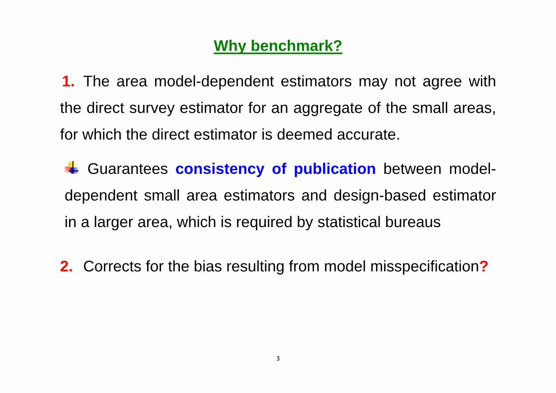
Why benchmark?

1. The area model-dependent estimators may not agree with

the direct survey estimator for an aggregate of the small areas,

for which the direct estimator is deemed accurate.

Guarantees consistency of publication between model-

dependent small area estimators and design-based estimator

in a larger area, which is required by statistical bureaus

2. Corrects for the bias resulting from model misspecification?

4

3. Problems considered in present presentation Consider e.g., a repeated monthly survey with sample

estimates dty in area d at month t. Denote by d̂tYtime-series

( d̂tYcross-section) the ‘optimal’ unbenchmarked predictor under an

appropriate times series (cross-sectional) model.

1- Should we benchmark, d̂tYtime-series or d̂tY

cross-section?

2- Does it matter which cross-sectional benchmarking method we use?

Distinguish between correct model specification and when the model is misspecified.

5

Problems considered in present presentation (cont.)

3- Develop a time series two-stage benchmarking

procedure for small area hierarchical estimates.

First stage: benchmark concurrent model-based estimators at

higher level of hierarchy to reliable aggregate of

corresponding survey estimates.

Second stage: benchmark concurrent model-based estimates

at lower level of hierarchy to first stage benchmarked estimate of higher level to which they belong.

6

Example: Labour Force estimates in the U.S.A

7

Content of presentation

1. Review cross-sectional and times series benchmarking

procedures for small area estimation;

2. Compare cross-sectional and times series benchmarking:

2.a Under correct model specification

2.b When models are misspecified

3. Review two-stage cross-sectional and times series

benchmarking procedures; (if time allows!!)

4. Apply time series two-stage benchmarking to monthly

unemployment series in the U.S.A.

8

Single- stage cross-sectional benchmarking procedures

(Pfeffermann & Barnard 1991): No BLUP benchmarked predictor exists!!

Pro-rata (ratio) benchmarking (in common use), model model

, 1 1ˆ ˆ ˆ/D Dbmkd d d d k kd kY Y b y b Y

)R ;

Limitations:

1- Adjusts all the small area model-based estimates the same

way, irrespective of their precision,

2- Benchmarked estimates not consistent: if sample size in area d increases but sample sizes in other areas unchanged, ˆ bmkd,Y R does not converge to true population value dY .

9

Additive single-stage cross-sectional benchmarking

model model, 1 1

ˆ ˆ ˆ( )D Dbmkd d k k k kk kY Y b y b Y

A d ;

1

Dd ddb

1.

Coefficients { }d measure precision (next slide); distribute

difference between benchmark and aggregate of model-based

estimates between the areas. Unbiased under correct model.

If 0d

d n

model

,ˆ ˆbmkd d dY Y YA consistent.

If modelˆPlim( ) 0k

k knY y

Area k with accurate estimate

does not contribute to benchmarking in other areas.

‘Easy’ to estimate variance of ,ˆ bmkdY A .

10

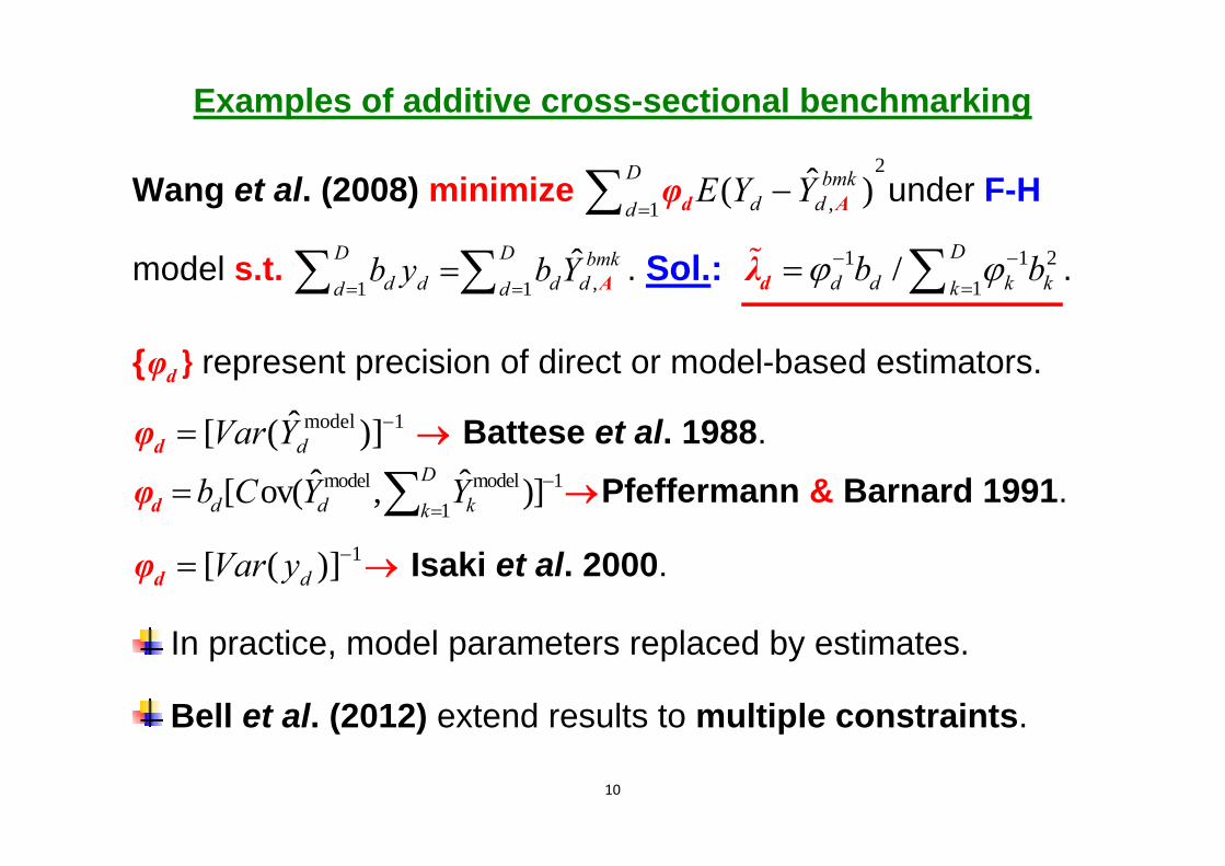
Examples of additive cross-sectional benchmarking

Wang et al. (2008) minimize 2

,1ˆ( )D bmk

d ddE Y Y

d Aφ under F-H

model s.t. ,1 1ˆD D bmk

d d d dd db y b Y

A . Sol.: 1 1 2

1/ D

d d k kkb b

dλ .

{ dφ } represent precision of direct or model-based estimators. model 1ˆ[ ( )]dVar Y dφ Battese et al. 1988.

model model 11

ˆ ˆ[ ov( , )]Dd d kkb C Y Y

dφ Pfeffermann & Barnard 1991.

1[ ( )]dVar y dφ Isaki et al. 2000.

In practice, model parameters replaced by estimates.

Bell et al. (2012) extend results to multiple constraints.

11

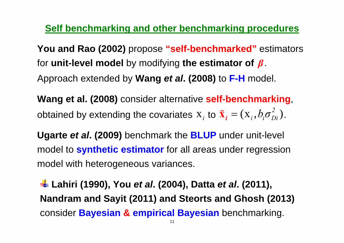
Self benchmarking and other benchmarking procedures

You and Rao (2002) propose “self-benchmarked” estimators for unit-level model by modifying the estimator of β . Approach extended by Wang et al. (2008) to F-H model.

Wang et al. (2008) consider alternative self-benchmarking, obtained by extending the covariates x i to (x , )2

i i Dib σ ix .

Ugarte et al. (2009) benchmark the BLUP under unit-level model to synthetic estimator for all areas under regression model with heterogeneous variances.

Lahiri (1990), You et al. (2004), Datta et al. (2011), Nandram and Sayit (2011) and Steorts and Ghosh (2013) consider Bayesian & empirical Bayesian benchmarking.

12

Small area single-stage time series benchmarking

Basic idea: Fit a time series model to direct estimators in all the areas, incorporate benchmark constraints into model equations. Variances obtained as part of model fitting.

Pfeffermann & Tiller (2006) consider the following model for total unemployment in census divisions.

1( ,..., )t t DtY Y Y = true division totals, 1( , , )t t Dty y y = direct estimates, 1( , , )t t Dte e e = sampling errors.

2 21, , , ,( ) 0 [ , , ]t t t t t t D ty Y e E e E e e ; , Σ Diagτt .

Division sampling errors independent between divisions but

highly auto-correlated within a division, and heteroscedastic.

Sampling rotation: (4 in, 8 out, 4 in).

13

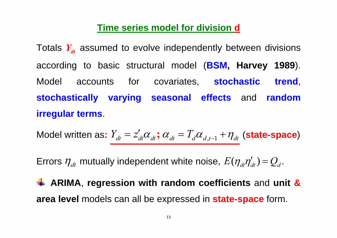
Time series model for division d

Totals dtY assumed to evolve independently between divisions

according to basic structural model (BSM, Harvey 1989).

Model accounts for covariates, stochastic trend,

stochastically varying seasonal effects and random irregular terms.

Model written as: , 1dt dt dt dt d d t dtY z T ; (state-space)

Errors dt mutually independent white noise, ( )dt dt dE Q .

ARIMA, regression with random coefficients and unit & area level models can all be expressed in state-space form.

14

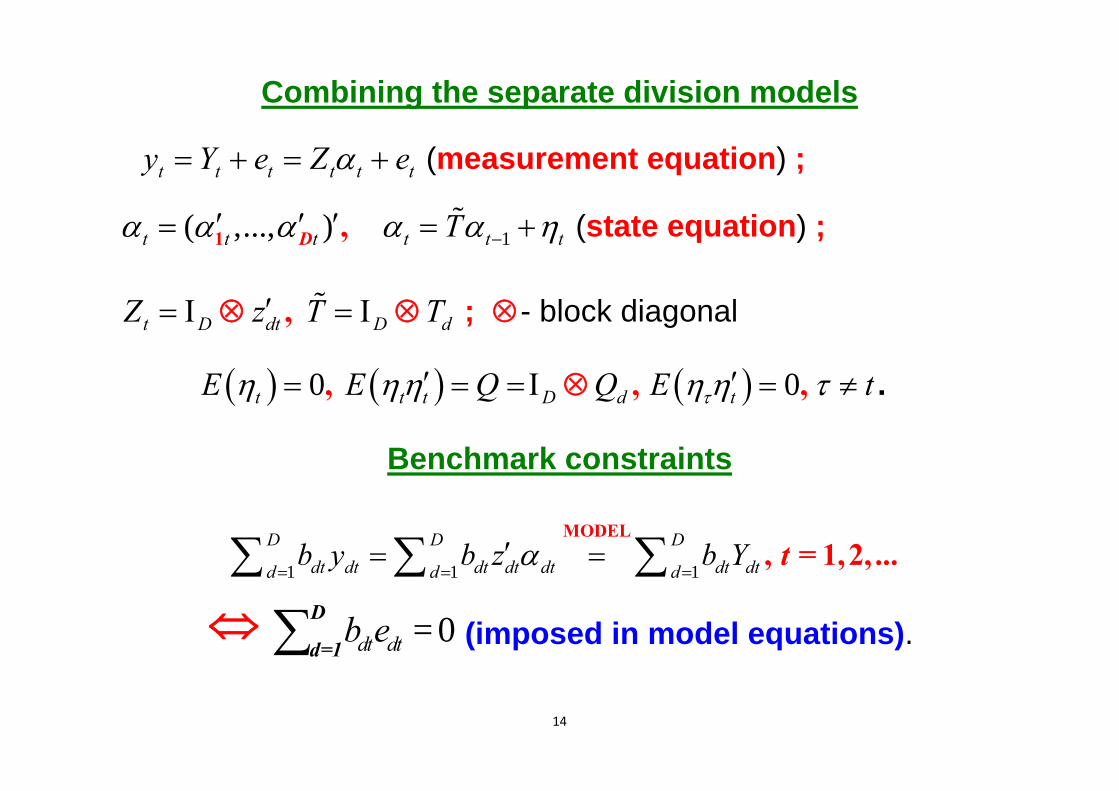
Combining the separate division models

t t t t t ty Y e Z e (measurement equation) ;

( ,..., )t t t 1 ,D 1t t tT (state equation) ;

t D dt D dZ z T T , ; - block diagonal

0 0t t t D d tE E Q Q E t , , , .

Benchmark constraints

1 1 1

D D Ddt dt dt dt dt dt dtd d db y b z b Y

MODEL, = 1,2, ...t

= 0dt dtb eD

d=1 (imposed in model equations).

15

Time series benchmarked predictor

Denote by ˆt,uα the state predictor at time t without imposing

the constraint 0Ddt dtd=1b e = at time t , but imposing the

constraints in previous time points.

Define, ,1ˆ[ ( )]D

ft dt dt dt u dtdVar b z

;

, ,1ˆ ˆ[( ) ( )]D

dft dt u dt dt dt dt u dtdCov b z

, .

1, ,1 1

ˆ ˆ( )ˆ D Ddt dt u dt dft ft dt dt dt dt dt ud dz z b y b z

bmk

dtY .

11

Ddt dt dft ftdb z

=1.

16

Properties of time series benchmarked predictor

1, ,1 1

ˆ ˆ ˆ( )D Dbmkdt dt dt u dt dft ft dt dt dt dt dt ud dY z z b y b z

.

ˆ bmkdtY member of cross-sectional benchmarked predictors,

model model, 1 1

ˆ ˆ ˆ( )D Dbmkd d k k k kk kY Y b y b Y

A dλ (Wang et al. 2008).

ˆ ˆmodeldt dt dt,uY = z α un-benchmarked predictor at time t;

1-1

1 21

ˆ ˆ{ [( ) ( )]}Dmodel modeldt dt dtdt dt dt dt kt kt ktD k=1

dt dftkt ktk

b bφ = =b Cov Y -Y , b Y Yz δb

;dtλ

Pfeffermann & Barnard (1991).

17

Properties of time series benchmarked predictor (cont.)

(a)- unbiasedness: if 1 , 1ˆ( ) 0bmkd,t- d tE Y Y ˆ( ) 0bmk

dt dtE Y Y .

To warrant unbiasedness under the model, it suffices to

initialize at time 1t = with unbiased predictor.

(b)- Consistency: Plim( ) 0d

dt dtny Y

& ˆPlim( ) 0

d

bmkdt dtnY y

ˆPlim( ) 0d

bmkdt dtnY Y

(even if model misspecified).

(c) ˆ( )bmkdt dtY YVar accounts for variances and covariances of

sampling errors, variances and covariances of benchmark

errors 1 1

D Ddt dt dt dt dtd db y b z

and their covariances with

division sampling errors, and variances of model components.

18

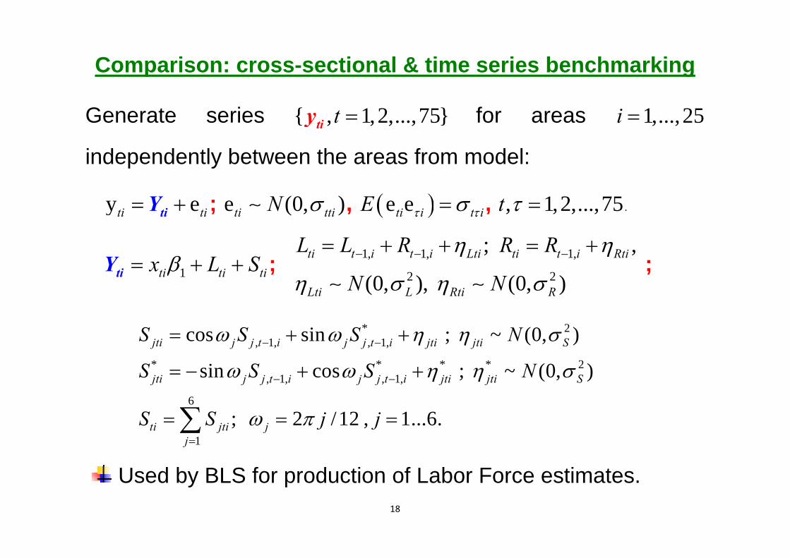
Comparison: cross-sectional & time series benchmarking

Generate series { , 1,2,...,75}t tiy for areas 1,...,25i

independently between the areas from model:

y eti ti tiY ; e (0, )ti ttiN , e eti i t iE , , 1,2,...,75t .

1ti ti tix L S tiY ; 1, 1, 1,

2 2

; ,

(0, ), (0, )ti t i t i Lti ti t i Rti

Lti L Rti R

L L R R R

N N

;

* 2, 1, , 1,

* * * * 2, 1, , 1,

6

1

cos sin ; ~ (0, )

sin cos ; ~ (0, )

; 2 /12 , 1...6.

jti j j t i j j t i jti jti S

jti j j t i j j t i jti jti S

ti jti jj

S S S N

S S S N

S S j j

Used by BLS for production of Labor Force estimates.

19

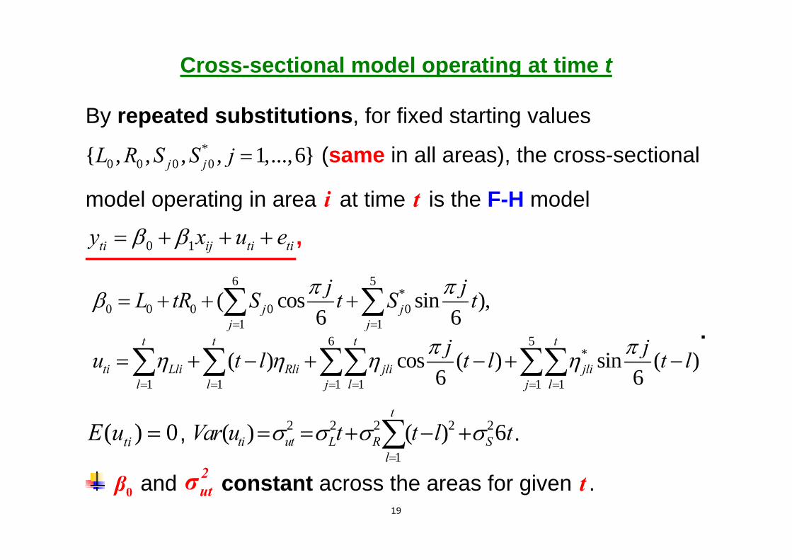
Cross-sectional model operating at time t

By repeated substitutions, for fixed starting values *

0 0 0 0{ , , , , 1,...,6}j jL R S S j (same in all areas), the cross-sectional

model operating in area i at time t is the F-H model

0 1ti ij ti tiy x u e ,

6 5*

0 0 0 0 01 1

6 5*

1 1 1 1 1 1

( cos sin ),6 6

( ) cos ( ) sin ( )6 6

j jj j

t t t t

ti Lli Rli jli jlil l j l j l

j jL tR S t S t

j ju t l t l t l

.

( ) 0tiE u , 2 2 2 2 2

1

( ) ( ) 6t

ti ut L R Sl

Var u t t l t

.

0β and 2utσ constant across the areas for given t .

20

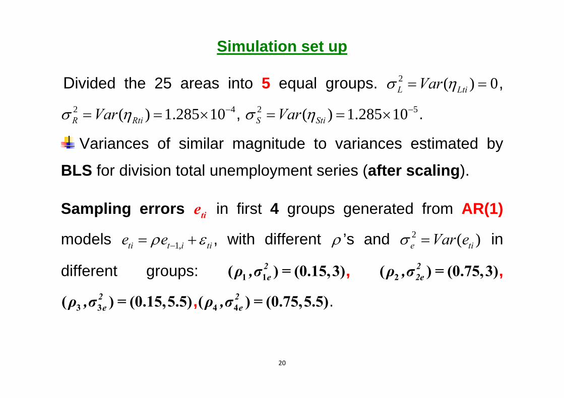
Simulation set up

Divided the 25 areas into 5 equal groups. 2 ( ) 0L LtiVar , 2 4( ) 1.285 10R RtiVar , 2 5( ) 1.285 10S StiVar .

Variances of similar magnitude to variances estimated by

BLS for division total unemployment series (after scaling).

Sampling errors tie in first 4 groups generated from AR(1)

models 1,ti t i tie e , with different ’s and 2 ( )e tiVar e in

different groups: 1 1( ) (0.15,3)2eρ ,σ = , 2( ) (0.75,3)2

2eρ ,σ = ,

3 3( ) (0.15,5.5)2eρ ,σ = , 4 4( ) (0.75,5.5)2

eρ ,σ = .

21

Simulation set up (cont.)

For group 5 used variances and autocorrelations estimated for

scaled total unemployment series in division of West North

Central. 4.4 15.5tti . First three autocorrelations are 0.38,

0.21, 0.12. Autocorrelations at lags 11-13 around 0.10.

1 1.5β = and started with *0 0 0 00, 1, 0, 1,...,6j jR L S S j ,

such that E( ) = (1+1.5 )ti iY x for all ( )t,i .

We compare the bias and RPMSE at t=25,50,75.

22

Simulation set up (cont.)

For each method re-estimated model parameters at each of

three time points with 2u estimated by F-H method and BSM

variances estimated by mle.

True 2uσ at three time points are 25 0.632σ , 50 5.202σ , 75 17.722σ .

Variances & autocorrelations of sampling errors known.

Same model parameters for five areas in each group.

Used true U.S.A State x-values.

Results in figures below are group averages of empirical bias and RPMSE over 400 simulated series.

23

Root Prediction MSE under correct model specification

24


25


26

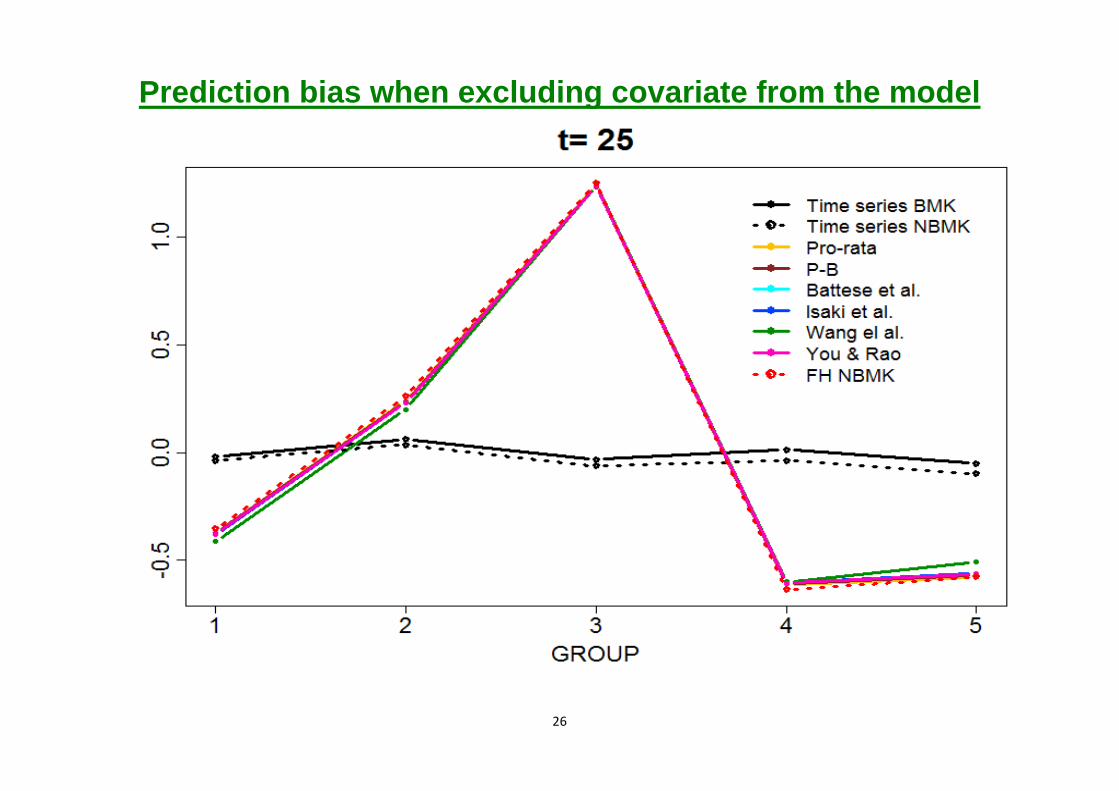
Prediction bias when excluding covariate from the model

27


28


29

Mean R- Square when regressing y on x

Group

Time 1 2 3 4 5 2utσ

t=25 0.484 0.754 0.738 0.386 0.317 0.630

t=50 0.444 0.463 0.605 0.337 0.374 5.200

t=75 0.415 0.432 0.616 0.296 0.262 17.720

30

Root PMSE when excluding covariate from the model

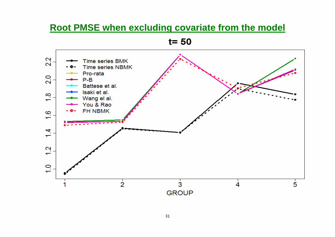
31


32


33

Conclusions

1- The cross-sectional procedures perform similarly and with 25 areas, there is no loss in efficiency from benchmarking.

2- Cross-sectional benchmarking does not correct for bias.

3- For sufficiently long time series, the extra efforts of fitting time series models and benchmarking the predictors are well rewarded in terms of the RPMSE.

4- The length of time series required for dominating the cross-sectional benchmarked methods depends on variances of sampling errors and correlations between them.

Time series predictors can be enhanced by smoothing.

34

Two-stage time series benchmarking

First stage: benchmark concurrent model-based estimates at

higher level of hierarchy to reliable aggregate of

corresponding survey estimates.

Second stage: benchmark concurrent model-based estimates

at lower level of hierarchy to first stage benchmarked estimate of higher level to which they belong.

Ghosh and Steorts (2013) consider Bayesian two-stage

cross-sectional benchmarking, applied in a single run.

35

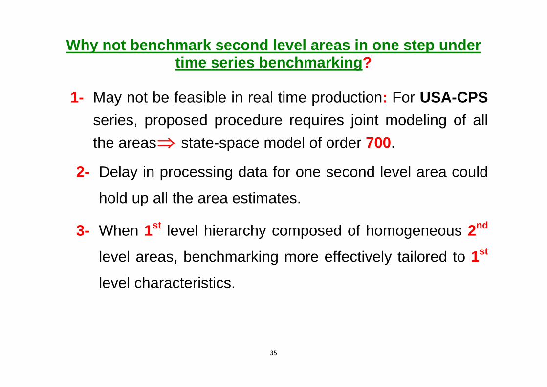
Why not benchmark second level areas in one step under time series benchmarking?

1- May not be feasible in real time production: For USA-CPS

series, proposed procedure requires joint modeling of all the areas state-space model of order 700.

2- Delay in processing data for one second level area could

hold up all the area estimates.

3- When 1st level hierarchy composed of homogeneous 2nd

level areas, benchmarking more effectively tailored to 1st

level characteristics.

36

Second-stage time series benchmarking

Suppose S ‘states’ in Division d;

Direct 2, , , , , *, , * ,( ) 0 ( , )ds t ds t ds t ds t ds ds t s s ds ty Y e E e Cov e e ; ,

Target , , ,

, , 1 , , , , * , * ,( ) 0, ( )

ds t ds t ds t

ds t ds ds t ds t ds t ds t ds t t t ds t

Y z

T E E Q

;

,

Benchmark: , , , , ,1 1ˆ ˆS S

ds t ds t ds t ds t ds ts sb y b z

bmk

dtY

Guarantees that model-based estimates at lower level add

up to published estimate at higher level to which they belong.

Benchmark error: , , ,1ˆ ˆ( ) ( )Sbmk bmkdt dt dt dt ds t ds t ds tsY Y z b z

bmk

dtr .

37

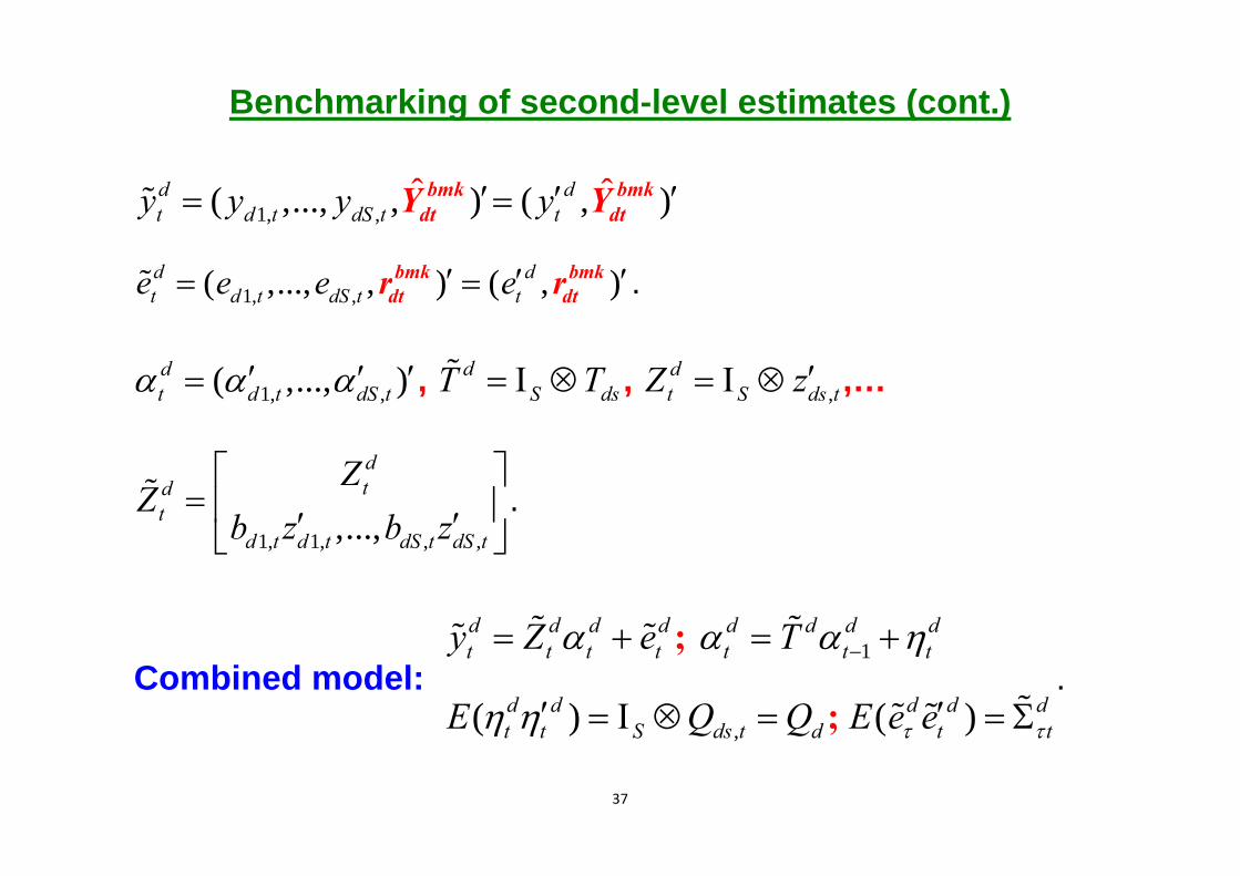
Benchmarking of second-level estimates (cont.)

1, ,( ,..., ˆ, )dt d t dS ty y y bmk

dtY ˆ( , )dty bmk

dtY

1, ,( ,..., , ) ( , )d dt d t dS t te e e e bmk bmk

dt dtr r .

1, ,( ,..., )dt d t dS t , d

S dsT T , ,dt S ds tZ z ,…

1, 1, , ,,...,

dtd

td t d t dS t dS t

ZZ

b z b z

.

Combined model: 1

,( ) ( )

d d d d d d d dt t t t t t t

d d d d dt t S ds t d t t

y Z e T

E Q Q E e e

;

;

.

38

Empirical results

Total unemployment, CPS-USA, Jan1990 - Dec2009. First level- Census divisions, Second level- States. Illustrate:

1- Consistency of benchmarked predictors

2- Robustness to model failure

39

Consistency of benchmarked predictors

S.E.( )ds,t ds,ty / y (left) ˆ bmkds,t ds,tY / y (right)

Massachusetts

0.00

0.05

0.10

0.15

0.20

0.25

Jan-90 Jan-94 Jan-98 Jan-02 Jan-06

0.7

0.8

0.9

1.0

1.1

1.2

1.3

1.4


40

Consistency of benchmarked predictors

[S.E.( )ds,t ds,ty / y ] (left) [ ˆ bmkds,t ds,tY / y ] (right)

New Hampshire

0.000.050.100.150.200.250.300.350.40

Jan-90 Jan-94 Jan-98 Jan-02 Jan-060.6

0.8

1.0

1.2

1.4

1.6

1.8


41

Direct, Benchmarked and Unbenchmarked estimates of Total Unemployment, Georgia (numbers in 000’s).

50

100

150

200

250

300

350

400


CPS BMK UNBMK

42

Direct, Benchmarked and Unbenchmarked estimates of Total Unemployment, Alabama (numbers in 000’s).

50

70

90

110

130

150

170


CPS BMK UNBMK

43

Conclusions

1. Two-stage time series benchmarking consistent and

protects against abrupt changes in time series model.

2. Due to bias correction, two-stage time series

benchmarking occasionally produces predictors with lower

RPMSE than unbenchmarked predictors (not illustrated).

3. Methodology can be extended to other time series models

or to three- or higher-stage benchmarking.

4. Proposed method produces variances of benchmarked

predictors as part of the model fitting.

Cross-Sectional Vs. Time Series Benchmarking in Small Area ...

Documents

Transcript of Cross-Sectional Vs. Time Series Benchmarking in Small Area ...