CROSS-LINGUAL WORD SENSE DISAMBIGUATION FORLOW-RESOURCE HYBRID MACHINE TRANSLATION

Alexander James Rudnick

Submitted to the faculty of the University Graduate School

in partial fulfillment of the requirements

for the degree

Doctor of Philosophy

in the School of Informatics, Computing, and Engineering,

Indiana University

December 2018

Accepted by the Graduate Faculty, Indiana University, in partial fulfillment of the

requirements for the degree of Doctor of Philosophy.

Doctoral Committee

Michael E. Gasser, Ph.D.

Sandra C. Kübler, Ph.D.

Markus Dickinson, Ph.D.

David J. Crandall, Ph.D.

John S. DeNero, Ph.D.

Date of Defense: November 6, 2018

ii

Copyright © 2018

Alexander James Rudnick

Some Rights Reserved.

This work is licensed under a Creative Commons Attribution 4.0 International License. To

view a copy of the license, please visit http://creativecommons.org/licenses/by/4.0/

iii

For my mother, Lenoir, who challenges me to be as great as she thinks I am.

iv

ACKNOWLEDGEMENTS

A doctoral thesis is a heck of a thing, and I could not have done it without the help of a

great number of people, some of whom I would like to acknowledge here.

I’d first like to thank Lindsey Kuper, my lovely wife, for putting up with me (in general,

but especially) throughout our tenure in graduate school. We’re out of the cold now.

I’d like to thank my wonderful parents, Lenoir and Jim, for their continuous love, en-

couragement and confidence. I’d like to thank some of my dearest lifelong friends for their

support and inspiration, both recently and throughout our lives. In addition to his perennial

warmth, humor and curiosity, Ryan Allen gave me an enormous boost by completing his

own doctoral work[1]; he powered through some occasionally less-than-ideal circumstances

to finish what he set out to do. Martin Robinson, Brett Thompson and Sydney Jackson

(among others!) listened to me complain and shared in my joys, as they’ve been known to

do, providing sounding boards for ideas, both sensible and absurd, and emotional support

as necessary.

I’d like to thank the Google Atlanta diaspora, especially Joel Webber and Bruce Johnson,

for helping me get a foot in the door at one of the world’s great machine learning and NLP

companies. You did so much for my confidence and drive, and you sent me off to graduate

school with a spring in my step and a chip on my shoulder. I hope you realize how much

it’s meant to me. I’d also like to thank members of the Google Translate team, both current

and former, for being such great mentors, colleagues and friends. Apurva Shah, Jeff Klinger,

Klaus Macherey, Wolfgang Macherey, Jason Smith, Lee Marshall, Julie Cattiau, Richard

Zens, Mengmeng Niu, Manisha Jain and Macduff Hughes all come to mind as especially

helpful and supportive, but the whole Google Translate crew is lovely people, and if you

happen to be reading this, you probably helped me out, so thank you.

I’d like to thank the Bloomington Area Runners Association, especially Katie, Andrew,

Zach, Cliff, Mike, Sara, Sarah, and Ben & Steph, for your friendship and camaraderie,

v

keeping me relatively healthy and happy during my time in Bloomington.

And I’d like to thank my committee for their encouragement, support, warmth, skepti-

cism, feedback, and patience.

vi

Alexander James Rudnick

CROSS-LINGUAL WORD SENSE DISAMBIGUATION FOR LOW-RESOURCE

HYBRID MACHINE TRANSLATION

This thesis argues that cross-lingual word sense disambiguation (CL-WSD) can be

used to improve lexical selection for machine translation when translating from a resource-

rich language into an under-resourced one, especially when relatively little bitext is avail-

able. In CL-WSD, we perform word sense disambiguation, considering the senses of a

word to be its possible translations into some target language, rather than using a sense

inventory developed manually by lexicographers.

Using explicitly trained classifiers that make use of source-language context and of

resources for the source language can help machine translation systems make better

decisions when selecting target-language words. This is especially the case when the

alternative is hand-written lexical selection rules developed by researchers with linguistic

knowledge of the source and target languages, but also true when lexical selection would

be performed by a statistical machine translation system, when there is a relatively small

amount of available target-language text for training language models.

In this work, I present the Chipa system for CL-WSD and apply it to the task of

translating from Spanish to Guarani and Quechua, two indigenous languages of South

America. I demonstrate several extensions to the basic Chipa system, including tech-

niques that allow us to benefit from the wealth of available unannotated Spanish text

and existing text analysis tools for Spanish, as well as approaches for learning from

vii

bitext resources that pair Spanish with languages unrelated to our intended target lan-

guages. Finally, I provide proof-of-concept integrations of Chipa with existing machine

translation systems, of two completely different architectures.

Michael E. Gasser, Ph.D.

Sandra C. Kübler, Ph.D.

Markus Dickinson, Ph.D.

David J. Crandall, Ph.D.

John S. DeNero, Ph.D.

viii

TABLE OF CONTENTS

Acknowledgements . . . . . . . . . . . . . . . . . . . . . . . . . . . . . . . . . . v

Abstract . . . . . . . . . . . . . . . . . . . . . . . . . . . . . . . . . . . . . . . . vii

Chapter 1: Overview . . . . . . . . . . . . . . . . . . . . . . . . . . . . . . . . 1

1.1 WSD in Machine Translation . . . . . . . . . . . . . . . . . . . . . . . . . . 2

1.2 Thesis Statement . . . . . . . . . . . . . . . . . . . . . . . . . . . . . . . . . 5

1.3 Questions to Address . . . . . . . . . . . . . . . . . . . . . . . . . . . . . . . 5

1.4 Dissertation Structure . . . . . . . . . . . . . . . . . . . . . . . . . . . . . . 5

1.5 Previously Published Work . . . . . . . . . . . . . . . . . . . . . . . . . . . 6

Chapter 2: Background . . . . . . . . . . . . . . . . . . . . . . . . . . . . . . . 8

2.1 Word-Sense Disambiguation . . . . . . . . . . . . . . . . . . . . . . . . . . . 8

2.2 Cross-Lingual Word Sense Disambiguation . . . . . . . . . . . . . . . . . . . 13

2.3 Hybrid MT . . . . . . . . . . . . . . . . . . . . . . . . . . . . . . . . . . . . 15

2.4 Paraguay and the Guarani Language . . . . . . . . . . . . . . . . . . . . . . 17

2.4.1 Online Language Tools for Guarani . . . . . . . . . . . . . . . . . . . 18

2.5 Quechua . . . . . . . . . . . . . . . . . . . . . . . . . . . . . . . . . . . . . . 18

Chapter 3: Related Work . . . . . . . . . . . . . . . . . . . . . . . . . . . . . . 20

ix

3.1 CL-WSD in vitro . . . . . . . . . . . . . . . . . . . . . . . . . . . . . . . . . 20

3.1.1 Multilingual Evidence for CL-WSD . . . . . . . . . . . . . . . . . . . 21

3.2 WSD with Sequence Models . . . . . . . . . . . . . . . . . . . . . . . . . . . 22

3.3 Lexical Selection in RBMT . . . . . . . . . . . . . . . . . . . . . . . . . . . 23

3.4 CL-WSD for Statistical Machine Translation . . . . . . . . . . . . . . . . . . 24

3.5 WSD for lower-resourced languages . . . . . . . . . . . . . . . . . . . . . . . 26

3.6 CL-WSD at Senseval and SemEval . . . . . . . . . . . . . . . . . . . . . . . 27

3.7 Translation into Morphologically Rich Languages . . . . . . . . . . . . . . . 29

Chapter 4: Data Sets, Tasks and Evaluation . . . . . . . . . . . . . . . . . . 31

4.1 Measuring CL-WSD Classification Accuracy . . . . . . . . . . . . . . . . . . 32

4.2 Measuring MT Improvements . . . . . . . . . . . . . . . . . . . . . . . . . . 33

4.3 Data Sets and Preprocessing . . . . . . . . . . . . . . . . . . . . . . . . . . . 34

4.3.1 Source-side annotations . . . . . . . . . . . . . . . . . . . . . . . . . 34

4.3.2 Preprocessing . . . . . . . . . . . . . . . . . . . . . . . . . . . . . . . 35

4.3.3 Lemmatization . . . . . . . . . . . . . . . . . . . . . . . . . . . . . . 41

4.3.4 Alignment . . . . . . . . . . . . . . . . . . . . . . . . . . . . . . . . . 43

4.3.5 A deeper dive: producing Spanish-Guarani bitext . . . . . . . . . . . 44

4.4 Exploring the Bitext . . . . . . . . . . . . . . . . . . . . . . . . . . . . . . . 48

Chapter 5: The Baseline Chipa System . . . . . . . . . . . . . . . . . . . . . 56

5.1 Classification Results for the Baseline System . . . . . . . . . . . . . . . . . 58

5.2 For Comparison: the Baseline Chipa System On the SemEval 2010 and 2013Shared Tasks . . . . . . . . . . . . . . . . . . . . . . . . . . . . . . . . . . . 63

x

Chapter 6: Learning from Monolingual Data . . . . . . . . . . . . . . . . . . 68

6.1 Monolingual features from existing NLP tools . . . . . . . . . . . . . . . . . 69

6.2 Brown Clustering . . . . . . . . . . . . . . . . . . . . . . . . . . . . . . . . . 71

6.2.1 Clustering in practice . . . . . . . . . . . . . . . . . . . . . . . . . . 73

6.2.2 Classification features based on Brown clusters . . . . . . . . . . . . 77

6.3 Neural Word Embeddings . . . . . . . . . . . . . . . . . . . . . . . . . . . . 79

6.3.1 From word embeddings to classification features . . . . . . . . . . . . 81

6.4 Neural Document Embeddings . . . . . . . . . . . . . . . . . . . . . . . . . . 82

6.5 Experiments . . . . . . . . . . . . . . . . . . . . . . . . . . . . . . . . . . . . 84

6.6 Experimental Results . . . . . . . . . . . . . . . . . . . . . . . . . . . . . . . 85

6.6.1 Results: adding syntactic features . . . . . . . . . . . . . . . . . . . . 86

6.6.2 Results: adding clustering features . . . . . . . . . . . . . . . . . . . 86

6.6.3 Results: combining sparse features . . . . . . . . . . . . . . . . . . . 88

6.6.4 Results: word2vec embeddings alone . . . . . . . . . . . . . . . . . . 89

6.6.5 Results: doc2vec embeddings alone . . . . . . . . . . . . . . . . . . . 92

6.6.6 Results: combining neural embeddings with sparse features . . . . . . 93

6.7 Discussion . . . . . . . . . . . . . . . . . . . . . . . . . . . . . . . . . . . . . 94

Chapter 7: Learning from Multilingual Data . . . . . . . . . . . . . . . . . . 96

7.1 Supplemental multilingual corpora . . . . . . . . . . . . . . . . . . . . . . . 98

7.1.1 Europarl . . . . . . . . . . . . . . . . . . . . . . . . . . . . . . . . . . 98

7.1.2 Bible translations . . . . . . . . . . . . . . . . . . . . . . . . . . . . . 99

7.2 CL-WSD with Markov Networks . . . . . . . . . . . . . . . . . . . . . . . . 100

xi

7.3 Classifier stacking . . . . . . . . . . . . . . . . . . . . . . . . . . . . . . . . . 103

7.3.1 Annotating the bitext with stacking predictions . . . . . . . . . . . . 103

7.4 Considering domain mismatches . . . . . . . . . . . . . . . . . . . . . . . . . 104

7.5 Experiments . . . . . . . . . . . . . . . . . . . . . . . . . . . . . . . . . . . . 106

7.6 Experimental Results . . . . . . . . . . . . . . . . . . . . . . . . . . . . . . . 106

7.6.1 Results: classifier stacking with Europarl . . . . . . . . . . . . . . . . 107

7.6.2 Results: classifier stacking with Bibles . . . . . . . . . . . . . . . . . 107

7.6.3 Results: classifier stacking with both Europarl and Bibles . . . . . . 107

7.7 Discussion . . . . . . . . . . . . . . . . . . . . . . . . . . . . . . . . . . . . . 111

Chapter 8: Integration Into Machine Translation Systems . . . . . . . . . . 112

8.1 Integrating Chipa into Phrase-Based Statistical Machine Translation . . . . 113

8.1.1 Interfacing between Moses and Chipa . . . . . . . . . . . . . . . . . . 115

8.1.2 Moses SMT for Spanish-Guarani . . . . . . . . . . . . . . . . . . . . 117

8.2 Integrating Chipa into Rule-Based Machine Translation . . . . . . . . . . . . 118

8.2.1 The SQUOIA RBMT system . . . . . . . . . . . . . . . . . . . . . . 118

8.3 Translation Evaluation for Spanish-Guarani . . . . . . . . . . . . . . . . . . 120

8.4 Translation Evaluation for Spanish-Quechua . . . . . . . . . . . . . . . . . . 122

8.5 Discussion . . . . . . . . . . . . . . . . . . . . . . . . . . . . . . . . . . . . . 125

Chapter 9: Summary and Outlook . . . . . . . . . . . . . . . . . . . . . . . . 126

9.1 Applying techniques like this to neural machine translation . . . . . . . . . . 130

9.2 Building resources for Guarani and other under-represented languages . . . . 131

xii

References . . . . . . . . . . . . . . . . . . . . . . . . . . . . . . . . . . . . . . . 134

Curriculum Vitae

xiii

CHAPTER 1

OVERVIEW

A thing with just one meaning has scarcely any meaning at all.

– Marvin Minsky, Society of Mind [2]

In this dissertation, I investigate techniques for lexical selection in machine translation,

with the goal of supporting language pairs for which there is little training data available

for the target language. I propose that cross-lingual word sense disambiguation (CL-WSD)

is a feasible and practical means for lexical selection in this setting. I demonstrate this with

translation experiments covering several language pairs, focusing on translating from Spanish

to Guarani (a co-official language of Paraguay) and Spanish to Quechua (broadly spoken

around the Andes mountain range), and including some experiments involving English.

I describe new CL-WSD approaches, including the use of unsupervised clustering on

source-language text and multilingual corpora for the source language as a source of clas-

sification features. I also evaluate their effectiveness in practice. All of these techniques

have been implemented in a new CL-WSD software system called Chipa1. We also integrate

Chipa into two machine translation systems of different architectures to show its practical

applicability.

The research presented here is motivated in large part to allow primarily rule-based

machine translation (RBMT) systems to make use of any available bitext training data, so

that they can improve their translations without their human authors having to write new

rules. Despite the enormous success of statistical machine translation (SMT) approaches

over the past twenty years, they typically require large bitext corpora to be useful. RBMT1Chipa the software is named for chipa the snack food, popular in many parts of South America. It is

a cheesy bread made from cassava flour, often served in a bagel-like shape in Paraguay. Also chipa means‘rivet, bolt, screw’ in Quechua; something for holding things together. The software is available athttp://github.com/alexrudnick/chipa under the GPL.

1

approaches remain attractive for many language pairs due to a simple dearth of training

data, and there is an active RBMT community working on developing machine translation

systems for the world’s under-resourced and under-represented languages.

My hope for this work is that it will provide techniques and tools useful for anyone

working on machine translation into these languages, whatever the architecture of their MT

software, allowing them to make use of bitext as it becomes available for their language pair.

This combination of strategies is what is meant by “hybrid” in this work. We would like to

combine existing RBMT systems with statistical methods where possible, neither throwing

away the efforts and insights of linguists, nor ignoring the benefits of machine learning and

corpus-based approaches.

1.1 WSD in Machine Translation

To appreciate the word-sense disambiguation problem embedded in machine translation,

consider for a moment the different senses of “have” in English. In have a sandwich, have

a bath2, have an argument, and even have a good argument, the meaning of the verb “to

have” is quite different. It would be surprising for our target language, especially if it is not

closely related, to use a single light verb in all of these distinct contexts. Even in a language

as closely related as Spanish, we see these English expressions rendered with some different

verbs: tomar un bocadillo (‘have a sandwich’) but tener un argumento (‘have an argument’),

for example. By cross-lingual word sense disambiguation (CL-WSD), I mean exactly this

problem: we consider tomar and tener to be two different senses of have – there are certainly

more, for a verb like have – and the CL-WSD software must label each source-language word

with its correct translation.

Another concrete example, due to Annette Rios [3], surfaces when translating from Span-

ish to Quechua. Here we see different lexicalization patterns in Spanish and Quechua for

transitive motion verbs. The Spanish lemmas contain information about the path of the2Compare with “take a bath”, which has an additional metaphorical interpretation meaning “serious

financial loss”

2

movement, e.g. traer - ’bring (here)’ vs. llevar - ’take (there)’. Quechua roots, on the other

hand, use a suffix (-mu) to express direction, but instead lexicalize information about the

manner of movement and the object that is being moved. Some of these verbs are as follows:

general motion verbs:

• pusa-(mu-): ‘take/bring a person’

• apa-(mu-)-: ‘take/bring an animal or an inanimate object’

motion verbs with manner:

• marq’a-(mu-): ‘take/bring something in one’s arms’

• q’ipi-(mu-): ‘take/bring something on one’s back or in a bundle’

• millqa-(mu-): ‘take/bring something in one’s skirts’

• hapt’a-(mu-): ‘take/bring something in one’s fists’

• lluk’i-(mu-): ‘take/bring something below their arms’

• rikra-(mu-): ‘take/bring something on one’s shoulders’

• rampa-(mu-): ‘take/bring a person holding their hand’

The correct translation of Spanish traer or llevar into Quechua thus depends on the

object being moved, and more descriptive translations can be chosen, given context clues.

Furthermore, different languages simply make different distinctions about the world. The

Spanish hermano ’brother’, hijo ’son’ and hija ’daughter’ all translate to different Quechua

terms based on the person with respect to whom we are describing the referent; a daughter

relative to her father is ususi, but when described relative to her mother, warmi wawa [4].

Chipa, then, must somehow make these distinctions automatically if it is to help trans-

lation systems generate valid Quechua. It is possible to do this with hand-crafted lexical

selection rules, or by treating this as a machine learning problem and basing lexical selections

on the available data, or by some combination of the two.

3

Lexical ambiguity presents a daunting challenge for rule-based machine translation sys-

tems. Several translations of a given word may all be syntactically valid in context. Even

when choosing among near-synonyms, we would like to respect the selectional preferences of

the target language so as to produce natural-sounding output text.

Writing lexical selection rules by hand, while possible in principle and an approach taken

by many MT system implementors, is tedious and error-prone. Bilingual informants, if avail-

able, may not be able to enumerate the contexts in which they would choose one alternative

over another, and there will be many thousands of words that might need to be translated

in any given source language. Thus we would like to learn from corpora when possible.

Given a sufficient bitext corpus, we can discover the different possible translations for each

source-language word, and by applying supervised learning, we can learn how to discriminate

between them.

We do not have very large sentence-aligned bitext corpora for most language pairs. Con-

veniently, however, we can get started by using the Bible as training data; it contains many

commonly used words and contains enough text for us to meaningfully train our systems.3 In the future, we would like to see larger bitext corpora constructed for under-resourced

language pairs by their respective communities. Our research group has been working on

this problem in parallel, though that is not the focus of this dissertation.

The major contributions of this work will be new approaches for CL-WSD, demonstra-

tions that they can be used in practice for translating from higher-resourced languages into

lower-resourced ones, and demonstrations that they can be integrated into practical machine

translation systems, thus improving word choice. Additionally, on a practical level we will

develop a suite of reusable open-source software, including the CL-WSD engine and demo

MT systems of different architectures for for Spanish-Guarani and Spanish-Quechua.

All of the software used in this dissertation has been developed in public reposito-3The Bible has been translated into a substantial fraction of the world’s languages and contains more

than thirty thousand verses (roughly, sentences) in a variety of text genres. For an overview of using theBible for multilingual NLP applications, please see Resnik et al. [5] and Mayer and Cysouw [6].

4

ries, and is freely available online at http://github.com/hltdi and http://github.com/

alexrudnick.

1.2 Thesis Statement

Cross-lingual word sense disambiguation is a feasible and practical means for lexical selection

in a hybrid machine translation system for a language pair with relatively modest resources.

1.3 Questions to Address

1. Can we use monolingual resources from the source language to improve accuracy on

the cross-lingual word sense disambiguation task?

2. Can we use multilingual resources, such as bitext corpora pairing the source language

with languages other than the current target language?

3. Which kinds of machine translation systems can benefit from CL-WSD?

1.4 Dissertation Structure

In the following chapters, I will discuss the relevant background information and investigate

these questions, as follows.

• Chapter 2 gives some background on word sense disambiguation, its history, and its

applications in machine translation, as well as on Spanish and Guarani, the languages

of Paraguay, and some of the social context for this translation pair.

• Chapter 3 reviews some recent work on CL-WSD and its applications.

• Chapter 4 presents the data sets used in this work, and our evaluation metrics for this

project.

5

• Chapter 5 discusses the basic architecture of the Chipa system and its performance on

the previously presented evaluation metrics.

• Chapter 6 explores some approaches for learning from the available resources for Span-

ish to give us better representations for translating out of it.

• Chapter 7 expands our approaches to include the multilingual resources for Spanish,

integrating CL-WSD classifiers for languages other than Guarani and Quechua.

• Chapter 8 presents practical applications of Chipa; here we will see how to integrate

CL-WSD software into different running machine translation systems.

• Finally, in Chapter 9, we will conclude and describe possible work for the future.

1.5 Previously Published Work

This dissertation draws heavily from several previously published papers, in which my coau-

thors and I explore early versions of some of the ideas and techniques described here. They

are as follows:

• Rudnick 2011, “Towards Cross-Language Word Sense Disambiguation for Quechua”

[7], in which I explored a simple CL-WSD system for Quechua adjectives.

• Rudnick, Liu and Gasser 2013, “HLTDI: CL-WSD Using Markov Random Fields for

SemEval-2013 Task 10” [8], a SemEval submission in which we explored the use of

multilingual evidence for CL-WSD.

• Rudnick and Gasser 2013, “Lexical Selection for Hybrid MT with Sequence Labeling”

[9], in which we explored using Maximum-Entropy Markov Models (MEMMS) for CL-

WSD for Spanish-Guarani.

6

• Rudnick, Rios and Gasser 2014, “Enhancing a Rule-Based MT System with Cross-

Lingual WSD” [3], in which we integrated Chipa into an RBMT system for Spanish-

Quechua and explored monolingual clustering to learn from Spanish data.

• Rudnick, Skidmore, Samaniego and Gasser 2014, “Guampa: a Toolkit for Collaborative

Translation” [10], which describes our system for building larger corpora through en-

listing the Guarani-language activist community to help. Guampa, or at least the idea

of engaging the language-activist and language-learning communities, figures largely

into the future of this work, rather than having been helpful for data gathering as of

yet.

7

CHAPTER 2

BACKGROUND

In this chapter, I will discuss some of the relevant background, including a short overview of

word-sense disambiguation broadly, its history with respect to machine translation, and how

the cross-lingual framing of WSD addresses some of the difficulties in successfully applying

WSD techniques to MT. I also give a short description of the languages we would like to

support with this work, Guarani and Quechua.

2.1 Word-Sense Disambiguation

Word types often – perhaps always – have many possible meanings. Given a string of char-

acters or an utterance, the reader or listener must do some computational work to interpret

the received message, and this may fail. In the simplest case, one could be faced with a

homophone or homograph and need to distinguish between different lexemes that could be

intended. There could be technical or jargon senses that conflict with colloquial uses of

a word; consider the many different meanings of “kernel”, “type” and “kind” in computer

science and mathematics. In the most difficult case, the usages can be hyperbolic, metaphor-

ical, sarcastic, or oblique references. Understanding these usages will require understanding

the broader discourse context and the goals of the speaker. Discourse modeling is outside

the scope of this work, but in practice, for machine translation, we will need to get some

sense of the particular meaning of polysemous words in context.

What we mean by word sense disambiguation is just this: when faced with a token in

a piece of text, we want to be able to decide which word sense from a sense inventory is

the intended meaning. The sense inventory might come from a pre-set ontology built by

lexicographers, such as a dictionary or a wordnet1, or it might have been discovered in some1Such as WordNet®, the original wordnet for English [11]

8

Figure 2.1: Some of the WordNet 3.1 senses for “take”: there are two noun senses and 42distinct verb senses, though we only show the first ten. In WordNet and similar projects,word senses are called synsets, as there will be a set of synonyms that share the sense.

automatic way. Word-sense disambiguation tasks have historically been divided into two

varieties, where lexical sample tasks require labeling occurrences of some small number of

words types, and all-words tasks, in which every word in the input text must be labeled[12].

In NLP applications that must handle arbitrary text, this distinction breaks down somewhat,

as the application will encounter previously unseen words for which there are no known senses

in the ontology.

When making use of WSD for some other purpose – say in information retrieval, infor-

mation extraction, or machine translation – choosing an appropriate sense inventory can

be a difficult design task, as applications may require different granularities, while different

lexicographers will have made their own editorial decisions about what constitutes a distinct

sense of a word.

9

Treating WSD as a supervised learning problem requires labeled training data, which

for this task means text where each token has been annotated with its appropriate sense

identifier. Such corpora must be created manually specifically for this purpose, and this

kind of annotation is very labor-intensive, especially when annotating data for an all-words

WSD task, as the annotators must consider the many possible senses for each word, and new

words will occur during the course of annotation.

Sense-annotated corpora have been created for supervised WSD for both the lexical

sample and all-words settings, but they are only available for a few languages, due to the

time and effort required to prepare them. Some famous sense-annotated corpora include

the “hard/line/serve” corpus, originally prepared by Leacock et al. [13, 14], which marks

occurrences of the adjective “hard”, noun “line” and verb “serve” with their respective senses

from WordNet.2 These feature roughly four thousand annotated instances of each word.

Larger lexical sample data sets 3 were prepared for the first three Senseval events [15, 16, 17]

each of which featured thousands of instances of 35 to 73 different word types. For Senseval-

2 and Senseval-3, verbs were labeled with senses from the WordSmyth online dictionary-

thesaurus4 rather than their senses from WordNet, as the WordNet sense distinctions for

English verbs are very fine-grained, resulting in a very difficult task in the first Senseval.

Larger corpora annotating word senses for many but not all content words include the

sense-annotated portion of the American National Corpus [18], which provides a thousand

annotated usages of a hundred individual word types, each checked by several annotators,

with inter-annotator agreement data provided.

There have also been all-words annotated corpora, such as SemCor (described by Miller

et al. [19] and developed by Landes et al. [20]), a large subset of the Brown Corpus with all

content words manually annotated with their WordNet senses. “SemCor” is now often used

as a generalized term for corpora tagged with senses from a wordnet; there are such corpora2Available at http://www.d.umn.edu/~tpederse/data.html3Archived at the same URL4http://www.wordsmyth.net/

10

of varying sizes available for many different languages 5.

In order to ameliorate this WSD data acquisition bottleneck and allow WSD research

to move forward in the absence of annotated training data, researchers have also created

corpora with artificially-ambiguous “pseudo-words”, in which two distinct word types are

merged into a synthetic new word, but the original word that was used is noted; for example,

all occurrences of ‘shoe’ and “book” could be replaced with a synthetic token “bookshoe”.

The original uses are then considered two senses of the new pseudo-word, and researchers

can check whether their WSD algorithms can recover the original token.

Supervised learning approaches are by no means the only strand of research in WSD;

there are also unsupervised word-sense induction approaches that try to discover senses auto-

matically from corpora, knowledge-based algorithms that make use of hand-crafted resources

such as dictionaries and wordnets to label tokens – such as, classically, the Lesk Algorithm

[21], and more recently, graph-based algorithms that make use of the structure of very large

knowledge bases, such as Babelfy [22] – and a host of others. For a broad overview of the

different approaches to word senses, their disambiguation, and the history of the related

techniques, please see Agirre et al.’s book on the topic [12].

It has long been held that word sense disambiguation is a central problem in NLP ap-

plications, including machine translation. Even in popular culture, the dangers of misun-

derstanding and thus mistranslating individual words is well-understood; many have heard

the (apparently apocryphal [23]) story about an early MT system faced with the Biblical

saying “the spirit is willing but the flesh is weak” in Russian and producing (variations on

the story abound) “the vodka is good but the meat is rotten”. Warren Weaver described, in

his prescient 1949 memorandum [24], both an essentially modern conception of WSD and

why a translation system would need it.

As early as 1960, Yehoshua Bar-Hillel wrote that general-purpose machine translation5For a list of such corpora, see http://globalwordnet.org/wordnet-annotated-corpora/. The

English-language SemCor has been maintained and updated by Rada Mihalcea and is available at http://web.eecs.umich.edu/~mihalcea/downloads.html

11

(“fully automatic high-quality translation”, as it was called at the time) was impossible due

to the insurmountable task of writing WSD routines for all source-language words. [25]

During the past year I have repeatedly tried to point out the illusory character

of the FAHQT ideal even in respect to the mechanical determination of the

syntactical structure of a given source-language sentence... Here I shall show

that there exist extremely simple sentences in English – and the same holds, I

am sure, for any other natural language – which within certain linguistic contexts,

would be uniquely (up to plain synonymy) and unambiguously translated into

any other language by anyone with a sufficient knowledge of the two languages

involved, though I know of no program that would enable a machine to come up

with this unique rendering unless by a completely arbitrary and ad hoc procedure

whose futility would show itself in the next example.

A sentence of this kind is the following: The box was in the pen.

To produce a correct rendering of this sentence in Spanish, for example, the translation

system must decide between translating “pen” as corral (an enclosure, like for an animal) or

as pluma (the instrument for writing).

As of this writing, for this particular example, Google Translate picks the correct ren-

dering, although in September 2013, it chose the less-sensible “in the writing implement”

translation for Bar-Hillel’s example sentence (see Figure 2.2).

One wonders how this could have come about – we would hope that the n-gram language

model for Spanish would prefer sentences about things in enclosures to things in writing

implements. But the word en can be a translation of either the English “in” or “on”, and

pluma can also mean “feather”, so en la pluma will be attested in a large corpus of Spanish; we

could easily imagine a sentence containing “on the feather”. This situation is fairly complex.

In a translation task, even if we are able to assign a particular sense to a given word, we

must still map these senses to translations in the target language, and there is no guarantee

12

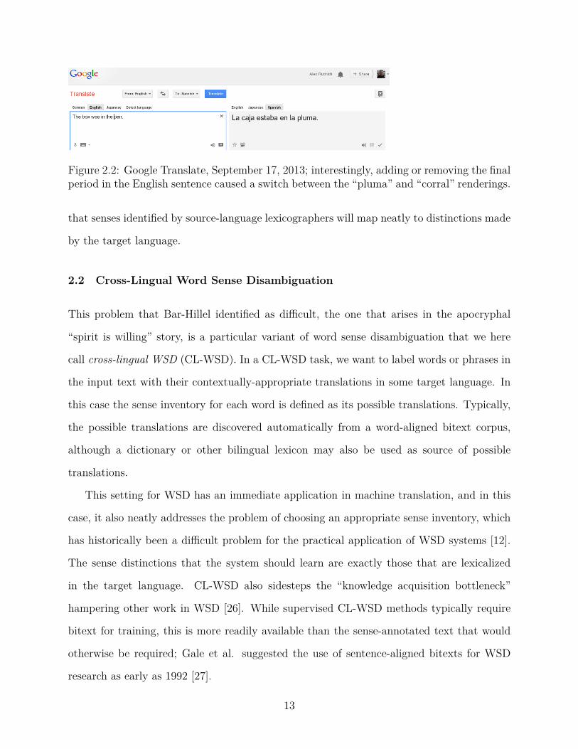
Figure 2.2: Google Translate, September 17, 2013; interestingly, adding or removing the finalperiod in the English sentence caused a switch between the “pluma” and “corral” renderings.

that senses identified by source-language lexicographers will map neatly to distinctions made

by the target language.

2.2 Cross-Lingual Word Sense Disambiguation

This problem that Bar-Hillel identified as difficult, the one that arises in the apocryphal

“spirit is willing” story, is a particular variant of word sense disambiguation that we here

call cross-lingual WSD (CL-WSD). In a CL-WSD task, we want to label words or phrases in

the input text with their contextually-appropriate translations in some target language. In

this case the sense inventory for each word is defined as its possible translations. Typically,

the possible translations are discovered automatically from a word-aligned bitext corpus,

although a dictionary or other bilingual lexicon may also be used as source of possible

translations.

This setting for WSD has an immediate application in machine translation, and in this

case, it also neatly addresses the problem of choosing an appropriate sense inventory, which

has historically been a difficult problem for the practical application of WSD systems [12].

The sense distinctions that the system should learn are exactly those that are lexicalized

in the target language. CL-WSD also sidesteps the “knowledge acquisition bottleneck”

hampering other work in WSD [26]. While supervised CL-WSD methods typically require

bitext for training, this is more readily available than the sense-annotated text that would

otherwise be required; Gale et al. suggested the use of sentence-aligned bitexts for WSD

research as early as 1992 [27].

13

WSD applied directly to machine translation has a long history; practical work in in-

tegrating WSD with statistical machine translation particularly dates back to early SMT

work at IBM [28]. Despite all of the ambiguities in translation, most statistical MT systems

do not use an explicit WSD module [12, Chapter 3]; the language model and phrase tables

of these systems mitigate lexical ambiguities by encouraging words used collocationally to

appear together in the output. Entire phrases6 such as verbs with their common objects

may be learned and stored in the phrase table, and the language model will encourage com-

mon collocations as well. CL-WSD techniques have been successfully used to improve SMT,

especially when it is applied not just to individual tokens but to phrases present in the

phrase table, as in the work of Carpuat and Wu [29]; there have also been discriminative

classifiers used to aid in selecting phrase table entries, as in the work of Žabokrtský et al.

[30], which is a similar intuition, even if not described by the authors in terms of word-sense

disambiguation.

This cross-lingual variant of WSD has received enough attention to warrant shared tasks

at recent SemEval workshops: SemEval 2010 Task 3 [31] and SemEval 2013 Task 10 [32] were

both classical cross-lingual lexical sample tasks. A similar task was also run in 2014 [33],

although this task provides a target-language context rather than a source-language one,

more closely representing the problem faced by an agent trying to help a second-language

learner compose a sentence in their L2 than that faced by a machine translation system.

Some approaches to the first two tasks, along with a number of other projects, are described

in Chapter 3.

In general, there is a many-to-many relationship across language boundaries between

words and their possible translations. This happens for a number of reasons: figurative or

metaphorical uses may not translate directly, obligatory information in one language may

be left unspecified in another, or the criteria for selecting a word may simply differ. To

give some familiar examples, a “leg” of a trip in English is typically translated as étape in6Not necessarily “phrases” in a syntactic sense, but subsequences of sentences

14

French, which is unrelated to limbs used for walking (see Figure 2.3 for a fuller view of the

situation’s complexity); translating “brother” to Japanese requires specifying whether the

brother is older (ani) or younger (otōto); a soap bubble or a ceramic plate can be destroyed

with the same word in Chinese, whereas English speakers distinguish between the verbs

“pop” and “break” [34].

To take a look at some apparently easier examples, let us also consider the following

usages of letter, from the test set of a recent SemEval shared task [32], and how to translate

them into Spanish.

(1) But a quick look at today’s letters to the editor in the Times suggest that here at least

is one department of the paper that could use a little more fact-checking.

(2) All over the ice were little Cohens, little Levys, their names sewed in block letters on

the backs of their jerseys.

We would want (1) to be translated with the word carta, and (2) to be translated with

letra or something similar. Google Translate (as of this writing) handles both of these

sentences well, rendering the first with “cartas” and the second with an even better choice,

translating the phrase “block letters” as mayúsculas. However longer-distance relationships,

search errors, or simple statistical accidents can still cause strange translations in practice.

2.3 Hybrid MT

Recently there has been renewed interest in machine translation systems that take into

account syntactic structure, linguistic knowledge, and semantic representations, perhaps

due to a perception that statistical approaches relying on flatter phrase-based representations

and hierarchical representations not based on linguistic intuitions are reaching a performance

plateau.

The boundaries between rule-based and statistical MT systems are becoming increasingly

blurred, and hybrid systems are being developed in both directions, with RBMT systems

15

Figure 2.3: Overlap of words related to “leg”; relationships between English and Frenchwords. Figure 21.2 from [35]; example originally from [36, Chapter 6].

incorporating components based on machine learning, as well as SMT systems making use

of linguistic knowledge for morphology and syntax. Rule-based components are especially

applicable in cases where the language pair involves predictable reordering through syntactic

divergences (as in the work of Collins et al. [37]) and in cases where one or both sides of the

translation pair exhibits rich morphology; morphological analysis and generation software

generally consists of hand-written rules in the form of finite-state transducers.

Additionally, for most of the world’s language pairs, there is simply no large bitext

corpus available, so training a purely statistical machine translation system is infeasible.7

As such, RBMT approaches are still relevant for many language pairs, and there is a vibrant

research community focused on building linguistically-informed primarily rule-based machine

translation systems.

We would like for RBMT or hybrid systems, once developed, to be able to make use of

any bitext resources that are available, or that become available later. Like SMT systems,

they should be able to produce better translations as larger corpora are developed, without7Techniques for learning from comparable corpora, such as translation spotting, are under development,

and there has been some work on building sufficiently large bitext corpora through crowdsourcing, but theseapproaches have not yet reached wide adoption.

16

additional code changes: giving RBMT systems the ability to learn from available bitext

resources is the main engineering goal for the Chipa software.

2.4 Paraguay and the Guarani Language

Guarani is an indigenous language spoken in Paraguay and the surrounding region. It is

the historical native language of the indigenous Guarani people. The word for the Guarani

language in Guarani is avañe’ẽ (“people’s language”, where ñe’e means “language”).

Guarani is unique among indigenous American languages in that a substantial number

of non-indigenous people speak it. The majority of Paraguayans are conversant in Guarani,

although they are likely to be bilingual with Spanish. In practice, many Paraguayans use a

combination of Guarani and Spanish called Jopará, which is the Guarani word for “mixture”.

Paraguay is officially a bilingual, pluricultural country, as described by its famous Ley

de Lenguas 8 (“Law of Languages”). However, the Guarani language is at a significant so-

cial and economic disadvantage and is typically not used in formal situations, as Spanish

is considered more prestigious. There are, however, an engaged activist community, many

Guarani-language educators, and a government agency devoted specifically to policy regard-

ing language. The Guarani language figures significantly into a sense of Paraguayan national

identity and history.

Guarani has a rich, polysynthetic, agglutinative morphology, in which roots can derive

into different parts of speech, and often several roots can combine into a single word. Guarani

morphology can mark tense, aspect (even on nouns), number, negation, and other features.

However, unlike Spanish, it has no grammatical gender. Guarani’s rich morphology can make

many NLP tasks, including ones seemingly as simple as spell-checking, rather challenging.

We are in contact with a number of collaborators in Paraguay, including language activists

and educators from the Ateneo de la Lengua y Cultura Guaraní 9 and the Fundación Yvy8http://www.cultura.gov.py/lang/es-es/2011/05/ley-de-lenguas-n%C2%BA-4251/9http://www.ateneoguarani.edu.py/

17

Marãe’ỹ 10, both of which are schools that offer training for Guarani-language translators.

We have also been discussing plans with several local software developers, including members

of the local One Laptop Per Child organization and the Secretariat of Language Policies.

Our crowdsourcing and collaborative translation system [10] is currently under development

with feedback from professors from the Ateneo and policymakers at the Secretariat.

2.4.1 Online Language Tools for Guarani

There are currently very few online language tools for Guarani; one of the largest available

ones are iGuarani 11, a searchable online dictionary and gisting translation system developed

by Paraguayan programmer Diego Alejandro Gavilán.

There is also a small searchable online dictionary developed by Wolf Lustig 12, which

has versions in Spanish, German, and English. He has graciously made this dictionary

available for our use; this could provide a fine starting point for a lexicon for Spanish-Guarani

translation systems.

The Guarani activist and education community has a presence on the Web, although

a startlingly large fraction of this presence is a single author, David Galeano Olivera, the

president of the Ateneo. He has collected a number of resources, written in Spanish and

Guarani, about the Guarani language and the culture surrounding it. 13

2.5 Quechua

Quechua is a group of closely related indigenous American languages spoken in South Amer-

ica, particularly around the Andes mountain range. There are many dialects of Quechua

spoken throughout the region, which have varying degrees of mutual intelligibility.

For the experiments in this work, we focus on the Cuzco dialect, spoken in and around the

Peruvian city of Cuzco. This choice is primarily for compatibility with the SQUOIA machine10http://yvymaraey.org/11http://iguarani.com/12http://www.uni-mainz.de/cgi-bin/guarani2/dictionary.pl13http://cafehistoria.ning.com/profiles/blogs/la-lengua-guarani-o-avanee-en

18

translation system, which can translate from Spanish into this dialect. Cuzco Quechua has

about 1.5 million speakers and some useful freely available language resources, including a

small treebank [38], bilingual dictionaries (such as one published by the Quechua language

academy [4]), and morphological analysis and generation software.

Quechuan languages also feature rich morphology. Particularly unfamiliar to speakers of

European languages may be evidentiality; Quechua words (of various parts of speech, not

only verbs [39]) can carry information about how a speaker came to know the information

contained in a sentence: whether it was directly observed, personally inferred or doubtful, or

whether it is hearsay. The Chipa software does not directly try to predict evidential markers,

but a machine translation system targeting Quechua will have to contend with this feature

of the language.

19

CHAPTER 3

RELATED WORK

In this chapter, I will review some of the recent related work, including techniques for

CL-WSD considered as a task on its own, the application of classifiers to lexical selection in

various machine translation architectures, techniques used in recent runnings of the SemEval

task on CL-WSD, and some relevant approaches for word-sense disambiguation more broadly.

The Chipa software and the work described in the rest of the dissertation draws heavily from

ideas described here; how particular ideas have been influential will be highlighted as we get

to them.

3.1 CL-WSD in vitro

Some of the related work on CL-WSD has studied the CL-WSD task in isolation, without

being embedded into a machine translation system or other NLP application, such as cross-

language information retrieval (CLIR).1 It is sensible to explore CL-WSD on its own for

several reasons. Firstly, even if our motivation for developing CL-WSD is to improve machine

translation output, from an engineering perspective, we still want to get a sense of how

well the individual components of our pipeline are functioning. Furthermore, if the MT

pipeline is relying on a CL-WSD system to help it with lexical selection, one expects that

improved disambiguation accuracy will result in better translations overall – though of course

in complex software, unexpected interactions may occur.1 CL-WSD has broader applications aside from its clear use in lexical selection for MT. When retrieving

documents in some target language based on a source-language query, we might want to first disambiguatethe user’s query with respect to target-language terms.

20

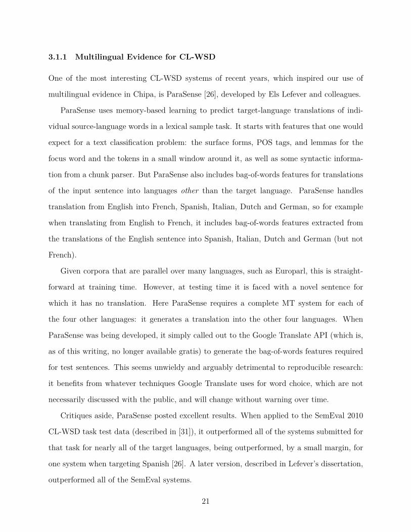
3.1.1 Multilingual Evidence for CL-WSD

One of the most interesting CL-WSD systems of recent years, which inspired our use of

multilingual evidence in Chipa, is ParaSense [26], developed by Els Lefever and colleagues.

ParaSense uses memory-based learning to predict target-language translations of indi-

vidual source-language words in a lexical sample task. It starts with features that one would

expect for a text classification problem: the surface forms, POS tags, and lemmas for the

focus word and the tokens in a small window around it, as well as some syntactic informa-

tion from a chunk parser. But ParaSense also includes bag-of-words features for translations

of the input sentence into languages other than the target language. ParaSense handles

translation from English into French, Spanish, Italian, Dutch and German, so for example

when translating from English to French, it includes bag-of-words features extracted from

the translations of the English sentence into Spanish, Italian, Dutch and German (but not

French).

Given corpora that are parallel over many languages, such as Europarl, this is straight-

forward at training time. However, at testing time it is faced with a novel sentence for

which it has no translation. Here ParaSense requires a complete MT system for each of

the four other languages: it generates a translation into the other four languages. When

ParaSense was being developed, it simply called out to the Google Translate API (which is,

as of this writing, no longer available gratis) to generate the bag-of-words features required

for test sentences. This seems unwieldy and arguably detrimental to reproducible research:

it benefits from whatever techniques Google Translate uses for word choice, which are not

necessarily discussed with the public, and will change without warning over time.

Critiques aside, ParaSense posted excellent results. When applied to the SemEval 2010

CL-WSD task test data (described in [31]), it outperformed all of the systems submitted for

that task for nearly all of the target languages, being outperformed, by a small margin, for

one system when targeting Spanish [26]. A later version, described in Lefever’s dissertation,

outperformed all of the SemEval systems.

21

In our earlier work, we prototyped a system that addresses some of the issues with

ParaSense [8]; these ideas are developed further in Chapter 7. Chipa requires neither a

locally running MT system nor access to an online translation API for its feature extraction,

but still learns from several mutually parallel bitexts that share a source language.

3.2 WSD with Sequence Models

To my knowledge, there has not been work that explicitly frames all-words CL-WSD as a se-

quence labeling problem, other than our earlier application of MEMMs to Spanish-Guarani

[9]. However, machine translation systems, and especially statistical machine translation

systems, address this problem implicitly – jointly along with other problems – when they

use language models to encourage coherent word choices in the generated text. The decom-

position of SMT systems into a translation model and a language model allows LMs to be

trained on very large target-language corpora. In contrast, in our earlier work on CL-WSD

with sequence models, we only trained on sentence-aligned bitext.

There have, however, been some uses of sequence models for monolingual WSD; in this

setting, systems can find an assignment disambiguating the entire input jointly. Molina et

al. [40] have described the use of hidden Markov models for WSD, situating all-words WSD

as a tagging problem. They also used this approach in a Senseval entry [41] in the English

all-words task at Senseval-3, where it posted results towards the middle of the pack.

Ciaramita and Altun [42] frame both coarse-grained WSD and information extraction as

a tagging problem, using a discriminative variation of HMMs trained with perceptrons [43]

to map nouns and verbs in the input text onto one of 41 “supersenses”, a small ontology

developed by Ciaramita and Johnson.

While it is not explicitly about sequence models, there is a related research program un-

derway in the world of graph-based algorithms for knowledge-based word-sense disambigua-

tion, exemplified by the work of Moro et al. [44]; they perform word-sense disambiguation

and entity linking jointly, searching for a globally coherent solution to both problems.

22

3.3 Lexical Selection in RBMT

A purely rule-based approach to lexical selection – a more declarative version of the special-

cased disambiguation procedures that Bar-Hillel imagined as futile – has been tried in many

cases, with variants in both direct and interlingual RBMT systems. In one recent example,

Bick presented a Danish-English RBMT system with purely rule-based lexical selection [45].

The Dan2eng system includes roughly 17, 000 individual Constraint Grammar rules for lexical

selection alone, over 70% of all of the rules written. Development took over two years, and

Bick suggests that statistical models (including target-language LMs) might be used in the

future to avoid having to cover all the idiosyncrasies of lexical transfer. A similar approach,

though not with the same enormous number of lexical selection rules, was taken by Brandt

et al. [46], with their Apertium-based Icelandic-English MT system.

Francis Tyers, in his dissertation work [47], develops a practical approach for improving

lexical selection for the Apertium RBMT system when parallel corpora are available. As he

describes in [48], his software learns finite-state transducers for lexical selection from parallel

corpora. His dissertation expands on this, additionally learning, via maximum entropy,

weights with which different rules can be applied in different contexts. He also describes

experiments in which linguists wrote lexical selection rules with the framework. Having

human linguists write rules in this formalism can improve MT output to an extent, but

seems tedious, as it took a full day’s work for a linguist to write 156 rules, and this only

covered lexical selection for 3% of the thousand-sentence test corpus.

In this formalism, translations are selected via rules that can reference the lexical items

and parts of speech surrounding the focus word; when a rule fires, it selects a translation.

These rules are stored in an XML encoding, so that they can be examined, modified, or

written from scratch by human linguists, but are then compiled to compact finite-state

transducers for speedy application.

Tyers’ system is intended to be both very fast, for use in practical translation systems, and

23

to produce easily human-interpretable lexical selection rules, for modification by linguists.

It is currently in use for some language pairs in the Apertium project.

3.4 CL-WSD for Statistical Machine Translation

While the idea has, for the most part, fallen by the wayside in recent years,2 some of the

earliest work on statistical machine translation at IBM included an explicit WSD module

[28]. Brown et al. considered the senses of a word to be its possible translations, explicitly

distancing their work from other WSD efforts that focused on dictionary senses. The WSD

module described in the 1991 paper used binary classifiers similar to decision stumps. Each

focus word was allocated a single classifier, which could check a single feature, e.g., the iden-

tity of the nearest noun to the right of the focus word. These simple classifiers would then

bias the decoder to choose a translation from one of two classes of target-language trans-

lations, which often significantly reduced the decoder’s uncertainty. The inclusion of WSD

improved the translation output markedly; the authors deemed 45 of the output sentences

“acceptable” with WSD enabled, over only 37 without it. Later versions of IBM’s CANDIDE

system included a more sophisticated disambiguation system: contextually-tuned transla-

tion models based on maximum entropy modeling for the most common words in the source

language [50].

The idea of training classifiers on source-language context to help lexical selection is an

attractive one, and has resurfaced several times in the SMT literature. However, by the early-

to-mid 2000s, phrase-based SMT techniques [51], which translate short coherent chunks of

text rather than individual words and thus often get correct word choice “for free”, seemed

to make WSD modules unnecessary. Work by Cabezas and Resnik [52] and early attempts

by Carpuat and Wu [53] cast doubt as to whether phrase-based SMT systems, or even

word-based SMT systems trained on large data sets, could benefit from WSD; Cabezas and2There are a number of papers on the topic, but for the past decade or so, the “standard” model of

phrase-based SMT has not included WSD as a component. There are a just three paragraphs on the topic inKoehn’s book on SMT [49, §5.3.6], and the major open-source SMT systems have not enabled WSD modulesby default.

24

Resnik, though expressing enthusiasm for future developments, did not manage to improve

translation performance with WSD, and initially (in 2005) Carpuat and Wu argued that

SMT could be considered a generalization of word-sense disambiguation. Vickrey et al. [54]

noted that lexical selection to translate phrases as units would be important for applications

in MT, though they did not implement it in their work on the topic.

Not long thereafter, Carpuat and Wu showed how to use classifiers to improve modern

phrase-based SMT systems with a series of papers on the topic [29, 55, 56, 57]. In this

work, they show that in order for phrase-based SMT systems to benefit from classifiers for

lexical selection, the system should do phrase-sense disambiguation, rather than word sense.

This is to say, the classifiers should be used to select the translations of source-language

phrases from the corresponding target-language phrases, better matching the model used by

the rest of the pipeline. Here Carpuat and Wu use an ensemble of classifiers, including naïve

Bayes, a maximum entropy model, an Adaboost classifier, and a nearest-neighbor model

in which feature vectors have been projected into a new space with a kernel and PCA has

been performed to reduce dimensionality. They used features based on local word context,

some syntactic features, and the position of the focus phrase in the sentence. Their classifiers

interact with the decoder by modifying the phrase table just before decoding, adding features

usable by the decoder’s log-linear model. This approach outperformed the earlier attempts

in which individual words had been labeled either with senses from some sense inventory or

with target-language translations; they posted significant improvements for Chinese-English

SMT on a variety of test sets and metrics.

There have been a number of related efforts in the SMT world recently. Gimpel and

Smith [58] build phrase table entries in which the probabilities of target-language phrases

are conditioned not only on the source-language phrase, but also on features extracted from

the broader source-language context; their approach is “omnivorous” in that it can include

any number of features based on source-language analysis. They tune feature weights directly

with MERT (Minimum Error Rate Training [59], a widely used optimization technique from

25

the SMT literature) to produce a linear model for the contextual probability of the target-

language phrase. Features used here include the n-grams in the surrounding context, the

parts of speech of the focus word and the surrounding context, a number of syntactic features

based on a parse of the input, and the focus phrase’s approximate position in the sentence.

Mauser et al. [60] present a similar approach, although in their work they model trans-

lations of individual words independently, rather than using phrases from the phrase table,

and their classifiers consider input sentences as sets of words. They argue that phrase-based

SMT models are already good at predicting sequences, and many of the signals that might

trigger a different word choice, especially in their source language, Chinese, can be placed

freely in the input text. They also include a probability model similar to IBM Model 1 [61],

but conditioned on two source-language words rather than one. Like IBM Model 1, this

model is trained with Expectation-Maximization.

Žabokrtský et al. [30] use discriminative MaxEnt models to adapt the “forward” trans-

lation model probabilities in an SMT system based on dependency grammars. While it has

much the same effect, this work does not describe itself in terms of word sense disambigua-

tion.

Recently, Tamchyna et al. – a team that notably includes Marine Carpuat – have in-

tegrated CL-WSD software into the popular open source Moses SMT system [62]. This

approach does not use one classifier per source phrase, as had been done in Carpuat’s ear-

lier work, but one enormous classifier for all known source words, trained with the Vowpal

Wabbit (VW) machine learning toolkit. This approach allows generalizations to be learned

across different source-language phrases, which might be otherwise lost. The software is

designed for speed and is significantly faster than earlier architectures, they report.

3.5 WSD for lower-resourced languages

Scaling WSD techniques to new languages is a particularly thorny issue; the resource acqui-

sition bottleneck presents a problem even for English. The problem is alleviated somewhat

26

when we are interested in supervised CL-WSD, with its reliance on bitext rather than sense-

annotated corpora.

There has been some work on using WSD techniques for translation into lower-resourced

languages. Špela et al. [63] discuss applying WSD to machine translation for the English-

Slovene language pair, using a graph-based WSD system and the linked Slovene wordnet to

disambiguate English words to aid in Slovene lexical selection.

Dinu and Kübler [64] presented work on monolingual WSD for Romanian. They use

memory-based learning for classification, with a small number of contextual features. With

all of its features included, the system substantially outperformed the “most frequent sense”

baseline, but adding a feature selection step caused a significant further improvement.

In other work on lower-resourced languages, Sarrafzdadeh et al. develop a version of the

Extended Lesk algorithm for Farsi [65], Lesk algorithms (due to early work by Michael Lesk

[21]) being a knowledge-based approach to WSD that relies on dictionaries, counting the

occurrences of words that occur in a particular sense’s dictionary definition; there have been

many variations on this theme.

One point that should be made about this dissertation is that it is ultimately not about

word-sense disambiguation for an under-resourced language. Here we are focusing on WSD

for Spanish, for which we have very large data sets and a number of good NLP tools. While

our sense inventory happens to be extracted from bitext corpora where the other languages

involved are under-resourced, the decisions to be made are about the meanings of Spanish

words.

3.6 CL-WSD at Senseval and SemEval

There have been many related Senseval and SemEval shared tasks, covering different varia-

tions on cross-lingual WSD.

Senseval-2 featured a Japanese Translation Task [66], in which Japanese words were to

be labeled with their most appropriate English translations from the provided translation

27

memory (TM); the task thus combined aspects of word sense disambiguation and example-

based machine translation.

At Senseval-3, there was an English-Hindi translation task [67], in which participants

were to label a lexical sample of English words with their Hindi translations. Here the gold

standard translations were created collaboratively online, using the Open Mind Word Expert

software developed by Chklovski and Mihalcea, but the set of possible translations were

extracted from a bilingual dictionary. There were two subtasks provided; in the more general

subtask, systems were provided with unannotated text in English. For the “translation-and-

sense” subtask, the provided text was previously-used Senseval-2 data, already annotated

with its WordNet senses. These annotations provided a significant boost to classification

accuracy for the participating systems.

In SemEval 2007, there were two related tasks covering translation between English

and Chinese. Task 5 [68] was a lexical sample task in which Chinese texts were manually

annotated with English translations from a predefined dictionary, and participants had to

predict these labels. Task 11 [69], in contrast, had its training and test data gathered

from automatically word-aligned parallel corpora, and the direction of translation was from

English to Chinese.

In the 2010 and 2013 SemEval CL-WSD tasks [31, 32], both organized by Lefever and

Hoste, participants were asked to translate twenty different polysemous English nouns into

five different European languages (Dutch, French, German, Italian and Spanish), given their

containing source-language sentence as context. There were no explicit bilingual dictionaries

provided as sense inventories; the possible target-language labels were those found in Eu-

roparl [70] through automatic word alignment, though they were lemmatized by hand. The

test set was manually annotated with the appropriate (lemmatized) translations from the

sense inventory for each of the five target languages.

Most recently, for SemEval 2014, there was a variant on the CL-WSD task: the Writing

Assistant task [33]. In this setting, rather than complete source-language sentences, short

28

source-language text segments were included in nearly complete target-language sentences,

representing the task faced by an agent assisting a writer trying to compose sentences in a

second language but facing gaps in their vocabulary.

3.7 Translation into Morphologically Rich Languages

Both Guarani and Quechua feature rich morphology, which means that the space of possible

output tokens in these languages is quite large. In order to build a complete MT system

targeting these languages, one needs a means to predict the appropriate morphological fea-

tures and synthesize correctly inflected words, either starting from lemmas and modeling

the inflection process, or simply by concatenating pieces of words during decoding. This

problem is large, difficult, and related to the problem of CL-WSD, but we consider it out

of scope in this work. For completeness, here we will quickly mention some of the work on

morphological prediction and generation for statistical and hybrid MT systems.

Koehn and Hoang describe factored phrase-based SMT models for predicting target-

language morphology [71]. In this kind of approach, instead of having one translation model

containing surface forms, there can be several different translation models. As a basic strat-

egy, they suggest having separate models for the translation of lemmas and another for

translating parts-of-speech and morphological features. This approach allows the MT sys-

tem to learn more generalized models, both for the translation of lemmas and for mapping

the morphological features of the source language to the target. Yeniterzi and Oflazer [72]

describe an application of this model for SMT on English-Turkish. They situate their work in

terms of the earlier strategy of considering Turkish inflectional and derivational morphemes

as “words” to be handled by the SMT system as normal and then recombined in a post-

processing step, which would sometimes fail when the morphemes were not generated in the

correct order. Contrastingly, their factored model produces Turkish lemmas, then finds the

relevant inflectional features based on English syntax.

Toutanova et al. describe another technique for generating rich morphology in SMT [73].

29

In their model, they consider inflection prediction separately from the task of producing

the target-language text. One version of their system produces fully-inflected text, which

may be changed by their inflection-prediction system; the other produces uninflected target-

language text, relying on the morphology prediction. In either case, the morphology of

all of the target-language lemmas is predicted with a Maximum Entropy Markov Model

(MEMM), a discriminative sequence prediction model that can take into account both any

features extracted from the analysis of the source sentence and its own previous morphology

predictions. They apply this model to both English-Russian and English-Arabic translation,

posting improvements for both phrase-based and tree-based SMT.

Chahuneau et al. have recently presented yet another method for SMT into morphologi-

cally rich languages [74]. Here they also use discriminative models to predict target-language

inflections based on the available source-language annotations, but instead of inflecting the

text after the decoder has been run, their system generates new phrase-table entries with

the appropriate inflections included, just before the decoder executes, allowing the decoder

to optimize for many concerns jointly, informed by the language model. Their software is

described in more detail in Schlinger et al. [75], and has had an open-source release.

30

CHAPTER 4

DATA SETS, TASKS AND EVALUATION

In this chapter, I describe the tasks and data sets that we will investigate for the rest

of the dissertation, so that we can measure performance in selecting translations for our

source-language lexical items. In order to evaluate our CL-WSD approaches and their effects

on translation quality, we will need to have a basis for comparison between our proposed

techniques and sensible baselines, including results reported by other researchers. Here

we cover some in vivo and in vitro approaches for evaluating CL-WSD systems, then we

characterize the corpus that we have available for the language pairs of interest.

As discussed in Section 2.1, for many years word sense disambiguation systems have been

evaluated in vitro and in a monolingual setting. The test sets for such WSD evaluations

include sentences hand-annotated with a word senses from a particular sense inventory, such

as, typically, the WordNet senses. These monolingual WSD evaluations often include both

coarse-grained and fine-grained distinctions and allow for several possible correct answers;

some word senses identified by lexicographers are more closely related than others. While

the senses in a sense inventory will contain many useful and interesting distinctions, they

do not necessarily make the distinctions most appropriate for a given task, which will vary

by application. As such, accuracy improvements on these tasks do not necessarily lead to

performance gains for an NLP system making use of word-sense disambiguations [76].

This style of evaluation relies on a fairly scarce resource: sentences hand-annotated with

a particular sense inventory. In the CL-WSD setting, where we consider target-language

lexical items to be the salient senses of source-language words, we could also ask annotators

to hand-label each word of our test sentences with their translations. For many language

pairs, however, this annotation task has nearly been performed by translators: the available

bitext allows us to find the translations of source words within the corresponding target-

31

language sentence.

4.1 Measuring CL-WSD Classification Accuracy

One straightforward in vitro approach for evaluating a CL-WSD system is to measure classi-

fication accuracy over pre-labeled data. Here by classification accuracy, we mean measuring

how often the system is able to correctly choose an appropriate translation for the focus word

in a given context. Strictly speaking, for this application, we do not have pre-labeled data:

our bitext does not come with sub-sentential alignments. But automatic word alignments

provide a good approximation, as long as our sentence alignments (or verse alignments, for

Bible text) are accurate. For the purposes of this work, we will assume that the automatic

word-level alignments are correct, putting in our best effort at preprocessing the available

text so that the aligner can produce useful output. This allows us to infer the labels for

source tokens – their translations into the target language – with high confidence.

Using our automatically-aligned bitext as labeled data allows us to closely mirror the

lexical selection task faced by an MT system while translating running text. We can train

classifiers for many different word types, but we will generally not have training examples

available for all words in the input at test time. This is a problem faced by data-driven NLP

systems broadly.

For comparison with other work, in Section 5.2 we run our systems on the SemEval CL-

WSD shared task test sets, which are publicly available. Our larger task here is framed in

the same way as the CL-WSD shared tasks from 2010 and 2013, so measuring performance

on these test sets allows a straightforward comparison between the variations explored in

this work and several other CL-WSD systems from recent years. These test sets are limited

in scope, however, and will only demonstrate Chipa’s performance for translating individual

English nouns. These comparisons are interesting in part because they show the strength

of the “most frequent sense” baseline – simply returning the most common translation in

the training data for a given focus word. Many of the posted results in the 2010 and 2013

32

SemEval competitions did not pass this bar; due to Zipfian distributions of words, the most

common lexical items in the target language are quite common. In that section we can

see how Chipa is situated among other recent CL-WSD systems on a that particular task,

translating English nouns, but this cannot be the whole of our evaluation for Chipa; our

more general goal for Chipa is to support MT from Spanish into lower-resourced languages.

4.2 Measuring MT Improvements

We will additionally want to conduct in vivo evaluations of our CL-WSD techniques as

applied to running MT systems. Here we can use standard approaches for evaluating MT,

such as BLEU and METEOR scores, or simply show that where word choices differ with

the application of CL-WSD, the changes are for the most part improvements. For these

experiments, we sample sentences from the available bitext – particularly sentences that

contain polysemous words for which we can train classifiers – and run the MT systems both

with and without the CL-WSD software enabled.

We want to make the argument that improved classification accuracy on CL-WSD tasks

leads to improved translation results. But in general, the addition of CL-WSD has not been

an overwhelming success in statistical machine translation, especially when we have large

corpora available for language modeling [29]. It seems intuitive that a classifier producing

correct word choices would lead an MT system to produce better results. But we do not

have a system that always indicates correct word choices, nor are we likely to have one in

the near future. And it is an empirical question, whether the suggestions made by the CL-

WSD system, imperfect as they are sure to be, will improve translation results. We could

imagine gains failing to materialize, for example, if the CL-WSD system’s correct choices are

mostly those that the MT system would have made on its own, say with the guidance of a

language model and phrase-table probabilities. We could imagine its incorrect choices being

misleading to the point of doing harm to our translation quality, or even correct CL-WSD

choices causing other cascading errors, perhaps by surprising the language model.

33

These experiments are described in more detail in Chapter 8, where I also discuss how

to integrate Chipa into the different machine translation packages.

4.3 Data Sets and Preprocessing

The largest corpus that we have available for all of our source and target languages is the

Bible. There are translations available for many different languages, and while these were

not always produced by native speakers, the translators are often driven by missionary zeal

to produce high-quality translations [5], so we can be reasonably confident of the (linguistic)

accuracy of our text.

In this work, we focus on one Bible translation per language. For Spanish, we use

the Reina-Valera translation (1995 edition), which I was able to scrape from a Bible study

website. Our Guarani translation, Ñandejara Ñe’e (1997 edition) was scraped from the same

site. Our Quechua version (the 2004 translation published by the Peruvian Bible Society)

was provided by Chris Loza and Rada Mihalcea; the preparation of the Quechua corpus is

described in Loza’s masters thesis [77]. For English, we use the public domain World English

Bible translation. While there are a large number of translations available online, different

“Bible societies” often own the associated copyrights and thus redistribution of the complete

texts is often restricted [6].

4.3.1 Source-side annotations

In order to gracefully include a variety of features and build on any available analysis tools

for the source language, Chipa’s input format and feature functions allow for arbitrary

annotations on source-language tokens.

Chipa’s input file format describes one token per line, with fields split by tabs. The first

field of a line is a token’s lemma, and the second field is its surface form. Following this

are an arbitrary number of annotations for that token, which may encode information such

as part-of-speech, dependency relations, or similar. Any arbitrary features that we think

34

the The pos=DETquick quick pos=ADJbrown brown pos=ADJfox fox pos=NOUNjump jumped pos=VERBover over POS=ADPthe the POS=DETlazy lazy POS=ADJsleep sleeping POS=VERBdog dog POS=NOUN. . POS=.

Figure 4.1: Example annotated sentence.

could be helpful can be added here; these annotations will typically be derived from external

NLP tools such as taggers or parsers, or come from unsupervised methods; exploring these

possibilities is the focus of Chapter 6. Sentence boundaries are indicated by blank lines. An

annotated sentence with one annotation per token might look like Figure 4.1, for example.

The Chipa software has been developed with a number of tools that consume and produce

this format, typically taking in sentences annotated in this way, calling another NLP tool to

generate more annotations, and then adding the new annotations to those already present.

The experiments in this chapter only use one of these tools, freeling_to_annotated.py,

which produces Chipa’s input format given output from Freeling[78], a suite of text analysis

tools that supports a variety of European languages, notably Spanish. In the following

chapters, we will make use of these tools and the extra information they make available to

our classifiers; in Chapter 6 we add annotations learnable with monolingual resources, and

in Chapter 7 we describe tools and annotations that require parallel data.

4.3.2 Preprocessing

There is a nontrivial amount of preprocessing required in order to get our Bible text into

a format suitable for our tools. This is largely due to the varying markup formats used by

different translation publishers. For each of the available translations, we need to understand

its formatting enough to know which text comes from which book, chapter, and verse number.

35

This triple uniquely identifies a unit of text, and verse numbers are nearly standardized

across translations. There are a few exceptions, however: translations produced by different

religious traditions may include different books. Most notably, Catholic editions have a

superset of the books found in modern Protestant editions, and include slightly different

chapters. Additionally, in some translations, such as our Guarani edition, a few verses have

been combined into a single segment for a more natural translation.

In any case, if a particular book/chapter/verse is present in two Bibles, then the two verses

are very likely translations of one another. Once we find all of the matching verses, we can

build a bitext corpus suitable for use in our pipeline. In all four of our translations, we find

all 66 books of the Protestant Bible. Furthermore, we find matches for nearly all of the verses

across all of the language pairs considered. For English/Spanish and Spanish/Quechua, the

intersection of book/chapter/verse tuples across Bibles contains over 99% of the verses in any

given Bible. For the Guarani translation, however, we are only able to match 95.2% of the

verses. The Guarani text contains fewer verses, 29, 867 versus the 31, 104 in Spanish, showing

that the translators were more willing here to combine verses and that the translations may

be more interpretive. To filter out matched text where different amounts of material have

been combined into the same verse number, we additionally use a sentence-alignment tool;

see Section 4.3.4 for details.

Our English translation is distributed in a format called USFM (Unified Standard Format

Markers), which is a markup language developed by a working group of Bible translators and

used widely by the Bible-related software community; see Figure 4.2 for some sample input

text in this format. 1 While there are a number of tools that consume USFM, I did not find

one that handles our particular use case of stripping metadata and simply mapping from

verses to flat text, so I wrote a short script, parse_usfm.py, to parse USFM and produce1See http://paratext.org/about/usfm for more about USFM. USFM is widely deployed; the website

from which we scraped the Spanish and Guarani corpora appears to render its HTML from a USFM source.There is an entire community of Bible software developers, and it has a wing that advocates Open Sourcesoftware and translations unencumbered by copyright. One could delve arbitrarily deeply into the historyof religious-text translators and their relationships with technology and copyright, but one has an NLPdissertation to write.

36

text in an easily-alignable format.

Our Spanish and Guarani corpora are extracted from HTML pages scraped from an

online Bible study website. In practice, the scraping was done by predicting the URLs for

each chapter of each book and requesting those URLs programmatically. We then extract

the text from the saved HTML pages with a Python script and the BeautifulSoup library

for HTML parsing. 2 As a side note, since websites change over time and we downloaded

the Guarani translation at an earlier date (from a mobile version of the site that is no longer

available), the HTML takes a significantly different structure in the Spanish and Guarani

editions, so they require different versions of the script for preprocessing; see Figures 4.4 and

4.5 respectively for representative Spanish and Guarani input.

Our Quechua translation came in an easily parseable format, with individual verses al-

ready identified by Loza and Mihalcea; for this corpus, relatively little preprocessing was

necessary since lines begin with the book, chapter, and verse already labeled. See Figure 4.3

for a sample of the input format. It is conceivable that there are inconsistencies introduced

by the text-extraction processes for these different data sources, but for the most part the

scripts seem reliable, since they result in approximately the same number of verses and to-

kens for our different languages, and the great majority of the sentences are alignable (see

subsequent discussion on bitext alignment). Additionally, hand inspection of the text for

the languages that I can personally read (English and Spanish) show that the text contains

fairly close translations, and loan words and similar named entities appear in the Quechua

and Guarani texts.

Each of the different formatting schemes uses its own encoding to identify the different

books of the Bible, so when producing output for alignment, we must map to a standard

encoding. For example, our Quechua edition marks the book of Lamentations with the

numerical code 31 (it is the thirty-first book in modern Catholic editions), but in the USFM

markup for the English translation, we find a header with the string “Lamentations”. For2http://www.crummy.com/software/BeautifulSoup/

37

\id LAM 25-LAM-web.sfm World English Bible (WEB)\ide UTF-8\h Lamentations\toc1 The Lamentations of Jeremiah\toc2 Lamentations\toc3 Lam\mt2 The\mt Lamentations\mt2 of Jeremiah\c 1\p\v 1 How the city sits solitary,\q2 that was full of people!\q She has become as a widow,\q2 who was great among the nations!\q She who was a princess among the provinces\q2 has become a slave!\b\q\v 2 She weeps bitterly in the night.\q2 Her tears are on her cheeks.\q Among all her lovers\q2 she has no one to comfort her.\q All her friends have dealt treacherously with her.\q2 They have become her enemies.

Figure 4.2: The first two verses of the Book of Lamentations (World English Bible transla-tion) in USFM format.

[999,31,1,1] ¡Ay, imaraqmi Jerusalenqa sapan kapushan, haqay hinaaskha runakunayoq llaqta! ¡Ay, imaraqmi viuda warmi hina kapushan,lliw suyukunaq uman kashaqqa! Mit'anipina llank'apushan, lliwllaqtakunaq ñust'an kashaqqa.

[999,31,1,2] Tutan-tutanmi unuy-parata waqayku- shan, uyapasp'aspay-p'aspallaña. Llapan munaqninkunamanta manan hukllapas kanchusonqochay- kuqnin. Llapan reqsinakuq-masinkunapas manan rikuqpastukupunkuchu, llapallanmi awqanman tukupunku.

Figure 4.3: The first two verses of the Book of Lamentations in Quechua, from the 2004Peruvian Bible Society translation. Whitespace changes added here for readability.

38

<div id="reader" class="content text_ltr"><a name="1"></a><a href="/bible/more/Lam.1.1"

style="color:black;text-decoration:none"><h2>El profeta </h2><span class="verse" id="Lam_1_1"><strong class="verseno">1</strong>&nbsp;¡Pobrecita de ti, Jerusalén! <br />Antes eras la más famosa <br />de todas las ciudades. <br />¡Antes estabas llena de gente, <br />pero te has quedado muy sola, <br />te has quedado viuda! <br />¡Fuiste la reina de las naciones, <br />pero hoy eres esclava de ellas! <br /> <p> </p></span>

</a><a name="2"></a><a href="/bible/more/Lam.1.2"

style="color:black;text-decoration:none"><span class="verse" id="Lam_1_2">

<strong class="verseno">2</strong>&nbsp;Olvidada y bañada en lágrimas <br />pasas todas las noches. <br />Muchos decían que te amaban, <br />pero hoy nadie te consuela. <br />Los que se decían tus amigos <br />hoy son tus enemigos. <br /><p> </p></span> </a>

Figure 4.4: The first two verses of the Book of Lamentations, Traducción en LenguajeActual (TLA) version, in HTML as scraped from the web. Whitespace changes added herefor readability.

39

<div class="ltr" data-abbreviation="gdc" data-reference="lam.1.gdc"data-usfm="LAM.1" id="version_primary">

<div class="version vid66 iso6393nhd" data-vid="66"data-iso6393="nhd">

<div class="book bkLAM"><div class="chapter ch1" data-usfm="LAM.1">

<div class="label">1</div><div class="s">

<span class="heading">Ñembyasy Jerusalén oñehundihaguére</span>

</div><div class="q1">

<span class="content" /><span class="verse v1" data-usfm="LAM.1.1">

<span class="label">1</span><span class="content">Ajépa ha'eñoajejuhu</span>

</span></div><div class="q1">

<span class="verse v1" data-usfm="LAM.1.1"><span class="content">upe távaguasuete,</span>

</span></div>

...

Figure 4.5: The beginning of the Book of Lamentations in Guarani, Ñandejara Ñe’e version,in HTML as scraped from the web. Whitespace changes added here for readability. Notethe metadata included here, suggesting that the HTML is generated programmatically froman underlying USFM document.

40

our Spanish and Quechua editions from the web, we find the code “LAM” in the markup.

In any case, we map each of these identifiers to a single code “Lam”, so that we can match

books, chapters and verses across translations.

4.3.3 Lemmatization

For each of our languages, whether on the source or target side, in addition to lowercasing

and verse-alignment, we extract the lemmas (the citation forms, normalized with respect

to inflection) from each surface word. Especially when working with smaller data sets and

morphologically rich languages, this is an important step, since it provides a small amount

of abstraction over the surface forms. Working primarily with lemmas rather than surface-

form words allows us to group, for example, the plural form of a word with its singular.

Dedicated morphological analysis software provides the necessary knowledge for mapping

from the (potentially complex or irregular) inflected forms to their associated lemmas.

For English and Spanish, we use the FreeLing suite of NLP tools [78] to extract lemmas.

FreeLing provides a variety of analyses, including tokenization, sentence splitting, multi-

word expression and named entity detection, part-of-speech tagging and parsing. We start

out using just a few of these tools – initially only tokenization and lemmatization. We

discuss making use of more of them in Chapter 6, leveraging the quality NLP tools that we

have for our resource-rich source languages. While it is a more pressing problem in more

morphologically rich languages, there are examples of morphological ambiguity in English

and Spanish. A familiar example from Spanish is that ir ’to go’ and ser ’to be’ sharing

their preterite-tense forms. However, the FreeLing analysis tools can typically resolve these

ambiguities for us3, and in this work we assume that the Freeling output is correct, or at

least correct enough to be useful for our purposes. In effect, we here assume that this kind of

ambiguity – ambiguities about the appropriate lemma for a given token – are satisfactorily3FreeLing performs morphological analysis jointly with part-of-speech tagging. Concretely, the token fue is

given the tag VSIS3S0 if it is deemed to be an inflection of ser, and the tag VMIS3S0 for an inflection of ir. Herethe ‘S’ stands for “semiauxiliary”. See http://nlp.lsi.upc.edu/freeling/doc/tagsets/tagset-es.html(page in Spanish) for more on the tagset used by FreeLing for Spanish.

41

resolved before the CL-WSD system itself comes into play.

The use of FreeLing for English is a noted improvement over initial experiments, which

used NLTK’s WordNet lemmatizer and default part-of-speech tagger [79]; these tools do not,

as distributed, support Spanish. The WordNet lemmatizer has a fairly small vocabulary,

did not provide a good strategy for dealing with unknown words, and could only address

nouns, verbs, and adjectives. There are a very large number of named entities in the source

text, most of which are not present in WordNet. It cannot, by itself, help us know that

“Zebulonites” is the plural of ”Zebulonite”. 37% of the tokens in our English translation of

the Bible are not present in WordNet; and many of these tokens are function words and

named entities. In any case, these words can often carry inflection.

For Guarani and Quechua, we use Michael Gasser’s ParaMorfo and AntiMorfo analyz-

ers.4 Guarani text is analyzed with ParaMorfo 1.1, and Quechua with AntiMorfo 1.2. These

packages are based on software originally developed for Ethiopian Semitic languages [80],

and use cascades of finite-state transducers (FSTs), which is a common approach in morpho-

logical analysis [81]. ParaMorfo and AntiMorfo use weighted FSTs to handle long-distance

dependencies between morphemes, but rather than having weights correspond to probabili-

ties to be combined with multiplication, the FSTs are weighted with feature structures that

are combined via unification. This approach was originally introduced by Amtrup [82]. In an

FST weighted with feature structures, the result of a successful traversal is the unification of

the feature structure “weights” on the traversed arcs, as well as an output string. All possible

paths through the FST are searched, though many of these paths will not lead to accepting

states, or will fail due to unification conflicts. Because a feature structure is accumulated

during the process of transduction, each traversal through the transducer retains a memory

of where it has been, permitting the incorporation of long-distance constraints such as those

relating the negative prefix and suffix of Guarani verbs.

Here the result of morphological analysis of a word is a root and a feature structure4Prof. Gasser’s morphology software for Guarani, Quechua, Spanish, and other languages is available at

http://homes.sice.indiana.edu/gasser/plogs.html

42

• Quechua: Llapan munaqninkunamanta manan hukllapas kanchu sonqochay- kuqnin.is analyzed by AntiMorfo as llapan munaqninkunamanta ma/mana huk/hukllaka/kanchu sonqochay - kuqnin. manan here could be an inflection of ma ’certainly’or mana ’no, none’. Similarly with huk ’one, another one’ / huklla ’only, lonesome,single’ and ka ’yours’ / kanchu (a kind of bird).

• Guarani: Upe che ro’o ha upe che pire ombyaipa, umi che kãngue omopẽmba. is an-alyzed by ParaMorfo as upe che so'o ha upe che pire ombyaipa , umi che kãmopẽ/pẽ . . Here omopẽmba is ambiguous, and could be an inflection of mopẽ ’tobreak (something)’ or pẽ ’to break (oneself)’.

Figure 4.6: Examples of morphological ambiguity in Quechua and Guarani, having been runthrough AntiMorfo and ParaMorfo. The Quechua text is the first sentence of Lamentations1:2; the Guarani is Lamentations 3:4.

representing the grammatical features of the word. For the basic version of Chipa, we are

only concerned with the lemmatized forms of the words in our corpora, so we ignore the

grammatical features for now. In cases of morphological ambiguity, which is to say cases

where a surface form could be an inflection of multiple distinct lemmas, we maintain this

ambiguity rather than trying to disambiguate from context. The different possible lemmas

are separated by a slash; there are examples of this in Figure 4.6. ParaMorfo and AntiMorfo,

for many cases, treat verbs with derivational affixes as lemmas in their own right; here for

simplicity we include both versions of the lemma5.

4.3.4 Alignment

As a precaution against verses that are not close translations, or perhaps have combined

several parts of the text together into one verse on only one side, we run the cdec [83]

filtering tool (filter-length.pl) with its default settings, which checks for unusual length

disparities in the bitext. This ends up removing roughly 7% of the verses6, but manual

inspection shows that those verses removed are in general very loose translations, or that5For example, in Guarani, ahechauka ’I show (cause to see)’ contains the causative suffix -uka. In this

case we treat both hechauka ’show’ and hecha ’see’ as lemmas (Gasser 2016, personal communication).6Specifically, length filtering removes 7.12% of the verse pairs for Spanish-English and thus English-

Spanish, 6.69% for Spanish-Guarani, and 6.72% for Spanish-Quechua.

43

additional material is present on one side.

Having tokenized, lowercased, verse-aligned and lemmatized, our corpora, we are ready

to extract word-level alignments. For this we use the fast_align tool from cdec [83], with

its default settings7 and the lemmatized text as input. fast_align runs several iterations

of Dyer et. al’s alignment algorithm, which is a variant of IBM Models 1 and 2, and was

shown to provide both relatively fast training times and good results for downstream MT

systems [84]. It improves on Model 1 by encouraging diagonal alignments, rather than Model

1’s simplistic view that any token in the source might just as well be aligned to any token

in the target, and on Model 2 in having fewer parameters to fit. In any case, it is the

default aligner for use with cdec. fast_align produces the single most likely one-to-many

word alignment for each verse, such that each source language token is linked with zero or

more target-language tokens in the corresponding verse. For a visualization of fast_align’s

output, see Figure 4.7.

4.3.5 A deeper dive: producing Spanish-Guarani bitext

To get a concrete idea about the process of producing our bitext and our annotated source

corpus, we will now step through the bitext production process for our Spanish-Guarani

language pair. For the precise process, please see the source code 8.

We consider the “raw materials” for this process to be the scraped Spanish and Guarani

bibles; see Figures 4.4 and 4.5 for examples. In order to replicate this work, or to extend it

to more languages, one will have to acquire bitext covering one’s preferred language. There

are translations in many different languages available on various Bible websites, however.

The result of the scraping process is a directory full of HTML files, the raw HTML that

was served by the Bible websites. For the sites that we scraped, each chapter is served as

an individual HTML file. From these HTML files, we must extract the flat text of all of the

available Bible verses. We do this with the get_verses.py, a tool that uses BeautifulSoup7With the command given at http://www.cdec-decoder.org/guide/fast_align.html8https://github.com/alexrudnick/terere/tree/master/bibletools

44

Amargamentellora

en

lanoche

y

laslagrimas

correnporsus

mejillas.

Pyha

repu

kuku

eha

sẽ , ha hesa

ym

ante

hová

reos

yry

.

Figure 4.7: A sample word alignment. The beginning of Lamentations 1:2, mapping fromSpanish to Guarani. Alignment produced with fast_align.

45

(3) He put the wood in order, and cut the bull in pieces, and laid it on the wood. He said,“Fill four jars with water, and pour it on the burnt offering, and on the wood.”

(4) Preparó la leña, cortó el buey en pedazos, lo puso sobre la leña,

Figure 4.8: Segments filtered due to length disparity. Our English and Spanish versions of1 Kings 18:33.

to parse the input HTML and navigate its structure, extracting the verse identifiers and

verse text as it goes. We call the output of get_verses.py a “Bible file”; it consists of

tab-separated values, one per line, in which (book, chapter, verse) tuples are paired with the

text of those verses.

We then call the print_bitext.py on pairs of Bible files. This script finds matching

verses (book, chapter, verse tuples) and produces bitext files in the format expected by

the cdec alignment tools, which is simply source-language segments and target-language seg-

ments, separated by |||. The output of print_bitext.py is called bible.es-gn.unfiltered,

which contains some non-parallel ”sentences” and is untokenized. Individual sentences have

not been preprocessed at all.

We then run a script from cdec, filter-length.pl, which filters out segments where

either side is too long, or where there is a large disparity in length between source and target

text, which indicates input segments that are not close translations. After this filtering step,

we have selected the bitext from which we will train Chipa. See Sentences 3 and 4 for an

example of a pair of segments that is filtered by this step. This is 1 Kings 18:33, and the

beginnings of these segments clearly have the same meaning; for the Spanish translation,

though, the material in the second sentence of the English text has simply been moved into

the subsequent verse (1 Kings 18:34) for whatever reason.

Given the sentence-aligned bitext corpus, which contains only the subset of the source and

target Bibles that we were able to verse-align (roughly, “sentence align”, in more common MT

terms, though a verse need not be a single sentence), we now want to preprocess the source

46

text to produce the annotated version used for training. We call cdec’s cut-corpus.pl to

select just the source side of the bitext, in this case the Spanish. Then we call Freeling to

do basic analysis on the input Spanish text: it provides tokenizing (for example, splitting

out punctuation adjacent to words), lemmatizing and tagging 9. Then we run a Python

script, freeling_to_annotated.py, to convert the FreeLing output format into Chipa’s

source-language input format.

Now on the target language side, we do something analogous, although less analysis

of the target text is required, and Freeling does not support our target languages. We

again use cut-corpus.pl to select just the target side, in this case the Guarani, and cdec’s

tokenize-anything.sh and lowercase.pl to tokenize and lowercase the Guarani text.

Then we run Chipa’s lemmatizer script over the Guarani text. It calls the ParaMorfo

morphological analyzer on the Guarani tokens, producing Guarani lemmas. In cases of

morphological ambiguity, we produce tokens that maintain that ambiguity, simply joining

the possible lemmas with a slash. Once lemmatization is complete, we have produced the

target-language lemmatized text.

Then we join together each line of the source-language lemmatized text with its corre-

sponding target-language lemmatized text, using cdec’s paste-files.pl script. The output

of this is the sentence-aligned, tokenized, lowercased, lemmatized bitext corpus, which is

ready for word alignment. To generate the word alignments, we call cdec’s fast_align tool.

After all of this preprocessing and alignment, we have produced three files of interest to

Chipa: first, we have the lemmatized bitext corpus. Second, we have the one-to-many word

alignments between the two sides of the bitext. These two files taken together constitute the

ground truth for the Chipa system – the source lemmas, and the subsequences of the target

text that are considered to be their translations. Note that these alignments could be NULL

– a source word could correspond with an empty subsequence of target-language tokens. At

test time, we will want to predict those translations, whatever they happen to be.9See the checked-in Freeling configuration file for the exact settings used: https://github.com/

alexrudnick/terere/blob/master/bibletools/freeling-config/es.cfg

47

The third file contains the annotated version of the source text, which includes all of the

information of the source side of the preprocessed bitext, in addition to the original surface

forms and the annotations extracted from FreeLing analysis. Further annotations can be

added by other tools; in general, annotated source-language corpora could contain whatever

kinds of signals we might like to add to aid classifiers in predicting translations. In Chapter

6, for example, we discuss features learnable with monolingual resources such as part of

speech tags, Brown clusters, and embeddings learned with neural networks. In Chapter 7,

we discuss features that require parallel corpora, such as CL-WSD predictions into languages

other than the current target language. But in all of these cases, the additional features are

passed to the classifiers via this corpus-annotation approach.

4.4 Exploring the Bitext

Even using only the Bible as bitext, we find a substantial number of training examples for

many of the most common word types, which, due to the Zipfian distribution of word types

in most texts, constitute a significant fraction of the tokens exhibited. The most common

lemmas and surface forms found in the source text are shown in Figures 4.9 and 4.10, but

here we see that the most common few dozen types cover the majority of the text, though

they are likely, as we will discuss later, to exhibit substantial ambiguity.

Once we skip past stop words, we also see that some of the most common word types in

the text are proper names (place names, personal names, names referring to God) or exhibit

very few translations in the target language, but for the most part we see, through the

aligned bitext, that the most common words are polysemous. To take a few salient examples

from the Spanish-English aligned text, the verb hacer can translate in a number of different

ways: ’do’, ’make’, ’cause’; for decir, we must choose between ’say’, ’tell’ or ’speak’; mujer

can mean either ’wife’ or ’woman’; and reina can translate to ’reign’ or ’queen’.

In the English-Spanish direction, we see that the ’be’ can be translated as either ser or

48

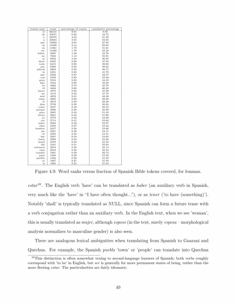
lemma type count percentage of corpus cumulative percentageel 66151 9.91 9.91

de 45671 6.84 16.75y 30370 4.55 21.30a 23684 3.55 24.85

que 18992 2.84 27.69en 14309 2.14 29.83su 11861 1.78 31.61

ser 11856 1.78 33.39haber 9205 1.38 34.76

no 7624 1.14 35.91se 6942 1.04 36.95

decir 6565 0.98 37.93todo 6415 0.96 38.89

por 6360 0.95 39.84jehová 6204 0.93 40.77

lo 6181 0.93 41.70uno 5822 0.87 42.57con 5549 0.83 43.40

para 5544 0.83 44.23hijo 5344 0.80 45.03

tu 4862 0.73 45.76él 4424 0.66 46.42

hacer 4372 0.65 47.08mi 4116 0.62 47.70

este 4052 0.61 48.30estar 3993 0.60 48.90

le 3874 0.58 49.48dios 3730 0.56 50.04

como 3257 0.49 50.53porque 3088 0.46 50.99

pero 2965 0.44 51.43tierra 2841 0.43 51.86

yo 2779 0.42 52.28rey 2714 0.41 52.68

sobre 2584 0.39 53.07ellos 2450 0.37 53.44

hombre 2417 0.36 53.80me 2381 0.36 54.15te 2363 0.35 54.51

dar 2301 0.34 54.85tener 2289 0.34 55.20israel 2193 0.33 55.52

día 2101 0.31 55.84entonces 2019 0.30 56.14

casa 2010 0.30 56.44cuando 1961 0.29 56.74

pues 1940 0.29 57.03pueblo 1924 0.29 57.32

ni 1807 0.27 57.59si 1685 0.25 57.84

Figure 4.9: Word ranks versus fraction of Spanish Bible tokens covered, for lemmas.

estar10. The English verb ’have’ can be translated as haber (an auxiliary verb in Spanish,

very much like the ’have’ in “I have often thought...”), or as tener (’to have (something)’).

Notably ’shall’ is typically translated as NULL, since Spanish can form a future tense with

a verb conjugation rather than an auxiliary verb. In the English text, when we see ’woman’,

this is usually translated as mujer, although esposo (in the text, surely esposa – morphological

analysis normalizes to masculine gender) is also seen.

There are analogous lexical ambiguities when translating from Spanish to Guarani and

Quechua. For example, the Spanish pueblo ’town’ or ’people’ can translate into Quechua10This distinction is often somewhat vexing to second-language learners of Spanish; both verbs roughly

correspond with ’to be’ in English, but ser is generally for more permanent states of being, rather than themore fleeting estar. The particularities are fairly idiomatic.

49

surface word type count percentage of corpus cumulative percentagede 45671 6.84 6.84

y 29944 4.49 11.33el 27483 4.12 15.44a 23684 3.55 18.99

que 18992 2.84 21.83la 18021 2.70 24.53

los 16236 2.43 26.97en 14309 2.14 29.11no 7624 1.14 30.25su 7115 1.07 31.32se 6942 1.04 32.36

por 6360 0.95 33.31jehová 6204 0.93 34.24

con 5549 0.83 35.07para 5544 0.83 35.90

las 5523 0.83 36.73lo 5132 0.77 37.50

sus 4748 0.71 38.21dios 3489 0.52 38.73

él 3401 0.51 39.24tu 3373 0.51 39.74

como 3257 0.49 40.23es 3235 0.48 40.72

mi 3103 0.46 41.18porque 3088 0.46 41.64

un 3041 0.46 42.10pero 2965 0.44 42.54

yo 2779 0.42 42.96tierra 2744 0.41 43.37hijos 2665 0.40 43.77

sobre 2585 0.39 44.16le 2570 0.38 44.54

dijo 2471 0.37 44.91rey 2397 0.36 45.27me 2381 0.36 45.63te 2363 0.35 45.98

ellos 2205 0.33 46.31israel 2193 0.33 46.64

hijo 2190 0.33 46.97todos 2166 0.32 47.29todo 2157 0.32 47.62

ha 2141 0.32 47.94entonces 2019 0.30 48.24

cuando 1961 0.29 48.53pues 1940 0.29 48.82casa 1836 0.28 49.10

ni 1807 0.27 49.37una 1805 0.27 49.64

pueblo 1691 0.25 49.89si 1685 0.25 50.15

Figure 4.10: Word ranks versus fraction of Spanish Bible tokens covered, for (case-insensitive)surface forms.

50

as l laqta ’town/city’, or runa ’person’. For translating from Spanish to Guarani, we see the

verb volver ’turn/return/repeat’ translated as jey ’again’, but also as jere ’turn’.

Figures 4.11 and 4.12 give the most common lemmas, after stopword removal, used in our

corpus for the four languages, along with their counts. In Figure 4.13, we see common lemmas

from Spanish along with their most likely translations into English, Guarani and Quechua

(as extracted from the bitext). For the purposes of this work, we will consider words to be

in-vocabulary for disambiguation if they appear at least fifty times in the training corpus;

we also do not include punctuation marks and stopwords (as defined by the default NLTK

stopword lists for English and Spanish) other than common verbs.

As an approximation of the difficulty of the classification task we face when addressing

these ambiguities, we can take a look at the entropy of the possible translations for various

source word types. One bit of entropy corresponds to a choice between two a priori equally

likely options. For example, if a given source word can be translated in four different ways,

and they are all equiprobable, this will be two bits of entropy. Of course in practice, some

translations will be much more common than others.

Some concrete examples of Spanish-language words with their entropy scores from the

source text are presented in Figure 4.14; a few words, such as dios and pueblo, seem straight-

forward to translate into English. Here we have less than 1 bit of uncertainty about the

translation a priori. But verbs often used in idiomatic expressions like hacer and poner

introduce much more uncertainty. Some of these numbers are higher than they would be

without the morphological analysis process normalizing gender; here both hijo ’son’ and hija

’daughter’ have been normalized to the masculine form. Lemmatization here does introduce

some apparent ambiguity, but it pools the evidence from the various surface forms into the

training data for a single classifier for that lemma, allowing us to take into account similari-

ties between the usage of, for example, hijo, hija, hijos and hijas. But a classifier with access

to the surface form will have an easier job than the entropy value suggests.

The values in this table are calculated with the familiar formula for entropy; the entropy

51

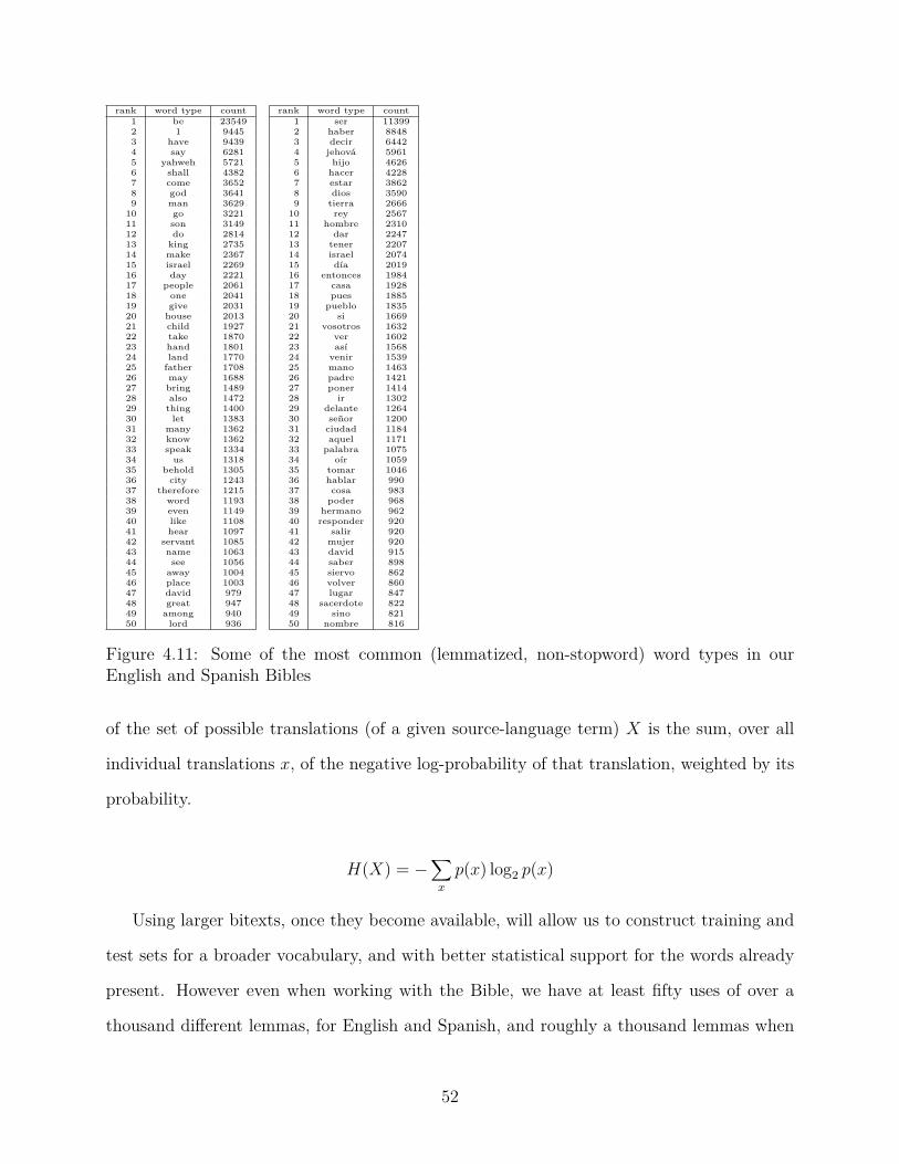
rank word type count1 be 235492 1 94453 have 94394 say 62815 yahweh 57216 shall 43827 come 36528 god 36419 man 3629

10 go 322111 son 314912 do 281413 king 273514 make 236715 israel 226916 day 222117 people 206118 one 204119 give 203120 house 201321 child 192722 take 187023 hand 180124 land 177025 father 170826 may 168827 bring 148928 also 147229 thing 140030 let 138331 many 136232 know 136233 speak 133434 us 131835 behold 130536 city 124337 therefore 121538 word 119339 even 114940 like 110841 hear 109742 servant 108543 name 106344 see 105645 away 100446 place 100347 david 97948 great 94749 among 94050 lord 936

rank word type count1 ser 113992 haber 88483 decir 64424 jehová 59615 hijo 46266 hacer 42287 estar 38628 dios 35909 tierra 2666

10 rey 256711 hombre 231012 dar 224713 tener 220714 israel 207415 día 201916 entonces 198417 casa 192818 pues 188519 pueblo 183520 si 166921 vosotros 163222 ver 160223 así 156824 venir 153925 mano 146326 padre 142127 poner 141428 ir 130229 delante 126430 señor 120031 ciudad 118432 aquel 117133 palabra 107534 oír 105935 tomar 104636 hablar 99037 cosa 98338 poder 96839 hermano 96240 responder 92041 salir 92042 mujer 92043 david 91544 saber 89845 siervo 86246 volver 86047 lugar 84748 sacerdote 82249 sino 82150 nombre 816

Figure 4.11: Some of the most common (lemmatized, non-stopword) word types in ourEnglish and Spanish Bibles

of the set of possible translations (of a given source-language term) X is the sum, over all

individual translations x, of the negative log-probability of that translation, weighted by its

probability.

H(X) = −∑

x

p(x) log2 p(x)

Using larger bitexts, once they become available, will allow us to construct training and

test sets for a broader vocabulary, and with better statistical support for the words already

present. However even when working with the Bible, we have at least fifty uses of over a

thousand different lemmas, for English and Spanish, and roughly a thousand lemmas when

52

rank word type count1 ha 320072 che 116493 upe 103004 kuéra 97515 ha’e 83946 nde 82027 ’e 80058 mba’e 79409 umi 7750

10 pe 634511 pende 622412 tupã 594113 haguã 560714 vaekue 507115 katu 474616 ’e/ha’e 463617 ñandejára 461718 ⟨japo 460619 opa/pa 432120 guasu 421821 ramo 404322 peteĩ 348323 yvy 297824 iko/ko 295025 ñe’ẽ 293826 ra’y 272427 ĩ 270628 rehe 269029 ⟨hetã 263630 vai 260631 ára 260632 me’ẽ 253233 avei 236034 ⟨hecha 232835 niko 229936 kuaa 221537 rupi 218238 ⟨hague 217039 ru 210540 hína 208041 po/porã 204942 ndive 194843 gua 192744 hikuái 190345 ore 189646 mburuvicha 176547 ko 173548 israel 172549 ñande 170450 ju 1659

rank word type count1 ni 135352 ma/mana 96303 chay 93074 runa 85345 señor 66946 hina 59507 ka 50288 pay 50129 paykuna 3613

10 hina/hinan 343011 ka/kay 315012 diospa 295013 qan 293014 ruwa 279515 chaymi 278316 llaqta 277517 suyu 268618 karqan 241519 ichaqa 228620 wasi 225021 churi 223222 qankuna 199123 huk 192524 israel 191425 ima 190126 diosqa 187227 p’unchay 186628 diosmi 185129 ama 182730 ri 175931 tukuy 166732 chayqa 157233 llaq/llaqta 151634 ka/kasha 149835 pacha 149136 kanqa 146637 ma 146438 chunka 144739 allin 137040 llapan 130241 muna 129942 llapa 128643 yupay/yupaycha 128244 warmi 124645 ayllu 122946 dios 118047 ri/riku 115648 kamachi 115149 rey 114950 hallp’a 1086

Figure 4.12: Some of the most common lemmatized word types in our Guarani (left) andQuechua (right) Bibles. Preprocessing does not force morphological disambiguation; if themorphological analyzer cannot choose a lemma, we separate possible lemmas with a slash.

53

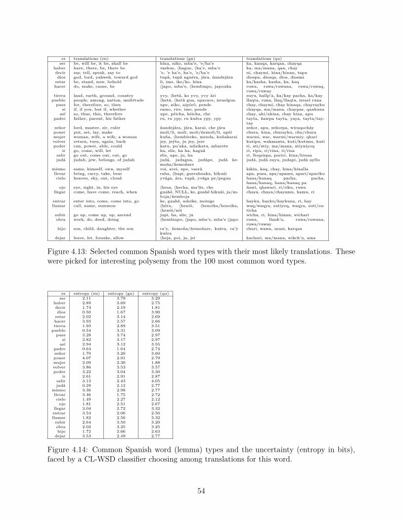
es translations (en) translations (gn) translations (qu)ser be, will be, it be, shall be hína, niko, mba’e, ’e/ha’e ka, kanqa, karqan, chayqa

haber have, there, be, there be vaekue, ⟨hague, ⟨ha’e, mba’e ka, ma/mana, qan, chaydecir say, tell, speak, say to ’e, ’e ha’e, ha’e, ’e/ha’e ni, chaymi, hina/hinan, tapudios god, lord, yahweh, toward god tupã, tupã nguéra, jára, ñandejára diospa, diosqa, dios, diosmi

estar be, stand, now, behold ĩi, ime, iko/ko, hína ka/kasha, kasha, ka, kaqhacer do, make, cause, he ⟨japo, mba’e, ⟨hembiapo, japouka ruwa, ruwa/ruwana, ruwa/ruwaq,

ruwa/ruwaytierra land, earth, ground, country yvy, ⟨hetã, ko yvy, yvy ári suyu, hallp’a, ka/kay pacha, ka/kay

pueblo people, among, nation, multitude ⟨hetã, ⟨hetã gua, opavave, israelgua llaqta, runa, llaq/llaqta, israel runapues for, therefore, so, then upe, niko, aipórõ, pende chay, chaymi, chay hinaqa, chayrayku

si if, if you, but if, whether ramo, rire, ime, pende chayqa, ma/mana, chaypas, qankunaasí so, thus, this, therefore upe, péicha, kóicha, che chay, ahi/ahina, chay hina, apu

padre father, parent, his father ru, ru ypy, ru kuéra ypy, ypy tayta, ñawpa tayta, yaya, tayta/tay-tay

señor lord, master, sir, ruler ñandejára, jára, karai, che jára señor, apu, señorpa, wiraqocháyponer put, set, lay, make moĩi/ĩi, moĩi, moĩi/ñemoĩi/ĩi, upéi chura, hina, churayku, chu/churamujer woman, wife, a wife, a woman kuña, ⟨hembireko, menda, kuñakarai warmi, war, warmi/warmiy, qharivolver return, turn, again, back jey, jeýta, ju jey, jere kutipu, wakmanta, kuti/kutimu, kutipoder can, power, able, could katu, pu’aka, ndaikatu, mbarete ti, ati/atiy, ma/mana, atiyniyoq

ir go, come, will, let ha, sĩie, ha ha, haguã ri, ripu, ri/rina, ri/risasalir go out, come out, out, go sĩie, upe, ju, ha ri, lloqsispa, puriri, hina/hinanjudá judah, jew, belongs, of judah judá, judagua, judápe, judá ñe-

moña/ñemoñarejudá, judá suyu, judapi, judá ayllu

mismo same, himself, own, myself voi, avei, upe, vaerã kikin, kaq, chay, hina/hinallallevar bring, carry, take, bear raha, ⟨hupi, guerahauka, hikuái apa, pusa, apa/apamu, apari/aparikucielo heaven, sky, out, cloud yvága, ára, tupã, yvága pe/pegua hana/hanaq pacha, pacha,

hana/hanaq, hana/hanaq paojo eye, sight, in, his eye ⟨hesa, ⟨hecha, ma’ĩie, che ñawi, qhawari, ri/riku, ruwa

llegar come, have come, reach, when guahẽ, NULL, ke, guahẽ hikuái, ja/m-boja/ñemboja

chaya, chaya/chayamu, hamu, ri

entrar enter into, come, come into, go ke, guahẽ, ndoike, moinge hayku, hayku/haykuna, ri, hayllamar call, name, summon ⟨héra, ⟨henói, ⟨henoika/henoika,

⟨henói/nóiwaq/waqya, sutiyoq, waqya, suti/su-ticha

subir go up, come up, up, ascend jupi, ha, sĩie, ju wicha, ri, hina/hinan, wichariobra work, do, deed, doing ⟨hembiapo, ⟨japo, mba’e, mba’e ⟨japo ruwa, llank’a, ruwa/ruwana,

ruwa/ruwayhijo son, child, daughter, the son ra’y, ñemoña/ñemoñare, kuéra, ra’y

kuérachuri, wawa, ususi, karqan

dejar leave, let, forsake, allow ⟨heja, poi, ja, jei kachari, ma/mana, wikch’u, ama

Figure 4.13: Selected common Spanish word types with their most likely translations. Thesewere picked for interesting polysemy from the 100 most common word types.

es entropy (en) entropy (gn) entropy (qu)ser 2.11 3.79 3.29

haber 2.89 3.69 2.75decir 1.74 2.19 1.81dios 0.50 1.67 3.90

estar 2.02 3.14 2.69hacer 3.93 2.57 2.66tierra 1.93 2.89 3.51

pueblo 0.54 3.31 3.09pues 3.28 3.74 2.97

si 2.82 3.17 2.97así 2.94 3.12 3.55

padre 0.64 1.64 2.74señor 1.70 3.20 3.60poner 4.07 2.91 2.79mujer 2.09 2.30 1.88volver 3.86 3.53 3.57poder 3.22 3.04 3.30

ir 2.61 2.91 2.87salir 3.13 2.43 4.05judá 0.29 2.12 2.77

mismo 3.36 2.98 2.77llevar 3.46 1.75 2.72cielo 1.49 2.27 2.12

ojo 1.81 2.51 2.67llegar 3.04 2.72 3.32

entrar 3.54 2.06 2.56llamar 1.82 2.56 3.32

subir 2.64 3.50 3.20obra 2.02 3.25 3.25hijo 1.72 2.66 2.63

dejar 3.53 2.49 2.77

Figure 4.14: Common Spanish word (lemma) types and the uncertainty (entropy in bits),faced by a CL-WSD classifier choosing among translations for this word.

54

translating Spanish into Guarani and Quechua.

In the next chapter, we will cover the archictecture of the Chipa system and evaluate its

baseline version on the tasks and data sets described here.

55

CHAPTER 5

THE BASELINE CHIPA SYSTEM

Here we describe the baseline version of the Chipa software and evaluate its performance

on the tasks described in the previous chapter. At its core, the Chipa software takes in a

word-aligned bitext corpus, with annotations for the source tokens. It then trains CL-WSD

classifiers for source-language word types on demand.

By default, the software holds all of the available bitext in memory, or optionally on

disk, when training from larger corpora. On request, it constructs a training set for learning

to disambiguate a particular lemma by retrieving all sentences that contain the lemma,

finding the instances of that lemma and its aligned translations, and extracting features (see

Figure 5.1) from the source sentence’s surface text and annotations. If a source-language

lemma has been seen aligned to only one target-language type, then this is simply noted, and

if the lemma is not present in the training data, then it is marked as out-of-vocabulary. This

situation will not arise in our in vitro evaluation, but during in vivo machine translation,

OOV words will occur in practice. In either of these cases, we do not train a classifier for

that lemma, since there is no ambiguity present in our examples and the Chipa software

cannot provide any useful guidance to its caller. A machine translation system may, for

example, refuse to translate sentences with OOV words, or more likely, will simply assume

the identity translation, effectively passing them through untranslated.

Since source-language tokens may be NULL-aligned (i.e., not all words in the source

text will have corresponding words in the target text), both in the training data and in

translations, Chipa provides the option to request classifiers that consider NULL as a valid

label for classification, or not, as appropriate for the translation application. For example,

function words found in one language may not need to have a surface representation in the

56

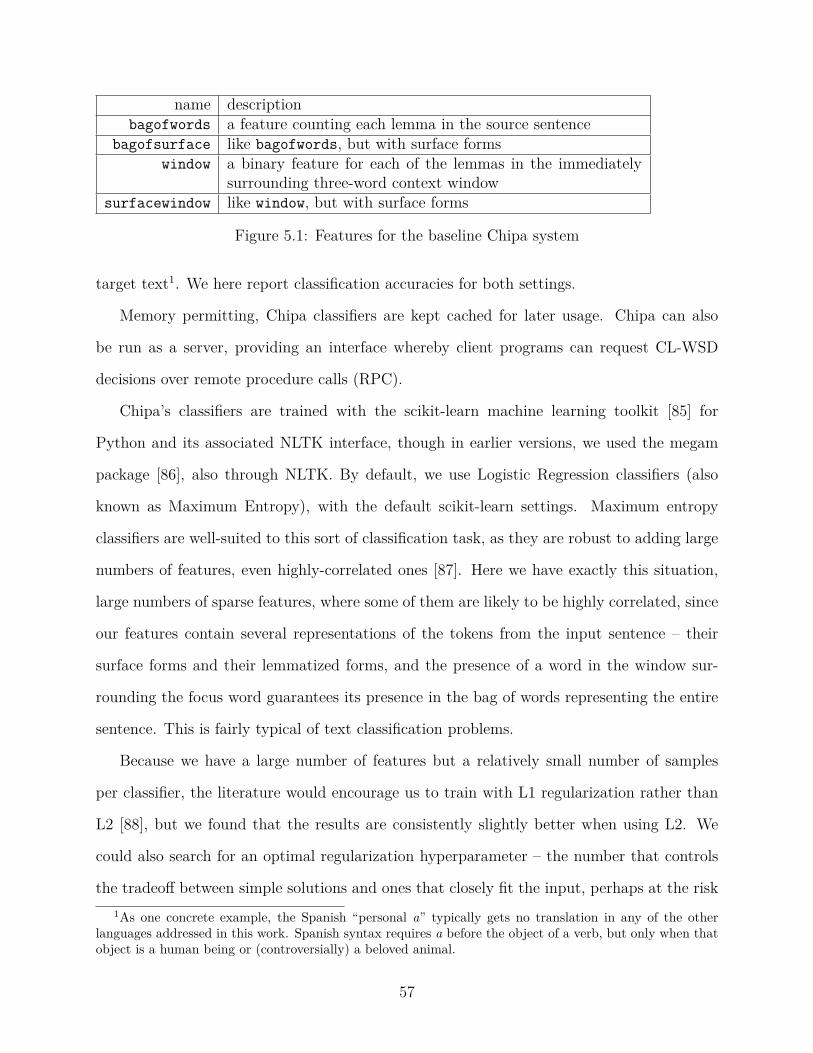
name descriptionbagofwords a feature counting each lemma in the source sentence

bagofsurface like bagofwords, but with surface formswindow a binary feature for each of the lemmas in the immediately

surrounding three-word context windowsurfacewindow like window, but with surface forms

Figure 5.1: Features for the baseline Chipa system

target text1. We here report classification accuracies for both settings.

Memory permitting, Chipa classifiers are kept cached for later usage. Chipa can also

be run as a server, providing an interface whereby client programs can request CL-WSD

decisions over remote procedure calls (RPC).

Chipa’s classifiers are trained with the scikit-learn machine learning toolkit [85] for

Python and its associated NLTK interface, though in earlier versions, we used the megam

package [86], also through NLTK. By default, we use Logistic Regression classifiers (also

known as Maximum Entropy), with the default scikit-learn settings. Maximum entropy

classifiers are well-suited to this sort of classification task, as they are robust to adding large

numbers of features, even highly-correlated ones [87]. Here we have exactly this situation,

large numbers of sparse features, where some of them are likely to be highly correlated, since

our features contain several representations of the tokens from the input sentence – their

surface forms and their lemmatized forms, and the presence of a word in the window sur-

rounding the focus word guarantees its presence in the bag of words representing the entire

sentence. This is fairly typical of text classification problems.

Because we have a large number of features but a relatively small number of samples

per classifier, the literature would encourage us to train with L1 regularization rather than

L2 [88], but we found that the results are consistently slightly better when using L2. We

could also search for an optimal regularization hyperparameter – the number that controls

the tradeoff between simple solutions and ones that closely fit the input, perhaps at the risk1As one concrete example, the Spanish “personal a” typically gets no translation in any of the other

languages addressed in this work. Spanish syntax requires a before the object of a verb, but only when thatobject is a human being or (controversially) a beloved animal.

57

of overfitting. We did try a few different values for the regularization parameter, but found

that the results were not dramatically different; furthermore, we do not want to overfit our

corpus by tuning parameters too much after running tests. Here we will keep the default

regularization setting of C = 1.0.

We have also tried a variety of classification algorithms; scikit-learn makes experimenta-

tion with different classifiers and parameter settings straightforward. In particular, we tried

random forests and linear support vector machines, as well as the familiar “most frequent

sense” baseline. For the baseline feature set, for the most part we see the the best perfor-

mance from the logistic regression classifiers with L2 normalization, although the differences

are not large; the other classification algorithms that we tried in these experiments did nearly

as well.

5.1 Classification Results for the Baseline System

In Figures 5.2, 5.3, 5.4, and 5.5, we see the results for the baseline Chipa system running

with a a variety of common classification algorithms, chosen for familiarity and availability

within our machine learning toolkit, on different language pairs. Here we report classification

accuracy as a percentage – there is only one reference translation given, and the classifier

only gets credit for predicting it correctly, independent of any other classification tasks. We

performed ten-fold cross-validation, using all of the available training data for each of the

lemmas in a given language pair’s bitext that appear at least fifty times.

As mentioned previously, there are two settings for this task; in the “regular” setting, we

consider “null” to be a valid translation, i.e., the classifier must consider the possibility that

the focus word is not explicitly represented in the target-language sentence. In the “nonnull”

setting, we only consider the instances where there is an alignment from the focus word to at

least one token in the target sentence. For most of the language pairs, we see that our results

in the “nonnull” setting are higher, which is not surprising, since there are fewer options to

pick from. In Spanish-Quechua (Figure 5.3), however, we see that the scores are lower in the

58

Figure 5.2: Baseline Chipa scores for Spanish-Guarani, by classifier.

59

Figure 5.3: Baseline Chipa scores for Spanish-Quechua, by classifier.

60

Figure 5.4: Baseline Chipa scores for Spanish-English, by classifier.

61

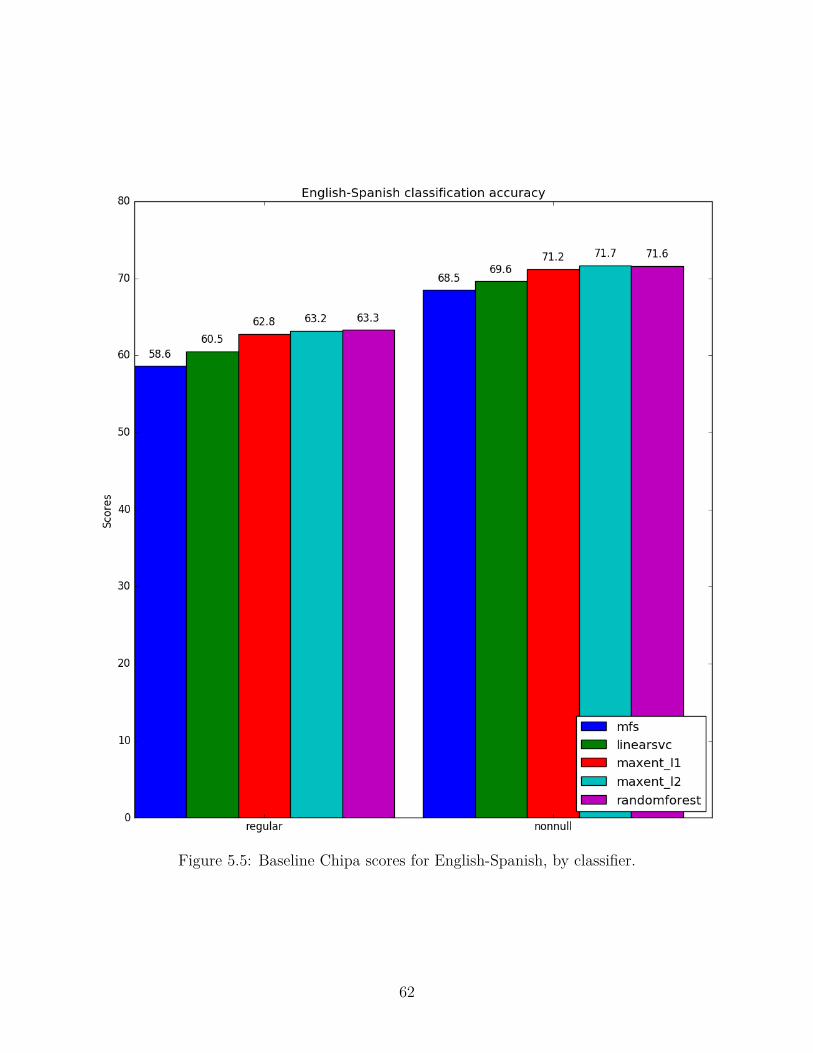
Figure 5.5: Baseline Chipa scores for English-Spanish, by classifier.

62

“nonnull” setting. This seems to be due to the Spanish and Quechua texts not being close

translations of one another – it is fairly likely that words in the Spanish text are simply not

present in the Quechua text, so when this possibility is eliminated, the classifier must make

a more difficult choice from among the remaining options.

In nearly all of the settings for this task, the use of a classifier outperformed the most-

frequent sense baseline. We see a little variety in the top results, for the four different

language pairs and both task settings, but the most successful classifiers here seem to be the

maximum entropy classifier with L2 regularization and random forests. The other classifiers

post slightly worse performance, but nearly always beat the MFS baseline.

So far, with commonly-used classifiers trained on commonly-used features, we achieve

a substantial boost on our ability to translate common polysemous words from Spanish

into two under-resourced languages, as well as between English and Spanish, over a simple

baseline. In subsequent chapters, we will see how to build on this simple approach, largely

through making additional features available to the learning algorithms.

5.2 For Comparison: the Baseline Chipa System On the SemEval 2010 and

2013 Shared Tasks

In order to situate this baseline Chipa system among other recent approaches to CL-WSD,

we ran Chipa on the SemEval CL-WSD test sets from 2010 and 2013, for English-Spanish. In

the full 2010 and 2013 tasks, systems were also asked to translate into four other European

languages: German, Dutch, French and Italian. Here for simplicity, we focus on English-

Spanish, since Chipa’s preprocessing pipeline already handles these languages, and the results

across language pairs were not drastically different in the original shared tasks. In this task,

we are presented with sentences in English, with a particular focus word marked, and the goal

is to select the lemma of a contextually appropriate translation for that word[31, 32]. The

task here guarantees that the appropriate translations are only those present in the Europarl

bitext, and several possible gold-standard translations are provided by human annotators.

63

We made no particular additional effort to tune Chipa for these tasks – it was run here

with the same settings used for the Spanish-Guarani and Spanish-Quechua CL-WSD tasks,

although the Chipa codebase is descended from a system originally built for the 2013 task

[8].

The training data for this task is considerably larger than the Bible text used for the main

CL-WSD task described in this work; Europarl bitext corpora contain nearly 2 million par-

allel sentences. We applied the preprocessing steps described in Section 4.3 to the Europarl

bitext, with the simplification that the individual sentences need not be extracted from the

various distribution formats used for Bibles. Here we use only a very small modification to

the Chipa system in order to address the larger training data size; rather than holding the

entire corpus in memory, the corpus is kept on disk and scanned for sentences that contain

the current focus word before we need to train the CL-WSD classifier for a given lemma.

There were two settings for the evaluation, best and oof. In either case, systems may

present multiple possible answers for a given translation, although in the best setting, the

first answer is given more weight in the evaluation, and the scoring encourages only returning

the top answer. In the oof setting, systems are asked to return the top-five most likely

translations. In both settings, the answers are compared against translations provided by

several human annotators for each test sentence, who provided a number of possible target-

language translations in lemmatized form. More points are given for matching the more

popular translations given by the annotators. For a complete explanation of the evaluation

and its scoring, please see the shared task descriptions.

The scores for the baseline Chipa system, as well as for other systems entered in the

2010 and 2013 competitions, are reported in Figures 5.6 and 5.7. In the 2010 competition,

none of the posted systems were able to beat the simple most-frequent-sense baseline for

the out-of-five setting, but Chipa surpasses it handily. Chipa also does better than all but

one of the posted systems in the one-best setting. On the 2013 test set, Chipa also did

fairly well, scoring better than several of the posted systems in the one-best setting, and

64

Figure 5.6: Scores on the SemEval 2010 test set, including results posted in the shared taskand the baseline Chipa system running on the same test set.

65

Figure 5.7: Scores on the SemEval 2013 test set, including results posted in the shared taskand the baseline Chipa system running on the same test set. When one team presentedmultiple results, here we take the best result from that team.

66

all but one of the posted systems in the best-of-five. It should be noted that in the 2013

competitions, one of the posted systems showing higher scores than the Chipa baseline was

“HLTDI”, developed by myself and Can Liu[8], which made use of early versions of some of

the techniques described in subsequent chapters.

But we see here that this straightforward approach, using a maximum entropy classifier

with features extracted from the words and lemmas surrounding the focus word, works quite

well compared with the other systems in the shared task, and so I claim that this system is

a sensible baseline on top of which we can build more advanced approaches.

67

CHAPTER 6

LEARNING FROM MONOLINGUAL DATA

While in this work our target languages are under-resourced, we have many resources avail-

able for the source languages. We would like to use these to make better sense of the input

text, giving our classifiers clearer signals and better representations for lexical selection in

the target language. The approaches considered in this chapter make additional features

or different representations available to the CL-WSD classifiers based on knowledge of the

source language, either gleaned through unsupervised methods or baked into extant tools.

Since we have relatively little bitext available for Spanish-Guarani and Spanish-Quechua, we

will need to lean more on our Spanish resources, software and data, in order to make better

sense of the input text.

Perhaps most saliently for Spanish, we have abundant monolingual text available, which

suggests that we could use unsupervised methods to discover regularities in the language,

yielding better features for our classifiers. This approach has been broadly successful in the

literature [89, 90], and here we adapt some of the methods explored in previous work on text

classification to our task.

Concretely, in this chapter we explore labels learned from existing NLP tools such as off-

the-shelf taggers and parsers for Spanish, Brown clustering [91], and a few related approaches

to neural embeddings. There are of course other related methods that one could investigate,

especially making use of the broader literature on distributional semantics, but we consider

them to be outside the scope of this work. First we will describe the methods used in some

detail, and then towards the end of the chapter, in Sections 6.5 and 6.6 respectively, we

describe experiments and present experimental results.

68

6.1 Monolingual features from existing NLP tools

There are a large number off-the-shelf NLP tools available for Spanish. Here we will look

into part of speech taggers and syntactic parsers specifically. Tagging can help us capture

abstractions over particular word types, and provides some disambiguation on its own. For

example, in Spanish, poder can be the infinitive verb “to be able”, or it can be a noun,

meaning “power, ability”. And if these different meanings are surfaced as different words in

the target language (as they are in English), then simply having an accurate POS tag makes

the CL-WSD task much easier. More generally, perhaps a noun in the window surrounding

a focus word could be indicative of a particular meaning.

Similarly, syntactic structure may also provide useful features. Verbs especially may have

drastically different translations in the target language based on their objects. There are

many familiar examples of this phenomenon, especially among the “light verbs” and “phrasal

verbs” with noncompositional meanings in English and Spanish.

In the Chipa software, we can make use of arbitrary annotations for the input text (see

Section 4.3.1), so adding more features based on analysis by external tools is straightforward.

As a first step, we synthesize features based on the part-of-speech tags of the tokens

surrounding the focus word, and using a syntactic parser, the heads and children of the

current focus word. In principle, we could use other annotations, such as sense annotations

from a monolingual WSD system, given a good one. This idea is akin to one that we will

explore in Chapter 7, in which we use Chipa itself (trained for other language pairs, and

with larger data sets) to provide annotations, effectively using some other target language

as a sense inventory for WSD.

For POS tagging, we run the open source FreeLing text analysis suite [78] on input

sentences. FreeLing can perform a number of analyses for Spanish, including POS tagging,

dependency parsing, lemmatization, and named entity recognition, of which the latter two

are part of the standard preprocessing done for all experiments in this work. When all the

69

text for an experiment is known beforehand, as in the experiments reported in this chapter,

we can run FreeLing during the data annotation step (see Section 4.3) and simply record

FreeLing’s output as text annotations. When running on novel test sentences, as in server

mode, we must run it on those sentences just before inference time.

Similarly, for syntactic features, we use MaltParser[92] 1 to get dependency parses of

the input sentence. This is also performed as a corpus annotation, making the syntactic

relationships for each token available during feature extraction. The parser here depends on

the POS tags produced by FreeLing. Conveniently, FreeLing and the espmalt parser model

assume the same tag set, but as with any pipeline of NLP systems, using the inferred output

from the tagger as input to the parser carries the risk that errors at early stages in the

pipeline could propagate and cause problems at the later stages of processing. Here we note

this concern but move on; it is a very general problem, and solutions to it are an open area

of research. The parser also depends on the coarse-grained “universal” POS tags [94], which

we map from the IULA tagset to universal coarse tags during corpus annotation.

Operationally, before training our CL-WSD system, we parse all of the training data with

the “espmalt” model, using the tags inferred by FreeLing during preprocessing, and store all

of MaltParser’s dependency parses on disk. Then with a corpus annotation script, we walk

those dependency graphs to find each token’s immediate syntactic head (or the root of the

sentence) and every token’s immediate syntactic children, if any. All of these dependency

heads and children are annotated in the training data, to be made available during feature

extraction. Then at feature extraction time, chipa turns these stored annotations into sparse

binary features. The list of all syntactic features made available to the classifier is given in

Figure 6.1.

To give a concrete example, consider the dependency graph for an English sentence

in Figure 6.2, and the scenario in which we want to classify the main verb of the sentence,1Available at http://maltparser.org/ ; in this work we use version 1.9.0 of the parser, and the “esp-

malt” pretrained model, which is available at http://www.iula.upf.edu/recurs01_mpars_uk.htm, andwas trained on the IULA Treebank[93], by researchers from the IULA group at Universitat Pompeu Fabra.

70

name descriptionpostag part-of-speech tag for the focus token

postag_left POS tag for the token to the left of focus tokenpostag_right ibid., for the right

head_lemma lemma of the focus word’s syntactic head, or ROOT if it hasno head).

head_surface ibid., but for the syntactic head’s surface form.child_lemma lemma of the syntactic child or children of the focus word.

Feature appears multiple times for multiple children.child_surface ibid., but for the children’s surface forms.

Figure 6.1: Additional syntactic features

The fluffy dogs chased the balls .

ROOT

subjamod

det obj

det

punct

Figure 6.2: An example dependency graph for an English sentence.

“chased”. The syntactic features that we would extract for this situation would be as follows:

postag(VERB), postag_left(NOUN), postag_right(DET) (assuming that the English sen-

tence has been labeled with Universal POS tags), head_lemma(ROOT), head_surface(ROOT)

(since the main verb is attached to the ROOT node of the dependency tree), child_lemma(dog),

child_lemma(ball) (the lemmas of the subject and object of the verb), and finally child_surface(dogs),

and child_surface(balls) (the surface forms of the subject and object of the verb).

6.2 Brown Clustering

The Brown clustering algorithm[91], also known as IBM clustering, as it was developed by

the Candide group at IBM, finds a hierarchical clustering for all the word types in a corpus,

such that words that are clustered nearby have similar usage patterns, and thus presumably

similar meanings. The tree of clusters is binary-branching, so the identity of a cluster is

simply its path from the root of the tree, and clusters that are close in the tree have similar

usage patterns. The desired number of “leaf” clusters must be set ahead of time as a tunable

71

P (w; C) =∏wi

p(wi|C(wi))p(C(wi)|C(wi−1)) (6.1)

Figure 6.3: The Brown clustering expression for the probability of a corpus with a specificclustering C. It is the product, for each token, of the probability of that token given its clus-ter, and the probability of that current cluster given the previous cluster. This is analogousto the “emission” and “transition” probabilities used in an HMM-based tagger.

parameter.

Each of the word types present in the input corpus is allocated to one of the leaf clusters,

such that the assignment attempts to maximize the probability of the input corpus. These

clusters were originally intended for use in class-based language modeling, and as such the

scoring function is the mutual information between subsequent tokens. Concretely, the

optimization process is searching for a clustering C that maximizes the probability of the

corpus w, according to the formula in Figure 6.3; intuitively, word types that occur in similar

bigrams should be in similar clusters.

Finding an optimal assignment of all word types in the corpus into these hierarchical

clusters is an intractable problem, but several greedy approaches that find local optima have

been explored in the literature. Notably, in addition to Liang’s approach, Franz Och’s mkcls

package (familiar to Moses users, and described in [95]) optimizes the same function when

assigning words to classes. In any case, with the available software running on modern

hardware, we can find a clustering for the corpora used in this work in a fairly short time,

on the order of hours.

Here our immediate use for these clusters is to create more features for our classifiers,

interpreting the clusters into which a word type falls as a tag for instances of that type.

These annotations give a more abstract, less sparse representation than surface forms or

lemmas, hopefully providing useful semantic and syntactic generalizations. We may also

preprocess the input to the clustering algorithm beforehand, as long as we can reproduce

the preprocessing for unseen input text at query time.

In applying Brown clusters to this task, we would like to answer several questions.

72

• Can learning Brown clusters from monolingual source text improve our performance

on this CL-WSD task?

• Does more source-language text help us learn more helpful Brown clusters, with respect

to the CL-WSD task? Can a large enough monolingual corpus help us overcome domain

mismatches?

• What kinds of preprocessing should we do on the source text? Particularly, should

Spanish source text be lemmatized?

6.2.1 Clustering in practice

In this work we use Percy Liang’s implementation 2 of Brown clustering [96]. We ran this

tool on two different monolingual corpora, the Spanish section of the Europarl corpus [70]

(2 million sentences) and a dump of Spanish-language Wikipedia (20 million sentences). In

all cases, we set the number of leaf clusters to 1000, which is the default for the package.

When working with Spanish, considering its relative morphological richness, we may consider

lemmatizing our input text before clustering. This decision will be more significant than it

would be for English, given the inflections present in Spanish, especially verb conjugations

and adjective-noun agreement. We might expect that Brown clustering on surface forms

would help us find abstractions over syntax, and that lemmatization will turn it towards

more semantic abstractions. This is an empirical question, and we briefly look into it here,

first by qualitatively examining the clusters that we learned, but later extrinsically evaluating

the clusters to see how they affect the CL-WSD task.

Figures 6.4, 6.5, 6.6 and 6.7 show some hand-selected illustrative examples of clusters

that we found in our monolingual Spanish corpora, Europarl and Wikipedia, in both surface-

form and lemmatized versions. Examining the output of the clustering algorithm, we see

some intuitively satisfying results; there are clusters corresponding to the names of many

countries, nouns referring to people by profession, and some semantically similar verbs. The2Available at https://github.com/percyliang/brown-cluster

73

category top twenty word types by frequencycountries Irlanda Francia Alemania Grecia Italia España Portu-

gal Rumanía Polonia Suecia Bulgaria Austria PalestinaCorea Finlandia Hungría Bélgica Bosnia DinamarcaEslovaquia

more countries Turquía Rusia China Israel Ucrania Croacia SerbiaGeorgia Europol Cuba Marruecos Canadá AlbaniaBrasil Moldova Libia Siria Suiza Sudáfrica Eslovenia

continuation verbs sigue siguen siga seguirá seguimos continúa sigan con-tinúe seguirán seguiremos continúan continuará sigosigamos continúen acabará continuarán continuaremoscontinuamos seguiré

proposition verbs propone establece prevé aprobó presentó mantienegarantice adopte tome adoptó decidió mantenga presen-tará establezca realiza proponen realice propuso adoptareconozca

past participles recibido tomado escuchado apoyado mantenido perdidoseguido debatido cumplido formulado encontrado leídodefendido examinado ofrecido discutido superado re-unido acogido consultado

feminine nouns formación educación tecnología infraestructura publici-dad enseñanza ocupación religión vivienda ética propa-ganda banda fusión huelga creatividad medicina manip-ulación tribuna cualificación comida

Figure 6.4: Selected clusters found in the surface version of Spanish Europarl

words listed in these figures are the top twenty terms from that cluster, by frequency in the

corpus. Note that the names given for the clusters were also chosen by hand, rather than

through some automatic process. It is reassuring that the clustering process, over all of these

corpora, is finding some interpretable generalizations in the text.

Comparing the lemmatized versus the surface-form versions of the clustering, we note

that, as expected, the clusters capture more syntactic regularities when given the inflected

forms. Consider, for example the cluster containing infraestructura in Figure 6.5, as com-

pared to its cluster in Figure 6.4. In the lemmatized version, we see that infraestructura falls

into a cluster primarily composed of words pertaining to transportation-related concepts,

such as vehículo ’vehicle’, billete ’ticket’ and avión ’airplane’. In the Wikipedia lemma clus-

ters, shown in Figure 6.7, we see some satisfying semantic clusters as well, such as adjectives

74

cluster description top twenty word types by frequencycountries francia irlanda alemania grecia italia españa rumanía

portugal polonia bulgaria suecia austria finlandia hun-gría bélgica japón gran_bretaña dinamarca eslovaquialuxemburgo

political entities comisión comisión_europea estados_miembrosgobierno_de_el_reino_unido presidente_putingobierno_de_los_estados_unidos pelota pres-idencia_de_la_ue presidente_lukashenkogobierno_de_israel presidente_klaus pres-idente_musharraf república_de_croaciacomisión_de_la_ue comité_de_expertos pres-idente_milosevic gobierno_de_sudán gob-ierno_de_zimbabue secretaría_general gob-ierno_de_irlanda

mostly abstract nouns riesgo gravedad lujo alivio molestia desperdi-cio riego horno superposición desprestigio vari-abilidad presupuesto_general deshumanizaciónadquirente cabildero desposeimiento streamliningvigía política_estructural_de_la_ue acuerdo_kedo

infrastructure infraestructura vehículo equipo buque instalación barcoavión motor planta ruta coche cabeza mina tren fusiónbillete fábrica camión arte pasaporte

common verbs pagar perseguir regir practicar percibir soportar gob-ernar sustentar recaudar abonar respirar profesar tragardevengar lucir pagar+le abanderar tributar glorificar so-bresalir

Figure 6.5: Selected clusters found in the lemmatized version of Spanish Europarl

describing political positions, verbs about making choices, and a cluster of locations, mostly

cities.

Contrastingly, on the surface-form side, the cluster that contains infraestructura does not

immediately reveal the same conceptual similarity: we see formación ’education (formal)’

creatividad ’creativity’, and comida ’food’ in the same cluster. While a few of the words

have similar meanings, the clustering seems to have found that these words cluster together

as singular feminine nouns, which is more of a syntactic commonality than a semantic one.

This is not to say that the surface-form clusters do not exhibit semantic relatedness; in the

“profession nouns” cluster in Figure 6.6, we see nouns that refer to people’s professions,

75

category top twenty word types by frequencysurnames León Castro Mendoza Franco Herrera Colón Guerrero

Rivera Miranda Silva Guzmán Medina Belgrano MolinaLara Guadalupe Juárez Hidalgo Trujillo Cáceres

women’s names Isabel Ana Rosa Teresa Juana Catalina Cristina Mar-garita Anna Mercedes Elena Laura Luisa Clara SofíaMarta Lucía Julia Gloria Alicia

conjugations of haber había habría haya hubiera habiendo he hubiese hemoshas habiéndose habíamos hubiere habia hayamos habéishabiéndolo habiéndole hubiéramos habremos hubieras

organization name parts Internacional Municipal Cultural Regional OficialHistórico Metropolitana Universitario Naval IndustrialUniversitaria Especial Musical Público Nobel Metropoli-tano Juvenil Comercial Penal Rural

profession nouns actor escritor compositor poeta productor médico pin-tor arquitecto músico abogado guitarrista historiador in-geniero sacerdote escultor empresario bajista guionistafilósofo investigador

cardinal directions sur norte oeste noroeste noreste sureste suroeste sudesteoriente sudoeste nordeste poniente voivodato NE centro-sur SW centro-norte centro-oeste sur-oeste nororiente

Figure 6.6: Selected clusters found in the surface version of Spanish Wikipedia

although it should also be noted that these are all singular masculine nouns. Also in the

Wikipedia surface clusters, we see a cluster containing almost entirely words referring to

cardinal directions3.

So a qualitative look at the clusters found in these corpora shows some promising regu-

larities found in the text. As expected, when we cluster on the surface forms, we find both

syntactic and semantic similarities, but using the lemmatized forms seems to push the clus-

ters towards conceptual similarity. It is still an empirical question which of these approaches

will help more for our CL-WSD task, so we will run experiments using each one.3With the inclusion of voivodato (English: ’voivodeship’ or Polish ’województwo’) which, I have just

learned from Wikipedia, is an administrative region in eastern Europe, similar to a historical duchy ormodern province.

76

category top twenty word types by frequencySpanish places castilla aragón granada toledo mendoza janeiro zamora

mallorca tenerife guadalupe ávila extremadura trujillosegovia cáceres baviera gimnasia soria catalunya maga-llanes

locations londres sudamérica oxford boston columbia cambridgeindiano harvard houston baltimore dallar berlin berkeleyleipzig stanford cleveland stuttgart sydney melbourneprinceton

common noun locations bosque lago puente jardín hotel coro pozo molino faroespejo almacén pantano muelle casino balneario arrecifecirco balcón rancho mosaico

parts of things elemento aspecto pieza instrumento factor componenterasgo ingrediente parámetro cualidad atributo trazo isó-topo acepción ítem alelo pasatiempo renglón morfismointrumentos

choice verbs elegir seleccionar escoger nominar reelegir redesignarungir sindicar preseleccionar cooptar procesionada re-electo re-elegido eligido reimplementar renominar elegiorecomisionar estandardizar indiscutidamente

political adjectives socialista republicano liberal comunista revolucionarioconservador radical nacionalista demócrata anar-quista unitario progresista independentista bolcheviquefascista marxista patriótico libertario socialdemócratamonárquico

empires romano colonial bizantino otomano inca visigodo mon-gol cartaginés mexica austrohúngaro galáctico motorscarolingio hitita incaico almohade virreinal isabelinoomeya lusitano

Figure 6.7: Selected clusters found in the lemmatized version of Spanish Wikipedia

6.2.2 Classification features based on Brown clusters

Given a clustering learned from a large monolingual corpus, we must still decide how to

extract classification features from those clusters. If we know, for example, that the token to

the left of the focus word is in cluster “010111111100”, what information do we provide to

the classifier? We could interpret this cluster atomically, as a tag for that token, and create

sparse features for an input sentence based on the clusters present in it, perhaps focusing on

the window surrounding the focus word. However, following the work of Turian et al. [89],

77

name descriptionbrown_bag Bag of all Brown clusters for the entire sentence

brown_window All Brown clusters for the three-token window around thefocus word

Figure 6.8: Features extracted from Brown clusters. These came in surface-form and lemmavariants, and were trained on both the Europarl for Spanish, and our Wikipedia dump.Additionally, we add variants for the 4, 6, and 10-bit prefixes of the clusters.

we also take the prefixes of each cluster’s bit strings at 4, 6, and 10 bits, taking advantage

of the hierarchical structure in the clusters, and used these separate sparse features.

As a concrete example using the lemmatized Wikipedia clusters, if we find that the lemma

rioplatense is in a three-token window around the current focus word, and that this lemma

is in cluster “111110111111111110”, then we extract the following features, setting each of

them to 1.

• brown_window_wikipedia_lemma(111110111111111110)

• brown_window_wikipedia_lemma_4(1111)

• brown_window_wikipedia_lemma_6(111110)

• brown_window_wikipedia_lemma_10(1111101111)

We additionally extract analogous features for all tokens in the sentence; these would be

called brown_bag_wikipedia_lemma, brown_bag_wikipedia_4, and so on. If we are using

clusters based on the surface forms, these simply do not have lemma in their name, and

features based on Europarl, are marked with europarl rather than wikipedia.

In cases of unknown words, where we do not have a cluster assignment for a word in

the input text, we simply do not extract cluster features for that word. This will happen in

practice, even for a fairly large monolingual corpus, but may be especially common in this

setting due to domain mismatches. Many biblical names, for example, are not present in

Europarl.

78

6.3 Neural Word Embeddings

Another rich source of features that has proved useful for many text classification problems

in recent years is neural word embeddings, perhaps most famously developed in the work

of Mikolov et al. [97] and their associated open source implementation of the technique,

word2vec4. In this work we investigate the use of “word2vec”-style word embeddings, as

well as the related technique, “doc2vec” or “paragraph vectors” [98, 99]. These techniques

let our classifiers operate on lower-dimensional dense vectors (of a few hundred dimensions,

typically), as opposed to the high-dimensional sparse vectors typically used in earlier NLP

literature5.

There is a rich literature on continuous representations for words; the idea has a long

lineage in NLP, and we could try any number of dimensionality reduction or distributional

semantics approaches here. However, recent empirical work by Baroni et al [90] (summed up

by the title of the paper, “Don’t Count, Predict!”) has shown that representations built dur-

ing discriminative learning tasks are typically more effective for text classification problems

similar to ours.

Unlike Brown Clustering, which infers hierarchical clusters for each word type, but like

other embedding techniques, word2vec learns multidimensional representations for word

types, turning the very sparse “one hot” representation in which words with similar uses or

meanings do not have any obvious similarity into a much denser continuous space, wherein

words with related meanings are placed nearby. These “embeddings”, or placements of word

types in a continuous space, are learned latently during some other classification task, and

are performed by the early layers of a neural network.

The word2vec model in particular has two variations, useful in different contexts. One,

called Continuous Bag-of-Words (CBOW) learns a classifier that can predict individual words4Available at https://code.google.com/archive/p/word2vec/5 What we might consider to be “symbolic” binary features used in machine learning systems for NLP in

recent decades – such as “the word ‘dog‘ appears in the sentence” – are effectively equivalent to these verysparse “one hot” representations of words, in which, for a vocabulary of size |V |, words are represented bya length-V vector in which all but one of the elements are 0.

79

based on their context, while the “skip-grams” variant does the reverse and learns to predict

context words based on an individual focus word. The received wisdom6 is that CBOW is

more appropriate when training on smaller data sets, but this is an empirical question, so

here we run experiments with both variants.

In either case, running a word2vec training process results in a static mapping from

word types to their embeddings in a vector space of a given size, typically a few hundred

dimensions. These embeddings have been shown to be helpful as features in a number

of different NLP tasks [90], allowing us to learn richer representations of word types from

plentiful unannotated monolingual text. This effectively turns what was a purely supervised

task, requiring labeled training data, into a semi-supervised task, in which the representation-

learning phase can be carried out on unlabeled data by synthesizing a supervised learning

task that can be performed with simple monolingual text as its training data.

We trained a variety of word2vec embeddings for our text classification tasks, again

training on the Spanish-language section of the Europarl corpus (roughly 57 million words

or 2 million sentences) and a dump of Spanish Wikipedia (449 million words, 20 million

sentences). We learned embeddings using both CBOW and skip-gram approaches, in 50,

100, 200, and 400 dimensions. We also used the associated word2phrase tool, distributed

with the public word2vec implementation, which finds collocations in the input text and

treats them as individual tokens. The same collocations must be identified in the input

text for their embeddings to be used. At lookup time, we keep a list of all the multiword

expressions present in the dictionary of embeddings, sorted from longest to shortest, first

considering number of tokens, then breaking ties by considering number of characters, and

greedily replace any of these multiword expressions (starting with the longest) found in the

input text with the token representing that MWE.6According to the TensorFlow tutorial on word2vec, available at https://www.tensorflow.org/

tutorials/word2vec

80

6.3.1 From word embeddings to classification features

We should note that, like Brown clusters, the embeddings learned for a word type are fixed

for that word type, and do not reflect the context of a particular token, so a focus word’s

embedding vector will not provide useful classification features on its own. This leaves us

with the problem of how to make use of the word vectors in a given sentence. Concretely,

we must decide how to combine several word vectors together, and which word vectors in

a sentence to choose for combination. A typical approach is to take element-wise sums or

averages over the embedding vectors for the tokens in a context [100, Chapter 8].

There are a variety of approaches we could take, even within summing and averaging.

We could sum (element-wise) all of the word vectors for all the tokens in the entire sentence.

We could only consider the words in a narrow window around the focus word. Or we could

perform a weighted sum, in which words nearer to the focus word are given more weight, but

these weights drop off according to some function, scaling with the distance from the focus

word. We might expect the tokens closest to the current focus word to be most important

for building a representation of the meaning of that word – which would lead us to expect

the best results from summing uniformly over the context window, or a weighted sum with

gradually dropping weights – or perhaps we might expect that we want to represent the

meaning of the entire sentence, and so could sum over all the tokens. How well any of these

approaches work in practice is an empirical question, so we run experiments using each of

these these different approaches, resulting in three different feature sets.

In the first feature set, called “window”, we present the classifier with the element-wise

sum of the vectors for the focus word (or the token containing the focus word, if it is inside a

multi-word expression) and the three tokens on either side. The resulting vector thus has the

same dimensionality as the word embeddings that we learned. Secondly, in the “fullsent”

feature set, we perform an unweighted element-wise sum of the word embeddings for the

entire input sentence. Finally, in the “pyramid” feature set, we sum the embeddings for each

token in a broad window around the focus word, but before summing, scale each embeddings

81

by max(0, 1.0 − (0.1 ∗ d)), where d is the distance between that token and the focus word.

For all of the variations considered here, whether we are using skipgrams or CBOW, for

whichever dimensionality we choose, and for any of the methods of combining the vectors,

when using these word embeddings without other resources, we end up representing a CL-

WSD problem as a dense vector of the same dimensionality as the current set of word

embeddings; these dense vectors can be passed along to any machine learning algorithm

that we care to use.

6.4 Neural Document Embeddings

Rather than coming up with representations for individual words and then combining them

to get a representation of a sentence or a local context, we might want a technique that

directly finds representations of sequences of text. One such technique, called “paragraph

vectors” or “doc2vec”, does just this. doc2vec was developed by some of the same re-

searchers that produced word2vec, and it can build representations for arbitrary sequences

of text, rather than individual word types [98, 99]. This approach takes unlabeled text and

learns representations for word types jointly with representations for each document. Here a

“document” is an arbitrary sequence of tokens, perhaps a single sentence, or perhaps much

longer, depending on the intended application.

Similar to word2vec, here doc2vec uses a neural network with a single hidden layer to

predict words in the current context. Here however, the hidden layer contains not only

an embedding trained for word types, but also an embedding for the current document.

Training proceeds by loading the current representation for the current word and the current

document, attempting to predict some other word in the context (analogous to training for

word2vec), and then updating both of these representations based on the gradients between

the desired output and the actual output.

Also similar to word2vec, there are two variants of the approach that can be used for

training. One variant of doc2vec, the “Distributed Memory Model of Paragraph Vectors”,

82

uses a paragraph embedding combined with word embeddings for several words in the current

context to predict a single individual word. The other variant, the “Distributed Bag of Words

model of Paragraph Vectors”, simply uses the current paragraph vector to predict all of the

words in the current context, which despite containing “bag of words” in its name, is more

closely analogous to the skip-gram artitecture for word2vec [99], since the model is trained

to predict the entire context based on a single embedding.

In either case, the resulting stored model consists of the embeddings for individual word

types. The embeddings for any particular document in the training set are not stored,

since that document is unlikely to appear again at inference time, but the embeddings for

individual word types provide a useful generalization, since they constrain embeddings for

new documents.

At inference time, doc2vec produces new vectors representing previously unseen docu-

ments based on these fixed word embedding vectors. In our work, as in many text classifi-

cation tasks, documents will be input sentences, or perhaps sentence-length Bible verses, or

smaller windows of text around a word-in-context. To produce a representation for a new

document, the embeddings for word types are held constant and we run stochastic gradient

descent optimization to infer an embedding for the current document, based on the fixed

word embeddings, such that it helps predict words in the current context.

doc2vec thus provides a straightforward approach for learning to produce representations

of new documents, based on an unlabeled training corpus. Here we use the implementation

of doc2vec provided by the gensim package 7, with its default settings, which uses the

“distributed memory” model [101].

In order to use doc2vec for our experiments, we train and save a doc2vec model on our 20

million sentences from Spanish-language Wikipedia. Then, during training data annotation

for the CL-WSD model, we pass over our bitext corpus, take the source-language sentence

from each training pair, and infer a new embedding for it based on that doc2vec model.7Available at https://radimrehurek.com/gensim/

83

These sentence-level embeddings are stored as a token annotation on the first token of each

sentence, so they can be made available during feature extraction. We can also show the

gensim software a small context window around the focus word, rather than the entire

sentence to generate a more focused representation.

In either case, the result is a dense vector of the specified dimensionality, again typically

a few hundred, which we can pass to whichever machine learning algorithm we like, as we

did previously with the vectors based on word2vec.

6.5 Experiments

Here we repeat the experiments from Chapter 5 for Spanish-Guarani and Spanish-Quechua,

using the features extracted from syntactic tools, Brown clusters, and the various kinds of

neural embeddings presented in this chapter. These experiments were carried out with the

top classification algorithms that we used in Chapter 5, focusing on maximum entropy (using

both L1 and L2 regularization) and random forests. While most of the experiments here are

a combination of the baseline features with the features introduced in this chapter, we also

used the neural embeddings features on their own, as a replacement for the baseline features.

While there are many possible combinations of the features, we did not run experiments for

all (exponentially many) possibilities exhaustively.

Specifically, we experimented with the following feature sets, based on the techniques

described in this chapter, for both Spanish-Guarani and Spanish-Quechua.

• POS tag features, with baseline features

• POS tag and dependency parse features, with baseline features

• Brown cluster features, with baseline features, in combinations of …

– trained on Europarl or Wikipedia

– based on lemmas or surface forms

84

– context-window only, or including both context-window and all clusters for the

sentence as a bag.

• word2vec embeddings on their own, in combinations of …

– trained on Europarl and Wikipedia

– skipgrams and CBOW

– using multi-word expression embeddings or not

– dimensions: 50, 100, 200, 400

– combination strategies: full sentence, context window, and “pyramid” (summing

embeddings with a weight that decreases with distance from the focus word)

• doc2vec embeddings on their own, trained on Wikipedia…

– embeddings for a full sentence or embeddings for a context window

• Combination of promising features: baseline features, with syntactic features and

Brown clusters (context window, surface form, Wikipedia).

• Combination of promising features: “pyramid” word2vec embeddings, with syntactic

features and Brown clusters (also context window, surface form, Wikipedia).

In the next section, we present and discuss the results from these experiments.

6.6 Experimental Results

This section contains many tables of numbers; in general, for each set of experimental results

presented, the top result for each setting is presented in italics, and the top result for a setting

presented in the whole chapter is presented in bold.

85

classifier es-gn regular es-gn non-null es-qu regular es-qu non-nullMFS 0.456 0.498 0.435 0.391

maxent l1baseline features 0.461 0.506 0.444 0.414

+pos tags features 0.464 0.510 0.449 0.420+all syntactic features 0.465 0.511 0.450 0.422maxent l2

baseline features 0.475 0.524 0.458 0.431+pos tags features 0.479 0.527 0.462 0.438

+all syntactic features 0.480 0.530 0.465 0.441random forest

baseline features 0.481 0.520 0.464 0.424+pos tags features 0.485 0.523 0.467 0.430

+all syntactic features 0.486 0.527 0.471 0.434

Figure 6.9: Classification results for adding syntactic features to the default feature set, ascompared with the MFS baseline.

6.6.1 Results: adding syntactic features

Taking a look at the scores from the features based on easily available Spanish-language

taggers and parsers, which are presented in Figure 6.9, we see small but fairly consistent

improvements over the baseline features as we add syntactic features. In all of our settings,

we see a few tenths of a percentage point gain by adding the POS tag features, and then

another small gain on top of that by adding syntactic dependency features.

These gains seem to be of roughly the same (small) magnitude; it is not obvious whether

any of the classifiers are more able to make use of the additional features than others, but

this is somewhat reassuring, and it looks like we are easily able to add some helpful features

when we have syntactic analysis tools available for our source language.

6.6.2 Results: adding clustering features

We see the experimental results for adding our Brown Cluster features (explained in Fig-

ure 6.8) in Figure 6.10. In general, we do not see gains from adding all of the Brown Cluster

features together; this typically seems to diminish performance by a few tenths of a percent-

86

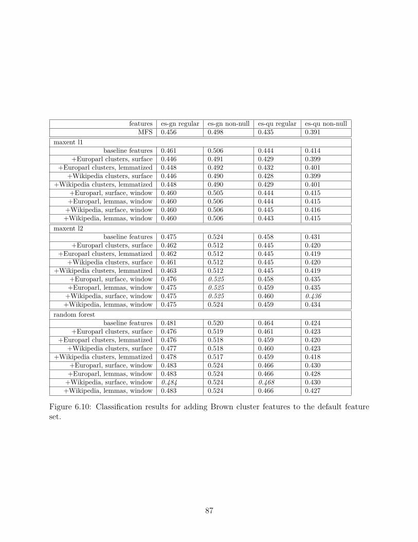
features es-gn regular es-gn non-null es-qu regular es-qu non-nullMFS 0.456 0.498 0.435 0.391

maxent l1baseline features 0.461 0.506 0.444 0.414

+Europarl clusters, surface 0.446 0.491 0.429 0.399+Europarl clusters, lemmatized 0.448 0.492 0.432 0.401

+Wikipedia clusters, surface 0.446 0.490 0.428 0.399+Wikipedia clusters, lemmatized 0.448 0.490 0.429 0.401

+Europarl, surface, window 0.460 0.505 0.444 0.415+Europarl, lemmas, window 0.460 0.506 0.444 0.415

+Wikipedia, surface, window 0.460 0.506 0.445 0.416+Wikipedia, lemmas, window 0.460 0.506 0.443 0.415

maxent l2baseline features 0.475 0.524 0.458 0.431

+Europarl clusters, surface 0.462 0.512 0.445 0.420+Europarl clusters, lemmatized 0.462 0.512 0.445 0.419

+Wikipedia clusters, surface 0.461 0.512 0.445 0.420+Wikipedia clusters, lemmatized 0.463 0.512 0.445 0.419

+Europarl, surface, window 0.476 0.525 0.458 0.435+Europarl, lemmas, window 0.475 0.525 0.459 0.435

+Wikipedia, surface, window 0.475 0.525 0.460 0.436+Wikipedia, lemmas, window 0.475 0.524 0.459 0.434

random forestbaseline features 0.481 0.520 0.464 0.424

+Europarl clusters, surface 0.476 0.519 0.461 0.423+Europarl clusters, lemmatized 0.476 0.518 0.459 0.420

+Wikipedia clusters, surface 0.477 0.518 0.460 0.423+Wikipedia clusters, lemmatized 0.478 0.517 0.459 0.418

+Europarl, surface, window 0.483 0.524 0.466 0.430+Europarl, lemmas, window 0.483 0.524 0.466 0.428

+Wikipedia, surface, window 0.484 0.524 0.468 0.430+Wikipedia, lemmas, window 0.483 0.524 0.466 0.427

Figure 6.10: Classification results for adding Brown cluster features to the default featureset.

87

age point, in many cases making the performance as a whole dip below the MFS baseline.

While they are intended to be helpful abstractions, we may be adding too many irrelevant

features, perhaps overwhelming the useful signals present in the baseline feature set. There

does not seem to be a consistent or significant change due to using the lemmatized or surface

forms.

However, we get substantially better results when we limit the Brown cluster features to

a narrow context words of three words on either side of the focus word; this seems to lead to

roughly the same results as the baseline features, for the maximum entropy classifiers. But

for the random forest classifiers, we see consistent gains of three to six tenths of a percentage

point. So for random forest classifiers, it seems worthwhile to add these window-based Brown

cluster features. Within the “window only” variants of the Brown cluster features, the scores

are fairly similar, but by a small margin we see the strongest results coming from using the

clusters trained on the surface form of our Spanish Wikipedia.

Neither of these corpora, Europarl or the Spanish Wikipedia, are similar in genre to the

Bible verses in our test set, but we can get a small benefit from adding the Brown cluster

features here. The substantially larger size of the Wikipedia corpus does not seem to confer

clusters that are much more helpful; if there had been a large performance gap between

using the Wikipedia and Europarl clusters, we could have run additional experiments with

clusters trained on a 2-million sentence sample of Wikipedia to determine whether it was

the additional size or the genre of the text that had improved performance.

6.6.3 Results: combining sparse features

We present the experimental results for combinations of all of the sparse features presented

in this chapter in Figure 6.11. Here in general we see some good gains over the baseline

features, from a few tenths of a percentage point to just over a full percentage point; we see

that as before, the maximum entropy classifiers do not seem to benefit from the addition

of Brown cluster features, but they do benefit from the syntactic features. The random

88

classifier es-gnregular

es-gnnon-null

es-quregular

es-qunon-null

MFS 0.456 0.498 0.435 0.391maxent l1

baseline features 0.461 0.506 0.444 0.414+syntactic features, maxent

l10.465 0.511 0.450 0.422

combined sparse features 0.464 0.510 0.448 0.422maxent l2

baseline features 0.475 0.524 0.458 0.431+syntactic features, maxent

l20.480 0.530 0.465 0.441

combined sparse features 0.479 0.530 0.465 0.443random forest

baseline features 0.481 0.520 0.464 0.424+syntactic features 0.486 0.527 0.471 0.434

combined sparse features 0.488 0.528 0.472 0.437

Figure 6.11: Results for baseline features with the sparse features introduced in this chapter:features from a POS tagger, a dependency parser, and Brown clustering.

forest classifiers benefit from both additional kinds of features; our best performance with

the sparse feature sets is with random forests given these combined features, and this is

consistent for both language pairs, and in the regular and non-null settings.

6.6.4 Results: word2vec embeddings alone

Taking a look at Figures 6.12 and 6.13, we see the results for the experiments for using

only word2vec embeddings for our features. There were many variations, but we see a few

general trends. We performed experiments for 50, 100, 200, and 400 dimensions, but the

dimensionality of the vectors did not seem to change the results more than a few tenths of a

percentage point. Here we report the results for 200 dimensions to save space and for easier

comparison; in general the results for 200 dimensions were on the slightly more favorable

side of representative. Also, because there were so many variations to try, some of the less

promising combinations were cut. Specifically, almost all of the experiments with the CBOW

embeddings, the “fullsent” combination approach, and random forest classifiers gave results

89

classifier es-gn regular es-gn non-null es-qu regular es-qu non-nullMFS 0.456 0.498 0.435 0.391

maxent l1baseline features 0.461 0.506 0.444 0.414fullsent, europarl 0.421 0.465 0.406 0.369

fullsent, europarl, mwes 0.421 0.465 - -fullsent, wikipedia 0.428 0.468 0.408 0.374

fullsent, wikipedia, mwes 0.428 0.469 - -pyramid, europarl 0.463 0.507 0.448 0.418

pyramid, europarl, mwes 0.462 0.505 0.447 0.418pyramid, wikipedia 0.469 0.512 0.453 0.424

pyramid, wikipedia, mwes 0.469 0.512 0.452 0.423window, europarl 0.462 0.506 0.447 0.417

window, europarl, mwes 0.460 0.504 0.447 0.416window, wikipedia 0.468 0.511 0.451 0.423

window, wikipedia, mwes 0.467 0.511 0.450 0.422maxent l2

baseline features 0.475 0.524 0.458 0.431fullsent, europarl 0.421 0.469 0.406 0.375

fullsent, europarl, mwes 0.421 0.469 - -fullsent, wikipedia 0.427 0.472 0.408 0.379

fullsent, wikipedia, mwes 0.427 0.472 - -pyramid, europarl 0.459 0.505 0.443 0.417

pyramid, europarl, mwes 0.457 0.504 0.443 0.418pyramid, wikipedia 0.465 0.512 0.449 0.424

pyramid, wikipedia, mwes 0.464 0.511 0.449 0.423window, europarl 0.455 0.501 0.440 0.414

window, europarl, mwes 0.453 0.500 0.439 0.413window, wikipedia 0.461 0.507 0.445 0.420

window, wikipedia, mwes 0.461 0.506 0.445 0.420random forest

baseline features 0.481 0.520 0.464 0.424fullsent, europarl 0.432 0.474 - -

fullsent, europarl, mwes 0.431 0.474 - -fullsent, wikipedia 0.432 0.477 - -

fullsent, wikipedia, mwes 0.433 0.476 - -window, europarl 0.447 0.491 - -

window, europarl, mwes 0.448 0.489 - -window, wikipedia 0.453 0.494 - -

window, wikipedia, mwes 0.451 0.493 - -

Figure 6.12: Results for classification using only word2vec skipgram embeddings to createfeatures. For space, here we only show results for 200-dimensional embeddings.

90

classifier es-gn regular es-gn non-null es-qu regular es-qu non-nullMFS 0.456 0.498 0.435 0.391

maxent l1baseline features 0.461 0.506 0.444 0.414fullsent, europarl 0.389 0.433 - -

fullsent, europarl, mwes 0.388 0.434 - -fullsent, wikipedia 0.391 0.433 - -

fullsent, wikipedia, mwes 0.391 0.433 - -pyramid, europarl - - 0.401 0.374

pyramid, wikipedia - - 0.401 0.375window, europarl 0.414 0.455 0.396 0.367

window, europarl, mwes 0.411 0.454 - -window, wikipedia 0.414 0.456 0.395 0.368

maxent l2baseline features 0.475 0.524 0.458 0.431fullsent, europarl 0.392 0.442 - -

fullsent, europarl, mwes 0.392 0.441 - -fullsent, wikipedia 0.394 0.440 - -

fullsent, wikipedia, mwes 0.394 0.441 - -pyramid, europarl - - 0.398 0.375

pyramid, wikipedia - - 0.398 0.377window, europarl 0.403 0.448 0.386 0.363

window, europarl, mwes 0.402 0.447 - -window, wikipedia 0.408 0.451 0.389 0.366

window, wikipedia, mwes 0.406 0.451 - -random forest

baseline features 0.481 0.520 0.464 0.424fullsent, europarl 0.432 0.472 - -

fullsent, europarl, mwes 0.431 0.474 - -fullsent, wikipedia 0.434 0.478 - -

fullsent, wikipedia, mwes 0.434 0.478 - -window, europarl 0.449 0.492 - -

window, europarl, mwes 0.448 0.489 - -window, wikipedia 0.452 0.494 - -

window, wikipedia, mwes 0.451 0.494 - -

Figure 6.13: Results for classification using only word2vec CBOW embeddings to createfeatures. For space, here we only show results for 200-dimensional embeddings.

91

lower than the MFS baseline, so not all combinations were carried out.

However, if we focus on Figure 6.12, we can see some fairly promising results. We

note that for the maxent classifiers, we can often surpass the MFS baseline by using the

word2vec embedding features alone, and for some settings, even surpass the baseline features.

Particularly, we note that using the “window” and “pyramid” results, we can do fairly well

– the “fullsent” approach does not seem to help here – and that for the L1-norm maxent

classifier, we can outperform the baseline features with word2vec features alone.

Interestingly, despite its strong performance on the sparse feature sets, the random forest

classifier does not do as well with the dense vectors; it does not outperform the MFS baseline.

In general, the L1-norm maxent classifier seems to do best with these feature sets, and the

embeddings trained on the larger (and more general-domain) Wikipedia corpus seem to be

most effective; using the multi-word expression embeddings seems to have little to no effect.

The “pyramid” combination scheme generally comes out on top. So this is encouraging, for

features for maxent classifiers.

6.6.5 Results: doc2vec embeddings alone

Taking a look at the results for using doc2vec embeddings on their own, presented in Fig-

ure 6.14, we see a few general trends. As with the word2vec feature sets, the random forests

did not outperform the MFS baseline when given a dense vector as input. Also as we saw

with the word2vec features, trying to build a representation of the entire sentence was not

as effective as building a vector to represent just the tokens around the focus word. The

full-sentence representations were more effective than the corresponding full-sentence vector

sums from word2vec, however – in a few instances they outperform the MFS baseline.

However, when we restrict the doc2vec optimizer to looking at a narrow context window

around the focus word, we outperformed the MFS baseline on all of the test sets, for maxent

classifiers. For some, but not all, of the L1-norm maxent cases, the doc2vec features surpass

the baseline features by a slim margin. There may be a way to make doc2vec embeddings,

92

classifier es-gn regular es-gn non-null es-qu regular es-qu non-nullMFS 0.456 0.498 0.435 0.391

maxent l1baseline features 0.461 0.506 0.444 0.414

fullsent 0.462 0.496 0.441 0.391window 0.463 0.502 0.445 0.395

maxent l2baseline features 0.475 0.524 0.458 0.431

fullsent 0.462 0.497 0.442 0.390window 0.467 0.506 0.449 0.402

random forestbaseline features 0.481 0.520 0.464 0.424

fullsent 0.420 0.497 0.404 0.390window 0.421 0.461 0.405 0.352

Figure 6.14: Top results for classification using only doc2vec embeddings to create features.For comparison, also included are the MFS baseline and the top results from the previouschapter.

or some other kind of document-level embedding features, work well for this setting, but

further exploration is outside the scope of this work.

6.6.6 Results: combining neural embeddings with sparse features

In Figure 6.15, we present the experimental results for combining the most successful word2vec

embeddings with the most promising additional sparse features described in this chapter.

In these experiments, we started with the 200-dimensional Wikipedia embeddings, com-

bined them in the “pyramid” style, and also made the Brown cluster and syntactic features

available to the classifiers to see if these would improve performance.

And in general, we see that the addition of these features does make an improvement over

using the word2vec features by themselves. In fact, for all of the classifiers, and each of the

test sets, we see an improvement over the word2vec features; this only results in consistent

improvements over the baseline features for the L1-norm maximum entropy classifer, how-

ever. But it is the best results presented thus far for that classifier, and the most effective

feature set that we have tried, using neural embeddings.

93

classifier es-gn regular es-gn non-null es-qu regular es-qu non-nullMFS 0.456 0.498 0.435 0.391

maxent l1baseline features 0.461 0.506 0.444 0.414word2vec alone 0.469 0.512 0.453 0.424

+sparse features 0.472 0.519 0.458 0.436maxent l2baseline features 0.475 0.524 0.458 0.431word2vec alone 0.465 0.512 0.449 0.424

+sparse features 0.472 0.522 0.458 0.438random forestbaseline features 0.481 0.520 0.464 0.424word2vec alone 0.452 0.493 0.438 0.394

+sparse features 0.461 0.504 0.449 0.410

Figure 6.15: Results for combining word2vec embeddings (Wikipedia skipgrams, 200 dimen-sions, “pyramid” strategy) with syntactic features and Brown clusters. For comparison, alsoincluded are the MFS baseline, word2vec results without additional features.

6.7 Discussion

In this chapter, we have shown a number of different approaches for making use of the

available resources for our source language in the CL-WSD task, including three different

ways of learning from unannotated source-language text – clustering and two kinds of neural

embeddings – and making use of existing source-language syntactic analysis tools.

Using each of these different tools, we were able to overcome the relatively strong most-

frequent sense baseline, and with many of the different feature sets, we were able to show

small but consistent gains over the baseline feature set described in the previous chapter.

Overall, the best results posted for Spanish-Guarani were with the combined sparse fea-

tures; the random forest classifier had the strongest results for the “regular” setting, and the

maximum entropy classifier with L2 regularization came out ahead for the non-null setting

(this result was tied with the one for using the syntactic features with maximum entropy,

L2 regularization). For Spanish-Quechua, the top results were similarly posted with the

combined sparse features, with random forests coming out ahead for the “regular” setting

94

and maximum entropy, L2, posting the best results for “non-null”.

All of the approaches explored in this chapter make more abstract representations of the

source text available to our classifiers, whether these representations were learned from the

available text, or encapsulate some kind of syntactic knowledge about the language.

We found, in general, that adding features that represent the text closely surrounding

the focus word was more effective than attempting to represent the entire source-language

sentence at once; we observed this effect for Brown cluster features, and for features built

from both word and document embeddings. Additionally, we found that we could not only

add some of these features to our baseline sparse feature set, but also that our new sparse

features could be added to dense feature vectors based on word2vec embeddings, resulting

in gains over using the neural embeddings by themselves.

In general, our random forest classifiers seem to benefit more from adding many sparse

features, like the ones we extracted from Brown clusters, than the maxent classifiers do.

However, the random forest classifiers do not perform as well when given dense vectors, like

those produced by word2vec and doc2vec. Contrastingly, the maximum entropy classifiers

have better performance in this setting.

In the next chapter, we will make use of another one of our available resources for a

resource-rich language like Spanish: bitext with other language pairs.

95

CHAPTER 7

LEARNING FROM MULTILINGUAL DATA

As discussed in previous chapters, while our target languages are under-resourced, we have

many resources available for our source languages. Concretely for Spanish, in addition to the

abundant monolingual text and off-the-shelf NLP tools discussed in Chapter 6, we have a

significant amount of bitext, pairing Spanish with languages other than our under-resourced

target languages. We would like to be able to learn from these available bitext corpora

when translating from Spanish to Guarani and Quechua, and ideally when translating from

resource-rich source languages into under-resourced target languages in general.

Each bitext corpus may contain useful examples of a given source language word, and

senses of that word may be lexicalized in distinct ways in different target languages, giving

us clues about the meaning of each token in its context. Selecting a contextually correct

translation for source-language words is evidence that we have understood the meaning of

those words, at least implicitly, in as far as sense distinctions are surfaced in the target

language. So we would like to be able to learn relationships between the senses of a given

source word as they are represented in different target languages. Two target languages

may happen to surface similar sense distinctions, perhaps due to being related languages,

or perhaps because a word sense ambiguity is unusual in the source language, or simply by

coincidence. Additionally, a combination of translations into several languages may provide

evidence for a certain lexical choice in the target language of interest.

In this chapter, we present strategies for learning from the available bitext corpora that

do not include our under-resourced target languages, to help us make better CL-WSD de-

cisions when translating into them. To establish consistent terminology, we will call these

supplemental bitext corpora. Primarily we discuss a “classifier stacking” approach, in which

we train “supplemental” CL-WSD classifiers translating from Spanish to other European lan-

96

guages, based on our supplemental corpora, and use their outputs to provide more features

for the Spanish to Quechua and Spanish to Guarani classifiers.

As a concrete example of how we can use classifier stacking, say we are trying to translate

a Spanish sentence to English and we would like to make a lexical selection for the word

estación, which can translate to English as either “station” (like a train station) or “season”.

(5) Mi estación favorita es la primavera.

If we had a Spanish to French CL-WSD system, and this system returned saison (rather

than gare, the French word for a train station) for this instance of estación, we would expect

that this would be a useful signal for our Spanish to English classifier, helping it pick the

“season” sense.

The approaches in this chapter are particularly informed by the work of Els Lefever et.

al (see especially [26]), in which entire source sentences are machine-translated into sev-

eral different target languages just before feature extraction, and these translated sentences

are used to produce features for CL-WSD classifiers. One drawback of this technique is

that it could be considered unwieldy from a software engineering perspective; it requires

multiple complete MT systems to perform CL-WSD, when we want to use CL-WSD as a

subcomponent of a machine translation system in the first place.

In earlier work, considering the work of Lefever et. al, we developed prototype CL-

WSD systems that made use of multilingual evidence [8] and produced some of the top

results in a SemEval shared task on CL-WSD [32]. We found here that our systems that

used multilingual evidence had better performance than the one that used only monolingual

features. Our top results in every language came from either classifier stacking or a classifier

based on Markov networks, an approach which we will discuss briefly in Section 7.2. This

suggests that it is possible to use evidence in several parallel corpora for CL-WSD without

translating input sentences into many target languages.

For the rest of the chapter, we will describe some of the supplemental bitext corpora

that we can use for CL-WSD from Spanish, the Markov network approach described in

97

our SemEval entry, and the classifier stacking approach. Then we present experiments and

experimental results using classifier stacking for Spanish-Guarani and Spanish-Quechua CL-

WSD tasks.

7.1 Supplemental multilingual corpora

Following our earlier work and that of Lefever et. al, we limit the scope of our supplemental

corpora to adding five additional languages; there is an enormous combinatorial space for

running experiments with different subsets of the available bitexts in different languages; in

the interest of not only constraining the search space, but also not fishing for impressive-

seeming results when we only have a small amount of bitext for the language pairs directly

addressed in this work, we will only make use of Spanish to Dutch, English, French, German,

and Italian. Note that these are all resource-rich European languages, not related to our

indigenous American target languages. So if we can learn from bitext pairing Spanish with

these languages, it suggests that our approaches can be applied to a broad range of target

languages. Experimenting with more language pairs, or different language pairs, may be

effective or appropriate in other settings, but here we consider it outside the scope of the

current effort.

7.1.1 Europarl

There are several freely available bitext resources for many European languages, especially

the official languages of the European Union. Through the Europarl corpus [70], for example,

we have bitext corpora in which Spanish is paired with English, German, French, and 17

other European languages. This corpus is derived from the human-translated proceedings

of European Parliament, and so its subject matter pertains to parliamentary procedure and

modern-day European policy issues; while it provides a substantial sample of bitext, it does

not at first glance seem particularly similar to our Bible bitext for Spanish-Guarani and

Spanish-Quechua. We will investigate the differences in text domain further in Section 7.4,

98

Language pair number of sentence pairsSpanish-Dutch 1, 801, 844

Spanish-English 1, 816, 554Spanish-French 1, 834, 957

Spanish-German 1, 747, 525Spanish-Italian 1, 740, 939

Figure 7.1: Classifier features based on classifier stacking, used in the experiments in thischapter.

but whether this text is helpful for our task in practice is an empirical question.

Using the automatic tools distributed with the corpus1, we produced sentence-aligned

and tokenized bitext, ending up with roughly 1.8 million sentence pairs per language pair,

though this number varies somewhat; see Figure 7.1 for specific bitext corpora sizes. We then

preprocess the extracted bitext with the same steps used on our Bible text, as described in

Section 4.3. Where possible, we lemmatize the target-language text with FreeLing. However,

as of this writing FreeLing does not support Dutch, so for Dutch, we use the Frog text analysis

tool2 [102] for lemmatization. With the exception of the different lemmatizer for Dutch, the

preprocessing steps are the same as those described in the previous chapters, resulting in

automatically aligned Spanish-Dutch, Spanish-English, Spanish-French, Spanish-German,

and Spanish-Italian bitext corpora for our experiments.

7.1.2 Bible translations

For the additional European languages, Bible translations were made available as part of

a project by Christodouloupoulos et al.[103]3. It is fortunate that these translations are

freely available online; as discussed previously in Section 4.3, not all languages have publicly

redistributable full-text Bibles available. As an additional convenience, the Bible transla-

tions provided by Christodouloupoulos et al. come in a standardized XML-based format4,1Available online at http://statmt.org/europarl/2Frog was developed by groups at Tilburg University and the University of Antwerp. It is available at

http://languagemachines.github.io/frog/3Their provided Bible text is available online at https://github.com/christos-c/bible-corpus4Appropriately called the Corpus Encoding Standard, described at https://www.cs.vassar.edu/CES/

99

making extraction of the text and reuse of the text with our tooling straightforward. Prepa-

ration and preprocessing for the supplemental Bible corpora proceeds as before, similarly

to the preparation done for our Europarl supplemental bitext and the Spanish-Guarani and

Spanish-Quechua Bibles bitext.

7.2 CL-WSD with Markov Networks

In our SemEval entry [8], we investigated a CL-WSD approach based on Markov networks

(also known as “Markov Random Fields”), building a network of interacting variables (see

Figure 7.2) to solve CL-WSD classification problems for the five target languages of the Se-

mEval 2013 task [32]. In this task, we were given English source sentences with an annotated

focus word (from a given set of possible focus words types), and asked to make correct lexi-

cal selections for translating into Dutch, French, German, Italian and Spanish. The ground

truth for the task was determined by human annotators familiar with those languages.

Here the nodes in our Markov network represent random variables that take on values

corresponding to the possible translations for each of the five target languages. The probabil-

ity distributions over these translations are produced by language-specific maximum entropy

classifiers, effectively applying the baseline Chipa system on the given input sentence.

The edges in the graph correspond to pairwise potentials that are derived from the joint

probabilities of target language labels co-occurring in the available bitext for the two target

languages along that edge of the graph. This approach thus requires a bitext corpus for each

pair of languages in the set of languages involved; for the SemEval task, we worked with a

subset of the Europarl corpus, provided by the task organizers, in which every sentence was

provided for all six languages.

We frame the task of finding the optimal translations into five languages jointly as a

MAP inference problem, wherein we try to maximize the joint probability of all five vari-

ables, given the single source language sentence. We perform inference with loopy belief

propagation [104], which is an approximate but tractable inference algorithm that, while

100

esde

nl

frit

Figure 7.2: The network structure used in the MRF system for SemEval: a complete graphwith five nodes, in which each node represents the random variable for the translation intoa target language.

giving no guarantees, often produces good solutions in practice. We used the formulation for

pairwise Markov networks that passes messages directly between the nodes rather than first

constructing a “cluster graph”, which is described in [105, §11.3.5.1] of Koller and Friedman’s

book on graphical models. This Markov network approach has the theoretically satisfying

property that it takes seriously the uncertainty present in the predictions of each of the

component classifiers and solves the entire problem jointly.

Intuitively, at each time step loopy belief propagation passes messages around the graph

that inform each neighbor about the estimate, from the perspective of the sender and what

it has heard from its other neighbors, of the minimum penalty that would be incurred if

the recipient node were to take a given label. As a concrete example, when the nl node

sends a message to the fr node at time step 10, this message is a table mapping from all

possible French translations of the current target word to their associated penalty values. The

message depends on three things: the probability distribution from a monolingual classifier

just for Dutch, joint probabilities estimated from our Dutch-French bitext, and the messages

from the es, it and de nodes from time step 9.

While we were able to achieve fairly good results with these MRF-based classifiers on the

Semeval CL-WSD task, our strategy for setting the weights in the Markov network requires,

for each edge in the graph, a parallel corpus for the corresponding language pair. The bitext

101

en

de

nl

fr

it

qu

Figure 7.3: Hypothetical network structure – not fully connected – that could be used fora Markov network translating from Spanish to all of the six languages shown, if we had abitext corpus for Spanish and every other language, for also for German-Quechua.

for each language pair need not be mutually parallel among all of the languages present;

each edge in the graph may correspond to an unrelated bitext corpus. Also, in principle

the graph need not be fully connected, as it was for our SemEval entry; see Figure 7.3 for

a hypothetical graph structure that could be used with the right bitext corpora available.

But this approach does require bitext between the source language and all other languages

involved, as well as our target language of interest and at least one of the other language,

so that our choices for that other language can inform our choices for the target language of

interest.

Considering the limited bitext resources available, this approach is less easily applicable

for the under-resourced target language use case; concretely, we do not have Europarl corpora

available for Quechua and Guarani. In the classifier stacking approach, it is clear how we

can include information from many heterogeneous sources. The Markov network approach

may be useful for future CL-WSD systems in other settings, but for now we will not make

further use of it for translating into under-resourced languages, since we do not have many

parallel corpora available for Guarani or Quechua.

102

7.3 Classifier stacking

The simpler approach that we use in practice in this work is a form of classifier stacking. In

order to predict the translation of a word into our intended target language, we use features

based on our predictions for translations of tokens in the current sentence into other available

target languages. For example, in our SemEval prototype systems, in order to translate an

English word into Spanish, we predict that word’s translations into French, Italian, Dutch

and German, and then encode those predicted translations as features for our English to

Spanish classifier.

This approach only requires that the classifiers used for generating new features make

some prediction based on the input text. These classifiers need not be trained from the

same source text, or depend on the same features, or even necessarily produce words as

output. Similar to our use of syntactic NLP tools in the previous chapter, we could use

any annotation on the text for extracting features, if we expect it will provide a meaningful

clue about the meaning of the input. For example, we could use this technique with a

monolingual WSD system that output word sense annotations and extract features from

these sense labels. However, in this work, our classifiers output predicted translations for

source-language tokens into other languages, having been trained on supplemental corpora.

We can use as features not only the predicted translation for the current token, but also

predicted translations for any tokens in the input sentence.

See Figure 7.4 for an overview of the features made available to classifiers based on these

supplemental classifiers in our stacking experiments.

7.3.1 Annotating the bitext with stacking predictions

Here we train the baseline Chipa system with the default feature set described in Chapter 5,

separately on Europarl bitext and verse-aligned Bible translations, for the same five Euro-

pean target languages. For all of the stacking classifiers mapping from Spanish to another

103

name descriptionstacking_en Predicted translation of the current token into English, if one

was available. Feature is not present if no prediction was madefor this token.

stacking_de,stacking_fr,stacking_it,stacking_nl

as before, but with a prediction into the corresponding lan-guage.

stacking_window The predictions for any tokens in the surrounding contextwindow, into any of the available languages for this run.

Figure 7.4: Classifier features based on classifier stacking, used in the experiments in thischapter.

European language, we trained a random forest classifier on the “nonnull” setting. So as a

result, we came up with ten different sets of stacking classifiers, the first five of which were

trained with Europarl data, and the latter five with Bible data.

We then annotate our bitext for Spanish-Guarani and Spanish-Quechua, finding each

instance of the in-vocabulary focus words for that language pair (see Section 4.4) and clas-

sifying that instance with each of the trained CL-WSD classifiers. The prediction for each

instance, for each classifier, is recorded as an annotation on that token (see Section 4.3.1), for

use in later feature extraction. If no prediction was made for a given token, either because a

word is not in our list of focus words for the given language pair, or because there were too

few instances of that word in the supplemental bitext, then no annotation is recorded.

7.4 Considering domain mismatches

We might be concerned about the domain mismatch between our larger supplemental bitexts,

from the Europarl corpus, and the Bible text that we are using for Spanish-Guarani and

Spanish-Quechua. The subjects discussed in European Parliament may not match that of

our Spanish-Guarani and Spanish-Quechua Bible corpora; we could imagine an unfortunate

scenario in which common word types used in the different corpora simply do not have large

overlaps. This issue is especially relevant for the techniques described in this chapter; if we

104

do not have any examples of a given word type in our supplemental bitext, then we cannot

train supplemental classifiers to help us with our main classification task.

Comparing our bitext corpora, we find that, indeed, many of the word types used in our

Spanish Bible translation either never appear, or only appear very rarely in the Europarl

text. However, while there are many word types that are commonly used in the Bible text

that never appear in our Europarl corpus, these make up a small fraction of the tokens of

the Bible text overall, and thus a small number of the CL-WSD problem instances in our

experiments.

Here we focus on word types that appear at least fifty times in the Bible bitext and are

thus included in our set of CL-WSD classification instances, per the standard established in

Chapter 4. Comparing, for example, our Spanish-German Europarl text with our Spanish-

Guarani Bible corpus, 24% of the focus word types for which we want to build classifiers

appear fewer than fifty times in the Europarl corpus. 13% appear fewer than ten times, and

6% of the word types never appear at all.

Out of the word types that appear in our Bible bitext but never in the Europarl bitext,

the majority are either names for people (e.g., Zacarías, Nabucodonosor, Balaam) or Biblical

locations (Galilea, Galaad). Other common themes are colocations referring to God (these

are joined into a single token during preprocessing; e.g., Cristo_Jesús, Señor_Jesucristo

and Dios_de_Israel. We also see concepts that are simply not often discussed in European

Parliament, such as fornicación (’fornication’), ungir (’to anoint’), heredad (’inheritance’),

and querubín (’cherub’)5.

However, turning our focus to tokens, rather than word types, our annotation process

based on the Europarl bitext is able to come up with some prediction for about 96.4%

of the Spanish-Guarani CL-WSD problems, so the absence of these particular word types,

should not, on its own, prevent the Europarl corpus from providing useful signal for the5Those familiar with the English word “cherub” and its Hebrew-style plural “cherubim” might expect

that the Spanish querubín would be plural. However, this word refers to a singular angel, and the plural ofquerubín is querubines.

105

great majority of our CL-WSD problems. We are left with the empirical matter of whether

training classifiers on a larger out-of-domain supplemental corpus will be more helpful for

our task than a small in-domain supplemental corpus.

7.5 Experiments

The experiments in this chapter are analogous to the ones in previous chapters, with the ad-

dition of features based on classifier stacking. We ran the same machine learning algorithms

on the same training and test sentences as in previous chapters, for both Spanish-Guarani

and Spanish-Quechua.

For all tasks in this section, we trained classifiers with the baseline features described

in Chapter 5, as well as the new features introduced in this chapter; these are presented in

Figure 7.4. We also trained classifiers with the addition of the syntactic features described in

Chapter 6. Classifier stacking experiments were done with both “English only” variants, in

which the only additional features added were based on the Spanish-English classifier, and

the “five languages” variant, where we added features based on the predictions for Spanish

to Dutch, English, French German and Italian. The predictions provided were based on

classifiers trained on Europarl, on the Bible, and then both classifiers together; this last

approach added two distinct sets of stacking features to the classifiers. In addition to simply

including the predictions for the current focus word as features, we also include features

based on predictions that we were able to make for any tokens in a context window three

tokens on either side of the current focus word.

7.6 Experimental Results

This section contains several tables of numbers; as before, for each set of experimental results

presented, the top result for each setting is presented in italics, and the top result for a setting

presented in the whole chapter, or a result tied for the top result, is presented in bold.

106

7.6.1 Results: classifier stacking with Europarl

In Figure 7.5, we present results for the experiments with stacking using the Europarl bitext.

We see a performance improvement here for the L2-norm maximum entropy and random

forest classifiers; for both language pairs and both settings, we see an improvement of two

to four tenths of a percentage point when using all five Europarl languages, and a smaller

benefit from using Spanish-English only.

7.6.2 Results: classifier stacking with Bibles

In Figure 7.6, we see our results for the experiments with stacking using Bibles as bitext.

In general, we see some of the most significant improvements in this work in these experi-

ments. The addition of features based on the classifiers trained on European-language Bibles

provided a performance boost comparable with (and largely greater than) that of using syn-

tactic analysis features. In general, we gain a few tenths of a percentage point by simply

adding the English-language Bible features, and then a few more tenths of a percent by

adding stacking predictions for the other four languages. In all of these cases, the inclusion

of syntactic features along with the stacking features seems to additionally help.

7.6.3 Results: classifier stacking with both Europarl and Bibles

Finally, in Figure 7.7, we show the results for experiments where we used stacking features

from both Bibles and the Europarl corpus. The results in general were quite similar those

we saw with using Bible stacking features alone; the inclusion of the features from classifiers

trained on Europarl did not provide additional benefit for our task, over using the features

from the supplemental Bible bitexts.

107

classifier es-gnregular

es-gnnon-null

es-quregular

es-qunon-null

MFS 0.456 0.498 0.435 0.391maxent l1

baseline features 0.461 0.506 0.444 0.414+all syntactic features 0.465 0.511 0.450 0.422

europarl stacking, en only 0.461 0.506 0.444 0.414europarl stacking, en only

+syntactic0.465 0.511 0.450 0.422

europarl stacking, 5 languages 0.460 0.505 0.444 0.414europarl stacking, 5 languages

+syntactic0.464 0.510 0.449 0.422

maxent l2baseline features 0.475 0.524 0.458 0.431

+all syntactic features 0.480 0.530 0.465 0.441europarl stacking, en only 0.476 0.525 0.458 0.433europarl stacking, en only

+syntactic0.481 0.530 0.466 0.442

europarl stacking, 5 languages 0.477 0.526 0.461 0.435europarl stacking, 5 languages

+syntactic0.482 0.531 0.467 0.444

random forestbaseline features 0.481 0.520 0.464 0.424

+all syntactic features 0.486 0.527 0.471 0.434europarl stacking, en only 0.482 0.522 0.464 0.425europarl stacking, en only

+syntactic0.486 0.527 0.472 0.436

europarl stacking, 5 languages 0.483 0.523 0.466 0.428europarl stacking, 5 languages

+syntactic0.487 0.527 0.473 0.438

Figure 7.5: Results for stacking with Europarl.

108

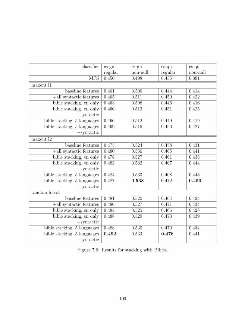
classifier es-gnregular

es-gnnon-null

es-quregular

es-qunon-null

MFS 0.456 0.498 0.435 0.391maxent l1

baseline features 0.461 0.506 0.444 0.414+all syntactic features 0.465 0.511 0.450 0.422bible stacking, en only 0.463 0.508 0.446 0.416bible stacking, en only

+syntactic0.466 0.513 0.451 0.425

bible stacking, 5 languages 0.466 0.512 0.449 0.419bible stacking, 5 languages

+syntactic0.469 0.516 0.453 0.427

maxent l2baseline features 0.475 0.524 0.458 0.431

+all syntactic features 0.480 0.530 0.465 0.441bible stacking, en only 0.478 0.527 0.461 0.435bible stacking, en only

+syntactic0.482 0.532 0.467 0.444

bible stacking, 5 languages 0.484 0.533 0.468 0.443bible stacking, 5 languages

+syntactic0.487 0.538 0.472 0.450

random forestbaseline features 0.481 0.520 0.464 0.424

+all syntactic features 0.486 0.527 0.471 0.434bible stacking, en only 0.484 0.525 0.466 0.428bible stacking, en only

+syntactic0.488 0.529 0.473 0.439

bible stacking, 5 languages 0.488 0.530 0.470 0.434bible stacking, 5 languages

+syntactic0.492 0.533 0.476 0.441

Figure 7.6: Results for stacking with Bibles.

109

classifier es-gnregular

es-gnnon-null

es-quregular

es-qunon-null

MFS 0.456 0.498 0.435 0.391maxent l1

baseline features 0.461 0.506 0.444 0.414+all syntactic features 0.465 0.511 0.450 0.422

both stacking, 5 languages 0.465 0.511 0.448 0.419both stacking, 5 languages

+syntactic0.468 0.516 0.452 0.426

maxent l2baseline features 0.475 0.524 0.458 0.431

+all syntactic features 0.480 0.530 0.465 0.441both stacking, 5 languages 0.484 0.533 0.469 0.444both stacking, 5 languages

+syntactic0.487 0.538 0.473 0.450

random forestbaseline features 0.481 0.520 0.464 0.424

+all syntactic features 0.486 0.527 0.471 0.434both stacking, 5 languages 0.489 0.530 0.471 0.434both stacking, 5 languages

+syntactic0.492 0.533 0.475 0.443

Figure 7.7: Results for stacking with Bibles.

110

7.7 Discussion

In this chapter we have described a straightforward approach for making use of supplemental

bitext corpora that pair our resource-rich source language with languages other than our

under-resourced target languages, adding annotations to our bitext corpus based on the

predictions of CL-WSD classifiers trained on these supplemental bitext corpora.

We see a small but consistent performance gains from this approach when we train

on corpora of a different domain (the Europarl corpora), and a larger gain when we train

on corpora that match the domain of our bitext for the under-resourced languages (our

multilingual Bibles). The gain from using the supplemental corpora with a close domain

match was roughly as large as that from adding syntactic annotations, described in the

previous chapter. Happily, we find that multilingual evidence and syntactic annotations can

be used together effectively; we can train the highest-performing CL-WSD classifiers in this

work so far by adding both sets of features.

In the next chapter, we will switch our focus to practical applications of CL-WSD and

the Chipa software, showing how it can be integrated into a sampling of MT systems of

different architectures, improving MT performance in practice.

111

CHAPTER 8

INTEGRATION INTO MACHINE TRANSLATION SYSTEMS

In this chapter, we demonstrate how our CL-WSD techniques can be integrated into run-

ning machine translation systems, with the goal of improving lexical selection in practice,

while minimizing code changes to the MT software. We translate from Spanish to Guarani

with Moses[106], an off-the-shelf phrase-based statistical MT system, and from Spanish to

Quechua with SQUOIA[107], a primarily rule-based MT system developed by Rios et al. at

the University of Zürich. These two integrations are meant to be simple proofs of concept,

rather than an attempt to define a best practice, but they demonstrate at least conceptually

how CL-WSD can be used with these kinds of translation systems. Afterwards, we look at

evaluating Chipa’s effect on MT output in both of these use cases.

A common thread in the MT settings addressed in this work is that there is a relatively

small amount of text available for training a target-side language model, so we should not

rely on the LM on its own for making contextually appropriate word choices. This problem

is especially significant for RBMT systems without weights built into their lexicons; many

translation options will be licensed for a given input word, and selecting the most appropriate

choice among them can be difficult. In SQUOIA, for example, there are some rules for lexical

selection, but they were written by hand and only cover a small subset of the system’s lexicon,

in a limited number of contexts.

The difficulty of resolving these ambiguities is mitigated for statistical machine transla-

tion systems for language pairs with substantial bitext corpora and target-language mono-

lingual corpora, as large n-gram language models and phrase tables containing common

multi-word expressions can encourage coherent word choices. However, for most language

pairs in the world, these resources are not readily available. As a result, many research

groups, especially those with backgrounds in Linguistics, have sought to build MT systems

112

based around rule-based approaches for under-resourced language pairs.

Given such a rule-based system, in cases where some training data is available, we can

investigate combining machine learning and rule-based approaches, resulting in hybrid MT

systems that can benefit from the small, but potentially growing resources for the relevant

language pair. These could include bitext corpora for the language pair, or with techniques

like the ones described in Chapters 6 and 7, monolingual resources such as source-language

corpora and NLP tools, or even bitext corpora pairing the source language with other target

languages. So adding trained CL-WSD classifiers to existing lexical selection rules can allow

these hybrid MT systems to make use of regularities that may not be obvious to human

rule-writers, providing lexical selection guidance for word types with sufficient coverage in

the training corpus.

With these additional classifiers, a primarily RBMT system can take advantage of sta-

tistical evidence without significantly changing its design, and gradually improve its word

choices as additional bitext or other resources become available. WSD techniques can also

be applied to statistical machine translation, as has been shown by, for example, Carpuat

et al. [29] and Tamchyna et al. [62]. In this chapter we demonstrate specifically how to add

the Chipa CL-WSD system to Moses, for a language pair with an under-resourced target

language.

Among other pieces of software related to this work, especially the corpus preparation

scripts, the code to integrate Chipa into these machine translation systems is bundled in a

package called Tereré 1.

8.1 Integrating Chipa into Phrase-Based Statistical Machine Translation

Moses2 is a mature, well-maintained and popular statistical machine translation package,

in broad use for both research and practical purposes. Like many SMT systems, Moses1Available at http://github.com/alexrudnick/terere ; Tereré is a cold variety of yerba mate brewed

with ice water; it is a specifically Paraguayan specialty.2Available at http://statmt.org/moses/

113

combines signals from different subcomponents when searching through the space of possible

translations for an input sentence. It does this using a log-linear model, in which each

component scores a candidate translation, and then the scores from the different components

are combined in a weighted sum. Some typical components are the probabilities learned for

a given phrase during phrase extraction (without regard to context) in both translation

directions, scores from the target-language language model, distortion models that reflect

estimated differences in word order between source and target languages, and a handful of

other features3.

Conveniently for our work here, Moses includes an interface for adding new feature func-

tions4 to be combined in the log-linear model, so we can add new information to help guide

the decoding process.

Scores in this framework are expected to represent log probabilities, meaning that, con-

cretely, they are real numbers less than 0, as the logarithm of a number between 0 and 1

will be negative. The decoder’s beam search procedure then attempts to maximize the total

score for a translation, which means finding a translation with a score as high as possible,

i.e., maximally close to 0.

During the search through the space of possible translations, Moses proposes candidate

translations for each source word to the Chipa feature function, and this function returns

a score based on how likely the translation seems to the CL-WSD system, considering the

source-language sentence context. This score is returned to Moses, which combines all of the

available features in a log-linear combination.

The weights for all of the features provided to the system (translation probabilities, LM

scores, CL-WSD scores, and perhaps others) are typically tuned on a development set with

Minimum Error-Rate Training, or “MERT” [59]; thus, if CL-WSD scores turn out to be

useful for achieving high BLEU scores on the development set sentences, Chipa’s feature3For an overview of techniques commonly used in phrase-based statistical MT, please see Koehn’s book

on the subject [49].4See http://www.statmt.org/moses/?n=Moses.FeatureFunctions for documentation.

114

function will be assigned more weight. If not, its advice will carry less weight than that of

more informative feature functions.

8.1.1 Interfacing between Moses and Chipa

The Moses decoder is written in C++, and the typical approach for adding new feature func-

tions is to write new C++ classes following the feature function interface. All of the feature

function classes are linked in with the decoder binary, and Moses users can configure their

SMT systems to use specific feature functions with a configuration file that references these

classes. However, the Chipa software is built in Python, so for simplicity of implementation

and to avoid having to add too many dependencies to Moses, we implemented a protocol for

communication between the Moses C++ code and the Chipa server, based on Unix pipes5;

see Figure 8.1 for a visual aid. Named Unix pipes, or FIFOs, allow the creation of a special

kind of filesystem object whereby messages can be passed between processes in the same

computer. Here Moses requests an evaluation for a certain translation of a source-language

phrase given the source-language sentence as context, and Chipa returns a score based on

how likely it considers that phrase, represented as a log probability.

Moses also allows for phrase tables to contain arbitrary annotations in their entries, and

one might ask whether it would be possible to avoid the trouble of implementing a new

feature function in C++, when we could simply add features to a translation of a phrase,

in the phrase table on disk. However, this misses the point of using our CL-WSD classifiers

– we want to know about which translation is most appropriate for a given source-language

phrase, in this context. We could imagine running our classifiers as a preprocessing step,

and simply producing a phrase table specific to each individual sentence that we want to

translate, but there could be multiple instances of a source phrase in a single input sentence.

So here we run our classifiers during decoding, using the current source sentence as context.

So concretely, during the search for a translation for an input sentence, the decoder5In earlier work with SQUOIA [3], we had communicated between Chipa and a machine translation

system with XML-RPC 6, but for simplicity of implementation, here we built a new text-based protocol.

115

Figure 8.1: Schematic diagram showing the relationship between the Moses decoder process,running the custom-made Chipa feature function, which communicates with the Chipa serverprocess. The Chipa server returns probability estimates for proposed target-language phrasesbased on the given source-sentence context, when available.

requests a score for each candidate phrase used to translate a source-language phrase. The

new Moses feature function then makes a call (over the FIFO communication channel) to

the Chipa server, which takes a string of tokenized surface-form Spanish as its input. The

Chipa server runs our standard text preprocessing pipeline for Spanish on demand, and then

trains a CL-WSD classifier for the lemma of the current focus token, unless a classifier has

already been trained for that lemma, in which case it is retrieved from memory. It then

extracts features and uses the CL-WSD classifier to estimate a probability distribution over

the possible translations for that focus word, given the current context. The Chipa server

passes back the log probability for the proposed translation for the current focus word.

For performance reasons, trained CL-WSD classifiers are kept in cache, as are the proba-

bility distributions for the translations of a given token in context. For focus words for which

we have no CL-WSD classifiers (i.e., they are not sufficiently supported in the training data,

or are considered stop words), the server returns a constant (log 0.5), and to avoid causing

search errors, probabilities are clipped to be in the range [0.01, 0.99]. Also, it should be noted

that Moses internally stores phrases using XML escaping, rather than the Unicode strings,

116

Guarani-language corpus sizeGuarani side of Bible bitext 27, 627 verses

All articles from gn.wikipedia.org 33, 894 sentences

Figure 8.2: Sizes of Guarani-language corpora for training the language model.

so the Chipa server must unescape these strings before working with them, and then pass

escaped strings back to Moses.

8.1.2 Moses SMT for Spanish-Guarani

We built a simple phrase-based SMT system with Moses and used the feature function API

mentioned previously to have Chipa score candidate translations. Our bitext, as with the

CL-WSD classifiers, was our Spanish-Guarani Bible corpus; specifically, we used the surface

forms for Spanish, but lemmas for the output Guarani. We sampled our development and

test sets from this bitext, taking 100 pairs of Bible verses for tuning, and 100 for testing.

For simplicity, we added a constraint to the Moses phrase-extraction system7 so that the

source side of all phrases must be at most one token long, to match the alignments used in

the previous chapters. Otherwise, we used the default settings for training a phrase-based

SMT system with Moses.

As is common practice with SMT systems, we trained our target-language model with

KenLM[108], based on both the target side of the bitext corpus, together with some mono-

lingual Guarani data, the text of the Guarani-language Wikipedia8. All input text for the

language model was preprocessed in the same way as our bitext, as described in Section 4.3,

and the language models were trained over lemmas, matching the target side of the bitext.

We tuned the decoder’s feature function weights with MERT, using the standard Moses

tuning scripts, over the sampled development set.

Experimental results for this MT system are discussed in Section 8.3.7Changes were made in phrase-extract/extract-main.cpp, for those familiar with the Moses codebase8Available at https://gn.wikipedia.org/ . Dumps of Wikimedia projects are available, in general, at

https://dumps.wikimedia.org/backup-index.html

117

8.2 Integrating Chipa into Rule-Based Machine Translation

8.2.1 The SQUOIA RBMT system

SQUOIA9 is a hybrid but primarily rule-based MT system, developed to translate Spanish

to Quechua10.

SQUOIA was developed by a team at the University of Zurich. For the most part, it is

a classical rule-based system, although the team has added machine learning techniques to

a few subcomponents, such as predicting verb morphology for cases when its rules cannot

reliably disambiguate [109]. It does not, by default, use machine learning for lexical selection

as such, although it does include a language model to help select among the translations

licensed by its transfer rules. Also its initial input analysis stages call open-source NLP

tools based on learned models. SQUOIA uses FreeLing [78] for morphological analysis and

named-entity recognition, Wapiti [110] for tagging, and DeSr [111] for parsing.

SQUOIA’s architecture is based on the Matxin system[112], which was originally intended

for translating from Spanish to Basque. It consists of a pipeline of smaller steps, each of

which passes along a tree describing the current input text and transformations that have

been applied to it, in XML form. As the steps progress, the input Spanish is analyzed

and gradually transformed into Quechua output. Many modules focus on very particular

aspects of the representation, leaving most of their input unchanged; for example, one phase

performs coreference resolution, and another phase uses rules to try to decide whether an

instance of the Spanish preposition de should be translated into Quechua as indicating the

ablative case (direction of motion), or the genitive case (possession). Please see Figure 8.3

for an overview of the most important steps in the SQUOIA pipeline.

In order to integrate Chipa CL-WSD into SQUOIA, we added an additional intermediate9Code available at https://github.com/a-rios/squoia ; the project is more broadly described at

https://www.cl.uzh.ch/en/research/machine-translation/hybridmt.html10Particularly the Cuzco dialect of Quechua, which is spoken around the Peruvian city of Cuzco. There

are many varieties of Quechua, as noted in Section 2.5, spoken across the Andes mountain range. SQUOIAalso supports translating Spanish to German.

118

step to the pipeline, occurring just after rule-based lexical disambiguation. This new module

reads the XML representation output by the previous step, extracts the original Spanish

input text from the intermediate representation, and finds lexical-selection ambiguities that

we can attempt to resolve with Chipa. These ambiguities are found where there are nodes

in the tree with several possible Quechua lemmas that could be chosen as a translation. It

then calls the Chipa CL-WSD classifiers to get an estimated probability distribution over

possible translations for that input focus word, in its particular context.

For each such node with such multiple translation possibilities, we look at each of the

translations under consideration by SQUOIA, and if any of them was the top classification

output from the Chipa classifiers, we constrain SQUOIA to take that choice by removing

the other available options. We could imagine other strategies for turning the output of the

Chipa classifiers into constraints on lexical selection here, such as removing lexical choices

that the classifier considers improbable, or enforcing that the MT system pick the available

choice with the highest score from the classifier, even if the one-best output from the classifier

was not under consideration. We did not experiment with other approaches here, only the

strategy in which, if the one-best output is an available choice, we take it.

A wrinkle to consider is that since Chipa classifiers for Spanish-Quechua use one-to-

many alignments, the classifier output can contain short Quechua phrases. Furthermore, the

classifiers are trained on the output of the AntiMorfo morphological analyzer for Quechua (see

Section 4.3.3 for details), so morphological ambiguities can make their way into the Chipa

output; this is represented by two or more lemmas adjoined with a slash. This happens, for

example, when multiple lemmas can plausibly inflect to the same surface form. However, the

SQUOIA bilingual lexicon contains specific lemmas; it means to pick a particular one, for a

specific meaning. In order to overcome both of these ontological mismatches, we consider a

candidate lemma to be a match if it is found anywhere in the Chipa output.

If there are no such overlapping translations, or if no Chipa classifier was available for

that word, we make no changes to the input tree, and allow SQUOIA to proceed as normal.

119

• Tokenization, morphological analysis, tagging, parsing.

• Disambiguating Spanish verbs with rules that match on contextual clues (low recall;the rules are manually crafted by linguists)

• Disambiguating Spanish verbs with an SVM classifier.

• Lexical lookup and transfer: insert all possible translations for every input token fromthe bilingual dictionary.

• Rule-based disambiguation, attempting to eliminate possible lexical-selection ambigu-ities and morphological choices. (similarly low coverage; it is not feasible for linguiststo write rules for all possible contexts for every word type in the lexicon)

• DISAMBIGUATION WITH CHIPA INSERTED HERE

• Syntactic transfer, building more Quechua-like syntactic structures (rule-based).

• Reordering based on new syntactic trees (rule-based).

• Use KenLM language models trained over Quechua words and morphemes to choosemost likely alternatives remaining.

• Morphological generation: produce Quechua surface forms with a finite state trans-ducer, output n-best list.

Figure 8.3: An overview of the steps in the SQUOIA MT system; there are a few more,handling specific circumstances and parts of speech.

Notably, since Chipa and SQUOIA do not share the same lexicon and bitext alignments may

be noisy, translations observed in the bitext may be unknown to the SQUOIA system, and

lexical entries in the SQUOIA dictionary may not be attested in the training data.

Having made any possible updates to the representation of our input sentences, we seri-

alize the current state to XML again, to pass the choices along to subsequent steps, which

complete the process of turning the input into Quechua output.

8.3 Translation Evaluation for Spanish-Guarani

In order to evaluate our phrase-based statistical machine translation system, with the in-

cluded CL-WSD classifiers, we sampled a test set from our bilingual Bible corpus, which,

120

setting BLEUMoses with Chipa enabled 16.24

Same system, with Chipa disabled 10.01

Figure 8.4: BLEU scores on our Spanish-Guarani test set. Note that this is translating tolemmatized Guarani, rather than having to predict fully-inflected forms.

like the development set, consists of 100 Bible verses. Verses are roughly sentence length,

and many in the corpus are complete sentences, but it is also common for verses to be part

of a longer sentence, or even to contain several sentences. For phrase-based SMT, this does

not require any particular changes to the system; the decoder simply tries to produce a

sequence of tokens and has no explicit concept of syntax. We tuned our Moses system on

the development set with Chipa enabled, and then for comparison, to see if the system was

getting useful information from CL-WSD, disabled the CL-WSD feature function.

For our experimental results here, we report BLEU scores for our lemmatized Guarani

output, compared with the lemmatized target side of the test set. See Figure 8.4 for a table

of the BLEU scores. Here we see that the system learned to rely on the output of Chipa

for useful guidance; when running with the same MERT-tuned weights, but the CL-WSD

classifiers disabled, we get a BLEU score drop of roughly six points. The presence or ab-

sence of guidance from Chipa changes our translation output significantly here – we produce

different output in 97 of the 100 test verses, across these two settings. For comparison,

we additionally tried tuning the same Moses system with the Chipa feature function dis-

abled, but found that the variance among BLEU scores for runs of this experiment was quite

high11, so comparison with our results for the tuned system with Chipa enabled do not seem

particularly illuminating.11This is due to the MERT search procedure starting at different, randomly-chosen points in the space of

weight assignments; the phenomenon is sometimes called “MERT noise” informally.

121

8.4 Translation Evaluation for Spanish-Quechua

In order to evaluate the effect of Chipa on lexical selection in a live translation task, we used

SQUOIA to translate a hundred verses sampled from our Spanish-Quechua Bible bitext, both

in its default settings, and with the addition of Chipa. The addition of SQUOIA resulted in

lexical selection changes for the SQUOIA output for 41 of the 100 verses translated; there

were 15 more changes only in order or punctuation (for a total of 56 sentences that differed

in some way), but the majority were local differences in word choice.

The BLEU scores for SQUOIA output on this test set were quite low (lower than one

BLEU point), and were not improved by adding Chipa’s CL-WSD. But this is a rather

more difficult task than our Spanish-Guarani setting, since we are attempting to generate

fully-inflected Quechua surface forms, rather than selecting appropriate lemmas, and BLEU

scoring requires us to match n-grams exactly, which is made less likely by the rich morphology,

including evidential markers, of Quechua. Additionally, as Rios notes [107, §5.9], translations

into Quechua tend to be fairly free, rather than close analogues of the source Spanish.

In any case, for evaluation, here we show examples of word choices that were changed

with the addition of Chipa CL-WSD, and, armed with our Spanish-Quechua dictionary[4],

determine whether they are more or less appropriate than the choices that the SQUOIA

system would have made on its own12. For some examples chosen from the sampled test

set, see Figure 8.6. Counts of how many changes were judged by a non-expert reader to be

improvements, neutral or unclear, or worse than the output without Chipa, are presented in

Figure 8.5.

One pattern that we find among the changed output is that Chipa tends to encourage

SQUOIA to choose churi (a son, when discussed with regard to his father) rather than the

more generic wawa, which can refer to any child; for most of the test sentences where we

saw this change happen, it seemed like an appropriate choice. For example, in Sentence 6,12Specifically, in this case, by “we”, we mean the author, a native English speaker who can read and speak

Spanish but not Quechua.

122

Total verses with lexical changes 41 (out of 100)Number of changes judged to be improvements 12

Number of changes judged to be neutral or unclear 22Number of changes judged to be worse 7

Figure 8.5: Evaluation by hand (by a non-Quechua-speaking author using a dictionary) ofthe changes to the Spanish-Quechua MT output with SQUOIA.

we are referring to a son of a particular man, so this seems like a good choice.

We see when translating Sentence 7 from Spanish to Quechua, without Chipa, SQUOIA

translates l lamando (’calling’) to sutikuspa, where suti is the sense of “llamar” that refers to

naming. However, with Chipa, SQUOIA picks waqyaspa, where waqyay is the communicative

sense, rather than the naming sense.

Many changes caused by Chipa seem to be different choices among near synonyms. For

example, in Sentence 8, without Chipa, we translate ardiente as k’anaq, which seems to be

a good translation, meaning “glowing, ardently burning”. With Chipa, it becomes ’yawraq’

’burning, glowing’. And one difference revealed an ambiguity in Spanish that is clearly

distinguished in Quechua: in Sentence 9, without Chipa, we translate labios ’lips’ as an

inflection of wirp’a, which apparently only refers to the lower lip; with Chipa, we choose an

inflection of sirphi, which seems to refer to only the upper lip 13.

We note in Sentence 10 a serious word-sense issue that Chipa did not manage to fix; in

both cases, SQUOIA failed to interpret llama as ’flame’14; this seems to be a cascading error

from part-of-speech tagging, as SQUOIA’s bundled tagger marked it as a verb. In any case,

without Chipa, we choose an inflection of waqya, which is the ’call out’ sense of llamar, and

with Chipa, we choose an inflection of suti, the ’naming’ sense. Neither of these are correct.13Also, more modern English translations seem to choose something like “innermost being” rather than

referring to one’s innards, but the King James Version uses the term “reins”, which apparently historicallyreferred to the kidneys.

14The Spanish token l lama can be an inflection of the verb llamar ’to call’, or as a noun, ’flame’, or ofcourse it can refer to llama the animal, which is a loan word from Quechua.

123

(6) Jehová dijo a Moisés: – Toma a Josué hijo de Nun, hombre en el cual hay espíritu, ypon tu mano sobre él. “Jehovah said to Moses: - Take Joshua son of Nun, man inwhom there is spirit, and put your hand on him.”, Numbers 27:18

(7) Pilato se sorprendió de que ya hubiera muerto, y llamando al centurión, le preguntó siya estaba muerto. “Pilate was surprised to hear that he had already died, and callingthe centurion, asked him if he was already dead.”, Mark 15:44

(8) Y cualquiera que no se postre y adore, inmediatamente será echado dentro de un hornode fuego ardiente. “And whoever does not fall down and worship will immediately bethrown into a blazing furnace.”, Daniel 3:6

(9) Y mis entrañas también se alegrarán cuando tus labios hablen con rectitud. “And myinnermost being will also rejoice when your lips speak with rectitude.”, Proverbs 23:16

(10) Por tanto, como la lengua del fuego consume el rastrojo y la llama devora la paja, asíserá su raíz como podredumbre y su flor se desvanecerá como polvo, porque desecharonla ley de Jehová de los ejércitos y abominaron la palabra del Santo de Israel. “Therefore,as a tongue of fire consumes straw and dry grass shrivels in the flame, so their roots willdecay and their blossoms will blow away like dust; for they have rejected the instructionof the Lord of Hosts and despised the word of the Holy One of Israel.”, Isaiah 5:24

Figure 8.6: Selected Spanish passages for which adding Chipa generated different Quechuatranslations.

124

8.5 Discussion

In this chapter we have demonstrated approaches for integrating our CL-WSD classifiers into

two different MT systems of completely different styles and architectures. First, we added

Chipa to Moses, a phrase-based statistical MT system, by adding an additional feature

function to the decoder’s log-linear model. Secondly, we integrated Chipa into SQUOIA, a

primarily rule-based hybrid MT system developed by computational linguists for an under-

resourced language pair. This second integration acts by making concrete lexical selection

choices in cases where the rule-based lexical selection routines have not made a firm decision,

but we have an available CL-WSD classifier.

Both of these integrations provide a proof-of-concept for how to integrate our CL-WSD

approaches into running MT systems, without changing the overall architecture of these

systems, and with very modest changes to their code. These integrations allow the MT

systems more ways to benefit from our available bilingual and monolingual resources, and

can result in better lexical selection, or at least provide a means to adapt an existing system

to a different domain.

In the final chapter, we will summarize the contributions of this work overall and discuss

some possible future directions.

125

CHAPTER 9

SUMMARY AND OUTLOOK

In this work, I have developed approaches for cross-lingual word sense disambiguation in the

setting where we are translating from a resource-rich language into an under-resourced one,

and implemented these approaches in running software. I have shown how cross-lingual word

sense disambiguation can be applied to lexical selection in hybrid machine translation for

language pairs with relatively modest resources, particularly when translating from Spanish

to two different indigenous languages of South America, Guarani and Quechua.

In the initial three chapters, we describe CL-WSD and situate it among efforts to integrate

word-sense disambiguation over the history of work on machine translation. In Chapter 1, we

explain how word-sense disambiguation is relevant to translation and lay out the structure

of the rest of the work.

In Chapter 2, we provide a broad overview of the field of word-sense disambiguation,

considering some framings for WSD that have been applied in the past, and the difficulties

that these framings cause when our goal is to support MT, or to process arbitrary running

text more generally. We explain how the CL-WSD framing overcomes two major difficulties

in applying WSD to machine translation in practice. Firstly, CL-WSD provides a concrete

sense inventory for lexical items in the source language, since we consider the senses of a

word to be its possible translations, and secondly, it provides a source of labeled training data

in the form of any available bitext, thus allowing us to apply supervised machine learning

techniques. Also in this chapter, we briefly describe Guarani and Quechua, two of the largest

indigenous languages in the Americas, and explain some motivations for building hybrid rule-

based and statistical MT systems to support them: for most of the world’s language pairs,

there are no large bitext corpora available, so using rule-based components may provide

a useful starting point for NLP systems, especially where there are well-known linguistic

126

regularities, such as morphology and syntax.

Chapter 3 covers some of the relevant related work, including some of the work most sim-

ilar to ours. Especially notable are the ParaSense work by Els Lefever [26], which pioneered

the use of multilingual corpora to support CL-WSD, and the development of learned lexical

selection models for Apertium, a mostly rule-based MT system, by Francis Tyers [47].

Having described relevant context and background information, in Chapter 4, we describe

the evaluation settings for our CL-WSD systems, as well as the available data sets for our

language pairs, and describe in detail the preprocessing steps that allow us to take sentence-

or verse-aligned bitext and produce training data suitable for training our classifiers. For

our in vitro evaluation setting, we can report classifier accuracy, or report benchmarks based

on shared tasks like the 2010 and 2013 SemEval CL-WSD tasks. For in vivo evaluation, we

want to look at the downstream task, and see how the addition of our CL-WSD approaches

contributes to machine translation quality, either through automatic metrics like BLEU, or

by examining MT output by hand.

We described, in Chapter 5, an initial version of the Chipa software based on common

text classification features – the tokens of the input text, their lemmas, and then also the

token and lemmas in a small context window around the focus word – and showed how it

outperforms the relatively strong most-frequent sense baseline. We compared a few differ-

ent machine learning algorithms on this task, and found that we got the best results with

either random forests or logistic regression classifiers, with L2 regularization, and this held

consistently, across language pairs. We also compared Chipa to other systems presented at

recent SemEval events for CL-WSD on the task of translating from English to other Euro-

pean languages, using considerably more training data. By applying Chipa to both of these

tasks, we showed that this initial approach is a fairly strong starting point, comparable with

CL-WSD systems developed by other research groups, and that it can be used in multiple

settings fairly successfully.

In Chapter 6, we extended our initial approach with strategies that make use of the avail-

127

able resources for Spanish, including NLP tools for analyzing Spanish text and unsupervised

learning techniques that allow us to learn representations for our classifiers from the wealth

of available unannotated Spanish text. We showed how to extract features based on syntac-

tic analyses of the input text, done with a POS tagger and a dependency parser, and how

adding these features provided modest, but very consistent, accuracy improvements. We

also showed some gains, especially when using random forest classifiers, by adding features

based on Brown clusters trained on larger samples of monolingual Spanish text. The best

results in the chapter came from adding these syntactic and Brown clustering features to

the baseline sparse feature set.

We also showed that we could use dense vector representations, built with word2vec and

doc2vec trained on available monolingual Spanish text, with moderate success. However,

these did not outperform the baseline sparse features for our task, at least not with the

data sets and machine learning techniques used in this work; particularly, our random forest

classifiers saw accuracy drops when using these features. We learned that when using these

dense representations, it is better to focus on the text immediately surrounding the focus

word, either by limiting the context window or by giving more weight to words close to the

focus word. Trying to build a doc2vec representation of the entire input text, or summing

the word embeddings uniformly across the text was less effective. Also, we found that it

was possible to combine the dense representations based on word embedding vectors with

the sparse features from syntactic analysis and Brown clustering, and that this gave us

performance boosts over using the dense features alone.

In Chapter 7, we showed how to use Chipa for classifier stacking, which allows us to learn

from bitext corpora that pair our source language with languages other than our intended

target language; this technique is broadly applicable when we want to translate out of a

language with many available bitext resources, and could also be applied when we have a

good monolingual WSD system available. Here we trained CL-WSD classifiers on both Bible

translations, which are available for many languages and directly match the domain of our

128

Spanish-Guarani and Spanish-Quechua corpora, and also Europarl bitext corpora, which are

much larger, at roughly 1.8 million sentence pairs. We showed that we are able to get some

gains by adding features based on the output of the Europarl-trained CL-WSD classifiers,

but larger gains when adding the output of the in-domain classifiers. Furthermore, the gains

are larger when adding classifier output for five different language pairs, rather than relying

on just Spanish-English CL-WSD, and these classifier stacking features work alongside the

syntactic features discussed in Chapter 6; our best results came from using them in tandem.

Finally, in Chapter 8, we demonstrated prototypes for integrating our CL-WSD classifiers

into existing machine translation systems of two completely different architectures, requiring

only small changes to existing code. We presented a phrase-based SMT system for Spanish-

Guarani1 that uses Chipa classifiers in a feature function that guides its decoding process. For

Spanish-Quechua, we augmented a primarily rule-based hybrid machine translation system,

using our classifiers to supplement the existing hand-written lexical selection rules. This first

integration shows how CL-WSD techniques can reasonably be applied to phrase-based SMT

even in relatively low-data scenarios2, when translating between two unrelated languages,

and the second is a proof-of-concept for how to add a CL-WSD into an existing rule-based

MT system, allowing it to learn from any available bitext, with increasing benefits as more

bitext is collected in the future

One interesting difficulty that came up, and is particularly relevant for MT systems

that deal with morphologically rich languages, is the potential for mismatches between the

different inventories of lemmas known to the interacting NLP systems; this is to say, the

recommendations made by the CL-WSD system must be, for the most part, lexical selections

that the MT system can make. Thankfully, for the most part the Chipa CL-WSD system

and SQUOIA have a large overlap in their inventories of Quechua citation forms, but this

need not be the case, and some care must be taken. For our integration of Chipa into

the Spanish-Guarani phrase-based SMT system, this difficulty was largely avoided, because1Ignoring, for the moment, the admittedly substantial problem of morphological generation.2There is prior work on using CL-WSD for SMT; see Section 3.4.

129

the lexical entries were all based on the output of the same morphological analyzers. In

both cases, we showed some modest improvements to MT output on a small test set, using

automatic metrics for Spanish-Guarani and manual evaluation for Spanish-Quechua.

9.1 Applying techniques like this to neural machine translation

During the course of this work, the field of machine translation has undergone a dramatic

shift, in which statistical MT research, and in many cases, practice[113], has moved from

phrase-based and tree-based SMT systems to models based on recurrent neural networks.

It may not be immediately useful to add explicit CL-WSD classifiers to a neural MT ar-

chitecture, although this is an empirical question. In a sense, though, we can say that NMT

systems are already performing CL-WSD; they have a vector representation of the whole

input sentence available while making output decisions, tuned specifically for the translation

task. This vector representation is similar to the doc2vec representations discussed in Chap-

ter 6, but uses deeper, and recurrent, networks. The sentence-encoding process in neural

machine translation thus automates much of the feature engineering work that would go into

building a CL-WSD system.

However, many of the difficulties addressed in this work still apply in the neural machine

translation setting. We still must come up with good ways to leverage the available corpora

and tools for resource-rich source languages, when we have little available bitext. Can source-

language taggers and parsers be integrated with NMT? Will this help when translating

into under-resourced languages? How can other existing NLP tools be applied, such as

monolingual WSD?

In our CL-WSD setting, we did not find immediate benefits when using neural embed-

dings based on comparatively large source-language corpora. How can monolingual source-

language resources be used for NMT, when only very small bitext corpora are available?

There has been some recent work, including by Johnson et al. [114], on training multilin-

gual neural machine translation systems that learn to share representations among different

130

translation tasks; these systems can even perform “zero shot” translation, in which a single

network trained to translate from, e.g., Portuguese to English and English to Spanish can

also translate reasonably well from Portuguese to Spanish. Additionally, there has been

work, such as that of Artetxe et al. [115] and Lample et al. [116], that creatively uses

back-translation and adversarial networks to make up for the lack of bitext for some lan-

guage pairs, but to my knowledge this has not yet been practically applied to translating

into under-resourced languages. Broadly, there do not yet seem to be widely-accepted ap-

proaches for leveraging existing resources to improve neural translation into under-resourced

languages, but neural machine translation is still in its early stages and the field is developing

rapidly.

Hopefully we will see effective strategies for making use of what we do have for building

NMT systems targeting under-represented and under-resourced languages in the near future.

9.2 Building resources for Guarani and other under-represented languages

While we have explored techniques in this work that allow us to lean somewhat on the

resources available for resource-rich source languages, a clear way to improve translation

for currently under-resourced languages is to make them less under-resourced. Languages

like Guarani and Quechua have a number of speakers comparable with that of some rela-

tively resource-rich European languages, as well as their own engaged activist communities.

Ethnologue, for example, reports3 that there are about six million Guarani speakers in the

world, which is more than the number of Danish or Norwegian speakers. To support these

languages and better serve these communities, we can as technologists find better ways to

work with the speakers of these languages.

While this work has focused on languages spoken in South America, there are under-

represented languages around the world with millions or possibly many millions of speakers,

but relatively little text on the web thus far, and no easily available MT or other NLP3https://www.ethnologue.com/language/grn

131

tools. Many languages in India and Southeast Asia are quite large by number of speakers,

but nonetheless dramatically under-resourced. However, Internet usage is spreading quickly

throughout the world, and the speakers of these languages are coming online; we are pre-

sented with great opportunities to build great linguistic resources and NLP tools for these

languages.

There have already been fairly successful campaigns by technologists to work with speak-

ers of these languages on resource-gathering projects for them. For example, in 2016, Mozilla

Paraguay managed to localize the Firefox web browser for Guarani, with the help of Guarani-

speaking volunteers, a local university, and Guarani-language activists4. Localizing an ap-

plication as complex as a web browser is an enormous task, requiring the translation of

thousands of sentence-length messages, along with the in-browser documentation. Also no-

tably, this task requires choosing appropriate Guarani-language terms for technical concepts.

As a success story directly pertinent to machine translation, in 2013, Google ran a crowd-

sourcing campaign in New Zealand that managed to collect enough training data to build

a phrase-based SMT system for the Māori language5; since then, Google Translate has op-

erated a crowdsourcing platform called Google Translate Community6, on which volunteers

can rate and submit translations, including for some languages that are not currently sup-

ported by the main Google Translate product. For languages that are already supported by

Google Translate, the submissions and ratings are used to improve MT output.

Our research group has started some efforts along these lines, but a more sustained

effort will be needed to provide benefits for language communities in practice. We (the au-

thor, working together with Alberto Samaniego and Taylor Skidmore, directed by Michael

Gasser) prototyped two websites for collecting Guarani and Spanish-Guarani language re-

sources, but these have not been used beyond the prototype stage. The first website is called4See a description of the process, and the launch announcement, at http://mozillanativo.org/2016/

lanzamiento-oficial-de-firefox-en-guarani.html (in Spanish). Firefox in Guarani can be downloadedat https://www.mozilla.org/gn/firefox/

5Post on the Google New Zealand blog: https://newzealand.googleblog.com/2013/12/kua-puta-google-whakamaori-ki-te-reo.html

6https://translate.google.com/community

132

“Tahekami”, which means let’s search together in Guarani. Tahekami7 is a repository of

Guarani and bilingual documents that allows full-text search and browsing documents by

tag. Our initial version of the site contained a collection of masters theses from the Ateneo

de Lengua y Cultura Guaraní. We developed a second website, called “Guampa” 8, which

is a bilingual wiki, designed to be used by Guarani speakers and learners to collaboratively

translate documents from Spanish to Guarani or vice-versa. We presented an initial ver-

sion of this software at LREC 2014[10]. This site is meant to serve at least three purposes:

helping Guarani-language learners practice and get feedback on their translations, creating

more Guarani-language documents for the web (we started initially with translating Spanish

Wikipedia), and building bitext corpora for training MT systems.

Michael Gasser is currently, as of 2018, developing successors to these websites, in the

form of mitmita and mainumby, online computer-aided translation systems for Amharic

and Guarani respectively9. The goal of these tools is to help users translate documents

by providing both searches over translation memories and automatic suggestions from an

integrated machine translation system.

In any case, while there remains much work to be done — both technical and social —

for supporting the under-represented languages of the world, it is outside the scope of this

dissertation, and will be addressed in the future, hopefully in part by the author.

7Prototype code at http://github.com/hltdi/gn-documents8A “guampa”, in Paraguay, is the cup from which one drinks yerba mate or tereré. The term “guampa” is

also local to Paraguay; in other parts of South America, the container itself is called a “mate”. The Guampasoftware is available at https://github.com/hltdi/guampa

9Code for these sites is being developed at https://github.com/hltdi/mitmita and https://github.com/hltdi/mainumby

133

REFERENCES

[1] Ryan Buchanan Allen. “Visions of Unity: Philosophical Realism in Late Fourteenth-

Century English Dream-Vision Poetry”. PhD thesis. University of Toronto, 2017.

[2] M. Minsky. Society Of Mind. Touchstone book. Simon & Schuster, 1988. isbn: 9780671657130.

[3] Alex Rudnick, Annette Rios, and Michael Gasser. “Enhancing a Rule-Based MT

System with Cross-Lingual WSD”. In: The 9th International Workshop of the Special

Interest Group on Speech and Language Technology for Minority Languages (SaLTMiL

2014). 2012.

[4] Academia Mayor de La Lengua Quechua. Diccionario: Quechua - Español - Quechua,

Qheswa - Español - Qheswa: Simi Taqe, 2da ed. Cusco, Perú, 2005.

[5] Philip Resnik, Mari Broman Olsen, and Mona T. Diab. “The Bible as a Parallel

Corpus: Annotating the ’Book of 2000 Tongues’”. In: Computers and the Humanities

33.1-2 (1999), pp. 129–153.

[6] Thomas Mayer and Michael Cysouw. “Creating a massively parallel Bible corpus”.

In: Proceedings of the Ninth International Conference on Language Resources and

Evaluation (LREC’14). Ed. by Nicoletta Calzolari et al. ACL Anthology Identifier:

L14-1215. Reykjavik, Iceland: European Language Resources Association (ELRA),

2014, pp. 3158–3163. isbn: 978-2-9517408-8-4.

[7] Alex Rudnick. “Towards Cross-Language Word Sense Disambiguation for Quechua”.

In: Proceedings of the Second Student Research Workshop associated with RANLP

2011. Hissar, Bulgaria: RANLP 2011 Organising Committee, 2011, pp. 133–138.

[8] Alex Rudnick, Can Liu, and Michael Gasser. “HLTDI: CL-WSD Using Markov Ran-

dom Fields for SemEval-2013 Task 10”. In: Second Joint Conference on Lexical and

134

Computational Semantics (*SEM), Volume 2: Proceedings of the Seventh Interna-

tional Workshop on Semantic Evaluation (SemEval 2013). 2013.

[9] Alex Rudnick and Michael Gasser. “Lexical Selection for Hybrid MT with Sequence

Labeling”. In: Proceedings of the Second Workshop on Hybrid Approaches to Transla-

tion. Sofia, Bulgaria: Association for Computational Linguistics, 2013, pp. 102–108.

[10] Alex Rudnick et al. “Guampa: a Toolkit for Collaborative Translation”. In: Proceed-

ings of the Ninth International Conference on Language Resources and Evaluation

(LREC’14). Ed. by Nicoletta Calzolari (Conference Chair) et al. Reykjavik, Iceland:

European Language Resources Association (ELRA), 2014. isbn: 978-2-9517408-8-4.

[11] George A. Miller. “WordNet: A Lexical Database for English”. In: Commun. ACM

38.11 (1995), pp. 39–41.

[12] Eneko Agirre and Philip Glenny Edmonds. Word Sense Disambiguation: Algorithms

and Applications. Vol. 33. Springer Science+ Business Media, 2006.

[13] Claudia Leacock, Geoffrey Towell, and Ellen Voorhees. “Corpus-based Statistical

Sense Resolution”. In: Proceedings of the Workshop on Human Language Technology.

HLT ’93. Princeton, New Jersey: Association for Computational Linguistics, 1993,

pp. 260–265. isbn: 1-55860-324-7.

[14] Claudia Leacock, George A Miller, and Martin Chodorow. “Using corpus statistics

and WordNet relations for sense identification”. In: Computational Linguistics 24.1

(1998), pp. 147–165.

[15] Adam Kilgarriff. “SENSEVAL: An Exercise in Evaluating Word Sense Disambigua-

tion Programs”. In: Proceedings of the First International Conference on Language

Resources and Evaluation (LREC’98). 1998, pp. 581–588.

[16] Philip Edmonds and Scott Cotton. “SENSEVAL-2: Overview”. In: Proceedings of

SENSEVAL-2 Second International Workshop on Evaluating Word Sense Disam-

135

biguation Systems. Toulouse, France: Association for Computational Linguistics, 2001,

pp. 1–5.

[17] Rada Mihalcea, Timothy Chklovski, and Adam Kilgarriff. “The Senseval-3 English

lexical sample task”. In: Senseval-3: Third International Workshop on the Evaluation

of Systems for the Semantic Analysis of Text. Ed. by Rada Mihalcea and Phil Ed-

monds. Barcelona, Spain: Association for Computational Linguistics, 2004, pp. 25–

28.

[18] Rebecca J Passonneau et al. “The MASC word sense sentence corpus”. In: Proceedings

of LREC. 2012.

[19] George A. Miller et al. “A Semantic Concordance”. In: Proceedings of the Workshop

on Human Language Technology. HLT ’93. Princeton, New Jersey: Association for

Computational Linguistics, 1993, pp. 303–308. isbn: 1-55860-324-7.

[20] Shari Landes, Claudia Leacock, and Randee I Tengi. “Building Semantic Concor-

dances”. In: WordNet: An Electronic Lexical Database. 1998, pp. 199–216.

[21] Michael Lesk. “Automatic sense disambiguation using machine readable dictionaries:

how to tell a pine cone from an ice cream cone.” In: Proceedings of the 5th Annual

International Conference on Systems Documentation, SIGDOC ’86. New York, NY:

ACM, 1986, pp. 24–26.

[22] Andrea Moro, Alessandro Raganato, and Roberto Navigli. “Entity Linking meets

Word Sense Disambiguation: A Unified Approach”. In: Transactions of the Association

for Computational Linguistics 2 (2014).

[23] John Hutchins. ““The whiskey was invisible”, or persistent myths of MT”. In: MT

News International 11 (1995), pp. 17–18.

[24] Warren Weaver. “Translation”. In: (1949).

[25] Yehoshua Bar-Hillel. “The Present Status of Automatic Translation of Languages”.

In: 1960.

136

[26] Els Lefever, Véronique Hoste, and Martine De Cock. “ParaSense or How to Use Par-

allel Corpora for Word Sense Disambiguation”. In: Proceedings of the 49th Annual

Meeting of the Association for Computational Linguistics: Human Language Tech-

nologies. Portland, Oregon, USA: Association for Computational Linguistics, 2011,

pp. 317–322.

[27] William A Gale, Kenneth W Church, and David Yarowsky. “A method for disam-

biguating word senses in a large corpus”. In: Computers and the Humanities 26.5-6

(1992), pp. 415–439.

[28] Peter F. Brown et al. “Word-Sense Disambiguation Using Statistical Methods”. In:

Proceedings of the 29th Annual Meeting of the Association for Computational Lin-

guistics. 1991, pp. 264–270.

[29] Marine Carpuat and Dekai Wu. “How Phrase Sense Disambiguation Outperforms

Word Sense Disambiguation for Statistical Machine Translation”. In: 11th Conference

on Theoretical and Methodological Issues in Machine Translation. 2007.

[30] Zdeněk Žabokrtský, Martin Popel, and David Mareček. “Maximum Entropy Transla-

tion Model in Dependency-Based MT Framework”. In: Proceedings of the Joint Fifth

Workshop on Statistical Machine Translation and MetricsMATR. Uppsala, Sweden:

Association for Computational Linguistics, 2010, pp. 201–206.

[31] Els Lefever and Véronique Hoste. “SemEval-2010 Task 3: Cross-Lingual Word Sense

Disambiguation”. In: Proceedings of the 5th International Workshop on Semantic Eval-

uation. Uppsala, Sweden: Association for Computational Linguistics, 2010, pp. 15–

20.

[32] Els Lefever and Véronique Hoste. “SemEval-2013 Task 10: Cross-Lingual Word Sense

Disambiguation”. In: Proceedings of the 7th International Workshop on Semantic

Evaluation (SemEval 2013). Atlanta, USA, 2013.

137

[33] Maarten van Gompel et al. “SemEval 2014 Task 5 - L2 Writing Assistant”. In: Pro-

ceedings of the 8th International Workshop on Semantic Evaluation (SemEval 2014).

Dublin, Ireland: Association for Computational Linguistics and Dublin City Univer-

sity, 2014, pp. 36–44.

[34] Asifa Majid et al. “The semantic categories of cutting and breaking events: A crosslin-

guistic perspective”. In: Cognitive Linguistics 18.2 (2007), pp. 133–152.

[35] Daniel Jurafsky and James H. Martin. Speech and Language Processing: An Introduc-

tion to Natural Language Processing, Computational Linguistics, and Speech Recogni-

tion. 1st. Upper Saddle River, NJ, USA: Prentice Hall PTR, 2000. isbn: 0130950696.

[36] W.J. Hutchins and H.L. Somers. An introduction to machine translation. Academic

Press, 1992. isbn: 9780123628305.

[37] Michael Collins, Philipp Koehn, and Ivona Kucerova. “Clause Restructuring for Sta-

tistical Machine Translation”. In: Proceedings of the 43rd Annual Meeting of the Asso-

ciation for Computational Linguistics (ACL’05). Ann Arbor, Michigan: Association

for Computational Linguistics, 2005, pp. 531–540.

[38] Annette Rios, Anne Göhring, and Martin Volk. “A Quechua–Spanish parallel tree-

bank”. In: Proceedings of 7th Workshop on Treebanks and Linguistic Theories (TLT-

7), Groningen. 2009.

[39] Serafín M. Coronel-Molina. Quechua Phrasebook. Lonely Planet Phrasebook Guides.

Lonely Planet, 2002. isbn: 9781864503814.

[40] Antonio Molina, Ferran Pla, and Encarna Segarra. “A Hidden Markov Model Ap-

proach to Word Sense Disambiguation”. In: IBERAMIA. 2002.

[41] Antonio Molina, Ferran Pla, and Encarna Segarra. “WSD system based on special-

ized Hidden Markov Model (upv-shmm-eaw)”. In: Senseval-3: Third International

Workshop on the Evaluation of Systems for the Semantic Analysis of Text. Ed. by

138

Rada Mihalcea and Phil Edmonds. Barcelona, Spain: Association for Computational

Linguistics, 2004, pp. 171–174.

[42] Massimiliano Ciaramita and Yasemin Altun. “Broad-Coverage Sense Disambiguation

and Information Extraction with a Supersense Sequence Tagger”. In: Proceedings of

the 2006 Conference on Empirical Methods in Natural Language Processing. Sydney,

Australia: Association for Computational Linguistics, 2006, pp. 594–602.

[43] Michael Collins. “Discriminative Training Methods for Hidden Markov Models: The-

ory and Experiments with Perceptron Algorithms”. In: Proceedings of the 2002 Con-

ference on Empirical Methods in Natural Language Processing. Association for Com-

putational Linguistics, 2002, pp. 1–8.

[44] Andrea Moro, Alessandro Raganato, and Roberto Navigli. “Entity Linking meets

Word Sense Disambiguation: a Unified Approach”. In: TACL 2 (2014), pp. 231–244.

[45] Eckhard Bick. “Dan2eng: Wide-Coverage Danish-English Machine Translation”. In:

Machine Translation Summit XI. 2007, pp. 37–43.

[46] Martha Dís Brandt et al. “Apertium-IceNLP: A rule-based Icelandic to English ma-

chine translation system”. In: The 15th Annual Conference of the European Associa-

tion for Machine Translation. 2011.

[47] F. M. Tyers. “Feasible lexical selection for rule-based machine translation”. PhD the-

sis. Departament de Llenguatges i Sistemes Infomàtics, Universitat d’Alacant, 2013.

[48] F. M. Tyers, F. Sánchez-Martínez, and M. L. Forcada. “Flexible finite-state lexi-

cal selection for rule-based machine translation”. In: Proceedings of the 17th Annual

Conference of the European Association of Machine Translation, EAMT12. 2012.

[49] Philipp Koehn. Statistical Machine Translation. Cambridge University Press, 2010.

isbn: 9780521874151.

139

[50] Adam L. Berger et al. “The Candide System for Machine Translation”. In: Proceed-

ings of the Workshop on Human Language Technology. HLT ’94. Plainsboro, NJ:

Association for Computational Linguistics, 1994, pp. 157–162. isbn: 1-55860-357-3.

[51] Philipp Koehn, Franz Josef Och, and Daniel Marcu. “Statistical phrase-based trans-

lation”. In: Proceedings of the 2003 Conference of the North American Chapter of the

Association for Computational Linguistics on Human Language Technology-Volume

1. Association for Computational Linguistics. 2003, pp. 48–54.

[52] Clara Cabezas and Philip Resnik. Using WSD Techniques for Lexical Selection in

Statistical Machine Translation. Tech. rep. CS-TR-4736/LAMP-TR-124/UMIACS-

TR-2005-42. DTIC Document, 2005.

[53] Marine Carpuat and Dekai Wu. “Word Sense Disambiguation vs. Statistical Ma-

chine Translation”. In: Proceedings of the 43rd Annual Meeting of the Association for

Computational Linguistics (ACL’05). Ann Arbor, Michigan: Association for Compu-

tational Linguistics, 2005, pp. 387–394.

[54] David Vickrey et al. “Word-Sense Disambiguation for Machine Translation”. In: Pro-

ceedings of Human Language Technology Conference and Conference on Empirical

Methods in Natural Language Processing. Vancouver, British Columbia, Canada: As-

sociation for Computational Linguistics, 2005, pp. 771–778.

[55] Marine Carpuat and Dekai Wu. “Improving Statistical Machine Translation Using

Word Sense Disambiguation”. In: Proceedings of the 2007 Joint Conference on Em-

pirical Methods in Natural Language Processing and Computational Natural Language

Learning (EMNLP-CoNLL). 2007, pp. 61–72.

[56] Marine Carpuat and Dekai Wu. “Evaluation of context-dependent phrasal transla-

tion lexicons for statistical machine translation”. In: 6th International Conference on

Language Resources and Evaluation (LREC). Marrakech (2008).

140

[57] Marine Carpuat and Dekai Wu. “Improving Statistical Machine Translation using

Word Sense Disambiguation”. In: Proceedings of the 2007 Joint Conference on Em-

pirical Methods in Natural Language Processing and Computational Natural Language

Learning. Prague: ACL, 2007.

[58] Kevin Gimpel and Noah A. Smith. “Rich Source-Side Context for Statistical Machine

Translation”. In: Proceedings of the Third Workshop on Statistical Machine Transla-

tion. Columbus, Ohio: Association for Computational Linguistics, 2008, pp. 9–17.

[59] Franz Josef Och. “Minimum Error Rate Training in Statistical Machine Translation”.

In: Proceedings of the 41st Annual Meeting of the Association for Computational Lin-

guistics. Sapporo, Japan: Association for Computational Linguistics, 2003, pp. 160–

167.

[60] Arne Mauser, Saša Hasan, and Hermann Ney. “Extending Statistical Machine Trans-

lation with Discriminative and Trigger-Based Lexicon Models”. In: Proceedings of the

2009 Conference on Empirical Methods in Natural Language Processing. Singapore:

Association for Computational Linguistics, 2009, pp. 210–218.

[61] Peter F. Brown et al. “The Mathematics of Statistical Machine Translation: Param-

eter Estimation”. In: Computational Linguistics 19.2 (1993), pp. 263–311.

[62] Aleš Tamchyna et al. “Integrating a Discriminative Classifier into Phrase-based and

Hierarchical Decoding”. In: The Prague Bulletin of Mathematical Linguistics 101.1

(2014), pp. 29–41.

[63] Špela Vintar, Darja Fišer, and Aljoša Vrščaj. “Were the clocks striking or surpris-

ing? Using WSD to improve MT performance”. In: Proceedings of the Joint Work-

shop on Exploiting Synergies between Information Retrieval and Machine Translation

(ESIRMT) and Hybrid Approaches to Machine Translation (HyTra). Avignon, France:

Association for Computational Linguistics, 2012, pp. 87–92.

141

[64] Georgiana Dinu and Sandra Kübler. “Sometimes less is more: Romanian Word Sense

Disambiguation Revisited”. In: Proceedings of the International Conference on Recent

Advances in Natural Language Processing. Borovets, Bulgaria, 2007.

[65] Bahareh Sarrafzadeh et al. “Cross Lingual Word Sense Disambiguation for Languages

with Scarce Resources”. In: Technical Report CSE-2011-01. Toronto, ON: York Uni-

versity, 2011.

[66] Sadao Kurohashi. “SENSEVAL-2 Japanese Translation Task”. In: Proceedings of

SENSEVAL-2 Second International Workshop on Evaluating Word Sense Disam-

biguation Systems. Toulouse, France: Association for Computational Linguistics, 2001,

pp. 37–40.

[67] Timothy Chklovski et al. “The Senseval-3 Multilingual English-Hindi Lexical Sample

Task”. In: Senseval-3: Third International Workshop on the Evaluation of Systems for

the Semantic Analysis of Text. Ed. by Rada Mihalcea and Phil Edmonds. Barcelona,

Spain: Association for Computational Linguistics, 2004, pp. 5–8.

[68] Peng Jin, Yunfang Wu, and Shiwen Yu. “SemEval-2007 Task 05: Multilingual Chinese-

English Lexical Sample”. In: Proceedings of the Fourth International Workshop on Se-

mantic Evaluations (SemEval-2007). Prague, Czech Republic: Association for Com-

putational Linguistics, 2007, pp. 19–23.

[69] Hwee Tou Ng and Yee Seng Chan. “SemEval-2007 Task 11: English Lexical Sample

Task via English-Chinese Parallel Text”. In: Proceedings of the Fourth International

Workshop on Semantic Evaluations (SemEval-2007). Prague, Czech Republic: Asso-

ciation for Computational Linguistics, 2007, pp. 54–58.

[70] Philipp Koehn. “Europarl: A Parallel Corpus for Statistical Machine Translation”. In:

Proceedings of The Tenth Machine Translation Summit. Phuket, Thailand, 2005.

[71] Philipp Koehn and Hieu Hoang. “Factored Translation Models”. In: Proceedings of

the 2007 Joint Conference on Empirical Methods in Natural Language Processing

142

and Computational Natural Language Learning (EMNLP-CoNLL). Prague, Czech

Republic: Association for Computational Linguistics, 2007, pp. 868–876.

[72] Reyyan Yeniterzi and Kemal Oflazer. “Syntax-to-Morphology Mapping in Factored

Phrase-Based Statistical Machine Translation from English to Turkish”. In: Proceed-

ings of the 48th Annual Meeting of the Association for Computational Linguistics.

Uppsala, Sweden: Association for Computational Linguistics, 2010, pp. 454–464.

[73] Kristina Toutanova, Hisami Suzuki, and Achim Ruopp. “Applying Morphology Gen-

eration Models to Machine Translation”. In: Proceedings of ACL-08: HLT. Columbus,

Ohio: Association for Computational Linguistics, 2008, pp. 514–522.

[74] Victor Chahuneau et al. “Translating into Morphologically Rich Languages with Syn-

thetic Phrases”. In: Proceedings of the 2013 Conference on Empirical Methods in Nat-

ural Language Processing. Seattle, Washington, USA: Association for Computational

Linguistics, 2013, pp. 1677–1687.

[75] Eva Schlinger, Victor Chahuneau, and Chris Dyer. “morphogen: Translation into

Morphologically Rich Languages with Synthetic Phrases”. In: The Prague Bulletin of

Mathematical Linguistics 100 (2013), pp. 51–62.

[76] Philip Resnik. “WSD in NLP Applications”. In: Word Sense Disambiguation: Algo-

rithms and Applications. Springer Science+ Business Media, 2006.

[77] Christian E. Loza. “Cross Language Information Retrieval For Languages with Scarce

Resources”. MA thesis. University of North Texas, 2009.

[78] Lluís Padró and Evgeny Stanilovsky. “FreeLing 3.0: Towards Wider Multilinguality”.

In: Proceedings of the Language Resources and Evaluation Conference (LREC 2012).

ELRA. Istanbul, Turkey, 2012.

[79] Steven Bird, Ewan Klein, and Edward Loper. Natural Language Processing with

Python. O’Reilly Media, 2009.

143

[80] Michael Gasser. “Semitic morphological analysis and generation using finite state

transducers with feature structures”. In: Proceedings of the 12th Conference of the

European Chapter of the ACL. 2009.

[81] Kenneth R. Beesley and Lauri Karttunen. Finite State Morphology. CSLI Publica-

tions, 2003.

[82] Jan Amtrup. “Morphology in Machine Translation Systems: Efficient Integration of

Finite State Transducers and Feature Structure Descriptions”. In: Machine Transla-

tion 18 (2003).

[83] Chris Dyer et al. “cdec: A Decoder, Alignment, and Learning Framework for Finite-

State and Context-Free Translation Models”. In: Proceedings of the ACL 2010 System

Demonstrations. Uppsala, Sweden: Association for Computational Linguistics, 2010,

pp. 7–12.

[84] Chris Dyer, Victor Chahuneau, and Noah A. Smith. “A Simple, Fast, and Effective

Reparameterization of IBM Model 2”. In: Proceedings of the 2013 Conference of the

North American Chapter of the Association for Computational Linguistics: Human

Language Technologies. Atlanta, Georgia: Association for Computational Linguistics,

2013, pp. 644–648.

[85] F. Pedregosa et al. “Scikit-learn: Machine Learning in Python”. In: Journal of Machine

Learning Research 12 (2011), pp. 2825–2830.

[86] Hal Daumé III. “Notes on CG and LM-BFGS Optimization of Logistic Regression”.

2004.

[87] Kamal Nigam, John Lafferty, and Andrew McCallum. “Using maximum entropy for

text classification”. In: IJCAI-99 workshop on machine learning for information fil-

tering. Vol. 1. 1999, pp. 61–67.

144

[88] Andrew Y Ng. “Feature selection, L1 vs. L2 regularization, and rotational invariance”.

In: Proceedings of the Twenty-First International Conference on Machine Learning.

2004, p. 78.

[89] Joseph Turian, Lev-Arie Ratinov, and Yoshua Bengio. “Word Representations: A

Simple and General Method for Semi-Supervised Learning”. In: Proceedings of the 48th

Annual Meeting of the Association for Computational Linguistics. Uppsala, Sweden,

2010, pp. 384–394.

[90] Marco Baroni, Georgiana Dinu, and Germán Kruszewski. “Don’t count, predict! A

systematic comparison of context-counting vs. context-predicting semantic vectors”.

In: Proceedings of Association for Computational Linguistics (ACL) 1 (2014).

[91] Peter F Brown et al. “Class-based n-gram Models of Natural Language”. In: Compu-

tational linguistics 18.4 (1992), pp. 467–479.

[92] Joakim Nivre, Johan Hall, and Jens Nilsson. “MaltParser: A data-driven parser-

generator for dependency parsing”. In: In Proc. of LREC-2006. 2006, pp. 2216–2219.

[93] Montserrat Marimon et al. “The IULA Treebank”. In: Proceedings of the Eight In-

ternational Conference on Language Resources and Evaluation (LREC’12). Ed. by

Nicoletta Calzolari (Conference Chair) et al. Istanbul, Turkey: European Language

Resources Association (ELRA), 2012. isbn: 978-2-9517408-7-7.

[94] Slav Petrov, Dipanjan Das, and Ryan McDonald. “A Universal Part-of-Speech Tagset”.

In: Proceedings of the Eight International Conference on Language Resources and

Evaluation (LREC’12). Ed. by Nicoletta Calzolari (Conference Chair) et al. Istan-

bul, Turkey: European Language Resources Association (ELRA), 2012. isbn: 978-2-

9517408-7-7.

[95] Franz Josef Och. “An efficient method for determining bilingual word classes”. In:

Proceedings of the ninth conference on European chapter of the Association for Com-

putational Linguistics. Association for Computational Linguistics. 1999, pp. 71–76.

145

[96] Percy Liang. “Semi-supervised learning for natural language”. MA thesis. MIT, 2005.

[97] Tomas Mikolov et al. “Distributed Representations of Words and Phrases and their

Compositionality”. In: Advances in Neural Information Processing Systems 26. 2013,

pp. 3111–3119.

[98] Andrew M. Dai, Christopher Olah, and Quoc V. Le. “Document embedding with

paragraph vectors”. In: NIPS Deep Learning Workshop. 2015.

[99] Quoc V. Le and Tomas Mikolov. “Distributed Representations of Sentences and Doc-

uments”. In: International Conference on Machine Learning. 2014.

[100] Yoav Goldberg. Neural Network Methods for Natural Language Processing. Vol. 37.

Synthesis Lectures on Human Language Technologies. San Rafael, CA: Morgan &

Claypool, 2017. isbn: 978-1-62705-298-6.

[101] Radim Řehůřek and Petr Sojka. “Software Framework for Topic Modelling with Large

Corpora”. In: Proceedings of the LREC 2010 Workshop on New Challenges for NLP

Frameworks. Valletta, Malta: ELRA, 2010, pp. 45–50.

[102] A Van den Bosch et al. “An Efficient Memory-based Morphosyntactic Tagger and

Parser for Dutch”. In: Selected Papers of the 17th Computational Linguistics in the

Netherlands Meeting. Ed. by F. van Eynde et al. Leuven, Belgium, 2007.

[103] Christos Christodouloupoulos and Mark Steedman. “A massively parallel corpus: the

Bible in 100 languages”. In: Language Resources and Evaluation 49.2 (2015), pp. 375–

395.

[104] Kevin P. Murphy, Yair Weiss, and Michael I. Jordan. “Loopy Belief Propagation for

Approximate Inference: An Empirical Study”. In: UAI ’99: Proceedings of the Fifteenth

Conference on Uncertainty in Artificial Intelligence. Stockholm, Sweden, 1999.

[105] D. Koller and N. Friedman. Probabilistic Graphical Models: Principles and Techniques.

MIT Press, 2009.

146

[106] Philipp Koehn et al. “Moses: Open Source Toolkit for Statistical Machine Transla-

tion”. In: Proceedings of the 45th Annual Meeting of the Association for Computational

Linguistics Companion Volume Proceedings of the Demo and Poster Sessions. Prague,

Czech Republic: Association for Computational Linguistics, 2007, pp. 177–180.

[107] Annette Rios. “A Basic Language Technology Toolkit for Quechua”. PhD thesis. Uni-

versity of Zurich, 2015.

[108] Kenneth Heafield. “KenLM: Faster and Smaller Language Model Queries”. In: Pro-

ceedings of the EMNLP 2011 Sixth Workshop on Statistical Machine Translation.

Edinburgh, Scotland, United Kingdom, 2011, pp. 187–197.

[109] Annette Rios Gonzales and Anne Göhring. “Machine Learning Disambiguation of

Quechua Verb Morphology”. In: Proceedings of the Second Workshop on Hybrid Ap-

proaches to Translation. Sofia, Bulgaria: Association for Computational Linguistics,

2013, pp. 13–18.

[110] Thomas Lavergne, Olivier Cappé, and François Yvon. “Practical Very Large Scale

CRFs”. In: Proceedings the 48th Annual Meeting of the Association for Computational

Linguistics (ACL). Uppsala, Sweden, 2010.

[111] Giuseppe Attardi et al. “Multilingual Dependency Parsing and Domain Adaptation

using DeSR”. In: Proceedings of the CoNLL Shared Task Session of EMNLP-CoNLL

2007. Association for Computational Linguistics, 2007, pp. 1112–1118.

[112] Iñaki Alegria et al. “An Open Architecture for Transfer-based Machine Translation

between Spanish and Basque”. In: Workshop on Open-source machine translation at

Machine Translation Summit X. 2005.

[113] Yonghui Wu et al. “Google’s Neural Machine Translation System: Bridging the Gap

between Human and Machine Translation”. In: CoRR abs/1609.08144 (2016).

147

[114] Melvin Johnson et al. “Google’s Multilingual Neural Machine Translation System:

Enabling Zero-Shot Translation”. In: Transactions of the Association for Computa-

tional Linguistics 5 (2017), pp. 339–351.

[115] Mikel Artetxe et al. “Unsupervised Neural Machine Translation”. In: International

Conference on Learning Representations. 2018.

[116] Guillaume Lample et al. “Unsupervised Machine Translation Using Monolingual Cor-

pora Only”. In: International Conference on Learning Representations. 2018.

148

VITA

Alex Rudnick

Education

Indiana University, School of Informatics and Computing and Engineering, 2009–

2018

Ph.D. Computer Science, December 2018.

Research committee: Michael E. Gasser (co-chair), Sandra Kübler (co-chair),

Markus Dickinson, David J. Crandall, John S. DeNero.

Dissertation: Cross-lingual Word Sense Disambiguation for Low-Resource Hybrid

Machine Translation.

Georgia Institute of Technology, College of Computing, 2001–2007

M.S. Computer Science, May 2007.

B.A. Computer Science (with high honors), May 2005.

Employment history

Google

Software Engineer, Google Translate team, Mountain View, California. Septem-

ber 2014–present.

Software Engineering Intern, Google Translate team, Mountain View, California.

Summer 2012.

Software Engineering Intern, Google Translate team, Mountain View, California.

Summer 2011.

Software Engineering Intern, Google Research, New York City. Summer 2010.

Software Engineer, Google Web Toolkit team, Atlanta, Georgia. August 2007–

July 2009.

Publications, tech reports, and workshop presentations

Clayton A. Davis, Giovanni Luca Ciampaglia, Luca Maria Aiello, Keychul Chung,

Michael D. Conover, Emilio Ferrara, Alessandro Flammini, Geoffrey C. Fox, Xiaoming

Gao, Bruno Gonçalves, Przemyslaw A. Grabowicz, Kibeom Hong, Pik-Mai Hui, Scott

McCaulay, Karissa McKelvey, Mark R. Meiss, Snehal Patil, Chathuri Peli Kankana-

malage, Valentin Pentchev, Judy Qiu, Jacob Ratkiewicz, Alex Rudnick, Benjamin

Serrette, Prashant Shiralkar, Onur Varol, Lilian Weng, Tak-Lon Wu, Andrew J. Younge,

Filippo Menczer.

OSoMe: the IUNI observatory on social media. In PeerJ Computer Science, October

2016.

Yonghui Wu, Mike Schuster, Zhifeng Chen, Quoc V. Le, Mohammad Norouzi, Wolf-

gang Macherey, Maxim Krikun, Yuan Cao, Qin Gao, Klaus Macherey, Jeff Klingner,

Apurva Shah, Melvin Johnson, Xiaobing Liu, Łukasz Kaiser, Stephan Gouws, Yoshikiyo

Kato, Taku Kudo, Hideto Kazawa, Keith Stevens, George Kurian, Nishant Patil, Wei

Wang, Cliff Young, Jason Smith, Jason Riesa, Alex Rudnick, Oriol Vinyals, Greg

Corrado, Macduff Hughes, Jeffrey Dean.

Google’s Neural Machine Translation System: Bridging the Gap between Human and

Machine Translation. Google tech report released on arXiv, September 2016.

Alex Rudnick, Levi King, Can Liu, Markus Dickinson and Sandra Kübler

IUCL: Combining Information Sources for SemEval Task 5. Proceedings of the 8th

International Workshop on Semantic Evaluation (SemEval 2014).

Alex Rudnick, Taylor Skidmore, Alberto Samaniego and Michael Gasser.

Guampa: a Toolkit for Collaborative Translation. Ninth International Conference on

Language Resources and Evaluation (LREC 2014).

Alex Rudnick, Annette Rios and Michael Gasser. Enhancing a Rule-Based MT Sys-

tem with Cross-Lingual WSD. The 9th International Workshop of the Special Interest

Group on Speech and Language Technology for Minority Languages (SaLTMiL 2014).

Alex Rudnick and Michael Gasser. Lexical Selection for Hybrid MT with Sequence

Labeling. Second Workshop on Hybrid Approaches to Translation (HyTra 2013).

Alex Rudnick, Can Liu and Michael Gasser. HLTDI: CL-WSD Using Markov Ran-

dom Fields for SemEval-2013 Task 10. Proceedings of the 7th International Workshop

on Semantic Evaluation (SemEval 2013).

Pavel Golik, Boulos Harb, Ananya Misra, Michael Riley, Alex Rudnick and Eugene

Weinstein. Mobile Music Modeling, Analysis and Recognition. International Confer-

ence on Acoustics, Speech, and Signal Processing (ICASSP) 2012.

Karissa McKelvey, Alex Rudnick, Michael Conover and Filippo Menczer. Visual-

izations of Communication on Social Media: Making Big Data Accessible. Computer

Supported Cooperative Work 2012 - Collective Intelligence as Community Discourse

and Action.

Alex Rudnick. Towards Cross-Language Word Sense Disambiguation for Quechua.

RANLP 2011 Student Research Workshop.

Alex Rudnick. A resource-light approach to learning verb valencies. Machine Trans-

lation and Morphologically-rich Languages 2011.

James Clawson, Kent Lyons, Alex Rudnick, Robert A. Iannucci Jr. and Thad

Starner. Automatic whiteout++: correcting mini-QWERTY typing errors using key-

press timing. In CHI’08: Proceeding of the twenty-sixth annual SIGCHI conference on

Human factors in computing systems, pages 573-582.

James Clawson, Alex Rudnick, Kent Lyons and Thad Starner. Automatic Whiteout:

Discovery and Correction of Typographical Errors in Mobile Text Input. In Mobile-

HCI’07: Proceedings of the 9th conference on Human-computer interaction with mobile

devices and services.

Teaching

Course Instructor

CSCI B490: Natural Language Processing, Indiana University. Fall 2012. Taught

a special topics course on Natural Language Processing for about thirty under-

graduates at Indiana University. Covered basic ideas from linguistics and machine

learning, sequence models and tagging, context-free grammars and parsing. Gave

overviews of speech recognition and machine translation.

Teaching Assistant

Google Tech Exchange: Machine Learning. Fall 2018. Helped run a machine

learning class for students from Historically Black Colleges and Universities (HB-

CUs) and Hispanic-Serving Institutions at Google.

CSCI B553: Probabilistic Graphical Models, Indiana University. Fall 2013.

David Crandall’s class on probabilistic graphical models, covering Bayes Net-

works, Markov Networks, exact and approximate inference on them, and some

applications from computer vision and NLP.

CSCI B651: Natural Language Processing, Indiana University. Fall 2010. Michael

Gasser’s introductory NLP course; wrote some new homework assignments, in-

troduced the ideas behind automatic speech recognition and grammar extraction.

C211: Introduction to Computer Science, Indiana University. Fall 2009, Spring

2010, Spring 2011. Helped run Indiana’s introductory CS class in Scheme. Wrote

class-infrastructure software, including a web application to assign lab partners

and a system to manage student programming contests.

CS2130: Languages and Translation, Georgia Institute of Technology. Spring

2003, Fall 2003, Spring 2004. Georgia Tech’s course covering C programming

and basic ideas behind compilers. Wrote new assignments and automatic grading

programs. Taught weekly recitations and review sessions.

Other Teaching

Recurse Center, Hacker in Residence. December 2013. Met with Recurse Center

students, had discussions and pair programming sessions on their projects, and

gave talks and workshops about NLP.

Institute for Computing Education, Georgia Institute of Technology. Summers

2005, 2006, 2007. Helped teach a Media Computation summer camp for high

school and middle school students, as well as high school computer science teach-

ers. Taught media concepts and basic programming with Python, Alice, and

Scratch.

Service and Open Source contributions

Conference and workshop reviewer for: LREC 2018, COLING 2016, LREC 2014, Se-

mEval 2013, ACL 2012, CICLing 2011, COLING 2010, CIKM 2009.

Project member and committer for NLTK, the Natural Language Toolkit for Python.

Contributor to CLDR, the Unicode Common Locale Data Repository.

Other activities

Distance running (12 marathons so far), juggling, recreational cycling. Playing the

drums.

Competed (with Martin Robinson) as Team “They Are On A Team” in the ICFP

Programming Contest, 2014.

Competed (with Lindsey Kuper) as Team K&R in the ICFP Programming Contest,

2016, 2011, 2009, 2008.