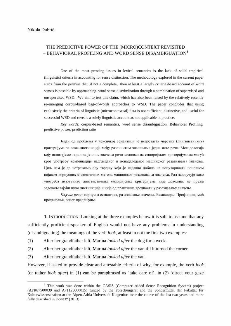
Nikola Dobrić

THE PREDICTIVE POWER OF THE (MICRO)CONTEXT REVISITED

– BEHAVIORAL PROFILING AND WORD SENSE DISAMBIGUATION1

One of the most pressing issues in lexical semantics is the lack of solid empirical

(linguistic) criteria in accounting for sense distinction. The methodology explored in the current paper

starts from the premise that, if not a complete, then at least a largely criteria-based account of word

senses is possible by approaching word sense discrimination through a combination of supervised and

unsupervised WSD. We aim to test this claim, which has also been raised by the relatively recently

re-emerging corpus-based bag-of-words approaches to WSD. The paper concludes that using

exclusively the criteria of linguistic (microcontextual) data is not sufficient, distinctive, and useful for

successful WSD and reveals a solely linguistic account as not applicable in practice.

Key words: corpus-based semantics, word sense disambiguation, Behavioral Profiling,

predictive power, prediction ratio

Један од проблема у лексичкој семантици је недостатак чврстих (лингвистичких)

критеријума за опис дистинкција међу различитим значењима једне исте речи. Методологија

коју испитујемо тврди да је опис значења речи заснован на емпиријским критеријумима могућ

кроз употребу комбинације надгледаног и ненадгледаног машинског разазнавања значења.

Циљ нам је да истражимо ову тврдњу која је недавно добила на популарности поновном

појавом корпусних статистичких метода машинског разазнавања значења. Рад закључује како

употреба искључиво лингвистичких емпиријских критеријума није довољна, не пружа

задовољавајући ниво дистинкције и није од практичне вредности у разазнавању значења.

Кључне речи: корпусна семантика, разазнавање значења. Бехавиорал Профилинг, моћ

предвиђања, опсег предвиђања

1. INTRODUCTION. Looking at the three examples below it is safe to assume that any

sufficiently proficient speaker of English would not have any problems in understanding

(disambiguating) the meanings of the verb look, at least in not the first two examples:

(1) After her grandfather left, Marina looked after the dog for a week.

(2) After her grandfather left, Marina looked after the van till it turned the corner.

(3) After her grandfather left, Marina looked after the van.

However, if asked to provide clear and attestable criteria of why, for example, the verb look

(or rather look after) in (1) can be paraphrased as ‘take care of’, in (2) ‘direct your gaze

1 This work was done within the CASIS (Computer Aided Sense Recognition System) project

(AFR87500039 and A71125000015) funded by the Forschungsrat and the Sondermittel der Fakultät für

Kulturwissenschaften at the Alpen-Adria-Universität Klagenfurt over the course of the last two years and more

fully described in DOBRIĆ (2013).

2

towards someone or something’ while in (3) it can read both, even the most experienced

linguists would be very hard pressed to do so.2 This problem of an apparent lack of decisive

criteria for defining word senses and clearly discriminating between them has always been a

burning issue of lexical semantics to the point that it fundamentally questions the possibility

to provide a clear account of polysemy. The problem is quite obvious when one looks, for

example, at the discrepancies between the paraphrases and the number of the senses of one

and the same lexeme given in different dictionaries despite the fact that they usually reference

each other (TEUBERT 2005: 11), as well as when one tries to use any machine translation

(MT) software (GUERBEROF ARENAS 2010: 4–5). However, relatively recently we could

witness the resurrection of a statistical view of lexical meanings promising to bring more

attestable criteria to the disambiguation table3.

The theoretical background of this view of the nature of lexical meaning can be seen

in the all-inclusive usage-based account of language (EVANS – GREENE 2006: 27), which

suggests that there is no fundamental difference between the lexicon and the grammar of a

language since they can both be seen as carrying meaning (or aspects of it). In this way,

lexicon and grammar mutually complement each other regarding their semantic (and

cognitive) information and how they contribute to their form–meaning relationship (ONYSKO

2011). This view of language, in essence, sees particular uses of a given lexical item as

dependent on their place within a multidimensional network comprised of linguistic (semantic

and syntactic) microcontextual knowledge (the microcontext here referring to the smallest

speech unit, that being a sentence or a clause), where each instance redefines and strengthens

the network as it is added to those elements in the network to which it is most similar (GRIES

2010: 338). The linguistic theories that promote such a view of lexical meaning include

Construction Grammar (GOLDBERG 1995; CROFT 2001); Pattern Grammar (HUNSTON –

FRANCIS 2000); Emergent Grammar (HOPPER 1987; BYBEE 1998); Lexical Functional

Grammar (HALLIDAY 1994; BRESNAN 2001); Norms and Exploitations Theory (HANKS

2009; 2013); and others.4 The practical WSD methodology based on this theoretical view

2 Despite the assertion that verbs together with prepositions should not be an issue in disambiguation

(due to the apparent compositionality of their combined meanings), if we were to observe some joint occurrences

as multi-word expressions with non-compositional meanings – expressions such as for example ‘look after’ or

‘look through’ – we can see that they cannot be easily interpreted from their constituent meanings in a

compositional manner, that they are in many cases very ambiguous, and are hence an issue in sense

disambiguation. 3 The author would like to thank Alexander Onysko for his input during the writing of this paper as

well as the reviewers whose comments helped to navigate the more troublesome aspects of the topic at hand. 4 In fact the idea originally stems from historical-philological linguistics and the view of sense as

defined by language use; structuralist and neostructuralist views on sense as a function of distribution; and the

first major lexicographic works based on language corpora as well (GEERAERTS 2010: 1–179).

3

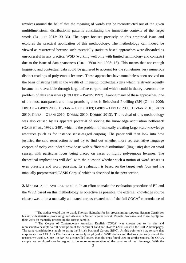
revolves around the belief that the meaning of words can be reconstructed out of the given

multidimensional distributional patterns constituting the immediate contexts of the target

words (DOBRIĆ 2013: 33–36). The paper focuses precisely on this empirical issue and

explores the practical application of this methodology. The methodology can indeed be

viewed as resurrected because such essentially statistics-based approaches were discarded as

unsuccessful in any practical WSD (working well only with limited terminology and contexts)

due to the issue of data sparseness (IDE – VÉRONIS 1998: 15). This means that not enough

linguistic and contextual data could be gathered to account for the sometimes very numerous

distinct readings of polysemous lexemes. These approaches have nonetheless been revived on

the basis of strong faith in the wealth of linguistic (contextual) data which relatively recently

became more available through large online corpora and which could in theory overcome the

problem of data sparseness (COLLIER – PACEY 1997). Among many of these approaches, one

of the most transparent and most promising ones is Behavioral Profiling (BP) (GRIES 2006;

DIVJAK – GRIES 2006; DIVJAK – GRIES 2009; GRIES – DIVJAK 2009; DIVJAK 2010; GRIES

2010; GRIES – OTANI 2010; DOBRIĆ 2010; DOBRIĆ 2013). The revival of this methodology

was also caused by its apparent potential of solving the knowledge acquisition bottleneck

(GALE ET AL. 1992a: 249), which is the problem of manually creating large-scale knowledge

resources (such as for instance sense-tagged corpora). The paper will then look into how

justified the said resurrection is and try to find out whether more representative language

corpora of today can indeed provide us with sufficient distributional (linguistic) data on word

senses, with particular focus being placed on cases of highly polysemous lexemes. The

theoretical implications will deal with the question whether such a notion of word senses is

even plausible and worth pursuing. Its evaluation is based on the target verb look and the

manually preprocessed CASIS Corpus5 which is described in the next section.

2. MAKING A BEHAVIORAL PROFILE. In an effort to make the evaluation procedure of BP and

the WSD based on this methodology as objective as possible, the external knowledge source

chosen was to be a manually annotated corpus created out of the full COCA6 concordance of

5 The author would like to thank Thomas Hainscho for his programming support; Herman Cesnik for

his aid with statistical processing; and Alexandra Galler, Verena Novak, Pamela Prohaska, and Tjasa Zemlja for

their work on manually processing the corpus sample. 6 The Corpus of Contemporary American English (COCA) was chosen due to its size and

representativeness (for a full description of the corpus at hand see DAVIES (2001) or visit the COCA homepage).

The same considerations apply to using the British National Corpus (BNC). At this point one may remark that

corpora such as COCA or BNC are not commonly employed in WSD studies and that was precisely one of the

reasons we used it. Since it is far less a controlled source than the ones found used in similar studies, the COCA

sample we employed can be argued to be more representative of the vagaries of real language. With the

4

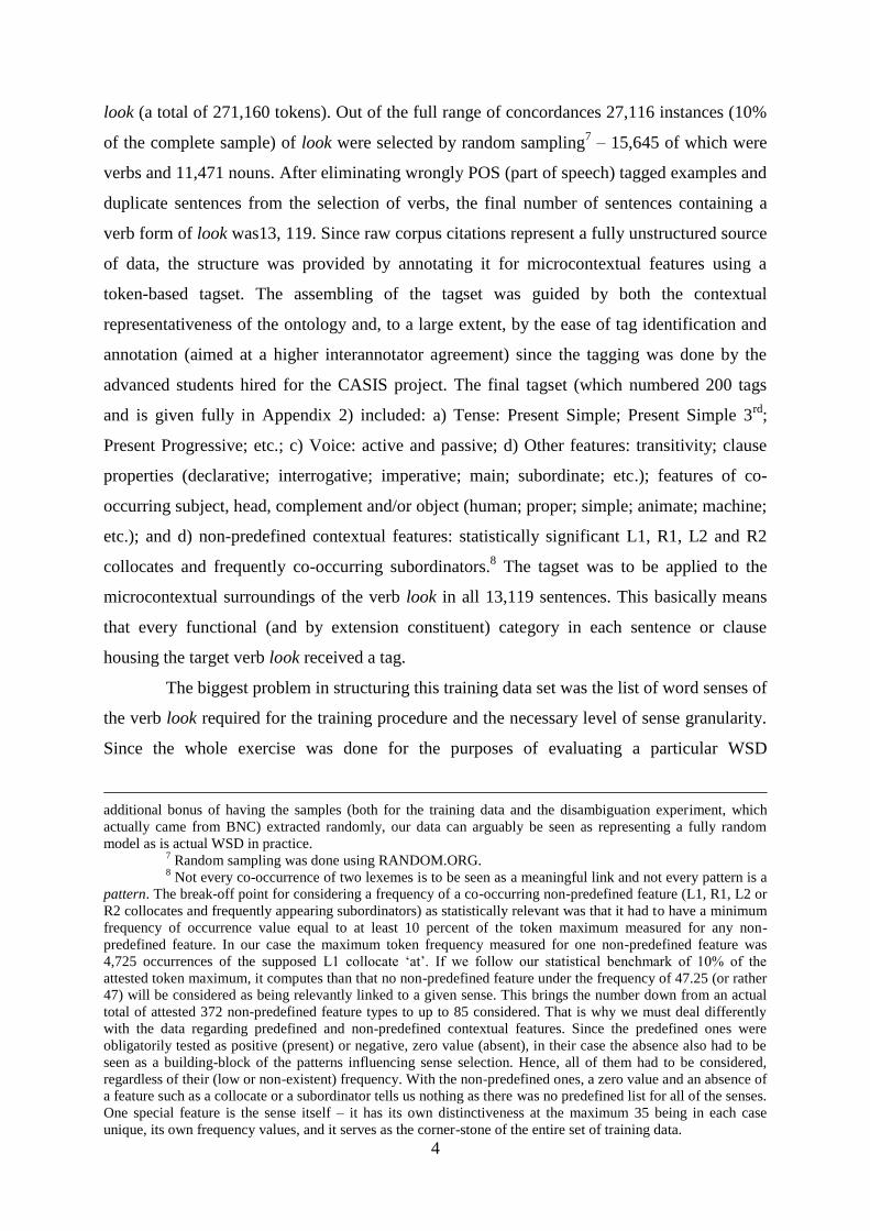
look (a total of 271,160 tokens). Out of the full range of concordances 27,116 instances (10%

of the complete sample) of look were selected by random sampling7 – 15,645 of which were

verbs and 11,471 nouns. After eliminating wrongly POS (part of speech) tagged examples and

duplicate sentences from the selection of verbs, the final number of sentences containing a

verb form of look was13, 119. Since raw corpus citations represent a fully unstructured source

of data, the structure was provided by annotating it for microcontextual features using a

token-based tagset. The assembling of the tagset was guided by both the contextual

representativeness of the ontology and, to a large extent, by the ease of tag identification and

annotation (aimed at a higher interannotator agreement) since the tagging was done by the

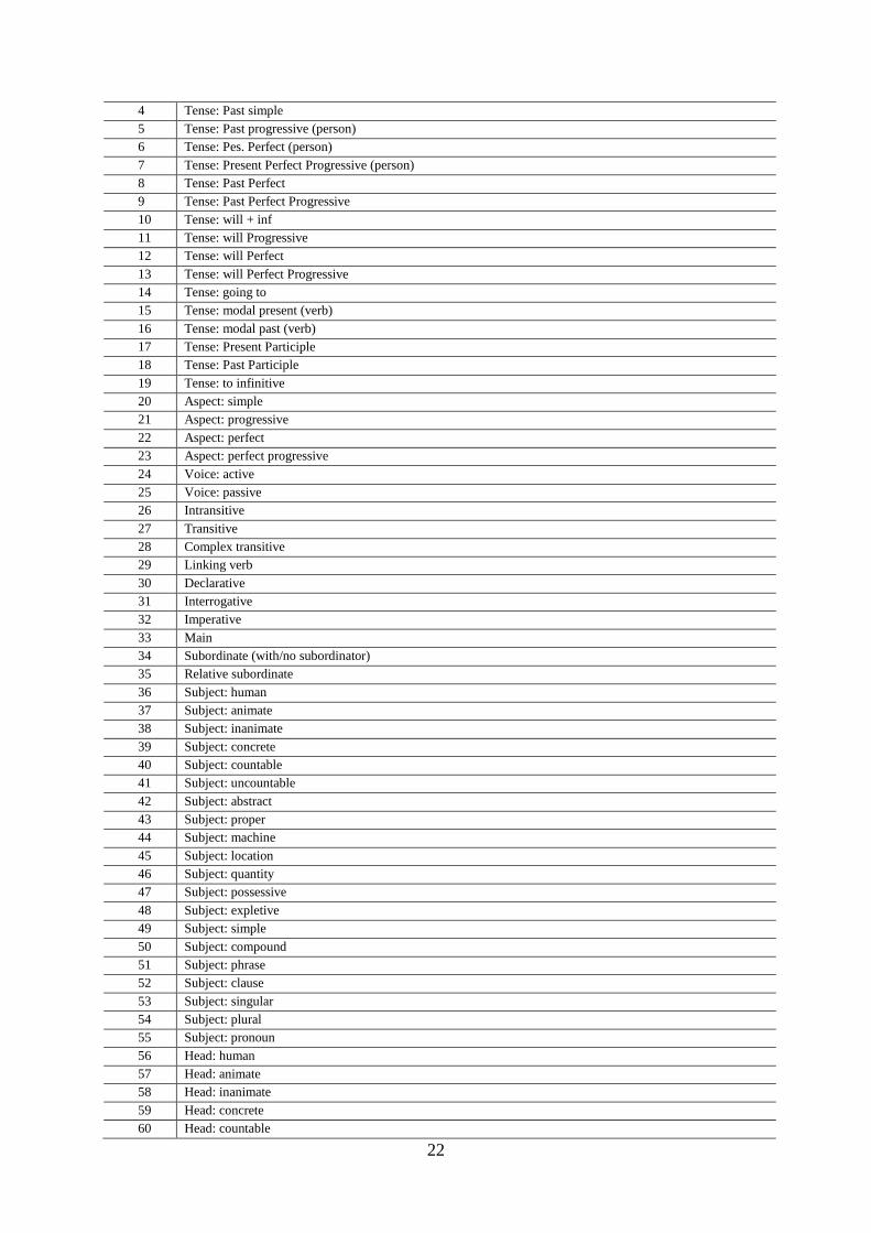
advanced students hired for the CASIS project. The final tagset (which numbered 200 tags

and is given fully in Appendix 2) included: a) Tense: Present Simple; Present Simple 3rd

;

Present Progressive; etc.; c) Voice: active and passive; d) Other features: transitivity; clause

properties (declarative; interrogative; imperative; main; subordinate; etc.); features of co-

occurring subject, head, complement and/or object (human; proper; simple; animate; machine;

etc.); and d) non-predefined contextual features: statistically significant L1, R1, L2 and R2

collocates and frequently co-occurring subordinators.8 The tagset was to be applied to the

microcontextual surroundings of the verb look in all 13,119 sentences. This basically means

that every functional (and by extension constituent) category in each sentence or clause

housing the target verb look received a tag.

The biggest problem in structuring this training data set was the list of word senses of

the verb look required for the training procedure and the necessary level of sense granularity.

Since the whole exercise was done for the purposes of evaluating a particular WSD

additional bonus of having the samples (both for the training data and the disambiguation experiment, which

actually came from BNC) extracted randomly, our data can arguably be seen as representing a fully random

model as is actual WSD in practice. 7 Random sampling was done using RANDOM.ORG.

8 Not every co-occurrence of two lexemes is to be seen as a meaningful link and not every pattern is a

pattern. The break-off point for considering a frequency of a co-occurring non-predefined feature (L1, R1, L2 or

R2 collocates and frequently appearing subordinators) as statistically relevant was that it had to have a minimum

frequency of occurrence value equal to at least 10 percent of the token maximum measured for any non-

predefined feature. In our case the maximum token frequency measured for one non-predefined feature was

4,725 occurrences of the supposed L1 collocate ‘at’. If we follow our statistical benchmark of 10% of the

attested token maximum, it computes than that no non-predefined feature under the frequency of 47.25 (or rather

47) will be considered as being relevantly linked to a given sense. This brings the number down from an actual

total of attested 372 non-predefined feature types to up to 85 considered. That is why we must deal differently

with the data regarding predefined and non-predefined contextual features. Since the predefined ones were

obligatorily tested as positive (present) or negative, zero value (absent), in their case the absence also had to be

seen as a building-block of the patterns influencing sense selection. Hence, all of them had to be considered,

regardless of their (low or non-existent) frequency. With the non-predefined ones, a zero value and an absence of

a feature such as a collocate or a subordinator tells us nothing as there was no predefined list for all of the senses.

One special feature is the sense itself – it has its own distinctiveness at the maximum 35 being in each case

unique, its own frequency values, and it serves as the corner-stone of the entire set of training data.

5

methodology, it was easy to decide on a finely grained selection of senses. To obtain the

selection itself, however, two major issues had to be considered: firstly, it is quite impossible

to capture all of the possible interpretations and productive uses of a lexeme in any

constructed list of senses (KILGARRIFF 2006: 30); and secondly, any enumerative approach to

word senses involves using one of several equally subjective sources − either dictionaries

(paper or machine-readable), WordNet entries, parallel corpora, or native speaker intuition

(IDE – WILKS 2006: 78). Regarding first the theoretical considerations, any reference to

objective criteria of what a sense is and how to determine the ‘real’ number of senses of one

polysemous lexeme is extremely problematic due to the contextual dependence of lexical

meaning and semantic open-endedness of lexemes. The issue is still very much a burning one

in lexical semantics even after being debated extensively over the last century or so without a

clear result (see GEERAERTS (2010) for an in-depth discussion). As for the practical side, we

can see that we were faced with four possible concrete options: using a bilingual parallel

corpus which would validate the senses of words through having them confirmed by a

translated form, using WordNet inventories of senses, using parallel (translated) corpora or

using native speakers’ intuition in identifying possible readings. The choice was made

difficult by the fact that the drawbacks of subjectivity and the mentioned theoretical issues

apply to all of these possible methods – the translated equivalents found in a parallel corpus

also depend on the subjective sense identification of the respective translator, the WordNet

senses are intrinsically of the same nature as the ones in dictionaries when it comes to their

inventory, while it is a known fact that native speakers’ intuition cannot be as highly valued in

semantics as it is when dealing with grammar since it is far too varied. In light of this and as

practical considerations beg making a choice and contemporary lexical semantic theory offers

no perfect solutions, using a cross-referenced set of meanings from a number of respected

monolingual dictionaries was chosen, namely a set extracted from New Oxford Dictionary of

English, Oxford English Dictionary, and The Oxford Dictionary of Idioms. It is the most

commonly employed technique in WSD studies and other practically orientated lexicographic

exercises as it is least time-consuming due to the (electronically) accessible nature of

dictionary entries (e.g. WordNet senses can be difficult to extract). Hence, observing entries

in the said three dictionaries and combining them together yielded 42 very finely grained

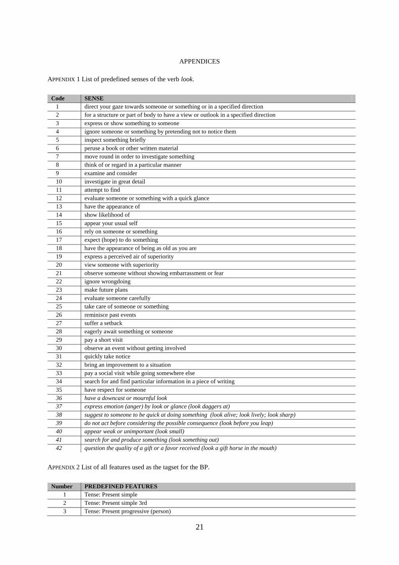
paraphrases of the senses of the verb look to be used in the experiment. The list of senses

generated in this manner (and given in Appendix 1) served as the crucial linking marker also

annotated by human annotators for every of the 13,119 sentences in the training corpus during

manual processing.

6

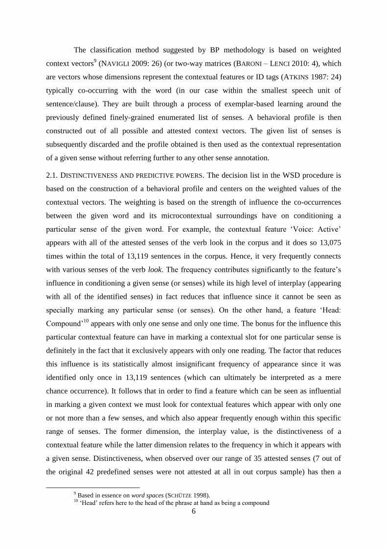
The classification method suggested by BP methodology is based on weighted

context vectors9 (NAVIGLI 2009: 26) (or two-way matrices (BARONI – LENCI 2010: 4), which

are vectors whose dimensions represent the contextual features or ID tags (ATKINS 1987: 24)

typically co-occurring with the word (in our case within the smallest speech unit of

sentence/clause). They are built through a process of exemplar-based learning around the

previously defined finely-grained enumerated list of senses. A behavioral profile is then

constructed out of all possible and attested context vectors. The given list of senses is

subsequently discarded and the profile obtained is then used as the contextual representation

of a given sense without referring further to any other sense annotation.

2.1. DISTINCTIVENESS AND PREDICTIVE POWERS. The decision list in the WSD procedure is

based on the construction of a behavioral profile and centers on the weighted values of the

contextual vectors. The weighting is based on the strength of influence the co-occurrences

between the given word and its microcontextual surroundings have on conditioning a

particular sense of the given word. For example, the contextual feature ‘Voice: Active’

appears with all of the attested senses of the verb look in the corpus and it does so 13,075

times within the total of 13,119 sentences in the corpus. Hence, it very frequently connects

with various senses of the verb look. The frequency contributes significantly to the feature’s

influence in conditioning a given sense (or senses) while its high level of interplay (appearing

with all of the identified senses) in fact reduces that influence since it cannot be seen as

specially marking any particular sense (or senses). On the other hand, a feature ‘Head:

Compound’10

appears with only one sense and only one time. The bonus for the influence this

particular contextual feature can have in marking a contextual slot for one particular sense is

definitely in the fact that it exclusively appears with only one reading. The factor that reduces

this influence is its statistically almost insignificant frequency of appearance since it was

identified only once in 13,119 sentences (which can ultimately be interpreted as a mere

chance occurrence). It follows that in order to find a feature which can be seen as influential

in marking a given context we must look for contextual features which appear with only one

or not more than a few senses, and which also appear frequently enough within this specific

range of senses. The former dimension, the interplay value, is the distinctiveness of a

contextual feature while the latter dimension relates to the frequency in which it appears with

a given sense. Distinctiveness, when observed over our range of 35 attested senses (7 out of

the original 42 predefined senses were not attested at all in out corpus sample) has then a

9 Based in essence on word spaces (SCHÜTZE 1998).

10 ‘Head’ refers here to the head of the phrase at hand as being a compound

7

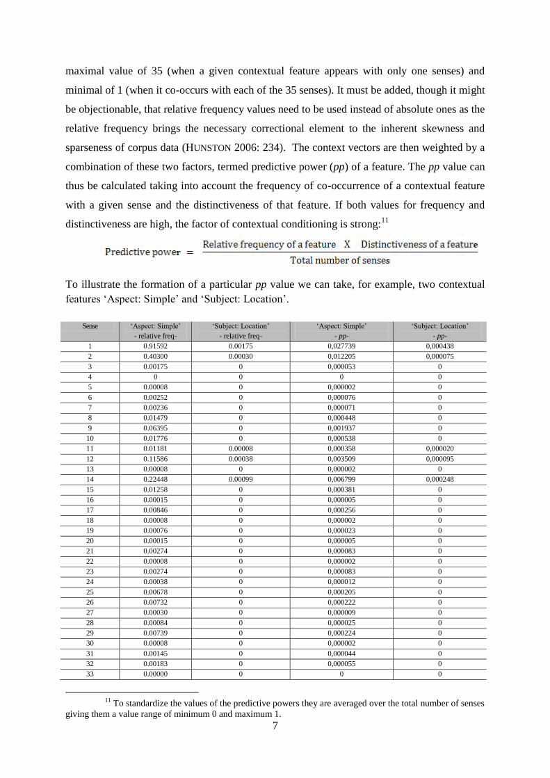
maximal value of 35 (when a given contextual feature appears with only one senses) and

minimal of 1 (when it co-occurs with each of the 35 senses). It must be added, though it might

be objectionable, that relative frequency values need to be used instead of absolute ones as the

relative frequency brings the necessary correctional element to the inherent skewness and

sparseness of corpus data (HUNSTON 2006: 234). The context vectors are then weighted by a

combination of these two factors, termed predictive power (pp) of a feature. The pp value can

thus be calculated taking into account the frequency of co-occurrence of a contextual feature

with a given sense and the distinctiveness of that feature. If both values for frequency and

distinctiveness are high, the factor of contextual conditioning is strong:11

To illustrate the formation of a particular pp value we can take, for example, two contextual

features ‘Aspect: Simple’ and ‘Subject: Location’.

Sense ‘Aspect: Simple’

- relative freq-

‘Subject: Location’

- relative freq-

‘Aspect: Simple’

- pp-

‘Subject: Location’

- pp-

1 0.91592 0.00175 0,027739 0,000438

2 0.40300 0.00030 0,012205 0,000075

3 0.00175 0 0,000053 0

4 0 0 0 0

5 0.00008 0 0,000002 0

6 0.00252 0 0,000076 0

7 0.00236 0 0,000071 0

8 0.01479 0 0,000448 0

9 0.06395 0 0,001937 0

10 0.01776 0 0,000538 0

11 0.01181 0.00008 0,000358 0,000020

12 0.11586 0.00038 0,003509 0,000095

13 0.00008 0 0,000002 0

14 0.22448 0.00099 0,006799 0,000248

15 0.01258 0 0,000381 0

16 0.00015 0 0,000005 0

17 0.00846 0 0,000256 0

18 0.00008 0 0,000002 0

19 0.00076 0 0,000023 0

20 0.00015 0 0,000005 0

21 0.00274 0 0,000083 0

22 0.00008 0 0,000002 0

23 0.00274 0 0,000083 0

24 0.00038 0 0,000012 0

25 0.00678 0 0,000205 0

26 0.00732 0 0,000222 0

27 0.00030 0 0,000009 0

28 0.00084 0 0,000025 0

29 0.00739 0 0,000224 0

30 0.00008 0 0,000002 0

31 0.00145 0 0,000044 0

32 0.00183 0 0,000055 0

33 0.00000 0 0 0

11

To standardize the values of the predictive powers they are averaged over the total number of senses

giving them a value range of minimum 0 and maximum 1.

8

34 0.00015 0 0,000005 0

35 0.00198 0 0,000060 0

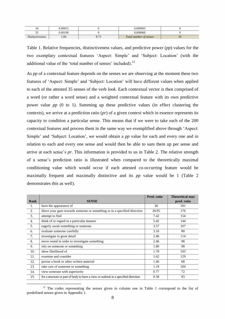
Distinctiveness 1.06 8.75 Total number of senses 35

Table 1. Relative frequencies, distinctiveness values, and predictive power (pp) values for the

two exemplary contextual features ‘Aspect: Simple’ and ‘Subject: Location’ (with the

additional value of the ‘total number of senses’ included).12

As pp of a contextual feature depends on the senses we are observing at the moment these two

features of ‘Aspect: Simple’ and ‘Subject: Location’ will have different values when applied

to each of the attested 35 senses of the verb look. Each contextual vector is then comprised of

a word (or rather a word sense) and a weighted contextual feature with its own predictive

power value pp (0 to 1). Summing up these predictive values (in effect clustering the

contexts), we arrive at a prediction ratio (pr) of a given context which in essence represents its

capacity to condition a particular sense. This means that if we were to take each of the 200

contextual features and process them in the same way we exemplified above through ‘Aspect:

Simple’ and ‘Subject: Location’, we would obtain a pp value for each and every one and in

relation to each and every one sense and would then be able to sum them up per sense and

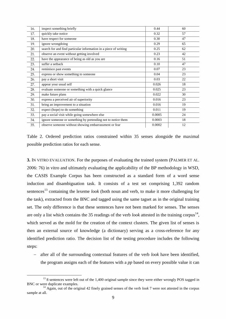
arrive at each sense’s pr. This information is provided to us in Table 2. The relative strength

of a sense’s prediction ratio is illustrated when compared to the theoretically maximal

conditioning value which would occur if each attested co-occurring feature would be

maximally frequent and maximally distinctive and its pp value would be 1 (Table 2

demonstrates this as well).

Rank

SENSE

Pred. ratio Theoretical max

pred. ratio

1. have the appearance of 36 181

2. direct your gaze towards someone or something or in a specified direction 28.95 176

3. attempt to find 7.42 154

4. think of or regard in a particular manner 5.42 144

5. eagerly await something or someone 3.57 107

6. evaluate someone carefully 3.16 80

7. investigate in great detail 2.46 114

8. move round in order to investigate something 2.46 98

9. rely on someone or something 1.80 98

10. show likelihood of 1.78 103

11. examine and consider 1.62 129

12. peruse a book or other written material 1.46 68

13. take care of someone or something 1.19 104

14. view someone with superiority 0.77 72

15. for a structure or part of body to have a view or outlook in a specified direction 0.58 83

12

The codes representing the senses given in column one in Table 1 correspond to the list of

predefined senses given in Appendix 1.

9

16. inspect something briefly 0.44 60

17. quickly take notice 0.32 57

18. have respect for someone 0.30 47

19. ignore wrongdoing 0.29 65

20. search for and find particular information in a piece of writing 0.25 62

21. observe an event without getting involved 0.23 42

22. have the appearance of being as old as you are 0.16 51

23. suffer a setback 0.10 47

24. reminisce past events 0.07 23

25. express or show something to someone 0.04 23

26. pay a short visit 0.03 22

27. appear your usual self 0.026 18

28. evaluate someone or something with a quick glance 0.025 23

29. make future plans 0.022 30

30. express a perceived air of superiority 0.016 23

31. bring an improvement to a situation 0.016 19

32. expect (hope) to do something 0.011 19

33. pay a social visit while going somewhere else 0.0005 24

34. ignore someone or something by pretending not to notice them 0.0003 18

35. observe someone without showing embarrassment or fear 0.0002 12

Table 2. Ordered prediction ratios constrained within 35 senses alongside the maximal

possible prediction ratios for each sense.

3. IN VITRO EVALUATION. For the purposes of evaluating the trained system (PALMER ET AL.

2006: 76) in vitro and ultimately evaluating the applicability of the BP methodology in WSD,

the CASIS Example Corpus has been constructed as a standard form of a word sense

induction and disambiguation task. It consists of a test set comprising 1,392 random

sentences13

containing the lexeme look (both noun and verb, to make it more challenging for

the task), extracted from the BNC and tagged using the same tagset as in the original training

set. The only difference is that these sentences have not been marked for senses. The senses

are only a list which contains the 35 readings of the verb look attested in the training corpus14

,

which served as the mold for the creation of the context clusters. The given list of senses is

then an external source of knowledge (a dictionary) serving as a cross-reference for any

identified prediction ratio. The decision list of the testing procedure includes the following

steps:

after all of the surrounding contextual features of the verb look have been identified,

the program assigns each of the features with a pp based on every possible value it can

13

8 sentences were left out of the 1,400 original sample since they were either wrongly POS tagged in

BNC or were duplicate examples. 14

Again, out of the original 42 finely grained senses of the verb look 7 were not attested in the corpus

sample at all.

10

have in every context attested in the training set, linked to every possible contextual

vector individually;

the program identifies the highest possible pp for every contextual vector;

the senses which correspond to these contextual vectors are then identified in the

reference list of 35 senses;

the program then calculates the prs out of theses highest pps; and

it churns out the sense(s) with the highest pr(s) as accurate WSD. 15

In order to illustrate this point on an example we can take one sentence out of the CASIS

Example Corpus (coming originally from BNC) and break down the procedure:

(4) He tossed his horse's reins to a groom and went storming off looking for Dacourt.

Mimicking the original annotation procedure, all of the relevant contextual features

(following the original tagset) have been manually marked. The subsequent annotation

(copied from the corpus tagger used in both the training and evaluation data processing)

shows how one of the mentioned student annotators processed the sentence from example (4):

POS of look: verb

Related Tags16

Tense: Past simple

Aspect: simple

Voice: active

intransitive/transitive/complex transitive/linking verb: transitive

declarative/interrogative/imperative: declarative

main/subordinate/relative subordinate: main

Tagged sentence features

Subject:

o pronoun

Object:

o human

o uncountable

15

The actual WSD within the CASIS Example Corpus can be attempted by any interested parties by

logging in at http://casis.uni-klu.ac.at/casis_example/users/login – username/email: guest1@test.at, password:

guest1. 16

Relating to the clause containing the target lexeme and its main verb.

11

o simple

o singular

L1: off

L2: storming

R1: for17

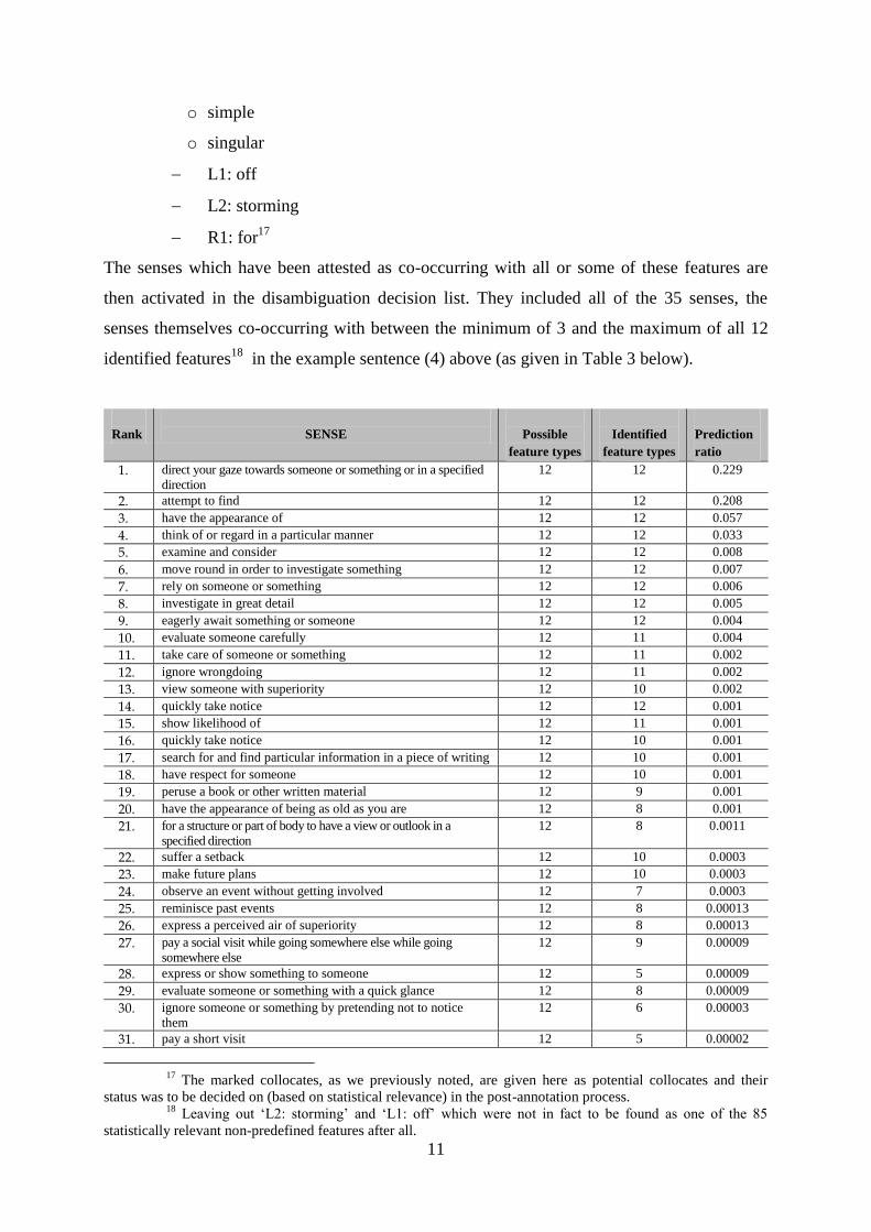
The senses which have been attested as co-occurring with all or some of these features are

then activated in the disambiguation decision list. They included all of the 35 senses, the

senses themselves co-occurring with between the minimum of 3 and the maximum of all 12

identified features18

in the example sentence (4) above (as given in Table 3 below).

Rank

SENSE

Possible

feature types

Identified

feature types

Prediction

ratio

1. direct your gaze towards someone or something or in a specified

direction

12 12 0.229

2. attempt to find 12 12 0.208

3. have the appearance of 12 12 0.057

4. think of or regard in a particular manner 12 12 0.033

5. examine and consider 12 12 0.008

6. move round in order to investigate something 12 12 0.007

7. rely on someone or something 12 12 0.006

8. investigate in great detail 12 12 0.005

9. eagerly await something or someone 12 12 0.004

10. evaluate someone carefully 12 11 0.004

11. take care of someone or something 12 11 0.002

12. ignore wrongdoing 12 11 0.002

13. view someone with superiority 12 10 0.002

14. quickly take notice 12 12 0.001

15. show likelihood of 12 11 0.001

16. quickly take notice 12 10 0.001

17. search for and find particular information in a piece of writing 12 10 0.001

18. have respect for someone 12 10 0.001

19. peruse a book or other written material 12 9 0.001

20. have the appearance of being as old as you are 12 8 0.001

21. for a structure or part of body to have a view or outlook in a

specified direction

12 8 0.0011

22. suffer a setback 12 10 0.0003

23. make future plans 12 10 0.0003

24. observe an event without getting involved 12 7 0.0003

25. reminisce past events 12 8 0.00013

26. express a perceived air of superiority 12 8 0.00013

27. pay a social visit while going somewhere else while going

somewhere else

12 9 0.00009

28. express or show something to someone 12 5 0.00009

29. evaluate someone or something with a quick glance 12 8 0.00009

30. ignore someone or something by pretending not to notice

them

12 6 0.00003

31. pay a short visit 12 5 0.00002

17

The marked collocates, as we previously noted, are given here as potential collocates and their

status was to be decided on (based on statistical relevance) in the post-annotation process. 18

Leaving out ‘L2: storming’ and ‘L1: off’ which were not in fact to be found as one of the 85

statistically relevant non-predefined features after all.

12

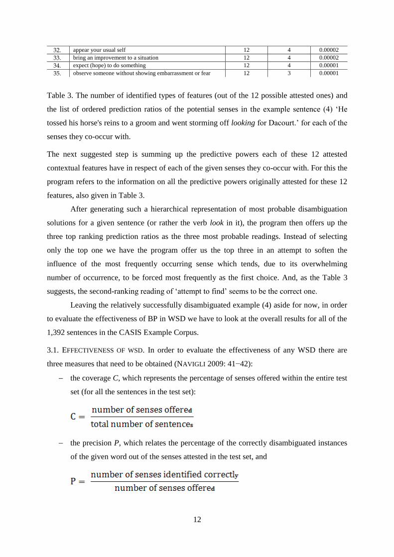
32. appear your usual self 12 4 0.00002

33. bring an improvement to a situation 12 4 0.00002

34. expect (hope) to do something 12 4 0.00001

35. observe someone without showing embarrassment or fear 12 3 0.00001

Table 3. The number of identified types of features (out of the 12 possible attested ones) and

the list of ordered prediction ratios of the potential senses in the example sentence (4) ‘He

tossed his horse's reins to a groom and went storming off looking for Dacourt.’ for each of the

senses they co-occur with.

The next suggested step is summing up the predictive powers each of these 12 attested

contextual features have in respect of each of the given senses they co-occur with. For this the

program refers to the information on all the predictive powers originally attested for these 12

features, also given in Table 3.

After generating such a hierarchical representation of most probable disambiguation

solutions for a given sentence (or rather the verb look in it), the program then offers up the

three top ranking prediction ratios as the three most probable readings. Instead of selecting

only the top one we have the program offer us the top three in an attempt to soften the

influence of the most frequently occurring sense which tends, due to its overwhelming

number of occurrence, to be forced most frequently as the first choice. And, as the Table 3

suggests, the second-ranking reading of ‘attempt to find’ seems to be the correct one.

Leaving the relatively successfully disambiguated example (4) aside for now, in order

to evaluate the effectiveness of BP in WSD we have to look at the overall results for all of the

1,392 sentences in the CASIS Example Corpus.

3.1. EFFECTIVENESS OF WSD. In order to evaluate the effectiveness of any WSD there are

three measures that need to be obtained (NAVIGLI 2009: 41−42):

the coverage C, which represents the percentage of senses offered within the entire test

set (for all the sentences in the test set):

the precision P, which relates the percentage of the correctly disambiguated instances

of the given word out of the senses attested in the test set, and

13

the recall R, or accuracy, which represents the ratio between the correctly identified

senses and the total number of possible (or rather listed) ones:

A successful WSD method would then have R ≤ P (equal when C=1 and the coverage is total,

as it normally is in targeted WSD). BP-based WSD tested on the CASIS Example Corpus

gives us the weighted mean of the relationship between the precision and accuracy or the F-

score (ARTILES ET AL. 2009) of 0.289. When we compare it to the less competitive random

sense baseline (calculated as the chance or random choice of a sense from within the reference

dictionary relating to each target word within the test set (GALE ET AL. 1992b) of 2,05255e-

519

we can see that it easily exceeds this lower bound. The comparison with the perceived

upper bound or the interannotator agreement (ITA) bound (DUFFIELD ET AL. 2007) must

however be manually performed and elaborated on.20

4. RESULTS. Manual inspection of the way in which the BP-based WSD success relates to the

ITA bound must, first of all, consider the last step in the program’s decision list. The CASIS

Example Corpus suggests as accurate the senses corresponding to the top 3 ranked prs (as

seen in Figure 1, rank 1 corresponding to the highest pr as offered by the decision list, ranks 2

and 3 to the next two in size) in an effort to compensate for the issues of the dominance of the

most frequently occurring senses (KILGARRIFF – ROSENZWIEG 2000; KILGARRIFF 2004). It is

the closer look at these senses offered as the top three that exposes the real problem of the

accuracy of the methodology.

19

The value of a random baseline is inherently low as we are looking at a random probability of

identifying a particular sense within a combination of 35 possible senses and 1,392 sentences containing the

target lexeme. It is calculated using the following formula (simplified from NAVIGLI (2009: 42–43):

.

20 The paper does not provide any information on the ITA scores in terms of human-based

disambiguation scores even though it is the one aspired bound. The reason is that even though a level or a

measurement of human-based WSD agreement is something we can intuitively recognize, it is problematic and

poorly adapted quantitative measurement when applied to language data. The major problem of using something

like the Kappa statistics, which is the widely accepted manner of measuring agreement in categorization tasks, is

precisely in its lack of applicability to language-related categorization. One of the causes of such a problematic

nature is due to the lack of a finite/standard version of language performance. In addition to that, there is the

problem of comparing the results of ITA (expressed by a certain value of the Kappa coefficient) with some

existing benchmark or a standard of similar ITA when annotations (of similar or even any kind) are concerned in

an effort to discern one score as successful or not. See for instance FLEISS ET AL. (1979), GWET (2002) or

TENFJORD ET AL. (2006) for a lengthier discussion of using Kappa statistics in measuring ITA.

14

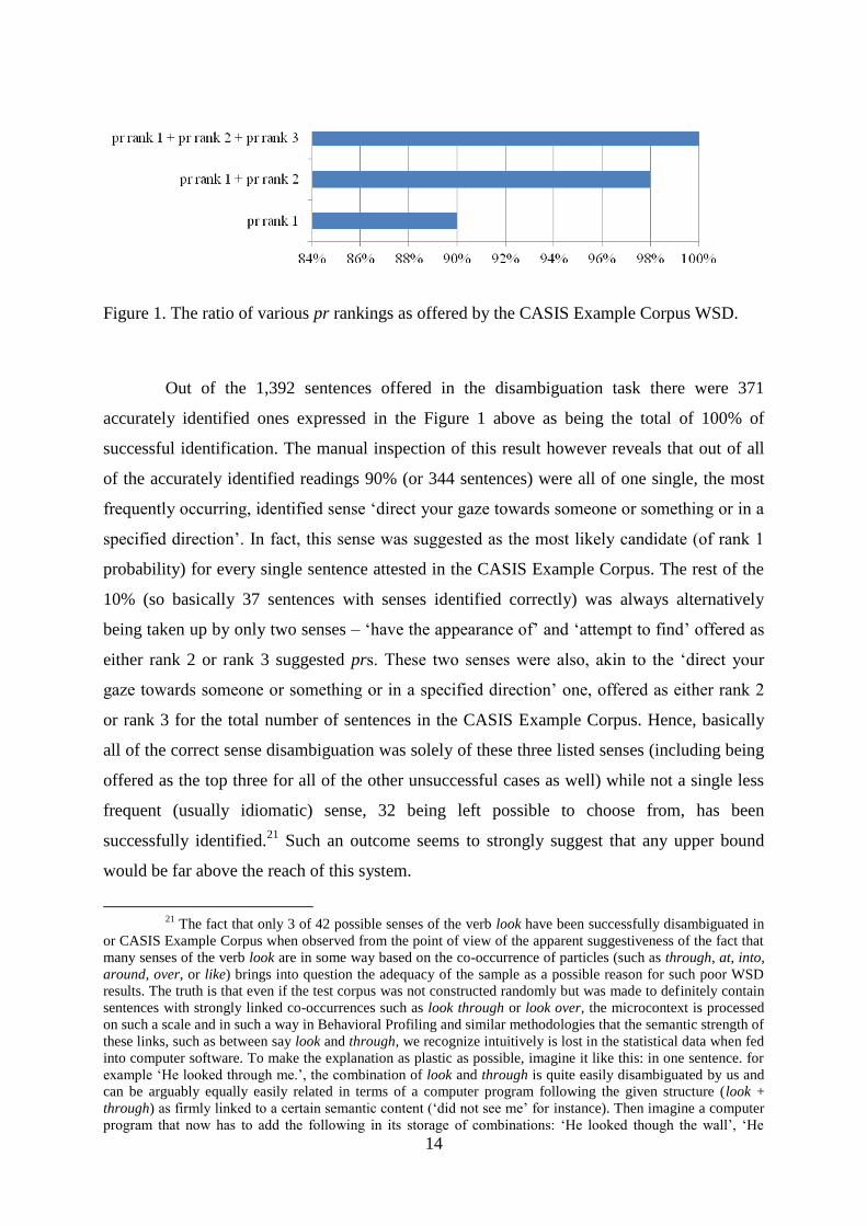
Figure 1. The ratio of various pr rankings as offered by the CASIS Example Corpus WSD.

Out of the 1,392 sentences offered in the disambiguation task there were 371

accurately identified ones expressed in the Figure 1 above as being the total of 100% of

successful identification. The manual inspection of this result however reveals that out of all

of the accurately identified readings 90% (or 344 sentences) were all of one single, the most

frequently occurring, identified sense ‘direct your gaze towards someone or something or in a

specified direction’. In fact, this sense was suggested as the most likely candidate (of rank 1

probability) for every single sentence attested in the CASIS Example Corpus. The rest of the

10% (so basically 37 sentences with senses identified correctly) was always alternatively

being taken up by only two senses – ‘have the appearance of’ and ‘attempt to find’ offered as

either rank 2 or rank 3 suggested prs. These two senses were also, akin to the ‘direct your

gaze towards someone or something or in a specified direction’ one, offered as either rank 2

or rank 3 for the total number of sentences in the CASIS Example Corpus. Hence, basically

all of the correct sense disambiguation was solely of these three listed senses (including being

offered as the top three for all of the other unsuccessful cases as well) while not a single less

frequent (usually idiomatic) sense, 32 being left possible to choose from, has been

successfully identified.21

Such an outcome seems to strongly suggest that any upper bound

would be far above the reach of this system.

21

The fact that only 3 of 42 possible senses of the verb look have been successfully disambiguated in

or CASIS Example Corpus when observed from the point of view of the apparent suggestiveness of the fact that

many senses of the verb look are in some way based on the co-occurrence of particles (such as through, at, into,

around, over, or like) brings into question the adequacy of the sample as a possible reason for such poor WSD

results. The truth is that even if the test corpus was not constructed randomly but was made to definitely contain

sentences with strongly linked co-occurrences such as look through or look over, the microcontext is processed

on such a scale and in such a way in Behavioral Profiling and similar methodologies that the semantic strength of

these links, such as between say look and through, we recognize intuitively is lost in the statistical data when fed

into computer software. To make the explanation as plastic as possible, imagine it like this: in one sentence. for

example ‘He looked through me.’, the combination of look and through is quite easily disambiguated by us and

can be arguably equally easily related in terms of a computer program following the given structure (look +

through) as firmly linked to a certain semantic content (‘did not see me’ for instance). Then imagine a computer

program that now has to add the following in its storage of combinations: ‘He looked though the wall’, ‘He

15

5. DISCUSSION. Using a relatively simplified analysis in our experiment and actually

performing all of the steps manually rather than employing the suggested elaborate statistical

methods, such as the commonly used hierarchical cluster analysis (GRIES 2006: 93) or

equally elaborate learning algorithms (NG 1997), has allowed us to break down the BP

methodology of WSD into its most transparent constituents. Such a methodical step-by-step

analysis pinpointed the exact stumbling block of the approach. Confirming then the

mentioned findings of earlier similar research endeavors we can see that the reason why using

only linguistic (microcontextual) information as the source of knowledge in WSD (as BP

seems to be indicating) failed to satisfy the ITA standards is again related to data sparseness

(at various levels).

We have demonstrated that, even when drawing on large contemporary corpora,

there is not enough quantitative data to provide sufficient and sufficiently detailed information

about the senses of a given word. Out of 42 senses compiled from dictionaries (which do not

even foresee the open-endedness of polysemous lexical networks) only 35 were identified in

the corpus. Furthermore, out of those 35 identified senses some were found as few as only

once, while others, indicating again the skewness of the data, appeared more than 5,000 times

(within 13,119 random sentences). Even if this sort of data skewness could be compensated

for by employing elaborate statistic(al) methods (GRIES 2009), data sparseness affected the

identification of the contextual features and the structure of the contextual vectors as well.

The less frequently occurring senses offered just a small chance to attest a sufficient

number of co-relating contextual features in order to exceed the level of chance co-

occurrences. This issue had a major effect on the pps of the features as the frequency of a

contextual feature is one of the two dimensions that construe them. The other dimension of

the pps, the distinctiveness of the contextual features, was also affected by the problem of data

sparseness. Indeed the number of truly distinctive contextual features (the ones that appeared

with only one particular sense) was also very low.

looked through the spy glass’, ‘He may look through and through as a lumberjack’, and theoretically, having in

mind the semantic open-endedness of language, countless other similar combinations. How semantically

meaningful is the look + through combination when expanded over thousands of sentences of the sample itself,

let alone of the theoretical lack of finiteness in real language, and compared to the existence of thousands of

other lexeme + look + lexeme combinations. The bottom line, as we have demonstrated, is that applying strictly

linguistic data of the microcontext in a statistical manner, due to frequency problems that combinations cause (in

terms of occurrences and co-occurrences) and due to their immense overlap (as we saw through appearing with

various meanings of the verb look just in one simple example), almost all of what we perceive as strong semantic

links, such as the suggested look through, gets devalued in quantitative terms, skewed by inherent frequency

discrepancies between senses of a polysemous lexeme, and subsequently more often than not fails to be

recognizable by WSD software.

16

The question that arises at this point is whether data sparseness could be addressed

perhaps by increasing the size of the sample further in an attempt to increase the amount of

quantifiable data or by extending the ontology of the contextual features in order to define the

context vectors in more depth. The first reason why neither of these solutions would bear

fruit is that it would be very demanding to manually process the extremely large numbers of

sentences (and here we are talking millions since thousands did not suffice), especially if we

include more complex ontologies (such as theta roles or argument structures for example). 22

The second and more important reason why it would not work, even if we attempted it as an

exercise in theoretical semantics, is that the results presented above seem to indicate that the

quantitative discrepancy between the very frequently occurring senses and the least frequently

occurring ones would again considerably influence both the distinctiveness and the frequency

of occurrence and co-occurrence of the contextual features. If we break down the

argumentation, the more frequent a sense the more co-occurring features it can be identified

with and the more diverse those features are And even though some authors, such as DIVJAK

(2010), argue that, for verbs, the analysis of polysemy plays at the coarse-grained inter-

constructional level and that by including constructional information (such as argument

structure) in building behavioral profiles of verbs, WSD results would be more positive.

Looking at the results obtained by our reduced and simplified procedure alone, we can see

that no additional information we could include in a behavioral profile of verbs, even for the

sake of a theoretical exercise (as practically they are not of much use in WSD seeing that

constructional information are difficult to tackle automatically), would not yield better results.

The claim is that major frequency misbalance between the senses and the distinctiveness

problems in BP information of any kind this causes render the methodology impotent when it

comes to practical WSD. It is unlikely that a sufficient number of prediction-powerful

contextual features (i.e. distinctive and at the same time frequent enough) can be found within

any possible contextual environment regardless of the complexity of the ontology we may

choose (including constructional information) or the size of the corpus we may opt for. The

result of any such WSD approach, based entirely on microcontextual linguistic data and

unsupported by various advanced and debatable statistical scaffolding, would most likely

mirror what we have seen in the experiment presented above – the predictive powers would

be higher for the more frequent senses and would decline (nearing zero) for the less frequent

ones, all due to multifaceted data sparseness. The problem ultimately seems to derive from the

22

As employing solely unsupervised context clustering still leads only to working with coarsely

grained sense discrimination (PALMER ET AL. 2004).

17

fact that the analysis eventually models cognition and cognition probably does not work with

as clear-cut distinctions and hence the lack of distinctive data.

These practical implications actually relate back the main theoretical backbone of the

methodology: that you can know a word by the company it keeps (FIRTH 1957: 16). The

theoretical conclusion that seems unavoidable is that when it comes to semantic meaning and

the manner in which the multiple meanings interplay within a polysemous lexical item, the

microcontextual conditioning is simply not strong enough and hence you cannot know a word

by its (immediate) company. The problem of data sparseness in this respect, however, does

not refer to the impossibility of gathering enough data as corpora available these days number

hundreds of millions of words and the manner of their processing is constantly being

improved. Instead, data sparseness should be understood as the impossibility of finding

enough microcontextual, solely linguistic, features which would be distinctive enough so they

exclusively condition a particular reading to that extent that its conditioning is now distinctive

enough to separate it from other related finely grained senses of the same polysemous item

(again regardless of the complexity of the ontology we might use to describe the microcontext

at hand or the size of the corpus we may be working with). Most contextual features co-occur

very widely – the more frequent the sense the greater the need imposed by its use to occur in

more diverse contexts.

In the end, it seems that using methods such as Behavioral Profiling as the basis of

WSD can give us only so much rope to go down the rabbit’s hole that is semantic meaning.

Meaning is so context dependent (including here various kinds of contexts starting with the

micro one all the way up to what we may term general knowledge) that turning it solely into a

list of coded rules and linguistic data alone and presenting it as a matter of numbers does seem

unattainable. Hence, it is important to be aware of the limitations of these methods and of the

limitations of the application of statistics to WSD and ultimately understand the methodology

as perhaps only one in an arsenal of tools which may aid us in successful WSD, the practical

usefulness of which, when we have in mind the amount of (manual) input these methods

usually require, is still to be ascertained.

REFERENCES

ARTILES, Javier, Enrique AMIG´O, Gonzalo JULIO. The Role of Named Entities in Web People Search. Philipp

Koehn and Rada Mihalcea (eds.). Proceedings of the 2009 Conference on Empirical Methods in Natural

Language Processing (EMNLP '09). Stroudsburg: Association for Computational Linguistics, 2009, 534–

542.

18

ATKINS, Beryl. T. Sue. Semantic ID Tags: Corpus Evidence for Dictionary Senses. Proceedings of the Third

Annual Conference of the UW Center for the New Oxford English Dictionary. Waterloo: University of

Waterloo, 1987, 17–36.

BARONI, Marco, Alessandro LENCI. Distributional Memory: A General Framework for Corpus-based Semantics.

Computational Linguistics 36/4 (2010): 673–721.

BRESNAN, Joan. Lexical-Functional Syntax. New York: Blackwell, 2001.

BYBEE, Joan. A Functionalist Approach to Grammar and its Evolution. Evolution of Communication 2/2 (1998):

249–278.

COLLIER, Alex, Mike PACEY. A Large-scale Corpus System for Identifying Thesaural Relations. Magnus Ljung

(ed.). Corpus-Based Studies in English: Papers from the 17th

International Conference on English

Language Research on Computerized Corpora (ICAME 17). Amsterdam & Atlanta: Rodopi, 1997, 87–

100.

CROFT, William. Radical Construction Grammar: Syntactic Theory in Typological Perspective. New York:

Oxford University Press, 2001.

DAVIES, Mark. The Corpus of Contemporary American English as the First Reliable Monitor Corpus of English.

Literary and Linguistic Computing 2 (2011): 447–465.

DIVJAK, Dagmar, Stefan GRIES. Ways of Trying in Russian: Clustering Behavioral Profiles. Corpus Linguistics

and Linguistic Theory 2/1 (2006): 23–60.

DIVJAK, Dagmar, Stefan GRIES. Corpus-based Cognitive Semantics: A Contrastive Study of Phrasal Verbs in

English and Russian. Katarzyna Dziwirek and Barbara Lewandowska-Tomaszczyk (eds.). Studies in

Cognitive Corpus Linguistics. Frankfurt am Main: Peter Lang, 2009, 273–296.

DIVJAK, Dagmar. Structuring the Lexicon: A Clustered Model for Near-synonymy. Berlin & New York: Mouton

de Gruyter, 2010.

DOBRIĆ, Nikola. Word Sense Disambiguation Using ID Tags – Identifying Meaning in Polysemous Words in

English. Duško Vitas and Cvetana Krstev (eds.). Proceedings of the 29th International Conference on

Lexis and Grammar/LGC. Belgrade: Faculty of Mathematics at the University of Belgrade, 2010, 97–105.

DOBRIĆ, Nikola. The Theory and Practice of Corpus-based Semantics. Tübingen: Narr Francke Attempto

Verlag, 2013.

DUFFIELD, Jill, Jena HWANG, Susan BROWN, Dmitry DLIGACH, Sarah VIEWEG, Jenny DAVIS, Martha PALMER.

Criteria for the Manual Grouping of Verb Senses. Branimir Boguraev, Nancy Ide, Adam Meyers, Shigeko

Nariyama, Manfred Stede, Janyce Wiebe and Graham Wilcock (eds.). Proceedings of the Linguistic

Annotation Workshop. Prague: Association for Computational Linguistic, 2007, 46–52.

EVANS, Vyvyan, Melanie GREEN. Cognitive Linguistics: An Introduction. Mahwah: Erlbaum, 2006.

FIRTH, John. Papers in Linguistics. London: Oxford University Press, 1957.

FLEISS, Joseph, Joseph NEE, Richard LANDIS. Large Sample Variance of Kappa in the Case of Different Sets of

Raters. Psychological Bulletin 86 (1979): 974–977.

GALE, William, Kenneth CHURCH, David YAROWSKY. A Method for Disambiguating Word Senses in a Large

Corpus. Computers and the Humanities 26 (1992a): 415–439.

GALE, William, Kenneth CHURCH, David YAROWSKY. Estimating Upper and Lower Bounds on the Performance

of Word-sense Disambiguation Programs. Henry Thompson (ed.), Proceedings of the 30th

Annual

19

Meeting of the Association for Computational Linguistics. Newark: Association for Computational

Linguistics, 1992b, 249–256.

GEERAERTS, Dirk. Theories of Lexical Semantics. New York: Oxford University Press, 2010.

GOLDBERG, Adele. Constructions: A Construction Grammar Approach to Argument Structure. Chicago:

University of Chicago Press, 1995.

GRIES, Stefan. Corpus-based Methods and Cognitive Semantics: The Many Senses of to Run. Stefan Gries and

Anatol Stefanowitsch (eds.). Corpora in Cognitive Linguistics: Corpus-based Approaches to Syntax and

Lexis. Berlin & New York: Mouton de Gruyter, 2006, 57–99.

GRIES, Stefan. Statistics for Linguistics with R: A Practical Introduction. Berlin & New York: Mouton de

Gruyter, 2009.

GRIES, Stefan. Behavioral Profiles: A Fine-Grained and Quantitative Approach in Corpus-based Lexical

Semantics. Mental Lexicon 3/5 (2010): 323–346.

GRIES, Stefan, Dagmar DIVJAK. Behavioral Profiles: A Corpus-Based Approach to Cognitive Semantic Analysis.

Vyvyan Evans and Stéphanie Pourcel (eds.). New Directions in Cognitive Linguistics. Amsterdam-

Philadelphia: John Benjamins, 2009, 57–75.

GRIES, Stefan, Naoki OTANI. (2010. Behavioral Profiles: A Corpus-Based Perspective on Synonymy and

Antonymy. ICAME Journal 34, 121–150.

GUERBEROF ARENAS, Ana. Exploring Machine Translation on the Web. Tradumàtica: traducció i tecnologies de

la informació i la comunicació 8 (2010): 1–6.

GWET, K. Kappa Statistic is not Satisfactory for Assessing the Extent of Agreement between Raters. Statistical

Methods for Inter-Rater Reliability Assessment Series 1 (2002): 1–6.

HALLIDAY, M.A.K. An Introduction to Functional Grammar. Abingdon: Hodder Education Publishers, 1994.

HANKS, Patrick. The Linguistic Double Helix: Norms and Exploitations. Dana Hlaváčková, Aleš Horák, Klára

Osolsobě and Pavel Rychlý (eds.). After Half a Century of Slavonic Natural Language Processing. Brno:

Masaryk University, 2009, 63–90.

HANKS, Patrick. Lexical Analysis: Norms and Exploitations. Cambridge: MIT Press, 2013.

HOPPER, Paul. Emergent Grammar. Berkeley Linguistics Conference 13 (1987): 139–157.

HUNSTON, Susan, Gill FRANCIS. Pattern Grammar. A Corpus-driven Approach to the Lexical Grammar of

English. Amsterdam & Philadelphia: John Benjamins, 2000.

HUNSTON, Susan. Corpus Linguistics. Keith Brown (ed.). Encyclopedia of Language and Linguistics, 14-volume

set, second edition. Cambridge: Elsevier, 2006, 234–248.

IDE, Nancy, Jean VÉRONIS. Word Sense Disambiguation: The State of the Art. Computational Linguistics 24

(1998): 1–40.

IDE, Nancy, Yorick WILKS. Making Sense about Sense. Eneko Agirre and Philip Edmonds (eds.). Word Sense

Disambiguation: Algorithms and Applications. New York: Springer, 2006, 47–73.

KAPLAN, Abraham. An Experimental Study of Ambiguity and Contex. Mechanical Translation 2/2 (1955): 39–

46.

KILGARRIFF, Adam. How Dominant is the Commonest Sense of a Word? Petr Sojka, Ivan Kopecek and Karel

Pala (eds.). Text, Speech, Dialogue. Lecture Notes in Artificial Intelligence Vol. 3206. New York:

Springer, 2004, 103–112.

20

KILGARRIFF, Adam. Word Senses. Eneko Agirre and Philip Edmonds (eds.). Word Sense Disambiguation:

Algorithms and Applications. New York: Springer, 2006, 29–46.

KILGARRIFF, Adam, Joseph ROSENZWIEG. English Senseval: Report and Results. Maria Gavrilidou, George

Carayannis, Stella Markantonatu, Stelios Piperidis and Gregory Stainhaouer (eds.). Proceedings of LREC-

2000, Second International Conference on Language Resources and Evaluation. Athens: ELDA, 2000,

1239–1244.

NODE: New Oxford Dictionary of English (eds. Judy Pearsall and Patrick Hanks), 1. Oxford: Oxford University

Press, 2001.

NAVIGLI, Roberto. Word Sense Disambiguation: A Survey. ACM Computing Surveys 41/2 (2009): 1–69.

NG, Hwee Tou. Exemplar-based Word Sense Disambiguation: Some Recent Improvements. Claire Cardie and

Ralph Weischedel (eds.). Proceedings of the 2nd

Conference on Empirical Methods in Natural Language

Processing. Rhode Island: The Association for Computational Linguistics, 1997, 208–213.

ODI: The Oxford Dictionary of Idioms (ed. Jennifer Speake), 1. Oxford: Oxford University Press, 2000.

OED: Oxford English Dictionary (ed. John Simpson and Edmund S. Weiner), 2. Oxford: Oxford University

Press, 1989.

ONYSKO, Alexander. Boundaries of Language? A Glance from a Cognitive Semantics Point of View. Peter

Holzer, Manfred Klienpointner, Julia Pröll and Ulla Ratheiser (eds.). An den Grenzen der Sprache.

Innsbruck: Innsbruck University Press, 2011, 237–254.

PALMER, Marhta, Olga BABKO-MALAYA, Hoa Trang DANG. Different Sense Granularities for Different

Applications. Robert Porzel (ed.). Proceedings of the 2nd

Workshop on Scalable Natural Language

Understanding Systems (HLT-NAACL 2004). Boston: Association for Computational Linguistics, 2004,

49–56.

PALMER, Marhta, Hwee Tou NG, Hoa Trang DANG. Evaluation of WSD Systems. Eneko Agirre and Philip

Edmonds (eds.). Word Sense Disambiguation: Algorithms and Applications. New York: Springer, 2006,

75–106.

SCHÜTZE, Heinrich. Automatic Word Sense Discrimination. Computational Linguistics 24/1 (1998): 97–123.

TENFJORD, Kari, Jon Erik HAGEN, Hilde JOHANSEN. The Hows and Whys of Coding Categories in a Learner

Corpus (or “How and Why an Error-Tagged Learner Corpus is not Ipso Facto One Big Comparative

Fallacy”). Rivista di psicolinguistica applicata 6/3 (2006): 93–108.

TEUBERT, Wolfgang. My Version of Corpus Linguistics. International Journal of Corpus Linguistics 10/1

(2005): 1–13.

SOURCES

BRITISH NATIONAL CORPUS – http://www.natcorp.ox.ac.uk/. [accessed 05.11.2011]

CASIS CORPUS – http://casis.uni-klu.ac.at/users/login [accessed 20.09.2011].

CASIS EXAMPLE CORPUS – http://casis.uni-klu.ac.at/casis_example/ [accessed 20.09.2011].

CORPUS of CONTEMPORARY AMERICAN ENGLISH – http://www.americancorpus.org/. [accessed 10.06.2011]

RANDOM.ORG – http://www.random.org [accessed 20.09.2011].

21

APPENDICES

APPENDIX 1 List of predefined senses of the verb look.

Code SENSE

1 direct your gaze towards someone or something or in a specified direction

2 for a structure or part of body to have a view or outlook in a specified direction

3 express or show something to someone

4 ignore someone or something by pretending not to notice them

5 inspect something briefly

6 peruse a book or other written material

7 move round in order to investigate something

8 think of or regard in a particular manner

9 examine and consider

10 investigate in great detail

11 attempt to find

12 evaluate someone or something with a quick glance

13 have the appearance of

14 show likelihood of

15 appear your usual self

16 rely on someone or something

17 expect (hope) to do something

18 have the appearance of being as old as you are

19 express a perceived air of superiority

20 view someone with superiority

21 observe someone without showing embarrassment or fear

22 ignore wrongdoing

23 make future plans

24 evaluate someone carefully

25 take care of someone or something

26 reminisce past events

27 suffer a setback

28 eagerly await something or someone

29 pay a short visit

30 observe an event without getting involved

31 quickly take notice

32 bring an improvement to a situation

33 pay a social visit while going somewhere else

34 search for and find particular information in a piece of writing

35 have respect for someone

36 have a downcast or mournful look

37 express emotion (anger) by look or glance (look daggers at)

38 suggest to someone to be quick at doing something (look alive; look lively; look sharp)

39 do not act before considering the possible consequence (look before you leap)

40 appear weak or unimportant (look small)

41 search for and produce something (look something out)

42 question the quality of a gift or a favor received (look a gift horse in the mouth)

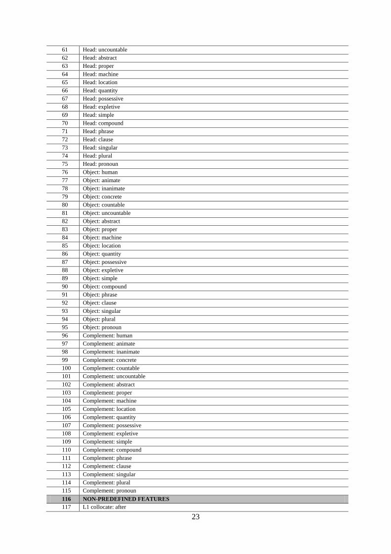
APPENDIX 2 List of all features used as the tagset for the BP.

Number PREDEFINED FEATURES

1 Tense: Present simple

2 Tense: Present simple 3rd

3 Tense: Present progressive (person)

22

4 Tense: Past simple

5 Tense: Past progressive (person)

6 Tense: Pes. Perfect (person)

7 Tense: Present Perfect Progressive (person)

8 Tense: Past Perfect

9 Tense: Past Perfect Progressive

10 Tense: will + inf

11 Tense: will Progressive

12 Tense: will Perfect

13 Tense: will Perfect Progressive

14 Tense: going to

15 Tense: modal present (verb)

16 Tense: modal past (verb)

17 Tense: Present Participle

18 Tense: Past Participle

19 Tense: to infinitive

20 Aspect: simple

21 Aspect: progressive

22 Aspect: perfect

23 Aspect: perfect progressive

24 Voice: active

25 Voice: passive

26 Intransitive

27 Transitive

28 Complex transitive

29 Linking verb

30 Declarative

31 Interrogative

32 Imperative

33 Main

34 Subordinate (with/no subordinator)

35 Relative subordinate

36 Subject: human

37 Subject: animate

38 Subject: inanimate

39 Subject: concrete

40 Subject: countable

41 Subject: uncountable

42 Subject: abstract

43 Subject: proper

44 Subject: machine

45 Subject: location

46 Subject: quantity

47 Subject: possessive

48 Subject: expletive

49 Subject: simple

50 Subject: compound

51 Subject: phrase

52 Subject: clause

53 Subject: singular

54 Subject: plural

55 Subject: pronoun

56 Head: human

57 Head: animate

58 Head: inanimate

59 Head: concrete

60 Head: countable

23

61 Head: uncountable

62 Head: abstract

63 Head: proper

64 Head: machine

65 Head: location

66 Head: quantity

67 Head: possessive

68 Head: expletive

69 Head: simple

70 Head: compound

71 Head: phrase

72 Head: clause

73 Head: singular

74 Head: plural

75 Head: pronoun

76 Object: human

77 Object: animate

78 Object: inanimate

79 Object: concrete

80 Object: countable

81 Object: uncountable

82 Object: abstract

83 Object: proper

84 Object: machine

85 Object: location

86 Object: quantity

87 Object: possessive

88 Object: expletive

89 Object: simple

90 Object: compound

91 Object: phrase

92 Object: clause

93 Object: singular

94 Object: plural

95 Object: pronoun

96 Complement: human

97 Complement: animate

98 Complement: inanimate

99 Complement: concrete

100 Complement: countable

101 Complement: uncountable

102 Complement: abstract

103 Complement: proper

104 Complement: machine

105 Complement: location

106 Complement: quantity

107 Complement: possessive

108 Complement: expletive

109 Complement: simple

110 Complement: compound

111 Complement: phrase

112 Complement: clause

113 Complement: singular

114 Complement: plural

115 Complement: pronoun

116 NON-PREDEFINED FEATURES

117 L1 collocate: after

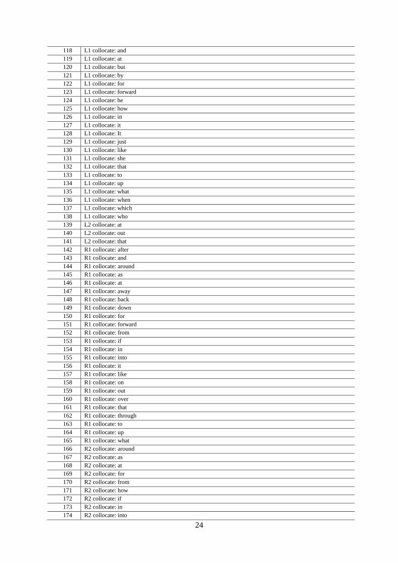
24

118 L1 collocate: and

119 L1 collocate: at

120 L1 collocate: but

121 L1 collocate: by

122 L1 collocate: for

123 L1 collocate: forward

124 L1 collocate: he

125 L1 collocate: how

126 L1 collocate: in

127 L1 collocate: it

128 L1 collocate: It

129 L1 collocate: just

130 L1 collocate: like

131 L1 collocate: she

132 L1 collocate: that

133 L1 collocate: to

134 L1 collocate: up

135 L1 collocate: what

136 L1 collocate: when

137 L1 collocate: which

138 L1 collocate: who

139 L2 collocate: at

140 L2 collocate: out

141 L2 collocate: that

142 R1 collocate: after

143 R1 collocate: and

144 R1 collocate: around

145 R1 collocate: as

146 R1 collocate: at

147 R1 collocate: away

148 R1 collocate: back

149 R1 collocate: down

150 R1 collocate: for

151 R1 collocate: forward

152 R1 collocate: from

153 R1 collocate: if

154 R1 collocate: in

155 R1 collocate: into

156 R1 collocate: it

157 R1 collocate: like

158 R1 collocate: on

159 R1 collocate: out

160 R1 collocate: over

161 R1 collocate: that

162 R1 collocate: through

163 R1 collocate: to

164 R1 collocate: up

165 R1 collocate: what

166 R2 collocate: around

167 R2 collocate: as

168 R2 collocate: at

169 R2 collocate: for

170 R2 collocate: from

171 R2 collocate: how

172 R2 collocate: if

173 R2 collocate: in

174 R2 collocate: into

25

175 R2 collocate: like

176 R2 collocate: on

177 R2 collocate: over

178 R2 collocate: through

179 R2 collocate: to

180 R2 collocate: up

181 R2 collocate: what

182 Subordinator: after

183 Subordinator: and

184 Subordinator: as

185 Subordinator: at

186 Subordinator: but

187 Subordinator: for

188 Subordinator: from

189 Subordinator: how

190 Subordinator: if

191 Subordinator: in

192 Subordinator: like

193 Subordinator: that

194 Subordinator: then

195 Subordinator: through

196 Subordinator: to

197 Subordinator: what

198 Subordinator: when

199 Subordinator: which

200 Subordinator: while

201 Subordinator: who

Резиме

ПОНОВНИ ПОГЛЕД НА ПРЕДВИЂАЈУЋУ МОЋ (МИКРО)КОНТЕКСТА – БЕХАВИОРАЛ

ПРОФИЛИНГ И РАЗАЗНАВАЊЕ ЗНАЧЕЊА

Као што још увек можемо видети у савременој лексикографској пракси, чини се да је једини

заиста успешан модус разазнавања значења речи и даље само лична људска процена. Обновљена вера у

велике репрезентативне рачунарске корпусе језика и недавна поновна појава корпусних статистичких

метода машинског разазнавања значења поново стављају у фокус идеју да је, ако не потпун онда

већински, опис значења речи заснован на емпиријским (лингвистичким) критеријумима ипак могућ. Рад

полази од прегледа теоријске и практичне природе ове идеје и лексичко-семантичке методологије коју

предлаже. Главни циљ рада је, међутим, да испита тачност тврдње о могућем искључиво лингвистичком

(статистичком) опису лексичких значења. Тестирање ове тврдње се спроводи кроз пример примене једне

од најскоријих верзија сличне методологије (Бехавиорал Профилинг) на веома вишезначни глагол look

(гледати) у енглеском језику. Закључак који се намеће после примене и практичног тестирања дате

методологије на правој употреби машинског разазнавања речи је да употреба само лингвистичких

(микроконтекстуалних) критеријума при опису значења није довољна јер дати критеријуми нису

довољно дистинктивни те стога сама методологија није од употребне вредности у лексикографској

пракси и при машинском разазнавању значења.

Nikola Dobrić

Alpen-Adria-Universität Klagenfurt

26

Universitätsstraße 65-67

9020 Klagenfurt

Austria

Nikola.Dobric@uni-klu.ac.at