J. Harju et al. (Eds.): WWIC 2008, LNCS 5031, pp. 13–26, 2008. © Springer-Verlag Berlin Heidelberg 2008

Cross-Layer Modeling of TCP SACK Performance over Wireless Channels with Completely

Reliable ARQ/FEC

Dmitri Moltchanov, Roman Dunaytsev, and Yevgeni Koucheryavy

Department of Communications Engineering, Tampere University of Technology P.O. Box 553, FIN-33101, Tampere, Finland {moltchan,dunaytse,yk}@cs.tut.fi

Abstract. We propose an analytical model for a TCP SACK connection run-ning over a wireless channel with completely reliable ARQ/FEC. We develop the model in two steps. At the first step, we consider the service process of the wireless channel and derive the probability distribution function of the time re-quired to successfully transmit a single IP packet over the wireless channel. This distribution is used at the next step of the modeling where we derive the expression for TCP SACK steady state goodput. The developed model allows to quantify the effect of many implementation-specific parameters on TCP per-formance in wireless domain. We also demonstrate that TCP spurious timeouts, reported in many empirical studies, do not occur when wireless channel condi-tions are stationary and their presence in empirical measurements should be at-tributed to non-stationary behavior of wireless channel characteristics.

1 Introduction

Nowadays, about 80-90% of all packets and bytes traversed over the Internet are TCP traffic and there is no indication that these numbers may decline in the future. Predict-ing TCP behavior in various environments is crucial for better understanding and op-timizing TCP performance over modern networks. TCP congestion and flow control mechanisms pose significant challenges for a performance modeler. Given additional complexity of local error concealment mechanisms implemented at wireless channels previous works on TCP performance in wireless domain were mainly limited to simu-lation and measurement studies (e.g., see [1] and references therein). While empirical studies are extremely useful in TCP performance evaluation, it is a difficult task to simulate and explore TCP behavior across the range of all possible operational condi-tions and low-level protocols settings. In this case, an analytical cross-layer model is extremely beneficial because it allows to study the protocol performance over the en-tire parameter space and very easily apply the “what if” test to the different scenarios.

Due to negligibly low error ratio of current wired networks, performance degrada-tion mainly stems from buffering procedures. The situation is much more complicated in wireless networks, where, in addition to performance degradation induced by buff-ering procedures, we also have to take into account those delays and losses occurring due to unreliable nature of wireless transmission media. Being inherently prone to

14 D. Moltchanov, R. Dunaytsev, and Y. Koucheryavy

transmission errors, wireless access technologies implement error concealment tech-niques including automatic repeat request (ARQ) and forward error correction (FEC). However, even in the presence of these local error recovery mechanisms bit errors may still propagate to higher layers resulting in loss or excessive delay of IP packets triggering TCP congestion control procedures. Therefore, the choice of local error concealment parameters may severely affect TCP performance.

In this paper, we develop a cross-layer model for a TCP SACK connection running over a wireless channel. The performance parameter of interest is the long-term steady state goodput of a single TCP SACK connection. The wireless channel charac-teristics are assumed to be stationary and modeled by a homogenous Markov process. We also assume that ARQ and FEC are both implemented at the wireless channel. The proposed model highlights many interesting features of TCP performance in wireless environment. Among other conclusions, we demonstrate that TCP spurious timeouts, reported in many empirical studies, do not occur when wireless channel conditions are stationary and should be attributed to non-stationary behavior of wire-less channel characteristics.

The rest of the paper is organized as follows. The system model is described in Section 2. The cross-layer model is introduced in Sections 3 and 4. Numerical results are discussed in Section 5. Finally, conclusions are summarized in Section 6.

2 System Model

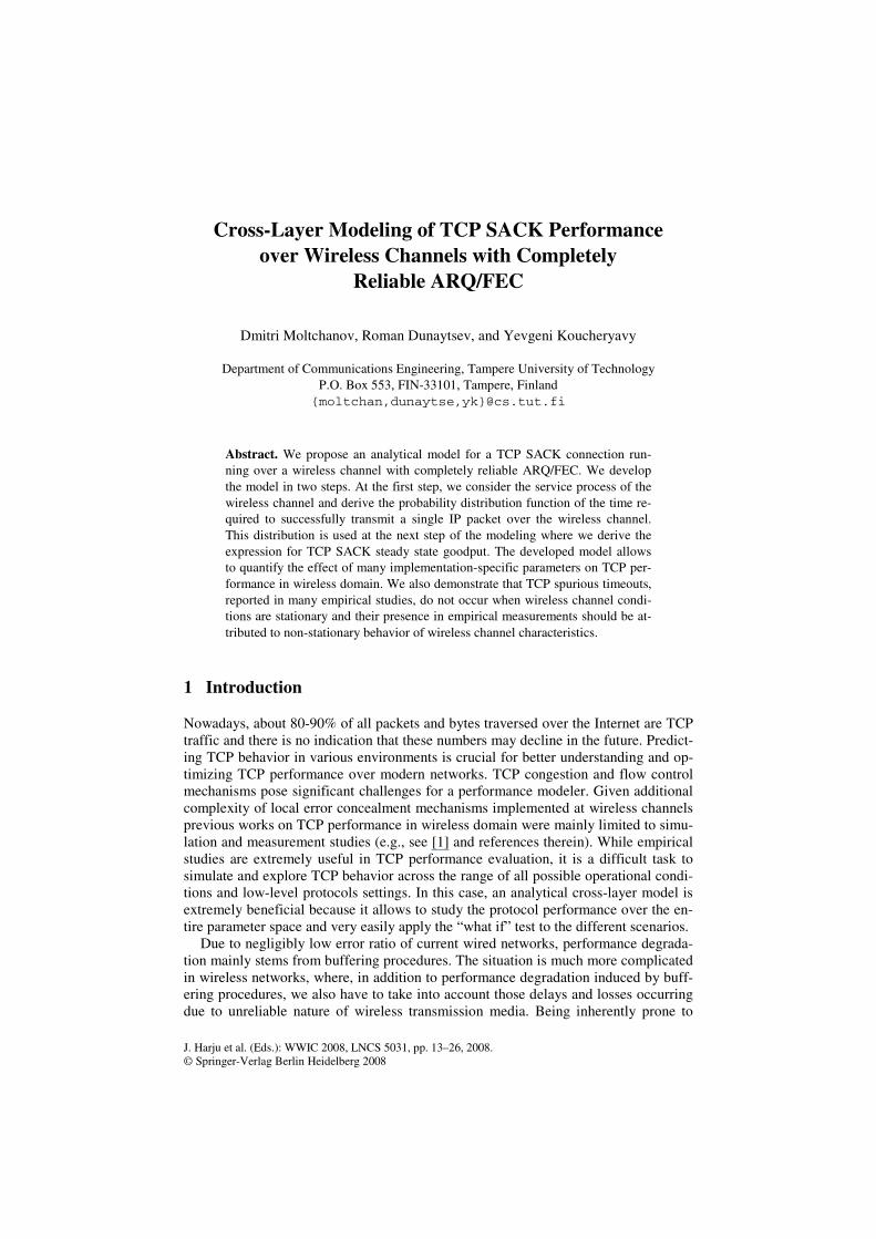
The system of interest is illustrated in Fig. 1. We consider a TCP connection between two hosts such that the last link on the end-to-end path from the sender to the receiver is a wireless channel. In this paper, we consider the wireless channel as a bottleneck. Since such scenario is common in wireless communications, we do not resort to a par-ticular wireless access technology. Instead, we consider a number of features this channel includes. We assume that ARQ and FEC functionalities are both imple-mented at the wireless channel and ARQ operates according to either stop-and-wait or selective acknowledgement regime.

Fig. 1. System model

Since nearly all TCP implementations now support the selective acknowledgement (SACK) option, we assume that the sender and the receiver are both SACK-capable and use the SACK option under all permitted circumstances in accordance to [2], [3], and [4]. We consider an application process which always has data to send, thus the

Cross-Layer Modeling of TCP SACK Performance over Wireless Channels 15

sender always sends full-sized TCP segments (i.e., containing MSS bits of data) when-ever congestion window (cwnd) allows. We assume that the receiver’s buffer is suffi-ciently large, so TCP send rate is not limited by inappropriately small value of the advertised receive window. We also assume that the time needed to send a window of segments is smaller than the round-trip time (RTT). These assumptions are justified for modern high-performance computers. Since we are focusing on the performance of a single TCP connection running over a wireless channel, we do not consider here competing traffic effects and assume that data are transmitted only in one direction: from the sender to the receiver (see Fig. 1).

Let the service rate of the wireless bottleneck link be μ bits per second and the

buffer size at the intermediate system be B IP packets, where all IP packets are of the same size and consist of MTU bits. The queue at the intermediate system is the queue of IP packets waiting to be transmitted over the wireless channel. The queue man-agement is assumed to be FIFO Drop-Tail, so any packet arriving when the buffer is full will be lost.

Data packets are buffered at the IP layer of the intermediate system and transmitted one after another to the data-link layer. Once a current packet is successfully deliv-ered next packet is taken from the buffer at the IP layer. At the data-link layer, IP packets are segmented into equal-sized frames. ARQ at the data-link layer is assumed to be completely reliable meaning that a frame is always delivered irrespective of the number of retransmissions it takes. However, if the number of data-link retransmis-sions causes the RTT to exceed the current value of the TCP retransmission timeout (RTO) [5], the TCP retransmission timer will expire, leading to a spurious TCP time-out followed by unnecessary retransmission of the last window of data and congestion control procedures invocation.

We also assume that the wireless channel in the reverse direction is completely re-liable. Indeed, feedback acknowledgements are usually small in size and well pro-tected by FEC code. Thus, we assume that packet losses happen only in the direction from the sender to the receiver due to buffer overflow at the intermediate system. Fi-nally, we assume that ACK-packets are delivered instantaneously over the wireless channel. All these assumptions were used in many studies and found to be appropriate for relatively high-speed wireless channels [6], [7]. Note that the described model is also suitable to represent “ideal” Selective Repeat ARQ scheme as in [8], [9].

3 Service Process of the Wireless Channel

3.1 Bit Error Model

In this paper, we represent bit error process using a covariance-stationary two-state Markov modulated process. Using relatively simple algorithm outlined below it al-lows to capture first- and second-order statistical characteristics in terms of error rate and lag-1 autocorrelation coefficient. Note that the extension to the case of general fi-nite-state Markov chain (FSMC) and its variants is straightforward [10].

We model the bit error process using a two-state Markov modulated process. Let { ( ), 0,1, }EW l l = … , ( ) {0,1}EW l ∈ , denote the model with the modulating Markov

chain { ( ), 0,1, }ES l l = … , ( ) {0,1}ES l ∈ . The model is completely defined using the set

16 D. Moltchanov, R. Dunaytsev, and Y. Koucheryavy

of matrices ( )ED k , 0,1k = , containing transition probabilities from state i to state

j with or without incorrect reception of a channel symbol. To parameterize a covari-

ance stationary binary process, only mean and lag-1 autocorrelation coefficient have to be captured. In our previous work, we have showed that there is a unique switched Bernoulli process (SBP) matching mean and lag-1 autocorrelation of covariance sta-tionary bit error observations [11]. This model is given by

1,

2,

(1) 0,(1 (1)) [ ],

(1) 1,(1 (1))(1 [ ]),EE E E

EE E E

fK E W

fK E W

αβ

== − ⎧⎧⎨ ⎨ == − −⎩ ⎩

(1)

where 1, (1)Ef and 2, (1)Ef are probabilities of error in states 1 and 2, respectively, Eα

and Eβ are transition probabilities from state 1 to state 2 and from state 2 to state 1,

respectively, (1)EK is the lag-1 autocorrelation of bit error observations, [ ]EE W is

the mean of bit error observations. Details of the algorithm are outlined in [11].

3.2 Frame Error Model

Assume that the length of frames is constant and equals to m bits. Consider the sto-chastic process { ( ), 0,1, }NW n n = … , ( ) {0,1, }NW n m∈ … , n lm= , describing the num-

ber of incorrectly received bits in consecutive bit patterns of length m . This process is doubly stochastic, modulated by the underlying Markov chain { ( ), 0,1, }NS n n = …

and can be completely parameterized via parameters of the bit error process { ( ), 0,1, }EW l l = … as shown below.

To parameterize { ( ), 0,1, }NW n n = … , we have to determine m-step transition prob-

abilities of the modulating Markov chain { ( ), 0,1, }ES l l = … with exactly k ,

0,1, ,k m= … , incorrectly received bits. Denote the probability of transition from state

i to state j for the Markov chain { ( ), 0,1, }NS n n = … with exactly k , 0,1, ,k m= … ,

incorrectly received bits in a bit pattern of length m by

, ( ) Pr{ ( ) , ( ) | ( 1) }N ij N N Nd k W n k S n j S n i= = = − = .

01

1

2 02

0 2

(0) (0),

(1) (0) (1) (0),

(2) (0) (1) (0) (1) (0),

( ) (1).

mN E

m k kN E E E

k m

mk m i k i

N E E E E Ek i m k

mN E

D D

D D D D

D D D D D D

D m D

− −

= −−

− − −

= = − −

=

=

=

=

∑

∑ ∑…

(2)

Let the set of matrices ( )ND k , 0,1, ,k m= … , contains these transition probabili-

ties. These matrices can be found using ( )ED k , 0,1k = , as given in (2), were ( )ND i ,

3, 4, , 2i m= −… , can be obtained by induction from (1)ND or ( 1)ND m − . The easiest

Cross-Layer Modeling of TCP SACK Performance over Wireless Channels 17

way is to induce ( )ND i , 2,3, , 2i m= ⎢ ⎥⎣ ⎦… , from (1)ND and ( )ND i ,

2, 3, , 2i m m m= − − ⎡ ⎤⎢ ⎥… , from ( 1)ND m − .

Note that computation according to (2) is a challenging task and becomes impossi-ble when m is large. Instead, one may use the recursive method as outlined below.

Let us extend the definition of ( )ND k , 0,1, ,k m= … , as follows. We denote the

probability of transition from state i to state j for the Markov chain

{ ( ), 0,1, }NS n n = … with exactly k , 0,1, ,k m= … , incorrectly received bits in a bit

pattern of length m by , ( , )N ijd k m . Let the set of matrices ( , )ND k m , 0,1, ,k m= … ,

contains these transition probabilities. Since at most two errors may occur in two con-secutive slots, we have the following expression for ( , 2)ND i , 0,1,2i = :

0

( , 2) ( ) ( ), 0,1,2,i

N E Ek

D i D k D i k i=

= − =∑ (3)

where (2)ED is the matrix of zeros. Recursively, we get

0

0

0

( ,3) ( , 2) ( ), 0,1, 3,

( , 4) ( ,3) ( ), 0,1, 4,

( , ) ( , 1) ( ), 0,1, , ,

i

N N Ek

i

N N Ek

i

N N Ek

D i D k D i k i

D i D k D i k i

D i m D k m D i k i m

=

=

=

= − =

= − =

= − − =

∑

∑

∑

…

…

…

…

(4)

where ( )ED k , 2k ≥ , and ( , )ND i m , 1i m≥ + , are all zero matrices. Taking this into

account we finally have

( , 1) (0,1), 0,( , )

( , 1) (0,1) ( 1, 1) (1,1), 0,N N

NN N N N

D i k D iD i k

D i k D D i k D i

− =⎧= ⎨ − + − − ≠⎩

(5)

where ( ,1) ( )N ED i D i= , 0,1i = .

The latter equation gives ( )ND k , 0,1, ,k m= … , for a given m . Using the pro-

posed approach the computational complexity decreases significantly and the model can be used for large values of m .

Consider now the frame error process { ( ), 0,1, }FW n n = … , ( ) {0,1}FW n ∈ , where

“0” indicates the correct reception of a frame, “1” denotes the incorrect frame recep-tion. Let us denote the transition probability from state i to state j for the Markov

chain { ( ), 0,1, }FS n n = … with exactly k , 0,1k = , incorrectly received frames by

, ( )F ijd k , 0,1k = . These probabilities are then combined in the matrices (0)FD and

(1)FD . The process { ( ), 0,1, }NW n n = … , ( ) {0,1, , }NW n m∈ … , describing the number

of bit errors in consecutive frames is related to the frame error process { ( ), 0,1, }FW n n = … , ( ) {0,1,..., }FW n m∈ , as follows:

18 D. Moltchanov, R. Dunaytsev, and Y. Koucheryavy

1

0

(0) ( ), (0) ( ),T

T

F m

F N F Nk k F

D D k D D k−

= =

= =∑ ∑ (6)

where TF is the so-called frame error threshold determining whether a certain frame

is correctly received or not. Expressions (6) are interpreted as follows: if the number of incorrectly received bits in a frame is greater or equal to a computed value of the frame error threshold ( Tk F≥ ), then the frame is incorrectly received and ( ) 1FW n = .

Otherwise ( Tk F< ), it is correctly received and ( ) 0FW n = .

Assume now that the number of bit errors that can be corrected by a FEC code in a frame of length m is l . Then the frame error threshold is 1TF l= + and the frame is

incorrectly received whenever Tk F≥ . Otherwise, it is correctly received. Thus, the

transition probability matrices (6) take the following form:

1

0

(0) ( ), (1) ( ).T

T

F m

F N F Nk k F

D D k D D k−

= =

= =∑ ∑ (7)

3.3 Packet Service Process

Consider now the service process of IP packets at the data-link layer. We assume that each frame requires exactly a unit time to be transmitted over the wireless channel. All IP packets are of the same length and segmented to v frames at the data-link layer. This assumption is not restrictive as data-link frames are usually of fixed size. Due to impairments introduced by wireless transmission medium successful delivery of frames may take random duration in time. As a result, successful delivery of an IP packet is also a random variable with a certain distribution. To parameterize the ser-vice process of an IP packet we have to find its service time distribution.

Let ( )Pf k , , 1,k m m= + … , be the probability function (PF) of the delay of an IP

packet. Consider the IP packet service process describing the number of slots required to successfully transmit a single IP packet. In order to correctly transmit an IP packet, we have to correctly transmit all the frames to which this packet is segmented. Thus, the minimum time to transmit an IP packet is the time to successfully transmit all m frames from first attempts. Since the data-link layer is completely reliable the maxi-mum transmission time of the packet is virtually unlimited.

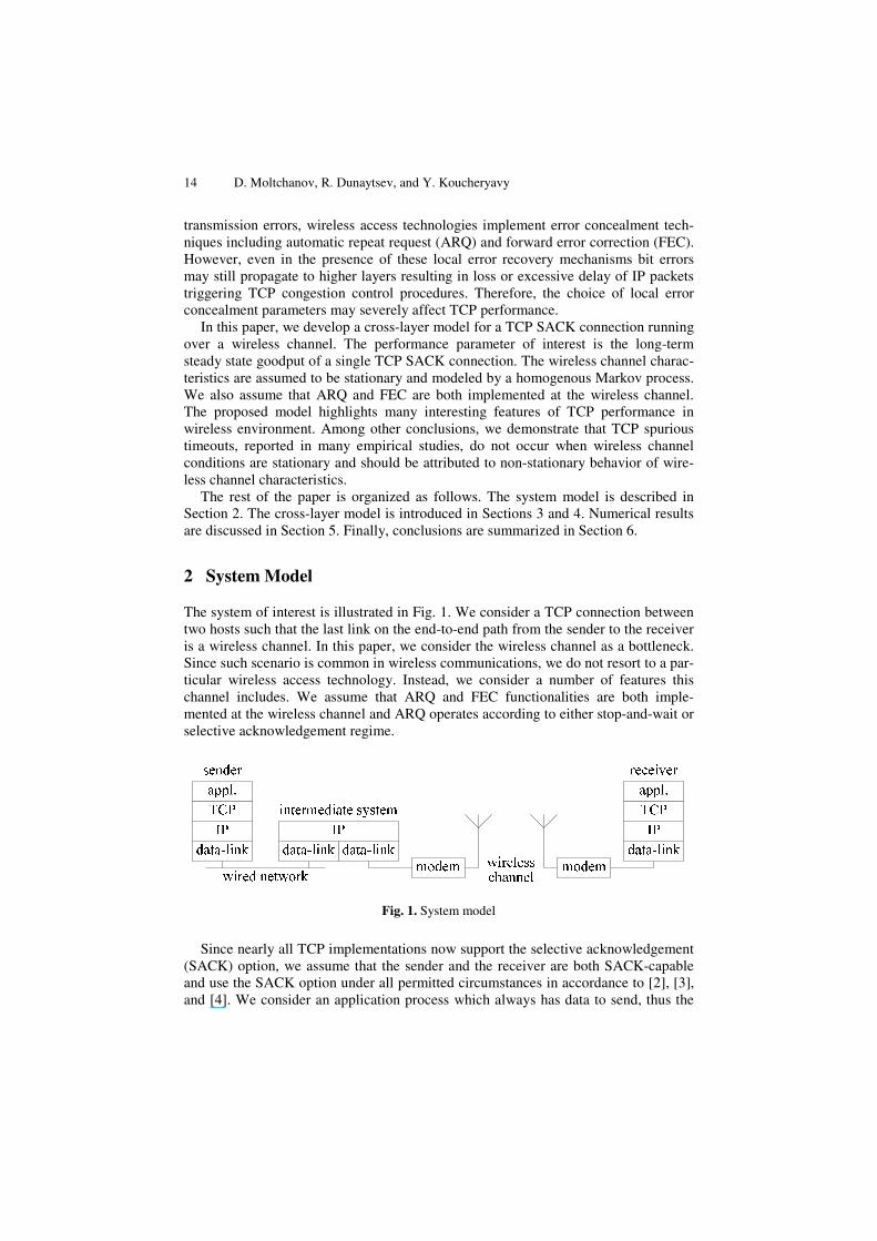
Firstly, consider the situation when all the frames in a packet are correctly trans-mitted in their first attempts. In this case, the duration of packet transmission is ex-actly v slots. In order for service time of the packet to be ( 1)v + slots, there should be

exactly one incorrectly transmitted frame in a sequence of v frames. Generalizing to ( )v i+ slots delay, we note that there should be exactly i transmission attempts that

failed to transmit a frame correctly. Since any packet transmission should end with correctly received frame, the last case can be interpreted as having ( 1)v i+ − errors in

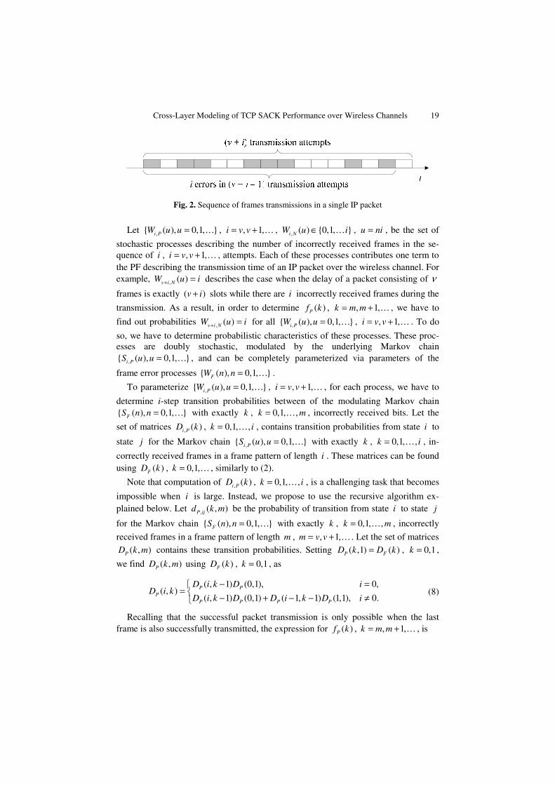
( )v i+ transmission attempts. The sequence of frames transmissions in a packet is

illustrated in Fig. 2, where grey rectangles denote incorrect frame reception and white rectangles stand for correct frame reception.

Cross-Layer Modeling of TCP SACK Performance over Wireless Channels 19

Fig. 2. Sequence of frames transmissions in a single IP packet

Let ,{ ( ), 0,1, }i PW u u = … , , 1,i v v= + … , , ( ) {0,1, }i NW u i∈ … , u ni= , be the set of

stochastic processes describing the number of incorrectly received frames in the se-quence of i , , 1,i v v= + … , attempts. Each of these processes contributes one term to the PF describing the transmission time of an IP packet over the wireless channel. For example, , ( )v i NW u i+ = describes the case when the delay of a packet consisting of ν

frames is exactly ( )v i+ slots while there are i incorrectly received frames during the

transmission. As a result, in order to determine ( )Pf k , , 1,k m m= + … , we have to

find out probabilities , ( )v i NW u i+ = for all ,{ ( ), 0,1, }i PW u u = … , , 1,i v v= + … . To do

so, we have to determine probabilistic characteristics of these processes. These proc-esses are doubly stochastic, modulated by the underlying Markov chain

,{ ( ), 0,1, }i PS u u = … , and can be completely parameterized via parameters of the

frame error processes { ( ), 0,1, }FW n n = … .

To parameterize ,{ ( ), 0,1, }i PW u u = … , , 1,i v v= + … , for each process, we have to

determine i-step transition probabilities between of the modulating Markov chain { ( ), 0,1, }FS n n = … with exactly k , 0,1, ,k m= … , incorrectly received bits. Let the

set of matrices , ( )i PD k , 0,1, ,k i= … , contains transition probabilities from state i to

state j for the Markov chain ,{ ( ), 0,1, }i PS u u = … with exactly k , 0,1, ,k i= … , in-

correctly received frames in a frame pattern of length i . These matrices can be found using ( )FD k , 0,1,k = … , similarly to (2).

Note that computation of , ( )i PD k , 0,1, ,k i= … , is a challenging task that becomes

impossible when i is large. Instead, we propose to use the recursive algorithm ex-plained below. Let , ( , )P ijd k m be the probability of transition from state i to state j

for the Markov chain { ( ), 0,1, }FS n n = … with exactly k , 0,1, ,k m= … , incorrectly

received frames in a frame pattern of length m , , 1,m v v= + … . Let the set of matrices ( , )PD k m contains these transition probabilities. Setting ( ,1) ( )P FD k D k= , 0,1k = ,

we find ( , )PD k m using ( )FD k , 0,1k = , as

( , 1) (0,1), 0,( , )

( , 1) (0,1) ( 1, 1) (1,1), 0.P P

PP P P P

D i k D iD i k

D i k D D i k D i

− =⎧= ⎨ − + − − ≠⎩

(8)

Recalling that the successful packet transmission is only possible when the last frame is also successfully transmitted, the expression for ( )Pf k , , 1,k m m= + … , is

20 D. Moltchanov, R. Dunaytsev, and Y. Koucheryavy

( )( ) ( , 1) (0) ,P k P Ff k D k v k D eπ= − − (9)

where e is the vector of ones of appropriate size, kπ is the steady state probability

vector of ,{ ( ), 0,1, }k PW n n = … . Vectors kπ , , 1,k v v= + … , can be found as the solu-

tion of the following matrix equations: kk F kDπ π= , 1k eπ = .

4 TCP SACK Model

In this section, we consider the evolution of a TCP SACK connection and derive ex-pression for its long-term steady state goodput, where the goodput is the useful num-ber of bits received by the destination per second. The developed model is based on the fluid model approach, first proposed in [12].

Let the round-trip path delay of the wired network be τ seconds. The system per-formance bottleneck is determined by the limited service rate of the wireless channel. In contrast to the wired network, where multiple packets can be sent without waiting for the first packet to reach the other end of the link, the wireless channel cannot hold multiple packets in the air at once since the previously transmitted packet should be successfully delivered before starting a new transmission. Thus, the bandwidth-delay product of the network path can be found as 1C MTUμτ= + . The maximum num-

ber of IP packets that can be accommodated in the network is ( )C B+ , assuming that

there are C packets in flight and the buffer at the intermediate system is fully occu-pied. Since 1B ≥ , it implies that 3C B+ ≥ .

Let us consider steady state TCP SACK behavior in the absence of delay spikes caused by wireless channel impairments. In this case, the connection experiences pe-riodic packet losses: each time cwnd exceeds the maximum number of packets that can be accommodated in the network, the last packet in a window of data is dropped due to buffer overflow at the intermediate system. According to the sliding window algorithm, after the lost segment ( )C B+ more segments are sent, triggering duplicate

ACKs. As long as 3C B+ ≥ , the sender receives enough duplicate ACKs to trigger the loss recovery algorithm [4]. Thus, the cyclical evolution of TCP SACK is as fol-lows. A cycle starts after a segment loss is detected via three duplicate ACKs. Then the current cwnd is set to roughly ( ) 2C B+ and the congestion avoidance phase be-

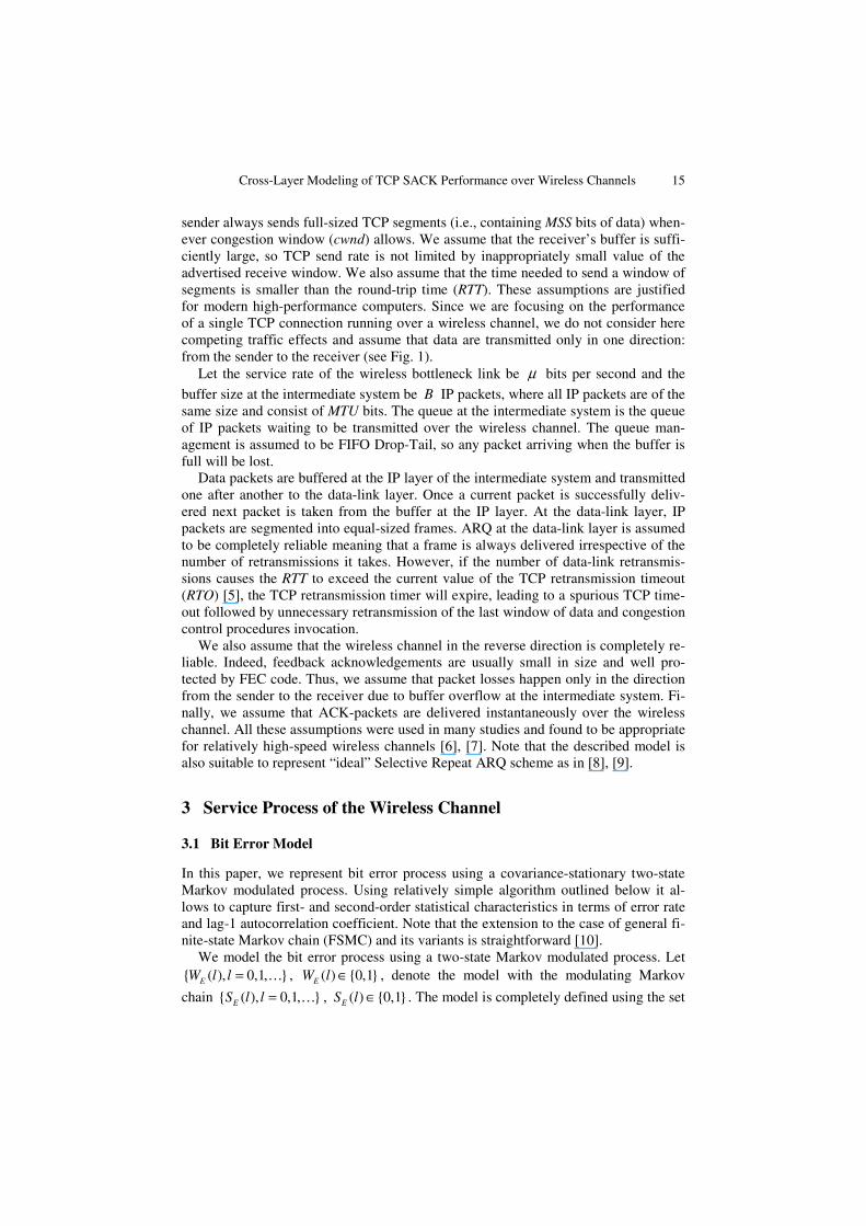
gins. The receiver sends one ACK for every -thb segment it gets, so cwnd increases linearly with a slope of 1 b segments per RTT until cwnd C B= + (see Fig. 3). Fac-

tor b depends on the acknowledgement strategy of the receiver: as specified in [13], a TCP should use delayed ACKs, sending an ACK for at least every second data seg-ment ( 2b = ); however, it is also allowed to send an ACK for every data segment ( 1b = ). The next additive increase of cwnd leads to new buffer overflow and the cur-rent cycle ends. Thus, we consider a cycle to be a period between two consecutive losses. Since any lost segment can be recovered within a single RTT by using the SACK-based loss recovery algorithm, we are neglecting the details of the loss recov-ery phase between cycles as having negligible effect on TCP SACK performance.

Cross-Layer Modeling of TCP SACK Performance over Wireless Channels 21

0 0 0000

00

00

00

B

B

B

(C+B)

Time (RTT)

Time (RTT)

Time (RTT)

Time (RTT)

Time (RTT)

Time (RTT)

Queue size (pkts)

cwnd (pkts)

B = C B > C B < C

+

2

C B⎛ ⎞⎜ ⎟⎝ ⎠

+

2

C B⎛ ⎞⎜ ⎟⎝ ⎠

+

2

C B⎛ ⎞⎜ ⎟⎝ ⎠

+

2

C Bb⎛ ⎞⎜ ⎟⎝ ⎠

+

2

C Bb⎛ ⎞⎜ ⎟⎝ ⎠

+

2

C Bb⎛ ⎞⎜ ⎟⎝ ⎠

+

2

C Bb⎛ ⎞⎜ ⎟⎝ ⎠

+

2

C Bb⎛ ⎞⎜ ⎟⎝ ⎠

+

2

C Bb⎛ ⎞⎜ ⎟⎝ ⎠

(C+B) (C+B)

Queue size (pkts)Queue size (pkts)

cwnd (pkts) cwnd (pkts)

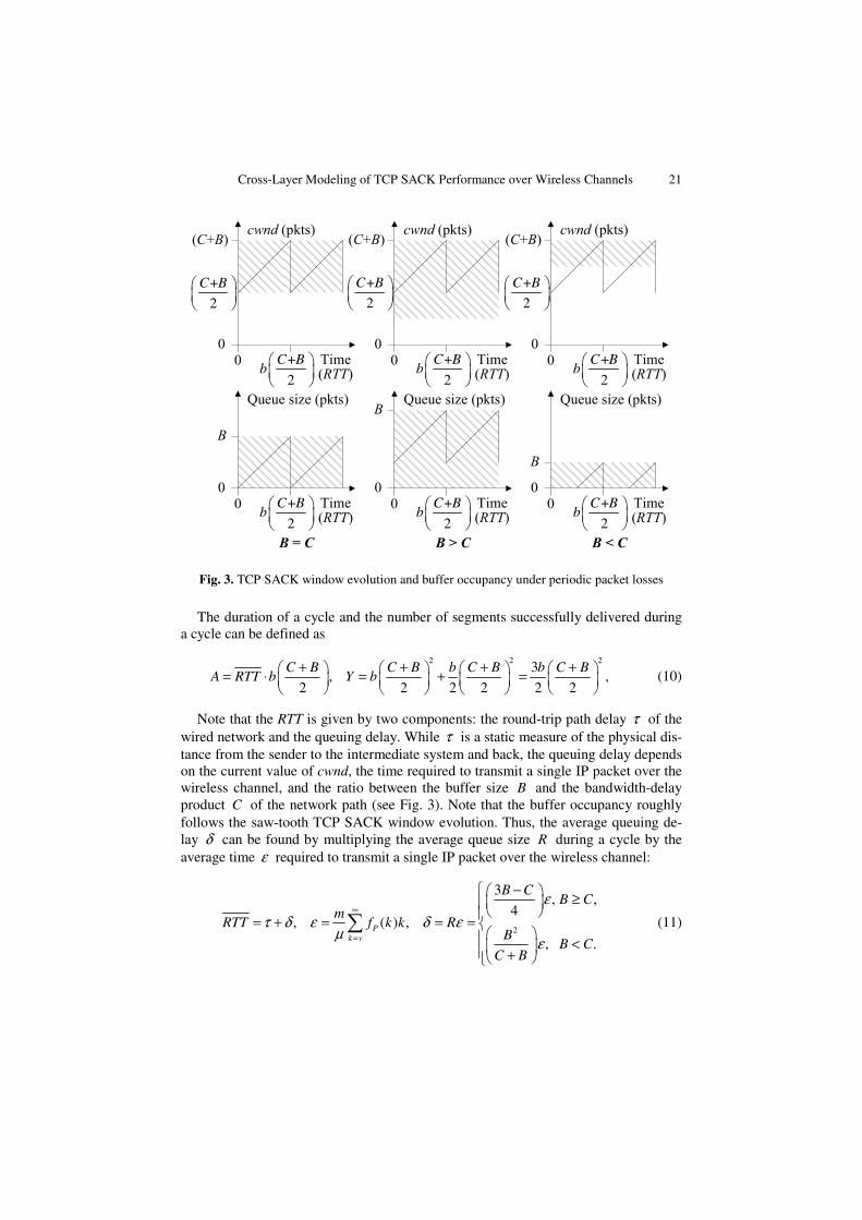
Fig. 3. TCP SACK window evolution and buffer occupancy under periodic packet losses

The duration of a cycle and the number of segments successfully delivered during a cycle can be defined as

2 2 23

, ,2 2 2 2 2 2

C B C B b C B b C BA RTT b Y b

+ + + +⎛ ⎞ ⎛ ⎞ ⎛ ⎞ ⎛ ⎞= ⋅ = + =⎜ ⎟ ⎜ ⎟ ⎜ ⎟ ⎜ ⎟⎝ ⎠ ⎝ ⎠ ⎝ ⎠ ⎝ ⎠

(10)

Note that the RTT is given by two components: the round-trip path delay τ of the wired network and the queuing delay. While τ is a static measure of the physical dis-tance from the sender to the intermediate system and back, the queuing delay depends on the current value of cwnd, the time required to transmit a single IP packet over the wireless channel, and the ratio between the buffer size B and the bandwidth-delay product C of the network path (see Fig. 3). Note that the buffer occupancy roughly follows the saw-tooth TCP SACK window evolution. Thus, the average queuing de-lay δ can be found by multiplying the average queue size R during a cycle by the average time ε required to transmit a single IP packet over the wireless channel:

2

3, ,

4, ( ) ,

, .P

k v

B CB C

mRTT f k k R

BB C

C B

ετ δ ε δ ε

με

∞

=

⎧ −⎛ ⎞ ≥⎜ ⎟⎪⎝ ⎠⎪= + = = = ⎨⎛ ⎞⎪ <⎜ ⎟⎪ +⎝ ⎠⎩

∑ (11)

22 D. Moltchanov, R. Dunaytsev, and Y. Koucheryavy

Let us consider the effect of delay spikes on the long-term steady state goodput of a TCP SACK connection. As it was pointed out in [1], a TCP spurious timeout occurs when the RTT value suddenly increases to the extent that it exceeds the duration of the TCP retransmission timer, RTO. In the considered scenario, the completely reliable data-link layer can cause a sudden delay due to bit errors on the wireless channel.

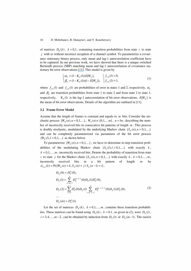
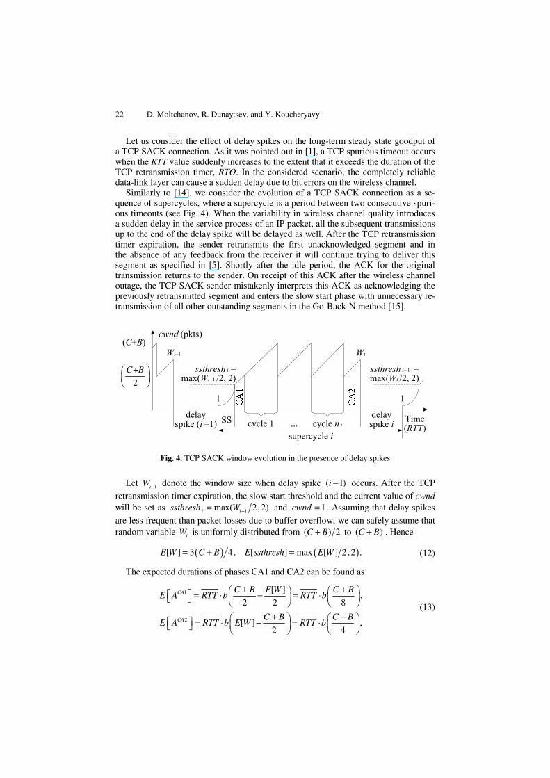
Similarly to [14], we consider the evolution of a TCP SACK connection as a se-quence of supercycles, where a supercycle is a period between two consecutive spuri-ous timeouts (see Fig. 4). When the variability in wireless channel quality introduces a sudden delay in the service process of an IP packet, all the subsequent transmissions up to the end of the delay spike will be delayed as well. After the TCP retransmission timer expiration, the sender retransmits the first unacknowledged segment and in the absence of any feedback from the receiver it will continue trying to deliver this segment as specified in [5]. Shortly after the idle period, the ACK for the original transmission returns to the sender. On receipt of this ACK after the wireless channel outage, the TCP SACK sender mistakenly interprets this ACK as acknowledging the previously retransmitted segment and enters the slow start phase with unnecessary re-transmission of all other outstanding segments in the Go-Back-N method [15].

(C+B)

Time (RTT)

cwnd (pkts)

Wi

ssthresh i =max(Wi–1 /2, 2)

cycle 1 cycle n i...

1

delayspike i

supercycle i

1

SS

Wi–1

delayspike (i –1)

+

2

C B⎛ ⎞⎜ ⎟⎝ ⎠

ssthresh i+1 =max(Wi /2, 2)

Fig. 4. TCP SACK window evolution in the presence of delay spikes

Let 1iW − denote the window size when delay spike ( 1)i − occurs. After the TCP

retransmission timer expiration, the slow start threshold and the current value of cwnd will be set as 1max( 2,2)i issthresh W −= and 1cwnd = . Assuming that delay spikes

are less frequent than packet losses due to buffer overflow, we can safely assume that random variable iW is uniformly distributed from ( ) 2C B+ to ( )C B+ . Hence

( ) ( )[ ] 3 4, [ ] max [ ] 2,2 .E W C B E ssthresh E W= + = (12)

The expected durations of phases CA1 and CA2 can be found as

1

2

[ ],

2 2 8

[ ] ,2 4

CA

CA

C B E W C BE A RTT b RTT b

C B C BE A RTT b E W RTT b

+ +⎛ ⎞ ⎛ ⎞⎡ ⎤ = ⋅ − = ⋅⎜ ⎟ ⎜ ⎟⎣ ⎦ ⎝ ⎠ ⎝ ⎠+ +⎛ ⎞ ⎛ ⎞⎡ ⎤ = ⋅ − = ⋅⎜ ⎟ ⎜ ⎟⎣ ⎦ ⎝ ⎠ ⎝ ⎠

(13)

Cross-Layer Modeling of TCP SACK Performance over Wireless Channels 23

and the expected number of segments delivered during these phases can be defined as

2 21

2 22

[ ] [ ] [ ] 7,

2 2 2 2 2 2 2 8

5[ ] [ ] .

2 2 2 2 2 4

CA

CA

C B E W E W b C B E W b C BE Y b

C B C B b C B b C BE Y b E W E W

+ + +⎛ ⎞ ⎛ ⎞ ⎛ ⎞⎡ ⎤ = − + − =⎜ ⎟ ⎜ ⎟ ⎜ ⎟⎣ ⎦ ⎝ ⎠ ⎝ ⎠ ⎝ ⎠

+ + + +⎛ ⎞⎛ ⎞ ⎛ ⎞ ⎛ ⎞⎡ ⎤ = − + − =⎜ ⎟⎜ ⎟ ⎜ ⎟ ⎜ ⎟⎣ ⎦ ⎝ ⎠⎝ ⎠ ⎝ ⎠ ⎝ ⎠

(14)

The number of segments delivered during the slow start (SS) phase can be closely

approximated as a geometric series 121 ( 1) ( 1)i iN NSSiY γ γ γ γ γ−= + + + + = − −… ,

where 1 1 bγ = + [16]. Taking into account that in the slow start phase of the -thi

supercycle cwnd growths exponentially from 1 to issthresh , we get that

( )11max 2, 2iN

iWγ −−= . Hence the expected duration of the slow start phase and the

number of segments successfully delivered during this phase can be expressed as

( )[ ] [ ] 2

max log ,2 , max ,3 .2 2 1

SS SSE W E WE A RTT E Yγ

γ γγ

⎛ ⎞⎛ ⎞ −⎛ ⎞⎡ ⎤ ⎡ ⎤= ⋅ = ⎜ ⎟⎜ ⎟⎜ ⎟⎣ ⎦ ⎣ ⎦ ⎜ ⎟−⎝ ⎠⎝ ⎠ ⎝ ⎠ (15)

Combining (10)-(15), we define TCP SACK long-term steady state goodput as

( )( )( )

1 2

1 2

[ ] [ ] [ ] ( [ ] 1),

[ ] [ ] [ ] [ ]

SS CA CA

SS CA CA

MSS Y Q E Y E Y E Y E WG

A Q E T E A E A E A

+ + + − −=

+ + + + (16)

where Q is the probability of TCP retransmission timer expiration, ( [ ] 1)E W − is the

expected number of spuriously retransmitted segments during the slow start phase, [ ]E T is the expected duration of a delay spike. Using (9) we have

[ ] ( ) , ( ) ,P Pk n k n

mE T f k k Q f k

ε εμ

∞ ∞

= =⎡ ⎤ ⎡ ⎤⎢ ⎥ ⎢ ⎥

= =∑ ∑ (17)

where n , 1n ≥ , relates to the granularity of the TCP retransmission timer.

5 Numerical Analysis

Firstly, let us consider whether delay spikes often occur on the wireless channels be-having in stationary manner. In order to do so, we estimate probabilities of delay spike for different input parameters. In what follows, to visualize the effect of differ-ent parameters we choose the following settings: [ ] {0.01,0.02, ,0.09}EE W ∈ … ,

(1) {0.0,0.1, ,0.9}EK ∈ … , (255,131,18) and (255,87,26) BCH FEC codes,

1500MTU = bytes, 1460MSS = bytes, 384μ = kbit/s, 10τ = ms, 80B = packets.

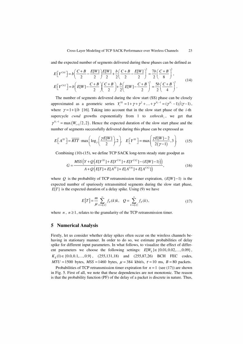
Probabilities of TCP retransmission timer expiration for 1n = (see (17)) are shown in Fig. 5. First of all, we note that these dependencies are not monotonic. The reason is that the probability function (PF) of the delay of a packet is discrete in nature. Thus,

24 D. Moltchanov, R. Dunaytsev, and Y. Koucheryavy

depending of the value of the mean delay the probability of TCP retransmission timer expiration computed according to (17) may slightly vary. Indeed, this probability is just mass of the PF for all k which are greater than [ ]PE f⎡ ⎤⎢ ⎥ . When [ ]PE f is closer

to [ ]PE f⎢ ⎥⎣ ⎦ than to [ ]PE f⎡ ⎤⎢ ⎥ , there is more probability mass in the right hand part of

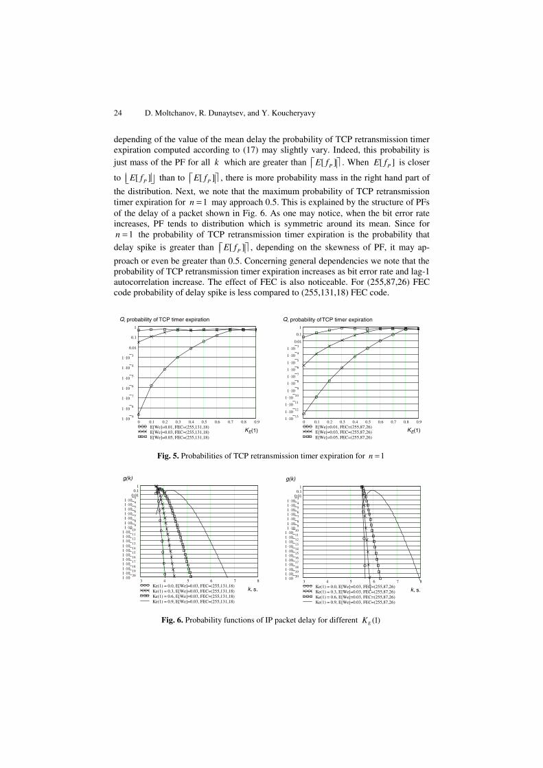
the distribution. Next, we note that the maximum probability of TCP retransmission timer expiration for 1n = may approach 0.5. This is explained by the structure of PFs of the delay of a packet shown in Fig. 6. As one may notice, when the bit error rate increases, PF tends to distribution which is symmetric around its mean. Since for

1n = the probability of TCP retransmission timer expiration is the probability that

delay spike is greater than [ ]PE f⎡ ⎤⎢ ⎥ , depending on the skewness of PF, it may ap-

proach or even be greater than 0.5. Concerning general dependencies we note that the probability of TCP retransmission timer expiration increases as bit error rate and lag-1 autocorrelation increase. The effect of FEC is also noticeable. For (255,87,26) FEC code probability of delay spike is less compared to (255,131,18) FEC code.

0 0.1 0.2 0.3 0.4 0.5 0.6 0.7 0.8 0.91 .10

9

1 .108

1 .107

1 .106

1 .105

1 .104

1 .103

0.01

0.1

1

E[We]=0.01, FEC=(255,131,18)E[We]=0.03, FEC=(255,131,18)E[We]=0.05, FEC=(255,131,18)

Q, probability of TCP timer expiration

KE(1)

0 0.1 0.2 0.3 0.4 0.5 0.6 0.7 0.8 0.91 .10

131 .10

121 .10

111 .10

101 .10

91 .10

81 .10

71 .10

61 .10

51 .10

41 .10

30.01

0.1

1

E[We]=0.01, FEC=(255,87,26)E[We]=0.03, FEC=(255,87,26)E[We]=0.05, FEC=(255,87,26)

Q, probability of TCP timer expiration

KE(1)

Fig. 5. Probabilities of TCP retransmission timer expiration for 1n =

3 4 5 6 7 81 .10

201 .10

191 .10

181 .10

171 .10

161 .10

151 .10

141 .10

131 .10

121 .10

111 .10

101 .10

91 .10

81 .10

71 .10

61 .10

51 .10

41 .10

30.01

0.11

Ke(1) = 0.0, E[We]=0.03, FEC=(255,131,18)Ke(1) = 0.3, E[We]=0.03, FEC=(255,131,18)Ke(1) = 0.6, E[We]=0.03, FEC=(255,131,18)Ke(1) = 0.9, E[We]=0.03, FEC=(255,131,18)

g(k)

k, s.

3 4 5 6 7 81 .10

201 .10

191 .10

181 .10

171 .10

161 .10

151 .10

141 .10

131 .10

121 .10

111 .10

101 .10

91 .10

81 .10

71 .10

61 .10

51 .10

41 .10

30.01

0.11

Ke(1) = 0.0, E[We]=0.03, FEC=(255,87,26)Ke(1) = 0.3, E[We]=0.03, FEC=(255,87,26)Ke(1) = 0.6, E[We]=0.03, FEC=(255,87,26)Ke(1) = 0.9, E[We]=0.03, FEC=(255,87,26)

g(k)

k, s.

Fig. 6. Probability functions of IP packet delay for different (1)EK

Cross-Layer Modeling of TCP SACK Performance over Wireless Channels 25

It is important to note that probability of TCP retransmission timer expiration is negli-gible when n is greater than 1. For example, already for 1.5n = the probability of TCP retransmission timer expiration is less than 10E-15 for [ ] 0.09EE W = , (1) 0.9EK = , and

both FEC codes. In accordance with [5], n should be always greater than 1. Moreover, coarse-grained (500 ms) clocks, traditionally used by TCP implementations to measure the RTT and compute the RTO, also lead to large values of n (e.g., 2n ≥ ).

TCP SACK long-term steady state goodput as a function of [ ]EE W , (1)EK , and

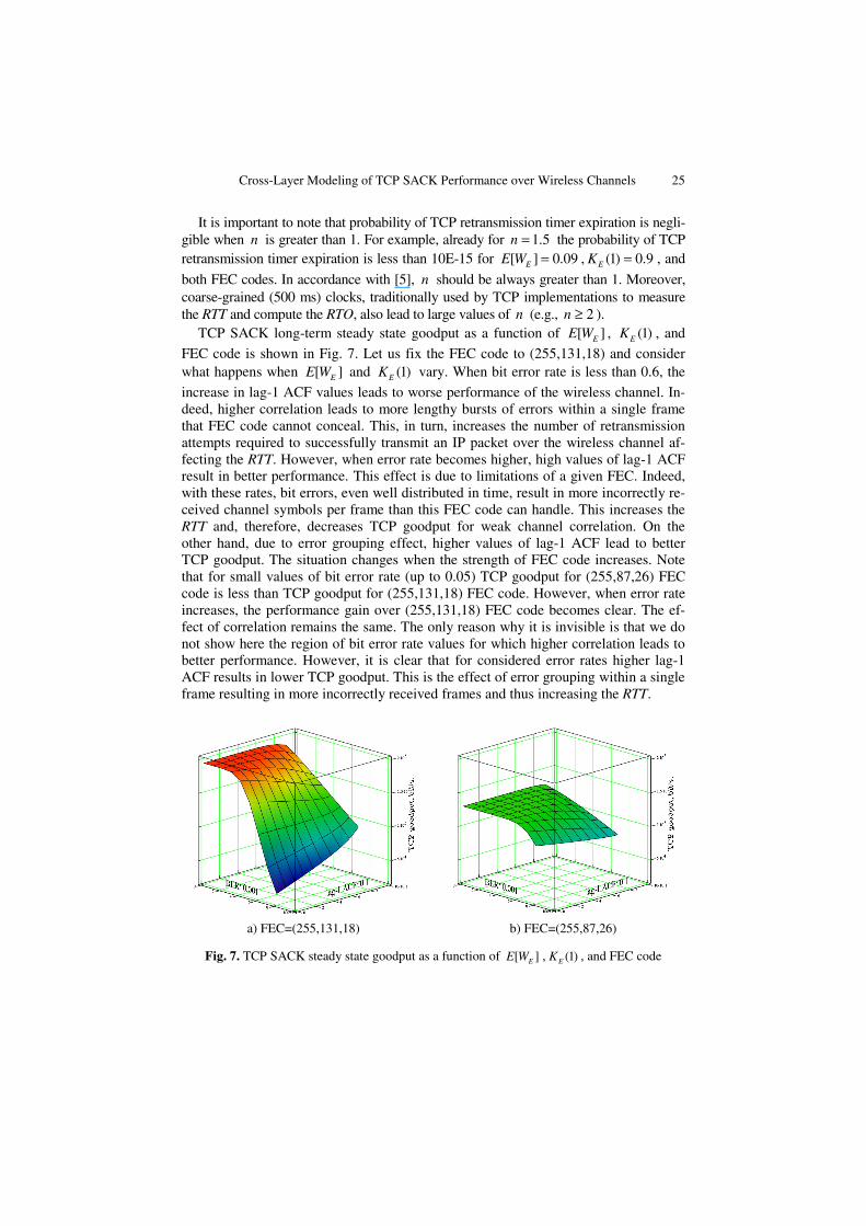
FEC code is shown in Fig. 7. Let us fix the FEC code to (255,131,18) and consider what happens when [ ]EE W and (1)EK vary. When bit error rate is less than 0.6, the

increase in lag-1 ACF values leads to worse performance of the wireless channel. In-deed, higher correlation leads to more lengthy bursts of errors within a single frame that FEC code cannot conceal. This, in turn, increases the number of retransmission attempts required to successfully transmit an IP packet over the wireless channel af-fecting the RTT. However, when error rate becomes higher, high values of lag-1 ACF result in better performance. This effect is due to limitations of a given FEC. Indeed, with these rates, bit errors, even well distributed in time, result in more incorrectly re-ceived channel symbols per frame than this FEC code can handle. This increases the RTT and, therefore, decreases TCP goodput for weak channel correlation. On the other hand, due to error grouping effect, higher values of lag-1 ACF lead to better TCP goodput. The situation changes when the strength of FEC code increases. Note that for small values of bit error rate (up to 0.05) TCP goodput for (255,87,26) FEC code is less than TCP goodput for (255,131,18) FEC code. However, when error rate increases, the performance gain over (255,131,18) FEC code becomes clear. The ef-fect of correlation remains the same. The only reason why it is invisible is that we do not show here the region of bit error rate values for which higher correlation leads to better performance. However, it is clear that for considered error rates higher lag-1 ACF results in lower TCP goodput. This is the effect of error grouping within a single frame resulting in more incorrectly received frames and thus increasing the RTT.

a) FEC=(255,131,18) b) FEC=(255,87,26)

Fig. 7. TCP SACK steady state goodput as a function of [ ]EE W , (1)EK , and FEC code

26 D. Moltchanov, R. Dunaytsev, and Y. Koucheryavy

6 Conclusion

In this paper, we proposed an analytical model for a TCP SACK connection running over a covariance stationary wireless channel with completely reliable ARQ/FEC. The proposed model allows to evaluate the effect of many parameters of wireless channels on TCP performance making it suitable for performance optimization stud-ies. These parameters include stochastic properties of wireless channel characteristics, the size of protocol data units at different layers, the strength of FEC code, the pres-ence of ARQ, the buffer size at the IP layer, and the service rate of the wireless chan-nel. Among other conclusions, we show that TCP spurious timeouts do not occur when wireless channel conditions are stationary.

The developed model is a general framework rather than a model for particular wireless access technology. To use it in practical evaluation of different technologies this framework should be extended by adding particular details of state-of-the-art wireless systems.

References

1. Gurtov, A.: Efficient Data Transport in Wireless Overlay Networks. Ph.D. Thesis, Univer-sity of Helsinki, Finland (2004)

2. Mathis, M., Mahdavi, J., Floyd, S., Romanow, A.: TCP Selective Acknowledgement Op-tions. RFC 2018 (1996)

3. Floyd, S., Mahdavi, J., Mathis, M., Podolsky, M.: An Extension to the Selective Acknowl-edgement (SACK) Option for TCP. RFC 2883 (2000)

4. Blanton, E., Allman, M., Fall, K., Wang, L.: A Conservative Selective Acknowledgement (SACK)-based Loss Recovery Algorithm for TCP. RFC 3517 (2003)

5. Paxson, V., Allman, M.: Computing TCP’s Retransmission Timer. RFC 2988 (2000) 6. Zorzi, M., Rao, R., Milstein, L.: ARQ Error Control for Fading Mobile Radio Channels.

IEEE Transactions on Vehicular Technology 46(2), 445–455 (1997) 7. Zorzi, M., Rao, R.: Throughput Analysis of Go-Back-N ARQ in Markov Channels with

Unreliable Feedback. IEEE ICC, 1232–1237 (1995) 8. Krunz, M., Kim, J.-G.: Fluid Analysis of Delay and Packet Discard Performance for QoS

Support in Wireless Networks. IEEE JSAC 19(2), 384–395 (2001) 9. Fantacci, A.: Queuing Analysis of the Selective Repeat Automatic Repeat Request Proto-

col for Wireless Packet Networks. IEEE Transactions on Vehicular Technology 45(2), 258–264 (1996)

10. Swarts, J., Ferreira, H.: On the Evaluation and Application of Markov Channel Models in Wireless Communications. IEEE VTC 1, 117–121 (1999)

11. Moltchanov, D., Koucheryavy, Y., Harju, J.: Simple, Accurate and Computationally Efficient Wireless Channel Modeling Algorithm. In: Braun, T., Carle, G., Koucheryavy, Y., Tsaoussi-dis, V. (eds.) WWIC 2005. LNCS, vol. 3510, pp. 234–245. Springer, Heidelberg (2005)

12. Mathis, M., Semke, J., Mahdavi, J., Ott, T.: The Macroscopic Behavior of the TCP Con-gestion Avoidance Algorithm. Computer Communication Review 27(3), 67–82 (1997)

13. Braden, R. (ed.): Requirements for Internet Hosts. RFC 1122 (1989) 14. Fu, S., Atiquzzaman, M.: Modelling TCP Reno with Spurious Timeouts in Wireless Mo-

bile Environments. ICCCN, 391–396 (2003) 15. Guan, Y., et al.: Simulation Study of TCP Eifel Algorithms. OPNETWORK (2005) 16. Cardwell, N., Savage, S., Anderson, T.: Modeling TCP Latency. In: IEEE INFOCOM, pp.

1742–1751 (2000)