Cross-layer analytical modeling of wirelesschannels for accurate performance evaluation

Dmitri Moltchanov, Yevgeni Koucheryavy, Jarmo Harju

Institute of Communication Engineering,Tampere University of Technology,

P.O.Box 553, Tampere, Finland{moltchan,yk,harju}@cs.tut.fi

Abstract. An intention to adopt IP protocol for future mobile commu-nication and subsequent extension of Internet services to the air interfacecalls for advanced performance modeling approaches. To provide a toolfor accurate performance evaluation of IP-based applications runningover the wireless channels we propose a novel cross-layer wireless chan-nel modeling approach. We extend the small-scale propagation modelrepresenting the received signal strength to IP layer using the cross-layermappings. Proposed model is represented by the IP packet error processand retains memory properties of initial signal strength process. Con-trarily to those approaches developed to date, our model requires lessrestrictive assumptions regarding behavior of the small-scale propaga-tion model at layers above physical. We compare results obtained usingour model with those, published to date, and show that our approachallows to get more accurate estimators of IP packet error probabilities.

1 Introduction

While next generation (NG) mobile systems are not completely defined, thereis a common agreement that they will rely on IP protocol as a consistent end-to-end transport technology. The motivation is to introduce a unified serviceplatform for future ’mobile Internet’ known as ’NG All-IP’ mobile systems.

To date only a few studies devoted to IP layer performance evaluation at theair interface have been published. Survey of literature has shown that most stud-ies were devoted to analysis of the data-link layer protocols [1, 2]. Additionally,approaches developed to date, adopt quite restrictive assumptions regarding theperformance of wireless channels at layers above physical. As a result, they maylead to incorrect estimation of IP layer performance parameters.

In this paper we propose a novel cross-layer wireless channels modeling ap-proach. We extend the small-scale propagation model representing the receivedsignal strength to IP layer using the cross-layer mappings. The proposed modelis represented by the IP packet error process, retains memory properties of initialsignal strength process and captures specific peculiarities of protocols at layersbelow IP. We show that our approach allows to get more accurate estimators ofIP packet error probabilities compared to those approaches used to date.

Our paper is organized as follows. In Section 2 we overview propagationcharacteristics of wireless channels and models used to capture them. In section3 we propose our extension to IP layer and define model that provides IP packeterror probabilities. In Section 4 we provide numerical comparison of our approachwith that one widely used in literature. Conclusions are drawn in the last section.

2 Propagation characteristics of wireless channels

The propagation path between the transmitter and a receiver may vary fromsimple line-of-sight (LOS) to very complex ones due to diffraction, reflection andscattering. To represent performance of wireless channels propagation models areused. We distinguish between large-scale and small-scale propagation models [3].

When a mobile user moves away from the transmitter over large distances thelocal average received signal strength gradually decreases. This signal strengthis predicted using the large-scale propagation models. However, such models[4–6] do not take into account rapid variations of the received signal strength.As a result, they cannot be effectively used in performance evaluation studies.Indeed, when a mobile user moves over short distances the instantaneous signalstrength varies rapidly. The reason is that the received signal is a sum of manycomponents coming from different directions. Propagation models characterizingrapid fluctuations of the received signal strength over short time duration arecalled small-scale propagation models. In the presence of dominant non-fadingcomponent the small-scale propagation distribution is Rician. As the dominantcomponent fades away Rician distribution degenerates to Rayleigh one.

The small-scale propagation models capture characteristics of wireless chan-nel on a finer granularity than large-scale ones. Additionally, these models im-plicitly take into account movements of users over short travel distances [7, 8].In what follows, we restrict our attention to the small-scale propagation models.

2.1 Model of small-scale propagation characteristics

Assume a discrete-time environment, i.e. time axis is slotted, the slot durationis constant and given by ∆t = (ti+1 − ti), i = 0, 1, . . . . We choose ∆t such thatit equals to the time to transmit a single symbol at the wireless channel. Hence,the choice of ∆t depends on properties of the physical layer.

Small-scale propagation characteristics are often represented by the stochas-tic process {L(n), n = 0, 1, . . . } modulated by the discrete-time Markov chain{SL(n), n = 0, 1, . . . }, SL(n) ∈ {1, 2, . . . ,M} each state of which is associatedwith conditional probability distribution function of the received signal strength[9, 10]. The underlying modulation allows to take into account autocorrelationproperties of the signal strength process. Since it is allowed for the Markov pro-cess {SL(n), n = 0, 1, . . . } to change state in every time slot, every bit mayexperience different received signal strengths.

An illustration of such a model is shown in the Fig. 1 where states are as-sociated with conditional distribution functions FL(k∆f |i)(∆f) = Pr{L(n) =

k∆f |SL(n) = i}, k = 1, 2, . . . , N , i = 1, 2, . . . ,M , where N is the number of binsto which the signal strength is partitioned and ∆f is the discretization interval.Let DL and πL = (π1, π2, . . . , πM ) be the one-step transition probability ma-trix and the stationary probability vector of {SL(n), n = 0, 1, . . . } respectively.Parameters M , DL, FL(k∆f |i)(∆f), must be estimated from statistical data [9,10]. For the ease of notation we will use FL(k|i) instead of FL(k∆f |i)(∆f).

1 2 M...

NkffkFL ,,2,1),)(1|( ���� NkffkFL ,,2,1),)(2|( ���� NkfMfkFL ,,2,1),)(|( ����

Fig. 1. An illustration of the Markov model for small-scale propagation characteristics.

3 Wireless channel model at IP layer

The small-scale propagation model of the received signal strength defined inthe previous section cannot be directly used in performance evaluation studiesand must be properly extended to IP layer at which QoS usually is defined.To do so we have to take into account specific peculiarities of layers below IPincluding modulation schemes at the physical layer, data-link error concealmenttechniques and possible segmentation procedures between different layers. As aresult, the IP layer wireless channel model must be a complex cross-layer functionof underlying layers and propagation characteristics.

In the following subsections we define models of incorrect reception of theprotocol data units (PDU) at different layers. For this purpose we implicitlyassume that these PDUs are consecutively transmitted at corresponding layers.

3.1 Bit error process

Consider a certain state i of the Markov chain {SL(n), n = 0, 1, . . . } associatedwith the conditional probability distribution function FL(k|i), k = 1, 2, . . . , N ,of the received signal strength. Since the probability of a single bit error is thedeterministic function of the received signal strength [3], all values of FL(k|i)that are less or equal to a computed value of the so-called bit error threshold BT

cause bit error. Those values which are greater than BT do not cause bit error.So that each state i, i = 1, 2, . . . ,M of the Markov process {SL(n), n = 0, 1, . . . }can be now associated with the following bit error probability pE,i:

pE,i = Pr{E(n) = 1|SE(n) = i} =BT∑k=1

Pr{L(n) = k|SL(n) = i}, (1)

where {E(n), n = 0, 1, . . . }, E(n) ∈ {0, 1} is the bit error process for which 1 de-notes an incorrectly received bit, 0 denotes a correctly received bit, {SE(n), n =0, 1, . . . } is the underlying Markov chain of {E(n), n = 0, 1, . . . }. Note that{SL(n), n = 0, 1, . . . } and {SE(n), n = 0, 1, . . . } are actually the same andπE = πL, DE = DL, where DE and πE are one-step transition probabilitymatrix and stationary distribution vector of {SE(n), n = 0, 1, . . . } respectively.BT must be estimated based on a modulation scheme and other specific featuresof physical layer utilized at a given wireless channel [3].

Let us denote by dE,ij(k) = Pr{E(n) = k, SE(n) = j|SE(n − 1) = i},k = 0, 1, the transition probability from the state i to state j with correct(k = 0) and incorrect (k = 1) bit reception respectively. These probabilities canbe represented in a compact form using matrices DE(1) and DE(0) such thatDE(1) + DE(0) = DE . In our case the state from which the transition occurscompletely determines the bit error probability. The state to which transitionoccurs is used for convenience of matrix notation useful in the following.

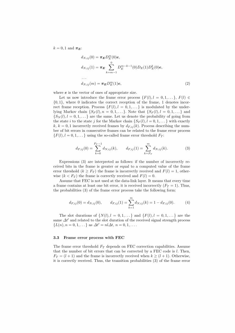
3.2 Frame error process without FEC

Assume that the length of the frame is constant and equals to m bits. Thesequence of consecutively transmitted bits, denoted by gray rectangles, is shownin the Fig. 2, where (l − 1), l, (l + 1) denote time intervals whose length equalsto the time to transmit a single frame; k, i, j, denote the state of the Markovchain {SE(n), n = 0, 1, . . . } in the beginning of these intervals.

Consider the stochastic process {N(l), l = 0, 1, . . . }, N(l) ∈ {0, 1, . . . ,m},describing the number of incorrectly received bits in consecutive bit patterns ofthe length m. This process is doubly stochastic one modulated by the underlyingMarkov chain {SN (l), l = 0, 1, . . . }. {N(l), l = 0, 1, . . . } and can be completelydefined via parameters of the bit error process.

t

k

...1 m

l-1

i

...1 m

l

j

...1 m

l+1

......

Fig. 2. Sequence of consecutively transmitted bits at the wireless channel.

Let us denote the probability of going from the state i to the state j for theMarkov chain {SN (l), l = 0, 1, . . . } with exactly k, k = 0, 1, . . . ,m incorrectlyreceived bits in a bit pattern of the length m by dN,ij(k) = Pr{N(l) = k, SN (l) =j|SN (l − 1) = i}. These transition probabilities can be found using DE(k),

k = 0, 1 and πE :

dN,ij(0) = πEDmE (0)e,

dN,ij(1) = πE

0∑k=m−1

Dm−k−1E (0)DE(1)Dk

E(0)e,

. . .

dN,ij(m) = πEDmE (1)e, (2)

where e is the vector of ones of appropriate size.Let us now introduce the frame error process {F (l), l = 0, 1, . . . }, F (l) ∈

{0, 1}, where 0 indicates the correct reception of the frame, 1 denotes incor-rect frame reception. Process {F (l), l = 0, 1, . . . } is modulated by the under-lying Markov chain {SF (l), n = 0, 1, . . . }. Note that {SF (l), l = 0, 1, . . . } and{SN (l), l = 0, 1, . . . } are the same. Let us denote the probability of going fromthe state i to the state j for the Markov chain {SF (l), l = 0, 1, . . . } with exactlyk, k = 0, 1 incorrectly received frames by dF,ij(k). Process describing the num-ber of bit errors in consecutive frames can be related to the frame error process{F (l), l = 0, 1, . . . } using the so-called frame error threshold FT :

dF,ij(0) =FT −1∑k=0

dN,ij(k), dF,ij(1) =m∑

k=FT

dN,ij(k). (3)

Expressions (3) are interpreted as follows: if the number of incorrectly re-ceived bits in the frame is greater or equal to a computed value of the frameerror threshold (k ≥ FT ) the frame is incorrectly received and F (l) = 1, other-wise (k < FT ) the frame is correctly received and F (l) = 0.

Assume that FEC is not used at the data-link layer. It means that every timea frame contains at least one bit error, it is received incorrectly (FT = 1). Thus,the probabilities (3) of the frame error process take the following form:

dF,ij(0) = dN,ij(0), dF,ij(1) =m∑

k=1

dN,ij(k) = 1 − dF,ij(0). (4)

The slot durations of {N(l), l = 0, 1, . . . } and {F (l), l = 0, 1, . . . } are thesame ∆t′ and related to the slot duration of the received signal strength process{L(n), n = 0, 1, . . . } as ∆t′ = nl∆t, n = 0, 1, . . . .

3.3 Frame error process with FEC

The frame error threshold FT depends on FEC correction capabilities. Assumethat the number of bit errors that can be corrected by a FEC code is l. Then,FT = (l + 1) and the frame is incorrectly received when k ≥ (l + 1). Otherwise,it is correctly received. Thus, the transition probabilities (3) of the frame error

process take the following form:

dF,ij(0) =l∑

k=0

dN,ij(k), dF,ij(1) =m∑

k=l+1

dN,ij(k). (5)

3.4 IP packet error process

Assume that IP packet is segmented into z frames of equal size at the data-link layer.1 The sequence of consecutively transmitted frames, denoted by grayrectangles, is shown in the Fig. 3, where (h− 1), h, (h+1) denote time intervalswhose length equals to the time to transmit a single packet; k, i, j, denote thestate of the Markov chain {SF (n), n = 0, 1, . . . } in the beginning of intervals.

Consider the stochastic process {M(h), h = 1, 2, . . . }, M(h) ∈ {0, 1, . . . , z},describing the number of incorrectly received frames in a consecutive frame pat-terns of the length z. This process is modulated by the Markov chain {SM (h), h =0, 1, . . . } and can be defined via parameters of the frame error process.

t

k

...1 z

h-1

i

...1 z

h

j

...1 z

h+1

......

Fig. 3. Sequence of consecutively transmitted frames at the wireless channel.

Let us denote the probability of going from state i to state j for the Markovchain {SM (h), h = 0, 1, . . . } with exactly k, k = 0, 1, . . . , z incorrectly receivedframes in a frame pattern of length z by dM,ij(k) = Pr{M(h) = k, SM (h) =j|SM (h − 1) = i}. These transition probabilities can be found using DF (k),k = 0, 1 and πF of {F (l), l = 0, 1, . . . } as follows:

dM,ij(0) = πF DzF (0)e,

dM,ij(1) = πF

0∑k=z−1

Dz−k−1F (0)DF (1)Dk

F (0)e,

. . .

dM,ij(z) = πF DzF (1)e, (6)

where πF is the stationary distribution vector of {SF (l), l = 0, 1, . . . }.Let us now introduce the packet error process {P (h), h = 0, 1, . . . }, P (h) ∈

{0, 1}, where 0 indicates the correct reception of the packet, 1 denotes incorrect

1 Assumption of the constant frame size does not restrict the generality of the resultsas long as only one traffic source is allowed to be active at any instant of time forwhich only data-link error concealment techniques are possible (e.g., IP telephony).

packet reception. Process {P (h), h = 0, 1, . . . } is modulated by the underly-ing Markov chain {SP (h), h = 0, 1, . . . }. Note that {SP (h), h = 0, 1, . . . } and{SM (h), h = 0, 1, . . . } are the same. Let us denote the probability of going fromthe state i to the state j for the Markov chain {SP (h), h = 0, 1, . . . } with exactlyk, k = 0, 1 incorrectly received packets by dP,ij(k). Process {M(h), h = 0, 1, . . . }describing the number of incorrectly received frames in consecutively transmit-ted packets can be related to the packet error process {P (h), h = 0, 1, . . . } usingthe so-called packet error threshold PT :

dP,ij(0) =PT −1∑k=0

dM,ij(k), dP,ij(1) =z∑

k=PT

dM,ij(k) = 1 − dM,ij . (7)

Expressions (7) are interpreted as follows: if the number of incorrectly re-ceived frames in a packet is greater or equal to a computed value of the packeterror threshold (k ≥ PT ) the packet is incorrectly received and P (h) = 1. Other-wise, it is correctly received and P (h) = 0. Since no error correction proceduresare defined for IP layer, PT = 1 and only dM,ij(0) must be computed in (6).That is, every time a packet contains at least one incorrectly received frame, thewhole packet is received incorrectly.

The slot durations of {P (h), h = 0, 1, . . . } and {M(h), h = 0, 1, . . . } are thesame ∆t′′ and related to the slot duration of the received signal strength process{L(n), n = 0, 1, . . . } as ∆t′′ = nlh∆t, n = 0, 1, . . . .

3.5 Illustration of the proposed extension

An illustration of proposed cross-layer mapping is shown in Fig. 4 where timediagrams of {L(n), n = 0, 1, . . . }, {E(n), n = 0, 1, . . . }, {N(l), l = 0, 1, . . . },{F (l), l = 0, 1, . . . }, {M(h), h = 0, 1, . . . }, {P (h), h = 0, 1, . . . } are shown. Errorthresholds BT , FT and PT must estimated as outlined previously and then usedto compute transition probabilities of error processes at different layers.

To define models of the incorrect reception of PDUs at different layers weimplicitly assumed that appropriate PDUs are consecutively transmitted at cor-responding layers. Hence, the IP packet error process is conditioned on the eventof consecutive transmission of packets.

4 Comparison of the proposed approach

Let us now compare the proposed approach with that one developed and usedto date. We consider two cases: (1) the signal strength is assumed to be constantduring the frame transmission time (2) the signal strength is mapped to the IPlayer model in accordance with our approach. In what follows, we use subscripts 1and 2 to denote performance estimators obtained using corresponding approach.

Assume that the wireless channel at the physical layer is represented by theMarkov chain with M = 4, pE,i = 0, i = 1, 2, 3, pE,4 �= 0 and the following

{N(l),l=0,1,..}, FT=2

l{E(n),n=0,1,..}

{F(l),l=0,1,..}

l

n

{M(h),h=0,1,..}, PT=1

h

{P(h),h=0,1,..}

h

BT

n

{L(n),n=0,1,..}Physical layer

Physical layer

Data-link layer

Data-link layer

Network layer

Network layer

Fig. 4. Illustration of proposed cross-layer mapping.

transition probability matrix:

PE =

⎛⎜⎜⎝

0.42 0.18 0.24 0.160.18 0.42 0.04 0.360.07 0.03 0.54 0.360.03 0.07 0.09 0.81

⎞⎟⎟⎠ . (8)

We also assume that exactly one IP packet is mapped into one frame at thedata-link layer. It can be easily shown that this assumption provides the bestpossible conditions at the IP layer.

4.1 Packet error processes without FEC

Assume that the length of the frame is m bits and FEC is not used at the data-link layer. Then, the conditional mean of the incorrectly received packets2 isgiven by the following expressions:

E1[P ] =4∑

i=1

πE,i

m−1∑k=0

(1 − pE,i)kpE,i, E2[P ] = 1 − πEDmE (0)e. (9)

The estimated values of the conditional mean of the incorrectly received IPpackets for different values of m and pE,4 are shown in the Table 1. Comparing

2 This performance parameter can be interpreted as the mean number of the incor-rectly received IP packets given that packets are generated according to Bernoulliprocess with probability of a single arrival set to 1.

obtained results we note that the assumption of the same received signal strengthduring the frame transmission time significantly overestimates the actual perfor-mance of wireless channels when the channel coherence time is comparable withthe time to transmit a single symbol.

Table 1. Conditional mean number of incorrectly received packets (no FEC)

m pE,4 = 0.3 pE,4 = 0.1E1[P ] E2[P ] E1[P ] E2[P ]

100 0.622 1.000 0.622 0.998

500 0.622 1.000 0.622 1.000

2000 0.622 1.000 0.622 1.000

4.2 Packet error processes with FEC

Consider now the effect of FEC. Assume that the FEC code may correct up to lbit errors i.e. FT = l + 1. Then, the conditional mean of the incorrectly receivedpackets is given by the following expressions:

E1[P ] =4∑

i=1

πE,i

m∑k=FT

(km

)(1 − pE,i)kpm−k

E,i ,

E2[P ] =4∑

i=1

πE,i

m∑k=FT

dN,ij(k)e. (10)

Results for different values of l, m and pE,4 are shown in the Table 2. For illus-trative purposes some non-realistic values of (m, l) are also included. Comparingobtained results we note that the assumption of the same received signal strengthduring the frame transmission time significantly underestimates or overestimatesthe actual performance of wireless channel depending on correction capabilitiesof FEC code. Our approach provides exact values of conditional mean of the in-correctly received packets when the channel coherence time is comparable withthe time to transmit a single symbol at the wireless channel.

5 Conclusions and future work

We extended the small-scale propagation model representing the received signalstrength of the wireless channel to IP layer using the cross-layer mappings. Ourmodel is represented by the IP packet error process and retains memory proper-ties of the initial signal strength process. We compare results obtained using ourmodel with those presented in literature and show that our approach allows to

Table 2. Conditional mean number of incorrectly received packets (FEC)

(m, l) pE,4 = 0.3 pE,4 = 0.1E1[P ] E2[P ] E1[P ] E2[P ]

(100,5) 0.622 1.000 0.622 0.587

(100,10) 0.622 0.976 0.622 0.054

(100,20) 0.622 0.328 0.622 8E-8

(500,20) 0.622 1.000 0.622 0.975

(500,40) 0.622 1.000 0.622 0.052

(500,100) 0.622 0.233 0.622 <10E-10

(2000,100) 0.622 1.000 0.622 0.986

(2000,200) 0.622 1.000 0.622 4E-6

(2000,300) 0.622 1.000 0.622 <10E-10

get more accurate estimators of IP packet error probabilities when the channelcoherence time is comparable with the time to transmit a single symbol.

The proposed model entirely relies on classic small-scale propagation modeland does not take into account the signal strength attenuation caused by move-ments of the user over the large distances. The aim of our further work is toextend our approach to mobility-dependent propagation characteristics.

References

1. M. Krunz and J.-G. Kim. Fluid analysis of delay and packet discard performancefor QoS support in wireless networks. IEEE JSAC, 19(2):384–395, February 2001.

2. M. Zorzi, R. Rao, and L. Milstein. ARQ error control for fading mobile radiochannels. IEEE Trans. on Veh. Tech., 46(2):445–455, May 1997.

3. T. Rappaport. Wireless communications: principles and practice. Communicationsengineering and emerging technologies. Prentice Hall, 2nd edition, 2002.

4. T. Okumura, E. Omori, and Fakuda K. Field strength and its variability inVHF and UHF land mobile service. Review of electrical communication labora-tory, 16(9/10):825–873, September/October 1968.

5. J. Andersen, T. Rappaport, and S. Yoshida. Propagation measurements and mod-els for wireless communications channels. IEEE Comm. Mag., 33:42–49, Nov. 1995.

6. S. Seidel and T. Rappaport. Site-specific propagation prediction for wireless in-building personal communication system design. IEEE Trans. on Veh. Tech.,43(4):879–891, November 1994.

7. A. Saleh and R. Valenzuela. A statistical model for indoor multipath propagation.IEEE JSAC, 5(2):128–137, February 1987.

8. D. Durgin and T. Rappaport. Theory of multipath shape factors for small-scalefading wireless channels. IEEE Trans. on Ant. and Propag., 48:682–693, May 2000.

9. Q. Zhang and S. Kassam. Finite-state markov model for Rayleigh fading channels.IEEE Trans. on Comm., 47(11):1688–1692, November 1999.

10. J. Swarts and H. Ferreira. On the evaluation and application of markov channelmodels in wireless communications. In Proc. VTC’99, pages 117–121, 1999.