CREATING DRY SORBENT IN-JECTION 3D MODEL WITH SYSTEM PARAMETER CALCU-LATION

THESIS - MASTER'S DEGREE PROGRAMME

TECHNOLOGY, COMMUNICATION AND TRANSPORT

A u t h o r / s :

Achmad Yusuf

SAVONIA UNIVERSITY OF APPLIED SCIENCES THESIS Abstract

Field of Study Technology, Communication and Transport Degree Programme Master’s Degree Programme in Energy Engineering

Author(s) Achmad Yusuf Title of Thesis

Creating Dry Sorbent Injection 3D model with system parameter calculation

Date 17 January 2022 Pages/Appendices 80/4

Supervisor(s) Teija Honkanen, Harri Heikura Client Organisation /Partners Sumitomo SHI FW Energia Oy Abstract Speed, efficiency and competitiveness are major factors for any business to become a winning company. To gain

that companies need tools such as Plant Design Management Systems (PDMS), and design solutions for a cost-effective flue gas cleaning technologies such as Dry Sorbent Injection (DSI). DSI is a pollution control technology of injecting a dry alkaline mineral into a flue gas stream to reduce acid gas emissions (i.e SO2, SO3, H2SO4, HCl, HF, Hg, dioxins and furans). The use of this technology is expanding rapidly as a low capital cost solution for compliance with environmental control requirements. The purpose of this thesis was to create DSI Model using PDMS software by importing a calculation result value from another system and to explore the science behind all calculation. A literature review on dry sorbent was conducted. There are some variations of DSI so with these tools a designer can modify and take Material Take

Off (MTO) quickly which is important in the bidding phase and the design phase. The output of this thesis is DLL, a Library that contains the lines of code of the programming language and con-sists of functions, classes, variables, and user interfaces. PDMS customization is needed to create an interface between PDMS and .Net Framework, which is software developed by Microsoft. Source code compilation creates DLL needed in the PDMS environment. In this thesis, the phrase "DLL" is referred to as a "Tool" instead. Then this tool can be accessed from a pulldown menu.

Keywords PDMS, 3D Model, Baghouse, Flue Gas Cleaning, DSI, Dry Sorbent Injection, Pulse Jet, Cost

PREFACE

First of all, I want to thank God for giving us health in this pandemic, therefore I can do thesis work

and thanks to my family for their support.

I would like to thank Teija Honkanen for her big effort to supervise me in this thesis. She came to

my office to conduct a thesis meeting with Sumitomo Supervisor Pasi Liimatainen and Ari Ojala.

Thank you very much, Pasi and Ari, for your time, precious guidance, and giving me the opportunity

to take this subject as my master's thesis topic plan.

Varkaus 17 January 2022

Achmad Yusuf

4 (91)

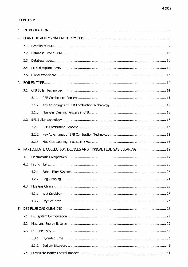
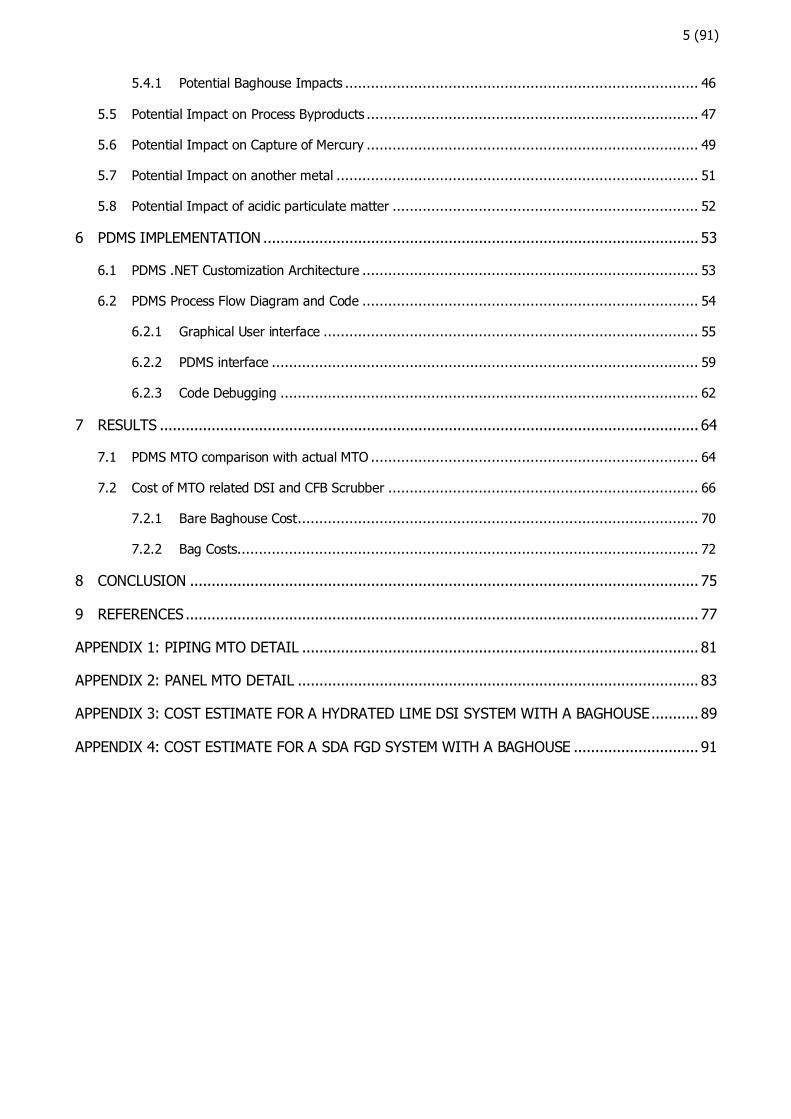
CONTENTS

1 INTRODUCTION .................................................................................................................... 8

2 PLANT DESIGN MANAGEMENT SYSTEM .................................................................................. 9

2.1 Benefits of PDMS .............................................................................................................. 9

2.2 Database Driven PDMS .................................................................................................... 10

2.3 Database types .............................................................................................................. 11

2.4 Multi discipline PDMS ...................................................................................................... 11

2.5 Global Workshare ........................................................................................................... 12

3 BOILER TYPE ....................................................................................................................... 14

3.1 CFB Boiler Technology..................................................................................................... 14

3.1.1 CFB Combustion Concept ...................................................................................... 14

3.1.2 Key Advantages of CFB Combustion Technology ....................................................... 15

3.1.3 Flue Gas Cleaning Process in CFB ........................................................................... 16

3.2 BFB Boiler technology ..................................................................................................... 17

3.2.1 BFB Combustion Concept ...................................................................................... 17

3.2.2 Key Advantages of BFB Combustion Technology ....................................................... 18

3.2.3 Flue Gas Cleaning Process in BFB ........................................................................... 18

4 PARTICULATE COLLECTION DEVICES AND TYPICAL FLUE GAS CLEANING ............................ 19

4.1 Electrostatic Precipitators ................................................................................................. 19

4.2 Fabric Filter ................................................................................................................... 21

4.2.1 Fabric Filter Systems ............................................................................................ 22

4.2.2 Bag Cleaning ...................................................................................................... 24

4.3 Flue Gas Cleaning ........................................................................................................... 26

4.3.1 Wet Scrubber ..................................................................................................... 27

4.3.2 Dry Scrubber ...................................................................................................... 27

5 DSI FLUE GAS CLEANING ..................................................................................................... 28

5.1 DSI system Configuration ................................................................................................ 28

5.2 Mass and Energy Balance ................................................................................................ 29

5.3 DSI Chemistry................................................................................................................ 31

5.3.1 Hydrated Lime .................................................................................................... 32

5.3.2 Sodium Bicarbonate ............................................................................................. 43

5.4 Particulate Matter Control Impacts .................................................................................... 44

5 (91)

5.4.1 Potential Baghouse Impacts .................................................................................. 46

5.5 Potential Impact on Process Byproducts ............................................................................. 47

5.6 Potential Impact on Capture of Mercury ............................................................................. 49

5.7 Potential Impact on another metal .................................................................................... 51

5.8 Potential Impact of acidic particulate matter ....................................................................... 52

6 PDMS IMPLEMENTATION ..................................................................................................... 53

6.1 PDMS .NET Customization Architecture .............................................................................. 53

6.2 PDMS Process Flow Diagram and Code .............................................................................. 54

6.2.1 Graphical User interface ....................................................................................... 55

6.2.2 PDMS interface ................................................................................................... 59

6.2.3 Code Debugging ................................................................................................. 62

7 RESULTS ............................................................................................................................. 64

7.1 PDMS MTO comparison with actual MTO ............................................................................ 64

7.2 Cost of MTO related DSI and CFB Scrubber ........................................................................ 66

7.2.1 Bare Baghouse Cost ............................................................................................. 70

7.2.2 Bag Costs........................................................................................................... 72

8 CONCLUSION ...................................................................................................................... 75

9 REFERENCES ....................................................................................................................... 77

APPENDIX 1: PIPING MTO DETAIL ............................................................................................ 81

APPENDIX 2: PANEL MTO DETAIL ............................................................................................. 83

APPENDIX 3: COST ESTIMATE FOR A HYDRATED LIME DSI SYSTEM WITH A BAGHOUSE ........... 89

APPENDIX 4: COST ESTIMATE FOR A SDA FGD SYSTEM WITH A BAGHOUSE ............................. 91

6 (91)

Abbreviations and definitions

API = Application Programming Interface

APTI = Air Pollution Training Institute

ASTM = American Society for Testing and Materials

BBR = Bottom Bag Removal

BET = Brunauer Emmet Teller

BFB = Bubbling Fluidized Bed

B-PAC = Brominated- Powdered Activated Carbon

CAF = Common Application Framework

CCR = Coal Combustion Residue

CFB = Circulating Fluidized Bed

CFM = Cubic Feet Per Min

CO = Carbon monoxide

CO = Cotton

CS-ESP =Cold Side Electrostatic Precipitators

DLL = Dynamic Link Library

DSI = Dry Sorbent Injection

EPA = Environmental Protection Agency

ESP = Electrostatic Precipitators

FF = Fabric Filter

FG = Fiberglass

FGC = Flue Gas Condensers

GCA = Gross Cloth Area

GUI = Graphical User Interface

HA = Homopolymer Acrylic

HCl = Hydrogen Chloride

HF = Hydrogen Fluoride

HS-ESP = Hod Side Electrostatic Precipitators

LEL = Lower Explosive Limit

MCR = Maximum Continuous Rating

MMACF = Million Actual Cubic Feet

MTO = Material Take Off

NA = Not Applicable

NO = Nomex

NOx = Nitric oxide

NSR = Normal Stoichiometric Ratio

NX = Nextel

P8 = P84

PAC = Powdered Activated Carbon

PDMS = Plant Design Management System

PE = Polyester

PJFF = Pulse Jet Fabric Filter

7 (91)

PML = Programming Macro Language

PP = Polypropylene

PRB = Powder River Basin

RH = Re Heater

RT = Ryton

SBC = Sodium Bicarbonate

SCR = Selective Catalytic Reduction

SD = Spray Dryer

SDA = Spray Dryer Absorber

SH = Super Heater

SHI = Sumitomo Heavy Industry

SNCR = Selective Non Catalytic Reduction

SO2 = Sulphur dioxide

SO3 = Sulphur trioxide

SPLP = Synthetic Precipitation Leaching Procedure

TF = Teflon Felt

TR = Top bag Removal (Snap in)

8 (91)

1 INTRODUCTION

Sumitomo SHI – Foster Wheeler has been using PDMS for more than 20 years. They started by us-

ing first version PDMS 11.0, 12.0 and 12.1. So many PDMS development projects have been done.

One of PDMS development projects is relating to this thesis that creating 3D model for dry sorbent

injection.

The purpose of this thesis was to create DSI Model using PDMS software by importing calculation

result value from another system and getting more understanding the science behind all calculation

including Dry sorbent literature study. There are some variations of DSI thus with this tools designer

can modified and can take Material Take Off (MTO) quickly which is important in bidding Phase and

design Phase.

This thesis consists of three parts. The first of main components was PDMS Setting environment,

PDMS customization, Piping Catalog and specification which can be setup on admin and paragon

module.

The second one is user interface and code behind creation. All coding is done with C# by using

AVEVA API which built by Visual studio 2017.

The last one is Dry sorbent injection literature Study, the main focuses were in dry flue gas cleaning

process and reducing of the acid gases hydrogen chloride (HCl) and sulphur dioxide (SO2), and ab-

sorbent. Type of absorbent is important variable which influences flue gas emissions.

Nobody can deny the value of a digital 3D model in the modern era. Every business will eventually

migrate to digitalization. AVEVA PDMS software significantly simplifies the process of creating a digi-

tal 3D model. A digital 3D model of the DSI baghouse was created using the PDMS software.

A water boiler is designed to operate at pressures greater than 160 psi (1.1 MPa) and/or tempera-

tures in excess of 250°F (120°C). (ASME BPVC, 2015)

9 (91)

2 PLANT DESIGN MANAGEMENT SYSTEM

CAD Center was founded in 1967 and changed its name to Aveva in 2001 from UK Head Quarter at

Cambridge. First version of PDMS (Plant Design Management System) was published in in 1976 and

used in SHI FW since 1997. Last version is PDMS 12.1 SP4 currently in use. 3D modeling is the pro-

cess of creating a mathematical representation of any surface of an object in three dimensions using

specialized software in 3D computer graphics. The product is referred to as a 3D model. A 3D artist

or a 3D modeler are terms used to describe someone who works with 3D models. One company

which produced this specialized software is CAD Centre (Computer Aided Design Center). PDMS is

AVEVA’s 3D Plant Design Software which is Capable to provide Full Range of solutions for Project

Life Cycle, customizable, multiuser, and multi-discipline. PDMS can be applicable on design and con-

struction project in Offshore, onshore, Boiler powerplant and nuclear powerplant.

2.1 Benefits of PDMS

There are some benefits of using PDMS, these are consistent and reliable component data, manage-

able specification, manageable component connection, and avoid component interferences. In the

following paragraph there are some explanations from PDMS how all of them can be achieved.

PDMS Ensures that component data is consistent and reliable. All piping component sizes and geom-

etries are predefined and saved in a catalogue by PDMS, and the designer cannot change them.

This ensures that all objects are accurate in size and are consistent across the design, regardless of

how many people are working on the project. Usually each fitting’s size must be determined before

it can be drawn In a design environment that exclusively uses 2D drawing techniques. This is a

time-consuming and error-prone operation, with design flaws frequently discovered only during the

erection stage of the project. (Aveva 1, 2013)

PDMS refers to engineering specifications that can be defined. Specifications are used in design ap-

plications for Piping, Hangers and Supports, HVAC, Cable trays and Steelwork to assist component

selection. All specifications store in paragon Module and specify the exact components to be used.

(Aveva 1, 2013)

PDMS Ensures that the geometry and connectivity are correct. PDMS can check all of design errors

using built in data consistency procedures to check all or individual parts of the design model. De-

sign errors can occur in a variety of ways, such as incorrect fitting lengths, incompatible flange rat-

ings, or simple alignment errors. (Aveva 1, 2013)

PDMS prevents Component interferences. Traditional drawing office techniques are still prone to hu-

man error, despite a wealth of skill and experience in plant design. When utilizing conventional 2D

10 (91)

methods to lay out complex pipe runs and general arrangements in tight areas, clashes between

elements attempting to share the same physical space unavoidably occur. (Aveva 1, 2013)

PDMS allows us to avoid such issues in two ways, the first is that, by viewing the design interac-

tively during the design process, visual checks on the model from various viewpoints are possible.

Potential issues can thus be resolved as they arise. (Aveva 1, 2013)

Second, by utilizing PDMS’s powerful clash checking facility, which will detect clashes anywhere in

the plant. This can be done both interactively and selectively. (Aveva 1, 2013)

All dimensions and annotations were obtained directly from the design database.

Extracted information from the PDMS database, such as arrangement drawings, piping isometrics

and reports, will always be the most recent available because it is only stored in one source.

Throughout the course of a project, information changes and drawings must be reissued. When this

occurs, drawings, reports, and other documents can be easily updated and reissued. (Aveva 1,

2013)

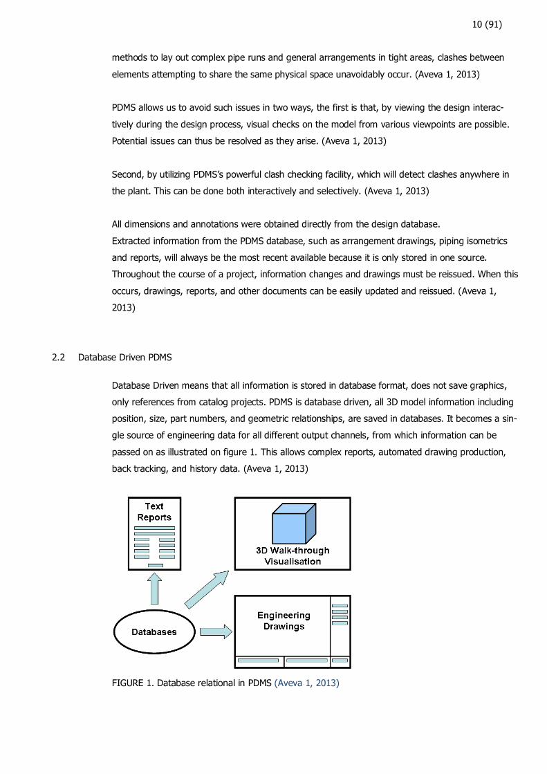
2.2 Database Driven PDMS

Database Driven means that all information is stored in database format, does not save graphics,

only references from catalog projects. PDMS is database driven, all 3D model information including

position, size, part numbers, and geometric relationships, are saved in databases. It becomes a sin-

gle source of engineering data for all different output channels, from which information can be

passed on as illustrated on figure 1. This allows complex reports, automated drawing production,

back tracking, and history data. (Aveva 1, 2013)

FIGURE 1. Database relational in PDMS (Aveva 1, 2013)

11 (91)

2.3 Database types

A PDMS project is the complete collection of information pertaining to a single design project. The

project is identified by a name, which is assigned by the Project Administrator when the project is

first started. When a user wants to work on a project using PDMS, the project name is used to iden-

tify the project to the system. This enables the monitoring and control of access rights and the use

of system resources. (Aveva 1, 2013)

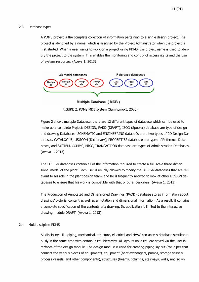
FIGURE 2. PDMS MDB system (Sumitomo-1, 2020)

Figure 2 shows multiple Database, there are 12 different types of database which can be used to

make up a complete Project: DESIGN, PADD (DRAFT), ISOD (Spooler) database are type of design

and drawing Databases. SCHEMATIC and ENGINEERING databa0s e are two types of 2D Design Da-

tabases. CATALOGUE, LEXICON (Dictionary), PROPERTIES databas e are types of Reference Data-

bases, and SYSTEM, COMMS, MISC, TRANSACTION database are types of Administration Databases.

(Aveva 1, 2013)

The DESIGN databases contain all of the information required to create a full-scale three-dimen-

sional model of the plant. Each user is usually allowed to modify the DESIGN databases that are rel-

evant to his role in the plant design team, and he is frequently allowed to look at other DESIGN da-

tabases to ensure that his work is compatible with that of other designers. (Aveva 1, 2013)

The Production of Annotated and Dimensioned Drawings (PADD) database stores information about

drawings' pictorial content as well as annotation and dimensional information. As a result, it contains

a complete specification of the contents of a drawing. Its application is limited to the interactive

drawing module DRAFT. (Aveva 1, 2013)

2.4 Multi discipline PDMS

All disciplines like piping, mechanical, structure, electrical and HVAC can access database simultane-

ously in the same time with certain PDMS hierarchy. All layouts on PDMS are saved via the user in-

terfaces of the design module. The design module is used for creating piping lay out (the pipes that

connect the various pieces of equipment), equipment (heat exchangers, pumps, storage vessels,

process vessels, and other components), structures (beams, columns, stairways, walls, and so on

12 (91)

that support and provide access to operational equipment and pipework) and Pipe Supports. All in-

formation in PDMS are saved to objects in the hierarchy which is described on figure below. (Aveva

1, 2013)

FIGURE 3. The PDMS Design database hierarchy (Aveva 1, 2013)

With the exception of the WORLD, all database elements in this hierarchical structure are owned by

other elements. Elements that are owned by another element, such as a ZONE and a SITE, are re-

ferred to as members of the owning element. The ZONE is a member of the SITE. If Piping disci-

pline wants to create Flange or valve model they have to create Site, Zone, Pipe and Branch. The

way How to save element looks like Windows explorer on Windows operating system. (Aveva 1,

2013)

2.5 Global Workshare

Global workshare means all PDMS databases can be shared with each of the branch office locations,

as illustrated in the figure below. Database projects are distributed by PDMS to the entire remote

location server. For headquarter location PDMS server, it is called a Hub, and a Satelite is for remote

location server or branch office. When a user designs or works with a satellite version, it will be up-

dated to the Hub or central location. Data is available for users at other locations to read. + means

full right access on the current location as shown on picture below (Aveva 1, 2013)

13 (91)

FIGURE 4. Global user guide (Aveva 2, 2013)

14 (91)

3 BOILER TYPE

The boiler is an equipment used to make steam. Steam can be used to drive turbines in power

plants and function as a temperature guard in the petroleum distillation. In another words, a boiler

is used to turn energy from a combustion process into heat or power. ASME 2015 section I classi-

fied boiler become six boilers: miniature boilers, power boilers, electric boilers, solar receiver steam

generators, heat recovery steam generators, and high-temperature water boilers. This thesis fo-

cuses on power boilers. (ASME BPVC, 2015)

A power boiler is a boiler that produces steam or other vapor at a pressure greater than 15 psi (100

kPa) for use elsewhere. An electric boiler is a power boiler or a high-temperature water boiler that

uses electricity as its heat source. A solar receiver steam generator is a boiler system that converts

water to steam by utilizing solar energy as the primary source of thermal energy. Solar energy is

typically concentrated onto the solar receiver using a mirror array that focuses solar radiation on the

heat transfer surface. A heat recovery steam generator (HRSG) is a boiler that uses a hot gas

stream with high ramp rates and temperatures, such as the exhaust of a gas turbine, as its primary

source of thermal energy. (ASME BPVC, 2015)

3.1 CFB Boiler Technology

CFB is an abbreviation and it comes from Circulating Fluidized Bed. CFB technology is an ideal Tech-

nology to be used for large scale power generation with broad range of solid biomass fuels. CFB

technology with pure biomass firing is available up to 600 MWe scale and with coal co-firing up to

800MWe scale. Fuel flexibility has an important role in reducing the costs and environmental effects

of energy production both in pure biomass plants and in coal and biomass co-combustion.

(Sumitomo-2, 2021)

3.1.1 CFB Combustion Concept

Combustion is defined as the complete exothermic oxidation of a fuel with sufficient oxygen or air to

produce heat, steam, and/or electricity. The final gaseous product of combustion is then referred to

as a flue gas. The fuels used for this purpose are primarily hydrocarbons (natural gas, coal, fuel oil,

wood, and so on), which are converted to CO2 and H2O. Other fuel components may produce by-

products such as ash and gaseous pollutants, requiring the use of emission control equipment. Solid

fuels such as coal, peat, or biomass are typically fired at air factors 1.1 - 1.5, or 110-150 percent of

the oxygen required for complete oxidation of the fuel's hydrocarbon fraction to CO2 and H2O.

(Zevenhoven and Kilpinen, 2005)

Figure five below explains the CFB Combustion Concept. Bed material exiting furnace is separated in

solids separator and returned back to furnace(a). Unburnt Fuel / coal particles are recycled back

15 (91)

with help of separator (steam cooled cyclone). Moderate combustion temperature (800-900 C) ena-

bles: SOx removal in furnace with limestone injection and low thermal NOx formation(b). Part of

heat surfaces can be located to solids return flow enabling effective heat transfer In corrosion-free

environment INTREX SH/RH (c). Bed material (sand, fuel ash, limestone) in furnace is fluidized with

primary air. Fuel is fed to bed in lower part of furnace(d). (Sumitomo-3, 2020)

FIGURE 5. CFB Combustion Concept (Sumitomo-3, 2020)

in part b when lime is injected to the furnace there is two-stage process. First calcination can take

place as illustrated by the following chemical equation.

CaCO3 → CaO + CO2 1

and second is Desulfurization reaction @ 700 °C to 850 °C temperature

CaO + SO₂ + ½ O₂ → CaSO₄

2

3.1.2 Key Advantages of CFB Combustion Technology

Here are presented some key advantages of CFB Combustion Technology. Fuel adaptability means

that circulating solids provide high thermal inertia for stable combustion over wide range of fuels

such as coal, lignite, peat, wood chips, pellets, pet.coke, and oil shale. Another benefits are simple

16 (91)

emission control, very low NOx, low CO and sulfur capture in the furnace. CFB combustion technol-

ogy offers high reliability, low maintenance, and no ash slagging, which minimizes furnace corrosion

and fouling. (Sumitomo-3, 2020)

3.1.3 Flue Gas Cleaning Process in CFB

The fuel is burned in a bed material of mostly sand, which is fluidized by combustion air supplied

from below. The advantages of this technology include the ability to use low-grade fuels such as wet

sludges or waste-derived fuels, relatively low NOx emissions due to the low combustion tempera-

ture, and the ability to trap sulfur by adding limestone or lime to the bed. (Zevenhoven and

Kilpinen, 2005)

Nitric oxide formation from fuel nitrogen could be significantly reduced. By arranging local zones in

the furnace with a reducing atmosphere. This can also be accomplished by rearranging the combus-

tion air supply, a process known as air staging. (Zevenhoven and Kilpinen, 2005)

It is also possible to reduce nitric oxide to molecular nitrogen by adding ammonia to the flue gases

at around 900 °C. As a byproduct, water is formed. This is known as the Selective Non-Catalytic Re-

duction (SNCR) process. (Zevenhoven and Kilpinen, 2005)

The SNCR method requires the presence of oxygen in order to function. Ammonia decomposes to

amino radicals (NHi) due to the presence of OH radicals and oxygen atoms (O), which react with

nitric oxide:

NH3 + OH + O → NHi + NO →N2 3

The method is only effective at temperatures ranging from 850 to 1000 °C. When the temperature

rises, NH3 begins to react with nitric oxide instead. If the temperature is lower, the NH3 decomposes

slowly, resulting in a significant NH3 slip. (Zevenhoven and Kilpinen, 2005)

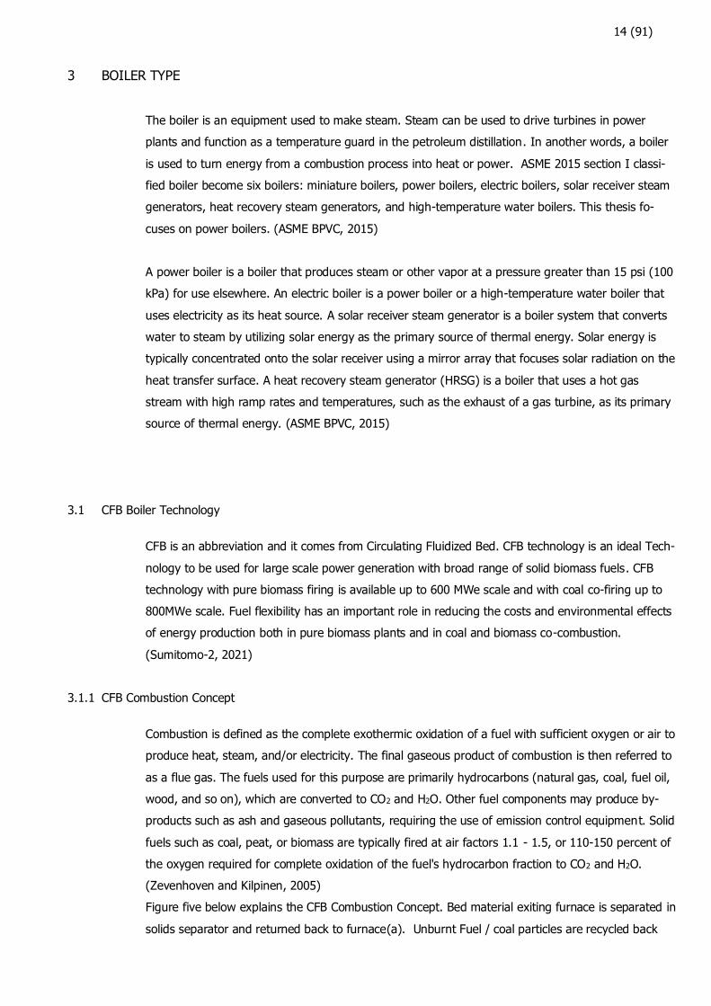
Circular Scrubber Technology’s sulfur capture exceeds 95%(<200 mg/Nm3 SOx), Scrubber uses

40% less water than wet FGD, and capital cost is 50% less than in wet FGD. There are two stages

in the CFB scrubber technology, first is emission capture such as HCl, HF, and SOx in absorber, and

the second one is particulate control in fabric filter, as illustrated in the figure below. (Sumitomo-4,

2021)

17 (91)

FIGURE 6. Scrubber technology in CFB Combustion (Sumitomo-4, 2021)

Flue gas with fly ash enters the bottom of the absorber, flowing upward through venturi to acceler-

ate the gas causing turbulence flow. The gas and solids enter the baghouse where solids are cap-

tured and recycled back to the absorber to capture more pollutants. Pollutant SO2 can be reduced

by at least 85% and up to 99%, SO3 can be reduced by at least 90% and up to 99%, HCl can be

reduced by at least 95% and up to 99%, HF can be reduced by at least 95% and up to 99%, and

Hg can be reduced by at least 60% and up to 99%. (Sumitomo-5, 2020)

3.2 BFB Boiler technology

BFB is abbreviation for Bubbling Fluidized Bed Boiler. Sumitomo Bubbling Fluid Bed steam genera-

tors have a history of reliable operation and have brought value to many clients due to their ability

to burn high moisture and high ash fuels. Sumitomo has progressively advanced the state of BFB

technology by incorporating design improvements like our rugged step grid, staged air mixing and

gas recirculation systems. (Sumitomo-6, 2020)

3.2.1 BFB Combustion Concept

The fuel is burned inside furnace above a fluidized bed consisting of natural sand. The fluidizing air

is blown at a lower velocity, and the bed materials behave like a boiling fluid but remain in the bed.

When air velocity is getting higher the bed becomes turbulent with rapid mixing of the particles,

bubbling of sand bed is similar with a boiling liquid. A lower density object will float, while a higher

density object will sink. A fluidized combustion bed temperature is 850-900ºC. It is recommended

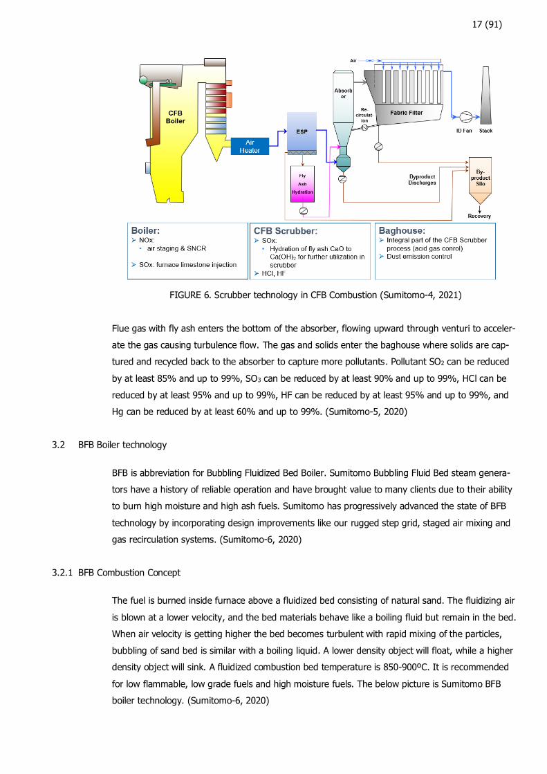
for low flammable, low grade fuels and high moisture fuels. The below picture is Sumitomo BFB

boiler technology. (Sumitomo-6, 2020)

18 (91)

FIGURE 7. Flue Gas conventional technology on BFB Combustion (Sumitomo-6, 2020)

3.2.2 Key Advantages of BFB Combustion Technology

Sumitomo BFB combustion technology has some benefits. The first is the Stepped Grid, which has

been designed for the most difficult fuels. The second benefit is high gas residence time to ensure

dioxin, CO, and fly ash carbon decomposition. The third benefit is wide superheater, evaporator,

and economizer tube bank spacing and retractable soot blowing to maintain high boiler efficiency

and long tube life. The last benefit is low gas velocity for minimum heat transfer surface erosion.

(Sumitomo-6, 2020)

3.2.3 Flue Gas Cleaning Process in BFB

Multiple levels of secondary air (air staging) and SNCR or SCR technology can be used to minimize

NOx formation. SO2 control can be achieved with calcium carbonate injection or with flue gas

scrubber technique. Flue gas flow is conducted to electro static precipirator where the dust

components are captured before flue gas enters the stack. After flue gas treatment, cleaned flue

gas is released to the atmosphere. (Sumitomo-6, 2020)

19 (91)

4 PARTICULATE COLLECTION DEVICES AND TYPICAL FLUE GAS CLEANING

There are two common Particulate Collection Devices more frequently used, the First is ESP (Elec-

trostatic precipitators) and second one is FF (Fabric Filter). The difference between ESP and FF

comes down to the Basic Idea of Cleaning Method. (APTI Course, 2021-04-05)

4.1 Electrostatic Precipitators

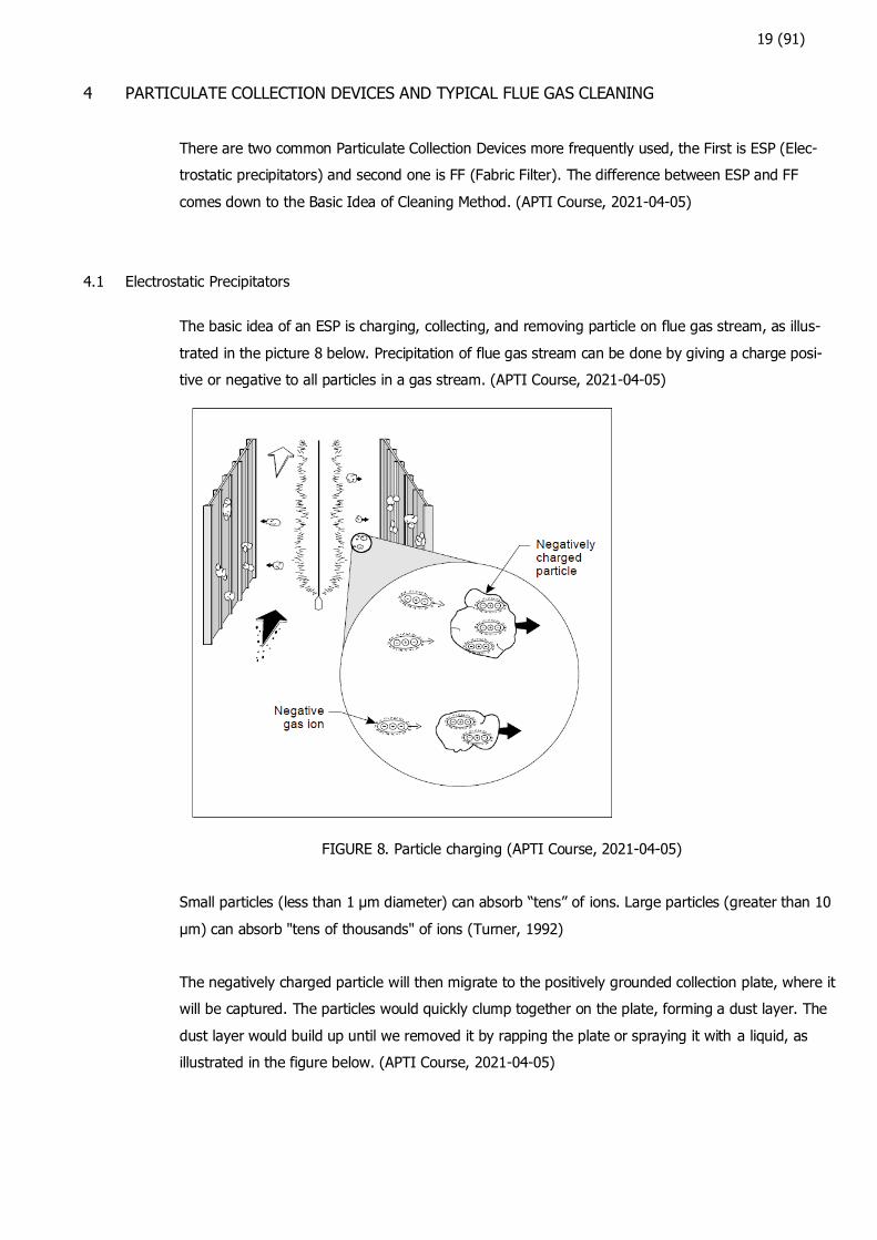
The basic idea of an ESP is charging, collecting, and removing particle on flue gas stream, as illus-

trated in the picture 8 below. Precipitation of flue gas stream can be done by giving a charge posi-

tive or negative to all particles in a gas stream. (APTI Course, 2021-04-05)

FIGURE 8. Particle charging (APTI Course, 2021-04-05)

Small particles (less than 1 μm diameter) can absorb “tens” of ions. Large particles (greater than 10

μm) can absorb "tens of thousands" of ions (Turner, 1992)

The negatively charged particle will then migrate to the positively grounded collection plate, where it

will be captured. The particles would quickly clump together on the plate, forming a dust layer. The

dust layer would build up until we removed it by rapping the plate or spraying it with a liquid, as

illustrated in the figure below. (APTI Course, 2021-04-05)

20 (91)

FIGURE 9. Particle collection at collection electrode (APTI Course, 2021-04-05)

Figure below shows thin wires called discharge electrodes which are placed between large plates

called collection electrodes, which are grounded. Discharge electrodes create a strong electrical field

that ionizes flue gas, and this ionization charges particles in the gas. Collection electrodes collect

charged particles. Rappers remove dust that has accumulated on both collection electrodes and dis-

charge electrodes by vibration, shock, or water spray. (APTI Course, 2021-04-05)

FIGURE 10. Typical dry electrostatic precipitator (APTI Course, 2021-04-05)

21 (91)

4.2 Fabric Filter

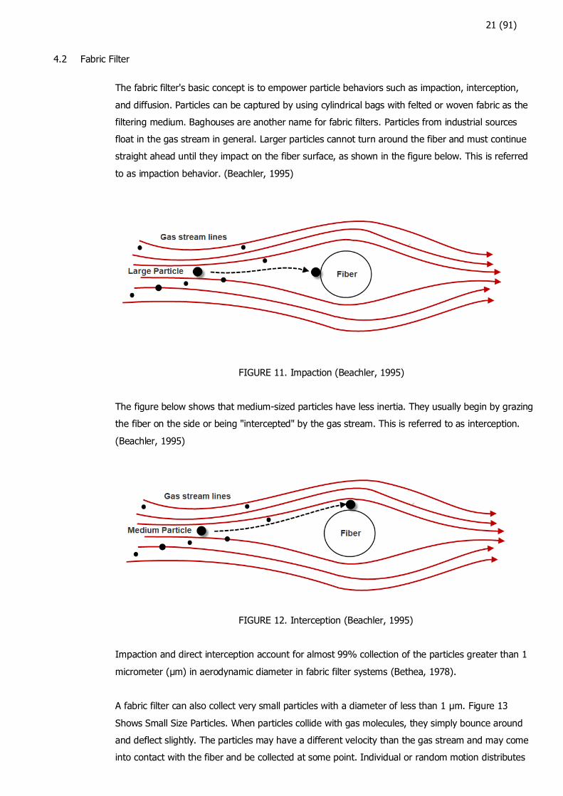
The fabric filter's basic concept is to empower particle behaviors such as impaction, interception,

and diffusion. Particles can be captured by using cylindrical bags with felted or woven fabric as the

filtering medium. Baghouses are another name for fabric filters. Particles from industrial sources

float in the gas stream in general. Larger particles cannot turn around the fiber and must continue

straight ahead until they impact on the fiber surface, as shown in the figure below. This is referred

to as impaction behavior. (Beachler, 1995)

FIGURE 11. Impaction (Beachler, 1995)

The figure below shows that medium-sized particles have less inertia. They usually begin by grazing

the fiber on the side or being "intercepted" by the gas stream. This is referred to as interception.

(Beachler, 1995)

FIGURE 12. Interception (Beachler, 1995)

Impaction and direct interception account for almost 99% collection of the particles greater than 1

micrometer (μm) in aerodynamic diameter in fabric filter systems (Bethea, 1978).

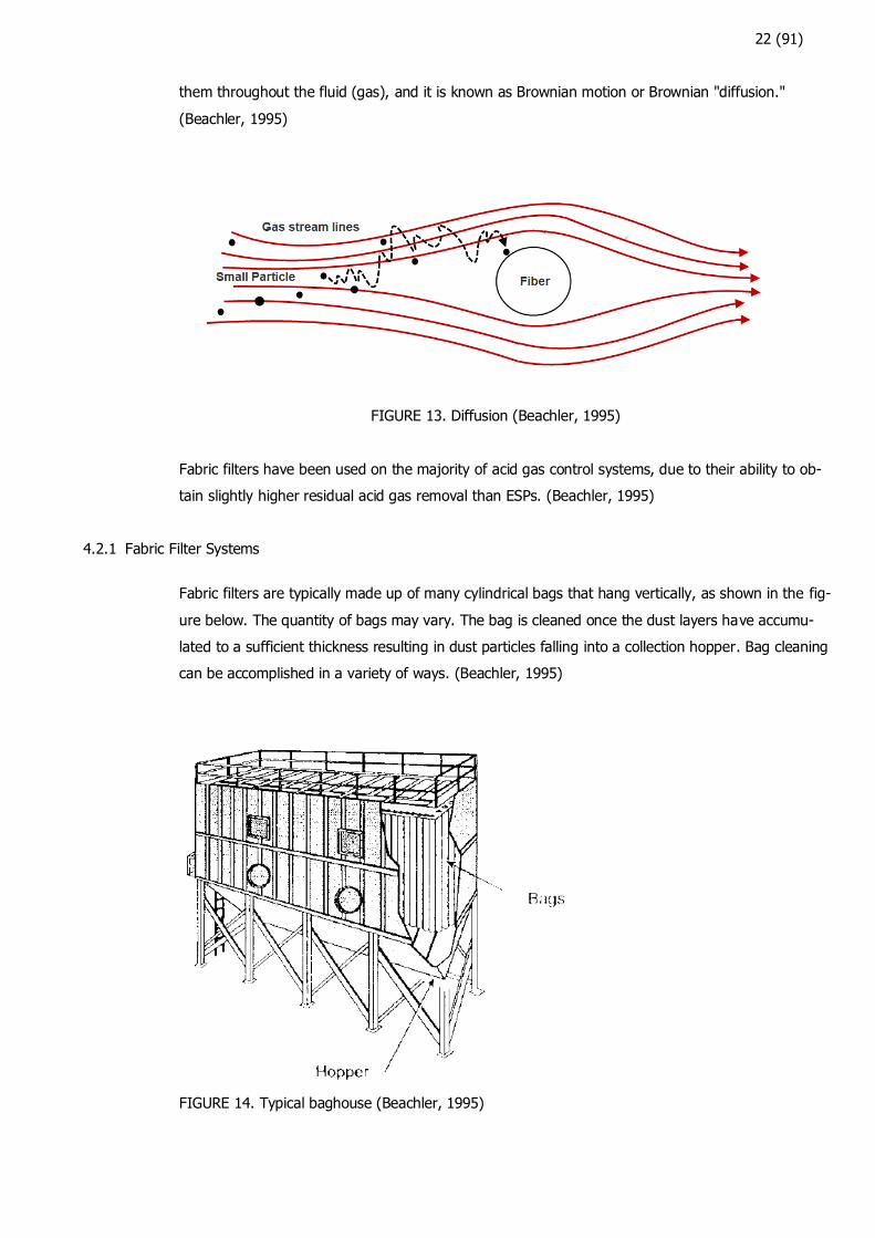
A fabric filter can also collect very small particles with a diameter of less than 1 μm. Figure 13

Shows Small Size Particles. When particles collide with gas molecules, they simply bounce around

and deflect slightly. The particles may have a different velocity than the gas stream and may come

into contact with the fiber and be collected at some point. Individual or random motion distributes

22 (91)

them throughout the fluid (gas), and it is known as Brownian motion or Brownian "diffusion."

(Beachler, 1995)

FIGURE 13. Diffusion (Beachler, 1995)

Fabric filters have been used on the majority of acid gas control systems, due to their ability to ob-

tain slightly higher residual acid gas removal than ESPs. (Beachler, 1995)

4.2.1 Fabric Filter Systems

Fabric filters are typically made up of many cylindrical bags that hang vertically, as shown in the fig-

ure below. The quantity of bags may vary. The bag is cleaned once the dust layers have accumu-

lated to a sufficient thickness resulting in dust particles falling into a collection hopper. Bag cleaning

can be accomplished in a variety of ways. (Beachler, 1995)

FIGURE 14. Typical baghouse (Beachler, 1995)

23 (91)

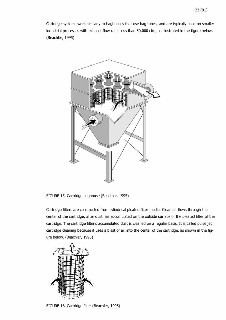
Cartridge systems work similarly to baghouses that use bag tubes, and are typically used on smaller

industrial processes with exhaust flow rates less than 50,000 cfm, as illustrated in the figure below.

(Beachler, 1995)

FIGURE 15. Cartridge baghouse (Beachler, 1995)

Cartridge filters are constructed from cylindrical pleated filter media. Clean air flows through the

center of the cartridge, after dust has accumulated on the outside surface of the pleated filter of the

cartridge. The cartridge filter's accumulated dust is cleaned on a regular basis. It is called pulse jet

cartridge cleaning because it uses a blast of air into the center of the cartridge, as shown in the fig-

ure below. (Beachler, 1995)

FIGURE 16. Cartridge filter (Beachler, 1995)

24 (91)

4.2.2 Bag Cleaning

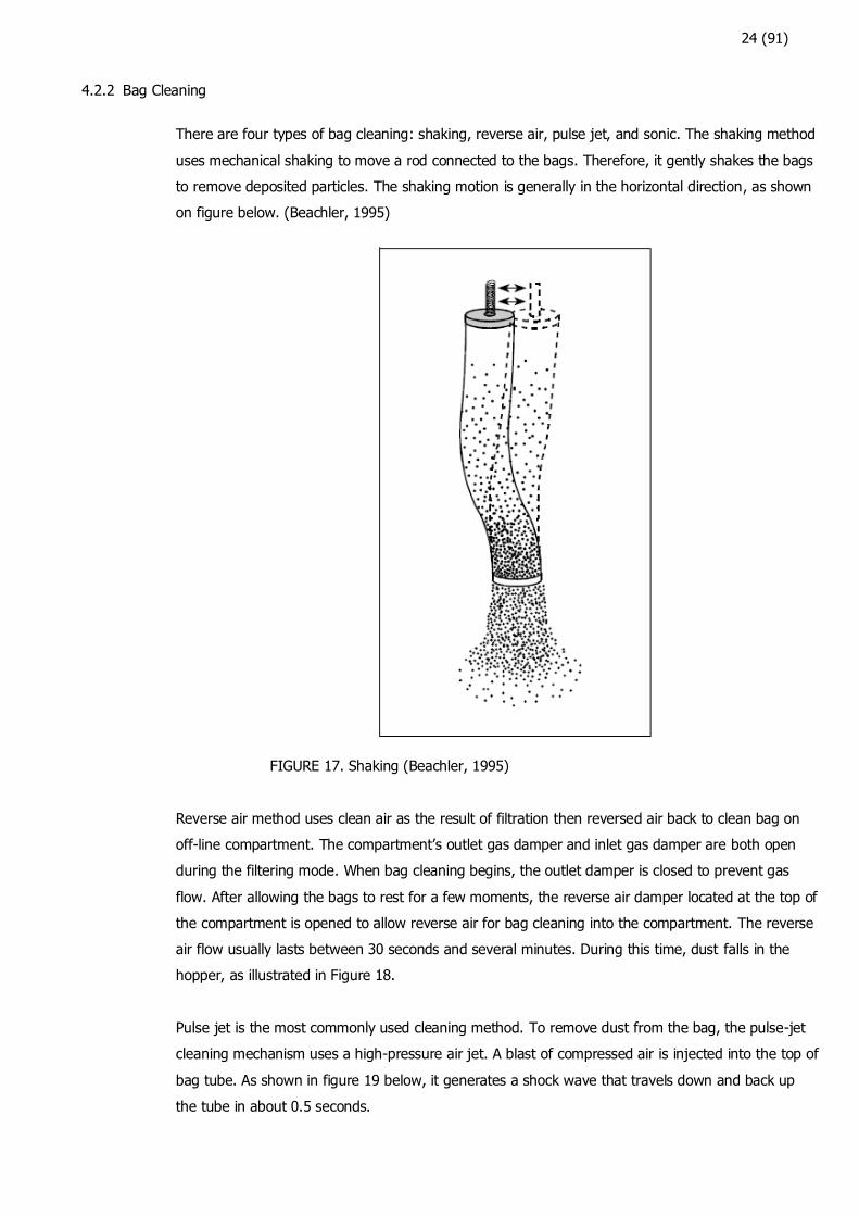
There are four types of bag cleaning: shaking, reverse air, pulse jet, and sonic. The shaking method

uses mechanical shaking to move a rod connected to the bags. Therefore, it gently shakes the bags

to remove deposited particles. The shaking motion is generally in the horizontal direction, as shown

on figure below. (Beachler, 1995)

FIGURE 17. Shaking (Beachler, 1995)

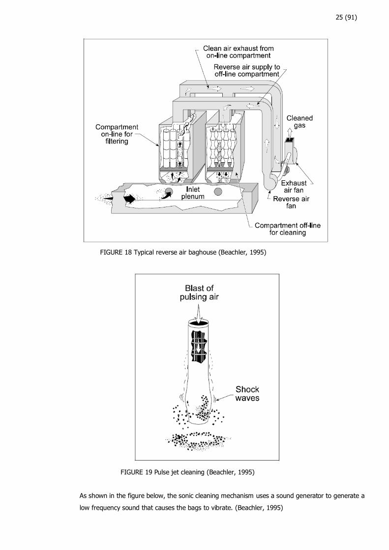
Reverse air method uses clean air as the result of filtration then reversed air back to clean bag on

off-line compartment. The compartment’s outlet gas damper and inlet gas damper are both open

during the filtering mode. When bag cleaning begins, the outlet damper is closed to prevent gas

flow. After allowing the bags to rest for a few moments, the reverse air damper located at the top of

the compartment is opened to allow reverse air for bag cleaning into the compartment. The reverse

air flow usually lasts between 30 seconds and several minutes. During this time, dust falls in the

hopper, as illustrated in Figure 18.

Pulse jet is the most commonly used cleaning method. To remove dust from the bag, the pulse-jet

cleaning mechanism uses a high-pressure air jet. A blast of compressed air is injected into the top of

bag tube. As shown in figure 19 below, it generates a shock wave that travels down and back up

the tube in about 0.5 seconds.

25 (91)

FIGURE 18 Typical reverse air baghouse (Beachler, 1995)

FIGURE 19 Pulse jet cleaning (Beachler, 1995)

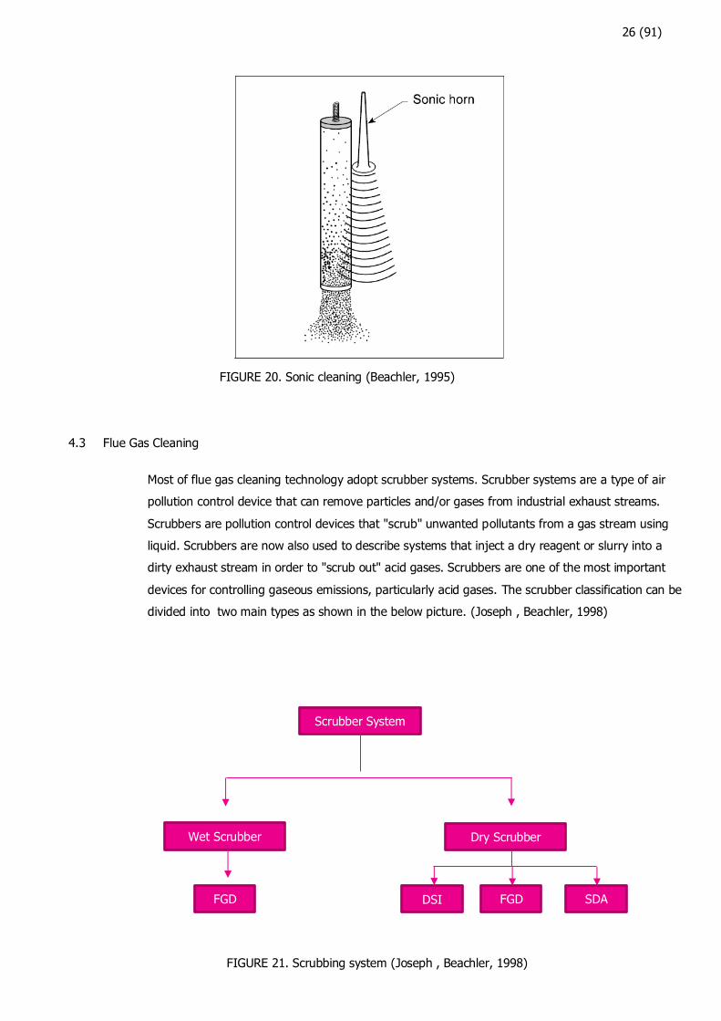
As shown in the figure below, the sonic cleaning mechanism uses a sound generator to generate a

low frequency sound that causes the bags to vibrate. (Beachler, 1995)

26 (91)

FIGURE 20. Sonic cleaning (Beachler, 1995)

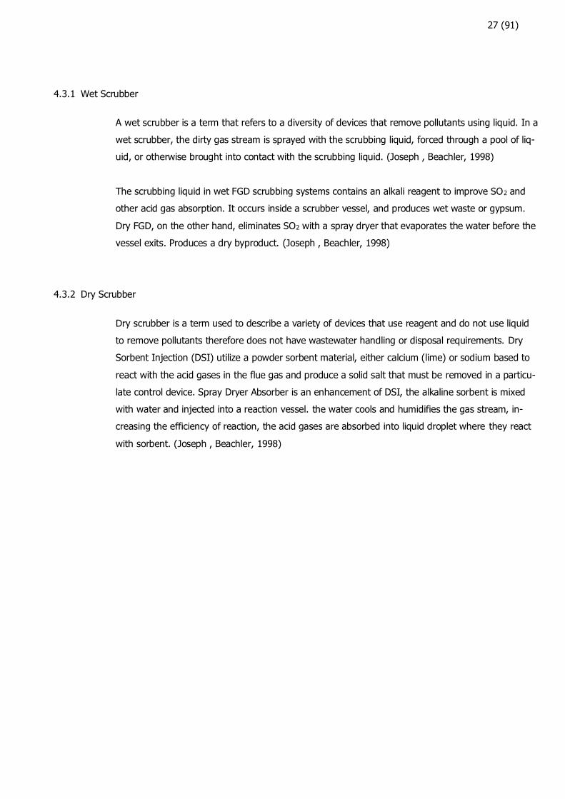
4.3 Flue Gas Cleaning

Most of flue gas cleaning technology adopt scrubber systems. Scrubber systems are a type of air

pollution control device that can remove particles and/or gases from industrial exhaust streams.

Scrubbers are pollution control devices that "scrub" unwanted pollutants from a gas stream using

liquid. Scrubbers are now also used to describe systems that inject a dry reagent or slurry into a

dirty exhaust stream in order to "scrub out" acid gases. Scrubbers are one of the most important

devices for controlling gaseous emissions, particularly acid gases. The scrubber classification can be

divided into two main types as shown in the below picture. (Joseph , Beachler, 1998)

FIGURE 21. Scrubbing system (Joseph , Beachler, 1998)

Scrubber System

Wet Scrubber Dry Scrubber

DSI SDA FGD FGD

27 (91)

4.3.1 Wet Scrubber

A wet scrubber is a term that refers to a diversity of devices that remove pollutants using liquid. In a

wet scrubber, the dirty gas stream is sprayed with the scrubbing liquid, forced through a pool of liq-

uid, or otherwise brought into contact with the scrubbing liquid. (Joseph , Beachler, 1998)

The scrubbing liquid in wet FGD scrubbing systems contains an alkali reagent to improve SO2 and

other acid gas absorption. It occurs inside a scrubber vessel, and produces wet waste or gypsum.

Dry FGD, on the other hand, eliminates SO2 with a spray dryer that evaporates the water before the

vessel exits. Produces a dry byproduct. (Joseph , Beachler, 1998)

4.3.2 Dry Scrubber

Dry scrubber is a term used to describe a variety of devices that use reagent and do not use liquid

to remove pollutants therefore does not have wastewater handling or disposal requirements. Dry

Sorbent Injection (DSI) utilize a powder sorbent material, either calcium (lime) or sodium based to

react with the acid gases in the flue gas and produce a solid salt that must be removed in a particu-

late control device. Spray Dryer Absorber is an enhancement of DSI, the alkaline sorbent is mixed

with water and injected into a reaction vessel. the water cools and humidifies the gas stream, in-

creasing the efficiency of reaction, the acid gases are absorbed into liquid droplet where they react

with sorbent. (Joseph , Beachler, 1998)

28 (91)

5 DSI FLUE GAS CLEANING

The Dry Sorbent Injection (DSI) is a sulfur dioxide (SO2), sulfur trioxide (SO3), hydrogen chloride

(HCl) and hydrogen fluoride (HF) reduction that uses an alkali sorbent as the injection material. The

alkali sorbent is injected into ductwork/reaction chamber to react with pollutants and then is re-

moved by a particulate removal device such as an electrostatic precipitator or a fabric filter. (Joseph

, Beachler, 1998)

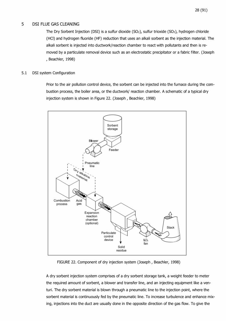
5.1 DSI system Configuration

Prior to the air pollution control device, the sorbent can be injected into the furnace during the com-

bustion process, the boiler area, or the ductwork/ reaction chamber. A schematic of a typical dry

injection system is shown in Figure 22. (Joseph , Beachler, 1998)

FIGURE 22. Component of dry injection system (Joseph , Beachler, 1998)

A dry sorbent injection system comprises of a dry sorbent storage tank, a weight feeder to meter

the required amount of sorbent, a blower and transfer line, and an injecting equipment like a ven-

turi. The dry sorbent material is blown through a pneumatic line to the injection point, where the

sorbent material is continuously fed by the pneumatic line. To increase turbulence and enhance mix-

ing, injections into the duct are usually done in the opposite direction of the gas flow. To give the

29 (91)

acid gases more time to react with the sorbent, an expansion/reaction chamber may be provided.

(Joseph , Beachler, 1998)

To achieve moderate acid gas control, for example, 50% SO2 removal and 90% HCl removal on mu-

nicipal and medical waste combustion, the basic dry injector procedure described above can be

used. Cooling and/or humidifying the flue gas stream can improve the efficiency of acid gas re-

moval. Between 204oC to 315oC, the exhaust gases from industrial boilers or waste combustors. A

heat exchanger or dry quench chamber can be used to cool the flue gases before they reach the

injection point. As the flue gas temperature is cooled, the sorbent and acid gases react faster. In

order to ensure that all the water droplets used to quench are evaporated, the temperature must be

maintained at 148-176oC.

Another way to boost the overall effectiveness of dry scrubbing systems is to recycle some of the

collected particles and unreacted sorbent. Additional sorbent (beyond the stoichiometric amount)

must be injected since it is difficult to blend a dry solid and a gas stream. As a result, the baghouse

or electrostatic precipitator collects unreacted sorbent. Recycled material can sometimes be returned

to the injection point.

To obtain high removal efficiencies while utilizing relatively affordable calcium sorbents, the majority

of dry injection systems must run at greater stoichiometric ratios than a spray drier. To ensure mod-

erate acid gas control, for example, stoichiometric ratios of 2.0 to 4.0 are utilized in municipal waste

combustors. This increased use of sorbents limitations their use to smaller sources such as medical

waste incinerators.

5.2 Mass and Energy Balance

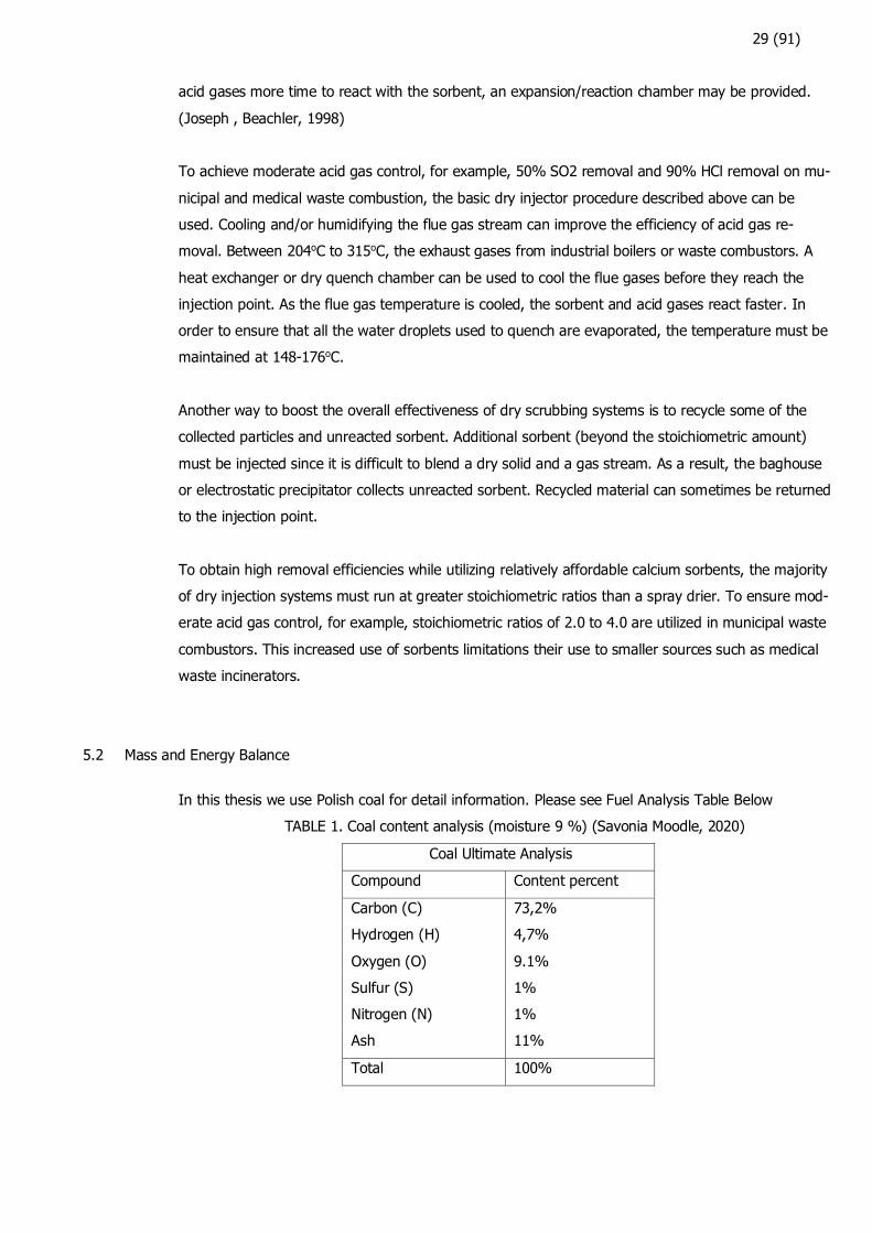
In this thesis we use Polish coal for detail information. Please see Fuel Analysis Table Below

TABLE 1. Coal content analysis (moisture 9 %) (Savonia Moodle, 2020)

Coal Ultimate Analysis

Compound Content percent

Carbon (C) 73,2%

Hydrogen (H) 4,7%

Oxygen (O) 9.1%

Sulfur (S) 1%

Nitrogen (N) 1%

Ash 11%

Total 100%

30 (91)

Here below is amount of air flow rate and flue gas rate calculation based on coal content analysis.

TABLE 2. Oxygen Calculation (Savonia Moodle, 2020)

Material

(A)

Com-

posi-

tion in

%

(B)

input

weight

kg/kgpa

(C)

Molecu-

lar

Weight

Kg/Kmol

(D)

consumed

Kmol/Kgpa

C/D

(E)

Amount of

O2 needed

Kmol/Kgpa

C/D

(F)

Molecular

Weight O2

Kg/Kmol

(G)

Amount of

O2 needed

Kg/Kgpa

FXG

(H)

Combustion Reac-

tion

C 73.2% 0.732 12.01 0.0609 0.0609 32 1.95 C+O2->CO2

H2 4.7% 0.047 2.016 0.0233 0.0117 32 0.37 2H2+O2->2H2O

O2 9.1% 0.091 32 0.0028 -0.0028 32 -0.09

S 1% 0.01 32 0.0003 0.0003 32 0.01 S+O2->SO2

N2 1% 0.01

ASH 11% 0.11

total 100% 1 0.0701 32 2.24

Amount of oxygen consumed for coal combustion is 0.0701 kmol/kg fuel. The composition of air

79% N2 and 21% O2 leads to total N2 needed 0,0701 X (79%/21%)=0.2635 kmol/kgpa. N2 needed

in kg/kgpa is 0.2635 X molecular weight of N2 ( 0.2635 X 28 =7.386) .Thus total Air needed is

O2+N2 (2.24+7.386=9.63 kg/kgpa ).

TABLE 3. Flue Gas Composition

Material

Amount of Ma-

terial in

Kmol/Kgpa

Reaction

Product

Amount of Flue

Gas Produced

Kmol/Kgpa

Proportion in

dry Flue Gas

Proportion in

Wet Flue Gas

C 0.0609 CO2 0.0609 0.188 0.1751

H2 0.0233 H2O 0.0233 0 0.0670

S 0.0003 SO2 0.0003 0.001 0.0009

N2 0.2635 0.8114 0.7570

total (dry) 0.3247 1.0000

total (wet) 0.3481 1.000

As shown in table 3, the total amount of flue gas produced in dry conditions is CO2+ SO2+ N2

(0.0609 + 0.0003 + 0.2635 = 0,3247 Kmol/Kgpa ). In wet conditions, the total amount of flue gas

produced is CO2+ H2O+SO2+ N2 (0.0609 +0.0233+0.0003 +0.2635=0.3481 Kmol/Kgpa).

TABLE 4. Amount of Flue Gas Calculation

Material

(A)

Amount of Flue Gas in

Kmol/Kgpa

(B)

Molecular Weight

Kg/Kmol

(C)

Amount of Flue Gas in

Kg/Kgpa

(B) X (C)

(D)

CO2 0.0609 44.01 2.68

H2O 0.0233 18.016 0.42

SO2 0.0003 64 0.02

N2 0.2635 28.02 7.38

total (dry) 10.09

total (Wet) 10.51

31 (91)

Table above shows that the amount of flue gas in coal combustion is 10.51 kg per kg of coal

burned.

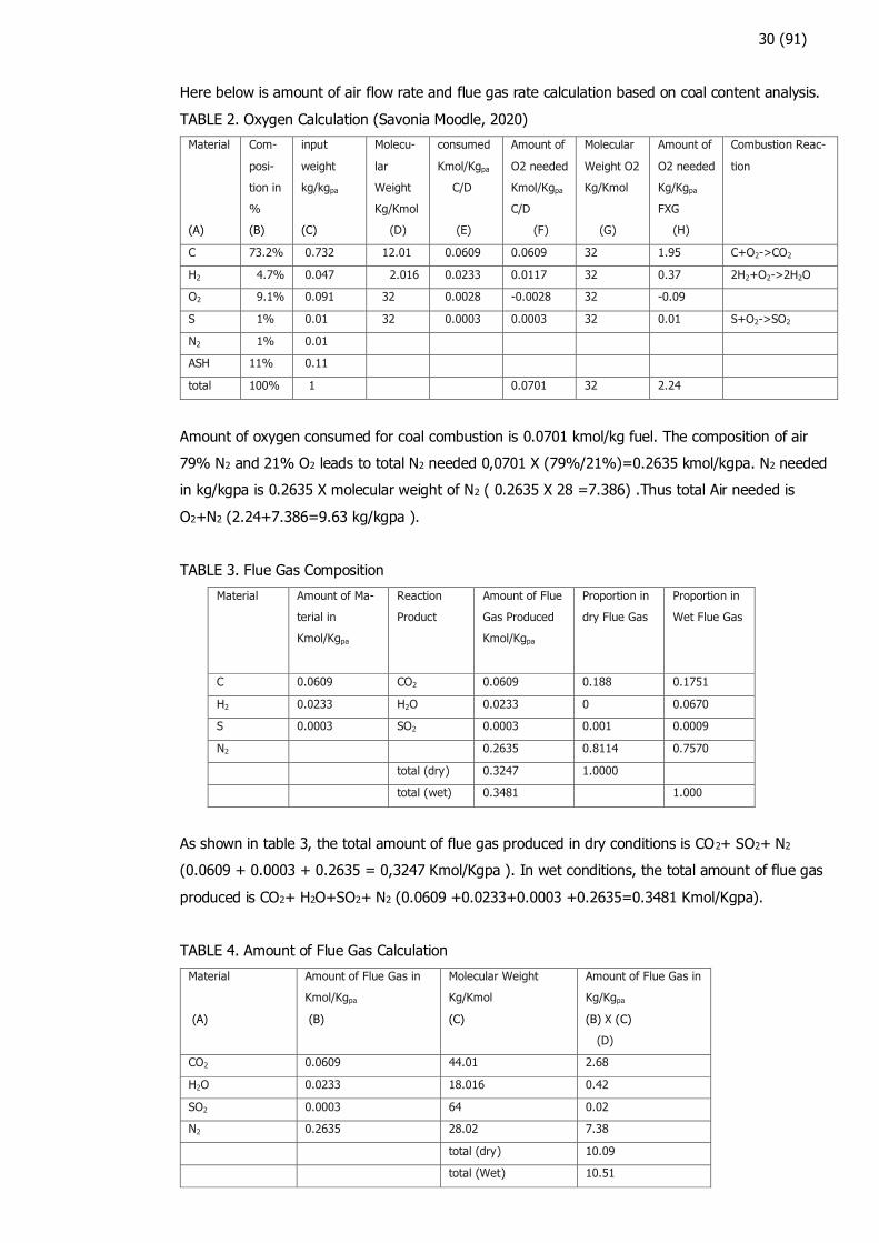
5.3 DSI Chemistry

The reaction between acid gas and the alkaline material takes place on the surface of these solid

sorbent particles. It is called adsorption mechanism as the primary removal mechanism. The alkaline

materials are generally calcium hydroxide or sodium – based reagents that have large surface areas

to aid adsorbing the acid gas as shown in figure below. Adsorption occurs when the acid gas mole-

cules adhere to the surface of the solid sorbent. Absorption occurs when the acid gases dissolve in

the liquid droplets. (Joseph , Beachler, 1998)

FIGURE 23. The mechanism of acid gas removal adapted from Jose and Beachler (Joseph ,

Beachler, 1998)

Due to the need for humidity, absorption mechanism is used to reduce acid gases whereas adsorp-

tion mechanism is used to reduce metal emissions. (Teija, 2022)

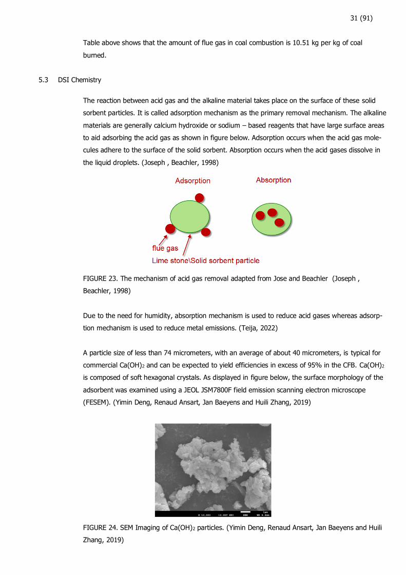
A particle size of less than 74 micrometers, with an average of about 40 micrometers, is typical for

commercial Ca(OH)2 and can be expected to yield efficiencies in excess of 95% in the CFB. Ca(OH)2

is composed of soft hexagonal crystals. As displayed in figure below, the surface morphology of the

adsorbent was examined using a JEOL JSM7800F field emission scanning electron microscope

(FESEM). (Yimin Deng, Renaud Ansart, Jan Baeyens and Huili Zhang, 2019)

FIGURE 24. SEM Imaging of Ca(OH)2 particles. (Yimin Deng, Renaud Ansart, Jan Baeyens and Huili

Zhang, 2019)

32 (91)

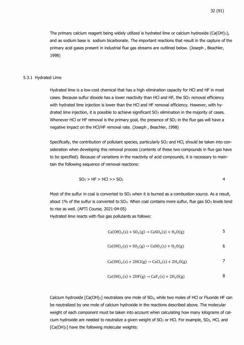
The primary calcium reagent being widely utilized is hydrated lime or calcium hydroxide (Ca(OH)2),

and as sodium base is sodium bicarbonate. The important reactions that result in the capture of the

primary acid gases present in industrial flue gas streams are outlined below. (Joseph , Beachler,

1998)

5.3.1 Hydrated Lime

Hydrated lime is a low-cost chemical that has a high elimination capacity for HCl and HF in most

cases. Because sulfur dioxide has a lower reactivity than HCl and HF, the SO2 removal efficiency

with hydrated lime injection is lower than the HCl and HF removal efficiency. However, with hy-

drated lime injection, it is possible to achieve significant SO2 elimination in the majority of cases.

Whenever HCl or HF removal is the primary goal, the presence of SO2 in the flue gas will have a

negative impact on the HCl/HF removal rate. (Joseph , Beachler, 1998)

Specifically, the contribution of pollutant species, particularly SO2 and HCl, should be taken into con-

sideration when developing this removal process (contents of these two compounds in flue gas have

to be specified). Because of variations in the reactivity of acid compounds, it is necessary to main-

tain the following sequence of removal reactions:

SO3 > HF > HCl >> SO2 4

Most of the sulfur in coal is converted to SO2 when it is burned as a combustion source. As a result,

about 1% of the sulfur is converted to SO3. When coal contains more sulfur, flue gas SO3 levels tend

to rise as well. (APTI Course, 2021-04-05)

Hydrated lime reacts with flue gas pollutants as follows:

Ca(OH)2(s) + SO3(g) → CaSO4(s) + H2O(g) 5

Ca(OH)2(s)+ SO2(g) → CaSO3(s) + H2O(g) 6

Ca(OH)2(s)+ 2HCl(g) → CaCl2(s)+ 2H2O(g) 7

Ca(OH)2(s)+ 2HF(g) → CaF2(s) + 2H2O(g) 8

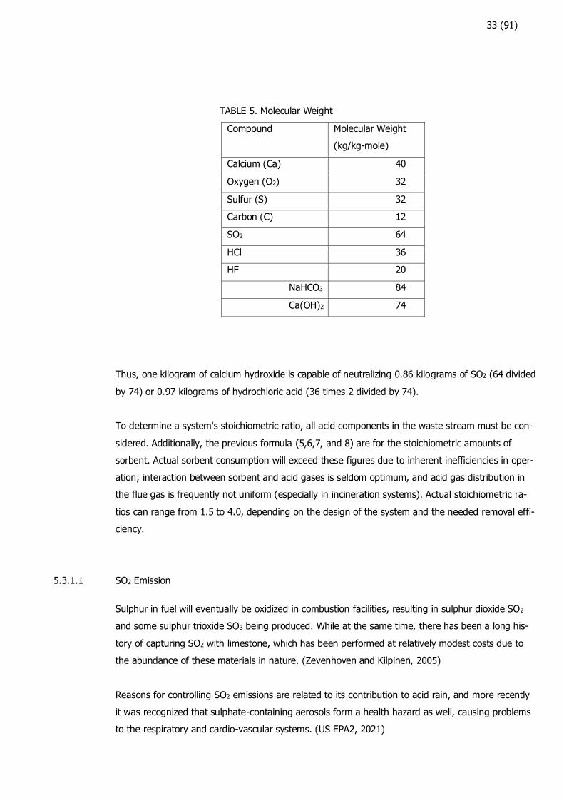
Calcium hydroxide [Ca(OH)2] neutralizes one mole of SO2, while two moles of HCl or Fluoride HF can

be neutralized by one mole of calcium hydroxide in the reactions described above. The molecular

weight of each component must be taken into account when calculating how many kilograms of cal-

cium hydroxide are needed to neutralize a given weight of SO2 or HCl. For example, SO2, HCl, and

[Ca(OH)2] have the following molecular weights:

33 (91)

TABLE 5. Molecular Weight

Compound Molecular Weight

(kg/kg-mole)

Calcium (Ca) 40

Oxygen (O2) 32

Sulfur (S) 32

Carbon (C) 12

SO2 64

HCl 36

HF 20

NaHCO3 84

Ca(OH)2 74

Thus, one kilogram of calcium hydroxide is capable of neutralizing 0.86 kilograms of SO2 (64 divided

by 74) or 0.97 kilograms of hydrochloric acid (36 times 2 divided by 74).

To determine a system's stoichiometric ratio, all acid components in the waste stream must be con-

sidered. Additionally, the previous formula (5,6,7, and 8) are for the stoichiometric amounts of

sorbent. Actual sorbent consumption will exceed these figures due to inherent inefficiencies in oper-

ation; interaction between sorbent and acid gases is seldom optimum, and acid gas distribution in

the flue gas is frequently not uniform (especially in incineration systems). Actual stoichiometric ra-

tios can range from 1.5 to 4.0, depending on the design of the system and the needed removal effi-

ciency.

5.3.1.1 SO2 Emission

Sulphur in fuel will eventually be oxidized in combustion facilities, resulting in sulphur dioxide SO2

and some sulphur trioxide SO3 being produced. While at the same time, there has been a long his-

tory of capturing SO2 with limestone, which has been performed at relatively modest costs due to

the abundance of these materials in nature. (Zevenhoven and Kilpinen, 2005)

Reasons for controlling SO2 emissions are related to its contribution to acid rain, and more recently

it was recognized that sulphate-containing aerosols form a health hazard as well, causing problems

to the respiratory and cardio-vascular systems. (US EPA2, 2021)

34 (91)

The entire amount of sulfur dioxide released can be calculated. If a 150MW CFB plant consumes 70

T/h of coal with an average energy content of roughly 20.000 kJ/kg and a sulfur concentration of

1%, as indicated in Table 1, Assume that 95 percent of the sulfur in fuel interacts via Reaction 9

below.

S + O2 → SO2 9

Percentage of sulfur in the coal that converts to SO2: 95 percent conversion factor came from an

Environmental Protection Agency (EPA) document in the 1980s.

Mass of Fuel sulfur = Amount of Fuel X Content of Sulfur in Fuel % 10

70.000 𝑘𝑔

ℎ∗

1

100 = 700

𝑘𝑔

ℎ 11

Total amount of sulfur in the coal is 700 kg /hr. Total amount of Sulfur quantity can be converted to

kilomoles per hour. Amount of kilomoles of sulfur per hour is 21,87 kmol /h, as shown here below.

700 𝑘𝑔

ℎ∗ 𝑘𝑔 𝑚𝑜𝑙𝑒 𝑆

32 𝑘𝑔 𝑆= 21,87

𝑘𝑚𝑜𝑙 𝑆

ℎ 12

𝑆𝑡𝑜𝑖𝑐ℎ𝑖𝑜𝑚𝑒𝑡𝑟𝑖𝑐 𝑆𝑂2 = 1 ∗ (𝑘 𝑚𝑜𝑙 𝑆) 13

21,87𝑘𝑚𝑜𝑙 𝑆

ℎ∗0.95 ∗ 𝑘𝑔 𝑆 𝑐𝑜𝑛𝑣𝑒𝑟𝑡𝑒𝑑

𝑘𝑔 ∗ 𝑆 𝑡𝑜𝑡𝑎𝑙∗ 1 ∗ 𝑘𝑚𝑜𝑙 𝑆𝑂21 ∗ 𝑘𝑚𝑜𝑙 𝑆

= 20.78 𝑘𝑚𝑜𝑙 𝑆𝑂2

ℎ 14

According to equation 9, 95% mole S converted to SO2 is 20,78 kmol SO2/h.

20.78 𝑘𝑚𝑜𝑙 𝑆𝑂2

ℎ∗ 64

𝑘𝑔

𝑘𝑚𝑜𝑙 𝑆𝑂2= 1330

𝑘𝑔

ℎ 15

Thus, the total mass of SO2 emitted per hour is 1330 kg/h. 1330 kg/hr of SO2 is formed in Furnace

and it will react with limestone.

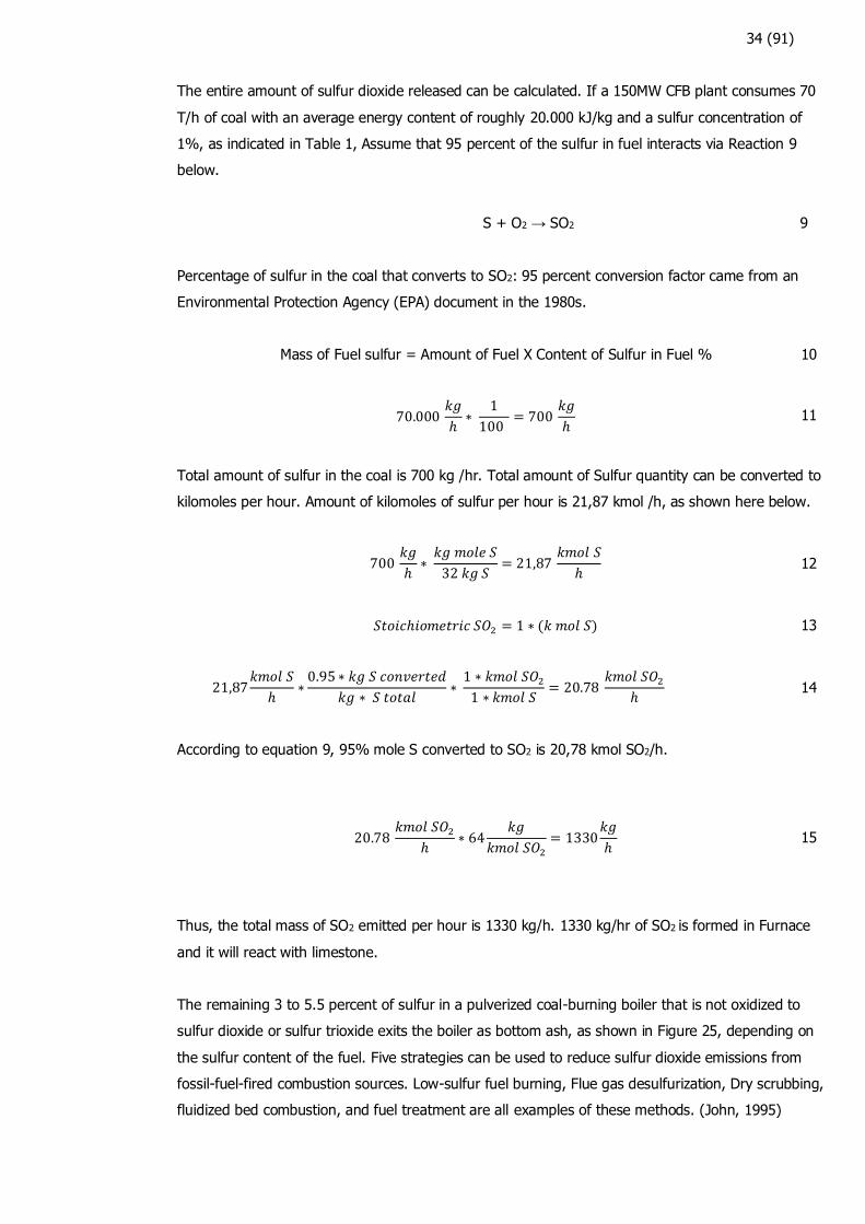
The remaining 3 to 5.5 percent of sulfur in a pulverized coal-burning boiler that is not oxidized to

sulfur dioxide or sulfur trioxide exits the boiler as bottom ash, as shown in Figure 25, depending on

the sulfur content of the fuel. Five strategies can be used to reduce sulfur dioxide emissions from

fossil-fuel-fired combustion sources. Low-sulfur fuel burning, Flue gas desulfurization, Dry scrubbing,

fluidized bed combustion, and fuel treatment are all examples of these methods. (John, 1995)

35 (91)

FIGURE 25. Conversion of fuel sulfur (John, 1995)

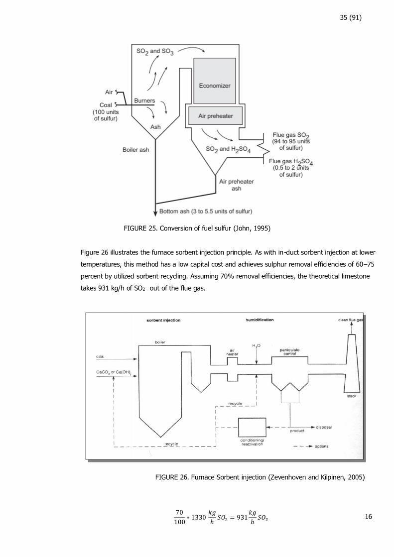
Figure 26 illustrates the furnace sorbent injection principle. As with in-duct sorbent injection at lower

temperatures, this method has a low capital cost and achieves sulphur removal efficiencies of 60–75

percent by utilized sorbent recycling. Assuming 70% removal efficiencies, the theoretical limestone

takes 931 kg/h of SO2 out of the flue gas.

FIGURE 26. Furnace Sorbent injection (Zevenhoven and Kilpinen, 2005)

70

100∗ 1330

𝑘𝑔

ℎ𝑆𝑂2 = 931

𝑘𝑔

ℎ𝑆𝑂2 16

36 (91)

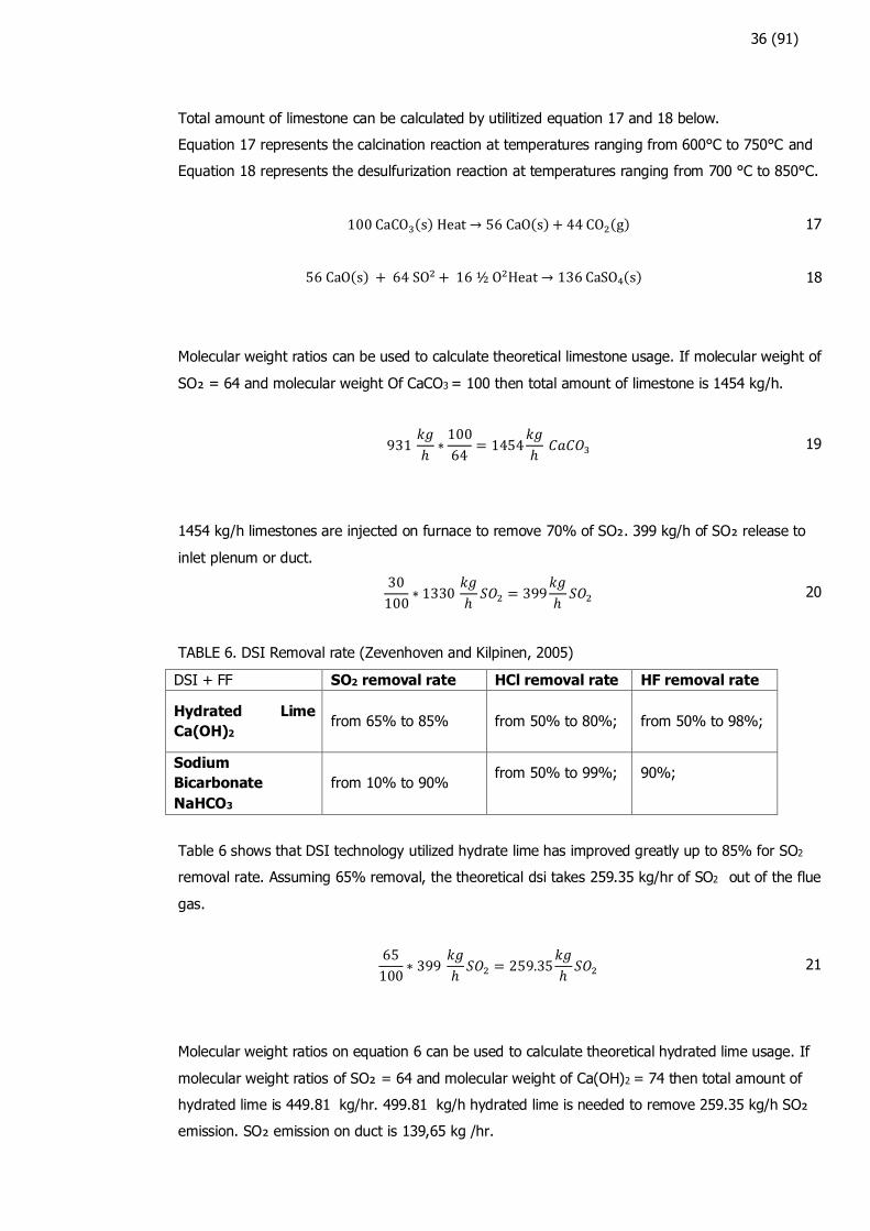
Total amount of limestone can be calculated by utilitized equation 17 and 18 below.

Equation 17 represents the calcination reaction at temperatures ranging from 600°C to 750°C and

Equation 18 represents the desulfurization reaction at temperatures ranging from 700 °C to 850°C.

100 CaCO3(s) Heat → 56 CaO(s) + 44 CO2(g) 17

56 CaO(s) + 64 SO2+ 16 ½ O2Heat → 136 CaSO₄(s) 18

Molecular weight ratios can be used to calculate theoretical limestone usage. If molecular weight of

SO₂ = 64 and molecular weight Of CaCO3 = 100 then total amount of limestone is 1454 kg/h.

931 𝑘𝑔

ℎ∗100

64= 1454

𝑘𝑔

ℎ 𝐶𝑎𝐶𝑂3 19

1454 kg/h limestones are injected on furnace to remove 70% of SO₂. 399 kg/h of SO₂ release to

inlet plenum or duct.

30

100∗ 1330

𝑘𝑔

ℎ𝑆𝑂2 = 399

𝑘𝑔

ℎ𝑆𝑂2 20

TABLE 6. DSI Removal rate (Zevenhoven and Kilpinen, 2005)

DSI + FF SO2 removal rate HCl removal rate HF removal rate

Hydrated Lime

Ca(OH)2 from 65% to 85%

from 50% to 80%;

from 50% to 98%;

Sodium

Bicarbonate

NaHCO3

from 10% to 90% from 50% to 99%;

90%;

Table 6 shows that DSI technology utilized hydrate lime has improved greatly up to 85% for SO2

removal rate. Assuming 65% removal, the theoretical dsi takes 259.35 kg/hr of SO2 out of the flue

gas.

65

100∗ 399

𝑘𝑔

ℎ𝑆𝑂2 = 259.35

𝑘𝑔

ℎ𝑆𝑂2 21

Molecular weight ratios on equation 6 can be used to calculate theoretical hydrated lime usage. If

molecular weight ratios of SO₂ = 64 and molecular weight of Ca(OH)2 = 74 then total amount of

hydrated lime is 449.81 kg/hr. 499.81 kg/h hydrated lime is needed to remove 259.35 kg/h SO₂

emission. SO₂ emission on duct is 139,65 kg /hr.

37 (91)

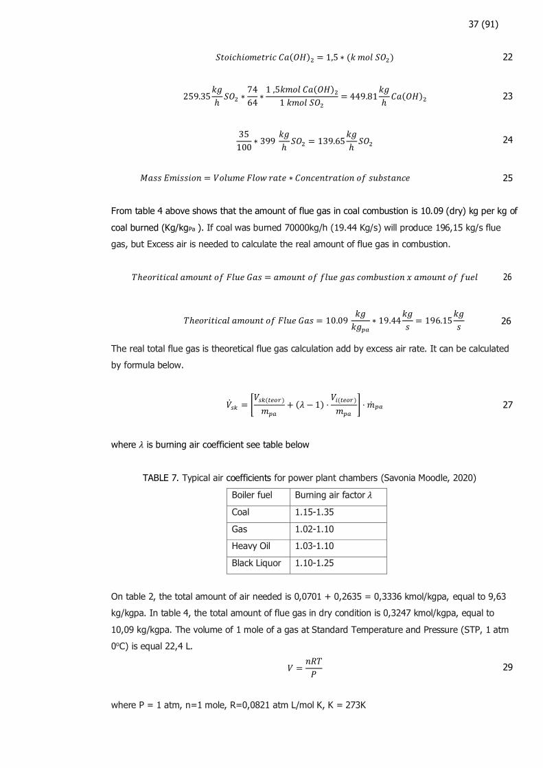
𝑆𝑡𝑜𝑖𝑐ℎ𝑖𝑜𝑚𝑒𝑡𝑟𝑖𝑐 𝐶𝑎(𝑂𝐻)2 = 1,5 ∗ (𝑘 𝑚𝑜𝑙 𝑆𝑂2) 22

259.35𝑘𝑔

ℎ𝑆𝑂2 ∗

74

64∗1 ,5𝑘𝑚𝑜𝑙 𝐶𝑎(𝑂𝐻)21 𝑘𝑚𝑜𝑙 𝑆𝑂2

= 449.81𝑘𝑔

ℎ𝐶𝑎(𝑂𝐻)2 23

35

100∗ 399

𝑘𝑔

ℎ𝑆𝑂2 = 139.65

𝑘𝑔

ℎ𝑆𝑂2 24

𝑀𝑎𝑠𝑠 𝐸𝑚𝑖𝑠𝑠𝑖𝑜𝑛 = 𝑉𝑜𝑙𝑢𝑚𝑒 𝐹𝑙𝑜𝑤 𝑟𝑎𝑡𝑒 ∗ 𝐶𝑜𝑛𝑐𝑒𝑛𝑡𝑟𝑎𝑡𝑖𝑜𝑛 𝑜𝑓 𝑠𝑢𝑏𝑠𝑡𝑎𝑛𝑐𝑒 25

From table 4 above shows that the amount of flue gas in coal combustion is 10.09 (dry) kg per kg of

coal burned (Kg/kgPa ). If coal was burned 70000kg/h (19.44 Kg/s) will produce 196,15 kg/s flue

gas, but Excess air is needed to calculate the real amount of flue gas in combustion.

𝑇ℎ𝑒𝑜𝑟𝑖𝑡𝑖𝑐𝑎𝑙 𝑎𝑚𝑜𝑢𝑛𝑡 𝑜𝑓 𝐹𝑙𝑢𝑒 𝐺𝑎𝑠 = 𝑎𝑚𝑜𝑢𝑛𝑡 𝑜𝑓 𝑓𝑙𝑢𝑒 𝑔𝑎𝑠 𝑐𝑜𝑚𝑏𝑢𝑠𝑡𝑖𝑜𝑛 𝑥 𝑎𝑚𝑜𝑢𝑛𝑡 𝑜𝑓 𝑓𝑢𝑒𝑙 26

𝑇ℎ𝑒𝑜𝑟𝑖𝑡𝑖𝑐𝑎𝑙 𝑎𝑚𝑜𝑢𝑛𝑡 𝑜𝑓 𝐹𝑙𝑢𝑒 𝐺𝑎𝑠 = 10.09 𝑘𝑔

𝑘𝑔𝑝𝑎∗ 19.44

𝑘𝑔

𝑠= 196.15

𝑘𝑔

𝑠 26

The real total flue gas is theoretical flue gas calculation add by excess air rate. It can be calculated

by formula below.

�̇�𝑠𝑘 = [𝑉𝑠𝑘(𝑡𝑒𝑜𝑟)

𝑚𝑝𝑎+ (𝜆 − 1) ⋅

𝑉𝑖(𝑡𝑒𝑜𝑟)

𝑚𝑝𝑎] ⋅ �̇�𝑝𝑎 27

where 𝜆 is burning air coefficient see table below

TABLE 7. Typical air coefficients for power plant chambers (Savonia Moodle, 2020)

Boiler fuel Burning air factor 𝜆

Coal 1.15-1.35

Gas 1.02-1.10

Heavy Oil 1.03-1.10

Black Liquor 1.10-1.25

On table 2, the total amount of air needed is 0,0701 + 0,2635 = 0,3336 kmol/kgpa, equal to 9,63

kg/kgpa. In table 4, the total amount of flue gas in dry condition is 0,3247 kmol/kgpa, equal to

10,09 kg/kgpa. The volume of 1 mole of a gas at Standard Temperature and Pressure (STP, 1 atm

0oC) is equal 22,4 L.

𝑉 =𝑛𝑅𝑇

𝑃 29

where P = 1 atm, n=1 mole, R=0,0821 atm L/mol K, K = 273K

38 (91)

𝑉 =1 𝑚𝑜𝑙

0,0821(𝑎𝑡𝑚 𝐿)

𝑚𝑜𝑙 𝐾∗273𝐾

1 𝑎𝑡𝑚=22,4L

30

Assume for this coal combustion 𝜆 = 1.2

�̇�𝑠𝑘 = ⌊0,3247 𝑘𝑚𝑜𝑙

𝑘𝑔𝑝𝑎∗ 22,4

𝐿

𝑚𝑜𝑙 + (1,2 − 1) ∗ 0,3336

𝑘𝑚𝑜𝑙

𝑘𝑔𝑝𝑎∗ 22,4

𝐿

𝑚𝑜𝑙⌋ ∗ 19,44

𝑘𝑔

𝑠 31

�̇�𝑠𝑘 = ⌊7,273 𝑘𝐿

𝑘𝑔𝑝𝑎+ (1,2 − 1) ∗ 7,47

𝑘𝐿

𝑘𝑔𝑝𝑎⌋ ∗ 19,44

𝑘𝑔

𝑠 32

�̇�𝑠𝑘 = ⌊7,273 𝑘 ∗ 0,001𝑚3

𝑘𝑔𝑝𝑎+ (1,2 − 1) ∗ 7,47

𝑘 ∗ 0,001𝑚3

𝑘𝑔𝑝𝑎⌋ ∗ 19,44

𝑘𝑔

𝑠 33

�̇�𝑠𝑘 = [7,273 + 1,494]𝑚3(𝑛)

𝑘𝑔𝑝𝑎∗ 19,44

𝑘𝑔

𝑠 34

�̇�𝑠𝑘 = [8,76] ⋅ 19,44𝑀3(𝑛)

𝑠= 170,43

𝑀3(𝑛)

𝑠= 613.549

𝑀3(𝑛)

ℎ 35

The real total flue gas is 613.549m3(n)/h therefore the concentration of substance SO2 is

227,50 SO2 mg/(N)m3 (O2 content 3.5 %). it is calculated by utilizing equation 25, we can determine

concentration of SO2 in dry flue gas.

𝐶𝑜𝑛𝑐𝑒𝑛𝑡𝑟𝑎𝑡𝑖𝑜𝑛 𝑜𝑓 𝑠𝑢𝑏𝑡𝑎𝑛𝑐𝑒 (𝑆𝑂2) =139,65

𝑘𝑔ℎ

613.549𝑚3(𝑛)ℎ

=139.650.000

𝑚𝑔ℎ

613.549 𝑚3(𝑛)ℎ

36

𝐶𝑜𝑛𝑐𝑒𝑛𝑡𝑟𝑎𝑡𝑖𝑜𝑛 𝑜𝑓 𝑠𝑢𝑏𝑡𝑎𝑛𝑐𝑒 (𝑆𝑂2) = 227,50 𝑚𝑔

(𝑁)𝑚3 (O2 content 3.5 %) 37

The Amount of O2 Content of the Flue Gas is 3.5%

𝜆 =21

21− 𝑋𝑂2(𝑚𝑖𝑡) 38

1,2 =21

21 − 𝑋𝑂2(𝑚𝑖𝑡) 39

𝑋𝑂2(𝑚𝑖𝑡) = 3,5 40

Refer to DIRECTIVE 2001/80/EC OF THE EUROPEAN PARLIAMENT AND OF THE COUNCIL (O2 con-

tent 6 %), Oxygen (O2) content 0% should be interpolated to Oxygen (O2) content 6% by below

equation

39 (91)

𝑂𝑥𝑦𝑔𝑒𝑛 𝑐𝑜𝑟𝑟𝑒𝑐𝑡𝑖𝑜𝑛 𝑓𝑎𝑐𝑡𝑜𝑟 =(21− 𝑟𝑒𝑓𝑒𝑟𝑒𝑛𝑐𝑒 𝑜𝑥𝑦𝑔𝑒𝑛)

(21 −𝑚𝑒𝑎𝑠𝑢𝑟𝑒𝑑 𝑜𝑥𝑦𝑔𝑒𝑛) 41

𝑂𝑥𝑦𝑔𝑒𝑛 𝑐𝑜𝑟𝑟𝑒𝑐𝑡𝑖𝑜𝑛 𝑓𝑎𝑐𝑡𝑜𝑟 =(21 − 6)

(21− 3.5)= 0,8 42

𝐶𝑜𝑛𝑐𝑒𝑛𝑡𝑟𝑡𝑖𝑜𝑛 𝑎𝑡 𝑟𝑒𝑓𝑒𝑟𝑒𝑛𝑐𝑒 𝑐𝑜𝑛𝑑𝑖𝑡𝑖𝑜𝑛𝑠

= 𝐶𝑜𝑛𝑐𝑒𝑛𝑡𝑟𝑎𝑡𝑖𝑜𝑛 𝑎𝑠 𝑚𝑒𝑎𝑠𝑢𝑟𝑒𝑑 𝑥 𝐶𝑜𝑟𝑟𝑒𝑐𝑡𝑖𝑜𝑛 𝑓𝑎𝑐𝑡𝑜𝑟 𝑓𝑜𝑟 𝑜𝑥𝑦𝑔𝑒𝑛

43

𝐶𝑜𝑛𝑐𝑒𝑛𝑡𝑟𝑎𝑡𝑖𝑜𝑛 𝑎𝑡 𝑟𝑒𝑓𝑒𝑟𝑒𝑛𝑐𝑒 𝑐𝑜𝑛𝑑𝑖𝑡𝑖𝑜𝑛𝑠 = 227,50𝑚𝑔

(𝑁)𝑚3∗ 0,8 = 182,11

𝑚𝑔

(𝑁)𝑚3 44

The concentration of substance SO2 is 182,11 SO2 mg/(N)m3 (O2 content 6%)(dry). As shown figure

below if thermal efficiency is 50 MWth the SO2 emission should be less than or equal 2000 mg/Nm3.

In case if thermal efficiency is 500 MWth it should be 400 mg/Nm3. (European Council, 2001).

For plant size 100-500 can use formula as shown on table 8 below.

𝐸𝑚𝑖𝑠𝑠𝑖𝑜𝑛 𝑠𝑡𝑎𝑛𝑑𝑎𝑟𝑑 = 2000 − 4 (𝑃 − 100) 45

where P = Plant size in MW thermal

𝐸𝑚𝑖𝑠𝑠𝑖𝑜𝑛 𝑠𝑡𝑎𝑛𝑑𝑎𝑟𝑑 = 2000− 4 (150− 100)=1800 46

The concentration of substance SO2 is 182,11 SO2 mg/(N) m3 (O2 content 6%) (dry), which is less

than 1800 mg/(N) m3 (O2 content 6%) (dry). DSI technology complies with Emission standard for

EU.

FIGURE 27. Emission limit value for SO2 (O2 content 6 %) Solid Fuel (European Council, 2001)

40 (91)

TABEL 8. SO2 Emission standard for EU – Solids Fuel (Zevenhoven and Kilpinen, 2005)

Fuel

Plant size

(MW th)

Emission standard

(mg/m3 STP ,dry)

Comments

Solid 50-100 2000@6% O2 If problem then removal 60%

Solid

100-500 2000 -4 (P-100) @6% O2 If problem then removal

100-300 MWth>75%

300-500 MWth>90%

Solid

>500 400@6% O2 If problem then removal 92% or

95%

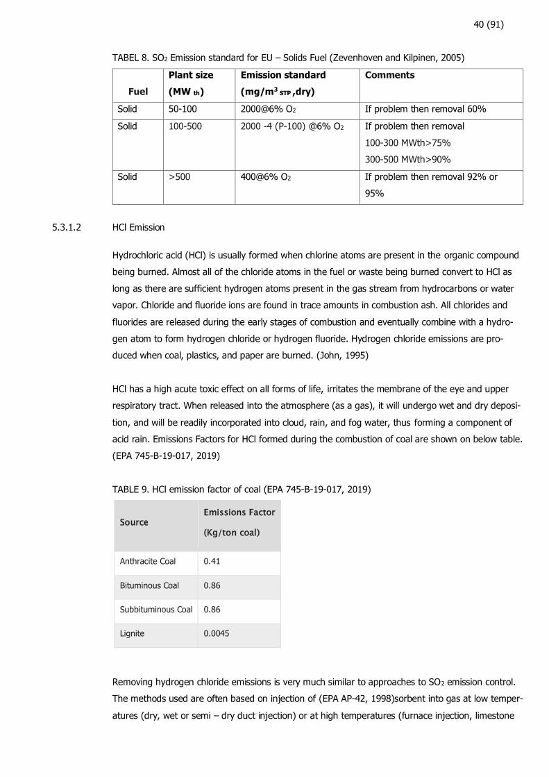
5.3.1.2 HCl Emission

Hydrochloric acid (HCl) is usually formed when chlorine atoms are present in the organic compound

being burned. Almost all of the chloride atoms in the fuel or waste being burned convert to HCl as

long as there are sufficient hydrogen atoms present in the gas stream from hydrocarbons or water

vapor. Chloride and fluoride ions are found in trace amounts in combustion ash. All chlorides and

fluorides are released during the early stages of combustion and eventually combine with a hydro-

gen atom to form hydrogen chloride or hydrogen fluoride. Hydrogen chloride emissions are pro-

duced when coal, plastics, and paper are burned. (John, 1995)

HCl has a high acute toxic effect on all forms of life, irritates the membrane of the eye and upper

respiratory tract. When released into the atmosphere (as a gas), it will undergo wet and dry deposi-

tion, and will be readily incorporated into cloud, rain, and fog water, thus forming a component of

acid rain. Emissions Factors for HCl formed during the combustion of coal are shown on below table.

(EPA 745-B-19-017, 2019)

TABLE 9. HCl emission factor of coal (EPA 745-B-19-017, 2019)

Source Emissions Factor

(Kg/ton coal)

Anthracite Coal 0.41

Bituminous Coal 0.86

Subbituminous Coal 0.86

Lignite 0.0045

Removing hydrogen chloride emissions is very much similar to approaches to SO2 emission control.

The methods used are often based on injection of (EPA AP-42, 1998)sorbent into gas at low temper-

atures (dry, wet or semi – dry duct injection) or at high temperatures (furnace injection, limestone

41 (91)

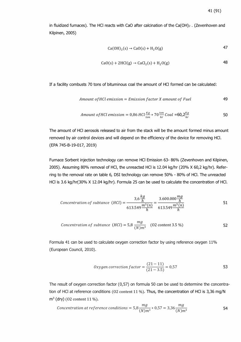
in fluidized furnaces). The HCl reacts with CaO after calcination of the Ca(OH)2 . (Zevenhoven and

Kilpinen, 2005)

Ca(OH)2(s) → CaO(s)+ H2O(g) 47

CaO(s) + 2HCl(g) → CaCl2(s)+ H2O(g) 48

If a facility combusts 70 tons of bituminous coal the amount of HCl formed can be calculated:

𝐴𝑚𝑜𝑢𝑛𝑡 𝑜𝑓𝐻𝐶𝑙 𝑒𝑚𝑖𝑠𝑠𝑖𝑜𝑛 = 𝐸𝑚𝑖𝑠𝑠𝑖𝑜𝑛 𝑓𝑎𝑐𝑡𝑜𝑟 𝑋 𝑎𝑚𝑜𝑢𝑛𝑡 𝑜𝑓 𝐹𝑢𝑒𝑙 49

𝐴𝑚𝑜𝑢𝑛𝑡 𝑜𝑓𝐻𝐶𝑙 𝑒𝑚𝑖𝑠𝑠𝑖𝑜𝑛 = 0,86 𝐻𝐶𝑙𝐾𝑔

𝑡𝑜𝑛∗ 70

𝑡𝑜𝑛

ℎ𝑟𝐶𝑜𝑎𝑙 =60,2

𝐾𝑔

ℎ𝑟 50

The amount of HCl aerosols released to air from the stack will be the amount formed minus amount

removed by air control devices and will depend on the efficiency of the device for removing HCl.

(EPA 745-B-19-017, 2019)

Furnace Sorbent injection technology can remove HCl Emission 63- 86% (Zevenhoven and Kilpinen,

2005). Assuming 80% removal of HCl, the unreacted HCl is 12.04 kg/hr (20% X 60,2 kg/hr). Refer-

ring to the removal rate on table 6, DSI technology can remove 50% - 80% of HCl. The unreacted

HCl is 3.6 kg/hr(30% X 12.04 kg/hr). Formula 25 can be used to calculate the concentration of HCl.

𝐶𝑜𝑛𝑐𝑒𝑛𝑡𝑟𝑎𝑡𝑖𝑜𝑛 𝑜𝑓 𝑠𝑢𝑏𝑡𝑎𝑛𝑐𝑒 (𝐻𝐶𝑙) =3,6𝑘𝑔ℎ

613.549𝑚3(𝑛)ℎ

=3.600.000

𝑚𝑔ℎ

613.549𝑚3(𝑛)ℎ

51

𝐶𝑜𝑛𝑐𝑒𝑛𝑡𝑟𝑎𝑡𝑖𝑜𝑛 𝑜𝑓 𝑠𝑢𝑏𝑡𝑎𝑛𝑐𝑒 (𝐻𝐶𝑙) = 5,8 𝑚𝑔

(𝑁)𝑚3 (O2 content 3.5 %) 52

Formula 41 can be used to calculate oxygen correction factor by using reference oxygen 11%

(European Council, 2010).

𝑂𝑥𝑦𝑔𝑒𝑛 𝑐𝑜𝑟𝑟𝑒𝑐𝑡𝑖𝑜𝑛 𝑓𝑎𝑐𝑡𝑜𝑟 =(21− 11)

(21− 3.5)= 0,57 53

The result of oxygen correction factor (0,57) on formula 50 can be used to determine the concentra-

tion of HCl at reference conditions (O2 content 11 %). Thus, the concentration of HCl is 3,36 mg/N

m3 (dry) (O2 content 11 %).

𝐶𝑜𝑛𝑐𝑒𝑛𝑡𝑟𝑎𝑡𝑖𝑜𝑛 𝑎𝑡 𝑟𝑒𝑓𝑒𝑟𝑒𝑛𝑐𝑒 𝑐𝑜𝑛𝑑𝑖𝑡𝑖𝑜𝑛𝑠 = 5,8𝑚𝑔

(𝑁)𝑚3∗ 0,57 = 3,36

𝑚𝑔

(𝑁)𝑚3 54

42 (91)

Thus, DSI technology complies with EU standard for combustion plants firing solid fuels, with HCl

emission levels expected to be less than 10 mg/Nm³ (European Council, 2010)

5.3.1.3 HF Emission

If fluorine atoms are present in the organic compound being burned, hydrofluoric acid (HF) will usu-

ally be formed. Hydrogen Fluoride is a strong acid which contributes to acid rain and can heavily

impact the flora around an emission point, as well as human health. Irritation to skin, eye, nose,

throat, and breathing passage (Environmental Healt & Engineering inc, 2011). EPA reports an emis-

sion factor of 0.068 kg/ton for coal combustion under a variety of firing conditions as shown table

below. (EPA AP-42, 1998)

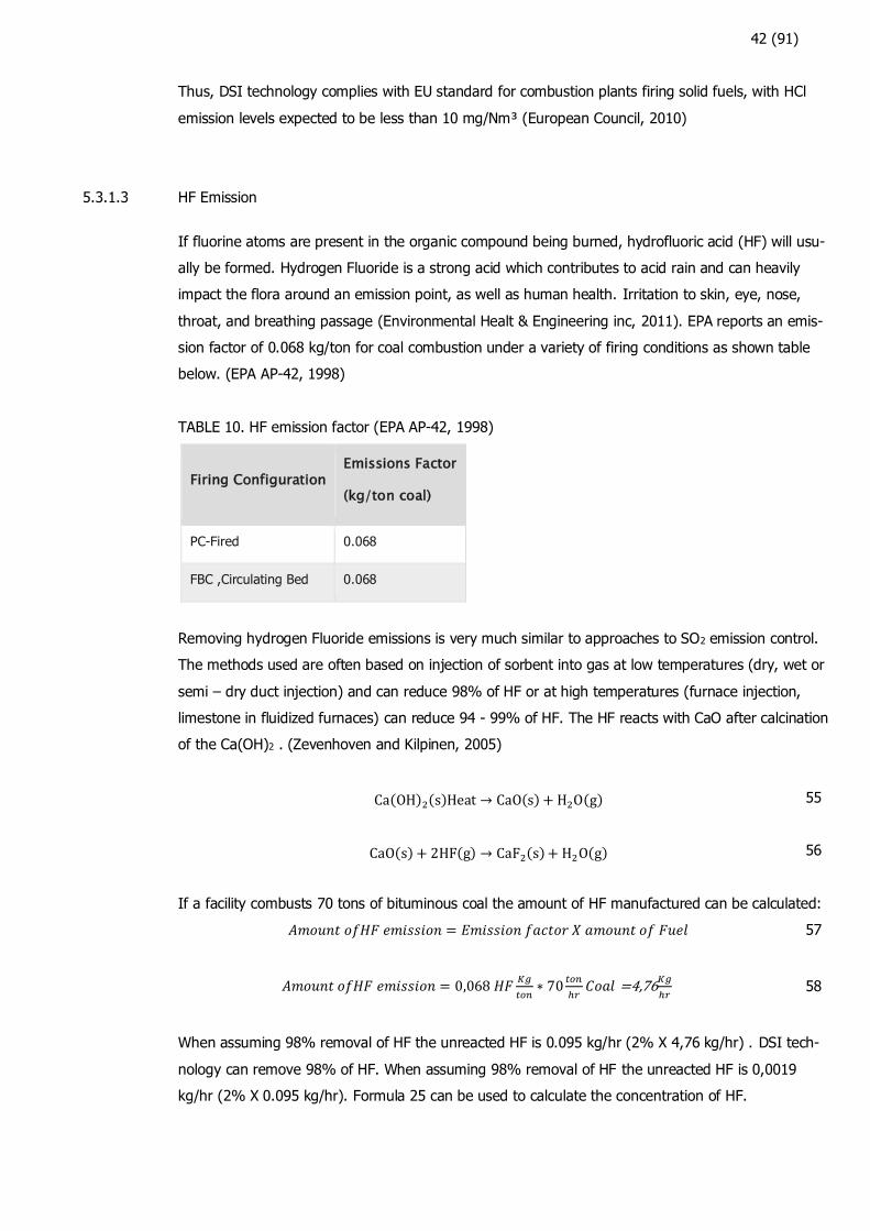
TABLE 10. HF emission factor (EPA AP-42, 1998)

Firing Configuration Emissions Factor

(kg/ton coal)

PC-Fired 0.068

FBC ,Circulating Bed 0.068

Removing hydrogen Fluoride emissions is very much similar to approaches to SO2 emission control.

The methods used are often based on injection of sorbent into gas at low temperatures (dry, wet or

semi – dry duct injection) and can reduce 98% of HF or at high temperatures (furnace injection,

limestone in fluidized furnaces) can reduce 94 - 99% of HF. The HF reacts with CaO after calcination

of the Ca(OH)2 . (Zevenhoven and Kilpinen, 2005)

Ca(OH)2(s)Heat → CaO(s) + H2O(g) 55

CaO(s) + 2HF(g) → CaF2(s)+ H2O(g) 56

If a facility combusts 70 tons of bituminous coal the amount of HF manufactured can be calculated:

𝐴𝑚𝑜𝑢𝑛𝑡 𝑜𝑓𝐻𝐹 𝑒𝑚𝑖𝑠𝑠𝑖𝑜𝑛 = 𝐸𝑚𝑖𝑠𝑠𝑖𝑜𝑛 𝑓𝑎𝑐𝑡𝑜𝑟 𝑋 𝑎𝑚𝑜𝑢𝑛𝑡 𝑜𝑓 𝐹𝑢𝑒𝑙 57

𝐴𝑚𝑜𝑢𝑛𝑡 𝑜𝑓𝐻𝐹 𝑒𝑚𝑖𝑠𝑠𝑖𝑜𝑛 = 0,068 𝐻𝐹𝐾𝑔

𝑡𝑜𝑛∗ 70

𝑡𝑜𝑛

ℎ𝑟𝐶𝑜𝑎𝑙 =4,76

𝐾𝑔

ℎ𝑟 58

When assuming 98% removal of HF the unreacted HF is 0.095 kg/hr (2% X 4,76 kg/hr) . DSI tech-

nology can remove 98% of HF. When assuming 98% removal of HF the unreacted HF is 0,0019

kg/hr (2% X 0.095 kg/hr). Formula 25 can be used to calculate the concentration of HF.

43 (91)

𝐶𝑜𝑛𝑐𝑒𝑛𝑡𝑟𝑎𝑡𝑖𝑜𝑛 𝑜𝑓 𝑠𝑢𝑏𝑡𝑎𝑛𝑐𝑒 (𝐻𝐹) =0,0019

𝑘𝑔ℎ

613.549𝑚3(𝑛)ℎ

=1.900

𝑚𝑔ℎ

613.549 𝑚3(𝑛)ℎ

59

𝐶𝑜𝑛𝑐𝑒𝑛𝑡𝑟𝑎𝑡𝑖𝑜𝑛 𝑜𝑓 𝑠𝑢𝑏𝑡𝑎𝑛𝑐𝑒 (𝐻𝐹) = 0,00309 𝑚𝑔

(𝑁)𝑚3 (O2 content 3.5 %) 60

Formula 43 can be used to calculate oxygen correction factor by using reference oxygen 11% and

oxygen correction factor is 0,57. (European Council, 2010).

𝐶𝑜𝑛𝑐𝑒𝑛𝑡𝑟𝑎𝑡𝑖𝑜𝑛 𝑎𝑡 11%𝑂2(𝑑𝑟𝑦) = 0,00309𝑚𝑔

(𝑁)𝑚3∗ 0,57 = 0,00177

𝑚𝑔

(𝑁)𝑚3 61

Thus, DSI technology complies with the EU standard for combustion plants firing solid fuels, with HF

hydrogen fluoride emission levels expected to be less than 1 mg/Nm³ (European Council, 2010)

5.3.2 Sodium Bicarbonate

Another often used sorbent is sodium bicarbonate, which is quite effective against HCl and SO2. High

amounts of acid gas elimination are possible at lower feed rates than with hydrated lime. This sorbent,

however, is more expensive than hydrated lime. Solvay's recent pilot plant experiments at an inde-

pendent site prove that dry injection of sodium bicarbonate can achieve more than 99% removal rates

for HCl. The studies successfully illustrate sodium sorbents' selectivity for removing HCl in a medium

to high sulfur environment. A sodium DSI system injects a sorbent straight into the hot flue gas duct,

where it rapidly reacts with HCl, SO2, SO3, and HF, reducing NOx in some cases. Field testing has

demonstrated that this method is capable of removing almost all SO3 and HCl, as well as well over

90% of SO2. Many waste incinerators in Europe and coal-fired power plants in the United States have

already implemented this technology. (Yougen Kong, Michael Wood, 2012)

Sodium bicarbonate in its natural state is too coarse to be injected directly. As a result, milling is

necessary. This milling is performed by vendors or by the end user at the point of usage. When milled

on-site, the particle size target is 90% less than 20 microns. (Yougen Kong, Michael Wood, 2012)

The minimum temperature of flue gas at the sorbent injection point should be 135 oC. Generally,

higher temperatures result in improved performance. The maximum temperature that is recom-

mended is 815 oC. Sodium bicarbonate (NaHCO3) is calcined into sodium carbonate (Na2CO3) after

being injected into hot flue gas (> 135 oC), as shown in the following equation:

2 NaHCO3(s) σ > 135℃ → Na2CO3(s) + CO2(g) + H2O(g) 62

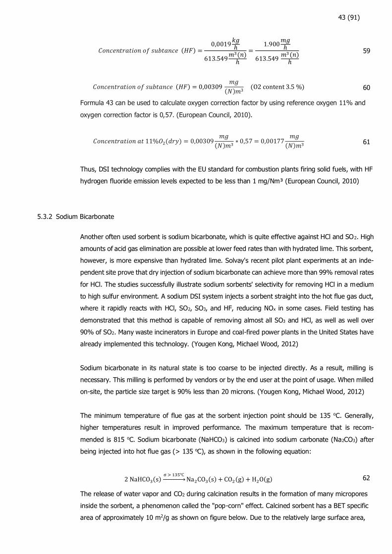
The release of water vapor and CO2 during calcination results in the formation of many micropores

inside the sorbent, a phenomenon called the "pop-corn" effect. Calcined sorbent has a BET specific

area of approximately 10 m2/g as shown on figure below. Due to the relatively large surface area,

44 (91)

sodium carbonate reacts rapidly with acid gases such as SO2, SO3, HCl, and HF. (Yougen Kong,

Michael Wood, 2012)

FIGURE 28. Calcined Sodium Bicarbonate Under Microscope (Yougen Kong, Michael Wood, 2012)

The calcined Sodium bicarbonate reacts with flue gas pollutants as follows:

Na2CO3(s)+ SO2(g) +1

2O2(g) → Na2SO4(s) + CO2(g) 63

Na2CO3(s) + 2HCl(g) → 2NaCl(s) + CO2(g) + H2O(g) 64

Na2CO3(s) + 2HF(g) → 2NaF(s)+ CO2(g) +H2O(g) 65

The calcination leads to a greater specific surface area (BET). The greater the available reaction sur-

face, the more efficient the reduction performance of the sodium carbonate. The removal process

also generally increases in line with a rise in temperature. (Yougen Kong, Michael Wood, 2012)

5.4 Particulate Matter Control Impacts

Particulate Matter (PM) is One of the major pollutants from bituminous and subbituminous coal com-

bustion. Uncontrolled PM emission from coal fired boiler include the ash from combustion of the fuel

as well as unburnt carbon resulting from incomplete combustion. Coal ash may either settle out in

the boiler (bottom ash) or entrain in the flue gas (fly ash). PM emission rate is affected by the distri-

bution of ash between the bottom ash and fly ash. Boiler load also affects the PM emission. (EPA

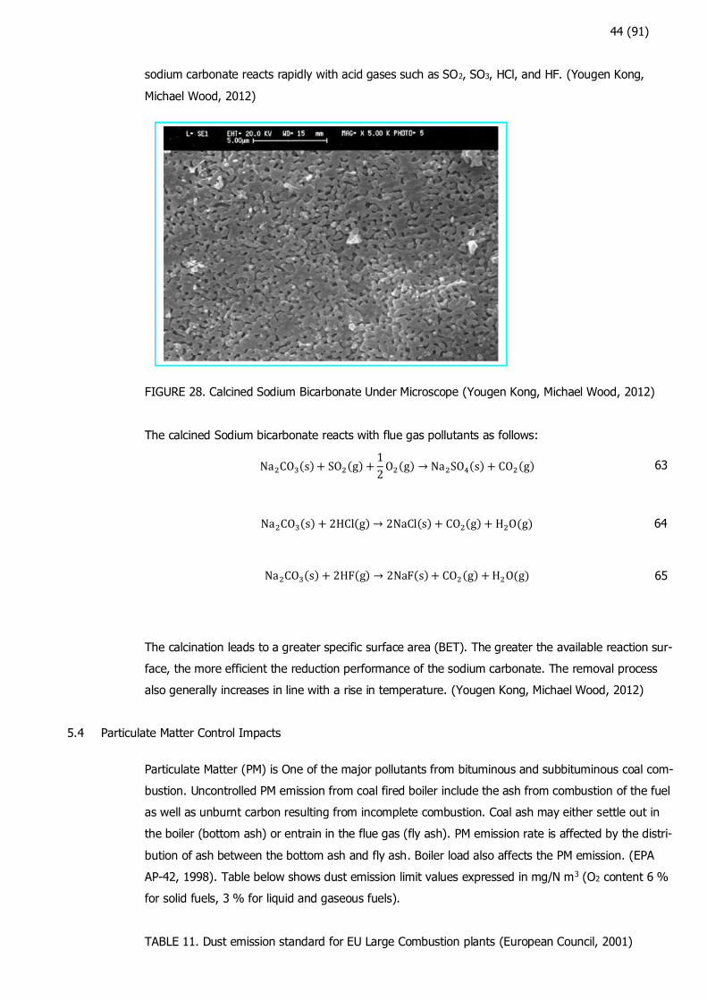
AP-42, 1998). Table below shows dust emission limit values expressed in mg/N m3 (O2 content 6 %

for solid fuels, 3 % for liquid and gaseous fuels).

TABLE 11. Dust emission standard for EU Large Combustion plants (European Council, 2001)

45 (91)

Type of Fuel Rated thermal input (MW) Emission limit values

(mg /Nm3)

Solid ≥500 50

Solid <500 100

liquid all plants 50

Particulate matter entrained in the gas stream along with the gaseous contaminants can have a sig-

nificant effect on the collector's efficiency and reliability. Particulate matter can accumulate in these

areas, obstructing normal gas flow. Particulate matter has a particularly negative impact if it is rela-

tively large (i.e., > 3 micrometers) or sticky. If the gaseous contaminant control system is prone to

failures caused by particulate matter, a pre-collector may be required. Extremely small particles (less

than 1 µm in diameter) can be efficiently collected in a baghouse or fabric filter. (John, 1995)

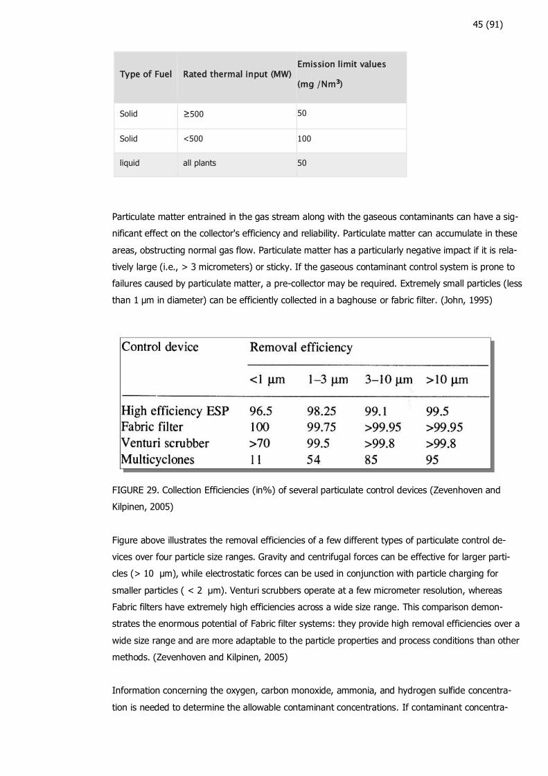
FIGURE 29. Collection Efficiencies (in%) of several particulate control devices (Zevenhoven and

Kilpinen, 2005)

Figure above illustrates the removal efficiencies of a few different types of particulate control de-

vices over four particle size ranges. Gravity and centrifugal forces can be effective for larger parti-

cles (> 10 μm), while electrostatic forces can be used in conjunction with particle charging for

smaller particles ( < 2 μm). Venturi scrubbers operate at a few micrometer resolution, whereas

Fabric filters have extremely high efficiencies across a wide size range. This comparison demon-

strates the enormous potential of Fabric filter systems: they provide high removal efficiencies over a

wide size range and are more adaptable to the particle properties and process conditions than other

methods. (Zevenhoven and Kilpinen, 2005)

Information concerning the oxygen, carbon monoxide, ammonia, and hydrogen sulfide concentra-

tion is needed to determine the allowable contaminant concentrations. If contaminant concentra-

46 (91)

tions, oxygen concentrations, and gas temperatures are in the hazardous range, many of the or-

ganic and inorganic chemicals collected can be ignited. These potentially explosive circumstances

must be anticipated and carefully avoided during the control system's design. (John, 1995)

Modifications to the combustion process (applicable to small fired boilers) and postcombustion treat-

ments are the two most important PM control strategies (applicable to most boiler type and sizes).

The use of a fabric filter or a baghouse to limit particulate matter emissions from coal-fired combus-

tion sources can be achieved after the combustion process. (EPA AP-42, 1998). More contact be-

tween the gas and the injected sorbent is achieved with fabric filters or baghouses than with elec-

trostatic precipitators (ESPs), resulting in improved removal at any given reagent treatment rate.

(NESCAUM, 2011)

Dry sorbent injection will increase the quantity of particulate and the composition of particulate col-

lected in the particulate control device will change from just fly ash to sorbents and reaction prod-

ucts. It also increases dust loading and may impact operation of the baghouse.

(Michael,Joshua,Curt and friend, 2016)

5.4.1 Potential Baghouse Impacts

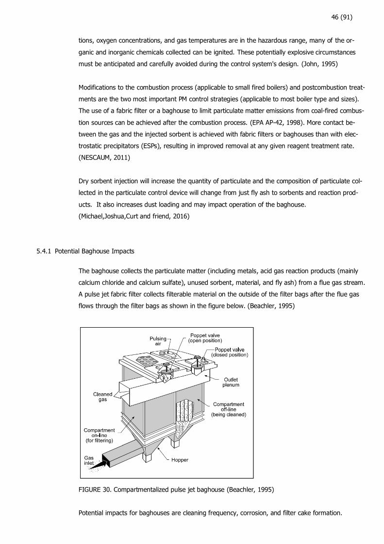
The baghouse collects the particulate matter (including metals, acid gas reaction products (mainly

calcium chloride and calcium sulfate), unused sorbent, material, and fly ash) from a flue gas stream.

A pulse jet fabric filter collects filterable material on the outside of the filter bags after the flue gas

flows through the filter bags as shown in the figure below. (Beachler, 1995)

FIGURE 30. Compartmentalized pulse jet baghouse (Beachler, 1995)

Potential impacts for baghouses are cleaning frequency, corrosion, and filter cake formation.

47 (91)

With the additional PM loading from DSI, the baghouse pressure drop or cleaning frequency will in-

crease. It is possible that the pressure drop will increase if the bag cleaning controls are configured

to run on a timer. If pressure drop control is used to manage cleaning events, the frequency of

cleaning will rise. The plant will determine which technique of control is the most appropriate for

actual baghouse operation. (Michael,Joshua,Curt and friend, 2016)

Corrosion in the system's backend and baghouse is often minimized when calcium and sodium-

based sorbents are injected for acid gas mitigation. This is also true when using halogenated acti-

vated carbon in conjunction with a calcium or sodium-based sorbent and/or a high calcium oxide fly

ash. (Michael,Joshua,Curt and friend, 2016)

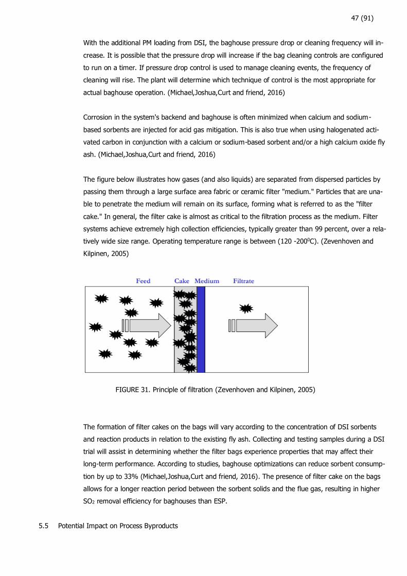
The figure below illustrates how gases (and also liquids) are separated from dispersed particles by

passing them through a large surface area fabric or ceramic filter "medium." Particles that are una-

ble to penetrate the medium will remain on its surface, forming what is referred to as the "filter

cake." In general, the filter cake is almost as critical to the filtration process as the medium. Filter

systems achieve extremely high collection efficiencies, typically greater than 99 percent, over a rela-

tively wide size range. Operating temperature range is between (120 -2000C). (Zevenhoven and

Kilpinen, 2005)

FIGURE 31. Principle of filtration (Zevenhoven and Kilpinen, 2005)

The formation of filter cakes on the bags will vary according to the concentration of DSI sorbents

and reaction products in relation to the existing fly ash. Collecting and testing samples during a DSI

trial will assist in determining whether the filter bags experience properties that may affect their

long-term performance. According to studies, baghouse optimizations can reduce sorbent consump-

tion by up to 33% (Michael,Joshua,Curt and friend, 2016). The presence of filter cake on the bags

allows for a longer reaction period between the sorbent solids and the flue gas, resulting in higher

SO2 removal efficiency for baghouses than ESP.

5.5 Potential Impact on Process Byproducts

48 (91)

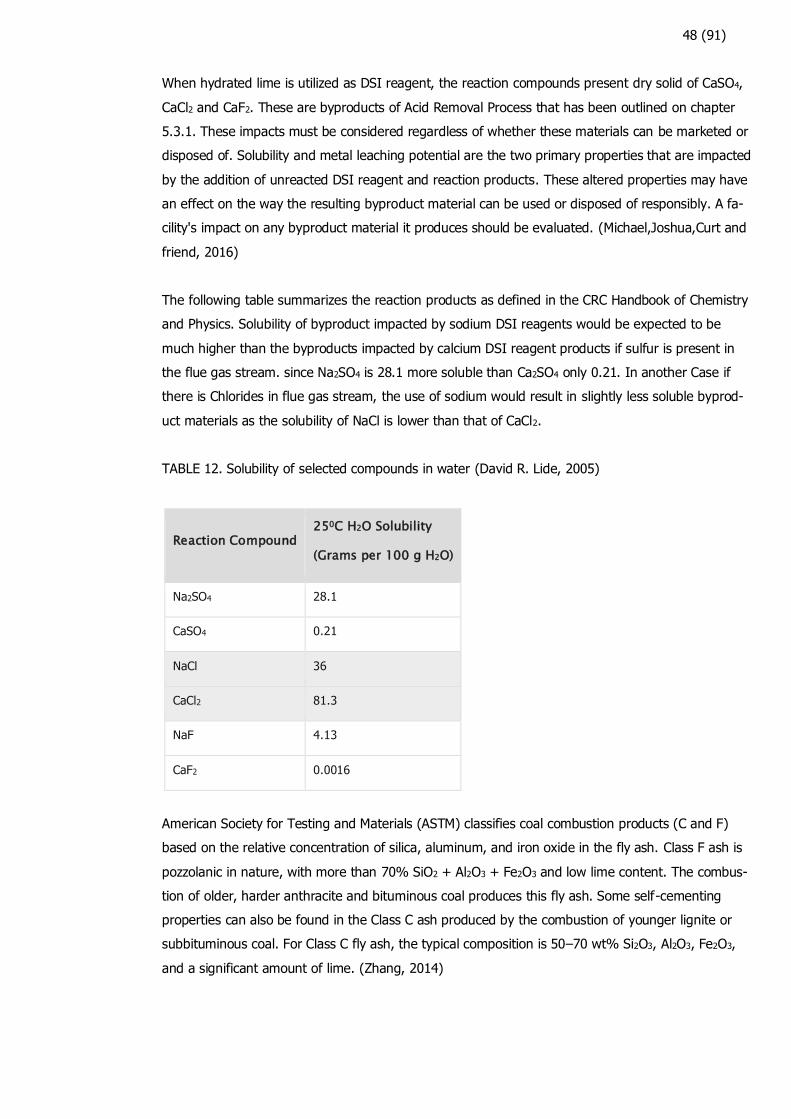
When hydrated lime is utilized as DSI reagent, the reaction compounds present dry solid of CaSO4,

CaCl2 and CaF2. These are byproducts of Acid Removal Process that has been outlined on chapter

5.3.1. These impacts must be considered regardless of whether these materials can be marketed or

disposed of. Solubility and metal leaching potential are the two primary properties that are impacted

by the addition of unreacted DSI reagent and reaction products. These altered properties may have

an effect on the way the resulting byproduct material can be used or disposed of responsibly. A fa-

cility's impact on any byproduct material it produces should be evaluated. (Michael,Joshua,Curt and

friend, 2016)

The following table summarizes the reaction products as defined in the CRC Handbook of Chemistry

and Physics. Solubility of byproduct impacted by sodium DSI reagents would be expected to be

much higher than the byproducts impacted by calcium DSI reagent products if sulfur is present in

the flue gas stream. since Na2SO4 is 28.1 more soluble than Ca2SO4 only 0.21. In another Case if

there is Chlorides in flue gas stream, the use of sodium would result in slightly less soluble byprod-

uct materials as the solubility of NaCl is lower than that of CaCl2.

TABLE 12. Solubility of selected compounds in water (David R. Lide, 2005)

Reaction Compound 250C H2O Solubility

(Grams per 100 g H2O)

Na2SO4 28.1

CaSO4 0.21

NaCl 36

CaCl2 81.3

NaF 4.13

CaF2 0.0016

American Society for Testing and Materials (ASTM) classifies coal combustion products (C and F)

based on the relative concentration of silica, aluminum, and iron oxide in the fly ash. Class F ash is

pozzolanic in nature, with more than 70% SiO2 + Al2O3 + Fe2O3 and low lime content. The combus-

tion of older, harder anthracite and bituminous coal produces this fly ash. Some self-cementing

properties can also be found in the Class C ash produced by the combustion of younger lignite or

subbituminous coal. For Class C fly ash, the typical composition is 50–70 wt% Si2O3, Al2O3, Fe2O3,

and a significant amount of lime. (Zhang, 2014)

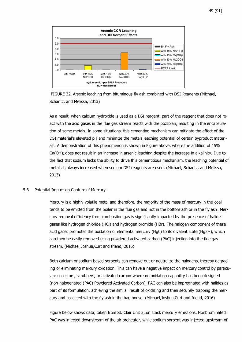
49 (91)

FIGURE 32. Arsenic leaching from bituminous fly ash combined with DSI Reagents (Michael,

Schantz, and Melissa, 2013)

As a result, when calcium hydroxide is used as a DSI reagent, part of the reagent that does not re-

act with the acid gases in the flue gas stream reacts with the pozzolan, resulting in the encapsula-

tion of some metals. In some situations, this cementing mechanism can mitigate the effect of the

DSI material's elevated pH and minimize the metals leaching potential of certain byproduct materi-

als. A demonstration of this phenomenon is shown in Figure above, where the addition of 15%

Ca(OH)2 does not result in an increase in arsenic leaching despite the increase in alkalinity. Due to

the fact that sodium lacks the ability to drive this cementitious mechanism, the leaching potential of

metals is always increased when sodium DSI reagents are used. (Michael, Schantz, and Melissa,

2013)

5.6 Potential Impact on Capture of Mercury

Mercury is a highly volatile metal and therefore, the majority of the mass of mercury in the coal

tends to be emitted from the boiler in the flue gas and not in the bottom ash or in the fly ash. Mer-

cury removal efficiency from combustion gas is significantly impacted by the presence of halide

gases like hydrogen chloride (HCl) and hydrogen bromide (HBr). The halogen component of these

acid gases promotes the oxidation of elemental mercury (Hg0) to its divalent state (Hg2+), which

can then be easily removed using powdered activated carbon (PAC) injection into the flue gas

stream. (Michael,Joshua,Curt and friend, 2016)

Both calcium or sodium-based sorbents can remove out or neutralize the halogens, thereby degrad-

ing or eliminating mercury oxidation. This can have a negative impact on mercury control by particu-

late collectors, scrubbers, or activated carbon where no oxidation capability has been designed

(non-halogenated (PAC) Powdered Activated Carbon). PAC can also be impregnated with halides as

part of its formulation, achieving the similar result of oxidizing and then securely trapping the mer-

cury and collected with the fly ash in the bag house. (Michael,Joshua,Curt and friend, 2016)

Figure below shows data, taken from St. Clair Unit 3, on stack mercury emissions. Nonbrominated

PAC was injected downstream of the air preheater, while sodium sorbent was injected upstream of

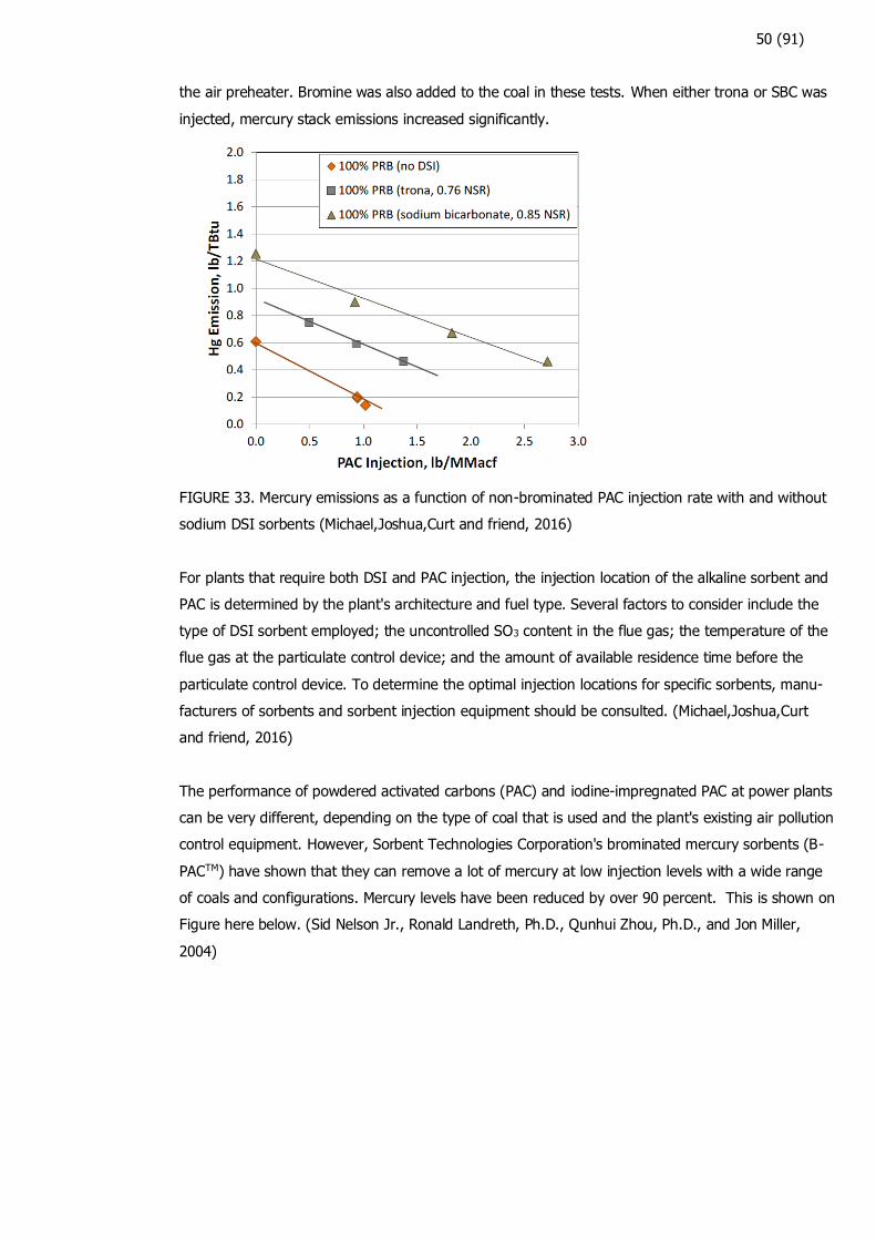
50 (91)

the air preheater. Bromine was also added to the coal in these tests. When either trona or SBC was

injected, mercury stack emissions increased significantly.

FIGURE 33. Mercury emissions as a function of non-brominated PAC injection rate with and without

sodium DSI sorbents (Michael,Joshua,Curt and friend, 2016)

For plants that require both DSI and PAC injection, the injection location of the alkaline sorbent and

PAC is determined by the plant's architecture and fuel type. Several factors to consider include the

type of DSI sorbent employed; the uncontrolled SO3 content in the flue gas; the temperature of the

flue gas at the particulate control device; and the amount of available residence time before the

particulate control device. To determine the optimal injection locations for specific sorbents, manu-

facturers of sorbents and sorbent injection equipment should be consulted. (Michael,Joshua,Curt

and friend, 2016)

The performance of powdered activated carbons (PAC) and iodine-impregnated PAC at power plants

can be very different, depending on the type of coal that is used and the plant's existing air pollution

control equipment. However, Sorbent Technologies Corporation's brominated mercury sorbents (B-

PACTM) have shown that they can remove a lot of mercury at low injection levels with a wide range

of coals and configurations. Mercury levels have been reduced by over 90 percent. This is shown on

Figure here below. (Sid Nelson Jr., Ronald Landreth, Ph.D., Qunhui Zhou, Ph.D., and Jon Miller,

2004)

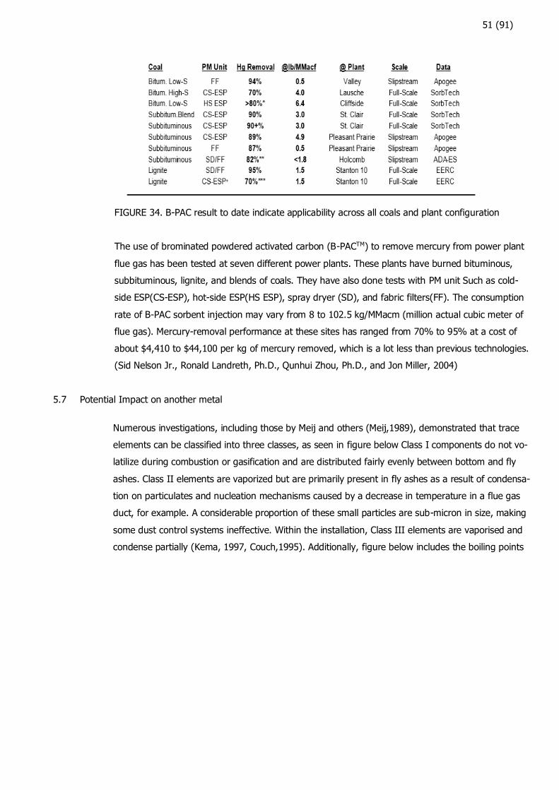
51 (91)

FIGURE 34. B-PAC result to date indicate applicability across all coals and plant configuration

The use of brominated powdered activated carbon (B-PACTM) to remove mercury from power plant

flue gas has been tested at seven different power plants. These plants have burned bituminous,

subbituminous, lignite, and blends of coals. They have also done tests with PM unit Such as cold-

side ESP(CS-ESP), hot-side ESP(HS ESP), spray dryer (SD), and fabric filters(FF). The consumption

rate of B-PAC sorbent injection may vary from 8 to 102.5 kg/MMacm (million actual cubic meter of

flue gas). Mercury-removal performance at these sites has ranged from 70% to 95% at a cost of

about $4,410 to $44,100 per kg of mercury removed, which is a lot less than previous technologies.

(Sid Nelson Jr., Ronald Landreth, Ph.D., Qunhui Zhou, Ph.D., and Jon Miller, 2004)

5.7 Potential Impact on another metal

Numerous investigations, including those by Meij and others (Meij,1989), demonstrated that trace

elements can be classified into three classes, as seen in figure below Class I components do not vo-

latilize during combustion or gasification and are distributed fairly evenly between bottom and fly

ashes. Class II elements are vaporized but are primarily present in fly ashes as a result of condensa-

tion on particulates and nucleation mechanisms caused by a decrease in temperature in a flue gas

duct, for example. A considerable proportion of these small particles are sub-micron in size, making

some dust control systems ineffective. Within the installation, Class III elements are vaporised and

condense partially (Kema, 1997, Couch,1995). Additionally, figure below includes the boiling points

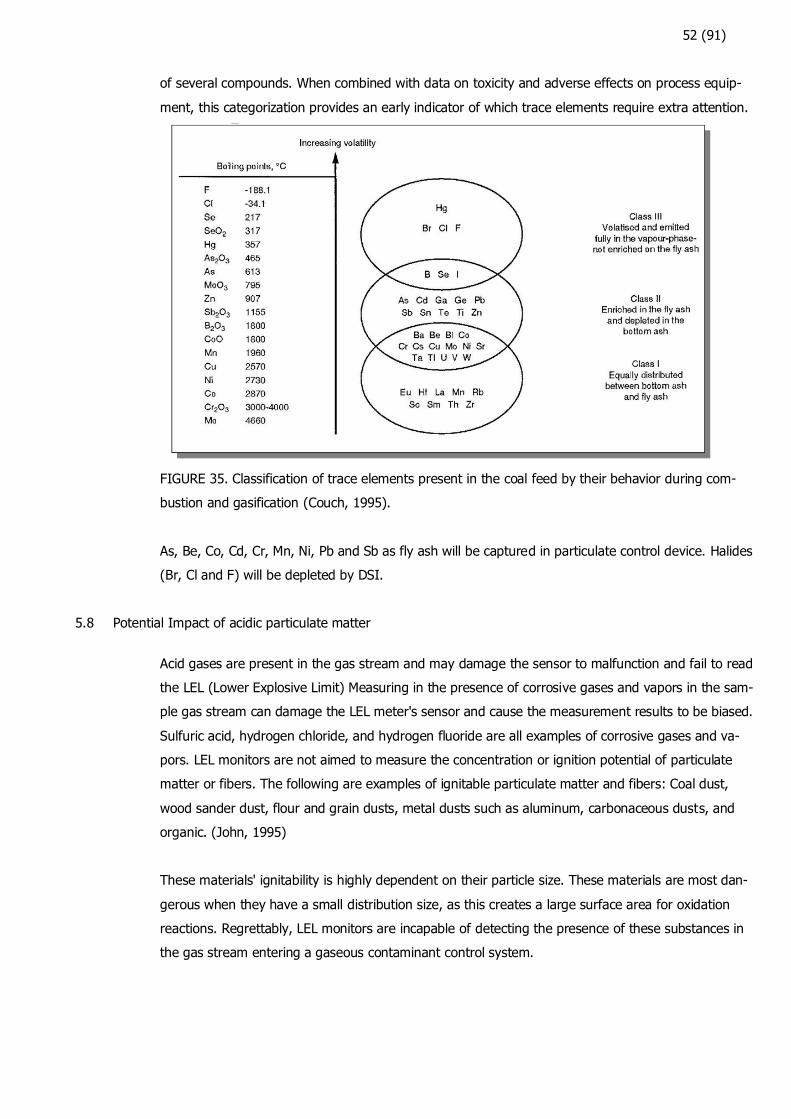
52 (91)

of several compounds. When combined with data on toxicity and adverse effects on process equip-

ment, this categorization provides an early indicator of which trace elements require extra attention.

FIGURE 35. Classification of trace elements present in the coal feed by their behavior during com-

bustion and gasification (Couch, 1995).

As, Be, Co, Cd, Cr, Mn, Ni, Pb and Sb as fly ash will be captured in particulate control device. Halides

(Br, Cl and F) will be depleted by DSI.

5.8 Potential Impact of acidic particulate matter

Acid gases are present in the gas stream and may damage the sensor to malfunction and fail to read

the LEL (Lower Explosive Limit) Measuring in the presence of corrosive gases and vapors in the sam-

ple gas stream can damage the LEL meter's sensor and cause the measurement results to be biased.

Sulfuric acid, hydrogen chloride, and hydrogen fluoride are all examples of corrosive gases and va-

pors. LEL monitors are not aimed to measure the concentration or ignition potential of particulate

matter or fibers. The following are examples of ignitable particulate matter and fibers: Coal dust,

wood sander dust, flour and grain dusts, metal dusts such as aluminum, carbonaceous dusts, and

organic. (John, 1995)

These materials' ignitability is highly dependent on their particle size. These materials are most dan-

gerous when they have a small distribution size, as this creates a large surface area for oxidation

reactions. Regrettably, LEL monitors are incapable of detecting the presence of these substances in

the gas stream entering a gaseous contaminant control system.

53 (91)

6 PDMS IMPLEMENTATION

PDMS has provided user interface customization via dot Net Framework and PDMS Macro. All code

can be written via dot Net C# and programming macro language. While PML is a powerful language

within PDMS, it suffers from a lack of fundamental resources such as a debug tool, a graphical inter-

face for creating forms, and the ability to communicate with third-party software in a practical man-

ner. The new.NET APIs address these PML deficiencies while also opening up a whole new world of

possibilities for developing new interfaces with other software or just for customizing existing soft-

ware. Microsoft began developing the.NET framework in the early 1990's, but the first beta version

was not published for almost ten years. It is currently at version 4.0, however PDMS only supports

version 3.5, .NET programming is built on DLL, which means that the code is compiled to a.dll file

instead of an.exe file. When PDMS is opened, it calls this.dll file. in this way, an external application

that connects to and interacts with PDMS could be developed. (Rbasniak, 2013)

6.1 PDMS .NET Customization Architecture

.NET is not an abbreviation; it is a Microsoft product that integrates all platforms, including desktop

apps, mobile apps, and cloud, into a single framework. The .NET APIs provided access to a variety

of features of the product, including the Graphical User Interface, the database, and geometry. As

part of AVEVA's 'continual progression' strategy, the.NET customization capability has been provided

in a way that it may be utilized in conjunction with the existing PML-based customization. By utiliz-

ing PML.NET, a PML upgrade that enables the PML programmer to call.NET code, customization that

takes advantage of the characteristics of both.NET generated code and PML can be accomplished.

(Aveva 3, 2012)

FIGURE 36..Net customization Architecture

The diagram above displays two new approaches of customisation that utilize technology. The first

is accomplished through the use of a.NET Addin, while the second is accomplished through the use

of PML.NET. Both approaches enable dynamic loading of a.NET assembly (DLL) into a module at

runtime. in this thesis .Net Addins is used. The Common Application Framework (CAF) is an extensi-

ble framework that provides.NET programmers with access to a variety of services that support in

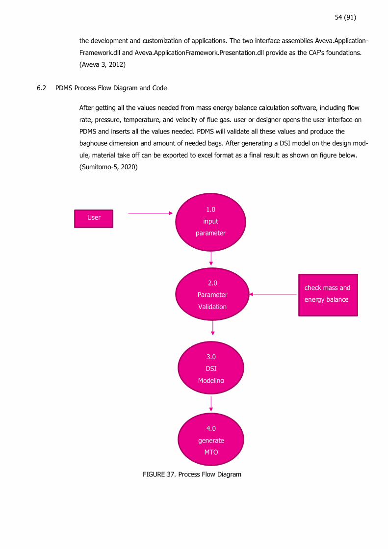
54 (91)

the development and customization of applications. The two interface assemblies Aveva.Application-

Framework.dll and Aveva.ApplicationFramework.Presentation.dll provide as the CAF's foundations.

(Aveva 3, 2012)

6.2 PDMS Process Flow Diagram and Code

After getting all the values needed from mass energy balance calculation software, including flow

rate, pressure, temperature, and velocity of flue gas. user or designer opens the user interface on

PDMS and inserts all the values needed. PDMS will validate all these values and produce the

baghouse dimension and amount of needed bags. After generating a DSI model on the design mod-

ule, material take off can be exported to excel format as a final result as shown on figure below.

(Sumitomo-5, 2020)

FIGURE 37. Process Flow Diagram

User 1.0

input

parameter

2.0

Parameter

Validation

3.0

DSI

Modeling

check mass and

energy balance

4.0

generate

MTO

55 (91)

6.2.1 Graphical User interface

Graphical user interface is illustrated here below. user selects the used component from tablist “DSI”

(a) for dry sorbent injection model and creates DSI name on combobox (b). GUI shows component

attributes in Datagridview (c). User selects wanted variations for the component by checking option

value on filter type and outlet type (d). Number of row bag and Modules/ compartments can be de-

terminated by checking combobox (e).

FIGURE 38.The GUI of Program

When user press confirm button (f), program checks that dimension values are available and if val-

ues appear to be invalid the program will leave background of cells with suspicious values red. Back-

ground of the cells with a confirmed value will turn green and “Build” button(g) will be activated. If

”Build” button is pressed the 3D model will be shown on PDMS design layout and Button Run MTO

list and export csv will be activated(h). Thereby MTO will be exported to excel file.

The number of bags can be calculated by formula below. (Beachler, 1995)

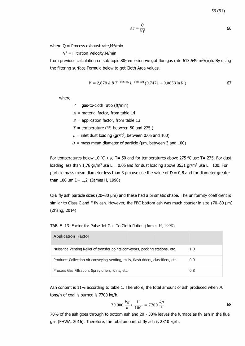
56 (91)

𝐴𝑐 =𝑄

𝑉𝑓 66

where Q = Process exhaust rate,M3/min

Vf = Filtration Velocity,M/min

from previous calculation on sub topic S02 emission we got flue gas rate 613.549 m3/(n)h. By using

the filtering surface Formula below to get Cloth Area values.

𝑉 = 2,878 𝐴 𝐵 𝑇−0,2335 𝐿−0,06021(0,7471 + 0,0853 ln𝐷 ) 67

where

𝑉 = gas-to-cloth ratio (ft/min)

𝐴 = material factor, from table 14

𝐵 = application factor, from table 13

𝑇 = temperature (oF, between 50 and 275 )

𝐿 = inlet dust loading (gr/ft3, between 0.05 and 100)

𝐷 = mass mean diameter of particle (μm, between 3 and 100)

For temperatures below 10 oC, use T= 50 and for temperatures above 275 oC use T= 275. For dust

loading less than 1,76 gr/m3 use L = 0.05 and for dust loading above 3531 gr/m3 use L =100. For

particle mass mean diameter less than 3 μm use use the value of D = 0,8 and for diameter greater

than 100 μm D= 1,2. (James H, 1998)

CFB fly ash particle sizes (20–30 μm) and these had a prismatic shape. The uniformity coefficient is

similar to Class C and F fly ash. However, the FBC bottom ash was much coarser in size (70–80 μm)

(Zhang, 2014)

TABLE 13. Factor for Pulse Jet Gas To Cloth Ratios (James H, 1998)

Application Factor

Nuisance Venting Relief of transfer points,conveyors, packing stations, etc. 1.0

Producct Collection Air conveying-venting, mills, flash driers, classifiers, etc. 0.9

Process Gas Filtration, Spray driers, kilns, etc. 0.8

Ash content is 11% according to table 1. Therefore, the total amount of ash produced when 70

tons/h of coal is burned is 7700 kg/h.

70.000 𝑘𝑔

ℎ∗ 11

100 = 7700

𝑘𝑔

ℎ 68

70% of the ash goes through to bottom ash and 20 - 30% leaves the furnace as fly ash in the flue

gas (FHWA, 2016). Therefore, the total amount of fly ash is 2310 kg/h.

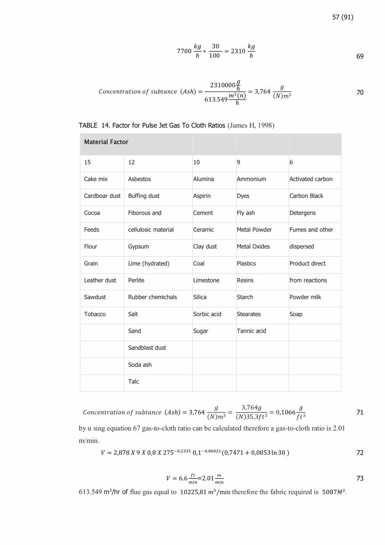
57 (91)

7700 𝑘𝑔

ℎ∗ 30

100 = 2310

𝑘𝑔

ℎ

69

𝐶𝑜𝑛𝑐𝑒𝑛𝑡𝑟𝑎𝑡𝑖𝑜𝑛 𝑜𝑓 𝑠𝑢𝑏𝑡𝑎𝑛𝑐𝑒 (𝐴𝑠ℎ) =2310000

𝑔ℎ

613.549𝑚3(𝑛)ℎ

= 3,764 𝑔

(𝑁)𝑚3 70

TABLE 14. Factor for Pulse Jet Gas To Cloth Ratios (James H, 1998)

Material Factor

15 12 10 9 6

Cake mix Asbestos Alumina Ammonium Activated carbon

Cardboar dust Buffing dust Aspirin Dyes Carbon Black

Cocoa Fiborous and Cement Fly ash Detergens

Feeds cellulosic material Ceramic Metal Powder Fumes and other

Flour Gypsum Clay dust Metal Oxides dispersed

Grain Lime (hydrated) Coal Plastics Product direct

Leather dust Perlite Limestone Resins from reactions

Sawdust Rubber chemichals Silica Starch Powder milk

Tobacco Salt Sorbic acid Stearates Soap

Sand Sugar Tannic acid

Sandblast dust

Soda ash

Talc

𝐶𝑜𝑛𝑐𝑒𝑛𝑡𝑟𝑎𝑡𝑖𝑜𝑛 𝑜𝑓 𝑠𝑢𝑏𝑡𝑎𝑛𝑐𝑒 (𝐴𝑠ℎ) = 3,764 𝑔

(𝑁)𝑚3=

3,764𝑔

(𝑁)35,3𝑓𝑡3= 0,1066

𝑔

𝑓𝑡3 71

by u sing equation 67 gas-to-cloth ratio can be calculated therefore a gas-to-cloth ratio is 2.01

m/min.

𝑉 = 2,878 𝑋 9 𝑋 0,8 𝑋 275−0,2335 0,1−0,06021(0,7471 + 0,0853 ln 30 ) 72

𝑉 = 6.6𝑓𝑡

𝑚𝑖𝑛=2.01

𝑚

𝑚𝑖𝑛 73

613.549 m3/hr of flue gas equal to 10225,81 𝑚3/min therefore the fabric required is 5087𝑀2.

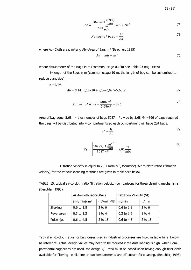
58 (91)

𝐴𝑐 =10225,81

𝑚3(𝑛)𝑚𝑖𝑛

2.01𝑚𝑚𝑖𝑛

= 5087𝑚2 74

𝑁𝑢𝑚𝑏𝑒𝑟 𝑜𝑓 𝑏𝑎𝑔𝑠 =𝐴𝑐

𝐴𝑏

75

where Ac=Cloth area, m2 and Ab=Area of Bag, m2 (Beachler, 1995)

𝐴𝑏 = 𝜋𝑑𝑡 + 𝜋𝑟2

76

where d=Diameter of the Bags in m (common usage 0,18m see Table 23 Bag Prices)

t=length of the Bags in m (common usage 10 m, the length of bag can be customized to

reduce plant size)

𝜋 =3,14

𝐴𝑏 = 3,14𝑥 0,18𝑥10+ 3,14𝑥0,092=5,68𝑚2 77

𝑁𝑢𝑚𝑏𝑒𝑟 𝑜𝑓 𝑏𝑎𝑔𝑠 =5087𝑚2

5,68𝑚2= 896

78

Area of bag equal 5,68 m2 thus number of bags 5087 m2 divide by 5,68 M2 =896 of bags required

the bags will be distributed into 4 compartments so each compartment will have 224 bags.

𝑉𝑓 =𝑄

𝐴𝑐

79

𝑉𝑓 = [10225,81

𝑚3

𝑚𝑖𝑛5087 𝑚2

] = 2,01𝑚

𝑚𝑖𝑛

80

Filtration velocity is equal to 2,01 m/min(3,35cm/sec). Air to cloth ratios (filtration

velocity) for the various cleaning methods are given in table here below.

TABLE 15. typical air-to-cloth ratio (filtration velocity) comparisons for three cleaning mechanisms

(Beachler, 1995)

Air-to-cloth ratio(Q/Ac) Filtration Velocity (Vf)

(m3/min)/ m2 (ft3/min)/ft2 m/min ft/min

Shaking 0.6 to 1.8 2 to 6 0.6 to 1.8 2 to 6

Reverse-air 0.3 to 1.2 1 to 4 0.3 to 1.2 1 to 4

Pulse -jet 0.6 to 4.5 2 to 15 0.6 to 4.5 2 to 15

Typical air-to-cloth ratios for baghouses used in industrial processes are listed in table here below

as reference. Actual design values may need to be reduced if the dust loading is high. when Com-

partmental baghouses are used, the design A/C ratio must be based upon having enough filter cloth

available for filtering while one or two compartments are off-stream for cleaning. (Beachler, 1995)

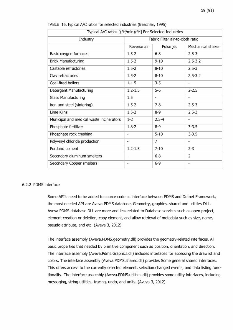
59 (91)

TABLE 16. typical A/C ratios for selected industries (Beachler, 1995)

Typical A/C ratios [(ft3/min)/ft2] For Selected Industries

Industry Fabric Filter air-to-cloth ratio

Reverse air Pulse jet Mechanical shaker

Basic oxygen furnaces 1.5-2 6-8 2.5-3

Brick Manufacturing 1.5-2 9-10 2.5-3.2

Castable refractories 1.5-2 8-10 2.5-3

Clay refractories 1.5-2 8-10 2.5-3.2

Coal-fired boilers 1-1.5 3-5 -

Detergent Manufacturing 1.2-1.5 5-6 2-2.5

Glass Manufacturing 1.5 - -

iron and steel (sintering) 1.5-2 7-8 2.5-3

Lime Kilns 1.5-2 8-9 2.5-3

Municipal and medical waste incinerators 1-2 2.5-4 -

Phosphate fertilizer 1.8-2 8-9 3-3.5

Phosphate rock crushing - 5-10 3-3.5

Polyvinyl chloride production - 7 -

Portland cement 1.2-1.5 7-10 2-3

Secondary aluminum smelters - 6-8 2

Secondary Copper smelters - 6-9 -

6.2.2 PDMS interface

Some API’s need to be added to source code as interface between PDMS and Dotnet Framework,

the most needed API are Aveva PDMS database, Geometry, graphics, shared and utilities DLL.

Aveva PDMS database DLL are more and less related to Database services such as open project,

element creation or deletion, copy element, and allow retrieval of metadata such as size, name,

pseudo attribute, and etc. (Aveva 3, 2012)

The interface assembly (Aveva.PDMS.geometry.dll) provides the geometry-related interfaces. All

basic properties that needed by primitive component such as position, orientation, and direction.

The interface assembly (Aveva.Pdms.Graphics.dll) includes interfaces for accessing the drawlist and

colors. The interface assembly (Aveva.PDMS.shared.dll) provides Some general shared interfaces.

This offers access to the currently selected element, selection changed events, and data listing func-

tionality. The interface assembly (Aveva.PDMS.utilities.dll) provides some utility interfaces, including

messaging, string utilities, tracing, undo, and units. (Aveva 3, 2012)

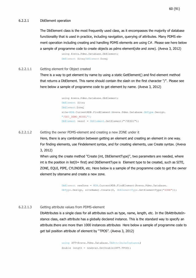
60 (91)

6.2.2.1 DbElement operation

The DbElement class is the most frequently used class, as it encompasses the majority of database

functionality that is used in practice, including navigation, querying of attributes. Many PDMS ele-

ment operation including creating and handling PDMS elements are using C#. Please see here below

a sample of programme code to create objects as pdms element(site and zone). (Aveva 3, 2012)

using Aveva.Pdms.Database.DbElement;

DbElement Site;DbElement Zone;

6.2.2.1.1 Getting element for Object created

There is a way to get element by name by using a static GetElement() and find element method

that returns a DbElement. This name should contain the slash on the first character "/". Please see

here below a sample of programme code to get element by name. (Aveva 3, 2012)

using Aveva.Pdms.Database.DbElement;

DbElement Site;

DbElement Zone;

site=MDB.CurrentMDB.FindElement(Aveva.Pdms.Database.DbType.Design,

"/DSI_DEMO_MODEL");

DbElement vess1 = DbElement.GetElement("/VESS1");

6.2.2.1.2 Getting the owner PDMS-element and creating a new ZONE under it

Here, there is any combination between getting an element and creating an element in one way.

For finding elements, use Findelement syntax, and for creating elements, use Create syntax. (Aveva

3, 2012)

When using the create method "Create (int, DbElementType)", two parameters are needed, where

int is the position in list(0= first) and DbElementType is Element type to be created, such as SITE,

ZONE, EQUI, PIPE, CYLINDER, etc. Here below is a sample of the programme code to get the owner

element by sitename and create a new zone.

DbElement newZone = MDB.CurrentMDB.FindElement(Aveva.Pdms.Database.

DbType.Design, siteName).Create(0, DbElementType.GetElementType("ZONE"));

6.2.2.1.3 Getting attribute values from PDMS-element

DbAttributes is a single class for all attributes such as type, name, length, etc. In the DbAttributeIn-

stance class, each attribute has a globally declared instance. This is the standard way to specify an

attribute.there are more than 1000 instances attributes Here below a sample of programme code to

get tail position attribute of element by “TPOS”. (Aveva 3, 2012)

using ATT=Aveva.Pdms.Database.DbAttributeInstance;

double length = newbran.GetDouble(ATT.TPOS);

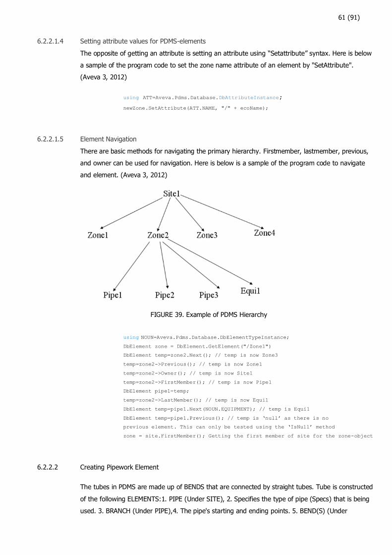
61 (91)

6.2.2.1.4 Setting attribute values for PDMS-elements

The opposite of getting an attribute is setting an attribute using “Setattribute” syntax. Here is below

a sample of the program code to set the zone name attribute of an element by "SetAttribute".

(Aveva 3, 2012)

using ATT=Aveva.Pdms.Database.DbAttributeInstance;

newZone.SetAttribute(ATT.NAME, "/" + ecoName);

6.2.2.1.5 Element Navigation

There are basic methods for navigating the primary hierarchy. Firstmember, lastmember, previous,

and owner can be used for navigation. Here is below is a sample of the program code to navigate

and element. (Aveva 3, 2012)

FIGURE 39. Example of PDMS Hierarchy

using NOUN=Aveva.Pdms.Database.DbElementTypeInstance;

DbElement zone = DbElement.GetElement("/Zone1")

DbElement temp=zone2.Next(); // temp is now Zone3

temp=zone2->Previous(); // temp is now Zone1

temp=zone2->Owner(); // temp is now Site1

temp=zone2->FirstMember(); // temp is now Pipe1

DbElement pipe1=temp;

temp=zone2->LastMember(); // temp is now Equi1

DbElement temp=pipe1.Next(NOUN.EQUIPMENT); // temp is Equi1

DbElement temp=pipe1.Previous(); // temp is ‘null’ as there is no

previous element. This can only be tested using the ‘IsNull’ method

zone = site.FirstMember(); Getting the first member of site for the zone-object

6.2.2.2 Creating Pipework Element

The tubes in PDMS are made up of BENDS that are connected by straight tubes. Tube is constructed

of the following ELEMENTS:1. PIPE (Under SITE), 2. Specifies the type of pipe (Specs) that is being

used. 3. BRANCH (Under PIPE),4. The pipe's starting and ending points. 5. BEND(S) (Under

62 (91)

BRANCH),6. Bends automatically connect the tube's straight section. Here is below, an implementa-

tion of these steps in the program code. (Aveva 4, 2013)

zone = MDB.CurrentMDB.FindElement(Aveva.Pdms.Database.DbType.Design, "/" + zoneName);

pipe = zone.CreateLast(DbElementType.GetElementType("PIPE"));

pipe.SetAttribute(DbAttributeInstance.NAME, "/" + pipeName);

pipe.SetAttribute(DbAttributeInstance.PSPE, pipeSpec);

bran = pipe.Create(branCounter, DbElementType.GetElementType("BRANCH"));

bran.SetAttribute(DbAttributeInstance.NAME, branch_name+ branCounter);

bran.SetAttribute(DbAttributeInstance.HPOS, Position.Create(headXpos, headYpos, headZpos));

bran.SetAttribute(DbAttributeInstance.TPOS, Position.Create(tailXpos, tailYpos, tailZpos));

bend = bran.Create(bendCounter, DbElementType.GetElementType("BEND"));

bend.SetAttribute(DbAttributeInstance.LSTU, tubeSpc);

FIGURE 40. Creating BEND as Pipe work element

6.2.3 Code Debugging

Debugging is one of the good features of Microsoft visual studio. Go to debug pulldown menu and

choose attach to process menu and below picture will appear. PDMS design Application Running in

des.exe can be chosen to debug. Yellow line will appear on each line when tracing for code. It's pos-

sible to observe what the code is doing in real time using the debugger. (Microsoft, 2021)

63 (91)

FIGURE 41. Debugging programme code

64 (91)

7 RESULTS

Here are presented some comparisons between PDMS MTO and Actual MTO for DSI System, and

Cost of MTO comparison between DSI and CFB Scrubber.

7.1 PDMS MTO comparison with actual MTO

PDMS MTO means all components that have been modeled or built can be extracted to report or list

of materials with quantity and type. The width and depth of compartment can be calculated by mul-

tiplying number of columns and diameter of bag and by adding space between bags. From previous

calculation total of 224 bags are needed for each compartment and can be arranged to columns of

16 bags and rows of 14 bags.

FIGURE 42. Plan and side view of bag on Pulse-jet cleaning system (Filsonfilters, 2021)

The table below shows the PDMS MTO summary of pipe consumption. The detailed MTO can be

seen in Appendix 1.

TABLE 17. PDMS MTO for Piping pipeline

Size Description Dimension standard Pipeline Spec

Quantity (m)

88.9 Pipe DIN 2448 OD tes2222_tubes FURNACE_OD 249.057

88.9 Pipe DIN 2448 OD Total 249.057

The table below shows the PDMS MTO Summary of panel consumption. The height of panel is 3250

mm. It comes from 16 bags, multiplied by 180 and added by the distance of bag center to the Side

wall. The detailed MTO can be seen in Appendix 2.

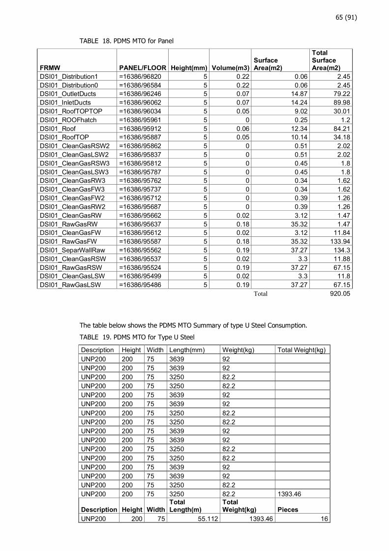
65 (91)

TABLE 18. PDMS MTO for Panel

FRMW PANEL/FLOOR Height(mm) Volume(m3) Surface Area(m2)

Total Surface Area(m2)

DSI01_Distribution1 =16386/96820 5 0.22 0.06 2.45

DSI01_Distribution0 =16386/96584 5 0.22 0.06 2.45

DSI01_OutletDucts =16386/96246 5 0.07 14.87 79.22

DSI01_InletDucts =16386/96062 5 0.07 14.24 89.98

DSI01_RoofTOPTOP =16386/96034 5 0.05 9.02 30.01

DSI01_ROOFhatch =16386/95961 5 0 0.25 1.2

DSI01_Roof =16386/95912 5 0.06 12.34 84.21

DSI01_RoofTOP =16386/95887 5 0.05 10.14 34.18

DSI01_CleanGasRSW2 =16386/95862 5 0 0.51 2.02

DSI01_CleanGasLSW2 =16386/95837 5 0 0.51 2.02

DSI01_CleanGasRSW3 =16386/95812 5 0 0.45 1.8

DSI01_CleanGasLSW3 =16386/95787 5 0 0.45 1.8

DSI01_CleanGasRW3 =16386/95762 5 0 0.34 1.62

DSI01_CleanGasFW3 =16386/95737 5 0 0.34 1.62

DSI01_CleanGasFW2 =16386/95712 5 0 0.39 1.26

DSI01_CleanGasRW2 =16386/95687 5 0 0.39 1.26

DSI01_CleanGasRW =16386/95662 5 0.02 3.12 1.47

DSI01_RawGasRW =16386/95637 5 0.18 35.32 1.47

DSI01_CleanGasFW =16386/95612 5 0.02 3.12 11.84

DSI01_RawGasFW =16386/95587 5 0.18 35.32 133.94

DSI01_SeparWallRaw =16386/95562 5 0.19 37.27 134.3

DSI01_CleanGasRSW =16386/95537 5 0.02 3.3 11.88

DSI01_RawGasRSW =16386/95524 5 0.19 37.27 67.15

DSI01_CleanGasLSW =16386/95499 5 0.02 3.3 11.8

DSI01_RawGasLSW =16386/95486 5 0.19 37.27 67.15

Total 920.05

The table below shows the PDMS MTO Summary of type U Steel Consumption.

TABLE 19. PDMS MTO for Type U Steel

Description Height Width Length(mm) Weight(kg) Total Weight(kg)

UNP200 200 75 3639 92

UNP200 200 75 3639 92

UNP200 200 75 3250 82.2

UNP200 200 75 3250 82.2

UNP200 200 75 3639 92

UNP200 200 75 3639 92

UNP200 200 75 3250 82.2

UNP200 200 75 3250 82.2

UNP200 200 75 3639 92

UNP200 200 75 3639 92

UNP200 200 75 3250 82.2

UNP200 200 75 3250 82.2

UNP200 200 75 3639 92

UNP200 200 75 3639 92

UNP200 200 75 3250 82.2

UNP200 200 75 3250 82.2 1393.46

Description Height Width Total Length(m)

Total Weight(kg) Pieces

UNP200 200 75 55.112 1393.46 16

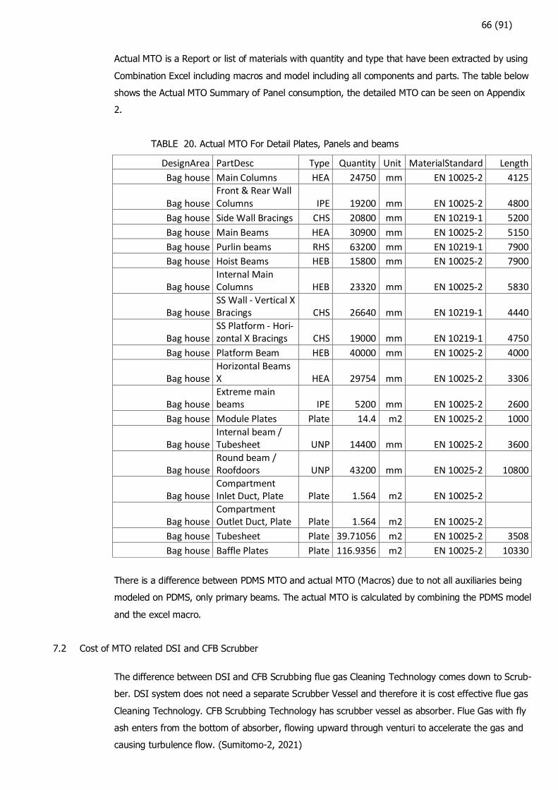
66 (91)

Actual MTO is a Report or list of materials with quantity and type that have been extracted by using

Combination Excel including macros and model including all components and parts. The table below

shows the Actual MTO Summary of Panel consumption, the detailed MTO can be seen on Appendix

2.

TABLE 20. Actual MTO For Detail Plates, Panels and beams

DesignArea PartDesc Type Quantity Unit MaterialStandard Length

Bag house Main Columns HEA 24750 mm EN 10025-2 4125

Bag house Front & Rear Wall Columns IPE 19200 mm EN 10025-2 4800

Bag house Side Wall Bracings CHS 20800 mm EN 10219-1 5200

Bag house Main Beams HEA 30900 mm EN 10025-2 5150

Bag house Purlin beams RHS 63200 mm EN 10219-1 7900

Bag house Hoist Beams HEB 15800 mm EN 10025-2 7900

Bag house Internal Main Columns HEB 23320 mm EN 10025-2 5830

Bag house SS Wall - Vertical X Bracings CHS 26640 mm EN 10219-1 4440

Bag house SS Platform - Hori-zontal X Bracings CHS 19000 mm EN 10219-1 4750

Bag house Platform Beam HEB 40000 mm EN 10025-2 4000

Bag house Horizontal Beams X HEA 29754 mm EN 10025-2 3306

Bag house Extreme main beams IPE 5200 mm EN 10025-2 2600

Bag house Module Plates Plate 14.4 m2 EN 10025-2 1000

Bag house Internal beam / Tubesheet UNP 14400 mm EN 10025-2 3600

Bag house Round beam / Roofdoors UNP 43200 mm EN 10025-2 10800

Bag house Compartment Inlet Duct, Plate Plate 1.564 m2 EN 10025-2

Bag house Compartment Outlet Duct, Plate Plate 1.564 m2 EN 10025-2

Bag house Tubesheet Plate 39.71056 m2 EN 10025-2 3508

Bag house Baffle Plates Plate 116.9356 m2 EN 10025-2 10330

There is a difference between PDMS MTO and actual MTO (Macros) due to not all auxiliaries being

modeled on PDMS, only primary beams. The actual MTO is calculated by combining the PDMS model

and the excel macro.

7.2 Cost of MTO related DSI and CFB Scrubber

The difference between DSI and CFB Scrubbing flue gas Cleaning Technology comes down to Scrub-

ber. DSI system does not need a separate Scrubber Vessel and therefore it is cost effective flue gas

Cleaning Technology. CFB Scrubbing Technology has scrubber vessel as absorber. Flue Gas with fly

ash enters from the bottom of absorber, flowing upward through venturi to accelerate the gas and

causing turbulence flow. (Sumitomo-2, 2021)

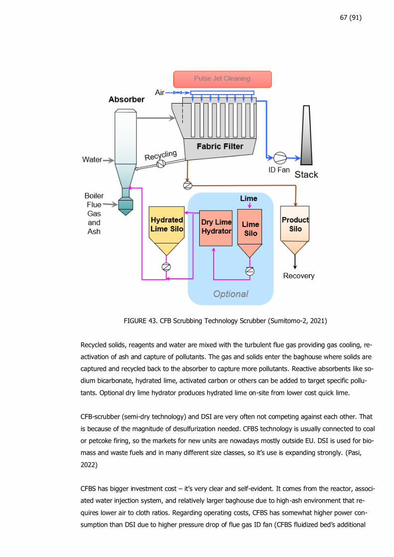
67 (91)

FIGURE 43. CFB Scrubbing Technology Scrubber (Sumitomo-2, 2021)

Recycled solids, reagents and water are mixed with the turbulent flue gas providing gas cooling, re-

activation of ash and capture of pollutants. The gas and solids enter the baghouse where solids are

captured and recycled back to the absorber to capture more pollutants. Reactive absorbents like so-

dium bicarbonate, hydrated lime, activated carbon or others can be added to target specific pollu-

tants. Optional dry lime hydrator produces hydrated lime on-site from lower cost quick lime.

CFB-scrubber (semi-dry technology) and DSI are very often not competing against each other. That

is because of the magnitude of desulfurization needed. CFBS technology is usually connected to coal

or petcoke firing, so the markets for new units are nowadays mostly outside EU. DSI is used for bio-

mass and waste fuels and in many different size classes, so it’s use is expanding strongly. (Pasi,

2022)

CFBS has bigger investment cost – it’s very clear and self-evident. It comes from the reactor, associ-

ated water injection system, and relatively larger baghouse due to high-ash environment that re-

quires lower air to cloth ratios. Regarding operating costs, CFBS has somewhat higher power con-

sumption than DSI due to higher pressure drop of flue gas ID fan (CFBS fluidized bed’s additional

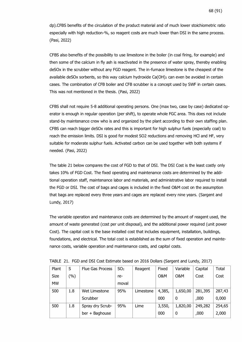
68 (91)

dp).CFBS benefits of the circulation of the product material and of much lower stoichiometric ratio

especially with high reduction-%, so reagent costs are much lower than DSI in the same process.

(Pasi, 2022)

CFBS also benefits of the possibility to use limestone in the boiler (in coal firing, for example) and

then some of the calcium in fly ash is reactivated in the presence of water spray, thereby enabling

deSOx in the scrubber without any FGD reagent. The in-furnace limestone is the cheapest of the

available deSOx sorbents, so this way calcium hydroxide Ca(OH)2 can even be avoided in certain

cases. The combination of CFB boiler and CFB scrubber is a concept used by SWF in certain cases.

This was not mentioned in the thesis. (Pasi, 2022)

CFBS shall not require 5-8 additional operating persons. One (max two, case by case) dedicated op-

erator is enough in regular operation (per shift), to operate whole FGC area. This does not include

stand-by maintenance crew who is and organized by the plant according to their own staffing plan.

CFBS can reach bigger deSOx rates and this is important for high sulphur fuels (especially coal) to

reach the emission limits. DSI is good for modest SO2 reductions and removing HCl and HF, very

suitable for moderate sulphur fuels. Activated carbon can be used together with both systems if

needed. (Pasi, 2022)

The table 21 below compares the cost of FGD to that of DSI. The DSI Cost is the least costly only

takes 10% of FGD Cost. The fixed operating and maintenance costs are determined by the addi-

tional operation staff, maintenance labor and materials, and administrative labor required to install

the FGD or DSI. The cost of bags and cages is included in the fixed O&M cost on the assumption

that bags are replaced every three years and cages are replaced every nine years. (Sargent and

Lundy, 2017)

The variable operation and maintenance costs are determined by the amount of reagent used, the

amount of waste generated (cost per unit disposal), and the additional power required (unit power

Cost). The capital cost is the base installed cost that includes equipment, installation, buildings,

foundations, and electrical. The total cost is established as the sum of fixed operation and mainte-

nance costs, variable operation and maintenance costs, and capital costs.

TABLE 21. FGD and DSI Cost Estimate based on 2016 Dollars (Sargent and Lundy, 2017)

Plant

Size

MW

S

(%)

Flue Gas Process SO2

re-

moval

Reagent Fixed

O&M

Variable

O&M

Capital

Cost

Total

Cost

500 1.8 Wet Limestone

Scrubber

95% Limestone 4,385,

000

1,650,00

0

281,395

,000

287,43

0,000

500 1.8 Spray dry Scrub-

ber + Baghouse

95% Lime 3,550,

000

1,820,00

0

249,282

,000

254,65

2,000

69 (91)

500 1.8 DSI + Baghouse 70% Trona 415,00

0

4,580,00

0

19,489,

000

24,484

,000

500 1.8 DSI + Baghouse 70% Hydrated

Lime

385,00

0

2,455,00

0

15,860,

000

18,700

,000

DSI systems are quite different with FGD. The major cost for the DSI system is the sorbent itself.

The sorbent feed rate is proportional to sulfur generation rate, particulate collection device, and re-

moval efficiency. While a DSI project can be completed in less than a year from contract award to

commercial operation, A FGD project requires three years. A DSI system requires two additional op-

erators, but a FGD system requires eight additional operators and required water treatment. Capital

cost calculation includes Equipment, installation, building, Foundations, and Electrical. DSI capital

costs are calculated at 10% of the cost of FGD, as shown in the table above indicates. There is a

significant cost difference between DSI and FGD, a full cost comparison may be seen in Appendix 3

and 4. Below picture is Lhoist’s DSI super-sack test skid system.

FIGURE 44. Lhoist’s DSI super-sack test skid system (Gerald Hunt and Melissa Sewell, 2015)

It is consisted of a DSI Hopper capable of holding approximately 1500 kilograms of hydrated lime.

Another component, a Screw Feeder with Variable Frequency Drive (VFD) is used to meter sorbent

into the eductor and control the sorbent injection rate between approximately 13,6 and 450 kg/hr. A

positive displacement blower that pressurizes ambient air to be used as motive air for transporting

sorbent from the pick-up point to the exhaust gas. A desiccant-filled air compressor to provide dry

air to fluidize the bottom of the hopper and clean the dust collector filter bags. A dust collector and

vent fan are used to mitigate the emission of fugitive dust. A reclaim auger is used to return fugitive

dust collected by the dust collector to the hopper. Four load cells (one for each trailer leg), a sum-

mation box, and a scale read-out are included to keep track of the trailer's weight. (Gerald Hunt and

Melissa Sewell, 2015)

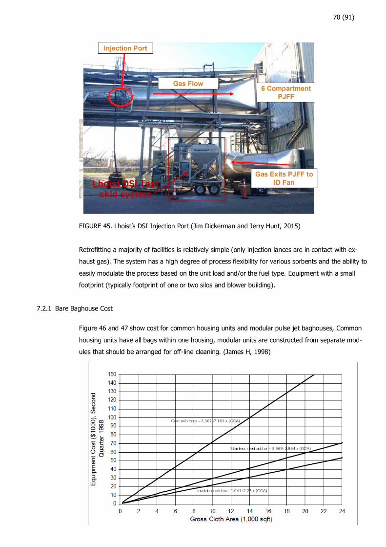
70 (91)

FIGURE 45. Lhoist’s DSI Injection Port (Jim Dickerman and Jerry Hunt, 2015)

Retrofitting a majority of facilities is relatively simple (only injection lances are in contact with ex-

haust gas). The system has a high degree of process flexibility for various sorbents and the ability to

easily modulate the process based on the unit load and/or the fuel type. Equipment with a small

footprint (typically footprint of one or two silos and blower building).

7.2.1 Bare Baghouse Cost

Figure 46 and 47 show cost for common housing units and modular pulse jet baghouses, Common

housing units have all bags within one housing, modular units are constructed from separate mod-

ules that should be arranged for off-line cleaning. (James H, 1998)

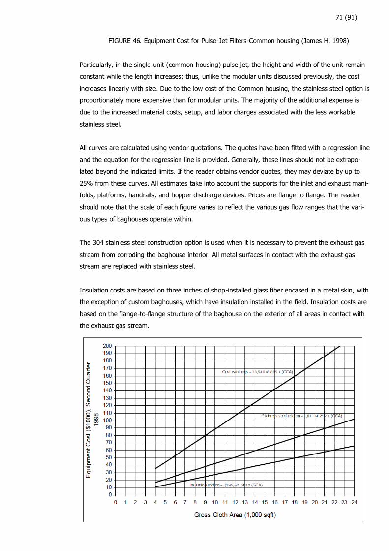
71 (91)

FIGURE 46. Equipment Cost for Pulse-Jet Filters-Common housing (James H, 1998)

Particularly, in the single-unit (common-housing) pulse jet, the height and width of the unit remain

constant while the length increases; thus, unlike the modular units discussed previously, the cost

increases linearly with size. Due to the low cost of the Common housing, the stainless steel option is

proportionately more expensive than for modular units. The majority of the additional expense is

due to the increased material costs, setup, and labor charges associated with the less workable

stainless steel.

All curves are calculated using vendor quotations. The quotes have been fitted with a regression line

and the equation for the regression line is provided. Generally, these lines should not be extrapo-

lated beyond the indicated limits. If the reader obtains vendor quotes, they may deviate by up to

25% from these curves. All estimates take into account the supports for the inlet and exhaust mani-

folds, platforms, handrails, and hopper discharge devices. Prices are flange to flange. The reader

should note that the scale of each figure varies to reflect the various gas flow ranges that the vari-

ous types of baghouses operate within.

The 304 stainless steel construction option is used when it is necessary to prevent the exhaust gas

stream from corroding the baghouse interior. All metal surfaces in contact with the exhaust gas

stream are replaced with stainless steel.

Insulation costs are based on three inches of shop-installed glass fiber encased in a metal skin, with

the exception of custom baghouses, which have insulation installed in the field. Insulation costs are

based on the flange-to-flange structure of the baghouse on the exterior of all areas in contact with

the exhaust gas stream.

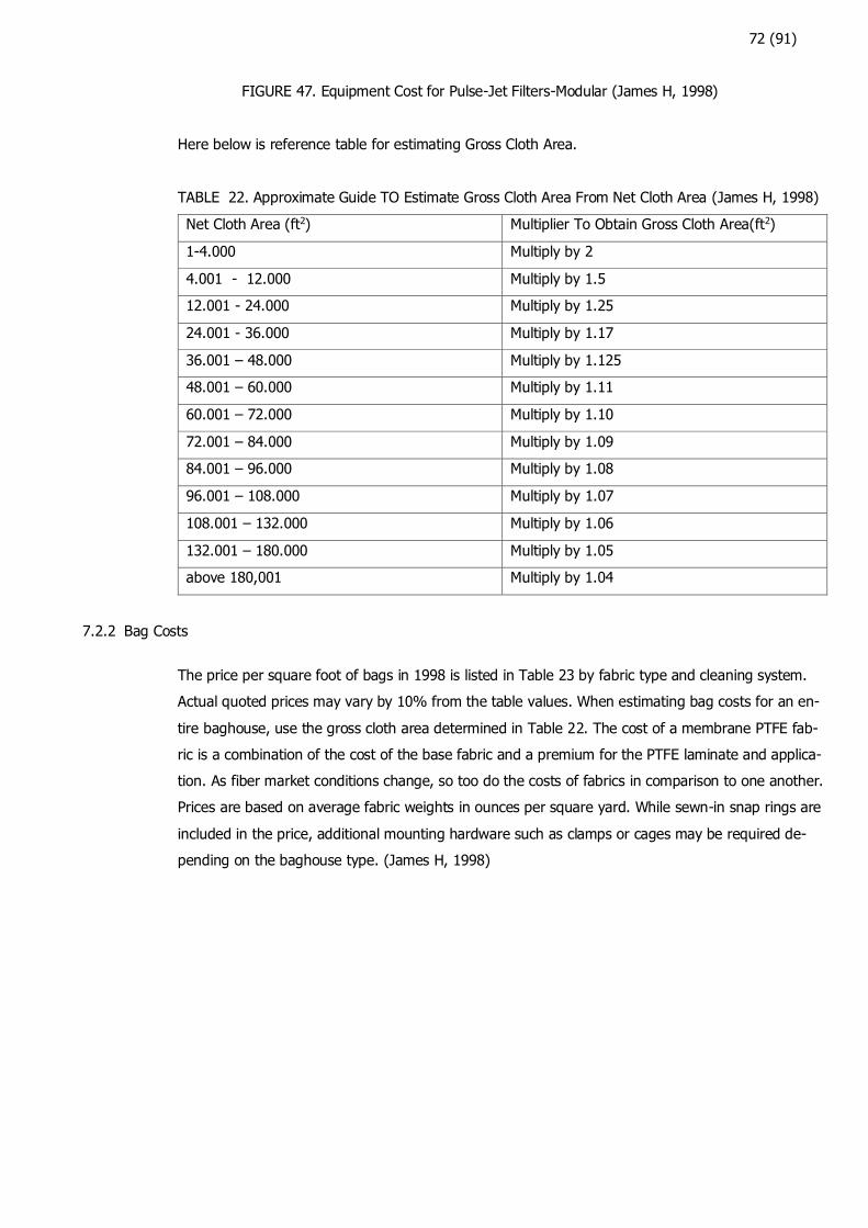
72 (91)

FIGURE 47. Equipment Cost for Pulse-Jet Filters-Modular (James H, 1998)

Here below is reference table for estimating Gross Cloth Area.

TABLE 22. Approximate Guide TO Estimate Gross Cloth Area From Net Cloth Area (James H, 1998)

Net Cloth Area (ft2) Multiplier To Obtain Gross Cloth Area(ft2)

1-4.000 Multiply by 2

4.001 - 12.000 Multiply by 1.5

12.001 - 24.000 Multiply by 1.25

24.001 - 36.000 Multiply by 1.17

36.001 – 48.000 Multiply by 1.125

48.001 – 60.000 Multiply by 1.11

60.001 – 72.000 Multiply by 1.10

72.001 – 84.000 Multiply by 1.09

84.001 – 96.000 Multiply by 1.08

96.001 – 108.000 Multiply by 1.07

108.001 – 132.000 Multiply by 1.06

132.001 – 180.000 Multiply by 1.05

above 180,001 Multiply by 1.04

7.2.2 Bag Costs

The price per square foot of bags in 1998 is listed in Table 23 by fabric type and cleaning system.

Actual quoted prices may vary by 10% from the table values. When estimating bag costs for an en-

tire baghouse, use the gross cloth area determined in Table 22. The cost of a membrane PTFE fab-

ric is a combination of the cost of the base fabric and a premium for the PTFE laminate and applica-

tion. As fiber market conditions change, so too do the costs of fabrics in comparison to one another.

Prices are based on average fabric weights in ounces per square yard. While sewn-in snap rings are

included in the price, additional mounting hardware such as clamps or cages may be required de-

pending on the baghouse type. (James H, 1998)

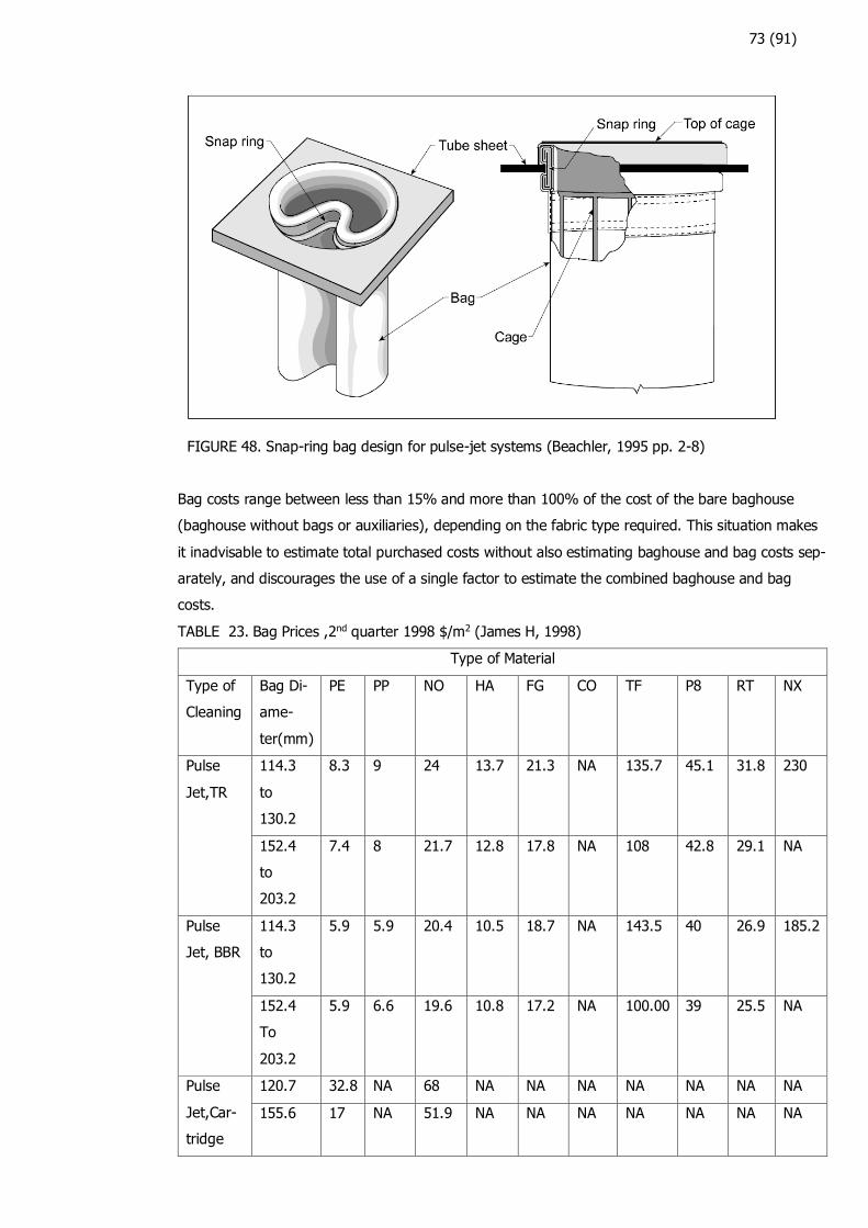
73 (91)

FIGURE 48. Snap-ring bag design for pulse-jet systems (Beachler, 1995 pp. 2-8)

Bag costs range between less than 15% and more than 100% of the cost of the bare baghouse

(baghouse without bags or auxiliaries), depending on the fabric type required. This situation makes

it inadvisable to estimate total purchased costs without also estimating baghouse and bag costs sep-

arately, and discourages the use of a single factor to estimate the combined baghouse and bag

costs.

TABLE 23. Bag Prices ,2nd quarter 1998 $/m2 (James H, 1998)

Type of Material

Type of

Cleaning

Bag Di-

ame-

ter(mm)

PE PP NO HA FG CO TF P8 RT NX

Pulse

Jet,TR

114.3

to

130.2

8.3 9 24 13.7 21.3 NA 135.7 45.1 31.8 230

152.4

to

203.2

7.4 8

21.7 12.8 17.8 NA 108 42.8 29.1 NA

Pulse

Jet, BBR

114.3

to

130.2

5.9 5.9 20.4 10.5 18.7 NA 143.5 40 26.9 185.2

152.4

To

203.2

5.9 6.6 19.6 10.8 17.2 NA 100.00 39 25.5 NA

Pulse

Jet,Car-

tridge

120.7 32.8 NA 68 NA NA NA NA NA NA NA

155.6 17 NA 51.9 NA NA NA NA NA NA NA

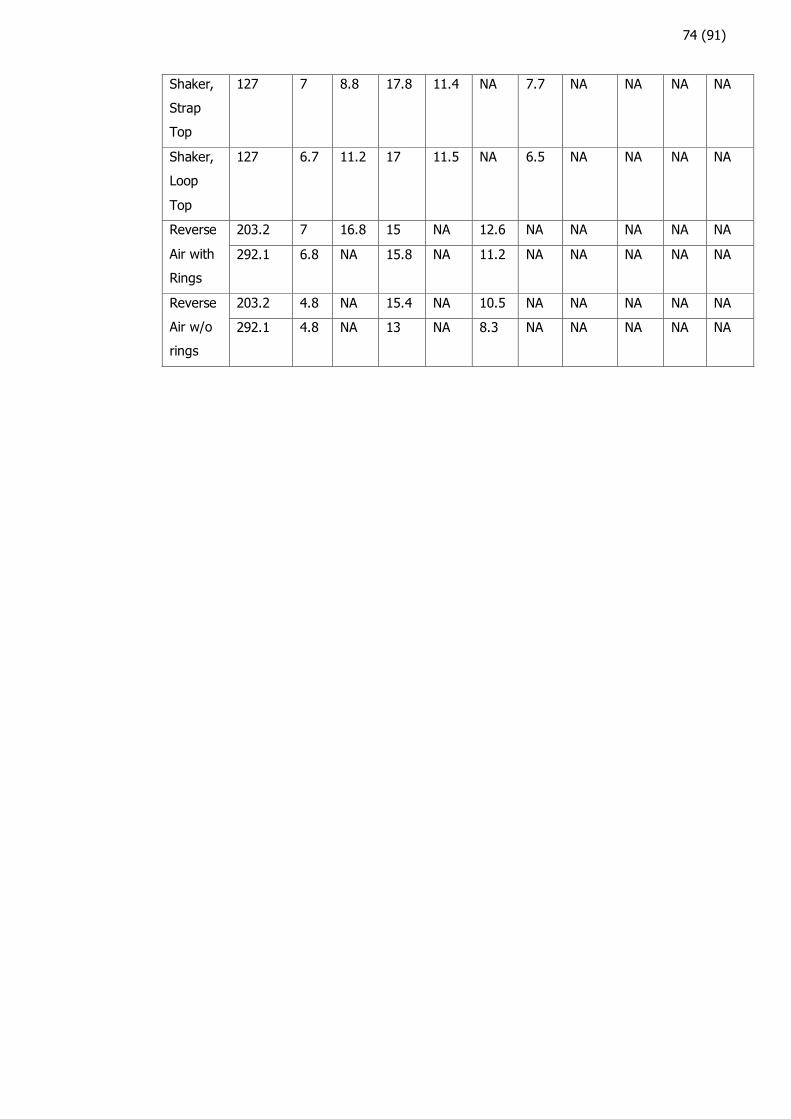
74 (91)

Shaker,

Strap

Top

127 7 8.8 17.8 11.4 NA 7.7 NA NA NA NA

Shaker,

Loop

Top

127 6.7 11.2 17 11.5 NA 6.5 NA NA NA NA

Reverse

Air with

Rings

203.2 7 16.8 15 NA 12.6 NA NA NA NA NA

292.1 6.8 NA 15.8 NA 11.2 NA NA NA NA NA

Reverse

Air w/o

rings

203.2 4.8 NA 15.4 NA 10.5 NA NA NA NA NA

292.1 4.8 NA 13 NA 8.3 NA NA NA NA NA

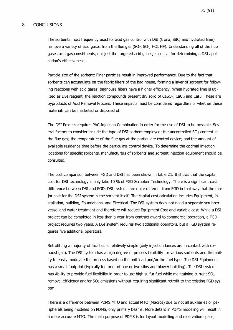
75 (91)

8 CONCLUSIONS

The sorbents most frequently used for acid gas control with DSI (trona, SBC, and hydrated lime)

remove a variety of acid gases from the flue gas (SO2, SO3, HCl, HF). Understanding all of the flue

gases acid gas constituents, not just the targeted acid gases, is critical for determining a DSI appli-

cation's effectiveness.

Particle size of the sorbent: Finer particles result in improved performance. Due to the fact that

sorbents can accumulate on the fabric filters of the bag house, forming a layer of sorbent for follow-

ing reactions with acid gases, baghouse filters have a higher efficiency. When hydrated lime is uti-

lized as DSI reagent, the reaction compounds present dry solid of CaSO4, CaCl2 and CaF2. These are

byproducts of Acid Removal Process. These impacts must be considered regardless of whether these

materials can be marketed or disposed of.

The DSI Process requires PAC Injection Combination in order for the use of DSI to be possible. Sev-

eral factors to consider include the type of DSI sorbent employed; the uncontrolled SO3 content in

the flue gas; the temperature of the flue gas at the particulate control device; and the amount of

available residence time before the particulate control device. To determine the optimal injection

locations for specific sorbents, manufacturers of sorbents and sorbent injection equipment should be

consulted.

The cost comparison between FGD and DSI has been shown in table 21. It shows that the capital

cost for DSI technology is only take 10 % of FGD Scrubber Technology. There is a significant cost

difference between DSI and FGD. DSI systems are quite different from FGD in that way that the ma-

jor cost for the DSI system is the sorbent itself. The capital cost calculation includes Equipment, in-

stallation, building, Foundations, and Electrical. The DSI system does not need a separate scrubber

vessel and water treatment and therefore will reduce Equipment Cost and variable cost. While a DSI

project can be completed in less than a year from contract award to commercial operation, a FGD

project requires two years. A DSI system requires two additional operators, but a FGD system re-

quires five additional operators.

Retrofitting a majority of facilities is relatively simple (only injection lances are in contact with ex-

haust gas). The DSI system has a high degree of process flexibility for various sorbents and the abil-

ity to easily modulate the process based on the unit load and/or the fuel type. The DSI Equipment

has a small footprint (typically footprint of one or two silos and blower building). The DSI system

has Ability to provide fuel flexibility in order to use high sulfur fuel while maintaining current SO2

removal efficiency and/or SO2 emissions without requiring significant retrofit to the existing FGD sys-

tem.

There is a difference between PDMS MTO and actual MTO (Macros) due to not all auxiliaries or pe-

ripherals being modeled on PDMS, only primary beams. More details in PDMS modeling will result in

a more accurate MTO. The main purpose of PDMS is for layout modelling and reservation space,

76 (91)

therefore there is no need for detailed modeling. The actual MTO is calculated by combining the

PDMS model and the Excel macro.

Nobody can deny the importance of a digital 3D model nowadays. AVEVA PDMS software facilitates

the creation of a digital 3D model with numerous advantages. Using the PDMS software, a digital 3D

model of the DSI baghouse was created. All parameter values that have been created on 3D model

and the theory behind it have been explained in this thesis including Dry Sorbent Injection Theory

and Baghouse Calculation. DSI as Cost Effective Technology Can be Proven. As Recommendation,

All Parameter values that have been used in this DLL do not connect directly to Material energy bal-

ance calculation. In the next development phase, the data from material energy balance calculation

should be received directly to the DLL so it would make parameter validation more accurate. It is

understandable given that energy balance calculation software was not available at the time this

thesis was written.

77 (91)

9 REFERENCES

APTI Course. 2021-04-05. https://www.neundorfer.com/knowledgebase-posts/operation/.

https://www.neundorfer.com/wp-content/uploads/2016/05/ESP-KnowledgeBase-01-Operation.pdf.

[Online] 05. 04 2021-04-05. [Viitattu: 05. 04 2021.] https://www.neundorfer.com/wp-

content/uploads/2016/05/ESP-KnowledgeBase-01-Operation.pdf.

ASME BPVC. 2015. ASME Boiler and Pressure Vessel Code An International Code Rule for

Construction of Power Boiler. Rules for Construction of Power Boiler. [Online] The American Society

of Mechanical Engineers, 2015. [Viitattu: 30. 10 2021.]

https://www.academia.edu/40816183/2015_ASME_Boiler_and_Pressure_Vessel_Code_An_Internati

onal_Code_R_ules_for_Construction_of_Power_Boilers_SECTION_I.

Aveva 1, Solutions. 2013. Getting Started with AVEVA Plant, Plant Functions. s.l. : Aveva

Solutions Limited C:\AVEVA\Plant\PDMS12.1\Documentation\GS.chm, 2013.

Aveva 2, Solution. 2013. Running Global Projects. cambridge : Aveva Solutions Limited

C:\AVEVA\Plant\PDMS12.1\Documentation\PDGRGP.chm, 2013.

Aveva 3, Solution. 2012. .NET Customization User Guide. Cambridge : Aveva Solution

C:\AVEVA\Plant\PDMS12.1\Documentation\NCUG.chm, 2012.

Aveva 4, Solution. 2013. Pipework Design User Guide. Cambridge : Aveva Solution

C:\AVEVA\Plant\PDMS12.1\Documentation\PDUV.chm, 2013.

Beachler, David S. 1995. Fabric Filter Operation Review: Self-instructional Manual : APTI Course

SI:412A. USA : Industrial Extension Service, College of Engineering, North Carolina State University,

1995, 1995. pdfslide.net_epa-air-pollution-lesson.pdf.

Bethea, R.M. 1978. Air Pollution Control TEchnology : An Engineering Analysis Poit of View. New

York : Van Nostrand Reinhold, 1978.

Couch, G.R. 1995. Power from coal - where to remove impurities. London : IEA Coal Research,

report, 1995. IEACR/82.

David R. Lide. 2005. CRC Handbook of Chemistry and Physics. Physical Constants of Inorganic

Compounds. [Online] CRC Press, 2005.

https://dl.icdst.org/pdfs/files/415f61e9082c7d23df09fb15605aa59d.pdf.

Environmental Healt & Engineering inc. 2011. Emissions of Hazardous Air Pollutants From

Coal-Fired Power Plants. [Online] Environmental Healt & Engineering Inc, 7. 03 2011.

https://www.lung.org/getmedia/25962184-d2fc-42f8-b5a3-8ece3257fbab/emissions-of-hazardous-

air.pdf.pdf.

EPA 745-B-19-017. 2019. Hydrochloric Acid (acid aerosols including mists, vapors, gas, fog, and

other airborne forms of any particle size). [Online] 15. 01 2019. [Viitattu: 15. 01 2021.]

https://ofmpub.epa.gov/apex/guideme_ext/f?p=guideme:gd:::::gd:hcl.

EPA AP-42. 1998. AP-42 Section 1.1. Bituminous and Subbituminous coal combustion.

https://www3.epa.gov/ttnchie1/ap42/ch01/. [Online] EPA, september 1998. [Viitattu: 10. 3 2021.]

https://www3.epa.gov/ttnchie1/ap42/ch01/final/c01s01.pdf.

European Council. 2001. the European Parliament and of the Council. Directive 2001/80/EC of

the European Parliament and of the Council of 23 October 2001 on the limita-tion of emissions of

certain pollutants into the air from large combustion plants. [Online] 16. 04 2001. https://eur-

lex.europa.eu/legal-content/EN/TXT/PDF/?uri=CELEX:32001L0080&from=EN.

78 (91)

—. 2010. the European Parliament and of the Council. Directive 2010/75/EU of the European

Parliament and of the Council of 24 November 2010 on the limita-tion of emissions of certain

pollutants into the air from industrial installation. [Online] 16. 04 2010. https://eur-

lex.europa.eu/legal-content/EN/TXT/?uri=celex%3A32010L0075.

FHWA. 2016. Federal Highway Administration Research and Technology. User Guidelines for Waste

and Byproduct Materials in Pavement Construction. [Online] Federal Highway Administration, 3. 8

2016. https://www.fhwa.dot.gov/publications/research/infrastructure/structures/97148/cfa51.cfm.

FHWA-RD-97-148.

Filsonfilters. 2021. Pulse Jet Bag Filters. [Online] filsonfilters, 20. 12 2021.

https://www.filsonfilters.com/pulse-jet-bag-filters/.

Gerald Hunt and Melissa Sewell. 2015. Utilizing Dry Sorbent Injection Technology to Improve

Acid Gas Control. [Online] Lhoist North America, 20. 10 2015. [Viitattu: 17. 08 2021.]

https://www.sorbacal.com/sites/default/files/downloadcenter/utilizing_dry_sorbent_injection_techno

logy_to_improve_acid_gas_control.pdf.

James H, Turner. 1998. Baghouse and Filters. new jersey : U.S Environmental Protection Agency

, 1998. cs6ch1.pdf.

Jim Dickerman and Jerry Hunt. 2015. Simultaneous HCl and Hg Control with a Single Sorbent

and DSI System. [Online] Lhoist, 14. 7 2015. [Viitattu: 27. 2 2022.]

https://www.sorbacal.com/sites/default/files/downloadcenter/reinhold_-

_simultaneous_hcl_and_hg_control.pdf.

John, R. Richards. 1995. Control of gaseous Emissions, Student MAnual APTI Course 415 third

Edition, North Carolina University. https://nepis.epa.gov/. [Online] 16. 04 1995.

https://nepis.epa.gov/Exe/ZyNET.exe/2000MBJN.txt?ZyActionD=ZyDocument&Client=EPA&Index=1

991%20Thru%201994&Docs=&Query=&Time=&EndTime=&SearchMethod=1&TocRestrict=n&Toc=

&TocEntry=&QField=&QFieldYear=&QFieldMonth=&QFieldDay=&UseQField=&IntQFieldOp=0&ExtQ

Fiel.

Joseph , Beachler. 1998. Scrubber System Operation Review Self -Intructional Manual APTI

Course SI:412C second edition. s.l. : Nort Carolina State University, 1998. NC 27695.

Kema. 1997. Behaviour, control and emissions of trace species by coal-fired power plants in

Europe. Arnhem, the Netherlands : Report 83428.SP.08 97P01.07B KEMA, 1997.

Meij. 1989. Tracking trace elements at a coal fired plant equipped with a wet flue gas

desulphurisation facility”. Tracking trace elements at a coal fired plant equipped with a wet flue gas

desulphurisation facility”. s.l. : Kema Sci. & Technol, 1989.

Michael, Schantz, and Melissa. 2013. The Growth of Dry Sorbent Injection (DSI) and the impact

on Coal Combustion Residue. [Online] American Waste Management Association Annual Conference

and Exhibition, 2013.

https://www.sorbacal.com/sites/default/files/downloadcenter/lna_growth_of_dsi_and_impact_on_co

al_combustion_residue_-_2013_woca.pdf https://www.sorbacal.com/asia_en/dry-process#!/dry-

sorbent-injection--dsi.

Michael,Joshua,Curt and friend. 2016. DRY SORBENT INJECTION FOR ACID GAS CONTROL :

PROCESS CHEMISTRY , WASTE DISPOSAL AND PLANT OPERATIONAL IMPACTS INSTITUTE OF

CLEAN AIR COMPANIES JULY 2016. https://www.icac.com/search/all.asp?bst=dsi. [Online] 2016.

79 (91)

[Viitattu: 17. 08 2020.]

https://cdn.ymaws.com/www.icac.com/resource/resmgr/white_papers/ICAC_Industrial_DSI_Ancillar

.pdf.

Microsoft. 2021. First look at the Visual Studio Debugger. [Online] Microsoft, 08. 06 2021.

https://docs.microsoft.com/en-us/visualstudio/debugger/debugger-feature-tour?view=vs-2022.

NESCAUM. 2011. Northeast States for Coordinated Air Use Management. [Online] 31. 03 2011.

https://www.nescaum.org/documents/coal-control-technology-nescaum-report-20110330.pdf/.

Pasi, Liimatainen. 2022. Client's Thesis Supervisor, Sumitomo - FW : Interview, 04. 05 2022.

Rbasniak. 2013. PML II and PML.NET, which one now? [Online] June 2013.

https://pdfcoffee.com/pdms-pmlnet-basics-pdf-free.html.

Sargent and Lundy. 2017. IPM v6 - Emission Control Technologies Attachment 5-2: SDA FGD

Cost Development Methodology. [Online] EPA, January 2017. [Viitattu: 20. 1 2022.]

https://www.epa.gov/airmarkets/ipm-v6-emission-control-technologies-attachment-5-2-sda-fgd-

cost-development-methodology.

Savonia Moodle. 2020. https://moodle.savonia.fi/. https://moodle.savonia.fi/. [Online] 05. 04

2020. [Viitattu: 05. 04 2020.]

https://www.iso.org/standard/60857.html#:~:text=ISO%2014001%3A2015%20specifies%20the,to

%20enhance%20its%20environmental%20performance.&text=ISO%2014001%3A2015%20can%2

0be,to%20systematically%20improve%20environmental%20management..

Sid Nelson Jr., Ronald Landreth, Ph.D., Qunhui Zhou, Ph.D., and Jon Miller. 2004.

Accumulated Power-Plant Mercury-Removal Ex-perience with Brominated PAC Injection. [Online]

2004. [Viitattu: 05. 05 2021.]

https://www.researchgate.net/publication/255019451_Accumulated_Power-Plant_Mercury-

Removal_Experience_with_Brominated_PAC_Injection.

Sumitomo-1. 2020. SFW PDMS 12 Design training. SFW PDMS 12 Design training. Varkaus :

Sumitomo - FW, 2020.

Sumitomo-2. 2021. Circulating Fluidized Bed Scrubbing technology. Varkaus : sumitomo, 2021.

Sumitomo-3. 2020. CFB Combustion Concept. [Online] 16. 04 2020. http://fiportal.shi-

fw.com/SFW_Intranet/SBD/_layouts/15/start.aspx#/Presentation%20Modules/Forms/AdvancedCFBT

echForRepoweringProjects_KNU_4Mar2014MoscowRUS.pptx.

Sumitomo-4. 2021. Flue Gas Cleaning Process. [Online] 16. 04 2021. http://fiportal.shi-

fw.com/SFW_Intranet/SBD/_layouts/15/WopiFrame.aspx?sourcedoc=/SFW_Intranet/SBD/Presentati

on%20Modules/Module_033_CFB_Low_Rank_Fuels.pptx&action=default.

Sumitomo-5. 2020. CFB Scrubber TEchnology. [Online] 25. 06 2020. [Viitattu: 25. 06 2020.]

http://fiportal.shi-

fw.com/SFW_Intranet/SBD/_layouts/15/WopiFrame2.aspx?sourcedoc=/SFW_Intranet/SBD/Presenta

tion%20Modules/Module_060_CFBS.pptx&action=default.

Sumitomo-6. 2020. Bubbling Fluid Bed Boilers. [Online] 16. 04 2020. [Viitattu: 16. 04 2020.]

http://fiportal.shi-

fw.com/SFW_Intranet/SBD/_layouts/15/WopiFrame2.aspx?sourcedoc=/SFW_Intranet/SBD/Presenta

tion%20Modules/Module_020_BFB_Boilers.pptx&action=default.

Teija, Honkanen. 2022. Lecturer, Savonia UAS : Interview, 6. 05 2022.

80 (91)

Turner, J.H,P.A Lawless, T. Yamamoto,D. W Coy, G.p. Greiner, J.d. McKenna, and W. M.

Vatavuk. 1992. Electostatic Precipitators. New York : Air and Waste MAnagement Association,

1992. Air Pollution Engineering Manual.

US EPA2. 2021. Sulfur Dioxide (SO2) Pollution. United State Environment Protection Agency.

[Online] 15. 01 2021. [Viitattu: 15. 01 2021.] https://www.epa.gov/so2-pollution/sulfur-dioxide-

basics.

Yimin Deng, Renaud Ansart, Jan Baeyens and Huili Zhang. 2019. Flue Gas Desulphurization

in Circulating Fluidized Beds. [Online] October 2019. [Viitattu: 1. 09 2020.]

https://www.researchgate.net/publication/336583438_Flue_Gas_Desulphurization_in_Circulating_Fl

uidized_Beds Flue-Gas-Desulphurization-in-Circulating-Fluidized-Beds_dsi.pdf. Energies 2019, 12,

3908; doi:10.3390/en12203908.

Yougen Kong, Michael Wood. 2012. Dry Sorbent Injection With Trona Or Sodium Bicarbonate

For HCl Treatment. www.pollutiononline.com. [Online] 22. January 2012. [Viitattu: 10. 12 2020.]

https://www.pollutiononline.com/doc/dry-sorbent-injection-with-trona-or-sodium-0001 EPA-R06-

OAR-2016-0611-0042_content (1).pdf.

Yusuf, Achmad. 2020. Creating DRY SORBENT INJECTION 3D Model By System Parameter

Calculation. Varkaus : Savonia UAS, 2020.

Zevenhoven and Kilpinen. 2005. CONTROL OF POLLUTANTS IN FLUE GASES AND FUEL GASES.

Helsinki : the Helsinki University of Technology course ENE-47.153, 2005. s. 37. ISBN 951-22-5527-

8.

Zhang, Xing. 2014. coal combustion wastes. Management of coal combustion wastes. January :

IEA Clean Coal Centre, 2014.

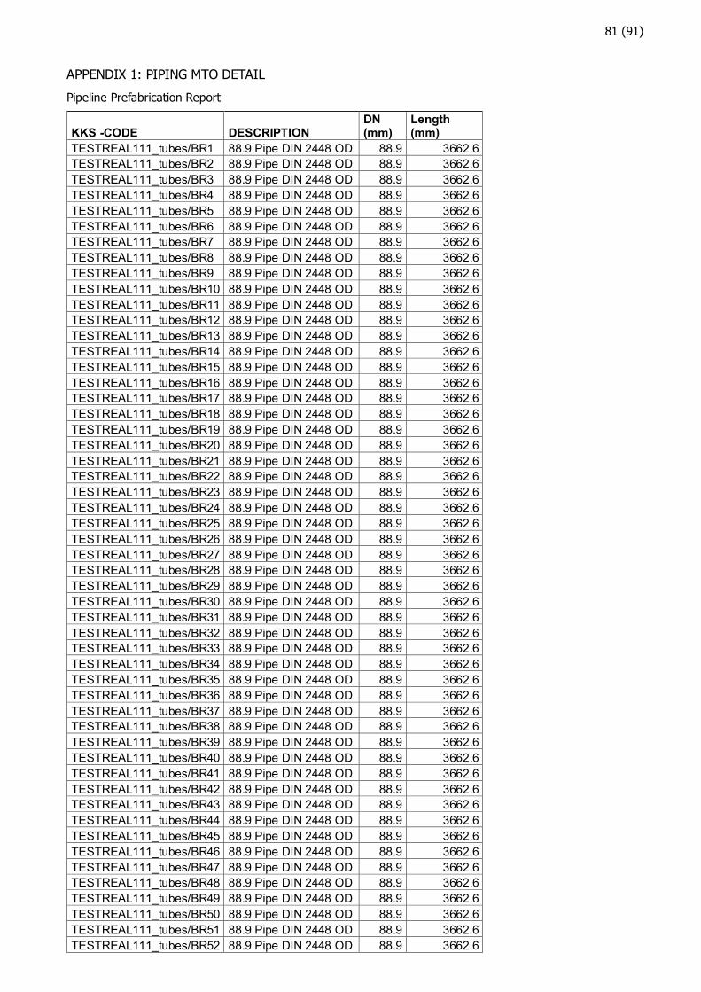
81 (91)

APPENDIX 1: PIPING MTO DETAIL

Pipeline Prefabrication Report

KKS -CODE DESCRIPTION DN (mm)

Length (mm)

TESTREAL111_tubes/BR1 88.9 Pipe DIN 2448 OD 88.9 3662.6

TESTREAL111_tubes/BR2 88.9 Pipe DIN 2448 OD 88.9 3662.6

TESTREAL111_tubes/BR3 88.9 Pipe DIN 2448 OD 88.9 3662.6

TESTREAL111_tubes/BR4 88.9 Pipe DIN 2448 OD 88.9 3662.6

TESTREAL111_tubes/BR5 88.9 Pipe DIN 2448 OD 88.9 3662.6

TESTREAL111_tubes/BR6 88.9 Pipe DIN 2448 OD 88.9 3662.6

TESTREAL111_tubes/BR7 88.9 Pipe DIN 2448 OD 88.9 3662.6

TESTREAL111_tubes/BR8 88.9 Pipe DIN 2448 OD 88.9 3662.6

TESTREAL111_tubes/BR9 88.9 Pipe DIN 2448 OD 88.9 3662.6

TESTREAL111_tubes/BR10 88.9 Pipe DIN 2448 OD 88.9 3662.6

TESTREAL111_tubes/BR11 88.9 Pipe DIN 2448 OD 88.9 3662.6

TESTREAL111_tubes/BR12 88.9 Pipe DIN 2448 OD 88.9 3662.6

TESTREAL111_tubes/BR13 88.9 Pipe DIN 2448 OD 88.9 3662.6

TESTREAL111_tubes/BR14 88.9 Pipe DIN 2448 OD 88.9 3662.6

TESTREAL111_tubes/BR15 88.9 Pipe DIN 2448 OD 88.9 3662.6

TESTREAL111_tubes/BR16 88.9 Pipe DIN 2448 OD 88.9 3662.6

TESTREAL111_tubes/BR17 88.9 Pipe DIN 2448 OD 88.9 3662.6

TESTREAL111_tubes/BR18 88.9 Pipe DIN 2448 OD 88.9 3662.6

TESTREAL111_tubes/BR19 88.9 Pipe DIN 2448 OD 88.9 3662.6

TESTREAL111_tubes/BR20 88.9 Pipe DIN 2448 OD 88.9 3662.6

TESTREAL111_tubes/BR21 88.9 Pipe DIN 2448 OD 88.9 3662.6

TESTREAL111_tubes/BR22 88.9 Pipe DIN 2448 OD 88.9 3662.6

TESTREAL111_tubes/BR23 88.9 Pipe DIN 2448 OD 88.9 3662.6

TESTREAL111_tubes/BR24 88.9 Pipe DIN 2448 OD 88.9 3662.6

TESTREAL111_tubes/BR25 88.9 Pipe DIN 2448 OD 88.9 3662.6

TESTREAL111_tubes/BR26 88.9 Pipe DIN 2448 OD 88.9 3662.6

TESTREAL111_tubes/BR27 88.9 Pipe DIN 2448 OD 88.9 3662.6

TESTREAL111_tubes/BR28 88.9 Pipe DIN 2448 OD 88.9 3662.6

TESTREAL111_tubes/BR29 88.9 Pipe DIN 2448 OD 88.9 3662.6

TESTREAL111_tubes/BR30 88.9 Pipe DIN 2448 OD 88.9 3662.6

TESTREAL111_tubes/BR31 88.9 Pipe DIN 2448 OD 88.9 3662.6

TESTREAL111_tubes/BR32 88.9 Pipe DIN 2448 OD 88.9 3662.6

TESTREAL111_tubes/BR33 88.9 Pipe DIN 2448 OD 88.9 3662.6

TESTREAL111_tubes/BR34 88.9 Pipe DIN 2448 OD 88.9 3662.6

TESTREAL111_tubes/BR35 88.9 Pipe DIN 2448 OD 88.9 3662.6

TESTREAL111_tubes/BR36 88.9 Pipe DIN 2448 OD 88.9 3662.6

TESTREAL111_tubes/BR37 88.9 Pipe DIN 2448 OD 88.9 3662.6

TESTREAL111_tubes/BR38 88.9 Pipe DIN 2448 OD 88.9 3662.6

TESTREAL111_tubes/BR39 88.9 Pipe DIN 2448 OD 88.9 3662.6

TESTREAL111_tubes/BR40 88.9 Pipe DIN 2448 OD 88.9 3662.6

TESTREAL111_tubes/BR41 88.9 Pipe DIN 2448 OD 88.9 3662.6

TESTREAL111_tubes/BR42 88.9 Pipe DIN 2448 OD 88.9 3662.6

TESTREAL111_tubes/BR43 88.9 Pipe DIN 2448 OD 88.9 3662.6

TESTREAL111_tubes/BR44 88.9 Pipe DIN 2448 OD 88.9 3662.6

TESTREAL111_tubes/BR45 88.9 Pipe DIN 2448 OD 88.9 3662.6

TESTREAL111_tubes/BR46 88.9 Pipe DIN 2448 OD 88.9 3662.6

TESTREAL111_tubes/BR47 88.9 Pipe DIN 2448 OD 88.9 3662.6

TESTREAL111_tubes/BR48 88.9 Pipe DIN 2448 OD 88.9 3662.6

TESTREAL111_tubes/BR49 88.9 Pipe DIN 2448 OD 88.9 3662.6

TESTREAL111_tubes/BR50 88.9 Pipe DIN 2448 OD 88.9 3662.6

TESTREAL111_tubes/BR51 88.9 Pipe DIN 2448 OD 88.9 3662.6

TESTREAL111_tubes/BR52 88.9 Pipe DIN 2448 OD 88.9 3662.6

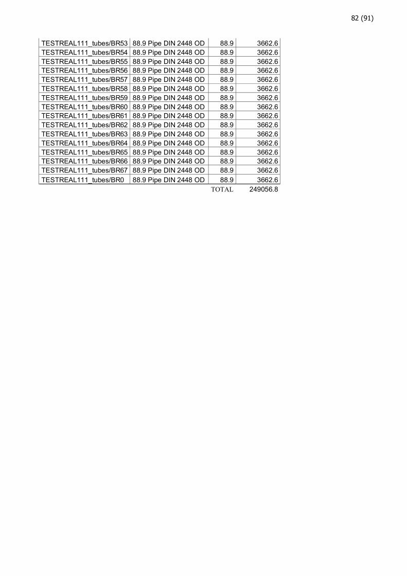
82 (91)

TESTREAL111_tubes/BR53 88.9 Pipe DIN 2448 OD 88.9 3662.6

TESTREAL111_tubes/BR54 88.9 Pipe DIN 2448 OD 88.9 3662.6

TESTREAL111_tubes/BR55 88.9 Pipe DIN 2448 OD 88.9 3662.6

TESTREAL111_tubes/BR56 88.9 Pipe DIN 2448 OD 88.9 3662.6

TESTREAL111_tubes/BR57 88.9 Pipe DIN 2448 OD 88.9 3662.6

TESTREAL111_tubes/BR58 88.9 Pipe DIN 2448 OD 88.9 3662.6

TESTREAL111_tubes/BR59 88.9 Pipe DIN 2448 OD 88.9 3662.6

TESTREAL111_tubes/BR60 88.9 Pipe DIN 2448 OD 88.9 3662.6

TESTREAL111_tubes/BR61 88.9 Pipe DIN 2448 OD 88.9 3662.6

TESTREAL111_tubes/BR62 88.9 Pipe DIN 2448 OD 88.9 3662.6

TESTREAL111_tubes/BR63 88.9 Pipe DIN 2448 OD 88.9 3662.6

TESTREAL111_tubes/BR64 88.9 Pipe DIN 2448 OD 88.9 3662.6

TESTREAL111_tubes/BR65 88.9 Pipe DIN 2448 OD 88.9 3662.6

TESTREAL111_tubes/BR66 88.9 Pipe DIN 2448 OD 88.9 3662.6

TESTREAL111_tubes/BR67 88.9 Pipe DIN 2448 OD 88.9 3662.6

TESTREAL111_tubes/BR0 88.9 Pipe DIN 2448 OD 88.9 3662.6

TOTAL 249056.8

83 (91)

APPENDIX 2: PANEL MTO DETAIL

Panel Report

FRMW PANEL/FLOOR

Height(mm)

Volume(m3)

Surface Area(m2)

Total Surface Area(m2)

TESTREAL111_Distribution1 =16386/34690 6 0.01 1.16

=16386/34680 3250 0.2 0.06

=16386/34674 6 0.01 1.16

=16386/34664 3250 0.2 0.06 2.45

TESTREAL111_Distribution0 =16386/34474 6 0.01 1.16

=16386/34464 3250 0.2 0.06

=16386/34458 6 0.01 1.16

=16386/34448 3250 0.2 0.06 2.45

TESTREAL111_OutletDucts =16386/34258 5 0.01 1.8

=16386/34252 5 0.01 1.8

=16386/34246 5 0.01 1.8

=16386/34240 5 0 0.92

=16386/34234 5 0 0.92

=16386/34228 5 0.01 1.16

=16386/34222 5 0.01 1.16

=16386/34216 5 0 0.92

=16386/34210 5 0 0.92

=16386/34204 5 0.01 1.16

=16386/34198 5 0.01 1.16

=16386/34187 5 0.01 1.8

=16386/34181 5 0.01 1.8

=16386/34175 5 0.01 1.8

=16386/34169 5 0 0.92

=16386/34163 5 0 0.92

=16386/34157 5 0.01 1.16

=16386/34151 5 0.01 1.16

=16386/34145 5 0 0.92

=16386/34139 5 0 0.92

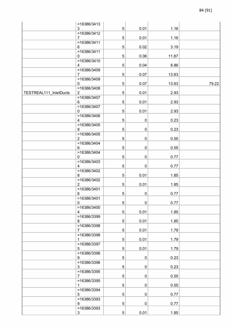
84 (91)

=16386/34133 5 0.01 1.16

=16386/34127 5 0.01 1.16

=16386/34116 5 0.02 3.19

=16386/34110 5 0.06 11.87

=16386/34104 5 0.04 8.86

=16386/34097 5 0.07 13.93

=16386/34090 5 0.07 13.93 79.22

TESTREAL111_InletDucts =16386/34082 5 0.01 2.93

=16386/34076 5 0.01 2.93

=16386/34070 5 0.01 2.93

=16386/34064 5 0 0.23

=16386/34058 5 0 0.23

=16386/34052 5 0 0.55

=16386/34046 5 0 0.55

=16386/34040 5 0 0.77

=16386/34034 5 0 0.77

=16386/34028 5 0.01 1.85

=16386/34022 5 0.01 1.85

=16386/34016 5 0 0.77

=16386/34010 5 0 0.77

=16386/34004 5 0.01 1.85

=16386/33998 5 0.01 1.85

=16386/33987 5 0.01 1.79

=16386/33981 5 0.01 1.79

=16386/33975 5 0.01 1.79

=16386/33969 5 0 0.23

=16386/33963 5 0 0.23

=16386/33957 5 0 0.55

=16386/33951 5 0 0.55

=16386/33945 5 0 0.77

=16386/33939 5 0 0.77

=16386/33933 5 0.01 1.85

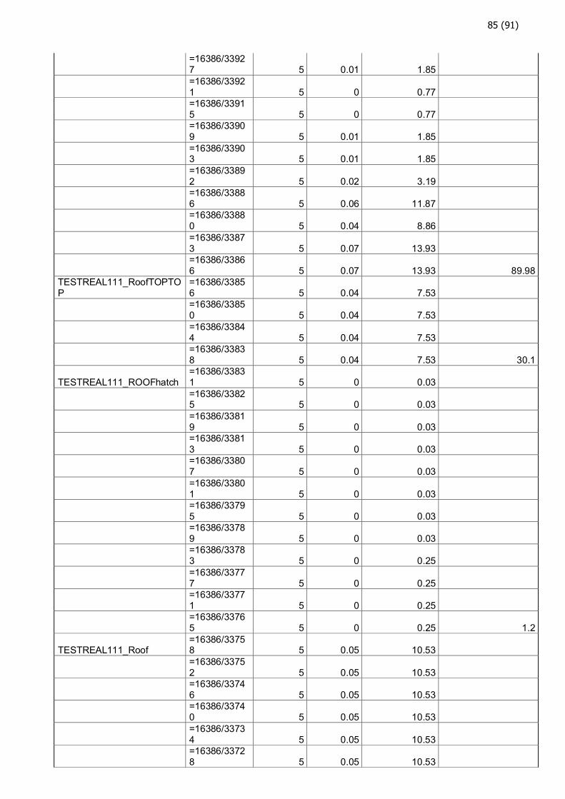
85 (91)

=16386/33927 5 0.01 1.85

=16386/33921 5 0 0.77

=16386/33915 5 0 0.77

=16386/33909 5 0.01 1.85

=16386/33903 5 0.01 1.85

=16386/33892 5 0.02 3.19

=16386/33886 5 0.06 11.87

=16386/33880 5 0.04 8.86

=16386/33873 5 0.07 13.93

=16386/33866 5 0.07 13.93 89.98

TESTREAL111_RoofTOPTOP

=16386/33856 5 0.04 7.53

=16386/33850 5 0.04 7.53

=16386/33844 5 0.04 7.53

=16386/33838 5 0.04 7.53 30.1

TESTREAL111_ROOFhatch =16386/33831 5 0 0.03

=16386/33825 5 0 0.03

=16386/33819 5 0 0.03

=16386/33813 5 0 0.03

=16386/33807 5 0 0.03

=16386/33801 5 0 0.03

=16386/33795 5 0 0.03

=16386/33789 5 0 0.03

=16386/33783 5 0 0.25

=16386/33777 5 0 0.25

=16386/33771 5 0 0.25

=16386/33765 5 0 0.25 1.2

TESTREAL111_Roof =16386/33758 5 0.05 10.53

=16386/33752 5 0.05 10.53

=16386/33746 5 0.05 10.53

=16386/33740 5 0.05 10.53

=16386/33734 5 0.05 10.53

=16386/33728 5 0.05 10.53

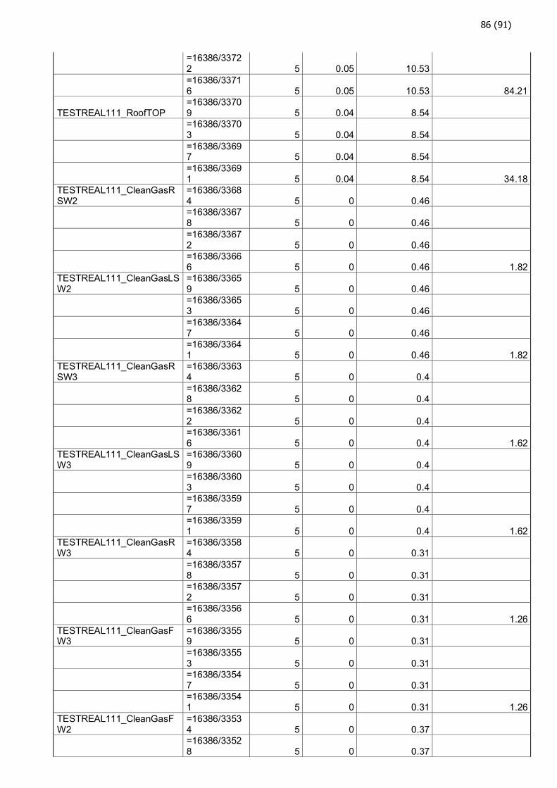
86 (91)

=16386/33722 5 0.05 10.53

=16386/33716 5 0.05 10.53 84.21

TESTREAL111_RoofTOP =16386/33709 5 0.04 8.54

=16386/33703 5 0.04 8.54

=16386/33697 5 0.04 8.54

=16386/33691 5 0.04 8.54 34.18

TESTREAL111_CleanGasRSW2

=16386/33684 5 0 0.46

=16386/33678 5 0 0.46

=16386/33672 5 0 0.46

=16386/33666 5 0 0.46 1.82

TESTREAL111_CleanGasLSW2

=16386/33659 5 0 0.46

=16386/33653 5 0 0.46

=16386/33647 5 0 0.46

=16386/33641 5 0 0.46 1.82

TESTREAL111_CleanGasRSW3

=16386/33634 5 0 0.4

=16386/33628 5 0 0.4

=16386/33622 5 0 0.4

=16386/33616 5 0 0.4 1.62

TESTREAL111_CleanGasLSW3

=16386/33609 5 0 0.4

=16386/33603 5 0 0.4

=16386/33597 5 0 0.4

=16386/33591 5 0 0.4 1.62

TESTREAL111_CleanGasRW3

=16386/33584 5 0 0.31

=16386/33578 5 0 0.31

=16386/33572 5 0 0.31

=16386/33566 5 0 0.31 1.26

TESTREAL111_CleanGasFW3

=16386/33559 5 0 0.31

=16386/33553 5 0 0.31

=16386/33547 5 0 0.31

=16386/33541 5 0 0.31 1.26

TESTREAL111_CleanGasFW2

=16386/33534 5 0 0.37

=16386/33528 5 0 0.37

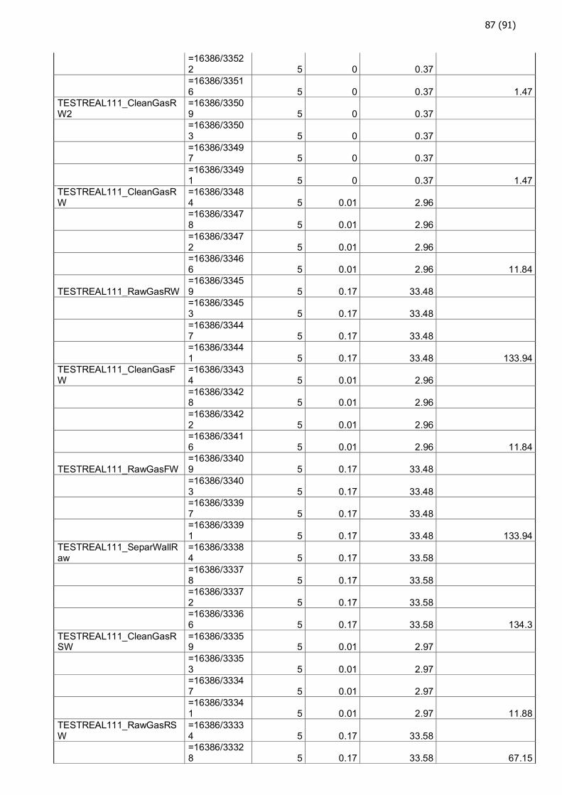
87 (91)

=16386/33522 5 0 0.37

=16386/33516 5 0 0.37 1.47

TESTREAL111_CleanGasRW2

=16386/33509 5 0 0.37

=16386/33503 5 0 0.37

=16386/33497 5 0 0.37

=16386/33491 5 0 0.37 1.47

TESTREAL111_CleanGasRW

=16386/33484 5 0.01 2.96

=16386/33478 5 0.01 2.96

=16386/33472 5 0.01 2.96

=16386/33466 5 0.01 2.96 11.84

TESTREAL111_RawGasRW =16386/33459 5 0.17 33.48

=16386/33453 5 0.17 33.48

=16386/33447 5 0.17 33.48

=16386/33441 5 0.17 33.48 133.94

TESTREAL111_CleanGasFW

=16386/33434 5 0.01 2.96

=16386/33428 5 0.01 2.96

=16386/33422 5 0.01 2.96

=16386/33416 5 0.01 2.96 11.84

TESTREAL111_RawGasFW =16386/33409 5 0.17 33.48

=16386/33403 5 0.17 33.48

=16386/33397 5 0.17 33.48

=16386/33391 5 0.17 33.48 133.94

TESTREAL111_SeparWallRaw

=16386/33384 5 0.17 33.58

=16386/33378 5 0.17 33.58

=16386/33372 5 0.17 33.58

=16386/33366 5 0.17 33.58 134.3

TESTREAL111_CleanGasRSW

=16386/33359 5 0.01 2.97

=16386/33353 5 0.01 2.97

=16386/33347 5 0.01 2.97

=16386/33341 5 0.01 2.97 11.88

TESTREAL111_RawGasRSW

=16386/33334 5 0.17 33.58

=16386/33328 5 0.17 33.58 67.15

88 (91)

TESTREAL111_CleanGasLSW

=16386/33321 5 0.01 2.97

=16386/33315 5 0.01 2.97

=16386/33309 5 0.01 2.97

=16386/33303 5 0.01 2.97 11.88

TESTREAL111_RawGasLSW

=16386/33296 5 0.17 33.58

=16386/33290 5 0.17 33.58 67.15

920.05

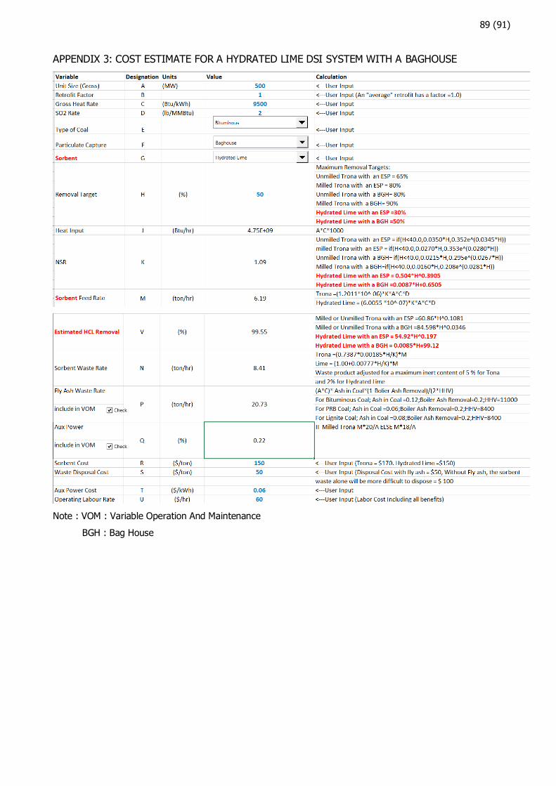
89 (91)

APPENDIX 3: COST ESTIMATE FOR A HYDRATED LIME DSI SYSTEM WITH A BAGHOUSE

Note : VOM : Variable Operation And Maintenance

BGH : Bag House

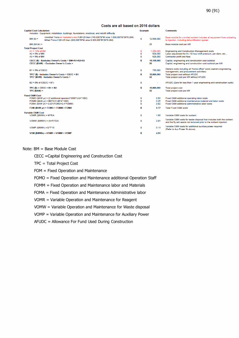
90 (91)

Note: BM = Base Module Cost

CECC =Capital Engineering and Construction Cost

TPC = Total Project Cost

FOM = Fixed Operation and Maintenance

FOMO = Fixed Operation and Maintenance additional Operation Staff

FOMM = Fixed Operation and Maintenance labor and Materials

FOMA = Fixed Operation and Maintenance Administrative labor

VOMR = Variable Operation and Maintenance for Reagent

VOMW = Variable Operation and Maintenance for Waste disposal

VOMP = Variable Operation and Maintenance for Auxiliary Power

AFUDC = Allowance For Fund Used During Construction

91 (91)

APPENDIX 4: COST ESTIMATE FOR A SDA FGD SYSTEM WITH A BAGHOUSE