Computer Physics Communications 185 (2014) 3344–3357

Contents lists available at ScienceDirect

Computer Physics Communications

journal homepage: www.elsevier.com/locate/cpc

CPMC-Lab: A Matlab package for Constrained Path Monte Carlocalculations✩

Huy Nguyen a,b, Hao Shi b, Jie Xu b, Shiwei Zhang b,∗

a Department of Physics, Reed College, Portland, OR 97202, USAb Department of Physics, College of William and Mary, Williamsburg, VA 23185, USA

a r t i c l e i n f o

Article history:Received 15 March 2014Received in revised form29 July 2014Accepted 1 August 2014Available online 12 August 2014

Keywords:QuantumMonte CarloAuxiliary field quantum Monte CarloConstrained Path Monte CarloSign problemHubbard modelPedagogical software

a b s t r a c t

We describe CPMC-Lab, aMatlab program for the constrained-path and phaseless auxiliary-field MonteCarlo methods. These methods have allowed applications ranging from the study of strongly correlatedmodels, such as the Hubbard model, to ab initio calculations in molecules and solids. The presentpackage implements the full ground-state constrained-path Monte Carlo (CPMC) method inMatlabwitha graphical interface, using the Hubbard model as an example. The package can perform calculations infinite supercells in any dimensions, under periodic or twist boundary conditions. Importance samplingand all other algorithmic details of a total energy calculation are included and illustrated. This open-source tool allows users to experiment with various model and run parameters and visualize the results.It provides a direct and interactive environment to learn the method and study the code with minimaloverhead for setup. Furthermore, the package can be easily generalized for auxiliary-field quantumMonteCarlo (AFQMC) calculations in many other models for correlated electron systems, and can serve as atemplate for developing a production code for AFQMC total energy calculations in real materials. Severalillustrative studies are carried out in one- and two-dimensional lattices on total energy, kinetic energy,potential energy, and charge- and spin-gaps.

Program summaryProgram title: CPMC-LabCatalogue identifier: AEUD_v1_0Program summary URL: http://cpc.cs.qub.ac.uk/summaries/AEUD_v1_0.htmlProgram obtainable from: CPC Program Library, Queen’s University, Belfast, N. IrelandLicensing provisions: Standard CPC licence, http://cpc.cs.qub.ac.uk/licence/licence.htmlNo. of lines in distributed program, including test data, etc.: 2850No. of bytes in distributed program, including test data, etc.: 24838Distribution format: tar.gzProgramming language:Matlab.Computer: The non-interactive scripts can be executed on any computer capable of running Matlabwith all Matlab versions. The GUI requires Matlab R2010b (version 7.11) and above. Operating system:Windows, Mac OS X, Linux.RAM: Variable.Classification: 7.3.External routines:MatlabNature of problem:Obtaining ground state energy of a repulsive Hubbard model in a supercell in any number of dimensions.Solution method:In the Constrained Path Monte Carlo (CPMC) method, the ground state of a many-fermion system isprojected from an initial trial wave function by a branching random walk in an overcomplete basis ofSlater determinants. Constraining the determinants according to a trial wave function |ΨT ⟩ removes the

✩ This paper and its associated computer program are available via the Computer Physics Communication homepage on ScienceDirect (http://www.sciencedirect.com/science/journal/00104655).∗ Corresponding author.

E-mail address: shiwei@wm.edu (S. Zhang).

http://dx.doi.org/10.1016/j.cpc.2014.08.0030010-4655/© 2014 Elsevier B.V. All rights reserved.

H. Nguyen et al. / Computer Physics Communications 185 (2014) 3344–3357 3345

exponential decay of the signal-to-noise ratio characteristic of the sign problem. The method is exact if|ΨT ⟩ is exact.Unusual features:Direct and interactive environment with a Graphical User Interface for beginners to learn and study theConstrained Path Monte Carlo method with minimal overhead for setup.Running time:The sample provided takes a few seconds to run, the batch sample a few minutes.

© 2014 Elsevier B.V. All rights reserved.

1. Introduction

The study of interacting quantummany-body systems remainsan outstanding challenge, especially systems with strong particleinteractions, where perturbative approaches are often ineffective.Numerical simulations provide a promising approach for studyingsuch systems. One of the most general numerical approaches isquantum Monte Carlo (QMC) methods based on auxiliary fields,which are applied in condensed matter physics, nuclear physics,high-energy physics and quantum chemistry. These methodsallow essentially exact calculations of ground-state and finite-temperature equilibrium properties of interacting many fermionsystems.

As is well-known, however, these methods suffer from the signproblem which severely limits their applicability. Considerableprogress has been achieved in circumventing this problem by con-straining the random walks while sampling the space of auxil-iary fields [1]. Many applications of this method involve latticeswhere there is a sign problem, for example, Hubbard-like modelswhere the local interactions lead to auxiliary-fields that are real. Inthese cases the method is known as Constrained Path Monte Carlo(CPMC) [2,3]. The method can also be generalized to treat realis-tic electron–electron interactions to allow for ab initio calculationson real materials [4,5]. For these systems there is a phase prob-lem because the Coulomb interaction leads to complex auxiliaryfields. In such systems, the method is referred to as phaseless orphase-free auxiliary-field QMC (AFQMC). In both cases (lattice andcontinuum), the idea behind the method is to constrain the signor phase of the overlap of the sampled Slater determinants witha trial wave function. The constraint eliminates the sign or phaseinstability and restores low power (typically to the third power ofsystem size) computational scaling. Applications to systems rang-ing from lattice models [6,7] of correlated systems to solids [8,9]to atoms and molecules [10] have shown that these methods arevery accurate, even with simple trial wave functions taken directlyfrom Hartree–Fock or density-functional calculations.

Since these methods combine standard mean-field approacheswith stochastic QMC, they pose a formidable barrier to beginners.As such, it is useful to have a pedagogical platform to learn themethods and to aid further code development. In this paper, wepresent a Matlab package that fulfills these roles. The packageillustrates the CPMCmethod for the Hubbardmodel, with a graph-ical interface. The ground-state energy is calculated using im-portance sampling and implementing the full algorithmic details.With this open-source package, calculations can be performeddirectly on Hubbard-like models in any dimensions, under anyboundary conditions. It will be straightforward to generalize thecode for applications in many other models of correlated elec-tron systems. Furthermore, the code contains the core QMC algo-rithmic ingredients for a total energy AFQMC calculation. Theseingredients can be combined with standard electronic structuremachineries [11] (see, e.g., Refs. [12,13]) to develop a productioncode for AFQMC total energy calculations in molecules and solids.

The tool presented here allows users to experiment with var-ious model and run parameters and visualize the results. For thispurposeMatlab offersmany advantages over traditional program-ming languages such as FORTRAN or C. As an interpreted language,Matlab requires no compilation, is platform-independent andallows easy interaction with the algorithm during runtime.Matlab also provides an array of tools to visualize results fromcomputations including a full graphical user interface (GUI). Theseadvantages make the package a better choice for our purposes, asdiscussed above, than regular ‘‘production’’ codes, despite a largediscrepancy in computational speed.We provide several examplesand include more questions in the exercises, which illustrate theusage of the code, key algorithmic features, how to compute vari-ous properties in the Hubbard model, and how to generalize it forother applications. As a pedagogical tool, the package can be usedin combination with the lecture notes in Ref. [1] and referencestherein.

The remainder of the paper is organized as follows. In Section 2we introduce the formalism and various technical ingredients ofthe CPMC method, and notations used in the rest of this paper. InSection 3 the actual algorithm is outlined in detail. An overviewof the software package and instructions is given in Section 4,including a list of exercises. In Section 5, we briefly discussthe computational cost and comment on the relation betweenthis package and one written in a more conventional numericalprogramming language. Then in Section 6, we present severalapplications which illustrate algorithmic issues; benchmark themethod; discuss CPMC calculations of the kinetic energy, potentialenergy and double occupancy; and report several new CPMCresults on the spin- and charge-gaps. We summarize in Section 7and include a list of some usefulMatlab commands in Appendix.

2. Method and notation

The ground-state CPMC algorithm has two main components.The first component is the formulation of the ground state pro-jection as an open-ended importance-sampled random walk. Thisrandom walk takes place in Slater determinant space ratherthan configuration space like in Green’s function Monte Carlo(GFMC) [14,15]. There are two ways to perform this random walk.Traditional projector QMC uses an exact unconstrained projectionthat suffers from exponential scaling in computational cost withincreasing system size due to the sign problem. In contrast, CPMCachieves polynomial scaling by using an approximate constrainedprojection, which becomes exact if the trial wave function (usedto impose the constraint) is identical to the ground state. Further-more, importance sampling makes CPMC a more efficient way todo projector QMC in many cases. The second component is theconstraint of the paths of the random walk so that any Slaterdeterminant generated during the random walk maintains an ap-propriate overlap with a known trial wave function |ψT⟩. This con-straint eliminates the sign decay, making the CPMC method scalealgebraically instead of exponentially, but introduces a systematic

3346 H. Nguyen et al. / Computer Physics Communications 185 (2014) 3344–3357

error in the algorithm. These two components are independent ofeach other, and can be used separately. We call the combination ofthese two components the ground-state CPMC algorithm. This sec-tion only briefly reviews the application of CPMC to the Hubbardmodel. The reader is referred to Refs. [1,2] and references thereinfor a discussion of the Hubbard model implementation and gener-alization of this theory to other, more realistic Hamiltonians.

2.1. Slater determinant space

The CPMC method works with a chosen one-particle basis. ABorn–Oppenheimer Hamiltonianwith standard electronic interac-tions does not mix the spins. We assume in the discussion belowthat the Hamiltonian conserves total Sz , and that the number ofelectrons with each spin component is fixed. It is straightforwardto treat a Hamiltonian that does mix the spin species [16].

We will use the following notation:

• M: the number of single-electron basis states, e.g. the numberof lattice sites in the Hubbard model.• |χi⟩: the ith single-particle basis state (i = 1, 2, . . . ,M).• cĎi and ci: creation and annihilation operators for an electron in|χi⟩. ni ≡ cĎi ci is the corresponding number operator.• N: the number of electrons. Nσ is the number of electrons with

spin σ (σ =↑ or ↓). As expected, Nσ ≤ M .• ϕ: a single-particle orbital. The coefficients in the expansionϕ =

i ϕi|χi⟩ =

i c

Ďi ϕi|0⟩ in the single particle basis {|χi⟩}

can be conveniently expressed as anM-dimensional vector:ϕ1ϕ2...ϕM

. (1)

• |φ⟩: a many-body wave function which can be written asa Slater determinant. Given N different single-particle or-bitals, we form a many-body wave function from their anti-symmetrized product:

|φ⟩ ≡ ϕĎ1 ϕ

Ď2 · · · ϕ

ĎN |0⟩ (2)

where the operator ϕĎm ≡

i c

Ďi ϕi,m creates an electron in the

mth single-particle orbital as described in Eq. (1).• Φ: an M × N matrix which represents the coefficients of the

orbitals used to construct a Slater determinant |φ⟩:

Φ ≡

ϕ1,1 ϕ1,2 · · · ϕ1,Nϕ2,1 ϕ2,2 · · · ϕ2,N...

......

ϕM,1 ϕM,2 · · · ϕM,N

. (3)

Each column of thismatrix is anM-dimensional vector and rep-resents a single-particle orbital described by Eq. (1). For brevity,we will subsequently refer to this M × N matrix as a Slater de-terminant.• |Ψ ⟩ (upper case): amany-bodywave functionwhich is not nec-

essarily a single Slater determinant, e.g. the many-body groundstate |Ψ0⟩.

We list several properties of a Slater determinant. First, for anytwo non-orthogonal Slater determinants, |φ⟩ and |φ′⟩, it can beshown that their overlap integral, which is a number, is given by:

⟨φ|φ′⟩ = detΦĎΦ ′

, (4)

whereΦĎ is the conjugate transpose of the matrixΦ .

Second, the operation on any Slater determinant in Eq. (2) bythe exponential of a one body operator

B = exp

Mij

cĎi Uijcj

(5)

simply leads to another Slater determinant [17]:

B|φ⟩ = φ′ Ď1 φ′ Ď2 · · · φ

′ ĎN |0⟩ ≡ |φ

′⟩ (6)

with φ′ Ďm =

j cĎj Φ′

jm and Φ ′ ≡ eUΦ , where the matrix U isformed from elementsUij. Since B ≡ eU is anM×M squarematrix,the operation of B on |φ⟩ simply involvesmultiplying eU , anM×Mmatrix, toΦ , an M × N matrix.

As mentioned above, operations on the spin-up sector do notaffect the spin-down sector and vice versa. Thus it is convenient torepresent each Slater determinant as two independent spin parts:

|φ⟩ = |φ↑⟩ ⊗ |φ↓⟩. (7)

The corresponding matrix representation is

Φ = Φ↑ ⊗ Φ↓ (8)

where Φ↑ and Φ↓ have dimensions M × N↑ and M × N↓,respectively. The overlap between any two Slater determinants issimply the product of the overlaps of individual spin determinants:

⟨φ|φ′⟩ =σ=↑,↓

⟨φσ |φ′σ ⟩ = det(Φ↑)ĎΦ ′

↑· det

(Φ↓)ĎΦ ′

↓. (9)

Any operator B described by Eq. (5) acts independently on the twospin parts:

B|φ⟩ = B↑|φ↑⟩ ⊗ B↓|φ↓⟩. (10)

Each of the spin components of B can be represented as anM ×M matrix. Applying B to a Slater determinant simply involvesmatrix multiplications for the ↑ and ↓ components separately,leading to another Slater determinant |φ′⟩ as in Eq. (6) i.e. the resultis B↑Φ↑ ⊗ B↓Φ↓. Unless specified, the spin components of B areidentical i.e. B↑ = B↓ (note the absence of a hat on B to denote thematrix of the operator B).

2.2. The Hubbard Hamiltonian

The one-band Hubbard model is a simple paradigm of a systemof interacting electrons. Its Hamiltonian is given by

H = K + V = −t⟨ij⟩σ

(cĎiσ cjσ + cĎjσ ciσ )+ U

i

ni↑ni↓, (11)

where t is the hoppingmatrix element, and cĎiσ and ciσ are electroncreation and destruction operators, respectively, of spin σ on sitei. The Hamiltonian is defined on a lattice of dimensionM =

d Ld.

The lattice sites serve as the basis functions here, i.e., |χi⟩ denotesan electron localized on the site labeled by i. The notation ⟨ ⟩ in Eq.(11) indicates nearest-neighbors. The on-site Coulomb repulsion isU > 0, and themodel only has two parameters: the strength of theinteractionU/t and the electron density (N↑+N↓)/M . In this paperwe will use t as the unit of energy and set t = 1.

The difference between the Hubbard Hamiltonian and a generalelectronic Hamiltonian is in the structure of the matrix elementsin K and V . In the latter, K is specified by hopping integrals ofthe form Kij, while V is specified by Coulomb matrix elementsof the form Vijkl, with i, j, k, l in general running from 1 to M . Interms of the CPMC method, the structure of K makes essentiallyno difference. The structure of V , however, dictates the form of

H. Nguyen et al. / Computer Physics Communications 185 (2014) 3344–3357 3347

the Hubbard–Stratonovich transformation (see Section 2.3.1). Forthe Hubbard interaction, the resulting one-body propagators turnout to be real, as shown below, while for the general case complexpropagators arise and cause a phase problem [1].

2.3. Ground-state projection

Wewill focus on ground-state calculations in this paper. (Finite-temperature generalizations to the grand-canonical ensemblealso exist [18,19].) The ground-state wave function |Ψ0⟩ can beobtained from any trial wave function |ΨT⟩ that is not orthogonalto |Ψ0⟩ by repeated applications of the ground-state projectionoperator

Pgs = e−∆τ(H−ET) (12)

where ET is the best guess of the ground-state energy. That is, if thewave function at the nth time step is |Ψ (n)

⟩, the wave function atthe next time step is given by

|Ψ (n+1)⟩ = e−∆τ(H−ET)|Ψ (n)

⟩. (13)

With a small ∆τ , the second-order Trotter approximation canbe used:

e−∆τ H = e−∆τ(K+V ) ≈ e−∆τ K/2e−∆τ V e−∆τ K/2. (14)

The residual Trotter error can be removed by, for example, extrap-olation with several independent runs of sufficiently small∆τ val-ues. We illustrate this technique in an exercise in Section 4.2.2.

2.3.1. The Hubbard–Stratonovich transformationIn Eq. (14), the kinetic energy (or, more generally, one-body)

propagator BK/2 ≡ e−∆τ K/2 has the same form as Eq. (5). How-ever, the potential energy propagator e−∆τ V does not. A Hubbard–Stratonovich (HS) transformation can be employed to transforme−∆τ V into the desired form. In the Hubbardmodel, we can use thefollowing:

e−∆τUni↑ni↓ = e−∆τU(ni↑+ni↓)/2xi=±1

p(xi) eγ xi(ni↑−ni↓), (15)

where γ is given by cosh(γ ) = exp(∆τU/2). We interpret p(xi) =1/2 as a discrete probability density function (PDF) with xi = ±1.

In Eq. (15), the exponent on the left, which comes from theinteraction term V on the ith site, is quadratic in n, indicating theinteraction of two electrons. The exponents on the right, on theother hand, are linear inn, indicating twonon-interacting electronsin a common external field characterized by xi. Thus an interactingsystem has been converted into a non-interacting system livingin fluctuating external auxiliary fields xi, and the summation overall such auxiliary-field configurations recovers the many-bodyinteractions. The special form of HS for the Hubbard interaction isdue to Hirsch [20]. The linearized operator on the right hand sidein Eq. (15) is the spin (ni↑ − ni↓) on each site.

In this paper and in the code, we will use the discrete spindecomposition in Eq. (15). There exist other ways to do the HStransformation, e.g. based on the Gaussian integral:

eA2=

1√2π

∞

−∞

dx e−x2/2

e√2x A. (16)

There is also a charge version of the discrete HS transformationinvolving the linearized operator ni↑+ni↓, the total charge on eachsite.

Different forms of the HS transformation can have differentefficiencies in different situations. In particular, preserving theappropriate symmetries of the system can significantly reduce the

statistical fluctuations and reduce the error from the constrained-path approximation [7].

Since we represent a Slater determinant as individual spindeterminants in Eq. (7), it is convenient to spin-factorize Eq. (15)as

e−∆τUni↑ni↓ =xi=±1

p(xi)b↑V (xi)⊗ b↓V (xi)

(17)

where the spin-dependent operator bσV (xi) on the ith lattice site isdefined as

bσV (xi) = e−[∆τU/2−s(σ ) γ xi]cĎiσ ciσ (18)

and s(↑) = +1 and s(↓) = −1. The related operator bV(xi) (i.e.without σ ) includes both the spin up and spin down parts. Belowwe will use the corresponding symbol without hat (bV) to denotethe matrix representation of the operator (bV) associated with thatsymbol.

The potential energy propagator e−∆τ V over all sites is theproduct of the propagators e−∆τUni↑ni↓ over each site:

e−∆τ V =x

P(x)σ=↑,↓

BσV (x) (19)

where x = {x1, . . . , xM} is one configuration of auxiliary fieldsover all M sites and BσV (x) =

i bσV (xi) is the x-dependent product

of the spin-σ propagators over all sites. The overall PDF here isP(x) =

i p(xi) =

12

M, to be distinguished from the PDF p for

one individual auxiliary field xi in Eq. (17).Now the projection operator in Eq. (12) can be expressed

entirely in terms of operators in Eq. (5)

Pgs ≈ e∆τETx

P(x)σ=↑,↓

BσK/2BσV (x)B

σK/2. (20)

As noted in Eq. (10),BK/2 has an↑ and a↓ component, each ofwhichis an M × M matrix. Applying each BK/2 to a Slater determinant|φ⟩ simply involvesmatrix multiplications with thematrix BK/2 forthe ↑ and ↓ components ofΦ separately, leading to another Slaterdeterminant |φ′⟩ as in Eq. (6). The same holds for BV.

2.3.2. A toy model for illustrationLet us take, for example, a simple one-dimensional four-site

Hubbard model with N↑ = 2, N↓ = 1 and open boundary con-dition. The sites are numbered sequentially.

First let us examine the trivial case of free electrons i.e. U = 0.We can write down the one-electron Hamiltonian matrix, which isof dimension 4× 4:

H =

0 −1 0 0−1 0 −1 00 −1 0 −10 0 −1 0

. (21)

Direct diagonalization gives us the eigenstates of H from whichwe immediately obtain the matrix Φ0 for the ground-state wavefunction |ψ0⟩:

Φ0 =

0.3717 −0.60150.6015 −0.37170.6015 0.37170.3717 0.6015

⊗0.37170.60150.60150.3717

(22)

where the first matrix contains two single-particle orbitals (twocolumns) for the two ↑ electrons and the second matrix containsone single-electron orbital for the one ↓ electron. Each single-electron orbital is an eigenvector of H .

3348 H. Nguyen et al. / Computer Physics Communications 185 (2014) 3344–3357

The matrixΦ0 represents |φ0⟩ in the same way that Eq. (3) rep-resents Eq. (2). Of course, the solution above is also the restrictedHartree–Fock solution to the interacting problem.Wewill often useΦ0 as the trial wave function in CPMC below.

Next we consider the interacting problem, with U > 0. Apply-ing the HS transformation of Eq. (15) to Eq. (14), we have

Pgs =e∆τET−∆τU(N↑+N↓)/2

×

x

P(x) BK/2 ·

eγ x1 0 0 00 eγ x2 0 00 0 eγ x3 00 0 0 eγ x4

· BK/2

⊗ BK/2 ·

e−γ x1 0 0 00 e−γ x2 0 00 0 e−γ x3 00 0 0 e−γ x4

· BK/2

(23)

where x = {x1, x2, x3, x4} and P(x) = 12

4. This is just Eq. (20)

specialized to a four-site lattice.

2.4. Random walk in Slater determinant space

The first component of the CPMC algorithm is the reformulationof the projection process as branching, open-ended random walksin Slater determinant space (instead of updating a fixed-lengthpath in auxiliary-field space).

Let us define BV(x) =σ BσV (x) as we have done for bV. Apply-

ing the HS-transformed propagator in Eq. (20) to one projectionstep in Eq. (13) gives

|φ(n+1)⟩ = e∆τETx

P(x)BK/2BV(x)BK/2

|φ(n)⟩. (24)

In the Monte Carlo (MC) realization of this iteration, werepresent the wave function at each stage by a finite ensemble ofSlater determinants, i.e.

|Ψ (n)⟩ ∝

k

|φ(n)k ⟩ (25)

where k labels the Slater determinants and an overall normaliza-tion factor of the wave function has been omitted. These Slater de-terminants will be referred to as random walkers.

The iteration in Eq. (24) is achieved stochastically by MCsampling of x. That is, for each random walker |φ(n)k ⟩, we choosean auxiliary-field configuration x according to the PDF P(x) andpropagate the determinant to a new determinant via |φ(n+1)k ⟩ =

BK/2BV(x)BK/2|φ(n)k ⟩.

We repeat this procedure for all walkers in the population.These operations accomplish one step of the random walk. Thenew population represents |Ψ (n+1)

⟩ in the sense of Eq. (25),i.e. |Ψ (n+1)

⟩ ∝

k |φ(n+1)k ⟩. These steps are iterated until sufficient

data has been collected. After an equilibration phase, all walkersthereon are MC samples of the ground-state wave function |Ψ0⟩

and ground-state properties can be computed.Wewill refer to thistype of approach as free projection. In practice, branching occursbecause of the re-orthonormalization of the walkers, which wediscuss below in Section 2.8. We emphasize that the statisticalerror bar can be reduced significantly with more ‘‘optimal’’ formsof HS transformations to extend the reach of free-projectioncalculations (see e.g., Refs. [1,7]).

2.5. Importance sampling

To improve the efficiency of Eq. (24) and make it a practicaland scalable algorithm, an importance sampling scheme [1,14,15]

is required. In the procedure just described above, no informationis contained in the sampling of x on the importance of the resultingdeterminant in representing |Ψ0⟩. Computing the mixed estimatorof the ground-state energy

Emixed ≡⟨φT|H|Ψ0⟩

⟨φT|Ψ0⟩(26)

requires estimating the denominator by

k⟨φT|φk⟩ where |φk⟩

are random walkers after equilibration. Since these walkers aresampled with no knowledge of ⟨φT|φk⟩, terms in the summationover |φk⟩ can have large fluctuations that lead to large statisticalerrors in the MC estimate of the denominator, thereby in that ofEmixed.

With importance sampling, first we define an importancefunction:

OT(φk) ≡ ⟨φT|φk⟩, (27)

which estimates the overlap of a Slater determinant |φ⟩ with theground-state wave function (approximated here by a trial wavefunction). As in Diffusion Monte Carlo (DMC) [21], we also assigna weight wk = OT(φk) to each walker. This weight is initialized tounity for all walkers since in the initial ensemble, |φ(0)k ⟩ = |φT⟩ forall k.

We then iterate a formally different butmathematically equiva-lent version of Eq. (24):

|φ(n+1)⟩ ←x

P(x)B(x)|φ(n)⟩ (28)

where

B(x) = BK/2BV(x)BK/2. (29)

The walkers |φ(n)⟩ are now sampled from a new distribution. Theyschematically represent the ground-state wave function by:

|Ψ (n)⟩ ∝

k

w(n)|φ(n)k ⟩

OT(φ(n)k )

, (30)

in comparison to Eq. (25).The modified function P(x) in Eq. (28) is P(x) = M

i p(xi),where the probability for sampling the auxiliary-field at eachlattice site is given by

p(xi) = OT(φ(n)k,i )

OT(φ(n)k,i−1)

p(xi) (31)

where

|φ(n)k,i−1⟩ = bV (xi−1) bV (xi−2) . . . bV (x1) |φ

(n)k ⟩ (32)

is the current state of the kth walker, |φ(n)k ⟩, after its first (i − 1)fields have been sampled and updated, and

|φ(n)k,i ⟩ = bV (xi)|φ

(n)k,i−1⟩ (33)

is the next sub-step after the ith field is selected and the walkeris updated. Note that in the notation above |φ(n)k,0⟩ = |φ

(n)k ⟩ and

|φ(n)k,M⟩ = |φ

(n+1)k ⟩. As expected, P(x) is a function of both the

current and future positions in Slater-determinant space. Further,P(x) modifies P(x) such that the probability of sampling x isincreased when x leads to a determinant with larger overlapwith |φT⟩ and is decreased otherwise. In each p(xi), xi can onlytake the value of +1 or −1 and can be sampled by a heatbath-like algorithm: choosing xi from the PDF p(xi)/Ni where thenormalization factor is

Ni ≡p(xi = +1)+p(xi = −1), (34)

H. Nguyen et al. / Computer Physics Communications 185 (2014) 3344–3357 3349

and carrying a weight for the walker

w(n)k,i = Niw

(n)k,i−1, (35)

in which we have used the same notation as in Eqs. (32) and (33).The ratio of the overlaps in Eq. (31), involving a change of only onesite (or even a few sites if desired), can be computed quickly usingthe Sherman–Morrison formula, as shown in the code. The inverse

of the overlapmatrix(ΦT)

ĎΦ(n)k

−1is kept and updated after each

xi is selected.It should be pointed out that a significant reduction in computa-

tional cost is possible in the present code. Because the free-electrontrial wave function is used here, the overlap matrix can be triviallyupdated after each application of BK/2. In the code, however, theupdate is still carried out explicitly in order to allow for a moregeneral form of the trial wave function.

We note that, for a general continuous auxiliary-field, theimportance sampling can be achieved by a force bias [1,4,22]. Theabove discrete version can be viewed as a two-point realization ofthe continuous case.

2.6. The sign problem and the constrained path approximation

2.6.1. The sign problemThe sign problem occurs because of the fundamental symmetry

between the fermion ground state |Ψ0⟩ and its negative−|Ψ0⟩ [23].This symmetry implies that, for any ensemble of Slater deter-minants {|φ⟩} which gives a Monte Carlo representation of theground-state wave function, there exists another ensemble {−|φ⟩}which is also a correct representation. In other words, the Slaterdeterminant space can be divided into two degenerate halves (+and−) whose bounding surface N is defined by ⟨Ψ0|φ⟩ = 0. Thissurface is in general unknown. Except for some special cases [20],walkers do cross N in their propagation by Pgs, causing the signproblem. At the instant such a walker lands on N , the walker willmake no further contribution to the representation of the groundstate at any later time because

⟨Ψ0|φ⟩ = 0 H⇒ ⟨Ψ0|e−τH |φ⟩ = 0 for any τ . (36)

Paths that result from such a walker have equal probabilities ofbeing in either half of the Slater determinant space [1]. Computedanalytically, they would cancel and make no contribution in theground-state wave function. However, because the random walkhas no knowledge of N , these paths continue to be sampled(randomly) in the random walk and become Monte Carlo noise.

To eliminate the decay of the signal-to-noise ratio, we imposethe constrained path approximation. It requires that each randomwalker at each step have a positive overlap with the trial wavefunction |φT⟩:

⟨φT|φ(n)k ⟩ > 0. (37)

This yields an approximate solution to the ground-statewave func-tion, |Ψ c

0 ⟩ =

φ |φ⟩, in which all Slater determinants |φ⟩ satisfyEq. (37). Note that from Eq. (36), the constrained path approxima-tion becomes exact for an exact trial wave function |ψT⟩ = |Ψ0⟩.The constrained path approximation is easily implemented by re-defining the importance function in Eq. (27):

OT(φk) ≡ max{⟨φT|φk⟩, 0}. (38)

This prevents walkers from crossing the trial nodal surface N andentering the ‘‘−’’ half-space as defined by |φT⟩.Wenote that impos-ing Eq. (37) is fundamentally different from just discarding the neg-ative contributions in the denominator of Eq. (26); the constrainedpath condition results in a distribution of walkers that vanishessmoothly at the interface between the ‘‘+’’ and ‘‘−’’ parts of the

determinant space. The use of a finite ∆τ causes a small disconti-nuity which is a form of Trotter error in the constraint; this errorcan be further reduced [24].

2.6.2. Twist boundary condition and the phase problemOur simulations are carried out in supercells of finite sizes. For

most quantities that we wish to calculate, the periodic boundarycondition (PBC) causes large finite-size effects, often compoundedby significant shell effects [3]. In order to reduce these effects andreach the thermodynamic limit more rapidly, it is more effectiveto use the twist boundary condition (TBC) and average over thetwist angles [3,25] (TABC). Under the TBC, the wave functionΨ (r1, r2, . . . , rN) gains a phase when electrons hop around latticeboundaries:

Ψ (. . . , rj + L, . . .) = eiL·2Ψ (. . . , rj, . . .), (39)

where L is the unit vector along L and the twist angle 2 =

(θx, θy, θz, . . .) is a parameter with θd ∈ (−π, π] for d = x, y,z, . . . . It is implemented straightforwardly as a modification tothe matrix elements in the K part of the Hamiltonian. A twistis equivalent to shifting the underlying momentum space gridby (θx/Lx, θy/Ly, θz/Lz, . . .). Symmetry can be used to reduce therange of2. One could either choose to have a special grid of2 val-ues [11] or choose them randomly [3,25]. In the illustrations wewill use the latter. The QMC results are averaged, and the MC er-ror bar will be the combined statistical errors from the random 2

distribution and from each QMC calculation for a particular 2.With a general twist angle, the AFQMC method will have a

‘‘phase problem’’ instead of the sign problem described above.This is because the hopping matrix elements in K now havecomplex numbers which make the orbitals in the random walkerscomplex. The stochastic nature of the random walk will then leadto an asymptotic distribution which is symmetric in the complexplane [1,4]. For each walker |φ⟩, instead of a +|φ⟩ and −|φ⟩ as inthe sign problem, there is now an infinite set {eiθ |φ⟩} (θ ∈ [0, 2π ])from which the random walk cannot distinguish.

The phase problem that occurs in the present case is a ‘‘milder’’form of the most general phase problem, because here the phasesarise from the one-body hopping term instead of the two-bodyinteraction term. The latter takes place in a long-range Coulombinteraction, for example. In that case, the phase problem is con-trolled with the phaseless or phase-free approximation [1,4].When the phase only enters as a one-body boundary condition,the stochastic auxiliary-fields are not directly coupled to complexnumbers. A simple generalization of the constrained-path approx-imation suffices [3]: at each step of propagation, the randomwalk-ers are required to satisfy the constraint

Re

⟨φT|φ

(n+1)k ⟩

⟨φT|φ(n)k ⟩

> 0 (40)

where |φ(n)k ⟩ and |φ(n+1)k ⟩ are the current and proposed walkers.

Note that Eq. (38) is a special case of Eq. (40) because ⟨φT|φ(0)k ⟩ > 0

and all overlaps are real when K is real. We emphasize that, whenthe HS transformation leads to complex one-body propagators asin the case of realistic electronic problems, an extra step is requiredto ‘‘importance-transform’’ the propagators using the phase of theoverlap [1,4].

2.6.3. Systematic error from the constrained-path approximation, andits reduction and removal

Most applications have used a single-determinant |ψT⟩ takendirectly from a Hartree–Fock (HF) or density-functional theory(DFT) calculations. In the Hubbard model, the restricted HF wave

3350 H. Nguyen et al. / Computer Physics Communications 185 (2014) 3344–3357

Fig. 1. Illustration of the sign problem. The blue and red curves show the energyduring a projection from τ = 0 to τ = 7.5 with and without the constraint,respectively. The dashed black line shows the exact result. The CP error bars aretoo small to be seen. To improve clarity, only every other CP energy measurementsare shown for τ > 2.6. (For interpretation of the references to color in this figurelegend, the reader is referred to the web version of this article.)

function is the same as the free-electron wave function, whilethe unrestricted HF wave function breaks spin-symmetry andallows, for example, antiferromagnetism and spin-density-wavestates [26]. A large number of benchmarks have been carried outwith these wave functions [1,7].

Fig. 1 illustrates the effectiveness of the constrained pathapproximation. The system is a 4 × 4 lattice with 7 spin-↑ and7 spin-↓ electrons, U = 4 and 2 = (0.02π, 0.04π). The free-projection (FP) run exhibits growing statistical fluctuations as afunction of projection time, indicative of the sign problem. Withthe constraint, CPMC fluctuations are always smaller with thesame amount of computational cost, and they are independent ofprojection time. The CPMC results converge to a value below theexact result (horizontal line).

Multi-determinant trial wave functions can reduce the system-atic error because they are better variational wave functions [27].Usingwave functions that restore symmetries of the systemcan re-duce the systematic error significantly [7]. The symmetry restora-tion can be either in the form of a multi-determinant trial wavefunction or from symmetry projection [16]. For example, using a10-determinant symmetry trial wave function can reduce the sys-tematic error in the CPMC result for the system in Fig. 1 with peri-odic boundary condition by a significant factor [7].

Recently, it has been demonstrated [7,8,28] that free-projectionand release-constraint calculations allow systematic removalof the constrained-path bias by ‘‘lifting’’ the constraint (andbringing back the sign problem). This offers another avenue forsystematically improvable AFQMC calculations.

2.7. Energy measurement

CPMC-Lab uses the mixed estimator in Eq. (26) for the ground-state energy which, for an ensemble {|φ⟩}, is given by:

Emixed =

kwk EL [φT, φk]

kwk

(41)

where the local energy EL is:

EL [φT, φ] =⟨φT|H|φ⟩⟨φT|φ⟩

. (42)

This quantity can be easily evaluated for any walker φ as follows.For any pair of non-orthogonal Slater determinants |φT⟩ and |φ⟩,

we can calculate the one-body equal-time Green’s function as:

⟨cĎjσ ciσ ⟩ ≡⟨φT|c

Ďjσ ciσ |φ⟩

⟨φT|φ⟩=Φσ[ (Φσ

T )ĎΦσ]−1(Φσ

T )Ďij . (43)

This immediately enables the computation of the kinetic en-ergy term

φT

−t⟨ij⟩σ cĎiσ cjσφ. The potential energy term

φT

Ui cĎi↑ci↑c

Ďi↓ci↓

φ does not have the formof Eq. (43), but canbe reduced to that form by an application of Wick’s theorem:

⟨cĎi↑ci↑cĎi↓ci↓⟩ = ⟨c

Ďi↑ci↑⟩⟨c

Ďi↓ci↓⟩ + ⟨c

Ďi↑ci↓⟩⟨ci↑c

Ďi↓⟩

= ⟨cĎi↑ci↑⟩⟨cĎi↓ci↓⟩. (44)

The reduction to the last line occurs because the ↑ and ↓ spinsectors are decoupled in both |φT⟩ and |φ⟩. (This is not the casein a pairing [29] or generalized Hartree–Fock wave function [16].The former is the desired form for U < 0. The latter can be usedto improve the quality of the trial wave function for U > 0, and isnecessary if the Hamiltonian contains spin–orbit coupling.)

The mixed estimator for the energy arises naturally fromimportance sampling, and reduces the statistical variance of thecomputed result. A drawback of the mixed estimator is that theground-state energy obtained in AFQMC under the constrainedpath approximation is not variational [1]. The mixed estimatorsfor observables which do not commute with the Hamiltonian arebiased. The back-propagation technique can be used to obtain pureestimates [2,22].

2.8. Other implementation issues

2.8.1. Population controlAs the random walk proceeds, some walkers may accumulate

very large weights while some will have very small weights.These different weights cause a loss of sampling efficiency becausethe algorithm will spend a disproportionate amount of timekeeping track of walkers that contribute little to the energyestimate. To eliminate the inefficiency of carrying these weights,a branching scheme is introduced to ‘‘redistribute’’ the weightswithout changing the statistical distribution. In such a scheme,walkers with large weights are replicated and walkers with smallweights are eliminated with the appropriate probability.

However, because branching might cause the population tofluctuate in an unbounded way (e.g. to grow to infinity or to perishaltogether), we perform population control to eliminate this insta-bility at the cost of incurring a bias when the total weight of thewalkers is modified. This bias can be reduced by carrying a historyof overall weight correction factors. However, the longer this his-tory is included in the energy estimators, the higher the statisti-cal noise. In this package we use a simple ‘‘combing’’ method [30],which discards all history of overall weight normalizations. Wenote that there exist more elaborate approaches [2,21,30], forexample, keeping a short history of the overallweight renormaliza-tion. The length of the history to keep should be a compromise be-tween reducing bias (long) and keeping statistical fluctuation frombecomingmuch larger (short). The effect of population control andhow to extrapolate away the bias are illustrated in the Exercises.

2.8.2. Re-orthonormalizationRepeated multiplications of BK/2 and BV to a Slater determi-

nant in Eq. (24) lead to numerical instability, such that round-offerrors dominate and |φ(n)k ⟩ represents an unfaithful propagationof |φ(0)k ⟩. This instability is controlled by periodically applying themodified Gram–Schmidt orthonormalization to each Slater deter-minant. For each walker |φ⟩, we factor its corresponding matrix

H. Nguyen et al. / Computer Physics Communications 185 (2014) 3344–3357 3351

Fig. 2. The GUI tab that allows the user to set all the parameters of the calculation. (For interpretation of the references to color in this figure legend, the reader is referredto the web version of this article.)

as Φ = QR where R is a upper triangular matrix and Q is a ma-trix whose columns are orthonormal vectors representing the re-orthonormalized single-particle orbitals. After this factorization,Φis replaced by Q and the corresponding overlap OT by OT/ det(R)because Q contains all the information about the walker |φ⟩whileR only contributes to the overlap of |φ⟩.With importance sampling,only the information in Q is relevant and R can be discarded.

3. Algorithm

(1) For each walker, specify its initial state. Here we use the trialwave functionΦT as the initial state and assign the weightwand overlap OT each a value of unity.

(2) If the weight of a walker is nonzero, propagate it via BK/2 asfollows:(a) Perform the matrix–matrix multiplication

Φ ′ = BK/2Φ (45)(recall the convention that BK/2 denotes the matrix ofBK/2) and compute the new importance functionO′T = OT(φ

′). (46)(We can also work in momentum space, e.g., by using fastFourier transforms.)

(b) If O′T = 0, update the walker, weight and OT asΦ ← Φ ′ , w← w O′T/OT, OT ← O′T. (47)

(3) If the walker’s weight is still nonzero, propagate it via BV(x)as follows(a) Compute the inverse of the overlap matrix

Oinv =

Φ

ĎTΦ

−1. (48)

(b) For each auxiliary field xi, do the following:(i) Computep(xi)(ii) Sample xi and update the weight as

w← w[p(xi = +1)+p(xi = −1)]. (49)(iii) If the weight of the walker is still not zero, propagate

the walker by performing the matrix multiplicationΦ ′ = bV(xi)Φ (50)and then update OT and Oinv.

(4) Repeat step 2.(5) Multiply the walker’s weight by a normalization factor:

w← w e∆τET (51)

where ET is an adaptive estimate of the ground state energyE0 and is calculated using the mixed estimator in (41).

(6) Repeat steps 2–5 for all walkers in the population. This formsone step of the random walk.

(7) If the population of walkers has achieved a steady-statedistribution, periodically makemeasurements of the ground-state energy.

(8) Periodically adjust the population of walkers. (See Sec-tion 2.8.1.)

(9) Periodically re-orthonormalize the columns of thematricesΦrepresenting the walkers. (See Section 2.8.2.)

(10) Repeat this process until an adequate number of measure-ments have been collected.

(11) Compute the final average of the energy measurements andthe standard error of this average and then stop.

4. Package overview and instructions

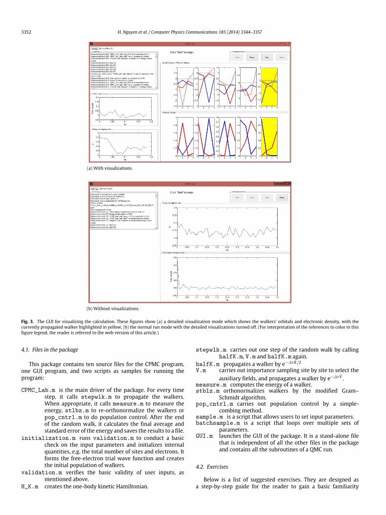
The package can be run either directly from the command lineor from the GUI. The GUI requires Matlab R2010b (version 7.11)and above but the non-interactive scripts can run on any versionof Matlab. The GUI is meant to minimize the initial learningprocess and should be used only for small systems and shortruns. Its visualization can be used to help understand how therandom walkers propagate and how the auxiliary-fields build inthe electron correlation. Figs. 2 and 3 show the program’s GUIwhich allows users to input model parameters such as the numberof sites and electrons, the twist condition, the interaction strengthand the hopping amplitude. The run parameters allow virtuallyany combination that the user chooses to configure the AFQMCrun, including the number of walkers, the time step ∆τ , thenumbers of blocks for equilibration and measurement, the size ofthe blocks, the intervals for carrying out population control andstabilization and so on. There are two tabs. The first gives theGUI for run parameters, while the second shows the progress ofthe calculation. Under the second tab, the total denominator ofthe mixed estimator and the calculated energy are monitored asa function of the imaginary time τ .

The run could also be set in a more detailed visualizationmode. The structure of the randomwalker orbitals is illustrated byplotting the orbital coefficients, alongwith the electronic ‘‘density’’⟨niσ ⟩ for each spin at site i, defined as ⟨niσ ⟩ = ⟨φk|niσ |φk⟩ for the kthwalker. Fig. 3 shows this feature, inwhich a snapshot is highlightedfor a four-site calculation.

3352 H. Nguyen et al. / Computer Physics Communications 185 (2014) 3344–3357

(a) With visualizations.

(b) Without visualizations.

Fig. 3. The GUI for visualizing the calculation. These figures show (a) a detailed visualization mode which shows the walkers’ orbitals and electronic density, with thecurrently propagated walker highlighted in yellow, (b) the normal run mode with the detailed visualizations turned off. (For interpretation of the references to color in thisfigure legend, the reader is referred to the web version of this article.)

4.1. Files in the package

This package contains ten source files for the CPMC program,one GUI program, and two scripts as samples for running theprogram:

CPMC_Lab.m is the main driver of the package. For every timestep, it calls stepwlk.m to propagate the walkers.When appropriate, it calls measure.m to measure theenergy, stlbz.m to re-orthonormalize the walkers orpop_cntrl.m to do population control. After the endof the random walk, it calculates the final average andstandard error of the energy and saves the results to a file.

initialization.m runs validation.m to conduct a basiccheck on the input parameters and initializes internalquantities, e.g. the total number of sites and electrons. Itforms the free-electron trial wave function and createsthe initial population of walkers.

validation.m verifies the basic validity of user inputs, asmentioned above.

H_K.m creates the one-body kinetic Hamiltonian.

stepwlk.m carries out one step of the random walk by callinghalfK.m, V.m and halfK.m again.

halfK.m propagates a walker by e−∆τ K/2V.m carries out importance sampling site by site to select the

auxiliary fields, and propagates a walker by e−∆τ V .measure.m computes the energy of a walker.stblz.m orthonormalizes walkers by the modified Gram–

Schmidt algorithm.pop_cntrl.m carries out population control by a simple-

combing method.sample.m is a script that allows users to set input parameters.batchsample.m is a script that loops over multiple sets of

parameters.GUI.m launches the GUI of the package. It is a stand-alone file

that is independent of all the other files in the packageand contains all the subroutines of a QMC run.

4.2. Exercises

Below is a list of suggested exercises. They are designed asa step-by-step guide for the reader to gain a basic familiarity

H. Nguyen et al. / Computer Physics Communications 185 (2014) 3344–3357 3353

Table 1Parameters and exact results for sample runs.

system (kx,ky) ⟨K⟩ ⟨V ⟩ E0

2× 1 1 ↑ 1 ↓ (+0.0819,+0.0000) −3.54222 1.09963 −2.442604× 1 2 ↑ 2 ↓ (+0.0819,+0.0000) −3.29161 1.17491 −2.116718× 1 4 ↑ 4 ↓ (+0.0819,+0.0000) −7.65166 3.04575 −4.605912× 4 3 ↑ 2 ↓ (+0.0819,−0.6052) −13.7778 1.65680 −12.12103× 4 3 ↑ 3 ↓ (+0.02, 0.04) −15.2849 1.29311 −13.99184× 4 5 ↑ 5 ↓ (0, 0) −22.5219 2.94100 −19.58094

with the code and learn the most essential features of a CPMC orAFQMC calculation. The concepts covered in the first few exercisesare universal, such as auto-correlation time, statistical errors,equilibration time, Trotter errors, population control bias, and soon. It is essential to master them before any production runs. Theother exercises are more open-ended. Their goal is to help thereader gainmore insight and facilitate real applications. In the nextsection, several example applications are shown.

4.2.1. Running the sample script sample.mThe first assignment is to run a ‘‘sample’’. To run the script

sample.m, put all the files in this package directly under thecurrent directory. Type ‘‘sample’’ (without quotes) and hit Enterto run the script. The main function CPMC_Lab will return thevalues of E_ave and E_err to the workspace, and save moredetailed data in the ∗.mat file named by sampledatafile. Themain function will also plot a figure of the energies from eachmeasurement block, E(i_blk) vs. i_blk × N_blksteps ×deltau.

Save the figure via the File menu and explain its behavior.Obtain a rough estimate for how much imaginary time isneeded to equilibrate. This interval, τeq, corresponds to the inputdeltau×N_blksteps×N_eqblk. Nowmodify the parametersto include an ‘‘equilibration’’ phase. Do statistical analysis onthe ‘‘measurement’’ phase or do a loop over different valuesof N_blksteps. We provide with the package a sample batchrun script, batchsample.m, that loops over multiple sets ofparameters. Determine theminimum length of eachmeasurementblock (N_blksteps) necessary to obtain uncorrelated results anda reliable estimate of the statistical error.

Now modify the parameters using the correct N_eqblk andN_blksteps for a few ‘‘standard’’ runs. Table 1 gives the exactenergies for several systems (U/t = 4) for comparison.

4.2.2. Controlling the basic run parametersLet us next study the behaviors of the Trotter error and

population control bias:

1. Run the code for a few different values of ∆τ (deltau),e.g. 0.025, 0.05, and 0.1, and examine the convergence of theenergies as a function of deltau. Note that the number of stepsin each block, N_blksteps, the frequency of measurement,itv_em (and optionally itv_modsvd and itv_pc) should beadjusted to obtain comparable statistics.

2. Run the code for several values of population size (N_wlk),e.g. 10, 20, 40, and 80, and examine the population bias(systematic error vs. the population size). Note that with fewerwalkers in the population, more blocks will be needed to getcomparable statistical accuracy.

4.2.3. Calculating E_K and E_V separatelyThe program only outputs the total ground state energy. The

mixed-estimate for other observables is biased, as mentionedearlier. The standard way to calculate unbiased expectation valuesis to use the back-propagation technique (see Refs. [22,31]). Let us

calculate the kinetic energyE_K and the potential energyE_V in analternative way. From the Hellman–Feynman theorem, we have

E_V =

ψ(U)

U dHdU

ψ(U) = UdEdU. (52)

Obtain dEdU by finite difference with three separate total energy

calculations at (U−∆U),U , and (U+∆U)with a small∆U . Higher-order finite difference methods can also be used for more accurateresults as illustrated in Section 6. Some exact results at U = 4 arelisted in Table 1 for comparison. For the two-dimensional system inthe last three rows, obtain a resultwith sufficiently small statisticalerror bars to examine the systematic error from the constrainedpath approximation.

4.2.4. The hydrogen moleculeLet us study the system of two interacting fermions on two

sites: N_up = 1, N_dn = 1, Lx = 2 and Ly = 1. We settx = 1 and kx = 0 (ty and ky will be ignored when Ly = 1).Study the properties of the system as the interaction strength Uis varied (while keeping t = 1). This can be viewed as a crudemodel (minimal basis) for breaking the bond in a H2 molecule. Asthe distance between the two protons increases, the interactionstrength U/t increases.

1. Run the QMC code at different values of U and compare yourresults with the exact solution:

E =12

U −

U2 + 64

. (53)

2. Plot E_K and E_V vs. U. Explain their behaviors.3. Obtain the double occupancy ⟨n1↑n1↓⟩ (see Section 4.2.3). From

it, derive the correlation function ⟨n1↑n2↓⟩. Explain its behaviorvs. U.

4.2.5. Ground-state energy of a chainLet us study the half-filled Hubbard model in one dimension

and how the energy converges with respect to system size. Runthe program for a series of lattice sizes (e.g. 2 × 1, 4 × 1, 6 × 1,8×1, . . .), each averaging over a set of random twist angleskx. Plotthe energy per site vs.1/L2, and examine its convergence behavior.(In Section 6 a detailed example is given.)

4.2.6. Addition to the program: other correlation functionsProgram in the mixed estimator of some observables, e.g. the

one-body density matrix ⟨cĎiσ cjσ ⟩, the spin–spin correlation func-tion ⟨SiSj⟩ (where Si = ni↑ − ni↓), and the charge–charge correla-tion function ⟨(ni↑+ni↓)(nj↑+nj↓⟩). Calculate the mixed estimatefor E_K and E_V and compare with the results from Section 4.2.3.

5. Computational speed

As mentioned in Section 1, a major drawback of the Matlabpackage is that it is significantly slower than a standard productioncode written in FORTRAN or C. This is outweighed by theadvantages in pedagogical value and in providing the clearest

3354 H. Nguyen et al. / Computer Physics Communications 185 (2014) 3344–3357

(a) Total energy. (b) Potential energy (inset: double occupancy ⟨n↑n↓⟩).

(c) Kinetic energy.

Fig. 4. The total, potential and kinetic energies vs. the interaction strength U for a 16-site ring with 5 spin-↑ and 7 spin-↓ electrons. CPMC results (red error bars) arecompared with exact diagonalization (ED) (blue solid curves). Restricted (cyan) and unrestricted (magenta) Hartree–Fock results have also been drawn for comparison inpanel (a). The inset in panel (b) shows the double occupancy ⟨n↑n↓⟩. (For interpretation of the references to color in this figure legend, the reader is referred to the webversion of this article.)

algorithmic foundation. From this foundation, the users couldbuild a CPMC or phase-free AFQMC code tailored toward theirown applications. As illustrated in the next section, significantapplications can be carried with the presentMatlab code as is.

Here we give some rough comparisons between the Matlabcode and a production code in FORTRAN. To provide an idea of thetiming difference, we describe two examples. For the calculationat U = 4 in a 4 × 4 lattice with 5 spin-↑ and 5 spin-↓ electrons(the same number of lattice sites as Fig. 4), the FORTRAN codetakes 1 min to run on an Intel Core i7-2600 3.40 GHz processor,compared to 32 min for the Matlab code. Scaling up the systemsize to a 128×1 lattice with 65 spin-↑ and 63 and spin-↓ electrons(the largest system in Fig. 6), the FORTRAN code requires 186 minwhile the Matlab code takes 460 min. The parameters for bothruns are deltau = 0.01, N_wlk = 1000, N_blksteps = 40,N_eqblk = 10, N_blk = 50, itv_modsvd = 5, itv_pc = 40and itv_Em = 40.

Using OpenMP, Matlab can automatically speed up compu-tations in a multi-core environment. Furthermore, Matlab userswith Matlab’s Parallel Computing Toolbox installed can easilyparallelize the code by distributing the propagation of individualwalkers over multiple processor cores. This is done by (1) chang-ing the main for loop in stepwlk.m into a parfor loop and (2)opening a pool of n parallel Matlab workers with the commandmatlabpool(‘open’, n) before the equilibration phase begins inCPMC_Lab.m.

The computational cost of the CPMC and phase-free AFQMCmethods scales algebraically, roughly as the third power of systemsize. (Different pieces of the code scale as different combinations ofN andM .) The memory required to run CPMC-Lab is proportionalto the product of (the basis size)× (the number of electrons)× (the

number of random walkers). The random walkers are only looselycoupled. The approach is ideally suited for a distributed massivelyparallel environment [32].

6. Illustrative results

Fig. 4 compares energy calculations by CPMC-Lab against exactdiagonalization (ED) results for a one-dimensional 16-siteHubbardmodel with 5 spin-↑ and 7 spin-↓ electrons. The parameters of therun are N_wlk = 5000, deltau = 0.01, N_blksteps = 40,N_blk = 150, N_eqblk = 30, itv_pc = 5, itv_Em = 40and itv_modsvd = 1. The potential energy is obtained by theHellman–Feynman method of Eq. (52), where the derivative dE

dU iscalculated using the five-point stencil. The kinetic energy is simplythe difference between the total and potential energies.

In one-dimension, the CPMC method is exact. As seen in thefigure, the agreement between CPMC and ED results is excellent.As the interaction strength U increases, the kinetic energy alsoincreases because more electrons are excited to occupy highersingle-particle levels. The potential energy is non-monotonic asa consequence of two opposing tendencies. Double occupancy⟨n↑n↓⟩ (shown in the inset) is rapidly reduced as the interactionis increased. On the other hand, the growing value of U increasesthe potential energy linearly.

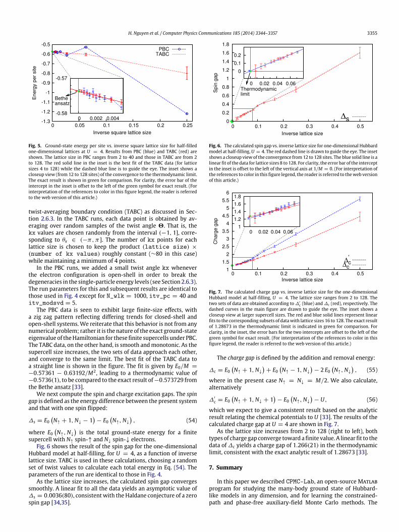
We next compute ground-state properties of the one-dimen-sional Hubbard model in the thermodynamic limit. Since our QMCcalculations are performed in finite-sized supercells, it is impor-tant to reduce finite-size effects and obtain better convergence asM → ∞. In Fig. 5, we show the calculated ground-state energyper site vs. the supercell size at half-filling for U = 4. We com-pare two sets of data, one with PBC (Γ -point) and the other with

H. Nguyen et al. / Computer Physics Communications 185 (2014) 3344–3357 3355

Fig. 5. Ground-state energy per site vs. inverse square lattice size for half-filledone-dimensional lattices at U = 4. Results from PBC (blue) and TABC (red) areshown. The lattice size in PBC ranges from 2 to 40 and those in TABC are from 2to 128. The red solid line in the inset is the best fit of the TABC data (for latticesizes 4 to 128) while the dashed blue line is to guide the eye. The inset shows acloseup view (from 12 to 128 sites) of the convergence to the thermodynamic limit.The exact result is shown in green for comparison. For clarity, the error bar of theintercept in the inset is offset to the left of the green symbol for exact result. (Forinterpretation of the references to color in this figure legend, the reader is referredto the web version of this article.)

twist-averaging boundary condition (TABC) as discussed in Sec-tion 2.6.3. In the TABC runs, each data point is obtained by av-eraging over random samples of the twist angle 2. That is, thekx values are chosen randomly from the interval (−1, 1], corre-sponding to θx ∈ (−π, π]. The number of kx points for eachlattice size is chosen to keep the product (lattice size) ×(number of kx values) roughly constant (∼80 in this case)while maintaining a minimum of 4 points.

In the PBC runs, we added a small twist angle kx wheneverthe electron configuration is open-shell in order to break thedegeneracies in the single-particle energy levels (see Section 2.6.3).The run parameters for this and subsequent results are identical tothose used in Fig. 4 except for N_wlk = 1000, itv_pc = 40 anditv_modsvd = 5.

The PBC data is seen to exhibit large finite-size effects, witha zig zag pattern reflecting differing trends for closed-shell andopen-shell systems.We reiterate that this behavior is not from anynumerical problem; rather it is the nature of the exact ground-stateeigenvalue of theHamiltonian for these finite supercells under PBC.The TABC data, on the other hand, is smooth andmonotonic. As thesupercell size increases, the two sets of data approach each other,and converge to the same limit. The best fit of the TABC data toa straight line is shown in the figure. The fit is given by E0/M =−0.57361 − 0.63192/M2, leading to a thermodynamic value of−0.5736(1), to be compared to the exact result of−0.573729 fromthe Bethe ansatz [33].

We next compute the spin and charge excitation gaps. The spingap is defined as the energy difference between the present systemand that with one spin flipped:

∆s = E0N↑ + 1,N↓ − 1

− E0

N↑,N↓

, (54)

where E0N↑,N↓

is the total ground-state energy for a finite

supercell with N↑ spin-↑ and N↓ spin-↓ electrons.Fig. 6 shows the result of the spin gap for the one-dimensional

Hubbard model at half-filling, for U = 4, as a function of inverselattice size. TABC is used in these calculations, choosing a randomset of twist values to calculate each total energy in Eq. (54). Theparameters of the run are identical to those in Fig. 4.

As the lattice size increases, the calculated spin gap convergessmoothly. A linear fit to all the data yields an asymptotic value of∆s = 0.0036(80), consistentwith the Haldane conjecture of a zerospin gap [34,35].

Fig. 6. The calculated spin gap vs. inverse lattice size for one-dimensional Hubbardmodel at half-filling,U = 4. The red dashed line is drawn to guide the eye. The insetshows a closeup view of the convergence from12 to 128 sites. The blue solid line is alinear fit of the data for lattice sizes 8 to 128. For clarity, the error bar of the interceptin the inset is offset to the left of the vertical axis at 1/M = 0. (For interpretation ofthe references to color in this figure legend, the reader is referred to theweb versionof this article.)

Fig. 7. The calculated charge gap vs. inverse lattice size for the one-dimensionalHubbard model at half-filling, U = 4. The lattice size ranges from 2 to 128. Thetwo sets of data are obtained according to∆′c (blue) and∆c (red), respectively. Thedashed curves in the main figure are drawn to guide the eye. The inset shows acloseup view at larger supercell sizes. The red and blue solid lines represent linearfits to the corresponding subsets of datawith lattice sizes 16 to 128. The exact resultof 1.28673 in the thermodynamic limit is indicated in green for comparison. Forclarity, in the inset, the error bars for the two intercepts are offset to the left of thegreen symbol for exact result. (For interpretation of the references to color in thisfigure legend, the reader is referred to the web version of this article.)

The charge gap is defined by the addition and removal energy:

∆c = E0N↑ + 1,N↓

+ E0

N↑ − 1,N↓

− 2 E0

N↑,N↓

, (55)

where in the present case N↑ = N↓ = M/2. We also calculate,alternatively

∆′c = E0N↑ + 1,N↓ + 1

− E0

N↑,N↓

− U, (56)

which we expect to give a consistent result based on the analyticresult relating the chemical potentials to U [33]. The results of thecalculated charge gap at U = 4 are shown in Fig. 7.

As the lattice size increases from 2 to 128 (right to left), bothtypes of charge gap converge toward a finite value. A linear fit to thedata of∆c yields a charge gap of 1.266(21) in the thermodynamiclimit, consistent with the exact analytic result of 1.28673 [33].

7. Summary

In this paper we described CPMC-Lab, an open-source Matlabprogram for studying the many-body ground state of Hubbard-like models in any dimension, and for learning the constrained-path and phase-free auxiliary-field Monte Carlo methods. The

3356 H. Nguyen et al. / Computer Physics Communications 185 (2014) 3344–3357

package illustrates the constrained-path Monte Carlo method,with a graphical interface. The ground-state energy is calculatedusing importance sampling and implementing the algorithmicdetails of a total energy calculation. This tool allows users toexperiment with various model and run parameters and visualizethe results. It provides a direct and interactive environment tolearn the method and study the code with minimal overhead forsetup. Furthermore, it provides a foundation and template forbuilding a CPMC or phase-free AFQMC calculation for essentiallyany interactingmany-fermion systemwith two-body interactions,including ab initio calculations in molecules and solids.

Acknowledgments

We gratefully acknowledge support by the US National ScienceFoundation Grant Nos. DMR-1006217 and DMR-1409510 (H.N.,J.X., and S.Z.), by the Department of Energy under Grant No. DE-SC0008627 (H.S. and S.Z.) and by Reed College under the SummerExperience Award (H.N.). Computing support was provided bya DOE INCITE Award and from William and Mary’s SciClonecluster.

Appendix. Some usefulMatlab commands

• Tab completion is available in the Matlab command windowfor the names of functions and scripts (either built-in, on thesearch path or in the current directory) and variables in thecurrent workspace.• Ending a command with semicolon suppresses its output.• To display the value of the variable variablename:

variablename

• Todisplay a brief description and the syntax forfunctionnamein the command window:

help functionname

• To call a function:

[out1,out2 ,...]=myfunc(in1,in2,...)

• To run the script scriptname:

scriptname

• To set display format to long (15 decimal places) instead of thedefault short (4 decimal places):

format long

• To load the variables from a *.mat file into the workspace:

load filename.mat

or double click the *.mat file or select Import Data from theworkspace menu• To remove all variables from the workspace:

clear

• To generate an m× n matrix containing pseudorandom valuesdrawn from the standard uniform distribution on (0, 1):

rand (m, n)

• To create a new individual figure window on the screen:

figure

• To close all the figure windows:

close all

• To plot each column in the (real) matrix Ydata vs. the index ofeach value:

plot(Ydata)

• To plot each column in the matrix Ydata vs. Xdata:

plot(Xdata,Ydata)

• To plot each vector in Yn vs. the corresponding vector Xn on thesame axes:

plot(X1,Y1,X2,Y2,...,Xn,Yn)

• To plot Ydata vs. Xdatawith symmetric error bars 2*Err(i)long:

errorbar(Xdata,Ydata,Err)

• To hold the plot so that subsequent plotting commands add tothe existing graph instead of replacing it:

hold all

• To put a title string at the top-center of the current axes:

title(‘string ’)

• To label the x-axis:

xlabel(‘string ’)

and similarly for the y-axis.

References

[1] S. Zhang, Auxiliary-field quantumMonte Carlo for correlated electron systems,in: E. Pavarini, E. Koch, U. Schollwock (Eds.), Emergent Phenomena inCorrelated Matter Modeling and Simulation, vol 3, Forschungszentrum Julich,2013, p. 15.1, iSBN 978-3-89336-884-6. Free online at http://www.cond-mat.de/events/correl13.

[2] S. Zhang, J. Carlson, J.E. Gubernatis, Constrained path monte carlo method forfermion ground states, Phys. Rev. B 55 (1997) 7464.

[3] C.-C. Chang, S. Zhang, Spatially inhomogeneous phase in the two-dimensional repulsive hubbard model, Phys. Rev. B 78 (2008) 165101.http://dx.doi.org/10.1103/PhysRevB.78.165101.

[4] S. Zhang, H. Krakauer, Quantum monte carlo method using phase-freerandom walks with slater determinants, Phys. Rev. Lett. 90 (2003) 136401.http://dx.doi.org/10.1103/PhysRevLett.90.136401.

[5] W.A. Al-Saidi, S. Zhang, H. Krakauer, Auxiliary-field quantum monte carlocalculations of molecular systems with a gaussian basis, J. Chem. Phys. 124(22) (2006) 224101. http://dx.doi.org/10.1063/1.2200885.

[6] C.-C. Chang, S. Zhang, Spin and charge order in the doped hubbard model:Long-wavelength collective modes, Phys. Rev. Lett. 104 (2010) 116402.http://dx.doi.org/10.1103/PhysRevLett.104.116402.

[7] H. Shi, S. Zhang, Symmetry in auxiliary-field quantum monte carlo calcula-tions, Phys. Rev. B 88 (2013) 125132.

[8] W. Purwanto, H. Krakauer, S. Zhang, Pressure-induced diamond to β-tintransition in bulk silicon: A quantummonte carlo study, Phys. Rev. B 80 (2009)214116. http://dx.doi.org/10.1103/PhysRevB.80.214116.

[9] F. Ma, S. Zhang, H. Krakauer, Excited state calculations in solids by auxiliary-field quantum monte carlo, New J. Phys. 15 (2013) 093017.

[10] W. Purwanto, H. Krakauer, Y. Virgus, S. Zhang, Assessing weak hydrogenbinding on Ca+ centers: An accurate many-body study with large basis sets,J. Chem. Phys. 135 (2011) 164105.

[11] R.M. Martin, Electronic Structure: Basic Theory and Practical Methods,Cambridge University Press, Cambridge, UK, 2004.

[12] X. Gonze, B. Amadon, P.-M. Anglade, J.-M. Beuken, F. Bottin, P. Boulanger,F. Bruneval, D. Caliste, R. Caracas, M. Ct, T. Deutsch, L. Genovese, P. Ghosez,M. Giantomassi, S. Goedecker, D. Hamann, P. Hermet, F. Jollet, G. Jomard,S. Leroux, M. Mancini, S. Mazevet, M. Oliveira, G. Onida, Y. Pouillon, T.Rangel, G.-M. Rignanese, D. Sangalli, R. Shaltaf, M. Torrent, M. Verstraete,G. Zerah, J. Zwanziger, Abinit: First-principles approach to material andnanosystem properties, Comput. Phys. Comm. 180 (12) (2009) 2582–2615.http://dx.doi.org/10.1016/j.cpc.2009.07.007. 40 YEARS OF CPC: A celebratoryissue focused on quality software for high performance, grid and novelcomputing architectures. URL http://www.sciencedirect.com/science/article/pii/S0010465509002276.

[13] M. Valiev, E. Bylaska, N. Govind, K. Kowalski, T. Straatsma, H.V. Dam, D. Wang,J. Nieplocha, E. Apra, T. Windus, W. de Jong, Nwchem: A comprehensive andscalable open-source solution for large scalemolecular simulations, ComputerPhysics Communications 181 (9) (2010) 1477–1489. http://dx.doi.org/10.1016/j.cpc.2010.04.018.URL http://www.sciencedirect.com/science/article/pii/S0010465510001438.

H. Nguyen et al. / Computer Physics Communications 185 (2014) 3344–3357 3357

[14] M.H. Kalos, D. Levesque, L. Verlet, Helium at zero temperature with hard-sphere and other forces, Phys. Rev. A 9 (1974) 2178.

[15] D.M. Ceperley, M.H. Kalos, Quantummany-body problems, in: K. Binder (Ed.),Monte CarloMethods in Statistical Physics, Springer-Verlag, Heidelberg, 1979,pp. 145–194. (Chapter 4).

[16] H. Shi, C. Jimenez-Hoyos, G.E. Scuseria, S. Rodríguez-Guzmán, R. Zhang,Symmetry-projected wavefunctions in quantum monte carlo calculations,Phys. Rev. B 89 (2014) 125129.

[17] D.R. Hamann, S.B. Fahy, Energymeasurement in auxiliary-fieldmany-electroncalculations, Phys. Rev. B 41 (1990) 11352–11363. http://dx.doi.org/10.1103/PhysRevB.41.11352.

[18] S. Zhang, Finite-temperature monte carlo calculations for systems withfermions, Phys. Rev. Lett. 83 (1999) 2777.

[19] B.M. Rubenstein, S. Zhang, D.R. Reichman, Finite-temperature auxiliary-fieldquantum monte carlo technique for bose-fermi mixtures, Phys. Rev. A 86(2012) 053606. http://dx.doi.org/10.1103/PhysRevA.86.053606.

[20] J.E. Hirsch, Two-dimensional hubbard model: Numerical simulation study,Phys. Rev. B 31 (1985) 4403.

[21] C.J. Umrigar, M.P. Nightingale, K.J. Runge, A diffusion Monte Carlo algorithmwith very small time-step errors, J. Chem. Phys. 99 (4) (1993) 2865.

[22] W. Purwanto, S. Zhang, Quantum monte carlo method for the ground stateof many-boson systems, Phys. Rev. E 70 (2004) 056702. http://dx.doi.org/10.1103/PhysRevE.70.056702.

[23] S. Zhang, M.H. Kalos, Exact monte carlo calculation for few-electron systems,Phys. Rev. Lett. 67 (1991) 3074.

[24] S. Zhang, Finite-temperature calculations of correlated electron systems,Computer Physics Communications 127 (1) (2000) 150–155. http://dx.doi.org/10.1016/S0010-4655(00)00029-1. URL http://www.sciencedirect.com/science/article/pii/S0010465500000291.

[25] C. Lin, F.H. Zong, D.M. Ceperley, Twist-averaged boundary conditions incontinuum quantum monte carlo algorithms, Phys. Rev. E 64 (2001) 016702.http://dx.doi.org/10.1103/PhysRevE.64.016702. URL http://link.aps.org/doi/10.1103/PhysRevE.64.016702.

[26] J. Xu, C.-C. Chang, E.J. Walter, S. Zhang, Spin- and charge-density wavesin the hartree-fock ground state of the two-dimensional hubbard model,J. Phys.: Condens. Matter. 23 (50) (2011) 505601. http://stacks.iop.org/0953-8984/23/i=50/a=505601.

[27] W. Purwanto, S. Zhang, H. Krakauer, Excited state calculations using phaselessauxiliary-field quantum Monte Carlo: Potential energy curves of low-lying C2singlet states, J. Chem. Phys. 130 (9) (2009) 094107. http://dx.doi.org/10.1063/1.3077920. URL http://link.aip.org/link/?JCP/130/094107/1.

[28] S. Sorella, Linearized auxiliary fieldsmonte carlo technique: Efficient samplingof the fermion sign, Phys. Rev. B 84 (2011) 241110. http://dx.doi.org/10.1103/PhysRevB.84.241110. URL http://link.aps.org/doi/10.1103/PhysRevB.84.241110.

[29] J. Carlson, S. Gandolfi, K.E. Schmidt, S. Zhang, Auxiliary-field quantum montecarlo method for strongly paired fermions, Phys. Rev. A 84 (2011) 061602.http://dx.doi.org/10.1103/PhysRevA.84.061602. URL http://link.aps.org/doi/10.1103/PhysRevA.84.061602.

[30] M. Calandra Buonaura, S. Sorella, Numerical study of the two-dimensionalheisenberg model using a green function monte carlo technique with a fixednumber of walkers, Phys. Rev. B 57 (1998) 11446–11456. http://dx.doi.org/10.1103/PhysRevB.57.11446.

[31] S. Zhang, J. Carlson, J.E. Gubernatis, Constrained path quantum monte carlomethod for fermion ground states, Phys. Rev. Lett. 74 (1995) 3652.

[32] K.P. Esler, J. Kim, D.M. Ceperley, W. Purwanto, E.J. Walter, H. Krakauer, S.Zhang, P.R.C. Kent, R.G. Hennig, C. Umrigar, M. Bajdich, J. Kolorenc, L. Mitas,A. Srinivasan, QuantumMonte Carlo algorithms for electronic structure at thepetascale; the Endstation project, J. Phys. Conf. Ser. 125 (2008) 012057. 15pp,http://stacks.iop.org/1742-6596/125/012057.

[33] E.H. Lieb, F.Y. Wu, Absence of mott transition in an exact solution of the short-range, one-band model in one-dimension, Phys. Rev. Lett. 20 (1968) 1445.

[34] F. Haldane, Continuum dynamics of the 1-d heisenberg antiferromagnet:Identification with the o(3) nonlinear sigma model, Phys. Lett. A 93 (9) (1983)464–468. http://dx.doi.org/10.1016/0375-9601(83)90631-X.

[35] F.D.M. Haldane, Nonlinear field theory of large-spin heisenberg antiferromag-nets: Semiclassically quantized solitons of the one-dimensional easy-axis neelstate, Phys. Rev. Lett. 50 (15) (1983) 1153.