Cost-Sensitive Analysis in Multiple Time Series Prediction

Cost-Sensitive Analysis in Multiple Time Series Prediction

C. K. Walgampaya

Department of Computer Science

University of Louisville

Louisville KY, USA

[email protected]

M. Kantardzic

Department of Computer Science

University of Louisville

Louisville KY, USA

[email protected]

Abstract - In this paper we propose a new methodology

for Cost-Benefit analysis in a multiple time series

prediction problem. The proposed model is evaluated in a

real world application based on a network of wireless

sensors distributed in energy production plants in a region.

These sensors generate multiple time series data

representing energy production. To build the prediction

model for total energy production in the region we have

used three common forecasting techniques, Support Vector

Machines (SVMs), Multilayer Perceptron (MLP), and

Multiple Regression (MR). For training and testing of the

models we have used the data from year 2002 to 2004. We

analyzed the quality of total energy prediction with

different subsets of sensors. We build our cost-benefit

model for the prediction process as a function of sensors in

a distributed network and estimated the optimum number

of sensors that will balance the expenses of the system with

the prediction accuracy.

Keywords: time series, prediction, distributed sensors, cost

benefit analysis.

1 Introduction You may have been intensely creative in generating

solutions to a problem, and rigorous in your selection of the

best one available. This solution may still not be worth

implementing, as you may invest a lot of time and money in

solving a problem that is not worthy of this effort.

Cost/Benefit Analysis is a relatively simple and widely used

technique for deciding whether to make a change [1]. Profit

and costs drive the utility of every corporate decision. As

corporate decision making, from strategic to operational

planning, is based upon future realizations of the decision

parameters [2]. The real trick to doing a cost benefit

analysis well, is making sure you include all the costs and

all the benefits and properly quantify them.

Cost-benefit analysis has already attracted much

attention from the machine learning and data mining

communities [3]. As it is stated in the Technological

Roadmap of the MLnetII project (European Network of

Excellence in Machine Learning) the inclusion of costs into

learning and classification is one of the most relevant topics

of future machine learning research [4].

In the literature of cost sensitive analysis for data

mining applications, most emphasis is given to

classification problems. Recent research and related

publications show that cost sensitive analysis is not deeper

analyzed, modeled, and applied to prediction problems.

Conversely, data mining methods for regression and time

series analysis generally disregard economic utility and

apply simple accuracy measures [2]. Only some theoretical

approaches exist for specific data mining techniques such

as neural networks and support vector machines.

In this research we propose a new approach and

develop a methodology to apply the cost benefit analysis to

real world prediction problem. Our application is prediction

of energy production. Data for our research is collected

from a patented distributed wireless sensor network of

energy plants. In this paper, we have proposed a model for

cost-benefit analysis in a multiple time series prediction

problem. We have identified three distinct areas of the cost

function and analyzed the behavior in each region. We have

experimentally found out the threshold values

corresponding to these regions. Prediction model of total

energy production is built using SVMs, MLP and MR

techniques. Results are compared and analyzed. We have

discussed how this methodology can be utilized in similar

distributed systems.

Following a brief introduction to related work in

section 2, Section 3 introduces multiple time series

prediction problem and its formalization for prediction of

energy production based on daily sensor data. We report

our recent research efforts in introducing cost sensitive

analysis for this real world prediction application in Section

4. Conclusions are given in Section 5.

2 Related Work In recent years data mining community has attempted

incorporating cost benefit analysis into classification

problems, where the “Cost” could be interpreted as

misclassification cost, training cost, test cost, or others [5].

Among all different types of costs, the misclassification

cost is the most popular one. In general, misclassification

cost is described by a cost matrix C , with ( ),C i j

indicating the cost of predicting that an example belongs to

class i when in fact it belongs to class j [6]. Hollmen et al.,

and Elkan introduce a cost model that incorporates the

specific properties of objects to be classified. Instead of a

Conference on Data Mining | DMIN'06 | 17

fixed misclassification cost matrix, they utilize a more

general matrix of cost functions. These functions operate on

the data to be classified and are re-calculated for each data

point separately [7], [8].

Most of the existing cost sensitive classifiers assume

that datasets are either noise free or noise in the datasets is

less significant. However, real-world data is never perfect

and suffer from noise that may impact models created from

data. Zhu and Wu have addressed the problem of class

noise, which means the errors introduced in the class labels.

They have studied the noise impacts on cost sensitive

learning and proposed a cost guided noise handling

approach for effective learning [6]. The class imbalance

problem has been recognized as a crucial problem in

machine learning and data mining. Such a problem is

encountered in a large number of domains, and it can lead

to poor performance of the learning method [9]. It has been

indicated that cost-sensitive learning is a good solution to

the class imbalance problem and Zhou and Liu have studied

methods that address the class imbalance problem applied

to cost-sensitive neural networks [3].

Similarly, for predictive data mining problems of

regression and time series analysis the costs arising from

invalid point prediction, costs of underprediction versus

overprediction, etc are also analyzed in the literature. Crone

et al. have analyzed the efficiency of a linear asymmetric

cost function in inventory management decisions, training a

multilayer perceptron to find a cost efficient stock-level for

a set of seasonal time series directly from the data [2]. A

similar work has been proposed by Christoffersen and

Diebold by introducing a new technique for solving

prediction problems under asymmetric loss using

piecewise-linear approximations to the loss function [10].

Wang and Stockton have investigated how the

constraints imposed by changing export market affect the

identification of “cost estimating relationships” and

investigated their relative benefits and limitations in terms

of their effects on the overall cost model development

process. A neural network architecture has been used and a

series of experiments have been undertaken to select an

appropriate network [11].

Cost estimation generally involves predicting labor,

material, utilities or other costs over time given a small

subset of factual data on “cost drivers.” Alice has examined

the use of regression and MLP models in terms of

performance, stability and ease of use to build cost

estimating relationships. The results show that MLP have

performed well when dealing with data which there is little

prior knowledge about the cost estimating relationship to

select for regression modeling. However regression models

have shown significant improvements in terms of accuracy

in cases where an appropriate cost estimating function can

be identified [12].

3 Prediction of Total Energy

Production This paper presents our research results in analysis of

distributed energy production in a region, and development

of prediction model based on data collected from multiple

distributed sensors related to specific power plants. These

energy plants operate through out the year continuously.

Each plant keeps record of real-time power production and

transmission flows for facilities, current plant output and

real time changes and variations in flow, power plant usage,

start-ups, and supply availability. These data are taken at

specific time intervals and they vary from a fraction of a

second to a day. The sampling frequency depends on the

type of data that are collected at the energy plant.

The data for our analysis comprises, readings of

sensors at 200 distributed energy plants, and the cumulative

variable that correspond to the total energy production of

those 200 energy plants. The data set that we are using is

collected daily and we use a repository of three years from

year 2002 to year 2004. It has 365 data for each plant in

years 2002, 2003 and 366 data records for each plant in

year 2004. These historic data can be used to build and

improve analytical models used for short and long term

energy production forecasting. They are currently used by

energy trading and marketing firms and federal regulatory

agencies including Homeland Security.

Prediction systems have to obtain these data sets at a

cost. Getting data from more energy plants to make

prediction means increase in expenses. Our goal is to

predict the total energy production with reduced number of

sensors, where we can compromise between the expenses

for collecting data and the quality of prediction accuracy.

Based on the analysis of different multiple time series

prediction techniques we have selected SVM, MLP and

MR as the best candidates for our study in building cost

sensitive prediction model [13, 14, 15]. Our approach

shows that it is possible to estimate the total energy

production using reduced number of sensor stations. The

modeling results and general approach may be used in other

systems to determine the required number of sensors to be

used for data collection.

3.1 Data Collection and Preprocessing The data for analysis is collected daily for the years

from year 2002 to year 2004. Most of the machine learning

techniques including MLP and SVM require that all data

sets to be normalized. We use MATLAB to normalize data

between -1, +1 for 200 energy plants. In the raw data set

there are some entries with 0 values. They correspond to

days in which a sensor does not record a value for a given

day. In our problem all those 0 values are taken as actually

recorded values after verifying with the authorities [16].

18 Conference on Data Mining | DMIN'06 |

We have used year 2002 and year 2003 data as

training data set and year 2004 data as testing data. Main

goals of our research are a) To estimate and compare the

quality of different prediction methodologies, and b) To

estimate optimum number of sensors, which will give the

best results balancing expenses of the system. We used

three prediction methodologies: MLP, SVMs, and MR.

Accuracy of each model is estimated, by computing the

correlation coefficient, between actual values and predicted

values in the testing data set. Prediction accuracy is

dependent on the amount of sensors we use, i.e. number of

energy plant inputs we use in the prediction. To verify this

we have built training and testing data sets by varying the

number of sensors from which the data are collected. In our

study we considered data from 10, 20, 30, 40, 70, 100, 130,

170 and 190 plant inputs.

3.2 Experimental Results In MLP, SVM, and MR a selected number of sensors

data (time series) are used in prediction. We have 200

sensors as data sources, and there are various ways of

selecting the subset. Selection of a subset of sensors (in our

case 10, 20, 30, 40 …etc.) will cause combinatorial

explosion. We made one heuristic approximation in this

step to eliminate computational complexity. Each of 200

sensor time series is compared with the total energy

production by computing the correlation factor. We wanted

to estimate how much each of sensor measurements are

correlated to the output. Then, we sorted sensors based on

the correlation factor, and selected subset is a portion of top

ranked sensors.

We used a feed forward neural network with back-

propagation learning using only one hidden layer. The

algorithm was implemented in MATLAB ver6.5.

Experiments showed that equal number of input and hidden

nodes give the best results in prediction. Inputs to the

network are the data columns corresponding to sensors’

recordings at each plant throughout the year and the single

output represents predicted value for the energy production

in the region. We have experimented the MLP model with

different combinations of the parameters and determined

that the values 0.001 for accuracy parameter and 0.04 for

learning rate with Tangent-Sigmoid activation function give

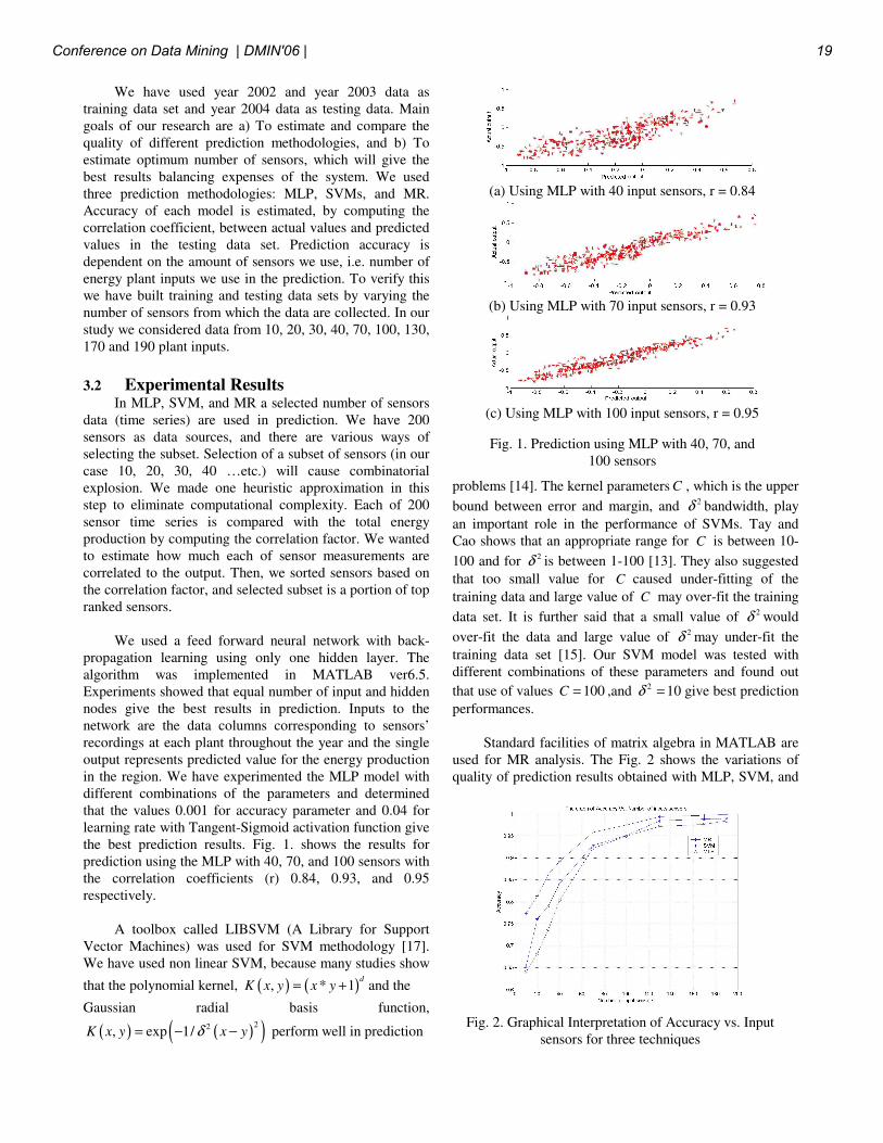
the best prediction results. Fig. 1. shows the results for

prediction using the MLP with 40, 70, and 100 sensors with

the correlation coefficients (r) 0.84, 0.93, and 0.95

respectively.

A toolbox called LIBSVM (A Library for Support

Vector Machines) was used for SVM methodology [17].

We have used non linear SVM, because many studies show

that the polynomial kernel, ( ) ( ), * 1d

K x y x y= + and the

Gaussian radial basis function,

( ) ( )( )22, exp 1/K x y x yδ= − − perform well in prediction

problems [14]. The kernel parameters C , which is the upper

bound between error and margin, and 2δ bandwidth, play

an important role in the performance of SVMs. Tay and

Cao shows that an appropriate range for C is between 10-

100 and for 2δ is between 1-100 [13]. They also suggested

that too small value for C caused under-fitting of the

training data and large value of C may over-fit the training

data set. It is further said that a small value of 2δ would

over-fit the data and large value of 2δ may under-fit the

training data set [15]. Our SVM model was tested with

different combinations of these parameters and found out

that use of values 100C = ,and 2 10δ = give best prediction

performances.

Standard facilities of matrix algebra in MATLAB are

used for MR analysis. The Fig. 2 shows the variations of

quality of prediction results obtained with MLP, SVM, and

(a) Using MLP with 40 input sensors, r = 0.84

(b) Using MLP with 70 input sensors, r = 0.93

(c) Using MLP with 100 input sensors, r = 0.95

Fig. 1. Prediction using MLP with 40, 70, and

100 sensors

Fig. 2. Graphical Interpretation of Accuracy vs. Input

sensors for three techniques


MR for different number of input time series.

Detailed comparison of these techniques and

discussion about optimal number of sensors for different

models are given in our previous article. The hypothesis

that optimal number of sensors should be the trade off

between accuracy of prediction and costs of the monitoring

system is the initiating point of the current research [16].

4 Cost Benefit Analysis in Multiple

Time Series Prediction Should we collect data from all plants? If not what

would be the optimum number of plants to use for

prediction? What are economic benefits from the prediction

system? These questions are essential part in analysis of a

solution for our prediction system based on distributed

sensors system which monitors energy production. A cost

benefit analysis for multiple time series prediction, we are

developing and applying in this research, will give some of

the answers.

There are several costs involved in building our

prediction system. They can be of two types: fixed cost and

variable cost. In an optimization problem, fixed cost only

shifts the cost curve into a higher or lower level. So, we

only considered variable cost in our analysis. In building

and maintaining the sensor system, these expenses

correspond to hardware installation and maintenance, data

collection, data processing and data analysis. These

expenses would include,

1) 11

C : Cost of purchasing proper equipments for data

collection, data processing and data analysis.

2) 12

C : Cost of installing sensor stations which are

located in geographically distributed area. This will

include hiring of skilled technicians, traveling, etc.

3) 13

C : Cost of maintaining the system. Maintenance

includes both regular and periodic maintenances such

as replacements of necessary equipment.

4) 14

C : Cost of communication equipments, computers

and software for transmission of data from sensors to a

central computer, including the cost of laying out the

wired or wireless network and its own maintenance

costs.

We can approximate the total cost “1

Cost ” as a linear

function of number of sensors:

1 1

*Cost C n= (1)

where:

- n is the number of sensors and

-1 1

4

1i

C Ci

= ∑=

is a constant which include all expenses

discussed above.

1Cost may also include a risk factors that would compensate

increase of prices, depreciation etc. For these reasons it

should be determined very carefully by experts in the

domain.

Accuracy of prediction is a nonlinear function of the

number of sensors [16]. Table 1 shows the experimental

results for models approximated with different polynomials

with corresponding error of approximation for MLP. We

selected the polynomial model with relative small error and

at the same time enough simple. We experimentally

confirmed that polynomial function of third order makes a

good approximation of the prediction non-linearity y :

( )1 2 3 4

2 3* * *ny a a n a n a n= + + + (2)

where:

-1 2 3 4, ,a a a and a are constants and they should be

determined experimentally for a selected prediction system,

and

- n is the number of sensors.

“Benefits” in a prediction system, may be defined as

“negative cost” in the total cost function [5], because

benefits are turnovers to a system. We assume that with

increasing quality of prediction, the user of the system will

financially benefit and make more profit.

Benefits: 2

""Cost of the prediction process may be

approximated analytically with a function proportional to

the prediction function ( )y n ,

2 2

( )Cost C y n= − ∗ (3)

where:

-2

C is a constant which includes financial benefits

from better prediction for 1%, and it is determined by

experts in the domain. The negative sign shows that the

benefits represent a negative cost function. The total cost

C is a sum of costs and benefits,

1 2

C Cost Cost= + (4)

or substituting components,

( )1 2

( )nC C n C y n= ∗ − ∗ (5)

The goal is to minimize function ( )C n with respect to n .

Minimization of cost function will result in a maximum of

profit of the prediction system. Determining the minimum

of cost function C , will specify corresponding number of

Table 1. variation of prediction error

Polynomial Square error

Linear 0.0300

Polynomial second order 0.0029

Polynomial third order 0.0009

Polynomial fourth order 0.0007


sensors n , and also corresponding ( )y n - prediction

accuracy of a system for a given architecture.

Obviously, that minimum of the function depends on the

constants 1

C and2

C . When we rearrange the cost function

C , to the form

1

2

2

( * ( ))C

C C n y nC

= ∗ − (6)

we may assume that 2

C is a scaling factor and only the

quotient 1

2

'CC

C= will influence the minimum of a cost

function C . Therefore, we consider in our further

formalizations, analysis and minimization, that the cost

function is in a form '* ( )C C n y n= − .

4.1 Cost Benefit Model

We experimentally determined parameters in

analytical formulae ( )y n for the MLP (MLP

y ), SVMs

(SVM

y ) and MR (MR

y ) methodologies. We can find the

analytical relationship between the accuracy and the

number of inputs for each of the techniques applying a

curve fitting procedure and assuming that the function is a

polynomial third order. The approximated equations fits the

graphs of Fig. 2.: 2 7 3

0.597 0.00815* 0.000058* 1.4*10 *MLP

Y n n n−

= + − + (7)

2 7 30.548 0.00831* 0.000054* 1.2*10 *

SVMY n n n

−= + − + (8)

2 7 30.719 0.00573* 0.000040* 0.9*10 *

MRY n n n

−= + − + (9)

The derived cost function '* ( )C C n y n= − , for each data

mining technique is obtained by substituting corresponding,

experimentally determined, ( )y n :

For Neural Network

' 2 7 3( (0.597 0.00815* 0.000058* 1.4*10 * ))MLP

C C n n n n−= ∗ − + − + (10)

For Support Vector Machines

' 2 7 3( (0.548 0.00831* 0.000054* 1.2*10 * ))MR

C C n n n n−= ∗ − + − + (11)

For Multiple Regression

2 7 3'( (0.719 0.00573* 0.000040* 0.9*10 * ))MR

C C n n n n−= ∗ − + − + (12)

These three functions represent our cost-benefit models for

prediction. Each model is based on two input parameters:

'C -ratio of cost constants, and n - number of sensors.

4.2 Interpretation of Experimental Results

We can analyze how the actual cost function changes

with values of constant 1 2

C C or'

C , and we will try to find

a minimum of these functions for different '

C values using

experimental results.

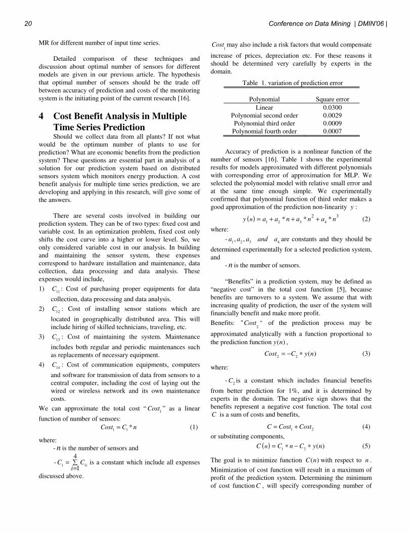
4.2.1 Large Benefits

Fig. 3. gives a plot for cost function C for very small

value of '

0.0001C = based on our experimental results.

Three graphs represent the three applied prediction

methodologies. Small'

C means that the value of 2

C is very

high, relative to the value of 1

C i.e. the users estimate that

the benefit of prediction accuracy is very high and its

overweight any cost 1

C for sensor installation and

maintenance. As it is expected, the cost function C is

continuously decreasing function, where its minimum is

with maximum number of sensors n (in our case 200). That

means, we accept all expenses for installation of all 200

sensors and there is no prediction system. Output will be

just calculated as a sum of all sensors values. Even if the

sensors are expensive, it is not a sufficient reason to

influence the cost function which is minimum for maximum

n .

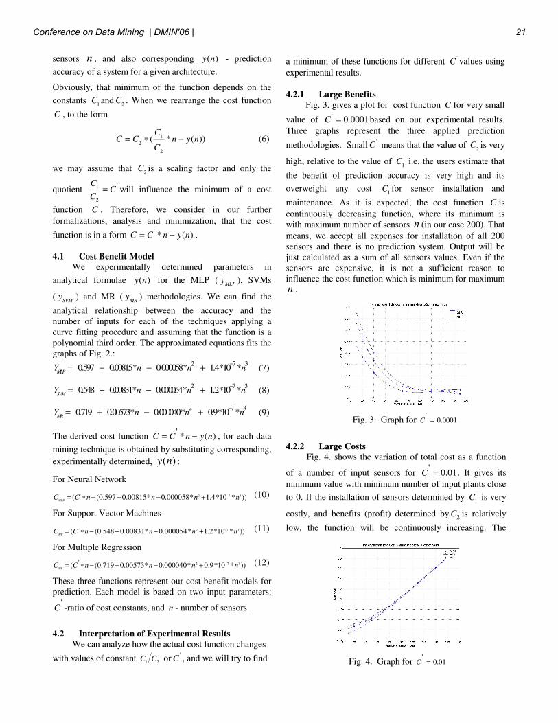
4.2.2 Large Costs

Fig. 4. shows the variation of total cost as a function

of a number of input sensors for '

0.01C = . It gives its

minimum value with minimum number of input plants close

to 0. If the installation of sensors determined by 1

C is very

costly, and benefits (profit) determined by 2C is relatively

low, the function will be continuously increasing. The

Fig. 3. Graph for '

0.0001C =

Fig. 4. Graph for '

0.01C =


solution may found at extremely small number of sensors

(close to 0), Again, we do not need prediction system

because the expenses are so high, that the system is not

economically feasible.

4.2.3 Costs and Benefits are Balanced

The most interesting case is when the relation between

constants 1

C and 2

C is such that the function C is neither

continuously increasing nor decreasing. The minimum of

the cost function C occurs between minimum and

maximum of n . We believe that it is the common case in

real world applications. Minimum value for total cost C ,

will determine necessary number of sensors to obtain

maximum benefits from the prediction system. Based on the

number of sensors we can estimate the quality of prediction

for the recommended configuration.

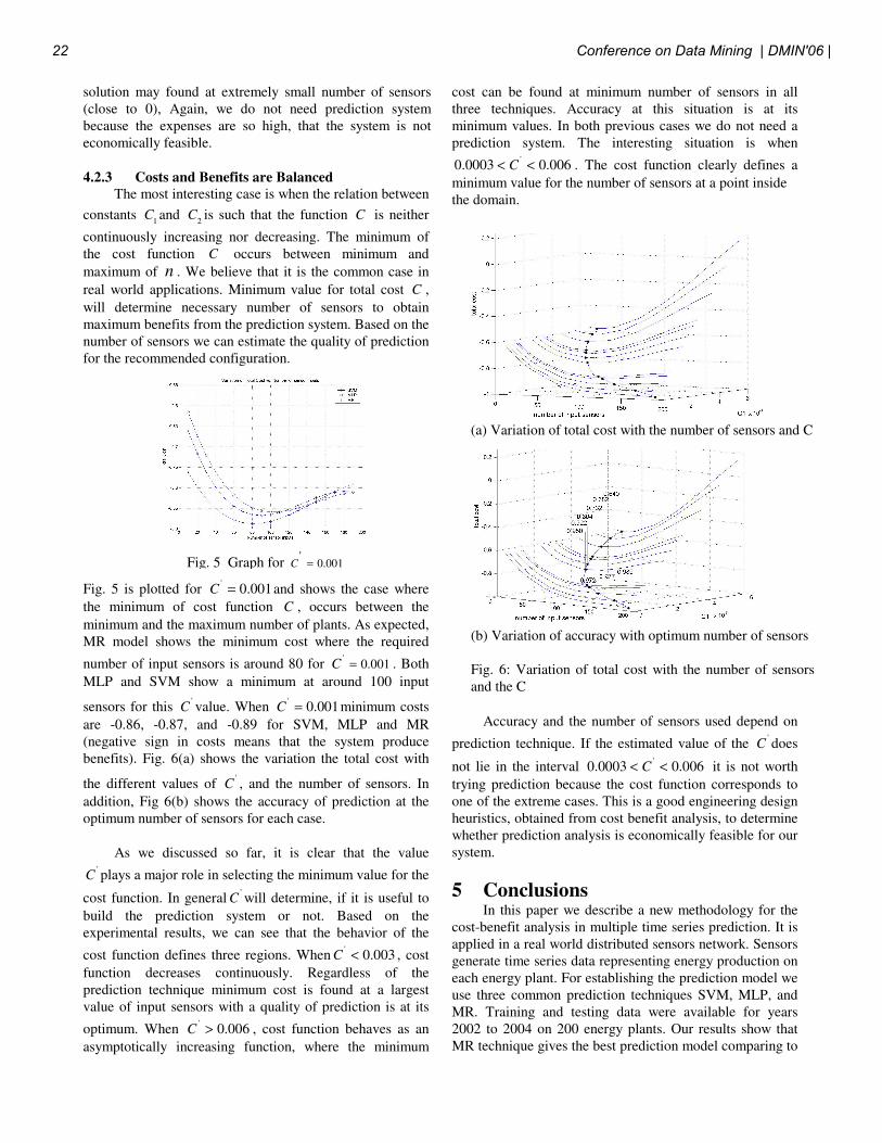
Fig. 5 is plotted for '

0.001C = and shows the case where

the minimum of cost function C , occurs between the

minimum and the maximum number of plants. As expected,

MR model shows the minimum cost where the required

number of input sensors is around 80 for '

0.001C = . Both

MLP and SVM show a minimum at around 100 input

sensors for this '

C value. When '

0.001C = minimum costs

are -0.86, -0.87, and -0.89 for SVM, MLP and MR

(negative sign in costs means that the system produce

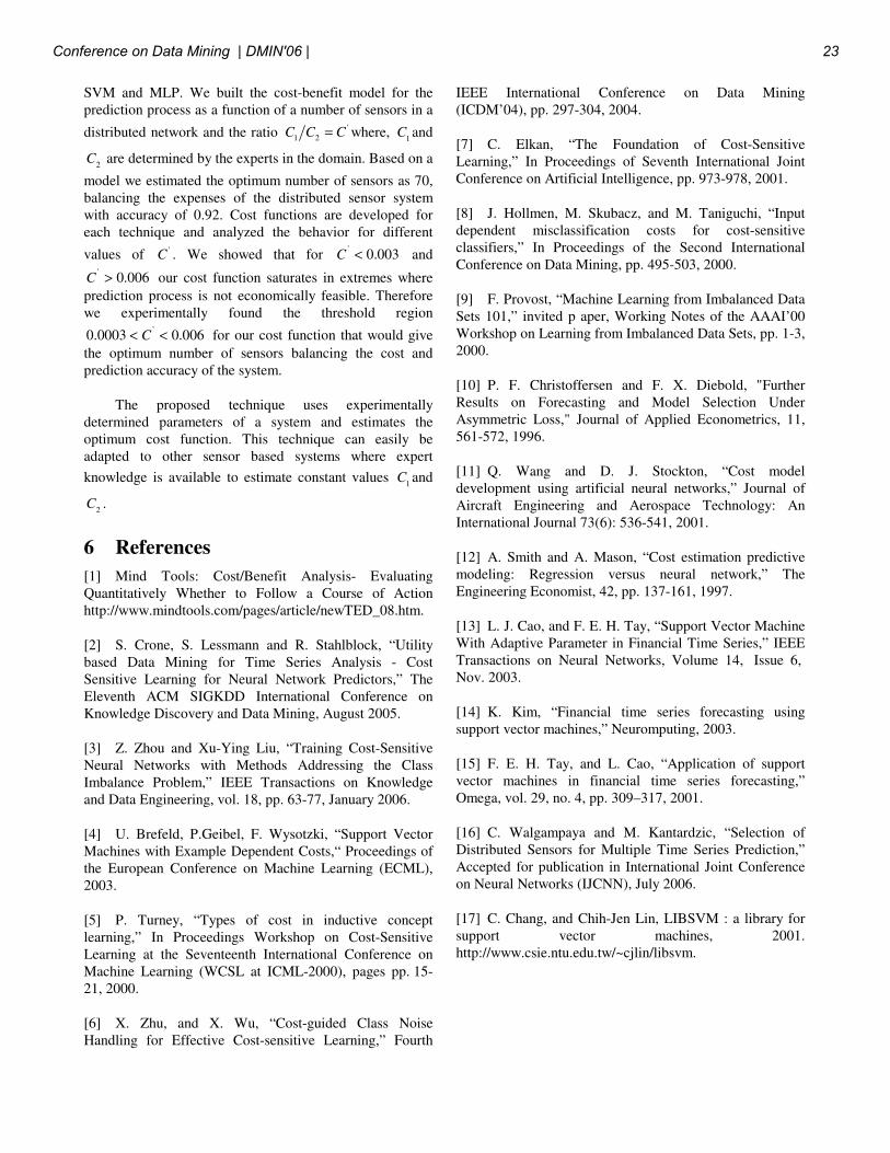
benefits). Fig. 6(a) shows the variation the total cost with

the different values of '

C , and the number of sensors. In

addition, Fig 6(b) shows the accuracy of prediction at the

optimum number of sensors for each case.

As we discussed so far, it is clear that the value '

C plays a major role in selecting the minimum value for the

cost function. In general'

C will determine, if it is useful to

build the prediction system or not. Based on the

experimental results, we can see that the behavior of the

cost function defines three regions. When'

0.003C < , cost

function decreases continuously. Regardless of the

prediction technique minimum cost is found at a largest

value of input sensors with a quality of prediction is at its

optimum. When '

0.006C > , cost function behaves as an

asymptotically increasing function, where the minimum

cost can be found at minimum number of sensors in all

three techniques. Accuracy at this situation is at its

minimum values. In both previous cases we do not need a

prediction system. The interesting situation is when '

0.0003 0.006C< < . The cost function clearly defines a

minimum value for the number of sensors at a point inside

the domain.

Accuracy and the number of sensors used depend on

prediction technique. If the estimated value of the '

C does

not lie in the interval '

0.0003 0.006C< < it is not worth

trying prediction because the cost function corresponds to

one of the extreme cases. This is a good engineering design

heuristics, obtained from cost benefit analysis, to determine

whether prediction analysis is economically feasible for our

system.

5 Conclusions In this paper we describe a new methodology for the

cost-benefit analysis in multiple time series prediction. It is

applied in a real world distributed sensors network. Sensors

generate time series data representing energy production on

each energy plant. For establishing the prediction model we

use three common prediction techniques SVM, MLP, and

MR. Training and testing data were available for years

2002 to 2004 on 200 energy plants. Our results show that

MR technique gives the best prediction model comparing to

Fig. 5 Graph for '

0.001C =

(a) Variation of total cost with the number of sensors and C

(b) Variation of accuracy with optimum number of sensors

Fig. 6: Variation of total cost with the number of sensors

and the C


SVM and MLP. We built the cost-benefit model for the

prediction process as a function of a number of sensors in a

distributed network and the ratio '

1 2C C C= where,

1C and

2C are determined by the experts in the domain. Based on a

model we estimated the optimum number of sensors as 70,

balancing the expenses of the distributed sensor system

with accuracy of 0.92. Cost functions are developed for

each technique and analyzed the behavior for different

values of 'C . We showed that for '

0.003C < and '

0.006C > our cost function saturates in extremes where

prediction process is not economically feasible. Therefore

we experimentally found the threshold region '

0.0003 0.006C< < for our cost function that would give

the optimum number of sensors balancing the cost and

prediction accuracy of the system.

The proposed technique uses experimentally

determined parameters of a system and estimates the

optimum cost function. This technique can easily be

adapted to other sensor based systems where expert

knowledge is available to estimate constant values 1

C and

2C .

6 References

[1] Mind Tools: Cost/Benefit Analysis- Evaluating

Quantitatively Whether to Follow a Course of Action

http://www.mindtools.com/pages/article/newTED_08.htm.

[2] S. Crone, S. Lessmann and R. Stahlblock, “Utility

based Data Mining for Time Series Analysis - Cost

Sensitive Learning for Neural Network Predictors,” The

Eleventh ACM SIGKDD International Conference on

Knowledge Discovery and Data Mining, August 2005.

[3] Z. Zhou and Xu-Ying Liu, “Training Cost-Sensitive

Neural Networks with Methods Addressing the Class

Imbalance Problem,” IEEE Transactions on Knowledge

and Data Engineering, vol. 18, pp. 63-77, January 2006.

[4] U. Brefeld, P.Geibel, F. Wysotzki, “Support Vector

Machines with Example Dependent Costs,“ Proceedings of

the European Conference on Machine Learning (ECML),

2003.

[5] P. Turney, “Types of cost in inductive concept

learning,” In Proceedings Workshop on Cost-Sensitive

Learning at the Seventeenth International Conference on

Machine Learning (WCSL at ICML-2000), pages pp. 15-

21, 2000.

[6] X. Zhu, and X. Wu, “Cost-guided Class Noise

Handling for Effective Cost-sensitive Learning,” Fourth

IEEE International Conference on Data Mining

(ICDM’04), pp. 297-304, 2004.

[7] C. Elkan, “The Foundation of Cost-Sensitive

Learning,” In Proceedings of Seventh International Joint

Conference on Artificial Intelligence, pp. 973-978, 2001.

[8] J. Hollmen, M. Skubacz, and M. Taniguchi, “Input

dependent misclassification costs for cost-sensitive

classifiers,” In Proceedings of the Second International

Conference on Data Mining, pp. 495-503, 2000.

[9] F. Provost, “Machine Learning from Imbalanced Data

Sets 101,” invited p aper, Working Notes of the AAAI’00

Workshop on Learning from Imbalanced Data Sets, pp. 1-3,

2000.

[10] P. F. Christoffersen and F. X. Diebold, "Further

Results on Forecasting and Model Selection Under

Asymmetric Loss," Journal of Applied Econometrics, 11,

561-572, 1996.

[11] Q. Wang and D. J. Stockton, “Cost model

development using artificial neural networks,” Journal of

Aircraft Engineering and Aerospace Technology: An

International Journal 73(6): 536-541, 2001.

[12] A. Smith and A. Mason, “Cost estimation predictive

modeling: Regression versus neural network,” The

Engineering Economist, 42, pp. 137-161, 1997.

[13] L. J. Cao, and F. E. H. Tay, “Support Vector Machine

With Adaptive Parameter in Financial Time Series,” IEEE

Transactions on Neural Networks, Volume 14, Issue 6,

Nov. 2003.

[14] K. Kim, “Financial time series forecasting using

support vector machines,” Neuromputing, 2003.

[15] F. E. H. Tay, and L. Cao, “Application of support

vector machines in financial time series forecasting,”

Omega, vol. 29, no. 4, pp. 309–317, 2001.

[16] C. Walgampaya and M. Kantardzic, “Selection of

Distributed Sensors for Multiple Time Series Prediction,”

Accepted for publication in International Joint Conference

on Neural Networks (IJCNN), July 2006.

[17] C. Chang, and Chih-Jen Lin, LIBSVM : a library for

support vector machines, 2001.

http://www.csie.ntu.edu.tw/~cjlin/libsvm.


Cost-Sensitive Analysis in Multiple Time Series Prediction

Documents

Transcript of Cost-Sensitive Analysis in Multiple Time Series Prediction