Cost-effectiveness of

screening for colorectal

cancer with once-only

flexible sigmoidoscopy

and faecal occult

blood test Eline Aas Institute of Health Management and Health Economics UNIVERSITY OF OSLO HEALTH ECONOMICS RESEARCH PROGRAMME Working paper 2008: 6

HERO

Cost-effectiveness of screening for colorectal cancer with

once-only flexible sigmoidoscopy and faecal occult blood test

Eline Aas* University of Oslo

Institute for Health Management and Health Economics,

HERO

Health Economics Research Programme at the University of Oslo HERO 2008

* Eline Aas, Institute for Health Management and Health Economics and HERO, University of Oslo, Norway, eline.aas@medisin.uio.no I would like to thank Tor Iversen and John Dagsvik for helpful comments during the work of this paper and Statistics Norway for good collaboration during the data collection. Financal support from The Research Council of Norway through the Health Economics Research programme at the University of Oslo is acknowledged. NORCCAP (Norwegian Colorectal Cancer Prevention) and especially Geir Hoff are acknowledged. I will thank Per-Olov Johansson, Ivar S. Kristiansen, Jia Zhiyang, John Cairns and participants at the 6th European conference in Health Economics ( Budapest July 2006), at the Workshop in Health Economics at Voksenåsen (Oslo, 2006) and the 27th Nordic Health Economists’ Study Group (Copenhagen, 2006). Health Economics Research Programme at the University of Oslo

Financial support from The Research Council of Norway is acknowledged. ISSN 1501-9071 (print version.), ISSN 1890-1735 (online), ISBN 82-7756-190-3

1

Abstract On the basis of a randomized controlled trial we estimate the cost per life-year gained for six

different strategies for colorectal cancer screening. Individuals in the age group 50 to 64 years

were randomly selected for either flexible sigmoidoscopy or a combination of flexible

sigmoidoscopy and a faecal occult blood test. A comprehensive dataset was collected from

the trial to estimate costs and gained life-years. There are some indications that screening for

colorectal cancer can be cost-effective, but the results are not statistically significant after this

short follow-up period.

Keywords – screening; cost-effectiveness analysis; colorectal cancer; multinomial logit;

probabilistic sensitivity analysis

JEL: I10, I18, C41, C52

2

1. Introduction

Colorectal cancer is one of the most frequent types of cancer in the Western World; in

Norway it is the most prevalent. Screening or mass-examination of individuals without

symptoms of cancer allows cancer to be diagnosed and treated at an asymptomatic stage. In

addition, removal of polyps discovered during screening may prevent the development of

future cancers. Since population screening is resource-demanding, a careful analysis of costs

and health benefits needs to be undertaken to ensure that screening represents an efficient use

of societal resources. In many European countries screening for colorectal cancer has already

been introduced without proper evidence of its cost-effectiveness.

The aim of this paper is to study whether screening for colorectal cancer is socially

beneficial. If screening enables us to diagnose cancers in the asymptomatic stage, the cancers

are less severe and the probability of surviving will increase. Removal of polyps is expected

to prevent the development of future cancers. Prevention of future cancers will both reduce

the probability of developing colorectal cancer and the probability of dying from colorectal

cancer. These two effects will increase the health benefit. Further, the conclusion depends on

consequences of screening on resource allocation.

We develop a model to evaluate the cost-effectiveness of screening for colorectal

cancer. The health benefit is measured as life-years gained and defined as the difference in

life-expectancy for the screening group and the control group. Life expectancy depends on the

probability of developing colorectal cancer, the probability of surviving from colorectal

cancer and the probability of dying from causes other than colorectal cancer. These

probabilities are estimated in the paper; screening is expected to reduce the two first

probabilities. Total screening costs are analysed from a societal perspective and include costs

such as direct program costs, treatment costs and production losses.

From such a cost-effectiveness model we can derive information about the cost of

screening per life-year gained; the marginal cost per life-year gained, by including an

additional test; and the effect on cost of screening including avoided treatment costs and

production gains.

The analysis is based on a comprehensive dataset collected from a randomized trial in

Norway (NORCCAP – Norwegian Colorectal Cancer Prevention). This is a once-only

screening with flexible sigmoidoscopy or flexible sigmoidoscopy in combination with a

faecal occult blood test (FOBT). The Norwegian trial, together with screenings in the UK

(Atkin et al. 2002), Italy (Segnan et al. 2002) and the US (Weissfeld et al. 2005), are the first

3

randomized controlled trial of this type. The data set includes individual level data on trial

costs, use of health care services, labour market participation, travel expenses, incidences of

cancer with stage description, date of death, and socio-economic variables such as income,

education, age, and gender.

No screening is chosen as the comparator in this analysis. The study is undertaken

from a societal perspective on the basis of ‘intention to treat’. ‘Intention to treat’ means that

the comparison is made between those who were invited to screening versus those who were

not, regardless of whether they had a screening examination or not. Because non-participants

to screening are selective, we would introduce bias by comparing those who actually had

screening with the control group. By including only participants, we cannot be certain

whether the findings stem from the intervention or the fact that there is selection bias with

regard to participation. Findings from sub-groups, such as participants and non-participants,

along with findings for the whole intervention group will provide important information about

how the effects are distributed among the sub-groups.

Results from the cost-effectiveness analysis show that the cost per life-year gained

depends on which categories of costs are considered. When direct program costs are included

screening with a combination of flexible sigmoidoscopy and FOBT for the age group 55 to 59

years is the most cost-effective alternative, while when indirect program costs are included, a

combination of flexible sigmoidoscopy and FOBT for the age group 60 to 64 years is

preferable to other preventive health measures. Inclusion of treatment costs implies that

screening with a combination of flexible sigmoidoscopy and FOBT for the age group 55 to 59

years increases the cost per life-year gained, and thus become the most cost-effective

screening strategy. The sensitivity analysis indicates that our findings are not robust.

The paper is structured as follows: Section 2 describes the randomized control trial.

Section 3 presents the structure of the model and how the expected life-years and life-years

gained are estimated. The estimation of the transition probabilities used in the model is

presented in Section 4, where Section 4.1 and 4.2 present the estimation of the transitions

from well to colorectal cancer or death and the transition from colorectal cancer to death,

respectively. In Section 5 we present the four categories of screening costs used in the

analysis: direct and indirect programme costs, and direct and indirect programme

consequences. Section 6 presents life expectancy and cost-effectiveness results based on the

four different screening cost alternatives, and Section 7 contains the uncertainty analyses. In

Section 8 the underlying assumptions on which the results are based are discussed and

compared with the literature. Section 9 offers some conclusions.

4

2. Data NORCCAP (Norwegian colorectal cancer prevention, see Bretthauer et al. (2002)),

was a randomized controlled trial in the period 1999-2001. NORCCAP was implemented in

two counties: Telemark (165,855 inhabitants in 2003) and Oslo (517,401 inhabitants in 2003).

Each year from 1999 to 2001, approximately 7,000 individuals were invited to participate in

NORCCAP (3,500 from each county). In 1999 and 2000 individuals between 55 and 64 years

were invited, while individuals between 50 and 54 years were invited in 2001. After one

reminder letter, the overall participation rate reached 65 percent for the whole period. The

probability of participation depends on individual characteristics such as income, travel

expenses, expected benefit from screening, and the use of health care services (Aas, 2004 and

2005).

The NORCCAP trial was a once-only screening, and the screening methods used were

flexible sigmoidoscopy and FOBTs1. Half of the intervention/screening group was offered

flexible sigmoidoscopy and the other half flexible sigmoidoscopy in combination with FOBT.

Flexible sigmoidoscopy enables the physician to observe the inside of the large intestine from

the rectum through the distal part of the colon (about 50 cm of the total colon), called the

sigmoid colon. This procedure makes it possible to look for polyps2, which are early signs of

cancer. The FOBT is self-administered and requires stool samples on three consecutive days.

The samples are smeared onto cards containing chemically impregnated paper and forwarded

to the laboratory at the time of screening participation.

Figure 1 describes the patient flow in NORCCAP. A participant fulfilling the

inclusion criteria3 has to empty his4 bowels before undergoing the sigmoidoscopy. The

sigmoidoscopy results can be either positive or negative, where a positive sigmoidoscopy is

defined as having an adenoma < 10 mm and/or having a polyp ≥ 10 mm (it is more than 95

percent certain that such a polyp is an adenoma). Adenomas are growths that are benign, but

some are known to have the potential, over time, to transform into cancer. If the individual

was invited to a combination of flexible sigmoidoscopy and a FOBT, the FOBT is analysed

after the sigmoidoscopy. An individual with a positive sigmoidoscopy is referred for a work-

up colonoscopy, independent of the result of the FOBT, while the individual with a negative

sigmoidoscopy is referred for a colonoscopy only if the FOBT is positive. Colonoscopy, like

1 The FOBT used here is a FlexSureOBT®, an immunochemical test for human blood. 2 Polyps are outgrowths in the colon. The larger they are, the more likely they are to develop into cancer in the future. 3 The exclusion criteria for NORCCAP included being treated for cancer and taking anticoagulants. 4 Both males and females participated in the screening, but we refer to the individual as he.

5

flexible sigmoidoscopy, enables the physician to observe the inside of the large intestine.

Unlike flexible sigmoidoscopy, colonoscopy is an examination of the entire large intestine,

both rectum and colon.

Negative sigm. Positive flex. sigm.: Polyp≥10mm Adenoma<10mm

FOBT

Negative FOBT

Positive FOBT

Work-up colonoscopy

Flexible sigmoidoscopy

Enema of the bowel

All participants Excluded

Figure 1: NORCCAP and patient flow for individuals undergoing flexible sigmoidoscopy alone or in combination with FOBT.

6

In NORCCAP the total screening group and control group were randomly drawn with

regard to date of birth (see details in A1). The total screening group consists of all individuals

invited to the screening, i.e., the participants, non-participants, the individuals excluded, and

the individuals from whom the invitation letter was returned unopened. The criteria related to

which cases to include in the sample are important in order to have comparable datasets. In

the total screening group we have included all colorectal cancers and deaths from the start of

the year in which they were invited. For individuals in the control group born in 1935 to 1945

we have included all colorectal cancers and deaths from the start of either 1999 or 2000,

depending on the year in which they were included in the control group (see A1 for details).

For individuals born in 1946 to 1950 we have included all colorectal cancers and deaths from

the start of 2001. As a consequence the control group was reduced from 79,808 to 79,191.

The total screening group originally consisted of 20,780 but was reduced to 20,559 because

86 individuals declined the data merger, 45 individual died and 131 developed colorectal

cancer or died from it before the screening period.

In Table 1 the number of asymptomatic and symptomatic cancers, CRC deaths and

deaths from causes other than CRC are reported according to age group and screening

strategy. From the Table we see that there is a decline in colorectal cancer deaths for the two

oldest age groups of 40 to 50 percent. The decline is largest for the groups offered a

combination of flexible sigmoidoscopy and FOBT.

Table 1: Proportions of asymptomatic and symptomatic diagnosed colorectal cancers and deaths, both colorectal cancer and causes other than colorectal cancer according to screening group and age (numbers in parenthesis). Age group

Screening group

Asymp-tomatic

Symptomatic CRC deaths Deaths (other causes)

50 to 54

Control (37,496) FS (3,454) COMB (3,464)

-

0.0015 (5) 0.0014 (5)

0.0023 (86) 0.0009 (3) 0.0023 (8)

0.0005 (18) 0.0006 (2) 0.0006 (2)

0.0182 (685) 0.0182 (63) 0.0159 (55)

55 to 59

Control (26,230) FS (4,307) COMB (4,174)

-

0.0023 (10) 0.0019 (8)

0.0055 (144) 0.0030 (13) 0.0041 (17)

0.0021 (54) 0.0014 (6) 0.0012 (5)

0.0375 (984) 0.0345 (149) 0.0314 (131)

60 to 64 Control (15,465) FS (2,528) COMB (2,632)

-

0.0024 (6) 0.0027 (7)

0.0100 (155) 0.0095 (24) 0.0084 (22)

0.0031 (48) 0.0020 (5) 0.0015 (4)

0.0588 (909) 0.0570 (144) 0.0517 (136)

7

The dataset includes information about age, gender, date and cause of death, number

of social security recipients, and labour market status from Statistics Norway. Data on

incidences, time of diagnosis, and cancer stage of advancement at the time of diagnosis are

obtained from the Cancer Registry of Norway; Baseline findings are from NORCCAP

(Gondal et al. 2003). Information on both inpatient and outpatient services are from the

National Patient Register and the National Insurance Administration. The data are from 1999

to 2004.

3. Structure of the model The expected benefits from screening for colorectal cancer using flexible

sigmoidoscopy alone or in combination with FOBT are an increased probability of surviving

cancer and a reduced number of future incident cancers. The first effect is a result of earlier

detection of cancer since colorectal cancer often is diagnosed at a very late stage, which is

negatively correlated with the survival probability. The second effect is a consequence of the

removal of polyps from the colon, which otherwise could develop into cancer in the future. In

this paper we apply the number of life-years gained as the effect measure.

Below we present a modelling framework for analysing the effect of screening on life

expectancy. Several types of probabilities form the foundation of the model. The probabilities

are presented in Table 2 where three types are of specific interest; the probability of

developing colorectal cancer; the probability of dying from colorectal cancer, and; the

probability of dying from causes other than colorectal cancer. If screening reduces the two

first probabilities, life-expectancy will increase. The model consists of a number of mutually

exclusive states, black and grey ovals, as displayed in Figure 2. The individual will always be

in one and only one of the states at a given moment in time. During one cycle the individual

can move from one state to another or remain in the same state. A set of transition

probabilities describes the movement between the different states. Figure 2 presents the model

applied to the estimation of costs and life-years gained for individuals invited to flexible

sigmoidoscopy. In this model a cycle is one calendar year. The main states in the model are

well, sick (defined as either having asymptomatic or symptomatic colorectal cancer), and

dead. The white ovals represent intermediate states of screening procedures, which the patient

may enter and leave during one cycle. Grey and black ovals are states in which the individuals

can stay for at least one full cycle.

8

Table 2: The probability applied in the model with definitions*. Probability Definition

12 ( )q X The transition probability at age X in screening group g of being well and dying from causes other than colorectal cancer.

13 ( )q X The transition probability at age X in screening group g of being well and diagnosed with a symptomatic colorectal cancer.

32 ( ; )Aq v X The transition probability at age X of dying during treatment of an asymptomatic diagnosed colorectal cancer, where v refers to year after diagnosis.

32 ( ; )Sq v X The transition probability at age X of dying during treatment of a symptomatic diagnosed colorectal cancer, where v refers to year after diagnosis.

a The probability of participating in screening group g. h The probability of having a work-up colonoscopy in screening group g. c The probability of being diagnosed with an asymptomatic colorectal cancer in

screening group g. k The probability in screening group, g of being recommended to take a follow-up

colonoscopy t years after the screening. m The probability in screening group g of having a valid FOBT. p The probability in screening group g of being well at the start

* The estimates are reported in Appendix A2, A3 and A4.

An individual invited to screening has a probability a of participating in the screening

and (1-a) of not participating (for various reasons). All non-participants are assumed to be

well. When participants are examined by flexible sigmoidoscopy, a proportion of them, h, are

referred further to a work-up colonoscopy, while (1-h) are defined as well. For individuals

referred to a colonoscopy, the probability of having asymptomatic cancer is equal to c . As

asymptomatic cancers are only diagnosed at the screening, the probability that an individual

referred to colonoscopy is well is defined as (1 )c− . Let p be the probability of being

diagnosed with an asymptomatic cancer, then (1 )p− is the probability of being well at the

start.

Let t = 1, 2,…., 36, refer to the cycle (or year), superscripts S and A refer to whether

the cancer are symptomatic and asymptomatic and the states be enumerated as follows: well is

state one, death is state two and colorectal cancer is state three. The transition probability of

being well at age X and diagnosed with symptomatic colorectal cancer is 13 ( )q X and the

transition probability at age X of being well and dying of causes other than colorectal cancer

is 12 ( )q X . Let v = 1, 2, 3 and 4 refer to duration (years) from diagnosis, then the probabilities

of dying during treatment of asymptomatic cancer is equal to 32 ( ; )Aq v X and the probability of

dying during treatment of symptomatic cancer is equal to ( )32 ;Sq v X . The details about the

transition probabilities are presented in the next section.

9

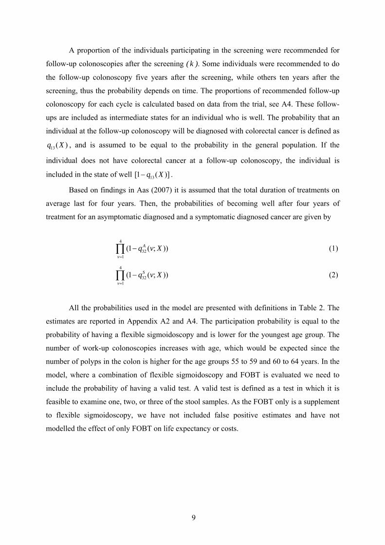
A proportion of the individuals participating in the screening were recommended for

follow-up colonoscopies after the screening ( k ). Some individuals were recommended to do

the follow-up colonoscopy five years after the screening, while others ten years after the

screening, thus the probability depends on time. The proportions of recommended follow-up

colonoscopy for each cycle is calculated based on data from the trial, see A4. These follow-

ups are included as intermediate states for an individual who is well. The probability that an

individual at the follow-up colonoscopy will be diagnosed with colorectal cancer is defined as

13 ( )q X , and is assumed to be equal to the probability in the general population. If the

individual does not have colorectal cancer at a follow-up colonoscopy, the individual is

included in the state of well 13[1 ( )]q X− .

Based on findings in Aas (2007) it is assumed that the total duration of treatments on

average last for four years. Then, the probabilities of becoming well after four years of

treatment for an asymptomatic diagnosed and a symptomatic diagnosed cancer are given by

4

321

(1 ( ; ))A

v

q v X=

−∏ (1)

4

321

(1 ( ; ))S

v

q v X=

−∏ (2)

All the probabilities used in the model are presented with definitions in Table 2. The

estimates are reported in Appendix A2 and A4. The participation probability is equal to the

probability of having a flexible sigmoidoscopy and is lower for the youngest age group. The

number of work-up colonoscopies increases with age, which would be expected since the

number of polyps in the colon is higher for the age groups 55 to 59 and 60 to 64 years. In the

model, where a combination of flexible sigmoidoscopy and FOBT is evaluated we need to

include the probability of having a valid test. A valid test is defined as a test in which it is

feasible to examine one, two, or three of the stool samples. As the FOBT only is a supplement

to flexible sigmoidoscopy, we have not included false positive estimates and have not

modelled the effect of only FOBT on life expectancy or costs.

10

Well

FlexSigm

Symptomatic CRC 1

Work-up colonoscopy

Asymptomatic CRC 1

( )32 1;Sq X

12 ( )q X

32 (1; )Aq X

13 ( )q X

321 (4; )Sq X−

(1 – h)

c

(1 )c−

h

321 (1; )Aq X−

321 (1; )Sq X−

Other

Invited to Flex. Sigm.

a (1 – a)

Follow-up colonoscopy

k 131 ( )q X−

13 ( )q X

1

Asymptomatic CRC 2

Asymptomatic CRC 3

Asymptomatic CRC 4

Dead

Symptomatic CRC 2

Symptomatic CRC 3

Symptomatic CRC 4

32(2; )

A

q X

32 (4; )Aq X

32 (3; )Aq X

321 (3; )Aq X−

321 (2; )Sq X− 321 (3; )Sq X−

32 (2; )Sq X 32 (3; )Sq X

32 (4; )Sq X

321 (2; )Aq X−

321 (4; )Aq X−

Figure 2: Screening by flexible sigmoidoscopy where black and grey ovals represent states in which patients remain for at least a full 1-year cycle. The white ovals represent intermediate states of screening procedures which patients may enter and leave during a cycle. The arrows represent transition between various states.

11

Based on the model introduced above, we can simulate life expectancy for the

different screening strategies and the control group. Let the nine screening groups be

represented by g = FS5054, FS5559, FS6064, COMB5054, COMB5559, COMB6064, C5054,

C5559 and C6064, where g = 1, 2, …,9, respectively and ( )gL t be the surviving probability at

time t for screening group g. Since time of death is distributed over the cycle, we include half-

cycle correction, which reduce the health benefit (survival probability) to the half in the first

and the last cycle. Total life expectancy LE for screening group g is then given by

1

20.5[ (1) ( )] ( )Tg g g g

tLE L L T L t−

== + ∑ .

The probability of surviving t = 1 for screening group g at age tX is given by:

12 1 13 1

13 1 32 1

32 1

(1) 0.5{(1 )[1 ( ) ( )]

(1 ) ( )[1 (1; )]

[1 (1; )]}

g

S

A

L p q X q X

p q X q X

p q X

= − − −

+ − −

+ −

(3)

The first line of (3) is the probability of remaining in the state well during cycle one, i.e. not

dying from causes other than colorectal cancer and not being diagnosed with colorectal

cancer. The second line is the probability of surviving the first year of treatment for

symptomatic cancer, while the last line represents the probability of surviving the first year of

treatment for asymptomatic cancer. The probability of surviving until the start of cycle three

is given by

12 1 13 1 12 2 13 2

13 1 32 1 32 2

12 1 13 1 2 13 2 32 2

32 1 32

(2) (1 )[1 ( ) ( )][1 ( ) ( )]

(1 ) ( )[1 (1; )][1 (2; )]

(1 )[1 ( ) ( )](1 ) ( )[1 (1; )]

[1 (1; )][1

g

S S

S

A

L p q X q X q X q X

p q X q X q X

p q X q X k q X q X

p q X q

= − − − − −

+ − − −

+ − − − + −

+ − − 2(2; )]A X

(4)

Equation (4) contains of four parts: The first line in is the probability of remaining in the state

well through cycle two, i.e. not dying from other causes than colorectal cancer or being

diagnosed with symptomatic cancer in cycle two. Further, the second line is the probability of

surviving until the third year of treatment for a symptomatic cancer diagnosed in cycle one.

Line three is the probability of surviving until the second year of treatment of a symptomatic

12

cancer diagnosed in cycle two. The last line is the probability of being diagnosed with an

asymptomatic colorectal cancer in cycle one and surviving until the third year of treatment.

312 131

13 1 32 1 32 2 32 3

12 1 13 1 13 2 32 2 32 3

12

(3) (1 ) [1 ( ) ( )]

(1 ) ( )[1 (1; )][1 (2; )][1 (3; )]

(1 )[1 ( ) ( )] ( )[1 (1; )][1 (2; )]

(1 ) [1 (

gt ttS S S

S S

L p q X q X

p q X q X q X q X

p q X q X q X q X q X

p q X

== − − −

+ − − − −

+ − − − − −

+ − −

∏

213 13 3 32 31

32 1 32 2 32 3

) ( )] ( )[1 (1; )]

[1 (1; )][1 (2; )][1 (3; )]

St tt

A A A

q X q X q X

p q X q X q X=

− −

+ − − −

∏ (5)

where (5) is the probability of surviving until cycle 4. Let T = 36 and r be the discount rate,

then life-years gained (LYG) for screening group 1 is given by

{ }1 ( 1) 7(1 ) t gLYG r LE LE− −= + − (6)

4. Transition probabilities

4.1 Transition from well to colorectal cancer or to death from causes other than colorectal

cancer

In this Section we estimate the transitions from well to colorectal cancer ( 13q ) and

from well to death ( 12q ). We have data on colorectal cancer diagnosis and deaths from 1999

to 2004 for which number of years of observation ranges from a maximum of six (for

individuals invited in 1999) to a minimum of four (for individuals invited in 2001). The

variation in age ranges from 50 to 69 years.

Because groups were limited we have simplified the estimation by assuming that

observations for an individual are independent over time. This implies that an individual

surviving six years is counted as six different individuals all being well, while an individual

surviving until dying after four years is counted as three well individuals and one dying. If

there are unobserved individual-specific factors that are correlated over time, the transition

over years will not be independent and accordingly the estimates of the model parameters will

be biased. This potential bias is however not expected to have an impact on the comparison

between the screening group and the control group because there is no reason to believe that

the correlation over time will be affected of screening.

13

Let j refer to the state to which the individual can transfer, j = 2 and 3. The transitions

are independent of time and duration, but change with age, X, and intervention group,

g=FS5054, FS5559, FS6064, COMB5054, COMB5559, COMB6064, C5054, C5559 and

C6064. The probability for individual i to transform from well to CRC or death is assumed to

be given by the multinomial logit model:

0 1

02 12 03 131 ( )

1

j i i jg

i i i ig g

g X

i j g X g X

eq Xe e

β β

β β β β

+

+ +

∑= ∑ ∑+ +

(7)

where i = 1, 2, …. N, j=2 and 3, 02 03 12 13, , and β β β β are parameters to be estimated by the

model. Let Yi1j = 1 if individual i goes from state 1 to state j. From this we can derive the log

likelihood function5

LogL = 3

1 11 2log ( )N

i j i ji jY q X

= =∑ ∑ (8)

The parameters in (8) are estimated by the maximum likelihood method6. The results

from the estimation are reported in Table 3 and presented according to age groups. The

transition from well to both death and colorectal cancer increases with age.

For all age groups in Table 3, the control group for a specific age group is the

reference group and the parameter estimates are only reported for the screening strategies

within the relevant age group. For the age group 60 to 64 years, there are no significant

differences between the control and the two intervention groups with regard to the effect on

death and colorectal cancer. For the age group 55 to 59 years a combination of flexible

sigmoidoscopy and FOBT has a significant negative effect on death, while only flexible

sigmoidoscopy has a significant negative effect on the probability of developing colorectal

cancer. In the age group 50 to 54 years the only significant effect is the negative effect on the

probability of developing colorectal cancer for the individuals invited to only flexible

sigmoidoscopy.

5 For further details on multinomial logit, see Green (2002) 6 Estimated with STATA release 8.

14

Table 3: Parameters estimates of the multinomial logit model (SD in parenthesis). No. of observations is 687604 Transition from well (1) to:

Variable

60 to 64 years

55 to 59 years

50 to 54 years

Death (j=2)

Age 0.00033 (0.00003)*** 0.00033 (0.00003)*** 0.00033 (0.00003)*** Screening group C5054 - - Ref. FS5054 - - 0.00003(0.0005) COMB5054 - - -0.00052(0.0005) C5559 - Ref. - FS5559 - -0.00032 (0.0003) - COMB5559 - -0.0007 (0.0003)** - C6064 Ref. - - FS6064 -0.00013 (0.00036) - - COMB6064 -0.00054 (0.00034) - - Colorectal cancer (j=3)

Age 0.00004 (0.00001)*** 0.00004 (0.00001)*** 0.00004 (0.00001)*** Screening group C5054 - - Ref. FS5054 - - -0.00036 (0.0001)*** COMB5054 - - 0.00001(0.00021) C5559 - Ref. - FS5559 - -0.00026 (0.0001)*** - COMB5559 - -0.00015(0.0001) - C6064 Ref. - - FS6064 -0.00009 (0.00011) - - COMB6064 -0.00002 (0.00012) - - *** Significant at 1 percent level, ** Significant at 5 percent level, * Significant at 10 percent level

The estimated coefficients are used to predict the transition probabilities for the age

groups 50 to 67. The predicted probabilities are then used to simulate the surviving

probabilities for the first six cycles. However, as the variation in age is limited, we used

information from the Cancer Registry of Norway and Statistics Norway to predict the

transitions from cycle 7. From cycle 7, it is assumed that for a given age the transitions are

equal for the screening groups and the control group. Hence, due to insufficient information,

we do not include the effect of screening on the probability of developing colorectal cancer in

the future. The transitions are reported in Appendix, A3.

4.2 Transition from colorectal cancer to death

In this Section we estimate the transitions from colorectal cancer to death 32 ( ; )Aq v X

and 32 ( ; )Sq v X the first four years after diagnosis. We have data on colorectal cancer diagnosis

and deaths from 1999 to 2004 for which number of years of observation ranges from a

15

maximum of six (for individuals invited in 1999) to a minimum of four (for individuals

invited in 2001). The variation in age ranges from 50 to 69 years. In Aas (2007) it is shown

that the transition from colorectal cancer to death is independent of duration within the age

group 50 to 69, thus the probability of dying during treatment of asymptomatic and

symptomatic cancer are 32 32( ) and ( )A Sq X q X , respectively. From Aas (2007) we know that

treatment costs for colorectal cancer are approximately zero five years after diagnosis. Based

on this, we assume that all individuals, except those dying during treatment, are treated for

colorectal cancer within four years of diagnosis. The transitions are assumed to depend on age

at the time of diagnosis, X, and whether the cancer is diagnosed due to symptoms or not7. The

transition probability for individual i diagnosed with an asymptomatic and symptomatic

cancer to die one out of four years of treatment of colorectal cancer is then estimated by the

logit models:

14

321( ) 1

1 i Aj

AXq X

e β⎛ ⎞= − ⎜ ⎟+⎝ ⎠

(9)

14

321( ) 1

1 i Aj

SXq X

e β⎛ ⎞= − ⎜ ⎟+⎝ ⎠

(10)

To estimate the probability in (9) we use data for 41 asymptomatic cancers out of

which two died within four years of treatment. To estimate (10) we use 471 symptomatic

cancers out of which 159 died during four years of treatment. We use the maximum

likelihood method8. The results are presented in Table 4. We see that age do not have any

significant effect on the probability of dying, thus the probability of dying during four years

of treatment is independent of both age and duration. The probability of dying is then constant

over the four years. For asymptomatic diagnosed cancer 32 ( ) 0.012Aq X = and for symptomatic

cancer 32 ( ) 0.097Sq X = . The transitions are reported in A3. The predicted probabilities are

used to simulate the conditional probability of being well at the start of cycle t and surviving

until cycle t+1 for the six first cycles.

7 The transition is in Aas (2007) shown to depend on variables like education and Dukes stages, but these factors are not included here since they are not needed in the estimation of life-expectancy. 8 Estimated with STATA release 8.

16

Table 4: Parameter estimates from the logit model (SD in parenthesis). No of observation are 513 out of which 41 is asymptomatic. Screening group Variable Coefficients Asymptomatic diagnosed cancer Age - 0.0058 (0.009) Symptomatic diagnosed cancer Age - 0.0033 (0.005) *** significant at a 1 per cent level, ** significant at a 5 per cent level, * significant at a 10 per cent level

Technically, the model can predict transition for all cycles, but as we know that

increasing age is expected to reduce survival and survival is also expected to depend on the

duration (Cancer Registry of Norway, 2003), we do not use the result in Table 4 to predict

beyond cycle six. From cycle 7 we supplement with data from the Cancer Registry of Norway

and Statistics Norway (Statistics Norway, 2004). From cycle seven, the deaths during

treatment of symptomatic colorectal cancer include only colorectal cancer as cause of death.

From the Cancer Registry of Norway we know that the probability of dying depends on time

from diagnosis, about 58 percent of the deaths occur within the first year and 20, 13, and 9

percent during the second, third, and fourth years, respectively (the transitions used are

reported in A3).

5. Screening costs We divided the costs into four categories, which allow us to analyse how inclusion of

different cost estimates affect the cost per life-year gained. It also facilitates comparison with

relevant literature because previous analyses on cost-effectiveness of colorectal cancer

screening include various cost estimates.

The first category encompasses the direct program costs and includes the opportunity

cost of all resources used to carry out the screening (Table 5). The cost of invitations to

screening and reminder letters is a rough estimate that includes stamps, envelopes, and letters.

Reimbursement from the National Insurance Administration is used to estimate the cost of

diagnostic sigmoidoscopy and therapeutic colonoscopy. On the basis of a Norwegian study

(Samdata somatikk, 2004) we have adjusted all the fees from the National Insurance

Administration by a factor of 1.5 to reflect the true cost. The price of Laxabon® for bowel

cleansing before a colonoscopy is the market price the individual has to pay at the pharmacy.

17

Table 5: Direct program costs, unit price, and source of information (prices from 2003)

Screening costs Unit cost (Euro) Source

Invitation letter 2 Expert opinion

Reminder 2 Expert opinion

Diagnostic sigmoidoscopy 180 The National Insurance Administration

Therapeutic colonoscopy (inclusive

polypectomy and biopsy)

225 The National Insurance Administration

Laxabon® - bowel cleansing 8.75 Market price

FOBT test in the letter 3 Expert opinion

FOBT examination 5 Expert opinion

The indirect program cost is the second cost category and includes the individual’s

travel expenses to the screening and, if required, to the colonoscopy (if he had a high or low

risk adenoma). From Aas (2004, 2005) we know that average travel expenses for those

participating were 9 Euro. Furthermore, the indirect program costs also contain production

losses resulting from travel time to the screening examination and/or to the colonoscopy and

the time used on the sigmoidoscopy and/or the colonoscopy examination. On average, the

time travelling to the screening centre for a flexible sigmoidoscopy screening examination or

colonoscopy is 1 hour and 15 minutes, see Aas (2005). Preparation at the centre and

sigmoidoscopy takes about 45 minutes so the total screening time (travelling and

sigmoidoscopy) is two hours. Since the colonoscopy requires bowel preparation before the

examination9 and the examination itself is more extensive than a flexible sigmoidoscopy, it is

assumed that total colonoscopy time (travelling and colonoscopy) is one day. Because there is

almost no unemployment in Norway, we use the human capital approach to estimate the

opportunity cost of the production loss. The production losses depend on the age of the

individual because the proportion working declines with age. From Aas (2004, 2005) we

know that the proportion working in the age groups 50 to 54 years, 55 to 59 years, and 60 to

64 years is 0.82, 0.81 and 0.62, respectively. Production loss per day is calculated on the basis

of gross income reported for individuals responding to the survey used in Aas (2004, 2005).

From Table 6 we see that the production loss declines with age, which can be

explained by an increasing proportion working part time in the older age groups. We have

assumed the opportunity cost for individuals not working is equal to zero.

9 The bowel cleansing has to start at 4 pm on the day before the colonoscopy.

18

Table 6: Indirect program costs, unit price and source of information (2003)

Screening costs Cost (Euro) Source

Travel expenses 9 Aas (2004, 2005)

Production loss per day

50 to 54 311 Aas (2004, 2005)

55 to 59 306 Aas (2004, 2005)

60 to 64 288 Aas (2004, 2005)

The third category is direct program consequences. There are two direct program

consequences with regard to treatment cost of colorectal cancer. The first effect is reduced

future treatment cost resulting from reduction in future incidence of colorectal cancer and the

second effect reflects the fact that screening allows diagnosis of asymptomatic cancers, which

are less expensive to treat10. In Table 7 treatment cost is presented for symptomatic and

asymptomatic cancers and includes surgery, chemotherapy, and follow-up colonoscopies

(radiotherapy is not included). The treatment follows certain standard procedures (Norwegian

Gastrointestinal Cancer Group, 1999), but there is room for individual variation. The

treatment costs are estimated on the basis of information about inpatient stays and outpatient

consultations from the National Patient Register and the National Insurance Administration.

We use hospital reimbursement as the basis for estimating treatment costs. The hospitals have

“activity-based financing” based on diagnosis-related groups (DRG). The DRG system

classifies hospital services into groups that are medically related and homogeneous with

regard to use of resources. DRGs describe a hospital's case-mix. In Norway there are

approximately 500 different DRGs. Each DRG11 is given a weight that reflects the treatment

cost. For outpatient services the fee for service only partly covers the true cost. On the basis

of a Norwegian study (Samdata somatikk, 2004) we have adjusted all the reimbursements

from the National Insurance Administration by a factor of 1.5 so that they reflect the true cost.

We use the DRG weights for 2003 for all years since there have been no major changes in the

treatment for colorectal cancer.

To estimate the treatment cost we use all registered care directly related to the

treatment of colorectal cancer from our database12. The data stems from the National Patient

10 Details will be published a forthcoming paper by Aas, 2007. The effect of screening on treatment cost – the case of colorectal cancer. 11 The unit price of a DRG is equal to Euro 3,706 in 2003. 12 For details on the estimation of the estimation of treatment costs, see Aas (2007).

19

Register with the appropriate fees, DRGs, and DRG weights. Treatment costs are estimated

for asymptomatic cancers and symptomatic cancers. The estimation is done in several steps:

first, calculating treatment cost per registration; second, estimating total treatment costs per

month for the stage by adding the treatment cost per registration for each month for all

individuals in the stage; third, estimating the average treatment costs per month for the stage

by dividing total treatment cost per month for that stage by the sum of individuals diagnosed

with cancer at that stage and alive in that specific month; fourth, adjusting the average

treatment cost per month for estimated survival per month according to Dukes stage; and

finally, adding together the average treatment cost per month over the whole period to arrive

at the expected colorectal cancer treatment cost for either a Dukes stage or a participation

group.

On average, the treatment period lasts for four years after diagnosis, see Aas (2007). In

the model we assume that recurrences are indirectly captured in the treatment cost. The

treatment of symptomatic cancers costs about 9,000 Euro more than asymptomatic cancers.

Table 7: Treatment cost for colorectal cancer according to date of diagnosis and year from diagnosis Category First Second Third Fourth Total Symptomatic cancers 18,880 4,718 2,734 1,908 28,240 Asymptomatic cancers 16,416 2,058 493 196 19,163

In addition to treatment costs, the direct consequences also include costs related to

future recommended follow-up colonoscopies. The recommendation for the majority of

colorectal cancer patients is to have a five-year follow-up colonoscopy, but for some patients

an earlier follow-up plus an additional colonoscopy up to ten years after screening are

recommended. The last follow-up is in cycle 11. We use the costs per colonoscopy in Table 6.

Probabilities are reported in Appendix A4.

Finally, the fourth category of costs is the indirect program consequences. This

includes travel expenses and production loss resulting from future recommended

colonoscopies and production gain due to early detection or reduced severity. If the screening

prevents future incidences, this could also result in production gains. We use the estimates of

travel expenses and production loss reported in Table 6 and the probabilities in Appendix A4

to calculate production loss for future recommended colonoscopies.

20

Table 8: Descriptive statistics on the number of days of sick leave according to age group and time of diagnosis (asymptomatic and symptomatic) Age group Diagnosis Mean N Std. dev 50-54

Symptomatic

262.06

34

145.9 Asymptomatic 199.83 6 199.6 55-59

Symptomatic

294.32

34

177.8 Asymptomatic 281.92 13 119.3 60-64

Symptomatic

235.26

53

148.7 Asymptomatic 255.67 9 114.8 Total

Symptomatic

259.39

121

157.3 Asymptomatic 255.89 28 136.5

To estimate production gains we test whether or not there are differences in the

number of days of sick leave after a cancer diagnosis between asymptomatic diagnosed

cancers and symptomatic cancers. We use information from Statistics Norway about a

number of social security recipients, labour market status, and number of days of sick leave to

estimate the production gain. In Table 8 the number of days of sick leave is reported for

individuals working at the time of diagnosis according to age group and whether the cancer

was diagnosed at an asymptomatic or symptomatic stage. While there is almost no difference

in number of days of sick leave according to symptomatic or asymptomatic stage for the two

oldest age groups, there is a difference for individuals in the age group 50 to 54 years. This

indicates that early diagnosis results in some production gains for the youngest age group.

However, because the standard deviation is large, the difference is not statistically significant

and we have therefore not included production gains in the model.

Let gC be total screening costs for screening group g over all cycles. The incremental

screening costs ( CΔ ) for screening group 1 is then given by

1 ( 1) 1 7(1 ) tC r C C− − ⎡ ⎤Δ = + −⎣ ⎦ (11)

6. Results In this analysis we simulate cost per life-year gained for six alternative strategies13.

There are three age groups (50-54, 55-59, 60-64 years) and two screening interventions,

13 We use TreeAge Pro 2005 in the estimation of the model.

21

flexible sigmoidoscopy alone or in a combination with FOBT. We discount both costs and

effects and apply a discount rate equal to four percent, which is according to Norwegian

guidelines from The Norwegian Ministry of Finance (2005). Based on equation (6) and (11),

cost per life-year gained for ( gCE ) for screening group 1 will then be given by

1

11

CCELYGΔ

= (12)

In Table 9 the estimated life expectancy ( gLE ) in years is reported for all six strategies and

the control groups based on the principle of ‘intention to treat’. The expected life-years gained

(LYG) are also reported. The largest gain in life expectancy is in the age group 60 to 64 years,

for an individual invited to both flexible sigmoidoscopy and FOBT; the age group 55 to 59

years invited to a combination of flexible sigmoidoscopy and FOBT has the second largest

gain. From the findings in Tables 1 and 3, we would expect that largest increase in life-years

would be for individuals in the age groups 55 to 59 years or 60 to 64 years. The probability of

dying during treatment of an asymptomatic diagnosed cancer is 5 percent each year

(compared with 11.5 percent for a symptomatic diagnosed cancer). There is a large difference

in life-years gained between screening with only flexible sigmoidoscopy and the combination

of flexible sigmoidoscopy and FOBT. The results are driven by the difference in the

probability of dying from causes other than colorectal cancer. As the samples in the different

screening groups are small with regard to death, the difference can occur by chance. If,

however, there is a positive relationship between the probability of dying during treatment of

colorectal cancer and deaths from causes other than colorectal cancer (for instance from

pneumonia), early detection may also reduce the probability of dying from other causes

during the first years after the screening.

Initially, 2,632 individuals in the age group 60 to 64 years were invited to a

combination of flexible sigmoidoscopy and FOBT. Given the increase in life expectancy

shown in Table 9, a total number of 237 life-years are gained14. From Statistics Norway we

find average life expectancy for an individual 62 years of age to be approximately 20 years;

thus, approximately 12 individuals could live until the age 8215. As the number of life-years

gained is zero for the age group 50 to 54 with only flexible sigmoidoscopy, reporting cost-

effectiveness is not meaningful.

14 2,632*0.09 = 237 life-years gained. 15 237/20 = 12

22

Table 9 also presents the results from the cost-effectiveness analyses presented. There

are four different estimations representing different cost categories. In three out of four

alternatives, screening the age group 55 to 59 years with a combination of flexible

sigmoidoscopy and FOBT is the most cost-effective alternative.

When only direct program costs are considered, the cost per life-year gained is Euro

1,63316. The second most cost-effective alternative is screening the age group 60 to 64 years

with a combination of the two tests, closely followed by the age group 55 to 59 years

examined only with flexible sigmoidoscopy. Inclusion of indirect program costs increases the

cost per life-year gained to Euro 2,156, but it also changes the most cost-effective alternative

to the age groups 60 to 64 years with both flexible sigmoidoscopy and FOBT. The change in

the most cost-effective alternative can be explained by a higher proportion working in the age

group 55 to 59 years. The difference in cost-effectiveness between the second and third most

cost-effective alternatives increases since a larger proportion is working in the younger age

groups.

Taking direct program consequences into consideration increases the costs per life-

year gained for all screening strategies, and changes the ranking of the most cost-effective

alternative. Inclusion of direct program consequences implies a reduction in cost per life-year

gained for both screening strategies in the age group 55 to 59, while for the other age groups

it implies an increase in cost per life-year gained. This changes the ranking of the strategies as

the inclusion of treatment costs implies that the most cost-effective alternative changes to the

age group 55 to 59 years with a combination of the two tests. The age group 60 to 64 years

with a combination of the two tests has the second lowest cost per life-year gained. The

increase in cost per life-year gained in the age group 55 to 59 years is smaller than the

increase in cost per life-year gained in the age group 60 to 64 years, which can be explained

by different proportions of asymptomatic diagnosed cancers. In the age group 60 to 64 years,

the asymptomatic cancers constitute of a smaller proportion of the total number of diagnosed

cancers than in the younger age groups (see Table 1). Direct program consequences include

costs resulting from future follow-up colonoscopy. These costs will, for all alternatives,

increase the cost per life-year gained and do not change the ranking of the strategies.

16 147/0.09=1,633

23

Table 9: Life-years, screening costs and costs per life-year gained according to screening strategy and groups of screening costs (monetary units in Euro) Strategy Effect Cost alt. 1* Cost alt. 2** Cost alt. 3*** Cost alt. 4**** LE LYG Cost CE Cost CE Cost CE Cost CE C5054

16.74

-

0

0

724

724

FS5054 16.74 0.00 137 - 189 - 1,025 - 1,034 - COMB5054 16.76 0.02 119 5,950 172 8,600 1,005 14,050 1,013 14,450 C5559

15.37

-

0

0

948

948

FS5559 15.41 0.04 151 3,775 208 5,200 1,155 5,175 1,169 5,525 COMB5559 15.46 0.09 147 1,633 203 2,255 1,165 2,411 1,177 2,544 C6064

13.83

-

0

0

1,040

1,040

FS6064 13.84 0.01 153 15,300 194 19,400 1,271 23,100 1,285 24,500 COMB6064 13.92 0.09 151 1,678 194 2,156 1,259 2,433 1,271 2,567 * Cost alternative 1 includes the direct program costs ** Cost alternative 2 includes the direct and indirect program costs *** Cost alternative 3 includes the direct and indirect program costs and direct program consequences **** Cost alternative 4 includes the direct and indirect program costs and direct and indirect program consequences

A reduction in future incidences implies a further reduction in the cost per life-year

gained. Access to additional data can help determine whether or not the screening method will

prevent future incidence of cancer.

The last cost alternative consists of the indirect programme costs. These costs are

related to travel expenses, the use of Laxabon® for bowel cleansing, and production loss due

to time used on future recommended follow-up colonoscopies. The age group 55 to 59 years

screened with a combination of flexible sigmoidoscopy and FOBT is also the most cost-

effective alternative in this cost alternative.

In Table 10 the incremental cost-effectiveness ratio (ICER) based on cost alternative 4

in Table 9 is reported. The ICER is defined as the incremental cost per incremental effect.

Because screening is a once-only event, all screening strategies are mutually exclusive and

must be compared. The screening strategies are reported in ascending order according to cost,

where costs reported are the difference in cost between a screening group and the control

group. The incremental cost is the increase in cost between screening strategies17. Life-years

gained (LYG) (also reported in Table 9) and incremental LYG18 are reported in columns four

and five, respectively. The ICER is reported in column six19 and we see that the ICER for the

age group 55 to 59 years with a combination of flexible sigmoidoscopy and FOBT is Euro

160. All the other screening strategies are dominated because the incremental cost is positive

and the incremental effect is ether zero or negative.

17 The incremental cost for COMB5559 is equal to 229 – 221 = 8 18 The incremental effect for COMB5559 is equal to 0.09 – 0.04 = 0.05 19 The incremental effect for COMB5559 is equal to 8/0.05 = 160

24

Table 10: The incremental cost-effectiveness ratio according to screening strategy. Monetary units in Euro. Strategy ∆C* Incremental

cost LYG Incremental LYG ICER

FS5559 221 0.04 COMB5559 229 8 0.09 0.05 160 COMB6064 231 2 0.09 0.00 (Dominated) FS6064 240 9 0.01 -0.08 (Dominated) COMB5054 289 49 0.02 -0.07 (Dominated) FS5054 310 21 0.00 -0.09 (Dominated) *Cost alternative 4 includes the direct and indirect program costs and direct and indirect program consequences

7. Sensitivity analysis The estimation of life-years gained and costs in the model consists of several factors.

Some of these factors are uncertain. In this section we want to test whether the inclusion of

uncertainty changes the findings from Section 6, and give an indication of which type of

uncertainty tends to most affect the findings.

Two types of sensitivity analysis are included in this paper. First, we use deterministic

sensitivity analysis to see how one factor at a time influences cost-effectiveness. Second, we

include a probabilistic sensitivity analysis (PSA), which is a parametric method, as we make

assumptions about the distribution. Both the U.S. panel on cost-effectiveness analysis (Gold

et al. (1996)) and the National Institute of Clinical Excellence (NICE) in the UK (2006) have

suggested using PSA to deal with uncertainty in cost-effectiveness models because a well-

conducted PSA will provide a more realistic representation of variations in the model results.

All uncertainty in the parameters is included simultaneously in a PSA. The uncertainty in a

specific parameter is represented by a distribution.

In Table 11 the results from the deterministic sensitivity analysis are presented. All of

the alternatives are based on the fourth cost alternative (all costs included) from Table 9 in

Section 6. In alternative 1 we have increased the value in the fee-for-service for

sigmoidoscopy and colonoscopy to account for uncertainty in the estimate of the true

marginal cost. Alternative 1 includes the cost per life-year gained by assuming a doubling of

the fee-for-service (Samdata somatikk, 2004). The cost per life-year gained is increased for all

strategies, but the ranking remains unchanged.

The simulation of treatment costs is based on stage of advancement. Because

treatment costs increase with stage of advancement, the treatment costs for asymptomatic

25

cancers is lower than for symptomatic cancers20. Stage of advancement is measured in groups

and not on a continuous scale, thus there will be variations in costs within each group and our

predictions will be the expected costs of recommended treatment. In addition, even though

there are guidelines for the treatment of colorectal cancer, health personnel at one hospital or

within one hospital may have different views on the amount or type of treatment, like

chemotherapy, necessary for a specific patient. The cost predictions are based on fees and

DRGs. These are average predictions and in some situations do not reflect the true treatment

cost for a particular patient. For example, the same type of treatment according to the DRG

for two individuals of different ages may call for a different use of resources. If the older

individual recovers more slowly, he will need a longer stay in hospital than the younger

individual, a difference that is not necessarily reflected in the DRG. Complications due to

treatment of other diseases concurrent to the treatment for colorectal cancer may also result in

variations in treatment costs. Alternative 2 in Table 10 shows the cost-effectiveness based on

the assumption that the treatment costs for asymptomatic cancers is equal to the treatment

costs for symptomatic cancers. This assumption increases the cost per life-year gained for all

screening strategies, for the most cost-effective alternative by about Euro 5,500.

Table 11: The effect on costs per life-year gained of changing the value of some of the factors used in the model according to screening strategy (monetary units in Euro). Strategy Alt 1 Alt 2 Alt 3 Alt 4 ∆C CE ∆C CE ∆C CE LE CE C5054 724 724 724 28.79 FS5054 1,078 - 1,773 - 1,031 - 28.78 - COMB5054 1,051 16,350 1,749 51,250 1,010 14,300 28.80 31,000C5559 948 948 948 25.23 FS5559 1,218 6,750 1,862 22,850 1,167 5,475 25.29 3,683COMB5559 1,223 3,056 1,714 8,511 1,175 2,522 25.38 1,527C6064 1,040 1,040 1,040 21.41 FS6064 1,335 29,500 1,874 83,400 1,291 25,100 21.43 12,250COMB6064 1,331 3,233 1,866 9,178 1,277 2,633 21.60 1,215Alt 1: The cost of sigmoidoscopy and colonoscopy is 240 Euro and 300 Euro, respectively. Alt 2: Equal treatment costs for asymptomatic and symptomatic diagnosed cancers Alt 3: Production loss per individual estimated to be equal to 225 Euro for all three age groups Alt 4: No discounting of health benefits

The third alternative includes a different prediction of the production loss resulting

from time required for the screening and the colonoscopy. The estimates used in the

simulation of total screening costs are based on Aas (2004, 2005), however, not all

participants answered the questionnaire so the estimates could be biased. We therefore include

20 For details, see Aas (2007).

26

an estimate from another Norwegian study (Hem, 2000) where the average wage per day is

equal to Euro 225. From Table 11 we see that this change implies a very small to change the

cost-effectiveness.

Although the recommended procedure is to discount both costs and health effects at

the same rate (NICE, 2006 and Drummond et al., 2005), there are arguments for not

discounting health benefits at all or for doing so using a lower discount rate than for costs (see

Drummond et al., 2005). We have included an alternative where the health benefits are not

discounted in order to see the magnitude of the effect of discounting on the health benefits.

Comparing the findings in Table 11 with the life-expectancy in Table 9, we see that life-

expectancy for most alternatives will increase by eight to twelve life years, and that all cost-

effectiveness ratios decline. The ranking is unchanged.

In Section 4 we concluded that estimates of the differences in number of days of sick

leave are too uncertain to be included in the model. Still, there were some indications in Table

8 that there were potential production gains in the age group 50 to 54 years. We have

therefore tried to estimate the difference in number of days of sick leave that would be needed

to change the ranking of the cost-effectiveness in Table 9. In order for the age group 50 to 54

years with both flexible sigmoidoscopy and FOBT to be ranked as the most cost-effective

strategy, the difference in number of days of sick leave would have to be 505 days.

From the deterministic sensitivity analysis we see that there are changes in the cost-

effectiveness levels and the rankings, but the changes are relatively small. Thus, any decisive

change in the cost-effectiveness must stem from uncertainty in the estimates of the transition

probabilities.

In the probabilistic sensitivity analysis we include the uncertainty in the cost of

sigmoidoscopy and colonoscopy, variation in the treatment costs, together with uncertainty in

the transition probabilities. The cost of sigmoidoscopy and colonoscopy are assumed to be

uniformly distributed with variation from 1.5 to 2 times higher than the fee for service

reimbursement from the National Insurance Administration (Samdata somatikk, 2004).

With regard to the distribution of the treatment costs, we use findings from the

bootstrap in Aas (2007). Bootstrapping is a method for assigning measures of accuracy to

statistical estimates, in the present case the treatment cost estimates. We use bootstrapping to

estimate the standard error (see Efron and Thibshirani 1993) of the treatment cost shown in

Table 7. The bootstrap standard error is estimated by using the original samples. A bootstrap

sample (equal to n) of treatment cost in year 1 is obtained by random sampling n times, with

replacement, from the original sample, which means that some of the observations will be

27

sampled once, others several times and some not at all. The method generates a large number

of bootstrap samples, each of size n. We reapply the estimator (for instance the treatment cost

in year 1) from each bootstrap sample and calculate the standard deviation. Mean and 95

percent confidence intervals are presented in Table 12 according to asymptomatic or

symptomatic diagnosed cancer and year from diagnosis. The confidence interval is

overlapping for the two first years. Because colorectal cancer treatment cost only has positive

values, we use gamma distributions to represent uncertainty (Spiegelhalter et al., 2004). To

estimate the coefficients in the gamma distribution, we use calculated mean and variance from

the bootstrap. The assumptions used in the PSA are presented in Appendix A5.

Table 12: Mean and 95 percent confidence intervals for mean treatment costs for asymptomatic and symptomatic diagnosed cancers according to year from diagnosis. Numbers in Euro. Year Asymptomatic Symptomatic

Mean 95 percent CI Mean 95 percent CI 1 16,416 (13,638 – 20,127) 18,880 (17,614 – 20,461) 2 2,058 (923 – 4,161) 4,718 (3,509 – 6,385) 3 493 (238 – 1,091) 2,734 (1,608 – 4,692) 4 196 (91 – 463) 1,908 (582 – 6,837)

We include uncertainty in the transition probabilities by letting the transition

probabilities for each stage vary by ten percent, and let the variation be represented by a

uniform distribution. For each stage, the estimated coefficients represent by a minimum and a

maximum value. We then use a Monte Carlo simulation to estimate the uncertainty in the

parameters by selecting values from the distributions. Monte Carlo simulation in TreeAge

recalculates the model repeatedly as a form of (deterministic) sensitivity analysis. We assume

that the parameters are independent. The results from the PSA analysis are presented in Table

13.

The first column in Table 13 presents the mean life-years for all groups. The second

column reports the 95 percent confidential interval for life-years for the six screening groups.

All confidence intervals are overlapping with the mean life-years for the corresponding

control group. For instance, the mean life-years in the age group 55 to 59 years are 15.36 for

the control group. The 95 percent confidential interval for the mean life-years for the age

group 55 to 59 years with only flexible sigmoidoscopy and the combination of the two tests

are 15.14 to 15.70 and 15.17 to 15.74, respectively. The third column presents the mean costs

from the PSA analysis, while the fourth column reports the 95 percent confidence interval for

28

the screening costs for the six screening groups. For all screening strategies, the costs are

significantly higher than the control group. The results from the PSA imply that the results are

statistically non-significant for all screening groups, both with respect to costs and life-

expectancy.

Table 13: Mean and 95 percent confidential interval from PSA of screening cost and life-year according to screening strategy. Numbers in Euro. Strategy Mean

life-years 95 percent CI Mean costs 95 percent CI

C5054

16.74

-

724

FS5054 16.74 (16.52 – 16.96) 1,032 (940 – 1,132) COMB5054 16.75 (16.52 – 16.95) 1,011 (896 – 1,145) C5559

15.36

948

FS5559 15.42 (15.14 – 15.70) 1,167 (1,070 – 1,271) COMB5559 15.46 (15.17 – 15.74) 1,180 (1,054 – 1,317) C6064

13.83

1,040

FS6064 13.84 (13.53 – 14.19) 1,284 (1,175 – 1,402) COMB6064 13.92 (13.61 – 14.26) 1,269 (1,147 – 1,404)

8. Discussion As pointed out in the introduction, NORCCAP is one of four RCTs that evaluate once-

only flexible sigmoidoscopy, but several cohort studies have also been conducted. Frazier et

al. (2000) find that the cost per life-year gained for a once-only flexible sigmoidoscopy at the

age of 55 is $ 1,200. Leshno et al. (2003) find that the cost per life-year gained is about $

1,237 for a combination of annual FOBT and flexible sigmoidoscopy every fifth year when

only those participants with high-risk polyps are referred to a follow-up colonoscopy. If the

criterion for a follow-up colonoscopy is changed to any adenomatous polyp regardless of size

or histology, the cost per life-year gained is $ 2,486. Sonnenberg et al (2000) find that the cost

per life-year gained is $ 74,032 for a combination of annual FOBT and flexible

sigmoidoscopy every fifth year. All of these studies include direct program costs and

consequences, but not indirect program costs and consequences.

We know from RCT that FOBT significantly reduces cancer mortality (Mandel et al.,

1993, Hardcastle et al., 1996, Kronborg et al., 1996 and 2004). The reduction is between 16

and 20 percent. Gyrd-Hansen et al. (1998) find that the cost per life-year gained is Euro

29

2,27721 when screening individuals 65 to 74 years every second year. This estimate does not

include treatment costs, which would be expected to reduce the cost per life-year gained.

Whynes et al. (1998) finds that the cost per QALY gained is between Euro 2,164 and Euro

8,977 depending on time horizon in the analysis and the costs included22.

In this study, cost-effectiveness analysis is applied to estimate costs per life-year

gained. Estimating the health effect in life-years gained implies that every year the individual

is not dead counts equally. It is a simple measure to capture, but it only includes the effect of

screening on mortality and not the gain from screening on morbidity. Drummond et al. (2005)

present some situations where it is preferable to use quality adjusted life-years (QALY). For

example, when the expected health effects include both mortality and morbidity, and when it

is relevant to make comparisons with other programs using QALYs as a health measure. A

QALY represents a measure for which improvement in quality of life and not perfect health is

the main outcome. In this study, the model counts a year not dead as one year, while if we had

included QALYs in the analysis, a year under treatment would not be counted as one year.

Introducing QALYs as the health measure will have an uncertain effect on the cost-

effectiveness because it will affect the health outcome in several ways: first, participation in

screening will imply a reduction in quality of life, as participation could heighten anxiety.

Second, during treatment for colorectal cancer the quality of life will be reduced. An

asymptomatic cancer is less severe; hence, quality of life should be expected to be higher for

individuals diagnosed with asymptomatic cancer than with a symptomatic cancer. Finally,

screening with flexible sigmoidoscopy and colonoscopy is expected to reduce the prevalence

of colorectal cancer. The first effect will increase the cost per QALY, the second and third

effects will reduce the cost per QALY. The total effect is therefore uncertain. We know from

a cost-effectiveness analysis of a follow-up program of colorectal treatment, that the QALY

of Dukes B and Dukes C are measured to 0.83, see Norum and Olsen (1997). As QALYs are

often used in economic evaluations, using life-years gained makes it difficult to compare

different strategies or different health programs; thus, further research should also include an

estimate with QALYs.

Two types of biases can occur in an evaluation of cost per life-year gained of a

screening program: length bias and lead-time bias. Length bias occurs because screen-

detected cancers are prone to be less aggressive cancers. An aggressive cancer has a short

asymptomatic period, defined as the period in which the cancer can be diagnosed with a

21 The costs are in 1993 DKK and Euro 1 = DKK 7.466 22 The costs are in £ 1995-96 and Euro 1 = £ 0.633

30

screening test. Therefore, most aggressive cancers are diagnosed due to symptoms. The less

aggressive cancers are over-represented in the screening cohort because they have a longer

asymptomatic period and are more likely to be present (detectable) at any particular point in

time (time of the screening examination). As the probability of cure and survival is higher for

a patient with less aggressive cancer than for patients with more aggressive cancers, screening

may not have an effect on survival. Lead-time bias occurs when screening falsely prolongs

survival. Through screening, the cancer is diagnosed earlier than when diagnosed due to

symptoms, but the outcome in terms of date of death remains unchanged by screening

intervention. Thus, the individual will gain no additional life-years. The time for diagnosis has

only been moved forward. The patient's awareness of having cancer and level of anxiety will

be extended causing a reduction in quality of life.

Lead time bias can only influence the findings in this model because of potential bias

in the estimation of the transition from treatment of asymptomatic diagnosed colorectal cancer

to death. In the estimation of survival we normalise all the dates of diagnosis to zero, i.e.

survival is measured as the time alive from the time of diagnosis. Thus we can not be sure

whether increased survival is due to earlier diagnosis or true prolonged survival. To adjust for

this potential bias, we have run the model with the assumption that the transition from

treatment of asymptomatic diagnosed colorectal cancer to death is the same as for

symptomatic diagnosed cancers. Life-years gained changes by definition for all age groups,

but with two decimals the change can only be seen in the age group 50 to 54 years with a

reduction of 0.01 for both screening groups. This indicates that lead time bias is not a serious

problem in this cost-effectiveness analysis.

A multinomial logit is used to estimate the transition from well to colorectal cancer or

death. If observations for the same individual are not independent over periods, the estimated

transition will be biased. For example, if the probability of staying well depends on individual

characteristics the observations will not be independent. We tried to estimate a model that

took into account that the observations may not be independent, but are not included because

finding proper starting values in the maximum likelihood estimations was problematic. Future

research should focus on this problem in order to further improve the modelling.

Whether false positives are a problem in this analysis depends on the definition of

false positive. If false positive is defined as undergoing treatment of colorectal cancer without

having colorectal cancer, there are no false positives. But, if false positive is defined as the

proportion of the individuals referred to a work-up colonoscopy that never would have

developed colorectal cancer, false positives do exist in this analysis. In the NORCCAP study

31

the criteria for a work-up colonoscopy was a positive flexible sigmoidoscopy and/or a

positive FOBT. A positive sigmoidoscopy is defined as having an adenoma ≤ 10 mm and/or

having a polyp ≥ 10 mm (it is more than 95 percent certain that such a polyp is an adenoma).

As only a proportion of these adenomas and polyps develop into cancer in the future, many

are examined with colonoscopy without any personal benefit. How to define the inclusion

criteria for a work-up colonoscopy requires that the proportion of false positives is balanced

with the proportion of false negatives. If the number of individuals referred to work-up

colonoscopy is reduced the number of false positives will decline, while the number of false

negatives will increase.

As a consequence of reducing the incidence of colorectal cancer and postponing

deaths, individuals will, on average, live longer. There are several changes in resource

allocation that are not included in the analyses, such as increased use and need of: nursing

homes, home nursing care and help services, terminal care, and visits to a general practitioner.

There has been a discussion in the literature about whether or not these costs should be

included in the cost-effectiveness analysis, see Garber and Phelps (1997), Meltzer (1997),

Weinstein et al. (1997) and Johannesson and Meltzer (1998). Obtaining estimates of these

costs is difficult because of the lack of available data. Including these future costs will

increase the cost per life-year gained in all health care interventions, thus inclusion of future

costs in screening for colorectal cancer will not necessarily entail that screening becomes less

preferable compared with other interventions. On the other hand, these future costs will have

a greater impact on the cost per life-year gained for the age group 60 to 64 than for the age

group 55 to 59 years and 50 to 54 years due to discounting. Future costs in the last years of

life will, for instance, be discounted for 10 more years in the age group 50 to 54 years than in

the age group 60 to 64 and thus weigh relatively less in the cost per life-years gained.

9. Concluding remarks The results of this study indicate that screening for colorectal cancer by means of

FOBT combined with flexible sigmoidoscopy is cost-effective for the age groups 55 to 59

years and 60 to 64 years depending on which screening costs are included in the model. When

the screening costs include direct program costs, screening the age group 55 to 59 years is the

most cost-effective, while when indirect direct program costs are included screening the age

group 60 to 64 years with a combination of flexible sigmoidoscopy and FOBT is most cost-

32

effective. Inclusion of treatment costs implies that screening with a combination of flexible

sigmoidoscopy and FOBT in the age group 55 to 59 years is most cost-effective.

As the differences in the transition probabilities and costs are non-significant, the cost-

effectiveness analyses are not robust. If the robustness improves with the availability of

additional data, the insurer would have a stronger argument for introducing screening to the

age group 55 to 59 years in the general population. In the model any differences between the

screening groups and the control group with regard to the probability of developing colorectal

cancer are only included for the six first cycles. Thus the effect of screening on future

probability of developing colorectal cancer is not included. Additional data will continually

update this transition from well to colorectal cancer and any effect of screening on the

probability of developing cancer will gradually be included.

To improve our understanding of the consequences of once-only screening for

colorectal cancer with flexible sigmoidoscopy and FOBT, there should be more research on

the dynamics in the transitions between different states. Access to more data can give us the

information needed. Further, there is much information to be obtained from the different

subsamples, e.g. participants, non-participants, and those excluded. If the probability of

developing cancer among non-participants is higher than in the control group, the insurer has

an argument for trying to increase participation in screening.

33

References Aas, E., 2004. Hvem er det som møter frem til screening? Økonomisk Forum. 2004:7, 34 –

44.

Aas, E., 2005. Pecuniary compensation increases the participation rate in screening for

colorectal cancer. HERO-report.

Aas, E., 2007. The effect of screening on treatment costs – the case of colorectal cancer.

Unpublished paper.

Atkin, W.S., Cook, C.F., Cuzick, J., Edwards, R., Northover, J.M.A., Wardle, J., 2002. Single

flexible sigmoidoscopy screening to prevent colorectal cancer: baseline findings of

UK multicentre randomised trial. Lancet (359). 1291 – 1298.

Bretthauer, M., Gondal, G., Larsen, I.K., Carlsen, E., Eide, T.J., Grotmol, T., Skovlund, E.,

Tveit, K.M., Vatn, M.H., Hoff, G., 2002. Design, Organization and Management of a

Controlled Population Screening Study for Detection of Colorectal Neoplasia.

Scandinavian Journal of Gastroenterology 5. 569 – 573.

Cancer Registry of Norway, 2003, “Cancer in Norway 2003,

(www.kreftregisteret.no/forekomst%202003/Kreft_i_Norge2003)

Drummond, M.F., Sculpher, M.J., Torrance, G.W., O´Brian, B.J., Stoddardt, G.L., 2005.

Methods for the Economic evaluation of Health Care Programmes. Oxford Univeristy

Press. New York.

Efron, B., Tibshirami, R.J, 1993. An introduction to the Bootstrap. Chapman & Hall.

Fenn, P., McGuire, A., Backhouse, A.Jones, D., 1996.Modelling programme costs in

economic evaluation. Journal of Health Economics (15), 115 – 125.

Frazier, A.L., Colditz, G.A., Fuchs, C.S., Kuntz, K.M., 2000. Cost-Effectiveness of Screening

for Colorectal Cancer in the General Population. JAMA (15), 1954 – 1961.

Garber, A.M., Phelps, C.E., 1997. Economic foundation of cost-effectiveness analysis.

Journal of Health Economics (16), 1 – 31.

Gold, M.R., Siegel, J.E., Russell, L.B., Weinstein, M.C., 1996. Cost-effectiveness in Health

and Medicine. Oxford University Press. New York.

Gondal, G., Grotmol, T., Hofstad, B., Bretthauer, M., Eide, T.J., Hoff, G., 2003. The

Norwegian Colorectal Cancer Prevention (NORCCAP) Screening Study – Baseline

Findings and Implementation for Clinical Work-up in Age Groups 50 – 64 Years.

Scandinavian Journal of Gastroenterology (6). 635 – 642.

Greene, W., 2002. Econometric analysis. Fifth edition. Prentice-Hall Inc.

34

Gyrd-Hansen, D., Søgaard, J., Kronborg, O., 1998. Colorectal cancer screening: Efficiency

and effectiveness. Health Economics (7), 9 – 20.

Hardcastle J.D,, Chamberlain, J.O., Robinson, M.H.E., Moss, S.M., Amar, S.S., Balfour,

T.W., et al., 1996. Randomised controlled trial of faecal occult blood screening for

colorectal cancer. Lancet (348), 1472-7.

Hem, K.G., 2000. Økonomiske konsekvenser av sykefravær (Economic consequences of sick

leave). STFT78 A00508. SINTEF Unimed.

Johannesson, M., Meltzer, D., 1998. Some reflections on cost-effectiveness analysis. Health

Economics (7), 1 – 7.

Kronborg, O., Fenger, C., Olsen, J., Jørgensen, O.D., Sødergaard, O., 1996. Randomized

study of screening for colorecal cancer with faecal occult-blood test. Lancet (348).

1467 – 1471.

Kronborg, O., Jørgensen, O.D., Fenger, C., Rasmussen, M., 2004. Randomized study of

biennial screening for with faecal occult blood test: results after nine screening rounds.

Scand Journal of Gastroenterol (39). 846-51.

Leshno, M, Halpern, Z., Arber, N., 2003. Cost-Effectiveness of Colorectal Cancer Screening

in the Average Risk Population. Health Care Management Science (6), 165-174.

Mandel, J.S., Bond, J.H., Church, T.R., Snover, D.C., Bradley, G.M., Schuman, L.M., et al,

1993. Reducing mortality from colorectal cancer by screening for fecal occult blood.

Minnesota Colon Cancer Control Study. New England Journal of Medicin 19, 1365-

71.

Meltzer, D, 1997. Accounting for future costs in medical cost-effectiveness analysis. Journal

of Health Economics. 16, 33 – 64.

National Institute for Health and Clinical Excellence (NICE), 2006, “The guidelines Manual”,

London: National Institute for Health and Clinical Excellence. Available from

www.nice.org.uk

Norsk Gastrointestinal Cancer Gruppe (NGICG), 1999. Kolorektalcancer og analcancer. En

veiledning for leger. PDC Tangen a.s. Aurskog.

http://www.ngicg.no/gronnbok/gronnbok.htm.

Norum, J, JA Olsen, 1997. A cost-effectiveness approach to the Norwegian follow-up

programme in colorectal cancer. Annals of Oncology. 8, 1081 – 1087.

Samdata somatikk, 2004. Sammenligningsdata for den somatiske spesialisthelsetjenesten

2003. SINTEF Helse rapport 1/04.

35

Segnan, N., Senore, C., Andreoni, B., Aste, H., Bonelli, L., Crosta, C., et al., 2002. Baseline

finding of the Italian multicenter randomiced controlled trial of ‘Once-Only

sigmoidoscopy’ SCORE. Journal of National Cancer institute (94). 1763 – 1772.

Sonnenberg, A, F. Delcò, J.M. Inadomi. “Cost-Effectiveness of Colonoscopy in Screening for

Colorectal Cancer,” Annals of Internal Medicine, 2000; 8, 573-584.

Spiegelhalter D.J, Abrams, K.R., Myles, J.P., 2004. Bayesian Approaches to Clinical Trials

and Health-Care Evaluation. John Wiley & Sons Ltd. England.

STATA release 8, 2003. Users guides. A Stata Press Publication. Texas.

Statistics Norway, 2004. Dødsårsaksregisteret (Population statistics, deaths).

http://www.ssb.no/emner/02/02/10/dode/

The Norwegian Ministry of Finance, 2005. Veileder i samfunnsøkonomiske analyser

(Guidelines in economic evaluation).

http://odin.dep.no/filarkiv/258190/Veileder_samf.ok.analyser_2005.pdf.

TreeAge pro, 2005. Users manual. TreeAge Software inc.

Weinstein, M.C.,Manning, W.G., 1997. Theoretical issues in cost-effectiveness analysis.

Journal of Health Economics (16), 121 – 128.

Weissfeld, J.L., Schoen, R.E., Pinsky P.E., Bresalier R.S., Church, T., Yurgalevitch S.,

Austin, J.H., Prorok, P.C., Gohagen, J.K., 2002. Flexible sigmoidoscopy in the

PLCO cancer screening trial: results from the baseline screening screening

examination of a randomized trial. Journal of National Cancer Institute (13), 568 –

573.

Whynes, D., Neilson, A.R., Walker, A.R., Hardcastle, J.D., 1998. “Faecal occult blood

screening for colorectal cancer: Is it cost-effective? Health Economics (7), 21 – 29.

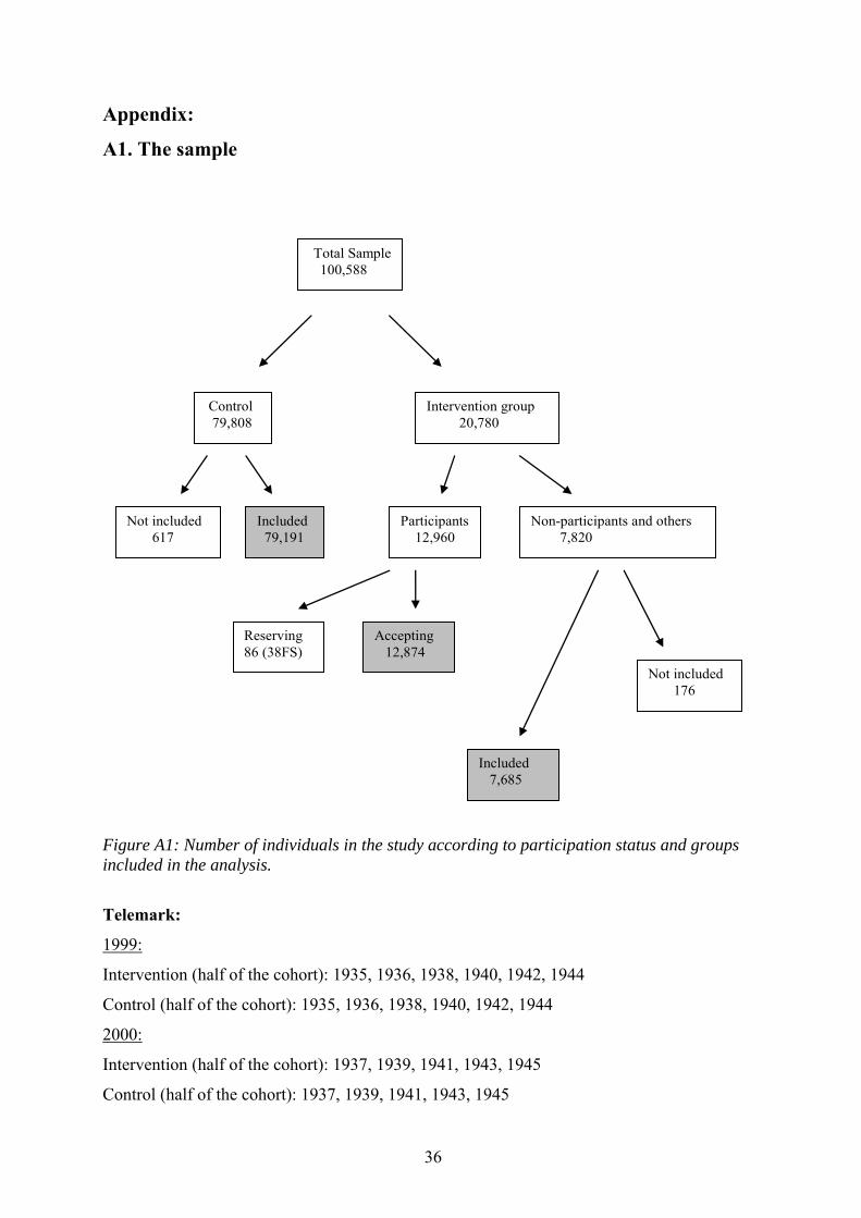
36

Appendix:

A1. The sample

Total Sample 100,588

Control 79,808

Intervention group 20,780

Not included 617

Included 79,191

Participants 12,960

Non-participants and others 7,820

Reserving 86 (38FS)

Accepting 12,874

Included 7,685

Not included 176

Figure A1: Number of individuals in the study according to participation status and groups included in the analysis.

Telemark:

1999:

Intervention (half of the cohort): 1935, 1936, 1938, 1940, 1942, 1944

Control (half of the cohort): 1935, 1936, 1938, 1940, 1942, 1944

2000:

Intervention (half of the cohort): 1937, 1939, 1941, 1943, 1945

Control (half of the cohort): 1937, 1939, 1941, 1943, 1945

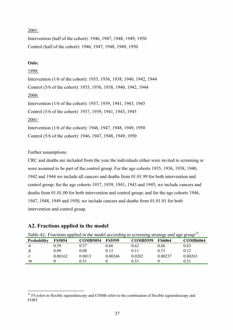
37

2001:

Intervention (half of the cohort): 1946, 1947, 1948, 1949, 1950

Control (half of the cohort): 1946, 1947, 1948, 1949, 1950

Oslo:

1999:

Intervention (1/6 of the cohort): 1935, 1936, 1938, 1940, 1942, 1944

Control (5/6 of the cohort): 1935, 1936, 1938, 1940, 1942, 1944

2000:

Intervention (1/6 of the cohort): 1937, 1939, 1941, 1943, 1945

Control (5/6 of the cohort): 1937, 1939, 1941, 1943, 1945

2001:

Intervention (1/6 of the cohort): 1946, 1947, 1948, 1949, 1950

Control (5/6 of the cohort): 1946, 1947, 1948, 1949, 1950

Further assumptions:

CRC and deaths are included from the year the individuals either were invited to screening or

were assumed to be part of the control group. For the age cohorts 1935, 1936, 1938, 1940,

1942 and 1944 we include all cancers and deaths from 01.01.99 for both intervention and

control group; for the age cohorts 1937, 1939, 1941, 1943 and 1945, we include cancers and

deaths from 01.01.00 for both intervention and control group; and for the age cohorts 1946,

1947, 1948, 1949 and 1950, we include cancers and deaths from 01.01.01 for both

intervention and control group.

A2. Fractions applied in the model Table A1: Fractions applied in the model according to screening strategy and age group23. Probability FS5054 COMB5054 FS5559 COMB5559 FS6064 COMB6064a 0.59 0.57 0.66 0.62 0.66 0.63 h 0.09 0.08 0.12 0.11 0.13 0.12 c 0.00162 0.0013 0.00246 0.0202 0.00237 0.00263 m 0 0.51 0 0.51 0 0.51

23 FS refers to flexible sigmoidoscopy and COMB refers to the combination of flexible sigmoidoscopy and FOBT

38

A3. Descriptive statistics Table A2: The estimated transition from well to death from causes other than colorectal cancer applied in the model according screening strategy, age group and stage. Stage 50 to 54 years 55 to 59 years 60 to 64 years

C FS COMB C FS COMB C FS COMB 0 0.00205 0.00207 0.00180 0.0047 0.0044 0.0039 0.0072 0.0070 0.0063 1 0.00222 0.00224 0.00195 0.0051 0.0047 0.0042 0.0078 0.0075 0.0068 2 0.00241 0.00242 0.00211 0.0055 0.0051 0.0046 0.0084 0.0082 0.0073 3 0.00260 0.00262 0.00228 0.0060 0.0055 0.0050 0.0091 0.0088 0.0079 4 0.00282 0.00284 0.00247 0.0065 0.0060 0.0054 0.0099 0.0096 0.0086 5 0.00305 0.00307 0.00267 0.0070 0.0065 0.0058 0.0107 0.0103 0.0093 6 0.00576 0.00576 0.00576 0.0079 0.0079 0.0079 0.0136 0.0136 0.0136 7 0.00585 0.00585 0.00585 0.0101 0.0101 0.0101 0.0157 0.0157 0.0157 8 0.00706 0.00706 0.00706 0.0105 0.0105 0.0105 0.0172 0.0172 0.0172 9 0.00697 0.00697 0.00697 0.0122 0.0122 0.0122 0.0192 0.0192 0.0192

10 0.00706 0.00706 0.00706 0.0128 0.0128 0.0128 0.0212 0.0212 0.0212 11 0.00793 0.00793 0.00793 0.0136 0.0136 0.0136 0.0230 0.0230 0.0230 12 0.01007 0.01007 0.01007 0.0157 0.0157 0.0157 0.0261 0.0261 0.0261 13 0.01045 0.01045 0.01045 0.0172 0.0172 0.0172 0.0285 0.0285 0.0285 14 0.01220 0.01220 0.01220 0.0192 0.0192 0.0192 0.0330 0.0330 0.0330 15 0.01282 0.01282 0.01282 0.0212 0.0212 0.0212 0.0365 0.0365 0.0365 16 0.01356 0.01356 0.01356 0.0230 0.0230 0.0230 0.0394 0.0394 0.0394 17 0.01574 0.01574 0.01574 0.0261 0.0261 0.0261 0.0453 0.0453 0.0453 18 0.01716 0.01668 0.01668 0.0285 0.0285 0.0285 0.0555 0.0555 0.0555 19 0.01924 0.01876 0.01876 0.0330 0.0330 0.0330 0.0622 0.0622 0.0622 20 0.02119 0.02119 0.02119 0.0365 0.0365 0.0365 0.0679 0.0679 0.0679 21 0.02298 0.02298 0.02298 0.0394 0.0394 0.0394 0.0722 0.0722 0.0722 22 0.02611 0.02611 0.02611 0.0453 0.0453 0.0453 0.0863 0.0863 0.0863 23 0.02855 0.02779 0.02779 0.0555 0.0555 0.0555 0.0917 0.0917 0.0917 24 0.03299 0.03223 0.03223 0.0622 0.0622 0.0622 0.1033 0.1033 0.1033 25 0.03648 0.03648 0.03648 0.0679 0.0679 0.0679 0.1144 0.1144 0.1144 26 0.03942 0.03942 0.03942 0.0722 0.0722 0.0722 0.1342 0.1342 0.1342 27 0.04528 0.04528 0.04528 0.0863 0.0863 0.0863 0.1487 0.1487 0.1487 28 0.05547 0.05499 0.05499 0.0917 0.0917 0.0917 0.1609 0.1609 0.1609 29 0.06218 0.06170 0.06170 0.1033 0.1033 0.1033 0.1795 0.1795 0.1795 30 0.06791 0.06791 0.06791 0.1144 0.1144 0.1144 0.2031 0.2031 0.1605 31 0.07217 0.07217 0.07217 0.1342 0.1342 0.1342 0.2122 0.2122 0.1791 32 0.08630 0.08630 0.08630 0.1487 0.1487 0.1487 0.2404 0.2404 0.2031 33 0.09169 0.09001 0.09001 0.1609 0.1609 0.1609 0.2504 0.2504 0.2122 34 0.10335 0.10167 0.10167 0.1795 0.1795 0.1795 0.2854 0.2854 0.2404 35 0.11441 0.11441 0.11441 0.2031 0.2031 0.2031 0.3204 0.3204 0.2504 36 0.13418 0.13418 0.13418 0.2122 0.2122 0.2122 0.2854 0.2854 0.2854

39

Table A3: The estimated transition from well to colorectal cancer applied in the model according to screening strategy, age group and stage. Stage 50 to 54 years 55 to 59 years 60 to 64 years

C FS COMB C FS COMB C FS COMB 0 0.00027 0.00028 0.00027 0.00071 0.00039 0.00047 0.00125 0.00119 0.00105 1 0.00029 0.00030 0.00029 0.00075 0.00042 0.00050 0.00133 0.00128 0.00112 2 0.00031 0.00032 0.00031 0.00081 0.00044 0.00054 0.00142 0.00136 0.00120 3 0.00033 0.00034 0.00033 0.00086 0.00047 0.00057 0.00152 0.00146 0.00128 4 0.00035 0.00036 0.00035 0.00092 0.00051 0.00061 0.00162 0.00156 0.00137 5 0.00037 0.00039 0.00038 0.00098 0.00054 0.00065 0.00173 0.00166 0.00146 6 0.00089 0.00089 0.00089 0.00140 0.00140 0.00126 0.00227 0.00227 0.00227 7 0.00140 0.00140 0.00140 0.00227 0.00227 0.00204 0.00313 0.00313 0.00313 8 0.00140 0.00140 0.00140 0.00227 0.00227 0.00204 0.00313 0.00313 0.00313 9 0.00140 0.00140 0.00140 0.00227 0.00227 0.00204 0.00313 0.00313 0.00313

10 0.00140 0.00140 0.00140 0.00227 0.00227 0.00204 0.00313 0.00313 0.00313 11 0.00140 0.00140 0.00140 0.00227 0.00227 0.00204 0.00313 0.00313 0.00313 12 0.00227 0.00227 0.00227 0.00313 0.00313 0.00282 0.00413 0.00413 0.00413 13 0.00227 0.00227 0.00227 0.00313 0.00313 0.00282 0.00413 0.00413 0.00413 14 0.00227 0.00227 0.00227 0.00313 0.00313 0.00282 0.00413 0.00413 0.00413 15 0.00227 0.00227 0.00227 0.00313 0.00313 0.00282 0.00413 0.00413 0.00413 16 0.00227 0.00227 0.00227 0.00313 0.00313 0.00282 0.00413 0.00413 0.00413 17 0.00313 0.00313 0.00313 0.00413 0.00413 0.00372 0.00476 0.00476 0.00476 18 0.00313 0.00313 0.00313 0.00413 0.00413 0.00372 0.00476 0.00476 0.00476 19 0.00313 0.00313 0.00313 0.00413 0.00413 0.00372 0.00476 0.00476 0.00476 20 0.00313 0.00313 0.00313 0.00413 0.00413 0.00372 0.00476 0.00476 0.00476 21 0.00313 0.00313 0.00313 0.00413 0.00413 0.00372 0.00476 0.00476 0.00476 22 0.00413 0.00413 0.00413 0.00476 0.00476 0.00428 0.00464 0.00464 0.00464 23 0.00413 0.00413 0.00413 0.00476 0.00476 0.00428 0.00464 0.00464 0.00464 24 0.00413 0.00413 0.00413 0.00476 0.00476 0.00428 0.00464 0.00464 0.00464 25 0.00413 0.00413 0.00413 0.00476 0.00476 0.00428 0.00464 0.00464 0.00464 26 0.00413 0.00413 0.00413 0.00476 0.00476 0.00428 0.00464 0.00464 0.00464 27 0.00476 0.00476 0.00476 0.00464 0.00464 0.00418 0.00464 0.00464 0.00464 28 0.00476 0.00476 0.00476 0.00464 0.00464 0.00418 0.00464 0.00464 0.00464 29 0.00476 0.00476 0.00476 0.00464 0.00464 0.00418 0.00464 0.00464 0.00464 30 0.00476 0.00476 0.00476 0.00464 0.00464 0.00418 0.00464 0.00464 0.00464 31 0.00476 0.00476 0.00476 0.00464 0.00464 0.00418 0.00464 0.00464 0.00464 32 0.00464 0.00464 0.00464 0.00464 0.00464 0.00418 0.00464 0.00464 0.00464 33 0.00464 0.00464 0.00464 0.00464 0.00464 0.00418 0.00464 0.00464 0.00464 34 0.00464 0.00464 0.00464 0.00464 0.00464 0.00418 0.00464 0.00464 0.00464 35 0.00464 0.00464 0.00464 0.00464 0.00464 0.00418 0.00464 0.00464 0.00464 36 0.00464 0.00464 0.00464 0.00464 0.00464 0.00418 0.004644 0.004644 0.004644

40

Table A4: The estimated transition from colorectal cancer to death for symptomatic diagnosed cancers applied in the model according to time from diagnosis, age group and stage. Stage Symptomatic diagnosed cancers Year 1 Year 2 Year 3 Year 4

5054 5559 6064 5054 5559 6064 5054 5559 6064 5054 5559 6064 0 0.123 0.123 0.123 0.123 0.123 0.123 0.123 0.123 0.123 0.123 0.123 0.123 1 0.123 0.123 0.123 0.123 0.123 0.123 0.123 0.123 0.123 0.123 0.123 0.123 2 0.123 0.123 0.123 0.123 0.123 0.123 0.123 0.123 0.123 0.123 0.123 0.123 3 0.123 0.123 0.123 0.123 0.123 0.123 0.123 0.123 0.123 0.123 0.123 0.123 4 0.123 0.123 0.123 0.123 0.123 0.123 0.123 0.123 0.123 0.123 0.123 0.123 5 0.123 0.123 0.123 0.123 0.123 0.123 0.123 0.123 0.123 0.123 0.123 0.123 6 0.227 0.227 0.227 0.078 0.078 0.078 0.051 0.051 0.051 0.035 0.035 0.035 7 0.227 0.227 0.227 0.078 0.078 0.078 0.051 0.051 0.051 0.035 0.035 0.035 8 0.227 0.227 0.199 0.078 0.078 0.069 0.051 0.051 0.045 0.035 0.035 0.031 9 0.227 0.227 0.199 0.078 0.078 0.069 0.051 0.051 0.045 0.035 0.035 0.031

10 0.227 0.227 0.199 0.078 0.078 0.069 0.051 0.051 0.045 0.035 0.035 0.031 11 0.227 0.227 0.209 0.078 0.078 0.072 0.051 0.051 0.047 0.035 0.035 0.032 12 0.227 0.227 0.209 0.078 0.078 0.072 0.051 0.051 0.047 0.035 0.035 0.032 13 0.227 0.199 0.347 0.078 0.069 0.120 0.051 0.045 0.078 0.035 0.031 0.054 14 0.227 0.199 0.347 0.078 0.069 0.120 0.051 0.045 0.078 0.035 0.031 0.054 15 0.227 0.199 0.35 0.078 0.069 0.121 0.051 0.045 0.078 0.035 0.031 0.054 16 0.227 0.209 0.35 0.078 0.072 0.121 0.051 0.047 0.078 0.035 0.032 0.054 17 0.227 0.209 0.345 0.078 0.072 0.119 0.051 0.047 0.077 0.035 0.032 0.054 18 0.199 0.347 0.345 0.069 0.120 0.119 0.045 0.078 0.077 0.031 0.054 0.054 19 0.199 0.347 0.345 0.069 0.120 0.119 0.045 0.078 0.077 0.031 0.054 0.054 20 0.199 0.35 0.345 0.069 0.121 0.119 0.045 0.078 0.077 0.031 0.054 0.054 21 0.209 0.35 0.345 0.072 0.121 0.119 0.047 0.078 0.077 0.032 0.054 0.054 22 0.209 0.345 0.343 0.072 0.119 0.118 0.047 0.077 0.077 0.032 0.054 0.053 23 0.347 0.345 0.36 0.120 0.119 0.124 0.078 0.077 0.081 0.054 0.054 0.056 24 0.347 0.345 0.373 0.120 0.119 0.129 0.078 0.077 0.084 0.054 0.054 0.058 25 0.35 0.345 0.373 0.121 0.119 0.129 0.078 0.077 0.084 0.054 0.054 0.058 26 0.35 0.345 0.373 0.121 0.119 0.129 0.078 0.077 0.084 0.054 0.054 0.058 27 0.345 0.343 0.373 0.119 0.118 0.129 0.077 0.077 0.084 0.054 0.053 0.058 28 0.345 0.36 0.373 0.119 0.124 0.129 0.077 0.081 0.084 0.054 0.056 0.058 29 0.345 0.373 0.373 0.119 0.129 0.129 0.077 0.084 0.084 0.054 0.058 0.058 30 0.345 0.373 0.352 0.119 0.129 0.121 0.077 0.084 0.079 0.054 0.058 0.055 31 0.345 0.373 0.352 0.119 0.129 0.121 0.077 0.084 0.079 0.054 0.058 0.055 32 0.343 0.373 0.352 0.118 0.129 0.121 0.077 0.084 0.079 0.053 0.058 0.055 33 0.36 0.373 0.352 0.124 0.129 0.121 0.081 0.084 0.079 0.056 0.058 0.055 34 0.373 0.373 0.352 0.129 0.129 0.121 0.084 0.084 0.079 0.058 0.058 0.055 35 0.373 0.352 0.352 0.129 0.121 0.121 0.084 0.079 0.079 0.058 0.055 0.055 36 0.373 0.352 0.352 0.129 0.121 0.121 0.084 0.079 0.079 0.058 0.055 0.055

41

A4. Follow-up colonoscopy Table A5: Proportion of follow-up colonoscopy applied in the model according to screening strategy, age group and stage. Stage 50 to 54 years 55 to 59 years 60 to 64 years FS COMB FS COMB FS COMB 0 0 0.0003 0.0002 0.0003 0.0004 0.0004 1 0.0005 0.0022 0.003 0.003 0.0028 0.0034 2 0.0027 0.0011 0.002 0.0018 0.0008 0.0008 3 0.0043 0.0052 0.0205 0.0154 0.0261 0.0226 4 0.0049 0.0036 0.0306 0.0288 0.0352 0.0283 5 0.0281 0.0263 0.0064 0.0048 0.0028 0.0023 6 0 0.0011 0.001 0 0 0 7 0.0011 0 0.0007 0 0.0004 0.0008 8 0.0019 0.0005 0.0042 0.0035 0.0036 0.006 9 0.0019 0.0016 0.0057 0.0053 0.0032 0.0034 10 0.0005 0.0027 0.0005 0.001 0 0.0004 11 0 0 0 0.005 0 0 12 0 0 0 0 0 0 A5. Assumptions in the sensitivity analysis Based on Figure A1 to A8, we assume that treatment costs are gamma distributed with α and

λ can be estimated from the following two definitions:

Mean = α/λ

Variance = α/λ²

Table A6: Assumptions in the probabilistic sensitivity analysis ranking the four years of treatment. Mean and variance are reported in NOK. Year Mean St.dev. α λ Symptomatic 1 2 3 4

18,880 4,718 2,734 1,908

785 735 721 1,361

578.00 41.05 14.49 1.91

0.0306 0.0087 0.0053 0.0010

Asymptomatic 1 2 3 4

16,416 2,058 493 196

1,610 765 194 82

103.00 7.27 6.46 5.71

0.0063 0.0035 0.0131 0.0291

42

0.2

.4.6

Frac

tion

0 100000 200000 300000Treatment costs

Year 1Treatment cost - asymptomatic diagnosed cancer

Figure A1: Treatment cost for asymptomatic diagnosed cancers during the first year after time of diagnosis. Numbers in NOK.

0.2

.4.6

.8Fr

actio

n

0 50000 100000 150000Treatment costs

Year 2Treatment cost - asymptomatic diagnosed cancer

Figure A2: Treatment cost for asymptomatic diagnosed cancers during the second year after time of diagnosis. Numbers in NOK.

43

0.2

.4.6

.8Fr

actio

n

0 5000 10000 15000 20000Treatment costs

Year 3Treatment cost - asymptomatic diagnosed cancer

Figure A3: Treatment cost for asymptomatic diagnosed cancers during the third year after time of diagnosis. Numbers in NOK.

0.2

.4.6

.81

Frac

tion

0 2000 4000 6000 8000Treatment costs

Year 4Treatment cost - asymptomatic diagnosed cancer

Figure A4: Treatment cost for asymptomatic diagnosed cancers during the fourth year after time of diagnosis. Numbers in NOK.

44

0.0

5.1

.15

.2.2

5Fr

actio

n

0 200000 400000 600000Treatment costs

Year 1Treatment cost - symptomatic diagnosed cancer

Figure A5: Treatment cost for symptomatic diagnosed cancers during the first year after time of diagnosis. Numbers in NOK.

0.2

.4.6

.8Fr

actio

n

0 100000 200000 300000Treatment costs

Year 2Treatment cost - symptomatic diagnosed cancer

Figure A6: Treatment cost for symptomatic diagnosed cancers during the second year after time of diagnosis. Numbers in NOK.

45

0.2

.4.6

.8Fr

actio

n

0 50000 100000 150000 200000Treatment costs

Year 3Treatment cost - symptomatic diagnosed cancer

Figure A7: Treatment cost for symptomatic diagnosed cancers during the third year after time of diagnosis. Numbers in NOK.

0.2

.4.6

.8Fr

actio

n

0 50000 100000 150000 200000Treatment costs

Year 4Treatment cost - symptomatic diagnosed cancer

Figure A8: Treatment cost for symptomatic diagnosed cancers during the fourth year after time of diagnosis. Numbers in NOK.