Cosegmentation Revisited:

Models and Optimization

Sara Vicente1, Vladimir Kolmogorov1, and Carsten Rother21 University College London

2 Microsoft Research Cambridge

Abstract. The problem of cosegmentation consists of segmenting thesame object (or objects of the same class) in two or more distinct im-ages. Recently a number of different models have been proposed for thisproblem. However, no comparison of such models and corresponding op-timization techniques has been done so far. We analyze three existingmodels: the L1 norm model of Rother et al. [1], the L2 norm model ofMukherjee et al. [2] and the “reward” model of Hochbaum and Singh [3].We also study a new model, which is a straightforward extension of theBoykov-Jolly model for single image segmentation [4].In terms of optimization, we use a Dual Decomposition (DD) techniquein addition to optimization methods in [1, 2]. Experiments show a signif-icant improvement of DD over published methods. Our main conclusion,however, is that the new model is the best overall because it: (i) hasfewest parameters; (ii) is most robust in practice, and (iii) can be opti-mized well with an efficient EM-style procedure.

1 Introduction

The task of Figure-Ground segmentation is a widely studied problem in computervision. Given a single image there are techniques that attempt to automaticallypartition the image into multiple objects and background. If the goal is to havea single object segmented, i.e. a binary segmentation, there is the natural am-biguity of which object is the desired one. In this case interactive segmentationtechniques must be considered where the user gives additional hints.

There are many interesting application scenarios where multiple images areavailable. This means each image depicts the “same” foreground object in frontof potentially arbitrary backgrounds. In contrast to the single image case, thetask of segmenting the common object automatically in all images is now well-defined. This task is called “cosegmentation” and was first addressed in [1].Let us be more precise on the definition of the “same” foreground object. Inthis paper we use the definition of [1–3] where the only constraint is that thedistribution of some appearance features of the foreground region in each imagehave to be similar. The appearance features can encode different information,like color and texture, and various similarity measures can be envisioned. Thisdefinition allows for a wide range of applications. One application is to create avisual summary from personal photo collections, by segmenting automatically allinstances of the same object, e.g. a person and a dog [5]. Another application isto use the segmentation of the common object to efficiently edit all occurrencesof this object in one step, e.g. by changing its contrast [6]. The practical challenge

2 S. Vicente, V.Kolmogorov, C. Rother

in the case of segmenting the same object is that distributions may not matchexactly, due to changes in illumination, in viewpoint or object (self-)occlusion.Our definition of cosegmentation can potentially also be used for segmentingdifferent objects of the same class. An example of an unsupervised object-classrecognition and segmentation system is [7], where more features are used otherthan appearance, e.g. shape. It can be expected that for most object classes,appearance features alone are not strong enough, hence this application is outof the scope of this paper.

Very recently in [8] the authors used a different formulation of the cosegmen-tation problem. They casted it into a clustering problem with two cluster. Theyshow results for image pairs and for multiple images of objects of the same class.

It is worth mentioning that several recent papers considered a simplifiedcosegmentation problem where user interaction is available. In [5] the authorssegment several images of the same object, assuming one of those images is hand-segmented. They model local appearance and edge profiles from the segmentedimage in order to “transduct” such segmentation into the remaining images. In[9, 6] the user input is in the form of foreground/background scribbles in one ormany images from the collection. In [9] the authors discuss how the choice of theseed image influences the performance of their method. In [6] a way of guidingthe user interactions is presented. We envision that the insights of this paperwill also help to improve the task of interactive cosegmentation.

The goal of this paper is to examine theoretically and practically differentmodels and optimization methods for cosegmentation. To achieve this we limitourselves to the task of cosegmenting two images only, with color as the only ap-pearance feature, and where distributions are expressed in terms of histograms.We consider three existing models [1–3], which differ only in the distance mea-sure between the two color histograms. We also consider a new model, whichis a straightforward extension from a single to multiple images of Boykov-Jolly[4]. For a fair comparison we improved on existing optimization methods for themodels in [1, 2]. We achieved this by using a Dual Decomposition technique. Fora quantitative comparison we built a dataset of 100 image-pairs with varyinglevels of complexity by simulating changes in scale and illumination.

The paper is organized as follows. Section 2 introduces the four different mod-els and discusses some of their properties. Since the optimization for some modelsis NP-hard, it is important to choose the best possible optimization procedure.In Sect. 3 we review such methods. In Sect. 4 we compare experimentally boththe models and the optimization methods and conclude which are the betterperforming methods.

2 Models

We start this section by introducing some notation:

– xp ∈ {0, 1} is the label for pixel p, where p ∈ P = P1 ∪ P2 and P1, P2 arerespectively the set of pixels in image 1 and image 2. We use letter k ∈ {1, 2}for denoting the image number.

– zp is the appearance of pixel p (e.g. color or texture) and such measurementis quantized into a finite number of bins. Variable b ranges over histogram

Cosegmentation Revisited: Models and Optimization 3

bins (b ∈ {1, ..., B} where B is the total number of bins), and Pkb denotesthe set of pixels p in image k whose measurement zp falls in bin b.

– ℎk is the empirical un-normalized histogram of foreground pixels for imagek: it is a vector of size B with components ℎkb =

∑

p∈Pkbxp.

As stated earlier, one of the goals of this paper is to compare different coseg-mentation models that have been previously proposed. Such models fit into asingle framework, where the cosegmentation problem is formulated as an energyoptimization, with an energy of the following form:

E(x) =∑

p

wpxp +∑

(p,q)

wpq∣xp − xq∣+ �Eglobal(ℎ1, ℎ2) (1)

Jointly, the first two terms form the traditional MRF term for both images, wherewp is the unary weight for each pixel and wpq is the pairwise weight. The lastterm, Eglobal, encodes a similarity measure between the foreground histogramsof both images and � is the weight for that term.

Following [1], we will use a ballooning term for the first term, constant forevery pixel: wp = �. This biases the solution to one of the possible labels and itis important to prevent trivial solutions (i.e. both images being labeled totallybackground or foreground). If the bias is not present (i.e. if wp = 0 and theenergy does not have unary terms) such trivial solutions are always a globaloptimum of the energy. Alternatively, in [2, 3] the authors used user interactionto compute pixel-dependent unary terms [10]. We are interested in automaticcosegmentation so unary terms based on user interaction are not available.

The second term is a contrast sensitive smoothness term whose weight is

given by wpq =(�i+�c exp−�∥zp−zq∥

2)dist(p,q) with � =

(

2⟨

(zp − zq)2⟩)−1

, where ⟨⋅⟩

denotes expectation over the image and �i, �c are respectively the weight forIsing prior and for the contrast sensitive term.

The models differ in the way the term Eglobal in equation (1) is defined.

Model A: L1-norm This model was first introduced in [1] and it was derivedfrom a generative model. The global term in the energy was defined as follows:

Eglobal =∑

b

∣ℎ1b − ℎ2b∣ (2)

where the L1-norm is used to compute foreground histograms similarity.

Model B: L2-norm This formulation was introduced in [2] and it was definedas follows:

Eglobal =∑

b

(ℎ1b − ℎ2b)2

(3)

It is similar to the previous formulation in equation (2), with the difference thatthe norm used to measure histogram similarity is the L2-norm instead of the L1-norm. The authors motivate this change by arguing that such a model has someinteresting properties and allows the use of alternative optimization methods.

Model C: Reward model In [3] the authors used the following global term:

Eglobal = −∑

b

ℎ1b ⋅ ℎ2b (4)

They motivate the use of such a model by replacing the penalization term witha rewarding term.

4 S. Vicente, V.Kolmogorov, C. Rother

Recall that the original formulation in [2, 3] uses pixel-dependent unary terms,while we use a constant ballooning force: wp = �.

Both model A and model B lead to NP-hard optimization problems [1], whilemodel C leads to a submodular problem that can be efficiently optimized withgraph cuts [3].

Model D: Boykov-Jolly model The last model that we consider is a nat-ural extension of the generative model for binary image segmentation in [4, 1,11]. These papers use a separate appearance model for each of the two regions(background and foreground). In our case we have three regions - two separatebackgrounds and one common foreground. Accordingly, we introduce three ap-pearance models - �B1 , �B2 and �F . This leads to a generative model with theposterior described by the following energy function:

E(

x, �B1 , �B2 , �F)

=∑

(p,q)

wpq∣xp − xq∣+ �∑

k

∑

p∈Pk

U(xp, �Bk , �F ) (5)

where

U(xp, �B , �F ) =

{

− log(Pr(zp∣�F )) if xp = 1

− log(Pr(zp∣�B)) if xp = 0

(6)

Since we are interested in automatic cosegmentation, the appearance models�B1 , �B2 and �F are not available in advance. In order to compute them, weminimize energy (5) jointly over segmentation and appearance models using anEM-style technique proposed in [11].

Model D is quite similar to the model used by Batra et al. [6] for interactivecosegmentation; the only difference is that Batra et al. used a single backgroundmodel for all images. Model D also bears some resemblance to the generativemodel of Rother et al. [1] but there are some differences. In [1], the motivation wasmodel selection, since two competitive models were considered: one where bothimages shared the same foreground appearance model and another where theyhad independent appearance models. The segmentation was then chosen so thatthe first model had higher posterior probability. In our case, we consider only asingle model and try to find jointly the segmentation and appearance models thatmaximize the posterior probability. This formulation should be more appropriatewhen we know in advance that the two images have a common object. Also, itappears to lead to a simpler optimization problem: generalizing an EM-styleprocedure to the model in [1] is not straightforward.

2.1 An alternative formulation of model D

To gain more insights into model D, we express its energy in a different wayusing the approach in [12]. It is known that for a fixed segmentation x, optimalhistograms that minimize energy (5) are simply the empirical histograms:

�Fb =ℎ1b + ℎ2b

H1 +H2�Bkb =

ℎkb

Hk

(7)

where we introduced the following notation: Hk =∑

b ℎkb is the total numberof foreground pixels in image k, ℎkb = ∣Pkb∣ − ℎkb is the number of backgroundpixels in image k belonging to bin b, and Hk = ∣Pk∣ −Hk is the total number of

Cosegmentation Revisited: Models and Optimization 5

background pixels in image k. Note, all quantities ℎkb, ℎkb, Hk, Hk are functionsof the segmentation x (recall that ℎkb =

∑

p∈Pkbxp).

Following [12], we plug histograms (7) into the energy (5). Then the energybecomes of the form (1) with no unary terms (wp = � = 0) and the followingglobal term:

Eglobal =∑

b

� (ℎ1b + ℎ2b) +∑

k,b

�(

ℎkb

)

− � (H1 +H2)−∑

k

�(

Hk

)

(8)

where �(z) = −z log z is a concave function.In the case of a single image the Boykov-Jolly model prefers assigning pixels in

the same bin either entirely to the background or entirely to the foreground [12];this leads to “compact” histograms. A similar fact holds for model D (the proofis entirely analogous to that in [12]).

Proposition 1. Function (8) has a minimizer x such that for each (k, b), pixelsin Pkb are either all labeled as 0 or all labeled as 1.

2.2 Remarks on model properties

Before presenting an experimental comparison of the models, we would like togive some informal remarks which may give insights into their relative perfor-mance. We will first consider models A, B and D, and come back to model C atthe end.

We believe that a fundamental difference of model D from other models isthat it takes into account the prior knowledge that all regions are represented bycompact histograms. For the case of a single image, the bias of the Boykov-Jollymodel was discussed in [12]: it prefers segmentations in which pixels that fallin the same bin are assigned to the same segment (background or foreground),and among such segmentations the model picks the most balanced one, i.e. thesegmentation in which the areas of the background and the foreground match.We conjecture that these properties carry over to the cosegmentation case. Itcan be shown, for example, that if the two images are identical and all bins areof the same size (i.e. ∣Pkb∣ = const for all k, b) then the global term will beminimized by a segmentation in which exactly half of the bins are assigned tothe foreground. Due to a bias towards balanced segmentation we did not use the“ballooning force” for model D, i.e. we chose � = 0, which produced reasonableresults. In contrast, the other models required this extra parameter � in orderto avoid trivial solutions.

Unlike model D, models A and B do not impose any penalty if pixels in thesame bin, Pkb, are assigned to two different segments. We argue that this hasboth pros and cons, as illustrated by two scenarios below.

Scenario 1 Assume that the background colors do not overlap with the fore-ground nor with the other background. Furthermore, suppose that the fore-ground regions in the two images match only partially, for example, due to anillumination change or scaling. Thus, we have ∣Pkb∣ > ∣Pkb∣ for some bin b where

k ∈ {1, 2}, k ∕= k. Models A and B will bias ∣Pkb∣ − ∣Pkb∣ pixels to an incorrectlabel. In contrast, model D should not be affected; it will assign all pixels in Pkb

and Pkb to the foreground, as desired.

6 S. Vicente, V.Kolmogorov, C. Rother

Scenario 2 Let us now assume that we have “camouflage” in one of the images,i.e. colors of the background and the foreground overlap. Thus, we again have∣Pkb∣ > ∣Pkb∣, but now the behavior of models A and B will be correct, whilemodel D will try to incorrectly assign all pixels in Pkb to the foreground (or tothe background).

We conclude that without camouflage model D should cope better with illu-mination and scale changes than model A and especially than model B. On theother hand, models A and B should be more robust to a camouflage in one ofthe images.

Let us now return to model C. Assume for simplicity that there are no pair-wise terms. The energy can then be written as E(x) =

∑

b Eb(ℎ1b, ℎ2b) where

Eb(ℎ1b, ℎ2b) = �(ℎ1b + ℎ2b)− �ℎ1b ⋅ ℎ2b

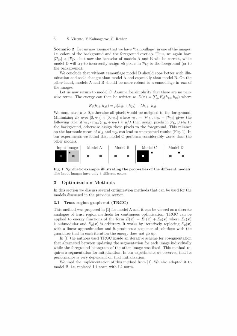
We must have � > 0, otherwise all pixels would be assigned to the foreground.Minimizing Eb over [0, n1b] × [0, n2b] where n1b = ∣P1b∣, n2b = ∣P2b∣ gives thefollowing rule: if n1b ⋅ n2b/(n1b + n2b) ≤ �/� then assign pixels in P1b ∪ P2b tothe background, otherwise assign these pixels to the foreground. This relianceon the harmonic mean of n1b and n2b can lead to unexpected results (Fig. 1). Inour experiments we found that model C performs considerably worse than theother models.

Input images Model A Model B Model C Model D

Fig. 1. Synthetic example illustrating the properties of the different models.The input images have only 3 different colors.

3 Optimization Methods

In this section we discuss several optimization methods that can be used for themodels discussed in the previous section.

3.1 Trust region graph cut (TRGC)

This method was proposed in [1] for model A and it can be viewed as a discreteanalogue of trust region methods for continuous optimization. TRGC can beapplied to energy functions of the form E(x) = E1(x) + E2(x) where E1(x)is submodular and E2(x) is arbitrary. It works by iteratively replacing E2(x)with a linear approximation and it produces a sequence of solutions with theguarantee that in each iteration the energy does not go up.

In [1] the authors used TRGC inside an iterative scheme for cosegmentationthat alternated between updating the segmentation for each image individuallywhile the foreground histogram of the other image was fixed. This method re-quires a segmentation for initialization. In our experiments we observed that itsperformance is very dependent on that initialization.

We used the implementation of this method from [1]. We also adapted it tomodel B, i.e. replaced L1 norm with L2 norm.

Cosegmentation Revisited: Models and Optimization 7

3.2 Quadratic pseudo boolean optimization

In [2] the authors observed that model B is represented by a quadratic pseudo-boolean function. Indeed, histograms ℎ1 and ℎ2 depend linearly on x: ℎkb =∑

p∈Pkbxp. Therefore, expanding expression (ℎ1b − ℎ2b)

2 yields a sum of lin-ear terms and quadratic terms of the form cpqxpxq, some of which are non-submodular. Mukherjee et al. [2] formulated a linear programming relaxation ofthe problem, which is equivalent to the roof duality relaxation [13, 14] for thequadratic function E(x). This relaxation can be solved via a maxflow algorithm,and it yields a partial solution: the nodes are divided into labeled and unlabeled,with the guarantee that the labels of the labeled nodes are optimal. An impor-tant question is how to set the segmentation for unlabeled nodes. Mukherjeeet al. [2] use the segmentation obtained by minimizing energy E(x) withoutthe global term Eglobal. In our experiments we use a constant ballooning force(wp = �), so this procedure assigns the same label to all unlabeled nodes.

Note that, model C is also represented by a quadratic function, but unlikethe previous case this quadratic function is submodular. Therefore, model C canbe optimized exactly by a single call to a maxflow algorithm [3].

3.3 Dual Decomposition (DD)

Dual Decomposition (DD) is a popular technique for solving combinatorial op-timization problems [15], which proved to be very successful for MRF opti-mization [16–19, 12]. The idea of DD is to decompose the original problem intosmaller, easier subproblems that can be efficiently optimized. Combining the so-lution of such subproblems yields a lower bound for the initial problem. Thislower bound is then maximized over different decompositions. We applied thistechnique to models A, B and D as described below.

Dual decompositions for models A and B Let us write the correspondingoptimization problems as follows:

minx,y

EMRF (x) +∑

b

g(yb) (9a)

s.t. yb =∑

p∈P1b

xp −∑

p∈P2b

xp ≡∑

k,p

abpxp b = 1, ..., B (9b)

where g is a convex function: g(y) = �∣y∣ for model A and g(y) = �y2 for modelB. Coefficients abp are defined as follows: abp = 1 if p ∈ P1b; abp = −1 if p ∈ P2b

and abp = 0 otherwise.

We form a standard Lagrangian function by relaxing constraints (9b) andintroducing a Lagrangian multiplier �:

L(x,y,�) = EMRF (x) +∑

b

g(yb) +∑

b

�b

(

yb −∑

p

abpxp

)

(10)

Minimizing the Lagrangian over (x,y) gives a lower bound on the original prob-lem:

8 S. Vicente, V.Kolmogorov, C. Rother

�(�) = minx,y

L(x,y,�) (11a)

= minx

⎡

⎣EMRF (x)−∑

p,b

abp�bxp

⎤

⎦+∑

b

minyb

[g(yb) + �byb] (11b)

�(�) ≤ E(x) (11c)

In order to obtain the tightest bound, we need to solve the following maximiza-tion problem:

max�

�(�) (12)

This problem is dual to (9b). Function �(�) is concave; similar to [17–19], weuse a subgradient method to maximize it. In order to compute a subgradient fora given vector �, we need to solve 1+B minimization subproblems in (11b). Thefirst subproblem requires minimizing a submodular energy with pairwise terms,which can be efficiently done using graph cuts. Solving subproblems for bins bis straightforward.

It remains to specify how to choose a primal solution x. Let xt be a minimizerof the first subproblem in (11b) at step t of the subgradient method. Amonglabelings xt, we choose the solution with the minimum cost E(xt).

Dual decompositions for model D We obtained a lower bound by relaxingconstraints Hk =

∑

p xk and using the fact that Hk ≡ ∣Pk∣ − Hk. Details arevery similar to those in [12].

4 Experimental results

In this section we describe the experimental results. We start by giving detailson the setup used to compare the different models. In section 4.1, we comparethe performance of the different optimization methods, and in section 4.2, usingthe best optimization procedure for each model, we compare the performanceand robustness of such models.

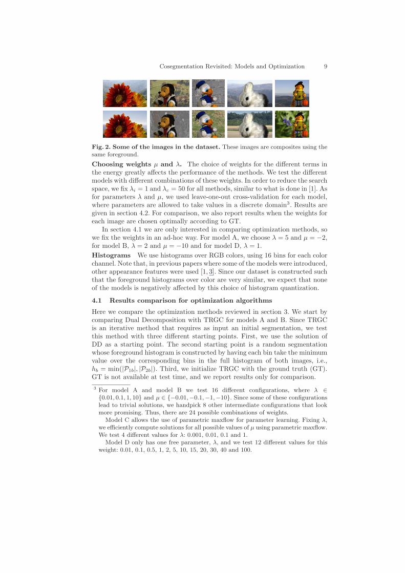
Dataset Given the difficulty in acquiring ground truth data for the cosegmenta-tion problem, we used composites of 40 different backgrounds with 20 foregroundobjects from the database in [20], for which high quality alpha mattes are avail-able. The database in [20] has more than 20 images; we selected objects withfewer transparencies. Representative images out of these 20 pairs are shown inFig. 2.

We resized the images so that their maximum side is 150 pixels. Some ofthe models and optimization methods discussed are limited to small images, inparticular, model C and QPBO. Both these optimization methods require theconstruction of graphs that grow quadratically with the size of the image.

The use of exactly the same foreground object in both images ensures thatthe histograms over pure foreground pixels match. The choice of such simplifieddataset is justified by the intuition that if the models and optimization methodsfail in this scenario, they will also fail in a realistic scenario where the foregroundhistograms may differ. In section 4.2 we also test more realistic scenarios byvarying the size and illumination in one of the images.

Cosegmentation Revisited: Models and Optimization 9

Fig. 2. Some of the images in the dataset. These images are composites using thesame foreground.

Choosing weights � and �. The choice of weights for the different terms inthe energy greatly affects the performance of the methods. We test the differentmodels with different combinations of these weights. In order to reduce the searchspace, we fix �i = 1 and �c = 50 for all methods, similar to what is done in [1]. Asfor parameters � and �, we used leave-one-out cross-validation for each model,where parameters are allowed to take values in a discrete domain3. Results aregiven in section 4.2. For comparison, we also report results when the weights foreach image are chosen optimally according to GT.

In section 4.1 we are only interested in comparing optimization methods, sowe fix the weights in an ad-hoc way. For model A, we choose � = 5 and � = −2,for model B, � = 2 and � = −10 and for model D, � = 1.

Histograms We use histograms over RGB colors, using 16 bins for each colorchannel. Note that, in previous papers where some of the models were introduced,other appearance features were used [1, 3]. Since our dataset is constructed suchthat the foreground histograms over color are very similar, we expect that noneof the models is negatively affected by this choice of histogram quantization.

4.1 Results comparison for optimization algorithms

Here we compare the optimization methods reviewed in section 3. We start bycomparing Dual Decomposition with TRGC for models A and B. Since TRGCis an iterative method that requires as input an initial segmentation, we testthis method with three different starting points. First, we use the solution ofDD as a starting point. The second starting point is a random segmentationwhose foreground histogram is constructed by having each bin take the minimumvalue over the corresponding bins in the full histogram of both images, i.e.,ℎb = min(∣P1b∣, ∣P2b∣). Third, we initialize TRGC with the ground truth (GT).GT is not available at test time, and we report results only for comparison.

3 For model A and model B we test 16 different configurations, where � ∈{0.01, 0.1, 1, 10} and � ∈ {−0.01,−0.1,−1,−10}. Since some of these configurationslead to trivial solutions, we handpick 8 other intermediate configurations that lookmore promising. Thus, there are 24 possible combinations of weights.

Model C allows the use of parametric maxflow for parameter learning. Fixing �,we efficiently compute solutions for all possible values of � using parametric maxflow.We test 4 different values for �: 0.001, 0.01, 0.1 and 1.

Model D only has one free parameter, �, and we test 12 different values for thisweight: 0.01, 0.1, 0.5, 1, 2, 5, 10, 15, 20, 30, 40 and 100.

10 S. Vicente, V.Kolmogorov, C. Rother

The results for model A are shown in the first part of Table 1. Note that in[1], where TRGC was proposed, DD was not used as a starting point. For thismodel, the difference between TRGC-DD and DD is very small, since TRGCstarting with DD only improves the energy for two images.

Table 1. Comparison of optimization methods for Models A and B. Wecompare TRGC (using 3 different initial solutions), Dual Decomposition, and QPBO(only for model B). For each model, the first row shows for how many images eachmethod gives the best energy. The second row is the gap between the energy and thelower bound (LB) obtained by DD. The values are normalized: first we add a constantto each term of the energy so that the minimum of each term becomes 0, and thenscale the energy so that the lower bound corresponds to 100. The last row is the errorrate: percentage of misclassified pixels over the total number of pixels.

TRGCDD QPBO

From DD From hist From GT

Model

A Best energy: # cases 20 0 0 18 -

Distance from LB 100.24 106.5 101.15 100.24 -

Error rate 3.7% 8.1% 3.2% 3.7% -

Model

B Best energy: # cases 13 0 7 3 0

Distance from LB 101.59 107.56 101.77 104.20 197.29

Error rate 3.93% 5.96% 2.85% 3.92% 51.77%

The results for model B are shown in the second part of Table 1. AlthoughQPBO also provides a lower bound, we used the lower bound obtained by DualDecomposition since in our experiments, it was always better than the one pro-vided by QPBO.

We conclude that a combination of DD and TRGC, using DD solution as astarting point for TRGC, is the best performing method for both model A andB, and this is the method used in the next section for model comparison.

Surprisingly, the performance obtained for the QPBO method contrasts withthe one reported in [2], since for this experiment the number of pixels left un-labeled by this method was 90%. Note that in [2], the authors used a differentspatially varying unary term which may induce differences. They also report thatthe performance of the method deteriorates when weight � is increased. In thecase considered, where wp is constant, small values of � lead to trivial solutions.

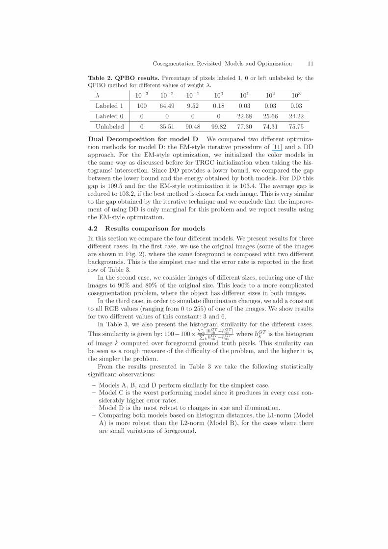
In order to better understand why QPBO fails, we ran the method witha fixed ballooning force, � = −10, and different values of �. In Table 2, weshow the percentage of pixels that were labeled one, zero, or left unlabeled. Forintermediate values of �, the number of unlabeled pixels is more than 90%. Forsuch values, QPBO is not reliable as an optimization method. On the otherhand, for extreme values of �, QPBO labels more pixels, but the resulting modelis not meaningful, for example, for the case � = 10−3, all pixels for all imagesconsidered were labeled 1.

Cosegmentation Revisited: Models and Optimization 11

Table 2. QPBO results. Percentage of pixels labeled 1, 0 or left unlabeled by theQPBO method for different values of weight �.

� 10−3 10−2 10−1 100 101 102 103

Labeled 1 100 64.49 9.52 0.18 0.03 0.03 0.03

Labeled 0 0 0 0 0 22.68 25.66 24.22

Unlabeled 0 35.51 90.48 99.82 77.30 74.31 75.75

Dual Decomposition for model D We compared two different optimiza-tion methods for model D: the EM-style iterative procedure of [11] and a DDapproach. For the EM-style optimization, we initialized the color models inthe same way as discussed before for TRGC initialization when taking the his-tograms’ intersection. Since DD provides a lower bound, we compared the gapbetween the lower bound and the energy obtained by both models. For DD thisgap is 109.5 and for the EM-style optimization it is 103.4. The average gap isreduced to 103.2, if the best method is chosen for each image. This is very similarto the gap obtained by the iterative technique and we conclude that the improve-ment of using DD is only marginal for this problem and we report results usingthe EM-style optimization.

4.2 Results comparison for models

In this section we compare the four different models. We present results for threedifferent cases. In the first case, we use the original images (some of the imagesare shown in Fig. 2), where the same foreground is composed with two differentbackgrounds. This is the simplest case and the error rate is reported in the firstrow of Table 3.

In the second case, we consider images of different sizes, reducing one of theimages to 90% and 80% of the original size. This leads to a more complicatedcosegmentation problem, where the object has different sizes in both images.

In the third case, in order to simulate illumination changes, we add a constantto all RGB values (ranging from 0 to 255) of one of the images. We show resultsfor two different values of this constant: 3 and 6.

In Table 3, we also present the histogram similarity for the different cases.

This similarity is given by: 100−100×∑

b∣ℎGT

1b −ℎGT2b ∣

∑bℎGT1b

+ℎGT2b

where ℎGTk is the histogram

of image k computed over foreground ground truth pixels. This similarity canbe seen as a rough measure of the difficulty of the problem, and the higher it is,the simpler the problem.

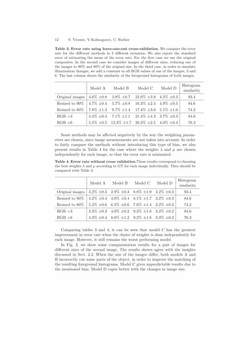
From the results presented in Table 3 we take the following statisticallysignificant observations:

– Models A, B, and D perform similarly for the simplest case.– Model C is the worst performing model since it produces in every case con-

siderably higher error rates.– Model D is the most robust to changes in size and illumination.– Comparing both models based on histogram distances, the L1-norm (Model

A) is more robust than the L2-norm (Model B), for the cases where thereare small variations of foreground.

12 S. Vicente, V.Kolmogorov, C. Rother

Table 3. Error rate using leave-one-out cross-validation. We compare the errorrate for the different methods in 3 different scenarios. We also report the standarderror of estimating the mean of the error rate. For the first case we use the originalcomposites. In the second case we consider images of different sizes, reducing one ofthe images to 90% and 80% of the original size. In the third case, in order to simulateillumination changes, we add a constant to all RGB values of one of the images, 3 and6. The last column shows the similarity of the foreground histograms of both images.

Model A Model B Model C Model DHistogram

similarity

Original images 4.6% ±0.8 3.9% ±0.7 22.0% ±3.9 4.3% ±0.3 93.4

Resized to 90% 4.7% ±0.4 5.7% ±0.8 16.3% ±2.4 4.9% ±0.5 84.6

Resized to 80% 7.8% ±1.3 9.7% ±1.4 17.4% ±3.0 5.1% ±1.0 74.2

RGB +3 4.4% ±0.4 7.1% ±1.1 21.4% ±4.3 3.7% ±0.3 84.6

RGB +6 5.5% ±0.5 12.3% ±1.7 20.3% ±2.5 4.0% ±0.4 76.3

Some methods may be affected negatively by the way the weighting param-eters are chosen, since image measurements are not taken into account. In orderto fairly compare the methods without introducing this type of bias, we alsopresent results in Table 4 for the case where the weights � and � are chosenindependently for each image, so that the error rate is minimized.

Table 4. Error rate without cross validation.These results correspond to choosingthe best weights � and � according to GT for each image individually. They should becompared with Table 3.

Model A Model B Model C Model DHistogram

similarity

Original images 3.2% ±0.3 2.9% ±0.3 8.8% ±1.9 3.2% ±0.3 93.4

Resized to 90% 4.2% ±0.4 4.0% ±0.4 8.1% ±1.7 3.2% ±0.3 84.6

Resized to 80% 5.2% ±0.6 6.2% ±0.6 7.0% ±1.4 3.2% ±0.3 74.2

RGB +3 3.3% ±0.3 4.0% ±0.2 9.3% ±1.8 3.2% ±0.2 84.6

RGB +6 4.3% ±0.4 8.0% ±1.2 9.2% ±1.8 3.3% ±0.2 76.3

Comparing tables 3 and 4, it can be seen that model C has the greatestimprovement in error rate when the choice of weights is done independently foreach image. However, it still remains the worst performing model.

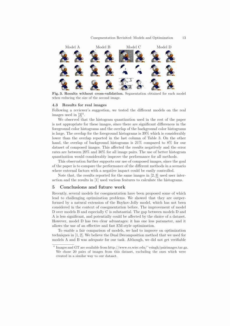
In Fig. 3, we show some cosegmentation results for a pair of images fordifferent sizes of the second image. The results shown agree with the insightsdiscussed in Sect. 2.2. When the size of the images differ, both models A andB incorrectly cut some parts of the object, in order to improve the matching ofthe resulting foreground histograms. Model C gives unpredictable results due tothe mentioned bias. Model D copes better with the changes in image size.

Cosegmentation Revisited: Models and Optimization 13

Model A Model B Model C Model D

Fig. 3. Results without cross-validation. Segmentation obtained for each modelwhen reducing the size of the second image.

4.3 Results for real images

Following a reviewer’s suggestion, we tested the different models on the realimages used in [3]4.

We observed that the histogram quantization used in the rest of the paperis not appropriate for these images, since there are significant differences in theforeground color histograms and the overlap of the background color histogramsis large. The overlap for the foreground histograms is 39% which is considerablylower than the overlap reported in the last column of Table 3. On the otherhand, the overlap of background histograms is 21% compared to 8% for ourdataset of composed images. This affected the results negatively and the errorrates are between 20% and 30% for all image pairs. The use of better histogramquantization would considerably improve the performance for all methods.

This observation further supports our use of composed images, since the goalof the paper is to compare the performance of the different methods in a scenariowhere external factors with a negative impact could be easily controlled.

Note that, the results reported for the same images in [2, 3] used user inter-action and the results in [1] used various features to calculate the histograms.

5 Conclusions and future work

Recently, several models for cosegmentation have been proposed some of whichlead to challenging optimization problems. We showed that they are outper-formed by a natural extension of the Boykov-Jolly model, which has not beenconsidered in the context of cosegmentation before. The improvement of modelD over models B and especially C is substantial. The gap between models D andA is less significant, and potentially could be affected by the choice of a dataset.However, model D has two clear advantages: it has one less parameter, and itallows the use of an effective and fast EM-style optimization.

To enable a fair comparison of models, we had to improve on optimizationtechniques in [1, 2]. We believe the Dual Decomposition method that we used formodels A and B was adequate for our task. Although, we did not get verifiable

4 Images and GT are available from http://www.cs.wisc.edu/˜vsingh/pairimages.tar.gz.We chose 20 pairs of images from this dataset, excluding the ones which werecreated in a similar way to our dataset.

14 S. Vicente, V.Kolmogorov, C. Rother

global minima, the gap between the lower bound and the energy was smallenough, and furthermore, using ground truth to initialize an iterative technique(TRGC) led to higher energies compared to DD.

In the future, we plan to gather a larger and more challenging dataset ofimages for cosegmentation, including the ones used in Sect. 4.3. The focus willbe on the construction of discriminative histograms, that take into account notonly color but also other features like SIFT and Gabor filters as in [8].

Acknowledgements We thank Vikas Singh for answering questions abouthis implementation.

References

1. Rother, C., Kolmogorov, V., Minka, T., Blake, A.: Cosegmentation of image pairsby histogram matching - incorporating a global constraint into MRFs. In: CVPR.(2006)

2. Mukherjee, L., Singh, V., Dyer, C.R.: Half-integrality based algorithms for coseg-mentation of images. In: CVPR. (2009)

3. Hochbaum, D.S., Singh, V.: An efficient algorithm for co-segmentation. In: ICCV.(2009)

4. Boykov, Y., Jolly, M.P.: Interactive graph cuts for optimal boundary and regionsegmentation of objects in N-D images. In: ICCV. (2001)

5. Cui, J., Yang, Q., Wen, F., Wu, Q., Zhang, C., Cool, L.V., Tang, X.: Transductiveobject cutout. In: CVPR. (2008)

6. Batra, D., Kowdle, A., Parikh, D., Luo, J., Chen, T.: iCoseg: Interactive co-segmentation with intelligent scribble guidance. In: CVPR. (2010)

7. Winn, J., Jojic, N.: Locus: learning object classes with unsupervised segmentation.In: ICCV. (2005)

8. Joulin, A., Bach, F., Ponce, J.: Discriminative clustering for image co-segmentation. In: CVPR. (2010)

9. Batra, D., Parikh, D., Kowdle, A., Chen, T., Luo, J.: Seed image selection ininteractive cosegmentation. In: ICIP. (2009)

10. Personal communication with Vikas Singh.11. Rother, C., Kolmogorov, V., Blake, A.: Grabcut - interactive foreground extraction

using iterated graph cuts. SIGGRAPH (2004)12. Vicente, S., Kolmogorov, V., Rother, C.: Joint optimization of segmentation and

appearance models. In: ICCV. (2009)13. Hammer, P.L., Hansen, P., Simeone, B.: Roof duality, complementation and per-

sistency in quadratic 0-1 optimization. Math. Programming 28 (1984) 121–15514. Boros, E., Hammer, P.L.: Pseudo-boolean optimization. Discrete Applied Mathe-

matics 123(1-3) (2002) 155 – 22515. Bertsekas, D.: Nonlinear Programming. Athena Scientific (1999)16. Wainwright, M., Jaakkola, T., Willsky, A.: MAP estimation via agreement on trees:

Message-passing and linear-programming approaches. IEEE Trans. InformationTheory 51(11) (2005) 3697–3717

17. Schlesinger, M.I., Giginyak, V.V.: Solution to structural recognition (MAX,+)-problems by their equivalent transformations. Part 1. Control Systems and Com-puters (2007) 3–15

18. Schlesinger, M.I., Giginyak, V.V.: Solution to structural recognition (MAX,+)-problems by their equivalent transformations. Part 2. Control Systems and Com-puters (2007) 3–18

19. Komodakis, N., Paragios, N., Tziritas, G.: MRF optimization via dual decompo-sition: Message-passing revisited. In: ICCV. (2005)

20. Rhemann, C., Rother, C., Wang, J., Gelautz, M., Kohli, P., Rott, P.: A perceptuallymotivated online benchmark for image matting. In: CVPR. (2009)