machine learning and optimization models to assess ... - CORE

MACHINE LEARNING AND OPTIMIZATION MODELS TO ASSESS AND ENHANCE

SYSTEM RESILIENCE

By

Xiaoge Zhang

Dissertation

Submitted to the Faculty of the

Graduate School of Vanderbilt University

in partial fulfillment of the requirements

for the degree of

DOCTOR OF PHILOSOPHY

in

Interdisciplinary Studies: Systems Engineering and Operations Research

May 31st, 2019

Nashville, Tennessee

Approved:

Professor Sankaran Mahadevan

Professor Gautam Biswas

Professor Mark Ellingham

Professor Hiba Baroud

Dr. Kai Goebel

Dr. Shankar Sankararaman

To my wife, Jing Li

ii

ACKNOWLEDGMENTS

Over the past five years, I have learnt a lot with the support of many precious friends,

classmates, group members, university faculty, and family members. Reflecting on the past

five years I have spent at Vanderbilt, there are countless valuable memories and moments I

will keep in mind forever. The rich experience at Vanderbilt will be a lifelong treasure for

my personal life and professional career development. The diverse culture and work envi-

ronment with colleagues from all over the world has enabled me to learn and think about

many problems from different perspectives. Herein, I would like to take this opportunity to

thank all those who helped me to overcome the difficulties and challenges in my graduate

study, and helped to make this dissertation a successful end.

First and foremost, I would like to express my heartfelt gratitude to my advisor Prof.

Sankaran Mahadevan for all the dedication, diligence, patience, and rigor that he has de-

voted to mentoring me throughout my graduate study. He has taught me how to be a good

researcher. Over the past five years, he has been an exemplary person for me to follow. The

joy and enthusiasm he has for his research is contagious and motivational for me, even at

the times of difficulties during Ph.D pursuit. I am deeply indebted to Dr. Mahadevan for

his encouragement and enormous support during my Ph.D study. I am looking forward to

opening a new chapter in our relationship for the rest of my professional career.

Besides my advisor, I would also like to gratefully acknowledge the other members of

my Ph.D committee: Prof. Gautam Biswas, Prof. Mark Ellingham, Prof. Hiba Baroud as

well as two external committee members Dr. Kai Goebel and Dr. Shankar Sankararaman,

for their insightful comments and valuable feedback, but also for the constructive criticisms

they raised which motivated me to deepen my research from different perspectives. Among

many other things, I am thankful to Dr. Kai Goebel and Dr. Shankar Sankararaman for their

mentorship during my internship at NASA Ames Research Center in the fall of 2016 and

our fruitful collaboration thereafter.

iii

I will forever be thankful to my former advisor Prof. Yong Deng at Southwest Univer-

sity (now at University of Electronic Science and Technology of China). Prof. Yong Deng

has always been very helpful and supportive for my career development, and he has been

a good teacher, mentor, and scientist. Without him, I would not have been to pursue my

study at Vanderbilt.

It was a great experience to work with so many brilliant people at Vanderbilt University.

In particular, I was lucky to work with Dr. Zhen Hu, who was the go-to person for most

members of our risk and reliability research group. I would like to thank Dr. You Ling,

Dr. Chen Liang, Dr. Guowei Cai, Dr. Chenzhao Li and Dr. Saideep Nannapaneni for their

tireless support and helpful suggestions. I would also like to thank Paromita Nath for all

the discussions in understanding and tackling challenging research problems. In addition, I

would like to extend my appreciation to many colleagues and collaborators: Prof. Matthew

Weinger, Prof. Nathan Lau, Dr. Abhinav Subramanian, Dr. Xinyang Deng, Dr. Daijun

Wei, Chao Yan, Jin-Zhu Yu, Cai Gao, Thushara De Silva, Amy Jungmin Seo and Tianzi

Wang (graduate students at Virginia Tech), Dennis Deardorff (graduate student at Virginia

Tech, retired licensed nuclear power plant control room operator), and many others, in no

particular order, for all the precious time we have spent together and all the fun we have

had, without which this dissertation will not have been possible.

Lastly, I would like to thank my family for their boundless care, love and encourage-

ment. Especially, I am deeply thankful to my wife for her selfless support and invaluable

sacrifice she has made after I moved to USA. Without her constant encouragement, I could

not have survived during the first year in face of the challenges from new culture and lan-

guage.

The financial support for the research presented in this dissertation was from the follow-

ing agencies (I) NASA University Leadership Initiative program (Grant No. NNX17AJ86A,

Project Technical Monitor: Dr. Kai Goebel) through subcontract to Arizona State Uni-

versity (Principal Investigator: Dr. Yongming Liu); (II) the U.S. Department of Energy

iv

through a NEUP grant No. DENE 0008267 (Principal Investigator: Dr. Matthew Weinger,

Vanderbilt University; Monitor: Dr. Bruce Hallbert, Idaho National Laboratory); and (III)

the research internship at NASA Ames Research Center as mentioned above. Some of the

numerical studies were conducted at the Advanced Computing Center for Research and

Education (ACCRE) at Vanderbilt University. All these sources of support are gratefully

acknowledged.

v

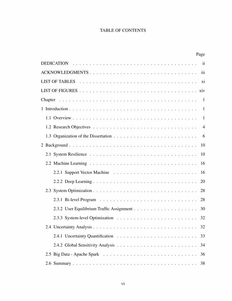
TABLE OF CONTENTS

Page

DEDICATION . . . . . . . . . . . . . . . . . . . . . . . . . . . . . . . . . . . . . ii

ACKNOWLEDGMENTS . . . . . . . . . . . . . . . . . . . . . . . . . . . . . . . . iii

LIST OF TABLES . . . . . . . . . . . . . . . . . . . . . . . . . . . . . . . . . . . xi

LIST OF FIGURES . . . . . . . . . . . . . . . . . . . . . . . . . . . . . . . . . . . xiv

Chapter . . . . . . . . . . . . . . . . . . . . . . . . . . . . . . . . . . . . . . . . . 1

1 Introduction . . . . . . . . . . . . . . . . . . . . . . . . . . . . . . . . . . . . . . 1

1.1 Overview . . . . . . . . . . . . . . . . . . . . . . . . . . . . . . . . . . . . . 1

1.2 Research Objectives . . . . . . . . . . . . . . . . . . . . . . . . . . . . . . . 4

1.3 Organization of the Dissertation . . . . . . . . . . . . . . . . . . . . . . . . . 6

2 Background . . . . . . . . . . . . . . . . . . . . . . . . . . . . . . . . . . . . . . 10

2.1 System Resilience . . . . . . . . . . . . . . . . . . . . . . . . . . . . . . . . 10

2.2 Machine Learning . . . . . . . . . . . . . . . . . . . . . . . . . . . . . . . . 16

2.2.1 Support Vector Machine . . . . . . . . . . . . . . . . . . . . . . . . . 16

2.2.2 Deep Learning . . . . . . . . . . . . . . . . . . . . . . . . . . . . . . . 20

2.3 System Optimization . . . . . . . . . . . . . . . . . . . . . . . . . . . . . . . 28

2.3.1 Bi-level Program . . . . . . . . . . . . . . . . . . . . . . . . . . . . . 28

2.3.2 User Equilibrium Traffic Assignment . . . . . . . . . . . . . . . . . . . 30

2.3.3 System-level Optimization . . . . . . . . . . . . . . . . . . . . . . . . 32

2.4 Uncertainty Analysis . . . . . . . . . . . . . . . . . . . . . . . . . . . . . . . 32

2.4.1 Uncertainty Quantification . . . . . . . . . . . . . . . . . . . . . . . . 33

2.4.2 Global Sensitivity Analysis . . . . . . . . . . . . . . . . . . . . . . . . 34

2.5 Big Data - Apache Spark . . . . . . . . . . . . . . . . . . . . . . . . . . . . 36

2.6 Summary . . . . . . . . . . . . . . . . . . . . . . . . . . . . . . . . . . . . . 38

vi

3 Deep Learning Models for Early Warning of the Occurrences of Hazardous Events 39

3.1 Introduction . . . . . . . . . . . . . . . . . . . . . . . . . . . . . . . . . . . 39

3.2 SWIM SFDPS Data Overview . . . . . . . . . . . . . . . . . . . . . . . . . . 45

3.3 Proposed Method . . . . . . . . . . . . . . . . . . . . . . . . . . . . . . . . 47

3.3.1 SFDPS Message Processing . . . . . . . . . . . . . . . . . . . . . . . 48

3.3.2 Model Construction . . . . . . . . . . . . . . . . . . . . . . . . . . . . 52

3.3.3 Model Integration . . . . . . . . . . . . . . . . . . . . . . . . . . . . . 57

3.3.4 Safety Measure . . . . . . . . . . . . . . . . . . . . . . . . . . . . . . 59

3.3.5 Summary . . . . . . . . . . . . . . . . . . . . . . . . . . . . . . . . . 60

3.4 Computational Results . . . . . . . . . . . . . . . . . . . . . . . . . . . . . . 61

3.4.1 Data . . . . . . . . . . . . . . . . . . . . . . . . . . . . . . . . . . . . 62

3.4.2 Model Training and Assessment . . . . . . . . . . . . . . . . . . . . . 62

3.4.3 Safety Assessment . . . . . . . . . . . . . . . . . . . . . . . . . . . . 66

3.5 Summary . . . . . . . . . . . . . . . . . . . . . . . . . . . . . . . . . . . . . 67

4 Ensemble Machine Learning Models for Risk Prediction of the Consequences of

Hazardous Events . . . . . . . . . . . . . . . . . . . . . . . . . . . . . . . . . . . 69

4.1 Introduction . . . . . . . . . . . . . . . . . . . . . . . . . . . . . . . . . . . 69

4.2 Aviation Safety Reporting System . . . . . . . . . . . . . . . . . . . . . . . . 75

4.3 Proposed Methodology . . . . . . . . . . . . . . . . . . . . . . . . . . . . . 79

4.3.1 Risk-based Event Outcome Categorization . . . . . . . . . . . . . . . . 81


4.3.3 Model Fusion . . . . . . . . . . . . . . . . . . . . . . . . . . . . . . . 88

4.3.4 Event-level Outcome Analysis . . . . . . . . . . . . . . . . . . . . . . 97

4.3.5 Summary . . . . . . . . . . . . . . . . . . . . . . . . . . . . . . . . . 98

4.4 Computational Results . . . . . . . . . . . . . . . . . . . . . . . . . . . . . . 99

4.4.1 Data Description . . . . . . . . . . . . . . . . . . . . . . . . . . . . . 99

4.4.2 Experimental Analysis . . . . . . . . . . . . . . . . . . . . . . . . . . 101

vii

4.5 Summary . . . . . . . . . . . . . . . . . . . . . . . . . . . . . . . . . . . . . 109

5 Human Reliability Analysis in Diagnosing and Correcting System Malfunctions . 111

5.1 Introduction . . . . . . . . . . . . . . . . . . . . . . . . . . . . . . . . . . . 111

5.2 Experimental study . . . . . . . . . . . . . . . . . . . . . . . . . . . . . . . 114

5.2.1 Participants . . . . . . . . . . . . . . . . . . . . . . . . . . . . . . . . 114

5.2.2 Experimental Environment . . . . . . . . . . . . . . . . . . . . . . . . 115

5.2.3 Scenario Development . . . . . . . . . . . . . . . . . . . . . . . . . . 116

5.2.4 Experimental Procedures . . . . . . . . . . . . . . . . . . . . . . . . . 117

5.2.5 Operator Performance Measures . . . . . . . . . . . . . . . . . . . . . 118

5.3 Data Analysis . . . . . . . . . . . . . . . . . . . . . . . . . . . . . . . . . . 121

5.3.1 Scenario Characteristics Extraction . . . . . . . . . . . . . . . . . . . . 123

5.3.2 Physiological Data Analysis . . . . . . . . . . . . . . . . . . . . . . . 127

5.3.3 Eye Tracking Data Analysis . . . . . . . . . . . . . . . . . . . . . . . 134

5.3.4 Expert-rated Task Performance . . . . . . . . . . . . . . . . . . . . . . 140

5.4 Quantitative Model Development . . . . . . . . . . . . . . . . . . . . . . . . 142


5.5 Summary . . . . . . . . . . . . . . . . . . . . . . . . . . . . . . . . . . . . . 150

6 Performance Assessment of Algorithmic Response to Hazardous Events . . . . . . 154

6.1 Introduction . . . . . . . . . . . . . . . . . . . . . . . . . . . . . . . . . . . 154

6.2 Proposed Methodology for Aircraft Re-routing . . . . . . . . . . . . . . . . . 160

6.2.1 Problem Description . . . . . . . . . . . . . . . . . . . . . . . . . . . 161

6.2.2 System Model . . . . . . . . . . . . . . . . . . . . . . . . . . . . . . . 163

6.2.3 Stochastic Variables Considered . . . . . . . . . . . . . . . . . . . . . 166

6.2.4 Mathematical Model of Aircraft Re-routing Optimization . . . . . . . . 173

6.3 Proposed Methodology for Performance Assessment . . . . . . . . . . . . . . 175

6.3.1 System Failure Time . . . . . . . . . . . . . . . . . . . . . . . . . . . 176

6.3.2 Variance-based Sensitivity Analysis . . . . . . . . . . . . . . . . . . . 177

viii

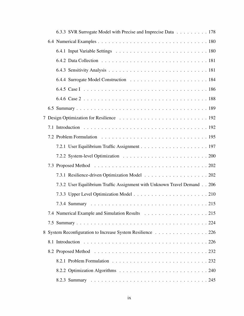
6.3.3 SVR Surrogate Model with Precise and Imprecise Data . . . . . . . . . 178

6.4 Numerical Examples . . . . . . . . . . . . . . . . . . . . . . . . . . . . . . . 180

6.4.1 Input Variable Settings . . . . . . . . . . . . . . . . . . . . . . . . . . 180

6.4.2 Data Collection . . . . . . . . . . . . . . . . . . . . . . . . . . . . . . 181

6.4.3 Sensitivity Analysis . . . . . . . . . . . . . . . . . . . . . . . . . . . . 181

6.4.4 Surrogate Model Construction . . . . . . . . . . . . . . . . . . . . . . 184

6.4.5 Case I . . . . . . . . . . . . . . . . . . . . . . . . . . . . . . . . . . . 186

6.4.6 Case 2 . . . . . . . . . . . . . . . . . . . . . . . . . . . . . . . . . . . 188

6.5 Summary . . . . . . . . . . . . . . . . . . . . . . . . . . . . . . . . . . . . . 189

7 Design Optimization for Resilience . . . . . . . . . . . . . . . . . . . . . . . . . 192

7.1 Introduction . . . . . . . . . . . . . . . . . . . . . . . . . . . . . . . . . . . 192

7.2 Problem Formulation . . . . . . . . . . . . . . . . . . . . . . . . . . . . . . 195

7.2.1 User Equilibrium Traffic Assignment . . . . . . . . . . . . . . . . . . . 197

7.2.2 System-level Optimization . . . . . . . . . . . . . . . . . . . . . . . . 200

7.3 Proposed Method . . . . . . . . . . . . . . . . . . . . . . . . . . . . . . . . 202

7.3.1 Resilience-driven Optimization Model . . . . . . . . . . . . . . . . . . 202

7.3.2 User Equilibrium Traffic Assignment with Unknown Travel Demand . . 206

7.3.3 Upper Level Optimization Model . . . . . . . . . . . . . . . . . . . . . 210

7.3.4 Summary . . . . . . . . . . . . . . . . . . . . . . . . . . . . . . . . . 215

7.4 Numerical Example and Simulation Results . . . . . . . . . . . . . . . . . . 215

7.5 Summary . . . . . . . . . . . . . . . . . . . . . . . . . . . . . . . . . . . . . 224

8 System Reconfiguration to Increase System Resilience . . . . . . . . . . . . . . . 226

8.1 Introduction . . . . . . . . . . . . . . . . . . . . . . . . . . . . . . . . . . . 226

8.2 Proposed Method . . . . . . . . . . . . . . . . . . . . . . . . . . . . . . . . 232

8.2.1 Problem Formulation . . . . . . . . . . . . . . . . . . . . . . . . . . . 232

8.2.2 Optimization Algorithms . . . . . . . . . . . . . . . . . . . . . . . . . 240

8.2.3 Summary . . . . . . . . . . . . . . . . . . . . . . . . . . . . . . . . . 245

ix

8.3 Numerical Examples . . . . . . . . . . . . . . . . . . . . . . . . . . . . . . . 246

8.3.1 Example 1 . . . . . . . . . . . . . . . . . . . . . . . . . . . . . . . . . 247

8.3.2 Example 2 . . . . . . . . . . . . . . . . . . . . . . . . . . . . . . . . . 256

8.4 Summary . . . . . . . . . . . . . . . . . . . . . . . . . . . . . . . . . . . . . 260

9 Summary and Future Work . . . . . . . . . . . . . . . . . . . . . . . . . . . . . . 262

9.1 Summary of Accomplishments . . . . . . . . . . . . . . . . . . . . . . . . . 262

9.2 Future Work . . . . . . . . . . . . . . . . . . . . . . . . . . . . . . . . . . . 265

9.3 Concluding Remarks . . . . . . . . . . . . . . . . . . . . . . . . . . . . . . . 267

BIBLIOGRAPHY . . . . . . . . . . . . . . . . . . . . . . . . . . . . . . . . . . . 269

x

LIST OF TABLES

Table Page

3.1 Sample flight trajectory parsed from SFDPS messages on January 11st 2019 50

3.2 Performance comparisons on trajectory deviation prediction . . . . . . . . . 66

3.3 Performance comparisons on flight state prediction . . . . . . . . . . . . . 66

4.1 A sample incident/accident record extracted from ASRS . . . . . . . . . . 76

4.2 Two examples of event synopsis in ASRS . . . . . . . . . . . . . . . . . . 78

4.3 Mapping between risk levels and event outcomes . . . . . . . . . . . . . . 83

4.4 Performance metrics for the two trained models. Here, the support column

denotes the number of occurrences of each class in the actual observation,

the consistent prediction column represents the number of consistent pre-

dictions between the two models for each class, and consistent prediction

accuracy denotes the proportion of records in the consistent model predic-

tions that are correctly labeled. The five numerical values 1, 2, 3, 4, and 5

denote the five risk categories from low risk to high risk . . . . . . . . . . . 94

4.5 The number of records belonging to each risk category . . . . . . . . . . . 99

4.6 Confusion matrix . . . . . . . . . . . . . . . . . . . . . . . . . . . . . . . 99

4.7 Performance metrics for the two trained models. Here, the support column

denotes the number of occurrences of each class in the actual observation,

the consistent prediction column represents the number of consistent pre-

dictions between the two models for each class, and consistent prediction

accuracy denotes the proportion of records in the consistent model predic-

tions that are correctly labeled. The five numerical values 1, 2, 3, 4, and 5

denote the five risk categories from low risk to high risk . . . . . . . . . . . 102

4.8 Model predictions with respect to test record a . . . . . . . . . . . . . . . 103

xi

4.9 Event synopsis of test record a . . . . . . . . . . . . . . . . . . . . . . . . 108

5.1 Modified Halden Task Complexity Scale (HTCS) questionnaire used in the

experiment . . . . . . . . . . . . . . . . . . . . . . . . . . . . . . . . . . 118

5.2 Sample process overview measure items . . . . . . . . . . . . . . . . . . . 119

5.3 Sample malfunction and OPAS rating items in the first scenario . . . . . . 120

5.4 Difficulty ratings for Scenario 1 . . . . . . . . . . . . . . . . . . . . . . . 123

5.5 HTCS workload ratings on the first scenario . . . . . . . . . . . . . . . . . 123

5.6 Operators’ situation awareness on the malfunction events in the first sce-

nario (SO: simulator operator, RO: reactor operator, BOP: balance-of-plant-

side operator, US: unit supervisor) . . . . . . . . . . . . . . . . . . . . . . 124

5.7 Event-related data analysis results for the skin conductance response . . . . 131

5.8 Skin conductance response-derived features . . . . . . . . . . . . . . . . . 133

5.9 Eye tracking data-derived features . . . . . . . . . . . . . . . . . . . . . . 140

5.10 Expert-rated task performance . . . . . . . . . . . . . . . . . . . . . . . . 141

5.11 Transformation of expert ratings into numerical counts (for one malfunc-

tion in one scenario) . . . . . . . . . . . . . . . . . . . . . . . . . . . . . 142

5.12 Prediction accuracy of the four individual models . . . . . . . . . . . . . . 148

6.1 Assumed probability distributions for the input variables. . . . . . . . . . . 182

6.2 Goodness-of-fitness statistics as defined by Stephens [1] . . . . . . . . . . . 187

6.3 Goodness-of-fit statistics. . . . . . . . . . . . . . . . . . . . . . . . . . . . 187

6.4 System reliability analysis. . . . . . . . . . . . . . . . . . . . . . . . . . . 188

6.5 Case 2: system reliability analysis. . . . . . . . . . . . . . . . . . . . . . . 188

7.1 Best solution found by the cross entropy method without the consideration

of the impact of disruptive event e. . . . . . . . . . . . . . . . . . . . . . . 220

xii

7.2 Best solution found by the cross entropy method when the impact of dis-

ruptive event e is considered. . . . . . . . . . . . . . . . . . . . . . . . . . 222

xiii

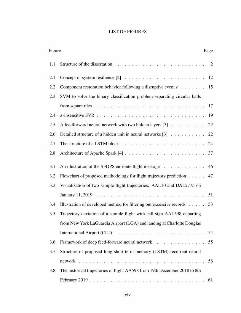
LIST OF FIGURES

Figure Page

1.1 Structure of the dissertation . . . . . . . . . . . . . . . . . . . . . . . . . . 2

2.1 Concept of system resilience [2] . . . . . . . . . . . . . . . . . . . . . . . 12

2.2 Component restoration behavior following a disruptive event e . . . . . . . 15

2.3 SVM to solve the binary classification problem separating circular balls

from square tiles . . . . . . . . . . . . . . . . . . . . . . . . . . . . . . . . 17

2.4 ε-insensitive SVR . . . . . . . . . . . . . . . . . . . . . . . . . . . . . . . 19

2.5 A feedforward neural network with two hidden layers [3] . . . . . . . . . . 22

2.6 Detailed structure of a hidden unit in neural networks [3] . . . . . . . . . . 22

2.7 The structure of a LSTM block . . . . . . . . . . . . . . . . . . . . . . . . 24

2.8 Architecture of Apache Spark [4] . . . . . . . . . . . . . . . . . . . . . . . 37

3.1 An illustration of the SFDPS en-route flight message . . . . . . . . . . . . 46

3.2 Flowchart of proposed methodology for flight trajectory prediction . . . . . 47

3.3 Visualization of two sample flight trajectories: AAL10 and DAL2775 on

January 11, 2019 . . . . . . . . . . . . . . . . . . . . . . . . . . . . . . . 51

3.4 Illustration of developed method for filtering out excessive records . . . . . 53

3.5 Trajectory deviation of a sample flight with call sign AAL598 departing

from New York LaGuardia Airport (LGA) and landing at Charlotte Douglas

International Airport (CLT) . . . . . . . . . . . . . . . . . . . . . . . . . . 54

3.6 Framework of deep feed-forward neural network . . . . . . . . . . . . . . . 55

3.7 Structure of proposed long short-term memory (LSTM) recurrent neural

network . . . . . . . . . . . . . . . . . . . . . . . . . . . . . . . . . . . . 56

3.8 The historical trajectories of flight AA598 from 19th December 2018 to 8th

February 2019 . . . . . . . . . . . . . . . . . . . . . . . . . . . . . . . . . 61

xiv

3.9 DNN prediction on trajectory deviation . . . . . . . . . . . . . . . . . . . . 62

3.10 Comparisons on the trajectory predictions of flight AA598 . . . . . . . . . 63

3.11 LSTM prediction of flight trajectory . . . . . . . . . . . . . . . . . . . . . 64

3.12 Comparison of LSTM model predictions before and after integration with

the DNN model . . . . . . . . . . . . . . . . . . . . . . . . . . . . . . . . 65

3.13 Performance comparison of separation distance . . . . . . . . . . . . . . . 67

4.1 Distribution of outcomes for all incidents/accidents between January 2006

and December 2017 . . . . . . . . . . . . . . . . . . . . . . . . . . . . . . 73

4.2 Hybrid machine learning framework for risk prediction . . . . . . . . . . . 80

4.3 Distribution of risk outcomes after recategorization of incidents/accidents

from January 2006 to December 2017 . . . . . . . . . . . . . . . . . . . . 84

4.4 Proposed fusion rule to integrate the two models . . . . . . . . . . . . . . . 89

4.5 Datasets and model inputs . . . . . . . . . . . . . . . . . . . . . . . . . . . 100

4.6 Proportion of each class in the records with disagreeing predictions . . . . . 105

4.7 The performance of hybrid model versus support vector machine (SVM),

ensemble of deep neural networks (DNN), and ordinal logistic regression

(OLR) . . . . . . . . . . . . . . . . . . . . . . . . . . . . . . . . . . . . . 106

4.8 Confusion matrix. (a) the hybrid method, (b) support vector machine, (c)

deep neural networks. The entry in the i-th row and j-th column corre-

sponds to the percentage of samples from class i that were classified as

class j. 1: low, 2: moderately medium, 3: medium, 4: moderately high, 5:

high . . . . . . . . . . . . . . . . . . . . . . . . . . . . . . . . . . . . . . 107

4.9 The probabilistic event outcomes for test record a . . . . . . . . . . . . . . 108

5.1 Simulated control room configuration. Left: reactor operator workstations;

Center: large screen display; Right: turbine operator workstation . . . . . . 114

5.2 Configuration of experimental team members in the observation gallery . . 116

xv

5.3 Proposed methodology . . . . . . . . . . . . . . . . . . . . . . . . . . . . 122

5.4 Conversion process for situation awareness ratings . . . . . . . . . . . . . . 126

5.5 Cleaning of the skin conductance response signal . . . . . . . . . . . . . . 128

5.6 Event-related data analysis on the skin conductance response . . . . . . . . 130

5.7 Quantitative metrics related to skin conductance response . . . . . . . . . . 131

5.8 The respiration data of the unit supervisor in the first scenario . . . . . . . . 133

5.9 Snapshot of the experimental set up with IR markers and their IDs . . . . . 134

5.10 Mapped eye tracking data . . . . . . . . . . . . . . . . . . . . . . . . . . . 135

5.11 Areas of interest in the first malfunction of the first scenario. Larger fonts

indicate the IR marker IDs, while smaller fonts are the labels for the impor-

tant regions . . . . . . . . . . . . . . . . . . . . . . . . . . . . . . . . . . 136

5.12 The fixation duration on the important regions . . . . . . . . . . . . . . . . 136

5.13 Number of clusters corresponding to the eye movement of the first mal-

function in the first scenario . . . . . . . . . . . . . . . . . . . . . . . . . . 138

5.14 Model inputs and outputs . . . . . . . . . . . . . . . . . . . . . . . . . . . 143

5.15 Correlations among the 22 input variables . . . . . . . . . . . . . . . . . . 145

5.16 Framework of the quantitative model . . . . . . . . . . . . . . . . . . . . . 147

5.17 Predicted numerical counts for ten validation malfunctions (rating value is

2: minor delays in response to malfunction events) . . . . . . . . . . . . . . 149

6.1 Framework of aircraft re-routing optimization and performance assessment 159

6.2 Aircraft re-routing process . . . . . . . . . . . . . . . . . . . . . . . . . . 161

6.3 A snapshot of the simulation system . . . . . . . . . . . . . . . . . . . . . 164

6.4 Radar performance uncertainty . . . . . . . . . . . . . . . . . . . . . . . . 170

6.5 System workflow . . . . . . . . . . . . . . . . . . . . . . . . . . . . . . . 172

6.6 First-order Sobol’ indices . . . . . . . . . . . . . . . . . . . . . . . . . . . 183

6.7 System failure time prediction with ε-SVR model . . . . . . . . . . . . . . 185

6.8 First case: System performance assessment . . . . . . . . . . . . . . . . . 185

xvi

6.9 Two Goodness-of-fit plots for various distributions fitted to continuous data

(Weibull, Lognormal, normal, gamma, and exponential distributions fitted

to 20,000 samples) . . . . . . . . . . . . . . . . . . . . . . . . . . . . . . 186

6.10 Performance assessment . . . . . . . . . . . . . . . . . . . . . . . . . . . 189

7.1 Flowchart of the proposed methodology . . . . . . . . . . . . . . . . . . . 203

7.2 A simple network to demonstrate the proposed method to deal with user

equilibrium with unknown travel demand between resident zones and ser-

vice centers . . . . . . . . . . . . . . . . . . . . . . . . . . . . . . . . . . 207

7.3 Test network 1: A 25-node transportation network . . . . . . . . . . . . . . 217

7.4 Illustration of dummy node and auxiliary links . . . . . . . . . . . . . . . . 219

7.5 Convergence of gradient projection algorithm for one instance of service

center configuration . . . . . . . . . . . . . . . . . . . . . . . . . . . . . . 220

7.6 The evolution of constructing service center at each candidate site . . . . . 221

7.7 The evolution of objective function value over iterations . . . . . . . . . . . 222

7.8 Comparison of travel time and service time in different scenarios . . . . . . 224

8.1 Structure of the proposed method . . . . . . . . . . . . . . . . . . . . . . . 233

8.2 BPR function . . . . . . . . . . . . . . . . . . . . . . . . . . . . . . . . . 234

8.3 Contraflow illustration . . . . . . . . . . . . . . . . . . . . . . . . . . . . 235

8.4 An illustration of crossing elimination at an intersection. The blue arrows

denote the direction of traffic flow in each lane, the red triangles mean that

the roadway is blocked, and the labels in purple represent the order that will

be used to encode the problem . . . . . . . . . . . . . . . . . . . . . . . . 236

8.5 Contraflow illustration . . . . . . . . . . . . . . . . . . . . . . . . . . . . 237

8.6 Test network 1: Sioux-Falls network . . . . . . . . . . . . . . . . . . . . . 248

8.7 The convergence process of the relative gap when the threshold value is 10−3251

8.8 The convergence process of total travel time in the Sioux-Falls network. . . 252

xvii

8.9 The reconfigured Sioux-Falls network . . . . . . . . . . . . . . . . . . . . 253

8.10 The link flow distribution of the best system reconfiguration in the Sioux-

Falls network . . . . . . . . . . . . . . . . . . . . . . . . . . . . . . . . . 254

8.11 The reconfigured Sioux-Falls network when the waiting time increases from

2 to 20 . . . . . . . . . . . . . . . . . . . . . . . . . . . . . . . . . . . . . 255

8.12 Test network 2: a 25-node artificial net . . . . . . . . . . . . . . . . . . . . 256

8.13 The convergence process of total travel time in the 25-node network . . . . 258

8.14 The reconfigured 25-node network . . . . . . . . . . . . . . . . . . . . . . 259

xviii

Chapter 1

Introduction

1.1 Overview

Considering the socio-economic impact and independent nature of many large-scale

complex systems in our daily life, it is critical to ensure that they are operated at a desirable

performance level. To accomplish this goal, it is important to monitor the variation of sys-

tem performance over time and diagnose malfunction events/faults as soon as possible for

the purpose of taking corresponding actions to eliminate system malfunctions and main-

taining system performance at the desirable level in the presence of different sources of

aleatory and epistemic uncertainty. Specifically, aleatory uncertainty refers to the inherent

natural variability in the system that is irreducible, while epistemic uncertainty represents

the uncertainty caused by the lack of knowledge, which can be reduced by collecting more

information. Typically, when the system works normally, a straightforward way to measure

its performance is to model the different sources of uncertainty with appropriate distribu-

tions, then propagate such uncertainty sources through a system model, thereby projecting

the input variables to the performance metric of the investigated system. However, if some

disturbance or anomalous event happens to the system, one challenge arising here is that

it is difficult to describe the operations of many real-world systems with mathematical and

physical equations due to the complicated characteristics of system malfunctions or exter-

nal extreme events, the partial loss of system functionalities, the involvement and decisions

of human operators, and the lack of explicit relationships between the features elicited from

heterogeneous data and the system performance.

In face of the disastrous effect caused by the unanticipated events, in this dissertation,

we aim to assess and mitigate their impact on the performance of engineering systems from

a resilience perspective such that the system performance can be restored to its original level

1

Assessment during operation

Response assessment

Resource optimization

1. Forecast when abnormal events occur

2. Predict the consequence of abnormalevents

3. Reliability of human response incorrecting system malfunctions

4. Effectiveness of algorithmic responseto hazardous events

5. Design of physical facility locations

6. System reconfiguration

Preparedness

Research ObjectiveCategory

Response

Restoration

Resilience

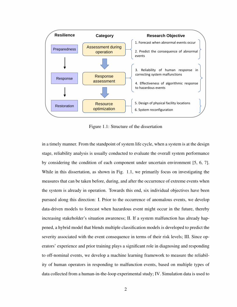
Figure 1.1: Structure of the dissertation

in a timely manner. From the standpoint of system life cycle, when a system is at the design

stage, reliability analysis is usually conducted to evaluate the overall system performance

by considering the condition of each component under uncertain environment [5, 6, 7].

While in this dissertation, as shown in Fig. 1.1, we primarily focus on investigating the

measures that can be taken before, during, and after the occurrence of extreme events when

the system is already in operation. Towards this end, six individual objectives have been

pursued along this direction: I. Prior to the occurrence of anomalous events, we develop

data-driven models to forecast when hazardous event might occur in the future, thereby

increasing stakeholder’s situation awareness; II. If a system malfunction has already hap-

pened, a hybrid model that blends multiple classification models is developed to predict the

severity associated with the event consequence in terms of their risk levels; III. Since op-

erators’ experience and prior training plays a significant role in diagnosing and responding

to off-nominal events, we develop a machine learning framework to measure the reliabil-

ity of human operators in responding to malfunction events, based on multiple types of

data collected from a human-in-the-loop experimental study; IV. Simulation data is used to

2

characterize the performance of algorithmic response in managing an abnormal event; V.

We investigate a design-for-resilience methodology, focusing on number and locations of

centers that respond to a disastrous event; VI. We also investigate a system reconfiguration

strategy for resilient response to the increased demands caused by an extreme event.

As shown in Fig. 1.1, the six measures described above aim to assess and enhance

system resilience from different views. In particular, the first two measures focus on the

construction of predictive models to forecast characteristics pertaining to anomalous events.

Specifically, the former method emphasizes forecasting when the abnormal event is about

to occur, while the latter focuses on predicting the outcome of hazardous event. The third

and fourth actions center on characterizing the effectiveness of human and algorithmic re-

sponses in mitigating the impact of extreme event. The third action evaluates the reliability

of human operators in responding to malfunction events, while the fourth action measures

the effectiveness of a rerouting strategy in mitigating the impact of closure of a destination

airport. The last two strategies aim to increase the resilience of engineering systems from

an optimization point of view. The fifth strategy designs a resilient logistics service cen-

ter distribution by accounting for the potential impact of natural disasters, while the last

strategy optimizes the reconfiguration of an already existing traffic network to mitigate the

system-wide congestion caused by the large-volume evacuation out of disaster-prone area.

To accomplish the aforementioned goals, we leverage state-of-the-art machine learning

and optimization techniques to develop quantitative models for the investigated engineer-

ing systems, in which the complex patterns and the connections between system state vari-

ables are mined and represented in the data-driven models appropriately. In this regard,

computational efficiency is a major concern when training machine learning models for

system performance assessment. To address this challenge, several strategies have been

implemented to improve the model efficiency. I. Data-driven global sensitivity analysis is

performed to identify dominant input variables, so that the input variables with negligible

effect on system performance are eliminated accordingly, thus significantly reducing the

3

problem dimension; II. Correlation analysis among input variables is conducted. If the

correlation coefficient between any two input variables is larger than a threshold, the two

variables are assumed to carry similar information. In this case, only one of them needs

to be retained as input to the model, thereby removing redundant variables. III. Resilient

distributed big data techniques, e.g., Apache Spark, are utilized to process large volumes

of raw data, from which significant features in the raw data can be derived in an efficient

manner, thereby accelerating large-scale data processing; IV. We train deep learning mod-

els on GPU in the Advanced Computing Center for Research and Education (ACCRE) at

Vanderbilt University. By doing this, the time needed for training each model is reduced

substantially.

In the rest of this chapter, Section 1.2 briefly describes the proposed research objectives

in this dissertation, and Section 1.3 introduces the organization of the dissertation section

by section.

1.2 Research Objectives

The overall goal of the proposed research is to develop rigorous and efficient machine

learning-based models for assessing system resilience and to leverage optimization models

to strengthen the system’s ability in withstanding extreme events. To achieve this goal, we

investigate several possible measures that can be taken before, during, and after the occur-

rence of extreme events. Thus, six individual objectives are pursued in order to achieve the

overall goal.

The first objective is to predict system behavior over time based on massive historical

data and forecast when an anomalous event is about to happen in the future. The method-

ology is illustrated with a flight trajectory prediction problem in order to assess the safety

of separation between aircraft in the air transportation system. A hybrid model blending

one-step-ahead prediction from a trained deep feedforward neural network and 2-minutes-

ahead prediction from a trained recurrent neural network is developed to forecast the future

4

trajectories of multiple flights, where epistemic model prediction uncertainty is character-

ized following a Bayesian approach. Such multi-fidelity strategy achieves both accuracy

and efficiency for safety assessment in realistic applications.

The second objective is to examine a wide variety of anomalous events from docu-

mented incident reports for the purpose of characterizing the risk associated with the con-

sequence of hazardous events given an observed system malfunction. A hybrid model

blending support vector machine and an ensemble of deep neural networks is developed to

predict the severity associated with the consequence of abnormal aviation incidents. While

the models developed in the first objective are based on numerical data, the models in the

second objective are based on categorical and text data.

The third objective is to develop a machine learning framework so as to measure the re-

liability of human operators in eliminating off-nominal malfunction events. To achieve this

goal, different malfunction events are injected into the system an an experimental study,

and the heterogeneous data featuring operator response are collected. An empirical model

fusing heterogeneous data is developed to quantify the operator’s performance in respond-

ing to malfunction events.

The fourth objective is to evaluate the performance of response strategy in managing

abnormal situations. The method is illustrated for an aircraft rerouting strategy in han-

dling a disruptive event caused by the closure of a destination airport, in which the interac-

tions among system components and the multiple sources of uncertainty arising at different

stages are considered. With the data collected from a dynamic simulation mimicking the

aircraft rerouting process, we train a support vector regression-based model to assess the

effectiveness of this strategy in mitigating the impact of airport closure.

The fifth objective is to optimally design a service center configuration that is resilient

in withstanding the impact of disruptive events. Specifically, we investigate a pre-disaster

resilience-based design optimization approach for logistics service centers configuration. A

bi-level program is formulated, and the impact of potential disruptive events is accounted

5

for by the upper-level decision maker. The objective of the formulated bi-level program is

to maximize the resilience of the service center configuration, thereby enhancing the ability

of the system to withstand unexpected events.

The sixth objective focuses on system reconfiguration strategies of existing systems

for achieving resilience when subjected to extreme events. Specifically, we optimize the

operational resilience of a traffic network to mitigate the congestion caused by the large

volume evacuation out of the disaster-prone zones when confronted with an extreme event.

A bi-level mathematical optimization model is formulated to mitigate the incurred traffic

congestion through two network reconfiguration schemes: contraflow (also referred to as

lane reversal), and crossing elimination at intersections. The system reconfiguration strate-

gies are optimized to maximize the resilience of the transportation network in withstanding

the extreme event.

1.3 Organization of the Dissertation

The subsequent chapters of this dissertation will be devoted to the objectives proposed

above.

Chapter 2 first defines system resilience in a quantitative manner, which will be used in

Chapters 7 and 8 as the performance indicator. Next, Chapter 2 provides a brief introduc-

tion to several state-of-the-art machine learning algorithms, including: (1) support vector

machine, (2) deep learning: deep feedforward neural network, recurrent neural network.

Besides, a Bayesian neural network framework is introduced as a generic means to char-

acterize model prediction uncertainty. Afterwards, we review uncertainty analysis that is

used to quantify the uncertainties arising at different stages in complex systems. In parallel,

global sensitivity analysis is introduced to measure the contribution of each random vari-

able to system-level variability. Following the uncertainty analysis, a bi-level optimization

program is introduced to characterize the interactions among different decision makers in

order to increase system resilience. Finally, a unified big data analytics engine Apache

6

Spark is introduced to process large volumes of raw data in Chapter 2.

Chapter 3 focuses on the first objective: developing deep learning models to forecast

the occurrence of abnormal events. The proposed methodology is illustrated with en-route

flight trajectory prediction in the air transportation system in order to support en-route

safety assessment. The following steps are pursued: (1) a unified big data engine Apache

Spark is used to process large volume of raw data obtained from Federal Aviation Admin-

istration (FAA) in the Flight Information Exchange Model (FIXM) format; (2) two deep

learning models are trained with historical flight trajectories to predict the future state of

flight trajectory from different perspectives; (3) the two trained deep learning models are

combined to achieve both accuracy and efficiency; and (4) the integrated model is used to

forecast the trajectories of multiple flights, and then assess the safety between two flights

based on separation distance.

Chapter 4 focuses on the second objective. It facilitates the “proactive safety” paradigm

to increase system resilience with a focus on predicting the severity associated with the

consequence of abnormal aviation events in terms of their risk levels. The following steps

are pursued: (1) the incidents reported in the Aviation Safety Reporting System (ASRS) are

categorized into five risk groups; (2) a support vector machine model is used to discover

the relationships between the event synopsis in text format and event consequence; (3)

an ensemble of deep neural networks is trained to model the associations between event

contextual features and event outcomes, (4) an innovative fusion rule is developed to blend

the prediction results from the two trained machine learning models; and (5) the prediction

of risk level categories is extended to event-level outcomes through a probabilistic decision

tree.

Chapter 5 focuses on the third objective. It analyzes the reliability of human opera-

tors in terms of their response to malfunction events. The following steps are pursued: (1)

Simulator experimental data is collected on nine licensed operators in three-person crews

completing ten scenarios with each incorporating two to four malfunction events; (2) in-

7

dividual operator performance is monitored using eye tracking technology and physiolog-

ical recordings of skin conductance response and respiratory function. Expert-rated event

management performance is the outcome to be modelled based on eye tracking and physi-

ological data; and (3) the heterogeneous data sources are integrated using a support vector

machine with bootstrap aggregation to develop a trained quantitative prediction model.

Chapter 6 focuses on the fourth objective. It investigates the effectiveness of a rerouting

strategy in face of the shutdown of an airport due to extreme weather, along the following

steps: (1) an aircraft re-routing optimization model is formulated to make periodic re-

routing decisions with the objective of minimizing the overall distance travelled by all the

aircraft; (2) the performance of this aircraft re-routing system is analyzed using system

failure time as the metric, considering multiple sources of uncertainties; and (3) a Support

Vector Regression (SVR) surrogate model is developed to efficiently construct the system

failure time distribution to measure the performance of re-routing strategy.

Chapter 7 focuses on the fifth objective. It investigates a pre-disaster resilience-based

design optimization approach for logistics service centers configuration, along the follow-

ing steps: (1) a bi-level program is formulated, and the impact of potential disruptive events

is accounted for by the upper-level decision maker. Two decision variables are involved:

location of the service center and its capacity; (2) the objective of the formulated bi-level

program is to maximize the resilience of the service center configuration, thereby increas-

ing the ability of the system to withstand unexpected events, and (3) a multi-level cross-

entropy method is leveraged to generate samples that gradually concentrates all its mass in

the proximity of the optimal solution in an iterative way.

Chapter 8 focuses on the sixth objective. It conducts investigation on the optimization

of system reconfiguration strategies to mitigate the congestion caused by emergency evac-

uation out of disaster-prone zones. The following steps are pursued: (1) the traffic system

performance is restored through two reconfiguration schemes: contraflow (also referred

to as lane reversal), and crossing elimination at intersections; (2) a bi-level mathematical

8

model is developed to represent the two reconfiguration schemes and characterize the inter-

actions between traffic operators and passengers; and (3) a probabilistic solution discovery

algorithm is used to obtain the near-optimal reconfiguration solution that maximizes the

system resilience.

Chapter 9 provides a summary of contributions made in this dissertation and the re-

search directions worthy of investigation in the future.

9

Chapter 2

Background

This chapter first introduces system resilience modeling, then describes several state-of-

the-art machine learning algorithms that are extensively used in the literature. Afterwards,

we briefly review uncertainty analysis, system optimization, and a big data analytics frame-

work. Following this structure, we define system resilience in a quantitative manner in Sec-

tion 2.1. Next, two major machine learning algorithms, namely support vector machine and

deep learning, are reviewed. The basic concept of support vector machine is firstly intro-

duced in Section 2.2.1. In parallel, two popular deep learning algorithms: deep feedforward

neural network and recurrent neural network, are introduced in Section 2.2.2. Besides, a

Bayesian neural network, as a generic means to characterize the prediction uncertainty of

neural networks, is introduced following Section 2.2.2. In Section 2.3, a bi-level optimiza-

tion framework is introduced to model the interactions between multiple decision makers

at different levels. In Section 2.4, we describe the categorization of uncertainties arising

at various stages, and introduce global sensitivity analysis to measure the contribution of

random variable to the system-level variability. Finally, Section 2.5 introduces the concept

of a big data engine – Apache Spark – to process large volumes of raw data.

2.1 System Resilience

System resilience is a complex term, and it is a time-dependent function of many fac-

tors, e.g., the type of the disaster (flood, hurricane, earthquake, or others), characteristics of

the disaster (i.e., location and temporal evolution of the disaster), the impact of the extreme

event on the system, the property of the original system (i.e., redundancy, vulnerability),

and operational flexibility (what options are available to restore the system in response to

the extreme event). As a widely acknowledged concept, resilience has received extensive

10

attentions from the risk analysis community following Holland’s seminal study [8]. During

the past ten years, numerous efforts have been dedicated to the development of quantita-

tive measures/metrics to evaluate system resilience in response to different types of natural

disasters or intentional attacks with applications to telecommunication systems [9], water-

way network [10], electrical power system [11], and others [12, 13, 14, 15]. For exam-

ple, Bruneau et al. [16] proposed a quantitative metric to measure the community seismic

resilience as the extent to which the social communities are able to carry out recovery activ-

ities to mitigate the social disruption of future earthquakes. Henry and Ramirez-Marquez

[2] defined system resilience as a time-dependent function, which is the ratio of the deliv-

ery function of the system that recovers over time and the initial performance loss caused

by disruptive event. Baroud et al. [17] measured the importance of network components

according to their contribution to the network resilience in inland waterway networks. In a

recent study, Fotouhi et al. [18] formulated a bi-level, mixed-integer, stochastic program to

quantify the resilience of an interdependent transportation-power network. Hosseini et al.

[19] provided a comprehensive review on the recent advancements along the definition and

quantification of system resilience in a variety of disciplines.

Even through there is no universally accepted resilience metric, all the aforementioned

metrics share several significant characteristics: (I) resilience is regarded as a time-dependent

metric. Obviously, the resilience of a system varies over time and is pertinent to the type

of disruption; (II) realistic models need to be constructed to model the disturbance caused

by the disruptive event and its impact on the system (absorptive ability, restoration abil-

ity); (III) an appropriate performance metric needs to be defined to characterize the system

behavior before, during and after the disruption; (IV) reasonable functions need to be devel-

oped to associate the preventive (or pre-disaster activities) and corrective actions (or post-

disaster activities) to the system performance. These key features substantially differentiate

resilience from other measures of system performance, such as, reliability, sustainability,

fault-tolerance, and flexibility.

11

Reliability Preparedness Recoverability

Time

Degradation

Disruption event e

t0 te td ts tf

Recovery action

Ψ(t0)

Ψ(t)

Ψ(td)

Ψ(tf)

S0

Stable original

state

System

degradation

Sd

Disrupted

state

System

recovery

Sf

Stable

recovered state

Per

form

an

ce

metr

ic

Figure 2.1: Concept of system resilience [2]

Consider an infrastructure system, such as a power network system, transportation sys-

tem, inland waterway network etc. If unexpected disruptions occur, its state transitions can

be modelled using Fig. 2.1. To quantify the system resilience R, we introduce a system

performance function ψ (t) to describe the system behavior at time t. Commonly used

representations of this function can be network capacity, travel time, traffic flow, system

throughput, or network connectivity depending on the specific system under consideration.

As can be observed in Fig. 2.1, there are several distinct stages to characterize the transition

of the system over time:

– Before the occurrence of the disruption, the original system is operated at the as-

designed state S0;

– Once the disruption event e happens at time te, the system performance starts to

degrade over time due to the failure of system components or the loss of partial func-

tionality. The system performance continues to degrade until it reaches a maximum

disrupted state ψ(Sd) at time td .

12

– In response to the disturbance, certain measures are carried out to recover the system

functionality. At this stage, two different activities get involved: repair and system

recovery. Preparation refers to the time required for identifying the system malfunc-

tion and repairing or replacing the impaired components. When all the preparation

work is completed, the system performance begins to recover from the disrupted state

Sd at time ts. With time, the system performance restores to a new stable state S f ,

and is maintained thereafter.

Let R(t) denote the resilience of a system at time t, since resilience describes the ratio

of system recovery at time t to the loss suffered by the system at some previous point in

time td , then R(t) can be expressed by the following equation [20]:

R(t) =Recovery(t)

Loss(td), t > td. (2.1)

As shown in Fig. 2.1, ψ (t0) describes the value of the system service function cor-

responding to the stable state S0. The system performance remains at this level until the

occurrence of the disruptive event e at time te, upon which the system resilience is exhib-

ited. Once the disruptive event e occurs, the system performance degrades gradually until

it converges to a stable disrupted state Sd at time td , and the system delivery function value

corresponding to this disrupted state is ψ (td), which is lower than its original value ψ (t0).

After a duration ts− td , the recovery action is taken at time ts, which restores the system

from the disrupted state Sd to a new stable state S f with system performance function value

ψ(t f)

at time t f . Based on the above definitions, the system resilience given the disruptive

event e can be defined as [20]:

R(

t f∣∣e)= ψ

(t f∣∣e)−ψ (td|e)

ψ (t0)−ψ (td|e)(2.2)

The above system resilience metric helps to quantify the impact of different restoration

actions and operations on the recovery of system performance. In general, the higher the

13

resilience value, the stronger the system’s ability to recover. Along this direction, one

study worthy of mention is that Zhang et al. [21] developed a nonlinear function to model

the characteristics of each system component in the presence of the disruptive event e:

u∗i j (t) = ui j

[ai j +λi j ·

(1−ai j

)·(

1− e−bi jt)]

(2.3)

where ui j denotes the original performance of a component (i, j), t represents the duration

after the disruption, u∗i j (t) represents the restored component capacity at time t, ai j de-

notes the disrupted capacity retained in link (i, j) after the disruption, bi j characterizes the

restoration speed of link (i, j), and λi j is the ratio used to denote the degree to which the

link is able to recover compared to its original performance.

This nonlinear function incorporates core resilience concepts (i.e., absorptive capacity

and restorative ability) and the time to recovery in modelling the component resilience.

In addition, the non-linear function defined in Eq. (2.3) is also equipped with the ability

to characterize the variability of component performance restoration speed over time. Of-

ten, when we restore a complex component, the part that takes the least amount of time

or resources will be repaired first, whereas the part which consumes the largest amount

of resources or time will be repaired last. From this point of view, the speed of compo-

nent performance restoration gets slower and slower over time [22]. This feature has been

captured by the nonlinear function defined in Eq. (2.3).

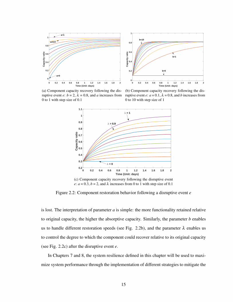
In addition, the extra parameters, a, b, and λ introduced in this function increase the

flexibility of this function, which enables us to handle the component recovery process in

multiple different applications. Fig. 2.2a illustrates these concepts. Specifically, we fix

the parameters b and λ at 2 and 0.8, respectively, and increase the value of a from 0 to

1 in a step size of 0.1. As can be observed, when a = 0, the component loses all of its

capacity. With the increase of parameter a, more capacity along the component is retained.

Especially when a = 1, the component is immune to this disruptive event, and no capacity

14

0 0.2 0.4 0.6 0.8 1 1.2 1.4 1.6 1.8 2Time (Unit: days)

0

0.2

0.4

0.6

0.8

1

Cap

acit

y ra

tio

a=0

a=1

a=0.9

(a) Component capacity recovery following the dis-ruptive event e: b = 2, λ = 0.8, and a increases from0 to 1 with step size of 0.1

0 0.2 0.4 0.6 0.8 1 1.2 1.4 1.6 1.8 2Time (Unit: days)

0

0.2

0.4

0.6

0.8

1

Cap

acit

y ra

tio

b=0

b=1

b=10

(b) Component capacity recovery following the dis-ruptive event e: a = 0.1, λ = 0.8, and b increases from0 to 10 with step size of 1

0 0.2 0.4 0.6 0.8 1 1.2 1.4 1.6 1.8 2Time (Unit: days)

0.2

0.3

0.4

0.5

0.6

0.7

0.8

0.9

1

1.1

Cap

acit

y ra

tio

λ = 0

λ = 1

λ = 0.9

(c) Component capacity recovery following the disruptive evente: a = 0.3, b = 2, and λ increases from 0 to 1 with step size of 0.1

Figure 2.2: Component restoration behavior following a disruptive event e

is lost. The interpretation of parameter a is simple: the more functionality retained relative

to original capacity, the higher the absorptive capacity. Similarly, the parameter b enables

us to handle different restoration speeds (see Fig. 2.2b), and the parameter λ enables us

to control the degree to which the component could recover relative to its original capacity

(see Fig. 2.2c) after the disruptive event e.

In Chapters 7 and 8, the system resilience defined in this chapter will be used to maxi-

mize system performance through the implementation of different strategies to mitigate the

15

impact of extreme events.

2.2 Machine Learning

In practice, physical-based models, such as, closed-form equations and physical laws,

are widely used to describe many engineering systems. However, a number of physics-

based models use parameterized form of approximations to represent the actual complex

physical processes that are not fully understood. The calibration of parameters in physics-

based models are computationally expensive due to the combinatorial nature of the search

space. More importantly, it is impossible to describe many engineering systems through

mathematical and physical equations, e.g., email filtering, computer vision. In face of these

challenges, since the data pertaining to these systems can be collected easily in the big data

era, researchers have switched to develop data-driven models to learn explainable rela-

tionships between system input variables and the quantities of interest with state-of-the-art

machine learning algorithms. In this section, we introduce two classes of commonly used

machine learning algorithms, namely support vector machine and deep learning models.

2.2.1 Support Vector Machine

Support vector machine (SVM) is a powerful tool for classification and function esti-

mation problems since its introduction by Vapnic within the context of statistical learning

theory and risk minimization [23]. Over the past decades, SVM has been successfully

applied in pattern classification [24], image segmentation [25], object detection [26], and

other problems [27].

Fig. 2.3 demonstrates the fundamental idea of classification using SVM in a 2-D space.

A number of data points (x1,y1) , . . . ,(xi,yi), i = 1, . . . ,N are distributed in the 2-D space,

where xi ∈ Rd is a vector containing multiple features, and yi ∈ {±1} is a class indicator

with value either -1 or +1, which are denoted as circles and squares in Fig. 2.3, respectively.

Suppose we have some hyperplane to separate the positive from the negative classes; there

16

b

Figure 2.3: SVM to solve the binary classification problem separating circular balls fromsquare tiles

exists a linear function in the following form:

f (x) = ωΦ(x)+b (2.4)

where Φ is a kernel function in the form of Φ(xi)TΦ(xj)

that maps the training data from

the input space into a higher dimensional feature space, such that for each training example

xi, the mapped hyperplane satisfies the following constraints:

w ·Φ(xi)+b≥ 1, for yi =+1,

w ·Φ(xi)+b≤−1, for yi =−1.(2.5)

The two constraints can be combined into one equation:

yi (w ·Φ(xi)+b)−1≥ 0, ∀i (2.6)

Our objective is to find a hyperplane to separate the two classes, where w is normal

to the hyperplane. Since there are many hyperplanes to separate the two classes, the SVM

classifier is based on the hyperplane that maximizes the separation margin between the two

classes if the mapped data is linearly separable in the projected high dimensional space.

If the mapped data is not linearly separable, a positive penalty parameter C is usually in-

17

troduced to penalize the misclassified samples. The introduction of the penalty parameter

allows some data to be unclassified or on the wrong side of the decision boundary. By

varying the value of C, we can decide the width of the margin between the separating

hyperplane and the closest data point. Mathematically, the parameters of the nonlinear

function are determined by the following minimization problem:

min12‖w‖2 +C

N

∑i=1

ξi (2.7)

subject to:

yi (w ·Φ(xi)+b)≥ 1−ξi, ξi ≥ 0; i = 1,2, . . . ,N (2.8)

where ξi is a slack variable introduced to relax the separability constraint formulated in Eq.

(2.6).

As a variant of SVM, support vector regression (SVR) also reveals promising capabil-

ities for regression problems. Since SVR has greater generalization ability and guarantees

global minima for given training data, it has drawn the attention of researchers and has

been applied in many practical applications, e.g., financial time series forecasting [28], and

travel time prediction [29]. Different from neural networks, SVR formulates the learning

process as a quadratic programming optimization problem with linear constraints.

Consider a typical regression problem with a set of data (xi,yi), i = 1, . . . ,N, where xi

is a vector of the model inputs, yi is the actual value. The objective of regression analysis

is to determine a function f (x) so as to predict the desired targets accurately. To address

the regression problem, we define a cost function to measure the degree of discrepancy

between the predicted value and the actual value. A commonly used cost function in SVR

is the robust ε-insensitive loss function Lε , which is defined as [23]:

Lε ( f (x) ,y) =

| f (x)− y|− ε, i f | f (x)− y|> ε,

0 otherwise.(2.9)

18

where ε is a user-prescribed parameter to measure the approximation accuracy placed on

the training data points.

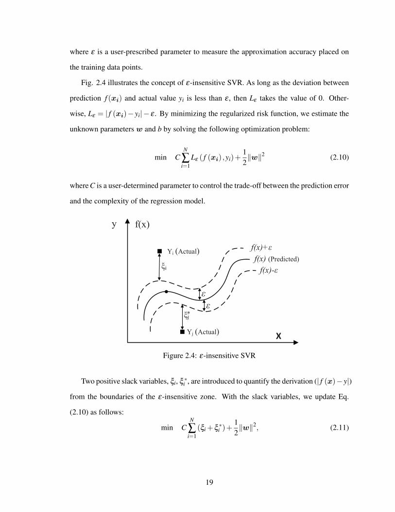
Fig. 2.4 illustrates the concept of ε-insensitive SVR. As long as the deviation between

prediction f (xi) and actual value yi is less than ε , then Lε takes the value of 0. Other-

wise, Lε = | f (xi)− yi|− ε . By minimizing the regularized risk function, we estimate the

unknown parameters w and b by solving the following optimization problem:

min CN

∑i=1

Lε ( f (xi) ,yi)+12‖w‖2 (2.10)

where C is a user-determined parameter to control the trade-off between the prediction error

and the complexity of the regression model.

f(x)+

f(x)-

f(x)

Figure 2.4: ε-insensitive SVR

Two positive slack variables, ξi, ξ ∗i , are introduced to quantify the derivation (| f (x)− y|)

from the boundaries of the ε-insensitive zone. With the slack variables, we update Eq.

(2.10) as follows:

min CN

∑i=1

(ξi +ξ∗i )+

12‖w‖2, (2.11)

19

subject to yi− (w ·Φ(xi)+b)≤ ε +ξi,

w ·Φ(xi)+b− yi ≤ ε +ξ ∗i ,

ξi,ξ∗i ≥ 0, i = 1, . . . ,N.

With the help of Lagrange multipliers and KKT conditions, Eq. (2.11) yields the fol-

lowing dual Lagrangian form [23]:

max −ε

N

∑i=1

(αi +α∗i )+

N

∑i=1

(α∗i −αi)yi−12

N

∑i, j=1

(α∗i −αi)(α∗j −α j

)K(xi,xj

),

(2.12)

subject to N∑

i=1(αi−α∗i ) = 0,

0≤ αi,α∗i ≤C, i = 1, . . . ,N.

(2.13)

where αi,α∗i are the optimum Lagrange multipliers, and K is the kernel function defined

as:

K (x1,x2) = Φ(x1)Φ(x2) . (2.14)

The optimal weight vector of the regression hyperplane isw∗=N∑

i=1(αi−α∗i )xi. Hence,

the general form of the SVR-based regression function can be written as:

f (x,w) = f (x,α,α∗) =N

∑i=1

(αi−α∗i )K (x,xi)+b. (2.15)

2.2.2 Deep Learning

In the past decade, deep learning has gained increasing attentions due to its promising

features in automatic feature extraction and end-to-end modeling [30, 31]. The key ad-

vantage of deep learning over the classical machine learning algorithms is that it is able to

learn appropriate representations from the raw data with multiple levels of abstraction in

an automatic manner that are needed for detection or classification. Typically, conventional

20

machine learning algorithms require manually designed rigorous feature extractor to elicit

informative features from raw data (e.g., image) that usually needs careful engineering and

a considerable amount of domain expertise, from which the classifier is able to learn and

differentiate patterns revealed in the extracted features. Whereas, deep learning is able to

extract features embodied in massive raw data with multiple levels of representation (e.g.,

orientation, location, motifs, and their combinations in images) from the training data au-

tomatically. As a result, it frees us from the design of a hand-engineered feature extractor

to transform the raw data into a suitable representation or feature vector. In this section, we

briefly introduce the underlying mechanisms for two neural networks, namely feedforward

neural network, and recurrent neural network. In addition, a framework is introduced to

characterize model prediction uncertainty following a Bayesian approach.

2.2.2.1 Feedforward Neural Network

The feedforward neural network was the first and simplest type of artificial neural net-

work devised [31]. As revealed by its name, feedforward neural network is a computer

system consisting of a number of feedforward, highly-connected neurons. These connected

neurons represent the knowledge through a continuing process of stimulation by the envi-

ronment in which the network is embedded. In general, there are four key components in a

feedforward neural network: neuron, activation function, cost function, and optimization.

Fig. 2.5 illustrates a feedforward neural network with two hidden layers and each hidden

layer having four neurons. As can be observed, the neural network has one input layer to

receive input variables, two hidden layers, and an output layer.

Inside each hidden neuron (e.g., the blue solid cells in Fig. 2.5) is a module composed of

four parts: input links, input function, activation function, and output link. Fig. 2.6 shows

the detailed structure of a hidden unit in the neural network. The input links represent the

values of input variables received from preceding layer. Next, the input function performs

a weighted sum operation on the values of input links, then pass the summed value to an

21

Input layer Hidden layer 1 Hidden layer 2

Output layer

Figure 2.5: A feedforward neural network with two hidden layers [3]

activation function. The activation function squashes the weighted sum value to a fixed

range, and pass it to the next layer. Mathematically, the aforementioned operations within

each hidden unit can be represented as:

ai = g(ini) = g

(m

∑j=0

a jWj,i

)(2.16)

where i denotes the i-th hidden layer, W0,i is the bias, Wj,i ( j 6= 0) represents the weight

along each input link, g is an activation function, and m is the number of input links.

∑ 𝑎𝑎𝑖𝑖

Input links Input function

Activation function Output Output links

𝑎𝑎𝑗𝑗𝑊𝑊𝑗𝑗,𝑖𝑖

𝑊𝑊0,𝑖𝑖𝑎𝑎0 = −1

𝑎𝑎𝑖𝑖 = 𝑔𝑔 𝑖𝑖𝑛𝑛𝑖𝑖

𝑖𝑖𝑛𝑛𝑖𝑖𝑔𝑔

Bias Weight

Figure 2.6: Detailed structure of a hidden unit in neural networks [3]

The activation function can take many different forms, such as sigmoid function (g(z)=

22

11+e−z ), rectified linear unit function (g(z) = max(0,z)), and hyperbolic tangent function

(g(z) = 21+e−2z − 1), etc. As mentioned earlier, all the activation functions have similar

purpose to squash the input value within a fixed range.

In a similar way, the input variable can be passed through a stack of hidden layers.

Finally, we obtain the value at the output layer in the neural network and use it as the

model prediction. Similar to other machine learning algorithms, a cost function is defined

to measure how far off our predictions are away from the actual values. A variety of cost

functions (e.g., mean squared error loss, binary cross-entropy, hinge loss) are available

depending on the purpose of the learning task (e.g., classification, regression). With the

computed loss value at each iteration, backpropagation algorithms calculate the error at the

output and then distribute it back through the network layers using chain rule to compute

gradients for each layer. Next, adjustments are applied to the weights in each layer of

the feedforward network so as to minimize the loss value in the next iteration. The same

procedures continue until the loss function converges to a stable value.

2.2.2.2 Recurrent Neural Network

Different from the feedforward neural network, recurrent neural network contains a

feedback loop that is connected to the past decisions (e.g., the information contained in

the hidden cell) and ingests their own outputs moment after moment as input, which en-

ables the network to learn the temporal dependencies in time series (or sequence) data. By

preserving the sequential information and passing information from one step to the next

through the hidden state variables, the RNN manages to maintain a memory of the tem-

poral correlation between events separated by many moments. This feature makes it ideal

to handle time series data. Among RNNs, the long short-term memory (LSTM) RNN as

proposed by Hochreiter and Schmidhuber [32] has received increasing attention because

it overcomes the vanishing and exploding gradients problem by enabling the network to

learn when to forget the previous hidden states and when to update the hidden states by

23

integrating with new memory in an adaptive manner [32].

X +

tanh

X

ht

Xt

X

tanh

ht-1

Ct-1

Ct

ht

Neural Network

Layer

Pointwise

Operation

Vector

TransferConcatenate Copy

ft

it ot

Figure 2.7: The structure of a LSTM block

To briefly introduce the concept of LSTM recurrent neural network, Fig. 2.7 shows

the graphical representation of all the mathematical operations going on within a LSTM

block. Let {x1, · · · ,xT} denote a general input sequence for a LSTM, where xt represents

a k-dimensional input vector at the t-th time step. The most important element in a LSTM

block is the cell state as represented by the horizontal line running through the top of the

diagram in Fig. 2.7. The first step in the LSTM block is to decide what information to

forget, which is determined by a sigmoid layer called “forget gate layer” as denoted in

Eq. (2.17). The output of the forget gate layer is a value varying from 0 to 1, where 0

indicates the information in the previous cell state Ct−1 is completely thrown away, and

1 reveals that the information in the previous cell state is completely retained. In the next

step, decision is made regarding what new information to store in the cell state. In this

case, a sigmoid “input gate layer” is firstly used to determine what values to update (see.

Eq. (2.18)), then a tanh layer creates a set of candidate values Ct to be added to the new cell

24

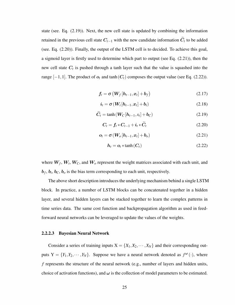
state (see. Eq. (2.19)). Next, the new cell state is updated by combining the information

retained in the previous cell state Ct−1 with the new candidate information Ct to be added

(see. Eq. (2.20)). Finally, the output of the LSTM cell is to decided. To achieve this goal,

a sigmoid layer is firstly used to determine which part to output (see Eq. (2.21)), then the

new cell state Ct is pushed through a tanh layer such that the value is squashed into the

range [−1,1]. The product of ot and tanh(Ct) composes the output value (see Eq. (2.22)).

ft = σ(W f [ht−1,xt ]+b f

)(2.17)

it = σ (Wi [ht−1,xt ]+bi) (2.18)

Ct = tanh(WC [ht−1,xt ]+bC) (2.19)

Ct = ft ∗Ct−1 + it ∗ Ct (2.20)

ot = σ (Wo [ht−1,xt ]+bo) (2.21)

ht = ot ∗ tanh(Ct) (2.22)

whereW f ,Wi,WC, andWo represent the weight matrices associated with each unit, and

b f , bi, bC, bo is the bias term corresponding to each unit, respectively.

The above short description introduces the underlying mechanism behind a single LSTM

block. In practice, a number of LSTM blocks can be concatenated together in a hidden

layer, and several hidden layers can be stacked together to learn the complex patterns in

time series data. The same cost function and backpropagation algorithm as used in feed-

forward neural networks can be leveraged to update the values of the weights.

2.2.2.3 Bayesian Neural Network

Consider a series of training inputs X = {X1,X2, · · · ,XN} and their corresponding out-

puts Y = {Y1,Y2, · · · ,YN}. Suppose we have a neural network denoted as fω (·), where

f represents the structure of the neural network (e.g., number of layers and hidden units,

choice of activation functions), andω is the collection of model parameters to be estimated.

25

Since there are so many model parameters to estimate, one crucial question is to assess how

much to trust the prediction of the trained model for new input value. With model predic-

tion uncertainty beforehand, the prediction with high uncertainty and extreme cases can

be handled in an explicit manner, thereby informing decision making with confidence. In

the Bayesian context, we aim to infer the posterior distribution of model parameters ω that

are most likely to generate the observed data X and Y. To achieve this, in the Bayesian

approach, we assign a prior distribution over the space of model parameters p(ω) to rep-

resent our prior belief on each candidate model parameter in generating the observed data,

then a likelihood function p(y|x,ω) (ω ∈ ω) is constructed to characterize the probability

of generating the observed data given model parameter ω . The Bayesian inference aims at

identifying a posterior distribution p(ω|X,Y) over model parameters ω. Given the data X

and Y, the posterior distribution exactly models how likely a variety of model parameters

ω are in generating them. With the posterior distribution, given a new data point x∗, the

predictive distribution of x∗ can be obtained by marginalizing out the posterior distribution:

p(y∗|x∗,X,Y) =∫

p(y∗|x∗,ω)p(ω|X,Y)dω (2.23)

In neural networks, a popular way to define the prior distributions is to place a Gaussian

distribution p(ω) = N (0,I ) over a neural network’s weights while the bias vectors are

often assumed to be point estimates for the sake of simplicity [33]. The aforementioned

procedures are often referred to as posterior inference. Unfortunately, it is computation-

ally prohibitive to perform exact Bayesian inference with the classical algorithms (e.g.,

MCMC methods such as Gibbs sampling, Metropolis-Hastings) due to the non-linearity

and non-conjugacy in deep neural networks, while most traditional algorithms for approx-

imate Bayesian inference are not scalable in many deep neural networks with thousands of

parameters. Furthermore, to characterize prediction uncertainty, the number of parameters

to be estimated in these models is typically doubled for the same network size as mentioned

26

earlier, which further increases the difficulty to make these algorithms scalable.

Gal and Ghahramani [34, 35], Gal [36] have developed a novel easy-to-implement al-

ternative to MCMC, which is referred to as Monte Carlo dropout (MC dropout). As shown

in Ref. [34], a deep neural network (NN) with arbitrary depth and non-linearities, with

dropout applied before every weight layer, is mathematically equivalent to an approxima-

tion to the deep Gaussian process model [37]. To be specific, in a feedforward deep neural

network, with dropout, we generate random samples using a Bernoulli distribution for each

unit in the input layer and the hidden layers. Each sample takes the value of 1 with a

probability of pi. If the value of the binary variable is zero, then the corresponding unit

is dropped accordingly. The implementation of dropout to a neural network amounts to

sampling a thinner network from it with some units temporarily being removed. In back

propagation, the value of each binary variable is used in updating the value of neural net-

work weights. The dropout neural networks are trained in a way similar to standard neural

nets with stochastic gradient descent. By doing this, we obtain a number of trained thinner

neural network.

More importantly, the same Monte Carlo dropout strategy can also be leveraged to ap-

proximate model prediction uncertainty following a Bayesian approach in other types of

neural networks, such as recurrent neural networks [35]. The key idea in the Monte Carlo

dropout method is to approximate Bayesian inference with variational inference by defining

a variational parametric distribution q(ω). Next, we minimize the Kullback–Leibler diver-

gence between the approximating distribution and full posterior with Eq. (2.24), which is

a measure of similarity between the two distributions.

KL(q(ω)‖ p(ω|X ,Y )) ∝−∫

q(ω) logp(Y |X ,ω)dω +KL(q(ω)‖ p(ω))

=−N∑

i=1

∫q(ω) logp(Yi| f ω (Xi))dω +KL(q(ω)‖ p(ω))

(2.24)

The MC dropout strategy has several promising features in comparison with other state-

of-the-art approaches. First of all, it does not require any change of the existing model

27

structure or optimization objective function. Instead, it is very straightforward to be im-

plemented. Specifically, MC dropout is applied before each hidden layer, then the model

output can be seen as random samples generated from the posterior prediction distribu-

tions [36]. Secondly, without loss of generality, MC dropout can be used to characterize

prediction uncertainty in a variety of neural networks, such as feed-forward deep neural

networks, recurrent neural networks, and convolutional neural networks.

2.3 System Optimization

In this section, we introduce a bi-level optimization program to characterize the inter-

actions between decision makers at different levels. In the subsequent chapters, the bi-level

program will be used to model the effect of different actions and strategies in mitigating

the traffic congestion caused by extreme events.

2.3.1 Bi-level Program

In many engineering systems, multiple decisions makers are usually involved while

each player has their own objectives and constraints. To characterize the interactions among

the multiple decision makers at different levels, we form a hierarchical structure to nest each

optimization task within the other. In the most simplest case, if there are only two deci-

sion makers in the system, the problem is usually formulated as a bi-level program. The

outer optimization problem (upper level) is commonly referred to as leader’s optimization

problem, while the inner optimization problem (lower level) is typically known as the fol-

lower’s optimization problem. Take the traffic system as an example, in the upper-level,

traffic planners act as leaders and make changes (e.g., build new road, introduce new sig-

nal pattern) to the traffic system, while passengers act as followers to choose any path that

minimizes their travel time from origin to destination freely. Even though traffic planners

can influence the travelers’ path-choosing behavior by the decisions/policies they make

related to the traffic system, but have no control over travelers’ behavior in choosing the

28

path. Hence, when traffic planners make any changes to the traffic system, it is important

to account for the dynamics of travelers’ behavior. From a mathematical point of view, this

problem can be formulated as:

(U0) minu

F (x,u)

s.t. G(x,u)≤ 0(2.25)

where the vector x= x(u) is determined via optimizing the following problem:

(L0) minx

f (x,u)

s.t. g (x,u)≤ 0(2.26)

where the vector u in the upper level problem (U0) represents the system planers’ deci-

sions, e.g., building new roads, link capacity expansion, and traffic signal configurations.

The vector x represents the equilibrium state of travelers’ path-choosing behavior, which

will be introduced in detail in the next section.

From the above bi-level program, it can be observed that the goal of the upper level

problem (U0) is to minimize the value of objective function F through optimizing the

decision variable u subject to the constraints G while the lower level decision vector x

acts as parameters. Likewise, the lower level problem (L0) aims at minimizing the value

of objective function f via optimizing the decision variable x under the constraint g, while

the upper level decision vector u acts as parameters. The bi-level optimization problem can

also be regarded as a Stackelberg game [38], where the decision maker in the upper level

has the leadership in playing the game first and carry out a set of operations/changes to

the system, and the system users in the lower level react optimally to the decision makers’

choice. The two players are connected by the response function x= x(u). In other words,

the two players are influenced by each other’s decision through this function. For example,

when traffic planners make any changes to the traffic network, they need to account for

users’ path-choosing behavior, which is represented by the vector x in the lower level

29

problem. Once any changes are made to the network, the network users’ path-choosing

behavior changes accordingly given the updated state u of the traffic network.

2.3.2 User Equilibrium Traffic Assignment

In a traffic network, each network user non-cooperatively seeks to minimize his/her own

total travel cost by taking the shortest path from the origin to the destination. Since the link

cost is a monotonically increasing function of traffic flow, the travel time gets increased

accordingly when the number of travelers along the shortest path increases. As a result,

travelers switch to other alternate paths with shorter travel times. The same process con-

tinues until nobody can decrease their travel time by shifting to any other route. Under the

resulting state, the traffic flow assignment in the network converges to an equilibrium state,

and this state is also referred to as the Wardrop user equilibrium traffic assignment [39],

where nobody can reduce the travel time by unilaterally changing their routes. Past studies

have shown that traffic network enhancements (e.g., addition of a new road, road capacity

expansion) without the consideration of users’ path-choosing behavior might increase the

network-wide congestion [40], which is also referred to as Braess’s paradox [41]. Hence,

it is essential to account for network users’ path-choosing behavior when we make any

changes to a traffic network.

Consider a connected network G(V,E), where V denotes the set of nodes, and E repre-

sents the set of links. Let OD denote the set of origin-destination pairs in the network, (s, t)

be one of the origin-destination pairs, where (s, t) ∈ OD, and ds,t be the amount of traffic

demand from the origin s to the destination t. Suppose qs,tp represents the flow along the

path p that originates at node s and destines at node t, then we have:

∑p∈Ps,t

qs,tp = ds,t , ∀(s, t) ∈OD. (2.27)

where Ps,t denotes a set of cycle-free paths connecting the origin node s with the destination

30

node t. The constraint imposed by Eq. (2.27) indicates that the total amount of flow along

all the paths connecting the origin node s with the destination node t must be equal to the

demand between the origin-destination pair (s, t). Obviously, all the traffic flows must be

non-negative, thus we have:

qs,tp ≥ 0, ∀p ∈ Ps,t , ∀(s, t) ∈OD. (2.28)

Let a (a ∈ E) be one link in the network G, and xa denotes the traffic flow along link a,

then we have:

xa = ∑(s,t)∈OD

∑p∈Ps,t

qs,tp δ

s,ta,p, ∀a ∈ E. (2.29)

where δs,ta,p is a binary variable. When δ

s,ta,p = 1, it means that link a is a segment constituting

the path p (p ∈ Ps,t). Otherwise, δs,ta,p = 0.

Given the above notations and constraints, the user equilibrium traffic assignment with

fixed demand can be mathematically formulated as the following nonlinear optimization

program:

(L1) Min f = ∑a∈E

xa∫0

ta (x)dx

s.t. xa = ∑(s,t)∈OD

∑p∈Ps,t

qs,tp δ

s,ta,p, ∀a ∈ E,

∑p∈Ps,t

qs,tp = ds,t , ∀(s, t) ∈OD,

qs,tp ≥ 0, ∀p ∈ Ps,t , ∀(s, t) ∈OD.

(2.30)

where f is the objective function, ta (x) is a monotonically increasing function denoting the

relationship between the travel time and the traffic flow along link a, xa is the total traffic

flow on link a, OD is the set of origin-destination traffic demand pairs, ds,t is the traffic

demand among the origin-destination pair (s, t) ((s, t) ∈OD), and qs,tp denotes the traffic

flow along the path p (p ∈ Ps,t) that connects origin node s with destination node t.

31

2.3.3 System-level Optimization

Although user equilibrium characterizes the path-choosing behavior of the traffic net-

work users, it does not model the system-level decision maker’s goal. Different from user

equilibrium, system optimization models the problem from the perspective of the traffic

planner, and it aims at coordinating all the travelers to choose the paths in such a way

that the total travel time in the entire network is minimized. Mathematically, the system

optimum assignment model with fixed demand can be expressed as follows:

(U1) Min F = ∑a∈E

xata (xa)


∑p∈Ps,t

qs,tp δ

s,ta,p, ∀a ∈ E,

∑p∈Ps,t

qs,tp = ds,t , ∀(s, t) ∈OD,

qs,tp ≥ 0, ∀p ∈ Ps,t , ∀(s, t) ∈OD.

(2.31)

Obviously, from the objective function formulated in U1, it can be seen that system

optimum assignment has a different goal from the user equilibrium traffic assignment, and

it aims at minimizing the total system travel time by coordinating the drivers’ behavior in

choosing the routes. In this case, the system congestion is minimised as drivers are told

which routes to use.

2.4 Uncertainty Analysis

The uncertainty emerging in the design, analysis, and operation of engineering systems

play a significant role in affecting their performance. In this section, we introduce the prin-

cipal sources of uncertainty arising in engineering systems, and review global sensitivity

analysis method to measure the contribution of each random variable to system variability.

32

2.4.1 Uncertainty Quantification

While many sources of uncertainty may exist, they are generally categorized into two

classes: aleatory (natural variability) and epistemic uncertainty (lack of knowledge) [42].

The aleatory uncertainty refers to the inherent physical variability and randomness in a

quantity. For example, when you roll a dice, you get a random experimental outcome each

time when you run the experiment, then this is an example of aleatory uncertainty. To

characterize aleatory uncertainty, we usually represent the random quantity as a probability

distribution. On the contrary, epistemic uncertainty denotes the uncertainty that is caused

by lack of knowledge. For example, due to insufficient experimental data, we cannot have

an exact estimate on model parameters. While the aleatory uncertainty is irreducible, the

epistemic uncertainty can be reduced by gathering more data or by refining the mathemat-

ical models.

Since aleatory uncertainty is irreducible, researchers have devoted more efforts on the

modeling and quantification of epistemic uncertainty in recent years. The epistemic uncer-

tainty is typically divided into two subcategories: statistical uncertainty and model uncer-

tainty [43, 44]. Due to the inadequacies in the available data (e.g., sparse data, ambiguity in

data, erroneous data), statistical uncertainty might arise on the deterministic quantity or the

distribution characteristics of random variables. Several theories have been developed to

address this challenge, such as Dempster-Shafer evidence theory [45], fuzzy sets [46, 47],

and possibility theory [48]. Model uncertainty arises due to the uncertainty in model pa-

rameters, solution approximation, model discretization error, and model form assumption,

etc.

In this dissertation, we focus on the quantification of one of the model uncertainty –

model parameter uncertainty. Specifically, model parameter uncertainty denotes the un-

certainty in the model parameters due to natural variability or limited data or both. As

mentioned in Chapter 2.2.2.3, the uncertainty of the parameters in the deep neural net-

works is characterized following a Bayesian manner. Instead of having a deterministic

33

point estimate for each weight variable in neural networks, a prior distribution p(ω) is

used to denote our belief on the values of weight variables in deep neural networks. Next,

the prior distribution p(ω) is combined with a likelihood function p(y|x,ω) (ω ∈ ω) that

denotes the probability of generating the observed data to infer the posterior distribution

p(ω|X,Y) on model parameters. By doing this, for a new data point x∗, we have a predic-

tive distribution p(y∗|x∗,X,Y) and the posterior distribution characterizes the uncertainty

in the model prediction as a distribution, from which we measure the uncertainty in model

prediction explicitly.

2.4.2 Global Sensitivity Analysis

Global sensitivity analysis is used to quantify the influence of stochastic model inputs

on the output variability of a physical or mathematical model [49]. Among the abundant

literature on sensitivity measures, Sobol’ indices based on variance decomposition have

received much attention. Consider the model:

y = f (x) (2.32)

where y is the output, x = (x1, · · · ,xp) are p independent input variables, f is the model

function. These contributions of the variance of a single model input or a group of model

inputs to the output variance of f are quantified using the following sensitivity indices:

Si =Vxi

(Ex−i (y|xi)

)V (y)

, Si j =Vxix j

(Ex−ix− j

(y|xix j

))V (y)

−Si−S j (2.33)

where x−i denotes all of the variables in x except xi. Here, Si is the first order Sobol’

index quantifying the sensitivity of output variance to an individual variable xi by itself

(individual effect). The second order index Si j quantifies the sensitivity to the interaction

between variable xi and x j. The larger an index value is, the greater is the importance of

the corresponding variable or group of variables.

34

According to the theorem of variance decomposition, we have:

V (y) = Exi

(Vx−i (y|xi)

)+Vxi

(Ex−i (y|xi)

)(2.34)

which implies that:

Si = 1−Exi

(Vx−i (y|xi)

)V (y)

(2.35)

The methods used for global sensitivity analysis can be broadly classified into two

groups: analytical methods and sampling-based approaches. In the analytical methods, the

key idea is to approximate the original model y= f (x) with cheap algebraic surrogate mod-

els, such as Polynomial Chaos Expansion (PCE) model [50], or Kriging models [51]. Once

the surrogate model is trained, the Sobol’ indices are calculated analytically. For example,

Sudret [50] constructed surrogate models with generalized polynomial chaos expansions

(PCE), and derived analytical solution that computes the Sobol indices as a post-processing

of the PCE coefficients. Wang et al. [51] built Kriging-based surrogate model to estimate

the variance of conditional expectation for each random variable. Likewise, Ciuffo et al.

[52] developed a robust Kriging emulator based on the recursive use of the DACE tool [53],

and demonstrated that the variance-based sensitivity indices estimated based on the Krig-

ing emulator were approximately identical to those derived by the complete variance-based

approach.

In sampling-based approaches, a double-loop Monte Carlo simulation is typically re-

quired to estimate Sobol’ indices Si. The inner loop Vx−i (y|xi) in Eq. (2.35) requires fixing

xi and changing all the other variables x−i. The outer loop Exi (•) requires fixing xi at differ-

ent locations, and these selected locations are sampled from the distribution of xi. In recent

years, significant progress has been made along this direction: design of experiments [54]

and spectral approaches have been used to reduce the number of samples needed for global

sensitivity analysis [55, 56]. For example, Kucherenko et al. [57] developed quasi-Monte

Carlo (QMC) method to speed up the convergence rate of sampling-based approaches on

35

sensitivity estimates. Tissot and Prieur [58] utilized randomized orthogonal arrays to es-

timate first-order Sobol’ indices. As a typical spectral approach, Fourier amplitude sensi-

tivity test (FAST) [55] is used to perform sensitivity analysis. For more details, Ref. [59]

provides a detailed review on sampling-based sensitivity analysis.

2.5 Big Data - Apache Spark

With the advent of big data era, a large volume of data is readily available, which poses

tremendous computational challenges. Since data sizes have outpaced the computational

capability of single machine, new systems need to be developed to scale out computations

to multiple nodes. To fulfill the computational need of massive data analysis, Apache Spark

has emerged as a unified engine for large-scale data analysis across a wide range of fields

because it can handle a large body of processing workloads that need to be processed by

separate engines before, including SQL, streaming, machine learning, and graph process-

ing [60, 61, 62]. Different from the rigid map-then-reduce disk-based model, Apache Spark

performs all the data transformation and actions in memory. By doing this, Apache Spark

achieves 100 times faster speed than the classical open-source framework Hadoop which

is designed for distributed storage and processing of very large data sets across clusters of

computers on disk in performance.

Fig. 2.8 shows the architecture of the Apache Spark computing platform. As can be

observed, Spark core is the foundation of the Apache Spark computing platform. With

the resilient distributed dataset (RDD) application program interface (API), Apache Spark

provides a unified interface for processing large-scale data in various formats, such as,

JSON, XML, Hbase, MySQL, etc. Moreover, Spark supports a variety of advanced pro-

gramming languages, like Scala, Java, Python to name a few. The extensive APIs support

of data transformations and actions in these high-level programming languages is essential

for data analysis and machine learning algorithms in the upper-level libraries. In addition

to support large-scale data management, Spark core also offers major functionalities for in-

36

Figure 2.8: Architecture of Apache Spark [4]

memory cluster computing management, including job scheduling, memory management,

data shuffling, and fault recovery. Such functionalities makes it easy to develop applica-

tions with Spark, where cluster memory, storage disk, and CPU will be utilized to their

maximum level.

As shown in Fig. 2.8, above the DataFrame API is several upper-level libraries for per-

forming various SQL queries [60], constructing machine learning algorithms [63], GraphX

for graph processing [64], Spark Streaming for analyzing streaming data [62], as well as

third-party packages for handling other tasks. The inclusion of these versatile functional-

ities reduces the workload significantly for developing large-scale data analytics and ma-

chine learning algorithms.

37

2.6 Summary

In this chapter, we review two commonly used machine learning algorithms: support

vector machine and deep neural networks including deep feedforward neural network and

recurrent neural network. In parallel, a Bayesian neural network is introduced as a generic

framework to characterize model prediction uncertainty. Next, a quantitative metric has

been defined to measure system resilience, and a bi-level optimization framework is for-

mulated to model the interactions among multiple decision makers at different levels. The

basic concepts of uncertainty quantification techniques are reviewed in Section 2.4, and

global sensitivity analysis is introduced to measure the contribution of each random vari-

able on the system-level variability. Finally, a big data engine Apache Spark is described

to process large volume of data with scalable performance.

In Chapter 3, the big data engine Apache Spark is used to process massive raw data

in an effective manner, then deep neural networks are trained to forecast the flight trajec-

tories. In Chapter 4, the support vector machine and deep feedforward neural network

are trained to predict the risk levels of abnormal event. In Chapters 5 and 6, support vec-

tor machine models are trained to measure operator performance and the effectiveness of

rerouting strategy in handling off-nominal events, respectively. The bi-level program and

system resilience concept are used in Chapters 7 and 8 to optimize transportation system

performance. The quantification of model prediction uncertainty is illustrated for the flight

trajectory prediction and aircraft rerouting problems in Chapters 3 and 5, respectively.

38

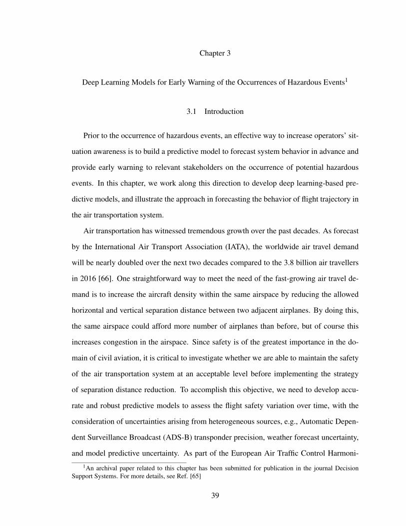
Chapter 3

Deep Learning Models for Early Warning of the Occurrences of Hazardous Events1

3.1 Introduction

Prior to the occurrence of hazardous events, an effective way to increase operators’ sit-

uation awareness is to build a predictive model to forecast system behavior in advance and

provide early warning to relevant stakeholders on the occurrence of potential hazardous

events. In this chapter, we work along this direction to develop deep learning-based pre-

dictive models, and illustrate the approach in forecasting the behavior of flight trajectory in

the air transportation system.

Air transportation has witnessed tremendous growth over the past decades. As forecast

by the International Air Transport Association (IATA), the worldwide air travel demand

will be nearly doubled over the next two decades compared to the 3.8 billion air travellers

in 2016 [66]. One straightforward way to meet the need of the fast-growing air travel de-

mand is to increase the aircraft density within the same airspace by reducing the allowed

horizontal and vertical separation distance between two adjacent airplanes. By doing this,

the same airspace could afford more number of airplanes than before, but of course this

increases congestion in the airspace. Since safety is of the greatest importance in the do-

main of civil aviation, it is critical to investigate whether we are able to maintain the safety

of the air transportation system at an acceptable level before implementing the strategy

of separation distance reduction. To accomplish this objective, we need to develop accu-

rate and robust predictive models to assess the flight safety variation over time, with the

consideration of uncertainties arising from heterogeneous sources, e.g., Automatic Depen-

dent Surveillance Broadcast (ADS-B) transponder precision, weather forecast uncertainty,

and model predictive uncertainty. As part of the European Air Traffic Control Harmoni-

1An archival paper related to this chapter has been submitted for publication in the journal DecisionSupport Systems. For more details, see Ref. [65]

39

sation and Integration Programme (EATCHIP) managed by the European Organisation for

the Safety of Air Navigation (EUROCONTROL), trajectory prediction is also highlighted

as an essential operational requirement in the European Air Traffic Management (EATM)

modernisation programme [67].

At the forefront of transformation to future National Airspace System (NAS), an im-

portant upgrade in the Next Generation Air Transportation System (NextGen) is the tran-

sition from radar-based operations to satellite-based navigation and surveillance. Together

with Automatic Dependent Surveillance–Broadcast (ADS-B) system, satellite-based oper-

ations provide enhanced accuracy for aircraft navigation, surveillance, and position track-

ing [68, 69]. With the centralized NAS data sharing backbone – System Wide Information

Management (SWIM), real-time, accurate flight, surveillance, weather, and aeronautical

information is broadcast to related stakeholders on a regular basis. As mentioned in the

Federal Aviation Administration (FAA) report on the future of the NAS [70], one signifi-

cant need in NextGen is to develop predictable and efficient services across tower, terminal,

and en route domains, which can then be used to assist controllers to handle off-nominal

events or demand-capacity imbalances in a more strategic and efficient manner. Along this

direction, flight trajectory prediction is an important constituent need, and accurate predic-

tion of flight trajectory is vital to avoid accidents and reduce errors while ensuring safety

and efficiency.

In brief, flight trajectory is the core information that is used by the system as a basis

for distributing flight information to relevant airlines and air traffic control (ATC) units,

facilitating the timely coordination between sectors and units, correlating flight data with

tracks, monitoring the adherence of an aircraft with its assigned route, and detecting and

resolving conflicts. In this respect, trajectory prediction algorithms are a crucial compo-

nent of decision support tools (DST) for conflict detection and resolution, arrival metering,

and other applications in air traffic management automation. Considering its paramount

importance in assuring the safety of the air transportation system, a large number of studies

40

have emphasized the development of models and algorithms for flight trajectory prediction

(TP) over the past decades [71]. For example, Prats et al. [72] used an iterative quasi-

Newton method to find depature flight trajectory for the purpose of minimizing the noise

annoyance. de Leege et al. [73] trained a machine learning model to predict flight arrival

time over points along the fixed arrival route based on generalized linear models (GLM),

where aircraft state parameters (i.e., aircraft type, aircraft ground speed, aircraft altitude)

and meteorological conditions (i.e., surface wind, altitude wind) were used as model in-

puts. Gong and McNally [74] developed a versatile methodology for automated trajectory

prediction analysis such that the error measurements were sensitive to small trajectory pre-

diction algorithm changes. Franco et al. [75] developed a probabilistic approach to predict

aircraft flight time and fuel consumption during the cruise phase, in which they accounted

for wind prediction uncertainty (both along-track winds and crosswinds) provided by En-

semble Weather Forecasting.

The above literature review reveals that trajectory prediction has gained growing inter-

est of researchers with different backgrounds from a variety of domains. The current state-

of-the-art approaches for trajectory prediction can be categorized into two major classes:

physics-based models and data-driven models. In physics-based models, the aircraft is rep-

resented as a point mass, and Newton’s law is utilized to associate the force/thrust generated

by the aircraft engine with the inertial acceleration of its mass [76]. Typically, physics-

based models are represented as a set of differential equations. Given the initial state of

an aircraft (i.e., mass, thrust, position, velocity, bank angle) and meteorological conditions

(i.e., wind velocity and direction), we predict the successive points of future aircraft trajec-

tory by integrating the differential equations over a time interval. Take the Base of Aircraft

Data (BADA) as an example, it is an aircraft performance model designed with a mass-

varying, kinetic approach as developed and maintained by EUROCONTROL [77], which

is used for trajectory computation, simulation and prediction in Air Traffic Management

(ATM). However, physics-based models typically require explicit modeling of aircraft per-

41

formance procedures and the real-time aircraft state (i.e., thrust, speed intent), while the

models and most of model inputs might not be always readily available to the ground-

based systems due to commercial sensitivity. Considering such a significant deficiency in

physics-based models, researchers have shifted to data-driven models for predicting flight

trajectory by learning from the historical flight trajectory data with machine learning and

data mining techniques [78, 79]. In particular, with the advent of the big data era, a large

amount of flight trajectory data becomes available, which makes the mining of complex

trajectory patterns and feature interactions from the massive historical flight trajectory data

possible. For example, Alligier and Gianazza [80] applied a machine learning approach

to predict aircraft mass and speed intent on the climb phase with the ADS-B data coming

from the OpenSky network. Di Ciccio et al. [81] developed an automated prediction model

to detect flight diversions based on the flight track updates (i.e., position, velocity, altitude,

and intended destination) such that the receiving parties could respond in a timely way

to unexpected events that occurred to the flight. Among machine learning models, deep

learning (or deep neural networks) has gained popularity due to its promising features in

automatic feature extraction and end-to-end modeling [30, 31]. In quite a few domains,

recurrent neural network has demonstrated outstanding performance in predicting the tra-

jectory evolution [82, 83, 84]. For example, Moradi Kordmahalleh et al. [85] developed

a sparse recurrent neural network with flexible topology to make trajectory prediction 6

and 12 hours ahead of four catastrophic Atlantic hurricanes. Alahi et al. [86] proposed a

Long Short Term Memory (LSTM)-based recurrent neural network to jointly reason across

multiple individuals to predict human trajectories in a scene, in which one LSTM was

trained for each trajectory and the information was shared between the LSTMs through the

introduction of a new social pooling layer. Wu et al. [87] incorporated the constraint of

topological structure on trajectory modeling, and developed two recurrent neural network-

based models to make trajectory prediction.

Model prediction uncertainty is an important consideration in machine learning [88,

42

89]. In particular, in the aviation sector, it is extremely important to account for trajectory

prediction uncertainty because it is closely related to risk assessment in decision making

activities pertaining to maintaining flight safety, e.g., separation distance. In this study,

we characterize model prediction uncertainty from a Bayesian perspective. Bayesian prob-

ability theory provides a mathematically well-grounded approach to reason about model

prediction uncertainty. However, given the large number of parameters to be optimized

in deep learning, the implementation of Bayesian inference in deep learning is usually

unachievable due to several reasons. First of all, if we represent each parameter in deep

learning as a parametric distribution (e.g., normal distribution), then the number of param-

eters in the neural network will be doubled (i.e., mean and variance), which will further in-

crease the computational burden in training the neural network. Secondly, the non-linearity

and non conjugacy in neural networks make closed-form Bayesian inference impossible.

Thirdly, given the large number of layers and parameters in deep learning, the conventional

inference algorithms (i.e., MCMC, Metropolis–Hastings algorithm) are computationally

intractable in the context of deep learning. Recently, Gal and Ghahramani [90, 34, 35]

proposed that dropout can be interpreted as a variational approximation to the posterior of

a Bayesian neural network. More importantly, the variational approximation to Bayesian

inference with dropout does not sacrifice either computational complexity or model predic-

tion accuracy. From then on, dropout implementation to approximate Bayesian inference

has drawn tremendous attention with applications to forecasting the number of trips at

Uber [91, 92], camera relocalization [93].

In this study, we train two separate Bayesian neural networks to make predictions on

flight trajectory behavior. With the massive flight and track data in Flight Information

Exchange Model (FIXM) and custom XML format streamed from Federal Aviation Ad-

ministration (FAA) System Wide Information Management (SWIM), a robust distributed

computing platform – Apache Spark – is leveraged to parse the flight data from SWIM

flight data publication service (SFDPS) [94, 95], from which the data pertaining to actual

43

flight trajectory, target flight trajectory, aircraft states (e.g., velocity, altitude, and position),

as well as historical flight trajectory is extracted. Next, we build two Bayesian neural net-

work models: in the first model, a feed-forward Bayesian neural network (DNN) is trained

for one-step-ahead prediction on the deviation between actual trajectory and target flight

trajectory. In the second model, a long short-term memory (LSTM) recurrent neural net-

work (RNN) is trained with historical flight trajectory data to make long-term predictions

on the future state of an ongoing flight. Afterwards, the two models are blended through a

discrepancy term to make accurate trajectory prediction for ongoing flights. A separation

distance-based safety indicator is developed to measure flight safety in the air transportation

system. The major contributions we have made in this chapter are multifold.

1. We develop an efficient program based on a high performance computing platform

– Apache Spark – to parse the raw SFDPS data in FIXM format, which lays a firm

foundation for the development of subsequent Bayesian deep learning models.

2. Two individual Bayesian neural networks are trained to make flight trajectory pre-

diction from different angles. In the first model, a feed-forward deep neural network

is trained to make single-step predictions on the deviation between actual flight tra-

jectory and target flight trajectory. In the second model, a LSTM recurrent neural

network is trained to make longer-term prediction of the future states (i.e., latitude,

longitude, altitude, velocity) of an ongoing flight.

3. The two Bayesian neural networks are integrated together for making accurate long-

term predictions for ongoing flights. By doing this, we leverage the advantages of

both models: the high prediction accuracy of the DNN and long-term prediction

capability of the LSTM RNN.

4. In both models, model prediction uncertainty is accounted using the dropout strategy,

and propagated through the integrated models with Monte Carlo samples.

44

5. A probabilistic safety indicator is used to measure the horizontal and vertical separa-

tion distance between two flights.

3.2 SWIM SFDPS Data Overview

SWIM is a National Airspace System (NAS)-wide information system that supports

Next Generation Air Transportation System (NextGen) goals. Acting as a digital data-

sharing backbone, SWIM enables increased common situational awareness and improved

NAS agility to deliver the right information to the right people at the right time [96]. This

information-sharing platform offers a single point of access for aviation data ranging from

flight data to weather information. Users with granted credentials from FAA have access to

the SWIM database via subscription to particular channels (i.e., SWIM Terminal Data Dis-

tribution System – STDDS, Time Based Flow Management – TBFM, Traffic Flow Manage-

ment System – TFMS, SWIM Flight Data Publication Service – SFDPS, Wx, and others).

Over the past one year, we have focused on analyzing flight trajectory data by subscrib-

ing to the SWIM flight data publication service (SFDPS) stream. In brief, SFDPS provides

real-time en route flight data via batched track messages and custom FIXM formats to NAS

consumers.

Fig. 3.1 shows a specific SFDPS tracking message for a flight operated by the Jet-

Blue airline that departs from the Logan International Airport (code: KBOS) and arrives

at the Baltimore–Washington International Airport (code: KBWI) on October 16 in 2018

from SWIM. As can be observed, all the en-route flight tracking information is stored in

the International Civil Aviation Organization (ICAO) Flight Information Exchange Model

(FIXM) format. In each tracking message, there are five major types of information: flight

origin and destination, timestamp, en route flight information (i.e., flight speed and velocity,

altitude, position, target altitude and position), flight ID and supplemental data. In SFDPS,

flight tracking information are broken out by flight with just one track update per flight in

one message. The flight tracking messages are updated on a regular basis of 12 seconds

45

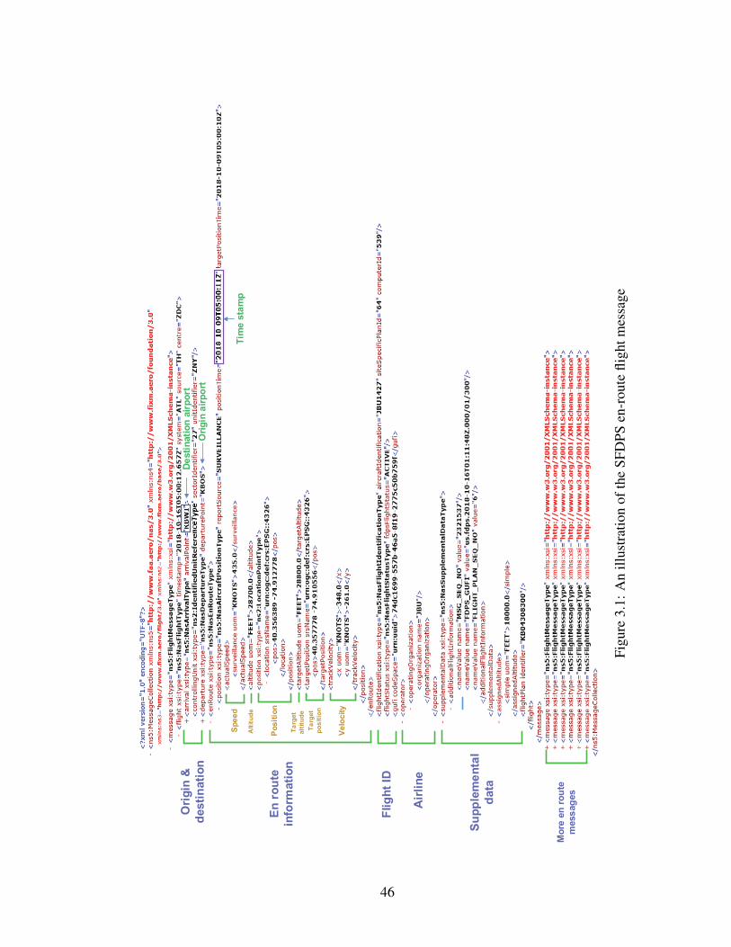
Ori

gin

&

desti

nati

on

En

ro

ute

info

rmati

on

Flig

ht

ID

Air

lin

e

Su

pp

lem

en

tal

data

De

sti

nati

on

air

po

rt

Ori

gin

air

po

rt

Sp

ee

d

Po

sit

ion

Ve

loc

ity

Ta

rget

po

sit

ion

Ta

rget

alt

itu

de

Alt

itu

de

Mo

re e

n r

ou

te

mess

ag

es

Tim

e s

tam

p

Figu

re3.

1:A

nill

ustr

atio

nof

the

SFD

PSen

-rou

tefli

ghtm

essa

ge

46

for an active flight while the flight is in an Air Route Traffic Control Center’s (ARTCC)

airspace. Since there are more than 20,000 commercial flights within the airspace of USA

every day, we stream nearly 100 GB of SFDPS messages from SWIM per day. Given such

big data, an efficient method is needed to parse the flight trajectory data from the massive

FIXM files.

3.3 Proposed Method

In this section, a four-step approach is developed to train two individual Bayesian deep

learning models from the massive historical flight trajectory data to support the assess-

ment of flight safety. The overall framework of the proposed methodology is illustrated

in Fig. 3.2. In the first step, we develop a scalable program with a unified distributed

high-performance computing framework – Apache Spark – to process a large volume of

raw flight tracking messages in FIXM format. After the information pertaining to flight

trajectory is extracted from the raw data, two individual Bayesian deep learning models

are trained to make predictions on the future state of ongoing flights from different per-

spectives. Next, the predictions from the two deep learning models are fused together

to enhance the model prediction accuracy as well as to reduce the model prediction uncer-

tainty. Finally, the fused models are then utilized to make trajectory predictions on multiple

flights and evaluate the safety of two given flights, where separation distance is used as a

quantitative safety metric.

Figure 3.2: Flowchart of proposed methodology for flight trajectory prediction

47

3.3.1 SFDPS Message Processing

As mentioned before, SFDPS publishes a wide variety of en route messages, such as

en route flight data messages, en route airspace data messages, en route operational data

messages, and en route general messages. Among all the published messages, we are

most interested in the information relevant to flight trajectory including flight ID, origin

and destination, and en-route position surveillance data (e.g., latitude, longitude, and alti-

tude). Within the US airspace, there are more than 20,000 commercial flights every day.

In terms of data volume, more than 100 GB of SFDPS messages is broadcast by SWIM

and streamed to the local storage disk. As shown in Fig. 3.1, all the significant content

is batched in FIXM format. To meet the intensive computational requirements of massive

data analysis, we leverage a general-purpose scalable high-performance computing frame-

work – Apache Spark – to parse the large volume of SFDPS messages in FIXM format. As

a unified engine for big data analytics, Apache Spark combines a core engine for distributed

computing with an advanced programming model for in-memory data processing through

a data sharing schema – resilient distributed dataset (RDD). The Spark framework’s in

memory programming model results in up-to 100 times faster than Hadoop in big data an-

alytics [97]. Besides, Apache Spark offers rich APIs in high-level languages (e.g., Python,

Java, Scala) for performing complex data operations, such as data transformation, SQL

query [4]. Last but not the least, Apache Spark supports operating on a rich set of data

sources through the DataFrame interface, such as JSON, CSV, database connection, and

XML etc.

In this study, we utilize the spark-xml library for parsing and querying FIXM data

within Apache Spark [98]. After the raw FIXM data is parsed, we designate the row tag

as ‘flight’, then spark-xml library transforms the content within this row tag into a row

consisting of all the attribute names and their values. Next, we filter out flight tracking

information that contains track updates for individual flights from all the SFDPS messages

by specifying the source of tracking messages as ‘TH’ (see Fig. 3.1), then we group the

48

trajectory data by flight date and flight ID, and rank them according to the position time

(see Fig. 3.1 for more details). The sorted flight trajectory data is then outputted as a single

CSV file per flight by Apache Spark in parallel. By adopting Apache Spark to process the

raw SFDPS messages, the required time of performing all the aforementioned operations

on SFDPS messages spanning a time duration of 24 hours decreases dramatically from

nearly one week to approximately 10 hours on a Windows 10 desktop with an Inter Core

i7-4790 CPU (3.60 GHz) and 16 GB memory. Table 3.1 shows a small portion of processed

tracking information for an American Airline flight with Call Sign (or flight ID) AAL10

that departed from Los Angeles International Airport (ICAO code: KLAX) and destined at

John F. Kennedy International Airport (ICAO code: KJFK) on January 11, 2019.

Significant flight trajectory information, such as timestamp, flight position, and flight

state derived from the SFDPS messages, is illustrated in Table 3.1. To be more specific,

the second column reveals the airline that operates this flight. The subsequent two columns

show the departure and arrival airports of this flight as represented by four-letter ICAO

airport codes, respectively. The next two columns (position time and target position time

represent the time instant associated with the current position of an active flight and the

time associated with the raw radar return, respectively. As can be seen from the column

position time, flight position comprised of latitude, longitude, and altitude is periodically

updated approximately at intervals of 12 seconds, except the shaded cells. The next three

columns show the aircraft state at corresponding position time. Specifically, the column

actual speed denotes the ground speed of the flight in the unit of knots per hour. The next

two columns X and Y velocity describe the flight speed along the X and Y components

tracked by radar surveillance. Similarly, the target altitude represents the assigned altitude

or flight level in feet. For example, an assigned altitude of 1700 means that the aircraft

is to fly at 1,700 feet. The preceding column actual altitude denotes the actual flight level

at each time instant. The actual position indicates the actual location of an active flight in

latitude/longitude format as reported by surveillance, and target position shows the target

49

IDA

irlin

eA

rriv

alPo

int

Dep

artu

rePo

int

Posi

tion

Tim

eTa

rget

Posi

tion

Tim

eA

ctua

lSp

eed

Xve

loci

tyY

velo

city

Act

ual

Alti

tude

Targ

etA

ltitu

deA

ctua

lPos

ition

Targ

etPo

sitio

n

1A

AL

KJF

KK

LA

X2019-01-11T23:16:26.000-06:00

2019-01-12T05:16:26Z

210

-201

-61

2100

2100

33.9

3055

6-1

18.4

5777

833

.930

556

-118

.457

778

2A

AL

KJF

KK

LA

X2019-01-11T23:16:38.000-06:00

2019-01-12T05:16:38Z

210

-190

-89

2300

2300

33.9

2472

2-1

18.4

7027

833

.924

722

-118

.470

000

3A

AL

KJF

KK

LA

X2019-01-11T23:17:02.000-06:00

2019-01-12T05:17:02Z

218

-171

-135

2600

2600

33.9

0833

3-1

18.4

9277

833

.908

333

-118

.493

333

4A

AL

KJF

KK

LA

X2019-01-11T23:17:14.000-06:00

2019-01-12T05:17:14Z

238

-145

-188

3000

3000

33.8

9666

7-1

18.5

0361

133

.897

778

-118

.504

167

5A

AL

KJF

KK

LA

X2019-01-11T23:17:25.000-06:00

2019-01-12T05:17:25Z

248

-89

-232

3600

3600

33.8

8388

9-1

18.5

0861

133

.884

722

-118

.509

167

6A

AL

KJF

KK

LA

X2019-01-11T23:17:37.000-06:00

2019-01-12T05:17:37Z

246

-20

-245

4200

4200

33.8

7027

8-1

18.5

0916

733

.871

389

-118

.510

278

7A

AL

KJF

KK

LA

X2019-01-11T23:17:49.000-06:00

2019-01-12T05:17:49Z

242

-12

-242

4800

4800

33.8

5722

2-1

18.5

1000

033

.857

500

-118

.510

556

8A

AL

KJF

KK

LA

X2019-01-11T23:18:01.000-06:00

2019-01-12T05:18:01Z

242

-12

-241

5400

5400

33.8

4388

9-1

18.5

1083

333

.844

722

-118

.512

222

9A

AL

KJF

KK

LA

X2019-01-11T23:18:13.000-06:00

2019-01-12T05:18:13Z

242

-12

-241

5800

5800

33.8

3055

6-1

18.5

1166

733

.831

389

-118

.513

333

10A

AL

KJF

KK

LA

X2019-01-11T23:18:25.000-06:00

2019-01-12T05:18:25Z

242

-13

-241

6300

6300

33.8

1666

7-1

18.5

1277

833

.817

222

-118

.513

611

11A

AL

KJF

KK

LA

X2019-01-11T23:18:37.000-06:00

2019-01-12T05:18:37Z

243

-13

-242

6800

6800

33.8

0305

6-1

18.5

1361

133

.803

333

-118

.515

000

12A

AL

KJF

KK

LA

X...

......

......

......

......

13A

AL

KJF

KK

LA

X2019-01-11T02:30:22.000-06:00

2019-01-11T08:30:22Z

528

528

1635

000

3500

037

.926

667

-87.

8072

2237

.928

056

-87.

8080

5614

AA

LK

JFK

KL

AX

2019-01-11T02:30:22.000-06:00

2019-01-11T08:30:22Z

532

532

1535

000

3500

037

.928

333

-87.

8066

6737

.928

889

-87.

8072

2215

AA

LK

JFK

KL

AX

2019-01-11T02:30:34.000-06:00

2019-01-11T08:30:34Z

528

528

1635

000

3500

037

.927

778

-87.

7700

0037

.929

444

-87.

7705

5616

AA

LK

JFK

KL

AX

2019-01-11T02:30:34.000-06:00

2019-01-11T08:30:34Z

532

532

1535

000

3500

037

.929

444

-87.

7697

2237

.930

278

-87.

7697

2217

AA

LK

JFK

KL

AX

2019-01-11T02:30:46.000-06:00

2019-01-11T08:30:46Z

528

528

1735

000

3500

037

.928

611

-87.

7330

5637

.928

889

-87.

7341

6718

AA

LK

JFK

KL

AX

2019-01-11T02:30:46.000-06:00

2019-01-11T08:30:46Z

532

531

1535

000

3500

037

.930

000

-87.

7327

7837

.929

722

-87.

7333

3319

AA

LK

JFK

KL

AX

......

......

......

......

...20

AA

LK

JFK

KL

AX

2019-01-11T04:08:47.000-06:00

2019-01-11T10:08:47Z

126

-108

6413

0013

0040

.613

611

-73.

6952

7840

.613

056

-73.

6950

0021

AA

LK

JFK

KL

AX

2019-01-11T04:08:54.000-06:00

2019-01-11T10:08:54Z

139

-116

7613

0013

0040

.617

500

-73.

7005

5640

.616

667

-73.

7002

7822

AA

LK

JFK

KL

AX

2019-01-11T04:08:57.000-06:00

2019-01-11T10:08:57Z

126

-109

6312

0012

0040

.616

667

-73.

7013

8940

.617

222

-73.

7008

3323

AA

LK

JFK

KL

AX

2019-01-11T04:09:11.000-06:00

2019-01-11T10:09:11Z

126

-109

6311

0011

0040

.620

556

-73.

7100

0040

.621

111

-73.

7080

5624

AA

LK

JFK

KL

AX

2019-01-11T04:09:24.000-06:00

2019-01-11T10:09:24Z

125

-108

6290

090

040

.623

889

-73.

7186

1140

.623

333

-73.

7180

5625

AA

LK

JFK

KL

AX

2019-01-11T04:09:34.000-06:00

2019-01-11T10:09:34Z

122

-105

6280

080

040

.626

944

-73.

7238

8940

.627

500

-73.

7208

3326

AA

LK

JFK

KL

AX

2019-01-11T04:09:48.000-06:00

2019-01-11T10:09:48Z

122

-104

6360

060

040

.631

111

-73.

7322

2240

.631

667

-73.

7297

2227

AA

LK

JFK

KL

AX

2019-01-11T04:10:02.000-06:00

2019-01-11T10:10:02Z

122

-104

6450

050

040

.634

722

-73.

7408

3340

.634

167

-73.

7411

1128

AA

LK

JFK

KL

AX

2019-01-11T04:10:11.000-06:00

2019-01-11T10:10:11Z

121

-103

6340

040

040

.636

944

-73.

7463

8940

.636

389

-73.

7472

2229

AA

LK

JFK

KL

AX

2019-01-11T04:10:15.000-06:00

2019-01-11T10:10:15Z

121

-103

6330

030

040

.638

333

-73.

7491

6740

.638

611

-73.

7486

1130

AA

LK

JFK

KL

AX

2019-01-11T04:10:31.000-06:00

2019-01-11T10:10:15Z

121

-103

6330

030

040

.643

056

-73.

7588

8940

.638

611

-73.

7486

11

Tabl

e3.

1:Sa

mpl

efli

ghtt

raje

ctor

ypa

rsed

from

SFD

PSm

essa

ges

onJa

nuar

y11

st20

19

50

position of the flight at the given time instant.

(a) American Airlines AAL10: Los Angeles Interna-tional Airport (LAX) to John F. Kennedy InternationalAirport (JFK)

(b) Delta Airlines DAL2775: Seattle TacomaInternational Airport (SEA) to Hartsfield Jack-son Atlanta International Airport (ATL)

Figure 3.3: Visualization of two sample flight trajectories: AAL10 and DAL2775 on Jan-uary 11, 2019

As implied by the variation of actual flight altitude shown in Table 3.1, we observe that

taking off and landing are also included in the derived flight trajectory. With respect to

the flight speed, it gradually increases from 210 knots per hour to the maximum value 532

knots per hour during the cruise phase. During the landing phase, the actual flight speed

significantly reduces in accordance with the decrease of altitude until touchdown. With

the derived flight trajectory, we project the trajectory data on the map to check whether

any large segment of flight trajectory is missing. Fig. 3.3 shows the visualization of the

full trajectory of two sample flights, namely American Airline AAL10 from Los Angeles

International Airport (LAX) to John F. Kennedy International Airport (JFK); and Delta

Airline DAL2775 from Seattle Tacoma International Airport (SEA) to Hartsfield Jackson

Atlanta International Airport (ATL) both on January 11st 2019. The map visualization

helps to verify the integrity of each derived flight trajectory quickly. If any explicit gap

exists in the visualized flight trajectory, we are able to locate the missing flight trajectory

segments in an efficient manner.

51

3.3.2 Model Construction

3.3.2.1 Data Processing

Prior to model construction, flight trajectory data needs to be preprocessed such that all

the reported flight positions have equal time intervals. In this regard, two specific issues

need to be addressed. First of all, since an aircraft can be tracked by several radars simul-

taneously, the same flight position and state might be reported multiple times, as shown by

the green shaded cells in Table 3.1. Besides, the time interval between two consecutively

reported flight positions might be much less than the regular position tracking frequency of

12 seconds. For example, the duration between two timestamps shown in the 20th and 21st

row is only 7 seconds, as shown by the blue shaded cells in Table 3.1. The rows with du-

plicated records can be dropped in a straightforward manner by retaining only one unique

record in the dataset. While for the case of excessive records as indicated in the blue shaded

cells in Table 3.1, we develop a method to maintain the correct records subject to the 12

seconds time interval constraint. As shown in Fig. 3.4, suppose the timestamp of the cur-

rent record is ‘2019-01-11T04:08:47.000-06:00’, then the expected timestamp of the next

record should be ‘2019-01-11T04:08:59.000-06:00’. Next, we define a search region com-

prised of a fixed number of four rows following the current record, and identify the record

that has the minimum distance away from the expected timestamp of next record within

the search region, which is ‘2019-01-11T04:08:58.000-06:00’ in this case. All the records

between the current record and the identified next record are then eliminated accordingly.

Afterwards, we treat the identified next record as the current record and start searching for

the new next record. The same procedures are repeated until all the excessive records are

eliminated from the dataset.

On the other hand, the red shaded cells in Table 3.1 indicate that the time interval be-

tween the two records is 24 seconds (other values like 36 seconds, 48 seconds etc. are also

observed in the original dataset), which implies that one (or multiple) record(s) is(are) miss-

52

2019-01-11T04:08:47.000-06:00

2019-01-11T04:08:54.000-06:00

2019-01-11T04:08:57.000-06:00

2019-01-11T04:08:58.000-06:00

2019-01-11T04:09:11.000-06:00

2019-01-11T04:09:24.000-06:00

Current record

Identified next record

Search region

Figure 3.4: Illustration of developed method for filtering out excessive records

ing. To address this issue, we first determine how many records are missing in-between,

then linear interpolation is used to make up the missing records for the sake of simplicity.

With the aforementioned operations, we thereby guarantee that all the flight positions in

the dataset have equal time intervals. The equal time intervals play a significant role for the

subsequent model construction.

3.3.2.2 Trajectory Deviation Prediction by Feed-forward Deep Neural Network

Considering the information shown in Table 3.1, flight trajectory prediction can be car-

ried out from several different perspectives. Since flight plan is already given, one straight-

forward approach is to forecast the deviation between the actual flight trajectory and the

filed target trajectory over time. The critical question to be addressed here is that given

the deviation from the filed flight plan at present and the current airplane state, we aim to

predict the trajectory deviation in the next time instant. To accomplish this goal, we build

a feed-forward neural network consisting of three hidden layers with each hidden layer

having 32, 64, and 32 hidden units, respectively, and use rectified linear units (ReLU) as

the activation functions across all the layers. Fig. 3.5 shows the distribution of trajectory

deviation of a sample flight with flight ID AAL598. As can be observed, flight trajectory

deviation primarily occurs along the dimension of latitude and longitude, while the alti-

tude of the actual trajectory complies with the target altitude across the entire course of the

flight. Such phenomenon is observed in almost all of the commercial flights we analyzed.

53

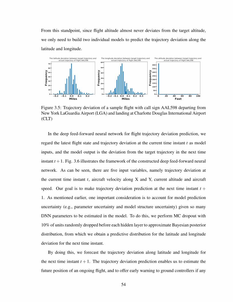
From this standpoint, since flight altitude almost never deviates from the target altitude,

we only need to build two individual models to predict the trajectory deviation along the

latitude and longitude.

Figure 3.5: Trajectory deviation of a sample flight with call sign AAL598 departing fromNew York LaGuardia Airport (LGA) and landing at Charlotte Douglas International Airport(CLT)

In the deep feed-forward neural network for flight trajectory deviation prediction, we

regard the latest flight state and trajectory deviation at the current time instant t as model

inputs, and the model output is the deviation from the target trajectory in the next time

instant t+1. Fig. 3.6 illustrates the framework of the constructed deep feed-forward neural

network. As can be seen, there are five input variables, namely trajectory deviation at

the current time instant t, aircraft velocity along X and Y, current altitude and aircraft

speed. Our goal is to make trajectory deviation prediction at the next time instant t +

1. As mentioned earlier, one important consideration is to account for model prediction

uncertainty (e.g., parameter uncertainty and model structure uncertainty) given so many

DNN parameters to be estimated in the model. To do this, we perform MC dropout with

10% of units randomly dropped before each hidden layer to approximate Bayesian posterior

distribution, from which we obtain a predictive distribution for the latitude and longitude

deviation for the next time instant.

By doing this, we forecast the trajectory deviation along latitude and longitude for

the next time instant t + 1. The trajectory deviation prediction enables us to estimate the

future position of an ongoing flight, and to offer early warning to ground controllers if any

54

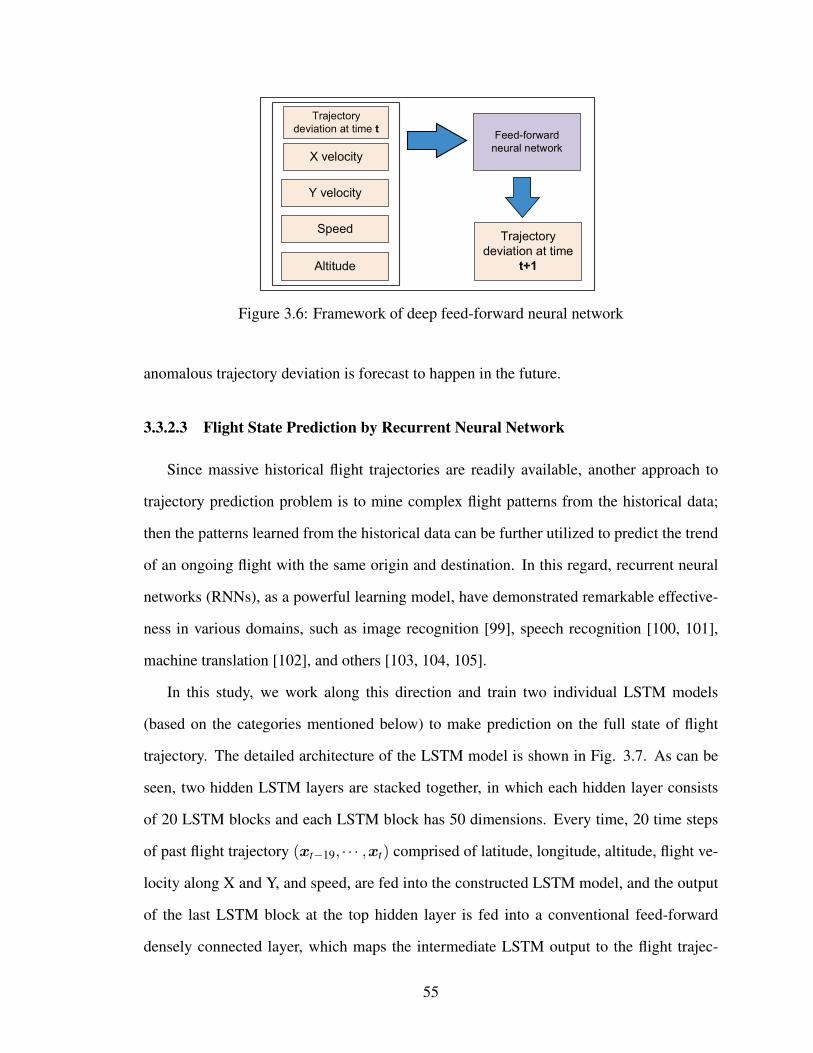
Trajectory

deviation at time t

X velocity

Y velocity

Altitude

Speed

Feed-forward

neural network

Trajectory

deviation at time

t+1

Figure 3.6: Framework of deep feed-forward neural network

anomalous trajectory deviation is forecast to happen in the future.

3.3.2.3 Flight State Prediction by Recurrent Neural Network

Since massive historical flight trajectories are readily available, another approach to

trajectory prediction problem is to mine complex flight patterns from the historical data;

then the patterns learned from the historical data can be further utilized to predict the trend

of an ongoing flight with the same origin and destination. In this regard, recurrent neural

networks (RNNs), as a powerful learning model, have demonstrated remarkable effective-

ness in various domains, such as image recognition [99], speech recognition [100, 101],

machine translation [102], and others [103, 104, 105].

In this study, we work along this direction and train two individual LSTM models

(based on the categories mentioned below) to make prediction on the full state of flight

trajectory. The detailed architecture of the LSTM model is shown in Fig. 3.7. As can be

seen, two hidden LSTM layers are stacked together, in which each hidden layer consists

of 20 LSTM blocks and each LSTM block has 50 dimensions. Every time, 20 time steps

of past flight trajectory (xt−19, · · · ,xt) comprised of latitude, longitude, altitude, flight ve-

locity along X and Y, and speed, are fed into the constructed LSTM model, and the output

of the last LSTM block at the top hidden layer is fed into a conventional feed-forward

densely connected layer, which maps the intermediate LSTM output to the flight trajec-

55

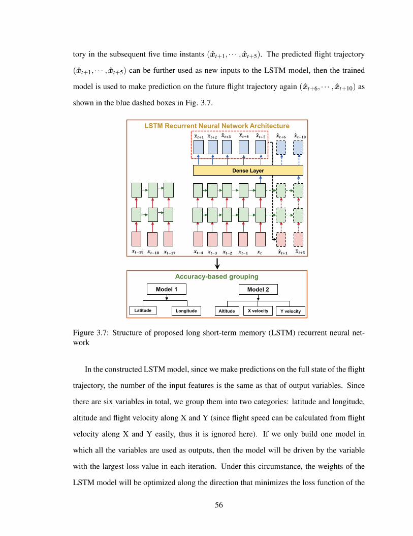
tory in the subsequent five time instants (xt+1, · · · , xt+5). The predicted flight trajectory

(xt+1, · · · , xt+5) can be further used as new inputs to the LSTM model, then the trained

model is used to make prediction on the future flight trajectory again (xt+6, · · · , xt+10) as

shown in the blue dashed boxes in Fig. 3.7.

LSTM Recurrent Neural Network Architecture

Accuracy-based grouping

Model 1 Model 2

Latitude Longitude Altitude Y velocityX velocity

Dense Layer

Figure 3.7: Structure of proposed long short-term memory (LSTM) recurrent neural net-work

In the constructed LSTM model, since we make predictions on the full state of the flight

trajectory, the number of the input features is the same as that of output variables. Since

there are six variables in total, we group them into two categories: latitude and longitude,

altitude and flight velocity along X and Y (since flight speed can be calculated from flight

velocity along X and Y easily, thus it is ignored here). If we only build one model in

which all the variables are used as outputs, then the model will be driven by the variable

with the largest loss value in each iteration. Under this circumstance, the weights of the

LSTM model will be optimized along the direction that minimizes the loss function of the

56

variable with the largest loss value. Since the five response variables share many common

parameters in the first two LSTM layers, the dominance of the variable with the largest loss

value results in the ignorance of the optimization of the weights for the remaining variables.

Therefore, we categorize the five response variables with similar loss values in the same

group, and train two individual LSTM models to address the deficiency in building one

single model. By grouping the variables with similar loss values together, we also maintain

the different prediction precision demand specific to each variable. In particular, since

a small prediction error in latitude and longitude is a large value in terms of distance in

reality, there is an important need for high prediction precision for both variables. If the

other variables (e.g., velocity) dominate the loss function, then the prediction precision for

latitude and longitude will be compromised significantly.

To obtain the Bayesian posterior distribution for model prediction, we perform Monte

Carlo dropout for both inputs, outputs, and recurrent layers with a dropout probability of

0.05 following the guidance in Gal and Ghahramani [35]. The MC dropout enables us to

have an approximated Bayesian posterior distribution on the future state of flight trajectory

of interest, in which the uncertainty on each aspect of flight trajectory is estimated properly.

3.3.3 Model Integration

As introduced before, two individual models are trained to make predictions on flight

trajectory from different views. Specifically, the feed-forward deep neural network (DNN)

makes a one-step-ahead prediction with high accuracy on the deviation of the actual flight

trajectory away from the filed flight plan, while the LSTM model forecasts the full state

of flight trajectory for a longer term (e.g., five steps or longer) but has a relatively low

accuracy in comparison with the DNN model. Integration of the two models will have both

high prediction accuracy and longer-term prediction capability.

Suppose we have observations on the actual flight trajectory up to the time instant t,

DNN predicts flight trajectory deviation at the next time instant t + 1 based on the degree

57

of trajectory deviation at the previous time instant t. Given the predicted deviation at time

instant t + 1, the predicted flight position at time t + 1 by DNN is readily available by

combining the predicted deviation and the filed flight plan. Suppose the LSTM model

utilizes the past 20 observed trajectory data to predict the state of flight along the subsequent

five time instants t +1, · · · , t +5. Let DNN’s trajectory deviation prediction at time instant

t +1 be denoted by τt+1; then we have:

E (yt+1) = qt+1 +E (τt+1) (3.1)

where qt+1 denotes the planed flight position including latitude, longitude, and altitude at

the time instant t +1, E (τt+1) is the mean value of DNN’s trajectory deviation prediction

at time instant t + 1, and E (yt+1) represents the mean value of DNN’s prediction on the

flight trajectory at time instant t +1.

Considering the two response variables (latitude and longitude) shared by the two mod-

els, one straightforward way to integrate the two models is to correct the low-accuracy

model with the results from high-accuracy model through a discrepancy term as calculated

following Eq. (3.2).

∆t+1 = E (yt+1)−E(xc

t+1)

(3.2)

where E(xc

t+1)

denotes the mean value of LSTM model’s prediction on the two common

quantities (latitude and longitude) at the time instant t + 1, and ∆t+1 represents the dis-

crepancy between DNN’s mean predictions and LSTM model’s mean predictions.

Once the discrepancy between the two model predictions in latitude and longitude pre-

diction at time t +1 is estimated, then the LSTM model’s prediction on the two quantities

for the subsequent time instants t + 1, · · · , t + 5 can be updated accordingly by adding the

discrepancy term to its predictions as shown in Eq. (3.3).

xci = x

ci +∆t+1, ∀i ∈ [t +1, · · · , t +5] (3.3)

58

where xci denotes the updated LSTM model prediction on latitude, longitude, and altitude

for the subsequent time instants t +1, · · · , t +5.

Thus, by combining DNN prediction yt+1 with the LSTM model prediction xt+1, both

high accuracy and longer-term prediction capability are achieved in the integrated model.

3.3.4 Safety Measure

The objective of trajectory prediction is to assess the en-route flight safety of the NAS.

Separation distance, as a widely used safety metric during the en-route phase, is used as a

quantitative metric in this study to measure the system safety. In the en-route airspace, the

minimum horizontal separation distance is 5 nautical miles, while no aircraft should come

vertically closer than 300 metres at an altitude of 29,000 feet [76]. With the probabilistic

predictions on the trajectory of any two given flights, the safety metric used in this study is

mathematically formulated in the following equation.

I[

p(dh

i (xci (A) ,x

ci (B))< δ

h)> λ and p(dv

i (xci (A) ,x

ci (B))< δ

v)> λ

], ∀i∈ [t +1, · · · , t +5]

(3.4)

where xci (A) and xc

i (B) denote the integrated model’s predictions on the trajectories of

flight A and B, respectively; dhi (x

ci (A) ,x

ci (B)) and dv

i (xci (A) ,x

ci (B)) represent the hori-

zontal and vertical separation distance between the two flights A and B as forecast by the

integrated model. Since the trajectory prediction of the integrated model is a probabilistic

quantity, a probabilistic metric p(dh

i (xci (A) ,x

ci (B))< δ h) and p(dv

i (xci (A) ,x

ci (B))< δ v)

are defined to measure the degree to which the horizontal and vertical separation distance

is violated against the recommended threshold values δh and δv, respectively. Herein, I [·]

is an indicator function; if both the horizontal are vertical separation distance are violated,

then the indicator function takes a value of one, indicating that the safety of the two flights

in terms of separation distance is compromised. Otherwise, its takes a value of zero to

indicate the two flights are safe in terms of separation distance.

59

With the introduction of the probabilistic safety indicator, the trajectory prediction from

the integrated model is related to the safety condition between any two given flights. In par-

ticular, since the LSTM model has a long-term prediction ability, if the probability of sep-

aration distance violation forecast by the integrated model is above some threshold prob-

ability value, then the ground controllers could be alerted to take appropriate actions to

increase the separation distance between the two flights.

3.3.5 Summary

The methodology developed in this section tackles the problem of en-route flight tra-

jectory prediction in the NAS following a four-step procedure (see Fig. 3.2).

1. Considering the large volume of raw SFDPS messages in FIXM format, Apache

Spark is leveraged to extract important trajectory information (i.e., flight position,

aircraft velocity) pertaining to each flight. SQL query is performed to group flight

trajectory by flight ID and date, and to save flight trajectory as a single CSV file per

flight with Apache Spark. Data pre-processing techniques are used to drop redundant

data and impute missing data.

2. Two deep learning models are trained to predict flight trajectory from different an-

gles: A deep feed-forward neural network is constructed for one-step-ahead predic-

tion of the deviation of actual flight trajectory from its corresponding flight plan, and

a LSTM recurrent neural network is developed to make longer-term prediction of the

flight trajectory. The uncertainty in both models is quantified following a Bayesian

approach and approximated with Monte Carlo dropout.

3. To fully exploit the advantages of both the deep learning models, we propose to inte-

grate them through a discrepancy term calculated as the difference between the two

models’ mean predictions. By doing this, the integrated model retains both LSTM

60

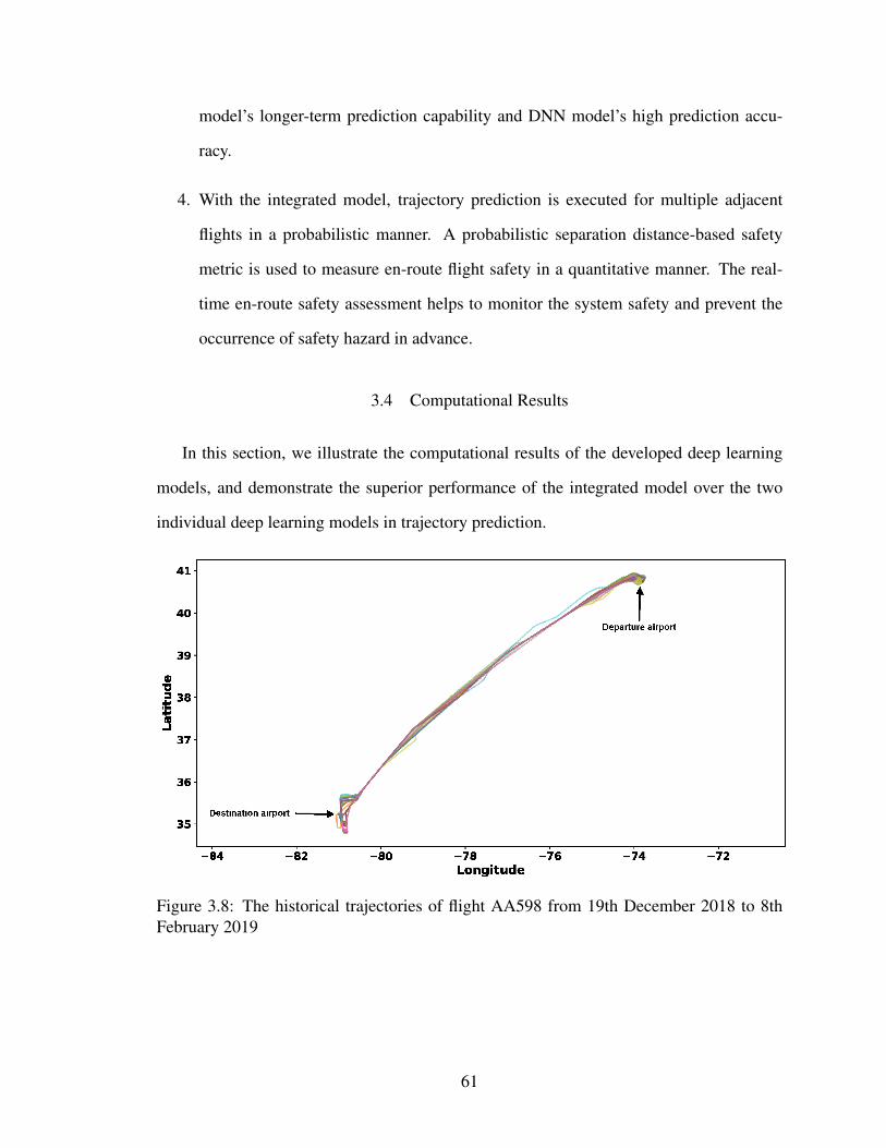
model’s longer-term prediction capability and DNN model’s high prediction accu-

racy.

4. With the integrated model, trajectory prediction is executed for multiple adjacent

flights in a probabilistic manner. A probabilistic separation distance-based safety

metric is used to measure en-route flight safety in a quantitative manner. The real-

time en-route safety assessment helps to monitor the system safety and prevent the

occurrence of safety hazard in advance.

3.4 Computational Results

In this section, we illustrate the computational results of the developed deep learning

models, and demonstrate the superior performance of the integrated model over the two

individual deep learning models in trajectory prediction.

Figure 3.8: The historical trajectories of flight AA598 from 19th December 2018 to 8thFebruary 2019

61

3.4.1 Data

We streamed SFDPS messages from 19th December 2018 to 8th February 2019. In

terms of data volume, nearly 4.2 TB of SFDPS messages is processed with Apache Spark,

from which we extract flight trajectories for 48 days. In order to demonstrate the trajectory

prediction of an ongoing flight, we pick a flight trajectory on a randomly selected date and

use it to test the prediction performance of the deep learning models, while the remaining

flight trajectories are used to train the two deep learning models. We pick a specific flight

AA598 for the sake of illustration. Fig. 3.8 shows the trajectories of flight AA598 from

19th December 2018 to 8th February 2019. The top right and bottom left corners indicate

the departure airport (LaGuardia Airport) and destination airport (Charlotte Douglas Inter-

national Airport), respectively. Obviously, the flight trajectory varies from day to day as

impacted by traffic flow control, different weather conditions, and other factors.

0 100 200 300 400Time (Unit: 12 seconds)

0.006

0.004

0.002

0.000

0.002

0.004

0.006

0.008

Lati

tude

dev

iati

on

True value Prediction Mean

(a) Mean latitude deviation prediction vs actual val-ues on sample flight AA598

0 100 200 300 400Time (Unit: 12 seconds)

0.008

0.006

0.004

0.002

0.000

0.002

0.004

0.006

0.008

Long

itud

e de

viat

ion

True value Prediction Mean

(b) Mean longitude deviation prediction vs actualvalues on sample flight AA598

Figure 3.9: DNN prediction on trajectory deviation

3.4.2 Model Training and Assessment

Prior to the training of DNN model, the input and output data is normalized with the

MinMaxScaler. When training the DNN model, we use the Adam optimizer with a learning

rate of 0.001 to optimize the weights of deep neural networks for 15,000 iterations. Dropout

with a probability of 0.1 is applied before each hidden layer to avoid overfitting during

training. Two individual DNN models are trained for predicting the trajectory deviation

62

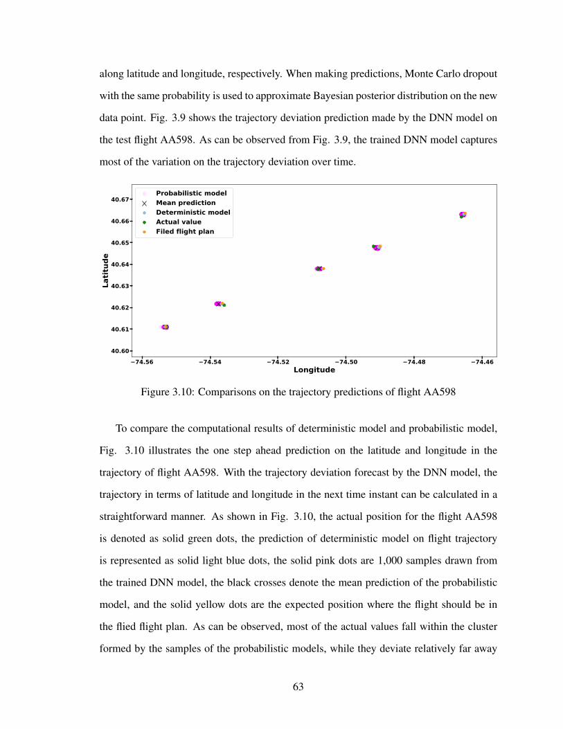
along latitude and longitude, respectively. When making predictions, Monte Carlo dropout

with the same probability is used to approximate Bayesian posterior distribution on the new

data point. Fig. 3.9 shows the trajectory deviation prediction made by the DNN model on

the test flight AA598. As can be observed from Fig. 3.9, the trained DNN model captures

most of the variation on the trajectory deviation over time.

74.56 74.54 74.52 74.50 74.48 74.46Longitude

40.60

40.61

40.62

40.63

40.64

40.65

40.66

40.67

Lati

tude

Probabilistic modelMean predictionDeterministic modelActual valueFiled flight plan

Figure 3.10: Comparisons on the trajectory predictions of flight AA598

To compare the computational results of deterministic model and probabilistic model,

Fig. 3.10 illustrates the one step ahead prediction on the latitude and longitude in the

trajectory of flight AA598. With the trajectory deviation forecast by the DNN model, the

trajectory in terms of latitude and longitude in the next time instant can be calculated in a

straightforward manner. As shown in Fig. 3.10, the actual position for the flight AA598

is denoted as solid green dots, the prediction of deterministic model on flight trajectory

is represented as solid light blue dots, the solid pink dots are 1,000 samples drawn from

the trained DNN model, the black crosses denote the mean prediction of the probabilistic

model, and the solid yellow dots are the expected position where the flight should be in

the flied flight plan. As can be observed, most of the actual values fall within the cluster

formed by the samples of the probabilistic models, while they deviate relatively far away

63

from the prediction of the deterministic model. Hence, the probabilistic model outperforms

the deterministic model in the latitude and longitude prediction. The inclusion of model

prediction uncertainty enables us to assess the level of uncertainty and risk involved when

making decisions in a quantitative manner.

36.8 36.9 37.0 37.1 37.2 37.3Latitude

79.5

79.4

79.3

79.2

79.1

79.0

78.9

Long

itud

e

Input DataRNN PredictionActual Value

(a) Mean latitude and longitude prediction byLSTM model vs actual values on sample flightAA598

0 5 10 15 20 25 30Time (Unit:12 seconds)

2000

4000

6000

8000

10000

12000

14000

Alti

tude

(U

nit:

feet

)

Input DataActual ValueRNN Prediction

(b) Mean altitude prediction by LSTM model vsactual values on sample flight AA598

Figure 3.11: LSTM prediction of flight trajectory

We retain the same trajectory to verify the performance of the trained LSTM model. To

avoid model overfitting, regularization is performed on layer parameters, and L2 regular-

ization is applied to the recurrent connections. The LSTM model has two stacked layers

with each layer having 20 LSTM blocks. The output of the last LSTM block at the top

hidden layer is flattened and fed into a densely connected layer. Two individual models

are trained with the same LSTM architecture. The first model predicts the flight latitude

and longitude along the subsequent five time steps, while the second model forecasts the

flight altitude, and velocities along X and Y in the subsequent five time steps. To make

even longer prediction, we take the LSTM model’s prediction as new inputs, and feed them

into the trained LSTM model to make predictions again. Fig. 3.11 shows the predictions of

LSTM model on the latitude, longitude, and altitude of the test flight AA598 for the next

10 time instants (2 minutes). From LSTM’s predictions, we observe that it demonstrates

promising performance in predicting the flight trajectory over time. There is slight discrep-

ancy between LSTM model’s prediction and the actual values. The powerful longer-term

prediction ability in the LSTM model enables us to have a 2-minutes-ahead view on the

64

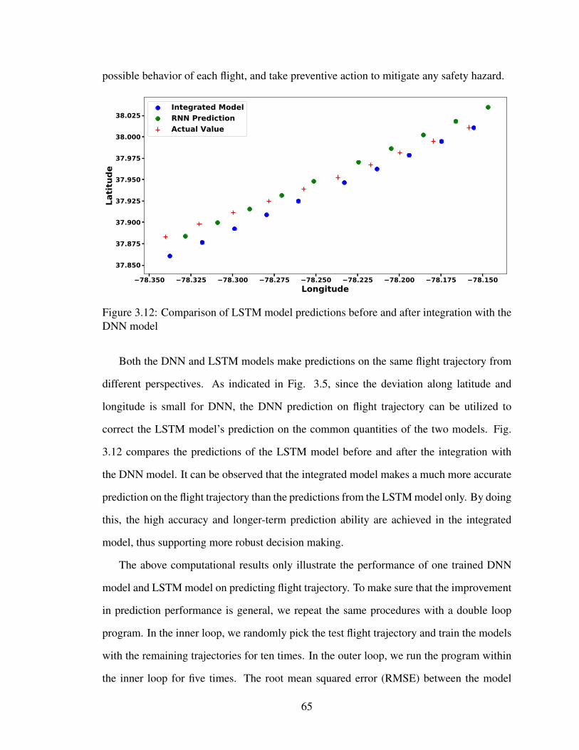
possible behavior of each flight, and take preventive action to mitigate any safety hazard.

78.350 78.325 78.300 78.275 78.250 78.225 78.200 78.175 78.150Longitude

37.850

37.875

37.900

37.925

37.950

37.975

38.000

38.025La

titu

deIntegrated ModelRNN PredictionActual Value

Figure 3.12: Comparison of LSTM model predictions before and after integration with theDNN model

Both the DNN and LSTM models make predictions on the same flight trajectory from

different perspectives. As indicated in Fig. 3.5, since the deviation along latitude and

longitude is small for DNN, the DNN prediction on flight trajectory can be utilized to

correct the LSTM model’s prediction on the common quantities of the two models. Fig.

3.12 compares the predictions of the LSTM model before and after the integration with

the DNN model. It can be observed that the integrated model makes a much more accurate

prediction on the flight trajectory than the predictions from the LSTM model only. By doing

this, the high accuracy and longer-term prediction ability are achieved in the integrated

model, thus supporting more robust decision making.

The above computational results only illustrate the performance of one trained DNN

model and LSTM model on predicting flight trajectory. To make sure that the improvement

in prediction performance is general, we repeat the same procedures with a double loop

program. In the inner loop, we randomly pick the test flight trajectory and train the models

with the remaining trajectories for ten times. In the outer loop, we run the program within

the inner loop for five times. The root mean squared error (RMSE) between the model

65

predictions and actual values is used as a metric to compare all the models. Since training

deep learning models, especially LSTM models, is time-consuming, we accelerate the run-

ning speed of the program by executing it on a NVIDIA Pascal GPU. Table 3.2 compares

the performance of the deterministic and probabilistic deep learning models on the trajec-

tory deviation prediction. Here, we use the mean value of probabilistic model prediction

to calculate the RMSE. As indicated in the comparison results, the RMSE of the proba-

bilistic DNN model has reduced by 2% and 74% for the latitude and longitude deviation

prediction, respectively. Similarly, we compare the performance of the LSTM model and

the integrated model on flight state prediction. As shown in Table 3.3, the integrated model

demonstrates a much better performance on the common quantities of the two models: lat-

itude and longitude prediction. The value of RMSE is reduced by 47% and 53% compared

to the LSTM model, respectively. These cross-validation results show that the integrated

model achieves much higher accuracy in flight state prediction.

Table 3.2: Performance comparisons on trajectory deviation prediction

Deterministic Probabilistic

Latitude Longitude Latitude (µ) Longitude (µ)Root Mean Squared Error 3.36×10−2 9.73×10−2 3.29×10−2 2.51×10−2

Table 3.3: Performance comparisons on flight state prediction

LSTM Model Integrated Model LSTM Model

Latitude Longitude Latitude Longitude Altitude X Velocity Y VelocityRoot Mean Squared Error 2.48×10−2 2.96×10−2 1.32×10−2 1.38×10−2 650 16.29 20.11

3.4.3 Safety Assessment

To measure the flight safety, we pick another flight UAL1767 that starts from Denver

International Airport and ends at Ronald Reagan Washington National Airport on 23rd

January, 2019. Once the deep learning models are trained, we calculate the horizontal

and vertical separation distances between the two flights. Fig. 3.13 compares the model

66

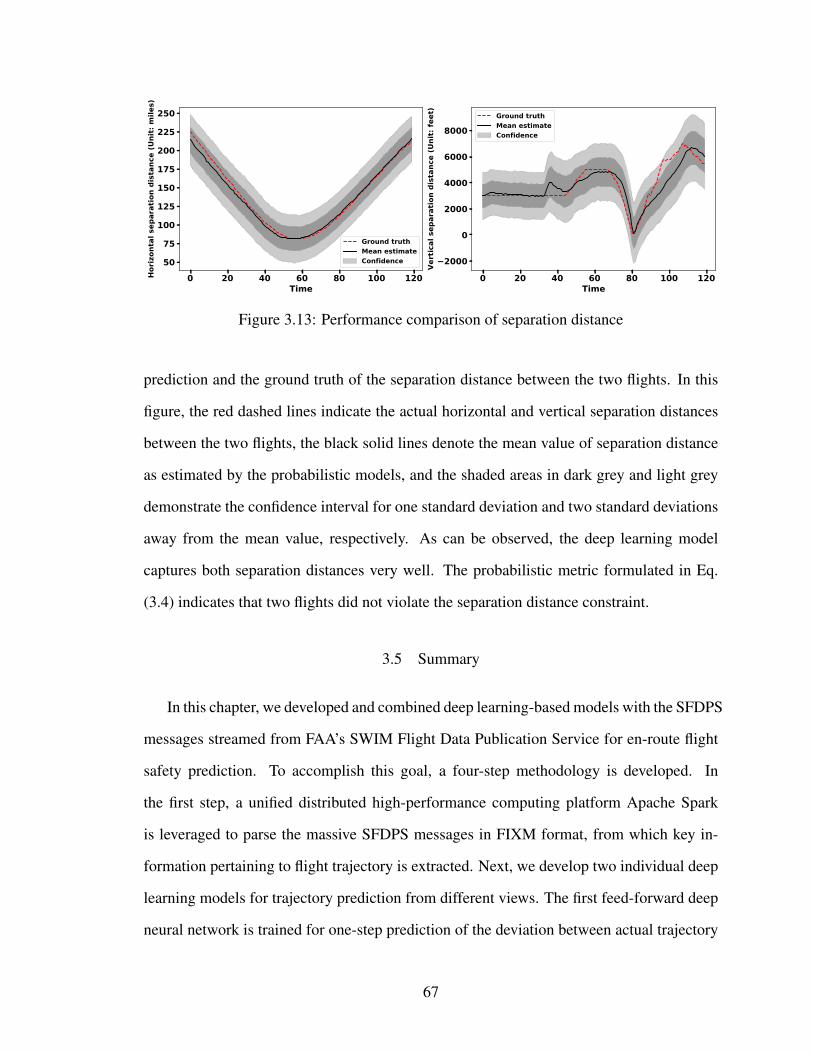
0 20 40 60 80 100 120Time

50

75

100

125

150

175

200

225

250

Hor

izon

tal s

epar

atio

n di

stan

ce (

Uni

t: m

iles)

Ground truthMean estimateConfidence

0 20 40 60 80 100 120Time

2000

0

2000

4000

6000

8000

Vert

ical

sep

arat

ion

dist

ance

(U

nit:

feet

)

Ground truthMean estimateConfidence

Figure 3.13: Performance comparison of separation distance

prediction and the ground truth of the separation distance between the two flights. In this

figure, the red dashed lines indicate the actual horizontal and vertical separation distances

between the two flights, the black solid lines denote the mean value of separation distance

as estimated by the probabilistic models, and the shaded areas in dark grey and light grey

demonstrate the confidence interval for one standard deviation and two standard deviations

away from the mean value, respectively. As can be observed, the deep learning model

captures both separation distances very well. The probabilistic metric formulated in Eq.

(3.4) indicates that two flights did not violate the separation distance constraint.

3.5 Summary

In this chapter, we developed and combined deep learning-based models with the SFDPS

messages streamed from FAA’s SWIM Flight Data Publication Service for en-route flight

safety prediction. To accomplish this goal, a four-step methodology is developed. In

the first step, a unified distributed high-performance computing platform Apache Spark

is leveraged to parse the massive SFDPS messages in FIXM format, from which key in-

formation pertaining to flight trajectory is extracted. Next, we develop two individual deep

learning models for trajectory prediction from different views. The first feed-forward deep

neural network is trained for one-step prediction of the deviation between actual trajectory

67

and target flight trajectory. The second LSTM recurrent neural network is utilized for make

longer-term prediction on the full state of the flight trajectory. In the third step, the two deep

learning models are integrated via a discrepancy term, which is calculated as the discrep-

ancy between DNN prediction and LSTM prediction on the common response variables

(i.e., latitude and longitude). The integration of the two deep learning models preserves

both the high accuracy of the DNN model and the longer-term prediction ability of LSTM

model. Finally, the same approach is extended to multiple flights, and we are then able

to predict the en-route flight safety, in which probabilistic separation distance is used as a

quantitative safety metric.

The proposed methodology has made several significant contributions to the state-of-

the-art studies towards flight trajectory prediction using machine learning from historical

data. First of all, we utilize a distributed computing engine Apache Spark to process a large

volume of raw data in FIXM format, and it demonstrates scalable and promising perfor-

mance. The same strategy can be implemented to handle more complex aeronautical data

in the future, such as weather data. Secondly, different from existing studies, we charac-

terize the model prediction uncertainty following a Bayesian approach. The quantification

of model prediction uncertainty allows us to make decisions with probabilistic information

on the safety risk. Thirdly, the trained deep learning models offer new insights to view

the trajectory prediction from different angles. By integrating the two models together, we

not only improves the overall prediction accuracy, but also retain a longer-term prediction

capability.

This chapter develops a multi-fidelity deep learning-based model for system behavior

prediction, the idea of multi-fidelity approach can be generalized to many other applica-

tions. In particular, by blending two prediction models together, we achieve both long-term

prediction capability and high prediction accuracy. The fast and accurate prediction of sys-

tem behavior enabled by the multi-fidelity model greatly improves operators’ preparedness

for hazardous events, thereby increasing system resilience.

68

Chapter 4

Ensemble Machine Learning Models for Risk Prediction of the Consequences of

Hazardous Events1

4.1 Introduction

In addition to predicting when a hazardous event is about to happen (as in the previous

chapter), another perspective to strengthen the resilience of a system is that, given that

an anomalous event has already occurred, we can increase the preparedness of relevant

stakeholders for the consequences of the hazardous event. One means to achieve this goal

is to equip the stakeholders with a tool to forecast the consequence of any abnormal event

with the anomalous behavior of the system observed so far. In this chapter, we develop an

ensemble machine learning approach to predict the outcomes of the abnormal events, and

illustrate the approach using aviation incidents.

As mentioned earlier in Chapter 3, the air traffic is experiencing a steady and tremen-

dous growth, and the rapid increase in air traffic demand poses a tremendous operational

challenge on the air transportation system, which is already struggling to cope with the

current demand. Over the past decades, numerous efforts have been dedicated to the de-

velopment on comprehensive safety metrics as well as qualitative/quantitative approaches

to detect anomalous behavior, assess the safety, and quantify the risk associated with one

subsystem (i.e., airport ground operations, flight tracking, or taxiway and runway system)

or a mixture of subsystems in the air transportation system [106]. In general, there are two

principal strategies to enhance the air transportation system safety: (I) increase system/-

subsystem reliability, i.e., reduce the probability of operators making mistakes or systems

having malfunctions; and (II) improve the operators’ preparedness. Although tremendous

progress has been made over the past decades for enhancing the air transportation system

1An archival paper related to this chapter has been published in the journal Decision Support Systems.For more details, see Ref. [69]

69

safety, most of the studies emphasize identifying the accident precursors and initiating cor-

rective actions to prevent future errors, which can be grouped into the first strategy. Among

the existing studies, much of the effort has been devoted to investigating human factors

induced accidents and constructing causal models [107, 108]. For example, Wiegmann and

Shappell [109] described the Human Factors Analysis and Classification System (HFACS)

and provided aviation case studies on human factor analysis with HFACS. However, air

transportation is a complex system of systems involving many varied but yet interlinking

distributed networks of human operators, technical/technological procedures and systems,

and organizations/stakeholders. The scarcity in the operational data and the involvement

of a variety of human operators are major challenges that severely affect the prediction of

erroneous operation, and challenge the assessment and improvement of the system reliabil-

ity.

As mentioned in Chapter 1, the first set of measures we take to enhance system re-

silience is to increase operators’ situation awareness on the dynamic evolution of hazardous

events. As indicated in chapter 3, we accomplish this goal by enhancing operators’ situ-

ation awareness on the future state of en-route flight trajectory by learning from massive

historical trajectory data. By doing this, we equip operators with a look-ahead ability, from

which they gain a better sense on the moment when the loss of flight separation distance

occurs (separation distance is the event we investigate in Chapter 3). On the other hand, if

system malfunction already happens, one way to strengthen operators’ preparedness is to

get them ready for the consequence of anomalous events. By doing this, when a hazardous

event occurs, the operator can take appropriate safety measures to reduce the cost of the

consequence caused by the hazardous event with the minimum time [110, 111, 20].

In Chapter 4, we emphasize the “proactive safety” paradigm [112] and work along this

direction with a focus on strengthening the capability and efficiency of the operators in re-

sponse to the abnormal events with appropriate actions, thereby mitigating the consequence

or severity of hazardous events. In this connection, a large number of incident/accident re-

70

ports have been filed over the past half century together. A few machine learning studies

have been carried out to analyze these reports. For example, Oza et al. [113] developed

two algorithms – Mariana and nonnegative matrix factorization-based algorithm – to per-

form multi-label classification for the reports of Aviation Safety Reporting System (ASRS).

Budalakoti et al. [114] presented a set of algorithms to detect and characterize anomalies

in discrete symbol sequences arising from recordings of switch sensors in the cockpits of

commercial airliners. These studies have not explored the intricate relationships between

abnormal event characteristics and the induced consequences. This chapter aims to mine

the complex associations between anomalous event behavior and the consequence of these

events through the development of a hybrid machine learning model. This type of anal-

ysis will help to develop a decision support system that can learn the patterns in the data

and help the analyst examine incidents/accidents quickly and systematically, thus assisting

the risk manager in risk quantification, priority setting, resource allocation and decision

making in support of the implementation of proactive safety paradigm.

While in Chapter 3, flight trajectory is represented as numerical values, the anoma-

lous incidents in this chapter, their characteristics, and event consequences are primarily

depicted in the categorical and text format. To develop the model for event consequence

prediction, we have utilized the Aviation Safety Reporting System (ASRS), which is as

a state-of-the-art aviation incident database that provides a plethora of incidents/accidents

that occur over the course of the past several decades. The incident reports are submitted by

pilots, air traffic controllers, dispatchers, cabin crew, maintenance technicians, and others,

and describe both unsafe occurrences and hazardous situations [115]. ASRS covers almost

all the domains of aircraft operations that could go wrong. However, it is a non-trivial

task to build a model from the ASRS data for the prediction of risk associated with the

consequence of hazardous events due to the following challenges:

1. High-dimensional data. Each incident record consists of more than 50 items rang-

ing from the operational context (weather, visibility, flight phase, and flight condi-

71

tions) to the characteristics of the anomalous operation (aircraft equipment, malfunc-

tion type, and event synopsis). The url https://asrs.arc.nasa.gov/docs/dbol/ASRS

CodingTaxonomy.pdf gives a detailed description of each item. Besides, air traffic

operation is a complex system composed of a number of programs and personnel. It

is likely for the incident to occur at any phase and location due to a variety of factors

(i.e., operation violation, visibility, human factors etc.), which makes it hard for the

machine learning algorithm to predict the exact level of risk associated with each

event outcome.

2. Primarily categorical data. Over 99% of the items in the ASRS database are categor-

ical, and only one attribute (crew size) is numerical in each record. Although the

categorical information offers a high-level description of the context of each inci-

dent, very limited information specific to each abnormal event can be derived from

such categorical information, e.g., how did the incident happen, how did the incident

evolve over time in the system, what operation the pilot took to resolve the issue,

etc. Since the categorical features are not informative, how to blend the predictions

of the model trained by the categorical features and the predictions from the model

trained by other informative indicators (e.g., event synopsis) without compromising

the model performance is an issue worthy of investigation.

3. Unstructured data. One important unstructured attribute is event synopsis, which is

a concise summary of the incident/accident in the form of text. Mining causal re-

lationships from the unstructured text data is a daunting task [116]. A common

characteristic in handling text data is to transform it into numerical data in the rep-

resentation of term frequency of each individual document. Along this direction,

researchers have developed numerous techniques to elicit useful knowledge from

the text data, e.g., support vector machine [117], latent Dirichlet allocation-based

topic mining [118, 119, 120], Naıve Bayes-based document classification [121], k-

72

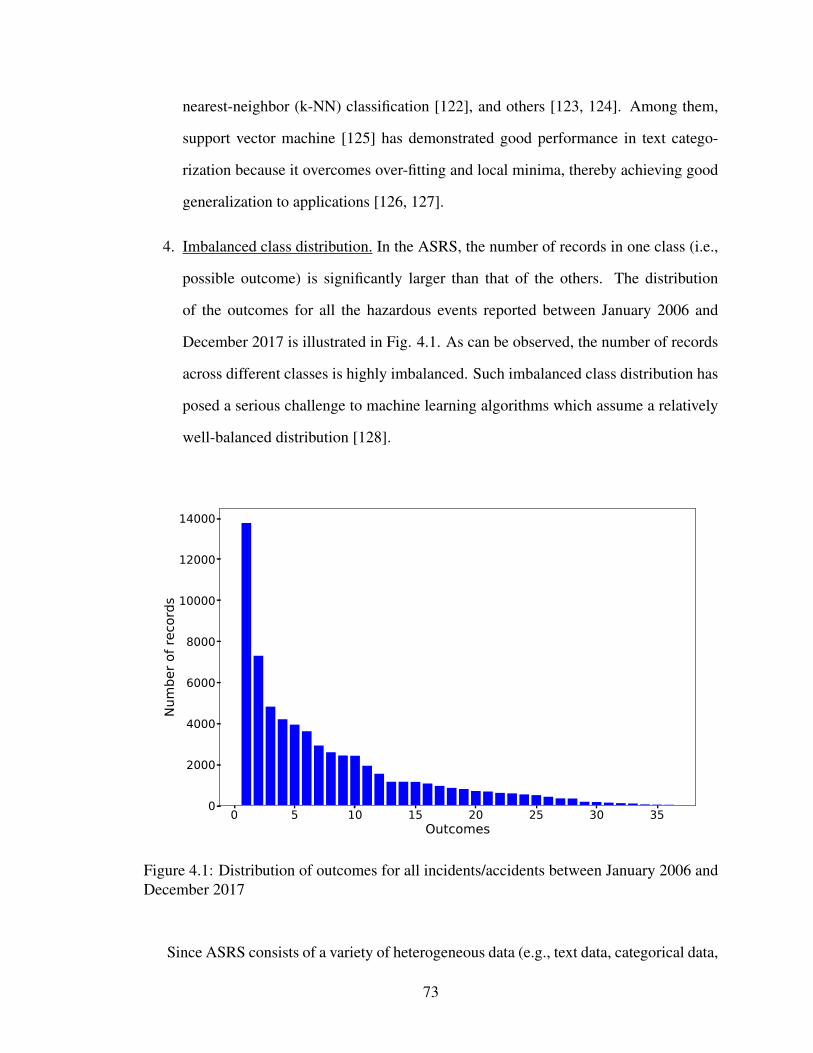
https://asrs.arc.nasa.gov/docs/dbol/ASRS_CodingTaxonomy.pdf

https://asrs.arc.nasa.gov/docs/dbol/ASRS_CodingTaxonomy.pdf

nearest-neighbor (k-NN) classification [122], and others [123, 124]. Among them,

support vector machine [125] has demonstrated good performance in text catego-

rization because it overcomes over-fitting and local minima, thereby achieving good

generalization to applications [126, 127].

4. Imbalanced class distribution. In the ASRS, the number of records in one class (i.e.,

possible outcome) is significantly larger than that of the others. The distribution

of the outcomes for all the hazardous events reported between January 2006 and

December 2017 is illustrated in Fig. 4.1. As can be observed, the number of records

across different classes is highly imbalanced. Such imbalanced class distribution has

posed a serious challenge to machine learning algorithms which assume a relatively

well-balanced distribution [128].

0 5 10 15 20 25 30 35Outcomes

0

2000

4000

6000

8000

10000

12000

14000

Numbe

r of records

Figure 4.1: Distribution of outcomes for all incidents/accidents between January 2006 andDecember 2017

Since ASRS consists of a variety of heterogeneous data (e.g., text data, categorical data,

73

and numerical data), it is challenging to develop one single model to learn from the entire

dataset for predicting the risk associated with the consequence of hazardous events. In

this chapter, we adopt the “divide and conquer” strategy to split the data into two parts:

structured and unstructured, and develop a hybrid model to handle the two types of data,

respectively. By doing this, we are able to leverage the strengths of each model in pro-

cessing certain type of data. Compared with building a single model, the dimension of

the problem is reduced significantly. With respect to categorical data, considering its high-

dimensional feature space, deep learning might be a good candidate to discover the highly

intricate relationship between event contextual characteristics and event consequence due to

its powerful ability in establishing a dense representation of the feature space, which makes

it effective in learning high-order features from the raw data [129, 130]. As a result, a deep

learning model is developed to process the categorical data for the purpose of learning the

associations between event contextual features and event outcomes. In parallel, a support

vector machine model is trained to identify the relationships between text-based event syn-

opsis and the risk level associated with the consequence of each incident. Afterwards, the

predictions from the two machine learning models are fused together for quantifying the

risk associated with the consequence of each incident. Finally, the prediction on risk level

categorization is extended to event-level outcomes through a probabilistic decision tree.

Compared to the current state of the art in machine learning for aviation safety, we make

the following contributions:

1. We have developed a machine learning methodology to learn the relationships be-

tween abnormal event characteristics and their consequences. We focus on the data

set that has a large number of outcomes and imbalance of available data regarding

these outcomes. This challenge is overcome by grouping the event outcomes into

five risk categories and by up-sampling the minority classes.

2. A probabilistic fusion rule is developed to blend the predictions of multiple machine

learning models that are built on different segments of the available data. Specifi-

74

cally, a hybrid model blending SVM prediction on unstructured data and deep neural

network ensemble on structured data is developed to quantify the risk of the conse-

quence of hazardous events, in which the record-level prediction probabilities, class-

level prediction accuracy in each respective model, and the proportion of each class

in the records with disagreeing predictions are considered in model fusion.

4.2 Aviation Safety Reporting System

The Aviation Safety Reporting System (ASRS) is a program operated by the National

Aeronautics and Space Administration (NASA) with the ultimate goal of increasing avi-

ation system safety by discovering system safety hazards hidden in the multitude of air

traffic operations. Over the past few decades, ASRS has become one of the world’s largest

sources of information on aviation safety and human factors [115]. As one of its primary

tasks, ASRS collects, processes, and analyzes voluntarily submitted aviation incident/sit-

uation reports from pilots, flight attendants, air traffic controllers, dispatchers, cabin crew,

ground workers, maintenance technicians, and others involved in aviation operations.

Reports submitted to ASRS include both unsafe occurrences and hazardous situations.

Each submitted report is first screened by two analysts to provide the initial categorization

and to determine the triage of processing. During this process, ASRS analysts identify

hazardous situations from the reports, and issue an alert message to persons in a position to

correct them. Based on the initial categorization, ASRS analysts might aggregate multiple

reports on the same event to form one database “record”. If any information needs to be

further clarified, ASRS analysts might choose to call a reporter over the telephone to gather

more information. After all the necessary information is collected, the reports are codified

using the ASRS taxonomy and recorded in the database. Next, some critical information in

each record is de-identified; then ASRS distributes the incident/accident records gathered

from these reports to all the stakeholders in positions of authority for future evaluation and

potential corrective action development.

75

Table 4.1: A sample incident/accident record extracted from ASRS

Attribute Content

Time / Day Date : 201702Local Time Of Day : 0601-1200

PlaceLocale Reference.Airport : BUR.AirportState Reference : CAAltitude.MSL.Single Value : 2500

Environment

Flight Conditions : VMCWeather Elements / Visibility.Visibility : 10Light: DaylightCeiling.Single Value : 12000

Aircraft

Reference : XATC / Advisory.Center : BURAircraft Operator : PersonalMake Model Name : PA-28R Cherokee Arrow All SeriesCrew Size.Number Of Crew : 1Operating Under FAR Part : Part 91Flight Plan : VFRMission : PersonalFlight Phase : Initial ApproachRoute In Use : Visual ApproachAirspace.Class D : VNY

Component Aircraft Component : Engine AirProblem : Malfunctioning

Person

Reference : 1Location Of Person : XLocation In Aircraft : Flight DeckReporter Organization : PersonalFunction.Flight Crew : Single PilotQualification.Flight Crew : PrivateExperience.Flight Crew.Total : 175Experience.Flight Crew.Last 90 Days : 30Experience.Flight Crew.Type : 175ASRS Report Number.Accession Number : 1428684Human Factors : Confusion

Events

Anomaly.Deviation - Altitude : Excursion From Assigned AltitudeAnomaly.Deviation - Track / Heading : All TypesAnomaly.Deviation - Procedural : ClearanceAnomaly.Inflight Event / Encounter : Unstabilized ApproachDetector.Person : Air Traffic ControlWhen Detected : In-flightResult.Flight Crew : Returned To ClearanceResult.Flight Crew : Became ReorientedResult.Air Traffic Control : Issued New ClearanceResult.Air Traffic Control : Issued Advisory / Alert

AssessmentsContributing Factors / Situations : Airspace StructureContributing Factors / Situations : Human FactorsPrimary Problem : Human Factors

SynopsisPA28R pilot reported becoming confused during a VFR flight to BUR andlined up on VNY. BUR Tower detected the error and issued a new headingand climb back to assigned altitude.

76

Table 4.1 presents a sample situation record extracted from the ASRS database. As can

be observed, each record has more than 20 fields ranging from event occurrence location to

event characteristics. Here, we briefly introduce several primary attributes in each record:

1. Time and location of the abnormal event: The incident in Table 4.1 occurred on

February 2017 at the BUR airport in USA. Here, BUR is the International Air Trans-

port Association (IATA) code of the airport, and it refers to the Hollywood Burbank

Airport located in Los Angeles County, California. Besides, the record also provides

the basic altitude above Mean Sea Level (MSL). In this case, the hazardous event

occurred when the flight was at an altitude of 2500 feet.

2. Environment: This describes the surrounding conditions encompassing the aircraft

operations. Examples are: flight conditions (VMC, IMC, marginal, or mixed), and

weather elements such as visibility, light, and ceiling. Here, VMC refers to visual

meteorological condition (VMC) under visual flight rules (VFR) flight. In VMC,

pilots have sufficient visibility to fly the aircraft maintaining visual separation from

the terrain and other aircraft. Different from VMC, instrument meteorological con-

dition (IMC) represents the category that describes weather conditions that require

pilots to fly primarily by reference to instruments under instrument flight rules (IFR).

Visibility and cloud ceiling are two key factors in determining whether the weather

condition is VMC or IMC, and the boundary between IMC and VMC is known as

VMC minima. “Marginal VMC” refers to conditions above but close to one VMC

minima or more.

3. Aircraft: This attribute reports the basic aircraft and flight information, including the

aircraft make and model, flight type (personal or commercial), the number of crew

onboard, flight plan, flight mission, flight phase, and the airspace class the flight is

in. Such information details the specific flight phase in which the hazardous event

occurs. The basic aircraft information also enables us to have an understanding of

77

the scale of the possible event consequence.

4. Component: If there is any mechanical failure in the aircraft, the record will have

the component field, and it describes which aircraft component is faulty (i.e., engine,

nosewheel, transponder etc.) and the type of the problem as well (i.e., malfunc-

tioning, improperly operated, or others). This field might be empty if there is no

component malfunction.

5. Person: Person describes the fundamental information of the personnel that reports

the problem. For example, the location of the person, his/her location in the aircraft,

the reporter organization, the qualification of the reporter, and the contributing human

factor (e.g., fatigue, distraction, confusion, and time pressure).

6. Events: This attribute provides the basic characteristics of anomalous behavior and

its consequence. In this record, BUR Tower detected the excursion of the flight from

the assigned altitude and issued course correction to avoid the traffic. After taking

course correction to avoid traffic, the pilot did not maintain the same course heading

to Burbank while ATC assumed that the pilot was on correct heading. As a result,

the BUR Tower recognized the error and issued a new heading and commanded the

pilot to climb back to the assigned altitude to perform landing from the very start.

7. Assessments: Assessments provide evaluation of the root cause and other factors that

contribute to the occurrence of the abnormal event.

Table 4.2: Two examples of event synopsis in ASRS

Date Event Synopsis

February, 2017A319 Flight Attendant reported smoke in the cabin near the overwingexits during climb.

January, 2017A319 flight crew reported fumes in the flight deck. After a short timethey began to experience problems concentrating and the onset of inca-pacitation.

78

8. Synopsis: All the above fields are categorical except the crew size. The last row

of Table 4.1 and Table 4.2 provide several sample event synopses elicited from the

ASRS database. As can be observed, event synopses gives a brief summary of the

cause of the problem, and how the abnormal event evolves over time. Such infor-

mation is helpful for us to assess the severity of the hazardous event and analyze

possible consequences.

The above descriptions provide a brief introduction to the physical meanings of some

important fields in each record. In ASRS, other records might differ from the above sample

records in certain fields or they might have additional fields which are absent in the sample

record due to the difference in the type and characteristics of the abnormal event.

4.3 Proposed Methodology

We develop a hybrid method to estimate the risk of the event consequence with the con-

sideration of operational conditions and event characteristics. To build the hybrid model,

we investigate the incidents/accidents that occurred from January 2006 to December 2017.

The detailed proposed framework is outlined in Fig. 4.2, which shows a four-step pro-

cedure. In the first step, we perform a risk-based event outcome categorization. That is

we employ the level of risk as a quantitative metric to measure the severity of the event

outcome and collapse all the possible event outcomes into five categories: high risk, mod-

erately high risk, medium risk, moderately medium risk, and low risk. Given the restruc-

tured categories, two models are developed in the second step to process the unstructured

data (text data) and structured data (categorical and numerical information). Specifically,

a support vector machine (SVM) model is developed to represent the relationship between

event synopsis and the risk pertaining to the event outcome, and an ensemble of deep neural

networks (DNN) is trained to predict the level of risk based on contextual features of each

abnormal event. In the third step, we develop an innovative fusion rule to blend the pre-

diction results from the SVM and DNN models. Finally, the risk-level prediction is further

79

expanded to event-level outcome analysis in through a probabilistic tree.

Text Data

(Event synopsis)

Word

Text Preprocessing

TF-IDF matrix

Flight phase

Weather visibility

Primary problem

Event

Light

crew sizePersons involved

equipment

Contextual features

Event outcome

1. Plane crashed23. Physical injury4. ...High Risk

Medium Risk

1. General evacuated2. Flight crew landed as

1. Air t control provided assistance2. Flight Crew Returned To Gate

Low Risk

isk

Risk

Risk

Moderately

high Risk

Structural data

System Output

Moderately

medium Risk

1. Flight crew diverted2. Flight crew overcame equipment problem

1. General maintenance

2. General release refused

Hybrid Model

Probabilistic rule to fuse the prediction

results from the two models

1

3

ASRS reports

Categorical or

numerical data

Model

Support Vector Machine Ensemble of Deep Neural Networks..

.

2

Risk level 4

Figure 4.2: Hybrid machine learning framework for risk prediction

80

4.3.1 Risk-based Event Outcome Categorization

As shown in Fig. 4.1, there are 36 unique event outcomes among the incident reports.

Because almost all of the contextual features are categorical, they are uninformative indica-

tors of the event outcome considering that one contextual condition might correspond to a

large number of event outcomes that belong to different risk levels. For example, if we are

only given the weather visibility, it is challenging to predict what might happen because the

information is too limited. In other words, there exist too many possible scenarios given

the weather visibility. From this perspective, event synopsis is the only attribute left that

can help us to differentiate the event outcome. Since the event synopsis embodies the com-

plex event evolution process, it is difficult to use the current state-of-the-art text mining

techniques to understand the semantics, discover the causal relationships, mine the event

sequences, and associate with the event consequence from such a short and condensed re-

port. Considering that there are 36 unique event outcomes, the machine learning algorithm

is challenged by the lack of significant predictors in the ASRS records that can be used to

distinguish the event outcomes.

Another challenge is that the class distribution is severely imbalanced. In such circum-

stances, the standard classification algorithms are often biased toward the majority class,

leading to a high misclassification rate for the minority class [131, 132, 133]. To overcome

this problem, one popular way is to generate additional samples by randomly duplicating

observations from the existing records in the minority class with replacement (referred to

as up-sampling in the rest of the chapter) so as to balance the number of records for the

majority and minority classes. Since the ratio between the majority class 1 and minority

class 36 is larger than 1000, a large number of samples needs to be generated to increase

the number of records for the minority class. As can be observed from Fig. 4.1, this is

also true for many other minority classes. Therefore, some additional operations need to be

considered to reduce the number of samples that need to be generated. Also, the prediction

model built with the upsampled data needs to account for the upsampling.

81

The last issue is that one abnormal event might result in multiple outcomes. For exam-

ple, as shown in the eighth row of Table 4.1, there are four different types of outcomes (as

underlined in Table 4.1) for this sample record. It is impossible to train four individual ma-

chine learning models with each model being used to predict a particular event outcome.

Besides, accident/incident records with multiple consequences are not rare in the ASRS

database, and occupy almost 50% of the entire data.

To address the above three challenges, we develop a risk-based event outcome catego-

rization, where each event outcome is associated with a specific risk indicator out of five

categories: high risk, moderately high risk, medium risk, moderately medium risk, and low

risk. According to the severity of event consequence, each event is assigned to a particular

risk group based on expert opinion. Table 4.3 reports the five risk categories and the set

of outcomes belonging to that risk category. By doing this, we collapse the original 36

unique event outcomes into five groups, and project the event outcome to one of the five

risk groups. Now, even if an event has multiple consequences, we can identify the highest

risk group corresponding to the outcomes of that event, and use it to indicate the amount

of risk related to that abnormal event. Another benefit is that the number of samples that

need to be generated to balance the majority and minority classes is reduced by a large fac-

tor. Fig. 4.3 illustrates the class distribution after the collapse operation. It can be noticed

that the class distribution is in better shape compared to the distribution of the original 36

classes. The ratio between the class with the most number of records and the class with

the least number of records is reduced from 1000 to 2.1. The decrease in the number of

samples that need to be generated also mitigates the computational effort for the machine

learning models constructed in the next section.


The ASRS data can be classified into two groups: structured data and unstructured data.

In particular, structured data include numerical data (e.g., crew size) and categorical data

82

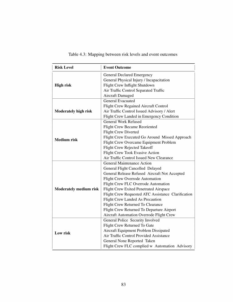
Table 4.3: Mapping between risk levels and event outcomes

Risk Level Event Outcome

High risk

General Declared EmergencyGeneral Physical Injury / IncapacitationFlight Crew Inflight ShutdownAir Traffic Control Separated TrafficAircraft Damaged

Moderately high risk

General EvacuatedFlight Crew Regained Aircraft ControlAir Traffic Control Issued Advisory / AlertFlight Crew Landed in Emergency Condition

Medium risk

General Work RefusedFlight Crew Became ReorientedFlight Crew DivertedFlight Crew Executed Go Around Missed ApproachFlight Crew Overcame Equipment ProblemFlight Crew Rejected TakeoffFlight Crew Took Evasive ActionAir Traffic Control Issued New Clearance

Moderately medium risk

General Maintenance ActionGeneral Flight Cancelled DelayedGeneral Release Refused Aircraft Not AcceptedFlight Crew Overrode AutomationFlight Crew FLC Overrode AutomationFlight Crew Exited Penetrated AirspaceFlight Crew Requested ATC Assistance ClarificationFlight Crew Landed As PrecautionFlight Crew Returned To ClearanceFlight Crew Returned To Departure AirportAircraft Automation Overrode Flight Crew

Low risk

General Police Security InvolvedFlight Crew Returned To GateAircraft Equipment Problem DissipatedAir Traffic Control Provided AssistanceGeneral None Reported TakenFlight Crew FLC complied w Automation Advisory

83

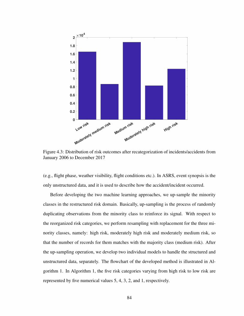
Low risk

Moderately medium ris

k

Medium risk

Moderately high risk

High risk

0

0.2

0.4

0.6

0.8

1

1.2

1.4

1.6

1.8

210

4

Figure 4.3: Distribution of risk outcomes after recategorization of incidents/accidents fromJanuary 2006 to December 2017

(e.g., flight phase, weather visibility, flight conditions etc.). In ASRS, event synopsis is the

only unstructured data, and it is used to describe how the accident/incident occurred.

Before developing the two machine learning approaches, we up-sample the minority

classes in the restructured risk domain. Basically, up-sampling is the process of randomly

duplicating observations from the minority class to reinforce its signal. With respect to

the reorganized risk categories, we perform resampling with replacement for the three mi-

nority classes, namely: high risk, moderately high risk and moderately medium risk, so

that the number of records for them matches with the majority class (medium risk). After

the up-sampling operation, we develop two individual models to handle the structured and

unstructured data, separately. The flowchart of the developed method is illustrated in Al-

gorithm 1. In Algorithm 1, the five risk categories varying from high risk to low risk are

represented by five numerical values 5, 4, 3, 2, and 1, respectively.

84

Algorithm 1 : Hybrid model developmentInput: Two already trained models: support vector machine M1 and ensemble deep

neural networks M2, and test dataset D = {(x1,y1) ,(x2,y2) , . . . ,(xm,ym)}Process:

1: for t = 1 to m do2: if M1 (xt) = M2 (xt) then3: Output the prediction4: else if M1 (xt) 6= M2 (xt) then5: Calculate the proportion of each class in the records with disagreeing predic-

tions6:

p( j) =N j−λ j×Nc

j5∑

k=1

(Nk−λk×Nc

k

) , for j = 1,2, . . . ,5

7: Compute record-level prediction probabilities for xt in the two trained modelsM1 and M2

8: Compute the model predictions for record xi9:

p(Y s

xt= i)

∝

5

∑j=1

p(Y = i| Y s = j

)× p

(Y s

xt= j)×

N j−λ j×Ncj

5∑

k=1

(Nk−λk×Nc

k

)

p(

Y dxt= i)

∝

5

∑j=1

p(Y = i|Yd = j

)× p

(Y d

xt= j)×

N j−λ j×Ncj

5∑

k=1

(Nk−λk×Nc

k

)

10: Return the label with the highest prediction probability from p(Ys

xt

)and

p(Yd

xt

)11: end if12: end for

Output: hybrid model prediction

4.3.2.1 Support Vector Machine for Text-based Classification

Regarding the text data, our objective is to automatically categorize the abnormal event

into the correct risk category based on the content of the event synopsis. In the past decades,

a large number of statistical and computational methods have been developed for classifi-

cation based on text data [124, 134], for example, Naıve Bayes [135, 6], support vector

85

machine [136], maximum entropy [137], and others [138]. As described in Section 2.2.1,

support vector machine (SVM) has been found to provide a higher prediction accuracy

than most other techniques [139] due to the introduction of a structural risk minimization

function, which entails finding an optimal hyperplane to separate the different classes with

the maximum margin. The structural risk minimization (regularization term) function en-

ables SVM to have a good generalization characteristic, thereby guaranteeing the lower

classification error on unseen instances.

The first essential step in applying SVM for text classification is to transform the text

data into numerical feature vectors; this is referred to as text representation. Since the text

descriptions of the incidents/accidents appear in the form of long sentences in different

records, we employ the bag-of-words (BoW) representation to transform the text data into

numerical features. Specifically, we utilize the tokenizer in the natural language processing

toolbox to split raw text into sentences, words and punctuation [140]. Afterwards, all the

stop words and punctuation are eliminated from the BoW representation, and we extract

distinct words from all the event synopsis records, assign a fixed integer id to each term

present in any event synopsis, and represent the content of a document as a vector in the

term space, which is also referred to as a vector space model. However, in many cases, term

frequency alone might not be adequate in differentiating the documents. For example, since

the word ‘the’ is a very common term that appears in every document, the term frequency

method will tend to incorrectly emphasize documents with the usage of frequent terms

(such as, ‘the’, ‘a’) but carrying very little information about the contents of the document,

while more meaningful terms might be shadowed. As developed by Sparck Jones [141], the

term frequency-inverse document frequency (TF-IDF) method overcomes this drawback

by determining the relative frequency of a word in a document compared to the inverse

proportion of that word across all the documents, which is defined as:

tf-idf(t,d) = tf(t,d)×(

1+ log1+nd

1+df(d, t)

)(4.1)

86

where tf(t,d) is the number of occurrences of term t in document d, nd is the total number

of documents, and df(d, t) is the number of documents that contain the term t.

By performing this operation, we can increase the term’s discriminating ability and

make the weight of terms suitable to be used by the classifier. Given the TF-IDF vector

representation of each event synopsis, we feed it into a support vector machine model in

order to identify a hyperplane that separates the different classes with the maximum margin.

In the next section, we will discuss the details on how to tune the model parameters in the

support vector machine model.

4.3.2.2 Ensemble of Deep Neural Networks

With respect to the structured data, there are 29 different data items after removing the

attributes which are empty in 80% of the records. As shown in Fig. 4.2, the structured

data can be further classified into three groups: flight conditions, event characteristics,

and operations. The flight conditions primarily depict the basic operational condition for

each flight, including the weather condition, airport visibility, aircraft characteristics (i.e.,

model, flight mission, and flight plan), the persons involved (i.e., location of person, re-

porter organization), and other contributing factors (i.e., ATC equipment, human factors,

and communication ambiguity). The flight conditions specify the context in which the

accident/incident occurs. Next, the event characteristics describe the important features

pertaining to the accident/incident, including the severity of the aircraft equipment prob-

lem (less severe or critical), the type of the event (illness, smoke, fire, procedural deviation,

or airspace violation), whether passengers were involved in the event, the detecting person,

as well as the time when event is detected (routine inspection, maintenance, or in-flight).

The event characteristics enable us to have a better resolution in understanding a variety of

aspects of the incident, for example, what is the cause of the event, when it happened, and

the severity of the problem. Third, when the pilot or other operator is faced with the prob-

lem, they take certain measures to resolve the issue (e.g., flight crew took evasive action,

87

or flight crew executed an emergency landing as precaution). All the event outcomes are

displayed in the dashed box in the diagram at the bottom right of Fig. 4.2.

Considering the dimension of the input variables, we leverage the deep neural network

(DNN, also referred to as deep learning) to learn the associations between the contextual

features and event outcomes. Over the last five years, DNN has been proven to be very

good at discovering intricate structures in high-dimensional data [30, 103], and has dra-

matically improved the performance of the state-of-the-art in image classification [142],

speech recognition [143], and natural language understanding [144]. Since deep learning

requires very little engineering by hand, it can be updated by additional collection of ab-

normal event records in the ASRS database. Leveraging the powerful capabilities of deep

learning, we have developed an ensemble of feedforward deep neural networks in which

each network consists of two hidden layers with each hidden layer having 24 and 12 neu-

rons. The construction and performance of the ensemble of deep neural networks will be

discussed in the next section.

4.3.3 Model Fusion

As described above, we develop two models: one for the unstructured data, and the

other one for the structured data. How to fuse the prediction results of the two trained

models is the next challenge. Many approaches have been developed to address this issue,

including majority voting schemes (unanimous voting, simple majority, and majority vot-

ing), weighted sum, and support function fusion based on the ranking of each predicted

class in terms of the estimated likelihood in each individual classifier [145]. Several chal-

lenges arise when we attempt to fuse the predictions from the two models by using these

strategies. First of all, since there are only two models here, majority voting is not possible

when the two models have different predictions. Secondly, as there are five classes in the

risk-based event outcome categorization, weighted sum is inappropriate to be implemented

in this circumstance. For example, suppose the support vector machine and the deep neural

88

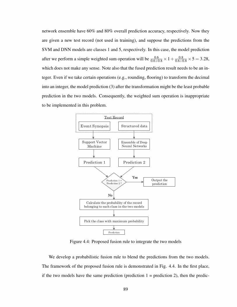
network ensemble have 60% and 80% overall prediction accuracy, respectively. Now they

are given a new test record (not used in training), and suppose the predictions from the

SVM and DNN models are classes 1 and 5, respectively. In this case, the model prediction

after we perform a simple weighted sum operation will be 0.60.6+0.8×1+ 0.8

0.6+0.8×5 = 3.28,

which does not make any sense. Note also that the fused prediction result needs to be an in-

teger. Even if we take certain operations (e.g., rounding, flooring) to transform the decimal

into an integer, the model prediction (3) after the transformation might be the least probable

prediction in the two models. Consequently, the weighted sum operation is inappropriate

to be implemented in this problem.

Event Synopsis Structured data

Support Vector

Machine

Ensemble of Deep Neural Networks

Prediction 1 Prediction 2

Prediction 1 =

Prediction 2 ?

Yes

No

Calculate the probability of the record belonging to each class in the two models

Output the prediction

Prediction

Test Record

Pick the class with maximum probability

Figure 4.4: Proposed fusion rule to integrate the two models

We develop a probabilistic fusion rule to blend the predictions from the two models.

The framework of the proposed fusion rule is demonstrated in Fig. 4.4. In the first place,

if the two models have the same prediction (prediction 1 = prediction 2), then the predic-

89

tion result is easy to be determined. If the two models have different predictions, then we

calculate the probability of the test record belonging to each class among the five risk cate-

gories in each model. To illustrate the proposed method, Table 4.4 reports the performance

metrics of the two models on a validation dataset. The validation dataset consists of N1,

N2, N3, N4, and N5 records in the five respective classes, where Asi, j and Ad

i, j represents the

number of records that actually belong to class i but are labelled as class j in the support

vector machine and DNN ensemble, respectively. The third to the seventh columns present

the confusion matrix of the trained support vector machine on the validation dataset, while

the confusion matrix of the deep learning ensemble is reported in the thirteenth to seven-

teenth column. The ninth column of Table 4.4 reports the number of consistent predictions

between the two trained models on the validation dataset, while the tenth column reports

the accuracy of the correctly labeled records among the consistent predictions of the two

models in the validation dataset.

When the two models have disagreeing predictions, one important underlying mech-

anism when developing the fusion strategy is: since no model is perfect, each model is

expected to have misclassifications or make erroneous predictions. However, the valuable

information embodied in the misclassifications should be further utilized to correct the

model predictions on the subsequent unseen test dataset in a way that makes up the class

that the observation should belong to if we know how often the model mislabels the class

as other classes. Considering the various types of misclassifications that the trained model

is prone to make, one way to achieve this objective is to increase the probability of labeling

the observation as the correct class, while reducing the probability of labeling the record

as the predicted class given by the model. Fortunately, such information can be derived

from the confusion matrix. In fact, a confusion matrix not only provides class-level model

prediction accuracy, but also the probability of mislabeling a record as other classes. Next,

we will utilize the model misclassification probability to correct the model prediction on

new test records. Suppose the two models have different predictions on a new test record

90

a; there are three important considerations in determining the probability of the new test

record a belonging to each of the five classes i in the two models:

1. Record-level prediction probabilities: As mentioned earlier, two models have been

trained: support vector machine and a deep neural network ensemble. The record-

level probability p(Ya = i) measures the probability that the trained model assigns the

test record a to a given class i. To be specific, with respect to the DNN ensemble, the

record-level prediction probabilities can be measured as the ratio of the most frequent

prediction to the total number of model predictions (which is 10, in this case). For

example, if the most frequent prediction of the ten models is class 5, and it appears

six times out of the ten model predictions, then the model prediction probability for

this particular record belonging to class 5 is 6/10 (0.6). Regarding the support vector

machine, since samples far away from the separating hyperplane are presumably

more likely to be classified correctly, we can use the distance from the hyperplane as

a measure of record-level prediction probability following the method introduced in

Ref. [146].

2. Proportion of each class in the records with disagreeing predictions: When the two

models are trained, there are the same number of records belonging to each class

in the training dataset. In other words, the data is balanced for each class in the

training dataset. However, when we use the trained models to make predictions on

test records, we only need decisions when the two trained models have inconsistent

predictions. With respect to the set of disagreeing predictions, the actual proportion

of records belonging to each class might be different (imbalanced) from the training

dataset (balanced). The use of the model trained by the balanced class distribution

will result in a biased estimator if it is directly utilized for making predictions on the

set of records with inconsistent model predictions.

To address this issue, we introduce a weight factor to correct the trained model to

91

fit the class distribution in the set of records with disagreeing model predictions,

thereby ensuring that the updated estimator is unbiased. The number of records with

consistent model predictions in each class is complementary to the amount of records

with inconsistent model predictions in that class. In general, the more records the two

classifiers agree on, the less the number of records the two classifiers disagree on. As

a result, we formulate the following equation to represent the total number of records

with inconsistent model predictions across all the classes considered:

T =5

∑i=1

(Ni−λi×Nci ) (4.2)

where i is the class label, Ni denotes the actual number of records that should have

been labeled as class i, Nci represents the number of consistent predictions between

the two models on all the records, and λi is the model accuracy with respect to the

consistent predictions.

Considering the total number of disagreeing predictions across all the classes, the

proportion w.r.t. class j is:

p( j) =N j−λ j×Nc

j

T(4.3)

Given the already correctly labeled samples by the two trained models, the proba-

bility of a new test record a that results in disagreeing predictions between the two

models belonging to class j is p( j).

3. Class-level accuracy: This measures the degree of consistency between model pre-

dictions and actual observations. Mathematically, it can be represented as: p(Y = i| Y = j

),

where Y = j represents the samples with model predictions being class j, and p(Y = i| Y = j

)(j 6= i) quantifies the proportion of samples with model predic-

tions being class j that should have been labeled as class i. In particular, when j = i,

then p(Y = i| Y = i

)measures the ratio of samples actually belonging to class i

to the number of samples with model predictions being class i, which can also be

92

referred to as a likelihood function. In other words, the likelihood function measures

the probability of observing the data given the prediction. Such a quantitative metric

p(Y = i| Y = i

)measures the accuracy of the trained model in making predictions

with respect to class i.

If we only consider the special case (i= j), then the Bayes factor (or likelihood ratio)

can be used to help decide which model supports our observation better from the two

trained models, thereby assisting the model selection [147]. However, the Bayes

factor does not consider the information embodied in the model misclassifications.

Therefore, we propose an equation below to handle all the possible situations existing

in the five-class classification problem by utilizing the information contained in the

term p(Y = i| Y = j

). The quantitative metric p

(Y = i| Y = j

)is equivalent to

the confusion matrix used in the performance evaluation on the validation dataset.

By utilizing the metric p(Y = i| Y = j

), we relate the model predictions to the

actual observations, from which we compute the probability of a test record a actually

belonging to a given class i in the subsequent sections.

For a given new test record a, the proposed fusion rule based on the above three con-

siderations is:

p(Ya = i) =5

∑j=1

[p(Y = i| Y = j

)p(

Ya = j)× p( j)

p( j)

](4.4)

where p(Y = i| Y = j

)(j 6= i) is the model misclassification rate, in which the model

prediction is class j while the actual observation is class i; when j= i, then p(Y = i| Y = i

)denotes the model prediction precision with respect to class i, p( j) is the proportion of class

j in the set of inconsistent model predictions, p( j) represents the proportion of class j in

the training dataset, and p(

Ya = j)

represents the confidence of the model in classifying

the test record a as class j.

93

Tabl

e4.

4:Pe

rfor

man

cem

etri

csfo

rth

etw

otr

aine

dm

odel

s.H

ere,

the

supp

ortc

olum

nde

note

sth

enu

mbe

rof

occu

rren

ces

ofea

chcl

ass

inth

eac

tual

obse

rvat

ion,

the

cons

iste

ntpr

edic

tion

colu

mn

repr

esen

tsth

enu

mbe

rof

cons

iste

ntpr

edic

tions

betw

een

the

two

mod

els

for

each

clas

s,an

dco

nsis

tent

pred

ictio

nac

cura

cyde

note

sth

epr

opor

tion

ofre

cord

sin

the

cons

iste

ntm

odel

pred

ictio

nsth

atar

eco

rrec

tlyla

bele

d.T

hefiv

enu

mer

ical

valu

es1,

2,3,

4,an

d5

deno

teth

efiv

eri

skca

tego

ries

from

low

risk

tohi

ghri

sk

Supp

ortV

ecto

rM

achi

neSh

ared

Att

ribu

tes

Dee

pL

earn

ing

Ens

embl

ePr

edic

ted

Lab

elSu

ppor

tC

onsi

sten

tPr

edic

tion

Con

sist

entP

redi

ctio

nA

ccur

acy

Pred

icte

dL

abel

12

34

51

23

45

TrueLabel

1A

s 1,1

As 1,

2A

s 1,3

As 1,

4A

s 1,5

N1

Nc 1

λ1

TrueLabel

1A

d 1,1

Ad 1,

2A

d 1,3

Ad 1,

4A

d 1,5

2A

s 2,1

As 2,

2A

s 2,3

As 2,

4A

s 2,5

N2

Nc 2

λ2

2A

d 2,1

Ad 2,

2A

d 2,3

Ad 2,

4A

d 2,5

3A

s 3,1

As 3,

2A

s 3,3

As 3,

4A

s 3,5

N3

Nc 3

λ3

3A

d 3,1

Ad 3,

2A

d 3,3

Ad 3,

4A

d 3,5

4A

s 4,1

As 4,

2A

s 4,3

As 4,

4A

s 4,5

N4

Nc 4

λ4

4A

d 4,1

Ad 4,

2A

d 4,3

Ad 4,

4A

d 4,5

5A

s 5,1

As 5,

2A

s 5,3

As 5,

4A

s 5,5

N5

Nc 5

λ5

5A

d 5,1

Ad 5,

2A

d 5,3

Ad 5,

4A

d 5,5

94

By substituting Eq. (4.3) into Eq. (4.4), we have:

p(Ya = i) =5

∑j=1

[p(Y = i| Y = j

)p(

Ya = j)× 1

p( j)×

N j−λ j×Ncj

T

](4.5)

Since all the five classes are evenly distributed in the training dataset, p( j) is a constant,

which can be ignored, then we have:

p(Ya = i) ∝

5

∑j=1

[p(Y = i| Y = j

)p(

Ya = j)×

N j−λ j×Ncj

T

](4.6)

Next, we perform the normalization operation following Eq. (4.7) such that the sum of

the probability over the five classes in each model is 1.

p(Ya = i) =

5∑j=1

[p(Y = i| Y = j

)p(

Ya = j)× N j−λ j×Nc

jT

]5∑

i=1

5∑j=1

[p(Y = i| Y = j

)p(

Ya = j)× N j−λ j×Nc

jT

] (4.7)

With respect to the support vector machine, the likelihood function p(Y = i| Y = j

)is calculated as:

p(Y = i| Y s = j

)=

Asi, j

5∑

i=1As

i, j

(4.8)

where Asi, j denotes the number of samples with model predictions being class j, but actually

belonging to class i in the validation dataset.

In a similar way, the metric p(Y = i| Y = j

)in the DNN ensemble is computed ac-

cordingly. Given the model classification performance p(Y = i| Y = j

), the probability

95

of test record a belonging to each class in each model is computed as below:

p(Y sa = i) ∝

5∑j=1

p(Y = i| Y s = j

)× p

(Y s

a = j)× N j−λ j×Nc

j5∑

k=1(Nk−λk×Nc

k)

∝

5∑j=1

Asi, j

5∑

i=1As

i, j

× p(

Y sa = j

)× N j−λ j×Nc

j5∑

k=1(Nk−λk×Nc

k)

p(Y d

a = i)

∝5∑j=1

p(Y = i|Yd = j

)× p

(Y d

a = j)× N j−λ j×Nc

j5∑

k=1(Nk−λk×Nc

k)

∝

5∑j=1

Adi, j

5∑

i=1Ad

i, j

× p(

Y da = j

)× N j−λ j×Nc

j5∑

k=1(Nk−λk×Nc

k)

· · · · · ·

(4.9)

where p(Y sa = i) and p

(Y d

a = i)

represent the probability of support vector machine and

deep learning models in labeling the test record as class i, the termN j−λ j×Nc

j5∑

k=1Nk−λk×Nc

k

in Eq.

(4.9) denotes the proportion of records belonging to class j in the set of inconsistent model

predictions; the terms Asi, j and Ad

i, j represent the samples belonging to class i but labeled

as class j in the two respective models, and p(

Y sa = j

)and p

(Y d

a = j)

are the prediction

confidence of the two respective models to classify the test record a as class j.

After normalizing the probability of the test record a belonging to each class in each

model, we select the predicted class with the maximum probability from the two models

as the hybrid model prediction. By considering the three factors, the proposed method

successfully adjusts the trained model to suit the classification with respect to the records

within the inconsistent model predictions. After we obtain the probability of the test record

belonging to each class in each model, then we assign the test record to the class with the

maximum probability.

96

4.3.4 Event-level Outcome Analysis

After the risk-level category that the test record should belong to is probabilistically

determined, then event-level outcome can be derived by measuring the event synopsis sim-

ilarity between the test record a and other records belonging to the same risk category. One

popular way to measure document similarity is based on the content overlap between two

documents [148] as represented in Eq. (4.10).

sim(di,d j

)=

k∑

m=1wm,i×wm, j√

k∑

m=1(wm,i)

2×

√k∑

m=1

(wm, j

)2

(4.10)

where di and d j denote two documents, wm,i (wm, j) is the frequency of object (words, or

terms) om present in document di (d j), and k is the number of unique objects across all the

documents.

The similarity metric defined in Eq. (4.10) measures the cosine of the angle between

vector-based representations of the two documents. Since there are multiple documents be-

longing to the same risk category as the test record a, we formulate the following equation

to address such issues:

p(e = k |Ya = j ) =1ck

ck

∑v=1

sim(da,dI(v)

)(4.11)

where ck denotes the number of records having event outcome k in the training dataset, and

I(v) denotes the index of the v-th record having event outcome k in the training dataset.

Afterwards, a normalization operation can be performed by taking into account all the

possible event outcomes in the j-th risk category.

p(e = k |Ya = j ) =p(e = k |Ya = j )

K∑

k=1p(e = k |Ya = j )

(4.12)

97

where K represents the number of possible event consequences in the j-th risk category.

By considering the event outcomes in the corresponding risk category, a decision tree

can be constructed to demonstrate the probability of each event to occur. In this way, the

risk-level category can be mapped to event-level outcome.

4.3.5 Summary

The methodology developed in this section tackles the problem of risk quantification

regarding the consequences of abnormal events in the national airspace system with a four-

step procedure (see Fig. 4.2):

1. We reorganize all the incidents/accidents based on the risk associated with the con-

sequence of each hazardous event. The risk-based event outcome categorization

enables us to collapse the original 36 unique event outcomes into five groups, and

project the event outcome to the dimension of risk quantification in the representation

of five risk groups: high risk, moderately high risk, medium risk, moderately medium

risk, and low risk. Considering the five risk groups, up-sampling is performed to bal-

ance the number of records between minority classes and majority classes.

2. Two models are developed to process the structured data and unstructured data, re-

spectively. To handle the structured data in high dimension, an ensemble of deep

neural networks are trained to associate the event contextual features with the event

outcomes. A support vector machine model is used to discover the relationships

between event synopsis and event consequence.

3. A probabilistic fusion decision rule is developed to blend the predictions by the two

machine learning models. When the prediction results are inconsistent, a quantitative

metric is proposed to compute the likelihood that the test record belongs to each

predicted class, from which we can determine the class the test record should be

assigned to.

98

4. Once the test record is assigned to a specific risk category, we map the risk-level cat-

egory to event-level outcomes through a probabilistic tree, in which all the possible

event outcomes in the corresponding risk category are considered.

4.4 Computational Results

4.4.1 Data Description

We collected 12 years of incident reports (from January 2006 to December 2017) from

ASRS, thus obtaining 64,573 records. The number of records belonging to each risk class

is shown in Table 4.5. To address the imbalance, we up-sample the three minority classes

(high, moderately high, and moderately medium) with replacement to get the same amount

of data as in the majority class to form a balanced dataset. After up-sampling, the dataset

contains 18,841 records for the high, moderately high, medium, and moderately medium

risk classes respectively, and 16,508 number of records in the low risk category. After the

up-sampling operation, there are 91,872 number of records in total.

Table 4.5: The number of records belonging to each risk category

Class High Moderately high Medium Moderately medium LowNumber of records 12327 8261 18841 8636 16508

All the input variables are summarized in Fig. 4.5, and they are grouped into two cat-

egories: unstructured data and structured data. The structured data includes 29 different

variables ranging from aircraft information to event characteristics, while the unstructured

(text) data only includes event synopsis. With the 29 structured variables and one unstruc-

tured variable, we train the SVM and DNN models.

Table 4.6: Confusion matrix

Predicted as positive Predicted as negativeActually positive True Positives (TP) False Negative (FN)Actually negative False Positives (FP) True Negative (TN)

99

Place

Variables in structured data Unstructured variable

Event Synopsis• Locale reference

• State reference

• Flight conditions

• Weather elements visibility

• Work environment factor

• Light

Environment

Aircraft

Component

Events

Person

Assessments

• ATC advisory center

• Aircraft operator

• Make model name

• Crew size

• Flight plan

• Mission

• Flight phase

• Route in use

• Airspace class

• Aircraft component

• Manufacturer

• Location of person

• Location in aircraft

• Reporter

organization

• Function

• Qualification

• Human factors

• Anomaly

• Detector

• When detected

• Were passengers

involved in event

• Contributing factor situation

• Primary problem

Figure 4.5: Datasets and model inputs

Given a trained classifier and a test dataset, the relationship between model predictions

and true observations can be represented as a confusion matrix, as illustrated in Table 4.6.

To assess the performance of every machine learning model, we adopt three most com-

monly used performance metrics.

1. Precision: Mathematically, Precision ( TPTP + FP ) is the ratio of correctly predicted pos-

itive observations to the total predicted positive observations, and high precision typ-

ically corresponds to low false positive predictions.

2. Recall: Recall is defined as Recall ( TPTP + FN ) quantifies the ratio of correctly labeled

positive observations to all the positive observations in the actual class. It measures

the ability of the trained model in identifying positive observations from all the sam-

ples that should have been labeled as positive.

3. The F1 score is the weighted average of precision and recall, which is mathematically

described as F1 = 2× precision∗recallprecision+recall . In the F1 score, the relative contribution of

100

precision and recall is the same. In other words, the F1-measure is the harmonic

mean of precision and recall.

4.4.2 Experimental Analysis

We split the 91,872 records into three parts: training set (85%), validation set (5%), and

test set (10%). The training set is used to guide the machine learning algorithms to optimize

the relevant parameters so as to minimize prediction error; the validation set is utilized to

develop the performance metrics for an unseen dataset (i.e., prediction accuracy). With the

performance metrics obtained from the validation dataset, we then blend the predictions

from the two trained models for the test dataset.

Regarding the SVM estimator for text classification, we leverage grid search to optimize

the relevant hyperparameters. Specifically, we optimize the loss function (hinge, log, per-

ceptron, squared loss, etc.), the regularization function (l1, l2, or elasticnet), the coefficient

of regularization function ([10−2,10−5]), and the range of N-gram (N-gram is a contiguous

sequence of n items from a given sample of text). The grid search exhaustively generates

candidates from the set of parameter values, and evaluates all the possible combinations of

parameter values on the training dataset and selects the best combination. After the optimal

hyperparameters are identified, we run the trained support vector machine algorithm on the

validation data to obtain its performance metrics. The left part of Table 4.7 reports the

performance metrics of the trained support vector machine model on the validation dataset.

In the DNN model, all the categorical features are encoded using one hot encoding. We

randomly select 85% records from the training dataset to train a deep neural network, then

we repeat the same procedure ten times to obtain an ensemble of deep neural networks.

Every DNN has the same structure – 8 hidden layers and 40 neurons per layer. We choose

an Adam Optimizer [149] with a learning rate of 0.001 to perform backward propagation

in adjusting the weight variables with the objective of minimizing the categorical cross

101

Tabl

e4.

7:Pe

rfor

man

cem

etri

csfo

rth

etw

otr

aine

dm

odel

s.H

ere,

the

supp

ortc

olum

nde

note

sth

enu

mbe

rof

occu

rren

ces

ofea

chcl

ass

inth

eac

tual

obse

rvat

ion,

the

cons

iste

ntpr

edic

tion

colu

mn

repr

esen

tsth

enu

mbe

rof

cons

iste

ntpr

edic

tions

betw

een

the

two

mod

els

for

each

clas

s,an

dco

nsis

tent

pred

ictio

nac

cura

cyde

note

sth

epr

opor

tion

ofre

cord

sin

the

cons

iste

ntm

odel

pred

ictio

nsth

atar

eco

rrec

tlyla

bele

d.T

hefiv

enu

mer

ical

valu

es1,

2,3,

4,an

d5

deno

teth

efiv

eri

skca

tego

ries

from

low

risk

tohi

ghri

sk

Supp

ortV

ecto

rM

achi

neSh

ared

Att

ribu

tes

Dee

pN

eura

lNet

wor

ksPr

edic

ted

Lab

elSu

ppor

tC

onsi

sten

tPr

edic

tion

Con

sist

entP

redi

ctio

nA

ccur

acy

Pred

icte

dL

abel

12

34

51

23

45

TrueLabel

155

082

205

6941

947

491

0.82

TrueLabel

156

774

204

4656

214

951

2713

1210

1798

80.

932

2593

128

528

315

365

592

119

5998

844

80.

763

208

7249

597

116

416

743

943

2510

3493

60.

964

1911

4892

729

520

1734

2288

397

686

10.

935

3827

4528

838

102

entropy as defined in Eq. (4.13).

L(Y , Y d

)=−1

n

n

∑i=1

[Yi logY d

i

](4.13)

where n is the number of training samples, Yi is a one-hot-encoding representation of the

actual observation with the corresponding class label being 1 and the values of other classes

being zero, and Y di is the probabilistic estimation of ensemble deep learning models on the

record i.

After the ten deep neural networks are trained, we use them to make predictions on the

validation dataset, and the results are reported in Table 4.7. It is observed that the DNN

ensemble does not perform as well as the SVM model in terms of precision and recall for

classes 2, 3, and 5 due to the low level of information contained in the categorical features.

As shown in the ninth column of Table 4.7, the two trained models agree on 491, 988, 448,

936, and 961 predictions with respect to the five classes. Among the consistent predictions

of the two models, 401, 922, 339, 897, and 804 predictions with respect to the five classes

are correctly classified, from which we can compute the ratio of consistent predictions that

are correctly labeled in the validation dataset. Next, we utilize the two trained models to

make predictions on the test dataset. With the performance metrics acquired on the vali-

dation dataset, we blend the predictions of the two models. Suppose the two models have

probabilistic classifications on the test record a as shown in Table 4.8; each cell represents

the probability that the test example a is a member of the class. Regarding the test record a,

the SVM model supports class 5 the most, whereas the DNN ensemble assigns the highest

probability to class 2.

Table 4.8: Model predictions with respect to test record a

Model 1 2 3 4 5

SVM 0.10 0.20 0.20 0.20 0.30DNN 0.20 0.40 0.10 0.02 0.28

103

Following the method introduced before, the total number of inconsistent model pre-

dictions is T = (947−401)+(1017−922)+(988−339)+(1034−897)+(976−804) =

1599. Then the proportion of each class in the disagreeing records is calculated as:

p=

[0.34 0.06 0.40 0.09 0.11

]

Then the probability of assigning the test record a to class 1 in the SVM model is computed

as:

p(Y sa = 1) ∝

5∑j=1

[p(

Y = 1|Y s = j)× p

(Y s = j

)× p( j)

]= 550

550+14+153+16+20 ×0.1×0.34+ 8282+951+65+7+17 ×0.2×0.06

+ 205205+27+592+43+34 ×0.2×0.4+ 69

69+13+119+943+22 ×0.2×0.09

+ 4141+12+59+25+883 ×0.3×0.11

= 0.0468

In a similar way, the probabilities of labeling the test record a as other classes in the

SVM model is calculated:

p(Y sa = 2) ∝ 0.0137, p(Y s

a = 3) ∝ 0.0646

p(Y sa = 4) ∝ 0.0193, p(Y s

a = 5) ∝ 0.0324

After normalization, the probability of the test record belonging to each class in the

SVM model is:

p(Y sa = 1) = 0.26, p(Y s

a = 2) = 0.08, p(Y sa = 3) = 0.37,

p(Y sa = 4) = 0.11, p(Y s

a = 5) = 0.18.

Likewise, with the DNN ensemble, the probabilities of the test record a belonging to

class 1 to 5 are calculated as:

p(Y d

a = 1)= 0.35, p

(Y d

a = 2)= 0.15, p

(Y d

a = 3)= 0.28,

p(Y d

a = 4)= 0.04, p

(Y d

a = 5)= 0.18.

104

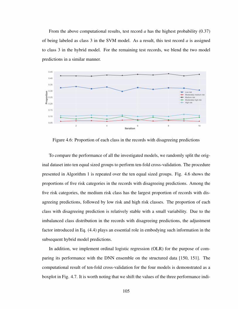
From the above computational results, test record a has the highest probability (0.37)

of being labeled as class 3 in the SVM model. As a result, this test record a is assigned

to class 3 in the hybrid model. For the remaining test records, we blend the two model

predictions in a similar manner.

Figure 4.6: Proportion of each class in the records with disagreeing predictions

To compare the performance of all the investigated models, we randomly split the orig-

inal dataset into ten equal sized groups to perform ten-fold cross-validation. The procedure

presented in Algorithm 1 is repeated over the ten equal sized groups. Fig. 4.6 shows the

proportions of five risk categories in the records with disagreeing predictions. Among the

five risk categories, the medium risk class has the largest proportion of records with dis-

agreeing predictions, followed by low risk and high risk classes. The proportion of each

class with disagreeing prediction is relatively stable with a small variability. Due to the

imbalanced class distribution in the records with disagreeing predictions, the adjustment

factor introduced in Eq. (4.4) plays an essential role in embodying such information in the

subsequent hybrid model predictions.

In addition, we implement ordinal logistic regression (OLR) for the purpose of com-

paring its performance with the DNN ensemble on the structured data [150, 151]. The

computational result of ten-fold cross-validation for the four models is demonstrated as a

boxplot in Fig. 4.7. It is worth noting that we shift the values of the three performance indi-

105

cators of ordinal logistic regression by +0.4 for the sake of demonstrating the four models’

performance deviation clearly. As can be observed, the hybrid model outperforms SVM,

DNN ensemble, and OLR in terms of precision, recall and F1 score. More importantly, the

hybrid model has a much smaller deviation for all the performance metrics when compared

to all the other three models. In other words, it has the most stable prediction capability,

thereby making it the best candidate for quantifying the risk of abnormal events. Since

OLR is inferior to the other three models, we do not analyze its performance any further.

From a quantitative viewpoint, based on the cross-validation results, the proposed hybrid

model yields a better performance in precision, with an average score of 0.81, 3% higher

than the scores of SVM and 6% higher than DNN ensemble models. The proposed hybrid

model also outperforms the other two models regarding the recall rate. In other words, the

hybrid model has a better performance in correctly identifying the records that actually be-

long to each class. Besides, the F1 score of the hybrid model is 3% higher than the support

vector machine and 6% higher than deep neural networks on average. Regarding the pre-

dictions on the structured data, ordinal logistic regression performs much worse than deep

learning ensemble. In summary, the proposed decision rule to fuse the predictions from the

two models is effective in enhancing the hybrid model performance.

Figure 4.7: The performance of hybrid model versus support vector machine (SVM), en-semble of deep neural networks (DNN), and ordinal logistic regression (OLR)

In addition to the boxplot illustrated in Fig 4.7, statistical t-test is also used to check

whether there is a significant difference in the prediction performance of the four mod-

106

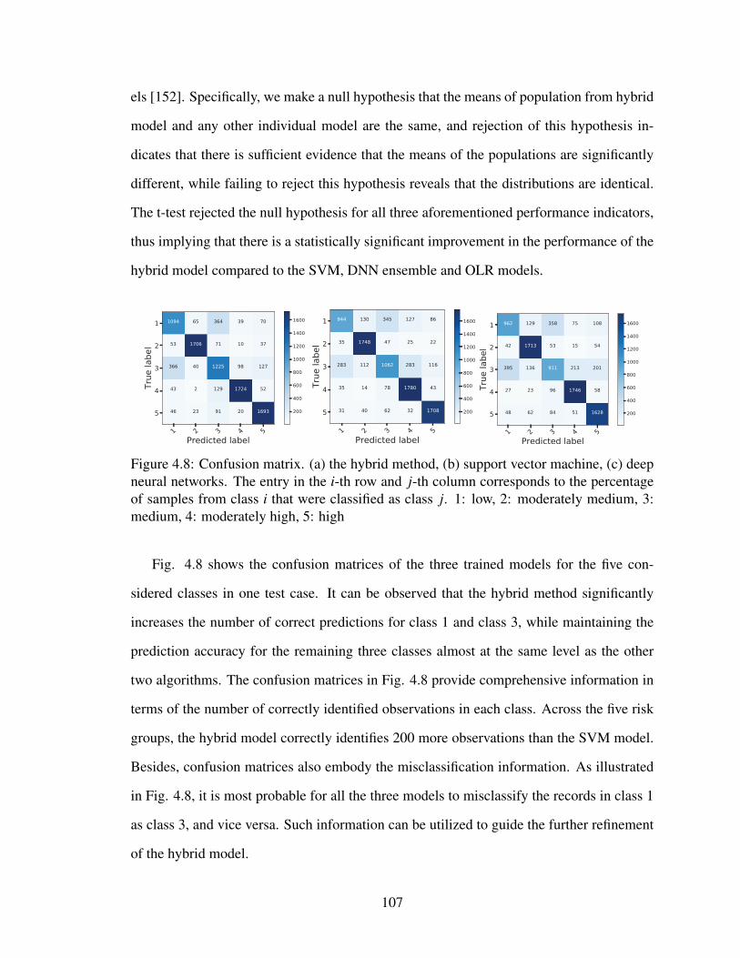
els [152]. Specifically, we make a null hypothesis that the means of population from hybrid

model and any other individual model are the same, and rejection of this hypothesis in-

dicates that there is sufficient evidence that the means of the populations are significantly

different, while failing to reject this hypothesis reveals that the distributions are identical.

The t-test rejected the null hypothesis for all three aforementioned performance indicators,

thus implying that there is a statistically significant improvement in the performance of the

hybrid model compared to the SVM, DNN ensemble and OLR models.

Figure 4.8: Confusion matrix. (a) the hybrid method, (b) support vector machine, (c) deepneural networks. The entry in the i-th row and j-th column corresponds to the percentageof samples from class i that were classified as class j. 1: low, 2: moderately medium, 3:medium, 4: moderately high, 5: high

Fig. 4.8 shows the confusion matrices of the three trained models for the five con-

sidered classes in one test case. It can be observed that the hybrid method significantly

increases the number of correct predictions for class 1 and class 3, while maintaining the

prediction accuracy for the remaining three classes almost at the same level as the other

two algorithms. The confusion matrices in Fig. 4.8 provide comprehensive information in

terms of the number of correctly identified observations in each class. Across the five risk

groups, the hybrid model correctly identifies 200 more observations than the SVM model.

Besides, confusion matrices also embody the misclassification information. As illustrated

in Fig. 4.8, it is most probable for all the three models to misclassify the records in class 1

as class 3, and vice versa. Such information can be utilized to guide the further refinement

of the hybrid model.

107

Table 4.9: Event synopsis of test record a

Date Event Synopsis

March, 2017

After initiating descent on a visual approach with glideslope out of ser-vice; an A319 Flight Crew initiated a go-around when flight directorcaused airspeed increase and climb to intercept altitude set for ILS topreviously assigned runway.

10.14%

Event outcomes

13.26%

11.74%

19.26%

11.87%

10.5%

10.66%

12.57%

Medium risk

General Work Refused

Flight Crew Became Reoriented

Flight Crew Diverted

Flight Crew Executed Go Around Missed Approach

Flight Crew Overcame Equipment Problem

Flight Crew Rejected Takeoff

Flight Crew Took Evasive Action

Air Traffic Control Issued New Clearance

Figure 4.9: The probabilistic event outcomes for test record a

Considering that the test record a is labeled as class 3 (medium risk), and the event

synopsis of the test record a is shown in Table 4.9, then a tree is built to demonstrate the

likelihood of the occurrence of every event outcome in the medium risk category. By mea-

suring the similarity between the event synopsis of test record a and that of other records in

the medium risk category, the probability for test record a having each outcome is obtained,

and the result is illustrated in Fig. 4.9. The red filled node is a chance node used to identify

the event in a decision tree where a degree of uncertainty exists. In this case, since the hy-

brid model does not have the capability to make event-level outcome prediction, we expand

108

the risk-level prediction to event-level outcome prediction by considering all the possible

event outcomes under the corresponding risk category. Along each line is shown the prob-

ability of each event to occur. As can be seen, it is most probable for the test record a to

have event outcome “Flight Crew Executed Go Around Missed Approach”, followed by

“Flight Crew Became Reoriented” and “Air Traffic Control Issued New Clearance”. With

respect to other risk categories, similar diagrams can be constructed to represent event-level

outcomes. Such event-level outcomes enable to connect the root cause (i.e., malfunction)

and the consequence of the incident at the event outcome level.

4.5 Summary

This chapter developed a hybrid machine learning model by blending support vector

machine and an ensemble of deep neural networks, in order to quantify the risk pertaining

to the consequence of hazardous events in the air transportation system. The SVM model is

trained using the event synopsis text, while the DNN ensemble is trained using categorical

and numerical data. By merging the predictions from the two models, we formulate a

hybrid model to assess the severity of abnormal event outcomes in terms of their risk levels

using 64,573 reports on incidents/accidents that were reported between January 2006 and

December 2017.

Several contributions have been made in the developed approach. First, we develop a

risk-based event outcome categorization strategy to project the event outcomes in the space

of risk quantification by collapsing the original 36 unique event outcomes into five risk

groups. Secondly, we propose a support vector machine and deep learning-based hybrid

model to make prediction on the risk level associated with the event outcome by analyz-

ing the event contextual features and event description in an integrated way. Thirdly, an

innovative fusion rule is developed to blend the predictions from the two trained machine

learning algorithms. Finally, a probabilistic tree is constructed to map the risk-level pre-

diction to event-level outcomes. The results demonstrate that the developed hybrid model

109

outperforms the individual models in terms of precision, recall and F1 score.

The development of predictive model in this chapter enhances operators’ situation

awareness on the evolution of hazardous events and prepare them for the consequence

of system malfunction events in advance. With the prediction on malfunction event con-

sequence, operators have more time to prepare necessary resources and take appropriate

measures and actions to prevent the escalation of anomalous events in the system. Even

though the predictive models developed in Chapters 3 and 4 increase operators’ situation

awareness on abnormal events significantly, what matters more is that how human opera-

tors respond in the presence of system malfunction events and how reliable their responses

are, which will be investigated in Chapter 5.

110

Chapter 5

Human Reliability Analysis in Diagnosing and Correcting System Malfunctions1

5.1 Introduction

There are numerous malfunction events that could happen in a system and each off-

nominal event has its own characteristics w.r.t. event detection, diagnosis, and correction.

Even if the operators (i.e., pilots, controllers) are well-trained, it is not certain that they

will take appropriate actions to eliminate system malfunctions effectively in emergency

situations. Hence, this chapter is motivated to investigate the reliability of the human op-

erators in diagnosing and correcting system malfunctions, and we illustrate the approach

with control room operator assessment in a nuclear power plant.

In handling anomalous events, operators’ prior experience and training play an essential

role in affecting their effectiveness in responding to the malfunction events. To measure

the reliability of operators in eliminating malfunction events, we analyze the results of an

experimental study to characterize the performance of operators in responding to system

disturbances. Such research is important to support ongoing efforts to modernize the nu-

clear power plant (NPP) control rooms with fully digital instrumentation and control (I&C)

design. Researchers and practitioners are investigating new technologies to modernize the

user interfaces in NPP control rooms (e.g., design and layout of the graphics, informative-

ness of the alarm system, and ecological interfaces) so that important information regarding

situations can be displayed with appropriate level of salience and effort to access, thereby

enhancing the situation awareness of the operators [154, 155, 156]. Thus innovative hu-

man reliability analysis (HRA) methods are needed to verify the expected improvements

in ensuring safe, reliable, cost-competitive production of electricity [157]. It is essential to

assess the performance of each crew team in maintaining the plant safety margin when the

1An archival paper related to this chapter has been published in the journal Reliability Engineering &System Safety. For more details, see Ref. [153]

111

new I&C technologies are introduced.

To support such assessment, quantitative methods need to be developed to predict the

operator performance based on his/her responses in different contexts and scenarios [154].

As indicated by Mosleh et al. [158], the improvement of human reliability models requires

the inclusion of cognitive theories and measurable human responses. Recent research is

making noticeable advancement in using physiological data for HRA [159], in which fif-

teen graduate students were employed to participate a reactor shutdown scenario in the

control room in a mid-fidelity simulation environment. In transportation, Healey and Pi-

card [160] tracked a number of physiological indicators, including electrocardiogram, elec-

tromyogram, skin conductance, and respiration, while drivers followed a set route through

open roads in the greater Boston area. This study demonstrated that physiological sig-

nals were good indicators of the driver stress. Liang and Lee [161] developed a layered

algorithm that integrates a Dynamic Bayesian Network (DBN) with supervised clustering

to detect the cognitive distraction using eye movement data (i.e., blink frequency, fixation

duration, pursuit duration, and pursuit direction) and driving performance measures.

Adopting a similar direction, we develop an information fusion approach that lever-

ages physiological and eye tracking data for predicting operator performance in respond-

ing to the malfunction events. A significant difference between our investigation and other

HRA models is that the approach developed in this chapter aims at predicting the opera-

tor performance while other HRA models aim at producing failure probability values of

human operators in different scenarios through human-in-the-loop experiments. The dif-

ference in research objective has resulted in a distinct data collection and model structure

in our study. Specifically, we innovate an information fusion approach built on data from

a full-scope, human-in-the-loop simulation experiment that was performed at the Center

for Advanced Engineering and Research (CAER), Forest, Virginia [162, 163]. The exper-

iment employed a full-scale Generic Pressurized Water Reactor (GPWR) simulator in the

CAER control room research facility and recruited nine previously licensed operators to

112

form three crews. Each crew included the positions of unit supervisor (US), reactor-side

operator (RO) and balance-of-plant-side operator (BOP). Ten scenarios were developed to

test the performance of each group. Each experimental scenario consists of two to four

malfunction events. The experimental data include: scenario characteristics, eye tracking

data, physiological data (i.e., skin conductance response and respiration), expert-rated task

performance (i.e., Operator Performance Assessment System – OPAS [164]), self-rated

task performance, subjective workload ratings (the Halden Task Complexity Scale [165]),

situation awareness (SA) (the Process Overview Measure [166]), and subjective SA con-

fidence ratings. Our information fusion extracted and fused numerous features from these

heterogeneous sources of information by a support vector machine model to predict the

operator performance.

The methodology pursued in this chapter has the following components:

1. Quantitative modeling: A novel quantitative model based on empirical data is de-

veloped to predict the control room operator performance, based on physiological

and eye tracking data collected in simulator experiments as well as task workload,

operators’ situation awareness (SA) and SA confidence level.

2. Information fusion: We innovate a framework to integrate multiple, heterogeneous

sources of information. By utilizing various data analytic techniques, we elicit nu-

merous features from the different types of data. These features are incorporated in

the empirical data model for predicting the operator performance.

3. Expert rating: We develop an approach to transform linguistic (categorical) ratings

by experts on the items belonging to each malfunction into numerical counts.

4. Dimension reduction: Correlation analysis is performed among the extracted physio-

logical features. If the correlation coefficient between any two physiological features

is larger than a threshold, the two variables are assumed to carry similar information.

113

In this case, only one of them is selected as input to the model, thereby reducing the

problem dimension.

5. Ensemble modeling: We integrate the support vector machine technique with boot-

strap aggregating to build ensembles of models to leverage the complete dataset and

improve the prediction accuracy given 22 input variables but only 107 records. The

trained quantitative models are then used to predict the performance of the crew team

in other scenarios, and the ensemble model outperforms the individual models in pre-

diction accuracy.

5.2 Experimental study

This section briefly describes the role of each participant, experimental environment,

scenario development process, experimental procedures, and measures of operator perfor-

mance.

Figure 5.1: Simulated control room configuration. Left: reactor operator workstations;Center: large screen display; Right: turbine operator workstation

5.2.1 Participants

Nine previously licensed operators (n = 9) were recruited to form three crews of three

members each. Each crew was composed of one reactor operator (RO), one unit super-

114

visor (US), and one balance-of-plant (BOP) operator. The three operators have different

roles and responsibilities in maintaining the normal operations of NPP. Specifically, the

reactor operator is primarily concerned with managing the nuclear reactor, monitoring the

power-generating equipment, and controlling the amounts of nuclear reactivity through the

control panel; the unit supervisor is mainly responsible for supervising and coordinating

the activities of the control room staff to guarantee the nominal operations of NPP; and the

balance-of-plant operator’s principal responsibility is to ensure that the generated power

flow is equivalent to the amount of energy that is consumed by the market. Each partici-

pant maintained the assigned position for the entire week.

5.2.2 Experimental Environment

A full-scale Generic Pressurized Water Reactor (GPWR) simulator [167] in the CAER

control room was used as the experimental platform. The GPWR simulator provides real-

time simulation of actual nuclear plant operations, and is therefore an effective tool for

evaluating control room design and operator performance. Fig. 5.1 shows the reactor

and turbine operator in the CAER control room, and the hard-wired panels of the GPWR

simulator are displayed across forty eight 24-inch computer monitors. The paper-based and

digital NPP operation procedure manuals are located at the supervisor workstation in the

center of the control room.

On one side of the control room is an observation gallery enclosed by one-way mirrors

for the experimenters to observe the responses and actions of crew members interacting

with the simulator. All the equipment used to collect the physiological data are installed in

this room. As illustrated in Fig. 5.2, the observation gallery is divided into three parts. The

middle of the observation gallery is equipped for the simulator operator (SO) to initialize

the simulator conditions and inject the malfunction during the simulation trial. The left and

right of the observation gallery are equipped for experimenters whose primary tasks are

to rate the operator’s performance according to their observations of the plant parameters

115

Figure 5.2: Configuration of experimental team members in the observation gallery

and participant behaviours. To support experimenter observation and ratings, the Noldus

Observer XT [168] is used to provide or integrate multi-channel audio, multi-angle video,

annotations of operator behavior, physiological data, and plant simulator logs.

5.2.3 Scenario Development

A process expert, recently retired as the simulation trainer at an NPP facility, developed

the initial set of non-site specific process events for all the scenarios to test participants,

who were previously licensed operators. The initial set of process events in each scenario

were then tested and refined at the CAER facility with the support of a second simulation

trainer, who was recently retired from the NPP simulated by the GPWR. This assistant

scenario developer helped fine-tune the individual events to achieve the desired nuclear

and thermo-hydraulic process behaviors in the simulator.

The refined scenarios were further evaluated with two additional pilot operators, who

were also retired NPP operators (these pilot operators subsequently served as the human

performance raters in this study). The pilot operators were not previously exposed to the

scenarios in any way. They commented (i.e., think aloud) on the plant process behaviors

as they acted as operators monitoring, diagnosing, and controlling the GPWR for the 10

refined scenarios. The scenario developer refined the scenarios to final specification after

116

addressing the pilot operators’ concerns raised from the perspective of the participants.

In addition, two process experts independently rated each event in each scenario on four

different dimensions of difficulty: detection, diagnosis, intervention, and restoration. Each

dimension was rated on a five-point Likert scale [169].

5.2.4 Experimental Procedures

Before the data collection, a retired NPP operator trainer familiarized the participat-

ing operators with the GPWR power plant systems, and guided the practice on operating

the GPWR for one day and a half. After the training, the operators took part in a prac-

tice scenario to get accustomed to all the items in the experimental trial, i.e., wearing the

physiological gear, calibration of the devices, and completing the questionnaires.

All the operators wore several data collection instruments: wireless microphones (BOP,

RO, US), TobiiTM eye tracking glasses (BOP, US) [170], BIOPAC BN-PPGED electroder-

mal activity transmitters [171] (RO, US), and BIOPAC BN-RESP-XDCR thoracic expan-

sion (i.e., breathing) transducers [172] (RO, US). The selection of the data collection in-

struments was based on practicality in terms of comfort and setup time, availability to the

research team, and relevance of the measurements according to the literature.

During the experiment, the participants completed ten different scenarios, and each

scenario consisted of two to four malfunction events of varying difficulty levels. Each crew

acted as if they were on duty to eliminate the malfunction events to maintain the plant safety

as well as to bring the plant back to steady state. Each scenario lasted for nearly 1.5 hours,

and was subdivided into two periods. A “scenario-freeze” (lasting around 20 minutes) was

defined to signal the termination of each period. During this freeze period, the operators

responded to human performance questionnaires at workstations away from the control

room area. The entire experiment protocol takes one week to test the performance of each

crew on the ten scenarios.

117

5.2.5 Operator Performance Measures

Data was collected on a variety of factors: plant performance (based on simulator logs

including alarms, and trend graphs), task performance (both expert- and self-ratings), work-

load, situation awareness (SA), SA confidence, and physiological measures (electrodermal

activity, thoracic expansion, and eye tracking). The selection of these performance mea-

sures was based on the key human factors engineering design goals prescribed by the NRC

in NUREG 0711 [173]. In the subsections, we briefly describe these human performance

measures.

5.2.5.1 Workload

Table 5.1: Modified Halden Task Complexity Scale (HTCS) questionnaire used in the ex-periment

Workload items How difficult was this scenario with respect to:

Item 1 Ambiguous, misleading or missing information on the displaysItem 2 Ambiguous, misleading or missing feedback on control actionsItem 3 Time for planning and responding to the plant event/disturbanceItem 4 Execution of every single task complicated by many simultaneous tasksItem 5 Collection and utilization of information to handle the plant disturbance

A modified Halden Task Complexity Scale (HTCS) [174] was used to measure the oper-

ator workload. The HTCS, originally developed by the Halden Reactor Project in Norway,

is a subjective task-complexity scale that measures the degree of difficulty encountered by

the control room operators. In this experiment, all the operators rated the five items shown

in Table 5.1 on a seven-point Likert scale [169] varying from ‘very difficult’ (1) to ‘very

easy’ (7).

5.2.5.2 Situation Awareness

Situation awareness (SA) was assessed through the Process Overview Measure (POM) [175,

176], in which a series of queries were employed to elicit the operator’s awareness on the

118

Table 5.2: Sample process overview measure items

Compared to its value when the “charging pumps discharge header high-low flow” alarm (ALB 06-1-1) was received?1. Median Tavg Recorder indication is now:What is your confidence in your answer?

Lower Same HigherNot Conf Neutral Conf

2. Pressurizer Level indication (LI-461) is now:What is your confidence in your answer?


3. Main Generator Gross Electrical Output is now:What is your confidence in your answer?


4. VCT Level indication (LI-115) is now:What is your confidence in your answer?


5. Charging Flow indication (FI-122) is now:What is your confidence in your answer?


6. RHX Letdown Temperature indication (TI-140) is now:What is your confidence in your answer?


changes in relevant plant parameters pertaining to the malfunction event. Table 5.2 presents

six process overview queries that were administered during one scenario-freeze. Each ques-

tion elicited the operator’s awareness on the parameter change: whether the parameter had

“increased”, “decreased”, or “remained the same” after the introduction of the abnormal

event. In addition to the situation awareness on the parameter change, the operators were

instructed to provide a confidence rating specific to their response to each query, i.e., “confi-

dent”, “neutral”, or “not confident”. During each simulator freeze, the operators completed

the six process overview queries and corresponding confidence ratings. These queries are

used to measure each operator’s understanding of the plant state change, and are closely

related to the operator’s performance in resolving the malfunction. The confidence ratings

are used to indicate the operator meta-awareness (i.e., limitation of their own knowledge)

that would be relevant to direct their monitoring behavior.

5.2.5.3 Expert-rated Task Performance

The task performance of each team was rated independently by the two process experts

using the rating sheet developed according to the Operator Performance Assessment Sys-

tem (OPAS) [164]. The performance rating items were developed by the scenario designer,

and included the expected stepwise operator reactions to eliminate the corresponding mal-

functions. Table 5.3 shows a sample of OPAS rating items for the first scenario (note: there

119

Table 5.3: Sample malfunction and OPAS rating items in the first scenario

Malfunction & Expected Operator Actions Range of Performance Score

Malfunction: LT-459 failureDETECTION* Responds to alarms for decreasing PZR level and in-creasing CHG flow* Team compares channels of PZR level identifying thefailed channel

Expert use of available diverse indications. 3Minor delays in checking diverse indica-tions.

2

Significant lapses in use of available indi-cations delay response to failure.

1

Diverse indications not used effectively. 0

DIAGNOSIS* When LT-459 < 17% Team IDs:* Letdown has isolated* PZR heaters OFF

Timely ID Letdown isolated and heatersoff.

3

Minor delay in ID. 2IDs but does not recognize significance. 1Does not identify letdown isolation &heaters off.

0

RESPONSETakes action to limit PZR Level increase:* Reduces CHG to minimum ( 0gpm)* Reduces seal injection within limits

CHG to 0 gpm and Seal Injection to mini-mum.

3

CHG to 0gpm but no Seal Injection adjust-ment.

2

CHG reduced but not to 0 gpm. 1CHG not reduced. 0

RESPONSEMonitors parameters:* PZR Level* RCS Pressure* Blender AUTO makeup

Broad awareness and verification of opera-tion.

3

Occasional monitoring – generally aware. 2Few checks not aware of some AUTOMakeups.

1

No monitoring. 0

RESPONSEUtilizes ALB 9-4-3 to:* Deselect LT-459 (control & RCDR)* Initiate OWP-RP* Resets & energizes PZR Heaters

All aspects of ARP properly implemented. 3Deselects but a few other aspects not ad-dressed.

2

Slow to deselect – several aspects not ad-dressed.

1

Fails utilize ARP. 0

RESPONSEOP-107, Sect. 1.4 (L/D):* Proper sequence for valve operation* Proper PCV operation (no RV lift)* Proper CHG flow for Letdown Flow

All aspects of Letdown rest properly per-formed.

3

Minor challenges to RV or Letdown cool-ing.

2

Lifts RV, inadequate CHG flow 1Not performed. 0

RESPONSERestore PZR level to program:* Adequate CHG for letdown* Steady trend toward program* Restores control system to AUTO

Level toward program – control back toAUTO.

3

Level toward program – maintains MANcontrol.

2

Slow to restore level – few T alarms 1No attempt to restore level, inadequatecooling.

0

120

are four malfunction events in the first scenario, Table 5.3 only describes the first malfunc-

tion event and the correct procedures to resolve the malfunction), in which the malfunction

and expected operator actions are clearly demonstrated. The sample illustrates that each

item included predefined performance criteria associated with a score between zero and

three. The score zero implies failing to complete the step and three represents an ideal

response.

Two process experts (retired, formerly licensed NPP operators) rated the participants on

the corresponding OPAS items from the observation gallery based on the observed behavior

of the participants as well as the process parameter values from the simulator, and the

integrated audio/video information from the Noldus Observer XT. Rater 1 was present for

all three weeks of the experiment, while Rater 2 was only present for weeks 1 and 3. The

two raters were separated by a partition in the gallery and refrained from discussion to

minimize mutual rating influence.

5.3 Data Analysis

This section presents the analysis performed on the different types of experimental

data, and introduces the analytic techniques used to derive significant features from these

heterogeneous data. These features subsequently serve as inputs to the quantitative model

for predicting the operator performance.

The developed methodology consists of four parts, as illustrated in Fig. 5.3. First,

we extract the context characteristics of each scenario from the relevant documents, e.g.,

scenario reports. These data provide scenario-wide features, including scenario difficulty,

task complexity, and workload. The linguistic ratings on participants’ situation aware-

ness are converted into numerical scores by comparing the responses of the operators to

those provided by the simulator operator and incorporating the operator confidence rat-

ings. Second, the physiological data, e.g., skin conductivity (also known as electrodermal

activity or EDA) and respiration data, are subjected to event-related analysis to identify

121

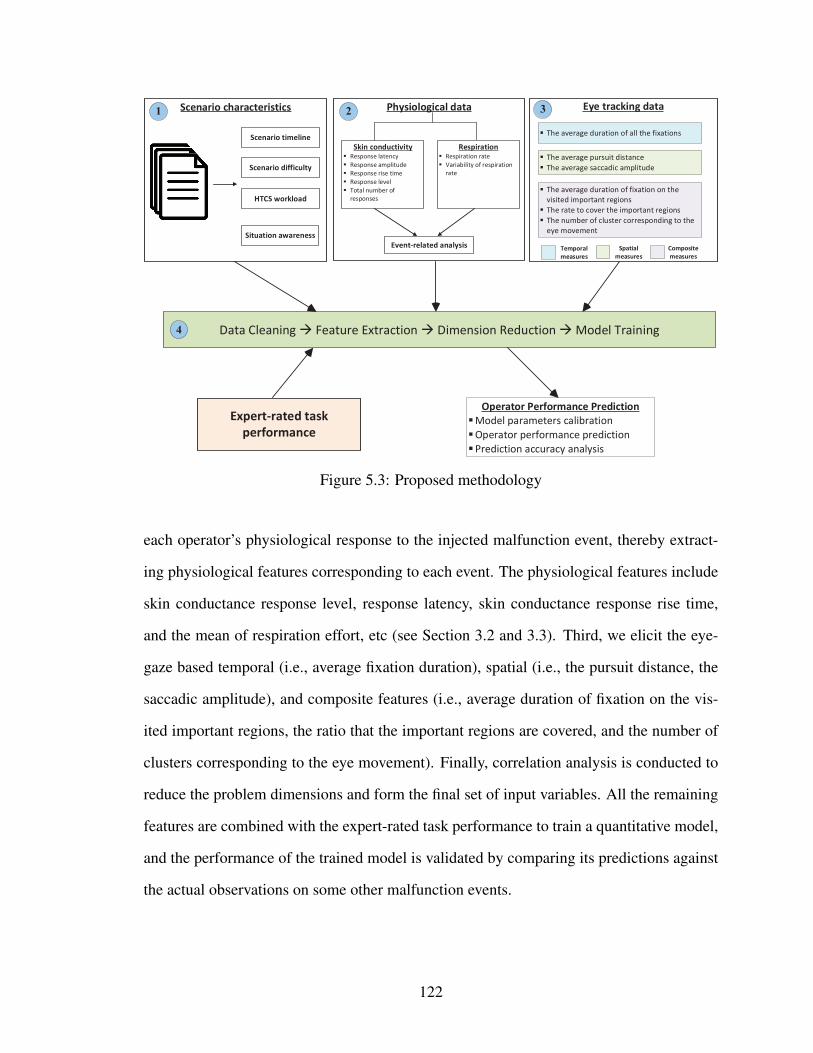
Eye tracking data

§ The average duration of fixation on the

visited important regions

§ The rate to cover the important regions

§ The number of cluster corresponding to the

eye movement

§ The average pursuit distance

§ The average saccadic amplitude

§ The average duration of all the fixations

Temporal

measures

Spatial

measures

Composite

measures

Data Cleaning à Feature Extraction à Dimension Reduction à Model Training

Operator Performance Prediction

§ Model parameters calibration

§ Operator performance prediction

§ Prediction accuracy analysis

Expert-rated task

performance

Scenario characteristics

Scenario timeline

Scenario difficulty

HTCS workload

Situation awareness

Physiological data

Skin conductivity

§ Response latency

§ Response amplitude

§ Response rise time

§ Response level

§ Total number of

responses

Respiration

§ Respiration rate

§ Variability of respiration

rate

Event-related analysis

1 2 3

4

Figure 5.3: Proposed methodology

each operator’s physiological response to the injected malfunction event, thereby extract-

ing physiological features corresponding to each event. The physiological features include

skin conductance response level, response latency, skin conductance response rise time,

and the mean of respiration effort, etc (see Section 3.2 and 3.3). Third, we elicit the eye-

gaze based temporal (i.e., average fixation duration), spatial (i.e., the pursuit distance, the

saccadic amplitude), and composite features (i.e., average duration of fixation on the vis-

ited important regions, the ratio that the important regions are covered, and the number of

clusters corresponding to the eye movement). Finally, correlation analysis is conducted to

reduce the problem dimensions and form the final set of input variables. All the remaining

features are combined with the expert-rated task performance to train a quantitative model,

and the performance of the trained model is validated by comparing its predictions against

the actual observations on some other malfunction events.

122

5.3.1 Scenario Characteristics Extraction

Table 5.4: Difficulty ratings for Scenario 1

Scenario Malfunction event Rater Detection Diagnosis Intervention Restoration

1 1 1 2 2 3 21 1 2 2 2 3 2

Table 5.5: HTCS workload ratings on the first scenario

Scenario Week Day Rater Workload item Score

1 3 2 RO 1 21 3 2 RO 2 21 3 2 RO 3 31 3 2 RO 4 21 3 2 RO 5 31 3 2 BOP 1 31 3 2 BOP 2 31 3 2 BOP 3 31 3 2 BOP 4 31 3 2 BOP 5 31 3 2 US 1 11 3 2 US 2 21 3 2 US 3 31 3 2 US 4 21 3 2 US 5 2

As indicated in Fig. 5.3, the scenario-wide characteristics are embodied in several data

sources, including the scenario difficulty, HTCS workload, and situation awareness of each

operator on each scenario. In the remainder of the chapter, we take one scenario as an ex-

ample to illustrate the data available to us. Table 5.4 presents the two process experts’ diffi-

culty ratings on four dimensions (detection, diagnosis, intervention, and restoration) for the

first malfunction event in the first scenario. Many existing studies have demonstrated that

the difficulty of the scenario is closely correlated with performance. For example, Healey

& Picard [160] showed that the driver’s stress was heavily influenced by the driving condi-

tions (highway driving, or city driving) because the roads with higher traffic flow increase

the driver’s cognitive workload, thus decreasing his performance accordingly. The scenario

123

difficulty plays a similar role in this study. The scenario with higher overall difficulty rating

are hypothesized to decrease the situation awareness and task performance.

Another important factor is workload measured through the HTCS. The participated

operators rated five items shown in Table 5.1 on a 7-point Likert scale. Table 5.5 shows

the specific HTCS workload ratings on the first scenario by the three operators in the first

crew. The workload ratings are useful indicators on the operators’ perceived challenges in

monitoring abnormal plant states, the possible causes of such states, as well as the number

and type of tasks that need to be accomplished to eliminate such abnormal events. If too

many tasks are assigned to one operator, then the operator is overloaded with the assigned

tasks, his performance will be impacted.

Table 5.6: Operators’ situation awareness on the malfunction events in the first scenario(SO: simulator operator, RO: reactor operator, BOP: balance-of-plant-side operator, US:unit supervisor)

Scenario Week Day Rater Item Score Confidence Converted numerical values

1 3 2 SO 1 same confident -1 3 2 SO 2 lower confident -1 3 2 SO 3 same confident -1 3 2 SO 4 higher confident -1 3 2 SO 5 lower confident -1 3 2 SO 6 higher confident -1 3 2 RO 1 same confident -31 3 2 RO 2 same confident 31 3 2 RO 3 same neutral -21 3 2 RO 4 higher confident -31 3 2 RO 5 lower confident -31 3 2 RO 6 higher not confident -11 3 2 BOP 1 same neutral -21 3 2 BOP 2 same neutral 21 3 2 BOP 3 higher confident 31 3 2 BOP 4 higher confident -31 3 2 BOP 5 lower neutral -21 3 2 BOP 6 higher neutral -21 3 2 US 1 higher neutral 21 3 2 US 2 same confident 31 3 2 US 3 higher confident 31 3 2 US 4 higher confident -31 3 2 US 5 same confident 31 3 2 US 6 same neutral 2

Situation awareness indicates the operator’s mental awareness on the system states and

124

the mechanisms causing abnormal events. In an NPP, when an abnormal situation occurs

in an NPP, operators perform situation assessment by monitoring the relevant plant pa-

rameters, then process the information to establish appropriate situation models to explain

the plant’s state. If the situation model precisely reflects the plant’s state, the operator is

considered to have good situation awareness. As the plant state evolves, the operators must

periodically re-sample or monitor the relevant process parameters based on their confidence

of whether the parameters might have deviated from the knowledge generated from prior

sampling of process information. In this study, the items listed in Table 5.2 are utilized to

measure each operator’s perceived understanding and confidence on the changes of the rel-

evant system parameters of the nuclear power plant. The correct responses to the parameter

changes provided an indication of their situation awareness on the entire process; whereas,

the confidence ratings provided an indication of operator meta-awareness or meta-SA on

their own understanding on the plant process. Operators who were confident and accurate

in their awareness of parameter changes most likely engaged in appropriate sampling of

process information, whereas, operators who were less confident in their accurate aware-

ness of parameter changes would more likely sample the wrong process information.

Table 5.6 illustrates each operator’s specific responses to the questions listed in Table

5.2. The sixth and seventh column represents the operator response and confidence on

the parameter changes in linguistic terms, respectively. In addition to the three operators’

(BOP, US, and RO) responses, we have responses from the Simulator Operator (SO). It is

worth noting that prior to the data collection, the scenario developer acted as the simulator

operator for all the scenarios to evaluate the actual parameter changes. Thus, the ratings

from the simulation operator can be considered as true states of the system.

One challenge here is how to convert the linguistic terms into numerical values. Here,

we replace the linguistic ratings “higher”, “same”, and “lower” using +1, 0, and -1 re-

spectively, then compare the responses of the operators to those provided by the simulator

operator to obtain the deviation between their situation awareness. As shown in Fig. 5.4,

125

Simulator operator’s response

+1 0 -1

Operator’s

actual

response

+1 0 1 2

0 -1 0 1

-1 -2 -1 0


+1 0 -1

Operator’s

actual

response

+1 0 1 2

0 1 0 1

-1 2 1 0

Replace zero with

-1


+1 0 -1

Operator’s

actual

response

+1 -1 1 2

0 1 -1 1

-1 2 1 -1

If the operator is

neutral (2)


+1 0 -1

Operator’s

actual

response

+1 -2 2 4

0 2 -2 2

-1 4 2 -2

Figure 5.4: Conversion process for situation awareness ratings

the table in the top left shows the difference among the two raters after we subtract the

simulator operator’s rating from the operator’s actual rating. The values of all the diagonal

elements are zero because the operator’s situation awareness conforms with the simula-

tor operator’s. Afterwards, we take their absolute values to measure the relative distance

between the two operators’ ratings, which is shown in the table at the top right of Fig.

5.4. Next, we substitute the different confidence ratings “confident”, “neutral”, and “not

confident” with +3, +2, and +1 respectively. The product of the confidence rating and the

relative distance of the operators’ response from the simulator operator’s response is used

as an indicator of situation awareness for each operator in understanding the impact of the

abnormal events on the plant states. As can be observed from the table at the top right, if the

ratings between the simulator and the plant operator are the same, we cannot distinguish the

different confidence levels because the product of the two factors is always zero whether

the operator is confident (0×3 = 0), neutral (0×2 = 0), or not confident (0×1 = 0).

To address this issue, we substitute the zeros in this table with ‘-1’ if the responses of

the simulator operator and the participant operator are the same, as shown in the table at the

bottom right. Afterwards, we multiply the relative distance with the corresponding confi-

126

dence level to acquire the situation awareness of each operator. From the table at the bottom

left of Fig. 5.4, we can differentiate the different confidence levels of the plant operator if

his/her response conforms with the simulator operator’s response. Another consideration

is that the lower the numerical values, the better the situation awareness, therefore this

justifies replacing zero with -1. The last column in Table 5.6 displays the converted nu-

merical values for the three participating operators, and these values will be utilized in the

quantitative model in the following sections.

Another problem is that some of the data on confidence ratings related to the situation

awareness are missing (about 16% of the values in the seventh column in Table 5.6). In

this case, since we do not know the degree of operator’s confidence on the plant parameter

change, the lack of such knowledge forces us to provide a value that reveals no preference

on the operator’s confidence. Hence, we replace the missing values with the confidence

rating “neutral”.

5.3.2 Physiological Data Analysis

5.3.2.1 Skin Conductance Response Data Analysis

Electrodermal activity is an umbrella term for autonomic changes in the electrical prop-

erties of the skin. A widely used measure is skin conductance response (SCR). The fun-

damental mechanism of the skin conductance response is to apply electrical potential and

then measure the current flow between two points of skin contact. The skin conductance

response is the most useful indicator on the dynamic changes of the participating opera-

tor’s emotional and cognitive states. In fact, this metric has been proposed for detecting

vehicle driver’s stress [160], assessing aircrew workload [177], and evaluating the cogni-

tive workload [178] because they can be collected continuously without interfering with

the operator’s task performance.

In this study, we used the Electrodermal Activity (EDA) BioNomadix module from the

BIOPAC Systems to collect the skin conductance response for the unit supervisor and the

127

Figure 5.5: Cleaning of the skin conductance response signal

reactor operator. Here, we pick a particular waveform of the skin conductance response

from the unit supervisor in one scenario to illustrate the data analysis procedures using the

software AcqKnowledge 5.0.1. Fig. 5.5 shows four steps of the data cleaning operations.

Initially, we load the raw data into the software and the original tonic skin conductance

signal is shown at the very top of Fig. 5.5. Tonic skin conductance, also known as Skin

Conductance Level (SCL), is generally considered as the level of skin conductance in the

absence of any particular discrete environmental event or external stimuli. In our study,

128

1,000 samples are collected per second to characterize the tonic skin conductance. To

reduce the computational burden and speed up the analysis, we resample the waveform at a

rate of 62.5 samples per second, and the resampled waveform is displayed in the second row

of Fig. 5.5. The multiple square-wave spikes in the resampled waveform are the artifacts of

the signals because the skin conductance cannot change in such a huge magnitude within

such a short time. Hence, we apply a median-based smoothing with a factor of 63 samples,

from which about 20% of artifacts in the original EDA signal are removed. The third

row of Fig. 5.5 shows a processed waveform, in which many higher transient spikes have

disappeared while some lower transient spikes remain. Since these lower transient spikes

cover a spectrum of wide area, the median smoothing operation fails to eliminate these

large artifacts. To remove these mild spikes, we zoom into the signal and manually connect

the endpoints of each spike using a straight line. The most bottom graph in Fig. 5.5 shows

the final waveform after cleaning the data.

Afterwards, we conduct event-related data analysis to identify the consequent skin con-

ductance responses driven by each injected malfunction event. The three-step procedure

is demonstrated in Fig. 5.6. First, we construct a new phasic EDA signal by subtracting

the (median value smoothing) filtered waveform from the original. Since median value

smoothing discards the areas of rapid change, subtracting this smoothed waveform from

the original enables us to focus on sections where the data are changing rapidly. The phasic

skin conductance, also referred to as skin conductance response (SCR), is a common reac-

tion to short-term events that occur in the presence of discrete environmental stimuli, and

the stimuli usually cause an abrupt increase in the skin conductance, or “peaks” in the skin

conductance. The phasic skin conductance facilitates the quantification on the magnitude

and duration of each operator in physiological response to the abnormal event. The top two

graphs of Fig. 5.6 represent the original waveforms of the phasic skin conductance and the

skin conductance response, respectively. The blue markers in the waveform represent the

SCR, but they are not related to any stimuli yet.

129

Figure 5.6: Event-related data analysis on the skin conductance response

To relate the SCR to malfunctions, we load the scenario timeline by importing mark-

ers from Observer XT. The middle graph of Fig. 5.6 illustrates four different malfunction

events for this scenario. The scenario timeline specifies the important time stamps when

each malfunction starts or ends, and the “scenario-freeze”. The integration of the time-

line and the phasic skin conductance signal provides the foundation for the subsequent

event-related data analysis. Finally, event-related data analysis is performed, resulting in

the bottom graph of Fig. 5.6. The red water drops represent the response related to that

130

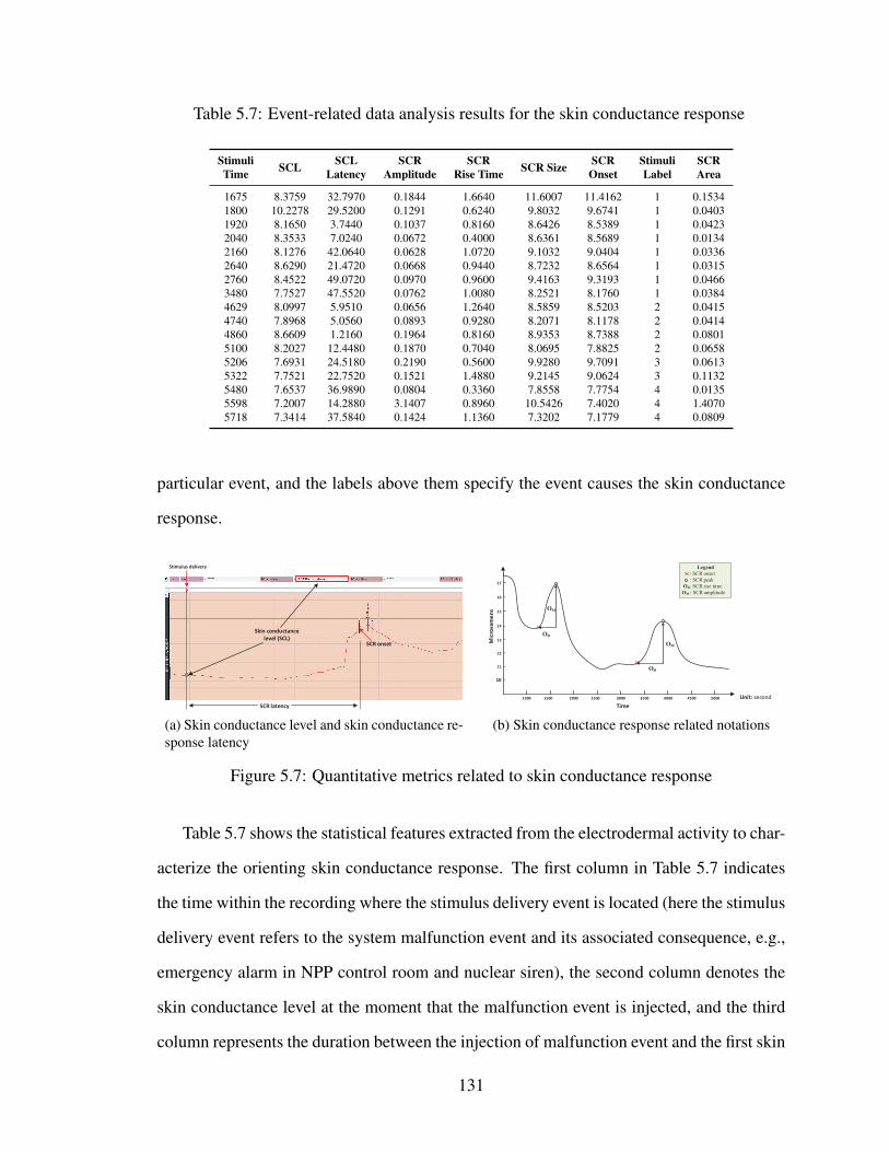
Table 5.7: Event-related data analysis results for the skin conductance response

StimuliTime SCL SCL

LatencySCR

AmplitudeSCR

Rise Time SCR Size SCROnset

StimuliLabel

SCRArea

1675 8.3759 32.7970 0.1844 1.6640 11.6007 11.4162 1 0.15341800 10.2278 29.5200 0.1291 0.6240 9.8032 9.6741 1 0.04031920 8.1650 3.7440 0.1037 0.8160 8.6426 8.5389 1 0.04232040 8.3533 7.0240 0.0672 0.4000 8.6361 8.5689 1 0.01342160 8.1276 42.0640 0.0628 1.0720 9.1032 9.0404 1 0.03362640 8.6290 21.4720 0.0668 0.9440 8.7232 8.6564 1 0.03152760 8.4522 49.0720 0.0970 0.9600 9.4163 9.3193 1 0.04663480 7.7527 47.5520 0.0762 1.0080 8.2521 8.1760 1 0.03844629 8.0997 5.9510 0.0656 1.2640 8.5859 8.5203 2 0.04154740 7.8968 5.0560 0.0893 0.9280 8.2071 8.1178 2 0.04144860 8.6609 1.2160 0.1964 0.8160 8.9353 8.7388 2 0.08015100 8.2027 12.4480 0.1870 0.7040 8.0695 7.8825 2 0.06585206 7.6931 24.5180 0.2190 0.5600 9.9280 9.7091 3 0.06135322 7.7521 22.7520 0.1521 1.4880 9.2145 9.0624 3 0.11325480 7.6537 36.9890 0.0804 0.3360 7.8558 7.7754 4 0.01355598 7.2007 14.2880 3.1407 0.8960 10.5426 7.4020 4 1.40705718 7.3414 37.5840 0.1424 1.1360 7.3202 7.1779 4 0.0809

particular event, and the labels above them specify the event causes the skin conductance

response.

Stimulus delivery

Skin conductance

level (SCL)SCR onset

SCR latency

(a) Skin conductance level and skin conductance re-sponse latency

10

11

12

13

14

15

16

17

1000 1500 2000 2500 3000 3500 4000 4500 5000 Unit: second

Mic

rose

me

ns

Time

OD

OD

OM

OM

Legend

: SCR onset

: SCR peak

OD: SCR rise time OM : SCR amplitude

(b) Skin conductance response related notations

Figure 5.7: Quantitative metrics related to skin conductance response

Table 5.7 shows the statistical features extracted from the electrodermal activity to char-

acterize the orienting skin conductance response. The first column in Table 5.7 indicates

the time within the recording where the stimulus delivery event is located (here the stimulus

delivery event refers to the system malfunction event and its associated consequence, e.g.,

emergency alarm in NPP control room and nuclear siren), the second column denotes the

skin conductance level at the moment that the malfunction event is injected, and the third

column represents the duration between the injection of malfunction event and the first skin

131

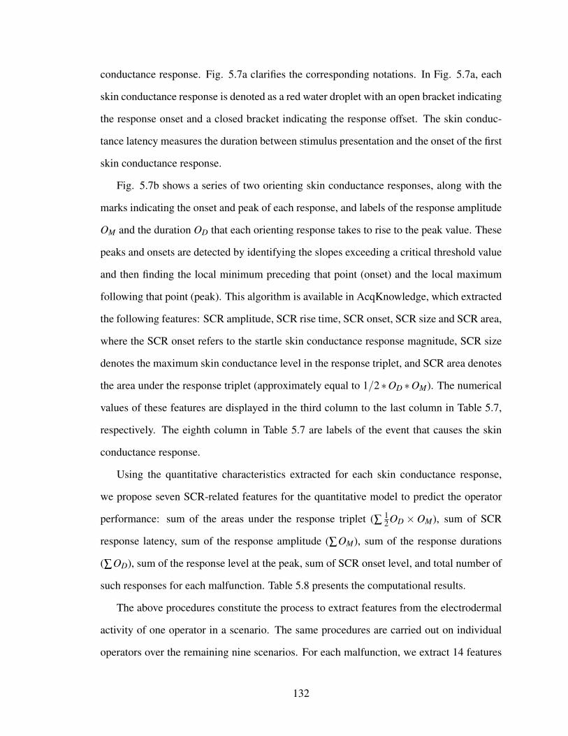
conductance response. Fig. 5.7a clarifies the corresponding notations. In Fig. 5.7a, each

skin conductance response is denoted as a red water droplet with an open bracket indicating

the response onset and a closed bracket indicating the response offset. The skin conduc-

tance latency measures the duration between stimulus presentation and the onset of the first

skin conductance response.

Fig. 5.7b shows a series of two orienting skin conductance responses, along with the

marks indicating the onset and peak of each response, and labels of the response amplitude

OM and the duration OD that each orienting response takes to rise to the peak value. These

peaks and onsets are detected by identifying the slopes exceeding a critical threshold value

and then finding the local minimum preceding that point (onset) and the local maximum

following that point (peak). This algorithm is available in AcqKnowledge, which extracted

the following features: SCR amplitude, SCR rise time, SCR onset, SCR size and SCR area,

where the SCR onset refers to the startle skin conductance response magnitude, SCR size

denotes the maximum skin conductance level in the response triplet, and SCR area denotes

the area under the response triplet (approximately equal to 1/2∗OD ∗OM). The numerical

values of these features are displayed in the third column to the last column in Table 5.7,

respectively. The eighth column in Table 5.7 are labels of the event that causes the skin

conductance response.

Using the quantitative characteristics extracted for each skin conductance response,

we propose seven SCR-related features for the quantitative model to predict the operator

performance: sum of the areas under the response triplet (∑ 12OD ×OM), sum of SCR

response latency, sum of the response amplitude (∑OM), sum of the response durations

(∑OD), sum of the response level at the peak, sum of SCR onset level, and total number of

such responses for each malfunction. Table 5.8 presents the computational results.

The above procedures constitute the process to extract features from the electrodermal

activity of one operator in a scenario. The same procedures are carried out on individual

operators over the remaining nine scenarios. For each malfunction, we extract 14 features

132

Table 5.8: Skin conductance response-derived features

Malfunction TotalSCR Area

TotalSCR Latency

Total SCRAmplitude

Total SCRRise Time

TotalSCR Size

TotalSCR Onset

Number ofResponses

1 0.3996 233.2450 0.7872 7.4880 74.1773 73.3901 82 0.2289 24.6710 0.5383 3.7120 33.7978 33.2595 43 0.1745 47.2700 0.3711 2.0480 19.1426 18.7715 24 1.5014 88.8610 3.3634 2.3680 25.7187 22.3552 3

(7 features * 2 operators) to characterize the skin conductance response.

5.3.2.2 Respiration Data Analysis

In this experiment, the participants wore a respiration belt around the abdomen/chest,

and their thoracic expansion and contraction while breathing was measured continuously

through the BioNomadix Respiration Transducer at 2000 Hz, providing high resolution

signal waveforms. Past studies have showed that the respiration data might be a useful

metric in quantifying the operator’s stress level [160]. Thus, we include the respiration

data in the quantitative model. Fig. 5.8 presents the respiration signal of the unit supervisor

in one scenario.

Mean Standard deviation

Figure 5.8: The respiration data of the unit supervisor in the first scenario

Two statistical features are extracted from the respiration data on unit supervisor and

reactor operator for each malfunction: the mean of the thoracic expansion, and the standard

deviation of the expansion. Fig. 5.8 shows that the numerical values for the unit supervisor

and scenario are 6.63556 and 1.68542 volts, respectively. Similarly, we follow the same

133

method to derive the features for the reactor operator, which are 6.6369 and 1.6855 volts,

respectively. Hence, for each malfunction, we acquire four different features (2 features *

2 operators) from the respiration data for each malfunction. In a similar way, we process

all the other respiration data to elicit these features.

5.3.3 Eye Tracking Data Analysis

The eye movement data were collected at 50 Hz using the Tobii eye tracking glasses.

In the experiment, the unit supervisor (US) and balance-of-plant-side operator (BOP) were

equipped with Tobii eye tracking glasses. The eye tracking system consists of one high-

definition camera used to capture what is in front of the participant, eye tracking sensors to

record the eye gaze, and infraRed (IR) sensors to detect IR markers and thus determine the

direction of the operator’s gaze. The IR markers are small devices attached at the edges or

corners of the displays in the control room for broadcasting their exact locations to Tobii

Glasses. A snapshot of the experimental set up and IR markers is shown in Fig. 5.9. There

are 29 IR markers distributed over different locations of the control room to cover the entire

display. Each IR marker has a unique ID number, and they can be combined together to

define different areas of interest. Next, a recording unit is connected to the eye tracker via

HDMI cable to store the data on an SD memory card. Finally, the videos captured by the

eye tracking glasses are analyzed by the software Tobii Studio to identify the horizontal

and vertical coordinates of eye fixations, the duration of each fixation, and eye movement

traces.

Figure 5.9: Snapshot of the experimental set up with IR markers and their IDs

134

Tobii Studio can map the eye gaze videos of Tobii glasses on to an imported static

image (see Fig. 5.9) indicated with placement and ID of the IR markers. After importing

the recorded eye-gaze video data into the software, we extract the starting and ending time

from the system logs and drag the timeline marker to the corresponding locations to set

the start and the end of the malfunction, from which we create a video segment for that

malfunction. Then, we import the static image with placement and ID of the IR markers

identified, the coordinates of eye movement from the eye tracking glasses are mapped

onto the control room displays. Fig. 5.10 presents an example of the analysis results,

that correspond to one operator’s eye movement activities in resolving one of the scenario

malfunctions. In Fig. 5.10, the size of the dots indicates the fixation duration, the numbers

within the dots represent the order of gaze fixations, and the lines connecting the dots

denote the eye movement trails. These quantitative values enable us to elicit the temporal

and spatial features described in Fig. 5.3 (e.g., fixation duration and pursuit distance).

Figure 5.10: Mapped eye tracking data

The scenario reports provide the expected (or correct) operator response that enable

another process expert to derive the important regions in the displays. Fig. 5.11 illustrates

the important regions that are related to the diagnosis and elimination of the first malfunc-

tion in the first scenario. Fig. 5.11 shows nine important regions representing different

information sources must be monitored to achieve accurate the diagnosis and elimination

of the malfunction. These important regions are known as Areas of Interest (AOIs), i.e.,

a field of view that hold significant meaning or indicate a specific source of information.

135

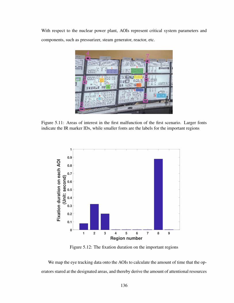
With respect to the nuclear power plant, AOIs represent critical system parameters and

components, such as pressurizer, steam generator, reactor, etc.

1

2

3

4

5

6

7

8

9

Figure 5.11: Areas of interest in the first malfunction of the first scenario. Larger fontsindicate the IR marker IDs, while smaller fonts are the labels for the important regions

1 2 3 4 5 6 7 8 9

Region number

0

0.1

0.2

0.3

0.4

0.5

0.6

0.7

0.8

0.9

1

Fix

ati

on

du

rati

on

on

each

AO

I

(Un

it:

seco

nd

)

Figure 5.12: The fixation duration on the important regions

We map the eye tracking data onto the AOIs to calculate the amount of time that the op-

erators stared at the designated areas, and thereby derive the amount of attentional resources

136

that each operator allocated to different valuable information sources. As indicated in Ref.

[179], the attention-resource effectiveness measure is a promising metric for quantifying

the human performance. One composite metric developed in Ref. [179] is the fixation-to-

importance (FIR) ratio, and it is defined as the relative attentional resources spent on the

information source divided by the relative importance of that source. Herein, we assume

all the regions are equally important. Thus, the amount of time that each operator spent

on the important AOIs (relevant to each malfunction) is used as a metric to measure the

attentional resource allocation. Fig. 5.12 shows fixation duration on each AOI for one mal-

function in the first scenario, illustrating that the operator allocated most of his attention

to the 8th region and the 2nd region, but missed five other important regions. From such

quantitative information, we derive two composite features: the average fixation duration

on the visited important regions, and the ratio of the important regions that are visited by

the operator. According to Fig. 5.12, we calculate the coverage ratio as 4/9 (4 out of 9),

and the average fixation duration on the visited important regions is 0.37 seconds. In addi-

tion, we utilize the Tobii Studio to calculate the number of clusters for the eye movement

in response to this malfunction, and the result is shown in Fig. 5.13. We assume that the

number of clusters reflects the operator’s perceived understanding of the malfunction event

and his consequent actions in distributing the attentional resources. The three composite

features mentioned above (fixation duration in important regions, coverage ratio, and num-

ber of clusters) provide quantitative connections to the performance of each crew team in

resolving the system malfunction and allocating valuable attentional resources.

With respect to the temporal characteristics of eye movement, we use the average du-

ration of all the gaze fixations as a measure to represent the fixation duration. By using

such a metric, we can identify where the operator allocates more attentional resources.

Regarding the spatial features of eye movement, numerous studies have shown the link be-

tween saccade, cognitive workload, and distraction [180, 181]. For example, Rantanen and

Goldberg [182] found that the visual field shrank 7.8% in a moderate-workload counting

137

Figure 5.13: Number of clusters corresponding to the eye movement of the first malfunctionin the first scenario

task and 13.6% during a cognitively demanding counting task. Thus, the measurements

on saccade are good candidates to predict the cognitive workload. In general, saccades are

extremely fast jumps from one fixation to the other, and the saccade pattern is an indicator

on the operator’s problem understanding and confusion. In this study, we employ two dif-

ferent metrics – average pursuit distance and average saccadic amplitude – to represent the

spatial features of eye movement. For the sake of completeness, we clarify the meanings of

all the six features in Table 5.9 and their significance in assisting the prediction of operator

performance.

• Fixation duration measures the average duration for all the fixations, and is an indi-

cation of information processing and cognitive activities. This metric indicates how

much attentional resources are allocated to specific regions, and whether the specific

regions are closely related to the malfunction. The longer fixation duration indicates

more difficulty in extracting information and more effort, from which we can further

analyze their performance.

• Pursuit distance is the spatial distance between two consecutive fixation locations

138

and represents the operator’s effort when locating the root cause of the malfunction,

diagnosing the system states, and searching for possible solutions.

• Saccadic amplitude measures the distance in visual degrees between the previous

fixation location to the current fixation location. The pattern in the saccadic ampli-

tude reflects the operator’s perceived problem understanding and the confusion in

diagnosing the system malfunction. Any saccade larger than 90 degrees from the

preceding saccade indicates a rapid change in the search direction.

• The number of clusters reveals the operator’s attentional resource distribution across

the displays, and indicates the viewer’s region-of-interest, from which we can mea-

sure the operator’s perceived complexity in understanding the situation.

• Duration in important regions indicates the average duration of operators’ eye fixa-

tion on the visited important regions and reflects the degree to which each operator

correctly understands and diagnoses the system malfunction. In general, the longer

the operators fixate on the important regions, the more likely that they will eliminate

the malfunction successfully.

• Coverage ratio indicates how many important regions are visited by the operators

and whether the operators fully grasp the situation. If all the important regions are

visited by the operators, they may have a higher chance to identify the root cause to

the malfunction.

The above six features enable quantitative analysis of the operator’s eye movement

from three different perspectives: temporal, spatial, and composite. Table 5.9 summarizes

the six different features elicited from the eye tracking data for the four malfunctions in the

first scenario. We repeat the same procedures to derive the same features for all the other

malfunctions and scenarios.

139

Table 5.9: Eye tracking data-derived features

Malfunction FixationDuration

PursuitDistance

SaccadicAmplitude

Number ofClusters

Durationin Important Regions

CoverageRatio

1 1.9481 2.7268 2.2374 6 0.3700 0.44002 2.2778 4.1321 2.6285 6 1.1440 0.71003 1.7876 3.5518 2.3329 3 0.5025 0.67004 0.4680 0 6.7900 1 0 0

5.3.4 Expert-rated Task Performance

The team performance was rated by two process experts independently according to the

OPAS items. Table 5.10 lists a small number of the OPAS items that the scenario developer

specified for the first two malfunctions in one scenario. These items cover a wide spectrum

of operator tasks, from simple identification of the problem to a ready-made solution to

eliminate the malfunction. The last two columns of Table 5.10 show the specific ratings

of the two process experts on the team performance in the detection, diagnosis, response

and coordination in resolving the abnormal events. The last two rows of Table 5.10, the

expert ratings are missing as some crews failed to reach the last malfunction event in some

scenarios or pursued some unexpected control actions that rendered some performance

items irrelevant. Thus, about 11% data on the expert-rated task performance is missing.

We propose dealing with the missing values by replacing them with an average value of

2 for the rating because we do not have the knowledge regarding the operator’s specific

performance in accomplishing the task.

Since the team performance is reflected in the expert ratings, the goal of our quantitative

model is to predict these numerical values listed in the last two columns of 5.10. As each

malfunction has numerous rating items, it is difficult to establish a model to accommodate

so many factors and associate the specific operations in each item to the team performance.

Further, each malfunction event has a different number of rating items, the content of each

rating item and the number of rating items in each malfunction event are only same for the

same scenario. As such, we will not have enough data to train the model to predict ratings

140

Table 5.10: Expert-rated task performance

Scenario Itemnumber Event Item

type Description R1Score

R2Score

1 1 1 detectionLT-459 failure

*Responds to alarms for decreasing PZR level and increasing CHG flow.*Team compares channels of PZR level identifying the failed channel.

3 3

1 2 1 diagnosisWhen LT-459 < 17% Team IDs:

*Letdown has isolated*PZR heaters OFF

3 3

1 3 1 responseTakes action to limit PZR Level increase:

*Reduces CHG to minimum ( 0gpm)*Reduces Seal Injection within limits.

2 2

1 4 1 response

Monitors parameters:*PZR Level

*RCS Pressure*Blender AUTO makeup

3 3

1 5 1 response

Utilizes ALB 9-4-3 to:*Deselect LT-459 (control & RCDR)

*Initiate OWP-RP*Resets & energizes PZR Heaters

3 3

1 6 1 response

OP-107, Sect. 1.4 (L/D):*Proper sequence for valve operation*Proper PCV operation (no RV lift)

*Proper CHG flow for Letdown Flow

3 2

1 7 1 response

Restore PZR level to program:*Adequate CHG for Letdown*Steady trend toward program

*Restores control system to AUTO

3 3

1 8 2 detection

Detects transient - reduced steam demand:*Rods inserting

*Tavg increases (Tavg/Tref deviation)*Steam & Feed flow decreases

3 2

1 9 2 diagnosisChecks cause for reduced steam demand

*Turbine Load decrease?*Valve closure?

2 2

1 10 2 diagnosisIdentifies #3 GV closed

*Light indication on Turbine section*Position indication available

2 3

1 11 2 response

Stabilizes plant at reduced power*Rods above insertion limit*Verifies/restores Delta Flux

*Evaluates Turbine load adjustment*Considers Boration.

3 3

1 12 2 coordination

Coordinates recovery*Dispatch operator to check

*Contact MAINT*Notify OMOC

*Determines continued ops allowed

3 3

1 13 2 detection

Detects transient - reduced steam demand:*Rods inserting

*Tavg increases (Tavg/Tref deviation)*Steam & Feed flow decreases

- -

1 14 2 diagnosisChecks cause for reduced steam demand

*Turbine Load decrease?*Valve closure?

- -

141

Table 5.11: Transformation of expert ratings into numerical counts (for one malfunction inone scenario)

Expert rating 0 1 2 3

Numerical counts 0 0 1 6

for specific performance items because only three crews take part in the same scenario. To

address this issue, we aggregate the expert ratings and transform them into numerical counts

to compress the number of items that the surrogate model needs to predict. Specifically,

instead of predicting the rating value for each item, we predict the frequencies of different

rating values in the expert rating. For example, for the first event in the first scenario, we

have converted the first expert’s (R1) ratings into a frequency table (Table 5.11). Table 5.11

shows rating values 2 and 3 appear once and six times in the expert-rated team performance

for this particular malfunction, respectively. This avoids predicting the rating values for the

seven items in the first malfunction. The dimension of system response is fixed to four

individual variables across all the scenarios.

Compared with aggregating the expert-rated team performance into one value, the four-

variable representation provides relatively higher resolution to examine the expert-rated

team performance for each malfunction, from which team performance under different

NPP control room designs can be better characterized and compared. In contrast, with an

aggregated value that is averaged over the rating items within a malfunction, it is difficult to

compare team performance across teams, for example, when they have the same aggregated

performance scores.

5.4 Quantitative Model Development

In this section, we develop a quantitative model to predict the operator performance in

resolving the malfunction events. The input and output variables are summarized in Fig.

5.14. The input variables include the HTCS workload and situation awareness ratings from

142

the three operators (BOP, US, and RO), the scenario difficulty rated by the two process

experts, the features extracted from the physiological data on the two operators (BOP and

US), and the features from the eye tracking data. The model output is a vector of four

values denoting the numerical counts that each rating value of task performance assigned

by the process experts to individual operator.

HTCS workload

(BOP, US, RO)

Scenario difficulty Situation awareness

(BOP, US, RO)

Psychological features

(RO, US)

Input variables Output variable

Expert-rated operator

performance

Total response

latency

Toal SCR

area

Total SCR

Amplitude

Total SCR

Rise time

Total

SCR size

Total SCR

onset

Count of

responses

Mean of

respiration rate

Standard deviation

of respiration rate

Eye tracking data

• Fixation duration

• Pursuit distance

• Saccadic amplitude

• Fixation duration on

important regions

• Number of clusters

• Coverage ratio

Figure 5.14: Model inputs and outputs

Regarding the input variables, we have 15 (5 items * 3 operators) variables for the

HTCS workload, 18 (6 * 3) variables representing the three operators’ situation awareness,

8 (4 * 2) variables denoting the scenario difficulty, 14 (7 * 2) features derived from the

skin conductance response, 4 (2 * 2) variables extracted from the respiration data, and 6

variables from the eye tracking data. In total, there are 65 (15 + 18 + 8 + 14 + 4 + 6 = 65)

different input variables. To reduce the dimension of the input variables in the model, we

perform the following operations:

1. We average the difficulty ratings of the two process experts over four criteria (detec-

tion, diagnosis, intervention, and restoration) on each scenario to acquire an aggre-

gated indicator of the scenario difficulty. As a result, the eight variables that are used

to represent the scenario difficulty are represented by one summarized variable.

143

2. The HTCS workload is averaged over the five workload items and three operators,

by which we obtain a comprehensive evaluation on the workload for each scenario.

In this way, we reduce the number of variables from 15 to 1.

3. The situation awareness of each operator is averaged over the six items listed in the

questionnaire. Thus, we reduced the number of variables used to denote the situation

awareness from 18 to 3.

4. We conduct correlation analysis among the elicited physiological features. If the cor-

relation coefficient between any two physiological features is larger than a threshold

(We ranked the correlations among the physiological variables from the highest to

the lowest and then chose the average value (0.85) of the correlations ranked in top

10%.), the two variables likely carry similar information. In this case, we only re-

tain one of the variables because one of them will suffice to feed the model. This

procedure eliminates seven variables extracted from the physiological data: total am-

plitude, total size, total onset, count of response from the reactor operator, total rise

time, total onset, and count of response from the unit supervisor.

Through the above operations, the number of model inputs is reduced from 65 to 22.

The 22 variables retained in the final model are: scenario difficulty (1 feature), HTCS

workload (1 feature), situation awareness of BOP, US, and RO (3 features), physiological

features (11 features: total response latency, total SCR area, total SCR rise time, mean of

respiration rate, and standard deviation of respiration rate of RO; total response latency,

total SCR area, total SCR amplitude, total SCR size, mean of respiration rate, and standard

deviation of respiration rate of US), and eye tracking features (6 features: fixation duration,

pursuit distance, saccadic amplitude, fixation duration on important regions, number of

clusters, and coverage ratio). Fig. 5.15 illustrates the correlation matrix among the 22

input variables. As can be observed, all the considered input variables do not exhibit high

correlations after the removal of highly correlated variables.

144

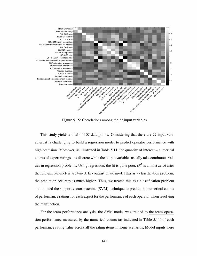
HTCS work

load

Scenar

io d

ifficu

lty

RO: SCR ar

ea

RO: SCR la

tency

RO: SCR si

ze

RO: SCR m

ean re

spira

tion

RO: sta

ndard d

eviat

ion o

f res

piratio

n

US: SCR ar

ea

US: SCR la

tency

US: SCR am

plitude

US: SCR si

ze

US: mea

n of r

espira

tion ra

te

US: sta

ndard d

eviat

ion o

f res

piratio

n rate

BOP: situ

atio

n awar

enes

s

US: situ

atio

n awar

enes

s

RO: situ

atio

n awar

enes

s

Fixatio

n dura

tion

Pursuit

distan

ce

Sacca

dic am

plitude

Fixatio

n dura

tion o

n importa

nt reg

ions

Number

of c

lust

ers

Covera

ge rat

io

HTCS workloadScenario difficulty

RO: SCR areaRO: SCR latency

RO: SCR sizeRO: SCR mean respiration

RO: standard deviation of respirationUS: SCR area

US: SCR latencyUS: SCR amplitude

US: SCR sizeUS: mean of respiration rate

US: standard deviation of respiration rateBOP: situation awareness

US: situation awarenessRO: situation awareness

Fixation durationPursuit distance

Saccadic amplitudeFixation duration on important regions

Number of clustersCoverage ratio

-0.8

-0.6

-0.4

-0.2

0

0.2

0.4

0.6

0.8

1

Figure 5.15: Correlations among the 22 input variables

This study yields a total of 107 data points. Considering that there are 22 input vari-

ables, it is challenging to build a regression model to predict operator performance with

high precision. Moreover, as illustrated in Table 5.11, the quantity of interest – numerical

counts of expert ratings – is discrete while the output variables usually take continuous val-

ues in regression problems. Using regression, the fit is quite poor, (R2 is almost zero) after

the relevant parameters are tuned. In contrast, if we model this as a classification problem,

the prediction accuracy is much higher. Thus, we treated this as a classification problem

and utilized the support vector machine (SVM) technique to predict the numerical counts

of performance ratings for each expert for the performance of each operator when resolving

the malfunction.

For the team performance analysis, the SVM model was trained to the team opera-

tion performance measured by the numerical counts (as indicated in Table 5.11) of each

performance rating value across all the rating items in some scenarios, Model inputs were

145

collected from heterogeneous sources, including the HTCS workload, situation awareness

ratings from the three operators (BOP, US, and RO), the scenario difficulty, the features

extracted from the physiological data on the two operators (BOP and US), and features

extracted from the eye tracking data. The ultimate classification results provide the team

performance level in the representation of numerical counts of each rating value over all

the rating items when handling the malfunction events under the particular control room

design.


It is a challenging task to build a quantitative model to predict operator performance for

several reasons:

• The nuclear power plant is a complex system. The operators respond to the unex-

pected malfunctions through a series of cognitive activities. The physiological data

on the operators might not fully characterize their cognitive activities and situational

awareness.

• Although the problem dimension is reduced to 22, it is challenging to build a model

to make predictions with high accuracy with only 107 records.

• The correlations among the input variables and outputs are found to be weak (the

correlations vary within the range [−0.3217,0.3826]). Thus, none of the inputs to

the model is particularly dominant.

• As mentioned earlier, the data set contains missing values. For example, of 16%

data are missing for the confidence level in the situation awareness, and 11% of the

expert-rated task performance data are missing.

As mentioned previously, we model it as a classification problem rather than a regres-

sion problem for better performance. Specifically, we use the “LIBSVM” Matlab toolbox

146

developed by Chang and Lin [183] to build SVM classification models, in which the poly-

nomial kernel function is used as the kernel function:

K(xi,xj

)=(xTi xj+ c

)d(5.1)

where xi and xj are the vectors denoting the features of two samples i and j, d is the

degree of kernel function, and c≥ 0 is a parameter used to control the impact of the order

of the kernel function.

Entire data

Part I

Part II

Training data

sample 1

Training data

sample 2

Training data

sample n

Training samples

...

Model 1 Model 2 Model n...

Prediction

1

Prediction

2

Prediction

n...

Operator

performance

estimation

Figure 5.16: Framework of the quantitative model

Next, we build four individual models to predict the numerical counts corresponding

to each rating value as indicated in Table 5.11. For all the four models, we set the value

of parameter d the same: d = 3. With respect to the value of parameter C for each class,

147

Table 5.12: Prediction accuracy of the four individual models

Rating value 0 1 2 3

Classes [0, 1, 2, 3, 6] [0, 1, 2, 3, 4] [0, 1, 2, 3, 4] [0, 1, 2, 3, 4, 5, 6, 7, 8]Prediction accuracy 83.33% 75.50% 82.28% 75.13% ([mode-1, mode + 1])

we make its value inversely proportional to the number of data belonging to each class in

the training dataset, thereby overcoming the imbalanced class distribution. As mentioned

earlier, since the size of the problem dimension is relatively large compared to the number

of data records, any single model might not be adequate to capture different patterns equally

well. Different from an individual model, ensembles of models build their outcome from

a combination of the outcomes of individual models, and they have been shown to be

effective in addressing many practical problems because of their prediction accuracy and

stability as well as the advantage in avoiding overfitting [184, 185]. Herein, we integrate

the support vector machine with bootstrap aggregating to improve the prediction accuracy

by combining the classification results from numerous models trained by randomly selected

samples.

The framework of the proposed methodology is illustrated in Fig. 5.16. The entire

data is split into two parts: Part I is used for training the model, and Part II is used for

verifying the performance of the trained model. We randomly select 10 records to validate

the performance of the trained model. Then we randomly choose 85% data of Part I data

for 100 times and each combination of the randomly chosen samples is used to train one

model. Thus, we have 100 trained models. Then all the trained models are used to predict

the system response for the verification data. To measure the prediction accuracy, for the

first three models, we use majority voting to determine the class because the majority voting

represents the class predicted most often by the 100 base classifiers and it also helps to

cancel out the impact of random variation. Then we compare the results against the actual

numerical counts. For the fourth model, we count the times the actual numerical count

falls within the interval [mode - 1, mode + 1] and divide it by the number of validation

148

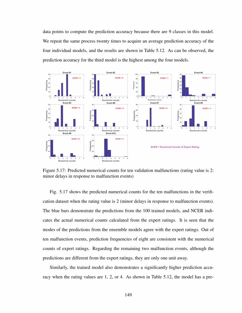
data points to compute the prediction accuracy because there are 9 classes in this model.

We repeat the same process twenty times to acquire an average prediction accuracy of the

four individual models, and the results are shown in Table 5.12. As can be observed, the

prediction accuracy for the third model is the highest among the four models.

0 1 2 3 4 5 6 7 8

Numerical counts

0

10

20

30

40

50

Fre

qu

en

cy

Event #1

0 1 2 3 4 5 6 7 8

Numerical counts

0

10

20

30

40

50

Fre

qu

en

cy

Event #2

0 1 2 3 4 5 6 7 8

Numerical counts

0

20

40

60

80

100

Fre

qu

en

cy

Event #3

0 1 2 3 4 5 6 7 8

Numerical counts

0

10

20

30

40

50

60

Fre

qu

en

cy

Event #4

0 1 2 3 4 5 6 7 8

Numerical counts

0

10

20

30

40

50

Fre

qu

en

cy

Event #5

0 1 2 3 4 5 6 7 8

Numerical counts

0

20

40

60

80

Fre

qu

en

cy

Event #6

0 1 2 3 4 5 6 7 8

Numerical counts

0

10

20

30

40

50

Fre

qu

en

cy

Event #8

0 1 2 3 4 5 6 7 8

Numerical counts

0

20

40

60

80

Fre

qu

en

cy

Event #9

0 1 2 3 4 5 6 7 8

Numerical counts

0

20

40

60

80

Fre

qu

en

cy

Event #10

0 1 2 3 4 5 6 7 8

Numerical counts

0

20

40

60

80

Fre

qu

en

cy

Event #7

NCER = 0

NCER = 3

NCER = 3NCER = 2

NCER = 4 NCER = 1 NCER = 1

NCER = 0

NCER = 0

NCER = Numerical Counts of Expert Rating

NCER = 3

Figure 5.17: Predicted numerical counts for ten validation malfunctions (rating value is 2:minor delays in response to malfunction events)

Fig. 5.17 shows the predicted numerical counts for the ten malfunctions in the verifi-

cation dataset when the rating value is 2 (minor delays in response to malfunction events).

The blue bars demonstrate the predictions from the 100 trained models, and NCER indi-

cates the actual numerical counts calculated from the expert ratings. It is seen that the

modes of the predictions from the ensemble models agree with the expert ratings. Out of

ten malfunction events, prediction frequencies of eight are consistent with the numerical

counts of expert ratings. Regarding the remaining two malfunction events, although the

predictions are different from the expert ratings, they are only one unit away.

Similarly, the trained model also demonstrates a significantly higher prediction accu-

racy when the rating values are 1, 2, or 4. As shown in Table 5.12, the model has a pre-

149

diction accuracy of 83% and 76% for the rating value 0 (i.e., failing to eliminate the mal-

function) and 1 (significant lapse in performing the task), respectively. Since there are nine

unique numerical counts for the rating value 3 (timely response to malfunction events), we

checked whether the actual numerical count fell within the prediction interval [mode - 1,

mode + 1], and the model had an accuracy of 75.1%. The performance analysis across the

four rating values illustrates that the proposed methodology can significantly predict the

team performance through fusing the heterogeneous sources of data. In addition, to assess

the relative contribution to prediction accuracy of physiological data versus eye tracking

data, we created SVM models that used each of these sources individually. Neither model

outperformed the model containing both data sources the fused model outperformed the

two alternative models by 1% to 7%, respectively, in predicting the team performance.

5.5 Summary

This chapter presents an application of information fusion to develop a data-driven

model to assess the operator performance in restoring system performance by eliminating

abnormal events in NPP control rooms. Based on a dataset from a full-scope nuclear power

plant simulator experiment recruiting previously licensed operators, we have developed a

method that combines support vector machine with bootstrap aggregating to build a data-

driven model for predicting crew performance. Our method first extracts numerous features

from a heterogeneous dataset and then fuses the quantitative information derived from the

diverse sources, thereby learning the relations between the elicited features and crew per-

formance. Despite the limited amount of data (107 records), the best trained ensemble

model, which contains 22 input variables/features, has an 82.28% accuracy in predicting

crew performance in terms of the numerical counts of expert ratings (on an ordinal scale

between zero and three). This ensemble model of the full heterogeneous dataset is superior

to SVM models built with either physiological or eye-tracking data, and substantially bet-

ter than simple correlation between performance outcome (i.e., OPAS) and any individual

150

input features. Further, we can expect additional data are expected to improve the predic-

tion accuracy of operator performance. The overall results of this study thus illustrate that

the proposed information fusion approach is promising for estimating performance of NPP

operators.

The principal merit of the proposed information fusion methodology is in combining

diverse data sources for model prediction. First, the 22 input features are highly hetero-

geneous, deriving from scenario characteristics, subjective ratings of workload, situation

awareness of process parameters, eye-tracking data, respiration rate, and skin conduc-

tance response. Second, the Pearson-product moment correlation analysis indicates that

the strength of correlation between all the 22 input features and performance outcome of

interest is at best moderate (between -0.32 and 0.38), suggesting that none of the features

is dominantly predictive. Yet, the trained ensemble model is able to predict the operator

performance outcome at a reasonable accuracy (prediction accuracy of 75%-83%), indi-

cating that information fusion can capitalize on diverse measurement types, each of which

improves performance prediction incrementally.

Our results also suggest the merit of employing physiological measurements in esti-

mating operator performance. Physiological measurements, besides eye-tracking, in high

fidelity NPP control room simulator experiments are virtually non-existent in the litera-

ture [186]. Our empirical data-driven model shows a reasonable predictive relationship

between operator physiological indicators and visual activity and crew performance. The

proposed approach can be used to provide a means for comparing crew performances under

different operating conditions through the various physiological indicators and eye move-

ment activity. The results of this study is encouraging for further research in physiological

measures for assessing crew performance.

A method for building human performance data models could be invaluable to assess

operator qualification and control room design given many on-going modernization and

new construction projects. While the literature contains a few quantitative assessments of

151

nuclear power plant operators [187, 188, 189], most studies rely on either subjective discus-

sion or rudimentary quantitative methods (e.g., simple correlation statistics) of integrating

results of multiple measurement dimensions (e.g., SA, workload, eye-gaze). In contrast, we

describe a quantitative data-driven approach to fuse different performance dimensions that

could provide a more holistic and precise assessment of operator qualification and control

room design than the current state-of-research or practice [179, 190].

The proposed empirical approach has several features that maybe useful to the next

generation human reliability models. The proposed framework may reduce demand on

experts to rate task performance, which has been identified as one of the major needs in

the next generation models [186]. In addition, the physiological responses and eye-gaze

behaviors may provide additional objective measures of operator performance [191]. As

indicated in Ref. [186], the next generation human reliability methods need to be detailed

enough to support data collection and experimental validation. We specify a set of in-

put features and corresponding extraction methods for diverse types of experimental data,

providing guidance to researchers and practitioners for carrying out operator assessment

with an information fusion approach. The direct measurable factors on each operator (i.e.,

skin conductance response, respiration data, and eye movements) might also enhance the

model’s capability to predict individual and crew performance. Finally, the results of this

study indicates that our methodology, or the information fusion approach in general, can

yield meaningful prediction of operator performance with a reasonable amount of data that

individual NPPs can feasibly generate more than the data available in our study through the

mandatory simulation training of professional operators.

The reliability analysis of nuclear power plant control room operator in dealing with

system malfunctions deepens our understanding on the response effectiveness of human

operators. By assessing the response effectiveness of human operators, it might enable

us to pinpoint the directions (e.g., upgrading to ecological interface, developing diagnosis

decision aiding tools) to move towards for the sake of enhancing operators’ responsive-

152

ness. For example, the interface can be improved to include more salient features, which

will enable operators to diagnose anomalous system behavior quickly; visualization deci-

sion support systems can be integrated in the NPP control room to support and speed up

operators’ diagnosis process. Such operations in improving human response effectiveness

will significantly strengthen the resilience of the human-in-the-loop system against distur-

bances, and accelerate the speed of restoring system performance to normal level.

In addition to human response, the algorithms/strategies taken to handle emergency sit-

uation also plays an essential role in system performance recovery. In Chapter 6, we focus

on characterizing the effectiveness of algorithmic response in handling extreme events.

153

Chapter 6

Performance Assessment of Algorithmic Response to Hazardous Events1

6.1 Introduction

In addition to human operators, the strategies that are used to manage hazardous events

also have an explicit impact on the degree to which system performance could be restored.

In this chapter, we develop a simulation-based approach to investigate the effectiveness of

an algorithmic response in mitigating the impact of extreme event. In particular, we analyze

how long the system survives under a given algorithmic strategy with the consideration of

uncertainties arising from multiple sources, and the proposed method is illustrated with a

rerouting algorithm that is used to respond to the closure of a destination airport.

Consider a disruptive event caused by an abnormal weather condition that results in the

closure of an airport. Under this circumstance, we need to seek feasible alternate routes

for all the aircraft that are flying towards this airport based on the characteristics of each

aircraft and available space at nearby airports. In the literature, many measures, such as

delaying flights already en route by restricting miles-in-trail or other means, and Ground

Delay Programs (GDPs) [192], have been investigated to alleviate the congestion caused

by the closure of an airport. Compared with other possible measures, aircraft re-routing is

one of the most commonly used strategies because it imposes less controller workload, and

the risk is very low. Currently, many ATFM operators, such as the Air Traffic Command

Center (ATCC) coordinating flow management in US, are called upon to reschedule and

re-route the aircraft so as to minimize the delay costs caused by congestion. Specifically,

in the context of airline operations, prior to the disruption, the aircraft are scheduled to fly

a set of routes as planned. Upon the occurrence of a disruption, the initial routes become

infeasible, which calls for aircraft re-routing, that is to identify a new feasible route for

1An archival paper related to this chapter has been published in the journal Decision Support Systems.For more details, see Ref. [27]

154

each aircraft.

There is extensive literature on flight re-routing to minimize congestion cost [193, 194,

195, 196, 197]. In particular, Odoni presented seminal work [198] to model the flow man-

agement problem (FMP) as a discretized representation of flows, which is fundamental to

the approaches developed subsequently. Bertsimas and Patterson [199] extended the Air

Traffic Flow Management (ATFM) model to account for the re-routing of soon-to-depart

or airborne flights. Subsequently, they developed a dynamic network flow approach to

address the problem of determining how to reroute aircraft when faced with dynamically

changing weather conditions [200]. Matos and Ormerod [201] discussed the issues in Eu-

ropean ATFM and identified the needs in terms of Decision Support Systems (DSS) for

re-routing flights. In response to Matos and Ormerod, Leal and Powell [202] attempted to

build a re-routing decision support system in Europe by identifying participants and investi-

gating the requirements for re-routing systems. To respond to aircraft grounding and delays

experienced over the course of the day, Bard and Arguello [203] proposed a time-band op-

timization model for reconstructing aircraft routing, in which the time horizon transformed

from the routing problem is discretized. Balen and Bil [204] analyzed an optimal aircraft

re-routing plan in a free flight environment in the case of airspace closure and developed a

software to re-route the aircraft around the closed airspace. Recently, an integer program-

ming model has been proposed in [205] for large-scale instances of the ATFM problem

covering all the stages of each flight, i.e., take off, cruise, and landing. Subsequently, a

method is proposed in [206] based on [205], which accounts for the airspace volume. Sem-

inal work is presented in [207] on ATFM rerouting under uncertainty in airport arrival and

departure capacity, air sector capacity and flight demand. Rosenberger et al. [208] devel-

oped an optimization model for aircraft recovery (ARO) that reschedules legs and reroutes

aircraft by minimizing an objective function involving rerouting and cancellation costs.

Some of the above studies have considered uncertainty, but mostly related to the ex-

ternal environment, e.g., uncertainty in weather prediction [201, 209, 210]. Even when

155

some studies focus on the inherent uncertainty in the air traffic control (ATC) system, only

one or two system components are taken into consideration, such as ground and departure

delays [211]. Aircraft re-routing is a complicated process, in which several subsystems

are involved, such as radar performance, message communication, airport resource man-

agement, etc. Visit https://www.faa.gov/air traffic/flight across america/ for details on the

process of a flight across the USA. At each phase, several sources of variability and uncer-

tainty emerge in different subsystems. These uncertainty sources have a significant effect

on the air traffic, which challenges the management techniques and decision support sys-

tems classically used by the researchers.

In the past years, several studies have made significant effort in the development of

management policy or decision support systems in the presence of uncertainty because the

problem under uncertainty is completely different from the deterministic case. For exam-

ple, to cope with the uncertainty in the travel demands and traffic conditions, Balbo et al.

[212] developed an adaptive solution to the bus network management problem by utilizing

multi-agent approach to model the various bus network activities. To design the optimal

policy for the transportation networks, Pathak et al. [213] proposed an agent-based model,

in which they accounted for both aleatory uncertainties (e.g., random demand, randomness

in speed) and epistemic uncertainty (e.g., the incomplete information of user behavior).

Yoon et al. [214] developed a computer-based training prototype to improve the emergency

response and recovery effectiveness under the pressures of incomplete and erroneous in-

formation. As mentioned earlier, due to the uncertainty arisen in the ATC system, there is

also an increasing demand for developing a decision support system with the consideration

of the multiple sources of uncertainties emerging in the re-routing process [215]. Prior

to developing the decision support system, we need to answer several questions: where

the uncertainties come from, how to characterize these uncertainties, how to propagate the

uncertainties through the system, and how to quantify their influence on the system perfor-

mance. Answering these questions will lay a firm foundation for the development of ATC

156

https://www.faa.gov/air_traffic/flight_across_america/

decision support system under uncertainty.

In this chapter, we consider re-routing aircraft given the occurrence of an abnormal

weather condition. Thus, the weather condition is given and there is no uncertainty, es-

pecially considering the short duration of the re-routing simulation. As indicated in the

chapter later, there are 10 simulation cycles in our analysis, and each simulation cycle lasts

for 5 minutes, which means the total simulation duration is only 50 minutes. We assume

that there is no uncertainty in forecasting the weather condition for the 50 minutes; this is

reasonable given the current technology for monitoring and forecasting the weather. On the

other hand, our focus is on the inherent uncertainty sources within the re-routing system,

e.g., message communication, radar, aircraft, and airport. By investigating their effect on

the system performance, we aim to establish the foundation for the design optimization

of the re-routing system. Obviously, weather is an external condition and is not a design

variable.

Since aircraft re-routing is a complicated process, there are many interactions among

the components, e.g. radar and decision maker, decision maker and airport, airport and

aircraft. Moreover, the status of the aircraft (e.g., detected or not, registered or not, as-

signed or not) and radar (e.g., beam orientation) are varying over time. Simulation methods

[213, 216] are capable of capturing the time-varying updates and the information exchange

between the multiple components of such systems. As a result, we construct a simulation-

based approach to mimic the aircraft re-routing process and account for the aforementioned

multiple sources of uncertainties. Compared to the current state of the art, we have made

the following contributions :

1. We develop a simulation framework to model the aircraft re-routing process and in-

corporate a formulation for optimal re-routing assignments. Our simulation frame-

work considers the aircraft re-routing process as a system of systems, and enables us

to have a comprehensive understanding of the system work flow and the interactions

among various systems. Such a simulation-based approach facilitates quantitative

157

evaluation of the re-routing methodology.

2. We analyze various uncertainty sources in the systems involved in the re-routing

process (aircraft, radars, communication systems, and neighboring airports), and

perform the simulation and re-routing optimization by incorporating the uncertain

sources. Incorporation of uncertainty sources is essential in ensuring a robust and

reliable re-routing system.

3. We develop a methodology to quantitatively evaluate the performance of the re-

routing system by considering the effect of the various uncertainty sources on the

system performance, and incorporate reliability analysis techniques for this purpose.

4. We incorporate novel stochastic sensitivity analysis techniques to quantify the rela-

tive contributions of the different uncertainty sources on the system performance; this

facilitates a quantitative basis for optimal allocation of limited resources to improve

the system performance.

5. We incorporate surrogate modeling to improve the computational efficiency and en-

able fast analysis of system performance. This helps to quantitatively evaluate and

compare several different competing strategies for re-routing optimization and sys-

tem improvement.

In our simulation system, there are three core modules: radar system, communication

system, and the assignment algorithm, which will be introduced in Section 2. The following

uncertainty sources have been considered in this chapter:

• Radar performance: Radar performance depends on three parameters, namely: ini-

tial orientation, detection radius, and beam rotation speed. All three parameters are

stochastic and follow different distributions.

• Neighboring airports: Space availability (gate, runway, and airspace) at each airport

is uncertain, and is varying with time.

158

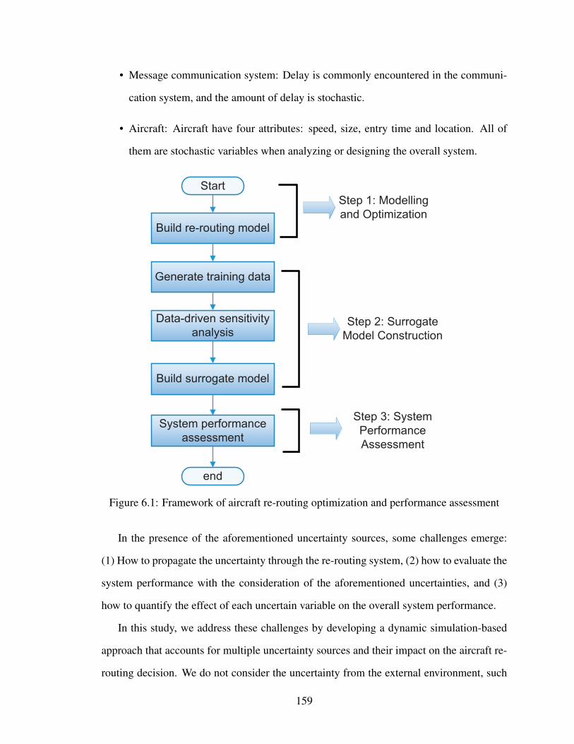
• Message communication system: Delay is commonly encountered in the communi-

cation system, and the amount of delay is stochastic.

• Aircraft: Aircraft have four attributes: speed, size, entry time and location. All of

them are stochastic variables when analyzing or designing the overall system.

Figure 6.1: Framework of aircraft re-routing optimization and performance assessment

In the presence of the aforementioned uncertainty sources, some challenges emerge:

(1) How to propagate the uncertainty through the re-routing system, (2) how to evaluate the

system performance with the consideration of the aforementioned uncertainties, and (3)

how to quantify the effect of each uncertain variable on the overall system performance.

In this study, we address these challenges by developing a dynamic simulation-based

approach that accounts for multiple uncertainty sources and their impact on the aircraft re-

routing decision. We do not consider the uncertainty from the external environment, such

159

as the uncertainty in weather prediction; that is, we consider re-routing for a given weather

condition. We focus on the aleatory uncertainty in the re-routing system related to message

transmission, radar performance, demand from incoming aircraft, and space availability at

nearby airports.

An optimization model is constructed to make periodic assignments of the registered

aircraft with the objective of minimizing the overall travel distance. We use the system fail-

ure time, which is defined as the time instant that at least one aircraft in the simulation runs

out of fuel, as a metric to measure the re-routing system performance. Since the duration of

each simulation is limited, the system performance is not available in all simulations. An

effective strategy is developed to extract the lower bound of the system failure time from

right-censored data. The above procedures are represented as Step 1 in Fig. 6.1.

As stated previously, we are interested in evaluating the re-routing system performance

in terms of the system failure time. To achieve this objective, a large number of simu-

lations is required to build the probability distribution of system failure time. However,

each simulation is very time consuming. Hence, we build a surrogate model to replace

the original simulation. Since there are too many random input variables, we implement

a data-driven sensitivity analysis method to identify the dominant variables, then build the

surrogate model using support vector regression with the identified dominant variables.

Then we construct the system failure time distribution using the surrogate model. The

aforementioned processes are denoted as Steps 2 and 3 in Fig. 6.1.

6.2 Proposed Methodology for Aircraft Re-routing

In this section, we introduce the components of the proposed re-routing methodology –

problem description, airspace system model, uncertainties considered and the assignment

algorithm.

160

Regional radar A

Regional radar B

Regional radar C

Regional radar D

Decision Maker

P1

P3

P2

Message

Aircraft enters

the region

Radar

detection

Time

Re-routing

assignment

Communication to

the aircraft through

assigned airport

Aircraft

re-routed

Figure 6.2: Aircraft re-routing process

6.2.1 Problem Description

In the United States, the control of air traffic is carried out at 22 regional centers that

receive information from aircraft and ground-based radars on location, altitude, and speed

of the aircraft. The Air Traffic Command Center (ATCC) aggregates all the information

collected by the 22 regional centers to reschedule and reroute flights when a hazardous

event (e.g., bad weather) occurs [200]. In this study, as shown in Fig. 6.2, we characterize

this process in a simplified manner using a five-step procedure:

(1) In the first phase, the aircraft enters the region at a randomly generated location and

time instant, and flies towards its destination airport at a constant speed. We assume

that the flight path follows a straight line in a 2-D space that connects the entry location

and the destination airport.

(2) The time when the aircraft enters the region of interest is Entry Time. Once the aircraft

161

enters the region, it is detected after some time by either a regional radar or a local radar.

The detection time is uncertain depending on the radar’s orientation, detection angle,

and detection radius. The time instant the aircraft is detected by the radar is Detection

Time. Once a radar detects an incoming aircraft, it sends a message to the decision

maker (DM). This message might be delayed. When DM receives the message from

the radar, the aircraft is registered in the system. The time instant when the aircraft is

registered in the system is called Registration Time.

(3) The DM periodically makes re-routing assignments for all the aircraft that are regis-

tered in the system and waiting to be re-routed. The re-routing decision for a particular

aircraft requires the corresponding resources to be available and compatible, i.e., the

aircraft of a particular size can only land at the airport with available airspace, run-

way, and gate that are suitable for that aircraft size. The specific assignment algorithm

will be developed in Section 6.2.4. The time instant when the aircraft is re-assigned is

called Assignment Time.

(4) After the assignment decision is made, DM sends a message to the assigned airport.

When the assigned airport receives the message, it sends an acknowledgement message

to DM. It also sends a message to the assigned aircraft to establish further communica-

tion for landing. All three messages can be delayed.

(5) When the aircraft receives the message from the assigned airport, it sends an acknowl-

edgement message to the assigned airport and starts flying towards the assigned airport.

After the aircraft arrives at the assigned airport, the corresponding resources, e.g., gate,

runway, and airspace, are released for future assignment. We name the time when the

aircraft lands safely as Leaving System Time.

Obviously, aircraft re-routing is a complicated process, where multiple subsystems and

components are involved, and the uncertainty related to each component further intensifies

162

the complexity of this problem. In this study, the system performance we are interested in

is measured by the system failure time metric, defined as below:

Definition 6.2.1 System failure time: When at least one aircraft runs out of fuel, the re-

routing system fails at that time instant. This time instant is defined as the system failure

time.

Since several uncertain variables contribute to the variability of system performance,

we are motivated to quantify the contribution of each uncertain variable, thus facilitating

our decision making process for the purpose of enhancing system performance. To achieve

these objectives, a simulation-based approach is used to characterize the re-routing process,

by which we are able to capture the complex interactions among various subsystems. In

the following sections, we introduce the modelling of each component and subsystem in

the re-routing process.

6.2.2 System Model

In this section, we introduce the simulation model we built to account for the various

uncertainties in the process, related to airports, aircraft, radar, and communication. Before

formulating the problem, we need to introduce the fundamental assumptions with respect

to each component, in order to facilitate the discussion.

6.2.2.1 Region

Region refers to the specific area where we perform the simulation; all the components

(e.g. radar, aircraft, airport), are operated within the region. For the sake of illustration,

in the numerical example, we use a 500× 500 square area as shown in Fig. 6.3 as our

simulation space. In reality, the region can be any shape, e.g., polygons, triangle, or any

other shape.

163

0 50 100 150 200 300 350 400 450 5000

50

100

150

200

250

300

350

400

450

500

250

coverage

aircraft not yet registered

aircraft registered and waiting to be assigned

aircraft t

Figure 6.3: A snapshot of the simulation system

6.2.2.2 Aircraft

In the re-routing problem considered, the aircraft are assumed to be flying towards

a single destination airport at a constant speed. For each aircraft, we need to generate its

entry time, entry location, aircraft size, speed, and remaining miles. Each of these variables

is associated with uncertainty; we will discuss these uncertainties in Section 6.2.3. For the

sake of simplicity, in the re-routing simulation, we only consider the aircraft flying into the

region and heading towards the closed airport. As shown in Fig. 6.3, the airport indicated

164

by a dashed circle in the center of the square is closed due to extreme weather, hence all

the aircraft heading towards this airport will be re-routed to other alternate airports.

6.2.2.3 Nearby Airports

A very important component in the re-routing decision is space availability at the nearby

airports. In this study, we choose 16 airports for the sake of illustration as shown in Fig.

6.3, but our simulation can handle any number of available airports for re-routing the air-

craft. The availability of runways, gates, and airspace in each airport is considered by the

assignment algorithm. In order to guarantee the safe landing of the aircraft, all the nec-

essary facilities need to be available. There are several uncertain variables related to the

space availability, and these will be introduced in Section 6.2.3.

6.2.2.4 Radars

Once an aircraft enters the region of interest, it might be detected by the radars in the

system. Two different types of radar are considered: regional radars and airport (local)

radars. The only difference between them is the detection radius. Regional radars have

larger detection radius than local ones. The locations of all the radars are fixed. In this

study, we consider three uncertain variables related to radar: radar’s initial orientation,

radar beam rotation speed, and radar range, which will be described in Section 6.2.3 in

detail. In this study, we use a sparse cluster of radars for the sake of illustration, but the

simulation is general to account for the case with a high density of radars within the region.

6.2.2.5 Communication

There are many communications among the various components, for example, radar

needs to send message to the decision maker to inform the newly detected aircraft. Cur-

rently, controller-pilot data link communication (CPDLC) is a commonly used means of

communication between controller and pilot [217]. There is a sequence of messages be-

tween the pilot and the controller, which is referred to as dialogue. The duration of the

165

dialogue is variable, depending on several factors, such as clarity of the vocal phraseology,

controller workload, and the deviation of the revised route from the original one. All these

factors increase our uncertainty in estimating the time of the communication.

Such delay has significant influence on the controller-pilot communication, manifested

in increased number of “step-ons” (instances when a pilot or a controller begins his/her

transmission before the previous transmission is over, resulting in interference blocking

both transmissions), increased controller and pilot workload, and increased risk of violat-

ing aircraft separation [218]. Typically, controllers control traffic by issuing specific in-

structions and commands to pilots, then the pilots, after an unavoidable delay, execute the

instructed maneuvers. If the time delays are long or have significant variability, accurate

prediction of their consequences becomes difficult, thus substantially increasing controllers

mental workload and the probability of errors [219]. Therefore, understanding the effects

of communication delay on system performance is important. In Ref. [218], several sources

of uncertainty: audio delay (AD), pilot delay (PD), and controller delay (CD), were identi-

fied, and two experiments were performed to examine the impact of systemic delay in the

pilot-controller communication loop. The cumulative effect of communication delays may

be of significance depending on the specific context. In particular, in congested airspaces,

the controller often has a limited number of alternatives to choose from, and the success of

his or her control actions will depend on the appropriate timing of the issued command and

the pilot’s response.

6.2.3 Stochastic Variables Considered

Note that in our case, initially, we do not know the relative contribution of each stochas-

tic variable (aircraft, nearby airports, radar performance, and communication delays) on the

system performance. Therefore, it is reasonable to first include all of them in our model;

later, sensitivity analysis is used to identify the significant variables to be included in the

model. In the following sections, we introduce the modeling of the uncertainty associated

166

with each variable one by one.

6.2.3.1 Aircraft

With respect to the aircraft, we consider four different stochastic variables:

- Entry Time: Entry time determines when the aircraft enters the simulation region. Since

the Poisson distribution is frequently used to express the probability of a given number of

events occurring in a given amount of time if these events occur with a known average rate

[220], we use it to generate the sequence of aircraft to enter the region in each simulation

cycle. Thus, the inter-arrival time is modeled by an exponential distribution.

- Entry Location: The exact entry location of each aircraft could be anywhere on the

boundary of the region. Since we use a square to represent the region of interest, two

uniform random variables are used to characterize this uncertainty. The first variable de-

termines one of four edges indicating the approach direction, while the other one specifies

the location on the randomly selected edge. Using two independent random variables al-

lows us to adjust the proportion of aircraft entries from different directions; for example,

more aircraft could enter the region from the bottom edge if we assign a larger weight to

it.

- Size: Aircraft of similar size have approximately the same passenger capacities, ranges,

and velocities. Once an aircraft’s arrival time and location are simulated, its size is ran-

domly selected in the simulation. In this study, aircraft are assumed to have three differ-

ent sizes: large, medium, and small. We assume aircraft size is randomly selected among

three options – large, medium, and small – with equal probabilities.

- Speed: Aircraft speed is related to its size. Typically, aircraft of larger size have higher

cruise speed. In addition, even among the aircraft of the same size, the speed might vary

from aircraft to aircraft. In this study, we assume three different lognormal distributions

to represent the speed for aircraft of large, medium, and small sizes, respectively.

167

- Remaining Miles: The number of remaining miles depends on the amount of fuel re-

maining in the aircraft. It is difficult to know the exact number of remaining miles of

each aircraft. Thus, we use a lognormal distribution to characterize this uncertainty. The

standard deviation is assumed to be 10 miles, and the mean value is assumed to be the

product of a factor β and the distance from the aircraft entry location to the farthest

airport in the region. This is only for the sake of illustration; the uncertainty regarding re-

maining miles can be represented in different ways. For example, the mean value could

also be the distance from the entry location to the destination airport, multiplied by a

factor greater than unity.

6.2.3.2 Nearby Airports

In reality, each nearby airport might have different numbers of runways, gates, and

airspace. To characterize the variability across the airports, we represent their mean values

using variables κ , ξ , and η , which follow three different uniform distributions. In addition

to that, for a given airport, there are aircraft arrivals and departures over time, which will

occupy or release the resources over time. Two types of sampling are implemented in

this chapter to represent this variability: at the beginning of each simulation, the mean

values κ , ξ , and η are randomly generated; in each assignment cycle, we make specific

realizations with respect to the available runways, gates, and airspace, by which we account

for the dynamic change of available space at each nearby airport. The above three types

of spaces are classified by three different sizes of aircraft: large, medium, and small. In

order to guarantee the safe landing of an aircraft in an airport, all three types of spaces

should be available and suitable for that aircraft size. Then we account for the physical

relationship between aircraft size and airport availability. For example, if the airport cannot

accommodate large size aircraft, the variables κ , ξ , η corresponding to large size aircraft

will be zero.

168

6.2.3.3 Radar Performance Uncertainty

In reality, the radar performance is affected by many factors, such as the power density

at the target position, reflected power, radar cross section, antenna gain etc. The target

detection not only depends on the power density at the target position, but also on how much

power is reflected in the direction of the radar. A commonly used equation to compute the

maximum radar detection range is [221]:

R = 4

√PS ·G2 ·λ 2 ·ρ

PE · (4π)3 (6.1)

where PS is the transmit power, G is the antenna gain, λ is the transmit wavelength, ρ is

the radar cross section, and PE is the power received by radar antenna, expressed as

PE =PS ·G ·ρ(4π)2 ·R4

(6.2)

As shown in Eq. (6.2), the power received by the radar PE is inversely proportional

to R4, while the strength of the received power will influence whether the target can be

detected accurately or not. Suppose PEmin is the smallest power that can be detected by the

radar; if the power is less than PEmin , then it is not usable because it is lost in the noise of the

receiver. In other words, the probability of detecting a given target is associated with the

strength of the received power, while the received power varies with the distance between

the target and the center of the antenna beam. In addition to distance, when electromag-

netic waves cross airlayers at different density, the occurrence of refraction results in the

dispersion of the transmitter energy, which affects the energy received by the receiving an-

tenna. Except refraction and dispersion, some other phenomena also have significant effect

on radar’s performance, e.g., interference with other signals, noise in the radar signal. An-

other important factor is the radar cross section ρ , and it is related to the angle formed by

the aircraft flight path and the beam orientation.

These uncertainties are important for safety in aircraft operations. As indicated in

169

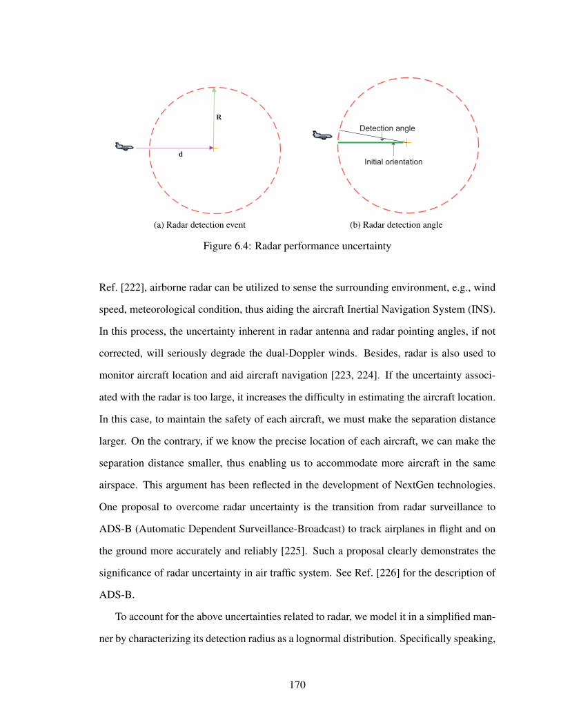
(a) Radar detection event (b) Radar detection angle

Figure 6.4: Radar performance uncertainty

Ref. [222], airborne radar can be utilized to sense the surrounding environment, e.g., wind

speed, meteorological condition, thus aiding the aircraft Inertial Navigation System (INS).

In this process, the uncertainty inherent in radar antenna and radar pointing angles, if not

corrected, will seriously degrade the dual-Doppler winds. Besides, radar is also used to

monitor aircraft location and aid aircraft navigation [223, 224]. If the uncertainty associ-

ated with the radar is too large, it increases the difficulty in estimating the aircraft location.

In this case, to maintain the safety of each aircraft, we must make the separation distance

larger. On the contrary, if we know the precise location of each aircraft, we can make the

separation distance smaller, thus enabling us to accommodate more aircraft in the same

airspace. This argument has been reflected in the development of NextGen technologies.

One proposal to overcome radar uncertainty is the transition from radar surveillance to

ADS-B (Automatic Dependent Surveillance-Broadcast) to track airplanes in flight and on

the ground more accurately and reliably [225]. Such a proposal clearly demonstrates the

significance of radar uncertainty in air traffic system. See Ref. [226] for the description of

ADS-B.

To account for the above uncertainties related to radar, we model it in a simplified man-

ner by characterizing its detection radius as a lognormal distribution. Specifically speaking,

170

we consider the following uncertainties related to the radar:

• The detection radius varies from radar to radar. In the numerical example, regional

radars are assumed to have a detection radius following a lognormal distribution

LN(Rr,10) whereas local radars have a detection radius of LN(Rl,5). In the simula-

tion, we implement different realizations for each radar. When the distance d is less

than the specific radar range realization R, where d is the distance from the aircraft

to the center of the radar (see Fig. 6.4a), then the detection event occurs.

• The exact time when the aircraft is detected also depends on the initial orientation

and radar beam rotation speed. The initial orientation of the radar beam varies from

radar to radar. In this study, the initial orientation is assumed to follow a uniform

distribution U(0,2π). The beam rotation speed determines the sector that a radar can

cross in a second. Suppose the radar antenna has 2 revolutions per minute (RPM),

then it covers a 120 sector in one second. The beam rotation speed also varies from

radar to radar. A lognormal distribution is used to characterize the variability of the

beam rotation speed. As shown in Fig. 6.4b, an aircraft can be detected only when it

is within the detection sector.

6.2.3.4 Communication Delays

When disruption or inclement weather happens, the Air Traffic Command Center (ATCC)

contacts each airline’s Airline Operations Center (AOC) to inform about the necessity of

re-routing. In this process, the regional radar and associated operators need to send mes-

sages to ATCC on the aircraft status, e.g., its altitude, location, and original landing airport.

Based on the information collected from the ground-based radars, ATCC re-routes the cor-

responding flight to the available airport [200]. Multiple communications emerge in this

process. Once the flight plan is filed, the communication starts between aircraft (pilot) and

assigned airport (controller). Prior to landing, all Instrument Flight Rule (IFR) flights are

conducted with controller-pilot communication regarding the status of runway clearance,

171

Aircraft: Entry into the region

Radar: Detect aircraft, send

message to DM

Message

DM: Register aircraft

DM: Re-route aircraft, send

message to assigned airport

Assigned aircraftAssigned airportAcknowledgement

message

Sending message

Se

nd

ing

m

essage

Acknow

ledgem

ent

message

Figure 6.5: System workflow

gate availability, and taxiways [227]. Each time the communication occurs, message delay

or loss arises with a given probability.

In this chapter, we simulate the above process in a simplified manner, in which the DM

plays the role of ATCC. Fig. 6.5 illustrates the specific system work flow. There are three

types of communication: registration, message communication between DM and assigned

airport, and communication between assigned airport and assigned aircraft. Message delay

can happen in any of three communications shown in Fig. 6.5. For the sake of simplicity,

all delays are simulated using independent but identical lognormal distributions LN(md,4)

seconds. If the message delay exceeds a predefined threshold, the message is treated as

lost. To avoid message loss, each message sender periodically checks for acknowledgement

(every 40 secs for the sake of illustration), and sends a repeat message if acknowledgement

is not received.

172

List of Symbols

αi j A variable used to denote the size of aircraft i. If j = 1, the size is large; if j = 2,

the aircraft’s size is medium; if j = 3, its size is small

ASi Speed of aircraft i.

dt(i,k) Distance between the ith aircraft and the kth airport at time t

LFit The remaining miles for ith airplane at time t

M The number of airports in the system

Pt The number of aircraft at time t

SGkjt The number of available gates for airplanes of size j in the kth airport at time t

SRkjt The number of available runways for airplanes of size j in the kth airport at time t

SSkjt The number of available airspace for airplanes of size j in the kth airport at time t

δikt A binary variable. δikt = 1, if ith aircraft is assigned to the kth airport at time t.

Otherwise, δikt = 0

6.2.4 Mathematical Model of Aircraft Re-routing Optimization

In the aircraft re-routing problem, suppose we have Pt aircraft in the region at time t and

M airports. The DM makes periodic re-routing assignments. The objective is to the total

distance travelled by all the airplanes, for safety and economic reasons [228, 229], subject

to system resources. The optimization problem can be formulated as:

MinimizePt

∑i=1

M

∑k=1

dt (i,k)δikt (6.3)

s.t.

δikt = 0 or 1, (6.4)

173

M

∑k=1

δikt = 1, i = 1, . . . ,Pt (6.5)

3

∑j=1

αi j = 1, i = 1, . . . ,Pt (6.6)

M

∑k=1

Pt

∑i=1

δikt = Pt , (6.7)

P(LFit−dt (i,k)≥ 0)≥ 0.9δikt , i = 1, . . . ,Pt , k = 1, . . . ,M (6.8)

Pt

∑i=1

αi jδikt ≤ min(SRkjt ,SGk

jt ,SSkjt) j = 1, . . . ,3, k = 1, . . . ,M (6.9)

LFit = LFi0−ASi× t, i = 1, . . . ,Pt (6.10)

where the decision variable δikt is binary, defined as:

δikt =

1, if the ith aircraft is assigned to the kth airport at time t

0, otherwise.

The constraint in Eq. (6.5) requires that each aircraft registered in the system in the current

cycle must be assigned to one of the available airports. Eq. (6.6) imposes aircraft size re-

strictions. Eq. (6.7) requires that all the aircraft registered before time t should be assigned

at time t. Eq. (6.8) is a reliability constraint. Both LFit and dt(i,k) are random variables.

This constraint requires that the remaining miles in any aircraft is larger than the distance

between the aircraft and the assigned airport with a probability of 0.9. Eq. (6.9) imposes

the constraint that the number of aircraft of size j assigned to airport k should be less than

the number of available resources in size j in airport k (runways, gates, and airspace). Con-

straint (6.10) denotes the relationship between the remaining miles and time, where LFi0

indicates the initial remaining miles for ith aircraft.

This is an integer linear programming problem, in which only δikt is the decision vari-

able. In this study, we use the built-in algorithm – intlinprog – in Matlab to approach the

solution of this problem.

174

When the assignment model formulated in Eq. (6.3) cannot make feasible assignment

of all the registered aircraft, i.e., space is not available at any of the nearby airports for

some of the registered aircraft, we do not consider the system to have failed immediately.

Instead, we build a waiting queue for the registered but yet unassigned aircraft. According

to the available space, e.g., runways, gates, and airspaces, at all the airports, we select the

same number of aircraft from the waiting queue to make the assignment. There are many

ways to rank the aircraft in the waiting queue, e.g., by registration time, or by remaining

miles. For the sake of illustration, we carry out a “first-come first-served” (FCFS) strategy

to order the aircraft in the waiting queue according to their registration time.

The optimization objective formulated in Eq. (6.3) is only for the sake of illustration,

there are many other alternatives in real-world applications. In some programs, the airline

company or ATCC aims to minimize the delay costs, e.g., passengers’ delay, by re-routing

certain flights. When some unexpected disruptions occur, passengers are inconvenienced

and various costs are incurred. From the airline’s perspective, their goal is to minimize the

influence caused by disruption, e.g., minimizing deviations from the original schedule. In

this study, we focus more on the uncertainty involved in the re-routing process rather than

the optimization objective. Hence, for the sake of illustration, we minimize the total dis-

tance travelled by all the assigned aircraft to ensure safe landing within available remaining

miles for as many aircraft as possible.

6.3 Proposed Methodology for Performance Assessment

In this section, we describe the extraction of the system failure time from the re-routing

simulation, conduct variance-based sensitivity analysis to identify significant variables, and

construct an SVR surrogate model with precise and imprecise data in order to construct the

probability distribution of system failure time.

175

6.3.1 System Failure Time

As mentioned in Section 2, system failure time (see definition 2.1) is the metric of

interest in analyzing the re-routing system performance. To build the system failure time

distribution efficiently, the following analyses need to be performed:

• Given a specific input variable setting, how to efficiently predict the system failure

time distribution without running the entire simulation?

• How to quantify the contribution of each uncertain input variable towards the vari-

ance of the output of interest, i.e. system failure time?

In each simulation, we have a fixed duration T to run the simulation to see if the system

survives or fails. However, in some cases, the system survives longer than time T , which

results in right-censored data defined as below.

Definition 6.3.1 Type 1 Censored Data: Consider reliability testing of n (non-repairable)

units taken randomly from a population. During T hours, we observe r (0≤ r≤ n) failures.

The exact failure times are t1, t2, . . . , tr, and the other n− r units survive the entire T -hour

test without failing. This type of censoring is named “right censored” data since the times

of failure to the right (i.e., larger than T ) are not available.

Since the times of failure to the right (i.e., larger than T ) are missing for some simula-

tions, the challenge is how to estimate the system failure time. But when the system fails,

we have the information of all the aircraft waiting to be assigned, and we can identify the

aircraft with the least remaining miles. Here, we apply a conservative strategy by using

the lower bound of the system failure time as the actual system failure time. Suppose the

least remaining miles is LFmin, the following theorem can be utilized to estimate the system

failure time.

Theorem 6.3.1 If LFmin is less than the minimum distance between the aircraft current

location and all the airports, given its mileage consumption rate r, the time to failure is:

SFT = T +LFmin

r(6.11)

176

where T represents the duration of the simulation.

Since LFmin is less than the minimum distance between its current location and all

the nearby airports, in the subsequent assignments, it is impossible to make a feasible

assignment. As a result, its remaining survival time determines how long the system can

survive further. If LFmin is larger than the minimum distance, then we only know that the

system survives longer than the SFT in Eq. (6.11), thus SFT captures the lower bound of

the system failure time. In this case, the system failure time can only be expressed as an

interval: [SFT ,+∞].

6.3.2 Variance-based Sensitivity Analysis

The sensitivity of a model output to the stochastic inputs can be measured through the

relative contribution of each stochastic input to the variance of the output; the well known

Sobol’ indices (defined in Appendix C) are commonly used for this purpose. As mentioned

in Appendix C, to compute Sobol’ indices, a double-loop Mente Carlo simulation is re-

quired. There are 24 stochastic variables in our system. To calculate xi’s sensitivity, in the

inner loop, we need to fix xi and change all the other variables x−i. Whereas, the outer

loop requires fixing xi at different values. Suppose both inner loop and outer loop have 100

cycles, then 10,000 simulations are needed, which in turn takes a large amount of time to

collect the data. This is only sensitivity analysis for one single variable, not to mention

sensitivity analysis for the remaining 23 variables. Assume that only 1000 simulations are

affordable.

Fortunately, an efficient data-driven sensitivity analysis method has been recently de-

veloped [230], based on the concept of stratified sampling [231]. Suppose we divide the

range of an input variable xi into equally probable intervals φ ={

φ 1, · · · ,φ M}, then the

first-order Sobol’ index can be computed as:

Si = 1−Eφ

(Vφ l (y)

)V (y)

, l = 1, · · ·M. (6.12)

177

where Vφ l (y) represents the variance of y when xi is in the subspace φ l , V (y) denotes the

variance of the system response y. See Ref. [230] for details of this approach.

6.3.3 SVR Surrogate Model with Precise and Imprecise Data

Generally speaking, in reliability analysis, the failure rate is quite small [232], e.g.,

10−4, 10−5. If we aim to use simulation-based approaches to quantify the system failure

probability, a large number of samples is required to estimate the failure probability. Sup-

pose the failure probability is 10−4, then we expect to obtain 1 failure data point out of

10,000 samples on average. In our re-routing simulation, each simulation lasts a duration

of 2 to 10 minutes; depending on initial input variable settings, suppose we wish to collect

10,000 samples from the system, this will take 20,000 to 100,000 minutes, which is pro-

hibitive. As a result, we need to build a surrogate model to replace the original simulation

in order to efficiently build the system failure time distribution.

As mentioned earlier, system failure is not necessarily observed in all simulations. In

such cases, we represent its survival time as an interval: [SFT ,+∞], where SFT denotes

the lower bound of system failure time. Suppose the dataset we have collected from the

re-routing simulation is represented by U, which we divide it into two separate groups:

right-censored data, denoted by U1, and uncensored point targets, denoted by U2.

Consider a censored data point xi ∈ U1, in this setting, we want the predicted survival

time for xi to be within the range [SiFT ,+∞], where Si

FT denotes the lower bound of system

failure time for xi. As long as the predicted value is larger than SiFT , there is no penalty.

Otherwise, we penalize if the predicted survival time is less than SiFT . Hence, the robust

ε-insensitive cost function Lε for xi can be updated as follows:

Lε ( f (x) ,y) =

SiFT − f (x)− ε if Si

FT − f (x)> ε,

0 otherwise.(6.13)

178

Obviously, the loss function for the right-censored data U1 becomes one sided, that is:

SiFT −w ·φ (xi)−b≤ ε +ξi, xi ∈ U1, (6.14)

subject to,

ξi ≥ 0.

For the point target xi ∈ U2, its loss function is still two-sided, that is:yi− (w ·φ (xi)+b)≤ ε +ξi,

w ·φ (xi)+b− yi ≤ ε +ξ ∗i ,

ξi,ξ∗i ≥ 0.

(6.15)

By combining the above equations, we now propose the following formula for SVR

regression in the re-routing system:

min C1N

N

∑i=1

(ξi +ξ∗i )+

12‖w‖2 (6.16)

subject to,

SiFT −w ·φ (xi)−b≤ ε +ξi, if x1 ∈ U1,

yi− (w ·φ (xi)+b)≤ ε +ξi, if x1 ∈ U2,(6.17a)

w ·φ (xi)+b− yi ≤ ε +ξ∗i , if x1 ∈ U2, (6.17b)

ξi,ξ∗i ≥ 0, i = 1, . . . ,N. (6.17c)

As can be noted from the above equations, we take advantage of all the useful infor-

mation available in the data. By introducing Lagrange multipliers αi for the inequalities

(6.17a), and α∗i for the inequalities (6.17b), the dual of the above problem can be formu-

lated as:

max −ε

N

∑i=1

(αi +α∗i )+ ∑

xi∈U2

(α∗i −αi)yi− ∑xi∈U1

αiSiFT−

12

N

∑i, j=1

(α∗i −αi)(α∗j −α j

)K(xi,xj

)(6.18)

179

subject to:

∑i

αi−α∗i = 0,

0≤ α,α∗ ≤C.

(6.19)

where α∗i = 0, ∀xi ∈ U1. By maximizing the objective function (6.18), for a new variable

x, its function value is represented by f (x) =N∑

i=1(αi−α∗i )K (x,xi)+b.

The performance of ε-SVR is mainly influenced by three parameters: kernel function

K, C, and ε . Currently, there are no unified rules for determining these parameters [233].

A common approach is to select their values by trial and error. In this study, we implement

a grid search cross-validation approach to choose their values.

The prediction performance of the SVR model can be evaluated using the following

performance measure, namely relative mean errors (RME):

RME =1n

n

∑i=1

∣∣∣∣yi− y∗iyi

∣∣∣∣ (6.20)

where yi is the actual value, and y∗i is the forecast value. For censored data, if y∗i ≥ yi, then

RME is 0. RME measures the deviation between actual and predicted values. The smaller

its value is, the closer are the predicted system failure times to the values from the original

simulation model.

6.4 Numerical Examples

In this section, two numerical examples are given to demonstrate the proposed method

for the aircraft re-routing and system performance assessment.

6.4.1 Input Variable Settings

Table 6.1 lists the random variables, their distributions and parameters. These variables

can be grouped into two classes: system variables (e.g., regional radar range, local radar

range, regional radar detection angle, local radar detection angle, message delay, and space

180

availability), and aircraft variables (remaining miles ratio, speed, and arrival rate). Besides,

each radar’s initial orientation follows a uniform distribution U(0,2π). In this chapter, we

assume all these stochastic variables, e.g., message delay, radar beam rotation speed, are

independent from each other. If there are correlations between the stochastic variables, it

can be easily included in MCS simulations. Well-established methods [220] are available

in the literature to generate MCS samples with correlated factors.

6.4.2 Data Collection

In our analysis, each simulation lasts for 10 cycles, each of duration 5 minutes. Every

5 minutes, the re-routing system makes feasible assignment decisions, pairing registered

aircraft with airports based on available space. Based on the probability distributions for

each variable described in Table 1, we run 2000 simulations and collect 2000 data points.

Among them, 71 data points are found to be right-censored.

As mentioned previously, the space availability at each nearby airport is associated with

three resources: runway, gate and airspace. In Table 6.1, the availabilities are represented

by three variables with their means κ , ξ , and η . As shown in Eq. (6.9), the assignment

algorithm is constrained by the minimum available resources among runway, gate, and

airspace. Thus, min(κ,ξ ,η) is used to characterize the space availability at each nearby

airport. In this way, 16 variables are employed to represent the space availability at the

nearby airports. Thus, a total of 25 input variables are used to characterize the system

inputs, and the system failure time is the only output.

6.4.3 Sensitivity Analysis

Due to the appearance of right-censored data, we cannot perform global sensitivity

analysis directly because we do not know the exact system failure time for some of the

simulations. Since we could only estimate the lower bound of the system failure time

for right-censored data, to perform sensitivity analysis, we need to use a crisp number to

181

Tabl

e6.

1:A

ssum

edpr

obab

ility

dist

ribu

tions

fort

hein

putv

aria

bles

.

Var

iabl

esN

umbe

rsD

istr

ibut

ions

and

para

met

ers

Para

met

erra

nges

Uni

t

Reg

iona

lrad

arra

nge

1L

ogno

rmal

:mea

nR

r,st

dev

10R

r∼

U[4

0,60

]m

iles

Loc

alra

darr

ange

1L

ogno

rmal

:mea

nR

l,st

dev

5R

l∼

U[1

4,24

]m

iles

Rad

arbe

amro

tatio

nsp

eed

1L

ogno

rmal

:mea

nB

s,st

dev

0.3

Bs∼

U[1.8,2.2]

RPM

(rev

olut

ion

perm

inut

e)In

itial

orie

ntat

ion

16U

nifo

rmU[0,2∗π

]M

essa

gede

lay

1L

ogno

rmal

:mea

nm

d,s

tdev

4m

d∼

U[2

5,50

]se

cond

s

Spac

eav

aila

bilit

yat

airp

ortk

16

R

unw

ay–

Log

norm

al:m

ean

κ,s

tdev

1κ∼

U[1,3]

Gat

e–

Log

norm

al:m

ean

ξ,s

tdev

5ξ∼

U[0,2

4]A

irsp

ace

–L

ogno

rmal

:mea

nη

,std

ev3

η∼

U[0,9]

Arr

ival

rate

1Po

isso

n:λ

λ∼

U[2

0,30

]fiv

em

inut

esR

emai

ning

mile

sra

tioβ

1U

nifo

rmβ∼

U[0.6,1]

Air

craf

tspe

eds

3

L

arge

–L

ogno

rmal

:mea

nν

,std

ev65

ν∼

U[5

46,6

09]

mile

spe

rhou

rM

ediu

m–

Log

norm

al:m

ean

ς,s

tdev

40ς∼

U[3

45,4

14]

mile

spe

rhou

rSm

all–

Log

norm

al:m

ean

χ,s

tdev

28χ∼

U[2

26,2

92]

mile

spe

rhou

r

182

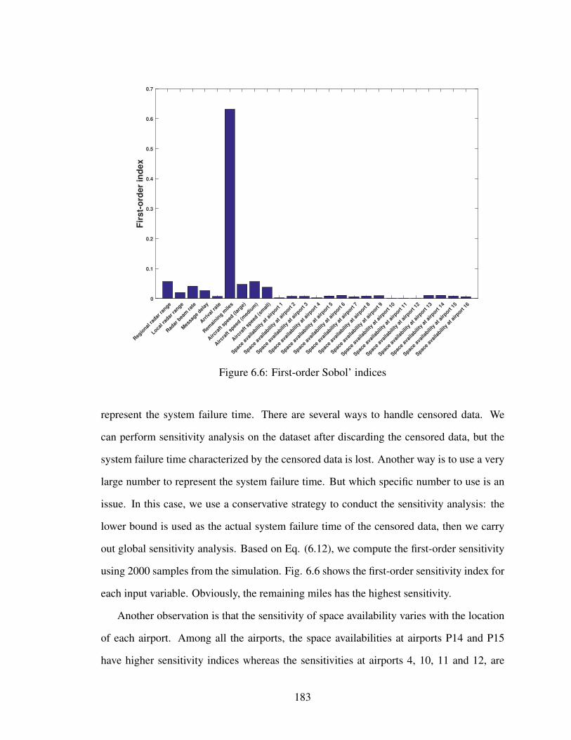
Reg

ional

radar

range

Local r

adar

range

Rad

ar b

eam

rate

Mes

sage

delay

Arriv

al ra

te

Rem

ainin

g mile

s

Airc

raft

spee

d (lar

ge)

Airc

raft

spee

d (med

ium

)

Airc

raft

spee

d (sm

all)

Space

avai

labili

ty a

t airp

ort 1

Space

avai

labili

ty a

t airp

ort 2

Space

avai

labili

ty a

t airp

ort 3

Space

avai

labili

ty a

t airp

ort 4

Space

avai

labili

ty a

t airp

ort 5

Space

avai

labili

ty a

t airp

ort 6

Space

avai

labili

ty a

t airp

ort 7

Space

avai

labili

ty a

t airp

ort 8

Space

avai

labili

ty a

t airp

ort 9

Space

avai

labili

ty a

t airp

ort 1

0

Space

avai

labili

ty a

t airp

ort 1

1

Space

avai

labili

ty a

t airp

ort 1

2

Space

avai

labili

ty a

t airp

ort 1

3

Space

avai

labili

ty a

t airp

ort 1

4

Space

avai

labili

ty a

t airp

ort 1

5

Space

avai

labili

ty a

t airp

ort 1

6

Fir

st-

ord

er

ind

ex

0

0.1

0.2

0.3

0.4

0.5

0.6

0.7

Figure 6.6: First-order Sobol’ indices

represent the system failure time. There are several ways to handle censored data. We

can perform sensitivity analysis on the dataset after discarding the censored data, but the

system failure time characterized by the censored data is lost. Another way is to use a very

large number to represent the system failure time. But which specific number to use is an

issue. In this case, we use a conservative strategy to conduct the sensitivity analysis: the

lower bound is used as the actual system failure time of the censored data, then we carry

out global sensitivity analysis. Based on Eq. (6.12), we compute the first-order sensitivity

using 2000 samples from the simulation. Fig. 6.6 shows the first-order sensitivity index for

each input variable. Obviously, the remaining miles has the highest sensitivity.

Another observation is that the sensitivity of space availability varies with the location

of each airport. Among all the airports, the space availabilities at airports P14 and P15

have higher sensitivity indices whereas the sensitivities at airports 4, 10, 11 and 12, are

183

negligible. The sensitivity of space availability at each airport is greatly influenced by the

complicated interactions in the system. In the assignment model, the overall travelling

distance is affected by the location of the registered aircraft. But the time that an aircraft

is registered is affected by other factors, e.g., its entry time and location, and the time it is

detected by the radar. When the aircraft is registered determines its location, which in turn

influences our assignment decision.

6.4.4 Surrogate Model Construction

Based on the sensitivity analysis result shown in Fig. 6.6, we eliminate the variables

with low contribution to the overall system variance, thus reducing the problem dimension

and accelerating the surrogate model construction. Among the 25 random variables con-

sidered in this study, we remove ten variables with low sensitivity indices. The 15 variables

that are retained in the surrogate model are: regional radar range, local radar range, radar

beam rate, message delay, remaining miles, aircraft speed (large), aircraft speed (medium),

aircraft speed (small), and the space availability at airports 5, 6, 8, 9, 13, 14 and 15.

Next, cross validation is used to determine parameter values. The data is split into ten

groups: nine out of ten are used to train the model, and the remaining one is used to validate

the performance of the trained model. Then grid search is used to search the space of these

variables using exponentially growing sequences of C and ε to identify good values of

the parameters (for example, C = 2−4,2−2,20,22,24). We try three kernel functions: linear

kernel, Gaussian kernel, and polynomial kernel. The kernel functionK, with parameter set

of C and ε , which yields the minimum RME, is selected. It is found that the parameter set

C = 2−3,ε = 2−10, and γ = 22 gives the best prediction result (minimizing the test RME).

Fig. 6.7 shows the comparison results between the actual simulations and the SVR

surrogate model predictions for 200 data points. The SVR predictions (with polynomial

kernel) show good agreement with the observed system failure time. The relative mean er-

ror is 7.3%, which indicates that the SVR model is reasonably accurate. If higher accuracy

184

Data Point

0 20 40 60 80 100 120 140 160 180 200

Syste

m F

ailu

re T

ime (

secs)

1500

2000

2500

3000

3500

4000

4500

5000

Original simulations

SVR predictions

Figure 6.7: System failure time prediction with ε-SVR model

is desired, more runs of the original re-routing simulation are needed.

System failure time (secs)500 1000 1500 2000 2500 3000 3500 4000 4500

pd

f

×10-4

0

1

2

3

4

5

6

7

8

9

Figure 6.8: First case: System performance assessment

185

6.4.5 Case I

With the surrogate model constructed in the previous section, we evaluate the system

performance by randomly sampling the 15 variables within their ranges. Fig. 6.8 shows

the system failure time distribution based on 20,000 samples.

Given the 20,000 samples, we fit the data using five candidate distributions: Weibull,

lognormal, normal, gamma, and exponential. The parameters related to these distributions

are estimated by maximizing the corresponding likelihood function. Two goodness-of-fit

plots are shown in Fig. 6.9 to demonstrate the performance of each candidate distribution.

Fig. 6.9(a) compares the density functions of the fitted distributions along with the his-

togram of the empirical distribution, and Fig. 6.9(b) denotes the comparisons between the

CDF plot of both the empirical distribution and the fitted distributions. As can be observed,

Gamma and Lognormal distributions give reasonable agreement with the data.

Histogram and theoretical densities

Data

1500 2000 2500 3000 3500 4000

0e

+0

02

e−

04

4e

−0

46

e−

04

8e

−0

4

Weibull

Lognormal

Normal

Gamma

Exponential

0 5000 10000 15000 20000 25000

15

00

20

00

25

00

30

00

35

00

40

00

Q−Q plot

Theoretical quantiles

Em

piric

al qu

an

tile

s

Weibull

Lognormal

Normal

Gamma

Exponential

Density

Figure 6.9: Two Goodness-of-fit plots for various distributions fitted to continuous data(Weibull, Lognormal, normal, gamma, and exponential distributions fitted to 20,000 sam-ples)

In addition, three well-known quantitative tests are employed to quantify the goodness-

186

Table 6.2: Goodness-of-fitness statistics as defined by Stephens [1]

Statistic General formula Computational formula

Kolmogorov-Smirnov (KS) sup |Fn (x)−F (x)|

max(D+,D−)D+ = max

i=1,...,n

( in −Fi

)D− = max

i=1,...,n

(Fi− i−1

n

)Cramer-von Mises (CvM) n

∫ +∞

−∞(Fn (x)−F (x))2dx 1

12n +n∑

i=1

(Fi− 2i−1

n

)2

Anderson-Darling (AD) n∫ +∞

−∞

(Fn(x)−F(x))2

F(x)(1−F(x)) dx −n− 1n

n∑

i=1(2i−1) log(Fi (1−Fn+1−i))

Table 6.3: Goodness-of-fit statistics.

Weibull Lognormal Normal Gamma Exponential

Kolmogorov-Smirnov statistic 0.06790564 0.04280514 0.06185114 0.04557395 0.489977Cramer-von Mises statistic 29.82418846 15.17619515 23.01538695 15.60813899 1322.880084Anderson-Darling statistic 199.44501732 95.18102060 143.27729802 98.24155121 6221.194507

of-fitness of each candidate distribution: Kolmogorov-Smirnov, Cramer-von Mises, and

Anderson-Darling, which are defined in Table 6.2. The statistical test results are shown

in Table 6.3. Among the candidate distributions considered, the lognormal distribution

has the lowest statistical error in all three tests. In other words, the lognormal distribution

fits the data best. The parameters of the best-fitted lognormal distribution are: µ = 7.79,

σ = 0.1786. Suppose we want to estimate the probability that the system survives longer

than 2600s; the results are shown in Table 6.4. As can be noted, there is a 6.3% deviation of

the system reliability estimation between the fitted distribution and the actual simulation.

But considering the two approximations in estimating the system reliability, our prediction

is very precise. Specifically, when we build the surrogate model from the 2,000 simulation

data, there is approximation error between the simulation data and the surrogate model,

which is about 7.3%. When we fit the distributions according to the samples generated by

the surrogate model, the second approximation arises. Thus, the 6.3% prediction discrep-

ancy is within the range of the deviation caused by the two approximations.

In addition, the Kaplan-Meier estimator fits the data very well. Since the simulation

lasts for 3,000s, when we estimate P(SFT > 2600), there is no right-censored data involved.

187

Table 6.4: System reliability analysis.

Original simulation Lognormal distribution Kaplan-Meier estimator

P(SFT > 2600) 0.3255 0.3408 0.3255P(SFT > 4200) 0.023 0.012 0.0337

In this case, the Kaplan-Meier estimator is equivalent to the empirical cdf. In contrast, when

we evaluate the probability of P(SFT > 4200), censored data arises. It can be observed that

the Kaplan-Meier estimator overestimates the probability of P(SFT > 4200). However, the

fitted distribution gives a more conservative prediction for this example when compared

with the Kaplan-Meier estimator.

6.4.6 Case 2

In this section, we broaden the range of the mean for the space availability at the nearby

airports: κ ∼U [1,6], ξ ∼U [0,48], and η ∼U [0,18]. Since the upper bound in the mean

values of available runways, gates, and airspace has increased, the system survives a longer

time than Case I. Following the same procedure, we collect 1,000 data points, of which

600 are found to be right-censored. The system failure time of the right-censored data is

represented by an interval [SFT ,∞]. As long as the predictions of our surrogate model fall

within the range, there is no penalty. In other words, the prediction can be any number

in the range [SFT ,∞]. Thus, the right-censored data contributes to the uncertainty in the

surrogate model prediction. The performance of the surrogate model will deteriorate if

there are more right-censored data due to the increase in uncertainty.

Table 6.5: Case 2: system reliability analysis.

Original simulation Surrogate model Kaplan-Meier estimator

P(SFT > 2600) 0.6766 0.7311 0.6747P(SFT > 3844) 0.5978 0.5885 0.4012

Contrary to the first case, the average error of the surrogate model has risen to 18% in

188

-5000 0 5000 10000 15000 20000

System failure time (secs)

0

0.2

0.4

0.6

0.8

1

1.2

pd

f

×10-4

(a) Case 2: System performance assessment

-5000 0 5000 10000 15000

System failure time (secs)

0

0.2

0.4

0.6

0.8

1

CD

F

Surrogate model

Simulation

Kaplan-Meier

(b) Case 2: Comparisons of cumulative distributionfunction

Figure 6.10: Performance assessment

the second case due to the increase of right-censored data. Fig. 6.10a shows the system

failure time distribution. Since some of the system failure time predictions in the surrogate

model are negative, we cannot fit it using the four candidate distributions. Table 6.5 shows

the comparison results among original simulation, surrogate model, and Kaplan-Meier es-

timator. Fig. 6.10b shows the comparisons of cumulative distribution function. When the

time is less than 3,844s, there are only 2 right-censored data out of 402 points. The Kaplan-

Meier estimator is equivalent to the empirical CDF if there is no right-censored data. As a

result, the Kaplan-Meier estimator nearly coincides with the empirical cdf. When the time

is larger than 3,844s, all the system responses are right-censored. The Kaplan-Meier esti-

mate of system reliability then becomes a constant 0.4012. However, the surrogate model

still fits the cumulative distribution of system failure time very well, as shown in Fig. 6.10b

and Table 6.5.

6.5 Summary

This chapter assesses system resilience through measuring the effectiveness of an al-

gorithmic response in handling extreme events, in which system survival time is used a

quantitative metric. By simulating different scenarios and configurations, we quantify the

189

survival rate of a response strategy in mitigating the impact of extreme event. In particular,

we evaluate the performance of a re-routing strategy in alleviating the impact of an air-

port closure caused by extreme events. We assess the effectiveness of the response action

in the presence of uncertainty arising from several different sources (radar performance,

communication system, aircraft characteristics, and space availability in nearby airports)

and develops an support vector regression-based approach to assess the performance of

the proposed methodology. A simulation-based approach is used to characterize the actual

re-routing process and account for the uncertainty contributed by several heterogeneous

subsystems. Based on the simulation data, we employ a data-driven sensitivity analysis

method to quantify the contribution of each uncertain variable towards the overall variance

of system response. The variables with the lowest importance are removed to reduce the

problem dimension. A support vector regression surrogate model is built for predicting the

system failure time and constructing the probability distribution for the failure time of the

re-routing system.

Our contributions are several fold. First of all, since the current aircraft re-routing is

operated manually, it is hard to assess the performance of aircraft re-routing operations. In

this study, we develop a simulation-based model to accommodate the various uncertainties

arising in this process, and it allows us to evaluate the performance of the proposed re-

routing algorithm quantitatively. Secondly, based on the simulation, we perform sensitivity

analysis to quantify the contribution of each stochastic variable to the system reliability.

The sensitivity analysis results enable us to identify which factor affects the system per-

formance most, thus providing a quantitative basis for decisions such as component design

optimization and specific operational measures in order to improve system performance.

Given limited resources to improve the system performance, the sensitivity analysis result

provides the guidance to optimally allocate the limited resources. Thirdly, our study mod-

els the aircraft re-routing from a system of systems perspective considering the interactions

of multiple subsystems, and integrates the uncertainties arising from each subsystem (radar

190

detection, re-routing assignment, and communication system). In this way, we are able to

view this problem from a systemic point of view, have a comprehensive understanding of

the system work flow, and characterize the relationship among the subsystems. At last, the

construction of surrogate model improves the computational efficiency and facilitates fast

analysis of system performance, thus supporting real-time decision-making.

Our work brings several benefits to the practitioners (airline dispatcher and air traffic

controller) when extreme weather affects the original aircraft routes. With the aforemen-

tioned uncertainties considered, we provide quantitative analysis on the performance of

aircraft re-routing operation. In this sense, the airline dispatcher is able to make risk-averse

decisions given the system failure time distribution given a specific set of system param-

eters. In addition, since as the technology is moving towards the Next Generation Air

Transportation System (NextGen), there is a huge demand for automatic operations in or-

der to reduce the amount of information the air crew must process at one time [234, 235].

This chapter provides a case study of evaluating the performance of a re-routing algorithm

under uncertainty, and the simulation platform we have built is extendable to test the perfor-

mance of other re-routing algorithms with additional constraints imposed, e.g., separation

assurance.

The assessment of algorithmic response gains our insights on the effectiveness of al-

gorithms/strategies in handling extreme events. The reliability analysis of algorithmic re-

sponse illustrates the resilience of algorithmic strategy in different realizations of uncertain

environment when dealing with extreme events. To increase system resilience further, more

effective algorithms with robust performance in uncertain environment needs to be devel-

oped. The methodology developed in this chapter offers a general framework to evaluate

the effectiveness for more advanced algorithms to be developed in the future. Since the

purpose of assessing the response strategies is to make the system more resilient, in Chap-

ter 7, we explore the design for resilience in infrastructure systems from an optimization

point of view.

191

Chapter 7

Design Optimization for Resilience1

7.1 Introduction

The previous two chapters investigate the effectiveness of human and algorithmic re-

sponse in dealing with extreme events in existing systems, respectively. In this chapter, we

move towards designing the system for resilience. The overall goal of this chapter is to

enable resilience from an optimization perspective such that the system is equipped with

the capability to withstand extreme events, and we illustrate the developed method with an

application in the configuration of a logistics service center system.

Over the past few years, there has been a growing interest in the design for resilience

in terms of system configuration, logistics operations, and resource allocation. Likewise,

when determining the configuration (location and capacity) of logistics service centers (a

system consisting of multiple service centers distributed within an area to serve customers),

resilience is also an important and essential consideration. Take large global companies as

an example, they often distribute their manufacturing plants all over the world (global out-

sourcing) to reduce the operation cost and enhance business agility. In today’s competitive

world, the manufacturing plants distributed around the world are vulnerable to disruptions

caused by various factors, such as natural disasters, strikes etc. These disruptions often

result in immediate and significant loss in their revenue and market share, especially when

alternative competing enterprise can offer the same product or service. A recent major fire

at Ford caused the shutdown of the Dearborn truck plant and the full halt of F-150 produc-

tion line in all its manufacturing plants due to parts shortages. As reported by the Detroit

News [237], this disruption might have a potential damage to Ford’s second-quarter per-

formance and market share. In addition to global companies, regional service centers like

1An archival paper related to this chapter has been submitted to IEEE Transactions on Reliability forpublication. For more details, see Ref. [236]

192

banks and supermarkets often perform periodic renovation and store upgrades at certain

branches, which might result in congestion in other stores within the same area, thereby

causing a decrease in customer satisfaction. In worse cases, the customers might divert

to other companies because of the heavy congestion or long travel distance to other alter-

native stores. Thus, it is imperative to take such factors (i.e., planned regular renovation,

and unexpected disruptive events) into consideration in determining the configuration of

logistics service centers, whereas current studies considering the effect of random branch

breakdown on system performance and including resilience in the selection of logistics

distribution center are comparatively rare and limited.

In this chapter, we are motivated to bridge this research gap through the development of

a resilience-based framework to optimize the configuration of logistics service centers with

the consideration of the impact of random branch breakdown and other possible disruption

scenarios. In realistic scenarios, the number, locations, and sizes of distribution centers

significantly affect the quality of customer service as measured by the time that is needed

for each customer to reach the service center together with the amount of waiting time in

line and processing time at the service center. Hence, the distribution of service centers has

a significant impact on customers’ decisions in choosing the branch that he is going to be

served. Whereas, from the viewpoint of the planner, the company can only afford to build

a limited number of service centers due to budget constraints. Thus, service centers must

be designed and distributed reasonably with the consideration of customers’ behavior. The

interactions between planner and customers can also be analyzed from the game theory

point of view. Specifically, the planner, as a top-level decision maker, can determine where

to open and deploy the service center, thereby influencing customers’ service-choosing be-

havior, but has no control over which distribution center the customers choose to be served.

From the customers’ perspective, they are free to choose distribution/service centers based

on their own habits and behaviors (i.e., minimum distance, minimum travel time, or other

personal preferences), but do not have control over the location of the service center. The

193

interactions between planner and customers can be represented as a leader-follower game,

in which the planner acts as the leader in making an initial move at determining the loca-

tions of service center, while the customers freely choose the service center based on the

decision made by the planner. Mathematically, it can be modeled as a bi-level optimization

program, where the planner determines the locations and configurations of logistics centers

in the upper level, while the customers take corresponding reaction based upon the decision

made by the planner.

To characterize the impact of potential disruptions due to some extreme event, we ran-

domly pick a fixed number of service centers and make them closed simultaneously. Since

the impacted service centers are closed, customers shift to other alternate centers that are

still in service, which might cause traffic congestion and long queues. Thus, we formu-

late the objective as mitigating the expected congestion incurred by the closing of certain

service centers during the service center restoration period; thus, developing a resilient ser-

vice center distribution subject to a fixed amount of budget. The problem is formulated as a

nonlinear integer optimization problem, and our goal is to design a resilient logistics center

distribution such that the expected customer service time can be minimized. Specifically,

there are two decision variables in this problem: where to locate the service centers and

the number of servers at each service center. A multi-level cross-entropy algorithm is de-

veloped to tackle the bi-level optimization problem to approach the near-optimal solution

within limited time. In comparison with the current state-of-the-art studies, we have made

the following contributions:

1. We develop a new formulation of user equilibrium traffic assignment in the service

centers configuration, where the travel demand between each pair of origin and des-

tination nodes is unknown in advance.

2. We propose an innovative method to determine the customer demand at each service

center with the introduction of dummy node and auxiliary links.

194

3. The upper-level model not only considers the travel time of each user from different

zones to the service centers, but also their average waiting time in line and processing

time within each service center.

4. To tackle the challenging bi-level optimization problem formulated in this chapter,

a multi-level cross entropy method is leveraged to find an importance sampling that

gradually concentrates all its mass in the vicinity of the optimal state.

7.2 Problem Formulation

Logistics service center location, as a crucial issue, plays a significant role in main-

taining the daily operations of societal activities ranging from financial services to grocery

shopping. Typically, there are two major considerations in determining the configuration

of logistic distribution centers, namely where to deploy the service center (location), and

what should be the design capacity of each service center (capacity). In this chapter, we

account for these two major factors in the configuration of resilient logistics center distri-

bution so that it is able to recover from different disruptive events in an efficient manner.

In practice, the configuration of service centers and customer demand distribution among

the established service centers are determined by two individual entities. By varying the

location and capacity of service centers, decision maker can influence customers’ choice

by making some service centers more attractive than others, but has no control over cus-

tomers’ choice behavior. Whereas, each customer compares and chooses the service center

based on his/her own habit and preference (e.g., travel distance, travel time, or perceived

waiting time at each service center). As can be observed, there is an explicit hierarchical

relationship between the two players in this problem. The interactions between the leader

(decision maker) and follower (customers) can be mathematically modeled with bi-level

programming [238] as follows.

(U0) minx

F (x,y)

s.t. G(x,y)≤ 0,(7.1)

195

where x denotes the decision variables in the upper-level model, while y = y(x) is deter-

mined by the optimization problem in the lower-level model:

(L0) miny

f (x,y)

s.t. g (x,y)≤ 0.(7.2)

where y represents the vector of variables resulting from the non-cooperative competition

behavior among the customers in the lower-level model given the actions (x) taken by

the decision maker in the upper-level model. F is the objective function in the upper-level

model, e.g., minimizing the system total travel cost, f is the objective function in the lower-

level model, e.g., minimizing the cumulative customer travel cost, and G and g denote the

system constraints in the upper and lower level problems, e.g., flow conservation, balanced

demand and supply.

In general, the objectives that the two players have are usually conflicting with each

other in the system. To be more specific, users in the lower-level model (L0) typically aim

to maximize the individual utility function through the optimization of decision variable y

subject to constraints g while the variable x in the upper-level model acts as parameters.

Conversely, the upper-level model F aims to minimize the total system travel cost via the

optimization of the location and capacity associated with each service center as represented

by the decision vector x, while decision variable y is regarded as parameters. The partition

of the control over the two decision vectors between two ordered levels imposes to model

the problem as a bi-level program. Through the response function y = y(x), the actions of

two players are coupled together, thereby influencing each other’s decision. From the sys-

tem design viewpoint, each decision vector x corresponds to a particular configuration of

service center distribution. Given each system design, the customer selects a service center

that maximizes his/her own utility function. As a result, a unique traffic flow distribution

emerges in the network, which further influences the design objective formulated in the

upper-level model.

196

7.2.1 User Equilibrium Traffic Assignment

As introduced in the previous section, given the service center configuration, each cus-

tomer makes their own choice to minimize the travel cost. Suppose travel time is the only

consideration for each customer, at the initial stage, all the customers choose the service

center that needs the least amount of travel time. With time going on, traffic flow accu-

mulates along the minimum-cost path, thereby resulting in congestion. Since travel cost

depends on traffic flow, the emergence of congestion on certain paths leads to the increase

in their travel time. Given the updated travel time along each path, customers shift to other

service centers via other paths with shorter travel time. The same non-cooperative compe-

tition behavior continues until no customer can reduce his/her travel time by unilaterally

shifting to other service centers through other routes. Eventually, the system converges to

an ultimate traffic equilibrium state, where no customer could reduce the travel time by

making other movements. Such state is also referred to as Wardrop user equilibrium [239],

and one important principal can be established at the user equilibrium state: the travel time

along all the used paths is the same and less than those that would be experienced by a

single vehicle on any unused route.

However, in the context of service center distribution problem, its user equilibrium state

differs from the user equilibrium state of transportation system in two major aspects.

1. If the locations of service distribution centers are given, there are two decisions made

by each customer in choosing the service center. Specifically, the first decision is

which center he/she plans to go to, and the second decision is which path he/she

should take to go to the service center he/she just chooses. These two decisions are

combined together and made simultaneously to achieve his/her objective in mini-

mizing the total travel time. Whereas, in transportation system, each passenger only

needs to determine which path to take to reach the target location because the desti-

nation is already known in advance.

197

2. Another primary difference is that the traffic demand between each origin-destination

(OD) pair is explicitly given in the transportation system. While in the service center

distribution problem, we only know the number of customers at each community (or

region), and no explicit value is given to indicate the number of customers between

each resident zone and service center.

The above two features differ the user equilibrium in the context of service center dis-

tribution problem from the classical user equilibrium defined in Section 2.3. To address

the new challenges, we formulate a new user equilibrium traffic assignment for the service

center configuration problem in this chapter. Consider a directed network G (V,E), where

V and E denote the set of nodes and edges in graph G , and V = {v1, ...,vn}, where n ≥ 2.

Suppose the number of customers at each node (zone) vi is denoted by di, there is a set of

candidate sites M, where logistics distribution centers could be established. Here, a binary

variable zm (m ∈ M) is used to indicate whether to construct logistics distribution center

at site m or not. If logistics distribution center at site m is constructed, then zm takes the

value of 1; otherwise, zm takes the value of 0. Suppose the number of customers that each

service center m serves is represented by λm, since all the customers should be served by

some service center, then we have:

n

∑i=1

di = ∑m∈M

λm (7.3)

where λm denotes the amount of customers that is served by logistics distribution center m,

and di denotes the customer demand at node vi. Obviously, only after the logistics service

center at site m is established, then it is able to serve customers, which implies the following

constraint:

0≤ λm ≤ ωzm,∀ m ∈M. (7.4)

where ω is an arbitrarily large positive constant. When zm = 0, then λm cannot be positive.

As a result, we have 0 ≤ λm ≤ 0, and it implies that λm can only take the value of zero

198

because logistics distribution center m is not established. But if zm = 1, then λm can be as

large as desired.

Suppose Pi,m denote the set of cycle-free paths from the customer at node vi to the

service center m, qi,mp represent the number of customers along the path p connecting the

customer at node vi with service center m, then we have:

n

∑i=1

∑p∈Pi,m

qi,mp = λm, ∀ m ∈M. (7.5)

The above constraint imposes that the total number of customers along all the paths

connecting all the customer nodes and service center m should be equal to the amount of

customers that logistics distribution center m serves. Obviously, the number of customers

along each path must be non-negative, thus we have:

qi,mp ≥ 0, ∀p ∈ Pi,m, for i = 1,2, · · · ,n, m ∈M. (7.6)

Let a (a ∈ E) be one link in the network G, xa denote the traffic flow along link a, then

the total amount of flow along link a is expressed as:

xa =n

∑i=1

∑m∈M

∑p∈Pi,m

qi,mp δ

i,ma,p , ∀a ∈ E. (7.7)

where δi,ma,p is a binary variable indicating whether link a is a segment constituting path p

(p ∈ Pi,m). When δi,ma,p = 1, it reveals that link a is a segment constituting path p; otherwise,

δi,ma,p = 0.

With the above notations, the user equilibrium traffic assignment in the context of logis-

tics distribution center location can be formulated as the following nonlinear optimization

199

problem:

min f = ∑a∈E

xa∫0

ta (x)dx

s.t. xa =n∑

i=1∑

m∈M∑

p∈Pi,mqi,m

p δi,ma,p , ∀a ∈ E,

n∑

i=1di = ∑

m∈Mλm,

n∑

i=1∑

p∈Pi,mqi,m

p = λm, ∀ m ∈M,

qi,mp ≥ 0, ∀p ∈ Pi,m, for i = 1,2, · · · ,n, m ∈M,

0≤ λm ≤ ωzm, ∀m ∈M.

(7.8)

where f is a function denoting the cumulative travel cost for all the customers, ta (x) is

a monotonically increasing function to represent the relationship between traffic flow and

travel time, and zm is a binary variable indicating the establishment of logistics distribution

center at candidate site m (m ∈M) or not.

7.2.2 System-level Optimization

At the system level, system planner needs to make two individual decisions simultane-

ously with regard to the configuration of logistics service centers subject to a fixed amount

of budget, and the goal of system planner is to minimize the total travel and service time

for all the customers within the city. To be specific, the first decision is with regard to

where the service centers should be constructed among the set of candidate sites M given

the limited amount of investment, and the second decision is what should be the design ca-

pacity of each distribution center in terms of its capability in serving how many customers

on average per hour. Suppose the total budget that the system planner has is denoted by

a variable T . The cost of constructing each distribution center, for the sake of simplicity,

is a nonlinear monotonically increasing function of its design capacity, while the capacity

of each distribution center has an explicit impact on its serving capability, thereby affect-

ing the waiting time of each customer in line before they are served. From the previous

200

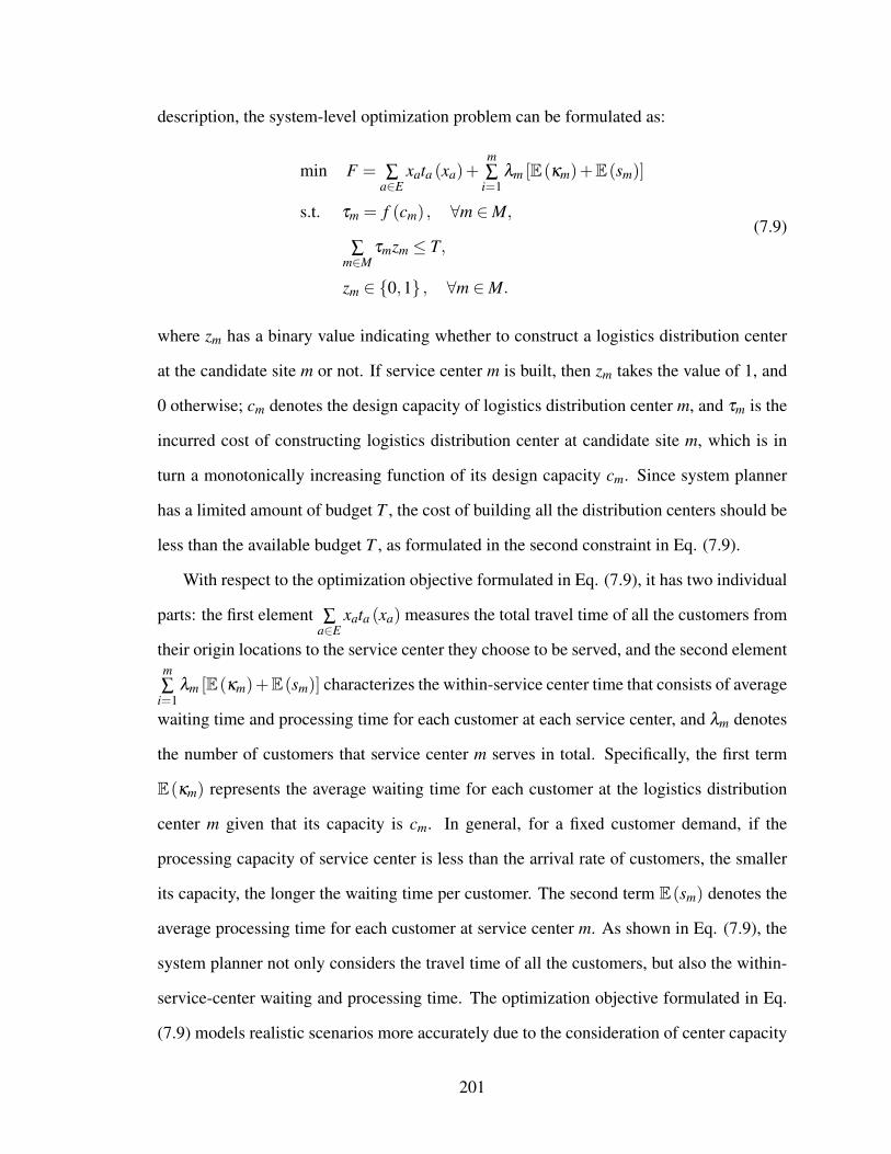
description, the system-level optimization problem can be formulated as:

min F = ∑a∈E

xata (xa)+m∑

i=1λm [E(κm)+E(sm)]

s.t. τm = f (cm) , ∀m ∈M,

∑m∈M

τmzm ≤ T,

zm ∈ {0,1} , ∀m ∈M.

(7.9)

where zm has a binary value indicating whether to construct a logistics distribution center

at the candidate site m or not. If service center m is built, then zm takes the value of 1, and

0 otherwise; cm denotes the design capacity of logistics distribution center m, and τm is the

incurred cost of constructing logistics distribution center at candidate site m, which is in

turn a monotonically increasing function of its design capacity cm. Since system planner

has a limited amount of budget T , the cost of building all the distribution centers should be

less than the available budget T , as formulated in the second constraint in Eq. (7.9).

With respect to the optimization objective formulated in Eq. (7.9), it has two individual

parts: the first element ∑a∈E

xata (xa) measures the total travel time of all the customers from

their origin locations to the service center they choose to be served, and the second elementm∑

i=1λm [E(κm)+E(sm)] characterizes the within-service center time that consists of average

waiting time and processing time for each customer at each service center, and λm denotes

the number of customers that service center m serves in total. Specifically, the first term

E(κm) represents the average waiting time for each customer at the logistics distribution

center m given that its capacity is cm. In general, for a fixed customer demand, if the

processing capacity of service center is less than the arrival rate of customers, the smaller

its capacity, the longer the waiting time per customer. The second term E(sm) denotes the

average processing time for each customer at service center m. As shown in Eq. (7.9), the

system planner not only considers the travel time of all the customers, but also the within-

service-center waiting and processing time. The optimization objective formulated in Eq.

(7.9) models realistic scenarios more accurately due to the consideration of center capacity

201

and service time at each service center, which makes the current research effort different

from the state-of-the-art literature studies.

As modeled in the upper-level model of bi-level formulation for logistics distribution

center location optimization, the system planner makes decisions with regard to the config-

uration of logistics center distribution in terms of service center location and its capacity

to maximize the performance of the system in serving the customers distributed across a

region. The formulated optimization objective models the significant considerations of sys-

tem planner in an appropriate manner through the configuration optimization of logistics

service centers.

7.3 Proposed Method

In this section, we mathematically formulate a bi-level optimization model for enabling

resilience in the configuration of logistics distribution centers. The objective of the upper-

level model is to maximize the resilience of the logistics center distribution system subject

to disruptions, while the customers traffic assignment is characterized in the lower-level

model. To tackle the traffic assignment in the lower-level model, a dummy node and aux-

iliary links are created to determine the corresponding customer demand allocation among

the service centers, then gradient projection method is utilized to determine the traffic as-

signment along the links in the traffic network. In the upper-level model, the logistics dis-

tribution center optimization problem is recast as a nonlinear integer optimization problem,

and a multiple level cross-entropy optimization algorithm is leveraged to identify the near-

optimal solution within limited amount of time. The flowchart of the proposed methodol-

ogy is summarized in Fig. 7.1.

7.3.1 Resilience-driven Optimization Model

In reality, unanticipated disruptions might lead to the shutdown of some service centers,

e.g., human-induced fire in factory or extreme weather events (i.e., flood, storm). Decision

202

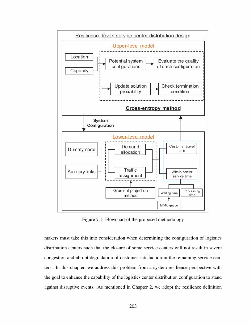
Resilience-driven service center distribution design

Upper-level model

Lower-level model

Location

Capacity

Dummy nodeDemand

allocation

Traffic

assignment

System Configuration

Customer travel

time

With in center

service time

Gradient projection method

Potential system

configurations

Evaluate the quality

of each configuration

Update solution

probability

Check termination

condition

Cross-entropy method

Waiting timeProcessing

time

Auxiliary links

M/M/c queue

Figure 7.1: Flowchart of the proposed methodology

makers must take this into consideration when determining the configuration of logistics

distribution centers such that the closure of some service centers will not result in severe

congestion and abrupt degradation of customer satisfaction in the remaining service cen-

ters. In this chapter, we address this problem from a system resilience perspective with

the goal to enhance the capability of the logistics center distribution configuration to stand

against disruptive events. As mentioned in Chapter 2, we adopt the resilience definition

203

developed by Henry and Ramirez-Marquez [2] as illustrated in Fig. 2.1, which is a time-

dependent function of the performance of a system before, during, and after the disruptive

event.

From Fig. 2.1, the system of interest experiences three different stages when disruptive

event e occurs. Prior to the occurrence of the disruptive event, the system operates at an as-

planned state S0 with a stable performance ψ (t0). At time instant te, when disruptive event

e happens, since the system is vulnerable to this disruption, its performance starts to drop

down gradually from the time instant te due to the failure of certain system components or

the loss of partial system functionality. The same performance degradation continues un-

til the time instant td when its performance drops to a maximum disrupted but stable state

ψ (td). With the preparation of recovery resources at time instant td and the implementation

of restoration action at time instant ts, system performance starts to restore to a better level

from time instant ts until arriving a best post-disruption level ψ(t f)

at time instant t f . Con-

sidering the variation of system performance ψ (t) before, during, and after the occurrence

of the disruptive event e, system resilience is defined as the ratio of system performance

that has been restored from the implementation of recovery action to the performance loss

caused by the disruptive event e, as mathematically formulated in Eq. (2.1) in Chapter 2.

From Eq. (2.1), it can be observed that resilience measures the recoverability ability

and restoration speed of a system in the presence of disruptive events. With respect to the

system of service center distribution, it is susceptible to several different types of disrup-

tive events in practice. For example, human-induced fire could cause the closure of truck

manufacturing plant, as revealed in the Ford example in the introduction, which severely

damages Ford’s global supply chain network. Natural disasters (e.g., storm, flood) might

hit a city unexpectedly and result in several service centers failing to offer services to cus-

tomers. Besides, service center usually performs renovation and upgrade to enable more

advanced functionality on a regular basis. All the aforementioned disruptive events lead

to the closure of some of the logistics distribution service centers. Suppose W , which is

204

a subset of M (W ⊆ M), denotes the set of logistics service centers that are damaged by

the disruptive event e. When the disruptive event e happens, customers shift to other logis-

tics distribution centers that are still in service, then the following mathematical model is

formulated to describe the new user equilibrium under this circumstance:

min f (e) = ∑a∈E

∫ xa0 ta (x) dx

s.t. xa =n∑

i=1∑

m∈M\W∑

p∈Pi,mqi,m

p δi,ma,p , ∀a ∈ E,

n∑

i=1di = ∑

m∈M\Wλm,

n∑

i=1∑

p∈Pi,mqi,m

p = λm, ∀m ∈M\W,

qi,mp ≥ 0, ∀p ∈ Pi,m, for i = 1,2, . . . ,n, m ∈M\W,

0≤ λm ≤ ωzm, ∀m ∈M\W.

(7.10)

In this case, for a given service center configuration, the shutdown of certain service

centers causes an increase in the customer demand allocation among remaining service

centers accordingly, thereby resulting in traffic congestion in the transportation system and

within-center waiting time in line and processing time. Customers may be less patient/loyal

to the company when a disruptive event diminishes a system’s ability to offer the service

in a timely manner. As a result, it is important to account for these factors in the decision

making pertaining to the configuration of service centers in a city. From a systematic point

of view, given the occurrence of disruptive event e, the total travel time and service time

for all the customers corresponding to the traffic flow at the new user equilibrium can be

updated as follows:

F(e) = ∑a∈E

xata (xa)+m∑

i=1λm [E (κm)+E (sm)] ∀m ∈M\W. (7.11)

Since disruptive event e has an explicit impact on customers’ traveling time and service

time, the goal of our study is to help system planner design a resilient service center con-

figuration with the consideration of the effect of possible disruptive events on the system

205

in advance such that the traffic congestion and long waiting time can be mitigated when

disruptive event actually happens. In this circumstance, by adopting the resilience defini-

tion developed by Henry and Ramirez-Marquez [2], the resilience of a given service center

configuration is measured as below:

R(u′,e

)=

F (u,e)−F (u′,e)F (u,e)−F (u)

(7.12)

where u= (z,c) is a vector consisting of two decision variables z and c corresponding to

whether to construct a service center and the design capacity of each established service

center at each candidate location m (m ∈ M), u and u′

represent two service center con-

figurations with and without the consideration of the potential impact of disruptive event e,

respectively. F (u) denotes the total time spent by all the customers before the occurrence

of disruptive event e, F (u,e) measures the total time consumed by all the customers in

the system configuration u after disruptive event e happens, and F(u′,e)

models the total

consumed time in the resilient design configuration u′when event e occurs.

The research goal of the proposed study is to help system operators to plan ahead and

prepare for any potential disruptive event such that the configured system has enough room

and buffer in response to the possible disruptive events through the optimization of decision

variable u.

7.3.2 User Equilibrium Traffic Assignment with Unknown Travel Demand

As mentioned earlier, unlike conventional transportation system, no specific value is

given to indicate the travel demand between each resident zone and service center in the

logistics service center distribution system. To address this issue, we introduce a dummy

node θ and auxiliary links to determine the customer demand allocation among the already

established service centers and the corresponding traffic flow assignment along each link.

As illustrated in Fig. 7.2, suppose yellow circles represent the service centers that are

established in different locations, light blue solid squares denote the zones where customers

206

2

3

4

n

1 m

1

5

Θ

Figure 7.2: A simple network to demonstrate the proposed method to deal with user equi-librium with unknown travel demand between resident zones and service centers

are distributed, and the solid links indicate the road segments that connect customers and

service centers. Given customer demand di at each zone, an approach needs to be developed

to determine the customer demand allocation at each service center. To tackle this problem,

a dummy node θ is created and added into the network. In parallel, several auxiliary links

are created to connect the service centers with dummy node θ . The travel time along the

artificial (dashed) links is set at a negligible value. Since all the customers’ demand needs

to be satisfied, then we have:n

∑i=1

di = λθ (7.13)

where λθ denotes the number of customers that the artificially created service center θ

serves.

With the introduction of dummy node θ , the traffic assignment equilibrium with un-

known demand between origins and destinations degenerates to the classical traffic assign-

ment problem. Since the demand at node θ is now known, which is the sum of customer

demand over all the city zones, a number of algorithms that are used for solving classical

207

traffic assignment problems, such as Frank-Wolfe [240], gradient projection [241], bush-

based algorithms [242, 243], and other algorithms [244, 7, 245], can be then utilized to

tackle this problem thereafter. Since the dummy node θ is only connected with service

centers, all the traffic flow that destinies at dummy node θ must go through one of these

links connecting service centers with dummy node. As a consequence, we are able to ob-

tain the corresponding customer demand allocation at each service center as well as the

traffic flow assignment in the network when it reaches user equilibrium. Since the travel

time along the artificially created links is negligible, following Wardrop’s user equilibrium

principle, the equilibrium state in the service center configuration problem investigated can

be characterized as: the travel time along all the used paths from customer zones to all the

service centers are minimized, and no customer could reduce the travel time by unilaterally

switching to other service centers or taking other routes.

For the sake of completeness, we briefly introduce the gradient projection method that is

leveraged to tackle the traffic assignment equilibrium problem for its efficiency and simplic-

ity [241]. Simply speaking, gradient projection approach solves traffic assignment problem

by exploiting the separability of the origin-destination (OD) pairs, and it operates directly

on the space of path flows. Suppose K(i,θ) denote the set of paths with positive traffic

flow between OD pair city zone i and dummy node θ . At each iteration, gradient projec-

tion method moves traffic flow to the shortest path from all the other non-shortest paths in

set K(i,θ) while keeping the path flows of other OD pairs fixed. Afterwards, traffic flow

along the paths is projected to the links, from which the travel time along each link is up-

dated accordingly. The same procedures are repeated over all the other OD pairs until the

predefined algorithm termination condition is met.

To be more specific, given the updated link travel cost, the shortest path among each

OD pair (i,θ) is updated and added to the set of paths K(i,θ) if the found shortest path

is shorter than the current shortest path. In parallel, paths that carry no flow are removed

from the set K(i,θ). The aforementioned two operations correspond to line 11 in Algorithm

208

Algorithm 2 : Gradient Projection Algorithm for Traffic Assignment Problem1: Initialize the network G, customer demand zone i (i = 1,2, · · · ,n), dummy node

θ , and the link cost function t.2: Generate initial shortest path for each OD pair3: for each OD pair (i,θ) ∈OD do4: Find the shortest path p from node θ to i5: Assign all the travel demand among OD pair (i,θ) to the shortest path p6: Store the found shortest path p in the set K(i,θ)7: end for8: Project the path flow on the links and update the link cost9: while the convergence termination condition is not met do

10: for each OD pair (i,θ) ∈OD do11: Update path cost yp, ∀p ∈ Pi,θ

12: Improve the path set Pi,θ

13: if Ps,t is improved or∣∣Pi,θ

∣∣> 2 then14: Shift the flow from the costlier paths to the shortest path15: Project the path flow on the links and update the link cost16: Remove unused paths from the set K(i,θ)17: end if18: end for19: end while

2. Afterwards, traffic flow is shifted from costlier paths to the shortest path continuously

until the algorithm termination criteria is satisfied. See more details on path flow shift in

Ref. [241]. With respect to the termination of the algorithm, we adopt a commonly used

convergence indicator as defined in Eq. (7.14) to decide when to halt the algorithm:

RGAP = 1−∑

i∈(1,2,··· ,m)di,θ · pi,θ

min

∑a∈E

xa · ta(7.14)

where di,θ denotes the total traffic flow from zone i to dummy node θ , pi,θmin represents the

travel time along the shortest path between OD pair (i,θ), xa and ta denotes the traffic flow

and travel time along any given link a in the network, respectively.

A general framework of gradient projection method is briefly summarized in Algorithm

2. At the first step, traffic flow along each path is determined with the all-or-nothing (AON)

209

operation. Since there is no traffic flow in the network, all the travel demand is assigned

to the shortest path between each OD pair (i,θ), then these found shortest paths are saved

in the set K(i,θ). Meanwhile, path flow is projected on the links, and the link travel cost

is updated accordingly. Afterwards, the shortest path given the updated link travel cost is

found, and traffic flow is shifted from all the other non-shortest path to the shortest path.

The same procedures continues until the convergence termination condition is met.

7.3.3 Upper Level Optimization Model

In the upper-level model, there are two decision variables: z and c (as discussed in

Section 7.3.1, see Eq. (7.12)), where z is a vector consisting of binary variables denoting

whether to build a service center at the candidate site m (m ∈M) or not, while c represents

the design capacity of each established service center, e.g., the number of tellers in a bank.

As mentioned previously, the time spent in the service center is composed of two

individual parts: waiting time in the queue and service time in the system. To charac-

terize the waiting time of each customer, we model the flow of customers as a M/M/c

queue [246, 247]. In the M/M/c queue, the arrival of customers at each service center is

characterized as a Markovian process (M) following a Poisson process with arrival rate λ ;

the service times are memoryless (M) following an exponential distribution with parameter

µ; there are c identical servers to offer the same type of service (1≤ c≤ ∞), and the sys-

tem has an a single queue for all the customers who cannot be served upon arrival [248].

Customers who arrive to find all the c servers busy join a single queue and wait as long

as necessary for service. With the aforementioned notations, the utilization of the M/M/c

service system can be computed as:

ρ =λ

cµ(7.15)

For the M/M/c queue, the mean number of customers in the queue is calculated as

210

follows [249]:

Lq =P0

(λ

µ

)cρ

c!(1−ρ)2 (7.16)

where

P0 = 1/

[c−1

∑m=0

(cρ)m

m!+

(cρ)c

c!(1−ρ)

](7.17)

where P0 denotes the probability that there is zero customer in the system.

After determining Lq, the mean waiting time for the customers in the queue is calculated

with Little’s law [250]:

Wq =Lq

λ=

1λ

P0

(λ

µ

)cρ

c!(1−ρ)2 (7.18)

The total time that each customer spends in the system is the waiting time plus service

time, which can be expressed as:

W = Wq +1µ

(7.19)

By combining the findings in queue theory with the optimization objective formulated

in the upper-level model, it can be observed the total time in the M/M/c system depends

on three factors: the mean arrival rate (λ ), the number of servers (c), and the mean service

rate (µ). As mentioned in the previous subsection, gradient projection algorithm provides

the distribution of customer demand among all the service centers, from which we estimate

the mean rate of arrival at each service center based upon the assumption that customers

are uniformly distributed over the eight working hours every day. Meanwhile, the number

of servers (c) corresponds to the design capacity (c) in the upper-level optimization model.

Once the mean service rate is given, then the average stay of customers in the system at

each service center can be estimated with Eq. (7.19).

In the formulated bi-level optimization problem, both lower-level and upper-level ob-

jective functions are nonlinear. As proved by Hansen et al. [251], bi-level optimization is

strongly NP-hard, and it has been shown that merely evaluating a solution for optimality is

also NP-hard task [252]. Even in the simplest case of linear bi-level programs, where the

211

lower level problem has a unique optimal solution for all the parameters, it is not likely to

find a polynomial algorithm that is capable of solving the linear bi-level program to global

optimality [253]. In this chapter, to tackle the challenging bi-level optimization problem,

we leverage an innovative cross entropy method, which was originally developed by Ru-

binstein to estimate the probability of rare event [254, 255, 256]. To date, cross-entropy

method has been extensively used for mixed integer nonlinear programming [257], net-

work reliability optimization [258, 259, 260], facility layout optimization [261], resource

allocation in stochastic systems [262], and others [263, 264].

The gist of cross-entropy method is that locating an optimal or near-optimal solution

with random search is a low-probability event. The cross entropy method aims to update the

sampling distribution of the random search in an adaptive manner such that the rare event

is more likely to happen over iterations. To accomplish this goal, the cross entropy method

estimates a sequence of distributions that converges to a distribution with probability mass

centered on the region of near-optimal solutions. In general, when solving an optimization

problem, there are two major steps in the cross entropy method:

1. Generate random samples following a parameterised probability distribution.

2. Update the parameters of the probability distribution such that the updated distribu-

tion is able to generate “better” samples in the next iteration.

With respect to the resilient service center configuration problem, our objective is to find

an optimal decision variable u to maximize the objective function defined in Eq. (7.12).

Let u∗ be the optimal solution and γ∗=R(u∗,e), the starting point of cross entropy method

is to associate an estimation problem with this optimization problem, as formulated below:

l = P(R(U ,e)≥ γ∗) = E

[I{R(U ,e)≥γ∗}

]=∫

I{R(u,e)≥γ∗} f (u;v)du (7.20)

where the random variableU has a probability density function (pdf) f (·;v) parameterized

by a finite-dimensional real vector v over the feasible region U , and I{R(u,e)≥γ∗} is an indi-

212

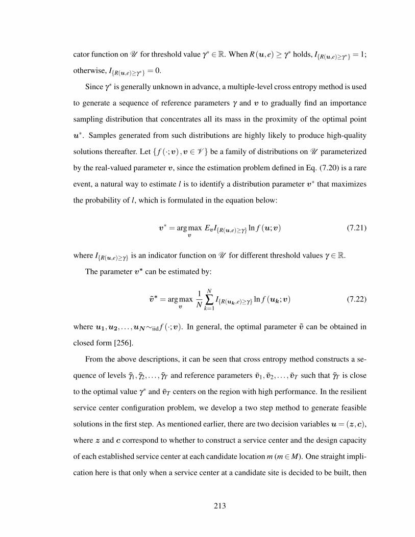
cator function on U for threshold value γ∗ ∈R. When R(u,e)≥ γ∗ holds, I{R(u,e)≥γ∗}= 1;

otherwise, I{R(u,e)≥γ∗} = 0.

Since γ∗ is generally unknown in advance, a multiple-level cross entropy method is used

to generate a sequence of reference parameters γ and v to gradually find an importance

sampling distribution that concentrates all its mass in the proximity of the optimal point

u∗. Samples generated from such distributions are highly likely to produce high-quality

solutions thereafter. Let { f (·;v) ,v ∈ V } be a family of distributions on U parameterized

by the real-valued parameter v, since the estimation problem defined in Eq. (7.20) is a rare

event, a natural way to estimate l is to identify a distribution parameter v∗ that maximizes

the probability of l, which is formulated in the equation below:

v∗ = argmaxv

EvI{R(u,e)≥γ} ln f (u;v) (7.21)

where I{R(u,e)≥γ} is an indicator function on U for different threshold values γ ∈ R.

The parameter v∗ can be estimated by:

v∗ = argmaxv

1N

N

∑k=1

I{R(uk,e)≥γ} ln f (uk;v) (7.22)

where u1,u2, . . . ,uN∼iid f (·;v). In general, the optimal parameter v can be obtained in

closed form [256].

From the above descriptions, it can be seen that cross entropy method constructs a se-

quence of levels γ1, γ2, . . . , γT and reference parameters v1, v2, . . . , vT such that γT is close

to the optimal value γ∗ and vT centers on the region with high performance. In the resilient

service center configuration problem, we develop a two step method to generate feasible

solutions in the first step. As mentioned earlier, there are two decision variables u= (z,c),

where z and c correspond to whether to construct a service center and the design capacity

of each established service center at each candidate location m (m∈M). One straight impli-

cation here is that only when a service center at a candidate site is decided to be built, then

213

it is necessary to generate specific value as its planned capacity. Following this logic, we

generate the configuration for decision vector z first with equal probability because there

is no information on which service center should be built. When the samples generated in

the first step indicate that service center is going to be constructed, then we generate its

design capacity. Otherwise, we set its design capacity as zero for the candidate sites with

no service center. Once the initial possible solutions are generated, cross entropy method

is then leveraged to update the probability distribution such that the algorithm eventually

converges to optimal or near optimal solutions. The structure of the cross entropy method

is summarized in Algorithm 3.

Algorithm 3 : Cross Entropy Algorithm for Bi-level Optimization1: Choose initial parameter vector v0, let Ne = [ρN], and set t = 1

2: Generate u1,u2, · · · ,uN∼iid f (, ; vt−1). Calculate the traffic assignment at user equi-

librium corresponding to the randomly generated samples as well as the objective value

of the upper-level model. Rank the samples from smallest to biggest based on the ob-

jective values of upper-level model: R(1) ≤ R(2) ≤ ·· · ≤ R(N). Let γt be the (1− ρ)

sample quantile of performance, which is γt = R(N−Ne+1)

3: Solve the stochastic program defined in Eq. (7.22) with the same sample

u1,u2, · · · ,uN , and let the solution denoted by vt

4: If the termination condition is met, then the algorithm ends; otherwise, set t = t+1, go

back to Step 2

As illustrated in Algorithm 3, N denotes the sample size, ρ is a predetermined rarity

parameter, and [ρN] denotes the minimum integer not less than ρN. Another thing worthy

of mention is that a smoothing factor α is often introduced to combine the current estimated

distribution parameter with the distribution parameter used in the previous iteration.

vt = αvt +(1−α) vt−1 (7.23)

where vt denotes the solution to the optimization problem formulated in Eq. (7.22), and

0≤ α ≤ 1.

214

7.3.4 Summary

The methodology developed in this chapter tackles the resilient service center distribu-

tion configuration problem with a four-step procedure:

1. We formulate a logistics service center distribution problem, in which system re-

silience is taken into consideration to measure the potential impact caused by disrup-

tive events.

2. Customers’ path choosing behavior is characterized as a traffic assignment problem,

in which a dummy node is introduced to determine the customer demand allocation

among all the service centers.

3. In the upper-level model, both the travel time and within center processing time is

considered. To measure the within center processing time, we model the interaction

between customers and service centers as a M/M/c queue.

4. To solve the formulated bi-level optimization problem, cross entropy method is uti-

lized to generate a family of probability distributions with probability mass gradually

converging to the proximity of the optimal state.

7.4 Numerical Example and Simulation Results

In this section, a numerical example is used to demonstrate the effectiveness of the

developed method in increasing the resilience of service center configuration. To solve this

problem, some parameters need to be specified first. First of all, the number of servers that

can be established at each service center needs to be an integer, and the maximum number

of servers allowed at each service center is set as 6 in this study. Secondly, with respect to

the mean service rate, it is a parameter independent of waiting time, and we assume that

each server is able to serve 18 customers per hour (µ = 18). In other words, each customer

slightly more than 3 minutes to have service on average. To measure customer’s travel time,

215

we take the most commonly used BPR link cost function in the literature to characterize

the relationship between travel time and traffic flow, which is shown in Eq. (7.24).

ta (xa) = t0a

(1+0.15

(xa

χa

)4). (7.24)

where t0a , xa, and χa denote the free-flow travel time, the current traffic flow, and the road

capacity along link a, respectively. In this study, we set the threshold value of convergence

indicator RGAP as 10−3 to determine when to terminate the gradient projection traffic

assignment algorithm.

Since there is a limit on the budget as defined in Eq. (7.9), we develop a nonlinear

function as shown in Eq. (7.25) to represent the relationship between the design cost and

corresponding capacity (c) for service centers.

τ (c) = 8c+0.6c2 (7.25)

where τ (c) represents the incurred cost.

Regarding the cross entropy method, we generate 40,000 samples in total at each itera-

tion to represent a small portion of service center configurations. The generation of service

center configurations follows a two-step procedure. In the first step, binary vectors are

generated following independent Bernoulli random variables with the probability of estab-

lishing service center among all the candidate sites initialized as z0 = 0.5. In the second

step, with respect to each instance generated in the first step, the number of servers is as-

signed to each service center following a uniform distribution for the values ranging from

1 to the maximum number of server allowed at each service center. Given the randomly

generated samples, we set ρ as 0.1, and the top 10% elite solutions are used to update

the probability of having each specific service center constructed with specific number of

servers in the configuration, and the smoothing factor α is set at a value of 0.5 to combine

the distribution parameter in two consecutive iterations. The updated probabilities are used

216

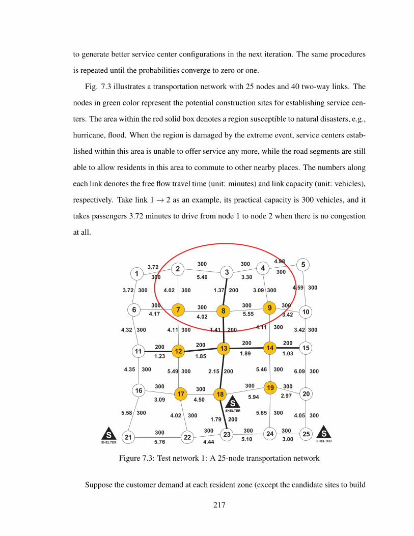
to generate better service center configurations in the next iteration. The same procedures

is repeated until the probabilities converge to zero or one.

Fig. 7.3 illustrates a transportation network with 25 nodes and 40 two-way links. The

nodes in green color represent the potential construction sites for establishing service cen-

ters. The area within the red solid box denotes a region susceptible to natural disasters, e.g.,

hurricane, flood. When the region is damaged by the extreme event, service centers estab-

lished within this area is unable to offer service any more, while the road segments are still

able to allow residents in this area to commute to other nearby places. The numbers along

each link denotes the free flow travel time (unit: minutes) and link capacity (unit: vehicles),

respectively. Take link 1→ 2 as an example, its practical capacity is 300 vehicles, and it

takes passengers 3.72 minutes to drive from node 1 to node 2 when there is no congestion

at all.

2 4

8

1213

1618

23

300 300

300

300 300 300 300

300

200

300 300 200300

300

200 200 200

300 200 300

300 300 200 300 300

300300

300 300

300300

200

300300

300 300 300 300

3.72

5.40 3.30

4.02 1.37 3.094.59

4.32

4.174.02

5.55

3.424.11

1.414.11

4.35 5.49 2.15 5.46 6.09

1.23 1.851.89 1.03

3.09 4.505.94 2.97

5.584.02

1.79

5.854.05

3.005.104.445.76

3.427 9

17

19

33.72

300

4.98

300

21

10

151411

6

1

5

20

2224 25 S

SHELTER

SSHELTER

SSHELTER

Figure 7.3: Test network 1: A 25-node transportation network

Suppose the customer demand at each resident zone (except the candidate sites to build

217

service centers) is 100 customers per day. In other words, there are 1700 customers that

need to be served by all the service centers in one day. The system planner has a total

budget of T = 240 to construct service centers in this region. As the customer demand

between each service center and resident zone is unknown, a dummy node and auxiliary

edges are created to connect all the service centers with the dummy node. To illustrate this

idea, Fig. 7.4 shows a network where we decide to build three service centers at node 2, 5

and 8, respectively. Although the demand between each service center and resident zone

is unknown, the total customer demand at the dummy node 26 is known (1700), which is

equal to the summation of customer demand over all the resident zones. One thing worthy

of mention is that the free-flow travel time along the dummy links is set at a very small value

(e.g., 0.0001), while the road capacity along the auxiliary links is set at a relatively large

value (i.e., 10000). By adding dummy node 26 and auxiliary links into this network, the

customer demand at node 26 is known now. The introduction of auxiliary node and links

not only allows to estimate the customer demand at each service center, but also enables

to calculate the traffic assignment along each road segment. The same idea also applies to

other service center configurations.

Given the customer demand at each resident zone, the cross entropy method first gen-

erates 40,000 random samples to represent the possible service center configurations con-

sisting of service center construction site and the corresponding number of servers at each

constructed site. Afterwards, the gradient projection algorithm is used to deal with the user

equilibrium traffic assignment. Fig. 7.5 shows the convergence trend for one system con-

figuration. As can be observed, the gradient projection method converges to the predefined

precision at a fast rate.

Once the customer demand allocation at each service center is determined, the average

customer waiting time in line and service time for each service center configuration is

calculated accordingly, where the interaction between each service center and customers

is modeled as a M/M/c queue. Afterwards, the value of objective function defined in Eq.

218

2 4

8

1213

1618

23

300 300

300

300 300 300 300

300

200

300 300 200300

300

200 200 200

300 200 300

300 300 200 300 300

300300

300 300

300300

200

300300

300 300 300 300

3.72

5.40 3.30

4.02 1.37 3.094.59

4.32

4.174.02

5.55

3.424.11

1.414.11

4.35 5.49 2.15 5.46 6.09

1.23 1.851.89 1.03

3.09 4.505.94 2.97

5.584.02

1.79

5.854.05

3.005.104.445.76

3.427 9

17

19

33.72

300

4.98

300

21

10

151411

6

1

5

20

2224 25

26

Figure 7.4: Illustration of dummy node and auxiliary links

(7.11) is acquired. Next, the top 10% feasible solutions out of the 40,000 samples is used to

update the probability of having each candidate service center and corresponding number

of servers established accordingly. Next, the aforementioned same procedures are repeated

with the updated probability until the probability converges to zero or one. Fig. 7.6 shows

the convergence of establishing service center at each candidate site. At first (t = 1), all the

candidate sites have the same probability of 0.5 to build service center. With the increase

of iterations, only the probability of site 2, 8, 11, 14, 18, and 25 converges to one, while

the probability of all the other candidate sites (5, 21) reduces to zero gradually. Since

all the probabilities converge to stable values within only 25 iterations, it demonstrates

219

0 5 10 15 20 25 30

Iterations

0

0.01

0.02

0.03

0.04

0.05

0.06

0.07

0.08

0.09

0.1

RG

AP

Figure 7.5: Convergence of gradient projection algorithm for one instance of service centerconfiguration

the effectiveness of the cross entropy method in tackling the challenging combinatorial

optimization problem. Fig. 7.7 shows the changing trend of objective function value over

25 iterations.

Table 7.1: Best solution found by the cross entropy method without the consideration ofthe impact of disruptive event e.

Candidate site ID 2 5 8 11 14 18 21 25Construction of service center X × X X X X × X

Number of servers 3 0 4 4 5 4 0 3

If we do not account for the influence of extreme events on this region, then the best

service center configuration found by the cross entropy method is reported in Table 7.1. As

can be observed, service center 14 has the largest number of servers, followed by service

centers 8, 11, and 18. Whereas, service centers 2 and 25 have the least number of servers.

The total incurred cost for such a service center configuration is 238.6, which is slightly

less than the total budget 240. The total travel time and service time for all the customers

220

Figure 7.6: The evolution of constructing service center at each candidate site

is 12,356. If we take into consideration of the extreme event impact, it implies that service

centers 2 and 8 will get closed because they fall within the disaster-prone zone. If the two

221

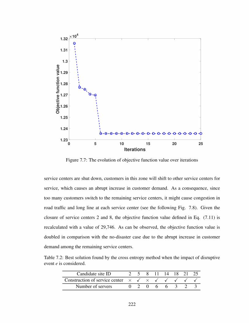
0 5 10 15 20 25

Iterations

1.23

1.24

1.25

1.26

1.27

1.28

1.29

1.3

1.31

1.32

Ob

jec

tiv

e f

un

cti

on

va

lue

104

Figure 7.7: The evolution of objective function value over iterations

service centers are shut down, customers in this zone will shift to other service centers for

service, which causes an abrupt increase in customer demand. As a consequence, since

too many customers switch to the remaining service centers, it might cause congestion in

road traffic and long line at each service center (see the following Fig. 7.8). Given the

closure of service centers 2 and 8, the objective function value defined in Eq. (7.11) is

recalculated with a value of 29,746. As can be observed, the objective function value is

doubled in comparison with the no-disaster case due to the abrupt increase in customer

demand among the remaining service centers.

Table 7.2: Best solution found by the cross entropy method when the impact of disruptiveevent e is considered.

Candidate site ID 2 5 8 11 14 18 21 25Construction of service center × X × X X X X X

Number of servers 0 2 0 6 6 3 2 3

222

In contrast, if we take into account the impact of extreme event in advance, the new

service center configuration should be able to absorb the negative effect of disruptive event

e, thereby alleviating the impact of disruptive event on the performance of service centers.

In this regard, the service center configuration should not only work for the regular scenario,

but also for the circumstance that disruptive event e occurs. Hence, the regular objective

function (without disaster) needs to be joined with the new objective function value in the

circumstance that disruptive event e occurs, and these two functions have same weight

(0.5). Given these considerations, the cross entropy method with same parameter settings

is used to find out the best service center configuration. Table 7.2 shows the best solution

found by cross entropy method after 25 iterations. As can be observed, different from

the service center configuration illustrated in Table 7.1, no service center is established in

candidate sites 2 and 8 in consideration of the potential impact of extreme event. Instead,

two service centers are established at candidate sites 5 and 21 with the same number of

servers. Besides, the number of servers in the service centers established at candidate site

11 and 14 is increased accordingly. By doing this, the new service center configuration

avoids the costly consequence caused by the disruptive event. Such a design incurs a total

investment of 234.8, and has an objective function value of 13,443.

Fig. 7.8 compares the travel time, service time for all the customers with and without

extreme event under the two designs. In the original service center configuration, when

disruptive event e occurs, the total service time increases substantially because too many

customers shift to other service centers, which result in a dramatic rise in customers’ aver-

age waiting time. On the contrary, the extreme event has no impact on the travel time and

service time in the resilient service center configuration. Although the travel time for the

resilient design is slightly larger than the travel time of original design in the no-disaster

case, the service time remains the same level even if the extreme event occurs. Follow-

ing the resilience definition formulated in Eq. (7.12), the resilience of new service center

223

Travel time Service time0

0.5

1

1.5

2

2.5

Tim

e

104

Orignal design: disaster not happen

Orignal design: disaster happens

Resilient design: disaster not happen

Resilient design: disaster happens

Figure 7.8: Comparison of travel time and service time in different scenarios

configuration in responding to the disruptive event e is calculated as:

R(u′,e)=

29746−1344329746−12356

= 0.9375 (7.26)

7.5 Summary

In this chapter, a comprehensive bi-level optimization model is developed to optimize

the service center distribution to increase its capability in withstanding the impact of an

unanticipated extreme event. A bi-level program is formulated to characterize the inter-

actions between customers and system planners. From the perspective of customers, they

behave in a non-cooperative manner to pick a service center with the shortest travel time,

and eventually converge to a user equilibrium state, where nobody could reduce the travel

time by unilaterally shifting to other service centers or alternative routes. A dummy node

224

and auxiliary links are introduced to find the customer demand allocation among service

centers, from which a gradient projection algorithm is used to identify customer flow as-

signment in the traffic network. In the upper-level model, both customers’ travel time and

service time composed of average waiting time in a line and mean processing time, as well

as the potential impact of extreme event are considered. To tackle the bi-level optimization

problem, a multi-level cross entropy method is utilized to generate samples in an adaptive

manner, which gradually converges probability mass towards the optimal solution. The

new configuration of logistics service center in this chapter implies that the impact of nat-

ural disaster on infrastructure system can be mitigated to a large extent if the system is

designed with resilience.

This chapter leverages optimization techniques to identify the optimal system config-

uration to enable resilience in an infrastructure system. The optimization of system con-

figuration significantly strengthens the ability of the system against disruptive events. This

chapter focused on designing an entirely new service center configuration, where none

existed before. In practice, it is more common that some service centers or components

already exist in the system before the design. Under this circumstance, instead of design-

ing a new system, we need to redesign or reconfigure pre-existing system components to

achieve resilience. In the next chapter, we focus on reconfiguring pre-existing components

to enhance the resilience of a transportation system.

225

Chapter 8

System Reconfiguration to Increase System Resilience1

8.1 Introduction

The previous chapter addressed the design for resilience in a new system, i.e., no com-

ponent exists in the system before the design. A more realistic scenario in practice is that

the system has been operated for a while, and that we aim to improve the resilience in the

legacy system by adding new components or other operations. In this chapter, we leverage

optimization algorithms to address this problem. We optimize actions that can be taken

in an already existing system to enhance the effectiveness of the system in responding to

emergency situations, and illustrate the developed method in a transportation network.

In recent years, it has become a high priority for many countries to increase the re-

silience in existing infrastructure systems, such as, power grids [266], transportation net-

works [267], and telecommunication networks [268]. By implementing a variety of mea-

sures before, during, and after the occurrence of disruptive events, the outcome of the

low-probability-high-consequence natural disasters can be mitigated dramatically. Typi-

cally, the approaches used to increase the resilience of any system can be grouped into

three categories.

1. Increase system redundancy: System redundancy is concerned with constructing re-

dundant paths/links to offer the same type of service, or building multiple paths/links

with every path/link used for each specific scenario. It has been used as an effec-

tive way to reduce the probability of the system failing to provide the required ser-

vice [269, 270]. For example, Jenelius [271] demonstrated that redundant road links

played an important role as backup alternatives in transportation systems when other

links in the network were disrupted. However, this strategy has been criticized for1An archival paper related to this chapter is to appear in the journal Risk Analysis. For more details, see

Ref. [265]

226

several reasons. First of all, it is usually time-consuming to construct new paths/links

for infrastructure systems, especially for transportation systems. Secondly, enor-

mous financial resources are in need to be invested to build new paths/links, while

the construction of new paths/links based on previous disasters does not necessarily

guarantee mitigation from unforeseen future disaster events.

2. System hardening strategies: System hardening strategies aim at making physical

changes to the infrastructure system to strengthen its innate ability to resist disrup-

tive events. Typically, retrofit/fortification actions have been investigated to pro-

tect critical system components such that they are able to withstand certain disas-

ters [272, 273, 274]. Along this direction, research efforts have been dedicated to

prioritizing project investment in hardening system components. For example, Tho-

risson and Lambert [275] as well as Thekdi and Lambert [276] leveraged corridor

trace analysis to identify sections of transportation systems at risk when stressed

in terms of increased traffic, accidents, deteriorating physical conditions, and oth-

ers, thus offering insights on prioritization of projects for increasing the resilience

of the transportation system. Qin et al. [277] formulated a mathematical model to

solve a fortification planning problem through optimizing the location of fortified

facilities, the inventory of pre-positioning emergency, and the assignment of emer-

gency transportation for an existing logistics system with capacitated facilities and

limited protection investment budget. However, system hardening usually consumes

large amount of resources because it involves reinforcing the construction materials.

More importantly, one hardening strategy typically can only handle certain types of

extreme events.

3. Operational resilience strategies: Operational resilience is an umbrella term used to

represent the activities and operations for increasing the system flexibility and recon-

figurability [278]. For example, Kim et al. [279] proposed scalable computational

227

heuristics to determine the optimal contraflow network configuration, and demon-

strated that contraflow approaches could reduce the total evacuation time by 40%

percent or more. In comparison with the previous two strategies, operational re-

silience strategies have demonstrated promising features, and it has been extensively

studied to restore power, transportation, and manufacturing system performance in

the aftermath of extreme events [280, 281, 282, 283]. First of all, this strategy is eco-

nomically achievable compared to the aforementioned two strategies. For example,

in the power grid, we only need to install switching devices across the network, from

which we are able to adjust the topology of power system in response to disruptive

events. Secondly, this strategy makes the infrastructure system flexible and reconfig-

urable. By changing the open/close status of the switching devices in the power grid,

the system has a series of possible configurations. By adopting an appropriate con-

figuration, we are able to isolate the fault, reconnect the station with other normally

operating feeders, thus recovering the power supply to the blackout area.

The above discussion indicates that among the three mainstream strategies for increas-

ing system resilience, operational resilience strategy has advantages over the other two

approaches from the economic and operational point of view. System reconfiguration, as

a major means to achieve operational resilience strategy, can be an effective measure in

mitigating the consequence of disruptive events. Indeed, several studies already leverage

this strategy to restore system performance. For example, Daigle et al. [284] demonstrated

that a robot could recover from damage to sustain performance through an autonomous

process of self-modeling and self-reconfiguration [285]. Daigle et al. [284] used circuit

breakers and relays to enable a number of distinct power distribution configurations for the

purpose of mitigating the effect of different types of faults in a spacecraft power distribution

system. Arıkan et al. [286] implemented aircraft cruise speed control in recovering system

performance and mitigating delays in the presence of airline disruption. Fang and Sansavini

[287] combined capacity expansion and transmission switch installation in electric systems

228

to increase the reconfigurability for the sake of alleviating the impact of disruptive events.

Recently, Yodo et al. [288] utilized control theory to adapt the configuration of the system

to maintain a desirable level of system performance in response to external disturbance.

In the presence of a natural disaster, transportation networks play a vital role in evac-

uating the residents who live in the affected area. Evacuating a large population out of

the disaster prone areas within a limited time is an important strategy in mitigating the

impact of a disaster [289]. For example, Kumar, Romanski, and Van Hentenryck [290]

formulated a mixed integer programming (MIP) model to determine the most effective in-

frastructure enhancements for evacuation planning. Another study worthy of mention con-

ducted by Lambert et al. [291] estimated the number of evacuees in a particular region and

assigned the trips to the transportation system to analyze the traffic system performance for

emergency management in several disaster scenarios. One common problem arising under

this circumstance is that the abrupt increase in the traffic demand results in severe traffic

jam during the evacuation process. For example, traffic jams occurred along major free-

ways leading out of the Houston area during Hurricane Harvey [292]. Similar phenomena

have been observed in past evacuations due to Hurricane Katrina and Rita [293]. As pointed

out by Lambert et al. [291], reversed lanes and ramp metering can be used to increase traf-

fic operations, thereby improving system performance. In this chapter, we work along this

direction to investigate how to leverage system reconfiguration strategies and develop an

integrated approach to reconfigure the road network for restoring the performance of the

transportation system. To that end, two simple and operable strategies are considered for

their simplicity and generality to be implemented in transportation systems.

1. Contraflow. Contraflow, also referred to as lane reversal, denotes reversing the direc-

tion of the lanes to increase the outbound evacuation capacity. Since it can increase

the directional capacity of a roadway immediately and significantly without the need

to plan, design, and construct additional lanes, this strategy has been highly effective

in reallocating the road capacities to accommodate unbalanced traffic demand. In

229

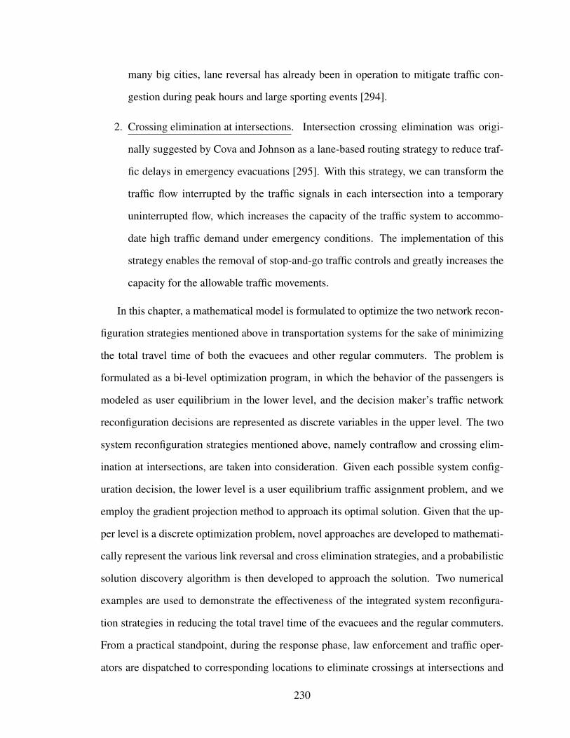
many big cities, lane reversal has already been in operation to mitigate traffic con-

gestion during peak hours and large sporting events [294].

2. Crossing elimination at intersections. Intersection crossing elimination was origi-

nally suggested by Cova and Johnson as a lane-based routing strategy to reduce traf-

fic delays in emergency evacuations [295]. With this strategy, we can transform the

traffic flow interrupted by the traffic signals in each intersection into a temporary

uninterrupted flow, which increases the capacity of the traffic system to accommo-

date high traffic demand under emergency conditions. The implementation of this

strategy enables the removal of stop-and-go traffic controls and greatly increases the

capacity for the allowable traffic movements.

In this chapter, a mathematical model is formulated to optimize the two network recon-

figuration strategies mentioned above in transportation systems for the sake of minimizing

the total travel time of both the evacuees and other regular commuters. The problem is

formulated as a bi-level optimization program, in which the behavior of the passengers is

modeled as user equilibrium in the lower level, and the decision maker’s traffic network

reconfiguration decisions are represented as discrete variables in the upper level. The two

system reconfiguration strategies mentioned above, namely contraflow and crossing elim-

ination at intersections, are taken into consideration. Given each possible system config-

uration decision, the lower level is a user equilibrium traffic assignment problem, and we

employ the gradient projection method to approach its optimal solution. Given that the up-

per level is a discrete optimization problem, novel approaches are developed to mathemati-

cally represent the various link reversal and cross elimination strategies, and a probabilistic

solution discovery algorithm is then developed to approach the solution. Two numerical

examples are used to demonstrate the effectiveness of the integrated system reconfigura-

tion strategies in reducing the total travel time of the evacuees and the regular commuters.

From a practical standpoint, during the response phase, law enforcement and traffic oper-

ators are dispatched to corresponding locations to eliminate crossings at intersections and

230

reverse certain lanes as decided by the optimization algorithm. Meanwhile, appropriate

road signs need to be placed at right locations to increase drivers’ situation awareness of

the new traffic patterns. During the restoration phase, after the system reconfiguration de-

cisions are implemented, system performance gradually improves over time because the

outbound capacity for emergency evacuees to travel from impacted areas to shelters are in-

creased significantly. Compared to the current state of the art, we have made the following

contributions:

1. System reconfiguration strategies (contraflow and crossing elimination at intersec-

tions) are considered for the purpose of mitigating the severe congestion caused by

the evacuation of a large number of residents within the disaster impacted areas.

These reconfiguration strategies facilitate the timely reorganization of the transporta-

tion system in response to the large scale evacuation, thereby strengthening emer-

gency preparedness and increasing the system resilience.

2. Novel approaches are developed to mathematically represent the various contraflow

and crossing elimination configuration options. Given the system reconfiguration

representation, a bi-level optimization model is formulated to maximize the system

resilience, in which users’ path-choosing behavior is modeled as user equilibrium

traffic assignment in the lower level optimization model, and the traffic system oper-

ators’ reconfiguration decisions in terms of link reversal and crossing elimination are

represented in the upper level optimization model.

3. Efficient solution algorithms are leveraged to tackle the formulated bi-level optimiza-

tion problem. To be specific, the gradient projection approach is used to shift the

flow among the paths connecting the same origin-destination pair continuously until

the traffic assignment converges to a stable state. A probabilistic solution discovery

algorithm is developed to iteratively update the probability of taking each possible

system reconfiguration action at the component level, eventually finding the near-

231

optimal strategies for maximizing the system resilience.

8.2 Proposed Method

In this section, we mathematically formulate the bi-level optimization problem, in

which the different system reconfigurations (contraflow and crossing elimination at inter-

sections) are modeled as decision variables in the upper level model, and the user equi-

librium traffic assignment based on Wardrop’s first principle is characterized in the lower

level model. The structure of the proposed method is illustrated in Fig. 8.1. The first step

is to express the system reconfiguration strategies and the incurred link capacity change

in a mathematical form. Afterwards, consider the mathematical representation, the pos-

sible system reconfiguration option with respect to each component is combined with the

probability of choosing that particular option to generate candidate system reconfiguration

designs. To the lower level traffic network users, such designs are perceived in the form

of link reversal and roadway block. For a given particular reconfiguration, the lower level

traffic assignment problem is solved by an efficient gradient projection method through

shifting the flow from costlier paths to the shortest path for each origin-destination pair

until the user equilibrium traffic assignment converges, from which we are able to evaluate

the performance in terms of total travel time for all the network users with respect to all the

randomly generated system reconfiguration designs. By utilizing a probabilistic solution

discovery algorithm, we can update the probability of choosing each option at the compo-

nent level based on the performance of the previously generated designs, and new candidate

reconfiguration designs can be sampled based on the updated probability to approach better

solution.

8.2.1 Problem Formulation

As mentioned earlier, our objective is to leverage available system reconfiguration

strategies to mitigate traffic congestion and restore performance of the traffic network dur-

232

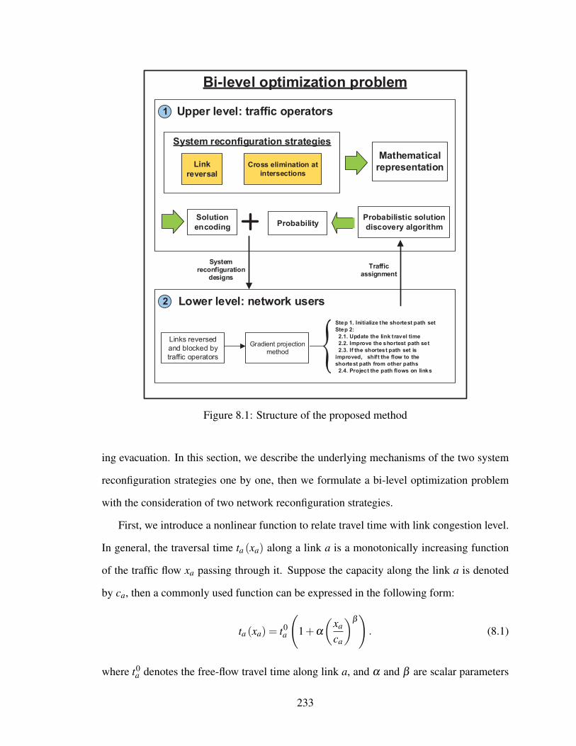
Bi-level optimization problem

Upper level: traffic operators

Lower level: network users

System reconfiguration

designs

Traffic assignment

Links reversed

and blocked by

traffic operators

Gradient projection method

1

2

Link

reversal

Cross elimination at

intersections

System reconfiguration strategies

Probabilistic solution

discovery algorithm

Mathematical

representation

Step 1. Initialize the shortest path set

Step 2:

2.1. Update the link travel time

2.2. Improve the shortest path set

2.3. If the shortest path set is

improved, shif t the flow to the

shortest path from other paths

2.4. Project the path flows on links

ProbabilitySolution

encoding

Figure 8.1: Structure of the proposed method

ing evacuation. In this section, we describe the underlying mechanisms of the two system

reconfiguration strategies one by one, then we formulate a bi-level optimization problem

with the consideration of two network reconfiguration strategies.

First, we introduce a nonlinear function to relate travel time with link congestion level.

In general, the traversal time ta (xa) along a link a is a monotonically increasing function

of the traffic flow xa passing through it. Suppose the capacity along the link a is denoted

by ca, then a commonly used function can be expressed in the following form:

ta (xa) = t0a

(1+α

(xa

ca

)β). (8.1)

where t0a denotes the free-flow travel time along link a, and α and β are scalar parameters

233

that can be specified from statistical analysis through curve fitting on the data obtained

from uninterrupted freeway.

The above function was developed by U.S. Bureau of Public Roads (BPR) [296]. Fig.

8.2 illustrates several typical shapes of link travel time functions when α and β take dif-

ferent values while the capacity ca is fixed at a constant value of 5. As can be observed,

travel time increases exponentially when the traffic flow exceeds link capacity ca. To im-

prove the traffic system efficiency, it is beneficial for us to implement different strategies to

reconfigure the traffic system for the sake of adapting to the traffic demand and controlling

the traffic congestion below certain level.

0

Lin

k t

ravel ti

me a

lon

g lin

k a

: t a(x

a)

ca

ta

0

Traffic flow along link a: xa

= 1,

= 4

= 1.2,

= 4 = 2.1,

= 3

Figure 8.2: BPR function

8.2.1.1 Contraflow

Contraflow refers to reversing the direction of one or more lanes of a roadway for the

sake of moving traffic in the opposite direction. In emergency situations, by reversing

the inbound lanes to the outbound direction, contraflow can increase the traffic system

outbound capacity significantly.

234

s 1 t

4

4

4

4

s 1 t8

Before contraflow configuration

After contraflow configuration

8

{40}

{40}

Figure 8.3: Contraflow illustration

To illustrate the concept of contraflow, a simple evacuation situation is shown in Fig.

8.3. Suppose some residents need to be evacuated from node s to node t, and node 1 serves

as the transshipment node. The number within the parentheses indicates the number of

persons to be evacuated, and the number along each link denotes the link capacity (number

of persons per minute). As can be observed, the capacity is the same for all the two-way

links. Since the traffic demand (40) is much higher than the link capacity (4), there will be

severe congestion along links s→ 1 and 1→ t. By reversing the direction of links t → 1

and 1→ s, we double the system outbound evacuation capacity, as shown in the graph at

the bottom of Fig. 8.3. In addition, the link congestion is reduced significantly as the travel

demand to link capacity ratio drops from 10 to 5. By taking advantage of the contraflow

reconfiguration strategy, one can increase the network outbound capacity, mitigate the link

level congestion, and reduce the total time in evacuating people out of disaster-impacted

area significantly.

8.2.1.2 Crossing Elimination at Intersections

Crossing elimination is demonstrated to be effective in improving the traffic flow move-

ment efficiency by prohibiting certain turning movements. By doing so, the intersections

that interrupt the traffic flow are removed from the system. As a result, the traffic move-

235

(a) (b) (c)

(d) (e) (f)

1

2

3

4

Figure 8.4: An illustration of crossing elimination at an intersection. The blue arrowsdenote the direction of traffic flow in each lane, the red triangles mean that the roadway isblocked, and the labels in purple represent the order that will be used to encode the problem

ments at intersections are free from the stop-and-go traffic control. The traffic movements

at intersections become more smooth, and the system is capable of accommodating more

traffic at the intersections within the same time.

In this study, we assume that partial crossing elimination is not allowed. In other words,

when we block one roadway of an intersection, both of the two-way links are blocked.

This constraint also helps to keep the problem size at a reasonable scale. Typically, all four

roadways at an intersection have the same link capacity. To balance traffic and avoid traffic

interaction, we impose that the number of blocked roads must be an even number. In other

words, it is not allowed to block one or three roadways. In this way, the traffic signal is no

longer needed at the intersection. Fig. 8.4 illustrates six possible road block configurations

(C24 = 6). Each configuration represents a unique way to block the roadways. It can be

236

seen that the traffic flow pattern is changed due to the crossing elimination reconfiguration

strategy. Without the control of the traffic signal, traffic movements will become smoother

than before.

8.2.1.3 Mathematical Formulation

To represent the aforementioned two reconfiguration strategies in a mathematical form,

two additional variables are introduced, which are indicated as below:

1. λa: the contraflow configuration of link a (a ∈ E). If λa = 0, no contraflow operation

is carried out on link a. If λa = 1, we reverse the roadway that has the opposite

direction with the current roadway. If λa =−1, we reverse the roadway a itself. For

example, with respect to the link 1→ 2 shown in Fig. 8.5, if λ1→2 = 1, the direction

of link 2→ 1 is reversed; if λ1→2 = −1, the direction of link 1→ 2 is reversed; if

λ1→2 = 0, no link is reversed and the directions of the two links remain the same.

1 2

ac-

ac

Figure 8.5: Contraflow illustration

To illustrate the mathematical representation of contraflow configuration, a simple

example is given in Fig. 8.5. As can be observed, there are two-way traffic roads

between node 1 and node 2. Let ca and c−a denote the link capacity from node 1

to node 2 and from node 2 to node 1, respectively. As mentioned previously, when

λa = 1, the link that has opposite orientation with the roadway 1→ 2 is reversed. In

this example, the link from node 2 to node 1 is reversed. Thus, we have the updated

link capacity along link a as follows:

c∗a = ca +λa · c−a = ca + c−a ,

c∗−a = c−a −λa · c−a = ca− c−a .(8.2)

237

where c∗a and c∗−a represent the updated capacity of the link from node 1 to node 2

and the link from node 2 to node 1, respectively.

If λa =−1, the link from node 1 to node 2 is reversed, then the capacity for link a is

updated as:

c∗a = ca +λa · c−a = ca− c−a ,

c−∗a = c−a −λa · c−a = ca + c−a .(8.3)

If λa = 0, the above two equations still hold. In summary, no matter which roadway

is reversed, the two equations always hold. Thus, they are used to represent the new

link capacity after the contraflow reconfiguration. Hence, for any link a (a ∈ E), we

have: c∗a = ca +λa · c−a ,

c−∗a = c−a −λa · c−a .(8.4)

2. ξi: the crossing elimination configuration at each intersection, where I (i ∈ I) is the

set of intersections that are reconfigured in the network G. ξi is a vector consisting

of four binary variables, and each variable denotes whether to block one roadway

of intersection i or not. When the value of the variable in ξi is 1, it indicates that

the roadway is blocked. Otherwise, the roadway is not blocked. For example, fol-

lowing the order shown in Fig. 8.4 (a) to encode the problem, the crossing elimina-

tion configuration shown in Fig. 8.4(a) can be represented as: ξi =

[0 1 0 1

]because the second and fourth roadways are blocked in this configuration. The la-

bels in purple fonts shown in Fig. 8.4(a) are used to represent the order in which

the decisions related to each roadway is encoded. Likewise, the second and third

crossing elimination configurations can be represented as ξi =

[0 1 1 0

]and

ξi =

[1 1 0 0

], respectively. In this way, each crossing elimination configura-

tion has a unique representation.

Given the above notations, the bi-level optimization model for reconfiguring the traffic

238

network G can be formulated as:

(U2) Min F = ∑a∈E

xata (xa) (8.5a)

s.t.4

∑j=1

ξi ( j) = 2, i ∈ I∗, (8.5b)

I∗ ⊆ I, (8.5c) c∗a = ca +λa · c−a ,

c−∗a = c−a −λa · c−a ,∀a ∈ E, (8.5d)

λa = 0 or −1 or 1, ∀a ∈ E, (8.5e)

ca = 0 and c−a = 0, if a ∈ ω. (8.5f)

ω = {m(i, j)|ξi ( j) = 1,∀i ∈ I, j ∈ {1,2,3,4}} . (8.5g)

(L2) Min f = ∑a∈E

xa∫0

ta (x)dx, (8.5h)


∑p∈Ps,t

qs,tp δ

s,ta,p, ∀a ∈ E, (8.5i)

∑p∈Ps,t

qs,tp = ds,t , ∀(s, t) ∈OD, (8.5j)

qs,tp ≥ 0, ∀p ∈ Ps,t , ∀(s, t) ∈OD, (8.5k)

xa ≤ κa, ∀a ∈ E. (8.5l)

where ξi ( j) denotes the value of the j-th element in vector ξi, I denotes the set of all the

intersections in network G, I∗ represents the set of intersections that are reconfigured, and

ω denotes the set of roadways that are blocked in the crossing elimination strategy, and

m is a function mapping the j blocked roadway at the i-th intersection to the node label

space. With respect to the system constraints, Eq. (8.5b) requires that two roadways must

be blocked in each intersection as introduced before, Eq. (8.5d) models the updated link

capacity along link a, in which λ is a discrete variable with three possible values (0,−1 and

+1), and Eq. (8.5f) denotes that the capacity along link a reduces to zero if it is blocked.

239

Algorithm 4 : Gradient Projection Algorithm1: Initialize the network G, origin-destination demand OD, link capacity c, and the2: link cost function ta (a ∈ E).3: for each OD pair (s, t) ∈OD do4: Find the shortest path p from node s to t5: Assign all the travel demand among OD pair (s, t) to the shortest path p6: Store the found shortest path p in the set P7: end for8: Generate initial shortest path for each OD pair9: while the convergence termination condition is not met do

10: for each OD pair (s, t) ∈OD do11: Update path cost yp, ∀p ∈ Ps,t

12: Improve the path set Ps,t

13: if Ps,t is improved or |Ps,t | ≥ 2 then14: Shift the flow from the costlier paths to the shortest path15: Project the path flow on the links and update the link cost16: Remove unused paths from the set P17: end if18: end for19: end while20: Project the path flow on the links and update the link cost

8.2.2 Optimization Algorithms

In this section, we introduce two algorithms to tackle the lower level and upper level

optimization problems formulated in the last section.

8.2.2.1 Lower Level Optimization Problem

Given the contraflow configuration and the crossing elimination strategies, the lower

level optimization problem can be formulated as a traffic assignment problem (TAP). Many

algorithms have been proposed for solving this problem [241, 245]. In this study, we choose

the gradient projection method [241] due to its efficiency and simplicity. The gradient

projection method exploits the separability of the origin-destination pairs, and it operates

on the path space to shift the flow from costlier paths to the shortest path for each origin-

destination pair during the iterations. The overall framework of the gradient projection

240

algorithm is illustrated in Algorithm 4.

As can be seen from Algorithm 4, the gradient projection method employs an all-or-

nothing (AON) assignment to initialize the traffic assignment, in which all travel demand

ds,t is assigned to the shortest path p connecting each origin-destination pair (s, t)∈OD. A

set P is constructed to keep track of all the paths with positive traffic flow. Next, path flow

is projected on all the links, and the link cost is updated accordingly. Given the updated

link cost, the shortest path among each origin-destination pair is updated. Suppose the

travel time along the current shortest path u ∈ Ps,t connecting the origin-destination pair

(s, t) is yu. If the found shortest path is not in the set P, then we add it to this set. Next,

gradient projection method moves the flow to the shortest path u from all other paths of

Ps,t . Considering the travel time yu along the shortest path, the direction of descent for

other paths can be expressed as:

dp = yu− yp, ∀p ∈ Ps,t , p 6= u,

du =− ∑p∈Ps,t , p6=u

dp.(8.6)

where dp measures the descent direction in terms of travel time between the current short-

est path u and costlier path p. Given the direction of descent dp, gradient projection moves

a certain amount of traffic flow from costlier paths p to the current shortest path u to equi-

librate their travel time.

In order to determine the appropriate amount of flow to be shifted from the costlier

paths to the shortest path, a linear search along the descent direction is formulated to find

the optimal step size as indicated below:

Lp = Lp + γdp, ∀p ∈ Ps,t . (8.7)

where γ denotes the step size.

Now the problem is how to find the optimal value for the step size γ . By projecting the

241

descent direction of the path flow on all the links then we have:

g(γ) = min ∑a∈A

∫ xa+γya0 ta (x) dx

s.t. 0≤ γ ≤ γub.

(8.8)

where y =(y1, . . . ,y|A|

)is the direction of descent along the links after the projection,

A is the set of links that are either in path p ∈ Ps,t (p 6= u) or in the shortest path u but

not in both, xa is the current flow of link a, and γub is an upper bound on the step size

that guarantees the new solution is still feasible. The value of γub can be easily derived

as γub = mink

{ −Lmaxp

dp

∣∣∣dp < 0}, ∀p ∈ Ps,t [297], where Lmax

p is the maximum amount of

flow to be shifted on the condition that dp is less than zero.

Obviously, problem (8.8) is a one-dimensional optimization problem. A variety of

techniques are available to determine the optimal step size that is used to move the path

flow. In this study, we use the bisection technique proposed in Ref. [298] to find the

optimal value of γ to minimize the objective function defined in Eq. (8.8). Once the value

of γ is determined, we can shift the flow to the shortest path from other costlier paths of

Ps,t . After the path flow move is accomplished, we project the path flow on all the links

and update the link cost. Meanwhile, the path with zero flow is eliminated from set P.

The above procedures finish one step of analysis for a single origin-destination pair,

and the same process is repeated for the remaining origin-destination pairs. After the path

flows among all origin-destination pairs are analyzed and optimized, one iteration of the

gradient projection method is completed. The algorithm continues the same procedures

until the convergence termination condition is met. In this study, we take one commonly

used metric – relative gap – as a convergence measure, which is defined as below:

RGAP = 1−∑

(s,t)∈ODds,t · ps,t

min

∑a∈E

fa · ta(8.9)

where ds,t denotes the travel demand between the origin-destination pair (s, t), ps,tmin is the

242

travel cost of the shortest path between origin-destination pair (s, t), fa and ta represent the

link flow and link cost associated with link a, respectively.

In this study, when the relative gap is less than a predefined threshold, the algorithm

stops. When the algorithm converges, we obtain the amount of flow associated with each

link, from which we compute the value of the objective function defined in Eq. (2.31).

8.2.2.2 Upper Level Optimization Problem

As mentioned previously, whenever a system reconfiguration strategy is implemented,

a corresponding user equilibrium traffic assignment can be obtained by the gradient pro-

jection method. Given the user equilibrium traffic assignment, we are able to compute the

total travel time for all users as indicated in the upper level objective function. In this sec-

tion, our goal is to identify the optimal reconfiguration strategy that minimizes the total

travel time with the consideration of users’ path-choosing behavior. There are two decision

variables in the upper level optimization problem, λa (a ∈ E) and ξi (i ∈ I). Both of the

decision variables are discrete. Since it is computationally intractable to derive an analyt-

ical solution to this optimization problem, we leverage a powerful evolutionary method –

probabilistic solution discovery algorithm – to identify the near-optimal solution within a

reasonable time.

The probabilistic solution discovery algorithm was originally developed by Ramirez-

Marquez and Rocco [299], and it searches for the best solution in a probabilistic manner

by updating the probability of every individual element in the solution space to be a certain

value. In general, there are three steps in the probabilistic solution discovery algorithm:

strategy development, strategy analysis, and solution discovery. In the strategy develop-

ment step, with respect to the upper level optimization problem, a large number of possible

solutions are randomly generated. The values of the two decision variables are specified in

the following manner.

1. With respect to the contraflow configuration, for each link a, three design values are

243

possible: 0,−1, and 1. Since we do not know whether to reverse a link or not, all

the three values are initially assigned with equal probability (1/3). Hence, we use

three separate intervals πa:[0, 1

3

],[1

3 ,23

], and

[23 ,1]

to represent the probability to

choose each particular decision value. Then a random number in the range [0,1] is

generated. If the generated number is within the range[0, 1

3

], then λa = 0. If the

generated number falls within the range[1

3 ,23

], then λa =−1. Otherwise, λa = 1. It

is worth mentioning that only one variable λa is needed to represent all the contraflow

configurations related to a two-way roadway.

2. Regarding the crossing elimination at the intersections, there are four binary variables

in the decision vector ξi (i∈ I). First, we need to determine whether to reconfigure an

intersection or not. Since we do not know whether an intersection should be recon-

figured at the beginning, then an uninformative probability 0.5 is used as the value

of blocking each intersection. In other words, reconfiguration and no reconfiguration

have the probability of 0.5 for each intersection at the beginning. With that probabil-

ity, a binary value is randomly generated with the probability to represent different

realizations. As indicated earlier, if an intersection is reconfigured, only two road-

ways are blocked at that intersection (4∑j=1ξi ( j) = 2, i ∈ I∗). Likewise, the unit is

divided into four equal intervals: πi: [0,0.25] , [0.25,0.50] , [0.50,0.75] and [0.75,1].

Next, two numbers in the range [0,1] are randomly generated. If the two numbers

fall within the same interval, only one roadway is blocked, then two other random

numbers are needed to be generated. The same process repeats until the two gener-

ated random numbers fall within different intervals. Depending on which interval the

value of each generated random number falls within, we decide the specific value for

each binary variable in the decision vector ξi.

Repeating the above procedure, we utilize Monte Carlo simulation (MCS) to generate

a fixed number – called SAMPLE – of potential network reconfiguration strategies. The

algorithm terminates when the probability of every decision value in the solution space

244

converges to a stable value.

In the strategy analysis step, we compute the total travel time for the network users

corresponding to each potential network reconfiguration strategy generated before, denoted

by ψ (κ), where κ is a vector consisting of the decision variables λa (a ∈ E) and ξi (i ∈ I).

All the generated network reconfiguration strategies are ranked in an ascending order by

their objective values. By analyzing all the generated network reconfiguration strategies,

we identify the best solution found so far.

In the solution discovery step, a fixed number of solutions, denoted by TOP, are saved in

the set K. A small fraction of size S of ordered strategies are used to update the probability

of each decision value appearing in the top-ranked solutions. After normalizing the proba-

bilities for each decision variable, we construct the updated probability intervals πa (a ∈ E)

and πi (i ∈ I) for each variable. Given the new intervals πa and πi, the algorithm goes back

to the first step and generate new candidate solutions for the next iteration. The algorithm

will terminate when πa and πi do not change any more. The procedures of the probabilistic

solution discovery algorithm are summarized in Algorithm 5 below.

8.2.3 Summary

The proposed methodology in this section solves the bi-level optimization problem us-

ing a three-step procedure. First, the different network reconfiguration strategies are repre-

sented in a mathematical form. Given the mathematical representation, a bi-level program

is formulated to characterize the complex interactions between the traffic operators and

the traffic network users. Secondly, for a specified system reconfiguration, to determine

the user equilibrium traffic assignment of the lower level optimization problem, a gradient

projection method is used to shift the flow from costlier paths to the shortest path among

each origin-destination pair, in which bisection method is used to determine the appropriate

amount of flow to be shifted. Finally, a probabilistic solution discovery algorithm is devel-

oped to identify the best system reconfiguration strategy with the consideration of users’

245

Algorithm 5 : Probabilistic Solution Discovery Algorithm1: Initialize SAMPLE, S, TOP, πa (a ∈ E), πi (i ∈ I), τ = 1, K = Φ;2: while τ < T do3: STEP 1: (Strategy Development)4: for h = 1 to SAMPLE do5: Generate potential network reconfiguration strategies:

κτ,1 = (· · · ,λa, · · ·) , ∀a ∈ E,κτ,2 = (· · · ,ξi, · · ·) , ∀i ∈ I.κh

τ =[κτ,1 κτ,2

]6: end for7: STEP 2: (Strategy Analysis)8: (a): Compute the user equilibrium traffic assignment corresponding to each ran-

domly generated strategy κhτ with gradient projection method as described in Algo-

rithm 4;9: (b): Calculate the total travel time corresponding to the user equilibrium traffic

assignment;10: (c): List all the solutions in an ascending order by their objective values;11: STEP 3: (Solution Discovery)

K→ K∪{

ψ

(κ(1)τ

),ψ(κ(2)τ

), . . . ,ψ

(κ(TOP)τ

)}τ → τ +1

Update the probability of link to be present in the optimal solution12: Use the top S solutions in the ordered solution set to update πa and πi.13: end while

path-choosing behavior so as to minimize the travel time of all the users across the network.

By measuring the amount of total travel time that is reduced by the network reconfiguration

strategies, the system resilience can be calculated in a straightforward way.

8.3 Numerical Examples

In this section, two numerical examples are used to illustrate the procedures of proposed

method in alleviating the traffic congestion and improving traffic system performance. As

a well-known problem, user equilibrium traffic assignment has been extensively studied.

Hence, the data on many transportation networks is readily available from the literature

246

(see Refs. [242, 300]), we use the same data and BPR link travel time function as shown in

Eq. (8.10) to illustrate the effectiveness of the proposed method.

ta (xa) = t0a

(1+0.15

(xa

ca

)4). (8.10)

where t0a , xa, and ca denote the free-flow travel time, the current flow, and the capacity

along link a, respectively.

The value of relative gap is set as 10−3. The parameters of probabilistic solution dis-

covery algorithm are set as: SAMPLE = 1000, TOP = 100, and T = 5. All the algorithms

are implemented in C++ under Windows 10 with 16.0 GB RAM, Intel Core i7-4790 CPU,

8 Core, 3.60 GHz.

8.3.1 Example 1

Fig. 8.6 shows the Sioux-Falls network with 24 nodes and 76 links. The characteristics

of all the links in this network are available at the website: https://github.com/zxgcqupt/

TransportationNetworks/blob/master/SiouxFalls/SiouxFalls net.tntp. The Sioux-Falls is a

symmetrical transportation system, in which all the two-way roadways have identical ca-

pacity and free-flow travel time. In this chapter, for the sake of simplicity, we only consider

the nodes that have four outgoing and ingoing links as intersections. In this case, there are

six intersections in the Sioux-Falls network at nodes 8, 11, 15, 16, 20 and 22, and they are

highlighted in yellow circles.

Now suppose an extreme event is going to hit the city, and all the areas within the red

circle are expected to be impacted by this disruptive event. To mitigate the consequence of

this disruption, all the residents within this particular area need to be evacuated as quickly

as possible. As indicated by the blue arrows, there are five primary routes to evacuate the

residents out of the disaster impacted zones to the three shelters indicated by black triangles

in Fig. 8.6. Before the flood, the travel demand from the nodes within the red circle to all

247

https://github.com/zxgcqupt/TransportationNetworks/blob/master/SiouxFalls/SiouxFalls_net.tntp

https://github.com/zxgcqupt/TransportationNetworks/blob/master/SiouxFalls/SiouxFalls_net.tntp

1 2

3

12

13

64 5

11 10 16

89 7

18

14

23

24 21

15

22

17

19

20S

SHELTER

SSHELTER

SSHELTER

Figure 8.6: Test network 1: Sioux-Falls network

the other nodes is almost evenly distributed across the network. The detailed traffic demand

data is available at the website: https://github.com/olga-perederieieva/TAsK/blob/master/

Data/SiouxFalls trips.txt. For example, the regular traffic demand between node 2 and all

the other nodes is:

d2,1 = 100, d2,3 = 100, d2,4 = 200, d2,5 = 100

d2,6 = 400, d2,7 = 200, d2,8 = 400, d2,9 = 200

d2,10 = 600, d2,11 = 200, d2,12 = 100, d2,13 = 300,

· · ·

248

https://github.com/olga-perederieieva/TAsK/blob/master/

Data/SiouxFalls_trips.txt

Now, since there are a large number of vehicles moving towards the three shelters that

are distributed in different locations across the network at the same time, the traffic demand

between the nodes within the red circle and the shelters increases abruptly. The roadways

that transport disaster-impacted residents to the designated shelters face a higher travel de-

mand than usual and traffic congestion might occur thereafter. To simulate this effect, we

assume all the travel demand that originally starts from the nodes within the red circle and

ends at all the other nodes across the network now only ends at the three individual shelters.

For example, as shown above, there is different traffic demand from node 2 to all the other

nodes in the network. Now, all the traffic demand ends at the three nodes that the shelters

are located. For the sake of simplicity, we assume the traffic demand is evenly distributed

at the three shelters. Then we have:

d2,13 = 1333, d2,20 = 1333, d2,23 = 1333,

d5,13 = 2033, d5,20 = 2033, d5,23 = 2033,

d6,13 = 2533, d6,20 = 2533, d6,23 = 2533,

d8,13 = 5567, d8,20 = 5567, d8,23 = 5567,

d9,13 = 5400, d9,20 = 5400, d9,23 = 5400.

In addition to the travel demand from the emergency evacuations, the regular com-

muters who stay outside of the impacted areas still need to drive from their homes to the

workplaces. To account for this, we add the travel demand among other origin-destination

pairs into the origin-destination demand matrix. The final traffic demand through the net-

work under consideration is shown in Eq. (8.11), where the numbers in bold indicate the

demand arising from the emergency evacuations.

Given the traffic demand from both the evacuees and the regular commuters, we first

solve the lower level optimization problem using the gradient projection algorithm. Fig.

8.7 demonstrates the convergence process of the relative gap for one system reconfiguration

design. As can be observed, the gradient projection algorithm converges to the predefined

249

12

34

56

78

910

1112

1314

1516

1718

1920

2122

2324

10

00

00

00

00

00

00

300

500

500

400

100

300

300

100

400

300

100

20

00

00

00

00

00

013

330

00

00

013

330

013

330

30

00

00

010

00

030

030

020

010

010

010

020

010

00

00

010

010

00

40

020

00

00

00

012

000

600

600

500

500

800

500

100

200

300

200

400

500

200

50

00

00

00

00

00

020

330

00

00

020

330

020

330

60

00

00

00

00

00

025

330

00

00

025

330

025

330

750

00

100

400

00

00

019

0050

070

040

020

050

014

0010

0020

040

050

020

050

020

010

08

00

00

00

00

00

00

5567

00

200

020

5567

00

5567

09

00

00

00

00

00

00

5400

00

00

00

5400

00

5400

010

1300

030

012

000

019

000

00

020

0019

0021

000

4400

3900

700

1800

025

0012

0026

0018

0080

011

500

030

00

00

500

00

00

010

000

1400

1400

1000

100

400

600

400

1100

1300

600

1220

00

200

600

00

700

00

2000

00

1300

700

700

700

600

200

300

400

300

700

700

500

130

00

00

00

00

00

00

00

00

400

00

00

00

1430

00

100

010

00

200

00

2100

070

060

00

070

070

010

030

050

040

012

0011

0040

015

500

010

050

00

050

00

00

1400

700

700

00

015

0020

00

1100

800

010

0040

016

500

020

080

00

014

000

044

0014

0070

060

070

012

000

2800

500

1300

1600

600

1200

500

300

1740

00

100

500

00

1000

00

3900

1000

600

500

700

1500

2800

060

017

0017

0060

017

0060

030

018

100

00

100

00

200

00

700

200

200

100

100

200

500

600

030

040

010

030

010

00

1930

00

030

00

050

00

025

0060

050

060

050

00

1600

1700

400

1200

012

0024

0070

040

0

(8

.11)

250

threshold within 0.1 second. In a similar way, the gradient projection method is used to ap-

proach the user equilibrium traffic assignment for all the other randomly generated system

reconfigurations.

0 0.01 0.02 0.03 0.04 0.05 0.06 0.07 0.08 0.09 0.1

Time (Unit: second)

10-4

10-3

10-2

10-1

100

Rela

tive G

ap

Figure 8.7: The convergence process of the relative gap when the threshold value is 10−3

Given the traffic assignment at the user equilibria, we can evaluate the total travel time

of all the network users. Next, the probabilistic solution discovery algorithm is used to

iteratively update the probability of assigning each state to every decision variable in the

solution space based on the total travel time of the randomly generated reconfiguration

designs in the last iteration. Fig. 8.8 illustrates the total travel time for all the users over the

iterations. To account for the waiting time of each vehicle at the intersections that are not

blocked, we follow National Association of City Transportation Officials [301] and take a

commonly used waiting time – 2 minutes – for every vehicle that passes the intersection.

Under this consideration, the total travel time of all the users in the original traffic system

is 4898226. The best reconfiguration strategy found by the algorithm is shown in Fig. 8.9.

251

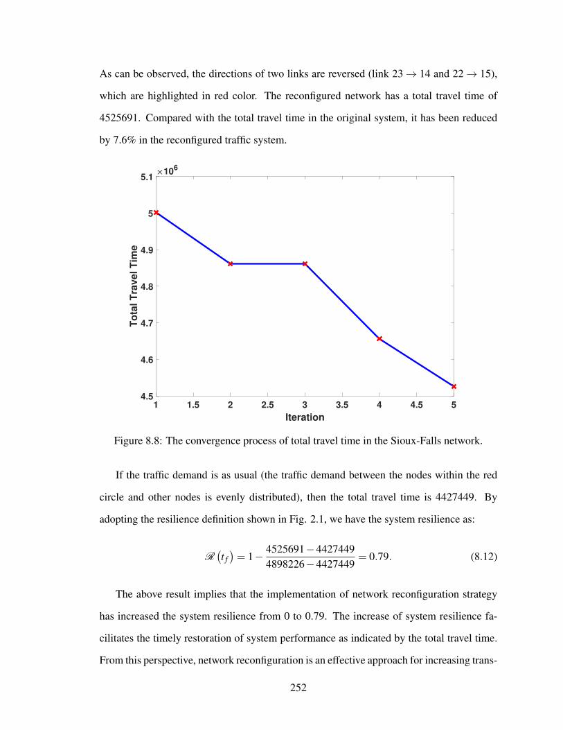
As can be observed, the directions of two links are reversed (link 23→ 14 and 22→ 15),

which are highlighted in red color. The reconfigured network has a total travel time of

4525691. Compared with the total travel time in the original system, it has been reduced

by 7.6% in the reconfigured traffic system.

1 1.5 2 2.5 3 3.5 4 4.5 5

Iteration

4.5

4.6

4.7

4.8

4.9

5

5.1

To

tal T

ravel T

ime

106

Figure 8.8: The convergence process of total travel time in the Sioux-Falls network.

If the traffic demand is as usual (the traffic demand between the nodes within the red

circle and other nodes is evenly distributed), then the total travel time is 4427449. By

adopting the resilience definition shown in Fig. 2.1, we have the system resilience as:

R(t f)= 1− 4525691−4427449

4898226−4427449= 0.79. (8.12)

The above result implies that the implementation of network reconfiguration strategy

has increased the system resilience from 0 to 0.79. The increase of system resilience fa-

cilitates the timely restoration of system performance as indicated by the total travel time.

From this perspective, network reconfiguration is an effective approach for increasing trans-

252

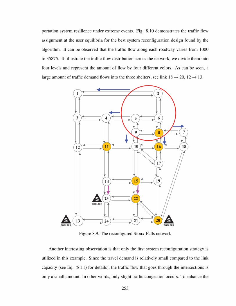
portation system resilience under extreme events. Fig. 8.10 demonstrates the traffic flow

assignment at the user equilibria for the best system reconfiguration design found by the

algorithm. It can be observed that the traffic flow along each roadway varies from 1000

to 35875. To illustrate the traffic flow distribution across the network, we divide them into

four levels and represent the amount of flow by four different colors. As can be seen, a

large amount of traffic demand flows into the three shelters, see link 18→ 20, 12→ 13.

1 2

3

12

13

64 5

11 10 16

89 7

18

14

23

24 21

15

22

17

19

20SSHELTER

SSHELTER

SSHELTER

Figure 8.9: The reconfigured Sioux-Falls network

Another interesting observation is that only the first system reconfiguration strategy is

utilized in this example. Since the travel demand is relatively small compared to the link

capacity (see Eq. (8.11) for details), the traffic flow that goes through the intersections is

only a small amount. In other words, only slight traffic congestion occurs. To enhance the

253

1 2

3

12

13

64 5

11 10 16

89 7

18

14

23

24 21

15

22

17

19

20S

SHELTER

SSHELTER

SSHELTER

1000 4487 7975 11462 14950 18437 21925 25412 28900 32387 35875

Figure 8.10: The link flow distribution of the best system reconfiguration in the Sioux-Fallsnetwork

importance of intersections in the network but without increasing the computational work-

load, we increase the waiting time for each vehicle going through the intersection that is not

blocked from 2 to 20. In this case, the reconfigured traffic system found by the proposed

method is illustrated in Fig. 8.11. In this case, both system reconfiguration strategies are

used. Specifically, two intersections (intersection 8 and 22) are blocked due to the increase

of waiting time: with respect to intersection 8, links connecting node 8 and node 9, node

8 to node 16, are blocked although there is a small amount of traffic demand from node 8

to node 16, and such traffic demand can be satisfied using other alternate routes; regard-

254

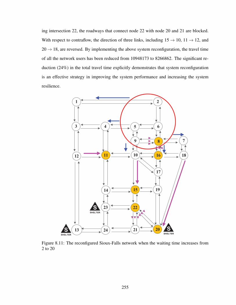
ing intersection 22, the roadways that connect node 22 with node 20 and 21 are blocked.

With respect to contraflow, the direction of three links, including 15→ 10, 11→ 12, and

20→ 18, are reversed. By implementing the above system reconfiguration, the travel time

of all the network users has been reduced from 10948173 to 8266862. The significant re-

duction (24%) in the total travel time explicitly demonstrates that system reconfiguration

is an effective strategy in improving the system performance and increasing the system

resilience.

1 2

3

12

13

64 5

11 10 16

89 7

18

14

23

24 21

15

22

17

19

20SSHELTER

SSHELTER

SSHELTER

Figure 8.11: The reconfigured Sioux-Falls network when the waiting time increases from2 to 20

255

8.3.2 Example 2

Fig. 8.12 shows a network with 25 nodes and 40 two-way links. All the two-way links

have symmetric link capacity and travel time, which are indicated by the two numbers

along each link. Each node is labeled by the number within the circle. As can be noticed,

there are nine intersections in this network, and they distribute at the center of the traffic

system to connect the nodes at the top and bottom layers. With respect to the links in the

network, they are in two different categories: freeways indicated by the bold links have a

free-flow speed of 55 mph and a practical capacity of 200 vehicles, and other links have a

free-flow speed of 20 mph and a capacity of 300 vehicles.

2 4

8

1213

1618

23

300 300

300

300 300 300 300

300

200

300 300 200300

300

200 200 200

300 200 300

300 300 200 300 300

300300

300 300

300300

200

300300

300 300 300 300

3.72

5.40 3.30

4.02 1.37 3.094.59

4.32

4.174.02

5.55

3.424.11

1.414.11

4.35 5.49 2.15 5.46 6.09

1.23 1.851.89 1.03

3.09 4.505.94 2.97

5.584.02

1.79

5.854.05

3.005.104.445.76

3.427 9

17

19

33.72

300

4.98

300

21

10

151411

6

1

5

20

2224 25 S

SHELTER

SSHELTER

SSHELTER

Figure 8.12: Test network 2: a 25-node artificial net

Suppose the area within the red ellipse is going to be hit by a catastrophic disaster, and

all the residents need to be evacuated away from this area. Three evacuation shelter centers

have been set up in three different locations across the network. All the residents within the

256

disaster-impacted region will be evacuated to the three shelters. Similar to the last example,

we assume that the travel demand from the disaster-impacted zones to the three shelters are

the same, and they are given as below:

d2,18 = 800, d2,21 = 800, d2,25 = 800,

d3,18 = 650, d3,21 = 650, d3,25 = 650,

d4,18 = 780, d4,21 = 780, d4,25 = 780,

d7,18 = 560, d7,21 = 560, d7,25 = 560,

d8,18 = 420, d8,21 = 420, d8,25 = 420,

d9,18 = 600, d9,21 = 600, d9,25 = 600.

(8.13)

From the travel demand shown in Eq. (8.13), it can be observed that node 2 has the

highest travel demand to the three shelters, followed by node 4 and node 3. In addition

to that, the traffic demand of the regular commuters among other nodes outside of the

disaster-impacted zone are also taken into consideration, which are indicated as below:

d1,10 = 70, d1,15 = 60, d1,19 = 50,

d6,16 = 120, d6,19 = 60, d6,25 = 70,

d11,15 = 100, d11,20 = 80, d11,23 = 90,

d15,12 = 50, d15,17 = 80, d15,24 = 110,

d16,20 = 100, d16,23 = 80.

(8.14)

Considering the above travel demand, the proposed method is leveraged to reconfigure

the traffic system in such a way that the total travel time for all the network users is min-

imized. Fig. 8.13 shows the convergence process of the total travel time. It can be seen

that the total travel time converges to a stable value within five iterations. The best system

reconfiguration found by the probabilistic solution discovery algorithm is illustrated in Fig.

8.14. The direction of six links are reversed, and they are 6→ 7, 11→ 6, 7→ 8, 14→ 9,

18→ 13, and 19→ 14. In other words, there are six one-way links in the reconfigured

257

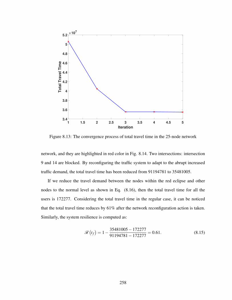
1 1.5 2 2.5 3 3.5 4 4.5 5

Iteration

3.4

3.6

3.8

4

4.2

4.4

4.6

4.8

5

5.2

To

tal

Trav

el T

ime

107

Figure 8.13: The convergence process of total travel time in the 25-node network

network, and they are highlighted in red color in Fig. 8.14. Two intersections: intersection

9 and 14 are blocked. By reconfiguring the traffic system to adapt to the abrupt increased

traffic demand, the total travel time has been reduced from 91194781 to 35481005.

If we reduce the travel demand between the nodes within the red eclipse and other

nodes to the normal level as shown in Eq. (8.16), then the total travel time for all the

users is 172277. Considering the total travel time in the regular case, it can be noticed

that the total travel time reduces by 61% after the network reconfiguration action is taken.

Similarly, the system resilience is computed as:

R(t f)= 1− 35481005−172277

91194781−172277= 0.61. (8.15)

258

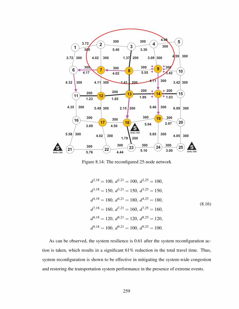
2 4

8

1213

1618

23

300 300

300

300 300 300 300

300

200

300 300 200300

300

200 200 200

300 200 300

300 300 200 300 300

300300

300 300

300300

200

300300

300 300 300 300

3.72

5.40 3.30

4.02 1.37 3.094.59

4.32

4.17 4.02 5.55

3.424.11

1.414.11

4.35 5.49 2.15 5.46 6.09

1.23 1.851.89 1.03

3.09 4.505.94 2.97

5.584.02

1.79

5.854.05

3.005.104.445.76

3.427 9

17

19

33.72

300

4.98

300

21

10

151411

6

1

5

20

2224 25 S

SHELTER

SSHELTER

SSHELTER

Figure 8.14: The reconfigured 25-node network

d2,18 = 100, d2,21 = 100, d2,25 = 100,

d3,18 = 150, d3,21 = 150, d3,25 = 150,

d4,18 = 180, d4,21 = 180, d4,25 = 180,

d7,18 = 160, d7,21 = 160, d7,25 = 160,

d8,18 = 120, d8,21 = 120, d8,25 = 120,

d9,18 = 100, d9,21 = 100, d9,25 = 100.

(8.16)

As can be observed, the system resilience is 0.61 after the system reconfiguration ac-

tion is taken, which results in a significant 61% reduction in the total travel time. Thus,

system reconfiguration is shown to be effective in mitigating the system-wide congestion

and restoring the transportation system performance in the presence of extreme events.

259

8.4 Summary

In this chapter, we consider the travel demand arising from emergency evacuations out

of the disaster-impacted zones. To mitigate the system-wide traffic congestion, we lever-

age two system reconfiguration strategies, namely lane reversal and crossing elimination

at intersections, and develop an integrated approach to increase the system resilience. The

objective of the proposed approach is to minimize the total travel time for both the regular

commuters and emergent evacuees. The issue investigated in this chapter is formulated

as a bi-level optimization problem, in which the lower level problem is modeled as user

equilibrium traffic assignment, and decision maker’s system-level traffic network recon-

figuration decisions are characterized as discrete variables in the upper level problem. A

gradient projection method is utilized to approach the traffic assignment at the user equi-

libria, and a probabilistic solution discovery algorithm is developed to identify the best

system reconfiguration in terms of contraflow and blocking roadways at each intersection

so that the total travel time of all the users is minimized. Two numerical examples have

demonstrated that the developed method reduces the total travel time and restores the traffic

system performance significantly.

The proposed approach and the numerical examples provide significant managerial in-

sights on the implementation of simple yet effective operations in mitigating the severe

system-wide congestion triggered by extreme events. The bi-level optimization enables

managers to make timely and rational system reconfiguration decisions by accounting for

the complex user driving behavior. More importantly, from a practical standpoint, the

implementation of system reconfiguration does not consume a lot of resources, which sig-

nificantly enhances the operational flexibility of managers and the system’s quick respon-

siveness to a variety of emergency situations.

The reconfiguration strategy developed in this chapter has great potential to be applied

into many other systems for the purpose of increasing their resilience. By optimally recon-

figuring the system components and topology properly, different reconfiguration options

260

and operation paradigms become readily available. By doing this, the system is equipped

with the capability to respond to different disruptive scenarios that impair different system

components. The flexibility enabled by system reconfiguration together with the relatively

less investment that is needed to achieve the reconfiguration make it a promising solution

to improve system resilience.

261

Chapter 9

Summary and Future Work

9.1 Summary of Accomplishments

The overall objective of this dissertation is to develop comprehensive machine learn-

ing and optimization models to assess and enhance the resilience of engineering systems.

Towards this end, we have investigated a series of assessment, prevention, and restora-

tion methodologies that can be taken before, during, and after the occurrence of hazardous

events. This target is approached by leveraging state-of-the-art machine learning algo-

rithms to build data-driven predictive models as well as effective sampling-based optimiza-

tion algorithms to approach challenging discrete bi-level optimization problems. The mea-

sures taken to enhance system resilience in this dissertation can be broadly classified into

three categories: 1. construction of predictive models to increase the operators’ situation

awareness on the dynamic evolution of hazardous events; 2. assessment of the effective-

ness of human and algorithmic responses in handling off-nominal events; 3. utilization

of optimization algorithms to enable resilience in new and legacy systems. The three sets

of strategies investigated in this dissertation form a closed loop for enhancing system re-

silience in terms of the actions that can be taken before, during, and after the occurrence

of anomalous events. With respect to each objective, the specific accomplishments and

innovations made in this dissertation are summarized below.

Deep Learning Models for Early Warning of the Occurrences of Hazardous Events:

In Chapter 3, an innovative methodology is developed for making long-term prediction on

system behavior with high accuracy, and three critical issues are addressed in this study:

(1) an efficient big data engine Apache Spark is leveraged to parse a large volume of raw

data with scalable performance; (2) two deep learning models are trained to make pre-

dictions on system behavior from different views, in which Monte Carlo dropout is used

262

to characterize model prediction uncertainty following a Bayesian approach; (3) the two

models are integrated together via a discrepancy term, thereby retaining both long-term

prediction capability and high prediction accuracy; (4) the integrated model is expanded

to make predictions on multiple system components, and a probabilistic safety metric is

defined to measure system safety. A highlight is that we characterize the uncertainty in

the prediction made by the trained deep learning models. The inclusion of model predic-

tion uncertainty not only improves the model prediction accuracy, but also significantly

increases the confidence of relevant stakeholders in decision making.

Ensemble Machine Learning Models for Risk Prediction on the Consequence of

Anomalous Events In Chapter 4, two conventional machine learning algorithms are used

to predict the severity of the consequence associated with anomalous events in terms of

their risk levels. The major innovation in this chapter is the development of a probabilistic

fusion rule to determine which model prediction outcome to count on when their predic-

tions disagree. The proposed probabilistic fusion rule considers three levels of information:

record-level prediction confidence, class-level prediction accuracy, and the proportion of

each class in the set of records with disagreeing predictions. By doing this, the misclas-

sification information is further utilized to correct model predictions on the subsequent

unseen test dataset. The fusion rule accounts for the various types of misclassifications

that the trained model is prone to make, thereby increasing the probability of labeling the

observation as the target class.

Human Reliability Analysis in Diagnosing and Correcting System Malfunctions:

In Chapter 5, an information fusion methodology is developed to assess the human perfor-

mance in eliminating off-nominal events. We fuse heterogeneous data with an ensemble

of support vector machine-based learning models. Despite the limited amount of data, the

trained model demonstrates a promising performance in predicting crew performance pre-

diction. This ensemble model of the full heterogeneous dataset is superior to SVM models

built with any subset of the heterogeneous data, and substantially better than simple corre-

263

lation between performance outcome and any individual input features. The development

of such an ensemble model helps to quantitatively measure the reliability in the operators’

response to system malfunction events.

Performance Assessment of Algorithmic Response to Hazardous Events: In Chap-

ter 6, we evaluate the effectiveness of an algorithmic response in dealing with anomalous

event. The first crucial contribution made along this front is to construct a dynamic sim-

ulation model to characterize the complex interactions among system components, and

incorporate the uncertainties arising at different stages. The dynamic simulation model

facilitates the quantitative evaluation of the effectiveness of algorithmic response in miti-

gating the impact of airport closure caused by extreme event. The second important con-

tribution is to develop a support vector regression-based surrogate model to handle both

precise and right-censored data. The development of SVR-based surrogate model facili-

tates fast evaluation of the performance of algorithmic response at different configurations,

thus supporting real-time decision-making.

Design Optimization for Resilience: In Chapter 7, we develop a resilience-based

framework to optimize the configuration of an infrastructure system. The significant contri-

bution made in this chapter is to account for multiple factors (i.e., travel time, waiting time,

service time) in the objective function. To tackle this challenging bi-level optimization

problem, a multi-level cross entropy method is leveraged to generate a family of probabil-

ity distributions with probability mass gradually converging to the proximity of the optimal

state, which is the second major contribution made in this chapter.

System Reconfiguration to Increase System Resilience: In Chapter 8, we address

an optimization problem for reconfiguring transportation system for the sake of mitigating

the traffic congestion caused by the large volume evacuation out of disaster-prone areas.

The innovation in this chapter is to investigate multiple implementable and economically

achievable operations to deal with different evacuation scenarios in a timely manner. Math-

ematical models are developed to represent system reconfiguration schemes and character-

264

ize the interactions between traffic operators and passengers. A probabilistic solution dis-

covery algorithm is used to obtain the near-optimal solution. The proposed method offers

insights for staging efficient evacuations with the reconfiguration of system typologies, and

equips the transportation system with the ability to respond to different emergency scenar-

ios quickly.

9.2 Future Work

Several areas that are worthy of further investigation are identified in this section.

For the flight trajectory prediction in Chapter 3, future work needs to develop visual-

ization of safety assessment at the sector or national level. The visualization will greatly

help operators pinpoint the position with the highest safety risk in a timely manner, thereby

improving operators and controller’s performance in maintaining the system safety dra-

matically. Another direction to move towards is to incorporate the probabilistic forecast on

weather conditions into the deep learning models so as to characterize the effect of weather

on flight trajectory.

With respect to the ensemble machine learning for prediction on the consequence of

hazardous events in Chapter 4, if the actions taken by the pilot or other operators involved

in the response to abnormal events are available, it will be useful to extend the developed

hybrid model to account for such important information. The inclusion of such information

helps us to identify risk mitigation actions for unforeseen events in the future by learning

from the actions that have been taken in past.

For the reliability assessment of crew performance in Chapter 5, future work needs

to extend the proposed method to include the plant states (i.e., process parameters in the

simulator logs) for quantifying the consequences of operator actions and thus their perfor-

mance. In addition, other relevant physiological indicators, such as electroencephalogram,

electrocardiogram and pupillometry, can be collected for modeling to increase prediction

accuracy as wearable sensors are improving in capabilities rate, battery life), comfort (i.e.,

265

size) and cost.

Regarding the performance assessment of response strategy in Chapter 6, further work

is needed w.r.t. data mining techniques to construct more realistic distributions to character-

ize the uncertainty related to each system component. Secondly, the reliability estimation

carried out in this chapter can be investigated towards reliability-based optimization of the

system variables (e.g., airport capacity and message delay) in order to improve the system

performance. Thirdly, we model gate capacity as a hard constraint, while planes can stop

on the tarmac and be unloaded by stairway, thus it is more reasonable to model gate ca-

pacity as a soft constraint in reality. Another future direction worthy of investigation is to

adapt the dynamic simulation to a more realistic situation with a higher density of radars

that cover the entire region.

With respect to the resilience-driven optimization framework for logistics service cen-

ters in Chapter 7, future work needs to investigate the combined effect of multiple individ-

ual events as well as the cascading effect of an individual disruptive event in a complex en-

gineering system. Future work can explore the implementation of the cross entropy method

in high-performance computing platforms (i.e., MapReduce, Spark) in order to accelerate

the computational speed for large-scale optimization. Finally, the planned distribution of

service centers investigated in Chapter 7 avoids any locations that could be impacted by

the unexpected extreme event, it will be worthy to investigate the case where some service

center locations that could be affected are actually used.

For system reconfiguration in transportation system presented in Chapter 8, future work

can increase the robustness of the system reconfiguration strategy by accommodating travel

demand uncertainty. In addition, it will be helpful to investigate how the system resilience

varies if the extreme event hits different locations in the transportation system. Additional

traffic system control and optimization strategies (e.g., traffic flow control, ramp metering,

and intelligent traffic signal) can be integrated into the framework proposed in this chapter,

thereby enhancing the system reconfiguration capability and the flexibility of the system in

266

response to different disruptive events.

The proposed strategies for response effectiveness assessment and resilience optimiza-

tion in this dissertation need to be investigated and validated for large-scale infrastructure

systems. One challenge arising during this process is how to resolve the large-scale opti-

mization problems. Effective approximation optimization algorithms need to be developed

to solve the formulated complex optimization problems, so that provide decision makers

can respond to extreme events in a timely manner. Last but not the least, most of optimiza-

tion models developed in this dissertation are deterministic. The aleatory and epistemic

uncertainties arising at various stages need to be represented appropriately and included in

the optimization model, thereby increasing the robustness of the optimization model.

9.3 Concluding Remarks

This dissertation focused on the investigation of measures to assess and strategies to in-

crease the resilience of engineering systems by leveraging state-of-the-art machine learning

and optimization algorithms. The proposed methodologies address several significant chal-

lenges in system resilience assessment and enhancement, and make the following contri-

butions: (1) multiple predictive models are developed to build ensemble machine learning

models, which increase the operators’ situation awareness and understanding on the evo-

lution trajectory of hazardous events, such as when the anomalous event is about to occur,

and what is the consequence of an anomalous event; (2) we evaluate the response effec-

tiveness of both human and algorithmic responses in withstanding the impact of extreme

event, such as the performance of a crew in diagnosing and correcting system malfunctions,

and the adopted rerouting strategy in handling inbound flights when the destination airport

shuts down abruptly; (3) optimization algorithms are leveraged to achieve or improve sys-

tem resilience through the design of a new system or reconfiguration of an existing system.

The resilience embedded into the system together with the modeling of interactions among

different players and components allows the system to restore from disruptive scenarios to

267

normal performance in a timely manner.

The machine learning and optimization models will be of high value to decision makers.

One the one hand, the predictive models significantly increase the decision maker’s under-

standing and situation awareness regarding the system’s evolution trajectory and the effect

of various response actions on system performance. On the other hand, the implementation

of optimization algorithms helps the system to restore closer to its original performance

following the disruptive event. All of these new developments help to improve the system

resilience against unanticipated events, thereby showing significant potential for practical

application.

268

BIBLIOGRAPHY

[1] Ralph B D’Agostino. Goodness-of-fit-techniques, volume 68. CRC press, 1986.

[2] Devanandham Henry and Jose Emmanuel Ramirez-Marquez. Generic metrics and

quantitative approaches for system resilience as a function of time. Reliability Engi-

neering & System Safety, 99:114–122, 2012.

[3] Vivienne Sze, Yu-Hsin Chen, Tien-Ju Yang, and Joel S Emer. Efficient processing

of deep neural networks: A tutorial and survey. Proceedings of the IEEE, 105(12):

2295–2329, 2017.

[4] Salman Salloum, Ruslan Dautov, Xiaojun Chen, Patrick Xiaogang Peng, and

Joshua Zhexue Huang. Big data analytics on Apache Spark. International Jour-

nal of Data Science and Analytics, 1(3-4):145–164, 2016.

[5] Marvin Rausand and Arnljot Høyland. System reliability theory: models, statistical

methods, and applications, volume 396. John Wiley & Sons, 2004.

[6] Xiaoge Zhang, Sankaran Mahadevan, and Xinyang Deng. Reliability analysis with

linguistic data: An evidential network approach. Reliability Engineering & System

Safety, 162:111–121, 2017.

[7] Xiaoge Zhang and Sankaran Mahadevan. A game theoretic approach to network

reliability assessment. IEEE Transactions on Reliability, 66(3):875–892, 2017.

[8] Crawford S Holling. Resilience and stability of ecological systems. Annual Review

of Ecology and Systematics, 4(1):1–23, 1973.

[9] Mayada Omer, Roshanak Nilchiani, and Ali Mostashari. Measuring the resilience

of the trans-oceanic telecommunication cable system. IEEE Systems Journal, 3(3):

295–303, 2009.

269

[10] Hiba Baroud, Jose E Ramirez-Marquez, Kash Barker, and Claudio M Rocco.

Stochastic measures of network resilience: Applications to waterway commodity

flows. Risk Analysis, 34(7):1317–1335, 2014.

[11] Mathaios Panteli and Pierluigi Mancarella. Modeling and evaluating the resilience

of critical electrical power infrastructure to extreme weather events. IEEE Systems

Journal, 11(3):1733–1742, 2015.

[12] Lijuan Shen, Beatrice Cassottana, and Loon Ching Tang. Statistical trend tests for

resilience of power systems. Reliability Engineering & System Safety, 177:138–147,

2018.

[13] Xiaoge Zhang, Zili Zhang, Yajuan Zhang, Daijun Wei, and Yong Deng. Route selec-

tion for emergency logistics management: A bio-inspired algorithm. Safety Science,

54:87–91, 2013.

[14] Yacov Y Haimes, Kenneth Crowther, and Barry M Horowitz. Homeland security

preparedness: Balancing protection with resilience in emergent systems. Systems

Engineering, 11(4):287–308, 2008.

[15] Zhen Hu and Sankaran Mahadevan. Resilience assessment based on time-dependent

system reliability analysis. Journal of Mechanical Design, 138(11):111404, 2016.

[16] Michel Bruneau, Stephanie E Chang, Ronald T Eguchi, George C Lee, Thomas D

ORourke, Andrei M Reinhorn, Masanobu Shinozuka, Kathleen Tierney, William A

Wallace, and Detlof Von Winterfeldt. A framework to quantitatively assess and

enhance the seismic resilience of communities. Earthquake Spectra, 19(4):733–752,

2003.

[17] Hiba Baroud, Kash Barker, Jose E Ramirez-Marquez, et al. Importance measures

for inland waterway network resilience. Transportation Research Part E: Logistics

and Transportation Review, 62:55–67, 2014.

270

[18] Hossein Fotouhi, Seksun Moryadee, and Elise Miller-Hooks. Quantifying the re-

silience of an urban traffic-electric power coupled system. Reliability Engineering

& System Safety, 163:79–94, 2017.

[19] Seyedmohsen Hosseini, Kash Barker, and Jose E Ramirez-Marquez. A review of

definitions and measures of system resilience. Reliability Engineering & System

Safety, 145:47–61, 2016.

[20] Kash Barker, Jose Emmanuel Ramirez-Marquez, and Claudio M Rocco. Resilience-

based network component importance measures. Reliability Engineering & System

Safety, 117:89–97, 2013.

[21] Xiaoge Zhang, Sankaran Mahadevan, Shankar Sankararaman, and Kai Goebel.

Resilience-based network design under uncertainty. Reliability Engineering & Sys-

tem Safety, 169:364–379, 2018.

[22] Rahul Nair, Hakob Avetisyan, and Elise Miller-Hooks. Resilience framework for

ports and other intermodal components. Transportation Research Record: Journal

of the Transportation Research Board, (2166):54–65, 2010.

[23] Vladimir Vapnik. The nature of statistical learning theory. Springer Science &

Business Media, 2013.

[24] Zhiquan Qi, Yingjie Tian, and Yong Shi. Robust twin support vector machine for

pattern classification. Pattern Recognition, 46(1):305–316, 2013.

[25] Xiang-Yang Wang, Ting Wang, and Juan Bu. Color image segmentation using pixel

wise support vector machine classification. Pattern Recognition, 44(4):777–787,

2011.

[26] Chia-Feng Juang and Guo-Cyuan Chen. A TS fuzzy system learned through a sup-

271

port vector machine in principal component space for real-time object detection.

IEEE Transactions on Industrial Electronics, 59(8):3309–3320, 2012.

[27] Xiaoge Zhang and Sankaran Mahadevan. Aircraft re-routing optimization and per-

formance assessment under uncertainty. Decision Support Systems, 96:67–82, 2017.

[28] Chi-Jie Lu, Tian-Shyug Lee, and Chih-Chou Chiu. Financial time series forecast-

ing using independent component analysis and support vector regression. Decision

Support Systems, 47(2):115–125, 2009.

[29] Chun-Hsin Wu, Jan-Ming Ho, and Der-Tsai Lee. Travel-time prediction with sup-

port vector regression. IEEE Transactions on Intelligent Transportation Systems, 5

(4):276–281, 2004.

[30] Yann LeCun, Yoshua Bengio, and Geoffrey Hinton. Deep learning. Nature, 521

(7553):436–444, 2015.

[31] Jurgen Schmidhuber. Deep learning in neural networks: An overview. Neural Net-

works, 61:85–117, 2015.

[32] Sepp Hochreiter and Jurgen Schmidhuber. Long short-term memory. Neural Com-

putation, 9(8):1735–1780, 1997.

[33] Radford M Neal. Bayesian learning for neural networks, volume 118. Springer

Science & Business Media, 2012.

[34] Yarin Gal and Zoubin Ghahramani. Dropout as a bayesian approximation: Repre-

senting model uncertainty in deep learning. In International Conference on Machine

Learning, pages 1050–1059, 2016.

[35] Yarin Gal and Zoubin Ghahramani. A theoretically grounded application of dropout

in recurrent neural networks. In Advances in Neural Information Processing Sys-

tems, pages 1019–1027, 2016.

272

[36] Yarin Gal. Uncertainty in deep learning. PhD thesis, PhD thesis, University of

Cambridge, 2016.

[37] Andreas Damianou and Neil Lawrence. Deep Gaussian processes. In Artificial

Intelligence and Statistics, pages 207–215, 2013.

[38] Heinrich Von Stackelberg. Market structure and equilibrium. Springer Science &

Business Media, 2010.

[39] John Glen Wardrop. Some theoretical aspects of road traffic research. Proceedings

of the Institution of Civil Engineers, 1(3):325–362, 1952.

[40] John D Murchland. Braess’s paradox of traffic flow. Transportation Research, 4(4):

391–394, 1970.

[41] Richard Steinberg and Willard I Zangwill. The prevalence of braess’ paradox. Trans-

portation Science, 17(3):301–318, 1983.

[42] Armen Der Kiureghian and Ove Ditlevsen. Aleatory or epistemic? does it matter?

Structural Safety, 31(2):105–112, 2009.

[43] Saideep Nannapaneni and Sankaran Mahadevan. Reliability analysis under epis-

temic uncertainty. Reliability Engineering & System Safety, 155:9–20, 2016.

[44] Kyle Neal, Zhen Hu, Sankaran Mahadevan, and Jon Zumberge. Discrepancy predic-

tion in dynamical system models under untested input histories. Journal of Compu-

tational and Nonlinear Dynamics, 14(2):021009, 2019.

[45] Glenn Shafer. A mathematical theory of evidence, volume 42. Princeton university

press, 1976.

[46] Lotfi A Zadeh. Fuzzy sets. Information and control, 8(3):338–353, 1965.

273

[47] Xiaoge Zhang, Yong Deng, Felix TS Chan, Peida Xu, Sankaran Mahadevan, and

Yong Hu. IFSJSP: a novel methodology for the job-shop scheduling problem based

on intuitionistic fuzzy sets. International Journal of Production Research, 51(17):

5100–5119, 2013.

[48] Didier Dubois and Henri Prade. Possibility theory. Springer, 2012.

[49] Andrea Saltelli, Marco Ratto, Terry Andres, Francesca Campolongo, Jessica Cari-

boni, Debora Gatelli, Michaela Saisana, and Stefano Tarantola. Global sensitivity

analysis: the primer. John Wiley & Sons, 2008.

[50] Bruno Sudret. Global sensitivity analysis using polynomial chaos expansions. Reli-

ability Engineering & System Safety, 93(7):964–979, 2008.

[51] Pan Wang, Zhenzhou Lu, and Zhangchun Tang. An application of the Kriging

method in global sensitivity analysis with parameter uncertainty. Applied Mathe-

matical Modelling, 37(9):6543–6555, 2013.

[52] Biagio Ciuffo, Jordi Casas, Marcello Montanino, Josep Perarnau, and Vincenzo

Punzo. Gaussian process metamodels for sensitivity analysis of traffic simulation

models: Case study of AIMSUN mesoscopic model. Transportation Research

Record, 2390(1):87–98, 2013.

[53] Søren Nymand Lophaven, Hans Bruun Nielsen, and Jacob Søndergaard. Dace-A

Matlab Kriging toolbox, version 2.0. 2002.

[54] Stefano Tarantola, Debora Gatelli, and Thierry Alex Mara. Random balance designs

for the estimation of first order global sensitivity indices. Reliability Engineering &

System Safety, 91(6):717–727, 2006.

[55] Andrea Saltelli and Ricardo Bolado. An alternative way to compute Fourier am-

274

plitude sensitivity test (FAST). Computational Statistics & Data Analysis, 26(4):

445–460, 1998.

[56] Gregory J McRae, James W Tilden, and John H Seinfeld. Global sensitivity analy-

sisa computational implementation of the Fourier amplitude sensitivity test (FAST).

Computers & Chemical Engineering, 6(1):15–25, 1982.

[57] Sergei Kucherenko, Balazs Feil, Nilay Shah, and Wolfgang Mauntz. The identifi-

cation of model effective dimensions using global sensitivity analysis. Reliability

Engineering & System Safety, 96(4):440–449, 2011.

[58] J-Y Tissot and Clementine Prieur. A randomized orthogonal array-based procedure

for the estimation of first-and second-order Sobol’indices. Journal of Statistical

Computation and Simulation, 85(7):1358–1381, 2015.

[59] Clementine Prieur and Stefano Tarantola. Variance-based sensitivity analysis: The-

ory and estimation algorithms. Handbook of Uncertainty Quantification, pages

1217–1239, 2017.

[60] Michael Armbrust, Reynold S Xin, Cheng Lian, Yin Huai, Davies Liu, Joseph K

Bradley, Xiangrui Meng, Tomer Kaftan, Michael J Franklin, Ali Ghodsi, et al. Spark

SQL: Relational data processing in Spark. In Proceedings of the 2015 ACM SIG-

MOD International Conference on Management of Data, pages 1383–1394. ACM,

2015.

[61] Joseph E Gonzalez, Reynold S Xin, Ankur Dave, Daniel Crankshaw, Michael J

Franklin, and Ion Stoica. GraphX: Graph processing in a distributed dataflow frame-

work. In 11th USENIX Symposium on Operating Systems Design and Implementa-

tion (OSDI 14), pages 599–613, 2014.

[62] Matei Zaharia, Tathagata Das, Haoyuan Li, Timothy Hunter, Scott Shenker, and Ion

Stoica. Discretized streams: Fault-tolerant streaming computation at scale. In Pro-

275

ceedings of the Twenty-fourth ACM Symposium on Operating Systems Principles,

pages 423–438. ACM, 2013.

[63] Xiangrui Meng, Joseph Bradley, Burak Yavuz, Evan Sparks, Shivaram Venkatara-

man, Davies Liu, Jeremy Freeman, DB Tsai, Manish Amde, Sean Owen, et al. Mllib:

Machine learning in Apache Spark. The Journal of Machine Learning Research, 17

(1):1235–1241, 2016.

[64] Joseph E Gonzalez. From graphs to tables the design of scalable systems for graph

analytics. In Proceedings of the 23rd International Conference on World Wide Web,

pages 1149–1150. ACM, 2014.

[65] Xiaoge Zhang and Sankaran Mahadevan. Bayesian neural networks for flight tra-

jectory prediction and safety assessment. Decision Support Systems, Under Review,

2019.

[66] IATA forecasts passenger demand to double over 20 years. http://www.iata.org/

pressroom/pr/Pages/2016-10-18-02.aspx, Accessed: 2017-12-28.

[67] EU ROCONTROL. European organisation for the safety of air navigation. 1997.

[68] Shankar Sankararaman, Indranil Roychoudhury, Xiaoge Zhang, and Kai Goebel.

Preliminary investigation of impact of technological impairment on trajectory-based

operation. In 17th AIAA Aviation Technology, Integration, and Operations Confer-

ence, page 4488, 2017.

[69] Xiaoge Zhang and Sankaran Mahadevan. Ensemble machine learning models for

aviation incident risk prediction. Decision Support Systems, 116:48–63, 2019.

[70] Federal Aviation Administration, U.S. Department of Transportation. The future of

the nas, June 2016. https://www.faa.gov/nextgen/media/futureofthenas.pdf.

276

http://www.iata.org/pressroom/pr/Pages/2016-10-18-02.aspx

http://www.iata.org/pressroom/pr/Pages/2016-10-18-02.aspx

https://www.faa.gov/nextgen/media/futureofthenas.pdf

[71] Javier Lovera Yepes, Inseok Hwang, and Mario Rotea. New algorithms for aircraft

intent inference and trajectory prediction. Journal of Guidance, Control, and Dy-

namics, 30(2):370–382, 2007.

[72] Xavier Prats, Vicenc Puig, Joseba Quevedo, and Fatiha Nejjari. Multi-objective

optimisation for aircraft departure trajectories minimising noise annoyance. Trans-

portation Research Part C: Emerging Technologies, 18(6):975–989, 2010.

[73] Arjen de Leege, Marinus van Paassen, and Max Mulder. A machine learning ap-

proach to trajectory prediction. In AIAA Guidance, Navigation, and Control (GNC)

Conference, page 4782, 2013.

[74] Chester Gong and Dave McNally. A methodology for automated trajectory predic-

tion analysis. In AIAA Guidance, Navigation, and Control Conference and Exhibit,

page 4788, 2004.

[75] Antonio Franco, Damian Rivas, and Alfonso Valenzuela. Probabilistic aircraft tra-

jectory prediction in cruise flight considering ensemble wind forecasts. Aerospace

Science and Technology, 82:350–362, 2018.

[76] Matthew Daigle, Indranil Roychoudhury, Liljana Spirkovska, Kai Goebel, Shankar

Sankararaman, John Ossenfort, and Chetan S Kulkarni. Real-time prediction of

safety margins in the national airspace. In 17th AIAA Aviation Technology, Integra-

tion, and Operations Conference, page 4388, 2017.

[77] Angela Nuic, Damir Poles, and Vincent Mouillet. BADA: An advanced aircraft

performance model for present and future ATM systems. International Journal of

Adaptive Control and Signal Processing, 24(10):850–866, 2010.

[78] Xiangmin Guan, Renli Lv, Liang Sun, and Yang Liu. A study of 4D trajectory pre-

diction based on machine deep learning. In 2016 12th World Congress on Intelligent

Control and Automation (WCICA), pages 24–27. IEEE, 2016.

277

[79] Samet Ayhan and Hanan Samet. Aircraft trajectory prediction made easy with pre-

dictive analytics. In Proceedings of the 22nd ACM SIGKDD International Confer-

ence on Knowledge Discovery and Data Mining, pages 21–30. ACM, 2016.

[80] Richard Alligier and David Gianazza. Learning aircraft operational factors to im-

prove aircraft climb prediction: A large scale multi-airport study. Transportation

Research Part C: Emerging Technologies, 96:72–95, 2018.

[81] Claudio Di Ciccio, Han Van der Aa, Cristina Cabanillas, Jan Mendling, and Jo-

hannes Prescher. Detecting flight trajectory anomalies and predicting diversions in

freight transportation. Decision Support Systems, 88:1–17, 2016.

[82] Mohammad Assaad, Romuald Bone, and Hubert Cardot. A new boosting algorithm

for improved time-series forecasting with recurrent neural networks. Information

Fusion, 9(1):41–55, 2008.

[83] Florent Altche and Arnaud De La Fortelle. An LSTM network for highway trajectory

prediction. In 2017 IEEE 20th International Conference on Intelligent Transporta-

tion Systems (ITSC), pages 353–359. IEEE, 2017.

[84] Zhiyuan Shi, Min Xu, Quan Pan, Bing Yan, and Haimin Zhang. LSTM-based flight

trajectory prediction. In International Joint Conference on Neural Networks, 2018.

[85] Mina Moradi Kordmahalleh, Mohammad Gorji Sefidmazgi, and Abdollah Homaifar.

A sparse recurrent neural network for trajectory prediction of Atlantic hurricanes. In

Proceedings of the Genetic and Evolutionary Computation Conference 2016, pages

957–964. ACM, 2016.

[86] Alexandre Alahi, Kratarth Goel, Vignesh Ramanathan, Alexandre Robicquet, Li Fei-

Fei, and Silvio Savarese. Social LSTM: Human trajectory prediction in crowded

spaces. In Proceedings of the IEEE Conference on Computer Vision and Pattern

Recognition, pages 961–971, 2016.

278

[87] Hao Wu, Ziyang Chen, Weiwei Sun, Baihua Zheng, and Wei Wang. Modeling tra-

jectories with recurrent neural networks. In Proceedings of the 26th International

Joint Conference on Artificial Intelligence, pages 3083–3090. AAAI Press, 2017.

[88] Zoubin Ghahramani. Probabilistic machine learning and artificial intelligence. Na-

ture, 521(7553):452, 2015.

[89] Charles Blundell, Julien Cornebise, Koray Kavukcuoglu, and Daan Wierstra. Weight

uncertainty in neural network. In International Conference on Machine Learning,

pages 1613–1622, 2015.

[90] Yarin Gal and Zoubin Ghahramani. Bayesian convolutional neural networks with

bernoulli approximate variational inference. arXiv preprint arXiv:1506.02158,

2015.

[91] Lingxue Zhu and Nikolay Laptev. Deep and confident prediction for time se-

ries at Uber. In 2017 IEEE International Conference on Data Mining Workshops

(ICDMW), pages 103–110, 2017.

[92] Nikolay Laptev, Jason Yosinski, Li Erran Li, and Slawek Smyl. Time-series extreme

event forecasting with neural networks at Uber. In International Conference on

Machine Learning, number 34, pages 1–5, 2017.

[93] Alex Kendall and Roberto Cipolla. Modelling uncertainty in deep learning for cam-

era relocalization. In 2016 IEEE International Conference on Robotics and Automa-

tion (ICRA), pages 4762–4769. IEEE, 2016.

[94] Matei Zaharia, Reynold S Xin, Patrick Wendell, Tathagata Das, Michael Arm-

brust, Ankur Dave, Xiangrui Meng, Josh Rosen, Shivaram Venkataraman, Michael J

Franklin, et al. Apache Spark: A unified engine for big data processing. Communi-

cations of the ACM, 59(11):56–65, 2016.

279

[95] Marianela Garcıa Lozano, Jonah Schreiber, and Joel Brynielsson. Tracking geo-

graphical locations using a geo-aware topic model for analyzing social media data.

Decision Support Systems, 99:18–29, 2017.

[96] Ahmad Usmani. System wide information management. In 2010 Integrated Com-

munications Navigation and Surveillance Conference (ICNS), pages 1–17. IEEE,

2010.

[97] James G Shanahan and Laing Dai. Large scale distributed data science using Apache

Spark. In Proceedings of the 21th ACM SIGKDD International Conference on

Knowledge Discovery and Data Mining, pages 2323–2324. ACM, 2015.

[98] Spark-xml. https://github.com/databricks/spark-xml, Accessed: 2019-02-12.

[99] Haonan Yu, Jiang Wang, Zhiheng Huang, Yi Yang, and Wei Xu. Video paragraph

captioning using hierarchical recurrent neural networks. In Proceedings of the IEEE

Conference on Computer Vision and Pattern Recognition, pages 4584–4593, 2016.

[100] Alex Graves and Navdeep Jaitly. Towards end-to-end speech recognition with re-

current neural networks. In International Conference on Machine Learning, pages

1764–1772, 2014.

[101] Alex Graves, Abdel-rahman Mohamed, and Geoffrey Hinton. Speech recognition

with deep recurrent neural networks. In 2013 IEEE International Conference on

Acoustics, Speech and Signal Processing, pages 6645–6649. IEEE, 2013.

[102] Shujie Liu, Nan Yang, Mu Li, and Ming Zhou. A recursive recurrent neural network

for statistical machine translation. In Proceedings of the 52nd Annual Meeting of the

Association for Computational Linguistics, volume 1, pages 1491–1500, 2014.

[103] Joerg Evermann, Jana-Rebecca Rehse, and Peter Fettke. Predicting process be-

haviour using deep learning. Decision Support Systems, 100:129–140, 2017.

280

https://github.com/databricks/spark-xml

[104] Ming Liang and Xiaolin Hu. Recurrent convolutional neural network for object

recognition. In Proceedings of the IEEE Conference on Computer Vision and Pattern

Recognition, pages 3367–3375, 2015.

[105] Bharat Singh, Tim K Marks, Michael Jones, Oncel Tuzel, and Ming Shao. A multi-

stream bi-directional recurrent neural network for fine-grained action detection. In

Proceedings of the IEEE Conference on Computer Vision and Pattern Recognition,

pages 1961–1970, 2016.

[106] Lucio Flavio Vismari and Joao Batista Camargo Junior. A safety assessment method-

ology applied to CNS/ATM-based air traffic control system. Reliability Engineering

& System Safety, 96(7):727–738, 2011.

[107] Fedja Netjasov and Milan Janic. A review of research on risk and safety modelling

in civil aviation. Journal of Air Transport Management, 14(4):213–220, 2008.

[108] ALC Roelen, R Wever, AR Hale, L Goossens, R Cooke, R Lopuhaa, M Simons,

and PJL Valk. Causal modeling for integrated safety at airports. In Proceedings of

ESREL, pages 1321–1327, 2003.

[109] Douglas A Wiegmann and Scott A Shappell. A human error approach to aviation

accident analysis: The human factors analysis and classification system. Routledge,

2017.

[110] Huan-Jyh Shyur. A quantitative model for aviation safety risk assessment. Comput-

ers & Industrial Engineering, 54(1):34–44, 2008.

[111] Xi Chen, Indranil Bose, Alvin Chung Man Leung, and Chenhui Guo. Assessing

the severity of phishing attacks: A hybrid data mining approach. Decision Support

Systems, 50(4):662–672, 2011.

281

[112] Kathleen L McFadden and Elizabeth R Towell. Aviation human factors: a frame-

work for the new millennium. Journal of Air Transport Management, 5(4):177–184,

1999.

[113] Nikunj Oza, J Patrick Castle, and John Stutz. Classification of aeronautics system

health and safety documents. IEEE Transactions on Systems, Man, and Cybernetics,

Part C (Applications and Reviews), 39(6):670–680, 2009.

[114] Suratna Budalakoti, Ashok N Srivastava, and Matthew E Otey. Anomaly detection

and diagnosis algorithms for discrete symbol sequences with applications to airline

safety. IEEE Transactions on Systems, Man, and Cybernetics, Part C (Applications

and Reviews), 39(1):101–113, 2009.

[115] ASRS program briefing. https://asrs.arc.nasa.gov/docs/ASRS

ProgramBriefing2016.pdf, Accessed: 2017-12-28.

[116] Yao Liu, Cuiqing Jiang, and Huimin Zhao. Using contextual features and multi-view

ensemble learning in product defect identification from online discussion forums.

Decision Support Systems, 105:1–12, 2018.

[117] Thorsten Joachims. Text categorization with support vector machines: Learning

with many relevant features. In European Conference on Machine Learning, pages

137–142. Springer, 1998.

[118] Yibo Wang and Wei Xu. Leveraging deep learning with LDA-based text analytics to

detect automobile insurance fraud. Decision Support Systems, 105:87–95, 2018.

[119] Feng Wang, Tianhua Xu, Tao Tang, MengChu Zhou, and Haifeng Wang. Bilevel

feature extraction-based text mining for fault diagnosis of railway systems. IEEE

Transactions on Intelligent Transportation Systems, 18(1):49–58, 2017.

282

https://asrs.arc.nasa.gov/docs/ASRS_ProgramBriefing2016.pdf

https://asrs.arc.nasa.gov/docs/ASRS_ProgramBriefing2016.pdf

[120] Runyu Chen, Yitong Zheng, Wei Xu, Minghao Liu, and Jiayue Wang. Secondhand

seller reputation in online markets: A text analytics framework. Decision Support

Systems, 108:96–106, 2018.

[121] Alan S Abrahams, Weiguo Fan, G Alan Wang, Zhongju John Zhang, and Jian Jiao.

An integrated text analytic framework for product defect discovery. Production and

Operations Management, 24(6):975–990, 2015.

[122] Gongde Guo, Hui Wang, David Bell, Yaxin Bi, and Kieran Greer. Using kNN model

for automatic text categorization. Soft Computing, 10(5):423–430, 2006.

[123] Min-Ling Zhang and Zhi-Hua Zhou. Multilabel neural networks with applications

to functional genomics and text categorization. IEEE Transactions on Knowledge

and Data Engineering, 18(10):1338–1351, 2006.

[124] Man Lan, Chew Lim Tan, Jian Su, and Yue Lu. Supervised and traditional term

weighting methods for automatic text categorization. IEEE Transactions on Pattern

Analysis and Machine Intelligence, 31(4):721–735, 2009.

[125] Simon Tong and Daphne Koller. Support vector machine active learning with appli-

cations to text classification. Journal of Machine Learning Research, 2(Nov):45–66,

2001.

[126] Vladimir Naumovich Vapnik and Vlamimir Vapnik. Statistical learning theory, vol-

ume 1. Wiley New York, 1998.

[127] Nan Li and Desheng Dash Wu. Using text mining and sentiment analysis for online

forums hotspot detection and forecast. Decision Support Systems, 48(2):354–368,

2010.

[128] Yuchun Tang, Yan-Qing Zhang, Nitesh V Chawla, and Sven Krasser. SVMs model-

283

ing for highly imbalanced classification. IEEE Transactions on Systems, Man, and

Cybernetics, Part B, 39(1):281–288, 2009.

[129] Weinan Zhang, Tianming Du, and Jun Wang. Deep learning over multi-field categor-

ical data. In European Conference on Information Retrieval, pages 45–57. Springer,

2016.

[130] Yelong Shen, Xiaodong He, Jianfeng Gao, Li Deng, and Gregoire Mesnil. A latent

semantic model with convolutional-pooling structure for information retrieval. In

Proceedings of the 23rd ACM International Conference on Conference on Informa-

tion and Knowledge Management, pages 101–110. ACM, 2014.

[131] Victoria Lopez, Alberto Fernandez, Salvador Garcıa, Vasile Palade, and Francisco

Herrera. An insight into classification with imbalanced data: Empirical results and

current trends on using data intrinsic characteristics. Information Sciences, 250:

113–141, 2013.

[132] Jose F Dıez-Pastor, Juan J Rodrıguez, Cesar Garcıa-Osorio, and Ludmila I

Kuncheva. Random balance: ensembles of variable priors classifiers for imbalanced

data. Knowledge-Based Systems, 85:96–111, 2015.

[133] Nitesh V Chawla, Kevin W Bowyer, Lawrence O Hall, and W Philip Kegelmeyer.

SMOTE: synthetic minority over-sampling technique. Journal of Artificial Intelli-

gence Research, 16:321–357, 2002.

[134] Shulong Tan, Yang Li, Huan Sun, Ziyu Guan, Xifeng Yan, Jiajun Bu, Chun Chen,

and Xiaofei He. Interpreting the public sentiment variations on Twitter. IEEE Trans-

actions on Knowledge and Data Engineering, 26(5):1158–1170, 2014.

[135] Andrew McCallum, Kamal Nigam, et al. A comparison of event models for Naıve

Bayes text classification. In AAAI-98 Workshop on Learning for Text Categorization,

volume 752, pages 41–48. Citeseer, 1998.

284

[136] Joseph Lilleberg, Yun Zhu, and Yanqing Zhang. Support vector machines and

word2vec for text classification with semantic features. In 2015 IEEE 14th Inter-

national Conference on Cognitive Informatics & Cognitive Computing (ICCI* CC),

pages 136–140. IEEE, 2015.

[137] Shenghuo Zhu, Xiang Ji, Wei Xu, and Yihong Gong. Multi-labelled classification

using maximum entropy method. In Proceedings of the 28th Annual International

ACM SIGIR Conference on Research and Development in Information Retrieval,

pages 274–281. ACM, 2005.

[138] Dino Isa, Lam H Lee, VP Kallimani, and Rajprasad Rajkumar. Text document pre-

processing with the Bayes formula for classification using the support vector ma-

chine. IEEE Transactions on Knowledge and Data Engineering, 20(9):1264–1272,

2008.

[139] Soumen Chakrabarti, Shourya Roy, and Mahesh V Soundalgekar. Fast and accurate

text classification via multiple linear discriminant projections. The VLDB Journal,

12(2):170–185, 2003.

[140] Natural language toolbox. https://www.nltk.org/, Accessed: 2018-04-02.

[141] Karen Sparck Jones. IDF term weighting and IR research lessons. Journal of Doc-

umentation, 60(5):521–523, 2004.

[142] Alex Krizhevsky, Ilya Sutskever, and Geoffrey E Hinton. Imagenet classification

with deep convolutional neural networks. In Advances in Neural Information Pro-

cessing Systems, pages 1097–1105, 2012.

[143] Geoffrey Hinton, Li Deng, Dong Yu, George E Dahl, Abdel-rahman Mohamed,

Navdeep Jaitly, Andrew Senior, Vincent Vanhoucke, Patrick Nguyen, Tara N

Sainath, et al. Deep neural networks for acoustic modeling in speech recognition:

285

https://www.nltk.org/

The shared views of four research groups. IEEE Signal Processing Magazine, 29

(6):82–97, 2012.

[144] Ronan Collobert, Jason Weston, Leon Bottou, Michael Karlen, Koray Kavukcuoglu,

and Pavel Kuksa. Natural language processing (almost) from scratch. Journal of

Machine Learning Research, 12:2493–2537, 2011.

[145] Michał Wozniak, Manuel Grana, and Emilio Corchado. A survey of multiple classi-

fier systems as hybrid systems. Information Fusion, 16:3–17, 2014.

[146] Bianca Zadrozny and Charles Elkan. Transforming classifier scores into accurate

multiclass probability estimates. In Proceedings of the Eighth ACM SIGKDD In-

ternational Conference on Knowledge Discovery and Data Mining, pages 694–699.

ACM, 2002.

[147] Shankar Sankararaman and Sankaran Mahadevan. Model validation under epistemic

uncertainty. Reliability Engineering & System Safety, 96(9):1232–1241, 2011.

[148] Per Ahlgren and Cristian Colliander. Document–document similarity approaches

and science mapping: Experimental comparison of five approaches. Journal of In-

formetrics, 3(1):49–63, 2009.

[149] Diederik P Kingma and Jimmy Ba. Adam: A method for stochastic optimization. In

International Conference on Learning Representation, pages 1–13. ACM, 2015.

[150] Jason DM Rennie and Nathan Srebro. Loss functions for preference levels: Re-

gression with discrete ordered labels. In Proceedings of the IJCAI Multidisciplinary

Workshop on Advances in Preference Handling, pages 180–186. Kluwer Norwell,

MA, 2005.

[151] Fabian Pedregosa-Izquierdo. Feature extraction and supervised learning on fMRI:

from practice to theory. PhD thesis, Universite Pierre et Marie Curie-Paris VI, 2015.

286

[152] Zhi-Hua Zhou. Ensemble methods: foundations and algorithms. Chapman and

Hall/CRC, 2012.

[153] Xiaoge Zhang, Sankaran Mahadevan, Nathan Lau, and Matthew B Weinger. Multi-

source information fusion to assess control room operator performance. Reliability

Engineering & System Safety, doi: 10.1016/j.ress.2018.10.012, 2019.

[154] Catherine M Burns, Gyrd Skraaning Jr, Greg A Jamieson, Nathan Lau, Jordanna

Kwok, Robin Welch, and Gisle Andresen. Evaluation of ecological interface design

for nuclear process control: situation awareness effects. Human Factors, 50(4):663–

679, 2008.

[155] Paulo VR Carvalho, Isaac L dos Santos, Jose Orlando Gomes, Marcos RS Borges,

and Stephanie Guerlain. Human factors approach for evaluation and redesign of

human–system interfaces of a nuclear power plant simulator. Displays, 29(3):273–

284, 2008.

[156] Nathan Lau, Greg A Jamieson, Gyrd Skraaning Jr, and Catherine M Burns. Ecolog-

ical interface design in the nuclear domain: An empirical evaluation of ecological

displays for the secondary subsystems of a boiling water reactor plant simulator.

IEEE Transactions on Nuclear Science, 55(6):3597–3610, 2008.

[157] Jeffrey C Joe and Ronald L Boring. Using the human systems simulation laboratory

at idaho national laboratory for safety focused research. In Advances in Human

Factors in Energy: Oil, Gas, Nuclear and Electric Power Industries, pages 193–

201. Springer, 2017.

[158] A Mosleh, JA Forester, RL Boring, SM Hendrickson, AM Whaley, SH Shen,

DL Kelly, JYH Chang, VN Dang, JH Oxstrand, et al. A model-based human re-

liability analysis framework. In Proceedings of the International Conference on

Probabilistic Safety Assessment and Management (PSAM10), 2010.

287

[159] Sheue-Ling Hwang, Yi-Jan Yau, Yu-Ting Lin, Jun-Hao Chen, Tsun-Hung Huang,

Tzu-Chung Yenn, and Chong-Cheng Hsu. Predicting work performance in nuclear

power plants. Safety Science, 46(7):1115–1124, 2008.

[160] Jennifer A Healey and Rosalind W Picard. Detecting stress during real-world driving

tasks using physiological sensors. IEEE Transactions on Intelligent Transportation

Systems, 6(2):156–166, 2005.

[161] Yulan Liang and John D Lee. A hybrid Bayesian network approach to detect driver

cognitive distraction. Transportation Research Part C: Emerging Technologies, 38:

146–155, 2014.

[162] Bob Bailey, Carl Elks, Nathan Lau, and Matt Demas. Progress and lessons learned

in establishing the integrated control room and operator performance laboratory (in-

control) for digital instrumentation and control and human factors research in nuclear

power. Proc. of the 9th American Nuclear Society International Topical Meeting on

Nuclear Plant Instrumentation, Control and Human-Machine Interface Technolo-

gies, pages 2109–2120, 2015.

[163] Matt Demas, Nathan Lau, and Carl Elks. Advancing human performance assessment

capabilities for integrated system validation-A human-in-the-loop experiment. Proc.

of the 9th American Nuclear Society International Topical Meeting on Nuclear Plant

Instrumentation, Control and Human-Machine Interface Technologies, pages 1051–

1064, 2015.

[164] Gyrd Skraaning Jr. The operator performance assessment system (OPAS). Technical

report, Institutt for Energiteknikk, 1998.

[165] Per Øivind Braarud. Subjective task complexity and subjective workload: Criterion

validity for complex team tasks. International Journal of Cognitive Ergonomics, 5

(3):261–273, 2001.

288

[166] Nathan Lau, Greg A Jamieson, and Gyrd Skraaning Jr. Situation awareness ac-

quired from monitoring process plants–the process overview concept and measure.

Ergonomics, 59(7):976–988, 2016.

[167] GSE systems. http://www.gses.com/training-applications/, Accessed: 2017-05-17.

[168] The observer XT. http://www.noldus.com/human-behavior-research/products/the-

observer-xt, Accessed: 2017-05-17.

[169] I Elaine Allen and Christopher A Seaman. Likert scales and data analyses. Quality

Progress, 40(7):64, 2007.

[170] Tobii eye tracking glass. https://www.tobii.com/, Accessed: 2017-05-17.

[171] BN-PPGED. http://www.biopac.com/product/bionomadix-ppg-and-eda-amplifier/,

Accessed: 2017-05-17.

[172] Bionomadix respiration transducer. https://www.biopac.com/product/respiration-

transducer-bionomadix/, Accessed: 2017-05-17.

[173] J M O’Hara, J C Higgins, S A Fleger, and P A Pieringer. Human factors engineering

program review model NUREG-0711, rev 3. US Nuclear Regulatory Commission,

2012.

[174] Per Oeivind Braarud. Subjective task complexity in the control room. Technical

report, Institutt for Energiteknikk, 2000.

[175] Nathan Lau, Greg A Jamieson, and Gyrd Skraaning Jr. Inter-rater reliability of

query/probe-based techniques for measuring situation awareness. Ergonomics, 57

(7):959–972, 2014.

[176] Nathan Lau, Greg A Jamieson, and Gyrd Skraaning Jr. Empirical evaluation of

the process overview measure for assessing situation awareness in process plants.

Ergonomics, 59(3):393–408, 2016.

289

http://www.gses.com/training-applications/

http://www.noldus.com/human-behavior-research/products/the-observer-xt

http://www.noldus.com/human-behavior-research/products/the-observer-xt

https://www.tobii.com/

http://www.biopac.com/product/bionomadix-ppg-and-eda-amplifier/

https://www.biopac.com/product/respiration-transducer-bionomadix/

https://www.biopac.com/product/respiration-transducer-bionomadix/

[177] Michael J Skinner and Peter A Simpson. Workload issues in military tactical airlift.

The International Journal of Aviation Psychology, 12(1):79–93, 2002.

[178] Curtis S Ikehara and Martha E Crosby. Assessing cognitive load with physiologi-

cal sensors. In System Sciences, 2005. HICSS’05. Proceedings of the 38th Annual

Hawaii International Conference on, pages 295a–295a. IEEE, 2005.

[179] Jun Su Ha and Poong Hyun Seong. A human–machine interface evaluation method:

A difficulty evaluation method in information searching (DEMIS). Reliability Engi-

neering & System Safety, 94(10):1557–1567, 2009.

[180] James G May, Robert S Kennedy, Mary C Williams, William P Dunlap, and Julie R

Brannan. Eye movement indices of mental workload. Acta Psychologica, 75(1):

75–89, 1990.

[181] Mary M Hayhoe. Advances in relating eye movements and cognition. Infancy, 6(2):

267–274, 2004.

[182] Esa M Rantanen and Joseph H Goldberg. The effect of mental workload on the

visual field size and shape. Ergonomics, 42(6):816–834, 1999.

[183] Chih-Chung Chang and Chih-Jen Lin. LIBSVM: a library for support vector ma-

chines. ACM Transactions on Intelligent Systems and Technology (TIST), 2(3):27,

2011.

[184] Jan Kodovsky, Jessica Fridrich, and Vojtech Holub. Ensemble classifiers for ste-

ganalysis of digital media. IEEE Transactions on Information Forensics and Secu-

rity, 7(2):432–444, 2012.

[185] Piero Baraldi, Francesca Mangili, and Enrico Zio. A Kalman filter-based ensem-

ble approach with application to turbine creep prognostics. IEEE Transactions on

Reliability, 61(4):966–977, 2012.

290

[186] Ali Mosleh and YH Chang. Model-based human reliability analysis: prospects and

requirements. Reliability Engineering & System Safety, 83(2):241–253, 2004.

[187] IS Kim. Human reliability analysis in the man–machine interface design review.

Annals of Nuclear Energy, 28(11):1069–1081, 2001.

[188] Guo-Feng Liang, Jhih-Tsong Lin, Sheue-Ling Hwang, Fei-Hui Huang, Tzu-Chung

Yenn, and Chong-Cheng Hsu. Evaluation and prediction of on-line maintenance

workload in nuclear power plants. Human Factors and Ergonomics in Manufactur-

ing & Service Industries, 19(1):64–77, 2009.

[189] Xiaoyan Su, Sankaran Mahadevan, Peida Xu, and Yong Deng. Dependence assess-

ment in human reliability analysis using evidence theory and AHP. Risk Analysis,

35(7):1296–1316, 2015.

[190] Jussi K Vaurio. Human factors, human reliability and risk assessment in license

renewal of a nuclear power plant. Reliability Engineering & System Safety, 94(11):

1818–1826, 2009.

[191] Bruce Hallbert, David Gertman, Erasmia Lois, Julie Marble, Harold Blackman, and

James Byers. The use of empirical data sources in HRA. Reliability Engineering &

System Safety, 83(2):139–143, 2004.

[192] Jing Xiong and Mark Hansen. Value of flight cancellation and cancellation deci-

sion modeling: ground delay program postoperation study. Transportation Research

Record: Journal of the Transportation Research Board, (2106):83–89, 2009.

[193] Benjamin G Thengvall, Jonathan F Bard, and Gang Yu. Balancing user preferences

for aircraft schedule recovery during irregular operations. IIE Transactions, 32(3):

181–193, 2000.

291

[194] Matthew E Berge, Michael L Carter, Aslaug Haraldsdottir, Bruno Repetto, and Laura

Kang. Airline schedule recovery in flow management: An application for departure

re-routing. In 25th Digital Avionics Systems Conference, 2006 IEEE/AIAA, pages

1–9. IEEE, 2006.

[195] Virot Chiraphadhanakul and Cynthia Barnhart. Robust flight schedules through slack

re-allocation. EURO Journal on Transportation and Logistics, 2(4):277–306, 2013.

[196] Andrea D’Ariano, Marco Pistelli, and Dario Pacciarelli. Aircraft retiming and

rerouting in vicinity of airports. Intelligent Transport Systems, IET, 6(4):433–443,

2012.

[197] Jens Clausen, Allan Larsen, Jesper Larsen, and Natalia J Rezanova. Disruption

management in the airline industry–concepts, models and methods. Computers &

Operations Research, 37(5):809–821, 2010.

[198] Amedeo R Odoni. The flow management problem in air traffic control. Flow Control

of Congested Networks, 38:269, 2012.

[199] Dimitris Bertsimas and Sarah Stock Patterson. The air traffic flow management

problem with enroute capacities. Operations Research, 46(3):406–422, 1998.

[200] Dimitris Bertsimas and Sarah Stock Patterson. The traffic flow management rerout-

ing problem in air traffic control: A dynamic network flow approach. Transportation

Science, 34(3):239–255, 2000.

[201] Paula Leal De Matos and Richard Ormerod. The application of operational research

to european air traffic flow management–understanding the context. European Jour-

nal of Operational Research, 123(1):125–144, 2000.

[202] PA Leal de Matos and PL Powell. Decision support for flight re-routing in Europe.

Decision Support Systems, 34(4):397–412, 2003.

292

[203] Jonathan F Bard, Gang Yu, and Michael F Arguello. Optimizing aircraft routings in

response to groundings and delays. IIE Transactions, 33(10):931–947, 2001.

[204] CH van Balen, Cees Bil, et al. Optimal re-routing of aircraft around closed airspace

in free flight. In 26th American Institute of Aeronautics and Astronautics Applied

Aerodynamics Conference, pages 1–10, 2008.

[205] Dimitris Bertsimas, Guglielmo Lulli, and Amedeo Odoni. An integer optimization

approach to large-scale air traffic flow management. Operations Research, 59(1):

211–227, 2011.

[206] Andrew M Churchill, David J Lovell, and Michael O Ball. Evaluating a new formu-

lation for large-scale traffic flow management. In Proceedings of the 8th USA/Europe

Air Traffic Seminar (ATM09), volume 310, 2009.

[207] A Agustı, Antonio Alonso-Ayuso, Laureano F Escudero, Celeste Pizarro, et al. On

air traffic flow management with rerouting. part ii: Stochastic case. European Jour-

nal of Operational Research, 219(1):167–177, 2012.

[208] Jay M Rosenberger, Ellis L Johnson, and George L Nemhauser. Rerouting aircraft

for airline recovery. Transportation Science, 37(4):408–421, 2003.

[209] Maryam Kamgarpour, Vera Dadok, and Claire Tomlin. Trajectory generation for

aircraft subject to dynamic weather uncertainty. In 2010 49th IEEE Conference on

Decision and Control (CDC), pages 2063–2068. IEEE, 2010.

[210] Gillian Clare and Arthur Richards. Air traffic flow management under uncertainty:

application of chance constraints. In Proceedings of the 2nd International Confer-

ence on Application and Theory of Automation in Command and Control Systems,

pages 20–26. IRIT Press, 2012.

293

[211] Nikolas Pyrgiotis, Kerry M Malone, and Amedeo Odoni. Modelling delay propa-

gation within an airport network. Transportation Research Part C: Emerging Tech-

nologies, 27:60–75, 2013.

[212] Flavien Balbo and Suzanne Pinson. Dynamic modeling of a disturbance in a multi-

agent system for traffic regulation. Decision Support Systems, 41(1):131–146, 2005.

[213] Surya Pathak, Mark McDonald, and Sankaran Mahadevan. A framework for design-

ing policies for networked systems with uncertainty. Decision Support Systems, 49

(2):121–131, 2010.

[214] Sang Won Yoon, Juan D Velasquez, BK Partridge, and Shimon Y Nof. Transporta-

tion security decision support system for emergency response: A training prototype.

Decision Support Systems, 46(1):139–148, 2008.

[215] Maria Prandini, Luigi Piroddi, Stephane Puechmorel, and Silvie Luisa Brazdilova.

Toward air traffic complexity assessment in new generation air traffic management

systems. IEEE Transactions on Intelligent Transportation Systems, 12(3):809–818,

2011.

[216] Bernard P Zeigler, Herbert Praehofer, and Tag Gon Kim. Theory of modeling and

simulation: integrating discrete event and continuous complex dynamic systems.

Academic press, 2000.

[217] Controller-pilot data link communications. https://en.wikipedia.org/wiki/Controller-

pilot data link communications, Accessed: 2016-09-24.

[218] Esa M Rantanen, Jason S McCarley, and Xidong Xu. Time delays in air traffic

control communication loop: effect on controller performance and workload. The

International Journal of Aviation Psychology, 14(4):369–394, 2004.

294

https://en.wikipedia.org/wiki/Controller-pilot_data_link_communications

https://en.wikipedia.org/wiki/Controller-pilot_data_link_communications

[219] Francis T Durso and Carol A Manning. Air traffic control. Reviews of Human

Factors and Ergonomics, 4(1):195–244, 2008.

[220] A Haldar and Sankaran Mahadevan. Probability, reliability and statistical methods

in engineering design. John Wiley & Sons, New York, 2000.

[221] Soren W Henriksen. Radar-range equation. In IEEE Proceedings, volume 63, page

813, 1975.

[222] Brian L Bosart, Wen-Chau Lee, and Roger M Wakimoto. Procedures to improve

the accuracy of airborne doppler radar data. Journal of Atmospheric and Oceanic

Technology, 19(3):322–339, 2002.

[223] James Farrell. Integrated aircraft navigation. Elsevier, 2012.

[224] Fredrik Gustafsson, Fredrik Gunnarsson, Niclas Bergman, Urban Forssell, Jonas

Jansson, Rickard Karlsson, and P-J Nordlund. Particle filters for positioning, navi-

gation, and tracking. IEEE Transactions on Signal Processing, 50(2):425–437, 2002.

[225] Krishna Sampigethaya, Radha Poovendran, and Linda Bushnell. A framework for

securing future e-enabled aircraft navigation and surveillance. In AIAA Proceedings,

pages 1–10, 2009.

[226] ADSB over satellite. https://directory.eoportal.org/web/eoportal/satellite-missions/

a/ads-b, Accessed: 2016-12-13.

[227] Controller-pilot communications. http://virtualskies.arc.nasa.gov/communication/

11.html, Accessed: 2016-02-16.

[228] Mike C Bartholomew-Biggs, Steven C Parkhurst, and Simon P Wilson. Global op-

timization approaches to an aircraft routing problem. European Journal of Opera-

tional Research, 146(2):417–431, 2003.

295

https://directory.eoportal.org/web/eoportal/satellite-missions/a/ads-b

https://directory.eoportal.org/web/eoportal/satellite-missions/a/ads-b

http://virtualskies.arc.nasa.gov/communication/11.html

http://virtualskies.arc.nasa.gov/communication/11.html

[229] Mohamed Haouari, Najla Aissaoui, and Farah Zeghal Mansour. Network flow-based

approaches for integrated aircraft fleeting and routing. European Journal of Opera-

tional Research, 193(2):591–599, 2009.

[230] Chenzhao Li and Sankaran Mahadevan. An efficient modularized Monte Carlo

method to estimate the first order Sobol’ index. Reliability Engineering and Sys-

tem Safety, 153:110–121, 2016.

[231] Bertrand Iooss and Mathieu Ribatet. Global sensitivity analysis of computer models

with functional inputs. Reliability Engineering & System Safety, 94(7):1194–1204,

2009.

[232] Rudiger Rackwitz. Reliability analysisa review and some perspectives. Structural

Safety, 23(4):365–395, 2001.

[233] Vladimir Cherkassky and Yunqian Ma. Practical selection of SVM parameters and

noise estimation for SVM regression. Neural Networks, 17(1):113–126, 2004.

[234] Thomas Prevot, Jeffrey Homola, and Joey Mercer. Initial study of controller/automa-

tion integration for nextgen separation assurance. In AIAA Guidance, Navigation,

and Control (GNC) Conference and Exhibit, 2008.

[235] Joey Mercer, Jeffrey Homola, Christopher Cabrall, Lynne Martin, Susan Morey,

Ashley Gomez, and Thomas Prevot. Human-automation cooperation for separation

assurance in future nextgen environments. In Proceedings of the International Con-

ference on Human-Computer Interaction in Aerospace, page 1. ACM, 2014.

[236] Xiaoge Zhang, Zhen Hu, and Sankaran Mahadevan. A resilience-driven optimiza-

tion model for the configuration of logistics service centers. IEEE Transactions on

Reliability, Under Review, 2019.

296

[237] Ford halts F-150 production over parts shortage. https://www.detroitnews.com/

story/business/autos/ford/2018/05/09/ford-trucks-production-halted/34718903/.

Accessed: 2018-06-10.

[238] T John Kim and Sunduck Suh. Toward developing a national transportation planning

model: a bilevel programming approach for korea. The Annals of Regional Science,

22(1):65–80, 1988.

[239] Stella C Dafermos and Frederick T Sparrow. The traffic assignment problem for a

general network. Journal of Research of the National Bureau of Standards B, 73(2):

91–118, 1969.

[240] Maria Mitradjieva and Per Olov Lindberg. The stiff is movingconjugate direction

Frank-Wolfe methods with applications to traffic assignment. Transportation Sci-

ence, 47(2):280–293, 2013.

[241] Olga Perederieieva, Matthias Ehrgott, Andrea Raith, and Judith YT Wang. A frame-

work for and empirical study of algorithms for traffic assignment. Computers &

Operations Research, 54:90–107, 2015.

[242] Yu Marco Nie. A class of bush-based algorithms for the traffic assignment problem.

Transportation Research Part B: Methodological, 44(1):73–89, 2010.

[243] Guido Gentile. Local user cost equilibrium: a bush-based algorithm for traffic as-

signment. Transportmetrica A: Transport Science, 10(1):15–54, 2014.

[244] Larry J LeBlanc, Edward K Morlok, and William P Pierskalla. An efficient approach

to solving the road network equilibrium traffic assignment problem. Transportation

Research, 9(5):309–318, 1975.

[245] Xiaoge Zhang and Sankaran Mahadevan. A bio-inspired approach to traffic network

297

https://www.detroitnews.com/story/business/autos/ford/2018/05/09/ford-trucks-production-halted/34718903/

https://www.detroitnews.com/story/business/autos/ford/2018/05/09/ford-trucks-production-halted/34718903/

equilibrium assignment problem. IEEE Transactions on Cybernetics, 48(4):1304–

1315, 2018.

[246] M Yasin Ulukus. The m/m/s queue. Wiley Encyclopedia of Operations Research

and Management Science, 2010.

[247] Zeynep Aksin, Mor Armony, and Vijay Mehrotra. The modern call center: A multi-

disciplinary perspective on operations management research. Production and Oper-

ations Management, 16(6):665–688, 2007.

[248] Robert B Cooper. Introduction to queueing theory. North Holland,, 1981.

[249] Laurence A Baxter. Probability, statistics, and queueing theory with computer sci-

ences applications, 1992.

[250] John DC Little. A proof for the queuing formula: L= λ w. Operations Research, 9

(3):383–387, 1961.

[251] Pierre Hansen, Brigitte Jaumard, and Gilles Savard. New branch-and-bound rules for

linear bilevel programming. SIAM Journal on Scientific and Statistical Computing,

13(5):1194–1217, 1992.

[252] Luis Vicente, Gilles Savard, and Joaquim Judice. Descent approaches for quadratic

bilevel programming. Journal of Optimization Theory and Applications, 81(2):379–

399, 1994.

[253] Ankur Sinha, Pekka Malo, and Kalyanmoy Deb. A review on bilevel optimization:

from classical to evolutionary approaches and applications. IEEE Transactions on

Evolutionary Computation, 22(2):276–295, 2018.

[254] Reuven Y Rubinstein. Optimization of computer simulation models with rare events.

European Journal of Operational Research, 99(1):89–112, 1997.

298

[255] Pieter-Tjerk De Boer, Dirk P Kroese, Shie Mannor, and Reuven Y Rubinstein. A

tutorial on the cross-entropy method. Annals of Operations Research, 134(1):19–67,

2005.

[256] Reuven Y Rubinstein and Dirk P Kroese. Simulation and the Monte Carlo method,

volume 10. John Wiley & Sons, 2016.

[257] Rishabh P Kothari and Dirk P Kroese. Optimal generation expansion planning via

the cross-entropy method. In Simulation Conference (WSC), Proceedings of the

2009 Winter, pages 1482–1491. IEEE, 2009.

[258] K-P Hui, Nigel Bean, Miro Kraetzl, and Dirk P Kroese. The cross-entropy method

for network reliability estimation. Annals of Operations Research, 134(1):101, 2005.

[259] Dirk P Kroese, Kin-Ping Hui, and Sho Nariai. Network reliability optimization via

the cross-entropy method. IEEE Transactions on Reliability, 56(2):275–287, 2007.

[260] Fulya Altiparmak and Berna Dengiz. A cross entropy approach to design of reliable

networks. European Journal of Operational Research, 199(2):542–552, 2009.

[261] Xiu Ning and Pingke Li. A cross-entropy approach to the single row facility layout

problem. International Journal of Production Research, 56(11):3781–3794, 2017.

[262] Izack Cohen, Boaz Golany, and Avraham Shtub. Resource allocation in stochastic,

finite-capacity, multi-project systems through the cross entropy methodology. Jour-

nal of Scheduling, 10(3):181–193, 2007.

[263] Andre Costa, Owen Dafydd Jones, and Dirk Kroese. Convergence properties of the

cross-entropy method for discrete optimization. Operations Research Letters, 35(5):

573–580, 2007.

[264] Basima Elshqeirat, Sieteng Soh, Suresh Rai, and Mihai Lazarescu. Topology design

299

with minimal cost subject to network reliability constraint. IEEE Transactions on

Reliability, 64(1):118–131, 2015.

[265] Xiaoge Zhang, Sankaran Mahadevan, and Kai Goebel. Network reconfiguration

for increasing transportation system resilience under extreme events. Risk Analysis,

doi:10.1111/risa.13320, 2019.

[266] Zhaohong Bie, Yanling Lin, Gengfeng Li, and Furong Li. Battling the extreme: A

study on the power system resilience. Proceedings of the IEEE, 105(7):1253–1266,

2017.

[267] Elise Miller-Hooks, Xiaodong Zhang, and Reza Faturechi. Measuring and maximiz-

ing resilience of freight transportation networks. Computers & Operations Research,

39(7):1633–1643, 2012.

[268] Korn Vajanapoom, David Tipper, and Sira Akavipat. Risk based resilient network

design. Telecommunication Systems, 52(2):799–811, 2013.

[269] Min Ouyang. A mathematical framework to optimize resilience of interdependent

critical infrastructure systems under spatially localized attacks. European Journal of

Operational Research, 262(3):1072–1084, 2017.

[270] Jian Gang Jin, Loon Ching Tang, Lijun Sun, and Der-Horng Lee. Enhancing metro

network resilience via localized integration with bus services. Transportation Re-

search Part E: Logistics and Transportation Review, 63:17–30, 2014.

[271] Erik Jenelius. Redundancy importance: Links as rerouting alternatives during road

network disruptions. Procedia Engineering, 3:129–137, 2010.

[272] Abdullahi M Salman, Yue Li, and Mark G Stewart. Evaluating system reliability and

targeted hardening strategies of power distribution systems subjected to hurricanes.

Reliability Engineering & System Safety, 144:319–333, 2015.

300

[273] Yanling Lin and Zhaohong Bie. Tri-level optimal hardening plan for a resilient

distribution system considering reconfiguration and dg islanding. Applied Energy,

210:1266–1279, 2018.

[274] James H Lambert, Joshua L Tsang, and Shital A Thekdi. Risk-informed investment

for tropical cyclone preparedness of highway signs, signals, and lights. Journal of

Infrastructure Systems, 19(4):384–394, 2012.

[275] Heimir Thorisson and James H Lambert. Multiscale identification of emergent and

future conditions along corridors of transportation networks. Reliability Engineering

& System Safety, 167:255–263, 2017.

[276] Shital A Thekdi and James H Lambert. Integrated risk management of safety and

development on transportation corridors. Reliability Engineering & System Safety,

138:1–12, 2015.

[277] Xuwei Qin, Xiao Liu, and Lixin Tang. A two-stage stochastic mixed-integer pro-

gram for the capacitated logistics fortification planning under accidental disruptions.

Computers & Industrial Engineering, 65(4):614–623, 2013.

[278] David L Alderson, Gerald G Brown, and W Matthew Carlyle. Operational models

of infrastructure resilience. Risk Analysis, 35(4):562–586, 2015.

[279] Sangho Kim, Shashi Shekhar, and Manki Min. Contraflow transportation network

reconfiguration for evacuation route planning. IEEE Transactions on Knowledge

and Data Engineering, 20(8):1115–1129, 2008.

[280] Cristinel Ababei and Rajesh Kavasseri. Efficient network reconfiguration using min-

imum cost maximum flow-based branch exchanges and random walks-based loss

estimations. IEEE Transactions on Power Systems, 26(1):30–37, 2011.

301

[281] B Amanulla, Saikat Chakrabarti, and SN Singh. Reconfiguration of power distribu-

tion systems considering reliability and power loss. IEEE Transactions on Power

Delivery, 27(2):918–926, 2012.

[282] Pavel Vrba and Vladimır Marik. Capabilities of dynamic reconfiguration of

multiagent-based industrial control systems. IEEE Transactions on Systems, Man,

and Cybernetics-Part A: Systems and Humans, 40(2):213–223, 2010.

[283] Kyu-Han Kim and Kang G Shin. Self-reconfigurable wireless mesh networks.

IEEE/ACM Transactions on Networking (TON), 19(2):393–404, 2011.

[284] Matthew J Daigle, Indranil Roychoudhury, Gautam Biswas, Xenofon D Koutsoukos,

Ann Patterson-Hine, and Scott Poll. A comprehensive diagnosis methodology for

complex hybrid systems: A case study on spacecraft power distribution systems.

IEEE Transactions on Systems, Man, and Cybernetics-Part A: Systems and Humans,

40(5):917–931, 2010.

[285] Josh Bongard, Victor Zykov, and Hod Lipson. Resilient machines through continu-

ous self-modeling. Science, 314(5802):1118–1121, 2006.

[286] Ugur Arıkan, Sinan Gurel, and M Selim Akturk. Flight network-based approach for

integrated airline recovery with cruise speed control. Transportation Science, 51(4):

1259–1287, 2017.

[287] Yiping Fang and Giovanni Sansavini. Optimizing power system investments and

resilience against attacks. Reliability Engineering & System Safety, 159:161–173,

2017.

[288] Nita Yodo, Pingfeng Wang, and Melvin Rafi. Enabling resilience of complex engi-

neered systems using control theory. IEEE Transactions on Reliability, 67(1):53–65,

2018.

302

[289] Ziyou Gao, Yunchao Qu, Xingang Li, Jiancheng Long, and Hai-Jun Huang. Simu-

lating the dynamic escape process in large public places. Operations Research, 62

(6):1344–1357, 2014.

[290] Kunal Kumar, Julia Romanski, and Pascal Van Hentenryck. Optimizing infrastruc-

ture enhancements for evacuation planning. In Proceedings of the Thirtieth AAAI

Conference on Artificial Intelligence, pages 3864–3870. AAAI Press, 2016.

[291] James H Lambert, Ayse I Parlak, Qian Zhou, John S Miller, Michael D Fontaine,

Thomas M Guterbock, Janet L Clements, and Shital A Thekdi. Understanding and

managing disaster evacuation on a transportation network. Accident Analysis &

Prevention, 50:645–658, 2013.

[292] Traffic jams during hurricane evacuations are entirely preventable. https:

//qz.com/1073562/hurricane-irma-evacuations-are-not-doomed-to-create-traffic-

jams-if-done-right/, 2017. Accessed: 2017-11-19.

[293] Todd Litman. Lessons from katrina and rita: What major disasters can teach trans-

portation planners. Journal of Transportation Engineering, 132(1):11–18, 2006.

[294] Jing Zhao, Wanjing Ma, Yue Liu, and Xiaoguang Yang. Integrated design and op-

eration of urban arterials with reversible lanes. Transportmetrica B: Transport Dy-

namics, 2(2):130–150, 2014.

[295] Thomas J Cova and Justin P Johnson. A network flow model for lane-based evacu-

ation routing. Transportation Research Part A: Policy and Practice, 37(7):579–604,

2003.

[296] Bureau of public roads. Traffic Assignment Manual. U.S. Department of Commerce,

Urban Planning Division, Washington, DC, 1964.

303

https://qz.com/1073562/hurricane-irma-evacuations-are-not-doomed-to-create-traffic-jams-if-done-right/



[297] Lin Cheng, Xiangdong Xu, and Songlin Qiu. Constrained newton methods for trans-

port network equilibrium analysis. Tsinghua Science & Technology, 14(6):765–775,

2009.

[298] Y Sheffy. Urban transportation networks: equilibrium analysis with mathematical

programming methods. Traffic Engineering Control. Prentice-Hall, ISBN: 0-13-93-

972, 1985.

[299] Jose Emmanuel Ramirez-Marquez and Claudio M Rocco. All-terminal network

reliability optimization via probabilistic solution discovery. Reliability Engineering

& System Safety, 93(11):1689–1697, 2008.

[300] Robert B Dial. A path-based user-equilibrium traffic assignment algorithm that obvi-

ates path storage and enumeration. Transportation Research Part B: Methodological,

40(10):917–936, 2006.

[301] Signal cycle lengths. https://nacto.org/publication/urban-street-design-guide/

intersection-design-elements/traffic-signals/signal-cycle-lengths/, 2018. Accessed:

2018-11-14.

304

https://nacto.org/publication/urban-street-design-guide/intersection-design-elements/traffic-signals/signal-cycle-lengths/

https://nacto.org/publication/urban-street-design-guide/intersection-design-elements/traffic-signals/signal-cycle-lengths/

machine learning and optimization models to assess ... - CORE

Documents

Transcript of machine learning and optimization models to assess ... - CORE