Design Optimization for a CNC Machine - PDXScholar

Portland State University Portland State University

PDXScholar PDXScholar

Dissertations and Theses Dissertations and Theses

Winter 4-10-2018

Design Optimization for a CNC Machine Design Optimization for a CNC Machine

Alin Resiga Portland State University

Follow this and additional works at: https://pdxscholar.library.pdx.edu/open_access_etds

Part of the Mechanical Engineering Commons

Let us know how access to this document benefits you.

Recommended Citation Recommended Citation Resiga, Alin, "Design Optimization for a CNC Machine" (2018). Dissertations and Theses. Paper 4257. https://doi.org/10.15760/etd.6141

This Thesis is brought to you for free and open access. It has been accepted for inclusion in Dissertations and Theses by an authorized administrator of PDXScholar. Please contact us if we can make this document more accessible: [email protected].

https://pdxscholar.library.pdx.edu/

https://pdxscholar.library.pdx.edu/open_access_etds

https://pdxscholar.library.pdx.edu/etds

https://pdxscholar.library.pdx.edu/open_access_etds?utm_source=pdxscholar.library.pdx.edu%2Fopen_access_etds%2F4257&utm_medium=PDF&utm_campaign=PDFCoverPages

http://network.bepress.com/hgg/discipline/293?utm_source=pdxscholar.library.pdx.edu%2Fopen_access_etds%2F4257&utm_medium=PDF&utm_campaign=PDFCoverPages

http://library.pdx.edu/services/pdxscholar-services/pdxscholar-feedback/

https://doi.org/10.15760/etd.6141

mailto:[email protected]

Design Optimization for a CNC Machine

by

Alin Resiga

A thesis submitted in partial fulfillment of therequirements for the degree of

Master of Sciencein

Mechanical Engineering

Thesis Committee:Sung Yi ChairFaryar EtesamiChien Wern

Portland State University2018

Abstract

Minimizing cost and optimization of nonlinear problems are important for industries

in order to be competitive. The need of optimization strategies provides significant

benefits for companies when providing quotes out for products. Accurate and easily

attained estimates allow for less waste, tighter tolerances, and better productivity.

The Nelder–Mead Simplex method with exterior penalty functions was employed to

solve optimum machining parameters. Two case studies were presented for optimizing

cost and time for a multiple tools scenario. In this study, the optimum machining

parameters for milling operations were investigated. Cutting speed and feed rate are

considered as the most impactful design variables across each operation. Single tool

process and scalable multiple tool milling operations were studied. Various optimiza-

tion methods were discussed. The Nelder-Mead Simplex method showed to be simple

and fast.

i

Biography

Alin Resiga is a Master of Science candidate in the mechanical engineering department

at Portland State University. He received a Bachelor of Science degree in Mechanical

Engineering, from Portland State University in 2015. His senior capstone project was

the Electro-Mechanical Nosecone Separation Mechanism. After earning his BS degree,

he joined Intel Corporation. Currently he works in the technology and manufacturing

group.

ii

Acknowledgements

The author wishes to express his sincere gratitude to his parents Valentina and Ioan

Resiga, his extended family, his advisor Dr. Sung Yi, his coworkers at Intel, his

friends, his girlfriend, Portland State University and the office administrators on the

4th floor.

iii

Table of Contents

Abstract i

Biography ii

Acknowlegdements iii

List of Tables vi

List of Figures vii

Acknowlegdements viii

Chapter 1: Introduction 1

Chapter 2: Previous work 22.1 Previous optimization methods . . . . . . . . . . . . . . . . . . . . . 3

2.1.1 The Method of Feasible Direction . . . . . . . . . . . . . . . . 32.1.2 Genetic Algorithm . . . . . . . . . . . . . . . . . . . . . . . . 42.1.3 Continuous Ant Colony Algorithm . . . . . . . . . . . . . . . 52.1.4 Tabu search method . . . . . . . . . . . . . . . . . . . . . . . 92.1.5 Particle Swarm Optimization . . . . . . . . . . . . . . . . . . 10

Chapter 3: Nelder–Mead Simplex with exterior penalty 123.1 Nelder–Mead Flow Chart . . . . . . . . . . . . . . . . . . . . . . . . . 14

Chapter 4: Optimization model 174.1 Unit cost . . . . . . . . . . . . . . . . . . . . . . . . . . . . . . . . . . 174.2 Unit time . . . . . . . . . . . . . . . . . . . . . . . . . . . . . . . . . 234.3 Profit rate . . . . . . . . . . . . . . . . . . . . . . . . . . . . . . . . . 254.4 Constraints . . . . . . . . . . . . . . . . . . . . . . . . . . . . . . . . 26

4.4.1 Power . . . . . . . . . . . . . . . . . . . . . . . . . . . . . . . 274.4.2 Surface finish . . . . . . . . . . . . . . . . . . . . . . . . . . . 284.4.3 Cutting forces . . . . . . . . . . . . . . . . . . . . . . . . . . . 30

4.5 General equation . . . . . . . . . . . . . . . . . . . . . . . . . . . . . 314.6 Case Study 1 . . . . . . . . . . . . . . . . . . . . . . . . . . . . . . . 334.7 Case study 2 . . . . . . . . . . . . . . . . . . . . . . . . . . . . . . . . 41

Chapter 5: Results 455.1 Validating the objective equation . . . . . . . . . . . . . . . . . . . . 45

iv

5.2 Validating the penalty function . . . . . . . . . . . . . . . . . . . . . 465.3 Constraint violation . . . . . . . . . . . . . . . . . . . . . . . . . . . . 485.4 Optimal design variables: Case study 1 . . . . . . . . . . . . . . . . . 495.5 Cost after each cut: Case study 1 . . . . . . . . . . . . . . . . . . . . 505.6 Time after each cut: Case study 1 . . . . . . . . . . . . . . . . . . . . 515.7 Sensitivity study . . . . . . . . . . . . . . . . . . . . . . . . . . . . . 525.8 Optimal design variables: Case study 2 . . . . . . . . . . . . . . . . . 545.9 Cost after each cut: Case study 2 . . . . . . . . . . . . . . . . . . . . 555.10 Time after each cut: Case study 2 . . . . . . . . . . . . . . . . . . . . 56

Chapter 6: Conclusion 57

Preface: Biography 59

v

List of Tables

4.1 Parameters for Case Study 1[7]. . . . . . . . . . . . . . . . . . . . . . 334.2 Constants for Case study 1[7]. . . . . . . . . . . . . . . . . . . . . . . 344.3 Required machining operation Case study 1[7]. . . . . . . . . . . . . . 344.4 Tools data for Case study 1[7]. . . . . . . . . . . . . . . . . . . . . . . 364.5 Tools data parameters Case study 2. . . . . . . . . . . . . . . . . . . 434.6 Required machining operation for Case study 2. . . . . . . . . . . . . 434.7 Tools data Case study 2. . . . . . . . . . . . . . . . . . . . . . . . . . 44

5.1 Validating the ability to calculate the correct cost unit cu. . . . . . . 455.2 Validating the ability to calculate the correct time unit tu. . . . . . . 465.3 Error from the original paper[7]. . . . . . . . . . . . . . . . . . . . . . 475.4 Power constraints are violated in the genetic methods for operation

one and three. . . . . . . . . . . . . . . . . . . . . . . . . . . . . . . . 485.5 Optimal design parameters for case study one. . . . . . . . . . . . . . 505.6 Simplex beats handbook and method of feasible direction. . . . . . . 525.7 When the initial guess is set at a local minimum. . . . . . . . . . . . 535.8 Optimal design parameters for case study 2. . . . . . . . . . . . . . . 54

vi

List of Figures

2.1 Flow chart of continuous ant colony method[1]. . . . . . . . . . . . . 82.2 Distribution of ants for local and global search[1]. . . . . . . . . . . . 9

3.1 Nelder-Mead flow chart overview. . . . . . . . . . . . . . . . . . . . . 16

4.1 Drawing of Case study 1[7]. . . . . . . . . . . . . . . . . . . . . . . . 354.2 Case study 1: Operation one. . . . . . . . . . . . . . . . . . . . . . . 374.3 Case study 1: Operation two. . . . . . . . . . . . . . . . . . . . . . . 384.4 Case study 1: Operation three. . . . . . . . . . . . . . . . . . . . . . 394.5 Case study 1: Operation four. . . . . . . . . . . . . . . . . . . . . . . 404.6 Case study 1: Operation five. . . . . . . . . . . . . . . . . . . . . . . 414.7 Drawing of case study 2. . . . . . . . . . . . . . . . . . . . . . . . . . 42

5.1 Cost after each operation in Case study 1. . . . . . . . . . . . . . . . 505.2 Time after each operation in Case study 1. . . . . . . . . . . . . . . . 515.3 Cost after each operation in Case study 2. . . . . . . . . . . . . . . . 555.4 Time after each operation in Case study 2. . . . . . . . . . . . . . . . 56

vii

Nomenclature

A Chip cross sectional area (mm2)a, arad Axial depth of cut, radial depth of cut (mm)C Constant in cutting speed equationca Clearance angle of the tool (degrees)Ci (i = 1, 2, ...8) Coefficients carrying constants valuescl, co Labour cost, overhead cost ($/min)

cm, cmat, ctMachining cost, cost of raw material per part, cost of acutting tool ($)

Cu Unit cost ($)d Cutter diameter (mm)e Machine tool efficiency factor (%)F Feed rate (mm/min)f , fo Feed rate, (mm/tooth) optimumFC , FC(per) Cutting force, Permitted cutting force (N)

FF , FR, FTFeeding, radial and tangential forces resulting from all activecutting teeth (N)

G, g Slenderness ratio, exponent of slenderness ratio.

KDistance to be traveled by the tool to perform the operation(mm)

Ki (i = 1, 2, 3) Coefficients carrying constant valuesKp Power constant depending on the workpiece material (kW)la Lead (corner) angle of the tool ( ◦)

mNumber of machining operations required to produce theproduct

N Spindle speed (rev/min)n Tool life exponent (unitless)P , Pm Required power for the operation, motor power (kW)Pr Total profit rate ($/min)

QContact proportion of cutting edge with workpiece perrevolution (unitless)

RSale price of the product excluding material, setup and toolchanging costs ($)

Ra, Ra(at)Arithmetic value of surface finish, and attainable surfacefinish (µm)

Sp Sale price of the product ($)T Tool life (min)Tu Unit time (min)tm, ts, ttc Machining time, set-up time, tool changing time (min)

V , VoCutting speed, recommended by handbook, optimum(m/min)

w Exponent of chip cross-sectional area (unitless)W Tool wear factor (unitless)z Number of cutting teeth of the tool

viii

Chapter 1: Introduction

Chapter 1: Introduction

Establishing efficient machining parameters has been an important problem and is a

consistent and difficult obstacle for operators to work on. Most operators use best

known practices found in handbooks. Depth of cut, feed rate, and cutting speed have

shown the greatest effects on the cost and time of the machining operations[2]. Depth

of cut is usually predetermined by the workpiece geometry and operation sequence.

The depth of cut requires the operator to choose a particular drill bit that is long

enough to cut the whole operational part in one try. When the depth of cut is not

long enough to cut the whole part, additional operations may be added to make up

for the missing depth. The additional operation follows the same pattern but is done

for the depth of the part is adequate to meet the requirements. The problem of

determining the machining settings becomes reduced to selecting the proper cutting

speed and feed rate combination. The drill bit is either long enough and doesn’t need

additional operations, or it is not. The cutting speed and feed rate has the greatest

impact on the cost and time of the unit. Other settings have a much smaller impact

but they are not changed because of the difficulty of changing such parameters. For

example, the cost of labor does not change significantly from shop to shop inside a

city, whereas the cutting speed and feed rate may vary significantly.

1

Chapter 2: Previous work


Optimizing machining practices have been investigated by many researchers[1, 7, 8].

Much of the fundamental work has already been done in terms of objective function

and sensitivity studies. Recently, the work is now directed towards how the optimal

values are calculated and whether the validity of the constraints holds up. Some

researches[1] have built on fundamental work[7] such as establishing the objective

equation with parameters and case studies. Methods for optimization fall into three

categories, derivative, non derivative and genetic. Genetic Algorithm methods are

more complicated to understand. Some of these studies showed to have errors be-

cause they violated the constraints citebaskar. Other researchers[8] had showed that

the Cuckoo Search Algorithm could produce better optimal design values than those

obtained by Tolouei-Tad et all[7]. The Cuckoo Search Algorithm is in the same cate-

gory as other Genetic Algorithms. However, the research paper [8] does not have the

input design values. It is difficult to compare how accurate their findings[8] were to

the original paper[7].

The Genetic Algorithm approach has become a popular method of solving op-

timization problems due to not requiring a derivative. Genetic Algorithms have been

designed to with the intent to not get stuck at local minimums. Genetic Algorithms

tend to have wider range of testing by testing in the feasible range and infeasible

range. A wider range of testing leads to a better method for comparing local mini-

mums to a global minimum. The intent of Genetic Algorithms is they will be helpful

2


in naturally complex problems such as CNC machining, where the values are es-

pecially difficult to differentiate. Several researchers have reached different optimal

values [1, 7, 8], although it is easy to figure out which inputs lead to the optimum.

It is not easy to figure out which constraints are violated, which assumptions are

wrong and which machining practices are missed. There were errors in the original

paper[7] with the power constraints and the surface finish. However, such errors were

discussed in either reference papers[1][8]. The constraints errors are discussed more

in the 5.2 section of the present study. The reference papers[1][8] did not address the

power and surface finish constraints.

2.1 Previous optimization methods

2.1.1 The Method of Feasible Direction

The method of feasible direction used by [7] is a derivative method. The method finds

the derivative of the objective function and then finds the greatest rate of change.

The greatest rate of change predicts where the global minimum is. The method starts

out with an initial guess X0 as recommended by the handbook. Each iteration in the

search direction is carried out as

3


Xq = Xq−1 + a∗Sq (2.1)

where q is the iteration number and S is the vector search direction in the design space.

The Scalar a∗ defines the distance of move in the search direction. It is important to

find the search direction without violating the constraints. Selecting the initial point

to the handbook recommendation cuts down on the number of iterations. Some things

to consider are that Xq−1 is inside the feasible region the gradient otherwise it should

stop. If Xq−1 is on the boundary of one or more constraints maximize β according to

∇F (X)S+β ≤ 0 and ∇gj(X)S+θβ ≤ 0 by calculating Sq with linear programming.

This method benefits from having high-speed programming language such as Fortran

because iterations are costly.

2.1.2 Genetic Algorithm

The Genetic Algorithm (GA) method[1] is a more complicated method than the

method of feasible direction. However, the GA method has qualities that are reminis-

cent of a shotgun approach where the spread is very wide. The GA method emulates

the selection of natural genetics. All the same principles that exist in chromosome

pairing exist in this Algorithm. Various mutations of inputs in the objective function

4


try to survive in a race to the global minimum.

1. It begins by choosing a code to represent problem parameter, a selection op-erator, a crossover operator and a mutation operator. Choose population sizeN, crossover probability pc and mutation probability pm. Initialize a randompopulation of strings of size 10. set it = 0.

2. Evaluate each string in the population.

3. if it ≥ itmax (or) if other termination criteria is satisfied, terminate.

4. Perform reproduction on the population.

5. Perform crossover on the random pairs of string.

6. Perform bit-wise mutation.

7. Evaluate strings in the new population. set it = it+ 1 and go to step 3.

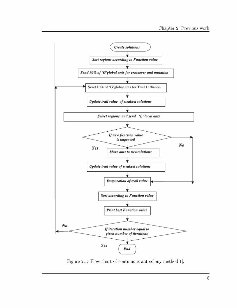
2.1.3 Continuous Ant Colony Algorithm

Similar to the Genetic Algorithm, the Continuous Ant Colony Algorithm (CACO)

tries to emulate nature. The Continuous Ant Colony Algorithm (CACO) has a global

search and a local search. The global search has three parts- Random Walk, Mutation

and Trail Diffusion. Random walk has 90% of the solution randomly chosen in the

feasible range. The inferior solutions are replaced with randomly selected solution

from superior solutions. Mutations occurs after the random walk step occur. In the

mutation step, the possible solutions are randomly add or subtract a value to each

variable of the newly created solutions. The solutions are part of the inferior region

5


with a probability equal to a suitable defined mutations probability.

∆(T,R) = R(1− r(1−T )b) (2.2)

where r is a random number from [0.1]. 4 is the rate of change in variables of

the variables of T and R. R is a maximum step size. T is a ratio of the current

iteration number to that of the total number of iterations. b is the positive parameter

controlling the degree of nonlinearity[1]. Lastly, trail diffusion applies to inferior

solutions that were not considered during the random walk and mutation stages. The

two parent’s weight are selected at random. The variables of the children’s positions

can have any combination of the parent’s solutions.

x(child) = (α)xi(parent1) + (1− α)xi(parent2) (2.3)

where α is the weighted uniform random variable that predicts how much of each

parent’s input is carried to the child. α variable ranges from 0 to 1. 1 − α is set

up so the second parent will make up the remainder. For local search the region i is

selected with the probability equation.

6


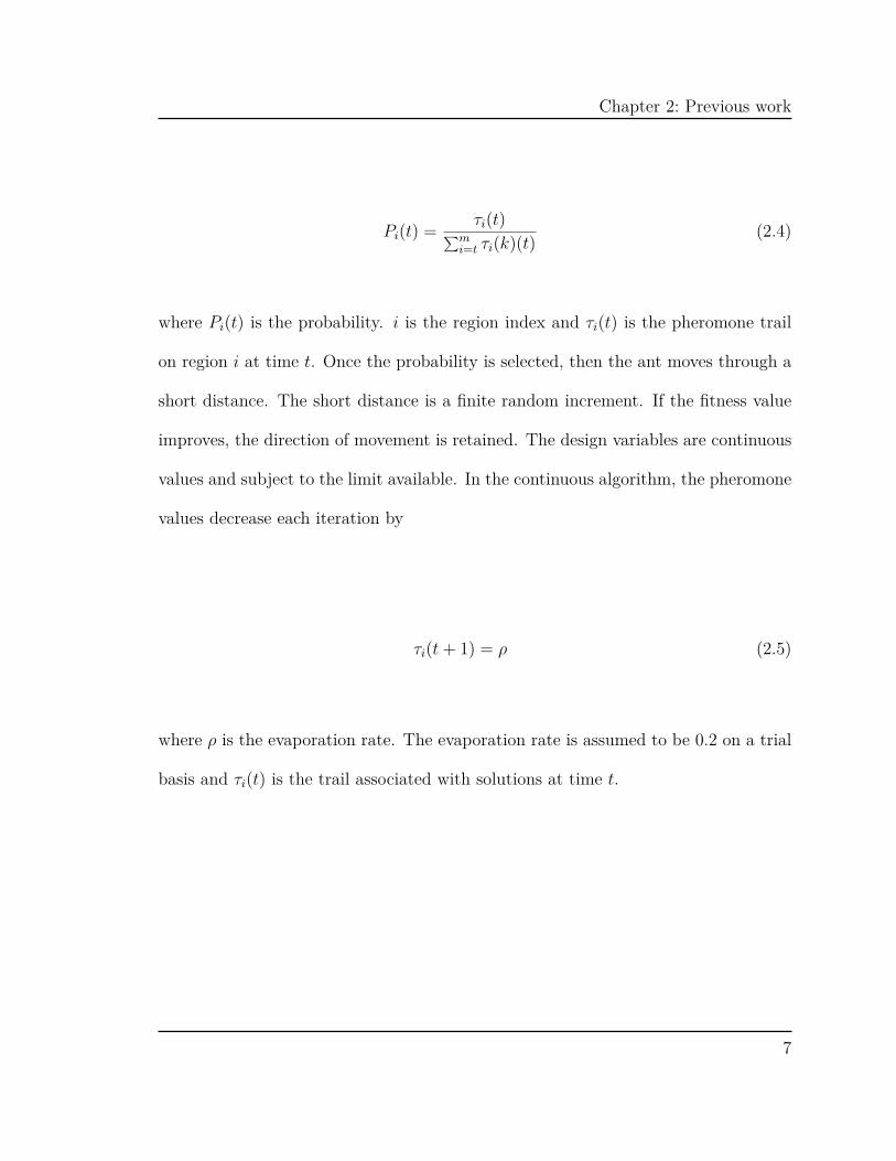
Pi(t) = τi(t)∑mi=t τi(k)(t) (2.4)

where Pi(t) is the probability. i is the region index and τi(t) is the pheromone trail

on region i at time t. Once the probability is selected, then the ant moves through a

short distance. The short distance is a finite random increment. If the fitness value

improves, the direction of movement is retained. The design variables are continuous

values and subject to the limit available. In the continuous algorithm, the pheromone

values decrease each iteration by

τi(t+ 1) = ρ (2.5)

where ρ is the evaporation rate. The evaporation rate is assumed to be 0.2 on a trial

basis and τi(t) is the trail associated with solutions at time t.

7


Figure 2.1: Flow chart of continuous ant colony method[1].

8


Figure 2.2: Distribution of ants for local and global search[1].

2.1.4 Tabu search method

The Tabu search method is part of the group of Genetic Algorithms. The design

variables are coded as string in binary and the strings increase in digits based on

how accurate the desired answer is. The initial solution is selected using a random

function. The termination is selected by the user choice. The Tabu search method

will run as many iterations as stated.

9


Then a neighborhood is determined with a subset of another neighborhood[1].

At this point the neighborhoods are compared to select the best profit rate to maxi-

mize. The best seed is chosen and updated inside the Tabu list. If the next iteration

is better than the best. Then the previous iteration is set the next iteration as the

best. The process begins again with a new value. Terminatition is if it passes the ini-

tial set iterations count[1]. Without a termination value to compare it the converging

solution it becomes difficult to know when to stop. One idea would be to stop when

the same optimal input lead to same outputted solution. However, it could lead to a

solution that is always progressively better than the previous iteration.

2.1.5 Particle Swarm Optimization

The Particle Swarm Optimization (PSO) method works by following another method

seen in nature, bird flocking. First, each particle is initialized. Then calculate the

fitness value of each particle. If the fitness values is better than the best fitness value

in history, set the current value as the best.[1] Choose the particle with the best

fitness value of all time, and then the particles become gbest[]. For each particle, the

particle velocity can be calculated as

10


v[] = v[] + c1rand()(pbest[]− [present[]) + c2rand()(gbest[]− present[]))

present[] = present[] + v[](2.6)

where v[] is the particle velocity, present[] is the current particle solution and rand[]

is a random number between (0, 1).c1, c2 are learning factors. Particle velocities in

each dimension are limited to a maximum velocity. If the sum of the acceleration

causes the velocity to exceed the maximum velocity, then the constraint specified for

the user is limited to the maximum. In other words, the velocity is stopped at velocity

maximum or stopped at the maximum constraint.

11

Chapter 3: Nelder–Mead Simplex with Exterior Penalty


The Nelder–Mead Simplex method can be used to find the minimum dollar amount of

the objective function in a multidimensional space. The Nelder-Mead Simplex method

can be used for other variables than money. The method is applied to nonlinear op-

timization problems for which the derivatives may not be known. The Nelder–Mead

Simplex method is useful when the derivative equations become costly to compute ev-

ery iteration. In this present study, the design variables are limited to fourteen terms.

Increasing the design variables in the Nelder-Mead Simplex method is straightforward.

The Nelder–Mead method works by creating a large range of values, marking the best,

worst and second worst values.

The exterior penalty function adds value to the objective function when the

constraints are violated. The penalty function prevents the Nelder-Mead Simplex al-

gorithm from going down to negative infinity. If a constraint is violated the objective

function starts to increase due to the penalty function. If the objective function is

increased, the Nelder-Mead Simplex algorithm will move away from that particular

value. The Nelder–Mead Simplex method uses four methods to converge the Simplex

triangle into a solution. These four methods are Reflection, Expansion, Contraction,

and Shrink[5]. Reflection flips the triangle’s top corner to the other side due to a

better group of solutions being shown on the other side. Expansion extends one of

the legs in the triangle so it is able to cover a better best-case solution. Contraction

moves one of the legs inside the triangle, which eliminates bad solutions are shown.

12


Lastly, shrinking is when each of the points become closer to the best-case.

The penalty value becomes an important setting that needs to be fine-tuned.

The magnitude of scale for the objective function and penalty function should match

each other. The magnitude of scale can be altered by changing the penalty value.

The penalty value is changed to what makes the penalty function have the same mag-

nitude of scale as the objective function. Anything less than the same magnitude will

result in the Simplex triangle overstepping the optimal values. Anything too large

will also result in a centroid of the Simplex triangle being out of the feasible range.

If the centroid moves outside of the feasible range, the Simplex triangle will not re-

cover. The penalty value becomes more difficult to fine tune for multiple constraints.

If there are multiple constraints violated at the same time, the magnitude of scale for

the penalty function is going to be significantly larger than if only one constraint is

violated. It is more difficult to pick the correct penalty value if the objective equation

has a lot of design values. In the present study, the penalty value was set to 1000.

Each set of design variables is restricted to its own constraints. The termination value

is determined from equation 3.1.

Once the penalty value is set, the next step becomes setting the Simplex pa-

rameters. Optimizing the parameters of the Nelder–Mead method become its own

optimization problem. Most Nelder-Mead Simplex parameters tend to cluster the

around following points called universal points α = 1, γ = 2, ρ = 0.5, and σ = 0.5

[4]. Although the parameters tend to cluster to particular values, each problem needs

fine tuning. One way of approaching the fine tuning of the Nelder–Mead parameters

13


is to create a for loop for each parameter with an upper limit and a lower limit.

The for loop is intended to test each setting to see how the increase value will affect

the optimal design values. The limits for the for loops is usually the universal point

plus or minus 15%. The method for setting the limits is called the Resiga method.

For simple problems fine tuning the Simplex parameter is easy because computation

time is small. For more complicated objective functions, the step between the limit

is larger. Smaller steps will reduce the computation time.

ε =

√√√√ 1N + 1

N+1∑i=1

(xi − xo)2 (3.1)

3.1 Nelder–Mead Flow Chart

Like most optimization problems, the initial estimate is set to a value inside the

feasible range. The feasible range is where the constraints are not violated. There

is an initial step that is done in a positive direction and negative direction for each

design variables for each operation. After each possible answer is calculated, a Simplex

triangle is created from these possible answers.

A Simplex triangle is a group of possible answers that holds an optimal solution.

The Simplex triangle has two times the number of design variables times the number

of operations. In Case study 1, there were twenty points in the Simplex triangle. If the

14


objective equation is in two dimension, the Simplex triangle is a true triangle. If there

are more than three design variables the Simplex triangle becomes a polymorphic

shape.

At this point, the worst case, second worst case, and best cases is defined in

the Simplex triangle. The Simplex triangle is fed through the flowchart below that

is contracted, reflected, expanded and finally shrink, until the termination value is

satisfied. Any value that is violates a constraint will have an additional value tacked

onto it.

15


Initial guess (cases)

xn+1 = Worst xn = Second Worstx1 = Best xr = Reflection

xe = Expansion xo = Centroidxc = Contraction xi = Each point

Initial Simplex method

Check for termination

Reflectionf(x1) < f(xr) < f(xn)

xnew = xr

f(xe) < f(xr)xe = xo + γ(xr − xo)Expansionf(xr) < f(x1)

xnew = xe

xnew = xr

Contractionf(xr > f(xn) xc = xo + ρ(xn+1 − xo) f(xc) < f(xn+1)

xnew = xc

Replace the worstcase with x new

Shrink by xi =x1 + σ ∗ (xi − x1)

Stop

no

no

no

no

no

yes

yes

yes

yes

yes

Figure 3.1: Nelder-Mead flow chart overview. 16

Chapter 4: Optimization model


There are two ways to maximize profit, minimize the cost per unit or the time per

unit [7]. Having only cost minimized or time will result in a solution that is not

optimal as the overall goal is to maximize the profit. Money is a byproduct of both

dollar amount and time spent. The income received for a unit will not change even

if the design variables change. However, the profit may indeed change if cost or time

spent is reduced. A simple first attempt equation is

Pr = Sp − cu

tu(4.1)

The following sections will discuss how to cost per unit and time per unit equations

are modeled and what assumptions were made.

4.1 Unit Cost

The cost of designing a model is broken into four separate groups: the cost of raw

material, set-up cost, machining cost and tool changing cost.

17


cu = cmat + (cl + co)ts + (cl + co)tm + (clttc + ct + cottc)tmT

(4.2)

Equation 4.2 is for a single tool. However this can be extended to i-th tool. i is the

amount of operations done. Through a series of equations, machine time for milling

operations can be determined by

tm = K

F= tKfzN

with N = 1000Vπd

(4.3)

is simplified to:

tm = πdK

1000V fz (4.4)

All of the factors that go into the tool life can be grouped together in a constant such

as

18


K1 = πdK

1000z (4.5)

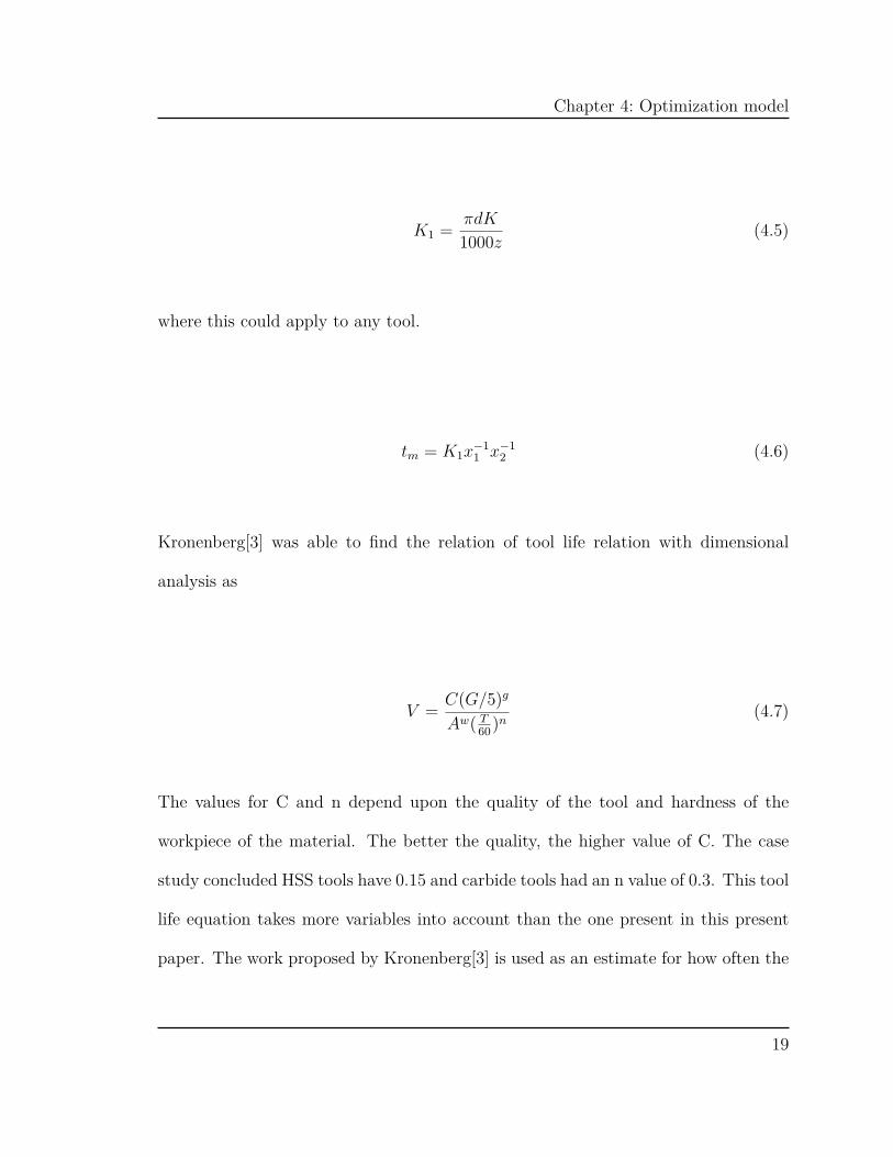
where this could apply to any tool.

tm = K1x−11 x−1

2 (4.6)

Kronenberg[3] was able to find the relation of tool life relation with dimensional

analysis as

V = C(G/5)g

Aw( T60)n

(4.7)

The values for C and n depend upon the quality of the tool and hardness of the

workpiece of the material. The better the quality, the higher value of C. The case

study concluded HSS tools have 0.15 and carbide tools had an n value of 0.3. This tool

life equation takes more variables into account than the one present in this present

paper. The work proposed by Kronenberg[3] is used as an estimate for how often the

19


tool needs replacement.

T = 60[C(G/5)g

AwV] 1

n (4.8)

The equation is now solved for tool life through experimental methods. The cutting

edge cannot be in contact with the workpiece the whole time, a proportion value Q is

required to account for the lack of cutting. The proportional value is also taken into

account when the using half of the radial depth of cut.

T = 60Q

[C(G/5)g

AwV] 1

n (4.9)

Substituting the values of slenderness ratio G = afand the chip cross-sectional area

to A = af :

T = 60QC

1n 5

−gn a

g−wn V

−1n f

−(w+g)n (4.10)

Parallel to the K1, which combines all the tool coefficients without the design vari-

20


ables, into a single value. The tool life impact coefficients is combined to K2.

K2 = 60QC

1n 5

−gn a

g−wn (4.11)

Then tool life equations is simplified to only require the K2 with the design variables.

T = K2V−1n f

−(w+g)n (4.12)

K2 is related the coefficients of cost of the tool life and K1 is related the machine

time, tm

Tis analogous K1

K2. K1

K2is simplified to K3. K3 is considered a depreciation

variable tasked with modeling how much impact one single operation has on the tool

life.

tmT

= K3V−1n

−1f−(w+g)

n−1 (4.13)

K3 = K1

K2(4.14)

21


K1 and K3 are plugged into the general cost per unit equation 4.2.

cu = cmat + (cl + co)ts + (cl + co)K1x−11 x−1

2 +

(clttc + ct + cottc)K3V−1n

−1f−(w+g)

n−1

(4.15)

Equation 4.15 is defined for only a single tool. This is the case for production lines

where machining of each feature is devoted to a particular machine. In single-tool

operation tool changing time is a function of the ratio of machining time to tool

life. In the case of multi-tool operations, tool changing time for each tool used is

considered regardless of this ratio. Equation 4.15 can be extended it to the i-th term

up to m operations. When more machines are taken into consideration equation 4.15

changes to equation 4.16.

cu = cmat + (cl + co)ts +m∑

i=1(cl + co)K1i

V −1i f−1

i +

m∑i=1

ctiK3i

V−1ni

−1i f

−(w+g)ni

−1i +

o∑i=1

(cl + co)ttci

(4.16)

where ttciis the time spent changing tools and cti

is the cost of machining. o is the

number of tools. The equation is simplified more so there is only the design variables:

22


cu = C1 +m∑

i=1C2i

V −1i f−1

i +m∑

i=1C3i

V−1ni

−1i f

−(w+g)ni

−1i +

o∑i=1

C4i(4.17)

where C1 is the cost of setting up the tools. C2iis the cost of the actual work. C3i

is

the cost of doing the actual work over the lifetime of the tool, or depreciation. Finally

C4itakes into account the cost of switching tools. Out of the equations above only

C2iand C3i

have design variables. Therefore, for optimization purposes, C1 and C4i

can be discarded when creating the objective equation. C1 and C4iare important to

finding the overall cost but not important to optimization.

cmi=

m∑i=1

C2iV −1

i f−1i +

m∑i=1

C3iV

−1ni

−1i f

−(w+g)ni

−1i (4.18)

where cmiis the machining cost per operation. Equation 4.18 does not include the

cost of setting up and swapping tools. cmiis a nonlinear equation.

4.2 Unit Time

The unit time for a single tool is defined by:

23


tu = ts + tm + ttctmT

(4.19)

The solution for tm and tm

Thave already been derived in Unit cost section.

tu = ts +m∑

i=1K1i

V −1i f−1

i + ttcK3V−1n

−1f−(w+g)

n−1 (4.20)

and for multiple tools then it becomes:

tu = ts +m∑

i=1K1i

V −1i f−1

i +o∑

i=1ttci

(4.21)

The only terms that have the design variables are the tm, all the other terms cannot

be optimized.

tmi=

m∑i=1

K1iV −1

i f−1i (4.22)

where tmiis the machining time per operation.

24


4.3 Profit Rate

For a single tool, the profit rate Pr can be defined:

Pr = Sp − cu

tu(4.23)

For any tool, it become to the i-th term

Pri= Ri − cmi

tmi

(4.24)

where

Ri = Rtmi

tm(4.25)

R = Sp − (C1 +o∑

i=1C4i

) (4.26)

where o is the number of tools.

25


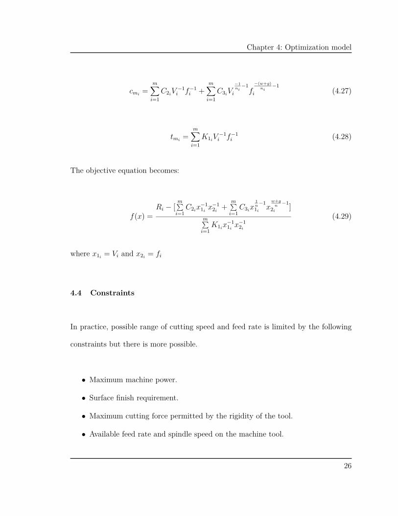
cmi=

m∑i=1

C2iV −1

i f−1i +

m∑i=1

C3iV

−1ni

−1i f

−(w+g)ni

−1i (4.27)

tmi=

m∑i=1

K1iV −1

i f−1i (4.28)

The objective equation becomes:

f(x) =Ri − [

m∑i=1

C2ix−1

1ix−1

2i+

m∑i=1

C3ix

1n

−11i

xw+g

n−1

2i]

m∑i=1

K1ix−1

1ix−1

2i

(4.29)

where x1i= Vi and x2i

= fi

4.4 Constraints

In practice, possible range of cutting speed and feed rate is limited by the following

constraints but there is more possible.

• Maximum machine power.

• Surface finish requirement.

• Maximum cutting force permitted by the rigidity of the tool.

• Available feed rate and spindle speed on the machine tool.

26


• Maximum heat generated by cutting.

In this particular study, heat generated by the cutting was captured inside the tool

life equation from cu, specifically in C3i.

4.4.1 Power

The power equation is explained in equation 4.30.

P = 0.78KpWzarada

60πde V f 0.8 (4.30)

The machining parameters are selected to use maximum machine power. The required

machining power should not exceed available motor power. Therefore, the power

constraint is rewritten as:

C5V f0.8 ≤ 1 (4.31)

27


where

C5 = 0.78KpWzarada

60πdePm

(4.32)

4.4.2 Surface Finish

The arithmetic value of surface finish in plain milling be represented by:

Ra = 318f2

4d (4.33)

and for face milling:

Ra = 318 f

tan(la) + cot(ca) (4.34)

The required surface finish Ra must not exceed the maximum attainable surface finish

Ra(at) under the conditions. Therefore, the surface finish for end milling becomes:

C6f2 ≤ 1 (4.35)

28


where

C6 = 318(4d)−1

Ra(at)(4.36)

and for face milling,

C7f ≤ 1 (4.37)

where

C7 = 318(tan(la) + cot(ca))−1

Ra(at)(4.38)

Although C6 and C7 are separate equation only one of them is enacted depending if

the operation is a face mill or an end mill.

29


4.4.3 Cutting Forces

The total cutting force applied to the cutting tool in a milling operation is a result

of tangential, feed and radial forces:

FC = (F 2T + F 2

F + F 2R)1/2 (4.39)

These force values are determined from equation 4.39 due [7] to calculating the forces

experimentally. It is difficult to create a single equation that calculates the cutting

force because some measurements are far too difficult to measure. Difficult factors

that go into cutting forces is the tool’s deflection, chatter, chip geometry and fluid

dynamic equations. However, it instead is approximated with equation 4.40 for each

direction of the force.

FT = Kcaf (4.40)

The Kc value is found tabular. The total cutting force FC resulting from the machin-

ing operation must not exceed the permitted cutting force FC(per). The permitted

cutting force for each tool is its maximum limit for cutting forces. Therefore, the

30


cutting force constraint becomes:

C8FC ≤ 1 (4.41)

where

C8 = l/FC(per) (4.42)

4.5 General equation

The objective equation is the terms, which involve the design variables. The objective

equation is the equation being optimized. All other parameters not captured below

do not affect the overall setting of the design variables. The objective equation is

defined as:

f(x) =Ri − [

m∑i=1

C2ix−1

1ix−1

2i+

m∑i=1

C3ix

1n

−11i

xw+g

n−1

2i]

m∑i=1

K1ix−1

1ix−1

2i

(4.43)

where x1i= Vi and x2i

= fi.

The objective equation is subject to:

31


g1(x) = C5x1x0.82 − 1 ≤ 0 (4.44)

g2(x) = C6x22 − 1 ≤ 0 for end milling (4.45)

g2(x) = C7x2 − 1 ≤ 0 for face milling (4.46)

g3(x) = C8Fc − 1 ≤ 0 (4.47)

x1 ≥ 0 x2 ≥ 0 (4.48)

The equations from 4.44 are combined together with the Penalty value. If the con-

straint is violated, a penalty value is multiplied to the equation it had violated. The

new objective function is constructed by adding the constraints with the penalty

function:

y(x) =m∑

i=1[kp(i)g1(x, i) + kp(i)g2(x, i) + kp(i)g3(x, i) + kp(i)x1(i) + kp(i)x2(i)] (4.49)

where each term inside the bracket is single column matrix for every operation.

kp = 0||1000 (4.50)

32


The overall equation is now the objective function plus any Penalty value that occurs

from violating the constraint F (x) = f(x) + y(x). x is a 2-by-m matrix, where m is

the number of operations and 2 is the number of design variables per operation. If the

objective equation includes the depth of cut, the x-matrix would become a 3-by-m.

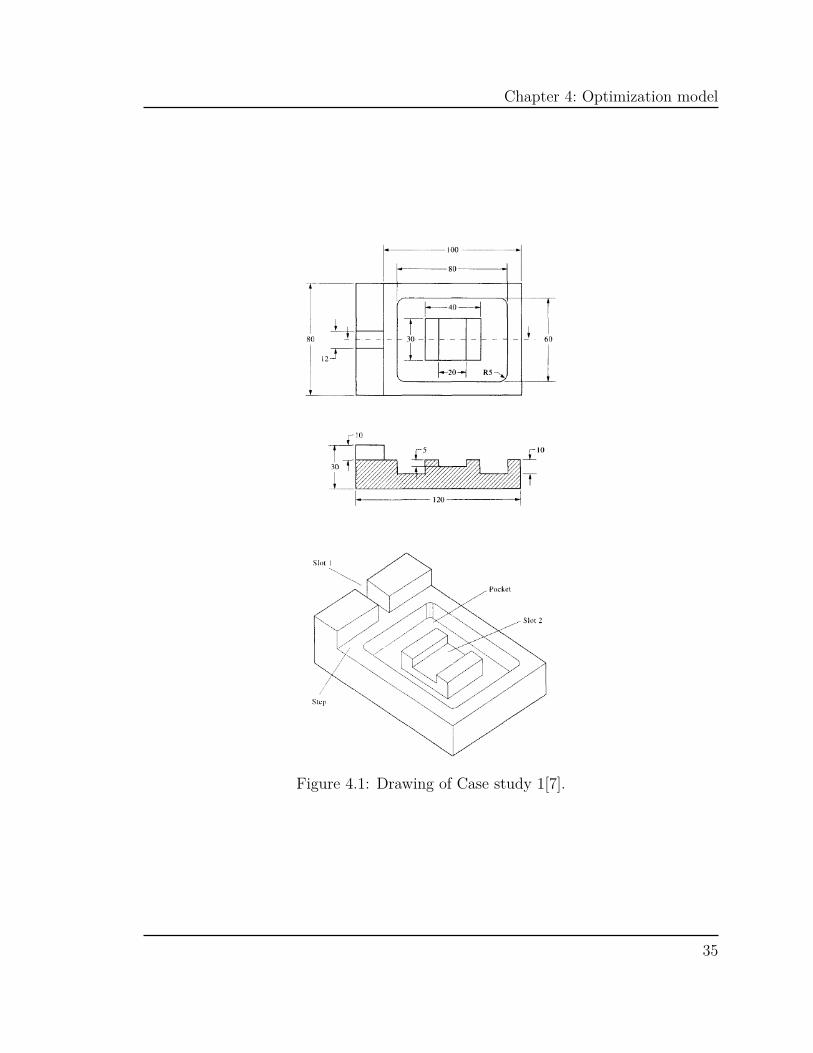
4.6 Case Study 1

Case study 1 is from the original paper[7] as an example to compare results between

the Nelder-Mead Simplex method and other methods. Below, there is the set param-

eters in Table 4.2 which sets up the cost and tool life parameters. The representation

of the unit is capture in Figure 4.1 as well as the operational cuts and the machine

parameters in Tables 4.3 and 4.4.

Table 4.1: Parameters for Case Study 1[7].

Machine tool data:Type: Vertical CNC milling machine Pm = 8.5 kW, e = 95%Material data:Quality: 10L50 leaded steel. Hardness = 225 BHN

33


Table 4.2: Constants for Case study 1[7].

Sp = $25cmat = $0.50co = $1.45 per minc1 = $0.45 per mints = 2 mintct = 0.5 minC = 33.98 for HSS toolsw = 0.28

C = 100.05 for carbidetool

Kp = 2.24W = 1.1n = 0.15 for HSS toolsn = 0.3 for carbide toolg = 0.14

Table 4.3: Required machining operation Case study 1[7].

Operation Operation Tool a (mm) K (mm) Ra (µm)No. Type Number1 Face milling 1 10 450 22 Corner milling 2 5 90 63 Pocket milling 2 10 450 54 Slot milling 3 10 32 -5 Slot milling 3 5 84 1

34


Figure 4.1: Drawing of Case study 1[7].

35


Table 4.4: Tools data for Case study 1[7].

Tool Tool Quality YTS d CL z Price SD Helx la caNo Type (MPa) (mm) ($) (mm) angle1 Face mill Carbide 50 2 6 49.50 25 15 45 52 Corner mill HSS 1035 10 6 4 7.55 10 45 0 53 Pocket mill HSS 1035 12 5 4 7.55 10 45 0 5

The case study above requires multi-tool operations. The cost of the unit is solved

using the Nelder-Mead Simplex method. Case Study 1 is used to compare the hand-

book optimal values[6] to the optimized values in other papers[7]. The five operations

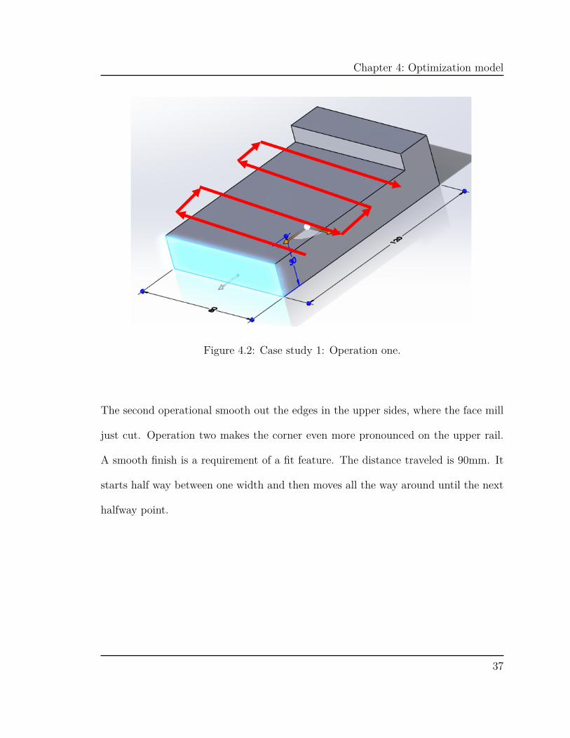
of Case Study 1 is represented in the following Figures 4.2, 4.3, 4.4, 4.5, and 4.6. The

first operation performs a snake pattern changing direction four times. The face mill

operation uses half of the radial depth of cut. For operation one, the radial depth of

cut would be 25mm. The K distance traveled would have been 450mm. The drill bit

would move 25mm passed the edge and then move 50mm passed the exit cut.

36


Figure 4.2: Case study 1: Operation one.

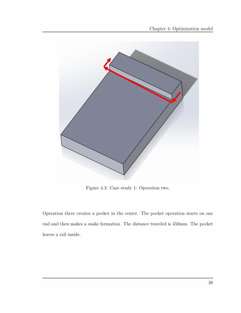
The second operational smooth out the edges in the upper sides, where the face mill

just cut. Operation two makes the corner even more pronounced on the upper rail.

A smooth finish is a requirement of a fit feature. The distance traveled is 90mm. It

starts half way between one width and then moves all the way around until the next

halfway point.

37


Figure 4.3: Case study 1: Operation two.

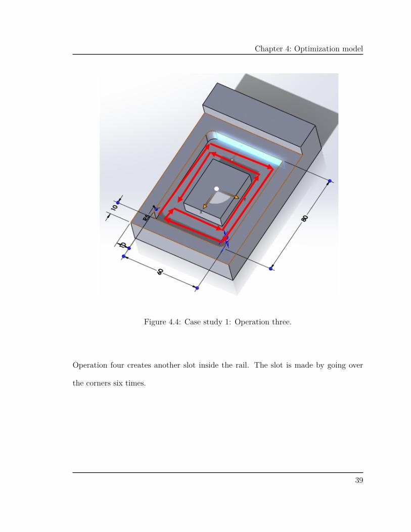
Operation three creates a pocket in the center. The pocket operation starts on one

end and then makes a snake formation. The distance traveled is 450mm. The pocket

leaves a rail inside.

38


Figure 4.4: Case study 1: Operation three.

Operation four creates another slot inside the rail. The slot is made by going over

the corners six times.

39


Figure 4.5: Case study 1: Operation four.

The last operation creates the slot on the rail inside the pocket. The slot is 20mm

wide and the same height as the rail before the slot. The depth of the cut is 5mm,

leaving some space between the surface of pocket operation and face mill operation.

40


Figure 4.6: Case study 1: Operation five.

4.7 Case study 2

Case study 2 is done in order to get an impression on how easy it is to swap operation

and consequently, the impact. Using the journal bearing sub from PSAS NSR Figure

4.7, the required tool parameters from Table 4.5 are kept the same. The initial guess

41


is one that is within the feasible range.

Figure 4.7: Drawing of case study 2.

42


Table 4.5: Tools data parameters Case study 2.

Sp = $25cmat = $0.50co = $1.45 per minc1 = $0.45 per mints = 2 mintct = 0.5 minC = 33.98 for HSS toolsw = 0.28

C = 100.05 for carbidetool

Kp = 2.24W = 1.1n = 0.15 for HSS toolsn = 0.3 for carbide toolg = 0.14

Table 4.6: Required machining operation for Case study 2.

Operation Operation Tool a (mm) K (mm) Ra (µm)No. Type Number1 Face milling 1 10 50 22 Corner milling 2 10 50 23 Slot milling 2 5 52 54 Pocket milling 3 10 40 25 End milling 3 10 50 56 Hole milling 4 7 5 17 Hole milling 5 3.2 1.5 1

43


Table 4.7: Tools data Case study 2.

Tool Tool Quality YTS d CL z Price SD Helx la caNo Type (MPa) (mm) ($) (mm) angle1 Face mill Carbide 50 2 6 49.50 25 15 45 52 Corner mill HSS 1035 8 6 4 7.55 10 45 0 53 Pocket mill HSS 1035 10 5 4 7.55 10 45 0 54 Drill mill HSS 1035 10 5 4 16.50 10 45 0 55 Drill mill HSS 1035 5 5 4 9.99 10 45 0 5

44

Chapter 5: Results

Chapter 5: Results

5.1 Validating the objective equation

Validating the objective equation is done by comparing the inputs of other optimal

solutions. The following tables show the objective equation is designed exactly like

the other researchers. In many calculated inputs the error was less than 1% as seen

in Table 5.1 and Table 5.2. However, some discrepancies are seen below.

Validating the solution is very important that it confirms the method of solving

the of evaluating the objective equation is all the same. The validation of the objective

equation allows a general foundation for building the exterior penalty function and

the Nelder-Mead Simplex method. Once the objective function and penalty function

is validated, sensitivity studies can be conducted. Sensitivity studies provide insight

on possible improvements and of how big of an impact other parameters are. The

objective function is constructed in the optimization model section.

Table 5.1: Validating the ability to calculate the correct cost unit cu.

Methods Known cu Calculated cu Error($) ($)

The method of feasible direction[7] 11.350 11.654 2.6%GA[1] 9.401 9.4023 0.5%CACO[1] 10.202 10.202 0%Tabu search [1] 11.295 11.292 0.03%Particle Swarm optimization [1] 9.316 9.316 0%

45

Chapter 5: Results

Table 5.2: Validating the ability to calculate the correct time unit tu.

Method Known tu Calculate tu Error(minute) (minute)

The method of feasible direction[7] 5.48 5.478 0.04%GA[1] 4.229 4.230 0.01%CACO[1] 5.438 4.657 16.8%Tabu[1] 4.231 4.230 0.02%Particle Swarm optimization[1] 4.089 4.089 0%

5.2 Validating the penalty function

While verifying the objective equation proved to be inside the feasible area[7], veri-

fying the penalty function was not as simple. For the original paper/citetolouei-tad,

the power value of the end mill for operation four and five with tool number three,

the research paper used the wrong diameter. When the diameter is set to 10mm,

the power equation is equal to 8.01 kW for operation four and 6.67 kW for operation

five. When the diameter is set to 12mm the power equation, the power equal to 6.67

kW for operation four, and 4.27 kW for operation five. The research paper[7] states

the power value at optimal solution is 8.03 kW. For the remainder of this study, the

assumption is that the diameter should have been 12 and the power constant should

have been 6.67 kW with the current optimization parameters.

Another issue that was not easily understood was the radial depth of cut is

half of the diameter for operation one, face milling. This is a common practice in

machining but not obvious from just reading.

46

Chapter 5: Results

Lastly, the surface finish uses the wrong equation from the original paper[7]

for operation two and three. Operation two and three is corner milling and pocket

milling, which uses the end mill tool number two. The paper[7] states that plain

milling and end milling could be represented by Ra = 318f2

4d, however when evaluating

the optimal input with the plain mill equation the value is more than 93% off. The

error in surface equation is considered to be a typo for face milling and that end

milling tools should actually use the face mill equation Ra = 318ftan(la)+cot(ca) .

Table 5.3: Error from the original paper[7].

Power constraint, wrong diameter usedPower (kW ) d=10 (mm) Error d=12 (mm) Error

Operation four 8.03 8.01 0.25% 6.67 16.94%Operation five 5.17 5.13 0.77% 4.27 17.41%

Radial depth of cut is halfarad (mm) arad = d

2 (mm) Error arad = d (mm) ErrorOperation one 8.5 8.46 0.44% 16.93 99.12%

Surface finish uses the wrong equation from paper[7]

Ra (µm) Ra = 318ftan(la)+cot(ca) (µm) Error Ra = 318f2

4d(µm) Error

Operation two 5.96 5.95 0.10% 0.36 93.89%Operation three 4.99 4.98 0.20% 0.25 94.90%

As seen below in Table 5.4 the following methods violated the original power

constraint of 8.5 kW that Table 4.1 stated.

47

Chapter 5: Results

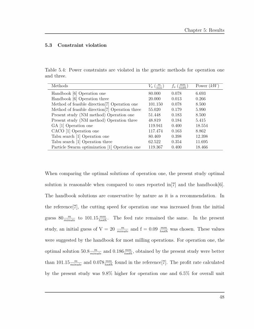
5.3 Constraint violation

Table 5.4: Power constraints are violated in the genetic methods for operation oneand three.

Methods Vo ( mmin

) fo ( mmtooth

) Power (kW )Handbook [6] Operation one 80.000 0.078 6.693Handbook [6] Operation three 20.000 0.013 0.266Method of feasible direction[7] Operation one 101.150 0.078 8.500Method of feasible direction[7] Operation three 55.020 0.179 5.990Present study (NM method) Operation one 51.448 0.183 8.500Present study (NM method) Operation three 48.819 0.184 5.415GA [1] Operation one 119.941 0.400 18.554CACO [1] Operation one 117.474 0.163 8.862Tabu search [1] Operation one 80.469 0.398 12.398Tabu search [1] Operation three 62.522 0.354 11.695Particle Swarm optimization [1] Operation one 119.367 0.400 18.466

When comparing the optimal solutions of operation one, the present study optimal

solution is reasonable when compared to ones reported in[7] and the handbook[6].

The handbook solutions are conservative by nature as it is a recommendation. In

the reference[7], the cutting speed for operation one was increased from the initial

guess 80 mminute

to 101.15 mmtooth

. The feed rate remained the same. In the present

study, an initial guess of V = 20 mminute

and f = 0.09 mmtooth

was chosen. These values

were suggested by the handbook for most milling operations. For operation one, the

optimal solution 50.8 mminute

and 0.186 mmtooth

, obtained by the present study were better

than 101.15 mminute

and 0.078 mmtooth

found in the reference[7]. The profit rate calculated

by the present study was 9.8% higher for operation one and 6.5% for overall unit

48

Chapter 5: Results

when compared to reference[7]. The upper limits for cutting speed was set to 120 mmin

and 0.4 mmtooth

. In the present study both design variables are in the middle whereas

the original paper[7] only one design variable is in the middle and the other design

variable is near the maximum. The group of Genetic Algorithms methods have their

design variables maxed on both of them. Maxing both design variables has to lead

to power constraint being violated when the handbook recommends only one design

variable to maxed.

5.4 Optimal design variables: Case study 1

Assuming the same errors as the original paper, the optimal solution of the present

study had a better profit rate. The improvement on profit rate was due to the

Nelder–Mead Simplex method parameters and the initial guess. The Nelder–Mead

method started with the standard universal parameters α = 1, γ = 2, ρ = 0.5, and

σ = 0.5[4]. After some fine tuning the present study was able to arrive a better result,

using the following Simplex parameters α = 0.75, β = 0.8 γ = 2.45, ρ = 0.4, and

σ = 0.4.

The initial guess allowed the Nelder-Mead Simplex Method to slow down the

cutting speed and increase the feed rate instead of speeding up the cutting speed.

Although the handbook recommendation was still better than the present study’s

initial guess, a better optimal solution was found.

49

Chapter 5: Results

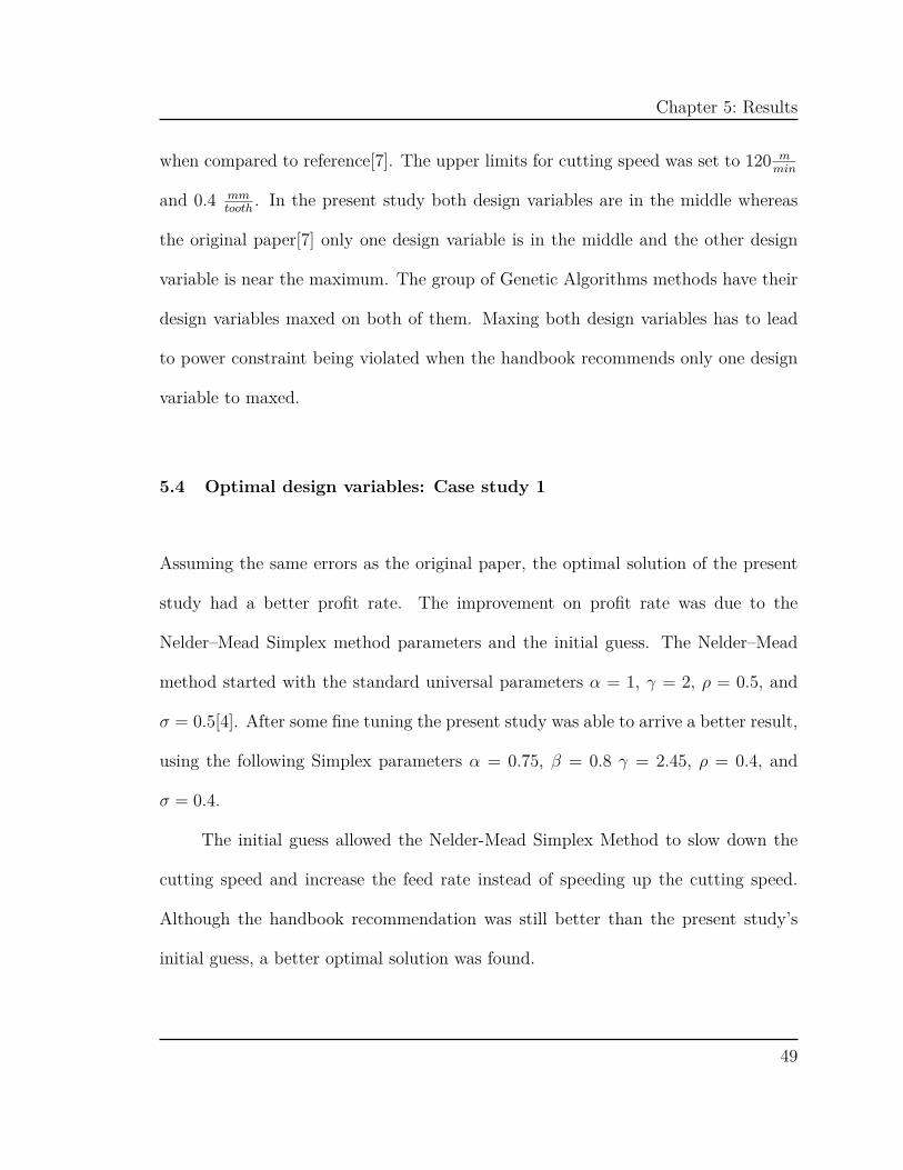
Table 5.5: Optimal design parameters for case study one.

Operation number Operation Tool a Vo fo

No. Type Number (mm) ( mmin

) ( mmtooth

)1 Face milling 1 10 50.800 0.1862 Corner milling 2 5 49.880 0.2073 Pocket milling 2 10 47.997 0.1974 Slot milling 3 10 47.369 0.1865 Slot milling 3 5 46.571 0.176

Cost unit ($) 10.93Time unit (minute) 5.32

Optimal values from Table 5.5 compare well to optimal values[7].

5.5 Cost after each cut: Case study 1

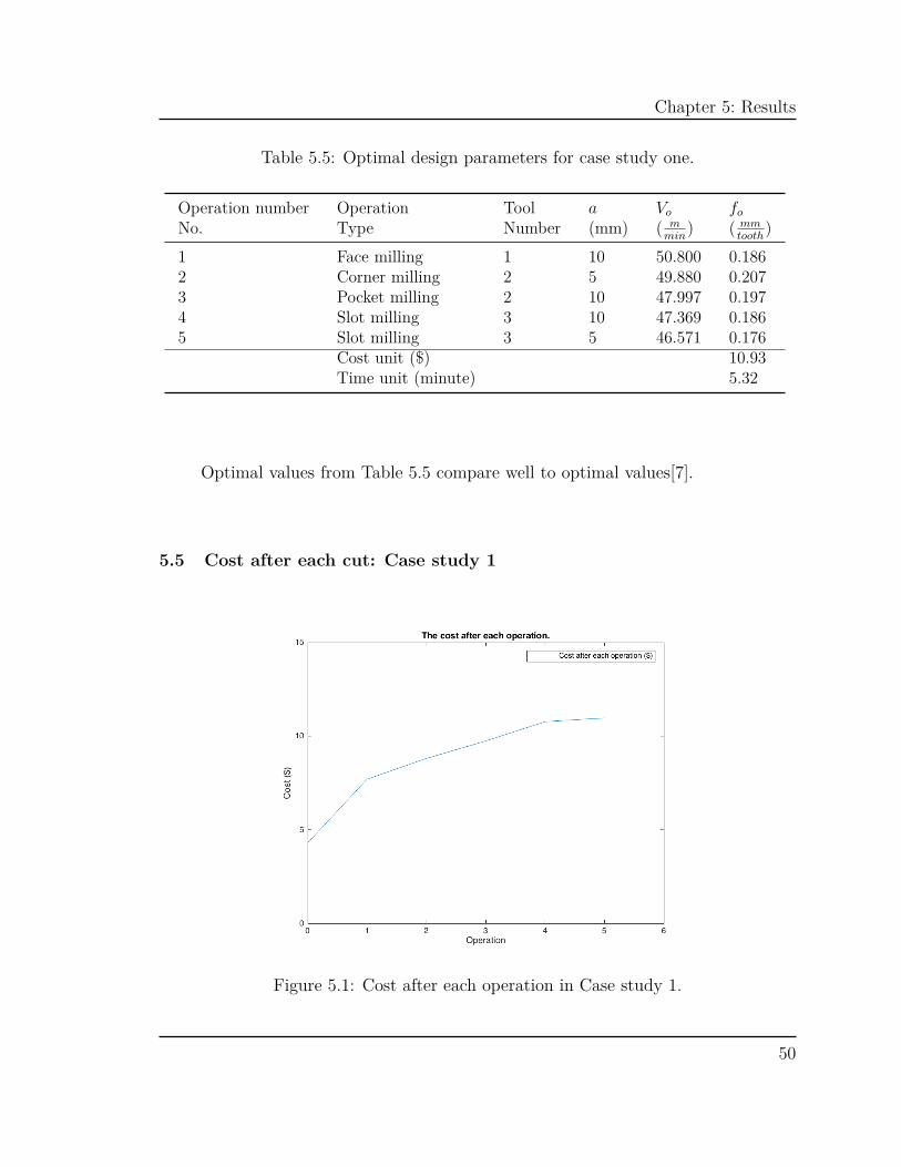
Figure 5.1: Cost after each operation in Case study 1.

50

Chapter 5: Results

The present study noticed that the most significant cost was at the start, before any

operation occurred. Then there is a slow gradual increase after the first operation in

Figure 5.1.

5.6 Time after each cut: Case study 1

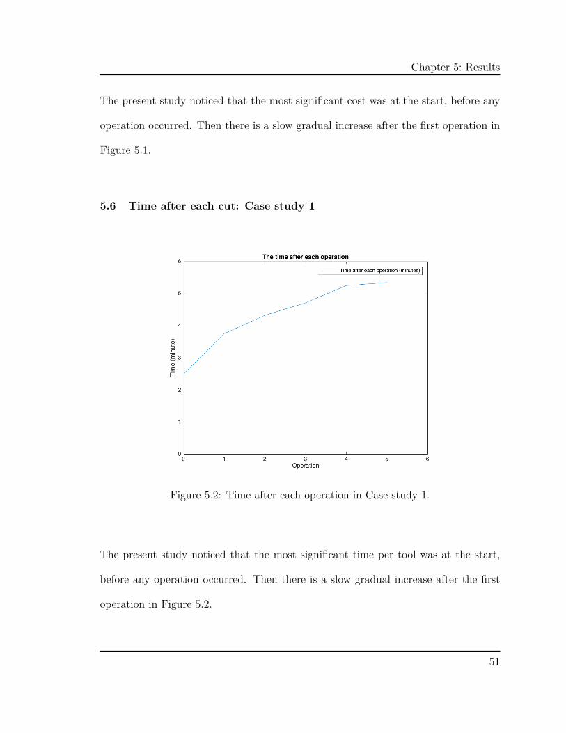
Figure 5.2: Time after each operation in Case study 1.

The present study noticed that the most significant time per tool was at the start,

before any operation occurred. Then there is a slow gradual increase after the first

operation in Figure 5.2.

51

Chapter 5: Results

5.7 Sensitivity study

Table 5.6: Simplex beats handbook and method of feasible direction.

Method Cu Tu Pr

($) (minute) ( $minute

)Handbook [6] 18.36 9.40 0.71Method of feasible direction[7] 11.35 5.48 2.49Present study (NM method) 10.92 5.32 2.65GA method[1] 9.40 4.23 3.69CACO method[1] 10.20 5.44 2.72Tabu search [1] 11.30 4.23 3.24Particle Swarm optimization [1] 9.32 4.09 3.85

The Nelder-Mead Simplex method was not able to outperform every method but cer-

tainly able to outdo the original Method of feasible direction and what the handbook

recommenders. When doing a sensitivity study of the optimal setting, the values con-

verge to the same spot and could not move from it. When an optimal solution does

not move from an initial guess it shows it is at minimum. When the initial guess is set

to a minimum the group of Genetic Algorithms methods had found, they were able

to improve their results slightly. However, the initial guess had already violated the

constraints leading to a result that had less of a penalty applied. Without selecting

a value in a feasible range the Nelder-Mead Simplex method was useless.

The Nelder-Mead Simplex method would improve on these infeasible estimates

but it would still fail and terminate before it was able to move back in the feasible re-

gion. See below for an example of how the algorithm would push an optimal solution

52

Chapter 5: Results

in the infeasible range. If the initial guess had been changed to something close to

the optimal solution but still in the feasible range, the Simplex triangle would quickly

converge to the same minimum. The Nelder-Mead Simplex method would have the

algorithm terminate at a local minimum often and a lot of the optimal values was

determinate by the initial guess. Multiple trials are required to find a solution better

than the Method of feasible direction. The Nelder-Mead Simplex algorithm takes

1.78 second to run with 2586 calls to objective function and penalty function. The

programming language is MATLAB. The hardware was 2015 2.7 GHz Intel Core i5

processor and 8 GB 1867 MHz DDR3 memory.

Table 5.7: When the initial guess is set at a local minimum.

Initial Vi fi After Vo fo

Guess ( mmin

) ( mmtooth

) initial Guess ( mmin

) ( mmtooth

)101.1500 0.0780 97.5293 0.078263.2600 0.2140 63.9030 0.215755.0200 0.1790 56.0067 0.179747.4600 0.2480 48.1160 0.249142.7200 0.3880 42.9899 0.3885

f(x) ( $minute

) 15.57 -3.9844e+03

Table 5.7 shows how the Penalty function can change the objective function

significantly when the inputs are altered. Each of the values in Table 5.7 had been

tweaked a little bit but had not actually improved anything. The optimal values had

actually made it significantly worst because they started to violate the constraints.

53

Chapter 5: Results

When changing the cost of labor, and cost of overhead to $9.45 a minute, it caused

the cost per unit to increase but it did not actually increase the constraints.

The constraints were still set to keep the tool working for a long time. A new

optimization problem occurs if the cost of labor is far more expensive than the part.

The tool life does not matter as much and replacing the tool all the time is a better

solution than making the tool cut slower. If the parameters in Table 4.2 are to

change significantly new Nelder-Mead Simplex parameters are required and further

fine tuning is necessary.

5.8 Optimal design variables: Case study 2

Table 5.8: Optimal design parameters for case study 2.

Operation Operation Tool a (mm) Vo fo

No. Type Number ( mmin

) ( mmtooth

)1 Face milling 1 10 47.497 0.2042 Corner milling 2 10 40.278 0.1823 Slot milling 2 5 53.915 0.1734 Pocket milling 3 10 49.788 0.1905 End milling 3 10 54.082 0.1656 Drill milling 4 7 47.488 0.1587 Drill milling 5 3.2 44.982 0.152

Cost unit ($) 10.02Time unit (minute) 4.73Profit rate ( $

minute) 3.17

54

Chapter 5: Results

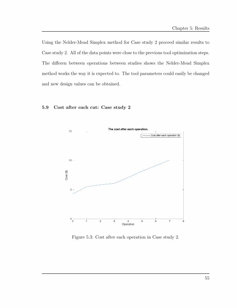
Using the Nelder-Mead Simplex method for Case study 2 proceed similar results to

Case study 2. All of the data points were close to the previous tool optimization steps.

The differen between operations between studies shows the Nelder-Mead Simplex

method works the way it is expected to. The tool parameters could easily be changed

and new design values can be obtained.

5.9 Cost after each cut: Case study 2

Figure 5.3: Cost after each operation in Case study 2.

55

Chapter 5: Results

5.10 Time after each cut: Case study 2

Figure 5.4: Time after each operation in Case study 2.

Both the cost and time per operation mirror each other for both case studies. In

order to maximize profit, both cost and time must be minimized. This has created

an equilibrium between both factors.

56

Chapter 6: Conclusion


The Nelder-Mead Simplex method was able to find an optimal value better than the

handbook. The initial guess became really important. If an initial guess set one

close the handbook, it would begin to increase the cutting speed. If the initial guess

was towards to lower end it would settle for optimal solutions in the middle. The

Simplex parameters started off at the universal Simplex values but some fine tuning

is required. For faster optimization the Simplex parameters are set to for loops that

would compare every parameter to each other. The previous for loops for these Sim-

plex parameters were used for an estimate for the best Simplex parameters.

Errors in the power constraint and surface finish were found in the papers[1, 7].

The particular knowledge of machining is as much if not more than the mathemat-

ical knowledge to set up the Nelder-Mead Simplex method. The Simplex variation

designed by the present study showed how a new case study could be developed and

did much of the preemptive white paper calculations required to go from theory to

application. The new case study provided more complex tools, that were not included

in the original design.

Nonetheless, the estimation for an optimal solution that will not violate the

constraints is calculated extremely fast. The constraints in this objective function

are the determining factor for the optimal solutions. Many of other paper’s[1] opti-

mal solution to violate the initial constraints brought by the original paper[7]. These

constraints proved to be the defining factor that allowed the optimization method

57


optimal solutions to converge to a reasonable solution. The Nelder-Mead Simplex

method is able to improve on previous results while keeping the computation to a

minimum. The success is dependent on to the algorithm’s parameters and the initial

guess attempted at different points.

58

Biography

[1] Baskar, N., Saravanan, R., Asokan, P. and Prabhaharan, G. (2005), “Optimizationof machining parameters for milling operations using non-conventional methods.”International Journal Adance Manufacturing Technology, 25, 1078–1088.

[2] Kant, G. and Sangwan, K.S. (2014), “Prediction and optimization of machiningparameters for minimizing power consumption and surface roughness in machin-ing.” Journal of Cleaner Production, 83, 151–164.

[3] Kronenberg, M. (1966), “Machining science and application.” Pergamon Press,Oxford.

[4] Lagarias, J. C., Reeds, J. A., Wright, M.H, and Wright, P.E. (2013), “Convergenceproperties of the Nelder-Mead Simplex method in low dimensions.” Society forIndustrial and Applied Mathematics, 9, 112–147.

[5] Nelder, J. A. and Mead, R. (1965), “A Simplex method for function minimization.”The Computer Journal, 7, 308–313.

[6] Machinability Data Center Technical Staff (1980), Machining Data Handbook, 3edition, volume 1.

[7] Tolouei-Rad, M. and Bidhendi, I.M. (1996), “On the optimization of machiningparameters for milling operations.” International Journal Machine Manufacturing,37, 1–16.

[8] Yildiz, A. R. (2013), “Cuckoo search algorithm for the selection of optimal ma-chining parameters in milling operations.” International Journal Adance Manu-facturing Technology, 64, 55–61.

Design Optimization for a CNC Machine - PDXScholar

Documents

Transcript of Design Optimization for a CNC Machine - PDXScholar