ABSTRACT

Title of dissertation: PREDICTING THE TRANSPORTPROPERTIES OF AEROSOL PARTICLESIN CREEPING FLOWFROM THE CONTINUUMTO THE FREE MOLECULE REGIME

James Corson, Doctor of Philosophy, 2018

Dissertation directed by: Professor Michael R. ZachariahDepartment of Chemicaland Biomolecular Engineering

The transport of nanoscale aerosol particles plays an important role in many

natural and industrial processes. Despite its importance, the transport behavior

of aerosol aggregates is poorly understood, largely due its complex dependence on

particle size, shape, and orientation. Often, these particles are in the transition

regime, where neither the continuum approximation for large particles nor the free

molecule approximation for small particles is valid.

At present, methods for calculating the aerodynamic force on and diffusive

behavior of fractal aggregates in the transition regime either rely upon scaling laws

fitted to experimental data or computationally-intensive direct simulation Monte

Carlo or molecular dynamics approaches. Thus, there is a pressing need for a new

method for determining aerosol transport properties.

This dissertation introduces such a method for calculating the drag and torque

on an aerosol aggregate as a function of the primary sphere size and the aggregate

size and shape. This method is an extension of Kirkwood-Riseman theory to the

transition regime, using an appropriate model for interactions between the individual

spheres in an aggregate.

This dissertation also describes the application of this extended Kirkwood-

Riseman (EKR) method to a number of problems related to aerosol transport, in-

cluding computation of the scalar translational and rotational friction coefficients of

aggregates formed by diffusion-limited processes, analysis of the effects of alignment

on particle migration in an electric field, and the strength of interactions between

particles due to their effects on the surrounding fluid flow field.

In each of these applications, results from the EKR method are in good agree-

ment with published experimental data and computational results. EKR results

also demonstrate that particle translational and rotational behavior becomes more

continuum-like as both primary particle size and the number of spheres in the ag-

gregate increase.

Using these results, new correlations have been developed for the translational

and rotational friction coefficients of aggregates formed by diffusion-limited processes

(e.g. soot); these correlations are more accurate than the empirical models currently

available in the literature.

PREDICTING THE TRANSPORT PROPERTIESOF AEROSOL PARTICLES IN CREEPING FLOW

FROM THE CONTINUUM TO THE FREE MOLECULE REGIME

by

James Corson

Dissertation submitted to the Faculty of the Graduate School of theUniversity of Maryland, College Park in partial fulfillment

of the requirements for the degree ofDoctor of Philosophy

2018

Advisory Committee:Professor Michael R. Zachariah, ChairDr. George W. MulhollandProfessor Richard V. CalabreseProfessor Panagiotis DimitrakopoulosProfessor Elaine S. Oran

c© Copyright byJames Corson

2018

Dedication

To my wife, Holly, who convinced me to go back to school to earn my Ph.D.

Were it not for her encouragement, I would still be Mr. Corson.

ii

Acknowledgments

First and foremost, I would like to thank my adviser, Prof. Michael Zachariah,

as well as Dr. George Mulholland. They provided me with valuable guidance

throughout my time at the University of Maryland, from suggesting that I take

on a more focused and manageable project than the mess I had in my mind when

I started at Maryland, to introducing me to the Kirkwood-Riseman method that

plays such a prominent role in this dissertation, to mentioning ways to improve my

papers and presentations. I could not ask for two better advisers.

I would also like to thank Prof. Howard Baum in the Department of Fire

Protection Engineering at the University of Maryland for introducing me to the

BGK model and explaining how one might go about solving the Boltzmann transport

equation for flow around a sphere in the transition regime.

Thank you to Dr. Walid Keyrouz and Dr. Derek Juba at the National Institute

of Standards and Technology, who provided me with the ZENO code. I have used

the Deepthought2 cluster at Maryland to run Zeno and some of my own codes; thank

you to the Division of Information Technology for maintaining the cluster and to

Prof. Jeffery Klauda in the Department of Chemical and Biomolecular Engineering

for helping me get an initial allocation to the cluster.

Finally, thank you to my wonderful family and friends, especially my parents

and my wife. My parents always encouraged me to challenge myself and instilled in

me the work ethic needed to complete all 21 years (!) of my formal education. My

iii

wife encouraged me to go back to school for my Ph.D. and supported me throughout

my time at Maryland, for which I am forever grateful.

This research was performed while under appointment to the U.S. Nuclear

Regulatory Commission Graduate Fellowship Program.

iv

Table of Contents

List of Tables x

List of Figures xii

List of Abbreviations xv

1 Introduction 11.1 Aerosol Basics . . . . . . . . . . . . . . . . . . . . . . . . . . . . . . . 31.2 Creeping Flow . . . . . . . . . . . . . . . . . . . . . . . . . . . . . . . 51.3 Aerosol Transport . . . . . . . . . . . . . . . . . . . . . . . . . . . . . 9

1.3.1 Continuum Regime . . . . . . . . . . . . . . . . . . . . . . . . 101.3.2 Free Molecule Regime . . . . . . . . . . . . . . . . . . . . . . 141.3.3 Transition Regime . . . . . . . . . . . . . . . . . . . . . . . . 16

1.4 Experimental Techniques for Obtaining Particle Size . . . . . . . . . 201.4.1 Mobility Measurements . . . . . . . . . . . . . . . . . . . . . . 211.4.2 Optical Measurements . . . . . . . . . . . . . . . . . . . . . . 24

1.5 Scope of the Dissertation . . . . . . . . . . . . . . . . . . . . . . . . . 25

2 The BGK Model Equation 312.1 Introduction . . . . . . . . . . . . . . . . . . . . . . . . . . . . . . . . 312.2 Solution of the Krook Equation for Isothermal Mass Transfer to a

Sphere . . . . . . . . . . . . . . . . . . . . . . . . . . . . . . . . . . . 382.3 Solution of the Krook Equation for Uniform Flow Around a Sphere . 43

2.3.1 Derivation of the Governing Equations . . . . . . . . . . . . . 432.3.2 Numerical Methods . . . . . . . . . . . . . . . . . . . . . . . . 62

2.4 Conclusions . . . . . . . . . . . . . . . . . . . . . . . . . . . . . . . . 67

3 Friction Coefficient for Translating Particles 693.1 Introduction . . . . . . . . . . . . . . . . . . . . . . . . . . . . . . . . 693.2 Velocity field . . . . . . . . . . . . . . . . . . . . . . . . . . . . . . . 723.3 Kirkwood-Riseman theory . . . . . . . . . . . . . . . . . . . . . . . . 763.4 Results . . . . . . . . . . . . . . . . . . . . . . . . . . . . . . . . . . . 793.5 Discussion . . . . . . . . . . . . . . . . . . . . . . . . . . . . . . . . . 83

v

4 Analytical Expression for the Friction Coefficient of DLCA Aggregates basedon Extended Kirkwood-Riseman Theory 854.1 Introduction . . . . . . . . . . . . . . . . . . . . . . . . . . . . . . . . 854.2 Theoretical Methods . . . . . . . . . . . . . . . . . . . . . . . . . . . 89

4.2.1 Kirkwood-Riseman Theory . . . . . . . . . . . . . . . . . . . . 894.2.2 Flow around a Sphere . . . . . . . . . . . . . . . . . . . . . . 924.2.3 Application of BGK Results to Kirkwood-Riseman Theory . . 96

4.3 Results and Discussion . . . . . . . . . . . . . . . . . . . . . . . . . . 974.3.1 Comparison to Experimental Data and Power-Law Models . . 984.3.2 Uncertainty in the Calculated Friction Coefficients . . . . . . . 1054.3.3 Analytical Expression for Friction Coefficients of Aggregates . 108

4.4 Conclusions . . . . . . . . . . . . . . . . . . . . . . . . . . . . . . . . 111

5 Calculating the Rotational Friction Coefficient of Fractal Aerosol Particlesin the Transition Regime using Extended Kirkwood-Riseman Theory 1155.1 Introduction . . . . . . . . . . . . . . . . . . . . . . . . . . . . . . . . 1155.2 Drag and torque on a rigid particle . . . . . . . . . . . . . . . . . . . 117

5.2.1 Kirkwood-Riseman Theory . . . . . . . . . . . . . . . . . . . . 1195.2.2 Extension to the Transition Regime . . . . . . . . . . . . . . . 1235.2.3 Monte Carlo Calculations for Free Molecule Drag and Torque 125

5.3 Results . . . . . . . . . . . . . . . . . . . . . . . . . . . . . . . . . . . 1295.3.1 Continuum regime . . . . . . . . . . . . . . . . . . . . . . . . 1295.3.2 Free Molecule Regime . . . . . . . . . . . . . . . . . . . . . . 1325.3.3 Transition Regime . . . . . . . . . . . . . . . . . . . . . . . . 134

5.4 Discussion . . . . . . . . . . . . . . . . . . . . . . . . . . . . . . . . . 140

6 Analytical Expression for the Rotational Friction Coefficient of DLCA Ag-gregates over the Entire Knudsen Regime 1426.1 Introduction . . . . . . . . . . . . . . . . . . . . . . . . . . . . . . . . 1426.2 Theoretical Methods . . . . . . . . . . . . . . . . . . . . . . . . . . . 143

6.2.1 Extended Kirkwood-Riseman Method for the Rotational Fric-tion Coefficient . . . . . . . . . . . . . . . . . . . . . . . . . . 145

6.2.2 Adjusted Sphere Method for the Rotational Friction Coefficient1506.2.3 Scaling Laws for the Rotational Friction Coefficient in the

Continuum and Free Molecule Regimes . . . . . . . . . . . . . 1526.3 Results and Discussion . . . . . . . . . . . . . . . . . . . . . . . . . . 154

6.3.1 Comparison to Experimental Data . . . . . . . . . . . . . . . 1556.3.2 Comparison to Results in the Continuum and Free Molecule

Limits . . . . . . . . . . . . . . . . . . . . . . . . . . . . . . . 1566.3.3 Relative Importance of Translational and Rotational Diffusion 1616.3.4 Uncertainty in the Calculated Rotational Friction Coefficients 1636.3.5 Analytical Expression for Rotational Friction Coefficients of

DLCA Aggregates . . . . . . . . . . . . . . . . . . . . . . . . 1676.4 Conclusions . . . . . . . . . . . . . . . . . . . . . . . . . . . . . . . . 170

vi

7 The Effect of Electric Field Induced Alignment on the Electrical Mobility ofFractal Aggregates 1727.1 Introduction . . . . . . . . . . . . . . . . . . . . . . . . . . . . . . . . 1727.2 Theoretical Methods . . . . . . . . . . . . . . . . . . . . . . . . . . . 174

7.2.1 Particle Orientation in an Electric Field . . . . . . . . . . . . 1757.2.2 Average Drift Velocity of a Particle in an Electric Field . . . . 1797.2.3 Friction Tensor for an Aggregate . . . . . . . . . . . . . . . . 181

7.3 Results . . . . . . . . . . . . . . . . . . . . . . . . . . . . . . . . . . . 1837.3.1 Comparison to Experimental Data . . . . . . . . . . . . . . . 1837.3.2 Effects of Aggregate Size and Field Strength on Mobility . . . 185

7.4 Discussion . . . . . . . . . . . . . . . . . . . . . . . . . . . . . . . . . 1927.4.1 General Observations . . . . . . . . . . . . . . . . . . . . . . . 1927.4.2 Validity of the Slow Rotation Assumption . . . . . . . . . . . 1937.4.3 Polarizability Versus Friction . . . . . . . . . . . . . . . . . . 1947.4.4 Using Field-dependent Mobility to Evaluate Particle Shape . . 196

7.5 Conclusions . . . . . . . . . . . . . . . . . . . . . . . . . . . . . . . . 198

8 Hydrodynamic Interactions between Particles 2008.1 Introduction . . . . . . . . . . . . . . . . . . . . . . . . . . . . . . . . 2008.2 Theoretical methods . . . . . . . . . . . . . . . . . . . . . . . . . . . 202

8.2.1 Two spheres in continuum flow . . . . . . . . . . . . . . . . . 2038.2.2 Aggregates in continuum flow . . . . . . . . . . . . . . . . . . 2068.2.3 Extended Kirkwood-Riseman theory . . . . . . . . . . . . . . 2098.2.4 Point force approach . . . . . . . . . . . . . . . . . . . . . . . 211

8.3 Two particle results . . . . . . . . . . . . . . . . . . . . . . . . . . . . 2148.3.1 Sphere results . . . . . . . . . . . . . . . . . . . . . . . . . . . 2158.3.2 Aggregate results . . . . . . . . . . . . . . . . . . . . . . . . . 217

8.4 Discussion . . . . . . . . . . . . . . . . . . . . . . . . . . . . . . . . . 2198.4.1 Aerosol clouds . . . . . . . . . . . . . . . . . . . . . . . . . . . 2218.4.2 Additional considerations . . . . . . . . . . . . . . . . . . . . 225

8.5 Conclusions . . . . . . . . . . . . . . . . . . . . . . . . . . . . . . . . 227

9 NGDE: A MATLAB-based Code for Solving the Aerosol General DynamicEquation 2299.1 Introduction . . . . . . . . . . . . . . . . . . . . . . . . . . . . . . . . 2299.2 Overview of Numerical Methods for Solving the GDE . . . . . . . . . 2329.3 NGDE Code Description . . . . . . . . . . . . . . . . . . . . . . . . . 235

9.3.1 Coagulation . . . . . . . . . . . . . . . . . . . . . . . . . . . . 2369.3.2 Nucleation . . . . . . . . . . . . . . . . . . . . . . . . . . . . . 2389.3.3 Surface Growth . . . . . . . . . . . . . . . . . . . . . . . . . . 2409.3.4 Solution Strategy . . . . . . . . . . . . . . . . . . . . . . . . . 242

9.4 Sample Results . . . . . . . . . . . . . . . . . . . . . . . . . . . . . . 2459.4.1 Pure Coagulation . . . . . . . . . . . . . . . . . . . . . . . . . 2459.4.2 Pure Surface Growth . . . . . . . . . . . . . . . . . . . . . . . 2489.4.3 Nucleation and Coagulation . . . . . . . . . . . . . . . . . . . 251

vii

9.4.4 Full GDE for Condensation of Aluminum . . . . . . . . . . . . 2529.5 Limitations of NGDE . . . . . . . . . . . . . . . . . . . . . . . . . . . 2559.6 NGDEplot . . . . . . . . . . . . . . . . . . . . . . . . . . . . . . . . . 2579.7 Conclusions . . . . . . . . . . . . . . . . . . . . . . . . . . . . . . . . 259

10 Conclusions and Recommendations for Future Work 26310.1 Conclusions . . . . . . . . . . . . . . . . . . . . . . . . . . . . . . . . 26310.2 Recommendations for Future Work . . . . . . . . . . . . . . . . . . . 268

10.2.1 Friction Coefficient Expressions for non-DLCA Aggregates . . 26810.2.2 Aggregates with Polydisperse Primary Spheres . . . . . . . . . 26910.2.3 Rotational and Coupling Interactions . . . . . . . . . . . . . . 27210.2.4 Brownian Dynamics . . . . . . . . . . . . . . . . . . . . . . . 273

A Derivation of Expressions in Chapter 2 278A.1 Derivation of the Expression for g [Eq. (2.42)] . . . . . . . . . . . . . 278A.2 Derivation of the Source Term Expressions (Eqns. 2.40–2.41) . . . . . 284A.3 Derivation of H . . . . . . . . . . . . . . . . . . . . . . . . . . . . . . 289A.4 Derivation of the Drag Expression (Eq. (2.54)) . . . . . . . . . . . . . 296

B BGK Results 301

C Monte Carlo Drag and Torque Results 327C.1 Drag on a Translating Sphere . . . . . . . . . . . . . . . . . . . . . . 327C.2 Drag on an Aggregate . . . . . . . . . . . . . . . . . . . . . . . . . . 327C.3 Torque on a Rotating Sphere . . . . . . . . . . . . . . . . . . . . . . . 328

D Relationship between the Rotation and Coupling Interaction Tensors and theFlow around a Sphere 329

E Supplemental Material for Chapter 7 333E.1 Euler Angles . . . . . . . . . . . . . . . . . . . . . . . . . . . . . . . . 333E.2 Probability Distributions . . . . . . . . . . . . . . . . . . . . . . . . . 333E.3 Sample Calculation . . . . . . . . . . . . . . . . . . . . . . . . . . . . 335E.4 Effects of Knudsen Number and the Number of Primary Spheres on

Fully-Aligned Particle Mobility . . . . . . . . . . . . . . . . . . . . . 341

F NGDE User Manual 351F.1 Running NGDE and NGDEplot . . . . . . . . . . . . . . . . . . . . . 351F.2 Description of Input and Output . . . . . . . . . . . . . . . . . . . . 356

F.2.1 NGDE Input (ngdein) . . . . . . . . . . . . . . . . . . . . . . 356F.2.2 NGDEplot Input (plotoptions) . . . . . . . . . . . . . . . . 358F.2.3 NGDE and NGDEplot Output . . . . . . . . . . . . . . . . . 359

F.3 Code Structure . . . . . . . . . . . . . . . . . . . . . . . . . . . . . . 361F.3.1 NGDE Subroutines . . . . . . . . . . . . . . . . . . . . . . . . 361F.3.2 NGDE Main Program . . . . . . . . . . . . . . . . . . . . . . 364

F.4 Summary . . . . . . . . . . . . . . . . . . . . . . . . . . . . . . . . . 365

viii

G MATLAB Codes Referenced in this Disseration 367G.1 Code for Calculating the Velocity around a Sphere . . . . . . . . . . . 367

G.1.1 Code Listing for bgk sphere par . . . . . . . . . . . . . . . . 369G.2 Codes for Calculating the Friction and Diffusion Tensors . . . . . . . 382

G.2.1 Code Listing for continuum tensors . . . . . . . . . . . . . . 382G.2.2 Code Listing for continuum tensors 3rd . . . . . . . . . . . . 384G.2.3 Code Listing for bgk tensors . . . . . . . . . . . . . . . . . . 387

G.3 Codes for Calculating the Average Friction Coefficient of a Particlein an Electric Field . . . . . . . . . . . . . . . . . . . . . . . . . . . . 391G.3.1 Code Listing for avg bgk velocity . . . . . . . . . . . . . . . 391G.3.2 Code Listing for avg bgk drag . . . . . . . . . . . . . . . . . . 394

G.4 Codes for Hydrodynamic Interactions between Particles . . . . . . . . 398G.4.1 Code Listing for bgk two particles . . . . . . . . . . . . . . 398G.4.2 Code Listing for bgk cloud . . . . . . . . . . . . . . . . . . . 402

Bibliography 407

Publications and Presentations 420

ix

List of Tables

3.1 Comparison of my results for F/FFM to Millikan’s data and to resultsfrom previous computational studies . . . . . . . . . . . . . . . . . . 75

5.1 Continuum friction coefficient for fractal aggregates, normalized bythe monomer friction results . . . . . . . . . . . . . . . . . . . . . . . 132

5.2 Free molecule results for fractal aggregates, normalized by the mon-omer friction results . . . . . . . . . . . . . . . . . . . . . . . . . . . 133

6.1 Comparison of EKR results to experimental data from the literature . 156

8.1 Speed of two spheres moving parallel to their line of centers, relativeto the speed of isolated spheres subjected to the same external force . 206

8.2 Speed of two spheres moving anti-parallel to their line of centers,relative to the speed of isolated spheres subjected to the same externalforce . . . . . . . . . . . . . . . . . . . . . . . . . . . . . . . . . . . . 207

8.3 Speed of two spheres moving perpendicular to their line of centers,relative to the speed of isolated spheres subjected to the same externalforce . . . . . . . . . . . . . . . . . . . . . . . . . . . . . . . . . . . . 207

9.1 Moments, Mi, of the particle size distribution for the pure coagulationcalculation . . . . . . . . . . . . . . . . . . . . . . . . . . . . . . . . . 249

B.1 Results for a = 0.01 (Kn = 88.8) . . . . . . . . . . . . . . . . . . . . . 302B.2 Results for a = 0.025 (Kn = 35.5) . . . . . . . . . . . . . . . . . . . . 303B.3 Results for a = 0.05 (Kn = 17.8) . . . . . . . . . . . . . . . . . . . . . 304B.4 Results for a = 0.075 (Kn = 11.8) . . . . . . . . . . . . . . . . . . . . 305B.5 Results for a = 0.1 (Kn = 8.88) . . . . . . . . . . . . . . . . . . . . . 306B.6 Results for a = 0.25 (Kn = 3.55) . . . . . . . . . . . . . . . . . . . . . 307B.7 Results for a = 0.5 (Kn = 1.78) . . . . . . . . . . . . . . . . . . . . . 308B.8 Results for a = 0.75 (Kn = 1.18) . . . . . . . . . . . . . . . . . . . . . 309B.9 Results for a = 1.0 (Kn = 0.888) . . . . . . . . . . . . . . . . . . . . . 310B.10 Results for a = 1.25 (Kn = 0.710) . . . . . . . . . . . . . . . . . . . . 311B.11 Results for a = 1.5 (Kn = 0.592) . . . . . . . . . . . . . . . . . . . . . 312

x

B.12 Results for a = 1.75 (Kn = 0.5074) . . . . . . . . . . . . . . . . . . . 313B.13 Results for a = 2.0 (Kn = 0.444) . . . . . . . . . . . . . . . . . . . . . 314B.14 Results for a = 2.5 (Kn = 0.355) . . . . . . . . . . . . . . . . . . . . . 315B.15 Results for a = 3.0 (Kn = 0.296) . . . . . . . . . . . . . . . . . . . . . 316B.16 Results for a = 4.0 (Kn = 0.222) . . . . . . . . . . . . . . . . . . . . . 317B.17 Results for a = 5.0 (Kn = 0.178) . . . . . . . . . . . . . . . . . . . . . 318B.18 Results for a = 6.0 (Kn = 0.148) . . . . . . . . . . . . . . . . . . . . . 319B.19 Results for a = 7.0 (Kn = 0.1269) . . . . . . . . . . . . . . . . . . . . 320B.20 Results for a = 8.0 (Kn = 0.111) . . . . . . . . . . . . . . . . . . . . . 321B.21 Results for a = 9.0 (Kn = 0.0987) . . . . . . . . . . . . . . . . . . . . 322B.22 Results for a = 10.0 (Kn = 0.0888) . . . . . . . . . . . . . . . . . . . 323B.23 Results for a = 50 (Kn = 0.0178) . . . . . . . . . . . . . . . . . . . . 324B.24 Results for a = 100 (Kn = 0.00888) . . . . . . . . . . . . . . . . . . . 325B.25 Results for c1 and c2 . . . . . . . . . . . . . . . . . . . . . . . . . . . 326

E.1 Coordinates of the center of each sphere in my sample aggregate . . . 337

xi

List of Figures

1.1 Differential mobility analyzer . . . . . . . . . . . . . . . . . . . . . . 21

2.1 Geometry for the mass transfer problem . . . . . . . . . . . . . . . . 402.2 Geometry for Eq. 2.25 . . . . . . . . . . . . . . . . . . . . . . . . . . 452.3 Geometry for Eq. 2.26 . . . . . . . . . . . . . . . . . . . . . . . . . . 462.4 Geometry for determining A(r0) . . . . . . . . . . . . . . . . . . . . . 51

3.1 Ratio of the calculated drag from the Krook equation to the freemolecule drag . . . . . . . . . . . . . . . . . . . . . . . . . . . . . . . 74

3.2 Open and dense 20 particle aggregates . . . . . . . . . . . . . . . . . 803.3 Comparison of my results for the slip correction factor to DSMC

results for a dimer and open and dense 20-particle aggregates . . . . . 813.4 Calculated slip correction factors for a range of aggregate morpholo-

gies, plotted versus the aggregate Knudsen number . . . . . . . . . . 83

4.1 Friction factor results for fractal aggregates with primary sphere di-ameter 19.5 nm in ambient air (Kn = 7) . . . . . . . . . . . . . . . . 99

4.2 Comparison of self-consistent field results to other models for thescalar friction factor for several Knudsen numbers . . . . . . . . . . . 101

4.3 Ratio of friction coefficients from other models to my results . . . . . 1034.4 Normalized friction coefficient results for a range of aggregate sizes . . 1044.5 Relationship between the mobility radius and the radius of gyration

for several Knudsen numbers . . . . . . . . . . . . . . . . . . . . . . . 1054.6 Normalized friction coefficient as a function of the primary sphere

Knudsen number and the number of primary spheres, N , calculatedusing Eq. (4.38) . . . . . . . . . . . . . . . . . . . . . . . . . . . . . . 111

4.7 Error of my harmonic sum model for the friction coefficient relativeto my EKR results for a range of Knudsen numbers . . . . . . . . . . 112

5.1 Representations of the fractal aggregates used in this study . . . . . . 1305.2 Calculated rotational slip correction factor for a dimer, linear hex-

amer, and octahedral hexamer . . . . . . . . . . . . . . . . . . . . . . 1365.3 Calculated rotational slip correction factor for four fractal aggregates 137

xii

5.4 Rotational slip correction factor plotted versus an aggregate Knudsennumber . . . . . . . . . . . . . . . . . . . . . . . . . . . . . . . . . . 139

6.1 Rotational friction coefficient results for Kn = 0.1, 1, 2, and 10 . . . . 1596.2 Ratio of rotational friction coefficients for N = 2000 . . . . . . . . . 1606.3 Ratio of the characteristic translational diffusion time to the charac-

teristic rotational diffusion time for DLCA aggregates . . . . . . . . . 1626.4 Torque on each sphere of two rotating 20-particle aggregates . . . . . 1666.5 Ratio of the drag on each sphere in a rotating 20-particle aggregate

to the drag on an isolated sphere . . . . . . . . . . . . . . . . . . . . 1676.6 Error in the analytical expression for the rotational friction coefficient

relative to my EKR results . . . . . . . . . . . . . . . . . . . . . . . . 169

7.1 Comparison of my calculated orientation-averaged mobilities to pub-lished experimental data . . . . . . . . . . . . . . . . . . . . . . . . . 186

7.2 Normalized mobility as a function of electric field strength for 100-sphere and 1000-sphere aggregates . . . . . . . . . . . . . . . . . . . . 188

7.3 Normalized mobility as a function of electric field strength for aggre-gates with primary sphere radii of 25 nm and 5 nm . . . . . . . . . . 189

7.4 Maximum electric field strength at which particles are randomly ori-ented . . . . . . . . . . . . . . . . . . . . . . . . . . . . . . . . . . . . 190

7.5 Ratio of fully-aligned to random electric mobilities . . . . . . . . . . . 1917.6 Reduced rotation velocity for a range of primary sphere sizes and

Knudsen numbers . . . . . . . . . . . . . . . . . . . . . . . . . . . . . 193

8.1 Two spheres in the parallel, anti-parallel, and perpendicular flow con-figurations, and two 10-sphere aggregates with random orientationsin parallel flow . . . . . . . . . . . . . . . . . . . . . . . . . . . . . . 202

8.2 Speed of two spheres moving parallel, anti-parallel, and perpendicularto their line of centers . . . . . . . . . . . . . . . . . . . . . . . . . . 216

8.3 Hydrodynamic force on an aggregate as a function of the distancebetween its center of mass and the center of mass of an identicalaggregate . . . . . . . . . . . . . . . . . . . . . . . . . . . . . . . . . 218

8.4 Effects of orientation on the hydrodynamic force on one of two 500-sphere aggregates with primary sphere Kn = 2.7 . . . . . . . . . . . . 219

8.5 Average velocity for a cloud of spheres . . . . . . . . . . . . . . . . . 224

9.1 NGDE volume nodes . . . . . . . . . . . . . . . . . . . . . . . . . . . 2359.2 Illustration of the NGDE algorithm . . . . . . . . . . . . . . . . . . . 2439.3 Non-dimensional size distribution for the pure coagulation problem . 2479.4 Size distribution calculated by NGDE for the pure surface growth

sample problem . . . . . . . . . . . . . . . . . . . . . . . . . . . . . . 2509.5 Volume-mean particle diameter calculated by NGDE for the pure

surface growth problem . . . . . . . . . . . . . . . . . . . . . . . . . . 2519.6 Particle size distribution at select times for nucleation and coagula-

tion of aluminum . . . . . . . . . . . . . . . . . . . . . . . . . . . . . 252

xiii

9.7 Critical volume and nucleation rate for nucleation and coagulation ofaluminum . . . . . . . . . . . . . . . . . . . . . . . . . . . . . . . . . 253

9.8 Particle size distribution at select times for nucleation, coagulation,and surface growth of aluminum . . . . . . . . . . . . . . . . . . . . . 254

9.9 Nucleation rate and saturation ratio early in the simulation for nu-cleation, coagulation, and surface growth of aluminum by NGDE . . . 254

9.10 Monomer and total particle concentration for nucleation, coagulation,and surface growth of aluminum . . . . . . . . . . . . . . . . . . . . . 255

9.11 Screenshot of the particle size distribution movie from NGDEplot . . 2609.12 Screenshot of the light scattering movie from NGDEplot . . . . . . . 261

E.1 Representation of the Euler angles that relate the body-fixed coordi-nates to the space-fixed coordinates . . . . . . . . . . . . . . . . . . . 334

E.2 Probability distributions for particles with 652 primary spheres with5 nm radii . . . . . . . . . . . . . . . . . . . . . . . . . . . . . . . . . 336

E.3 Ratio of fully-aligned to random electric mobilities for wide range ofprimary sphere Knudsen numbers and the number of primaries . . . . 342

E.4 Comparison of the continuum mobility and radius of gyration ratios . 345E.5 Comparison between the average continuum mobility ratio and the

average radius of gyration ratio as a function of N . . . . . . . . . . . 346E.6 Comparison of the free molecule mobility and projected area ratios . 347E.7 Comparison between the average free molecule mobility ratio and the

average projected area ratio as a function of N . . . . . . . . . . . . . 348

xiv

List of Abbreviations

APM Aerosol Particle Mass [analyzer]ASM Adjusted Sphere MethodBGK Bhatnagar-Gross-Krook [model]DLCA Diffusion-Limited Cluster AggregationDMA Differential Mobility AnalyzerDSMC Direct-Simulation Monte CarloEKR Extended Kirkwood-Riseman [method]GDE General Dynamic EquationKR Kirkwood-Riseman [theory]MC Monte CarloNGDE Nodal General Dynamic Equation [solver]ODE Ordinary Differential EquationPA Projected AreaPFDMA Pulsed Field Differential Mobility AnalyzerPSD Particle Size DistributionRPY Rotne-Prager-Yamakawa [tensor]SPD Self-Preserving DistributionTDMA Tandem Differential Mobility Analyzer

xv

Chapter 1: Introduction

Nanoscale aerosol particles formed at high temperature are found in many

natural and engineered environments [1–3]. A particle’s size and shape significantly

affect its transport properties, most notably the aerodynamic force it experiences as

it moves through an external force field [4–6]. Research on this topic is motivated

by the widespread use of aerosol reactors for the manufacturing of carbon black,

ceramics (e.g. SiO2 and TiO2), catalysts, and optical fibers present in numerous

consumer products [2, 7–10]; the impacts of aerosols generated in the combustion of

fossil fuels or from volcanic eruptions on climate, both through direct absorption or

scattering of incident solar radiation and through its influence on cloud formation

[11–16]; and the adverse human health effects of particle uptake by the body [17–20]

and exposure to radioactive particles from nuclear reactor accidents [21–25].

In many practical situations, these aerosol particles move very slowly with

respect to the surrounding gas. As a result, one can neglect inertial effects in the

fluid and treat the particle as if it is in the creeping flow regime. This significantly

simplifies the fluid dynamics and makes problems of aerosol transport more tractible.

A further simplification is to treat particles as if they are spherical. The

equivalent sphere size may be based on the particle mass – as if often done in aerosol

1

dynamics codes [26, 27] – or on its aerodynamic behavior, such as its experimentally-

measured mobility. Using this equivalent sphere size, one can estimate any number

of transport properties (e.g. diffusion and friction coefficients, coagulation rates,

phoretic velocities, etc.) using various theoretical or experimental relations that

have been developed for spheres [2].

Unfortunately, particles are often non-spherical. In fact, particles formed by

random processes are often fractal aggregates of N spheres (or monomers) with

radius a. The number of primary spheres in a fractal aggregate is related to the

radius of gyration Rg of the particle by

N = k0

(Rg

a

)df(1.1)

Here, df and k0 are the fractal dimension and prefactor. One important class of

particles, those formed by diffusion-limited cluster-to-cluster aggregation (DLCA),

have a fractal dimension of approximately 1.78 and a prefactor around 1.3 [4].

Treating a fractal aggregate as a sphere with an equivalent mass or equivalent

mobility leads to an erroneous estimate of particle migration, coagulation, and depo-

sition rates. There are existing methods for calculating the drag on a non-spherical

particle, but most of these methods are only applicable in the continuum [28–31]

or free molecule [32–36] regimes corresponding to particles much larger or much

smaller than the mean free path of gas molecules. However, nano-scale aerosols

typically have characteristic sizes that place them in the transition regime between

the continuum and free molecule limits. There is also some ambiguity as to how one

2

should approach a situation where the aerosol is an aggregate of very many small

spheres (a λ, where a is the sphere diameter and λ the mean free path) while the

characteristic size of the aggregate (such as Rg) is comparable to or larger than λ.

Methods for calculating the drag on a particle in the transition regime are largely

based on fits to empirical data [37–39], or rely on expensive computational methods

such as the direct simulation Monte Carlo (DSMC) method [40, 41].

This dissertation describes a new method for calculating the drag and torque

on an aggregate in creeping flow when continuum approaches are invalid. Before

describing my method and presenting my results, I will first provide brief intro-

ductions to concepts in aerosol physics that are relevant to my dissertation. This

introduction includes basic definitions on topics such as aerosol particle size distri-

butions, an overview of creeping flow and its characteristics, review of the existing

literature on drag and torque on particles in creeping flow, and a discussion of per-

tinent experimental equipment and methods used in aerosol transport studies that

play some role in validating my theoretical methods. To conclude the introduction,

I will outline the remaining scope of my dissertation.

1.1 Aerosol Basics

Aerosols are two-phase systems consisting of a dispersed phase of solid particles

or liquid droplets in a continuous gas phase [1–3]. The particles may form from gas-

phase processes (such as condensation of super-saturated vapor) or from breakup of

solids or liquids. Gas-phase processes typically produce smaller particles (i.e. less

3

than 1 µm in diameter), while disintegration processes yield larger particles [2].

Particle size is often described in terms of the non-dimensional Knudsen number,

which is defined as the ratio of the mean free path of molecules in the gas to the

characteristic size of the particle, Kn = λ/L. The mean free path is the average

distance gas molecules travel between collisions, which is a function of the size of

the gas molecules and their number density and is equal to approximately 65 nm

for air at standard temperature and pressure [2]. The mean free path can be related

to the gas viscosity through relations that depend on the choice of molecular model

(e.g. hard sphere, Lennard-Jones) for the gas [40]. The characteristic size of a

particle depends on its shape; for spheres, the radius is the characteristic size, while

for more general shapes one can use the mobility radius or radius of gyration. The

radius of gyration is a purely geometric quantity, while the mobility radius depends

on the interaction between the particle and the fluid [2]. This topic will be discussed

later in this introduction.

As mentioned previously, many aerosol particles are fractal-like aggregates of

many smaller, primary spheres, that form when the primary spheres coagulate and

stick together. Generally speaking, aggregates contain spheres with a distribution

of sizes; however, the standard deviation in the primary sphere diameter is often

small when compared to the mean diameter [38, 42–44]. As a result, most studies of

aerosol fractal aggregate transport assume that the primary spheres are all the same

size [2, 4]. Primary sphere sizes range from a few nanometers up to about 0.1 µm [2],

while aggregates may include tens, hundreds or even thousands of primary spheres

[2, 4, 7, 42–44].

4

Aerosol systems typically consist of particles with a range of sizes; this range

is described by the particle size distribution n(v, t), where n(v, t)dv is the number of

particles per unit gas volume at time t with particle volume between v and v + dv.

The size distribution can represent either spherical particles or aggregates [2]. The

evolution of this size distribution with time is described by the general dynamic

equation [2, 3, 45]. This equation accounts for changes in the distribution due to

coagulation, condensation/evaporation, and particle formation and removal. Many

of the terms in the general dynamic equation depend on the transport properties of

the system. Thus, one must be able to accurately describe the transport properties

(e.g. drag and torque on the particles as a function of the gas properties and the

particle size, shape, and orientation) in order to predict the dynamic behavior of

the aerosol. Again, this is the primary motivation for the research described in this

dissertation.

1.2 Creeping Flow

The statistical behavior of a dilute gas is described by the Boltzmann transport

equation,

∂f

∂t+ c · ∇f +

FEm· ∂f∂c

=δf

δt

∣∣∣∣coll

(1.2)

where f(r, c, t)drdc is the number of gas molecules in differential volume dr with

velocity c + dc at time t, ∇f is the spatial gradient of f(r, c, t), ∂f/∂c is its

gradient with respect to the molecular velocity, and FE/m is the external force

(e.g. electrical, magnetic) per unit mass on the molecules [40, 46]. The right-hand

5

side of the above equation is the collision integral. Thus, the Boltzmann equation

tracks the probability distribution of molecular velocities as a function of position

and time, accounting for convection (the second term on the left-hand side), external

forces on the molecules (the third term on the left-hand side), and collisions between

gas molecules that alter their velocities (the term on the right-hand side) [40]. It

is a complicated integro-differential equation that can only be solved for a very

small number of cases [46]. (See Chapter 2 for more details about the Boltzmann

equation.)

For near-equilibrium situations where the smallest length scale of the prob-

lem is much greater than the mean free path of the gas (i.e. Kn 1), one can

use Chapman-Enskog theory to derive the mass, momentum, and energy balance

equations that govern continuum transport [47]. Conservation of momentum for

near-equilibrium, continuum flow in an incompressible, Newtownian fluid is given

by the Navier-Stokes equation,

ρ

(∂u

∂t+ u · ∇u

)= −∇p+ µ∇2u+ ρg (1.3)

where u(x, t) is the bulk gas velocity at position x at time t, g is gravitational

acceleration, and ρ, p, and µ are the gas density, pressure, and viscosity. The

coefficients of viscosity, diffusion, and heat conduction that appear in the continuum

transport equations can be related to the molecular velocity distribution function

through the Chapman-Enskog expansion. (See Refs. [40, 46] for further discussion

on this topic.)

6

The Navier-Stokes equation is less complicated than the Boltzmann equation,

but it is still a non-linear differential equation, making it difficult to solve analytically

except in special cases. However, we can significantly simplify the equation for cases

where the inertial terms (i.e. the left-hand side of the Navier-Stokes equation) are

negligible, leading to the Stokes equation governing creeping flow in the continuum:

0 = −∇P + µ∇2u (1.4)

Here, ∇P ≡ ∇p+ρg combines the pressure term with the gravitational term, which

can be done because gravity is a conservative vector field [48].

The Stokes equation is valid for Re 1, where the Reynolds number repre-

sents the ratio of inertial to viscous forces and is defined as Re ≡ ρUL/µ. Here, U

and L are the characteristic speed and length scale in the problem. (For a sphere

with radius a moving with velocity U0, U = |U0| and L = a.) The Mach number

(Ma ≡ U/cs, where cs is the speed of sound in the gas) must also be very small for

the creeping flow approximation to be valid, though in the continuum the Reynolds

number condition is typically more restrictive. (Note that the Mach number must

be small in order for a gas flow to be considered incompressible.) Unlike the Boltz-

mann and Navier-Stokes equations, the Stokes equation is linear, which gives it a

number of interesting mathematical properties, some of which I will discuss later.

From a practical standpoint, it makes the equation much easier to solve.

For non-continuum flow, Eq. (1.4) no longer applies; however, one can still be

in the creeping flow regime, provided the usual conditions of very low Reynolds and

7

Mach numbers are satisfied. This allows us to simplify the Boltzmann equation to

determine the flow field around and drag on an aerosol particle, as I will explain in

more detail in this dissertation. (See, especially, Chapters 2 and 3.)

Before describing the methods one might use to calculate the drag on a particle,

I must first introduce two important features resulting from the linearity of the

creeping flow equations (whether the Stokes equation for continuum flow or the

BGK equation – the subject of Chapter 2 – for non-continuum flow).

First, there is a linear relationship between the translational and rotational

velocities UO and ω of a particle and the drag and torque F and TO exerted by the

fluid on the particle [49]:

F = −Ξt ·UO −Ξ†O,c ·ω (1.5a)

T = −ΞO,c ·UO −Ξ†O,r ·ω (1.5b)

Here, the translational, rotational, and translation-rotation coupling friction ten-

sors Ξt, ΞO,r, and ΞO,c are functions of the particle size, shape, and orientation. The

coupling tensor reflects the fact that in general, a translating particle can experience

a net torque, which can induce particle rotation. Likewise, a rotating particle can

experience a net force that induces particle translation. The dagger symbol repre-

sents the transpose of the tensor, while the subscript O signifies that the variable is

defined with respect to the center of mass of the particle (i.e. UO is the translational

velocity of particle center of mass). Note that Ξt and ΞO,r are symmetric. For

8

isotropic particles such as spheres, the coupling tensor is zero, while the transla-

tional and rotational tensors are Ξt = ζtI and ΞO,r = ζO,rI. Here, I is the identity

tensor and ζt and ζO,r are the (scalar) translational and rotational friction coeffi-

cients for the sphere, which are given in the following section. Thus, for an isotropic

particle one need only determine two coefficients to describe the force and torque on

a particle with specified velocity. For an arbitrary particle, one must determine 21

parameters: the 6 independent components of Ξt, the 6 independent components of

ΞO,r, and all 9 components of ΞO,c.

The second important consequence of the linearity of the creeping flow equa-

tions is that one may solve the equations using superposition. This means that we

may add up the velocity results for problems where the solution is known (e.g. Stokes

flow around a sphere moving through an infinite fluid) to get results for a different

problem where the solution is more difficult to determine (e.g. two spheres in Stokes

flow), provided the superposed solution satisfies the equation and boundary condi-

tions of the more difficult problem [48]. This property of linear equations forms the

basis for the Kirkwood-Riseman approach that I will discuss shortly.

1.3 Aerosol Transport

While the work described in this dissertation primarily concerns transport of

particles in the transition regime, it is necessary to first review the theoretical devel-

opment of the drag on a particle in the continuum and free molecule regimes. There

are two main reasons for doing so: first, the extended Kirkwood-Riseman (EKR)

9

method introduced in this dissertation incorporates elements from the continuum

and free molecule regimes; second, the drag computed using the EKR method should

approach the continuum and free molecule expressions in the limits of very small

and very large Knudsen numbers. Thus, the review of aerosol particle transport

is divided into sections relevant to the continuum, free molecule, and transition

regimes.

1.3.1 Continuum Regime

The creeping (or Stokes) flow equation forms the basis for any study of the

behavior of particles in low-Reynolds-number flow in the continuum. Stokes [50] was

the first to solve the creeping motion equation [Eq. (1.4)] for a sphere with radius

a, resulting in the expression now know as Stokes’ law,

F = −6πµaU ≡ −ζct,0U (1.6)

where ζct,0 is the translational friction coefficient for a sphere in continuum flow. One

can also solve Eq. (1.4) for a sphere rotating with angular velocity ω; the torque on

the rotating sphere is given by

T = −8πµa3ω ≡ −ζcr,0ω (1.7)

where ζcr,0 is the rotational friction coefficient for a sphere in continuum flow about

its center of mass.

10

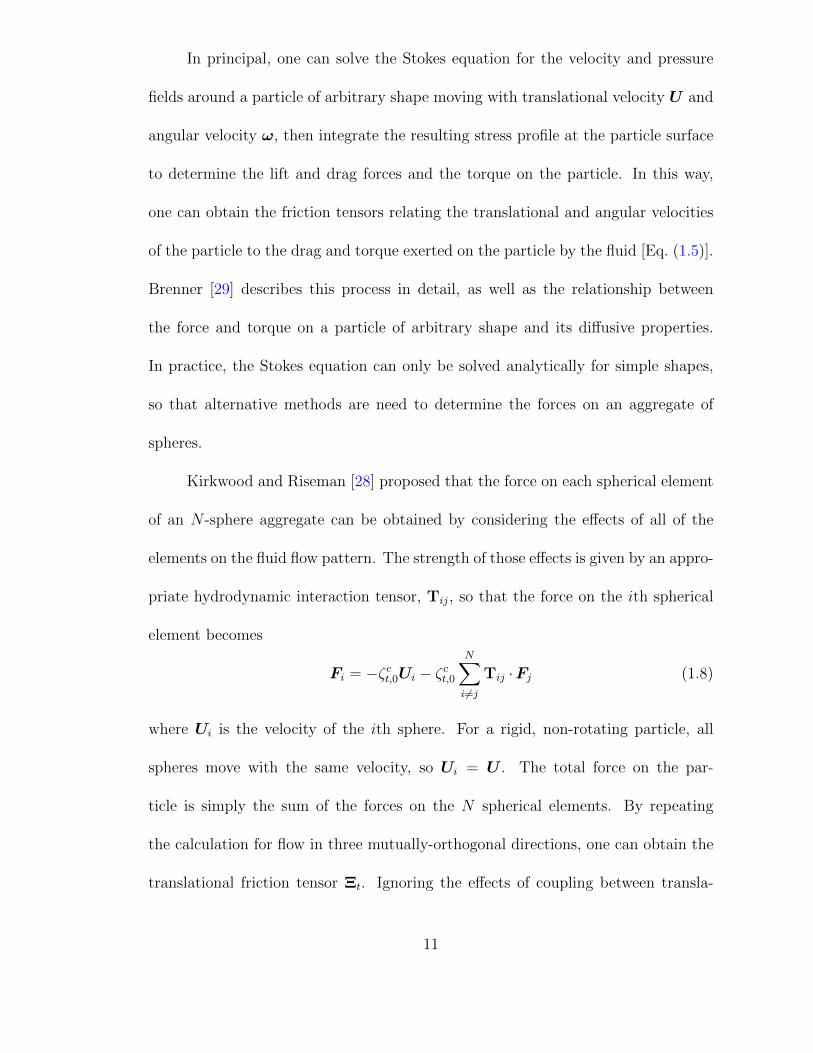
In principal, one can solve the Stokes equation for the velocity and pressure

fields around a particle of arbitrary shape moving with translational velocity U and

angular velocity ω, then integrate the resulting stress profile at the particle surface

to determine the lift and drag forces and the torque on the particle. In this way,

one can obtain the friction tensors relating the translational and angular velocities

of the particle to the drag and torque exerted on the particle by the fluid [Eq. (1.5)].

Brenner [29] describes this process in detail, as well as the relationship between

the force and torque on a particle of arbitrary shape and its diffusive properties.

In practice, the Stokes equation can only be solved analytically for simple shapes,

so that alternative methods are need to determine the forces on an aggregate of

spheres.

Kirkwood and Riseman [28] proposed that the force on each spherical element

of an N -sphere aggregate can be obtained by considering the effects of all of the

elements on the fluid flow pattern. The strength of those effects is given by an appro-

priate hydrodynamic interaction tensor, Tij, so that the force on the ith spherical

element becomes

Fi = −ζct,0Ui − ζct,0N∑i 6=j

Tij ·Fj (1.8)

where Ui is the velocity of the ith sphere. For a rigid, non-rotating particle, all

spheres move with the same velocity, so Ui = U . The total force on the par-

ticle is simply the sum of the forces on the N spherical elements. By repeating

the calculation for flow in three mutually-orthogonal directions, one can obtain the

translational friction tensor Ξt. Ignoring the effects of coupling between transla-

11

tional and rotational motion, the scalar translational friction coefficient ζt is the

harmonic mean of the eigenvalues of Ξt [29, 49].

The Kirkwood-Riseman (KR) framework can also be used to calculate the

torque on a rotating particle and the coupling between translational and rota-

tional motions, as described in the works of Garcia de la Torre and colleagues

(e.g. Refs. [51–53]). This procedure accounts for rotational and coupling hydro-

dynamic interactions and yields the rotational and coupling friction tensors, Ξr and

Ξc. From the three friction tensors, one obtains the translation, rotation, and cou-

pling diffusion tensors through a generalization of the Stokes-Einstein law derived

by Brenner [29].

Kirkwood and Riseman originally applied their theory to flexible macromole-

cules; Bernal et al. [51] and Chen et al. [30] later applied the theory to rigid macro-

molecules and fractal aggregates, respectively. KR theory has been used extensively

to compute the transport properties of macromolecules, colloids, and fractal aggre-

gates [30, 51–56].

In its original form, KR theory used the Oseen tensor for Tij. Subsequent

applications of the theory for pure translational motion have used the Rotne-Prager-

Yamakawa (RPY) tensor [57, 58]. More complicated translational, rotational, and

coupling hydrodynamic interaction tensors are also available in the literature [59–

61]. Carrasco and Garcıa de la Torre [53] have shown that KR theory with the RPY

tensor yields translational friction coefficients within a few percent of the friction

coefficients calculated with more sophisticated methods for the simple particles they

studied.

12

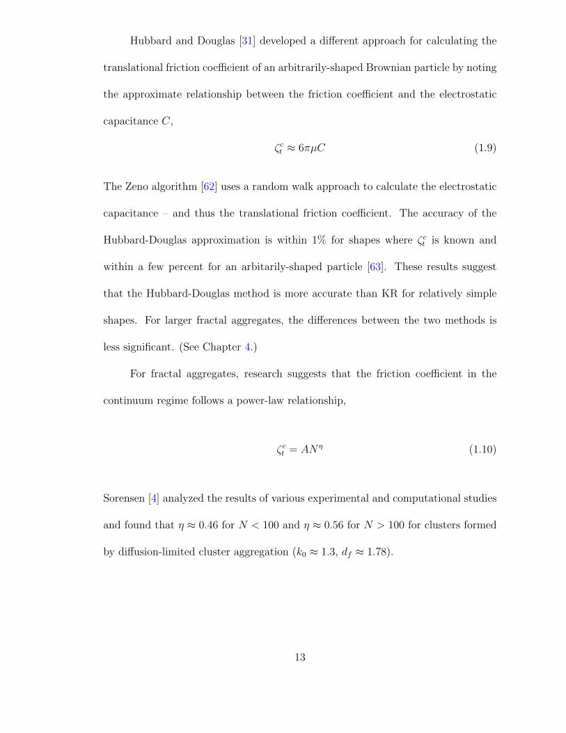
Hubbard and Douglas [31] developed a different approach for calculating the

translational friction coefficient of an arbitrarily-shaped Brownian particle by noting

the approximate relationship between the friction coefficient and the electrostatic

capacitance C,

ζct ≈ 6πµC (1.9)

The Zeno algorithm [62] uses a random walk approach to calculate the electrostatic

capacitance – and thus the translational friction coefficient. The accuracy of the

Hubbard-Douglas approximation is within 1% for shapes where ζct is known and

within a few percent for an arbitarily-shaped particle [63]. These results suggest

that the Hubbard-Douglas method is more accurate than KR for relatively simple

shapes. For larger fractal aggregates, the differences between the two methods is

less significant. (See Chapter 4.)

For fractal aggregates, research suggests that the friction coefficient in the

continuum regime follows a power-law relationship,

ζct = ANη (1.10)

Sorensen [4] analyzed the results of various experimental and computational studies

and found that η ≈ 0.46 for N < 100 and η ≈ 0.56 for N > 100 for clusters formed

by diffusion-limited cluster aggregation (k0 ≈ 1.3, df ≈ 1.78).

13

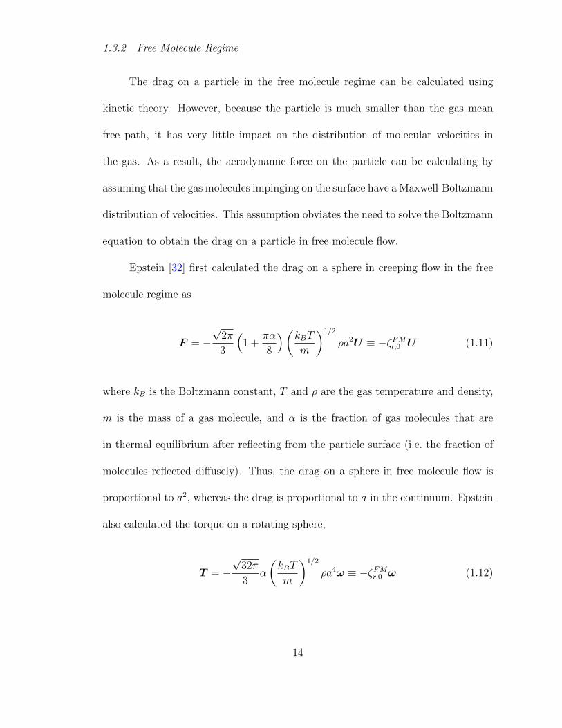
1.3.2 Free Molecule Regime

The drag on a particle in the free molecule regime can be calculated using

kinetic theory. However, because the particle is much smaller than the gas mean

free path, it has very little impact on the distribution of molecular velocities in

the gas. As a result, the aerodynamic force on the particle can be calculating by

assuming that the gas molecules impinging on the surface have a Maxwell-Boltzmann

distribution of velocities. This assumption obviates the need to solve the Boltzmann

equation to obtain the drag on a particle in free molecule flow.

Epstein [32] first calculated the drag on a sphere in creeping flow in the free

molecule regime as

F = −√

2π

3

(1 +

πα

8

)(kBTm

)1/2

ρa2U ≡ −ζFMt,0 U (1.11)

where kB is the Boltzmann constant, T and ρ are the gas temperature and density,

m is the mass of a gas molecule, and α is the fraction of gas molecules that are

in thermal equilibrium after reflecting from the particle surface (i.e. the fraction of

molecules reflected diffusely). Thus, the drag on a sphere in free molecule flow is

proportional to a2, whereas the drag is proportional to a in the continuum. Epstein

also calculated the torque on a rotating sphere,

T = −√

32π

3α

(kBT

m

)1/2

ρa4ω ≡ −ζFMr,0 ω (1.12)

14

showing that the torque is proportional to a4 for free molecule flow, compared to a3

in the continuum regime [32].

Dahneke [33] extended Epstein’s analysis to develop analytic expressions for

the drag on various convex bodies. The analysis is more complicated for concave

bodies – such as fractal aggregates – due to shielding of incoming molecules by parts

of the surface and the possibility of multiple collisions between a molecule and the

particle. Thus, numerical techniques are required for concave bodies. These tech-

niques track the trajectories of gas molecules near the particle to determine whether

or not the molecules hit the particles. For those molecules that hit the surface,

the momentum transfer is computed using an appropriate reflection law. Chan and

Dahneke [34] used this ballistic approach to compute the drag on straight chain

aggregates for flow parallel and perpendicular to the long axis of the chain. Meakin

and Deutch [55] applied the approach to determine the drag on fractal aggregates

and found that the drag is proportional to the projected area of the aggregate.

Mackowski [36] performed a similar analysis and developed an empirical correlation

for the translational friction coefficient as a function of the fractal dimension and

prefactor and the number of spheres for the range of parameters studied.

One could also apply the ballistic approach to compute the torque on a rotating

particle, though it does not appear anyone has done so based on the dearth of

information in the literature. Instead, researchers have used simplified techniques

to estimate the rotational friction or diffusion coefficient of aggregates in the free

molecule regime [6].

For fractal aggregates, results suggest that there is a power-law relationship

15

between the free molecule translational friction coefficient and the number of spheres

in the aggregate; this is similar to the observed behavior in the continuum. Sum-

marizing the available experimental and computational results in the literature,

Sorensen [4] recommended a power-law exponent of η ≈ 0.92 for DLCA clusters of

all sizes in the free molecule regime.

1.3.3 Transition Regime

As the particle size increases, the assumption that the particle has no impact

on the molecular velocity distribution around the particle no longer holds, and a

more rigorous application of kinetic theory is required. In the transition regime, the

drag can be obtained by solving the Boltzmann equation and integrating the stress

on the surface of the profile. However, the Boltzmann equation is exceeding difficult

to solve even for the simple case of a sphere, so significant simplifications are needed

to make the problem tractable. These simplifications will be described shortly, but

first I will focus on empirical models based on experimental data.

Millikan [64] laid the groundwork for determining the drag on a sphere in

the transition regime. Data from his famous oil drop experiments demonstrates

the transition between the continuum and free molecule regimes, where the drag is

proportional to a and a2, respectively. To cover the entire Knudsen number range,

one can apply a slip correction factor Cc(Kn) to Stokes’ law,

ζt,0 =6πµa

Cc(Kn)(1.13)

16

where the slip correction factor has the form

Cc(Kn) = 1 + Kn[A+B exp(−C/Kn)] (1.14)

The coefficients A, B, and C are selected to fit the experimental data; the coefficients

of Davies [65] and Allen and Raabe [66] are commonly used in aerosol applications.

Eq. (1.13) approaches the continuum and free molecule friction coefficients defined

in Eqs. (1.6) and (1.11) for Kn 1 and Kn 1, respectively.

Other researchers have developed empirical models for the drag on fractal

aggregates in the transition regime. Rogak et al. [37] proposed substituting the

projected area radius (aPA =√

PA/π) for a in Eq. (1.13). Lall and Friedlander [38]

suggested that the drag on an aggregate with fractal dimension less than 2 can be

approximated as a straight chain. Their correlation applies Chan and Dahneke’s

results for chain elements in the free molecule regime [34]. Finally, Eggersdorfer

et al. [39] relate the mobility radius (i.e. the radius of a sphere with the same drag

as the particles) to the number of primary spheres and the fractal dimension and

prefactor of the aggregate. The resulting model is similar to Rogak’s model for

particles formed by DLCA. These three models provide simple relationships for the

drag on fractal aggregates, though they are only valid near the free molecule regime.

(See Chapter 4.)

Dahneke [67] proposed an adjusted sphere method (ASM) for particles of ar-

bitrary shape, where the drag on the particle is given by an expression analogous

to Eq. (1.13). The difference is that a and Kn should be replaced by an appropri-

17

ate characteristic length and aggregate Knudsen number. Through scaling analysis,

Zhang et al. [41] demonstrated that the appropriate characteristic length is the hy-

drodynamic radius RH (i.e. the radius of a sphere that has the same drag as the

particle in continuum flow), and the aggregate Knudsen number is

Knagg = πλRH/PA (1.15)

where PA is the projected area of the particle. RH can be computed using the KR

or Hubbard-Douglas methods, and PA can be computed using ballistic methods.

Thus, the aggregate Knudsen number is proportional to the ratio of continuum and

free molecule measures of the drag. The drag calculated using the ASM is in good

agreement with experimental and computational results [41, 68, 69].

A number of researchers have managed to solve simplified forms of the Boltz-

mann equation for spheres and other axisymmetric bodies. Cercignani and Pagani

[70] described the general approach for solving the Boltzmann equation with the

Bhatnagar-Gross-Krook (BGK) model [71] in place of the Boltzmann collision opera-

tor using a variational technique. The BGK model assumes that the non-equilibrium

distribution of molecular velocities in the gas relaxes to an equilibrium distribution

after one collision. Kogan [72] has shown that this approximation is valid for most

physical situations. The variational approach of Cercignani and Pagani is valid for

any axisymmetric body.

Cercignani et al. [73] applied that technique to determine the drag on a sphere

as a function of Knudsen number. Their results are within a few percent of a fit

18

to Millikan’s data over a wide range of Knudsen numbers. Loyalka and colleagues

[74–76] obtained the velocity profile around the sphere as well as the drag using

methods similar to Cercignani et al. [73]. Later, Loyalka [77] and Takata et al.

[78] solved the problem using a linearized form of the Boltzmann collision operator.

The velocity and drag results from these studies are similar to the previous BGK

model results, which were obtained at a significantly lower computational cost than

the linearized Boltzmann results. Loyalka [77] also solved the linearized Boltzmann

equation to determine the velocity around and torque on a rotating sphere in the

transition flow regime.

In principal, one could solve the Boltzmann or BGK equation numerically to

obtain the drag on and flow field around a particle with arbitrary shape, but this is

exceedingly difficult in practice, especially for concave particles. One approach for

doing so is the direct simulation Monte Carlo method [40], which tracks a number

of test molecules and reconstructs the velocity distribution in the gas from the

behavior of these test molecules. This method is computationally expensive and is

less accurate near the continuum regime due to the finite size of the test domain

[41].

Melas et al. [79] determined the friction coefficient for aggregates in the near-

continuum regime by solving the Laplace equation with a slip boundary condition.

This approach is an extension of the Hubbard-Douglas approach (which uses the

stick boundary condition at the particle surface). Melas et al. [80] estimated that

this approach is valid for Kn < 2, meaning some other approach is needed for

particles closer to the free molecule regime.

19

Tandon and Rosner [81] developed a method for calculating the friction co-

efficient for fractal aggregates using a porous sphere approach. The porosity is a

function of radial position in the sphere and is obtained from the pair distribution

function for the orientation-averaged coordinates of monomers in the aggregate. The

velocity around the porous sphere is governed by the Stokes equations, while the

flow within the sphere is obtained by solving the Brinkman equation [4, 81]. Rosner

and Tandon [82] have shown that the porous sphere method gives friction coefficient

results in good agreement with the Adjusted Sphere Method of Dahneke [67] and

Zhang et al. [41] for any primary sphere size, provided the aggregate is large enough

that one can accurately treat the outer flow using the Stokes equation. In other

words, the aggregate size (e.g. the radius of gyration) must be very large compared

to the gas mean free path. Again, this means that a different approach is needed

for aggregates closer to the free molecule regime.

1.4 Experimental Techniques for Obtaining Particle Size

The work contained in this dissertation focuses on the theory of aerosol physics;

that is, I have not performed an experiments to support this work. Fortunately,

there is some data in the published literature to validate – or at least qualitatively

support – my theoretical results. To aid the reader in understanding comparisons

between the results in this dissertation and available experimental data, I will pro-

vide an overview of the experimental techniques used to size aerosol particles that

are pertinent to my own work.

20

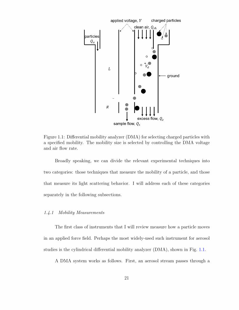
Figure 1.1: Differential mobility analyzer (DMA) for selecting charged particles witha specified mobility. The mobility size is selected by controlling the DMA voltageand air flow rate.

Broadly speaking, we can divide the relevant experimental techniques into

two categories: those techniques that measure the mobility of a particle, and those

that measure its light scattering behavior. I will address each of these categories

separately in the following subsections.

1.4.1 Mobility Measurements

The first class of instruments that I will review measure how a particle moves

in an applied force field. Perhaps the most widely-used such instrument for aerosol

studies is the cylindrical differential mobility analyzer (DMA), shown in Fig. 1.1.

A DMA system works as follows. First, an aerosol stream passes through a

21

neutralizer to obtain a known equilibrium charge distribution [2, 83]. The aerosol

stream enters the the cylindrical DMA at flow rate Qa along with a stream of clean

air (i.e. the sheath flow, Qsh). Particles are advected with the sheath flow; at the

same time, positively charged particles drift from the outer cylinder wall to the inner

wall, which has a negative potential. This drift velocity is the velocity required to

balance the electrical and aerodynamic drag forces on the particle:

ζtVd = qE (1.16)

Here, ζt is the particle translational friction coefficient, Vd is the drift velocity, q

is the charge on the particle, and E is the electric field strength. The field and

drift velocity are in the same direction. Particles that travel a radial distance R

in the time they travel an axial distance L pass through the slit in the DMA. The

remaining particles either deposit on the outer (negatively charged particles) or

inner (positively charged particles with higher mobility than the sampled particles)

wall of the DMA or pass out of the DMA with the excess flow. One selects the

voltage (and thus the field strength) and the sheath flow rate to obtain particles

with a desired electrical mobility Z, where

Z =VdE

=q

ζ(1.17)

By scanning through a series of voltages and counting the number of particles in the

sample flow at each voltage (e.g. with a condensation particle counter, as explained

22

in Chapter 6 of Friedlander [2]), one can determine the particle size distribution for

the aerosol that enters the DMA [2].

Often, researchers present the mobility as an equivalent sphere size by solving

Eq. (1.13) implicitly to find the mobility diameter dm [37–39, 43, 44, 68, 84]. Of

course, for a sphere the mobility diameter is equivalent to its geometric diameter.

The situation is much more complicated for fractal aggregates, so it is difficult to

obtain information about particle mass from a DMA. Furthermore, the DMA selects

some particles that have multiple charges in addition to those with a single charge,

which results in some error in the size distribution (since the larger, multiply-charged

particles have the same electrical mobility as the smaller, singly-charged particles).

To address these difficulty, systems for characterizing non-spherical particles

often involve both mobility measurements in a DMA and mass measurements in an

aerosol particle mass (APM) analyzer [43, 44, 85, 86]. Just as a DMA relies on a

balance between the electric force and the aerodynamic drag on a particle, an APM

sizes particles by balancing the electric force with the centrifugal force. When the

two forces are equal, the particle passes through the APM; otherwise, the particle

deposits on the inner or outer wall of the APM. In this way, one can size-select

particles based on their mass-to-charge ratio.

Researchers have developed other systems using combined mass and/or mo-

bility measurements to obtain additional size and shape information about aerosol

particles [44, 87, 88]. In many cases, mass and mobility measurements are sup-

plemented by information about primary particle size from transmission electron

microscopy (TEM) images; this information can be used with basic assumptions

23

about the fractal dimension of the aggregate to estimate the number of primary

spheres it contains [6, 44].

1.4.2 Optical Measurements

The second class of aerosol instruments that are relevant to my research in-

volve measuring the intensity of light scattered by the particles. (See Bohren and

Huffman [89] for the detailed discussion on the theory of light scattering by small

particles.) These optical instruments are used for a variety of purposes, from de-

termining the number density of particles in a gas stream (e.g. in a condensation

particle counter), to obtaining information about particle shape, to determining the

rotational diffusion coefficient of a particle. I will focus my attention on the latter

application.

In general, the angular distribution of the light scattered by a particle is a

function of that particle’s orientation. In the absence of a strong external force

field, the light scattered by a nano-scale aerosol particle is an average over all orien-

tations, where all orientations are equally probable due to the randomizing effects

of Brownian motion. However, particles can become aligned in a strong electric field

if the interaction energy between the induced dipole in the particle and the field is

much larger in magnitude than the Brownian energy kBT , where kB is the Boltz-

mann constant and T is the temperature. By measuring the change in scattered

light intensity when the field is on and off, one can obtain some information about

the shape of particles. One can also obtain the rotational diffusion coefficient of a

particle by turning off the field and measuring the time required for the scattered

24

light intensity to relax to a value corresponding to the random particle orientation.

Such measurements have been reported in the literature for soot particles from var-

ious sources [90, 91]; I will later compare my results for the rotational diffusion

coefficients of soot-like aggregates to the experimental data of Colbeck et al. [91].

This experimental technique also offers an alternative approach to the method I

describe in Chapter 7 for obtaining particle shape information.

1.5 Scope of the Dissertation

This dissertation describes a method [92] for calculating the drag on an aggre-

gate of spheres in point contact in the transition flow regime, based on Kirkwood-

Riseman theory originally developed for the continuum regime [28]. Generally speak-

ing, Chapters 2, 3, and 5 introduce the method, while Chapters 4 and 6-8 focus on

applications of the method.

In Chapter 2, I discuss the Bhatnagar-Gross-Krook model equation and its

solution for flow around a sphere as a function of the Knudsen number. This chapter

follows the earlier work of Loyalka and colleagues [74–76]. I include this discussion

because my EKR method uses the flow around an isolated sphere to determine the

drag and torque on an N -sphere aggregate.

In Chapter 3, I develop a new approach for computing the hydrodynamic

friction tensor and scalar friction coefficient for an aerosol fractal aggregate in the

transition regime [92]. My approach involves solving the BGK equation for the ve-

locity field around a sphere and using the velocity field to calculate the force on

25

each primary sphere in the aggregate due to the presence of the other spheres. It

is essentially an extension of Kirkwood-Riseman theory from the continuum flow

regime to the entire Knudsen range (Knudsen number from 0.01 to 100 based on

the primary sphere radius). Results compare well to published Direct Simulation

Monte Carlo results and converge to the correct continuum and free molecule limits.

My calculations for clusters with up to 100 spheres support the theory that aggre-

gate slip correction factors collapse to a single curve when plotted as a function of

an appropriate aggregate Knudsen number. This self-consistent field approach cal-

culates the friction coefficient very quickly, so the approach is well-suited for testing

existing scaling laws in the field of aerosol science and technology, as I demonstrate

for the adjusted sphere scaling method.

In Chapter 4, I use the self-consistent field method described in Chapter 3 to

calculate the translational friction coefficient of fractal aerosol particles formed by

diffusion-limited cluster aggregation (DLCA) [93]. The method involves solving the

Bhatnagar-Gross-Krook model for the velocity around a sphere in the transition flow

regime. The velocity and drag results are then used in an extension of Kirkwood-

Riseman theory to obtain the drag on the aggregrate. Results span a range of

primary sphere Knudsen numbers from 0.01 to 100 for clusters with up to N =

2000 primary spheres. Calculated friction coefficients are in good agreement with

experimental data and approach the correct continuum and free molecule limits

for small and large Knudsen numbers, respectively. Results show that particles

exhibit more continuum-like behavior as the number of primary spheres increase,

even when the primary particle is in the free molecule regime; as an illustrative

26

example, the friction coefficient for aggregates with primary sphere Kn = 1 are

approximately equal to the continuum friction coefficient for N > 500. I estimate

that the calculations are within 10% of the true values of the friction coefficients

for the range of Kn and N presented here. Finally, I use my results to develop an

analytical expression (Equation 4.38) for the friction coefficient over a wide range

of aggregate and primary particle sizes.

In Chapter 5, I apply extended Kirkwood-Riseman theory to compute the

translation, rotation, and coupling friction tensors and the scalar rotational friction

coefficient for an aerosol fractal aggregate in the transition flow regime [94]. The

method can be used for particles consisting of spheres in contact. The approach

considers only the linear velocity of the primary spheres in a rotating aggregate

and ignores rotational and coupling interactions between spheres. I show that this

simplified approach is within approximately 40% of the true value for any particle

for Knudsen numbers between 0.01 and 100. The method is especially accurate (i.e.

within about 5%) near the free molecule regime, where there is little interaction

between the particle and the flow field, and for particles with low fractal dimension

(less than ≈ 2) consisting of many spheres, where the average distance between

spheres is large and translational interaction effects dominate. Results suggest that

there is a universal relationship between the rotational friction coefficient and an

aggregate Knudsen number, defined as the ratio of continuum to free molecule ro-

tational friction coefficients.

In Chapter 6, I apply the EKR method to calculate the rotational friction co-

efficient for fractal aerosol particles in the transition flow regime [95]. The method

27

considers hydrodynamic interactions between spheres in a rotating aggregate due

to the linear velocities of the spheres. Results are consistent with electro-optical

measurements of soot alignment. Calculated rotational friction coefficients are also

in good agreement with continuum and free molecule results in the limits of small

(Kn = 0.01) and large (Kn = 100) primary sphere Knudsen numbers. As demon-

strated for the translational friction coefficient (Chapter 4), the rotational friction

coefficient approaches the continuum limit as either the primary sphere size or the

number of primary spheres increases. I apply my results to develop an analytical

expression (Equation 6.26) for the rotational friction coefficient as a function of the

primary sphere size and number of primary spheres. One important finding is that

the ratio of the translation to rotational diffusion times is nearly independent of clus-

ter size. I include an extension of previous scaling analysis for aerosol aggregates to

include rotational motion.

In Chapter 7, I study the effects of electric field strength on the mobility of

soot-like fractal aggregates (fractal dimension of 1.78) [96]. The probability dis-

tribution for the particle orientation is governed by the ratio of the interaction

energy between the electric field and the induced dipole in the particle to the energy

associated with Brownian forces in the surrounding medium. I use the extended

Kirkwood-Riseman method to calculate the friction tensor for aggregates of up to

2000 spheres, with primary sphere sizes in the transition and near-free-molecule

regimes. My results for electrical mobility versus field strength are in good agree-

ment with published experimental data for soot, which show an increase in mobility

on the order of 8% from random to aligned orientations. My calculations show

28

that particles become aligned at decreasing field strength as particle size increases

because particle polarizability increases with volume. Large aggregates are at least

partially aligned at field strengths below 1000 V/cm, though the small change in mo-

bility means that alignment is not an issue in many practical applications. However,

improved DMAs would be required to take advantage of small changes in mobility

to provide shape characterization.

In Chapter 8, I present a method for calculating the hydrodynamic interac-

tions between particles in the kinetic (or transition) regime, characterized by non-

negligible particle Knudsen numbers. Such particles are often present in aerosol

systems. The method is based on my extended Kirkwood-Riseman theory [92],

which accounts for interactions between spheres using the velocity field around a

translating sphere as a function of Knudsen number. Results for the two-sphere

problem at small Knudsen numbers are in good agreement with those obtained us-

ing Felderhof’s interaction tensors for mixed slip-stick boundary conditions, which

are accurate to order r−7 [97]. The strength of interactions decreases with increasing

Knudsen number. Results for two fractal aggregates demonstrate that one can apply

a point force approach for interactions between particles in the transition regime;

the interaction tensor is similar to the Oseen tensor for continuum flow. Using this

point force approach, I present an analysis for the settling of an unbounded cloud of

particles. The analysis shows that for sufficiently high volume fractions and cloud

radii, the cloud behaves as a gas droplet in continuum flow even when the individual

particles are small relative to the mean free path of the gas. The method presented

here can be applied in a Brownian dynamics simulation analogous to Stokesian

29

dynamics to study the behavior of a dense aerosol system.

Chapter 9 is the Reference Manual for the NGDE code. The NGDE code uses

a nodal method to solve the general dynamic equation for an aerosol undergoing

coagulation, nucleation, and surface growth. This method is similar to widely-

used sectional methods for solving the general dynamic equation, but by dividing

the particle size distribution into discrete volume nodes, it eliminates many of the

mathematical complexities of sectional methods. I have converted the original C

version of NGDE to the MATLAB language, added a dynamic time step algorithm

that reduces the code execution time by orders of magnitude, and created a new

post-processing tool for viewing the evolution of the particle size distribution and the

light scattering, extinction, and absorption coefficients. Results of sample problems

compare well to results obtained from other methods. Because of NGDE’s simplicity

and accuracy, it is well-suited for use as part of courses in aerosol dynamics.

The main body of the dissertation closes with a summary of the important

conclusions of my research in Chapter 10.

30

Chapter 2: The BGK Model Equation

2.1 Introduction

Solution of the density, velocity, and temperature fields around a sphere in

the transition regime (0.01 < Kn < 100) requires consideration of the Boltzmann

equation or its derivatives. For steady flow, the Boltzmann equation can be written

in dimensional form as

c · ∇f =δf

δt

∣∣∣∣coll

(2.1)

where c is the molecular velocity, f = f(r, c) is the molecular velocity distribution

function, and the term on the right-hand side of the equation is the collision op-

erator.1 The distribution function is defined such that f(r, c)drdc represents the

number of gas molecules in differential volume dr centered at location r that have

a velocity between c and c+ dc.

The collision operator can be written as the difference between two terms. The

1Throughout this chapter, I am using bold symbols to denote vectors, bold symbols with hatsto denote unit vectors, the subscript ∞ to denote properties far from the perturbation, and atilde over dimensional quantities that also appear in non-dimensional form without the tilde. Toexpand on the latter point, I do not add a tilde to all dimensional quantities; I only add it toexplicitly differentiate between dimensional and non-dimensional variants of the same quantity.For example, temperature always appears as T because I only use it as a dimensional quantity,whereas the molecular velocity c appears with and without the tilde to signify dimensional andnon-dimensional variants.

31

first (positive) term represents the rate at which molecules are scattered into the

interval [c, c+dc] as a result of collisions, while the second (negative) term represents

the molecules in this velocity interval that are scattered out of the interval due to

collisions with other molecules. The collision operator is the chief source of difficulty

in the Boltzmann equation; it makes solving the equation analytically impossible

for all but the simplest cases.

To address this difficulty, Bhatnagar, Gross, and Krook [71] proposed a sim-

plified form of the collision operator,

δf

δt

∣∣∣∣coll

=f0(r, c)− f(r, c)

τ(c)(2.2)

where τ(c) is the (velocity-dependent) mean collision time in the gas and

f0 = n

(m

2πkBT

)3/2

exp

[−m|c− U |

2

2kBT

](2.3)

is the Maxwell-Boltzmann distribution at the local number density n, bulk velocity

U , and temperature T . The BGK model for the collision operator expresses the fact

that any distribution f decays to the Maxwellian distribution, where the relaxation

time can be approximated as the time between collisions [71, 72]. The second term

on the right-hand side of Eqn. (2.2) has the same general form as the depletion term

in the Boltzmann collision operator: in both cases, depletion is directly proportional

to f(r, c) and to the frequency of collisions between molecules with velocity c and

all other molecules. Strictly speaking, the collision frequency is a function of the

32

molecular velocity, though it is possible to use an average collision time [46] (hence

the appearance of the mean collision time τ in later equations). The f0 term in

Eq. (2.2) does not have a direct mathematical relationship to the replenishing term

in the Boltzmann equation. Instead, this term in the BGK model assumes that the

distribution relaxes to the local Maxwellian distribution after one collision. Kogan

[72] has demonstrated that in most physical situations, the velocity distribution after

one collision is fairly close to the equilibrium distribution. Thus, the BGK model

is a reasonable approximation to the Boltzmann collision operator, especially for

near-equilibrium situations like creeping flow of a sphere at the same temperature

as the surrounding gas.

Based on the preceding discussion, we can simplify our equation for the dis-

tribution function by substituting the BGK model for the collision operator in the

Boltzmann equation. The resulting equation is known as the Krook equation. For

steady flow, we have

c · ∇f =f0(r, c)− f(r, c)

τ(c)(2.4)

We can non-dimensionalize the above equation by defining the variables

c =c

(2kBT∞/m)1/2(2.5a)

U =U

(2kBT∞/m)1/2(2.5b)

r =r

τ(2kBT∞/m)1/2(2.5c)

33

where τ is the collision time averaged over all molecular velocities. Setting the mean

collision time as τ = µ/p (where p is pressure) and the viscosity as µ = 0.499λρc, the

non-dimensional sphere radius is related to the Knudsen number by the following

expression:2

r0 =r0

τ(2kBT∞/m)1/2=

√π

1.996Kn−1 (2.5d)

Applying the length and velocities scales in Eq. (2.5), the non-dimensional

Krook equation for steady flow becomes

c · ∇f = f0(r, c)− f(r, c) (2.6)

While the Krook equation is much simpler than the Boltzmann equation, the

Krook equation is still difficult to solve because the number density, bulk velocity,

and temperature that appear in f0 are all functions of the local conditions in the

gas. In other words, these variables each depend on f .

To simplify the equation further, we can treat any disturbance in the distribu-

tion function as a small perturbation to the linearized far-away distribution function

f∞(1 + 2c ·U∞),3

f ≈ f∞(1 + 2c ·U∞ + h) (2.7)

2The definition of the mean collision time comes from the Chapman-Enskog solution of theKrook equation, which shows that µ from the Chapman-Enskog solution is identical to µ forcontinuum flow if we set µ = pτ [46]. The expression relating the viscosity to the mean free pathapplies to monatomic gases [46], but it is a reasonable approximation for air and is used in manyaerosol studies in the literature (e.g. [41, 73])

3Here, we have linearized the Maxwellian distribution defined in Eq. (2.3) by expanding thedistribution in powers of U∞. This approach assumes that the stream velocity is very smallcompared to the thermal speed, which is certainly true for creeping flow.

34

where

f∞ = n∞

(m

2πkBT∞

)3/2

exp

(− mc2

2kBT∞

)(2.8)

We can also linearize the Maxwellian distribution to get

f0 ≈f∞(1 + 2c ·U∞) +∂[f(1 + 2c ·U)]

∂n

∣∣∣∣∞

(n− n∞)

+∂[f(1 + 2c ·U)]

∂U

∣∣∣∣∞· (U −U∞) +

∂[f(1 + 2c ·U)]

∂T

∣∣∣∣∞

(T − T∞)

=f∞

[1 + 2c ·U∞ +

(n

n∞− 1

)+ 2c · (U −U∞) +

(c2 − 3

2

)(T

T∞− 1

)]

f0 ≈ f∞

[1 + 2c ·U∞ + ε1 + c · ε2 +

(c2 − 3

2

)ε3

](2.9)

where

n(r) = n∞(1 + ε1) (2.10a)

U (r) = U∞ +1

2ε2 (2.10b)

T (r) = T∞(1 + ε3) (2.10c)

and ε1, ε2, and ε3 are perturbations to the far-field number density, velocity, and

temperature, respectively. These perturbations will be defined shortly.

From kinetic theory, the number density, bulk velocity, and temperature are

defined in terms of moments of the distribution function f :

n =

∫fdc (2.11a)

35

U =1

n

∫cfdc (2.11b)

3

2T =

1

n

∫c2fdc (2.11c)

We define the pertrubation ε1 and ε2 by substituting Eq. (2.7) into Eqns. (2.11a)

and (2.11b), respectively:

n =

∫f∞(1 + 2c ·U∞ + h)dc = n∞ + n∞π

−3/2

∫h exp(−c2)dc = n∞(1 + ε1)

U =1

n∞

∫f∞(1 + 2c ·U∞ + h)cdc = U∞ + π−3/2

∫hc exp(−c2)dc = U∞ +

1

2ε2

Similarly, we define the temperature perturbation by substituting Eq. (2.7) into

Eq. (2.11c):

3

2T =

1

n

∫f∞(1 + 2c ·U∞ + h)c2dc

3

2T∞(1 + ε3) =

1

n∞(1 + ε1)

∫f∞(1 + 2c ·U∞ + h)c2dc

3

2T∞(1 + ε1 + ε3 + ε1ε3) =

3

2T∞ + π−3/2

∫c2h exp(−c2)dc

ε3 =2

3

[π−3/2

∫c2h exp(−c2)dc− 3

2ε1

]=

2

3π3/2

∫h exp(−c2)

(c2 − 3

2

)dc

Note that we have ignored the ε1ε3 term because it is of order ε2 (and thus very small

compared to the other terms in the equation). To summarize, the number density,

bulk velocity, and temperature perturbations are moments of the perturbation to

the distribution function h and are defined as

ε1(r) = (h, 1) (2.12a)

36

ε2(r) = 2(h, c) (2.12b)

ε3(r) =2

3

(h, c2 − 3

2

)(2.12c)

where the inner product (h(r, c), g(c)) is defined as

(h, g) = π−3/2

∫ ∞−∞

hg exp(−c2)dc (2.13)

We can apply the linearized forms of f and f0 given by Eqns. (2.7) and (2.9)

to Eq. (2.6):

c · ∇f =f0 − f

c · ∇[f∞(1 + 2c ·U∞ + h)] =f∞

[1 + 2c ·U∞ + ε1 + c · ε2 +

(c2 − 3

2

)ε3

]− f∞(1 + 2c ·U∞ + h)

c · ∇h =ε1 + c · ε2 +

(c2 − 3

2

)ε3 − h

This equation can be written as

c · ∇h = Lh (2.14)

where the operator L is defined as

Lh = ε1 + c · ε2 +2

3

(c2 − 3

2

)ε3 − h (2.15)

It is in this form [i.e. Eqns. (2.14) and (2.15)] that the Krook equation appears in

37

papers by Cercignani and Pagani [70] and Lea and Loyalka [75].

Now that I have completed the derivation of the BGK model and Krook equa-

tion, I can apply the equation to practical problems of mass transfer to and flow

around a sphere. I will first discuss briefly the isothermal mass transfer problem

because it is simpler mathematically than the flow problem, and thus it provides

a good introduction for solving the Krook equation. Once I have discussed solving

the condensation problem, I will turn my attention to the problem most relevant to

this dissertation, that of uniform flow around a sphere. Note that in solving these

problems, I am following the derivation of Lea [74].

2.2 Solution of the Krook Equation for Isothermal Mass Transfer to

a Sphere

Let us start by considering mass transfer of a dilute vapor to a sphere. There is

no bulk flow, so ε2 = 0. We will also assume that the region of interest is isothermal,

so ε3 = 0. This leaves us with the following equation for the perturbation to the

distribution function:

c · ∇h = (h, 1)− h (2.16)

We can write this equation in terms of the characteristic path, s:

dh

ds+h

c=

(h, 1)

c(2.17)

38

Here, the derivative along the characteristic path is related to the diffusion term on

the left-hand side of Eq. (2.14) by

Ω · ∇h =Ωx∂h

∂x+ Ωy

∂h

∂y+ Ωz

∂h

∂z

=∂x

∂s

∂h

∂x+∂y

∂s

∂h

∂y+∂z

∂s

∂h

∂z

=dh

ds

where Ω = c/c is the direction vector of the molecular velocity. The geometry of

this problem is shown in Fig. 2.1.

We can solve Eq. (2.17) using an integration factor, giving

h(r, c) = exp(−sc

)∫ s

−∞exp

(s′′

c

)h′′

cds′′ (2.18)

where h = h(rp + s Ω, c Ω) and h′′ = h(rp + s′′Ω, c Ω). Substituting s′ = s − s′′ =

|r − r′| (see Fig. 2.1), our integral equation becomes

h(r, c) =

∫ ∞0

exp

(−s′

c

)(h′)

cds′ (2.19)

where h′ = h(r−s′Ω, c Ω). The above equation applies to all paths that are outside

of the solid angle ω. Within the solid angle, we must account for the boundary

condition at the surface, which in this case is

h(r, c) = 0, c · n > 0, r = r0er (2.20)

39

Figure 2.1: Geometry for the mass transfer problem (adapted from Fig. 1 of Lea[74])

40

This BC represents the fact that all vapor molecules that reach the sphere are

absorbed and none are reflected. With this condition, the contribution to h from

points within solid angle ω are

h(r, c) =

∫ |r−r0|0

exp

(−s′

c

)(h′, 1)

cds′ (2.21)

where the upper limit of integration is the distance between point r and the surface

of the sphere.

For this problem, we are most interested in the number density moment ε1 =

(h, 1). Taking the moment of Eq. (2.19), we get

ε1 =π−3/2

∫ ∞0

∫ ∞0

exp(−c2)

cexp

(−s′

c

)ε1(s′)ds′dc

=π−3/2

∫ ∞0

∫ ∞0

∫θ

∫φ

c exp

(−c2 − s′

c

)ε1(s′) sin θdφdθds′dc

=π−3/2

∫ ∞0

∫θ

∫φ

T1 (s′)ε(s′) sin θdφdθds′

=π−3/2

∫T1 (|r − r′|)|r − r′|2

ε1(r′)dr′

where

Tn(x) =

∫ ∞0

cn exp(−c2 − x

c

)dc (2.22)

and the integration includes the region outside of solid angle ω.4 More information

about Tn(x) can be found in Section 27.5 of Abramowitz and Stegun [98]. We get

4In deriving the equation for ε1, we first write the integral over molecular velocities in terms ofpolar coordinates, i.e. dc = c2dcdΩ = c2 sin θdφdθdc. Because the unit vector Ω appears in boththe spatial and velocity components of h, and because s′ and c are independent variables, we canswitch the order of integration over ds′ and dc and write sin θdφdθds′ = dsdΩ/s′ 2 = dr′/s′ 2.

41

the same result if we take the moment of Eq. (2.21), except the integration bounds

the region inside solid angle ω between point r and the surface of the sphere. Thus,

our equation for the number density moment is

ε1(r) = π−3/2

∫V

T1 (|r − r′|)|r − r′|2

ε1(r′)dr′ (2.23)

where V includes all points in space that can be reached from r without first passing

through the sphere.

It is possible to solve Eq. (2.23) numerically by providing an initial guess for

ε1 (either as a function or as a set of values are specified values of r), performing

the integration for a set of radii, comparing the resulting ε1(r) to the initial guess,

and iterating (i.e. using Newton’s method or some other suitable technique). Note

Eq. (2.23) only gives ε1(r) up to some constant multiplier, since if we multiply ε1(r′)

by a constant in the integral, we get ε1(r) multiplied by that same constant. One

obtains the correct numerical values by noting that far from the sphere, the vapor

concentration is given by the Chapman-Enskog solution for diffusion [21, 99]. It is

possible to simplify Eq. (2.23) further by integrating over the angles θ and φ, leaving

only the integral over the radius. The procedure is similar to the procedure that I

will describe in the next section for flow around a sphere. For further information

on solving the mass transfer problem, refer to Lea [74].

42

2.3 Solution of the Krook Equation for Uniform Flow Around a

Sphere

I will now consider the problem that is more pertinent to this dissertation,

that of uniform flow around a sphere in the transition regime. I will start with the

derivation of the equations, then I will consider the numerical strategies that I will

use to solve the problem.

2.3.1 Derivation of the Governing Equations

For this problem, let us consider the situation where the sphere is at the same

temperature as the surrounding gas. Note that this does not mean the flow field is

isothermal [76, 78], so we must consider all of the terms in the Krook equation.5

We start by writing Krook equation with the diffusion term as a derivative

along the characteristic path, as we did for the problem of mass transfer to the

sphere:

dh

ds+h

c=

1

c

[(h, 1) + 2c · (h, c) +

2

3

(c2 − 3

2

)(h, c2 − 3

2

)](2.24)

Again, we can apply an integrating factor to convert the integro-differential

5In continuum flow, the flow field is isothermal, but this is not the case outside of the continuumregime. However, Law and Loyalka [76] have shown that accounting for temperature fluctuationshas only a minor impact on the calculated velocity profile and drag force. Their published resultscompare favorably to the earlier results of Lea and Loyalka [75] that assume an isothermal flowfield. Nevertheless, I will account for ε3 6= 0 in my calculations because it better represents thephysics of the problem.

43

equation to an integral equation, which gives us

h(r, c) =

∫ ∞0

1

cexp

[−s′

c

] [(h′, 1) + 2c · (h′, c) +

2

3

(c2 − 3

2

)(h′, c2 − 3

2

)]ds′

(2.25)

for the region of space outside of the solid angle ω and

h(r, c) = h0 exp[−sc

]+

∫ s

0

1

cexp

[−(s− s′)

c

] [(h′, 1) + 2c · (h′, c)

+2

3

(c2 − 3

2

)(h′, c2 − 3

2

)]ds′ (2.26)

for the region of space in the solid angle ω between r and the surface of the sphere.

In Eq. (2.25), s′ = |r − r′| and h′ = h(r − s′Ω, c). In Eq. (2.26), s − s′ = |r − r′|,

h′ = h(r0+s′Ω, c), h0 = h(r0, c) (i.e. the value of h at the surface of the sphere), and

s = |r−r0|. (See Fig. 2.2 for the geometry described by Eq. 2.25 and Fig. 2.3 for the

geometry described by Eq. 2.26.) The integral terms in these two equations represent

the contribution to h from molecules whose last collision was with another gas

molecule, while the non-integral term on the right-hand side of Eq. (2.26) describes

the contribution to h from molecules whose previous collision was with the sphere.

Next, we must take the moments of h(r, c) to find ε1(r), ε2(r), and ε3. We

44

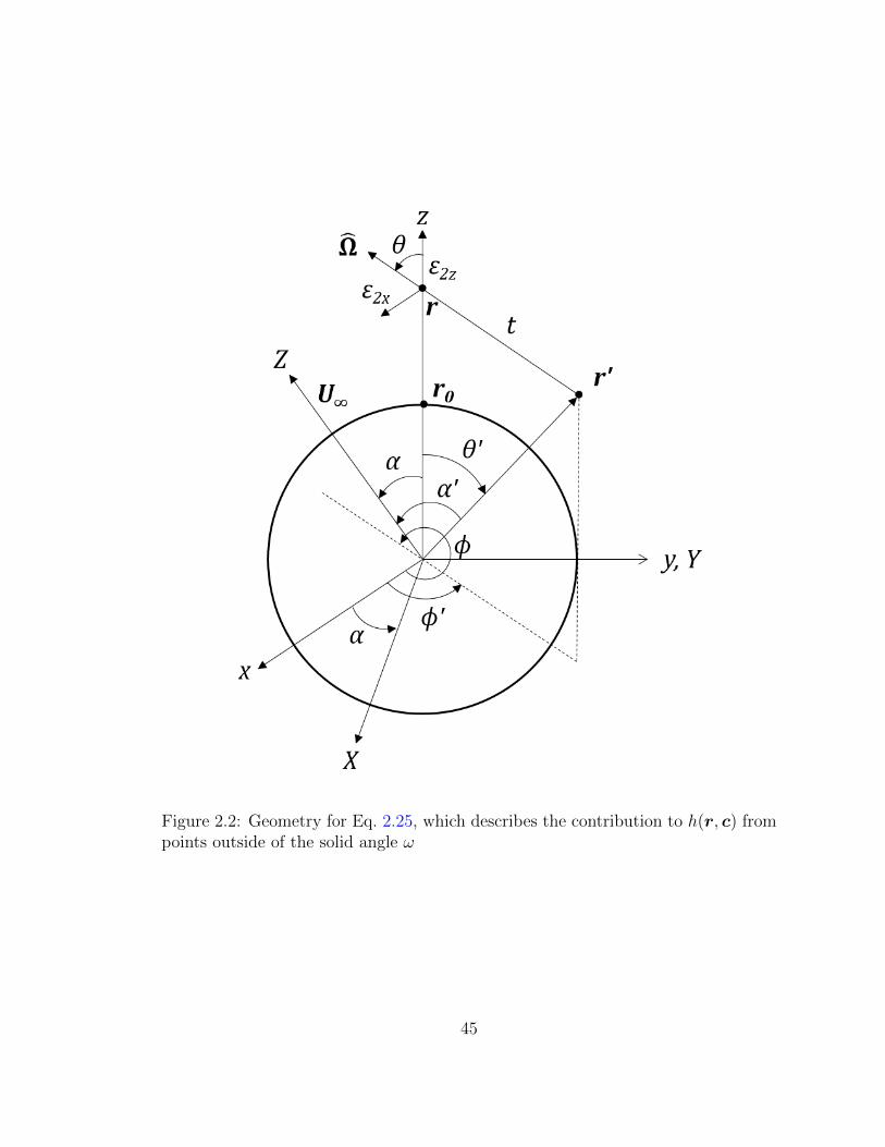
Figure 2.2: Geometry for Eq. 2.25, which describes the contribution to h(r, c) frompoints outside of the solid angle ω

45

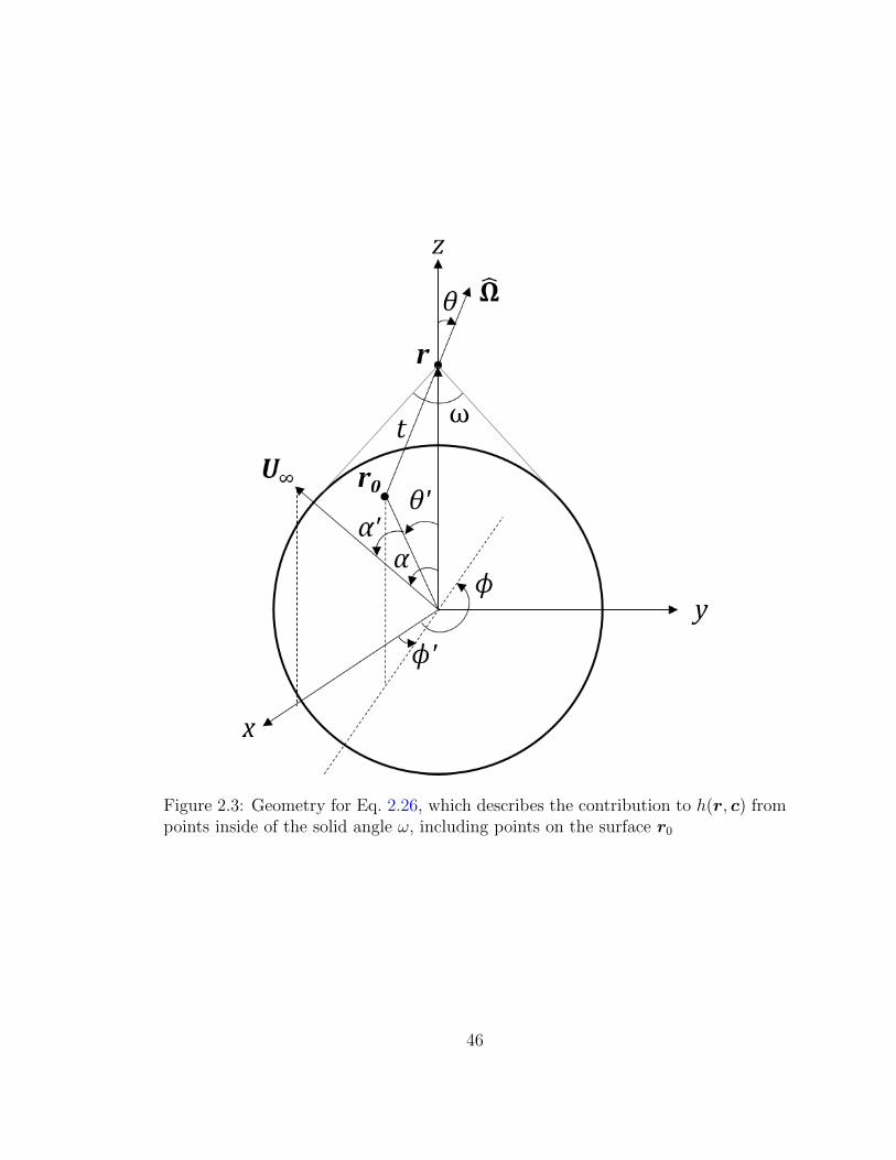
Figure 2.3: Geometry for Eq. 2.26, which describes the contribution to h(r, c) frompoints inside of the solid angle ω, including points on the surface r0

46

start by taking the moment (h, 1) using Eq. (2.25):

ε1(r) =π−3/2

∫ ∞0

∫ ∞0

1

cexp

[−s′

c

] [(h′, 1) + 2c · (h′, c)

+2

3

(c2 − 3

2

)(h′, c2 − 3

2

)]ds′dc

=π−3/2

∫ ∞0

∫θ

∫φ

∫ ∞0

c sin θ exp

[−s′

c

] [(h′, 1) + 2c · (h′, c)

+2

3

(c2 − 3

2

)(h′, c2 − 3

2

)]dcdφdθds′

=π−3/2

∫ ∞0

∫θ

∫φ

sin θ

[T1(s′)(h′, 1) + 2 T2(s′)Ω · (h′, c)

+2

3

(T3(s′)− 3

2T1(s′)

)(h′, c2 − 3

2

)]dφdθds′

=π−3/2

∫dr′

|r − r′|2

[T1 ε1(r′) + T2 Ω · ε2 +

(T3−

3

2T1

)ε3(r′)

]

The argument of the Tn functions in the last equality is |r − r′|.

Taking the moment (h, 1) using Eq. (2.26) gives the same result for the integral

over ds′ (i.e. the second term on the right-hand side of the equation), so now we

must determine the contribution from the surface of the sphere. This is simply∫h0 exp(−c2 − s

c)dc, where again s = |r − r0|. Thus, the perturbation to the

number density is

ε1(r) = π−3/2

∫C

h(r0, c) exp

(−c2 − |r − r0|

c

)dc

+

∫V

dr′

|r − r′|2

[T1 ε1(r′) + T2 Ω · ε2(r′) +

(T3−

3

2T1

)ε3(r′)

](2.27)

The domain C accounts for all molecules reflected from the sphere whose trajectory

47

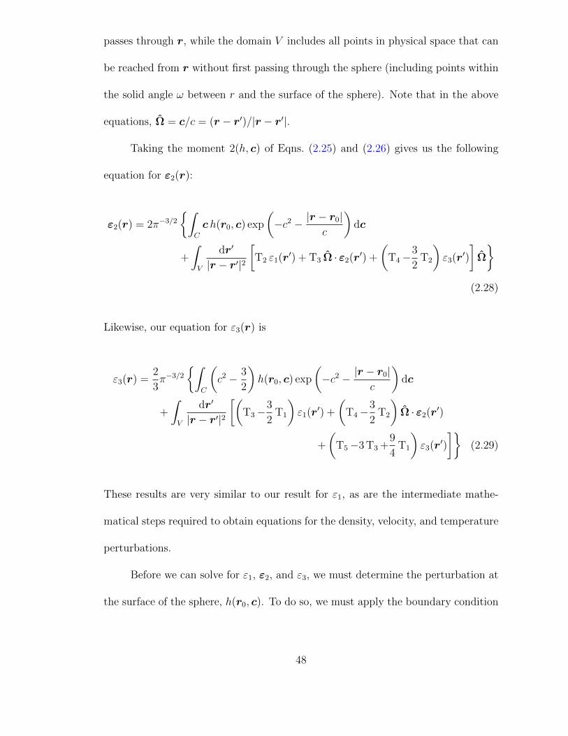
passes through r, while the domain V includes all points in physical space that can

be reached from r without first passing through the sphere (including points within

the solid angle ω between r and the surface of the sphere). Note that in the above

equations, Ω = c/c = (r − r′)/|r − r′|.

Taking the moment 2(h, c) of Eqns. (2.25) and (2.26) gives us the following

equation for ε2(r):

ε2(r) = 2π−3/2

∫C

ch(r0, c) exp

(−c2 − |r − r0|

c

)dc

+

∫V

dr′

|r − r′|2

[T2 ε1(r′) + T3 Ω · ε2(r′) +

(T4−

3

2T2

)ε3(r′)

]Ω

(2.28)

Likewise, our equation for ε3(r) is

ε3(r) =2

3π−3/2

∫C

(c2 − 3

2

)h(r0, c) exp

(−c2 − |r − r0|

c

)dc

+

∫V

dr′

|r − r′|2

[(T3−

3

2T1

)ε1(r′) +

(T4−

3

2T2

)Ω · ε2(r′)

+

(T5−3 T3 +

9

4T1

)ε3(r′)

](2.29)

These results are very similar to our result for ε1, as are the intermediate mathe-

matical steps required to obtain equations for the density, velocity, and temperature

perturbations.

Before we can solve for ε1, ε2, and ε3, we must determine the perturbation at

the surface of the sphere, h(r0, c). To do so, we must apply the boundary condition

48

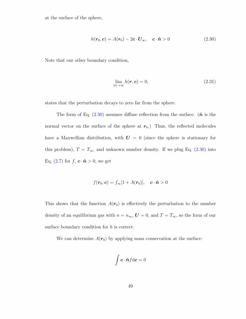
at the surface of the sphere,

h(r0, c) = A(r0)− 2c ·U∞, c · n > 0 (2.30)

Note that our other boundary condition,

lim|r|→∞

h(r, c) = 0, (2.31)

states that the perturbation decays to zero far from the sphere.

The form of Eq. (2.30) assumes diffuse reflection from the surface. (n is the

normal vector on the surface of the sphere at r0.) Thus, the reflected molecules

have a Maxwellian distribution, with U = 0 (since the sphere is stationary for

this problem), T = T∞, and unknown number density. If we plug Eq. (2.30) into

Eq. (2.7) for f , c · n > 0, we get

f(r0, c) = f∞[1 + A(r0)], c · n > 0

This shows that the function A(r0) is effectively the perturbation to the number

density of an equilibrium gas with n = n∞, U = 0, and T = T∞, so the form of our

surface boundary condition for h is correct.

We can determine A(r0) by applying mass conservation at the surface:

∫c · nfdc = 0

49

Physically, this integral states that the net mass flux at the surface of the sphere

is zero. Breaking our integral into two parts – the molecules moving towards the

surface and those moving from the surface – and substituting for f , we get

∫c · n>0

c · nf∞(1 + 2c ·U∞ + h)dc = −∫c · n<0

c · nf∞(1 + 2c ·U∞ + h)dc

The constant terms cancel in the integrals due to the symmetry of the Maxwellian

distribution, so our mass balance becomes

∫c · n>0

c · n exp(−c2)(2c ·U∞ + h0)dc = −∫c · n<0

c · n exp(−c2)(2c ·U∞ + h0)dc

(2.32)

For the term on the left-hand side, we can substitute Eq. (2.30) for h and

perform the integration,

∫c · n>0

c · n exp(−c2)(2c ·U∞ + h0)dc =

∫c · n>0

c · n exp(−c2)A(r0)dc

=A

∫c · n>0

c Ω · n exp(−c2)dc

=A

∫ π/2

0

dθ

∫ 2π

0

dφ

∫ ∞0

dc c3 cos θ sin θ exp(−c2)

=π

2A(r0)

We can also integrate the first term on the right-hand side (i.e. the term

involving c ·U∞). Before performing the integration, we will define α as the angle

between n and U∞, θ as the polar angle between n and Ω, and φ as the angle

between U sinα and sin θ. (See Fig. 2.4.) These definitions will be used to evaluate

50

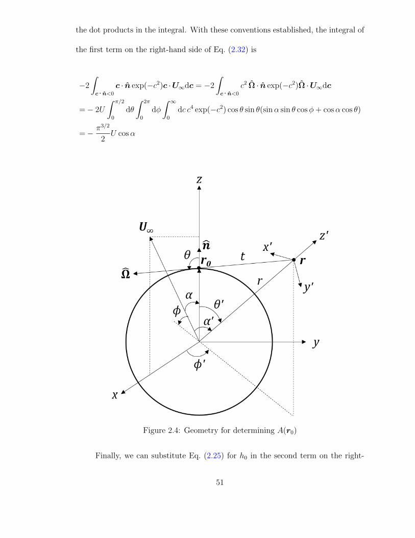
the dot products in the integral. With these conventions established, the integral of

the first term on the right-hand side of Eq. (2.32) is

−2

∫c · n<0

c · n exp(−c2)c ·U∞dc = −2

∫c · n<0

c2 Ω · n exp(−c2)Ω ·U∞dc

=− 2U

∫ π/2

0

dθ

∫ 2π

0

dφ

∫ ∞0

dc c4 exp(−c2) cos θ sin θ(sinα sin θ cosφ+ cosα cos θ)

=− π3/2

2U cosα

Figure 2.4: Geometry for determining A(r0)

Finally, we can substitute Eq. (2.25) for h0 in the second term on the right-

51

hand side of Eq. (2.32) and perform the integration:

∫c · n<0

hc · n exp(−c2)dc

=

∫c · n<0

dc

∫ ∞0

ds′c

c· n exp

[−c2 − s′

c

] [(h′, 1) + 2c · (h′, c)

+2

3

(c2 − 3

2

)(h, c2 − 3

2

)]=

∫ ∞0

ds′∫

Ω · n<0

dΩ

∫ ∞0

dc c2 exp

[−c2 − s′

c

] [(h′, 1) + 2c · (h′, c)

+2

3

(c2 − 3

2

)(h, c2 − 3

2

)](Ω · n)

=

∫V

dr

|r − r0|2

[T2(|r − r0|)ε1(r) + T3(|r − r0|)Ω · ε2(r)

+

(T4(|r − r0|)−

3

2T2(|r − r0|)

)](Ω · n)

Combining these results, we get an equation for A(r0):

A(r0) =−√πU cosα

− 2

π

∫V

dr

|r − r0|2

[T2 ε1(r) + T3 Ω · ε2(r) +

(T4−

3

2T2

)ε3(r)

](Ω · n)

(2.33)

The argument of the Tn functions in the last equality is |r−r0|. The integral in the

equation above sums up the contribution of all molecules that reach the point on

the sphere r0 and are reflected from the surface. The integration domain is every

point in space with a direct line of sight to the point r0 on the surface of the sphere.

We now substitute our boundary condition Eq. (2.30) for h0 in Eqns. (2.27–

52

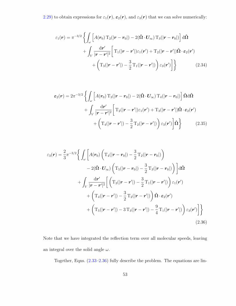
2.29) to obtain expressions for ε1(r), ε2(r), and ε3(r) that we can solve numerically:

ε1(r) = π−3/2

∫ω

[A(r0) T2(|r − r0|)− 2(Ω ·U∞) T3(|r − r0|)

]dΩ

+

∫V

dr′

|r − r′|2

[T1(|r − r′|)ε1(r′) + T2(|r − r′|)Ω · ε2(r′)

+

(T3(|r − r′|)− 3

2T1(|r − r′|)

)ε3(r′)

](2.34)

ε2(r) = 2π−3/2

∫ω

[A(r0) T3(|r − r0|)− 2(Ω ·U∞) T4(|r − r0|)

]ΩdΩ

+

∫V

dr′

|r − r′|2

[T2(|r − r′|)ε1(r′) + T3(|r − r′|)Ω · ε2(r′)

+

(T4(|r − r′|)− 3

2T2(|r − r′|)

)ε3(r′)

]Ω

(2.35)

ε3(r) =2

3π−3/2

∫ω

[A(r0)

(T4(|r − r0|)−

3

2T2(|r − r0|)

)− 2(Ω ·U∞)

(T5(|r − r0|)−

3

2T3(|r − r0|)

)]dΩ

+

∫V

dr′

|r − r′|2

[(T3(|r − r′|)− 3

2T1(|r − r′|)

)ε1(r′)

+

(T4(|r − r′|)− 3

2T2(|r − r′|)

)Ω · ε2(r′)

+

(T5(|r − r′|)− 3 T3(|r − r′|)− 9

4T1(|r − r′|)

)ε3(r′)

](2.36)

Note that we have integrated the reflection term over all molecular speeds, leaving

an integral over the solid angle ω.

Together, Eqns. (2.33–2.36) fully describe the problem. The equations are lin-

53

ear, which guarantees a unique solution for ε1(r), ε2(r), and ε3(r). These equations

are also valid for any geometry, not just for a sphere, provided the integration bounds

are appropriately specified. In theory, we should be able to solve these equations

directly; however, such an attempt would be very computationally expensive.

Fortunately, we can simplify the governing equations for ε1, ε2, and ε3 further.

Let us define the following vectors:

ψ(r) =

ψ1(r)

ψ2(r)

ψ3(r)

ψ4(r)

=

ε1(r)

1√2ε2r(r)

1√2ε2θ(r)√

32ε3(r)

(2.37)

S(r) = π−3/2

ε(0)1 (r)

√2 ε

(0)2z (r)

√2 ε

(0)2x (r)√

23ε

(0)3

= SA(r) + SU(r) (2.38)

ε2z(r) and −ε2x(r) are the perturbations in the r- and θ-velocity, respectively.6 The

source term S(r) corresponds to the first term in Eqns. (2.34) and (2.35); SU(r)

is the part of the source term containing U∞ and SA(r) is the other part. These

definitions are consistent with the work of Cercignani and Pagani [70] and Law and

6The negative sign before ε2x is due to the fact that the positive x-axis used to define ε2x

points in the direction of decreasing θ. Thus, ε2x = −ε2θ. I recognize that this discrepancy can beconfusing, but I am simply retaining the nomenclature used by Lea [74].

54

Loyalka [76]. We can now write our problem as follows:

ψ(r) = Lψ(r′) + S(r) (2.39a)

Lψ(r′) ≡ π−3/2

∫V

Λψ(r′)dr′

|r − r′|2(2.39b)

Λψ(r′) ≡

T1 ε1 + T2 Ω · ε2 +(T3−3

2T1

)ε3

√2[T2 ε1 + T3 Ω · ε2 +

(T4−3

2T2

)ε3

]Ωz

√2[T2 ε1 + T3 Ω · ε2 +

(T4−3

2T2

)ε3

]Ωx√

23

[(T3−3

2T1

)ε1 +

(T4−3

2T2

)Ω · ε2 +

(T5−3 T3 +9

4T1

)ε3

]

(2.39c)

Here, Ω = (r−r′)/|r−r′|, Ωx and Ωz are the x- and z-components of the molecular

trajectory Ω, the argument of the Tn functions is |r− r′|, and the perturbations εn

are a function of r′.

Let us consider each of the terms in Eq. (2.39). Again, we can break up the

source term into the portion that involves U∞ and the portion that includes A(r0).

For a sphere, the source terms SU and SA are

SU(r) = U

WU1(r) cosα

WU2(r) cosα

WU3(r) sinα

WU4(r) cosα

(2.40)

55

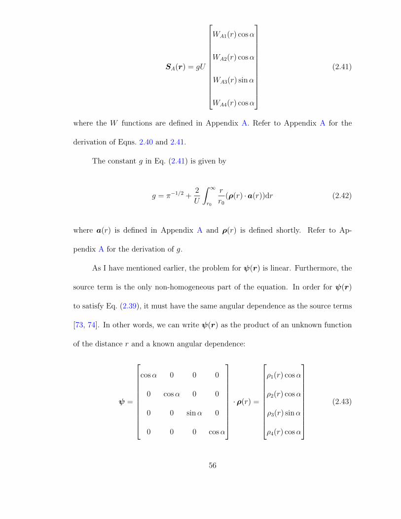
SA(r) = gU

WA1(r) cosα

WA2(r) cosα

WA3(r) sinα

WA4(r) cosα

(2.41)

where the W functions are defined in Appendix A. Refer to Appendix A for the

derivation of Eqns. 2.40 and 2.41.

The constant g in Eq. (2.41) is given by

g = π−1/2 +2

U

∫ ∞r0

r

r0

(ρ(r) ·a(r))dr (2.42)

where a(r) is defined in Appendix A and ρ(r) is defined shortly. Refer to Ap-

pendix A for the derivation of g.

As I have mentioned earlier, the problem for ψ(r) is linear. Furthermore, the

source term is the only non-homogeneous part of the equation. In order for ψ(r)

to satisfy Eq. (2.39), it must have the same angular dependence as the source terms

[73, 74]. In other words, we can write ψ(r) as the product of an unknown function

of the distance r and a known angular dependence:

ψ =

cosα 0 0 0

0 cosα 0 0

0 0 sinα 0

0 0 0 cosα

·ρ(r) =

ρ1(r) cosα

ρ2(r) cosα

ρ3(r) sinα

ρ4(r) cosα

(2.43)

56

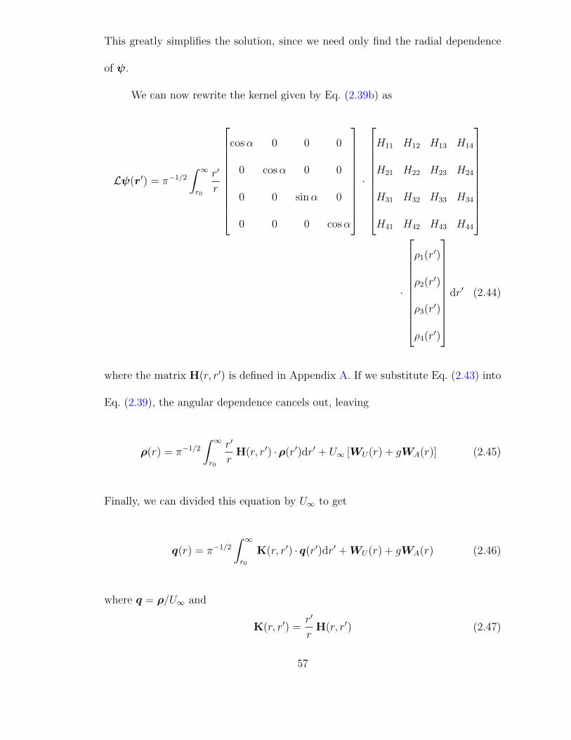
This greatly simplifies the solution, since we need only find the radial dependence

of ψ.

We can now rewrite the kernel given by Eq. (2.39b) as

Lψ(r′) = π−1/2

∫ ∞r0

r′

r

cosα 0 0 0

0 cosα 0 0

0 0 sinα 0

0 0 0 cosα

·

H11 H12 H13 H14

H21 H22 H23 H24

H31 H32 H33 H34

H41 H42 H43 H44

·

ρ1(r′)

ρ2(r′)

ρ3(r′)

ρ4(r′)

dr′ (2.44)

where the matrix H(r, r′) is defined in Appendix A. If we substitute Eq. (2.43) into

Eq. (2.39), the angular dependence cancels out, leaving

ρ(r) = π−1/2

∫ ∞r0

r′

rH(r, r′) ·ρ(r′)dr′ + U∞ [WU(r) + gWA(r)] (2.45)

Finally, we can divided this equation by U∞ to get

q(r) = π−1/2

∫ ∞r0

K(r, r′) · q(r′)dr′ +WU(r) + gWA(r) (2.46)

where q = ρ/U∞ and

K(r, r′) =r′

rH(r, r′) (2.47)

57

This is the equation that we will solve to find the density, velocity, and temperature

perturbations, which are related to q by

ε1(r) = U∞q1(r) cosα (2.48a)

ε2z(r) =√

2U∞q2(r) cosα (2.48b)

ε2x(r) =√

2U∞q3(r) sinα (2.48c)

ε3(r) =

√2

3U∞q4(r) cosα (2.48d)

Again, α is the angle between the free stream velocity and r, ε2z(r) is the perturba-

tion in the radial velocity, and −ε2x(r) is the perturbation in the θ-velocity. Thus,

the local density and velocity profiles are (in non-dimensional form)

n(r, α) = n∞ [1 + q1(r)U∞ cosα] (2.49a)

u2r(r, α) =

[1 +

1√2q2(r)

]U∞ cosα (2.49b)

u2θ(r, α) = −[1 +

1√2q3(r)

]U∞ sinα (2.49c)

T (r, α) = T∞

[1 +

√2

3q4(r)U∞ cosα

](2.49d)

Since I am also interested in the drag force on the sphere, I must relate the

58

drag to q(r). Let us start by writing the expression for the stress tensor,

pij(r) = m

∫cicjf(r, c)dc =

ρ∞2δij + ρ∞π

−3/2

∫cicj e−c

2

h(r, c)dc (2.50)

where ρ∞/2 is the static pressure far from the sphere and δij is the Kronecker delta.

(Note that pij must be multiplied by (2kbT∞/m) to get the appropriate dimensions of

the stress tensor.) The static pressure is related to the unperturbed distribution f∞,

while the shear stress distribution is related to the perturbation h. Going forward,

we can ignore the static pressure contribution to the stress tensor because it will

not contribute to the drag force.

To compute the drag force, we must compute the shear stress tensor at the

surface of the sphere:

τij(r0) = ρ∞π−3/2

∫c · n<0

cicj e−c2

h(r, c)dc

+ ρ∞π−3/2

∫c · n>0

cicj e−c2

h(r, c)dc (2.51)

Here, we have explicitly divided the bounds of the integral in Eq. (2.50) into the set

of molecules moving towards the surface and the set of molecules moving away from

the surface of the sphere. Substituting Eq. (2.25) into the integral for c · n < 0 and

Eq. (2.26) into the integral for c · n > 0, we get

τij(r0) =ρ∞π−3/2

∫V

[T3 ε1(r) + T4 Ω · ε2(r) +

(T5−

3

2T3

)ε3(r)

]ΩiΩj

dr

|r − r0|

59

+ ρ∞π−3/2A(r0)

∫c · n>0

cicj e−c2

dc− ρ∞π−3/22U∞ ·∫c · n>0

c cicj e−c2

dc

(2.52)

where Ω = (r0 − r)/|r0 − r|, the argument of the Tn functions is |r − r0|, and

V is the space above the plane tangent to the sphere at r0. This expression gives

the shear stress tensor in terms of the coordinate system (x, y, z) in Fig. 2.2, where

the z-axis is along the vector normal to the surface at r0 and the velocity U∞ is in

the xz-plane. However, we want to know the drag force in the coordinate system

(X, Y, Z) in Fig. 2.2, where U∞ is along the Z-direction. Thus, we must write the

shear stress tensor in terms of (X, Y, Z):

ΠXX =τxx cos2 α− 2τxz sinα cosα + τzz sin2 α

ΠY Y =τyy

ΠZZ =τxx sin2 α + 2τxz sinα cosα + τzz cos2 α (2.53)

ΠXZ =τxz cos2 α + (τxx − τzz) sinα cosα− τxz sin2 α = ΠZX

ΠXY =ΠY X = ΠY Z = ΠZY = 0

Here, α is the angle between U∞ and n. (See Fig. 2.4).

The drag is then the integral over the surface of the sphere of the normal

component of the shear force,

FD =

(2kBT∞m

)r2

0

∫S

Π · ndS

60

In the (X, Y, Z) coordinate system, the drag is in the negative Z-direction, i.e. in

the direction opposite the flow, so we need only consider the Z-component of the

drag:

FD,Z =

(2kBT∞m

)r2

0

∫S

(ΠZX ,ΠZY ,ΠZZ) · (− sinα, 0, cosα)dS

=

(2kBT∞m

)1/2

r20

∫S

(−ΠZX sinα + ΠZZ cosα)dS

Substituting our expressions for Πij into the above equation for the drag, we get

FD,Z =

(2kBT∞m

)r2

0

∫S

(τxz sinα + τzz cosα)dS

Using Eq. (2.52) for the components τzx and τzz of the shear stress tensor and

performing a lot of algebra, we get the following expression for the drag:

FD,Z = −ρ∞3

(2πkBT∞

m

)1/2

U r20

2π1/2

r20

∫ ∞r0

r2[q1(r)WU1(r)− q2(r)WU2(r)

− 2q3(r)WU3(r) + q4(r)WU4(r)]dr + [8− gπ1/2]

(2.54)

The details of this derivation can be found in Appendix A.

Taking the ratio of the drag we obtain from the BGK model to the free molec-

ular drag,

FD,fm = −ρ∞3

(2πkBT∞

m

)1/2

U r20(8 + π)

we get the following drag ratio:

61

FD =

2π1/2

r20

∫ ∞r0

r2[q1(r)WU1(r)− q2(r)WU2(r)

− 2q3(r)WU3(r) + q4(r)WU4]dr + [8− gπ1/2]

(8 + π)−1 (2.55)

2.3.2 Numerical Methods

Eq. (2.46) cannot be solved analytically for q(r), so we must solve the problem

numerically at discrete radial locations. One can choose any set of points at which

to solve Eq. (2.46), but it makes the most sense to use points corresponding to the

Gaussian quadrature nodes.

A brief introduction to the Gaussian quadrature formula is warranted at this

point. The integral of any function f(t) in the interval [−1, 1] can be approximated

by ∫ 1

−1

f(t)dt ≈N∑j=1

Ajf(tj) (2.56)

where t1, . . . , tN are nodes, Aj is the weight of the jth node, and f(tj) is the value

of f(t) at the jth node. The nodes and weights for a given N are available from any

number of sources (e.g. Table 25.4 of Abramowitz and Stegun [98]). We can change

the interval [−1, 1] to any interval [a, b], such that our approximation of the integral

becomes

∫ b

a

f(t)dt =b− a

2

∫ 1

−1

f

(b− a

2t+

a+ b

2

)dt

≈b− a2

n∑j=1

Ajf

(b− a

2tj +

a+ b

2

)(2.57)

62

The Gaussian quadrature formula works best when the function can be approxi-

mated by a polynomial in the interval [a, b]; particular care is needed when there are

singularities, as is the case for Hii when r = r′. Nevertheless, the Gaussian quadra-

ture formula generally provides accurate results using a relatively small number

of points, especially when compared to other numerical integration formulas like

the trapezoidal rule or Simpson’s rule. A good, concise explanation of Gaussian

integration may be found in Kreyszig [100].

With this brief introduction concluded, we will return to the discussion of the

problem of flow around a sphere. We start by rearranging Eq. (2.46):

q(r)− π−1/2

∫ R′

r0

K(r, r′) · q(r′)dr′

= π−1/2

∫ ∞R′

K(r, r′) · q(r′)dr′ +WU(r) + gWA(r) ≡ S′(r) (2.58)

Here, we have broken the kernel integral into two separate integrals: one over our

region of interest from r0 to R′, and another over the region farther away from the

sphere. The right-hand side of Eq. (2.58) can be thought of as an effective source

term S′(r) that includes both the contribution to q(r) from molecules reflected from

the sphere (i.e. the true source term) and the contribution of molecules that enter

the region of interest from farther away.

The function q(r) in Eq. (2.58) is a trial function for the perturbation far

from the sphere. Using the asymptotic solution of Takata et al. [78] for the density,

velocity, and temperature far from the sphere, our trial function for q on the right-

63

hand side of Eq. (2.58) is

q(r) =

(γc1

r0

− c3

)(r0

r

)2

√2

[c1r0

r+ c2

(r0

r

)3]

1√2

[c1r0

r− c2

(r0

r

)3]

c3

(r0

r

)2

(2.59)

Here, c1, c2, and c3, are constants to be determined for each Kn number, while

γ = 1.270 is a constant appropriate for hard-sphere molecules. For r0 1 (i.e. for

continuum flow), c1 = −32, c2 = 1

2, and c3 = 0, as we can verify by solving the Stokes

equation for flow around a sphere.

We must make one final modification to our governing equation:

q(r)

[1− π−1/2

∫ R′

r0

K(r, r′)dr′

]− π−1/2

∫ R′

r0

K(r, r′) · [q(r′)− q(r)] dr′ = S′(r)

(2.60)

Here, we added and subtracted the term∫

K(r, r′)q(r)dr′ from the left side. We have

done this to deal with the singularities in the kernel at r = r′. Because kernel the is

infinite at this point, it will cause problems when we use our Gaussian integration

formula to calculate the integral. By adding and subtracting a term, we end up

multiplying the singular points by zero, which minimizes the problems caused by

the singularities in K.

64

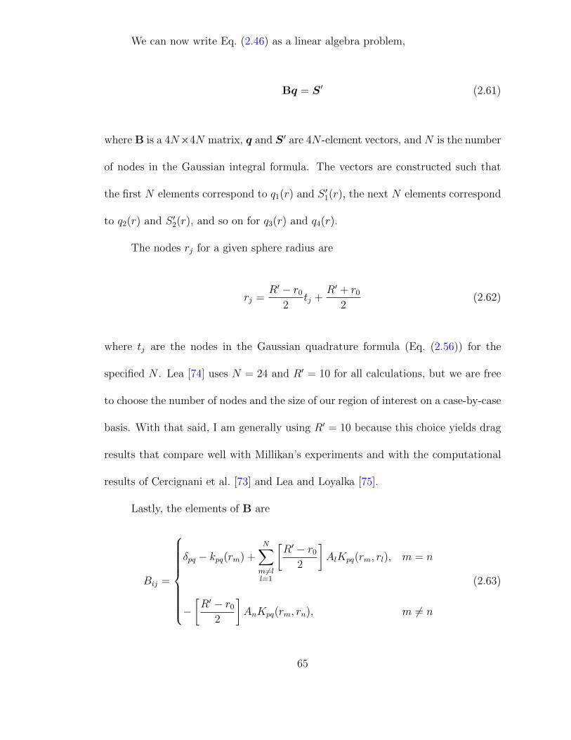
We can now write Eq. (2.46) as a linear algebra problem,

Bq = S′ (2.61)

where B is a 4N×4N matrix, q and S′ are 4N -element vectors, and N is the number

of nodes in the Gaussian integral formula. The vectors are constructed such that

the first N elements correspond to q1(r) and S ′1(r), the next N elements correspond

to q2(r) and S ′2(r), and so on for q3(r) and q4(r).

The nodes rj for a given sphere radius are

rj =R′ − r0

2tj +

R′ + r0

2(2.62)

where tj are the nodes in the Gaussian quadrature formula (Eq. (2.56)) for the

specified N . Lea [74] uses N = 24 and R′ = 10 for all calculations, but we are free

to choose the number of nodes and the size of our region of interest on a case-by-case

basis. With that said, I am generally using R′ = 10 because this choice yields drag

results that compare well with Millikan’s experiments and with the computational

results of Cercignani et al. [73] and Lea and Loyalka [75].

Lastly, the elements of B are

Bij =

δpq − kpq(rm) +N∑m 6=ll=1

[R′ − r0

2

]AlKpq(rm, rl), m = n

−[R′ − r0

2

]AnKpq(rm, rn), m 6= n

(2.63)

65

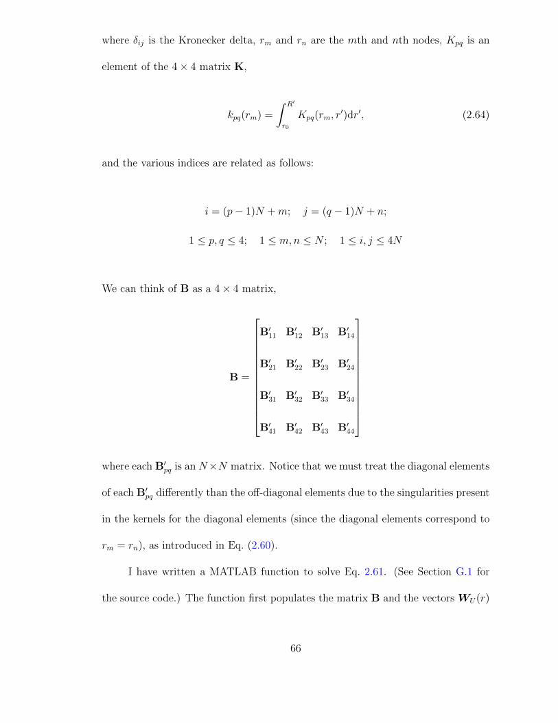
where δij is the Kronecker delta, rm and rn are the mth and nth nodes, Kpq is an

element of the 4× 4 matrix K,

kpq(rm) =

∫ R′

r0

Kpq(rm, r′)dr′, (2.64)

and the various indices are related as follows:

i = (p− 1)N +m; j = (q − 1)N + n;

1 ≤ p, q ≤ 4; 1 ≤ m,n ≤ N ; 1 ≤ i, j ≤ 4N

We can think of B as a 4× 4 matrix,

B =

B′11 B′12 B′13 B′14

B′21 B′22 B′23 B′24

B′31 B′32 B′33 B′34

B′41 B′42 B′43 B′44

where each B′pq is an N×N matrix. Notice that we must treat the diagonal elements

of each B′pq differently than the off-diagonal elements due to the singularities present

in the kernels for the diagonal elements (since the diagonal elements correspond to

rm = rn), as introduced in Eq. (2.60).

I have written a MATLAB function to solve Eq. 2.61. (See Section G.1 for

the source code.) The function first populates the matrix B and the vectors WU(r)

66

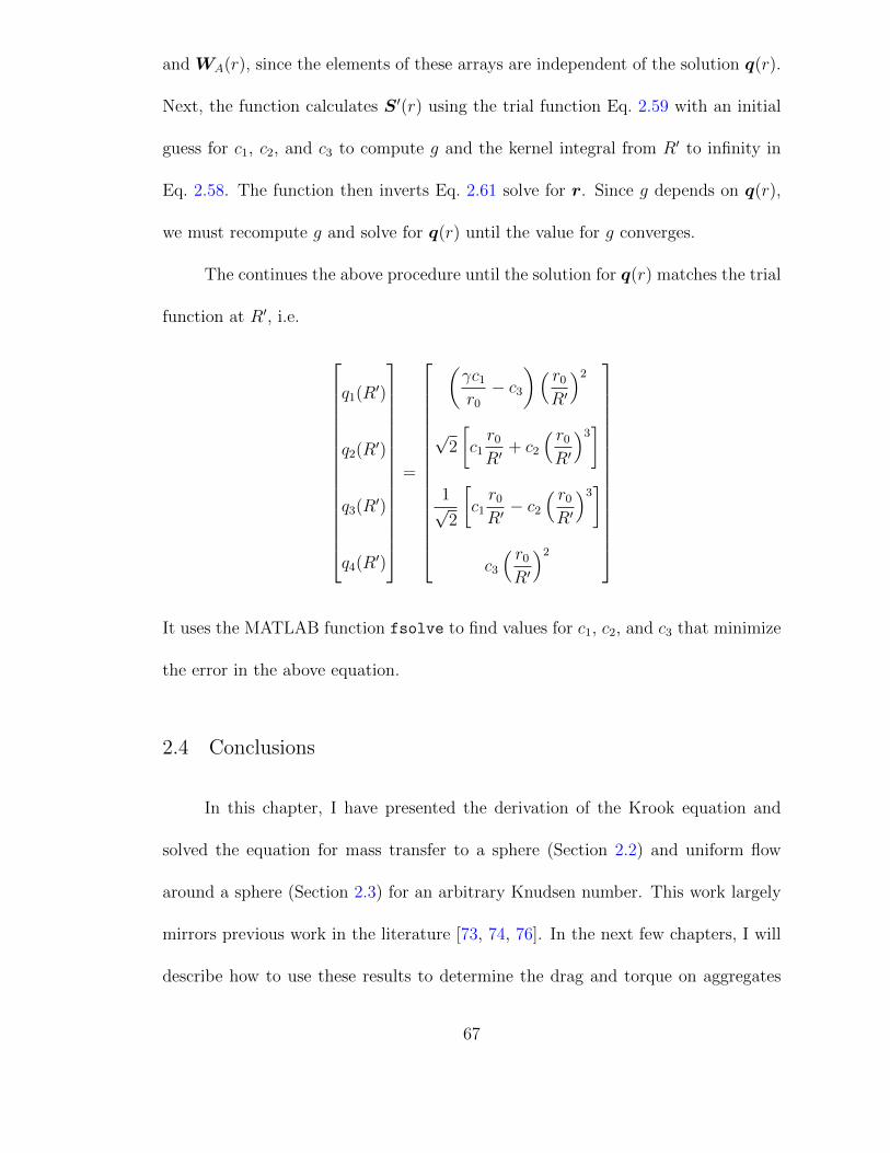
and WA(r), since the elements of these arrays are independent of the solution q(r).

Next, the function calculates S′(r) using the trial function Eq. 2.59 with an initial

guess for c1, c2, and c3 to compute g and the kernel integral from R′ to infinity in

Eq. 2.58. The function then inverts Eq. 2.61 solve for r. Since g depends on q(r),

we must recompute g and solve for q(r) until the value for g converges.

The continues the above procedure until the solution for q(r) matches the trial

function at R′, i.e.

q1(R′)

q2(R′)

q3(R′)

q4(R′)

=

(γc1

r0

− c3

)( r0

R′

)2

√2

[c1r0

R′+ c2

( r0

R′

)3]

1√2

[c1r0

R′− c2

( r0

R′

)3]

c3

( r0

R′

)2

It uses the MATLAB function fsolve to find values for c1, c2, and c3 that minimize

the error in the above equation.

2.4 Conclusions

In this chapter, I have presented the derivation of the Krook equation and

solved the equation for mass transfer to a sphere (Section 2.2) and uniform flow

around a sphere (Section 2.3) for an arbitrary Knudsen number. This work largely

mirrors previous work in the literature [73, 74, 76]. In the next few chapters, I will

describe how to use these results to determine the drag and torque on aggregates

67

consisting of N spheres in point contact and apply this method to various aerosol

physics problems.

68

Chapter 3: Friction Coefficient for Translating Particles

3.1 Introduction

Aerosol fractal aggregates formed from the coagulation of smaller, spherical

primary particles are found in many natural and industrial settings. Understanding

the forces on these aggregates is important in a number of science and engineering

disciplines, including combustion, fire safety, atmospheric and environmental sci-

ences, materials engineering [2], and nuclear reactor safety [21]. The translational

drag force for a particle moving slowly relative to the surrounding fluid – given

by F = −ζU0, where U0 is the particle relative velocity and ζ is the orientation-

averaged scalar friction factor – is particularly important because it influences the

transport properties of the particle, including its diffusion coefficient and electrical

mobility.

In many practical applications, the primary sphere radius a is significantly less

than the mean free path of the surrounding gas (λ ≈ 65 nm at standard temperature

and pressure and an order of magnitude higher near a flame), so that the primary

sphere is in or near the free molecule flow regime. At the same time, the radius of

gyration Rg for the agglomerate may be comparable to or larger than the mean free

path, so that the aggregate is in the transition flow regime. As one example, for

69

carbonaceous soot a ≈ 5− 30 nm and Rg ≈ 30− 1000 nm.

There are a number of theories and techniques for computing the translational

friction factor of macromolecules and particle aggregates in the continuum regime,

including Kirkwood-Riseman (KR) theory [28] and its extensions by Rotne and

Prager [57], Yamakawa [58], and Chen et al. [30], as well as algorithms that use the

Hubbard and Douglas analogy between the electrostatic capacitance and the friction

factor [31, 63, 101]. Likewise, there are established methods for computing ζ in the

free molecule regime that simulate the ballistic nature of interactions between gas

molecules and aggregates [34–36, 102].

In contrast, there are few approaches for the transition regime. Melas et al.

[79] estimated the friction coefficient in the near-continuum regime by solving the

Laplace equation with a slip boundary condition at the surface of the particle. In a

follow-up paper, the authors determined that their Collision Rate Method is valid

for Knudsen numbers less than 2 [80].

Dahneke [67] developed the adjusted sphere method for the transition regime,

which applies a slip correction factor to the continuum friction factor. The key to

this development is the identification of an aggregate Knudsen number that reduces

a problem involving two length scales (primary radius and aggregate radius of gyra-

tion) to a single dimensionless length. Dahneke’s approach is similar to the approach

used to calculate the drag on a sphere in the transition regime, but the adjusted

sphere method uses an adjusted Knudsen number based on geometric descriptions

of the particle in the continuum (hydrodynamic radius, RH) and free molecular

(projected area, PA) regimes.

70

Through scaling analysis, Zhang et al. [41] developed an approach analogous

to the adjusted sphere method and demonstrated that the approach yields friction

factors comparable to Direct Simulation Monte Carlo (DSMC) results for the ag-

gregates they studied (spheres, dimers, and dense and open 20-particle aggregates).

However, it requires knowledge of the hydrodynamic radius and the projected area

of the particle, which may take tens of minutes to a few hours to obtain compu-

tationally for a single particle. Obtaining RH and PA experimentally is possible,

but it requires painstaking TEM measurements [68]. More rigorous computational

techniques for calculating the transition regime friction factor – such as DSMC

or molecular dynamics – are time consuming: for instance, the reported DSMC

calculation times in Ref. [41] were on the order of one CPU week for a given Knud-

sen number and a given aggregate. Thus, a self-consistent field theory method for

quickly estimating the scalar friction factor of an aggregate across the Knudsen

range is highly desirable.

In this chapter, I present a new approach for computing the hydrodynamic

friction tensor H and the scalar friction coefficient ζ for fractal aggregates across the

entire Knudsen range. This approach involves solving for the velocity field around a

sphere in the transition regime and using the velocity field to compute the friction

factor for the aggregate. In essence, this approach is an extension of KR theory

[28] from the continuum regime to the transition regime. I will first present the

solution of the Krook equation for the velocity field around a sphere, which follows

the procedure developed by Lea and Loyalka [75] and Law and Loyalka [76]. I then

describe the extension of KR theory to the transition regime. Finally, I compare my

71

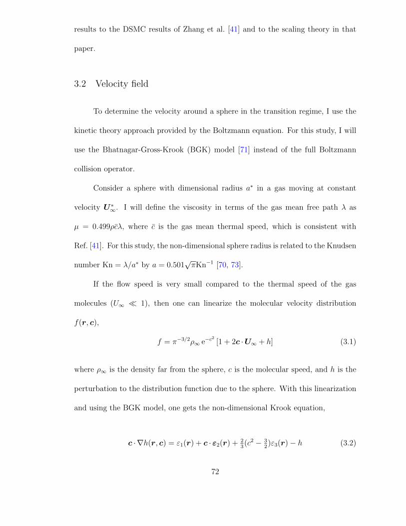
results to the DSMC results of Zhang et al. [41] and to the scaling theory in that

paper.

3.2 Velocity field

To determine the velocity around a sphere in the transition regime, I use the

kinetic theory approach provided by the Boltzmann equation. For this study, I will

use the Bhatnagar-Gross-Krook (BGK) model [71] instead of the full Boltzmann

collision operator.

Consider a sphere with dimensional radius a∗ in a gas moving at constant

velocity U ∗∞. I will define the viscosity in terms of the gas mean free path λ as

µ = 0.499ρcλ, where c is the gas mean thermal speed, which is consistent with

Ref. [41]. For this study, the non-dimensional sphere radius is related to the Knudsen

number Kn = λ/a∗ by a = 0.501√πKn−1 [70, 73].

If the flow speed is very small compared to the thermal speed of the gas

molecules (U∞ 1), then one can linearize the molecular velocity distribution

f(r, c),

f = π−3/2ρ∞ e−c2

[1 + 2c ·U∞ + h] (3.1)

where ρ∞ is the density far from the sphere, c is the molecular speed, and h is the

perturbation to the distribution function due to the sphere. With this linearization

and using the BGK model, one gets the non-dimensional Krook equation,

c · ∇h(r, c) = ε1(r) + c · ε2(r) + 23(c2 − 3

2)ε3(r)− h (3.2)

72

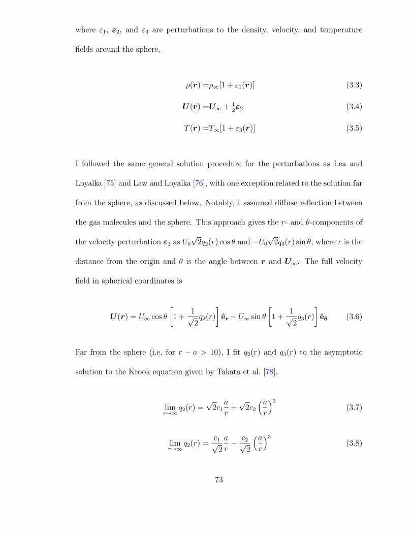
where ε1, ε2, and ε3 are perturbations to the density, velocity, and temperature

fields around the sphere,

ρ(r) =ρ∞[1 + ε1(r)] (3.3)

U(r) =U∞ + 12ε2 (3.4)

T (r) =T∞[1 + ε3(r)] (3.5)

I followed the same general solution procedure for the perturbations as Lea and

Loyalka [75] and Law and Loyalka [76], with one exception related to the solution far

from the sphere, as discussed below. Notably, I assumed diffuse reflection between

the gas molecules and the sphere. This approach gives the r- and θ-components of

the velocity perturbation ε2 as U0

√2q2(r) cos θ and −U0

√2q3(r) sin θ, where r is the

distance from the origin and θ is the angle between r and U∞. The full velocity

field in spherical coordinates is

U(r) = U∞ cos θ

[1 +

1√2q2(r)

]er − U∞ sin θ

[1 +

1√2q3(r)

]eθ (3.6)

Far from the sphere (i.e. for r − a > 10), I fit q2(r) and q3(r) to the asymptotic

solution to the Krook equation given by Takata et al. [78],

limr→∞

q2(r) =√

2c1a

r+√

2c2

(ar

)3

(3.7)

limr→∞

q2(r) =c1√

2

a

r− c2√

2

(ar

)3

(3.8)

73

Lea and Loyalka [75] and Law and Loyalka [76] used a slightly different form of the

solution for large distances from the sphere, but otherwise my approach is consistent

with the approach in Refs. [75, 76].

I present my solution of the drag as the ratio between drag F for the specified

Knudsen number and the free molecule drag FFM . As shown in Figure 3.1, my drag

results compare favorably (i.e within 2-3%) with a fit to Millikan’s oil drop data [64]

reported by Cercignani et al. [73],

F

FFM=

A+B

2π−1/2a+ A+B exp[−2π−1/2Ca](3.9)

where A = 1.234, B = 0.414, and C = 0.876. My results are also consistent with

previous calculations [73, 75, 76, 78], as shown in Table 3.1. (See Appendix B for

more detailed results.)

Figure 3.1: Ratio of the calculated drag from the Krook equation to the free moleculedrag. Results are compared to a fit to Millikan’s data [64]

74

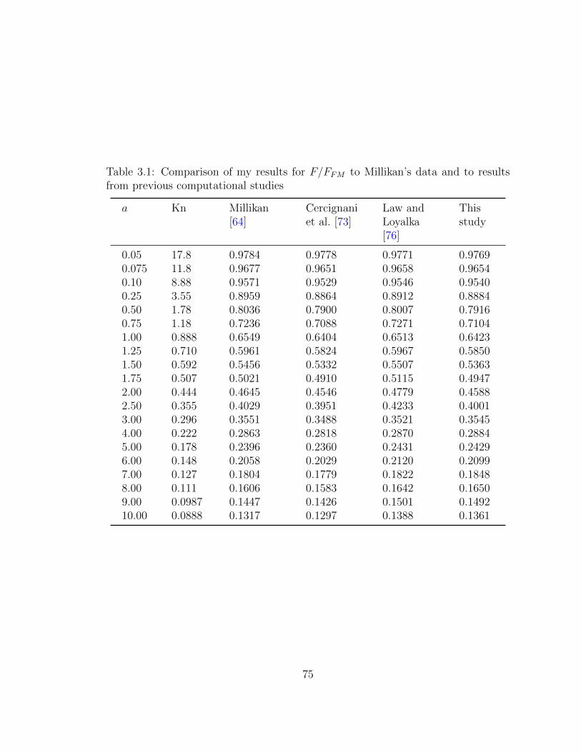
Table 3.1: Comparison of my results for F/FFM to Millikan’s data and to resultsfrom previous computational studies

a Kn Millikan[64]

Cercignaniet al. [73]

Law andLoyalka[76]

Thisstudy

0.05 17.8 0.9784 0.9778 0.9771 0.97690.075 11.8 0.9677 0.9651 0.9658 0.96540.10 8.88 0.9571 0.9529 0.9546 0.95400.25 3.55 0.8959 0.8864 0.8912 0.88840.50 1.78 0.8036 0.7900 0.8007 0.79160.75 1.18 0.7236 0.7088 0.7271 0.71041.00 0.888 0.6549 0.6404 0.6513 0.64231.25 0.710 0.5961 0.5824 0.5967 0.58501.50 0.592 0.5456 0.5332 0.5507 0.53631.75 0.507 0.5021 0.4910 0.5115 0.49472.00 0.444 0.4645 0.4546 0.4779 0.45882.50 0.355 0.4029 0.3951 0.4233 0.40013.00 0.296 0.3551 0.3488 0.3521 0.35454.00 0.222 0.2863 0.2818 0.2870 0.28845.00 0.178 0.2396 0.2360 0.2431 0.24296.00 0.148 0.2058 0.2029 0.2120 0.20997.00 0.127 0.1804 0.1779 0.1822 0.18488.00 0.111 0.1606 0.1583 0.1642 0.16509.00 0.0987 0.1447 0.1426 0.1501 0.149210.00 0.0888 0.1317 0.1297 0.1388 0.1361

75

3.3 Kirkwood-Riseman theory

Kirkwood and Riseman [28] demonstrated that the force on the ith element

of an N -element polymer chain is given by

Fi = −ζ0(U0 − ui)− ζ0

n∑i 6=j

Tij ·Fj (3.10)

whereU0 is the unperturbed fluid velocity, ui is the velocity of the ith chain element,

ζ0 is the friction factor given by Stokes’ law, and Tij is the hydrodynamic interaction

tensor. The total force on the chain is the vector sum of the forces on the chain

elements, F =∑N

i Fi.

The original derivation used the Oseen tensor for Tij. Rotne and Prager [57]

and Yamakawa [58] derived a modified hydrodynamic tensor Tij that accounts for

the curvature of the chain elements and hydrodynamic interactions between two

elements,

Tij =1

8πµrij

[I +

rijrijr2ij

]+

2a2

3r2ij

[I− 3rijrij

r2ij

](3.11)

where rij is the vector from the ith element to the jth element and rij is the distance

between the elements. Chen, Deutch, and Meakin later applied this approach to

find the translational drag force on a fractal aerosol particle [30, 54, 55].

Rotne and Prager [57] and Yamakawa [58] noted the similarities between their

modified interaction tensor and the solution of Stokes flow around a stationary

sphere. One can write the perturbation to the velocity caused by the sphere in the

76

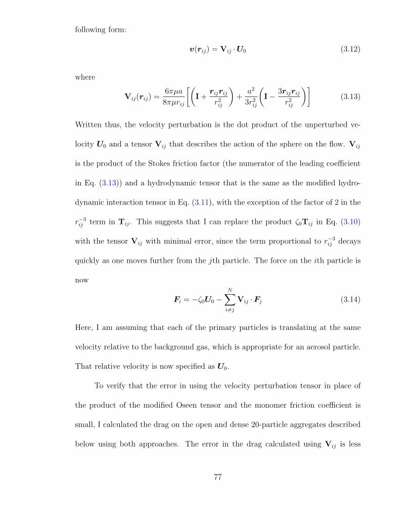
following form:

v(rij) = Vij ·U0 (3.12)

where

Vij(rij) =6πµa

8πµrij

[(I +

rijrijr2ij

)+

a2

3r2ij

(I− 3rijrij

r2ij

)](3.13)

Written thus, the velocity perturbation is the dot product of the unperturbed ve-

locity U0 and a tensor Vij that describes the action of the sphere on the flow. Vij

is the product of the Stokes friction factor (the numerator of the leading coefficient

in Eq. (3.13)) and a hydrodynamic tensor that is the same as the modified hydro-

dynamic interaction tensor in Eq. (3.11), with the exception of the factor of 2 in the

r−3ij term in Tij. This suggests that I can replace the product ζ0Tij in Eq. (3.10)

with the tensor Vij with minimal error, since the term proportional to r−3ij decays

quickly as one moves further from the jth particle. The force on the ith particle is

now

Fi = −ζ0U0 −N∑i 6=j

Vij ·Fj (3.14)

Here, I am assuming that each of the primary particles is translating at the same

velocity relative to the background gas, which is appropriate for an aerosol particle.

That relative velocity is now specified as U0.

To verify that the error in using the velocity perturbation tensor in place of

the product of the modified Oseen tensor and the monomer friction coefficient is

small, I calculated the drag on the open and dense 20-particle aggregates described

below using both approaches. The error in the drag calculated using Vij is less

77

than 2% for the dense aggregate and less than 1% for the open aggregate. This

error decreases as the number of primary spheres increases, as expected from the

r−3ij dependence.

To extend KR theory from the continuum regime to the transition regime,

I set ζ0 equal to the friction coefficient for a sphere that I calculated using the

Krook equation and write the hydrodynamic tensor Vij in terms of the velocity

perturbation ε2,

Vij = −q2(rij)√2

rijrijr2ij

− q3(rij)√2

(I− rijrij

r2ij

)(3.15)

I obtain the orientation-averaged translational friction factor for the particle by

following the approach outlined in Happel and Brenner [49]: I calculate F /U0 for

three mutually-orthogonal particle orientations, compute the eigenvalues λm of the

resulting friction tensor, and set the friction coefficient equal to the harmonic average

of the eigenvalues,

ζ =

(1

λ1

+1

λ2

+1

λ3

)−1

(3.16)

Note that the friction tensor is symmetrical (allowing for some numerical uncer-

tainty) in the transition regime, as it is in continuum flow.

Because my drag results from the Krook equation are non-dimensionalized

by the free molecule drag force, I obtain the dimensional scalar friction factor by

multiplying by the free molecule friction factor for the primary sphere,

ζ∗ = ζπ(8 + π)

2.994

µ

λa2 (3.17)

78

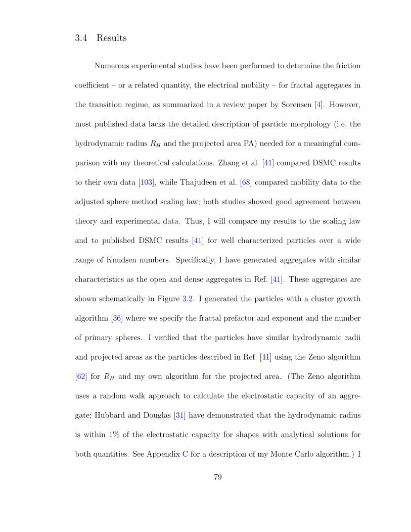
3.4 Results

Numerous experimental studies have been performed to determine the friction

coefficient – or a related quantity, the electrical mobility – for fractal aggregates in

the transition regime, as summarized in a review paper by Sorensen [4]. However,

most published data lacks the detailed description of particle morphology (i.e. the

hydrodynamic radius RH and the projected area PA) needed for a meaningful com-

parison with my theoretical calculations. Zhang et al. [41] compared DSMC results

to their own data [103], while Thajudeen et al. [68] compared mobility data to the

adjusted sphere method scaling law; both studies showed good agreement between

theory and experimental data. Thus, I will compare my results to the scaling law

and to published DSMC results [41] for well characterized particles over a wide

range of Knudsen numbers. Specifically, I have generated aggregates with similar

characteristics as the open and dense aggregates in Ref. [41]. These aggregates are

shown schematically in Figure 3.2. I generated the particles with a cluster growth

algorithm [36] where we specify the fractal prefactor and exponent and the number

of primary spheres. I verified that the particles have similar hydrodynamic radii

and projected areas as the particles described in Ref. [41] using the Zeno algorithm

[62] for RH and my own algorithm for the projected area. (The Zeno algorithm

uses a random walk approach to calculate the electrostatic capacity of an aggre-

gate; Hubbard and Douglas [31] have demonstrated that the hydrodynamic radius

is within 1% of the electrostatic capacity for shapes with analytical solutions for

both quantities. See Appendix C for a description of my Monte Carlo algorithm.) I

79

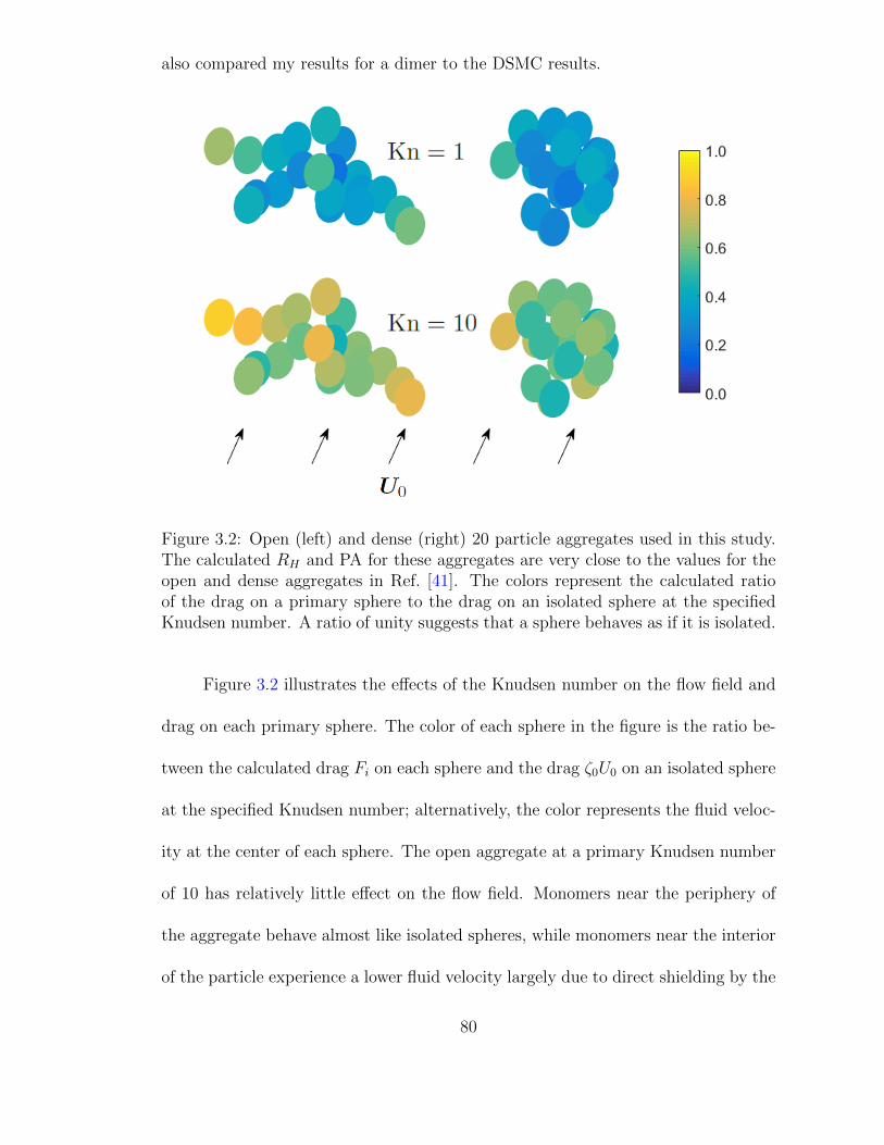
also compared my results for a dimer to the DSMC results.

Figure 3.2: Open (left) and dense (right) 20 particle aggregates used in this study.The calculated RH and PA for these aggregates are very close to the values for theopen and dense aggregates in Ref. [41]. The colors represent the calculated ratioof the drag on a primary sphere to the drag on an isolated sphere at the specifiedKnudsen number. A ratio of unity suggests that a sphere behaves as if it is isolated.

Figure 3.2 illustrates the effects of the Knudsen number on the flow field and

drag on each primary sphere. The color of each sphere in the figure is the ratio be-

tween the calculated drag Fi on each sphere and the drag ζ0U0 on an isolated sphere

at the specified Knudsen number; alternatively, the color represents the fluid veloc-

ity at the center of each sphere. The open aggregate at a primary Knudsen number

of 10 has relatively little effect on the flow field. Monomers near the periphery of

the aggregate behave almost like isolated spheres, while monomers near the interior

of the particle experience a lower fluid velocity largely due to direct shielding by the

80

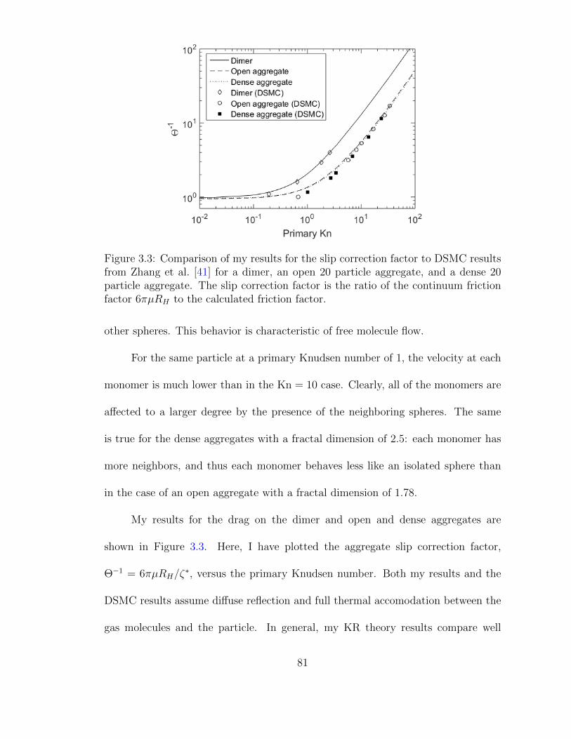
Figure 3.3: Comparison of my results for the slip correction factor to DSMC resultsfrom Zhang et al. [41] for a dimer, an open 20 particle aggregate, and a dense 20particle aggregate. The slip correction factor is the ratio of the continuum frictionfactor 6πµRH to the calculated friction factor.

other spheres. This behavior is characteristic of free molecule flow.

For the same particle at a primary Knudsen number of 1, the velocity at each

monomer is much lower than in the Kn = 10 case. Clearly, all of the monomers are

affected to a larger degree by the presence of the neighboring spheres. The same

is true for the dense aggregates with a fractal dimension of 2.5: each monomer has

more neighbors, and thus each monomer behaves less like an isolated sphere than

in the case of an open aggregate with a fractal dimension of 1.78.

My results for the drag on the dimer and open and dense aggregates are

shown in Figure 3.3. Here, I have plotted the aggregate slip correction factor,

Θ−1 = 6πµRH/ζ∗, versus the primary Knudsen number. Both my results and the

DSMC results assume diffuse reflection and full thermal accomodation between the

gas molecules and the particle. In general, my KR theory results compare well

81

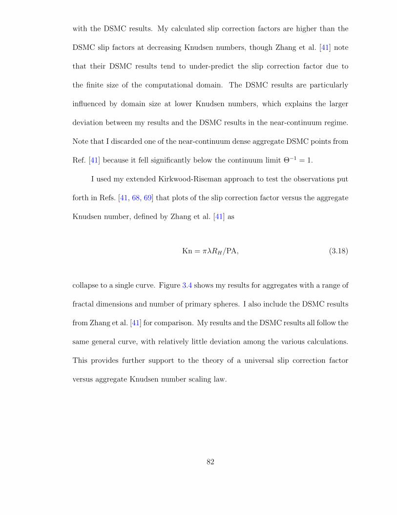
with the DSMC results. My calculated slip correction factors are higher than the

DSMC slip factors at decreasing Knudsen numbers, though Zhang et al. [41] note

that their DSMC results tend to under-predict the slip correction factor due to

the finite size of the computational domain. The DSMC results are particularly

influenced by domain size at lower Knudsen numbers, which explains the larger

deviation between my results and the DSMC results in the near-continuum regime.

Note that I discarded one of the near-continuum dense aggregate DSMC points from

Ref. [41] because it fell significantly below the continuum limit Θ−1 = 1.

I used my extended Kirkwood-Riseman approach to test the observations put

forth in Refs. [41, 68, 69] that plots of the slip correction factor versus the aggregate

Knudsen number, defined by Zhang et al. [41] as

Kn = πλRH/PA, (3.18)

collapse to a single curve. Figure 3.4 shows my results for aggregates with a range of

fractal dimensions and number of primary spheres. I also include the DSMC results

from Zhang et al. [41] for comparison. My results and the DSMC results all follow the

same general curve, with relatively little deviation among the various calculations.

This provides further support to the theory of a universal slip correction factor

versus aggregate Knudsen number scaling law.

82

Figure 3.4: Calculated slip correction factors for a range of aggregate morphologies,plotted versus the aggregate Knudsen number. DSMC results from Zhang et al. [41]are included for comparison.

3.5 Discussion

I have introduced a new approach for computing the translational friction

coefficient for a fractal aerosol particle across the entire Knudsen range, given the

particle’s coordinates and primary sphere radius. Coordinates can be generated

using a cluster growth algorithm, as I have done for this study, or they can be

obtained from TEM images, using methods described in the literature (e.g. Ref. [68]).

The solution method is also very fast: it takes approximately 10 seconds on

a single processor to obtain the friction coefficient for approximately 50 Knudsen

numbers for a 20-particle aggregate. Furthermore, my Kirkwood-Riseman results

converge to the correct continuum and free molecule limits obtained using the

Hubbard-Douglas approximation for the continuum and a ballistic approach for

83

the free molecule aggregate friction factor.

Over the parameter range examined, my results support the validity of the

adjusted sphere/scaling method developed by Dahneke [67] and Zhang et al. [41] and

promoted by more recent studies [68, 69, 79, 80]. Because the Kirkwood-Riseman

approach can provide results quickly across the Knudsen range, this approach may

be preferable to DSMC for evaluating scaling laws (such as those developed by

Rogak et al. [37], Lall and Friedlander [38], and Eggersdorfer et al. [39]) that relate

the friction coefficient to the number of primary spheres in the aggregate.

While I have focused on the friction coefficient in this chapter, my method

also determines the friction tensor, which is important when considering particle

alignment in an external force field [5]. This is discussed further in Chapter 7.

Finally, I emphasize that my results assume diffuse reflection between the gas

molecules and the particle. This is consistent with past computational studies for

fractal aerosol particles (e.g. Refs. [36, 41]) and with experimental results, which

suggest that most collisions are diffuse [32]. With that said, the Kirkwood-Riseman

approach could be applied for alternative reflection models, provided one solves the

Krook equation for the velocity using the appropriate boundary condition at the

surface of the sphere.

84

Chapter 4: Analytical Expression for the Friction Coefficient of DLCA

Aggregates based on Extended Kirkwood-Riseman The-

ory

4.1 Introduction

Aerosol particles formed at high temperature are often fractal aggregates de-

scribed under the assumption of equally-sized spherical primary particles as

N = k0

(Rg

a

)df(4.1)

where N is the number of primary spheres, Rg is the radius of gyration of the

agglomerate, a is the primary sphere radius, and df and k0 are the fractal dimension

and prefactor.

The transport properties of these particles (e.g. the diffusion coefficient, set-

tling velocity, and electrical mobility) can be related to the particle scalar friction

coefficient ζt, which is defined by the relationship between the drag force and the

relative velocity between the particle and the fluid,

Fd = ζt(uf − up) = ζtU (4.2)

85

where uf and up are the velocities of the fluid and the particle, respectively. Knowl-

edge of the friction coefficient is crucial to predicting particle diffusional, phoretic,

and electrostatic behavior in real-world applications.

For the simple case of a sphere with radius a, the friction coefficient is given

by Stokes’ law,

ζt =6πµa

Cc(Kn)(4.3)

where µ is the gas viscosity, Kn = λ/a is the Knudsen number, λ is the gas mean

free path, and Cc is the Cunningham slip correction factor,1

Cc(Kn) = 1 + Kn

[A+B exp

(− C

Kn

)](4.4)

Spheres that are very large compared to the mean free path (Kn → 0) are in the

continuum regime. In this case, the slip correction is unity, and the continuum

friction factor is simply

ζct,0 = 6πµa (4.5)

Spheres that are very small compared to the mean free path are in the free molecule

regime, where the friction coefficient is given by Epstein’s equation,

ζFMt,0 =

π(8 + απ)

2.994

µ

λa2 (4.6)

The momentum accommodation coefficient α is equal to unity for purely diffuse re-

1In this work, I define the viscosity by the relation µ = 0.499ρcλ, where ρ is the gas densityand c is the mean thermal speed. This expression describes a hard sphere gas. Furthermore, I useDavies’ coefficients (A = 1.257, B = 0.4, and C = 1.1) [65] in the slip correction factor.

86

flection and zero for purely specular reflection at the surface of the particle. Epstein

[32] determined that most collisions are diffuse.

Determination of the friction coefficient is much more complicated for fractal

aggregates. In the continuum regime, the friction coefficient is given by

ζt = 6πµRH (4.7)

where RH is the particle hydrodynamic radius, which may be obtained by applying

either the Kirkwood-Riseman [30, 54–56] or Hubbard-Douglas [31, 101] method.

For the free molecule regime, one can obtain the friction coefficient using a ballistic

approach [34–36], such that the friction coefficient is related to the orientation-

averaged projected area of the particle.

Both computational and experimental results seem to support power-law type

relationships between the number of primary spheres in the aggregate and the fric-

tion coefficient:

ζt = ANη (4.8)

Sorensen [4] reviewed available experimental data for particles formed by diffu-

sion limited cluster aggregation (DLCA) and proposed exponents of 0.46 forN < 100

and 0.56 for N > 100 in the continuum regime and 0.92 for all N in the free molecule

regime.

In many practical applications, the primary sphere radius is smaller than the

gas mean free path, such that the primary spheres may be in the free molecule

87

flow regime. For situations in which the primary sphere Knudsen number is in

the free molecular regime, many researchers (e.g. [34–36]) have used free molecu-

lar techniques to compute the scalar friction coefficient for fractal aerosol particles.

However, the agglomerate size characterized by the radius of gyration may be com-

parable to or larger than the mean free path, which leads to some ambiguity about

the appropriate flow regime. Therefore, an alternate approach is needed to deter-

mine the friction coefficient for particles whose geometric measures (primary sphere

radius and radius of gyration) lie in the transition flow regime.

To date, most of the approaches for transition regime drag are based on extrap-

olation of free molecule or continuum methods to the transition regime or power-law

fits to experimental data. One exception is the adjusted sphere method (ASM) de-

veloped by Dahneke [67] and [41], which applies a slip correction to the continuum

drag based on an aggregate Knudsen number,

ζt,ASM =6πµRH

Cc(Knagg)(4.9)

Knagg =πλRH

PA(4.10)

where the hydrodynamic radius RH and the projected area PA are continuum

and free molecular measures of particle size, respectively. Zhang et al. [41] found

good agreement between the friction coefficient computed using the adjusted sphere

method and Direct Simulation Monte Carlo (DSMC) results for a dimer and for

open (df = 1.78, k0 = 1.3) and dense (df = 2.5, k0 = 1.5) 20-particle aggregates

88

for a range of aggregate Knudsen numbers. For this approach one must obtain the

hydrodynamic radius and projected area, either through TEM analysis or through

moderately expensive computational models mentioned previously.

Recently, I developed a self-consistent field method to compute the friction

coefficient for a fractal aggregate across the entire Knudsen range (Chapter 3).

This method is based on Kirkwood-Riseman theory for the drag on a particle or

macromolecule in continuum flow. Initial applications of the self-consistent method

show good agreement with DSMC results [41] and with the adjusted sphere method.

Here, I apply my self-consistent field method to compute the scalar friction

coefficient for a wide range of primary sphere radii and aggregate sizes. I compare

the results to experimental data in the literature [43, 44] and to the predictions

of other models that have been developed for the transition regime, including the

adjusted sphere method and the correlations developed by Rogak et al. [37], Lall

and Friedlander [38], and Eggersdorfer et al. [39].

4.2 Theoretical Methods

4.2.1 Kirkwood-Riseman Theory

Consider an aggregate consisting of N identically-size spherical particles of ra-

dius a. Kirkwood and Riseman [28] demonstrated that the force on the ith spherical

element can be obtained by considering the effects of all the other elements on the

89

fluid flow pattern, as described by

Fi = ζct,0Ui − ζct,0N∑i 6=j

Tij ·Fj (4.11)

Here, ζct,0 = 6πµa is the friction coefficient on the primary spheres as given by Stokes’

law, Ui is the velocity of the ith sphere,2 and Tij is the hydrodynamic interaction

tensor. The original version of the theory uses the Oseen tensor for Tij.

Later researchers extended this approach to fractal aerosol particles [30, 54, 55]

and colloids [56]. These later studies used the modified form of the Oseen tensor

derived independently by Rotne and Prager [57] and Yamakawa [58]:

Tij =1

8πµrij

[(I +

rijrijr2ij

)+

2a2

3r2ij

(I− 3rijrij

r2ij

)](4.12)

Here, rij is the vector from the ith particle to the jth particle.

These applications of Kirkwood-Riseman theory involve objects in continuum

flow. We now wish to extend this approach to the transition flow regime, using

appropriate expressions for the friction coefficient ζt,0 and the hydrodynamic inter-

action tensor Tij.

We start by dividing Eq. (4.11) by the friction coefficient to give the fluid

velocity at a point ri:

u(ri) = Ui −N∑i 6=j

Tij ·Fj (4.13)

In other words, the fluid velocity at a point is the sum of the free stream velocity

2If the particle is rigid and if it is not rotating, then Ui = U , where U is the particle velocity.

90

and the velocity perturbations caused by each primary sphere in the particle.

For uniform Stokes flow around an isolated sphere, the velocity obtained by

solving the Navier-Stokes equation can be written in the form

u(r) = U −V ·U (4.14)

where

V(r) =3a

4r

[(I +

rijrijr2ij

)+

a2

3r2ij

(I− 3rijrij

r2ij

)](4.15)

is the velocity perturbation tensor at the point r and r is the distance of that point

from the origin (i.e. the center of the sphere). We can also write the velocity as

u(r) = U −T′(r) ·F (4.16)

where

T′(r) ≡ V(r)

ζct,0=

1

8πµr

[(I +

rijrijr2ij

)+

a2

3r2ij

(I− 3rijrij

r2ij

)](4.17)

and F = ζct,0U is the drag force on the sphere.

The tensor T′ is the same as the Rotne-Prager-Yamakawa hydrodynamic in-

teraction tensor [Eq. (4.12)], with the exception of the factor of 2 in the r−3 term.

Since we are primarily concerned with the velocity perturbation at distances greater

than 2a from the sphere, we can ignore the factor of 2 with minimal error and re-

place Tij in Eq. (4.11) with T′. Now, the drag force on the ith sphere of a fractal

91

particle is

Fi = ζct,0Ui −N∑i 6=j

Vij ·Fj (4.18)

where Vij is the velocity perturbation at the ith sphere caused by the jth sphere.

Of course, there is no reason to make the approximation T′(r) ≈ Tij(r)

for continuum flow. However, this approximation allows us to extend Kirkwood-

Riseman theory to the transition regime because solving for the velocity profile

around an isolated sphere in the transition regime is considerably easier than explic-

itly considering the hydrodynamic interaction between two spheres in the transition

regime. Numerous solutions of the former problem are available in the literature

[75, 76, 78, 104], whereas we have not been able to find any reference to the latter

problem.

Before we proceed further with our derivation of the force on a fractal aggregate

in the transition regime, we will first consider the solution of the kinetic equation

for the velocity around a sphere.

4.2.2 Flow around a Sphere

Consider steady flow around a sphere in the transition regime.3 The gas den-

sity, velocity, and temperature far from the sphere are ρ∞, U∞, and T∞, respectively.

In the absence of external forces, the Boltzmann equation can be written as

c · ∇f(r, c) =δf

δt

∣∣∣∣coll

(4.19)

3More information about solving the kinetic equation for flow around a sphere in the transitionregime can be found in Chapter 2.

92

where f is the velocity distribution function and c is the gas molecular velocity. The

right-hand side of Eq. (4.19) is the collision operator, which describes the evolution

of the distribution function as a result of collisions between gas molecules. The

full collision operator is exceedingly complicated, so we will consider the simplified

collision operator proposed by Bhatnagar, Gross, and Krook [71]:

δf

δt

∣∣∣∣coll, BGK

= ν[f0(r, c)− f(r, c)] (4.20)

Here, ν is the collision frequency and f0 is the Maxwellian velocity distribution at

point r,

f0(r, c) = n

(m

2πkBT

)3/2

exp

(−m|c−U |

2

2kBT

)(4.21)

where m is the mass of a gas molecule, kB is the Boltzmann constant, and n, U ,

and T are the local gas number density, bulk velocity, and temperature. Essentially,

the BGK model assumes that the non-equilibrium distribution f relaxes to the

equilibrium distribution f0 after one collision, with the collision frequency given by

ν = p/µ, where p is the gas pressure.

If the velocity of the gas around the sphere is small relative to the thermal

speed of the gas molecules and the perturbation caused by the sphere is relatively

small, then the distribution function can be linearized, giving

f(r, c) ≈ f∞[1 + 2c ·U∞ + h(r, c)] (4.22)

The Maxwellian distribution f∞ represents a gas with zero velocity at the far-away

93

gas density and temperature. The first two terms of the linearization represent the

distribution far from the sphere, while the function h represents the perturbation

to the distribution caused by the sphere. Likewise, the linearized local Maxwellian

distribution can be written

f0(r, c) ≈ f∞[1 + 2c ·U∞ + ε1 + c · ε2 + (c2 + 32)ε3 (4.23)

where ε1, ε2, and ε3 are perturbations to the density, velocity, and temperature of

the gas defined below as moments of the distribution function h.

Now define the following non-dimensional variables:

f ? = f

[n

(m

2kBT

)3/2]−1

= π−3/2 exp(−|c? −U ?|2

)c? = c

(m

2kBT

)1/2

(4.24)

r? =r

ν

(m

2kBT

)1/2

= r

√π

1.996λ

The final expression for the non-dimensional radius makes use of the previously

defined expressions for the collision frequency and the viscosity of a hard sphere

gas. With these definitions, the linearized, non-dimensional BGK equation is

c? · ∇h = ε1 + c? · ε2 + (c?2 − 32)ε3 − h (4.25)

94

with the moments related to the gas number density, velocity, and temperature by

n

n∞= 1 + ε1 = 1 + π3/2

∫h exp(−c?2)dc?

U ? = U ?∞ + 1

2ε2 = U ?

∞ + π−3/2

∫hc exp(−c?2)d2c? (4.26)

T

T∞= 1 + ε3 = 1 + 2

3π−3/2

∫h(c?2 − 3

2) exp(−c?2)d2c?

The integrals in the moment equations represent triple integrals over the entire

molecular velocity space. The boundary conditions for flow around a sphere are

diffuse reflection at the sphere surface and vanishing h far from the sphere.

Lea and Loyalka [75] solved the above problem numerically for the number

density and velocity perturbations around the sphere assuming isothermal conditions

(ε3 = 0). Their solution procedure involved solving for the perturbations using a

Gaussian quadrature out to a radius of a? + 10, or about 8.9 mean free paths from

the surface, then matching the numerical solution at a?+10 to a trial function based

on the continuum (Stokes flow) solution. They adjusted the numerical coefficients

of the trial function until the inner and outer solutions converged. Law and Loyalka

[76] applied this approach for non-isothermal conditions.

We follow the general approach of Loyalka and colleagues, but using the

asymptotic solution to the BGK equation for large r [78] as the trial function for

r? > a? + 10. Like in continuum flow, the velocity in the transition regime can be

written as separable radial and angular components,

ε2r =√

2U?∞q2(r) cos θ

95

ε2θ = −√

2U?∞q3(r) sin θ (4.27)

where q2 and q3 are functions describing the radial dependence of the r- and θ-

components of the velocity perturbation obtained by solving the BGK equation.

These functions depend on the primary sphere radius, so that the solution procedure

applies to a specific Knudsen number. We can also obtain the friction coefficient from

the solution of the BGK equation. In general, our velocity results compare well with

the velocities reported by Takata et al. [78] based on their solution of the linearized

Boltzmann equation, and our drag results compare well with Millikan’s data [64].

Note, however, that our calculated friction coefficients for the near continuum regime

(Kn < 0.1) are less accurate, likely due to numerical error that is more prominent

for lower Knudsen numbers.4 We will discuss this point further in Section 4.3.2.

4.2.3 Application of BGK Results to Kirkwood-Riseman Theory

I now apply Kirkwood-Riseman theory to particles in the transition regime by

explicitly writing the friction coefficient and velocity tensor in Eq. (4.18) as functions

of the primary sphere Knudsen number,

Fi = ζt,0(Kn)Ui −N∑i 6=j

Vij(Kn) ·Fj

4This is because the friction coefficient obtained from our solution of the BGK equation isnon-dimensionalized by the free molecule friction coefficient (Epstein’s equation). As a result, thefriction coefficient decays to zero for decreasing Knudsen number, meaning numerical errors aremore prominent for the near-continuum regime.

96

where the velocity perturbation tensor is

Vij(Kn) = −q2(rij,Kn)√2

rijrijr2ij

− q3(rij,Kn)√2

(I− rijrij

r2ij

)(4.28)

For primary spheres separated by distances r?ij < a?+10, q2 and q3 are tables of data;

for spheres separated by greater distances, q2 and q3 are the asymptotic solutions to

the BGK equation for large r with coefficients chosen to match the inner solution

for that Knudsen number.

Eq. (4.18) gives the force on each primary sphere for a given flow velocity.

(Dividing Eq. (4.18) by the friction coefficient ζt,0 gives the velocity at each primary

sphere.) The total force on the particle is the vector sum of the force on each primary

sphere. I obtain the friction tensor Ξt by solving Eq. (4.18) for the velocity in three

mutually orthogonal directions. The force on the particle for arbitrary fluid velocity

is then

Fd = Ξt ·U (4.29)

In the slow rotation limit, the scalar friction factor is the harmonic mean of the

three eigenvalues of the friction tensor [49]. In the fast rotation limit, the scalar

friction factor is the arithmetic mean of the eigenvalues [105].

4.3 Results and Discussion

I have calculated the scalar friction coefficient for a large range of primary

sphere sizes and number of primary spheres. All calculations involve particles with

97

df = 1.78 and k0 = 1.3, which are representative of aggregates formed by DLCA.

The particles have been generated with an algorithm that imitates cluster-cluster

aggregation. Due to limitations with our fractal generator, aggregate size is capped

at 2000 primary spheres. In this chapter, I am reporting the friction coefficient for

the slow rotation limit, meaning I am taking the harmonic average of the friction

tensor eigenvalues.

4.3.1 Comparison to Experimental Data and Power-Law Models

Figure 4.1 compares the results of my friction coefficient calculations for a pri-

mary sphere Knudsen number of 7 to tandem differential mobility analyzer (TDMA)

and combined DMA and aerosol particle mass analyzer (DMA-APM) results [43, 44].

The primary sphere size for the TDMA 80− 300 nm and DMA-APM curves was

experimentally-determined to be 19.5 nm with a standard deviation of 6.1 nm, while

the primary sphere size is assumed to be 19.5 nm for the TDMA 30− 100 nm curve

[44]. My self-consistent field results compare very well to the experimental data.

Furthermore, the self-consistent results support the observation of Shin et al. [43]

that deviations from a power-law relationship at high N may be due to hydrody-

namic interactions among the primary spheres in the aggregate.

Next, we compare our friction coefficient results to the results from three

models for DLCA particle drag in the transition regime.

The Lall and Friedlander [38] model,

ζLF =c?Nµa

Kn(4.30)

98

Figure 4.1: Friction factor results for fractal aggregates with primary sphere diam-eter 19.5 nm in ambient air (Kn = 7). TDMA and DMA-APM results [43, 44] areshown for comparison.

is based on the calculations of Chan and Dahneke [34] for the drag on straight chain

aggregates in the free molecular regime. Here, c? = 9.17 is a dimensionless drag

force that assumes 93% diffuse reflection and 7% specular reflection. Chan and

Dahneke [34] argued that Eq. (4.30) should be valid for aggregates with N > 12

that have occasional kinks and branches. Implicit in Lall & Friedlander’s model

is that the aggregate behaves as if it is in the free molecule regime as long as the

primary spheres are in the free molecule regime. The model of Eggersdorfer et al.

[39] model relates the mobility radius – or the radius of a sphere that has the same

drag as the particle – to the number of particles through the relationship

rm,E = a

(N

kα

)1/2Dα

(4.31)

where kα = 1.1 and Dα = 1.08 are based on DLCA simulations. The friction

99

coefficient is obtained by substituting the mobility radius into Stokes’ law,

ζm,E =6πµrm,ECc(λ/rm,E)

(4.32)

Finally, Rogak et al. [37] noted that the mobility radius is approximately equal to

the orientation-averaged projected area radius for particles with mobility radii less

than 200 nm. Thus, I compare my results to the friction coefficient calculated using

the particle projected area:

ζm,R =6πµ

√PA/π

Cc(λ/√

PA/π)(4.33)

I also compare my results to friction coefficients calculated using the adjusted sphere

method, Eq. (4.9). I computed the particle hydrodynamic radius using the Zeno code

[62], which uses the Hubbard-Douglas approximation, and I computed the projected

area using my own algorithm (Appendix C).

Figure 4.2 shows the comparison between my results and the aforementioned

models for primary sphere Knudsen numbers of 100, 10, 1, and 0.1, corresponding

to sphere radii of 6800 nm, 680 nm, 68 nm, and 6.8 nm, respectively. I also includes

free molecule results obtained with my own free molecule code and continuum results

obtained with Zeno on select figures. All of the models give results for Kn = 100 for

all N that are very similar to the free molecular limit, which is not surprising given

the very small primary sphere size. However, for large N all of the models – with the

exception of the Lall & Friedlander model – begin to diverge from the free molecular

100

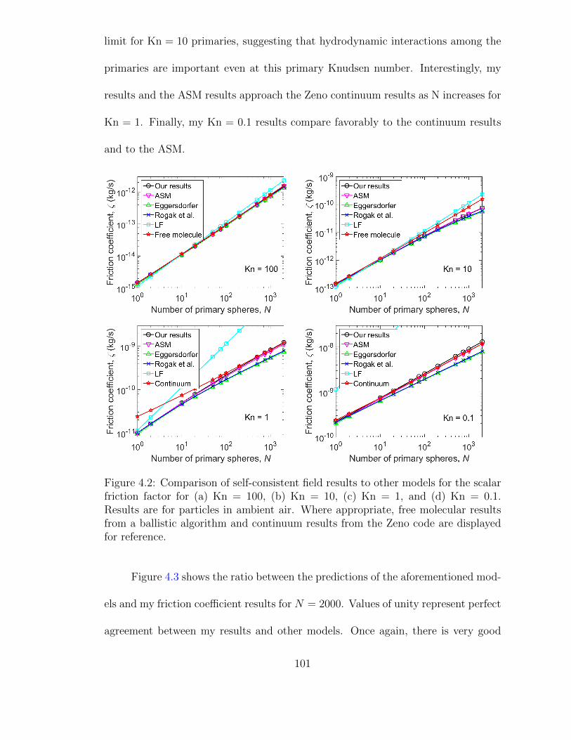
limit for Kn = 10 primaries, suggesting that hydrodynamic interactions among the

primaries are important even at this primary Knudsen number. Interestingly, my

results and the ASM results approach the Zeno continuum results as N increases for

Kn = 1. Finally, my Kn = 0.1 results compare favorably to the continuum results

and to the ASM.

Figure 4.2: Comparison of self-consistent field results to other models for the scalarfriction factor for (a) Kn = 100, (b) Kn = 10, (c) Kn = 1, and (d) Kn = 0.1.Results are for particles in ambient air. Where appropriate, free molecular resultsfrom a ballistic algorithm and continuum results from the Zeno code are displayedfor reference.

Figure 4.3 shows the ratio between the predictions of the aforementioned mod-

els and my friction coefficient results for N = 2000. Values of unity represent perfect

agreement between my results and other models. Once again, there is very good

101

agreement with the adjusted sphere method across the entire Knudsen range. The

Eggersdorfer and Rogak friction coefficients are notably lower than our results at low

to moderate primary sphere Knudsen numbers, though it is important to reiterate

that this comparison is for large aggregates (N = 2000). The agreement between the

models is better for smaller aggregates at lower primary sphere Knudsen numbers,

as indicated in Figure 4.2.

Additionally, Figure 4.3 illustrates how the aggregate approaches the con-

tinuum limit for decreasing Knudsen number: the ratio of the continuum result

calculated using the Zeno code to my Kirkwood-Riseman results is near unity for a

primary sphere Knudsen number as high as 2. This figure explicitly shows the differ-

ence between using the monomer friction coefficient from the BGK model solution

and using the monomer friction coefficient from the Cunningham slip correction fac-

tor. Differences are largest for small Knudsen numbers, though results are in good

agreement with the continuum results at low Knudsen number whether one uses the

BGK friction coefficient or the Cunningham slip coefficient for ζt,0 in Eq. (4.18).

Figure 4.4 clearly illustrates how the friction coefficient diverges from the free

molecular limit and exhibits more continuum-like behavior as the particle size (both

in terms of N and a) increases. Here, calculated friction coefficients are normalized

to the monomer friction coefficient for several primary sphere Knudsen numbers in

the transition regime. The power law exponent [i.e. η from Eq. (4.8)] decreases

from a value of approximately 0.9 – corresponding to the free molecule regime – as

both the number of primary spheres and the primary sphere size increases, until it

reaches a limit of approximately 0.54 for the continuum regime. The free molecule

102

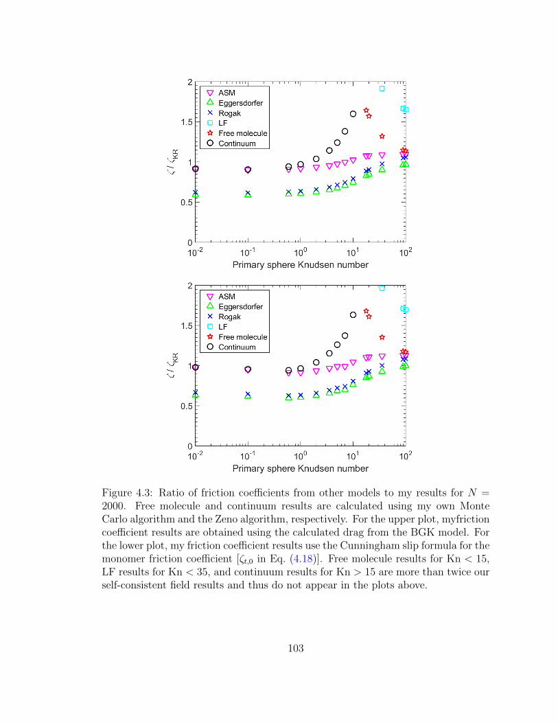
Figure 4.3: Ratio of friction coefficients from other models to my results for N =2000. Free molecule and continuum results are calculated using my own MonteCarlo algorithm and the Zeno algorithm, respectively. For the upper plot, myfrictioncoefficient results are obtained using the calculated drag from the BGK model. Forthe lower plot, my friction coefficient results use the Cunningham slip formula for themonomer friction coefficient [ζt,0 in Eq. (4.18)]. Free molecule results for Kn < 15,LF results for Kn < 35, and continuum results for Kn > 15 are more than twice ourself-consistent field results and thus do not appear in the plots above.

103

and continuum values are in agreement with previous observations [4]. The change

in the power law exponent reinforces the importance of accounting for hydrodynamic

interactions among primary spheres, even for fairly open aggregates with primary

spheres in the near-free molecular regime.

Figure 4.4: Normalized friction coefficient results for a range of aggregate sizes.

Previously researchers have looked at the evolution of the ratio between the

mobility radius and the radius of gyration as the number of primary spheres in-

creases. Figure 4.5 compares my self-consistent field results for this ratio (β =

Rm/Rg) to the same calculation in the continuum (where the mobility radius and

the hydrodynamic radius are equivalent) and free molecule regimes. Our results

agree with previous observations [54–56] that β approaches an asymptotic value in

the continuum regime. My results also agree qualitatively with the general obser-

vations of Sorensen [4], specifically Figure 2 of that work. However, my asymptotic

results for Kn = 0.01 and Kn = 0.1 are approximately 0.85, which is significantly

104

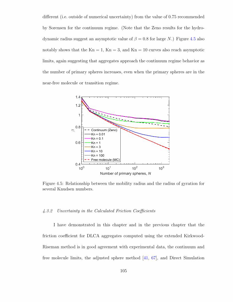
different (i.e. outside of numerical uncertainty) from the value of 0.75 recommended

by Sorensen for the continuum regime. (Note that the Zeno results for the hydro-

dynamic radius suggest an asymptotic value of β = 0.8 for large N .) Figure 4.5 also

notably shows that the Kn = 1, Kn = 3, and Kn = 10 curves also reach asymptotic

limits, again suggesting that aggregates approach the continuum regime behavior as

the number of primary spheres increases, even when the primary spheres are in the

near-free molecule or transition regime.

Figure 4.5: Relationship between the mobility radius and the radius of gyration forseveral Knudsen numbers.

4.3.2 Uncertainty in the Calculated Friction Coefficients

I have demonstrated in this chapter and in the previous chapter that the

friction coefficient for DLCA aggregates computed using the extended Kirkwood-

Riseman method is in good agreement with experimental data, the continuum and

free molecule limits, the adjusted sphere method [41, 67], and Direct Simulation

105

Monte Carlo results [41]. But the question becomes, how accurate is the extended

Kirkwood-Riseman method? To answer this question, I provide a very rough esti-

mate of the error in my results.

There are two primary sources of error in my calculations: the BGK results

for the velocity around and drag on a sphere in the transition flow regime, and

the Kirkwood-Riseman method itself. There is ample discussion in the literature

about the accuracy of the Kirkwood-Riseman method for continuum flow; see Refs.

[4, 31, 106, 107] for a small sample. I refer the reader to the literature for a thorough

discussion. I simply note that in my experience, the Kirkwood-Riseman results

(using either the Stokes flow velocity perturbation or the Rotne-Prager tensor) is

within 3% of the Zeno results for DLCA aggregates with 102000 primary spheres.

For N = 10, the Kirkwood-Riseman method underpredicts the friction factor by less

than 3%. At N = 2000, the Kirkwood-Riseman result is approximately 2% greater

than the Zeno result. Thus, I estimate the error in our calculated transition regime

friction coefficients due to the Kirkwood-Riseman method itself is on the order of a

few percent.

The second source of error is related to the solution of the BGK equation. From

this solution, I obtain the velocity around a sphere and the ratio of the drag on the

sphere to the free molecule drag. One can easily estimate the error in the drag on

a sphere by comparing my results from the BGK equation to the drag from Stokes’

law with the Cunningham slip correction factor. Applying Davies’ coefficients in

the slip correction formula, the calculated error in the BGK drag results is less than

3% for Kn ¿ 0.2. (One obtains similar errors when using the coefficients of Allen

106

and Raabe [66] in the slip correction factor.) The error is greater at lower Knudsen

numbers, as noted in Section 4.2.2; for Kn = 0.01, the BGK drag is approximately

7% greater than the drag from Stokes’ law. For most of the Knudsen range, the

error in my calculated drag force is comparable to the error in Stokes’ law for the

slip regime (either due to the model parameters used in the slip correction factor

or to experimental uncertainties); the BGK results are only in significant error near

the continuum regime.

We can compare our velocity results to the linearized Boltzmann equation

results of Takata et al. [78]. The linearized Boltzmann model is more rigorous than

the BGK model, but its associated computational cost is much higher than that

required to solve the BGK model. Takata et al. present the velocities as a function

of the parameter k∞ =√πKn/2. My velocity results are generally within 1-2%

of the linearized Boltzmann results for Kn = 0.11, 1.1, and 11 (k∞ = 0.1, 1, and

10). From these comparisons of the BGK velocity and drag results to the linearized

Boltzmann results and to Stokes’ flow in the continuum limit, I estimate that the

error in my aggregate friction coefficient results due to the use of the BGK model

is less than 5% for Kn > 0.2 and up to 10% for 0.01 < Kn < 0.2.

Combining the two sources of error, I would estimate the overall error in my

EKR results to be less than 10% for most of the Knudsen range. This estimate

is supported by comparing my friction coefficient results to the ASM results for

N = 2000 (Figure 4.3): the difference is less than 10% for 0.01 < Kn < 100.

Also, my calculated friction coefficient results for a primary sphere Knudsen number

greater than 5 are within 10% of the direct simulation Monte Carlo results of Zhang

107

et al. [41] for a 20-particle aggregate with a fractal dimension of 1.78 and a prefactor

of 1.3 (Chapter 3).

4.3.3 Analytical Expression for Friction Coefficients of Aggregates

While the Kirkwood-Riseman method is capable of providing the friction co-

efficient of an aggregate quickly – within seconds for N ∼ 100 and within minutes

for N ∼ 1000 – it is still not fast enough for use in an aerosol dynamics code. Thus,

it would be beneficial to use my friction coefficient results to develop a simple model

that provides the friction coefficient given only the number of primary spheres, the

primary sphere size, and the gas properties.

Sorensen and Wang [108] proposed computing the friction coefficient in the

transition regime as the harmonic sum of the continuum and free molecule expres-

sions,

ζ−1t = (ζct )

−1 + (ζFMt )−1 (4.34)

For a sphere, the continuum and free molecule friction coefficients are given by

Stokes’ law [Eq. (4.5)] and Epstein’s equation [Eq. (4.6)], respectively. I adopt this

approach for my model of the friction coefficient of DLCA aggregates with fractal

dimension and prefactor of 1.78 and 1.3.

I start by writing the continuum and free molecule aggregate friction coeffi-

cients as power laws,

ζmt,agg = ζm [ANη + (1− A)] (4.35)

where ζm is the continuum (m = c) or free molecule (m = FM) monomer friction

108

coefficient from Eq. (4.5) or Eq. (4.6), and A and η are model parameters obtained

from fits to the continuum (Zeno) or free molecule (Monte Carlo) results for N = 1

to 2000. We include the 1 − A term in the power law fits to give the correct

friction coefficient for a monomer. The free molecule coefficients AFM = 0.843

and ηFM = 0.939 are in excellent agreement with Mackowski’s correlation for the

free molecule friction coefficient (AFM = 0.847 and ηFM = 0.94 for k0 = 1.3 and

df = 1.78) [36]. The continuum coefficients Ac = 0.852 and ηc = 0.535 from

my Zeno results are also in good agreement with previous studies, as reported in

Sorensen’s review article [4].

Taking the harmonic sum of the continuum and free molecule power law fits, I

obtain the following expression for the aggregate friction coefficient as a function of

the number of primary spheres, the primary sphere radius, and the gas properties:

ζt6πµa

=

[AcNηc + (1− Ac)]−1 +BKn [AFMN

ηFM + (1− AFM)]−1−1(4.36)

Here, B = 1.612 for a hard-sphere gas with a momentum accommodation coefficient

of unity (i.e. pure diffuse reflection), consistent with my assumptions throughout

this chapter. For a monomer in the transition regime, the above relation reduces to

ζt,0 =6πµa

1 +BKn(4.37)

Sorensen and Wang [108] point out that the monomer friction coefficient given by

the harmonic sum is up to 10% less than the friction coefficient given by Stokes’

109

law with the slip correction factor. Thus, I apply a correction factor to my model

to give the same monomer drag as Stokes’ law. The final result is Eq. (4.38), which

provides an easily deployed analytic result to compute the friction coefficient over a

wide range of aggregate and primary particle sizes.

ζt6πµa

=1 + 1.612Kn

Cc(Kn)

[(0.852N0.535 + 0.148

)−1

+1.612Kn(0.843N0.939 + 0.157

)−1]−1

(4.38)

Figure 4.6 plots the friction coefficient calculated from Eq. (4.38) as a function

of primary sphere Knudsen number and the number of primary spheres. Results are

normalized using Stokes’ law evaluated for a = λ/Kn. The figure shows a clear tran-

sition between continuum behavior, where the friction coefficient is proportional to

1/a for a given number of primary spheres, and free molecule behavior characterized

by a 1/a2 dependence. (The normalized coefficients have no dependence on a in the

continuum and a 1/a dependence in the free molecule regime.) This figure shows

that the transition from the continuum regime to the free molecule regime occurs at

larger Knudsen numbers as the number of primary spheres increases, demonstrating

once again that particles exhibit more continuum-like behavior as both the Knudsen

number and the number of primary spheres increase.

Figure 4.7 shows the error in my fit relative to my self-consistent field results,

error =ζt,fit − ζt,EKR

ζt,EKR(4.39)

110

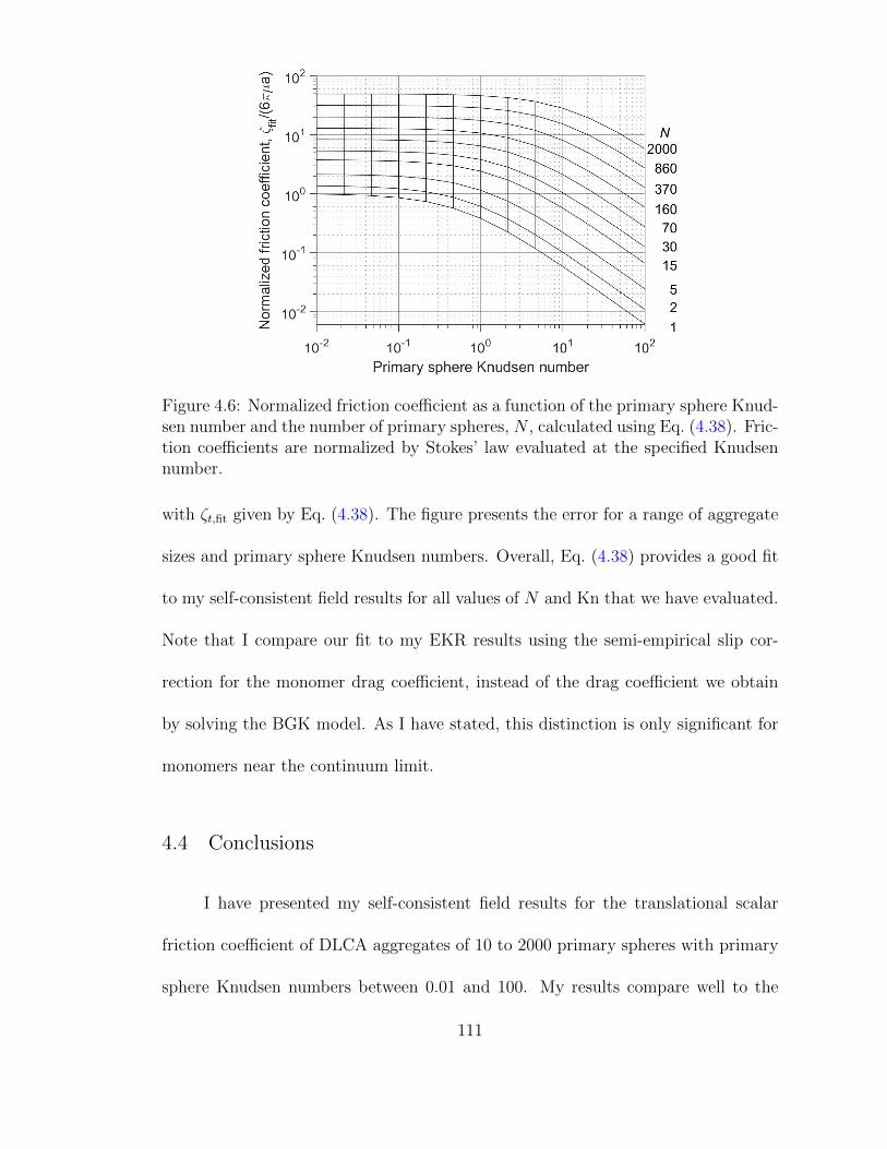
Figure 4.6: Normalized friction coefficient as a function of the primary sphere Knud-sen number and the number of primary spheres, N , calculated using Eq. (4.38). Fric-tion coefficients are normalized by Stokes’ law evaluated at the specified Knudsennumber.

with ζt,fit given by Eq. (4.38). The figure presents the error for a range of aggregate

sizes and primary sphere Knudsen numbers. Overall, Eq. (4.38) provides a good fit

to my self-consistent field results for all values of N and Kn that we have evaluated.

Note that I compare our fit to my EKR results using the semi-empirical slip cor-

rection for the monomer drag coefficient, instead of the drag coefficient we obtain

by solving the BGK model. As I have stated, this distinction is only significant for

monomers near the continuum limit.

4.4 Conclusions

I have presented my self-consistent field results for the translational scalar

friction coefficient of DLCA aggregates of 10 to 2000 primary spheres with primary

sphere Knudsen numbers between 0.01 and 100. My results compare well to the

111

Figure 4.7: Error of my harmonic sum model for the friction coefficient, Eq. (4.38),relative to my extended Kirkwood-Riseman friction coefficient results for a rangeof Knudsen numbers. Error is calculated with Eq. (4.39); the EKR results in thisequation use the monomer friction coefficient from Stokes’ law instead of the frictioncoefficient computed from the BGK model.

112

experimental data of Shin et al. [43, 44] and to the friction coefficient from the

adjusted sphere method [41, 67]. I estimate that my results are within approximately

10% of the true friction coefficient for DLCA aggregates up to 2000 primary spheres

for 0.01 < Kn < 100, though I would need to compare my results to experimental

data over a wide range of primary sphere Knudsen numbers and aggregate sizes

to verify this estimate. These results have been obtained by taking the harmonic

mean of the eigenvalues of the translational friction tensor. The difference between

the harmonic and arithmetic averages of the eigenvalues is generally less than 1%,

which is consistent with previous calculations for low-aspect-ratio particles in the

free molecule regime [105]. This difference is minor compared to the estimated

uncertainty in my results.

One significant finding of this study is that aggregate drag becomes more

continuum-like as the number of primary spheres increases, even for primary sphere

Knudsen numbers near the free molecule regime. Thus, one should not use free

molecule techniques to compute the drag on an aggregate unless the aggregate size

is very small with respect to the gas mean free path. This finding supports the theory

behind the adjusted sphere method, that one can calculate the drag on an aggregate

using an aggregate Knudsen number instead of the primary sphere Knudsen number.

My method is fast, but not fast enough to implement in an aerosol dynamics

code. The same is true of the adjusted sphere method, unless one already knows the

hydrodynamic radius and projected area of an aggregate. For this reason, I have

compared my results to the harmonic sum of power laws for the friction coefficient in

the continuum and free molecule regimes. The result presented in Eq. (4.38) provides

113

an analytical expression for the drag over a range of aggregate and primary particle

size. The simple model is within 8% of my self-consistent field results for the entire

range of aggregate sizes and primary sphere Knudsen numbers that I have studied.

This analysis is for fractal clusters generated using a cluster-cluster aggregation

method for a fractal dimension of 1.78 and a prefactor of 1.3.

114

Chapter 5: Calculating the Rotational Friction Coefficient of Frac-

tal Aerosol Particles in the Transition Regime using Ex-

tended Kirkwood-Riseman Theory

5.1 Introduction

Nanoscale aerosol particles consisting of many spheres in point contact are

formed in many natural and synthetic processes. The size, shape, and orientation

of these particles greatly affect their transport properties [4, 5], optical properties

[90, 91, 109], degree of alignment in an external field [6, 90, 91, 109], filtration

efficiency [110], and their effects in biological systems, including lung deposition

[19, 20].

Much of the theoretical and experimental literature on the transport properties

of nano-scale aerosol particles focuses on the translational friction coefficient (or,

equivalently, the electrical mobility). There is comparatively little focus on the

rotational friction or diffusion coefficients, which affect particle alignment in an

external field and relaxation time from an aligned state to a fully random state

[6, 90, 91, 109]. Inclusion of rotational dynamics is also important when considering

particle coagulation rates in Brownian motion simulations [111].

115

There are analytical expressions available in the literature for the torque on

(or the rotational diffusion coefficient of) simple shapes – such as spheres, rods,

and ellipsoids – in both the continuum [29, 49, 112] and free molecule regimes

[3, 113, 114]. However, there are no such expressions for complicated shapes such

as fractal aggregates. Garcia de la Torre and colleagues have extensively studied

the rotational problem for rigid particles consisting of multiple spheres in point

contact in the continuum regime [51–53, 107, 115]. More will be said about their

work shortly. There are far fewer studies available for the free molecule regime. Li

et al. [6] approximate the torque on a fractal aggregate rotating in a quiescent fluid

by considering only the linear velocity of each sphere and neglecting the effects of

shielding by the other spheres in the cluster, thereby providing an upper bound for

the torque. I am unaware of any more detailed methods for calculating the torque

on a fractal aggregate in either the free molecule or the transition flow regime. This

is significant because in many aerosol applications the primary spheres are much

smaller than the mean free path of the gas.

In this chapter, I discuss the application of my extended Kirkwood-Riseman

(EKR) theory [92] to the translational and rotational motion of fractal aggregates

in the transition flow regime. In Section 5.2 I provide the equations for the drag

and torque on a rigid particle, as introduced by Brenner [29]; I describe how one

can apply Kirkwood-Riseman theory to the problem; and I employ Monte Carlo to

compute the drag and torque on a translating or rotating particle, which I use to

validate the EKR method. I present my results for the rotational friction coefficient

as a function of Knudsen number and compare my results for Kn 1 and Kn 1

116

to the continuum and free molecule limits in Section 5.3.

5.2 Drag and torque on a rigid particle

Consider a rigid particle with center of mass moving at velocity UO and rotat-

ing with angular velocity ω, where point O is the origin of the system. For particles

in Stokes (i.e. low Reynolds number) flow, the force F and torque TO on the particle

are given by

F = −Ξt ·UO −Ξ†O,c ·ω (5.1)

TO = −ΞO,c ·UO −ΞO,r ·ω (5.2)

where Ξt, ΞO,r, and ΞO,c are the friction tensors for translation, rotation, and

translation-rotation coupling, respectively, and Ξ†O,c is the transpose of the coupling

tensor. The coupling and rotation tensors are defined with respect to the origin, O,

while the translation tensor is independent of the origin.

Brenner [29] proved that these friction tensors are related to the translation,

rotation, and coupling diffusion tensors by the generalized Stokes-Einstein relation

DO = kTM−1O , (5.3)

where DO and MO are the 6× 6 grand diffusion and friction matrices given by

DO =

DO,t D†O,c

DO,c Dr

(5.4)

117

MO =

Ξt Ξ†O,c

ΞO,c ΞO,r

(5.5)

Rewriting Eq. (5.3) as MO · DO = kT I, where I is the identity tensor, one can

show that the translation, rotation, and coupling diffusion tensors are related to the

friction tensors by [29, 52]

DO,t = kT (Ξt −Ξ†O,c ·Ξ−1O,r ·ΞO,c)

−1 (5.6)

Dr = kT (ΞO,r −ΞO,c ·Ξ−1t ·Ξ

†O,c)

−1 (5.7)

DO,c = −kT Ξ−1O,r ·ΞO,c · (Ξt −Ξ†O,c ·Ξ

−1O,r ·ΞO,c)

−1 (5.8)

According to Brenner [29], the translation and coupling tensors are most mean-

ingful when computed at the center of diffusion. At this point D, the coupling tensor

ΞD,c is symmetrical. The vector from the origin to the center of diffusion rOD can

be expressed as [29, 52]

rOD =

D22r +D33

r −D12r −D13

r

−D12r D11

r +D33r −D23

r

−D13r −D23

r D11r +D22

r

−1

·

D23O,c −D32

O,c

D31O,c −D13

O,c

D12O,c −D21

O,c

(5.9)

The translation and coupling tensors at the center of diffusion are given by

Dt = DO,t − rOD ×Dr × rOD + D†O,c × rOD − rOD ×DO,c (5.10)

118

Dc = DO,c + Dr × rOD (5.11)

Finally, I can write the scalar translational diffusion coefficient as [52]

Dt = kT/ζt = 13

Tr (Dt) (5.12)

where ζt is the translational friction coefficient and Tr (Dt) is the trace of the trans-

lation diffusion tensor. Similarly, I can define scalar rotational diffusion and friction

coefficients as

Dr = kt/ζr = 13

Tr (Dr) (5.13)

5.2.1 Kirkwood-Riseman Theory

Based on the preceding discussion, one can fully describe the translational and

rotational behavior of a rigid particle, provided one can obtain the translation, ro-

tation, and coupling friction tensors. I will now describe one approach for obtaining

those tensors for rigid particles consisting of N spherical elements in the continuum

regime. For this discussion, I will consider the case where all N elements have the

same radii ai = a, though this need not be the case when applying the general

framework described here. I will later discuss how to extend this approach to the

transition flow regime.

Kirkwood and Riseman [28] demonstrated that the drag on a particle in contin-

uum flow can be calculated by considering the hydrodynamic interactions between

each pair of spheres in the aggregate. Initially, hydrodynamic interactions between

spheres were calculated using the Oseen tensor. Later authors introduced more so-

119

phisticated hydrodynamic interaction tensors to account for the finite size of the

spherical elements [57, 58] and for rotational and translation-rotation coupling ef-

fects [59–61]. In all of these cases, the relationship between the linear velocity ui

and angular velocity ωi of the ith spherical element and the force Fj and torque Tj

at the center of each of the N elements is [53]

− ui =N∑j=1

Qtij ·Fj +

N∑j=1

(Qcij)† ·Tj (5.14)

− ωi =N∑j=1

Qcij ·Fj +

N∑j=1

Qrij ·Tj (5.15)

where Qtij, Qr

ij, and Qcij are the translation, rotation, and coupling hydrodynamic

tensors between the ith and jth spherical elements. These tensors will be defined

shortly.

This linear system of equations can be written in matrix form as

−

UPW

=

Qt (Qc)†

Qc Qr

FTP

(5.16)

where UP ,W , F , and TP are the 3N -element vector containing the linear velocities,

angular velocities, forces, and torques on the N spherical elements; and Qt, Qr,

and Qc are the 3N × 3N matrices of the translation, rotation, and coupling tensors

for all ij-pairs. Note that subscript P indicates that the property is evaluated at

the center of each element. For example, the linear velocity of the ith sphere that

appears in UP is ui = uO + ω × ri, where ri = (xi, yi, zi) is the vector from the

120

origin to the center of the ith element. Inverting Eq. (5.16), I get

FTP

= −

St (Sc)†

Sc Sr

UPW

(5.17)

where St (Sc)†

Sc Sr

=

Qt (Qc)†

Qc Qr

−1

(5.18)

Carrasco and Garcıa de la Torre [53] show that the 3 × 3 submatrices of the

3N × 3N S matrices are related to the translation, rotation, and coupling friction

tensors in Eqs. (5.1) and (5.2) by

Ξt =N∑i=1

N∑j=1

Stij (5.19)

ΞO,r =N∑i=1

N∑j=1

[Srij − Scij ·Aj + Ai · (Scij)† −Ai ·Stij ·Aj

](5.20)

ΞO,c =N∑i=1

N∑j=1

[Scij + Ai ·Stij

](5.21)

where

Ai =

0 −zi yi

zi 0 −xi

−yi xi 0

(5.22)

Carrasco and Garcıa de la Torre [53] summarize the hydrodynamic theories

of Reuland et al. [59], Mazur and Van Saarloos [60], and Goldstein [61] and show

121

that the hydrodynamic interaction tensors Qtij, Qr

ij, and Qcij all agree to order r−3

ij .

These tensors are given by

Qtij =

δijζt,0

I +3(1− δij)

4ζt,0

[a

rij

(I +

rijrijr2ij

)+

2a3

3r3ij

(I− 3rijrij

r2ij

)](5.23)

Qrij =

δijζr,0

I +(1− δij)

2ζr,0

a3

r3ij

[3rijrijr2ij

− I

](5.24)

Qcij = −(1− δij)

ζr,0

a3

r3ij

ε · rij (5.25)

where

ε · rij =

0 zij −yij

−zij 0 xij

yij −xij 0

, (5.26)

δij is the Kronecker delta, and ζt,0 = 6πµa and ζr,0 = 8πµa3 are the continuum

friction and torque coefficients. Note that the second term in Eq. (5.23) is the

Rotne-Prager-Yamakawa tensor [57, 58] [Eq. (3.11)].

Carrasco and Garcıa de la Torre [53] determined that including terms of order

lower than r−3ij in the interaction tensors did not significantly improve results for

the simple shapes that they analyzed. Since the effect of these lower order terms

drop off rapidly for larger particles, one can safely ignore these terms for the larger

particles I will consider in this paper.

122

5.2.2 Extension to the Transition Regime

I now wish to extend this Kirkwood-Riseman framework to the transition flow

regime. I start by multiplying Eqs. (5.14) and (5.15) by the monomer friction coeffi-

cient ζt,0 and the monomer torque coefficient ζr,0, respectively. As Rotne and Prager

[57] and Yamakawa [58] have noted, the product of the Rotne-Prager-Yamakawa ten-

sor and the Stokes’ law friction coefficient is similar to the flow field Vij around a

translating sphere in Stokes flow,

v(rij) = Vij ·U0 (5.27)

where Vij is given by Eq. (3.13). The difference between Vij and ζt,0Tij is a factor

of 2 in the r−3ij term in ζt,0Tij.

Recently, Corson et al. [92] exploited the similarity between Tij and the flow

around a sphere to extend Kirkwood-Riseman theory to the transition flow regime by

solving for the velocity around a sphere as a function of Knudsen number (Kn = λ/a,

where λ is the mean free path of molecules in the gas) and substituting the resulting

Vij(Kn)/ζt,0(Kn) for the second term in Eq. (5.23). This gives the drag on the ith

element of a purely-translating N -element particle as

Fi = −ζt,0(Kn)UO −N∑i 6=j

Vij(Kn) ·Fj (5.28)

123

In this case, the translation hydrodynamic interaction tensor is given by

Qtij(Kn) =

1

ζt,0(Kn)[δijI + (1− δij)Vij(Kn)] (5.29)

Similarly, I show in Appendix D that the (1−δij) terms in the rotation and cou-

pling hydrodynamic interaction tensors are directly related to the flow field around

a rotating sphere. Thus, solving for the velocity around and torque on a rotat-

ing sphere in the transition flow regime would provide expressions for Qrij(Kn) and

Qcij(Kn). This approach should be accurate to order r−3

ij , subject to the accuracy

of the numerical solution to the kinetic equation in the transition regime and the

small error introduced by omitting a factor of 2 in the r−3ij term in the translation

hydrodynamic interaction tensor. (These errors are discussed in Chapters 3 and 4).

To get the friction tensors for a given particle, one would populate and invert the

6N × 6N Q matrix and apply Eqs. (5.19)–(5.21).

Alternatively, one can apply a simplified approach to determine the friction

and diffusion tensors for a particle in the transition regime. Ignoring rotation and

coupling hydrodynamic interactions, the friction tensors are given by [51, 52]

Ξt =N∑i=1

N∑j=1

Stij(Kn) (5.30)

ΞO,c =N∑i=1

N∑j=1

ri × Stij(Kn) (5.31)

ΞO,r = −N∑i=1

N∑j=1

ri × Stij(Kn)× rj (5.32)

124

Here, St is the inverse of the 3N×3N translation matrix Qt, rather than a 3N×3N

block of the 6N × 6N Q matrix in Eq. (5.16). This approach is equivalent to

considering only the linear velocity ω × ri of each spherical element and ignoring

their angular velocities. One obvious flaw of this method is that it predicts zero

torque on a rotating sphere and on a chain of spheres rotating around its long axis.

Garcıa de la Torre and Rodes [107] suggest adding Nζr,0 to the diagonal elements

of ΞO,r to partially compensate for this error.

For my transition flow regime calculations, I will apply the simplified approach

given by Eqs. (5.30)–(5.32). This avoids the need to solve the kinetic equation for

a rotating sphere in the transition flow regime and requires inverting a 3N × 3N

matrix instead of a 6N × 6N matrix. However, I will apply the volume correction

of Garcıa de la Torre and Rodes [107] to the rotational friction tensor, using the

approximate expression for the ratio of the torque to the free molecule torque given

by Loyalka [77] [Eq. (44) in that work]. As I will demonstrate, the simplified

approach is sufficiently accurate for larger particles, for which the O(r−3ij ) terms in

the interaction tensors become less important.

5.2.3 Monte Carlo Calculations for Free Molecule Drag and Torque

In Chapters 3 and 4, I compared my results for the translational friction coef-

ficient to published experimental data and analytical results for the transition flow

regime. Unfortunately there is very little information on the rotational diffusion ten-

sor in the transition flow regime. In order to test the extended Kirkwood-Riseman

method I must compare to results in the continuum and free molecule limits. Con-

125

tinuum results will be taken from published results in the literature (where available)

or obtained using the hydrodynamic interaction tensors given by Eqs. (5.23)-(5.25).

I now describe my approach for calculating the friction tensors in the free molecule

limit.

Previous authors [34–36] have used a ballistic approach to calculate the drag

on a translating particle in free molecule flow. I use the same approach, but now

I consider both translational and rotational motion, and I calculate both the drag

and the torque on the particle.

The procedure is as follows. Consider the general case in which the bulk gas

velocity is a combination of translational velocity UO in the positive x-direction and

angular velocity ω about the x-axis. (For small translational and angular velocities,

this is practically equivalent to a particle moving with translational velocity UO in

the negative x-direction and rotating with angular velocity −ω, but it is easier to

consider the case in which the particle is stationary [77].) Surround the particle by

a launch sphere with radius R, randomly select starting locations on the surface of

the launch sphere, and define local coordinates (x?, y?, z?), where x? is the inward

normal for the position on the launch sphere. To determine the momentum of gas

molecules leaving the launch sphere, sample from the distribution of velocities of

gas molecules entering the launch sphere,

f(cx? , cy? , cz?) = Kcx? e−[c?−(UO+ω×R)?]2/2RT (5.33)

where c? = (cx? , cy? , cz?) is molecular velocity in the local coordinate system, R and

126

T are the gas constant and the gas temperature, the bulk gas velocity UO +ω ×R

is written in terms of local coordinates, and K is a normalization constant defined

such that ∫ ∞0

dcx?

∫ ∞−∞

d2cy?

∫ ∞−∞

d2cz? f = 1

If the molecule trajectory intersects the particle, calculate the momentum transfer

for diffuse reflection from the surface. For diffuse reflection, the molecule direction

is sampled from a cosine-squared distribution for the polar angle and an isotropic

distribution for the azimuthal angle, while the molecule speed is sampled from the

Maxwell-Boltzmann distribution

f(c) = 4π

√(1

2πRT

)3

c2 e−c2/2RT (5.34)

Continue to follow the molecule trajectory until it exits the launch and account for

multiple collisions between the gas molecule and the particle. After launching M

molecules, calculate the total drag and torque on the particle:

F =A

M

M∑i=1

φipi (5.35)

T =A

M

M∑i=1

φiri × pi (5.36)

Here, A is the launch sphere surface area, pi is the momentum transferred to the

particle by the ith molecule, and ri is the point at which the molecule collides with

the particle. The quantity φi is the flux of gas molecules entering the launch sphere

127

at Ri [40],

φi = n

√RT2π

e−s

2 cos2 θi +√πs cos θi[1 + erf(s cos θi)]

(5.37)

where n is the gas number density, s = U/RT is the ratio of the bulk velocity to

the molecular velocity in the gas, and θi is the angle between the bulk velocity and

the inward normal to the launch sphere at Ri.

Using the above procedure, I determine the translation friction tensor by set-

ting the angular velocity of the flow field equal to zero and calculating the drag F x,

F y, and F z for flow in the x-, y-, and z-directions. For a translation velocity much

less than the thermal speed√

2RT , the friction tensor is

Ξt =1

UO

F xx F y

x F zx

F xy F y

y F zy

F xz F y

z F zz

where F y

x signifies the x-component of the force on the particle for flow in the y-

direction. The pure translation calculation (i.e. ω = 0) also gives the coupling

tensor from the torque on the particle per Eq. (5.2). Finally, I calculate the rotation

friction tensor by setting the translation velocity to zero and calculating the torque

for rotation about the x-, y-, and z-axes.

I have tested my Monte Carlo drag and torque code by comparing my results

to published calculation results of Mackowski [36] for the translational friction coef-

ficient (taken as the harmonic average of the eigenvalues of the friction tensor) and

128

by comparing to simple test cases (e.g. a sphere rotating about its center, a sphere

rotating about an axis at a fixed distance from its center) for the torque problem.

All of my Monte Carlo results are in excellent agreement with results from alternate

calculation methodologies. (See Appendix C.) Furthermore, my calculated transla-

tion and rotation friction tensors are symmetrical to within the error in the Monte

Carlo calculations. Thus, I can use my Monte Carlo code to evaluate the results of

my EKR results in the free molecule limit.

5.3 Results

To verify that the extended Kirkwood-Riseman method produces reasonable

results across a wide range of Knudsen numbers, I will compare my calculated

rotational friction coefficient ζr to its values in the continuum and free molecule

limits. I first discuss the continuum and free molecule results.

5.3.1 Continuum regime

Before presenting my results for the rotational friction coefficient in the transi-

tion flow regime, it is appropriate to consider the effect of neglecting the rotational

and coupling hydrodynamic interaction tensors on ζr in the continuum. This is-

sue is discussed in depth in the works of Garcia de la Torre and colleagues (e.g.

Refs. [53, 115]). I will be using the EKR method to calculate the translation and

rotation friction coefficients of a dimer, a linear hexamer, and an octrahedral hex-

amer, so I will briefly discuss the results of Carrasco and Garcıa de la Torre [53]

129

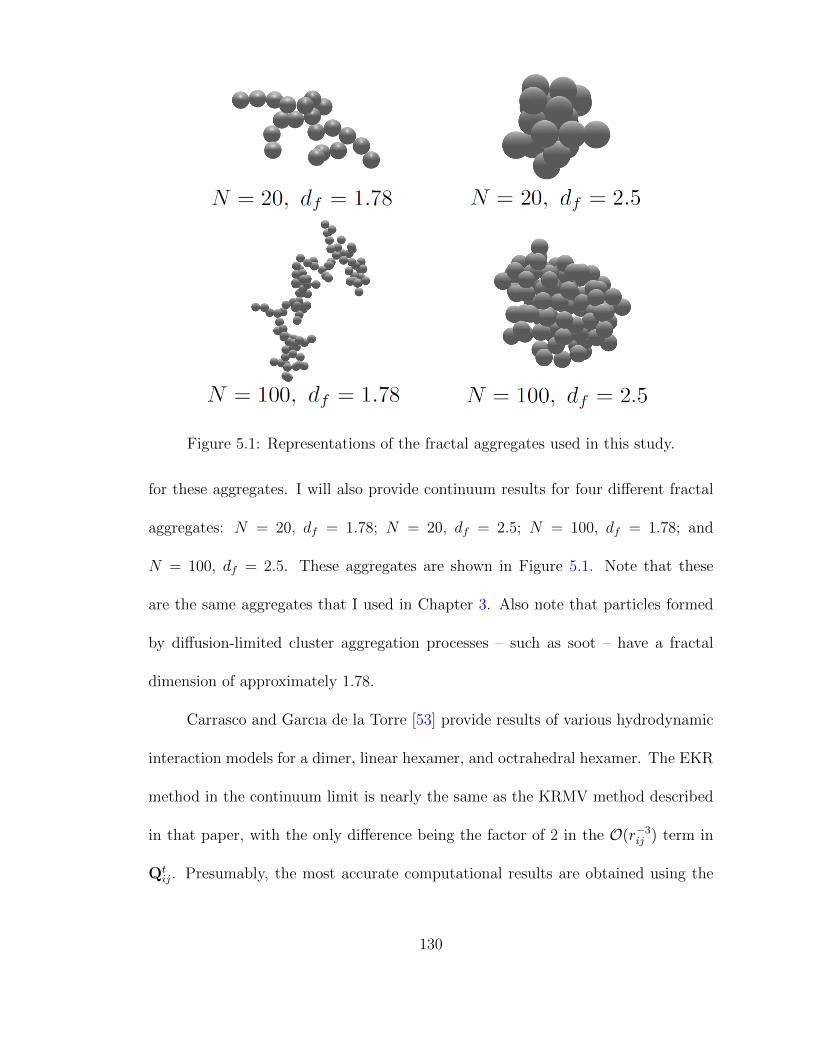
Figure 5.1: Representations of the fractal aggregates used in this study.

for these aggregates. I will also provide continuum results for four different fractal

aggregates: N = 20, df = 1.78; N = 20, df = 2.5; N = 100, df = 1.78; and

N = 100, df = 2.5. These aggregates are shown in Figure 5.1. Note that these

are the same aggregates that I used in Chapter 3. Also note that particles formed

by diffusion-limited cluster aggregation processes – such as soot – have a fractal

dimension of approximately 1.78.

Carrasco and Garcıa de la Torre [53] provide results of various hydrodynamic

interaction models for a dimer, linear hexamer, and octrahedral hexamer. The EKR

method in the continuum limit is nearly the same as the KRMV method described

in that paper, with the only difference being the factor of 2 in the O(r−3ij ) term in

Qtij. Presumably, the most accurate computational results are obtained using the

130

shell method, where each spherical element in the aggregate is replaced by a large

number of frictional units and hydrodynamic interactions are described using the

Oseen tensor. I will compare my extended Kirkwood-Riseman results in the con-

tinuum limit to the shell method results for the linear and octrahedral hexamers.

Exact results are available for a dimer in continuum flow [49], so I will compare

my extended Kirkwood-Riseman results to the exact values. Based on Table II of

Carrasco and Garcıa de la Torre [53], I would expect the EKR results to underpre-

dict the translational friction coefficient (or overpredict the translational diffusion

coefficient) and overpredict the rotational friction coefficient. I would expect better

agreement for less compact aggregates, like linear chains or fractals with df = 1.78,

and better agreement for the translational friction coefficient than for the rotational

friction coefficient.

Table 5.1 shows translational and rotational friction coefficients for the four

fractal aggregates mentioned previously. The Table includes ζt and ζr computed us-

ing terms up to order O(r−3ij ) in the interaction tensors (the 3RD method described

by Carrasco and Garcıa de la Torre [53]) and using the extended Kirkwood-Riseman

method (EKR, where I use the Stokes flow solution around a sphere for the trans-

lation interaction tensor and set the coupling and rotation hydrodynamic interac-

tion tensors to zero). Translational friction results are normalized by Stokes’ law,

ζt,0; rotational results are normalized to the monomer rotational friction coefficient,

ζr,0 = 8πµa3.

The difference between ζc,3RDt and ζc,EKR

t is small (< 2%) for the cases shown

here. The difference in the rotational friction coefficient is much larger, with the

131

Table 5.1: Continuum friction coefficient for fractal aggregates, normalized by themonomer friction results. Friction coefficients are calculated using terms up toorder r−3

ij in the hydrodynamic interaction tensors (3RD) or my extended Kirkwood-Riseman theory (EKR) in the continuum limit.

Case ζc,3RDt ζc,EKR

t ζc,3RDr ζc,EKR

r

N = 20, df = 1.78 4.35 4.31 94.5 110.8N = 100, df = 1.78 10.3 10.2 1292.0 1376.7N = 20, df = 2.5 3.41 3.37 42.5 57.5N = 100, df = 2.5 6.71 6.64 313.6 398.2

greatest difference (35%) occurring for N = 20, df = 2.5. The difference decreases

as the average distance between spheres increases due to the reduced importance

of the O(r−2ij ) and O(r−3

ij ) terms in the coupling and rotation interaction tensors,

respectively. These trends are consistent with the results of Carrasco and Garcıa

de la Torre [53] and Garcıa de la Torre et al. [115].

It is important to note that the 3RD method tends to underpredict the ro-

tational friction coefficient (or overpredict the rotational diffusion coefficient) com-

pared to more computationally-intensive methods like the shell model [53, 115]. On

the other hand, the EKR method appears to overpredict the friction coefficient. In

other words, the difference between my EKR results in the continuum and the true

value of the rotational friction coefficient may be less than that suggested by the

results in Table 5.1. I shall return to this subject in Section 5.4.

5.3.2 Free Molecule Regime

I have computed the free molecule translational and rotational friction coef-

ficients for the seven aggregates described in the previous section. The results are

shown in Table 5.2; the values in the table are normalized to the free molecule

132

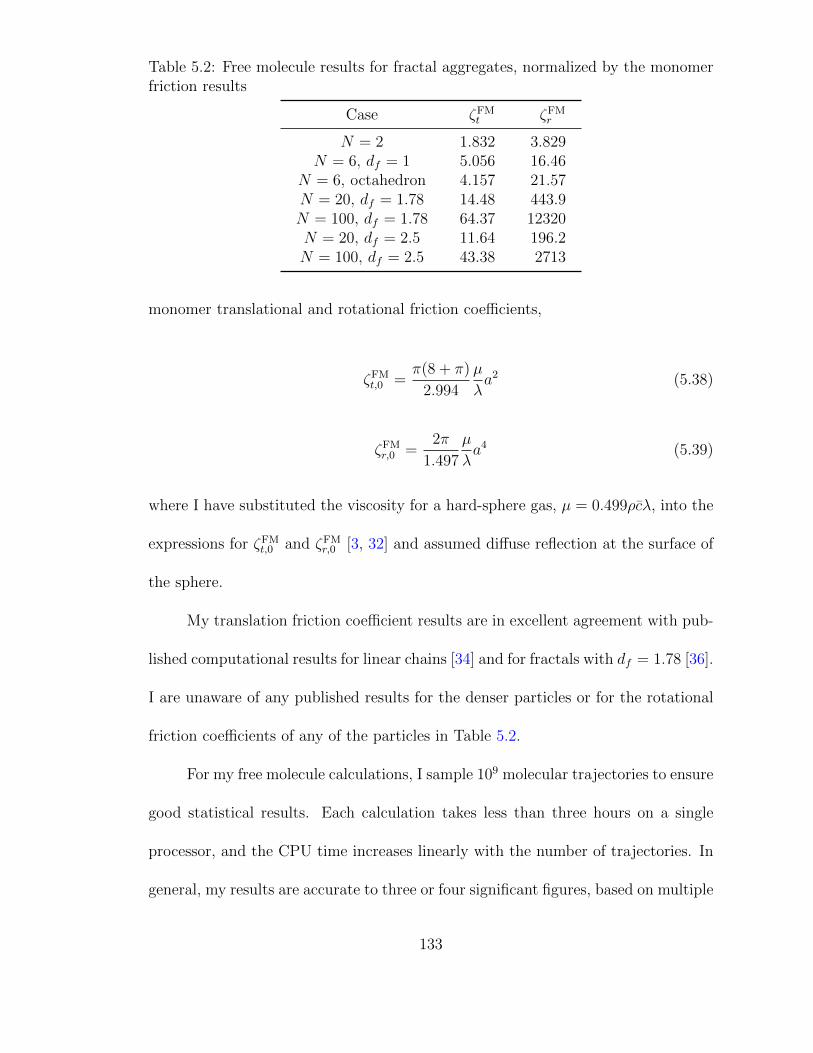
Table 5.2: Free molecule results for fractal aggregates, normalized by the monomerfriction results

Case ζFMt ζFM

r

N = 2 1.832 3.829N = 6, df = 1 5.056 16.46

N = 6, octahedron 4.157 21.57N = 20, df = 1.78 14.48 443.9N = 100, df = 1.78 64.37 12320N = 20, df = 2.5 11.64 196.2N = 100, df = 2.5 43.38 2713

monomer translational and rotational friction coefficients,

ζFMt,0 =

π(8 + π)

2.994

µ

λa2 (5.38)

ζFMr,0 =

2π

1.497

µ

λa4 (5.39)

where I have substituted the viscosity for a hard-sphere gas, µ = 0.499ρcλ, into the

expressions for ζFMt,0 and ζFM

r,0 [3, 32] and assumed diffuse reflection at the surface of

the sphere.

My translation friction coefficient results are in excellent agreement with pub-

lished computational results for linear chains [34] and for fractals with df = 1.78 [36].

I are unaware of any published results for the denser particles or for the rotational

friction coefficients of any of the particles in Table 5.2.

For my free molecule calculations, I sample 109 molecular trajectories to ensure

good statistical results. Each calculation takes less than three hours on a single

processor, and the CPU time increases linearly with the number of trajectories. In

general, my results are accurate to three or four significant figures, based on multiple

133

calculations performed for each case. This level of accuracy is more than sufficient

for most practical applications.

5.3.3 Transition Regime

I have performed my extended Kirkwood-Riseman calculations for the seven

particles discussed above for Knudsen numbers ranging from 0.01 to 100. In Chap-

ter 3, I reported the translational friction coefficient as a function of Knudsen number

for the fractal particles, calculated using the harmonic mean of the eigenvalues of

the translational friction tensor Ξt. The difference between ζt computed using this

approach and ζt computed using Eq. (5.12) is less than 1%.

Figure 5.2 presents my results for the scalar rotational friction coefficient ζr

[defined in Eq. (5.13)] of a dimer, linear hexamer, and octahedral hexamer. Results

are presented as a slip correction factor,

Cr(Kn) ≡ ζcrζEKRr (Kn)

(5.40)

where the continuum rotational friction coefficient ζcr is calculated using the best

available method. (Cr is analogous to the Cunningham slip correction factor, which

represents the ratio between Stokes’ law and the friction coefficient for a sphere in

the transition regime. It is also analogous to the parameter Θ−1, defined by Zhang

et al. [41] as the ratio of the continuum friction coefficient to the transition regime

friction coefficient for an aggregate.) For the dimer, ζcr is given by the exact solution

to the Stokes equation [49]; for the hexamers, ζcr is taken as the shell method solution

134

from Carrasco and Garcıa de la Torre [53]. The free molecule limit for each particle

is shown as a dashed line. Note that the curves representing the dimer and the

linear hexamer nearly coincide due to the chosen normalization used in the plot.

At small Knudsen numbers, the rotational friction coefficient approaches a

constant value that differs from the continuum value for the aggregate ζcr because

my calculations neglect rotational and coupling hydrodynamic interactions, as dis-

cussed in Section 5.3.1 and illustrated by the results in Table 5.1. At large Knudsen

numbers, ζEKRr is in excellent agreement with my Monte Carlo calculations for the

free molecule rotational friction coefficient (within 5% at Kn=100). The slight dis-

crepancy between the solid and dashed lines in the free molecule limit are due to

numerical uncertainty in the Monte Carlo calculations and interpolation error in ap-

plying my results for the velocity around a sphere to Vij(Kn) in Eq. (5.28). (Note

that I use a Gaussian quadrature to solve for the velocity within approximately 10

mean free paths of the sphere surface. Thus, interpolation errors are most significant

near the free molecule regime, where the sphere radius is comparable to the node

spacing.) These results suggest that rotational and coupling interactions between

primary spheres are negligible at large Knudsen numbers, as one would expect due

to the nature of free molecule flow.

Figure 5.3 presents my results for ζEKRr for the fractal particles. Again, the

results are plotted as a slip correction factor, but in this case the continuum rota-

tional friction coefficient is calculated using the 3RD method. Note that the two

N = 20 curves appear to lie on top of each other, as do the two N = 100 curves;

again, this is due to the chosen normalization.

135

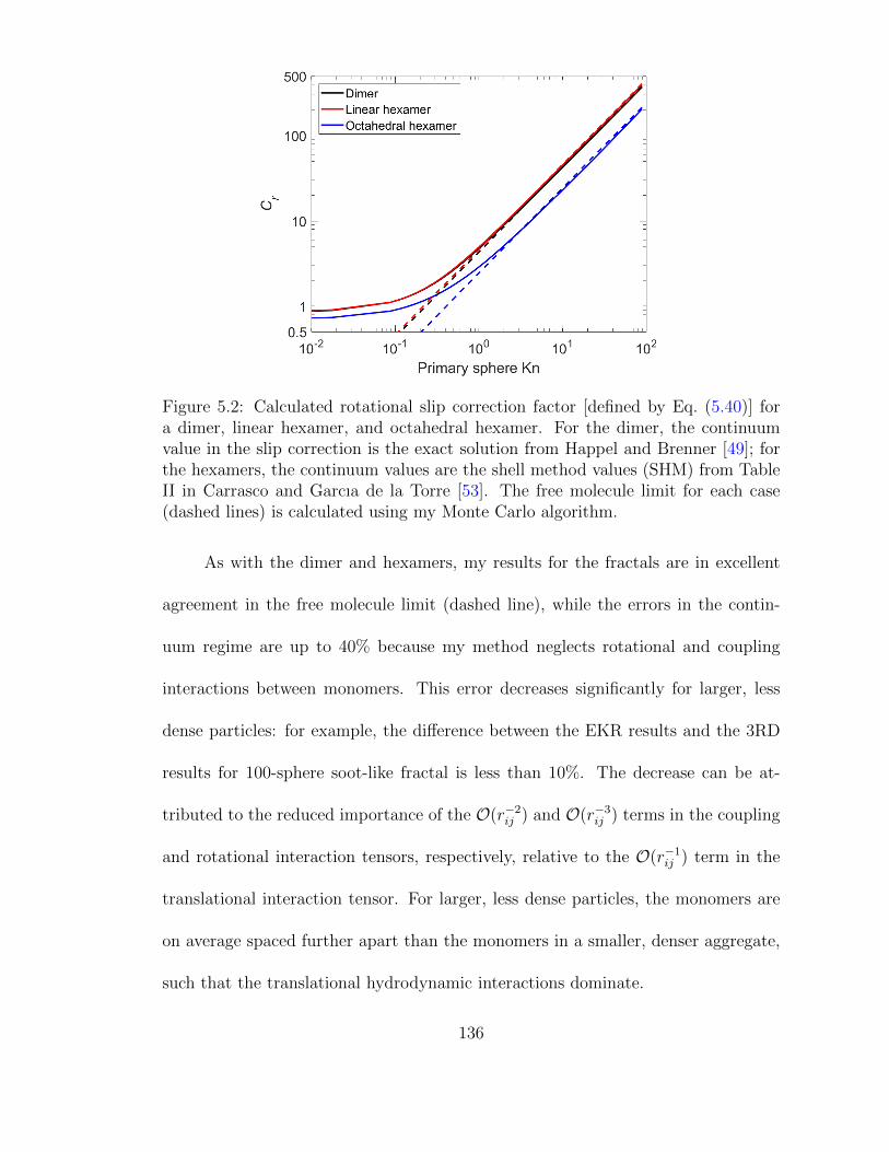
Figure 5.2: Calculated rotational slip correction factor [defined by Eq. (5.40)] fora dimer, linear hexamer, and octahedral hexamer. For the dimer, the continuumvalue in the slip correction is the exact solution from Happel and Brenner [49]; forthe hexamers, the continuum values are the shell method values (SHM) from TableII in Carrasco and Garcıa de la Torre [53]. The free molecule limit for each case(dashed lines) is calculated using my Monte Carlo algorithm.

As with the dimer and hexamers, my results for the fractals are in excellent

agreement in the free molecule limit (dashed line), while the errors in the contin-

uum regime are up to 40% because my method neglects rotational and coupling

interactions between monomers. This error decreases significantly for larger, less

dense particles: for example, the difference between the EKR results and the 3RD

results for 100-sphere soot-like fractal is less than 10%. The decrease can be at-

tributed to the reduced importance of the O(r−2ij ) and O(r−3

ij ) terms in the coupling

and rotational interaction tensors, respectively, relative to the O(r−1ij ) term in the

translational interaction tensor. For larger, less dense particles, the monomers are

on average spaced further apart than the monomers in a smaller, denser aggregate,

such that the translational hydrodynamic interactions dominate.

136

Figure 5.3: Calculated rotational slip correction factor [defined by Eq. (5.40)] forfour fractal aggregates. The continuum rotational friction coefficient that appears inthe slip correction is calculated using the 3RD method, and the Knudsen-number-dependent friction coefficient is calculated using my EKR method. The free molec-ular limit for each aggregate (dashed lines) is calculated using my Monte Carloalgorithm.

Dahneke [67] and Zhang et al. [41] posited there exists for the translational

friction coefficient a universal relationship between the friction coefficient in the

transition flow regime and an aggregate Knudsen number,

ζctζt(Knagg)

= Cc(Knagg) (5.41)

where Cc is the Cunningham slip correction factor. Zhang et al. [41] showed using

dimensional analysis that the appropriate aggregate Knudsen number for transla-

tional friction is

Knagg =πλRH

PA(5.42)

where RH and PA are the hydrodynamic radius and projected area of the aggregate,

137

which characterize particle size in the continuum and free molecule regimes, respec-

tively. In other words, the aggregate Knudsen number is proportional to the ratio

between the continuum and free molecule friction coefficients for the aggregate.

This Adjusted Sphere Method implies that plots of the aggregate translational

slip correction factor [Eq. (5.41)] versus the aggregate Knudsen number [Eq. (5.42)]

fall on the same universal curve, regardless of particle shape. Experimental and com-

putational studies [41, 68, 69, 92, 93] suggest that this is indeed the case. Based on

this evidence, I propose that the rotational slip correction factor [Eq. (5.40)] should

exhibit similar behavior when plotted against an appropriate aggregate Knudsen

number. Since the translational aggregate Knudsen number is proportional to the

ratio of continuum to free molecule friction coefficients, I posit that the rotational

aggregate Knudsen number is

Knr,agg =ζcrζFMr

=23.952

8 + π

ζc?rζFM?r

Kn (5.43)

where Kn is the primary sphere Knudsen number and ζc?r ≡ ζcr/ζcr,0 and ζFM?

r ≡

ζFMr /ζFM

r,0 are the dimensionless continuum and free molecule rotational friction co-

efficients for the aggregate.

Figure 5.4 shows my rotational friction coefficient results plotted as the rota-

tional slip correction factor versus the aggregate Knudsen number [Eq. (5.43)]. The

dimensionless continuum friction coefficients are calculated with the same reference

method used in Figs. 5.2 and 5.3 (i.e. the exact solution for the dimer [49], the shell

method for the hexamers [53], and the 3RD method for the 20- and 100-particle ag-

138

Figure 5.4: Rotational slip correction factor plotted versus an aggregate Knudsennumber. The aggregate Knudsen number is the ratio of the friction coefficient cal-culated as if the aggregate is in continuum flow to the friction coefficient calculatedas if the aggregate is in free molecule flow. Continuum friction coefficients are calcu-lated using the same reference method used to calculate the slip correction factor Cr,while the free molecule coefficients are calculated using my Monte Carlo algorithm

gregates). The dimensionless free molecule friction coefficients are calculated using

my Monte Carlo algorithm. Roughly speaking, all of the aggregates exhibit the same

behavior when plotted in this manner. The differences among the curves near the

continuum regime are likely due to neglecting rotational and coupling hydrodynamic

interactions when calculating the rotational friction coefficient, as discussed previ-

ously. Errors in the calculated continuum friction coefficient may also contribute to

the spread among the curves. My results suggest that the aggregate rotational fric-

tion coefficient follows some universal function of the rotational aggregate Knudsen

number.

139

5.4 Discussion

I have applied my extended Kirkwood-Riseman theory to calculate the rota-

tional friction coefficient for aerosol particles in the transition flow regime. This

approach ignores rotational and translation-rotation coupling interactions between

spheres. These effects become less important as the number of primary spheres

increase and as the primary sphere size decreases. The former effect is due to the

dominance of the O(r−1ij ) term in the translational interaction tensor over the lower

order terms in the rotational and coupling interaction tensors. The latter effect

occurs because smaller particles perturb the flow field less than large particles.

Consistent with this discussion, my EKR results are in excellent agreement

with my Monte Carlo results for large Knudsen numbers (i.e. within 5% for Kn =

100). The agreement is not as good in the continuum regime: I have observed errors

as high as 40% for dense aggregates relative to the rotational friction coefficient

computed considering terms up to order O(r−3ij ) in the interaction tensors. The EKR

results are in better agreement with the 3RD results for less dense fractal aggregates.

It is also worth mentioning that the EKR and 3RD methods respectively under-

and over-predict the rotational friction coefficient compared to the computationally-

intensive shell method, so the rotational friction coefficient computed using the EKR

method is mostly likely in better agreement with the true friction coefficient than

my results in Table 5.1 and Figure 5.3 suggest.

My results also suggest that there is a universal relationship between the ro-

tational friction coefficient and an aggregate Knudsen number. This is analogous to

140

relationship between the translational friction coefficient and the aggregate Knudsen

number introduced by Dahneke [67] and Zhang et al. [41], which is supported by

experimental data and computational results [41, 68, 69, 92, 93]. For the rotational

friction coefficient, the appropriate aggregate Knudsen number is the ratio of the

aggregate continuum and free molecule friction coefficients.

I could improve the accuracy of my method – particularly near the contin-

uum regime – if I considered pairwise rotational and coupling interactions between

primary spheres in the aggregate. As I have demonstrated (Appendix D), the rota-

tional and coupling interaction tensors are related to the flow field around a rotating

sphere; one could solve the kinetic equation for flow around a rotating sphere as a

function of Knudsen number to obtain the appropriate interaction tensors in the

transition flow regime. With that said, my simplified method is sufficiently accu-

rate for most practical purposes – particularly for larger aggregates with a fractal

dimension of 1.78.

Finally, I will note that while I have focused exclusively on the scalar friction

coefficient, my method also provides the translation, rotation, and coupling friction

tensors. Thus, the extended Kirkwood-Riseman method can be used when consid-

ering alignment of aerosol particles in an external field [6, 90, 91, 109, 114] or when

simulating Brownian diffusion of small particles.

141

Chapter 6: Analytical Expression for the Rotational Friction Co-

efficient of DLCA Aggregates over the Entire Knudsen

Regime

6.1 Introduction

The rotational behavior of an aerosol particle can be characterized by the

rotational friction and diffusion coefficients ζr and Dr, which are related by the

Stokes-Einstein relationship ζr = kBT/Dr. The rotational behavior can be impor-

tant to evaluating the average drift velocity [105, 116] and particle alignment in

external electric field and subsequent relaxation [5, 6, 90, 91, 109].

For fractal aggregates that consist of many nano-sized spheres in contact,

determining the rotational friction/diffusion coefficient is a difficult problem. This

is due to two principal factors: the complicated, fractal-like shape of the aggregates,

and the fact that the particle size is often comparable to the mean free path of the

molecules in the gas. The latter complication means that the particles are in the

transition flow regime, where one must use kinetic theory to solve for the forces

and torques exerted by the gas on the aggregates. For these fractal-like particles,

the relationship between the number of spheres in the aggregate and its radius of

142

gyration is

N = k0

(Rg

a

)df(6.1)

where df and k0 are the fractal dimension and prefactor. For particles formed

by diffusion-limited cluster aggregation (DLCA), which is the focus of this work,

k0 ≈ 1.3 and df ≈ 1.78.

In this chapter, I build on my the work on the rotational friction coefficient of

aggregates described in the previous chapter. Here, I apply my extended Kirkwood-

Riseman (EKR) theory to determine the rotational friction coefficient of DLCA

aggregates over a parameter range of interest to aerosol scientists. I use my results

to generate a simple analytical expression for the rotational friction coefficient, as a

function of primary sphere size and the number of spheres in the aggregate.

6.2 Theoretical Methods

The force and torque on a rigid particle moving slowly relative to the sur-

rounding fluid can be expressed as

F = −Ξt ·UO −Ξ†O,c ·ω (6.2)

TO = −ΞO,c ·UO −ΞO,r ·ω (6.3)

where point O is the center of mass of the particle; UO and ω are the translational

and rotational velocities of the particle; and Ξt, ΞO,r, and ΞO,c are the translational,

rotational, and translation-rotation coupling friction tensors. The translational,

143

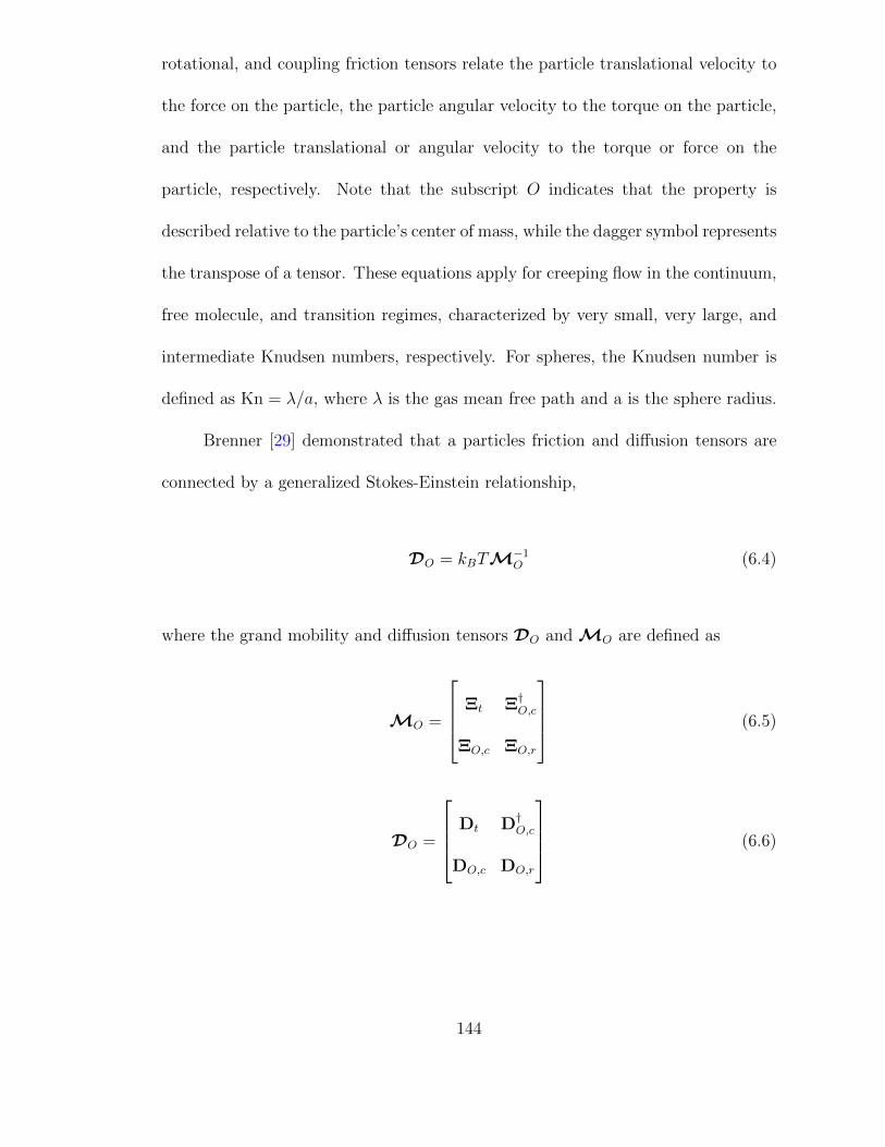
rotational, and coupling friction tensors relate the particle translational velocity to

the force on the particle, the particle angular velocity to the torque on the particle,

and the particle translational or angular velocity to the torque or force on the

particle, respectively. Note that the subscript O indicates that the property is

described relative to the particle’s center of mass, while the dagger symbol represents

the transpose of a tensor. These equations apply for creeping flow in the continuum,

free molecule, and transition regimes, characterized by very small, very large, and

intermediate Knudsen numbers, respectively. For spheres, the Knudsen number is

defined as Kn = λ/a, where λ is the gas mean free path and a is the sphere radius.

Brenner [29] demonstrated that a particles friction and diffusion tensors are

connected by a generalized Stokes-Einstein relationship,

DO = kBTM−1O (6.4)

where the grand mobility and diffusion tensors DO andMO are defined as

MO =

Ξt Ξ†O,c

ΞO,c ΞO,r

(6.5)

DO =

Dt D†O,c

DO,c DO,r

(6.6)

144

The scalar friction and diffusion coefficients are obtained from the trace of the

rotational diffusion tensor:

Dr = kBT/ζr = 13

Tr(Dr) (6.7)

Analytical expressions are available for the rotational friction/diffusion coef-

ficient of simple shapes in the continuum [29, 49, 112] and free molecule regimes

[3, 113, 114], but more approximate methods are needed for fractal-like aggregates

of touching spheres. The rotation problem has been studied extensively by Garcia

de la Torre and colleagues for rigid particles in continuum flow [51, 53, 115]. Li et al.

[6] used a simplified approach in the free molecule regime that ignored shielding by

other spheres in the aggregate. In principle, one could use a Monte Carlo approach

in the free molecule regime analogous to that used to compute the translational

friction coefficient [see e.g. [34, 36, 117, 118]] by replacing the linear velocity field

by a rotating velocity field, though no one appears to have published any results

using this approach.

Unfortunately, in many practical situations aerosol particles are fractal-like

aggregates in the transition flow regime, so a different approach is needed to analyze

their rotational behavior. In the previous chapter, I demonstrated that my extended

Kirkwood-Riseman (EKR) method can be applied to the rotational problem.

6.2.1 Extended Kirkwood-Riseman Method for the Rotational Friction Coefficient

Kirkwood and Riseman [28] developed a method to determine the force exerted

145

by a fluid on a particle or m acromolecule consisting of N spherical elements in

continuum flow, whereby the force on each element is equal to the force on an

isolated sphere minus the perturbations to the flow field caused by the other spheres:

Fi = −ζct,0Ui − ζct,0N∑i 6=j

Tij ·Fj (6.8)

Tij =1

8πµrij

[(I +

rijrijr2ij

)+

2a2

3r2ij

(I− 3rijrij

r2ij

)](6.9)

Here, ζr,0 = 6πµa is the monomer translational friction coefficient, Ui is the velocity

of the ith sphere in the aggregate, and Tij is the hydrodynamic interaction tensor

that quantifies the effects of the jth sphere on the ith sphere. Applications of KR

theory often use the Rotne-Prager-Yamakawa (RPY) tensor [57, 58], Eq. (6.9), for

Tij, which is accurate to O(r−3ij ), where rij is the distance between the ith and jth

sphere.

The product of the monomer friction coefficient and the RPY tensor is similar

to the solution for Stokes flow around a sphere Vij, where u(rij) = Vij ·Uj is

the velocity around a sphere moving with velocity Uj. Noting this, I introduced

my extended Kirkwood-Riseman (EKR) method by replacing ζt,0Tij in Eq. (6.8)

with the velocity tensor for flow around a sphere in the transition regime, Vij(Kn)

(Chapters 3 and 4):

Fi = −ζt,0(Kn)Ui −N∑i 6=j

Vij ·Fj (6.10)

As noted in the above equation, both the velocity tensor and the monomer friction

coefficient are functions of the primary sphere Knudsen number. These functions are

146

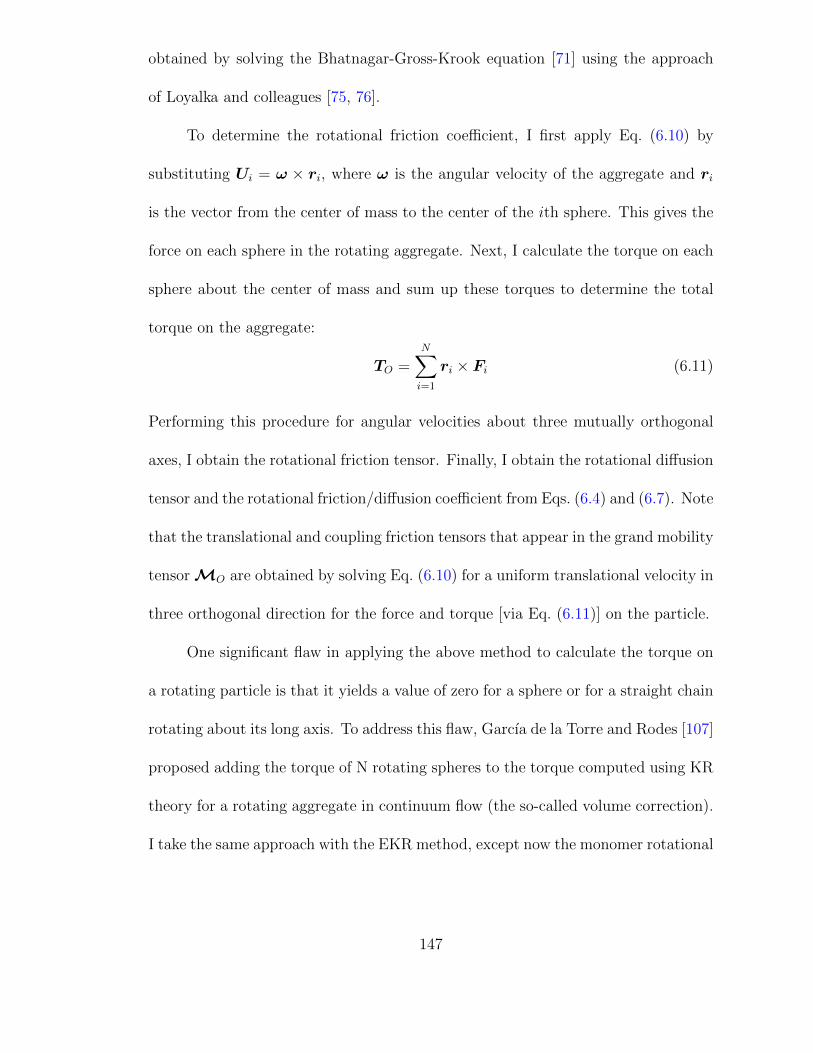
obtained by solving the Bhatnagar-Gross-Krook equation [71] using the approach

of Loyalka and colleagues [75, 76].

To determine the rotational friction coefficient, I first apply Eq. (6.10) by

substituting Ui = ω × ri, where ω is the angular velocity of the aggregate and ri

is the vector from the center of mass to the center of the ith sphere. This gives the

force on each sphere in the rotating aggregate. Next, I calculate the torque on each

sphere about the center of mass and sum up these torques to determine the total

torque on the aggregate:

TO =N∑i=1

ri × Fi (6.11)

Performing this procedure for angular velocities about three mutually orthogonal

axes, I obtain the rotational friction tensor. Finally, I obtain the rotational diffusion

tensor and the rotational friction/diffusion coefficient from Eqs. (6.4) and (6.7). Note

that the translational and coupling friction tensors that appear in the grand mobility

tensorMO are obtained by solving Eq. (6.10) for a uniform translational velocity in

three orthogonal direction for the force and torque [via Eq. (6.11)] on the particle.

One significant flaw in applying the above method to calculate the torque on

a rotating particle is that it yields a value of zero for a sphere or for a straight chain

rotating about its long axis. To address this flaw, Garcıa de la Torre and Rodes [107]

proposed adding the torque of N rotating spheres to the torque computed using KR

theory for a rotating aggregate in continuum flow (the so-called volume correction).

I take the same approach with the EKR method, except now the monomer rotational

147

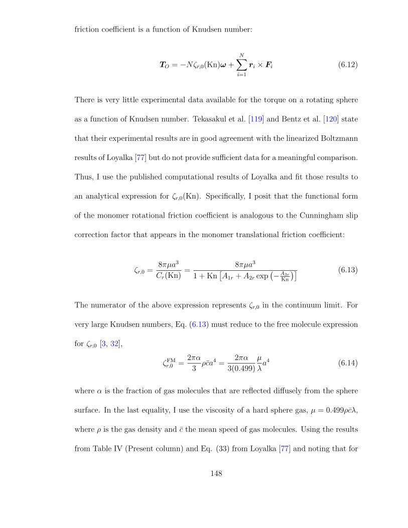
friction coefficient is a function of Knudsen number:

TO = −Nζr,0(Kn)ω +N∑i=1

ri × Fi (6.12)

There is very little experimental data available for the torque on a rotating sphere

as a function of Knudsen number. Tekasakul et al. [119] and Bentz et al. [120] state

that their experimental results are in good agreement with the linearized Boltzmann

results of Loyalka [77] but do not provide sufficient data for a meaningful comparison.

Thus, I use the published computational results of Loyalka and fit those results to

an analytical expression for ζr,0(Kn). Specifically, I posit that the functional form

of the monomer rotational friction coefficient is analogous to the Cunningham slip

correction factor that appears in the monomer translational friction coefficient:

ζr,0 =8πµa3

Cr(Kn)=

8πµa3

1 + Kn[A1r + A2r exp

(−A3r

Kn

)] (6.13)

The numerator of the above expression represents ζr,0 in the continuum limit. For

very large Knudsen numbers, Eq. (6.13) must reduce to the free molecule expression

for ζr,0 [3, 32],

ζFMr,0 =

2πα

3ρca4 =

2πα

3(0.499)

µ

λa4 (6.14)

where α is the fraction of gas molecules that are reflected diffusely from the sphere

surface. In the last equality, I use the viscosity of a hard sphere gas, µ = 0.499ρcλ,

where ρ is the gas density and c the mean speed of gas molecules. Using the results

from Table IV (Present column) and Eq. (33) from Loyalka [77] and noting that for

148

diffuse reflection A1r +A2r = 5.988, I get the following values for the coefficients in

the rotational slip correction factor: A1r = 3.930, A2r = 2.058, and A3r = 0.3277.

A second concern in employing the EKR method is that it ignores rotational

and translation-rotation coupling interactions between spheres. Simply put, the lin-

ear and rotational motions of a sphere can induce a rotation or torque in another

sphere, in accordance with Faxns second law [49]. The rotational and coupling hy-

drodynamic interaction tensors are (to order r−3ij ) equal to vorticity field around

a rotating sphere and the vorticity field around a translating sphere, respectively.

Thus, one would need to compute these fields as a function of Knudsen number to

account for rotational and coupling effects. In addition, one would now need to in-

vert a 6N -by-6N matrix (instead of a 3N -by-3N matrix, as in the current method)

to obtain the translational, rotational, and coupling friction tensors. (See Chap-

ter 5 for further discussion.) Rotational and coupling hydrodynamic interactions

are weaker (i.e. lower order in rij) than the translational hydrodynamic interactions

described by Tij, so I ignore these effects in the EKR method. The resulting error is

appreciable (around 30-40%) for very small, dense (i.e. high fractal dimension) ag-

gregates but decreases as the aggregate size (and thus the average distance between

spheres) increases (Chapter 5). I will discuss this further later in this chapter.

To apply my method for calculating the rotational friction coefficient, one

simply needs the coordinates of the primary spheres in the particle (either from a

cluster-cluster aggregation algorithm, as I use for this study, from a detailed Brow-

nian simulation, or from a TEM image) and the velocity field around a sphere. (See

Appendix B for velocity results at select Knudsen numbers.) Given this informa-

149

tion, one forms a 3N-by-3N matrix where each 3-by-3 block is Qij = [δijI + (1 −

δij)Vij(Kn)]/ζr,0(Kn) and δij is the Kronecker delta. The tensor Vij is a function

of primary size and the vector connecting the ith and jth spheres. In other words,

one solves Eq. (6.10) as a linear algebra problem to obtain the force on each sphere

and uses these results and Eq. (6.12) to determine the torque on the particle. Re-

peating this procedure for three mutually orthogonal angular velocities, one obtains

the rotational friction tensor. See the previous chapter for further discussion.

6.2.2 Adjusted Sphere Method for the Rotational Friction Coefficient

The extended Kirkwood-Riseman method can be applied to determine the

friction tensors of an aggregate in the transition flow regime, given the coordinates

of the spheres in the aggregate and the velocity around a sphere as a function of

the primary sphere Knudsen number. From these friction tensors, one can obtain

the rotational friction or diffusion coefficient. Here, I propose a parametric method

of determining the rotational friction coefficient that does not rely on the EKR

method. This parametric method is based on the adjusted sphere method (ASM) of

Dahneke and Zhang et al. for determining the translational friction coefficient. My

preliminary results showed that the adjusted sphere approximation can be applied

to the rotational friction coefficient (Chapter 5).

Dahneke [67] and Zhang et al. [41] posited that there is a universal relation-

ship between the translational friction coefficient of an aggregate and an aggregate

Knudsen number:

ζt,ASM =6πµRH

Cc(Knt,agg)(6.15)

150

Knt,agg =πλRH

PA(6.16)

Here, the hydrodynamic radius RH and orientation-averaged projected area PA

are continuum and free molecular measures of the particle size, respectively. The

adjusted sphere method allows one to compute the translational friction coefficient

of an aggregate given its hydrodynamic radius and projected area.

Melas et al. [80] show that this aggregate Knudsen number is proportional to

the ratio of continuum and free molecule expressions for the translational friction

coefficient. I propose an analogous approach for the rotational friction coefficient:

ζr,ASM =ζcr

Cr(Knr,agg)(6.17)

Knr,agg =ζcr

(A1r + A2r)ζFMr

(6.18)

Here, ζcr and ζFMr are the aggregate rotational friction coefficients computed using

continuum and free molecular methods, respectively. The rotational slip correction

factor formula is the same as Cr defined in Eq. (6.13) and used to compute the

monomer rotational friction coefficient; likewise, coefficients A1r +A2r = 5.988, just

as in the monomer formula.

The adjusted sphere method is useful if one wants to obtain the rotational

friction coefficient without worrying about the details of the EKR method. However,

ASM incorporates both the continuum and free molecule friction coefficients for an

aggregate, and obtaining these expressions typically requires methods at least as

complex as the EKR method.

151

6.2.3 Scaling Laws for the Rotational Friction Coefficient in the Continuum and

Free Molecule Regimes

Given the complications involved in determining the rotational friction coef-

ficient of fractal aggregates, it is useful to develop a simple relationship between

the aggregate size and structure (i.e. the monomer size, the number of monomers,

and the fractal dimensions) and its rotational friction coefficient. Here, I present

some theoretical considerations for this relationship in both the continuum and free

molecule regimes and use those considerations to develop upper bounds for the ro-

tational friction coefficient. Later, I will use my results for the rotational friction

coefficient of DLCA aggregates to improve these simple relationships in the contin-

uum and free molecule regimes and to introduce a new expression for the transition

regime.

I begin with the continuum regime, where I will use an analogy with the

translational friction coefficient to develop the relationship between the aggregate

size and structure and the rotational friction coefficient. As mentioned in the previ-

ous section, one can define the hydrodynamic radius as the radius of a sphere with

the same translational friction coefficient as the aggregate. Computational studies

have shown that this hydrodynamic radius is roughly proportional to the radius of

gyration [4, 54, 93], such that the translational friction coefficient can be estimated

as ζct ∼ 6πµRg. By the same rationale, one can replace the sphere radius in the

expression for the rotational friction coefficient with the radius of the gyration of

152

the aggregate:

ζcr ∼ 8πµR3g (6.19)

Using Eq. (6.1), I obtain a scaling relationship between the aggregate size and

structure and the rotational friction coefficient:

ζcr ∼ k−3/df0 ζcr,0N

3/df (6.20)

For DLCA aggregates with df ≈ 1.78, ζcr would scale with N1.685 based on this

simplified analysis. For the free molecule regime, I use the approach introduced by Li

et al. [6] to estimate the rotational relaxation time of an aggregate. In this approach,

one assumes that the drag on each sphere in a rotating aggregate is equal to the

drag on an isolated sphere moving with linear velocity Ui = ω× ri. Computing the

torque Ti = r × Fi on each sphere and summing over all spheres in the aggregate,

the torque becomes T ∼ ζFMt,0 NR

2g1ω, where Rg1 is the radius of gyration about

the axis of rotation and ζFMt,0 is the free molecule translational friction coefficient.

Replacing Rg1 with Rg and using Eq. (6.1), I obtain a scaling relationship between

the aggregate size and structure and the rotational friction coefficient in the free

molecule regime:

ζFMr ∼ k

−2/df0 ζFM

r,0 N1+(2/df ) (6.21)

Note that I have also substituted the free molecule rotational friction coefficient

for the product a2ζFMt,0 , since the two expressions are related by a constant of order

unity. For DLCA aggregates, ζFMr would scale with N2.124 based on this simplified

153

analysis.

The above expressions are analogous to the power-law relationship between

the translational friction coefficient and the number of spheres in the aggregate

observed in numerous experimental and computational studies, as summarized by

Sorensen [4]. However, the exponents in Eqs. (6.20) and (6.20) are much higher

than the exponents in the translational friction power laws [approximately 0.54 and

0.94 in the continuum and free molecule regimes, respectively [4, 93]], resulting in a

much larger variation in the rotational friction coefficient for increasing N .

6.3 Results and Discussion

I have used my EKR method to determine the rotational friction coefficient

for DLCA aggregates (k0 ≈ 1.3 and df ≈ 1.78) with between 5 and 2000 primary

spheres and for primary sphere Knudsen numbers between 0.01 and 100. I have also

independently calculated ζr,ASM for these aggregates. The free molecule rotational

friction coefficients that appear in the aggregate rotational Knudsen number are cal-

culated using a Monte Carlo algorithm (Appendix C, while the continuum friction

coefficients are calculated using a KR-based method that accounts for translational,

rotational, and coupling hydrodynamic interactions between spheres in the aggre-

gate. (Specifically, I use the 3RD method described by Carrasco and Garcıa de la

Torre [53], which includes terms up to order O(r−3ij ) in the hydrodynamic interaction

tensors. See Appendix D for more information about rotational and coupling hydro-

dynamic interactions.) For each aggregate size, I determine the friction coefficients

154

of 20 different aggregates generated by a cluster-cluster algorithm. Thus, each data

point in the following graphs represents the average of 20 realizations of aggregates

with the same fractal dimension, prefactor, and number of primary spheres.

6.3.1 Comparison to Experimental Data

There is unfortunately a very limited databased for comparison. Colbeck et al.

[91] determined the rotational relaxation time of soot from the combustion of gaso-

line and other fuels using electro-optic scattering. In this technique, one compares

the intensity of scattered light for particles aligned in an electric field to that of

randomly-oriented particles. The measured relaxation time is related to the rota-

tional diffusion coefficient by τr = 1/(6Dr). For gasoline combustion generated soot

the measured relaxation time was about 4 ms.

Colbeck et al. provide SEM images of soot from the various fuels they used in

their study. Based on these images, the maximum aggregate length for the gasoline

soot [Figure 2(a) of [91]] is approximately 4000 nm. Since the largest aggregates

dominate the light scattering, I base my calculations on the larger clusters. The

authors do not specify the primary sphere size or the number of spheres in the

aggregate, so I must estimate these properties based on information available in the

literature. Koylu and Faeth [42] measured the primary sphere diameter of soot from

several gaseous and liquid hydrocarbons, including n-heptane (35 nm), isopropanol

(30 nm), benzene (50 nm), and toluene ((51 nm)). Thus, the mean primary sphere

diameter for soot from gasoline combustion is likely in the range of 30− 50 nm,

depending on the fraction of aromatics in the fuel blend.

155

Table 6.1: Comparison of EKR results to experimental data from Colbeck et al.[91].

PrimarySphereDiameter(nm)

Radius ofGyration(nm)

Number ofPrimarySpheres

RotationalRelaxationTime (ms)

N/A N/A N/A 4a

35 1000 508 0.9640 1000 400 0.9645 1000 325 0.9150 1000 269 0.8835 1500 1045 3.640 1500 824 3.545 1500 668 3.650 1500 554 3.4

aExperimental result for gasoline (petrol), from Table 3 of [91]

Using primary sphere sizes of 35, 40, 45, and 50 nm; fractal dimension and

prefactor of 1.78 and 1.3; and a radius of gyration equal to 25% or 37.5% of the

maximum aggregate length,1 I can estimate the number of primary spheres in the

aggregate. Results for the rotational relaxation times for aggregates generated with

the above properties are listed in Table 6.1. It is seen that the results are weakly

dependent on the primary sphere size for a fixed radius of gyration. My results

based on these simple estimates of the aggregate properties for the larger radius of

gyration are in good agreement with the experimental results.

6.3.2 Comparison to Results in the Continuum and Free Molecule Limits

The continuum and free molecule results exhibit the following power-law rela-

tionship between the rotational friction coefficient and the number of spheres in the

1These are bounding estimates. Note that the algorithm we use to generate our aggregatesyields particles whose radii of gyration are ∼ 30− 33% of the maximum length.

156

aggregate:

ζcr = 0.713ζcr,0N1.627 (6.22)

ζFMr = 1.184ζFM

r,0 N2.019 (6.23)

The exponents in these equations are within 5% of the exponents derived from the

simple scaling analysis in the previous section. In both the continuum and free

molecule regimes, the exponent obtained from my KR and Monte Carlo results

are slightly lower than the exponents from my scaling analysis. In the continuum,

this may be due to the fact that the hydrodynamic radius of a rotating aggregate

increases more slowly than the radius of gyration with increasing aggregate size.

Note that this behavior is observed for the translational friction coefficient. In the

free molecule regime, the exponent based on the MC calculations is lower than the

exponent from my scaling analysis because the scaling analysis does not account for

the effects of shielding by other spheres in the aggregate on the drag on each sphere.

The effects of shielding increase with aggregate size, which explains the reduced

exponent in Eq. (6.23) versus Eq. (6.21).

The large variation in the friction coefficient with N shown in Eqs. (6.22)

and (6.23) is evident in Figure 6.1. This figure also shows my EKR and rotational

adjusted sphere method results at Knudsen numbers of 0.1, 1, 2, and 10. All results

are normalized to the monomer rotational friction coefficient at the primary sphere

Knudsen number specified in each plot. At Kn = 0.1, the aggregates behave as if

they are in the continuum, as expected. Likewise, at Kn = 10 the aggregates exhibit

free molecular behavior, though the EKR and ASM results begin to diverge from

157

the free molecular limit at large N . At Kn = 1 and Kn = 2, the rotational friction

coefficient approaches the continuum limit at large N . These trends are analogous

to the trends in the translational friction coefficient as a function of primary sphere

Knudsen number and the number of spheres (Chapter 4); the notable difference

is that for the translational friction coefficient, the transition to continuum-like

behavior occurs at a higher Knudsen number and for aggregates with fewer primary

spheres. The reason for this is as follows. First, in the absence of any hydrodynamic

interactions or any shielding by other monomers, the torque on each monomer is

proportional to r2i cos θ, where θ is the angle between ri and the axis of rotation.

Second, the spheres furthest from the center of mass are less influenced by the other

spheres, and thus behave more as if they are isolated. As a result, the spheres

in the extremities of the aggregate experience a higher drag force than spheres in

the interior of the particle. Combining these two effects, the spheres furthest from

the center of mass have the largest effect on the rotational friction coefficient, and

these spheres behave most like they are isolated spheres whose drag force is given

by ζt,0(Kn)ωri. The shielding effect is also evident for the translational friction

coefficient, but since all the spheres move at the same translational velocity and

are weighted equally (not by the distance from the center of mass), the behavior of

the interior spheres dominates the aggregate translational friction coefficient. This

explains why the rotational friction coefficient transitions to continuum-like behavior

at lower Kn and higher N relative to the translational friction coefficient.

Given the nature of log-log plots in general and the six-order-of-magnitude

variation in the rotational friction coefficient between N = 1 and N = 2000, it is

158

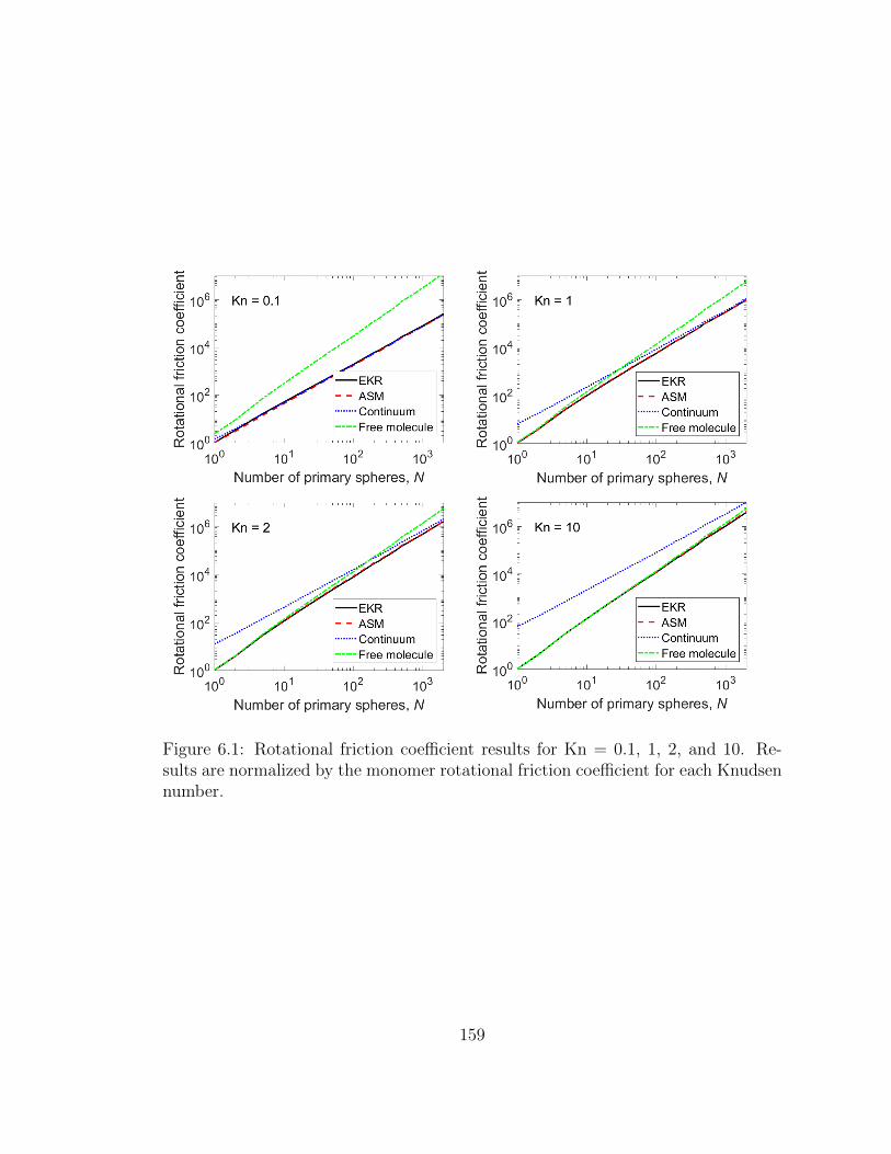
Figure 6.1: Rotational friction coefficient results for Kn = 0.1, 1, 2, and 10. Re-sults are normalized by the monomer rotational friction coefficient for each Knudsennumber.

159

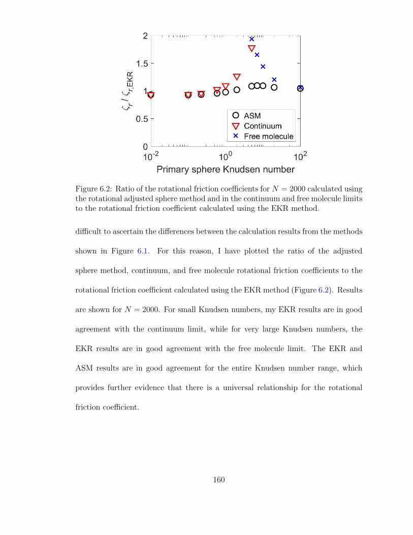
Figure 6.2: Ratio of the rotational friction coefficients for N = 2000 calculated usingthe rotational adjusted sphere method and in the continuum and free molecule limitsto the rotational friction coefficient calculated using the EKR method.

difficult to ascertain the differences between the calculation results from the methods

shown in Figure 6.1. For this reason, I have plotted the ratio of the adjusted

sphere method, continuum, and free molecule rotational friction coefficients to the

rotational friction coefficient calculated using the EKR method (Figure 6.2). Results

are shown for N = 2000. For small Knudsen numbers, my EKR results are in good

agreement with the continuum limit, while for very large Knudsen numbers, the

EKR results are in good agreement with the free molecule limit. The EKR and

ASM results are in good agreement for the entire Knudsen number range, which

provides further evidence that there is a universal relationship for the rotational

friction coefficient.

160

6.3.3 Relative Importance of Translational and Rotational Diffusion

One consideration in many aerosol studies is the relative importance of rota-

tional effects on aerosol transport properties. Studies often ignore rotational effects

[e.g. on coagulation rates and the resulting shapes of aggregates [121, 122]]. This

approach is valid if rotational diffusion is negligible relative to translational diffu-

sion, i.e. if particle orientation changes very little in the time it takes for the particle

to diffuse an appreciable distance. The relative importance of rotation on particle

transport is captured by the ratio of a characteristic translation time to a charac-

teristic rotation time. Defining the characteristic translation and rotation times as

the time required for the particle to diffuse one radius of gyration and rotate one

radian, this ratio becomes

τtτr

=R2g/6Dt

1/6Dr

=R2gζt

ζr(6.24)

Figure 6.3 shows this ratio as a function of primary sphere Knudsen number

and the number of primary spheres, calculated using both my EKR results and

analytic expressions for the translational and rotational friction coefficients (intro-

duced in Section 6.3.5 below). Note that the choppy nature of the EKR plot is due

to large variations in the rotational friction coefficient for a given set of aggregate

parameters, as discussed in the next section. The exact magnitude of the results in

this figure is insignificant since I am choosing arbitrary translational and rotational

diffusion distances; nevertheless, the results show that in the time it takes an ag-

gregate to diffuse one radius of gyration, it has rotated significantly. Simply put,

translational and rotational diffusion are equally important. This is true for all of

161

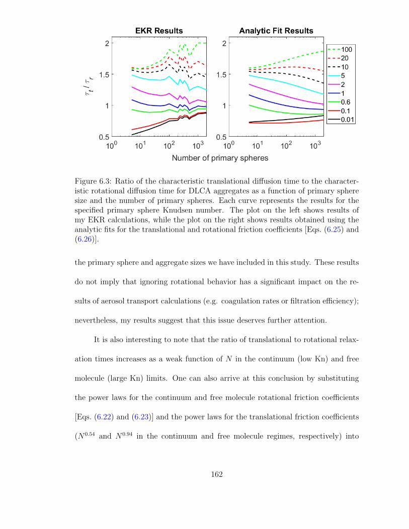
Figure 6.3: Ratio of the characteristic translational diffusion time to the character-istic rotational diffusion time for DLCA aggregates as a function of primary spheresize and the number of primary spheres. Each curve represents the results for thespecified primary sphere Knudsen number. The plot on the left shows results ofmy EKR calculations, while the plot on the right shows results obtained using theanalytic fits for the translational and rotational friction coefficients [Eqs. (6.25) and(6.26)].

the primary sphere and aggregate sizes we have included in this study. These results

do not imply that ignoring rotational behavior has a significant impact on the re-

sults of aerosol transport calculations (e.g. coagulation rates or filtration efficiency);

nevertheless, my results suggest that this issue deserves further attention.

It is also interesting to note that the ratio of translational to rotational relax-

ation times increases as a weak function of N in the continuum (low Kn) and free

molecule (large Kn) limits. One can also arrive at this conclusion by substituting

the power laws for the continuum and free molecule rotational friction coefficients

[Eqs. (6.22) and (6.23)] and the power laws for the translational friction coefficients

(N0.54 and N0.94 in the continuum and free molecule regimes, respectively) into

162

Eq. (eqn:rsoot:relaxation).2 In between, the situation is more complicated: the

transition to continuum-like behavior happens at lower N and higher Kn for trans-

lational transport compared to rotational transport, which explains the decrease in

the characteristic diffusion ratio at moderate Knudsen numbers.

6.3.4 Uncertainty in the Calculated Rotational Friction Coefficients

In Chapter 4, I discussed the uncertainty in my calculated translational friction

coefficients. There, I identified two main sources of uncertainty: the uncertainty in

the calculated velocity tensor and monomer friction coefficient that appear in the

EKR method, and KR theory itself. These factors also contribute to the uncertainty

in the rotational friction coefficient. However, I must add two additional sources of

uncertainty: the effects of neglecting rotational and coupling hydrodynamic interac-

tions and variations in the friction coefficient for aggregates with the same number

of primary spheres and the same fractal dimension and prefactor.

As I have mentioned, the linear and rotational velocities of each sphere in the

aggregate can induce a torque in the other spheres. In the continuum, the rotational

and coupling interactions are order O(r−3ij ) and O(r−2

ij ), respectively, as compared to

the translational hydrodynamic interaction tensor, which has leading terms of order

O(r−1ij ). As a result, I expect that the error in the EKR method would decrease

with increasing aggregate size due to the increase in the average distance between

monomers. My results confirm this expectation: the difference between the EKR

2Note that if one applies the simple scaling arguments from Section 6.2.3 [translational frictioncoefficient proportional to the radius of gyration in the continuum and to the number of primaryspheres in the free molecule regime, and rotational friction coefficients given by Eqs. (6.20) and(6.21)], one predicts that the ratio is independent of N in the continuum and free molecule regimes.

163

and continuum results at Kn = 0.01 is approximately 25% for N = 5 and 8% for N =

2000. That 8% difference at N = 2000 mirrors the difference between my calculated

monomer translational friction coefficient and the friction coefficient given by Stokes

law (Chapter 4), suggesting that the effects of coupling and rotational hydrodynamic

interactions are negligible for large aggregates. Expressions for the rotational and

coupling interaction tensors are unavailable for non-continuum flow, so it is difficult

to estimate the effects of neglecting these effects in the transition regime. However,

note that the EKR and free molecule results at Kn = 100 are within 5% for the

entire aggregate size range we studied. This suggests that rotational and coupling

interactions decrease in importance with increasing Knudsen number, as well as

for increasing aggregate size. As a result, the uncertainty in the rotational friction

coefficients computed using the EKR method is comparable to the uncertainty in my

computed translational friction coefficients (i.e. ∼ 10%) for all aggregates near the

free molecule regime and for large aggregates for any flow regime. This uncertainty

is larger (i.e. ∼ 25%) for small DLCA aggregates near the continuum regime.

The sources of uncertainty discussed above might better be termed “sources

of error,” since they represent differences between my results and the true rota-

tional friction coefficient. The final source of uncertainty is just that: variability in

the resulting rotational friction coefficient for the same input (namely, the primary

sphere Knudsen number, the number of primary spheres, and the fractal dimension

and prefactor). My reported results represent averages of results from 20 trials for

each set of inputs; here, the variability is due to differences in the coordinates of the

spheres that comprise the aggregate. For the translational friction coefficient, this

164

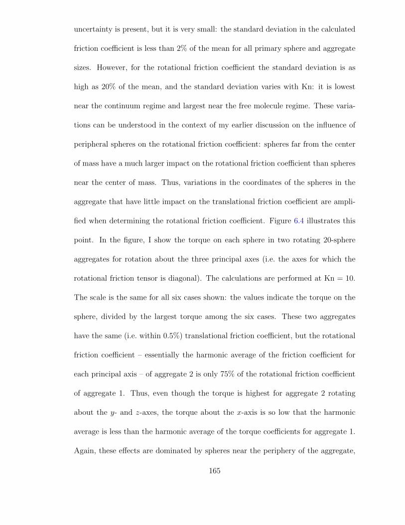
uncertainty is present, but it is very small: the standard deviation in the calculated

friction coefficient is less than 2% of the mean for all primary sphere and aggregate

sizes. However, for the rotational friction coefficient the standard deviation is as

high as 20% of the mean, and the standard deviation varies with Kn: it is lowest

near the continuum regime and largest near the free molecule regime. These varia-

tions can be understood in the context of my earlier discussion on the influence of

peripheral spheres on the rotational friction coefficient: spheres far from the center

of mass have a much larger impact on the rotational friction coefficient than spheres

near the center of mass. Thus, variations in the coordinates of the spheres in the

aggregate that have little impact on the translational friction coefficient are ampli-

fied when determining the rotational friction coefficient. Figure 6.4 illustrates this

point. In the figure, I show the torque on each sphere in two rotating 20-sphere

aggregates for rotation about the three principal axes (i.e. the axes for which the

rotational friction tensor is diagonal). The calculations are performed at Kn = 10.

The scale is the same for all six cases shown: the values indicate the torque on the

sphere, divided by the largest torque among the six cases. These two aggregates

have the same (i.e. within 0.5%) translational friction coefficient, but the rotational

friction coefficient – essentially the harmonic average of the friction coefficient for

each principal axis – of aggregate 2 is only 75% of the rotational friction coefficient

of aggregate 1. Thus, even though the torque is highest for aggregate 2 rotating

about the y- and z-axes, the torque about the x-axis is so low that the harmonic

average is less than the harmonic average of the torque coefficients for aggregate 1.

Again, these effects are dominated by spheres near the periphery of the aggregate,

165

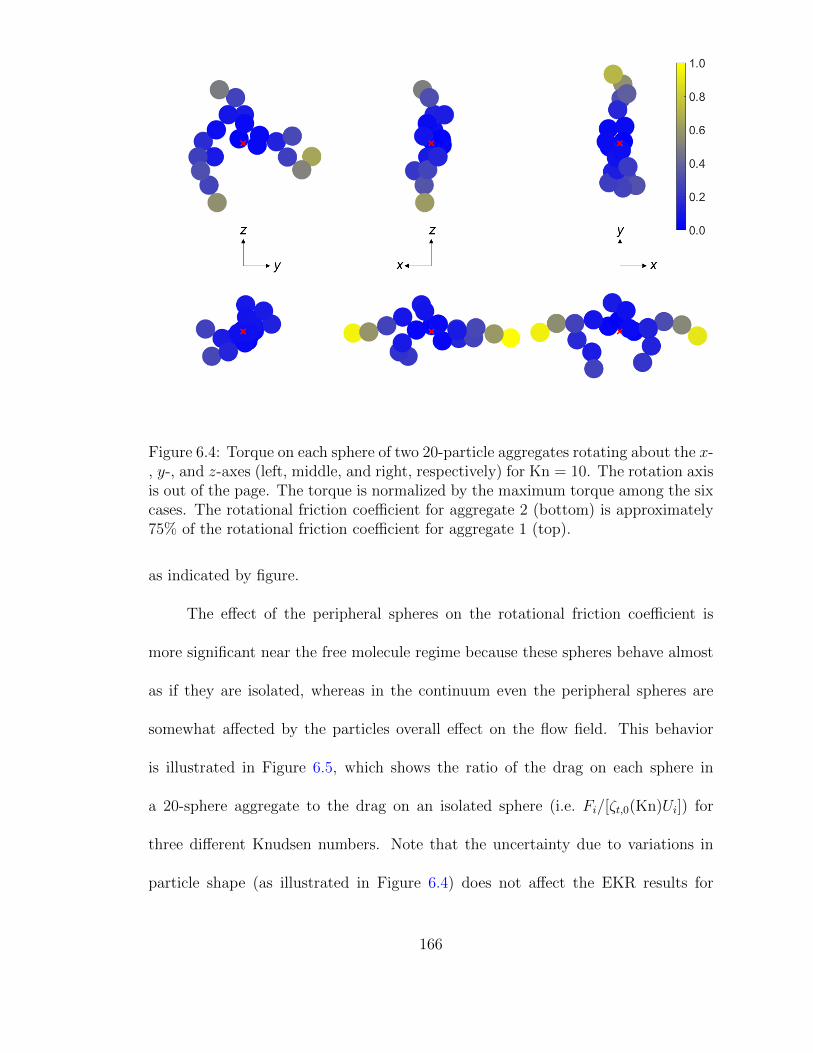
Figure 6.4: Torque on each sphere of two 20-particle aggregates rotating about the x-, y-, and z-axes (left, middle, and right, respectively) for Kn = 10. The rotation axisis out of the page. The torque is normalized by the maximum torque among the sixcases. The rotational friction coefficient for aggregate 2 (bottom) is approximately75% of the rotational friction coefficient for aggregate 1 (top).

as indicated by figure.

The effect of the peripheral spheres on the rotational friction coefficient is

more significant near the free molecule regime because these spheres behave almost

as if they are isolated, whereas in the continuum even the peripheral spheres are

somewhat affected by the particles overall effect on the flow field. This behavior

is illustrated in Figure 6.5, which shows the ratio of the drag on each sphere in

a 20-sphere aggregate to the drag on an isolated sphere (i.e. Fi/[ζt,0(Kn)Ui]) for

three different Knudsen numbers. Note that the uncertainty due to variations in

particle shape (as illustrated in Figure 6.4) does not affect the EKR results for

166

Figure 6.5: Ratio of the drag on each sphere in a 20-particle aggregate to the dragon an isolated sphere (i.e. the monomer momentum shielding factor). Here, theparticle is rotating about the z-axis (out of the page). A value of unity indicatesthat the sphere behaves as if it is isolated, while a value near zero indicates that theperturbations caused by the other spheres have a significant impact on the drag.

individual particle realizations; rather it represents the variation in the rotational

friction coefficient for the same set of inputs.

6.3.5 Analytical Expression for Rotational Friction Coefficients of DLCA Aggre-

gates

Previously, I developed an analytical expression for the translational friction

coefficient of DLCA aggregates [Eq. (4.38) in Chapter 4] that I verified with my

EKR results:

ζt6πµa

=1 + 1.612Kn

Cc(Kn)

[(0.852N0.535 + 0.148

)−1

+1.612Kn(0.843N0.939 + 0.157

)−1]−1

(6.25)

167

I will use the same approach to develop an analytical expression for the rotational

friction coefficient, which may be used to quickly estimate the characteristic rota-

tional relaxation time for a Brownian particle.

My expression is based on the harmonic sum of the continuum and free

molecule power-law expressions for the rotational friction coefficient [Eqs. (6.22)

and (6.23)]. In addition, I have added a term to each power law to give the correct

value for the monomer friction coefficient, and I have corrected for the fact that

the harmonic sum of the continuum and free molecule monomer friction coefficients

differs from the monomer friction coefficient given by Eq. (6.13). The resulting

expression is

ζr8πµa3

=1 + 5.988Kn

Cr(Kn)

[(0.713N1.63 + 0.287

)−1

+5.988Kn(1.184N2.02− 0.184

)−1]−1

(6.26)

Figure 6.6 shows the error in the fit relative to my EKR results:

error =ζr,fit − ζr,EKR

ζr,EKR

(6.27)

The error is within approximately 15% for much of the primary sphere Knudsen

number and aggregate size range studied here, though the error for smaller aggre-

gates near the continuum regime is higher. Again, this is because the continuum

power-law expression is based on results from a more rigorous method of calculating

the rotational friction coefficient, where I account for rotational and coupling hydro-

168

Figure 6.6: Error in the analytical expression for the rotational friction coefficient[Eq. (6.26)] relative to my EKR results. This error is defined by Eq. (6.27).

dynamic interactions. Thus, the error in Eq. (6.26) relative to the true rotational

friction coefficient near the continuum regime is likely much lower than indicated

by Figure 6.6, which shows the error relative to the EKR results that overestimate

the rotational friction coefficient for small aggregates near the continuum regime.

However, my fit does not account for uncertainties in the rotational friction coeffi-

cient due to variations in the aggregate shape. Thus, the true error in the fit may

be as high as 30% for a given aggregate. This is still acceptable given the lack of

alternative methods for estimating the rotational friction coefficient in the transition

regime.

169

6.4 Conclusions

I have presented my self-consistent field results for the rotational friction co-

efficient of DLCA aggregates consisting of 5 to 2000 primary spheres with primary

sphere Knudsen numbers between 0.01 and 100. My results are in good agreement

with the continuum and free molecule limits for small and large Knudsen numbers,

respectively. The computed relaxation times from an aligned to randomly oriented

agglomerate are consistent with the measurements by Colbeck et al. [91] for soot

produced from gasoline. I estimate that my calculated rotational friction coefficients

are within 30% of the true value for the range of parameters I have studied, with

the greatest errors occurring for small aggregates near the continuum regime and

significantly better agreement for all aggregates near the free molecule regime and

for large aggregates in any flow regime.

I have used the EKR method to calculate the ratio of translational to rota-

tional characteristic diffusion times. A potentially important finding is that this

ratio is nearly independent of cluster size. My results show that aggregates rotate

significantly in the time it takes to diffuse one radius of gyration. This finding sug-

gests that further study is needed to assess the importance of rotation on aerosol

coagulation and deposition behavior.

I have introduced an analytic expression for the rotational friction coefficient

of DLCA aggregates (df = 1.78 and k0 = 1.3). This simple model can be applied to

quickly estimate the characteristic rotational relaxation time for studies involving

particle alignment in an external field. I have extended scaling analyses for the con-

170

tinuum and free molecule friction coefficients to the rotational problem, which can

also be used to estimate the rotational friction/diffusion coefficient of an aggregate

in these limits.

I have also provided an expression for the monomer rotational friction coef-

ficient as a function of Knudsen number, based on the computational results of

Loyalka [77]. This expression includes a slip correction factor with the same general

form as the Cunningham slip correction factor used for the translational friction

coefficient of a sphere.

171

Chapter 7: The Effect of Electric Field Induced Alignment on the

Electrical Mobility of Fractal Aggregates

7.1 Introduction

The transport behavior of nano-scale particles depends on particle size, shape,

and orientation. In the absence of an external field, Brownian motion randomizes

the particle orientation, such that the measured transport property (e.g. intensity

of scattered light, particle mobility) represents an average over all equally-likely par-

ticle orientations. In a strong field, particles become aligned in an orientation that

minimizes their energy in the field [1, 105]. This effect has been demonstrated ex-

perimentally by placing particles in an external electric field and measuring changes

in scattered light intensity [90, 91] or electrical mobility [5, 6, 87, 123] as the field

strength changes.

One common experimental technique for sizing nanoparticles involves using a

differential mobility analyzer (DMA) to determine the mobility of particles in an

electric field. The particle transport behavior is often expressed in terms of the

mobility diameter, which is the diameter of a sphere that has the same mobility as

the particle. For spherical particles, the measured mobility diameter is equal to the

172

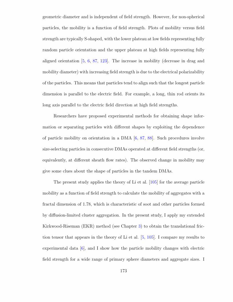
geometric diameter and is independent of field strength. However, for non-spherical

particles, the mobility is a function of field strength. Plots of mobility versus field

strength are typically S-shaped, with the lower plateau at low fields representing fully

random particle orientation and the upper plateau at high fields representing fully

aligned orientation [5, 6, 87, 123]. The increase in mobility (decrease in drag and

mobility diameter) with increasing field strength is due to the electrical polarizability

of the particles. This means that particles tend to align such that the longest particle

dimension is parallel to the electric field. For example, a long, thin rod orients its

long axis parallel to the electric field direction at high field strengths.

Researchers have proposed experimental methods for obtaining shape infor-

mation or separating particles with different shapes by exploiting the dependence

of particle mobility on orientation in a DMA [6, 87, 88]. Such procedures involve

size-selecting particles in consecutive DMAs operated at different field strengths (or,

equivalently, at different sheath flow rates). The observed change in mobility may

give some clues about the shape of particles in the tandem DMAs.

The present study applies the theory of Li et al. [105] for the average particle

mobility as a function of field strength to calculate the mobility of aggregates with a

fractal dimension of 1.78, which is characteristic of soot and other particles formed

by diffusion-limited cluster aggregation. In the present study, I apply my extended

Kirkwood-Riseman (EKR) method (see Chapter 3) to obtain the translational fric-

tion tensor that appears in the theory of Li et al. [5, 105]. I compare my results to

experimental data [6], and I show how the particle mobility changes with electric

field strength for a wide range of primary sphere diameters and aggregate sizes. I

173

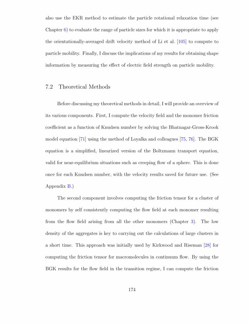
also use the EKR method to estimate the particle rotational relaxation time (see

Chapter 6) to evaluate the range of particle sizes for which it is appropriate to apply

the orientationally-averaged drift velocity method of Li et al. [105] to compute to

particle mobility. Finally, I discuss the implications of my results for obtaining shape

information by measuring the effect of electric field strength on particle mobility.

7.2 Theoretical Methods

Before discussing my theoretical methods in detail, I will provide an overview of

its various components. First, I compute the velocity field and the monomer friction

coefficient as a function of Knudsen number by solving the Bhatnagar-Gross-Krook

model equation [71] using the method of Loyalka and colleagues [75, 76]. The BGK

equation is a simplified, linearized version of the Boltzmann transport equation,

valid for near-equilibrium situations such as creeping flow of a sphere. This is done

once for each Knudsen number, with the velocity results saved for future use. (See

Appendix B.)

The second component involves computing the friction tensor for a cluster of

monomers by self consistently computing the flow field at each monomer resulting

from the flow field arising from all the other monomers (Chapter 3). The low

density of the aggregates is key to carrying out the calculations of large clusters in

a short time. This approach was initially used by Kirkwood and Riseman [28] for

computing the friction tensor for macromolecules in continuum flow. By using the

BGK results for the flow field in the transition regime, I can compute the friction

174

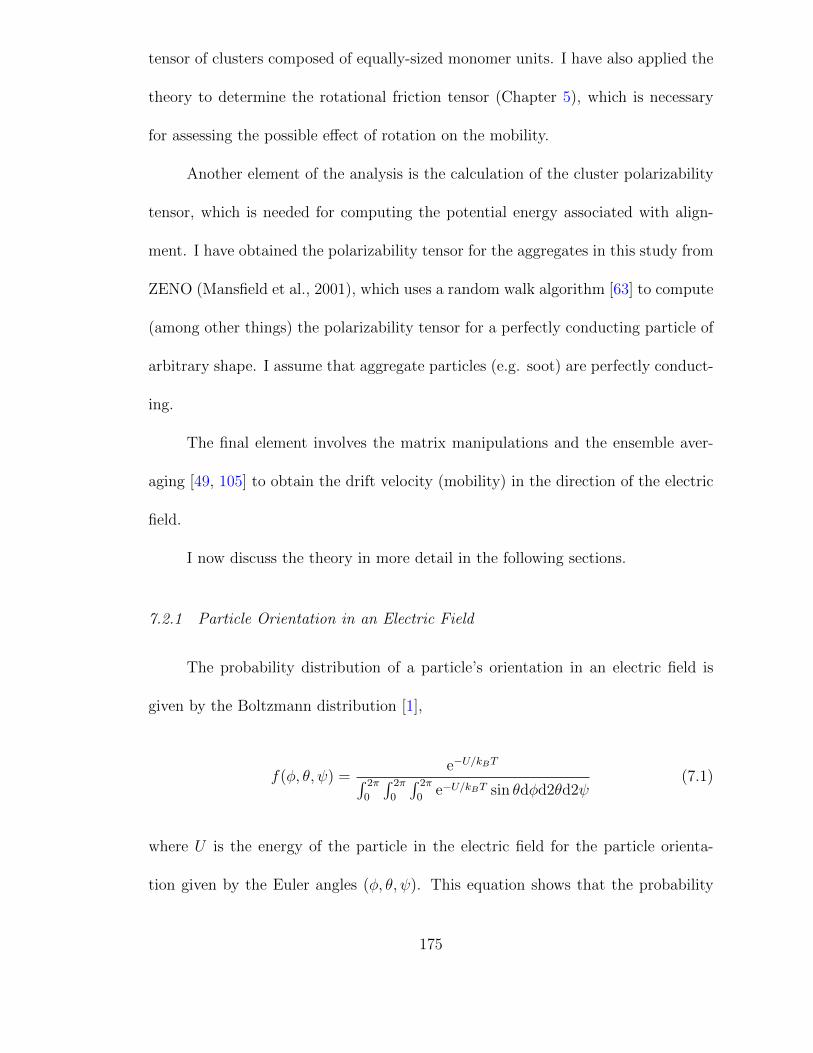
tensor of clusters composed of equally-sized monomer units. I have also applied the

theory to determine the rotational friction tensor (Chapter 5), which is necessary

for assessing the possible effect of rotation on the mobility.

Another element of the analysis is the calculation of the cluster polarizability

tensor, which is needed for computing the potential energy associated with align-

ment. I have obtained the polarizability tensor for the aggregates in this study from

ZENO (Mansfield et al., 2001), which uses a random walk algorithm [63] to compute

(among other things) the polarizability tensor for a perfectly conducting particle of

arbitrary shape. I assume that aggregate particles (e.g. soot) are perfectly conduct-

ing.

The final element involves the matrix manipulations and the ensemble aver-

aging [49, 105] to obtain the drift velocity (mobility) in the direction of the electric

field.

I now discuss the theory in more detail in the following sections.

7.2.1 Particle Orientation in an Electric Field

The probability distribution of a particle’s orientation in an electric field is

given by the Boltzmann distribution [1],

f(φ, θ, ψ) =e−U/kBT∫ 2π

0

∫ 2π

0

∫ 2π

0e−U/kBT sin θdφd2θd2ψ

(7.1)

where U is the energy of the particle in the electric field for the particle orienta-

tion given by the Euler angles (φ, θ, ψ). This equation shows that the probability

175

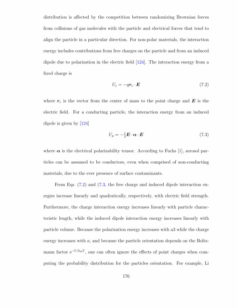
distribution is affected by the competition between randomizing Brownian forces

from collisions of gas molecules with the particle and electrical forces that tend to

align the particle in a particular direction. For non-polar materials, the interaction

energy includes contributions from free charges on the particle and from an induced

dipole due to polarization in the electric field [124]. The interaction energy from a

fixed charge is

Ue = −qre ·E (7.2)

where re is the vector from the center of mass to the point charge and E is the

electric field. For a conducting particle, the interaction energy from an induced

dipole is given by [124]

Up = −12E ·α ·E (7.3)

where α is the electrical polarizability tensor. According to Fuchs [1], aerosol par-

ticles can be assumed to be conductors, even when comprised of non-conducting

materials, due to the ever presence of surface contaminants.

From Eqs. (7.2) and (7.3, the free charge and induced dipole interaction en-

ergies increase linearly and quadratically, respectively, with electric field strength.

Furthermore, the charge interaction energy increases linearly with particle charac-

teristic length, while the induced dipole interaction energy increases linearly with

particle volume. Because the polarization energy increases with a3 while the charge

energy increases with a, and because the particle orientation depends on the Boltz-

mann factor e−U/kBT , one can often ignore the effects of point charges when com-

puting the probability distribution for the particles orientation. For example, Li

176

et al. [5] determined that the ratio of polarization energy to fixed charge energy is

greater than 10 for carbon nanotubes with mobility diameters greater than 100 nm,

while Zelenyuk and Imre [87] observed no effects of particle charge on the mobility

of aligned doublets with primary sphere diameters of 240 nm. Also, for a conduct-

ing particle the charge can move rapidly, so that one can consider the charge to be

distributed evenly throughout the particle [124]. Based on these considerations, I

will consider only the polarization energy when computing the particle mobility.

To evaluate the probability distribution [Eq. (7.1)], it helps to define two coor-

dinate systems: a body-fixed coordinate system (x′, y′, z′) that rotates with the par-

ticle, and a space-fixed (or laboratory) coordinate system (x, y, z). (See Figure E.1

in Appendix E.) For convenience, I will choose the body-fixed axes to coincide with

the principal axes of the polarizability tensor. In this representation, the minimum

polarization energy occurs when the electric field is along the z′-direction. I will set

the space-fixed axes so that the z-axis is parallel to the electric field.

The relationship between a vector in laboratory coordinates and a vector in

body-fixed coordinates is given by the following relationship:

b = A · b′ (7.4)

The rotation matrix A represents three successive rotations from the body-fixed

system to the space-fixed system. For the ZXZ sequence of rotations, the rotation

177

matrix is given by

A =

cosφ cosψ − cos θ sinφ sinψ − cosφ sinψ − cos θ sinφ cosψ sinφ sin θ

sinφ cosψ + cos θ cosφ sinψ − sinφ sinψ + cos θ cosφ cosψ − cosφ sin θ

sinψ sin θ cosψ sin θ cos θ

(7.5)

where φ, θ, and ψ are the angles of the first, second, and third rotations, respectively.

One useful property of the rotation matrix is that its inverse is equal to its transpose

(Gel’fand, et al., 1963). Because of this property and my choice of laboratory

coordinates, the electric field in body-fixed coordinates is given by

E′ =

sinψ sin θ

cosψ sin θ

cos θ

E (7.6)

where E is the field strength. This shows that the probability distribution is a

function of only two of the three Euler angles. Using the above expression for the

electric field and noting that the polarizability tensor in body-fixed coordinates is

diagonal, I can explicitly write the interaction energy as

U = −12(α1 sin2 ψ sin2 θ + α2 cos2 ψ sin2 θ + α3 cos2 θ)E2 (7.7)

where α3 > α2 > α1 are the eigenvalues of the polarizability tensor.

178

7.2.2 Average Drift Velocity of a Particle in an Electric Field

We use the probability distribution in Eq. (7.1) to calculate the average drift

velocity – and thus the mobility – of a particle in an electric field [105]. The drift

velocity is obtained by balancing the electric force on the particle with the aerody-

namic force for a given particle orientation:1

Vd = qΞ−1t ·E (7.8)

Here, Ξt is the translational friction tensor and q is the charge on the particle.

Combining Eqs. (7.1) and (7.8), we get the following expression for the particle

orientation-averaged drift velocity for a given electric field strength:

〈Vd〉 =q∫ 2π

0

∫ 2π

0

∫ 2π

0

(Ξ−1t ·E

)e−U/kBT sin θd2φd2θd2ψ∫ 2π

0

∫ 2π

0

∫ 2π

0e−U/kBT sin θd2φd2θd2ψ

(7.9)

In general, the orientation-averaged drift velocity is not parallel to the electric

field. However, the component of the drift velocity parallel to the electric field is

typically much larger than the components of the velocity perpendicular to the field.

For example, the perpendicular components of the drift velocity for soot-like fractal

aggregates are typically less than 5% of the parallel component. Thus, we can define

the particle mobility in terms of the parallel component of the orientation-averaged

drift velocity,

Z = 〈Vd,z〉/E (7.10)

1The linear relationship between the velocity and the drag force is valid in the creeping flowregime, which applies for all of the conditions considered in this study.

179

Again, I have positioned the laboratory-fixed coordinate system so that the electric

field is in the z-direction. The z-component of the drift velocity can be written in

terms of the Euler angles and the components of the friction tensor in body-fixed

coordinates:

〈Vd,z〉 = qE(M33〈cos2 θ〉+M22〈cos2 ψ sin2 θ〉+M11〈sin2 ψ sin2 θ〉

+M12〈sin 2ψ sin2 θ〉+M13〈sinψ sin 2θ〉+M23〉 cosψ sin 2θ〉)

(7.11)

Here, the angle brackets indicate orientation averages based on the distribution given

by Eq. (7.1) and the Mijs are components of the mobility tensor (i.e. the inverse of

the friction tensor) in body-fixed coordinates, i.e.

M ≡

M11 M12 M13

M12 M22 M23

M13 M23 M33

= (Ξ′t)−1

(7.12)

In going from Eq. (7.9) to Eq. (7.11), I use the relation between the body-fixed

(Ξ′t) and space-fixed (Ξt) friction tensors, Ξ−1t = A · (Ξ′t)

−1 ·A†, where the dagger

symbol denotes the transpose of the rotation matrix. Note that Eq. (7.11) reduces

to the expressions given by Li et al. [5] for the special case of an axisymmetric body,

where M12 = M13 = M23 = 0, M11 = M22 = M⊥, and M33 = M‖.

For a randomly-oriented particle, the averaged mobility is

Zrand =q

3

(1

ζ1

+1

ζ2

+1

ζ3

)(7.13)

180

where ζ1 > ζ2 > ζ3 are the eigenvalues of the translational friction tensor. At very

high field strengths, the particle will be oriented in the direction that minimizes the

electric field interaction energy. Thus, the high-field mobility is

Zalign = qk · (Ξ′t)−1 · k = qM33 (7.14)

where k is the unit vector in the z-direction.

7.2.3 Friction Tensor for an Aggregate

To calculate the orientation-averaged mobility of soot-like particles, one must

be able to determine the translational friction tensor for fractal aggregates con-

sisting of N primary spheres with radius a, where the Knudsen number of the

primaries (Kn = λ/a) is in the transition regime between continuum (Kn 1) and

free molecule (Kn 1) limits. To do so, I will use my extension (Chapter 3) of

Kirkwood-Riseman theory [28] from the continuum regime to the transition regime.

Kirkwood and Riseman proposed a method for calculating the translational

friction coefficient for a macromolecule or particle consisting of spherical subunits.

The drag on each sphere in the aggregate is obtained by considering the effects of

the other spheres in the particle on the flow field. The resulting force is the sum of

the drag on an isolated particle and the perturbations due to the other spheres:

F = −ζ0Ui − ζ0

N∑i 6=j

Tij ·Fj (7.15)

181

Here, ζ0 = 6πµa is the friction coefficient for a sphere, given by Stokes law; Ui is the

velocity of the ith sphere; and Tij is the hydrodynamic interaction tensor. Carrasco

and Garcıa de la Torre [53] discuss some of the hydrodynamic interaction tensors

that have been proposed in the past and the relative accuracy of the various forms of

Tij. They conclude that the Rotne-Prager-Yamakawa (RPY) tensor [57, 58] – which

is accurate to order r−3ij , where rij is the distance between spheres – is sufficiently

accurate for practical purposes.

Noting that the product of the RPY tensor and the monomer friction coeffi-

cient is similar to the tensor Vij describing the flow field around a sphere moving

with velocity Ui (i.e. u(rij) = Vij ·Ui), I proposed replacing ζ0Tij with Vij, the

velocity field around a moving sphere in the transition flow regime:

F = −ζ0(Kn)Ui −N∑i 6=j

Vij(Kn) ·Fj (7.16)

This extended Kirkwood-Riseman (EKR) approach is valid for creeping flow for any

Knudsen number, provided one can accurately solve for the velocity field around a

sphere as a function of Kn.

I obtain the velocity field and the monomer friction coefficientthat appear

in Eq.(7.16) by solving the Bhatnagar-Gross-Krook model equation [71] using the

method of Loyalka and colleagues [75, 76]. The BGK equation is a simplified,

linearized version of the Boltzmann transport equation, valid for near-equilibrium

situations such as creeping flow of a sphere. (See Chapter 2.) I solve Eq. (7.16) for

unit particle velocity in the x-, y-, and z-directions to determine the translational

182

friction tensor. My EKR results for the translational friction coefficient of fractal

aggregates compare well to published experimental data and calculational results

(Chapters 3 and 4).

7.3 Results

To determine the orientation-averaged mobility of fractal aggregates, I solve

Eq. (7.11) with the translational friction tensor calculated using the EKR method

and the polarizability tensor [which appears in the potential energy term, Eq. (7.7),

that affects particle orientation] obtained from ZENO [62]. ZENO uses a random

walk algorithm [63] to compute (among other things) the polarizability tensor for

a perfectly conducting particle of arbitrary shape. Again, I assume that soot par-

ticles are perfectly conducting. The polarizability and friction tensors are specified

in terms of the body-fixed axes, which correspond to the principal axes of the po-

larizability tensor, as discussed previously. I obtain the orientation averages in

Eq. (7.11) by integrating numerically using a 2D quadrature method (MATLAB

function integral2). I generate the aggregates using a cluster-cluster algorithm

[36]. For each N , I generate 20 clusters and present the average results of the 20

cases.

7.3.1 Comparison to Experimental Data

Li et al. [6] used a pulsed-field differential mobility analyzer (PFDMA) to de-

termine the electrical mobility of soot aggregates composed of 5-nm-radius primaries

183

(Kn = 13.5 for λ = 67.3 nm). They size-selected aggregates with mobility diame-

ters of approximately 129 nm, 154 nm, and 200 nm in a DMA operated at high field

(∼ 7000− 8000 V/cm), then used the PFDMA to measure the mobility of these

aggregates as a function of electric field strength.

For my calculations, I must first estimate the aggregate size and structure from

the reported mobilities. Like Li et al., I assume that the aggregates have a fractal

morphology,

N = k0

(Rg

a

)df(7.17)

with fractal dimension df = 1.78 and prefactor k0 = 1.3. I determine the number of

primaries iteratively until I obtain a set of particles whose average random mobility

(as calculated using my EKR method) is in good agreement with the experimental

mobility at low field. I repeat this procedure for the three data sets, corresponding to

mobility diameters of 129 nm, 154 nm, and 200 nm. As an initial guess for N , I solve

for N in my expression for the friction coefficient of DLCA aggregates [Eq. (4.38)

of Chapter 4]:

ζt6πµa

=1 + 1.612Kn

Cc(Kn)

[(0.852N0.535 + 0.148

)−1

+1.612Kn(0.843N0.939 + 0.157

)−1]−1

(7.18)

The friction coefficient is related to the mobility by ζt = q/Z.

Figure 7.1 compares the results of my calculations to data from Li et al. [6].

Overall, the results are in good agreement with the data enabling me to consider a

184

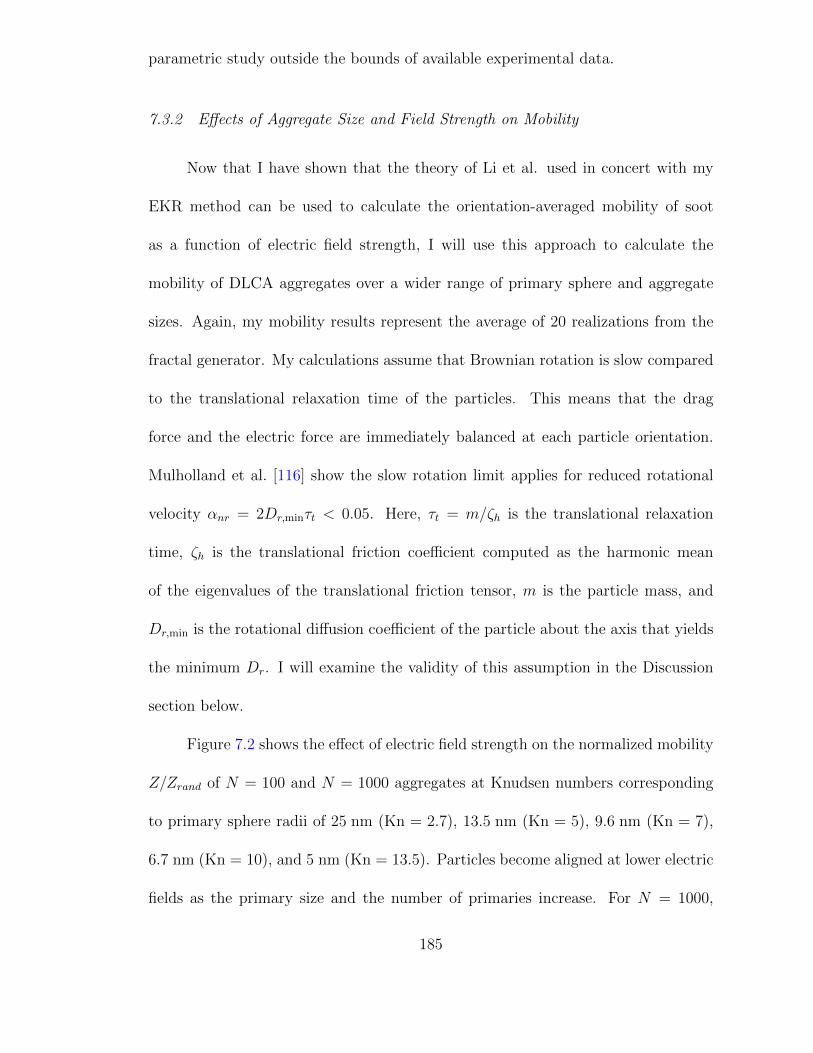
parametric study outside the bounds of available experimental data.

7.3.2 Effects of Aggregate Size and Field Strength on Mobility

Now that I have shown that the theory of Li et al. used in concert with my

EKR method can be used to calculate the orientation-averaged mobility of soot

as a function of electric field strength, I will use this approach to calculate the

mobility of DLCA aggregates over a wider range of primary sphere and aggregate

sizes. Again, my mobility results represent the average of 20 realizations from the

fractal generator. My calculations assume that Brownian rotation is slow compared

to the translational relaxation time of the particles. This means that the drag

force and the electric force are immediately balanced at each particle orientation.

Mulholland et al. [116] show the slow rotation limit applies for reduced rotational

velocity αnr = 2Dr,minτt < 0.05. Here, τt = m/ζh is the translational relaxation

time, ζh is the translational friction coefficient computed as the harmonic mean

of the eigenvalues of the translational friction tensor, m is the particle mass, and

Dr,min is the rotational diffusion coefficient of the particle about the axis that yields

the minimum Dr. I will examine the validity of this assumption in the Discussion

section below.

Figure 7.2 shows the effect of electric field strength on the normalized mobility

Z/Zrand of N = 100 and N = 1000 aggregates at Knudsen numbers corresponding

to primary sphere radii of 25 nm (Kn = 2.7), 13.5 nm (Kn = 5), 9.6 nm (Kn = 7),

6.7 nm (Kn = 10), and 5 nm (Kn = 13.5). Particles become aligned at lower electric

fields as the primary size and the number of primaries increase. For N = 1000,

185

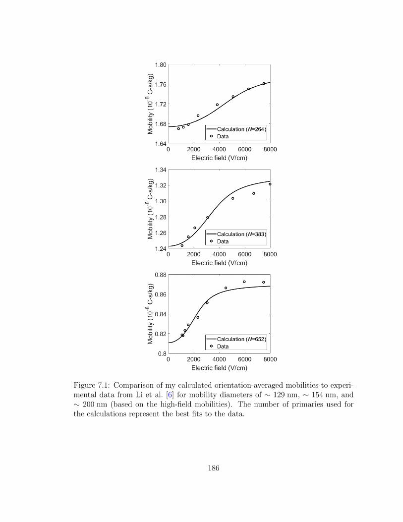
Figure 7.1: Comparison of my calculated orientation-averaged mobilities to experi-mental data from Li et al. [6] for mobility diameters of ∼ 129 nm, ∼ 154 nm, and∼ 200 nm (based on the high-field mobilities). The number of primaries used forthe calculations represent the best fits to the data.

186

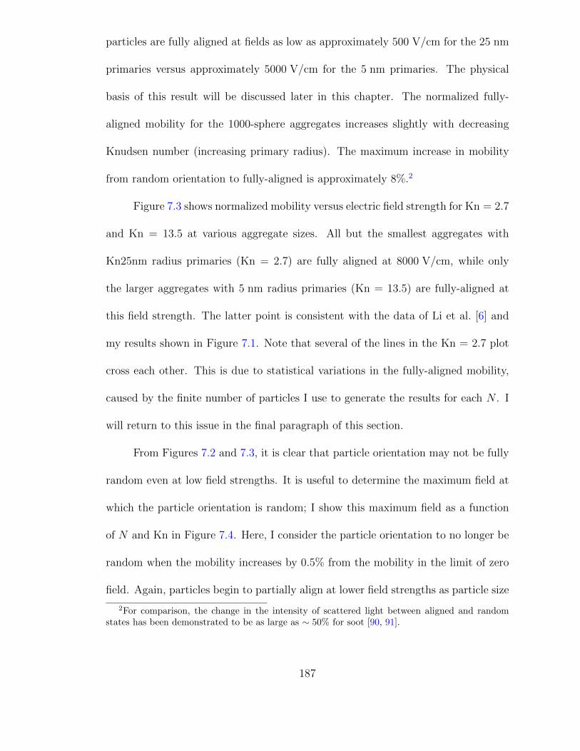
particles are fully aligned at fields as low as approximately 500 V/cm for the 25 nm

primaries versus approximately 5000 V/cm for the 5 nm primaries. The physical

basis of this result will be discussed later in this chapter. The normalized fully-

aligned mobility for the 1000-sphere aggregates increases slightly with decreasing

Knudsen number (increasing primary radius). The maximum increase in mobility

from random orientation to fully-aligned is approximately 8%.2

Figure 7.3 shows normalized mobility versus electric field strength for Kn = 2.7

and Kn = 13.5 at various aggregate sizes. All but the smallest aggregates with

Kn25nm radius primaries (Kn = 2.7) are fully aligned at 8000 V/cm, while only

the larger aggregates with 5 nm radius primaries (Kn = 13.5) are fully-aligned at

this field strength. The latter point is consistent with the data of Li et al. [6] and

my results shown in Figure 7.1. Note that several of the lines in the Kn = 2.7 plot

cross each other. This is due to statistical variations in the fully-aligned mobility,

caused by the finite number of particles I use to generate the results for each N . I

will return to this issue in the final paragraph of this section.

From Figures 7.2 and 7.3, it is clear that particle orientation may not be fully

random even at low field strengths. It is useful to determine the maximum field at

which the particle orientation is random; I show this maximum field as a function

of N and Kn in Figure 7.4. Here, I consider the particle orientation to no longer be

random when the mobility increases by 0.5% from the mobility in the limit of zero

field. Again, particles begin to partially align at lower field strengths as particle size

2For comparison, the change in the intensity of scattered light between aligned and randomstates has been demonstrated to be as large as ∼ 50% for soot [90, 91].

187

Figure 7.2: Normalized mobility as a function of electric field strength for 100-sphere(top) and 1000-sphere (bottom) aggregates.

188

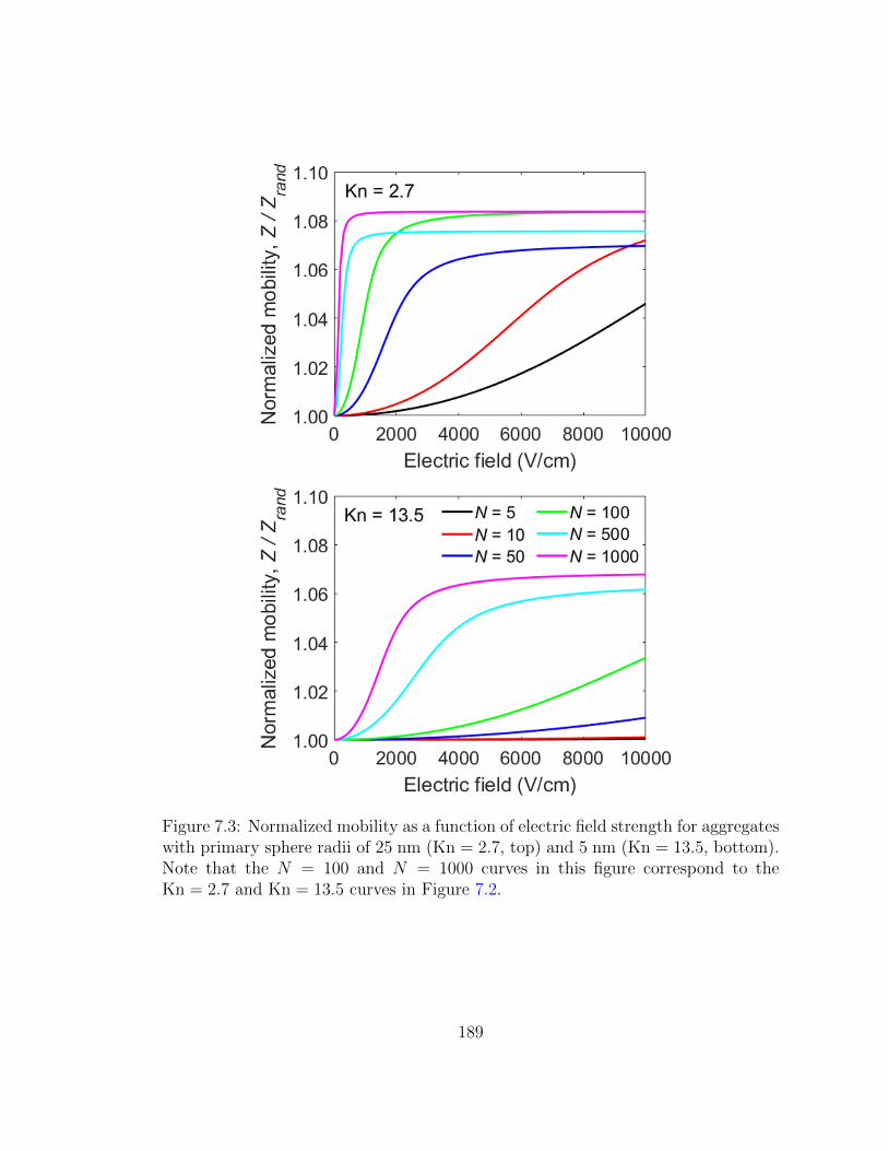
Figure 7.3: Normalized mobility as a function of electric field strength for aggregateswith primary sphere radii of 25 nm (Kn = 2.7, top) and 5 nm (Kn = 13.5, bottom).Note that the N = 100 and N = 1000 curves in this figure correspond to theKn = 2.7 and Kn = 13.5 curves in Figure 7.2.

189

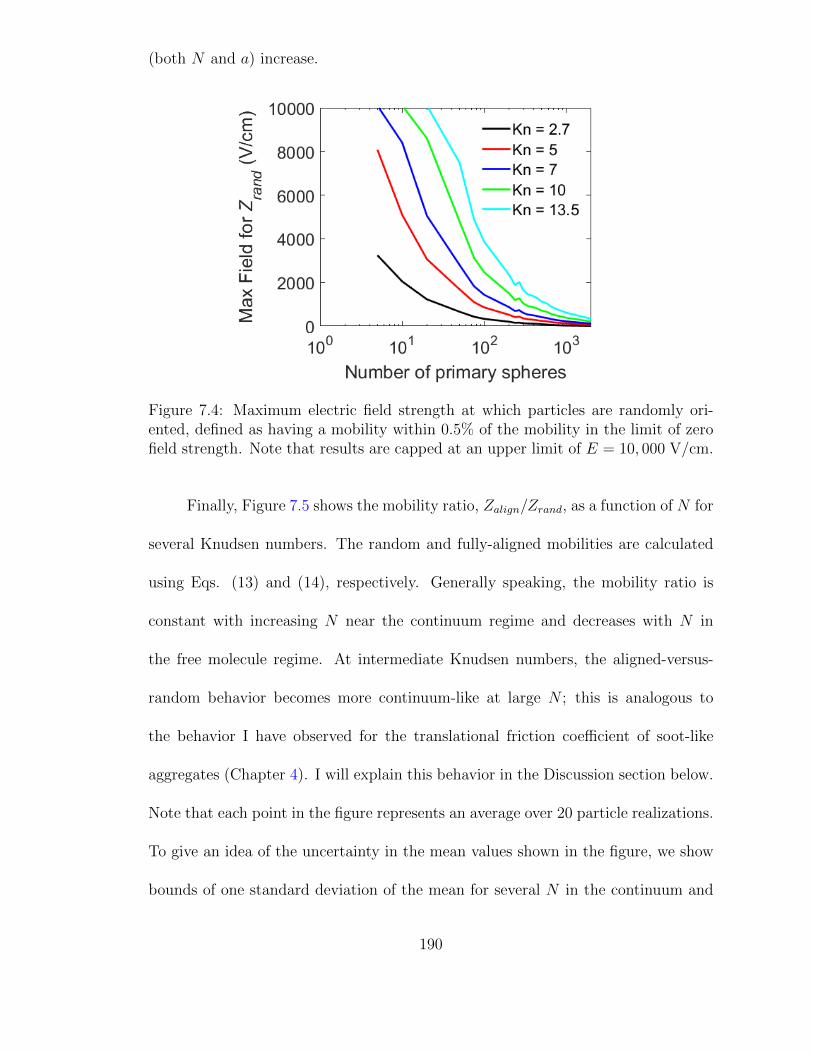
(both N and a) increase.

Figure 7.4: Maximum electric field strength at which particles are randomly ori-ented, defined as having a mobility within 0.5% of the mobility in the limit of zerofield strength. Note that results are capped at an upper limit of E = 10, 000 V/cm.

Finally, Figure 7.5 shows the mobility ratio, Zalign/Zrand, as a function of N for

several Knudsen numbers. The random and fully-aligned mobilities are calculated

using Eqs. (13) and (14), respectively. Generally speaking, the mobility ratio is

constant with increasing N near the continuum regime and decreases with N in

the free molecule regime. At intermediate Knudsen numbers, the aligned-versus-

random behavior becomes more continuum-like at large N ; this is analogous to

the behavior I have observed for the translational friction coefficient of soot-like

aggregates (Chapter 4). I will explain this behavior in the Discussion section below.

Note that each point in the figure represents an average over 20 particle realizations.

To give an idea of the uncertainty in the mean values shown in the figure, we show

bounds of one standard deviation of the mean for several N in the continuum and

190

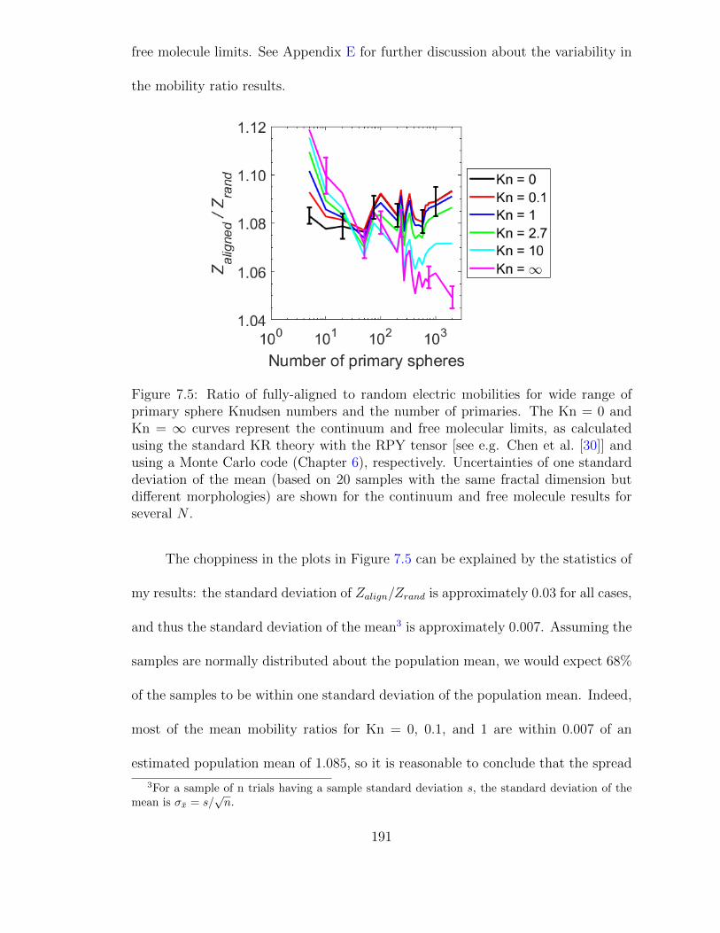
free molecule limits. See Appendix E for further discussion about the variability in

the mobility ratio results.

Figure 7.5: Ratio of fully-aligned to random electric mobilities for wide range ofprimary sphere Knudsen numbers and the number of primaries. The Kn = 0 andKn = ∞ curves represent the continuum and free molecular limits, as calculatedusing the standard KR theory with the RPY tensor [see e.g. Chen et al. [30]] andusing a Monte Carlo code (Chapter 6), respectively. Uncertainties of one standarddeviation of the mean (based on 20 samples with the same fractal dimension butdifferent morphologies) are shown for the continuum and free molecule results forseveral N .

The choppiness in the plots in Figure 7.5 can be explained by the statistics of

my results: the standard deviation of Zalign/Zrand is approximately 0.03 for all cases,

and thus the standard deviation of the mean3 is approximately 0.007. Assuming the

samples are normally distributed about the population mean, we would expect 68%

of the samples to be within one standard deviation of the population mean. Indeed,

most of the mean mobility ratios for Kn = 0, 0.1, and 1 are within 0.007 of an

estimated population mean of 1.085, so it is reasonable to conclude that the spread

3For a sample of n trials having a sample standard deviation s, the standard deviation of themean is σx = s/

√n.

191

in Zalign/Zrand is partially due to my finite sample size.

7.4 Discussion

7.4.1 General Observations

My results show that particle alignment occurs at decreasing electric field

strengths as the primary sphere Knudsen number decreases (primary sphere radius

increases) and as the number of primaries increases. This occurs because polariz-

ability is proportional to volume, so that interaction energy between the electric

field and the induced dipole increases with volume. The particle becomes fully

aligned when the magnitude of the interaction energy is significantly greater than

the Brownian energy kBT .

I also show that the ratio of fully-aligned to random mobility is a function of

the number of primary spheres and the primary sphere size. Near the continuum

regime, the mobility ratio is approximately constant with N ; near the free molecule

regime, the mobility ratio decreases with N . I discuss this topic in some detail in Ap-

pendix E, but the brief explanation is as follows: the mobility of an aggregate in the

continuum and free molecule regimes is roughly inversely proportional to the radius

of gyration [4, 54, 93] and the orientation-averaged projected area [41], respectively.

Similarly, the continuum and free molecule aligned mobilities are correlated to the

inverses of the radius of gyration about the major axis of the polarizability tensor

(i.e. the z′-axis), Rgz′ , and the projected area in the plane normal to the z′-axis,

PAz′ . (See Appendix E.) Averaged over 20 cases, the ratio Rg/Rgz′ is approximately

192

constant (after accounting for the statistical fluctuations described above) with N ,

while PA/PAz′ decreases with N , mirroring the trends in the mobility ratios in the

continuum and free molecule limits.

7.4.2 Validity of the Slow Rotation Assumption

My calculations assume that Brownian rotation is slow compared to transla-

tional relaxation, i.e. the aggregates are in the slow rotation limit. To assess the

validity of this assumption, I use the EKR method to determine the translational

friction coefficient (ζh, the harmonic average of the eigenvalues of the friction ten-

sor) and the minimum rotational diffusion coefficient. Using these calculated friction

and diffusion coefficients, I compute the reduced rotation velocity αnr, as shown in

Figure 7.6.

Figure 7.6: Reduced rotation velocity for a range of primary sphere sizes and Knud-sen numbers. Soot density is taken as 2 g/mL [125, 126]. Particles with a reducedrotation velocity less than 0.05 (the dotted line) are in the slow rotation limit.

193

The figure shows that particles with Knudsen numbers less than 13.5 and more

than approximately 50 primary spheres are in the slow rotation limit (αnr < 0.05

[116]); none of the particles in this study are in the fast rotation limit (αnr > 10).

Note that for fast rotation, one should use an orientation-averaged drag approach to

calculate the mobility, as opposed to the orientation-averaged drift velocity approach

in the slow rotation limit. At low field strength, the fast rotation limit yields a scalar

friction coefficient equal to the arithmetic average of the eigenvalues, instead of the

harmonic average in the slow rotation limit [105]. (The two approaches yield the

same result for the fully aligned case.) Thus, some of the particles included in

this study are not in the slow rotation limit. However, the maximum difference

between the mobility calculated using the averaged drift velocity is at most 1% less

than the mobility calculated using the averaged drag force for the particles in this

study (i.e. those with fractal dimensions of 1.78). In other words, it makes little

difference which approach one uses to calculate the mobility of DLCA aggregates.

The distinction becomes more significant for particles with a large aspect ratio, such

as long, thin rods, where there is a large difference between the largest and smallest

eigenvalues of the friction tensor.

7.4.3 Polarizability Versus Friction

A conducting particle in an electric field will orient itself to minimize its in-

teraction energy with the field, in the absence of any Brownian thermal forces. The

minimum energy occurs when the charge separation in the particle is greatest. This

means that a rod or a chain of spheres will orient itself such that its long axis is

194

parallel to the electric field, while the fractal particles in this study are oriented such

that the axis through the most widely separated two spheres is parallel to the field.

One would expect that the minimum drag force also occurs when it moves along its

most elongated direction. This is exactly the case for axisymmetric particles like

rods and cylinders, so that the most likely orientation of the particle in an electric

field is the orientation with the minimum drag. For fractals, the situation is more

complicated: there is a finite angle between the eigenvector of the friction tensor

corresponding to the minimum drag and the principal axis of the polarizability ten-

sor (the most favorable orientation). In most cases, this angle is small (< 10),

though I have observed angles as large as 25 between these two eigenvectors. This

means that the most favorable orientation does not necessarily minimize the drag

for fractals.

A somewhat related issue is that translating particles with arbitrary shape

experience a torque, where the relationship between the particle velocity and the

torque exerted by the fluid on the particle is governed by the coupling tensor [49]. For

non-skew particles (such as rods and cylinders), there is no translational-rotational

coupling, but for skew particles like fractals the coupling tensor is non-zero. The

question is whether or not the hydrodynamic torque is sufficient to overcome the

interaction energy between the induced dipole and the field and reorient the particle.

To answer this question, I calculated the coupling torque on 1000-sphere ag-

gregates with a primary sphere Knudsen number of 13.5, using the EKR method

to determine the coupling tensor and the orientation-averaged drift velocity at a

field strength of 4000 V/cm (roughly corresponding to the minimum field strength

195

at which the particle is fully aligned). The resulting torque is more than two or-

ders of magnitude lower than the interaction energy. I repeated this calculation for

N = 100, Kn = 2.7, and E = 200 V/cm; again, the coupling torque is significantly

lower than the interaction energy. This shows that the coupling torque has no effect

on the particle orientation at high field strength.4

7.4.4 Using Field-dependent Mobility to Evaluate Particle Shape

My results clearly show that particle mobility increases with electric field from

a fully random state at low fields to a fully oriented state at higher fields. The

transition occurs at decreasing fields for increasing particle size (both in terms of

primary sphere size and the number of primaries), as expected since polarizability

is proportional to particle volume.

This behavior has prompted some researchers to propose methods to separate

particles with different shapes by exploiting the changes in mobility at different

electric fields, such as by size-selecting particles in a DMA followed by separation

with second DMA operated at a different field strength [87, 88]. Using this method,

one can distinguish between spheres (or aggregates with fractal dimension near

3) and more elongated particles like rods, chains, prolate ellipsoids, or soot-like

aggregates, since the mobility of a sphere does not change with field strength. In

practice, this technique may not be feasible for some particle sizes due to limitations

4At low field strength, translational-rotational coupling has a small but noticeable effect on theorientation-averaged drag force. For this reason, one must account for rotational and translation-rotation coupling effects when determining the translational diffusion of skew particles [29]. Tofully account for rotational and coupling effects at intermediate fields – where both hydrodynamictorques and induced-dipole energies affect particle orientation – one could use a Brownian approachsimilar to that of Fernandes and Garcıa de la Torre [127].

196

of current commercially available DMA operating conditions and configurations. For

example, Li et al. [6] estimate that they cannot operate their experimental system

at fields below 1000 V/cm. At this field strength, larger particles are fully-aligned

(see Figures 7.2 and 7.3), so measuring the mobility at fields of 1000 V/cm and

e.g. 8000 V/cm would yield the same result and lead to the erroneous conclusion

that the particle is spherical. At the other end of the size spectrum, small fractals

experience minimal changes in mobility over the range of electric fields studied here.

It may also be difficult to operate a DMA at a low enough field to ensure that the

particle orientation is fully random. One can consult Figure 7.4 to determine if it

is possible to select randomly oriented particles for the operating conditions of ones

DMA setup.

There are also issues distinguishing between two non-spherical particles with

different shapes. For example, the fully-aligned mobility of a doublet in continuum

flow is 8% greater than the mobility of a randomly oriented doublet [49, 53]. This

is comparable to the increase in mobility from random to fully-aligned orientations

for the soot particles included in this study. Thus, a doublet with primary size

near the continuum regime and a soot-like particle with the same low-field mobility

will behave similarly at higher voltages, making it difficult to distinguish between

these particles. As another example, I looked at the effect of the prefactor [k0 in

Eq. (7.17)] on the mobility of DLCA aggregates. While the prefactor does affect

the mobility (with lower prefactors resulting in decreased mobility for the same

number of primary spheres), it has little effect on the ratio of the fully-aligned to

fully random mobilities.

197

Beyond the experimental issues mentioned above, it is also difficult to accu-

rately calculate the mobility of a fractal aggregate in the transition regime. I have

estimated that the EKR method yields orientation-averaged translational friction

coefficients within 10% of the true value (Chapter 4), which translates to uncertain-

ties in any estimate of the primary sphere size or the number of primary spheres.

An obvious example is my attempt to fit my results to the data of Li et al. (2016),

as illustrated by Figure 7.1: my estimated aggregate sizes (in terms of N) are likely

within about 10% of the true value (though the actual error estimate depends on

the relationship between N and the friction coefficient). This situation is simplified

by the fact that we know the primary sphere size from TEM measurements, and we

have a good estimate of the fractal dimension and prefactor from numerous studies

of soot. (See Sorensen [4] for a review of these studies.)

In total, the above factors mean that while it may be theoretically possi-

ble to extract shape information from DMA measurements made at different field

strengths, it is difficult, and probably further consideration should be given to de-

velopment of DMA configurations optimized for this purpose.

7.5 Conclusions

I have applied the EKR method for calculating the translational friction tensor

of fractal aggregates to verify the theory of Li et al. [105] for the average mobility

of a particle in an electric field. My results compare well to published experimental

data for soot [6]. Furthermore, I use the EKR method to calculate the average

198

mobility of aggregates over a range of primary sphere sizes in the transition and near

free molecule regimes with up to 2000 primary spheres. The maximum increase in

mobility from random to fully-aligned orientations is approximately 8% for the soot-

like aggregates (df = 1.78, k0 = 1.3) included in this study. While my calculations

cover the Knudsen number range of 2.7 to 13.5 – which represents a representative

range of primary sphere sizes in soot particles (see, e.g. [6, 42]) – this approach is

valid for any primary sphere size and number of primaries, provided the particle is

in the slow rotation limit. See Chapters 4 and 6 for translational and rotational

friction coefficient results at larger and smaller Knudsen numbers.

While it is theoretically possible to use the relationship between mobility and

field strength to obtain size and shape information about particles or to separate par-

ticles with similar mobility but different shapes, my results suggest there are several

practical issues related to the experimental setup and to the accuracy of the meth-

ods used to relate the data to size and shape information. It is especially difficult

to obtain shape information for either very large or very small soot-like aggregates

because large aggregates are fully aligned at even very low field strengths and small

aggregates require very high field strengths to align. In these limits, the measured

mobility at low (∼ 1000 V/cm) and high (∼ 8000 V/cm) field strengths would be

nearly equal, which would suggest – incorrectly – that these fractal aggregates are

actually spherical.

199

Chapter 8: Hydrodynamic Interactions between Particles

8.1 Introduction

The vast majority of the literature on aerosol particle transport treats the

particles as if they are isolated when calculating the drag. This approach is valid

for very dilute aerosols, where the average separation between particles is large, and

thus hydrodynamic interactions between particles are negligible. For example, the

mean settling velocity of a system of spheres in continuum flow is U0(1 − 6.55φ),

where φ is the particle volume fraction and U0 is the velocity each sphere would

have if it was alone in an infinite fluid [128]. As another example, the viscosity of a

suspension of spheres in continuum flow is µ(1 + 2.5φ), where µ is the fluid viscosity

[2]. Clearly, the interaction effects on the settling velocity and suspension viscosity

are negligible for aerosol systems consisting of spheres at typical volume fractions.

However, there are situations where one might expect interactions between

particles to be more significant. Sorensen et al. [129] has demonstrated that aerogels

can form under certain conditions in sooting flames. In this process, fractal aggre-

gates formed by diffusion limited cluster aggregation (DLCA) reach a critical size

and begin to fill the entire physical volume because the aggregate fractal dimension

(df ≈ 1.78) is less than the spatial dimension. One would expect hydrodynamic in-

200

teractions between the soot aggregates to be more significant than between spheres

at the same volume fraction, due to the stringy nature of the DLCA aggregates.

More generally, for coagulating systems aerosol particles must approach each other,

so that interparticle hydrodynamic interactions may affect the coagulation rate.

Much of the literature on hydrodynamic interactions between particles focuses

on spheres in the continuum regime [1, 128, 130–136]. Little attention has been

paid to interactions between particles in the transition (or kinetic) flow regime,

when the particle size is comparable to the gas mean free path, as is often the case

in aerosol systems [2, 4]. Such an investigation is now possible using my theory for

hydrodynamic interactions in the kinetic regime [92].

The present study examines the forces exerted by aerosol particles on their

neighbors due to hydrodynamic interactions between the particles and the surround-

ing fluid. I consider both spheres and soot-like fractal aggregates moving parallel,

anti-parallel and perpendicular to their line of centers. (See Figure 8.1.) I employ

the extended Kirkwood-Riseman (EKR) method [92] to solve for the hydrodynamic

forces on the particles in the transition flow regime as a function of the separation

distance between particles, the Knudsen number (Kn ≡ λ/a), where λ is the gas

mean free path and a is the sphere radius) of the primary sphere(s) that comprise

the particles, and the number of primary spheres in the particle. As an example of

a situation where hydrodynamic interactions may be significant, I present calcula-

tions for the settling velocity of a cloud in an unbounded medium. Throughout this

study, I assume the particles are in the creeping flow regime (Re 1, Ma

1).

201

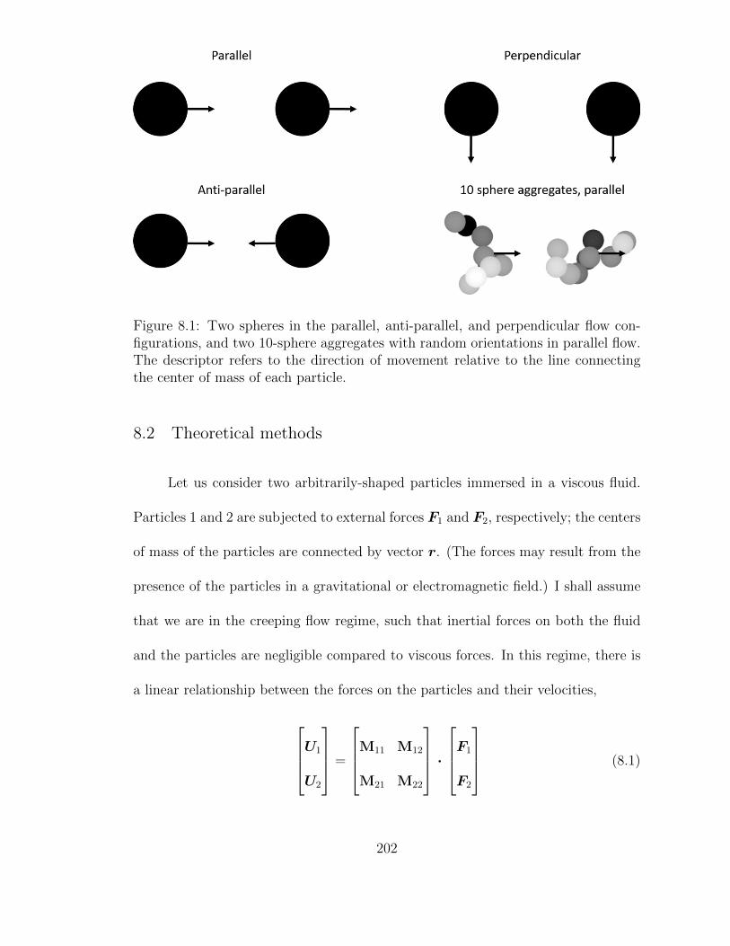
Figure 8.1: Two spheres in the parallel, anti-parallel, and perpendicular flow con-figurations, and two 10-sphere aggregates with random orientations in parallel flow.The descriptor refers to the direction of movement relative to the line connectingthe center of mass of each particle.

8.2 Theoretical methods

Let us consider two arbitrarily-shaped particles immersed in a viscous fluid.

Particles 1 and 2 are subjected to external forces F1 and F2, respectively; the centers

of mass of the particles are connected by vector r. (The forces may result from the

presence of the particles in a gravitational or electromagnetic field.) I shall assume

that we are in the creeping flow regime, such that inertial forces on both the fluid

and the particles are negligible compared to viscous forces. In this regime, there is

a linear relationship between the forces on the particles and their velocities,

U1

U2

=

M11 M12

M21 M22

·F1

F2

(8.1)

202

where Mij is the mobility tensor that relates the force on particle j to the velocity of

particle i. The mobility tensors are functions of the size and shape of both particles

and the distance between them. As r → ∞, hydrodynamic interactions between

particles become negligible. In this case, M12 = M21 ≈ 0, and the mobility tensors

M11 and M22 are simply the inverses of the translational friction tensors Ξt for

particles 1 and 2, defined by the relation

F = −Ξt ·U = −M−1ii ·U (8.2)

My goal is to determine the mobility tensors for particles in the transition

flow regime as a function of particle size, shape, and separation distance. Before

tackling this problem, it is worth considering the simpler case of two spheres in

continuum flow. From there, I will describe how one can approach the problem for

fractal aggregates in the continuum, before discussing how to apply the extended

Kirkwood-Riseman method for particles in the transition regime.

8.2.1 Two spheres in continuum flow

The instantaneous velocity of two spheres subjected to external forces F1 and

F2 has been studied by a number of authors [49, 97, 130, 131, 134, 137]. Exact

solutions are available for two spheres moving parallel and perpendicular to their

line of centers. For arbitrary r, the problem can be solved using the method of

reflections, whereby the mobility tensors are determined as expansions in powers

of the inverse of interparticle separation distance r. (See Happel and Brenner [49]

203

for more information about the method of reflections, including its application to

the two-sphere problem and to the problem of a particle in a tube.) Since the

mobility tensors are symmetric about the line of centers connecting the spheres, we

can formally write

Mij = Aijrr

r2+Bij

(I− rr

r2

)(8.3)

where the non-dimensional coefficients Aij and Bij can be written as expansions in

powers of r−n,

Aij =∞∑n=0

aij,nr−n (8.4a)

Bij =∞∑n=0

bij,nr−n (8.4b)

One obtains the coefficients aij,n and bij,n from the method of reflections.

One can include successive terms in the expansions for Aij and Bij to obtain

increasingly accurate results for the mobility tensors. The simplest approach is the

point force approximation, where Mii = ζ−1i I, Mij is given by the Oseen tensor (the

r−1 term in Eq. (8.5) below), and ζi = 6πµai is the monomer friction coefficient for

a sphere with radius ai. The next level of approximation yields Mii = ζ−1i I and

Mij =1

8πµr

[(I +

rr

r2

)+

(a2i + a2

j

3r2

)(I− 3rr

r2

)]=

1

8πµr

[(1−

a2i + a2

j

3r2

)2rr

r2+

(1 +

a2i + a2

j

3r2

)(I− rr

r2

)](8.5)

for i 6= j. For ai = aj, Eq. (8.5) reduces to the Rotne-Prager-Yamakawa tensor

[57, 58]. Batchelor [134] provides expressions for the mobility tensors accurate to

204

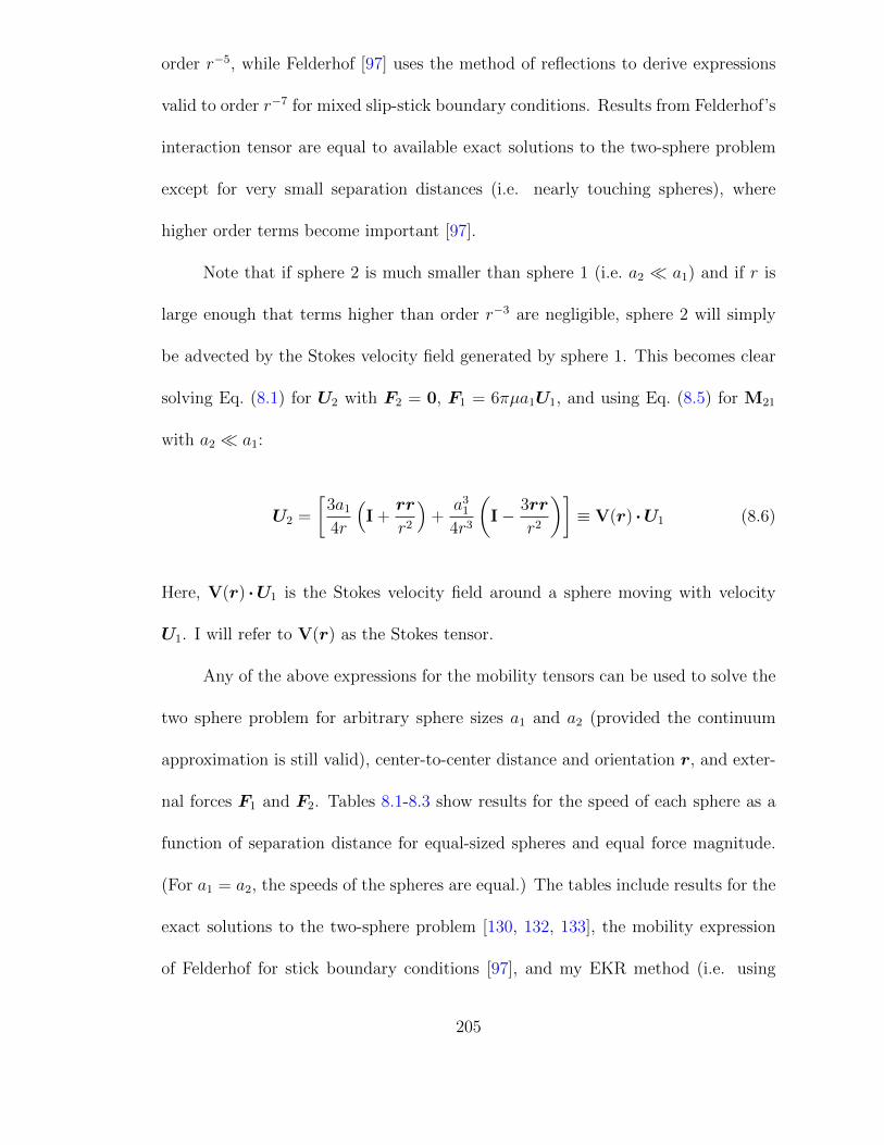
order r−5, while Felderhof [97] uses the method of reflections to derive expressions

valid to order r−7 for mixed slip-stick boundary conditions. Results from Felderhof’s

interaction tensor are equal to available exact solutions to the two-sphere problem

except for very small separation distances (i.e. nearly touching spheres), where

higher order terms become important [97].

Note that if sphere 2 is much smaller than sphere 1 (i.e. a2 a1) and if r is

large enough that terms higher than order r−3 are negligible, sphere 2 will simply

be advected by the Stokes velocity field generated by sphere 1. This becomes clear

solving Eq. (8.1) for U2 with F2 = 0, F1 = 6πµa1U1, and using Eq. (8.5) for M21

with a2 a1:

U2 =

[3a1

4r

(I +

rr

r2

)+

a31

4r3

(I− 3rr

r2

)]≡ V(r) ·U1 (8.6)

Here, V(r) ·U1 is the Stokes velocity field around a sphere moving with velocity

U1. I will refer to V(r) as the Stokes tensor.

Any of the above expressions for the mobility tensors can be used to solve the

two sphere problem for arbitrary sphere sizes a1 and a2 (provided the continuum

approximation is still valid), center-to-center distance and orientation r, and exter-

nal forces F1 and F2. Tables 8.1-8.3 show results for the speed of each sphere as a

function of separation distance for equal-sized spheres and equal force magnitude.

(For a1 = a2, the speeds of the spheres are equal.) The tables include results for the

exact solutions to the two-sphere problem [130, 132, 133], the mobility expression

of Felderhof for stick boundary conditions [97], and my EKR method (i.e. using

205

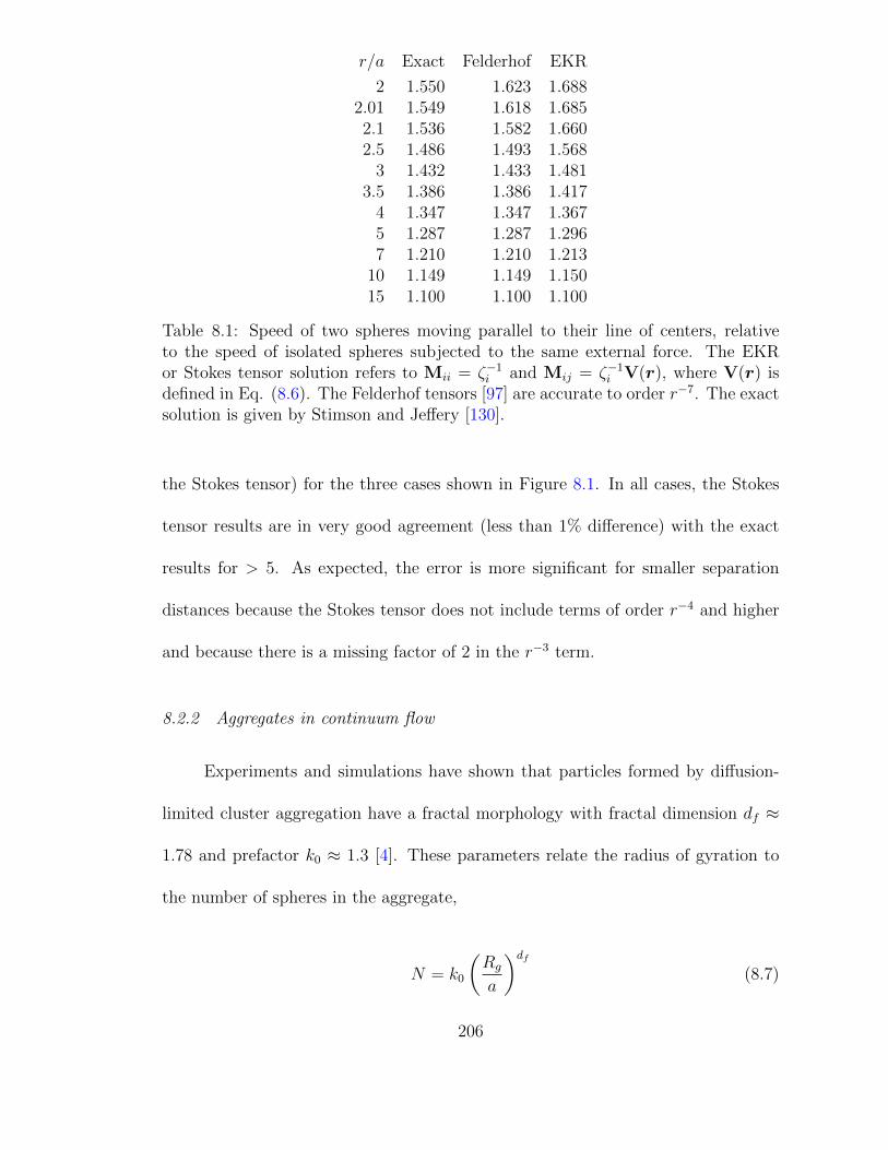
r/a Exact Felderhof EKR

2 1.550 1.623 1.6882.01 1.549 1.618 1.6852.1 1.536 1.582 1.6602.5 1.486 1.493 1.568

3 1.432 1.433 1.4813.5 1.386 1.386 1.417

4 1.347 1.347 1.3675 1.287 1.287 1.2967 1.210 1.210 1.213

10 1.149 1.149 1.15015 1.100 1.100 1.100

Table 8.1: Speed of two spheres moving parallel to their line of centers, relativeto the speed of isolated spheres subjected to the same external force. The EKRor Stokes tensor solution refers to Mii = ζ−1

i and Mij = ζ−1i V(r), where V(r) is

defined in Eq. (8.6). The Felderhof tensors [97] are accurate to order r−7. The exactsolution is given by Stimson and Jeffery [130].

the Stokes tensor) for the three cases shown in Figure 8.1. In all cases, the Stokes

tensor results are in very good agreement (less than 1% difference) with the exact

results for > 5. As expected, the error is more significant for smaller separation

distances because the Stokes tensor does not include terms of order r−4 and higher

and because there is a missing factor of 2 in the r−3 term.

8.2.2 Aggregates in continuum flow

Experiments and simulations have shown that particles formed by diffusion-

limited cluster aggregation have a fractal morphology with fractal dimension df ≈

1.78 and prefactor k0 ≈ 1.3 [4]. These parameters relate the radius of gyration to

the number of spheres in the aggregate,

N = k0

(Rg

a

)df(8.7)

206

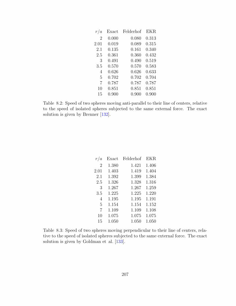
r/a Exact Felderhof EKR

2 0.000 0.080 0.3132.01 0.019 0.089 0.3152.1 0.135 0.161 0.3402.5 0.361 0.360 0.432

3 0.491 0.490 0.5193.5 0.570 0.570 0.583

4 0.626 0.626 0.6335 0.702 0.702 0.7047 0.787 0.787 0.787

10 0.851 0.851 0.85115 0.900 0.900 0.900

Table 8.2: Speed of two spheres moving anti-parallel to their line of centers, relativeto the speed of isolated spheres subjected to the same external force. The exactsolution is given by Brenner [132].

r/a Exact Felderhof EKR

2 1.380 1.421 1.4062.01 1.403 1.419 1.4042.1 1.392 1.399 1.3842.5 1.326 1.328 1.316

3 1.267 1.267 1.2593.5 1.225 1.225 1.220

4 1.195 1.195 1.1915 1.154 1.154 1.1527 1.109 1.109 1.108

10 1.075 1.075 1.07515 1.050 1.050 1.050

Table 8.3: Speed of two spheres moving perpendicular to their line of centers, rela-tive to the speed of isolated spheres subjected to the same external force. The exactsolution is given by Goldman et al. [133].

207

Notable examples of DLCA aggregates include soot, as well as titania and other

ceramic powders synthesized in aerosol flame reactors [7].

In the previous section, I reviewed how one can solve the two sphere problem

to various levels of approximation. I now describe how to use a similar approach for

aggregates.

In approaches based on Kirkwood-Riseman theory [28], one uses any of the

above expressions for the interactions between pairs of spheres to determine the force

on a macromolecule or particle consisting of N spherical subunits. The resulting

system of equations is analogous to Eq. (8.1):

−Ui =∑j=1

Mij ·Fj (8.8)

Here, Fj is the force exerted by the fluid on the jth primary sphere in an aggregate,

which is unknown, whereas in Eq. (8.1) Fj represents the known external force on

the jth particle in a two-particle system. (The negative sign appearing in Eq. (8.8)

is a consequence of the shift from the force exerted by the particle – as in Eq. (8.1)

– to the force exerted on the ith primary sphere by the fluid.) To determine the

force on a macromolecule or particle whose subunits have velocities Ui, one solves

the above linear system for the force on each sphere, then sums over all spheres

to get the total force. Alternatively, if the total external force on the particle is

given (e.g. gravity or the force on charged particle in an electric field), one can

solve Eq. (8.8) iteratively to get the particle velocity such that the calculated force

distribution is consistent with the total force.

208

KR-based treatments rely on the underlying linearity of the Stokes flow equa-

tions. In their original formulation, Kirkwood and Riseman [28] set Mij = δijζ−1i +

(1 − δij)Tij, where δij is the Kronecker delta and Tij is the Oseen tensor. Later

applications of KR theory [30, 56, 107] replace the Oseen tensor with the Rotne-

Prager-Yamakawa tensor. One can use higher order approximations for the mobility

tensors (e.g. the Felderhof expressions); one can also account for multi-body effects

using mobility tensors derived by Mazur and Van Saarloos [60]. However, Carrasco

and Garcıa de la Torre [53] have shown that using these more rigorous methods to

calculate a particles friction and diffusion tensors offer little improvement over using

KR-theory with the Rotne-Prager-Yamakawa tensor.

One can use the same KR-based methods to determine the forces between two

aggregates: one again solves the system of equations given by Eq. (8.8), but now

one sums over the spheres in each aggregate to determine the total hydrodynamic

force. Again, one can perform this calculation for aggregates with specified velocities

or specified external forces. By comparing this result to the force on an isolated

aggregate, one can determine the effect of the second aggregate on the mobility of

the first.

8.2.3 Extended Kirkwood-Riseman theory

The previous subsections have focused on situations where the continuum ap-

proach is valid. For particles consisting of spheres with diameters on the order

of tens of nanometers moving through air at standard temperature and pressure

(λ ≈ 67 nm), one cannot use the expressions for interactions between particles in

209

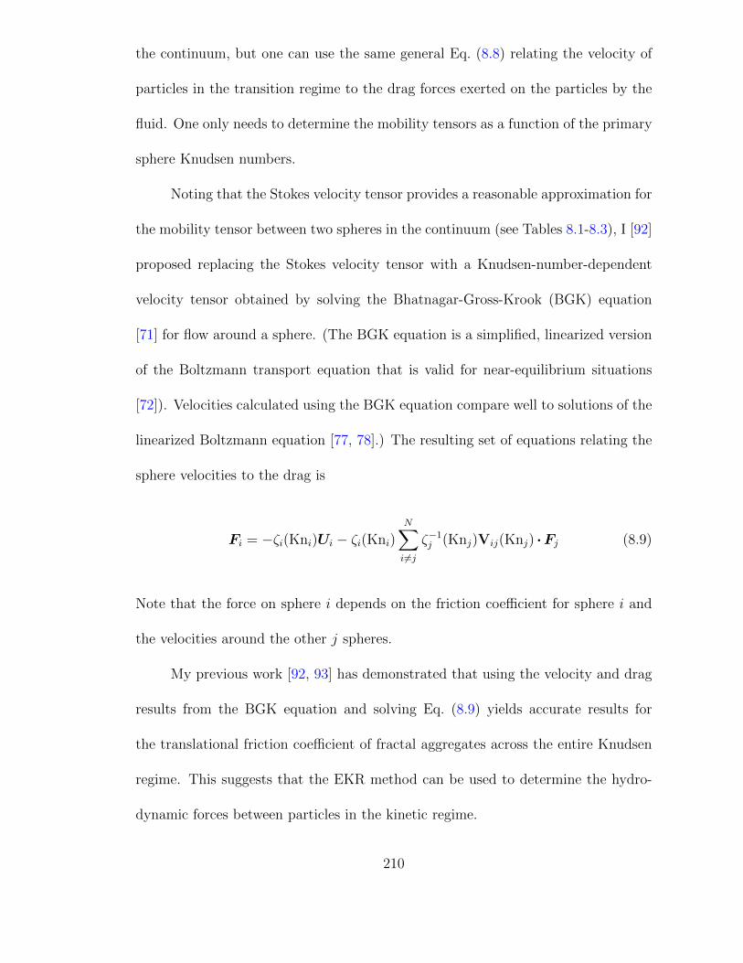
the continuum, but one can use the same general Eq. (8.8) relating the velocity of

particles in the transition regime to the drag forces exerted on the particles by the

fluid. One only needs to determine the mobility tensors as a function of the primary

sphere Knudsen numbers.

Noting that the Stokes velocity tensor provides a reasonable approximation for

the mobility tensor between two spheres in the continuum (see Tables 8.1-8.3), I [92]

proposed replacing the Stokes velocity tensor with a Knudsen-number-dependent

velocity tensor obtained by solving the Bhatnagar-Gross-Krook (BGK) equation

[71] for flow around a sphere. (The BGK equation is a simplified, linearized version

of the Boltzmann transport equation that is valid for near-equilibrium situations

[72]). Velocities calculated using the BGK equation compare well to solutions of the

linearized Boltzmann equation [77, 78].) The resulting set of equations relating the

sphere velocities to the drag is

Fi = −ζi(Kni)Ui − ζi(Kni)N∑i 6=j

ζ−1j (Knj)Vij(Knj) ·Fj (8.9)

Note that the force on sphere i depends on the friction coefficient for sphere i and

the velocities around the other j spheres.

My previous work [92, 93] has demonstrated that using the velocity and drag

results from the BGK equation and solving Eq. (8.9) yields accurate results for

the translational friction coefficient of fractal aggregates across the entire Knudsen

regime. This suggests that the EKR method can be used to determine the hydro-

dynamic forces between particles in the kinetic regime.

210

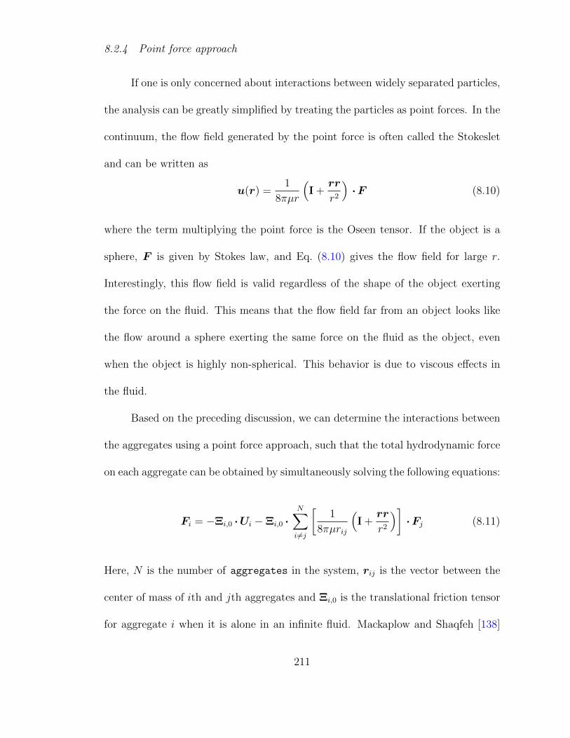
8.2.4 Point force approach

If one is only concerned about interactions between widely separated particles,

the analysis can be greatly simplified by treating the particles as point forces. In the

continuum, the flow field generated by the point force is often called the Stokeslet

and can be written as

u(r) =1

8πµr

(I +

rr

r2

)·F (8.10)

where the term multiplying the point force is the Oseen tensor. If the object is a

sphere, F is given by Stokes law, and Eq. (8.10) gives the flow field for large r.

Interestingly, this flow field is valid regardless of the shape of the object exerting

the force on the fluid. This means that the flow field far from an object looks like

the flow around a sphere exerting the same force on the fluid as the object, even

when the object is highly non-spherical. This behavior is due to viscous effects in

the fluid.

Based on the preceding discussion, we can determine the interactions between

the aggregates using a point force approach, such that the total hydrodynamic force

on each aggregate can be obtained by simultaneously solving the following equations:

Fi = −Ξi,0 ·Ui −Ξi,0 ·N∑i 6=j

[1

8πµrij

(I +

rr

r2

)]·Fj (8.11)

Here, N is the number of aggregates in the system, rij is the vector between the

center of mass of ith and jth aggregates and Ξi,0 is the translational friction tensor

for aggregate i when it is alone in an infinite fluid. Mackaplow and Shaqfeh [138]

211

demonstrated that the point force approach applied to the problem of sedimentation

of fibers in a semi-dilute homogeneous suspension, yields results similar to those of

a more sophisticated Monte Carlo simulation of the problem.

The point force approach should also be valid in the transition regime, albeit

with a Knudsen-number-dependent hydrodynamic interaction tensor in place of the

Oseen tensor. In fact, the transition regime interaction tensor should have the same

form as the Oseen tensor but with a different coefficient in place of 1/8. This is

because the fluid velocity far from a sphere has the general form

u(r) = −c1(Kn)

2

a

r

(I +

rr

r2

)·U = − c1(Kn)

2ζi,0(Kn)

a

r

(I +

rr

r2

)·F (8.12)

where U is the sphere velocity, F is the force exerted by the sphere on the fluid,

and c1(Kn) is a coefficient that can be obtained by solving the BGK or linearized

Boltzmann equation for flow around a sphere [78, 92]. In the continuum, c1 = −3/2,

and Eq. (8.12) reduces to Eq. (8.10).

Substituting Eq. (8.12) for the Oseen tensor in Eq. (8.11), we get the following

result for a system of N aerosol aggregates:

Fi = −Ξi,0(Kni) ·Ui −Ξi,0(Kni) ·N∑i 6=j

[−c1(Knj,eff)

2ζj,0

(I +

rr

r2

)]·Fj (8.13)

Here, aj,eff is the radius and Knj,eff = λ/aj,eff the Knudsen number of a sphere with

friction coefficient ζj,0 = |Ξj,0(Knj) ·Uj/Uj|, where Ξj,0(Knj) is the friction tensor

for aggregate j alone in an infinite fluid and Uj is the velocity of aggregate j. One

212

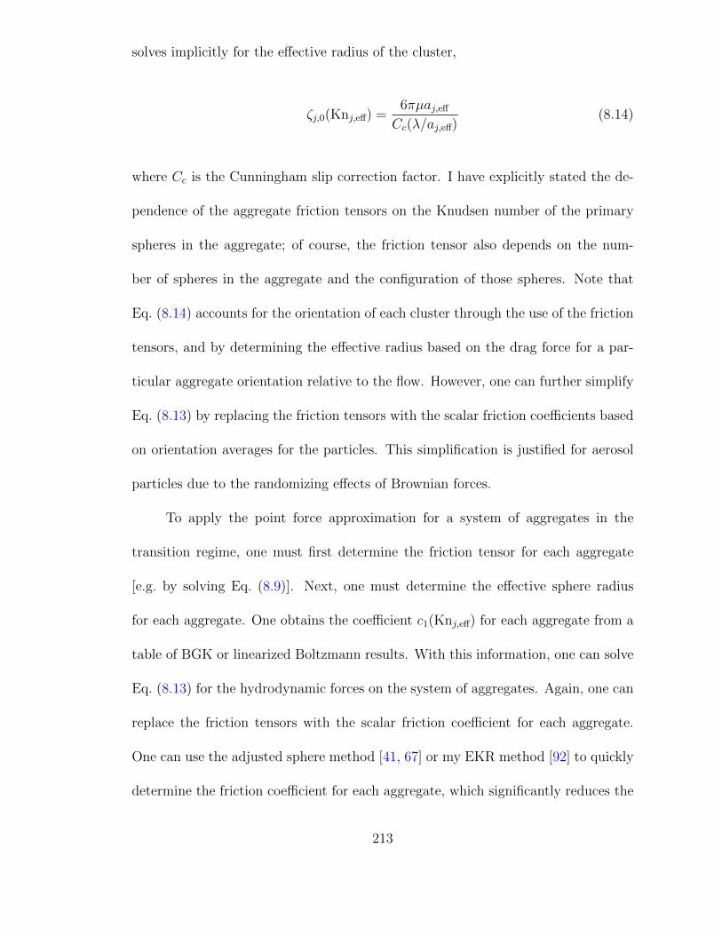
solves implicitly for the effective radius of the cluster,

ζj,0(Knj,eff) =6πµaj,eff

Cc(λ/aj,eff)(8.14)

where Cc is the Cunningham slip correction factor. I have explicitly stated the de-

pendence of the aggregate friction tensors on the Knudsen number of the primary

spheres in the aggregate; of course, the friction tensor also depends on the num-

ber of spheres in the aggregate and the configuration of those spheres. Note that

Eq. (8.14) accounts for the orientation of each cluster through the use of the friction

tensors, and by determining the effective radius based on the drag force for a par-

ticular aggregate orientation relative to the flow. However, one can further simplify

Eq. (8.13) by replacing the friction tensors with the scalar friction coefficients based

on orientation averages for the particles. This simplification is justified for aerosol

particles due to the randomizing effects of Brownian forces.

To apply the point force approximation for a system of aggregates in the

transition regime, one must first determine the friction tensor for each aggregate

[e.g. by solving Eq. (8.9)]. Next, one must determine the effective sphere radius

for each aggregate. One obtains the coefficient c1(Knj,eff) for each aggregate from a

table of BGK or linearized Boltzmann results. With this information, one can solve

Eq. (8.13) for the hydrodynamic forces on the system of aggregates. Again, one can

replace the friction tensors with the scalar friction coefficient for each aggregate.

One can use the adjusted sphere method [41, 67] or my EKR method [92] to quickly

determine the friction coefficient for each aggregate, which significantly reduces the

213

complexity of the problem.

Using the point force approach is beneficial because one can significantly reduce

the number of simultaneous equations that one must solve compared to considering

the pairwise interactions among all of the spheres in all of the aggregates. This

is especially useful if one is considering a system consisting of identical aggregates

(such that one need only determine the friction tensor once) or if one is considering

interactions between coagulating aerosols (such that the friction tensors for the ag-

gregates remain constant until two particles coagulate, at which point one need only

calculate the friction tensor for the new particle). While the point force approach is

strictly valid only for widely separated particles, I will show in the following section

that this approach provides reasonable results even when the aggregates are fairly

close together.

8.3 Two particle results

I have used my extended Kirkwood-Riseman method [Eq. (8.9)] to determine

the hydrodynamic forces between two aggregates moving parallel, anti-parallel, and

perpendicular to their line of centers in the transition flow regime. I start by consid-

ering two spheres, then move to the case of two fractal aggregates. For simplicity,

I will focus on cases where the two particles are identical, though I do consider the

effects of orientation for the aggregate calculations.

214

8.3.1 Sphere results

Figure 8.2 shows the results for two spheres moving parallel, anti-parallel,

and perpendicular to their line of centers. Results are plotted as a function of

separation distance for three different Knudsen numbers. Here, I show the ratio of

the velocity of each sphere subjected to the same external force (albeit in opposite

directions for the anti-parallel case) to the velocity it would have if was alone in

an infinite medium subjected to the same force. Note that one can obtain the

effect on the hydrodynamic force for specified velocity by taking the inverse of the

results in Figure 2. I also present the velocities calculated using Felderhofs mobility

tensors [97] for mixed slip-stick boundary conditions for Kn = 0.1. These tensors

are accurate to order r−7 and are expected to yield nearly exact results except for

very small separation distances for this near-continuum situation.

The figure shows that my EKR results are in good agreement with the Felder-

hof mobility tensor results for near-continuum conditions (or near-stick boundary

conditions, in the case of the Felderhof results). For r/a > 3, the two methods yield

results within about 2% of each other; this is not surprising, since the higher order

terms in the expansions representing the mobility tensors decay quickly with in-

creasing separation. The error is still fairly low (< 8%) for touching spheres moving

parallel and perpendicular to their line of centers but is much more significant for

the anti-parallel configuration. This is because my EKR method ignores lubrication

forces between the particles, whereas Felderhofs mobility tensors partially account

for these forces through the higher order terms in the expansion.

215

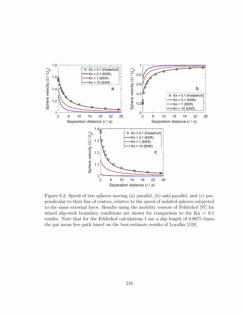
Figure 8.2: Speed of two spheres moving (a) parallel, (b) anti-parallel, and (c) per-pendicular to their line of centers, relative to the speed of isolated spheres subjectedto the same external force. Results using the mobility tensors of Felderhof [97] formixed slip-stick boundary conditions are shown for comparison to the Kn = 0.1results. Note that for the Felderhof calculations I use a slip length of 0.9875 timesthe gas mean free path based on the best-estimate results of Loyalka [139].

216

As expected, the strength of the hydrodynamic interactions between spheres

decreases with increasing Knudsen number. For the perpendicular configuration, the

two spheres behave almost as if they are isolated even when they are in contact at

high Knudsen number; the effect is more important in the parallel and anti-parallel

configurations, likely due to direct shielding of incoming gas molecules by the other

sphere and molecules that collide with both spheres before colliding with other gas

molecules.

As we saw in the previous section, the long-range hydrodynamic interactions

have a r−1 dependence in the continuum, as given by the Oseen tensor. The r−1

dependence is also evident in my transition regime results in Figure 8.2. The coef-

ficient of the r−1 term is a function of the Knudsen number. This result is directly

related to the asymptotic behavior of the velocity field at large distances from a

sphere, as I have discussed in Section 8.2.4 above.

8.3.2 Aggregate results

Figure 8.3 shows the results for two aggregates moving parallel to their line of

centers. Results are shown for two aggregates with 10 spheres each and for two ag-

gregates with 1000 spheres. The results are presented as the ratio of the drag on one

of the aggregates to the drag on that aggregate when it is alone in an infinite fluid.

Solid lines represent the full EKR solution [Eq. (8.9)], while the dotted lines repre-

sent the point force results [Eq. (8.13)]. From the figures, the point force solution

is sufficiently accurate for all but the closest separations, which greatly simplifies

any analysis of the effects of hydrodynamic interactions between aggregates. Also,

217

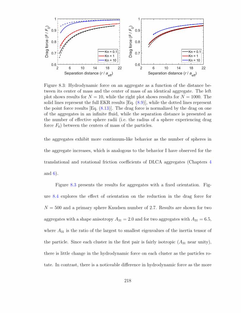
Figure 8.3: Hydrodynamic force on an aggregate as a function of the distance be-tween its center of mass and the center of mass of an identical aggregate. The leftplot shows results for N = 10, while the right plot shows results for N = 1000. Thesolid lines represent the full EKR results [Eq. (8.9)], while the dotted lines representthe point force results [Eq. (8.13)]. The drag force is normalized by the drag on oneof the aggregates in an infinite fluid, while the separation distance is presented asthe number of effective sphere radii (i.e. the radius of a sphere experiencing dragforce F0) between the centers of mass of the particles.

the aggregates exhibit more continuum-like behavior as the number of spheres in

the aggregate increases, which is analogous to the behavior I have observed for the

translational and rotational friction coefficients of DLCA aggregates (Chapters 4

and 6).

Figure 8.3 presents the results for aggregates with a fixed orientation. Fig-

ure 8.4 explores the effect of orientation on the reduction in the drag force for

N = 500 and a primary sphere Knudsen number of 2.7. Results are shown for two

aggregates with a shape anisotropy A31 = 2.0 and for two aggregates with A31 = 6.5,

where A31 is the ratio of the largest to smallest eigenvalues of the inertia tensor of

the particle. Since each cluster in the first pair is fairly isotropic (A31 near unity),

there is little change in the hydrodynamic force on each cluster as the particles ro-

tate. In contrast, there is a noticeable difference in hydrodynamic force as the more

218

Figure 8.4: Effects of orientation on the hydrodynamic force on one of two 500-sphere aggregates with primary sphere Kn = 2.7 (sphere radius of 25 nm at roomtemperature). Results are presented as the ratio of the force on an aggregate for thespecified separation distance to the force on the aggregate alone in an infinite fluidat a particular orientation. Each line represents a randomly chosen orientation foreach aggregate in the two-aggregate system. The left figure is for an aggregate withanisotropy A31 = 2.0, while the right figure is for an aggregate with A31 = 6.5.

anisotropic particles rotate. This is especially true for small separation distances.

Note that in each case I normalize by the force on the particle for that particular

orientation.

8.4 Discussion

My results show that hydrodynamic interactions between particles in the tran-

sition flow regime are significant for small separation distances and still noticeable

at separations of more than 10 sphere diameters or 20 times the radius of gyra-

tion of an aggregate. The effect is stronger near the continuum than near the free

molecule regime and stronger for parallel and anti-parallel configurations than for

perpendicular configurations for all particle sizes.

With that said, hydrodynamic interactions likely have little effect on mea-

219

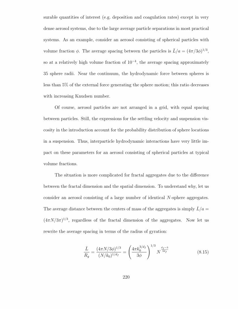
surable quantities of interest (e.g. deposition and coagulation rates) except in very

dense aerosol systems, due to the large average particle separations in most practical

systems. As an example, consider an aerosol consisting of spherical particles with

volume fraction φ. The average spacing between the particles is L/a = (4π/3φ)1/3,

so at a relatively high volume fraction of 10−4, the average spacing approximately

35 sphere radii. Near the continuum, the hydrodynamic force between spheres is

less than 5% of the external force generating the sphere motion; this ratio decreases

with increasing Knudsen number.

Of course, aerosol particles are not arranged in a grid, with equal spacing

between particles. Still, the expressions for the settling velocity and suspension vis-

cosity in the introduction account for the probability distribution of sphere locations

in a suspension. Thus, interparticle hydrodynamic interactions have very little im-

pact on these parameters for an aerosol consisting of spherical particles at typical

volume fractions.

The situation is more complicated for fractal aggregates due to the difference

between the fractal dimension and the spatial dimension. To understand why, let us

consider an aerosol consisting of a large number of identical N -sphere aggregates.

The average distance between the centers of mass of the aggregates is simply L/a =

(4πN/3π)1/3, regardless of the fractal dimension of the aggregates. Now let us

rewrite the average spacing in terms of the radius of gyration:

L

Rg

=(4πN/3φ)1/3

(N/k0)1/df=

(4πk

3/df0

3φ

)1/3

Ndf−3

3df (8.15)

220

Here, k0 and df are the prefactor and fractal dimension of the aggregates. For

DLCA aggregates (k0 ≈ 1.3, df ≈ 1.78), and for a volume fraction of 10−4, the

average spacing between aggregates is 24 radii of gyration for N = 10 and 8.3 radii

of gyration for N = 1000. Since the radius of gyration is approximately equal to the

effective hydrodynamic radius of a particle in continuum flow, we can consult the

near-continuum results in Figure 8.3 to estimate the hydrodynamic force between the

aggregates in the parallel flow configuration at these average separation distances.

For N = 1000, the drag force for the parallel configuration is approximately 85% of

the drag at infinite separation distance for Kn = 0.1. Compare this to the result for

a system of spheres in continuum flow, where the average separation is 34 radii, and

the force at this separation is 96% of the force at infinite separation for Kn = 0.1.

8.4.1 Aerosol clouds

One interesting problem involving hydrodynamic interactions among particles

is the settling of an unbounded aerosol cloud in a gravitational field. This prob-

lem has been studied extensively for spherical particles in the continuum. (For a

small sample, refer to the works of Burgers [131] or to Fuchs [1].) The behavior

of the particle cloud depends on the volume fraction of particles in the cloud. For

sufficiently low volume fractions, the particles behave as if they are isolated, as one

would expect. In this case, the velocity of each particle is obtained by balancing the

gravitational force Fg with the drag force,

vs1 =Fgζ0

(8.16)

221

For high volume fractions, the particles entrain the surrounding fluid, and the cloud

behaves as a gas bubble with the same viscosity as the fluid surrounding the cloud

[1, 131]. In this case, the velocity of the cloud is given by

vs2 =43πR3nFg

5πµR=

4R2nFg15µ

(8.17)

where R is the radius of the cloud and n is the number concentration of particles.

In the first equality, I explicitly write the velocity as the ratio between the total

gravitational force on the cloud and the drag on a spherical bubble with equal

viscosity in the inner and outer fluids. The particles behave as if they are isolated

when vs2/vs1 1 and as a cloud with velocity given by Eq. (8.17) when vs2/vs1 1

[1].

The above analysis is applicable for aggregates in continuum flow, with a few

important caveats. First, one must use appropriate values for the gravitational and

drag forces on the aggregate. Second, the effects of the aggregates on the effective

viscosity of the cloud must be negligible; of course, this restriction also applies to

the aforementioned case of spherical particles. Additionally, I will ignore the effects

of hydrodynamic interactions on the orientation of the aggregates. I will address

this restriction in more detail in the following section. With the above caveats, we

can write the ratio vs2/vs1 for a cloud consisting of identical N -sphere aggregates as

vs2vs1

=6φζ?0R

2

5Na2(8.18)

222

where ζ?0 ≡ 6πµaζ0 is the non-dimensional friction coefficient for the aggregate when

it is alone in an infinite fluid. Note that the volume fraction is simply the number

density times the volume of one aggregate, i.e. φ = 43πa3Nn.

Now, I will consider whether or not the above analysis applies to particles

– whether spheres or aggregates – in the transition regime. (Again, if one wishes

to consider aggregates, the analysis is subject to the caveats mentioned above for

particles in continuum flow.) To do so, I will consider an idealized situation: a cloud

of radius R that consists of identical particles in a cubic lattice. For this problem,

each particle experiences the same external force, so we can directly solve Eq. (8.13)

for the velocity of each particle in the cloud, Ui. If Fuchs analysis is applicable for

particles in the transition regime, then the calculated velocity should approach that

given by Eq. (8.17) when the ratio vs2/vs1 [Eq. (8.18)] is much greater than unity

and should approach Fg/ζ0 when the result of Eq. (8.18) is much less than unity.

Figure 8.5 shows the average particle velocity in the aerosol cloud as a function

of the aerosol volume fraction. The calculations are performed for 25-nm-radius

spheres (Kn = 2.7) and a 25-m-radius cloud. Average velocities are normalized by

the settling velocity of an isolated sphere (i.e. by vs1). The figure shows that for

vs2/vs1 1, the average velocity of particles in the cloud approaches vs2, and for

vs2/vs1 1, the particles behave as if they are isolated.

These results show that a cloud of aerosol particles can behave as a gas droplet

in continuum flow even when the individual particles are small relative to the mean

free path of the gas. This occurs for sufficiently large cloud sizes and particle volume

fractions.

223

Figure 8.5: Average velocity for a cloud of spheres, normalized by the settlingvelocity of a single particle, vs1. The velocity of a gas bubble having the samevolume fraction and cloud radius is also shown. For vs2/vs1 1, the average velocityapproaches the gas bubble velocity, and the two curves coincide. For vs2/vs1 1,the particles behave as if they are isolated.

224

Of course, in real-world situations the cloud will not be perfectly spherical, nor

will it be composed of monodisperse particles arranged in a regular grid. Neverthe-

less, we can reach some qualitative conclusions about the behavior of a real-world

cloud of aerosol particles from the results of the ideal case. First, the deposition

velocity of the particles in the cloud may be significantly greater than the deposition

velocity of an isolated particle. This enhanced settling velocity is due to the fact

that the particles entrain the surrounding fluid. Second, a collection of particles

that behave as if they are in the transition flow regime when they are isolated (or

when the volume fraction is very small) can behave like a cloud of continuum par-

ticles when the particle volume fraction increases. This is because the long-range

hydrodynamic interactions between particles decay as 1/r, regardless of the size of

the particle relative to the gas mean free path.

8.4.2 Additional considerations

Before concluding, I will address a number of assumptions that I have made for

my analysis. First, I have ignored rotational effects when considering interactions

between particles. The complete description of two particles has the same general

form as Eq. (8.1), but one replaces the 3-element velocity and force vectors with

6-element vectors that include the angular velocity of and torque exerted by the

particle, respectively. Likewise, one would need to incorporate rotational effects in

the generalized mobility tensors Mij, which now have size 6-by-6. See Brenner [29]

or Carrasco and Garcıa de la Torre [53] for the effects of rotation on a single particle

in the continuum and my previous work [94] for how one might consider rotational

225

effects in the kinetic regime. The two-particle principles follow from the application

of KR-based theories to single-particle systems.

Second, I have mostly ignored Brownian effects in my calculations, except to

note that Brownian forces would likely randomize the orientations of aggregates in

an aerosol. Strictly speaking, one must account for hydrodynamic interactions when

determining the probability distribution for the particle orientation. For example,

Mackaplow and Shaqfeh [138] have performed dynamic simulations showing non-

Brownian fibers aligning with gravity due to hydrodynamic effects. Therefore, the

orientation of aerosol aggregates will depend on the competition between hydrody-

namic effects that tend to align particles and Brownian effects that tend to random-

ize their orientation. This is analogous to the behavior of a perfectly-conducting

aerosol particle in an external electric field [96, 105].

Additionally, Brownian forces affect the spatial distribution of particles in a

cloud or suspension. Diffusion is partially responsible (along with shear) for breakup

of clouds [1], so the analysis in the previous section applies only for some initial pe-

riod while the cloud remains intact. For statistically homogeneous systems, one

must account for the particle probability distribution when determining suspension

behavior. In principle, one can apply the methods used in Stokesian dynamics sim-

ulations (see, e.g., Ermak and McCammon [135] and Brady and Bossis [136]) for

non-continuum flows, provided one modifies the hydrodynamic interaction terms

in the algorithms. I have provided here the translational hydrodynamic interac-

tion tensors, while I describe how to account for rotational and translation-rotation

coupling effects elsewhere (Chapter 5).

226

Third, my calculations have been performed for isothermal conditions. As

Fuchs notes, cloud behavior is often driven by temperature differences between the

cloud interior and the surrounding gas [1]. Because aerosols are often generated in

non-isothermal systems (e.g. flames), one must take care in applying my analysis to

real-world systems.

Finally, my calculations assume the particles are in an unbounded, non-periodic

system. Note that in periodic, statistically homogeneous suspensions, the sedimen-

tation velocity decreases with increasing particle volume fraction [128]. In contrast,

unbounded clouds of particles settle at a faster rate as volume fraction increases, as

is clear from Eq. (8.18). The difference is due to the gas behavior: for an unbounded

cloud, the gas can flow around the cloud to occupy the space vacated by the settling

cloud, whereas the gas must flow between the particles in the opposite direction of

the sedimentation velocity. This counter flow serves to reduce the sedimentation

velocity of the periodic suspension.

8.5 Conclusions

I have described how one would apply my extended Kirkwood-Riseman theory

to interactions between spheres and aggregate particles as a function of the distance

between particles and the particle size and shape (number of spheres, primary sphere

Knudsen number, fractal dimension). I have provided sample results for the effects

of hydrodynamic interactions between two spheres and two aggregates. In both

cases, the interactions are weaker than for particles in continuum flow, and the

227

interaction strength decreases with increasing Knudsen number. Note that in many

aerosols of engineering interest, the particle volume fraction is very small, and on

average one can rightly neglect these interactions. However, for aerosols near the

gel point, such interactions may be important.

I have applied my method to an unbounded cloud of spheres with non-negligible

Knudsen numbers and shown that it behaves similarly to a cloud of larger particles.

This analysis applies to an isothermal, spherical cloud of particles arranged in a reg-

ular grid, but the conclusion that hydrodynamic interactions among a large group

of particles can significantly affect settling behavior also applies in less restrictive

conditions.

The above work provides some of the hydrodynamic interaction terms neces-

sary to perform a Brownian dynamics simulation of an aerosol consisting of parti-

cles with non-negligible Knudsen numbers. One could either apply the point force

method described here or my more complicated EKR method to account for Brow-

nian (through the generalized Stokes-Einstein relation; see Ermak and McCammon

[135]) and hydrodynamic effects on the aerosol behavior. One can also account for

rotational effects using the EKR method, as discussed elsewhere [94]. Taken to-

gether, this work can form the basis for a dynamic simulation of a dense aerosol

system.

228

Chapter 9: NGDE: A MATLAB-based Code for Solving the Aerosol

General Dynamic Equation

The previous chapters in this dissertation have largely concentrated on single-

particle behavior (the exception being the study of interparticle hydrodynamic inter-

actions in Chapter 8). For the present chapter, I will shift my focus to the dynamic

behavior of an aerosol system undergoing nucleation, surface growth, and coagula-

tion. Note that this chapter provides the technical background for the NGDE code.

The User Manual for the code is included as Appendix F. One can obtain the NGDE

code on the Zachariah Group website.

9.1 Introduction

The behavior of an aerosol system is governed by the general dynamic equation

[2, 3, 45], which can be written as

∂n

∂t=

1

2

∫ v

0

β(v − v′, v′)n(v′, t)n(v − v′, t)dv′ −∫ ∞

0

β(v, v′)n(v, t)n(v′, t)dv′

− ∂

∂v[n(v, t)G(v, t)] + S(v, t)−R(v, t) (9.1)

229

Here, n(v, t) is the particle size distribution (PSD) as a function of time t and particle

volume v, where n(v, t)dv is the number of aerosol particles per unit volume of gas

with particle volume between v and v+dv; β(v, v′) is the collision kernel for particles

with volumes v and v′; G(v, t) is the growth rate of particles with volume v due to

condensation/evaporation; S(v, t) is the rate at which particles are added to the

system (e.g. by homogeneous nucleation); and R(v, t) is the rate at which particles

are removed from the system (e.g. by deposition on surfaces). The integrals represent

how the size distribution changes due to coagulation.1

Eq. (9.1) is non-linear integro-differential equation that can be solved ana-

lytically only for a small number of cases. (See, for example, Refs. [140, 141]).

Thus, one must typically resort to numerical methods to solve for the evolution of

the PSD with time. However, solving the GDE numerically is complicated by the

orders-of-magnitude difference in volume between the smallest and largest particles

in an aerosol. As suggested by the bounds of the integrals in Eq. (9.1), one must

determine the size distribution for an infinite range of particle sizes. Fortunately,

the physical characteristics of the system allow one to establish upper and lower

bounds for the size distribution. For example, large particles may deposit quickly

due to gravitational forces, so one can assume particles greater than some upper

bound have an infinite removal rate. On the other hand, no particle can be smaller

than a single molecule (ignoring of course the subatomic domain), thus establishing

a natural lower bound for the size distribution. In addition, thermodynamic con-

1The integrals in Eq. (9.1) only account for growth due to particle-particle collisions. Of course,it is possible that two particles could collide with sufficient energy to break them into smallerparticles, but such high-energy collisions are rare in situations of interest to the aerosol scientistand are therefore ignored in Eq. (9.1).

230

siderations limit the smallest stable size of molecular clusters, such that one can

ignore particles consisting of fewer molecules than some critical size. Even with

these simplifications, solving the GDE numerically is hardly a trivial endeavor.

This chapter describes a fairly simple method for solving the general dynamic

equation: a MATLAB-based code using a nodal method that is similar in principle

to the sectional method pioneered by Gelbard and colleagues [26, 142, 143]. The

MATLAB version of the NGDE code is based on an earlier version of the code [27]

written in C. A number of new features have added to the MATLAB version of the

code. The most significant additions are the implementation of a dynamic time-step

algorithm that significantly speeds up the calculation run-time and the introduction

of a post-processing tool for visualizing the code results.

Before the NGDE code is described in detail, a brief overview of various tech-

niques used to solve the GDE numerically is provided. Next, the constituent models

for nucleation, coagulation, and surface growth used in NGDE; the dynamic time-

step algorithm; and the available calculation types and general solution procedure

are described. Results are presented for a few sample problems. These results are

compared to the results of other numerical solutions of the problems published in the

literature. The chapter closes with a discussion about the limitations of NGDE and

the ways in which one may improve the code, as well as a brief introduction to the

post-processing tool NGDEplot. More details about running NGDE, code input and

output, and code structure can be found in the NGDE User Manual (Appendix F).

231

9.2 Overview of Numerical Methods for Solving the GDE

Numerical methods for solving the GDE can be divided into three broad

classes: J-space methods, moment methods, and sectional methods [45]. J-space

methods [144] involve transforming the continuous PSD to J-space, integrating the

J-space distribution function with respect to time, and taking the inverse transform

to obtain the PSD as a function of time. Moment methods [145] start by assuming

some form for the size distribution and its moments (i.e. the product of the distri-

bution and powers of the particle volume, integrated over all volumes) and involve

solving for the evolution of the moments of the size distribution. In addition to the

integration schemes needed to solve for the time-dependent evolution of the PSD

(e.g. the Euler method or Kunge-Kutta method), both J-space and moment meth-

ods require the use of quadrature formulas to integrate the distribution or moment

equations with respect to volume. For this reason, these methods are somewhat

mathematically complex and can prove a hindrance for the novice aerosol scientist.

On the other hand, sectional methods [26, 142, 143] are more intuitive ways of

solving the general dynamic equation that make fewer assumptions about the shape

of the size distribution. These methods divide the size distribution into discrete size

bins and solve the GDE for each size bin as a system of coupled equations. The

number concentration of particles in bin k at time t is defined as

Nk(t) =

∫ vk

vk−1

n(v, t)dv (9.2)

232

where vk−1 and vk are the lower and upper bounds (in terms of volume) of bin k.

The evolution of the number concentration of particles in bin k can be written as

dNk

dt=

dNk

dt

∣∣∣∣coag

+dNk

dt

∣∣∣∣nucl

+dNk

dt

∣∣∣∣growth

+dNk

dt

∣∣∣∣dep

(9.3)

where the first, second, and third terms on the right-hand-side represent the changes

in the number concentration in bin k due to coagulation, nucleation, and surface

growth. These terms will be discussed later in this chapter. The final term in the

equation represents losses due to deposition. Deposition is not considered in NGDE;

nevertheless, this term is included in the above equation for completeness, in case

one wishes to include deposition in NGDE in the future. (See Section 9.5.) For the

sectional method, one must also track the total volume (or mass) of particles within

each size bin,

Vk(t) =

∫ vk

vk−1

vn(v, t)dv (9.4)

using an equation similar to the equation above for the number concentration.

One complication inherent in sectional methods is that one must use average

properties within each bin to calculate the coagulation and growth rates. For ex-

ample, consider the increase in the number concentration of particles in bin k due

to coagulation of particles in bins i and j, βijkNiNj. Here, βijk must represent the

collision kernel for all particles with volumes within bins i and j that combine to

233

form particles with volumes within bin k. This collision kernel is defined as

βijk ≡

∫ vivi−1

∫ vjvj−1

θ(v′i, v′j, vk)β(v′i, v

′j)n(v′i, t)n(v′j, t)dv

′jdv

′i

Ni(t)Nj(t)(9.5)

where θ(v′i, v′j, vk) is a function such that θ = 1 when vk−1 < v′i + v′j < vk and θ = 0

otherwise [142]. In other words, θ ensures that only collisions between particles

whose combined volume is within bin k are included in the average collision kernel.

To evaluate βijk, one must properly define the function θ, which is difficult to do

in practice. Furthermore, one must make some assumption about the form of the

particle size distribution within each bin, i.e. n(v, t) for vi−1 < v < vi and vj−1 <

v < vj. Similar considerations apply when determining the rates of condensation

and evaporation from particles in bin k.

These issues can be avoided by replacing the finite bins with discrete particle

size nodes, such that particles can only exist at the nodes. Thus, there is no need to

determine average properties within each size bin; instead, one need only determine

the collision kernel for discrete particle sizes. This nodal method is markedly simpler

than standard sectional methods, making it an ideal solution technique for anyone

first learning about the general dynamic equation (or for anyone who wants to

avoid the mathematical complexities of more rigorous techniques). While it has its

limitations – which will be discussed later in this chapter – the nodal method yields

results that are sufficiently accurate for many applications.

234

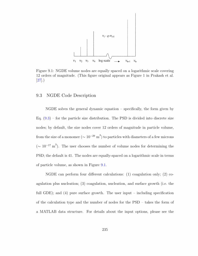
Figure 9.1: NGDE volume nodes are equally spaced on a logarithmic scale covering12 orders of magnitude. (This figure original appears as Figure 1 in Prakash et al.[27].)

9.3 NGDE Code Description

NGDE solves the general dynamic equation – specifically, the form given by

Eq. (9.3) – for the particle size distribution. The PSD is divided into discrete size

nodes; by default, the size nodes cover 12 orders of magnitude in particle volume,

from the size of a monomer (∼ 10−29 m3) to particles with diameters of a few microns

(∼ 10−17 m3). The user chooses the number of volume nodes for determining the

PSD; the default is 41. The nodes are equally-spaced on a logarithmic scale in terms

of particle volume, as shown in Figure 9.1.

NGDE can perform four different calculations: (1) coagulation only; (2) co-

agulation plus nucleation; (3) coagulation, nucleation, and surface growth (i.e. the

full GDE); and (4) pure surface growth. The user input – including specification

of the calculation type and the number of nodes for the PSD – takes the form of

a MATLAB data structure. For details about the input options, please see the

235

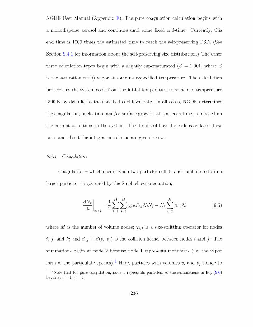
NGDE User Manual (Appendix F). The pure coagulation calculation begins with

a monodisperse aerosol and continues until some fixed end-time. Currently, this

end time is 1000 times the estimated time to reach the self-preserving PSD. (See

Section 9.4.1 for information about the self-preserving size distribution.) The other

three calculation types begin with a slightly supersaturated (S = 1.001, where S

is the saturation ratio) vapor at some user-specified temperature. The calculation

proceeds as the system cools from the initial temperature to some end temperature

(300 K by default) at the specified cooldown rate. In all cases, NGDE determines

the coagulation, nucleation, and/or surface growth rates at each time step based on

the current conditions in the system. The details of how the code calculates these

rates and about the integration scheme are given below.

9.3.1 Coagulation

Coagulation – which occurs when two particles collide and combine to form a

larger particle – is governed by the Smoluchowski equation,

dNk

dt

∣∣∣∣coag

=1

2

M∑i=2

M∑j=2

χijkβi,jNiNj −Nk

M∑i=2

βi,kNi (9.6)

where M is the number of volume nodes; χijk is a size-splitting operator for nodes

i, j, and k; and βi,j ≡ β(vi, vj) is the collision kernel between nodes i and j. The

summations begin at node 2 because node 1 represents monomers (i.e. the vapor

form of the particulate species).2 Here, particles with volumes vi and vj collide to

2Note that for pure coagulation, node 1 represents particles, so the summations in Eq. (9.6)begin at i = 1, j = 1.

236

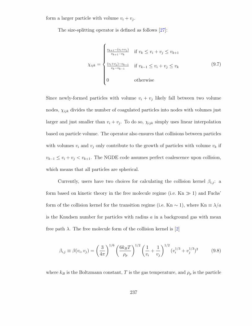
form a larger particle with volume vi + vj.

The size-splitting operator is defined as follows [27]:

χijk =

vk+1−(vi+vj)

vk+1−vkif vk ≤ vi + vj ≤ vk+1

(vi+vj)−vk−1

vk−vk−1if vk−1 ≤ vi + vj ≤ vk

0 otherwise

(9.7)

Since newly-formed particles with volume vi + vj likely fall between two volume

nodes, χijk divides the number of coagulated particles into nodes with volumes just

larger and just smaller than vi + vj. To do so, χijk simply uses linear interpolation

based on particle volume. The operator also ensures that collisions between particles

with volumes vi and vj only contribute to the growth of particles with volume vk if

vk−1 ≤ vi + vj < vk+1. The NGDE code assumes perfect coalescence upon collision,

which means that all particles are spherical.

Currently, users have two choices for calculating the collision kernel βi,j: a

form based on kinetic theory in the free molecule regime (i.e. Kn 1) and Fuchs’

form of the collision kernel for the transition regime (i.e. Kn ∼ 1), where Kn ≡ λ/a

is the Knudsen number for particles with radius a in a background gas with mean

free path λ. The free molecule form of the collision kernel is [2]

βi,j ≡ β(vi, vj) =

(3

4π

)1/6(6kBT

ρp

)1/2(1

vi+

1

vj

)1/2

(v1/3i + v

1/3j )2 (9.8)

where kB is the Boltzmann constant, T is the gas temperature, and ρp is the particle

237

density. Fuchs’ form [1] is given by [146]

βi,j = 2πDiDj(dpi + dpj)

[dpi + dpj

dpi + dpj + 2(g2i + g2

j )1/2

+8(Di +Dj)

(c2i + c2

j)1/2(dpi + dpj)

]−1

(9.9)

where

Kni =2λ

dpi(9.10a)

ci =

(8kBT

πmi

)1/2

(9.10b)

`i =8Di

πci(9.10c)

gi =1

3dpi`i[(dpi + `i)

3 − (d2pi + `2

i )3/2]− dpi (9.10d)

Di =kBT

3πµdpi

(5 + 4Kni + 6Kn2

i + 18Kn3i

5−Kni + (8 + π)Kn2i

)(9.10e)

and dpi, is the diameter, mi the mass, ci the mean thermal speed, and Di the

diffusion coefficient of particles with volume vi.

9.3.2 Nucleation

Nucleation occurs when a non-equilibrium, supersaturated vapor condenses

to return to equilibrium; condensation on existing particles is known as heteroge-

neous nucleation, while condensation to form new particles is called homogeneous

nucleation [2]. In the context of the NGDE code, nucleation strictly refers to ho-

mogeneous nucleation; condensation on existing particles falls under the purview of

surface growth, as discussed in the next subsection.

238

New particles form when monomers collide to form stable molecular clusters.

Clusters with fewer monomers than the critical cluster size k? are unstable and

quickly dissociate, while clusters consisting of k? monomers are stable and tend to

grow rapidly. The critical cluster size is a function of the vapor properties and the

thermodynamic conditions (e.g. saturation ratio, temperature, pressure) of the sys-

tem. There are a number of models for calculating the critical cluster size and the

nucleation rate; NGDE uses classical nucleation theory with the self-consistent cor-

rection (SCC) proposed by Girshick and Chiu [147]. For this model, the nucleation

rate Jk and critical cluster size k? are

Jk = n2sSv1

(2σ

πm1

)0.5

exp

(θ − 4θ3

27 ln2 S

)(9.11)

k? =

(2

3

θ

lnS

)3

(9.12)

This corresponds to a critical particle volume of

v? = k?v1 =π

6

(4σv1

kBT lnS

)3

(9.13)

In these equations, ns is the monomer concentration at saturation; σ is the sur-

face tension of the condensed species; θ = s1σ/kBT is the non-dimensional surface

tension; and s1, v1, and m1 are the surface area, volume. and mass of a monomer.

Since the critical volume v? is unlikely to be exactly equal to any of the volume

nodes, NGDE places nucleated particles in the node just larger than v? and adjusts

239

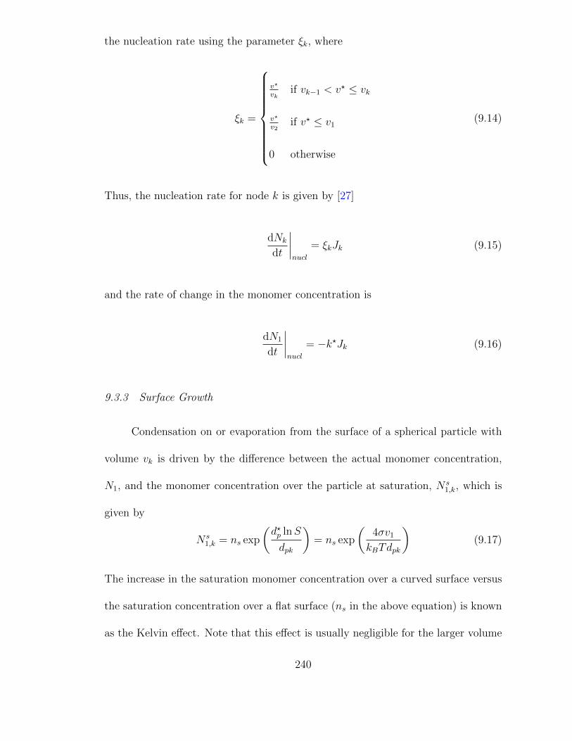
the nucleation rate using the parameter ξk, where

ξk =

v?

vkif vk−1 < v? ≤ vk

v?

v2if v? ≤ v1

0 otherwise

(9.14)

Thus, the nucleation rate for node k is given by [27]

dNk

dt

∣∣∣∣nucl

= ξkJk (9.15)

and the rate of change in the monomer concentration is

dN1

dt

∣∣∣∣nucl

= −k?Jk (9.16)

9.3.3 Surface Growth

Condensation on or evaporation from the surface of a spherical particle with

volume vk is driven by the difference between the actual monomer concentration,

N1, and the monomer concentration over the particle at saturation, N s1,k, which is

given by

N s1,k = ns exp

(d?p lnS

dpk

)= ns exp

(4σv1

kBTdpk

)(9.17)

The increase in the saturation monomer concentration over a curved surface versus

the saturation concentration over a flat surface (ns in the above equation) is known

as the Kelvin effect. Note that this effect is usually negligible for the larger volume

240

nodes used in NGDE, but it plays a major role in the behavior of smaller parti-

cles. Condensation and evaporation rates also depend upon the collision frequency

between monomers and particles.

Incorporating the above effects, the condensation/evaporation rate for node k

is

dNk

dt

∣∣∣∣growth

= α1 + α2 − α3 − α4 (9.18)

where

α1 =

v1

vk−vk−1β1,k−1(N1 −N s

1,k−1)Nk−1 if N1 > N s1,k−1

0 otherwise

(9.19a)

α2 =

− v1vk+1−vk

β1,k+1(N1 −N s1,k+1)Nk+1 if N1 < N s

1,k+1

0 otherwise

(9.19b)

α3 =

v1

vk+1−vkβ1,k(N1 −N s

1,k)Nk if N1 > N s1,k

0 otherwise

(9.19c)

α4 =

− v1vk−vk−1

β1,k(N1 −N s1,k)Nk if N1 < N s

1,k

0 otherwise

(9.19d)

Here, α1 and α2 represent an increase in Nk due to condensation on particles with

volume vk−1 and evaporation from particles with volume vk+1, respectively, while

α3 and α4 represent a decrease in Nk due to condensation on and evaporation from

241

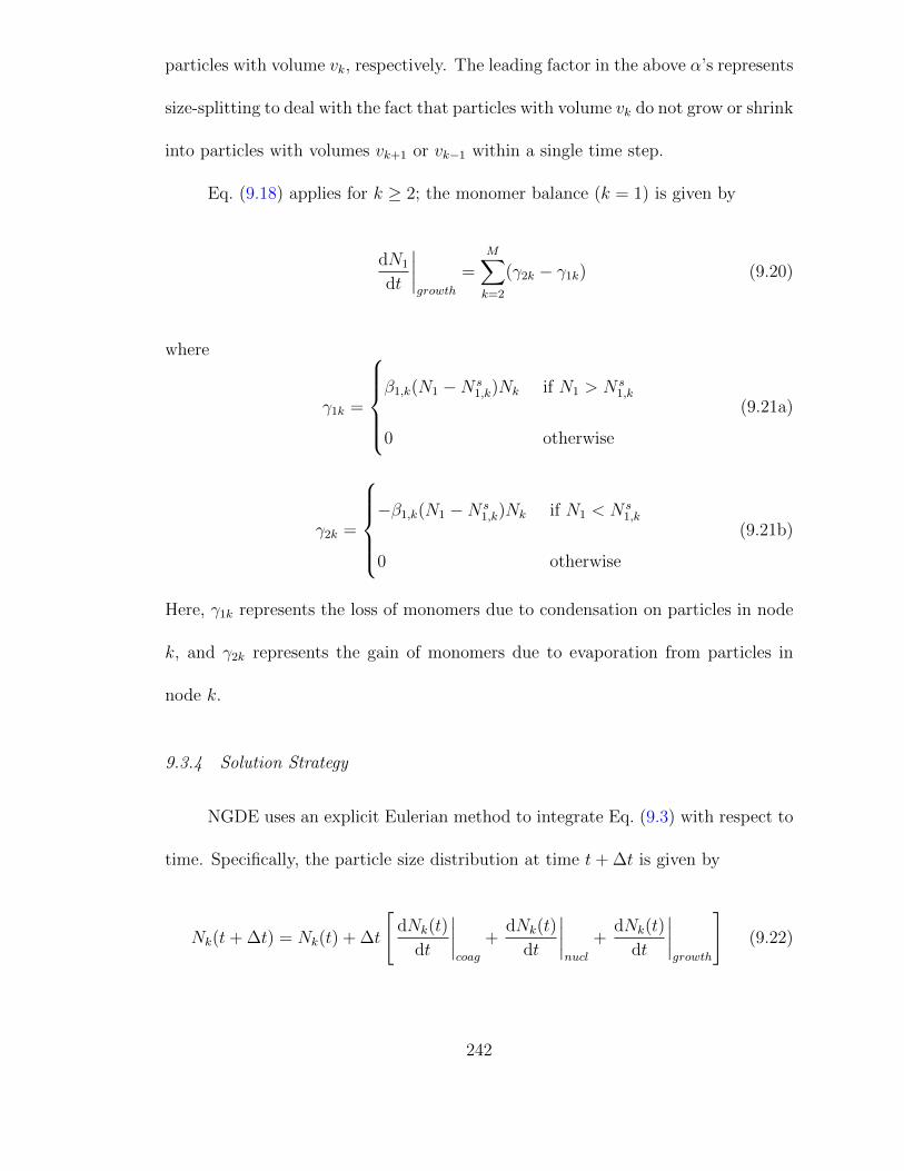
particles with volume vk, respectively. The leading factor in the above α’s represents

size-splitting to deal with the fact that particles with volume vk do not grow or shrink

into particles with volumes vk+1 or vk−1 within a single time step.

Eq. (9.18) applies for k ≥ 2; the monomer balance (k = 1) is given by

dN1

dt

∣∣∣∣growth

=M∑k=2

(γ2k − γ1k) (9.20)

where

γ1k =

β1,k(N1 −N s

1,k)Nk if N1 > N s1,k

0 otherwise

(9.21a)

γ2k =

−β1,k(N1 −N s

1,k)Nk if N1 < N s1,k

0 otherwise

(9.21b)

Here, γ1k represents the loss of monomers due to condensation on particles in node

k, and γ2k represents the gain of monomers due to evaporation from particles in

node k.

9.3.4 Solution Strategy

NGDE uses an explicit Eulerian method to integrate Eq. (9.3) with respect to

time. Specifically, the particle size distribution at time t+ ∆t is given by

Nk(t+ ∆t) = Nk(t) + ∆t

[dNk(t)

dt

∣∣∣∣coag

+dNk(t)

dt

∣∣∣∣nucl

+dNk(t)

dt

∣∣∣∣growth

](9.22)

242

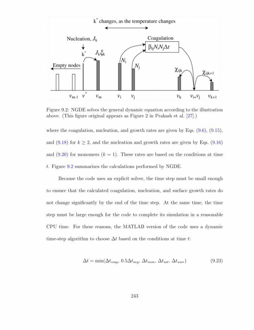
Figure 9.2: NGDE solves the general dynamic equation according to the illustrationabove. (This figure original appears as Figure 2 in Prakash et al. [27].)

where the coagulation, nucleation, and growth rates are given by Eqs. (9.6), (9.15),

and (9.18) for k ≥ 2, and the nucleation and growth rates are given by Eqs. (9.16)

and (9.20) for monomers (k = 1). These rates are based on the conditions at time

t. Figure 9.2 summarizes the calculations performed by NGDE.

Because the code uses an explicit solver, the time step must be small enough

to ensure that the calculated coagulation, nucleation, and surface growth rates do

not change significantly by the end of the time step. At the same time, the time

step must be large enough for the code to complete its simulation in a reasonable

CPU time. For these reasons, the MATLAB version of the code uses a dynamic

time-step algorithm to choose ∆t based on the conditions at time t:

∆t = min(∆tcoag, 0.5∆tneg, ∆tmon, ∆tsat, ∆tuser) (9.23)

243

The ∆t’s are defined as follows:

∆tcoag =0.001

βminNtot

(9.24a)

is 0.1% of the characteristic coagulation time, where βmin = min(βi,j) for i, j ≥ 2

and Ntot is the total number concentration of particles (excluding monomers);

∆tneg = mink

(∣∣∣∣ Nk

dNk/dt

∣∣∣∣) (9.24b)

is the minimum time at which the number concentration in any node would become

negative based on current coagulation, nucleation, and growth rates;

∆tmon =0.001N1

|dN1/dt|(9.24c)

is the time in which the monomer concentration changes by 0.1%;

∆tsat =

∣∣∣∣∣ 0.01SPsdTdtN1kB

(1− D

T

)∣∣∣∣∣ (9.24d)

is the time in which the saturation ratio changes by 1%, where Ps is the saturation

vapor pressure, dT/dt is the cooldown rate and D is a constant used to determine

the saturation vapor pressure; and

∆tuser = 10−4 (9.24e)

244

is a user-specified maximum time step. The time-step algorithm has a number of

hard-wired coefficients, including those used to specify the allowable fraction of the

characteristic coagulation time and the allowable changes in the number concentra-

tion of particles, the number concentration of monomers, and the saturation ratio.

The chosen values of these parameters reflect the desire to minimize the required

calculation time while ensuring the calculation results are reasonable.

9.4 Sample Results

Sample problems have been developed to test the NGDE code. Test problems

for pure coagulation and pure surface growth are used to validate the relevant models

in the code. Additional sample problems representing combined nucleation and

coagulation and the full GDE are presented to show that the code is producing

reasonable results. All of the sample problems are for aluminum in argon gas.

The sample problems are described in the following subsections.

9.4.1 Pure Coagulation

An interesting feature of coagulating systems is that after a sufficiently long

time, the non-dimensional aerosol size distribution ψ = φn(v, t)/N2tot becomes in-

dependent of time and of the initial conditions of the system [2, 148, 149]. This

time-independent PSD is known as the self-preserving distribution (SPD). Here, the

non-dimensional particle volume is η = Ntotv/φ, Ntot and φ are the total number

concentration and volume fraction of particles in the system, and n(v, t)dv is the

245

number concentration of particles with volume between v and v + dv at time t.

The first test problem for NGDE involves coagulation of an initially monodis-

perse aerosol with a particle diameter of 1 nm and number concentration of 1024 m−3

.

The calculation is performed at T = 1773 K for aluminum particles with density

ρp = 2700kg/m3. The calculated PSD should collapse to the self-preserving distri-

bution after time [149]

tSPD =τf

βfN0

(9.25)

where

βf =

(3

4π

)1/6(6kBT

ρp

)1/2

v1/60 (9.26)

is the free molecule coagulation coefficient for particles with volume v0, N0 and v0

are the initial number concentration and volume of particles in the aerosol, and τf

is a time constant for coagulation in the free molecule regime. Vemury et al. [149]

found τf ≈ 5 when the bins in their sectional code are spaced such that vk = 2vk−1.

Thus, the self-preserving distribution should be reached after tSPD = 30 ns for the

initial conditions of this problem.

To test the effects of NGDE node spacing on the results, the pure coagulation

calculation has been performed with 21, 41, and 101 nodes, corresponding to node

spacings of vk = 4.0vk−1, vk = 2.0vk−1, and vk = 1.3vk−1. For all cases, the non-

dimensional size distribution ψ becomes independent of time and is approximately

equal to the self-preserving distribution ψf as calculated by Vemury et al. [149].

The results are shown in Figure 9.3. For all three cases, the calculated size dis-

tribution reaches a constant distribution by approximately 30 ns, which is in good

246

Figure 9.3: Non-dimensional size distribution for the pure coagulation problem after1 µs, compared to the SPD for the free molecule regime, as determined by Vemuryet al. [149] using an accurate sectional method. The calculated size distributionreaches a self-preserving distribution by 30 ns and remains constant until the endof the calculation at 30 µs (i.e. 1000 times the estimated tSPD). Note that thedifference between the PSD calculated by NGDE and the self-preserving distributioncalculated by Vemury et al. [149] is due in part to ambiguities in defining a “binwidth” for a size distribution with “zero-width” nodes.

agreement with tSPD found by Vemury et al. [149].3 For the case with 101 nodes,

the distribution from NGDE is in excellent agreement with the SPD, but there are

noticeable differences between the distribution from NDGE with 21 and 41 nodes

and the SPD. These differences are due in part to ambiguity in defining a bin width

for calculating n: for a sectional code, the bin width is simply the difference between

the largest and smallest particle volume in each bin, but for a nodal code, the “bins”

are zero-width nodes. In Figure 9.3 and in the NGDEplot post-processing tool, the

bin widths are set to ∆vk = (vk+1 − vk−1)/2, i.e. “bin” k has upper bound at the

midpoint between nodes k and k + 1 and lower bound at the midpoint between

nodes k − 1 and k.

An additional way to evaluate the NGDE results is to compare the moments of

3This is based on the time at which the moments of the particle size distribution are approxi-mately equal to the steady-state values of the moments given in Table 9.1.

247

the calculated distribution to the moments of the self-preserving distribution. The

ith moment of the non-dimensional particle size distribution is defined as

Mi =

∫ ∞0

ηiφdη (9.27)

where i is any real number. Many of these moments are related to important proper-

ties of the aerosol size distribution: i = 0 represents the total number concentration

of particles; i = 1/3, 2/3, and 1 are proportional to the mean diameter, surface area,

and volume of particles in the system; and i = 2 is proportional to the intensity of

light scattered by the particles when they are much smaller than the wavelength of

incident light.

As shown in Table 9.1, the NGDE results with 101 nodes are in excellent

agreement with the SPD results, with differences of approximately 7% for the second

moment and less than 2% for all other moments. The NGDE results for 41 nodes

are in good agreement (less than 9% difference from the SPD) for all but the second

moment of the distribution (42% difference). These results suggest that using 41

nodes to represent 12 orders of magnitude in volume yields sufficiently accurate

results for pure coagulation.

9.4.2 Pure Surface Growth

The second test problem involves condensation of aluminum vapor on a mono-

disperse aerosol as the system cools from 1773 K to 300 K at 1000 K/s. Particles

are placed in node 25 out of 41, corresponding to a particle diameter of 79 nm. The

248

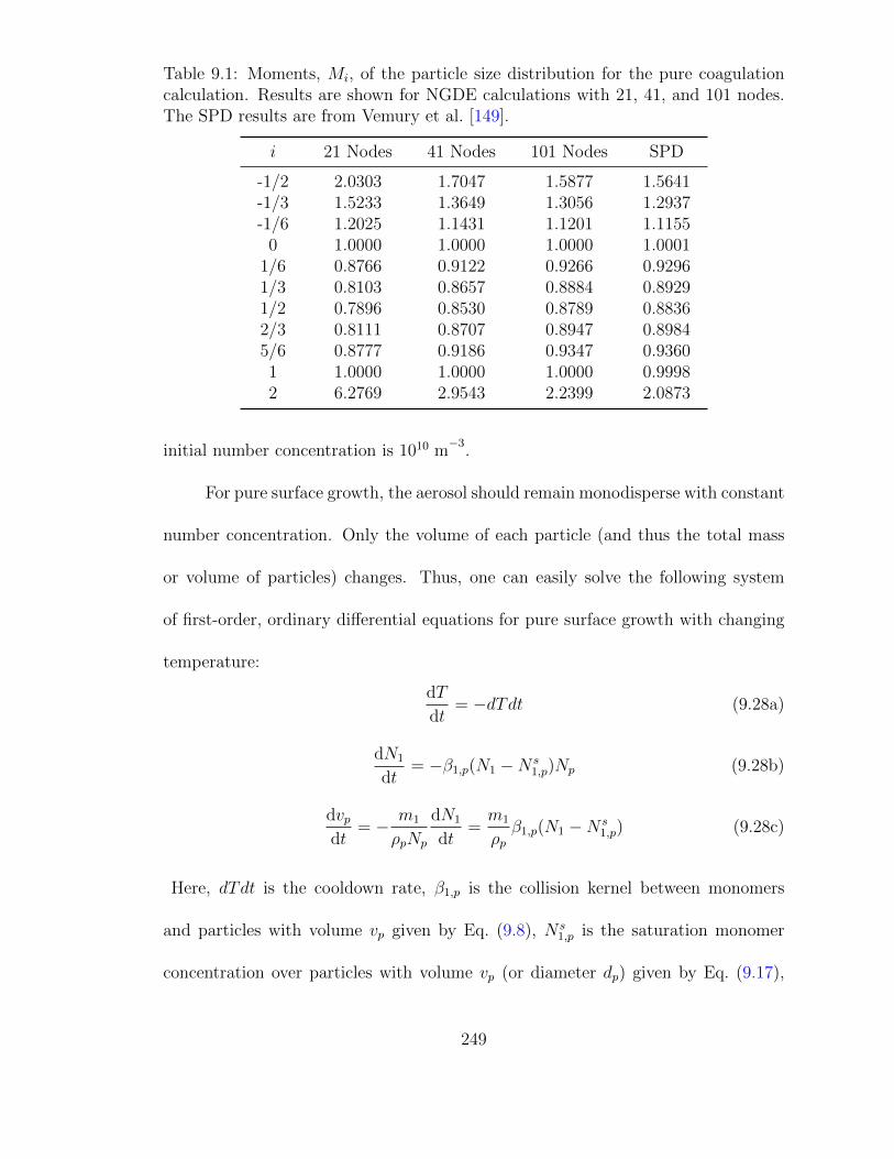
Table 9.1: Moments, Mi, of the particle size distribution for the pure coagulationcalculation. Results are shown for NGDE calculations with 21, 41, and 101 nodes.The SPD results are from Vemury et al. [149].

i 21 Nodes 41 Nodes 101 Nodes SPD

-1/2 2.0303 1.7047 1.5877 1.5641-1/3 1.5233 1.3649 1.3056 1.2937-1/6 1.2025 1.1431 1.1201 1.1155

0 1.0000 1.0000 1.0000 1.00011/6 0.8766 0.9122 0.9266 0.92961/3 0.8103 0.8657 0.8884 0.89291/2 0.7896 0.8530 0.8789 0.88362/3 0.8111 0.8707 0.8947 0.89845/6 0.8777 0.9186 0.9347 0.93601 1.0000 1.0000 1.0000 0.99982 6.2769 2.9543 2.2399 2.0873

initial number concentration is 1010 m−3

.

For pure surface growth, the aerosol should remain monodisperse with constant

number concentration. Only the volume of each particle (and thus the total mass

or volume of particles) changes. Thus, one can easily solve the following system

of first-order, ordinary differential equations for pure surface growth with changing

temperature:

dT

dt= −dTdt (9.28a)

dN1

dt= −β1,p(N1 −N s

1,p)Np (9.28b)

dvpdt

= − m1

ρpNp

dN1

dt=m1

ρpβ1,p(N1 −N s

1,p) (9.28c)

Here, dTdt is the cooldown rate, β1,p is the collision kernel between monomers

and particles with volume vp given by Eq. (9.8), N s1,p is the saturation monomer

concentration over particles with volume vp (or diameter dp) given by Eq. (9.17),

249

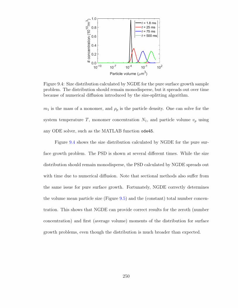
Figure 9.4: Size distribution calculated by NGDE for the pure surface growth sampleproblem. The distribution should remain monodisperse, but it spreads out over timebecause of numerical diffusion introduced by the size-splitting algorithm.

m1 is the mass of a monomer, and ρp is the particle density. One can solve for the

system temperature T , monomer concentration N1, and particle volume vp using

any ODE solver, such as the MATLAB function ode45.

Figure 9.4 shows the size distribution calculated by NGDE for the pure sur-

face growth problem. The PSD is shown at several different times. While the size

distribution should remain monodisperse, the PSD calculated by NGDE spreads out

with time due to numerical diffusion. Note that sectional methods also suffer from

the same issue for pure surface growth. Fortunately, NGDE correctly determines

the volume mean particle size (Figure 9.5) and the (constant) total number concen-

tration. This shows that NGDE can provide correct results for the zeroth (number

concentration) and first (average volume) moments of the distribution for surface

growth problems, even though the distribution is much broader than expected.

250

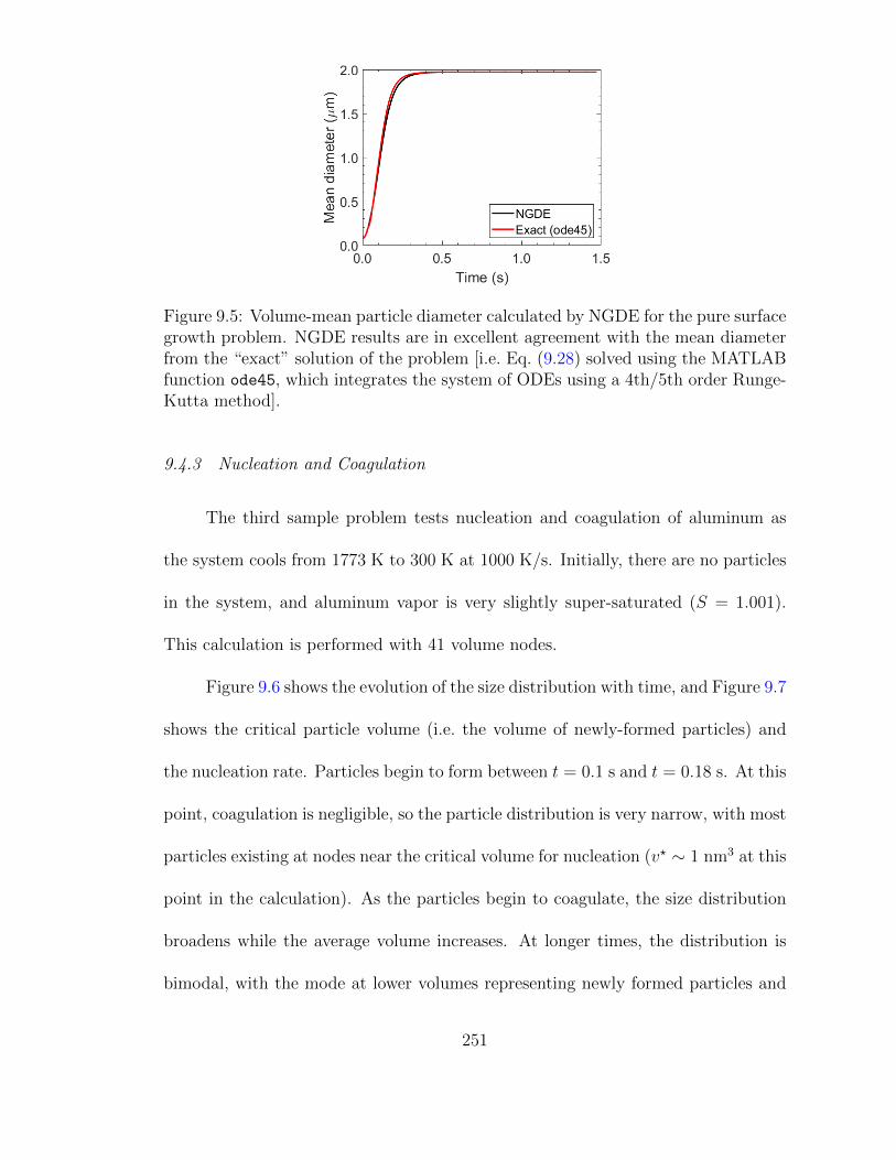
Figure 9.5: Volume-mean particle diameter calculated by NGDE for the pure surfacegrowth problem. NGDE results are in excellent agreement with the mean diameterfrom the “exact” solution of the problem [i.e. Eq. (9.28) solved using the MATLABfunction ode45, which integrates the system of ODEs using a 4th/5th order Runge-Kutta method].

9.4.3 Nucleation and Coagulation

The third sample problem tests nucleation and coagulation of aluminum as

the system cools from 1773 K to 300 K at 1000 K/s. Initially, there are no particles

in the system, and aluminum vapor is very slightly super-saturated (S = 1.001).

This calculation is performed with 41 volume nodes.

Figure 9.6 shows the evolution of the size distribution with time, and Figure 9.7

shows the critical particle volume (i.e. the volume of newly-formed particles) and

the nucleation rate. Particles begin to form between t = 0.1 s and t = 0.18 s. At this

point, coagulation is negligible, so the particle distribution is very narrow, with most

particles existing at nodes near the critical volume for nucleation (v? ∼ 1 nm3 at this

point in the calculation). As the particles begin to coagulate, the size distribution

broadens while the average volume increases. At longer times, the distribution is

bimodal, with the mode at lower volumes representing newly formed particles and

251

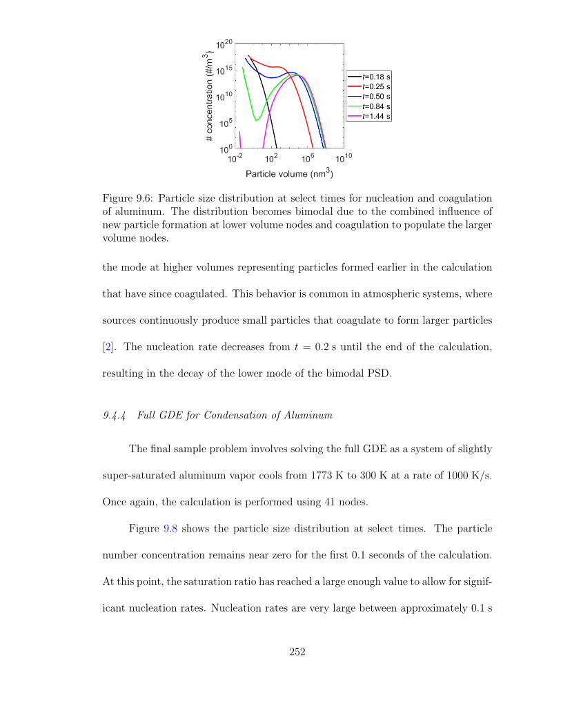
Figure 9.6: Particle size distribution at select times for nucleation and coagulationof aluminum. The distribution becomes bimodal due to the combined influence ofnew particle formation at lower volume nodes and coagulation to populate the largervolume nodes.

the mode at higher volumes representing particles formed earlier in the calculation

that have since coagulated. This behavior is common in atmospheric systems, where

sources continuously produce small particles that coagulate to form larger particles

[2]. The nucleation rate decreases from t = 0.2 s until the end of the calculation,

resulting in the decay of the lower mode of the bimodal PSD.

9.4.4 Full GDE for Condensation of Aluminum

The final sample problem involves solving the full GDE as a system of slightly

super-saturated aluminum vapor cools from 1773 K to 300 K at a rate of 1000 K/s.

Once again, the calculation is performed using 41 nodes.

Figure 9.8 shows the particle size distribution at select times. The particle

number concentration remains near zero for the first 0.1 seconds of the calculation.

At this point, the saturation ratio has reached a large enough value to allow for signif-

icant nucleation rates. Nucleation rates are very large between approximately 0.1 s

252

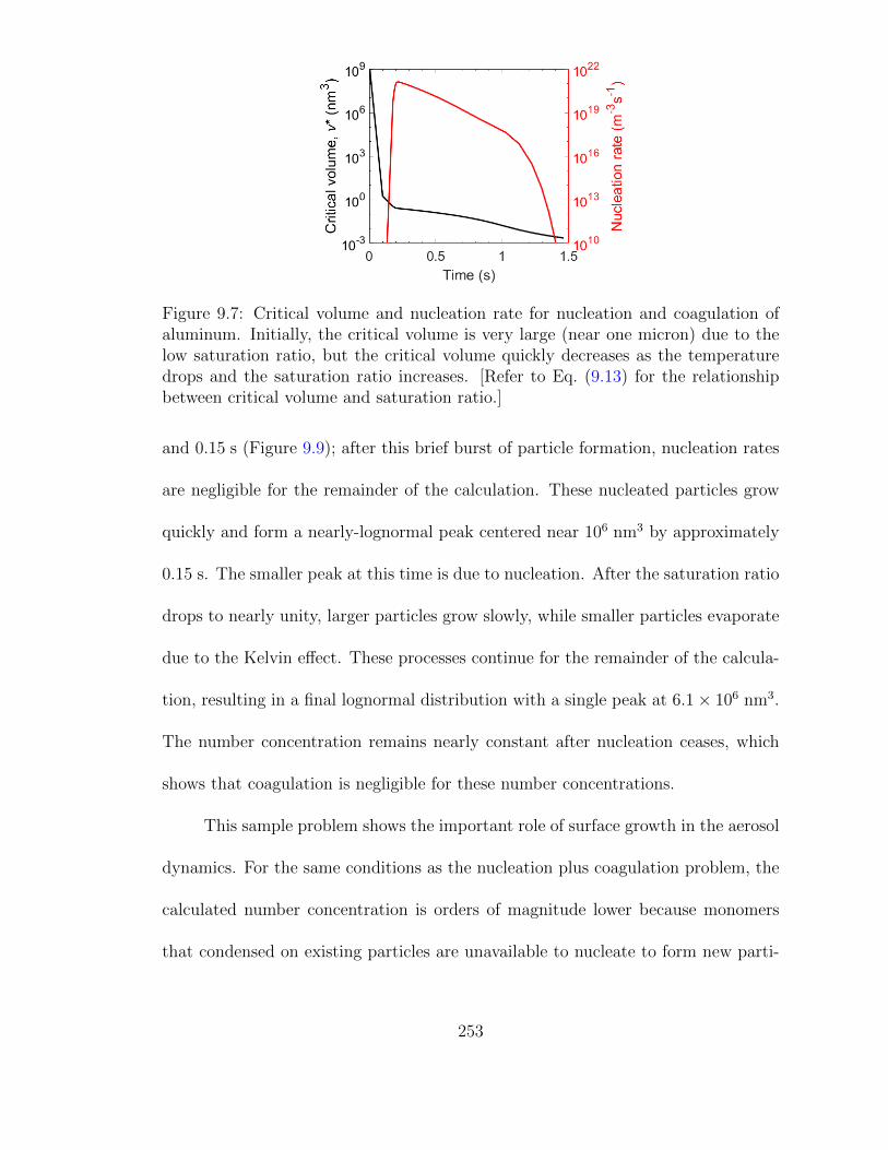
Figure 9.7: Critical volume and nucleation rate for nucleation and coagulation ofaluminum. Initially, the critical volume is very large (near one micron) due to thelow saturation ratio, but the critical volume quickly decreases as the temperaturedrops and the saturation ratio increases. [Refer to Eq. (9.13) for the relationshipbetween critical volume and saturation ratio.]

and 0.15 s (Figure 9.9); after this brief burst of particle formation, nucleation rates

are negligible for the remainder of the calculation. These nucleated particles grow

quickly and form a nearly-lognormal peak centered near 106 nm3 by approximately

0.15 s. The smaller peak at this time is due to nucleation. After the saturation ratio

drops to nearly unity, larger particles grow slowly, while smaller particles evaporate

due to the Kelvin effect. These processes continue for the remainder of the calcula-

tion, resulting in a final lognormal distribution with a single peak at 6.1× 106 nm3.

The number concentration remains nearly constant after nucleation ceases, which

shows that coagulation is negligible for these number concentrations.

This sample problem shows the important role of surface growth in the aerosol

dynamics. For the same conditions as the nucleation plus coagulation problem, the

calculated number concentration is orders of magnitude lower because monomers

that condensed on existing particles are unavailable to nucleate to form new parti-

253

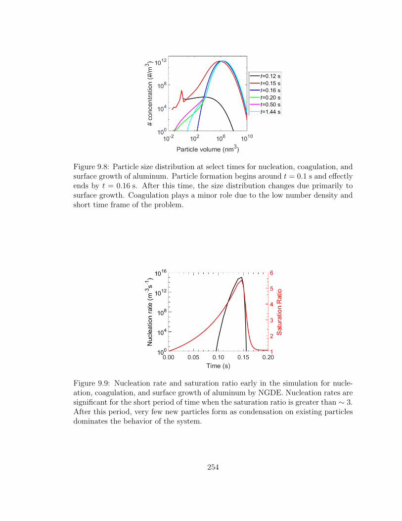
Figure 9.8: Particle size distribution at select times for nucleation, coagulation, andsurface growth of aluminum. Particle formation begins around t = 0.1 s and effectlyends by t = 0.16 s. After this time, the size distribution changes due primarily tosurface growth. Coagulation plays a minor role due to the low number density andshort time frame of the problem.

Figure 9.9: Nucleation rate and saturation ratio early in the simulation for nucle-ation, coagulation, and surface growth of aluminum by NGDE. Nucleation rates aresignificant for the short period of time when the saturation ratio is greater than ∼ 3.After this period, very few new particles form as condensation on existing particlesdominates the behavior of the system.

254

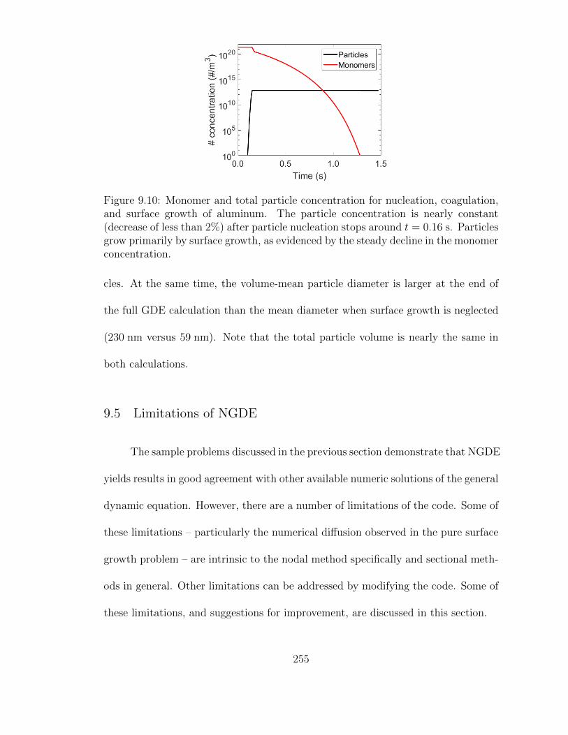
Figure 9.10: Monomer and total particle concentration for nucleation, coagulation,and surface growth of aluminum. The particle concentration is nearly constant(decrease of less than 2%) after particle nucleation stops around t = 0.16 s. Particlesgrow primarily by surface growth, as evidenced by the steady decline in the monomerconcentration.

cles. At the same time, the volume-mean particle diameter is larger at the end of

the full GDE calculation than the mean diameter when surface growth is neglected

(230 nm versus 59 nm). Note that the total particle volume is nearly the same in

both calculations.

9.5 Limitations of NGDE

The sample problems discussed in the previous section demonstrate that NGDE

yields results in good agreement with other available numeric solutions of the general

dynamic equation. However, there are a number of limitations of the code. Some of

these limitations – particularly the numerical diffusion observed in the pure surface

growth problem – are intrinsic to the nodal method specifically and sectional meth-

ods in general. Other limitations can be addressed by modifying the code. Some of

these limitations, and suggestions for improvement, are discussed in this section.

255

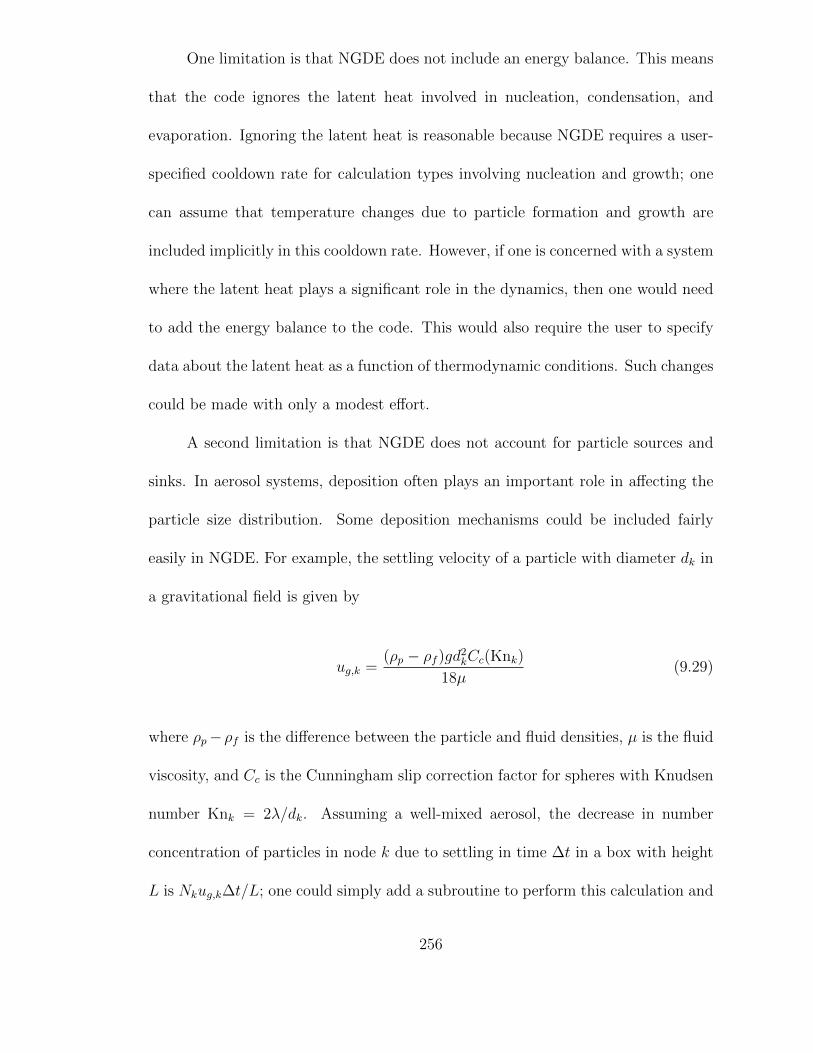
One limitation is that NGDE does not include an energy balance. This means

that the code ignores the latent heat involved in nucleation, condensation, and

evaporation. Ignoring the latent heat is reasonable because NGDE requires a user-

specified cooldown rate for calculation types involving nucleation and growth; one

can assume that temperature changes due to particle formation and growth are

included implicitly in this cooldown rate. However, if one is concerned with a system

where the latent heat plays a significant role in the dynamics, then one would need

to add the energy balance to the code. This would also require the user to specify

data about the latent heat as a function of thermodynamic conditions. Such changes

could be made with only a modest effort.

A second limitation is that NGDE does not account for particle sources and

sinks. In aerosol systems, deposition often plays an important role in affecting the

particle size distribution. Some deposition mechanisms could be included fairly

easily in NGDE. For example, the settling velocity of a particle with diameter dk in

a gravitational field is given by

ug,k =(ρp − ρf )gd2

kCc(Knk)

18µ(9.29)

where ρp−ρf is the difference between the particle and fluid densities, µ is the fluid

viscosity, and Cc is the Cunningham slip correction factor for spheres with Knudsen

number Knk = 2λ/dk. Assuming a well-mixed aerosol, the decrease in number

concentration of particles in node k due to settling in time ∆t in a box with height

L is Nkug,k∆t/L; one could simply add a subroutine to perform this calculation and

256

include it as a loss term in the particle mass balance. Similarly, one could add a

subroutine to add particles to a given volume node to represent an aerosol source

term.

Another limitation is that NGDE is written with specific situations in mind:

coagulation of an initially monodisperse aerosol; nucleation, coagulation, and sur-

face growth for an initially saturated system experiencing a constant decrease in

temperature; and surface growth on a monodisperse aerosol for a constant change

in temperature. It may be desirable to allow for some flexibility in the calculation

types, such as allowing the user to specify a polydisperse size distribution or non-

constant cooldown rate. Fortunately, many such changes would require only minor

changes to the code and code input. Even less effort is required to modify some of

the hard-wired parameters (e.g. initial saturation ratio, maximum allowable change

in saturation ratio in the dynamic time-step algorithm) in the code. For guidance

in changing the code, please refer to the NGDE User Manual (Appendix F).

9.6 NGDEplot

As part of the conversion of NGDE to MATLAB, a new post-processing tool

has been developed to display how certain parameters evolve with time. Currently,

NGDEplot can create movies showing the evolution of the particle size distribu-

tion (in various forms) and/or the scattering, absorption, and extinction coefficients

for the distribution. The user can save the frames for later playback using MAT-

LAB’s movie command. In addition, NGDEplot can display static plots showing

257

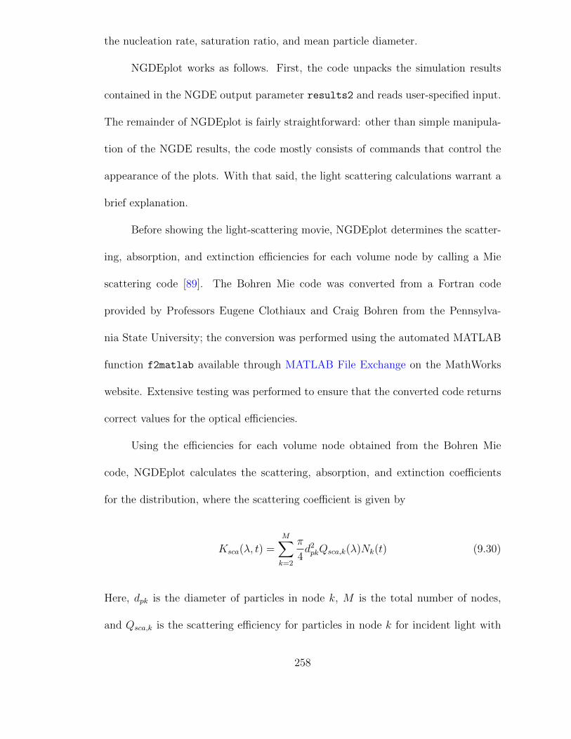
the nucleation rate, saturation ratio, and mean particle diameter.

NGDEplot works as follows. First, the code unpacks the simulation results

contained in the NGDE output parameter results2 and reads user-specified input.

The remainder of NGDEplot is fairly straightforward: other than simple manipula-

tion of the NGDE results, the code mostly consists of commands that control the

appearance of the plots. With that said, the light scattering calculations warrant a

brief explanation.

Before showing the light-scattering movie, NGDEplot determines the scatter-

ing, absorption, and extinction efficiencies for each volume node by calling a Mie

scattering code [89]. The Bohren Mie code was converted from a Fortran code

provided by Professors Eugene Clothiaux and Craig Bohren from the Pennsylva-

nia State University; the conversion was performed using the automated MATLAB

function f2matlab available through MATLAB File Exchange on the MathWorks

website. Extensive testing was performed to ensure that the converted code returns

correct values for the optical efficiencies.

Using the efficiencies for each volume node obtained from the Bohren Mie

code, NGDEplot calculates the scattering, absorption, and extinction coefficients

for the distribution, where the scattering coefficient is given by

Ksca(λ, t) =M∑k=2

π

4d2pkQsca,k(λ)Nk(t) (9.30)

Here, dpk is the diameter of particles in node k, M is the total number of nodes,

and Qsca,k is the scattering efficiency for particles in node k for incident light with

258

wavelength λ. The extinction coefficient is calculated by replacing Qsca in the above

equation with Qext, while the absorption coefficient is simply Kabs = Kext − Ksca.

(Note that the optical cross sections are also functions of the refractive index of

the particles.) The optical coefficients are calculated at each time t for a range

wavelengths that includes the visible spectrum, as well as portions of the ultraviolet

and infrared spectra. Note that the summation begins at k = 2 unless the NGDE

results are from a pure coagulation calculation, in which case the summation begins

at k = 1.

More information about running NGDEplot can be found in the NGDE User

Manual (Appendix F). Sample screenshots of the size distribution and light scatter-

ing movies are shown in Figures 9.11 and 9.12.

9.7 Conclusions

The NGDE code uses a nodal method to solve the general dynamic equation

for the evolution of an aerosol particle size distribution with time. The method is

similar to sectional methods, but the discrete nature of the nodes makes the resulting

code much simpler than sectional codes. Even with this simplified approach, the

NGDE code gives results in good agreement with available results obtained using

other methods. Because of its simplicity and accuracy, NGDE is well-suited to serve

as a teaching tool in college courses on aerosol physics and dynamics.

The MATLAB version of the code includes a new dynamic time-step algorithm

that decreases the code execution time by orders of magnitude. For example, the

259

Figure 9.11: Screenshot of the particle size distribution movie from NGDEplot. Thisstill is from the end of full GDE sample problem described in Section 9.4.4.

260

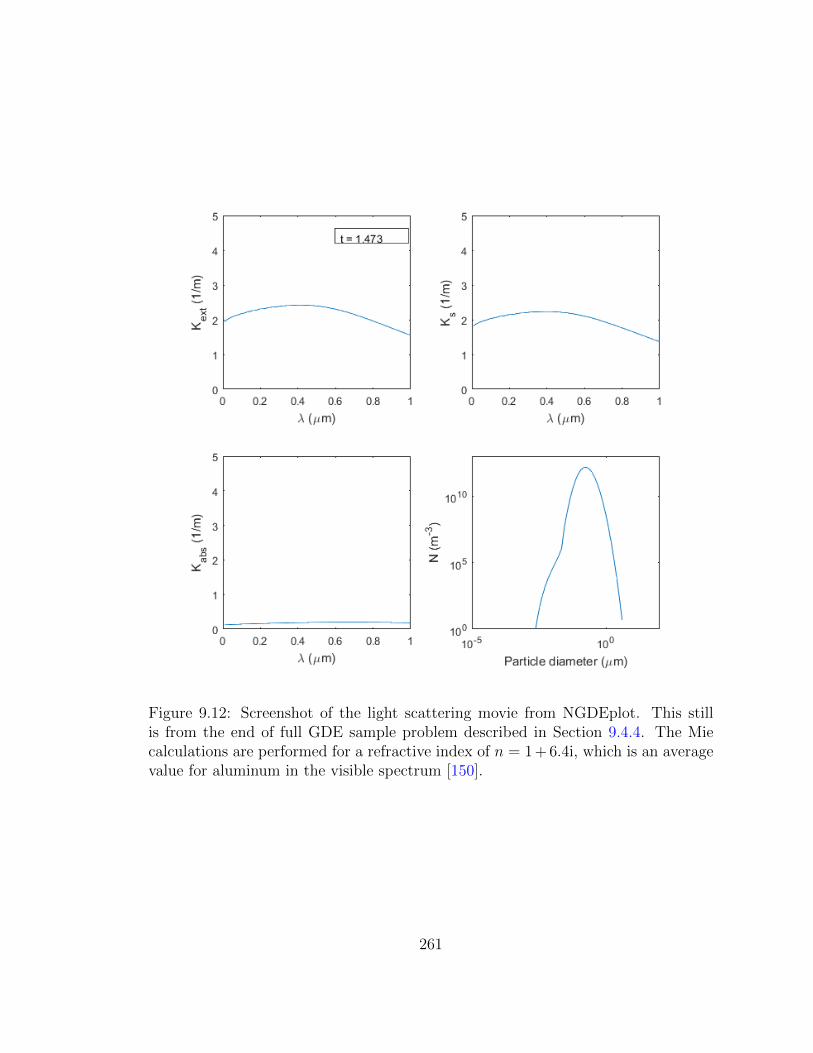
Figure 9.12: Screenshot of the light scattering movie from NGDEplot. This stillis from the end of full GDE sample problem described in Section 9.4.4. The Miecalculations are performed for a refractive index of n = 1 + 6.4i, which is an averagevalue for aluminum in the visible spectrum [150].

261

full GDE sample problem described in Section 9.4.4 takes approximately 10 minutes

to run with the dynamic time-step algorithm in MATLAB but more than a day to

run in the original C version of the code. Furthermore, the MATLAB version of

NGDE comes with post-processing tool NGDEplot that utilizes MATLAB’s built-

in plotting features to display results for the particle size distribution and the light

scattering, absorption, and extinction coefficients.

262

Chapter 10: Conclusions and Recommendations for Future Work

In this dissertation, I have described my method for determining the force and

torque on aggregates in the transition regime and discussed its use to study various

problems related to aerosol particle physics. Now, I will summarize the important

conclusions of my work and suggest areas for further study.

10.1 Conclusions

I have developed a method for calculating the translational, rotational, and

coupling friction tensors for aggregates consisting of spheres in point contact when

the primary sphere Knudsen number is in the transition regime (i.e. 0.01 < Kn <

100). My method addresses an important practical problem because a significant

fraction of terrestrial aerosols is generated as aggregates of very small primary

spheres [4, 7]. It synthesizes two previous approaches for computing the transport

properties of particles: the Kirkwood-Riseman method originally developed in the

late 1940s to determine the intrinsic viscosity and translational diffusion of polymers

[28], and the efforts of Loyalka and others to determine the velocity around a sphere

in rarefied flow [75–78]. Since that time, researchers have made significant improve-

ments to KR theory for describing hydrodynamic interactions between spheres in

263

the continuum [30, 51, 57, 58, 97]; however, no effort had been made to extend

this approach to the transition regime using the results of Loyalka. This gap in

the literature is likely due to the analytical and numerical complexities involved in

solving the Boltzmann transport equation for each primary sphere Knudsen number

of interest, even when the equation is posed in a simplified form like the Bhatnagar-

Gross-Krook equation [71]. My method plugs this gap and extends KR theory to

the transition regime in order to improve predictions of the transport behavior of

aerosol aggregates consisting of nano-scale primary spheres.

From the friction tensors determined using my method, one can obtain the

translational and rotational friction coefficients by averaging over all particle orienta-

tions; one can also obtain the diffusion tensors and coefficients through a generalized

Stokes-Einstein relation. Results for the translational friction coefficient compare

well to Direct Simulation Monte Carlo results and experimental data published

in the literature. The calculated translational friction coefficients also approach

the continuum and free molecule results from the Zeno algorithm and a Monte

Carlo algorithm in the limit of very small and very large primary sphere Knudsen

numbers, respectively. This suggests that the friction and diffusion coefficients ob-

tained using my method can be used in various relations describing aerosol transport

(e.g. to determine gravitational settling rates, electrical mobilities, or coagulation

rates for non-spherical particles), while the friction and diffusion tensors can be used

in aerosol dynamics simulations (e.g. for coagulation or Brownian motion).

Based on this success in calculating the friction tensors and coefficients, I

have applied the method to study a number of problems related to aerosol physics.

264

First, I looked at the effects of primary sphere size (characterized by the Knudsen

number) and the number of spheres (N) on the translational and rotational friction

coefficients of particles formed by diffusion-limited cluster aggregation. In both

cases, I found that the friction coefficients approach the continuum limit as the

Knudsen number decreases or as the number of spheres increases. For example,

DLCA aggregates consisting of 1000 spheres are in the continuum limit even when

the primary sphere Knudsen number is unity. This supports the general premise

of the Adjusted Sphere Method [41, 67], that one can determine the translational

friction coefficient of an aggregate using an aggregate Knudsen number based on its

hydrodynamic radius (i.e. a continuum measure of particle size) and its orientation-

averaged projected area (i.e. a free molecular measure of particle size). In response

to this finding, I showed that one can determine the rotational friction coefficient

using an aggregate Knudsen number for rotational motion that is proportional to

the ratio of continuum and free molecule rotational friction coefficients.

As part of this effort to determine the translational and rotational friction coef-

ficients, I showed that the ratio of translational to rotational characteristic diffusion

times is near unity for DLCA aggregates, regardless of primary sphere or aggregate

size. In other words, these particles rotate significantly during the average time

required to diffuse one radius of gyration. This finding is significant because most

aerosol studies ignore the effects of rotation on the particle dynamics. My results

suggest the effect of rotation on particle dynamics requires further study.

One major advantage of my method compared to the DSMC method is that

it is very fast: one can determine the friction tensors for aggregates with 100 pri-

265

mary spheres within seconds, while aggregates with 2000 spheres take minutes on a

single processor. (Compare this to DSMC, which takes days on a single processor

to determine the friction coefficient for a 20-sphere aggregate [41]). However, the

required computational time is still too excessive to incorporate this method in an

aerosol dynamics code. Therefore, I have used my results for the translational and

rotational friction coefficients of DLCA aggregates to develop an analytical expres-

sion that returns these coefficients as a function of the primary sphere radius, the

number of spheres in the aggregate, and the gas properties. My analytical expression

for the translational friction coefficient is more accurate than previous correlations

for DLCA aggregates [37–39] when compared to my EKR results. The rotational

friction coefficient expression appears to be the first of its kind published in the

literature. Researchers can use these expressions to quickly estimate the friction

coefficients for soot-like aggregates.

Next, I applied my EKR method to determine the orientation-averaged mo-

bility of a particle in an electric field. The mobility is a function of particle size and

field strength due to the interaction of the induced dipole in the particle with the

electric field. My orientation-averaged mobility results as a function of field strength

are in good agreement with experimental data published in the literature. In gen-

eral, for DLCA aggregates the mobility is less than 10% greater when the particle

is aligned with the field than when all orientations are equally probable (i.e. at very

low field strengths). Thus, one could in theory use the relationship between mobility

and field strength to obtain size information or to separate particles with similar

mobility at one field strength but different shapes (and hence different mobilities

266

from each other at a different field strength). However, my results suggest there are

several practical issues related to the experimental setup and to the accuracy of the

methods used to relate the data to size and shape information (such as my EKR

method). It is especially difficult to obtain shape information for either very large

or very small soot-like aggregates because it is difficult to operate a DMA at low

enough voltages to ensure that large aggregates have a fully random orientation,

and small aggregates require very high field strengths to align. In these limits, the

measured mobility at low and high field strengths would be nearly equal, which

would suggest – incorrectly – that these fractal aggregates are actually spherical.

Finally, I showed that one can use my method to determine the hydrodynamic

forces between spheres or aggregates in the transition regime, where the centers of

mass of the particles are separated by a distance r. This effort is a natural ex-

tension of the single-particle work discussed in the earlier chapters of my work: it

includes the interactions among the primary spheres in multiple aggregates as well

as within one aggregate. I have demonstrated that while the strength of interactions

between particles weakens as the primary sphere Knudsen number decreases, such

interactions follow the characteristic 1/r behavior observed for continuum particles.

From this result, I described how one can adopt the point force method for widely

separated particles in the continuum to particles in the transition regime; the only

difference is the leading coefficient that appears in the Oseen hydrodynamic inter-

action tensor. I have used this point force approach to show that a spherical cloud

of particles with non-negligible Knudsen numbers behaves just like a cloud in the

continuum, provided certain conditions (e.g. cloud radius, particle volume fraction)

267

are satisfied.

In addition to my work in calculating the transport behavior of aggregates, I

have made significant improvements to the NGDE code, which solves the general

dynamic equation for the change in the aerosol size distribution due to nucleation,

coagulation, and surface growth. In particular, I converted the code from C to

MATLAB to make use of MATLAB’s built-in plotting features, I added a dynamic

time-step algorithm to significantly reduce code execution time and improve code

stability, and I developed a post-processing tool to generate movies showing the

evolution of the size distribution and the optical properties of the aerosol. These

improvements will enhance the code’s intended use in teaching students about the

effects of nucleation, coagulation, and surface growth on aerosol dynamics.

10.2 Recommendations for Future Work

10.2.1 Friction Coefficient Expressions for non-DLCA Aggregates

Much of my work has focused on DLCA aggregates because such particles

are found in many areas of interest to the aerosol science. However, it is possible

to form particles with other fractal dimensions. (See, for example, Figure 8.3 of

Friedlander [2].) One could use my EKR method to determine the functional rela-

tionship between the primary sphere size and number of spheres in the aggregate

and its translational and rotational friction coefficients in order to develop analytic

expressions similar to my expressions for DLCA aggregates [Eqs. (4.38) and (6.26)].

One could include these expressions in an aerosol dynamics code to account for the

268

transport behavior of aggregates as a function of the primary sphere size, number

of primary spheres, and fractal dimension.

Similarly, one could compare the properties of aggregates generated with the

Mackowski algorithm – which I have used to create the particles used in this study

– with those generated by direct numerical simulation of the aggregate trajecto-

ries. This is of interest to determine how well the properties of particles generated

by a simplified algorithm match the properties of particles from a more realistic,

Langevin-style simulation (as described below).

10.2.2 Aggregates with Polydisperse Primary Spheres

All of my calculations involve aggregates that consist of equally-sized primary

spheres. This is an idealized situation; in reality, aggregates typically consist of

primary spheres with some distribution of radii. Bernal et al. [51] have demonstrated

how one can account for polydispersity in the continuum, and Spyrogianni et al.

[151] have applied the method to determine the effect of polydispersity on aggregate

settling rates. Now, I will describe how to address this issue in the transition regime.

To account for polydispersity, we must make a slight change to my extended

Kirkwood-Riseman method. In the continuum, the force on the ith sphere with

radius ai moving with velocity ui is given by

Fi = −ζct,0(ai)ui − ζct,0(ai)N∑i 6=j

Tij(ai, aj, rij) ·Fj (10.1)

where aj is the radius of the jth sphere and the hydrodynamic interaction tensor is a

269

function of ai, aj, and the distance between the spheres. My EKR method replaces

the hydrodynamic interaction tensor with the quotient of the velocity tensor and

the monomer friction coefficient for sphere j. Thus, to account for polydisperse

primaries, my EKR method becomes

Fi = −ζt,0(Kni)ui − ζt,0(Kni)N∑i 6=j

ζ−1t,0 (Knj)Vij(Knj, rij) ·Fj (10.2)

The only difference between this expression and the expression for monodisperse

primaries is the appearance of the friction coefficient ratio ζt,0(Kni)/ζt,0(Knj) for

primary spheres with Knudsen numbers of Kni ≡ λ/ai and Knj ≡ λ/aj. For mono-

disperse primaries (Kni = Knj ≡ Kn), the ratio cancels, leaving the expression that

has appeared throughout the earlier chapters of this disseration,

Fi = −ζt,0(Kn)ui −N∑i 6=j

Vij(Kn) ·Fj

There are a number of practical challenges that must be addressed in order

to determine the friction coefficient of aggregates with polydisperse primaries. The

first challenge is to generate the coordinates for the spheres in the aggregates. The

Mackowski algorithm I have been using creates aggregates with unit primary sphere

size. One would need to modify the algorithm to account for polydisperse primaries.

One could do so by sampling the primary sphere sizes from a specified distribution

(such as a lognormal distribution a geometric standard deviation σg = 1.2, in agree-

ment with experiments of soot formation in premixed diffusion flames Koylu and

270

Faeth [42]). Alternatively, one could obtain particles from a dynamic simulation of

particle aggregation [151].

Also, one would need to make significant modifications to my MATLAB pro-

gram for calculating the friction tensors (bgk tensors; see Appendix G) to account

for polydispersity. Currently, my program loads the velocity and monomer friction

coefficient results obtained by solving the BGK equation. These results are stored

in individual MATLAB data files indexed by the non-dimensional monomer radius

r0 [defined by Eq. (2.5d)]. To account for polydisperse primaries, one would need to

access multiple data files, each one associated with the Knudsen number of one of

the monomers in the aggregate. This would require there to be a file of BGK results

for each primary sphere Knudsen number. Alternatively, one could compile all of

the BGK results in a table and interpolate based on the primary sphere Knudsen

number and the distance between spheres. Likewise, one would need to interpolate

to determine the coefficients c1 and c2 [see Eq. (2.59)] for the velocity far from the

sphere. Such changes would not be difficult to implement.

With that said, it is unlikely that accounting for polydispersity would have

a significant impact on aggregate transport properties. For example, Spyrogianni

et al. [151] found that aggregates in the continuum with polydisperse primaries

settle faster than aggregates with monodisperse aggregates with equal mean primary

diameters, but only because the polydisperse aggregates have greater mass than the

monodisperse aggregates. In other words, the settling velocity of aggregates in the

continuum is unaffected by monomer polydispersity, once one corrects for differences

in particle mass. Nevertheless, this does not guarantee that the same behavior would

271

be observed in the transition regime, especially if there is a broad distribution of

primary sizes. (See, for example, the particles described in Ref. [152].) One could

test whether or not this is the case using my EKR method, with Eq. (10.2) to

account for polydispersity.

10.2.3 Rotational and Coupling Interactions

My EKR method ignores rotational and coupling hydrodynamic interactions

between spheres in an aggregate. Such interactions are weaker than the translational

interactions included in my method, so one can safely neglect these effects when

the average distance between spheres in the aggregate increases. However, when

the average distance between spheres is small, rotational and coupling interactions

become significant, and the error in the rotational friction coefficient calculated

using the EKR method can be large (up to 40% for the cases I have studied).

Expressions for the rotational and coupling hydrodynamic interaction tensors

in the continuum are available in the literature, as summarized by Carrasco and

Garcıa de la Torre [53]. I have shown that to order r−3ij , the rotational and coupling

hydrodynamic interaction tensors are related to the vorticity and velocity fields

around a rotating sphere. (See Appendix D.) This suggests that one could obtain

the rotational and coupling interaction tensors as a function of Knudsen number by

solving the BGK equation for the flow field around a rotating sphere. Loyalka [77]

has already performed this calculation; unfortunately, the paper does not provide

detailed results for the velocity around the rotating sphere, nor does it go into much

detail about the solution procedure. Still, the problem is not significantly different

272

from the translating sphere problem; the main difference is in the far-field velocity

distribution function, where instead of a uniform translational velocity U there is a

position-specific velocity ω×r. The rotational problem is slightly more complicated

due to this difference, but in principal one can use the same approach developed by

Lea [74] that I have described in Chapter 2.

After obtaining the velocity and vorticity fields around a rotating sphere – and

thus the coupling and rotational hydrodynamic interaction tensors as a function of

Knudsen number – the next step would be to incorporate these tensors in the EKR

method. The approach is analogous to the method described by Carrasco and Garcıa

de la Torre [53] for calculating the force and torque on a particle in the continuum;

the only difference is that one replaces the continuum translational, rotational, and

coupling interaction tensors with the velocity field around a translating sphere, the

vorticity field around a rotating sphere, and the velocity field around a rotating

sphere obtained by solving the BGK equation as a function of Knudsen number.

This effort should significantly improve the accuracy of the calculated rotational

friction coefficient, especially for small aggregates near the continuum regime.

10.2.4 Brownian Dynamics

The final suggested extension of my research is to incorporate my EKR method

into Brownian dynamics simulations to study the effects of particle rotation and

hydrodynamic interactions on various parameters of interest to the aerosol scien-

tist (e.g. coagulation rates, sedimentation rates, the size and shape of coagulated

aerosols). This would involve solving the Langevin equations for each particle in an

273

N -particle system. The Langevin equations for particle i describe its translational

and rotational velocities (ui and ωi) and position in space-fixed coordinates and

orientation in particle-fixed coordinates (xi and (φi, ωi, ψi)):

dmiuidt

= −Ξt,i ·ui −Ξ†c,i ·ωi +N∑j=1

FH,ij + FE,i + FB,i (10.3)

Ii ·dωidt

+ ωi × (Ii ·ωi) = −Ξc,i ·ui −Ξr,i ·ωi +N∑j=1

TH,ij + TE,i + TB,i (10.4)

dxidt

= ui (10.5)

dε1idt

dε2idt

dε3idt

dηidt

=

1

2

ηiωx′,i − ε3iωy′,i + ε2iωz′,i

ε3iωx′,i + ηiωy′,i − ε1iωz′,i

−ε2iωx′,i + ε1iωy′,i + ηiωz′,i

−ε1iωx′,i − ε2iωy′,i − ε3iωz′,i

(10.6)

In these equations, mi is the mass, Ii is moment of inertia tensor, FE,i and TE,i

are the external forces and torques (e.g. from an electric field), and FB,i and TB,i

are fluctuating Brownian forces and torques on particle i, while FH,ij and TH,ij

are the hydrodynamic force and torque on particle i due to particle j. Note that

the rotational velocity and orientation are written in terms of the particle-fixed

axes (x′i, y′i, z′i), which are related to the co-moving axes (i.e. the axes parallel to the

space-fixed axes that translate with the particle) by the Euler angles (φi, θi, ψi). The

friction tensors represent the friction on the particle when it is alone in an infinite

fluid (i.e. ignoring the effects of the other particles) and are written in terms of the

274

co-moving axes. Eq. (10.6) is written in terms of the Euler quaternion (ε1i, ε2i, ε3i, ηi),

which is related to the Euler angles. (See Ref. [153].) Note that in principal one

must consider the effects of all of the particles when determining the fluctuating

Brownian force and torque on particle i [136].

Previous studies of Brownian dynamics are restricted to the continuum or free

molecule limits [121, 127, 154, 155]. Many of these studies use simplified meth-

ods to calculation the aggregate friction coefficient, though Fernandes and Garcıa

de la Torre [127] apply methods based on Kirkwood-Riseman theory to determine

the translational friction tensor Ξt. Furthermore, the rotational dynamics are of-

ten neglected for fractal aggregates [121, 127, 154, 155], though they have been

considered in studies of simple shapes shapes such as ellipsoids [153, 156]. Hydro-

dynamic interactions are included in Stokesian dynamics simulations for particles in

the continuum [135, 136] but are typically excluded for non-continuum particles.

Eqs. (10.3)–(10.6) can be solved for a system of particles to determine the

effects of the rotation and/or hydrodynamic interactions on the dynamic behavior

of the system. To do so, one would have to repeat the simulation multiple times,

average the results, and compare various figures of merit (e.g. coagulation rates,

sedimentation rates, particle size and fractal dimension) to the same parameters for

simulations of the same system that neglect rotational and hydrodynamic effects.

During the calculation, one would need to perform the EKR calculation at each

time step to determine the friction tensors, hydrodynamic forces and torques, and

probability distribution for the Brownian forces and torques for each particle.

One could also perform a Brownian simulation for a single aggregate in an

275

external field; in this case, one need only perform the EKR calculation for the

friction tensors of the particle at the start of the simulation. Calculations could be

performed for a range of external field strengths. Results of Brownian trajectories

for zero field strength can be used to evaluate the results for the translational and

rotational diffusion coefficients computed using rigid body hydrodynamic theory

(i.e. the results described in Chapters 3–6). Brownian dynamics results for non-zero

field strength could be used to determine the electrical mobility of a particle and

can be compared to the results of the particle alignment calculations described in

Chapter 7.

Ultimately, these Brownian simulations can be used to evaluate the validity of

various assumptions (e.g. treating aggregates as equivalent spheres, ignoring rotation

effects, neglecting hydrodynamic interactions) typically made in studies of cluster

aggregation kinetics and other dynamic aerosol processes.

Clearly, this suggested project would be a substantial undertaking, both in set-

ting up the problem (i.e. writing the code to solve the Langevin equations above) and

in ensemble-averaging and interpreting the results. Additionally, one needs access

to powerful computing resources to tackle this problem, given the large number of

simulations that would be required to account for the statistical fluctuations inher-

ent in solving the problem and the computational time required to perform a single

Brownian trajectory. Given these issues, as well as the likelihood that rotational

and hydrodynamic effects may only have minor effects on the dynamic behavior of

aerosol systems, it is hardly surprising that this problem has received little atten-

tion in the literature. Nevertheless, my method for calculating the friction tensors of

276

aerosol aggregates in the transition regime provides one of the missing pieces needed

to tackle this difficult problem.

277

Appendix A: Derivation of Expressions in Chapter 2

In this Appendix, I present derivations for several expressions that appear in

the solution of the BGK equation for flow around a sphere, as presented in Chapter 2.

A.1 Derivation of the Expression for g [Eq. (2.42)]

In this section, I will present the derivation of the constant g in Eq. (2.42) for

flow around a sphere. This derivation follows Appendix D of Lea [74], but I have

included more of the intermediate steps for clarity. I have also included information

from Law and Loyalka [76] because that study accounts for non-isothermal condi-

tions around the sphere. For this derivation, I will refer to the angles defined in

Fig. 2.4.

We start by writing the velocity perturbation vector in terms of coordinates

(x′, y′, z′):

ε2(r) =√

2 ρ3 sinα′ ex′ +√

2 ρ2 cosα′ ez′ (A.1)

Note that the z′-direction is simply er; the y′ direction is chosen to be perpendicular

to the plane containing U∞ and ez′ ; and the x′ direction is of course mutually

278

orthogonal to the y′- and z′-directions:

ez′ = er, ey′ =ez′ × eU

sinα′, ex′ = ey′ × ez′ (A.2)

We must now write out the local coordinates (x′, y′, z′), in terms of coordinates

(x, y, z). First, we write ez′ in terms of (x, y, z):

ez′ = sin θ′ cosφ′ ex + sin θ′ sinφ′ ey + cos θ′ ez (A.3)

Next, we write eU in terms of (x, y, z):

eU = sinα ex + cosα ez (A.4)

Next, we evaluate the cross product to determine ey′ :

ey′ =1

sinα′[

sin θ′ sinφ′ cosα ex

+ (sinα′ cos θ′ − sin θ′ cosφ′ cosα) ey − sin θ′ sinφ′ sinα ez

](A.5)

Finally, we evaluate the cross product to determine ex′ :

ex′ =1

sinα′[ (

sinα cos2 θ′ − cosα sin θ′ cos θ′ cosφ′ + sinα sin2 θ′ sin2 φ′)ex

−(cosα sin θ′ cos θ′ sinφ′ + sinα sin2 θ′ sinφ′ cosφ′

)ey

+(cosα sin2 θ′ − sinα sin θ′ cos θ′ cosφ′

)ez

](A.6)

279

Now that we have defined the coordinates (x′, y′, z′) in terms of coordinates

(x, y, z), we can write our velocity perturbation vector in terms of coordinates

(x, y, z):

ε2(r) =√

2[ρ2 cosα′ sin θ′ cosφ′ + ρ3

(sinα cos2 θ′ − cosα sin θ′ cos θ′ cosφ′

+ sinα sin2 θ′ sin2 φ′)]

ex +[ρ2 cosα′ sin θ′ sinφ′

− ρ3

(cosα sin θ′ cos θ′ sinφ′ + sinα sin2 θ′ sinφ′ cosφ′

)]ey

+[ρ2 cosα′ cos θ′ + ρ3

(cosα sin2 θ′ − sinα sin θ′ cos θ′ cosφ′

)]ez

(A.7)

We can now consider our equation for the source term, Eq. (2.33):

A(r0) =−√πU cosα

− 2

π

∫V

dr

|r − r0|2

[T2 ε1(r) + T3 Ω · ε2(r) +

(T4−

3

2T2

)ε3(r)

](Ω · n)

Here, we have simply written out the triple integral in terms of Cartesian coordi-

nates. Again, the argument of the Tn functions is |r−r0|. Before proceeding further,

we will introduce a new coordinate system, (r, t, φ′), where r is the distance from

the origin to point r, t = |r − r0|, and φ′ is the angle of rotation about the z-axis,

with φ′ = 0 corresponding to the positive x-axis. These coordinates are related to

the (x, y, z) coordinates by the following expressions:

x = r sin θ′ cosφ′ (A.8a)

280

y = r sin θ′ sinφ′ (A.8b)

z = r cos θ′ (A.8c)

where the angles θ and θ′ are

cos θ′ =r2 + r2

0 − t2

2r0r(A.9a)

cos θ =t2 + r2

0 − r2

2r0t(A.9b)

r sin θ′ = t sin θ =

√(2rr0)2 − (r2 + r2

0 − t2)2

2r0

(A.9c)

Note that θ and θ′ are independent of φ′.

The Jacobian determinant of coordinates (r, t, φ′) is tr/r0. In these coordi-

nates, our equation for A(r0) becomes

A(r0) = −√πU cosα− 2

π

∫ ∞r0

drr

r0

∫ √r2−r20

r−r0

dt

t

∫ 2π

0

dφ′[

T2(t)ε1(r)

+ T3(t)Ω · ε2(r) +

(T4(t)− 3

2T2(r)

)ε3(r)

](cos θ)

Here, θ is the angle between n and Ω, ε2 is given by Eq. (A.7), and

Ω =r0 − r|r0 − r|

= − sin θ cosφ′ex − sin θ sinφ′ey + cos θez

We can integrate over φ′ analytically. We start with the term involving ε1(r).

We use Eq. (2.48a) to write the density perturbation in terms of its radial and

281

angular components, write cosα′ in terms of the angles (α, θ′, φ′), and integrate over

φ′:

∫ 2π

0

dφ′ T2(t)ε1(r) = T2(t)ρ1(r)

∫ 2π

0

dφ′ cosα′

= T2(t)ρ1(r)

∫ 2π

0

dφ′ [cosα cos θ′ + sinα sin θ′ cosφ′]

=2πT2(t)ρ1(r) cosα cos θ′

We get a very similar result for ε3, with ρ1 replaced by ρ4 and the appropriate Tn

functions.

For the term involving ε2(r), we must first evaluate the dot product Ω · ε2(r):

Ω · ε2(r) =√

2[ρ2 cosα′(cos θ cos θ′ − sin θ sin θ′ cos2 φ′ − sin θ sin θ′ sin2 φ′)

+ ρ3(cosα sin θ sin θ′ cos θ′ cos2 φ′ − sinα sin θ cos2 θ′ cosφ′

− sinα sin θ sin2 θ′ sin2 φ′ cosφ′ + cosα sin θ sin θ′ cos θ′ sin2 φ′

+ sinα sin θ sin2 θ′ sin2 φ′ cosφ′ + cosα cos θ sin2 θ′

− sinα cos θ sin θ′ cos θ′ cosφ′)]

=√

2[ρ2(cos θ cos θ′ − sin θ sin θ′)(cosα cos θ′ + sinα sin θ′ cosφ′)

+ ρ3(cosα sin θ sin θ′ cos θ′ − sinα sin θ cos2 θ′ cosφ′

+ cosα cos θ sin2 θ′ − sinα cos θ sin θ′ cos θ′ cosφ′)]

282

When we separate the terms involving sinα from those involving cosα,

Ω · ε2(r) =√

2 cosα[ρ2(cos θ cos2 θ′ − sin θ sin θ′ cos θ′)

+ ρ3(sin θ sin θ′ cos θ′ + cos θ sin2 θ′)]

+√

2 sinα[ρ2(cos θ sin θ′ cos θ′ cosφ′ − sin θ sin2 θ′ cosφ′)

− ρ3(sin θ cos2 θ′ cosφ′ + cos θ sin θ′ cos θ′ cosφ′)]

we can see that the term involving sinα are odd functions of φ′. This means that

these terms will disappear when we integrate over φ′. On the other hand, the term

involving cosα does not depend on φ′, so the integral is simply the cosα term

multiplied by 2π:

∫ 2π

0

dφ′ T3(t)Ω · ε2(r) = 2√

2πT3(t)[ρ2(cos θ cos2 θ′ − sin θ sin θ′ cos θ′)

+ ρ3(sin θ sin θ′ cos θ′ + cos θ sin2 θ′)]

Thus, we can write the function A(r0) as

A(r0) = gU cosα (A.10)

where the constant g is defined by

g = −π1/2 + 2

∫ ∞r0

drr

r0

[q(r) ·a(r)]

283

a1(r) =− 2

∫ √r2−r20

r−r0

dt

tT2(t) cos θ cos θ′

a2(r) =− 2√

2

∫ √r2−r20

r−r0

dt

tT3(t) cos θ(cos θ cos2 θ′ − sin θ sin θ′ cos θ′)

a3(r) =− 2√

2

∫ √r2−r20

r−r0

dt

tT3(t) cos θ(sin θ sin θ′ cos θ′ + cos θ sin2 θ′)

a4(r) =− 2

(2

3

)1/2 ∫ √r2−r20

r−r0

dt

t

(T4(t)− 3

2T2(t)

)cos θ cos θ′

Finally, we plug in our expressions for cos θ, cos θ′, sin θ, and sin θ′ to get our

expression for g:

g = −π1/2 + 2

∫ ∞r0

drr

r0

[q(r) ·a(r)] (A.11)

a1(r) =1

2r20r

∫ √r2−r20

r−r0

[t4 − 2r2t2 + (r4 − r4

0)]T2(t)

t2dt (A.12)

a2(r) =−1

2√

2r20r

2

∫ √r2−r20

r−r0

[t6 − t4(r2 + r2

0)− t2(r2 − r20)2

+ (r2 − r20)(r4 − r4

0)]T3(t)

t3dt (A.13)

a3(r) =1

2√

2r20r

2

∫ √r2−r20

r−r0

[t6 − t4(3r2 + r2

0) + t2(r2 − r20)(3r2 + r2

0)

− (r2 − r20)2]T3(t)

t3dt (A.14)

a4(r) =

(2

3

)1/21

2r20r

∫ √r2−r20

r−r0

[t4 − 2r2t2 + (r4 − r2

0)] [

T4(t)− 3

2T2(t)

]dt

t2(A.15)

A.2 Derivation of the Source Term Expressions (Eqns. 2.40–2.41)

In this section, I will present the derivation of the W terms that appear in the

source term expressions for flow around a sphere. This derivation follows Appendix

284

C of Lea [74], but I have included more of the intermediate steps for clarity. I have

also included information from Law and Loyalka [76] to account for non-isothermal

conditions. For this derivation, I will refer to the angles defined in Fig. 2.3.

We start by writing the source terms SA(r) and SU(r),

SA1(r) =π−3/2

∫ω

A(r0) T2(|r − r0|)dΩ

SA2(r) =√

2π−3/2

∫ω

A(r0) T3(|r − r0|)ΩzdΩ

SA3(r) =√

2π−3/2

∫ω

A(r0) T3(|r − r0|)ΩxdΩ

SA4(r) =

√2

3π−3/2

∫ω

A(r0)

(T4(|r − r0|)−

3

2T2(|r − r0|)

)dΩ

SU1(r) =− 2π−3/2

∫ω

Ω ·U∞T3(|r − r0|)dΩ

SU2(r) =− 2√

2π−3/2

∫ω

Ω ·U∞T4(|r − r0|)ΩzdΩ

SU3(r) =− 2√

2π−3/2

∫ω

Ω ·U∞T4(|r − r0|)ΩxdΩ

SU4(r) =− 2

√2

3π−3/2

∫ω

Ω ·U∞(

T5(|r − r0|)−3

2T3(|r − r0|)

)dΩ

where dΩ = sin θdθdφ, Ωx = sin θ cosφ, and Ωx = cos θ. Introducing the variable t,

where

t = |r − r0| = arccos

(t2 + r2 − r2

0

2rt

)

sin θdθ =r2 − r2

0 − t2

2rt2dt

285

the source term equations become

SA1(r) =π−3/2

∫ √r2−r20

r−r0dt T2(t)

[r2 − r2

0 − t2

2rt2

] ∫ 2π

0

dφA(r0)

SA2(r) =√

2π−3/2

∫ √r2−r20

r−r0dt T3(t) cos θ

[r2 − r2

0 − t2

2rt2

] ∫ 2π

0

dφA(r0)

SA3(r) =√

2π−3/2

∫ √r2−r20

r−r0dt T3(t) sin θ

[r2 − r2

0 − t2

2rt2

] ∫ 2π

0

dφA(r0) cosφ

SA4(r) =

√2

3π−3/2

∫ √r2−r20

r−r0dt

(T4(t)− 3

2T2(t)

)[r2 − r2

0 − t2

2rt2

] ∫ 2π

0

dφA(r0)

SU1(r) =− 2π−3/2

∫ √r2−r20

r−r0dt T3(t)

[r2 − r2

0 − t2

2rt2

] ∫ 2π

0

dφ (Ω ·U∞)

SU2(r) =− 2√

2π−3/2

∫ √r2−r20

r−r0dt T4(t) cos θ

[r2 − r2

0 − t2

2rt2

] ∫ 2π

0

dφ (Ω ·U∞)

SU3(r) =− 2√

2π−3/2

∫ √r2−r20

r−r0dt T4(t) sin θ

[r2 − r2

0 − t2

2rt2

] ∫ 2π

0

dφ (Ω ·U∞) cosφ

SU4(r) =− 2

√2

3π−3/2

∫ √r2−r20

r−r0dt

(T5(t)− 3

2T3(t)

)[r2 − r2

0 − t2

2rt2

]×∫ 2π

0

dφ (Ω ·U∞)

We can integrate analytically over φ, but first we must write A(r0) and Ω ·U∞

in terms of the angles α, θ, and φ. The dot product is

Ω ·U∞ =(

sinα, 0, cosα)·(

sin θ cosφ, sin θ sinφ, cos θ)

= sinα sin θ cosφ+ cosα cos θ

As we saw in Section A.1,

A(r0) = gU cosα′ = gU(cosα cos θ′ − sinα sin θ′ cosφ)

286

We can substitute these expressions into our integrals over φ:

∫ 2π

0

dφA(r0) =gU

∫ 2π

0

(cosα cos θ′ − sinα sin θ′ cosφ)dφ

=2πgU cosα cos θ′∫ 2π

0

dφA(r0) cosφ =gU

∫ 2π

0

cosφ(cosα cos θ′ − sinα sin θ′ cosφ)dφ

=− πgU sinα sin θ′∫ 2π

0

dφ Ω ·U∞ =

∫ 2π

0

(sinα sin θ cosφ+ cosα cos θ)dφ

=2π cosα cos θ∫ 2π

0

dφ Ω ·U∞ cosφ =

∫ 2π

0

cosφ(sinα sin θ cosφ+ cosα cos θ)dφ

=π sinα sin θ

Thus, our source terms are

SA1(r) =2π−1/2gU cosα

∫ √r2−r20

r−r0dt T2(t)

[r2 − r2

0 − t2

2rt2

]cos θ′

SA2(r) =2√

2π−1/2gU cosα

∫ √r2−r20

r−r0dt T3(t)

[r2 − r2

0 − t2

2rt2

]cos θ cos θ′

SA3(r) =−√

2π−1/2gU sinα

∫ √r2−r20

r−r0dt T3(t)

[r2 − r2

0 − t2

2rt2

]sin θ sin θ′

SA4(r) =2

(2

3π

)1/2

gU cosα

∫ √r2−r20

r−r0dt

[T4(t)− 3

2T2(t)

] [r2 − r2

0 − t2

2rt2

]cos θ′

SU1(r) =− 4π−1/2 cosα

∫ √r2−r20

r−r0dt T3(t)

[r2 − r2

0 − t2

2rt2

]cos θ

SU2(r) =− 4√

2π−1/2 cosα

∫ √r2−r20

r−r0dt T4(t)

[r2 − r2

0 − t2

2rt2

]cos2 θ

SU3(r) =− 2√

2π−1/2 sinα

∫ √r2−r20

r−r0dt T4(t)

[r2 − r2

0 − t2

2rt2

]sin2 θ

287

SU4(r) =− 4

(2

3π

)1/2

cosα

∫ √r2−r20

r−r0dt

[T5(t)− 3

2T3(t)

] [r2 − r2

0 − t2

2rt2

]cos θ

Finally, we must write cos θ, cos θ′, sin θ, and sin θ′ in terms of r, t, and r0 and

substitute these expressions into our source term equations:

cos θ′ =r2 + r2

0 − t2

2r0r(A.16a)

cos θ =t2 + r2 − r2

0

2rt(A.16b)

r0 sin θ′ = t sin θ =

√(2rr0)2 − (r2 + r2

0 − t2)2

2r(A.16c)

This gives us the final expression for the source terms:

SA(r) = gU

WA1(r) cosα

WA2(r) cosα

WA3(r) sinα

WA4(r) cosα

(A.17)

SU(r) = U

WU1(r) cosα

WU2(r) cosα

WU3(r) sinα

WU4(r) cosα

(A.18)

288

WA1(r) =1

2√πr2r0

∫ [t4 − 2r2t2 + (r4 − r4

0)] T2(t)

t2dt (A.19)

WA2(r) =1

2√

2πr3r0

∫ [t6 − (r2 + r2

0)t4 − (r2 − r20)2t2 (A.20)

+(r2 + r20)(r2 − r2

0)2] T3(t)

t3dt (A.21)

WA3(r) =−1

4√

2πr3r0

∫ [t6 − (3r2 + r2

0)t4 + (r2 − r20)(3r2 + r2

0)t2 (A.22)

−(r2 − r20)3] T3(t)

t3dt (A.23)

WA4(r) =

(2

3

)1/21

2√πr2r0

∫ [t4 − 2r2t2 + (r4 − r4

0)] [

T4(t)− 3

2T2(t)

]dt

t2(A.24)

WU1(r) =1√πr2

∫ [t4 − (r2 − r2

0)2] T3(t)

t3dt (A.25)

WU2(r) =1√

2πr3

∫ [t6 + t4(r2 − r2

0)− t2(r2 − r20)2 − (r2 − r2

0)3] T4(t)

t4dt (A.26)

WU3(r) =−1

2√

2πr3

∫ [t6 − t4(3r2 + r2

0) + t2(r2 − r20)(3r2 + r2

0) (A.27)

−(r2 − r20)3] T4(t)

t4dt (A.28)

WU4(r) =

(2

3

)1/21√πr2

∫ [t4 − (r2 − r2

0)2] [

T5(t)− 3

2T3(t)

]dt

t3(A.29)

The integration limits are r − r0 and√r2 − r2

0.

A.3 Derivation of H

In this section, I will present the derivation of the H terms that appear in the

equations for flow around a sphere. This derivation follows Appendix E of Lea [74],

but I have included more of the intermediate steps for clarity. I have also included

information from Law and Loyalka [76] to account for non-isothermal conditions.

For this derivation, I will refer to the angles defined in Fig. 2.2.

289

We start by writing Lψ(r′) from Eq. (2.39b):

Lψ(r′) = π−3/2

∫r′ 2dr′

∫sin θ′dθ′

∫dφ′ Λψ(r′)

1

|r − r′|2

Λψ(r′) ≡

T1 ε1(r′) + T2 Ω · ε2(r′) +(T3−3

2T1

)ε3(r′)

√2[T2 ε1(r′) + T3 Ω · ε2(r′) +

(T4−3

2T2

)ε3(r′)

]Ωz

√2[T2 ε1(r′) + T3 Ω · ε2(r′) +

(T4−3

2T2

)ε3(r′)

]Ωx√

23

[(T3−3

2T1

)ε1(r′) +

(T4−3

2T2

)Ω · ε2(r′) +

(T5−3 T3 +9

4T1

)ε3(r′)

]

Note that the argument of ε1, ε2, and ε3 is r′. Here, we have explicitly written the

volume integral in polar coordinates, though we have not written the integration

bounds because the bounds are difficult to formulate in these coordinates. Instead,

it makes sense to transform the integral over θ′ to an integral over t ≡ |r − r′|. We

relate t to θ′ by

t =√r2 + r′ 2 − 2rr′ cos θ′

Taking the derivative of both sides, we get

dt =rr′ sin θ′√

r2 + r′ 2 − 2rr′ cos θdθ′ =

rr′ sin θ′

tdθ′

Thus, our differential volume is now

dr′ = r′ 2 sin θ′dr′dθ′dφ′ =r′

rtdr′dtdφ′ (A.30)

290

and Eq. (2.39b) becomes

Lψ(r′) = π−3/2

∫ ∞r0

r′

rdr′∫ √r2−r20+

√r′ 2−r20

|r−r′|

dt

t

∫ 2π

0

dφ′ Λψ(r′)

Next, we must write the expression Λψ(r′) in terms of the angles defined in

Fig. 2.2. The density and temperature perturbations are simply

ε1(r′) = ρ1(r′) cosα′ = ρ1(r)[cosα cos θ′ + sinα sin θ′ cosφ′]

ε3(r′) =

(2

3

)1/2

ρ4(r′) cosα′ =

(2

3

)1/2

ρ4(r)[cosα cos θ′ + sinα sin θ′ cosφ′]

This is the same expression that we used in Section A.1. Similarly, we have

Ω =r − r′

|r − r′|= − sin θ cosφ′ex − sin θ sinφ′ey + cos θez

and

Ω · ε2(r′) =√

2 cosα[ρ2(cos θ cos2 θ′ − sin θ sin θ′ cos θ′)

+ ρ3(sin θ sin θ′ cos θ′ + cos θ sin2 θ′)]

+√

2 sinα[ρ2(cos θ sin θ′ cos θ′ cosφ′ − sin θ sin2 θ′ cosφ′)

− ρ3(sin θ cos2 θ′ cosφ′ + cos θ sin θ′ cos θ′ cosφ′)]

291

Integrating over φ′, we have

∫ 2π

0

ε1(r′)dφ′ =2πρ1(r′) cos θ′ cosα∫ 2π

0

Ω · ε2(r′)dφ′ =2√

2π[ρ2(cos θ cos2 θ′ − sin θ sin θ′ cos θ′)

+ ρ3(sin θ sin θ′ cos θ′ + cos θ sin2 θ′)]

cosα∫ 2π

0

ε1(r′)Ωzdφ′ =2πρ1(r′) cos θ cos θ′ cosα∫ 2π

0

Ω · ε2(r′)Ωzdφ′ =2√

2π[ρ2(cos2 θ cos2 θ′ − sin θ cos θ sin θ′ cos θ′)

+ ρ3(sin θ cos θ sin θ′ cos θ′ + cos2 θ sin2 θ′)]

cosα∫ 2π

0

ε1(r′)Ωxdφ′ =− πρ1(r′) sin θ sin θ′ sinα∫ 2π

0

Ω · ε2(r′)Ωxdφ′ =√

2π[ρ2(sin2 θ sin2 θ′ − sin θ cos θ sin θ′ cos θ′)

+ ρ3(sin2 θ cos2 θ′ + sin θ cos θ sin θ′ cos θ′)]

sinα

292

We can now write Lψ(r′) as

Lψ(r′) = π−1/2

∫ ∞r0

r′

r

cosα 0 0 0

0 cosα 0 0

0 0 sinα 0

0 0 0 cosα

·

H11 H12 H13 H14

H21 H22 H23 H24

H31 H32 H33 H34

H41 H42 H43 H44

·

ρ1(r′)

ρ2(r′)

ρ3(r′)

ρ4(r′)

dr′

where

H11(r, r′) =2

∫cos θ′

T1(t)

tdt

H12(r, r′) =2√

2

∫ [cos θ cos2 θ′ − sin θ sin θ′ cos θ′

] T2(t)

tdt

H13(r, r′) =2√

2

∫ [sin θ sin θ′ cos θ′ + cos θ sin2 θ′

] T2(t)

tdt

H14(r, r′) =2

(2

3

)1/2 ∫cos θ′

[T3(t)− 3

2T1(t)

]dt

t

H21(r, r′) =2√

2

∫cos θ cos θ′

T2(t)

tdt

H22(r, r′) =4

∫ [cos2 θ cos2 θ′ − sin θ cos θ sin θ′ cos θ′

] T3(t)

tdt

H23(r, r′) =4

∫ [sin θ cos θ sin θ′ cos θ′ + cos2 θ sin2 θ′

] T3(t)

tdt

H24(r, r′) =2√

2

(2

3

)1/2 ∫cos θ cos θ′

[T4(t)− 3

2T2(t)

]dt

t

H31(r, r′) =−√

2

∫sin θ sin θ′

T2(t)

tdt

293

H32(r, r′) =2

∫ [sin2 θ sin2 θ′ − sin θ cos θ sin θ′ cos θ′

] T3(t)

tdt

H33(r, r′) =2

∫ [sin2 θ cos2 θ′ + sin θ cos θ sin θ′ cos θ′

] T3(t)

tdt

H34(r, r′) =−√

2

(2

3

)1/2 ∫sin θ sin θ′

[T4(t)− 3

2T2(t)

]dt

t

H41(r, r′) =2

(2

3

)1/2 ∫cos θ′

[T3(t)− 3

2T1(t)

]dt

t

H42(r, r′) =2√

2

(2

3

)1/2 ∫ [cos θ cos2 θ′ − sin θ sin θ′ cos θ′

] [T4(t)− 3

2T2(t)

]dt

t

H43(r, r′) =2√

2

(2

3

)1/2 ∫ [sin θ sin θ′ cos θ′ + cos θ sin2 θ′

] [T4(t)− 3

2T2(t)

]dt

t

H44(r, r′) =2

(2

3

)∫cos θ′

[T5(t)− 3 T3(t) +

9

4T1(t)

]dt

t

Finally, we will write cos θ, cos θ′, sin θ, and sin θ′ in terms of r′, r, and t:

cos θ′ =r2 + r′ 2 − t2

2rr′(A.31a)

cos θ =t2 + r2 − r′ 2

2rt(A.31b)

r′ sin θ′ = t sin θ =

√(2rr′)2 − (r2 + r′ 2 − t2)2

2r(A.31c)

Substituting these expressions into the above equations for H(r, r′), we get

H11(r, r′) =−1

rr′

∫ [t2 − (r2 + r′ 2)

] T1(t)

tdt (A.32)

H12(r, r′) =1√

2rr′ 2

∫ [t4 − 2r2t2 − (r′ 4 − r4)

] T2(t)

t2dt (A.33)

H13(r, r′) =−1√2rr′ 2

∫ [t4 − 2(r′ 2 + r2)t2 + (r′ 2 − r2)2

] T2(t)

t2dt (A.34)

H14(r, r′) =−√

2√3rr′

∫ [t2 − (r2 + r′ 2)

] [T3(t)− 3

2T1(t)

]dt

t(A.35)

294

H21(r, r′) =−1√2r2r′

∫ [t4 − 2r′ 2t2 − (r4 − r′ 4)

] T2(t)

t2dt (A.36)

H22(r, r′) =1

2r2r′ 2

∫ [t6 − t4(r′ 2 + r2)− t2(r2 − r′ 2)2

+(r′ 2 − r2)(r′ 4 − r4)] T3(t)

t3dt (A.37)

H23(r, r′) =−1

2r2r′ 2

∫ [t6 − t4(3r′ 2 + r2) + t2(r′ 2 − r2)(3r′ 2 + r2)

−(r′ 2 − r2)3] T3(t)

t3dt (A.38)

H24(r, r′) =−1√3r2r′

∫ [t4 − 2r′ 2t2 − (r4 − r′ 4)

] [T4(t)− 3

2T2(t)

]dt

t(A.39)

H31(r, r′) =1

2√

2r2r

∫ [t4 − 2(r′ 2 + r2)t2 + (r2 − r′ 2)2

] T2(t)

t2dt (A.40)

H32(r, r′) =−1

4r2r′ 2

∫ [t6 − t4(3r2 + r′ 2) + t2(r2 − r′ 2)(3r2 + r′ 2)

−(r2 − r′ 2)3] T3(t)

t3dt (A.41)

H33(r, r′) =1

4r2r′ 2

∫ [t6 − t4(3r2 + 3r′ 2)

+t2(3r4 + 2r2r′ 2 + 3r′ 4)− (r4 − r′ 4)(r2 − r′ 2)] T3(t)

t3dt (A.42)

H34(r, r′) =1

2√

3r2r

∫ [t4 − 2(r′ 2 + r2)t2

+(r2 − r′ 2)2] [

T4(t)− 3

2T2(t)

]dt

t(A.43)

H41(r, r′) =−√

2√3rr′

∫ [t2 − (r2 + r′ 2)

] [T3(t)− 3

2T1(t)

]dt

t(A.44)

H42(r, r′) =1√

3rr′ 2

∫ [t4 − 2r2t2 − (r′ 4 − r4)

] [T4(t)− 3

2T2(t)

]dt

t(A.45)

H43(r, r′) =−1√3rr′ 2

∫ [t4 − 2(r′ 2 + r2)t2

+(r′ 2 − r2)2] [

T4(t)− 3

2T2(t)

]dt

t(A.46)

H44(r, r′) =−2

3rr′

∫ [t2 − (r2 + r′ 2)

] [T5(t)− 3 T3(t) +

9

4T1(t)

]dt

t(A.47)

295

where the integration extends from |r − r′| to√r2 + r2

0 +√r′ 2 − r2

0.

A.4 Derivation of the Drag Expression (Eq. (2.54))

In this section, I will present the derivation of the expression for the drag,

Eq. (2.54). For this section, I will be using the same coordinates that I used in

Section A.1.

We will start by writing our expression for the shear stress [Eq. (2.52)] in

compressed form:

τij(r0) = ρ∞ [Bij + Cij −Dij] (A.48)

Bij ≡ π−3/2

∫V

[T3(|r − r0|)ε1(r) + T4(|r − r0|)Ω · ε2(r)

+

(T5(|r − r0|)−

3

2T3(|r − r0|)

)ε3(r)

]ΩiΩj

dr

|r − r0|(A.49a)

where

Cij ≡ π−3/2A(r0)

∫c · n>0

cicj e−c2

dc (A.49b)

Dij ≡ π−3/22U∞ ·∫c · n>0

c cicj e−c2

dc (A.49c)

In terms of this new notation, the drag force is

FD,Z = ρ∞

(2kBT∞m

)r2

0

∫ 2π

0

dφ

∫ π

0

dα sinα[(Bzx + Czx −Dzx) sinα

+ (Bzz + Czz −Dzz) cosα]

(A.50)

296

where α is the angle between U∞ and n.

We will first focus on the expression Bij. In terms of the coordinates (r, t, φ′)

from Section A.1, we have

Bij = π−3/2

∫ ∞r0

drr

r0

∫ √r2−r20

r−r0

dt

t

∫ 2π

0

dφ′[T3(t)ε1(r)− T4(t)Ω · ε2(r)

]ΩiΩj

Next, we substitute the expressions for ε1(r) and U∞ · ε2(r) from Section A.1 into

the integral:

Bij =π−3/2

∫dr

r

r0

∫dt

t

∫dφ′[

T3(t)ρ1(r)(

cosα cos θ′ + sinα sin θ′ cosφ′)

+√

2 T4(t) cosαρ2(r)

(cos θ cos2 θ′ − sin θ sin θ′ cos θ′

)+ ρ3

(sin θ sin θ′ cos θ′

+ cos θ sin2 θ′)

+√

2 T4(t) sinαρ2(r)

(cos θ sin θ′ cos θ′ cosφ′

− sin θ sin2 θ′ cosφ′)− ρ3(r)

(sin θ cos2 θ′ cosφ′ + cos θ sin θ′ cos θ′ cosφ′

)+

√2

3

(T5(t)− 3

2T3(t)

)ρ4(r)

(cosα cos θ′ + sinα sin θ′ cosφ′

)]ΩiΩj

We can integrate analytically over φ′ for each i, j. As we saw in the derivation

of the drag force, we need only consider two components of the shear stress tensor,

τzx and τzz. Thus, we will only perform the integration for Bzx and Bzz. In these

coordinates, Ωx = − sin θ cosφ′ and Ωz = cos θ. The integral will be non-zero only

for even functions of φ′, meaning terms containing cosφ′ will be zero while terms

containing cos2 φ′ are multiplied by π and terms independent of φ′ are multiplied by

297

2π. Thus, the terms Bzx and Bzz are

Bzx =π−1/2U sinα

∫dr

r

r0

∫dt

t

[− T3(t)q1(r) sin θ cos θ sin θ′

+√

2 T4(t)q2(r)(

sin2 θ cos θ sin2 θ′ − sin θ cos2 θ sin θ′ cos θ′)

+√

2 T4(t)q3(r)(

sin2 θ cos θ cos2 θ′ + sin θ cos2 θ sin θ′ cos θ′)

−√

2

3

(T5(t)− 3

2T3(t)

)ρ4(r) sin θ cos θ sin θ′

](A.51)

Bzz =2π−1/2U cosα

∫dr

r

r0

∫dt

t

[T3(t)q1(r) cos2 θ cos θ′

+√

2 T4(t)q2(r)(

cos3 θ cos2 θ′ − sin θ cos2 θ sin θ′ cos θ′)

+√

2 T4(t)q3(r)(

cos3 θ sin2 θ′ + sin θ cos2 θ sin θ′ cos θ′)

+

√2

3

(T5(t)− 3

2T3(t)

)ρ4(r) cos2 θ cos θ′

](A.52)

We will eventually substitute Eq. (A.9) for cos θ, cos θ′, sin θ, and sin θ′, but we will

defer that substitution until later in this section.

Let us now turn our attention to Cij and Dij. In terms of the (x, y, z) coordi-

nates, with z normal to the sphere at r0, these expressions are

Cij = π−3/2gU cosα

∫ ∞0

dcz

∫ ∞−∞

dcy

∫ ∞−∞

dcx cicj e−c2x−c2y−c2z

Dij = 2π−3/2U

∫ ∞0

dcz

∫ ∞−∞

dcy

∫ ∞−∞

dcx (cx sinα + cz cosα)cicj e−c2x−c2y−c2z

Here, we have substituted A(r0) = gU cosα and U∞ · c = Ucz cosα into our ex-

pressions for Cij and Dij, respectively. The above integrals are straightforward to

298

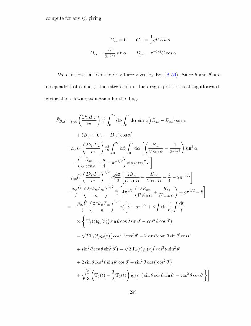
compute for any ij, giving

Czx = 0 Czz =1

4gU cosα

Dzx =U

2π1/2sinα Dzz = π−1/2U cosα

We can now consider the drag force given by Eq. (A.50). Since θ and θ′ are

independent of α and φ, the integration in the drag expression is straightforward,

giving the following expression for the drag:

FD,Z =ρ∞

(2kBT∞m

)r2

0

∫ 2π

0

dφ

∫ π

0

dα sinα[(Bzx −Dzx) sinα

+ (Bzz + Czz −Dzz) cosα]

=ρ∞U

(2kBT∞m

)r2

0

∫ 2π

0

dφ

∫ π

0

dα

[(Bzx

U sinα− 1

2π1/2

)sin3 α

+

(Bzz

U cosα+g

4− π−1/2

)sinα cos2 α

]=ρ∞U

(2kBT∞m

)1/2

r20

4π

3

[2Bzx

U sinα+

Bzz

U cosα+g

4− 2π−1/2

]=ρ∞U

3

(2πkBT∞

m

)1/2

r20

[4π1/2

(2Bzx

U sinα+

Bzz

U cosα

)+ gπ1/2 − 8

]=− ρ∞U

3

(2πkBT∞

m

)1/2

r20

[8− gπ1/2 + 8

∫dr

r

r0

∫dt

t

×

T3(t)q1(r)(

sin θ cos θ sin θ′ − cos2 θ cos θ′)

−√

2 T4(t)q2(r)(

cos3 θ cos2 θ′ − 2 sin θ cos2 θ sin θ′ cos θ′

+ sin2 θ cos θ sin2 θ′)−√

2 T4(t)q3(r)(

cos3 θ sin2 θ′

+ 2 sin θ cos2 θ sin θ′ cos θ′ + sin2 θ cos θ cos2 θ′)

+

√2

3

(T5(t)− 3

2T3(t)

)q4(r)

(sin θ cos θ sin θ′ − cos2 θ cos θ′

]

299

We next substitute Eq. (A.9) for cos θ, cos θ′, sin θ, and sin θ′:

FD,Z =− ρ∞U

3

(2πkBT∞

m

)1/2

r20

[8− gπ1/2 +

∫dr

2π1/2r2

r20

×q1(r)√πr2

∫dt

T3(t)

t3[t4 − (r2 − r2

0)2]

− q2(r)√2πr3

∫dt

T4(t)

t4[t6 + t4(r2 − r2

0)− t2(r2 − r20)2 − (r2 − r2

0)3]

+q3(r)√2πr3

∫dt

T4(t)

t4[t6 − t4(3r2 + r2

0) + t2(3r2 + r20)(r2 − r2

0)− (r2 − r20)3]

+

√2q4(r)√3πr2

∫dt

t3

[T5(t)− 3

2T3(t)

] [t4 − (r2 − r2

0)2]]

The integrals over t in the above expressions are the WU expressions from

Section A.2. After replacing the integrals over t with Eqns. (A.25–A.28), we arrive

at our final expression for the drag in terms of q(r) (Eq. (2.54)):

FD,Z = −ρ∞U3

(2πkBT∞

m

)1/2

r20

[8− gπ1/2 +

∫dr

2π1/2r2

r20

q1(r)WU1(r)

− q2(r)WU2(r)− 2q3(r)WU3(r) + q4(r)WU4(r)

]

300

Appendix B: BGK Results

My method for calculating the drag on an aerosol fractal aggregate in the

transition regime requires knowledge of the velocity field around a sphere. I de-

termined the velocity field using the Bhatnagar-Gross-Krook model [71] in the lin-

earized Boltzmann equation, following the procedure of Lea and Loyalka [75] and

Law and Loyalka [76]. I am providing results here in case anyone wishes to apply

my method for calculating the drag force on an aggregate.

I have listed the calculated values of q2(r) and q3(r) for a range of Knudsen

numbers in Tables B.1–B.24. I have included the values for c1 and c2 in Table B.25.

These variables have been defined Chapter 3. Note that when I compute the drag

force on an aggregate, I use the asymptotic solutions for q2 and q3 when the distance

rij between primary spheres is greater than the maximum r in the tables below.

301

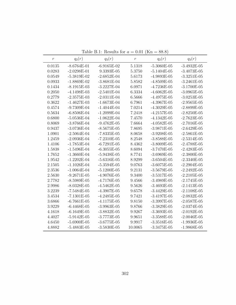
Table B.1: Results for a = 0.01 (Kn = 88.8)

r q2(r) q3(r) r q2(r) q3(r)

0.0135 -8.6764E-01 -6.9165E-02 5.1318 -5.3060E-05 -3.4932E-050.0283 -2.0298E-01 9.3393E-05 5.3750 -5.1404E-05 -3.4073E-050.0549 -5.3819E-02 -2.6852E-04 5.6173 -4.9893E-05 -3.3251E-050.0933 -1.8869E-02 -3.8681E-04 5.8582 -4.8509E-05 -3.2461E-050.1434 -8.1915E-03 -3.2227E-04 6.0971 -4.7236E-05 -3.1700E-050.2050 -4.1498E-03 -2.5401E-04 6.3334 -4.6062E-05 -3.0965E-050.2779 -2.3575E-03 -2.0311E-04 6.5666 -4.4975E-05 -3.0253E-050.3622 -1.4627E-03 -1.6673E-04 6.7961 -4.3967E-05 -2.9565E-050.4574 -9.7309E-04 -1.4044E-04 7.0214 -4.3029E-05 -2.8899E-050.5634 -6.8506E-04 -1.2099E-04 7.2418 -4.2157E-05 -2.8250E-050.6800 -5.0536E-04 -1.0622E-04 7.4570 -4.1342E-05 -2.7623E-050.8069 -3.8766E-04 -9.4762E-05 7.6664 -4.0582E-05 -2.7016E-050.9437 -3.0736E-04 -8.5675E-05 7.8695 -3.9871E-05 -2.6429E-051.0901 -2.5064E-04 -7.8335E-05 8.0658 -3.9208E-05 -2.5861E-051.2459 -2.0936E-04 -7.2310E-05 8.2548 -3.8588E-05 -2.5314E-051.4106 -1.7853E-04 -6.7291E-05 8.4362 -3.8009E-05 -2.4788E-051.5838 -1.5496E-04 -6.3055E-05 8.6094 -3.7470E-05 -2.4283E-051.7652 -1.3660E-04 -5.9438E-05 8.7741 -3.6969E-05 -2.3800E-051.9542 -1.2202E-04 -5.6316E-05 8.9299 -3.6504E-05 -2.3340E-052.1505 -1.1026E-04 -5.3594E-05 9.0763 -3.6075E-05 -2.2904E-052.3536 -1.0064E-04 -5.1200E-05 9.2131 -3.5679E-05 -2.2492E-052.5630 -9.2671E-05 -4.9076E-05 9.3400 -3.5317E-05 -2.2105E-052.7782 -8.5989E-05 -4.7176E-05 9.4566 -3.4989E-05 -2.1745E-052.9986 -8.0328E-05 -4.5462E-05 9.5626 -3.4693E-05 -2.1413E-053.2239 -7.5484E-05 -4.3907E-05 9.6578 -3.4429E-05 -2.1108E-053.4534 -7.1301E-05 -4.2485E-05 9.7421 -3.4197E-05 -2.0832E-053.6866 -6.7661E-05 -4.1175E-05 9.8150 -3.3997E-05 -2.0587E-053.9229 -6.4468E-05 -3.9963E-05 9.8766 -3.3829E-05 -2.0374E-054.1618 -6.1649E-05 -3.8832E-05 9.9267 -3.3693E-05 -2.0192E-054.4027 -5.9142E-05 -3.7773E-05 9.9651 -3.3588E-05 -2.0046E-054.6450 -5.6900E-05 -3.6775E-05 9.9917 -3.3516E-05 -1.9936E-054.8882 -5.4883E-05 -3.5830E-05 10.0065 -3.3475E-05 -1.9868E-05

302

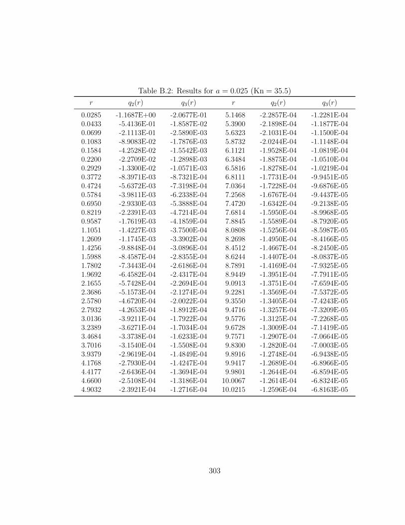
Table B.2: Results for a = 0.025 (Kn = 35.5)

r q2(r) q3(r) r q2(r) q3(r)

0.0285 -1.1687E+00 -2.0677E-01 5.1468 -2.2857E-04 -1.2281E-040.0433 -5.4136E-01 -1.8587E-02 5.3900 -2.1898E-04 -1.1877E-040.0699 -2.1113E-01 -2.5890E-03 5.6323 -2.1031E-04 -1.1500E-040.1083 -8.9083E-02 -1.7876E-03 5.8732 -2.0244E-04 -1.1148E-040.1584 -4.2528E-02 -1.5542E-03 6.1121 -1.9528E-04 -1.0819E-040.2200 -2.2709E-02 -1.2898E-03 6.3484 -1.8875E-04 -1.0510E-040.2929 -1.3300E-02 -1.0571E-03 6.5816 -1.8278E-04 -1.0219E-040.3772 -8.3971E-03 -8.7321E-04 6.8111 -1.7731E-04 -9.9451E-050.4724 -5.6372E-03 -7.3198E-04 7.0364 -1.7228E-04 -9.6876E-050.5784 -3.9811E-03 -6.2338E-04 7.2568 -1.6767E-04 -9.4437E-050.6950 -2.9330E-03 -5.3888E-04 7.4720 -1.6342E-04 -9.2138E-050.8219 -2.2391E-03 -4.7214E-04 7.6814 -1.5950E-04 -8.9968E-050.9587 -1.7619E-03 -4.1859E-04 7.8845 -1.5589E-04 -8.7920E-051.1051 -1.4227E-03 -3.7500E-04 8.0808 -1.5256E-04 -8.5987E-051.2609 -1.1745E-03 -3.3902E-04 8.2698 -1.4950E-04 -8.4166E-051.4256 -9.8848E-04 -3.0896E-04 8.4512 -1.4667E-04 -8.2450E-051.5988 -8.4587E-04 -2.8355E-04 8.6244 -1.4407E-04 -8.0837E-051.7802 -7.3443E-04 -2.6186E-04 8.7891 -1.4169E-04 -7.9325E-051.9692 -6.4582E-04 -2.4317E-04 8.9449 -1.3951E-04 -7.7911E-052.1655 -5.7428E-04 -2.2694E-04 9.0913 -1.3751E-04 -7.6594E-052.3686 -5.1573E-04 -2.1274E-04 9.2281 -1.3569E-04 -7.5372E-052.5780 -4.6720E-04 -2.0022E-04 9.3550 -1.3405E-04 -7.4243E-052.7932 -4.2653E-04 -1.8912E-04 9.4716 -1.3257E-04 -7.3209E-053.0136 -3.9211E-04 -1.7922E-04 9.5776 -1.3125E-04 -7.2268E-053.2389 -3.6271E-04 -1.7034E-04 9.6728 -1.3009E-04 -7.1419E-053.4684 -3.3738E-04 -1.6233E-04 9.7571 -1.2907E-04 -7.0664E-053.7016 -3.1540E-04 -1.5508E-04 9.8300 -1.2820E-04 -7.0003E-053.9379 -2.9619E-04 -1.4849E-04 9.8916 -1.2748E-04 -6.9438E-054.1768 -2.7930E-04 -1.4247E-04 9.9417 -1.2689E-04 -6.8966E-054.4177 -2.6436E-04 -1.3694E-04 9.9801 -1.2644E-04 -6.8594E-054.6600 -2.5108E-04 -1.3186E-04 10.0067 -1.2614E-04 -6.8324E-054.9032 -2.3921E-04 -1.2716E-04 10.0215 -1.2596E-04 -6.8163E-05

303

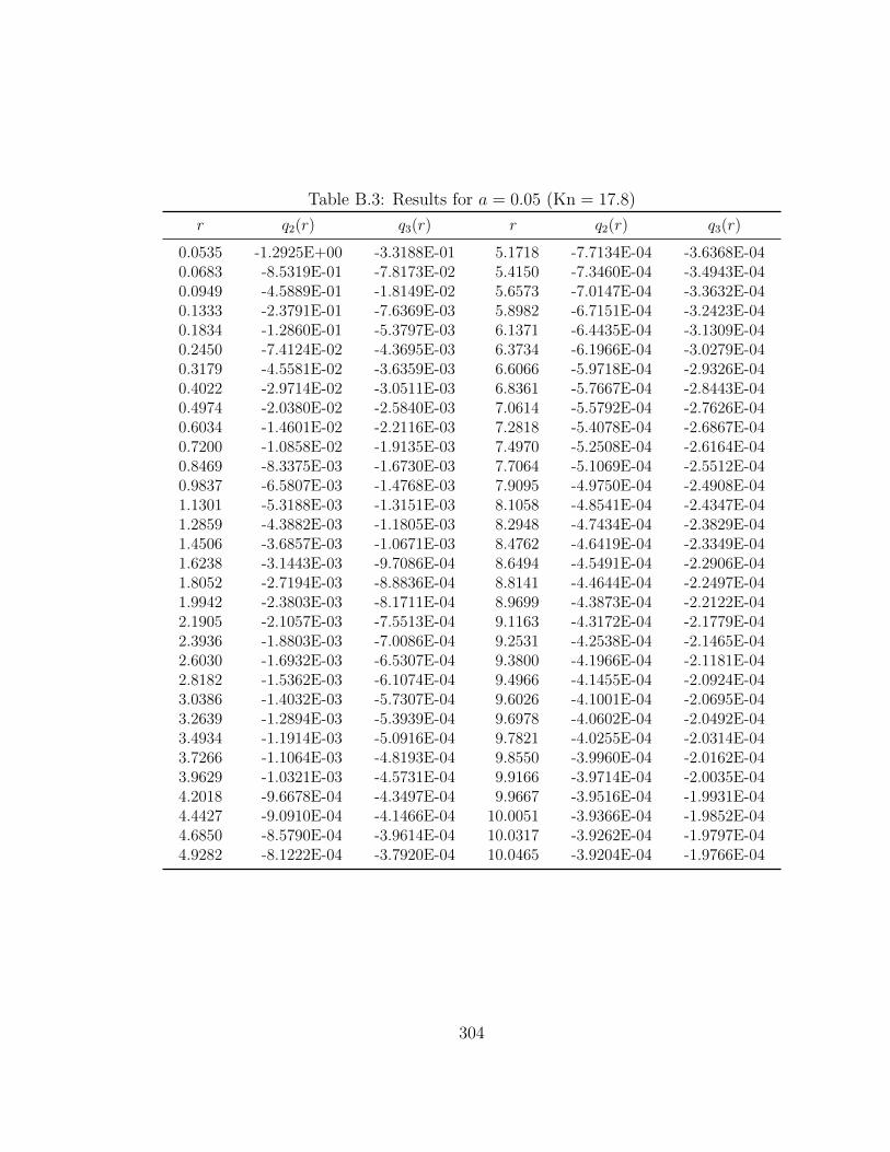
Table B.3: Results for a = 0.05 (Kn = 17.8)

r q2(r) q3(r) r q2(r) q3(r)

0.0535 -1.2925E+00 -3.3188E-01 5.1718 -7.7134E-04 -3.6368E-040.0683 -8.5319E-01 -7.8173E-02 5.4150 -7.3460E-04 -3.4943E-040.0949 -4.5889E-01 -1.8149E-02 5.6573 -7.0147E-04 -3.3632E-040.1333 -2.3791E-01 -7.6369E-03 5.8982 -6.7151E-04 -3.2423E-040.1834 -1.2860E-01 -5.3797E-03 6.1371 -6.4435E-04 -3.1309E-040.2450 -7.4124E-02 -4.3695E-03 6.3734 -6.1966E-04 -3.0279E-040.3179 -4.5581E-02 -3.6359E-03 6.6066 -5.9718E-04 -2.9326E-040.4022 -2.9714E-02 -3.0511E-03 6.8361 -5.7667E-04 -2.8443E-040.4974 -2.0380E-02 -2.5840E-03 7.0614 -5.5792E-04 -2.7626E-040.6034 -1.4601E-02 -2.2116E-03 7.2818 -5.4078E-04 -2.6867E-040.7200 -1.0858E-02 -1.9135E-03 7.4970 -5.2508E-04 -2.6164E-040.8469 -8.3375E-03 -1.6730E-03 7.7064 -5.1069E-04 -2.5512E-040.9837 -6.5807E-03 -1.4768E-03 7.9095 -4.9750E-04 -2.4908E-041.1301 -5.3188E-03 -1.3151E-03 8.1058 -4.8541E-04 -2.4347E-041.2859 -4.3882E-03 -1.1805E-03 8.2948 -4.7434E-04 -2.3829E-041.4506 -3.6857E-03 -1.0671E-03 8.4762 -4.6419E-04 -2.3349E-041.6238 -3.1443E-03 -9.7086E-04 8.6494 -4.5491E-04 -2.2906E-041.8052 -2.7194E-03 -8.8836E-04 8.8141 -4.4644E-04 -2.2497E-041.9942 -2.3803E-03 -8.1711E-04 8.9699 -4.3873E-04 -2.2122E-042.1905 -2.1057E-03 -7.5513E-04 9.1163 -4.3172E-04 -2.1779E-042.3936 -1.8803E-03 -7.0086E-04 9.2531 -4.2538E-04 -2.1465E-042.6030 -1.6932E-03 -6.5307E-04 9.3800 -4.1966E-04 -2.1181E-042.8182 -1.5362E-03 -6.1074E-04 9.4966 -4.1455E-04 -2.0924E-043.0386 -1.4032E-03 -5.7307E-04 9.6026 -4.1001E-04 -2.0695E-043.2639 -1.2894E-03 -5.3939E-04 9.6978 -4.0602E-04 -2.0492E-043.4934 -1.1914E-03 -5.0916E-04 9.7821 -4.0255E-04 -2.0314E-043.7266 -1.1064E-03 -4.8193E-04 9.8550 -3.9960E-04 -2.0162E-043.9629 -1.0321E-03 -4.5731E-04 9.9166 -3.9714E-04 -2.0035E-044.2018 -9.6678E-04 -4.3497E-04 9.9667 -3.9516E-04 -1.9931E-044.4427 -9.0910E-04 -4.1466E-04 10.0051 -3.9366E-04 -1.9852E-044.6850 -8.5790E-04 -3.9614E-04 10.0317 -3.9262E-04 -1.9797E-044.9282 -8.1222E-04 -3.7920E-04 10.0465 -3.9204E-04 -1.9766E-04

304

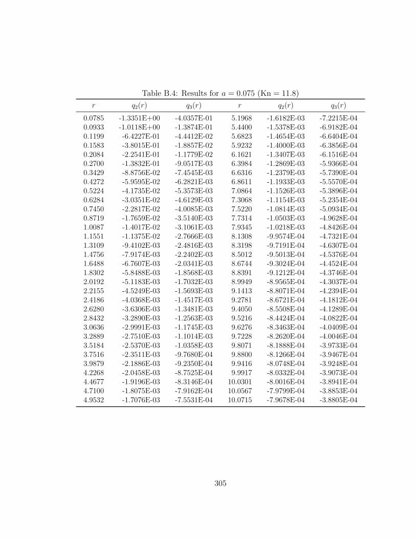
Table B.4: Results for a = 0.075 (Kn = 11.8)

r q2(r) q3(r) r q2(r) q3(r)

0.0785 -1.3351E+00 -4.0357E-01 5.1968 -1.6182E-03 -7.2215E-040.0933 -1.0118E+00 -1.3874E-01 5.4400 -1.5378E-03 -6.9182E-040.1199 -6.4227E-01 -4.4412E-02 5.6823 -1.4654E-03 -6.6404E-040.1583 -3.8015E-01 -1.8857E-02 5.9232 -1.4000E-03 -6.3856E-040.2084 -2.2541E-01 -1.1779E-02 6.1621 -1.3407E-03 -6.1516E-040.2700 -1.3832E-01 -9.0517E-03 6.3984 -1.2869E-03 -5.9366E-040.3429 -8.8756E-02 -7.4545E-03 6.6316 -1.2379E-03 -5.7390E-040.4272 -5.9595E-02 -6.2821E-03 6.8611 -1.1933E-03 -5.5570E-040.5224 -4.1735E-02 -5.3573E-03 7.0864 -1.1526E-03 -5.3896E-040.6284 -3.0351E-02 -4.6129E-03 7.3068 -1.1154E-03 -5.2354E-040.7450 -2.2817E-02 -4.0085E-03 7.5220 -1.0814E-03 -5.0934E-040.8719 -1.7659E-02 -3.5140E-03 7.7314 -1.0503E-03 -4.9628E-041.0087 -1.4017E-02 -3.1061E-03 7.9345 -1.0218E-03 -4.8426E-041.1551 -1.1375E-02 -2.7666E-03 8.1308 -9.9574E-04 -4.7321E-041.3109 -9.4102E-03 -2.4816E-03 8.3198 -9.7191E-04 -4.6307E-041.4756 -7.9174E-03 -2.2402E-03 8.5012 -9.5013E-04 -4.5376E-041.6488 -6.7607E-03 -2.0341E-03 8.6744 -9.3024E-04 -4.4524E-041.8302 -5.8488E-03 -1.8568E-03 8.8391 -9.1212E-04 -4.3746E-042.0192 -5.1183E-03 -1.7032E-03 8.9949 -8.9565E-04 -4.3037E-042.2155 -4.5249E-03 -1.5693E-03 9.1413 -8.8071E-04 -4.2394E-042.4186 -4.0368E-03 -1.4517E-03 9.2781 -8.6721E-04 -4.1812E-042.6280 -3.6306E-03 -1.3481E-03 9.4050 -8.5508E-04 -4.1289E-042.8432 -3.2890E-03 -1.2563E-03 9.5216 -8.4424E-04 -4.0822E-043.0636 -2.9991E-03 -1.1745E-03 9.6276 -8.3463E-04 -4.0409E-043.2889 -2.7510E-03 -1.1014E-03 9.7228 -8.2620E-04 -4.0046E-043.5184 -2.5370E-03 -1.0358E-03 9.8071 -8.1888E-04 -3.9733E-043.7516 -2.3511E-03 -9.7680E-04 9.8800 -8.1266E-04 -3.9467E-043.9879 -2.1886E-03 -9.2350E-04 9.9416 -8.0748E-04 -3.9248E-044.2268 -2.0458E-03 -8.7525E-04 9.9917 -8.0332E-04 -3.9073E-044.4677 -1.9196E-03 -8.3146E-04 10.0301 -8.0016E-04 -3.8941E-044.7100 -1.8075E-03 -7.9162E-04 10.0567 -7.9799E-04 -3.8853E-044.9532 -1.7076E-03 -7.5531E-04 10.0715 -7.9678E-04 -3.8805E-04

305

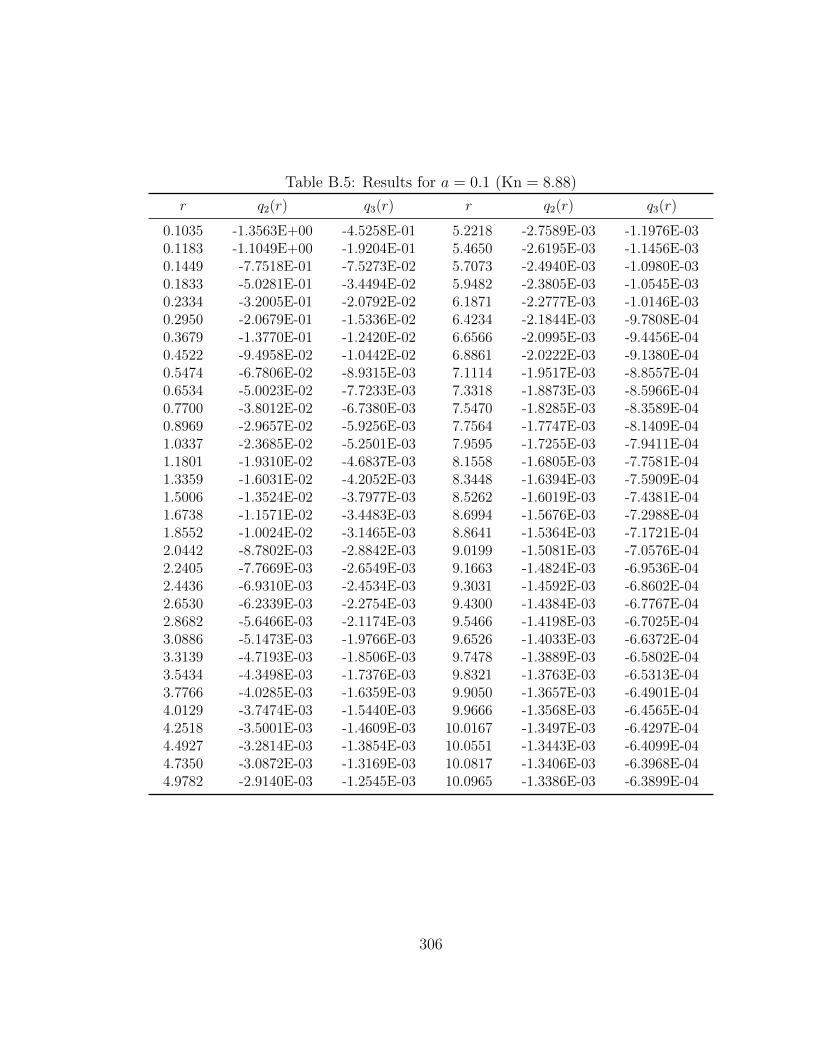
Table B.5: Results for a = 0.1 (Kn = 8.88)

r q2(r) q3(r) r q2(r) q3(r)

0.1035 -1.3563E+00 -4.5258E-01 5.2218 -2.7589E-03 -1.1976E-030.1183 -1.1049E+00 -1.9204E-01 5.4650 -2.6195E-03 -1.1456E-030.1449 -7.7518E-01 -7.5273E-02 5.7073 -2.4940E-03 -1.0980E-030.1833 -5.0281E-01 -3.4494E-02 5.9482 -2.3805E-03 -1.0545E-030.2334 -3.2005E-01 -2.0792E-02 6.1871 -2.2777E-03 -1.0146E-030.2950 -2.0679E-01 -1.5336E-02 6.4234 -2.1844E-03 -9.7808E-040.3679 -1.3770E-01 -1.2420E-02 6.6566 -2.0995E-03 -9.4456E-040.4522 -9.4958E-02 -1.0442E-02 6.8861 -2.0222E-03 -9.1380E-040.5474 -6.7806E-02 -8.9315E-03 7.1114 -1.9517E-03 -8.8557E-040.6534 -5.0023E-02 -7.7233E-03 7.3318 -1.8873E-03 -8.5966E-040.7700 -3.8012E-02 -6.7380E-03 7.5470 -1.8285E-03 -8.3589E-040.8969 -2.9657E-02 -5.9256E-03 7.7564 -1.7747E-03 -8.1409E-041.0337 -2.3685E-02 -5.2501E-03 7.9595 -1.7255E-03 -7.9411E-041.1801 -1.9310E-02 -4.6837E-03 8.1558 -1.6805E-03 -7.7581E-041.3359 -1.6031E-02 -4.2052E-03 8.3448 -1.6394E-03 -7.5909E-041.5006 -1.3524E-02 -3.7977E-03 8.5262 -1.6019E-03 -7.4381E-041.6738 -1.1571E-02 -3.4483E-03 8.6994 -1.5676E-03 -7.2988E-041.8552 -1.0024E-02 -3.1465E-03 8.8641 -1.5364E-03 -7.1721E-042.0442 -8.7802E-03 -2.8842E-03 9.0199 -1.5081E-03 -7.0576E-042.2405 -7.7669E-03 -2.6549E-03 9.1663 -1.4824E-03 -6.9536E-042.4436 -6.9310E-03 -2.4534E-03 9.3031 -1.4592E-03 -6.8602E-042.6530 -6.2339E-03 -2.2754E-03 9.4300 -1.4384E-03 -6.7767E-042.8682 -5.6466E-03 -2.1174E-03 9.5466 -1.4198E-03 -6.7025E-043.0886 -5.1473E-03 -1.9766E-03 9.6526 -1.4033E-03 -6.6372E-043.3139 -4.7193E-03 -1.8506E-03 9.7478 -1.3889E-03 -6.5802E-043.5434 -4.3498E-03 -1.7376E-03 9.8321 -1.3763E-03 -6.5313E-043.7766 -4.0285E-03 -1.6359E-03 9.9050 -1.3657E-03 -6.4901E-044.0129 -3.7474E-03 -1.5440E-03 9.9666 -1.3568E-03 -6.4565E-044.2518 -3.5001E-03 -1.4609E-03 10.0167 -1.3497E-03 -6.4297E-044.4927 -3.2814E-03 -1.3854E-03 10.0551 -1.3443E-03 -6.4099E-044.7350 -3.0872E-03 -1.3169E-03 10.0817 -1.3406E-03 -6.3968E-044.9782 -2.9140E-03 -1.2545E-03 10.0965 -1.3386E-03 -6.3899E-04

306

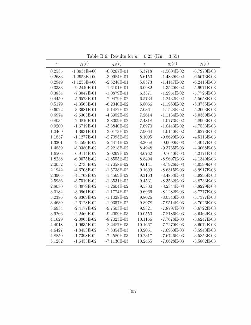
Table B.6: Results for a = 0.25 (Kn = 3.55)

r q2(r) q3(r) r q2(r) q3(r)

0.2535 -1.3934E+00 -6.0267E-01 5.3718 -1.5604E-02 -6.7970E-030.2683 -1.2953E+00 -3.9984E-01 5.6150 -1.4839E-02 -6.5073E-030.2949 -1.1258E+00 -2.5248E-01 5.8573 -1.4147E-02 -6.2415E-030.3333 -9.2440E-01 -1.6101E-01 6.0982 -1.3520E-02 -5.9971E-030.3834 -7.3047E-01 -1.0879E-01 6.3371 -1.2951E-02 -5.7725E-030.4450 -5.6573E-01 -7.9479E-02 6.5734 -1.2432E-02 -5.5658E-030.5179 -4.3563E-01 -6.2340E-02 6.8066 -1.1960E-02 -5.3755E-030.6022 -3.3681E-01 -5.1482E-02 7.0361 -1.1528E-02 -5.2003E-030.6974 -2.6303E-01 -4.3952E-02 7.2614 -1.1134E-02 -5.0389E-030.8034 -2.0816E-01 -3.8309E-02 7.4818 -1.0773E-02 -4.8903E-030.9200 -1.6719E-01 -3.3840E-02 7.6970 -1.0443E-02 -4.7533E-031.0469 -1.3631E-01 -3.0173E-02 7.9064 -1.0140E-02 -4.6273E-031.1837 -1.1277E-01 -2.7095E-02 8.1095 -9.8629E-03 -4.5113E-031.3301 -9.4596E-02 -2.4474E-02 8.3058 -9.6090E-03 -4.4047E-031.4859 -8.0380E-02 -2.2218E-02 8.4948 -9.3765E-03 -4.3068E-031.6506 -6.9114E-02 -2.0262E-02 8.6762 -9.1640E-03 -4.2171E-031.8238 -6.0075E-02 -1.8555E-02 8.8494 -8.9697E-03 -4.1349E-032.0052 -5.2735E-02 -1.7058E-02 9.0141 -8.7926E-03 -4.0599E-032.1942 -4.6708E-02 -1.5738E-02 9.1699 -8.6315E-03 -3.9917E-032.3905 -4.1708E-02 -1.4569E-02 9.3163 -8.4853E-03 -3.9295E-032.5936 -3.7519E-02 -1.3531E-02 9.4531 -8.3532E-03 -3.8733E-032.8030 -3.3979E-02 -1.2604E-02 9.5800 -8.2344E-03 -3.8229E-033.0182 -3.0961E-02 -1.1774E-02 9.6966 -8.1282E-03 -3.7777E-033.2386 -2.8369E-02 -1.1028E-02 9.8026 -8.0340E-03 -3.7377E-033.4639 -2.6128E-02 -1.0357E-02 9.8978 -7.9514E-03 -3.7026E-033.6934 -2.4177E-02 -9.7503E-03 9.9821 -7.8797E-03 -3.6722E-033.9266 -2.2469E-02 -9.2009E-03 10.0550 -7.8186E-03 -3.6462E-034.1629 -2.0965E-02 -8.7023E-03 10.1166 -7.7678E-03 -3.6247E-034.4018 -1.9635E-02 -8.2487E-03 10.1667 -7.7270E-03 -3.6074E-034.6427 -1.8453E-02 -7.8354E-03 10.2051 -7.6960E-03 -3.5943E-034.8850 -1.7398E-02 -7.4580E-03 10.2317 -7.6746E-03 -3.5853E-035.1282 -1.6453E-02 -7.1130E-03 10.2465 -7.6628E-03 -3.5802E-03

307

Table B.7: Results for a = 0.5 (Kn = 1.78)

r q2(r) q3(r) r q2(r) q3(r)

0.5035 -1.4050E+00 -7.2269E-01 5.6218 -5.2901E-02 -2.3187E-020.5183 -1.3617E+00 -5.7935E-01 5.8650 -5.0428E-02 -2.2238E-020.5449 -1.2801E+00 -4.5249E-01 6.1073 -4.8182E-02 -2.1364E-020.5833 -1.1674E+00 -3.5102E-01 6.3482 -4.6138E-02 -2.0559E-020.6334 -1.0369E+00 -2.7496E-01 6.5871 -4.4274E-02 -1.9816E-020.6950 -9.0248E-01 -2.2000E-01 6.8234 -4.2572E-02 -1.9131E-020.7679 -7.7481E-01 -1.8073E-01 7.0566 -4.1016E-02 -1.8499E-020.8522 -6.6010E-01 -1.5238E-01 7.2861 -3.9591E-02 -1.7916E-020.9474 -5.6080E-01 -1.3140E-01 7.5114 -3.8285E-02 -1.7378E-021.0534 -4.7688E-01 -1.1534E-01 7.7318 -3.7087E-02 -1.6881E-021.1700 -4.0698E-01 -1.0264E-01 7.9470 -3.5988E-02 -1.6422E-021.2969 -3.4918E-01 -9.2270E-02 8.1564 -3.4979E-02 -1.6000E-021.4337 -3.0151E-01 -8.3598E-02 8.3595 -3.4053E-02 -1.5610E-021.5801 -2.6217E-01 -7.6204E-02 8.5558 -3.3203E-02 -1.5252E-021.7359 -2.2960E-01 -6.9808E-02 8.7448 -3.2424E-02 -1.4922E-021.9006 -2.0252E-01 -6.4215E-02 8.9262 -3.1711E-02 -1.4620E-022.0738 -1.7987E-01 -5.9286E-02 9.0994 -3.1058E-02 -1.4343E-022.2552 -1.6081E-01 -5.4914E-02 9.2641 -3.0462E-02 -1.4089E-022.4442 -1.4468E-01 -5.1015E-02 9.4199 -2.9920E-02 -1.3858E-022.6405 -1.3094E-01 -4.7525E-02 9.5663 -2.9427E-02 -1.3648E-022.8436 -1.1916E-01 -4.4390E-02 9.7031 -2.8981E-02 -1.3458E-023.0530 -1.0900E-01 -4.1564E-02 9.8300 -2.8580E-02 -1.3287E-023.2682 -1.0018E-01 -3.9010E-02 9.9466 -2.8221E-02 -1.3134E-023.4886 -9.2497E-02 -3.6697E-02 10.0526 -2.7903E-02 -1.2999E-023.7139 -8.5759E-02 -3.4596E-02 10.1478 -2.7623E-02 -1.2879E-023.9434 -7.9821E-02 -3.2685E-02 10.2321 -2.7380E-02 -1.2776E-024.1766 -7.4569E-02 -3.0943E-02 10.3050 -2.7173E-02 -1.2688E-024.4129 -6.9899E-02 -2.9352E-02 10.3666 -2.7001E-02 -1.2615E-024.6518 -6.5733E-02 -2.7896E-02 10.4167 -2.6863E-02 -1.2556E-024.8927 -6.2003E-02 -2.6564E-02 10.4551 -2.6758E-02 -1.2512E-025.1350 -5.8652E-02 -2.5342E-02 10.4817 -2.6685E-02 -1.2481E-025.3782 -5.5631E-02 -2.4219E-02 10.4965 -2.6645E-02 -1.2464E-02

308

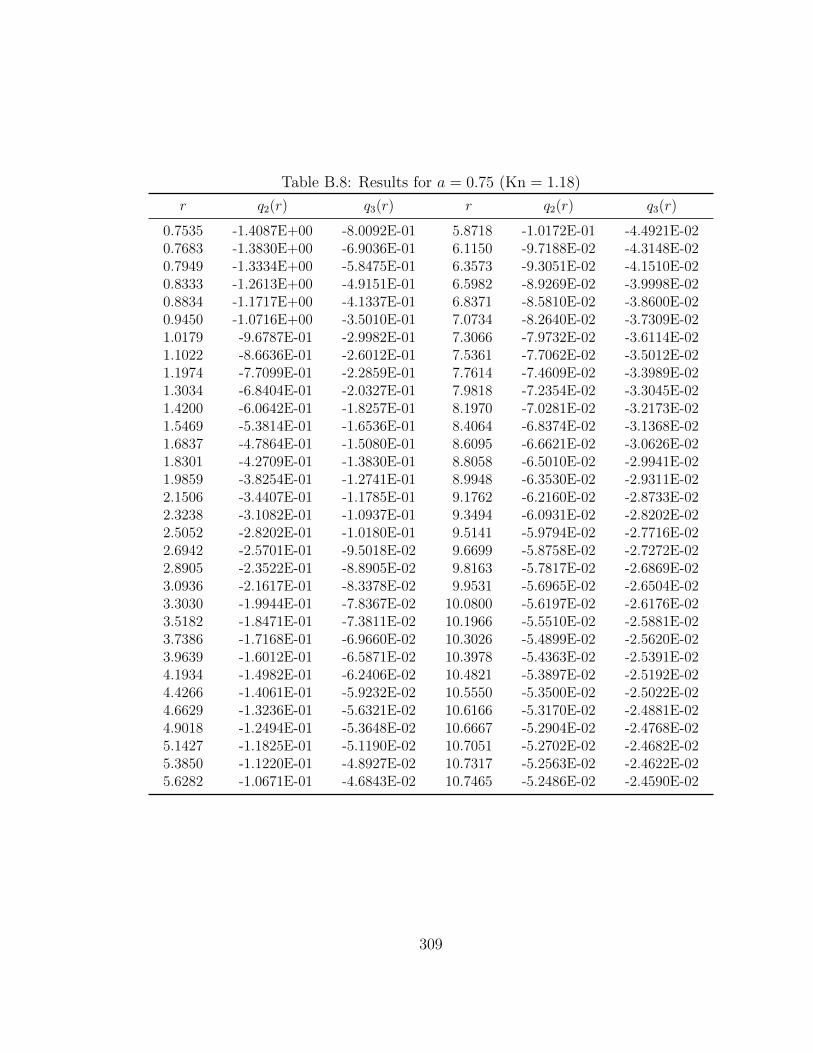
Table B.8: Results for a = 0.75 (Kn = 1.18)

r q2(r) q3(r) r q2(r) q3(r)

0.7535 -1.4087E+00 -8.0092E-01 5.8718 -1.0172E-01 -4.4921E-020.7683 -1.3830E+00 -6.9036E-01 6.1150 -9.7188E-02 -4.3148E-020.7949 -1.3334E+00 -5.8475E-01 6.3573 -9.3051E-02 -4.1510E-020.8333 -1.2613E+00 -4.9151E-01 6.5982 -8.9269E-02 -3.9998E-020.8834 -1.1717E+00 -4.1337E-01 6.8371 -8.5810E-02 -3.8600E-020.9450 -1.0716E+00 -3.5010E-01 7.0734 -8.2640E-02 -3.7309E-021.0179 -9.6787E-01 -2.9982E-01 7.3066 -7.9732E-02 -3.6114E-021.1022 -8.6636E-01 -2.6012E-01 7.5361 -7.7062E-02 -3.5012E-021.1974 -7.7099E-01 -2.2859E-01 7.7614 -7.4609E-02 -3.3989E-021.3034 -6.8404E-01 -2.0327E-01 7.9818 -7.2354E-02 -3.3045E-021.4200 -6.0642E-01 -1.8257E-01 8.1970 -7.0281E-02 -3.2173E-021.5469 -5.3814E-01 -1.6536E-01 8.4064 -6.8374E-02 -3.1368E-021.6837 -4.7864E-01 -1.5080E-01 8.6095 -6.6621E-02 -3.0626E-021.8301 -4.2709E-01 -1.3830E-01 8.8058 -6.5010E-02 -2.9941E-021.9859 -3.8254E-01 -1.2741E-01 8.9948 -6.3530E-02 -2.9311E-022.1506 -3.4407E-01 -1.1785E-01 9.1762 -6.2160E-02 -2.8733E-022.3238 -3.1082E-01 -1.0937E-01 9.3494 -6.0931E-02 -2.8202E-022.5052 -2.8202E-01 -1.0180E-01 9.5141 -5.9794E-02 -2.7716E-022.6942 -2.5701E-01 -9.5018E-02 9.6699 -5.8758E-02 -2.7272E-022.8905 -2.3522E-01 -8.8905E-02 9.8163 -5.7817E-02 -2.6869E-023.0936 -2.1617E-01 -8.3378E-02 9.9531 -5.6965E-02 -2.6504E-023.3030 -1.9944E-01 -7.8367E-02 10.0800 -5.6197E-02 -2.6176E-023.5182 -1.8471E-01 -7.3811E-02 10.1966 -5.5510E-02 -2.5881E-023.7386 -1.7168E-01 -6.9660E-02 10.3026 -5.4899E-02 -2.5620E-023.9639 -1.6012E-01 -6.5871E-02 10.3978 -5.4363E-02 -2.5391E-024.1934 -1.4982E-01 -6.2406E-02 10.4821 -5.3897E-02 -2.5192E-024.4266 -1.4061E-01 -5.9232E-02 10.5550 -5.3500E-02 -2.5022E-024.6629 -1.3236E-01 -5.6321E-02 10.6166 -5.3170E-02 -2.4881E-024.9018 -1.2494E-01 -5.3648E-02 10.6667 -5.2904E-02 -2.4768E-025.1427 -1.1825E-01 -5.1190E-02 10.7051 -5.2702E-02 -2.4682E-025.3850 -1.1220E-01 -4.8927E-02 10.7317 -5.2563E-02 -2.4622E-025.6282 -1.0671E-01 -4.6843E-02 10.7465 -5.2486E-02 -2.4590E-02

309

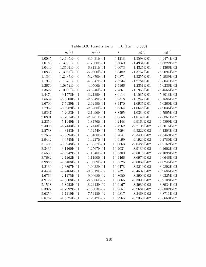
Table B.9: Results for a = 1.0 (Kn = 0.888)

r q2(r) q3(r) r q2(r) q3(r)

1.0035 -1.4105E+00 -8.6031E-01 6.1218 -1.5598E-01 -6.9474E-021.0183 -1.3930E+00 -7.7068E-01 6.3650 -1.4934E-01 -6.6822E-021.0449 -1.3591E+00 -6.8131E-01 6.6073 -1.4325E-01 -6.4366E-021.0833 -1.3087E+00 -5.9800E-01 6.8482 -1.3767E-01 -6.2094E-021.1334 -1.2437E+00 -5.2370E-01 7.0871 -1.3255E-01 -5.9989E-021.1950 -1.1678E+00 -4.5947E-01 7.3234 -1.2784E-01 -5.8041E-021.2679 -1.0852E+00 -4.0506E-01 7.5566 -1.2351E-01 -5.6236E-021.3522 -1.0000E+00 -3.5946E-01 7.7861 -1.1953E-01 -5.4565E-021.4474 -9.1578E-01 -3.2139E-01 8.0114 -1.1585E-01 -5.3018E-021.5534 -8.3500E-01 -2.8949E-01 8.2318 -1.1247E-01 -5.1586E-021.6700 -7.5939E-01 -2.6259E-01 8.4470 -1.0935E-01 -5.0260E-021.7969 -6.8989E-01 -2.3968E-01 8.6564 -1.0648E-01 -4.9036E-021.9337 -6.2683E-01 -2.1996E-01 8.8595 -1.0384E-01 -4.7905E-022.0801 -5.7014E-01 -2.0281E-01 9.0558 -1.0140E-01 -4.6861E-022.2359 -5.1949E-01 -1.8776E-01 9.2448 -9.9164E-02 -4.5899E-022.4006 -4.7443E-01 -1.7443E-01 9.4262 -9.7108E-02 -4.5015E-022.5738 -4.3443E-01 -1.6254E-01 9.5994 -9.5222E-02 -4.4203E-022.7552 -3.9894E-01 -1.5188E-01 9.7641 -9.3496E-02 -4.3459E-022.9442 -3.6745E-01 -1.4227E-01 9.9199 -9.1920E-02 -4.2780E-023.1405 -3.3948E-01 -1.3357E-01 10.0663 -9.0488E-02 -4.2162E-023.3436 -3.1460E-01 -1.2567E-01 10.2031 -8.9189E-02 -4.1602E-023.5530 -2.9242E-01 -1.1848E-01 10.3300 -8.8018E-02 -4.1098E-023.7682 -2.7262E-01 -1.1190E-01 10.4466 -8.6970E-02 -4.0646E-023.9886 -2.5488E-01 -1.0589E-01 10.5526 -8.6039E-02 -4.0245E-024.2139 -2.3897E-01 -1.0038E-01 10.6478 -8.5219E-02 -3.9892E-024.4434 -2.2466E-01 -9.5319E-02 10.7321 -8.4507E-02 -3.9586E-024.6766 -2.1175E-01 -9.0668E-02 10.8050 -8.3900E-02 -3.9325E-024.9129 -2.0008E-01 -8.6386E-02 10.8666 -8.3395E-02 -3.9108E-025.1518 -1.8952E-01 -8.2442E-02 10.9167 -8.2989E-02 -3.8934E-025.3927 -1.7992E-01 -7.8803E-02 10.9551 -8.2681E-02 -3.8802E-025.6350 -1.7119E-01 -7.5445E-02 10.9817 -8.2468E-02 -3.8711E-025.8782 -1.6324E-01 -7.2342E-02 10.9965 -8.2350E-02 -3.8660E-02

310

Table B.10: Results for a = 1.25 (Kn = 0.710)

r q2(r) q3(r) r q2(r) q3(r)

1.2535 -1.4115E+00 -9.0799E-01 6.3718 -2.1200E-01 -9.5307E-021.2683 -1.3987E+00 -8.3292E-01 6.6150 -2.0338E-01 -9.1777E-021.2949 -1.3739E+00 -7.5591E-01 6.8573 -1.9545E-01 -8.8505E-021.3333 -1.3365E+00 -6.8152E-01 7.0982 -1.8815E-01 -8.5469E-021.3834 -1.2872E+00 -6.1247E-01 7.3371 -1.8142E-01 -8.2654E-021.4450 -1.2281E+00 -5.5016E-01 7.5734 -1.7523E-01 -8.0043E-021.5179 -1.1616E+00 -4.9505E-01 7.8066 -1.6951E-01 -7.7621E-021.6022 -1.0906E+00 -4.4694E-01 8.0361 -1.6423E-01 -7.5375E-021.6974 -1.0178E+00 -4.0524E-01 8.2614 -1.5936E-01 -7.3293E-021.8034 -9.4558E-01 -3.6915E-01 8.4818 -1.5486E-01 -7.1363E-021.9200 -8.7559E-01 -3.3787E-01 8.6970 -1.5071E-01 -6.9576E-022.0469 -8.0911E-01 -3.1064E-01 8.9064 -1.4688E-01 -6.7922E-022.1837 -7.4689E-01 -2.8679E-01 9.1095 -1.4334E-01 -6.6393E-022.3301 -6.8934E-01 -2.6578E-01 9.3058 -1.4008E-01 -6.4981E-022.4859 -6.3654E-01 -2.4714E-01 9.4948 -1.3708E-01 -6.3679E-022.6506 -5.8841E-01 -2.3050E-01 9.6762 -1.3432E-01 -6.2480E-022.8238 -5.4473E-01 -2.1556E-01 9.8494 -1.3178E-01 -6.1378E-023.0052 -5.0519E-01 -2.0208E-01 10.0141 -1.2946E-01 -6.0369E-023.1942 -4.6946E-01 -1.8987E-01 10.1699 -1.2733E-01 -5.9447E-023.3905 -4.3720E-01 -1.7877E-01 10.3163 -1.2540E-01 -5.8607E-023.5936 -4.0806E-01 -1.6865E-01 10.4531 -1.2365E-01 -5.7845E-023.8030 -3.8175E-01 -1.5939E-01 10.5800 -1.2207E-01 -5.7159E-024.0182 -3.5796E-01 -1.5091E-01 10.6966 -1.2065E-01 -5.6544E-024.2386 -3.3642E-01 -1.4312E-01 10.8026 -1.1939E-01 -5.5997E-024.4639 -3.1690E-01 -1.3595E-01 10.8978 -1.1828E-01 -5.5517E-024.6934 -2.9919E-01 -1.2935E-01 10.9821 -1.1732E-01 -5.5100E-024.9266 -2.8308E-01 -1.2327E-01 11.0550 -1.1650E-01 -5.4745E-025.1629 -2.6841E-01 -1.1765E-01 11.1166 -1.1582E-01 -5.4449E-025.4018 -2.5503E-01 -1.1247E-01 11.1667 -1.1527E-01 -5.4211E-025.6427 -2.4281E-01 -1.0767E-01 11.2051 -1.1485E-01 -5.4031E-025.8850 -2.3163E-01 -1.0323E-01 11.2317 -1.1456E-01 -5.3906E-026.1282 -2.2140E-01 -9.9116E-02 11.2465 -1.1440E-01 -5.3838E-02

311

Table B.11: Results for a = 1.5 (Kn = 0.592)

r q2(r) q3(r) r q2(r) q3(r)

1.5035 -1.4121E+00 -9.4744E-01 6.6218 -2.6772E-01 -1.2157E-011.5183 -1.4022E+00 -8.8310E-01 6.8650 -2.5731E-01 -1.1719E-011.5449 -1.3832E+00 -8.1567E-01 7.1073 -2.4770E-01 -1.1313E-011.5833 -1.3542E+00 -7.4889E-01 7.3482 -2.3882E-01 -1.0935E-011.6334 -1.3156E+00 -6.8510E-01 7.5871 -2.3062E-01 -1.0585E-011.6950 -1.2683E+00 -6.2576E-01 7.8234 -2.2304E-01 -1.0259E-011.7679 -1.2139E+00 -5.7164E-01 8.0566 -2.1602E-01 -9.9564E-021.8522 -1.1544E+00 -5.2293E-01 8.2861 -2.0953E-01 -9.6754E-021.9474 -1.0919E+00 -4.7950E-01 8.5114 -2.0353E-01 -9.4147E-022.0534 -1.0281E+00 -4.4094E-01 8.7318 -1.9798E-01 -9.1728E-022.1700 -9.6463E-01 -4.0677E-01 8.9470 -1.9284E-01 -8.9485E-022.2969 -9.0283E-01 -3.7644E-01 9.1564 -1.8809E-01 -8.7407E-022.4337 -8.4358E-01 -3.4947E-01 9.3595 -1.8370E-01 -8.5484E-022.5801 -7.8750E-01 -3.2539E-01 9.5558 -1.7965E-01 -8.3707E-022.7359 -7.3494E-01 -3.0381E-01 9.7448 -1.7591E-01 -8.2066E-022.9006 -6.8605E-01 -2.8437E-01 9.9262 -1.7247E-01 -8.0555E-023.0738 -6.4085E-01 -2.6680E-01 10.0994 -1.6930E-01 -7.9166E-023.2552 -5.9924E-01 -2.5086E-01 10.2641 -1.6640E-01 -7.7892E-023.4442 -5.6104E-01 -2.3635E-01 10.4199 -1.6375E-01 -7.6726E-023.6405 -5.2605E-01 -2.2309E-01 10.5663 -1.6133E-01 -7.5665E-023.8436 -4.9405E-01 -2.1095E-01 10.7031 -1.5913E-01 -7.4702E-024.0530 -4.6479E-01 -1.9981E-01 10.8300 -1.5716E-01 -7.3834E-024.2682 -4.3805E-01 -1.8957E-01 10.9466 -1.5538E-01 -7.3055E-024.4886 -4.1361E-01 -1.8014E-01 11.0526 -1.5380E-01 -7.2363E-024.7139 -3.9125E-01 -1.7144E-01 11.1478 -1.5241E-01 -7.1755E-024.9434 -3.7078E-01 -1.6340E-01 11.2321 -1.5120E-01 -7.1226E-025.1766 -3.5204E-01 -1.5597E-01 11.3050 -1.5016E-01 -7.0776E-025.4129 -3.3486E-01 -1.4910E-01 11.3666 -1.4930E-01 -7.0402E-025.6518 -3.1909E-01 -1.4273E-01 11.4167 -1.4861E-01 -7.0100E-025.8927 -3.0460E-01 -1.3683E-01 11.4551 -1.4809E-01 -6.9871E-026.1350 -2.9128E-01 -1.3136E-01 11.4817 -1.4772E-01 -6.9714E-026.3782 -2.7902E-01 -1.2628E-01 11.4965 -1.4752E-01 -6.9626E-02

312

Table B.12: Results for a = 1.75 (Kn = 0.5074)

r q2(r) q3(r) r q2(r) q3(r)

1.7535 -1.4125E+00 -9.8074E-01 6.8718 -3.2190E-01 -1.4768E-011.7683 -1.4047E+00 -9.2461E-01 7.1150 -3.0991E-01 -1.4250E-011.7949 -1.3896E+00 -8.6480E-01 7.3573 -2.9882E-01 -1.3769E-011.8333 -1.3664E+00 -8.0441E-01 7.5982 -2.8854E-01 -1.3321E-011.8834 -1.3352E+00 -7.4547E-01 7.8371 -2.7901E-01 -1.2904E-011.9450 -1.2966E+00 -6.8939E-01 8.0734 -2.7018E-01 -1.2517E-012.0179 -1.2514E+00 -6.3702E-01 8.3066 -2.6199E-01 -1.2157E-012.1022 -1.2011E+00 -5.8879E-01 8.5361 -2.5439E-01 -1.1822E-012.1974 -1.1471E+00 -5.4482E-01 8.7614 -2.4735E-01 -1.1511E-012.3034 -1.0909E+00 -5.0498E-01 8.9818 -2.4082E-01 -1.1222E-012.4200 -1.0339E+00 -4.6901E-01 9.1970 -2.3477E-01 -1.0954E-012.5469 -9.7720E-01 -4.3658E-01 9.4064 -2.2916E-01 -1.0705E-012.6837 -9.2179E-01 -4.0731E-01 9.6095 -2.2398E-01 -1.0475E-012.8301 -8.6835E-01 -3.8089E-01 9.8058 -2.1918E-01 -1.0262E-012.9859 -8.1736E-01 -3.5696E-01 9.9948 -2.1475E-01 -1.0065E-013.1506 -7.6913E-01 -3.3523E-01 10.1762 -2.1067E-01 -9.8834E-023.3238 -7.2384E-01 -3.1546E-01 10.3494 -2.0691E-01 -9.7164E-023.5052 -6.8152E-01 -2.9741E-01 10.5141 -2.0346E-01 -9.5637E-023.6942 -6.4216E-01 -2.8089E-01 10.6699 -2.0031E-01 -9.4231E-023.8905 -6.0565E-01 -2.6574E-01 10.8163 -1.9743E-01 -9.2953E-024.0936 -5.7186E-01 -2.5182E-01 10.9531 -1.9481E-01 -9.1794E-024.3030 -5.4065E-01 -2.3899E-01 11.0800 -1.9245E-01 -9.0746E-024.5182 -5.1184E-01 -2.2716E-01 11.1966 -1.9033E-01 -8.9808E-024.7386 -4.8527E-01 -2.1623E-01 11.3026 -1.8844E-01 -8.8974E-024.9639 -4.6077E-01 -2.0613E-01 11.3978 -1.8678E-01 -8.8239E-025.1934 -4.3817E-01 -1.9677E-01 11.4821 -1.8533E-01 -8.7602E-025.4266 -4.1734E-01 -1.8810E-01 11.5550 -1.8410E-01 -8.7058E-025.6629 -3.9812E-01 -1.8006E-01 11.6166 -1.8307E-01 -8.6605E-025.9018 -3.8037E-01 -1.7260E-01 11.6667 -1.8224E-01 -8.6242E-026.1427 -3.6399E-01 -1.6567E-01 11.7051 -1.8161E-01 -8.5966E-026.3850 -3.4885E-01 -1.5923E-01 11.7317 -1.8118E-01 -8.5775E-026.6282 -3.3485E-01 -1.5324E-01 11.7465 -1.8094E-01 -8.5669E-02

313

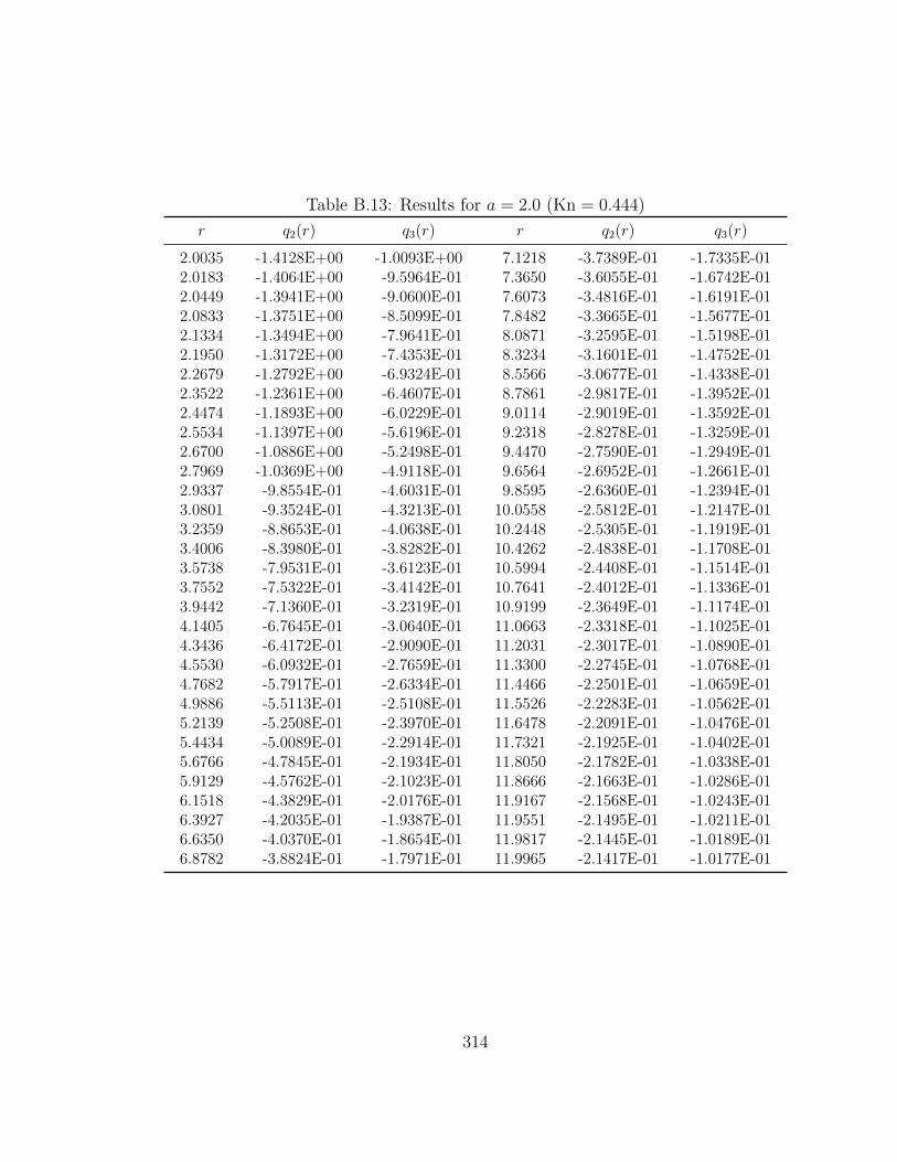
Table B.13: Results for a = 2.0 (Kn = 0.444)

r q2(r) q3(r) r q2(r) q3(r)

2.0035 -1.4128E+00 -1.0093E+00 7.1218 -3.7389E-01 -1.7335E-012.0183 -1.4064E+00 -9.5964E-01 7.3650 -3.6055E-01 -1.6742E-012.0449 -1.3941E+00 -9.0600E-01 7.6073 -3.4816E-01 -1.6191E-012.0833 -1.3751E+00 -8.5099E-01 7.8482 -3.3665E-01 -1.5677E-012.1334 -1.3494E+00 -7.9641E-01 8.0871 -3.2595E-01 -1.5198E-012.1950 -1.3172E+00 -7.4353E-01 8.3234 -3.1601E-01 -1.4752E-012.2679 -1.2792E+00 -6.9324E-01 8.5566 -3.0677E-01 -1.4338E-012.3522 -1.2361E+00 -6.4607E-01 8.7861 -2.9817E-01 -1.3952E-012.4474 -1.1893E+00 -6.0229E-01 9.0114 -2.9019E-01 -1.3592E-012.5534 -1.1397E+00 -5.6196E-01 9.2318 -2.8278E-01 -1.3259E-012.6700 -1.0886E+00 -5.2498E-01 9.4470 -2.7590E-01 -1.2949E-012.7969 -1.0369E+00 -4.9118E-01 9.6564 -2.6952E-01 -1.2661E-012.9337 -9.8554E-01 -4.6031E-01 9.8595 -2.6360E-01 -1.2394E-013.0801 -9.3524E-01 -4.3213E-01 10.0558 -2.5812E-01 -1.2147E-013.2359 -8.8653E-01 -4.0638E-01 10.2448 -2.5305E-01 -1.1919E-013.4006 -8.3980E-01 -3.8282E-01 10.4262 -2.4838E-01 -1.1708E-013.5738 -7.9531E-01 -3.6123E-01 10.5994 -2.4408E-01 -1.1514E-013.7552 -7.5322E-01 -3.4142E-01 10.7641 -2.4012E-01 -1.1336E-013.9442 -7.1360E-01 -3.2319E-01 10.9199 -2.3649E-01 -1.1174E-014.1405 -6.7645E-01 -3.0640E-01 11.0663 -2.3318E-01 -1.1025E-014.3436 -6.4172E-01 -2.9090E-01 11.2031 -2.3017E-01 -1.0890E-014.5530 -6.0932E-01 -2.7659E-01 11.3300 -2.2745E-01 -1.0768E-014.7682 -5.7917E-01 -2.6334E-01 11.4466 -2.2501E-01 -1.0659E-014.9886 -5.5113E-01 -2.5108E-01 11.5526 -2.2283E-01 -1.0562E-015.2139 -5.2508E-01 -2.3970E-01 11.6478 -2.2091E-01 -1.0476E-015.4434 -5.0089E-01 -2.2914E-01 11.7321 -2.1925E-01 -1.0402E-015.6766 -4.7845E-01 -2.1934E-01 11.8050 -2.1782E-01 -1.0338E-015.9129 -4.5762E-01 -2.1023E-01 11.8666 -2.1663E-01 -1.0286E-016.1518 -4.3829E-01 -2.0176E-01 11.9167 -2.1568E-01 -1.0243E-016.3927 -4.2035E-01 -1.9387E-01 11.9551 -2.1495E-01 -1.0211E-016.6350 -4.0370E-01 -1.8654E-01 11.9817 -2.1445E-01 -1.0189E-016.8782 -3.8824E-01 -1.7971E-01 11.9965 -2.1417E-01 -1.0177E-01

314

Table B.14: Results for a = 2.5 (Kn = 0.355)

r q2(r) q3(r) r q2(r) q3(r)

2.5035 -1.4132E+00 -1.0558E+00 7.6218 -4.7018E-01 -2.2274E-012.5183 -1.4087E+00 -1.0157E+00 7.8650 -4.5476E-01 -2.1548E-012.5449 -1.4000E+00 -9.7139E-01 8.1073 -4.4034E-01 -2.0870E-012.5833 -1.3866E+00 -9.2488E-01 8.3482 -4.2687E-01 -2.0237E-012.6334 -1.3682E+00 -8.7757E-01 8.5871 -4.1429E-01 -1.9646E-012.6950 -1.3449E+00 -8.3051E-01 8.8234 -4.0253E-01 -1.9095E-012.7679 -1.3168E+00 -7.8453E-01 9.0566 -3.9156E-01 -1.8581E-012.8522 -1.2844E+00 -7.4021E-01 9.2861 -3.8132E-01 -1.8101E-012.9474 -1.2483E+00 -6.9798E-01 9.5114 -3.7177E-01 -1.7654E-013.0534 -1.2093E+00 -6.5806E-01 9.7318 -3.6286E-01 -1.7237E-013.1700 -1.1680E+00 -6.2057E-01 9.9470 -3.5457E-01 -1.6850E-013.2969 -1.1251E+00 -5.8554E-01 10.1564 -3.4686E-01 -1.6490E-013.4337 -1.0815E+00 -5.5290E-01 10.3595 -3.3968E-01 -1.6156E-013.5801 -1.0378E+00 -5.2256E-01 10.5558 -3.3303E-01 -1.5846E-013.7359 -9.9433E-01 -4.9440E-01 10.7448 -3.2686E-01 -1.5560E-013.9006 -9.5171E-01 -4.6828E-01 10.9262 -3.2114E-01 -1.5295E-014.0738 -9.1024E-01 -4.4404E-01 11.0994 -3.1587E-01 -1.5051E-014.2552 -8.7018E-01 -4.2156E-01 11.2641 -3.1102E-01 -1.4827E-014.4442 -8.3172E-01 -4.0069E-01 11.4199 -3.0657E-01 -1.4622E-014.6405 -7.9499E-01 -3.8130E-01 11.5663 -3.0250E-01 -1.4434E-014.8436 -7.6005E-01 -3.6328E-01 11.7031 -2.9879E-01 -1.4264E-015.0530 -7.2694E-01 -3.4653E-01 11.8300 -2.9544E-01 -1.4110E-015.2682 -6.9564E-01 -3.3094E-01 11.9466 -2.9242E-01 -1.3972E-015.4886 -6.6614E-01 -3.1641E-01 12.0526 -2.8973E-01 -1.3849E-015.7139 -6.3837E-01 -3.0289E-01 12.1478 -2.8736E-01 -1.3740E-015.9434 -6.1228E-01 -2.9028E-01 12.2321 -2.8529E-01 -1.3646E-016.1766 -5.8779E-01 -2.7853E-01 12.3050 -2.8353E-01 -1.3566E-016.4129 -5.6482E-01 -2.6755E-01 12.3666 -2.8205E-01 -1.3499E-016.6518 -5.4331E-01 -2.5732E-01 12.4167 -2.8087E-01 -1.3445E-016.8927 -5.2317E-01 -2.4777E-01 12.4551 -2.7996E-01 -1.3404E-017.1350 -5.0431E-01 -2.3885E-01 12.4817 -2.7934E-01 -1.3376E-017.3782 -4.8667E-01 -2.3052E-01 12.4965 -2.7900E-01 -1.3360E-01

315

Table B.15: Results for a = 3.0 (Kn = 0.296)

r q2(r) q3(r) r q2(r) q3(r)

3.0035 -1.4134E+00 -1.0922E+00 8.1218 -5.5593E-01 -2.6910E-013.0183 -1.4101E+00 -1.0587E+00 8.3650 -5.3910E-01 -2.6070E-013.0449 -1.4036E+00 -1.0211E+00 8.6073 -5.2329E-01 -2.5283E-013.0833 -1.3935E+00 -9.8093E-01 8.8482 -5.0844E-01 -2.4547E-013.1334 -1.3797E+00 -9.3932E-01 9.0871 -4.9450E-01 -2.3859E-013.1950 -1.3621E+00 -8.9716E-01 9.3234 -4.8142E-01 -2.3216E-013.2679 -1.3405E+00 -8.5518E-01 9.5566 -4.6916E-01 -2.2615E-013.3522 -1.3153E+00 -8.1393E-01 9.7861 -4.5768E-01 -2.2053E-013.4474 -1.2868E+00 -7.7386E-01 10.0114 -4.4693E-01 -2.1530E-013.5534 -1.2554E+00 -7.3528E-01 10.2318 -4.3688E-01 -2.1041E-013.6700 -1.2216E+00 -6.9841E-01 10.4470 -4.2749E-01 -2.0586E-013.7969 -1.1859E+00 -6.6336E-01 10.6564 -4.1873E-01 -2.0162E-013.9337 -1.1489E+00 -6.3020E-01 10.8595 -4.1056E-01 -1.9768E-014.0801 -1.1111E+00 -5.9893E-01 11.0558 -4.0296E-01 -1.9402E-014.2359 -1.0728E+00 -5.6954E-01 11.2448 -3.9590E-01 -1.9064E-014.4006 -1.0347E+00 -5.4193E-01 11.4262 -3.8936E-01 -1.8751E-014.5738 -9.9688E-01 -5.1606E-01 11.5994 -3.8330E-01 -1.8462E-014.7552 -9.5978E-01 -4.9183E-01 11.7641 -3.7772E-01 -1.8196E-014.9442 -9.2361E-01 -4.6915E-01 11.9199 -3.7259E-01 -1.7952E-015.1405 -8.8855E-01 -4.4793E-01 12.0663 -3.6789E-01 -1.7730E-015.3436 -8.5472E-01 -4.2807E-01 12.2031 -3.6360E-01 -1.7527E-015.5530 -8.2224E-01 -4.0949E-01 12.3300 -3.5972E-01 -1.7344E-015.7682 -7.9115E-01 -3.9210E-01 12.4466 -3.5622E-01 -1.7180E-015.9886 -7.6150E-01 -3.7584E-01 12.5526 -3.5310E-01 -1.7033E-016.2139 -7.3329E-01 -3.6062E-01 12.6478 -3.5035E-01 -1.6904E-016.4434 -7.0650E-01 -3.4637E-01 12.7321 -3.4795E-01 -1.6792E-016.6766 -6.8112E-01 -3.3303E-01 12.8050 -3.4590E-01 -1.6696E-016.9129 -6.5710E-01 -3.2055E-01 12.8666 -3.4418E-01 -1.6616E-017.1518 -6.3442E-01 -3.0886E-01 12.9167 -3.4280E-01 -1.6552E-017.3927 -6.1301E-01 -2.9792E-01 12.9551 -3.4175E-01 -1.6503E-017.6350 -5.9283E-01 -2.8767E-01 12.9817 -3.4103E-01 -1.6469E-017.8782 -5.7382E-01 -2.7808E-01 12.9965 -3.4062E-01 -1.6451E-01

316

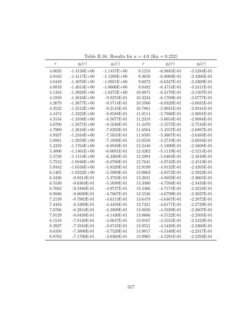
Table B.16: Results for a = 4.0 (Kn = 0.222)

r q2(r) q3(r) r q2(r) q3(r)

4.0035 -1.4138E+00 -1.1457E+00 9.1218 -6.9885E-01 -3.5284E-014.0183 -1.4117E+00 -1.1208E+00 9.3650 -6.8069E-01 -3.4266E-014.0449 -1.4076E+00 -1.0921E+00 9.6073 -6.6347E-01 -3.3309E-014.0833 -1.4014E+00 -1.0606E+00 9.8482 -6.4714E-01 -3.2411E-014.1334 -1.3928E+00 -1.0272E+00 10.0871 -6.3170E-01 -3.1567E-014.1950 -1.3816E+00 -9.9255E-01 10.3234 -6.1709E-01 -3.0777E-014.2679 -1.3677E+00 -9.5714E-01 10.5566 -6.0329E-01 -3.0035E-014.3522 -1.3512E+00 -9.2145E-01 10.7861 -5.9031E-01 -2.9341E-014.4474 -1.3322E+00 -8.8588E-01 11.0114 -5.7806E-01 -2.8691E-014.5534 -1.3108E+00 -8.5077E-01 11.2318 -5.6654E-01 -2.8084E-014.6700 -1.2871E+00 -8.1638E-01 11.4470 -5.5572E-01 -2.7516E-014.7969 -1.2616E+00 -7.8292E-01 11.6564 -5.4557E-01 -2.6987E-014.9337 -1.2344E+00 -7.5055E-01 11.8595 -5.3607E-01 -2.6493E-015.0801 -1.2059E+00 -7.1938E-01 12.0558 -5.2719E-01 -2.6034E-015.2359 -1.1764E+00 -6.8949E-01 12.2448 -5.1890E-01 -2.5608E-015.4006 -1.1461E+00 -6.6091E-01 12.4262 -5.1119E-01 -2.5214E-015.5738 -1.1154E+00 -6.3368E-01 12.5994 -5.0404E-01 -2.4849E-015.7552 -1.0846E+00 -6.0780E-01 12.7641 -4.9742E-01 -2.4513E-015.9442 -1.0538E+00 -5.8320E-01 12.9199 -4.9132E-01 -2.4205E-016.1405 -1.0232E+00 -5.5989E-01 13.0663 -4.8572E-01 -2.3922E-016.3436 -9.9314E-01 -5.3783E-01 13.2031 -4.8059E-01 -2.3665E-016.5530 -9.6364E-01 -5.1698E-01 13.3300 -4.7594E-01 -2.3433E-016.7682 -9.3486E-01 -4.9727E-01 13.4466 -4.7174E-01 -2.3224E-016.9886 -9.0690E-01 -4.7867E-01 13.5526 -4.6799E-01 -2.3037E-017.2139 -8.7982E-01 -4.6113E-01 13.6478 -4.6467E-01 -2.2872E-017.4434 -8.5369E-01 -4.4458E-01 13.7321 -4.6177E-01 -2.2729E-017.6766 -8.2854E-01 -4.2899E-01 13.8050 -4.5929E-01 -2.2607E-017.9129 -8.0438E-01 -4.1430E-01 13.8666 -4.5722E-01 -2.2505E-018.1518 -7.8126E-01 -4.0047E-01 13.9167 -4.5555E-01 -2.2423E-018.3927 -7.5916E-01 -3.8745E-01 13.9551 -4.5428E-01 -2.2360E-018.6350 -7.3806E-01 -3.7520E-01 13.9817 -4.5340E-01 -2.2317E-018.8782 -7.1796E-01 -3.6368E-01 13.9965 -4.5291E-01 -2.2293E-01

317

Table B.17: Results for a = 5.0 (Kn = 0.178)

r q2(r) q3(r) r q2(r) q3(r)

5.0035 -1.4139E+00 -1.1835E+00 10.1218 -8.1081E-01 -4.2599E-015.0183 -1.4125E+00 -1.1638E+00 10.3650 -7.9254E-01 -4.1455E-015.0449 -1.4097E+00 -1.1407E+00 10.6073 -7.7507E-01 -4.0376E-015.0833 -1.4054E+00 -1.1149E+00 10.8482 -7.5839E-01 -3.9363E-015.1334 -1.3995E+00 -1.0871E+00 11.0871 -7.4248E-01 -3.8403E-015.1950 -1.3918E+00 -1.0577E+00 11.3234 -7.2735E-01 -3.7502E-015.2679 -1.3821E+00 -1.0272E+00 11.5566 -7.1299E-01 -3.6656E-015.3522 -1.3705E+00 -9.9603E-01 11.7861 -6.9938E-01 -3.5861E-015.4474 -1.3569E+00 -9.6443E-01 12.0114 -6.8648E-01 -3.5116E-015.5534 -1.3414E+00 -9.3271E-01 12.2318 -6.7429E-01 -3.4417E-015.6700 -1.3241E+00 -9.0116E-01 12.4470 -6.6278E-01 -3.3763E-015.7969 -1.3050E+00 -8.6997E-01 12.6564 -6.5194E-01 -3.3151E-015.9337 -1.2844E+00 -8.3934E-01 12.8595 -6.4174E-01 -3.2580E-016.0801 -1.2624E+00 -8.0941E-01 13.0558 -6.3218E-01 -3.2048E-016.2359 -1.2392E+00 -7.8032E-01 13.2448 -6.2323E-01 -3.1553E-016.4006 -1.2151E+00 -7.5213E-01 13.4262 -6.1487E-01 -3.1094E-016.5738 -1.1902E+00 -7.2493E-01 13.5994 -6.0709E-01 -3.0669E-016.7552 -1.1647E+00 -6.9876E-01 13.7641 -5.9987E-01 -3.0277E-016.9442 -1.1388E+00 -6.7365E-01 13.9199 -5.9320E-01 -2.9916E-017.1405 -1.1128E+00 -6.4960E-01 14.0663 -5.8705E-01 -2.9586E-017.3436 -1.0867E+00 -6.2663E-01 14.2031 -5.8142E-01 -2.9285E-017.5530 -1.0608E+00 -6.0471E-01 14.3300 -5.7630E-01 -2.9011E-017.7682 -1.0351E+00 -5.8383E-01 14.4466 -5.7167E-01 -2.8766E-017.9886 -1.0098E+00 -5.6398E-01 14.5526 -5.6752E-01 -2.8546E-018.2139 -9.8498E-01 -5.4512E-01 14.6478 -5.6385E-01 -2.8353E-018.4434 -9.6072E-01 -5.2723E-01 14.7321 -5.6064E-01 -2.8184E-018.6766 -9.3707E-01 -5.1026E-01 14.8050 -5.5789E-01 -2.8040E-018.9129 -9.1414E-01 -4.9418E-01 14.8666 -5.5559E-01 -2.7920E-019.1518 -8.9191E-01 -4.7897E-01 14.9167 -5.5374E-01 -2.7823E-019.3927 -8.7045E-01 -4.6457E-01 14.9551 -5.5232E-01 -2.7749E-019.6350 -8.4977E-01 -4.5097E-01 14.9817 -5.5135E-01 -2.7699E-019.8782 -8.2989E-01 -4.3812E-01 14.9965 -5.5080E-01 -2.7670E-01

318

Table B.18: Results for a = 6.0 (Kn = 0.148)

r q2(r) q3(r) r q2(r) q3(r)

6.0035 -1.4140E+00 -1.2117E+00 11.1218 -8.9929E-01 -4.9006E-016.0183 -1.4129E+00 -1.1956E+00 11.3650 -8.8154E-01 -4.7774E-016.0449 -1.4109E+00 -1.1762E+00 11.6073 -8.6447E-01 -4.6609E-016.0833 -1.4078E+00 -1.1544E+00 11.8482 -8.4807E-01 -4.5508E-016.1334 -1.4035E+00 -1.1306E+00 12.0871 -8.3235E-01 -4.4468E-016.1950 -1.3978E+00 -1.1051E+00 12.3234 -8.1732E-01 -4.3488E-016.2679 -1.3907E+00 -1.0784E+00 12.5566 -8.0296E-01 -4.2564E-016.3522 -1.3821E+00 -1.0508E+00 12.7861 -7.8927E-01 -4.1695E-016.4474 -1.3719E+00 -1.0225E+00 13.0114 -7.7625E-01 -4.0877E-016.5534 -1.3602E+00 -9.9376E-01 13.2318 -7.6389E-01 -4.0109E-016.6700 -1.3469E+00 -9.6485E-01 13.4470 -7.5218E-01 -3.9389E-016.7969 -1.3322E+00 -9.3596E-01 13.6564 -7.4110E-01 -3.8714E-016.9337 -1.3161E+00 -9.0728E-01 13.8595 -7.3065E-01 -3.8083E-017.0801 -1.2987E+00 -8.7895E-01 14.0558 -7.2081E-01 -3.7494E-017.2359 -1.2802E+00 -8.5112E-01 14.2448 -7.1157E-01 -3.6946E-017.4006 -1.2606E+00 -8.2390E-01 14.4262 -7.0292E-01 -3.6438E-017.5738 -1.2401E+00 -7.9739E-01 14.5994 -6.9484E-01 -3.5964E-017.7552 -1.2189E+00 -7.7164E-01 14.7641 -6.8732E-01 -3.5527E-017.9442 -1.1972E+00 -7.4671E-01 14.9199 -6.8036E-01 -3.5125E-018.1405 -1.1750E+00 -7.2265E-01 15.0663 -6.7394E-01 -3.4756E-018.3436 -1.1525E+00 -6.9949E-01 15.2031 -6.6804E-01 -3.4419E-018.5530 -1.1299E+00 -6.7723E-01 15.3300 -6.6267E-01 -3.4115E-018.7682 -1.1073E+00 -6.5589E-01 15.4466 -6.5779E-01 -3.3838E-018.9886 -1.0848E+00 -6.3546E-01 15.5526 -6.5344E-01 -3.3593E-019.2139 -1.0624E+00 -6.1594E-01 15.6478 -6.4957E-01 -3.3376E-019.4434 -1.0403E+00 -5.9730E-01 15.7321 -6.4618E-01 -3.3186E-019.6766 -1.0187E+00 -5.7955E-01 15.8050 -6.4328E-01 -3.3024E-019.9129 -9.9739E-01 -5.6265E-01 15.8666 -6.4084E-01 -3.2889E-01

10.1518 -9.7661E-01 -5.4657E-01 15.9167 -6.3888E-01 -3.2780E-0110.3927 -9.5638E-01 -5.3130E-01 15.9551 -6.3739E-01 -3.2697E-0110.6350 -9.3673E-01 -5.1681E-01 15.9817 -6.3635E-01 -3.2640E-0110.8782 -9.1769E-01 -5.0307E-01 15.9965 -6.3578E-01 -3.2609E-01

319

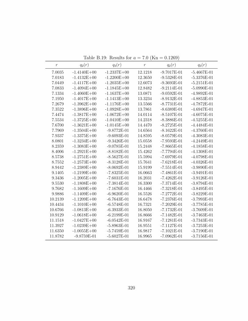
Table B.19: Results for a = 7.0 (Kn = 0.1269)

r q2(r) q3(r) r q2(r) q3(r)

7.0035 -1.4140E+00 -1.2337E+00 12.1218 -9.7017E-01 -5.4667E-017.0183 -1.4132E+00 -1.2200E+00 12.3650 -9.5328E-01 -5.3376E-017.0449 -1.4117E+00 -1.2035E+00 12.6073 -9.3693E-01 -5.2151E-017.0833 -1.4094E+00 -1.1845E+00 12.8482 -9.2114E-01 -5.0990E-017.1334 -1.4060E+00 -1.1637E+00 13.0871 -9.0592E-01 -4.9892E-017.1950 -1.4017E+00 -1.1413E+00 13.3234 -8.9132E-01 -4.8853E-017.2679 -1.3962E+00 -1.1176E+00 13.5566 -8.7731E-01 -4.7872E-017.3522 -1.3896E+00 -1.0928E+00 13.7861 -8.6389E-01 -4.6947E-017.4474 -1.3817E+00 -1.0672E+00 14.0114 -8.5107E-01 -4.6075E-017.5534 -1.3725E+00 -1.0410E+00 14.2318 -8.3886E-01 -4.5255E-017.6700 -1.3621E+00 -1.0145E+00 14.4470 -8.2725E-01 -4.4484E-017.7969 -1.3504E+00 -9.8772E-01 14.6564 -8.1622E-01 -4.3760E-017.9337 -1.3375E+00 -9.6093E-01 14.8595 -8.0579E-01 -4.3083E-018.0801 -1.3234E+00 -9.3426E-01 15.0558 -7.9593E-01 -4.2449E-018.2359 -1.3083E+00 -9.0785E-01 15.2448 -7.8665E-01 -4.1858E-018.4006 -1.2921E+00 -8.8182E-01 15.4262 -7.7794E-01 -4.1308E-018.5738 -1.2751E+00 -8.5627E-01 15.5994 -7.6979E-01 -4.0798E-018.7552 -1.2573E+00 -8.3128E-01 15.7641 -7.6218E-01 -4.0326E-018.9442 -1.2389E+00 -8.0692E-01 15.9199 -7.5514E-01 -3.9890E-019.1405 -1.2199E+00 -7.8325E-01 16.0663 -7.4861E-01 -3.9491E-019.3436 -1.2005E+00 -7.6031E-01 16.2031 -7.4262E-01 -3.9126E-019.5530 -1.1808E+00 -7.3814E-01 16.3300 -7.3714E-01 -3.8794E-019.7682 -1.1609E+00 -7.1676E-01 16.4466 -7.3218E-01 -3.8495E-019.9886 -1.1409E+00 -6.9620E-01 16.5526 -7.2772E-01 -3.8229E-01

10.2139 -1.1209E+00 -6.7643E-01 16.6478 -7.2376E-01 -3.7993E-0110.4434 -1.1010E+00 -6.5748E-01 16.7321 -7.2029E-01 -3.7785E-0110.6766 -1.0813E+00 -6.3933E-01 16.8050 -7.1732E-01 -3.7609E-0110.9129 -1.0618E+00 -6.2199E-01 16.8666 -7.1482E-01 -3.7463E-0111.1518 -1.0427E+00 -6.0542E-01 16.9167 -7.1281E-01 -3.7343E-0111.3927 -1.0239E+00 -5.8963E-01 16.9551 -7.1127E-01 -3.7253E-0111.6350 -1.0055E+00 -5.7459E-01 16.9817 -7.1021E-01 -3.7190E-0111.8782 -9.8759E-01 -5.6027E-01 16.9965 -7.0962E-01 -3.7156E-01

320

Table B.20: Results for a = 8.0 (Kn = 0.111)

r q2(r) q3(r) r q2(r) q3(r)

8.0035 -1.4141E+00 -1.2514E+00 13.1218 -1.0278E+00 -5.9716E-018.0183 -1.4135E+00 -1.2396E+00 13.3650 -1.0119E+00 -5.8386E-018.0449 -1.4122E+00 -1.2251E+00 13.6073 -9.9639E-01 -5.7121E-018.0833 -1.4104E+00 -1.2084E+00 13.8482 -9.8139E-01 -5.5920E-018.1334 -1.4078E+00 -1.1899E+00 14.0871 -9.6688E-01 -5.4780E-018.1950 -1.4044E+00 -1.1699E+00 14.3234 -9.5287E-01 -5.3700E-018.2679 -1.4000E+00 -1.1486E+00 14.5566 -9.3938E-01 -5.2678E-018.3522 -1.3947E+00 -1.1262E+00 14.7861 -9.2642E-01 -5.1712E-018.4474 -1.3884E+00 -1.1029E+00 15.0114 -9.1400E-01 -5.0800E-018.5534 -1.3811E+00 -1.0789E+00 15.2318 -9.0212E-01 -4.9940E-018.6700 -1.3726E+00 -1.0544E+00 15.4470 -8.9079E-01 -4.9130E-018.7969 -1.3631E+00 -1.0295E+00 15.6564 -8.8000E-01 -4.8370E-018.9337 -1.3526E+00 -1.0045E+00 15.8595 -8.6977E-01 -4.7656E-019.0801 -1.3410E+00 -9.7939E-01 16.0558 -8.6008E-01 -4.6988E-019.2359 -1.3284E+00 -9.5441E-01 16.2448 -8.5093E-01 -4.6364E-019.4006 -1.3149E+00 -9.2962E-01 16.4262 -8.4231E-01 -4.5782E-019.5738 -1.3006E+00 -9.0515E-01 16.5994 -8.3424E-01 -4.5242E-019.7552 -1.2855E+00 -8.8107E-01 16.7641 -8.2669E-01 -4.4741E-019.9442 -1.2697E+00 -8.5747E-01 16.9199 -8.1968E-01 -4.4279E-01

10.1405 -1.2534E+00 -8.3441E-01 17.0663 -8.1317E-01 -4.3855E-0110.3436 -1.2365E+00 -8.1194E-01 17.2031 -8.0719E-01 -4.3466E-0110.5530 -1.2193E+00 -7.9012E-01 17.3300 -8.0171E-01 -4.3114E-0110.7682 -1.2018E+00 -7.6897E-01 17.4466 -7.9675E-01 -4.2795E-0110.9886 -1.1840E+00 -7.4853E-01 17.5526 -7.9228E-01 -4.2510E-0111.2139 -1.1662E+00 -7.2881E-01 17.6478 -7.8831E-01 -4.2258E-0111.4434 -1.1483E+00 -7.0981E-01 17.7321 -7.8482E-01 -4.2039E-0111.6766 -1.1304E+00 -6.9156E-01 17.8050 -7.8182E-01 -4.1850E-0111.9129 -1.1127E+00 -6.7401E-01 17.8666 -7.7931E-01 -4.1693E-0112.1518 -1.0951E+00 -6.5722E-01 17.9167 -7.7729E-01 -4.1566E-0112.3927 -1.0778E+00 -6.4114E-01 17.9551 -7.7574E-01 -4.1470E-0112.6350 -1.0608E+00 -6.2578E-01 17.9817 -7.7467E-01 -4.1403E-0112.8782 -1.0441E+00 -6.1113E-01 17.9965 -7.7408E-01 -4.1367E-01

321

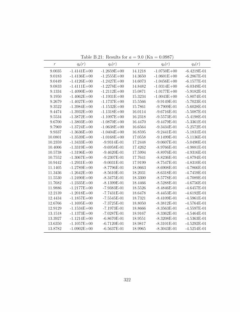
Table B.21: Results for a = 9.0 (Kn = 0.0987)

r q2(r) q3(r) r q2(r) q3(r)

9.0035 -1.4141E+00 -1.2659E+00 14.1218 -1.0750E+00 -6.4219E-019.0183 -1.4136E+00 -1.2555E+00 14.3650 -1.0601E+00 -6.2867E-019.0449 -1.4126E+00 -1.2427E+00 14.6073 -1.0456E+00 -6.1577E-019.0833 -1.4111E+00 -1.2278E+00 14.8482 -1.0314E+00 -6.0349E-019.1334 -1.4090E+00 -1.2112E+00 15.0871 -1.0177E+00 -5.9182E-019.1950 -1.4062E+00 -1.1931E+00 15.3234 -1.0043E+00 -5.8074E-019.2679 -1.4027E+00 -1.1737E+00 15.5566 -9.9149E-01 -5.7023E-019.3522 -1.3984E+00 -1.1532E+00 15.7861 -9.7909E-01 -5.6028E-019.4474 -1.3932E+00 -1.1318E+00 16.0114 -9.6716E-01 -5.5087E-019.5534 -1.3872E+00 -1.1097E+00 16.2318 -9.5573E-01 -5.4198E-019.6700 -1.3803E+00 -1.0870E+00 16.4470 -9.4479E-01 -5.3361E-019.7969 -1.3724E+00 -1.0638E+00 16.6564 -9.3434E-01 -5.2572E-019.9337 -1.3636E+00 -1.0404E+00 16.8595 -9.2441E-01 -5.1831E-01

10.0801 -1.3539E+00 -1.0168E+00 17.0558 -9.1499E-01 -5.1136E-0110.2359 -1.3433E+00 -9.9314E-01 17.2448 -9.0607E-01 -5.0490E-0110.4006 -1.3319E+00 -9.6958E-01 17.4262 -8.9766E-01 -4.9881E-0110.5738 -1.3196E+00 -9.4620E-01 17.5994 -8.8976E-01 -4.9316E-0110.7552 -1.3067E+00 -9.2307E-01 17.7641 -8.8236E-01 -4.8794E-0110.9442 -1.2931E+00 -9.0031E-01 17.9199 -8.7547E-01 -4.8310E-0111.1405 -1.2789E+00 -8.7796E-01 18.0663 -8.6908E-01 -4.7866E-0111.3436 -1.2642E+00 -8.5610E-01 18.2031 -8.6318E-01 -4.7459E-0111.5530 -1.2490E+00 -8.3475E-01 18.3300 -8.5778E-01 -4.7089E-0111.7682 -1.2335E+00 -8.1399E-01 18.4466 -8.5288E-01 -4.6756E-0111.9886 -1.2177E+00 -7.9383E-01 18.5526 -8.4846E-01 -4.6457E-0112.2139 -1.2018E+00 -7.7431E-01 18.6478 -8.4453E-01 -4.6192E-0112.4434 -1.1857E+00 -7.5545E-01 18.7321 -8.4109E-01 -4.5961E-0112.6766 -1.1695E+00 -7.3725E-01 18.8050 -8.3812E-01 -4.5764E-0112.9129 -1.1534E+00 -7.1973E-01 18.8666 -8.3563E-01 -4.5597E-0113.1518 -1.1373E+00 -7.0287E-01 18.9167 -8.3362E-01 -4.5464E-0113.3927 -1.1214E+00 -6.8670E-01 18.9551 -8.3208E-01 -4.5363E-0113.6350 -1.1057E+00 -6.7120E-01 18.9817 -8.3101E-01 -4.5292E-0113.8782 -1.0902E+00 -6.5637E-01 18.9965 -8.3043E-01 -4.5254E-01

322

Table B.22: Results for a = 10.0 (Kn = 0.0888)

r q2(r) q3(r) r q2(r) q3(r)

10.0035 -1.4141E+00 -1.2781E+00 15.1218 -1.1142E+00 -6.8287E-0110.0183 -1.4137E+00 -1.2689E+00 15.3650 -1.1004E+00 -6.6917E-0110.0449 -1.4129E+00 -1.2573E+00 15.6073 -1.0868E+00 -6.5613E-0110.0833 -1.4116E+00 -1.2439E+00 15.8482 -1.0735E+00 -6.4370E-0110.1334 -1.4099E+00 -1.2288E+00 16.0871 -1.0605E+00 -6.3185E-0110.1950 -1.4076E+00 -1.2123E+00 16.3234 -1.0479E+00 -6.2058E-0110.2679 -1.4047E+00 -1.1945E+00 16.5566 -1.0357E+00 -6.0987E-0110.3522 -1.4011E+00 -1.1757E+00 16.7861 -1.0239E+00 -5.9972E-0110.4474 -1.3969E+00 -1.1559E+00 17.0114 -1.0126E+00 -5.9011E-0110.5534 -1.3918E+00 -1.1354E+00 17.2318 -1.0016E+00 -5.8100E-0110.6700 -1.3860E+00 -1.1143E+00 17.4470 -9.9113E-01 -5.7241E-0110.7969 -1.3794E+00 -1.0926E+00 17.6564 -9.8110E-01 -5.6432E-0110.9337 -1.3719E+00 -1.0706E+00 17.8595 -9.7153E-01 -5.5670E-0111.0801 -1.3637E+00 -1.0484E+00 18.0558 -9.6243E-01 -5.4955E-0111.2359 -1.3546E+00 -1.0260E+00 18.2448 -9.5380E-01 -5.4286E-0111.4006 -1.3449E+00 -1.0036E+00 18.4262 -9.4563E-01 -5.3661E-0111.5738 -1.3343E+00 -9.8128E-01 18.5994 -9.3798E-01 -5.3079E-0111.7552 -1.3231E+00 -9.5912E-01 18.7641 -9.3079E-01 -5.2539E-0111.9442 -1.3113E+00 -9.3721E-01 18.9199 -9.2407E-01 -5.2039E-0112.1405 -1.2988E+00 -9.1562E-01 19.0663 -9.1784E-01 -5.1579E-0112.3436 -1.2859E+00 -8.9441E-01 19.2031 -9.1208E-01 -5.1158E-0112.5530 -1.2725E+00 -8.7365E-01 19.3300 -9.0680E-01 -5.0774E-0112.7682 -1.2587E+00 -8.5336E-01 19.4466 -9.0200E-01 -5.0428E-0112.9886 -1.2446E+00 -8.3360E-01 19.5526 -8.9768E-01 -5.0118E-0113.2139 -1.2303E+00 -8.1441E-01 19.6478 -8.9383E-01 -4.9843E-0113.4434 -1.2158E+00 -7.9579E-01 19.7321 -8.9045E-01 -4.9603E-0113.6766 -1.2012E+00 -7.7778E-01 19.8050 -8.8754E-01 -4.9397E-0113.9129 -1.1865E+00 -7.6038E-01 19.8666 -8.8509E-01 -4.9225E-0114.1518 -1.1718E+00 -7.4361E-01 19.9167 -8.8312E-01 -4.9086E-0114.3927 -1.1572E+00 -7.2747E-01 19.9551 -8.8160E-01 -4.8981E-0114.6350 -1.1427E+00 -7.1196E-01 19.9817 -8.8056E-01 -4.8907E-0114.8782 -1.1284E+00 -6.9708E-01 19.9965 -8.7998E-01 -4.8867E-01

323

Table B.23: Results for a = 50 (Kn = 0.0178)

r q2(r) q3(r) r q2(r) q3(r)

50.0035 -1.4142E+00 -1.3838E+00 55.1218 -1.3893E+00 -1.1870E+0050.0183 -1.4142E+00 -1.3823E+00 55.3650 -1.3875E+00 -1.1795E+0050.0449 -1.4142E+00 -1.3801E+00 55.6073 -1.3856E+00 -1.1722E+0050.0833 -1.4141E+00 -1.3775E+00 55.8482 -1.3837E+00 -1.1649E+0050.1334 -1.4140E+00 -1.3743E+00 56.0871 -1.3818E+00 -1.1579E+0050.1950 -1.4139E+00 -1.3708E+00 56.3234 -1.3799E+00 -1.1510E+0050.2679 -1.4138E+00 -1.3668E+00 56.5566 -1.3780E+00 -1.1443E+0050.3522 -1.4136E+00 -1.3625E+00 56.7861 -1.3760E+00 -1.1379E+0050.4474 -1.4134E+00 -1.3579E+00 57.0114 -1.3741E+00 -1.1314E+0050.5534 -1.4132E+00 -1.3529E+00 57.2318 -1.3722E+00 -1.1253E+0050.6700 -1.4129E+00 -1.3476E+00 57.4470 -1.3703E+00 -1.1193E+0050.7969 -1.4125E+00 -1.3420E+00 57.6564 -1.3685E+00 -1.1136E+0050.9337 -1.4121E+00 -1.3361E+00 57.8595 -1.3667E+00 -1.1082E+0051.0801 -1.4117E+00 -1.3299E+00 58.0558 -1.3649E+00 -1.1029E+0051.2359 -1.4112E+00 -1.3235E+00 58.2448 -1.3632E+00 -1.0979E+0051.4006 -1.4106E+00 -1.3168E+00 58.4262 -1.3615E+00 -1.0932E+0051.5738 -1.4099E+00 -1.3099E+00 58.5994 -1.3599E+00 -1.0887E+0051.7552 -1.4092E+00 -1.3029E+00 58.7641 -1.3584E+00 -1.0845E+0051.9442 -1.4084E+00 -1.2956E+00 58.9199 -1.3569E+00 -1.0805E+0052.1405 -1.4075E+00 -1.2882E+00 59.0663 -1.3555E+00 -1.0768E+0052.3436 -1.4066E+00 -1.2807E+00 59.2031 -1.3542E+00 -1.0734E+0052.5530 -1.4055E+00 -1.2730E+00 59.3300 -1.3530E+00 -1.0702E+0052.7682 -1.4044E+00 -1.2654E+00 59.4466 -1.3519E+00 -1.0674E+0052.9886 -1.4032E+00 -1.2575E+00 59.5526 -1.3509E+00 -1.0648E+0053.2139 -1.4019E+00 -1.2496E+00 59.6478 -1.3499E+00 -1.0624E+0053.4434 -1.4006E+00 -1.2417E+00 59.7321 -1.3491E+00 -1.0603E+0053.6766 -1.3992E+00 -1.2338E+00 59.8050 -1.3484E+00 -1.0586E+0053.9129 -1.3977E+00 -1.2258E+00 59.8666 -1.3478E+00 -1.0571E+0054.1518 -1.3961E+00 -1.2179E+00 59.9167 -1.3473E+00 -1.0559E+0054.3927 -1.3945E+00 -1.2101E+00 59.9551 -1.3465E+00 -1.0549E+0054.6350 -1.3928E+00 -1.2023E+00 59.9817 -1.3467E+00 -1.0543E+0054.8782 -1.3911E+00 -1.1946E+00 59.9965 -1.3466E+00 -1.0540E+00

324

Table B.24: Results for a = 100 (Kn = 0.00888)

r q2(r) q3(r) r q2(r) q3(r)

100.0035 -1.4141E+00 -1.3993E+00 105.1218 -1.4074E+00 -1.2950E+00100.0183 -1.4142E+00 -1.3986E+00 105.3650 -1.4069E+00 -1.2906E+00100.0449 -1.4142E+00 -1.3975E+00 105.6073 -1.4063E+00 -1.2864E+00100.0833 -1.4142E+00 -1.3962E+00 105.8482 -1.4058E+00 -1.2823E+00100.1334 -1.4142E+00 -1.3947E+00 106.0871 -1.4052E+00 -1.2780E+00100.1950 -1.4141E+00 -1.3930E+00 106.3234 -1.4046E+00 -1.2738E+00100.2679 -1.4141E+00 -1.3910E+00 106.5566 -1.4040E+00 -1.2698E+00100.3522 -1.4141E+00 -1.3889E+00 106.7861 -1.4035E+00 -1.2658E+00100.4474 -1.4140E+00 -1.3866E+00 107.0114 -1.4029E+00 -1.2620E+00100.5534 -1.4140E+00 -1.3841E+00 107.2318 -1.4023E+00 -1.2583E+00100.6700 -1.4139E+00 -1.3814E+00 107.4470 -1.4017E+00 -1.2546E+00100.7969 -1.4138E+00 -1.3786E+00 107.6564 -1.4011E+00 -1.2511E+00100.9337 -1.4137E+00 -1.3756E+00 107.8595 -1.4005E+00 -1.2477E+00101.0801 -1.4136E+00 -1.3724E+00 108.0558 -1.3999E+00 -1.2445E+00101.2359 -1.4135E+00 -1.3692E+00 108.2448 -1.3994E+00 -1.2413E+00101.4006 -1.4133E+00 -1.3657E+00 108.4262 -1.3989E+00 -1.2383E+00101.5738 -1.4131E+00 -1.3623E+00 108.5994 -1.3984E+00 -1.2355E+00101.7552 -1.4129E+00 -1.3585E+00 108.7641 -1.3979E+00 -1.2328E+00101.9442 -1.4127E+00 -1.3547E+00 108.9199 -1.3974E+00 -1.2303E+00102.1405 -1.4125E+00 -1.3508E+00 109.0663 -1.3969E+00 -1.2280E+00102.3436 -1.4122E+00 -1.3469E+00 109.2031 -1.3965E+00 -1.2258E+00102.5530 -1.4120E+00 -1.3427E+00 109.3300 -1.3961E+00 -1.2237E+00102.7682 -1.4117E+00 -1.3386E+00 109.4466 -1.3957E+00 -1.2219E+00102.9886 -1.4113E+00 -1.3343E+00 109.5526 -1.3954E+00 -1.2202E+00103.2139 -1.4110E+00 -1.3301E+00 109.6478 -1.3951E+00 -1.2187E+00103.4434 -1.4106E+00 -1.3257E+00 109.7321 -1.3948E+00 -1.2173E+00103.6766 -1.4102E+00 -1.3213E+00 109.8050 -1.3946E+00 -1.2162E+00103.9129 -1.4098E+00 -1.3170E+00 109.8666 -1.3944E+00 -1.2152E+00104.1518 -1.4094E+00 -1.3125E+00 109.9167 -1.3942E+00 -1.2145E+00104.3927 -1.4089E+00 -1.3082E+00 109.9551 -1.3941E+00 -1.2138E+00104.6350 -1.4084E+00 -1.3037E+00 109.9817 -1.3940E+00 -1.2134E+00104.8782 -1.4079E+00 -1.2993E+00 109.9965 -1.3940E+00 -1.2132E+00

325

Table B.25: Results for c1 and c2

r0 Kn c1 c2

0.01 88.8 -0.0269 -14.72120.025 35.5 -0.0379 -14.33330.05 17.8 -0.0564 -13.6869

0.075 11.8 -0.0748 -13.04040.1 8.88 -0.0932 -12.3940

0.25 3.55 -0.2147 -12.12160.5 1.78 -0.3826 -5.5702

0.75 1.18 -0.5148 -3.41011.0 0.888 -0.6205 -2.3438

1.25 0.710 -0.7061 -1.71671.5 0.592 -0.7767 -1.3043

1.75 0.5074 -0.8356 -1.01662.0 0.444 -0.8854 -0.80382.5 0.355 -0.9649 -0.51503.0 0.296 -1.0253 -0.32954.0 0.222 -1.1115 -0.10395.0 0.178 -1.1706 0.02686.0 0.148 -1.2137 0.11137.0 0.1269 -1.2468 0.17078.0 0.111 -1.2734 0.21539.0 0.0987 -1.2949 0.2489

10.0 0.0888 -1.3129 0.275850.0 0.0178 -1.4655 0.4651100 0.00888 -1.4857 0.4858

326

Appendix C: Monte Carlo Drag and Torque Results

I have developed a Monte Carlo algorithm to compute the drag and torque on

an N -sphere aggregate in the free molecule regime. The algorithm is described in

Section 5.2.3. Here, I compare the results of my Monte Carlo algorithm to exact

results (where available) and to the drag results of Mackowski [36].

C.1 Drag on a Translating Sphere

The drag on a sphere in creeping flow in the free molecule regime F0 is given

by Epstein’s equation [32]. For purely diffuse reflection, my Monte Carlo algorithm

gives the drag as FMC = 1.001F0, and thus my MC results are in very good agree-

ment with the exact solution.

C.2 Drag on an Aggregate

Mackowski [36] developed a correlation for the drag on a fractal aggregate as

a function of the number of monomers N , the fractal dimension df , and the fractal

prefactor k0. The correlation is based on the results of his own Monte Carlo cal-

culations. Using Mackowski’s correlation [Eq. (68) of Ref. [36]], the translational

friction coefficients, normalized by Epstein’s equation, for 20- and 100-sphere aggre-

327

gates with df = 1.78 and k0 = 1.3 are 14.15 and 64.23, respectively. In comparison,

my Monte Carlo results for the 20- and 100-sphere aggregates with these fractal

dimensions are 14.51 and 64.58, respectively. Thus, my MC results are in very good

agreement with Mackowski’s correlation.

C.3 Torque on a Rotating Sphere

Epstein [32] calculates the torque on a sphere rotating about an axis through

its center. Using my Monte Carlo algorithm, I get TMC = 0.995T0, which is in very

good agreement with the exact value.

For a sphere rotating slowly around an axis located a distance R from its

center, the magnitude of the torque is given by

T = ζt,0ωR2 + ζr,0ω (C.1)

In other words, the torque is the sum of the torque on a sphere rotating about its

center with angular velocity ω and the torque due to the linear velocity of the sphere

center ωR moving at a distance R from the origin. My Monte Carlo results for the

torque for R = a and R = 2a are 3.763ζr,0ω and 12.15ζr,0ω, respectively, where a is

the sphere radius. These results are in very good agreement with the exact results

T = 3.785ζr,0ω and T = 12.14ζr,0ω for a sphere rotating around an axis R = a and

R = 2a from its center.

328

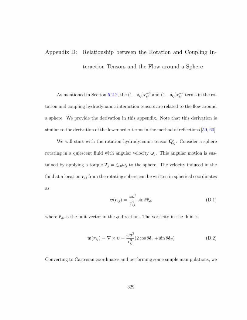
Appendix D: Relationship between the Rotation and Coupling In-

teraction Tensors and the Flow around a Sphere

As mentioned in Section 5.2.2, the (1−δij)r−3ij and (1−δij)r−2

ij terms in the ro-

tation and coupling hydrodynamic interaction tensors are related to the flow around

a sphere. We provide the derivation in this appendix. Note that this derivation is

similar to the derivation of the lower order terms in the method of reflections [59, 60].

We will start with the rotation hydrodynamic tensor Qrij. Consider a sphere

rotating in a quiescent fluid with angular velocity ωj. This angular motion is sus-

tained by applying a torque Tj = ζr,0ωj to the sphere. The velocity induced in the

fluid at a location rij from the rotating sphere can be written in spherical coordinates

as

v(rij) =ωa3

r2ij

sin θeφ (D.1)

where eφ is the unit vector in the φ-direction. The vorticity in the fluid is

w(rij) = ∇× v =ωa3

r3ij

(2 cos θer + sin θeθ) (D.2)

Converting to Cartesian coordinates and performing some simple manipulations, we

329

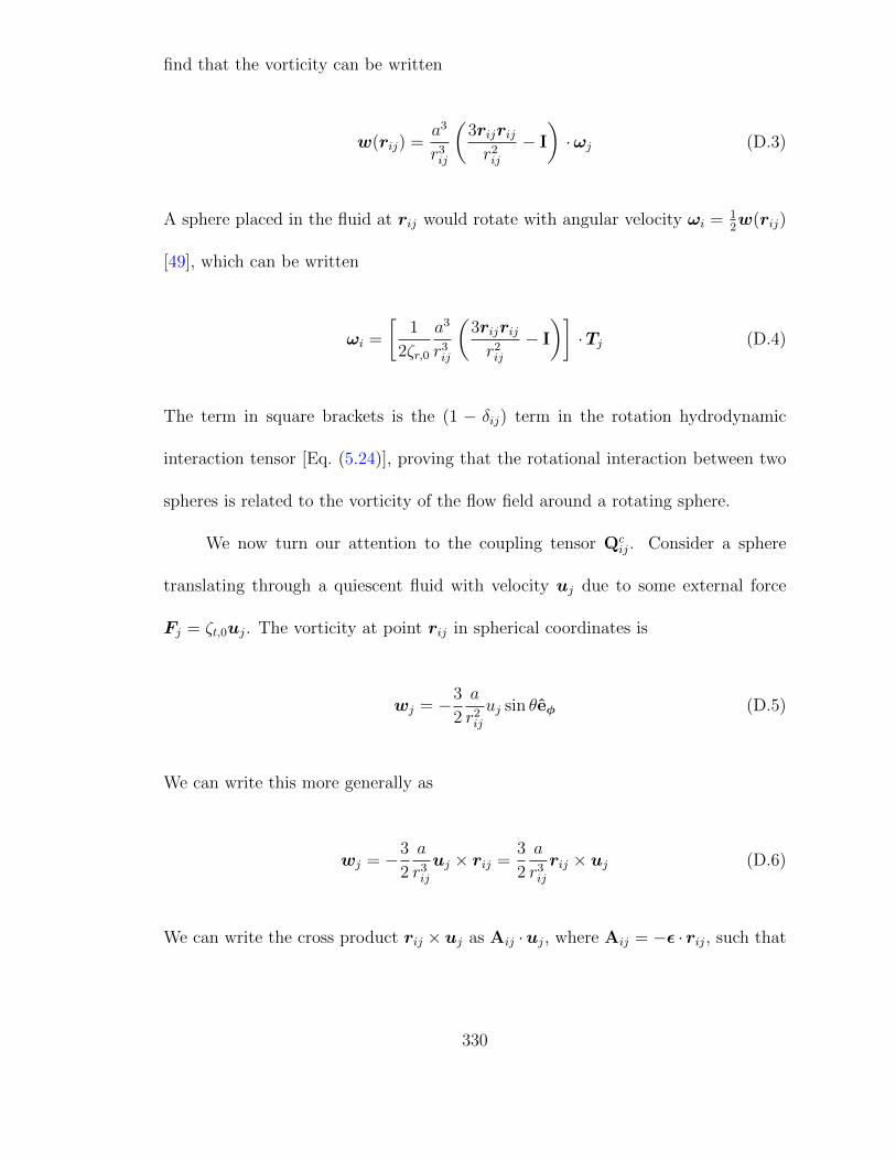
find that the vorticity can be written

w(rij) =a3

r3ij

(3rijrijr2ij

− I

)·ωj (D.3)

A sphere placed in the fluid at rij would rotate with angular velocity ωi = 12w(rij)

[49], which can be written

ωi =

[1

2ζr,0

a3

r3ij

(3rijrijr2ij

− I

)]·Tj (D.4)

The term in square brackets is the (1 − δij) term in the rotation hydrodynamic

interaction tensor [Eq. (5.24)], proving that the rotational interaction between two

spheres is related to the vorticity of the flow field around a rotating sphere.

We now turn our attention to the coupling tensor Qcij. Consider a sphere

translating through a quiescent fluid with velocity uj due to some external force

Fj = ζt,0uj. The vorticity at point rij in spherical coordinates is

wj = −3

2

a

r2ij

uj sin θeφ (D.5)

We can write this more generally as

wj = −3

2

a

r3ij

uj × rij =3

2

a

r3ij

rij × uj (D.6)

We can write the cross product rij × uj as Aij ·uj, where Aij = −ε · rij, such that

330

the vorticity becomes

wj = −(

3

2

a

r3ij

ε · rij)·uj (D.7)

Again, a sphere placed in the fluid at rij would rotate with angular velocity equal

to half the vorticity,

ωj = −(

3

4

a

r3ij

ε · rij)· Fj

6πµa(D.8)

Rearranging and introducing ζr,0 = 8πµa3, we get

ωj =

(−ε · rij

ζr,0

a3

r3ij

)·Fj (D.9)

The term in parentheses is the coupling interaction tensor Qcij given by Eq. (5.25).

This shows that the O(r−2ij ) term in the translation-rotation coupling interaction

tensor is given by the vorticity in the flow field for a translating sphere.

Alternatively, we can derive the coupling tensor by considering the velocity

field around a rotating sphere given by Eq. (D.1). Writing the velocity using the

cross product rij×ωj and converting the cross product to −(ε · rij) ·ωj, the velocity

becomes

v(rij) =a3

r3ij

(ε · rij) ·ωj (D.10)

Writing this equation using the torque applied on sphere j to maintain the angular

velocity ωj, we see that the fluid velocity at rij is

v(rij) =

(ε · rijζr,0

a3

r3ij

)·Tj (D.11)

331

The term in parentheses is the transpose of Qcij as written in Eq. (5.25), which

shows that the O(r−2ij ) term in (Qc

ij)† is given by the velocity field around a rotating

sphere.

332

Appendix E: Supplemental Material for Chapter 7

In this appendix, I provide a diagram of the body-fixed and space-fixed coor-

dinate systems used for my aggregate alignment calculations (Chapter 7), I show

probability distributions for one particle at different field strengths, I provide an ex-

ample calculation for one aggregate, and I expand upon my discussion of the effects

of Knudsen number and the number of primary spheres on fully-aligned particle

electrical mobility.

E.1 Euler Angles

The Euler angles (φ, θ, ψ) relate the body-fixed coordinates (x′, y′, z′) to the

space-fixed coordinates (x, y, z), as shown in Figure E.1. For our calculations, the

electric field is in the z-direction, and the principal axis of the polarizability tensor

is in the z′-direction. When the particle is aligned with the electric field, the z- and

z′-axes coincide.

E.2 Probability Distributions

Eq. (eqn:align:potential) gives the potential of a conducting particle in an elec-

tric field as a function of the polarizability tensor of the particle, the field strength,

333

Figure E.1: Representation of the Euler angles (φ, θ, ψ) that relate the body-fixedcoordinates (x′, y′, z′) to the space-fixed coordinates (x, y, z).

334

and the orientation of the particle relative to the field. When the electric field is

in the z-direction in space-fixed coordinates, the potential is a function of only two

of the three Euler angles shown in Figure E.1. In Figure E.2 below, I show the

probability distribution for a particle with 652 primary spheres with radius 5 nm at

three electric field strengths. The probability distribution is defined by Eq. (7.1). At

E = 1000 V/cm, the particle orientation is nearly random, while at E = 8000 V/cm,

the particle is aligned with the field. Note that the aligned particle can still rotate

around the principal axis of the polarizability tensor. Mobility results for this par-

ticle are shown in Figure 7.1.

E.3 Sample Calculation

The theory described in Chapter 7 requires one to determine the translational

friction tensor and the polarizability tensor for an aggregate in order to determine

the mobility of the particle at a given field strength. Here, I provide an example

problem for an aggregate with 10 primary spheres each having a radius a = 37.9 nm

(Kn = 1.78 for λ = 67.3 nm). The aggregate has a fractal dimension of 1.78 and

a prefactor of 1.3. The coordinates for the center of each sphere in the aggregate

are given in Table E.1. Coordinates are given relative to the center of mass of

the aggregate for an arbitrary Cartesian system. Velocity results for this Knudsen

number are available in Appendix B.

Using EKR theory (Chapters 4 and 6), one can determine the translational,

rotational, and coupling friction tensors in terms of the Cartesian coordinate system

335

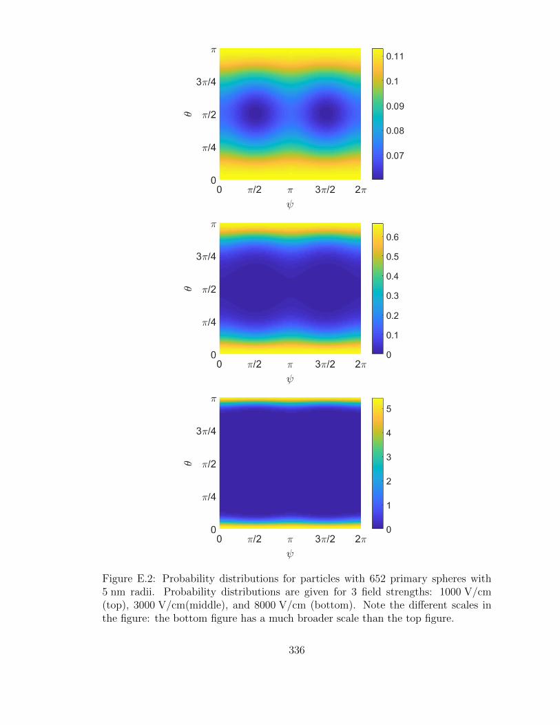
Figure E.2: Probability distributions for particles with 652 primary spheres with5 nm radii. Probability distributions are given for 3 field strengths: 1000 V/cm(top), 3000 V/cm(middle), and 8000 V/cm (bottom). Note the different scales inthe figure: the bottom figure has a much broader scale than the top figure.

336

Table E.1: Coordinates of the center of each sphere in my sample aggregate. Coordi-nates have been non-dimensionalized by the primary sphere radius. Since the centerof mass is at (0,0,0), simply multiply by the sphere radius to get the coordinates indimensional form.

Sphere x y z

1 -0.1717 -0.2663 -2.28872 2.0578 -0.0414 -0.27883 0.0587 -0.0934 -0.30964 0.3888 1.4840 -3.07745 -3.0183 -0.9897 2.33436 -1.7995 -1.6475 0.89157 -1.0953 -1.5832 -0.97948 -2.9090 0.6522 1.19769 3.1193 1.1203 2.2399

10 3.3692 1.3651 0.2707

in which the particle coordinates are given:

Ξt =

4.490 −0.2919 0.1575

−0.2919 4.710 0.1075

0.1575 0.1075 4.304

ζFMt,0 (E.1)

ΞO,r =

29.66 −7.276 1.057

−7.276 51.56 1.238

1.057 1.238 42.77

a2ζFMt,0 (E.2)

ΞO,c =

−0.6409 −0.3110 0.5337

0.9522 0.5417 0.2755

−0.7883 0.6892 0.0884

aζFMt,0 (E.3)

Here, ζFMt,0 is the free molecule friction coefficient based on the primary sphere radius.

337

For consistency with my velocity results, one should assume full thermal accommo-

dation when calculating the friction coefficient. The rotational and coupling tensors

are written with respect to the center of mass of the particle.

I obtain the polarizability tensor from ZENO [62]:

α =

513.0 114.1 −39.24

114.1 226.7 −31.19

−39.24 −31.19 394.1

ε0a3 (E.4)

Here, ε0 is the permittivity of free space. Note that ZENO uses stochastic methods

to obtain the polarizability tensor, so the code results can change slightly depend-

ing on the number of trials used in the calculation and on the initial seed to the

random number generator. Also note that the polarizability, translational friction,

and rotational friction tensors are symmetric, as expected.

For my calculations of the mobility as a function of electric field strength, I

choose the body-fixed coordinate system based on the eigenvectors of the polariz-

ability tensor: the z′-axis is the eigenvector associated with the largest eigenvalue of

the tensor, while the x′-axis coincides with the eigenvector of the smallest eigenvalue

of the tensor. In this coordinate system, the polarizability and translational friction

tensors become

α′ = V † ·α ·V =

185.4 0 0

0 382.3 0

0 0 566.0

ε0a3 (E.5)

338

Ξ′t = V † ·Ξt ·V =

4.869 0.0349 −0.1459

0.0349 4.404 −0.1777

−0.1459 −0.1777 4.232

ζFMt,0 (E.6)

where

V =

0.3193 0.2783 −0.9059

−0.9442 0.0116 −0.3293

−0.0811 0.9604 0.2664

(E.7)

is the tensor whose columns are the eigenvectors of α and V † is the transpose of that

tensor. I take the inverse of the translational friction tensor to obtain the mobility

tensor in body-fixed coordinates:

M = Ξ′t =

0.2056 −0.0013 0.0070

−0.0013 0.2275 0.0095

0.0070 0.0095 0.2369

(ζFMt,0

)−1(E.8)

Note that the mobility tensor in the body-fixed coordinate system is nearly, but

not quite, diagonal. For non-skew particles like spheres or prolate spheroids, the

eigenvectors for the polarizability a nd translational friction/mobility tensors would

be the same, and thus the mobility tensor would be diagonal in the body-fixed

system corresponding to the eigenvectors of the polarizability tensor.

From Eqs. (7.6) and (7.7) and the polarizability tensor above, the potential of

339

this particle in an electric field due to the induced dipole effects is

U = −12(185.4 sin2 ψ sin2 θ + 382.3 cos2 ψ sin2 θ + 566.0 cos2 θ)ε0a

3E2 (E.9)

where the angles are defined in Figure E.1. From Eqs. (7.8) and (7.9) and the

mobility tensor above, the mobility of the particle as a function of field strength is

Z =〈Vd,z〉E

=q

ζFMt,0

(0.2369〈cos2 θ〉+ 0.2275〈cos2 ψ sin2 θ〉+ 0.2056〈sin2 ψ sin2 θ〉

− 0.0013〈sin 2ψ sin2 θ〉+ 0.0070〈sinψ sin 2θ〉+ 0.0095〉 cosψ sin 2θ〉)

(E.10)

At very low field strengths, we get the mobility of the randomly oriented

particle, Zrand = 0.2233q/ζFMt,0 . At very high field strengths, we get the mobility

of the aligned particle, Zrand = 0.2369q/ζFMt,0 = 1.061Zrand. At a field strength of

5000 V/cm, we get Zrand = 0.2317q/ζFMt,0 = 1.038Zrand.

Note that we can also use my analytic expression for the translational friction

coefficient [Eq. (4.38) of Chapter 4] to obtain Zrand. From this expression, we get

Z?rand = 0.2289q/ζFM

t,0 = 1.025Zrand, where Zrand is the mobility we get from the

EKR method. This shows that my analytic expression gives a good estimate of the

friction coefficient or mobility of a randomly oriented DLCA particle, without having

to deal with the complexities of the EKR method. Note that my analytic expression

does not account for different morphologies (i.e. different sphere coordinates) for the

same primary sphere diameter, same N , and same fractal dimension.

340

E.4 Effects of Knudsen Number and the Number of Primary Spheres

on Fully-Aligned Particle Mobility

To evaluate the impact of particle size and flow regime on the aligned mobility

of soot-like particles, I calculated the random (electric field strength E → 0) and

fully-aligned (E → ∞) mobilities for a wide range of N and Kn. I also calculated

the random and fully-aligned mobilities using the standard Kirkwood-Riseman ap-

proach with the Rotne-Prager-Yamakawa hydrodynamic interaction tensor [see, for

example, [30]] and using a Monte Carlo code (Chapter 5 and Appendix C) for the

continuum (Kn = 0) and free molecular (Kn =∞) limits, respectively.

Figure 7.5 in the main body of this Disseration (repeated here as Figure E.3)

shows the calculated ratio of aligned to random mobility. The choppiness of the

graphs is due to the finite sample size of the aggregates I am using for these cal-

culations. The standard deviation of the mean of each data set (i.e. the mobility

ratio of 20 cases at a given Kn and N) is on the order of 0.007, which is significant

compared to the scale of the graph and the fluctuations in the mobility ratio with

N for a given Knudsen number. Accounting for these fluctuations due to the finite

sample size, we notice a few clear trends: while the mobility ratio is approximately

constant with N in the continuum regime, there is a clear decrease in mobility ratio

with increasing N near the free molecule regime. At intermediate Knudsen numbers,

the particles exhibit more continuum-like behavior with increasing N , which is con-

sistent with my earlier results for the translational friction coefficient (Chapter 4).

341

I will consider the physical reasons for these trends in the following paragraphs.

Figure E.3: Ratio of fully-aligned to random electric mobilities for wide range ofprimary sphere Knudsen numbers and the number of primaries. The Kn = 0 andKn = ∞ curves represent the continuum and free molecular limits, as calculatedusing the standard KR theory with the RPY tensor [see e.g. Chen et al. [30]] andusing a Monte Carlo code (Chapter 6), respectively. Uncertainties of one standarddeviation of the mean (based on 20 samples with the same fractal dimension butdifferent morphologies) are shown for the continuum and free molecule results forseveral N .

The continuum-like behavior of particles with many primary spheres at inter-

mediate Knudsen numbers has a straightforward explanation: as the particle size

increases, it has a larger effect on the velocity field of the surrounding fluid. In other

words, the particle behaves less like a collection of spheres in the transition regime

and more like an object that is large compared to the mean free path of molecules

in the fluid.

The behavior in the continuum and free molecular limits is more difficult to

explain. I will start by focusing on the continuum regime.

342

The continuum (randomly-oriented) friction coefficient can be written

ζ = 6πµRH (E.11)

where the hydrodynamic radius RH is the radius of a sphere that experiences the

same drag as the particle. Studies have shown that the hydrodynamic radius is

approximately equal to the radius of gyration for soot-like particles [4, 54, 93]. This

relationship between the hydrodynamic radius and the radius of gyration is only

valid for a randomly-oriented particle. Nevertheless, let us suppose that the drag

force on a particle in a fixed orientation moving in the z-direction is related to the

particles radius of gyration about the z-axis, which is defined as

Rgz =

√∑Ni (x2

i + y2i )

N(E.12)

for an aggregate of N spheres. Here, the center of the ith sphere is located at

(xi, yi, zi), while the center of mass of the particle is at the origin. Clearly, the

drag is not directly proportional to Rgz. As an example, the drag on a chain of

spheres or a rod moving parallel to its long axis increases with chain or rod length,

even though Rgz is independent of the chain or rod length. However, the drag

on a rod does increase as its radius increases (with length held constant), so a

larger Rgz corresponds to increased drag. I will look at the ratio of the radius of

gyration to the radius of gyration about the principal axis of the polarizability tensor

(i.e. the axis parallel to the particle velocity when the particle is fully-aligned with

343

the electric field) to evaluate whether trends in Rg/Rgz are correlated to trends in

the continuum mobility ratio Zalign/Zrand.1 If this is the case, we can use trends in

Rg/Rgz to qualitatively predict the effects of alignment on mobility.

To evaluate whether Rg/Rgz and Zalign/Zrand are correlated, I calculated these

ratios for all 20 cases for eachN and plotted the results in Figure E.4. I have included

results for N = 5, 10, 50, 100, 500, and 1000; results for other N are similar. In

general, aggregates with a low radius of gyration ratio also have a low mobility ratio.

Thus, we can conclude that there is a correlation between these two ratios.

As further verification of the correlation between Rg/Rgz and Zalign/Zrand, I

have computed the average ratios for a given N , then plotted the results in Fig-

ure E.5. Once again, we see that the ratios appear to be correlated.

Given that the radius of gyration ratio and the mobility ratio appear to be

correlated, we can look at the trends in Rg/Rgz to help explain the behavior of the

continuum curve in Figure E.3. Notably, there is less spread in the mean values of

Rg/Rgz versus N than there is in Zalign/Zrand for a given N , as evidenced by the

scale of the y-axis in Figure E.4 compared to the scale in Figure E.5. For example,

the ratio of the maximum to the minimum values of the mean Rg/Rgz vs. N is 1.14,

while for a typical set of 20 particles for a given N the ratio of maximum to minimum

values of Rg/Rgz is 1.65. Likewise, the continuum mobility ratio varies from 1.076

(at N = 50) to 1.094 (at N = 236 and N = 2000), while the minimum and maximum

mobility ratios for N = 100 (which represents an average case in terms of the spread

1Since the friction coefficient is approximately proportional to the radius of gyration, the mo-bility is inversely proportional to Rg.

344

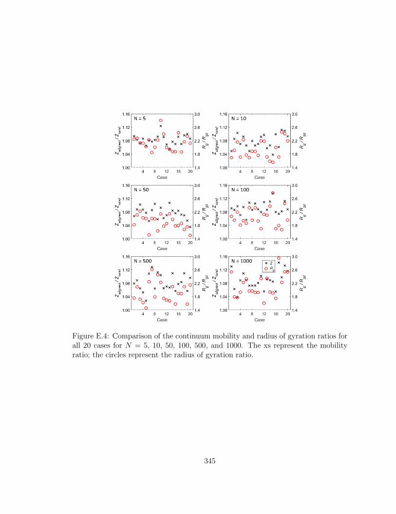
Figure E.4: Comparison of the continuum mobility and radius of gyration ratios forall 20 cases for N = 5, 10, 50, 100, 500, and 1000. The xs represent the mobilityratio; the circles represent the radius of gyration ratio.

345

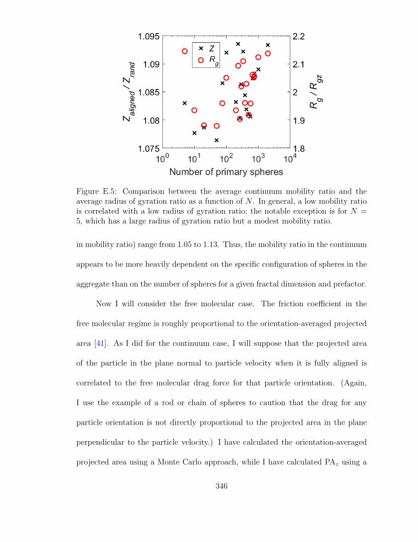
Figure E.5: Comparison between the average continuum mobility ratio and theaverage radius of gyration ratio as a function of N . In general, a low mobility ratiois correlated with a low radius of gyration ratio; the notable exception is for N =5, which has a large radius of gyration ratio but a modest mobility ratio.

in mobility ratio) range from 1.05 to 1.13. Thus, the mobility ratio in the continuum

appears to be more heavily dependent on the specific configuration of spheres in the

aggregate than on the number of spheres for a given fractal dimension and prefactor.

Now I will consider the free molecular case. The friction coefficient in the

free molecular regime is roughly proportional to the orientation-averaged projected

area [41]. As I did for the continuum case, I will suppose that the projected area

of the particle in the plane normal to particle velocity when it is fully aligned is

correlated to the free molecular drag force for that particle orientation. (Again,

I use the example of a rod or chain of spheres to caution that the drag for any

particle orientation is not directly proportional to the projected area in the plane

perpendicular to the particle velocity.) I have calculated the orientation-averaged

projected area using a Monte Carlo approach, while I have calculated PAz using a

346

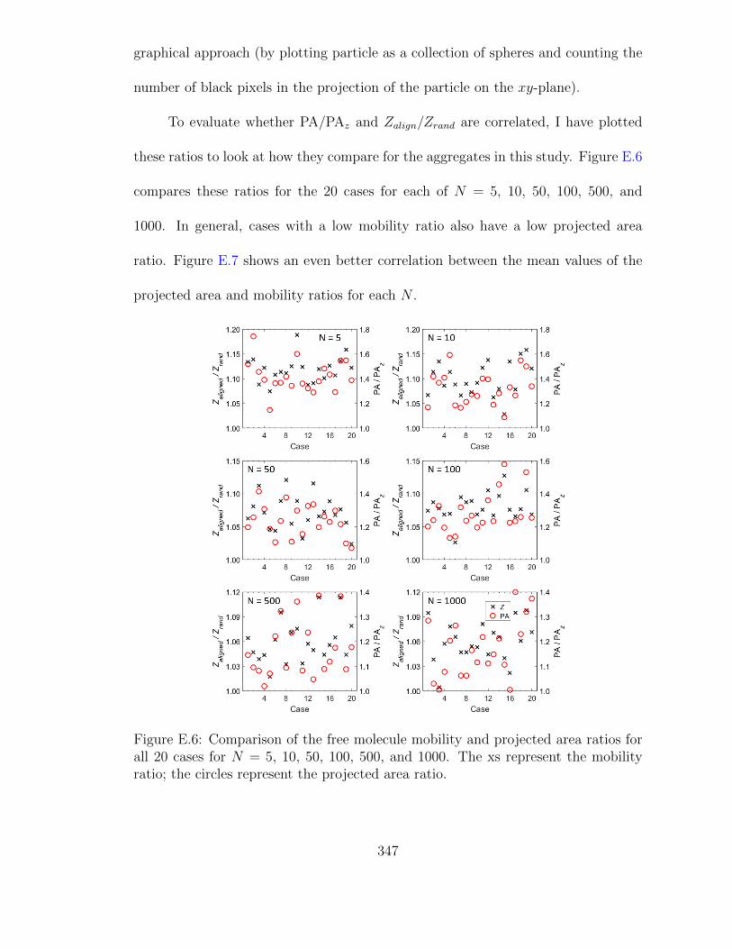
graphical approach (by plotting particle as a collection of spheres and counting the

number of black pixels in the projection of the particle on the xy-plane).

To evaluate whether PA/PAz and Zalign/Zrand are correlated, I have plotted

these ratios to look at how they compare for the aggregates in this study. Figure E.6

compares these ratios for the 20 cases for each of N = 5, 10, 50, 100, 500, and

1000. In general, cases with a low mobility ratio also have a low projected area

ratio. Figure E.7 shows an even better correlation between the mean values of the

projected area and mobility ratios for each N .

Figure E.6: Comparison of the free molecule mobility and projected area ratios forall 20 cases for N = 5, 10, 50, 100, 500, and 1000. The xs represent the mobilityratio; the circles represent the projected area ratio.

347

Figure E.7: Comparison between the average free molecule mobility ratio and theaverage projected area ratio as a function of N . In general, a low mobility ratio iscorrelated with a low projected area ratio. Both ratios decrease with increasing N .

Since PA/PAz and Zalign/Zrand appear to be correlated, we can use trends in

the projected area ratio to help explain the alignment behavior in Figure E.3. As the

number of primary spheres in the aggregate increases, the projected area on the plane

perpendicular to the principal axis of the polarizability tensor decreases relative to

the orientation-averaged projected area. In fact, the projected area varies little with

orientation at large N . This behavior contrasts with the continuum behavior, where

the average radius of gyration ratio is fairly constant with N .

My results demonstrate that the projected area and radius of gyration ratios

are correlated with the mobility ratio in the free molecular and continuum regimes,

respectively, and thus we can predict the trends in the mobility ratio based on the

trends of these surrogate measures. But why is this true?

In the continuum regime, the moving particle has a significant effect on the

348

velocity of the surrounding fluid. One way to think of this is as follows. The fluid

upstream of the particle must move out of the way to avoid the particle; the extent

of how far the fluid must move is related to the radius of gyration about the axis

parallel to the flow. A larger Rgz means the fluid must move further to get out of

the way of the particle, which explains the increase in drag (decrease in mobility).

In the free molecular regime, the particle has very little effect on the fluid

velocity. In fact, the particle has no effect on the velocity distribution of molecules

striking its surface (except for molecules that strike the particle more than once

between collisions with other fluid molecules), so we can use a ballistic approach for

calculating the drag [36, 54, 117, 118]. Thus, the projected area is related to the

free molecular drag: as projected area increases, gas molecules are more likely to

strike and transfer their momentum to the particle, thus increasing the drag.

In summary, the ratio of particle mobility in the limit of infinite field strength

to mobility in the limit of zero field strength decreases as the number of primary

spheres increases in the free molecular regime, while the ratio remains constant in

the continuum regime. The trends in the free molecular and continuum regimes can

be explained by trends in the projected area ratio and the radius of gyration ratio,

respectively. In the continuum regime, the ratio of particle radius of gyration to the

radius of gyration about the principal axis of the polarizability tensor (i.e. the axis

parallel to the particle velocity when the particle is fully aligned) varies little with

N . In the free molecular regime, the ratio of the orientation-averaged projected

area to the projected area in the plane perpendicular to the principal axis of the

polarizability tensor decreases with increasing N . Note that these trends are for

349

the average behavior at each N ; there are variations in the radius of gyration and

projected area ratios for aggregates with the same N , which in turn affect the

fully-aligned mobility behavior of the particles. The variations in mobility among

aggregates with the same N are large in the continuum regime compared to the

variations in the average mobility as a function of N . Finally, at intermediate

Knudsen numbers, particles exhibit more continuum-like behavior as the number

of primary spheres increases. This is because the aggregate behaves more like a

particle with characteristic dimension much larger than the mean free path than a

collection of spheres with radii smaller than the mean free path.

350

Appendix F: NGDE User Manual

This appendix serves as the User Manual for the Nodal General Dynamic

Equation (NGDE) solver described in Chapter 9. This manual refers to the MAT-

LAB version of the code; for the C version, see Prakash et al. [27]. Throughout this

documentation, text in this font represents a variable or expression in the code

or a MATLAB command.

The manual is divided into three sections: (1) instructions for running the

NGDE code and the post-processing tool; (2) detailed descriptions of input to NGDE

(ngde.m) and NGDEplot (ngde plot.m) and output from the codes; and (3) discus-

sion about the NGDE code structure. (The code for NGDEplot mostly consists of

MATLAB commands for plotting data, so discussion of NGDEplot is limited to its

input and output.) For information about the theoretical basis of NGDE and the

methods used to solve the general dynamic equation, refer to Chapter 9.

F.1 Running NGDE and NGDEplot

NGDE is distributed as a .zip archive containing the following files:

• ngde.m: the NGDE source code

• ngde plot.m: the NGDEplot source code

351

• rtpmie bohren mie.m: Mie scattering code used by NGDEplot. The Mie

scattering code is based on the Fortran source code in Appendix A of Bohren

and Huffman [89]; rtpmie bohren mie.m has been converted from the Fortran

source code provided by Professors Eugene Clothiaux and Craig Bohren from

the Pennsylvania State University.

• ngde sample problem.mat: MATLAB data file containing two MATLAB struc-

ture arrays, ngdein and plotoptions, that provide input to NGDE and

NGDEplot, respectively

To run NGDE, perform the following steps:

1. In MATLAB, navigate to the folder containing the files listed above. To do so,

click on the “Browse for folder” icon (circled in red in the screenshot below)

and open the folder containing the NGDE files. All of the files in the current

folder appear in the “Current Folder” panel.

352

2. Load the NGDE and NGDEplot input structures (ngdein and plotoptions).

This can be done by double-clicking on the ngde sample problem.mat data file

distributed with NGDE, or by double-clicking on any other MATLAB data file

that contains NGDE input. After double-clicking on the data file, you should

see the load(...) statement and the NGDE input structures appear in the

Command Window panel and in the Workspace panel, respectively. (See the

screenshot below.)

3. If desired, modify the NGDE input. To do so, double-click on the NGDE

structure array (named ngdein in the code distribution) in the Workspace

panel. This will bring up the structure array in the Variables panel. To change

any of the input parameters, select the appropriate value (e.g. the value of 300

next to the Tf field) and type in the desired value (e.g. type in 400 to end the

NGDE simulation when the temperature equals 400 K instead of 300 K).

353

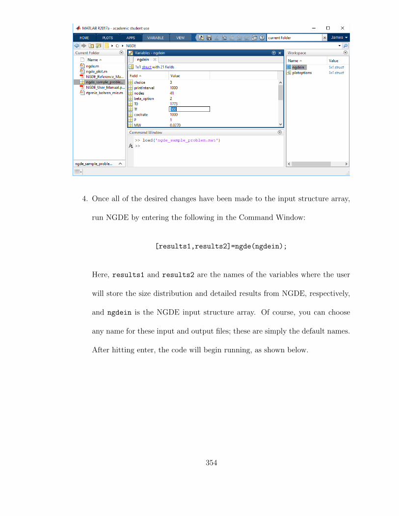
4. Once all of the desired changes have been made to the input structure array,

run NGDE by entering the following in the Command Window:

[results1,results2]=ngde(ngdein);

Here, results1 and results2 are the names of the variables where the user

will store the size distribution and detailed results from NGDE, respectively,

and ngdein is the NGDE input structure array. Of course, you can choose

any name for these input and output files; these are simply the default names.

After hitting enter, the code will begin running, as shown below.

354

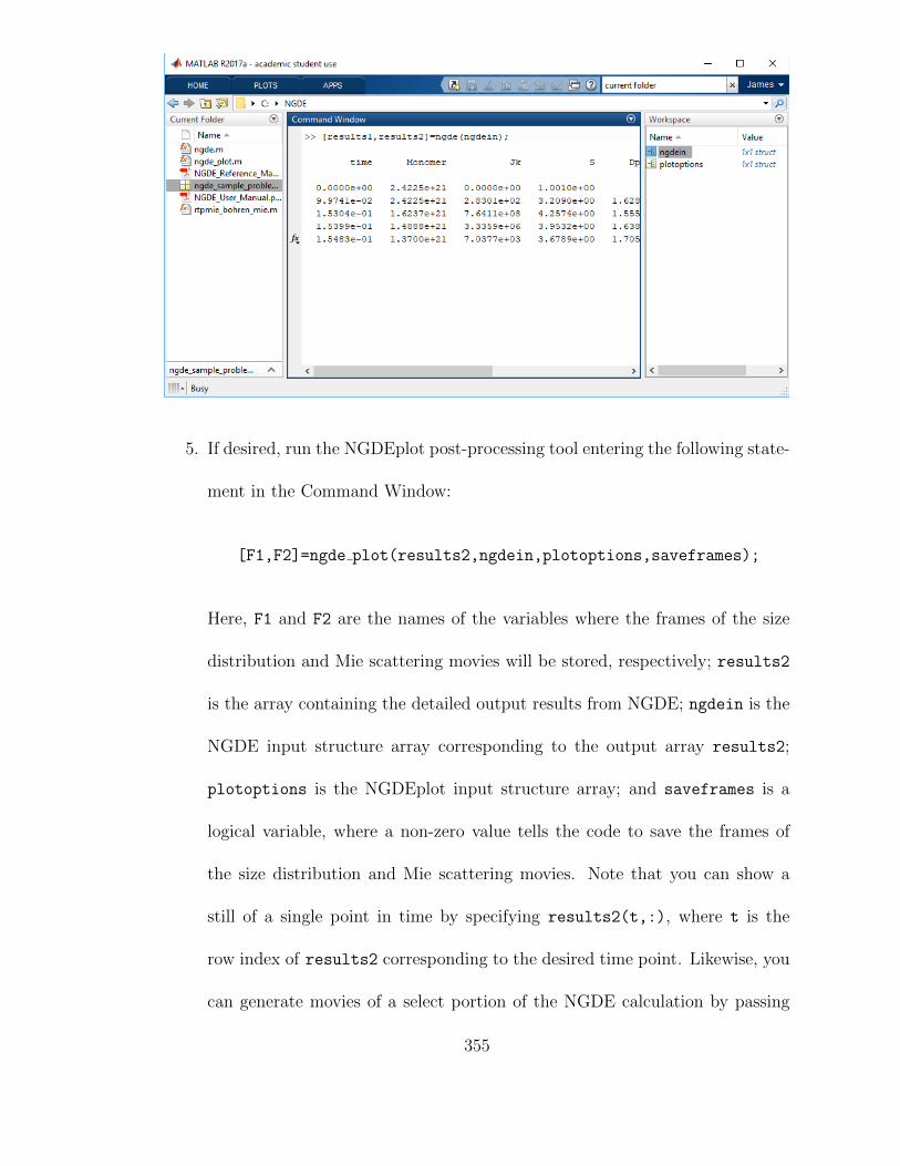
5. If desired, run the NGDEplot post-processing tool entering the following state-

ment in the Command Window:

[F1,F2]=ngde plot(results2,ngdein,plotoptions,saveframes);

Here, F1 and F2 are the names of the variables where the frames of the size

distribution and Mie scattering movies will be stored, respectively; results2

is the array containing the detailed output results from NGDE; ngdein is the

NGDE input structure array corresponding to the output array results2;

plotoptions is the NGDEplot input structure array; and saveframes is a

logical variable, where a non-zero value tells the code to save the frames of

the size distribution and Mie scattering movies. Note that you can show a

still of a single point in time by specifying results2(t,:), where t is the

row index of results2 corresponding to the desired time point. Likewise, you

can generate movies of a select portion of the NGDE calculation by passing

355

the appropriate rows from results2 to NGDEplot. You may also change the

NGDEplot input by double-clicking on the NGDEplot input structure array

(plotoptions by default) in the Workspace panel and changing the values of

the structure array fields.

F.2 Description of Input and Output

F.2.1 NGDE Input (ngdein)

The following parameters are included in the NGDE input structure array,

ngdein. The default values are for the “Full GDE” sample problem described in

Chapter 9.

Parameter Description

choice Calculation type. 1 = coagulation only, 2 = nucleation + co-

agulation, 3 = full GDE, 4 = surface growth only. DEFAULT

= 3

printInterval Number of timesteps between plot edits. Too small a value

will result in a very large output from the code, which may

use up excessive computer memory. DEFAULT = 1000

nodes Number of size nodes to use in the calculation. Note that the

code actually creates nodes+1 volume nodes, but the number

concentration in the final node is always zero. This is done to

prevent errors in the code. DEFAULT = 41

356

beta option Collision frequency function. 1 = free molecule regime, 2 =

Fuch’s form for FM and transition regime. DEFAULT = 2

T0 Initial temperature (K). DEFAULT = 1773

Tf Final temperature (K). Not used if choice = 1. DEFAULT

= 300

coolrate Cooldown rate for the calculation (K/s). Not used if choice

= 1. DEFAULT = 1000

P Pressure (atm). DEFAULT = 1

MW Molecular weight of the condensed species (kg/mol). DE-

FAULT = 0.027

rho Density of the condensed species (kg/m3). DEFAULT = 2700

A, B Constants for determining surface tension as a function of

temperature, given by sigma=(A-B*T)*1e-3, where sigma

has units of N/m. DEFAULT = 948, 0.202 (for aluminum)

C, D Constants for determining saturation vapor pressure

as a function of temperature and pressure, given by

Ps=exp(C-D./T).*101325, where Ps has units of Pa.

DEFAULT = 13.07, 36373 (for aluminum)

d Initial particle diameter (nm). Only used if choice = 1. DE-

FAULT = 1

N0 Initial particle number concentration (#/m3). Only used if

choice = 1 or 4. DEFAULT = 1e10

357

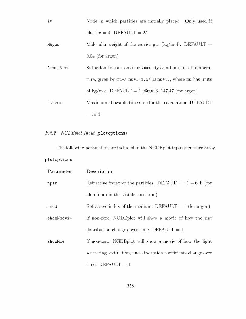
i0 Node in which particles are initially placed. Only used if

choice = 4. DEFAULT = 25

MWgas Molecular weight of the carrier gas (kg/mol). DEFAULT =

0.04 (for argon)

A mu, B mu Sutherland’s constants for viscosity as a function of tempera-

ture, given by mu=A mu*T^1.5/(B mu+T), where mu has units

of kg/m-s. DEFAULT = 1.9660e-6, 147.47 (for argon)

dtUser Maximum allowable time step for the calculation. DEFAULT

= 1e-4

F.2.2 NGDEplot Input (plotoptions)

The following parameters are included in the NGDEplot input structure array,

plotoptions.

Parameter Description

npar Refractive index of the particles. DEFAULT = 1 + 6.4i (for

aluminum in the visible spectrum)

nmed Refractive index of the medium. DEFAULT = 1 (for argon)

showNmovie If non-zero, NGDEplot will show a movie of how the size

distribution changes over time. DEFAULT = 1

showMie If non-zero, NGDEplot will show a movie of how the light

scattering, extinction, and absorption coefficients change over

time. DEFAULT = 1

358

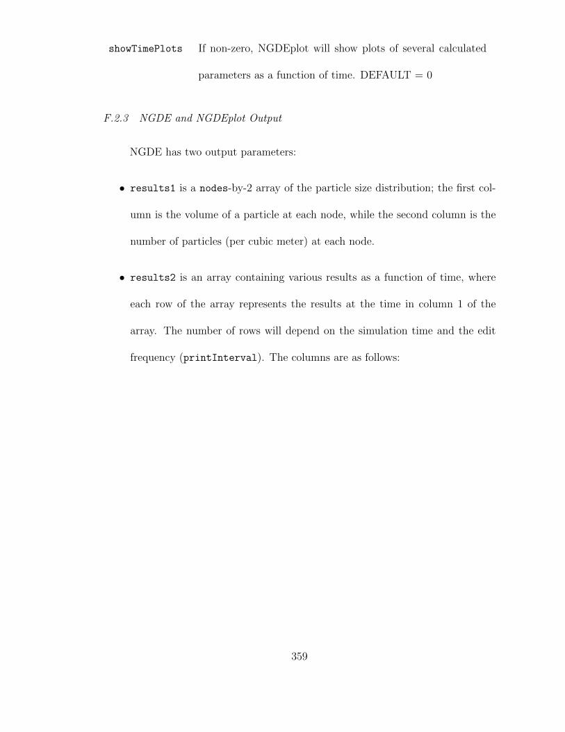
showTimePlots If non-zero, NGDEplot will show plots of several calculated

parameters as a function of time. DEFAULT = 0

F.2.3 NGDE and NGDEplot Output

NGDE has two output parameters:

• results1 is a nodes-by-2 array of the particle size distribution; the first col-

umn is the volume of a particle at each node, while the second column is the

number of particles (per cubic meter) at each node.

• results2 is an array containing various results as a function of time, where

each row of the array represents the results at the time in column 1 of the

array. The number of rows will depend on the simulation time and the edit

frequency (printInterval). The columns are as follows:

359

Column Description

1 The time, t

2:nodes+2 The number concentration at nodes 1 through nodes+1, N

[#/m3]

nodes+3 The nucleation rate, Jk [#/m3s]

nodes+4 The saturation ratio, S

nodes+5 The volume mean particle diameter, dpav [m]

nodes+6 The critical particle size for nucleation, kstar [# of

monomers]; nucleated particles are placed in the node with

particle volume just larger than the volume corresponding to

kstar monomers

nodes+7 The total volume concentration of particles, Vtot [m3]; note

that this does not include the volume of monomers

nodes+8 The number concentration of particles, Ntot [#/m3]; note

that this does not include the number concentration of

monomers

For more information about how these parameters are determined, see the technical

description of NGDE in Chapter 9.

NGDEplot has two output parameters, F1 and F2, which contain the frames

for the size distribution and Mie scattering movies generated by the code. If the user

chooses not save the frames (saveframes=0) or chooses not to generate one of the

movies (showNmovie=0 or showMie=0), then F1 and/or F2 will be zero. To replay

360

a movie using the saved frames, the user should use MATLAB’s movie command.

F.3 Code Structure

The goal of this section is to give users a better understanding of how the code

works and to identify some hardwired parameters or features that one can modify

to improve the code or tailor it to a specific application. The code is divided into

three main sections: (1) reading the input structure and initializing variables, (2)

subroutines common to more than one of the possible calculation types (see choice

in Section F.2.1), and (3) the main body of the program. The initialization step is

straightforward and will not be discussed here. The following subsections discuss

the subroutines and the main body of the code. These subsections largely focus on

code structure and logic; for the technical details, refer to Chapter 9 or to the code

itself.

F.3.1 NGDE Subroutines

After reading in the input structure and initializing variables, the NGDE

code defines a number of separate subroutines or functions, which are listed be-

low. To modify the code, simply find the appropriate subroutine and make the

desired changes.

361

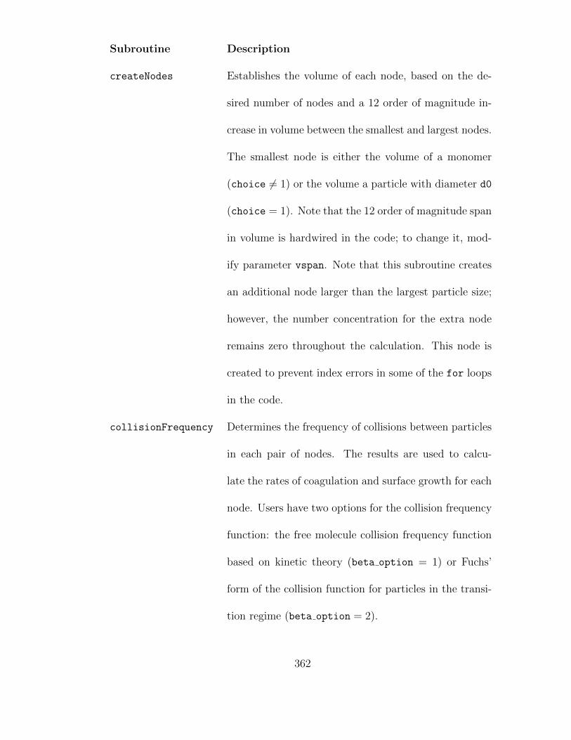
Subroutine Description

createNodes Establishes the volume of each node, based on the de-

sired number of nodes and a 12 order of magnitude in-

crease in volume between the smallest and largest nodes.

The smallest node is either the volume of a monomer

(choice 6= 1) or the volume a particle with diameter d0

(choice = 1). Note that the 12 order of magnitude span

in volume is hardwired in the code; to change it, mod-

ify parameter vspan. Note that this subroutine creates

an additional node larger than the largest particle size;

however, the number concentration for the extra node

remains zero throughout the calculation. This node is

created to prevent index errors in some of the for loops

in the code.

collisionFrequency Determines the frequency of collisions between particles

in each pair of nodes. The results are used to calcu-

late the rates of coagulation and surface growth for each

node. Users have two options for the collision frequency

function: the free molecule collision frequency function

based on kinetic theory (beta option = 1) or Fuchs’

form of the collision function for particles in the transi-

tion regime (beta option = 2).

362

sizeSplitting Populates the size-splitting array X that handles parti-

cles that coagulate to a size between two nodes.

dynamicTimestep Chooses a time step based on the behavior of the GDE

at each point in time. The overarching goal is to choose

the maximum time step that guarantees code stability.

The dynamic time-step algorithm selects the time step

as the minimum of five options: (1) 0.1% of the char-

acteristic coagulation time; (2) 50% of the maximum

time step that results in the number concentration in

any node decreasing to zero; (3) the time in which the

monomer concentration changes by 0.1%; (4) the time

in which the saturation ratio changes by 1%; (5) a user-

defined maximum time step, dtUser. The percentages

are hardwired parameters but can be modified by the

user if desired.

363

coagulation Calculates the coagulation rate for each node, based on

the current size distribution, the collision frequency for

each pair of nodes (see collisionFrequency above),

and the size-splitting array X.

surfaceGrowth Calculates the condensation and evaporation rates for

each node based on the current size distribution, satu-

ration monomer concentration for each node (account-

ing for the Kelvin effect), and the collision frequency

between monomers and particles.

printResults Writes results to the output array results2. See Sec-

tion F.2.3 for the structure of this array.

F.3.2 NGDE Main Program

After the above function definitions, the main body of the NGDE code begins.

This portion of the code uses if-else statements to branch into four segments, cor-

responding to the four calculation types as specified with the choice input variable.

Each branch has the same basic structure: there is an additional initalization step,

used to create the volume nodes, populate the size-splitting array X, and establish

the conditions (e.g. total particle volume Vtot, volume mean diameter dpav) at

time zero; next is a while loop, where the code marches forward in time until some

condition is met; and finally, the code stores the output in variables results1 and

results2.

364

The exit condition for each while loop depends on the calculation type. For

choice = 1, (pure coagulation), the calculation terminates at 1000 times the esti-

mated time to reach the self-preserving distribution, t SPD. The calculation starts

with an initially monodisperse aerosol. As the while loop marches the simulation

forward in time, the aerosol grows based on the conditions in the coagulation

subroutine.

For the other choices, the calculation ends when the system reaches Tf. Ini-

tially, the system is very slightly supersaturated (S = 1.001) at some user-specified

temperature (T0). Within the loop, the code calls the subroutines to determine

the time step and nucleation, coagulation, and surface growth rates, as appropriate

based on the calculation type. The code updates the size distribution and other

associated properties using the results of these subroutines.

F.4 Summary

This user manual has described the input, output, and general structure of the

NGDE code, as well as the input and output of the NGDEplot post-processing tool.

The user can control many of the parameters in the NGDE code using the ngdein

input structure; other parameters must be modified directly in the code, such as the

initial saturation ratio S, the exit conditions for the while loops (t < 1000 ∗ t SPD

for choice = 1 and T < Tf otherwise), and the span of the size distribution (12

orders of magnitude from the smallest to largest volume nodes, as specified by

vspan). To make more substantial changes to the code – such as the introduction

365

of new models for coagulation, nucleation, and growth, or changes to the constant-

cooldown conditions of the calculation – one would need to do so in the appropriate

subroutines or in the main body of the program.

366

Appendix G: MATLAB Codes Referenced in this Disseration

G.1 Code for Calculating the Velocity around a Sphere

Below I have included the source code for the MATLAB function used to calcu-

late the velocity around a sphere as a function of Knudsen number, bgk sphere par.

Note that the code takes advantage of MATLAB’s parallel computing features. For

serial execution (i.e. on one computer core), change the parfor loops to for loops.

Note that when calculating the density, velocity, and temperature perturba-

tions around and drag on the sphere as a function of r0 =√π/[4(0.499)Kn], I have

used nodes=64 and upper bound=10. I have experimented with different values of

these parameters, but these values seem to work best based on my limited sample

size.

bgk sphere par relies on two other MATLAB functions that I have written:

gaussquad, which returns the Gaussian quadrature nodes and weights, and abram,

which returns the Tn(x) functions that appear when solving the BGK equation.

Both of these files consist of long tables of data: gaussquad(n) uses a switch, case

structure to return the n node points and weights (tj and Aj in bgk sphere par),

while abram(x,n) interpolates from tables to return Tn(x) for each value of x pro-

vided. It would not be helpful to include the file listings here because they would

367

span over 100 pages. Instead, I will provide the information necessary to recreate

these files.

The Gaussian quadrature nodes and weights are available from various sources,

including Abramowitz and Stegun [98]. For gaussquad(n), I included nodes and

weights for n=2 to n=64 nodes; each set of data is its own case in the switch, case

structure. gaussquad(n) simply returns the nodes and weights for the specified

case.

I created the tables in abram(x,n) by numerically integrating the function in

MATLAB, using the following commands:

r=[0,logspace(-2,2,99)]’;

for i=1:length(r)

for n=0:9

T(i,j)=integral(@(c) exp(-c.^2-r(i)./c).*(c.^n),0,Inf);

end

end

The file abram(x,n) consists of the values of r and T, then the following lines:

Tn=x*0;

for i=1:length(x)

Tn(i)=interp1(r,T(:,n+1),x(i),’pchip’,0);

end

The code returns T(n).

See Chapter 2 and Appendix A for technical details of the BGK equation and

its solution for a translating sphere.

368

G.1.1 Code Listing for bgk sphere par

% Solve for the density, velocity, and temperature around a sphere

% of non-dimensional radius r0, using a Gaussian quadrature with

% user-specified number of nodes between r0 and r0+upper_bound.

% This function uses the asymptotic solution of the Krook equation

% for large r from (Takata et al., 1993). Otherwise, the equations

% and overall solution strategy follow (Lea & Loyalka, 1982) and

% (Law & Loyalka, 1986). See my dissertation (Corson, 2018) for

% more details.

function [rj,eps,coefs,drag]=bgk_sphere_par(r0,nodes,...

upper_bound,outfile)

tic

if nargin < 4

outfile=[’r0=’,num2str(r0),’_results.mat’];

end

%options for integral2

Int2Opts.Method=’iterated’;

Int2Opts.AbsTol=1e-6;

Int2Opts.RelTol=1e-3;

%Coefficient in (Takata et al., 1993) trial functions

gam=1.270;

%For r between r0 (the surface of the sphere) and

%rp=r0+upper_bound, the BGK equation is solved using a Gaussian

%quadrature. The nodes and weights tj and Aj are obtained

%from a separate function.

rp=r0+upper_bound;

[tj,Aj]=gaussquad(nodes);

rj=0.5*(r0*(1-tj)+rp*(1+tj));

%Results for c1, c2, and c3 based on earlier calculations;

%these are used to calculate initial guesses for the coefficients

%in the trial functions.

guesses=[0.00888,-0.0261,-14.7502,-0.8594;

0.010,-0.0269,-14.7212,-0.8591;

0.025,-0.0379,-14.3333,-0.8545;

369

0.050,-0.0564,-13.6869,-0.8468;

0.075,-0.0748,-13.0404,-0.8392;

0.100,-0.0932,-12.3940,-0.8315;

0.250,-0.2147,-12.1216,-0.2794;

0.500,-0.3826,-5.5702,-0.2417;

0.750,-0.5148,-3.4101,-0.2094;

0.888,-0.5760,-2.7445,-0.1935;

1.000,-0.6205,-2.3438,-0.1818;

2.000,-0.8854,-0.8038,-0.1103;

3.000,-1.0253,-0.3295,-0.0740;

4.000,-1.1115,-0.1039,-0.0532;

5.000,-1.1706,0.0268,-0.0418;

6.000,-1.2137,0.1113,-0.0335;

7.000,-1.2468,0.1707,-0.0280;

8.000,-1.2734,0.2153,-0.0246;

9.000,-1.2949,0.2489,-0.0208;

10.00,-1.3129,0.2758,-0.0184;

88.80,-1.4829,0.4830,-6.418e3-4;

100.0,-1.4857,0.4858,-5.1061e-4;

1000.,-1.5, 0.5, 0];

% Initialize vectors and matrices

ar1=zeros(nodes,1); ar2=ar1; ar3=ar1;

Wg1=zeros(nodes,1); Wg2=Wg1; Wg3=Wg1; Wu1=Wg1; Wu2=Wg1; Wu3=Wg1;

S1=zeros(nodes,1); S2=S1; S3=S1;

G11=S1; G12=S1; G13=S1; G21=S1; G22=S1; G23=S1; G31=S1;

G32=S1; G33=S1;

K11=zeros(nodes); K12=K11; K13=K11; K21=K11; K22=K11;

K23=K11; K31=K11; K32=K11; K33=K11;

A=zeros(4*nodes);

% Vectors and matrices that account for temperature fluctuation

ar4=ar1; Wg4=Wg1; Wu4=Wu1; K14=K11; K24=K11; K34=K11;

K41=K11; K42=K11; K43=K11; K44=K11;

G14=G11; G24=G11; G34=G11; G41=G11; G42=G11; G43=G11;

G44=G11; S4=S1;

%Loop to calculate a(r), which in turn is used to calculate the

%constant g that appears in the source term

parfor i=1:nodes

%for i=1:nodes

ar1(i)=1/(2*r0^2*rj(i))*integral(@(t) (t.^4-2*rj(i)^2*t.^2 ...

+(rj(i)^4-r0^4)).*abram(t,2)./(t.^2),rj(i)-r0, ...

sqrt(rj(i)^2-r0^2));

ar2(i)=-1/(2*sqrt(2)*r0^2*rj(i)^2)*integral(@(t) (t.^6-t.^4 ...

*(rj(i)^2+r0^2)-t.^2*(rj(i)^2-r0^2)^2+(rj(i)^2-r0^2) ...

370

*(rj(i)^4-r0^4)).*abram(t,3)./(t.^3),rj(i)-r0, ...

sqrt(rj(i)^2-r0^2));

ar3(i)=1/(2*sqrt(2)*r0^2*rj(i)^2)*integral(@(t) (t.^6-t.^4 ...

*(3*rj(i)^2+r0^2)+t.^2*(rj(i)^2-r0^2)*(3*rj(i)^2+r0^2) ...

-(rj(i)^2-r0^2)^3).*abram(t,3)./(t.^3),rj(i)-r0, ...

sqrt(rj(i)^2-r0^2));

ar4(i)=sqrt(2/3)/(2*r0^2*rj(i))*integral(@(t) (t.^4 ...

-2*rj(i)^2*t.^2+(rj(i)^4-r0^4)).*(abram(t,4) ...

-3/2*abram(t,2))./t.^2,rj(i)-r0,sqrt(rj(i)^2-r0^2));

end

% Loop to calculate the source term W(r)

parfor i=1:nodes

%for i=1:nodes

LL=rj(i)-r0;

UL=sqrt(rj(i)^2-r0^2);

tt=0.5*(LL*(1-tj)+UL*(1+tj));

C=(UL-LL)/2;

for j=1:nodes

Wg1(i)=Wg1(i)+1/(2*sqrt(pi)*rj(i)^2*r0)*(tt(j)^4 ...

-2*rj(i)^2*tt(j)^2+(rj(i)^4-r0^4)) ...

.*abram(tt(j),2)/tt(j)^2*Aj(j)*C;

Wg2(i)=Wg2(i)+1/(2*sqrt(2*pi)*rj(i)^3*r0)*(tt(j)^6 ...

-(rj(i)^2+r0^2)*tt(j)^4-(rj(i)^2-r0^2)^2*tt(j)^2 ...

+(rj(i)^2+r0^2)*(rj(i)^2-r0^2)^2).*abram(tt(j),3) ...

./tt(j)^3*Aj(j)*C;

Wg3(i)=Wg3(i)-1/(4*sqrt(2*pi)*rj(i)^3*r0)*(tt(j)^6 ...

-(3*rj(i)^2+r0^2)*tt(j)^4+(rj(i)^2-r0^2)*(3*rj(i)^2 ...

+r0^2)*tt(j)^2-(rj(i)^2-r0^2)^3).*abram(tt(j),3) ...

./tt(j)^3*Aj(j)*C;

Wu1(i)=Wu1(i)+1/(sqrt(pi)*rj(i)^2)*(tt(j)^4 ...

-(rj(i)^2-r0^2)^2).*abram(tt(j),3)./tt(j)^3*Aj(j)*C;

Wu2(i)=Wu2(i)+1/(sqrt(2*pi)*rj(i)^3)*(tt(j)^6+tt(j)^4 ...

*(rj(i)^2-r0^2)-tt(j)^2*(rj(i)^2-r0^2)^2 ...

-(rj(i)^2-r0^2)^3).*abram(tt(j),4)./tt(j)^4*Aj(j)*C;

Wu3(i)=Wu3(i)-1/(2*sqrt(2*pi)*rj(i)^3)*(tt(j)^6-tt(j)^4 ...

*(3*rj(i)^2+r0^2)+tt(j)^2*(rj(i)^2-r0^2)*(3*rj(i)^2 ...

+r0^2)-(rj(i)^2-r0^2)^3).*abram(tt(j),4) ...

./tt(j)^4*Aj(j)*C;

Wg4(i)=Wg4(i)+sqrt(2/3)/(2*sqrt(pi)*rj(i)^2*r0) ...

*(tt(j)^4-2*rj(i)^2*tt(j)^2+(rj(i)^4-r0^4)) ...

*(abram(tt(j),4)-3/2*abram(tt(j),2))/tt(j)^2*Aj(j)*C;

Wu4(i)=Wu4(i)+sqrt(2/3)/(sqrt(pi)*rj(i)^2)*(tt(j)^4 ...

-(rj(i)^2-r0^2)^2)*(abram(tt(j),5) ...

-3/2*abram(tt(j),3))/tt(j)^3*Aj(j)*C;

371

end

end

% Loop to evaluate the kernel K(rj(i),r)

parfor i=1:nodes

%for i=1:nodes

% These are the integrands of the H functions from Lea, 1982

H11=@(r,t) -1./(rj(i)*r).*abram(t,1).*(t.^2-(rj(i)^2+r.^2))./t;

H12=@(r,t) 1./(sqrt(2)*rj(i)*r.^2).*abram(t,2) ...

.*(t.^4-2*rj(i)^2*t.^2-(r.^4-rj(i)^4))./t.^2;

H13=@(r,t) -1./(sqrt(2)*rj(i)*r.^2).*abram(t,2) ...

.*(t.^4-2*(r.^2+rj(i)^2).*t.^2+(r.^2-rj(i)^2).^2)./t.^2;

H21=@(r,t) -1./(sqrt(2)*rj(i)^2*r).*abram(t,2) ...

.*(t.^4-2*r.^2.*t.^2-(rj(i)^4-r.^4))./t.^2;

H22=@(r,t) 1./(2*rj(i)^2*r.^2).*abram(t,3).*(t.^6-t.^4 ...

.*(r.^2+rj(i)^2)-t.^2.*(rj(i)^2-r.^2).^2 ...

+(r.^2-rj(i)^2).*(r.^4-rj(i)^4))./t.^3;

H23=@(r,t) -1./(2*rj(i)^2*r.^2).*abram(t,3).*(t.^6-t.^4 ...

.*(3*r.^2+rj(i)^2)+t.^2.*(r.^2-rj(i)^2) ...

.*(3*r.^2+rj(i)^2)-(r.^2-rj(i)^2).^3)./t.^3;

H31=@(r,t) 1./(sqrt(2)*2*rj(i)^2*r).*abram(t,2) ...

.*(t.^4-2*(rj(i)^2+r.^2).*t.^2+(rj(i)^2-r.^2).^2)./t.^2;

H32=@(r,t) -1./(4*rj(i)^2*r.^2).*abram(t,3).*(t.^6-t.^4 ...

.*(3*rj(i)^2+r.^2)+t.^2.*(rj(i)^2-r.^2) ...

.*(3*rj(i)^2+r.^2)-(rj(i)^2-r.^2).^3)./t.^3;

H33=@(r,t) 1./(4*rj(i)^2*r.^2).*abram(t,3).*(t.^6-t.^4 ...

.*(3*rj(i)^2+3*r.^2)+t.^2.*(3*rj(i)^4+2*rj(i)^2*r.^2 ...

+3*r.^4)-(rj(i)^4-r.^4).*(rj(i)^2-r.^2))./t.^3;

H14=@(r,t) -sqrt(2/3)./(rj(i)*r) ...

.*(abram(t,3)-3/2*abram(t,1)).*(t.^2-(rj(i)^2+r.^2))./t;

H24=@(r,t) -1./(sqrt(3)*rj(i)^2*r).*(abram(t,4) ...

-3/2*abram(t,2)).*(t.^4-2*r.^2.*t.^2-(rj(i)^4-r.^4))./t.^2;

H34=@(r,t) 1./(2*sqrt(3)*rj(i)^2*r) ...

.*(abram(t,4)-3/2*abram(t,2)).*(t.^4-2*(rj(i)^2+r.^2) ...

.*t.^2+(rj(i)^2-r.^2).^2)./t.^2;

H41=@(r,t) -sqrt(2/3)./(rj(i)*r).*(abram(t,3) ...

-3/2*abram(t,1)).*(t.^2-(rj(i)^2+r.^2))./t;

H42=@(r,t) 1./(sqrt(3)*rj(i)*r.^2) ...

.*(abram(t,4)-3/2*abram(t,2)) ...

.*(t.^4-2*rj(i)^2*t.^2-(r.^4-rj(i)^4))./t.^2;

H43=@(r,t) -1./(sqrt(3)*rj(i)*r.^2) ...

.*(abram(t,4)-3/2*abram(t,2)).*(t.^4-2*(r.^2+rj(i)^2) ...

.*t.^2+(r.^2-rj(i)^2).^2)./t.^2;

H44=@(r,t) -2./(3*rj(i)*r).*(abram(t,5)-3*abram(t,3) ...

+9/4*abram(t,1)).*(t.^2-(rj(i)^2+r.^2))./t;

372

% The G’s represent cases when the kernel is singular,

% i.e. when r=rj(i).

G11(i)=pi^(-1/2)*(integral2(@(r,t) r/rj(i).*(H11(r,t)), ...

r0,rj(i),@(r) abs(rj(i)-r),@(r) sqrt(rj(i)^2-r0^2) ...

+sqrt(r.^2-r0^2),Int2Opts)+integral2(@(r,t) ...

r/rj(i).*(H11(r,t)),rj(i),rp,@(r) abs(rj(i)-r), ...

@(r) sqrt(rj(i)^2-r0^2)+sqrt(r.^2-r0^2),Int2Opts));

G12(i)=pi^(-1/2)*(integral2(@(r,t) r/rj(i).*(H12(r,t)), ...

r0,rj(i),@(r) abs(rj(i)-r),@(r) sqrt(rj(i)^2-r0^2) ...

+sqrt(r.^2-r0^2),Int2Opts)+integral2(@(r,t) ...

r/rj(i).*(H12(r,t)),rj(i),rp,@(r) abs(rj(i)-r), ...

@(r) sqrt(rj(i)^2-r0^2)+sqrt(r.^2-r0^2),Int2Opts));

G13(i)=pi^(-1/2)*(integral2(@(r,t) r/rj(i).*(H13(r,t)), ...

r0,rj(i),@(r) abs(rj(i)-r),@(r) sqrt(rj(i)^2-r0^2) ...

+sqrt(r.^2-r0^2),Int2Opts)+integral2(@(r,t) ...

r/rj(i).*(H13(r,t)),rj(i),rp,@(r) abs(rj(i)-r), ...

@(r) sqrt(rj(i)^2-r0^2)+sqrt(r.^2-r0^2),Int2Opts));

G21(i)=pi^(-1/2)*(integral2(@(r,t) r/rj(i).*(H21(r,t)), ...

r0,rj(i),@(r) abs(rj(i)-r),@(r) sqrt(rj(i)^2-r0^2) ...

+sqrt(r.^2-r0^2),Int2Opts)+integral2(@(r,t) ...

r/rj(i).*(H21(r,t)),rj(i),rp,@(r) abs(rj(i)-r), ...

@(r) sqrt(rj(i)^2-r0^2)+sqrt(r.^2-r0^2),Int2Opts));

G22(i)=pi^(-1/2)*(integral2(@(r,t) r/rj(i).*(H22(r,t)), ...

r0,rj(i),@(r) abs(rj(i)-r),@(r) sqrt(rj(i)^2-r0^2) ...

+sqrt(r.^2-r0^2),Int2Opts)+integral2(@(r,t) ...

r/rj(i).*(H22(r,t)),rj(i),rp,@(r) abs(rj(i)-r), ...

@(r) sqrt(rj(i)^2-r0^2)+sqrt(r.^2-r0^2),Int2Opts));

G23(i)=pi^(-1/2)*(integral2(@(r,t) r/rj(i).*(H23(r,t)), ...

r0,rj(i),@(r) abs(rj(i)-r),@(r) sqrt(rj(i)^2-r0^2) ...

+sqrt(r.^2-r0^2),Int2Opts)+integral2(@(r,t) ...

r/rj(i).*(H23(r,t)),rj(i),rp,@(r) abs(rj(i)-r), ...

@(r) sqrt(rj(i)^2-r0^2)+sqrt(r.^2-r0^2),Int2Opts));

G31(i)=pi^(-1/2)*(integral2(@(r,t) r/rj(i).*(H31(r,t)), ...

r0,rj(i),@(r) abs(rj(i)-r),@(r) sqrt(rj(i)^2-r0^2) ...

+sqrt(r.^2-r0^2),Int2Opts)+integral2(@(r,t) ...

r/rj(i).*(H31(r,t)),rj(i),rp,@(r) abs(rj(i)-r),...

@(r) sqrt(rj(i)^2-r0^2)+sqrt(r.^2-r0^2),Int2Opts));

G32(i)=pi^(-1/2)*(integral2(@(r,t) r/rj(i).*(H32(r,t)), ...

r0,rj(i),@(r) abs(rj(i)-r),@(r) sqrt(rj(i)^2-r0^2) ...

+sqrt(r.^2-r0^2),Int2Opts)+integral2(@(r,t) ...

r/rj(i).*(H32(r,t)),rj(i),rp,@(r) abs(rj(i)-r), ...

@(r) sqrt(rj(i)^2-r0^2)+sqrt(r.^2-r0^2),Int2Opts));

G33(i)=pi^(-1/2)*(integral2(@(r,t) r/rj(i).*(H33(r,t)), ...

r0,rj(i),@(r) abs(rj(i)-r),@(r) sqrt(rj(i)^2-r0^2) ...

+sqrt(r.^2-r0^2),Int2Opts)+integral2(@(r,t) ...

373

r/rj(i).*(H33(r,t)),rj(i),rp,@(r) abs(rj(i)-r), ...

@(r) sqrt(rj(i)^2-r0^2)+sqrt(r.^2-r0^2),Int2Opts));

G14(i)=pi^(-1/2)*(integral2(@(r,t) r/rj(i).*(H14(r,t)), ...

r0,rj(i),@(r) abs(rj(i)-r),@(r) sqrt(rj(i)^2-r0^2) ...

+sqrt(r.^2-r0^2),Int2Opts)+integral2(@(r,t) ...

r/rj(i).*(H14(r,t)),rj(i),rp,@(r) abs(rj(i)-r), ...

@(r) sqrt(rj(i)^2-r0^2)+sqrt(r.^2-r0^2),Int2Opts));

G24(i)=pi^(-1/2)*(integral2(@(r,t) r/rj(i).*(H24(r,t)), ...

r0,rj(i),@(r) abs(rj(i)-r),@(r) sqrt(rj(i)^2-r0^2) ...

+sqrt(r.^2-r0^2),Int2Opts)+integral2(@(r,t) ...

r/rj(i).*(H24(r,t)),rj(i),rp,@(r) abs(rj(i)-r), ...

@(r) sqrt(rj(i)^2-r0^2)+sqrt(r.^2-r0^2),Int2Opts));

G34(i)=pi^(-1/2)*(integral2(@(r,t) r/rj(i).*(H34(r,t)), ...

r0,rj(i),@(r) abs(rj(i)-r),@(r) sqrt(rj(i)^2-r0^2) ...

+sqrt(r.^2-r0^2),Int2Opts)+integral2(@(r,t) ...

r/rj(i).*(H34(r,t)),rj(i),rp,@(r) abs(rj(i)-r), ...

@(r) sqrt(rj(i)^2-r0^2)+sqrt(r.^2-r0^2),Int2Opts));

G41(i)=pi^(-1/2)*(integral2(@(r,t) r/rj(i).*(H41(r,t)), ...

r0,rj(i),@(r) abs(rj(i)-r),@(r) sqrt(rj(i)^2-r0^2) ...

+sqrt(r.^2-r0^2),Int2Opts)+integral2(@(r,t) ...

r/rj(i).*(H41(r,t)),rj(i),rp,@(r) abs(rj(i)-r), ...

@(r) sqrt(rj(i)^2-r0^2)+sqrt(r.^2-r0^2),Int2Opts));

G42(i)=pi^(-1/2)*(integral2(@(r,t) r/rj(i).*(H42(r,t)), ...

r0,rj(i),@(r) abs(rj(i)-r),@(r) sqrt(rj(i)^2-r0^2) ...

+sqrt(r.^2-r0^2),Int2Opts)+integral2(@(r,t) ...

r/rj(i).*(H42(r,t)),rj(i),rp,@(r) abs(rj(i)-r), ...

@(r) sqrt(rj(i)^2-r0^2)+sqrt(r.^2-r0^2),Int2Opts));

G43(i)=pi^(-1/2)*(integral2(@(r,t) r/rj(i).*(H43(r,t)), ...

r0,rj(i),@(r) abs(rj(i)-r),@(r) sqrt(rj(i)^2-r0^2) ...

+sqrt(r.^2-r0^2),Int2Opts)+integral2(@(r,t) ...

r/rj(i).*(H43(r,t)),rj(i),rp,@(r) abs(rj(i)-r), ...

@(r) sqrt(rj(i)^2-r0^2)+sqrt(r.^2-r0^2),Int2Opts));

G44(i)=pi^(-1/2)*(integral2(@(r,t) r/rj(i).*(H44(r,t)), ...

r0,rj(i),@(r) abs(rj(i)-r),@(r) sqrt(rj(i)^2-r0^2) ...

+sqrt(r.^2-r0^2),Int2Opts)+integral2(@(r,t) ...

r/rj(i).*(H44(r,t)),rj(i),rp,@(r) abs(rj(i)-r), ...

@(r) sqrt(rj(i)^2-r0^2)+sqrt(r.^2-r0^2),Int2Opts));

for j=1:nodes

LL=abs(rj(i)-rj(j));

UL=sqrt(rj(i)^2-r0^2)+sqrt(rj(j)^2-r0^2);

tt=0.5*(LL*(1-tj)+UL*(1+tj));

C=(UL-LL)/2;

K11(i,j)=pi^(-1/2)*sum(rj(j)/rj(i)*H11(rj(j),tt).*Aj*C);

K12(i,j)=pi^(-1/2)*sum(rj(j)/rj(i)*H12(rj(j),tt).*Aj*C);

K13(i,j)=pi^(-1/2)*sum(rj(j)/rj(i)*H13(rj(j),tt).*Aj*C);

374

K21(i,j)=pi^(-1/2)*sum(rj(j)/rj(i)*H21(rj(j),tt).*Aj*C);

K22(i,j)=pi^(-1/2)*sum(rj(j)/rj(i)*H22(rj(j),tt).*Aj*C);

K23(i,j)=pi^(-1/2)*sum(rj(j)/rj(i)*H23(rj(j),tt).*Aj*C);

K31(i,j)=pi^(-1/2)*sum(rj(j)/rj(i)*H31(rj(j),tt).*Aj*C);

K32(i,j)=pi^(-1/2)*sum(rj(j)/rj(i)*H32(rj(j),tt).*Aj*C);

K33(i,j)=pi^(-1/2)*sum(rj(j)/rj(i)*H33(rj(j),tt).*Aj*C);

K14(i,j)=pi^(-1/2)*sum(rj(j)/rj(i)*H14(rj(j),tt).*Aj*C);

K24(i,j)=pi^(-1/2)*sum(rj(j)/rj(i)*H24(rj(j),tt).*Aj*C);

K34(i,j)=pi^(-1/2)*sum(rj(j)/rj(i)*H34(rj(j),tt).*Aj*C);

K41(i,j)=pi^(-1/2)*sum(rj(j)/rj(i)*H41(rj(j),tt).*Aj*C);

K42(i,j)=pi^(-1/2)*sum(rj(j)/rj(i)*H42(rj(j),tt).*Aj*C);

K43(i,j)=pi^(-1/2)*sum(rj(j)/rj(i)*H43(rj(j),tt).*Aj*C);

K44(i,j)=pi^(-1/2)*sum(rj(j)/rj(i)*H44(rj(j),tt).*Aj*C);

end

end

K=K11,K12,K13,K14;

K21,K22,K23,K24;

K31,K32,K33,K34;

K41,K42,K43,K44;

G=G11,G12,G13,G14;

G21,G22,G23,G24;

G31,G32,G33,G34;

G41,G42,G43,G44;

C=(rp-r0)/2;

% Set up coefficient matrix A(i,j)

for p=1:4

for q=1:4

for m=1:nodes

for n=1:nodes

i=(p-1)*nodes+m;

j=(q-1)*nodes+n;

if m==n

if p==q

A(i,j)=1;

end

A(i,j)=A(i,j)-Gp,q(m);

for l=1:m-1

A(i,j)=A(i,j)+C*Aj(l)*Kp,q(m,l);

end

for l=m+1:nodes

A(i,j)=A(i,j)+C*Aj(l)*Kp,q(m,l);

end

375

else

A(i,j)=-C*Aj(n)*Kp,q(m,n);

end

end

end

end

end

% Initial guesses for c1, c2, and c3

guess=interp1(guesses(:,1),guesses(:,2:4),r0,’linear’,’extrap’)’;

%Solve for the perturbations to the density, velocity, and

%temperature around the sphere, based on the values of the

%coefficients to the trial functions ("guess") for the solution

%far from the sphere. The function returns the difference

%between the calculated values of the perturbations from the

%gaussian quadrature solution and the values from the trial

%functions at the boundary between the inner and outer domains

%(r = r0 + upper_bound).

J=0;

function difference=findQ(guess)

J=J+1;

J %Print out the iteration number and the calculation time

toc

s1=zeros(nodes,1);s2=s1;s3=s1;s4=s1;

%Trial functions based on Takata (1993)

q1t=@(r) (gam*guess(1)/r0-guess(3))./(r/r0).^2;

q2t=@(r) sqrt(2)*guess(1)./(r/r0) ...

+sqrt(2)*guess(2)./(r/r0).^3;

q3t=@(r) 1/sqrt(2)*guess(1)./(r/r0) ...

-1/sqrt(2)*guess(2)./(r/r0).^3;

q4t=@(r) sqrt(3/2)*guess(3)./(r/r0).^2;

%Integrals involving q from r0+upper_bound to infinity

far1=integral2(@(r,t) r.*q1t(r)./(2*r0^2.*r) ...

.*(t.^4-2*r.^2.*t.^2+(r.^4-r0^4)).*abram(t,2) ...

./(t.^2),rp,Inf,@(r) r-r0,@(r) sqrt(r.^2-r0^2), ...

Int2Opts);

far2=-integral2(@(r,t) r.*q2t(r)./(2*sqrt(2)*r0^2*r.^2) ...

.*(t.^6-t.^4.*(r.^2+r0^2)-t.^2.*(r.^2-r0^2).^2 ...

+(r.^2-r0^2).*(r.^4-r0^4)).*abram(t,3)./(t.^3), ...

rp,Inf,@(r) r-r0,@(r) sqrt(r.^2-r0^2),Int2Opts);

far3=integral2(@(r,t) r.*q3t(r)./(2*sqrt(2)*r0^2*r.^2) ...

.*(t.^6-t.^4.*(3*r.^2+r0^2)+t.^2.*(r.^2-r0^2) ...

.*(3*r.^2+r0^2)-(r.^2-r0^2).^3).*abram(t,3)./(t.^3),...

rp,Inf,@(r) r-r0,@(r) sqrt(r.^2-r0^2),Int2Opts);

376

far4=integral2(@(r,t) r.*q4t(r)*sqrt(2/3)./(2*r0^2.*r) ...

.*(t.^4-2*r.^2.*t.^2+(r.^4-r0^4)).*(abram(t,4) ...

-1.5*abram(t,2))./(t.^2),rp,Inf,@(r) r-r0, ...

@(r) sqrt(r.^2-r0^2),Int2Opts);

src=-sqrt(pi)+2/r0*(sum(rj.*(q1t(rj).*ar1+q2t(rj).*ar2 ...

+q3t(rj).*ar3+q4t(rj).*ar4).*Aj*(rp-r0)/2) ...

+far1+far2+far3+far4);

W1=Wu1+src*Wg1;

W2=Wu2+src*Wg2;

W3=Wu3+src*Wg3;

W4=Wu4+src*Wg4;

parfor I=1:nodes

%for I=1:nodes

H11=@(r,t) -1./(rj(I)*r).*abram(t,1) ...

.*(t.^2-(rj(I)^2+r.^2))./t;

H12=@(r,t) 1./(sqrt(2)*rj(I)*r.^2).*abram(t,2) ...

.*(t.^4-2*rj(I)^2*t.^2-(r.^4-rj(I)^4))./t.^2;

H13=@(r,t) -1./(sqrt(2)*rj(I)*r.^2).*abram(t,2) ...

.*(t.^4-2*(r.^2+rj(I)^2).*t.^2 ...

+(r.^2-rj(I)^2).^2)./t.^2;

H21=@(r,t) -1./(sqrt(2)*rj(I)^2*r).*abram(t,2) ...

.*(t.^4-2*r.^2.*t.^2-(rj(I)^4-r.^4))./t.^2;

H22=@(r,t) 1./(2*rj(I)^2*r.^2).*abram(t,3).*(t.^6 ...

-t.^4.*(r.^2+rj(I)^2)-t.^2.*(rj(I)^2-r.^2).^2 ...

+(r.^2-rj(I)^2).*(r.^4-rj(I)^4))./t.^3;

H23=@(r,t) -1./(2*rj(I)^2*r.^2).*abram(t,3).*(t.^6 ...

-t.^4.*(3*r.^2+rj(I)^2)+t.^2.*(r.^2-rj(I)^2) ...

.*(3*r.^2+rj(I)^2)-(r.^2-rj(I)^2).^3)./t.^3;

H31=@(r,t) 1./(sqrt(2)*2*rj(I)^2*r).*abram(t,2) ...

.*(t.^4-2*(rj(I)^2+r.^2).*t.^2 ...

+(rj(I)^2-r.^2).^2)./t.^2;

H32=@(r,t) -1./(4*rj(I)^2*r.^2).*abram(t,3).*(t.^6 ...

-t.^4.*(3*rj(I)^2+r.^2)+t.^2.*(rj(I)^2-r.^2) ...

.*(3*rj(I)^2+r.^2)-(rj(I)^2-r.^2).^3)./t.^3;

H33=@(r,t) 1./(4*rj(I)^2*r.^2).*abram(t,3).*(t.^6 ...

-t.^4.*(3*rj(I)^2+3*r.^2)+t.^2.*(3*rj(I)^4 ...

+2*rj(I)^2*r.^2+3*r.^4)-(rj(I)^4-r.^4) ...

.*(rj(I)^2-r.^2))./t.^3;

H14=@(r,t) -sqrt(2/3)./(rj(I)*r).*(abram(t,3) ...

-3/2*abram(t,1)).*(t.^2-(rj(I)^2+r.^2))./t;

H24=@(r,t) -1./(sqrt(3)*rj(I)^2*r).*(abram(t,4) ...

-3/2*abram(t,2)).*(t.^4-2*r.^2.*t.^2 ...

-(rj(I)^4-r.^4))./t.^2;

H34=@(r,t) 1./(2*sqrt(3)*rj(I)^2*r).*(abram(t,4) ...

-3/2*abram(t,2)).*(t.^4-2*(rj(I)^2+r.^2) ...

377

.*t.^2+(rj(I)^2-r.^2).^2)./t.^2;

H41=@(r,t) -sqrt(2/3)./(rj(I)*r).*(abram(t,3) ...

-3/2*abram(t,1)).*(t.^2-(rj(I)^2+r.^2))./t;

H42=@(r,t) 1./(sqrt(3)*rj(I)*r.^2).*(abram(t,4) ...

-3/2*abram(t,2)).*(t.^4-2*rj(I)^2*t.^2 ...

-(r.^4-rj(I)^4))./t.^2;

H43=@(r,t) -1./(sqrt(3)*rj(I)*r.^2).*(abram(t,4) ...

-3/2*abram(t,2)).*(t.^4-2*(r.^2+rj(I)^2).*t.^2 ...

+(r.^2-rj(I)^2).^2)./t.^2;

H44=@(r,t) -2./(3*rj(I)*r).*(abram(t,5)-3*abram(t,3)...

+9/4*abram(t,1)).*(t.^2-(rj(I)^2+r.^2))./t;

s1(I)=pi^(-1/2)*integral2(@(r,t) r/rj(I).*(q1t(r) ...

.*H11(r,t)+q2t(r).*H12(r,t)+q3t(r).*H13(r,t) ...

+q4t(r).*H14(r,t)),rp,Inf,@(r) abs(rj(I)-r), ...

@(r) sqrt(rj(I)^2-r0^2)+sqrt(r.^2-r0^2),Int2Opts);

s2(I)=pi^(-1/2)*integral2(@(r,t) r/rj(I).*(q1t(r) ...

.*H21(r,t)+q2t(r).*H22(r,t)+q3t(r).*H23(r,t) ...

+q4t(r).*H24(r,t)),rp,Inf,@(r) abs(rj(I)-r), ...

@(r) sqrt(rj(I)^2-r0^2)+sqrt(r.^2-r0^2),Int2Opts);

s3(I)=pi^(-1/2)*integral2(@(r,t) r/rj(I).*(q1t(r) ...

.*H31(r,t)+q2t(r).*H32(r,t)+q3t(r).*H33(r,t) ...

+q4t(r).*H34(r,t)),rp,Inf,@(r) abs(rj(I)-r), ...

@(r) sqrt(rj(I)^2-r0^2)+sqrt(r.^2-r0^2),Int2Opts);

s4(I)=pi^(-1/2)*integral2(@(r,t) r/rj(I).*(q1t(r) ...

.*H41(r,t)+q2t(r).*H42(r,t)+q3t(r).*H43(r,t) ...

+q4t(r).*H44(r,t)),rp,Inf,@(r) abs(rj(I)-r), ...

@(r) sqrt(rj(I)^2-r0^2)+sqrt(r.^2-r0^2),Int2Opts);

end

S=[W1+s1;W2+s2;W3+s3;W4+s4];

Q=A\S;

oldsrc=0;

while abs((oldsrc-src)/src)>1e-6

oldsrc=src;

src=-sqrt(pi)+2/r0*(sum(rj.*(Q(1:nodes).*ar1 ...

+Q(nodes+1:2*nodes).*ar2+Q(2*nodes+1:3*nodes) ...

.*ar3+Q(3*nodes+1:4*nodes).*ar4).*Aj*(rp-r0)/2) ...

+far1+far2+far3+far4);

S=[Wu1+src*Wg1+s1;

Wu2+src*Wg2+s2;

Wu3+src*Wg3+s3;

Wu4+src*Wg4+s4];

Q=A\S;

end

difference=[Q(nodes)-q1t(rj(end));

Q(2*nodes)-q2t(rj(end));

378

Q(3*nodes)-q3t(rj(end));

Q(4*nodes)-q4t(rj(end))];

end

%Find coefficients in the trial functions for the perturbations

%in the density, velocity, and temperature far from the sphere

coefs=fsolve(@(x) findQ(x),guess);

%Based on the coefficients calculated above, find the drag on the

%sphere.

q1t=@(r) (gam*coefs(1)/r0-coefs(3))./(r/r0).^2;

q2t=@(r) sqrt(2)*coefs(1)./(r/r0)+sqrt(2)*coefs(2)./(r/r0).^3;

q3t=@(r) 1/sqrt(2)*coefs(1)./(r/r0)-1/sqrt(2)*coefs(2)./(r/r0).^3;

q4t=@(r) sqrt(3/2)*coefs(3)./(r/r0).^2;

far1=integral2(@(r,t) r.*q1t(r)./(2*r0^2.*r).*(t.^4-2*r.^2 ...

.*t.^2+(r.^4-r0^4)).*abram(t,2)./(t.^2),rp,Inf, ...

@(r) r-r0,@(r) sqrt(r.^2-r0^2),Int2Opts);

far2=-integral2(@(r,t) r.*q2t(r)./(2*sqrt(2)*r0^2*r.^2) ...

.*(t.^6-t.^4.*(r.^2+r0^2)-t.^2.*(r.^2-r0^2).^2+(r.^2-r0^2) ...

.*(r.^4-r0^4)).*abram(t,3)./(t.^3),rp,Inf,@(r) r-r0, ...

@(r) sqrt(r.^2-r0^2),Int2Opts);

far3=integral2(@(r,t) r.*q3t(r)./(2*sqrt(2)*r0^2*r.^2) ...

.*(t.^6-t.^4.*(3*r.^2+r0^2)+t.^2.*(r.^2-r0^2) ...

.*(3*r.^2+r0^2)-(r.^2-r0^2).^3).*abram(t,3)./(t.^3), ...

rp,Inf,@(r) r-r0,@(r) sqrt(r.^2-r0^2),Int2Opts);

far4=integral2(@(r,t) r.*q4t(r)*sqrt(2/3)./(2*r0^2.*r) ...

.*(t.^4-2*r.^2.*t.^2+(r.^4-r0^4)).*(abram(t,4) ...

-1.5*abram(t,2))./(t.^2),rp,Inf,@(r) r-r0, ...

@(r) sqrt(r.^2-r0^2),Int2Opts);

g=-sqrt(pi)+2/r0*(sum(rj.*(q1t(rj).*ar1+q2t(rj).*ar2 ...

+q3t(rj).*ar3+q4t(rj).*ar4).*Aj*(rp-r0)/2)...

+far1+far2+far3+far4);

W1=Wu1+g*Wg1;

W2=Wu2+g*Wg2;

W3=Wu3+g*Wg3;

W4=Wu4+g*Wg4;

parfor i=1:nodes

%for i=1:nodes

H11=@(r,t) -1./(rj(i)*r).*abram(t,1) ...

.*(t.^2-(rj(i)^2+r.^2))./t;

H12=@(r,t) 1./(sqrt(2)*rj(i)*r.^2).*abram(t,2) ...

.*(t.^4-2*rj(i)^2*t.^2-(r.^4-rj(i)^4))./t.^2;

H13=@(r,t) -1./(sqrt(2)*rj(i)*r.^2).*abram(t,2) ...

.*(t.^4-2*(r.^2+rj(i)^2).*t.^2+(r.^2-rj(i)^2).^2)./t.^2;

H21=@(r,t) -1./(sqrt(2)*rj(i)^2*r).*abram(t,2) ...

379

.*(t.^4-2*r.^2.*t.^2-(rj(i)^4-r.^4))./t.^2;

H22=@(r,t) 1./(2*rj(i)^2*r.^2).*abram(t,3) ...

.*(t.^6-t.^4.*(r.^2+rj(i)^2)-t.^2.*(rj(i)^2-r.^2).^2 ...

+(r.^2-rj(i)^2).*(r.^4-rj(i)^4))./t.^3;

H23=@(r,t) -1./(2*rj(i)^2*r.^2).*abram(t,3) ...

.*(t.^6-t.^4.*(3*r.^2+rj(i)^2)+t.^2.*(r.^2-rj(i)^2) ...

.*(3*r.^2+rj(i)^2)-(r.^2-rj(i)^2).^3)./t.^3;

H31=@(r,t) 1./(sqrt(2)*2*rj(i)^2*r).*abram(t,2) ...

.*(t.^4-2*(rj(i)^2+r.^2).*t.^2+(rj(i)^2-r.^2).^2)./t.^2;

H32=@(r,t) -1./(4*rj(i)^2*r.^2).*abram(t,3) ...

.*(t.^6-t.^4.*(3*rj(i)^2+r.^2)+t.^2.*(rj(i)^2-r.^2) ...

.*(3*rj(i)^2+r.^2)-(rj(i)^2-r.^2).^3)./t.^3;

H33=@(r,t) 1./(4*rj(i)^2*r.^2).*abram(t,3).*(t.^6-t.^4 ...

.*(3*rj(i)^2+3*r.^2)+t.^2.*(3*rj(i)^4+2*rj(i)^2*r.^2 ...

+3*r.^4)-(rj(i)^4-r.^4).*(rj(i)^2-r.^2))./t.^3;

H14=@(r,t) -sqrt(2/3)./(rj(i)*r).*(abram(t,3) ...

-3/2*abram(t,1)).*(t.^2-(rj(i)^2+r.^2))./t;

H24=@(r,t) -1./(sqrt(3)*rj(i)^2*r).*(abram(t,4) ...

-3/2*abram(t,2)).*(t.^4-2*r.^2.*t.^2-(rj(i)^4-r.^4))./t.^2;

H34=@(r,t) 1./(2*sqrt(3)*rj(i)^2*r).*(abram(t,4) ...

-3/2*abram(t,2)).*(t.^4-2*(rj(i)^2+r.^2).*t.^2 ...

+(rj(i)^2-r.^2).^2)./t.^2;

H41=@(r,t) -sqrt(2/3)./(rj(i)*r).*(abram(t,3) ...

-3/2*abram(t,1)).*(t.^2-(rj(i)^2+r.^2))./t;

H42=@(r,t) 1./(sqrt(3)*rj(i)*r.^2).*(abram(t,4) ...

-3/2*abram(t,2)).*(t.^4-2*rj(i)^2*t.^2 ...

-(r.^4-rj(i)^4))./t.^2;

H43=@(r,t) -1./(sqrt(3)*rj(i)*r.^2).*(abram(t,4) ...

-3/2*abram(t,2)).*(t.^4-2*(r.^2+rj(i)^2).*t.^2 ...

+(r.^2-rj(i)^2).^2)./t.^2;

H44=@(r,t) -2./(3*rj(i)*r).*(abram(t,5)-3*abram(t,3) ...

+9/4*abram(t,1)).*(t.^2-(rj(i)^2+r.^2))./t;

S1(i)=pi^(-1/2)*integral2(@(r,t) r/rj(i).*(q1t(r).*H11(r,t) ...

+q2t(r).*H12(r,t)+q3t(r).*H13(r,t)+q4t(r).*H14(r,t)), ...

rp,Inf,@(r) abs(rj(i)-r),@(r) sqrt(rj(i)^2-r0^2) ...

+sqrt(r.^2-r0^2),Int2Opts);

S2(i)=pi^(-1/2)*integral2(@(r,t) r/rj(i).*(q1t(r).*H21(r,t) ...

+q2t(r).*H22(r,t)+q3t(r).*H23(r,t)+q4t(r).*H24(r,t)), ...

rp,Inf,@(r) abs(rj(i)-r),@(r) sqrt(rj(i)^2-r0^2) ...

+sqrt(r.^2-r0^2),Int2Opts);

S3(i)=pi^(-1/2)*integral2(@(r,t) r/rj(i).*(q1t(r).*H31(r,t) ...

+q2t(r).*H32(r,t)+q3t(r).*H33(r,t)+q4t(r).*H34(r,t)), ...

rp,Inf,@(r) abs(rj(i)-r),@(r) sqrt(rj(i)^2-r0^2) ...

+sqrt(r.^2-r0^2),Int2Opts);

S4(i)=pi^(-1/2)*integral2(@(r,t) r/rj(i).*(q1t(r).*H41(r,t) ...

380

+q2t(r).*H42(r,t)+q3t(r).*H43(r,t)+q4t(r).*H44(r,t)), ...

rp,Inf,@(r) abs(rj(i)-r),@(r) sqrt(rj(i)^2-r0^2) ...

+sqrt(r.^2-r0^2),Int2Opts);

end

oldg=0;

S=[Wu1+g*Wg1+S1;Wu2+g*Wg2+S2;Wu3+g*Wg3+S3;Wu4+g*Wg4+S4];

eps=A\S;

while (abs(oldg-g)/abs(g))>1e-6

oldg=g;

g=-sqrt(pi)+2/r0*(sum(rj.*(eps(1:nodes).*ar1 ...

+eps(nodes+1:2*nodes).*ar2+eps(2*nodes+1:3*nodes).*ar3 ...

+eps(3*nodes+1:4*nodes).*ar4).*Aj*(rp-r0)/2) ...

+far1+far2+far3+far4);

S=[Wu1+g*Wg1+S1;Wu2+g*Wg2+S2;Wu3+g*Wg3+S3;Wu4+g*Wg4+S4];

eps=A\S;

end

C=(rp-r0)/2;

fardrag1=2/r0^2*integral2(@(r,t) q1t(r).*(t.^4-(r.^2-r0^2).^2) ...

.*abram(t,3)./t.^3,rp,Inf,@(r) r-r0,@(r) sqrt(r.^2-r0^2), ...

Int2Opts);

fardrag2=sqrt(2)/r0^2*integral2(@(r,t) q2t(r)./r.*(t.^6+t.^4 ...

.*(r.^2-r0^2)-t.^2.*(r.^2-r0^2).^2-(r.^2-r0^2).^3) ...

.*abram(t,4)./t.^4,rp,Inf,@(r) r-r0,@(r) sqrt(r.^2-r0^2), ...

Int2Opts);

fardrag3=sqrt(2)/r0^2*integral2(@(r,t) -q3t(r)./r.*(t.^6-t.^4 ...

.*(3*r.^2+r0^2)+t.^2.*(r.^2-r0^2).*(3*r.^2+r0^2) ...

-(r.^2-r0^2).^3).*abram(t,4)./t.^4,rp,Inf,@(r) r-r0, ...

@(r) sqrt(r.^2-r0^2),Int2Opts);

fardrag4=2/r0^2*integral2(@(r,t) sqrt(2/3)*q4t(r).*(t.^4 ...

-(r.^2-r0^2).^2).*(abram(t,5)-3/2*abram(t,3))./t.^3,rp, ...

Inf,@(r) r-r0,@(r) sqrt(r.^2-r0^2),Int2Opts);

drag=(fardrag1-fardrag2-fardrag3+fardrag4+2*sqrt(pi)/r0^2*C*Aj’ ...

*(rj.^2.*(eps(1:nodes).*Wu1-eps(nodes+1:2*nodes).*Wu2 ...

-2*eps(2*nodes+1:3*nodes).*Wu3+eps(3*nodes+1:4*nodes).*Wu4))...

+8-g*sqrt(pi))/(8+pi);

%Save the results of the calculation

save(outfile,’eps’,’coefs’,’drag’,’rj’)

end

381

G.2 Codes for Calculating the Friction and Diffusion Tensors

Below I have included the source code for the MATLAB functions used to cal-

culate the friction and diffusion tensors for an aggregate ofN spheres of unit radius in

the continuum and transition regimes. continuum tensors uses Kirkwood-Riseman

theory with the Rotne-Prager-Yamakawa tensor for translational interactions but ig-

nores rotational and coupling interactions. One can also use the Stokes’ velocity ten-

sor in place of the RPY tensor; simply comment in the appropriate lines, as indicated

in the source code. continuum tensors 3rd uses Kirkwood-Riseman theory with

translational, rotational, and coupling interaction tensors accurate to O(r−3ij ); this

is referred to as the 3RD approach. bgk tensors uses extended Kirkwood-Riseman

theory to solve for the friction and diffusion tensors in the transition regime.

See Chapters 3-6 for technical details of these calculations.

G.2.1 Code Listing for continuum tensors

%Solve for the translational, rotational, and coupling friction

%and diffusion tensors of an aggregate in the continuum flow

%regime using the Kirkwood-Riseman method with the

%Rotne-Prager-Yamakawa tensor. The results are given in

%non-dimensional form. For dimensional results, multiply the

%translational, coupling, and rotational friction tensors by

%6*pi*mu*a, 6*pi*mu*a^2, and 6*pi*mu*a^3, %respectively, where a

%is the radius of the primary spheres and mu is the gas viscosity.

%

%Input is as follows:

% bodfile: Text file containing the x,y,z coordinates of the

% spheres in the aggregate, or an N-by-3 matrix, where N is

% the number of spheres in the aggregate. See a sample file

% for the required format if a text file is to be provided.

382

%For details of the KR method, see the following sources:

% Carrasco, B. & Garcia de la Torre, J.,

% Journal of Chemical Physics 111 (1999): 4817.

% Corson, J. et al., Physical Review E 95 (2017): 013103.

% Corson, J., PhD. Dissertation, University of Maryland (2017).

%

function [Xit,Xic,Xir,DOt,DOc,Dr,rOD,DDt] ...

= continuum_tensors(bodfile)

%Read in the x,y,z coordinates of the spheres in the aggregate

if ischar(bodfile)

f=fopen(bodfile);

coords=textscan(f,’%6c %10.4f %10.4f %10.4f %5d’);

coords=[coords2,coords3,coords4];

fclose(f);

else

coords=bodfile;

end

M=size(coords,1); %Number of spheres

a=1; %Set sphere radius to unity

%Populate lower triangular portion of interaction matrix; because

%T is symmetric, we get complete matrix from T=T+T’. The factor

%of 0.5 used to create the identity matrix ensures that the values

%on the diagonal of T are all 1.

T=eye(3*M)*0.5;

for i=1:M

for j=1:i-1

rij=coords(j,:)-coords(i,:);

Rij=rij’*rij;

rij=norm(rij);

%Use the Rotne-Prager-Yamakawa tensor

T(3*i-2:3*i,3*j-2:3*j)=3/4*a/rij*(eye(3)+Rij/rij^2)...

+a^3/(2*rij^3)*(eye(3)-3*Rij/rij^2);

%Use velocity field for Stokes flow around a sphere

%T(3*i-2:3*i,3*j-2:3*j)=3/4*a/rij*(eye(3)+Rij/rij^2)...

% +a^3/(4*rij^3)*(eye(3)-3*Rij/rij^2);

end

end

%Form the symmetrical matrix T using the lower-triangular matrix

%populated above, invert it, and determine the friction tensors

%from the inverted matrix.

T=T+T’;

383

S=inv(T);

clear T

Xit=zeros(3); Xir=zeros(3); Xic=zeros(3);

for i=1:M

for j=1:M

Sij=S(3*i-2:3*i,3*j-2:3*j);

Ai=[0 -coords(i,3) coords(i,2);

coords(i,3) 0 -coords(i,1);

-coords(i,2) coords(i,1) 0];

Aj=[0 -coords(j,3) coords(j,2);

coords(j,3) 0 -coords(j,1);

-coords(j,2) coords(j,1) 0];

Xit=Xit+Sij; % Friction tensor;

Xic=Xic+Ai*Sij; % Coupling tensor at the origin

Xir=Xir-Ai*Sij*Aj; % Rotational friction tensor at the origin

end

end

Xir=Xir+eye(3)*M*4/3;

% Calculate diffusion tensors and vector from the origin

% to the center of diffusion

DOt=inv(Xit-Xic’*(Xir\Xic));

DOc=-inv(Xir)*Xic*inv(Xit-Xic’*(Xir\Xic));

Dr=inv(Xir-Xic*(Xit\Xic’));

rOD=[Dr(2,2)+Dr(3,3), -Dr(1,2), -Dr(1,3);

-Dr(1,2), Dr(1,1)+Dr(3,3), -Dr(2,3);

-Dr(1,3), -Dr(2,3), Dr(1,1)+Dr(2,2)]...

\[DOc(2,3)-DOc(3,2);

DOc(3,1)-DOc(1,3);

DOc(1,2)-DOc(2,1)];

A=[0 -rOD(3) rOD(2);rOD(3) 0 -rOD(1);-rOD(2) rOD(1) 0];

DDt=DOt-A*Dr*A+DOc’*A-A*DOc;

end

G.2.2 Code Listing for continuum tensors 3rd

%Solve for the translational, rotational, and coupling friction

%and diffusion tensors of an aggregate in the continuum flow

%regime using the Kirkwood-Riseman method with the

%terms up to order r_ij^-3 in the translational, rotational,

%and coupling hydrodynamic interaction tensors (i.e. the 3RD method

384

%mentioned by Carrasco & Garcia de la Torre, 1999). Results are

%given in non-dimensional form. For dimensional results, multiply

%the translational, coupling, and rotational friction tensors by

%6*pi*mu*a, 6*pi*mu*a^2, and 6*pi*mu*a^3, %respectively, where a

%is the radius of the primary spheres and mu is the gas viscosity.

%

%Input is as follows:

% bodfile: Text file containing the x,y,z coordinates of the

% spheres in the aggregate, or an N-by-3 matrix, where N is

% the number of spheres in the aggregate. See a sample file

% for the required format if a text file is to be provided.

%For details of the KR method, see the following sources:

% Carrasco, B. & Garcia de la Torre, J.,

% Journal of Chemical Physics 111 (1999): 4817.

% Corson, J. et al., Physical Review E 95 (2017): 013103.

% Corson, J., PhD. Dissertation, University of Maryland (2017).

%

function [Xit,Xic,Xir,DOt,DOc,Dr,rOD,DDt] ...

= continuum_tensors_3rd(bodfile)

%Read in the x,y,z coordinates of the spheres in the aggregate

if ischar(bodfile)

f=fopen(bodfile);

coords=textscan(f,’%6c %10.4f %10.4f %10.4f %5d’);

coords=[coords2,coords3,coords4];

fclose(f);

else

coords=bodfile;

end

M=size(coords,1); %Number of spheres

a=1; %Set sphere radius to unity

%Populate the hydrodynamic interaction matrix

T=zeros(6*M);

for i=1:M

% 3x3 matrices on the diagonal of T

T(3*i-2:3*i,3*i-2:3*i)=eye(3)/(6*a);

T(3*i-2+3*M:3*i+3*M,3*i-2+3*M:3*i+3*M)=eye(3)/(8*a^3);

for j=1:M

if i==j

continue

end

rij=coords(j,:)-coords(i,:);

385

Rij=rij’*rij;

epsrij=[0 rij(3) -rij(2);

-rij(3) 0 rij(1);

rij(2) -rij(1) 0]/norm(rij);

rij=norm(rij);

%Use the RPY tensor for translational interactions

T(3*i-2:3*i,3*j-2:3*j)=(3/4*a/rij*(eye(3)+Rij/rij^2)...

+a^3/(2*rij^3)*(eye(3)-3*Rij/rij^2))/(6*a);

%Rotation portion of the T, mu_rr

T(3*M+3*i-2:3*M+3*i,3*M+3*j-2:3*M+3*j)=(3*Rij/rij^2 ...

-eye(3))/(16*rij^3);

%Rotation-translation coupling, mu_rt

T(3*M+3*i-2:3*M+3*i,3*j-2:3*j)=-epsrij/(8*rij^2);

T(3*j-2:3*j,3*M+3*i-2:3*M+3*i)=epsrij/(8*rij^2);

end

end

%Invert the hydrodynamic interaction matrix T and determine

%the friction tensors from the inverted matrix.

S=inv(T);

clear T

Xit=zeros(3); Xir=zeros(3); Xic=zeros(3);

for i=1:M

for j=1:M

lam_tt=S(3*i-2:3*i,3*j-2:3*j);

lam_rt=S(3*i-2+3*M:3*i+3*M,3*j-2:3*j);

lam_tr=S(3*i-2:3*i,3*j-2+3*M:3*j+3*M);

lam_rr=S(3*i-2+3*M:3*i+3*M,3*j-2+3*M:3*j+3*M);

Ai=[0 -coords(i,3) coords(i,2);

coords(i,3) 0 -coords(i,1);

-coords(i,2) coords(i,1) 0];

Aj=[0 -coords(j,3) coords(j,2);

coords(j,3) 0 -coords(j,1);

-coords(j,2) coords(j,1) 0];

Xit=Xit+lam_tt; %Friction tensor

Xic=Xic+lam_rt+Ai*lam_tt; %Coupling tensor at the origin

Xir=Xir+lam_rr-lam_rt*Aj+Ai*lam_tr...

-Ai*lam_tt*Aj; %Rotational friction tensor at the origin

end

end

Xit=Xit/(6*a); Xic=Xic/(6*a); Xir=Xir/(6*a);

% Calculate diffusion tensors and vector from the origin

% to the center of diffusion

DOt=inv(Xit-Xic’*(Xir\Xic));

DOc=-inv(Xir)*Xic*inv(Xit-Xic’*(Xir\Xic));

Dr=inv(Xir-Xic*(Xit\Xic’));

386

rOD=[Dr(2,2)+Dr(3,3), -Dr(1,2), -Dr(1,3);

-Dr(1,2), Dr(1,1)+Dr(3,3), -Dr(2,3);

-Dr(1,3), -Dr(2,3), Dr(1,1)+Dr(2,2)]...

\[DOc(2,3)-DOc(3,2);DOc(3,1)-DOc(1,3);DOc(1,2)-DOc(2,1)];

A=[0 -rOD(3) rOD(2);rOD(3) 0 -rOD(1);-rOD(2) rOD(1) 0];

DDt=DOt-A*Dr*A+DOc’*A-A*DOc;

end

G.2.3 Code Listing for bgk tensors

%Solve for the translational, rotational, and coupling friction

%and diffusion tensors of an aggregate in the transition flow

%regime using the EKR method. The results are given in

%non-dimensional form. For dimensional results, multiply the

%translational, coupling, and rotational friction tensors by the

%following factors:

% Xit = Xit*zeta_0,epstein

% Xic = Xic*zeta_0,epstein*a

% Xir = Xir*zeta_0,epstein*a^2

%where

% zeta_0,epstein=pi*(8+pi)/2.994*mu/lambda*a^2

% a=r0*lambda*1.996/sqrt(pi) is the sphere radius

% lambda is the gas mean free path

% mu is the gas viscosity

%

%Input is as follows:

% bodfile: Text file containing the x,y,z coordinates of the

% spheres in the aggregate, or an N-by-3 matrix, where N is

% the number of spheres in the aggregate. See a sample file

% for the required format if a text file is to be provided.

% datafile: Matlab data file containing BGK results. This file

% should have four variables: rj, eps, coefs, drag. rj

% is a vector containing the radial nodes at which the BGK

% equation is solved. eps is a vector containing the BGK

% results for the density, radial velocity, tangential

% velocity, and temperature perturbations around the sphere.

% The first m elements of eps correspond to the density at

% nodes rj, the next m correspond to the radial velocity, etc.

% coefs is a vector of coefficients c_1, c_2, and c_3 that

% appear in the asymptotic solution of the BGK equation far

% from the sphere. drag is the drag on the sphere, normalized

387

% by zeta_0,epstein, as defined above.

% r0: Non-dimensional sphere radius, related to the sphere Knudsen

% number by r0=sqrt(pi)/(4*0.499*Kn). Note that the BGK

% results in datafile should correspond to r0.

%For details of the EKR method, see the following sources:

% Corson, J. et al., Physical Review E 95 (2017): 013103.

% Corson, J., PhD. Dissertation, University of Maryland (2017).

%

function [Xit,Xic,Xir,DOt,DOc,Dr,rOD,DDt] = bgk_tensors(bodfile,...

datafile,r0)

%Read in the x,y,z coordinates of the spheres in the aggregate

if ischar(bodfile)

f=fopen(bodfile);

coords=textscan(f,’%6c %10.4f %10.4f %10.4f %5d’);

coords=[coords2,coords3,coords4];

fclose(f);

else

coords=bodfile;

end

%Read BGK results from datafile

data=load(datafile);

radii=data.rj;

eps=data.eps;

coefs=data.coefs;

drag=data.drag;

%Results for the torque ratio T/T_fm from Loyalka (1992); results

%for R=0 to R=10 are from Table IV; results for R=25 to R=100 are

%from the slip formula, Eq. (42), with the slip coefficient equal

%to 0.9875.

Loyalka=[0,1;

0.1, 0.9901;

0.25,0.9803;

0.5, 0.9601;

0.75,0.9427;

1.0, 0.9206;

2.0, 0.8362;

3.0, 0.7514;

5.0, 0.6080;

7.0, 0.5044;

10.0,0.3996;

25.0,0.1902;

50.0,0.1004;

388

75.0,0.0682;

100.,0.0516];

M=size(coords,1); %Number of spheres

%Number of points at which the velocities are given

nodes=length(radii);

%Resize radii relative to the sphere radius

radii=radii/r0;

%Extract q2(r) and q3(r) from eps

q2=eps(nodes+1:2*nodes);

q3=eps(2*nodes+1:3*nodes);

%Define functions for the asymptotic (large r) solution to

%the BGK equation.

q2t=@(r) sqrt(2)*coefs(1)./(r)+sqrt(2)*coefs(2)./(r).^3;

q3t=@(r) 1/sqrt(2)*coefs(1)./(r)-1/sqrt(2)*coefs(2)./(r).^3;

%Populate lower triangular portion of interaction matrix; because

%T is symmetric, we get complete matrix from T=T+T’. The factor

%of 0.5 used to create the identity matrix ensures that the values

%on the diagonal of T are all 1.

T=eye(3*M)*0.5;

for i=1:M

for j=1:i-1

rij=coords(j,:)-coords(i,:);

Rij=rij’*rij;

rij=norm(rij);

%Interpolate from q2 and q3 rij < radii(end);

%otherwise, use the functions for the asymptotic

%solution for large r.

if rij < radii(end)

T(3*i-2:3*i,3*j-2:3*j)=-interp1(radii,q2,rij,...

’pchip’,’extrap’)/sqrt(2)*(Rij/rij^2)...

-interp1(radii,q3,rij,’pchip’,’extrap’)...

*(eye(3)-Rij/rij^2)/sqrt(2);

else

T(3*i-2:3*i,3*j-2:3*j)=-q2t(rij)/sqrt(2)...

*(Rij/rij^2)-q3t(rij)*(eye(3)-Rij/rij^2)...

/sqrt(2);

end

end

end

%Form the symmetrical matrix T using the lower-triangular matrix

%populated above, invert it, and determine the friction tensors

%from the inverted matrix.

T=T+T’;

389

S=drag*inv(T);

clear T

Xit=zeros(3); Xir=zeros(3); Xic=zeros(3);

for i=1:M

for j=1:M

Sij=S(3*i-2:3*i,3*j-2:3*j);

Ai=[0 -coords(i,3) coords(i,2);

coords(i,3) 0 -coords(i,1);

-coords(i,2) coords(i,1) 0];

Aj=[0 -coords(j,3) coords(j,2);

coords(j,3) 0 -coords(j,1);

-coords(j,2) coords(j,1) 0];

Xit=Xit+Sij; %Friction tensor;

Xic=Xic+Ai*Sij; %Coupling tensor at the origin

Xir=Xir-Ai*Sij*Aj; %Rotational friction tensor at the origin

end

end

Xir=Xir+eye(3)*M*4/(8+pi)...

*interp1(Loyalka(:,1),Loyalka(:,2),r0,’pchip’,’extrap’);

%Calculate diffusion tensors and vector from the origin to

%the center of diffusion

DOt=inv(Xit-Xic’*(Xir\Xic));

DOc=-inv(Xir)*Xic*inv(Xit-Xic’*(Xir\Xic));

Dr=inv(Xir-Xic*(Xit\Xic’));

rOD=[Dr(2,2)+Dr(3,3), -Dr(1,2), -Dr(1,3);

-Dr(1,2), Dr(1,1)+Dr(3,3), -Dr(2,3);

-Dr(1,3), -Dr(2,3), Dr(1,1)+Dr(2,2)]...

\[DOc(2,3)-DOc(3,2);DOc(3,1)-DOc(1,3);DOc(1,2)-DOc(2,1)];

A=[0 -rOD(3) rOD(2);rOD(3) 0 -rOD(1);-rOD(2) rOD(1) 0];

DDt=DOt-A*Dr*A+DOc’*A-A*DOc;

end

390

G.3 Codes for Calculating the Average Friction Coefficient of a Par-

ticle in an Electric Field

Below I have included the source code for the MATLAB functions used to

calculate the orientation-averaged translational friction coefficient for an aggre-

gate of N spheres of unit radius in an external electric field. The first function

(avg bgk velocity) uses the average-drift-velocity approach of Li et al. [105]; the

second function (avg bgk drag) uses Li et al.’s averaged-drag-force approach. The

user must provide the electric field strength; the polarizability tensor, or a Zeno out-

put file containing the tensor; and either the translational friction tensor normalized

by the free molecule friction coefficient of a primary sphere in the aggregate, or the

necessary information to perform the EKR calculation for the friction tensor. (See

the listing for bgk tensors above.)

See Chapter 7 for technical details of the orientation-averaged friction coeffi-

cient calculations.

G.3.1 Code Listing for avg bgk velocity

%This function calculates the scalar friction coefficient of an

%aggregate using the averaged-drift velocity approach of

%Li et al, 2014.

%

%Input parameters are as follows:

% ee: Electric field strength [W/cm**2].

% r0: Non-dimensional sphere radius, related to the sphere Knudsen

% number by r0=sqrt(pi)/(4*0.499*Kn). Note that the BGK

% results in datafile should correspond to r0.

391

% zenofile: File containing Zeno results (for the polarizability

% tensor), or a 3-by-3 matrix containing the polarizability

% tensor. If the polarizability tensor is provided, it

% must be provided in non-dimensional form, such that the

% dimensional polarizability tensor alpha is related to

% the non-dimensional zenofile by

% alpha=zenofile*a^3*epsilon_0, where epsilon_0 is the

% permittivity of free space and a is the primary sphere

% radius.

% bodfile: Text file containing the x,y,z coordinates of the

% spheres in the aggregate, or a 3-by-3 matrix containing

% the translational friction tensor. See a sample file

% for the required format if a text file is to be provided.

% If the translational friction tensor is provided, it must

% be in non-dimensional form, Xit=Xit/zeta_FM, where

% zeta_FM is the free molecule monomer friction coefficient

% from Epstein’s equation.

% datafile: Matlab data file containing BGK results. This file

% should have four variables: rj, eps, coefs, drag. rj

% is a vector containing the radial nodes at which the BGK

% equation is solved. eps is a vector containing the BGK

% results for the density, radial velocity, tangential

% velocity, and temperature perturbations around the sphere.

% The first m elements of eps correspond to the density at

% nodes rj, the next m correspond to the radial velocity, etc.

% coefs is a vector of coefficients c_1, c_2, and c_3 that

% appear in the asymptotic solution of the BGK equation far

% from the sphere. drag is the drag on the sphere, normalized

% by zeta_0,epstein, as defined above. If the

% translational friction tensor is provided (see entry for

% bodfile above), datafile is not used.

%

function [favg,F] = avg_bgk_velocity(ee,r0,zenofile,...

bodfile,datafile)

%Check to see whether or not the polarizability tensor

%has been provided

if size(zenofile) == [3,3]

alpha=zenofile;

else %If not, get polarizability tensor from specified file

f=fopen(zenofile);

C=textscan(f,’%s’);

if C1,161(1) == ’P’

alpha(:,1)=[str2double(C1,163(2:end-1));

str2double(C1,164(1:end-1));

392

str2double(C1,165(1:end-1))];

alpha(:,2)=[str2double(C1,166(1:end-1));

str2double(C1,167(1:end-1));

str2double(C1,168(1:end-1))];

alpha(:,3)=[str2double(C1,169(1:end-1));

str2double(C1,170(1:end-1));

str2double(C1,171(1:end-1))];

elseif C1,166(1) == ’P’

alpha(:,1)=[str2double(C1,168(2:end-1));

str2double(C1,169(1:end-1));

str2double(C1,170(1:end-1))];

alpha(:,2)=[str2double(C1,171(1:end-1));

str2double(C1,172(1:end-1));

str2double(C1,173(1:end-1))];

alpha(:,3)=[str2double(C1,174(1:end-1));

str2double(C1,175(1:end-1));

str2double(C1,176(1:end-1))];

else

alpha(:,1)=[str2double(C1,180(2:end-1));

str2double(C1,181(1:end-1));

str2double(C1,182(1:end-1))];

alpha(:,2)=[str2double(C1,183(1:end-1));

str2double(C1,184(1:end-1));

str2double(C1,185(1:end-1))];

alpha(:,3)=[str2double(C1,186(1:end-1));

str2double(C1,187(1:end-1));

str2double(C1,188(1:end-1))];

end

fclose(f);

end

%Diagonalize the polarizability tensor

[V,alpha]=eig(alpha);

if alpha(3,3)==max(alpha*[1;1;1])

P=eye(3);

elseif alpha(2,2)==max(alpha*[1;1;1])

P=[1,0,0;0,0,-1;0,1,0];

else

P=[0,0,-1;0,1,0;1,0,0];

end

alpha=P’*alpha*P;

%Convert to appropriate units

lambda=67.3e-9; %MFP [nm]

mu=1.85e-5; %viscosity [kg/m-s]

a=4*0.499*r0*lambda/sqrt(pi); %Primary sphere radius [m]

alpha=alpha*a^3*8.854e-12; %Polarizability tensor [C-m^2/V]

393

E=[0;0;1]; %Electric field is in the positive z-direction

ee=ee*100; %Convert electric field strength to W/m

kT=298*1.38e-23; %Brownian energy [J]; assume T = 298 K

pmax=0.5*ee^2*alpha(3,3)/kT; %Max potential energy between

%the aggregate and the field; normalized by the

%Brownian energy

zetafm=pi*(8+pi)/(6*0.499)*mu/lambda*a^2; %Monomer friction

%coefficient in the FM regime; used to dimensionalize the

%results of this Matlab function [kg/s]

%Check to see whether or not the friction tensor has been provided

if size(bodfile) == [3,3]

F=P’*V’*bodfile*V*P;

%If not, perform BGK calculation and rotate to the body-fixed axes

%defined by the polarizability tensor

else

F=bgk_tensors(bodfile,datafile,r0);

F=P’*V’*F*V*P;

end

K=inv(F); %K is the mobility matrix

%(i.e. the inverse of the friction matrix)

%Define functions for the probability and the z-component of

%the drift velocity as a function of orientation

p=@(ps,th) exp(0.5*(sin(ps).^2.*sin(th).^2*alpha(1,1)...

+cos(ps).^2.*sin(th).^2*alpha(2,2)...

+(cos(th).^2-1)*alpha(3,3))*ee^2/kT);

vz=@(ps,th) K(3,3)*cos(th).^2+K(2,2)*cos(ps).^2.*sin(th).^2 ...

+K(1,1)*sin(th).^2.*sin(ps).^2+K(1,2)*sin(th).^2.*sin(2*ps)...

+K(1,3)*sin(2*th).*sin(ps)+K(2,3)*cos(ps).*sin(2*th);

%Calculate the average friction coefficient

Q=integral2(@(ps,th) p(ps,th).*sin(th),0,2*pi,0,pi); %

%Q == partition function, used to normalize probability p

vd=integral2(@(ps,th) p(ps,th).*vz(ps,th).*sin(th),0,2*pi,0,pi)/Q;

favg=1/vd*zetafm; %Orientation-averaged friction coef [kg/s]

end

G.3.2 Code Listing for avg bgk drag

%This function calculates the scalar friction coefficient of an

%aggregate using the averaged-drag force approach of

394

%Li et al, 2014.

%

%Input parameters are as follows:

% ee: Electric field strength [W/cm**2].

% r0: Non-dimensional sphere radius, related to the sphere Knudsen

% number by r0=sqrt(pi)/(4*0.499*Kn). Note that the BGK

% results in datafile should correspond to r0.

% zenofile: File containing Zeno results (for the polarizability

% tensor), or a 3-by-3 matrix containing the polarizability

% tensor. If the polarizability tensor is provided, it

% must be provided in non-dimensional form, such that the

% dimensional polarizability tensor alpha is related to

% the non-dimensional zenofile by

% alpha=zenofile*a^3*epsilon_0, where epsilon_0 is the

% permittivity of free space and a is the primary sphere

% radius.

% bodfile: Text file containing the x,y,z coordinates of the

% spheres in the aggregate, or a 3-by-3 matrix containing

% the translational friction tensor. See a sample file

% for the required format if a text file is to be provided.

% If the translational friction tensor is provided, it must

% be in non-dimensional form, Xit=Xit/zeta_FM, where

% zeta_FM is the free molecule monomer friction coefficient

% from Epstein’s equation.

% datafile: Matlab data file containing BGK results. This file

% should have four variables: rj, eps, coefs, drag. rj

% is a vector containing the radial nodes at which the BGK

% equation is solved. eps is a vector containing the BGK

% results for the density, radial velocity, tangential

% velocity, and temperature perturbations around the sphere.

% The first m elements of eps correspond to the density at

% nodes rj, the next m correspond to the radial velocity, etc.

% coefs is a vector of coefficients c_1, c_2, and c_3 that

% appear in the asymptotic solution of the BGK equation far

% from the sphere. drag is the drag on the sphere, normalized

% by zeta_0,epstein, as defined above. If the

% translational friction tensor is provided (see entry for

% bodfile above), datafile is not used.

%

function [favg,F] = avg_bgk_drag(ee,r0,zenofile,bodfile,datafile)

%Check to see whether or not the polarizability tensor

%has been provided

if size(zenofile) == [3,3]

alpha=zenofile;

395

else %If not, get polarizability tensor from specified file

f=fopen(zenofile);

C=textscan(f,’%s’);

if C1,161(1) == ’P’

alpha(:,1)=[str2double(C1,163(2:end-1));

str2double(C1,164(1:end-1));

str2double(C1,165(1:end-1))];

alpha(:,2)=[str2double(C1,166(1:end-1));

str2double(C1,167(1:end-1));

str2double(C1,168(1:end-1))];

alpha(:,3)=[str2double(C1,169(1:end-1));

str2double(C1,170(1:end-1));

str2double(C1,171(1:end-1))];

elseif C1,166(1) == ’P’

alpha(:,1)=[str2double(C1,168(2:end-1));

str2double(C1,169(1:end-1));

str2double(C1,170(1:end-1))];

alpha(:,2)=[str2double(C1,171(1:end-1));

str2double(C1,172(1:end-1));

str2double(C1,173(1:end-1))];

alpha(:,3)=[str2double(C1,174(1:end-1));

str2double(C1,175(1:end-1));

str2double(C1,176(1:end-1))];

else

alpha(:,1)=[str2double(C1,180(2:end-1));

str2double(C1,181(1:end-1));

str2double(C1,182(1:end-1))];

alpha(:,2)=[str2double(C1,183(1:end-1));

str2double(C1,184(1:end-1));

str2double(C1,185(1:end-1))];

alpha(:,3)=[str2double(C1,186(1:end-1));

str2double(C1,187(1:end-1));

str2double(C1,188(1:end-1))];

end

fclose(f);

end

%Diagonalize the polarizability tensor

[V,alpha]=eig(alpha);

if alpha(3,3)==max(alpha*[1;1;1])

P=eye(3);

elseif alpha(2,2)==max(alpha*[1;1;1])

P=[1,0,0;0,0,-1;0,1,0];

else

P=[0,0,-1;0,1,0;1,0,0];

end

396

alpha=P’*alpha*P;

%Convert to appropriate units

lambda=67.3e-9; %MFP [nm]

mu=1.85e-5; %viscosity [kg/m-s]

a=4*0.499*r0*lambda/sqrt(pi); %Primary sphere radius [m]

alpha=alpha*a^3*8.854e-12; %Polarizability tensor [C-m^2/V]

E=[0;0;1]; %Electric field is in the positive z-direction

ee=ee*100; %Convert electric field strength to W/m

kT=298*1.38e-23; %Brownian energy [J]; assume T = 298 K

pmax=0.5*ee^2*alpha(3,3)/kT; %Max potential energy between

%the aggregate and the field; normalized by the

%Brownian energy

zetafm=pi*(8+pi)/(6*0.499)*mu/lambda*a^2; %Monomer friction

%coefficient in the FM regime; used to dimensionalize the

%results of this Matlab function [kg/s]

%Check to see whether or not the friction tensor has been provided

if size(bodfile) == [3,3]

F=P’*V’*bodfile*V*P;

%If not, perform BGK calculation and rotate to the body-fixed axes

%defined by the polarizability tensor

else

F=bgk_tensors(bodfile,datafile,r0);

F=P’*V’*F*V*P;

end

%Define functions for the probability and the z-component of

%the drag force as a function of orientation

p=@(ps,th) exp(0.5*(sin(ps).^2.*sin(th).^2*alpha(1,1)...

+cos(ps).^2.*sin(th).^2*alpha(2,2)...

+(cos(th).^2-1)*alpha(3,3))*ee^2/kT);

Fz=@(ps,th) F(3,3)*cos(th).^2+F(2,2)*cos(ps).^2.*sin(th).^2 ...

+F(1,1)*sin(th).^2.*sin(ps).^2+F(1,2)*sin(th).^2.*sin(2*ps)...

+F(1,3)*sin(2*th).*sin(ps)+F(2,3)*cos(ps).*sin(2*th);

%Calculate the average friction coefficient

Q=integral2(@(ps,th) p(ps,th).*sin(th),0,2*pi,0,pi); %

%Q == partition function, used to normalize probability p

Favg=integral2(@(ps,th) p(ps,th).*Fz(ps,th).*sin(th),0,2*pi,0,pi)/Q;

favg=Favg*zetafm; %Orientation-averaged friction coef [kg/s]

end

397

G.4 Codes for Hydrodynamic Interactions between Particles

Below I have included the source code for the MATLAB functions used to

determine the hydrodynamic interactions between particles (Chapter 8). The first

function (bgk two particles) determines the drag on each particle in a two particle

system for the specified coordinates of the spheres in each particle, the primary

sphere Knudsen number, the distance between the center of mass of each particle,

and the particle velocities. The second function (bgk cloud) calculates the velocity

of each particle in a spherical cloud based on the radius of the cloud and on the

particle volume fraction, friction coefficient, and Knudsen number.

See Chapter 8 for technical details of the hydrodynamic interaction calcula-

tions.

G.4.1 Code Listing for bgk two particles

%This function calculates the hydrodynamic force on each particle

%in a two-particle system. The interactions between primary spheres

%in the particles are determined using the extended

%Kirkwood-Riseman method (Corson et al., Phys. Rev. E. 95(1), 2017).

%Results are also given for the drag each particle would experience

%if it was isolated in an infinite fluid (i.e. when the separation

%distance between particles goes to infinity). The results are

%given in non-dimensional form. For dimensional

%results, multiply the forces following factor:

% F = F*zeta_0,epstein*U

%where

% zeta_0,epstein=pi*(8+pi)/2.994*mu/lambda*a^2

% a=r0*lambda*1.996/sqrt(pi) is the sphere radius

% lambda is the gas mean free path

% mu is the gas viscosity

% U is the unit used to specify particle velocities U1 and U2

398

%

%Input parameters are as follows:

% bodfile1: Text file containing the x,y,z coordinates of the

% spheres in aggregate 1, or an N-by-3 matrix, where N is

% the number of spheres in the aggregate. See a sample file

% for the required format if a text file is to be provided.

% bodfile2: Text file containing the x,y,z coordinates of the

% spheres in aggregate 2, or an N-by-3 matrix, where N is

% the number of spheres in the aggregate. See a sample file

% for the required format if a text file is to be provided.

% datafile: Matlab data file containing BGK results. This file

% should have four variables: rj, eps, coefs, drag. rj

% is a vector containing the radial nodes at which the BGK

% equation is solved. eps is a vector containing the BGK

% results for the density, radial velocity, tangential

% velocity, and temperature perturbations around the sphere.

% The first m elements of eps correspond to the density at

% nodes rj, the next m correspond to the radial velocity, etc.

% coefs is a vector of coefficients c_1, c_2, and c_3 that

% appear in the asymptotic solution of the BGK equation far

% from the sphere. drag is the drag on the sphere, normalized

% by zeta_0,epstein, as defined above.

% r0: Non-dimensional sphere radius, related to the sphere Knudsen

% number by r0=sqrt(pi)/(4*0.499*Kn). Note that the BGK

% results in datafile should correspond to r0.

% separation: Vector connecting the center of mass of particle 1

% to the center of mass of particle 2. The distance

% is in units of primary sphere radius.

% U1: Velocity of particle 1 in arbitrary units

% U2: Velocity of particle 2 in arbitrary units

%

function [F1,F2,F01,F02]=bgk_two_particles(bodfile1,bodfile2,...

datafile,r0,separation,U1,U2)

%Make sure separation is a row vector to prevent errors

separation=reshape(separation,[1 3]);

%Get coordinates for particles 1 and 2

if ischar(bodfile1)

f=fopen(bodfile1);

coords1=textscan(f,’%6c %10.4f %10.4f %10.4f %5d’);

coords1=[coords12,coords13,coords14];

fclose(f);

else

coords1=bodfile1;

399

end

if ischar(bodfile2)

f=fopen(bodfile2);

coords2=textscan(f,’%6c %10.4f %10.4f %10.4f %5d’);

coords2=[coords22,coords23,coords24];

fclose(f);

else

coords2=bodfile2;

end

%Add and subtract separation vectors from the coordinates

coords1=coords1+repmat(separation,length(coords1(:,1)),1)/2;

coords2=coords2-repmat(separation,length(coords2(:,1)),1)/2;

%Combine coordinates from particles 1 and 2 into one data structure

coords=[coords1;coords2];

data=load(datafile);

radii=data.rj;

eps=data.eps;

coefs=data.coefs;

drag=data.drag;

M=size(coords,1); %Total number of spheres in both particles

M1=size(coords1,1); %Number of spheres in particle 1

M2=size(coords2,1); %Number of spheres in particle 2

%Number of points at which the velocities are given

nodes=length(radii);

%Resize radii relative to the sphere radius

radii=radii/r0;

%Extract q2(r) and q3(r) from eps

q2=eps(nodes+1:2*nodes);

q3=eps(2*nodes+1:3*nodes);

q2t=@(r) sqrt(2)*coefs(1)./(r)+sqrt(2)*coefs(2)./(r).^3;

q3t=@(r) 1/sqrt(2)*coefs(1)./(r)-1/sqrt(2)*coefs(2)./(r).^3;

%Make matrix to store velocity of each sphere

U=zeros(3,M);

U(1,1:M1)=drag*U1(1);

U(2,1:M1)=drag*U1(2);

U(3,1:M1)=drag*U1(3);

U(1,M1+1:M)=drag*U2(1);

U(2,M1+1:M)=drag*U2(2);

U(3,M1+1:M)=drag*U2(3);

%Convert matrix to vectors to facilitate linear algebra solution

U=reshape(U,[3*M,1]);

400

%Populate lower triangular portion of interaction matrix;

%because T is symmetric, we get complete matrix from T=T+T’.

%The factor of 0.5 used to create the identity matrix ensures

%that the values on the diagonal of T are all 1.

T=eye(3*M)*0.5;

for i=1:M

for j=1:i-1

rij=coords(j,:)-coords(i,:);

Rij=rij’*rij;

rij=norm(rij);

%Use data from Lea and Loyalka, 1982, along with derived

%formula

if rij < radii(end)

T(3*i-2:3*i,3*j-2:3*j)=-interp1(radii,q2,rij,...

’pchip’,’extrap’)/sqrt(2)*(Rij/rij^2)...

-interp1(radii,q3,rij,’pchip’,’extrap’)...

*(eye(3)-Rij/rij^2)/sqrt(2);

else

T(3*i-2:3*i,3*j-2:3*j)=-q2t(rij)/sqrt(2)...

*(Rij/rij^2)-q3t(rij)*(eye(3)-Rij/rij^2)...

/sqrt(2);

end

end

end

%Form the symmetrical matrix T using the lower-triangular matrix

%we populated above

T=T+T’;

F=T\U;

F=reshape(F,[3,M])’;

%Determine the force on each particle

F1=sum(F(1:M1,:),1);

F2=sum(F(M1+1:M,:),1);

%Determine the force on each particle if it is isolated

S1=inv(T(1:3*M1,1:3*M1))*drag;

F01=zeros(3);

for i=1:M1

for j=1:M1

Sij=S1(3*i-2:3*i,3*j-2:3*j);

F01=F01+Sij; % Friction tensor for isolated particle 1

end

end

S2=inv(T(3*M1+1:3*M,3*M1+1:3*M))*drag;

F02=zeros(3);

for i=1:M2

for j=1:M2

401

Sij=S2(3*i-2:3*i,3*j-2:3*j);

F02=F02+Sij; % Friction tensor for isolated particle 2

end

end

end

G.4.2 Code Listing for bgk cloud

%This function calculates the velocity of each particle in

%a spherical cloud. The particles are arranged in a regular

%rectangular grid. Each particle is the same size and experiences

%the same external force (e.g. the force of gravity). The code

%uses a point force method for non-continuum particles.

%The results are given in non-dimensional form by dividing the

%velocity by the velocity each particle would have if it was

%alone in an infinite fluid experiencing the same external force.

%

%Input parameters are as follows:

% phi: Particle volume fraction in the cloud

% for the required format if a text file is to be provided.

% zeta: Friction coefficient for each particle, normalized by

% Epstein’s equation,

% zeta_0,epstein=pi*(8+pi)/2.994*mu/lambda*a^2

% N: Number of spheres in each particle; if N>1, each particle

% is an aggregate

% Kn: Primary sphere Knudsen number

% cloudrad: Radius of the circular cloud of particles

%

function [U,coords] = bgk_cloud(phi,zeta,N,Kn,cloudrad)

%Node spacing for aggregates with N spheres

L=(4*pi*N/(3*phi))^(1/3);

%Node points

nodes=0:L:L+cloudrad;

nodes=[-nodes(end:-1:2),nodes];

%Number of nodes. The cloud consists of a 3D, n-by-n-by-n grid of

%equally-spaced particles.

n=length(nodes);

%Set the grid coordinates

402

%coords=zeros(M,3);

M=0;

for i=1:n

for j=1:n

for k=1:n

if norm([nodes(i),nodes(j),nodes(k)])<=cloudrad

M=M+1;

coords(M,:)=[nodes(i),nodes(j),nodes(k)];

end

end

end

end

%Determine the effective sphere size and the coefficient c1

%in the hydrodynamic interaction term

Cc=@(Kn) 1+Kn.*(1.257+0.4*exp(-1.1./Kn));

aeff=fsolve(@(a) 1-(8+pi)*Cc(Kn./a)*zeta./(36*.499*Kn*a),1);

Kneff=Kn/aeff;

c1=get_c1(Kneff);

U=0*coords;

%Determine the velocities; the velocity of sphere i is

% u_i=[0;0;1]+sum_i\neq jT_ij*[0;0;1]

%where [0;0;1] is the normalized velocity the sphere

%would have if it was alone in an infinite fluid and T_ij

%is the velocity tensor around sphere j

for i=1:M

U(i,:)=[0,0,1];

for j=1:i-1

rij=coords(j,:)-coords(i,:);

Rij=rij’*rij;

rij=norm(rij);

T=-c1/2*aeff/rij*(eye(3)+Rij/rij^2)*[0;0;1];

U(i,:)=U(i,:)+T’;

end

for j=i+1:M

rij=coords(j,:)-coords(i,:);

Rij=rij’*rij;

rij=norm(rij);

T=-c1/2*aeff/rij*(eye(3)+Rij/rij^2)*[0;0;1];

U(i,:)=U(i,:)+T’;

end

end

403

end

function c1=get_c1(Kneff)

results=[0.00100000330103084,-1.50000000000000;

0.00888002931315389,-1.48570344760713;

0.0100000330103084,-1.48289594184936;

0.0177600586263078,-1.46549558211423;

0.0307267450282141,-1.43445528240899;

0.0319425514861651,-1.43196708006806;

0.0321740192505576,-1.43143453851274;

0.0439605411542272,-1.40531002377626;

0.0457733469750200,-1.40107279504826;

0.0462501526726765,-1.40004970203708;

0.0498878051300780,-1.39260388823354;

0.0710402345052311,-1.34737220217562;

0.0733886720095363,-1.34271424782340;

0.0746220950685201,-1.34015845200810;

0.0752544857046940,-1.33883481743332;

0.0888002931315389,-1.31287863666467;

0.0914524131117805,-1.30796980781124;

0.0934739927700409,-1.30416195054598;

0.0986669923683765,-1.29489226387913;

0.100000330103084,-1.29259732469631;

0.103256154804115,-1.28681575294805;

0.106347656444957,-1.28147952131604;

0.108293040404316,-1.27800956474164;

0.111000366414424,-1.27340641424302;

0.112833917575018,-1.27028453245384;

0.148000488552565,-1.21371512310943;

0.153368381919756,-1.20564257152255;

0.158571952020605,-1.19790999542810;

0.177600586263078,-1.17058108398838;

0.222000732828847,-1.11152705469468;

0.224810868687440,-1.10796421368653;

0.248740316895067,-1.07877454770160;

0.259649979916780,-1.06602375573901;

0.296000977105130,-1.02526711131977;

0.309408686869473,-1.01090376654656;

0.312677088491334,-1.00749077881340;

0.319425514861651,-1.00054637096953;

0.330112613871892,-0.989656069389966;

0.337643700119920,-0.982110085768983;

0.355201172526155,-0.964899381185821;

404

0.360976801347719,-0.959351241563024;

0.370001221381412,-0.950650149617769;

0.444001465657694,-0.885439122815643;

0.450762909297152,-0.879881745753469;

0.462501526726765,-0.870274716693120;

0.480001584494805,-0.856574960658491;

0.507430246465936,-0.835629618679835;

0.522354665479641,-0.824727150242144;

0.541465202021579,-0.811001567718485;

0.592001954210259,-0.776725108676454;

0.608221185832458,-0.766318500586142;

0.672729493420749,-0.727041807705684;

0.710402345052311,-0.706087358715459;

0.853848972418643,-0.635349895187173;

0.862138768267368,-0.631686617740032;

0.870591109132734,-0.627973793024235;

0.888002931315389,-0.620465383723801;

1.00000330103084,-0.575967854009263;

1.04348170542349,-0.560310261228538;

1.18400390842052,-0.514765064439723;

1.34545898684150,-0.470715703993602;

1.43226279244418,-0.449900766293788;

1.64141022424286,-0.406436008989048;

1.77600586263078,-0.382577551475560;

1.89339644203708,-0.363913509990032;

2.00000660206169,-0.348442640233600;

2.22000732828847,-0.320287048255757;

2.29458121786922,-0.311735817784993;

2.68278831213108,-0.273641427999317;

2.80127107670470,-0.263783862704728;

3.00000990309253,-0.248735495332713;

3.22910156841960,-0.231501041361636;

3.26471665924775,-0.231161177027969;

3.36364746710375,-0.224408494612492;

3.55201172526156,-0.214680751106139;

3.84416853383285,-0.200153427272282;

4.24881785318368,-0.182982441031353;

4.62501526726765,-0.169458890693224;

4.80001584494805,-0.163823640031794;

4.82610288758364,-0.163015430672425;

4.98878051300780,-0.158149023776157;

5.16280774020575,-0.153254881401797;

5.95975121688180,-0.134209619067310;

6.72729493420749,-0.117429350671894;

6.99214906547550,-0.115605358650687;

405

8.88002931315389,-0.0932081818613417;

10.0000330103084,-0.0849534017314433;

10.1139286026810,-0.0842245513328470;

11.2833917575018,-0.0775245651729286;

11.8400390842052,-0.0747839505227221;

13.4545898684150,-0.0681752177326948;

13.5988197751208,-0.0676599360292581;

16.8501504993432,-0.0583854353709664;

17.7600586263078,-0.0563648468965600;

20.0000660206169,-0.0522394912334894;

26.9909705566987,-0.0437872519905655;

34.0231008166816,-0.0387726176692985;

35.5201172526156,-0.0379489334389416;

88.8002931315389,-0.0268922634420460;

100.000330103084,-0.0260747426475103];

c1=interp1(results(:,1),results(:,2),Kneff);

end

406

Bibliography

[1] Fuchs, N. A. The Mechanics of Aerosols. Pergamon Press, Oxford, England,1964.

[2] Friedlander, S. K. Smoke, Dust, and Haze: Fundamentals of Aerosol Dynam-ics. Topics in chemical engineering. Oxford University Press, New York, 2edition, 2000.

[3] Williams, M. M. R. and Loyalka, S. K. Aerosol Science: Theory and Practice:With Special Applications to the Nuclear Industry. Pergamon Press, Oxford,1991.

[4] Sorensen, C. M. The mobility of fractal aggregates: A review. Aerosol Scienceand Technology, 45(7):765–779, 2011.

[5] Li, M., Mulholland, G. W., and Zachariah, M. R. The effect of orientation onthe mobility and dynamic shape factor of charged axially symmetric particlesin an electric field. Aerosol Science and Technology, 46(9):1035–1044, 2012.

[6] Li, M., Mulholland, G. W., and Zachariah, M. R. The effect of alignment onthe electric mobility of soot. Aerosol Science and Technology, 50(10):1003–1016, 2016.

[7] Pratsinis, S. E. Flame aerosol synthesis of ceramic powders. Progress inEnergy and Combustion Science, 24(3):197–219, 1998.

[8] Madler, L., Kammler, H. K., Mueller, R., and Pratsinis, S. E. Controlledsynthesis of nanostructured particles by flame spray pyrolysis. Journal ofAerosol Science, 33(2):369–389, 2002.

[9] Johannessen, T., Jensen, J. R., Mosleh, M., Johansen, J., Quaade, U., andLivbjerg, H. Flame synthesis of nanoparticles: Applications in catalysis andproduct/process engineering. Chemical Engineering Research and Design, 82(11):1444–1452, 2004.

[10] Strobel, R., Baiker, A., and Pratsinis, S. E. Aerosol flame synthesis of cata-lysts. Advanced Powder Technology, 17(5):457–480, 2006.

407

[11] Bluth, G. J. S., Doiron, S. D., Schnetzler, C. C., Krueger, A. J., and Walter,L. S. Global tracking of the SO2 clouds from the June, 1991 Mount Pinatuboeruptions. Geophysical Research Letters, 19(2):151–154, 1992.

[12] Minnis, P., Harrison, E. F., Stowe, L. L., Gibson, G. G., Denn, F. M., Doelling,D. R., and Smith, W. L. Radiative climate forcing by the Mount Pinatuboeruption. Science, 259(5100):1411–1415, 1993.

[13] Jacobson, M. Z. Strong radiative heating due to the mixing state of blackcarbon in atmospheric aerosols. Nature, 409(6821):695–697, 2001.

[14] Menon, S., Hansen, J., Nazarenko, L., and Luo, Y. Climate effects of blackcarbon aerosols in China and India. Science, 297(5590):2250–2253, 2002.

[15] Novakov, T., Ramanathan, V., Hansen, J. E., Kirchstetter, T. W., Sato, M.,Sinton, J. E., and Sathaye, J. A. Large historical changes of fossil-fuel blackcarbon aerosols. Geophysical Research Letters, 30(6), 2003.

[16] IPCC. Climate Change 2013: the physical science basis: Working Group Icontribution to the Fifth assessment report of the Intergovernmental Panel onClimate Change. Cambridge University Press, Cambridge, United Kingdomand New York, NY, USA, 2013. [Stocker, T.F., D. Qin, G.-K. Plattner, M.Tignor, S.K. Allen, J. Boschung, A. Nauels, Y. Xia, V. Bex and P.M. Midgley(eds.)].

[17] Brunner, T. J., Wick, P., Manser, P., Spohn, P., Grass, R. N., Limbach, L. K.,Bruinink, A., and Stark, W. J. In vitro cytotoxicity of oxide nanoparticles:Comparison to asbestos, silica, and the effect of particle solubility. Environ-mental science & technology, 40(14):4374–4381, 2006.

[18] Rojas-Martinez, R., Perez-Padilla, R., Olaiz-Fernandez, G., Mendoza-Alvarado, L., Moreno-Macias, H., Fortoul, T., McDonnell, W., Loomis, D.,and Romieu, I. Lung function growth in children with long-term exposure toair pollutants in Mexico City. American Journal of Respiratory and CriticalCare Medicine, 176(4):377–384, 2007.

[19] Branche, C. M., Schulte, P., and Geraci, C. Approaches to safe nanotech-nology – managing the health and safety concerns associated with engineerednanomaterials, 2009.

[20] Albanese, A., Tang, P. S., and Chan, W. C. W. The effect of nanoparticlesize, shape, and surface chemistry on biological systems. Annual review ofbiomedical engineering, 14:1–16, 2012.

[21] Loyalka, S. K. Mechanics of aerosols in nuclear reactor safety: A review.Progress in Nuclear Energy, 12(1):1–56, 1983.

408

[22] Devell, L., Tovedal, H., Bergstrom, U., Appelgren, A., Chyssler, J., and Ander-sson, L. Initial observations of fallout from the reactor accident at Chernobyl.Nature, 321(6067):192–193, 1986.

[23] Dubrova, Y. E., Nesterov, V. N., Krouchinsky, N. G., Ostapenko, V. A., et al.Human minisatellite mutation rate after the Chernobyl accident. Nature, 380(6576):683, 1996.

[24] Chino, M., Nakayama, H., Nagai, H., Terada, H., Katata, G., and Yamazawa,H. Preliminary estimation of release amounts of 131I and 137Cs accidentallydischarged from the Fukushima Daiichi nuclear power plant into the atmo-sphere. Journal of nuclear science and technology, 48(7):1129–1134, 2011.

[25] Morino, Y., Ohara, T., and Nishizawa, M. Atmospheric behavior, deposition,and budget of radioactive materials from the Fukushima Daiichi nuclear powerplant in March 2011. Geophysical Research Letters, 38(7), 2011.

[26] Gelbard, F. MAEROS User Manual. Technical Report NUREG/CR-1391,Sandia National Laboratories, December 1982.

[27] Prakash, A., Bapat, A. P., and Zachariah, M. R. A simple numerical algo-rithm and software for solution of nucleation, surface growth, and coagulationproblems. Aerosol Science and Technology, 37(11):892–898, 2003.

[28] Kirkwood, J. G. and Riseman, J. The intrinsic viscosities and diffusion con-stants of flexible macromolecules in solution. The Journal of Chemical Physics,16(6):565–573, 1948.

[29] Brenner, H. Coupling between the translational and rotational Brownian mo-tions of rigid particles of arbitrary shape: II. General theory. Journal of colloidand interface science, 23(3):407–436, 1967.

[30] Chen, Z.-Y., Deutch, J. M., and Meakin, P. Translational friction coefficientof diffusion limited aggregates. The Journal of chemical physics, 80(6):2982–2983, 1984.

[31] Hubbard, J. B. and Douglas, J. F. Hydrodynamic friction of arbitrarily shapedBrownian particles. Physical Review E, 47(5):R2983, 1993.

[32] Epstein, P. S. On the resistance experienced by spheres in their motion throughgases. Physical Review, 23(6):710, 1924.

[33] Dahneke, B. E. Slip correction factors for nonspherical bodies – II Freemolecule flow. Journal of Aerosol Science, 4(2):147–161, 1973.

[34] Chan, P. and Dahneke, B. Free-molecule drag on straight chains of uniformspheres. Journal of Applied Physics, 52(5):3106–3110, 1981.

409

[35] Meakin, P., Donn, B., and Mulholland, G. W. Collisions between point massesand fractal aggregates. Langmuir, 5(2):510–518, 1989.

[36] Mackowski, D. W. Monte Carlo simulation of hydrodynamic drag and ther-mophoresis of fractal aggregates of spheres in the free-molecule flow regime.Journal of aerosol science, 37(3):242–259, 2006.

[37] Rogak, S. N., Flagan, R. C., and Nguyen, H. V. The mobility and structureof aerosol agglomerates. Aerosol Science and Technology, 18(1):25–47, 1993.

[38] Lall, A. A. and Friedlander, S. K. On-line measurement of ultrafine aggre-gate surface area and volume distributions by electrical mobility analysis: I.Theoretical analysis. Journal of Aerosol Science, 37(3):260–271, 2006.

[39] Eggersdorfer, M. L., Grohn, A. J., Sorensen, C. M., McMurry, P. H., andPratsinis, S. E. Mass-mobility characterization of flame-made ZrO2 aerosols:Primary particle diameter and extent of aggregation. Journal of colloid andinterface science, 387(1):12–23, 2012.

[40] Bird, G. A. Molecular gas dynamics, Clarendon. Oxford, 1976.

[41] Zhang, C., Thajudeen, T., Larriba, C., Schwartzentruber, T. E., and Hogan Jr,C. J. Determination of the scalar friction factor for nonspherical particles andaggregates across the entire Knudsen number range by direct simulation montecarlo (DSMC). Aerosol Science and Technology, 46(10):1065–1078, 2012.

[42] Koylu, U. O. and Faeth, G. M. Structure of overfire soot in buoyant turbulentdiffusion flames at long residence times. Combustion and Flame, 89(2):140–156, 1992.

[43] Shin, W. G., Mulholland, G. W., Kim, S., Wang, J., Emery, M. S., and Pui,D. Y. H. Friction coefficient and mass of silver agglomerates in the transitionregime. Journal of Aerosol Science, 40(7):573–587, 2009.

[44] Shin, W. G., Mulholland, G. W., and Pui, D. Y. H. Determination of volume,scaling exponents, and particle alignment of nanoparticle agglomerates usingtandem differential mobility analyzers. Journal of Aerosol Science, 41(7):665–681, 2010.

[45] Seigneur, C., Hudischewskyj, A. B., Seinfeld, J. H., Whitby, K. T., Whitby,E. R., Brock, J. R., and Barnes, H. M. Simulation of aerosol dynamics: Acomparative review of mathematical models. Aerosol Science and Technology,5(2):205–222, 1986.

[46] Vincenti, W. G. and Kruger, C. H. Introduction to Physical Gas Dynamics,volume 1. Wiley, 1965.

[47] Chapman, S. and Cowling, T. The Mathematical Theory of Non-UniformGases. Cambridge University Press, 2 edition, 1952.

410

[48] Deen, W. M. Analysis of Transport Phenomena. Topics in chemical engi-neering. Oxford University Press, 2012. ISBN 9780199740284. URL https:

//books.google.com/books?id=60YsAwEACAAJ.

[49] Happel, J. and Brenner, H. Low Reynolds Number Hydrodynamics: WithSpecial Applications to Particulate Media. Prentice-Hall international seriesin the physical and chemical engineering sciences. Prentice-Hall, EaglewoodCliffs, NJ, 1965.

[50] Stokes, G. G. On the effect of the internal friction of fluids on the motion ofpendulums. Transactions of the Cambridge Philosophical Society, 9, 1851.

[51] Bernal, J. M. G., La Torre, D., and Garcıa, J. Transport properties and hydro-dynamic centers of rigid macromolecules with arbitrary shapes. Biopolymers,19(4):751–766, 1980.

[52] Garcıa de La Torre, J., Jimenez, A., and Freire, J. J. Monte Carlo calcu-lation of hydrodynamic properties of freely jointed, freely rotating, and realpolymethylene chains. Macromolecules, 15(1):148–154, 1982.

[53] Carrasco, B. and Garcıa de la Torre, J. Improved hydrodynamic interactionin macromolecular bead models. The Journal of chemical physics, 111(10):4817–4826, 1999.

[54] Meakin, P., Chen, Z.-Y., and Deutch, J. M. The translational friction coeffi-cient and time dependent cluster size distribution of three dimensional cluster–cluster aggregation. The Journal of Chemical Physics, 82(8):3786–3789, 1985.

[55] Meakin, P. and Deutch, J. M. Properties of the fractal measure describing thehydrodynamic force distributions for fractal aggregates moving in a quiescentfluid. The Journal of chemical physics, 86(8):4648–4656, 1987.

[56] Lattuada, M., Wu, H., and Morbidelli, M. Hydrodynamic radius of fractalclusters. Journal of colloid and interface science, 268(1):96–105, 2003.

[57] Rotne, J. and Prager, S. Variational treatment of hydrodynamic interactionin polymers. The Journal of Chemical Physics, 50(11):4831–4837, 1969.

[58] Yamakawa, H. Transport properties of polymer chains in dilute solution:Hydrodynamic interaction. The Journal of Chemical Physics, 53(1):436–443,1970.

[59] Reuland, P., Felderhof, B. U., and Jones, R. B. Hydrodynamic interaction oftwo spherically symmetric polymers. Physica A: Statistical Mechanics and itsApplications, 93(3-4):465–475, 1978.

[60] Mazur, P. and Van Saarloos, W. Many-sphere hydrodynamic interactions andmobilities in a suspension. Physica A: Statistical Mechanics and its Applica-tions, 115(1-2):21–57, 1982.

411

[61] Goldstein, R. F. Macromolecular diffusion constants: a calculational strategy.The Journal of chemical physics, 83(5):2390–2397, 1985.

[62] Mansfield, M. L., Douglas, J. F., and Garboczi, E. J. Intrinsic viscosity andthe electrical polarizability of arbitrarily shaped objects. Phys. Rev. E, 64:061401, Nov 2001. doi: 10.1103/PhysRevE.64.061401. URL http://link.

aps.org/doi/10.1103/PhysRevE.64.061401.

[63] Douglas, J. F., Zhou, H.-X., and Hubbard, J. B. Hydrodynamic friction andthe capacitance of arbitrarily shaped objects. Phys. Rev. E, 49:5319–5331,1994.

[64] Millikan, R. A. The general law of fall of a small spherical body through a gas,and its bearing upon the nature of molecular reflection from surfaces. PhysicalReview, 22(1):1, 1923.

[65] Davies, C. N. Definitive equations for the fluid resistance of spheres. Proceed-ings of the Physical Society, 57(4):259, 1945.

[66] Allen, M. D. and Raabe, O. G. Slip correction measurements of sphericalsolid aerosol particles in an improved Millikan apparatus. Aerosol Science andTechnology, 4(3):269–286, 1985.

[67] Dahneke, B. E. Slip correction factors for nonspherical bodies – III The formof the general law. Journal of Aerosol Science, 4(2):163–170, 1973.

[68] Thajudeen, T., Jeon, S., and Hogan, C. J. The mobilities of flame synthesizedaggregates/agglomerates in the transition regime. Journal of Aerosol Science,80:45–57, 2015.

[69] Gopalakrishnan, R., McMurry, P. H., and Hogan, C. J. The electrical mobili-ties and scalar friction factors of modest-to-high aspect ratio particles in thetransition regime. Journal of Aerosol Science, 82:24–39, 2015.

[70] Cercignani, C. and Pagani, C. D. Flow of a rarefied gas past an axisymmetricbody. I. General remarks. Physics of Fluids (1958-1988), 11(7):1395–1399,1968.

[71] Bhatnagar, P. L., Gross, E. P., and Krook, M. A model for collision processesin gases. I. Small amplitude processes in charged and neutral one-componentsystems. Physical Review, 94(3):511–525, 1954.

[72] Kogan, M. N. On the equations of motion of a rarefied gas. Journal of AppliedMathematics and Mechanics, 22(4):597–607, 1958.

[73] Cercignani, C., Pagani, C. D., and Bassanini, P. Flow of a rarefied gas pastan axisymmetric body. II. Case of a sphere. Physics of Fluids (1958-1988), 11(7):1399–1403, 1968.

412

[74] Lea, K.-C. Mass, Heat and Momentum Transfer to a Sphere in a RarefiedGas. PhD thesis, University of Missouri-Columbia, August 1980.

[75] Lea, K. C. and Loyalka, S. K. Motion of a sphere in a rarefied gas. Physics ofFluids (1958-1988), 25(9):1550–1557, 1982.

[76] Law, W. S. and Loyalka, S. K. Motion of a sphere in a rarefied gas. II. Roleof temperature variation in the knudsen layer. Physics of Fluids (1958-1988),29(11):3886–3888, 1986.

[77] Loyalka, S. K. Motion of a sphere in a gas: Numerical solution of the linearizedBoltzmann equation. Physics of Fluids A: Fluid Dynamics, 4(5):1049–1056,1992.

[78] Takata, S., Sone, Y., and Aoki, K. Numerical analysis of a uniform flow of ararefied gas past a sphere on the basis of the Boltzmann equation for hard-sphere molecules. Physics of Fluids A: Fluid Dynamics (1989-1993), 5(3):716–737, 1993.

[79] Melas, A. D., Isella, L., Konstandopoulos, A. G., and Drossinos, Y. Fric-tion coefficient and mobility radius of fractal-like aggregates in the transitionregime. Aerosol Science and Technology, 48(12):1320–1331, 2014.

[80] Melas, A. D., Isella, L., Konstandopoulos, A. G., and Drossinos, Y. A method-ology to calculate the friction coefficient in the transition regime: Applicationto straight chains. Journal of Aerosol Science, 82:40–50, 2015.

[81] Tandon, P. and Rosner, D. E. Translation Brownian diffusion coefficient oflarge (multiparticle) suspended aggregates. Industrial & engineering chemistryresearch, 34(10):3265–3277, 1995.

[82] Rosner, D. E. and Tandon, P. Aggregation-and rarefaction-effects on parti-cle mass deposition rates by convective-diffusion, thermophoresis or inertialimpaction: Consequences of multi-spherule ’momentum shielding’. AerosolScience and Technology, pages 1–17, 2017.

[83] Flagan, R. C. History of electrical aerosol measurements. Aerosol Science andTechnology, 28(4):301–380, 1998.

[84] Cheng, Y.-S., Allen, M. D., Gallegos, D. P., Yeh, H.-C., and Peterson, K. Dragforce and slip correction of aggregate aerosols. Aerosol Science and Technology,8(3):199–214, 1988.

[85] Ehara, K., Hagwood, C., and Coakley, K. J. Novel method to classify aerosolparticles according to their mass-to-charge ratioaerosol particle mass analyser.Journal of Aerosol Science, 27(2):217–234, 1996.

413

[86] Radney, J. G., Ma, X., Gillis, K. A., Zachariah, M. R., Hodges, J. T., andZangmeister, C. D. Direct measurements of mass-specific optical cross sectionsof single-component aerosol mixtures. Analytical chemistry, 85(17):8319–8325,2013.

[87] Zelenyuk, A. and Imre, D. On the effect of particle alignment in the DMA.Aerosol science and technology, 41(2):112–124, 2007.

[88] Li, M., You, R., Mulholland, G. W., and Zachariah, M. R. Development ofa pulsed-field differential mobility analyzer: A method for measuring shapeparameters for nonspherical particles. Aerosol Science and Technology, 48(1):22–30, 2014.

[89] Bohren, C. F. and Huffman, D. R. Absorption and Scattering of Light bySmall Particles. John Wiley & Sons, 1983.

[90] Weiss, R. E., Kapustin, V. N., and Hobbs, P. V. Chain-aggregate aerosolsin smoke from the Kuwait oil fires. Journal of Geophysical Research: Atmo-spheres, 97(D13):14527–14531, 1992.

[91] Colbeck, I., Atkinson, B., and Johar, Y. The morphology and optical prop-erties of soot produced by different fuels. Journal of aerosol science, 28(5):715–723, 1997.

[92] Corson, J., Mulholland, G. W., and Zachariah, M. R. Friction factor foraerosol fractal aggregates over the entire Knudsen range. Physical Review E,95(1):013103, 2017.

[93] Corson, J., Mulholland, G. W., and Zachariah, M. R. Analytical expressionfor the friction coefficient of DLCA aggregates based on extended Kirkwood-Riseman theory. Aerosol Science and Technology, 51(6):766–777, 2017.

[94] Corson, J., Mulholland, G. W., and Zachariah, M. R. Calculating the rota-tional friction coefficient of fractal aerosol particles in the transition regimeusing extended Kirkwood-Riseman theory. Physical Review E, 96(1):013110,2017.

[95] Corson, J., Mulholland, G. W., and Zachariah, M. R. Analytical expression forthe rotational friction coefficient of DLCA aggregates over the entire knudsenregime. Aerosol Science and Technology, 52(2):209–221, 2018. doi: 10.1080/02786826.2017.1390544.

[96] Corson, J., Mulholland, G. W., and Zachariah, M. R. The effect of electricfield induced alignment on the electrical mobility of fractal aggregates. AerosolScience and Technology, page in press, 2018.

[97] Felderhof, B. U. Hydrodynamic interaction between two spheres. Physica A:Statistical Mechanics and its Applications, 89(2):373–384, 1977.

414

[98] Abramowitz, M. and Stegun, I. A. Handbook of Mathematical Functions: WithFormulas, Graphs, and Mathematical Tables. Applied mathematics series.Dover Publications, 1964. ISBN 9780486612720.

[99] Loyalka, S. K. On the motion of aerosols in nonuniform gases. I. The Journalof Chemical Physics, 55(1):1–4, 1971.

[100] Kreyszig, E. Advanced Engineering Mathematics. John Wiley & Sons, 2010.ISBN 9780470458365.

[101] Zhou, H.-X., Szabo, A., Douglas, J. F., and Hubbard, J. B. A Browniandynamics algorithm for calculating the hydrodynamic friction and the electro-static capacitance of an arbitrarily shaped object. The Journal of ChemicalPhysics, 100(5):3821–3826, 1994.

[102] Shvartsburg, A. A. and Jarrold, M. F. An exact hard-spheres scattering modelfor the mobilities of polyatomic ions. Chemical Physics Letters, 261(1):86–91,1996.

[103] Cho, K., Hogan Jr, C. J., and Biswas, P. Study of the mobility, surface area,and sintering behavior of agglomerates in the transition regime by tandemdifferential mobility analysis. Journal of Nanoparticle Research, 9(6):1003–1012, 2007.

[104] Sone, Y. and Aoki, K. Forces on a spherical particle in a slightly rarefied gas.Rarefied Gas Dynamics, 51(pt 1):417–433, 1977.

[105] Li, M., Mulholland, G. W., and Zachariah, M. R. Understanding the mobilityof nonspherical particles in the free molecular regime. Physical Review E, 89(2):022112, 2014.

[106] Swanson, E., Teller, D. C., and de Haen, C. Creeping flow translationalresistance of rigid assemblies of spheres. The Journal of Chemical Physics, 72(3):1623–1628, 1980.

[107] Garcıa de la Torre, J. and Rodes, V. Effects from bead size and hydrodynamicinteractions on the translational and rotational coefficients of macromolecularbead models. The Journal of chemical physics, 79(5):2454–2460, 1983.

[108] Sorensen, C. M. and Wang, G. M. Note on the correction for diffusion anddrag in the slip regime. Aerosol Science and Technology, 33(4):353–356, 2000.

[109] Cheng, M. T., Xie, G. W., Yang, M., and Shaw, D. T. Experimental character-ization of chain-aggregate aerosol by electrooptic scattering. Aerosol Scienceand Technology, 14(1):74–81, 1991.

[110] Chen, S.-C., Wang, J., Fissan, H., and Pui, D. Y. H. Exposure assessmentof nanosized engineered agglomerates and aggregates using Nuclepore filter.Journal of nanoparticle research, 15(10):1955, 2013.

415

[111] Lattuada, M. Predictive model for diffusion-limited aggregation kinetics ofnanocolloids under high concentration. The Journal of Physical Chemistry B,116(1):120–129, 2011.

[112] Ortega, A. and Garcıa de la Torre, J. Hydrodynamic properties of rodlike anddisklike particles in dilute solution. The Journal of Chemical Physics, 119(18):9914–9919, 2003.

[113] Halbritter, J. Torque on a rotating ellipsoid in a rarefied gas. Zeitschrift furNaturforschung A, 29(12):1717–1722, 1974.

[114] Li, M., Mulholland, G. W., and Zachariah, M. R. Rotational diffusion co-efficient (or rotational mobility) of a nanorod in the free-molecular regime.Aerosol Science and Technology, 48(2):139–141, 2014.

[115] Garcıa de la Torre, J., del Rio Echenique, G., and Ortega, A. Improvedcalculation of rotational diffusion and intrinsic viscosity of bead models formacromolecules and nanoparticles. The Journal of Physical Chemistry B, 111(5):955–961, 2007.

[116] Mulholland, G. W., Hagwood, C. R., Li, M., and Zachariah, M. R. Effectof particle rotation on the drift velocity for nonspherical aerosol particles.Journal of Aerosol Science, 101:65–76, 2016.

[117] Larriba, C. and Hogan Jr, C. J. Ion mobilities in diatomic gases: Measurementversus prediction with non-specular scattering models. The Journal of PhysicalChemistry A, 117(19):3887–3901, 2013.

[118] Shrivastav, V., Nahin, M., Hogan, C. J., and Larriba-Andaluz, C. Benchmarkcomparison for a multi-processing ion mobility calculator in the free molecularregime. Journal of The American Society for Mass Spectrometry, 28:1540–1551, 2017.

[119] Tekasakul, P., Bentz, J. A., Tompson, R. V., and Loyalka, S. K. The spinningrotor gauge: Measurements of viscosity, velocity slip coefficients, and tangen-tial momentum accommodation coefficients. Journal of Vacuum Science &Technology A: Vacuum, Surfaces, and Films, 14(5):2946–2952, 1996.

[120] Bentz, J. A., Tompson, R. V., and Loyalka, S. K. Measurements of viscosity,velocity slip coefficients, and tangential momentum accommodation coeffi-cients using a modified spinning rotor gauge. Journal of Vacuum Science &Technology A: Vacuum, Surfaces, and Films, 19(1):317–324, 2001.

[121] Mountain, R. D., Mulholland, G. W., and Baum, H. Simulation of aerosolagglomeration in the free molecular and continuum flow regimes. Journal ofColloid and Interface Science, 114(1):67–81, 1986.

416

[122] Heinson, W. R., Pierce, F., Sorensen, C. M., and Chakrabarti, A. Crossoverfrom ballistic to Epstein diffusion in the free-molecular regime. Aerosol Scienceand Technology, 48(7):738–746, 2014.

[123] Kousaka, Y., Endo, Y., Ichitsubo, H., and Alonso, M. Orientation-specificdynamic shape factors for doublets and triplets of spheres in the transitionregime. Aerosol science and technology, 24(1):36–44, 1996.

[124] Bottcher, C. J. F. and Belle, O. C. V. Theory of Electric Polarization, Vol. 1:Dielectrics in Static Fields. Elsevier Scientific Publishing Company, Amster-dam, 1973.

[125] Dobbins, R. A. Soot inception temperature and the carbonization rate ofprecursor particles. Combustion and Flame, 130(3):204–214, 2002.

[126] Park, K., Kittelson, D. B., Zachariah, M. R., and McMurry, P. H. Measure-ment of inherent material density of nanoparticle agglomerates. Journal ofNanoparticle Research, 6(2):267–272, 2004.

[127] Fernandes, M. X. and Garcıa de la Torre, J. Brownian dynamics simulationof rigid particles of arbitrary shape in external fields. Biophysical journal, 83(6):3039–3048, 2002.

[128] Batchelor, G. K. Sedimentation in a dilute dispersion of spheres. Journal offluid mechanics, 52(2):245–268, 1972.

[129] Sorensen, C. M., Hageman, W. B., Rush, T. J., Huang, H., and Oh, C. Aero-gelation in a flame soot aerosol. Physical Review Letters, 80(8):1782–1785,1998.

[130] Stimson, M. and Jeffery, G. B. The motion of two spheres in a viscous fluid.Proceedings of the Royal Society of London. Series A, Containing Papers of aMathematical and Physical Character, 111(757):110–116, 1926.

[131] Burgers, J. M. Hydrodynamics. – On the influence of the concentration ofa suspension upon the sedimentation velocity (in particular for a suspensionof spherical particles). In Selected Papers of JM Burgers, pages 452–477.Springer, 1995.

[132] Brenner, H. The slow motion of a sphere through a viscous fluid towards aplane surface. Chemical engineering science, 16(3-4):242–251, 1961.

[133] Goldman, A., Cox, R., and Brenner, H. The slow motion of two identicalarbitrarily oriented spheres through a viscous fluid. Chemical EngineeringScience, 21(12):1151–1170, 1966.

[134] Batchelor, G. K. Brownian diffusion of particles with hydrodynamic interac-tion. Journal of Fluid Mechanics, 74(1):1–29, 1976.

417

[135] Ermak, D. L. and McCammon, J. A. Brownian dynamics with hydrodynamicinteractions. The Journal of chemical physics, 69(4):1352–1360, 1978.

[136] Brady, J. F. and Bossis, G. Stokesian dynamics. Annual review of fluidmechanics, 20(1):111–157, 1988.

[137] Smoluchowski, M. On the practical applicability of Stokes’ law of resistance,and the modifications of it required in certain cases. University Press, 1912.

[138] Mackaplow, M. B. and Shaqfeh, E. S. G. A numerical study of the sedimen-tation of fibre suspensions. Journal of Fluid Mechanics, 376:149–182, 1998.

[139] Loyalka, S. K. Slip and jump coefficients for rarefied gas flows: Variationalresults for Lennard-Jones and n (r)-6 potentials. Physica A: Statistical Me-chanics and its Applications, 163(3):813–821, 1990.

[140] Peterson, T. W., Gelbard, F., and Seinfeld, J. H. Dynamics of source-reinforced, coagulating, and condensing aerosols. Journal of colloid and inter-face science, 63(3):426–445, 1978.

[141] Gelbard, F. and Seinfeld, J. H. Exact solution of the general dynamic equationfor aerosol growth by condensation. Journal of Colloid and Interface Science,68(1):173–183, 1979.

[142] Gelbard, F., Tambour, Y., and Seinfeld, J. H. Sectional representations forsimulating aerosol dynamics. Journal of Colloid and Interface Science, 76(2):541–556, 1980.

[143] Gelbard, F. and Seinfeld, J. H. Simulation of multicomponent aerosol dynam-ics. Journal of colloid and Interface Science, 78(2):485–501, 1980.

[144] Suck, S. and Brock, J. Evolution of atmospheric aerosol particle size distri-butions via Brownian coagulation numerical simulation. Journal of AerosolScience, 10(6):581–590, 1979.

[145] Whitby, K. T. Determination of aerosol growth rates in the atmosphere usinglumped mode aerosol dynamics. Journal of Aerosol Science, 12(3):173–178,1981.

[146] Seinfeld, J. H. and Pandis, S. N. Atmospheric Chemistry and Physics: FromAir Pollution to Climate Change. John Wiley & Sons, New York, NY, 1998.

[147] Girshick, S. L. and Chiu, C.-P. Kinetic nucleation theory: A new expressionfor the rate of homogeneous nucleation from an ideal supersaturated vapor.The journal of chemical physics, 93(2):1273–1277, 1990.

[148] Friedlander, S. K. and Wang, C. S. The self-preserving particle size distri-bution for coagulation by Brownian motion. Journal of Colloid and InterfaceScience, 22(2):126–132, 1966.

418

[149] Vemury, S., Kusters, K. A., and Pratsinis, S. E. Time-lag for attainment ofthe self-preserving particle size distribution by coagulation. Journal of Colloidand Interface Science, 165(1):53–59, 1994.

[150] Brewster, M. Q. Thermal Radiative Transfer and Properties. John Wiley &Sons, 1992.

[151] Spyrogianni, A., Karadima, K. S., Goudeli, E., Mavrantzas, V. G., and Pratsi-nis, S. E. Mobility and settling rate of agglomerates of polydisperse nanopar-ticles. The Journal of chemical physics, 148(6):064703, 2018.

[152] Kelesidis, G. A., Goudeli, E., and Pratsinis, S. E. Morphology and mobilitydiameter of carbonaceous aerosols during agglomeration and surface growth.Carbon, 121:527–535, 2017.

[153] Feng, Y. and Kleinstreuer, C. Analysis of non-spherical particle transport incomplex internal shear flows. Physics of Fluids, 25(9):091904, 2013.

[154] Kolb, M., Botet, R., and Jullien, R. Scaling of kinetically growing clusters.Physical Review Letters, 51(13):1123, 1983.

[155] Meakin, P. The effects of rotational diffusion on the fractal dimensionalityof structures formed by cluster–cluster aggregation. The Journal of ChemicalPhysics, 81(10):4637–4639, 1984.

[156] Tian, L., Ahmadi, G., and Tu, J. Brownian diffusion of fibers. Aerosol Scienceand Technology, 50(5):474–486, 2016.

419

Publications and Presentations

Accepted publications

1. Corson, J., Mulholland, G. W., and Zachariah, M. R. Friction factor for

aerosol fractal aggregates over the entire Knudsen range. Physical Review E,

95(1):013103, 2017. DOI: 10.1103/PhysRevE.95.013103.

2. Corson, J., Mulholland, G. W., and Zachariah, M. R. Analytical expression

for the friction coefficient of DLCA aggregates based on extended Kirkwood-

Riseman theory. Aerosol Science and Technology, 51(6):766–777, 2017. DOI:

10.1080/02786826.2017.1300635.

3. Corson, J., Mulholland, G. W., and Zachariah, M. R. Calculating the rota-

tional friction coefficient of fractal aerosol particles in the transition regime

using extended Kirkwood-Riseman theory. Physical Review E, 96(1):013110,

2017. DOI: 10.1103/PhysRevE.96.013110.

4. Corson, J., Mulholland, G. W., and Zachariah, M. R. Analytical expres-

sion for the rotational friction coefficient of DLCA aggregates over the entire

knudsen regime. Aerosol Science and Technology, 52(2):209–221, 2018. DOI:

10.1080/02786826.2017.1390544.

5. Corson, J., Mulholland, G. W., and Zachariah, M. R. The effect of electric

field induced alignment on the electrical mobility of fractal aggregates. Aerosol

420

Science and Technology, 2018. DOI: 10.1080/02786826.2018.1427210.

Submitted publications

1. Corson, J., Mulholland, G. W., and Zachariah, M. R. Hydrodynamic Inter-

actions between Aerosol Particles in the Transition Regime. Journal of Fluid

Mechanics.

Delivered presentations (presenting author underlined)

1. Corson, J., Zachariah, M. R., Mulholland, G. W., and Baum, H. Extension

of Kirkwood-Riseman Theory across the Entire Range of Knudsen Numbers.

Annual Meeting of the American Physical Society Division of Fluid Dynamics.

Portland, OR. November 2016. (Platform presentation)

2. Corson, J., Mulholland, G. W., and Zachariah, M. R. Calculating the Trans-

lational Friction Coefficient of DLCA Aggregates in the Transition Regime.

American Association for Aerosol Research Annual Meeting. Raleigh, NC.

October 2017. (Platform presentation)

3. Corson, J., Mulholland, G. W., and Zachariah, M. R. Drag and Torque

on Fractal Aggregates in the Transition Regime. American Association for

Aerosol Research Annual Meeting. Raleigh, NC. October 2017. (Poster)

4. Corson, J., Mulholland, G. W., and Zachariah, M. R. Solving the GDE for

Nucleation, Surface Growth, and Coagulation using the Nodal Method. Amer-

ican Association for Aerosol Research Annual Meeting. Raleigh, NC. October

2017. (Poster)

421

5. Corson, J., Mulholland, G. W., and Zachariah, M. R. Drag and Torque on

Fractal Aerosol Aggregates Across the Entire Knudsen Regime. Fourteenth

Annual Symposium of the Burgers Program for Fluid Dynamics. College Park,

MD. November 2017. (Poster)

Planned presentations (abstract submitted)

1. Corson, J., Mulholland, G. W., and Zachariah, M. R. NGDE: A Simple,

MATLAB-based Code for Solving the General Dynamic Equation. 10th In-

ternational Aerosol Conference. St. Louis, MO. September 2018. (Platform

presentation)

2. Corson, J., Mulholland, G. W., and Zachariah, M. R. The Effect of Elec-

tric Field Induced Alignment on the Electrical Mobility of Fractal Aggregates.

10th International Aerosol Conference. St. Louis, MO. September 2018. (Plat-

form presentation)

422