i

ABSTRACT

Title of Document: USING SEDIMENT FLOCCULATION TO

REDUCE THE IMPACTS OF CHESAPEAKE BAY MICROCYSTIS AERUGINOSA HARMFUL ALGAL BLOOMS

Rebecca Certner, Haena Cho, Natalya Gallo,

Alexander Gibbons, Christine Kim, Tina Liu, Hannah Miller, Neelam Parikh, Matthew Wooten

Directed By: Dr. Kevin Sellner Harmful algal blooms (HABs) are proliferations of phytoplankton in marine

ecosystems. Cyanobacteria, often referred to as algae, are one of the many

microorganisms capable of reaching bloom abundances. In recent years, HABs have

increased in prevalence in the Chesapeake Bay due to eutrophication from nutrient

and pollution runoff into the watershed. Our research focused on the mitigation of

HABs, specifically blooms of Microcystis aeruginosa, a cyanobacterium that blooms

annually in the upper Chesapeake and its tributaries. Our mitigation approach used

sediment-flocculant mixtures to remove cyanobacteria cells from the water column.

We explored the environmental impact of our efforts and the potential for indigenous

grass restoration by incorporating submerged aquatic vegetation (SAV) seeds into our

mitigation technique. Based on our data regarding efficacy, cost, environmental

safety, and public opinion, we suggest mixtures consisting of local sediments and the

flocculant chitosan for use in mitigating M. aeruginosa HABs in the Chesapeake Bay.

ii

USING SEDIMENT FLOCCULATION TO REDUCE THE IMPACTS OF

MICROCYSTIS AERUGINOSA HARMFUL ALGAL BLOOMS IN THE CHESAPEAKE BAY

By

Team BREATHE (Bay Revitalization Efforts Against the Hypoxic Environment)

Rebecca Certner, Haena Cho, Natalya Gallo, Alexander Gibbons, Christine Kim, Tina Liu, Hannah Miller, Neelam Parikh, Matthew Wooten

Thesis submitted in partial fulfillment of the requirements of the Gemstone Program University of Maryland, College Park 2011

Advisory Committee: Dr. Kevin Sellner, Chair Dr. Claire Buchanan Dr. Charles Gallegos Dr. Alan Lewitus Mr. Marc Suddleson Ms. Cathy Wazniak

iii

© Copyright by Rebecca Certner, Haena Cho, Natalya Gallo, Alexander Gibbons, Christine Kim,

Tina Liu, Hannah Miller, Neelam Parikh, Matthew Wooten 2011

iv

Acknowledgements

We thank the following: Dr. Sellner for being a terrific four year mentor; Drs. Sengco and Gantt for their guidance throughout the research process; Dr. Straney for entrusting us with laboratory space for a year making it possible to finish our experiments; Drs. Paolisso, Lipton, and Deeds (Food and Drug Administration) for providing continuous sub-group support; Maryland Sea Grant, Smithsonian Environmental Research Center, and the Gemstone Program for the funding that made our research possible; Taylor Throwe for joining us as a summer research intern and with hopes that we did not scare her away from research; Tom Harrod and Bob Kackley for providing feedback on our drafts; C. Dawson and T. Herb (Maryland Department of Natural Resources) for field samples; S. Wilhelm (University of Tennessee) for cultures; C. Zimmerman (University of Maryland Center for Environmental Sciences-Chesapeake Biological Laboratory) for nutrient analyses; D. Vanko (Towson University) for clay mineralogy; and importantly, the Gemstone staff for providing the logistical support necessary to transition from a team of fumbling freshmen to a team of successful seniors.

v

Table of Contents Acknowledgements ...................................................................................................... iv

Table of Contents .......................................................................................................... v

List of Figures and Tables............................................................................................. x

Chapter 1: Introduction ................................................................................................. 1

1.1 Team BREATHE .......................................................................................... 1

1.2 The Status of Harmful Algal Blooms (HABs) .............................................. 2

1.3 The Status of the Chesapeake Bay ................................................................ 3

1.4 Current Approaches to Reducing Impacts of Harmful Algal Blooms .......... 4

1.5 The Problem: No Effective, Environmentally Safe, and Economically Feasible Strategy to Mitigate a Microcystis aeruginosa HAB in the Chesapeake Bay 7

1.6 Objectives ..................................................................................................... 8

1.7 Outline of the Study .................................................................................... 10

1.8 General Study Hypothesis........................................................................... 13

1.9 Contributions to the Research Field ............................................................ 14

Chapter 2: Literature Review ...................................................................................... 16

2.1 Harmful Algal Blooms ...................................................................................... 16

2.2 Sediment flocculation for Mitigating Harmful Algal Blooms .......................... 17

2.2.1 History of Harmful Algal Bloom Mitigation ................................................. 17

2.2.2 Mechanism of Sediment Flocculation ........................................................... 17

2.2.3 Sediment Flocculation Experiments .............................................................. 18

2.2.4 The Use of a Flocculant ................................................................................. 20

2.2.5 The Use of Chitosan as a Flocculant.............................................................. 20

2.2.6 The Addition of a Sediment-Chitosan Mixture to Field Bloom Conditions .. 22

2.3 Environmental Impacts and Considerations ..................................................... 22

2.3.1 Impacts of Sediment Flocculation ................................................................. 22

2.3.2 Submerged Aquatic Vegetation (SAV) ......................................................... 23

2.3.2.1 Status of SAV in the Chesapeake Bay ........................................................ 23

2.3.2.2 Incorporating SAV Seeds in the Clay+Chitosan Mixture .......................... 24

2.3.3 Microcystis aeruginosa Toxins ...................................................................... 25

2.3.3.1 Effects of Toxins Released by M. aeruginosa ............................................ 25

2.3.3.2 Neutralization of M. aeruginosa Toxins ..................................................... 26

2.4 Socio-economics ............................................................................................... 27

2.4.1 The Financial Impact of Harmful Algal Blooms ........................................... 27

2.4.2 Creating an Economically-Feasible Mitigation Mixture ............................... 29

2.4.3 Public Opinion on Clay Mitigation for Chesapeake Bay HABs.................... 29

Chapter 3: Sediment Flocculation ............................................................................... 31

3.1 Abstract ............................................................................................................. 31

3.2 Introduction ....................................................................................................... 31

3.2.1 Current Status of Harmful Algal Blooms Worldwide ................................... 31

3.2.2 Microcystis aeruginosa Harmful Algal Blooms ............................................ 32

3.2.3 The Contribution of Harmful Algal Blooms to Hypoxic Conditions in the Bay................................................................................................................................. 33

vi

3.2.4 Sediment Flocculation as a Mitigation Strategy for Harmful Algal Blooms. 33

3.2.5 The Chemical and Physical Mechanism of Sediment Flocculation ............... 34

3.2.6 Overview of Research Considerations ........................................................... 35

3.3 Materials and Methods ...................................................................................... 36

3.3.1 Culture Preparation & Field Bloom Collections and Characteristics ............ 36

3.3.2 Clay Collection and Composition .................................................................. 37

3.3.4 Clay Preparation in Clay Comparison Experiments in Mattawoman Water . 39

3.3.5 Sediment flocculation Experiments with Processed Clays and UTEX M.

aeruginosa............................................................................................................... 40

3.3.6 Local Sediment Preparation for Flocculation Experiments ........................... 40

3.3.7 Flocculant Preparation and Addition ............................................................. 40

3.3.8 Chitosan-sediment Flocculation Experiment Protocol .................................. 41

3.3.8.1 Flocculation Experiments in Deionized Water (DI) with UTEX 2667 M.

aeruginosa............................................................................................................... 41

3.3.8.2 Flocculation Experiments in Mattawoman Water with UTEX 2667 M.

aeruginosa............................................................................................................... 41

3.3.9 Statistical Analysis ......................................................................................... 42

3.4 Results ............................................................................................................... 42

3.4.1 Settling Rates of Bentonite in Mattawoman Creek Water vs. Saltwater ....... 42

3.4.2 Settling Rates of Various Clays in Mattawoman Creek Water ...................... 43

3.4.3 Sediment Flocculation Using Commercially-Available Processed Clays in Mattawoman Creek Water ...................................................................................... 44

3.4.4 Flocculation of Laboratory Cultured M. aeruginosa in DI ............................ 47

3.4.4.1 Effects of Sediment Concentration on Mixture Efficacy in DI .................. 50

3.4.4.2 Effects of Chitosan:Sediment Ratio on Removal Efficacy in DI ............... 50

3.4.4.3 Effects of Sediment and Chitosan Combination on Mixture Efficacy in DI................................................................................................................................. 50

3.4.4.4 Effects of Sediment Type on Mixture Efficacy in DI ................................. 51

3.4.5 Flocculation of Laboratory Cultured M. aeruginosa in Mattawoman Creek Water ....................................................................................................................... 54

3.4.5.1 Effects of Sediment Concentration on Mixture Efficacy in Mattawoman Creek Water ............................................................................................................ 55

3.4.5.2 Effects of Chitosan Ratio on Mixture Efficacy in Mattawoman Creek Water................................................................................................................................. 56

3.4.5.3 Effects of Sediment and Chitosan Combination on Mixture Efficacy in Mattawoman Creek Water ...................................................................................... 57

3.4.5.4 Effects of Sediment Type on Mixture Efficacy in Mattawoman Creek Water................................................................................................................................. 57

3.4.5.5 Differing Flocculation Results between DI and Mattawoman Creek Water................................................................................................................................. 58

3.4.5.6 Summary of Findings in Mattawoman Water ............................................. 59

3.4.5.7 Recommendations for Use .......................................................................... 60

3.4.6 Flocculation of Field Bloom M. aeruginosa in Mattawoman Creek Water .. 61

3.4.6.1 Effects of Sediment Concentration on Removal Efficacy with Field M.

aeruginosa............................................................................................................... 63

3.4.6.2 Effects of Chitosan Ratio on Removal Efficacy with Field M. aeruginosa 63

vii

3.4.6.3 Effects of Sediment and Chitosan Combination on Mixture Efficacy with Field M. aeruginosa ................................................................................................ 64

3.4.6.4 Effects of Sediment Type on Mixture Efficacy in Mattawoman Creek Water................................................................................................................................. 64

3.4.6.5 Predictability of Field Removal Based on Flocculation in DI and Mattawoman Creek Water ...................................................................................... 65

3.4.7 Effect of Growth Phase on Sediment-Chitosan Flocculation ........................ 68

3.5 Discussion ......................................................................................................... 69

3.5.1 Clay Structure and the Effectiveness of Processed vs. Local Clays in Chitosan-Sediment Mixtures .................................................................................. 70

3.5.2 Effect of Sediment Concentration and Chitosan:Sediment Ratio on Mixture Efficacy ................................................................................................................... 72

3.5.3 Effect of Salinity on Flocculation .................................................................. 74

3.5.4 Effect of Culture Age on Flocculation ........................................................... 76

3.5.5 Difficulty in Replicating Environmental Factors – The Light-Dark Cycle ... 77

3.5.6 HAB Resurfacing Implications and Suggestions ........................................... 78

Chapter 4: Impacts ...................................................................................................... 80

4.1 Abstract ............................................................................................................. 80

4.2 Introduction ....................................................................................................... 81

4.2.1 HAB Overview .............................................................................................. 81

4.2.2 HABs and Dissolved Oxygen ........................................................................ 81

4.2.3 HABs and SAV .............................................................................................. 82

4.2.4 Toxic HABs ................................................................................................... 82

4.2.5 Nutrient Levels and HABs ............................................................................. 82

4.2.6 Research Questions ........................................................................................ 83

4.2.7 Hypotheses ..................................................................................................... 83

4.3. Methods............................................................................................................ 85

4.3.1 Experimental Overview ................................................................................. 85

4.3.2 Aquaria Preparation ....................................................................................... 85

4.3.3 Experimental Design ...................................................................................... 86

4.3.3.1 Experiment 1 without SAV ......................................................................... 86

4.3.3.2 Experiment 2 with SAV .............................................................................. 87

4.3.3.3 Experiment 3 with SAV and Toxin ............................................................ 89

4.3.4 Nutrient Analyses........................................................................................... 91

4.3.5 Dissolved Oxygen .......................................................................................... 91

4.3.6 IVF ................................................................................................................. 91

4.3.7 SAV Analysis................................................................................................. 92

4.3.8 Toxin Analysis ............................................................................................... 92

4.3.9. Statistical Analyses ....................................................................................... 93

4.4 Results ............................................................................................................... 93

4.4.1 SAV Germination and Growth as a Function of Flocculation and Cyanobacteria Toxicity ........................................................................................... 93

4.4.1.1 Germination ................................................................................................ 93

4.4.1.2 Biomass ....................................................................................................... 95

4.4.1.3 Qualitative Observations ............................................................................. 96

4.4.2 DO Trends and Flocculation .......................................................................... 97

viii

4.4.3 Microcystin Trends and Flocculation ............................................................ 99

4.4.4 Flocculation and Nutrient Concentrations ................................................... 101

4.4.4.1 Without SAV ............................................................................................ 101

4.4.4.1.1 Ammonium ............................................................................................ 102

4.4.4.1.2 Nitrate+Nitrite ........................................................................................ 103

4.4.4.2 With SAV.................................................................................................. 104

4.4.4.2.1 Ammonium ............................................................................................ 104

4.4.4.2.2 Nitrate+Nitrite Concentrations and Flocculation ................................... 106

4.5 Discussion ....................................................................................................... 107

4.5.1 SAV Germination Rate is Enhanced by Flocculation at the Time of Seed Scatter ................................................................................................................... 107

4.5.2 Flocculation at the Time of Seed Scatter Results in Significantly Higher SAV Total Biomass at 3-4 Weeks Post-Germination .................................................... 108

4.5.3 Flocculation at the Time of Seed Scatter May Improve SAV Rooting and Stability ................................................................................................................. 109

4.5.4 SAV Summary ............................................................................................. 110

4.5.5 Fluctuation of Dissolved Oxygen Levels Increases for Mesocosms that Contain SAV ......................................................................................................... 111

4.5.6 Toxin Levels Appear to Be Lowered Through Flocculation ....................... 112

4.5.7 Mesocosm Conditions Alter the Effects of Flocculation on Nutrient Release............................................................................................................................... 114

Chapter 5: Socio-Economics..................................................................................... 117

5.1 Abstract ........................................................................................................... 117

5.2 Introduction ..................................................................................................... 117

5.2.1 Creating an Economically-Feasible Mitigation Mixture ............................. 123

5.2.2 Public Opinion on Clay Mitigation for HABs in the Chesapeake Bay........ 123

5.3 Methods........................................................................................................... 123

5.4 Results ............................................................................................................. 127

5.5 Discussion ....................................................................................................... 135

Chapter 6: Discussion and Implications ................................................................... 138

Chapter 7: Conclusion............................................................................................... 142

Appendices ................................................................................................................ 144

A. Appendix A – Sediment Flocculation .............................................................. 144

A.1 Kaolin Flocculation of M. aeruginosa ........................................................... 144

A.2 Removal Data for 88 Flocculation Trials in Deionized Water with Lab UTEX2667 M. aeruginosa.................................................................................... 144

A.3 Removal Data for 30 Flocculation Trials in Mattawoman Creek Water with Laboratory Cultured UTEX2667 M. aeruginosa .................................................. 169

A.4 Removal Data for 9 Flocculation Trials in Mattawoman Creek Water with Field M. aeruginosa Sample from Budd’s Creek Summer 2010 Bloom .............. 180

B. Appendix B – Impacts ...................................................................................... 184

B.1 Fluctuation in Phosphate Levels .................................................................... 184

C. Appendix C – Socio-economic ........................................................................ 185

C.1 Demographic Information .............................................................................. 185

C.2 Survey Questions............................................................................................ 185

C.3 Consent Form ................................................................................................. 187

ix

Bibliography ............................................................................................................. 190

x

List of Figures and Tables Figure 1.1. Team BREATHE Goals…………………………………………………11 Figure 3.1. Location of Local Sediments……………………………………………38 Table 3.1. Mineralogical Composition………………………………………………39 Figure 3.2. Flocculation of Bentonite…………………………………………….….43 Figure 3.3. Flocculation of Three Different Clays…………………………………..44 Figure 3.4. Flocculation of 0.5 g L-1 Montmorillonite and M. aeruginosa.…..……..45 Figure 3.5. Flocculation of 0.25 g L-1 Montmorillonite and M. aeruginosa………...46 Figure 3.6. 11 Most Effective Sediment-Chitosan Mixtures in Deionized Water…..47 Figure 3.7. Best Mixture for Each Sediment in Deionized Water…………………...48 Table 3.2. Flocculation Trials in Deionized Water…………………………………..49 Table 3.3. Flocculation Trials with Laboratory Cultured M. aeruginosa……………53 Figure 3.8. 10 Most Effective Chitosan-Sediment Mixtures………………………...54 Figure 3.9. Best Mixture for Each Sediment in Filtered Mattwoman Water………...55 Figure 3.10. Stancills A Removal Efficiency………………………………………..58 Figure 3.11. Bealeton Removal Efficiency…………………………………………..59 Figure 3.12. Comparison of 2 Effective Sediment-Chitosan Mixtures……………..61 Figure 3.13. Removal Abilities of 9 Sedimenet-Chitosan Mixtures…………………63 Figure 3.14. Differing Removal Ability Based on Water Treatment………………..66 Figure 3.15A. False Resuspension in Mattawoman Trials…………………………..67 Figure 3.15B. Explanation of False Resuspension in Mattawoman Trials…………..68 Figure 3.16. Flocculation of Montmorillonite and M. aeruginosa…………………..69 Table 4.1. Mesocosm Conditions for Assessing Impacts……………………………86 Table 4.2. Mesocosm Conditions for Assessing Impacts of Clay-Chitosan and SAV………………………………………………………………………………….87 Table 4.3. Summary of Flocculation Treatments, Experiment II……………………88 Table 4.4. Mesocosm Conditions in Experiment III…………………………………90 Figure 4.1. Germination Rate of Potamogeton perfoliatus and Ruppia maritime Seeds, Flocculated………………………………...………………………...……..…94 Figure 4.2. Germination Rate of Potamogeton perfoliatus and Ruppia maritime Seeds, Flocculated……………………………..…………………………………………….94 Figure 4.3. Total Submerged Aquatic Vegetation Biomass……………………..…..95 Figure 4.4. Submerged Aquatic Vegetation Grown, Flocculated……………………96 Figure 4.5. Effect of Flocculation……………………………………………………97 Figure 4.6. Diel DO Concentrations…………………………………………………98 Figure 4.7. Maximum DO Fluctuation………………………………………………99 Figure 4.8. Difference in Toxin Concentration, Before and After...……………….100 Figure 4.9. Difference in Toxin Concentration, 2 Weeks…………………………..100 Figure 4.10. Cell Densities for Each Treatment……………………………………102 Figure 4.11. Ammonium Levels, 22 Days….………………………………………103 Figure 4.12. Fluctuation in Levels of Nitrate+Nitrate……………………………...104 Figure 4.13. Ammonium Levels……………………………………………………105 Figure 4.14. Ammonium Concentrations…………………………………………..106

xi

Figure 4.15. Nitrate+Nitrate Concentrations………………………………………107 Figure 5.1. Map of Mattawoman Creek within Maryland…………………………120 Table 5.1. Cost Breakdown Per Component for Single Bloom Application………127 Table 5.2. Survey Results………………………………………………………….127 Figure 5.2. Total Willingness to Support…………………………………………..130 Figure 5.3. Total Willingness to Pay……………………………………………….130 Figure 5.4. Academia……………………………………………………………….131 Figure 5.5. Municipial League Members…………………………………………...132 Figure 5.6. Watermen………………………………………………………………133 Figure 5.7. Farmer………………………………………………………………….134 Figure 5.8. HAB Fact Sheet………………………………………………………...136

1

Chapter 1: Introduction

1.1 Team BREATHE

Team BREATHE (Bay Revitalization Efforts Against the Hypoxic Environment) was formed in

May 2008 by a motivated group of undergraduates in the Gemstone Program who recognized

and strove to improve the critical state of the Chesapeake Bay. The Gemstone Program is a

prestigious four-year multi-disciplinary Honors Program at the University of Maryland that

allows students to form research groups under the guidance of a mentor to target a specific

problem. The team undertakes four years of research, while also learning to apply for grants,

write scientific papers, and present at conferences. The four-year project culminates in a written

thesis and conference before a committee of experts during the team’s senior year.

Team BREATHE chose to concentrate on the growing threat of hypoxia in the Chesapeake Bay

because hypoxia significantly degrades water quality and limits the number of organisms that

can survive in the affected environment, thus decreasing biodiversity. Upon learning that a

leading cause of hypoxia is the decomposition of large algal blooms, which yield the low

dissolved oxygen areas, the team decided to focus on a strategy to reduce the negative impacts of

these blooms.

Team interest was sparked by an innovative case study from Lake Taihu, China. Blooms of

cyanobacteria have plagued local residents for the recent decade. Using a unique combination

of local clays and a flocculating agent, researchers there showed that sediment flocculation

succeeded in eliminating a large Microcystis aeruginosa bloom with few negative impacts

(Pan et al. 2006). Since M. aeruginosa is a major bloom former in the Chesapeake Bay as

well, Team BREATHE decided to explore various mitigation mixtures using local clays that

2

could submerge such a bloom while improving the surrounding environment. Thus, the bay

revitalization project was initiated.

1.2 The Status of Harmful Algal Blooms (HABs)

Harmful algal blooms are accumulations of algae or autotrophic cyanobacteria. Recent

summaries (Van Dolah 2001) suggest these high biomass events have increased both in

frequency and in severity globally. While HABs have been occurring naturally for thousands of

years, the combination of increased human population along coasts and perhaps global

warming have led to HABs becoming more prevalent (Glibert et al. 2005). The increase in

HAB occurrences is a major societal and environmental concern because of the detrimental

effects they have on the economy, the environment, and the people who directly interact with

the water.

HABs can manifest in both freshwater and marine waters (Glibert et al. 2005) and occur when

specific conditions arise that are conducive to one particular alga or cyanobacterium dominating

over all other species. The alga then divides or is physically concentrated to reach very high

levels for a particular ecosystem, creating bloom conditions. While algae at normal levels are the

base of the food web and hence a very important component of every aquatic community, HABs

can disrupt the delicate balance of the ecosystem in which they occur. As noted above, the

increase in HABs is often symptomatic of eutrophication, accompanying rising levels of

nutrients in an ecosystem caused by increased human presence (Anderson et al. 2002). The

conditions most crucial to bloom formation are temperature, salinity, water column stability,

concentrations, and in some cases, the ratio of nitrogen and phosphate in the water (Sellner et al.

2003).

3

1.3 The Status of the Chesapeake Bay

Currently, the Chesapeake Bay, an estuarine environment that varies in salinity throughout its

reaches, is faced with the threat of widespread hypoxia and anoxia and has been classified as

having severe seasonal hypoxia (Diaz 2001). Hypoxia is defined as a depletion of dissolved

oxygen (DO) in a body of water that hinders natural ecological interactions and harms native

biota, while anoxia is the complete absence of DO. Hypoxia (DO < 2.0 mg L-1) is fairly

common in the deep waters of estuaries, such as the Chesapeake Bay, where there is

permanent or seasonal stratification of the water column. This stratification occurs in the

Chesapeake Bay even with its generally shallow average depth of 10 m (Baker 1998). It

occurs when aerobic bacteria decompose phytoplankton and use dissolved oxygen at a faster

rate than the flora in the ecosystem, physical re-aeration, or diffusion can replace it.

Hypoxia is a major concern for the Chesapeake Bay because many organisms suffer from

inadequate DO in the water column. Researchers have found that even moderate DO

depressions have detrimental effects on individuals and populations in the Chesapeake Bay

(Breitbug et al. 1997; Breitburg 2002). Furthermore, large hypoxic areas often turn into dead

zones, or areas where the DO is so low that only a few unicellular organisms (primarily

bacteria) can be sustained. Once an area becomes a dead zone, it is very difficult to restore it to

its previous healthy state because many aerobic biota that are important in re-oxygenation,

such as submerged aquatic vegetation (one of the main producers of DO in shallow aquatic

environments), cannot survive in the dead zones and thus cannot re-aerate the water. Currently,

the Chesapeake Bay dead zone comprises about 50% of total bay volume during the summer

season, which may lead to a significant loss of both biodiversity and fisheries production.

4

Since hypoxia is a leading threat to the health of the Chesapeake Bay, it is important to target the

causes of hypoxia. A 52-year survey of DO in the Chesapeake Bay (1950-2001) showed that the

increase of hypoxic areas was positively correlated with an increased nitrate loading in the

Susquehanna River (Hagy et al. 2004), fueling elevated algal production and subsequent

decomposition (Malone 1992). These data support the general understanding that eutrophication

is the primary cause of increasing hypoxia. Eutrophication is defined as the excess production of

oxidizable organic matter derived from high nutrient loading into a body of water, and is usually

associated with areas of significant human population or agricultural activity (Kemp et al. 2005).

Since the Chesapeake Bay is surrounded by farmland and receives water from rivers that flow

through major cities, such as the Potomac River, it is under significant stress from excess

nutrient loads.

While hypoxia usually results from eutrophication, it is not a direct effect. Eutrophication creates

an environment that encourages a higher level of productivity than the marine ecosystem can

sustainably support. Greater nutrient loads lead to an increase in phytoplankton production,

including algal blooms (Anderson et al. 2002). While harmful algal blooms first lead to a surge

in dissolved oxygen levels through photosynthetic oxygen production, in later stages the bloom

leads to the formation of a hypoxic zone by stripping the water of dissolved oxygen as it respires

and decomposes. Thus, harmful algal blooms significantly contribute to the problem of hypoxia

in the Chesapeake Bay. One way to reduce the stress of decreasing DO levels is to target the

prevention and mitigation of harmful algal blooms.

1.4 Current Approaches to Reducing Impacts of Harmful Algal Blooms

There are currently two approaches to reducing HAB impacts: prevention and ex-post facto

5

responses. While a preventative approach is preferred because it treats the problem before a

bloom occurs, it is often much more difficult to implement because it relies heavily on

enforcement of firm environmental regulations across a watershed. While provisions have been

put into place to limit the amount of nutrient waste that can enter the Chesapeake Bay from

most point source dischargers (e.g., sewage treatment plants, industrial outfalls, etc.),

agricultural source reductions are voluntary and monitoring implementation of management

practices is difficult. Furthermore, an immediate reduction of nutrient inputs would not instantly

reduce the number of HABs because the Chesapeake Bay has been inundated with excess

nutrients for decades if not centuries (Kemp 2005), with substantial nutrient reservoirs in

groundwater (nitrogen) and soils (phosphorous) of the basin. Consequently, until nutrient loads

are successfully regulated, mitigation and control of blooms, known as ex-post facto

approaches, are important strategies that would allow limitation of the negative impacts of

HABs during and after a bloom event.

Historically, many HAB mitigation techniques have been successfully used; however, these are

often extremely costly and detrimental to the surrounding environment. For example, ozonation

has been used in several bodies of water where HABs are prevalent (Hoeger et al. 2002). While

ozonation succeeded in significantly reducing the density of algal cells in the water column, it

was extremely costly and therefore not feasible for application over a broad area. Because many

HABs cover large areas, this method is not feasible to implement to target HABs on a large

scale.

Other mitigation methods include chemical additions to the water column leading to cell death.

Some such chemicals include bluestone, potassium permanganate, javal, and chlorine (Wang

2005), as well as copper sulfate and phospholipids (Sun et al. 2004). While these chemicals do

6

succeed in killing algal cells, the process is expensive and harmful to other organisms in the

environment, including SAVs. Thus, the use of chemicals is not a desirable approach to

reducing the impacts of HABs.

Other research has focused on finding a natural biological control to reduce the impacts of

early stage HABs. Such research concentrates on introducing a grazer that consumes, or a

pathogen that kills the algal species forming the HAB at the beginning of the bloom. This

approach has not been widely used either, even though it is relatively effective, because it

requires constant monitoring and mass growing of grazer or pathogen stocks, which are

costly.

Currently, a promising method for HAB removal is the use of naturally occurring minerals, such

as sediments, to submerge a HAB through flocculation of the sediment and alga (Avnimelech et

al. 1982). Sediment flocculation relies on the interaction of two separate processes: chemical and

physical interactions between sediment particles and algal cells. Sediment particles, which are

positively charged in salt water, are attracted to the negatively charged algal cells, leading to

aggregation into larger particles (Sengco & Anderson 2003). The sediment particles and algal

cells first interact through collision, and then sink to the bottom as large aggregates in a process

known as sweep floc (Sengco & Anderson 2003). This mitigation method is particularly

promising because it is effective and studies to date indicate few negative impacts on the marine

environment. Furthermore, preliminary research has suggested that sediment flocculation

actually improves the environment, making HABs less likely in the future (Pan et al. 2006).

Additionally, if there are local clay or other sediment sources, sediment flocculation is likely the

most inexpensive mitigation method in the suite of techniques, and therefore, has greater

likelihood for implementation on a wide scale to control HABs.

7

1.5 The Problem: No Effective, Environmentally Safe, and Economically Feasible Strategy

to Mitigate a Microcystis aeruginosa HAB in the Chesapeake Bay

While a great range of mitigation techniques have been utilized globally to help suppress a suite

of HABs, few mitigation techniques are both economically feasible and environmentally safe.

While sediment flocculation comes closest to satisfying those criteria, it also poses certain

problems. For example, there are still gaps in the knowledge of how flocced sediment-algae

impact benthic organisms and the surrounding environment in the long and short term (Sengco et

al. 2001). Because sediment flocculation has never been used to mitigate a field bloom in the

Chesapeake Bay, this significant knowledge gap makes it difficult to determine whether or not

the mitigation technique is an appropriate procedure to implement in routine responses to these

recurring blooms.

Another challenge in the use of sediment flocculation for mitigating HABs is the scale of

application. Cyanobacteria HABs in particular can be extensive in size and dense in biomass and

thus require a large load of clay or sediment to submerge the entire bloom. Therefore,

inexpensive yet effective materials, such as local sediments, would be needed for frequent

interventions to successfully and cost-effectively submerge these blooms. Using local sediments

would also insure that new materials are not being introduced into the environment and likely be

more well-received by local citizens concerned about introducing foreign or exotic materials to

local waters.

HAB mitigation raises another environmental concern that must be considered, the fate of algal

bloom toxins. For example, since M. aeruginosa HABs produce toxins in about a third of

blooms, further research is needed to ensure that the chosen mitigation treatment can neutralize

the toxin or prevent its release and accumulation in the environment, ensuring that the chosen

8

mitigation method is environmentally safe.

Considering these factors, Team BREATHE attempted to design a mitigation method for a

Microcystis aeruginosa HAB in the Chesapeake Bay that would effectively mitigate the

bloom at low cost while yielding little environmental damage. In addition, the team tested

additives to the flocculation mixture that could potentially stimulate SAV growth. Prolonged

HABs can lead to submerged aquatic vegetation death requiring considerable time for

recolonization and environment recovery to healthy levels after a HAB bloom. Therefore,

embedding SAV-stimulating procedures in the mitigation technique could overcome this

problem while also aiding in SAV restoration efforts in the affected areas.

1.6 Objectives

A mitigation technique that effectively removes HABs in an environmentally and economically

responsible manner is a relatively new endeavor. Realizing this opportunity for HAB research,

our team sought a method to mitigate a Microcystis aeruginosa HAB in the Chesapeake Bay that

met these criteria. After considering other mitigation approaches and techniques, our team

decided to base our method on a successful sediment flocculation model that has been used in

other parts of the world to mitigate blooms (Sengco et al. 2004). We chose sediment flocculation

because clays and sediments may easily be obtained locally, reducing major expenses for

transporting the needed flocculation material, resulting in a more economically feasible method.

Additionally, clays and sediments are naturally occurring materials, eliminating addition of

foreign materials to the region’s spectrum of natural sediments.

Microcystis aeruginosa is a cyanobacterium and a prominent bloom former that has become

increasingly more prevalent in the upper tributaries of the Chesapeake Bay. In addition to its

9

large role in the Bay ecosystem, M. aeruginosa is also an extensively studied species. A source

for high oxygen demand and toxin release, M. aeruginosa can negatively impact Bay biota and

the people depending on the Bay, either for their livelihood or for their personal enjoyment.

Furthermore, M. aeruginosa blooms are typically very dense and therefore cause great losses to

the tourism industry (Anderson et al. 2000).

Our team sought to apply the traditional sediment flocculation model to Chesapeake Bay

Microcystis blooms with a focus on maximizing cyanobacteria cell removal while benefiting the

environment. In order to maximize cell removal, our team mixed local clays and sediments with

a flocculant, a compound that improves sediment-algae bonding and increases cell removal

efficiency with lower loading amounts of clay. We chose chitosan as our flocculant because it is

a naturally occurring compound found in crustacean shells that has been shown to increase algal

removal efficiency (Zou et al. 2006). Our team expanded the current sediment flocculation

model by also integrating a new component into the mixture that would benefit the environment.

We incorporated SAV seeds in our mixture to aid in restoration efforts of these grasses

throughout the region. These seeds would grow on the nutrient rich sediment-algae aggregate at

the bottom. The released nutrients from the sediment-algal mat would then support the growth of

germinating and growing plants.

In theory, the sediment particles will aggregate with the cyanobacteria cells with the aid of the

flocculant. This heavy aggregate will outweigh the buoyancy of the algal cells and will begin to

sink towards the bottom. As these aggregates move through the water column, they will

continuously pick up algal cells in a process called “sweep floc,” thus removing large portions of

the bloom. When the aggregate reaches the bottom, the algae will be unable to escape the

flocculant and decay over time releasing nutrients into the environment. To reduce nutrient

10

influx into the overlying water column which would exacerbate the HAB problem and promote

cell growth, SAV seeds were added to the sediment-flocculant mixture. These seeds would then

use the released nutrients for their germination and growth. Our mixture would not only mitigate

the bloom, but would also restore SAV to the area, making the ecosystem healthier through

habitat restoration, sediment retention, and eventually bloom limitation in the future. Therefore,

our approach is not only an ex-post facto method to mitigate the bloom, but also a potentially

preventative technique, because blooms are less likely to occur in healthy areas with normal

levels of SAV growth (Rabalais 2002).

1.7 Outline of the Study

Team BREATHE developed a clay mixture that would mitigate and ameliorate the effects of

Microcystis aeruginosa blooms in the Chesapeake Bay. To accomplish this broad goal, the team

split into sub-groups (Fig. 1.1) that would concentrate on specific aspects of the mitigation

process and its effect on the surrounding ecosystem. The main goal consisted of three different

focus areas: mixture efficacy in terms of algal removal, financial feasibility and citizen

acceptance, and environmental impacts. Each sub-group sought to contribute to one or more of

these elements.

11

Figure 1.1. Team BREATHE Goals.

The sediment flocculation sub-group worked together to create a sediment-flocculant mixture

that would be most effective at removing cyanobacteria from the water column. The sub-group

tested mixtures experimentally in the laboratory.

Financial feasibility and citizen interest and support were addressed by both the sediment

flocculation and socio-economics sub-groups. These sub-groups sought a flocculation mixture

that was both cost effective and acceptable to the public. This issue was addressed by using

local sediments and materials and assessing public reactions to algal bloom mitigation efforts.

The socio-economic sub-group also developed and distributed a survey that gauged public

opinion on field use of the clay mixture.

Lastly, the impacts sub-group addressed the third focus area, environmental implications of

administering the clay-flocculant mixture. The goal of adding the sediment-algae mixture was

not only to remove cells from the water, but also to restore the environment to a healthier state

deterring the occurrence of future blooms. Besides causing localized oxygen-poor areas, M.

aeruginosa can release toxins upon cell death, which have negative impacts on the flora and

12

fauna around the Chesapeake Bay (Ross 2005). The impacts sub-group analyzed toxin

production and whether the flocculation process neutralized or eliminated toxin from the water

column.

HABs also negatively impact the environment by causing SAV death through shading and

reducing sunlight for underwater grasses (Kemp et al. 2004). SAV are vital to a healthy aquatic

ecosystem, because they restore dissolved oxygen to the water column, provide habitat for

important shellfish and fish species, trap sediments, and assimilate excess nutrients (Orth et al.

2006). To address the bloom impact issue for SAV, the impacts sub-group performed

experiments investigating the effects of SAV seeds on flocculation. A mixture of SAV species

that typify areas where M. aeruginosa blooms were identified and seeds of these taxa were

incorporated into flocculation mixtures. The incorporation of SAV seeds would ideally result

in SAV growth and in turn, absorb excess nutrients in the water reducing the potential for

ambient or released nutrients supporting additional algal production.

The sediment flocculation sub-group provided data on the most effective clay mixtures for

routine use, as well as information on costs that would result in minimal expenses for future

adoption of the techniques for routine mitigation by public officials. The environmental impacts

sub-group identified sediment flocculation effects on benthic processes and SAV growth

accompanying burial of flocculated toxic and non-toxic cyanobacteria, to ensure that sediment

flocculation is an environmentally safe mitigation method. The socio-economics sub-group

focused on determining the most economically practical clay-flocculant mixture for routine use,

as well as assessing public support for use of the HAB mitigation methods. Determining public

opinion is crucial to final adoption of any strategy as a routine HAB mitigation technique, for

without public support, even the most effective and safe sediment flocculation techniques may

13

not be implemented due to public concerns (M. Sengco, pers. comm.; Kirkpatrick et al. 2010).

1.8 General Study Hypothesis

The overarching study approach was to develop an efficient, cost-effective, and environmentally

safe sediment flocculation technique to remove Microcystis aeruginosa blooms from fresh and

tidal-fresh surface waters of the Chesapeake Bay for eventual rapid adoption and use by local-

state officials in reducing bloom impacts in regional waters. For this reason, Team BREATHE

concentrated on determining the effectiveness of a suite of sediment and flocculant mixtures for

removing the cyanobacterium, M. aeruginosa, from suspension, at minimal costs, and with

minimal environmental impacts from mixture application.

The team hypothesized that three-layer clays would be more effective than double-layer clays or

other sediments as flocculating particles, while added flocculant (such as the crustacean shell

derivative chitosan) would increase reactivity to remove the highest bloom biomass at minimal

clay and flocculant levels. Therefore, the team concentrated on studying sediment-flocculant

interactions and the efficiencies of individual clay-chitosan mixtures in removing the bloom-

forming cyanobacterium M. aeruginosa from laboratory-generated and field collected blooms.

Furthermore, the team anticipated that the addition of SAV seeds into the mitigation mixture

would improve the condition of the Chesapeake Bay by stimulating SAV germination and

rooted stocks, fulfilling on-going restoration goals of the Chesapeake Bay (Boustany 2003).

SAVs can germinate in aerobic and anoxic conditions (Orth 2000), therefore making the

sediment-algae-SAV seed aggregate on the lighted bottom of the Bay an ideal environment for

new plant growth. The germinating SAV would then assimilate nutrients released from the

decomposing algae while restoring dissolved oxygen to the water column through

14

photosynthesis, reducing the likelihood of hypoxia.

Lastly, the team further postulated that a mitigation mixture using naturally occurring local

sediments would be more acceptable to the public than a mitigation mixture using imported or

synthetic chemicals. For this reason, the team concentrated on using local sediments found in the

Chesapeake Bay region, and using chitosan as a flocculant because it is a naturally occurring

biopolymer found in all arthropod shells, such as the native commercially available blue crab

(Callinecthes sapidus).

1.9 Contributions to the Research Field

Team BREATHE tested a new method to mitigate and prevent M. aeruginosa blooms in an

estuarine environment, specifically tidal-fresh regions of the Chesapeake Bay. Sediment

flocculation mitigation efforts have previously not been studied in an estuarine environment,

although lake studies with clays and clays with flocculants look very promising at reducing

cyanobacteria biomass. We looked at how SAV seeds could be incorporated into the flocculating

mixture to assist in SAV restoration, as at least one freshwater study suggests that sedimented

bloom biomass amended with SAV seeds can lead to successful grass growth and expansion.

New data on the effects of clay mitigation on toxin (microcystin-LR) release and fate in the

Chesapeake Bay would provide excellent baseline information for potential adoption of the

technique as a procedure for routine use in mitigating regional blooms. Furthermore, by

examining benthic responses (changes in nutrient levels following flocculation, DO

concentrations) to sedimenting blooms and sediment-flocculant mixtures in the Chesapeake Bay,

additional justification for use of the technique in future regional mitigation projects could be

derived.

15

Our results are important contributions to the research field because: 1) mitigating tidal-fresh

cyanobacteria blooms in the region has not been successful in the past; 2) SAV restoration has

never previously been associated with bloom mitigation in the region and SAV growth from

decomposing bloom biomass may foster new opportunities for ecosystem restoration; 3) toxin

fate, through interactions with the sediment and flocculant, or bloom fate, through assayed

benthic biogeochemical or organism response, will aid in broader adoption of mitigation

practices in the future; 4) cost projections can be easily made for adoption of the identified

method; and 5) public reactions to possible mitigation have deferred field manipulations in other

systems, so through a carefully constructed survey, public support might be garnered rather than

public fear and thus the proposed survey results will inform regional resource managers of public

support for field intervention, thereby alleviating government concerns over adverse public

reaction to intervention in the natural environment.

Our project has the potential to improve the water quality of the Chesapeake Bay by reducing

one of the leading causes of hypoxia, resulting from the increasing occurrence and severity of

HABs. Since the lower portions of the Chesapeake Bay have recently seen a large drop in SAV

populations (Moore 2000), the integration of SAV seeds into our mitigation mixture may

encourage more resource manager support and permission for field testing. Our team is

therefore contributing to improving the health of the Chesapeake Bay by concentrating on

reducing the negative impacts of a prominent blooms species, and therefore reducing the

creation of new hypoxic areas by aiding in SAV restoration efforts, and assessing public

opinion with a goal of encouraging control or mitigation of harmful algal blooms through direct

intervention.

16

Chapter 2: Literature Review

2.1 Harmful Algal Blooms

In recent years, harmful algal blooms (HABs) have become an increasing problem in many

bodies of water around the world. The Chesapeake Bay is just one such example that has been

affected. Microcystis aeruginosa, a cyanobacterium (commonly referred to as blue-green

algae), is a prevalent HAB in the Bay’s upper tributaries. In the large accumulations of cells

indicative of a bloom, M. aeruginosa diminishes dissolved oxygen (DO) levels, may release

toxins that threaten living resources, domestic animals, and humans along the bay, and

obstructs much needed sunlight to submerged aquatic vegetation (SAV) (Kemp et al. 2004).

Aside from the obvious environmental impacts, HABs, specifically M. aeruginosa blooms,

could therefore be detrimental to everything from human health to economics.

The switch from eukaryotic algae to blue-green algae is mostly attributed to recent changes in

water chemistry. More specifically, cyanobacteria thrive when the ratio of nitrogen to

phosphorus in the water changes to waters enriched in phosphorus, often resulting in a lower

ratio of nitrogen to phosphorus (Vis 2008). Cyanobacteria also prefer alkaline conditions and

slow moving bodies of water (Vis 2008). Further, cyanobacteria are able to overcome the

separation between the optimal depth of light and the location of nutrients needed for growth in

the water column through intracellular gas vesicles which allow for vertical movement in waters

despite little mixing (Ganf and Oliver 1982). The vesicles are hollow, gas-filled cylindrical

structures (Dunton 2005). During the day, cells float to the surface, the euphotic (lighted) zone,

in order to maximize photosynthesis while at night, through the accumulation of

photosynthetically-accumulated carbohydrates, cells sink to deeper depths to obtain nutrients

17

from nutrient-rich deeper layers (Ganf and Oliver 1982).

2.2 Sediment flocculation for Mitigating Harmful Algal Blooms

2.2.1 History of Harmful Algal Bloom Mitigation

Several mitigation techniques have been employed to suppress a diverse group of HAB species

in many different ecosystems. Though a few methods have been effective, few are economically

feasible or environmentally sound. A promising mitigation approach is a process involving the

flocculation of algal cells using sediments and chitosan, a cationic biopolymer. This chapter

addresses the studies that preceded and ultimately led to the use of a sediment-chitosan

flocculant, the science behind the mitigation process, and its effectiveness and implementation in

the laboratory and field.

There have been laboratory experiments testing the effect of biological controls on algal blooms,

namely grazers (zooplankton, fish, shellfish), though these studies have not been tested in the

field (Sengco 2004). The theory is that the addition of certain species that feed on the bloom

algae in an affected area will enable bloom control. Unfortunately, the release of toxins (a

common side effect of a HAB) and the costs of raising the densities of grazers necessary to

remove blooms 10s-100s of meters across prevent the use of grazers in many cases. Similar

suggestions for other biological controls (e.g., parasites, pathogens, viruses) proposed for other

HAB taxa face the same problems, and therefore in general biological controls have not been

routinely employed.

2.2.2 Mechanism of Sediment Flocculation

Clay particles and algal cells have negative surface charges and repel each other in de-ionized

solutions. However, in the presence of an electrolyte (calcium and sodium ions), algal cells form

18

aggregates with clay particles (Avnimelech et al. 1982). Electrolytes play a large role in the

flocculation process since the cations dissolved in the water form bridges between the negatively

charged sediment and algal cells and hold them together (Avnimelech et al. 1982). The

aggregate’s density eventually becomes sufficiently large to overcome any buoyancy control for

the alga and the aggregate sinks out of the water column in a process known as flocculation. As

more and more clay particles and algal cells associate, the aggregates become bigger and heavier.

Eventually, the aggregates, through the ballast added with accumulating clay particles, will

submerge and sink to the bottom and the algal cells eventually die due to lack of sunlight or

heterotrophic respiratory losses.

The aggregates sink because the weight of the sediment particles increases the density of the

cells thus exceeding the positive buoyancy of the algal cells. The sediment-algae aggregates sink

and subsequently form a gel-like sediment that does not re-suspend into the water column

(Avnimelech et al. 1982).

2.2.3 Sediment Flocculation Experiments

The mutual flocculation of sediment and algae has worked for many freshwater algal species

besides M. aeruginosa including Anabaena, Chlamydomonas, and Chlorella, with an algal cell’s

affinity for sediment particles varying across species (Avnimelech et al, 1982). The researcher

observed that sediment was most effective at removing Anabaena because, as a filamentous alga,

the sediment flocculated at the cross walls of the cells. Anabaena also secretes a layer of

mucilage that is thought to have contributed to the overall stickiness of the cells and thus aided in

the sediment-algae aggregation. Motile algal species were generally harder to submerge because

cell movement limited the formation of aggregates, though Chlamydomonas readily flocculated

19

with the sediment.

Flocculation has also worked for several types of clay. In Japan, montmorillonite and kaolinite

clay suspensions at 200 g m-2 were sprayed onto red tide outbreaks and the number of

Cochlodinium cells in the water column greatly diminished (Sengco 2004). In South Korea,

thousands of tons of dry yellow loess (a sediment containing kaolinite) sprayed at 400g m-2

over

another Cochlodinium bloom resulted in removal rates of 90%-99% (Sengco 2004).

Montmorillonites typically have higher cell removal rates than kaolinite because of their three-

layer structure that expands in water; kaolinite is a two-layer clay (Sengco 2004).

In another study, and as noted previously, clay and chitosan were combined in order to mitigate a

Microcystis aeruginosa bloom in Lake Taihu, China. The first part of the study compared the

ability of 26 different clays to remove M. aeruginosa cells from the water column (Pan et al.

2006a). Each type of clay was added at a concentration of 0.7 g L-1. The flocculating abilities of

the clays alone were classified based on their removal efficiency of the cyanobacteria cells. The

researchers then tested the same clays at different clay concentrations (0.7 to 0.1 g L-1) in order

to quantify how the concentration of the clay affected removal efficiency. Electrostatic

neutralization of the negative surface charges on the clay particles, clay particle size, and clay

structure were also considered when classifying the removal efficiency of the different clays.

Sepiolite was found to be the most effective clay in the removal of M. aeruginosa. The

effectiveness of this three-layer clay was attributed to its bridge-like structure that was better at

trapping and sinking the cells (Pan et al. 2006a). All clays except for sepiolite demonstrated an

increase in removal efficiency as the clay loading increased: 0.7 g L-1 was more effective than

the lowest concentration, 0.1 g L-1. Sepiolite exhibited a removal efficiency of 97% at 0.2 g L-1

20

and 90% at 0.1 g L-1. Surprisingly, electrostatic neutralization and particle size did not play a

large role in the flocculating abilities of the different clays, but the structure of the clay proved

very important in flocculating ability: clays like sepiolite, that had a more netted and branched

structure, were much more effective in removing algal cells.

2.2.4 The Use of a Flocculant

Flocculant addition led to further success in cell removal (Sengco 2004). Flocculants act as

‘sticking agents’. For example, the addition of polyaluminum chloride (PAC) increased the

adhesiveness of clay particles (Sengco 2004), taking the place of electrolytes in the sense that

they provide the cations that bridge the negatively charged clay particles and algal cells. When

combined with phosphatic clays (such as a Florida montmorillonite), PAC is especially effective

(Beaulieu 2005). Even in very low quantities (5 ppm or 5 mg L-1), PAC combined with clay is

very effective, removing up to 100% of Prymnesium parvum after a few days (Hagstrom 2005).

When PAC was added to a slurry of clay, cell removal was far more effective and the use of

PAC allowed for lower amounts of clay to be used (Beaulieu 2005) for effective removal of the

alga. One would expect, therefore, that in areas of low salinity, PAC can be used to help

flocculate blooms without overloading the system with clay.

Although effective in alga removal, finding a natural and, therefore, a renewable and

inexpensive agent would be preferable to the synthetic PAC. Chitosan is such an agent. A

naturally occurring biopolymer that significantly improves sediment flocculation, chitosan is

currently promising as it is a local source (made from crustacean shells, such as blue crabs

and lobsters) that is generally readily available in coastal areas.

2.2.5 The Use of Chitosan as a Flocculant

21

The use of chitosan revolutionized the flocculation process. As a common organic biopolymer

(one of the most abundant polymers in the world) derived from the shells of crustaceans such as

lobsters, shrimp, crabs, or insects as well as soils and water, it consists of randomly distributed b-

(1-4)-linked D-glucosamine (deacetylated units) and N-acetyl-D-glucosamine (acetylated units)

(Sengco 2003). The nature of these linkages creates the branched, cationic characteristic of the

molecule. The positively charged nature of the polysaccharide allows for adherence to negatively

charged surfaces (such as clay particles and algal cells) (Sengco 2003).

In several recent experiments, several methods have been explored to reduce the amount of

sediment needed to remove cells: surface charge modification, polyacrylamide modification

(PAM, similar to PAC), and chitosan modification. The addition of chitosan in the sediment

flocculation process in the laboratory yielded very positive results. Zou et al. (2006) determined

removal efficiencies of M. aeruginosa cells with the addition of chitosan in a sediment-chitosan

mixture.

The three methods used to increase flocculation efficiencies had varying success rates. Surface

charge modification was effective in the sense that it improved the removal rates of the algal

cells initially. However, the cells resuspended when the mixture reached equilibrium. PAM was

also an effective additive. The addition of chitosan was most effective. Because chitosan is

organic and biodegradable, Zou et al. (2006) suggested it was safer for the environment than

PAM. As a recommendation, the addition of chitosan to sediment flocculating slurries was

deemed the most effective method as it improved the netting structure of the clay and therefore

maximized algal cell removal while using the lowest possible sediment loading rate (Zou et al.

2006). The likely explanation for these results is that the positively charged chitosan molecules

22

formed bridges across many negatively charged sediment particles, promoting aggregation

resulting in the heavier aggregates linking together to sink faster, taking more algal cells with

them in the process.

2.2.6 The Addition of a Sediment-Chitosan Mixture to Field Bloom Conditions

With the information obtained in laboratory experiments, Pan et al. (2006b) tested the

sediment-chitosan mixture on a Lake Taihu bloom in China. Using special field enclosures in

the lake, the researchers added a 1:10 (chitosan to sediment) mixture to the M. aeruginosa

bloom . A very small loading of chitosan-modified soils, 0.025 g L-1, was sufficient to

submerge 99% of the cells after only 16 h. During the following month, the water column

concentration of chlorophyll a in the enclosures was monitored to determine if the bloom

survived the treatment and because the bloom did not resuspend, the mitigation efforts were

considered effective. Immediately after the sediment flocculation, Lake Taihu water quality

improved substantially. After one month, DO levels rose considerably and the bloom did not

return.

Pan and his co-workers (2006b) also tested the effect of salinity and pH on the flocculation

process. Without chitosan, an increase in salinity improved sediment-cyanobacteria

flocculation. However, the removal efficiency of the sediment-chitosan mixture decreased with

increasing salinity. Further analyses indicated that pH between 6 and 9 posed no threat to

sediment-chitosan flocculation but at pH levels exceeding 10, effectiveness dropped

significantly.

2.3 Environmental Impacts and Considerations

2.3.1 Impacts of Sediment Flocculation

23

The sediment-chitosan mixture used by Pan et al. (2006b) had no adverse affects on the

benthos, assessed by examining the native mussel population where there was no change in the

activity or health of the mussels after bloom mitigation. Additional research has shown that a

bloom reaching the bottom might result in other problems. One is high nutrient flux (e.g.,

Jasinski 1996) produced from decaying algae on the bottom.

Studies have shown that one of the potential repercussions of the flocculation method of

controlling blooms is the increased flux of suspended particles to the benthos. Particularly for

juvenile clams, excess suspended materials can result in burial, decrease in clearance rates, or

increase in pseudofeces production, leading to reduced growth and delay in reaching size refuge

from predators (Bricelj et al. 1984). Further detrimental effects of sediment flocculation can

occur with resuspension of particles in high-energy environments, resulting in as much as a 90%

decrease in clam shell growth rate (Archambault et al. 2003). Burial of existing SAV could also

occur, exacerbating low DO problems as well as nutrient fluxes from decomposition of the

flocculated and settled bloom biomass.

2.3.2 Submerged Aquatic Vegetation (SAV)

2.3.2.1 Status of SAV in the Chesapeake Bay

Submerged aquatic vegetation, or SAV, provides the ecological structure and habitat for some

of the Chesapeake’s living resources (Bradley 2008). The approximately twenty indigenous

grasses of the bay work together to provide a source of shelter, food, and oxygen for the Bay’s

inhabitants. Historically, these grasses were so dense that entire shallows of the Bay were

blanketed with a lush green carpet made entirely of these plants (Orth 1984).

However, due to the recent degradation of water quality in the Chesapeake Bay, SAV

24

populations have decreased significantly in the last 30 years (Bradley 2008) and therefore their

abundance and diversity are excellent indicators of the health of the water and level of pollution

within the ecosystem. SAVs have been impacted by excess sediment loads to the Bay from local

agriculture and human activities, leading to lower water clarity that blocks sunlight needed for

SAV growth (Bartleson 2000, Kemp et al. 2004). Nutrient runoff is also a leading cause of SAV

degradation. Nitrogen and phosphorus, when in excess, create ideal conditions for algal growth

as shade-producing epiphytes on SAV leaves. These algae, consisting of millions of individual

cells, can significantly reduce light penetration, diminishing the growth of the underlying aquatic

vegetation (Rabalais 2002).

SAVs improve water quality dramatically by absorbing excess nutrients, trapping excess

sediments, maintaining oxygen in the water, preventing erosion by stabilizing the benthos, and

providing habitats for Chesapeake Bay wildlife (Moore et al. 2004). For example, Moore

(2004) showed that crabs were 30 times more abundant in areas populated by SAV beds

compared to densities in unvegetated areas.

In 1978, SAV populations of the Chesapeake Bay dropped to 10% of historic levels (Orth

1984). This has driven the regional management community to set water quality criteria for

water clarity or alternatively SAV acres to be restored as mandated goals for the tidal system

(Bradley 2008). Restoration is supported by efforts in recent years to restore SAV populations

in the Chesapeake Bay, using replanting or seed dispersal to increase bed acres (Fonseca 1994,

Orth 2006, Best 2008).

2.3.2.2 Incorporating SAV Seeds in the Clay+Chitosan Mixture

With the tremendous environmental focus on the restoration of SAV in the Chesapeake Bay

25

(Bradley 2008), the incorporation of SAV seeds into our algal mitigation strategy would make

our project attractive to the management and restoration community of the Chesapeake Bay.

Because underwater grasses are so effective at absorbing excess nutrients in the water and

restoring oxygen levels (Barko 1981, Caffrey 1992, Dieberg 2002, Moore 2004), the

incorporation of SAV seeds into our mitigation could also provide another solution to reverse the

hypoxic effect of algal blooms in the photic zone. This water quality improvement would likely

reduce excess algal growth by re-assimilating regenerated nutrients released from the

decomposing flocculated algae, and therefore help prevent HABs from reoccurring, making our

mitigation plan a potential long-term solution to the detrimental occurrence of harmful algal

blooms.

2.3.3 Microcystis aeruginosa Toxins

2.3.3.1 Effects of Toxins Released by M. aeruginosa

In addition to the positive effects SAVs have on the environment, the impacts sub-group also

investigated the release of toxins from the cyanobacterium. Studies have shown that the most

potent and widespread toxin released by M. aeruginosa is microcystin-LR, abbreviated MCLR

(Carmichael 2001, Hoeger et al. 2002). MC-LR refers to the specific structural aspects of the

toxin that differentiate it from other toxins: MC refers to the toxin secreted, while LR refers to

the amino acids leucine and arginine that are unique to this variant (congener) of the toxin

(Carmichael 2001).

Previous research has linked the presence of this enterotoxin, a toxin that is synthesized and

resides inside the cell, to possible competitive benefits. Data from Hoeger et al. (2002) show that

microcystin was effective in killing Daphnia pulicaria, a grazer of the cyanobacterium. The

26

death of these water fleas could provide a competitive advantage to select for growth of these

strains of the cyanobacterium. Another advantage of the toxin is the possibility that it may act as

an intercellular signal (Dittman et al. 2001).

Besides its effects on Daphnia, MC-LR has many other attributes that are harmful to the

ecosystem. The toxin has the potential to reduce root length and increase peroxidase activity in

plants, inhibiting their defensive mechanisms (Chen et al. 2004). This would be extremely

detrimental to existing SAV or the germinating plants we incorporate in our mixtures. In higher

organisms, MC-LR affects the liver by binding to adenosine receptors located throughout the

organ. Once bound, the toxin disrupts the normal structure and function of the affected areas,

causing cirrhosis and tumors. In terms of overall health, presence of the toxin in the body can

cause diarrhea, sore throat, vomiting, blisters, and rash (WHO 2003).

2.3.3.2 Neutralization of M. aeruginosa Toxins

Current research has discovered many possible methods of toxin neutralization. Many of these

methods, including halogenation and ozonation, utilize the chemical properties of various

substances to attack the toxin and alter its chemical structure. These alterations prevent the toxin

from binding in its normal mode, thus mitigating the effects of toxins accumulated in the

environment.

Halogenation involves treating water containing MC-LR with diatomic halogen molecules such

as bromine or chlorine. Ozonation employs a similar process by using ozone instead of halogens,

with much greater success rates. These processes, although effective, often yield harmful by-

products (free radicals) and are expensive (Jungmann 1992).

27

A final method, and the one that is most pertinent to our research project, involves using clay

particles to adsorb the toxin. Clay particles are very effective, removing in one case up to 81%

of the toxin that was present in a water column (Perez et al, 2005). Among the clay particles

that were tested, kaolinite and montmorillonite were two of the most effective (Perez et al,

2005).

2.4 Socio-economics

2.4.1 The Financial Impact of Harmful Algal Blooms

The economic impacts of harmful algal blooms (HABs) are both diverse and widespread.

Consequently, there are many ways of estimating the financial impact of blooms. There is a clear

distinction between economic and scientific approaches to assessing effects from HABs.

Economists concern themselves primarily with changes in tangible financial values such as

monetary losses that are consequences of HABs (Hoagland & Scatasta 2006) with some studies

estimating losses from algal blooms reaching as high as one billion dollars, averaging $34

million to $82 million annually (Anderson et al. 2000).

Anderson et al. (2000) attributed costs to protecting human health, treating exposed citizens,

and monitoring/management and lost revenues for commercial fisheries and recreation/tourism.

Public health impacts represent approximately 45% of economic losses, with commercial

fishery reductions representing 37%. Such estimates are very conservative, not accounting for

economic multipliers (cascading effects across linked sectors), which could potentially triple

this amount (Anderson et al. 2000). They also do not factor in effects on untapped resources

(such as shellfish harvesting), whose harvest might be prevented due to toxicity resulting from

HABs (Anderson et al. 2000).

28

Public health comprises a significant economic impact. Algal toxins are responsible for more

than 60,000 intoxication incidents annually. In the past the Center for Disease Control and

Prevention estimated that about 20% of all food-borne outbreaks resulted from seafood

consumption, with half of this resulting from algal toxins. Other studies have shown that contact

with bloom water, exposure to aerosolized algal toxins, or consumption of contaminated seafood

result in human poisoning syndromes (Dolah et al. 2001).

In 1997 a bloom of Pfiesteria piscicida (a dinoflagellate) occurred in several Chesapeake Bay

tributaries, causing health problems for both marine life as well as humans in the region

(Magnien et al. 2001). It was estimated that about 50,000-80,000 menhaden were killed, and

although menhaden are not consumed by humans, public attention was still heavily drawn to the

Pfiesteria bloom (Hoagland et al. 2002). This provided a useful study of the dynamics between

science, public perceptions, and policy.

For the Pfiesteria scare, reports of poor health associated with contact with the alga, as well as

reports of menhaden with skin abnormalities and lesions, created an atmosphere bordering on

hysteria (Magnien et al. 2001). The public’s general reaction was so negative that the Governor

of Maryland closed several Chesapeake tributaries that were recreation and fishing centers. It

was estimated that the outbreak cost the seafood industry $46 million due to the “halo effect”

where the public heard of the menhaden contamination and abstained from consuming any

seafood (Anderson et al. 2000). The state of Maryland tried to avoid this by spending half a

million dollars on promotional efforts to try and decrease such effects on the market (Hoagland

et al. 2002).

The public sector holds a generally negative view towards HABs due to their negative effects

29

on human health as well as the aquatic environment. These views are re-enforced by these

economic losses and hence algal blooms remain very important not only in the scientific sector,

but the economic and public sectors as well.

2.4.2 Creating an Economically-Feasible Mitigation Mixture

In order for any mitigation procedure that includes the addition of a mixture of compounds to

regional waters to be acceptable to the government or its citizens for routine implementation, it

must cost significantly less than the losses sustained by businesses and other entities from the

bloom. Therefore, determining the most cost effective method to mitigate the bloom is

extremely important. The socio-economic sub-group concentrated on assembling the price of

local sediments and clays that can be used to effectively submerge an M. aeruginosa HAB as

well as all costs associated with applying the mixture, including supplies and labor, boat rental,

and mixture storage.

2.4.3 Public Opinion on Clay Mitigation for Chesapeake Bay HABs

Even if the mitigation mixture is effective in removing algal cells from the water, is cost

effective to adopt, and has no negative effects on the surrounding environment, it might not be

adopted as a routine intervention if the general public is strongly against direct application and

use in natural waters or ecosystems. In the past, the public has shown great unease at adding

substances to bodies of water, even if the substances are naturally occurring (Kirkpatrick et al.

2010).

The socio-economics sub-group therefore surveyed the public to determine attitudes towards

bloom mitigation using sediment flocculation, and attempted to educate the surveyed population

30

about the mitigation technique, in order to determine general public receptivity to the use of the

process in the field.

31

Chapter 3: Sediment Flocculation

3.1 Abstract

In recent years, harmful algal blooms (HABs) have become a major global concern because of

their increasing negative impact. The Chesapeake Bay is a model for the many bodies of water

that face serious ecological problems due to the growing frequency of HAB occurrences. One of

the most prominent bloom species in the Bay is Microcystis aeruginosa, a cyanobacterium that

forms high biomass (and occasionally toxic) blooms in tidal-fresh, low salinity regions of the

Bay every summer. Currently, there is no environmentally safe and cost-effective method for the

mitigation and control of Microcystis HABs once they occur. This research examines the process

of sediment flocculation and evaluates the ability of 88 different sediment mixtures to remove

Microcystis cells from the water column. Nine local sediments and two commercially available

clays were tested across a range of sediment concentrations and varying amounts of diluted

chitosan slurry to determine which mixtures most efficiently removed algal cells from

suspension. Sediment mixtures were tested in deionized water and local creek water with both

laboratory strains and field bloom samples of Microcystis. Flocculation results showed that local

sediments of relatively low concentration (0.25 g L-1) with a 1:50 or 1:100 chitosan to sediment

ratio could effectively remove algal cells from the water column (>90% total cell removal) in a

short time (<24 hr for 50% removal). Results indicate that flocculation using local sediments

may be a promising method for mitigating and controlling Microcystis HABs in the Chesapeake

Bay, and could be expanded to target a suite of HABs in other bodies of water.

3.2 Introduction

3.2.1 Current Status of Harmful Algal Blooms Worldwide

32

HABs are defined as the mass accumulation of a natural algal population that negatively affects

the surrounding ecosystem (Anderson et al. 2002). HABs are a current concern because of their

increasing occurrence worldwide due to urbanization along coastlines, eutrophication in bodies

of water, and global temperature warming (Anderson et al. 2002). While HABs have been

occurring naturally for thousands of years, their increase in frequency worldwide suggests that

new methods need to be developed to prevent, mitigate, and control them (Anderson et al. 2002).

Unchecked HABs have serious impacts on many aspects of environmental health, public safety,

and coastal industries. In recent years, new research has been conducted on developing

techniques that focus both on the prevention of cyanobacteria overgrowth and the control of

existing blooms. Some of these techniques have included copper sulfate application, ozonation,

and sediment flocculation (Sengco and Anderson 2003).

3.2.2 Microcystis aeruginosa Harmful Algal Blooms

Microcystis aeruginosa is a common cyanobacterium that forms HABs in low turbulence and

low salinity regions of the Chesapeake Bay, its tributaries, and many other bodies of water

globally. M. aeruginosa typically blooms in warm water conditions from the late spring to early

fall (Jöhnk et al. 2008). These blooms are characterized by high biomass accumulations that

cover surfaces of ponds, creeks, and estuaries with a blue-green film. Older blooms may form

thick scum layers, composed of a dead layer of cells on top supported by positively buoyant live

cells below, which block sunlight from reaching the benthos. Blooms can last from several days

to several months depending on water condition and turbulence. In approximately one third of

blooms sampled, M. aeruginosa was associated with production of microcystin-LR, a

hepatotoxin that has resulted in livestock and dog fatalities (Carmichael et al. 2001; MD Eyes on

the Bay http://mddnr.chesapeakebay.net/). In 2000, a toxic strain of M. aeruginosa was isolated

33

from the Sassafras River in Maryland, USA, a site of annual summer blooms near the

Chesapeake Bay (MD Department of Natural Resources http://www.dnr.state.md.us/).

3.2.3 The Contribution of Harmful Algal Blooms to Hypoxic Conditions in the Bay

One severe ecological problem caused by M. aeruginosa blooms is hypoxia, a condition

characterized by low dissolved oxygen (DO) levels (<2 mg DO L-1 at 20°C) that impair aerobic

metabolism in many living resources (Anderson et al. 2003). Hypoxic conditions occur when

heterotrophic metabolism, mostly bacterial, dominates aphotic depths of many organic-rich

systems. During blooms, settling bloom biomass and bacteria metabolizing dead algal cells

respire oxygen more quickly than the natural flora, water column turnover, and diffusion can re-

aerate ambient waters. While young blooms photosynthesize and increase the dissolved oxygen

of an area, older blooms composed of many dead cells decrease the dissolved oxygen of an area

by acting as a rich food source for bacteria. Thus, the natural cycle of many HABs including M.

aeruginosa leads to aquatic “dead zones,” areas where animals and plants cannot survive due to

the lack of available oxygen in the water (Sellner et al. 2003). Furthermore, blooms can limit

light penetration, thereby shading underlying portions of the water column and sediment. In

some cases this shading reduces the growth of other phytoplankton or attached autotrophs,

including submerged grasses, as well as other benthic organisms (Anderson et al. 2002). As a

result, HABs can drastically reduce the biomass of indigenous submerged aquatic vegetation

(SAV) in many systems, such as the Chesapeake Bay and its tributaries, and consequently

decrease the system’s ability to naturally restore dissolved oxygen to levels supporting aerobic

metabolism.

3.2.4 Sediment Flocculation as a Mitigation Strategy for Harmful Algal Blooms

34

Flocculation using sediments has been tested in a number of countries including nations of East

Asia, Australia, Sweden, and the United States (Sengco and Anderson 2004) as an effective

method for mitigating HABs. In the United States, Sengco et al. (2001) tested 25 domestic clays

for their ability to remove Karenia brevis, the Florida red tide dinoflagellate species, and

Aureococcus anophagefferens, the New York brown tide pelagophyte. Their findings indicate

that very low concentrations (0.25 g L-1) of a sediment slurry can effectively remove >90% of

the dinoflagellate from the water column, with lower efficiencies for Aureococcus. In China, Pan

et al. (2006a) tested 26 clays and minerals and determined their ability to effectively remove M.

aeruginosa cells from the water column and found that local soils could also be used to

effectively mitigate a field M. aeruginosa bloom in Lake Taihu, China (Pan et al. 2006b).

Further, Zou et al. (2006) found that clays and minerals could better remove M. aeruginosa cells

from the water column in low salinity conditions when modified with chitosan.

While in some countries like Japan and South Korea sediment flocculation is a common

mitigation response to HAB events (Sengco and Anderson 2004), it has been met with

opposition in the United States due to public concerns usually focused on the possible effects of

increased sedimentation on sensitive benthic flora and fauna as well as elevated turbidity and

nutrient enrichment from minerals such as the phosphorous found in phosphatic clays in Florida

(M. Sengco, pers. communication; Kirkpatrick et al. 2010). No research has been done on

estuarine systems in the U.S., which are areas that are particularly prone to HABs (Bricker et al.

2008).

3.2.5 The Chemical and Physical Mechanism of Sediment Flocculation

35

The phenomenon known as flocculation occurs due to electrostatic interactions between the net

negative surface charges of the algal cells and clay particles and the net positive charges of the

chitosan molecules (Labille et al. 2005). The sum of these combined electrostatic interactions

result in the formation of aggregates composed of the various charged, suspended particles in the

water column. Particles with similar surface charges repel each other as they meet, but the

opposite charges of the sediment and chitosan allow them to form aggregates upon particle

collision. As these particles aggregate into larger flocs, the weight of the much denser clay

particles begins to negate the positive buoyancy of the algal cells, which prompts the flocs to

sink through the water column. The bloom is quickly submerged in a process known as sweep

flocculation, characterized by the removal of colloidal particles from suspension en masse

(Raloff 2002). This is achieved as the growing aggregate sinks, collides, and continues to recruit

free particles.

3.2.6 Overview of Research Considerations

In this study, we explored the effectiveness of chitosan-sediment flocculation in the mitigation of

M. aeruginosa populations. Nine local and two commercially available sediments were mixed

with the biopolymer chitosan (deacetylated chitin) to form a slurry that was subsequently applied

to simulated M. aeruginosa blooms from cultures procured from the University of Texas at

Austin as well as samples brought into the laboratory from field blooms.

Previous studies have focused on the use of different sediments, primarily clays, as well as a

flocculant, such as chitosan or polyaluminum chloride (PAC), to remove algal cells from

suspension. As noted above in the work by Pan et al. (2006a) in their evaluation of commercially

available clays and minerals, these researchers found that the most effective flocculating clay

36

was 0.2 g L-1 of sepiolite, a magnesium-silicate clay, which achieved 97% of algal cell removal

in freshwater systems. We sought to achieve similar cell removal through the use of locally

obtained sediments to eliminate the introduction of foreign particles into the Chesapeake Bay as

well as reduce transportation costs for implementation in any mitigation program that might be

routinely pursued in the future.

Other considerations were important as well. Off the Florida coast, the addition of a flocculant

significantly reduced the amount of clay needed for effective K. brevis removal by an order of

magnitude (Sengco et al. 2001). Rather than add a synthetic inorganic macromolecule, such as

PAC found effective in other systems (Beaulieu et al. 2005) to the sediment slurry, chitosan was

chosen as a flocculant because of its abundant presence in the Bay system and because it is a

natural organic compound. Chitosan is a derivative of one of the most common biopolymers on

the planet, chitin, which is found in the exoskeletons of all crustacea, including the Chesapeake

Bay blue crab, Callinecthes sapidus. Its organic nature and simple molecular structure should

enable rapid metabolism in the natural environment, thus avoiding concerns of introducing a

synthetic chemical into a natural ecosystem.

3.3 Materials and Methods

3.3.1 Culture Preparation & Field Bloom Collections and Characteristics

Microcystis aeruginosa (UTEX 2667) was procured from the University of Texas at Austin and

grown using a BG 11 medium (Pan et al. 2006) prepared with deionized water (DI), under a 14 h

light/10 h dark cycle at 22°C. Cell abundance and growth rate were measured using in vivo

fluorescence (IVF) determined with a model 10-005R Turner Designs Fluorometer; a linear

37

regression between IVF and cell numbers (determined with a haemocytometer) was subsequently

established for estimating cell abundances.

Live samples and total cyanobacteria and M. aeruginosa abundances (Appendix 1) of field

cyanobacteria blooms from Budds Creek, Maryland were provided by C. Dawson and W. Butler

(MD Department of Natural Resources), respectively, in July 2010. Samples were placed under

fluorescent lighting under a 14 h light/10 h dark cycle at 22°C and subsequently used for

flocculation experiments. For the purposes of the experiments (removal of total cells, time to

removal of 50% of total cells), the IVF-cell abundance relationship from the laboratory-grown

M. aeruginosa (above) was used as a rough approximation of M. aeruginosa’s abundances for

these samples, even though it is recognized that other cyanobacteria and lesser amounts of

eukaryotic phytoplankton were present.

3.3.2 Clay Collection and Composition

Clays were obtained from a commercial supplier (Kaolin Thiel, Inc., for kaolin and Eytons Earth

for montmorillonite) and 5 locations across the watershed (Fig 3.1). Dr. D. Vanko of Towson

University determined the clay mineralogy of the locally obtained sediments using X-ray

diffraction. The composition of each of the nine local sediments is illustrated in Table 3.1.

Stancills A, B, Mudpond, and Whites clays were obtained from Stancills Inc, Perryville, MD.

Spotsylvania 1 and 2 and Bealeton sediment sediments were obtained from Luck Stone, Inc. in

Spotsylvania and Bealeton, VA, respectively. Tristate sediments were obtained from Tri-State

Stone & Building Supply, Inc., Bethesda, MD. Lastly, Accokeek sediments were obtained from

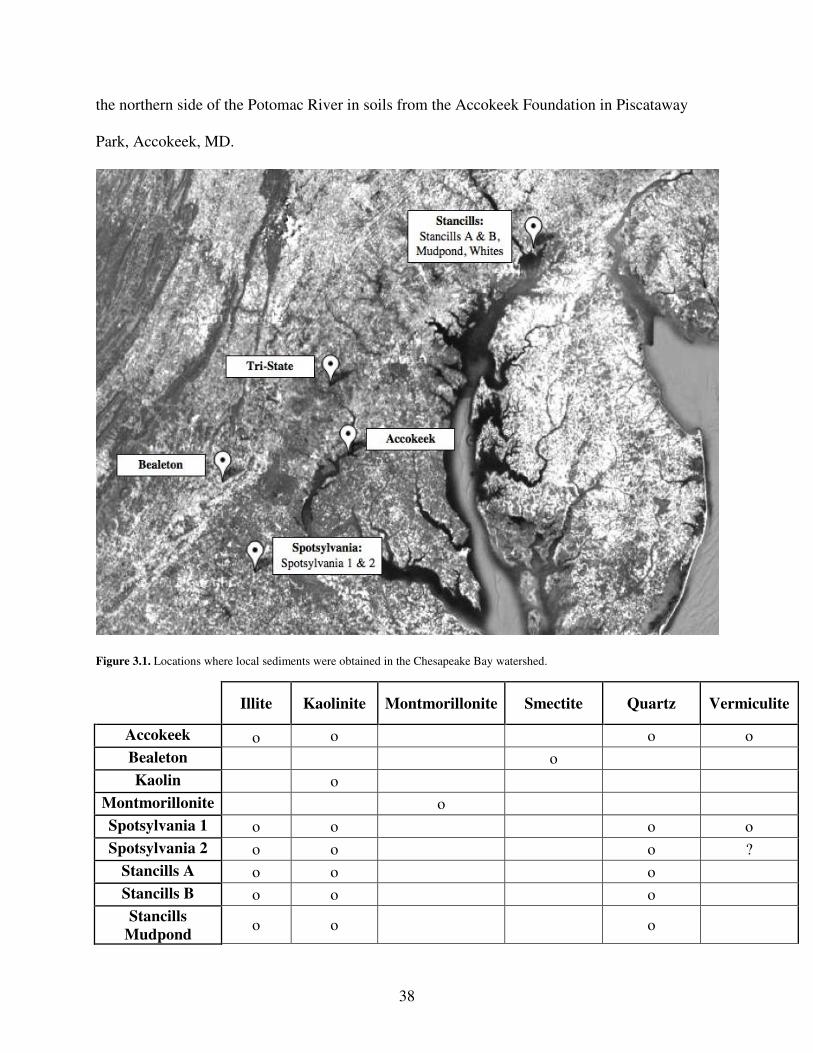
38

the northern side of the Potomac River in soils from the Accokeek Foundation in Piscataway

Park, Accokeek, MD.

Figure 3.1. Locations where local sediments were obtained in the Chesapeake Bay watershed.

Illite Kaolinite Montmorillonite Smectite Quartz Vermiculite

Accokeek o o o o

Bealeton o

Kaolin o

Montmorillonite o

Spotsylvania 1 o o o o

Spotsylvania 2 o o o ?

Stancills A o o o

Stancills B o o o

Stancills

Mudpond o o o

39

Stancills Whites o o o

Tri-State o o o

Table 3.1. Mineralogical composition of all sediments tested. Composition was determined using X-ray diffraction (D. Vanko,

Towson University).

3.3.3. Clay Preparation in Freshwater vs. Saltwater Experiments

For the first experiments, spectrophotometry was employed to follow clay distributions in

several water types. Experimental solutions were artificial seawater (ASW) at a salinity of 35

created using deionized water and salt (Instant Ocean) while Mattawoman water was obtained

from Mattawoman Creek, Maryland filtered through Whatman GF/F 47 mm filters, and

autoclaved. Three milliliters of ASW and filtered, autoclaved Mattawoman water were added to

3.5 mL spectrophotometer cuvettes followed by 0.5 mL of varying amounts of an 28 g L-1

bentonite clay slurry to create clay concentrations of 2.0, 1.0, 0.5, 0.25, 0.125, and 0.0625 g L-1.

Cuvettes were inverted and a first measurement of absorbance at 720 nm was taken immediately

with a spectrophotometer. The absorbance of all cuvettes was measured at several intervals for

160 min.

3.3.4 Clay Preparation in Clay Comparison Experiments in Mattawoman Water

Along with the bentonite slurry, two other commercially available clays were obtained (kaolin

and montmorillonite from Thiele Kaolin Company) and 28 g L-1 of stock clay slurries was made

by adding the dry clay powder to deionized water (DI). Three milliliters of filtered and

autoclaved Mattawoman water was added to 3.5 mL cuvettes followed by 0.5 mL of the clay

slurry of varying concentration. Final concentrations for all three clays in the cuvettes were 4.0,

2.0, 1.0, 0.5, 0.25, 0.125, and 0.0625 g L-1 for each. The cuvettes were inverted and absorbance

40

at 720 nm was measured immediately in the spectrophotometer and at regular intervals for the

next 160 min.

3.3.5 Sediment flocculation Experiments with Processed Clays and UTEX M. aeruginosa

UTEX M. aeruginosa stock culture was diluted with 3 mL DI and placed into spectrophotometer

cuvettes. 0.5 mL of clay slurry (either bentonite, kaolin, or montmorillonite) was added to each

cuvette containing M. aeruginosa cells to bring the concentration of clay in the cuvette to 2.0,

1.0, or 0.5 g L-1 (for bentonite and kaolin) and 0.5 or 0.25 g L-1 (for montmorillonite). The

cuvettes were inverted and the absorbance in each cuvette was promptly measured at 680 nm and

at regular intervals over several hours.

3.3.6 Local Sediment Preparation for Flocculation Experiments

Eleven sediment samples (kaolin, montmorillonite, tristate, Spotsylvania 1 and 2, Bealeton, and

Stancills A, B, White and Mudpond) were acquired from various local companies and quarries,

as described above. Thiele Kaolin provided samples in a fine powder while others were

unprocessed. The local sediments were manually ground with a mortar and pestle and filtered

through a 10-in diameter 250 µm USA Standard testing sieve. 10 g L-1 sediment slurries were

made by suspending a set amount of sediment in DI (e.g., 0.3 g in 30 mL DI, 0.4 g in 40 mL DI,

etc.).

3.3.7 Flocculant Preparation and Addition

Addition of flocculant was incorporated to further augment removal efficiency. Chitosan was

tested against M. aeruginosa in these experiments and was obtained from (Chitin Works, Inc.,

Cambridge, MD). The chitosan solution was made independently of the sediment slurry by

41

combining 0.5 g dry chitosan with 0.05 L 1% HCl and mixing until all chitosan had been

dissolved. Slurries of different chitosan to sediment concentrations were then derived at 1:10,

1:50, and 1:100 mixtures.

3.3.8 Chitosan-sediment Flocculation Experiment Protocol

3.3.8.1 Flocculation Experiments in Deionized Water (DI) with UTEX 2667 M. aeruginosa

Chitosan-sediment mixtures were pipetted into tubes containing suspended M. aeruginosa and

DI in 40 mL fluorometer tubes at an initial density of 107 cells mL-1. Tubes were prepared for

each sediment so that each trial consisted of 27 IVF tubes to yield three replicates at exposures of

0, 0.25 and 0.5 g clay L-1. IVF measurements were taken immediately upon addition, and tubes

were then placed in a rack to allow for flocculation to proceed uninterrupted. Readings were

taken at the same time each day (+/- 2 hours) and were taken for up to three weeks. IVF

measurements for each trial were averaged and used for analysis. Overall, 88 different chitosan-

sediment mixtures were used for the flocculation trials in deionized water. Two criteria were

used to determine which sediment mixtures best removed M. aeruginosa cells from the water

column: maximum percentage of cells removed and time to 50% cell removal.

3.3.8.2 Flocculation Experiments in Mattawoman Water with UTEX 2667 M. aeruginosa

Flocculation was also examined in Whatman GF/A filtered water from Mattawoman Creek (a

small creek entering the upper Potomac River and characterized by recurring M. aeruginosa

blooms). Cyanobacteria were suspended in filtered Mattawoman water and the procedure above

was followed for 30 chitosan-sediment mixtures that had been most effective in bloom removal

in DI. Flocculation was also tested in Whatman GF/A filtered water from Mattawoman Creek

42

and with M. aeruginosa populations collected from Budds Creek on the Eastern shore of

Chesapeake Bay.

3.3.9 Statistical Analysis

Results were analyzed with PASW Statistics 18 software, primarily employing one-way

ANOVAs. In each treatment, ANOVAs were used to determine which sediment concentration,

chitosan ratio, sediment to chitosan combination, and specific sediment type yielded similar or

differing results for two parameters: maximum percentage of cells removed and speed of

removal. Speed of removal was evaluated using three parameters: time to 50% removal, percent

cell removal at 24 h, or time to maximum percent cell removal. When Levene’s statistic was

significant (p < 0.05), variance was assumed to be unequal and Games-Howell post-hoc tests

were used. When Levene’s test was not significant (p > 0.05), variance was assumed to be equal

and Tukey’s post-hoc tests were used for comparing results. Repeated measures ANOVA was

not used because sphericity was violated (p < 0.05) due to the amount of variation in the trials.

3.4 Results

3.4.1 Settling Rates of Bentonite in Mattawoman Creek Water vs. Saltwater

43

0.00

0.10

0.20

0.30

0.40

0.50

0.60

0.70

0.80

0.90

1.00

0 20 40 60 80 100 120 140 160

Time (mins)

Ab

sorb

an

ce (

720

nm

)

Figure 3.2. Flocculation of 0.5 g L-1 bentonite in ASW and filtered Mattawoman Creek water. The absorbance of the clay was measured at 720 nm. Light gray line represents light absorption and therefore particle concentration in ASW. Dark gray line represents particle concentration in Mattawoman Creek water. Error bars show the standard deviation in the replicate measurements at each time period for each clay.

Figure 3.2 shows that bentonite in ASW settles more quickly than the clay in Mattawoman Creek

water. In ASW sweep floc is achieved earlier, at approximately 20 min, and the clay ultimately

settles more effectively, to below 0.1 units (O.D. or % transmittance). Sweep floc is observed by

the initial increase in absorbance and the subsequent decrease as clay particles bind together and

then settle out of the water column. The bentonite sample in Mattawoman Creek water did not

exhibit sweep floc formation until approximately 40 min and the clay did not sink out of

suspension as well as in ASW. This phenomenon was shown to occur across many bentonite

concentrations as well as with other types of clays (data not shown).

3.4.2 Settling Rates of Various Clays in Mattawoman Creek Water

44

0.00

0.10

0.20

0.30

0.40

0.50

0.60

0.70

0.80

0.90

1.00

0 20 40 60 80 100 120

Time (mins)

Ab

sorb

an

ce

(720 n

m)

Figure 3.3. Flocculation of three different clays at 0.5 g L-1 in filtered Mattawoman Creek water: montmorillonite (light gray curve), bentonite (dark gray curve), and kaolinite (black curve). The absorbance was measured at 720 nm. Error bars show the standard deviation in the absorptions for the three replicates for each clay.

In Figure 3.3, out of the three clays tested (montmorillonite, bentonite, and kaolin),

montmorillonite achieved sweep floc earlier (at approximately 15 min) and settled more

successfully (to below 0.05 abs units) than either bentonite or kaolin. Sweep floc for bentonite

was eventually noted, at approximately 35 min, while kaolin did not follow this trend. However,

bentonite did not ultimately settle more effectively than kaolin, which settled to yield

approximated 0.1 abs units, despite not exhibiting sweep floc.

3.4.3 Sediment Flocculation Using Commercially-Available Processed Clays in

Mattawoman Creek Water

45

0.00

0.10

0.20

0.30

0.40

0.50

0.60

0.70

0 20 40 60 80 100 120

Time (mins)

Ab

sorb

an

ce

(68

0 n

m)

Figure 3.4. Flocculation of 0.5 g L-1 montmorillonite and M. aeruginosa compared to the natural settling of the cells. Light gray denotes clay only, dark gray denotes clay and cells, and black denotes cells only. The absorbance of the cells was measured at 680 nm. The initial M. aeruginosa concentration was about 6.06X 107cells mL-1.

46

0.00

0.05

0.10

0.15

0.20

0.25

0.30

0.35

0.40

0.45

0.50

0 20 40 60 80 100 120

Time (mins)

Ab

sorb

an

ce (

680

nm

)

Figure 3.5. Flocculation of 0.25 g L-1 montmorillonite and M. aeruginosa compared to the settling cells. Light gray denotes clay only, dark gray denotes clay and cells, and black denotes cells only. The absorbance of the cells was measured at 680 nm. The initial M. aeruginosa concentration was about 6.06 x107 cells mL-1.

The addition of 0.5 g L-1 (Fig. 3.4) and 0.25 g L-1 (Fig. 3.5) montmorillonite to a M. aeruginosa

sample was able to reduce the number of cyanobacteria suspended in the water column. In each

trial, the cuvettes containing montmorillonite and Microcystis finished with a lower absorbance

than the control cuvettes containing only the cyanobacterium. In addition, we observed that the

sample containing the higher clay density of 0.5 g L-1 seemed to finish with a lower absorbance

(0.064 abs units) than the sample with the lower clay density of 0.25 g L-1 (end absorbance of

0.173 abs units). Further, for the clay sample at 0.5 g L-1, the clay-cell sample exhibited the

sweep floc settling pattern similar to the sample containing clay only, indicating that the cells

were incorporated into the flocculation process shown in Figures 3.4 and 3.5. The addition of

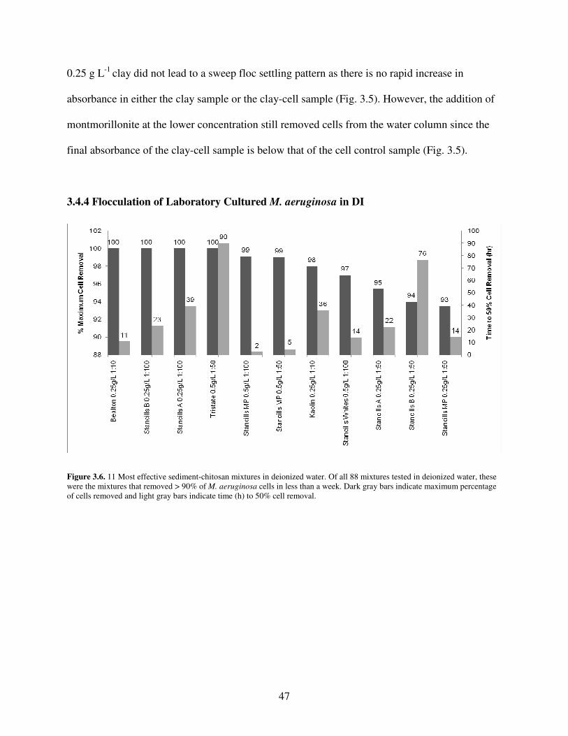
47

0.25 g L-1 clay did not lead to a sweep floc settling pattern as there is no rapid increase in

absorbance in either the clay sample or the clay-cell sample (Fig. 3.5). However, the addition of

montmorillonite at the lower concentration still removed cells from the water column since the

final absorbance of the clay-cell sample is below that of the cell control sample (Fig. 3.5).

3.4.4 Flocculation of Laboratory Cultured M. aeruginosa in DI

Figure 3.6. 11 Most effective sediment-chitosan mixtures in deionized water. Of all 88 mixtures tested in deionized water, these were the mixtures that removed > 90% of M. aeruginosa cells in less than a week. Dark gray bars indicate maximum percentage of cells removed and light gray bars indicate time (h) to 50% cell removal.

48

Figure 3.7. Best mixture for each sediment in deionized water. Of all 88 mixtures tested in deionized water, these 11 mixtures represent the most effective sediment concentration and chitosan:clay ratio for each of the 11 sediments used. Dark gray bars indicate maximum percentage of cells removed and light gray bars indicate time (h) to 50% cell removal.

Of the 88 sediment-chitosan mixtures tested for removal efficiency of M. aeruginosa (UTEX

2667) in DI, 24 mixtures showed ≥50% cell removal in less than one week (Table 3.2). Eleven

sediment-chitosan mixtures removed ≥90% of the suspended algal population in less than one

week (Fig. 3.6). Of these, Stancills Mudpond 0.5g/L 1:100 removed cells most rapidly, with 50%

of cells removed in 2 h. Tristate 0.5g/L 1:50 removed the cyanobacterium the least rapidly, with

50% of cells removed in 90 h. The other 9 mixtures fell within this range. Every sediment tried,

except for montmorillonite, had at least one sediment-chitosan combination that was able to

remove >90% of cells from the water column (Fig. 3.7) within the 3 week trial period. The best

sediment-chitosan combination for each of the 11 sediments tested is displayed in Figure 3.7.

49

Chitosan-Sediment Ratio

Clays

0.5gL-

1 0.5gL-1

1:10 0.5gL-1 1:50 0.5gL-1 1:100 0.25gL-

1 0.25gL-1 1:10 0.25gL-1 1:50 0.25gL-1 1:100

Kaolin ** ** **

Montmorillonite

Bealeton **

Spotsylvania 1 **

Spotsylvania 2 **

Accokeek ** **

Tristate ** ** **

Stancills A ** ** ** **

Stancills B ** ** **

Stancills Mudpond ** ** **

Stancills Whites ** **

Table 3.2. Flocculation Trials in Deionized Water. Results from 88 flocculation trials with laboratory-cultured M. aeruginosa (UTEX 2667) in deionized water and the range of chitosan-sediment mixtures tested. Grey shaded boxes indicate the most effective mixture for each sediment type based on maximum percentage cell removal and are graphically represented in Figure 3.7. Boxes with two asterisks indicate mixtures that removed > 50% of cells in less than a week. Boxes with a thick black border indicate mixtures that removed > 90% of cells in less than a week and are graphically represented in Figure 3.6. Removal data for all mixtures tried is available in Appendix section 7.1.2.

50

3.4.4.1 Effects of Sediment Concentration on Mixture Efficacy in DI

Of the 88 sediment-chitosan mixtures tested in deionized water (Table 3.2), there was no

significant difference in maximum percentage of cells removed (p = 0.263) between 0.5 g L-1

and 0.25 g L-1 sediment mixtures. The general trend was that 0.25 g L-1 sediment mixtures had

higher overall cell removal.

3.4.4.2 Effects of Chitosan:Sediment Ratio on Removal Efficacy in DI

The addition of chitosan improved the ability of the 11 sediments to flocculate M. aeruginosa

cells. Sediment mixtures with chitosan removed significantly better than mixtures with sediment

alone (p=0.000). No sediment mixtures showed ≥50% cell removal without the addition of

chitosan (Table 3.2). When all 88 sediment mixtures were included in the analysis, a

chitosan:sediment ratio of 1:50 resulted in greater percent cells removed than either 1:10

(p=0.000) or 1:100 (p = 0.050). The chitosan ratio did not significantly influence the speed of

removal across the 88 mixtures (p > 0.05).

3.4.4.3 Effects of Sediment and Chitosan Combination on Mixture Efficacy in DI

The sediment and chitosan combination significantly affected maximum cell removal (p < 0.05).

When evaluating the 8 different sediment-chitosan combinations tested (Table 3.2), 0.5 g L-1

1:50 mixtures were the most effective. They removed an average of 69.7% (+/- 24.7%) of cells

across the 11 sediments tested. This combination was significantly more effective than the

following mixtures: 0.5 g L-1 with no chitosan (p = 0.000), 0.25 g L-1 with no chitosan (p =

0.000), and 0.5 g L-1 1:10 (p = 0.001). However, there was no significant difference between

cells removed by 0.5 g L-1 1:50 mixtures and the following mixtures: 0.25 g L-1 1:100 (p=0.213),

0.25 g L-1 1:10 (p=0.358), 0.5 g L-1 1:100 (p=0.857), and 0.25 g L-1 1:50 (p=1.000).

51

3.4.4.4 Effects of Sediment Type on Mixture Efficacy in DI

Of the 11 sediments tested, kaolin, Bealeton, Spotsylvania 2, Accokeek, Stancills A, Stancills B,

Stancills Mudpond, and Stancills Whites exhibited ≥90% cell removal in < 1 week with certain

sediment-chitosan combinations (Table 3.2, Fig. 3.6). Kaolin showed the greatest cell removal

across all mixtures tried, but there was no significant difference in removal between kaolin and

Stancills Whites (p = 0.993), Stancills A (p = 0.990), Stancills Mudpond (p = 0.850), Tristate (p

= 0.746), Stancills B (p = 0.640), montmorillonite (p = 0.574), Spotsylvania 2 (p = 0.453), and

Bealeton (p = 0.207). There was a significant difference in removal between kaolin mixtures and

Spotsylvania 1 (p = 0.026) and Accokeek (p = 0.016) mixtures.

Stancills Mudpond showed the fastest cell removal, with ≥50% of cells removed in 2 h (Fig. 3.6)

with a 0.5 g L-1 sediment and 1:100 or 1:50 chitosan:sediment ratio. On the other hand,

montmorillonite showed limited cell removal across all chitosan:sediment ratios, with the best

mixture only removing 50% of M. aeruginosa cells after approximately 17 d (Fig. 3.7). Of the 11

sediments surveyed, mixtures with kaolin, Tristate, Stancills A, Stancills B, Stancills Mudpond,

and Stancills Whites removed ≥50% of algal cells in < 1 week in ≥3 of the 8 chitosan-sediment

combinations tested (Table 3.2).

3.4.4.5 Summary of Findings in DI

Based on these results in DI, kaolin, Tristate, and the 4 Stancills sediments were best able to

achieve high and fast cell removal. Of these, kaolin was the only clay not from the Chesapeake

Bay region. Sediment-chitosan combinations of 0.5 g L-1 1:50, 0.5 g L-1 1:100, 0.25 g L-1 1:50,

52

and 0.25 g L-1 1:10 consistently achieved high cell removal in ion-free water and therefore

became likely candidates for more exploratory use.

53

Chitosan-Sediment Ratio

Clays Tried 0.5gL-1 0.5gL-1

1:10 0.5gL-1

1:50 0.5gL-1 1:100 0.25gL-1 0.25gL-1 1:10 0.25gL-1 1:50 0.25gL-1 1:100

Kaolin ** ** **

Montmorillonite

Bealeton ** **

Spotsylvania 1 ** **

Spotsylvania 2 ** **

Accokeek **

Tristate ** ** **

Stancills A

Stancills B **

Stancills Mudpond ** **

Stancills Whites ** **

Table 3.3. Flocculation trials (30) with the laboratory cultured M. aeruginosa (UTEX 2667) in filtered Mattawoman Creek water. All boxes shaded in light gray were not tested. Dark gray boxes indicate the most effective mixture for each sediment type based on maximum percentage of cells removed and are graphically represented in Figure 3.9. Boxes with two asterisks indicate mixtures that removed >50% of cells in less than a week. Boxes with a thick black border indicate mixtures that removed >90% of cells in less than a week and are graphically represented in Figure 3.8. Removal data for all mixtures tried is available in Appendix section 7.1.3.

54

3.4.5 Flocculation of Laboratory Cultured M. aeruginosa in Mattawoman Creek Water

Figure 3.8. 10 Most effective chitosan-sediment mixtures in filtered Mattawoman Creek water with laboratory strains of M.

aeruginosa (UTEX 2667). Of the 30 mixtures tested, these mixtures removed >90% of cells in less than 1 week. Dark gray bars indicate maximum percentage of cells removed and light gray bars indicate time (h) to 50% cell removal.

Based on the results in DI, 30 sediment-chitosan mixtures were selected for testing in filtered

Mattawoman Creek water. Table 3.3 displays all mixtures tested and all mixtures that yielded

high cell removal. The same two criteria, maximum percentage of cells removed and time to

50% cell removal, were used to determine the most effective sediment-chitosan mixtures in

Mattawoman water. Of the 30 mixtures tested, 18 showed >50% cell removal in < 1 week (Table

3.3). Of these, 10 mixtures removed ≥90% cells in < 1 week (Fig. 3.8). Bealeton, Spotsylvania 2,

Tristate, Spotsylvania 1, and kaolin mixtures removed the highest percentage of cells (Table 3.3,

Fig. 3.8, Fig. 3.9). The most effective sediment-chitosan combination for each sediment tested is

displayed in Figure 3.9.

55

Figure 3.9. Best mixture for each sediment in filtered Mattawoman Creek water. Of all 30 mixtures tested, these 11 mixtures represent the most effective sediment concentration and chitosan:sediment ratio for each sediment used. Dark gray bars indicate maximum percentage of cells removed and light gray bars indicate time (h) to 50% cell removal. Stancills A and montmorillonite sediments never reached 50% cell removal and therefore do not have bars representing times to 50% removal.

3.4.5.1 Effects of Sediment Concentration on Mixture Efficacy in Mattawoman Creek

Water

Of the 30 mixtures tested, sediment mixtures with a 0.5 g L-1 sediment concentration removed M.

aeruginosa cells better than those with a concentration of 0.25 g L-1 (p = 0.005). When all 30

mixtures were included in the analysis, mixtures with a 0.5g L-1 sediment concentration removed

77.6% (+/- 22.1%) of cells across all mixtures tried, compared to 58.7% (+/- 35.1%) removed by

0.25 g L-1 mixtures. 0.5 g L-1 mixtures also removed cells from the water column faster (p =

0.001): 24 h post flocculation, 0.5 g L-1 mixtures had removed 59.0% (+/- 28.1%) of cells

compared to 35.4% (+/- 36.8%) removed by 0.25 g L-1 mixtures. However, when only mixtures

removing >90% cells in <1 week (Fig. 3.8) were included in the analysis, mixtures with a 0.25 g

L-1 sediment concentration showed greater maximum percentage of cells removed (p = 0.023)

56

than noted in the 0.5 g L-1 mixtures. 0.25 g L-1 mixtures removed an average of 99.1% (+/- 1.6%)

of the suspended cells compared to 97.2% (+/- 3.1%) removed by the 0.5 g L-1 mixtures. There

was no significant difference (p = 0.361) in removal speeds between 0.25 g L-1 and 0.5 g L-1

mixtures.

This discrepancy in results may indicate that 0.25 g L-1 mixtures are more sensitive to the

chitosan concentration used and the removal ability of the sediment used. To support this

hypothesis, of the 16 0.5 g L-1 mixtures tested, 13 were able to remove >50% of the cells in <1

week, and of those, 5 were able to remove >90% of cells in <1 week (Table 3.3). Of the 13 0.25

g L-1 mixtures tested, only 5 were able to remove >50% of cells in <1 week; however, all 5 of

these also removed >90% of cells in <1 week (Table 3.3).

3.4.5.2 Effects of Chitosan Ratio on Mixture Efficacy in Mattawoman Creek Water

A higher chitosan ratio significantly improved the ability of tested sediments to flocculate M.

aeruginosa cells (p < 0.000). Of the 30 mixtures tested, a chitosan:sediment ratio of 1:10

exhibited the greatest and fastest cell removal (p < 0.000), with an average maximum percentage

removal of 99.0% (+/- 1.6%) and with 82.4% (+/- 5.7%) of the cells removed in 24 h.

Chitosan:sediment mixtures of 1:50 showed significantly better cell removal than 1:100 mixtures

(p = 0.001) and removed cells faster from the water column (p = 0.004). 1:50 mixtures removed

a maximum of 68.1% (+/- 26.1%) of cells, with 48.9% (+/- 34.0%) removed in 24 h. 1:100

mixtures only removed a maximum of 44.7% (+/-27.6%) of cells, with 26.1% (+/- 27.4%)

removed in 24 h. No mixtures were able to achieve > 90% of cells in < 1 week with only a 1:100

chitosan:sediment ratio (Table 3.3, Fig. 3.8), thus showing the importance of chitosan addition

for high cell removal.

57

3.4.5.3 Effects of Sediment and Chitosan Combination on Mixture Efficacy in Mattawoman

Creek Water

Of the 30 mixtures tested, those with a sediment-chitosan combination of 0.5 g L-1 1:10 and 0.25

g L-1 1:10 removed algal cells similarly (p = 1.000) and better than all other combinations (p <

0.000) with an average maximum cell removal of > 98%. Following these, the best sediment-

chitosan combinations were: 0.5 g L-1 1:50, 0.5 g L-1 1:100, 0.25 g L-1 1:50, and 0.25 g L-1 1:100.

0.25 g L-1 1:10 mixtures showed the fastest removal rates (p < 0.000) compared to all other

sediment-chitosan combinations tested. 0.25 g L-1 1:10 mixtures removed an average of 84.3%

(+/- 5.7%) of cells in 24 h, compared to 78.6% (+/- 3.4%) of cells removed by 0.5 g L-1 1:10

mixtures in 24 h.

3.4.5.4 Effects of Sediment Type on Mixture Efficacy in Mattawoman Creek Water

Of the 11 sediments tested, certain Spotsylvania 1, Spotsylvania 2, Bealeton, kaolin, and Tristate

mixtures exhibited >90% cell removal in <1 week (Table 3.3, Fig. 3.8, Fig. 3.9). In all 30 trials,

Bealeton, Spotsylvania 2, Spotsylvania 1, kaolin, and Tristate exhibited the greatest overall

percentage of cells removed in the shortest time (Fig. 3.8, Fig. 3.9). Bealeton mixtures removed

an average maximum of 99.6% (+/- 1.7%) of cells, Spotsylvania 2 mixtures 97.4% (+/- 3.6%),

kaolin mixtures 94.7% (+/- 5.0%), and Tristate mixtures 90.8% (+/- 12.8%) of cells. These

mixtures removed significantly more M. aeruginosa cells than mixtures using Stancills Mudpond

(p = 0.042), montmorillonite (p < 0.000), Stancills A (p < 0.000), Stancills B (p < 0.000), and

Accokeek (p < 0.000). However, these 5 sediments were not tested using a 0.25g L-1 1:10 or 0.5g

L-1 1:10 sediment-chitosan combination (Table 3.3), which was determined to be the most

effective combination (see above?). For this reason, these sediments and sediment-chitosan

mixtures should be further tested.

58

3.4.5.5 Differing Flocculation Results between DI and Mattawoman Creek Water

Stancills sediments (A, B, Whites, and Mudpond) were significantly less effective at removing

M. aeruginosa cells in the filtered creek water than they were in DI (p < 0.000) (Tables 3.2, 3.3).

Stancills clays contain only kaolinite, illite, and some quartz and, from are nearly identical in

composition (see Table 3.1). All four sediments are considered non-swelling clays. These results

indicate that, contrary to our expectations, non-swelling clays flocculate better in deionized water

than in ionized Mattawoman water. The higher ion content of Mattawoman water appears to

negatively affect the ability of Stancills clays to flocculate M. aeruginosa cells. Of all Stancills

sediment mixtures tested in both DI and Mattawoman Creek water, those in DI removed an

average of 90.7% (+/- 17.7%) of cells compared to 59.6% (+/- 24.0%) in Mattawoman Creek

water. Figure 3.10 exhibits the decreased ability of Stancills A 0.25g L-1 1:100 mixture to remove

M. aeruginosa cells in Mattawoman water compared to DI.

59

Figure 3.10. Stancills A 0.25g L-1 1:100 removal efficiency in DI versus Mattawoman Creek water. Dashed line represents cell removal in deionized water, solid line represents cell removal in Mattawoman water. Error bars represent standard deviation of replicates. These results exhibit the greater ability of a Stancills A sediment mixture to remove algal cells in ion-free water than in Mattawoman Creek water containing dissolved cations and anions. These results were consistent with our general finding that Stancills sediments removed M. aeruginosa cells more poorly in Mattawoman water than in DI.

Unlike Stancills mixtures, Bealeton, Spotsylvania 1, and Spotsylvania 2 sediment mixtures

exhibited higher cell removal in Mattawoman Creek water than in DI (p = 0.047). These

sediments removed an average of 88.3% (+/- 24.3%) of cells suspended in Mattawoman Creek

water, compared to 76.4% (+/- 21.1%) of cells in DI. Figure 3.11 exhibits the increased ability of

Bealeton 0.25g L-1 1:10 to remove M. aeruginosa cells in Mattawoman water compared to

deionized water. There was no significant difference in the ability of kaolin (p = 0.987),

Accokeek (p = 0.109), and Tristate mixtures (p = 0.179) to remove cells in Mattawoman Creek

or DI.

Figure 3.11. Bealeton 0.5g L-1 1:10 removal efficiency in DI vs. Mattawoman Creek water. Dashed line represents cell removal in deionized water, solid line represents cell removal in ion-containing water from Mattawoman Creek. These results exhibit the greater ability of a Bealeton sediment mixture to remove algal cells in ion-rich natural water than in deionized water.

3.4.5.6 Summary of Findings in Mattawoman Water

60

Based on our results in Mattawoman Creek water, Bealeton, Spotsylvania 1, Spotsylvania 2,

Tristate, and kaolin mixtures were best able to achieve high and fast cell removal. Of these,

kaolin was the only clay not from the Chesapeake Bay region. Sediment-chitosan combinations

of 0.25 g L-1 1:10, 0.5 g L-1 1:10, and 0.5 g L-1 1:50 achieved high cell removal and could be

possible candidates for general use in field blooms. Generally, a greater chitosan concentration

was needed for cell removal in Mattawoman Creek water than in DI and cell removal was

achieved more rapidly in Mattawoman water than DI. The average time to 50% cell removal in

DI for mixtures removing >90% of cells in <1 week (Fig. 3.6) was 30.2 h (+/- 28.7 h) compared

to 11.6 h (+/- 3.5 h) in water from the creek (Fig. 3.8).

3.4.5.7 Recommendations for Use

Assuming that efficacy, cost, and environmental impact of mitigation are the most important

factors in choosing a mixture for intervention in a field bloom, the best mixture is one that uses

minimal sediment and chitosan and removes bloom cells from the water column quickly and

effectively. While many sediment mixtures were effective, based on our results, we identified

two mixtures that very effectively removed laboratory-grown M. aeruginosa cells as prime

candidates for use: Spotsylvania 1 0.25g L-1 1:50 and Stancills Mudpond 0.5g L-1 1:100.

Spotsylvania 1 0.25g L-1 1:50 mixture removed an average of 95.6% (+/- 3.0%) of cells with

77.0% (+/- 1.7%) removed in 24 h. Spotsylvania 1 0.25g L-1 1:50, should be used if sediment

addition to the environment is the greater concern. This factor may be a key issue for the public

and fishery managers since suspended sediments have been shown to cause gasping in some fish

species (Lewis et al. 2003). Stancills Mudpond 0.5g L-1 1:100 mixture removed an average of

78.6% (+/- 4.8%) of exposed laboratory-reared Microcystis cells with 73.8% (+/- 4.5%) removed

in 24 h. Stancills Mudpond 0.5g L-1 1:100 mixture is the best option if the cost of chitosan is the

61

critical factor in the adoption of a mixture. While Stancills sediments in general did not show

high cell removal, Stancills Mudpond 0.5g L-1 1:100 showed the highest cell removal of all

sediment mixtures tested in Mattawoman Creek water with a 1:100 chitosan:sediment ratio.

Further studies should test this sediment-chitosan combination using Bealeton, Spotsylvania 1,

and Spotsylvania 2 sediments, with laboratory grown and field bloom sub-samples.

Figure 3.12. Comparison of 2 effective sediment-chitosan mixtures in Mattawoman Creek water. The dark gray line represents removal of laboratory cultured M. aeruginosa by Spotsylvannia 1 0.25g L-1 1:50 and the light gray line represents cell removal by Stancills Mudpond 0.5g L-1 1:100. Error bars represent standard deviation of 3 replicates. Analysis based on removal efficiency, low chitosan, and low sediment considerations suggest that Spotsylvannia 1 0.25g L-1 1:50 and Stancills Mudpond 0.5g L-1 1:100 be used for flocculation of M. aerugionsa blooms.

3.4.6 Flocculation of Field Bloom M. aeruginosa in Mattawoman Creek Water

Flocculation results from the experiments using the laboratory M. aeruginosa strain were used to

select nine sediment-chitosan mixtures to test with a field sample of M. aeruginosa from a

summer 2010 Budds Creek Microcystis bloom. The nine mixtures tested were: Stancills

Mudpond 0.5g L-1 1:100, Stancills A 0.25g L-1 1:100, Stancills A 0.5g L-1 1:100, Stancills B 0.5g

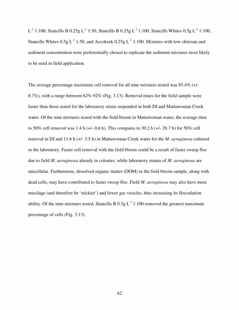
62

L-1 1:100, Stancills B 0.25g L-1 1:50, Stancills B 0.25g L-1 1:100, Stancills Whites 0.5g L-1 1:100,

Stancills Whites 0.5g L-1 1:50, and Accokeek 0.25g L-1 1:100. Mixtures with low chitosan and

sediment concentration were preferentially chosen to replicate the sediment mixtures most likely

to be used in field application.

The average percentage maximum cell removal for all nine mixtures tested was 85.4% (+/-

8.7%), with a range between 62%-92% (Fig. 3.13). Removal times for the field sample were

faster than those noted for the laboratory strain suspended in both DI and Mattawoman Creek

water. Of the nine mixtures tested with the field bloom in Mattawoman water, the average time

to 50% cell removal was 1.4 h (+/- 0.6 h). This compares to 30.2 h (+/- 28.7 h) for 50% cell

removal in DI and 11.6 h (+/- 3.5 h) in Mattawoman Creek water for the M. aeruginosa cultured

in the laboratory. Faster cell removal with the field bloom could be a result of faster sweep floc

due to field M. aeruginosa already in colonies, while laboratory strains of M. aeruginosa are

unicellular. Furthermore, dissolved organic matter (DOM) in the field bloom sample, along with

dead cells, may have contributed to faster sweep floc. Field M. aeruginosa may also have more

mucilage (and therefore be ‘stickier’) and fewer gas vesicles, thus increasing its flocculation

ability. Of the nine mixtures tested, Stancills B 0.5g L-1 1:100 removed the greatest maximum

percentage of cells (Fig. 3.13).

63

Figure 3.13. Removal abilities for 9 sediment-chitosan mixtures tested with field bloom samples suspended in filtered Mattawoman Creek water. Dark gray bars indicate maximum percentage of cells removed and light gray bars indicate time (h) to 50% cell removal.

3.4.6.1 Effects of Sediment Concentration on Removal Efficacy with Field M. aeruginosa

Chitosan-sediment mixtures with a higher sediment concentration (0.5g L-1) were more effective

(p = 0.002) at removing algal cells than those with a sediment concentration of 0.25g L-1. The

0.5g L-1 sediment mixtures removed an average of 90.5% (+/- 1.8%) of the bloom cells

compared to 79.0% (+/- 9.7%) by the 0.25g L-1 sediment mixtures. 0.5g L-1 sediment mixtures

also removed cells faster than mixtures with a 0.25g L-1 sediment concentration (p = 0.014).

3.4.6.2 Effects of Chitosan Ratio on Removal Efficacy with Field M. aeruginosa

64

There was no significant difference between the ability of sediment mixtures with a 1:50 and a

1:100 chitosan:sediment ratio to remove field bloom cells based on both maximum cell removal

(p = 0.446) and removal speed (p = 0.482). Although there was no significant difference, the

general trend of the data suggests that a chitosan:sediment ratio of 1:100 is able to remove cells

faster, but a 1:50 ratio removes more cells overall. Mixtures with a 1:50 chitosan to sediment

ratio removed an average of 88.5% (+/- 2.5%) of suspended cells, compared to 84.5% (+/- 9.7%)

of cells removed by 1:100 mixtures.

3.4.6.3 Effects of Sediment and Chitosan Combination on Mixture Efficacy with Field M.

aeruginosa

The 0.5g L-1 1:50 sediment-chitosan mixtures were most effective at removing field bloom cells

from the water column, followed by 0.5g L-1 1:100, 0.25g L-1 1:50, and 0.25g L-1 1:100 mixtures.

While there was no significant difference between the ability of 0.5g L-1 1:50 and 0.5g L-1 1:100

mixtures to remove suspended cells (p = 0.999), 0.5g L-1 1:50 removed cells significantly better

than 0.25g L-1 1:50 (p = 0.020) and 0.25g L-1 1:100 (p = 0.013) mixtures. Sediment-chitosan

combinations of 0.5g L-1 1:50 were able to remove an average of 90.6% (+/- 1.0%) of the field

bloom cells, irrespective of sediment source.

3.4.6.4 Effects of Sediment Type on Mixture Efficacy in Mattawoman Creek Water

When the efficacy of different sediment types was compared against each other (Stancills A, B,

Mudpond, Whites, and Accokeek) there was only a significant difference in removal ability

between Stancills Whites and Stancills Mudpond. Stancills Whites had greater maximum cell

removal (90.9% +/- 1.1%) than Stancills Mudpond (p=0.005) but had a slower removal rate in 24

h (p = 0.05). Of all the sediments tested, Stancills Whites was best able to keep cells from

resuspending and after one week post-flocculation had the greatest percentage of cells removed

65

(p < 0.000) than all other tested sediments. Stancills Whites’ rate of cell removal was the slowest

for all clays examined and required the longest time to maximum cell removal (p = 0.001).

3.4.6.5 Predictability of Field Removal Based on Flocculation in DI and Mattawoman

Creek Water

The same sediment-chitosan mixtures better removed field bloom populations than the UTEX

2667 laboratory strain of M. aeruginosa in Mattawoman Creek water (p < 0.000). There was no

significant difference between maximum removal of the laboratory cultured Microcystis in DI

and the Microcystis-dominated field bloom assemblage in Mattawoman Creek treatments (p =

0.747) when using the same chitosan-sediment mixtures. Overall, when evaluated on percentage

of total cells removed 24 h post-flocculation, field Microcystis bloom abundances showed faster

cell removal across the range of sediment mixtures tested than laboratory cultured Microcystis

blooms did in both DI and Mattawoman Creek water (p < 0.000).

While there was no significant difference between removal efficiency of lab M. aeruginosa in DI

and field bloom populations in Mattawoman Creek water (p = 0.747), removal times were

significantly lower in trials with field bloom samples in water from the creek (p < 0.000). This

means that the sediment-chitosan mixtures were able to remove field bloom cells from the water

column more rapidly but with similar efficiency. The average time to 50% cell removal for the

field bloom using the nine sediment-chitosan mixtures was 1.4 h (+/- 0.6 h) with a range between

0.43 - 5.21 h (Fig. 3.13). This range can be compared to the minimum time of 2 h needed to

remove 50% of UTEX 2667 M. aeruginosa in DI (Fig. 3.6) and a minimum time of 4 h needed to

remove 50% of UTEX 2667 M. aeruginosa cells in Mattawoman Creek water (Fig. 3.8).

66

Figure 3.14 illustrates a comparison of the ability of Stancills Mudpond 0.5g L-1 1:100 mixture to

flocculate M. aeruginosa cells in the three different treatments: laboratory strain in DI,

laboratory strain in Mattawoman Creek water, and the field bloom in Mattawoman Creek water.

Figure 3.14. Differing removal ability based on water treatment. The removal ability of Stancills 0.5g L-1 1:100 sediment-chitosan mixture in DI (black, squares), Mattawoman (light grey, triangles), and Mattawoman with field bloom assemblage (dark grey, diamonds). Error bars show standard deviation of replicates in each time period. In Mattawoman Creek water with the field bloom, cell removal occurs faster than in both DI and Mattawoman Creek water with the laboratory strain of M. aeruginosa, but then decreases over time.

The results show that cell removal is achieved most rapidly in filtered creek water, and occurs

faster when flocculating the field bloom M. aeruginosa-rich assemblage and not the laboratory

cultured M. aeruginosa. Flocculated field bloom material, however, appears to resurface 2 d

post-flocculation. Similarly, the laboratory M. aeruginosa strain in creek water also appears to

resurface. This phenomenon is actually due to the control population collapsing between day 2

and 4. Once the control population began to re-grow (at day 4), the percentage of cells removed

67

in the laboratory strain in filtered creek water increased again. In contrast, the percentage of total

cells removed in the field sample continued to decrease over time, suggesting cell resuspension

or regrowth (Fig. 3.14A, Fig. 3.14B).

Figure 3.15A and 3.15B demonstrate the described phenomenon of false resuspension with

flocculation by Stancills B 0.25g L-1 1:100 mixture in the field bloom experiment. While it

appears in Fig. 3.15A that cells are resuspending 2 d post flocculation, based on the decrease in

percentage of cells removed after day 2, this is not the case. Since the percentage of cells

removed is relative to the control, this decrease in percentage of cells removed is actually a result

of the control M. aeruginosa population crashing between days 2 and 4. Figure 3.15B illustrates

that there is no resuspension of the cells and the false resuspension is exhibited due to the severe

crash of the control population.

Figure 3.15A. False resuspension in Mattawoman trials after flocculation with Stancills B 0.25g L-1 1:100. Black diamond line represents cell removal after flocculation of the field bloom sample with Stancills B 0.25g L-1 1:100 sediment-chitosan mixture.

68

Error bars show standard deviation of replicates. The flocculated cells appear to partially resuspend after day 2 because the percentage of cells removed begins to decrease.

Figure 3.15B. Explanation of false resuspension in Mattawoman trials. Dashed lines show the control, the flocculated trial with Stancills B 0.25g L-1 1:100 mixture is indicated by the black line. Error bars show the standard deviation of replicates per sampling period. While it appears that the cells partially resuspend after day 2, this is due to the severe crash of the control population. No actual cell resuspension occurs since the number of cells in the experimental flocculated treatment ever increases.

Unfortunately there is no clear explanation for the crash of the control. It appears that the control

population collapsed in all experiments in water for the creek between days 2-4, suggesting that

some factor in the Mattawoman water may have negatively affected the fitness of both the

laboratory and field populations. Possible explanations for this crash could be viruses present in

the Mattawoman water. Mattawoman water was filtered and kept in dark conditions prior to use;

however, it was not autoclaved. As a result, some living organisms, including viruses, may have

survived. Nutrient limitation was probably not a contributing factor since there was no

population depression noted in the flocculation experiments in DI conditions.

3.4.7 Effect of Growth Phase on Sediment-Chitosan Flocculation

69

0.00

0.10

0.20

0.30

0.40

0.50

0.60

0.70

0 20 40 60 80 100 120

Time (mins)

Ab

sorb

an

ce (

680

nm

)

Figure 3.16. Flocculation of 0.5 g L-1 montmorillonite and M. aeruginosa in lag and stationary growth. The light gray curve represents the younger culture and the dark gray curve represents the older culture. The dashed lines correspond to the control groups for each culture age. The absorbance of the cells was measured at 680 nm. Error bars show the standard deviation in replicate sample absorbances recorded for each clay.

M. aeruginosa cells in stationary phase resisted flocculation more so than the younger culture as

shown in Figure 3.16. The addition of 0.5 g L-1 montmorillonite slurry was unable to sink the

cells to levels below the control population in the older culture though it proved an effective

mitigation technique for the younger culture. After treatment with 0.5 g L-1 montmorillonite in

both samples, the absorbance of the older culture was greater than the absorbance of the younger

culture indicating that more cells remained in suspension in the older than the younger culture.

3.5 Discussion

Overall, this study demonstrated that chitosan-sediment flocculation was successful in the

removal of M. aeruginosa cells from suspension along a range of sediment and flocculant

70

concentrations and ratios. In DI, chitosan-sediment mixtures of 0.5g L-1 sediment and a

chitosan:sediment ratio of 1:50 or 1:100 showed the greatest M. aeruginosa cell removal.

3.5.1 Clay Structure and the Effectiveness of Processed vs. Local Clays in Chitosan-

Sediment Mixtures

The specific chemical structure and composition of the various particles within each processed

sediment sample determined each mixture’s ability to effectively flocculate a bloom. This was

initially demonstrated by the experiment represented in Figure 3.3, in which different sediments

(at the same concentration) exhibited different settling patterns in filtered Mattawoman Creek

water. This was further demonstrated in Figs. 3.4 and 3.5 which both show the flocculation

ability of montmorillonite when combined with the cyanobacterium; montmorillonite was the

only processed clay that was able to effectively remove cells from the water column without the

addition of chitosan (Appendix A). However, when chitosan was added to the montmorillonite

slurry, the mixture was unable to remove cells unlike the other commercially available clay

kaolinite, which was very effective when combined with chitosan (Figs. 3.7, 3.9). This may be

due to the different properties of montmorillonite versus kaolinite. Montmorillonite is a three-

layered swelling clay that expands in the presence of water while kaolinite is more rigid in

structure with a low shrink-swell capacity. Our findings are contrary to the literature in which

montmorillonite was found to be more effective in the flocculation process when compared to

kaolinite (Pan et al. 2005). Differing experimental conditions impact the effectiveness of each

clay tested further proving that the most effective mixture depends on a variety of factors.

Furthermore, this study also demonstrated that local sediments were equally effective in the

removal of cyanobacteria cells as were the processed clays (p = 0.510) across all trials. As

71

aforementioned and in Tables 3.2 and 3.3, of the two processed sediments tested with chitosan,

kaolinite was able to effectively flocculate M. aeruginosa cells from the water column, but

montmorillonite was not. While kaolinite mixtures exhibited high cell removal, multiple other

local Chesapeake region sediments and their mixtures showed equally high removal and should

be preferentially used in mitigation depending on the nature and location of the bloom.

Furthermore, effective kaolinite mixtures typically required a high chitosan:sediment

concentration of 1:10 (Tables 3.2, 3.3), while some local sediment mixtures, such as Stancills B,

were effective at 0.25 g L-1 and 1:100 chitosan-sediment in DI water (Fig. 3.7). For example,

Stancills B at 0.5g L-1 1:100 chitosan-sediment in Mattawoman Creek water with field M.

aeruginosa (Fig. 3.9) showed high cell removal with a low chitosan concentration. As a result,

we would recommend this as a possible mitigation option for M. aeruginosa blooms in the Bay.

Previous studies (Pan et al. 2005) showed high cell removal through the use of chitosan-sediment

mixtures composed of processed clays similar to kaolinite and montmorillonite. However, the

uniformity of the processed clay may hinder the flocculation process. There are several

possibilities for why local sediments were equally effective as the processed sediments.

Estuaries, like the Chesapeake Bay, tend to be more dynamic and have more unpredictable

ecosystems than lakes, the latter the body of water used in flocculation experiments in China

(Pan et al. 2005). We found that the diversity of the local sediments allowed for successful

flocculation in many different conditions (concentration of cells, water/ion chemistry, etc). The

spectrum of particles within each local sediment sample as well as the varying

mineralogical/chemical characteristics of each sample based on its origin, allows for a variety of

densities, shapes, and charges in every sediment-chitosan slurry created using local sediments. A

72

slurry created with a large range of particle types is perhaps more likely to be successful at

submerging bloom cells across a wide range of environmental conditions. Processed clays,

though more predictable in their mineralogical and chemical characteristics, may only be

effective against a small range of bloom types due to the uniformity of the particles. The rapid

onset and unpredictability of many HABs necessitates a flexible mitigation technique, one that is

provided for by the variety inherent in local sediment samples. If it can be determined which

types of sediments are most effective in each type of water condition (taking into account

salinity, severity of the HAB, etc.), then the most effective chitosan-sediment mixture can be

customized to every mitigation need.

In addition to yielding superior cell removal, mixtures created from local sediments also provide

a more environmentally-friendly solution to HAB mitigation. Since all of the local sediments

tested in this study originate from the immediate Chesapeake Bay area (Fig. 3.1), it is quite likely

that sediments in the bay already contain some of these fine particles through runoff and erosion

and, therefore, there is significantly less danger of adding foreign contaminants. The use of local

sediments also greatly reduces the cost of the flocculation process since local sediments are often

discards from quarries and other mining companies and can be purchased inexpensively (Cho et

al. 2011).

3.5.2 Effect of Sediment Concentration and Chitosan:Sediment Ratio on Mixture Efficacy

Our results indicate that there is no significant difference between mixtures made with with 0.5

and 0.25 g L-1 sediment in DI water (Table 3.2). However, in Mattawoman Creek water, mixtures

containing 0.5 g L-1 were more effective than mixtures with lower sediment loading (Table 3.3).

73

Still, the addition of chitosan to mixtures with 0.25 g L-1 greatly improved the flocculation ability

of several sediment samples. As a result, we recommend that the latter sediment concentration be

used in initial application since it halves the sediment load to an ecosystem without

compromising the efficacy of the mitigation technique. However, since mixtures containing 0.5 g

L-1 sediment exhibited a slightly greater overall effectiveness it may be safer to use these

mixtures as a default if there is no time to test a chitosan-sediment mixture on a small sample of

the bloom prior to wide scale implementation.

As to the chitosan-sediment ratio, our results suggest that regardless of sediment source, a 1:10

chitosan-sediment ratio with 0.25 g L-1 sediment should be used as the default mixture if

maximum removal and fastest rates of removal are the major goals in field application (Table

3.3). However, even low sediment and low chitosan combinations such as 0.25 g L-1 1:50

chitosan-sediment can be used if cost and environmental impact are primary concerns. For

example, mixtures containing 0.25 g L-1 Spotsylvania and a 1:50 chitosan:sediment removed

99% of the M. aeruginosa cells in less than 1 week (Fig. 3.8). Since low sediment and low

chitosan mixtures are generally not as effective we recommend their use only when cost and

environmental safety are of great concern.

As aforementioned, although there was no significant difference in cell removal in mixtures with

ratios of 1:100 and 1:50 chitosan:sediment in DI, the general trend of our data seems to indicate

that 1:100 mixtures remove cells more quickly but 1:50 mixtures remove more cells overall.

Based on statistical analysis, mixtures with a 1:50 chitosan to sediment ratio removed an average

of 88.5% (+/- 2.5%) of suspended cells, compared to 84.5% (+/- 9.7%) of the cells removed by

74

mixtures with a 1:100 chitosan to sediment ratio. More mixtures of these two flocculant to

sediment ratios need to be tested in order to further verify this observation. This phenomenon

may be attributed to the greater netting that exists between sediment and chitosan in mixtures

with a higher chitosan concentration but a slower sweep floc process. Alternatively, mixtures

with a lower chitosan concentration may be less tightly bound to the sediment particles but more

freely move in the water column leading to a faster sweep floc.

3.5.3 Effect of Salinity on Flocculation

The salinity of the simulated bloom environment also affected the sinking rate of the algal cells

and thus the effectiveness of the chitosan-sediment mixtures (Fig. 3.2). Free ions increase the

chance of aggregation upon particle collision and thus ensure faster flocculation; the lower the

salinity, the longer the sweep flocculation process (Pan et al. 2005). In Mattawoman Creek

water, the time for the clay particles to settle was longer than in ASW (Fig. 3.2). Expanding on

this trend, sediment settling in deionized water should take longer than settling in creek water,

though this was not shown in all of the trials. Because Mattawoman water ion content insures it

as a better electrolyte than deionized water, flocculation should occur more rapidly during the

trials using filtered Mattawoman Creek water with the simulated bloom: the negatively charged

M. aeruginosa cells and clay particles clump more freely in the presence of dissolved cations in

the water. The greater concentration of cations inherent in creek water neutralize the net negative

surface charges characteristic of cyanobacteria cells and clay particles, thereby decreasing the

repulsion forces between them promoting aggregation and flocculation. As a result, we predict

that, in the field, flocculation times will be lower than those achieved in a laboratory setting since

every body of water has a higher ion content (salinity) than deionized water.

75

Based on these observations, it can be inferred that depending on the salinity of the aquatic

environment, different chitosan-sediment mixtures will be more effective in the removal of M.

aeruginosa cells. For example, 0.25 g L-1 of Stancills B at a 1:100 chitosan:sediment ratio was

one of the 10 more effective mixtures in deionized water. This mixture removed 100% of the

cells in the water column by the end of the experiment and only needed 23 h to remove 50% of

the cells (Fig. 3.7). However, this mixture was ineffective in filtered Mattawoman Creek water

and was unable to meet any of the parameters for an effective chitosan-sediment mixture: after a

week, more than 50% of the cells were still in suspension when this mixture was added to a

simulated bloom in creek water (Table 3.3). As a result, the mixtures most effective in deionized

water cannot be assumed to be most effective in ion-rich water. Also, creek water will naturally

contain a high amount of dissolved organic matter (DOM) that may influence the flocculation

process. DOM is charged (often differentially charged) and may either help or hinder the binding

of the sediment-chitosan mixture to cyanobacteria cells and other aggregates. Since DOM coats

everything that enters the water, it is important to take into consideration the quality and the

nature of the water in actual field bloom situations and assess the environment for the type and

concentration of DOM in a particular area before sediment-chitosan flocculation is attempted.

General familiarity with the affected area will be helpful in determining the most effective

mitigation technique. As a result, a greater range of chitosan-sediment mixtures than was tested

in Mattawoman Creek water may promote cell removal in additional trials. Separate experiments

comparing specific chitosan-sediment mixtures spanning a range of salinities as well as DOM

concentrations and qualities would lend better understanding to the ideal chemical composition

of sediment for each aquatic environment.

76

3.5.4 Effect of Culture Age on Flocculation

The results of this study also indicate that the age of M. aeruginosa cultures affects the

flocculation efficiency of the chitosan-sediment treatment (Fig. 3.16). It was shown that more

mature cultures are more difficult to submerge using sediment flocculation. The natural aging

process of cyanobacteria in the field is often accompanied by a shift from unicellular, free living

cells to colonies of several to hundreds of cells. This structural change is marked by several

physical transformations that may affect the cells’ vulnerability to flocculation.

First, many species, including M. aeruginosa, secrete extracellular polysaccharides. These sugars

may help to recruit single cells into a colony by increasing the overall ‘stickiness’ of the

individual cells (Avinmelech et al. 1982). Subsequently, colonies may have increased levels of

mucilage surrounding their cells. This may contribute to a colony’s resistance to flocculation as

the individual cells are harder to isolate and incorporate into larger flocs and are therefore more

difficult to submerge without the use of large amounts of sediment. Gas vesicles allow for the

vertical movement of M. aeruginosa cells in the water column and are thus important

contributors to positive buoyancy (Ganf et al. 1982). The buoyancy from many gas vesicles

within a colony may have an impact on the population’s resistance to flocculation.

Future studies may concentrate on determining the age at which a HAB is most vulnerable to

chitosan-sediment flocculation. Most of our experiments were carried out using cultures that

were in the stationary phase of growth. Since younger cultures, and all laboratory cultures, tend

to exist as free living cells rather than colonies, it is likely that these cells are more susceptible to

flocculation than are older cells. However, it is also possible that the colonial nature of the older

77

bloom leads to easier aggregation when chitosan and sediments are added. Our results suggested

that the second scenario is likely the case, since cell removal was achieved much more rapidly in

the flocculation experiments with the samples retrieved from a field bloom than in the

flocculation experiments with the UTEX 2667 laboratory strain. Additional studies taking

growth phase into account will perhaps be able to address this issue.

3.5.5 Difficulty in Replicating Environmental Factors – The Light-Dark Cycle

Cyanobacteria are the only known prokaryotes that possess a finely tuned circadian clock which

allows them to overcome the physical separation between the optimal depth for light and nutrient

acquisition in stratified aquatic environments (Ganf et al. 1982). Cyanobacteria species,

including M. aeruginosa, contain gas vesicles that facilitate the daily vertical migration of the

cells from the euphotic zone during the day to the nutrient-rich deeper waters below at night

without circulation of the water (Ganf et al. 1982). M. aeruginosa cells are naturally weighed

down by the accumulation of carbohydrates produced by daytime photosynthetic activity. As a

result, the cells slowly migrate downward late in the day and to lower light even dark deeper

depths at which point cell metabolism switches from net autotrophy from photosynthesis to

heterotrophy from respiration. At night, the carbohydrates made during the day are respired and

the buoyancy of the gas vesicles ensures a gradual ascent to permit return to shallower depths

above. Thus this daily vertical migration is tightly regulated by external light input and its

subsequent effect on cellular metabolism (Ganf et al. 1982, Elvitigala et al. 2009).

Since the diel rhythm is an important part of the cyanobacteria life cycle, future mitigation

studies may attempt to take advantage of the daily migration of cells and its effect on the

78

fluctuating buoyancy of the population. In this study, we did not attempt to mimic the light-dark

cycle that a bloom would be subjected to in the field. However, we believe that the time of day

that the mitigation technique is applied may significantly impact the removal efficiency of the

sediment-chitosan mixture. Since ballast within the cyanobacteria cells increases throughout the

day as photosynthesis loads the cell with carbohydrates, it may be most effective to apply the

flocculation treatment to an M. aeruginosa bloom late in the afternoon since this is the point at

which the cells are the heaviest and the cells may be most susceptible to sinking. The chitosan-

sediment mitigation would exacerbate the decreasing positive buoyancy and overcome the gas

vesicles’ buoyancy and drift towards the surface.

3.5.6 HAB Resurfacing Implications and Suggestions

Another possible area for future research is HAB resurfacing after flocculation. In the trials using

cells from a Budd’s Creek field bloom in Mattawoman Creek water, the simulated bloom seemed

to reappear in a few days after treatment with the sediment-chitosan mixtures. However, upon

further investigation, it was discovered that the supposed resuspension was actually the result of

the control populations of M. aeruginosa sample collapsing. Since the number of cells in the

control sample decreased it only ‘appeared’ that the mitigated samples were less effective over

time.

Even though none of our laboratory trials exhibited re-emergence of the HAB it is possible that

this will be a problem in the field since it is impossible to predict environmental conditions.

Water flow and currents may contribute to the resuspension of cells in the water column,

possibly leading to reestablishing populations near the surface and subsequent proliferation post-

flocculation. Also, the colonial nature of many field M. aeruginosa blooms significantly

79

contributes to the cells’ positive buoyancy. It is also possible that other algal species may take

over the open niche that was occupied by the M. aeruginosa. One way to address resuspension or

release of bottom populations is to apply multiple sediment-chitosan treatments to a bloom

spaced a few hours apart. Multiple treatments may help to submerge lower numbers of cells in

the water column and and further bury mitigated cells.

Due to the fact that our flocculated samples were not deprived of light post-flocculation, we

cannot predict how long it takes for M. aeruginosa cells to die once they are buried. Experiments

in the Impacts sub-group suggest that the green flocced M. aeruginosa layer in the bottom of the

lighted mesocosms disappeared after approximately 3 weeks (see Chapter 4). Though none of

our test tube trials trials showed resuspension, the cells never lost their green color and were thus

assumed to continue photosynthesis. In field application, this might not be a problem with

sufficient added sediment or if during mitigation cells were settled to aphotic depths. Light

would therefore not reach the flocculated populations and the cells would subsequently die from

internal respiratory demand and an inability to photosynthesize to replenish intracellular energy

and structural pools.

80

Chapter 4: Impacts

4.1 Abstract

Harmful algal blooms (HABs) negatively affect estuarine ecosystems, such as the Chesapeake

Bay, by diminishing dissolved oxygen (DO) levels in the water, releasing toxins, and blocking

sunlight needed by submerged aquatic vegetation (SAV). In order to reduce the impacts that

HABs have on the environment, we created a clay-flocculant mixture composed of 0.05 g L-1

chitosan and 0.5 g L-1of clay from local sediments designed to sink a simulated bloom of the

cyanobacterium Microcystis aeruginosa and clear the water column of the cyanobacteria’s toxin,

microcystin-LR, which is released during bloom conditions. To repair the damage that past

blooms may have had on native grasses, our mixture incorporated seeds from local subaquatic

macrophytes Ruppia maritima and Potamogeton perfoliatus to see whether the flocced and

settled bloom might decompose and fuel SAV growth. In order to evaluate the efficacy and

environmental safety of our mixture, we measured the effect of the mixture with seeds on

cyanobacteria in the water column, DO, toxins, and nutrient concentrations, and SAV

germination and growth. Our results showed that the seed-containing flocculant mixture greatly

reduced cyanobacteria in the water column and nutrient levels, for the latter an 81-90% decrease

in ammonium concentration. Results also indicate that the flocculation mixture was able to

temporarily remove toxin from the water column resulting in 36% lower toxin concentration than

control treatments. Further, the flocculation process played a key role in successful SAV seed

germination: When compared to non-flocculated trials, flocculated trials showed a 12% higher

rate of germination as well as a 192% increase in final SAV biomass which, in turn, led to higher

maximum DO readings by an average of 0.62 mg L-1. These results indicate that the sediment-

81

chitosan mixture holds promise as an effective and safe mitigation option for HABs and the on-

going regional commitment to SAV restoration in the Chesapeake Bay.

4.2 Introduction

4.2.1 HAB Overview

Harmful algal blooms (HABs) are one of the most prevalent problems that estuarine

environments face today. The large increase in HABs is often the result of eutrophication

(Anderson et al. 2003). Studies have shown that these blooms can be effectively mitigated by a

flocculation mixture of clay and chitosan (Gallo et al. in prep.). While this flocculation process

helps solve the immediate issue of the presence of the bloom, the other problems associated with

HABs, such as hypoxic environments, lower levels of submerged aquatic vegetation, greater

toxin presence in the water column, and increased nutrient flux, still need to be addressed

(Sellner et al. 2003).

4.2.2 HABs and Dissolved Oxygen

HABs are detrimental to the environment because they often strip the water of DO which other

organisms need to survive. An environment that has less than 2 mg DO·L-1, lower than normal

levels of dissolved oxygen (approximately 7 mg·L-1 at 20°C), is characterized as hypoxic

(Rabalais 2002). Hypoxic conditions occur when system respiration and aerobic bacteria

decomposing the algal cells use dissolved oxygen at a faster rate than the flora in the ecosystem,

or reaeration from diffusion, can replace it. Areas where dissolved oxygen is critically low are

not able to support life, and become known as dead zones, where neither aerobic flora nor fauna

can exist (Diaz 2001). The Chesapeake Bay is just one body of water that is having problems

with emerging new dead zones exacerbated by increasing hypoxic conditions. Often, these

hypoxic conditions emerge as a result of HABs (Sellner et al. 2003).

82

4.2.3 HABs and SAV

HABs often lead to large reductions in SAV in the bloom area (Kemp et al. 2005). SAV are

underwater grasses that grow naturally in a healthy aquatic ecosystem and provide dissolved

oxygen to the water through photosynthesis during the day and hence, SAV are one of nature’s

defenses against the formation of dead zones in photic depths. As a result, HABs not only strip

the water of dissolved oxygen through decomposition or nocturnal bloom respiration, but they

also severely limit the ability of the ecosystem to recover by causing massive SAV mortalities

(Kemp et al. 2005).

4.2.4 Toxic HABs

Apart from stripping the water column of needed dissolved oxygen and killing SAV, some

blooms also release toxins. This is the case for the cyanobacterium Microcystis aeruginosa,

which releases several microcystins, including microcystin-LR (a hepatotoxin) in about one-third

of all blooms (The Fish and Wildlife Institute 2005). Toxin release can negatively impact

organisms living in the Bay, domestic animals using shoreline areas, and people depending on

the Bay for both their livelihood and personal enjoyment.

4.2.5 Nutrient Levels and HABs

Additional problems also typify blooms. Phosphorus and nitrogen compounds (nitrate,

ammonium, organic compounds) that the blooms accumulate during growth (Ganf, 1982) are

released when blooms die. Therefore, high levels of dissolved nutrients remain, possibly

perpetuating growth of other planktonic or benthic autotrophs, thereby further fostering hypoxia

83

and anoxia noted above, from elevated respiratory demand or decomposition of this production

as the nutrient-supported biomasss settles to aphotic depths.

4.2.6 Research Questions

Based on this suite of problems associated with HABs, our research involved determining how

these negative bloom impacts could be mitigated. Previous research has shown that SAV have

many positive effects on the water column as they improve water quality dramatically by

absorbing excess nutrients, trapping excess sediments, maintaining DO, preventing erosion by

stabilizing the bottom sediments, and providing habitats for Chesapeake Bay wildlife (Kemp et

al. 2005). An example of this latter benefit was documented by Moore (2004) who showed that

blue crabs (Callinecthessapidus) were 30 times more abundant in areas populated by SAV beds

compared to non-vegetated areas.

Various approaches to reduce bloom impacts have been proposed and explored. For example,

blooms have been removed from the water column by a flocculation mixture of clay and chitosan

(Pan et al., 2006; Gallo et al., in prep.). Our research expanded on this work by incorporating

SAV seeds into the flocculation mixture in order to remove the bloom, foster bloom

decomposition and recycling, and stimulate SAV germination and growth. Furthermore, the SAV

would also reduce nutrient levels in the water column, while increasing dissolved oxygen content

during diurnal photosynthesis, as previously documented by Benson et al. (2007).

4.2.7 Hypotheses

Since we expected to see a higher level of nutrients in the flocculated than in the non-flocculated

mesocosms, we also expected to see a larger number of healthier SAV. We therefore

hypothesized that:

84

H1: The flocculated mesocosms should exhibit a higher germination rate than seen in

non-flocculated mesocosms.

H2: The flocculated mesocosms should exhibit a larger biomass of mature SAV than seen

in non-flocculated mesocosms.

With the greater amount of SAV and biomass from anticipated nutrients released from

flocculated bloom biomass, we expected to see an increase in DO during the light cycle (a

greater number of plants should produce more oxygen), and lower DO during the dark cycle

(systems with more plants should be using more oxygen for cellular respiration) for the

mesocosms that undergo flocculation:

H3: The flocculated mesocosms should exhibit larger fluctuations of DO between the

light and dark cycles than that seen in the non-flocculated mesocosms.

In addition to improving the mesocosms through greater SAV health and DO levels, the

flocculation mixture itself should also reduce the toxin in the water column by adsorbing it to the

clay particles:

H4: The flocculated mesocosms should exhibit a lower concentration of microcystin-LR

than that seen in the non-flocculated mesocosms.

Finally, the issue of nutrients in the water column could also be addressed by our mixture. Since

our assumption that SAV growth would be improved in flocculated mesocosms due to a higher

concentration of nutrients in these samples brought on by the decomposition of flocced and

settled cyanobacteria, this assumption must also be verified:

H5: The flocculated mesocosms should exhibit a higher concentration of nutrients than

that seen in non-flocculated mesocosms.

Additionally, if the SAV are able to use nutrients to reach higher germination rates and increased

biomass, these nutrients would no longer remain in the water column. Therefore, if a flocculated

mesocosm contains SAV, it should end up with a lower water column concentration of nutrients

than a flocculated mesocosm that does not contain SAV:

85

H6: The flocculated mesocosms that have SAV added with the mixture should have a

lower water column concentration of nutrients than seen in flocculated mesocosms

without SAV.

To test these hypotheses, we followed the effect of SAV seed additions to the sediment-chitosan

mitigation mixtures on in vivo fluorescence (IVF, a surrogate for chlorophyll in the

cyanobacterium), DO, phosphorus as ortho-phosphate, nitrate+nitrite, ammonium, microcystin-

LR, and SAV densities and biomass. Our results give support to the role of a SAV seed-

flocculation mixture as an effective bloom removal strategy that would also have a positive

impact on the ecosystem in the mitigation area.

4.3. Methods

4.3.1 Experimental Overview

Individual 2-L aquaria (HANDy “Paint Pal”® paint liners) were used to create conditions similar

to those that would be found in the upper Chesapeake and its tributaries during bloom periods.

The mesocosms were set up to assess flocculation impacts on a number of variables, including

abundances of the cyanobacterium M. aeruginosa (UTEX 2667 Non-Toxic, UTEX 2117 Toxic)

in the water column, dissolved oxygen, toxin levels, nutrient content, and SAV germination and

biomass. Each treatment was prepared using the same protocol to ensure uniformity across the

trials. Separate procedures were used to evaluate toxin levels.

4.3.2 Aquaria Preparation

Aquaria were prepared by adding approximately 5 cm of DI rinsed, store-purchased sand (1:1

Pavestone® High Desert Play Sand: Pavestone® Paver Sand) to the bottom of each container .

Three identically prepared containers were set up for each treatment. These De-chlorinated tap

water was then added to a final volume of 4 L.

86

4.3.3 Experimental Design

4.3.3.1 Experiment 1 without SAV

Four different experimental groups were established to mimic conditions which would be found

in the field without SAV. These groups were as follows: M. aeruginosa flocculated with clay-

chitosan (CMa), M. aeruginosa (Ma), clay-chitosan (C), and a control group containing only

sediment (S) (Table 4.1). 10 mL of M. aeruginosa UTEX LB 2389 was added to the CMa and

the Ma containers. Aquaria were filled with 20-25 cm of dechlorinated tap water followed by the

cyanobacterium at cell densities approximating 106 cells·mL-1. Containers were kept at

approximately 20°C in a fluorescent light growth chamber on a 12:12 hour L: D dark cycle for 4

weeks.

To prepare the clay-chitosan mixture, 600 mL of 0.5g kaolinite L-1 was added to 39.5 mL of

0.05g· L-1 of a chitosan solution (0.05g mL-1). 100 mL of this solution was then added to the

CMa and C containers. Containers were kept in a 12:12 light-dark cycle under fluorescent

lighting. DO, IVF, and nutrient samples were collected prior to and then over the time course of

the 28 d experiment. For assessing diel DO dynamics, DO readings were taken with an YSI

Model 85 conductivity, temperature, and DO meter and sensor and IVF with a Turner Designs®

Model 10-R Fluorometer at approximately 4-6 h intervals for 30-36 h.

Treatment # of Plots

Sand (S)

Clay/Chitosan (C)

Microcystis

aeruginosa

(Ma)

Flocced M.

aeruginosa (CMa) 3 X X X

M. aeruginosa

unflocced (Ma) 3 X X

Flocced trial without Ma (C)

3 X X

87

Sediment only (S) * X Table 4.1. Mesocosm conditions for assessing impacts of flocculating M. aeruginosa on experimental conditions.

4.3.3.2 Experiment 2 with SAV

Five different experimental groups were established to mimic conditions found in the field with

SAV. The groups were as follows: M. aeruginosa flocculated with clay-chitosan with SAV seeds

incorporated (CMaSAV), M. aeruginosa flocculated with SAV seeds incorporated (MaSAV), M.

aeruginosa flocculated with clay and chitosan (CMa), M. aeruginosa (Ma), and a control with

just clay-chitosan (C) (Table 4.2). As above, 10 mL of the cyanobacterium was added to the

CMa and the Ma containers.

Treatment # of Plots

Sand (S)

Clay/Chitosan (C)

Microcystis

aeruginosa

(Ma)

SAV Seeds (SAV)

Flocced M.

aeruginosa with SAV seeds (CMaSAV)

3 X X X X

Flocced M.

aeruginosa (CMa) 3 X X X

M. aeruginosa

unflocced with SAV Seeds (MaSAV)

3 X X X

M. aeruginosa

unflocced (Ma) 3 X X

Flocced trial without Ma (C)

3 X X

Sediment only (S) * X Table 1.2. Mesocosm conditions for assessing impacts of the clay-chitosan, and SAV seed mixtures on experimental conditions. *Indicates only 1 plot used for recordings.

Unlike prior flocs, three attempts at flocculation were made in this portion of the experiment

(Table 4.3). To prepare the clay-chitosan mixture, 6.095 mg montmorillonite was added to 1.2 L

of dechlorinated DI. To this, 6.0 mL of 10 g·L-1 chitosan were added. However, 100 mL of this

mixture failed to floc and settle the bloom. Subsequently, a mixture of 5.395 mg kaolinite in 1 L

of water with 1 mL of 10 g·L-1 chitosan was added but also failed to flocculate and settle the

88

bloom. Thereafter, a solution of 1200 mL of DI water containing 1.103 g of kaolinite and 1.015 g

montmorillonite L-1 was added to 39.5 mL of 0.05 g·L-1 of chitosan solution. 50 mL of this

solution was added to the CMaSAV, CMa, and C groups. The final mixture successfully

flocculated the cyanobacterium with all containers kept in a similar 12:12 L:D cycle. DO, IVF,

and nutrient samples were collected as above and germination rates of added seeds were also

determined by counting numbers of plants emerging within each container or treatment.

Flocculation #1 Flocculation # 2 Flocculation #3

Amount Clay Added (type)

6.095 g (montmorillonite)

5.395 g (kaolinite) 1.103 g (kaolinite) + 1.015 g

(montmorillonite)

Chitosan 6.0 mL of 10g L-1 chitosan solution

1.0 mL of 10g L-1 chitosan solution

39.5 mL of 0.05 g L-1 chitosan solution

Volume of Water of solution

1.2 L 1.0 L 1.2 L

Amount of Solution added to

mesocosm

100 mL 100 mL 50 mL

Table 4.3. Summary of flocculation treatments given in Experiment II.

Aquaria were filled with 20-25 cm of dechlorinated tap water followed by the cyanobacterium at

cell densities approximating 106 cells·mL-1. Containers were allowed to sit for 24 h and seeds (50

Ruppia maritima, 50 Potamogeton perfoliatus) were then scattered randomly along the surface

of the tanks. The flocculation mixtures were then added using a large spray pump to coat the

surface of the water.

Containers were kept at approximately 20°C in the growth chamber on the L: D dark cycle noted

above for several weeks. Weekly counts of germinating plants were taken to determine

germination rates. The time for the radicle to emerge from the seed coat or emerge from the

sediment was measured as accurately as possible, given the visibility constraints of identifying

an emergent radicle. Plant biomass was assessed weekly using plant rosette density m-2 of

sediment. Dissolved oxygen levels and IVF were assessed before the cyanobacterium was added,

89

immediately after sediment-flocculant addition, each day thereafter for 3 d, and weekly for five

weeks after flocculation.

4.3.3.3 Experiment 3 with SAV and Toxin

Ten different experimental groups were established to mimic conditions found in the field with

SAV and toxin. The groups were as follows: Toxic M. aeruginosa flocculated with clay-chitosan

with SAV seeds incorporated (CTMaSAV), non-toxic M. aeruginosa flocculated with clay-

chitosan with SAV seeds incorporated (CMaSAV), toxic M. aeruginosa flocculated with SAV

seeds incorporated (TMaSAV), non-toxic M. aeruginosa flocculated with SAV seeds

incorporated (MaSAV), toxic M. aeruginosa flocculated with clay-chitosan (CTMa), non-toxic

M. aeruginosa flocculated with clay-chitosan (CMa), toxic M. aeruginosa (TMa), non-toxic M.

aeruginosa (Ma), a control with just clay-chitosan (C), and a control (S) (Table 4.4). As above,

equal concentrations (106 cells·mL-1) of the toxic and non-toxic cyanobacterium were added to

the TMa and the Ma containers.

90

Treatment # of Plots

Sand (S)

Clay/Chitosan (C)

Toxic Microcystis

aeruginosa

(TMa)

Microcystis

aeruginosa

(Ma)

SAV Seeds (SAV)

Flocced Toxic M.

aeruginosa with SAV seeds

(CTMaSAV)

3 X X X X

Flocced M.

aeruginosa with SAV seeds (CMaSAV)

3 X X X X

Flocced Toxic M.

aeruginosa (CTMa) 3 X X X

Flocced M.

aeruginosa(CMa) 3 X X X

Toxic M.

aeruginosa non-flocced with SAV Seeds (TMaSAV)

3 X X X

M. aeruginosa non-flocced with SAV Seeds (MaSAV)

3 X X X

Toxic M.

aeruginosa non-flocced (TMa)

3 X X

M. aeruginosa non-flocced (Ma)

3 X X

Flocced trial without Ma (C)

3 X X

Sediment only (S) 3 X

Table 4.4. Mesocosm conditions in Experiment III for assessing impacts of the clay, chitosan, and SAV seed mixture on flocculating toxic and non-toxic M. aeruginosa.

91

To prepare the clay-chitosan mixture, 600 mL of 0.5 g kaolinite L-1 was added to 39.5 mL of

0.05 g·L-1 of chitosan solution (0.05g mL-1). 100 mL of this solution was then added to all

containers with C indicated in their nomenclature.

The same procedures described for the experiment above (Section 4.3.3.2) were used to assess

SAV growth, DO, nutrient levels, and IVF in the presence of a toxic strain.

4.3.4 Nutrient Analyses

For all experiments, samples for subsequent nutrient analysis were taken immediately above the

sediment surface at the following times: before and immediately after M. aeruginosa was added,

and immediately after the sediment-flocculant was added. Thereafter, samples were taken

weekly at the end of the dark cycle. Approximately 4 mL samples were collected, filtered

through rinsed Whatman GF/F filters, sealed, and frozen. Ortho-phosphate, nitrate + nitrite, and

ammonium were subsequently determined using an auto-analyzer and standard methods

(www.nasl.cbl.umces.edu 2004)

4.3.5 Dissolved Oxygen

Using the YSI sensor, DO (mg·L-1) measurements were taken approximately 2 cm from the

container bottoms until non-fluctuating readings were noted.

4.3.6 IVF

Approximately 40 mL of water were gently pipetted from each container and placed in a 60 mL

tube for determining sample in vivo fluorescence in the Turner Designs® Model 10-005R

92

fluorometer. Water from each tube was then transferred back into the container to preserve

sample volumes in each mesocosm.

4.3.7 SAV Analysis

For mesocosms containing SAV seeds, germinated plants were counted by eye and recorded.

Final biomass (wet and dry weights, 24 h at 60°C) of plants, rosette density, average plant

height, and average longest leaf length were assessed.

4.3.8 Toxin Analysis

KIMAX® glass 60 mL test tubes were acid washed in dilute hydrochloric acid. These tubes were

separated into three different conditions: flocculated M. aeruginosa (CMa), non-flocculated M.

aeruginosa (Ma), and clay-chitosan mixture without M. aeruginosa (C). The CMa tubes

contained 9 mL of toxic strain B2667 UTEX (~1.4·108 cells) M. aeruginosa, clay-chitosan

mixture (2 mL 0.5 g·mL-1 clay to 0.05 g·mL-1 chitosan), and DI water were added. The Ma tubes

contained 9 mL of toxic strain B2667 UTEX (~1.4·108 cells) M. aeruginosa and DI water. The C

tubes contained clay-chitosan mixture (2 mL 0.5 g·mL-1 clay to 0.05 g·mL-1 chitosan), and DI

water. Each test group had two replicates.

Two different types of measurement were taken for the samples: IVF and microcystin-LR

content. Fluorescence was measured as above with IVF converted to cells·mL-1 using a pre-

determined cell-IVF regression.

Microcystin-LR content was determined via ELISA using the EnviroLogix QualiTubeTM Kit.

Each measurement was taken before treatment, immediately after treatment, and then at regular

93

intervals thereafter (1, 2, 7, 14, and 21 d). When the measurements were not being taken, tubes

were stored on a bench at 25°C and at a light intensity of approximately 25 µmol·sec-1·m-2.

4.3.9. Statistical Analyses

Significance of results was evaluated with statistical tools provided by Microsoft Excel ®.

ANOVA figures were determined for all results that were believed to be significant. T-tests were

also utilized to determine the level of significance in each case. Results are indicated on all

figures with statistical significance.

4.4 Results

4.4.1 SAV Germination and Growth as a Function of Flocculation and Cyanobacteria

Toxicity

4.4.1.1 Germination

Hypothesis 1 (germination rate vs. flocculation) was tested with SAV without toxin (Section

4.3.3.2) and with SAV with toxin (Section 4.3.3.3). Germination of P. perfoliatus and R.

maritima seeds scattered immediately prior to flocculation is shown in Figures 4.1 and 4.2. The

experiment with only SAV (Fig. 4.1) demonstrated that germination in the presence of

flocculated cyanobacteria was higher than in the untreated condition; however, the difference

must be considered a possible pattern as the difference was just below significance (p<0.07). In

the experiment with SAV and toxin (Fig. 4.2), germination rates of the SAV species proved to be

significantly higher in the presence of non-toxic flocculated M. aeruginosa than in the presence

of untreated non-toxic cyanobacteria (p<0.02). However, no significant difference (p>0.10) was

found between the germination rates of seeds germinated in the presence of the toxic strain.

94

Figure 2. Germination rate of Potamogeton perfoliatus and Ruppia maritima seeds in the presence of flocculated M. aeruginosa. A possibly higher germination rate (p<0.07) was noted in the presence of flocculated M. aeruginosa (CMaSAV) compared to unflocculated M. aeruginosa (MaSAV)

Figure 4.2. Germination rate of Potamogeton perfoliatus and Ruppia maritima seeds in the presence of flocculated M.

aeruginosa. A significantly higher germination rate was noted in the presence of the flocculated non-toxic cyanobacterium (CMaSAV) compared to the untreated non-toxic cyanobacterium (MaSAV) (*, p<0.02). No significant effect was seen in the flocculation of the toxic strain.

95

4.4.1.2 Biomass

Hypothesis 2 (biomass of SAV vs. flocculation) was supported with data from experiments with

SAV without toxin (Section 4.3.3.2) and with SAV with toxin (Section 4.3.3.3). In the

experiment with only SAV, total biomass of the germinated SAV was assessed by dry weight

after 4 weeks of growth. As indicated in Figure 4.3, plants grown in the presence of flocculated

M. aeruginosa had significantly greater biomass than those grown in with untreated

cyanobacteria, as demonstrated by a paired t-test (p<0.02).

Figure 4.3. Total submerged aquatic vegetation biomass after 4 weeks of growth in the presence of flocculated cyanobacteria (CMaSAV) and cyanobacteria (MaSAV) not receiving sediment-chitosan. Biomass of SAV grown in plots in which M.

aeruginosa was flocculated at the time of seed scatter was significantly greater than SAV grown in the untreated control (* indicates a statistically significant difference, p<0.02).

The experiment with SAV and toxin showed similar results. Total biomass of the plants was

assessed by dry weight after 5 weeks of growth, a slightly longer growth period than the

experiment with only SAV. ANOVA analysis indicates that plants grown in the presence of non-

toxic flocculated cyanobacteria had significantly higher biomass (p<0.01) compared with the

96

non-flocculated control (Fig. 4.4). No significant effect on biomass was seen in the presence of

toxic flocculated M. aeruginosa when compared to the non-flocculated toxic control. In addition,

no significant difference was found when comparing SAV growth in the presence of flocculated

non-toxic and toxic strains of the cyanobacterium.

Figure 3. Submerged aquatic vegetation grown from seeds in the presence of flocculated cyanobacteria (CMaSAV, CTMaSAV) compared to controls (MaSAV, TMaSAV). CMaSAV and MaSAV were grown in the presence of a non-toxic strain of M.

aeruginosa, while CTMaSAV and TMaSAV were grown in the presence of a toxic strain. SAV dry weight was measured after removing all vegetation from plots after 5 weeks and drying for 48 h at 60ºC. Flocculation of the non-toxic strain at the time of SAV seed scatter resulted in significantly higher SAV biomass (*, p<0.01) compared with no treatment. No significant effect was seen from flocculation of the toxic strain.

4.4.1.3 Qualitative Observations

In addition to the increased biomass and germination rates, flocculation at the time of seed

scatter also seemed to provide other benefits to the plants that were difficult to quantify.

Displayed in Figure 4.5, seeds that germinated in the flocculated plots later appeared to be more

grounded and stable in the soil. Plants grown in the untreated conditions had roots growing

97

above the soil and were more susceptible to displacement with agitation of the container, while

plants in the flocculated plots had roots grounded in the soil and were less susceptible to

agitation.

Figure 4.5. Effect of flocculation at the time of seed scatter on the stability of vegetation. Plants grown in flocculated plots appear more grounded in the soil, with fewer roots growing above the sediment.

4.4.2 DO Trends and Flocculation

The experiment with only SAV (Section 4.3.3.2) provided substantial support for Hypothesis 3,

i.e., higher DO fluctuations as a function of flocculation and SAV. Dissolved oxygen levels in

the water column were assessed over a 30 h period on day 30 of the experiment, after SAV seeds

germinated and biomass was substantial (Fig. 4.6). Notably, samples with SAV experienced the

highest DO fluctuations over the light-dark cycle, ranging from 4.4 - 10.6 mg L-1. Samples with

SAV exhibited significantly higher DO fluctuations than their non-SAV counterparts (Fig. 4.7).

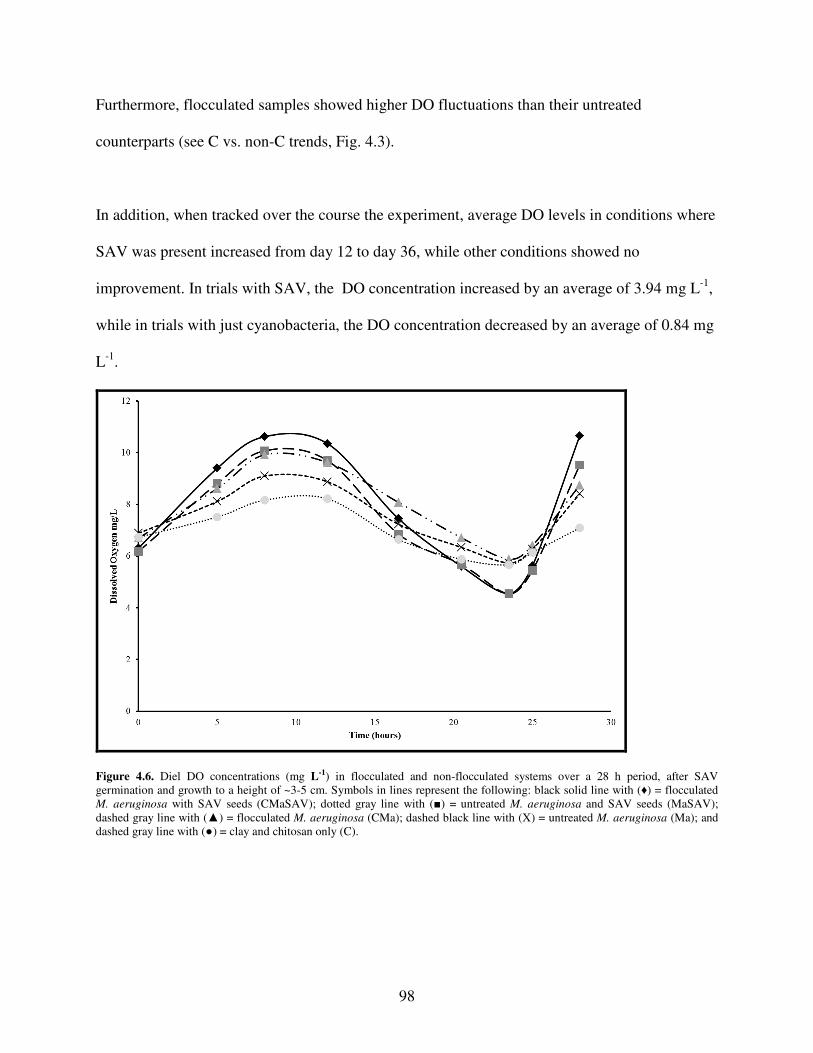
98

Furthermore, flocculated samples showed higher DO fluctuations than their untreated

counterparts (see C vs. non-C trends, Fig. 4.3).

In addition, when tracked over the course the experiment, average DO levels in conditions where

SAV was present increased from day 12 to day 36, while other conditions showed no

improvement. In trials with SAV, the DO concentration increased by an average of 3.94 mg L-1,

while in trials with just cyanobacteria, the DO concentration decreased by an average of 0.84 mg

L-1.

Figure 4.6. Diel DO concentrations (mg L-1) in flocculated and non-flocculated systems over a 28 h period, after SAV germination and growth to a height of ~3-5 cm. Symbols in lines represent the following: black solid line with (♦) = flocculated M. aeruginosa with SAV seeds (CMaSAV); dotted gray line with (■) = untreated M. aeruginosa and SAV seeds (MaSAV); dashed gray line with (▲) = flocculated M. aeruginosa (CMa); dashed black line with (X) = untreated M. aeruginosa (Ma); and dashed gray line with (●) = clay and chitosan only (C).

99

Figure 4. Maximum DO fluctuation over 28 h. Minimum DO levels (23.5 h) were subtracted from maximum DO levels (8 h) and plotted above. Significant differences were found between the following groups: flocculated M. aeruginosa and SAV seeds (CMaSAV) and flocculated M. aeruginosa alone (CMa) (*, p<0.01), non-flocculated M. aeruginosa and SAV seeds (MaSAV) and M. aeruginosa alone (Ma) (+, p<0.01).

4.4.3 Microcystin Trends and Flocculation

The experiment described in Section 4.3.8 Toxin Analysis provided some qualitative support for

Hypothesis 4 (flocculation leads to lower toxin concentrations). As shown in Figure 4.8, there

was an immediate initial drop in toxin concentration 0.5 h after flocculation (2.54 ppb), which

was smaller than the drop seen in the non-flocculated trial (1.06 ppb). However, as Figure 4.9

shows, this was followed by an increase in toxin concentration one day after treatment. This

increase was followed by a general decrease for the flocculated mesocosm, and a relatively

constant toxin concentration in the non-flocculated mesocosm.

100

Figure 5. Difference in toxin concentration before and after treatment. Notably, the flocculated sample (▲; CMa) has a decrease in toxin concentration of 2.54 ppb, while the non-flocculated sample (X ; Ma) has a decrease in toxin concentration of only 1.06 ppb.

Figure 4.9. Difference in toxin concentration over a period of 2 weeks. What cannot be seen in the graph is the very rapid decline in toxin levels in the first 10 min. Note that in the flocculated sample (▲; CMa), after an initial spike at ~1 d, a lower toxin concentration was maintained than in the non-flocculated sample (X ; Ma), beginning by day 2 and continuing for the remainder of the measurement period.

101

However, it should be stressed that, despite the fact that these data are an average of two trials,

due to the nature of the assay kit that was used, these results are largely qualitative. The test kit is

limited to accuracy with a lower bound of 0.2 ppb, and an upper bound of 5 ppb. As can be seen

in the graph, this maximum is exceeded for the flocculated containers 24 h into the experiment.

Therefore, the concentration noted must be viewed as a pattern or general indication of the

concentration change in the sample.

4.4.4 Flocculation and Nutrient Concentrations

Flocculation had visible and detectable impacts on nutrient concentrations, at least initially with

clear trends observed for ammonium and nitrate+nitrite. However, in multiple trials, phosphate

levels failed to show any significant patterns that reflected different treatments and therefore,

data from these trials are not provided (see Appendix B). Two different experiments were

performed to evaluate the impacts of flocculation in conditions with and without SAV.

4.4.4.1 Without SAV

The first experiment performed demonstrated the overall positive effect that our mixture had on

the environment in the absence of SAV. IVF for the water column showed that our mixture was

effective in flocculating bloom densities of M. aeruginosa in aquarium mesocosm conditions.

IVF through time also indicated the flocculated bloom kept the cells in bottom sediments as no

IVF increase was noted over the duration of the experiment (Fig. 4.10). At the start of

experimentation, two of the four trials contained bloom levels of M. aeruginosa. One of these

trials was treated with flocculant while the other remained untreated. In the treated trial, an

immediate decline in cell density was observed from bloom level conditions to levels below that

102

of the control. CMa (sediment-chitosan-M. aeruginosa) trials showed a 97.4% decrease in initial

concentration of M. aeruginosa cells in the water column following treatment. Non-flocculated

(Ma) trials showed only a 4% initial decrease in concentrations of the cyanobacterium. After 12

d, IVF in the CMa treatment indicated an overall decrease of 94.2% whereas suspended cell IVF

in the Ma trials decreased only 74.2% (Fig. 4.10).

Figure 4.10. Cell densities for each treatment over the course of the experiment. Ma(♦) (sample containing only M. aeruginosa) remained suspended in the water column for much longer than CMa(■) which demonstrates a rapid drop in cell density following flocculation. Cell densities remain below the controls (▲= C, X = Sediment Only) for the duration of the experiment.

4.4.4.1.1 Ammonium

Ammonium levels followed similar trends. Both trials containing M. aeruginosa saw a delayed

increase in concentrations of ammonium followed by a sharp decline; levels for M. aeruginosa

alone increased from ~0.02 to <0.4 mg L-1 from day 2 to day 7, whereas ammonium in flocced

samples (CMa) showed a similar increase from day 5 to day 15 (Fig. 4.11). By the end of the

experiment (22 d), ammonium in all mesocosm treatments were similar at ~0.02 mg L-1.

103

Figure 6. Ammonium levels (mg L-1) over the course of the 22 d experiment. Ma(■, M. aeruginosa only) trials show a faster rise in ammonium levels as well as a faster fall. CMa (♦, flocced M. aeruginosa) trials show a delayed rise in ammonium followed by a similar decline. Controls containing C (▲, chitosan-sediment) and sediment only (X) remained steady with minor fluctuations. Concentration at each point represents the mean of two replicates.

4.4.4.1.2 Nitrate+Nitrite

Nitrate+nitrite concentrations showed interesting patterns based on different treatments. For

flocculated trials, nitrate+nitrite levels remained low for the duration of the experiment. Trials

containing only clay, chitosan, and sediment showed similar constant levels, approximating 1.5-3

mg L-1 (Fig. 4.12). In contrast, nitrate+nitrite concentrations gradually increased (431%) for the

non-flocculated M. aeruginosa samples.

104

Figure 7. Fluctuation in levels of nitrate+nitrite over the course of the experiment. Ma(■) trials showed an constant increase in nitrate+nitrite levels starting around day 7 that continued until the end of the experiment at day 22. Fluctuations in nitrate+nitrite concentrations for CMa (♦) remained close to the levels of the controls (C = ▲, Sediment only = X). Concentrations at each point represent the mean of two replicates.

4.4.4.2 With SAV

4.4.4.2.1 Ammonium

Ammonium levels showed clear trends in the presence of SAV versus those without the plants.

An overall decrease in ammonium levels was noted with growing plants whereas those without

the grasses showed an overall increase in ammonium (Fig. 4.13). Trials with SAV saw between

an 81-90% decline in ammonium concentration by the end of the experiment, from 0.413 – 0.042

mg L-1. Comparatively, those trials that lacked the angiosperms saw an average ammonium level

increase of 4%.

This trend is observed more clearly when the two extremes of treatment are compared. Figure

4.13 demonstrates that ammonium levels declined in the flocculated mesocosms containing SAV

105

(CMASAV) following germination of seeds that began around day 10. Without SAV, Ma trials

showed a steady increase in ammonium concentration following day 15, to approximately 0.35

mg L-1, similar to near maximum levels seen on day 3. By day 23, ammonium levels for the

flocced M. aeruginosa samples containing plants (CMaSAV) had dropped below levels (<0.1 mg

L-1) seen in in mesocosms containing no Microcystis.

Figure 4.13. Ammonium levels for CMaSAV (flocced M. aeruginosa with SAV), Ma(X, cyanobacterium only), and C (control, no M. aeruginosa). CMaSAV(♦) shows an overall decrease in ammonium levels. Ma shows an initial decrease in ammonium levels with concentrations recovering to almost maximum values by the end of the experiment. C(●), the control trial, maintained fairly steady values between 0.05 and 0.15 mg L-1following day 5.

CMaSAV trials saw a 90% reduction overall in ammonium levels (0.413 – 0.042 mg L-1)

following an initial 10% increase in ammonium (0.373 – 0.413 mg L-1). MaSAV mesocosms (the

cyanobacterium + SAV seeds) were typified by a similar trend, showing an 81% (0.36 – 0.069

mg L-1) overall decrease in ammonium concentration following an initial ammonium increase of

237% (0.109 - 0.367 mg L-1). CMa containers, conversely, were typified by a 35% increase

(0.238 – 0.322 mg L-1) following an initial 277% increase in ammonium concentration (0.109 -

0.367 mg L-1) (Fig. 4.14).

106

Figure 4.14. Ammonium concentrations for each treatment over time. Each trial shows an initial ammonium level, ammonium 3 d after flocculation, and ammonium 30 d after flocculation. SAV trials show an overall decrease in ammonium vs. non-SAV trials, with the latter showing an overall increase.

In containers with only bottom sediment and the cyanobacterium (Ma), there was a 27%

decrease (0.468 – 0.342 mg L-1) in ammonium levels following a 277% increase (0.124 – 0.468

mg L-1). In SC, containing no M. aeruginosa and hence no intracellular nutrients, ammonium

levels remained fairly constant (Fig. 4.14).

4.4.4.2.2 Nitrate+Nitrite Concentrations and Flocculation

Patterns in nitrate+nitrite levels varied in response to flocculation, unlike ammonium levels

which varied in response to the presence of SAV. Flocculated containers had consistently lower

concentrations of nitrate+nitrite vs. aquaria in which bloom conditions were allowed to persist in

the absence of flocculation. CMaSAV (flocced M. aeruginosa with SAV) had an average

107

concentration of nitrate+nitrite 0.93 mg L-1 less than the populations without flocculation

(MaSAV), an average of 18%. Additionally, the average concentration of nitrate+nitrite was 1.01

mg L-1 less than noted in the containers with just the cyanobacterium and bottom sediment (Ma)

(Fig. 4.15).

Figure 4.15. Nitrate+nitrite concentrations shown as average difference over the course of the 30 d experiment. Flocced containers (CMaSAV = ♦) had consistently lower concentrations when compared to levels noted in non-flocced systems (MaSAV = ▲).

4.5 Discussion

4.5.1 SAV Germination Rate is Enhanced by Flocculation at the Time of Seed Scatter

Field and laboratory studies of aquatic plants have suggested that many different factors can

influence germination, such as salinity, temperature, light, hormones, and the sediment in which

seeds germinate (Baskin and Baskin 1998, Orth et al. 2000). However, many studies have

proposed that oxygen levels (or redox potential of the sediment) may be one of the most

important factors dictating the germination rate of many sea grasses (Kawasaki 1993, Moore et

al. 1993, Orth et al. 2000). These studies have found that systems with low dissolved oxygen or

reducing environments promote seed germination. In Kawasaki (1993), increased germination

108

was achieved by covering the seeds with sediments or lowering the oxygen content of the

surrounding waters. Furthermore, many species-specific studies report characteristic burial

depths ideal for germination of a particular species. For both Potamogeton perfoliatus and

Ruppia maritima, species used in this study, the reported ideal burial depth is less than 2 cm

(Ailstock 2007).

Based on these previous findings, we suggest that perhaps microzones of reduced DO in the

decomposing flocced Microcystis away from the lighted sides of the mesocosms may explain the

increased germination rate with flocculation seen in our current study. Flocculation at the time of

seed scatter lightly covers the seeds in a layer of clay, chitosan, and submerged cyanobacteria.

This, coupled with nutrient released from the dying flocced Microcystis may yield conditions

sufficient to increase germination rate.

4.5.2 Flocculation at the Time of Seed Scatter Results in Significantly Higher SAV Total

Biomass at 3-4 Weeks Post-Germination

The effects of water column clarity on SAV growth and abundance are well characterized in the

literature. Field and laboratory research has identified light as a major factor controlling SAV

abundance and distribution in the benthos (Dennison et al. 1993, Kemp et al. 2004). Thus, light

attenuation in the water column by phytoplankton or dissolved organic material can be

detrimental to the health of SAV beds below (Kemp et al. 2004). In this experiment, we were

able to demonstrate that flocculation was favorable for SAV, resulting in increased germination

rates and plant biomass. By removing cyanobacteria from the water column, presumably less

light was attenuated in the water column and therefore able to reach the aquatic plants below.

109

Additionally, contrary to potential increases in attenuation possible with adding sediment to the

water, adding the clay and chitosan mixture to the water did not increase light attenuation, as

mesocosm water columns remained particle free. Due to the properties of our mixture, it settles

out of the water very quickly (Chapter 3) and does not limit SAV growth in the benthos.

Flocculation at the time of seed scatter produced a two-fold increase in SAV biomass assessed 3

and 4 weeks after germination (Figs. 4.3, 4.4). This dramatic enhancement of growth suggests

that factors such as nutrients provided by decomposition and recycling from the flocculated

cyanobacteria contributed to SAV success. Submerged macrophytes take up the majority of their

nitrogen and phosphorous directly from the sediments through their roots (Barko and Smart

1980, 1981; Huebery and Gorham 1983;Barko 1986). Useable forms of these elements are

typically in low concentrations in the water column (Wetzel 1983). Ammonium and

nitrate+nitrite concentrations were appreciable in our mesocosms, reaching 0.4 and ~5 mg L-1,

with highest concentrations in systems without plants suggesting nutrient uptake by these

angiosperms reduces overall accumulations in the systems. Thus, we infer that the concentration

of flocculated cyanobacteria at the sediment surface enriched the sediment with nutrients

contributing to the substantial increase in SAV biomass seen with flocculation (these ideas are

further discussed in section 4.5.8).

4.5.3 Flocculation at the Time of Seed Scatter May Improve SAV Rooting and Stability

Through qualitative observation, we noted that SAV germinating in flocculated mesocosms

tended to be more stable than those germinating in untreated mesocosms. SAV in flocculated

environments were less susceptible to agitation of the container, and upon removing SAV from

110

the sediment for biomass quantification, it was noted that aquatic plants in the flocculated

mesocosms had a greater percentage of their roots below the sediment when compared with

controls. This observation suggests that SAV seed scatter coupled with flocculation may improve

restoration efforts when compared with seed scatter alone. As noted in the literature, one of the

most detrimental problems in SAV restoration is destruction of the plants by currents and waves

before they become established in the sediment (Fonseca 1994). Thus, better rooting and stability

mediated by flocculation could improve the success of restoration efforts.

4.5.4 SAV Summary

It is clear from our results that the coupling of SAV restoration and flocculation provides mutual

benefits for each. Incorporation of SAV seeds into the flocculation mixture prevents the release

of nutrients from flocced, settled, and decaying cells from cycling back into the water column.

Therefore, flocculation with SAV seeds and accompanying restoration offers a more permanent

solution for bloom mitigation by removing the HAB, controlling nutrient availability to

overlying phytoplankton for possible re-growth of HABs, and stimulating submerged grass

growth. Submerged aquatic vegetation can take up nutrients released from the flocculated

cyanobacteria, and once established can help to create a sustainable, balanced ecosystem by

providing habitat for benthic organisms and preventing sediment suspension.

In addition, it is clear that water clarity and quality are necessary for restoration of SAV (Kemp

2004, Freedman 2006, Jarvis 2008). However, improvement of these conditions naturally occurs

very slowly. Flocculation coupled with seed scatter immediately improves the water clarity by

removing suspended bloom biomass that shades the benthos and buries the seeds in a nutrient-

rich medium, promoting germination and quick, stable growth.

111

4.5.5 Fluctuation of Dissolved Oxygen Levels Increases for Mesocosms that Contain SAV

One of the key benefits of aquatic vegetation is its production of more DO through

photosynthesis (Benson et al. 2007). By increasing the overall levels of DO in the environment,

the harmful effects of hypoxia are alleviated. Since diel hypoxia is a problem often associated

with HABs (Sellner et al. 2003), the efficacy of HAB mitigation techniques may be improved by

incorporating ways to increase DO levels of the affected areas.

Our results show that our mitigation technique provided this benefit. As seen in Figure 4.6, trials

that incorporated SAV seeds had higher diurnal DO levels than noted in trials that did not

incorporate SAV seeds. This was true for both flocculated and non-flocculated mesocosms, and

may be attributed to SAV photosynthesis during the light cycle. Moreover, the average DO level

for the trials that included SAV increased over time, whereas the average DO level for the trials

that did not include SAV either remained the same or decreased over time.

Not surprisingly, the diurnal increase in DO in SAV-rich mesocosms is also accompanied by the

lowest nocturnal DO levels across the treatments (Fig. 4.6), leading the the largest diel

fluctuations in DO (Fig. 4.7). At night, in the absence of light, growing plants behave like any

other organism, heterotrophic because the plant tissue respires. Because the mesocosms with

SAV had the highest biomass, that additional tissue consumes oxygen in proportion to its mass,

leading to low oxygen concentrations at the end of dark period. Low levels of DO in the dark

accompanied by high DO levels in the light are common in areas dominated by SAV (e.g., Nixon

and Oviatt 1972) or any other biomass-rich system, When plants are actively growing,

photosynthetic oxygen production will exceed respiration (e.g., Menendez and Penuelas 1993)

112

and the system will remain aerobic and indicative of a healthy environment. Hypothesis 3

(larger DO fluctuations with SAV), therefore, is strongly supported by Experiment 2 (Figs. 4.7,

4.8).

4.5.6 Toxin Levels Appear to Be Lowered Through Flocculation

Since M. aeruginosa synthesizes microcystin-LR in approximately one third of all blooms (The

Fish and Wildlife Institute 2005), addressing ways to deal with this toxin in the water column is

important. Although ozonation and halogenation are sometimes used for detoxification, these

techniques produce harmful free radicals and are expensive (Jungmann 1992). Therefore, we

pursued treatment with clay particles, which have been reported to adsorb up to 81% of the toxin

found in solution (Perez et al. 2005). Since our flocculation mixture already contained clay

particles, this aspect of the research was particularly germane.

However, the technique we used to measure the concentration of microcystin in our mesocosms

was largely qualitative, since the range of the ELISA kit that we used was only 0.2 - 5.0 ppb.

Nevertheless, the trends observed using our assay are worth noting. As shown in Figure 4.8,

there was an initial decrease in toxin concentration of 2.54 ppb immediately following

flocculation. This decrease was larger than that seen in the non-flocculated mesocosm (1.06

ppb). From these limited results, it appears that the clay particles adsorbed about 60% of the

toxin in the water column.

Unfortunately, since the flocculation process kills the cyanobacteria and the toxin is released

from the cells upon lysing, it appears that flocculating the cyanobacteria causes an initial spike in

113

toxin concentration (Fig. 4.9), where 24 h after flocculation, the toxin concentration in the

flocculated sample had increased to 5.35 ppb, while the toxin concentration in the non-

flocculated sample had only increased to 4.35 ppb. Furthermore, since the assay is only accurate

to 5.0 ppb, this rapid toxin increase in the flocculated sample may be even higher than the noted

concentration. However, after this initial increase, it seems that whereas the non-flocculated

sample maintained a relatively stable toxin presence of approximately 4.5 ppb, toxin

concentration in the flocculated treatment steadily declined from its peak of 5.35 ppb to

approximately 2.5 ppb. This difference can be explained by the flocculation process. For the

mesocosms that underwent flocculation, the vast majority of the cyanobacteria settled to the

sediment and likely quickly killed. In the process, a large amount of toxin was released. After

this large initial release, the absence of viable cyanobacteria except at the mesocosm’s edge

prevented only minimal additional toxin production. Simultaneously, the large concentration of

toxin already present in the water column steadily declined, potentially through photolysis or

bacterial degradation. Past studies have estimated that the natural processes found in reservoir

water result in a half-life of less than a week for microcystin-LR (Cousins et al. 1996).

In contrast, non-flocculated Microcystis persisted, apparently reaching a relative equilibrium

(IVF was relatively constant, data not shown) with growth matched by mortality. Cells that were

slowly dying were also releasing toxin to replace toxin naturally degrading (Fig. 4.9): the toxin

concentration of the non-flocculated sample was relatively high and stable throughout the

measurement period.

114

These results suggest that although the flocculation process may create an initial increase in

toxin, this effect is only temporary and within 2 days, and definitely by 2 weeks, the long-term

benefits of flocculation vastly exceed the short-term temporary increase in soluble toxin.

Although the initial increase would potentially produce an acute exposure to flora and fauna, the

harmful conditions such as low DO (see above) created by the bloom might be more detrimental

to large macrofauna in the area in the first place. Additionally, this initial spike in toxin may be

remedied by another application of clay to adsorb more of the toxin (which was about 60%

effective in this qualitative experiment and was 81% effective in the more quantitative study

done by Perez et al. 2005). As noted in Chapter 3 with field M. aeruginosa bloom samples,

multiple additions of the clay-chitosan mixtures might be necessary, thereby not only removing

the HAB but the toxins it produces. Chronic exposure would be prevented by the adsorption of

the toxin to the clay particles.

4.5.7 Mesocosm Conditions Alter the Effects of Flocculation on Nutrient Release

Nutrient release from decomposing cells into surrounding waters contributes to the process of

eutrophication which leads to algal growth and proliferation (Anderson et al. 2003). In order to

address the problem of bloom mitigation in total, we had to ensure that cell removal following

flocculation and settlement did not further contribute to eutrophication.

A concern for removing suspended populations to the bottom is the remineralization of deposited

material and use of the recycled N and P pools for stimulating phytoplankton production again,

even leading to other blooms. In the present study, flocculation did result in temporary increases

in ammonium but these did not persist. Nitirate + nitrite concentrations declined through time

115

following flocculation, consistent with Pan et al. (2009) observations in Lake Taihu, China. M.

aeruginosa treated with flocculant consistently contained lower levels of nitrate+nitrate when

compared to the non-flocced trials: non-flocced mesocosms experienced a 437% increase in

nitrate+nitrite levels over the course of experimentation (1.37– 5.91mg L-1). Flocced systems,

comparatively, had lower concentrations (2.91 mg L-1 in treated bloom mesocosms, CMA) of

nitrate+nitrite at the end of the experiment, similar to the concentration observed for mesocosms

with only water and sediment (3.02 mg L-1). These results suggest that the flocculation process is

able to limit the release of nitrate+nitrite into the surrounding water column.

Most importantly, however, was the observation that if present, SAV would remove some of the

nutrient released from the flocculating, settling, and decomposing Microcystis population (see

Fig. 4.15). Flocculation of cyanobacteria cells provides plants with a reliable source of nitrogen

that fuels their growth. Figures 4.14 and 4.15 illustrate the ability of SAV to take up ammonium

and nitrate+nitrite and remove it from the surrounding water column. All trials that contained

SAV saw an overall decrease in these two nutrient pools. Conversely, trials that did not contain

SAV saw a consistent increase in the amount of ammonium and the oxidized N species in the

water column. This demonstrates that using SAV seeds in conjuncture with flocculation can be a

vital part of the mitigation strategy to address a spectrum of problems associated with HABs,

such as eutrophication and hypoxia.

4.5.8 Summary of Flocculation Impacts Our results suggest that with this treatment, we are not only removing the cyanobacteria bloom

quickly and effectively, but also may help prevent the reoccurrence of the bloom by naturally

116

restoring the ecosystem. The aquatic vegetation controls eutrophication and associated bloom

and restores DO levels, thereby creating a sustainably healthy environment. By incorporating

SAV into the mixture, we are now able to limit the impact of current blooms while ameliorating

past damage. Blooms in the past have resulted in the death of massive patches of SAV. In

addition to reducing water quality, SAV death limits the Bay’s ability to recover from the

repeated stress associated with bloom degradation, as well as reducing the system’s ability to

trap sediments and provide nursery habitats for valued living resources. SAV restoration means

restoring the Bay’s ability to maintain itself in the face of potential future damage. In this way,

the benefits of clay-flocculation extend beyond simply removing M. aeruginosa from the water

column. In addition to removing nutrients and toxin from the water column, results demonstrate

that flocculation of algae aids in the germination of SAV seeds. In this way, our methodology

utilizes a multifaceted approach to treating the many problems associated with algal blooms.

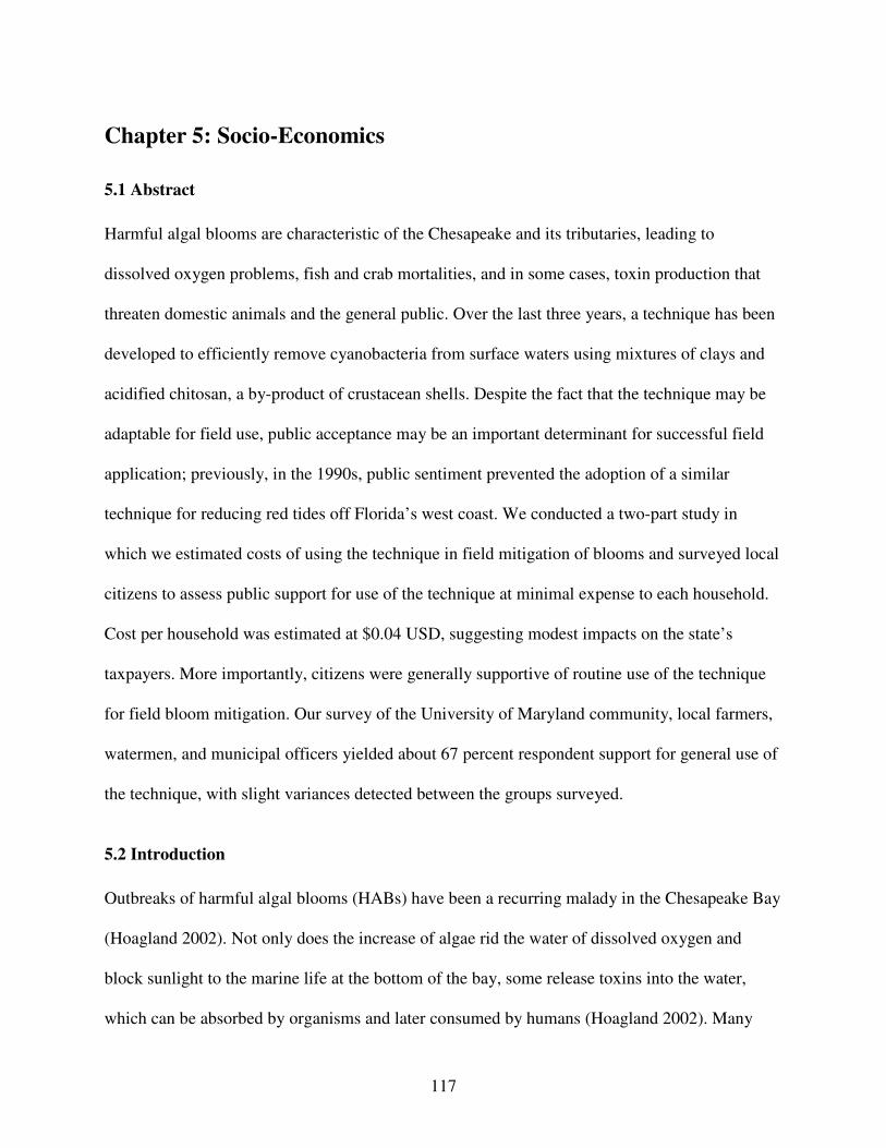
117

Chapter 5: Socio-Economics

5.1 Abstract

Harmful algal blooms are characteristic of the Chesapeake and its tributaries, leading to

dissolved oxygen problems, fish and crab mortalities, and in some cases, toxin production that

threaten domestic animals and the general public. Over the last three years, a technique has been

developed to efficiently remove cyanobacteria from surface waters using mixtures of clays and

acidified chitosan, a by-product of crustacean shells. Despite the fact that the technique may be

adaptable for field use, public acceptance may be an important determinant for successful field

application; previously, in the 1990s, public sentiment prevented the adoption of a similar

technique for reducing red tides off Florida’s west coast. We conducted a two-part study in

which we estimated costs of using the technique in field mitigation of blooms and surveyed local

citizens to assess public support for use of the technique at minimal expense to each household.

Cost per household was estimated at $0.04 USD, suggesting modest impacts on the state’s

taxpayers. More importantly, citizens were generally supportive of routine use of the technique

for field bloom mitigation. Our survey of the University of Maryland community, local farmers,

watermen, and municipal officers yielded about 67 percent respondent support for general use of

the technique, with slight variances detected between the groups surveyed.

5.2 Introduction

Outbreaks of harmful algal blooms (HABs) have been a recurring malady in the Chesapeake Bay

(Hoagland 2002). Not only does the increase of algae rid the water of dissolved oxygen and

block sunlight to the marine life at the bottom of the bay, some release toxins into the water,

which can be absorbed by organisms and later consumed by humans (Hoagland 2002). Many

118

blooms are caused by nutrient runoff from human activities in coastal basins, favoring excess

algal production (Anderson et al. 2000). When paired with existing bay conditions such as warm

temperatures, low salinity, and calm water columns, the introduced nutrients create optimal

conditions for an algal bloom. Such blooms disrupt the ecosystem in and around the bay, impact

local businesses, and can negatively affect the health of the general population residing along the

shore.

The economic repercussions of HABs are both diverse and widespread. Consequently, there are

various methods to estimate their financial impact. There is a clear distinction between economic

and scientific approaches for assessing the effects of HABs. Economists concern themselves

primarily with changes in tangible financial values such as monetary losses resulting from HABs

(Hoagland and Scatasta 2006). Studies have estimated that losses from algal blooms within the

U.S. are at least $82 million annually (Hoagland and Scatasta 2006).

The losses are attributed to costs associated with public health, commercial fisheries, recreation

and tourism, and monitoring and management. Public health impacts represent approximately

45% of economic losses, with commercial fishery reductions representing 37%. Such estimates

are very conservative in nature and do not account for economic multipliers (cascading impacts

from sector to sector), which could potentially triple this amount. They also do not include

untapped resources (such as the coast wide ban of shellfish harvest in Alaska) which cannot be

used (such as shellfish harvesting) due to toxicity resulting from HABs (Anderson et al. 2000).

119

Globally, HABs have been treated with numerous mitigation techniques; however, very few

assess accompanying environmental and economic impacts. Mitigating HABs through clay

flocculation of local sediments (Zou et al. 2006) is an innovative method that theoretically causes

minimal impact to system ecology at modest costs for materials and to local businesses. In our

research, we have expanded this previously documented clay flocculation technique by

conducting a cost assessment and surveying regional citizens on willingness for adopting such

mitigation techniques.

This paper focuses on the socio-economics of bloom mitigation specific to the state of Maryland.

We initially focused on Mattawoman Creek, a tributary of the Chesapeake Bay, as seen in Figure

5.1.

120

Figure 5.1. Map of Mattawoman Creek within MD.

121

Our clay mixture has been proven to be effective in removing tidal-fresh harmful algal blooms

present in the Chesapeake Bay (Gallo et al. in prep.). For the current research to be implemented

as a routine mitigation technique in bloom control by the state, however, cost consideration is

critical because the funds for bloom mitigation are ultimately derived from taxpayers. In

addition, public support must be neutral to positive: Maryland citizens must be willing to allow

bloom mitigation, regardless of how successful and harmless the technique appears, or state

officials will not adopt the technique as a standard mitigation protocol.

There is some history of economic impacts from and public reactions to HABs in the region.

Reports of generally poor health associated with contact with the reported harmful species

Pfiesteria piscicida, as well as reports of menhaden with skin abnormalities and lesions, created

an atmosphere bordering on hysteria in 1997 (Magnien et al. 2001). It was estimated that about

50,000-80,000 menhaden were killed, and although menhaden are not consumed by most

fishers, public attention was still heavily drawn to the bloom (Hoagland et al. 2002). The

public’s general reaction to the organism and its threat was so negative that the governor of

Maryland closed several Chesapeake tributaries that were recreation and fishing centers. It was

estimated that the outbreak cost the seafood industry $46 million due to the “halo effect” that

resulted from the public perceptions about menhaden contamination and possible human health

issues, leading to abstinence from seafood consumption (Anderson et al. 2000). The state of

Maryland tried to prevent this aversion by spending half a million dollars on promotional efforts

to try and decrease such effects on the market (Hoagland et al. 2002). Overall, as well, the

public sector holds a generally negative view towards harmful algal blooms due to their

negative effects on human health as well as the aquatic environment (Anderson et al. 2000).

122

These views are only perpetuated by these economic responses and hence algal blooms do not

only impact the scientific sector, but the economic and public sectors as well.

Public health comprises a significant economic impact. Algal toxins are responsible for more

than 60,000 intoxication incidents annually (Dolah et al. 2001). In the past, the Center for

Disease Control and Prevention estimated that about 20% of all food-borne illness outbreaks

result from seafood consumption, with half of these outbreaks resulting from algal toxins. Other

studies have shown that contact with bloom water, exposure to aerosolized algal toxins, or

consumption of contaminated seafood result in poisoning symptoms (Dolah et al. 2001).

The basis for our research stems from the attempts to mitigate Florida red tides. The Florida

coastline has long been affected by red tides of the dinoflagellate, Karenia brevis (Larkin 2007).

Like the HABs present in the Chesapeake Bay, K. brevis harmed flora, fauna, and humans who

had been exposed to its toxins (Sengco et al. 2002). These red tides led to fish kills and

symptoms typical of neurotoxic shellfish poisoning (NSP) in humans including gastrointestinal

symptoms such as nausea, diarrhea, and abdominal pain, and sometimes neurological symptoms

such as headache, vertigo, and lack of coordination (Alcock 2007).

Laboratory and field microcosm research results indicated that an effective clay mitigation

technique could likely be applied to red tides to remove bloom biomass; however, their

technique could not be implemented due to public dissent (Kuhar et al. 2009; Kirkpatrick et al.

2010; M. Sengco, pers. communication.). To garner public consent for use of sediment

flocculation in the future, we assessed initial reactions to our technique by surveying Maryland

123

residents from various regions and professions following delivery of a short summary on bloom

impacts and possible costs to the average household.

5.2.1 Creating an Economically-Feasible Mitigation Mixture

In order for the mitigation mixture to be acceptable to the government for routine

implementation, it must cost significantly less than the losses sustained by businesses, water

users, and the public from the HABs. Therefore, determining the most cost effective method to

mitigate the bloom was important. We concentrated on compiling the price of local sediments

and clays that can be used to effectively submerge a M. aeruginosa HAB. Furthermore, we

analyzed the cost of supplies and labor needed to mitigate the bloom.

5.2.2 Public Opinion on Clay Mitigation for HABs in the Chesapeake Bay

Even if the mitigation mixture is effective in removing algal cells from the water, is cost

effective for the government to adopt, and has no negative effects on the surrounding

environment, it might not be adopted if the general public is strongly against direct intervention

in natural waters or ecosystems. In the past, the public has shown great unease at adding

substances to bodies of water, even if the substances are naturally occurring (Kuhar et al. 2009).

5.3 Methods

We used a two-part study to examine costs for and palatability of routine use of the mitigation

technique. The first part of the process determined the overall cost of the production and

application of the clay-chitosan mixture, while the second component involved the development,

implementation, and analysis of a public survey to measure willingness to support the method’s

routine use.

124

Cost Estimates

In calculating the cost of producing and applying the mixture on the Chesapeake Bay, we

considered the costs of the clay and relevant components including the flocculant chitosan,

transportation, storage of clay, and manpower for application. The clay and sediment component

composed 0.02% of the total mixture cost, as the sediments are economical commodities and can

be purchased for a minimal cost, if not free of charge. Hypothetically, the sediment would be

extracted directly from the banks of the Bay adjacent to areas that commonly experience blooms

(Pan et al. 2010). By sourcing the clay directly from the Chesapeake Bay, the cost of transporting

it to the spray location would be eliminated. Currently, we have not determined the source for

SAV seeds but all seeds that have been used in our experiments have been donated by various

professional contacts, so we did not include it in the cost calculation for the clay-chitosan

mixture.

A summary of total expenses 2010 USD is presented in Table 5.1 with the intention of a single

application with duration of 3 days for 3.45 tons of water. We calculated the volume of the

bloom by finding the percent of the Bay with the appropriate salinity conditions, then taking 5%

of that volume. Chitosan is estimated to be needed at 0.25 grams per liter of affected water

(based off flocculation success rates with Stancills B sediment) and is priced at $5,362.50 per

unit (source: The Chitin Company, Cambridge, MA), where a unit is 220 pounds. This converted

to $48,750 per ton and when further interpolated for the estimated bloom volume of 3.45 tons,

amounted to a total of $168,000. Chitosan is a principal component of the flocculant, and without

it, the mixture would not effectively bind to algae in the blooms (Chapter 3). Taking into account

125

the fixed and variable costs of transportation and the manpower as well as spraying the mixture

onto the Bay, total logistical costs (includes machinery and manpower) account for $204,520 of

the total. Machinery costs are a major subset of the total logistical cost with necessary rental

costs for the barge, boat, truck, and excavator. The barge rental would cost $3,000 (source:

Smithbarge.com), the tugboat to pull the barge across the Bay carrying the flocculant would cost

$21,600 (source: Smithbarge.com), the truck rental to transport the local sediments to the barge

or to transport the excavator would cost $4,320 (source: Agriseek.com), and the excavator rental

would cost $600 (source: Abcrentalmaryland.com). Manpower would cost $18,000 for a total of

10 workers (each worker will receive $1,800 for three days of labor where each day would

consist of 12 work hours at an hourly rate of $50 per hour). As stated earlier, the entire

application would occur once and it would have duration of three days.

We determined the final cost per household by calculating the Maryland area of the Bay that is

affected (<5% of the entire Chesapeake Bay and tributary volume is affected by Microcystis

aeruginosa) (National Science Foundation 2006) to determine the amount of flocculant and labor

necessary. We then divided the total cost of flocculation by the number of tax-paying households

in the state of Maryland. The final individual household cost based on the 2009 Maryland state

census of 5 million households (Selected Economic Characteristics: 2005-2009; 2009) was

$0.04 per household. Post-bloom monitoring is already part of the state’s existing field program.

Public Survey

The purpose of the survey was to gauge public opinion for the application of the clay-chitosan

mixture to the Bay as well as their willingness to pay for the intervention. In the 1990s,

126

researchers discovered an effective solution to the abundant Florida red tides that were routinely

impacting the W. Florida coastline and its inhabitants. While the mitigation procedure was

determined to be harmless to the environment, it was not implemented because the local citizens

protested against the clay supplier, a company that was unpopular with Florida’s public and the

perception that the clay to be used in the mitigation was phosphorus-rich and therefore

potentially stimulatory to shelf production off W. Florida. Millions of dollars committed to the

mitigation research were effectively derailed from any societal benefits as the researchers had

not informed the public and received their support prior to conducting the research (M. Sengco,

pers. comm.). In order to avoid a similar situation in the Chesapeake Bay watershed, we

determined it was necessary to win the support of both the Maryland state government as well as

its taxpayers.

In order to gauge public opinion, we created a survey that measured respondents’ willingness to

support and pay for the project. We consulted Dr. Douglas Lipton and Dr. Michael Paolisso of

the University of Maryland to formulate our survey questions (see Appendix C), which were

reviewed and accepted by the Institutional Review Board (IRB). The IRB is a committee that

approves, monitors, and reviews biomedical and behavioral research involving human beings

with the intent of preserving their welfare. Under the guidance of both Lipton and Paolisso as

well as the IRB, we chose closed-ended questions based on the Likert scale for the majority of

the survey (D. Lipton, pers. comm.). During the span of a year, we surveyed various populations

in Maryland. We began by creating an on-line format that we disseminated via email and social

networks. In the spring of 2010, we surveyed parents, students, and faculty members on the

University of Maryland campus in College Park during the annual Maryland Day celebration.

127

That summer, we attended the Caroline County Farm Bureau’s Annual Picnic and the Calvert

County Watermen’s Day Festival where we received responses from farming and fishing

populations. And finally, in the fall of 2010, we surveyed attendees of the annual Maryland

Municipal League conference where delegates from all of Maryland’s cities, towns, and villages

were present.

5.4 Results

Following collection of costs of the mitigation elements for a single bloom (Table 5.1, elaborated

in Section 5.3 under Cost Estimates), we obtained an annual cost per taxpaying household of

$0.04. The estimate was derived by dividing the total costs by the small region of Maryland’s

tidal bay and tributaries that has previously supported cyanobacteria blooms (5% of Bay with

proper salinity conditions) by the number of taxpaying households in Maryland (5.5 million).

Item Cost (in 2010 USD)

Labor 18,000 Barge Rental 3,000 Tugboat Rental Truck Rental Excavator Rental

21,600 4,320 600

Chitosan 168,000 Sediment* 0

Total 215,520 Number households in state of Maryland 5,500,000

Cost per household 0.04 *Local sediment at flocculation site is at no cost Table 5.1. Cost breakdowns per component for single bloom application.

Group Respondent # # Supporting Mitigation

% Supporting Mitigation

Academia 384 250 65.1

Farmers 37 21 56.8

Watermen 38 28 73.7

Municipal League 39 33 84.6

Total 498 332 66.7

128

Table 5.2. Survey results of public willingness to routinely use the clay/chitosan technique to mitigate M. aeruginosa blooms in Maryland.

For the survey component of the project, we received 498 complete surveys in the course of a

year and a half (Table 5.2). Of those, 384 responses were garnered through electronic forms

distributed via social media and during Maryland Day at the University of Maryland College

Park. This survey group (henceforth referred to as “academia”) consisted mainly of

undergraduate and graduate students attending the university as well as family members and

members of the College Park community. The second survey group was the agricultural

community attending the Farm Bureau’s Annual Picnic in Caroline County, which garnered 37

responses (henceforth referred to as “farmers”), while the third and fourth survey groups were

from the Calvert County Watermen’s Day Festival (henceforth referred to as “watermen”) and

the Maryland Municipal League (MML) 2010 Fall Conference (henceforth referred to as

“municipal”), respectively. We collected 38 complete surveys from the watermen and 39 from

the MML conference delegates.

Support for use of the technique for bloom mitigation was seen across all four groups (Table

5.2). Overall 66.7% of the total surveyed population indicated that they would support the

method’s routine use (Fig. 5.2). The degree of support from the four groups was University of

Maryland (65.1%), farmers (55.6%), watermen (73.7%), and municipal officials (84.6%).

In addition, 330 people (66.2%) indicated that they were willing to pay at least $1 USD for

general technique implementation, an overall favorable willingness to pay (Fig. 5.3).

Demographic characteristics of the surveyed populations such as gender, age, household income,

education, and geographical location did not prove to be significant factors (p>0.05, chi square

129

test) in the way the different groups responded. A breakdown of each group’s support and fiscal

commitment to intervention is provided in Figures 5.4-5.7.

The reason for the apparent differences in the demographic groups is most likely attributed to the

amount of personal attention and information provided to the surveyed groups. At the MML

conference, we distributed a fact sheet (Fig. 5.8) and personally spoke to the attendees who were

there for professional reasons. Attendees were identifiable by name and hometown displayed on

their nametags, which may also have attributed to their more favorable responses. We, the

surveyors, were identified as University of Maryland students and potential constituents, and

thus may have influenced the municipal league members to respond more favorably, even though

confidentiality was assured. On the other hand, the Calvert County Watermen’s Day Festival and

the Farm Bureau’s Annual Picnic in Caroline County were both social events. Although the

demographic information (education, ethnicity, socio-economic status, etc.) is similar for both

groups, the outcomes of the surveys were significantly different (p<0.05, chi square test). The

watermen’s significantly greater positive response may have been influenced by the

individualized attention given to each person surveyed and the amount of information provided.

While a fact sheet was not provided, the surveyors provided background information about the

Bay similar to that in the fact sheet. The farmers were not given this and in addition, the

surveyor’s status as an undergraduate student and not an employee of any government agency

was not as emphasized as with the watermen. Thus, the farmers did not have as much contextual

information about the background research of Bay mitigation and also did not see the surveyors

in a more favorable manner, potentially causing their relatively more negative responses.

130

Figure 5.2. Proportion of surveyed individuals willing to support use of the sediment-chitosan mitigation technology in MD waters.

Figure 5.3. A breakout of sums surveyed individuals were willing to pay for use of the sediment-chitosan technology in MD waters .

131

Figure 5.4. Academia (a) support for intervention as well as (b) amounts willing to pay for the mitigation.

132

Figure 5.5. Municipial League Members (a) support for use of the technique in field bloom mitigation and (b) amounts they were willing to pay for the intervention.

133

Figure 5.6. Watermen’s (a) support of field mitigation and (b) amounts they were willing to pay for field applications.

134

Figure 5.7. Farmer (a) support for field intervention and (b) amounts they were willing to pay for the applications.

135

5.5 Discussion

The minimal costs calculated for routine mitigation of cyanobacteria blooms recurring in

Maryland’s tidal-fresh areas suggest that funding should not be a major problem for adoption of

the technique as a standard field procedure in state waters. With successful results using

sediments from the shore surrounding blooms in China, we have eliminated major transportation

costs because we also plan to use local sediments (Zou et al. 2006, Pan et al. 2010).

Future considerations include improved bloom monitoring practices and more efficient logistical

techniques such as the use of cement mixers in comparison to manual mixing of the flocculant.

We also recommend that the government consider public education opportunities to increase

overall approval and support. Cost-benefit analysis would also prove to be useful in comparing

the cost of flocculation to the potential gains of Chesapeake Bay watershed businesses.

The general support shown from the small surveyed population of Maryland citizens also

suggests that public sentiment might not be as restrictive as noted in Florida for routine treatment

of its recurring red tides. However, critical to the positive response identified in the survey is the

importance of effective communication with citizens prior to distribution of the questionnaire. At

the Watermen’s Day Festival and Maryland Municipal League (MML) Conference, members of

our research team were able to answer questions prompted by participants and provide more

detailed information. We distributed a HAB fact sheet at the MML conference (Fig. 5.8) and this

appeared to help in survey participation and understanding of the issue and intervention.

136

Figure 5.8. HAB Fact Sheet distributed at the MML prior to surveying meeting participants.

137

A portion of the academic population obtained information from our team at Maryland Day;

participants at the Farm Bureau’s Picnic were informed through a five minute oral summary and

dialog with the two survey distributors. This apparent discrepancy could possibly explain why

the watermen and municipal groups had higher percentages of support while academia and the

farmer groups were less supportive.

The effectiveness of outreach and education could be further tested in the future by carrying out

within-group studies, giving varying levels of information to people within the same group and

analyzing for differences in willingness to support. Efforts can be made to familiarize the public

at town hall meetings, radio spots, and televised video clips. Another way to further understand

factors behind support for or rejection of the proposed method is to ask questions of the groups

uncertain on technique application, thereby further indicating the importance of effective

education in public acceptance and method adoption.

138

Chapter 6: Discussion and Implications

Chesapeake Bay HABs are a recurring problem for the region, and our efforts to develop

possible mitigation strategies for ameliorating these impacts have resulted in clear results on

practical and effective interventions in these events. We found that local sediments acquired

from the immediate Chesapeake Bay area flocculated M. aeruginosa more effectively than the

processed clays obtained from commercial firms in other parts of the country. The range of

chemical structures and compositions within these local sediments and the possibility to create a

slurry of varying particle sizes and chemistries enable them to successfully submerge bloom

populations in a dynamic ever-changing environment like the Chesapeake Bay. In addition,

treatment with processed clays may pose a further threat, as they are not native to the area.

Our study can be expanded to develop experiments that we could not complete throughout our

time in the project. For example, the Mattawoman Creek water results suggested that further

trials should be conducted in order to determine the effect of salinity on flocculation. Previous

studies have shown that free ions typically found in field bloom water augment the flocculation

process by further aggregating bloom cells and clay particles together. Because salinity (~0.5)

and therefore ion content was higher in Mattawoman water, flocculation times were much

shorter, as opposed to trials conducted in deionized water. Therefore, chitosan-sediment mixtures

that flocculated most efficiently in deionized water are not necessarily the best options for

mitigating blooms in natural waters. Further studies should test all concentrations of sediment

and chitosan ratios in field bloom water.

Further experiments can be conducted to investigate the effect of bloom age on flocculation

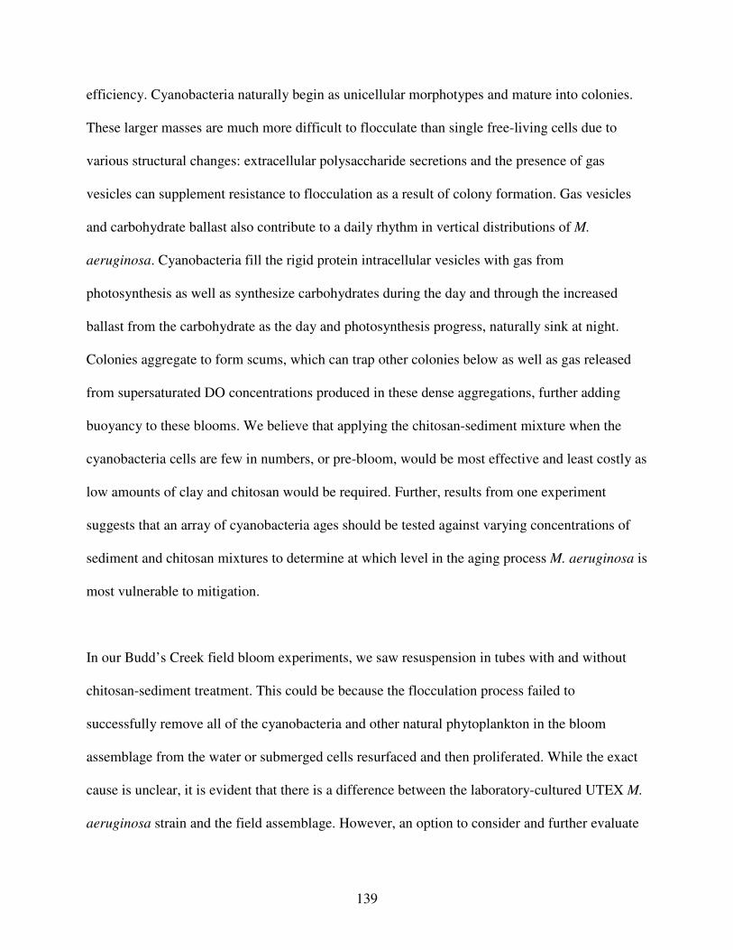
139

efficiency. Cyanobacteria naturally begin as unicellular morphotypes and mature into colonies.

These larger masses are much more difficult to flocculate than single free-living cells due to

various structural changes: extracellular polysaccharide secretions and the presence of gas

vesicles can supplement resistance to flocculation as a result of colony formation. Gas vesicles

and carbohydrate ballast also contribute to a daily rhythm in vertical distributions of M.

aeruginosa. Cyanobacteria fill the rigid protein intracellular vesicles with gas from

photosynthesis as well as synthesize carbohydrates during the day and through the increased

ballast from the carbohydrate as the day and photosynthesis progress, naturally sink at night.

Colonies aggregate to form scums, which can trap other colonies below as well as gas released

from supersaturated DO concentrations produced in these dense aggregations, further adding

buoyancy to these blooms. We believe that applying the chitosan-sediment mixture when the

cyanobacteria cells are few in numbers, or pre-bloom, would be most effective and least costly as

low amounts of clay and chitosan would be required. Further, results from one experiment

suggests that an array of cyanobacteria ages should be tested against varying concentrations of

sediment and chitosan mixtures to determine at which level in the aging process M. aeruginosa is

most vulnerable to mitigation.

In our Budd’s Creek field bloom experiments, we saw resuspension in tubes with and without

chitosan-sediment treatment. This could be because the flocculation process failed to

successfully remove all of the cyanobacteria and other natural phytoplankton in the bloom

assemblage from the water or submerged cells resurfaced and then proliferated. While the exact

cause is unclear, it is evident that there is a difference between the laboratory-cultured UTEX M.

aeruginosa strain and the field assemblage. However, an option to consider and further evaluate

140

is that during field application, cyanobacteria and other phytoplankton cells that have been

submerged after flocculation would have a difficult time resuspending because in many areas of

the bay and its tributaries, euphotic depths are so shallow that once on the bottom most of the

flocculated cells would be deprived of sunlight in the aphotic bottom areas of the bay. This was

not the case in the laboratory and may be responsible for bloom regrowth.

Impacts from mitigating these recurring bay Microcystis blooms may be slight, at least from the

limited experiments we have conducted. In shallow bloom areas, the addition of SAV seeds to

the mitigation mixture could lead to submerged grass germination and growth, using some of the

intracellular nutrients remineralized from the flocced and settled cyanobacteria as they

decompose in the surface sediments of the bottom. This, in turn, reduces accumulations of

nutrients in the overlying water column preventing additional phytoplankton production or other

HABs. The growing SAV also produce DO, aerating waters that would support the aerobic living

resources so valued in the bay ecosystem (crabs, oysters, juvenile fish) and if the beds become

established due to their firm root structure in the sedimented bloom material (see Chapter 4 ),

favors SAV expansion and meets the restoration goals of the region for this critical habitat.

Mitigation of toxin-producing blooms with the clay-chitosan mixtures might also reduce

dissolved toxin concentrations in bloom areas, although fate of that toxin to the benthos and

water column biota remains to be determined.

Finally, public support and modest costs for use of the technique in field bloom mitigation

appears to warrant future consideration by the state as one approach to addressing these recurring

141

and increasing problems to regional waters. Overall, in our cost-analysis, we found that the cost

per household would be $0.04, which is well within the range that survey respondents indicated

they were willing to pay. In addition, further survey results suggest positive opinions toward the

flocculation method. Sixty-five percent of survey respondents were supportive of the mitigation

technology and sixty-nine percent were willing to monetarily support implementation of the

procedure. What we did not anticipate was the number of people who were undecided. We

believe that continued public education would increase the level of support and future outreach

and education would likely increase awareness and acceptance.

142

Chapter 7: Conclusion Harmful algal blooms are responsible for oxygen depletion in the water column, the production

of toxins, and harm to benthic organisms. These effects can consequently lead to mass death in

fish as well as human illness due to the consumption of contaminated seafood. Our team’s goal

was to develop methods to mitigate M. aeruginosa blooms in the Chesapeake Bay and to restore

the damaged ecosystem. Our laboratory experiments demonstrated that the process of chitosan-

sediment flocculation is an effective means of removing blooms from the water column. The

restoration process is further augmented by the elimination of dissolved toxins and the

incorporation of submerged aquatic vegetation seeds into our mixture to support grass growth

and expansion.

As a team, we faced numerous challenges and fought through many limitations over the course

of the program’s three-year timeline. We began as a fourteen-person team under the guardianship

of three esteemed mentors. However, due to several unanticipated circumstances, we lost five

members along with two mentors a year into our research. In spite of this, or maybe as a result of

this, our team learned to adapt and modify our responsibilities in order to overcome these

setbacks. In the end, we were left with nine intelligent, passionate, and ambitious researchers.

Our mentor, who shared our passion for our research, never once wavered with his support or his

guidance. At the end of our three years, we emerged as a successful research team.

Our ultimate objective was to implement our mitigation techniques in the field on M. aeruginosa

blooms in the Chesapeake Bay. Unfortunately the three-year time limit did not allow us to

accomplish this goal ourselves. Our promising results, however, led to the expansion of a new

143

research team aided by our mentor, Mitigation of Microcystis in the Chesapeake (MMIC). The

MMIC group has received funding from the government’s recently established program entitled

the Prevention, Control, and Mitigation of Harmful Algal Blooms. The project will carry out and

hopefully accomplish our end goal: the development of a rapid-response and wide-scale method

that public staffs can use to mitigate a M. aeruginosa bloom when necessary. We believe and

have shown that chitosan-sediment flocculation is an effective, eco-friendly, and inexpensive

means for the mitigation of the Chesapeake’s M. aeruginosa blooms.

144

Appendices A. Appendix A – Sediment Flocculation

A.1 Kaolin Flocculation of M. aeruginosa

Flocculation of 1.0 (dark gray) and 0.5 g L-1 (light gray) Kaolin and M. aeruginosa compared to the natural settling of the cells (black). The absorbance of the cells was measured at 680 nm. Initial M. aeruginosa concentration was about 6.06 E+07 cells mL-1. Results showed that 1.0 g L-

1 and 0.5 g L-1 kaolin was unable to remove M. aeruginosa cells from the water column and did not sweep floc.

0.0

0.2

0.4

0.6

0.8

1.0

1.2

1.4

1.6

1.8

0 20 40 60 80 100 120 140 160

Time (mins)

Ab

sorb

an

ce

(680n

m)

A.2 Removal Data for 88 Flocculation Trials in Deionized Water with Lab UTEX2667 M.

aeruginosa

The left column shows cells removed over time based on the difference between cell density in the experimental treatment and density in the control. The cell density of the control is given at the top of the left column. Cell density was determined using IVF readings cells mL-1 = XXX*IVF (on the 1x10 scale) +/- YYY, r2 = ZZ. The “cells removed” data points are at times negative because sediment addition caused higher fluorescence levels. The column on the right shows percentage of cells removed over time for each experimental treatment. This was determined by dividing the cells removed (from the left column) by the cell density of the control (top of the left column) at each time point. The “% cells removed” data points are negative when sediment addition increased the fluorescence of the water column. Mixtures in bold removed >50% cells in <1 week and are indicated in Table 3.2.

145

ACCOKEEK in DI

CONTROL ACCOKEEK DI

time (hr) Cells/mL Cells/mL Cells/mL

0 5.36E+07 5.51E+07 5.86E+07

24 4.96E+07 4.67E+07 4.85E+07

47 4.71E+07 4.36E+07 4.71E+07

97 3.97E+07 3.95E+07 4.45E+07

122 4.21E+07 4.09E+07 4.38E+07

169 3.65E+07 2.88E+07 3.66E+07

193 3.56E+07 2.91E+07 3.84E+07

CELLS REMOVED

% CELLS REMOVED

Accokeek 0.5g/L DI Accokeek 0.5g/L DI

time (hr) time (hr)

0 -1.50E+06 -1.50E+06 -2.50E+06 0 -2.80% -2.72% -4.27%

24 -1.90E+06 -9.10E+06 -5.80E+06 24 -3.83% -19.49% -11.96%

47 -5.50E+06 -3.00E+06 -1.65E+07 47 -11.68% -6.88% -35.04%

97 -9.80E+06 -1.00E+06 -1.51E+07 97 -24.69% -2.53% -33.94%

122 -7.60E+06 -2.00E+05 -3.80E+06 122 -18.06% -0.49% -8.68%

169 -8.00E+06 -1.02E+07 -2.20E+07 169 -21.93% -35.43% -60.13%

193 -9.50E+06 -1.00E+07 -8.10E+06 193 -26.69% -34.38% -21.10%

CELLS REMOVED % CELLS REMOVED

Accokeek 0.25g/L Accokeek 0.25g/L

time (hr) time (hr)

0 -4.50E+06 -4.00E+06 2.00E+06 0 -8.40% -7.26% 3.41%

24 1.00E+06 -1.01E+07 -3.90E+06 24 2.02% -21.63% -8.04%

47 6.00E+05 -1.00E+07 -4.00E+06 47 1.27% -22.94% -8.49%

97 -4.80E+06 -5.80E+06 -1.80E+06 97 -12.09% -14.69% -4.05%

122 -1.50E+06 -3.00E+05 -7.00E+05 122 -3.56% -0.73% -1.60%

169 -4.00E+06 -7.80E+06 -3.70E+06 169 -10.96% -27.09% -10.11%

193 -4.00E+06 -4.80E+06 -2.00E+06 193 -11.24% -16.50% -5.21%

CELLS REMOVED % CELLS REMOVED

Accokeek 0.5g/L 1:10 Accokeek 0.5g/L 1:10

time (hr) time (hr)

0 -8.00E+06 2.50E+06 3.00E+06 0 -14.93% 4.54% 5.12%

24 -2.10E+07 -8.10E+06 -1.31E+07 24 -42.35% -17.35% -27.02%

47 -1.10E+07 -7.50E+06 -6.00E+06 47 -23.36% -17.21% -12.74%

97 -3.00E+06 9.00E+05 2.90E+06 97 -7.56% 2.28% 6.52%

122 1.70E+06 1.03E+07 1.07E+07 122 4.04% 25.19% 24.44%

169 6.20E+06 5.10E+06 1.19E+07 169 16.99% 17.72% 32.52%

146

193 1.07E+07 8.70E+06 1.60E+07 193 30.07% 29.91% 41.68%

CELLS REMOVED % CELLS REMOVED

Accokeek 0.25g/L 1:10 Accokeek 0.25g/L 1:10

time (hr) time (hr)

0 -1.20E+07 -3.50E+06 2.00E+06 0 -22.39% -6.35% 3.41%

24 -1.05E+07 -1.99E+07 1.40E+06 24 -21.17% -42.62% 2.89%

47 -9.00E+06 -1.70E+07 5.00E+05 47 -19.11% -39.00% 1.06%

97 -1.30E+07 -1.20E+07 5.00E+06 97 -32.76% -30.39% 11.24%

122 -3.50E+06 1.08E+07 8.20E+06 122 -8.32% 26.41% 18.73%

169 3.90E+06 -5.80E+06 6.90E+06 169 10.69% -20.15% 18.86%

193 1.30E+07 -2.50E+06 8.80E+06 193 36.53% -8.59% 22.92%

CELLS REMOVED % CELLS REMOVED

Accokeek 0.5g/L 1:50 Accokeek 0.5g/L 1:50

time (hr) time (hr)

0 5.00E+05 -6.50E+06 2.00E+06 0 0.93% -11.80% 3.41%

24 -3.00E+06 1.79E+07 6.90E+06 24 -6.05% 38.34% 14.23%

47 1.00E+06 1.45E+07 8.00E+06 47 2.12% 33.27% 16.99%

97 1.00E+06 1.70E+07 1.40E+07 97 2.52% 43.05% 31.47%

122 9.20E+06 2.22E+07 1.70E+07 122 21.86% 54.29% 38.82%

169 1.13E+07 9.50E+06 1.40E+07 169 30.97% 33.00% 38.26%

193 1.29E+07 1.61E+07 1.78E+07 193 36.25% 55.35% 46.37%

CELLS REMOVED % CELLS REMOVED

Accokeek 0.25g/L 1:50 Accokeek 0.25g/L 1:50

time (hr) time (hr)

0 -9.00E+06 -1.50E+06 3.20E+06 0 -16.79% -2.72% 5.46%

24 3.72E+07 3.61E+07 2.80E+07 24 75.02% 77.32% 57.75%

47 4.03E+07 3.61E+07 3.09E+07 47 85.58% 82.82% 65.62%

97 3.40E+07 3.33E+07 3.38E+07 97 85.67% 84.33% 75.98%

122 3.85E+07 3.65E+07 3.65E+07 122 91.48% 89.27% 83.36%

169 3.48E+07 2.39E+07 2.94E+07 169 95.37% 83.02% 80.35%

193 3.34E+07 2.45E+07 3.32E+07 193 93.85% 84.23% 86.49%

CELLS REMOVED % CELLS REMOVED

Accokeek 0.5g/L 1:100 Accokeek 0.5g/L 1:100

time (hr) time (hr)

0 -7.00E+06 -5.50E+06 4.00E+06 0 -13.06% -9.98% 6.83%

24 9.00E+06 -9.90E+06 -8.10E+06 24 18.15% -21.20% -16.71%

47 2.30E+07 -1.50E+07 -4.00E+06 47 48.84% -34.41% -8.49%

97 1.93E+07 -1.10E+06 1.27E+07 97 48.63% -2.79% 28.55%

122 2.45E+07 8.40E+06 1.82E+07 122 58.21% 20.54% 41.56%

169 2.26E+07 9.50E+06 1.89E+07 169 61.94% 33.00% 51.66%

193 2.24E+07 1.15E+07 2.20E+07 193 62.94% 39.54% 57.31%

147

CELLS REMOVED % CELLS REMOVED

Accokeek 0.25g/L 1:100 Accokeek 0.25g/L 1:100

time (hr) time (hr)

0 -1.10E+07 -3.50E+06 4.10E+06 0 -20.53% -6.35% 7.00%

24 -2.00E+07 -2.17E+07 -1.86E+07 24 -40.33% -46.48% -38.36%

47 1.00E+06 -1.65E+07 6.00E+06 47 2.12% -37.85% 12.74%

97 1.20E+06 -3.20E+06 1.40E+07 97 3.02% -8.10% 31.47%

122 7.70E+06 1.30E+06 1.41E+07 122 18.30% 3.18% 32.20%

169 9.80E+06 2.30E+06 1.51E+07 169 26.86% 7.99% 41.27%

193 1.12E+07 4.70E+06 1.63E+07 193 31.47% 16.16% 42.46%

BEALTON in DI

CONTROL Bealeton

time (hr) Cells/mL Cells/mL Cells/mL

0 5.56E+07 6.26E+07 5.76E+07

18 5.86E+07 6.06E+07 6.16E+07

42 7.76E+07 7.26E+07 6.96E+07

90 8.46E+07 7.76E+07 6.66E+07

138 5.06E+07 5.66E+07 5.16E+07

186 5.46E+07 5.86E+07 5.56E+07

305 6.66E+07 7.26E+07 6.51E+07

424 6.46E+07 8.06E+07 7.06E+07

CELLS REMOVED % CELLS REMOVED

Bealeton 0.5g/L Bealeton 0.5g/L

time (hr) time (hr)

0 -6.16E+07 -6.16E+07 -5.76E+07 0 -110.79% -98.40% -100.00%

18 -6.26E+07 -6.06E+07 -5.86E+07 18 -106.83% -100.00% -95.13%

42 -6.66E+07 -6.66E+07 -6.28E+07 42 -85.82% -91.74% -90.23%

90 -7.56E+07 -6.66E+07 -6.56E+07 90 -89.36% -85.82% -98.50%

138 -5.86E+07 -5.86E+07 -5.41E+07 138 -115.81% -103.53% -104.84%

186 -6.26E+07 -6.16E+07 -5.76E+07 186 -114.65% -105.12% -103.60%

305 -5.41E+07 -5.26E+07 -5.01E+07 305 -81.23% -72.45% -76.96%

424 -4.86E+07 -5.06E+07 -5.26E+07 424 -75.23% -62.78% -74.50%

CELLS REMOVED % CELLS REMOVED

Bealeton 0.25g/L Bealeton 0.25g/L

time (hr) time (hr)

0 -6.00E+06 1.00E+06 -8.00E+06 0 -10.79% 1.60% -13.89%

18 -2.00E+06 0.00E+00 0.00E+00 18 -3.41% 0.00% 0.00%

42 1.10E+07 7.00E+06 5.00E+06 42 14.18% 9.64% 7.18%

90 1.60E+07 6.00E+06 -1.00E+06 90 18.91% 7.73% -1.50%

138 -5.50E+06 -1.00E+06 -8.00E+06 138 -10.87% -1.77% -15.50%

148

186 -5.00E+06 -4.00E+06 -9.00E+06 186 -9.16% -6.83% -16.19%

305 1.00E+07 1.00E+07 4.50E+06 305 15.02% 13.77% 6.91%

424 4.00E+06 1.85E+07 1.20E+07 424 6.19% 22.95% 17.00%

CELLS REMOVED % CELLS REMOVED

Bealeton 0.5g/L 1:10 Bealeton 0.5g/L 1:10

time (hr) time (hr)

0 -5.00E+06 4.00E+06 -2.00E+06 0 -8.99% 6.39% -3.47%

18 -4.00E+06 -3.00E+06 -8.00E+06 18 -6.83% -4.95% -12.99%

42 2.00E+07 1.40E+07 1.00E+07 42 25.77% 19.28% 14.37%

90 3.10E+07 2.40E+07 1.30E+07 90 36.64% 30.93% 19.52%

138 8.20E+06 1.40E+07 1.35E+07 138 16.21% 24.73% 26.16%

186 1.90E+07 2.40E+07 2.30E+07 186 34.80% 40.96% 41.37%

305 4.20E+07 5.18E+07 4.50E+07 305 63.06% 71.35% 69.12%

424 4.20E+07 6.10E+07 5.15E+07 424 65.02% 75.68% 72.95%

CELLS REMOVED % CELLS REMOVED

Bealeton 0.25g/L 1:10 Bealeton 0.25g/L 1:10

time (hr) time (hr)

0 -8.00E+06 3.00E+06 -4.00E+06 0 -14.39% 4.79% -6.94%

18 4.48E+07 4.65E+07 4.63E+07 18 76.45% 76.73% 75.16%

42 7.21E+07 6.22E+07 5.99E+07 42 92.93% 85.67% 86.08%

90 8.19E+07 7.21E+07 6.25E+07 90 96.82% 92.93% 93.86%

138 4.95E+07 5.45E+07 5.02E+07 138 97.85% 96.31% 97.31%

186 5.38E+07 5.78E+07 5.42E+07 186 98.56% 98.66% 97.50%

305 6.69E+07 7.31E+07 6.58E+07 305 100.47% 100.71% 101.09%

424 6.50E+07 8.13E+07 7.13E+07 424 100.64% 100.88% 101.01%

CELLS REMOVED % CELLS REMOVED

Bealeton 0.5g/L 1:50 Bealeton 0.5g/L 1:50

time (hr) time (hr)

0 -5.00E+06 5.00E+06 -2.00E+06 0 -8.99% 7.99% -3.47%

18 -1.00E+06 1.00E+06 4.00E+06 18 -1.71% 1.65% 6.49%

42 1.80E+07 1.30E+07 8.50E+06 42 23.20% 17.91% 12.21%

90 2.50E+07 1.70E+07 7.00E+06 90 29.55% 21.91% 10.51%

138 -5.00E+06 6.50E+06 1.50E+06 138 -9.88% 11.48% 2.91%

186 -2.00E+06 6.00E+06 4.00E+06 186 -3.66% 10.24% 7.19%

305 1.10E+07 2.40E+07 2.40E+07 305 16.52% 33.06% 36.87%

424 1.80E+07 3.40E+07 2.80E+07 424 27.86% 42.18% 39.66%

CELLS REMOVED % CELLS REMOVED

Bealeton 0.25g/L 1:50 Bealeton 0.25g/L 1:50

149

time (hr) time (hr)

0 -7.00E+06 4.00E+06 -1.00E+06 0 -12.59% 6.39% -1.74%

18 -1.00E+06 0.00E+00 5.00E+06 18 -1.71% 0.00% 8.12%

42 1.10E+07 9.00E+06 7.50E+06 42 14.18% 12.40% 10.78%

90 2.30E+07 1.30E+07 8.00E+06 90 27.19% 16.75% 12.01%

138 -4.00E+06 1.00E+06 2.50E+06 138 -7.91% 1.77% 4.84%

186 -1.00E+06 4.00E+06 3.00E+06 186 -1.83% 6.83% 5.40%

305 1.58E+07 3.25E+07 2.70E+07 305 23.72% 44.77% 41.47%

424 2.63E+07 5.30E+07 3.10E+07 424 40.71% 65.76% 43.91%

CELLS REMOVED % CELLS REMOVED

Bealeton 0.5g/L 1:100 Bealeton 0.5g/L 1:100

time (hr) time (hr)

0 -8.00E+06 1.00E+06 -5.00E+06 0 -14.39% 1.60% -8.68%

18 -5.00E+06 1.00E+06 2.00E+06 18 -8.53% 1.65% 3.25%

42 1.30E+07 9.50E+06 8.50E+06 42 16.75% 13.09% 12.21%

90 2.20E+07 1.60E+07 7.00E+06 90 26.00% 20.62% 10.51%

138 -6.00E+06 3.50E+06 -4.00E+06 138 -11.86% 6.18% -7.75%

186 -8.00E+06 2.00E+06 -4.00E+06 186 -14.65% 3.41% -7.19%

305 5.50E+06 2.20E+07 1.05E+07 305 8.26% 30.30% 16.13%

424 8.00E+06 2.85E+07 2.10E+07 424 12.38% 35.36% 29.75%

CELLS REMOVED % CELLS REMOVED

Bealeton 0.25g/L 1:100 Bealeton 0.25g/L 1:100

time (hr) time (hr)

0 -6.00E+06 0.00E+00 -1.00E+06 0 -10.79% 0.00% -1.74%

18 -3.00E+06 5.00E+06 6.00E+06 18 -5.12% 8.25% 9.74%

42 1.20E+07 1.20E+07 8.00E+06 42 15.46% 16.53% 11.49%

90 2.00E+07 1.40E+07 6.00E+06 90 23.64% 18.04% 9.01% 138 -7.00E+06 4.00E+06 3.00E+06 138 -13.83% 7.07% 5.81% 186 -3.00E+06 4.00E+06 3.00E+06 186 -5.49% 6.83% 5.40%

305 5.50E+06 1.55E+07 1.65E+07 305 8.26% 21.35% 25.35% 424 2.50E+06 3.58E+07 1.95E+07 424 3.87% 44.42% 27.62%

MONTMORILLONITE in DI

CONTROL Montmorillonite

time (hr) Cells/mL Cells/mL Cells/mL

0 7.66E+07 8.16E+07 7.26E+07

50 6.15E+07 6.07E+07 6.05E+07

69 6.06E+07 5.96E+07 5.96E+07

117 5.71E+07 5.81E+07 5.76E+07

147 5.56E+07 5.61E+07 5.76E+07

218 5.46E+07 5.56E+07 5.66E+07

452 3.46E+07 3.41E+07 3.69E+07

150

CELLS REMOVED % CELLS REMOVED

Mont 0.5g/L Mont 0.5g/L

time (hr) time (hr)

0 -6.00E+06 -3.00E+06 -1.20E+07 0 -7.83% -3.68% -16.53%

50 -6.10E+06 -6.90E+06 -6.10E+06 50 -9.92% -11.37% -10.08%

69 -7.00E+06 -8.00E+06 -5.00E+06 69 -11.55% -13.42% -8.39%

117 -8.50E+06 -5.50E+06 -1.00E+06 117 -14.89% -9.47% -1.74%

147 -6.00E+06 -7.50E+06 -1.00E+06 147 -10.79% -13.37% -1.74%

218 0.00E+00 -3.00E+06 2.50E+06 218 0.00% -5.40% 4.42%

452 -3.00E+06 5.50E+06 8.30E+06 452 -8.67% 16.13% 22.49%

CELLS REMOVED % CELLS REMOVED

Mont 0.25g/L Mont 0.25g/L

time (hr) time (hr)

0 5.00E+06 9.00E+06 -2.00E+06 0 6.53% 11.03% -2.75%

50 -3.10E+06 -6.90E+06 -4.10E+06 50 -5.04% -11.37% -6.78%

69 -5.00E+06 -2.00E+06 -4.00E+06 69 -8.25% -3.36% -6.71%

117 -1.50E+06 3.50E+06 -4.00E+06 117 -2.63% 6.02% -6.94%

147 3.00E+06 5.00E+05 -1.00E+06 147 5.40% 0.89% -1.74%

218 1.00E+06 7.00E+06 4.00E+06 218 1.83% 12.59% 7.07%

452 1.77E+07 1.65E+07 2.10E+07 452 51.16% 48.39% 56.91%

CELLS REMOVED % CELLS REMOVED

Mont 0.5g/L 1:10 Mont 0.5g/L 1:10

time (hr) time (hr)

0 -9.00E+06 -3.00E+06 -1.20E+07 0 -11.75% -3.68% -16.53%

50 -5.10E+06 -3.90E+06 -6.10E+06 50 -8.29% -6.43% -10.08%

69 -4.00E+06 -6.00E+06 -8.00E+06 69 -6.60% -10.07% -13.42%

117 -3.50E+06 -1.50E+06 -5.00E+06 117 -6.13% -2.58% -8.68%

147 -5.00E+06 -5.00E+05 0.00E+00 147 -8.99% -0.89% 0.00%

218 5.90E+06 5.00E+06 5.00E+06 218 10.81% 8.99% 8.83%

452 1.65E+07 1.00E+07 2.98E+07 452 47.69% 29.33% 80.79%

CELLS REMOVED % CELLS REMOVED

Mont 0.25g/L 1:10 Mont 0.25g/L 1:10

time (hr) time (hr)

0 1.00E+06 7.00E+06 -4.00E+06 0 1.31% 8.58% -5.51%

50 -1.10E+06 1.00E+05 -6.10E+06 50 -1.79% 0.16% -10.08%

69 -3.00E+06 -2.00E+06 -8.00E+06 69 -4.95% -3.36% -13.42%

117 -5.00E+05 2.50E+06 2.00E+06 117 -0.88% 4.30% 3.47%

147 4.00E+06 5.00E+05 6.00E+06 147 7.19% 0.89% 10.42%

151

218 1.75E+07 1.00E+07 1.10E+07 218 32.05% 17.99% 19.43%

452 1.95E+07 1.65E+07 1.53E+07 452 56.36% 48.39% 41.46%

CELLS REMOVED % CELLS REMOVED

Mont 0.5g/L 1:50 Mont 0.5g/L 1:50

time (hr) time (hr)

0 3.00E+06 8.00E+06 -2.00E+06 0 3.92% 9.80% -2.75%

50 -1.00E+05 -9.00E+05 -2.10E+06 50 -0.16% -1.48% -3.47%

69 1.30E+07 -4.00E+06 -7.00E+06 69 21.45% -6.71% -11.74%

117 1.45E+07 1.55E+07 1.60E+07 117 25.39% 26.68% 27.78%

147 1.50E+07 1.65E+07 1.70E+07 147 26.98% 29.41% 29.51%

218 2.02E+07 2.10E+07 2.10E+07 218 37.00% 37.77% 37.10%

452 2.25E+07 1.95E+07 2.18E+07 452 65.03% 57.18% 59.08%

CELLS REMOVED % CELLS REMOVED

Mont 0.25g/L 1:50 Mont 0.25g/L 1:50

time (hr) time (hr)

0 0.00E+00 1.00E+07 4.00E+06 0 0.00% 12.25% 5.51%

50 -3.10E+06 1.00E+05 -9.90E+06 50 -5.04% 0.16% -16.36%

69 -7.00E+06 -7.00E+06 -8.00E+06 69 -11.55% -11.74% -13.42%

117 1.35E+07 1.65E+07 1.60E+07 117 23.64% 28.40% 27.78%

147 1.50E+07 1.75E+07 1.70E+07 147 26.98% 31.19% 29.51%

218 1.98E+07 2.15E+07 2.18E+07 218 36.26% 38.67% 38.52%

452 2.00E+07 1.90E+07 2.33E+07 452 57.80% 55.72% 63.14%

CELLS REMOVED % CELLS REMOVED

Mont 0.5g/L 1:100 Mont 0.5g/L 1:100

time (hr) time (hr)

0 -7.00E+06 -5.00E+06 -7.00E+06 0 -9.14% -6.13% -9.64%

50 -1.10E+06 2.10E+06 1.00E+05 50 -1.79% 3.46% 0.17%

69 -2.00E+06 1.00E+06 3.00E+06 69 -3.30% 1.68% 5.03%

117 -5.00E+05 -5.00E+05 2.00E+06 117 -0.88% -0.86% 3.47%

147 3.00E+06 1.50E+06 7.00E+06 147 5.40% 2.67% 12.15%

218 2.00E+06 8.00E+06 8.00E+06 218 3.66% 14.39% 14.13%

452 2.30E+07 1.65E+07 2.40E+07 452 66.47% 48.39% 65.04%

CELLS REMOVED % CELLS REMOVED

Mont 0.25g/L 1:100 Mont 0.25g/L 1:100

time (hr) time (hr)

0 2.00E+06 -3.00E+06 2.00E+06 0 2.61% -3.68% 2.75%

50 9.00E+05 -9.90E+06 -2.10E+06 50 1.46% -16.31% -3.47%

69 -5.00E+06 -1.00E+07 1.00E+06 69 -8.25% -16.78% 1.68%

152

117 1.50E+06 1.50E+06 2.00E+06 117 2.63% 2.58% 3.47%

147 1.50E+07 2.35E+07 9.00E+06 147 26.98% 41.89% 15.63%

218 2.30E+07 2.40E+07 1.60E+07 218 42.12% 43.17% 28.27%

452 2.40E+07 2.45E+07 2.33E+07 452 69.36% 71.88% 63.14%

SPOTSYLVANNIA 1 in DI

CONTROL Spots 1

time (hr) Cells/mL Cells/mL Cells/mL

0 6.36E+07 6.76E+07 7.16E+07

27 7.16E+07 7.56E+07 7.26E+07

68 8.26E+07 8.46E+07 8.46E+07

119 6.96E+07 7.26E+07 7.06E+07

167 7.66E+07 7.96E+07 7.66E+07

237 7.96E+07 8.76E+07 8.26E+07

286 6.06E+07 6.21E+07 6.27E+07

CELLS REMOVED % CELLS REMOVED

time (hr) Spots 1 0.5g/L time (hr) Spots 1 0.5g/L

0 -1.20E+07 -4.00E+06 -4.00E+06 0 -18.87% -5.92% -5.59%

27 4.00E+06 2.00E+06 1.00E+06 27 5.59% 2.65% 1.38%

68 1.10E+07 1.79E+07 1.60E+07 68 13.32% 21.16% 18.92%

119 3.00E+06 1.10E+07 4.00E+06 119 4.31% 15.15% 5.67%

167 9.01E+06 1.50E+07 1.10E+07 167 11.77% 18.86% 14.38%

237 1.00E+06 1.50E+07 8.00E+06 237 1.26% 17.13% 9.69%

286 -6.00E+06 3.50E+06 -1.40E+06 286 -9.90% 5.64% -2.23%

CELLS REMOVED % CELLS REMOVED

time (hr) Spots 1 0.25g/L time (hr) Spots 1 0.25g/L

0 -8.00E+06 -9.00E+06 -6.00E+06 0 -12.58% -13.32% -8.38%

27 4.00E+06 -3.00E+06 -9.00E+06 27 5.59% -3.97% -12.40%

68 9.00E+06 1.40E+07 6.00E+06 68 10.90% 16.55% 7.09%

119 2.00E+06 5.00E+06 7.00E+06 119 2.87% 6.89% 9.92%

167 1.30E+07 1.60E+07 1.30E+07 167 16.99% 20.12% 16.99%

237 -4.00E+06 1.00E+07 8.00E+06 237 -5.03% 11.42% 9.69%

286 -4.00E+06 -8.00E+05 1.00E+05 286 -6.60% -1.29% 0.16%

CELLS REMOVED % CELLS REMOVED

time (hr) Spots 1 0.5g/L 1:10 time (hr) Spots 1 0.5g/L 1:10

0 -8.00E+06 -3.00E+06 -4.00E+06 0 -12.58% -4.44% -5.59%

27 -6.00E+06 9.00E+06 -4.00E+06 27 -8.38% 11.91% -5.51%

68 1.50E+07 1.50E+07 1.60E+07 68 18.16% 17.73% 18.92%

119 2.00E+06 6.00E+06 5.00E+06 119 2.87% 8.27% 7.08%

167 9.01E+06 1.20E+07 1.10E+07 167 11.77% 15.09% 14.38%

237 1.30E+07 1.80E+07 1.30E+07 237 16.33% 20.55% 15.74%

286 -1.00E+05 -2.50E+06 -1.40E+06 286 -0.17% -4.03% -2.23%

153

CELLS REMOVED % CELLS REMOVED

time (hr) Spots 1 0.25g/L 1:10 time (hr) Spots 1 0.25g/L 1:10

0 -1.50E+07 -1.00E+07 -7.00E+06 0 -23.59% -14.80% -9.78%

27 -1.50E+07 -7.00E+06 -6.00E+06 27 -20.95% -9.26% -8.27%

68 -1.30E+07 1.59E+07 1.50E+07 68 -15.74% 18.80% 17.73%

119 3.00E+06 8.00E+06 7.00E+06 119 4.31% 11.02% 9.92%

167 8.01E+06 1.40E+07 1.10E+07 167 10.46% 17.60% 14.38%

237 8.00E+06 2.20E+07 1.60E+07 237 10.05% 25.12% 19.37%

286 -1.00E+06 3.50E+06 2.30E+06 286 -1.65% 5.64% 3.67%

CELLS REMOVED % CELLS REMOVED

time (hr) Spots 1 0.5g/L 1:50 time (hr) Spots 1 0.5g/L 1:50

0 -1.90E+07 -1.40E+07 -1.10E+07 0 -29.88% -20.71% -15.37%

27 -1.00E+07 7.00E+06 2.00E+06 27 -13.97% 9.26% 2.76%

68 3.60E+07 6.88E+07 5.60E+07 68 43.59% 81.34% 66.20%

119 4.60E+07 6.90E+07 5.52E+07 119 66.10% 95.06% 78.20%

167 5.90E+07 7.80E+07 6.36E+07 167 77.04% 98.01% 83.04%

237 6.82E+07 8.61E+07 7.04E+07 237 85.69% 98.30% 85.24%

286 5.30E+07 6.04E+07 5.23E+07 286 87.48% 97.28% 83.43%

CELLS REMOVED % CELLS REMOVED

time (hr) Spots 1 0.25g/L 1:50 time (hr) Spots 1 0.25g/L 1:50

0 -8.00E+06 -8.00E+06 2.00E+06 0 -12.58% -11.84% 2.79%

27 1.00E+07 -4.00E+06 1.40E+07 27 13.97% -5.29% 19.29%

68 2.40E+07 3.78E+07 3.03E+07 68 29.06% 44.69% 35.82%

119 1.40E+07 3.00E+07 3.00E+07 119 20.12% 41.33% 42.50%

167 2.20E+07 4.00E+07 4.20E+07 167 28.74% 50.27% 54.85%

237 3.40E+07 4.90E+07 5.42E+07 237 42.72% 55.94% 65.63%

286 2.75E+07 3.05E+07 3.86E+07 286 45.39% 49.12% 61.57%

CELLS REMOVED % CELLS REMOVED

time (hr) Spots 1 0.5g/L 1:100 time (hr) Spots 1 0.5g/L 1:100

0 -2.00E+07 -2.20E+07 -1.00E+07 0 -31.45% -32.55% -13.97%

27 -1.40E+07 -7.00E+06 -9.00E+06 27 -19.56% -9.26% -12.40%

68 -6.00E+06 -2.00E+06 -4.00E+06 68 -7.26% -2.36% -4.73%

119 -5.00E+06 -1.50E+07 -1.50E+07 119 -7.19% -20.66% -21.25%

167 1.40E+07 -1.09E+06 7.01E+06 167 18.29% -1.37% 9.15%

237 1.80E+07 1.72E+07 1.80E+07 237 22.62% 19.64% 21.79%

286 9.50E+06 1.00E+06 2.60E+06 286 15.68% 1.61% 4.15%

CELLS REMOVED % CELLS REMOVED

time (hr) Spots 1 0.25g/L 1:100 time (hr) Spots 1 0.25g/L 1:100

0 -1.40E+07 -2.20E+07 -1.40E+07 0 -22.02% -32.55% -19.56%

27 8.00E+06 2.00E+07 -1.70E+07 27 11.18% 26.46% -23.42%

154

68 1.70E+07 4.30E+07 -2.00E+06 68 20.58% 50.83% -2.36%

119 1.30E+07 5.10E+07 9.00E+06 119 18.68% 70.26% 12.75%

167 2.60E+07 2.70E+07 2.88E+07 167 33.96% 33.93% 37.61%

237 3.15E+07 7.46E+07 3.60E+07 237 39.58% 85.17% 43.59%

286 2.82E+07 5.16E+07 2.56E+07 286 46.54% 83.11% 40.84%

STANCILLS A in DI

CONTROL Stancills A

time (hr) Cells/mL Cells/mL Cells/mL

0 6.56E+07 7.46E+07 6.76E+07

27 5.86E+07 5.66E+07 6.16E+07

51 4.79E+07 4.97E+07 4.73E+07

73 3.66E+07 3.66E+07 3.66E+07

97 3.86E+07 4.01E+07 4.21E+07

121 4.16E+07 3.99E+07 3.96E+07

146 3.66E+07 3.51E+07 3.41E+07

170 3.64E+07 3.34E+07 3.32E+07

CELLS REMOVED % CELLS REMOVED

time (hr) Stancills A 0.5g/L time (hr) Stancills A 0.5g/L

0 -5.00E+06 -2.00E+06 -8.00E+06 0 -7.62% -2.68% -11.84%

27 8.00E+06 5.70E+06 1.50E+07 27 13.65% 10.07% 24.36%

51 3.00E+05 8.00E+05 1.70E+06 51 0.63% 1.61% 3.59%

73 -2.20E+06 -5.00E+05 -1.90E+06 73 -6.01% -1.37% -5.19%

97 -2.50E+06 -1.00E+06 4.00E+06 97 -6.48% -2.49% 9.50%

121 1.90E+06 -1.00E+06 3.80E+06 121 4.57% -2.51% 9.60%

146 1.00E+05 -1.50E+06 1.17E+07 146 0.27% -4.27% 34.32%

170 0.00E+00 -3.20E+06 1.47E+07 170 0.00% -9.58% 44.29%

CELLS REMOVED % CELLS REMOVED

time (hr) Stancills A 0.25g/L time (hr) Stancills A 0.25g/L

0 -9.00E+06 3.00E+06 -4.00E+06 0 -13.72% 4.02% -5.92%

27 5.20E+06 0.00E+00 2.70E+06 27 8.88% 0.00% 4.38%

51 -3.70E+06 -2.90E+06 -4.60E+06 51 -7.73% -5.84% -9.73%

73 -5.00E+05 -3.50E+06 1.50E+06 73 -1.37% -9.57% 4.10%

97 6.00E+06 3.50E+06 8.50E+06 97 15.55% 8.73% 20.20%

121 1.63E+07 2.30E+06 1.10E+07 121 39.19% 5.77% 27.79%

146 1.40E+07 1.03E+07 1.32E+07 146 38.26% 29.35% 38.72%

170 1.75E+07 1.30E+06 1.28E+07 170 48.09% 3.89% 38.57%

CELLS REMOVED % CELLS REMOVED

time (hr) Stancills A 0.5g/L 1:10 time (hr) Stancills A 0.5g/L 1:10

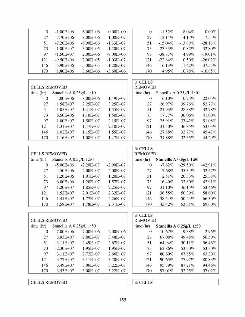
155

0 -1.00E+06 6.00E+06 0.00E+00 0 -1.52% 8.04% 0.00%

27 7.70E+06 8.00E+06 1.08E+07 27 13.14% 14.14% 17.54%

51 -7.20E+06 -6.90E+06 -1.33E+07 51 -15.04% -13.89% -28.13%

73 -1.00E+07 3.00E+05 -1.20E+07 73 -27.33% 0.82% -32.80%

97 -1.50E+07 2.00E+06 -8.00E+06 97 -38.87% 4.99% -19.01%

121 -9.50E+06 2.00E+05 -1.03E+07 121 -22.84% 0.50% -26.02%

146 -5.90E+06 -5.00E+05 -1.28E+07 146 -16.13% -1.42% -37.55%

170 1.80E+06 3.60E+06 -3.60E+06 170 4.95% 10.78% -10.85%

CELLS REMOVED % CELLS REMOVED

time (hr) Stancills A 0.25g/L 1:10 time (hr) Stancills A 0.25g/L 1:10

0 4.00E+06 8.00E+06 1.49E+07 0 6.10% 10.73% 22.05%

27 1.58E+07 2.25E+07 3.25E+07 27 26.97% 39.76% 52.77%

51 1.05E+07 1.41E+07 1.55E+07 51 21.93% 28.38% 32.78%

73 6.50E+06 1.10E+07 1.50E+07 73 17.77% 30.06% 41.00%

97 1.00E+07 1.50E+07 2.15E+07 97 25.91% 37.42% 51.08%

121 1.31E+07 1.47E+07 2.10E+07 121 31.50% 36.85% 53.05%

146 1.02E+07 1.15E+07 1.55E+07 146 27.88% 32.77% 45.47%

170 1.16E+07 1.08E+07 1.47E+07 170 31.88% 32.35% 44.29%

CELLS REMOVED % CELLS REMOVED

time (hr) Stancills A 0.5g/L 1:50 time (hr) Stancills A 0.5g/L 1:50

0 -5.00E+06 -2.20E+07 -2.90E+07 0 -7.62% -29.50% -42.91%

27 4.50E+06 2.00E+07 2.00E+07 27 7.68% 35.34% 32.47%

51 1.20E+06 1.01E+07 1.20E+07 51 2.51% 20.33% 25.38%

73 6.00E+06 1.20E+07 1.57E+07 73 16.40% 32.80% 42.91%

97 1.20E+07 1.85E+07 2.25E+07 97 31.10% 46.15% 53.46%

121 1.52E+07 2.01E+07 2.32E+07 121 36.55% 50.39% 58.60%

146 1.41E+07 1.77E+07 2.26E+07 146 38.54% 50.44% 66.30%

170 1.58E+07 1.78E+07 2.31E+07 170 43.42% 53.31% 69.60%

CELLS REMOVED % CELLS REMOVED

time (hr) Stancills A 0.25g/L 1:50 time (hr) Stancills A 0.25g/L 1:50

0 7.00E+06 7.00E+06 2.00E+06 0 10.67% 9.38% 2.96%

27 3.93E+07 2.80E+07 3.48E+07 27 67.08% 49.48% 56.50%

51 3.11E+07 2.49E+07 2.67E+07 51 64.94% 50.11% 56.46%

73 2.30E+07 1.95E+07 1.95E+07 73 62.86% 53.30% 53.30%

97 3.11E+07 2.72E+07 2.66E+07 97 80.60% 67.85% 63.20%

121 3.77E+07 3.11E+07 3.20E+07 121 90.65% 77.97% 80.83%

146 3.49E+07 3.06E+07 3.22E+07 146 95.39% 87.21% 94.46%

170 3.53E+07 3.08E+07 3.22E+07 170 97.01% 92.25% 97.02%

CELLS REMOVED % CELLS

156

REMOVED

time (hr) Stancills A 0.5g/L 1:100 time (hr) Stancills A 0.5g/L 1:100

0 7.00E+06 1.65E+07 1.50E+07 0 10.67% 22.12% 22.19%

27 3.18E+07 3.62E+07 3.70E+07 27 54.28% 63.97% 60.08%

51 2.63E+07 2.88E+07 2.68E+07 51 54.92% 57.96% 56.67%

73 2.18E+07 2.42E+07 2.35E+07 73 59.58% 66.14% 64.23%

97 2.75E+07 3.13E+07 3.25E+07 97 71.27% 78.08% 77.22%

121 3.22E+07 3.19E+07 3.15E+07 121 77.43% 79.97% 79.57%

146 2.90E+07 2.90E+07 2.77E+07 146 79.26% 82.65% 81.26%

170 2.99E+07 2.86E+07 2.79E+07 170 82.17% 85.66% 84.07%

CELLS REMOVED % CELLS REMOVED

time (hr) Stancills A 0.25g/L 1:100 time (hr) Stancills A 0.25g/L 1:100

0 -1.00E+06 -7.00E+06 0.00E+00 0 -1.52% -9.38% 0.00%

27 1.10E+07 1.50E+07 9.20E+06 27 18.78% 26.51% 14.94%

51 4.02E+07 3.44E+07 4.03E+07 51 83.95% 69.23% 85.22%

73 3.20E+07 3.40E+07 3.22E+07 73 87.46% 92.93% 88.01%

97 3.80E+07 3.93E+07 4.18E+07 97 98.48% 98.03% 99.32%

121 4.18E+07 3.94E+07 3.98E+07 121 100.51% 98.78% 100.54%

146 3.70E+07 3.27E+07 3.41E+07 146 101.13% 93.19% 100.04%

170 3.69E+07 2.70E+07 3.26E+07 170 101.41% 80.87% 98.23%

TRISTATE in DI

CONTROL Tristate

time (hr) Cells/mL Cells/mL Cells/mL

0 6.36E+07 6.76E+07 7.16E+07

27 7.16E+07 7.56E+07 7.26E+07

68 8.26E+07 8.46E+07 8.46E+07

119 6.96E+07 7.26E+07 7.06E+07

167 7.66E+07 7.96E+07 7.66E+07

237 7.96E+07 8.76E+07 8.26E+07

286 6.06E+07 6.21E+07 6.27E+07

CELLS REMOVED % CELLS REMOVED

time (hr) Tristate 0.5g/L time (hr) Tristate 0.5g/L

0 -5.00E+06 -5.20E+06 4.00E+06 0 -7.86% -7.69% 5.59%

27 -1.00E+07 -1.00E+06 1.00E+06 27 -13.97% -1.32% 1.38%

68 2.00E+07 1.90E+07 1.80E+07 68 24.22% 22.46% 21.28%

119 6.00E+06 8.00E+06 1.10E+07 119 8.62% 11.02% 15.58%

167 1.40E+07 1.70E+07 1.70E+07 167 18.29% 21.37% 22.21%

237 1.20E+07 2.10E+07 1.50E+07 237 15.08% 23.98% 18.16%

286 2.50E+06 3.50E+06 1.10E+06 286 4.13% 5.64% 1.75%

CELLS REMOVED % CELLS REMOVED

157

time (hr) Tristate 0.25g/L time (hr) Tristate 0.25g/L

0 -3.00E+06 -2.60E+06 5.00E+06 0 -4.72% -3.85% 6.98%

27 -5.00E+06 6.00E+06 -2.00E+06 27 -6.98% 7.94% -2.76%

68 1.01E+07 1.80E+07 1.20E+07 68 12.23% 21.28% 14.19%

119 8.00E+06 7.00E+06 8.00E+06 119 11.50% 9.64% 11.33%

167 1.30E+07 1.70E+07 1.40E+07 167 16.99% 21.37% 18.29%

237 2.00E+06 1.10E+07 1.10E+07 237 2.51% 12.56% 13.32%

286 -1.00E+06 5.00E+05 5.10E+06 286 -1.65% 0.81% 8.14%

CELLS REMOVED % CELLS REMOVED

time (hr) Tristate 0.5g/L 1:10 time (hr) Tristate 0.5g/L 1:10

0 -2.10E+07 -1.70E+07 -1.10E+07 0 -33.03% -25.15% -15.37%

27 -8.00E+06 -4.00E+06 -2.00E+06 27 -11.18% -5.29% -2.76%

68 -2.00E+06 0.00E+00 1.30E+07 68 -2.42% 0.00% 15.37%

119 -1.20E+07 -9.00E+06 1.00E+06 119 -17.24% -12.40% 1.42%

167 1.80E+07 2.10E+07 1.50E+07 167 23.51% 26.40% 19.60%

237 2.00E+07 2.80E+07 2.25E+07 237 25.13% 31.97% 27.24%

286 1.00E+07 1.15E+07 1.16E+07 286 16.50% 18.52% 18.50%

CELLS REMOVED % CELLS REMOVED

time (hr) Tristate 0.25g/L 1:10 time (hr) Tristate 0.25g/L 1:10

0 -1.70E+07 -8.00E+06 -3.00E+06 0 -26.73% -11.84% -4.19%

27 -1.00E+07 -2.10E+07 -5.00E+06 27 -13.97% -27.78% -6.89%

68 2.10E+07 1.40E+07 3.30E+07 68 25.43% 16.55% 39.01%

119 2.10E+07 4.00E+07 3.70E+07 119 30.18% 55.11% 52.42%

167 3.60E+07 6.75E+07 5.70E+07 167 47.01% 84.81% 74.43%

237 4.72E+07 7.95E+07 6.88E+07 237 59.31% 90.77% 83.31%

286 3.50E+07 5.60E+07 5.11E+07 286 57.77% 90.19% 81.51%

CELLS REMOVED % CELLS REMOVED

time (hr) Tristate 0.5g/L 1:50 time (hr) Tristate 0.5g/L 1:50

0 -1.30E+07 6.00E+06 7.00E+06 0 -20.44% 8.88% 9.78%

27 -1.60E+07 -3.70E+07 -2.90E+07 27 -22.35% -48.95% -39.95%

68 1.50E+07 3.70E+07 3.80E+07 68 18.16% 43.74% 44.92%

119 3.50E+07 4.90E+07 4.80E+07 119 50.30% 67.50% 68.00%

167 7.57E+07 8.02E+07 7.78E+07 167 98.84% 100.77% 101.58%

237 7.99E+07 8.85E+07 8.39E+07 237 100.39% 101.04% 101.59%

286 6.06E+07 6.29E+07 6.39E+07 286 100.02% 101.31% 101.93%

CELLS REMOVED % CELLS REMOVED

time (hr) Tristate 0.25g/L 1:50 time (hr) Tristate 0.25g/L 1:50

0 -1.10E+07 -9.00E+05 2.50E+06 0 -17.30% -1.33% 3.49%

27 1.30E+07 1.70E+07 1.10E+07 27 18.16% 22.49% 15.15%

68 3.20E+07 3.18E+07 3.10E+07 68 38.75% 37.59% 36.65%

119 3.00E+07 2.80E+07 2.30E+07 119 43.11% 38.57% 32.58%

167 4.10E+07 3.90E+07 3.10E+07 167 53.54% 49.01% 40.49%

158

237 4.90E+07 5.46E+07 4.00E+07 237 61.57% 62.34% 48.43%

286 3.90E+07 4.00E+07 3.01E+07 286 64.37% 64.42% 48.02%

CELLS REMOVED % CELLS REMOVED

time (hr) Tristate 0.5g/L 1:100 time (hr) Tristate 0.5g/L 1:100

0 -5.00E+06 -3.00E+06 1.00E+06 0 -7.86% -4.44% 1.40%

27 1.10E+07 2.00E+07 1.00E+07 27 15.37% 26.46% 13.78%

68 4.30E+07 2.90E+07 3.15E+07 68 52.07% 34.28% 37.24%

119 3.70E+07 2.80E+07 2.40E+07 119 53.17% 38.57% 34.00%

167 4.50E+07 4.09E+07 2.97E+07 167 58.76% 51.40% 38.79%

237 5.08E+07 5.45E+07 4.15E+07 237 63.83% 62.22% 50.25%

286 3.75E+07 3.46E+07 3.31E+07 286 61.89% 55.73% 52.80%

CELLS REMOVED % CELLS REMOVED

time (hr) Tristate 0.25g/L 1:100 time (hr) Tristate 0.25g/L 1:100

0 -9.00E+06 2.00E+06 6.00E+06 0 -14.15% 2.96% 8.38%

27 7.00E+06 1.10E+07 1.00E+07 27 9.78% 14.55% 13.78%

68 2.40E+07 2.20E+07 2.20E+07 68 29.06% 26.01% 26.01%

119 1.30E+07 1.70E+07 1.60E+07 119 18.68% 23.42% 22.67%

167 1.98E+07 2.32E+07 2.26E+07 167 25.86% 29.16% 29.52%

237 2.50E+07 3.65E+07 3.40E+07 237 31.41% 41.67% 41.17%

286 1.40E+07 1.90E+07 2.26E+07 286 23.11% 30.60% 36.05%

KAOLIN in DI

CONTROL Kaolin

time (hr) Cells/mL Cells/mL Cells/mL

0 7.66E+07 8.16E+07 7.26E+07

50 6.15E+07 6.07E+07 6.05E+07

69 6.06E+07 5.96E+07 5.96E+07

117 5.71E+07 5.81E+07 5.76E+07

147 5.56E+07 5.61E+07 5.76E+07

218 5.46E+07 5.56E+07 5.66E+07

452 3.46E+07 3.41E+07 3.69E+07

CELLS REMOVED % CELLS REMOVED

Kaolin 0.5g/L Kaolin 0.5g/L

time (hr) time (hr)

0 -4.94E+07 -4.64E+07 -5.34E+07 0 -64.49% -56.86% -73.55%

50 -5.55E+07 -5.83E+07 -5.65E+07 50 -90.24% -96.05% -93.39%

69 -4.94E+07 -5.44E+07 -5.24E+07 69 -81.52% -91.28% -87.92%

117 -4.59E+07 -4.39E+07 -4.20E+07 117 -80.39% -75.56% -72.92%

147 -3.60E+07 -4.05E+07 -3.40E+07 147 -64.75% -72.19% -59.03%

218 -2.20E+07 -2.50E+07 -1.90E+07 218 -40.29% -44.96% -33.57%

452 1.60E+07 1.45E+07 1.93E+07 452 46.24% 42.52% 52.30%

159

CELLS REMOVED % CELLS REMOVED

Kaolin 0.25g/L Kaolin 0.25g/L

time (hr) time (hr)

0 -2.94E+07 -2.64E+07 -3.24E+07 0 -38.38% -32.35% -44.63%

50 -3.31E+07 -3.59E+07 -3.51E+07 50 -53.82% -59.14% -58.02%

69 -2.60E+07 -3.00E+07 -3.30E+07 69 -42.90% -50.34% -55.37%

117 -1.75E+07 1.50E+06 -1.90E+07 117 -30.65% 2.58% -32.99%

147 -4.00E+06 -1.65E+07 -1.40E+07 147 -7.19% -29.41% -24.31%

218 2.00E+06 1.00E+06 2.00E+06 218 3.66% 1.80% 3.53%

452 1.63E+07 1.36E+07 1.98E+07 452 47.11% 39.88% 53.66%

CELLS REMOVED % CELLS REMOVED

Kaolin 0.5g/L 1:10 Kaolin 0.5g/L 1:10

time (hr) time (hr)

0 -6.04E+07 -5.84E+07 -6.44E+07 0 -78.85% -71.57% -88.71%

50 8.90E+06 8.10E+06 7.90E+06 50 14.47% 13.34% 13.06%

69 2.40E+07 1.90E+07 1.90E+07 69 39.60% 31.88% 31.88%

117 3.65E+07 3.75E+07 3.90E+07 117 63.92% 64.54% 67.71%

147 4.73E+07 4.67E+07 5.09E+07 147 85.09% 83.26% 88.39%

218 4.95E+07 5.11E+07 5.32E+07 218 90.68% 91.92% 94.01%

452 3.30E+07 3.29E+07 3.48E+07 452 95.40% 96.51% 94.34%

CELLS REMOVED % CELLS REMOVED

Kaolin 0.25g/L 1:10 Kaolin 0.25g/L 1:10

time (hr) time (hr)

0 -3.04E+07 -2.54E+07 -3.64E+07 0 -39.69% -31.13% -50.14%

50 5.49E+07 4.41E+07 4.89E+07 50 89.28% 72.65% 80.83%

69 5.23E+07 5.20E+07 5.16E+07 69 86.32% 87.27% 86.59%

117 5.49E+07 5.37E+07 5.01E+07 117 96.16% 92.44% 87.00%

147 5.41E+07 5.47E+07 5.59E+07 147 97.32% 97.52% 97.07%

218 5.38E+07 5.50E+07 5.47E+07 218 98.56% 98.94% 96.66%

452 3.38E+07 3.35E+07 3.52E+07 452 97.72% 98.28% 95.42%

CELLS REMOVED % CELLS REMOVED

Kaolin 0.5g/L 1:50 Kaolin 0.5g/L 1:50

time (hr) time (hr)

0 2.00E+06 7.00E+06 7.00E+06 0 2.61% 8.58% 9.64%

50 4.98E+07 3.41E+07 5.25E+07 50 80.98% 56.18% 86.79%

69 1.90E+07 4.00E+06 1.00E+07 69 31.35% 6.71% 16.78%

117 5.05E+07 4.32E+07 5.10E+07 117 88.46% 74.35% 88.56%

147 5.17E+07 4.30E+07 5.43E+07 147 93.00% 76.65% 94.29%

160

218 5.11E+07 4.41E+07 5.40E+07 218 93.61% 79.32% 95.42%

452 3.22E+07 2.83E+07 3.46E+07 452 93.09% 83.02% 93.79%

CELLS REMOVED % CELLS REMOVED

Kaolin 0.25g/L 1:50 Kaolin 0.25g/L 1:50

time (hr) time (hr)

0 -4.00E+06 -3.00E+06 -1.20E+07 0 -5.22% -3.68% -16.53%

50 6.00E+06 1.00E+05 7.40E+06 50 9.76% 0.16% 12.23%

69 5.24E+07 4.43E+07 5.24E+07 69 86.49% 74.33% 87.94%

117 2.15E+07 1.95E+07 2.10E+07 117 37.65% 33.56% 36.46%

147 1.90E+07 2.05E+07 2.20E+07 147 34.17% 36.54% 38.19%

218 2.36E+07 2.34E+07 2.60E+07 218 43.22% 42.09% 45.94%

452 2.00E+07 1.86E+07 2.38E+07 452 57.80% 54.55% 64.50%

CELLS REMOVED % CELLS REMOVED

Kaolin 0.5g/L 1:100 Kaolin 0.5g/L 1:100

time (hr) time (hr)

0 -4.00E+06 5.00E+06 -8.00E+06 0 -5.22% 6.13% -11.02%

50 -4.10E+06 2.00E+06 -2.30E+06 50 -6.67% 3.29% -3.80%

69 2.00E+06 4.00E+06 0.00E+00 69 3.30% 6.71% 0.00%

117 1.45E+07 2.35E+07 1.50E+07 117 25.39% 40.45% 26.04%

147 1.50E+07 2.15E+07 1.90E+07 147 26.98% 38.32% 32.99%

218 1.90E+07 2.52E+07 2.10E+07 218 34.80% 45.32% 37.10%

452 1.10E+07 1.45E+07 1.13E+07 452 31.79% 42.52% 30.62%

CELLS REMOVED % CELLS REMOVED

Kaolin 0.25g/L 1:100 Kaolin 0.25g/L 1:100

time (hr) time (hr)

0 -5.00E+06 4.00E+06 -1.20E+07 0 -6.53% 4.90% -16.53%

50 -9.10E+06 -5.90E+06 -1.41E+07 50 -14.80% -9.72% -23.31%

69 1.00E+06 1.00E+07 -9.00E+06 69 1.65% 16.78% -15.10%

117 -2.50E+06 9.50E+06 8.00E+06 117 -4.38% 16.35% 13.89%

147 7.30E+06 1.05E+07 1.10E+07 147 13.13% 18.72% 19.10%

218 1.10E+07 1.30E+07 1.42E+07 218 20.15% 23.38% 25.09%

452 1.20E+07 1.40E+07 1.93E+07 452 34.68% 41.06% 52.30%

STANCILLS WHITES in DI

CONTROL Stancill's Whites

time (hr) Cells/mL Cells/mL Cells/mL

0 6.26E+07 5.86E+07 5.91E+07

23 5.67E+07 5.66E+07 5.36E+07

46 5.19E+07 5.22E+07 4.90E+07

71 5.16E+07 5.04E+07 4.66E+07

161

191 4.76E+07 4.71E+07 4.06E+07

215 4.65E+07 4.66E+07 4.08E+07

287 5.26E+07 4.14E+07 4.45E+07

310 5.06E+07 4.36E+07 4.61E+07

CELLS REMOVED % CELLS REMOVED

White's 0.5g/L White's 0.5g/L

time (hr) time (hr)

0 -1.10E+07 -1.70E+07 -2.55E+07 0 -17.57% -29.01% -43.15%

23 -8.90E+06 -3.60E+06 -1.10E+07 23 -15.70% -6.36% -20.52%

46 -1.17E+07 -3.30E+06 -1.38E+07 46 -22.54% -6.32% -28.16%

71 -1.00E+07 -4.20E+06 -1.45E+07 71 -19.38% -8.33% -31.12%

191 8.80E+06 -2.50E+06 -1.25E+07 191 18.49% -5.31% -30.79%

215 9.90E+06 -2.00E+06 -1.08E+07 215 21.29% -4.29% -26.47%

287 4.40E+06 -1.09E+07 -1.70E+06 287 8.37% -26.33% -3.82%

310 7.70E+06 -7.50E+06 -5.00E+05 310 15.22% -17.20% -1.08%

CELLS REMOVED % CELLS REMOVED

White's 0.25g/L White's 0.25g/L

time (hr) time (hr)

0 -3.00E+06 -8.00E+06 0 -4.79% -13.65%

23 1.90E+06 -3.70E+06 23 3.35% -6.54%

46 -2.70E+06 -2.90E+06 46 -5.20% -5.56%

71 -1.00E+06 -5.20E+06 71 -1.94% -10.32%

191 -5.00E+06 -4.50E+06 191 -10.50% -9.55%

215 -7.10E+06 -2.00E+06 215 -15.27% -4.29%

287 7.70E+06 2.40E+06 287 14.64% 5.80%

310 1.19E+07 6.40E+06 310 23.52% 14.68%

CELLS REMOVED % CELLS REMOVED

White's 0.5g/L 1:10 White's 0.5g/L 1:10

time (hr) time (hr)

0 -2.40E+07 -1.80E+07 -2.25E+07 0 -38.34% -30.72% -38.07%

23 -2.69E+07 -2.10E+07 -2.90E+07 23 -47.44% -37.10% -54.10%

46 -1.47E+07 -1.04E+07 -1.76E+07 46 -28.32% -19.92% -35.92%

71 -3.00E+06 -4.20E+06 -1.40E+07 71 -5.81% -8.33% -30.04%

191 2.30E+07 2.45E+07 1.72E+07 191 48.32% 52.02% 42.36%

215 2.54E+07 2.65E+07 1.90E+07 215 54.62% 56.87% 46.57%

287 3.72E+07 2.64E+07 2.80E+07 287 70.72% 63.77% 62.92%

310 3.64E+07 3.00E+07 3.07E+07 310 71.94% 68.81% 66.59%

CELLS REMOVED % CELLS REMOVED

White's 0.25g/L 1:10 White's 0.25g/L 1:10

time (hr) time (hr)

0 -1.60E+07 -1.60E+07 -1.75E+07 0 -25.56% -27.30% -29.61%

23 -1.49E+07 -1.90E+07 -1.00E+07 23 -26.28% -33.57% -18.66%

162

46 -9.70E+06 -1.22E+07 -1.31E+07 46 -18.69% -23.37% -26.73%

71 -9.00E+06 -5.20E+06 -9.80E+06 71 -17.44% -10.32% -21.03%

191 1.88E+07 1.65E+07 8.00E+06 191 39.50% 35.03% 19.70%

215 1.94E+07 2.02E+07 1.20E+07 215 41.72% 43.35% 29.41%

287 2.99E+07 1.77E+07 2.11E+07 287 56.84% 42.75% 47.42%

310 2.98E+07 2.25E+07 2.40E+07 310 58.89% 51.61% 52.06%

CELLS REMOVED % CELLS REMOVED

White's 0.5g/L 1:50

time (hr) time (hr) White's 0.5g/L 1:50

0 5.00E+06 -4.00E+06 -4.50E+06 0 7.99% -6.83% -7.61%

23 4.04E+07 4.47E+07 4.39E+07 23 71.25% 78.98% 81.92%

46 4.38E+07 4.53E+07 4.29E+07 46 84.41% 86.80% 87.57%

71 4.52E+07 4.50E+07 3.98E+07 71 87.62% 89.31% 85.43%

191 4.11E+07 4.30E+07 3.32E+07 191 86.37% 91.32% 81.80%

215 4.06E+07 4.22E+07 3.32E+07 215 87.33% 90.58% 81.40%

287 4.58E+07 3.66E+07 3.60E+07 287 87.09% 88.43% 80.92%

310 4.45E+07 3.91E+07 3.87E+07 310 87.96% 89.70% 83.97%

CELLS REMOVED % CELLS REMOVED

White's 0.25g/L 1:50 White's 0.25g/L 1:50

time (hr) time (hr)

0 2.00E+06 -3.00E+06 -5.00E+06 0 3.19% -5.12% -8.46%

23 1.41E+07 1.41E+07 8.60E+06 23 24.87% 24.91% 16.04%

46 1.28E+07 1.33E+07 8.30E+06 46 24.66% 25.48% 16.94%

71 1.40E+07 1.40E+07 5.00E+06 71 27.13% 27.78% 10.73%

191 1.10E+07 1.27E+07 6.10E+06 191 23.11% 26.96% 15.02%

215 1.19E+07 1.61E+07 8.20E+06 215 25.59% 34.55% 20.10%

287 2.25E+07 1.61E+07 1.59E+07 287 42.78% 38.89% 35.73%

310 2.40E+07 2.10E+07 1.96E+07 310 47.43% 48.17% 42.52%

CELLS REMOVED % CELLS REMOVED

White's 0.5g/L 1:100 White's 0.5g/L 1:100

time (hr) time (hr)

0 -3.00E+06 -8.00E+06 -8.50E+06 0 -4.79% -13.65% -14.38%

23 4.22E+07 4.52E+07 4.91E+07 23 74.43% 79.86% 91.62%

46 4.63E+07 4.38E+07 4.64E+07 46 89.23% 83.93% 94.71%

71 4.82E+07 4.43E+07 4.49E+07 71 93.43% 87.92% 96.37%

191 4.60E+07 4.25E+07 4.08E+07 191 96.66% 90.25% 100.52%

215 4.47E+07 4.29E+07 4.12E+07 215 96.15% 92.08% 101.01%

287 5.08E+07 3.60E+07 4.48E+07 287 96.60% 86.98% 100.70%

310 4.79E+07 3.88E+07 4.63E+07 310 94.68% 89.01% 100.46%

CELLS REMOVED % CELLS REMOVED

White's 0.25g/L 1:100 White's 0.25g/L 1:100

time (hr) time (hr)

163

0 2.00E+06 0.00E+00 -5.00E+05 0 3.19% 0.00% -0.85%

23 7.90E+06 1.27E+07 7.20E+06 23 13.93% 22.44% 13.43%

46 5.40E+06 1.25E+07 6.40E+06 46 10.40% 23.95% 13.06%

71 6.00E+06 1.15E+07 4.50E+06 71 11.63% 22.82% 9.66%

191 1.91E+07 3.22E+07 7.10E+06 191 40.13% 68.37% 17.49%

215 2.24E+07 3.34E+07 1.13E+07 215 48.17% 71.67% 27.70%

287 3.32E+07 2.89E+07 1.29E+07 287 63.12% 69.81% 28.99%

310 3.31E+07 3.18E+07 1.67E+07 310 65.42% 72.94% 36.23%

SPOTSYLVANNIA 2 in DI

CONTROL Spots 2

time (hr) Cells/mL Cells/mL Cells/mL

0 5.56E+07 6.26E+07 5.76E+07

18 5.86E+07 6.06E+07 6.16E+07

42 7.76E+07 7.26E+07 6.96E+07

90 8.46E+07 7.76E+07 6.66E+07

138 5.06E+07 5.66E+07 5.16E+07

186 5.46E+07 5.86E+07 5.56E+07

305 6.66E+07 7.26E+07 6.51E+07

424 6.46E+07 8.06E+07 7.06E+07

CELLS REMOVED % CELLS REMOVED

time (hr) Spots 2 0.5g/L time (hr) Spots 2 0.5g/L

0 -4.00E+06 4.00E+06 0.00E+00 0 -7.20% 6.39% 0.00%

18 0.00E+00 -1.00E+06 2.00E+06 18 0.00% -1.65% 3.25%

42 1.67E+07 1.00E+07 8.00E+06 42 21.52% 13.78% 11.50%

90 2.70E+07 1.90E+07 8.00E+06 90 31.92% 24.49% 12.01%

138 -1.00E+06 4.50E+06 -5.00E+05 138 -1.98% 7.95% -0.97%

186 3.00E+06 7.00E+06 3.00E+06 186 5.50% 11.95% 5.40%

305 1.59E+07 2.21E+07 1.30E+07 305 23.88% 30.45% 19.97%

424 9.50E+06 2.95E+07 1.85E+07 424 14.71% 36.61% 26.21%

CELLS REMOVED % CELLS REMOVED

time (hr) Spots 2 0.25g/L time (hr) Spots 2 0.25g/L

0 -6.00E+06 -1.00E+06 -1.00E+06 0 -10.79% -1.60% -1.74%

18 -3.00E+06 0.00E+00 3.00E+06 18 -5.12% 0.00% 4.87%

42 1.55E+07 1.10E+07 1.08E+07 42 19.98% 15.15% 15.52%

90 2.50E+07 2.00E+07 1.10E+07 90 29.56% 25.78% 16.52%

138 -2.50E+06 4.00E+06 1.50E+06 138 -4.94% 7.07% 2.91%

186 -1.00E+06 6.00E+06 5.00E+06 186 -1.83% 10.24% 8.99%

305 1.15E+07 2.10E+07 1.45E+07 305 17.27% 28.93% 22.28%

424 3.00E+06 3.80E+07 2.50E+07 424 4.64% 47.15% 35.42%

CELLS REMOVED % CELLS REMOVED

time (hr) Spots 2 0.5g/L 1:10 time (hr) Spots 2 0.5g/L 1:10

0 -5.00E+06 3.00E+06 -8.00E+06 0 -8.99% 4.79% -13.89%

164

18 -1.10E+07 -7.00E+06 -7.00E+06 18 -18.78% -11.55% -11.37%

42 1.10E+07 2.00E+06 3.00E+06 42 14.18% 2.76% 4.31%

90 2.00E+07 1.20E+07 -4.00E+06 90 23.64% 15.47% -6.01%

138 -1.40E+07 -1.10E+07 -2.90E+07 138 -27.67% -19.44% -56.21%

186 -2.70E+07 -2.40E+07 -2.60E+07 186 -49.46% -40.96% -46.77%

305 -5.00E+06 8.00E+06 5.00E+05 305 -7.51% 11.02% 0.77%

424 3.00E+06 2.90E+07 1.45E+07 424 4.64% 35.99% 20.54%

CELLS REMOVED % CELLS REMOVED

time (hr) Spots 2 0.25g/L 1:10 time (hr) Spots 2 0.25g/L 1:10

0 -5.00E+06 -4.00E+06 -4.00E+06 0 -8.99% -6.39% -6.95%

18 1.90E+07 3.30E+07 3.20E+07 18 32.43% 54.47% 51.96%

42 4.89E+07 4.70E+07 4.51E+07 42 63.03% 64.75% 64.81%

90 6.50E+07 6.45E+07 5.05E+07 90 76.84% 83.13% 75.84%

138 3.92E+07 4.86E+07 4.42E+07 138 77.49% 85.88% 85.68%

186 4.85E+07 5.58E+07 5.19E+07 186 88.90% 95.24% 93.37%

305 6.48E+07 7.15E+07 6.36E+07 305 97.31% 98.50% 97.71%

424 6.31E+07 7.98E+07 6.98E+07 424 97.70% 99.02% 98.88%

CELLS REMOVED % CELLS REMOVED

time (hr) Spots 2 0.5g/L 1:50 time (hr) Spots 2 0.5g/L 1:50

0 -7.00E+06 4.00E+06 -5.00E+06 0 -12.59% 6.39% -8.68%

18 1.00E+06 4.00E+06 5.00E+06 18 1.71% 6.60% 8.12%

42 1.90E+07 1.70E+07 1.10E+07 42 24.49% 23.42% 15.81%

90 3.20E+07 2.60E+07 1.10E+07 90 37.83% 33.51% 16.52%

138 7.00E+06 1.50E+07 9.50E+06 138 13.84% 26.51% 18.42%

186 1.10E+07 2.00E+07 1.80E+07 186 20.15% 34.14% 32.38%

305 2.82E+07 4.97E+07 3.60E+07 305 42.35% 68.47% 55.31%

424 5.55E+07 4.75E+07 424 68.87% 67.29%

CELLS REMOVED % CELLS REMOVED

time (hr) Spots 2 0.25g/L 1:50 time (hr) Spots 2 0.25g/L 1:50

0 -3.00E+06 0.00E+00 -3.00E+06 0 -5.40% 0.00% -5.21%

18 -3.00E+06 5.00E+06 0.00E+00 18 -5.12% 8.25% 0.00%

42 1.52E+07 1.61E+07 8.00E+06 42 19.59% 22.18% 11.50%

90 3.00E+07 2.50E+07 7.00E+06 90 35.47% 32.22% 10.51%

138 3.50E+06 9.50E+06 0.00E+00 138 6.92% 16.79% 0.00%

186 9.00E+06 1.40E+07 7.00E+06 186 16.49% 23.90% 12.59%

305 2.38E+07 3.30E+07 1.45E+07 305 35.74% 45.46% 22.28%

424 2.25E+07 4.05E+07 2.30E+07 424 34.84% 50.26% 32.58%

CELLS REMOVED % CELLS REMOVED

time (hr) Spots 2 0.5g/L 1:100 time (hr) Spots 2 0.5g/L 1:100

0 -4.00E+06 0.00E+00 -7.00E+06 0 -7.20% 0.00% -12.16%

18 0.00E+00 0.00E+00 4.00E+06 18 0.00% 0.00% 6.49%

42 1.70E+07 1.00E+07 9.00E+06 42 21.91% 13.78% 12.93%

165

90 2.80E+07 2.10E+07 1.50E+07 90 33.10% 27.07% 22.53%

138 1.50E+06 1.00E+07 8.50E+06 138 2.97% 17.67% 16.48%

186 3.00E+06 1.50E+07 1.30E+07 186 5.50% 25.60% 23.39%

305 2.19E+07 3.62E+07 3.55E+07 305 32.89% 49.87% 54.54%

424 3.40E+07 4.20E+07 424 52.64% 52.12%

CELLS REMOVED % CELLS REMOVED

time (hr) Spots 2 0.25g/L 1:100 time (hr) Spots 2 0.25g/L 1:100

0 -4.00E+06 1.00E+06 -5.00E+06 0 -7.20% 1.60% -8.68%

18 2.00E+06 2.00E+06 -8.00E+06 18 3.41% 3.30% -12.99%

42 1.90E+07 1.20E+07 3.00E+06 42 24.49% 16.53% 4.31%

90 2.90E+07 2.00E+07 -7.00E+06 90 34.28% 25.78% -10.51%

138 5.00E+06 1.05E+07 -5.00E+06 138 9.88% 18.56% -9.69%

186 9.00E+06 1.30E+07 5.00E+06 186 16.49% 22.19% 8.99%

305 2.60E+07 3.98E+07 1.50E+07 305 39.05% 54.83% 23.05%

424 2.65E+07 4.80E+07 2.60E+07 424 41.03% 59.56% 36.83%

STANCILLS B in DI

CONTROL Stancills B

time (hr) Cells/mL Cells/mL Cells/mL

0 6.66E+07 6.46E+07 6.35E+07

26 6.06E+07 5.91E+07 4.71E+07

51 5.39E+07 5.44E+07 4.55E+07

98 4.46E+07 4.48E+07 3.96E+07

121 4.26E+07 4.36E+07 3.66E+07

145 4.31E+07 4.29E+07 3.96E+07

170 3.86E+07 3.76E+07 3.61E+07

194 3.86E+07 3.93E+07 3.84E+07

CELLS REMOVED % CELLS REMOVED

time (hr) Stancills B 0.5g/L time (hr) Stancills B 0.5g/L

0 -1.50E+07 -1.70E+07 -1.11E+07 0 -22.53% -26.32% -17.48%

26 1.00E+06 1.50E+06 -1.13E+07 26 1.65% 2.54% -24.00%

51 2.30E+06 4.00E+06 2.00E+05 51 4.27% 7.35% 0.44%

98 2.50E+06 5.20E+06 1.00E+06 98 5.61% 11.61% 2.53%

121 5.50E+06 8.00E+06 3.00E+06 121 12.91% 18.35% 8.20%

145 5.70E+06 8.60E+06 5.60E+06 145 13.23% 20.05% 14.15%

170 4.00E+06 6.50E+06 1.50E+06 170 10.37% 17.29% 4.16%

194 5.50E+06 1.37E+07 7.00E+06 194 14.25% 34.87% 18.23%

CELLS REMOVED % CELLS REMOVED

time (hr) Stancills B 0.25g/L time (hr) Stancills B 0.25g/L

0 -4.00E+06 -1.20E+07 -1.21E+07 0 -6.01% -18.58% -19.06%

26 2.20E+06 1.30E+06 -1.45E+07 26 3.63% 2.20% -30.79%

51 7.80E+06 8.30E+06 -6.10E+06 51 14.47% 15.26% -13.41%

98 1.25E+07 2.70E+06 -1.00E+06 98 28.03% 6.03% -2.53%

166

121 1.30E+07 2.00E+06 7.50E+06 121 30.53% 4.59% 20.50%

145 1.63E+07 2.39E+07 1.38E+07 145 37.83% 55.73% 34.86%

170 1.42E+07 2.05E+07 1.30E+07 170 36.80% 54.54% 36.02%

194 1.60E+07 2.24E+07 1.70E+07 194 41.46% 57.01% 44.28%

CELLS REMOVED % CELLS REMOVED

time (hr) Stancills 0.5g/L 1:10 time (hr) Stancills 0.5g/L 1:10

0 -1.70E+07 -1.80E+07 -1.41E+07 0 -25.53% -27.87% -22.21%

26 -6.00E+06 -6.50E+06 -3.15E+07 26 -9.90% -11.00% -66.90%

51 -2.00E+06 -8.20E+06 -1.41E+07 51 -3.71% -15.08% -31.00%

98 -4.00E+06 -1.80E+06 -1.30E+07 98 -8.97% -4.02% -32.84%

121 -1.00E+07 3.00E+06 -1.50E+07 121 -23.48% 6.88% -41.00%

145 -3.30E+06 4.30E+06 -8.20E+06 145 -7.66% 10.03% -20.71%

170 2.00E+05 -8.00E+05 -4.40E+06 170 0.52% -2.13% -12.19%

194 7.80E+06 8.50E+06 4.60E+06 194 20.21% 21.64% 11.98%

CELLS REMOVED % CELLS REMOVED

time (hr) Stancills 0.25g/L 1:10 time (hr) Stancills 0.25g/L 1:10

0 -8.00E+06 -1.50E+07 -1.11E+07 0 -12.01% -23.22% -17.48%

26 -1.00E+06 -2.50E+06 -7.30E+06 26 -1.65% -4.23% -15.50%

51 -2.70E+06 -6.10E+06 -1.31E+07 51 -5.01% -11.22% -28.80%

98 2.00E+06 2.20E+06 -7.00E+06 98 4.49% 4.91% -17.68%

121 2.00E+06 1.00E+06 -1.00E+07 121 4.70% 2.29% -27.33%

145 3.50E+06 8.70E+06 -6.00E+06 145 8.12% 20.29% -15.16%

170 2.00E+06 7.00E+06 -2.50E+06 170 5.18% 18.62% -6.93%

194 1.80E+06 8.20E+06 -2.20E+06 194 4.66% 20.87% -5.73%

CELLS REMOVED % CELLS REMOVED

time (hr) Stancills 0.5g/L 1:50 time (hr) Stancills 0.5g/L 1:50

0 -6.00E+06 -1.41E+07 -1.71E+07 0 -9.01% -21.83% -26.93%

26 -1.80E+06 -5.00E+05 -1.15E+07 26 -2.97% -0.85% -24.42%

51 9.00E+05 -2.00E+05 -9.20E+06 51 1.67% -0.37% -20.23%

98 8.00E+06 1.37E+07 6.50E+06 98 17.94% 30.59% 16.42%

121 8.00E+06 1.25E+07 5.50E+06 121 18.78% 28.68% 15.03%

145 1.29E+07 1.42E+07 1.20E+07 145 29.94% 33.11% 30.31%

170 1.20E+07 1.17E+07 1.15E+07 170 31.10% 31.13% 31.87%

194 1.42E+07 1.67E+07 1.38E+07 194 36.80% 42.51% 35.95%

CELLS REMOVED % CELLS REMOVED

time (hr) Stancills 0.25g/L 1:50 time (hr) Stancills 0.25g/L 1:50

0 -1.20E+07 -8.00E+06 -1.24E+07 0 -18.02% -12.39% -19.53%

26 2.17E+07 1.70E+07 2.50E+06 26 35.82% 28.77% 5.31%

51 2.40E+07 2.40E+07 1.59E+07 51 44.54% 44.13% 34.95%

98 2.46E+07 2.59E+07 2.16E+07 98 55.17% 57.83% 54.56%

121 2.65E+07 2.78E+07 2.15E+07 121 62.22% 63.78% 58.76%

145 3.70E+07 3.51E+07 3.50E+07 145 85.87% 81.84% 88.41%

167

170 3.61E+07 3.49E+07 3.45E+07 170 93.55% 92.85% 95.60%

194 3.79E+07 3.77E+07 3.81E+07 194 98.22% 95.96% 99.25%

CELLS REMOVED % CELLS REMOVED

time (hr) Stancills B 0.5g/L 1:100 time (hr) Stancills B 0.5g/L

1:100

0 -5.00E+06 -7.90E+06 -5.10E+06 0 -7.51% -12.23% -8.03%

26 2.37E+07 4.00E+06 2.00E+06 26 39.12% 6.77% 4.25%

51 3.09E+07 7.00E+06 9.90E+06 51 57.34% 12.87% 21.76%

98 3.08E+07 2.22E+07 2.10E+07 98 69.08% 49.57% 53.05%

121 3.08E+07 2.38E+07 1.86E+07 121 72.32% 54.60% 50.84%

145 3.39E+07 2.51E+07 2.65E+07 145 78.68% 58.52% 66.94%

170 3.21E+07 2.40E+07 2.52E+07 170 83.19% 63.85% 69.83%

194 3.29E+07 2.57E+07 2.88E+07 194 85.26% 65.41% 75.02%

CELLS REMOVED % CELLS REMOVED

time (hr) Stancills B 0.25g/L 1:100 time (hr) Stancills B 0.25g/L

1:100

0 -1.30E+06 -2.00E+06 1.90E+06 0 -1.95% -3.10% 2.99%

26 1.48E+07 4.15E+07 3.15E+07 26 24.43% 70.23% 66.90%

51 4.71E+07 4.42E+07 3.80E+07 51 87.40% 81.27% 83.54%

98 4.27E+07 4.16E+07 3.74E+07 98 95.77% 92.88% 94.47%

121 4.25E+07 4.20E+07 3.68E+07 121 99.79% 96.36% 100.58%

145 4.34E+07 4.23E+07 3.99E+07 145 100.72% 98.63% 100.79%

170 3.85E+07 3.72E+07 3.60E+07 170 99.77% 98.97% 99.76%

194 3.78E+07 3.95E+07 3.78E+07 194 97.96% 100.54% 98.47%

STANCILLS MUDPOND in DI

CONTROL Stancills MP

time (hr) Cells/mL Cells/mL Cells/mL

0 7.26E+07 7.06E+07 7.06E+07

2 7.26E+07 7.06E+07 7.06E+07

27 7.26E+07 8.26E+07 7.66E+07

52 6.46E+07 7.76E+07 7.46E+07

78 5.66E+07 5.71E+07 5.68E+07

99 6.21E+07 6.26E+07 5.96E+07

150 6.06E+07 6.86E+07 6.39E+07

169 5.86E+07 6.76E+07 5.51E+07

CELLS REMOVED % CELLS REMOVED

time (hr) Stancills MP 0.5g/L time (hr) Stancills MP 0.5g/L

0 1.00E+06 -6.00E+06 -3.00E+06 0 1.38% -8.50% -4.25%

2 1.00E+06 -6.00E+06 -3.00E+06 2 1.38% -8.50% -4.25%

27 -2.00E+06 8.00E+06 7.00E+06 27 -2.76% 9.69% 9.14%

52 0.00E+00 1.00E+07 1.10E+07 52 0.00% 12.89% 14.75%

78 2.00E+06 -7.00E+05 2.20E+06 78 3.53% -1.23% 3.87%

168

99 3.80E+06 5.00E+05 2.20E+06 99 6.12% 0.80% 3.69%

150 -1.00E+05 8.80E+06 7.50E+06 150 -0.17% 12.83% 11.74%

169 5.00E+05 1.05E+07 3.30E+06 169 0.85% 15.54% 5.99%

CELLS REMOVED % CELLS REMOVED

time (hr) Stancills MP 0.25g/L time (hr) Stancills MP 0.25g/L

0 8.00E+06 4.00E+06 2.00E+06 0 11.02% 5.67% 2.83%

2 1.40E+07 4.00E+06 2.00E+06 2 19.29% 5.67% 2.83%

27 1.10E+07 1.50E+07 8.00E+06 27 15.15% 18.16% 10.45%

52 6.00E+06 1.30E+07 8.00E+06 52 9.29% 16.76% 10.73%

78 1.70E+06 -1.50E+06 -3.80E+06 78 3.00% -2.63% -6.69%

99 5.60E+06 1.00E+06 1.00E+06 99 9.02% 1.60% 1.68%

150 5.50E+06 8.00E+06 4.10E+06 150 9.08% 11.66% 6.42%

169 2.80E+06 8.80E+06 -1.50E+06 169 4.78% 13.02% -2.72%

CELLS REMOVED % CELLS REMOVED

time (hr) Stancills MP 0.5g/L 1:10 time (hr) Stancills MP 0.5g/L 1:10

0 4.00E+06 2.00E+06 4.00E+06 0 5.51% 2.83% 5.67%

2 4.00E+06 2.00E+06 4.00E+06 2 5.51% 2.83% 5.67%

27 -3.00E+06 6.00E+06 1.00E+07 27 -4.13% 7.26% 13.06%

52 3.50E+06 3.00E+06 8.50E+06 52 5.42% 3.87% 11.40%

78 -1.00E+06 6.20E+06 -1.80E+06 78 -1.77% 10.86% -3.17%

99 6.50E+06 5.00E+06 1.00E+06 99 10.47% 7.99% 1.68%

150 6.40E+06 1.20E+07 5.30E+06 150 10.56% 17.50% 8.30%

169 2.20E+06 1.11E+07 -3.60E+06 169 3.76% 16.42% -6.53%

CELLS REMOVED % CELLS REMOVED

time (hr) Stancills MP 0.25g/L 1:10 time (hr) Stancills MP 0.25g/L 1:10

0 4.00E+06 2.00E+06 -8.00E+06 0 5.51% 2.83% -11.33%

2 6.00E+06 2.00E+06 -8.00E+06 2 8.27% 2.83% -11.33%

27 0.00E+00 1.40E+07 0.00E+00 27 0.00% 16.95% 0.00%

52 -6.00E+06 -1.00E+06 -2.00E+06 52 -9.29% -1.29% -2.68%

78 -1.90E+07 -1.05E+07 -2.08E+07 78 -33.58% -18.39% -36.63%

99 -2.15E+07 -1.20E+07 -2.30E+07 99 -34.63% -19.17% -38.60%

150 -1.00E+07 -8.00E+06 -1.77E+07 150 -16.50% -11.66% -27.70%

169 -7.00E+06 -3.80E+06 -1.95E+07 169 -11.95% -5.62% -35.40%

CELLS REMOVED % CELLS REMOVED

time (hr) Stancills MP 0.5g/L 1:50 time (hr) Stancills MP 0.5g/L 1:50

0 3.00E+06 0.00E+00 0.00E+00 0 4.13% 0.00% 0.00%

2 3.40E+07 3.15E+07 2.60E+07 2 46.84% 44.63% 36.83%

27 6.39E+07 7.07E+07 6.92E+07 27 88.03% 85.61% 90.35%

52 6.23E+07 7.25E+07 7.26E+07 52 96.46% 93.44% 97.33%

78 5.52E+07 5.33E+07 5.53E+07 78 97.55% 93.36% 97.38%

99 6.13E+07 5.96E+07 5.86E+07 99 98.73% 95.23% 98.34%

150 6.05E+07 6.60E+07 6.35E+07 150 99.85% 96.23% 99.39%

169

169 5.85E+07 6.51E+07 5.43E+07 169 99.85% 96.32% 98.57%

CELLS REMOVED % CELLS REMOVED

time (hr) Stancills MP 0.25g/L 1:50 time (hr) Stancills MP 0.25g/L 1:50

0 6.00E+06 2.00E+06 4.00E+06 0 8.27% 2.83% 5.67%

2 1.50E+07 1.00E+07 2.00E+07 2 20.66% 14.17% 28.33%

27 4.90E+07 5.80E+07 6.17E+07 27 67.50% 70.23% 80.56%

52 4.84E+07 6.60E+07 6.58E+07 52 74.94% 85.06% 88.22%

78 4.56E+07 4.72E+07 5.02E+07 78 80.58% 82.68% 88.40%

99 5.44E+07 5.35E+07 5.39E+07 99 87.62% 85.48% 90.45%

150 5.58E+07 6.18E+07 6.09E+07 150 92.10% 90.10% 95.32%

169 5.46E+07 6.23E+07 5.24E+07 169 93.19% 92.18% 95.12%

CELLS REMOVED % CELLS REMOVED

time (hr) Stancills MP 0.5g/L 1:100 time (hr) Stancills MP 0.5g/L 1:100

0 1.00E+06 -2.00E+06 0.00E+00 0 1.38% -2.83% 0.00%

2 4.20E+07 3.60E+07 3.00E+07 2 57.86% 51.00% 42.50%

27 6.13E+07 7.33E+07 6.71E+07 27 84.45% 88.75% 87.61%

52 6.12E+07 7.49E+07 7.31E+07 52 94.75% 96.54% 98.01%

78 5.45E+07 5.54E+07 5.62E+07 78 96.31% 97.04% 98.96%

99 6.05E+07 6.09E+07 5.90E+07 99 97.44% 97.30% 99.01%

150 5.95E+07 6.79E+07 6.40E+07 150 98.20% 99.00% 100.18%

169 5.74E+07 6.71E+07 5.51E+07 169 97.97% 99.28% 100.02%

CELLS REMOVED % CELLS REMOVED

time (hr) Stancills MP 0.25g/L 1:100 time (hr) Stancills MP 0.25g/L 1:100

0 3.00E+06 0.00E+00 1.00E+06 0 4.13% 0.00% 1.42%

2 2.25E+07 1.60E+07 6.00E+06 2 31.00% 22.67% 8.50%

27 3.50E+07 3.61E+07 1.55E+07 27 48.22% 43.71% 20.24%

52 3.40E+07 3.85E+07 2.10E+07 52 52.64% 49.62% 28.15%

78 2.91E+07 2.07E+07 9.20E+06 78 51.42% 36.26% 16.20%

99 3.53E+07 2.69E+07 1.10E+07 99 56.85% 42.98% 18.46%

150 3.82E+07 3.55E+07 2.10E+07 150 63.05% 51.76% 32.87%

169 3.80E+07 3.75E+07 1.45E+07 169 64.86% 55.48% 26.32%

A.3 Removal Data for 30 Flocculation Trials in Mattawoman Creek Water with

Laboratory Cultured UTEX2667 M. aeruginosa

The left column shows cells removed over time based on the difference between cell density in the experimental treatment and cell density in the control. The cell density of the control is given at the top of the left column. Cell density was determined using IVF readings (see A.2 for regression details). The “cells removed” data points are at times negative because sediment addition caused higher fluorescence levels. The column on the right shows percentage of cells removed over time for each experimental treatment. This was determined by dividing the cells removed (from the left column) by the cell density of the control (top of the left column) at each

170

time point. The “% cells removed” data points are negative when sediment addition increased the fluorescence of the water column. Mixtures in bold removed >50% cells in <1 week and are indicated in Table 3.3.

ACCOKEEK in MATTAWOMAN

CONTROL

time (hr) Cells/mL Cells/mL Cells/mL

0 6.16E+07 6.66E+07 6.26E+07

26 5.36E+07 5.66E+07 5.66E+07

75 3.86E+07 4.25E+07 4.28E+07

96 2.38E+07 2.28E+07 2.79E+07

165 1.08E+07 1.26E+07 1.48E+07

CELLS REMOVED % CELLS REMOVED

time (hr) Accokeek 0.25g/L 1:50 time (hr) Accokeek 0.25g/L 1:50

0 -5.00E+06 3.00E+06 -2.00E+06 0 -8.12% 4.51% -3.20%

26 8.50E+06 1.17E+07 1.08E+07 26 15.86% 20.68% 19.09%

75 4.80E+06 9.40E+06 7.90E+06 75 12.44% 22.12% 18.46%

96 4.00E+05 -1.10E+06 3.00E+05 96 1.68% -4.83% 1.08%

165 4.50E+06 6.00E+06 5.10E+06 165 41.71% 47.66% 34.49%

CELLS REMOVED % CELLS REMOVED

time (hr) Accokeek 0.5g/L 1:100 time (hr) Accokeek 0.5g/L 1:100

0 -4.00E+06 -3.00E+05 -2.20E+06 0 -6.49% -0.45% -3.52%

26 1.70E+07 1.82E+07 1.71E+07 26 31.72% 32.16% 30.22%

75 1.22E+07 1.34E+07 1.42E+07 75 31.62% 31.54% 33.19%

96 0.00E+00 -1.30E+06 5.50E+06 96 0.00% -5.70% 19.72%

165 2.10E+06 4.10E+06 6.10E+06 165 19.47% 32.57% 41.25%

CELLS REMOVED % CELLS REMOVED

time (hr) Accokeek 0.5g/L 1:50 time (hr) Accokeek 0.5g/L 1:50

0 -4.00E+06 1.00E+06 1.00E+06 0 -6.49% 1.50% 1.60%

26 3.38E+07 2.72E+07 3.20E+07 26 63.07% 48.07% 56.55%

75 2.59E+07 2.29E+07 2.40E+07 75 67.12% 53.90% 56.09%

96 1.69E+07 1.47E+07 1.81E+07 96 71.04% 64.51% 64.90%

165 4.90E+06 7.20E+06 8.60E+06 165 45.42% 57.20% 58.16%

KAOLIN in MATTAWOMAN

CONTROL Kaolin

time (hr) Cells/mL Cells/mL Cells/mL

0 6.76E+07 6.08E+07 6.66E+07

21 6.86E+07 6.01E+07 6.24E+07

44 6.56E+07 5.96E+07 6.07E+07

94 3.24E+07 2.49E+07 2.84E+07

171

114 2.17E+07 2.95E+07 1.97E+07

140 2.61E+07 3.06E+07 2.64E+07

165 2.44E+07 2.66E+07 2.86E+07

188 2.16E+07 2.45E+07 3.07E+07

CELLS REMOVED % CELLS REMOVED

time (hr) Kaolin 0.25g/L 1:10 time (hr) Kaolin 0.25g/L 1:10

0 -1.70E+07 -2.58E+07 -1.20E+07 0 -25.15% -42.44% -18.02%

21 6.08E+07 5.27E+07 5.86E+07 21 88.65% 87.70% 93.93%

44 6.13E+07 5.62E+07 5.96E+07 44 93.46% 94.31% 98.21%

94 3.12E+07 2.43E+07 2.80E+07 94 96.33% 97.64% 98.63%

114 2.08E+07 2.91E+07 1.94E+07 114 95.91% 98.68% 98.54%

140 2.55E+07 3.02E+07 2.59E+07 140 97.75% 98.73% 98.15%

165 2.36E+07 2.59E+07 2.77E+07 165 96.77% 97.41% 96.89%

188 2.07E+07 2.38E+07 2.99E+07 188 95.89% 97.19% 97.43%

CELLS REMOVED % CELLS REMOVED

time (hr) Kaolin 0.5g/L 1:10 time (hr) Kaolin 0.5g/L 1:10

0 -3.20E+07 -3.58E+07 -3.90E+07 0 -47.35% -58.89% -58.57%

21 5.50E+07 4.40E+07 5.10E+07 21 80.19% 73.23% 81.75%

44 5.64E+07 5.21E+07 5.17E+07 44 85.99% 87.43% 85.19%

94 2.99E+07 2.33E+07 2.76E+07 94 92.32% 93.62% 97.22%

114 2.11E+07 2.82E+07 1.86E+07 114 97.29% 95.63% 94.47%

140 2.57E+07 2.92E+07 2.53E+07 140 98.51% 95.46% 95.88%

165 2.36E+07 2.50E+07 2.71E+07 165 96.77% 94.03% 94.80%

188 2.05E+07 2.28E+07 2.90E+07 188 94.96% 93.11% 94.50%

CELLS REMOVED % CELLS REMOVED

time (hr) Kaolin 0.5g/L 1:50 time (hr) Kaolin 0.5g/L 1:50

0 -9.00E+06 -8.80E+06 -5.00E+06 0 -13.32% -14.48% -7.51%

21 5.55E+07 5.50E+07 4.99E+07 21 80.92% 91.53% 79.98%

44 5.60E+07 5.55E+07 5.20E+07 44 85.38% 93.14% 85.68%

94 2.57E+07 2.18E+07 2.24E+07 94 79.35% 87.59% 78.91%

114 1.51E+07 2.67E+07 1.47E+07 114 69.62% 90.55% 74.66%

140 1.93E+07 2.77E+07 2.31E+07 140 73.98% 90.56% 87.54%

165 1.67E+07 2.27E+07 2.22E+07 165 68.48% 85.38% 77.65%

188 1.40E+07 1.98E+07 2.41E+07 188 64.85% 80.86% 78.53%

MONTMORILLONITE in MATTAWOMAN

CONTROL Montmorillonite

time (hr) Cells/mL Cells/mL Cells/mL

0 6.76E+07 6.08E+07 6.66E+07

21 6.86E+07 6.01E+07 6.24E+07

44 6.56E+07 5.96E+07 6.07E+07

94 3.24E+07 2.49E+07 2.84E+07

114 2.17E+07 2.95E+07 1.97E+07

172

140 2.61E+07 3.06E+07 2.64E+07

165 2.44E+07 2.66E+07 2.86E+07

188 2.16E+07 2.45E+07 3.07E+07

CELLS REMOVED % CELLS REMOVED

time (hr) Montmorillonite 0.25g/L 1:100 time (hr) Montmorillonite 0.25g/L 1:100

0 -9.00E+06 -7.80E+06 -4.00E+06 0 -13.32% -12.83% -6.01%

21 -3.00E+06 -9.50E+06 -2.20E+06 21 -4.37% -15.81% -3.53%

44 -4.50E+06 -1.00E+07 -9.00E+05 44 -6.86% -16.78% -1.48%

94 -3.32E+07 -3.97E+07 -3.82E+07 94 -102.51% -159.51% -134.56%

114 -4.54E+07 -2.36E+07 -4.39E+07 114 -209.33% -80.03% -222.98%

140 -3.38E+07 -2.90E+07 -3.72E+07 140 -129.56% -94.81% -140.97%

165 -4.02E+07 -4.00E+07 -3.10E+07 165 -164.84% -150.44% -108.44%

188 -3.80E+07 -3.51E+07 -3.18E+07 188 -176.02% -143.34% -103.62%

CELLS REMOVED % CELLS REMOVED

time (hr) Montmorillonite 0.5g/L 1:50 time (hr) Montmorillonite 0.5g/L 1:50

0 7.00E+06 -1.80E+06 4.50E+06 0 10.36% -2.96% 6.76%

21 0.00E+00 -6.50E+06 4.80E+06 21 0.00% -10.82% 7.69%

44 3.00E+06 0.00E+00 7.30E+06 44 4.57% 0.00% 12.03%

94 7.70E+06 3.30E+06 -6.40E+06 94 23.77% 13.26% -22.54%

114 3.10E+06 1.14E+07 5.00E+06 114 14.29% 38.66% 25.40%

140 1.20E+06 1.10E+07 1.14E+07 140 4.60% 35.96% 43.20%

165 3.80E+06 7.00E+06 1.37E+07 165 15.58% 26.33% 47.92%

188 1.20E+06 6.00E+06 1.60E+07 188 5.56% 24.50% 52.14%

CELLS REMOVED % CELLS REMOVED

time (hr) Montmorillonite 0.25g/L 1:50 time (hr) Montmorillonite 0.25g/L 1:50

0 -2.00E+06 -4.80E+06 -2.20E+06 0 -2.96% -7.90% -3.30%

21 1.00E+07 -6.50E+06 -7.00E+05 21 14.58% -10.82% -1.12%

44 1.05E+07 9.00E+05 1.10E+06 44 16.01% 1.51% 1.81%

94 -3.20E+06 -7.50E+06 -1.02E+07 94 -9.88% -30.14% -35.93%

114 6.40E+06 1.29E+07 1.80E+06 114 29.51% 43.75% 9.14%

140 8.60E+06 1.07E+07 1.80E+06 140 32.97% 34.98% 6.82%

165 6.50E+06 8.80E+06 5.50E+06 165 26.65% 33.10% 19.24%

188 4.50E+06 7.50E+06 9.10E+06 188 20.84% 30.63% 29.65%

TRISTATE in MATTAWOMAN

CONTROL Tristate

time (hr) Cells/mL Cells/mL Cells/mL

0 6.76E+07 6.08E+07 6.66E+07

21 6.86E+07 6.01E+07 6.24E+07

44 6.56E+07 5.96E+07 6.07E+07

94 3.24E+07 2.49E+07 2.84E+07

114 2.17E+07 2.95E+07 1.97E+07

140 2.61E+07 3.06E+07 2.64E+07

173

165 2.44E+07 2.66E+07 2.86E+07

188 2.16E+07 2.45E+07 3.07E+07

CELLS REMOVED % CELLS REMOVED

time (hr) Tristate 0.5g/L 1:50 time (hr) Tristate 0.5g/L 1:50

0 3.10E+07 1.97E+07 2.72E+07 0 45.87% 32.41% 40.85%

21 6.08E+07 5.25E+07 5.69E+07 21 88.65% 87.37% 91.20%

44 6.21E+07 5.69E+07 5.75E+07 44 94.68% 95.49% 94.75%

94 3.13E+07 2.47E+07 2.79E+07 94 96.64% 99.24% 98.28%

114 2.10E+07 2.95E+07 1.94E+07 114 96.83% 100.04% 98.54%

140 2.55E+07 3.07E+07 2.63E+07 140 97.75% 100.37% 99.67%

165 2.34E+07 2.65E+07 2.81E+07 165 95.95% 99.67% 98.29%

188 2.01E+07 2.42E+07 3.01E+07 188 93.11% 98.82% 98.08%

CELLS REMOVED % CELLS REMOVED

time (hr) Tristate 0.25g/L 1:10 time (hr) Tristate 0.25g/L 1:10

0 2.50E+07 2.42E+07 1.40E+07 0 36.99% 39.81% 21.02%

21 5.88E+07 5.09E+07 4.88E+07 21 85.73% 84.71% 78.22%

44 6.21E+07 5.55E+07 5.44E+07 44 94.68% 93.14% 89.64%

94 3.14E+07 2.44E+07 2.77E+07 94 96.95% 98.04% 97.58%

114 2.11E+07 2.94E+07 1.92E+07 114 97.29% 99.70% 97.52%

140 2.55E+07 3.08E+07 2.60E+07 140 97.75% 100.69% 98.53%

165 2.32E+07 2.63E+07 2.79E+07 165 95.13% 98.92% 97.59%

188 2.01E+07 2.43E+07 3.01E+07 188 93.11% 99.23% 98.08%

CELLS REMOVED % CELLS REMOVED

time (hr) Tristate 0.5g/L 1:100 time (hr) Tristate 0.5g/L 1:100

0 1.45E+07 2.00E+06 2.00E+07 0 21.45% 3.29% 30.04%

21 5.15E+07 3.65E+07 4.50E+07 21 75.09% 60.74% 72.13%

44 5.10E+07 4.07E+07 4.63E+07 44 77.76% 68.30% 76.29%

94 2.09E+07 9.10E+06 1.75E+07 94 64.53% 36.56% 61.65%

114 1.00E+07 1.77E+07 1.03E+07 114 46.11% 60.02% 52.32%

140 1.47E+07 2.10E+07 1.76E+07 140 56.35% 68.65% 66.70%

165 1.39E+07 1.43E+07 1.73E+07 165 57.00% 53.78% 60.51%

188 1.06E+07 1.04E+07 1.77E+07 188 49.10% 42.47% 57.68%

SPOTSYLVANNIA 1 in MATTAWOMAN

CONTROL

time (hr) Cells/mL Cells/mL Cells/mL

0 6.81E+07 6.04E+07 5.91E+07

22 5.26E+07 5.41E+07 5.44E+07

47 5.41E+07 5.26E+07 4.86E+07

70 5.15E+07 4.96E+07 4.76E+07

96 3.21E+07 2.96E+07 2.76E+07

117 3.23E+07 2.87E+07 3.17E+07

174

141 3.28E+07 2.94E+07 2.87E+07

165 3.36E+07 2.86E+07 2.86E+07

CELLS REMOVED % CELLS REMOVED

time (hr) Spots 1 0.5g/L 1:50 time (hr) Spots 1 0.5g/L 1:50

0 7.50E+06 -2.20E+06 -9.50E+06 0 11.02% -3.64% -16.08%

22 4.30E+07 4.24E+07 4.53E+07 22 81.77% 78.39% 83.29%

47 5.01E+07 4.60E+07 4.46E+07 47 92.63% 87.47% 91.79%

70 4.87E+07 4.53E+07 4.40E+07 70 94.59% 91.35% 92.46%

96 2.94E+07 2.55E+07 2.38E+07 96 91.62% 86.18% 86.27%

117 3.01E+07 2.57E+07 2.99E+07 117 93.22% 89.58% 94.36%

141 3.15E+07 2.63E+07 2.70E+07 141 96.07% 89.49% 94.12%

165 3.22E+07 2.51E+07 2.68E+07 165 95.87% 87.80% 93.75%

CELLS REMOVED % CELLS REMOVED

time (hr) Spots 1 0.25g/L 1:50 time (hr) Spots 1 0.25g/L

1:50

0 6.50E+06 -1.40E+06 -8.50E+06 0 9.55% -2.32% -14.39%

22 4.09E+07 4.07E+07 4.29E+07 22 77.77% 75.25% 78.88%

47 4.94E+07 4.67E+07 4.48E+07 47 91.33% 88.80% 92.20%

70 4.87E+07 4.73E+07 4.57E+07 70 94.59% 95.39% 96.03%

96 2.89E+07 2.92E+07 2.61E+07 96 90.06% 98.69% 94.61%

117 3.07E+07 2.85E+07 3.10E+07 117 95.08% 99.34% 97.83%

141 3.13E+07 2.95E+07 2.83E+07 141 95.46% 100.38% 98.65%

165 3.21E+07 2.90E+07 2.85E+07 165 95.57% 101.44% 99.69%

CELLS REMOVED % CELLS REMOVED

time (hr) Spots 1 0.25g/L 1:100 time (hr) Spots 1 0.25g/L 1:100

0 1.50E+06 8.00E+05 -7.50E+06 0 2.20% 1.32% -12.69%

22 -1.70E+06 7.00E+06 -1.20E+06 22 -3.23% 12.94% -2.21%

47 6.00E+06 6.10E+06 -2.00E+06 47 11.09% 11.60% -4.12%

70 1.27E+07 1.32E+07 5.00E+05 70 24.67% 26.62% 1.05%

96 8.50E+06 7.90E+06 1.00E+06 96 26.49% 26.70% 3.62%

117 9.70E+06 5.10E+06 5.30E+06 117 30.04% 17.78% 16.73%

141 1.19E+07 6.80E+06 5.10E+06 141 36.29% 23.14% 17.78%

165 1.31E+07 6.90E+06 7.80E+06 165 39.00% 24.14% 27.28%

SPOTSYLVANNIA 2 in MATTAWOMAN

CONTROL

time (hr) Cells/mL Cells/mL Cells/mL

0 6.81E+07 6.04E+07 5.91E+07

22 5.26E+07 5.41E+07 5.44E+07

47 5.41E+07 5.26E+07 4.86E+07

70 5.15E+07 4.96E+07 4.76E+07

96 3.21E+07 2.96E+07 2.76E+07

117 3.23E+07 2.87E+07 3.17E+07

175

141 3.28E+07 2.94E+07 2.87E+07

165 3.36E+07 2.86E+07 2.86E+07

CELLS REMOVED % CELLS REMOVED

time (hr) Spots 2 0.25g/L 1:10 time (hr) Spots 2 0.25g/L 1:10

0 4.50E+06 -1.52E+07 -2.50E+06 0 6.61% -25.17% -4.23%

22 4.01E+07 4.59E+07 4.03E+07 22 76.25% 84.86% 74.10%

47 4.93E+07 4.87E+07 4.41E+07 47 91.15% 92.61% 90.76%

70 5.00E+07 4.78E+07 4.59E+07 70 97.11% 96.39% 96.45%

96 3.17E+07 2.86E+07 2.66E+07 96 98.79% 96.66% 96.42%

117 3.24E+07 2.84E+07 3.13E+07 117 100.35% 99.00% 98.78%

141 3.31E+07 2.93E+07 2.86E+07 141 100.95% 99.70% 99.69%

165 3.40E+07 2.85E+07 2.88E+07 165 101.23% 99.69% 100.74%

CELLS REMOVED % CELLS REMOVED

time (hr) Spots 2 0.5g/L 1:50 time (hr) Spots 2 0.5g/L 1:50

0 5.30E+06 3.00E+05 -3.50E+06 0 7.78% 0.50% -5.92%

22 3.79E+07 3.90E+07 4.53E+07 22 72.07% 72.10% 83.29%

47 4.85E+07 4.75E+07 4.38E+07 47 89.67% 90.32% 90.15%

70 4.82E+07 4.69E+07 4.47E+07 70 93.61% 94.58% 93.93%

96 2.90E+07 2.74E+07 2.50E+07 96 90.38% 92.61% 90.62%

117 2.99E+07 2.72E+07 2.97E+07 117 92.60% 94.81% 93.73%

141 3.03E+07 2.79E+07 2.65E+07 141 92.41% 94.94% 92.37%

165 3.10E+07 2.71E+07 2.66E+07 165 92.29% 94.80% 93.05%

BEALETON in MATTAWOMAN

CONTROL

time (hr) Cells/mL Cells/mL Cells/mL

0 6.81E+07 6.04E+07 5.91E+07

22 5.26E+07 5.41E+07 5.44E+07

47 5.41E+07 5.26E+07 4.86E+07

70 5.15E+07 4.96E+07 4.76E+07

96 3.21E+07 2.96E+07 2.76E+07

117 3.23E+07 2.87E+07 3.17E+07

141 3.28E+07 2.94E+07 2.87E+07

165 3.36E+07 2.86E+07 2.86E+07

CELLS REMOVED % CELLS REMOVED

time (hr) Bealeton 0.25g/L 1:10 time (hr) Bealeton 0.25g/L

1:10

0 7.50E+06 -1.82E+07 -6.50E+06 0 11.02% -30.14% -11.00%

22 4.04E+07 4.49E+07 4.60E+07 22 76.82% 83.01% 84.58%

47 4.93E+07 4.80E+07 4.48E+07 47 91.15% 91.28% 92.20%

70 4.95E+07 4.74E+07 4.55E+07 70 96.14% 95.59% 95.61%

96 3.10E+07 2.77E+07 2.62E+07 96 96.61% 93.62% 94.97%

117 3.18E+07 2.80E+07 3.09E+07 117 98.49% 97.60% 97.51%

176

141 3.27E+07 2.88E+07 2.74E+07 141 99.73% 98.00% 95.51%

165 3.33E+07 2.81E+07 2.68E+07 165 99.14% 98.29% 93.75%

CELLS REMOVED CELLS REMOVED

time (hr) Bealeton 0.5g/L 1:10 time (hr) Bealeton 0.5g/L 1:10

0 1.25E+07 6.30E+06 6.00E+06 0 18.36% 10.43% 10.15%

22 3.98E+07 3.97E+07 4.39E+07 22 75.68% 73.40% 80.72%

47 4.84E+07 4.94E+07 4.42E+07 47 89.48% 93.94% 90.97%

70 5.04E+07 4.88E+07 4.66E+07 70 97.89% 98.41% 97.92%

96 3.21E+07 2.92E+07 2.75E+07 96 100.04% 98.69% 99.68%

117 3.27E+07 2.86E+07 3.20E+07 117 101.28% 99.69% 100.98%

141 3.33E+07 2.90E+07 2.90E+07 141 101.56% 98.68% 101.09%

165 3.42E+07 2.83E+07 2.89E+07 165 101.82% 98.99% 101.09%

STANCILLS WHITES in MATTAWOMAN

CONTROL

time (hr) Cells/mL Cells/mL Cells/mL

0 7.66E+07 7.87E+07 7.16E+07

25 7.36E+07 7.06E+07 6.91E+07

47 6.46E+07 6.26E+07 6.67E+07

76 5.86E+07 5.57E+07 5.17E+07

120 3.25E+07 3.33E+07 2.96E+07

145 3.51E+07 3.61E+07 3.36E+07

168 3.41E+07 3.35E+07 3.11E+07

191 3.36E+07 3.29E+07 3.13E+07

CELLS REMOVED % CELLS REMOVED

time (hr) Stancills Whites 0.5g/L 1:50 time (hr) Stancills Whites 0.5g/L 1:50

0 -4.00E+06 1.00E+05 -1.60E+07 0 -5.22% 0.13% -22.35%

25 5.78E+07 5.50E+07 5.25E+07 25 78.55% 77.92% 75.99%

47 5.56E+07 5.42E+07 5.65E+07 47 86.08% 86.60% 84.72%

76 5.09E+07 4.83E+07 4.31E+07 76 86.88% 86.73% 83.38%

120 2.58E+07 2.65E+07 2.12E+07 120 79.41% 79.61% 71.65%

145 2.76E+07 2.91E+07 2.43E+07 145 78.66% 80.64% 72.35%

168 2.62E+07 2.68E+07 2.23E+07 168 76.86% 80.03% 71.73%

191 2.66E+07 2.68E+07 2.27E+07 191 79.19% 81.49% 72.55%

CELLS REMOVED % CELLS REMOVED

time (hr) Stancills Whites 0.5g/L 1:100 time (hr) Stancills Whites 0.5g/L 1:100

0 -3.00E+06 -3.90E+06 -9.00E+06 0 -3.92% -4.96% -12.57%

25 2.70E+07 2.60E+07 2.75E+07 25 36.69% 36.83% 39.80%

47 5.56E+07 5.34E+07 2.70E+07 47 86.08% 85.32% 40.49%

76 3.30E+07 3.56E+07 2.12E+07 76 56.33% 63.93% 41.02%

120 1.42E+07 1.46E+07 9.40E+06 120 43.71% 43.86% 31.77%

145 1.42E+07 1.50E+07 1.17E+07 145 40.47% 41.57% 34.83%

168 1.35E+07 1.28E+07 1.05E+07 168 39.60% 38.22% 33.78%

177

191 1.45E+07 1.20E+07 9.20E+06 191 43.17% 36.49% 29.40%

STANCILLS MUDPOND in MATTAWOMAN

CONTROL

time (hr) Cells/mL Cells/mL Cells/mL

0 7.66E+07 7.87E+07 7.16E+07

25 7.36E+07 7.06E+07 6.91E+07

47 6.46E+07 6.26E+07 6.67E+07

76 5.86E+07 5.57E+07 5.17E+07

120 3.25E+07 3.33E+07 2.96E+07

145 3.51E+07 3.61E+07 3.36E+07

168 3.41E+07 3.35E+07 3.11E+07

191 3.36E+07 3.29E+07 3.13E+07

CELLS REMOVED % CELLS REMOVED

time (hr) Stancills Mudpond 0.5g/L 1:50 time (hr) Stancills Mudpond 0.5g/L

1:50

0 1.00E+06 1.10E+06 -6.00E+06 0 1.31% 1.40% -8.38%

25 4.85E+07 4.95E+07 4.65E+07 25 65.91% 70.13% 67.31%

47 4.59E+07 4.64E+07 4.83E+07 47 71.07% 74.14% 72.43%

76 4.50E+07 4.43E+07 3.69E+07 76 76.81% 79.55% 71.39%

120 1.99E+07 2.13E+07 1.69E+07 120 61.25% 63.99% 57.12%

145 2.14E+07 2.35E+07 2.00E+07 145 60.99% 65.12% 59.55%

168 2.04E+07 2.11E+07 1.83E+07 168 59.85% 63.01% 58.87%

191 1.91E+07 2.08E+07 1.87E+07 191 56.87% 63.24% 59.77%

CELLS REMOVED % CELLS REMOVED

time (hr) Stancills Mudpond 0.5g/L 1:100 time (hr) Stancills Mudpond 0.5g/L

1:100

0 1.10E+06 6.10E+06 -6.00E+06 0 1.44% 7.75% -8.38%

25 6.08E+07 5.42E+07 5.10E+07 25 82.62% 76.78% 73.82%

47 5.52E+07 5.19E+07 5.24E+07 47 85.46% 82.92% 78.57%

76 5.15E+07 4.76E+07 4.00E+07 76 87.90% 85.48% 77.39%

120 2.52E+07 2.38E+07 1.94E+07 120 77.57% 71.50% 65.57%

145 2.69E+07 2.57E+07 2.27E+07 145 76.66% 71.21% 67.58%

168 2.70E+07 2.37E+07 2.15E+07 168 79.21% 70.77% 69.16%

191 2.68E+07 2.33E+07 2.27E+07 191 79.79% 70.85% 72.55%

CELLS REMOVED % CELLS REMOVED

time (hr) Stancills Mudpond 0.25g/L 1:50 time (hr) Stancills Mudpond 0.25g/L 1:50

0 -4.90E+06 -1.90E+06 -4.00E+06 0 -6.40% -2.41% -5.59%

25 1.30E+07 1.41E+07 2.00E+06 25 17.67% 19.98% 2.89%

47 5.90E+06 1.30E+07 9.10E+06 47 9.13% 20.77% 13.65%

76 1.30E+07 1.99E+07 4.05E+07 76 22.19% 35.73% 78.35%

178

120 1.02E+07 1.16E+07 6.40E+06 120 31.40% 34.85% 21.63%

145 1.10E+07 1.15E+07 7.50E+06 145 31.35% 31.87% 22.33%

168 9.70E+06 9.10E+06 6.30E+06 168 28.46% 27.17% 20.27%

191 8.00E+06 7.30E+06 4.70E+06 191 23.82% 22.20% 15.02%

STANCILLS A in MATTAWOMAN

CONTROL

time (hr) Cells/mL Cells/mL Cells/mL

0 7.66E+07 7.87E+07 7.16E+07

25 7.36E+07 7.06E+07 6.91E+07

47 6.46E+07 6.26E+07 6.67E+07

76 5.86E+07 5.57E+07 5.17E+07

120 3.25E+07 3.33E+07 2.96E+07

145 3.51E+07 3.61E+07 3.36E+07

168 3.41E+07 3.35E+07 3.11E+07

191 3.36E+07 3.29E+07 3.13E+07

CELLS REMOVED % CELLS REMOVED

time (hr) Stancills A 0.25g/L 1:100 time (hr) Stancills A 0.25g/L 1:100

0 1.00E+06 3.10E+06 4.00E+06 0 1.31% 3.94% 5.59%

25 4.50E+06 2.00E+06 4.50E+06 25 6.12% 2.83% 6.51%

47 -1.00E+06 -4.90E+06 6.00E+06 47 -1.55% -7.83% 9.00%

76 1.00E+06 0.00E+00 9.20E+06 76 1.71% 0.00% 17.80%

120 3.80E+06 8.60E+06 3.50E+06 120 11.70% 25.84% 11.83%

145 5.50E+06 9.00E+06 6.00E+06 145 15.67% 24.94% 17.86%

168 7.50E+06 8.70E+06 4.40E+06 168 22.00% 25.98% 14.15%

191 8.00E+06 9.50E+06 3.40E+06 191 23.82% 28.89% 10.87%

CELLS REMOVED % CELLS REMOVED

time (hr) Stancills A 0.5g/L 1:100 time (hr) Stancills A 0.5g/L 1:100

0 8.00E+06 4.10E+06 5.00E+06 0 10.45% 5.21% 6.98%

25 1.90E+07 1.30E+07 1.00E+07 25 25.82% 18.42% 14.47%

47 1.49E+07 7.60E+06 1.44E+07 47 23.07% 12.14% 21.59%

76 2.50E+07 1.38E+07 6.10E+06 76 42.67% 24.78% 11.80%

120 1.20E+07 1.47E+07 1.02E+07 120 36.94% 44.16% 34.47%

145 1.28E+07 1.65E+07 1.35E+07 145 36.48% 45.72% 40.19%

168 1.30E+07 1.50E+07 1.27E+07 168 38.14% 44.79% 40.85%

191 1.02E+07 1.53E+07 1.42E+07 191 30.37% 46.52% 45.38%

CELLS REMOVED % CELLS REMOVED

time (hr) Stancills A 0.25g/L 1:50 time (hr) Stancills A 0.25g/L 1:50

0 3.00E+06 4.10E+06 -1.30E+07 0 3.92% 5.21% -18.16%

25 1.40E+07 4.00E+06 7.00E+06 25 19.02% 5.67% 10.13%

47 1.12E+07 3.90E+06 1.30E+07 47 17.34% 6.23% 19.49%

76 2.45E+07 2.01E+07 1.56E+07 76 41.82% 36.09% 30.18%

179

120 1.48E+07 1.37E+07 9.40E+06 120 45.56% 41.16% 31.77%

145 1.15E+07 1.57E+07 1.28E+07 145 32.77% 43.50% 38.11%

168 1.13E+07 1.56E+07 1.25E+07 168 33.15% 46.58% 40.21%

191 9.80E+06 1.73E+07 1.37E+07 191 29.18% 52.60% 43.79%

STANCILLS B in MATTAWOMAN

CONTROL

time (hr) Cells/mL Cells/mL Cells/mL

0 7.66E+07 7.87E+07 7.16E+07

25 7.36E+07 7.06E+07 6.91E+07

47 6.46E+07 6.26E+07 6.67E+07

76 5.86E+07 5.57E+07 5.17E+07

120 3.25E+07 3.33E+07 2.96E+07

145 3.51E+07 3.61E+07 3.36E+07

168 3.41E+07 3.35E+07 3.11E+07

191 3.36E+07 3.29E+07 3.13E+07

CELLS REMOVED % CELLS REMOVED

time (hr) Stancills B 0.5g/L 1:100 time (hr) Stancills B 0.5g/L 1:100

0 1.00E+06 1.10E+06 -5.00E+06 0 1.31% 1.40% -6.98%

25 1.75E+07 8.00E+06 4.50E+06 25 23.78% 11.33% 6.51%

47 1.61E+07 6.00E+06 9.80E+06 47 24.93% 9.59% 14.70%

76 3.45E+07 4.61E+07 6.10E+06 76 58.89% 82.78% 11.80%

120 1.40E+07 1.32E+07 9.00E+06 120 43.09% 39.65% 30.42%

145 1.54E+07 1.45E+07 1.15E+07 145 43.89% 40.18% 34.24%

168 1.54E+07 1.19E+07 9.50E+06 168 45.18% 35.54% 30.56%

191 1.70E+07 1.13E+07 9.50E+06 191 50.61% 34.36% 30.36%

CELLS REMOVED % CELLS REMOVED

time (hr) Stancills B 0.25g/L 1:100 time (hr) Stancills B 0.25g/L 1:100

0 0.00E+00 -6.90E+06 -5.00E+06 0 0.00% -8.77% -6.98%

25 5.00E+06 -6.00E+06 -1.50E+06 25 6.79% -8.50% -2.17%

47 2.00E+06 -3.00E+06 -4.00E+05 47 3.10% -4.79% -0.60%

76 3.00E+06 2.01E+07 5.60E+06 76 5.12% 36.09% 10.83%

120 6.00E+06 1.07E+07 4.90E+06 120 18.47% 32.14% 16.56%

145 6.70E+06 1.15E+07 4.90E+06 145 19.09% 31.87% 14.59%

168 7.70E+06 8.90E+06 4.00E+06 168 22.59% 26.58% 12.87%

191 9.00E+06 7.80E+06 3.70E+06 191 26.80% 23.72% 11.83%

CELLS REMOVED % CELLS REMOVED

time (hr) Stancills B 0.25g/L 1:50 time (hr) Stancills B 0.25g/L 1:50

0 2.00E+06 3.10E+06 -9.00E+06 0 2.61% 3.94% -12.57%

25 1.30E+07 1.35E+07 1.45E+07 25 17.67% 19.13% 20.99%

47 1.01E+07 1.39E+07 1.82E+07 47 15.64% 22.21% 27.29%

76 2.20E+07 1.76E+07 1.41E+07 76 37.55% 31.60% 27.28%

120 1.08E+07 1.46E+07 7.80E+06 120 33.24% 43.86% 26.36%

180

145 1.21E+07 1.30E+07 9.00E+06 145 34.48% 36.02% 26.80%

168 1.45E+07 1.09E+07 8.30E+06 168 42.54% 32.55% 26.70%

191 1.46E+07 9.30E+06 6.70E+06 191 43.47% 28.28% 21.41%

A.4 Removal Data for 9 Flocculation Trials in Mattawoman Creek Water with Field M.

aeruginosa Sample from Budd’s Creek Summer 2010 Bloom

The column on the left shows cells removed over time based on the difference between cell density in the experimental treatment and cell density in the control. The cell density of the control is given at the top of the left column. Cell density was determined using IVF readings (see A.2 for regression). The “cells removed” data points are at times negative because sediment addition caused higher fluorescence levels. The column on the right shows % cells removed over time for each experimental treatment. This was determined by dividing the cells removed (from the left column) by the cell density of the control (top of the left column) at each time point. The “% cells removed” data points are negative when sediment addition increased the fluorescence of the water column. Mixtures in bold removed > 50% cells in < 1 week.

STANCILLS MUDPOND IN MATTAWOMAN & FIELD BLOOM

CONTROL

time (hr) Control 1: Control 2: Control 3:

0 7.46E+07 7.26E+07 7.16E+07

3.5 5.66E+07 5.85E+07 5.89E+07

27 4.51E+07 4.51E+07 4.31E+07

50.5 4.25E+07 4.37E+07 4.45E+07

75 3.46E+07 3.46E+07 3.41E+07

98 3.06E+07 2.78E+07 3.56E+07

125.3 2.76E+07 2.71E+07 2.43E+07

170.5 2.83E+07 2.55E+07 2.37E+07

195.75 2.89E+07 2.58E+07 2.07E+07

217 2.74E+07 2.56E+07 2.28E+07

CELLS REMOVED % CELLS REMOVED

time (hr) Stancills MP 0.5g/L 1:100 time (hr) Stancills MP 0.5g/L 1:100

0 2.49E+07 2.55E+07 2.32E+07 0 33.38% 35.13% 32.41%

3.5 4.61E+07 4.87E+07 4.94E+07 3.5 81.47% 83.26% 83.89%

27 3.88E+07 3.96E+07 3.80E+07 27 86.05% 87.83% 88.19%

50.5 3.74E+07 3.72E+07 3.92E+07 50.5 88.02% 85.15% 88.11%

75 2.90E+07 2.54E+07 2.74E+07 75 83.84% 73.44% 80.38%

98 2.19E+07 1.51E+07 2.72E+07 98 71.60% 54.34% 76.43%

125.3 1.65E+07 1.13E+07 1.45E+07 125.3 59.81% 41.72% 59.70%

170.5 1.93E+07 1.11E+07 1.44E+07 170.5 68.23% 43.55% 60.79%

195.75 2.08E+07 1.37E+07 1.25E+07 195.75 72.00% 53.13% 60.42%

217 2.09E+07 1.67E+07 1.57E+07 217 76.31% 65.26% 68.90%

STANCILLS A in MATTAWOMAN & FIELD BLOOM

CONTROL

time (hr) Control 1: Control 2: Control 3:

0 7.46E+07 7.26E+07 7.16E+07

181

3.5 5.66E+07 5.85E+07 5.89E+07

27 4.51E+07 4.51E+07 4.31E+07

50.5 4.25E+07 4.37E+07 4.45E+07

75 3.46E+07 3.46E+07 3.41E+07

98 3.06E+07 2.78E+07 3.56E+07

125.3 2.76E+07 2.71E+07 2.43E+07

170.5 2.83E+07 2.55E+07 2.37E+07

195.75 2.89E+07 2.58E+07 2.07E+07

217 2.74E+07 2.56E+07 2.28E+07

CELLS REMOVED % CELLS REMOVED

time (hr) Stancills A 0.25g/L 1:100 time (hr) Stancills A 0.25g/L 1:100

0 1.68E+07 1.55E+07 1.40E+07 0 22.52% 21.35% 19.56%

3.5 3.20E+07 2.30E+07 2.94E+07 3.5 56.55% 39.32% 49.93%

27 2.84E+07 2.94E+07 2.70E+07 27 62.99% 65.21% 62.66%

50.5 2.36E+07 2.39E+07 2.50E+07 50.5 55.55% 54.71% 56.19%

75 1.62E+07 1.47E+07 1.58E+07 75 46.84% 42.50% 46.35%

98 1.51E+07 9.80E+06 1.90E+07 98 49.37% 35.27% 53.39%

125.3 1.31E+07 1.12E+07 8.20E+06 125.3 47.48% 41.35% 33.76%

170.5 1.62E+07 1.30E+07 1.00E+07 170.5 57.27% 51.00% 42.22%

195.75 1.61E+07 1.26E+07 6.60E+06 195.75 55.73% 48.86% 31.90%

217 1.58E+07 1.32E+07 8.40E+06 217 57.69% 51.59% 36.86%

CELLS REMOVED % CELLS REMOVED

time (hr) Stancills A 0.5g/L 1:100 time (hr) Stancills A 0.5g/L 1:100

0 3.02E+07 2.94E+07 2.66E+07 0 40.49% 40.50% 37.16%

3.5 3.89E+07 4.40E+07 4.54E+07 3.5 68.74% 75.23% 77.10%

27 3.98E+07 4.06E+07 3.99E+07 27 88.27% 90.05% 92.60%

50.5 3.75E+07 3.95E+07 4.08E+07 50.5 88.26% 90.41% 91.71%

75 2.90E+07 3.06E+07 2.96E+07 75 83.84% 88.47% 86.83%

98 2.56E+07 2.35E+07 3.10E+07 98 83.69% 84.57% 87.11%

125.3 2.18E+07 2.29E+07 1.89E+07 125.3 79.02% 84.54% 77.82%

170.5 2.08E+07 2.03E+07 1.66E+07 170.5 73.53% 79.65% 70.08%

195.75 2.10E+07 1.99E+07 1.37E+07 195.75 72.69% 77.17% 66.22%

217 1.78E+07 1.80E+07 1.68E+07 217 64.99% 70.35% 73.72%

ACCOKEEK in MATTAWOMAN and FIELD BLOOM

CONTROL

time (hr) Control 1: Control 2: Control 3:

0 7.46E+07 7.26E+07 7.16E+07

3.5 5.66E+07 5.85E+07 5.89E+07

27 4.51E+07 4.51E+07 4.31E+07

50.5 4.25E+07 4.37E+07 4.45E+07

75 3.46E+07 3.46E+07 3.41E+07

98 3.06E+07 2.78E+07 3.56E+07

125.3 2.76E+07 2.71E+07 2.43E+07

182

170.5 2.83E+07 2.55E+07 2.37E+07

195.75 2.89E+07 2.58E+07 2.07E+07

217 2.74E+07 2.56E+07 2.28E+07

CELLS REMOVED % CELLS REMOVED

time (hr) Accokeek 0.25g/L 1:100 time (hr) Accokeek 0.25g/L 1:100

0 1.81E+07 1.81E+07 1.95E+07 0 24.27% 24.94% 27.24%

3.5 3.71E+07 3.54E+07 4.18E+07 3.5 65.56% 60.53% 70.98%

27 3.75E+07 3.40E+07 3.55E+07 27 83.17% 75.41% 82.39%

50.5 3.14E+07 3.36E+07 3.63E+07 50.5 73.90% 76.91% 81.60%

75 2.30E+07 2.25E+07 2.28E+07 75 66.50% 65.05% 66.89%

98 1.64E+07 1.16E+07 2.03E+07 98 53.62% 41.74% 57.04%

125.3 1.19E+07 1.15E+07 8.50E+06 125.3 43.13% 42.45% 35.00%

170.5 1.53E+07 1.37E+07 1.13E+07 170.5 54.09% 53.75% 47.70%

195.75 1.75E+07 1.56E+07 1.05E+07 195.75 60.58% 60.49% 50.75%

217 1.76E+07 1.61E+07 1.38E+07 217 64.26% 62.92% 60.56%

STANCILLS B in MATTAWOMAN AND FIELD BLOOM

CONTROL

time (hr) Control 1: Control 2: Control 3:

0 7.46E+07 7.26E+07 7.16E+07

3.5 5.66E+07 5.85E+07 5.89E+07

27 4.51E+07 4.51E+07 4.31E+07

50.5 4.25E+07 4.37E+07 4.45E+07

75 3.46E+07 3.46E+07 3.41E+07

98 3.06E+07 2.78E+07 3.56E+07

125.3 2.76E+07 2.71E+07 2.43E+07

170.5 2.83E+07 2.55E+07 2.37E+07

195.75 2.89E+07 2.58E+07 2.07E+07

217 2.74E+07 2.56E+07 2.28E+07

CELLS REMOVED % CELLS REMOVED

time (hr) Stancills B 0.25g/L 1:100 time (hr) Stancills B 0.25g/L 1:100

0 2.35E+07 1.82E+07 2.05E+07 0 31.51% 25.07% 28.64%

3.5 3.95E+07 3.97E+07 4.13E+07 3.5 69.80% 67.88% 70.13%

27 3.97E+07 3.66E+07 3.56E+07 27 88.05% 81.17% 82.62%

50.5 3.59E+07 3.68E+07 3.70E+07 50.5 84.49% 84.23% 83.17%

75 2.55E+07 2.80E+07 2.34E+07 75 73.72% 80.95% 68.65%

98 1.81E+07 2.04E+07 2.01E+07 98 59.17% 73.41% 56.48%

125.3 1.24E+07 1.45E+07 6.70E+06 125.3 44.95% 53.53% 27.59%

170.5 1.17E+07 1.58E+07 9.00E+06 170.5 41.36% 61.99% 37.99%

195.75 1.36E+07 1.42E+07 8.80E+06 195.75 47.08% 55.06% 42.54%

217 1.31E+07 1.10E+07 1.26E+07 217 47.83% 42.99% 55.29%

CELLS REMOVED % CELLS REMOVED

time (hr) Stancills B 0.25g/L 1:50 time (hr) Stancills B 0.25g/L 1:50

183

0 1.60E+07 1.20E+07 7.00E+06 0 21.45% 16.53% 9.78%

3.5 3.21E+07 3.78E+07 4.04E+07 3.5 56.73% 64.63% 68.60%

27 3.85E+07 3.94E+07 3.69E+07 27 85.39% 87.38% 85.64%

50.5 3.65E+07 3.73E+07 3.62E+07 50.5 85.91% 85.38% 81.37%

75 2.61E+07 2.97E+07 2.48E+07 75 75.46% 85.87% 72.75%

98 1.85E+07 2.23E+07 2.22E+07 98 60.48% 80.25% 62.38%

125.3 1.18E+07 2.10E+07 8.70E+06 125.3 42.77% 77.53% 35.82%

170.5 1.29E+07 1.85E+07 9.80E+06 170.5 45.60% 72.58% 41.37%

195.75 1.54E+07 1.87E+07 8.90E+06 195.75 53.31% 72.51% 43.02%

217 1.73E+07 1.77E+07 1.21E+07 217 63.17% 69.17% 53.10%

CELLS REMOVED % CELLS REMOVED

time (hr) Stancills B 0.5g/L 1:100 time (hr) Stancills B 0.5g/L 1:100

0 2.19E+07 1.92E+07 1.72E+07 0 29.36% 26.45% 24.03%

3.5 3.75E+07 4.36E+07 4.72E+07 3.5 66.27% 74.55% 80.15%

27 4.08E+07 4.16E+07 4.03E+07 27 90.49% 92.26% 93.53%

50.5 3.87E+07 4.03E+07 4.06E+07 50.5 91.08% 92.25% 91.26%

75 3.03E+07 3.05E+07 2.95E+07 75 87.60% 88.18% 86.54%

98 2.57E+07 2.25E+07 2.98E+07 98 84.02% 80.97% 83.74%

125.3 2.24E+07 2.14E+07 1.79E+07 125.3 81.19% 79.00% 73.70%

170.5 2.18E+07 2.00E+07 1.68E+07 170.5 77.06% 78.47% 70.92%

195.75 2.19E+07 1.98E+07 1.32E+07 195.75 75.81% 76.78% 63.81%

217 2.01E+07 1.80E+07 1.56E+07 217 73.39% 70.35% 68.46%

STANCILLS WHITES in MATTAWOMAN & FIELD BLOOM

CONTROL

time (hr) Control 1: Control 2: Control 3:

0 7.46E+07 7.26E+07 7.16E+07

3.5 5.66E+07 5.85E+07 5.89E+07

27 4.51E+07 4.51E+07 4.31E+07

50.5 4.25E+07 4.37E+07 4.45E+07

75 3.46E+07 3.46E+07 3.41E+07

98 3.06E+07 2.78E+07 3.56E+07

125.3 2.76E+07 2.71E+07 2.43E+07

170.5 2.83E+07 2.55E+07 2.37E+07

195.75 2.89E+07 2.58E+07 2.07E+07

217 2.74E+07 2.56E+07 2.28E+07

CELLS REMOVED % CELLS REMOVED

time (hr) Stancills Whites 0.5g/L 1:100 time (hr) Stancills Whites 0.5g/L 1:100

0 1.98E+07 1.71E+07 1.10E+07 0 26.55% 23.56% 15.37%

3.5 3.61E+07 4.04E+07 3.64E+07 3.5 63.79% 69.07% 61.81%

27 3.85E+07 3.85E+07 3.62E+07 27 85.39% 85.39% 84.01%

50.5 3.73E+07 3.81E+07 3.92E+07 50.5 87.79% 87.21% 88.11%

75 3.00E+07 3.03E+07 2.97E+07 75 86.74% 87.60% 87.13%

98 2.80E+07 2.55E+07 3.20E+07 98 91.54% 91.77% 89.92%

184

125.3 2.40E+07 2.50E+07 2.02E+07 125.3 86.99% 92.29% 83.17%

170.5 2.37E+07 2.29E+07 1.80E+07 170.5 83.78% 89.85% 75.99%

195.75 2.40E+07 2.29E+07 1.46E+07 195.75 83.08% 88.80% 70.57%

217 2.27E+07 2.17E+07 1.64E+07 217 82.88% 84.81% 71.97%

CELLS REMOVED % CELLS REMOVED

time (hr) Stancills Whites 0.5g/L 1:50 time (hr) Stancills Whites 0.5g/L 1:50

0 1.70E+07 1.60E+07 1.51E+07 0 22.79% 22.04% 21.09%

3.5 2.80E+07 3.07E+07 3.44E+07 3.5 49.48% 52.49% 58.42%

27 3.40E+07 3.40E+07 3.50E+07 27 75.41% 75.41% 81.23%

50.5 3.46E+07 3.30E+07 3.75E+07 50.5 81.43% 75.54% 84.29%

75 2.86E+07 2.61E+07 2.89E+07 75 82.69% 75.46% 84.78%

98 2.74E+07 2.39E+07 3.26E+07 98 89.58% 86.01% 91.60%

125.3 2.41E+07 2.44E+07 2.17E+07 125.3 87.36% 90.08% 89.34%

170.5 2.29E+07 2.31E+07 2.17E+07 170.5 80.95% 90.63% 91.61%

195.75 2.16E+07 2.32E+07 1.88E+07 195.75 74.77% 89.96% 90.87%

217 1.79E+07 2.10E+07 2.00E+07 217 65.36% 82.07% 87.77%

B. Appendix B – Impacts

B.1 Fluctuation in Phosphate Levels

Fluctuation in phosphate levels over the course of the experiment. Symbols in lines represent the following: black solid line with (♦) = flocculated M. aeruginosa with SAV seeds (CMaSAV); dashed gray line with (▲) = untreated M. aeruginosa and SAV seeds (MaSAV); dotted gray line with (■) = flocculated M. aeruginosa (CMa); dashed black line with (X) = untreated M. aeruginosa (Ma); and

185

dashed gray line with (●) = clay and chitosan only (C). All conditions show a general decrease of phosphate levels over time.

C. Appendix C – Socio-economic

C.1 Demographic Information

1. What is your age?

€ 18-25 years old

€ 26-35 years old

€ 36-45 years old

€ 46-55 years old

€ 56-65 years old

€ 66 years old or over 2. Please indicate your gender.

€ Male

€ Female 3. What is your highest level of education or current level if you are pursuing a degree?

€ High School

€ Undergraduate

€ Graduate level

€ Other 4. Please describe your racial/ethnic background.

€ White

€ Asian/Asian-American

€ Black/African-American

€ Hispanic/Latino

€ Native American

€ Other 5. What type of geographic area do you live in?

€ Rural

€ Suburban

€ Urban 6. What is your household income bracket?

€ $0-$20,000

€ $21,000-$40,000

€ $41,000-$75,000

€ $76,000-$100,000

€ $101,000-$200,000

€ Greater than $200,000

C.2 Survey Questions

186

1. If research scientists were to create a natural sediment mixture that could kill the algae bloom without harming plants and animals while also restoring natural grasses, would you support the use of the mixture in the Chesapeake Bay?

€ Yes

€ No

€ Need more information

2. Have you engaged in recreational activities near bodies of water during the past 12 months?

€ Yes

€ No If yes, please specify where. (i.e. Chesapeake Bay, Atlantic Ocean, a lake, a river, etc.)

3. How important is proximity to home, work, or school when you choose water-based recreational activities? (Circle one)

Not Important 1 2 3 4 5 Very Important 4. How important is quality of recreational activities when you choose water-based recreational activities? (Circle one)

Not Important 1 2 3 4 5 Very Important 5. How important is water quality and pollution when you choose water-based recreational activities? (Circle one)

Not Important 1 2 3 4 5 Very Important 6. What other factor(s) do you take into account when you choose water-based recreational activities?

7. How often do you visit the Chesapeake Bay?

€ I have a residence there.

€ More than 10 times per year

€ 5 to 10 times per year

€ Less than 5 times per year

€ Never 8. If the Chesapeake Bay was less polluted, would you be more likely to visit the Bay?

€ Yes

€ No

€ Maybe 9. The fact that the Bay is an unnatural murky color bothers me.

€ Strongly Agree

€ Agree

€ Neutral

€ Disagree

€ Strongly Disagree 10. Something should be done to clean up the Bay.

€ Strongly Agree

187

€ Agree

€ Neutral

€ Disagree

€ Strongly Disagree 11. I would support clean-up of the Bay by eliminating these blooms.

€ Strongly Agree

€ Agree

€ Neutral

€ Disagree

€ Strongly Disagree 12. I would need to know the cost of the treatment.

€ Strongly Agree

€ Agree

€ Neutral

€ Disagree

€ Strongly Disagree 13. I would need to know that the treatment does not harm other parts of the Bay’s plants or animals.

€ Strongly Agree

€ Agree

€ Neutral

€ Disagree

€ Strongly Disagree 14. I would need to know that the treatment does not harm the Bay’s restoration efforts.

€ Strongly Agree

€ Agree

€ Neutral

€ Disagree

€ Strongly Disagree 15. The bloom mitigation method we are proposing involves assembling a mixture of underwater plant seeds, local sediments, and chitosan (a derivative from shells of sea crustaceans such as crabs, shrimp, etc.). The mixture would be placed on boats and then sprayed directly on the algal blooms using hoses. If the state sought public funds to support this bloom mitigation method, how much would you be willing to pay?

€ Less than $1.00

€ $1.00 - $2.00

€ $2.01 - $5.00

€ $5.01 - $10.00

€ Do not know

€ Other: __________________

C.3 Consent Form

188

189

190

Bibliography Ailstock, M. S., Fleming, W. J., & Cooke, T. J. (1991). The Characterization of Axenic Culture

Systems Suitable for Plant Propagation and Experimental Studies of the Submersed Aquatic Angiosperm Potamogeton pectinatus (Sago Pondweed). Estuaries, 14(1), 57-64.

Alcock, F. (2007). An Assessment of Florida Red Tide: Causes, Consequences and Management Strategies. Mote Marine Laboratory Technical Report #1190.

Anderson, D. M., Glibert, P. M., & Burkholder, J. M. (2002). Harmful Algal Blooms and Eutrophication: Nutrient Sources, Composition, and Consequences. Estuaries, 25(4, Part B: Dedicated Issue: Nutrient Over-Enrichment in Coastal Waters: Global Patterns of Cause and Effect), 704-726.

Anderson, D. M., Hoagland, P., Kaoru, Y., & White, A. W. (2000). Estimated Annual Economic

Impacts from Harmful Algal Blooms (HABs) in the United States (Report No. WHOI-2000-11).

Anderson, D. M. G. P. M. B. J. M. (2002). Harmful Algal Blooms and Eutrophication Nutrient Sources, Composition, and Consequences. Estuaries and Coasts, Vol. 25(August), 704-726.

Archambault, M.-C., Bricelj, V. M., Grant, J., & Anderson, D. M. (2004). Effects of suspended and sedimented clays on juvenile hard clams, Mercenaria mercenaria, within the context of harmful algal bloom mitigation. Marine Biology, 144(3), 553-565.

Avnimelech, Y., Troeger, B. W., & Reed, L. W. (1982). Mutual Flocculation of Algae and Clay: Evidence and Implications. Science, 216(4541), 63-65.

Baker, B. (1998). Harmful Algal Blooms. Bioscience, 48(1), 12. Barko, J. (1986). Environmental Factors and Their Consideration in the Management of

Submerged Aquatic Vegetation: A Review. Journal of Aquatic Plant Management, 24(1), 1-10.

Barko, J. W., & Smart, R. M. (1981). Sediment-based nutrition of submersed macrophytes. Aquatic Botany, 10, 339-352.

Barko, J. W., & Smart, R. M. (1986). Sediment-Related Mechanisms of Growth Limitation in Submersed Macrophytes. Ecology, 67(5), 1328-1340.

Bartelson, R., Kemp, W., Murray, L., & Sturgis, R. B. (2000). Effects of Nutrients and Other

Water Quality Variables on Submerged Aquatic Vegetation in Chesapeake Bay:

Ecosystem Modeling Analysis (Report No. 3218). Annapolis, Maryland: US Environmental Protection Agency, Chesapeake Bay Program Liason Office.

Baskin, C. C., & Baskin, J. M. (1998). Seeds: ecology, biogeography, and evolution of dormancy

and germination. New York, New York: Academic Press. Beaulieu, S. E., Sengco, M. R., & Anderson, D. M. (2005). Using clay to control harmful algal

blooms: deposition and resuspension of clay/algal flocs. Harmful Algae, 4(1), 123-138. Benson, E., O’Neil, J., & Dennison, W. (2007). Using the aquatic macrophyte Vallisneria

americana (wild celery) as a nutrient bioindicator. Hydrobiologia, 596(1), 187-196. Best, E. P. H., Teeter, A. M., Landwehr, K. J., James, W. F., & Nair, S. K. (2008). Restoration

options for potential persistence of submersed aquatic vegetation: combining ecological, hydrodynamic and sediment transport modeling. Freshwater Biology, 53(4), 814-826.

Boustany, R. G. (2003). A Pre-vegetated Mat Technique for the Restoration of Submersed Aquatic Vegetation. Ecological Restoration, 21(2), 87-94.

191

Bradley, B., & November. (2008). NOAA Chesapeake Bay Office (Vol. 2008). Caffrey, J. M., & Kemp, W. M. (1992). Influence of the submersed plant, Potamogeton

perfoliatus, on nitrogen cycling in estuarine sediments. Limnol. Oceanogr., 37(7), 1483-1495.

Carmichael, W. W., Azevedo, S. M., An, J. S., Molica, R. J., Jochimsen, E. M., Lau, S., et al. (2001). Human fatalities from cyanobacteria: chemical and biological evidence for cyanotoxins. Environmental health perspectives, 109(7), 663-668.

Dennison, W. C., Orth, R. J., Moore, K. A., Stevenson, C., Carter, V., Kollar, S., et al. (1993). Assessing Water Quality with Submersed Aquatic Vegetation. BioScience, 43(2), 86-96.

Diaz, R. J. (2001). Overview of Hypoxia around the World. Journal of Environmental Quality,

30, 275-281. Dierberg, F. E., DeBusk, T. A., Jackson, S. D., Chimney, M. J., & Pietro, K. (2002). Submerged

aquatic vegetation-based treatment wetlands for removing phosphorus from agricultural runoff: response to hydraulic and nutrient loading. Water Research, 36(6), 1409-1422.

Dittmann, E., Erhard, M., Kaebernick, M., Scheler, C., Neilan, B. A., von Dohren, H., et al. (2001). Altered expression of two light-dependent genes in a microcystin-lacking mutant of Microcystis aeruginosa PCC 7806. Microbiology, 147(11), 3113-3119.

Dolah, F. M. V. (2000). Marine Algal Toxins: Origins, Health Effects, and Their Increased Occurrence. Environmental health perspectives, 108(, Supplement 1: Reviews in Environmental Health, 2000), 133-141.

Elvitigala, T. R., Pakrasi, H. B., & Ghosh, B. K. (2009). Modeling and Simulation of Diurnal Biological Processes in Cyanobacteria (pp. 343 - 348 ). St. Louis, MO: American Control Conference, 2009. ACC '09. .

Fonseca, M. S., Kenworthy, W. J., Courtney, F. X., & Hall, M. O. (1994). Seagrass Planting in the Southeastern United States: Methods for Accelerating Habitat Development. [10.1111/j.1526-100X.1994.tb00067.x]. Restoration Ecology, 2(3), 198-212.

Freedman, B., & Lacoul, P. (2006). Environmental influences on aquatic plants in freshwater ecosystems. Environmental Reviews, 14, 89-136(148).

Gallo, N., Certner, B., Parikh, N., Removal of Microcystis aeruginosa through sediment-chitosan

flocculation. University of Maryland. Unpublished Manuscript. 2011. Ganf, G. G., & Oliver, R. L. (1982). Vertical Separation of Light and Available Nutrients as a

Factor Causing Replacement of Green Algae by Blue-Green Algae in the Plankton of a Stratified Lake. The Journal of Ecology, 70(3), 829-844.

Glibert, P. M., Anderson, D. M., Gentien, P., Graneli, E., & Sellner, K. G. (2005). The global complex phenomena of harmful algal blooms. Oceanography, 18(2), 136-147.

Hagström, J. A., & Granéli, E. (2005). Removal of Prymnesium parvum (Haptophyceae) cells under different nutrient conditions by clay. Harmful Algae, 4(2), 249-260.

Hoagland, P., Anderson, D., Kaoru, Y., & White, A. (2002). The economic effects of harmful algal blooms in the United States: Estimates, assessment issues, and information needs. Estuaries and Coasts, 25(4), 819-837.

Hoagland, P. and Scatasta, S. (2006). The economic effects of harmful algal blooms. Ecological

Studies, 189. Huebert, D. B., & Gorham, P. R. (1983). Biphasic mineral nutrition of the submersed aquatic

macrophyte Potamogeton pectinatus L. Aquatic Botany, 16(3), 269-284. Jarvis, J. C., & Moore, K. A. (2008). Influence of environmental factors on Vallisneria

americana seed germination. Aquatic Botany, 88(4), 283-294.

192

Jungmann, D. (1992). Toxic Compounds Isolated from Microcystis PCC7806 That are More Active Against Daphnia Than Two Microcystins. Limnology and Oceanography, 37(8), 1777-1783.

Kawasaki, Y. (1993). Effects of some environmental factors on seed germination and seedling growth of Zostera marina. International Workshop on Seagrass Biology, 24-35.

Kemp, W. M., Batiuk, R., Bartleson, R., Bergstron, P., Carter, V., Gallegos, C. L., et al. (2004). Habitat Requirements for Submerged Aquatic Vegetation in Chesapeake Bay: Water Quality, Light Regine, and Physical-chemical Factors. Estuaries, 27(3), 363-377.

Kemp, W. M., Boynton, W. R., Adolf, J. E., Boesch, D. F., Boicourt, W. C., Brush, G., et al. (2005). Eutrophication of Chesapeake Bay: historical trends and ecological interactions. Marine Ecology Progress Series, 303, 1-29.

Kuhar, S. E., Nierenberg, K., Kirkpatrick, B., & Tobin, G.A. (2009). Public Perceptions of Florida Red Tide Risks. Risk Analysis, 29 (7), 963-969.

Labille, J., Thomas, F., Milas, M., & Vanhaverbeke, C. (2005). Flocculation of colloidal clay by bacterial polysaccharides: effect of macromolecule charge and structure. Journal of

Colloid and Interface Science, 284(1), 149-156. Larkin, S. (2007). Insights and Applications, Harmful Algal Blooms and Coastal Business:

Economic Consequences in Florida. Society & Natural Resources, 20(9), 849-859. Le, T. M. H., Pham, A. N., Collins, R. N., & Waite, T. D. (2008). Impact of soil consolidation

and solution composition on the hydraulic properties of coastal acid sulfate soils. Australian Journal of Soil Research, 46(2), 112-121.

Lewis, M. A., Dantin, D. D., Walker, C. C., Kurtz, J. C., & Greene, R. M. (2003). Toxicity of clay flocculation of the toxic dinoflagellate, Karenia brevis, to estuarine invertebrates and fish. Harmful Algae, 2(4), 235.

Lewis, M. A., Dantin, D. D., Walker, C. C., Kurtz, J. C., & Greene, R. M. (2003). Toxicity of clay flocculation of the toxic dinoflagellate, Karenia brevis, to estuarine invertebrates and fish. Harmful Algae, 2(4), 235-246.

Li, X., Weller, D. E., Gallegos, C. L., Jordan, T. E., & Kim, H.-C. (2007). Effects of Watershed and Estuarine Characteristics on the Abundance of Submerged Aquatic Vegetation in Chesapeake Bay Subestuaries. Estuaries and Coasts, 30(5), 840-854.

Lu, S., Tang, C., & Rengel, Z. (2004). Combined effects of waterlogging and salinity on electrochemistry, water-soluble cations and water dispersible clay in soils with various salinity levels. Plant and Soil, 264(1-2), 231-245.

Magnien, R. E. (2001). The Dynamics of Science, Perception, and Policy during the Outbreak of "Pfiesteria" in the Chesapeake Bay. Bioscience, 51(10), 843-852.

Malone, T. C., Conley, D. J., Fisher, T. R., Glibert, P. M., Harding, L. W., & Sellner, K. G. (1996). Scales of Nutrient-Limited Phytoplankton Productivity in Chesapeake Bay. Estuaries, 19(2, Part B: Dedicated Issue: Nutrients in Coastal Waters), 371-385.

Menendez, M. and Penuelas, J. 1993. Seasonal photosynthetic and respiratory responses of Ruppia cirrhosa (Petagna) Grande to changes in light and temperature. Archiv.

Hydrobiol. 129(2), 221-230. Mesocosm studies. (1988). 23. Cong. of the Int. Assoc. of Limnology, Hamilton (New Zealand),

8-14 Feb 1987, 159(3), 221-222. Moore, K., Wilcox, D., & Orth, R. (2000). Analysis of the abundance of submersed aquatic

vegetation communities in the Chesapeake Bay. Estuaries and Coasts, 23(1), 115-127-127.

193

Moore, K. A. (2004). Influence of Seagrasses on Water Quality in Shallow Regions of the Lower Chesapeake Bay. Journal of Coastal Research, 20, 162-178.

Moore, K. A., Orth, R. J., & Nowak, J. F. (1993). Environmental regulation of seed germination in Zostera marina L. (eelgrass) in Chesapeake Bay: effects of light, oxygen and sediment burial. Aquatic Botany, 45(1), 79-91.

National Science Foundation. (2006). Chesapeake Bay Mean Surface Salinity. Retrieved from The Center For High Resolution Neutron Scattering: http://www.ncnr.nist.gov/programs/CHRNS/pdf/salinity_summer.pdf

Nixon, S.W. and Oviatt, C.A. 1972. Preliminary measurements of midsummer metabolism in beds of eelgrass, Zostera marina. Ecology 53(1), 150-153.

Nutrient Analytical Services Laboratory. 2004 standard operating procedures. (2004). Retrieved from http://www.nasl.cbl.umces.edu/.

Orth, R., & Moore, K. (1984). Distribution and abundance of submerged aquatic vegetation in Chesapeake Bay: An historical perspective. Estuaries and Coasts, 7(4), 531-540-540.

Orth, R. J., Carruthers, T. J. B., Dennison, W. C., Duarte, C. M., Fourqurean, J. W., Heck Jr, K. L., et al. (2006). A Global Crisis for Seagrass Ecosystems. [Article]. Bioscience, 56(12), 987-996.

Orth, R. J., Harwell, M. C., Bailey, E. M., Bartholomew, A., Jawad, J. T., Lombana, A., et al. (2000). A review of issues in seagrass seed dormancy and germination: implications for conservation and restoration. Marine Ecology Progress Series, 200, 277-288.

Orth, R. J., Luckenbach, M. L., Marion, S. R., Moore, K. A., & Wilcox, D. J. (2006). Seagrass recovery in the Delmarva Coastal Bays, USA. Aquatic Botany, 84(1), 26-36.

Pan, G., Yang, B., Wang, D., Chen, H., Tian, B.-h., Zhang, M.-l., et al. (2009). In-Lake algal bloom removal and submerged vegetation restoration using modified local soils. Ecological Engineering, 37, 302-3008.

Pan, G., Zhang, M.-M., Chen, H., Zou, H., & Yan, H. (2006). Removal of cyanobacterial blooms in Taihu Lake using local soils. I. Equilibrium and kinetic screening on the flocculation of Microcystis aeruginosa using commercially available clays and minerals. Environmental Pollution, 141(2), 195-200.

Pan, G., Zou, H., Chen, H., & Yuan, X. (2006). Removal of harmful cyanobacterial blooms in Taihu Lake using local soils III. Factors affecting the removal efficiency and an in situ field experiment using chitosan-modified local soils. Environmental Pollution, 141(2), 206-212.

Pérez, S., & Aga, D. S. (2005). Recent advances in the sample preparation, liquid chromatography tandem mass spectrometric analysis and environmental fate of microcystins in water. LC-Tandem MS, 24(7), 658-670.

Rabalais, N. N. (2002). Nitrogen in Aquatic Ecosystems. AMBIO: A Journal of the Human

Environment, 31(2), 102-112. Raloff, J. (2002). Taming Toxic Tides. Science news, 162(22; 22), 344. Ross, C. Küpper, F.C., Vreeland, V.J., Waite, J.H., and Jacobs, R.S. Evidence of a latent

oxidative burst in relation to wound repair in the giant unicellular chlorophyte Dasycladus vermicularis, J. Phycol. 41 (2005) (3), pp. 531–541.

Selected Economic Characteristics: 2005-2009; 2009. U.S. Census Bureau Sellner, K. G., Doucette, G. J., & Kirkpatrick, G. J. (2003). Harmful algal blooms: causes,

impacts, and detection. Journal of Industrial Microbiological Biotechnology, 30, 383-406.

194

Sengco, M. R. (2004). A Fatal Attraction for Harmful Algae. Oceanus, 43(1), 39-42. Sengco, M. R., & Anderson, D. M. (2003). Controlling harmful algal blooms through clay

flocculation. Journal of Phycology, 39(S1), 51. Sengco, M. R., & Anderson, D. M. (2004). Controlling Harmful Algal Blooms Through Clay

Flocculation. Journal of Eukaryotic Microbiology, 51(2), 169-172. Sengco, M. R., Li, A., Tugend, K., Kulis, D., & Anderson, D. M. (2001). Removal of red- and

brown-tide cells using clay flocculation. I. Laboratory culture experiments with Gymnodinium breve and Aureococcus anophagefferens. Marine Ecology Progress

Series, 210, 41-53. Sun, X., & Choi, J. (2004). Recovery and fate of three species of marine dinoflagellates after

yellow clay flocculation. Hydrobiologia, 519(1-3), 153-165. Sun, X.-X., Choi, J.-K., & Kim, E.-K. (2004). A preliminary study on the mechanism of harmful

algal bloom mitigation by use of sophorolipid treatment. Journal of Experimental Marine

Biology and Ecology, 304(1), 35-49. Van Dolah, F. M., Roelk, D., & Greene, R. M. (2001). Health and Ecological Impacts of

Harmful Algal Blooms: Risk Assessment Needs. Human and Ecological Risk

Assessment, 7(5), 1329-1345. Wetzel, R. G. (1983). Limnology. 2nd ed. Saunders College Publishing, New York. 767. Zou, H., Pan, G., Chen, H., & Yuan, X. (2006). Removal of cyanobacterial blooms in Taihu

Lake using local soils II. Effective removal of Microcystis aeruginosa using local soils and sediments modified by chitosan. Environmental Pollution, 141(2), 201-205.