Abstract

Title of Dissertation: Experimental Investigation of a

Shrouded Rotor Micro Air Vehicle

in Hover and in Edgewise Gusts

Vikram Hrishikeshavan, Doctor of Philosophy, 2011

Dissertation directed by: Dr. Inderjit Chopra

Department of Aerospace Engineering

Due to the hover capability of rotary wing Micro Air Vehicles (MAVs), it is ofinterest to improve their aerodynamic performance, and hence hover endurance(or payload capability). In this research, a shrouded rotor configuration is stud-ied and implemented, that has the potential to offer two key operational benefits:enhanced system thrust for a given input power, and improved structural rigidityand crashworthiness of an MAV platform. The main challenges involved in real-ising such a system for a lightweight craft are: design of a lightweight and stiffshroud, and increased sensitivity to external flow disturbances that can affectflight stability. These key aspects are addressed and studied in order to assessthe capability of the shrouded rotor as a platform of choice for MAV applications.

A fully functional shrouded rotor vehicle (disk loading 60 N/m2) was de-signed and constructed with key shroud design variables derived from previousstudies on micro shrouded rotors. The vehicle weighed about 280 g (244 mmrotor diameter). The shrouded rotor had a 30% increase in power loading inhover compared to an unshrouded rotor. Due to the stiff, lightweight shroudconstruction, a net payload benefit of 20-30 g was achieved. The different com-ponents such as the rotor, stabilizer bar, yaw control vanes and the shroud weresystematically studied for system efficiency and overall aerodynamic improve-ments. Analysis of the data showed that the chosen shroud dimensions wasclose to optimum for a design payload of 250 g. Risk reduction prototypes werebuilt to sequentially arrive at the final configuration. In order to prevent pe-riodic oscillations in flight, a hingeless rotor was incorporated in the shroud.

The vehicle was successfully flight tested in hover with a proportional-integral-derivative feedback controller. A flybarless rotor was incorporated for efficiencyand control moment improvements. Time domain system identification of theattitude dynamics of the flybar and flybarless rotor vehicle was conducted abouthover. Controllability metrics were extracted based on controllability gramiantreatment for the flybar and flybarless rotor.

In edgewise gusts, the shrouded rotor generated up to 3 times greater pitchingmoment and 80% greater drag than an equivalent unshrouded rotor. In orderto improve gust tolerance and control moments, rotor design optimizations weremade by varying solidity, collective, operating RPM and planform. A rectangularplanform rotor at a collective of 18 deg was seen to offer the highest controlauthority. The shrouded rotor produced 100% higher control moments due topressure asymmetry arising from cyclic control of the rotor. It was seen thatthe control margin of the shrouded rotor increased as the disk loading increased,which is however deleterious in terms of hover performance. This is an importanttrade-off that needs to be considered. The flight performance of the vehicle interms of edgewise gust disturbance rejection was tested in a series of bench topand free flight tests. A standard table fan and an open jet wind tunnel setup wasused for bench top setup. The shrouded rotor had an edgewise gust tolerance ofabout 3 m/s while the unshrouded rotor could tolerate edgewise gusts greaterthan 5 m/s. Free flight tests on the vehicle, using VICON for position feedbackcontrol, indicated the capability of the vehicle to recover from gust impulseinputs from a pedestal fan at low gust values (up to 3 m/s).

Experimental Investigation of a

Shrouded Rotor Micro Air Vehicle

in Hover and in Edgewise Gusts

by

Vikram Hrishikeshavan

Dissertation submitted to the Faculty of the Graduate School of theUniversity of Maryland at College Park in partial fulfillment

of the requirements for the degree ofDoctor of Philosophy

2011

Advisory Committee:

Dr. Inderjit Chopra, Chairman/AdvisorDr. James BaederDr. Gordon LeishmanDr. Sean HumbertDr. Balakumar Balachandran, Dean’s Representative

c© Copyright byVikram Hrishikeshavan

2011

Acknowledgements

My advisor, Dr. Chopra, has been incredibly patient in guiding me in my devel-opment as a researcher. This along with key inputs and criticisms have been animportant factor in the completion of this research in a timely manner. He hasgiven me freedom to explore and engage myself in other interesting projects also.For all these, I am immensely grateful to him. I would also like to thank all of myother committee members: Dr. Baeder, Dr. Leishman, Dr. Humbert and Dr.Balachandran for evaluating my research and providing me with useful adviceand support. I would like to thank Dr. Humbert and Mr. Chris Kroninger forproviding me with resources at the Autonomous Vehicle Lab (AVL) and MotileRobotics Inc. respectively at different points of this research.

I worked with Dr. Tishchenko in one of my first projects, whose work ethicand tricks of the trade have inspired and taught me greatly. Jayant Sirohi’ssharp criticisms, knowledge and wit were other highlights early in my graduatestudies that helped hone and sharpen my thinking. I am very thankful to NitinGupta and Peter Copp for introducing me to the daunting world of electronicsand providing me with support as and when required. I would like to thankBen Hance and Shane Boyer for assisting me in integrating the different vehiclesand piloting them. I am also thankful to Joe Conroy, Greg Gremillion and BadriRanganathan for providing technical assistance and support with VICON relatedtasks and other issues.

At different stages of my research, I have received many important sugges-tions for which I would like to thank Paul Samuel, VT, Shreyas Ananthan, JasonPereira, Moble Benedict and Peter Copp. Discussions about the flow physics ofa shrouded rotor with Vinod Lakshminarayan have been greatly useful and eyeopening.

I cherish the JMP group luncheons with Arun, Abhishek, Asitav, Smita,Anand and Ria. All the people heretofore mentioned and others like Carlos,Jaye, Dean, Pranay, Monica, James and many others have made life in the labinteresting and fun. A big thanks to all my other friends who have made lifeoutside the lab fun and exciting.

Finally, and most importantly, I would like to thank my parents and mycompanion-to-be, Prakruthi, for their constant love, support, guidance, patienceand many many other things that one takes for granted. This would not havebeen possible without them.

ii

Table of Contents

List of Tables vii

List of Figures viii

Nomenclature xvii

1 Introduction 11.1 Motivation and Background . . . . . . . . . . . . . . . . . . . . . 1

1.1.1 Micro Air Vehicles . . . . . . . . . . . . . . . . . . . . . . 11.1.2 Technical challenges . . . . . . . . . . . . . . . . . . . . . 5

1.1.2.1 Performance of micro rotors . . . . . . . . . . . . 61.1.2.2 Flight stability and control . . . . . . . . . . . . 11

1.1.3 Performance improvement in hover: Shrouded rotor con-figuration . . . . . . . . . . . . . . . . . . . . . . . . . . . 141.1.3.1 Challenges in shrouded rotor implementation . . 16

1.2 Previous Work and Research . . . . . . . . . . . . . . . . . . . . . 171.2.1 Shrouded rotor / Ducted fan based vehicles . . . . . . . . 171.2.2 Experimental work: Shrouded rotor aerodynamic perfor-

mance . . . . . . . . . . . . . . . . . . . . . . . . . . . . . 221.2.2.1 Hover and axial flight . . . . . . . . . . . . . . . 241.2.2.2 Non-axial flow . . . . . . . . . . . . . . . . . . . 28

1.2.3 Analytical and CFD modeling of shrouded rotor aerody-namics . . . . . . . . . . . . . . . . . . . . . . . . . . . . . 31

1.2.4 Shrouded rotor flow control . . . . . . . . . . . . . . . . . 341.2.5 Shrouded rotor flight control design and testing . . . . . . 371.2.6 MAV flight performance in gusts . . . . . . . . . . . . . . 43

1.3 Current Research: Objectives and Approach . . . . . . . . . . . . 47

2 Vehicle Design and Hover Performance Studies 502.1 Overview . . . . . . . . . . . . . . . . . . . . . . . . . . . . . . . . 502.2 Design . . . . . . . . . . . . . . . . . . . . . . . . . . . . . . . . . 512.3 Rotor . . . . . . . . . . . . . . . . . . . . . . . . . . . . . . . . . 53

iii

2.3.1 Experiment set-up . . . . . . . . . . . . . . . . . . . . . . 532.3.1.1 Variation in air density . . . . . . . . . . . . . . . 55

2.3.2 Airfoil . . . . . . . . . . . . . . . . . . . . . . . . . . . . . 562.3.3 Blade planform . . . . . . . . . . . . . . . . . . . . . . . . 59

2.3.3.1 Note: micro rotor performance . . . . . . . . . . 642.4 Hiller Stabilizer Bar . . . . . . . . . . . . . . . . . . . . . . . . . . 65

2.4.1 Phased Hiller bar concept . . . . . . . . . . . . . . . . . . 662.4.2 Aerodynamic performance . . . . . . . . . . . . . . . . . . 72

2.5 Anti-torque Vanes . . . . . . . . . . . . . . . . . . . . . . . . . . . 762.5.1 Proof of concept and analysis . . . . . . . . . . . . . . . . 762.5.2 Integration and yaw control . . . . . . . . . . . . . . . . . 81

2.6 Shroud . . . . . . . . . . . . . . . . . . . . . . . . . . . . . . . . . 842.6.1 Principle . . . . . . . . . . . . . . . . . . . . . . . . . . . . 842.6.2 Design . . . . . . . . . . . . . . . . . . . . . . . . . . . . . 902.6.3 Aerodynamic performance . . . . . . . . . . . . . . . . . . 94

2.6.3.1 Comparison with unshrouded rotor . . . . . . . . 952.6.3.2 Division of thrust between rotor and shroud . . . 982.6.3.3 Effect of blade planform . . . . . . . . . . . . . . 992.6.3.4 Brushed blade tips . . . . . . . . . . . . . . . . . 106

2.6.4 Design of optimum shroud . . . . . . . . . . . . . . . . . . 1102.7 Vehicle Prototypes . . . . . . . . . . . . . . . . . . . . . . . . . . 112

2.7.1 TiFlyer . . . . . . . . . . . . . . . . . . . . . . . . . . . . 1122.7.2 Giant . . . . . . . . . . . . . . . . . . . . . . . . . . . . . 1132.7.3 TiShrov . . . . . . . . . . . . . . . . . . . . . . . . . . . . 113

2.8 Summary . . . . . . . . . . . . . . . . . . . . . . . . . . . . . . . 116

3 Control System Development and Hover Flight Testing 1173.1 Overview . . . . . . . . . . . . . . . . . . . . . . . . . . . . . . . . 1173.2 Definition of Axes . . . . . . . . . . . . . . . . . . . . . . . . . . . 1183.3 Open Loop Attitude Stability . . . . . . . . . . . . . . . . . . . . 119

3.3.1 Attitude damping in unshrouded rotor system . . . . . . . 1193.3.2 Ceiling suspension tests . . . . . . . . . . . . . . . . . . . 121

3.4 Control System Development . . . . . . . . . . . . . . . . . . . . 1273.4.1 Sensor . . . . . . . . . . . . . . . . . . . . . . . . . . . . . 1283.4.2 Attitude estimation . . . . . . . . . . . . . . . . . . . . . . 131

3.4.2.1 Rotation transformation . . . . . . . . . . . . . . 1313.4.2.2 Attitude estimation from gyroscope . . . . . . . . 1333.4.2.3 Attitude estimation using accelerometer . . . . . 1353.4.2.4 Complementary filter . . . . . . . . . . . . . . . . 135

3.4.3 Telemetry . . . . . . . . . . . . . . . . . . . . . . . . . . . 1393.4.4 Control feedback configuration . . . . . . . . . . . . . . . . 144

3.5 Bench-top test results . . . . . . . . . . . . . . . . . . . . . . . . . 148

iv

3.5.1 Servo tests . . . . . . . . . . . . . . . . . . . . . . . . . . . 1493.5.2 Pitch and roll DOF gimbal tests . . . . . . . . . . . . . . . 1503.5.3 Yaw DOF tests . . . . . . . . . . . . . . . . . . . . . . . . 152

3.5.3.1 Effect of ground on anti-torque capability of vanes1563.6 Free Flight Test Results . . . . . . . . . . . . . . . . . . . . . . . 1603.7 Summary . . . . . . . . . . . . . . . . . . . . . . . . . . . . . . . 169

4 Attitude Dynamics Identification in Hover 1704.1 Overview . . . . . . . . . . . . . . . . . . . . . . . . . . . . . . . . 1704.2 Rigid Body Equations of Motion . . . . . . . . . . . . . . . . . . . 171

4.2.1 Model simplifications . . . . . . . . . . . . . . . . . . . . . 1744.3 Flybarless Rotor . . . . . . . . . . . . . . . . . . . . . . . . . . . 1754.4 System Identification . . . . . . . . . . . . . . . . . . . . . . . . . 176

4.4.1 Methodology . . . . . . . . . . . . . . . . . . . . . . . . . 1784.4.1.1 Equation-error parameter estimation . . . . . . . 1804.4.1.2 Stepwise regression . . . . . . . . . . . . . . . . . 1814.4.1.3 Output-error method . . . . . . . . . . . . . . . . 182

4.4.2 Input-output data collection . . . . . . . . . . . . . . . . . 1834.4.3 Results . . . . . . . . . . . . . . . . . . . . . . . . . . . . . 186

4.5 Controllability metrics . . . . . . . . . . . . . . . . . . . . . . . . 1874.6 Model based controller . . . . . . . . . . . . . . . . . . . . . . . . 1924.7 Summary . . . . . . . . . . . . . . . . . . . . . . . . . . . . . . . 194

5 Performance and Control Moments of Shrouded Rotor in Edge-wise Flow 1975.1 Overview . . . . . . . . . . . . . . . . . . . . . . . . . . . . . . . . 1975.2 Performance in Edgewise Flow . . . . . . . . . . . . . . . . . . . . 198

5.2.1 Principle . . . . . . . . . . . . . . . . . . . . . . . . . . . . 1995.2.2 Shrouded rotor configurations . . . . . . . . . . . . . . . . 2005.2.3 Experiment set-up . . . . . . . . . . . . . . . . . . . . . . 2015.2.4 Results and discussion . . . . . . . . . . . . . . . . . . . . 207

5.2.4.1 Thrust . . . . . . . . . . . . . . . . . . . . . . . . 2075.2.4.2 Drag . . . . . . . . . . . . . . . . . . . . . . . . . 2095.2.4.3 Pitching moment . . . . . . . . . . . . . . . . . . 212

5.2.5 Shroud design modifications . . . . . . . . . . . . . . . . . 2145.3 Control Moment . . . . . . . . . . . . . . . . . . . . . . . . . . . 218

5.3.1 Control moment comparison . . . . . . . . . . . . . . . . . 2185.3.1.1 Experiment set-up . . . . . . . . . . . . . . . . . 2185.3.1.2 Results and Discussion . . . . . . . . . . . . . . . 219

5.3.2 Increasing control moment . . . . . . . . . . . . . . . . . . 2265.3.2.1 Cyclic pitch variation . . . . . . . . . . . . . . . 2265.3.2.2 Blade planform . . . . . . . . . . . . . . . . . . . 228

v

5.3.3 Control margin . . . . . . . . . . . . . . . . . . . . . . . . 2305.4 Summary . . . . . . . . . . . . . . . . . . . . . . . . . . . . . . . 233

6 Flight Tests in Edgewise Gusts: Bench Top and Free Flight 2356.1 Overview . . . . . . . . . . . . . . . . . . . . . . . . . . . . . . . . 2356.2 Bench-top tests . . . . . . . . . . . . . . . . . . . . . . . . . . . . 236

6.2.1 Table fan set-up . . . . . . . . . . . . . . . . . . . . . . . . 2366.2.2 Wind tunnel set-up . . . . . . . . . . . . . . . . . . . . . . 245

6.3 Free Flight Tests . . . . . . . . . . . . . . . . . . . . . . . . . . . 2536.4 Summary . . . . . . . . . . . . . . . . . . . . . . . . . . . . . . . 261

7 Conclusions and Recommendations for Future Work 2657.1 Conclusions . . . . . . . . . . . . . . . . . . . . . . . . . . . . . . 268

7.1.1 Vehicle design and hover performance . . . . . . . . . . . . 2687.1.2 Attitude dynamics and flight tests in hover (no flow dis-

turbances) . . . . . . . . . . . . . . . . . . . . . . . . . . . 2717.1.3 Force measurement and flight testing in hover with edge-

wise flow imposed . . . . . . . . . . . . . . . . . . . . . . . 2737.2 Future Work . . . . . . . . . . . . . . . . . . . . . . . . . . . . . . 276

Bibliography 278

vi

List of Tables

1.1 Comparison between existing shrouded rotor UAVs . . . . . . . . 23

2.1 Hiller bar design parameters . . . . . . . . . . . . . . . . . . . . . 732.2 Vehicle prototypes tested . . . . . . . . . . . . . . . . . . . . . . . 1122.3 Vehicles - weight breakdown . . . . . . . . . . . . . . . . . . . . . 114

3.1 Time delay estimates (breakdown) . . . . . . . . . . . . . . . . . 1433.2 Ziegler-Nichols Tuning Method . . . . . . . . . . . . . . . . . . . 148

4.1 Comparison between frequency and time response methods . . . . 1784.2 Identified model parameters for the flybar and flybarless rotor . . 1874.3 Comparison in controllability metrics between flybar and flybar-

less rotor . . . . . . . . . . . . . . . . . . . . . . . . . . . . . . . . 191

5.1 Change in control moment at 2.2 m/s wind speed and 3500 RPMcompared to 0 m/s condition . . . . . . . . . . . . . . . . . . . . . 226

vii

List of Figures

1.1 Examples of MAV operations in aerial surveillance missions andconfined spaces . . . . . . . . . . . . . . . . . . . . . . . . . . . . 2

1.2 Endurance of existing micro air vehicles . . . . . . . . . . . . . . . 51.3 Mass vs. Re for various man-made and natural flyers (taken from

[33]) . . . . . . . . . . . . . . . . . . . . . . . . . . . . . . . . . . 71.4 Effect of Re on maximum lift, minimum drag and maximum lift

to drag coefficient [32] . . . . . . . . . . . . . . . . . . . . . . . . 71.5 Effect of camber and taper on the FM of a 2 bladed rotor (tip Re

43,700) [35] . . . . . . . . . . . . . . . . . . . . . . . . . . . . . . 101.6 Flow visualization of a 2 bladed rotor using laser sheet at 300 wake

age [34] . . . . . . . . . . . . . . . . . . . . . . . . . . . . . . . . 101.7 Tip vortex trajectory for a two bladed MAV rotor (tip Re= 32,400):

CFD [39] and PIV [36] . . . . . . . . . . . . . . . . . . . . . . . . 111.8 Cross section of a shroud enclosing the rotor [50] . . . . . . . . . . 151.9 Shrouded rotor in non axial flow . . . . . . . . . . . . . . . . . . . 171.10 Venturi fuselage design by Stipa [54] . . . . . . . . . . . . . . . . 181.11 Shrouded rotors for manned V/STOL aircraft applications . . . . 191.12 Nord 500 Cadet tilt-duct aircraft . . . . . . . . . . . . . . . . . . 201.13 Shrouded rotors for thrust compounding and fan-in-fin applications 201.14 Shrouded rotors for unmanned V/STOL applications . . . . . . . 221.15 Shroud design parameters . . . . . . . . . . . . . . . . . . . . . . 281.16 Piasecki Airgeep in forward flight . . . . . . . . . . . . . . . . . . 291.17 Wake trajectory of a two bladed shrouded rotor (Iso-surfaces of

q-criterion) [124] . . . . . . . . . . . . . . . . . . . . . . . . . . . 331.18 CFD load distribution prediction on a hovering circular inlet shrouded

rotor facing edgewise flow [124] . . . . . . . . . . . . . . . . . . . 341.19 Piasecki’s patent of the Airgeep with movable spoilers for inlet

flow control [126] . . . . . . . . . . . . . . . . . . . . . . . . . . . 351.20 Ducted fan platform design with control vanes and spoilers [128] . 361.21 Tandem ducted fan design of Yoeli with inlet louvres and exit

vane flaps [129] . . . . . . . . . . . . . . . . . . . . . . . . . . . . 361.22 Auxillary control devices for flow control [106] . . . . . . . . . . . 38

viii

1.23 Synthetic jet flow control concept [133] . . . . . . . . . . . . . . . 391.24 Elimination of inlet flow separation a through a double duct design

[134] . . . . . . . . . . . . . . . . . . . . . . . . . . . . . . . . . . 391.25 Past control system design methodologies usually applied to (a)

Single prop, stator, control vane design (b) Coaxial prop, controlvane design . . . . . . . . . . . . . . . . . . . . . . . . . . . . . . 40

1.26 Shrouded rotor UAV prototype by Avanzini et. al. [144] . . . . . . 421.27 Typical operating flight conditions of animals and aircraft [147] . 44

2.1 Differences in configuration for attitude control of a shrouded ro-tor vehicle . . . . . . . . . . . . . . . . . . . . . . . . . . . . . . . 51

2.2 TiShrov: Shrouded rotor MAV design . . . . . . . . . . . . . . . . 522.3 Cyclic pitch actuation set-up . . . . . . . . . . . . . . . . . . . . . 532.4 Micro rotor hover test stand . . . . . . . . . . . . . . . . . . . . . 542.5 Variation of air density during experimental runs . . . . . . . . . 562.6 Maximum air density variation in summer and winter . . . . . . . 562.7 Variation of thrust and power with RPM for a two bladed rect-

angular rotor at different blade root collective . . . . . . . . . . . 572.8 Variation of thrust,power coefficient and FM with RPM for a two

bladed rectangular rotor at different blade root collective . . . . . 572.9 Circular camber airfoil . . . . . . . . . . . . . . . . . . . . . . . . 582.10 Airfoil performance (CFD prediction), Re = 50,000 . . . . . . . . 592.11 Airfoil performance (Noonan, 1989), Re ¿ 1 million . . . . . . . . 592.12 Taper and twise distribution of baseline blade . . . . . . . . . . . 602.13 Blade planforms tested for performance comparison . . . . . . . . 602.14 CT vs. CP . . . . . . . . . . . . . . . . . . . . . . . . . . . . . . . 622.15 CT/σ

2 vs. CP/σ3 to remove effect of solidity . . . . . . . . . . . . 62

2.16 FM vs. CT/σ . . . . . . . . . . . . . . . . . . . . . . . . . . . . . 622.17 FM vs. CT/σ

2 to remove effect of solidity . . . . . . . . . . . . . . 622.18 Mecanical power vs. thrust for different blade planforms and col-

lective settings . . . . . . . . . . . . . . . . . . . . . . . . . . . . 632.19 Comparison in power loading for different blade profiles . . . . . . 632.20 Operating blade loading for efficient rotor performance: compar-

ison between micro and full scale rotor . . . . . . . . . . . . . . . 642.21 Tip path plane variation for teetering and hingeless rotor . . . . . 672.22 Control cross coupling with a hingeless rotor . . . . . . . . . . . . 682.23 Passive cross coupling with a hingeless rotor . . . . . . . . . . . . 682.24 Cross coupling in Hingeless rotor (Numerical) . . . . . . . . . . . 702.25 Hingeless hub: phased Hiller bar . . . . . . . . . . . . . . . . . . . 702.26 Measurement of non-rotating flap frequency of the rotor blade . . 712.27 Set-up to measure Hiller bar phasing angle . . . . . . . . . . . . . 722.28 Variation of off-axis moment with phasing angle . . . . . . . . . . 72

ix

2.29 Variation of desired phasing with RPM . . . . . . . . . . . . . . . 732.30 Longitudinal control moment versus RPM for ±100 longitudinal

cyclic input . . . . . . . . . . . . . . . . . . . . . . . . . . . . . . 732.31 Effect of Hiller bar paddle collective on rotor performance (Bare

rotor FM 0.64) . . . . . . . . . . . . . . . . . . . . . . . . . . . . 752.32 Effect of Hiller bar phasing on FM . . . . . . . . . . . . . . . . . 762.33 Schematic of the vane set-up . . . . . . . . . . . . . . . . . . . . . 772.34 Body torque versus thrust for rotor with flat vanes at 00 inclina-

tion in rotor downwash . . . . . . . . . . . . . . . . . . . . . . . . 802.35 Net body torque versus thrust for curved vanes in downwash . . . 802.36 Effect of vanes on power consumed . . . . . . . . . . . . . . . . . 802.37 Vane arrangement . . . . . . . . . . . . . . . . . . . . . . . . . . . 812.38 Set-up to measure anti-torque and power penalty of X and H vanes 822.39 Anti-torque capability of X and H vanes . . . . . . . . . . . . . . 832.40 Power penalty with X and H vane configuration . . . . . . . . . . 832.41 X vanes integrated into body . . . . . . . . . . . . . . . . . . . . . 832.42 Control vane deflection for a given control input . . . . . . . . . . 842.43 Effect of control vane deflection on vane torque . . . . . . . . . . 842.44 Shrouded rotor operating principle . . . . . . . . . . . . . . . . . 852.45 Effect of shroud on wake contraction [50] . . . . . . . . . . . . . . 862.46 Shroud design parameters . . . . . . . . . . . . . . . . . . . . . . 902.47 Shroud designs . . . . . . . . . . . . . . . . . . . . . . . . . . . . 942.48 Shroud construction using vacuum bagging and oven treament . . 942.49 Set-up to measure shrouded rotor performance . . . . . . . . . . . 952.50 Variation of thrust and power coefficient with RPM for a two

bladed tapered shrouded rotor at different blade root collective . . 962.51 Comparison in aerodynamic performance between shrouded and

unshrouded rotor . . . . . . . . . . . . . . . . . . . . . . . . . . . 972.52 Set-up to measure individual contribution to total thrust from

rotor and shroud . . . . . . . . . . . . . . . . . . . . . . . . . . . 992.53 Contribution to total thrust from rotor and shroud . . . . . . . . 1002.54 Ratio of thrust from shroud to total thrust . . . . . . . . . . . . . 1002.55 Blade profiles tested in shroud configuration . . . . . . . . . . . . 1012.56 CT versus θ for shrouded rotor . . . . . . . . . . . . . . . . . . . . 1032.57 CTσe versus θ for shrouded rotor . . . . . . . . . . . . . . . . . . . 1032.58 CT versus θ for unshrouded rotor . . . . . . . . . . . . . . . . . . 1042.59 CTσe versus θ for unshrouded rotor . . . . . . . . . . . . . . . . . 1042.60 Effect of solidity on thrust coefficient . . . . . . . . . . . . . . . . 1052.61 Comparison in CP versus θ for shrouded and unshrouded rotor . . 1072.62 Comparison of power loading for the different blade profiles at 300

g operating thrust . . . . . . . . . . . . . . . . . . . . . . . . . . . 1082.63 Brushes incorporated in blade tips to improve performance . . . . 109

x

2.64 Performance of brushed blade tips . . . . . . . . . . . . . . . . . . 1102.65 Power required vs. rotor radius at different desired payloads . . . 1112.66 Power required to lift payload at different radii . . . . . . . . . . . 1112.67 Unshrouded rotor vehicle prototypes . . . . . . . . . . . . . . . . 1142.68 TiShrov - Shrouded rotor MAV . . . . . . . . . . . . . . . . . . . 115

3.1 Body fixed reference frame . . . . . . . . . . . . . . . . . . . . . . 1183.2 Attitude damping in a teetering rotor system . . . . . . . . . . . . 1203.3 Attitude damping in a hingeless rotor system . . . . . . . . . . . . 1213.4 Rotor configurations tested . . . . . . . . . . . . . . . . . . . . . . 1233.5 Schematic of the suspended vehicle . . . . . . . . . . . . . . . . . 1233.6 Vehicle oscillations considered about A . . . . . . . . . . . . . . . 1233.7 Suspended unshrouded and shrouded rotor vehicles . . . . . . . . 1243.8 Unshrouded teetering rotor up to 4000 RPM. Stable in attitude . 1243.9 Unshrouded hingeless rotor up to 4000 RPM. Stable in attitude . 1243.10 Shrouded teetering rotor (1700 RPM and upwards). Self sustained

oscillations . . . . . . . . . . . . . . . . . . . . . . . . . . . . . . . 1253.11 Non-uniform pressure distribution due to tilting of tip path plane

(teetering rotor) . . . . . . . . . . . . . . . . . . . . . . . . . . . . 1263.12 Variation of oscillation frequency with rotor RPM (shrouded tee-

tering rotor) . . . . . . . . . . . . . . . . . . . . . . . . . . . . . . 1263.13 Shrouded hingeless rotor (3300 RPM) . . . . . . . . . . . . . . . . 1273.14 Mitigation of external attitude disturbance (shrouded hingeless

rotor) . . . . . . . . . . . . . . . . . . . . . . . . . . . . . . . . . 1273.15 Inertial measurement unit for attitude estimation . . . . . . . . . 1283.16 Rotary platform for gyro calibration . . . . . . . . . . . . . . . . . 1303.17 Gyroscope response to rotational input . . . . . . . . . . . . . . . 1303.18 Vehicle orientation during maneuver . . . . . . . . . . . . . . . . 1313.19 Rotation sequence using Euler angles . . . . . . . . . . . . . . . . 1323.20 Pendulum set-up to compare gyro and accelerometer measurements1363.21 Attitude estimate comparison between gyro, accelerometer and

potentiometer . . . . . . . . . . . . . . . . . . . . . . . . . . . . . 1373.22 Complementary filter for attitude estimation . . . . . . . . . . . . 1383.23 Attitude estimate comparison between complementary filter out-

put and potentiometer . . . . . . . . . . . . . . . . . . . . . . . . 1383.24 Magnetometers not suitable for heading feedback . . . . . . . . . 1393.25 Telemetry of the control system set-up . . . . . . . . . . . . . . . 1403.26 Radio control transmitter interface . . . . . . . . . . . . . . . . . 1413.27 Pulse position modulated (PPM) signal from transmitter . . . . . 1413.28 Lumped time delay measurement in telemetry system . . . . . . . 1433.29 Delay between IMU state change and subsequent servo response . 1443.30 PID control scheme for hover control of TiShrov . . . . . . . . . . 145

xi

3.31 Error in velocity estimate from integrating accelerometer data . . 1463.32 Inner loop feedback control . . . . . . . . . . . . . . . . . . . . . . 1473.33 Servo set-up for controller testing . . . . . . . . . . . . . . . . . . 1493.34 Open loop step response of servo . . . . . . . . . . . . . . . . . . 1503.35 Response of the pitch servo to a commanded baseplate position

with proportional feedback control . . . . . . . . . . . . . . . . . 1513.36 Variation of steady state error with proportional gain . . . . . . . 1513.37 Response of the pitch servo to a commanded baseplate position

with proportional and integral feedback control . . . . . . . . . . 1513.38 Vehicle mounted on gimbal to test pitch/roll control . . . . . . . . 1533.39 Inner and outer bearings on gimbal set-up, top view . . . . . . . . 1533.40 Vehicle stabilized for hover in gimbal stand with P controller . . . 1543.41 Vehicle commanded for pitch attitude in gimbal stand with PI

controller . . . . . . . . . . . . . . . . . . . . . . . . . . . . . . . 1543.42 Test stand for yaw control . . . . . . . . . . . . . . . . . . . . . . 1553.43 Yaw stabilization of the vehicle with proportional control . . . . . 1553.44 Loss of vane effectiveness in ground effect (IGE) . . . . . . . . . . 1563.45 Yaw rate measurement as a function of height above ground . . . 1573.46 Effect of height above ground and rudder input on yaw rate (clock-

wise: -ve yaw rate) . . . . . . . . . . . . . . . . . . . . . . . . . . 1593.47 Set-up to measure effect of ground on vane effectiveness: con-

strained in yaw . . . . . . . . . . . . . . . . . . . . . . . . . . . . 1603.48 Loss of vane effectiveness as vehicle approaches ground . . . . . . 1613.49 Bi-directinal yaw authority IGE and OGE . . . . . . . . . . . . . 1623.50 Bi-directinal yaw authority IGE and OGE . . . . . . . . . . . . . 1633.51 Hover control of GIANT with no trim disturbance. Proportional

control. . . . . . . . . . . . . . . . . . . . . . . . . . . . . . . . . 1633.52 Hover control of GIANT with pitch forward trim disturbance.

Proportional control. . . . . . . . . . . . . . . . . . . . . . . . . . 1633.53 Hover with pitch forward trim disturbance. Proportional and in-

tegral control . . . . . . . . . . . . . . . . . . . . . . . . . . . . . 1643.54 Elimination of error due to trim disturbance by adding integral

feedback . . . . . . . . . . . . . . . . . . . . . . . . . . . . . . . . 1643.55 Unshrouded TiShrov . . . . . . . . . . . . . . . . . . . . . . . . . 1653.56 Free flight closed loop hover control. Proportional feedback . . . . 1653.57 Hover control of unshrouded TiShrov . . . . . . . . . . . . . . . . 1663.58 Low proportional gain: <20% stick input range/radian. Poor hover.1673.59 Stable hover control of TiShrov . . . . . . . . . . . . . . . . . . . 1673.60 Medium proportional gain: 50-80% stick input range/radian. Sat-

isfactory hover. . . . . . . . . . . . . . . . . . . . . . . . . . . . . 1673.61 High proportional gain: >120% stick input range/radian. Unsta-

ble hover. . . . . . . . . . . . . . . . . . . . . . . . . . . . . . . . 168

xii

3.62 Controller works satisfactorily as soon as vehicle comes out ofground effect . . . . . . . . . . . . . . . . . . . . . . . . . . . . . 168

4.1 Force, moment and kinematic notations . . . . . . . . . . . . . . . 1724.2 Flybar rotor head . . . . . . . . . . . . . . . . . . . . . . . . . . . 1754.3 Flybarless rotor head . . . . . . . . . . . . . . . . . . . . . . . . . 1754.4 Set-up to measure control moment . . . . . . . . . . . . . . . . . 1764.5 Control moments generated by flybar and flybarless rotor . . . . . 1774.6 System Identification . . . . . . . . . . . . . . . . . . . . . . . . . 1774.7 System identification procedure: Time-response method . . . . . . 1794.8 Gimbal set-up for vehicle pitch and roll motion . . . . . . . . . . 1834.9 Unfiltered gyro data . . . . . . . . . . . . . . . . . . . . . . . . . 1844.10 Short term fourier transform at t=15 s, predominantly rotor noise 1844.11 Gyro data filtered with zero phase lag low pass filter . . . . . . . 1854.12 Input-output data for flybar rotor in lateral direction . . . . . . . 1854.13 Input-output data for flybar rotor in longitudinal direction . . . . 1854.14 Input-output data for flybarless rotor in lateral direction . . . . . 1864.15 Input-output data for flybarless rotor in longitudinal direction . . 1864.16 Time domain verification: Flybar rotor (Lateral) . . . . . . . . . 1884.17 Time domain verification: Flybar rotor (Longitudinal) . . . . . . 1884.18 Time domain verification: Flybarless rotor (Lateral) . . . . . . . 1894.19 Time domain verification: Flybarless rotor (Longitudinal) . . . . 1894.20 Location of poles for flybar and flybarless rotor . . . . . . . . . . 1904.21 Comparison in det(W

1/2c ) between flybar and flybarless rotor . . . 192

4.22 Comparison in Frobenius norm between flybar and flybarless rotor 1924.23 LQR feedback configuration . . . . . . . . . . . . . . . . . . . . . 1954.24 Attitude disturbance rejection on spherical gimbal set-up with

LQR controller . . . . . . . . . . . . . . . . . . . . . . . . . . . . 195

5.1 Forces acting on a hovering shrouded rotor in edgewise flow . . . . 1985.2 Asymmetric pressure distribution in a hovering shrouded rotor

vehicle in edgewise flow . . . . . . . . . . . . . . . . . . . . . . . . 1995.3 Circular and elliptical inlet shroud designs tested . . . . . . . . . 2005.4 Variation of thrust coefficient with blade collective . . . . . . . . . 2015.5 Variation of power coefficient with blade collective . . . . . . . . . 2015.6 Performance comparison between circular inlet and elliptic inlet

shroud . . . . . . . . . . . . . . . . . . . . . . . . . . . . . . . . . 2025.7 Rotor set-up in front of open jet wind tunnel . . . . . . . . . . . . 2035.8 Sample velocity data from open jet wind tunnel . . . . . . . . . . 2035.9 Pitching moment measurement set-up . . . . . . . . . . . . . . . . 2055.10 Drag measurement using linear bearing mechanism . . . . . . . . 2055.11 Filtered pitching moment data with wind switched on . . . . . . . 206

xiii

5.12 Tare measurements of pitching moment of unpowered shroudedrotor in flow . . . . . . . . . . . . . . . . . . . . . . . . . . . . . . 207

5.13 Tare measurements of drag of unpowered shrouded rotor in flow . 2075.14 Thrust produced by unshrouded rotor in edgewise flow . . . . . . 2085.15 Electrical power input for unshrouded rotor in edgewise flow . . . 2085.16 Thrust produced by circular inlet rotor in edgewise flow . . . . . . 2085.17 Electrical power input for circular inlet shrouded rotor in edgewise

flow . . . . . . . . . . . . . . . . . . . . . . . . . . . . . . . . . . 2085.18 Thrust produced by elliptical inlet shrouded rotor in edgewise flow 2095.19 Electrical power input for elliptical inlet shrouded rotor in edge-

wise flow . . . . . . . . . . . . . . . . . . . . . . . . . . . . . . . . 2095.20 Drag versus RPM for unshrouded rotor . . . . . . . . . . . . . . . 2105.21 Drag versus RPM for circular inlet shrouded rotor . . . . . . . . . 2105.22 Drag versus RPM for elliptical inlet rotor . . . . . . . . . . . . . . 2115.23 Projected area of shroud inlet in the direction of edgewise flow . . 2115.24 Variation of drag versus edgewise flow speed at 3300 RPM . . . . 2115.25 Variation of drag versus rotor thrust at 2 m/s of edgewise flow

speed . . . . . . . . . . . . . . . . . . . . . . . . . . . . . . . . . . 2115.26 Nose-up pitching moment versus RPM for unshrouded rotor . . . 2135.27 Nose-up pitching moment versus RPM for circular inlet shrouded

rotor . . . . . . . . . . . . . . . . . . . . . . . . . . . . . . . . . . 2135.28 Nose-up pitching moment versus RPM for elliptical inlet rotor . . 2135.29 Variation of pitching moment versus edgewise flow speed at 3300

RPM . . . . . . . . . . . . . . . . . . . . . . . . . . . . . . . . . . 2135.30 Variation of pitching moment versus rotor thrust at 2 m/s of edge-

wise flow speed . . . . . . . . . . . . . . . . . . . . . . . . . . . . 2145.31 Reduction in asymmetric pressure distribution through a cut in

shroud . . . . . . . . . . . . . . . . . . . . . . . . . . . . . . . . . 2155.32 Shroud flap design . . . . . . . . . . . . . . . . . . . . . . . . . . 2165.33 Shroud vent design . . . . . . . . . . . . . . . . . . . . . . . . . . 2165.34 Shroud thrust ratio for different flap configurations. Reduced

thrust ratio implies more effective alleviation of pitching moment 2175.35 Shroud thrust ratio for different vent configurations . . . . . . . . 2175.36 Pitching moment generated by different flap deployment configu-

rations in quiescent hover conditions . . . . . . . . . . . . . . . . 2175.37 Actuators to deploy flaps or vents. Increase empty weight fraction

of vehicle (not desirable) . . . . . . . . . . . . . . . . . . . . . . . 2175.38 Variation of control moment versus RPM at different blade col-

lectives for the unshrouded rotor . . . . . . . . . . . . . . . . . . . 2215.39 Variation of control moment versus RPM at different blade col-

lectives for the circular lip shrouded rotor . . . . . . . . . . . . . . 221

xiv

5.40 Variation of control moment versus RPM at different blade col-lectives for the elliptic lip shrouded rotor . . . . . . . . . . . . . . 222

5.41 Cyclic input provided to a hingeless rotor . . . . . . . . . . . . . . 2225.42 Variation of thrust coefficient with blade collective . . . . . . . . . 2235.43 Maximum control moment comparison . . . . . . . . . . . . . . . 2235.44 Thrust distribution on shroud surface as a function of blade az-

imuth (CFD [124]) . . . . . . . . . . . . . . . . . . . . . . . . . . 2235.45 Effect of blade collective on shroud thrust ratio (CFD [124]) . . . 2235.46 Control moment augmentation from shroud . . . . . . . . . . . . 2245.47 Control moments in edgewise flow . . . . . . . . . . . . . . . . . . 2255.48 Effect of edgewise flow on control moments generated by the cir-

cular inlet shrouded rotor (M1 and M2 are the nose-up and nose-down moments respectively . . . . . . . . . . . . . . . . . . . . . 225

5.49 Swashplate with cyclic travel of ±100 . . . . . . . . . . . . . . . . 2275.50 Swashplate with cyclic travel of ±150 . . . . . . . . . . . . . . . . 2275.51 Effect of cyclic pitch travel on control moments . . . . . . . . . . 2275.52 Different blade profiles tested to maximize control moment . . . . 2295.53 Variation of thrust coefficient with blade collective for different

blade profiles in shrouded rotor . . . . . . . . . . . . . . . . . . . 2305.54 Maximum control moment comparison for the different blade plan-

forms (100 cyclic input) . . . . . . . . . . . . . . . . . . . . . . . . 2315.55 Effect of operating thrust on pitching moment at different blade

collectives at 0.9 m/s of edgewise flow . . . . . . . . . . . . . . . . 2325.56 Effect of operating thrust on pitching moment at different blade

collectives at 2.2 m/s of edgewise flow . . . . . . . . . . . . . . . . 2325.57 Pitch down control moment of the rectangular blade shrouded

rotor (with 150 cyclic travel) and edgewise pitching moment as afunction of thrust at 2 m/s of edgewise flow . . . . . . . . . . . . 232

6.1 Sources of edgewise gust . . . . . . . . . . . . . . . . . . . . . . . 2376.2 Axial velocity distribution at exit plane of Honeywell fan . . . . . 2376.3 Axial velocity distribution at different station locations in the fan

wake . . . . . . . . . . . . . . . . . . . . . . . . . . . . . . . . . . 2386.4 Nose up pitch moment at different fan setting (flybar rotor head) 2396.5 Effect of fan orientation on vehicle control . . . . . . . . . . . . . 2396.6 Closed shroud inlet profile . . . . . . . . . . . . . . . . . . . . . . 2406.7 Edgewise gust disturbance response: step input. Gust 3 m/s . . 2426.8 Edgewise gust disturbance response: Impulse. Peak gust 3 m/s . 2426.9 Pitch forward command before edgewise flow input: PI control . . 2446.10 Pitch forward command before edgewise flow input: P control . . 2446.11 Pitch forward command after edgewise flow input: PI control for

hover attitude and P control for non-hover attitude command . . 245

xv

6.12 Closed jet wind tunnel set-up . . . . . . . . . . . . . . . . . . . . 2466.13 Deteriorated hover performance as vehicle is transitioned into

closed jet wind tunnel test section . . . . . . . . . . . . . . . . . . 2476.14 Open jet wind tunnel set-up: Shrouded rotor . . . . . . . . . . . . 2486.15 Open jet wind tunnel set-up: Unshrouded rotor . . . . . . . . . . 2486.16 Different vehicle positions tested relative to flow . . . . . . . . . . 2496.17 Position 1: Shrouded rotor, Gust 1.9 m/s . . . . . . . . . . . . . 2506.18 Position 1: Unshrouded rotor . . . . . . . . . . . . . . . . . . . . 2506.19 Position 2: Shrouded rotor . . . . . . . . . . . . . . . . . . . . . . 2516.20 Position 2: Unshrouded rotor . . . . . . . . . . . . . . . . . . . . 2516.21 Position 3: Shrouded rotor . . . . . . . . . . . . . . . . . . . . . . 2526.22 Position 3: Unshrouded rotor . . . . . . . . . . . . . . . . . . . . 2526.23 Control input saturation at gusts > 2 m/s . . . . . . . . . . . . . 2536.24 Improved gust tolerance ( 3m/s) due to increased control margin

(Fig. 5.57) . . . . . . . . . . . . . . . . . . . . . . . . . . . . . . . 2546.25 Position feedback for station keeping in edgewise gusts . . . . . . 2556.26 Feedback control implementation . . . . . . . . . . . . . . . . . . 2556.27 Flapping board as source of gust . . . . . . . . . . . . . . . . . . 2566.28 0.5 m diameter fan gust setup . . . . . . . . . . . . . . . . . . . . 2576.29 0.75 m diameter fan gust setup . . . . . . . . . . . . . . . . . . . 2576.30 0.5 m diameter fan velocity profile . . . . . . . . . . . . . . . . . . 2586.31 0.75 m diameter fan velocity profile . . . . . . . . . . . . . . . . . 2586.32 Circular error probable (CEP) metric to characterize vehicle tra-

jectory . . . . . . . . . . . . . . . . . . . . . . . . . . . . . . . . . 2596.33 Hover position control of vehicle . . . . . . . . . . . . . . . . . . . 2606.34 Response of vehicle to control input disturbances . . . . . . . . . 2606.35 Response to gust from flapping board . . . . . . . . . . . . . . . . 2626.36 Response to gust from 0.5 m table-fan (1.4 m/s) . . . . . . . . . . 2626.37 Response to gust from 0.75 m table-fan (1.5 m/s) . . . . . . . . . 2636.38 CEP of shrouded rotor with 0.75 m diameter fan as source of gust 263

xvi

Nomenclature

A rotor disk area, m2

clα airfoil lift curve slope, 1/degCT rotor thrust coefficient, T/ρA(ΩR)2

CT/σ blade loadingc airfoil chord, mmcd airfoil drag coefficientcl airfoil lift coefficientDt shroud throat diameter, mIβ rotor flap moment of inertia, kg −m2

Lp,q lateral stability derivatives due to roll and pitch rate respectively, 1/sLδlat,δlon lateral control derivatives due to roll and pitch cyclic input respectively, rad/s2

L lift/blade NMp,q longitudinal stability derivatives due to roll and pitch rate respectively, 1/sMδlat,δlon longitudinal control derivatives due to roll and pitch cyclic input respectively, rad/s2

M control moment, N mp body roll rate, rad/sp body roll acceleration, rad/s2

q body pitch rate, rad/sq body pitch acceleration, rad/s2

r body yaw rate, rad/sR rotor radius, mt airfoil thickness, mm

δlat non-dimensional roll cyclic inputδlon non-dimensional pitch cyclic input∆theta cyclic pitch variation, radη motor efficiencyγR rotor Lock Numberκ induced power factorνβ non-dimensional rotating natural flap frequency, 1/revΩ rotor angular speed, rad/sφ Euler roll angle, radψ Euler yaw angle, radρ air density, kg/m3

σ rotor solidityσe thrust weighted rotor solidityσd shroud diffuser expansion ratio

xvii

θ Euler pitch angle, radθV angle of incidence of vane chord with respect to rotor axis, degθSwirl changei n angle of attack of rotor downwash due to swirl effects, degΘ blade root collective, deg

BEMT Blade-Element-Momentum TheoryCFD Computational Fluid dynamicsDL Disk Loading, N/m2

FM Figure of MeritIGE In Ground EffectLE Leading Edge of airfoilLQR Linear Quadratic RegulatorMAV Micro Air VehicleMSLISA Mean Sea Level International Standard AtmosphereOGE Out of Ground EffectPID Proportional-Integral-DerivativePL Power Loading, N/W or gram/WRPM Revolutions Per MinuteRe Reynolds numberTE Trailing Edge of airfoilUAV Unmanned Air VehicleVTOL Vertical/Take-Off and Landing

xviii

Chapter 1

Introduction

1.1 Motivation and Background

1.1.1 Micro Air Vehicles

With the rapid progress in microelectronics and manufacturing capability of

minitaturized components and microchips, a new class of small scale air vehi-

cles have received significant interest in the last decade. These vehicles were

termed Micro Air Vehicles (MAVs). According to the DARPA Small Business

Innovation Research program in 1996 [1], the MAV was defined as an aircraft

that would have no dimension larger than 15 cm, weigh about 100 g (with a

payload of 20 g) and have an endurace of one hour. They were envisioned to

complement existing unmanned air vehicles (UAV) in assisting military tasks

as man-portable, ’eye-in-the-sky’ flying robots to improve situational awareness

and minimize exposure of the soldier to risk. In addition, other potential applica-

tions for MAVs include biochemical sensing, targeting, communications, search

and rescue, traffic monitoring, fire rescue and power-line inspection. A recent

collaborative research effort [2] undertaken by U.S. Army Research Laboratory

1

(ARL) recognized that small scale aerial platforms have the potential to surveil

large areas of urban terrain and extend reach of small ground units into unknown

environments. For these tactical operations, they require the fidelity and capa-

bility to operate in confined spaces like alleyways, interior rooms, or caves (Fig.

1.1). Their low detectability and low noise signatures, maneuverability within

confined spaces, and potential for out of sight flight operations make them ideal

for military and civilian missions. For some of these missions, there is a need

to develop autonomous MAVs with good hover and loiter endurance capability,

high maneuverability to enable operation in closed spaces, and ability to tolerate

and overcome external aerodynamic disturbances such as wind gusts and flow

recirculation due to ground effects while flying in the vicinity of walls.

Figure 1.1: Examples of MAV operations in aerial surveillance missions andconfined spaces

MAVs have been developed in the past to accomplish some of these needs. The

existing MAV configurations can be classified based on the mechanism used to

generate aerodynamic forces for flight. These are fixed-wing, rotary-wing and

2

flapping-wing MAVs.

Fixed-wing MAVs : These were the first generation of MAVs developed, a good

example of which is the 80 gram Black Widow [3]. Other models are explained

in Refs. [4–7]. The wings are fixed to the airframe and lift is generated through

forward velocity provided by onboard propulsion. From a flight endurance per-

spective, these are the best performers for a given size and weight constraint.

For instance, the Black Widow has the best endurance/weight ratio of the ex-

isting MAVs (Fig. 1.2). Ongoing research in this area includes optimizing the

aerodynamic, aeroelastic and propulsive performance of these MAVs. Flexible

wing designs are studied in an attempt to improve tolerance to gusts and to

achieve controls without the use of conventional control surfaces.

Rotary-wing MAVs : These offer a significant advantage over fixed-wing MAVs in

that they have the ability to hover and thereby vastly enhance mission capabil-

ities. Many rotary wing MAVs have been developed such as the mesicopter [8],

quadcopter [9], micro coaxial rotor [10] and single rotor [11]. The hover en-

durance of these vehicles is low [12], due to dominant viscous effects of low

Reynolds number flow regimes at which these rotors operate in. Additionally,

from a flight mechanics perspective, there is significant cross coupling in lateral

and longitudinal motions and these vehicles are inherently unstable. Therefore

stability augmentation of a rotary-wing system can be challenging.

Flapping-wing MAVs : These configurations are inspired from avian based and

insect based flight. In the avian based mode (ornithopters), the wings are flapped

in a vertical plane which result in a propulsive force and the lift is subsequently

generated by a combination of wing flapping and forward speed. Ornithopters

have been built and flown successfully [13,14] especially by the hobby community

[15]. These vehicles do not have hover capability, which is possible with insect

3

based flight. In insect flight mode, the wings are typically flapped in a horizontal

plane, accompanied by large changes in wing pitch angle to produce lift even in

the absence of forward flight. Insects wing kinematics is high frequency and

is associated with unsteady aerodynamics including dynamic stall and stable

leading edge vortices [16–19]. Engineering challenges in replicating insect flight

include mechanical complexity and wear and tear of components due to high

frequency back and forth motions. Mentor was the first flapping MAV developed

using the clap and fling mechanism [21, 22]. Wood et. al. [23] developed a

3 gram flapper and conducted successful bench top hover tests albeit without

onboard power. A recent pathbreaking flapping wing design that was successfully

tested in free flight is Aerovironment’s Nano Hummingbird [24] (Fig. 1.2) which

weighs 19 g with a hover endurance of about 11 mins. It is modeled after

the hummingbird, displayed agile maneuvering capabilities and has a low noise

signature.

Among the hovering air platforms discussed above, rotor-based platforms are the

most advanced. This category includes single main rotor and multiple rotors.

A conventional single main rotor, tail rotor (SMTR) leads to a less compact

configuration. A coaxial configuration while being compact can be less efficient

in hover due to aerodynamic interference between rotors. Multiple rotors such as

tandem or quad-rotors do not lead to efficient compact configurations. Therefore,

it is important to investigate non-conventional configurations and anti-torque

systems for MAVs to improve compactness and efficiency.

Therefore, in this dissertation, a rotary wing MAV configuration is studied

that employs a shroud enclosing the rotor for performance and safety improve-

ments. Controllable vanes are placed in the rotor downwash to counter the rotor

torque. Key aspects such as aeromechanics, vehicle maneuverability and gust

4

Micro CommercialRc Heli [350g / 15min]

Black Widow [80g/22min]

We

igh

t (g

)

1000

Endurance (min)

10

100

10 20 30 40 50 600

MicroSTAR [110g/25min]

UM GIANT [250g/15 min]

CrazyFile(20g, 5min)

Challenge

UM MicroQuad (40g,5-10min)

AV NanoHummingbird(19g,11min)

Figure 1.2: Endurance of existing micro air vehicles

tolerance of the shrouded rotor are also studied.

1.1.2 Technical challenges

There are unique challenges associated with the development of each of the three

MAV configurations. The fluid flow is dominated by highly viscous and separa-

tion prone aerodynamic phenomena. The structural and propulsion design tools

do not scale satisfactorily at MAV level. Areas of advancement that can lead to

the development of high performance MAVs [12,25,26] include : 1) low Reynolds

number aerodynamics, experimental, analytical and computational models, 2)

micropropulsion/power sources, 3) lightweight, adaptive, and biologically in-

spired multifunctional materials and structures, 4) electronics minituarization,

5) efficient collision avoidance algorithms, robust navigation and control systems,

5

6) bio-inspired sensing techniques, and 7) system engineering tools . A discus-

sion of all of these is beyond the scope of this dissertation. Some key technical

challenges in the flight performance of small scale rotary wing vehicles are dis-

cussed in this section. For the purpose of this research, they are divided into

two broad categories: 1) performance, and 2) flight stability and control.

1.1.2.1 Performance of micro rotors

MAVs operate in low Reynolds number (Re) flow regimes (between 104 − 105)

as can be seen from Fig. 1.3. At these Reynolds numbers, viscous forces dom-

inate over inertial effects. The flow is mostly laminar, and the tendency for

flow separation in the face of adverse pressure gradients is higher, which limits

the maximum airfoil lift coefficients that can be achieved. McMasters and Hen-

derson [28] found that the maximum lift-to-drag performance of various airfoils

dramatically decreased for Re < 105. Figure 1.4 shows the drastically reduced

lift-to-drag ratio of a N60 airfoil as the Re is reduced below a critical value.

Baxter and East [25] found that as the Reynolds number decreases, the pro-

file drag increases and that the minimum drag/minimum power configuration of

fixed wing MAVs requires vehicles with lift coefficients in excess of three. These

indicate that the operating CL at which minimum drag and minimum power are

obtained are significantly higher than those required at more conventional flight

(Re > 105).

The same flow physics affects rotary-wing aerodynamics. As can be seen

from Fig. 1.2, the hover endurance of rotary wing MAVs is poor. The hover

performance of various rotary wing MAVs can be compared using two metrics:

Figure of Merit (FM): It is the ratio of the ideal power to the actual power

required to hover. The ideal power or the induced power consists of the power

6

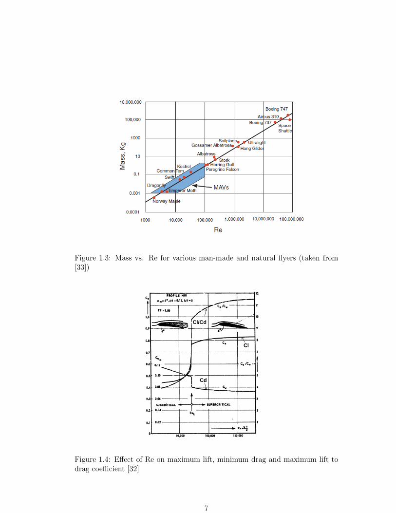
Figure 1.3: Mass vs. Re for various man-made and natural flyers (taken from[33])

Cl/Cd

Cl

Cd

Figure 1.4: Effect of Re on maximum lift, minimum drag and maximum lift todrag coefficient [32]

7

required to change the momentum of the fluid through the rotor. The actual

power is a combination of the non-ideal induced power (with losses included)

and profile power.

FM =1

κind + 2.6σ

(cl

3/2

cd

)−1 (1.1)

where cl is the mean blade lift coefficient, cd is the mean drag coefficient, σ is

rotor solidity and κind the non-ideal induced power factor. The FM of full-scale

rotors are in the range of 0.75-0.9 whereas MAV rotors have a maximum FM of

about 0.6-0.65. In a full-scale rotor, induced power accounts for about 70% of

the total power. At the MAV scale at high thrust coefficients, the profile power

can be up to 45% [12].

Power Loading : It is defined as the ratio of the thrust to power required to

hover. It can be expressed as a function of air density, disk loading (DL is ratio

of thrust to rotor disc area) and FM,

T

P= FM

√2ρ

DL(1.2)

or as a function of non-dimensionalised thrust and power coefficients,

T

P=CTCP

1

ΩR(1.3)

Full-scale rotors have CT/CP ratios of about 12-14 [27] whereas micro rotors

have maximum CT/CP values between 5-6.

In order to improve rotor efficiency, the design of the rotor system requires

significant optimization of the airfoil shape, blade chord and twist distribution at

low Re. From Eq.(1.1), it can be seen that both the induced power efficiency and

8

airfoil efficiency are important. Several studies [29–32] on low Re airfoils were

conducted in a attempt to maximize c3/2l /cd. It was found that at Re numbers

between 104−105, thin curved plate airfoils do not suffer a large drop in maximum

lift or an increase in minimum drag coefficients that airfoils such as N60 exhibit

(Fig. 1.4). The superior aerodynamic performance of sharpened-leading-edge

thin circular arc plates was shown by Laitone [29]. It was seen that the small

nose radii of the sharp nosed airfoils prevented flow separation over a range of

angles of attack. Hein and Chopra [34] and Bohorquez and Pines [35] carried out

systematic hover tests on two bladed rotors using the optimized thin circular arc

airfoils to examine the performance due to variations in airfoil camber, planform

and twist at tip Re between 40,000 and 50,000. It was found that 6%-9% camber

airfoils with a linear taper produced the best performance (Fig. 1.5). The effect

of twist was generally found to be small. Flow visualization studies [34, 36, 37]

of the rotor showed evidence of highly non-ideal inflow, spanwise distribution of

lift and slower formation of tip vortices(Fig. 1.6).

Computational fluid dynamics (CFD) studies were also conducted to model

and predict the flow structure of an MAV scale rotor. Schroeder and Baeder [38]

implemented a low Mach preconditioner in a compressible Reynolds-averaged-

Navier-Stokes overset structural mesh solver (OVERTURNS) to validate low

Reynolds number airfoil aerodynamics for MAV applications. Lakshminarayan

and Baeder [39] implemented the solver to investigate the flow characteristics of

a MAV rotor (Fig. 1.7). They found that the performance of the sharp leading

edge (LE) geometries increased FM by about 16% and power loading by 4%.

The total thrust produced by the blunt and sharp LE geometries was similar

but the blunt LE required larger power. It was also found that sharpening the

trailing edge did not result in performance improvements over a sharpened LE

9

Figure 1.5: Effect of camber and taper on the FM of a 2 bladed rotor (tip Re43,700) [35]

Figure 1.6: Flow visualization of a 2 bladed rotor using laser sheet at 300 wakeage [34]

10

blade.

CFD PIV

Figure 1.7: Tip vortex trajectory for a two bladed MAV rotor (tip Re= 32,400):CFD [39] and PIV [36]

As can be seen from above, there is scope for further improving rotor performance

by expanding the parameter space and studying novel rotor configurations. In

this research, one such configuration chosen is the shrouded rotor in which the

thrust of the rotor system is sought to be increased for the same input power.

The advantage of this configuration is that the previous improvements in MAV

scale rotor designs can be incorporated along with performance augmentations

from the shroud.

1.1.2.2 Flight stability and control

Helicopters are inherently unstable systems requiring constant attention from the

pilot. It is a multivariable system that requires four control inputs for 6 degree of

freedom (DOF) control. The coupling between longitudinal and lateral motions

make flight controls of a rotary wing system very challenging.

Existing micro scale rotor based MAVs have similar configuration as their

11

full-scale counterparts. However, since scale operates on physical dimensions

in different ways, the relative magnitude of the main forces change and thereby

modify dynamic characteristics. These scaling effects depend on how the physical

parameters and dimensions change with scale. For example, consider a full scale

helicopter scaled down by a factor ofN (all helicopter dimensions are scaled down

by N) and that the material density remains unchanged. This implies that the

weight will scale by a factor of 1/N3 and the moments of inertia by 1/N5. Clearly,

the relative magnitude of the inertial and gravitational forces change resulting in

a completely different dynamical system. In order to preserve dynamic similarity,

Froude and Mach scaling rules will have to be applied. Mettler [40] applied these

scaling laws on two full scale helicopters Bell UH-1H and Robinson R-22 and

two model scale helicopters Yamaha R-50 and MIT’s X-Cell. The scaling effects

confirmed that as the size of the rotorcraft is reduced, the system bandwidth

and sensitivity to control inputs increased.

This translates into an increased agility and also increases pilot workload.

This also implies that scaled down helicopters are difficult to control, and sta-

bilizer bars are typically used to compensate for these scaling effects. As we

move down to the micro scale, it therefore becomes necessary to also implement

high bandwidth electronic feedback systems for stability augmentation and con-

trol purposes. This can potentially enable the vehicle to have different dynamic

characteristics at different flight conditions. For example, high maneuverability

is desired while operating in cluttered environments (by increasing rate sensi-

tivity and bandwidth) and increased stability is desired during unmeasurable

input disturbances such as gusts. This opens up challenges in the control system

design for optimal performance for different design points which may require non-

linear control schemes and other approaches such as gain scheduling/switching

12

schemes.

Fully autonomous flight for unmanned rotorcraft requires high-authority con-

trol systems. Autonomous control and high maneuverability appear to define to-

day’s unmanned rotorcraft research field [40]. Weilenmann [41] used a model heli-

copter as a test bed to evaluate the performance of various multivariable control

design techniques (LQ,H∞, µ−synthesis) using a classical single-input single-

output (SISO) proportional-integral-derivative (PID) controller as a benchmark.

The results show that the multivariable model-based control-design methods out-

performed the classical SISO control systems using performance and stability

metrics such as bandwidth, cross-axis effects, disturbance rejection and stability

margin. Gavrilets et. al. [42] developed a simplified non-linear model of the

X-Cell and a control logic for automated execution of aerobatic maneuvers [43]

using a linear quadratic (LQ) control. Other studies involving dynamics mod-

eling and control system design for autonomous unmanned helicopters include

Refs. [44–46,48,49].

To summarize, rotary wing MAVs typically have much higher thrust/inertia

ratios compared to full-scale rotorcraft, which translate into increased control

sensitivity. Also, due to their small relative speeds, their sensitivity to input

disturbances from aerodynamic perturbations such as external gusts increases.

Therefore, the development of new configurations of rotary wing MAVs require

that in addition to performance studies, they be systematically studied for their

controllability, control system implementation and gust disturbance rejection,

which will be a key focus in this research.

In this section, key technical challenges in the development of micro scale

rotary wing vehicles are presented. In the next section, a basic introduction to

the performance improvement aspects of the shrouded rotor will be described.

13

The literature survey section discusses research and developmental work done

on ducted fan manned and unmanned vehicles in the area of experimental aero-

dynamics, analysis, flow control, flight dynamics and control, and the effect of

gusts on MAV flight performance.

1.1.3 Performance improvement in hover: Shrouded ro-

tor configuration

It was discussed earlier that the aerodynamic performance of micro rotors is

poor compared to full-scale rotors. Previous studies showed that with a careful

design of the airfoil and rotor, micro-rotor performance can be improved. In

conjunction with these design improvements, alternate rotor configurations can

be incorporated which may have potential for better performance than conven-

tional micro-rotors. One such configuration considered in this research is the

shrouded rotor.

Here the rotor is surrounded by a cylindrical shroud or duct. As mentioned

in Ref. [50], an arbitrary convention is that the enclosing structure is a duct

if the length of the cylinder is greater than the rotor diameter, otherwise it is

called a shroud or a short-chord duct. In this dissertation, the terms ‘shroud’

and ‘duct’ will be used interchangeably since previous literature has not been

consistent with the notation. Typically, the shroud has a rounded leading edge

and straight or tapered trailing edge, which form the inlet and diffuser sections of

the shroud respectively (Fig. 1.8). This configuration has been studied for over

half a century for applications in marine propellers, helicopter tail rotors, manned

and unmanned air vehicles. Past studies have shown significant improvement in

aerodynamic performance when compared to an unshrouded or ‘open’ rotor.

14

Figure 1.8: Cross section of a shroud enclosing the rotor [50]

Let TSR, TOR, PiSR and PiOR be the thrust generated by the shrouded rotor,

open (or unshrouded) rotor, induced power consumed by the shrouded rotor and

open rotor respectively. Also let σd be the contraction ratio of the shroud, i.e.,

the ratio of exit area of the rotor wake (area of cross section at diffuser exit)

to the area of the rotor disk. If the rotor area of the shrouded and unshrouded

rotors are the same, it can be shown from momentum theory that, At constant

induced power : Here, PiSR = PiOR

TSRTOR

= (2σd)1/3 (1.4)

At constant total thrust : Here, TSR = TOR

PiSRPiOR

=1√2σd

(1.5)

15

For a straight diffuser section, (σd = 1), it can be seen that momentum theory

predicts a 26% improvement in thrust for a shrouded rotor over an unshrouded

rotor at the same induced power. For the same total thrust, a 30% reduction in

induced power is predicted. Section 2.6 discusses these aspects in further detail.

In addition to these aerodynamic benefits, shrouded rotor offers two other

advantages over an unshrouded rotor: (1) the shroud protects the rotating blades

from damage by other objects and greatly enhances structural integrity of the

vehicle, and (2) it can potentially attenuate the noise signature of the rotor.

Therefore, there is a great incentive in incorporating a shroud in an MAV rotor

configuration.

1.1.3.1 Challenges in shrouded rotor implementation

However, it can be seen that to maximize thrust improvements, the weight of

the shroud should be a key factor. The shrouded rotor configuration is a viable

option as long as the increase in thrust over that of an open rotor is greater than

the weight of the shroud. Therefore, the shroud construction that results in a

sturdy lightweight structure is a significant challenge.

While ensuring efficient flight in hover, it is also important for the MAV to be

tolerant to cross winds and be able to transition quickly to translational flight.

However, the shrouded rotor has an undesirable characteristic of generating ad-

verse pitching moments when faced with edgewise flow (Fig. 1.9). Therefore,

this may limit the extent of operability of the MAV in gusty situations. An

evaluation of these forces and the control moments required to overcome them is

of importance in order to evaluate the effectiveness of the shrouded rotor MAV

as a platform of choice. This research will carefully address each of these issues.

16

Figure 1.9: Shrouded rotor in non axial flow

1.2 Previous Work and Research

1.2.1 Shrouded rotor / Ducted fan based vehicles

As early as 1923, a patent was issued by George Hamel [51] illustrating a fixed

wing aircraft with a fan-in-wing configuration in which the propellers were em-

bedded in the wings with their axes perpendicular to the wing chord. This was

in an attempt to combine the favourable characteristics of a helicopter in VTOL

mode and an airplane in fixed wing mode. However, no knowledge of potential

performance improvements of the fan shrouded in the wing was shown in the

patent. About a decade later, there was awareness of improvements in propul-

sive efficiency of ship propellers [52] by surrounding them with nozzle-shaped

appendages as indicated in a patent filed by Ludwig Kort [53]. Around 1933,

Luigi Stipa from Italy integrated an air propeller with a hollow airplane fuse-

lage [54] that was supposed to act as the diffuser section of the duct and he found

performance improvements compared to the open propeller in terms of thrust

17

increase and power decrease [55].

Figure 1.10: Venturi fuselage design by Stipa [54]

By the 1960s, there was considerable interest in the United States in develop-

ing vertical/short take-off and landing aircraft. This led to a lot of experimental

work and design of flying crafts (Fig. 1.11) such as the single shrouded propeller

Hiller VZ-1 [56], the tandem shrouded propeller Piasecki PA-59K Airgeep [57],

twin and quad tilt-ducted aircrafts such as the Doak VZ-4 [58] and Bell X-

22A [59] respectively and fan-in-wing aircraft such as the GE/Ryan XV-5 [60]

and Vanguard Omniplane [61]. Interestingly, data collected during the flight

tests of X-22 from 1960-1970 was used in the development of the V-22 Osprey.

A notable effort from Europe to develop ducted VTOL aircraft is the Nord 500

’Cadet’ with its tilt duct configuration (Fig. 1.12) [62]. In addition to V/STOL

applications, the shrouded propellers were also used as a means of thrust com-

pounding as found in aircrafts such as (Fig. 1.13) Mississippi State University’s

XV-11A Marvel [64] and Piasecki Pathfinder 16H,16H-1 [65]. Another applica-

tion was the shrouded tail-rotor or ’fan-in-fin’ helicopters which received research

18

Hille

r V

Z-1

Pia

se

ck

iA

irg

ee

pD

oa

kV

Z-4

Bell

X-2

2A

Rya

n X

V-5

Va

ng

ua

rd O

mn

ipla

ne

Fig

ure

1.11

:Shro

uded

roto

rsfo

rm

anned

V/S

TO

Lai

rcra

ftap

plica

tion

s

19

Figure 1.12: Nord 500 Cadet tilt-duct aircraft

Marvel XV-11A Piasecki Pathfinder 16H-1

RAH-66 Comanche Dauphin

Figure 1.13: Shrouded rotors for thrust compounding and fan-in-fin applications

20

interest in the 1970s. It was originally termed the ‘fenestron’ as developed by

Aerospatiale for their SA-341 Gazelle helicopter in 1970 [66]. In terms of power

efficiency and operational safety, the fenestron tail rotor was found to be superior

to a conventional tail rotor [67,118]. The Comanche and Dauphin helicopers em-

ploying the fenestron tail rotor are shown in Fig. 1.13. The XOH-1 observation

helicopter from Japan [69] and the Ka-60 helicopter from the Kamov Company,

Russia were examples of some other aircrafts with the fan-in-fin system.

Beyond the 1980s, interest grew in the development of unmanned VTOL

aircrafts that could assist humans in cluttered environments. Since these crafts

would operate in close proximity to humans, the shrouded rotor configuration

was a preferred choice due to the protection offered by the shroud [9]. For at-

titude control, these vehicles either commonly used guide vanes placed in the

propwash to generate moments or conventinoal rotor cyclic control. For coun-

tering the rotor torque, either stator vanes were used in the downwash or a

coaxial rotor system was incorporated. Some prominent UAVs employing the

shrouded/ducted rotor configuration are shown in Fig. 1.14. These include the

Airborne Remote Operated Device (AROD), developed by Sandia national lab-

oratories [70], the ‘Cypher’, developed by the Sikorsky Aircraft Corporation in

the 1990s for the US military’s Air-Mobile Ground Security and Surveillance

System program [71,72], Honeywell’s T-Hawk [73], Microcraft’s iSTAR [74] and

Georgia Tech’s GTSpy [75].

The disk loading of these vehicles were very large (greater than 300 N/m2).

A high disk loading configuration is inefficient in an unshrouded rotor setup.

The relative merits of reconfiguring an unshrouded rotor with a shroud are not

clear from an observation of these vehicle designs.

Therefore, in this research, a low disk loading shrouded rotor vehicle, TiShrov

21

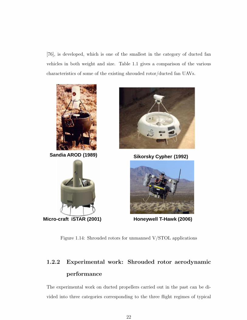
[76], is developed, which is one of the smallest in the category of ducted fan

vehicles in both weight and size. Table 1.1 gives a comparison of the various

characteristics of some of the existing shrouded rotor/ducted fan UAVs.

Sandia AROD (1989) Sikorsky Cypher (1992)

Micro-craft iSTAR (2001) Honeywell T-Hawk (2006)

Figure 1.14: Shrouded rotors for unmanned V/STOL applications

1.2.2 Experimental work: Shrouded rotor aerodynamic

performance

The experimental work on ducted propellers carried out in the past can be di-

vided into three categories corresponding to the three flight regimes of typical

22

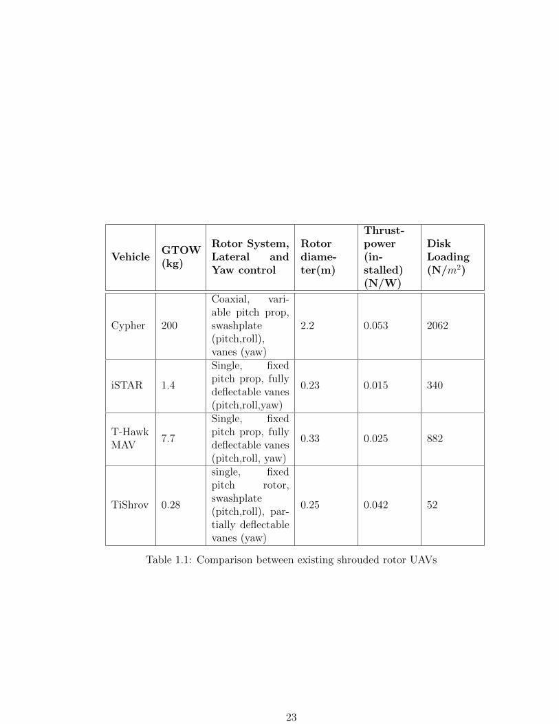
VehicleGTOW(kg)

Rotor System,Lateral andYaw control

Rotordiame-ter(m)

Thrust-power(in-stalled)(N/W)

DiskLoading(N/m2)

Cypher 200

Coaxial, vari-able pitch prop,swashplate(pitch,roll),vanes (yaw)

2.2 0.053 2062

iSTAR 1.4

Single, fixedpitch prop, fullydeflectable vanes(pitch,roll,yaw)

0.23 0.015 340

T-HawkMAV

7.7

Single, fixedpitch prop, fullydeflectable vanes(pitch,roll, yaw)

0.33 0.025 882

TiShrov 0.28

single, fixedpitch rotor,swashplate(pitch,roll), par-tially deflectablevanes (yaw)

0.25 0.042 52

Table 1.1: Comparison between existing shrouded rotor UAVs

23

ducted fan VTOL aircraft: 1) Static operation (Hovering flight), (2) Axial flow

(High-speed flight) and (3) Non-axial flow (transitional flight). The next two

sections briefly survey previous work done in these categories in terms of aero-

dynamic performance. A more detailed review can be found in [50,77].

1.2.2.1 Hover and axial flight

Here the flow field around the shroud is mostly axisymmetric and no lateral

and longitudinal moments are expected. The literature credits Ludwig Kort

[53] and Luigi Stipa [54] for performing some of the first scientific experimental

studies on optimizing the performance of propellers (marine and air respectively)

enclosed in a duct for improved thrust characteristics. The design of the ducted

propeller involved a variation of multiple parameters such as, 1) duct variables:

chord/diameter ratio, camber, leading edge radius, and chord line orientation

relative to axis, (2) propeller variables: solidity, overal pitch setting, distribution,

blade profile, and chord distribution, and (3) overall variable: propeller location

within shroud, tip clearance, etc.

These initial efforts along with Kruger in Germany [78] and Soloviev and

Churmack [79] in the USSR, van Manen [80], Kuchemann and Weber [81] and

Regenscheit in Germany [82] were limited to axial flow. These were not directly

aimed at VTOL applications. Much of the early efforts were to improve the

efficiency of regular airplane propellers designed for optimal performance in high-

speed cruising flight. The experiments of Stipa were restricted to large values

of chord/diameter ratio. The experiments of Soloviev and van Manen were

performed in water, and the propellers of Soloviev were designed for ships. The

effect of position of the propeller inside the shroud was not investigated.

Kruger [78] conducted tests on fifteen different annular-airfoil shrouds and

24

varied parameters such as the shroud chord, thickness, camber, inlet lip radius

and angle of incidence between the profile chordline and propeller axis. The mod-

els were tested at rest and in axial flow. It was seen that in static conditions, flow

separation was more prominent for shrouds with a sharper lip. In forward flight,

the thinner shroud had lesser drag, but the propeller thrust decreased faster.

External split rings were installed to alleviate this problem. Kruger noted that

the diffuser angle was not a significant parameter. Platt [83] conducted static

tests of contra-rotating, 48-inch diameter propellers with three shrouds of vary-

ing diffuser length and angle. In all cases, the difference in power consumption

was within 10%, which were found to be marginal. However all the shrouded

propellers performed twice as good as the open propeller. Along with tests from

Hubbard in 1950 [84] and Mort in 1966 [85, 86], it was commonly found that

increasing tip clearance led to a drop in shroud thrust (by up to 20% as reported

by Mort). In Hubbard’s and Platt’s experiments, the flow was found to separate

at the shroud leading edge at low propeller rotational speeds, but then was found

to re-attach as the speed was increased. Parlett [87] and Taylor [88] varied the

lip radius of the shroud and found that higher lip radii shrouds offered better

Figures of Merit.

By around 1966, Black, Wainauski and Rohrbach [89] conducted a compre-

hensive investigation of the effects of various shroud parameters using twelve

different shrouded propeller models, with a propeller diameter of 30 inches. The

parameters investigated included the exit area ratio, lip shape, shroud chord,

propeller location within shroud, number of blades, tip clearance and shroud

external shape. They found that the most powerful shrouded propeller variable

was the shroud exit area ratio. This was in contradiction with a few other stud-

ies, which noted that the diffuser angle was not very critical. They also obtained

25

greater than predicted improvements in thrust, up to 67% higher, for the same

ideal power. In agreement with other studies, they found that increasing the

input power by increasing rotational speed or collective, the suction forces on

the shroud inlet increased. In axial flow, the drag from the shroud resulted in

deteriorated performance, and also, a higher shroud exit area ratio was detri-

mental. In terms of propeller position within the duct, they found that having

the propeller forward gives the wake more length to achieve desired diffusion,

whereas having it rearward evens out any asymmetries in the inflow. They found

that the forward location performed better in axial flight whereas the rearward

location performed better in static conditions. A set of experiments conducted

on a coaxial ducted rotor by Lee and Leishman in 2008-2009 [90] showed that

the forward location of the propeller resulted in better performance in static

conditions.

With emphasis on UAV development in the 1980s, tests were also conducted

on smaller scale shrouded rotors. During the development of Sikorsky’s Cypher,

experiments were performed on the shroud design [91] and it was found that the

performance deteriorated as the inlet lip radius was decreased. A most interest-

ing result was that reducing the shroud length from 100%Dt to 5%Dt caused a

deterioration in thrust by only 10%. This was important from a weight savings

perspective. During the development of the 10-inch ‘Perching Unmanned Aerial

Vehicle’ (PUAV) [92], Dyer [93] investigated effects of various shroud parameters

and found that increasing the lip radius improved performance whereas increas-

ing the diffuser angle decreased performance, contrary to predictions. In 2004,

Martin and Tung [94] tested two 10-inch diameter shrouded rotor models. They

obtained a 37% improvement in thrust over the open rotor at the highest inlet lip

radius and lowest tip clearance. The trends they obtained were consistent with

26

expectations. From a potential flow analysis, they surmised that at increased

tip gap and decreased lip radius, there was a decrease in inlet suction. In order

to eliminate tip clearance, Martin and Boxwell [95] designed two shrouds, one

with a notch that was cut into the inner shroud surface at the propeller tip path

plane, and the other with a rearward-facing step that was cut into the inward

facing profile just above the tip path plane to accommodate the propeller. How-

ever, they found that the notched-shroud did not differ from the baseline model,

while the stepped shroud showed degraded performance. During the same time

period, Graf et.al. [96] tested effects of five different lip geometries on hover and

forward flight performance of a model based on the PUAV. It was found that

the circular arc lip produced slightly more thrust than the elliptical lip.

In an attempt to reconcile the shroud design parameter space at the MAV

scale, Pereira and Chopra [50] conducted systematic investigations of perfor-

mance of a 6.3 inch shrouded rotor. Significant performance gains in hover of

up to 50% reduction in power were obtained by optimizing parameters such as

inlet lip radius, tip clearance and diffuser length (Fig. 2.46). However, these

tests were conducted with a flat plate untwisted rotor and the reported perfor-

mance gains would have been lesser had the rotor in the open configuration been

optimized.

It can be seen from above that most of the rotors tested were in the sizes rang-

ing from one to several feet in rotor diameter. The few studies in the smaller scale

did not effectively true performance benefits between an optimized shrouded and

an optimized unshrouded rotor. Therefore, one of the purposes of this research

is to incorporate previous results in shroud design optimizations and systemati-

cally develop a shrouded rotor that has a better hover performance at a system

level than an optimized unshrouded rotor. This is the topic of discussion in

27

Figure 1.15: Shroud design parameters

Chapter 2.

1.2.2.2 Non-axial flow

This flow stage of the ducted fan usually occurs when the VTOL vehicle under-

goes transition from hover to forward flight Fig. 1.16. Other situations include

fan-in-fin applications and when the ducted fan acts as a source of propulsion and

is flown at an angle of attack. Due to the very complex flow phenomena that can

result in destabilizing and undesirable forces and moments, many experimental

studies were conducted in the past.

One of the earlier wind tunnel tests for a shrouded rotor in non-axial flow was

conducted by Parlett in 1955 [87] to investigate the effects of air speed and angle

of attack on the lift, drag, and pitching moment of a shrouded propeller model

over an angle of attack range from 00 to 900. Yaggy and Mort in 1961 [97, 98]

conducted wing tunnel studies of a 4 foot diameter ducted fan in order to evaluate

the forces and moments generated on a wing mounted duct. They found large

pitch-up moments when the ducted fan was operated at an angle of attack to

28

Figure 1.16: Piasecki Airgeep in forward flight

the air stream. This was the first study where it was suggested to use guide

vanes in the rotor downwash as a means to alleviate or reduce the magnitude of

these moments. To study the transition performance of a tilt-duct VTOL type

aircraft, Grunwald and Goodson [99, 100] investigated the aerodynamic loads

on an isolated shrouded propeller at angles of attack from −100 to 1000. They

found that the pitching moment developed by the propeller was only a relatively

small part of the overall pitching moment. Other studies investigating loads on

a ducted fan in non axial flow for manned VTOL applications are Fletcher [101],

Moser [102], Spreeman [103], Giulianetti [104].

During the design of the AROD UAV [70], Weir [105] conducted tests on

six different shrouded propeller configurations with the aim of obtaining transla-

tional flight data. Fleming et. al. [106] conducted tests on the PUAV type ducted

fan to evaluate effectiveness of flow control schemes to improve cross wind effec-

tiveness of this aircraft. They found that the aerodynamic drag on the vehicle

due to the deflection of the free stream through the diffuser was much greater

29

than the profile drag of the shroud itself. The pitch-up moment increased up to a

certain airspeed and then decreased to nose-down pitch moments. The authors

surmised that this was possibly due to separation of the flow from the wind-

ward side of the sharp leading edge. In Martin and Tung’s experiments [94], the

nose-down pitch moment at higher speeds was also observed. However the pitch

moments of their sharper-inlet shroud model was lesser, which was attributed to

separation of the flow from the inlet. Studies conducted by Graf et. al. [96] on

PUAV type ducted fan model showed the pitching moments to initially increase

with airspeed and then level off at higher airspeeds. For the different shroud

models tested, the ram drag (or momentum drag) averaged to about 80% of the

total drag. Lee and Leishman [122] conducted wind tunnel tests of a coaxial

ducted rotor system in order to measure the thrust characteristics as a function

of airpseed and angle of attack. However, pitching moment was not measured.

Pereira and Chopra [107] provided surface pressure and load cell measurements

of MAV scale shrouded rotor with varying airspeed and angle of attack. In axial

flow, the net thrust of the shrouded rotor deteriorated at high speeds due to the

drag of the shroud. In edgewise flow, the thrust of the shrouded and unshrouded

rotors increased with increasing airspeed. The power consumption of the un-

shrouded rotor increased whereas for the shrouded it remained about constant.

The drag of the shrouded rotor increased much more rapidly with airspeed. The

center of pressure for the shrouded rotor lay approximately 0.75 R further above

the location for the unshrouded rotor. They did note the asymmetry in pressure

distribution between the windward and leeward sides of the shroud in non-axial

flow that was responsible for the pitching moment.

It was seen from these studies that the effect of edgewise flow on a shrouded

rotor is that undesirable adverse pitching moment and drag are generated. This

30

problem can become severe for low disk-loading shrouded rotor configurations,

such as the research vehicle discussed in this dissertation. Therefore, it is im-

portant to measure the forces acting on the vehicle under these aerodynamic

conditions and isolate configurations and mechanisms that can improve the abil-

ity of the vehicle to tolerate and overcome these forces. This is the topic of

discussion in Chapter 5.

1.2.3 Analytical and CFD modeling of shrouded rotor

aerodynamics

To improve predictive capability that can aid shrouded rotor design as well as

flow field analysis numerical tools have been developed in the past. Analytical

methods for shrouded rotor performance prediction include blade element mo-

mentum theory, blade element vortex theory and more complicated potenital

flow models with boundary layer coupling. Sacks and Burnell [77] provided an

exhaustive account of different analytical methods existing till 1960. Recently

computational fluid dynamics (CFD) methods have been developed to predict

performance. The pioneers of potential-flow methods for shrouded rotors were

Kuchemann and Weber [108] who applied these solutions for annular airfoils in

a uniform flow by modeling the bodies as distributions of vortex rings over their

surfaces. Kriebel [109], and Mendenhall and Spangler [110, 111] developed and

consolidated predictions for force and pitching moment coefficients of a shrouded

propeller in steady flight at an angle of attack. Mendenhall’s algorithm was later

used by Weir in designing the AROD UAV. Fairchild [112] used a formulation

where the shroud was modeled as chordwise distribution of vortex rings and was

able to show that in axial flow, increasing the shroud chord causes greater re-

31

ductions in ideal power when compared to an open rotor. Goodman [113] was

the first to model the effect of finite tip clearance and formulated a correction

factor for efficiency measurements. Clark [114] and Wright et. al. [115] devel-

oped potential flow solutions for fan-in-fin applications. In 2003, Guerrero et.

al. [116] developed AVID-OAV for the analysis of ducted fan UAVs.

Blade element and momentum methods could not represent geometric char-

acteristics of the shroud unless empirical correction factors were used. Poten-

tial flow methods could not predict friction drag and stall characteristics [117].

Therefore, CFD methods have played an important, versatile role in design

and analysis of these complicated flow phenomena. Most of the CFD research

effort into shrouded rotors were for the fan-in-fin applications. Started by

Aerospatiale, some important references are [118–120], which involve a cou-

pled CFD-momentum theory analysis. More computationally-intensive, discrete

blade CFD model was used by Ruzicka et. al. [121]. This analysis showed how

the leakage flow around the blade tips is reduced as the tip clearance is reduced,

which results in increased system thrust and figure of merit. Lee et. al. [122]

demonstrated the importance of realistic 3-D tip modeling in a CFD analysis of

the Kamov fan-in-fin. Ahn and Lee [123] used a CFD model to parametrically

investigate the effects of varying inlet lip radius, diffuser angle and rotor radial

strength distribution.

A recent CFD study based on the configuration of the shrouded rotor in-

vestigated in this research was conducted by Lakshminarayan and Baeder in

2010 [124]. They used an overset structured mesh solver OVERTURNS that

solves the compressible RANS equations and employing low Mach precondition-

ing to take into account the low Reynolds number regimes of the shrouded rotor

operation. They obtained good comparison between experiments [76] and CFD

32

prediction. Figure 1.17 shows the wake trajectory of the two bladed shrouded

rotor. For a straight diffuser section and a chord-diameter ratio of 15%, the

Figure 1.17: Wake trajectory of a two bladed shrouded rotor (Iso-surfaces ofq-criterion) [124]

contraction ratio was observed to be about 0.85 and not 1 (as predicted from

momentum theory). They extended the analysis to study the effect of tip clear-

ance, diffuser angle, diffuser length and inlet shape (circular, elliptic). Of these,

the lowest tip clearance and an elliptic inlet shape gave the best performance

prediction. In an unpublished report by Lakshminarayan, the effect of edgewise

flow on the loads and pressure distribution of the shrouded rotor was studied.

Figure 1.18 shows the load distribution on the circular inlet shrouded rotor in

2 m/s of edgewise flow at the instant the two bladed rotor is aligned with the

flow direction. The asymmetry in pressure distribution between the windward

and leeward side can be clearly seen which was similar to the surface pressure

distribution measurements by Pereira and Chopra [107]. Key results from this

CFD study will be used to explain certain observations in Chapter 5.

33

Windward

Leeward Forward flight

Hover

Figure 1.18: CFD load distribution prediction on a hovering circular inletshrouded rotor facing edgewise flow [124]

1.2.4 Shrouded rotor flow control

When the shrouded rotor/ducted fan is in a non-axial flow regime at high angles

of attack (flow is almost perpendicular to rotor axis), phenomena such as inlet

lip separation at the leading edge of the shroud/duct occur. This can lead

to undesirable areas of recirculation, pressure loss, pitching moment and drag.

Therefore, studies have been conducted in the past to modify flow in the duct

inlet or exit for the various ducted fan configurations. Yaggy and Mort [98] were

probably the first to suggest and scientifically study the use of guide vanes in

the inlet and duct exit to reduce the nose-up pitching moment encountered by

the twin ducted Doak VZ-4 (Fig.1.11). They found significant reduction in the

pitching moment by modifying the duct exit flow through the vanes.

Patents on ducted fan vehicle design illustrated concepts for modifying the

flow in the duct inlet or exit. Piasecki’s patent [126] of the Airgeep had a

curious feature which was the use of a movable spoiler in the inner part of the

34

leading side of the duct. This had a serrated edge, which would control local

flow characteristics over the lip radius in an effort to reduce the drag generated

over this region primarily in edgewise flight. In the patent by Boyd et. al. [127],

a VTOL ducted fan vehicle design was proposed, which used adjustable stator

blades above the rotor for attitude control only.

Movable

spoiler

Figure 1.19: Piasecki’s patent of the Airgeep with movable spoilers for inlet flowcontrol [126]

Moller [128] in 1989 had a patent for a flying ducted fan platform with two

mutually perpendicular vane systems with variable camber flaps and exit flow

control features called multiple adjustable air deflector assemblies (Fig. 1.20).

Cycon in 2001 [130] modified the original design of the Sikorsky Cypher by

mounting high camber fixed wings to the ducted fan aft of the center of lift. This

would serve to counteract the nose-up moments generated in forward flgiht.

Yoeli’s [129] ducted fan based VTOL vehicle included a fuselage with two

counter rotating ducted fans along the longitudinal axis. A system of inlet

louvers and exit control surfaces were placed to produce side force, roll, pitch

and yaw moments on the vehicle Fig. 1.21.

35

Vanes

Spoilers

Figure 1.20: Ducted fan platform design with control vanes and spoilers [128]

Figure 1.21: Tandem ducted fan design of Yoeli with inlet louvres and exit vaneflaps [129]

36

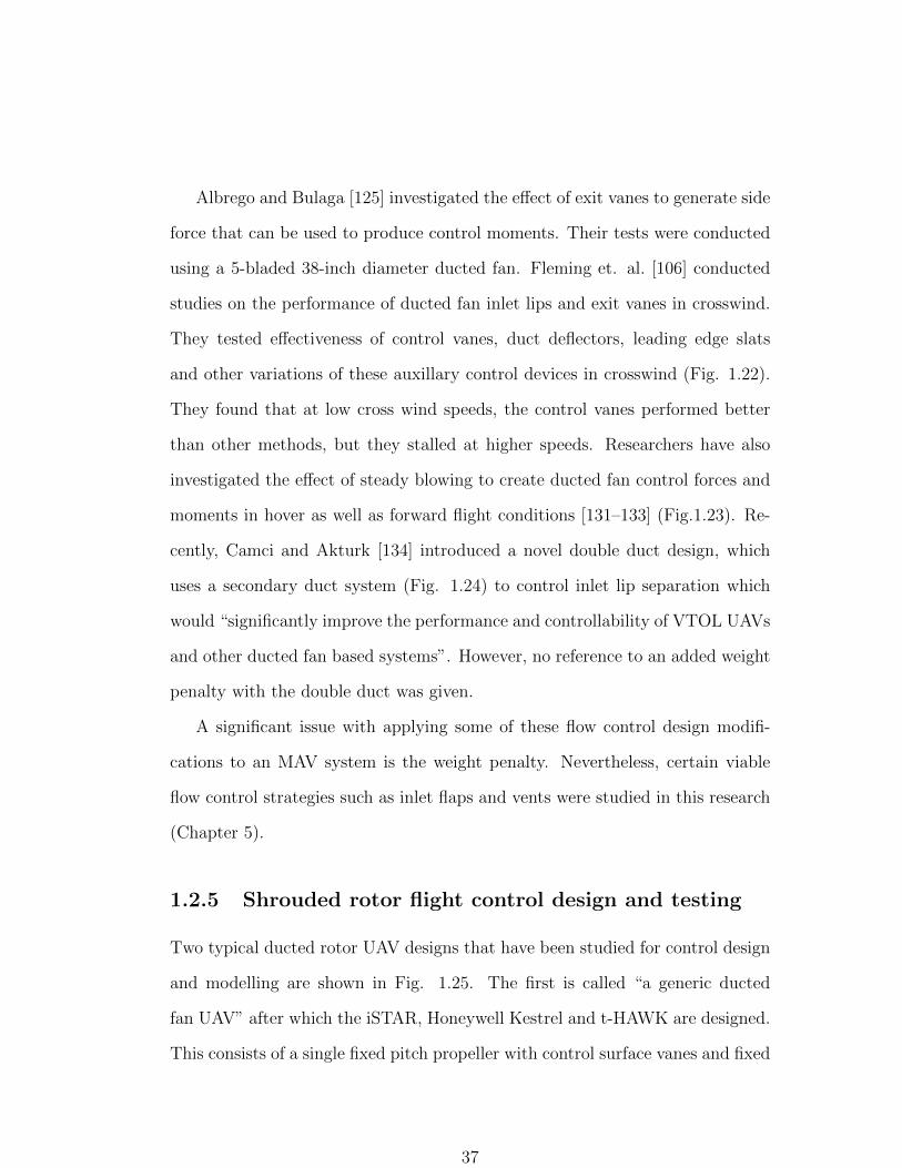
Albrego and Bulaga [125] investigated the effect of exit vanes to generate side

force that can be used to produce control moments. Their tests were conducted

using a 5-bladed 38-inch diameter ducted fan. Fleming et. al. [106] conducted

studies on the performance of ducted fan inlet lips and exit vanes in crosswind.

They tested effectiveness of control vanes, duct deflectors, leading edge slats

and other variations of these auxillary control devices in crosswind (Fig. 1.22).

They found that at low cross wind speeds, the control vanes performed better

than other methods, but they stalled at higher speeds. Researchers have also

investigated the effect of steady blowing to create ducted fan control forces and

moments in hover as well as forward flight conditions [131–133] (Fig.1.23). Re-

cently, Camci and Akturk [134] introduced a novel double duct design, which

uses a secondary duct system (Fig. 1.24) to control inlet lip separation which

would “significantly improve the performance and controllability of VTOL UAVs

and other ducted fan based systems”. However, no reference to an added weight

penalty with the double duct was given.

A significant issue with applying some of these flow control design modifi-

cations to an MAV system is the weight penalty. Nevertheless, certain viable

flow control strategies such as inlet flaps and vents were studied in this research

(Chapter 5).

1.2.5 Shrouded rotor flight control design and testing

Two typical ducted rotor UAV designs that have been studied for control design

and modelling are shown in Fig. 1.25. The first is called “a generic ducted

fan UAV” after which the iSTAR, Honeywell Kestrel and t-HAWK are designed.

This consists of a single fixed pitch propeller with control surface vanes and fixed

37

Figure 1.22: Auxillary control devices for flow control [106]

38

Figure 1.23: Synthetic jet flow control concept [133]

Figure 1.24: Elimination of inlet flow separation a through a double duct design[134]

39

stators placed in the propwash for achieving complete attitude control. The sec-

ond is called the “tail sitter” after which the Hovereye [135] is built. It consists

of two counter-rotating rigid props with control vanes (but no stators) in the

propwash for attitude control. These UAVs are designed to hover with the pro-

peller axis in the vertical direction and perform forward flight with the propeller

axis along the horizontal direction. It can be seen that this involves various flight

regimes involving the complex transition phase between hover and forward flight.

The vehicle dynamics may not render itself to a linear assumption under these

different modes. Therefore, many linear and non-linear control schemes have

been studied and developed that include linear PID control, switched robust

linear control, sliding mode control, linear and non-linear dynamic inversion,

backstepping with adaptive control, H∞ and receding horizon control.

(a) Generic ducted fan UAV (b) Tail-sitter

Figure 1.25: Past control system design methodologies usually applied to (a)Single prop, stator, control vane design (b) Coaxial prop, control vane design

Dunbar et. al. (2002) [136] presented a control system framework for the

40

Caltech ducted fan (a vehicle with the generic ducted UAV design with two

wings attached on the sides). They designed a model predictive controller, which

was successfully able to stabilize a step offset in x position (simulation). They

found that the region of attraction of the MPC controller was larger than the

static hover LQR controller and equivalent to a gain-scheduled LQR controller.

Franz et. al. (2002) [137] extended the control design of the Caltech ducted fan

to implement a receding horizon control. Here they found the performance to

be better than a gain scheduled LQR controller in terms of step response and

disturbance rejection.

Pflimlin et. al. (2004) [138] proposed a model for the tail sitter VTOL dy-

namics where the aerodynamic effects were seen as unknown perturbing terms.

An adaptive controller by means of backstepping techniques allowed the stabi-

lization of the vehicle’s position.

Hess and Ussery (2004) [139] showed a design for MIMO sliding mode con-

trollers for a generic ducted fan UAV. In order to reduce sensitivity to unmod-

eled dynamics, they used an asymptotic observer. In 2006, Hess and Bakhtiari-

Nejad [140] applied a pseudo-sliding mode control. They found that the con-

troller was robust to large steady wind gusts which was a problem for nonlinear

dynamic inversion control design.

Spaulding et. al. (2005) [141] showed that the nonlinear dynamic inversion

approach proved to be a good choice because it reduced the complex vehicle

dynamics to that of a simple integrator and covered the full flight envelope of

the ducted fan UAV without gain scheduling. The drawback, inherent with

dynamic inversion, of lack of robustness to model uncertainty was addressed.

They focused on the design of outer-loop regulators based on linear and non

linear metrics to make the overall system robust to model uncertainties and was

41

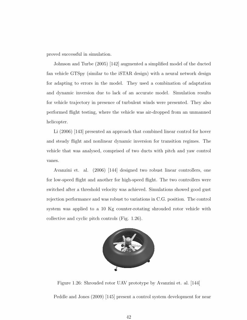
proved successful in simulation.

Johnson and Turbe (2005) [142] augmented a simplified model of the ducted

fan vehicle GTSpy (similar to the iSTAR design) with a neural network design

for adapting to errors in the model. They used a combination of adaptation

and dynamic inversion due to lack of an accurate model. Simulation results

for vehicle trajectory in presence of turbulent winds were presented. They also

performed flight testing, where the vehicle was air-dropped from an unmanned

helicopter.

Li (2006) [143] presented an approach that combined linear control for hover

and steady flight and nonlinear dynamic inversion for transition regimes. The

vehicle that was analysed, comprised of two ducts with pitch and yaw control

vanes.

Avanzini et. al. (2006) [144] designed two robust linear controllers, one

for low-speed flight and another for high-speed flight. The two controllers were

switched after a threshold velocity was achieved. Simulations showed good gust

rejection performance and was robust to variations in C.G. position. The control

system was applied to a 10 Kg counter-rotating shrouded rotor vehicle with

collective and cyclic pitch controls (Fig. 1.26).

Figure 1.26: Shrouded rotor UAV prototype by Avanzini et. al. [144]

Peddle and Jones (2009) [145] present a control system development for near

42

hover flight control of the tail-sitter. Successive loop closure control strategy

with feedback signal from linear decoupled estimators was used which provided

a robust solution. The functionality was verified by simulation and flight test

data.

Pflimlin et. al. (2010) [146] developed an aerodynamic model of the tail-

sitter from wind tunnel tests, derived equations of motion and linearized about

hover condition. Unstable poles in vehicle modes were identified and PID control

was implemented to stabilize the vehicle. Good agreement between simulation

and flight test results was shown.

These studies applied to conventional ducted fan designs that generate high

downwash velocities over control vanes. However, it is also necessary to study

and develop stability augmentation control systems for cyclic controlled, low disk

loading, shrouded rotor configurations, which is discussed in Chapter 3.

1.2.6 MAV flight performance in gusts

It is expected that MAVs encounter degraded, time varying flows. A study of

flight performance in these conditions is extremely important. Large commercial

aircraft can generally tolerate extreme wind conditions, but as the size and mass

of the aircraft decreases, the ability to maintain control reduces for a given wind

condition [148–150]. This is mainly due to the relatively low flight speeds and

moments of inertia of MAVs. A summary of flying speeds from Ref. [147] is

shown in Fig. 1.27 indicating the tolerable wind conditions for animals and

aircraft.

Since typical MAV missions involve low altitude flight, they operate in the

’roughness zone’ of the atmospheric boundary layer where the flow is time-

43

Figure 1.27: Typical operating flight conditions of animals and aircraft [147]

44

varying and the perturbations in local flow are comparable to the characteristic

speeds of MAVs. In the presence of winds, flight performance is tremendously

affected.

Hoover (1999) [151] stated that flexible wings could alleviate some of the

flow perturbations, but that small gusts have extremely deleterious effects on

small crafts. Jenkins et. al. in 2001 [152] analyzed the controllability of flexible

and rigid fixed wing MAVs (of 6 inch dimension) as the pilot performed flights

in steady and gusty wind situations. They performed spectral analysis of con-

trol input movement rates forming autospectra of differentiated stick position

data which was seen to provide a convenient yardstick for comparing the flying

qualities of their MAVs. They found that manueverability is strongly related

to how often the pilot must make rapid (1-10Hz) stick movements to maintain

stability during the flight. They also found the flexible wing MAVs outperform

rigid wing MAVs in terms of reduced control workload. However, no specific

information of the nature of the atmospheric condition or how it correlated it

with the MAV flight performance was given. In the outdoor flight demonstra-

tions of several flying wing MAVs by Walkins (2002) [153], it was noted that the

largest challenge to MAV flight was overcoming time varying flow perturbations,

particularly small vortices and eddies that produce random roll and pitch inputs.

Watkins noted that this would restrict the number of possible days/year that

the MAV could be used for outdoor activities.

Relatively little work has been done on quantifying the wind environment of

relatively slow flying craft close to the ground. In 2005, Milbank et. al. [154] and

later by Watkins et. al. [155] attempted to quantify and replicate typical flight

environments for MAVs operating close to ground for the purposes of replicating

the spatial and temporal turbulence characteristics in a wind tunnel.

45

Patel and Kroo (2006) [157] presented the design of simple control laws to

extract energy from flow disturbances. They showed that significant energy

savings are possible using active control laws. Due to the nature of the study,

no mention of flight performance of the MAVs in gusts was made.

Bieniawski et. al. [158] utilized an indoor motion capture flight facility to

evaluate the performance of a commercial quadrotor and fixed MAV, and control

algorithms in a controlled, repeatable environment.

In order to study dynamics of a quadrotor in wind, Waslander and Chang

(2009) [159] presented models for wind disturbances, developed an estimation

algorithm for current wind velocity experienced by the vehicle. The wind es-

timate was used to improve positioning accuracy by eliminating effect of wind

on feedback position control law and adding a wind compensator to mitigate

effect of expected wind disturbance. Patrick and Humbert (2010) [160] applied

optic flow and wide field integration (WFI) to perform station keeping and wind

rejection of a quadrotor. They used a controller based on H∞ formulation of

LQR to perform these tasks. Zarovy et. al. (2010) [161] conducted flight tests

of micro scale commercial coaxial rotorcraft in a motion capture flight testing

facility and observed the deteriorated performance at wind conditions as low as

2 m/s.

It is of interest to build upon these efforts and systematically study the

performance of a shrouded rotor MAV in degraded flow conditions, especially

since shrouded rotors are known to be more sensitive to adverse flow conditions

than unshrouded rotors. Details of these flight test experiments are discussed in

Chapter 6.

46

1.3 Current Research: Objectives and Approach

Limitations with previous work : The previous sections showed the signifi-

cant amount of experimental and analytical work performed in the area of ducted

fan manned and unmanned vehicles in the field of aerodynamics, dynamics and

control. However, most of these investigations were limited to rotors with diam-

eters from one to seven feet with tip Reynolds numbers of the order of 100,000

to 1 million. The few existing studies on micro scale shrouded rotors did not

carry out true assessment of shrouded rotor performance over that of efficient

unshrouded rotors. The design of the shroud itself which is a significant chal-

lenge in the development of a lightweight MAV has not been discussed. Most of

the existing ducted fan vehicles have disk loadings between 300-2000 N/m2, and

dimensions greater than one feet rotor diameter. Therefore, due to their high

downwash velocities, control vanes were used to generate pitch and roll moments.

This is however not practical for a compact MAV configuration with high con-

trol authority demands and therefore requires control mechanisms different from

conventional ducted fan UAVs. It was seen that rotary wing MAVs have high

bandwidth feedback requirements to successfully accomplish tasks that demand

high degree of external disturbance rejection as well as maneuverability. This

problem is exacerbated in the case of a shrouded rotor due to their increased

sensitivity to flow disturbances. Studies that have examined the capabilities of

a shrouded rotor MAV operating in external wind disturbances are generally

lacking in the literature. All the above factors need to be systematically studied

in order to determine the true capability of the shrouded rotor as a platform of

choice in MAV applications.

Objectives of present work : In order to reconcile the above needs, the fol-

47

lowing are the objectives of the present work:

1. To design and develop a low disk loading (< 100 N/m2) shrouded rotor

micro air vehicle with systematic hover performance measurements and

emphasis on lightweight shroud design and compare the hover performance

of a shrouded rotor with an unshrouded rotor system.

2. To design and implement classical and model based feedback control in

the MAV for semi-autonomous attitude stability augmentation in hover.

Conduct time domain system identification to assess feedback and sensing

requirements, and control sensitivity for the shrouded rotor in configura-

tions with and without a stabilizer bar.

3. Finally, to systematically study the aeromechanics of the shrouded rotor

in edgewise flow, compare gust disturbance rejection characteristics with

those of an unshrouded rotor and to study free flight performance in the

presence of external winds.

Organization of thesis : Chapter 2 describes the design of the shrouded rotor

MAV considered in this research. The performance and design issues of each

of the sub-components - low Re rotor design, Hiller stabilizer bar, anti-torque

vanes, shroud - are detailed. A comparison in system performance between the

shrouded and unshrouded rotor is made. The final section of the chapter dis-

cusses some initial vehicle prototypes constructed during this effort. In chapter

3, the open loop experiments detailing the attitude stability of the shrouded

rotor in comparison with an unshrouded rotor are presented. The need for in-

corporating a rotor with minimal excursions in tip path plane inside the shroud

is shown. A PID control system through a Ziegler-Nichols based gain tuning

48

is developed and flight tested on different vehicle prototypes in quiescent flow

conditions. In chapter 4, the attitude dynamics of the shrouded rotor vehicle is

studied about hover as the equilibrium condition. The salient advantages and

drawbacks of incorporating a flybarless rotor are discussed. System identifica-

tion of the vehicle constrained in translation is conducted in the time domain

based on a reduced order model. The effect of flybar and flybarless rotor on the

attitude dynamics is described.

Chapter 5 describes the performance of the shrouded when exposed to edge-

wise flow. The forces including thrust, drag and pitching moment produced by

a shrouded and unshrouded rotor configuration are measured and compared.

Control authority was compared and the ability to overcome destabilizing forces

in edgewise flows is studied. An open jet wind tunnel is used as the source

for edgewise flow. A few strategies to minimize adverse moments are discussed

and methods to improve control authority of the rotor configurations through

rotor planform design are detailed. In the final chapter, the ability of the vehi-

cle provided with attiude feedback control to correct for nose-up disturbance is

described in a series of bench top and free flight tests. For free flight, the ability

of the vehicle to perform station keeping in the presence of cross flow is studied

in a motion capture flight testing facility.

49

Chapter 2

Vehicle Design and Hover Performance

Studies

2.1 Overview

The main aim of developing a shrouded rotor vehicle is to realize performance

benefits over an unshrouded rotor vehicle of the same diameter while signifi-

cantly improving the crashworthiness of the system. As discussed in Chapter

1 the vehicle developed in this research is the smallest in the class of shrouded

rotor vehicles in weight and size. The design of the shrouded rotor micro air

vehicle (MAV) is described in this chapter. Salient features in construction,

configuration and control mechanisms are compared with previously developed

shrouded rotor vehicles. The design, hover performance and integration of the

sub-components of the vehicle system are then described.

50

2.2 Design

Most ducted fan UAVs such as the iSTAR, T-Hawk and AROD incorporate

a fixed pitch propeller placed in the diffuser section of the duct. In order to

counteract the propeller torque, a set of static stator vanes are placed in the

propwash. Additionally, for pitch and roll attitude control, a secondary set of

vanes are appropriately actuated to provide control moments. This is schemat-

ically shown in Fig. 2.1. It can be seen that for maximum attitude control

Vanes

Existing single prop ducted fan UAVs:

Vanes for pitch, roll and yaw control

TiShrov MAV:

Vanes for yaw control only

Swashplate

Figure 2.1: Differences in configuration for attitude control of a shrouded rotorvehicle

moments the distance between the vane center of pressure and vehicle C.G. has

to be increased. This may not be appropriate from a consideration of vehicle

compactness. It will also be shown later that the performance of vanes deterio-

rates in ground effect. Sikorsky’s Cypher, however, has a pair of coaxial counter

rotating rotors and does not require vanes for yaw control. It achieves attitude

control through cyclic pitch actuation. A recent experimental study showed

that performance benefits may not be realized by incorporating a coaxial rotor

in a duct [90]. Therefore, a single shrouded rotor is considered in this research.

51

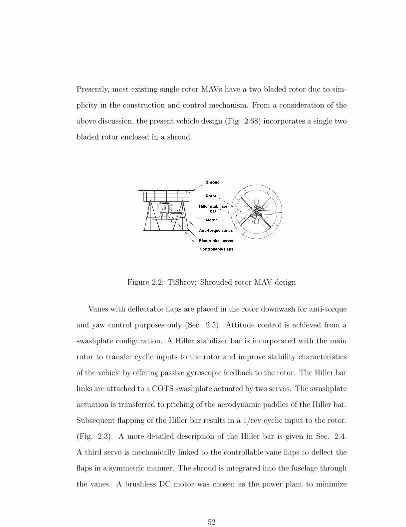
Presently, most existing single rotor MAVs have a two bladed rotor due to sim-

plicity in the construction and control mechanism. From a consideration of the

above discussion, the present vehicle design (Fig. 2.68) incorporates a single two

bladed rotor enclosed in a shroud.

Figure 2.2: TiShrov: Shrouded rotor MAV design

Vanes with deflectable flaps are placed in the rotor downwash for anti-torque

and yaw control purposes only (Sec. 2.5). Attitude control is achieved from a

swashplate configuration. A Hiller stabilizer bar is incorporated with the main

rotor to transfer cyclic inputs to the rotor and improve stability characteristics

of the vehicle by offering passive gyroscopic feedback to the rotor. The Hiller bar

links are attached to a COTS swashplate actuated by two servos. The swashplate

actuation is transferred to pitching of the aerodynamic paddles of the Hiller bar.

Subsequent flapping of the Hiller bar results in a 1/rev cyclic input to the rotor.

(Fig. 2.3). A more detailed description of the Hiller bar is given in Sec. 2.4.

A third servo is mechanically linked to the controllable vane flaps to deflect the

flaps in a symmetric manner. The shroud is integrated into the fuselage through

the vanes. A brushless DC motor was chosen as the power plant to minimize

52

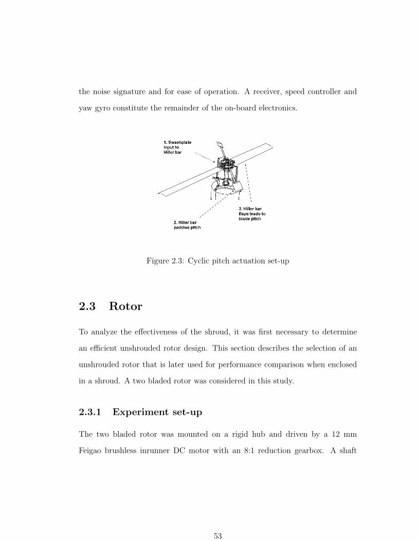
the noise signature and for ease of operation. A receiver, speed controller and

yaw gyro constitute the remainder of the on-board electronics.

Figure 2.3: Cyclic pitch actuation set-up

2.3 Rotor

To analyze the effectiveness of the shroud, it was first necessary to determine

an efficient unshrouded rotor design. This section describes the selection of an

unshrouded rotor that is later used for performance comparison when enclosed

in a shroud. A two bladed rotor was considered in this study.

2.3.1 Experiment set-up

The two bladed rotor was mounted on a rigid hub and driven by a 12 mm

Feigao brushless inrunner DC motor with an 8:1 reduction gearbox. A shaft

53

Shaft bodyHall

Switch

Torque sensorThrust sensor

Shaft bodyHall

Switch

Torque sensorThrust sensor

Figure 2.4: Micro rotor hover test stand

coupled the rotor with a thrust1 and torque load sensor2 assembly as shown in

Fig. 2.4. A pair of magnets installed on the gearwheel were used to trigger

a Hall sensor3 thereby determining the rotor speed. An optical tachometer4

was used to verify the speed of the rotor. The performance metrics of the

rotor were derived from a measurement of the thrust, torque and rotor RPM.

The sensor data were acquired by a National Instruments DAQCard 6062-E

data acquisition system and processed in LabVIEW. The data was sampled

at 1000 Hz which was about 15 times the maximum rotor RPM of interest.

This enabled sufficient filter bandwidth for signal conditioning purposes. The

11000 g load sensor with a resolution of 0.1 g. measurementsensors.honeywell.com. Thiswas later replaced by a 5000 g thrust balance ohaus.balances.com

225 in-oz capacity torque sensor from Transducer Techniqueswww.transducertechniques.com/rts-torque-sensor.cfm

3www.allegromicro.com

4www.monarchinstruments.com

54

thrust and torque measurements were an average of about 5000 data samples.

The average measurement errors in thrust,torque and RPM were determined

to be about 0.5 g, 0.2mN-m and 50 about statistical average respectively. The

mechanical power was determined by the product of torque(N-m) and rotor

speed(radians/second).

2.3.1.1 Variation in air density

The variation of air density with respect to sea level at 750 F is shown in Fig.

2.5 over the course of experimental tests in this research (the temperature in

the laboratory was maintained roughly at 750F ). This fluctuation is due to

external pressure variation on an hourly,daily and seasonal basis5. A comparison

in density fluctuation between summer and winter months is shown in Fig. 2.6.

Therefore the measured thrust and power data are normalised with respect to

the sea level conditions (MSLISA6 as follows,

T ′ = T

(ρSLρ

)(2.1)

P ′ = P

(ρSLρ

)(2.2)

Dimensional data presented in this research is normalized to the MSLISA condi-

tions at 750F . For accurate treatment, the pressure and temperature data should

be logged each time the experiment is performed. Similarly, the non dimensional

thrust coefficient (CT = T ′/ρA(ΩR)2), power coefficient (CP = P ′/ρA(ΩR)3)and

Figure of Merit (FM = (CT )3/2/√

2CP ) were extracted. It must be noted that

5Pressure information at the nearest weather station can be obtained fromhttp://cdo.ncdc.noaa.gov/qclcd/QCLCD

6MSLISA - Mean sea level international standard atmosphere

55

the error bars must incorporate fluctuations due to density. In the present case

a maximum variation in density of about 2% is considered.

0 20 40 60 80 1000.95

1

1.05

Days

/

SL a

t 75

0 F

Figure 2.5: Variation of air density dur-ing experimental runs

0 1 2 3 4 5 6 70.95

1

1.05

/

SL

Summer

Winter

Figure 2.6: Maximum air density varia-tion in summer and winter

For each test, a set(3) of RPM sweeps were done for each rotor collective

setting. This produces a variation in thrust and mechanical power that was

quadratic and cubic with RPM respectively. The trend was observed to be fairly

repeatable over multiple runs. Figure 2.7 shows the variation of MSLISA thrust

and power for a two bladed rectangular rotor

It can be seen that the thrust, power coefficients and FM (Fig. 2.8) were

fairly independent of operating RPM, indicating that Reynolds number effects

are not present at sufficiently high RPMs (greater than 2000). An average Figure

of Merit (FM) measured between 2500-3000 RPM was extracted.

2.3.2 Airfoil

The design of an MAV rotor has two main considerations - airfoil and blade

planform. At Reynolds numbers between 30,000 - 100,000, studies have shown

56

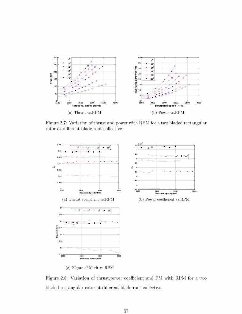
1500 2000 2500 3000 3500 40000

50

100

150

200

250

300

Rotational speed (RPM)

Th

rus

t (g

f)

70

100

140

180

220

260

(a) Thrust vs.RPM

1500 2000 2500 3000 3500 40000

5

10

15

20

25

30

35

40

Rotational speed (RPM)

Me

ch

an

ica

l P

ow

er

(W)

70

100

140

180

220

260

(b) Power vs.RPM

Figure 2.7: Variation of thrust and power with RPM for a two bladed rectangularrotor at different blade root collective

2000 2500 3000 35000

0.005

0.01

0.015

0.02

0.025

0.03

0.035

Rotational Speed (RPM)

CT

70 140 180 220

(a) Thrust coefficient vs.RPM

2000 2500 3000 35002.5

3

3.5

4

4.5

5

5.5

6

6.5

7

7.5x 10

-3

Rotational Speed (RPM)

CP

70 140 180 220

(b) Power coefficient vs.RPM

2000 2500 3000 35000.25

0.3

0.35

0.4

0.45

0.5

0.55

0.6

Rotational Speed (RPM)

Fig

ure

of

Meri

t

70 140 180 220

(c) Figure of Merit vs.RPM

Figure 2.8: Variation of thrust,power coefficient and FM with RPM for a two

bladed rectangular rotor at different blade root collective

57

that thin cambered airfoils have the best lift-to-drag ratios [29–31]. Additionally,

experiment and CFD studies [33, 34, 38, 39] have shown that sharpened leading

edge (LE) airfoils at these Re numbers have a lower drag coefficient and result

in rotors with lower profile losses. Therefore, a circular camber airfoil with a

sharpened LE and a thickness ratio (t/c) of about 2% was implemented in the

blade design (Fig. 2.9). Camber of the blade was set at 10% and is calculated

as

Camber = d/c =

(1

2tan(

θ

2)

)(2.3)

It must be noted that when taper is included, the effective camber of the airfoil

section decreases since the radius of curvature remains the same.

2

R

c

d

Figure 2.9: Circular camber airfoil

The micro and full-scale airfoil characteristics are shown in Figs. 2.10 and

2.11. The data for the MAV airfoils is from CFD prediction (Ref. [124]), since

there was no available experimental data. It can be clearly seen the MAV air-

foils have much lower lift to drag ratios than the full scale airfoils. Also at

the low reynolds numbers, as the camber of the airfoil is increased, Clmax and

(C1.5l /Cd)max increases.

58

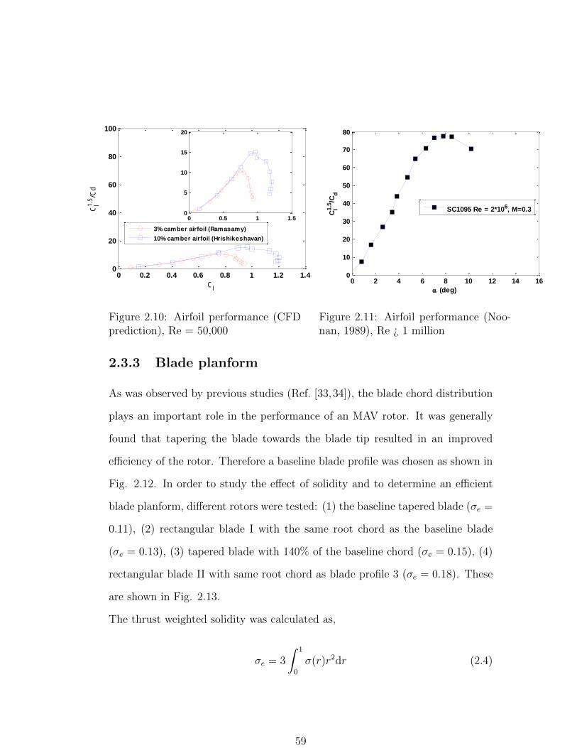
0 0.2 0.4 0.6 0.8 1 1.2 1.40

20

40

60

80

100

Cl

Cl1.5

/Cd

3% camber airfoil (Ramasamy)

10% camber airfoil (Hrishikeshavan)

0 0.5 1 1.50

5

10

15

20

Figure 2.10: Airfoil performance (CFDprediction), Re = 50,000

0 2 4 6 8 10 12 14 160

10

20

30

40

50

60

70

80

(deg)

Cl1.5

/Cd

SC1095 Re = 2*106, M=0.3

Figure 2.11: Airfoil performance (Noo-nan, 1989), Re ¿ 1 million

2.3.3 Blade planform

As was observed by previous studies (Ref. [33,34]), the blade chord distribution

plays an important role in the performance of an MAV rotor. It was generally

found that tapering the blade towards the blade tip resulted in an improved

efficiency of the rotor. Therefore a baseline blade profile was chosen as shown in

Fig. 2.12. In order to study the effect of solidity and to determine an efficient

blade planform, different rotors were tested: (1) the baseline tapered blade (σe =

0.11), (2) rectangular blade I with the same root chord as the baseline blade

(σe = 0.13), (3) tapered blade with 140% of the baseline chord (σe = 0.15), (4)

rectangular blade II with same root chord as blade profile 3 (σe = 0.18). These

are shown in Fig. 2.13.

The thrust weighted solidity was calculated as,

σe = 3

∫ 1

0

σ(r)r2dr (2.4)

59

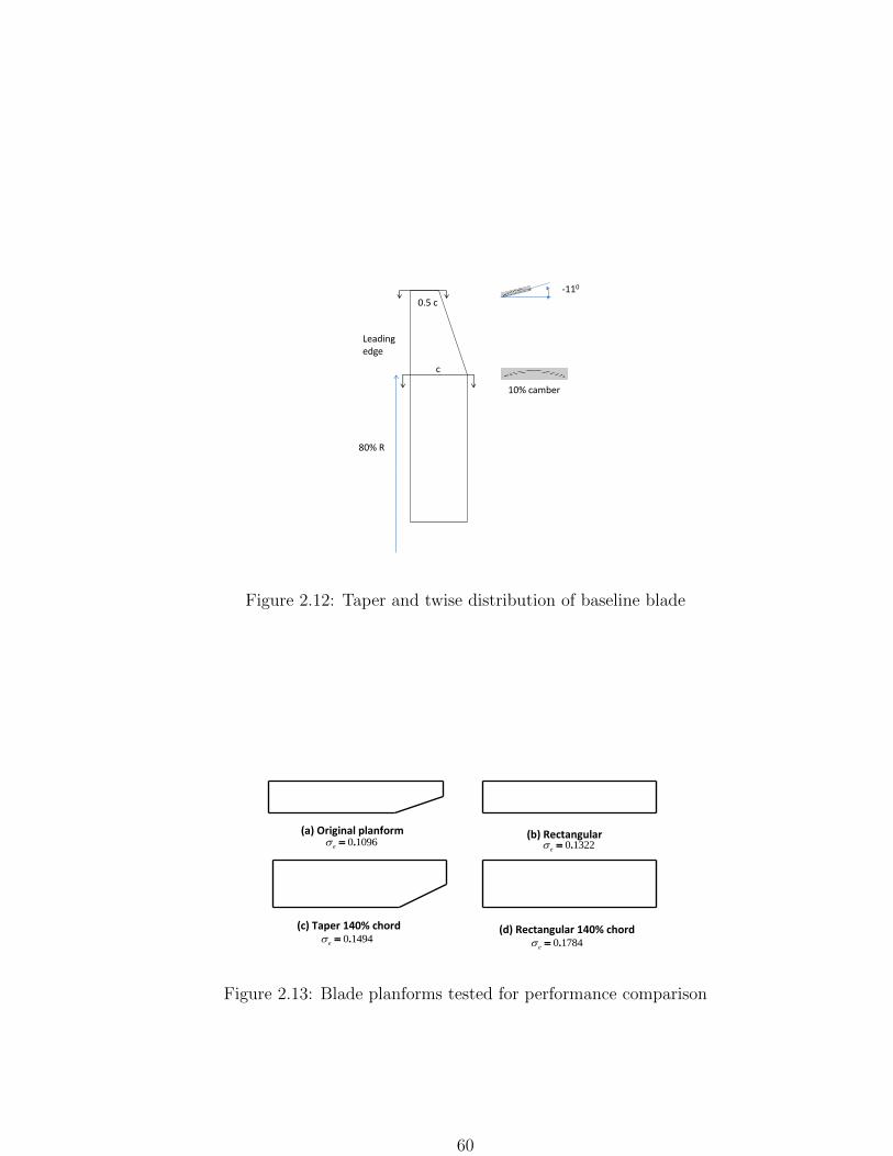
-110

10% camber

80% R

c

0.5 c

Leadingedge

Figure 2.12: Taper and twise distribution of baseline blade

(a) Original planform (b) Rectangular 0 1096.

e 0 1322.

e

0 1494.e

0 1784.e

(c) Taper 140% chord (d) Rectangular 140% chord

Figure 2.13: Blade planforms tested for performance comparison

60

It was used to account for the rotor planform, weighting the influence of the

tips more heavily than the inner rotor regions. The blades were constructed

from 3-layered 0/45/0 temperature cured carbon-epoxy prepreg fibers. This

construction produced stiff and lightweight blades . The blade chord was set

at 25 mm and the radius was 122 mm. Each two bladed rotor was tested on

the micro rotor test stand using the procedure described in Sec. 2.3.1. The

blade collective was varied up to 30 deg. Figure 2.14 shows the non-dimensional

power polar for the different blade planforms. As the solidity of the blade is

increased, expectedly CP also increased for a given CT . In order to remove the

effect of solidity, as suggested in Ref. [27], CP/σ3 is plotted versus CT/σ

2 in Fig.

2.15. It can be seen that for a given planform shape, the power polar collapses

for different solidities. In general, the tapered blades perform better than the

rectangular blades. The effect of solidity can also be seen in the Figure of Merit

variation as a function of CT/σ (Fig. 2.16) and CT/σ2 (Fig. 2.17). For the

tapered or the rectangular planform, solidity did not significantly affect rotor

performance. A maximum FM of about 0.64 for the tapered blade was obtained

at a blade loading of between 0.15-0.2. The dimensional power polars for the

different blades are shown in Fig. 2.18.

The power polars with the largest slopes for each blade profile are compared

in the form of power loading in Fig. 2.19. It can be clearly seen that the

tapered blades had the best performance. It must be mentioned that since the

comparison is made at the same disk loading, the efficient blade configuration

can be derived from the non-dimensional FM variation as well as the dimensional

power loading comparison. In conclusion, the baseline tapered blade was chosen

to be the optimum unshrouded rotor configuration for comparison purposes.

Maximum power loading was achieved at a wide range of collective (140 − 220).

61

0 0.005 0.01 0.015 0.02 0.0250.005

0.01

0.015

0.02

0.025

0.03

0.035

0.04

0.045

0.05

0.055

CP

CT

Taper rotor, = 0.11

Taper rotor, = 0.15

Rectangular rotor, = 0.13

Rectangular rotor, = 0.18

Figure 2.14: CT vs. CP

0.5 1 1.5 2 2.5 3 3.5 4 4.50.2

0.4

0.6

0.8

1

1.2

1.4

1.6

1.8

2

CP/3

CT/

2

Taper rotor, = 0.11

Taper rotor, = 0.149

Rectangular rotor, = 0.13

Rectangular rotor, = 0.18

Figure 2.15: CT/σ2 vs. CP/σ

3 to removeeffect of solidity

0 0.05 0.1 0.15 0.2 0.25 0.3 0.350.1

0.2

0.3

0.4

0.5

0.6

0.7

0.8

CT/

FM

Taper 60%R, = 0.1

Taper 80%R, =0.11

Taper 80%R, =0.15

Rectangular, =0.13

Rectangular, =0.18

Figure 2.16: FM vs. CT/σ

0 0.5 1 1.5 2 2.50.1

0.2

0.3

0.4

0.5

0.6

0.7

0.8

CT/2

FM

Taper 60%R, = 0.1

Taper 80%R, =0.11

Taper 80%R, =0.15

Rectangular, =0.13

Rectangular, =0.18

Figure 2.17: FM vs. CT/σ2 to remove

effect of solidity

62

0 10 20 30 40 500

50

100

150

200

250

300

350

Power (W)

Th

rus

t (g

)

100

140

180

220

260

300

(a) Baseline taper blade

0 10 20 30 40 500

50

100

150

200

250

300

350

Power (W)

Th

rus

t (g

)

70

140

180

220

260

300

(b) Rectangular blade

0 10 20 30 40 500

50

100

150

200

250

300

350

Power (W)

Th

rus

t (g

)

100

140

220

240

280

320

(c) Taper blade, 140% chord

0 10 20 30 40 500

50

100

150

200

250

300

350

Power (W)

Th

rus

t (g

)

120

160

200

240

280

300

(d) Rectangular blade, 140% chord

Figure 2.18: Mecanical power vs. thrust for different blade planforms and col-lective settings

30 80 130 180 230 2807

17

27

3740

Thrust (g)

Po

we

r L

oa

din

g (

g/W

)

Taper 80%R, =0.11

Taper 80%R, =0.15

Rectangular, =0.13

Rectangular, =0.18

Figure 2.19: Comparison in power loading for different blade profiles

63

2.3.3.1 Note: micro rotor performance

From Fig. 2.16 it is curious to see that the operating blade loading values (CT/σ)

for efficient performance of MAV scale rotors is generally high. The maximum

FM values of these rotors were plotted along with other micro rotor studies

published in literature [33,34,37], and are shown in Fig. 2.20.

0.05 0.1 0.15 0.2 0.250.3

0.35

0.4

0.45

0.5

0.55

0.6

0.65

0.7

0.75

0.8

CT/

Ma

x F

M

1/5 UH-60

Lorber (1989)

Ramasamy (2008)

Hein (2007)

Bohorquez (2007)

Hrishikeshavan

(2008)

Figure 2.20: Operating blade loading for efficient rotor performance: comparisonbetween micro and full scale rotor

Now, the mean lift coefficient of a rotor can be written as

CL = 6

(CTσ

)(2.5)

So, a high blade loading implies a high average lift coefficient. The rotors tested

by Ramasamy et al [37]. had circular airfoils with 3% camber while the other

rotors had cambers greater than 7%. We know from Fig. 2.10 that the maxi-

mum lift coefficient is greater for airfoils with higher camber. Therefore from Eq.

(2.5), the operating blade loading for the Ramasamy blades would be lower than

64

the higher camber blades which is what is observed in Fig. 2.20. Also, the lower

camber blades tested by Ramasamy would have mean lift coefficients between

0.6-0.9 while those tested by others would have CL between 0.9-1.2. From, Fig.

2.10 it can be seen that the operating lift coefficients for efficient airfoil perfor-

mance are higher for the 10% camber airfoil when compared with the 3% camber

airfoil. However, for the 10% camber airfoil, optimum airfoil performance is ob-

tained for lift coefficients below 1.2. Nevertheless, the rotor performance can be

qualitatively related at the airfoil and rotor level. However, in order to truly

reconcile micro airfoil characteristics with micro rotor performance, detailed ex-

periments need to be conducted to characterize airfoil performance at these low

Reynolds numbers.

2.4 Hiller Stabilizer Bar

MAV scale rotors are characterized by low time constants, i.e., they are more

agile compared to full scale rotors. This makes pilot control a difficult task. To

overcome this, stabilizer bars are usually coupled with the main rotor. The Lock

number (γR) of the rotor is defined as the ratio of the aerodynamic force to the

inertial force

γR =ρClαcRR

4

IbR(2.6)

where, Clα is the average lift curve slope of the rotor, cR is the chord of an

equivalent rectangular blade, R is the rotor radius and IbR is the flapping inertia

of the rotor. By incorporating a Hiller bar with the main rotor, the inertial force

contribution is increased, thus reducing the Lock number. Now, the rotor time

65

constant is defined as,

τ =16

γRΩ(2.7)

With the stabilizer bar, it becomes,

τ =16

γSΩ(2.8)

where, γS is the Lock number of the coupled rotor and stabilizer bar. Given that

γS < γR, we can see that the rotor time constant is significantly increased. This

implies a greater delay in response to external perturbations.

Additionally, the stabilizer bar can also be used as a control device by transferring

cyclic pitch command to the main rotor blade, either directly (Hiller bar), or

through a swashplate mixer (Bell/Hiller bar). An advantage of the Hiller bar is

the reduction in servo power required to introduce cyclic commands.

The basic configuration of the rotor/Hiller-bar is shown in Fig. 2.3. It consists

of a thin rigid rod with aerodynamic paddles attached to both ends. The bar

is connected to the main shaft by means of a teetering hinge. A flapping of the

Hiller bar directly results in feathering of the main rotor. Also, the blade flapping

axis is aligned with the Hiller bar axis for a teetering rotor, but not necessarily so

for a Hingeless rotor (Sec. 2.4.1). This section discusses two important aspects

while incorporating a Hiller bar with the main rotor: phased Hiller bar concept

and aerodynamic losses.

2.4.1 Phased Hiller bar concept

Experimental results show that as the clearance between the rotor blade tip and

the shroud diffuser wall increases, the shrouded rotor performance decreases.

66

This is very likely to occur with a shrouded teetering rotor. Consider the tip

plath plane (TPP) orientation shown in Fig. 2.21.

*

tip*

SHROUDED RIGID ROTOR

*

*constanttip

tip

SHROUDED TEETERING ROTOR

Figure 2.21: Tip path plane variation for teetering and hingeless rotor

It is clear that the tip clearance variation (δtip ) is greater for the teetering

rotor. In order to eliminate this, the flapping of the rotor must be restricted

by incorporating a hingeless rotor. A later section describes another reason for

incorporating a Hingless rotor. In addition to the restricted TPP motion, the

hingeless rotor transfers control moments to the body of higher magnitude than

a teetering or an articulated rotor. Therefore, the maneuverability of the vehicle

is significantly increased.

Now, a teetering rotor has a non dimensional rotational flap frequency νβ = 1.

This implies that when a blade pitch input is given, the rotor responds in flap

with a 900 phase delay. The Hiller bar flap (placed 900 with respect to the blade)

coincides with the blade pitch. Therefore, it can be seen that the Hiller bar and

the blade flap are in phase. In other words, a longitudinal cyclic input produces

a longitudinal control moment. However, for a hingeless rotor νβ > 1, the force

67

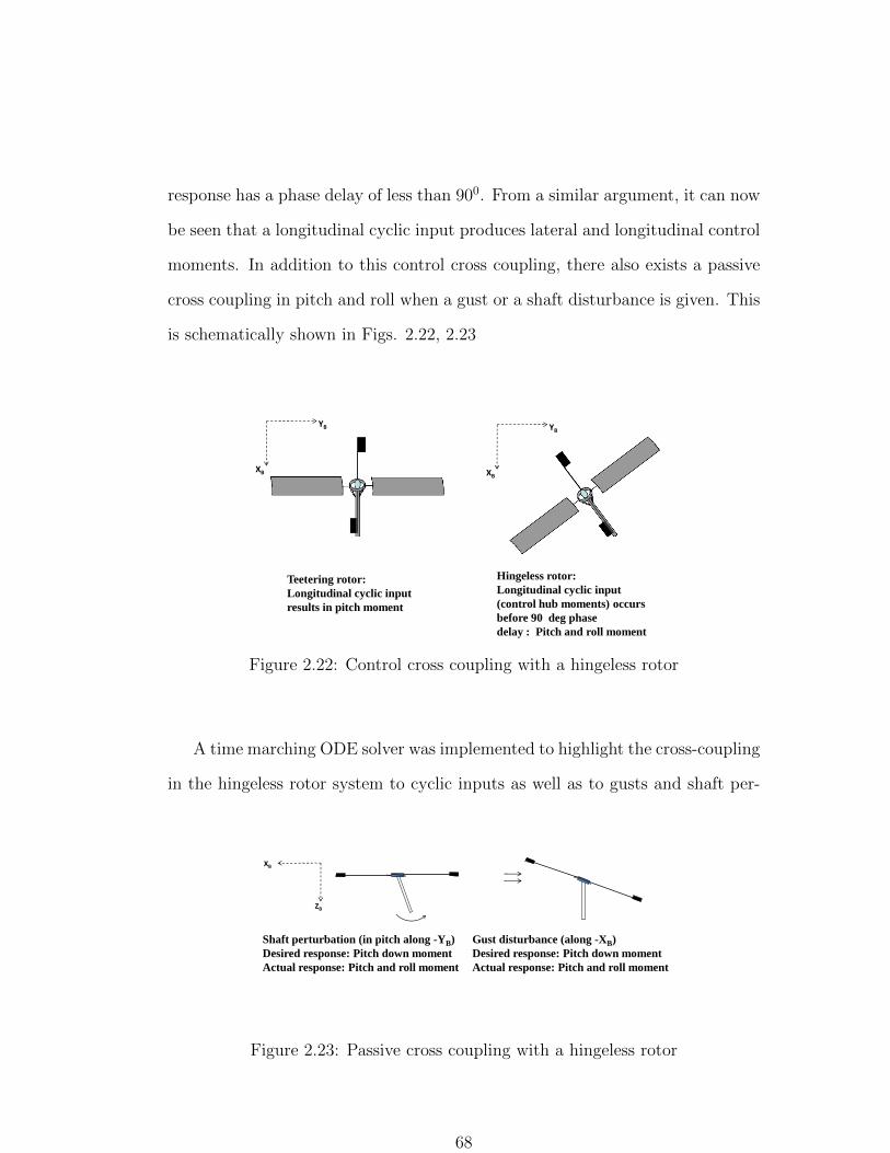
response has a phase delay of less than 900. From a similar argument, it can now

be seen that a longitudinal cyclic input produces lateral and longitudinal control

moments. In addition to this control cross coupling, there also exists a passive

cross coupling in pitch and roll when a gust or a shaft disturbance is given. This

is schematically shown in Figs. 2.22, 2.23

XB

YB

Teetering rotor:

Longitudinal cyclic input

results in pitch moment

Hingeless rotor:

Longitudinal cyclic input

(control hub moments) occurs

before 90 deg phase

delay : Pitch and roll moment

XB

YB

Figure 2.22: Control cross coupling with a hingeless rotor

A time marching ODE solver was implemented to highlight the cross-coupling

in the hingeless rotor system to cyclic inputs as well as to gusts and shaft per-

ZB

XB

Shaft perturbation (in pitch along -YB)

Desired response: Pitch down moment

Actual response: Pitch and roll moment

Gust disturbance (along -XB)

Desired response: Pitch down moment

Actual response: Pitch and roll moment

Figure 2.23: Passive cross coupling with a hingeless rotor

68

turbations. The Hiller bar and the hingeless rotor were modeled as a coupled

teetering rotor and a spring-restrained(spring constant kβ) teetering rotor re-

spectively. Servo pitch commands are given to the Hiller bar. The subsequent

flap response of the bar translates to cyclic inputs to the main rotor which deter-

mines the pitch and roll response at the C.G. The external perturbations such as

gusts, p, q, are introduced simultaneously to the Hiller bar and the main rotor.

The inflow ratio is assumed to be uniform. The effect of the different forms

of cross coupling is shown in Fig. 2.24. The cyclic input and the disturbances

are normalized to unity. It can be seen that as the spring stiffness is increased,

off-axis response increases.

In order to eliminate the control and passive cross coupling, the Hiller bar

flapping must be phased appropriately with the main rotor feathering. Therefore,

a hub was designed with circular slots to allow for adjustments in the Hiller bar

phasing as can be seen from Fig. 2.25.

The phase angle may be either determined from a knowledge of the rotat-

ing flap frequency of the rotor blade or from a direct measurement of off-axis

moments.

Theoretical Method : The force response delay for a given feathering input for

a rotor is given by

φ = tan−1

(γR

ν2β − 1

)(2.9)

where νβ is the non-dimensional rotating natural flap frequency of the rotor and

γR is the Lock number of the rotor. For a teetering rotor case, the phasing is

exactly 90 degrees (νβ = 1). For a hingeless rotor, this is less than 90 degrees

as νβ > 1. First, the non-dimensional non-rotating flap frequency νβNR was

determined. A blade impulse response setup (Fig: 2.26) was used to determine

69

0 2 4 6 8 10-0.018

-0.016

-0.014

-0.012

-0.01

-0.008

-0.006

-0.004

-0.002

0

Non dimensional flap stiffness k

No

n d

ime

ns

ion

alize

d B

od

y m

om

en

ts

Roll moment

Pitch moment

(a) Response to lateral cyclic input

0 2 4 6 8 10-0.02

-0.01

0

0.01

0.02

0.03

Non dimensional flap stiffness k

No

n d

ime

ns

ion

alize

d B

od

y m

om

en

ts

Roll Moment

Pitch Moment

(b) Response to shaft perturbation inpitch

0 2 4 6 8 10-0.2

-0.15

-0.1

-0.05

0

0.05

0.1

0.15

Non dimensional flap stiffness k

No

n d

imen

sio

nali

zed

Bo

dy m

om

en

ts

Roll moment

Pitch moment

(c) Response to gust disturbance

Figure 2.24: Cross coupling in Hingeless rotor (Numerical)

Figure 2.25: Hingeless hub: phased Hiller bar

70

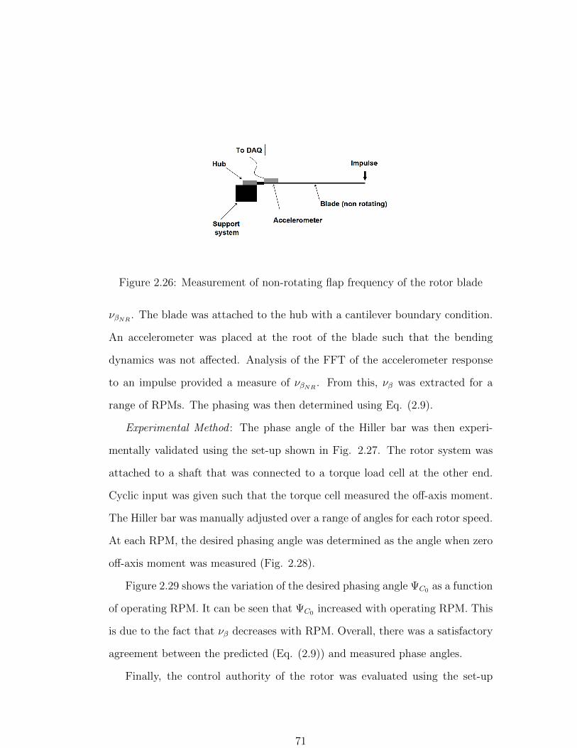
Figure 2.26: Measurement of non-rotating flap frequency of the rotor blade

νβNR . The blade was attached to the hub with a cantilever boundary condition.

An accelerometer was placed at the root of the blade such that the bending

dynamics was not affected. Analysis of the FFT of the accelerometer response

to an impulse provided a measure of νβNR . From this, νβ was extracted for a

range of RPMs. The phasing was then determined using Eq. (2.9).

Experimental Method : The phase angle of the Hiller bar was then experi-

mentally validated using the set-up shown in Fig. 2.27. The rotor system was

attached to a shaft that was connected to a torque load cell at the other end.

Cyclic input was given such that the torque cell measured the off-axis moment.

The Hiller bar was manually adjusted over a range of angles for each rotor speed.

At each RPM, the desired phasing angle was determined as the angle when zero

off-axis moment was measured (Fig. 2.28).

Figure 2.29 shows the variation of the desired phasing angle ΨC0 as a function

of operating RPM. It can be seen that ΨC0 increased with operating RPM. This

is due to the fact that νβ decreases with RPM. Overall, there was a satisfactory

agreement between the predicted (Eq. (2.9)) and measured phase angles.

Finally, the control authority of the rotor was evaluated using the set-up

71

Torque cell

Bearings

Moment transfer

shaft

Figure 2.27: Set-up to measure Hillerbar phasing angle

10 20 30 40 50 60 70-4

-3

-2

-1

0

1

2

3x 10

-3

Phasing (Deg)

Off

-axis

mo

men

t (N

-m)

1550 RPM

1250 RPM

0

1

0

2

Figure 2.28: Variation of off-axis mo-ment with phasing angle

shown in Fig. 2.27. The longitudinal control moment for maximum longitudi-

nal control input was measured as a function of rotor RPM (Fig. 2.30). The

cyclic pitch travel was ±100. Additionally, with the appropriate phasing, off-axis

moments were eliminated.

2.4.2 Aerodynamic performance

The Hiller stabilizer bar consists of aerodynamic paddles attached at each end of

a teetering bar. These paddles and the bar increase the profile drag of the rotor.

It is important to measure the profile losses and identify a Hiller bar design that

minimizes these losses.

The main parameters chosen for the Hiller bar design were the radius, paddle

area and paddle collective. Two representative designs were considered (Table

2.1).

HB-1 had a shorter paddle length as compared to HB-2 in order to maintain

the Lock numbers of the two designs in the same range. It can be seen that both

the designs significantly improved the rotor time constant (by up to a factor of

72

2400 2600 2800 3000 3200 340020

25

30

35

40

45

50

RPM

De

sir

ed

ph

as

ing

(d

eg

)

Experiment

Prediction

Figure 2.29: Variation of desired phas-ing with RPM

2000 2500 3000 35000

200

400

600

800

1000

RPMC

on

tro

l a

uth

ori

ty (

g-c

m)

Figure 2.30: Longitudinal control mo-ment versus RPM for ±100 longitudinalcyclic input

Component Radius(mm) Chord(mm)Paddlelength(mm)

Lock no. τ(s)

Tapered blade(Sec. 2.3.3)

122 23 − 4.2 0.015

HB-1 60 27 30 0.56 0.11HB-2 90 27 60 0.84 0.073

Table 2.1: Hiller bar design parameters

73

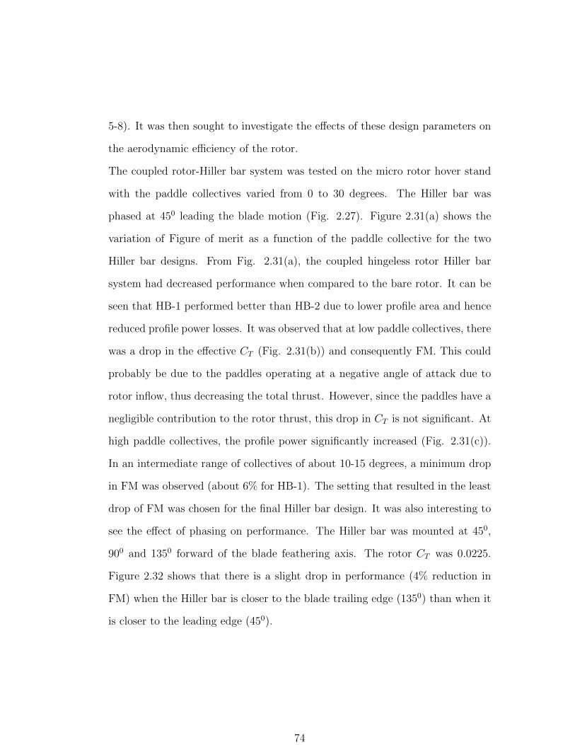
5-8). It was then sought to investigate the effects of these design parameters on

the aerodynamic efficiency of the rotor.

The coupled rotor-Hiller bar system was tested on the micro rotor hover stand

with the paddle collectives varied from 0 to 30 degrees. The Hiller bar was

phased at 450 leading the blade motion (Fig. 2.27). Figure 2.31(a) shows the

variation of Figure of merit as a function of the paddle collective for the two

Hiller bar designs. From Fig. 2.31(a), the coupled hingeless rotor Hiller bar

system had decreased performance when compared to the bare rotor. It can be

seen that HB-1 performed better than HB-2 due to lower profile area and hence

reduced profile power losses. It was observed that at low paddle collectives, there

was a drop in the effective CT (Fig. 2.31(b)) and consequently FM. This could

probably be due to the paddles operating at a negative angle of attack due to

rotor inflow, thus decreasing the total thrust. However, since the paddles have a

negligible contribution to the rotor thrust, this drop in CT is not significant. At

high paddle collectives, the profile power significantly increased (Fig. 2.31(c)).

In an intermediate range of collectives of about 10-15 degrees, a minimum drop

in FM was observed (about 6% for HB-1). The setting that resulted in the least

drop of FM was chosen for the final Hiller bar design. It was also interesting to

see the effect of phasing on performance. The Hiller bar was mounted at 450,

900 and 1350 forward of the blade feathering axis. The rotor CT was 0.0225.

Figure 2.32 shows that there is a slight drop in performance (4% reduction in

FM) when the Hiller bar is closer to the blade trailing edge (1350) than when it

is closer to the leading edge (450).

74

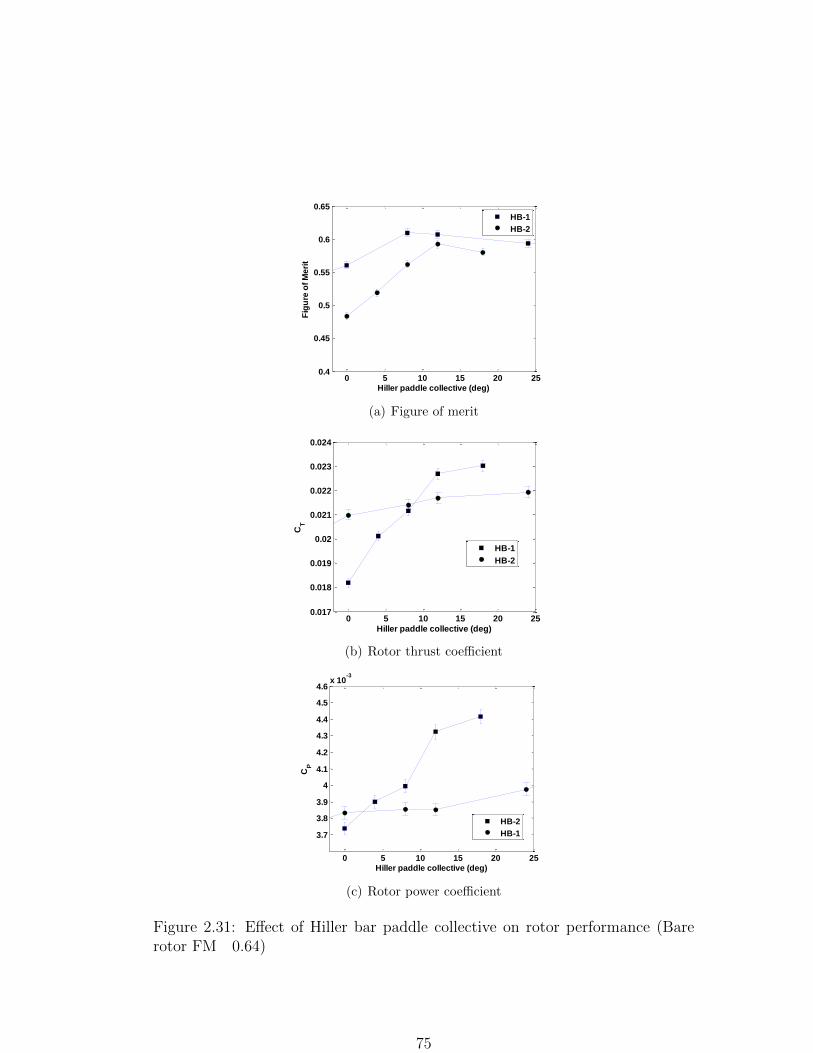
0 5 10 15 20 250.4

0.45

0.5

0.55

0.6

0.65

Hiller paddle collective (deg)

Fig

ure

of

Me

rit

HB-1

HB-2

(a) Figure of merit

0 5 10 15 20 250.017

0.018

0.019

0.02

0.021

0.022

0.023

0.024

Hiller paddle collective (deg)

CT

HB-1

HB-2

(b) Rotor thrust coefficient

0 5 10 15 20 25

3.7

3.8

3.9

4

4.1

4.2

4.3

4.4

4.5

4.6x 10

-3

Hiller paddle collective (deg)

CP

HB-2

HB-1

(c) Rotor power coefficient

Figure 2.31: Effect of Hiller bar paddle collective on rotor performance (Barerotor FM 0.64)

75

40 60 80 100 120 1400.55

0.56

0.57

0.58

0.59

0.6

0.61

0.62

0.63

0.64

0.65

Hiller phasing (deg)

FM

Figure 2.32: Effect of Hiller bar phasing on FM

2.5 Anti-torque Vanes

The anti-torque vane concept is one of the key design features for the prototype

vehicle designs described in this chapter. To improve the compactness of the ve-

hicle, the anti-torque system was designed with vanes installed in the downwash

of the main rotor instead of a conventional tail rotor.

2.5.1 Proof of concept and analysis

A series of experimental tests were performed to study the effectiveness of the

vane concept. For these studies, a 3 bladed fixed pitch rotor with a solidity of

0.15 and a diameter of 6′′ was used. The blades were rectangular in panform,

untwisted and with a circular arc airfoil section with a 6% camber. The blades

were set at a collective pitch of 180. The anti-torque vanes were assembled to

the central body holding the DC motor driving the main rotor. Four vanes were

installed, each with a chord of 3”. First, flat plates were used as vanes, which

were installed parallel to the rotor axis to study the presence of swirl in the

rotor downwash. The effect on the net torque on the body was measured. Then,

vanes with an 8% circular arc cross-section were tested. The vanes could be set

76

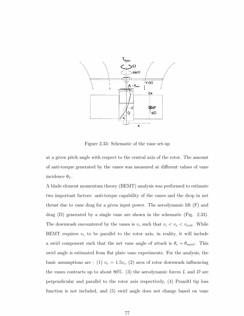
Figure 2.33: Schematic of the vane set-up

at a given pitch angle with respect to the central axis of the rotor. The amount

of anti-torque generated by the vanes was measured at different values of vane

incidence θV .

A blade element momentum theory (BEMT) analysis was performed to estimate

two important factors: anti-torque capability of the vanes and the drop in net

thrust due to vane drag for a given input power. The aerodynamic lift (F) and

drag (D) generated by a single vane are shown in the schematic (Fig. 2.33).

The downwash encountered by the vanes is vv such that vi < vv < vexit. While

BEMT requires vv to be parallel to the rotor axis, in reality, it will include

a swirl component such that the net vane angle of attack is θv + θswirl. This

swirl angle is estimated from flat plate vane experiments. For the analysis, the

basic assumptions are : (1) vv = 1.5vi, (2) area of rotor downwash influencing

the vanes contracts up to about 80%. (3) the aerodynamic forces L and D are

perpendicular and parallel to the rotor axis respectively, (4) Prandtl tip loss

function is not included, and (5) swirl angle does not change based on vane

77

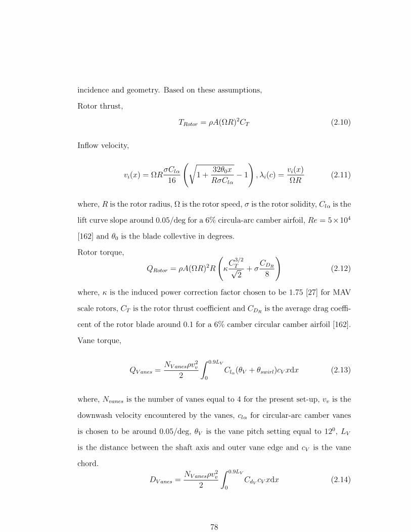
incidence and geometry. Based on these assumptions,

Rotor thrust,

TRotor = ρA(ΩR)2CT (2.10)

Inflow velocity,

vi(x) = ΩRσClα16

(√1 +

32θ0x

RσClα− 1

), λi(c) =

vi(x)

ΩR(2.11)

where, R is the rotor radius, Ω is the rotor speed, σ is the rotor solidity, Clα is the

lift curve slope around 0.05/deg for a 6% circula-arc camber airfoil, Re = 5×104

[162] and θ0 is the blade collevtive in degrees.

Rotor torque,

QRotor = ρA(ΩR)2R

(κC

3/2T√2

+ σCDR

8

)(2.12)

where, κ is the induced power correction factor chosen to be 1.75 [27] for MAV

scale rotors, CT is the rotor thrust coefficient and CDR is the average drag coeffi-

cent of the rotor blade around 0.1 for a 6% camber circular camber airfoil [162].

Vane torque,

QV anes =NV anesρv

2v

2

∫ 0.9LV

0

Clα(θV + θswirl)cV xdx (2.13)

where, Nvanes is the number of vanes equal to 4 for the present set-up, vv is the

downwash velocity encountered by the vanes, clα for circular-arc camber vanes

is chosen to be around 0.05/deg, θV is the vane pitch setting equal to 120, LV

is the distance between the shaft axis and outer vane edge and cV is the vane

chord.

DV anes =NV anesρv

2v

2

∫ 0.9LV

0

CdV cV xdx (2.14)

78

where, CdV for the 8% circular camber vanes, around 0.2 for an incidence angle

of about 150 [162].

Net torque (from (2.12) and (2.13)),

QNet = QRotor −Qvanes (2.15)

Net thrust (from (2.10) and (2.14)),

T = TRotor −DV anes (2.16)

Input electrical power,

PElec =QRotorΩ

η(2.17)

where η is the motor-gearbox efficiency chosen to be about 50% based on mea-

sured motor performance.

The experimentally measured torque on the body obtained by installing flat

plates in the downwash, parallel to the axis of the rotor (00 inclination), is

shown in Fig. 2.34. It can be seen that by just installing these flat vanes, the

total torque on the body is reduced by approximately 40% (θV for this flat plate

vane case is 00). Using this, the swirl angle was determined to be about 40.

This result was used to update the net vane angle of incidence and predict the

effect of vanes on the net body torque (2.15) and input power (2.17) at different

thrust levels (Fig. 2.35). It can be seen that with 8% circular camber vanes set

at 120 pitch setting, a 75% torque balance was achieved. From Fig. 2.36, a 10%

reduction in thrust was observed for a given input power due to the vane drag.

The results of the analysis compares satisfactorily with the experimental re-

sults. The circular arc vanes at a pitch angle of 120 reduce the torque on the

79

10 20 30 40 50 60 700.002

0.004

0.006

0.008

0.01

0.012

0.014

Thrust (g)

Bo

dy

to

rqu

e (

N-m

)

180 collective, isolated rotor

180 collective, rotor with flat vanes

Figure 2.34: Body torque versus thrust for rotor with flat vanes at 00 inclinationin rotor downwash

0 20 40 60 800

0.002

0.004

0.006

0.008

0.01

0.012

0.014

0

Thrust (g)

Bo

dy

to

rqu

e (

N-m

)

Rotor only (expt.)

Rotor with curved vanes (expt.)

Rotor only (anal.)

Rotor with curved vanes (anal.)

Figure 2.35: Net body torque versusthrust for curved vanes in downwash

0 10 20 30 40 50 60 70 800

2

4

6

8

10

12

14

16

Thrust (g)

Ele

ctr

ica

l P

ow

er

(W)

Rotor with curved vanes (expt.)

Rotor only (expt.)

Rotor with curved vanes (anal.)

Rotor only (anal.)

Figure 2.36: Effect of vanes on powerconsumed

80

X - Vanes H - Vanes

Figure 2.37: Vane arrangement

body by almost 80% (Fig. 2.35). The installation of the vanes results in an

increase in power required for a given thrust by approximately 10%. This per-

centage increase in power is similar to that typically required by a conventional

full-scale tail rotor. Based on the above results, it was seen that the concept

of vanes placed in the rotor downwash for countering rotor torque was viable.

For the final design, two fixed vanes and two vanes provided with controllable

trailing edge flaps for yaw control were incorporated.

2.5.2 Integration and yaw control

These vanes can be incorporated in the vehicle either in an X or an H config-

uration. This is schematically shown in Fig. 2.37. With the X configuration,

81

the vehicle axisymmetry is maintained and the structure of the vehicle becomes

sturdier. However in edgewise flight, the vanes could be a significant source of

profile drag. This limitation can be alleviated with the H configuration. The

effectiveness of the two configurations were measured using the set-up shown in

Fig. 2.38). Four rectangular (3”×5”), 8% camber circular arc carbon fiber vanes

b

Figure 2.38: Set-up to measure anti-torque and power penalty of X and H vanes

were attached to the shaft under the downwash of the rotor. The rotor thrust

coefficient was set at CT = 0.02. The H configuration was tested with different

spacing (b) between the vanes.

The results are shown in Fig. 2.39. For the rotor without vanes, the torque

increased linearly with thrust as expected. With the X configuration, torque is

reduced to almost zero irrespective of thrust for a vane collective of 120. Similar

torque reduction was observed with the H configuration for b = 25mm. However,

with higher values of b, the anti-torque reduced. This can be explained by the

fact that for b > 25mm, a portion of the vanes was ’outside’ the rotor downwash

resulting in a decrease in the effective aerodynamic surface capable of countering

82

20 40 60 80 100 120-5

0

5

10

15

20x 10

-3

Thrust (g)

To

rqu

e (

N-m

)

No vanes

H vanes, b=75 mm

H vanes, b=25 mm

X vanes

Figure 2.39: Anti-torque capability of Xand H vanes

0 20 40 60 80 100 1200

2

4

6

8

10

12

14

Thrust (g)

Ele

ctr

ica

l P

ow

er(

W)

No vanes

with H-vanes, b=25mm

with X-vanes

Figure 2.40: Power penalty with X andH vane configuration

the torque. Figure 2.40 shows electrical power versus thrust for the three con-

figurations. Both X and H vanes incurred a similar power penalty of about 10%

when compared to the isolated rotor case. Presently, for the purposes of axisym-

metry and a sturdy structure, the X vanes are incorporated. The vanes with

the controllable flaps are integrated into the vehicle as shown in Fig. 2.41 The

Figure 2.41: X vanes integrated into body

83

controllable flaps changed the vane incidence of two of the vanes by about 160

with maximum control input. As desired, the vane deflection for a given control

input was linear (Fig. 2.42). The yaw control authority at operating thrust of

about 250 g was measured as a function of control vane angle. The fixed vanes

had a collective of about 230. It can be seen that yaw control authority was

perfectly bi-directional and linear about trim (Fig. 2.43).

0 20 40 60 80 1006

8

10

12

14

16

18

20

22

24

26

Control input (%)

Co

ntr

ol v

an

e a

ng

le s

ett

ing

(d

eg

)

Figure 2.42: Control vane deflection fora given control input

8 10 12 14 16 18 20 22 24

-0.015

-0.01

-0.005

0

0.005

0.01

0.015

Control vane angle of attack (deg)

To

rqu

e (

N-m

)Yaw Trim

Figure 2.43: Effect of control vane de-flection on vane torque

2.6 Shroud

In this section, improvements in hover power loading of an efficient unshrouded

rotor (discussed in 2.3.3) by enclosing the rotor in a shroud are discussed.

2.6.1 Principle

In a shrouded rotor configuration, the thrust of a shrouded rotor includes two

parts, the thrust of the rotor and the additional thrust from the shroud. Figure

(2.44) shows a schematic of the principle of the shrouded rotor. The shroud

84

Figure 2.44: Shrouded rotor operating principle

consists of two sections: the inlet and the diffuser. The diffuser recovers kinetic

energy of the slipstream and increases mass flow rate through the rotor (for the

same total thrust produced by the shrouded and an unshrouded rotor). Opera-

tion of the rotor creates a low pressure above the rotor plane. This accelerates

flow over the shroud inlet surface. Suction force is generated as a result of this

airflow which results in an additional lift force. A summary of the momentum

theory analysis for the shrouded rotor aerodynamics is shown here which can

be used to explain improvements in hover performance. Detailed derivations of

these results can be found in [27,50].

Consider Fig. 2.45 that shows a schematic of the 2-D rotor wake for the

unshrouded and shrouded rotor. Momentum theory assumes inviscid, incom-

pressible, steady and quadi-one-dimensional flow. The rotor imparts only axial

momentum with no wake swirl. The wake of the shrouded rotor is assumed to

have expanded to ambient atmospheric pressure at the diffuser exit plane.

85

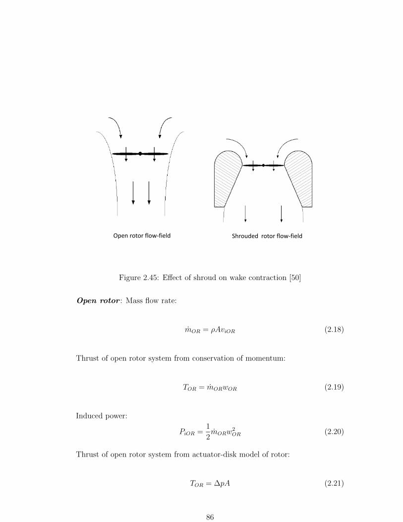
Open rotor flow-field Shrouded rotor flow-field

Figure 2.45: Effect of shroud on wake contraction [50]

Open rotor : Mass flow rate:

mOR = ρAviOR (2.18)

Thrust of open rotor system from conservation of momentum:

TOR = mORwOR (2.19)

Induced power:

PiOR =1

2mORw

2OR (2.20)

Thrust of open rotor system from actuator-disk model of rotor:

TOR = ∆pA (2.21)

86

Here, A is the rotor disk area, viOR is the induced velocity of flow across the

rotor disk, wOR is the velocity of the rotor wake at the location where wake

pressure is ambient and ∆p is the pressure differential across the rotor plane.

From conservation of energy and actuator-disk model of the rotor,

∆p =1

2ρw2

OR (2.22)

It follows that,

wOR = viOR (2.23)

viOR =

√TOR2ρA

(2.24)

PiOR =T

3/2OR√2ρA

(2.25)

Shrouded rotor : Unlike the open rotor, the exit area of the shrouded rotor

wake (Ae) is prescribed as the area of the diffuser exit plane.

Mass flow rate:

mSR=ρAviSR

=ρAewSR (2.26)

⇒ wSR =viSRσd

(2.27)

Total thrust of shrouded rotor system from conservation of momentum:

TSR=mSRwSR

=ρAv2iSRσd

(2.28)

87

⇒ viSR =

√σdTSRρA

(2.29)

Induced Power:

PiSR =T

3/2SR√

4σdρA(2.30)

where σd is the contraction ratio of the rotor wake (it is 0.5 for an open rotor

based on momentum theory). From Fig. 1.8 it can be seen that contribution

to total thrust of the shrouded rotor system comes from the rotor, inlet and

diffuser. It can be shown that,

Rotor thrust:

Trotor =TSR2σd

(2.31)

Diffuser thrust:

Tdiffuser = −TSR(σd − 1)2

2σd(2.32)

Inlet thrust:

Tinlet =TSRσd

2(2.33)

It can be seen that as the expansion ratio is increased, the diffuser increases the

downforce on the system (negative thrust), the rotor thrust decreases and the

inlet thrust increases. For a straight diffuser (σd = 1), the rotor and shroud inlet

share about 50% of the total thrust (this was experimentally measured in Sec.

2.6).

Comparisons between open and shrouded rotor performance : If the

rotor disk area for both the configurations are equal, the performance can be

compared in two ways,

88

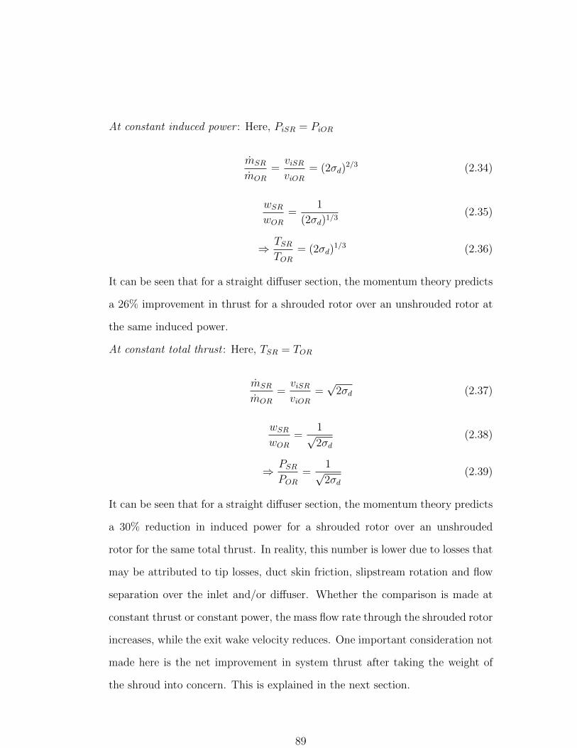
At constant induced power : Here, PiSR = PiOR

mSR

mOR

=viSRviOR

= (2σd)2/3 (2.34)

wSRwOR

=1

(2σd)1/3(2.35)

⇒ TSRTOR

= (2σd)1/3 (2.36)

It can be seen that for a straight diffuser section, the momentum theory predicts

a 26% improvement in thrust for a shrouded rotor over an unshrouded rotor at

the same induced power.

At constant total thrust : Here, TSR = TOR

mSR

mOR

=viSRviOR

=√

2σd (2.37)

wSRwOR

=1√2σd

(2.38)

⇒ PSRPOR

=1√2σd

(2.39)

It can be seen that for a straight diffuser section, the momentum theory predicts

a 30% reduction in induced power for a shrouded rotor over an unshrouded

rotor for the same total thrust. In reality, this number is lower due to losses that

may be attributed to tip losses, duct skin friction, slipstream rotation and flow

separation over the inlet and/or diffuser. Whether the comparison is made at

constant thrust or constant power, the mass flow rate through the shrouded rotor

increases, while the exit wake velocity reduces. One important consideration not

made here is the net improvement in system thrust after taking the weight of

the shroud into concern. This is explained in the next section.

89

Figure 2.46: Shroud design parameters

2.6.2 Design

In the recent study by Pereira and Chopra [50], an optimum combination of

design parameters for an MAV scale shrouded rotor (Fig. 2.46) was identified to

minimize these losses. Key conclusions from this study relevant to the present

design were: (1) a blade tip clearance δtip < 0.012R should be maintained for

good performance, (2) the diffuser angle (θd) plays a more important role than

the diffuser length (L), and (3) the outer portion of the shroud lip does not play

a major role in thrust production. Hence for weight savings, the lip chord can

be shortened.

It can be seen that for this concept to be viable, the thrust improvement offered

by a shrouded rotor for a given operating power should be at least greater than

the weight of the shroud itself. A design analysis based on simple momentum

theory to estimate the upper limit for the shroud mass is described below.

Let WUS be the weight of the unshrouded MAV, WShroud be the weight of the

90

shroud and WS be the weight of the shrouded MAV. Consequently,

WS = WShroud +WUS (2.40)

The mechanical power consumed by any rotor can be written as,

P = PP + PI (2.41)

The profile power (PP ) is mainly a function of rotor solidity and airfoil drag

coefficient. The induced power (PI) however depends on the structure of the

wake. Since the rotor configuration is fixed, it can be logically assumed that the

main differences in mechanical power consumption between an unshrouded and

shrouded rotor is from the induced power. Therefore, for a beneficial shroud

design,

PIS < PUS (2.42)

In non dimensional terms,

CPIS < CPIUS (2.43)

From simple momentum theory, for a given contraction ratio σD, the non-

dimensional induced power is given by,

CPI = κW 3/2

√4σDρA

(2.44)

Where, κ is the induced power factor that accounts for tip loss effects, non-

uniform inflow and swirl effects. W is the weight of the vehicle, A is the area of

91

the rotor disk which is maintained constant and ρ is the air density. Hence, for

CPIS < CPIUS (2.45)

It is required that,

κSW

3/2S√

4σDρA< κUS

W3/2US

2ρA(2.46)

This leads to,

WS

WUS

<

(κUSκS

)2/3

(2σD)1/3 (2.47)

Since the shroud diffuses the rotor tip vortex [113], the induced losses from a

shrouded rotor are expected to be lower than an unshrouded rotor. Consequently,

κUS > κS. A conservative estimate for the weight restriction for the shroud can

be made by assuming κUS ∼ κS. Hence, from (2.47) and (2.40),

WShroud <((2σD)1/3 − 1

)WUS (2.48)

For example, if the weight of the unshrouded vehicle is 250 grams, and if σD = 1,

the power loading of the vehicle can be improved by enclosing the rotor in a

shroud weighing less than 65 grams.

However, due to the shroud lip, the dimension of a shrouded rotor MAV in the

rotor plane is equal to an unshrouded rotor MAV with a larger rotor diameter.

To accommodate the effect of this increased size, the revised restriction for the

shroud weight becomes

WShroud <

((2A

A′σD

)1/3)WUS (2.49)

92

where A is the area of the rotor disk and A′ is the area of the shroud includ-

ing the shroud lip. Consider the previous example of a 250 grams unshrouded

rotor MAV with an 11” diameter rotor. For the same dimension, the shroud

would have a diameter of 11”. If the diameter of the rotor is 9” (1” shroud lip),

for power loading improvements, the weight of the shroud should not exceed 25

grams. In further discussion, this restriction is not made and a shrouded rotor

is compared with an unshrouded rotor with the same rotor diameter.

It can be seen that these weight restrictions pose challenges for the shroud con-

struction that include (1) lightweight material construction without compromis-

ing on shroud stiffness, and (2) smooth surface construction to ensure uniformity

in pressure distribution over the shroud inlet. Shroud construction iterations

were carried out based on two designs to determine a stiff, lightweight structure.

Shroud design 1 : A shroud structural frame was constructed out of 1-2 mm thick

strips made from cured carbon/epoxy that were suitably arranged to stiffen the

structure in torsion and in the radial direction. The frame was covered with

clear cellophane tape. The design is shown in Fig. 2.47. The shroud weight was

41 grams. For this design, rlip = 9%Dt, L = 15%Dt, σD = 1. The diffuser length

was restricted to save weight and minimize surface friction losses.

Shroud design 2 : This design consisted of a single ply of carbon fiber/epoxy

weave on a framework of unidirectional graphite epoxy stiffeners. The shroud

was constructed by laying up the plies on a female metal mold, vacuum bagging

and curing in an oven (Fig. 2.48). A chord-diameter ratio of 0.5 was chosen to

save weight. The shroud weighed about 45 grams.

Shroud design 1 was stiffer in the radial and out of plane torsion mode as com-

pared to shroud design 2, while the second design had a uniform shroud in-

let surface. However, a stiffer shroud was preferred to avoid undesirable rotor

93

Shroud Design 1 Shroud Design 2

Figure 2.47: Shroud designs

shroud interference. Hence, results of the performance tests discussed here are

with shroud design 1.

Figure 2.48: Shroud construction using vacuum bagging and oven treament

2.6.3 Aerodynamic performance

To estimate the aerodynamic performance of the shrouded rotor, shroud design 1

was tested on the micro rotor hover stand (Fig. 2.49). The shroud was integrated

94

to the rotor shaft stand through metal struts having a diameter of about 3 mm6.

The shroud was held to the struts through aluminum supports. This ensured a

sturdy shroud structure enclosing the rotor. The thrust and torque measurement

was the total force generated by the shrouded rotor system.

2.6.3.1 Comparison with unshrouded rotor

The most efficient unshrouded rotor from Fig. 2.19 was then tested in the

shrouded configuration (Fig. 2.49). A blade tip clearance of 0.015R was main-

tained. Care was taken to keep the clearance as uniform as possible. A lower

tip clearance resulted in rotor-shroud interference. This was one of the main

challenges in the operation of the shrouded rotor - trade off between higher tip

clearance and mechanical interaction between the rotor and shroud.

Aluminum support

structureMetal struts

Figure 2.49: Set-up to measure shrouded rotor performance

Figure 2.50 shows the variation of thrust and mechanical power coefficient of

6It was seen that the struts led to a thrust penalty that was within measurement error.Therefore this penalty was not factored into the results.

95

the shrouded rotor as a function of RPM. Like the unshrouded rotor case, it

can be seen that the shrouded rotor did not exhibit significant Reynolds num-

ber effects in the range of RPMs considered although the power coefficient did

increase (by about 5%) at lower RPMs. From Figure 2.50, it can also be de-

1800 2000 2200 2400 2600 2800 3000 3200 3400 36000

0.005

0.01

0.015

0.02

0.025

0.03

RPM

CT

7 deg 14 deg 18 deg 22 deg

(a) Thrust coefficient v.RPM

1800 2000 2200 2400 2600 2800 3000 3200 3400 36000

1

2

3

4

5x 10

-3

RPM

CP

7 deg 14 deg 18 deg 22 deg

(b) Power coefficient v.RPM

Figure 2.50: Variation of thrust and power coefficient with RPM for a two bladedtapered shrouded rotor at different blade root collective

duced that the thrust of the shrouded rotor system increased quadratically with

RPM and the power increased cubically with RPM. Figure 2.51(a)) compares

the most efficient performance obtained for the shrouded rotor with respect to

the unshrouded rotor. It can be clearly seen that the shrouded rotor has a bet-

ter aerodynamic performance than the unshrouded rotor. For example, for an

input mechanical power of 15 watts, the improvement in shrouded rotor thrust

was about 70 grams. This exceeded the weight of the shroud thus resulting in

a payload benefit of about 20-30 grams. Alternatively, by looking at the power

loading of the shrouded rotor system (Fig. 2.51(b)), it can be seen that at an

operating thrust of about 300 grams, the improvement in power loading is about

30%7.

7A previous study of an MAV scale shrouded rotor system showed a 60% improvement inpower loading with the shrouded rotor. It was noted in that study that comparisons were made

96

0 5 10 15 20 25 3050

100

150

200

250

300

Mechanical Power (W)

Th

rus

t (g

)

Unshrouded

Shrouded

(a) Mechanical power versus thrust

50 100 150 200 250 3008

13

18

23

28

Thrust (g)

Me

ch

an

ica

l P

ow

er

Lo

ad

ing

(g

/W)

Unshrouded Rotor

Shrouded Rotor

(b) Mechanical power loading versus thrust

Figure 2.51: Comparison in aerodynamic performance between shrouded andunshrouded rotor

97

2.6.3.2 Division of thrust between rotor and shroud

In order to measure the thrust individually generated by the rotor and shroud, it

was necessary to detach the shroud from the rotor stand and mount it separately.

This was done using the set-up shown in Fig. 2.52. Here, the rotor stand

was mounted on the first load balance. A metal structure was placed beneath

this balance and held a shroud through 4 aluminum struts. The shroud was

positioned in the rotor plane accordingly. This entire system including the rotor

stand and shroud was then mounted on a second balance. This balance measured

the total thrust generated by the shroud and the rotor, while the top balance

measured the rotor thrust alone. A subtraction of the two provides the thrust

generated by the shroud alone. For this experiment, it was necessary to increase

the tip clearance of the rotor to 0.03R since the rotor shaft was not directly

attached to the shroud. Hence any vibration in the shaft resulted in rotor-

shroud interference.

Figure 2.53 shows the division of thrust between the shroud and the rotor for

the rotor operated at 260 collective. It can be seen that a quadratic trend is

maintained with RPM for the three components. The rotor shared a higher

proportion of the total thrust compared to the shroud. The shroud also had a

significant contribution to the total thrust which was between 0.3 and 0.4 (Fig.

2.54). This is below the ideal momentum theory estimate of 0.5 which is expected

due to tip loss effects and diffuser wall skin friction drag. It is interesting to note

that this ratio increased marginally at higher RPMs. This could probably be due

to the effective establishment of suction pressure forces over the shroud inlet as

with an inefficient unshrouded rotor. The results shown in Fig. 2.51 show that performanceimprovements are indeed possible even with an efficient unshrouded rotor albeit not as highas 60%

98

the inflow velocity increases. It was also observed that the contribution to total

thrust from the rotor was less than the rotor thrust generated in the unshrouded

configuration. This can be explained by the fact that the inflow velocity in the

shrouded configuration is higher than the unshrouded configuration. Thus the

effective angle of attack is reduced and the rotor generates a lower thrust.

Figure 2.52: Set-up to measure individual contribution to total thrust from rotorand shroud

2.6.3.3 Effect of blade planform

It was seen in 2.3.3 that rectangular blades had a lower power loading than the

tapered blades. An explanation of this is that the tapered blades promote more

uniform inflow while keeping profile losses at a minimum. In order to study the

effect of rotor planform on the performance of the shrouded rotor, parametric

studies were conducted on a representative range of blade profiles (Fig. 2.55).

These are listed as follows: (1) the baseline tapered blade (σe = 0.11), (2) rect-

angular blade I with the same root chord as the baseline blade (σe = 0.13),

99

0 500 1000 1500 2000 2500 30000

50

100

150

200

250

RPM

Th

rus

t (g

)

Total thrust

Rotor thrust

Shroud thrust

Figure 2.53: Contribution to total thrust from rotor and shroud

1000 1200 1400 1600 1800 2000 2200 2400 2600 28000.2

0.22

0.24

0.26

0.28

0.3

0.32

0.34

0.36

0.38

0.4

RPM

TS

hru

d/T

To

tal

Figure 2.54: Ratio of thrust from shroud to total thrust

100

(a) Original planform (b) Rectangular 0 1096.

e 0 1322.

e

0 1494.e

0 1784.e

(c) Taper 140% chord (d) Rectangular 140% chord

(e) Inverse taper (f) Rectangular Hiller0 1325

e . 0 132

e .

Figure 2.55: Blade profiles tested in shroud configuration

101

(3) tapered blade with 140% of the baseline chord (σe = 0.15), (4) rectangular

blade II with same root chord as blade profile 3 (σe = 0.18), (5) inverse tapered

blade (σe = 0.13), and (6) rectangular hiller (σe = 0.13). Blade profiles 5 and

6 were designed with the same thrust weighted solidity as rectangular blade I.

The rotors were tested with shroud design 2 (Fig. 2.47) on the rotor hover stand

(δtip = 0.03R). A collective and RPM sweep was performed for each profile and

the thrust and power coefficients were extracted.

The shrouded rotor thrust coefficient (CT ) is plotted as a function of rotor collec-

tive (θ) in Fig. 2.56. It can be seen that as the solidity of the rotor is increased,

the CT − θ slope increases. By normalizing the thrust coefficient with rotor so-

lidity, the variation in the slope is reduced (Fig. 2.60). It can be seen that the

thrust coefficient stays linear up to about 34 degrees. Beyond this, the rotor

appeared to enter into stall. In comparison, Fig. 2.58 shows the CT − θ vari-

ation for the profiles tested in the unshrouded configuration. The variation in

CT − θ slope for planforms with different solidities was eliminated by normal-

izing it with rotor solidity (Fig. 2.59). The interesting observation is that the

unshrouded rotors entered stall at a much lower angle (250) than the shrouded

rotors. This indicates that blade stall is delayed for shrouded rotors, which could

be attributed to higher rotor inflow velocities. This implies that the blades can

operate at a higher range of collectives, or a larger cyclic input can be provided

in the shrouded rotor configuration to extract useful control moments.

Figure 2.61 shows the variation of power coefficient versus collective for blade

profiles 1-4 in the shrouded and unshrouded configuration. Interestingly, the

power coefficients of the blades 1 and 2 remain unchanged for the shrouded and

unshrouded case. For the 140% chord tapered blade and the 140% chord rectan-

gular blade, the change in power coefficient is not significant either. This is an

102

5 10 15 20 25 30 35 400

0.01

0.02

0.03

0.04

0.05

0.06

0.07

0.08

Collective (deg)

CT

Original

Rectangular

Taper 140% chord

Rectangular 140% chord

Figure 2.56: CT versus θ for shrouded rotor

5 10 15 20 25 30 35 400

0.1

0.2

0.3

0.4

0.5

Collective (deg)

CT/

e

Original

Rectangular

Taper 140% chord

Rectangular 140% chord

Figure 2.57: CTσe versus θ for shrouded rotor

103

5 10 15 20 25 30 35 400

0.01

0.02

0.03

0.04

0.05

0.06

0.07

0.08

Collective (deg)

CT

Original

Rectangular

Taper 140% chord

Rectangular 140% chord

Figure 2.58: CT versus θ for unshrouded rotor

5 10 15 20 25 30 35 400

0.1

0.2

0.3

0.4

0.5

Collective (deg)

CT/

e

Original

Rectangular

Taper 140% chord

Rectangular 140% chord

Figure 2.59: CTσe versus θ for unshrouded rotor

104

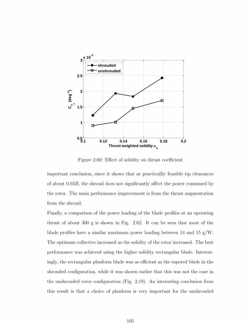
0.1 0.12 0.14 0.16 0.18 0.20.5

1

1.5

2

2.5

3x 10

-3

Thrust weighted solidity e

CT

(d

eg

-1)

shrouded

unshrouded

Figure 2.60: Effect of solidity on thrust coefficient

important conclusion, since it shows that at practicallly feasible tip clearances

of about 0.03R, the shroud does not significantly affect the power consumed by

the rotor. The main performance improvement is from the thrust augmentation

from the shroud.

Finally, a comparison of the power loading of the blade profiles at an operating

thrust of about 300 g is shown in Fig. 2.62. It can be seen that most of the

blade profiles have a similar maximum power loading between 14 and 15 g/W.

The optimum collective increased as the solidity of the rotor increased. The best

performance was achieved using the higher solidity rectangular blade. Interest-

ingly, the rectangular planform blade was as efficient as the tapered blade in the

shrouded configuration, while it was shown earlier that this was not the case in

the unshrouded rotor configuration (Fig. 2.19). An interesting conclusion from

this result is that a choice of planform is very important for the unshrouded

105

rotor, but is not a significant factor for the shroud. For the unshrouded ro-

tor, the rise in CP for the rectangular blade was not equally offset by a rise in

CT . Therefore, the unshrouded tapered blade had a better performance. In the

shrouded case, the rise in CP for the rectangular blade compared to the tapered

blade was the same as for the unshrouded rotor. However, the rise in CT was

much higher in the shrouded rotor case. An explanation for this could be that

the shroud diffuses the tip vortex, thus extracting extra thrust from the tip of

the shrouded rectangular blade.

It will be discussed in a later chapter (Chap. 5) about the requirement of a spe-

cific planform for the shrouded rotor for improving control moments. The results

discussed until that section will be for the shrouded tapered blade enclosed in

shroud design 2.

2.6.3.4 Brushed blade tips

It was discussed earlier that by increasing the tip clearance, the performance of

the shrouded rotor drops. A reason for this is that the suction pressure at the

blade tip is lost due to the tip vortex. This reduces the flow acceleration over the

shroud inlet and reduces the thrust generated by the shrouded rotor. Therefore

the tip clearance has to be minimized. The danger of this is the undesirable

rotor-shroud interactions. In order to minimize the tip-shroud interactions and

to effectively reduce tip clearance, brushes were included in the blade tips. It was

thought that the brushes would help sustain the suction pressure of the blade

tips.

As described before, the blades were constructed from a carbon fiber epoxy pre-

preg weave. After curing the blade, heat treatment from a soldering iron was

given to the tips of the blade until the epoxy was dissolved. The cross fibers were

106

5 10 15 20 25 30 35 400

0.005

0.01

0.015

0.02

0.025

0.03

Collective (deg)

CP

Unshrouded:Original

Unshrouded:Rectangular

Shrouded:Original

Shrouded:Rectangular

(a) Power coefficient versus collective for original chord blade profiles

5 10 15 20 25 30 35 400

0.005

0.01

0.015

0.02

0.025

0.03

Collective (deg)

CP

Unshrouded:140% chord Taper

Unshrouded: 140% chord Rectangular

Shrouded:140% chord Taper

Shrouded:140% chord Rectangular

(b) Power coefficient versus collective for 140% chord blade profiles

Figure 2.61: Comparison in CP versus θ for shrouded and unshrouded rotor

107

5 10 15 20 25 30 35 40 450

2

4

6

8

10

12

14

16

Collective (deg)

Po

we

r lo

ad

ing

(g

/W)

Original

Rectangular

Taper 140% chord

Rectangular 140% chord

Figure 2.62: Comparison of power loading for the different blade profiles at 300g operating thrust

108

removed and a smooth brush pattern consisting of carbon fibers remained. Care

was taken to avoid stressing the fibers during the heat treatment, as it resulted

in the fibers becoming brittle and withering. Figure 2.63 shows the brushed

blade tips and incorporation into the vehicle.

Figure 2.63: Brushes incorporated in blade tips to improve performance

The performance of the brushes were tested on the rotor hover stand. The

no-brush tip clearance was 3 mm. Two sets of brushes were tested, (1) short

brushes of length 3 mm, and (2) long brushes of length 6 mm. Figure 2.64(a)

shows a representative variation of thrust with RPM for the different blades at

a blade collective of 240. It can be seen that there was a slight improvement

in total thrust generated when the brushes were added. A comparison of the

torque-RPM (Fig. 2.64(b)), showed that the torque for the brushes were higher

109

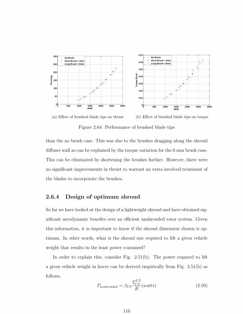
0 500 1000 1500 2000 2500 30000

50

100

150

200

250

300

RPM

Th

rus

t (g

)

No Brush

Short Brush = 3mm

Long Brush = 6mm

(a) Effect of brushed blade tips on thrust

0 500 1000 1500 2000 2500 30000

0.01

0.02

0.03

0.04

0.05

0.06

0.07

RPM

To

rqu

e (

N-m

)

No Brush

Short Brush = 3mm

Long Brush = 6mm

(b) Effect of brushed blade tips on torque

Figure 2.64: Performance of brushed blade tips

than the no brush case. This was due to the brushes dragging along the shroud

diffuser wall as can be explained by the torque variation for the 6 mm brush case.

This can be eliminated by shortening the brushes further. However, there were

no significant improvements in thrust to warrant an extra involved treatment of

the blades to incorporate the brushes.

2.6.4 Design of optimum shroud

So far we have looked at the design of a lightweight shroud and have obtained sig-

nificant aerodynamic benefits over an efficient unshrouded rotor system. Given

this information, it is important to know if the shroud dimension chosen is op-

timum. In other words, what is the shroud size required to lift a given vehicle

weight that results in the least power consumed?

In order to explain this, consider Fig. 2.51(b). The power required to lift

a given vehicle weight in hover can be derived empirically from Fig. 2.51(b) as

follows,

Punshrouded = βUST

3/2US

R(watts) (2.50)

110

0.05 0.1 0.15 0.2 0.25 0.3 0.35 0.40

10

20

30

40

50

60

Radius (m)

Sh

rou

ded

ro

tor:

Po

wer

req

uir

ed

to

lif

t p

aylo

ad

(N

)

Payload = 100 gms

Payload = 200 gms

Payload = 250 gms

Payload = 300 gms

Present

rotor radius

(0.121m) Optimum

rotor radius

(0.141m)

Figure 2.65: Power required vs. rotorradius at different desired payloads

1.5 2 2.5 310

12

14

16

18

20

22

24

26

28

30

Payload (N)

Sh

rou

ded

Ro

tor:

Po

wer

req

uir

ed

to

lift

paylo

ad

(W

)

R=5cm

R=10 cm

Design point R=12.1cm

R=14.1cm

R=20cm

Figure 2.66: Power required to lift pay-load at different radii

Pshrouded = βST

3/2US + kR3

R(watts) (2.51)

where TUS is the weight of the unshrouded rotor vehicle (or payload), R is the

rotor radius (or shroud size), and βUS = 0.789, βS = 0.478, and k = 250(N/m3)

are the empirical factors extracted from present data. It is assumed that the

weight of the shroud (kR3) increases as the cube of size. Using Eq. (2.51) the

power is plotted as a function of shroud size at different desired payloads in Fig.

2.65. It can be seen that at the design payload of 250 g, a 14 cm radius shroud

would require the least power for hover. However as can be seen from Fig. 2.66,

this power reduction is less than 5% when compared with the present design.

Therefore, the shroud size chosen in this research is close to optimum for a 250

g design payload.

111

2.7 Vehicle Prototypes

A series of risk reduction prototypes were constructed (2.2) and tested prior to

the testing of the shrouded rotor vehicle8.

Table 2.2: Vehicle prototypes testedPrototype Description

TiFlyerUnshrouded, teetering rotor withvanes. Metal body construction,Mass: 350 grams

GiantUnshrouded, teetering rotor withvanes. Carbon fiber structure.Mass: 240 grams

TiShrovShrouded, hingeless rotor withvanes. Carbon fiber structure.Mass: 260 grams

2.7.1 TiFlyer

The main goal of this prototype was to demonstrate the anti-torque vanes con-

cept in flight. It was constructed as shown in Fig. 2.67. A two bladed aluminum

sheet teetering rotor was incorporated with a Hiller stabilizer bar. The rotor

had a diameter of 250 mm and a blade solidity of 0.13. Lateral and longitudinal

control was achieved through cyclic control. A lightweight carbon fiber frame

was installed to protect the rotor and to add stiffness to the body. the vanes

were made of curved metal sheets and were held to the center body through

metal connector plates. Two of the vanes were provided with controllable sur-

faces which were actuated by a single servo in a symmetric manner. The weight

breakdown of the vehicle is given in Table 2.2. TiFlyer exhibited stable hover

characteristics and satisfactory maneuverability during flight testing.

8TiFlyer-1 and GIANT were developed by Dr. Jayant Sirohi and Dr. Marat Tishchenko

112

2.7.2 Giant

The next prototype was built with the goal of minimizing the vehicle weight. The

aluminum sheet blades were replaced with carbon/epoxy blades. This decreased

the blade weight from 4.2 to 2.6 grams. As a result, it was possible to construct

the hum from a lighter material (Delrin). Thin sheet carbon fiber vanes were

held to the center body through connector plates and to the outer carbon fiber

frame. A spider type swashplate was incorporated. Here, the swashplate motion

occured in the plane of the rotor. The two servos move the non-rotating part

in two orthogonal directions. The rotating part is attached to the non-rotating

part by a radial bearing, and the result of the servo motion is an eccentricity of

the center of rotation of the rotating part with respect to the main rotor shaft.

This eccentricity is used to transfer a cyclic pitch angle to the servo-paddle by

means of a control linkage sliding in a slot in the rotating part of the swashplate.

This reduced the number of moving parts and the mechanical integrity of the

actuation system was improved. The electronics, battery and motor remained

unchanged from that of TiFlyer. The weight breakdown of Giant is given in

Table. 2.3. It can be seen that a structural weight reduction was achieved by

using composite materials.

2.7.3 TiShrov

A third prototype vehicle to demonstrate the shrouded rotor concept was con-

structed. It can be seen that apart from the shroud, the key difference between

Giant and TiShrov was the choice of the hingless rotor. The phased Hiller bar-

rotor was driven by a 55 watt DC brushless motor. A COTS swashplate was

used to transfer inputs from two GWS micro servos to the phased Hiller bar

113

Table 2.3: Vehicles - weight breakdownPrototype TiFlyer Giant TiShrovComponent Mass (g) Mass (g) Mass (g)

Rotor System 30.5 18.3 25Swashplate 20 8.1 12Battery 106.2 53.3 53.3Motor 52.7 52.7 16.9Electronicsand servos

38 38 38

Structure 96.5 69.2 112Total 344 240 260

Figure 2.67: Unshrouded rotor vehicle prototypes

114

for pitch and roll control. The yaw control surfaces were actuated in a manner

similar to TiFlyer and Giant. The motor and gearbox were enclosed in an alu-

minum central body to which vanes, electronics and servos were attached. The

weight breakdown of the vehicle is shown in Table. 2.3. The Hingeless rotor of

TiShrov resulted in a much faster rotor response making it extremely difficult for

a human pilot to control. The development and implementation of a controller

for onboard stability augmentation will be discussed in the next chapter. With

shroud design 1, vehicle instabilities in flight were excessive. It was thought that

this could be due to the non uniform surface of the shroud that would result

in unstable moments transferred to the fuselage. Therefore shroud design 2 was

incorporated due to its smooth inlet surface. the modified shrouded rotor vehicle

TiShrov is shown in Fig. 2.68. The final vehicle dimension was about 245 mm

rotor diameter and weighed about 280 g.

Figure 2.68: TiShrov - Shrouded rotor MAV

115

2.8 Summary

In this chapter, a low disk loading shrouded rotor vehicle was designed and

constructed with key shroud design variables derived from previous studies on

micro shrouded rotors. The different components such as the rotor, stabilizer

bar, yaw control vanes and the shroud were systematically studied for system

efficiency and overall aerodynamic improvements. Risk reduction prototypes

were built to sequentially arrive at the final configuration. The final vehicle

weighed about 280 g with a rotor diameter of about 244 mm.

For both the shrouded and unshrouded rotors, the use of a sharpened lead-

ing edge airfoil yielded the best hover performance. While the tapered blade

planform had the best power loading in the unshrouded rotor configuration, the

effect of planform was negligible in the shrouded rotor setup. The shrouded

rotor yielded a 30% higher power loading than the unshrouded rotor, with the

shroud generating up to 30-35% of the total thrust. The stall angle of the blades

was about 40 deg for the shrouded rotor, more than 10 deg higher than that

for the unshrouded rotor. The Hiller stabilizer bar increased profile losses of

the rotor. By suitably adjusting the collective of the Hiller paddles, these losses

were minimized by about 6%. The anti torque vanes effectively countered rotor

torque, irrespective of rotor thrust. However, due to the vane drag (acting in the

vertical direction), the increase in power to maintain a given thrust was abotu

10% of the main rotor power.

116

Chapter 3

Control System Development and

Hover Flight Testing

3.1 Overview

The previous chapter discussed the development and testing of the subcompo-

nents of the vehicle and vehicle integration. It was seen that the vehicle con-

struction was modular thus enabling a simple conversion from a shrouded to

an unshrouded rotor configuration. Taking advantage of this construction, the

differences in passive stabliity in attitude rate dynamics (effect of translation not

considered) between a shrouded and unshrouded rotor MAV while incorporating

a teetering as well as a hingeless rotor are studied in this chapter. The develop-

ment of a closed loop flight controller to augment stability in hover flight is then

described. It must be mentioned that this chapter discusses hover flight results

in quiescent flow (no external gusts).

117

3.2 Definition of Axes

Figure 3.1 shows a rotary wing MAV in hover. The lateral, longitudinal and

vertical axes are chosen based on the standard helicopter convention. The rotor

is spinning counterclockwise with a rotation speed Ω. The position of the blade

(azimuth) is defined as follows: (a) negative lateral axis is 00, (b) positive longi-

tudinal axis is 900, (c) positive lateral axis is 1800, and (d) negative longitudinal

axis is 2700. The body attitude rates about the longitudinal, lateral and vertical

axes are pitch rate(q), roll rate(p) and yaw rate(r) respectively. The Euler an-

gles φ, θ and ψ represent the attitude position of the vehicle with respect to the

inertial frame. The mathematical expressions for these are described in a later

section.

X (Lateral)

Y (Longitudinal)

Z (Vertical)

p,

q,

r,

00

900

1800

2700

Figure 3.1: Body fixed reference frame

118

3.3 Open Loop Attitude Stability

3.3.1 Attitude damping in unshrouded rotor system

When an external disturbance in p or q is given to a hovering rotary wing MAV,

it is important for the vehicle to reject this disturbance. This enhances controlla-

bility and is possible through passive damping mechanisms available in the rotor

head. This is explained for the case of an unshrouded teetering and hingeless

rotor.

Unshrouded teetering rotor: Consider a hovering teetering rotor spinning

counterclockwise as shown in Fig. 3.2. The rotor is free to flap about a chordwise

axis perpendicular to the rotor shaft. It is assumed that the rotor shaft passes

through the C.G of the vehicle. A positive pitch rate disturbance is then given

to the rotor shaft. At that instant, due to the rotational inertia of the rotor, the

plane of rotation of the rotor remains unchanged. However, the tilting of the

shaft introduces a change in angle of attack of the two blades. Due to a positive

pitch rate, the angle of attack of the blade at 900 azimuth increases (maximum

positive lift) while the angle of attack of the blade at 2700 decreases (maximum

negative lift). With the 900 force-response delay of the teetering rotor, the plane

of rotation of the rotor tilts and realigns itself with the shaft albeit with a lag.

Thus, if the shaft continues to tilt, the plane of rotation will continue to lag

behind the shaft. This lag is expressed as,

δ

q=

16

γΩ(3.1)

As a result of this lag, the thrust vector is inclined at an angle δ with respect to

the shaft. Therefore, a restoring moment is generated that opposes and mitigates

119

the disturbance. The restoring moment is directly proportional to the pitch or

roll rate and is the primary source of attitude damping in a teetering rotor

system.

ZB

XB

T

C.G

Hovering teetering rotor Pitch rate disturbance provided

q

q

M

Restoring moment mitigates pitch rate disturbance

Figure 3.2: Attitude damping in a teetering rotor system

Unshrouded hingeless rotor: From the above discussion, it can be seen that

if the tilting of the rotor plane of rotation with respect to the shaft is restricted,

the restoring moment ceases to exist. Therefore, for a hingeless rotor, a Hiller bar

(flybar) has to be incorporated to enable damping in attitude. This is illustrated

in Fig. 3.3. When a pitch rate disturbance is given to a hovering flybar-hingeless

rotor, the hingeless rotor plane of rotation tilts along with the rotor shaft with

negligible lag. However, the flybar behaves similar to the teetering rotor. This

difference in the plane of rotation between the hingeless rotor and the flybar

results in a cyclic variation in angle of attack of the rotor. If the flybar is

appropriately phased to the rotor (Sec. 2.4.1), a restoring moment is generated

that is transferred to the rotor hub. This is the primary source of atttude

damping in a flybar-hingeless rotor system.

120

ZB

XB

T

C.G

Hovering flybar-hingeless rotor Pitch rate disturbance provided

q

q

M

Restoring moment due to longitudinal cyclic input

Figure 3.3: Attitude damping in a hingeless rotor system

3.3.2 Ceiling suspension tests

When the teetering rotor system was flight tested with the shroud in one of the

initial prototypes, violent oscillations were observed. As seen from Sec. 2.6.3,

a significant portion of the total thrust of a shrouded rotor is produced by the

shroud. Any variations in shroud center of pressure are immediately transferred

to the fuselage. Therefore, the mechanism of attitude damping in an unshrouded

teetering rotor may not be present in the shrouded case. In order to study the

passive attitude stability of the shrouded rotor and compare it to an unshrouded

rotor, a series of ceiling suspension tests were performed with a teetering and

hingeless rotor (Fig. 3.4). The vehicle was constructed in a modular fashion. A

shroud skeleton with no shroud surface was incorporated with the body to give

the unshrouded rotor configuration. A teetering and hingeless rotor set-up was

tested on both the shrouded and unshrouded MAVs. A carbon rod attached to

the shroud inlet served as the plane of suspension. The center of the carbon rod

121

was connected to the ceiling through a flexible nylon string with low torsional

stiffness.

The main advantages of the ceiling suspension tests over free flight tests for

preliminary understanding are: safety of vehicle from crashes and ability to

study vehicle oscillations for a wide range of RPMs. It must be mentioned that

this does not completely simulate a free flight condition since the fuselage motion

occurs about the point of suspension and not about the C.G.1. Therefore, these

tests were meant to be a qualitative indicator of passive stability. Figure 3.5

shows a schematic of the suspended vehicle. Here, A is the point of suspension, B

is the center of rotor plane and C is the center of gravity. From Fig. 3.6 it can be

seen that this is a double spherical pendulum setup. However, preliminary tests

suggested that θ1 was negligible. So, oscillations of the vehicle were effectively

considered about A.

Each configuration was tested with a teetering and hingeless rotor (Fig. 3.7).

The rotors were subjected to an RPM sweep (0-4200 RPM). An inertial measure-

ment unit (IMU) placed below the C.G measured oscillations about the point

of suspension A. It should be noted that oscillations arising were due to self

induced moments about A. The natural frequency of the suspended vehicle con-

figurations about A was determined to be greater than 4 Hz and not found to

influence the vehicle oscillations.

The baseline case of the suspended unshrouded teetering rotor vehicle was found

to be passively stable. Minor oscillations that may have developed were quickly

damped out (Fig. 3.8). Similar behavior was observed with the unshrouded

hingeless rotor (Fig. 3.9). This is an expected result (Sec. 3.3.1) because of the

1A direct access to the vehicle C.G. was incorporated in a later vehicle design iteration

122

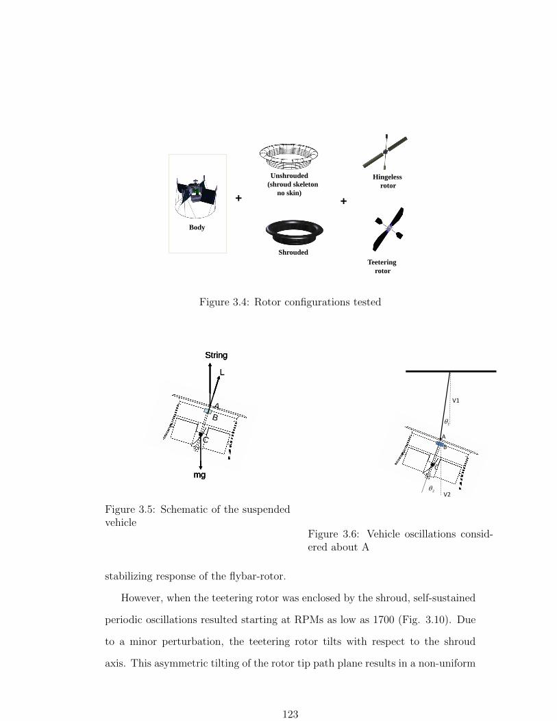
Body

Unshrouded

(shroud skeleton

no skin)

Shrouded

Hingeless

rotor

Teetering

rotor

+ +

Figure 3.4: Rotor configurations tested

A

B

C

String

mg

L

A

B

C

String

mg

A

B

C

String

mg

A

B

C

A

B

C

String

mg

L

Figure 3.5: Schematic of the suspendedvehicle

A

B

C

1

2

V1

V2

Figure 3.6: Vehicle oscillations consid-ered about A

stabilizing response of the flybar-rotor.

However, when the teetering rotor was enclosed by the shroud, self-sustained

periodic oscillations resulted starting at RPMs as low as 1700 (Fig. 3.10). Due

to a minor perturbation, the teetering rotor tilts with respect to the shroud

axis. This asymmetric tilting of the rotor tip path plane results in a non-uniform

123

Figure 3.7: Suspended unshrouded and shrouded rotor vehicles

5 10 15 20 25 30 35 40 45 50

-0.4

0

0.2

0.4

Time (s)

-0.2

Pit

ch a

ttit

ud

e

(ra

d)

Figure 3.8: Unshrouded teetering rotorup to 4000 RPM. Stable in attitude

20 25 30 35 40 45 50 55 60-0.5

-0.4

-0.3

-0.2

-0.1

0

0.1

0.2

0.3

0.4

0.5

Time (s)

Pit

ch

Att

itu

de

(ra

d)

Figure 3.9: Unshrouded hingeless rotorup to 4000 RPM. Stable in attitude

124

95 100 105 110 115 120

0

0.2

0.4

95 100 105 110 115 120

0.2

0.4

-0.2

-0.4

Time (s)

Pit

ch a

ttit

ud

e

(ra

d)

Figure 3.10: Shrouded teetering rotor (1700 RPM and upwards). Self sustainedoscillations

pressure distribution over the shroud inlet. As a result, oscillations of the vehicle

about the suspension point are induced. This is schematically shown in Fig. 3.11.

Figure 3.12 shows the variation of oscillation frequency with rotor RPM. It can

be clearly seen that there is an approximate inverse relationship between the

oscillation frequency and the rotor RPM (angular momentum). This may suggest

gyroscopic precessional effects although a detailed analysis of this phenomenon

was not performed.

It can be logically seen that a way of eliminating these periodic oscillations is to

incorporate a hingeless rotor. As expected, the shrouded flybar-hingeless rotor

(δtip = 0.03R) did not produce any oscillations at all RPMs (Fig. 3.13). Figure

3.14 shows that external disturbances in attitude get damped out effectively for

the shrouded hingeless rotor case. Another observation was that when the tip

clearance between the rotor tip and the shroud wall was not uniform azimuthally,

125

S1F

S2FS1 S2F <F

Figure 3.11: Non-uniform pressure distribution due to tilting of tip path plane(teetering rotor)

1600 1800 2000 2200 2400 2600 2800 3000 3200 34000.5

1

1.5

2

2.5

Rotor RPM

Osc

illa

tio

n f

req

uen

cy

(H

z)

Figure 3.12: Variation of oscillation frequency with rotor RPM (shrouded tee-tering rotor)

126

25 30 35 40 45 50 55 60

0.4

0.2

0

0.2

0.4

Time (s)

25 30 35 40 45 50 55 60

0.2

0

0.2

0.4

25 30 35 40 45 50 55 60

0

0.2

0.4

25 30 35 40 45 50 55 60

0

0.2

0.4

Pit

ch a

ttit

ud

e

(ra

d)

Figure 3.13: Shrouded hingeless rotor(3300 RPM)

20 25 30 35 40-0.5

-0.4

-0.3

-0.2

-0.1

0

0.1

0.2

0.3

0.4

Time (s)

Pit

ch

att

itu

de

(ra

d)

External

disturbance

Figure 3.14: Mitigation of external atti-tude disturbance (shrouded hingeless ro-tor)

self-sustained oscillations ocurred at high RPMs (greater than 3300). A possible

explanation for this is that at these high RPMs, any imbalance in the shroud

pressure distribution arising due to azimuthal non-uniformity in rotor-shroud

geometry could be pronounced enough to initiate and sustain the oscillations.

Two key conclusions derived from the above ceiling suspension tests are: (1) it

is necessary to incorporate a hingeless rotor in a shroud and minimize tip path

plane motion inside the shroud, and (2) a practical lightweight shroud design

may include non-uniformities in rotor-shroud geometry which could result in

oscillations in flight. As a result it is necessary to incorporate a closed loop

stability augmentation system to aid flight in hover.

3.4 Control System Development

This section looks at the development of a closed loop system to augment sta-

bility of the hingeless shrouded rotor vehicle in hover.

127

Yaw Gyro

Pitch and

Roll GyroBluetooth

transceiver

Triple axis

accelerometer

Sensor (analog)

board Processor (digital)

board

Weight: 30 grams

Figure 3.15: Inertial measurement unit for attitude estimation

3.4.1 Sensor

In order to provide closed loop feedback control, changes in the vehicle attitude

have to be measured. Inertial measurement unit (IMU) provides an established

method for estimating the changes in vehicle motion. It is a self contained sys-

tem and does not need information from an external source. The sensor used for

this study is a 6 degree of freedom MEMS based IMU 2. Figure 3.15 shows the

components and dimensions of the IMU. It weighs about 30 grams and is placed

on the orthogonal axes of the vehicle.

The IMU is a double decker unit with the sensor board on the top and a con-

troller board on the bottom. One IC triple axis MMA7260Q acclerometer 3, two

invensense IDG500 gyroscopes 4 are the sensors of interest that constitute the

sensor board. The controller board consists of a LPC2138 ARM7 processor that

converts the analog signal from each sensor into a 10 bit digital output with a

2www.sparkfun.com/products/8454

3www.sparkfun.com/datasheets/Accelerometers/MMA7260Q-Rev1.pdf

4www.sparkfun.com/datasheets/Components/SMD/DatasheetIDG500.pdf

128

user defined sampling frequency. The processor then concatenates the outputs

into a data packet with a head and tail bit for synchronization purposes. This

data packet is then streamed to a ground station via the integrated bluetooth

transmitter in the controller board. A sampling frequency of 200 Hz was chosen.

The accelerometer provides translational accelerations of the vehicle in the X,Y

and Z axes in the body frame including gravity. Therefore by suitable transfor-

mations, the total acceleration vector of the body in inertial space can be mea-

sured. If the body were stationary in space and merely tilting, the accelerometer

would provide information of the component of the gravity in the X,Y and Z

direction. It would hence act as an inclinometer. For hover control purposes, it

is reasonable to assume that translational accelerations will be minimal. Hence

the acclerometer is treated as an inclinometer. Calibration was done by individ-

ually aligning the gravity vector along each axis of the accelerometer. This was

determined to be 0.004gs2/m at a 6 ‘g’ sensitivity setting.

The gyroscopes provide the angular rates (p, q, r) of the vehicle about the X,Y

and Z axes in the body frame. Calibration of the gyroscope was done using

a stepper-motor rotary table5 (Fig. 3.16). The IMU was placed on the table

such that the axis of rotation aligned with each gyro axis. The gyro response

was constant for a given rotation speed (Fig 3.17(a)) and increased linearly with

speed (Fig 3.17(b)). The calibration for each gyro axis was found to be 0.03

rad/s.

5provided by the Autonomous Vehicle Lab, UMD

129

Rotary platform

Figure 3.16: Rotary platform for gyro calibration

0 5 10 15 20 25280

300

320

340

360

380

400

420

440

460

480

Time (sec)

Gy

ro r

aw

da

ta

(a) Gyro response to a constant rotation rate

-180 -160 -140 -120 -100 -80 -60 -40 -20 0-1

0

1

2

3

4

5

6

Gyro response

Pla

tfo

rm s

pe

ed

(ra

d/s

ec

)

(b) Calibration of gyro

Figure 3.17: Gyroscope response to rotational input

130

3.4.2 Attitude estimation

The two frames of reference of concern are the inertial frame and the body frame.

In order to estimate the absolute vehicle orientation, the data from the IMU in

the body frame have to be converted to in the inertial frame. Assume the vehicle

axes to be initially aligned with a fixed observer axis. After a certain maneuver,

the vehicle takes a new position (as shown in Fig. 3.18). In order to estimate

the vehicle orientation from IMU data, a transformation is required to convert

the initial fixed axes to the final body axes. For this study, the aircraft 3-2-1

sequence using Euler angles is employed.

XI

YI

ZI

XB

YB

ZB

Inertial frame

(Before maneuver)

Body frame

(After maneuver)

Figure 3.18: Vehicle orientation during maneuver

3.4.2.1 Rotation transformation

Let xI , yI , zI be the initial frame of reference (observer) and xB, yB, zB be

the final body frame of reference. These two frames can be related to each

other by three Euler angles: ψ (yaw angle), θ (pitch angle) and φ (roll angle).

The orientation change between the frames is divided into a sequence of three

rotations (Fig. 3.19).

131

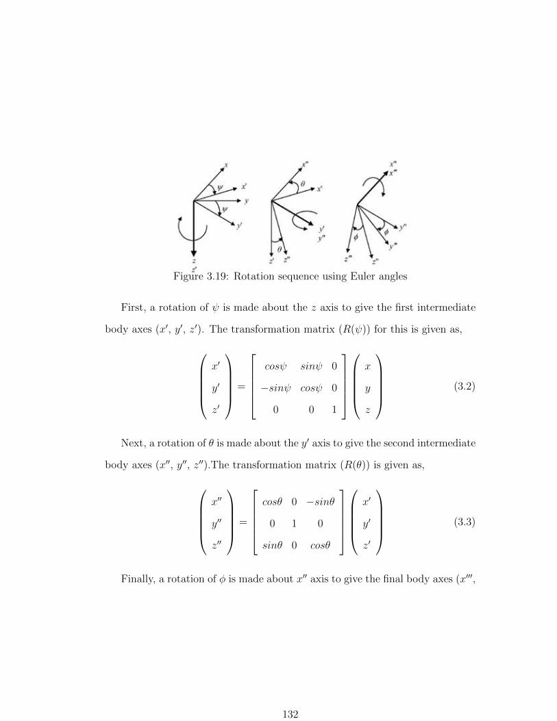
Figure 3.19: Rotation sequence using Euler angles

First, a rotation of ψ is made about the z axis to give the first intermediate

body axes (x′, y′, z′). The transformation matrix (R(ψ)) for this is given as,

x′

y′

z′

=

cosψ sinψ 0

−sinψ cosψ 0

0 0 1

x

y

z

(3.2)

Next, a rotation of θ is made about the y′ axis to give the second intermediate

body axes (x′′, y′′, z′′).The transformation matrix (R(θ)) is given as,

x′′

y′′

z′′

=

cosθ 0 −sinθ

0 1 0

sinθ 0 cosθ

x′

y′

z′

(3.3)

Finally, a rotation of φ is made about x′′ axis to give the final body axes (x′′′,

132

y′′′, z′′′) or (xb, yb, zb). The transformation matrix (R(φ)) is given as,

x′′′

y′′′

z′′′

=

1 0 0

0 cosφ −sinφ

0 sinφ cosφ

x′′

y′′

z′′

(3.4)

The equivalent transformation from x, y, z to xb, yb, zb is obtained by multi-

plying the individual transformation matrices R(φ),R(θ) and R(ψ) in that order

to give R(φ, θ, ψ),

xb

yb

zb

=

cθcψ cθsψ −sθ

−sψcφ+ sθsφcψ cψcφ+ sψsθsφ sφcθ

sψsφ+ sθcφcψ −cψsφ+ sψsθcφ cφcθ

x

y

z

(3.5)

An important property of these transformation matrices is that they are

orthonormal. This implies that the inverse transformation (from body to iner-

tial frame) can be easily obtained by taking a transpose of the rotation matrix

R(φ, θ, ψ).

3.4.2.2 Attitude estimation from gyroscope

It can be seen that the above rotation matrix provides a transformation between

two frames of reference at a given instant in time. For a continuous vehicle

motion, the Euler angles are time dependent. The rate of change of the Euler

angles are ψ, θ and φ respectively. Therefore, a first order time marching scheme

133

can be used to update the Euler angles as shown below,

ψ(t+ δt) = ψ(t) + ˙φ(t)δt

θ(t+ δt) = θ(t) + ˙θ(t)δt

φ(t+ δt) = φ(t) + ˙ψ(t)δt (3.6)

In order to estimate the Euler rates, an appropriate transformation of the gyro

angular rates has to be performed. The angular velocity ω provided by the gyro

data is

ω = pxb + qyb + rzb (3.7)

Equivalently, ω can also be expressed in terms of the Euler rates,

ω = ψxb + θy′′ + φz (3.8)

Using Eqs. (3.2), (3.3), (3.4), (3.7) and (3.8), the Euler rates can be expressed

in terms of the body rates measured by the gyro as,

φ

θ

ψ

=

1 sinφtanθ cosφtanθ

0 cosφ −sinφ

0 sinφcosθ

cosφcosθ

p

q

r

(3.9)

From the above equation, it can be seen that a drawback of the Euler angle

method is the singularity that occurs at θ = 900. In applications where high

values of pitch angle are expected to occur, a different way of measuring the

orientation will be required (Quarternions, Euler parameters etc). Since hover

flight is of interest in this study, the pitch angle is expected to be small. The

Euler angles can then be updated using Eqs. (3.9) and (3.6).

134

3.4.2.3 Attitude estimation using accelerometer

As discussed earlier, the accelerometers used for this study are used as inclinome-

ters. This implies, the changes in the component of gravity along the body axes

are registered by the accelerometer. Here, ax, ay and az are the components of

the gravity vector along xb, yb and zb axes respectively. Using the transformation

matrix (Eq. (3.5)) we get,

ax = −gsinθ

ay = gsinφcosθ

az = gcosφcosθ (3.10)

The pitch and roll angles can therefore be extracted as,

θ = sin−1−axg

φ = tan−1ayaz

(3.11)

3.4.2.4 Complementary filter

The last two sections discussed the extraction of Euler angles from two sources:

gyroscope and accelerometer. Each sensor has specific limitations when used

alone. The gyroscope is prone to drift in gyro bias. Integration of gyro data

will result in a rapid growth in error of the Euler angle estimate (as high as 1

deg /s for low cost MEMS gyros). Therefore it is not suitable for extracting low

frequency information. On the other hand, accelerometers are highly sensitive

to vibration (especially so in a rotor environment). Low pass filtering will cause

significant phase delays. As a result, accelerometers are not suitable for measur-

135

ing high frequency motion.

These limitations were illustrated using a pendulum set-up shown in Fig. 3.20

The IMU is placed about 10 inches below the axis of rotation. A shaker is at-

Potentiometer

IMU

Shaker

Figure 3.20: Pendulum set-up to compare gyro and accelerometer measurements

tached to the end of the pendulum to provide an adjustable oscillation input

to the pendulum. The gyro and accelerometer data were sampled at 200 Hz.

The attitude estimates from these sensors were compared to the output of a

potentiometer placed on the pendulum axis. A comparison between pitch an-

gle measurements by the gyro, accelerometer and potentiometer is shown for a

steady pitch hold case (Fig. 3.21(a)) and for an oscillatory case (Fig. 3.21(b)).

It can be clearly seen that the accelerometer provides accurate estimates when

the IMU is held steady. These estimates deteriorate at high frequencies. The op-

posite is true for the gyroscope. When the IMU is oscillating, the gyro readings

capture the high frequency motion satisfactorily wheras the gyro drift corrupts

the angular measurements when the IMU is held steady (or in low frequency

motion).

In order to combine the favourable high frequency characteristics of the gyro

136

2 4 6 8 10 12

0

5

10

15

20

25

30

35

40

Time (sec)

An

gle

(d

eg

)

Potentiometer

Gyroscope

Accelerometer

(a) Pitch-hold case

0 5 10 15 20 25 30-60

-40

-20

0

20

40

60

80

Time (s)

An

gle

(d

eg

)

Potentiometer

Accelerometer

Gyroscope

(b) Oscillating case

Figure 3.21: Attitude estimate comparison between gyro, accelerometer andpotentiometer

and low frequency response of the accelerometer, a complementary filter is used

as shown in Fig. 3.22 to provide the best estimation of the orientation. The

accelerometer data is filtered using Ga(s) to provide the low frequency estimate

of attitude and the gyro output is fed to Gg(s) to provide the high frequency

attitude estimate. A combination of the two provided the complementary filter

estimate of the attitude. For the study, a first order low and high pass filter was

found to be sufficient. The cut-off frequencies were 7 and 5 Hz respectively.

Gg(s) =4s

(2s+ 1)2

Ga(s) =4s+ 1

(2s+ 1)2(3.12)

Figure 3.23 shows a comparison between the complementary filter estimate

and the potentiometer measurement for the pendulum experiment. It can be

137

sGg(s)High pass

Ga(s)Low pass

Figure 3.22: Complementary filter for attitude estimation

seen that the resulting complementary filter output matches satisfactorily with

the potentiometer reading.

0 2 4 6 8 10 120

5

10

15

20

25

30

35

40

Time (sec)

An

gle

(d

eg

)

Potentiometer

Comp filter

(a) Pitch-hold case

0 5 10 15 20 25 30-60

-40

-20

0

20

40

60

80

Time (sec)

An

gle

(d

eg

)

Potentiometer

Complimentary Filter

(b) Oscillating case

Figure 3.23: Attitude estimate comparison between complementary filter outputand potentiometer

Data from the two sensors were used to provide pitch and roll attitude esti-

mates. An available secondary sensor for yaw attitude was the magnetometer.

However, data fusion of the yaw gyro and the magnetometers was not found to

be suitable. This was due to the fact that the magnetometer bias and sensitivity

138

were affected by the electromagnetic interference from the motor (Fig. 3.24).

Additionally, integration on the yaw gyro data was not performed. Later on,

flight tests demonstrated that yaw rate information was sufficient for yaw stabi-

lization.

0 5 10 15 20 25 30 35 40 45 50-0.25

-0.2

-0.15

-0.1

-0.05

0

0.05

0.1

0.15

Time (s)

No

rma

lize

d m

ag

re

ad

ing

Rotor off

Rotor on

00 Heading900

00 Heading

900

Bias change

due to motor EMI

Figure 3.24: Magnetometers not suitable for heading feedback

In conclusion, the vehicle states used for feedback control were φC , θC and ψg.

3.4.3 Telemetry

Figure 3.25 shows the data communication set-up for the off-board vehicle control

system. A ground station processes the IMU data. A change in vehicle state

triggers a control algorithm to initiate feedback action via signals generated by

a microcontroller. The signals are uplinked to an onboard radio receiver via the

trainer channel of an RC transmitter.

Off-board processing: The concatenated serial output from the gyros and

139

22

1

3Pulse code

IMU records

attitude change

Control box

generated

Servos respond

Bluetooth

72 MHz Radio

signal

Pulse code

IMU records

attitude change

Control box

generated

Servos respond

Bluetooth

72 MHz Radio

signal

1

3

Figure 3.25: Telemetry of the control system set-up

accelerometers are downlinked wirelessly via Bluetooth from the IMU to a bases-

tation for additional processing (Eqs. (3.6) - (3.12)). The reason for employing a

ground based setup is to enable minimal onboard processing. The ground station

can utilize faster processors and also enable monitoring of the data graphically.

This can be very useful for debugging purposes. Integration of an onboard con-

troller was also later achieved but is not described here to remain within scope.

The basestation processes the errors in vehicle attitude, and computes corrective

signals.

Signal pulse generation and transmission: It is then sought to emu-

late these corrective signals into stick commands just like a human pilot would

produce using the standard radio-control transmitter and receiver. The radio-

control (RC) transmitter (Fig. 3.26) converts the control stick movements and

bundles it serially into a multi channel signal. This coded radio signal car-

140

ries information from the control channels (pitch, roll, throttle and yaw) and

additional programmable channels. A typical RC transmitter codes about 5-8

channels. The structure of the signal is shown in Fig. 3.27. Typically the nor-

mal state of the pin is high and each signal frame has a width between 20-22

ms and the number of inverted pulses is equal to the number of channels. The

width of the first pulse corresponds to the position of the first servo and so on.

Each channel frame consists of two parts - a fixed time Tf 0.5 ms and a variable

time Tv 1 − 2 ms. So when a control input is given, Tv is varied. The space

between the pulse relating to the final channel and the start of the next frame

is called the synchronization time. This coded signal is referred to as a pulse

position modulated (PPM) signal. The PPM signal is transmitted wirelessly

to a receiver module installed on the vehicle. The transmission is done using

frequency modulation (intially at 72 MHz, later replaced with 2.4 GHz).

Throttle

Yaw

Pitch

Roll

Additional

channelsTrainer

switch

Antenna

Figure 3.26: Radio control transmitterinterface

20 - 22 ms

Ch1 Ch2 Ch3 Ch4

Channel width:

1 – 2 ms

Channel gap:

0.4 – 0.5 ms

Synchronization gap

Figure 3.27: Pulse position modulated(PPM) signal from transmitter

The generation and sampling of these high frequency PPM signals is time

critical and cannot be done by a PC running on a non-real time operating system.

141

To achieve this, a microcontroller is interfaced with the PC. This is cheaper and

faster to implement and simplifies application development using LabVIEW. A

PIC 18F8722 microcontroller was used for this purpose. The PIC individually

communicates with the PC (using a RS232 serial port) and with the transmitter

data port (from pins A4 and A5 on the PIC) . The microcontroller receives the

corrective signals from the basestation and converts it to a PPM signal that can

be wirelessly transmitted by flipping a trainer switch (Fig: 3.26). This set-up

was chosen since it provides system redundancy. Should the control system fail,

the vehicle can be reverted back to manual control.

Receiver and actuator: The purpose of the receiver is to decode the radio

PPM signal into pulse width modulated (PWM) signals. The individual PWM

signals are then fed into the pitch, roll, yaw servo actuators and speed controller

(for rotor RPM variation). The servo motor consists of a servo circuit, that

drives a motor to whose output shaft is connected a lever arm that tilts the

swashplate. The servo circuit interprets the width (Tv) as the amount of angular

rotation of the motor shaft. A potentiometer is used as a feedback element for

this purpose.

Latency: An important consideration for this set-up is the time delay (la-

tency) between stages 1 and 4 (Fig. 3.25) since this can affect the control system

bandwidth. The latency was experimentally determined using the set-up shown

in Fig. 3.28. The IMU and a potentiometer were attached to a pendulum. A

change in state of the IMU was instantly recorded by the potentiometer. A

control law was invoked such that the servo responded to any disturbance in the

IMU position. This servo response was instantly recorded by a laser displace-

ment sensor. A comparison in time history between the potentiometer and the

laser displacement sensor provided an estimate of the lumped time delay.

142

The average time delay between stages 1 and 4 was measured to be about 95

ms (Fig. 3.29). Table 3.1 presents estimates of the delays between each stage.

These estimates were compiled from various sources such as Avanzini [144]. It

can be seen that this compared well with the experimental latency measurement.

The time delay reduces the phase margin of the closed loop system. Tischler [47]

relates the control system bandwith to the lumped time delay as,

ωBW =0.37

τdelay(3.13)

This translated to a bandwidth of about 3.7 rad/s for the closed loop system.

Experimental flight testing indicated that the vehicle open loop rigid body modes

did not exceed 3 rad/s. The effectiveness of the present telemetry system for

closed loop control is therefore verified.

Receiver

Servo

Laser

displacement

sensor

IMU

Potentiometer

Receiver

Servo

Laser

displacement

sensor

IMU

Potentiometer

Figure 3.28: Lumped time delay measurement in telemetry system

Table 3.1: Time delay estimates (breakdown)Stage Delay estimate (ms)

IMU-Computer 25Processing 5-10

Transmitter-receiver 25-30Receiver-servo response 30

Total 85-95

143

IMU change

Servo response

Delay

IMU change

Servo response

Delay

Figure 3.29: Delay between IMU state change and subsequent servo response

3.4.4 Control feedback configuration

For autonomous hover flight of TiShrov, a suitable control algorithm must be

determined. For manual control, the pilot applies lateral, longitudinal cyclic and

vane inputs for changing the vehicle attitude in roll, pitch and yaw respectively.

For a full envelope flight, it is important to take into account the coupling be-

tween different axes and non-linear dynamical effects. However for the present

study, since near hover flight is of concern, the roll, pitch and yaw inputs are

treated as uncoupled and a linear single-input single-output (SISO) proportional-

integral-derivative (PID) controller was chosen and expected to give satisfactory

flight control results. The schematic of the PID control scheme is shown in Fig.

3.30.

It can be seen that the control loop is divided into two parts: inner (attitude)

and outer (translation) loop. The inner loop, which has a high bandwidth forms

the core of the controller and interacts directly to achieve the desired attitudes.

144

Figure 3.30: PID control scheme for hover control of TiShrov

The outer translational loop (lower bandwidth) is the secondarly controller which

develops translation commands through a generation of primary attitude com-

mands. From Sec. 3.4.1, the extraction of the attitude rates (p, q, r) and the

Euler angles (φ, θ, ψ) was described. The fundamental limitation of obtaining

translation velocity estimates for outer loop feedback is the integration of ac-

celerometer data. It is a well observed phenomenon that due to the acelerometer

noise levels, any integrated data will develop errors that would grow with time.

Figure 3.31 shows the drift in velocity estimates obtained through an integra-

tion of the accelerometer data with and without a low pass filter. A simplified

theoretical analysis [163] indicates that the error in estimated velocity for a sta-

tionary accelerometer is α√T where T is the integration time and α depends on

the standard deviation of the accelerometer noise and sampling frequency of the

data.

145

0 20 40-1

-0.5

0

0.5

1

1.5

m/s

ec

2

Xacc

10 hz low pass filter

0 20 40-1

0

1

2

Unfiltered Xacc

0 20 40-10

0

10

20

30

Time (sec)

cm

/se

c

Integrating filtered Xacc

0 20 40-10

0

10

20

30

Time (sec)

Integrating unfiltered Xacc

Figure 3.31: Error in velocity estimate from integrating accelerometer data

A common approach to overcome this is to periodically compare and re-

set the integrated data to an external reference. It was found that external

velocity/pressure sensors did not have sufficient resolution for the present appli-

cation in addition to the possibility of incorrect estimates due to effects of rotor

downwash. Other potential techniques of position/velocity feedback suitable for

indoor applications such as optic flow, visual feedback and Markov localization

techniques were beyond the scope of the present study and are not considered.

Therefore, only inner loop control was considered as shown in Fig. 3.32

Ziegler-Nichols PID gain tuning: The gains Kp, Ki, Kd are the proportional,

integral and derivative gains in the feedback loop with respect to each of the Euler

146

Figure 3.32: Inner loop feedback control

angles. Let e(t) be the deviation in vehicle pitch attitude from hover. Then,

e(t) = desired− θmeasured(t)

= −θmeasured(t) (3.14)

The PID controller in s-domain is,

Gc(s) = Kp

(1 +

1

Tis+ Tds

)(3.15)

where, Ti is the integration time and Td is the derivative time. Therefore, the

resulting controller action in time domain due to the pitch attitude error is,

Gc(t) = Kpe(t) +Ki

∫ t

0

e(τ)dτ +Kdde

dt(3.16)

147

Here the derivative gain Kd and the integral gain ki are related to Td and Ti as,

Ki =Kp

TiKd = KpTd (3.17)

In order to determine the gains for appropriate control action, the Ziegler-Nichols

method of gain-tuning is followed. Here, based on experimental step response,

the gains that result in marginal stability are chosen. The rules give a first-order

estimage of the gain values and provide a starting point for finer tuning. First,

the proportional gain is increased up to a critical value Kcr when the output

exhibits sustained oscillations. The period of these oscillations is Pcr. Once the

critical gain and corresponding period are experimentally determined, the values

of the different gains are chosen based on the rules shown in Table. 3.2

Table 3.2: Ziegler-Nichols Tuning MethodController Kp Ti Td

P 0.5Kcr ∞ 0PI 0.45Kcr 0.83 Pcr 0

PID 0.6Kcr 0.5Pcr 0.125Pcr

3.5 Bench-top test results

Prior to free flight hover tests, the controller was tested on different bench-top

configurations: (1) servo set-up, (2) pitch, roll DOF, and (3) yaw DOF.

148

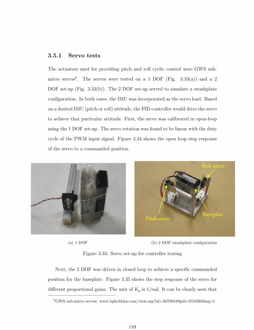
3.5.1 Servo tests

The actuators used for providing pitch and roll cyclic control were GWS sub-

micro servos6. The servos were tested on a 1 DOF (Fig. 3.33(a)) and a 2

DOF set-up (Fig. 3.33(b)). The 2 DOF set-up served to simulate a swashplate

configuration. In both cases, the IMU was incorporated as the servo load. Based

on a desired IMU (pitch or roll) attitude, the PID controller would drive the servo

to achieve that particular attitude. First, the servo was calibrated in open-loop

using the 1 DOF set-up. The servo rotation was found to be linear with the duty

cycle of the PWM input signal. Figure 3.34 shows the open loop step response

of the servo to a commanded position.

(a) 1 DOF (b) 2 DOF swashplate configuration

Figure 3.33: Servo set-up for controller testing

Next, the 2 DOF was driven in closed loop to achieve a specific commanded

position for the baseplate. Figure 3.35 shows the step response of the servo for

different proportional gains. The unit of Kp is 1/rad. It can be clearly seen that

6GWS sub-micro servos: www.bphobbies.com/view.asp?id=A0780189pid=S510303img=l

149

5 10 15-0.05

0

0.05

0.1

0.15

0.2

0.25

0.3

0.35

0.4

0.45

Time (sec)

Co

mm

an

de

d p

os

itio

n (

rad

)

Figure 3.34: Open loop step response of servo

as the value of Kp increases, the system damping reduces as Kp increases, and

the servo exhibits undampled oscillations at a Kcr. Based on Ziegler-Nichols

tuning method, a value of Kp/2 was chosen. It can also be seen that there is

a steady state error between the final swashplate position and the commanded

position. Figure 3.36 shows the variation of the steady state error with pro-

portional gain. it can be seen that this error reduces as the proportional gain

increases. The steady state error at a chosen value of Kp was eliminated by

including an appropriate integral gain Ki. This is shown in Fig. 3.37. The

overshoot in servo response can be reduced by incorporating Kd. However due

to undesirable spikes in servo response arising from data noise, the differential

control was discarded.

3.5.2 Pitch and roll DOF gimbal tests

The controller was next tested in the vehicle configuration in pitch and roll

degrees of freedom. In order to achieve this, the vehicle was mounted on a

gimbal stand as shown in Fig. 3.38. The gimbal stand would permit attitude

150

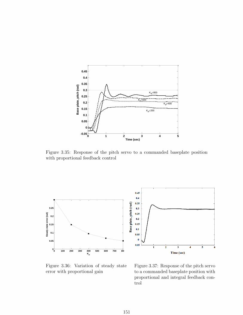
0 1 2 3 4 5-0.05

0

0.05

0.1

0.15

0.2

0.25

0.3

0.35

0.4

0.45

Time (sec)

Ba

se

pla

te, p

itc

h (

rad

)

KP=800

KP=600

KP=400

KP=200

Figure 3.35: Response of the pitch servo to a commanded baseplate positionwith proportional feedback control

0 100 200 300 400 500 600 700 8000

0.05

0.1

0.15

0.2

0.25

KP

Ste

ad

y s

tate

err

or

(ra

d)

Figure 3.36: Variation of steady stateerror with proportional gain

Figure 3.37: Response of the pitch servoto a commanded baseplate position withproportional and integral feedback con-trol

151

control tests to be carried out safely without the danger of crashing or running

out of indoor space. The gimbal ring was constructed from rigid, low density

industrial foam. Two sets of delrin bearings were inserted into the gimbal to

form the outer and inner axis of the gimbal (Fig. 3.39). Care was taken to

ensure that the pitch and roll axes of the gimbal coincided with the C.G. of the

vehicle. Even with the foam design, the pitch and roll inertias of the vehicle with

the gimbal had increased by up to 100%. In addition, taking the damping effect

of friction in the gimbal bearings into consideration, it is clear that the gimbal

stand does not completely simulate free flight conditions. Nevertheless, this was

viewed to be an important test for the controller prior to free flight tests. When

the vehicle was commanded for hover attitude with proportional feedback, it

was seen that the controller was able to achieve zero pitch and roll states of

the vehicle. Additionally the response to external disturbance was satisfactory

(Fig. 3.40). The disturbance was mitigated within about 4 seconds. Figure 3.41

shows the response of the vehicle to a pitch attitude command with external

disturbances using a PI controller. It can be seen that the vehice was able to

successfully achieve attitude hold as well as reject disturbances.

3.5.3 Yaw DOF tests

In order to test for control in yaw DOF, the vehicle was mounted on the stand

shown in Fig. 3.42. The vehicle was connected to a shaft that was mounted on

two radial bearings. It was ensured that the C.G of the vehicle lay on the shaft

axis. A disturbance in yaw was sought to be mitigated. As discussed earlier,

an appropriate feedback state for the yaw DOF was chosen to be the yaw rate.

Figure 3.43 shows the performance of the proportional (in yaw rate) feedback

152

Figure 3.38: Vehicle mounted on gimbal to test pitch/roll control

Outer

bearing

Inner

bearing

Figure 3.39: Inner and outer bearings on gimbal set-up, top view

153

30 40 50 60 70 80-0.5

0

0.5

Ro

ll,

(ra

d)

30 40 50 60 70 80-0.5

0

0.5

Time (s)

Pit

ch

, (

rad

)

Disturbance

Figure 3.40: Vehicle stabilized for hover in gimbal stand with P controller

0 10 20 30 40 50 60 70-0.5

-0.4

-0.3

-0.2

-0.1

0

0.1

0.2

0.3

0.4

0.5

Time (s)

Pit

ch

, (

rad

)

Disturbance

Position Control

Command

Figure 3.41: Vehicle commanded for pitch attitude in gimbal stand with PIcontroller

154

controller in mitigating yaw disturbances. It was seen that the vehicle control

response in yaw was acceptable.

Radial

bearings

Figure 3.42: Test stand for yaw control

30 35 40 45 50 55 60 65 70-10

-8

-6

-4

-2

0

2

4

6

8

10

Time (sec)

r (r

ad

/se

c)

Controller

switched on

External perturbations to

vehicle yaw

Figure 3.43: Yaw stabilization of the vehicle with proportional control

155

3.5.3.1 Effect of ground on anti-torque capability of vanes

Based on observation and pilot feedback during manual flight testing of the ini-

tial prototypes (Sec. 2.7), it was noticed that the anti-torque capability of the

vanes when operated in ground effect (IGE) was reduced. A possible explanation

for the deteriorated yaw control authority IGE is illustrated in Fig. 3.44. With

ground proximity, the pressure in the center of the rotor downwash increases.

This has two effects: (1) inflow velocity through the rotor decreases, and (2)

the rotor downwash is pushed radialy outward. A combination of these fac-

tors is probably responsible for the degradation in vane effectiveness in ground

effect. This effect was studied through unconstrained (string suspension) and

constrained set-ups. TiShrov was used for these studies since the presence of

the hingeless rotor and shroud was favorable for performing string suspension

studies.

Figure 3.44: Loss of vane effectiveness in ground effect (IGE)

Unconstrained setup to study vehicle yaw authority: The vehicle was

suspended by a string fixed to a carbon rod that was attached to the shroud

156

structure (Fig. 3.45). The height of the vehicle above the ground was varied

from IGE to OGE (out of ground effect) condition. The IMU yaw rate data

and rudder-throttle input from the transmitter was recorded. Yaw rate response

of the vehicle as a function of height was recorded. Also measured were the

pilot throttle and rudder stick inputs. Extra weight was added to the vehicle

to prevent string slackening. The rudder input was symmetrically swept about

the mean position in clockwise and anti-clockwise rotation. The rotor was spun

in the anti-clockwise direction (looking from top). As expected, a significant

difference in vehicle yaw response was observed between IGE (Fig. 3.46(a)) and

OGE conditions (Fig. 3.46(c)). With maximum control deflection, the vanes

were not able to counter the rotor torque in ground effect (height above ground

z/R = 1.3. It was seen that yaw authority improved as the vehicle came out of

ground effect. A maximum yaw rate of about 1.8-2 rad/s was attainable.

IMU – Yaw rate info

Low torsion stiffness

String

Support

IMU – Yaw rate info

Low torsion stiffness

String

Support

Figure 3.45: Yaw rate measurement as a function of height above ground

Constrained set-up to study yaw authority: By adjusting the vane an-

gle settings, it might be possible to achieve bi-directional yaw control for both

157

0 5 10 15 20 25 30 35 40 45 50-4

-2

0

2r

(rad

/sec)

0 5 10 15 20 25 30 35 40 45 500

50

100

Th

rott

le %

0 5 10 15 20 25 30 35 40 45 500

50

100

Time (sec)

Ru

dd

er

%

-ve vane

deflection

+ve vane

deflection

(a) z/R = 1.3

0 5 10 15 20 25 30 35 40 45 50-2

0

2

r (r

ad

/sec)

0 5 10 15 20 25 30 35 40 45 500

50

100

Th

rott

le %

0 5 10 15 20 25 30 35 40 45 500

50

100

Time (sec)

Ru

dd

er

%

(b) z/R = 1.9

158

0 5 10 15 20 25-2

0

2

r (r

ad

/sec)

0 5 10 15 20 250

50

100

Th

rott

le %

0 5 10 15 20 250

50

100

Time (sec)

Ru

dd

er

%

(c) z/R = 2.5

Figure 3.46: Effect of height above ground and rudder input on yaw rate (clock-wise: -ve yaw rate)

IGE and OGE conditions. This was tested in an experimental set-up illustrated

in Fig. 3.47. Maximum obtainable body torque from vane deflections was mea-

sured as a function of height above ground. From Fig. 3.48, it can be observed

that in OGE condition, the vehicle trimmed in yaw. This implied equal control

authority in clockwise and counterclockwise directions. Such was not the case

when the vehicle operated closer to the ground. It can be seen that for a fixed

vane and undeflected control vane setting of 23 and 16 deg respectively, equal

bi-directional yaw authority was achieved in OGE condition (Fig. 3.49). How-

ever, for the IGE condition, the vane angles had to be increased. Thus for a

given vane setting similar yaw authortiy cannot be achieved in IGE and OGE

conditions. Based on the above study, the vane pitch setting was appropriately

varied depending on the region of operation (IGE or OGE). Additionally, for an

159

OGE vane setting, fast take-off would be required for free flight testing to avoid

undesirable loss of yaw control in ground effect.

Figure 3.47: Set-up to measure effect of ground on vane effectiveness: constrainedin yaw

3.6 Free Flight Test Results

In the constrained tests described in the previous section, the controller was

tested to be effective in controlling the vehicle pitch, roll and yaw degrees of

freedom. However, the system parameters and conditions still differed from the

free flight case. It was therefore important to further test the controller in two

steps: First, with a couple of unshrouded teetering rotor vehicles that were

known to be open loop stable. Finally, to install the shroud and perform closed

loop flight tests. The first configuration tested was GIANT (described in Sec.

2.7). It is an unshrouded teetering rotor vehicle with anti-torque vanes. The trim

inputs for hover were initially determined from piloted flight tests. Proportional

160

0 500 1000 1500 2000 2500 3000

-0.01

-0.005

0

0.005

0.01

RPM

To

rqu

e (

N-m

)

z/R = 1.3

z/R = 1.5

z/R = 1.9

z/R =

(a) Vanes undeflected

0 500 1000 1500 2000 2500 3000

-0.01

-0.005

0

0.005

0.01

RPM

To

rqu

e (

N-m

)

z/R = 1.3

z/R = 1.5

z/R = 1.9

z/R =

(b) vanes deflected

Figure 3.48: Loss of vane effectiveness as vehicle approaches ground

161

8 10 12 14 16 18 20 22 24

-0.015

-0.01

-0.005

0

0.005

0.01

0.015

Control vane angle of attack (deg)

To

rqu

e (

N-m

)

Fixed vane angle

of attack ~ 230

IGE

OGE

Yaw Trim

Figure 3.49: Bi-directinal yaw authority IGE and OGE

feedback based on the vehicle pitch and roll attitude was superimposed on the

trim inputs. Closed loop control tests were then performed. Figure 3.50 shows a

snapshot of GIANT in free flight hover. The performance of the controller was

satisfactory when the trim inputs were exact (Fig. 3.51). However, in practice,

trim values changed due to vehicle crashes that resulted changes in CG position.

As a result, the controller operated on an erroneous trim input, and hover

attitude was not maintained (Fig. 3.52). This can be eliminiated by adding

integral control (Figs. 3.53, 3.54). It should be mentioned that integral feedback

reduces the stability margin of the closed loop system. It is therefore not a

preferred technique, if the trim inputs are known.

With the controller successfully tested on GIANT, the next configuration

that was tested for free flight was the unshrouded version of TiShrov (Fig. 3.55).

The procedure for controller testing was followed similar to that mentioned for

GIANT. Care was taken to maintain consistency in trim values to avoid the need

for inclusion of integral control. It can be seen from Figs. 3.56 and 3.57 that the

162

Figure 3.50: Bi-directinal yaw authority IGE and OGE

Figure 3.51: Hover control of GIANT with no trim disturbance. Proportionalcontrol.

Figure 3.52: Hover control of GIANT with pitch forward trim disturbance. Pro-portional control.

163

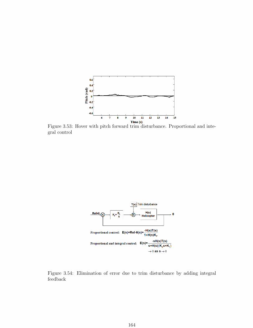
Figure 3.53: Hover with pitch forward trim disturbance. Proportional and inte-gral control

Figure 3.54: Elimination of error due to trim disturbance by adding integralfeedback

164

vehicle achieved stable free flight hover.

Figure 3.55: Unshrouded TiShrov

Figure 3.56: Free flight closed loop hover control. Proportional feedback

Next, flight tests were conducted with the shrouded rotor vehicle TiShrov.

The vehicle was tested with a hingeless rotor with a tip clearance of 3.2%R. A

series of trial and error tests were conducted to determine trim inputs such that

the vehicle lifted off vertically. With zero to low proportional gains, it can be

clearly seen that the vehicle was not stable (Fig. 3.58). The free flight rigid body

165

Figure 3.57: Hover control of unshrouded TiShrov

oscillation was about 0.5 Hz. As the gains were increased to between 50-80%

of the stick input range per radian, good hover performance was achieved with

very minimal oscillations about zero state (Figs. 3.59 and 3.60). However, once

the gains were increased further (>100% of the stick input range per radian),

the effect of reduced damping described earlier was observed (Fig. 3.61). It was

seen that the rigid body oscillation frequency increased to about 0.9 Hz at high

gains. The Ziegler-Nichols tuning criteria set the proportional gain to about 60%

of the stick input range per radian.

TiShrov was also found to be sensitive to ground effect. It was observed that

on a few occasions, upon slow rotor start up, the vehicle went into ground-effect-

induced instability and failed to gain altitude. As a result, fast start ups were

done, which solved the problem. Figure 3.62 shows the oscillations arising from

ground effect and the correction for attitude from the controller as soon as the

vehicle gained altitude.

166

Figure 3.58: Low proportional gain: <20% stick input range/radian. Poor hover.

Figure 3.59: Stable hover control of TiShrov

Figure 3.60: Medium proportional gain: 50-80% stick input range/radian. Sat-isfactory hover.

167

Figure 3.61: High proportional gain: >120% stick input range/radian. Unstablehover.

Figure 3.62: Controller works satisfactorily as soon as vehicle comes out ofground effect

168

3.7 Summary

From tests that studied passive stability of the shrouded rotor system, it was

seen that with a teetering rotor system, the shrouded rotor exhibited limit cy-

cle oscillations. Therefore it is necessary to incorporate a hingeless rotor in

a shroud to minimize tip path plane motion inside the shroud. A practical

lightweight shroud design may include non-uniformities in rotor-shroud geome-

try which could result in oscillations in flight. Therefore a closed loop stability

augmentation system is required to aid flight in hover. A closed loop feedback

system with wireless telemetry was implemented which had a latency of about

95 ms. This was seen to provide satisfactory closed loop performance in pitch,

roll and yaw using a proportional-integral-derivative feedback controller. The

various gains were determined using the Ziegler Nichols method. The shrouded

rotor vehicle performed satisfactorily in free flight hover. To prevent ground

effect induced instability, it was important to conduct fast lift-off of the vehi-

cle. Constrained and unconstrained tests of the vehicle yaw control indicated

that the control authority of the anti-torque vanes deteriorated in ground effect

(IGE). This is possibly due to the fact that in IGE conditions, the downwash

velocity is reduced and the region of flow over the vanes decreases.

169

Chapter 4

Attitude Dynamics Identification in

Hover

4.1 Overview

In the previous chapter, the hover flight tests of the vehicle incorporating a

phased Hiller bar (flybar) was discussed. A PID controller was used to satisfac-

torliy obtain stable hover in free flight. In this chapter, the attitude dynamics

of the shrouded rotor vehicle is studied about hover as the equilibrium condi-

tion. The salient advantages and drawbacks of incorporating a flybarless rotor

are discussed. The vehicle is constrained in translation to remove the effects

of translation on vehicle attitude. System identification of the vehicle is con-

ducted in the time domain, based on a reduced order attitude dynamics model.

The effect of the flybar and the flybarless rotor on the attitude dynamics is de-

scribed. Finally a model based controller framework is incorporated using the

derived model from system identification. This would serve as a platform for

incorporating an extended 6-DOF vehicle model in the future.

170

4.2 Rigid Body Equations of Motion

Consider the vehicle schematic shown in Fig. 4.1. Here, X,Y ,Z are the forces

acting along the lateral, longitudinal and vertical directions respectively. The

moments applied to the vehicle about the X,Y and Z axes are L, M and N

respectively. The non linear rigid body equations of motion can be summarized

as:

1. Force equilibrium equations

m(u+ qw − rv) = X (4.1)

m(v + ru− pw) = Y (4.2)

m(w + pv − qu) = Z (4.3)

2. Moment equilibrium equations

Ixxp− (Iyy − Izz)qr + Iyz(r2 − q2)− Ixz(pq + r) + Ixy(pr − q) = L (4.4)

Iyy q − (Izz − Ixz)pr + Ixz(p2 − r2)− Ixy(qr + p) + Iyz(pq − r) = M (4.5)

Izz r − (Ixz − Iyy)qr + Ixy(q2 − p2)− Iyz(pr + q) + Ixz(qr − p) = N (4.6)

3. Kinematic equations

p = φ− ψsinθ (4.7)

q = θcosφ+ ψsinφcosθ (4.8)

r = ψcosφcosθ − θsinφ (4.9)

171

p, , L

u,X

r, ,N

w,Z

q, ,M

v,Y

Figure 4.1: Force, moment and kinematic notations

The above equations can be expressed as

x = f(x,u) (4.10)

where x is the vehicle state vector, and u is the control input vector. Here,

x = [u, v, w, φ, θ, ψ, p, q, r]T (4.11)

u = [ulat, ulon, uthrottle, uped]; (4.12)

it is useful to linearize f(x,u) about a trim condition. Of interest in this study is

the hover equilibrium condition where the linear and angular velocities are zero.

The linearized small perturbation equations of motion can be written as:

u = X/m, v = Y/m, w = Z/m (4.13)

172

p = L/Ixx, q = M/Iyy, r = N/Izz (4.14)

φ = p, θ = q, ψ = r (4.15)

where X, Y, Z, L,M,N are assumed to be continuous functions of the vehicle

states and control variables. Using Taylor series expansion and retaining the

first order terms,

X/m = Xuu+Xvv +Xww +Xpp+Xqq +Xrr +Xδlatδlat + .. (4.16)

where

Xα =∂X/m

∂α(4.17)

The partial derivatives of the forces or moments with respect to the vehicle

states are the stability derivatives. The derivatives of the forces or moments

with respect to the vehicle control inputs are termed control derivatives. The

expressions for the other force and moment terms can be written in a similar

manner to Eq. (4.16). Therefore the non-linear differential equation of motion

(Eq. (4.10)) can be written in the linearized state-space form as,

x = Ax +Bu (4.18)

where A and B are the stability and control matrices. In the present study,

the attitude dynamics about hover is of interest. As a result, the reduced order

vehicle attitude dynamics model chosen for this purpose is,

p

q

=

Lp Lq

Mp Mq

p

q

+

Lδlat Lδlon

Mδlat Mδlon

δlat

δlon

(4.19)

173

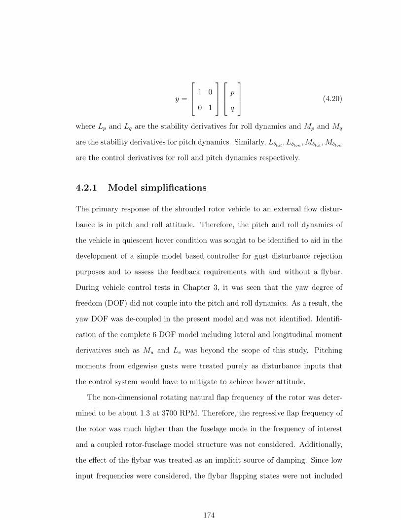
y =

1 0

0 1

p

q

(4.20)

where Lp and Lq are the stability derivatives for roll dynamics and Mp and Mq

are the stability derivatives for pitch dynamics. Similarly, Lδlat , Lδlon ,Mδlat ,Mδlon

are the control derivatives for roll and pitch dynamics respectively.

4.2.1 Model simplifications

The primary response of the shrouded rotor vehicle to an external flow distur-

bance is in pitch and roll attitude. Therefore, the pitch and roll dynamics of

the vehicle in quiescent hover condition was sought to be identified to aid in the

development of a simple model based controller for gust disturbance rejection

purposes and to assess the feedback requirements with and without a flybar.

During vehicle control tests in Chapter 3, it was seen that the yaw degree of

freedom (DOF) did not couple into the pitch and roll dynamics. As a result, the

yaw DOF was de-coupled in the present model and was not identified. Identifi-

cation of the complete 6 DOF model including lateral and longitudinal moment

derivatives such as Mu and Lv was beyond the scope of this study. Pitching

moments from edgewise gusts were treated purely as disturbance inputs that

the control system would have to mitigate to achieve hover attitude.

The non-dimensional rotating natural flap frequency of the rotor was deter-

mined to be about 1.3 at 3700 RPM. Therefore, the regressive flap frequency of

the rotor was much higher than the fuselage mode in the frequency of interest

and a coupled rotor-fuselage model structure was not considered. Additionally,

the effect of the flybar was treated as an implicit source of damping. Since low

input frequencies were considered, the flybar flapping states were not included

174

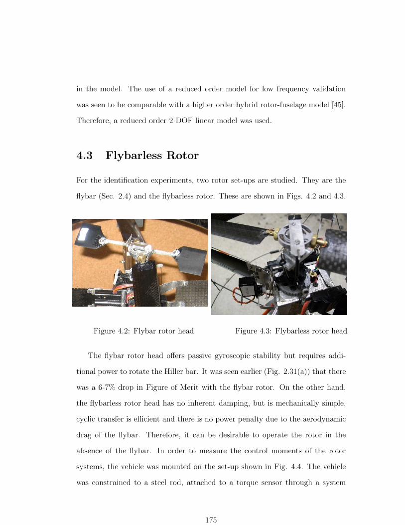
in the model. The use of a reduced order model for low frequency validation

was seen to be comparable with a higher order hybrid rotor-fuselage model [45].

Therefore, a reduced order 2 DOF linear model was used.

4.3 Flybarless Rotor

For the identification experiments, two rotor set-ups are studied. They are the

flybar (Sec. 2.4) and the flybarless rotor. These are shown in Figs. 4.2 and 4.3.

Figure 4.2: Flybar rotor head Figure 4.3: Flybarless rotor head

The flybar rotor head offers passive gyroscopic stability but requires addi-

tional power to rotate the Hiller bar. It was seen earlier (Fig. 2.31(a)) that there

was a 6-7% drop in Figure of Merit with the flybar rotor. On the other hand,

the flybarless rotor head has no inherent damping, but is mechanically simple,

cyclic transfer is efficient and there is no power penalty due to the aerodynamic

drag of the flybar. Therefore, it can be desirable to operate the rotor in the

absence of the flybar. In order to measure the control moments of the rotor

systems, the vehicle was mounted on the set-up shown in Fig. 4.4. The vehicle

was constrained to a steel rod, attached to a torque sensor through a system

175

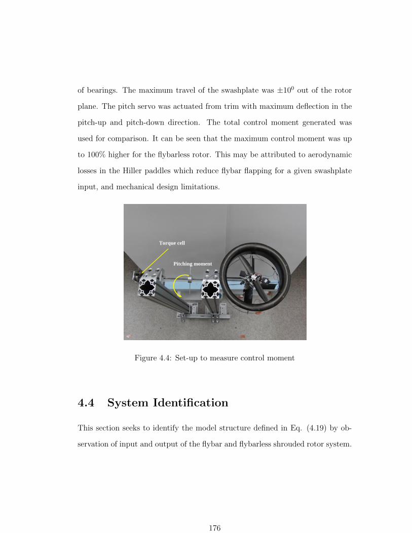
of bearings. The maximum travel of the swashplate was ±100 out of the rotor

plane. The pitch servo was actuated from trim with maximum deflection in the

pitch-up and pitch-down direction. The total control moment generated was

used for comparison. It can be seen that the maximum control moment was up

to 100% higher for the flybarless rotor. This may be attributed to aerodynamic

losses in the Hiller paddles which reduce flybar flapping for a given swashplate

input, and mechanical design limitations.

Torque cell

Pitching moment

Figure 4.4: Set-up to measure control moment

4.4 System Identification

This section seeks to identify the model structure defined in Eq. (4.19) by ob-

servation of input and output of the flybar and flybarless shrouded rotor system.

176

2000 2200 2400 2600 2800 3000 3200 3400 36000

200

400

600

800

1000

1200

1400

1600

RPM

Co

ntr

ol a

uth

ori

ty (

g-c

m)

Flybarless

Flybar

Co

ntr

ol m

om

en

t (g

-cm

)

Figure 4.5: Control moments generated by flybar and flybarless rotor

VEHICLE INPUT EXCITATION(u)

OUTPUT RESPONSE(z)

Figure 4.6: System Identification

177

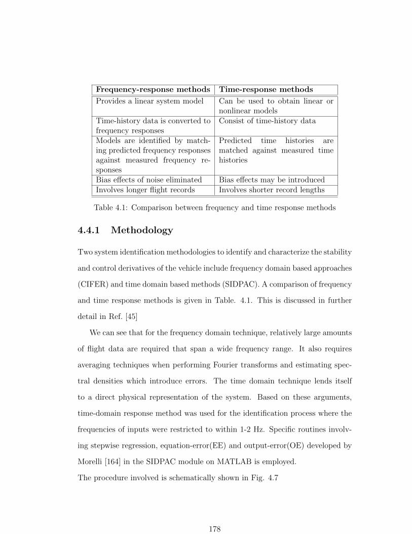
Frequency-response methods Time-response methods

Provides a linear system model Can be used to obtain linear ornonlinear models

Time-history data is converted tofrequency responses

Consist of time-history data

Models are identified by match-ing predicted frequency responsesagainst measured frequency re-sponses

Predicted time histories arematched against measured timehistories

Bias effects of noise eliminated Bias effects may be introducedInvolves longer flight records Involves shorter record lengths

Table 4.1: Comparison between frequency and time response methods

4.4.1 Methodology

Two system identification methodologies to identify and characterize the stability

and control derivatives of the vehicle include frequency domain based approaches

(CIFER) and time domain based methods (SIDPAC). A comparison of frequency

and time response methods is given in Table. 4.1. This is discussed in further

detail in Ref. [45]

We can see that for the frequency domain technique, relatively large amounts

of flight data are required that span a wide frequency range. It also requires

averaging techniques when performing Fourier transforms and estimating spec-

tral densities which introduce errors. The time domain technique lends itself

to a direct physical representation of the system. Based on these arguments,

time-domain response method was used for the identification process where the

frequencies of inputs were restricted to within 1-2 Hz. Specific routines involv-

ing stepwise regression, equation-error(EE) and output-error(OE) developed by

Morelli [164] in the SIDPAC module on MATLAB is employed.

The procedure involved is schematically shown in Fig. 4.7

178

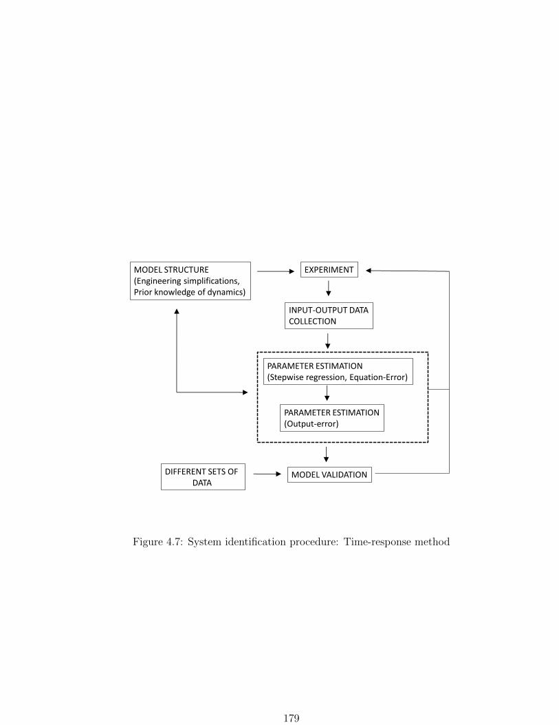
EXPERIMENT

INPUT-OUTPUT DATACOLLECTION

PARAMETER ESTIMATION(Stepwise regression, Equation-Error)

PARAMETER ESTIMATION(Output-error)

MODEL VALIDATION

MODEL STRUCTURE(Engineering simplifications,Prior knowledge of dynamics)

DIFFERENT SETS OF DATA

Figure 4.7: System identification procedure: Time-response method

179

4.4.1.1 Equation-error parameter estimation

If θ is the constant parameter vector to be estimated and x, u are the state and

input vectors respectively, then the output equation of the linear system is,

y(t) = x = X(x(t), u(t))θ (4.21)

and the measurement equation,

z(t) = y(t) + v(t) (4.22)

where v is random noise. It is therefore desired to choose θ such that the error

z(t) − y(t) is minimized. Let n be the size of θ. Typically, the size (N) of the

measurement vector is much larger than n. Therefore least squares parameter

estimation is performed. Here, we seek θ that minimizes a cost function,

θ = minθ

1

2(z −Xθ)T (z −Xθ) (4.23)

This can be re-written as,

θ = (XTX)−1XT z (4.24)

So the estimated vector is given by,

y = Xθ = X(XTX)−1XT z (4.25)

The columns of X are the regressors in the model. Care must be taken to ensure

that the regressors are not linearly dependent for the matrix inverse (XTX)−1

to exist. The equation-error formulation is a linear estimation problem and the

180

least-squres solution does not require iteration.

4.4.1.2 Stepwise regression

This is a computation technique to evaluate the relevance of a candidate regressor

for inclusion in the linear model, by deleting or adding regressors one at a time.

Stepwise regression starts by constructing a set of candidate regressors. The first

regressor that produces the highest absolute value of correlation with z is chosen.

This regressor is then removed from the subset of regressors and the procedure

is repeated. Two statistical metrics are used to evaluate the candidate model

terms that quantify the closeness of y and z.

Coefficient of determination, R2: This is defined as

R2 =SSRSST

(4.26)

where SST is the total sum of squares,

SST = zT z −Nz2 (4.27)

and SSR is the regression sum of squares,

SSR =∞∑i=1

[ ˆy(i)− z]2 (4.28)

Here, N is the size of the measurement vector and z is the mean of the mea-

surement vector. R2 is expressed as a percentage. The addition of a regressor

always increases R2, with the more influential term resulting in a greater change

in R2. An adequate model is achieved when R2 is not substantially changed by

the addition of a new model term.

181

F-ratio: The F ratio for testing significance of a regression is given as,

F =SSR/n

(SST − SSR)/N

=N

n

θTXT z −Nz2

zT z − θTXT z(4.29)

Additionally, the partial F ratio can be computed for an individual parameter

vector (θj),

Fp =θj

2

V ar(θj)(4.30)

Any regressor with Fp less than a cut-off value is removed from the model. For

95% confidence, the cut off value is taken as 20.

4.4.1.3 Output-error method

Here, it is assumed that the process noise (in the state equation) is neglected.

Therefore the states can be computed deterministically by a direct numerical

integration. A maximum likelihood cost function is chosen that involves weighted

squared differences between measured and computed outputs. This resulting

estimator is known as the output error method. It is a non linear least-squares

method for multiple outputs with output weighting that iteratively arrives at a

converged parameter vector θ and covariance matrix R. The initial estimates

for θ are taken from those estimated in the stepwise regression procedure. The

iterative scheme adopted is a modified Newton-Raphson method. The details of

this can be obtained from Ref. [164].

182

4.4.2 Input-output data collection

In order to remove the effect of translation on the attitude dynamics, the vehicle

was suspended from its C.G. position on a low-friction spherical gimbal set-up1.

This restricted the motion in yaw, but since the yaw DOF was decoupled from

the model, it is acceptable. The dynamics of the vehicle with and without the

IMU senses pitch

and roll

Spherical Bearing

Figure 4.8: Gimbal set-up for vehicle pitch and roll motion

flybar was extracted in a separate sequence of tests. For each sequence, the

vehicle was powered up to an operating RPM on the gimbal and trimmed out

to a level attitude. Care was taken that trim in yaw was also performed. Next,

a series of uncoupled lateral and longitudinal input sweeps were provided about

trim. The onboard IMU captured the vehicle response in terms of pitch (q) and

roll (p) rate. The frequency content of the inputs were restricted to less than

about 6 rad/s which was within the observed free flight pitch-roll body modes

(Fig. 3.59). Time history data for each input-output sequence was obtained by

combining data from individual tests and were sampled at 200Hz. The latency in

1This set-up differed from the one shown in Fig. 3.38. A modification in the vehicle designallowed a direct access to the vehicle C.G., unlike the previous set-up which had to incorporatean external gimbal ring.

183

open loop telemetry including actuator lag was measured to be about 50 ms and

was factored into the treatment of the output data. Figure 4.9 shows a sample

data of the unfiltered pitch rate of the vehicle measured by the IMU. A short

term fourier transform of the data (at t=15 s) shows that the noise content of the

signal (Fig. 4.10) is predominantly due to the rotor rotational frequency which

is at a sufficiently higher frequency than the body modes of interest. Therefore

a zero phase lag low pass filter can be applied to filter out the noise due to rotor

vibration (Fig. 4.11).

0 5 10 15 20 25-2

-1.5

-1

-0.5

0

0.5

1

1.5

2

Time (s)

Pit

ch

ra

te, q

(ra

d/s

)

Rotor switchedon

Figure 4.9: Unfiltered gyro data

0 20 40 60 80 100 1200

0.1

0.2

0.3

0.4

0.5

0.6

0.7

Frequency (Hz)

PS

D

Figure 4.10: Short term fourier trans-form at t=15 s, predominantly rotornoise

The lateral and longitudinal cyclic inputs were non dimensionalized using

the input control limits as the scaling factor such that, (δlat,δlon) ∈ [−1, 1]. Care

was taken to provide lateral and longitudinal inputs one at a time without cross

coupling of inputs. Figures 4.12 - 4.15 show sample input-output data in pitch

and roll for the flybar and flybarless rotor. The bias errors in inputs were removed

before performing system identification.

184

0 5 10 15 20 25-2

-1.5

-1

-0.5

0

0.5

1

1.5

2

Time (s)

Pit

ch

ra

te, q

(ra

d/s

)

unfiltered

filtered

Figure 4.11: Gyro data filtered with zero phase lag low pass filter

0 10 20 30 40 50-0.4

-0.2

0

0.2

0.4

la

t

0 10 20 30 40 50-1

-0.5

0

0.5

1

Time (s)

Ro

ll r

ate

, p

(ra

d/s

)

Figure 4.12: Input-output data for fly-bar rotor in lateral direction

20 30 40 50 60 70-0.5

0

0.5

lo

n

20 30 40 50 60 70-1

-0.5

0

0.5

1

Time (s)

Pit

ch

ra

te, q

(ra

d/s

)

Figure 4.13: Input-output data for fly-bar rotor in longitudinal direction

185

40 60 80 100 120 140-2

-1

0

1

Time (s)

Ro

ll r

ate

, p

(ra

d/s

)

40 60 80 100 120 140-0.1

-0.05

0

0.05

0.1

la

t

Figure 4.14: Input-output data for fly-barless rotor in lateral direction

20 30 40 50 60 70 80 90-1

-0.5

0

0.5

1

Time (s)

Pit

ch

ate

, q

(ra

d/s

)

20 30 40 50 60 70 80 90-0.1

-0.05

0

0.05

0.1

lo

n

Figure 4.15: Input-output data for fly-barless rotor in longitudinal direction

4.4.3 Results

The identified parameter vector for the flybar and flybarless rotor using the

model structure from Eq. (4.19) along with the statistical metrics is shown in

Table 4.4.3. The R2 and Fp values were seen to be satisfactory. It must be

mentioned that this is a first order model in attitude rates. Model accuracy

may be improved by including rotor and flybar dynamics as well. Time domain

verification of the identified model with actual flight data (a different input-

output data set than the one used for model extraction) for the flybar and

flybarless rotor shows a satisfactory comparison between model and flight data.

This is shown in Figs. 4.16 − 4.19. From the identified eigenvalues, it can be

seen that the flybar rotor has a stable pair of poles, whereas the flybarless rotor

has a pair of poles that suggest that the system is marginally unstable (Fig.

4.20). Additionally, this shows that the primary source of damping is the flybar.

The off-axis terms in the state matrix did not change significantly between the

flybar and flybarless set-up. This indicates gyroscopic cross-coupling, which is

purely a function of rotor angular momentum. The control derivatives in the

186

Parameter Flybar rotor Flybarless rotor

θ Fp (min. 20) θ FpLp(rad/s) -6.79 475 0.76 385Lq(rad/s) 1.7 400 1.65 370Lδlat(1/s) 23.85 2350 47 2020Lδlon(1/s) 1.6 2400 2 1950

R2(Lateral,%) 86 − 82 −Mq(rad/s) -6.85 510 0 410Mp(rad/s) -2.1 500 -1.66 380Mδlon(1/s) 24 2200 54.1 1970Mδlat(1/s) -1.56 2150 -2.96 1950R2(Long,%) 83 − 83 −Eigenvalues -6.82 ±1.882i 0.38 ±1.61i

Table 4.2: Identified model parameters for the flybar and flybarless rotor

control matrix is significantly higher (up to 100%) for the flybarless rotor. This

result agreed well with the control moment measurement (Fig. 4.5). Based on

these results, it can be seen that the vehicle can be satisfactorily modeled as a

system, which is of first order with respect to attitude rates. The control system

has to provide external rate damping to stabilize the system for the flybarless

set-up. This is a significant challenge considering the limited latency in off-board

telemetry. This problem can be circumvented by including electronic damping

on board the vehicle.

4.5 Controllability metrics

The above attitude dynamics models can be used to compare the two bare air-

frames (flybar and flybarless) in their effectiveness in arriving at a set of reachable

states x0 resulting from an arbitrary input u(t) ∈ LP2 (−∞, 0] of unit norm. A

controllability operator Ψc is considered which maps the time history of the in-

put u(t) from t = −∞ to a final state x0 at t = 0. The set of reachable states is

187

70 75 80 85 90-0.5

0

0.5

la

t

70 75 80 85 90-1

-0.5

0

0.5

1

p (

rad

/s)

Expt

Model

Figure 4.16: Time domain verification: Flybar rotor (Lateral)

70 75 80 85 90-0.5

0

0.5

lo

n

70 75 80 85 90-1

-0.5

0

0.5

1

Time (s)

q (

rad

/s)

Expt

Model

Figure 4.17: Time domain verification: Flybar rotor (Longitudinal)

188

20 25 30 35 40 45 50 55 60 65-10

-5

0

5

10

pd

ot

(ra

d/s

2)

20 25 30 35 40 45 50 55 60 65-0.2

-0.1

0

0.1

0.2

lat

Expt

Model

Figure 4.18: Time domain verification: Flybarless rotor (Lateral)

20 25 30 35 40 45 50 55 60 65-0.2

-0.1

0

0.1

0.2

lo

n

20 25 30 35 40 45 50 55 60 65-10

-5

0

5

10

Time (s)

qd

ot

(ra

d/s

2)

Expt

Model

Figure 4.19: Time domain verification: Flybarless rotor (Longitudinal)

189

-10 -8 -6 -4 -2 0 2-5

-4

-3

-2

-1

0

1

2

3

4

55

Real Axs

Ima

gin

ary

Ax

is

Flybar

Flybarless

Figure 4.20: Location of poles for flybar and flybarless rotor

then Ψcu. An infinite-time controllability gramian Wc is determined to quantify

this,

Wc = ΨcΨTc (4.31)

which can be computed from the dynamics model (A,B) using the continuous

time Lyapunov equation (Ref. [165])

AWc +WcAT +BBT = 0 (4.32)

Note that the above computation is only possible when A matrix is stable as

is the case for the flybar rotor. For cases when the A matrix is unstable as

in the flybarless rotor, the reader is referred to Zhou. et al. (Ref. [167]) for

detailed mathematical treatment. Here the A matrix is purely antistable (does

not have stable eigenvalues). Using Zhou’s method, a transformation matrix T

190

is computed which is the inverse of the eigenvector matrix of A. Following which,

A = TAT−1, B = TB (4.33)

The continuous time Lyapunov equation is then solved for,

− AP − PAT + BBT = 0 (4.34)

The controllability gramian is then given by,

Wc = T−1P (T−1)T (4.35)

Using the controllability gramians determined above, two control input rank-

ing criteria can be computed (Ref. [166]):

1) D-norm: det(W1/2c )

2) Frobenius norm:

√trace[(W

1/2c ).W

1/2c ]

These metrics are compared in Table 4.3 and Figs. 4.21 and 4.22.

Flybarrotor

Flybar ro-tor (withsame con-trol deriva-tives asflybarlessrotor

Flybarlessrotor

Flybarlessrotor (withsame con-trol deriva-tives asflybar rotor

D norm 42.2 186.7 3648 819Frobeniusnorm

9.2 19.4 87 41

Table 4.3: Comparison in controllability metrics between flybar and flybarlessrotor

It can be clearly seen that the flybarless rotor is much more controllable than the

191

10

500

1000

1500

2000

2500

3000

3500

4000

Flybarless

rotor with control

derivatives of

flybar rotor

Flybar

rotor with control

derivatives of

flybarless rotor

Flybar

rotor

Flybarless

rotor

Figure 4.21: Comparison in det(W1/2c )

between flybar and flybarless rotor

10

10

20

30

40

50

60

70

80

90

Flybarless

rotor

Flybarless

rotor with control

derivatives of

flybar rotor

Flybar

rotor with control

derivatives of

flybarless rotor

Flybar

rotor

Figure 4.22: Comparison in Frobeniusnorm between flybar and flybarless rotor

flybar rotor. This implies that it can reach a wider span of states for a given con-

trol input energy. It can be seen that if only the control derivatives are doubled,

the Frobenius norm doubles. In addition, the lack of damping in the flybarless

rotor further amplifies the controllability. However, for practical applications,

on-board damping will have to be provided and this effect on controllability will

be removed.

4.6 Model based controller

An LQR controller based on the simplified 2 DOF linear atittude dynamics model

of the vehicle was also designed. The state space attitude dunamics model of the

vehicle can be written using the state vector x, state matrix A, control vector u

and control matrix B, as:

x = Ax+Bu (4.36)

192

where,

x =

p

q

φ

θ∫φ∫θ

, A =

Lp Lq 0 0 0 0

Mp Mq 0 0 0 0

1 0 0 0 0 0

0 1 0 0 0 0

0 0 1 0 0 0

0 0 0 1 0 0

(4.37)

B =

Lδlat Lδlon

Mδlat Mδlon

0 0

0 0

0 0

0 0

, u =

δlat

δlon

(4.38)

The roll and pitch attitudes (φ,θ) as well as the integral of the roll and pitch

attitudes (∫φ,∫θ) are incorporated in the state vector. This facilitates feedback

of the integral, proportional and derivative of the vehicle Euler attitude angles.

In the design of the control system, it is of interest in choosing the control vector

u which minimizes a given performance index. For quadratic optimal control,

the following performance index is chosen,

J =

∫ ∞0

L(x, u)dt (4.39)

where L(x, u) is a quadratic function of x and u,

L = xTQx+ uTRu (4.40)

193

where Q is a positive-definite (or positive semi-definite) real symmetric matrix,

R is a positive-definite real symmetric matrix. The matrices Q and R determine

the relative importance of the state error (x) and the expenditure of the energy of

the control signals (u). A linear control law is used to minimize the performance

index J .

u = −Kx (4.41)

K = R−1BTP (4.42)

where K is the LQR gain and P is the unique, positive-semidefinite solution to

the algebraic Riccati equation:

ATP + PA− PBR−1BTP +Q = 0 (4.43)

The R matrix was set to unity and the elements in the Q matrix were decided

based on the Zeigler-Nichols approach. The LQR gains were computed using the

Control System Toolbox in LabVIEW. The LQR controller was implemented

as shown in Fig. 4.23 and was found to successfully mitigate pitch and roll

disturbances as can be seen from Fig. 4.24.

4.7 Summary

In this chapter, the development of a reduced order linear attitude dynamics

model of the vehicle was described. In order to determine the empirical model,

system identification was performed in the time domain using equation error and

output error based on maximum likelihood techniques. Two rotor systems were

considered for this - the flybar and flybarless rotor. The extracted model was

194

Figure 4.23: LQR feedback configuration

40 45 50 55 60 65 70-1

0

1

40 45 50 55 60 65 70-0.5

0

0.5

40 45 50 55 60 65 70-0.5

0

0.5

40 45 50 55 60 65 70-0.5

0

0.5

Time (s)

p(rad/s)

q (rad/s)

(rad)

(rad)

Disturbance

addedDisturbance

removed

Figure 4.24: Attitude disturbance rejection on spherical gimbal set-up with LQRcontroller

195

found to satisfactorily represent the vehicle as a first order system with respect

to attitude rates. Time domain verification indicated satisfactory comparison

between model and truth. It was found that the flybarless rotor had up to 100%

greater control power when compared to the flybar rotor. However, it was a

marginally unstable system since the damping offered by the flybar was removed.

As a result, flybarless rotor operation would require on-board electronic damping.

Comparison in controllability metrics such as Frobenius norm derived from the

controllability gramian indicates that the flybarless rotor is more controllable

than the flybar rotor. The source of this increased controllability is the reduced

damping and increased control moments.

196

Chapter 5

Performance and Control Moments of

Shrouded Rotor in Edgewise Flow

5.1 Overview

The results described so far were for the shrouded rotor operating in quiescent

flow conditions. In this chapter, the performance of the shrouded rotor when

exposed to edgewise flow is described. The forces produced by a shrouded ro-

tor operating in edgewise flow are measured and compared with those produced

by an unshrouded rotor. Bench top experiments that include measurements of

thrust, drag and pitching moment are made. An open jet wind tunnel was used

as the source for edgewise flow. The shrouded and unshrouded rotor configu-

rations were compared for their control moments and ability to overcome the

destabilizing forces in these flows. A few strategies to minimize the adverse

moments are discussed. Methods to improve the control moments of the rotor

configurations through rotor planform design will be detailed. Finally, sufficient

control margin to tolerate medium gusts of up to 2-3 m/s is ensured, that will

aid in the gust disturbance rejection tests discussed in the next chapter.

197

5.2 Performance in Edgewise Flow

When a hovering shrouded rotor vehicle faces an edgewise flow, it experiences the

following forces: (1) drag, in the direction of the flow and (2) pitching moment,

that tends to pitch the vehicle away from the flow. This is schematically shown

in Fig. 5.1. The side facing the flow is referred to as the windward side and the

region of the shroud away from the flow is the leeward side. If the flow is along

the negative X axis of the vehicle, the moment that pitches the vehicle away

from the wind (i.e. about the positive Y axis) is positive. These forces can be

many times in magnitude for a shrouded rotor when compared to an unshrouded

rotor. They tend to destabilize the vehicle from hover and make it extremely

difficult to achieve station keeping (hover in a constant position).

Thrust

Drag

Pitching moment

X

Z

Y

V

LeewardWindward

Figure 5.1: Forces acting on a hovering shrouded rotor in edgewise flow

198

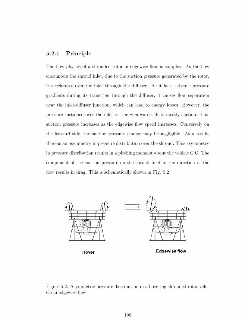
5.2.1 Principle

The flow physics of a shrouded rotor in edgewise flow is complex. As the flow

encounters the shroud inlet, due to the suction pressure generated by the rotor,

it accelerates over the inlet through the diffuser. As it faces adverse pressure

gradients during its transition through the diffuser, it causes flow separation

near the inlet-diffuser junction, which can lead to energy losses. However, the

pressure sustained over the inlet on the windward side is mostly suction. This

suction pressure increases as the edgewise flow speed increases. Conversely on

the leeward side, the suction pressure change may be negligible. As a result,

there is an asymmetry in pressure distribution over the shroud. This asymmetry

in pressure distribution results in a pitching moment about the vehicle C.G. The

component of the suction pressure on the shroud inlet in the direction of the

flow results in drag. This is schematically shown in Fig. 5.2

Figure 5.2: Asymmetric pressure distribution in a hovering shrouded rotor vehi-cle in edgewise flow

199

5.2.2 Shrouded rotor configurations

The baseline shroud discussed so far has a circular inlet profile. Now, a recent

CFD study by Lakshminarayan and Baeder [124] showed that performance im-

provements can be made if an elliptic inlet is chosen for the design. Therefore,

an elliptic inlet shroud was constructed using a two layer carbon fiber epoxy

weave. The construction was similar to the process shown in Fig. 2.48. The

schematics of the profiles along with the corresponding constructed shrouds are

shown in Fig. 5.3. Here the ellipse has a major chord to minor chord ratio of

2:1. It must be noted that since the chord to diamter ratio of the shrouds were

the same, the elliptic inlet shroud would have a greater mass owing to the excess

area of the shroud inlet.

lipr

lipr

lip2r

Circular inlet

Elliptical inlet

Figure 5.3: Circular and elliptical inlet shroud designs tested

The baseline rotor profile (a) from Fig. 2.55 was tested in the circular and

elliptic inlet configuration using the micro rotor hover stand (Fig. 2.49) at

different collectives. A tip clearance of about 0.02 R was maintained. Figure 5.4

shows variation of thrust coefficient with blade root collective for the circular

and elliptic inlet rotors respectively. It can be seen that at higher collectives,

200

the elliptic inlet shroud produces more thrust than the circular inlet shroud.

Interestingly, the differences in power coefficient of both the configurations are

small or within measurement error for the whole range of collectives. The best

power-thrust curves for the circular inlet and elliptic inlet shrouded rotors are

compared in Fig. 5.6. It was seen that a 10% improvement in power loading was

achieved with the elliptic inlet shroud. It is of interest to measure how the forces

produced in edgewise flow change for a more efficient shroud. To characterize

these forces, the unshrouded rotor, circular inlet and elliptic inlet shrouded rotor

were tested in edgewise flow conditions produced by an open jet wind tunnel.

10 15 20 25 30 350.01

0.015

0.02

0.025

0.03

0.035

0.04

0.045

Collective (deg)

CT

Circular inlet

Elliptic inlet

Figure 5.4: Variation of thrust coeffi-cient with blade collective

10 15 20 25 30 351

2

3

4

5

6

7

8x 10

-3

Collective (deg)

CP

Circular inlet

Elliptic inlet

Figure 5.5: Variation of power coeffi-cient with blade collective

5.2.3 Experiment set-up

It is of interest to measure the thrust, drag and pitching moment acting on the

hovering shrouded vehicle when exposed to edgewise flow. For this, the vehicle

was set-up in front of an open jet wind tunnel as shown in Fig. 5.7. The

dimensions of the wind tunnel test section was 22” × 22” and a turbulence level

201

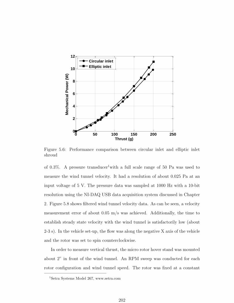
0 50 100 150 200 2500

2

4

6

8

10

12

Thrust (g)

Mech

an

ical P

ow

er

(W)

Circular inlet

Elliptic inlet

Figure 5.6: Performance comparison between circular inlet and elliptic inletshroud

of 0.3%. A pressure transducer1with a full scale range of 50 Pa was used to

measure the wind tunnel velocity. It had a resolution of about 0.025 Pa at an

input voltage of 5 V. The pressure data was sampled at 1000 Hz with a 10-bit

resolution using the NI-DAQ USB data acquisition system discussed in Chapter

2. Figure 5.8 shows filtered wind tunnel velocity data. As can be seen, a velocity

measurement error of about 0.05 m/s was achieved. Additionally, the time to

establish steady state velocity with the wind tunnel is satisfactorily low (about

2-3 s). In the vehicle set-up, the flow was along the negative X axis of the vehicle

and the rotor was set to spin counterclockwise.

In order to measure vertical thrust, the micro rotor hover stand was mounted

about 2” in front of the wind tunnel. An RPM sweep was conducted for each

rotor configuration and wind tunnel speed. The rotor was fixed at a constant

1Setra Systems Model 267, www.setra.com

202

Thrust

Drag

Pitching moment

Rotor configurations:

1) Unshrouded

2) Circular lip shroud

3) Elliptic lip shroud

Figure 5.7: Rotor set-up in front of open jet wind tunnel

15 20 25 30 350

0.5

1

1.5

2

Time (s)

Ve

loc

ity

(m

/s)

Figure 5.8: Sample velocity data from open jet wind tunnel

203

collective of 24 deg. The test procedure involved spinning the rotor up to a

desired RPM followed by powering on the wind tunnel. This was done to pre-

vent undesirable bending of the thrust stand before the rotor could reach the

commanded RPM. Also, the rotor torque was not measured as a function of

wind speed since the stand transferred bending moments to the torque load cell

thereby affecting the torque readings. This could be circumvented by support-

ing the stand through radial bearings that would absorb the bending moments.

However, since the thrust was of primary interest, this design modification was

not made. For drag and pitching moment measurement, a separate stand was

used that simultaneously measured both these forces. The rotor was mounted

vertically at the end of a horizontal shaft with the other end of the shaft coupled

with a torque load cell. The shaft was supported by two radial bearings that en-

abled complete transfer of loads to the torque load cell. It also ensured minimal

friction due to bending moments. Therefore, the pitching moments produced by

the vehicle were completely transferred to the load cell. The axis about which

the pitching moment was measured was kept constant, about 100 mm below the

rotor plane. The highest point of the circular lip shroud and elliptic lip shroud

was about 120 mm and 140 mm above the moment axis respectively. For the

drag, the rotor was mounted on a linear bearing mechanism that was connected

to a thrust load cell, which enabled drag measurement in the direction of the flow

without frictional losses. The pitching moment and drag measurement set-ups

are shown in Figs. 5.9 and 5.10.

Figure 5.11 shows a representative measurement of the pitching moment.

As explained in the previous chapter, vibration was due to rotor revolution

which enabled application of a zero phase lag filter to remove the noise. A

difference between the wind-off and rotor-on, and wind-on and rotor-on cases

204

Radialbearings

Open jet Wind tunnel(flow out of plane)

Drag load cell

Torque load cell

Horizontal shaftY

Z

Figure 5.9: Pitching moment measurement set-up

Edgewise flow

Drag load cell

Linear bearing

X

Y

Figure 5.10: Drag measurement using linear bearing mechanism

205

gave an averaged pitching moment for that particular wind speed and rotor

RPM. A similar procedure was adopted for the drag measurement. The average

measurement errors for each were within 3-5 %. The magnitude of vibration

recorded by the load sensors did not increase significantly when the wind was

turned on. The recorded pitching moment and drag also included the effect of

the bluff body in the flow. In order to remove this effect, tare measurements

were conducted. Here, the drag and moment were measured with the set-up in

the flow and the rotor unpowered. The tare values for the unshrouded rotor

were about 1-3 grams and 10-15 gram-cm at 2 m/s for the drag and pitching

moment respectively. This was considered to be within measurement error. The

tare measurements for the two shrouded rotors were similar to each other and

are shown in Figs. 5.12 and 5.13. These values were subtracted from the total

measured values (Fig. 5.11). Therefore, the results presented will purely be the

effect of a powered rotor in edgewise flow with bluff body drag and moment

removed.

0 5 10 15 20 25 30-3400

-3200

-3000

-2800

-2600

-2400

-2200

-2000

-1800

-1600

Time (s)

Pit

ch

ing

Mo

me

nt

(g-c

m)

unfiltered

filtered

Rotor on, wind offRotor on, wind on

Figure 5.11: Filtered pitching moment data with wind switched on

206

0.8 1 1.2 1.4 1.6 1.8 2 2.20

10

20

30

40

50

60

Wind (m/s)

Pit

ch

ing

mo

me

nt

(g-c

m)

Figure 5.12: Tare measurementsof pitching moment of unpoweredshrouded rotor in flow

0.8 1 1.2 1.4 1.6 1.8 2 2.20

1

2

3

4

5

6

7

Wind (m/s)

Dra

g (

g)

Figure 5.13: Tare measurements of dragof unpowered shrouded rotor in flow

5.2.4 Results and discussion

5.2.4.1 Thrust

When a hovering vehicle faces edgewise flow, it is of interest to see if the thrust

that balances weight is sustained. Figures 5.14 and 5.15 show the thrust pro-

duced and power required by the unshrouded rotor as a function of RPM at dif-

ferent edgewise flow speeds. It can be clearly seen that there is negligible change

in thrust produced and power required between quiescent and low edgewise flow

speeds. Now, from Fig. 5.2, there is an asymmetric pressure distribution pro-

duced by a shrouded rotor in edgewise flow. Therefore the vertical thrust from

the shrouded rotor may be different for both the conditions. However it can be

seen from Figs. 5.16 − 5.19 that neither the thrust nor power of the shrouded

rotors change at these low edgewise flow speeds. The thrust and power measure-

ment error at 3600 RPM was between 2-3%. This is interesting as it seems to

suggest that the asymmetry in pressure distribution does not affect the net ver-

207

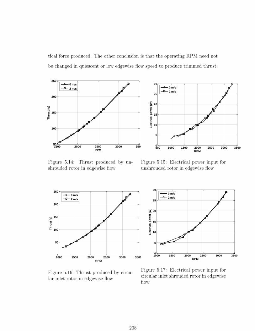
tical force produced. The other conclusion is that the operating RPM need not

be changed in quiescent or low edgewise flow speed to produce trimmed thrust.

1500 2000 2500 3000 350050

100

150

200

250

RPM

Th

rus

t (g

)

0 m/s

2 m/s

Figure 5.14: Thrust produced by un-shrouded rotor in edgewise flow

500 1000 1500 2000 2500 3000 35000

5

10

15

20

25

30

RPME

lec

tric

al p

ow

er

(W)

0 m/s

2 m/s

Figure 5.15: Electrical power input forunshrouded rotor in edgewise flow

1000 1500 2000 2500 3000 35000

50

100

150

200

250

RPM

Th

rus

t (g

)

0 m/s

2 m/s

Figure 5.16: Thrust produced by circu-lar inlet rotor in edgewise flow

1000 1500 2000 2500 3000 35000

5

10

15

20

25

30

RPM

Ele

ctr

ica

l p

ow

er

(W)

0 m/s

2 m/s

Figure 5.17: Electrical power input forcircular inlet shrouded rotor in edgewiseflow

208

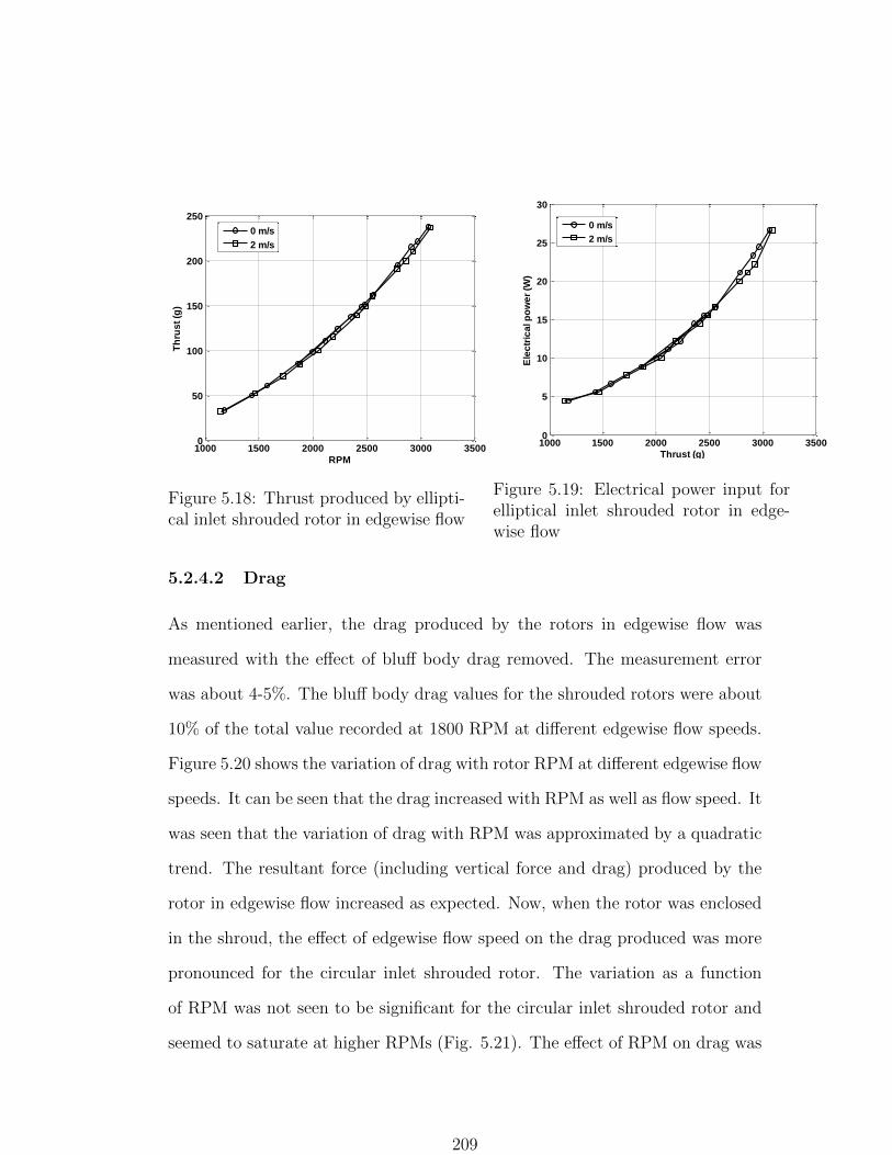
1000 1500 2000 2500 3000 35000

50

100

150

200

250

RPM

Th

rus

t (g

)

0 m/s

2 m/s

Figure 5.18: Thrust produced by ellipti-cal inlet shrouded rotor in edgewise flow

1000 1500 2000 2500 3000 35000

5

10

15

20

25

30

Thrust (g)

Ele

ctr

ica

l p

ow

er

(W)

0 m/s

2 m/s

Figure 5.19: Electrical power input forelliptical inlet shrouded rotor in edge-wise flow

5.2.4.2 Drag

As mentioned earlier, the drag produced by the rotors in edgewise flow was

measured with the effect of bluff body drag removed. The measurement error

was about 4-5%. The bluff body drag values for the shrouded rotors were about

10% of the total value recorded at 1800 RPM at different edgewise flow speeds.

Figure 5.20 shows the variation of drag with rotor RPM at different edgewise flow

speeds. It can be seen that the drag increased with RPM as well as flow speed. It

was seen that the variation of drag with RPM was approximated by a quadratic

trend. The resultant force (including vertical force and drag) produced by the

rotor in edgewise flow increased as expected. Now, when the rotor was enclosed

in the shroud, the effect of edgewise flow speed on the drag produced was more

pronounced for the circular inlet shrouded rotor. The variation as a function

of RPM was not seen to be significant for the circular inlet shrouded rotor and

seemed to saturate at higher RPMs (Fig. 5.21). The effect of RPM on drag was

209

greater for the elliptic inlet shrouded rotor and produced up to 70% higher drag

than the circular inlet shroud case at 2 m/s of edgewise flow speed (Fig. 5.22).

A possible explanation for this is shown in Fig. 5.23. The component of the

projected inlet area in the direction of the flow on the windward side is greater

for the elliptic inlet shroud. As a result, the resolved forces due to the pressure

distribution is higher for the elliptic inlet, thus producing higher drag. Figure

5.24 shows the drag produced by the three rotors as a function of edgewise flow

speed at 3300 RPM. The variation of drag with speed was seen to be mostly

linear. It was interesting to note that the slope of the drag-wind speed curve

was about 100% greater for the shrouded rotors. The previous observation of

drag variation with rotor RPM is better shown in Fig. 5.25. Here the drag is

plotted as a function of rotor thrust for the three rotors in 2 m/s of edgewise

flow. It can be seen that the magnitude of drag saturates as the rotor thrust

increases. This is an interesting conclusion from an MAV operation point of

view.

0 500 1000 1500 2000 2500 3000 3500 40000

10

20

30

40

50

60

RPM

Dra

g (

g)

0.9 m/s

1.3 m/s

1.7 m/s

2 m/s

Figure 5.20: Drag versus RPM for un-shrouded rotor

0 500 1000 1500 2000 2500 3000 3500 40000

10

20

30

40

50

60

RPM

Dra

g (

g)

0.9 m/s

1.3 m/s

1.7 m/s

2 m/s

Figure 5.21: Drag versus RPM for cir-cular inlet shrouded rotor

210

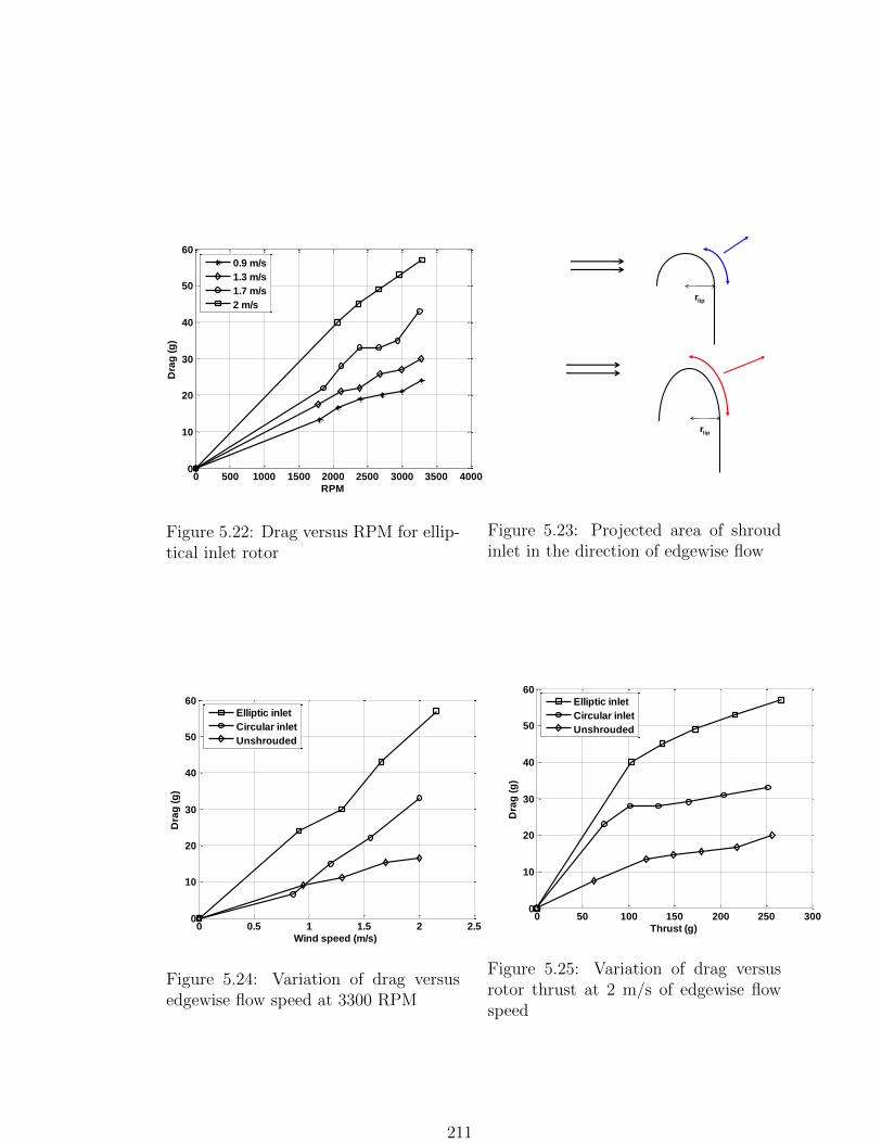
0 500 1000 1500 2000 2500 3000 3500 40000

10

20

30

40

50

60

RPM

Dra

g (

g)

0.9 m/s

1.3 m/s

1.7 m/s

2 m/s

Figure 5.22: Drag versus RPM for ellip-tical inlet rotor

lipr

lipr

Figure 5.23: Projected area of shroudinlet in the direction of edgewise flow

0 0.5 1 1.5 2 2.50

10

20

30

40

50

60

Wind speed (m/s)

Dra

g (

g)

Elliptic inlet

Circular inlet

Unshrouded

Figure 5.24: Variation of drag versusedgewise flow speed at 3300 RPM

0 50 100 150 200 250 3000

10

20

30

40

50

60

Thrust (g)

Dra

g (

g)

Elliptic inlet

Circular inlet

Unshrouded

Figure 5.25: Variation of drag versusrotor thrust at 2 m/s of edgewise flowspeed

211

5.2.4.3 Pitching moment

Figures 5.26− 5.28 show the pitching moments produced by the rotors in edge-

wise flow with the effect of moment due to bluff body drag removed. The mea-

surement error again was about 4-5%. The tare moment values for the shrodued

rotors were about 8% of the total value recorded at 1800 RPM at different

edgewise flow speeds. Each data point represents the difference in load cell

measurements between the wind-on and off cases. It can be seen that all the

configurations produced a positive pitching moment about the Y axis (nose-up)

with edgewise flow speed. The magnitude of these pitching moments increased

as the rotor RPM increased with the variation being approximately linear. As

in the case for drag, the pitching moment from the unshrouded rotor was not as

sensitive to edgewise flow speed as for the shrouded rotors. This effect can be

clearly seen in Fig. 5.29 where the moment-speed slope is almost twice for the

shrouded rotors. The circular and elliptical inlet shrouded rotors produced up

to 3-4 times higher pitching moments than the unshrouded rotor, respectively.

Analogous to the drag measurements, the pitching moments from the shrouded

rotors also seemed to saturate as the rotor thrust was increased. This is shown

in Fig. 5.30 at 2 m/s of edgewise speed. A possible explanation for this is that

as the rotor thrust is increased, the horizontal flow is more effectively channeled

through the shroud diffuser. This could explain the increased drag and pitching

moment as the thrust is increased from low values of thrust. However, at higher

values of thrust the momentum change of the edgewise flow through the diffuser

does not differ significantly with rotor thrust. As a result, the drag and pitching

moments may tend to saturate at high values of thrust. This has important

implications for the control margin of a shrouded rotor MAV, i.e., the amount

212

of excess control power available to alleviate a given pitching moment. This will

be discussed in further detail later.

0 500 1000 1500 2000 2500 3000 3500 40000

200

400

600

800

1000

1200

RPM

Pit

ch

ing

mm

en

t (g

-cm

)

0.95 m/s

1.3

1.7

2

Figure 5.26: Nose-up pitching momentversus RPM for unshrouded rotor

0 500 1000 1500 2000 2500 3000 35000

200

400

600

800

1000

1200

RPM

Pit

ch

ing

mo

me

nt

(g-c

m)

0.86 m/s

1.2 m/s

1.6m/s

2 m/s

Figure 5.27: Nose-up pitching momentversus RPM for circular inlet shroudedrotor

0 500 1000 1500 2000 2500 3000 35000

200

400

600

800

1000

1200

RPM

Pit

ch

mo

me

nt

(g-c

m)

0.9 m/s

1.3 m/s

1.7 m/s

2.2 m/s

Figure 5.28: Nose-up pitching momentversus RPM for elliptical inlet rotor

0 0.5 1 1.5 2 2.50

200

400

600

800

1000

Wind speed(m/s)

Pit

ch

ing

mo

me

nt

(g-c

m)

Open rotor

Elliptic lip shroud

Circular lip shroud

quadratic

Figure 5.29: Variation of pitching mo-ment versus edgewise flow speed at 3300RPM

213

0 50 100 150 200 250 3000

200

400

600

800

1000

1200

Thrust (g)

Pit

ch

ing

mo

me

nt

(g-c

m)

elliptical

circular

open

Figure 5.30: Variation of pitching moment versus rotor thrust at 2 m/s of edge-wise flow speed

5.2.5 Shroud design modifications

From the results discussed in the last section, it can be seen that the shrouded

rotors produce adverse pitching moments in edgewise flow many times in mag-

nitude compared to the unshrouded rotor. It had been discussed that the main

reason for this was the asymmetric pressure distribution on the windward and

leeward sides of the shroud. One way of reducing this would be to remove any

shroud surface on the windward and leeward side that sustain the asymmetric

suction pressures. This is shown schematically in Fig. 5.31. This implies that

we would like to selectively reduce the thrust generated by the shroud as it

encounters edgewise flow and restore the original shroud geometry in quiescent

flow. One way of reducing shroud thrust contribution is to cut open flaps or

vents into the shroud surface, that are deployed as and when edgewise flow is

encountered. The shroud flap design (Fig. 5.32) consisted of four flaps that were

214

cut out of a section of a shroud. Each flap was about 75 mm wide and used the

curved section of the shroud. The flaps were spaced at 90 degree intervals and

would actuate downwards to effectively remove a shroud section. The shroud

vent design (Fig. 5.33) uses four rectangular vents cut ino the surface of the

shroud. They were approximately 15 mm × 35 mm placed at the approximate

suction peak location of the shroud surface and were spaced at 90 degree in-

tervals. These vents would open during directional flight and gust situations to

reduce suction pressure asymmetry on the windward and leeward side and thus

minimize pitching moment.

Cut away

Asymmetry reduced

Figure 5.31: Reduction in asymmetric pressure distribution through a cut inshroud

A suitable method of analyzing the effectiveness of the flaps and vents was

to measure how much the thrust produced by the shroud reduced upon their

deployment in quiescent flow conditions. This was done using the shroud thrust

stand shown earlier in Fig. 2.52. The ratio of the shroud thrust to total thrust

was measured as a function of total thrust for each of the deployed configurations:

(a) 1 flap, (b) 2 opposite flaps, (c) all flaps, (d) 1 vent, (e) 2 opposite vents and

215

Figure 5.32: Shroud flap design Figure 5.33: Shroud vent design

(f) all vents. Figure 5.34 shows the effect of flap deployment on the shroud

thrust ratio. It can be seen that as expected, the effectiveness of the flaps

increased with the number of deployed flaps. The shroud thrust dropped by

up to 30% with all the four flaps deployed. However, from Fig. 5.35, it can

be seen that the vents did not reduce shroud thrust to the same extent (up to

20% with all vents deployed). This was because the area of the shroud inlet

removed by the vents was lesser than the flaps. Figure 5.36 shows the pitching

moment generated in hover condition for the one flap, two opposite flap and no

flap deployed cases. It can be clearly seen that as expected, deployment of one

flap created the maximum pitching moment since the asymmetry in pressure

distribution is the greatest. Therefore, in order to reduce pressure distribution

asymmetry in edgewise flow, deployment of one flap would be the most effective.

Expanding the cut section area of the shroud by either methods resulted in

increased shroud vibrations due to a loss in structural stiffness of the shroud.

Additionally, the flaps or vents would have to be deployed by actuators (Fig.

5.37) which would increase the empty weight fraction of the vehicle. This along

216

with the complex control strategy that would have to be employed made the flap

or the vent design modification very unsuitable for implementation in the MAV

shroud design.

100 150 200 250 3000.2

0.25

0.3

0.35

0.4

Ttotal

Ts

hro

ud/T

tota

l

No cut 1 flap 2 flap opposite 4 flaps

Figure 5.34: Shroud thrust ratio fordifferent flap configurations. Reducedthrust ratio implies more effective alle-viation of pitching moment

100 150 200 250 3000.2

0.25

0.3

0.35

0.4

Ttotal

Ts

hro

ud/T

tota

l

No cut 1 vent 2 vents opposite 4 vents

Figure 5.35: Shroud thrust ratio for dif-ferent vent configurations

1000 1500 2000 2500 3000 35000

50

100

150

200

250

300

350

400

450

RPM

Pit

ch

ing

Mo

me

nt

(g-c

m)

No flaps deployed

1 flap deployed

2 flaps deployed

1800 apart

Figure 5.36: Pitching moment generatedby different flap deployment configura-tions in quiescent hover conditions

Flap actuators

Flaps

Figure 5.37: Actuators to deploy flaps orvents. Increase empty weight fraction ofvehicle (not desirable)

217

5.3 Control Moment

The difficulties in implementing active flow control and shroud design modifi-

cations to aid in pitching moment alleviation in cross flow were discussed in

the previous section. Therefore, to simplify control methodology, the control

moments generated by cyclic input to the rotor itself are used to counter the ad-

verse forces. In this section, the magnitude of control moments generated by the

different rotor configurations (unshrouded, circular lip and elliptic lip shrouded

rotor) are compared. Strategies to enhance control moment are identified. Fi-

nally, the control margin offered by the shrouded rotor which limits the gust

tolerance limit is discussed.

5.3.1 Control moment comparison

5.3.1.1 Experiment set-up

The rotors were mounted on the stand shown in Fig. 4.4 for control moment

measurements in hover and edgewise flow.

Hover : For each case, maximum positive and negative pitch control moments

were measured by actuating maximum longitudinal cyclic of ±100. The sum of

the positive and negative pitch control moment magnitudes were compared to

remove any ambiguity in neutral swashplate setting. The baseline rotor from

Fig. 2.55 was used. For each case, the rotor was set at a given collective and an

RPM sweep was performed. At each RPM, positive and negative cyclic input

was given and the total control moment was measured.

Edgewise flow : As was discussed previously, a nose-up pitching moment is

generated when the rotors operate in edgewise flow. To alleviate this pitching

moment, a nose-down control moment is required. It is possible that the magni-

218

tude of the nose down control moments may differ between quiescent operating

conditions and in edgewise flow conditions. In order to determine this, the rotor

set-up was mounted in front of an open jet wind tunnel that was used to generate

edgewise flow of magnitude of up to 2 m/s. The control moments in the nose-

up and nose-down direction were measured and compared to those generated in

quiescent conditions.

5.3.1.2 Results and Discussion

Hover : The variation of control moment with RPM for different blade collec-

tives and rotor configurations is shown in Figs. 5.38−5.40. The magnitude of

control moment varied quadratically with RPM. Therefore, for maximum control

moments, the rotor operating RPM should be increased. This creates a trade-off

with rotor performance which will be discussed later. It can also be clearly seen

that for each of the rotors, there is a range of collectives beyond which the maxi-

mum control moment at a given RPM drops. For the unshrouded rotor, the peak

control moment was achieved at a collective of about 180 − 200. At collectives

greater than 260, the drop in control moment was at least 25%. For the shrouded

rotors, the peak control moment was achieved at collectves between 180 − 220.

At higher collectives, a 12-14% reduction in control moment was observed. To

explain this, consider a cyclic input given to a two bladed hingeless rotor, shown

in Fig. 5.41. The lift on each blade can be written as,

L1,2 = L±∆L =1

2ρ

∫ R

0

(Ωr)2cClα(θ0 ±∆θ − φ)dr (5.1)

where Clα is the lift curve slope of a blade airfoil section. It is assumed that

for the sake of simplicity that the angle of attack of all blade sections change

219

uniformly by ±∆θ, where ∆θ is the magnitude of cyclic pitch variation allowed

by the swashplate. For first order apporiximation, from Eq. (5.1), the hub

moment (M) can be written as,

M ∝ ∆L

∝ ρ

∫ R

0

(Ωr)2cClα∆θdr (5.2)

Now, Eq. (5.2) assumes that the lift curve slope is constant. However, if the

blade enters stall, the hub moments transferred will be reduced. This can hap-

pen when the blade is initially set at a high collective setting (θ0) and receives

an additional ∆θ of cyclic input. Figure 5.42 shows the variation of thrust co-

efficient with blade collective for the three rotor configurations. This provides a

good indication of the region where the blades enter stall. It can be seen that for

the unshrouded rotor, the CT − θ curve became non-linear at collectives beyond

about 220, whereas for the shrouded rotors, linearity was achieved till collectives

of about 300. As a result, the shrouded rotors were able to tolerate a wider range

of blade collective settings without a noticeable deterioraion in control moments

(Figs. 5.38−5.40).

A very interesting observation is the comparison of the maximum control mo-

ments offered by the three rotor configurations. This is shown in Fig. 5.43. It

can be seen that the circular lip and the elliptic lip shrouded rotors produced up

to 80% and 100% higher control moments than the unshrouded rotor, respec-

tively.

Inputs from CFD : Two interesting observations from a recent CFD study [124]

may offer further insights into this phenomenon: (1) at the instant of blade pas-

sage, the suction force developed on the shroud inlet reaches a peak that is about

220

400% greater than the location that is 900 in azimuth ahead of the blade. This

is shown in Fig. 5.44, and (2) the contribution to total thrust from the shroud

increases (almost linearly) as the blade collective is increased. This is shown in

Fig. 5.45. Now, Fig. 5.46 shows a schematic of a cyclic input given to a two

bladed shrouded hingeless rotor. Taking points (1) and (2) into consideration, we

can see that the region of the shroud where positive cyclic is given, the pressure

distribution on the shroud surface is higher than the region where negative cyclic

is provided. As a result, along with the rotor control moments, the shroud offers

additional pitching moment from the difference in suction pressure distributions.

Therefore we can see that cyclic input can be a very useful scheme incorporated

in a shrouded rotor for control purposes.

2000 2500 3000 3500 40000

500

1000

1500

2000

2500

RPM

To

tal C

on

tro

l M

om

en

t (g

-cm

)

180

200

220

240

260

280

Figure 5.38: Variation of control mo-ment versus RPM at different blade col-lectives for the unshrouded rotor

2000 2500 3000 3500 40000

500

1000

1500

2000

2500

RPM

To

tal C

on

tro

l M

om

en

tt (

g-c

m)

180

200

220

240

260

280

300

Figure 5.39: Variation of control mo-ment versus RPM at different blade col-lectives for the circular lip shrouded ro-tor

Edgewise flow : From the hover results, an asymmetric pressure distribution

on the shroud surface due to a cyclic input to the rotor augments the control

moment of the shrouded rotor. In edgewise flow however, this asymmetry might

be reduced and this may deteriorate the control moment of the rotor (Fig. 5.47).

221

2000 2500 3000 3500 40000

500

1000

1500

2000

2500

RPM

To

tal C

on

tro

l M

om

en

t (g

-cm

)

180

200

230

260

280

300

Figure 5.40: Variation of control moment versus RPM at different blade collec-tives for the elliptic lip shrouded rotor

r

c

dr

Figure 5.41: Cyclic input provided to a hingeless rotor

222

0 10 20 30 400

0.005

0.01

0.015

0.02

0.025

0.03

0.035

0.04

0.045

0.05

Collective (deg)

CT

Elliptical inlet

Circular inlet

Unshrouded

Figure 5.42: Variation of thrust coeffi-cient with blade collective

2000 2200 2400 2600 2800 3000 3200 3400 3600 3800 40000

500

1000

1500

2000

2500

RPM

To

tal C

on

tro

l M

om

en

t (g

-cm

)

Elliptic inlet shrouded rotor

Circular inlet shrouded rotor

Unshrouded rotor

Figure 5.43: Maximum control momentcomparison

Figure 5.44: Thrust distribution onshroud surface as a function of blade az-imuth (CFD [124])

Figure 5.45: Effect of blade collective onshroud thrust ratio (CFD [124])

223

+ve cyclic -ve cyclic

Control Authority =

Mrotor + MShroud

Figure 5.46: Control moment augmentation from shroud

Since alleviating the adverse pitching moment is of interest, the control moment

(into the wind) generated for the rotor configurations in edgewise flow is com-

pared with those generated in quiescent flow conditions. Figure 5.48 shows a

representative variation of control moment with RPM at different flow speeds

for the circular inlet shrouded rotor. It can be seen that there is a decrease in

control moment as flow speed increases. Table 5.1 summarizes the change in

control moment at an edgewise flow speed of about 2.2 m/s and a rotor RPM of

about 3500 for the different rotor configurations. Here M2 is the pitching mo-

ment into the wind that counters the adverse pitching moment due to edgewise

flow. The total control moment is given by M1 + M2. It can be seen that for

the unshrouded rotor, there was no significant change in control moment with

edgewise flow for the different collective settings. With the circular lip shrouded

however, there was a drop in M2 of up to 20% at higher collectives. This can

be minimized to about 8% at lower collectives (200 and below). For the elliptic

lip shroud, there was a small decrease in control moment at low collective and

224

no change at high collective. Therefore, by selecting an optimum operating col-

lective, the shrouded rotor can produce useful control moments in quiescent as

well as in edgewise flow.

+ve cyclic -ve cyclic

M2 (Nose-down

moment)

Figure 5.47: Control moments in edgewise flow

2000 2500 3000 3500 40000

500

1000

1500

2000

2500

RPM

Co

ntr

ol M

om

en

t (g

-cm

)

M1+M2 (Total) - Hover

M1+M2- 1.3m/s

M1+M2 - 2.2m/s

M2(Nose-Down) - Hover

M2 - 1.3m/s

M2 - 2.2m/s

Nose-Down

Total

Figure 5.48: Effect of edgewise flow on control moments generated by the circu-lar inlet shrouded rotor (M1 and M2 are the nose-up and nose-down momentsrespectively

225

Table 5.1: Change in control moment at 2.2 m/s wind speed and 3500 RPMcompared to 0 m/s conditionCollective Unshrouded Circular lip Elliptic lip

∆(M1 +M2) ∆(M2) ∆(M1 +M2) ∆(M2) ∆(M1 +M2) ∆(M2)20 deg -2% 0 -18% -8% -17% -5%22 deg -4% 0 -13% -8% -11% 024 deg -7% +8% -16% -19% -5% +3%26 deg - - -19% -19% 0 +3%28 deg - - -17% -14% 0% +15%

5.3.2 Increasing control moment

It is desired to improve the gust tolerance of the MAV. This can be achieved by,

(1) reduce pitching moment on vehicle due to edgewise flow, and (2) increase

control moments generated by the rotor. Since the pitching moment generated by

the elliptic inlet shrouded rotor outweighs the benefit in hover performance, the

circular inlet shrouded rotor is chosen for the studies described in the remaining

sections. This section identifies two ways to increase the control moment of the

shrouded rotor.

5.3.2.1 Cyclic pitch variation

It can be clearly seen from Eqs. (5.1) and (5.2) that the control moment can be

improved by, (1) increasing the magnitude of cyclic input, and (2) increasing the

differential lift on the two blades for a given cyclic input. To achieve the former,

the swashplate and pitch link arms were increased. Figures 5.49 and 5.50 show

the original swashplate design with ±100 cyclic input and the modified design

with ±150 cyclic input. Figure 5.51 compares the control moments generated

by the circular inlet shrouded rotor with maximum cyclic input using the two

swashplate designs. The blade was set at a collective of 200. It can be clearly seen

226

that a 50% increase in cyclic pitch travel resulted in almost a 50% improvement

in control moment. The cyclic travel however cannot be increased indefinitely

due to stall limits as was discussed in the previous section.

Figure 5.49: Swashplate with cyclictravel of ±100

Figure 5.50: Swashplate with cyclictravel of ±150

2000 2500 3000 3500 4000500

1000

1500

2000

2500

3000

RPM

To

tal C

on

tro

l M

om

en

t (g

-cm

)

Cyclic travel 150

Cyclic travel 100

Figure 5.51: Effect of cyclic pitch travel on control moments

227

5.3.2.2 Blade planform

From Eq. (5.1), it can be seen that for a given cyclic pitch input, the differential

lift can be increased by increasing the blade chord. For these tests, the circular

arc airfoil section was kept fixed. Hence, by having a larger blade chord, the

hub moment can be increased. Now, the thrust produced by the rotor increases

with rotor RPM, blade collective and blade chord. In order to maintain the

same operating thrust for a given vehicle, the larger chord (solidity) rotor must

either operate at a lower RPM or at a lower collective setting. From the previous

section, we have seen that the rotor must operate at high RPMs to generate more

control moments. This implies that the collective setting of the high solidity rotor

must be reduced. However, previous studies suggest that a low collective setting

may not be very efficient in hover. Therefore, it was important to measure

the trade-off between control moment and hover efficiency before arriving at

an optimum blade planform. For this, a representative set of blade profiles

were tested, shown in Fig. 5.52 (reproduced from Section 2.6 for clarity). These

profiles are listed as follows: (1) the baseline tapered blade, (2) rectangular blade

I with the same root chord as the baseline blade, (3) tapered blade with 140% of

the baseline chord, (4) rectuangular blade II with the same root chord as blade

profile 3, (5) inverse taper, and (6) rectangular hiller. Blade profiles 5 and 6 were

designed with the same thrust weighted solidity values as blade 2. In order to

evaulate the differential lift for a given cyclic input, the change in rotor thrust for

a given change in blade collective was measured. Figure 5.53 shows the variation

of thrust coefficient with blade collective in the shrouded rotor configuration. It

can be seen that as the rotor solidity increased, the CT − θ slope increased. The

CTθ values for the rectangular blades I and II were about 50% and 100% higher

228

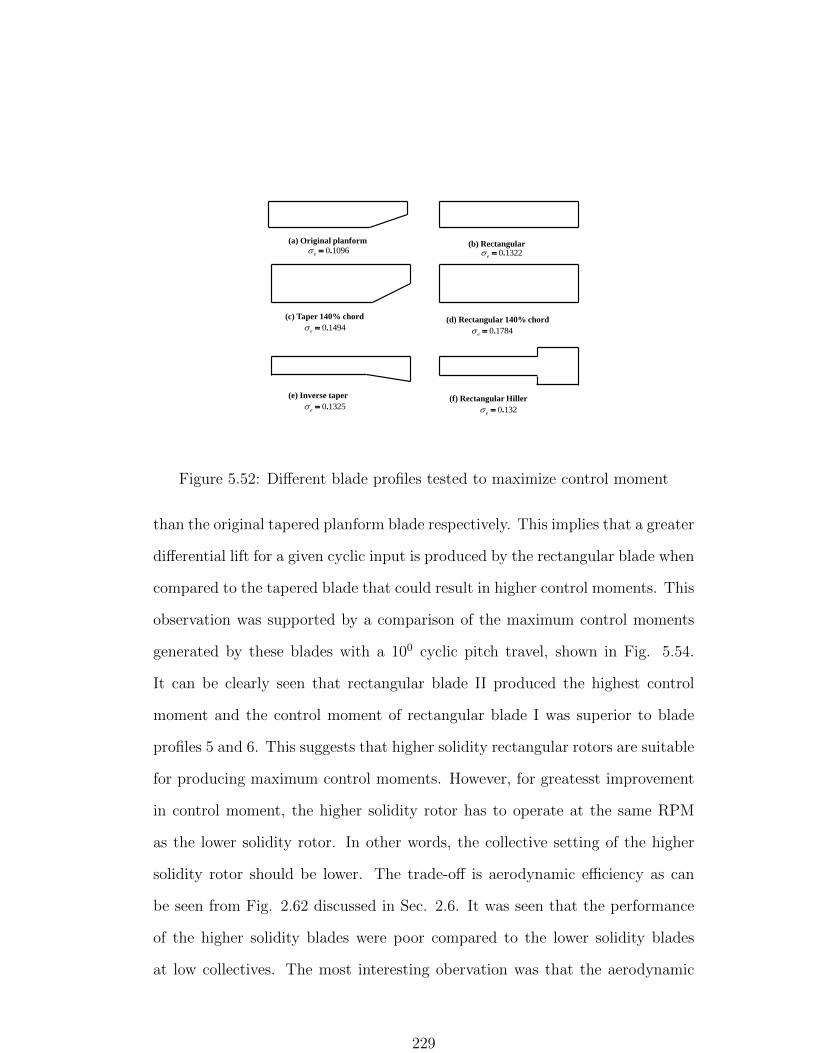
(a) Original planform (b) Rectangular 0 1096.

e 0 1322.

e

0 1494.e

0 1784.e

(c) Taper 140% chord (d) Rectangular 140% chord

(e) Inverse taper (f) Rectangular Hiller0 1325

e . 0 132

e .

Figure 5.52: Different blade profiles tested to maximize control moment

than the original tapered planform blade respectively. This implies that a greater

differential lift for a given cyclic input is produced by the rectangular blade when

compared to the tapered blade that could result in higher control moments. This

observation was supported by a comparison of the maximum control moments

generated by these blades with a 100 cyclic pitch travel, shown in Fig. 5.54.

It can be clearly seen that rectangular blade II produced the highest control

moment and the control moment of rectangular blade I was superior to blade

profiles 5 and 6. This suggests that higher solidity rectangular rotors are suitable

for producing maximum control moments. However, for greatesst improvement

in control moment, the higher solidity rotor has to operate at the same RPM

as the lower solidity rotor. In other words, the collective setting of the higher

solidity rotor should be lower. The trade-off is aerodynamic efficiency as can

be seen from Fig. 2.62 discussed in Sec. 2.6. It was seen that the performance

of the higher solidity blades were poor compared to the lower solidity blades

at low collectives. The most interesting obervation was that the aerodynamic

229

performance of the lower chord rectangular blade was very similar to the original

tapered blade. The rectangular blade I produced about 30% greater control

moment than the original blade. The performance drop at low collectives (180)

was the least among all the blade planforms. Therefore, it was chosen as the new

blade design for incorporation in the shrouded rotor with a collective setting of

180.

0 5 10 15 20 25 30 35 400

0.01

0.02

0.03

0.04

0.05

0.06

0.07

0.08

0.09

Collective (deg)

CT

Original

Rectangular

Taper 140% chord

Rectangular 140% chord

Inverse taper

Rectangular Hiller

Figure 5.53: Variation of thrust coefficient with blade collective for differentblade profiles in shrouded rotor

5.3.3 Control margin

From the above, the blade collective setting was shown to have an important

effect on the magnitude of control moments produced and on hover performance.

It is also of interest to find out whether the adverse pitching moment generated

in edgewise flow is affected by the collective setting for a given operating thrust.

In order to determine this, the rectangular blade circular inlet shrouded rotor

was tested in the open jet wind tunnel. The pitching moment was measured as a

230

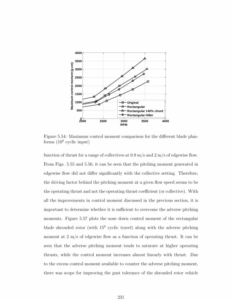
2000 2500 3000 3500 40000

500

1000

1500

2000

2500

3000

3500

4000

RPM

Ma

xim

um

co

ntr

ol m

om

en

t (g

-cm

)

Original

Rectangular

Rectangular 140% chord

Rectangular Hiller

Figure 5.54: Maximum control moment comparison for the different blade plan-forms (100 cyclic input)

function of thrust for a range of collectives at 0.9 m/s and 2 m/s of edgewise flow.

From Figs. 5.55 and 5.56, it can be seen that the pitching moment generated in

edgewise flow did not differ significantly with the collective setting. Therefore,

the driving factor behind the pitching moment at a given flow speed seems to be

the operating thrust and not the operating thrust coefficient (or collective). With

all the improvements in control moment discussed in the previous section, it is

important to determine whether it is sufficient to overcome the adverse pitching

moments. Figure 5.57 plots the nose down control moment of the rectangular

blade shrouded rotor (with 150 cyclic travel) along with the adverse pitching

moment at 2 m/s of edgewise flow as a function of operating thrust. It can be

seen that the adverse pitching moment tends to saturate at higher operating

thrusts, while the control moment increases almost linearly with thrust. Due

to the excess control moment available to counter the adverse pitching moment,

there was scope for improving the gust tolerance of the shrouded rotor vehicle

231

beyond 2 m/s.

0 100 200 300 400 5000

500

1000

1500

2000

2500

Thrust (g)

Pit

ch

-up

mo

me

nt(

g-c

m)

14 deg

18 deg

22 deg

Figure 5.55: Effect of operating thruston pitching moment at different bladecollectives at 0.9 m/s of edgewise flow

0 100 200 300 400 5000

500

1000

1500

2000

2500

Thrust (g)

Pit

ch

-up

mo

me

nt(

g-c

m)

14 deg

18 deg

22 deg

Figure 5.56: Effect of operating thruston pitching moment at different bladecollectives at 2.2 m/s of edgewise flow

0 100 200 300 400 5000

500

1000

1500

2000

2500

Thrust (g)

Mo

me

nt

(g-c

m)

Pitch-up moment-14 deg

Pitch-up moment-18 deg

Pitch-up moment-22 deg

Pitch-down control moment-14 deg

Pitch-down control moment-18 deg

Pitch-down control moment-22 deg

Figure 5.57: Pitch down control moment of the rectangular blade shrouded rotor(with 150 cyclic travel) and edgewise pitching moment as a function of thrust at2 m/s of edgewise flow

232

5.4 Summary

This chapter discussed the performance of the shrouded rotor MAV when ex-

posed to edgewise flow and control strategies to improve gust tolerance of the

vehicle. Two shroud designs were tested - circular inlet shroud and an ellip-

tic inlet shroud. Studies were conducted to compare the forces generated on the

shrouded and unshrouded rotor MAV using an open jet wind tunnel for edgewise

flow. Some of the key conclusions are:

(1)The elliptic inlet shrouded rotor with the highest hover efficiency (about

10% higher power loading than the circular inlet shroud) also had the greatest

adverse pitching moment -up to 400% higher than the unshrouded rotor. There-

fore, design metrics for MAV shroud must consider hover efficiency improvement

as well as reduction in the adverse pitching moment.

(2) The elliptic inlet shrouded rotor, which has a higher projected surface

area in the direction of the edgewise flow has greater drag (about 40% higher

than the circular inlet shrouded rotor). The vertical thrust generated by the

shrouded and unshrouded rotors remained unaffected by edgewise flow.

(3) The magnitude of the pitching moment depended on the operating thrust

and not on the operating thrust coefficient of the rotor. It was found to saturate

at higher values of thrust.

(4) The shrouded rotors produced up to 80-100% higher control moments

than the unshrouded rotor. The shroud-augmented control moments were gen-

erated from the asymmetric pressure distribution due to cyclic input to the

hingeless rotor. This is an important conclusion since it shows that cyclic pitch

variation is a useful scheme for shrouded rotor MAV control.

(5) When exposed to edgewise flow of up to 2 m/s, there was no reduction in

233

control moment in the unshrouded rotor. There was an optimum rotor collective

which resulted in the least reduction in control moment of the shrouded rotor.

This was determined to be about 220 for the circular inlet shrouded rotor with

an 8% drop in nose-down control moment.

(6) The onset of stall was delayed significantly in the shrouded rotor config-

uration by at least 5− 100. This implies that the shrouded rotor can tolerate a

higher cyclic pitch range and initial collective setting without any degradation

in control moments. An increase in cyclic pitch travel from 100 to 150 resulted

in a 30% improvement in control moment of the vehicle.

(7) It is beneficial to operate the rotor at low CT and high RPM for maxi-

mum control moment. Therefore blade profiles have to be chosen with the least

reduction in power loading at lower collectives.

(8) By replacing a tapered planform blade with a rectangular blade of same

rotor chord, the control moment was increased by about 30%, without significant

penalty in hover performance at lower collectives.

(9) It was found that the control moment increased linearly with operating

thrust while the pitching moment saturated at higher thrust levels. Therefore

for a given shroud area, the control margin of the shrouded rotor increases at

higher operating thrusts.

234

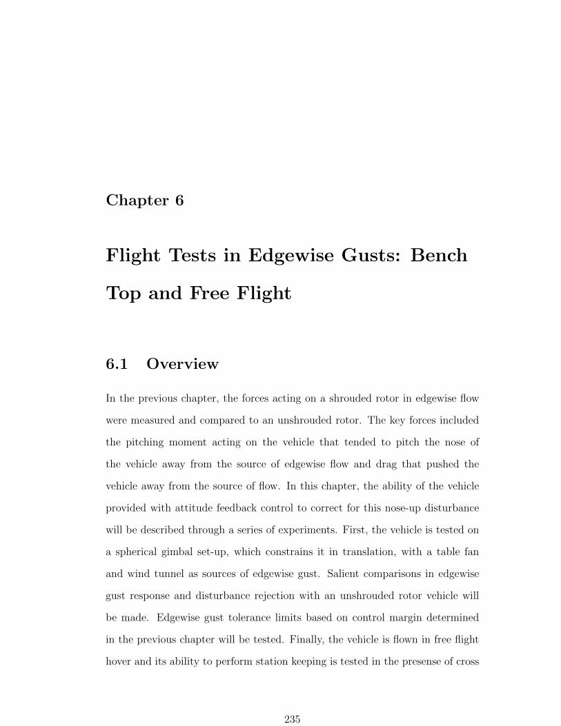
Chapter 6

Flight Tests in Edgewise Gusts: Bench

Top and Free Flight

6.1 Overview

In the previous chapter, the forces acting on a shrouded rotor in edgewise flow

were measured and compared to an unshrouded rotor. The key forces included

the pitching moment acting on the vehicle that tended to pitch the nose of

the vehicle away from the source of edgewise flow and drag that pushed the

vehicle away from the source of flow. In this chapter, the ability of the vehicle

provided with attitude feedback control to correct for this nose-up disturbance

will be described through a series of experiments. First, the vehicle is tested on

a spherical gimbal set-up, which constrains it in translation, with a table fan

and wind tunnel as sources of edgewise gust. Salient comparisons in edgewise

gust response and disturbance rejection with an unshrouded rotor vehicle will

be made. Edgewise gust tolerance limits based on control margin determined

in the previous chapter will be tested. Finally, the vehicle is flown in free flight

hover and its ability to perform station keeping is tested in the presense of cross

235

flow generated from a pedestal fan (with flow straighteners). A retro-reflective

marker pased position tracking system is used for position state information and

feedback.

6.2 Bench-top tests

Bench top gust disturbance rejection tests were conducted on the spherical gim-

bal stand (Fig. 4.8). The study focused on the disturbance rejection character-

istics of the vehicle when exposed to gusts from two sources: a standard table

fan and an open jet wind tunnel. The table fan set-up serves to illustrate sce-

narios where the size of the gust source is comparable to the size of the vehicle.

The wind tunnel set-up depicts situations where the vehicle is flown towards a

large window with a steady wind blowing through it. The two cases differ in the

amount of momentum drag generated and therefore require a different degree

of control moment to overcome the respective disturbances. Figure 6.1 shows a

schematic of these scenarios.

6.2.1 Table fan set-up

A Honeywell table fan was chosen for this purpose. It consisted of an 8” diameter

fan with flow straighteners in its wake. As a result, the wake of the fan was

mostly steady and irrotational. The fan had three levels of operation. Pitot

tube measurements were made at different radial and axial locations for each

level to determine the axial velocity magnitude. Figure 6.2 shows the velocity

distribution at the exit of the fan structure. The vehicle was mounted on the

spherical bearing set-up and placed at about 5”- 8” from the exit plane of the

fan (Fig. 6.3. These tests were conducted with the flybar rotor set-up. A

236

Scenario #1Table fan(Low momentum flux)

Scenario #2Window(High momentum Flux)

Figure 6.1: Sources of edgewise gust

proportional integral based attitude feedback control was implemented to reject

disturbances and maintain hover attitude. The pitching moment generated

-10 -5 0 5 100

2

4

6

8

10

Fan width (cm)

Ve

locit

y (

m/s

)

Level 1

Level 2

Level 3

BLOCKING DISK

Figure 6.2: Axial velocity distribution at exit plane of Honeywell fan

by the vehicle placed in the fan wake is shown in Fig. 6.4. It can be seen

237

Figure 6.3: Axial velocity distribution at different station locations in the fanwake

that with the flybar rotor head, the control moment limits was reached at a free

stream velocity of about 6 m/s (level 3). At this fan setting, the fan position was

varied in height and angle to obtain a qualitative understanding of changes in

controllability with fan orientation. It can be seen that as the angle between the

free stream and the rotor reduced, the controllability increased (Fig. 6.5). This

was expected since the momentum drag contribution to the pitching moment

reduced. The worst case scenario was when the top half of the vehicle was

exposed to the flow. Now, since the shroud inlet was not a closed profile, it

may be possible that flow separation and recirculation underneath the outer

portion of the inlet could affect controllability. To verify this, the outer portion

of the shroud was closed using plastic material as shown in Fig. 6.6. Tests

showed that this did not affect the magnitude of pitching moment for a given

flow speed. In other words, there was little difference in controllability between

238

a closed and an open shroud inlet profile. The vehicle was then mounted on

3 3.5 4 4.5 5 5.5 6 6.5350

400

450

500

550

600

650

700

750

Wind (m/s)

Mo

me

nt

(g-c

m)

Moment produced due to gust

Control authority limitControl moment limit

Figure 6.4: Nose up pitch moment at different fan setting (flybar rotor head)

Figure 6.5: Effect of fan orientation on vehicle control

239

Table fan

Closed inlet

profileOpen inlet

profile

Figure 6.6: Closed shroud inlet profile

the spherical bearing set-up and placed in the wake of the fan with the flow

perpendicular to the rotor thrust. Based on the above, the fan was operated at

level 1 to ensure that the vehicle had sufficient control moment to overcome the

edgewise gust disturbance. A pitot probe was placed close to the shroud inlet

to synchronize the vehicle attitude response and the gust disturbance. Care

was taken to minimize interference of the probe with the flow field and vehicle

structure. The pitot probe was sampled by NI-USB hardware at 1000 Hz. The

vehicle was initially commanded to hover attitude position at 3700 RPM. When

the vehicle was subjected to the edgewise gust field, the subsequent attitude

disturbance was sought to be mitigated by the attitude feedback controller. The

control loop was closed at 200 Hz. The controller included a proportional and

integral feedback of the error in euler attitude angles.

Step input : Figure 6.7 shows the response of the vehicle when subjected to a step

input and removal of gust field. The gust field was along the negative X axis of

the vehicle and the primary response was in the pitch axis. It can be seen that

240

in the step input phase, there was an initial sharp pitch back response which

subsequently settled to hover attitude within a mean settling time of about 4-

5 s1. Upon gust removal, the pre-existing control moment opposing the pitch

back moment due to the edgewise gust resulted in a pitch forward response due

to overcorrection. Ultimately it settled back to hover attitude within about 5

s. The proportional and integral gains were tuned to about 120% stick input

range/radian and 10% stick input range/rad-s respectively.

Impulse: An impulse in the edgewise gust field could also be given by initially

blocking the fan flow with a screen and impulsively removing and replacing the

screen. The gust impulse response is shown in Fig. 6.8. It can be seen that

for this case, the vehicle developed a larger attitude error than the step input

case. This is because, for the step input case, there was a rise time of about

2 s before maximum gust speed was achieved. This gave the controller time to

enable sufficient control moments to achieve hover attitude. This was not the

case for the impulse case where the maximum gust speed was reached within

a second. For the first gust impulse case, the vehicle began correcting itself

before the maximum gust velocity was recorded. Additionally, it can be seen

that although the peak velocity for the second impulse case was lower than the

first, the magnitude of pitch back response was the same. This indicated that

the rate of increase in gust velocity is as important a factor as the magnitude of

the gust velocity in characterizing the vehicle response to gusts.

Attitude-hold control : The previous two tests showed the ability of the vehicle

1The settling time described here refers to the time required for the mean attitude level toreach within 95% of the hover level. Transient dynamics are not considered

241

25 30 35 40 45 50-0.5

0

0.5

Pit

ch

att

itu

de

(ra

d)

25 30 35 40 45 500

1

2

3

Time (s)

Gu

st

(m/s

)

Disturbance

removed

Disturbance

input

Figure 6.7: Edgewise gust disturbance response: step input. Gust 3 m/s

45 50 55 60 65-0.5

0

0.5

Pit

ch

att

itu

de

(ra

d)

45 50 55 60 650

2

4

Time (s)

Gu

st

(m/s

)

Figure 6.8: Edgewise gust disturbance response: Impulse. Peak gust 3 m/s

242

to maintain hover attitude in the presense of edgewise gusts. It was also of

importance to test attitude-hold control of the vehicle in the presense of gusts.

Of particular interest was the pitch forward attitude-hold of the vehicle into the

flow (similar to a vehicle transitioning from hover to forward flight). For these

tests, a gust step input was provided. Two cases were considered - (1) pitch

forward command before edgewise flow input, and (2) pitch forward command

after edgewise flow input. The effect of including P and PI feedback gains were

studied for these cases. Figure 6.9 shows the response of the vehicle for the first

case using a PI controller. Initially, the vehicle was commanded to a pitch for-

ward position. Upon edgewise flow input, this position was disturbed which was

subsequently restored. However, a comparison in attitude-hold performance of

the vehicle before and after flow input showed that the PI controller performance

deteriorated when the flow input was given. The presence of oscillations about

the mean attitude position can be seen which suggested that the stability of

the closed loop system was reduced in the presence of external disturbance and

non-zero attitude reference. Figure 6.10 showed the vehicle performance with

a proportional controller. It can be clearly seen that for this case, oscillations

were significantly reduced. However, for disturbance rejection (original attitude

regained after disturbance), proportional control was not very effective. This

can be circumvented by tuning the gains and/or adjusting attitude reference in

real time. By modifying the controller to ’PI’ for hover and ’P’ for non-zero

attitude-hold, vehicle performance may be improved. This is shown in Fig. 6.11

where pitch forward command was given after flow input was turned on. Based

on these tests, it can be seen that caution must be taken before including integral

feedback in the controller. A combination of P and PI feedback may have to be

incorporated.

243

20 30 40 50 60-0.5

0

0.5

Pit

ch

att

itu

de

(ra

d)

20 30 40 50 60-1

0

1

2

3

Time (s)

Gu

st

(m/s

)

HoverPitch forward,no gust

Gust input

Pitch forward,In edgewise flow

Disturbancerejection

Figure 6.9: Pitch forward command before edgewise flow input: PI control

15 20 25 30-0.5

0

0.5

Pit

ch

att

itu

de

(ra

d)

15 20 25 30-1

0

1

2

3

Time (s)

Gu

st

(m/s

)

Pitch forward,no gust

Hoverattitude

Gust input No disturbancerejection

Pitch forwardreference attitudechanged

Figure 6.10: Pitch forward command before edgewise flow input: P control

244

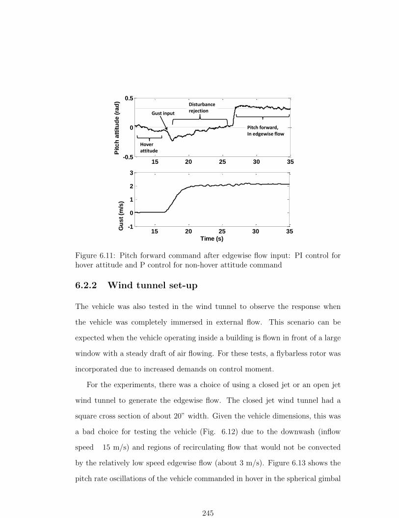
15 20 25 30 35-0.5

0

0.5

Pit

ch

att

itu

de

(ra

d)

15 20 25 30 35-1

0

1

2

3

Time (s)

Gu

st

(m/s

)

Hoverattitude

Gust input

Disturbancerejection

Pitch forward,In edgewise flow

Figure 6.11: Pitch forward command after edgewise flow input: PI control forhover attitude and P control for non-hover attitude command

6.2.2 Wind tunnel set-up

The vehicle was also tested in the wind tunnel to observe the response when

the vehicle was completely immersed in external flow. This scenario can be

expected when the vehicle operating inside a building is flown in front of a large

window with a steady draft of air flowing. For these tests, a flybarless rotor was

incorporated due to increased demands on control moment.

For the experiments, there was a choice of using a closed jet or an open jet

wind tunnel to generate the edgewise flow. The closed jet wind tunnel had a

square cross section of about 20” width. Given the vehicle dimensions, this was

a bad choice for testing the vehicle (Fig. 6.12) due to the downwash (inflow

speed 15 m/s) and regions of recirculating flow that would not be convected

by the relatively low speed edgewise flow (about 3 m/s). Figure 6.13 shows the

pitch rate oscillations of the vehicle commanded in hover in the spherical gimbal

245

setup. It can be seen that hover stability was severely affected as the vehicle

was transtioned into the test section of the wind tunnel. Since this would be

detrimental to further testing, an open jet wind tunnel set-up was considered.

Closed jet

wind tunnel

Figure 6.12: Closed jet wind tunnel set-up

Figures 6.14 and 6.15 show the open jet wind tunnel set-up for the shrouded

and unshrouded rotor. The flybarless rotor with the original tapered planform,

a cyclic travel of 100 and a collective setting of about 240 was used. The vehicle

was placed on a height adjustable gimbal stand with the leading edge of the

shroud about 2” from the exit plane of the wind tunnel. A pitot probe at the

exit plane recorded the time history of the gust and was synchronized with the

vehicle response data. Due to the size of the test section compared to vehicle

dimensions, it was possible to assess the effect of the edgewise flow impinging on

different regions of the shrouded and unshrouded rotor vehicles by adjusting the

height of the gimbal stand. For this, three different positions were considered

246

0 20 40 60 80 100 120 140-5

0

5

Time (s)

Pit

ch

ra

te, q

(ra

d/s

)

Vehicle moved into wind tunneltest section

Vehicle outsidewind tunnel test section

Figure 6.13: Deteriorated hover performance as vehicle is transitioned into closedjet wind tunnel test section

as shown in Fig. 6.16: (1) inlet in flow, (2) full body in flow, and (3) vanes in

flow. A comparison in gust response characteristics between the shrouded and

unshrouded rotors was made for these positions. The response of the shrouded

and unshrouded rotor MAV was compared at operating power of the shrouded

rotor.

The pitch up response when exposed to edgewise flow was seen for both

the MAVs. The shrouded rotor had sufficient control moment to tolerate an

edgewise gust of about 2 m/s. In contrast, the unshrouded rotor could tolerate

edgewise gusts of up to 4.8 m/s. Figures 6.18−6.22 shows the response of the

vehicles when subjected to an edgewise gust of about 1.9 m/s. The settling time

of the PI controller did not differ significantly. However, the shrouded rotor

showed a much larger pitch-up attitude error of up to 0.5 rad (Positions 1 and

2) when compared to the unshrouded rotor. This implies that in free flight,

247

Figure 6.14: Open jet wind tunnel set-up: Shrouded rotor

Figure 6.15: Open jet wind tunnel set-up: Unshrouded rotor

248

Figure 6.16: Different vehicle positions tested relative to flow

the thrust vector of the shrouded rotor vehicle would tilt (away from vertical)

to a much larger angle. This would result in a faster drop in vehicle altitude

when compared to the unshrouded rotor although, in reality, the vehicle is free

to translate (away from the source of gust) which might make this attitude tilt

less severe. In position 3, where the wakes of the rotors are affected by cross

flow, the shrouded rotor experienced greater oscillations than the unshrouded

rotor. However, in all cases, the controller was successfully able to reject the

disturbances due to edgewise gust.

Figure 6.23 shows the response of the shrouded rotor when exposed to edge-

wise flow of magnitudes greater than 2 m/s. It can be clearly seen that the

control inputs were saturated and the vehicle was unable to return to hover at-

titude. By incorporating the optimized planform and swashplate design settings

discussed in the previous chapter, the edgewise gust tolerance was increased to

249

20 25 30 35 40-0.5

0

0.5P

itc

h

att

itu

de (r

ad

)

20 25 30 35 400

1

2

Time (s)

Gu

st

(m/s

)

Figure 6.17: Position 1: Shrouded rotor, Gust 1.9 m/s

10 15 20 25 30 35 40-0.5

0

0.5

Pit

ch

att

itu

de (

rad

)

10 15 20 25 30 35 400

1

2

Time (s)

Gu

st

(m/s

)

Figure 6.18: Position 1: Unshrouded rotor

250

10 15 20 25 30 35 40 45-0.5

0

0.5P

itc

h

att

itu

de(r

ad

)

10 15 20 25 30 35 40 450

2

4

Time (s)

Gu

st

(m/s

)

Figure 6.19: Position 2: Shrouded rotor

5 10 15 20 25 30 35 40-0.5

0

0.5

Pit

ch

att

itu

de (

rad

)

5 10 15 20 25 30 35 400

1

2

Time (s)

Gu

st

(m/s

)

Figure 6.20: Position 2: Unshrouded rotor

251

20 25 30 35-0.5

0

0.5

Pit

ch

att

itu

de (

rad

)

20 25 30 350

2

4

Time (s)

Gu

st

(m/s

)

Figure 6.21: Position 3: Shrouded rotor

10 15 20 25 30 35 40 45-0.5

0

0.5

Pit

ch

att

itu

de (

rad

)

10 15 20 25 30 35 40 450

1

2

Time (s)

Gu

st

(m/s

)

Figure 6.22: Position 3: Unshrouded rotor

252

more than 3 m/s as shown in Fig. 6.24. The reduced settling time and initial

pitch-up attitude error can also be clearly seen.

10 20 30 40 50 60-0.5

0

0.5

Pit

ch

(ra

d)

10 20 30 40 50 60-1

-0.5

0

0.5

Time (s

Lo

ng

itu

dn

al c

on

tro

l

(no

n d

im)

Control inputsaturation

Unable to return tohover condition

Gust response

Figure 6.23: Control input saturation at gusts > 2 m/s

6.3 Free Flight Tests

The wind tunnel tests constrained the vehicle in position. Free flight tests were

then conducted in order to observe the vehicle response to edgewise gusts in

attitude and position. Additionally, the ability of the vehicle to maintain hover

attitude and position in space (station keeping) was studied. For this, the vehicle

was flown in a 30ft × 30ft × 40ft space 1. The facility was equipped with VICON

that tracked the vehicle motion and was used to provide position control of the

vehicle. The shrouded rotor MAV was fitted with retro-reflective markers that

1Experiments conducted at Motile Robotics Inc., Joppa, Maryland

253

15 20 25 30 35 40-0.2

0

0.2

Pit

ch

(ra

d)

15 20 25 30 35 40-0.5

0

0.5

Lo

ng

itu

din

al

co

ntr

ol

(no

n d

im)

15 20 25 30 35 400

0.1

0.2

Time (s)

Pit

ot

(vo

lts

)

Control input limit

Figure 6.24: Improved gust tolerance ( 3m/s) due to increased control margin(Fig. 5.57)

were tracked by 16 infrared cameras at a loop rate of 100 Hz. A snapshot from

the motion capture system is shown in Fig. 6.25. Changes in marker positions

were converted to changes in rigid body attitude and position of the vehicle.

Sensor fusion of an onboard IMU with the VICON data was done in LabVIEW.

A schematic of the feedback controller used for attitude and position control

is shown in Fig. 6.26. This was used to maintain the vehicle in hover at a

single point on the X-Y plane. It can be seen that for control, a proportional

feedback of the position error and a PID feedback of the Euler attitude error is

given. For these tests, the altitude (Z) of the vehicle was manually controlled

by adjusting the rotor RPM. In order to generate edgewise gust, three sources

were used: (1) flapping board (Fig. 6.27), (2) 0.5 m table fan (Fig. 6.28), and

(3) 0.7 m industrial fan (Fig. 6.29). The peak velocity of the gust from the

flapping board was about 1.5 m/s. It was difficult to map the velocity profile

254

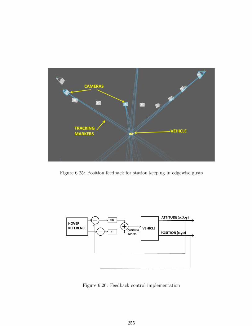
Figure 6.25: Position feedback for station keeping in edgewise gusts

Figure 6.26: Feedback control implementation

255

of this gust spatially. Figures 6.30 and 6.31 show the velocity profiles of sources

2 and 3. Honeycomb flow straighteners were installed in front of both of these

fans to ensure that the flow profile remain largely edgewise with minimum flow

circulation. One metric for characterizing the vehicle motion as it operates in

gust is the circular error probable (CEP). It is a circle that encircles 50% of the

trajectory of the vehicle when exposed to gusts (Fig. 6.32). Therefore, the CEP

is expected to be negligible in the absence of gusts.

Flapping board

Figure 6.27: Flapping board as source of gust

The vehicle was first flown in hover to determine the performance of the feedback

controller and for the purposes of determining suitable gains. Figure 6.33 shows

the vehicle states commanded in the hover flight mode. It can be seen that

the vehicle maintained a satisfactory hover attitude and the CEP of the vehicle

was about 100 mm. Next, the controller was tested for its ability to reject

disturbances in control inputs. Figure 6.34 shows the response of the vehicle to

256

Flow straightener

Figure 6.28: 0.5 m diameter fan gust setup

Figure 6.29: 0.75 m diameter fan gust setup

257

0

10

20

30

40

50

60

70

80

90

100

0 100 200 300 400 500 600 700

Loca

tio

n (

mm

)

Velocity (ft/min)

Figure 6.30: 0.5 m diameter fan velocity profile

0.4 0.6 0.8 1 1.2 1.4 1.6

0.6

0.7

0.8

0.9

1

1.1

1.2

1.3

1.4

1.5

He

igh

t O

ff G

rou

nd

[m

]

Wind Speed [m/s]

Average Wind Speed 4.8 m From Fan

Fan Diameter

Figure 6.31: 0.75 m diameter fan velocity profile

258

Figure 6.32: Circular error probable (CEP) metric to characterize vehicle tra-jectory

a control input disturbance. When the longitudinal control input disturbance

was given, the vehicle quickly returned to hover and error in position was slowly

damped out. This demonstrated the satisfactory performance of the controller

in quiescent conditions and in the presence of non-serodynamic disturbances.

For flight tests in gusts, the vehicle was first flown in hover position, the

edgewise gust input was then given and the vehicle was tracked as it attempted

to maintain the hover position. Figure 6.35 shows the response of the vehicle to a

gust from the flapping board. It can be seen that the vehicle responeded in both

the primary (pitch) and secondary (roll) axis. Minimal motion in translation

was observed. The attitude motion was damped within about 2 s which was

what was observed in the wind tunnel tests. When the 0.5 m diameter fan

was operated, the vehicle underwent an attitude error, deviated from position

and returned back to position, with a CEP of about 0.75 m. (Fig. 6.36). This

259

20 25 30 35 40 45 50-0.5

0

0.5

Att

itu

de

(ra

d)

20 25 30 35 40 45 50-1000

0

1000

Po

sit

ion

(m

m)

20 25 30 35 40 45 500

50

100

Time (s)

Co

ntr

ol in

pu

t

(un

its

)

Roll

Pitch

X

Y

Lateral

Longitudinal

Figure 6.33: Hover position control of vehicle

20 22 24 26 28 30 32-0.5

0

0.5

Pit

ch

(ra

d)

20 22 24 26 28 30 32-1000

0

1000

X (

mm

)

20 22 24 26 28 30 320

50

100

Time (s)

Lo

ng

itu

din

al

co

ntr

ol

inp

ut

(un

its) input disturbance

Figure 6.34: Response of vehicle to control input disturbances

260

represented a more persistent gust field than a flapping board. Minor oscillations

were observed in the vehicle attitude as it was damped out. It must be mentioned

that it was difficult to maintain a steady gust field and the orientation of the

gust in an edgewise direction when compared to the wind tunnel tests. Finally,

the vehicle was flown about 5 m in front of the 0.75 m diameter fan with the

flow along the negative X axis. Figure 6.37 shows the vehicle response in a flow

speed of 1.5 m/s. It can be seen that the vehicle response was highly coupled in

pitch and roll as it attemped to maintain hover position. The CEP of the vehicle

is shown in Fig. 6.38. It can be seen that the CEP of the vehicle at around 3

m/s of edgewise flow was about 15 times larger than in the no wind case. This

re-iterates the enhanced sensitivity of the shrouded rotor MAV to external flow

disturbances. Nevertheless, the vehicle was capable of satisfactory hover in the

presense of low edgewise flow speeds. Many instances of gust inputs involved

fairly turbulent, rotational flows which were difficult to characterize. It was

also observed that on these occasions, the vehicle was unable to react to sudden

changes in wind magnitude, leading to overcompensation and sudden crashes.

Since the control inputs were not yet completely saturated, there is scope of

improving the performance by increasing controller gains and bandwidth of the

feedback system.

6.4 Summary

For the edgewise gust disturbance tests, the unshrouded and shrouded rotor

vehicles were mounted on a spherical bearing setup to allow for pitch and roll

motion while restricting it in translation. With an 8” diameter fan (with flow

straighteners), the shrouded rotor vehicle could tolerate edgewise gusts of up to

261

10 12 14 16 18 20-0.5

0

0.5P

itc

h (

rad

)

10 12 14 16 18 20-0.5

0

0.5

Time (s)

Ro

ll (

rad

)

gust impulse

Figure 6.35: Response to gust from flapping board

50 55 60 65-0.5

0

0.5

Pit

ch

(ra

d)

50 55 60 65-2000

0

2000

X (

mm

)

50 55 60 650

50

100

Time(s)

Lo

ng

itu

dn

al

co

ntr

ol in

pu

t (u

nit

s)

Vehicle encounters

gust field

Figure 6.36: Response to gust from 0.5 m table-fan (1.4 m/s)

262

60 65 70 75 80-1

0

1

Att

itu

de

(ra

d)

60 65 70 75 80-2000

0

2000

Po

sit

ion

(m

m)

60 65 70 75 800

100

200

Time (s)

Cy

clic

in

pu

t

(un

is)

Roll

Pitch

X

Y

Lateral cyclic

Longitudinal cyclic

vehicle enters gust field

Figure 6.37: Response to gust from 0.75 m table-fan (1.5 m/s)

0 0.5 1 1.5 2 2.5 3 3.50

500

1000

1500

2000

2500

3000

Wind speed (m/s)

Cir

cu

lar

err

or

pro

ba

ble

(m

m)

Figure 6.38: CEP of shrouded rotor with 0.75 m diameter fan as source of gust

263

6 m/s. The mean settling time after an input disturbance was less than 5 s.

The wind tunnel setup was viewed as a source of gust when the vehicle is

operating near a large window. When the edgewise flow was introduced, the

shrouded rotor developed a higher nose-up attitude error than the unshrouded

rotor. This means that the shrouded rotor would have a larger tilt of the thrust

vector in its initial response to an edgewise gust. The mean settling time after

the introduction of the disturbance was about 5 s for both the vehicles. The

shrouded rotor could tolerate up to 3 m/s gusts while the tolerance was greater

than 5 m/s for the unshrouded rotor.

Free flight tests on the vehicle, using VICON for feedback control, indicated

the capability of the vehicle to recover from gust impulse inputs from a pedestal

fan. When exposed to edgewise flow, the vehicle could tolerate up to 3 m/s of

wind speed. The circular error probable of the vehicle trajectory was up to 15

times at 3 m/s as compared to the no wind case. This re-iterates the enhanced

sensitivity of the shrouded rotor to edgewise flow.

264

Chapter 7

Conclusions and Recommendations for

Future Work

In the past decade, with the progress of microsystem technology in electronics

and manufacturing, Micro Air Vehicles (MAVs) are fast emerging as viable aerial

platforms that can be used in a wide area of applications in the military and

civilian domain. These include perimeter surveillance, targeting, biochemical

sensing, traffic monitoring and many other operations that are dangerous, im-

practical or inconvenient for human involvement. They can be used to enhance

situational awareness, minimize risk exposure, aid manned-unmanned teaming

and integrate communication with Unmanned Ground Vehicles (UGVs). For

many of these applications, platforms are required that have hover and slow-

loiter capability, ability to perform quick and complex maneuvers, avoid obsta-

cles as well as tolerate aerodynamic disturbances such as wind gusts and flow

recirculation that may occur when flying close to ground or in the vicinity of

walls.

Rotary wing platforms have the potential to meet many of these requirements

primarily due to their ability to be aerodynamically efficient in hover (when

265

compared to fixed and flapping wing platforms). To provide high aerodynamic

control forces, fixed wing platforms must be travelling at high speeds. Flapping

wing MAVs would require high flapping frequencies which can be detrimental to

the life span of the vehicle due to high wear and tear from the unsteady inertial

forces. Rotary wing MAVs, on the other hand, can generate high dynamic pres-

sures by allowing for sufficiently high rotational speeds (steady inertial forces).

This translates to increased maneuverability at hover or near-hover conditions.

Due to many of these factors, there has been a lot of research into the develop-

ment of single and multi-rotor platforms.

However, there are significant technical challenges involved in the develop-

ment of small scale rotary wing systems. Some of these include: (1) poor aerody-

namic efficiency at the highly viscous, separation prone, low Reynolds number

flow regimes, (2) increased sensitivity to external disturbances (inertia scales

down by the fifth power of scale whereas the weight scales by only the cube

of scale), (3) limited high-bandwidth on-board electronics for feedback imple-

mentation, (4) lack of robust, stiff and lightweight structures, (5) poor energy

density and efficiency of micropropulsion technologies, among many more. It can

be seen that this is truly a multidisciplinary venture that involves advancements

in many areas in order to develop efficient, novel and fully functional platforms.

In the scope of this research, the aerodynamic performance, and flight stabil-

ity and control (with and without input disturbances) were studied as applicable

to one such novel MAV rotary wing configuration - the shrouded rotor. This con-

figuration offers three key operational benefits: (1) increased system thrust for

a given power input, (2) enhanced structural rigidity, rotor protection and op-

erational safety and (3) shroud can be retrofitted into an optimized rotary wing

platform, thus complementing efforts to optimize a conventional rotary wing

266

system as well as minimizing design costs to reconfigure platforms. However,

there are two significant challenges in the development of these platforms at mi-

cro scales: (1) development of a stiff and lightweight shroud so that the excess

system thrust offsets the excess weight due to the shroud, and (2) increased sensi-

tivity to flow disturbances when compared to conventional rotary wing systems,

especially edgewise gusts.

In this dissertation, these key aspects were addressed and studied in or-

der to assess the capability of the shrouded rotor as a platform of choice for

MAV applications. First, a low disk loading shrouded rotor vehicle was designed

and constructed with key shroud design variables derived from previous studies

on micro shrouded rotors. The different components such as the rotor, stabi-

lizer bar, yaw control vanes and the shroud were designed and systematically

studied for system efficiency and overall aerodynamic improvements. Risk re-

duction prototypes were built to sequentially arrive at the final configuration.

The passive stability of the shrouded and unshrouded rotor systems were then

studied in hover in quiescent conditions. Specific constraints related to rotor tip

path plane variation inside the shroud were derived. An attitude proportional-

integral-derivative (PID) controller based on wireless telemetry was implemented

to augment stability in hover. The PID gains were tuned based on the Ziegler-

Nichols tuning approach. In order to enhance maneuverability and reduce profile

losses, the stabilizer bar was removed. Implications on attitude dynamics were

then studied using a time domain system identification approach. A linear re-

duced order attitude dynamics model was derived to enable implementation of

a model based controller using the linear quadratic regulator. Next, the ability

of the unshrouded and shrouded rotor systems to reject external aerodynamic

disturbances (edgewise gusts from table fan and wind tunnel) while maintaining

267

hover attitude were studied. The aeromechanical forces generated on these sys-

tems in edgewise flow were systematically measured. A few design modifications

to the rotor system were identified and studied to improve the control moment

of the shrouded rotor system with the aim of improving edgewise gust tolerance.

Finally, with the aid of a motion capture system using retroreflective markers

and infrared cameras, a PID feedback controller was implemented with trans-

lational and attitude feedback. The purpose was to study the response of the

shrouded rotor vehicle to an edgewise gust and track its motion as it attempted

to hover at a particular station. The present research was concluded at this stage

to open up further research and development required in the area of MAV flight

performance in degraded flow conditions.

7.1 Conclusions

The following are some specific conclusions from the present work.

7.1.1 Vehicle design and hover performance

The vehicle consists of a two bladed single rotor enclosed in a shroud with anti-

torque vanes placed in the rotor downwash to counter rotor torque. The final

vehicle weighed about 280 g with a rotor diameter of about 244 mm.

1. Airfoil: In both the shrouded and unshrouded rotor configurations, the

use of a sharpened leading edge (LE) with a circular camber airfoil yielded

better hover performance over an unsharpened leading edge airfoil. This

was clearly illustrated in hover flight tests, where rotors with sharpened

and unsharpened LE would produce the same thrust, while the rotor torque

268

produced by the unsharpened LE resulted in severe loss of yaw trim. This

shows that the profile power losses with the unsharpened LE is greater.

2. Rotor planform: Parametric studies were conducted on different rotor plan-

forms in the shrouded and unshrouded rotor configurations (the effect of

rotor twist alone was not measured to be a significant factor). In the

unshrouded rotor configuration, a 2:1 taper ratio at 80% radial location

gave the highest Figure of Merit of about 0.64 (blade loading of between

0.15-0.2). It is noted that the blade loadings for efficient performance of

MAV blades are higher than for full scale rotors. It is difficult to reconcile

the rotor performance with the airfoil characteristics. A complete explana-

tion of this phenomenon requires a detailed experimental study of low Re

airfoils. At operating thrust, tapered blades (10g/W) had a 15% improve-

ment in power loading over rectangular blades(8.5 g/W). However, for a

shrouded rotor configuration, the rectangular planform was as efficient as

the tapered blade (power loading of about 14-15 g/W at operating thrust).

An explanation for this could be that in the shrouded rotor configuration,

the tip vortex is diffused and extra thrust is extracted from the tip of the

rectangular blade.

3. Shrouded rotor performance comparison: At an operating thrust of 300

grams, the power loading of the shrouded rotor was approximately 30%

higher than the unshrouded rotor (the rotor disk area was kept constant

and a tip clearance of 0.015R was maintained). For example, at an in-

put mechanical power of 15 watts, the shrouded rotor thrust was about

70 grams higher than the unshrouded rotor. After taking the weight of

the shroud into consideration (40-45 grams), this translates to a payload

269

benefit of about 20-30 grams.

4. A measurement of the individual thrust contributions showed that the

shroud produced up to 30-35% of the total system thrust in hover. This

result agreed well with CFD calculations.

5. The blades stalled at about 30 deg for the unshrouded rotor, while the

stall angle was close to 40 deg for the shrouded rotor. This delay in stall

is due to the fact that the inflow velocity in the shrouded configuration is

higher, resulting in a lower effective angle of attack.

6. Analysis of the above empirical data showed that the optimum shroud

diameter to lift an unshrouded rotor (or payload) of 250 g is about 14 cm.

This results in less than a 5% reduction in hover power compared to the

present set-up. Therefore, the shroud size chosen in this research is close

to optimum for a 250 g design payload.

7. Operation of the Hiller stabilizer bar reduced the effective rotor FM from

0.64 to about 0.61. This is primarily due to the profile losses associated

with the Hiller paddles. These losses can be minimized by choosing an

optimum pitch setting of the paddles. It was found to be about 12 deg.

The optimized Hiller bar configuration that minimized profile losses had a

radius of 60 mm and a paddle area of 8.5 cm2.

8. For countering rotor torque, a compact configuration was to incorporate

circular camber vanes in the downwash of the rotor. The vanes could

either be placed in an X or an H fashion. It was seen that either of these

configurations were effective in countering rotor torque irrespective of rotor

270

thrust. The penalty in power to maintain a constant thrust was about 10%

of the main rotor power, due to the downforce acting on these vanes.

9. The anti-torque effectiveness of these vanes reduced drastically in ground

effect (IGE) due to the modified structure of the rotor wake. Perfect bi-

directional yaw control was not achieved in IGE condition with the same

vane trim settings as for the out of ground effect condition.

7.1.2 Attitude dynamics and flight tests in hover (no flow

disturbances)

The differences in passive stability in attitude between a shrouded and un-

shrouded rotor MAV were compared. Implementation of a classical feedback

control system and flight testing is described. Open loop time domain system

identification was conducted to extract the attitude dynamics of a flybar and

flybarless shrouded rotor. Specific controllability metrics were extracted from

these models to enable quantitative comparison.

1. While a teetering rotor along with a stabilizer bar offers rotor damping

in the unshrouded rotor configuration, it induces limit cycle oscillations in

the shrouded rotor setup. This is due to the movement of the rotor tip

path plane, that results in asymmetric pressure distribution on the shroud.

This leads to a shift in center of lift and ultimately causes oscillations.

2. To prevent this, it is necessary to incorporate a rigid/hingeless rotor in the

shrouded rotor vehicle to minimize tip path plane movement.

3. The Hiller bar has to be appropriately phased with respect to the hingeless

rotor pitching axis to prevent active and passive cross coupling in pitch and

271

roll attitude motion. The hingeless rotor in the present vehicle has a non

dimensional rotating natural frequency of about 1.4. This requires the

Hiller bar to be phased about 40-45 degrees with respect to the main rotor

pitching axis at operating RPM. The phasing angle was experimentally

shown to monotonically increase with rotor RPM.

4. A proportional-integral-derivative feedback controller was successfully able

to stabilize the shrouded rotor vehicle in hover. The gains were tuned based

on the Ziegler-Nichols approach. A knowledge of the trim values was seen

to be a significant factor for achieving stable flight. Integral feedback

reduced stability margin of the vehicle and was only used in conditions

where trim values were not known.

5. The shrouded rotor vehicle was seen to be especially prone to oscillations

in pitch and roll close to the ground, probably due to asymmetric pressure

distribution on a tilted shroud surface in IGE conditions. In order to

minimize this ground effect induced instability, fast start-ups of the vehicle

were commanded.

6. A reduced order linear attitude dynamics model was identified using the

time domain system identification approach. This model compared satis-

factorily with flight test data at desired input frequencies below 2 Hz. The

yaw DOF was decoupled from vehicle pitch and roll.

7. In order to improve maneuverability and efficiency of the vehicle, it was

necessary to remove the stabilizer bar (flybar). A comparison in attitude

dynamics of the flybar and flybarless rotor showed that in the flybar setup,

the vehicle had stable poles while the flybarless rotor was marginally un-

272

stable.

8. Comparison in controllability metrics such as Frobenius norm derived from

the controllability gramian indicates that the flybarless rotor is more con-

trollable than the flybar rotor. The source of this increased controllability

is the reduced damping and increased control moments.

7.1.3 Force measurement and flight testing in hover with

edgewise flow imposed

Two shroud designs were tested - circular inlet shroud and an elliptic inlet

shroud. Studies were conducted to measure and compare the forces generated

on the shrouded and unshrouded rotor MAV using an open jet wind tunnel for

edgewise flow. For flight tests, bench top (table fan and wind tunnel) and free

flight tests (using motion capture facility) were conducted to assess flight per-

formance and disturbance rejection characteristics of the shrouded rotor with

closed loop feedback control in adverse flow conditions.

1. The elliptic inlet shrouded rotor with the highest hover efficiency (about

10% higher power loading than the circular inlet shroud) also had the

greatest adverse pitching moment,up to 4 times higher than the unshrouded

rotor. Therefore, design metrics for MAV shroud must consider hover

efficiency improvement as well as reduction in the adverse pitching moment.

2. The elliptic inlet shrouded rotor, which has a higher projected surface area

in the direction of the edgewise flow has greater drag (about 40% higher

than the circular inlet shrouded rotor). The vertical thrust generated by

the shrouded and unshrouded rotors remained unaffected by edgewise flow.

273

3. The magnitude of the pitching moment depended on the operating thrust

and not on the operating thrust coefficient of the rotor. It was found to

saturate at higher values of thrust.

4. The shrouded rotors produced up to 80-100% higher control moments than

the unshrouded rotor. The shroud-augmented control moments were gen-

erated from the asymmetric pressure distribution due to cyclic input to the

hingeless rotor. This is an important conclusion since it shows that cyclic

pitch variation is a useful scheme for shrouded rotor MAV control.

5. When exposed to edgewise flow of up to 2 m/s, there was no reduction

in control moment in the unshrouded rotor. There was an optimum rotor

collective which resulted in the least reduction in control moment of the

shrouded rotor. This was determined to be about 220 for the circular inlet

shrouded rotor with an 8% drop in nose-down control moment.

6. The onset of stall was delayed significantly in the shrouded rotor configu-

ration by at least 5−100. This implies that the shrouded rotor can tolerate

a higher cyclic pitch range and initial collective setting without any degra-

dation in control moments. An increase in cyclic pitch travel from 100 to

150 resulted in a 30% improvement in control moment of the vehicle.

7. It is beneficial to operate the rotor at low CT and high RPM for maximum

control moment. Therefore blade profiles have to be chosen with the least

reduction in power loading at lower collectives.

8. By replacing a tapered planform blade with a rectangular blade of same

rotor chord, the control moment was increased by about 30%, without

significant penalty in hover performance at lower collectives.

274

9. It was found that the control moment increased linearly with operating

thrust while the pitching moment saturated at higher thrust levels. There-

fore for a given shroud area, the control margin of the shrouded rotor

increases at higher operating thrusts.

10. For the gust disturbance tests, the unshrouded and shrouded rotor vehicles

were mounted on a spherical bearing setup to allow for pitch and roll

motion while restricting it in translation. With an 8” diameter fan (with

flow straighteners), the shrouded rotor vehicle could tolerate edgewise gusts

of up to 6 m/s. The mean settling time after an input disturbance was less

than 5 s.

11. The wind tunnel setup was viewed as a source of edgewise gust when the

vehicle is operating near a large window. When the edgewise flow was

introduced, the shrouded rotor developed a higher nose-up attitude error

than the unshrouded rotor. This means that the shrouded rotor would

have a larger tilt of the thrust vector in its initial response to an edgewise

gust. The mean settling time after the introduction of the disturbance was

about 5 s for both the vehicles. The shrouded rotor could tolerate up to 3

m/s gusts while the tolerance was greater than 5 m/s for the unshrouded

rotor.

12. Free flight tests on the vehicle, using VICON for feedback control, indicated

the capability of the vehicle to recover from gust impulse inputs from a

pedestal fan. When exposed to edgewise flow, the vehicle could tolerate

up to 3 m/s of wind speed. The circular error probable of the vehicle

trajectory was up to 15 times at 3m/s as compared to the no wind case.

This re-iterates the enhanced sensitivity of the shrouded rotor to edgewise

275

flow.

7.2 Future Work

The present vehicle incorporates a two bladed hingeless rotor due to the relative

simplicity in integrating cyclic control. CFD studies suggest that a major portion

of the suction pressure on the shroud surface is due to the pressure peak at the

instant a rotor blade passes a given location. Therefore, by increasing the number

of rotor blades, the number of suction pressure peaks can be increased that can

potentially improve hover performance. In addition to hover performance, the

effect of rotor control moment for a given operating thrust can be measured as a

function of number of blades. The generation of the adverse pitching moments

also will be affected. A systematic measurement of all these effects will be an

interesting and useful study.

A relatively simplified attitude dynamics model was identified in this research

with the yaw DOF decoupled. An obvious improvement for this would be to

improve the model fidelity by including higher order effects. It would be useful to

extend it to a 6 DOF model by incorporating translational DOF and measure the

effect of the longitudinal and lateral moment derivatives on the vehicle dynamics.

By appropriately filtering these effects into the feedback controller, the vehicle

response to a generalized gust disturbance can be improved. This will also help

in vehicle transition to forward flight, which is another flight regime not explored

in this research.

Control moment of the vanes were measured to be lower than a typical con-

ventional tail rotor. Mechanisms to improve this (either by imposing a higher

rotor downwash or vane area) need to be investigated. This will be required as

276

the vehicle enters into more demanding flight operations.

Onboard computation of Euler angles and rates would enable increased closed

loop control bandwidth. This would potentially improve disturbance rejection

characteristics of the vehicle.

Flight performance in uniform, steady edgewise flow was investigated in this

work. This can be extended to more complicated, time varying rotational flow

fields that typically exist in outdoor conditions.

A low disk loading for the rotor is beneficial for good hover performance,

but is deterimental to flight stability in disturbed flow. This trade-off can be

measured and verified using different shrouded rotor sizes and operating thrust

levels.

Finally, the utility of the shrouded rotor should be assessed at smaller scales

(3” and below) with a focus on the trade-off between thrust improvement and

material weight penalty. Due to the ubiquity of quad rotor systems today, it

would seem worthwhile to extend the performance benefits of a shrouded rotor

to a micro quad rotor configuration.

277

Bibliography

[1] McMichael, J.M, and Francis, USAF (Ret.), C. M. S., “Micro Air Vehi-cles: Toward a New Dimension in Flight, ” U.S Department of DefenseWeaponse Systems Technology Information Analysis Center (WSTIAC)Newsletter, Vol. 1, No. 1-3, Jan-Jul 2000.

[2] D.W. Beekman, J.N. Mait and T. L. Dogliaski, “Micro Autonomous Sys-tems and Technology at the Army Research Laboratory, ” in Proceedingsof the National Aerospace and Electronics Conference 2008.

[3] Grasmeyer, J., and Keenon, M.,“Development of the Black Widow MicroAir Vehicle,” AIAA Paper 2001-0127, Jan. 2001.

[4] Morris, S. J., “Design and Flight Test Results for Micro-Sized Fixed- Wingand VTOL Aircraft,” 1st International Conference on Emerging Technolo-gies for Micro Air Vehicles, 1997, pp. 117-131.

[5] Ifju, P. G., Jenkins, D. A., Ettinger, S., Lian, Y., Shyy, W. and Waszak,M. R., “Flexible-Wing-Based Micro Air Vehicles,” 40th AIAA AerospaceSciences Meeting and Exhibit, Reno, Nevada, January 2003.

[6] Peterson, B., Erath, B., Henry, K., Lyon, M., Walker, B., Powell, N.,Fowkes, K. and Bowman, W. J., “Development of a Micro Air Vehicle forMaximum Endurance and Minimum Size,” 41st AIAA Aerospace SciencesMeeting and Exhibit, Reno, Nevada, January 2003.

[7] Stewart, K.C., Blackburn, K., Wagener, J., Czabaranek, J., and Abate,G., “Development and Initial Flight Tests of a Single-Jointed Articulated-wing Micro Air Vehicle,” AIAA Atmospheric Flight Mechanics Conferenceand Exhibit, Honolulu, Hawaii, August, 2008.

[8] Kroo, I., and Kunz, P., “Meso-Scale Flight and Miniature Rotorcraft De-velopment,” Fixed and Flapping Wing Aerodynamics for Micro Air VehicleApplications, edited by T. J. Mueller, Progress in Astronautics and Aero-nautics, AIAA, Reston, VA, 2001, pp. 503-517.

278

[9] Young, L. A., Aiken, E.W., Johnson, J. L., Demblewski, R., Andrews, J.,and Klem, J., “New Concepts and Perspectives on Micro-Rotorcraft andSmall Autonomous Rotary Wing Vehicles,” Proceedings of the 20th AIAAApplied Aerodynamics Conference, AIAA, Reston, VA; also AIAA Paper2002-2816, June 2002.

[10] Bohorquez, F., Samuel, P., Sirohi, J., Pines, D., Rudd, L., and Perel, R.,“Design, Analysis and Hover Performance of a Rotary Wing Micro AirVehicle,” Journal of the American Helicopter Society, Vol. 48, No. 2, Apr2003, pp. 8090.

[11] Sirohi, J., Tishchenko, M., and Chopra, I., “Design and Testing of a Micro-Aerial Vehicle with a Single Rotor and Turning Vanes,” American Heli-copter Society 61st Annual Forum Proceedings, Grapevine, TX, Jun 13,2005.

[12] Pines, D., and Bohorquez, F., “Challenges Facing Future Micro-Air-VehicleDevelopment,” Journal of Aircraft, Vol. 43, (2), March/April 2006, pp. 290305.

[13] Deal. N.C. and Huang, P.A., “Remote Control Hovering Ornithopter,”46th AIAA Aerospace Sciences Meeting and Exhibit, Reno, Nevada, Jan.,2008.

[14] Grauer, J., and Hubbard, J., “Inertial Measurements from Flight Data ofa Flapping-Wing Ornithopter,” Journal of Guidance, Control and Dynam-ics, Vol. 32, No. 1, pp. 326-331.

[15] Kinkade, S., “Hobby Technik,” www.appingight.com, 2008.

[16] Ellington, C. P., “The Aerodynamics of Hovering Insect Flight,” Philo-sophical Transanctions of the Royal Society of London Series B, Vol. 305,No. 1122, Feb 1984, pp 1-181.

[17] Dickinson, M. H. and Gotz, K. G., “Unsteady Aerodynamic Performanceof Model Wings at Low Reynolds Numbers,” Journal of Experimental Bi-ology, Vol. 174, 1993, pp. 45-64.

[18] Singh, B., and Chopra, I., Insect-Based Hover-Capable Flapping Wingsfor Micro Air Vehicles: Experiments and Analysis, AIAA Journal, Vol. 46,No. 9, 2008, pp. 21152135.

[19] Shyy, W., Berg, M., and Ljungqvist, D., Flapping and Flexible Wings forBiological and Micro Air Vehicles, Progress in Aerospace Sciences, Vol. 35,No. 5, 1999, pp. 455506.

279

[20] Pornsin-Sirirak, T. N., Lee, S. W., Nassef, H., Grasmeye, J., Tai, Y. C.,Ho, C.M., and Keennon, M., “MEMS Wing Technology for a Battery-Powered Ornithopter,” Proceedings of the 13th IEEE Annual InternationalConference on MEMS 2000, pp. 779-804.

[21] Kornbluh, R., “Project Mentor: Biologically Inspired Platform,” KeynotePresentation at the 8th AIAA/CEAS Aeroacoustics Conference, 17-19June 2002, Breckenridge, Colorado.

[22] Zdunich, P., Bilyk, D., MacMaster, M., Loewen, D., DeLaurier, J., Ko-rnbluh, R., Low, T., Stanford, S., and Holeman, D., “Development andTesting of the Mentor Flapping-wing Micro Air Vehicle,” Journal of Air-craft, Vol. 44, No. 5, September- October 2007, pp. 1708-1711.

[23] R. J. Wood, “Design, fabrication, and analysis, of a 3DOF, 3 cm flappingwing MAV,” in Proc. IEEE/RSJ Int. Conf. Intell. Robots Syst., San Diego,CA, Oct. 2007, pp. 15761581.

[24] Nano Hummingbird: http://www.avav.com/uas/adc/nano/

[25] Baxter, D.R.J., East, R.A., “A Survey of Some Fundamental Issues inMicro- Air-Vehicle Design,” Proceedings 14th UAVs - Unmanned Air Ve-hicle Systems International Conference, United Kingdom; 12-14 Apr. 1999.pp. 34.1-34.13. 1999.

[26] Anderson, G., “Fundamental Physics of Micro Air Vehicles: Challengesand Opportunities,” Nano Air Vehicle Program, September, 2005.

[27] Leishman, J. G., Principles of Helicopter Aerodynamics, 1st ed., Cam-bridge Aerospace Series. Cambridge University Press, New York, NY, 2000.

[28] McMasters, J. H., and Henderson, M. L., Low Speed Single Element AirfoilSynthesis, Technical Soaring, Vol. 6, No. 2, 1980, pp. 121.

[29] Laitone, E.V., “Aerodynamic Lift at Reynolds Numbers Below 70,000,”AIAA Journal, Vol. 34, No. 9, pp 1941-1942.

[30] Laitone, E.V., “Wind Tunnel Tests of Wings at Reynolds Numbers Below70000,” Experiments in Fluids Vol. 23, 1997, pp 405-409.

[31] Pelletier, A. and Mueller, T.J., “Low Reynolds Number Aerodynamics ofLow- Aspect-Ratio, Thin/Flat/Cambered-Plate Wings,” Journal of Air-craft, Vol. 37, No. 5, pp. 825-832, September-October 2000.

[32] Schmitz, F. W., “Aerodynamics of Model Aircraft wing Measurements I,”R.T.P. Translation No 2460. Issued by Ministry of Aircraft Production.1983.

280

[33] Bohorquez, F., Rotor Hover Performance And System Design Of An Ef-ficient Coaxial Rotary Wing Micro Air Vehicle PhD thesis, University ofMaryland, College Park, Department of Aerospace Engineering, 2007.

[34] Hein, B. R., and Chopra, I., “Hover Performance of a Micro Air Vehicle:Rotors at Low Reynolds Number,” Journal of the American HelicopterSociety, Vol. 52, No. 3, Jul 2007, pp. 254262.

[35] Bohorquez, F., and Pines, D., “Hover Performance of Rotor Blades at LowReynolds Numbers for Rotary Wing Micro Air Vehicles: An Experimen-tal Study,” American Helicopter Society 59th Annual Forum Proceedings,Phoenix, AZ, May 68, 2003.

[36] Ramasamy, M., Leishman, J. G., and Lee, T. E., “Flow Field of a RotatingWing MAV,” Journal of Aircraft, Vol. 44, (4), July 2007, pp. 12361244.

[37] Ramasamy, M., Johnson, B., and Leishman, J. G., “Understanding theAerodynamic Efficiency of a Hovering Micro-Rotor,” Journal of the Amer-ican Helicopter Society, Vol. 53, (4), October 2008, pp. 412428.

[38] Schroeder, E., and Baeder, J. D., “Using Computational Fluid Dynamicsfor Micro-Air Vehicle Airfoil Validation and Prediction,” AIAA 2005-4841,23rd AIAA Applied Aerodynamics Conference, Toronto, Canada, June 69,2005.

[39] Lakshminarayan, V. K. and Baeder, J. D., “Computation Investigation ofMicro Hovering Rotor Aerodynamics,” Journal of the American HelicopterSociety, Vol. 55, No. 2, April 2010, pp. 220001-25.

[40] Mettler, B., Identification Modeling and Characteristics of Small Scale Ro-torcraft, Kluwer Academic Publishers, 2003.

[41] Weilenmann, M.W., Christen, U., and Geering, H.P., “Robust HelicopterPosition Control at Hover, ” Proceedings of the 1994 American ControlConference, Baltimore, MD, June, 1994, pp. 2491-2495.

[42] Gavrilets, V., Mettler, B., and Feron, E., “Nonlinear Model for a Small-SizeAcrobatic Helicopter,” AIAA 2001-4333, Proceedings of the AIAA Guid-ance, Navigation and Control Conferece, Montreal, Canada, Aug, 2001.

[43] Gavrilets, V., Mettler, B., and Feron, E., “Control Logic for AutomatedAerobatic Flight of a Miniature Helicopter,” Proceedings of the AIAAGuidance, Navigation and Control Conferece, Monterey, CA, Aug, 2002.

[44] Prasad, J.V.R., Calise, A.J., Corban, J.E., and Pei, Y., “Adaptive Non-linear Controller Synthesis and Flight Test Evaluation on an UnmannedHelicopter,” IEEE International Conference on Control Applications, 1999.

281

[45] Mettler, B., Tischler. M., and Kanade, T., “System Identification of Small-Size Unmanned Helicopter Dynamics,” American Helicopter Society 55thAnnual Forum Proceedings, Montreal, Quebec, Canada, May 25-27, 1999,Vol. 2, pp.1706-1717.

[46] Cheng, R.M., Tischler, M., and Schulei, G., “R-MAX Helicopter State-Space Model Identification in Hover and Forward-Flight,” Journal of theAmerican Helicopter Society, Vol. 51, (2), April 2006, pp. 202-210.

[47] Tischler, M., Fletcher,J. and Morris,P., “Applications of Flight ControlSystem Methods to an Advanced Combat Rotorcraft,” NASA TechnicalMemorandum 101054, 1989.

[48] Conroy, J.K., Humbert, S.J., and Pines, D.J., “System Identification ofa Rotary-Wing Micro Air Vehicle,” Journal of the American HelicopterSociety, Vol. 56, (2), Apr 2011, pp. 1-4.

[49] LaCivita, M., Papageorgious, G., Messner, W.C., and Kanade, T., “Designand Flight Testing of a High-Bandwidth H∞ Loop Shaping Controller for aRobotic Helicopter, ” AIAA-2002-4836, AIAA Guidance, Navigation andControl Conference, Monterey, CA, Aug., 2002.

[50] Pereira, J. L., Hover and Wind-Tunnel Testing of Shrouded Rotors forImproved Micro Air Vehicle Design Ph.D Thesis, Department of AerospaceEngineering, University of Maryland College Park, September 2008.

[51] Hamel, G., “Aeroplane,” US Patent No. 1,463,694, Jul 31, 1923 Applica-tion filed Apr 4, 1922; Serial No. 549,576.

[52] Thurston, S., and Amsler, R. C., ”Review of Marine Propellers and DuctedPropeller Propulsive Devices,” Journal of Aircraft, Vol. 3, No. 3, MayJun1966, pp. 255261.

[53] Kort, L., “Combined Device of a Ships Propeller Enclosed by a Nozzle,”US Patent No. 2,030,375, Feb 11, 1936 Application filed Sep 7, 1933; InGermany Jul 25, 1933; Serial No. 688,505.

[54] Stipa, L., “Stipa Monoplane with Venturi Fuselage,” NACA TM 753,Washington, DC, Sep 1934 Translated from Rivista Aeronautica, Vol. IX,No. 7, pp. 1337, Jul 1933.

[55] Stipa, L., “Experiments with Intubed Propellers,” NACA TM 655, Jan 30,1932 Translated from LAerotecnica (Rome), pp. 923-953, Aug 1931.

[56] Robertson, A.C., and Stuart, J., “Vertical Take-off Flying Platform,”United States Patent US 2,953,321, Sep. 20, 1960.

282

[57] Web source: http://www.piasecki.com/geepspa59k.php

[58] Web source: http://www.aviastar.org/helicopterseng/doakvz − 4.php

[59] Web Source: http://aerospaceweb.org/aircraft/research/x22/

[60] Web source: http://www.flightglobal.com/pdfarchive/view/1964/1964%20-%202594.html

[61] Web source: http://www.aiaa.org/tc/vstol/unbuilt/vanguard/

[62] Lazareff, M., “Aerodynamics of Shrouded Propellers,” The Aerodynam-ics of V/STOL Aircraft, AGARD-VKI Lecture Series, AGARDograph126, Rhode- Saint-Genese, Belgium, May 1317, 1968, P. E. Colin and J.Williams, Eds., no. D, AGARD and Von Karman Institute, pp. 237289.

[63] Gerdes, R.M., “Lift-Fan Aircraft - Lessons Learned from XV-5 flight ex-perience,” AIAA-1993-4838, AIAA International Powered Lift Conference,Santa Clara, CA, Dec 1-3, 1993.

[64] Web source: http://www.ae.msstate.edu/rfrl/pages/marvel.html

[65] Web source: http://www.piasecki.com/compound16h1a.php

[66] Mouille, R., “The Fenestron, Shrouded Tail Rotor of the SA.341 Gazelle,”Journal of the American Helicopter Society, Vol. 15, No. 4, Oct 1970, pp.31 37.

[67] Mouille, R., and dAmbra, F., “The Fenestron A Shrouded Tail Rotor Con-cept for Helicopters,” American Helicopter Society 42nd Annual ForumProceedings, Washington, D.C., Jun 25, 1986, pp. 597606.

[68] Vuillet, A., “Operational Advantages and Power Efficiency of the Fenestronas Compared to a Conventional Tail Rotor,” Vertiflite, Vol. 35, No. 5,Jul/Aug 1989, pp. 2429.

[69] Niwa, Y., ”The Development of the New Observation Helicopter (XOH-1),” AHS International 54th Annual Forum Proceedings, Washington,D.C., May 2022, 1998, pp. 12851297.

[70] “Airborne Remotely Operated Device (1982-1988),” World-Wide Web doc-ument, http://www.spawar.navy.mil/robots/air/arod/arod.html, Dec 10,1999.

[71] Thornberg, C. A., and Cycon, J. P., “Sikorsky Aircrafts Unmanned AerialVehicle, Cypher: System Description and Program Accomplishments,”American Helicopter Society 51st Annual Forum Proceedings, FortWorth,TX, May 911, 1995, pp. 804811.

283

[72] Walsh, D., and Cycon, J. P., “The Sikorsky Cypher(R) UAV: A Multi-Purpose Platform with Demonstrated Mission Flexibility,” AHS Inter-national 54th Annual Forum Proceedings, Washington, D.C., May 2022,1998, pp. 1410 1418.

[73] Mraz, S.J., Machine Design, Penton Media Publication, New York, NY,Dec 9, 2009, pp. 48.

[74] Lipera L., Colbourne J. D., Tischler M. B., Hossein Mansur M., RotkowitzM.C., and Patangui P., “The Micro Craft ISTAR Micro-Air Vehicle: Con-trol System Design and Testing,” American Helicopter Society 57th AnnualForum Proceedings, Washington, DC, May 9-11, 2001.

[75] Johnson,E., and Turbe,M., “Modeling, Control and Flight Testing of aSmall Ducted Fan Aircraft,” AIAA-2005-6281, AIAA Guidance, Naviga-tion, and Control Conference and Exhibit, San Francisco, CA, Aug. 15-18,2005.

[76] Hrishikeshavan, V., Sirohi, J., Tishchenko, M., and Chopra, I., “Design,Development and Testing of a Shrouded Rotor Micro Air Vehicle with AntiTorque Vanes,” Journal of the American Helicopter Society, Vol. 56, (1),Jan. 2011, pp. 1-11.

[77] Sacks, A. H., and Burnell, J. A., “Ducted Propellers A Critical Reviewof the State of the Art,” In Progress in Aeronautical Sciences, A. Ferri,D. Kuchemann, and L. H. G. Sterne, Eds., Vol. 3. Pergammon Press, TheMacmillan Company, New York, NY, 1962, Ch. Part 2, pp. 85135.

[78] Kruger, W., “On Wind Tunnel Tests and Computations Concerning theProblem of Shrouded Propellers,” NACA TM 1202, Feb 1949 Translationof ZWB Forschungsbericht Nr. 1949, Aerodynamischen Versuchsanstalt(AVA), Gottingen, Germany, Jan 21, 1944.

[79] Soloviev, U.I., Churmack, D.A. Marine Propulsion Devices. Pub. by Mil-itary Publishing House, Ministry of the Armed Forces, Moscow, USSR,1948. Translated by Rose Jermain, University of Alabama, March, 1951.

[80] van Manen, J.D., “Recent research on propellers in Nozzles”, Journal ofShip Research, pp. 13-46, July, 1957.

[81] Kuchemann, D., and Weber, J., “The Flow over Annular Aerofoils. ReportNo. VII - The Shrouded Propeller,” Translated and issued by TPA3, Tech-nical Information Bureau for Chief Scientist, Ministry of Supply, GreatBritaine. (NASA N-109).

284

[82] Regenscheit, B., “ Standschubmessungen an zwei ummantel-tenLuftschrauben,” AVA Report No. 42/W/32, Sep. 7, 1942.

[83] Platt, Jr., R. J., “Static Tests of a Shrouded and an Unshrouded Pro-peller,” NACA RM L7H25, Langley Memorial Aeronautical Laboratory,Langley Field, VA, Feb 9 1948.

[84] Hubbard, H. H., “Sound Measurements for Five Shrouded Propellers atStatic Conditions,” NACA TN 2024, Langley Memorial Aeronautical Lab-oratory, Langley Field, VA, Apr 1950.

[85] Mort, K. W., “Summary of Large-Scale Tests of Ducted Fans,” Conferenceon V/STOL and STOL Aircraft, Ames Research Center, Moffett Field,CA, Apr 1966, no. 8 in NASA-SP-116, NASA, pp. 97113.

[86] Mort, K. W., and Gamse, B., “A Wind-Tunnel Investigation of a 7-Foot-Diameter Ducted Propeller,” NASA TN D-4142, Ames Research Center,Moffett Field, CA, Aug 1967.

[87] Parlett, L. P., “Aerodynamic Characteristics of a Small-Scale ShroudedPropeller at Angles of Attack from 00 to 900,” NACA TN 3547, LangleyMemorial Aeronautical Laboratory, Langley Field, VA, Nov 1955.

[88] Taylor, R. T., “Experimental Investigation of the Effects of Some ShroudDesign Variables on the Static Thrust Characteristics of a Small-ScaleShrouded Propeller Submerged in a Wing,” NACA TN 4126, LangleyMemorial Aeronautical Laboratory, Langley Field, VA, Jan 1958.

[89] Black, D. M., Wainauski, H. S., and Rohrbach, C., ”Shrouded PropellersA Comprehensive Performance Study,” AIAA 5th Annual Meeting andTechnology Display, Philadelphia, PA, Oct 2124, 1968, no. AIAA-68-994,AIAA.

[90] Lee, T., Design and Performance of a Ducted Coaxial Rotor in Hoverand Forward Flight MS Thesis, Department of Aerospace Engineering,University of Maryland College Park, 2010.

[91] Cycon, J. P., Rosen, K. M., and Whyte, A. C., “Unmanned Flight VehicleIncluding Counter Rotating Rotors Positioned Within a Toroidal Shroudand Operable to Provide All Required Vehicle Flight Controls,” US PatentNo. 5,152,478, Oct 6, 1992 Filed May 18, 1990.

[92] Gupta, N., and Plump, J., “Design of a VTOL Micro Air Vehicle that In-corporates Counter-Rotating, Reversible Thrust Propellers,” AUVSI Un-manned Systems Conference, Baltimore, MD, Jul 31 Aug 2, 2001.

285

[93] Dyer, K. G., Aerodynamic Study of a Small, Ducted VTOL Aerial Ve-hicle PhD thesis, Massachusetts Institute of Technology, Department ofAeronautics and Astronautics, Cambridge, MA, Jun 2002.

[94] Martin, P., and Tung, C., “Performance and Flowfield Measurements ona 10- inch Ducted Rotor VTOL UAV,” American Helicopter Society 60thAnnual Forum Proceedings, Baltimore, MD, Jun 710, 2004.

[95] Martin, P. B., and Boxwell, D. A., “Design, Analysis and Experiments on a10-inch Ducted Rotor VTOL UAV,” AHS International Specialists Meetingon Unmanned Rotorcraft: Design, Control and Testing, Chandler, AZ, Jan1820, 2005.

[96] Graf, W., Fleming, J., and Gelhausen, P., “Ducted Fan Aerodynamicsin Forward Flight,” AHS International Specialists Meeting on UnmannedRotorcraft: Design, Control and Testing, Chandler, AZ, Jan 1820, 2005.

[97] Yaggy, P. F., and Goodson, K. W., “Aerodynamics of a Tilting Ducted FanConfiguration,” NASA TN D-785, Ames Research Center, Moffett Field,CA and Langley Research Center, Langley, VA, Mar 1961.

[98] Yaggy, P. F., and Mort, K. W., “A Wind-Tunnel Investigation of a 4-Foot-Diameter Ducted Fan Mounted on the Tip of a Semispan Wing,” NASATN D-776, Ames Research Center, March 1961.

[99] Grunwald, K. J., and Goodson, K. W., “Aerodynamic Loads on an IsolatedShrouded-Propeller Configuration for Angles of Attack from−100 to 1100,”NASA TN D-995, Langley Research Center, Jan 1, 1962.

[100] Grunwald, K. J., and Goodson, K. W., “Division of Aerodynamic Loadson a Semispan Tilting Ducted-Propeller Model in Hovering and TransitionFlight,” NASA TN D-1257, Langley Research Center, May 1, 1962.

[101] Fletcher, H. S., “Experimental Investigation of Lift, Drag and PitchingMoment of Five Annular Airfoils,” NACA TN 4117, Langley MemorialAeronautical Laboratory, Langley Field, VA, Oct 1957.

[102] Moser, H. H., “Some Effects of the Shroud on the Forward Flight Perfor-mance of the Lifting Fan,” Journal of the American Helicopter Society,Vol. 4, No. 2, Apr 1959, pp. 3944.

[103] Spreemann, K. P., “Wind-Tunnel Investigation of Longitudinal Aerody-namic Characteristics of a Powered Four-Duct-Propeller VTOL Model inTransition,” NASA TN D-3192, Langley Research Center, Langley Station,Hampton, VA, Apr 1966.

286

[104] Giulianetti, D. J., Biggers, J. C., and Maki, R. P., “Longitudinal Aerody-namic Characteristics in Ground Effect of a Large-Scale, V/STOL Modelwith Four Tilting Ducted Fans Arranged in a Dual Tandem Configura-tion,” NASA NASA TN-D-4218, Ames Research Center, Moffett Field,CA, Oct 1967.

[105] Weir, R. J., “Aerodynamic Design Considerations for a Free-Flying DuctedPropeller,” AIAA Atmospheric Flight Mechanics Conference, Minneapolis,MN, Aug 1988, no. AIAA-88-4377, pp. 420431.

[106] Fleming, J., Jones, T., Lusardi, J., Gelhausen, P., and Enns, D., “Im-proved Control of Ducted Fan UAVs in Crosswind Turbulence,” AHS 4thDecennial Specialists Conference on Aeromechanics, San Francisco, CA,Jan 2123, 2004.

[107] Pereira, J., and Chopra, I., “Performance and Surface Pressure Measure-ments on a MAV-Scale Shrouded Rotor in Translational Flight,” Ameri-can Helicopter Society 63rd Annual Forum, Virginia beach, Virginia, May2007.

[108] Kuchemann, D., and Weber, J., “Concerning the Flow About Ring-ShapedCowlings, Parts I-XIII,” NACA TM 1325-1360, 1951-1953.

[109] Kriebel, A. R., “Theoretical Stabiity Derivatives for a Ducted Propeller,”Journal of Aircraft, Vol. 1, No. 4, JulAug 1964, pp. 203210.

[110] Mendenhall, M. R., and Spangler, S. B., “Theoretical Study of Ducted FanPerformance,” NASA CR 1494, Jan 1, 1970.

[111] Mendenhall, M. R., and Spangler, S. B., “A Computer Program for thePrediction of Ducted Fan Performance,” NASA CR 1495, Feb 1, 1970.

[112] Fairchild, J. E., Batra, N. N., and Stewart, R. L., “Influence of Design Pa-rameters on Fan-in-Fin Static Performance,” American Helicopter Society29th Annual National Forum, May 1973.

[113] Goodman, T. R., “The Tip Correction for Wind-Tunnel Tests of Pro-pellers,” Journal of the Aeronautical Sciences, Vol. 23, No. 12, Dec 1956,pp. 10941098.

[114] Clark, D. R., “Aerodynamic Design Rationale for the Fan-in-Fin on the S-67 Helicopter,” American Helicopter Society 31st Annual National Forum,Washington, D.C., May 1315, 1975, no. Preprint No. 904.

[115] Wright, G. P., Driscoll, J. T., and Nickerson, Jr., J. D., “Handling Qualitiesof the H-76 FANTAIL TM Demonstrator,” American Helicopter Society47th Annual Forum Proceedings, 1991, pp. 123135.

287

[116] Guerrero, I., Londenberg, K., Gelhausen, P., and Myklebust, A., “A Pow-ered Lift Aerodynamic Analysis for the Design of Ducted Fan UAVs,”2nd AIAA Unmanned Unlimited Systems, Technologies and OperationsAerospace, San Diego, CA, Sep 1518, 2003, no. AIAA-2003-6567.

[117] Rajagopalan, R. G., and Zhaoxing, Z., ”Performance and Flow Field of aDucted Propeller,” AIAA/ASME/SAE/ASEE 25th Joint Propulsion Con-ference, Monterey, CA, Jul 1012, 1989, no. AIAA-89-2673.

[118] Vuillet, A., and Morelli, F., “New Aerodynamic Design of the Fenestron forImproved Performance,” Twelfth European Rotorcraft Forum, Garmisch-Partenkirchen, Federal Republic of Germany, Sep 2225, 1986, no. PaperNo.8.

[119] Rajagopalan, R. G., and Zhaoxing, Z., “Performance and Flow Field of aDucted Propeller,” AIAA/ASME/SAE/ASEE 25th Joint Propulsion Con-ference, Monterey, CA, Jul 1012, 1989, no. AIAA-89-2673.

[120] Rajagopalan, R. G., and Keys, C. N., “Detailed Aerodynamic Design ofthe RAH-66 FANTAILTM Using CFD,” American Helicopter Society 49thAnnual Forum Proceedings, St. Louis, MO, May 1921, 1993, pp. 11931206.

[121] Ruzicka, G. C., Strawn, R. C., and Meadowcroft, E. T., “Discrete BladeCFD Analysis of Ducted Tail Fan Flow,” 42nd AIAA Aerospace SciencesMeeting and Exhibit, Reno, NV, Jan 58, 2004, no. AIAA-2004-48.

[122] Lee, H. D., Kwon, O. J., and Joo, J., “Aerodynamic Performance Analysisof a Helicopter Shrouded Tail Rotor Using an Unstructured Mesh FlowSolver,” 5th Asian Computational Fluid Dynamics, Busan, Korea, Oct2730, 2003, no. Paper No. 8.

[123] Ahn, J., and Lee, K., “Performance Prediction and Design of a DuctedFan System,” 40th AIAA/ASME/SAE/ASEE Joint Propulsion Confer-ence and Exhibit, Fort Lauderdale, FL, Jul 1114, 2004, no. AIAA-2004-4196.

[124] Lakshminarayan, V. and Baeder, J., “Computational Investigation of aMicro-Scale Shrouded Rotor Aerodynamics in Hover,” American Heli-copter Society Specialists Meeting on Aeromechanics, San Francisco, CA,Jan 20-22, 2010.

[125] Abrego, A. I., and Bulaga, R. W., “Performance Study of a Ducted FanSystem,” American Helicopter Society Aerodynamics, Acoustics, and Testand Evaluation Technical Specialists Meeting, San Francisco, CA, Jan2325, 2002.

288

[126] Piasecki, F. N., 1965, “Flying platform,” U.S. Patent No: 3184183.

[127] Boyd, E. S., Mallory, M., and Skinner, L. R., 1970, “Vertical takeoff andlanding aircraft,” U.S. Patent No: 3519224.

[128] Moller, P. S., 1989, “Robotic or remotely controlled flying platform,” U.S.Patent No: 4795111.

[129] Yoeli, R., 2007, “Ducted fan vehicles particularly useful as vtol air- craft,”U.S. Patent No: 7275712.

[130] Cycon, J. P., Scott, M. W., and DeWitt, C. W., 2001, “Method of reducinga nose-up pitching moment on a ducted unmanned aerial ve- hicle,” U.S.Patent No: 6170778.

[131] Kondor. S., M. Heiges, .“Active Flow Control For Control of Ducted Ro-tor Systems,” AIAA Paper 2001-117, Proceedings, 39th AIAA AerospaceSciences Meeting & Exhibit, January 8-11, 2001, Reno, Nevada, 2001.

[132] Fung, P. H., M. Amitay, “Control of a Miniducted-Fan Unmanned AerialVehicle Using Active Flow Control,” Journal of Aircraft, Vol. 39, No. 4,2002, pp. 561-571.

[133] Ohanian, O.J., Ducted Fan Aerodynamics and Modeling, with Applicationsof Steady and Synthetic Jet Flow Control PhD thesis, University of Vir-ginia, Blacksburg, Department of Mechanical Engineering, 2011.

[134] Camci. C., and Akturk, A., “Double Duct Fan,” A technology descrip-tion document, Department of Aerospace Engineering, Pennsylvania StateUniversity, Sep. 2010.

[135] Binetti. P., Trouchet. D., Pollini. L., Innocenti. Mario., Hamel. T., andBras. F.L., “The Flight Control System of the Hovereye VTOL UAV,”Symposium for Platform Innovations and System Integration for Un-manned Air, Land and Sea Vehicles, May, 2007, Neuilly-sur-Seine, France.

[136] W.B. Dunbar, M.B. Milam, R. Franz, and R. M. Murray, “ Model predic-tive control of a thrust-vectored flight control experiment,” In 15th IFACWorld Congress, 2002.

[137] Franz, R., M. Milam, and J. Hauser, “Applied Receding Horizon Con-trol of the Caltech Ducted Fan, ” Proceedings of the American ControlConference, Anchorage, AK, May 8-10, 2002.

[138] Pflimlin, J. M., P. Soures, and T. Hamel, “Hovering Flight Stabilizationin Wind Gusts for Ducted Fan UAV,” 43rd IEEE Conference on Decisionand Control, Atlantis, Paradise Island, Bahamas, December 14-17, 2004.

289

[139] Hess, R. A., and Ussery, T. M., “Frequency-domain sliding mode designtechnique applied to the control of a ducted fan micro-air vehicle,” Journalof the American Helicopter Society, 49(1), 457467.

[140] Hess, R. A., and Bakhtiari-Nejad, M.,“ Sliding mode control of a nonlinearducted-fan UAV model,” In Proceedings of the AIAA guidance, navigation,and control conference and exhibit. Keystone, CO.,August 2124, 2006

[141] Spaulding, C. M., M. H. Nasur, M. B. Tischler, R. A. Hess, and J. A.Franklin, ”Nonlinear Inversion Control for a Ducted Fan UAV,” AIAAPaper 2005-6231, AIAA Atmospheric Flight Mechanics Conference andExhibit, San Francisco, California, 15- 18 August 2005.

[142] Johnson, E.N., and Turbe, M., , “Modeling, Control, and Flight Test-ing of a Small- Ducted Fan Aircraft,” Journal of Guidance, Control, andDynamics, Vol. 29, No. 4, 2006, pp. 769-779.

[143] Li, D., “Flight Control Design for Ducted Fan VTOL UAV,” Paper AIAA-2006-6714, AIAA Guidance, Navigation, and Control Conference and Ex-hibit, 21-24 August, Keystone, CO, 2006.

[144] Avanzini, G., U. Ciniglio, and G. de Matteis, “Full-Envelope Robust Con-trol of a Shrouded-Fan Unmanned Vehicle,” Journal of Guidance, Control,and Dynamics, Vol. 29, No. 2, March-April 2006.

[145] Peddle, I., and Jones,T.J.T., “Practical near hover flight control of a ductedfan,” . Control Engineering Practice, Vol. 17,2009, pp. 4858.

[146] Pflimlin, J. M., Binetti, P., Soures, P., Hamel, T., Trouchet, D., “Modelingand attitude control analysis of a ducted-fan micro aerial vehicle,” ControlEngineering Practice, Vol. 18, 2010, pp 209-218.

[147] Tennekes, H., The Simple Science of Flight, MIT Press, Cambridge, MA,1996.

[148] Nelson R. C., Flight Stability and Automatic Control, 1998, 2nd ed,McGraw-Hill, New York.

[149] Spedding, G.R., and Lissaman, P.B.S., “Technical aspects of microscaleflight systems,” Proceedings of the International Symposium on OptimalMigration, 2001.

[150] Holmes J. D., Wind Loading of Structures, 2001, Spon Press, London(ISBN 0-419-24610-X).

[151] Hoover A., “The size of Bluejays: Tiny planes to show their stuff in com-petition,”, 1999 http://www.napa.ufl.edu/99news/MAV99.htm

290

[152] Jenkins, D.A., Ifju, P.G., Abdulrahim, M. and Olipra, S., “ Assessment ofcontrollability of Micro Air Vehicles,” Proceedings of the 16th InternationalConference on UAVs, 2-4 April, 2001, Bristol, UK.

[153] Watkins, S., “Development of a Micro Air Vehicle,” Proceedings of the17th Bristol International Conference on Unmanned Air Vehicle Systems,April 8-10, 2002, Bristol University, UK.

[154] Milbank, J., Loxton, B.J., Watkins, S., and Melbourne, W.H., “Replica-tion of Atmospheric Conditions for the Purpose of Testing MAVs,” USAFProject No: AoARD 05-4075, Dec. 23, 2005.

[155] Watkins, S., Milbank, J., Loxton, B. J., and Melbourne, W. H., “Atmo-spheric winds and their implications for microair vehicles,” AIAA Journal, Vol. 44(11), 2006, pp. 25912600.

[156] Loxton, B.J., Abdulrahim, M., and Watkins, S., “An Investigation of Fixedand Rotary Wing MAV Flight in Replicated Atmospheric Turbulence, ”46th AIAA Aerospace Sciences Meeting and Exhibit, Reno, Nevada, Jan.,2008.

[157] Patel, C. K. and Kroo, I., “Control Law Design for Improving UAV Per-formance using Wind Turbulence,” AIAA Aerospace Sciences Meeting andExhibit, AIAA Paper 2006-0231, Reno, Nevada, January 2006.

[158] Bieniawski, S. R., Halaas, D., and Vian, J.,“ Micro-Aerial Vehicle Flightin Turbulent Environments: Use of an Indoor Flight Facility, for RapidDesign and Evaluation,” AIAA GNC Conference, Honolulu HI, August18-21, 2008.

[159] Waslander, S., and Wang,C., “ Wind disturbance estimation and rejec- tionfor quadrotor position control,” In AIAA Infotech@Aerospace Conferenceand AIAA Unmanned..Unlimited Conference, Seattle, Washington, Apr.6-9, 2009.

[160] Patrick, B., Optic flow based station-keeping and wind rejection for smallflying vehicles, MS Thesis, Department of Aerospace Engineering, Univer-sity of Maryland College Park, 2010.

[161] Zarovy. S., Costello, M., Mehta,A., Gremillion, G., Miller, D., Ran-ganathan, B., Humbert, J.S., and Samuel, P., “Experimental Study ofGust Effects on Micro Air Vehicles,” AIAA Atmospheric Flight MechanicsConference, Toronto, Ontario, Aug. 2-5, 2010.

291

[162] Null, W., and Shkarayev,S., “Effect of Camber on the Aerodynamics ofAdaptive-Wing Micro Air Vehicles,” Journal of Aircraft, Vol. 42, (6), 2005,pp. 1543-1547.

[163] Woolfson. M et al., “Dependece of inertial measurements of distance onaccelerometer noise,” Measurement Science Technology Vol. 13, pp. 1163-1172, 2002.

[164] Morelli, E., “System Identification Programs for Aircraft (SIDPAC),”AIAA Atmospheric Flight Mechanics Conference, Monterey, CA, August,2002.

[165] Skogestad, S. and Postlethwaite, I., “Multivariable Feedback Control,” Wi-ley Publishers, 2005.

[166] Humbert, J.S., and Faruque, I., “Analysis of Insect-Inspired WingstrokeKinematic Perturbatinos for Longitudinal Control,” Journal of Guidance,Control and Dynamics, Vol. 34, (2), 2011, pp. 618-622.

[167] Zhou, K., Salomon, G., and Wu, E., “Balanced Realization and ModelReduction for Unstable Systems,” International Journal of Robust andNonlinear Control, Vol. 9, 1999, pp. 183-199.

292