Correlation between the Maryland and Rome gravitational-wave detectors and the Mont Blanc, Kamioka...

IL NUOVO CIMENTO VOL. 106 B, N. 11 Novembre 1991

Correlation between the Maryland and Rome Gravitational-Wave Detectors and the Mont Blanc, Kamioka and IMB Particle Detectors During SN1987A.

M. AGLIETrA, A. CASTELLINA, W. FULGIONE, G. TRINCHERO and S. VERNETrO Istituto di Cosmogeofisica dcl CNR - Torino, Italia

P. ASTONE Istituto Nazionale di Fisica Nucleate, Sezione di Roma - Roma, Italia

G. BADINO and G. BOLOGNA Istituto di Fisica Generale deU'Universita - Torino, Italia

M. BASSAN, E. COCCIA and I. MODENA Dipartimento di Fisica dell'Universitd .Tor Vergata~ - Roma, Italia Istituto Nazionale di Fisica Nucleate, Sezione di Roma - Roma, Italia

P. BONIFAZI, M. G. CASTELLANO and M. VISCO

Istituto di Fisica dello Spazio Interplanetario dcl CNR, Frascati, Italia Istituto Nazionale di Fisica Nucleare, Sezione di Roma - Roma, Italia

C. CASTAGNOLI, P. GALEffrrI and O. SAAVEDRA lstituto di Cosmogeofisica del CNR - Torino, Italia Istituto di Fisica Generale dell'Universihi - Torino, Italia

C. COSMELLI

Dipartimento di Fisica, Universitd di Salerno, Italia Istituto Nazionale di Fisica Nucleate, Sezione di Roma - Roma, Italia

S. FRASCA, G. V. PALLOTI'INO, G. PIZZELLA, P. RAPAGNANI and F. RICCI Dipartimento di Fisica deU'Universit4 .La Sapienza, - Roma, Italia. Istituto Nazionale di Fisica Nucleare, Sezione di Roma - Roma, Italia

E. MAJORANA Istituto Nazionale di Fisica Nucleate, Sezione di Roma - Roma, Italia Dipartimento di Fisica dell'Universitd - Catania, Italia

D. GRETZ, J. WEBER and G. WILMOT Department of Physics and Astronomy, University of Maryland, MD, USA

(ricevuto il 50ttobre 1990; approvato il 14 Gennaio 1991)

1257

1258 M. AGLIETTA, A. CASTELLINA, W. FULGIONE, G. TRINCHERO, ETC.

Summary. -- Following a previously found correlation between the gravitational- wave detectors and the Mont Blanc particle detector, we have searched for a similar correlation between the data of the experiments mentioned in the title. We have found that both the Kamioka and the IMB data have a correlation with the gravitational-wave data that occurs with the same characteristics and at the same time of that already found with Mont Blanc. This correlation extends for a period of one or two hours centred at the hour 2:45 UT of 23 February 1987. It shows that the particle detector signals are delayed with respect to the gravitational-wave detector signals by (1.2 _+ 0.5) s. The probability that the additional correlation due to Kamioka and IMB is only accidental is estimated of the order of 10 -s or 10 -4.

PACS 97.60.Bw - Supernovae. PACS 04.80 - Experimental tests of general relativity and observations of gravitational radiation.

1. - I n t r o d u c t i o n .

The analysis[I-3] of the data recorded during the supernova SN1987A by the gravitational-wave (g.w.) antennas of Maryland (MGW) and Rome (RGW) and by the neutrino detectors of Mont Blanc (LSD), Kamioka (KCD) and Baksan (BST) has shown that a correlation exists among the data of these detectors during a period of one or two hours (centred at ~ 2 h 45 ~ ) that includes the time of the 5~ burst detected by LSD [4] at 2h52m~368 UT of 23 February 1987.

The correlation is such that the ~g.w. ,, signals precede the ~neutrino~ signals by a time of (1.1 +_ 0.5) s. The quotation marks mean that when we refer to g.w. or even to neutrinos, ~we refer to the events recorded by the corresponding detectors, without neither presuming nor excluding that a part or all of these events are actually due to physical g.w. or physical neutrinos,, [2].

More recently [5] the Baksan group took into consideration, in addition to their ,,neutrino,, signals, also the events due to muon showers and muons with large zenith angles, and found a correlation between them and the LSD data in the one-hour period centred at 2h45 m~. This result supports the hypothesis that the events, or some of the events, responsible for the correlations described in ref. [1, 2] and [3] were in fact not due to neutrinos.

At present there is no general agreement concerning the origin of the correlations. It is possible that new physics be needed. Therefore, before attempting exotic theories, it is mandatory that the statistical experimental evidence be very convincing.

In this paper we extend our investigation basing the reasoning over the two following points:

a) use of new experimental data obtained from the IMB collaboration,

b) particular care in any data selection and in the statistical choices.

We shall take into consideration the data from the following detectors:

1) the Maryland gravitational-wave room temperature antenna (MGW), 2) the Rome gravitational-wave room temperature antenna (RGW),

CORRELATION BETWEEN THE MARYLAND AND ROME ETC. 1259

3) the Mont Blanc particle detector (LSD), 4) the Kamiokande particle detector (KCD), 5) the IMB particle detector (IMB).

The key idea is to analyse all the data recorded by the detectors: not only those considered as signal because of their low probability of occurrence, but also those usually considered as background (according to statistical, not physical, argu- ments).

We thought it was of paramount importance to perform a correlation analysis among all the existing experimental data, since a supernova is a very rare phe- nomenon, and the 1987A is the only event observed so far near our galaxy, with high- ly sophisticated neutrino detectors and gravitational wave antennas. It is very likely that no other event like SN1987A will occur during our lifetime, since the latest naked-eye supernova was observed by Altobelli in Verona in 1604.

2. - T h e e x p e r i m e n t a l da ta .

We give here some information on the experimental data used in our analysis.

RGW and MGW. The data consist of two sequences of equally spaced, At = i s, energy values (expressed in kelvin) which represent the variations of the energy status of the g.w. antennas, ER (t) and EM (t) (t is the same for Rome and Maryland). The samples of each of the two series are independent one from each other (because the coherence time is < 1 s). Usually these data are due to the background noise of the antennas and follow, for properly working detectors, exponential distributions: exp[-E/EN], where EN is the noise temperature. We obtain experimentally EN(Rome) = 29 K and Es(Maryland)= 22 K, as expected from theoretical calcula- tions. We check that these statistics are stationary over the period we consider, that, in the present paper, extends from O h UT to 6 a UT of 23 February The reasons why this period ends at 6 h are: a) the Maryland antenna stopped to operate at 6 h because of an interruption of the power line due to a severe snow storm; b) during the operation of the Rome antenna after 6 a 30 m~ (7 a 30 ~ local time) the auxiliary accelerometer out- put was not at the background level as during the preceding hours but significantly higher because of human activity in the building. Using only the Rome data, we found no correlation with the data of LSD, KCD and IMB during the one-hour period (from 7 a UT to 8 a UT) at the time (7h35 m UT) ot the KCD, IMB and BST neutrino bursts.

LSD and KCD. They consist in two series of events characterized by their occurrence times and by the corresponding energies. We decided to use all the data sup- plied to us without any temporal or energy selection, except for KCD where we used only events with 7bhi t ~ 2 0 , which is a threshold often used by the Kamiokande group in their analysis [6]. We did not attempt to vary this threshold as we did not want to go through a process of many statistical trials. As regards LSD, the signals due to muons had been eliminated before these data analyses.

Particle data from IMB. The IMB detector[7], designed to search for proton de- cay, is located in the Morton Salt mine (Ohio) at a depth of 1570 m.w.e, and consists of 5 kton of water seen by 2048 photomultipliers (PMT). The detector is tr iggered when at least 25 PMT fire within 20 ns. For each event the absolute time (recorded to


+ 50 ms by means of a WWVB clock), the direction, the number of PMT fired and the number of photoelectrons are given. Very roughly one photoelectron corresponds to about 1 MeV of energy deposited in the detector. We indicate with E(IMB) the visible energy per event. Most of the events are due to cosmic-ray muons that cross the apparatus with a rate of approximatively 2.7 per second. The eight-neutrino burst at 7 h 35 ~ is easily found by putting an upper cut E(IMB) = 100 MeV. In total there are 64761 events from 0:00 to 8:00 UT of 23 February 1987.

3. - The data analys is algorithm.

We give here a brief summary of the algorithm we use for searching possible correlations between the data of different detectors. This is the same we originally used when we analysed the data of the g.w. detectors of Rome and Maryland and those of the neutrino detector of Mont Blanc [2]. The correlation is expressed in terms of the cross-correlation function C(~) between two time series: one representing the neutrino detector data (modelled as unit pulses), the other one representing the g.w. antenna data. The latter is expressed by the variable

(1) E(t) = E ~ (t) + E R (t) ,

i.e. the sum of the data of two antennas (EM(t) for Maryland, ER(t) for Rome, expressed in kelvin) (see ref. [2]).

The expression of the correlation function is

1,N, 1 ~ E(t~ + ~) (2) c (~ ) = ~ ,

where N~ is the number of ~neutrino, events over the period under consideration, t~i is the time of the i-th ~neutrino,, event, ~ is the time argument of the function C(~). The sum t~ + ~ is rounded to the nearest sampling time (expressed in seconds) for the g.w. data, which gives an acceptance window of correlation of +_ 0.5 s because the sampling time is At = 1 s. This means that, for ~ = 0, the contributions to C(~) come from the N~ g.w. data samples E(t) with t in the intervals t~i + 0.5 s.

The various values of C(~) have to be compared with the background in order to evaluate their statistical significance. For determining the background we compute

1,N, 1

(3) C(~l, ~2) -~- "~v ~ / [ E R (t~i § ~1 ) § EM (tvi § ~2)],

where #1 and ~2 are random numbers r ~ such that the quantities t~ + ~1,2 are within the same period. The quantity C(~x, #2) is computed N times with different random numbers but one time (see below). The distribution of C(#1, ~ ) follows the x 2 law, as we have shown experimentally in [2]. We expect that this distribution tends to be- come a Gaussian distribution for N, very large.

The comparison between the values of the correlation function (C(~)) and the background (C(#x, #2)), for each value of ~, is done by counting how many times, n out of N, the following inequality is verified:

(4) C(~1, {~2) ~ C(~).


Among the N values of C($1, ~e ), we include also just once the value obtained with ~1 = ~2 = ~, that is C(~). Thus n = 1 means that the quantity C(~) is larger than all the N - 1 background determinations.

The probability to have accidentally a background determination equal to or larger than C(~), for a given value of ~, is estimated to be

n(~) (5) P(~)= N '

which also represents the probability that the given value C(~) occurred by chance.

We stress that the probability deduced from the experimental distribution by such a procedure clearly does not involve any assumption about the statistical prop- erties of both the background and any possible superimposed signals.

4. - The c lock se t t ing for KCD.

The algorithm described in the previous section can be used only if the event times are known within about +_ 0.1 s. This is not the case for KCD whose absolute time has an uncertainty of + 1 minute. However, we can adjust the KCD times by imposing

3 t

2 :E

(3

E

,,t - I ~' z,.O ~ L ~ ~ L L ~ L ~

0 5 10 Do. of: COUr)tS/S

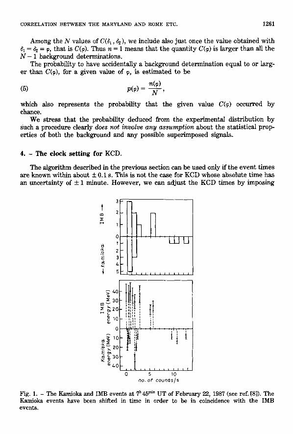
Fig. 1. - The Kamioka and IMB events at 7 h 45 rain UT of February 22, 1987 (see ref. [8]). The Kamioka events have been shifted in time in order to be in coincidence with the IMB events.


the (well-known) coincidence with IMB at about 7 h 35 ~n of 23 February. We take as sett ing procedure that illustrated in fig. 1 (see ref. [8]), which requires to add 7.8 seconds to the times recorded on the KCD magnetic tape. This correction has been used by various authors and it is equivalent to superimpose the middle of the first 5 KCD neutrino times to the middle of the first 3 IMB neutrino times. We could also superimpose the first two neutrinos of the two detectors, thereby obtaining a correction of 7.7 seconds: the effect of this small deviation on the analysis is, of course, negligible.

5. - S tandard dev ia t ions and probabi l i t ies .

Sometimes in science an experimental result is obtained with a computed probability to be due to chance so small that many people are convinced of its truth and various theoretical interpretations are given. Later, however, in some cases, new measurements or new data analyses showed that it was false.

The probability for a result to be accidental is often expressed in terms of number of standard deviations. Indicating with x the result of the measurement, with ~ the expected value and with ~ the standard error, the number of standard deviations is, as well known,

(6) fx-

The Gaussian distribution is often considered. For example ff ~ = 5 we get a probability p = 2.9.10 -7 that the experimental result expressed by x was accidental. Thus a new experimental result deviating by 5 standard deviations from the value expected from the application of the laws of physics should indicate that such laws are not valid in the area where the new measurement was done.

The reason why a result is sometimes found to be false even with large ~ values are, in our opinion, the following:

i) the use of the Gaussian law without having tested whether it is applicable, ii) wrong determination of the value of ~,

iii) wrong determination of the value of ~. At times, for example, the observation is indeed true, but it is due to a malfunc-

tioning of the experimental apparatus (cases li) and iii)) and therefore its explanation might be trivial. For instance, a detector could work properly for one month giving a background within the right random distribution and then it could fail (for several reasons) and give in a few seconds events that appear to be real signals.

All these problems have a good chance to show up when using only one detector, but, in our opinion, they are practically eliminated by using two or more detectors in coincidence. The reason for such a tremendous improvement in the reliability of an experimental result is due to the fact that with two detectors one can determine experimentally, and with high accuracy, the background, at the time of that result (not at other times), and therefore one can measure, and not just calculate, the probability that the result, obtained with the two detectors in coincidence, be accidental.

Should one then trust completely a result of a coincidence analysis when the probability that it he accidental is so small as, say, p ~ 10-57 The answer is again no, for

CORRELAT IO N B E T W E E N T H E M A R Y L A N D AND ROME ETC. 1263

the following reason based on the ,,statistical choices,, made in the data analysis. The basic problem in a statistical analysis of experimental data is, in fact, ,,when,, and ,,how,, choices are made. A p o s t e r i o r i choices, even if they lead to very small probabilities, cannot be used for accepting or rejecting an experimental result. In order that probabilities be significant it is necessary that they be computed on the basis of a pr/or/choices.

We have decided to base the present analysis of experimental data in coincidence on statistical choices which have been done in the past and have appeared over referred journals.

The only data analysis paper we have published so far on a referred journal is ref. [2]. In that paper we have considered correlation periods centred at 2h45 ~ of February 23 with a duration between one and two hours (fig. 9 of ref. [2]) and a delay between ,,gravitational wave,> and ,,neutrino,, signals of 1.2 second (fig. 5, 6, 7 and 8 of ref. [2]).

According to those choices, the analysis reported in what follows in this paper will assume:

a) a delay ~ = - 1.2 s,

b) a correlation period of 1�89 hour centred at 2 h 45 ~ .

In addition, the data analysis computer programs will be exactly the same ones we used to find the result of ref. [2].

6. - Results of the analysis.

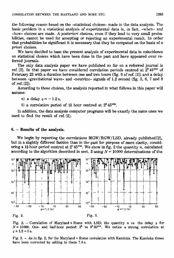
We begin by reporting the correlations MGW/RGW/LSD, already published [2], but in a slightly different fashion than in the past for purpose of more clarity, consid- ering a 1�89 period centred at 2h45 ~ . We show in fig. 2 the quantity n, calculated according to the algorithm described in sect. 3 using N = 10000 determinations of the

] J I ! ! I ,o~ ................. 1 ................. ! . . . . . . . . . . . . . . . .

- 5 0 - 3 0 - 1 0 10 r 1.2 (s)

30 50

1o'! N

10 z :

10 ~ !

10 0 ....................

- 5 0 - 3 0

Fig. 2. Fig. 3.

? I

. . . . . . . . . . . . . . . . . . . . . . . . . . . . . . . . . . . . i . . . . . . . . . . . . . . . .

- 10 10 30 50 cp § 1.2 (s)

Fig. 2. - Correlation of Maryland + Rome with LSD: the quantity n vs. the delay ~ for N = 10000. One- and half-hour period: 2 h to 3h30 m~. We notice a strong correlation at ~ + l . 2 = 0 s .

Fig. 3. - As in fig. 2, for the Maryland + Rome correlation with Kamioka. The Kamioka times have been corrected by adding to them 7.8 s.

1264 M. AGLIETrA, A. CASTELLINA, W. FULGIONE, G. TRINCItERO, ETC.

background, for 101 different values of the delay ~. Starting from ~ = - 1.2 s (choice a) of sect. 5) we change ~ by steps of 1 s up to + 50 s. In this way the 101 values of n in fig. 2 are all independent one from each other (see sect. 2). At ~ = - 1.2 s we have n = 1, which means that C(~ = - 1.2) is larger than all the 10000-1 determinations C(81,82) of the background. In order to improve this statistical result we have to in- crease N. Using N = 100000, we find n = 3 which means that the probability that the correlation peak at ~ = - 1.2 be accidental is of the order of 3.10 -5.

I t is important now to consider the results we find by applying exactly the ~m__e procedure to the data of KCD and IMB.

In fig. 3 we show the result for the MGW/RGW/KCD correlation. We notice that, also here, the correlation exhibits a peak at ~ = - 1.2 s, with a probability to be accidental of 19.10 -4 (as obtained from the comparison of C( - 1.2) with the background according to formula (5)).

We have also evaluated the probability of the correlation peak at ~ = - 1.2 s in a different way, as follows, by extending the ~ range shown in fig. 3 to the maximum possible in the 1�89 period (that is using no data outside that period):

(7) -2700 ~< ~ + 1.2 ~ 2700 s.

The integral distribution of the 5401 independent n(~) values obtained by this procedure is shown in fig. 4. We notice that we got by chance n ~ 19 (corresponding to C ( - 1.2) or smaller) about 22 times, out of 5401. This corresponds to a probability of 22/5401, about a factor of 2 larger than the previous estimation. We believe that this difference, if not acceptable within the statistical fluctuations, has the following explanation. When applying the algorithm described in sect. 3, we compute the background C(81, ~2) by using different random numbers for Rome (81) and Maryland (82). Here (fig. 4) we have changed ~ according to (7) but always taking the data of MGW and RGW at the same time. Therefore, ff a small correlation between MGW and RGW exists, then it is going to produce, qualitatively, the above small discrepancy.

We come now to the results of the MGW/RGW/IMB correlation. Here we have done a selection of the data (IMB) as discussed in what follows.

10 #

10 3

102:

10 ~ :

J ...-,"

J 24-00

2000

1600

1200

800

/-,-00

100 101 10 2 10 3 n 10 t* 0 300 350

Fig. 4. Fig. 5.

50 100 150 200 250 E(IMB)/100 (MeV)

Fig. 4. - Integral distribution of the n values obtained by extending the results of fig. 3 to 5401 different ~ values.

Fig. 5. - Energy distribution of the IMB events in the period 0 h to 8 h of February 23, 1987. E(IMB) is the total number of photoelectrons multiplied by 1 MeV.


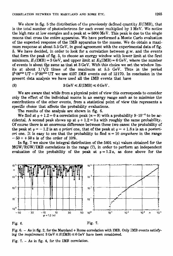
We show in fig. 5 the distribution of the previously defined quantity E(IMB), that is the total number of photoelectrons for each event multiplied by 1 MeV. We notice the high rate at low energies and a peak at = 5000 MeV. This peak is due to the single muons that cross the entire apparatus. We have performed a Monte Carlo evaluation of the expected response of the IMB apparatus to the muons. We do obtain a maximum response at about 5.5 GeV, in good agreement with the experimental data of fig. 5. We have decided, in order to look for a correlation between g.w. and the events that form the peak of fig. 5, to choose an energy window with lower limit at the first minimum, EI(IMB) = 3 GeV, and upper limit at E2(IMB) = 6 GeV, where the number of events is about the same as that at 3 GeV. With this choice we set the window lim- its at about 1 /V~ times of the maximum at 5.5 GeV. Thus in the period 2h0ff~UT + 3 h 3 0 ~ U T we use 4137 IMB events out of 12170. In conclusion in the present data analysis we have used all the IMB events that have

(8) 3 GeV ~< E(IMB) ~ 6 GeV.

We are aware that while from a physical point of view this corresponds to consider only the effect of the individual muons in an energy range such as to minimize the contributions of the other events, from a statistical point of view this represents a specific choice that affects the probability evaluations.

The results of the analysis axe shown in fig. 6. We find at ~ + 1.2 = 0 a correlation peak (n = 9) with a probability 9.10 -4 to be ac-

cidental. A second peak shows up at ~ + 1.2 = 3 s with roughly the same probability. Of course there is an enormous difference between these two cases: the probability of the peak at ~ = - 1.2 is an a pr/or/one, that of the peak at ~ = + 1.8 s is an a posteri- or/ one. It is easy to see that the probability to find n = 10 anywhere in the range - 50 + + 50 s is of the order of 10%.

In fig. 7 we show the integral distribution of the 5401 n(~) values obtained for the MGW/RGW/IMB correlations in the range (7), in order to perform an independent evaluation of the probability of the peak at ~= 1.2s, as done above for the

10 ~"

D

10 3

10 2

10 1

10 0

- 50

10 ~

10 3

10 2

10 ~ j -

=-

f z*

J J

--30 -10 10 30 50 100 101 102 103 n 10 l* ~+1 .2 (s)

Fig. 6. Fig. 7.

Fig. 6. - As in fig. 2, for the Maryland + Rome correlation with IMB. Only IMB events satisfy- ing the requirement 3 GeV _< E(IMB) _ 6 GeV have been considered.

Fig. 7. - As in fig. 4, for the IMB correlation.

1266 M. A G L I E T T A , A. C A S T E L L I N A , W. F U L G I O N E , G. T R I N C H E R O , ETC.

MGW/RGW/KCD data. We obtain n-< 10 only 2 times while we were expecting 5401.10/104= 5.4, which i s certainly within statistical fluctuations.

We want now to combine the results of the correlations with the three different particle detectors shown in fig. 2, 3 and 6. We do that by multiplying (nl"ne'n3) the three values of n, as a function of ~, from the above figures (using n = 0.3 for the correlation with LSD). The result is shown in fig. 8. We notice that only the correlation at p = - 1.2 s is exalted, while all others tend to cancel.

The probability that the observed multiple correlation at ~ = - 1.2 s be accidental is estimated in an experimental fashion, as we have always done, without using statistical models. We evaluate the product nl 'n2"n3 for the 5401 p values in the range given by (7), obtaining the integral distribution shown in fig. 9. The minimum value of the product (corresponding to ~ = - 1.2 s) is 19 • 0.3 x 9 = 51, which happened just once in 5401 independent trials. The next largest value is nz.n~.n3 - 106. Thus the probability for the result at ~ = - 1.2 s to be accidental is certainly much less than (5401) -I .

For improving the statistical accuracy we can obtain a number of n1"ne'n3 independent quantities much larger than 5401, by combining each nl value at a given phase r with values ns and ns at different phases. This procedure has been repeated 1000 times (each time with different combinations of phases), for a total of 5401 x 1000---5.4.10 s independent determinations of n~'ns.n3. The integral distribution of these values is shown in fig. 10, that is similar to fig. 9 except for the larger number of computed samples. The circle in fig. 10 indicates the above minimum nl-ns-n~ = 51. We notice that we still have not obtained by chance such a small value. Thus we estimate that the probability for obtaining nl-n2"n3 = 51 or smaller by chance is

1 1 106~. (9) P ~" 4 5 ~ 5 . 1 0 -8 ,

where the factor of 4 takes care for a reasonable extrapolation in fig. 10.

10 1 1 ~

10 9 ~ _

c i0~

- 5 0 - 3 0 - 10 10 30 50 q,-~ 1.2 (s)

10 4̀

10 3.

10 z

10

10 o 102

Fig. 8. Fig. 9.

l

z

/ J

l

10 :] 10 ~ 105 106 107 D 1 ' D2"D 3

Fig. 8. - The product of the n values shown in fig. 2, 3 and 6 vs, ~. We notice a very strong effect at ~+ 1.2=0s.

Fig. 9. - As in fig. 4 and 7, for the data of fig. 8. This figure shows that the value nl" n2. ns = 51 occurring in fig. 8 at ~ + 1.2 = 0 s occurs by chance very rarely (see text).


10 6 "1

"1

10 ~" "l

"i

10 z -~

!

1 0 0 : ~

102

/ /

. / /

J

10" 106 100 n 1 �9

/ , J

1 0 ~

-!

10 6 -= :

�9 -!

104"]

-!

i 02 . "

- 5 0

q [

r ~

1010 1012 --30 --10 10 30 50 ~+1 ,2 (S)

Fig . 10. F ig . 11.

Fig. 10. - As in fig. 9 with 5401 x 1000 independent determinations of nl"n~" n3.

Fig. 11. - The product of the n values shown in fig. 3 and 6 vs. ~.

One can argue that the above reasoning includes the correlation MGW/ / R G W / L S D which ought to represent the starting point, as one could suppose that it be affected by some statistical bias. On the other hand, it is very important to evaluate the probability of the correlations obtained with the new data (KCD and IMB), in- dependently from the results obtained with LSD [2].

We can remove LSD by multiplying just the n values of fig. 3 and fig. 6 (nl" n2) as shown in fig. 11. For the probability estimation we use the integral distribution of the 5401 nl'n2 values shown in fig. 12. At ~ = - 1 . 2 s we have nl'n2 = 171, which happened just once in 5401 trials. In this case a reasonable extrapolation gives an additional factor of the order of 3. Therefore the probability that the correlation at

= - 1.2s of fig. 11 be accidental turns out to be

1 1 5 .10 -s . (10) P = 3 5401

One important point was also the choice of the correlation period of 1�89 hour (choice b) of sect. 5). We have repeated the above analysis for two other periods: one hour and

.two hours, both centred at 2h45 ~n. The results are shown in table I. We conclude that

104."

103.

102 �9

10 1

10 0 ..

10 2 10/* f}l ' n2

Fig. 12. - As in fig. 9, for the data of fig. 11.

A A

10 6 10 0

1 2 6 8

T A B L E I .

M. AGLIETTA, A. CASTELLINA, W. FULGIONE, G. TRINCHERO, ETC.

1 hour 1�89 hour 2 hours

L S D n = 10 0.3 (*) 0.04 (**) K C D n = 33 19 646 IMB n = 14 9 62

K C D + I M B p ~ 6 . 1 0 - s ~ 5 . 1 0 -5 ~ 5 - 1 0 -s K C D + I M B + L S D p ~ 2 . 1 0 - 7 ~ 5 - 1 0 -s - 3 . 1 0 -s

In the upper part of the table we give the n values at ~ = - 1.2 e for N = 10000. ((*) N = 10 s, (**) N = 10s). In the lower part we give the probability estimations for the correlations of the g.w. with KCD and IMB and with KCD, IMB and LSD.

p=-1.2 (s)

,o, / 10 2

10 1

10 o

0 I Z.

Fig . 13.

2 3 h o u r ( U T )

Ko, r n i o k ~

_ ~ . I M B

LSD

cp = - I . 2 (s)

10 ~2

101C

8

lO 6

10 ~

0

Fig. 14.

1 2 h o u r ( U T )

5 6 3 4- 5 6

Fig . 13. - The n va lues obtained for the correlations of Maryland + R o m e w i t h L S D , Kamioka and IMB during periods of one hour from O h to 6 h o f February 23. We notice that all the correla- t ions occurr at the s a m e t ime.

F ig . 14. - The product o f the three n va lues obtained from fig. 13 v s . t ime.

10 ~"

. / 10 3 r

1o z .*"

/

10; ~ '

10 0 .....

10 ~ 10 6 10 8 1010 1012 /31 . r12./3 3

Fig. 15. - A s in fig. 9, for the one-hour period, 2 h 15 rah to 3 h 15 mi~ UT.


the additional correlation due to KCD and IMB is strong and occurs for all periods of time considered.

The last point of the present analysis is to extend the correlation study to periods of time not centred at 2h45 ~ . This is done in fig. 13 where we have taken ~ = - 1.2 s and 1-hour periods starting from 0:00 hour until 6:00 hour stepped by 1/4 hour (thus the points of fig. 13 are correlated 4 by 4). KCD, IMB and LSD show similar correlations with MGW and RGW at the same time. This is more evident in fig. 14 where again we show the product nl'n2"n3. In order to be able to calculate experimental probabilities we have obtained in fig. 15 the integral distribution of the nl-n2.n3 values for the one-hour period, by varying ~ in the range - 1800 ~< ~ + 1.2 < 1800 s for the period 2:15 to 3:15 UT.

In conclusion the new data (Kamiokande and IMB) exhibit a correlation with the GW detector data that shows up with the same characteristics and at the same time of that already found with Mont Blanc.

This result improves considerably the statistical validity of our previously published correlation.

We are grateful to the Kamiokande and IMB groups for letting us use their raw data. We thank A. De Rujula for his criticism and useful suggestions.

R E F E R E N C E S

[1] E. AMALDI et al.: Europhys. Le~., 3, 1325 (1987). [2] M. AGLIETTA et al.: Nuovo Cimento C, 12, 75 (1989). [3] M. AGLIETrA et al.: Nuovo Cimento C, 14, 171 (1991). [4] M. AGLIE2"rA et al.: Europhys. Lett., 3, 1315 (1987). [5] E. M. ALEXEYEV e~ a/.: JETP Le~., 49, 480 (1989). [6] K. S. HIRATA et al.: Phys. Rev. D, 38, 448 (1988). [7] R. M. BIONTA et al.: Phys. Rev. Le~., 58, 1494 (1987). [8] D. SCHRAMM and J. W. TRURAN: Phys. Rep., 189, 91 (1990).

84 - Il Nuovo Cimento B

Correlation between the Maryland and Rome gravitational-wave detectors and the Mont Blanc, Kamioka...

Documents

Transcript of Correlation between the Maryland and Rome gravitational-wave detectors and the Mont Blanc, Kamioka...