Correlating CPT data to stiffness parameters of sand in FEM

Delft University of Technology

Department: Geoscience & Engineering

Correlating CPT data to stiffnessparameters of sand in FEM

Author:Stef Engels

October 12, 2016

Delft University of Technology

Department: Geoscience & Engineering

Correlating CPT data to stiffnessparameters of sand in FEM

Graduation Committee:Prof. dr. K.G. Gavin

Ing. H.J. Everts (Tu Delft)Ir. J. Rindertsma (Van Oord)

Dr. ir. K.J. Bakker (Tu Delft)

Author:Stef Engels

student id: 4095359

To be publicly defended on October 27, 2016

Summary

Making foundation designs is one of the major tasks of a geotechnical engineer. To achievesuch a design, knowledge of the soil stiffness is required. Information about the soil stiffnesscan be obtained by either laboratory tests or in situ tests. Laboratory testing is timeconsuming, costly and sample disturbance is inevitable. In situ tests are done directlyon the soil encountered on the site and therefore are a good representation of the in situsoil state. CPT’s are the most performed in situ tests in geotechnical engineering. CPT’sare used to evaluate the subsurface based on the mechanical response translated to coneresistance and sleeve friction. Therefore it is desirable to find a correlation between soilstiffness and CPT results.

A lot of research has been done to correlate CPT results, such as the cone resistance, withthe stiffness of sand. It has been found that these correlations are highly variable and sitespecific. State parameters as consolidation state have a high influence on the soil stiffnessbut are difficult to evaluate from CPT results only.

In this thesis the correlation between cone resistance and stiffness parameters for sand isinvestigated based on a series of Zone Load Tests done at a site in Kuwait. In a Zone LoadTest a footing is loaded in steps and the settlement of the footing is measured. First ananalytical settlement analysis is done with existing methodologies which use correlationbetween cone resistance and soil stiffness. The predicted settlements according to thesemethods are compared with settlements measured in the field. Afterwards, a new sitespecific correlation between cone resistance and soil stiffness is proposed using regressionanalysis.

A verification of the new proposed correlation is done with the finite element programPLAXIS 2D. The numerical calculations were done with the Hardening Soil model usingan axisymmetric approach. Multiple Zone Load Tests are simulated with PLAXIS 2Dwhere the input parameters of the Hardening soil model are obtained from the proposedcorrelation. The numerical calculated settlement of the footing are in agreement with themeasurements in the field and therefore it can be concluded that the correlation found forthis site is valid. The general application of the proposed correlation is not confirmed.

The research done in this thesis is related to direct settlement. Time dependent be-haviour is excluded but could be of significant influence. Carbonate sands, as encounteredat the site, are sensitive for particle crushing. Particle crushing can lead to creep effectsand therefore it is advised to perform Plate Load Tests to get better insight in the creepbehaviour in the sand fill.

i

Acknowledgements

In February I started my research at Van Oord as a graduate student in Rotterdam. I amgrateful that I have got the opportunity to work in an organisation with big and interestingprojects and friendly colleagues. During the process I had a lot of help from my dailysupervisor ir. Rindertsma. When I was stuck in my research he always had ideas to setme back on track again. Furthermore I would like to thank ir. Karreman who guided methrough the project and who gave me the opportunity to start at Van Oord.

Furthermore I would like to thank the rest of committee for their involvement in myresearch. During the process dr. ir. Bakker showed a lot of interest in the subject and wasalways full enthusiasm to help me improve my research. I would like to thank ing. Evertsfor his faith in my abilities and sharing his experience with me. And finally I owe muchgratitude to prof. dr. Gavin. He recently joined the staff at Delft University of Technologyand he was very helpful right away. He always makes room in his schedule to get the bestout of his students.

Last but not least, I would like to thank my family and friends. My family alwayssupported me during my years as a student. Their love and support kept me going throughthe years. I would like to thank my grandmother for her faith, love and financial support.Furthermore I would like to thank all the friends I made during my studying period inDelft. We share great moments and great times are still ahead. Finally I want to thankNienke for her love and understanding during my period as a student.

Stef EngelsOctober 2016

ii

Contents

Summary . . . . . . . . . . . . . . . . . . . . . . . . . . . . . . . . . . . . . . . i

Acknowledgements . . . . . . . . . . . . . . . . . . . . . . . . . . . . . . . . . ii

Nomenclature . . . . . . . . . . . . . . . . . . . . . . . . . . . . . . . . . . . . v

1 Introduction 1

1.1 Research context . . . . . . . . . . . . . . . . . . . . . . . . . . . . . . . . . 1

1.2 Research project . . . . . . . . . . . . . . . . . . . . . . . . . . . . . . . . . 2

1.3 Thesis outline . . . . . . . . . . . . . . . . . . . . . . . . . . . . . . . . . . . 2

2 Project information 4

2.1 Site overview . . . . . . . . . . . . . . . . . . . . . . . . . . . . . . . . . . . 4

2.2 Soil conditions . . . . . . . . . . . . . . . . . . . . . . . . . . . . . . . . . . 5

3 Literature study 8

3.1 The Cone Penetration Test . . . . . . . . . . . . . . . . . . . . . . . . . . . 8

3.1.1 The CPT procedure . . . . . . . . . . . . . . . . . . . . . . . . . . . 8

3.1.2 Results and interpretation . . . . . . . . . . . . . . . . . . . . . . . . 9

3.2 Theoretical background . . . . . . . . . . . . . . . . . . . . . . . . . . . . . 10

3.2.1 Discussion of soil moduli . . . . . . . . . . . . . . . . . . . . . . . . . 10

3.2.2 Settling behaviour of soil . . . . . . . . . . . . . . . . . . . . . . . . 13

3.2.3 Compressive behaviour of sand . . . . . . . . . . . . . . . . . . . . . 14

3.2.4 Stress distribution underneath a shallow foundation . . . . . . . . . 15

3.2.5 Elastic settlement with constant Young’s modulus . . . . . . . . . . 16

3.2.6 Settlement analysis of a shallow foundation . . . . . . . . . . . . . . 17

3.3 CPT based methods for settlement of a shallow foundation . . . . . . . . . 18

3.3.1 De Beer and Martens (1957) . . . . . . . . . . . . . . . . . . . . . . 18

3.3.2 Schmertmann method (1978) . . . . . . . . . . . . . . . . . . . . . . 19

3.3.3 Modification Schmertmann suggested by Peck et al. (1996) . . . . . 22

3.3.4 Robertson (1990) . . . . . . . . . . . . . . . . . . . . . . . . . . . . . 23

3.4 Soil models for sand . . . . . . . . . . . . . . . . . . . . . . . . . . . . . . . 29

3.4.1 Mohr-Coulomb model . . . . . . . . . . . . . . . . . . . . . . . . . . 29

3.4.2 The Hardening Soil model . . . . . . . . . . . . . . . . . . . . . . . . 31

3.4.3 The Hardening Soil model with small-strain stiffness . . . . . . . . . 33

4 Zone Load Test procedure 35

4.1 Test set-up . . . . . . . . . . . . . . . . . . . . . . . . . . . . . . . . . . . . 35

4.2 Loading procedure and test results . . . . . . . . . . . . . . . . . . . . . . . 35

4.3 Test uncertainties . . . . . . . . . . . . . . . . . . . . . . . . . . . . . . . . . 37

4.4 Interpretation and assumptions . . . . . . . . . . . . . . . . . . . . . . . . . 38

5 Analytical settlement analysis 39

5.1 Zone Load Test Criteria . . . . . . . . . . . . . . . . . . . . . . . . . . . . . 39

5.2 Processing the CPT data . . . . . . . . . . . . . . . . . . . . . . . . . . . . 40

5.3 Overview of the procedure . . . . . . . . . . . . . . . . . . . . . . . . . . . . 43

5.4 Results and discussion . . . . . . . . . . . . . . . . . . . . . . . . . . . . . . 44

5.4.1 Comparison different site locations . . . . . . . . . . . . . . . . . . . 44

iv

5.4.2 Normality of the results . . . . . . . . . . . . . . . . . . . . . . . . . 455.4.3 Influence of the CaCO3 content . . . . . . . . . . . . . . . . . . . . . 495.4.4 Difference between analytical approach and reality . . . . . . . . . . 50

6 Site specific correlation 526.1 Compare back calculated secant modulus Es with ERob . . . . . . . . . . . 526.2 Regression analysis using one layer . . . . . . . . . . . . . . . . . . . . . . . 53

6.2.1 Correlation between qc and Es . . . . . . . . . . . . . . . . . . . . . 536.2.2 Correlation between Qtn and Es . . . . . . . . . . . . . . . . . . . . 566.2.3 Conclusion . . . . . . . . . . . . . . . . . . . . . . . . . . . . . . . . 57

6.3 Regression analysis using suggested layers . . . . . . . . . . . . . . . . . . . 576.3.1 Correlation between qc,weigthed and Es . . . . . . . . . . . . . . . . . 576.3.2 Correlation between Qtn,weigthed and Es . . . . . . . . . . . . . . . . 606.3.3 Conclusion . . . . . . . . . . . . . . . . . . . . . . . . . . . . . . . . 61

6.4 Regression analysis using 600 layers . . . . . . . . . . . . . . . . . . . . . . 626.4.1 Correlation between qc,weighted and Es . . . . . . . . . . . . . . . . . 626.4.2 Correlation between Qtn,weighted and Es . . . . . . . . . . . . . . . . 636.4.3 Conclusion . . . . . . . . . . . . . . . . . . . . . . . . . . . . . . . . 65

6.5 Interpretation of Es . . . . . . . . . . . . . . . . . . . . . . . . . . . . . . . 66

7 Numerical verification with PLAXIS 2D 677.1 Used correlation for verification . . . . . . . . . . . . . . . . . . . . . . . . . 677.2 Modelling approach . . . . . . . . . . . . . . . . . . . . . . . . . . . . . . . . 677.3 Parameter determination . . . . . . . . . . . . . . . . . . . . . . . . . . . . 697.4 Relating Es with Eref50 . . . . . . . . . . . . . . . . . . . . . . . . . . . . . . 727.5 Overview of the numerical validation . . . . . . . . . . . . . . . . . . . . . . 737.6 PLAXIS calculation . . . . . . . . . . . . . . . . . . . . . . . . . . . . . . . 73

7.6.1 PLAXIS model . . . . . . . . . . . . . . . . . . . . . . . . . . . . . . 737.6.2 Loading procedure and output . . . . . . . . . . . . . . . . . . . . . 767.6.3 Results . . . . . . . . . . . . . . . . . . . . . . . . . . . . . . . . . . 78

7.7 Influence of ZLT procedure . . . . . . . . . . . . . . . . . . . . . . . . . . . 797.8 Conclusion . . . . . . . . . . . . . . . . . . . . . . . . . . . . . . . . . . . . 80

8 Conclusions and recommendations 838.1 Introduction . . . . . . . . . . . . . . . . . . . . . . . . . . . . . . . . . . . . 838.2 Conclusions . . . . . . . . . . . . . . . . . . . . . . . . . . . . . . . . . . . . 838.3 Recommendations . . . . . . . . . . . . . . . . . . . . . . . . . . . . . . . . 84

Appendices 90A Functions in Mohr-Coulomb model . . . . . . . . . . . . . . . . . . . . . . . 90B Fitted nSBT chart Robertson . . . . . . . . . . . . . . . . . . . . . . . . . . 91C Settlement analysis ZLT . . . . . . . . . . . . . . . . . . . . . . . . . . . . . 92D Shapiro-Wilk test . . . . . . . . . . . . . . . . . . . . . . . . . . . . . . . . . 93E Soil specifications . . . . . . . . . . . . . . . . . . . . . . . . . . . . . . . . . 97F Comparison back calculated stiffness with Robertson stiffness . . . . . . . . 98G Calculating standardized residuals . . . . . . . . . . . . . . . . . . . . . . . 99

Nomenclature

Symbols

Symbol Units DescriptionRC % Relative compactionγd,field kg/m3 Dry field densityγd,max kg/m3 maximum dry densityDr % Relative densityqc MPa Cone resistanceqt MPa Corrected cone resistance¯qc,i MPa Average cone resistance in layer iqc,weighted − Weighted cone resistancefs MPa Sleeve frictionu MPa Pore pressureu0 MPa Hydrostatic pore pressureu2 MPa Measured pore pressureRf − Friction ratioE kPa Young’s modulusEs kPa Secant Young’s modulusEur kPa Unloading reloading Young’s modulusEt kPa Tangent Young’s modulus

Eref50 kPa Secant stiffness in standard drained triaxialtest

Erefoed kPa Tangent stiffness for primary oedometerloading

Erefur kPa Unloading/reloading stiffnessERob kPa Stiffness obtained with Robertson methods mm Settlementsi mm Settlement of layer ise mm Elastic settlementscreep mm Creep settlementv − Poisson’s ratioB m Foundation widthL m Foundation lengthIρ − Settlement influence factorIz − Strain influence factor

I′z − Corrected strain influence factorC − Compressibility coefficientσv0 MPa In situ total stress

σ′v0 MPa In situ effective stress

σ′0 kPa Effective overburden pressure

∆σ kPa Increase in pressureH m Layer thicknessCc − Compressibility indexe0 − Initial void ratio

vi

qb kPa Unit load acting on the baseC1 − Time dependent factorC2 − Depth dependent factor∆z m Thickness of a layern − Stress componentQtn − Normalized cone resistanceQtn,weighted − Weighted normalized cone resistance

¯Qtn,i − Average normalized cone resistance in layeri

Fr − Normalized friction ratioBq − Normalized pore pressurepa kPa Atmospheric pressureIc − Soil behaviour type indexIc,rw − Soil behaviour type index (Robertson and

Wride)Vs m/s Shear wave velocityVs1 m/s Normalized shear wave velocityαvs m/s2 Shear wave velocity factorρ kg/m3 Mass densityG kPa Shear modulusG0 kPa Small strain shear modulusGur kPa Unloading reloading shear modulusKG − Small strain shear modulus numberα − Significance levelαG − Shear modulus factorqult kPa Ultimate bearing capacityKE − Young’s modulus numberαE − Young’s modulus factorϕ ◦ Friction anglec kPa Cohesionψ ◦ Dilatancy angleσt kPa Tensile strengthK0 − Coefficient of lateral earth pressurem − Power for stress level dependency of stiff-

nessvur − Poisson’s ratio for unloading/reloadingpref kPa Reference stressKnc

0 − The value for K0 for normal consolidationRf − Failure ratio qf/qaγ − Shear strainγ0.7 − Reduction parameter when G reduces to

0.7G0

µ̂ − Estimated meanσ̂ − Estimated standard errorW − Weighting factorD m DiameterDe m Equivalent diameterzbot,i m Bottom coordinate of layer iztop,i m Top coordinate of layer i

Abbreviations

Abbreviation MeaningCPT Cone Penetration TestZLT Zone Load TestUCSC Unified Soil Classification SystemSBT Soil Behaviour TypeSBTn Normalized Soil Behaviour TypeCSL Critical State LinePSD Particle Size Distribution

Chapter 1

Introduction

1.1 Research context

In geotechnical engineering, providing accurate predictions of foundation settlements isone of the main challenges. The function of a foundation is to transfer loads from a givenstructure to the subsurface. The compressive loads imposed on the subsurface will leadto a permanent deformation of the soil, which is referred to as settlement. In order toprotect the integrity of the structure settlements should be kept within limits. It is theresponsibility of the geotechnical engineer to make an adequate foundation design in whichthe safety of a structure is guaranteed. The requirements regarding to settlements can befound in the Eurocode 7.

The earth’s subsurface is comprised of many different materials. Every specific typeof soil or rock has its own engineering properties with respect to stiffness and strengthparameters. Another difficulty which is typical for soils is that they are anisotropic andheterogeneous. These factors indicate that making a geotechincal design is quite a chal-lenging operation.

Fortunately experience in making a reliable design was gained over the last decades.Designs are typically based on laboratory tests and in situ tests. For laboratory testing,soil samples are obtained from the site and tested in the laboratory. Testing can be doneunder controlled circumstances, but the soil samples may not represent the actual in situconditions due to sample distortions as stress relief. In situ test are done directly on thesoil as encountered in the field. Therefore these test are highly representative as the soil istested in the in situ state. However, a large amount of in situ test can significantly increasecosts. The cost increase are due to expensive equipment and skilled personnel that has tobe brought to the site.

The most used in situ test is the Cone Penetration Test (CPT). With this test a conepenetrates the subsurface at a certain rate and measures the cone resistance, the sleevefriction and the pore pressure. A CPT is used to classify the soil layering and get a betterunderstanding of the subsurface. CPT’s are widely used because the are cost-effective andprovide valuable soil information. Because of the availability of CPT’s, it would be usefulto develop a methodology to make a geotechnical design based on CPT results.

In the past research was done on making settlement analysis based on CPT results(De Beer, E. Martens, 1957) (Schmertmann et al., 1978) (Peck et al., 1996) (Robertson,1990). However, the methods proposed to correlate CPT results to soil stiffness differ andthe results are not consistent.

1

Correlating CPT data to stiffness parameters of sand in FEM

1.2 Research project

As discussed in the previous section, accurate derivation of stiffness parameters from CTP’swould provide valuable information for foundation design. The idea of making an accurategeotechnical design based on CPT’s is cost-effective and time efficient. To this end themain research question can be formulated as:

Is it possible to predict stiffness parameters of sand with reasonable accuracy based on CPTresults?

A large amount of Zone Load Tests (ZLT’s) are performed on a hydraulic fill on a site inKuwait. These tests measures the settlement of a 3 m x 3 m footing on different locations.This thesis will use the data from these ZLT’s to investigate the possibility to developa correlation between CPT results and stiffness parameters of sand. The results will beverified by modelling ZLT’s in finite element software (PLAXIS 2D) and compare theresults with the measurements in the field.

To find a satisfying answer for this main research question, some other questions need tobe answered:

What kind of factors play an important role in the compressibility of sand?How does the layering of the deposit affect the results?Does the testing methodology influence the results?Is it possible to distinguish creep settlements during a ZLT?Is it possible to predict load-settlement behaviour based on CPT parameters?Are the obtained results representative for other sites?

1.3 Thesis outline

The structure of this thesis can be summarized in seven main categories:

1. Site specific information2. Theoretical background3. Test procedure4. Analysis of existing methods5. Site specific correlations6. Numerical verification with PLAXIS 2D7. Conclusions and recommendations

In Chapter 2 the project at the site in Kuwait will be discussed. An overview of the site isprovided to give an idea of the locations of the tests and the size of the site. Chapter 3 startswith the theoretical background with respect to foundation design. Afterwards a selectedamount of existing methods will be discussed that directly use CPT data for settlementanalysis. To conclude this chapter existing soil models for modelling the behaviour ofsandy soils will be presented. Chapter 4 evaluates the test procedure of a ZLT and theinterpretation of the output. This Chapter concludes with an overview of the assumptionsthat are used for further analysis. In Chapter 5 the methods presented in the literaturestudy are used to make a settlement prediction of a selected amount of ZLT’s. A settlementanalysis is done and compared with the measured settlements. This chapter provides aninsight in how the existing methods perform at this specific site. In Chapter 6 a regression

2 Chapter 1 Stef Engels


analysis will be done for a selected amount of representative ZLT’s. The objective inthis chapter is to obtain a site specific correlation between the cone resistance and thesecant Young’s modulus of sand. In Chapter 7 the representative ZLT’s are modelledusing FEM software (Plaxis 2D). The input parameters are based on the correlations thatare developed in Chapter 6. The objective to verify the correlations that are presentedearlier. In Chapter 8 the main conclusions are summarized and recommendations for futureresearch are made.

Chapter 1 Stef Engels 3

Chapter 2

Project information

2.1 Site overview

In Kuwait, a sand layer was constructed to serve as a suitable foundation layer for an oilrefinery. The site location is indicated in figure 2.1. At parts of the sites sabkha soil isencountered. This type of soil usually consists of soft weak silts and clays cemented withsalts. The mechanical behaviour of sabkha can be compared with clay. In some partsof the site the constructed sand layer is constructed on top of a sabkha layer. In otherareas the fill is constructed on a natural sand deposit. To reduce the settlements in thesubsurface, ground improvement techniques are applied. Several ground improvementmethods are used for the densification of the material. The improvement methods usedare Dynamic Compaction, Dynamic Replacement and Roller Compaction. Where sabkhalayers are present, sand columns can push through this layer with the Dynamic Compactiontechnique. The arching effect between the sand columns needs to reduce the compressionof this sabkha layer. A closer view of the site with elevation levels of the fill is provided infigure 2.3. The numbers in the figure indicate the height of the original ground level withrespect to the new ground level.

Figure 2.1: Location of the site

After the ground improvement is finished, several Zone Load Tests (ZLT’s) are performedto measure the settlement of a 3 m x 3 m square footing. In the ZLT procedure, a concretefooting is loaded in steps and the settlement of the footing is recorded during the process.The settlements are measured on four locations on the footing. The ZLT’s are performed

4


over the entire site. The results of these tests are used to evaluate if the settlementrequirements (less then 25 mm) are met. Some ZLT’s run for an entire month to getinformation about the long term settlement (creep) behaviour.

2.2 Soil conditions

After the compaction works are finished, Field Density Tests (FDT’s) are done. Theresults of these tests are presented in table 2.1. With this test the maximum dry densityis determined in the laboratory. This can be done with for instance the Proctor test.The maximum dry density is compared with the field density and this results in a newparameter called the relative compaction (RC). The RC is defined as:

RC =γd,fieldγd,max

· 100% (2.1)

Where:RC: Relative compactionγd,field: Measured dry field density after compactionγd,max: Maximum dry density

Research by Gomaa and Abdelrahman (2007) concluded that there is a very accuratepositive correlation between relative compaction and relative density. Sands from 20different sites were tested and the results are presented in figure 2.2. According to thisresearch the relative compaction is related to the relative density (Dr) according to:

Dr = 5.5 ·RC − 4.47 (2.2)

Figure 2.2: Correlation between relative compaction and relative density (Gomaa andAbdelrahman, 2007)

A relative compaction between 95% and 96% corresponds with a relative density between76% and 81%. Therefore it can be concluded that the compacted sand encountered on thesite can be classified as dense sand.



Table 2.1: Results of FDT tests

Parameter Unit FDT 1 FDT 2 FDT 3 FDT 4 FDT 5 Average

Wet density g/cm3 1.815 1.786 1.836 1.801 1.826 1.813

Dry density g/cm3 1.715 1.714 1.719 1.732 1.720 1.720

Max. dry density g/cm3 1.803 1.803 1.797 1.803 1.803 1.802

Relative compaction % 95.1 95.1 95.7 96.1 95.4 95.5



7 k

m

3,5

km

Figure 2.3: Site location with elevation levels


Chapter 3

Literature study

In this chapter a theoretical background is given and previous research is summarized.The main purpose of the literature study is to evaluate the available correlation methodsand the theoretical background that is used. Key is to understand why certain methodsperform better than others and learn what factors play a dominant role in correlatingCPT parameters to soil properties. In the first section of this literature study the generalCPT procedure is discussed. In the next section some theoretical background is given.Afterwards available correlation methods will be evaluated. Some earlier developed methodswill be analysed first, because it is useful to see how correlation methods have developedover time. Later on a more advanced method is explained. To finish the literature studydifferent soil models that can be used to model sand are briefly explained.

3.1 The Cone Penetration Test

The Cone Penetration Test (CPT) is the most widely used field test in geotechnicalengineering and every geotechnical engineer should be familiar with the interpretation ofthe results of this test. In this section the procedure and specifications of the CPT arebriefly explained.

3.1.1 The CPT procedure

In a CPT a cone, connected by rods, will be pushed into the soil with a certain constantpenetration rate. During the penetration continuous measurements are made of thepenetration resistance of the cone and the sleeve. When using a piezocone, measurementsof the pore pressure are registered as well. The definitions above are visualized in figure3.1. Standard electronic cones have a 60 degrees apex angle and a cross-sectional area ofeither 10 cm2 of 15 cm2 (Robertson and Cabal, 2015). Typical penetration rates are 1 to 2cm/s. The standard length for a rod is one meter.

Friction sleeve

Cone

Load cell

Rod

Apex angle

Diameter

Figure 3.1: Terminology of CPT components

8


For performing a CPT, pushing equipment is required. The pushing equipment on landgenerally consists of specially built units which can be truck or track mounted. A drillingrig can also be used as pushing equipment. When performing CPT’s on the seabed, differenttypes of equipment are required. In shallow water floating or jack-up barges can be used,where in deeper water seabed systems are used.

3.1.2 Results and interpretation

As stated before the CPT provides a continuous profile of the cone resistance (qc), thesleeve friction (fs) and the pore pressure (u) if a piezocone is used. The ratio between fsand qc determined as a percentage provides another parameter called the friction ratio(Rf ):

Rf =fsqc· 100% (3.1)

A typical CPT output profile is given in figure 3.2. In these results the readings of twoindividual CPT’s are represented in the same graph. One of the main advantages of theCPT is the possibility to determine the soil stratigraphy based on the output parametersqc, fs and Rf . One must keep in mind that soil classification based on a CPT relates tothe mechanical response of the material and therefore is not necessarily the same as thesoil classification based on the USCS (Unified Soil Classification System). In the USCSthe soil is classified based on sieving results and Atterberg limits. Various methods forsoil classification based on CPT’s exist (Begemann, 1965) (Schmertmann et al., 1978)(Robertson, 1990) (Ramsey, 2002). Some methods will be discussed in detail later in thisliterature study.

Figure 3.2: Typical result of two CPT’s (Robertson, 2009)



Before going into detail to much, some general statements can be made about the relationbetween the CPT output parameters and the soil type (Lunne and Robertson, 1997):

• Gravelly sand – Very low friction ratio and very high cone resistance• Sand - Low friction ratio and high tip resistance• Sandy silt or silty sand – Moderate friction ratio and moderate cone resistance• Clays – High friction ratio and low tip resistance• Peat and organic clays – Very high friction ratio and very low cone resistance

The rules of thumb summarized above are very general and should not be used withoutsupporting data. To provide an indication for the order of magnitude, friction ratios of 1-2% are considered to be very low, whereas friction ratios of 10-12 % are considered veryhigh. With the cone resistance measured values of 1-2 MPa are in the low category andvalues of 8-10 MPa are in the high category.

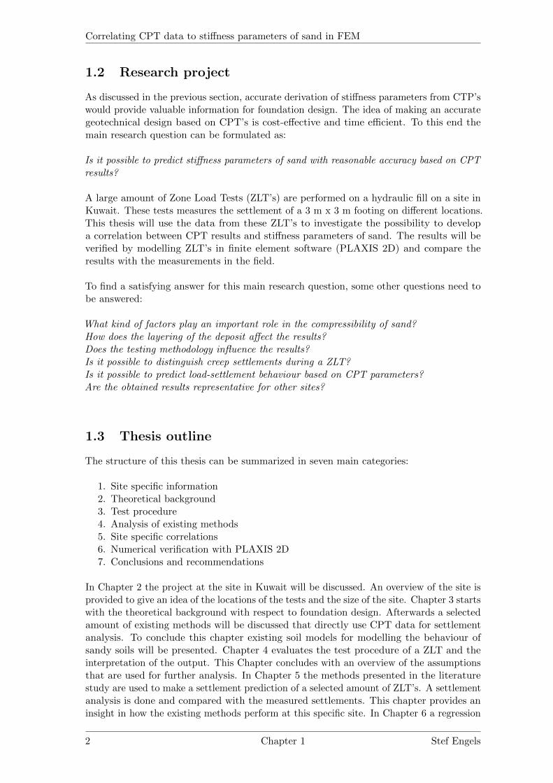
When interpreting CPT data there is another effect that influences the values of thereadings. During the penetration the cone tip induces passive soil failure (figure 3.3). Therecorded cone resistance is an average value across the influenced zone. When the coneis penetrating towards another layer as indicated in figure 3.3, caution should be takenby interpreting the readings. The instrumental cone senses soil resistance of about 21 cmahead of the advancing cone (Rogers, 2004). Due to this effect soil layers may be eitherstiffer or softer than the CPT results indicate.

Zone of Distubance

Less stiff layer

Stiffer layer

Passive failure zone due to advancing cone tip

Figure 3.3: Passive soil failure during a CPT

3.2 Theoretical background

3.2.1 Discussion of soil moduli

In geotechnical engineering the soil modulus is a complex parameter. Often the Young’smodulus (E) parameter is used as the deformability parameter for soil. One must keep inmind that the official term of the Young’s modulus relates to linear elastic behaviour for acontinuum material. Since soil is not a linear elastic material, the soil modulus is not theequal to the slope of the stress strain curve. This indicates that the soil modulus is stressdependent. Looking at a stress strain curve of a dense sand in a triaxial test, many soilmoduli can be obtained (figure 3.4). Furthermore an unloading reloading modulus can be



distinguished. The modulus during unloading reloading will be significantly higher thanwith normal loading. In figure 3.4 the different moduli are deliberately denoted with the Sinstead of E. The slope in the stress strain diagram is not the same as the soil modulus.An exception to this statement is the case where the confining stress in the triaxial test iszero.

SinitialStangent

Ssecant

Stress

Strain0

Figure 3.4: Stress-strain curve obtained from a triaxial test of dense sand

When drawing a slope from the origin to a arbitrary point in figure 3.4, a secant slopeSs is obtained and the secant modulus Es can be obtained from it. This is the modulusthat can be used to predict the settlement of a footing which is loaded for the first timeon a normally consolidated deposit. When the same footing is loaded on a deposit whichhas been subjected to higher loads in the past (overconsolidated), the unloading reloadingmodulus Eur should be used. The tangent slope St relates to the tangent modulus Et andcan be used to determine incremental movement when an incremental load is applied. Anexample is an expansion of a high existing building with an extra level. This illustratesthat the soil modulus which should be used depends on the application.

Influence of state factors

The following state factors have influence on the soil stiffness.

Packing of the particles: If the particles are packed close to each other, the value of themodulus tends to be high. The state can be measured by means of dry density and porosity.

Arrangement of particles: This refers to the structure of the soil. It must be notedthat although the dry density may be the same for two deposits, the structure can dedifferent. Coarse grained soils for example may have a dense or a loose structure and finegrained soils may have a dispersed or flocculated structure. Soils that are well gradedbehave stiffer than poorly graded soil since the voids are filled with finer particles.

Water content : The water content plays an important role because it has a direct in-fluence on the effective stress state of the soil. At low water contents (especially in finegrained soils) the water can bind the particles through suction. This will lead to anincreased value for the modulus. However, because of the lubrication effect of water, the



compaction of coarse grained soils with very low water content is less efficient than thecompaction with higher water content (Briaud, 2001). This would lead to a lower modulusfor lower water contents. There is an optimum value for the modulus as the water contentincreases.

Stress history : When the soil has been subjected to higher loads in the past, the soil isin an overconsolidated state. The soil will respond stiffer than a normally consolidateddeposit. Overconsolidation can be the result of glaciers that where present during the iceage. There are also soils that are still consolidating under there own weight. These soilsare in an underconsolidated state. This is the result of a higher deposition rate than therate that pore pressures can dissipate. These soils will have a lower modulus comparedwith normally consolidated soils.

Cementation: Soil cementation can be seen as glue between the particles. The suc-tion effect which is discussed earlier can also be seen as a glue acting between the particles,although this is temporary since it disappears with increasing water content. Furthermorethere is the process of chemical cementation. This is defined as the filling of intergranularpore space by deposition of a mineral cement brought in by circulating groundwater. Highlycemented soil will have a higher modulus. Chemical cementation will occur as a result oflithification of sediments. This is a very slow process and will not play a significant role ina new constructed hydraulic fill as encountered at the site.

Influence of load factors

Furthermore different load factors influences the soil stiffness. These load factors arediscussed.

Confining pressure: Soils under high confining pressure will behave stiffer than soilsunder lower confining pressure. The confining pressure is the mean of the principle stresses.Commonly used models for quantifying the effect of the confining pressure are createdby Kodner and Zelasko (1963) and Duncan and Chang (1970) . These models relate themodulus to the confining stress using a power law.

Stress level : Since soil behaviour is nonlinear, the stress level influences the stiffness.In most cases the secant modulus will decrease with increasing strain level.

Strain level : At very small strains the soil respond stiffer than at larger strains. Thisbehaviour is captured in the stiffness degradation curve which will be explained in detailin section 3.4.3.

Strain rate: Soils are viscous materials. The faster the loading is applied, the stifferthe response. The strain rate is defined as the accumulated strain per unit of time. Due tothis effect, standard CPT procedures are done with a specified penetration speed.

Number of loading cycles: When the loading process is repeated a number of times,the modulus of the soil will change. The larger the number of loading cycles, the smallerthe modulus becomes. This is consistent with the accumulation of strains with an increasingnumber of cycles.

Drainage effect : Two extreme cases can be distinguished, drained loading and undrained



loading. In drained loading pore pressures can dissipate immediately and no excess porepressure is generated. In coarse grained soils, drained loading conditions apply. Undrainedloading occurs when the pore pressures can not dissipate due to very low permeability.Much of the stiffness is then related to the compressibility of water, which will result in amuch higher stiffness than with drained loading.

3.2.2 Settling behaviour of soil

Settlement is defined as the volume reduction as a consequence of an increase in effectivestress. Different settlements can be distinguished:

Elastic/immediate settlements: These settlements occur quickly and are usually small.These settlements are related to the compression of the grain skeleton and the free gassesin the voids. Generally, not all immediate settlements are pure elastic. However, it isoften referred to as elastic settlement since elastic theory is usually used for the computation.

Consolidation: Compression that is associated with the expulsion of water. In granu-lar soils consolidation develop quickly. In cohesive soils where the permeability is low,consolidation develops slowly.

Creep: Compression that occurs without an increase of effective stress, but is relatedto the slow long-term compression of the grain skeleton.

In a ZLT, a footing is loaded to simulate the process of the settlement of a shallowfoundation. A footing is loaded up in steps by extending the jack between the footing andthe load. As a result, there will be a stress distribution in the soil which is dependent onthe interaction between the plate and the soil. Elastic theory is often used to estimatethe distributions of stresses in the subsurface due to footing pressure. Soils are generallyconsidered elastic-plastic materials. The use of elastic theory however, can be verifiedbecause of a reasonable match between the boundary conditions for footings and elasticsolutions (Ismael and Vesic, 1981). Another reason to use this approach is the lack ofacceptable alternatives. For a loaded footing, the pure elastic settlements will generally besmall compared to the total settlement. The major components of the settlement will occurdue to change in void ratio, particle rearrangement or grain crushing. When this occurs,little of the settlements will be recovered after the load is removed. This phenomena isassociated with the elasto-plastic stress-strain behaviour of the soil.

A lot of research is done to examine creep settlements in granular materials. Researchby McDowell and Khan (2003) concludes that one of the mechanisms that cause creep isparticle crushing and occurs within 24 hours. Carbonate sands are encountered on the siteand these sands are known as crushable. This means creep can be of significant influenceduring a ZLT. The effect of grain crushing can be visualized by comparing the particle sizedistributions (PSD’s) before and after loading. In sand however, the increase in fine contentis usually so small that this effect is hard to measure. Therefore McDowell and Khan(2003) tested the creep behaviour of pasta shells and compared it with creep behaviour ofsand. When compressing pasta shells the increase in fine content is much more significantand can clearly be seen when comparing the PSD’s. The research concluded that creepin both pasta and sand behaves in a similar way and that creep strains are proportionalto logarithmic time. This result is consistent with the hypothesis that all brittle granularmaterials behave essentially in the same way.



Figure 3.5: Type A compression behaviour of Ottawa sand (data from Roberts andde Souza (1958)) (Mesri and Vardhanabhuti (2009))

3.2.3 Compressive behaviour of sand

The compressive behaviour of granular soils can be different with other types of deposits.Compression leads to a denser packing of the material and increases particle locking. This,with engaging surface roughness among soil particles, increases the stiffness of the material(Vesic and Clough, 1968). On the other hand, particle damage and inter-particle slip areunlocking mechanisms which lead to a decrease in stiffness. When compressing a granularmass, both locking and unlocking mechanisms will act simultaneously. The most dominantof these two mechanisms will determine the compressive behaviour.

Particle damage may be quantified in three categories (Chuhan et al., 2003) (Mesriand Vardhanabhuti, 2009). Level I damage means abrasion or grinding of particle surfaceasperities. When level II damage occurs, particle surface protrusions and sharp particlecorners crush or break. At level III particle damage, Particles split, fracture or shatter.

According to Mesri and Vardhanabhuti (2009) three different types of primary compressionresponses can be distinguished for most granular soils. The responses are summarized interms of type A, B or C. The type of response can be determined by looking at the voidratio versus effective stress relationship (e versus σ

′v). For type A behaviour, three stages

of compression can be distinguished. In the first stage, small particle movements enhanceinter-particle locking. In this stage minor level I and level II damage occurs. The improvedlocking dominates the unlocking effects. This means that the stiffness increases with anincrease in σ

′v. At the second stage level III particle damage occurs. Particles start to

fracture and the unlocking effects become dominant. At this stage the stiffness decreaseswith an increase in stress. In the third and final stage, the stiffness gained from particlepacking exceeds the unlocking effect and the stiffness will increase continuously with anincreasing σv

′. Type A behaviour is often observed for clean well rounded, strong, coarseparticles (Nakata et al., 2001) (Chuhan et al., 2002). An example of type A behaviour isshown in figure 3.5.

With type B behaviour, the e versus σ′v relation also displays three stages. The first stage

is equivalent with type A behaviour, where the stiffness increases with an increase in σ′v.

In the second stage the improved packing and the unlocking effects (by level III particledamage) balance. This results in a constant stiffness with an increasing σv

′, which canbe seen by a constant slope in σ

′v - e space. The third stage is equal to the third stage



Figure 3.6: Type B compression behaviour of Ganga sand (data from Rahim (1989))(Mesri and Vardhanabhuti (2009))

Figure 3.7: Type C compression behaviour of carbonate sand (data from Chuhan et al.(2003)) (Mesri and Vardhanabhuti (2009))

of type A behaviour where the stiffness increases with an increase in σv′. A typical type

B response is presented in figure 3.6. In type C behaviour level I and level II particledamage begin at low values for σv

′. The locking effect of improved gradation and packingis dominant over the unlocking effect due to particle damage and inter-particle slippage.Level III particle damage may or may not occur at higher effective stresses (Chuhan et al.,2003). The stiffness continuously increases with an increasing σv

′. This type of response istypically observed in for angular weak particles, such as carbonate sands in presence withclay minerals, mica or very fine material. This type of behaviour is shown in figure 3.7.

3.2.4 Stress distribution underneath a shallow foundation

Boussinesq (1883) developed equations to determine the stress state for a point in thesubsurface due to surface loading. These equations are based on elastic theory and as-sumes that the soil mass is elastic, isotropic, homogeneous and has semi-infinite depth.Another assumptions is that the soil is weightless. Furthermore the stress state is alsodependable on the rigidity of the foundation and the type of soil. Various methods havebeen developed to determine the stress state at any point in the subsurface due to a surfaceload. An example of such a method is developed by Newmark (1942), who created an



influence charts for computing stresses in an elastic foundation. This method is derived byintergration of Boussinesq’s equation for a point load. The pressure distribution accordingto Newmark for a square foundation is shown in figure 3.8. The pressure isobars aredrawn underneath the footing. From this figure it can be seen that the stress increaseat a depth of two times the width of the footing, is only about 0.1 times the applied loading.

0.9

0.1

0.2

0.3

z/B

B

0

1

2

3

21012y/B

Figure 3.8: Newmark solution for stress distribution underneath a square footing

The solution of the stress distribution can be justified when the stress increase occurs in thesoil only. The real requirement to use the solution is not the pure elastic response of thesoil, but a constant ratio between stress and strain. If the stresses induced in the soil aresmall in comparison with the shear strength of the material, the Boussinesq solution can beused. In practice, the Boussinesq solution can be used safely in homogeneous deposits asclay, man-made fills and in uniform sands with limited thickness. In these kind of depositsthe stiffness will be approximately constant with depth. When the stiffness is increasingwith the depth, the Boussinesq stress distribution will not be valid and nonlinear elastic orelastic-plastic analyses should be done. A soil profile where the stiffness increases linearlywith depth is known as a Gibson soil profile. Another solution for the stress distribution inthe subsurface is provided by Westergaard (1938). This solution is similar to Boussinesqbut can be used when soils have alternating layers of material. This solution assumesthat there are only vertical deformations and no lateral deformations (one dimensionalcompression).

3.2.5 Elastic settlement with constant Young’s modulus

When a constant modulus of elasticity of the soil over the depth is assumed with an evenlydivided pressure, which acts on a homogeneous infinite half space which is isotropic andlinear elastic, the elastic settlement can be calculated according to elastic theory as:

se = qb ·B · Iρ ·1− v2

Es(3.2)



Where:qb is the unit load acting at the baseB is the foundation widthIρ is a settlement influence factorv is the Poisson’s ratioEs is the secant Young’s modulus

In this equation a settlement influence factor Iρ is introduced. This factor dependson the shape and the rigidity of the foundation. The values of v and Es are characteristicproperties of the soil.

3.2.6 Settlement analysis of a shallow foundation

When the settlement of a shallow foundation on a dense cohesionless soil is monitored,a load settlement curve as figure 3.9 is obtained. The sudden drop down in the curveindicates that the ultimate bearing capacity is reached. From the curvature, it can be seenthat the soil does not respond linear elastic but that the stiffness is stress dependent anddecreases with increasing stress level.

Load (kPa)

Settlement(mm)

Ultimate bearing capacity

Figure 3.9: Typical load settlement curve for a shallow foundation on dense sand

When the load settlement curve is plotted on a logarithmic scale for both the applied loadand settlement, the curve in figure 3.10 is obtained. Two straight lines can be distinguished.At the intersection point of these two straight lines a sudden drop in stiffness is observed.This point is known as the yield point. Before this point the soil response is dominated byelastic behaviour and afterwards the response is dominated by plastic behaviour. Thereshould be noted that though this is indicated as the elastic region, some plastic strainingcan be expected with every loading cycle. The location of the yield point depends onthe highest stress the soil has experienced in the past, the preconsolidation stress. Soilsthat have experienced a higher load in the past are by definition overconsolidated. Thebehaviour at stress levels below the preconsolidation stress is much stiffer than when thispoint is exceeded. This is caused by rearrangement of particles during previous loading. Infigure 3.9, the steeper slope after the preconsolidation stress indicates a significant decreasein stiffness, which is related to the original stiffness of the normally consolidated material.The line in the elastic region is called the re-compression line and the line in the plasticregion is called the virgin compression line.



log (load)

log (settlement)

yield point

Elastic Plastic

Figure 3.10: Load settlement curve in log-log space

3.3 CPT based methods for settlement of a shallow founda-tion

In engineering practice, many correlation methods to predict the settlement of a shallowfoundation have been developed over the years. In this section an overview of differentmethods is given. For the scope of this investigation only CPT related methods areconsidered. Two categories of methods can be distinguished. Methods based on observedsettlements and semi empirical methods. Semi empirical methods use a combination oftheoretical analysis and empirical relations.

3.3.1 De Beer and Martens (1957)

One of the methods that is based on observed settlement was created by De Beer, E.Martens (1957). They proposed the following expression to calculate the settlement of ashallow foundation in sand:

s = 2.3 · HC· log10(

σ′0 + ∆σ

σ′0

) (3.3)

C = 1.5 · qcσ

′0

(3.4)

Where:s is the settlementC is the compressibility coefficientσ

′0 is the effective overburden pressure at considered depth

∆σ is the increase of pressure at that depth due to foundation loadingH is the thickness of the layer considered

The strategy in this method is to divide the soil stratum in a convenient number of layers.The settlement of each layer is determined individually according to equation 3.3 andeventually the settlement of each layer is summed to evaluate the total settlement.

s =n∑i=1

si (3.5)

Where si represents the settlement of an individual layer and n represents the numberof layers. The value of ∆σ can be determined using the Boussinesq stress distribution



charts and should be determined at the center of each individual layer. De Beer (1965)concluded that the above method is only appropriate for normally consolidated sand. Foroverconsolidated sands a reduction factor needs to be applied which can be obtained fromcyclic Oedometer tests. According to Hough (1969) the value of Cc is determined:

Cc = a(e0 − b) (3.6)

Where:Cc is the compressibility index

The compressibility index Cc and the compressibility coefficient C are related via:

C =2.3

Cc· (1 + e0) (3.7)

Where:e0 is the initial void ratio

The empirical parameters a and b can be obtained from table 3.1.

Table 3.1: Values for empirical constants (Hough 1969)

Type of soilValues of constantsa b

Uniform cohesionless material

Clean gravel 0.05 0.50

Coarse sand 0.06 0.50

Medium sand 0.07 0.50

Fine sand 0.08 0.50

Inorganic silts 0.10 0.50

Well graded cohesionless soil

Silty sand and gravel 0.09 0.20

Clean, coarse to fine sand 0.12 0.35

Coarse to fine silty sand 0.15 0.25

Sandy silt (inorganic) 0.18 0.25

The value of b should be taken asthe minimal void ratio whenever thelatter is known or can convenientlybe determined

The method of De Beer (1965) was intended to provide a ”safe upper limit” with respect toexpected settlement. The values obtained from this method were compared with measuredsettlements of several bridge abutments and piers. The conclusion of this analysis was thatthe method overpredicts the settlement about two times.

3.3.2 Schmertmann method (1978)

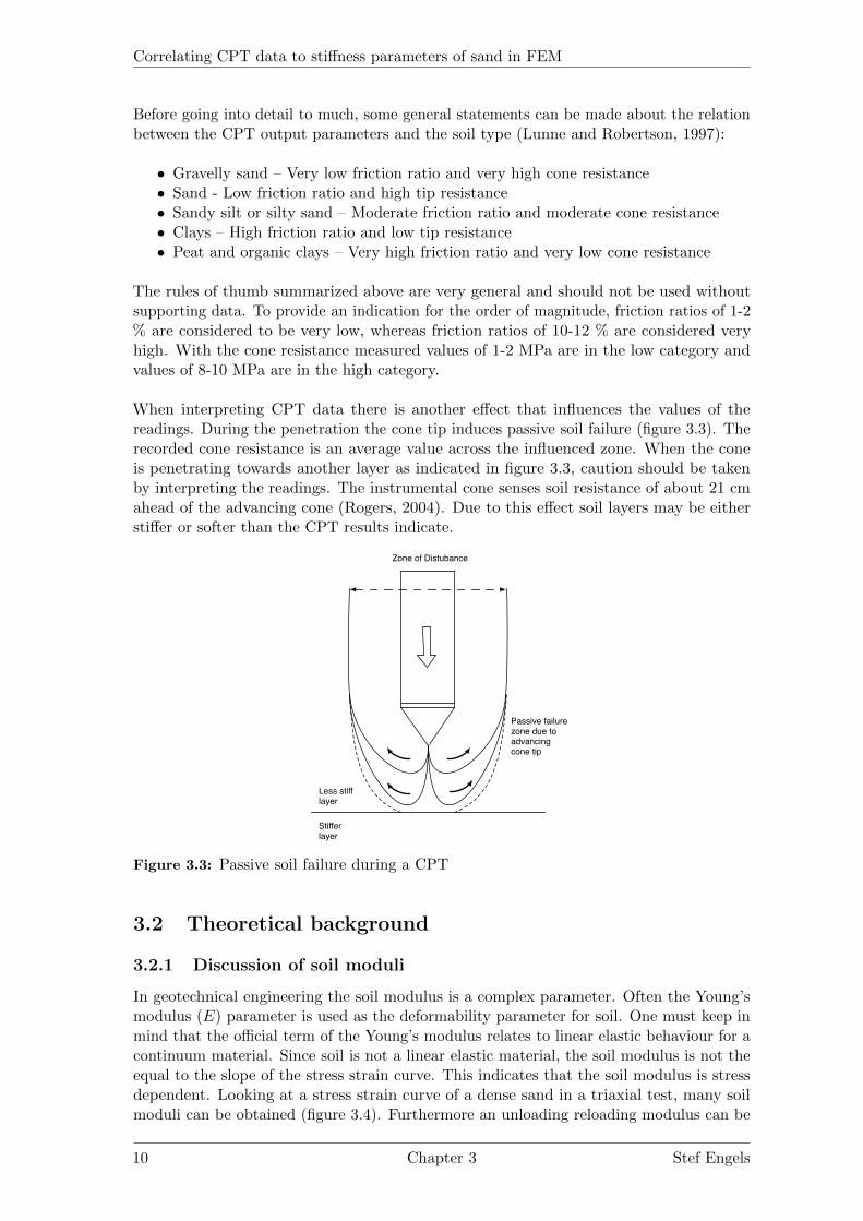
To start this section, the basic framework for calculating settlement is presented. Thisframework holds for the following described methods. The basic form of the equation is:

s = Iz ·qb ·BEs

(3.8)

Which can also be written in the form:

s = qb ·B ·∫ z

0

IzEsdz (3.9)



Where:εz is the vertical strainB is the footing widthIz is the strain influence factor at depth zEs is the secant Young’s modulus at depth zqb is the unit load acting on the base

The advantage of the form 3.9 over 3.8, is that the integral takes the soil layering anddifferent soil properties into account. The Schmertmann method is based on a physicalmodel of settlement which has been calibrated with empirical data. In this equation thestrain influence factor is introduced. The factor takes into account for different strain levelswith increasing depth. Measurements of settlements at various depths suggest a verticaldistribution of vertical strain, that starts from a finite value at foundation level, increaseswith depth to a maximum and then decreases with depth (Schmertmann, 1970)(Burlandand Burbridge, 1985). Schmertmann (1970) used a simplified diagram to determine thevariation of Iz with depth for square/circular and strip footing foundations. A revisedversion of this diagram was provided by Schmertmann et al. (1978) and can be seen infigure 3.11. The Young’s modulus varies with the value of the cone resistance qc.

1

2

0.2 Ipeak

4

L/B=1

L/B > 10

z = depth below footingB = width of footingL = length of the footing

z/B

Iz

3

0.1

Figure 3.11: Varying influence factor according to Schmertmann (1978)

For circular and rectangular footings holds:Iz = 0.1 at z = 0Iz(peak) at z = zp = 0.5BIz = 0 at z = z0 = 2B

For a footing where L/B > 10:Iz = 0.2 at z = 0Iz(peak) at z = zp = BIz = 0 at z = z0 = 4B

The peak value of the influence factor can be calculated according to:

Iz(peak) = 0.5 + 0.1 · ( qbσ

′0

)0.5 (3.10)



The approach is to divide the soil in multiple layers based on the measured value of thecone resistance qc. Depth and time factors are applied and allowance for previous existingin situ stresses are made. The obtained equation has the form:

s = C1 · C2 · qb ·n∑i=1

Iz,i ·∆ziEs,i

(3.11)

Where:C1 and C2 are depth and time dependent factorsqb is the net effective pressure applied at foundation levelIz,i is the average influence factor corresponding to the sublayer∆zi is the thickness of the sublayerEs,i is the average secant Young’s modulus for each sublayer

The suggested values for the coefficients are:

C1 = 1− 0.5 · q0qb

(3.12)

C2 = 1 + 0.2 · logt(years)

0.1(3.13)

The value of q0 is determined by the overburden pressure at the location of the footing.The secant Young’s modulus of each sublayer is determined with the average correspondingcone resistance ¯qc,i measured in that layer. The value according to Schmertmann et al.(1978) is taken as:Es,i = 2.5 · ¯qc,i for a circular/squared foundationEs,i = 3.5 · ¯qc,i for a strip foundation

The method of Schmertmann et al. (1978) is based on a series of tests done in a cal-ibration chamber from the University of Florida. The sand tested in the calibrationchamber was uniformly distributed and normally consolidated. The method has beenproven to be conservative since young sands were tested. The effects of “aging” andoverconsolidation were therefore neglected. Aging of soils refers to the observed phenomenathat soil properties change over time. Overconsolidated deposits will behave much stifferthan normally consolidated deposits. The total procedure of the Schmertmann method isgiven in figure 3.12.

Perform in situ tests for defining subsurface conditions

Consider the soil massfrom the base of the foundation to the influence depth

Divide this domain intolayers, based on the varying cone resistancevs. depth

Determine the strain influence diagram

Compute the value of the strain influence diagram in the middle of each layer

Compute the correctionfactors C1 and C2

Determine the stiffness of each layer based on cone resistance

Calculate thesettlement

Figure 3.12: Flowchart of the Schmertmann method



3.3.3 Modification Schmertmann suggested by Peck et al. (1996)

Peck et al. (1996) proposed a slightly different method. They suggested another variationof the strain influence factor with depth. The modification for the value of the straininfluence factor can be seen in figure 3.13.

1

2

0.2 Ipeak=0.6

4

L/B=1

L/B > 10z = depth below footingB = width of footingL = length of the footing

z/B

Iz

3

L/B=3

Figure 3.13: Varying influence factor according to Peck et al. (1996)

For the value of the influence factor holds:Iz = 0.2 at z = 0Iz(peak) = 0.6 at z = 0.5BIz = 0 at z = z0

The value of the influence depth z0 can be calculated as:

z0 = 2 ·B(1 + logL

B) ≤ 4 (3.14)

When the foundation level is not at the ground surface but is embedded, another valuefor Iz should be used. The method to determine the corrected strain influence factor I

′z

is published by Peck et al. (1996). This method makes a distinction between elastic orimmediate settlements and creep settlements. The elastic and creep settlements can becalculated according to:

se = qb ·n∑i=1

Iz ·∆zEs

(3.15)

screep =0.1

q̄c· z0 · log

t(days)

1(day)(3.16)

The parameter q̄c is the weighted average cone resistance measured through a sublayer.For the value of the stiffness Peck et al. (1996) suggest the following:Es,i = 3.5 · q̄c for a circular/squared foundationEs,i(L/B) = Ei(L/B = 1) · (1 + log L

B ) ≤ 1.4 for a rectangular foundation



3.3.4 Robertson (1990)

Normalized CPT parameters

The method Robertson (1990) suggest to use normalized and dimensionless CPT parameters.Dimensionless parameters correct for increasing soil stress with depth. The assessment ofsoil strength from cone resistance can be incorrect when this influence is not taken intoaccount. The three parameters are the normalized cone resistance Qtn, the normalizedsleeve friction Fr and the normalized pore pressure Bq. They are defined as:

Qtn = (qt − σv0pa

) · ( paσ

′v0

)n (3.17)

Fr =fs

qt − σv0· 100% (3.18)

Bq =u2 − u0qt − σv0

(3.19)

Where:qt is the corrected net cone resistanceσv0 is the in situ total stressσ

′v0 is the in situ effective stresspa is the atmospheric pressuren is the stress componentfs is the sleeve frictionu2 is the measured pore pressureu0 is the hydrostatic pore pressure

The corrected net cone resistance qt is determined using the value qc that is corrected forpore water pressure effect. When drained loading conditions apply there is no need forthis correction since excess pore pressures can dissipate immediately . Based on thesenormalized CPT parameters, Robertson (1990) developed a chart in which the soil can beclassified according to there mechanical response. Other more recent charts are developedby Eslami and Fellenius (2004). Both charts perform comparable accurate. A Qtn − FrSBTn (normalized Soil Behavior Type) chart and a Qtn−Bq SBTn chart were constructedby Robertson (1990). The Qtn − Fr chart was concluded to be more reliable. This chart isgiven in figure 3.14.



Figure 3.14: Qtn − Fr chart by Robertson (1990)

The normalized parameters can be used to calculate the so called Soil Behaviour TypeIndex Ic. When no measurements of the pore pressure are registered and parameter B isexcluded, a special index Ic,rw can be calculated according to Robertson and Wride (1998):

Ic,rw =√

3.47− logQtn2 + (1.22 + logFr)2 (3.20)

With the value of this index it is possible to classify the soil. The contours of this indexcan be plotted on the SBTn chart. This is done in figure 3.15. It can be seen that thecontours of Ic,rw follows the Robertson chart more accurately for low values of Ic,rw whichcorrespond with sandy soils.



Figure 3.15: Contours of Ic,rw plotted on the SBTn chart ((Robertson, 2009))

Appropriate stress component

The stress component n which was introduced earlier varies with the SBTn. A lot ofresearch is done on what this value n should be. Zhang et al. (2002) suggested that theparameter could be estimated using the SBTn index (Ic) and that Ic should be definedusing Qtn. Another approach is that n should vary with relative density (Boulanger andIdriss, 2004). The value of n is close to 1.0 for loose sand and n is less then 0.5 for densesand. Large studies in calibration chambers and centrifugal testing with sands with aconstant relative density have shown that the cone resistance increases nonlinear with theeffective stress for coarse grained soils. The n value which captures this nonlinearity isclose to n = 0.5 (Baldi et al., 1989). The nonlinearity is more present in dense sands thanin loose sands. This results in a larger n value for loose sands.

Research showed that the secant peak friction angle decreases with an increasing ef-fective stress (Bolton, 1986). The friction angle is essentially constant for very loose sands.This angle is denoted as the constant volume friction angle, or the critical state frictionangle. It is implied that the value of n should be close to one for very loose sands and forvery dense sands at very high stresses. When a dense sand experiences a very high stressstate, dilatancy is suppressed and grain crushing occurs (contractive behaviour). The pointwhere grain crushing occurs depends on grain characteristics. Sand which consists of silicarounded particles do not crush until a mean effective stress of about 2 MPa (Bolton, 1986).Angular silica sand and silty sand reach this point at about 1 MPa, whereas crushablesands as carbonate sands can experience grain crushing at a mean effective stress of 0.1MPa. During a CPT the stresses directly underneath the cone these values are reachedand grain crushing can occur. At the rest of the circular failure surface during a CPTthese values are not reached.

Based on earlier research, a generalized critical state line (CSL) is developed by Boulanger(2003). The CSL is presented in the void ratio - log effective stress space and is presentedin figure 3.16. At low mean effective confining stresses (lower than 200 kPa), the line isflattened. The line gets steeper at higher effective stresses. When the slope is small, thereis a strong connection between the relative density and the state parameter. A value ofn = 1 is appropriate when the normally consolidated line is parallel to the CSL (Wroth,



Figure 3.16: Critical state line and state parameter from Bolton (1986) (Boulanger, 2003)

1984). In sands, the CSL is nonlinear over a wide stress range and the consolidation varieswith respect to the CSL. It can be concluded that critical state soil mechanics supportsthe idea of a varying the n value to normalize penetration resistance. The n value variesbetween 0.5 for at low stresses and tends to go to 1.0 for higher stresses where the CSLgets straight and the consolidation line becomes parallel to the CSL.

The slope of the CSL can be linked to the SBT index Ic according to Jefferies and Been(2006). Based on the discussion above the following recommendation is made by Robertson(2009) for varying the stress component n with Ic and effective overburden stress:

n = 0.38 · Ic + 0.05˙σ′v0

pa− 0.15 (3.21)

Correlations for stiffness parameters

Now a connection needs to be made between the discussed parameters and the stiffness.This study focusses on coarse grained cohesionless soils where drained conditions apply.Eslaamizaad and Robertson (1997) and Mayne (2000) have determined that the loadsettlement response of a foundation can be accurately predicted by using the shear wavevelocity Vs. Although direct measurements of Vs are preferred, correlations between qcand Vs can be used as an estimate for lower risk projects. It has been shown that thevalue of Vs predominantly determined by the number and area of grain to grain contacts(Schneider et al., 2004). Therefore Vs depends on relative density, aging, cementation,effective stress state and arrangement of particles. The value for qc is also dominated byrelative density and stress state but to a lesser degree by age and cementation. A strongrelationship between Vs and qc exist, but some variability can be expected. Since Vs is adirect measurement of the small strain shear modulus G0, an improved linkage betweenCPT parameters and soil stiffness can be obtained.

With the normalized CPT parameters it is possible to approximate the normalized shearwave velocity Vs1 (Robertson, 2009):

Vs1 = (αvs ·Qtn)0.5 (3.22)



The factor αvs is defined as the shear wave velocity factor and has the unit m/s2. Thevalues for αvs can be estimated using the obtained value for Ic as follows:

αvs = 100.55·Ic+1.68 (3.23)

The value of the shear wave velocity Vs can then be determined according to:

Vs = [αvs ·(qt − σv)

pa]0.5 (3.24)

This general relationship is recommended for most Holocene- to Pleistocene-age depositswhich are predominately silica-based. At low shear strain levels the shear modulus has aconstant maximum value G0. This modulus is determined as:

G0 = ρ · V 2s (3.25)

Where ρ represents the mass density of the soil (kg/m3). The small strain shear modulusnumber KG is related to the small strain shear modulus as:

G0 = KG · pa · (σ

′v0

pa)n (3.26)

The relationships between the soil modulus and the cone resistance usually have the generalform:

G0 = αG · (qt − σv0) (3.27)

Where αG is the shear modulus factor for the estimation of G0. Because the stresscomponent for the derivation of Qtn and G0 is similar, it follows that:

αG =KG

Qtn(3.28)

The contours of KG and αG can be plotted on the SBTn chart. This is done in figure 3.17(Robertson, 2009).

Figure 3.17: Contours of αG and KG on the SBTn chart (Robertson 2009)



To determine the appropriate value of αG from Ic, the link with αvs can be used:

αG =ρ

pa· αvs (3.29)

When an average unit weight of γ = 18kN/m3 is taken and equations 3.23, 3.27 and 3.29are combined, G0 can be calculated as:

G0 = 0.0188 · [10(0.55Ic+1.68)] · (qt − σv0) (3.30)

The Young’s modulus E and the shear modulus G are interrelated via the Poisson’s ratiov as follows:

E = 2 · (1 + v) ·G (3.31)

For most soils v varies between 0.1 and 0.3 in drained conditions. Hence, for most coarsegrained soils holds E ∼ 2.5G. The small strain shear modulus obtained in equation ??needs to be reduced to an appropriate value of the shear modulus G. The amount ofsoftening is a function of the stress level (Eslaamizaad and Robertson, 1997). A simpleapproach to estimate the amount of softening according to Fahey and Carter (1993) is:

G

G0= 1− f · ( q

qult)g (3.32)

Where q represents the applied load and qult the failure load. The constants f and gdepends on soil type and stress history. According to Fahey and Carter (1993) and Mayne(2005) values of f = 1 and g = 0.3 are appropriate for uncemented soils which are nothighly structured. For many design application the stress level ranges from 0.2 to 0.3 incomparison with the stress level at failure. The ratio of G/G0 ranges then from 0.3 to 0.38.The simplified elastic solution for the Young’s modulus is approximately:

E ∼ 0.8G0 (3.33)

When a similar procedure is followed as with the shear modulus, the following relationscan be obtained for the Young’s modulus number KE and the modulus factor αE :

E = KE · pa · (σ

′v0

pa)n (3.34)

E = αE · (qt − σv0) (3.35)

αE =KE

Qtn(3.36)

When the equations 3.30 and 3.33 are combined, the appropriate value for αE and E canbe made:

αE = 0.015 · [10(0.55Ic+1.68)] (3.37)

E = 0.015 · [10(0.55Ic+1.68)] · (qt − σv0) (3.38)

It should be reminded that this value only applies for uncemented, predominately silica-based coarse grained soils of either Holocene- or Pleistocene age. Furthermore this predictionis only valid for specified assumptions for the Poisson’s ratio and stress level. The contoursfor KE and αE are given in figure 3.18.



Figure 3.18: Contours of αE and KE on the SBTn chart (Robertson 2009)

When the stress level increases (exceeds 0.25), the values for αE will be decreasing. Ifthe relation for the stiffness degradation curve according to Fahey and Carter (1993) andMayne (2005) is used, the stress level can be taken into account according to:

E = 0.047 · [1− (q

qult)0.3] · [10(0.55Ic+1.68)] · (qt − σ

′v0) (3.39)

When this methodology is used, the ultimate bearing stress qult needs to be determined.This value can be obtained by various analytical methods. With this methodology astiffness parameter can be calculated for each registered value of cone resistance and sleevefriction. The settlement can be calculated using this stiffness in the framework which isevaluated in section 3.3.2.

3.4 Soil models for sand

Before a qualitative numerical analysis with PLAXIS 2D can be done, some theory aboutsoil models needs to be evaluated. In this section, appropriate soil models for sand arebriefly explained.

3.4.1 Mohr-Coulomb model

Framework

The Mohr-Coulomb model is a linear elastic perfectly-plastic model. Since soil behaviouris nonlinear and depends at least on stress level, stress path and strain level, this is asimplified approach. Since this model is rather simple compared to the advanced models,it can be used to make a first estimation of soil behaviour. The linear elastic part is basedon Hooke’s law of elasticity. The perfectly plastic part is based on the Mohr-Coulombfailure criterion. This failure criterion is an extension of the friction law of Coulomb togeneral stress states. The occurrence of plastic strains can be determined using a so called”yield function” which is denoted with f . The full Mohr-Coulomb yield criterion consistsof six yield functions when formulated in principle stresses (Appendix A). Plastic yieldingwill occur when the condition f = 0 is satisfied. When f < 0 all generated strains arepurely elastic. In principle stress space, the yield surface can be seen in figure 3.19. In theMohr-Coulomb model the yield surface is fixed in space.



Figure 3.19: The Mohr-Coulomb yield surface in principle stress space (Brinkgreve andVermeer, 2016)

For determining the direction and magnitude of plastic straining, a plastic potential func-tion g is introduced. In plasticity analyses a distinction can be made between associatedand non-associated plasticity. With associated plasticity the yield function and plasticpotential function are the same and the direction of plastic strains is normal to the yieldsurface. As a result of this assumption a symmetric elasto-plastic material stiffness matrixis obtained. This reduces the calculation time. However, a non-associated plasticity frame-work is used in this model because theory of associated plasticity will overestimate dilatancy.

Furthermore it should be noted that Mohr-Coulomb model have the tendency to overpredict the shear strength in undrained behaviour.

Parameters

The Mohr-Coulomb model uses six soil parameters:E: Young’s modulusv: Poisson’s ratioc: Cohesionϕ: Friction angleψ: Dilatancy angleσt: Tension cut off and tensile strength

The stiffness parameter E is already discussed in detail. A suitable value for the Poisson’sratio needs to be chosen. This value is directly related to the value of the coefficient oflateral earth pressure K0 (ratio between σ

′h and σ

′v) according to:

K0 =v

(1− v)(3.40)

In the Mohr-Coulomb model v is evaluated by matching a realistic K0 value. In manycases this value will vary between 0.3 and 0.4 for v. For unloading reloading cases thevalues for v in the range of 0.15 and 0.25 will be more appropriate. With this methodologyit is impossible to create K0 values that exceed 1, as is observed in highly overconsoli-dated stress states. The cohesion c or undrained shear strength su has the dimensionof stress (kPa). In undrained loading cases the cohesion parameter in combination withϕ = 0 can be used to model undrained shear strength. The advantage of using thismethod to model undrained shear strength is that the user has control over the shear



strength, independent of the stress state and stress path followed. The Mohr-Coulombcriterion then reduces to a Tresca failure criterion. The unit of the friction angle ϕ is degrees.

The dilatancy angle ψ also has the unit degrees. The dilatancy is most dominant indense sands. It is dependent on friction angle and relative density. For quartz sands, thedilatancy can be estimated according to Brinkgreve and Vermeer (2016):

ψ ≈ ϕ− 30 (3.41)

For ϕ ≤ 30 the dilatancy angle is usually zero. A small negative value for ψ is only observedin extremely loose sands.

3.4.2 The Hardening Soil model

Framework

The Hardening Soil model is a more advanced soil model compared with the Mohr-Coulombmodel. Instead of a fixed yield surface, it allows the yield surface to expand in principlestress space due to plastic straining. Two different types of hardening can be distinguished:

Shear hardening : This type of hardening is used to model irreversible strains due todeviatoric loading.

Compaction hardening : This type of hardening is used to model irreversible strains due tocompression in oedometer loading and isotropic loading situations.

The 2-D representation of the yield surface in mean - deviatoric stress space is repre-sented in figure 3.20. Note that the cohesion is zero in this figure. The Hardening SoilModel is suitable for simulating the behaviour of different soil types. Some basic charac-teristics of the model are the stress dependency of stiffness (according to a power law),plastic straining due to deviatoric loading, plastic straining due to compression, elasticunloading/reloading and the use of the Mohr-Coulomb failure criterion. This model doesnot account for time dependent behaviour and softening.

Mean stress

Deviatoric stress

Mohr-Coulomb failure line

Compactionhardening

Shear hardening

Elastic region

Figure 3.20: Yield surface of the Hardening Soil model in mean-deviatoric stress space

Parameters

Some of the parameters used by the Hardening Soil model are the same as for the Mohr-Coulomb model. These parameters are:



Figure 3.21: Definition of Eref50 and Erefur for drained triaxial test results (Brinkgreve andVermeer, 2016)

c: Cohesionϕ: Friction angleψ: Dilatancy angleσt: Tension cut-off and tensile strength

The following parameters correspond with basic parameters for soil stiffness:Eref50 : Secant stiffness in standard drained triaxial test

Erefoed : Tangent stiffness for primary oedometer loadingErefur : Unloading/reloading stiffnessm: Power for stress level dependency of stiffness

Furthermore some advanced parameters are defined:vur: Poisson’s ratio for unloading/reloadingpref : Reference stressKnc

0 : The K0 value for normal consolidationRf : Failure ratio qf/qaσt: Tensile strength

Instead of the basic soil stiffness parameters, PLAXIS also accepts a compression in-dex Cc, swelling index Cs in combination with an initial void ratio e0. Although theHardening Soil model is a higher order approach for modelling soil behaviour, it is moredifficult to handle because of the large amount of input parameters. In contrast to theMohr-Coulomb model (elasticity based), the Hardening Soil model does not use a fixed

relationship between the triaxial stiffness Eref50 and the oedometer stiffness Erefoed . The

default value given by PLAXIS for the Erefur is three times the value of Eref50 . The definitions

of Eref50 and Erefur are visualized in figure 3.21. Furthermore, the value of Knc0 is not simply

a function of the Poisson’s ratio but an independent input parameter. Suggested is to usethe following correlation formula (Jaky, 1948):

Knc0 = 1− sinφ (3.42)

For the yield surface of the Hardening Soil model, both shear hardening and compactionhardening must be satisfied. The parameter Eref50 mainly controls the shear yield surface



and the parameter Erefoed controls the cap yield surface. The magnitude of the yield cap isdetermined by the isotropic pre-consolidation stress. The 3-D representation of the yieldcontour in principle stress state is given in figure 3.22

Figure 3.22: 3-D representation of the yield contour of the Hardening Soil model inprinciple stress space (Brinkgreve and Vermeer, 2016)

3.4.3 The Hardening Soil model with small-strain stiffness

The strain amplitude has influence on the value of the soil stiffness. When the strainamplitude increases the stiffness reduces non-linearly. When the decrease in stiffness isplotted against the logarithmic value of the strain, a typical S-shaped modulus stiffnessreduction curve is obtained (figure 3.23). With laboratory testing it is often not possibleto accurately determine the stiffness at very small strain levels. It turns out that withconventional laboratory testing, the stiffness measured at minimal strains already hasdecreased to less then half its initial value.

Figure 3.23: Stiffness reduction curve with increasing strain level (Atkinson and Sallfor,1991)



To take this stiffer behaviour at very small strains into account, the Hardening Soil modelwith small-strain (HS-small model) stiffness is developed. This model is implemented inPLAXIS. The HS-small model uses the same parameters as the Hardening Soil model,along with two additional parameters that describes the stiffness reduction curve. Theseadditional parameters are the small shear modulus (G0) and a parameter which is denotedby γ0.7. This parameter specifies the shear strain level where the secant shear modulus isreduced to a value of 70% of the value of G0. The degradation of stiffness can be describedby a hyperbolic law developed by Santos and Correira (2001):

GsG0

=1

1 + 0.385 · γγ0.7

(3.43)

This relationship holds when the value of G lies between G0 and Gur (unloading reloadingshear modulus). Between these values there is a degradation of stiffness. When G decreases

to Gur the behaviour is dominated by the Hardening Soil model parameters Eref50 and

Erefoed .


Chapter 4

Zone Load Test procedure

In this chapter the test procedure of the ZLT’s performed on the site are explained. Firstsome information is given about the test set-up. Next, the loading procedure will bediscussed and examples of some test results will be presented. Afterwards, uncertainties inthe test procedure will be elaborated. To conclude this chapter the interpretation of theresults and the assumptions that are done for further analysis will be evaluated.

4.1 Test set-up

In a ZLT, a 3 x 3 m squared footing is loaded in specified loading steps. The thicknessof the footing is 0.6 m. A schematic side view is presented in figure 4.1. Before theloading starts, all the weight of the concrete blocks is transferred to the subsoil throughthe supporting blocks. Loading up the footing will be done by extending the hydraulicjack which is included with a load cell. The measurement devices are connected to thereference beams. These beams are supported by piles that are installed further away fromthe footing. It is not exactly clear at how deep these piles penetrate into the sand. A moredetailed representation of the footing and the measuring devices is presented in figure 4.2.

Concrete blocks for loading

Steel bars

Concrete support blocks

Measering device for settlement

Loaded footingHydraulic jack

Reference beam

Figure 4.1: Schematized side view of a Zone Load Test

4.2 Loading procedure and test results

As stated before the loading procedure will be done in specified steps. The total durationof the ZLT is 59 hours. The loading steps and measured settlements for one specific testcan be found in table 4.1. The load will not be adjusted until the rate of settlement is lessthan 0.008 mm/min.

35


Figure 4.2: Close up from the loaded footing in a Zone Load Test

Table 4.1: Settlement registration of a zone load test

Duration of loading step(hours:minutes)

Working load(%)

Working pressure(kPa)

Average settlement(mm)

00:10 0 0 0.00

00:10 10 20 0.49

00:10 0 0 0.28

02:00 25 50 2.62

02:00 50 100 4.88

02:00 75 150 6.77

02:00 100 200 8.79

48:00 125 250 14.42

00:30 100 200 14.09

00:30 75 150 13.62

00:30 50 100 12.99

00:30 25 50 12.20

00:30 0 0 10.47

On the footing, four measuring devices are installed at different locations to measure thesettlement. Measurements are performed by four dial gauges that are placed in the middlebetween the corners of the footing. The average settlement registered by all four devicesis given in the table above. Typical output consist of a diagram that plots the appliedpressure versus the displacement (figure 4.3) and a diagram that shows the evolution ofsettlement in time (figure 4.4). After each loading step, the settlement increases duringthe time the pressure is hold. When the applied pressure is increased to 250 kPa and heldfor 48 hours, this phenomena can be clearly seen. This could occur due to the dissipationof pore pressures (consolidation) from less permeable layers. Another possibility is thatcreep occurs in the sand skeleton.



Figure 4.3: Pressure displacement curve for zone load test DV-113

Figure 4.4: Time displacement curve with the applied pressure for zone load test DV-113

4.3 Test uncertainties

The basic idea of a ZLT is to measure the settlement of a footing which is subjected toa certain load. In the ideal case, the test procedure should not influences the measuredsettlement. However, there are reasons to believe this can be of influence. Possible uncer-tainties related to the test procedure are summarized.

• Temperature influence: The difference in temperature at the site of Kuwait issignificant. Steel parts of the test set-up, like the reference beams are sensitive forthermal expansion. Thermal expansion leads to deflections in the reference beamsand could result in inaccuracies of the measurements.• Deflection of reference beam: The reference beams are supported at the ends. It

should be checked if the deformation due to its own weight is negligible with respectto the measured settlement.• Pre-loading of subsurface: All the load of the ZLT is present before the load is

transferred to the footing. Before the test begins this load is transferred into thesubsurface by the supporting blocks. This results in a stress distribution in thesubsurface. It should be checked if this procedure of testing is representative for thein situ soil state.



4.4 Interpretation and assumptions

The various methodologies explained in the literature study can only be used to determinethe direct settlements of granular soils. To fairly examine the accuracy of these methods,the settlement prediction needs to be compared to the direct measured settlement of thegrain skeleton. Therefore the large amount of extra settlement that is observed during 48hours at the constant load of 250 kPa will be excluded from the analysis. However it isinteresting to know more about the physical processes related to these extra settlements.It is possible that the extra settlement is related to creep in the sand fill. Time dependentdeformation can be the result of particle breakage (McDowell and Khan, 2003). Theyshowed that crushable materials can crush in time without an increase in load. Sincecrushable carbonate sands are encountered on the site, this could be an explanation for theextra observed settlement. Plate Load Tests can be done to determine whether the extrasettlement occurs in the sand fill. The diameter of the plate should be chosen as such, thatthe extra stress increments in the subsurface only occur in the sand fill.

Another explanation could be the generation of excess pore pressure. In that case, theextra settlement observed is the result of consolidation. For future projects, it is advised toinstall pore pressure meters to make sure if fully drained loading conditions can be assumed.

Before the loading starts, the test set-up is fully build up. Because of the weight ofthe concrete blocks, the subsurface is influenced before the loading starts. The stress inthe subsurface increases due to the load transfer from the supporting blocks to the sand.It is assumed that this influence can be ignored. For future tests it is advised to minimizethis effect. The influence of the test set-up is examined numerically in Chapter 7.

The design value of the pressure is 200 kPa. Therefore the direct settlement at 200kPa will be analysed. From table 4.1 can be seen that during the test an unloading step ispresent. The plastic strains generated during the unloading reloading cycle, will not betaken in to account. Therefore the settlement at 200 kPa in table 4.1 will be correctedwith 0.28 mm. The assumptions used for further analysis are summarized.

Assumptions• The settlement measured will be due to compression of the sand• The settlement at 200 kPa will be interpreted as direct settlement• Fully drained loading conditions apply• There is no suction above the groundwater table• The test set-up does not influence the in situ soil conditions• The Boussinesq stress distribution can be used• The loaded concrete footing is rigid


Chapter 5

Analytical settlement analysis

The different methodologies presented in the literature study are tested on existing sitedata in this chapter. The discussed methodologies are only applicable on sandy soils. Tomake an accurate analysis, only the ZLT’s on sandy soils should be considered. As statedin Chapter 2, the site consist of sandy, silty and sabkha soils. Therefore suitable locationsshould be selected that can be used in the analysis. In the first section of this chapter thecriteria for a suitable ZLT are evaluated. Afterwards the different methods are appliedto make a settlement prediction for each of the selected ZLT. Finally the results of thedifferent methods will be compared with the measured settlement of the footing in thefield.

5.1 Zone Load Test Criteria

Underneath every ZLT, five CPT’s are done before the testing procedure starts. The depthof the CPT depends on the site conditions. At some parts of the site, the CPT’s get stuckafter a few meters. In softer areas, the CPT can reach a depth that exceeds 12 metersbelow ground level. CPT’s can get stuck for different reasons. When the cone resistanceexceeds 40 MPa the pushing equipment is not able to push the cone further into the soil.Another possibility is that the cone hits a rock and tries to push it into the soil. Whenperforming a CPT there is always an amount of deflection (lateral movement) of the rods.When this deflection exceeds a certain limit, the CPT is stopped to prevent damagingthe equipment. The level of the site after the fill is placed is denoted as the ground level.The preferred subsurface underneath a ZLT consists of sandy soils only. However, a lotof tests can not be used when such a high criteria is set. Besides, the upper limit ofinformation available of the subsurface is the depth of the CPT. Whatever soil conditionsare encountered underneath is anyone’s guess. A criteria should be set as such, that asufficient amount of tests can be used in the analysis and that the compressive behaviouris dominated by sandy soils.

To extend the amount of tests for the analysis, some ZLT locations where sand is overlyingsabkha are also taken into account. Looking at the Boussinesq stress distribution theory,the stress increase in the subsurface due to a uniform loaded area decreases with depth.For a square footing of 3 x 3 m the stress increase at a depth of 5 m is about 0.15 timesthe applied pressure on the footing. In this analysis a sabkha layer is accepted when it islocated at 5 m or deeper with respect to the new ground level. Due to the low permeabilityof the sabkha undrained behaviour is expected. This means that all the load is taken bythe water in the voids and excess pore pressures can not dissipate. If this indeed is thecase the layer can be considered incompressible.

Another criterion that needs to be determined is when a CPT can be used in the analysis.The analytical methods discussed all use the Boussinesq stress distribution theory. In themethod of the De Beer, E. Martens (1957) the incremental stress is calculated according to

39


this theory. In the other methods the strain influence factor is introduced which is basedon the same theory. The simplified strain influence factor reaches a value of zero at a depthof 2 times the width for square footings. Therefore it is decided that the CPT must atleast penetrates 6 m into the subsurface before it is taken into account in the analysis.

5.2 Processing the CPT data

For the methodologies suggested by De Beer, E. Martens (1957), Schmertmann et al.(1978) and Peck et al. (1996) the subsurface should be divided into a convenient amount oflayers. To determine the layering underneath each ZLT, the normalized soil behaviour type(SBTn) chart is used (Robertson, 1990). This chart is discussed earlier in Section 3.3.4.Wang et al. (2013) showed that the Robertson chart can be estimated very accurately byfitting quadratic functions for every contour of the chart. The accuracy of this approach isvisualized in figure 5.1. The best fitted functions and intersection points as indicated inthe figure are provided in Appendix B.

Figure 5.1: Best fitting of the Robertson chart by quadractic functions by Wang et al.(2013)

The raw data of the CPT’s consist of measurements of the cone resistance and the sleevefriction for every 1 cm of penetration depth. These parameters can be converted tonormalized parameters as shown in section 3.3.4. When using Matlab and the best fittedcurves, all the registered points during the CPT can be plotted in the SBTn chart tovisualize what kind of soil is encountered.

An example of the processing of CPT’s under one ZLT is evaluated. As stated before undereach footing of 3 x 3 m there are five CPT’s available. The raw data is used as input inMatlab and all the five CPT’s are plotted in the same figure (figure 5.2). Important inthis figure is to note if the five profiles are consistent with each other. In the figure all theprofiles are quite similar, that indicates low variability in the horizontal direction betweenthe CPT’s. The high friction ratio and low cone resistance at approximately 5 m depth,



indicate the presence of a sabkha layer. Furthermore the original ground level (before thefill was constructed) is marked in the figure.

0 10 20 30 40Cone resistance (MPa)

0

1

2

3

4

5

6

7

Dep

th (m

)

Original Ground Level

0 1 2 3 4 5 6Friction ratio (%)

0

1

2

3

4

5

6

7

Dep

th (m

)


Figure 5.2: Five CPT’s underneath zone load test DD145

The following step in the procedure is to combine the profiles to one profile which representsthe mean values of the cone resistance and friction ratio (figure 5.3). In the criterion of theindividual CPT’s is stated that a profile should at least have a penetration depth 6 m inorder to be included in the analysis. As can be seen in figure 5.2 all the profiles satisfy thiscriterion. This means that all the profiles are used to calculate the mean profile. Whenan individual profile does not reach six meters penetration depth it is excluded from theanalysis and will not be taken into account when constructing the mean profile.Based on the mean values of the cone resistance and friction ratio, the normalized parametersare calculated according to the method of Robertson (1990) (Section 3.3.4). The formulasto determine these parameters are introduced earlier but are recapped:

Qtn = (qt − σv0pa

) · ( paσ

′v0

)n (5.1)

Fr =fs

qt − σv0· 100% (5.2)

Ic,rw =√

3.47− logQtn2 + (1.22 + logFr)2 (5.3)

n = 0.38 · Ic + 0.05˙σ′v0

pa− 0.15 (5.4)

Because the stress component n appears multiple times in this system, an iterative procedureis used to determine the value of n. This is done using Matlab until an accuracy within0.01 is reached. The result of the analysis are vectors with the normalized parameters forevery reading of the CPT. Afterwards the values for the normalized cone resistance andthe normalized friction ratio can be plotted in the Robertson SBTn chart. To do this the



0 10 20 30Cone resistance (MPa)

0

1

2

3

4

5

6

7

Dep

th (m

)


0 2 4 6Friction ratio (%)

0

1

2

3

4

5

6

7

Dep

th (m

)


Figure 5.3: The mean CPT profile underneath zone load test DD145

contours of the chart are estimated using the best fitting curve approach by (Wang et al.,2013). The result can be seen in figure 5.4.

10-1 100 101

Friction ratio, F (%)

100

101

102

103

Tip

resi

stan

ce, Q

tn

7 6 8 9

54

3

1 2

1=Sensitive fine grained2=Organic soils3=Clays4=Silt mixtures5=Sand mixtures6=Clean/silty sand7=(Gravelly) sand8=Very stiff sand/clayey sand9=Very stiff, fine grained

Figure 5.4: The normalized CPT data points in the SBTn chart of Robertson

As seen in section 3.3.4 in figure 3.15, specific values of Ic,rw correspond with the contoursof the SBTn chart. Using these specific Ic,rw values make it possible to estimate the soilclassification based on the normalized parameters. A profile of Ic,rw can be constructedwith respect to the depth. This gives an indication of the soil type and the soil layering. InMatlab a new layer is distinguished when the value of Ic,rw exceeds the indicated boundarieswhich are typical for a specific soil type. Furthermore is programmed that the minimallayer thickness is 25 cm. An example of the output is given in figure 5.5. The dotted



horizontal lines give an indication of the layering.

With this approach the suggested layers are automatically generated from the raw CPTdata. Care must be taken when using this soil layering. First of all the layering is basedon multiple CPT’s. When the individual CPT profiles significantly differ from each other,the approach of introducing horizontal layers is inaccurate because a high horizontalheterogeneity is observed. Furthermore, the contours of Ic,rw on Robertson chart fit theRobertson contours very well for low values of Fr and high values of Qtn, but the accuracydecreases when moving to the right bottom of the chart (figure 3.15). This means that thelayering indication based on Ic,rw is less accurate with increasing values of Ic,rw. Finallyit should be remembered that this method of soil classification is based on CPT resultsonly, which may have inconsistencies with soil classification based on the USCS (unifiedsoil classification system) where soils are classified based on sieving results and Atterberglimits.

0 0.5 1 1.5 2 2.5 3 3.5 4Soil Behaviour Type index

0

1

2

3

4

5

6

7

Dep

th (m

)

Gra

velly

san

d to

den

se s

and

Cle

an s

and

to s

ilty

sand

Silty

san

d to

san

dy s

ilt

Cla

yey

silt

to s

ilty

clay

Silty

cla

y to

cla

y

Cla

y to

org

anic

soi

ls

Figure 5.5: Variation of soil behaviour type index over the depth corresponding to zoneload test DD145

For each discussed methodology, a function is programmed in Matlab that evaluates thesettlement based on the CPT input data. For the De Beer, E. Martens (1957), Schmertmannet al. (1978) and Peck et al. (1996) methods, different layers needs to be distinguished.This is done based on the automated layering profile in combination with engineeringjudgement. Most of the methods use the strain influence diagram. Note that the Peck et al.(1996) method uses a modified strain influence diagram which is illustrated in figure 3.13.

5.3 Overview of the procedure

In this section a flowchart is presented that summarizes the procedure of the analyticalanalysis. The intermediate parameters are calculated with a Matlab program that calculatesall the parameters based on the 5 CPT’s that are done beneath one ZLT. The flowchart ispresented in figure 5.6.



Analytical analysis

Exclude CPT´s wheredepth < 6m

Calculate settlementwith Robertson method

Calculate settlement with Peck et al. method

Calculate settlement with Schmertmann method

Calculate settlement with De Beer & Martens method

Determine the strain influence diagram

Calculate the stress increase in the middle of the layer (Boussinesq)

Determine the averagecone resistance foreach layer

Suggest layering based on SBT index

Plot SBT index over the depth

Calculate the SBT indexfor every measurements

Calculate stiffness parameters according to Robertson

Calculate in situ stressstate

Calculate normalized Robertson parameters Q and F

tnr

Plot all the measurements on Robertson SBTn chart

Calculate mean q , f and plot the results

c s

5 CPT´s at each ZLT location

Figure 5.6: Flowchart of the procedure of the analytical analysis

5.4 Results and discussion

In this section the results of the analysis of the selected ZLT’s are presented. All of theseZLT’s met the criteria set in Section 5.1. In the first part of this section different siteconditions are compared. From the previous section it is mentioned that in this analysissome locations are included where sabkha and silt are encountered. A separate analysisis done for these locations to check whether this leads to inaccuracies. Afterwards, thesettlements are evaluated using all the described methods and compared to the measuredsettlement in the field. The error is calculated according to:

Error =(scalculated − smeasured)

smeasured· 100% (5.5)

When the error is calculated as in the equation above, negative values of the error indicatethat the calculated settlement is smaller than the measured settlement. This means anunder-prediction of the settlement and it should be noted that this is an unsafe situation.

5.4.1 Comparison different site locations

The methodologies that are used to evaluate the settlement during a ZLT are applicable tosandy soils only. Since the fill is constructed over a weaker layer and varies in thickness,



other soil types can be encountered as well in the influenced area underneath a ZLT. InSection 5.1 is explained which criteria concerning the ZLT’s are used for this analysis. Thecriteria set in that section are now examined.

To do such an examination, all the ZLT’s can be split up into three groups.

• Zone Load Test locations where only sand is encountered• Zone Load Test locations where sand and silt are encountered• Zone Load Test locations sand, silt and sabkha are encountered

For each group, the settlements are calculated using the proposed methodologies. Af-terwards, the error between the measured settlement and the calculated settlement isevaluated. The mean value of the error and the standard error of the error is determined.The results are summarized in table 5.1.

Table 5.1: Accuracy of different analytical methods

MethodError

mean (%) standard error (%)

De Beer and Martens 28 16

Schmertmann 42 13

Peck et al. -2 23

Robertson 0 20

The results of each individual test can be found in Appendix C. It can be seen that themean value and the standard error for each method of each group is quite similar. Thismeans that the error of each group is in the same order of magnitude. It can be concludedthat it is justified to extend the sample size with sabkha and silt locations when the criteriaof section 5.1 is met.

5.4.2 Normality of the results

It would be useful to recognize a certain pattern in the output. If the error of each methodfollows a certain well known distribution, it is possible to make a safe evaluation of thesettlement. Therefore the error of each method is evaluated and tested for normality. Withthis analysis it is possible to check whether it is likely that the values of the error arenormally distributed. When the error of a method is normally distributed, it is possible togive a worst case scenario regarding to the settlement based on an analytical calculationonly. There are certain statistical tests to check whether it is likely to assume a normaldistribution to a set of variables. The test that will be used here is the Shapiro-Wilk test(Shapiro and Wilk, 1965). The procedure is elaborated in Appendix D. The results of thistest will be combined with a graphical fit of the distribution to support the conclusion.

De Beer, E. Martens (1957)

The parameter that will be tested on normality is the error as defined in equation 5.5. Asstated earlier, the error indicates the accuracy of the expected settlement with respect to themeasured settlement in the ZLT. Negative values of the error indicate an underestimation ofthe settlement. Since 43 tests are evaluated, the sample size is equal to 43. The histogramplot with a fitted normal distribution is given in figure 5.7. The Shapiro-Wilk test utilizesthe null hypothesis principle. The null hypothesis states that the sample is normallydistributed. A p-value is calculated and this value is compared to a significance level α.The significance level that is used is α = 0.05. The Shapiro-Wilk test is programmed in



−30 −18 −6 6 18 30 42 540

2

4

6

8

10

12

14

Error (%)

Fre

qu

ency

Figure 5.7: Histogram of the error of the De Beer and Martens method with fitted normaldistribution

Matlab and a p-value of 0.047 is calculated. Since 0.047 > 0.05 the null hypothesis canbe rejected. It can be stated that the data is not normally distributed with a confidencelevel of 95%. Looking at figure 5.7 the sample does look normally distributed except forone test with an error of around -30%. It should be checked if this test procedure in thisZLT is done correctly and if measurement inaccuracies are likely. The author beliefs thatthere it is possible that the sample is normally distributed but there is insignificant proofto state that the error normally distributed.

Schmertmann et al. (1978)

The same procedure is followed for the Schmertmann et al. (1978) method. The histogramplot with the fitted normal distribution is given in figure 5.8. With Matlab, a p-value of0.25 is calculated. Because 0.25 > 0.05 the null hypothesis can not be rejected and retains.Looking at the fitted normal distribution it can be seen that there is indeed reason tobelieve that the sample is normally distributed.

When this distribution is assumed, a characteristic value for the error can be calculated.The estimated normal parameters (µ̂ and σ̂) are calculated with Matlab and are indicatedin the figure. Looking at the 95% confidence interval, it can be stated that the characteristicerror is:

Errorchar = µ̂− 1.645 · σ̂ = 42.4− 1.645 · 13.3 = 20.5% (5.6)

It can be concluded that when the settlements are calculated with the Schmertmannmethod, in 95% of the cases, the calculated settlement will overestimate the measuredsettlement with 20% or more.

Peck et al. (1996)

Since the method of Peck et al. (1996) follows a very similar procedure as Schmertmannet al. (1978) it is expected that the output has a similar distribution. The histogram withthe fitted normal distribution can be seen in figure 5.9. The calculated p-value is 0.27.



10 18 26 34 42 50 58 660

2

4

6

8

10

12

Error (%)

Fre

qu

ency

µ̂ = 42.4%σ̂ = 13.3%

Figure 5.8: Histogram of the error of the Schmertmann method with fitted normaldistribution

The null hypothesis is retained and looking at the figure a reasonable fit with the normaldistribution curve can be observed. There can be concluded that a normal distribution ofthe error is a reasonable assumption. Looking at the 95% confidence interval, it can bestated that the characteristic error is:

Errorchar = µ̂− 1.645 · σ̂ = −1.8− 1.645 · 23.2 = −40.1% (5.7)

−80 −60 −40 −20 0 20 40 60 800

2

4

6

8

10

12

Error (%)

Fre

qu

ency

µ̂ = −1.8%σ̂ = 23.2%

Figure 5.9: Histogram of the error of the Peck et al. method with fitted normal distribution

It can be concluded that when the settlements are calculated with the Peck et al. (1996)



−35−25−15 −5 5 15 25 350

2

4

6

8

Error (%)

Fre

qu

ency

µ̂ = 1.4%σ̂ = 19.8%

Figure 5.10: Histogram of the error of the Robertson method with fitted normal distribution

method, in 95% of the cases, the calculated settlement will underestimate the measuredsettlement with 40% or less.

Robertson (1990)

Finally, the results of the Robertson (1990) method are analysed. The histogram of theerror and the fitted normal distribution are presented in figure 5.10. A p-value of 0.16 iscalculated. Therefore the null hypothesis retains and according to the Shapiro-Wilk testthere is insignificant evidence to state that the sample is not normally distributed. Lookingat figure 5.10 however, this hypothesis can be questioned.

When a normal distribution is assumed, the characteristic error at the 95% confidenceinterval can be calculated as:

Errorchar = µ̂− 1.645 · σ̂ = 1.4− 1.645 · 19.8 = −31.2% (5.8)

It can be concluded that when the settlements are calculated with the Robertson method,in 95% of the cases, the calculated settlement will underestimate the measured settlementwith 31% or less.

Conclusion

To summarize the previous analysis some concluding remarks are made. The methodproposed by De Beer (1965) does not pas the Shapiro-Wilk test and therefore the errorof this method is assumed not to be normally distributed. Therefore it is hard to predictthe error between the expected settlement and the observed settlement. The error in themethod of Schmertmann et al. (1978), Peck et al. (1996) and Robertson (1990) is assumedto be normally distributed.



To guarantee that the settlement in the sand layer is not underestimated, with 95%confidence, the author advices:

• Reduce the calculated settlement with 20% in the Schmertmann et al. (1978) method• Increase the calculated settlement with 40% in the Peck et al. (1996) method• Increase the calculated settlement with 31% in the Robertson (1990) method

It has been shown that the Schmertmann et al. (1978) method is very conservative. Themethods of Peck et al. (1996) and Robertson (1990) give good results. The mean value ofthe error is very close to zero. The Robertson (1990) method is the most favourable sincethe mean value of the error is the closest to zero and the standard deviation is the smallest.The Schmertmann et al. (1978) method is the safest method, since the settlement is neverunderestimated. There should be noted that the results of this analysis are specific for thissite.

5.4.3 Influence of the CaCO3 content

As indicated before, the sands that are encountered on the site have a certain calciumcarbonate (CaCO3) content. The presence of CaCO3 is due to biological processes fromvarious forms of life like coral and shellfish. One of the characteristics of sands with a highCaCO3 content is that grain crushing occurs at lower stresses than silica based sands. Inthis section the influence of the CaCO3 content on the settlement behaviour of sand isinvestigated.

Test locations

Over the site, various tests are done to determine the CaCO3 content in the sand. Themeasurements for each test location are summarized in Appendix E. It can be seen thatnot on every location information about the CaCO3 content is available.

For this analysis two test groups are created. A test group in which the CaCO3 contentis considered high (CaCO3 > 70%) and a test group in which the CaCO3 content isconsidered low (CaCO3 < 15%). The test groups are give in table 5.2.

Table 5.2: Test locations with high and low CaCO3 content

Samples 1 2 3 4 5 6

CaCO3 > 70% DR107 DV113 DI121 DV128 DW129 DZ116

CaCO3 < 15% EZ105 DP154 DT159 BP150 DA117 DQ138

The influence of the CaCO3 content will be evaluated by looking at the error of thecalculated settlement with respect to the measured settlement. The distribution of theerrors will be compared between samples with high CaCO3 content and samples withlow CaCO3 content. Since the method of De Beer (1965) does not indicate a distributedoutput of the error, it is not analysed.

The estimated mean µ̂ and the estimated standard deviation σ̂ of the error for bothtest groups are given in table 5.3.



Table 5.3: Estimated normalized parameters for the error

Estimated normalized parameters µ̂(%) σ̂(%)

CaCO3 > 70%Schmertmann 42 14.07Peck et al. -2 24.5Robertson 10 18.72

CaCO3 < 20%Schmertmann 44 10.47Peck et al. 0 18.21Robertson -3 22.91

Conclusion

For the Schmertmann et al. (1978) and the Peck et al. (1996) method, the author believesthere is no reason to assume the CaCO3 content has a big influence on the expected errorof the calculations. The estimated mean and standard deviation are very comparable forboth high and low CaCO3 content (table 5.3).

For the Robertson (1990) method, the estimated mean of the high CaCO3 content samplesis significantly higher. This means that the expected settlement is higher than the observedsettlement samples with high CaCO3 content. In other words, the stiffness of the sandbody is higher than expected. This could be due to an increase in soil gradation duringgrain crushing. This conclusion is consistent with the type C compressive behaviour whichis explained in Section 3.2.3

It should be noted that the sample size of six is quite small due to lack of data available.Therefore the results of this analysis should be used as a guideline of what to expect ratherthan a definite conclusion. To come to a stronger conclusion more tests need to be done todetermine the CaCO3 content on more locations.

5.4.4 Difference between analytical approach and reality

In this section, some concluding remarks are made which summarizes the assumptions inthe analytical analysis which can differ from the reality. Most of the analytical methodsproposed use a simplified strain influence diagram which are explained in section 3.3.2 andsection 3.3.3. The influence diagrams are a simplification of the reality.

Furthermore the analytical methods are derived to predict direct settlement. Usingthese methods it is assumed that during a ZLT direct settlements are measured in the field.This is not necessarily the case. Looking at the evolution of the load-settlement curve of aZLT in time there is reason to believe that creep settlements can play a role. The mainreason that supports this hypothesis is the generation of strains when no incremental loadis applied.

Drained loading conditions are assumed, because mostly sand is encountered. How-ever, there are spots in the subsurface that contain silt. To make sure that no excess porepressures are generated, the pore pressures at these spots should be measured during aZLT. When there are excess pore pressures, the extra settlement can also be related to thedissipation of pore pressures in less permeable layers.

The analytical methods used in this thesis are all based on correlations between CPTparameters and stiffness parameters for sand. It is stated again that this methodology ishighly empirical and site specific. There are many uncertainties in correctly determine the



state and strength parameters of the soil based on two CPT variables (qc, fs) only.


Chapter 6

Site specific correlation

In this chapter the results of ZLT’s will be used to obtain a correlation between a secantYoung’s modulus and the cone resistance for the sand encountered at the site of Kuwait.The correlations in this chapter will be obtained by doing a linear regression analysis. Inthe first section the secant Young’s modulus will be evaluated and compared with thestiffness obtained from the method proposed by Robertson (1990).

During a ZLT a stress bubble develops underneath the loaded area (Section 3.2.4). Fromthis stress bubble it can be seen that the stress increments underneath the footing decreaseswith increasing depth. This means that the deeper layers have less influence than thelayers close to the footing. To take the effect of the stress distribution into account, thesimplified strain influence diagram as proposed by Schmertmann et al. (1978) will be used.Three separate analysis will be done.

In the first analysis, the compressing soil strata will be generalized as one layer withthe thickness equal to the influenced depth. For the second analysis the layering will beimplemented as suggested by the SBTn chart according to Robertson (1990). In the finalanalysis every measurement during the CPT will be considered a separate layer. For allthese cases the obtained correlations will be evaluated and compared.

6.1 Compare back calculated secant modulus Es with ERob

In this section back calculated values for the secant Young’s modulus are determined.These values are calculated using the measurements from the ZLT’s. According to Atkinson(2000) the settlement underneath a footing can be evaluated as:

s =qb ·B · (1− v2) · Iρ

Es(6.1)

Where:qb is the unit load acting on the baseB is the footing widthv is the Poisson’s ratioIρ the settlement influence factorEs is a secant Young’s modulus

The parameter Es represents an average secant Young’s modulus of the compressingsoil strata. Since soil stiffness is stress dependent the value of Es changes with stress level.For dense sand under drained loading conditions, a value of v = 0.35 can be used (Das,2010). The value of influence factor Iρ depends on the shape and rigidity of the footing,the embedded depth and the thickness of the foundation layer. Considering a rigid 3 x 3m squared footing at ground level, a value of Iρ = 0.89 can be used (Mayne and Poulos,1999).

52


−40 −20 0 20 40 60 80 100 1200

2

4

6

8

10

12

14

Percentage difference between Es and ERob(%)

Fre

qu

ency

Figure 6.1: Percentage difference between the back calculated value Es and the Robertsonstiffness parameter ERob

When using the measured direct settlement of the ZLT’s it is possible to find a value ofEs. This value is calculated for each of the selected ZLT’s. The calculated Es is comparedto the average stiffness obtained from Robertson’s method over the influenced area. Theresults are presented in Appendix F. The difference between the Es and ERob is visualizedin figure 6.1. There is no indication that this difference follows a well known distribution.Positive values of the percentage difference indicate that ERob is higher than Es. It can beconcluded that for the site in Kuwait, the Robertson (1990) method gives an indication ofthe secant Young’s modulus of the soil mass, but the accuracy is very limited. In extremecases the stiffness will be overestimated up to almost 100%.

6.2 Regression analysis using one layer

6.2.1 Correlation between qc and Es

Many research is done to find a direct correlation between the cone resistance qc and thesecant Young’s modulus Es. This direct correlation often has the form:

Es = α · qc (6.2)

Many researchers have tried to find a suitable value for the parameter α. The obtainedvalues of α usually vary between 2 and 5 (Lunne and Christofferson, 1983) (Schmertmannet al., 1978). Although the concept of relating Es to qc with one constant parameter soundsconvenient, care must be taken using such a correlation. Lehane et al. (2008) showed thatthere is a weak dependence between α and qc at small strain levels. At these strain levelscare should be taken using one constant value for α.

An analysis for this site is done to determine a suitable value for α. The compres-sion soil strata is generalized as one layer. This is first done for all the selected ZLT’s and



afterwards for the ZLT’s where only sand is encountered. The results are presented infigures 6.2 and 6.3.

α=-0,1585qc+6,2634R²=0,2957

0

1

2

3

4

5

6

7

5 7 9 11 13 15 17 19 21 23 25

α

qc(MPa)

Regressionanalysisusingonelayer

Figure 6.2: Regression analysis generalized as one layer

α=-0,3123qc+8,0552R²=0,6162

0

1

2

3

4

5

6

7

5 7 9 11 13 15 17 19 21

α

qc(MPa)


Figure 6.3: Regression analysis where only sand is encountered generalized as one layer

The dependence between α and qc can be clearly seen. This indicates that it would beinaccurate to use a constant value for α. The suggested linear regression is indicatedin both figures. The value of R2 indicates how well the scattered data points fit on thesuggested regression line. A value of R2 = 1 represents a perfect fit of the data points onthe regression line. In regression analysis the quality of the obtained relationship is notonly captured in the parameter R2. For a correct statistical analysis also the residualsneed to be examined. The residual is defined as:

Residual = Measured value− Predicted value (6.3)

The predicted value is obtained by using the relationship given by the regression line. Ina qualitatively good regression model the residuals do not show any correlation with thepredicted value and are normally distributed. This can be visualized in a residual plot. Toget a better understanding of the magnitudes of the residuals the standardized residuals



-2,5

-2

-1,5

-1

-0,5

0

0,5

1

1,5

2

2,5

2 2,5 3 3,5 4 4,5 5 5,5 6

Stan

dardre

sidu

al

Predictedvalueforα

Standardresidualsusingonelayer

Figure 6.4: Standardized residuals of α, sand generalized as one layer

can be calculated. The residuals are then scaled to values which can be compared tovalues belonging to a standard normal distribution. The procedure of calculating thesevalues is evaluated in Appendix G. The plot of the standardized residuals of figure 6.3is given in figure 6.4. It can be seen that the residuals look randomly distributed. Thehorizontal lines in the figure represents the 95% interval. This means that about 95% ofthe standard residuals should be in within this limits. Both criteria hold, which meansthat the regression analysis is correct.

It is clearly visible that the regression line is more accurate for the ZLT’s where only sandis encountered. Looking at the stiffness properties of sand at this site, figure 6.3 can beused. The values for α are roughly between 2 and 5, which is consistent with previousresearch. It is advised at these small strain levels to take the dependence between α andqc into account. When the dependency of Es with qc is plotted figure 6.5 is obtained. Inthis figure it seems that Es does not depend on the value of qc. It can be concluded thatgeneralizing the strata as one layer, the value of Es is independent of qc at this specificstrain level. The average value of Es = 50000 kPa can be used.

Es=-32,81qc+49974R²=9E-05

0

10000

20000

30000

40000

50000

60000

70000

5 7 9 11 13 15 17 19 21

E s(k

Pa)

Averageqc(MPa)


Figure 6.5: Regression analysis between Es with qc, sand generalized as one layer



The regression line in figure 6.2 is too limited in accuracy for practical applications.Therefore only the sand locations will be evaluated in further analysis.

6.2.2 Correlation between Qtn and Es

In the previous section the cone resistance is evaluated and correlated to the stiffnessparameter Es. In this section the same analysis is done with the normalized cone resistanceQtn. It is investigated if a direct correlation exist between Qtn with Es of the form:

Es = β ·Qtn (6.4)

Since Qtn is a dimensionless parameter the factor β will have the unit kPa. The regressionplots for both β and Es are plotted in figures 6.6 and 6.7.

β=-1,429Qtn+539,64R²=0,4434

0

50

100

150

200

250

300

350

400

450

100 120 140 160 180 200 220 240

β(kPa

)

AverageQtn


Figure 6.6: Regression analysis between β and Qtn, sand generalized as one layer

Es=14,778Qtn+46774R²=0,0025

0

10000

20000

30000

40000

50000

60000

70000

100 120 140 160 180 200 220 240

E s(k

Pa)

AverageQtn


Figure 6.7: Regression analysis between Es and Qtn, sand generalized as one layer

It can be seen that the results are quite similar to the previous analysis. Factor β isnegatively correlated with Qtn. The value of R2 is lower than in the previous regressionanalysis. This means that the regression line fits the data better when qc is correlated toα. The horizontal regression line in figure 6.7 indicates that stiffness does not depend on



Qtn and therefore the variables are uncorrelated. Be aware that this is the case for thisspecific stress level and only applies when the soil is generalized as one layer.

To check the validity of the correlation between Qtn and β the standardized residu-als are plotted in figure 6.8. The standard residuals plot between the 95% boundaries andlook random. Therefore the correlation is valid.

-2,5

-2

-1,5

-1

-0,5

0

0,5

1

1,5

2

2,5

200 220 240 260 280 300 320 340 360

Stan

dardre

sidu

als

Predictedvaluesforβ(kPa)

Standarresidualsusingonelayer

Figure 6.8: Standardized residuals of β, sand generalized as one layer

6.2.3 Conclusion

The soil strata is considered as one layer and a mean value of the cone resistance is used toobtain a direct correlation. When this approach is used, the correlation between qc and αis favourable over the correlation between Qtn and β. When this generalization is done, thevalue of the stiffness is uncorrelated with both qc ad Qtn. This indicates that a constantvalue of Es = 50000 kPa can be used for this specific site where the applied pressure onthe footing is 200 kPa.

6.3 Regression analysis using suggested layers

6.3.1 Correlation between qc,weigthed and Es

In the analytical analysis (Section 5.2), the layering is evaluated using the SBTn chartdeveloped by Robertson (1990). In this analysis the suggested layers are used. This meansthat the average qc of each layer is calculated. Each qc will be weighted by a certain factor.This factor needs to take into account that the upper layers have more influence on thesettlement then the deeper layers. The weight factor will be determined using the straininfluence factor Iz proposed by Schmertmann et al. (1978). The weight factor is evaluated as:

Wi =

∫ zbot,iztop,i

Izdz∫ 2B0 Izdz

(6.5)

By definition the summation of the weighting factors should equal a value of one, since theentire influenced area is taken into account.

n∑i=1

Wi = 1 (6.6)



α=-0,0945qc+5,1173R²=0,0953

0

1

2

3

4

5

6

5 7 9 11 13 15 17 19

α

Weightedaverageqc(MPa)

Regressionanalysisusingsuggestedlayers

Figure 6.9: Regression analysis between α and qc,weigthed using the suggested layering

The average weighted cone resistance that can be used for the analysis is then calculatedas:

qc,weighted =n∑i=1

Wi · ¯qc,i (6.7)

Where:n is the amount of layersWi is the weight factor for layer iztop,i the top coordinate of layer izbot,i is the bottom coordinate of layer i¯qc,i is the average cone resistance of layer iqc,weighted is the weighted cone resistance

In this analysis the correlation of the following form is investigated:

Es = α · qc,weighted (6.8)

The results of the regression analysis for both α and Es with qc,weigthed are plotted in figure6.9 and 6.10.

The correlation between α and qc,weigthed is very weak. The low value of R2 indicatesthat the fit does not accurately match the data and therefore this correlation should notbe used. The correlation between Es and qc,weigthed is better, but still the value of R2 isrelatively low. The standardized residuals of Es are plotted in figure 6.11. In this figureit can be seen that one data point is clearly plotting outside the 95% interval. Lookingat the magnitude of the standardized residual of this point in comparison with the otherstandardized residuals, this data point can be considered an outlier. Outliers can occurdue to mistakes in measurements or an experimental error. Since this outlier influences theresults significantly and is seems inconsistent with the rest of the data, it will be removed inthe following analysis. There is no ’rule of thumb’ that always apply dealing with excludingoutliers. Some statistical engineers drop them out of the analysis when the standardizedresidual is removed two standard deviations from zero.

When excluding the outlier, the obtained regression line for Es is represented by figure6.12. The value of R2 is much higher and a better correlation is obtained. This shows thatthe outlier has a significant effect on the accuracy of the regression line.



Es=2907,2qc+12427R²=0,3948

0

10000

20000

30000

40000

50000

60000

70000

5 7 9 11 13 15 17 19

E s(k

Pa)



Figure 6.10: Regression analysis between Es and qc,weigthed using the suggested layering

-2,5

-2

-1,5

-1

-0,5

0

0,5

1

1,5

2

2,5

30000 35000 40000 45000 50000 55000 60000

Stan

dardre

sidu

al

PredictedvalueforEs(kPa)

Standardresidualsusingsuggestedlayers

Figure 6.11: Standardized residuals of Es using the suggested layering

Es=3129,2qc+8401,8R²=0,53368

0

10000

20000

30000

40000

50000

60000

70000

5 7 9 11 13 15 17 19

E s(k

Pa)



Figure 6.12: Regression analysis between Es and qc,weigthed using suggested layering andexclude outlier



6.3.2 Correlation between Qtn,weigthed and Es

In this section the correlation between Qtn,weighted and Es will be evaluated when thesuggested layering based on the SBTn chart is used. Qtn,weighted is defined as:

Qtn,weighted =n∑i=1

Wi · ¯Qtn,i (6.9)

Where the weighting factors are the same as in equation 6.5 and ¯Qtn,i is the averagenormalized cone resistance in layer i. The obtained regression line for both β and Es aregiven in figures 6.13 and 6.14.

β=-0,1372Qtn+289,75R²=0,0073

0

50

100

150

200

250

300

350

400

100 120 140 160 180 200 220 240 260

β(kPa

)

WeightedaverageQtn


Figure 6.13: Regression analysis between β and Qtn,weigthed using suggested layering

Es=234,5Qtn+5450,8R²=0,4101

0

10000

20000

30000

40000

50000

60000

70000

100 120 140 160 180 200 220 240 260

E s(kPa

)

WeigthedaverageQtn


Figure 6.14: Regression analysis between Es and Qtn,weigthed, using suggested layering

No correlation is found between β and Qtn,weighted. A better correlation is found betweenEs and Qtn,weighted. This will be further investigated.

To check for outliers, the standardized residuals are plotted in figure 6.15. Also inthis plot one of the values lies outside the 95% confidence interval and deviate from theother values. This value will be considered as an outlier and is excluded from the analysis.



When the outlier is excluded the regression plot in figure 6.16 is the result. This correlationhas a higher value for R2 and can be used for technical design applications.

-2,5

-2

-1,5

-1

-0,5

0

0,5

1

1,5

2

2,5

3

35000 40000 45000 50000 55000 60000

Stan

dardre

sidu

al

PredictedvaluesforEs(kPa)

Standardresidualsusingsuggestedlayers

Figure 6.15: Standardized residuals of Es using suggested layering

Es=275,01Qtn-3570R²=0,6377

0

10000

20000

30000

40000

50000

60000

70000

120 140 160 180 200 220 240 260

E s(kPa

)

Qtn,weighted

Regressionanalyisisusingsuggestedlayers

Figure 6.16: Regression analysis between Es and Qtn,weigthed using suggested layering andexclude outlier

6.3.3 Conclusion

The obtained correlation between Qtn,weigthed and Es can be used when the SBTn basedlayering is used.

Es(kPa) = 275 ·Qtn,weighted − 3570 (6.10)

This correlation is more accurate than the one obtained between qc,weighted and Es. Thebest correlation using the suggested layers is slightly more accurate than when the soilstrata is generalized as one layer. Another difference is that when the soil is divided intomultiple layers, the stiffness positively correlate with the cone resistance. When the soilwas generalized as one layer the stiffness and cone resistance were uncorrelated.



6.4 Regression analysis using 600 layers

In the next analysis, every single measurement of the CPT will be considered as a separatelayer. In this analysis all the measured cone resistances will be used and weighted withthe influence factor proposed by Schmertmann et al. (1978). After the analysis it can beconcluded if the accuracy of the correlations increases when dividing the soil into morelayers. Since the strain influence diagram of Schmertmann et al. (1978) is used only thefirst 6 m of the sand is assumed to compress. Since measurements are registered every cmthe first 6 m will be divided into 600 layers. The weighting of the cone resistance will bedone in the same way as for the ”suggested layering” approach.

6.4.1 Correlation between qc,weighted and Es

A regression analysis is done to look for a direct correlation between the average weightedcone resistance qc,weighted and the stiffness parameter Es. The obtained regression lines forα and Es are presented in figures 6.17 and 6.18.

α=-0,0692qc+4,9815R²=0,0429

0

1

2

3

4

5

6

5 7 9 11 13 15 17 19

α


Regressionanalysisusing600layers

Figure 6.17: Regression analysis between α and qc,weigthed using 600 layers

Es=3520,3qc+6151,1R²=0,56384

0

10000

20000

30000

40000

50000

60000

70000

80000

5 7 9 11 13 15 17 19

E s(k

Pa)



Figure 6.18: Regression analysis between Es and qc,weigthed using 600 layers

qc,weighted seems uncorrelated (or very weakly correlated) with the parameter α and



is therefore not further analysed. qc,weighted shows positive correlation with Es. Thestandardized residuals are plotted to search for possible outliers (figure 6.19).

-2,5

-2

-1,5

-1

-0,5

0

0,5

1

1,5

2

2,5

32000 37000 42000 47000 52000 57000 62000

Stan

dardre

sidu

al


Standardresidualsusing600layers

Figure 6.19: Standardized residuals of Es using 600 layers

In this figure, it can be seen that one point plots outside the 95% confidence interval anddeviate from the rest of the data points. This point will be considered as an outlier andwill be excluded in a new regression analysis. The regression line obtained is representedby figure 6.20. A useful correlation exist between qc,weighted and Es due to a relatively highvalue for R2.

Es=3520,3qc+6151,1R²=0,56384

0

10000

20000

30000

40000

50000

60000

70000

80000

5 7 9 11 13 15 17 19

E s(k

Pa)



Figure 6.20: Regression analysis between Es and qc,weigthed using 600 layers and excludeoutlier

6.4.2 Correlation between Qtn,weighted and Es

In this section, the same analysis is performed with the normalized weighted cone resistance.The regression lines are presented in figures 6.21 and 6.22.



β=0,0208Qtn+267,83R²=0,0002

0

50

100

150

200

250

300

350

400

100 120 140 160 180 200 220 240 260

β(kPa

)

WeightedaverageQtn


Figure 6.21: Regression analysis between β and Qtn,weighted using 600 layers

Es=260,69Qtn+2006,1R²=0,4775

0

10000

20000

30000

40000

50000

60000

70000

100 120 140 160 180 200 220 240 260

E s(k

Pa)

WeightedaverageQtn


Figure 6.22: Regression analysis between Es and Qtn,weighted using 600 layers

No correlation is found between β and Qtn,weighted and therefore this will not be furtheranalysed. The positive correlation between Es and Qtn,weighted looks promising andtherefore the standardized residuals are evaluated (figure 6.23). The standard residualshave a random pattern but one outlier can be spotted. Therefore a new regression analysiswill be done excluding this outlier. The result can be found in figure 6.24. A high value forR2 is obtained which means that the data is well represented by the fitted regression line.



-2,5

-2

-1,5

-1

-0,5

0

0,5

1

1,5

2

2,5

35000 40000 45000 50000 55000 60000 65000

Stan

dardre

sidu

al


Standardresidualusing600layers

Figure 6.23: Standardized residuals for Es using 600 layers

Es=280,43Qtn-2814,5R²=0,6438

0

10000

20000

30000

40000

50000

60000

70000

80000

120 140 160 180 200 220 240 260

E s(k

Pa)

Qtn,weighted


Figure 6.24: Regression analysis between Es and Qtn,weighted using 600 layers and excludeoutlier

6.4.3 Conclusion

Dividing up the soil stratum into 600 layers increases the value of R2 slightly comparedto the suggested layering. However since the limited data points in the data set and thevalues of R2 are almost the same, both methods can be considered equally accurate inthis analysis. It is advised to use the correlation between Es and Qtn,weighted over thecorrelation between Es and qc,weigthed since this relationship is more accurate. The authorbelieves that correlations between Es and Qtn,weighted can be used in both the ”suggestedlayering” approach and ”600 layers” approach. The best correlation for the ”600 layers”approach is:

Es(kPa) = 280.43 ·Qtn,weighted − 2814.5 (6.11)

It should be emphasized that regression models are highly empirical and not necessarilycorrect. Furthermore they are probably site specific and therefore should be checked onother types of sand. Still it can be very useful for design purposes as long as one realizewhat the limitations of such an analysis are. As the great statistician George Box eversaid: ”Essentially, all models are wrong, but some are useful.”



ZLT's

Figure 6.25: Stiffness reduction curve with strain level of ZLT’s (Atkinson and Sallfor,1991)

6.5 Interpretation of Es

The previous sections proposed correlations between the secant Young’s modulus Es andthe (normalized) cone resistance. In this section some additional information is providedon the interpretation of the parameter Es.

As stated earlier the obtained value for Es is site specific. The value of the secantYoung’s modulus varies with both stress and strain level. Therefore there is never aunique value for the secant Young’s modulus. The parameter Es that is derived in theprevious sections corresponds with a stress level of 0.25. This means that the appliedfoundation pressure is about 0.25 times the failure load (ultimate bearing capacity). Whena different pressure is applied, the stress level changes and therefore the value of Es changes.

Stiffness also depends on strain level. Typical strains measured during a ZLT are inthe order of 0.1 - 0.3%. The typical stiffness degradation curve is an S-shaped curve inis presented in figure 6.25. In this figure the strain levels observed in the ZLT are alsoindicated. At these strain levels the soil stiffness is higher than the residual soil stiffness athigher strains. Therefore the values of Es can be high in comparison with the Eref50 that is

used in PLAXIS. How to relate Es to Eref50 is evaluated in section 7.4.


Chapter 7

Numerical verification with PLAXIS2D

In this chapter, the problem of the settlement in the ZLT’s is analysed numerically. Onlythe locations where sand is encountered are analysed. For this analysis PLAXIS 2D isused. This program evaluates the settlement based on a finite element calculation. Thesubsurface is modelled using the Hardening Soil model. The basic features of this modelsare discussed in section 3.4. This model is chosen over the HS-small model due to highuncertainties in evaluating the extra parameters (V0 and γ0.7). The objective of this analysisis to check the engineering application of one of the correlations that is derived in theprevious chapter. The correlation is verified by checking if it is possible to model the ZLTnumerically based on input stiffness parameters that are derived from CPT’s. The reader isreminded that this verification only holds for the site at Kuwait. Afterwards the influenceof the ZLT procedure is evaluated by using PLAXIS 3D. At the end of the chapter theobtained conclusions are summarized.

7.1 Used correlation for verification

One of the correlations that is derived in the previous chapter shall be checked with multiplenumerical calculations. Three different approaches were distinguished:

• Soil mass generalized as one layer• Suggested layering according to SBTn• Soil mass divided into 600 layers

In PLAXIS a convenient amount of soil layers can be introduced in the geometry of themodel. Dividing the soil mass into 600 layers of 1 cm is highly impractical. Thereforeit is chosen to evaluate the ”suggested layering” approach. Besides the correlation thatis derived using the SBTn layering can be considered just as accurate as the ”600 layer”approach. Therefore the correlation that will be evaluated is the correlation between theweighted normalized cone resistance and the secant Young’s modulus (Section 6.3.3):

Es(kPa) = 275 ·Qtn,weighted − 3570 (7.1)

7.2 Modelling approach

The general outline of the model that evaluates the settlement of a footing is drawn infigure 7.1. A soil mass is defined and this body is supported by roller supports at thebottom and at both sides. The roller supports on the sides prevent movements in thex-direction and the supports on the bottom prevent movements in the y direction. The useof PLAXIS 2D instead of PLAXIS 3D has the main advantage that the calculation timereduces significantly. Modelling problems in PLAXIS 2D can be either with a plane strain

67


model or an axisymmetric model. Using a plane strain model means that the strains canonly take place in the x- and y-direction and the strains in the z-direction are zero. Suchan approach can be used when modelling a strip foundation (when the length is about 10times bigger than the width of the foundation). For a square footing, significant strainingoccurs in the z direction and the plane strain model is not suitable. In the axisymmetricmodel the strains in all radial directions are equal. This means that the strains in thex-direction are equal to the strains in the z-direction. Using an axisymmetric approachimplies that the structure is symmetrical along the vertical y-axis.

When modelling the footing in the axisymmetric model, the geometry of figure 7.1 changes.Because of the symmetry along the vertical y-axis, only half of the geometry needs to bedefined. The half at the right hand side of the y-axis in figure 7.1 is drawn. In PLAXIS 2Dthe problem is rotated around the y-axis. The consequence of such a modelling approachis that the footing is now modelled as a circle instead of a square. The axisymmetricgeometry is visualized in figure 7.2. Because the square footing now is modelled as a circle,an equivalent diameter is calculated and implemented in the model. The approach is thatthe square footing is represent by a circular footing with an equal area (figure 7.3). Theequivalent diameter is calculated as:

De =2 ·D√π

(7.2)

For an accurate calculation it is advised that the width of the soil mass is modelled as fourtimes the width of the radius of the footing (figure 7.2). With this approach the stressinfluenced area due to the loaded footing should be captured.

x

y

z

Figure 7.1: General outline of the PLAXIS model



x

y

z

Symmetry axis

Rotation around the y-axis

3 x rr

Figure 7.2: Axisymmetric geometry of the footing in the PLAXIS model

DeD

Figure 7.3: Square footing modelled as equivalent circular footing

7.3 Parameter determination

Since the specific interest in this research is related to the mechanical behaviour of sand,the Hardening Soil model is a suitable model. Detailed information of this model andits parameters is provided in Section 3.4.2. Although this model has good features formodelling realistic soil behaviour, it can be difficult to determine the right values for theinput parameters. This section evaluates the determination of these parameters.

Volumetric weight (γ)

Both the saturated and unsaturated volumetric weight of the soil needs to be deter-mined because it has a direct influence on the in situ stress state of the soil. Obtainingthese values is relatively simple and can be done by weighting samples from the site. FieldDensity Tests (FDT’s) are performed on the site. With these tests the dry density and wet



density are determined. When the maximum density is determined in the laboratory, therelative compaction can also be determined. The results of the FDT performed on the siteare given in table 7.1.

Table 7.1: Results of FDT test

Parameter Unit FDT 1 FDT 2 FDT 3 FDT 4 FDT 5 Average

Wet density g/cm3 1.815 1.786 1.836 1.801 1.826 1.813

Dry density g/cm3 1.715 1.714 1.719 1.732 1.720 1.720

Max. dry density g/cm3 1.803 1.803 1.797 1.803 1.803 1.802

Relative compaction % 95.1 95.1 95.7 96.1 95.4 95.5

Cohesion (c)

Sands in general are cohesionless soils. Sands can also behave cohesive when the porepressures between the voids are negative (suction). An example where this phenomena canbe observed is with sand castles. In this analysis it is assumed that there is no suction.PLAXIS can handle cohesionless soils but is it advised to enter a small value for thecohesion to avoid numerical complications (Brinkgreve and Vermeer, 2016).

Friction angle (ϕ)

Specific test data from the site is available. Direct Shear Tests are done over the en-tire site to determine the friction angle ϕ. Although many tests are done, it should benoted that the friction angle can also vary over the depth. It is difficult to get an accuratemeasurement because of sampling disturbance. This problem is of specific relevance withsandy cohesionless soils. For the problem of the settlement of a loaded footing it is notexpected that a very accurate knowledge of the friction angle is required. The frictionangle determines the shape of the Mohr-Coulomb failure surface, but the ZLT is not afailure test. This does not mean that the friction angle has no influence at all, becausesome local failure can be expected but not an entire failure surface develops. Based on thetests available, a value of ϕ = 38◦ is used.

Poisson’s ratio (v)

The Poisson’s ratio can be calculated with triaxial test data by measuring the verti-cal and horizontal strains during the test. These tests are not available and therefore anestimation of the Poisson’s ratio is done. The sand at the site is dense sand and a Poisson’sratio of v = 0.35 can be used as an estimation (Das, 2010).

Angle of dilatancy (ψ)

The dilatancy angle ψ can be estimated from the friction angle. This parameter ispredominant for dense sands. Since compaction works are performed over the entire site,most of the sand encountered will be dense sand. The following formula can be used toestimate the dilatancy angle (Brinkgreve and Vermeer, 2016):

ψ = ϕ− 30 (7.3)

Overconsolidation ratio (OCR)

The overconsolidation ratio is an important parameter. Overconsolidated soils will respondmuch stiffer than normally consolidated soils. The overconsalidation ratio is defined as:



OCR =σ

′p

σ′v0

(7.4)

In the HS-small model, the pre-consolidation stress is the points that marks the tran-sition between elastic and plastic deformations. When the stress is smaller than thepre-consolidation stress the response is dominated by the unloading reloading stiffness ofthe soil mass. In the default settings of PLAXIS the unloading reloading stiffness of soil istypical 3 times as high as the stiffness of the normally consolidated material.

The value of the OCR decreases with depth. PLAXIS can handle only one value forthe OCR in each layer. Therefore the value of the OCR in the middle of each layer isdetermined and this value is used. The OCR is determined using two correlation formulas(Mayne, 2007):

K0 = 0.192 · ( qtσatm

)0.22 · ( σ′v0

σatm)−0.31 ·OCR0.27 (7.5)

K0 = (1− sin(ϕ)) ·OCRsin(ϕ) (7.6)

The correlation in equation 7.5 is developed from calibration chamber tests on clean sands.It is difficult to evaluate the stress history of sands. The use of the correlation given byequation 7.5 is rather limited when it is used on its own. However, if a relation betweenK0 and OCR is established (equation 7.6) it is possible to give a more accurate predictionof the OCR (Mayne, 2007). The correlation in equation 7.6 holds for soils that are nothighly cemented nor structured.

The approach is to vary OCR until the same value of K0 is obtained. This iterativeprocedure can be done using Matlab, where an initial value of the OCR is chosen. Theprocedure starts with OCR = 1 and compares the values of K0 calculated according toequations 7.5 and 7.6. When both values of K0 differ more than 0.01 an new value ofOCR = 1.01 is used. The procedure of increasing the OCR continuous until the differencein both values of K0 is less than 0.01.

Exponent m

The exponent m is the parameter which captures the stress dependency of stiffness.The value of this parameter varies between 0.5 and 1. In dense sand the nonlinearity ismore dominant than in loose sands. A value of m close to 0.5 would be appropriate tomodel this nonlinearity. Therefore a values of m = 0.5 is used for the compacted sandencountered at the site.

Stiffness parameters Eref50 , Erefoed and Erefur

The most challenging parameters to determine are the stiffness parameters. For a re-alistic simulation in a numerical model, extensive lab testing is needed for obtaining theseparameters. In this research however, the objective is to give a realistic indication of theseparameters based on correlation with CPT results. The procedure to relate Es obtainedfrom the correlation to Eref50 is explained in detail in the next section. The value for Erefur is

determined as 3 times the value of Eref50 which is recommended by Brinkgreve and Vermeer

(2016) when no extensive lab test results are available. The value for Erefoed is taken the

same as the value of Eref50 .

It is assumed that pore pressures can dissipate during the test, so drained conditions



apply. Therefore there is no need to specify parameters as void ratio or permeabilitycoefficients. More advanced parameters that are not discussed will be set as the defaultvalues that are recommended by PLAXIS.

7.4 Relating Es with Eref50

PLAXIS uses a specified value for the stiffness. The stiffness used in the Hardening Soilmodel is defined as a secant Young’s modulus at a specified confining pressure. Typicallythe reference confining pressure is equal to the atmospheric pressure which is 100 kPa. Thisis the secant Young’s modulus that will be observed in a triaxial test at a stress level of 0.5(50% of the failure load) where the cell pressure is 100 kPa. The definition is visualized infigure 7.4.

�

✏

�1

�1

Eref50

prefpref

Figure 7.4: Definition of Eref50

In the procedure suggested by Robertson (1990) also a secant Young’s modulus is obtained.

This secant Young’s modulus cannot directly be compared with the Eref50 that is used inPLAXIS. The stiffness Es obtained by Robertson (1990) follows from in situ measurementsand for a specified stress level of 0.25 (25% of the failure load). The secant Young’s modulusthat would be more appropriate for these conditions would be E25 at a confining pressurewhich is equal to the in situ soil state (Es = E25). The parameter is visualized in figure7.5.

�

✏

1

4

3

4

E25

�0v

�0h�

0h

�0v

Figure 7.5: Definition of E25

To compare both stiffness parameters, the parameter E25 need to be converted to a valueEref25 that corresponds with the same reference stress as Eref50 . This can be done using thefollowing formula:

E25 = Eref25 · (c · cosϕ− σ′

h · sinϕc · cosϕ− pref · sinϕ

) (7.7)



Table 7.2: Calculated values for Eref25 with varying values for Eref50 at pref = 100 kPa

Eref50 (kPa) Eref25 (kPa) Ratio

10000 13977 1.420000 27979 1.450000 69826 1.4100000 139652 1.4

The horizontal in situ stress is evaluated as:

σ′h = K0 · σ

′v (7.8)

The parameters Eref25 and Eref50 both correspond to a triaxial test at the same cell pressure(100 kPa). The two parameters can be related by looking at the stress strain diagram fromtriaxial tests under this cell pressure. This is done by using the ”Soil Test” mode which isavailable in PLAXIS 2D. The author suspects that there is a fixed ratio between the twostiffness parameter. To check this hypothesis, an analysis is done with four different valuesof Eref50 . From the obtained stress strain curves, the values of Eref25 can be calculated. Theresults are summarized in table 7.2. From this analysis can be concluded that a fixed ratiobetween the two parameters exist.

Eref25

Eref50

= 1.4 (7.9)

There should be noted that this ratio only holds when the parameter m equals 0.5 andwhen the reference pressure is equal to 100 kPa.

7.5 Overview of the numerical validation

In this section a flow chart is presented which summarizes the steps in the numericalprocedure. The intermediate steps are solved by a Matlab program which calculates all thenecessary parameters from the 5 CPT’s that are given as input. The flowchart is presentedin figure 7.6.

7.6 PLAXIS calculation

In this section, one of the ZLT will be implemented in PLAXIS. For all the other ZLT’sthat are included in the analysis, the same procedure is followed. Since the correlation isbased on 13 ZLT’s, 13 numerical calculations will be done. At the end, the analytical andnumerical results are compared with the field measurements.

7.6.1 PLAXIS model

First, the layering as determined in the SBTn will be implemented as different soil layersin the PLAXIS model. The considerations with respect to the dimensions of the totalgeometry in the x- and y-direction are already evaluated in section 7.2. The test that willbe evaluated as an example is ZLT with the code BC159. The SBTn chart and the layeringbased on this chart are presented in figures 7.7 and 7.8.

The layering that is suggested based on the soil behaviour type index (Ic,rw) is implementedin PLAXIS. The ground water table in the field is measured and is included as well. Theobtained geometry that is used in PLAXIS is presented in figure 7.9. The load and thefooting are also visible. The footing is modelled as a stiff concrete footing.



Numerical analysis

Exclude CPT´s where depth < 6m

Exclude the first 40 cm of the CPT

Assign the stiffness to each layer in PLAXIS and simulate the Zone Load Test

Calculate average stiffness for each layer with the correlation

Determine the layering based on SBT

Calculate the SBT indexfor every measurement

Calculate normalized Robertson parameters Q and F

tnr

Calculate in situ stressstate

Plot averaged profile

5 CPT´s at each ZLT location

Compare the displacements in PLAXIS with the measurements

Calculate PLAXIS input parameters for the HS model

Convert the calculated stiffness toPLAXIS stiffness parameter

Figure 7.6: Flowchart of the process in the numerical analysis

10-1 100 101

Normalized friction ratio, Fr(%)

100

101

102

103

Nor

mal

ized

cone

resist

ance

,Q

tn

7 6 8 9

5

4

3

1 2

1=Sensitive fine grained2=Organic soils3=Clays4=Silt mixtures5=Sand mixtures6=Clean/silty sand7=(Gravelly) sand8=Very stiff sand/clayey sand9=Very stiff, fine grained

Figure 7.7: The normalized CPT data points in the SBTn chart of Robertson (ZLT BC159)



0 0.5 1 1.5 2 2.5 3 3.5 4Soil Behaviour Type index

0

1

2

3

4

5

6

Dep

th(m

)

Gra

vel

lysa

nd

toden

sesa

nd

Cle

an

sand

tosilty

sand

Silty

sand

tosa

ndy

silt

Cla

yey

silt

tosilty

clay

Silty

clay

tocl

ay

Cla

yto

org

anic

soils

Figure 7.8: Suggested layering based on Ic,rw (ZLT BC159)

Figure 7.9: Geometry of ZLT BC159 in PLAXIS 2D using axisymmetric model



Table 7.3: Loading steps in PLAXIS analysis

Step Percentage Pressure (kPa)

1 0 02 25 503 50 1004 75 1505 100 200

7.6.2 Loading procedure and output

In the ZLT procedure the footing is loaded in a fixed amount of steps. The real ZLTprocedure includes an unloading reloading cycle which is not included. The loading from 0%until 100% of the design pressure is simulated in the PLAXIS analysis. The loading stepsare specified in table 7.3. To specify these load steps in PLAXIS the staged constructionoption is used. The different stages in the PLAXIS analysis are summarized in table 7.4.In this table also the mesh is visualized. A fine mesh is used and local mesh refinementsare made near the surface of the footing and in the top layers.

When the calculation is performed by PLAXIS, the displacement underneath the footing isknown. The displacements are visualized in figure 7.10. The displacement of the footing inZLT BC159 according to PLAXIS is 9 mm. The measured displacement on the site was9.1 mm. For this specific ZLT the PLAXIS simulation match reality with a high accuracy.

Figure 7.10: Displacements in the soil body according to PLAXIS (ZLT BC159)



Stage Description

In the initial stage PLAXIS performs theK0 procedure. The initial stresses are de-termined based on the values K0, the volu-metric weight and the groundwater table.

The footing is activated and the load isapplied according to the loading steps intable 7.3. The loading up till 100% is donein four steps.

The deformed mesh at 100% of the load ispresented. The deformations are scaled up20 times for a better visualization of thedeformed soil body.

Table 7.4: Overview of the different stages in PLAXIS



7.6.3 Results

The procedure explained in the previous section is done for every ZLT where only sand isencountered. This results in 13 different analyses. The numerical results are comparedwith the analytical results and the field measurements. The analytical method uses thecorrelation to obtain a value for the secant Young’s modulus and uses elastic theory tocalculate the settlement:

Es = 275 ·Qtn,weighted − 3570 (7.10)

s =qb ·B · (1− v2) · Iρ

Es(7.11)

The results of the analyses are compared in figure 7.11. The exact values of the displacementare presented in table 7.5. It can be seen that the errors in the numerical method aregenerally higher than in the analytical method. The settlements calculated by the numericalmethod lie within a range of 30% of the measured settlement. Negative values for theerror indicate an underprediction of the settlement. At small deformations the numericalmethod tends to underpredict the settlement. In the analytical analysis the settlementscalculated lie within range of 15% of the measured settlement.

DR10

7

DV11

3

DI1

21

DD12

1

BC15

9

BK15

7

AU14

6

BD14

4

BI1

48

CH14

6

CU11

0

CW

128

CT12

70

2

4

6

8

10

12

14

16

Set

tlem

ent

(mm

)

Analytical methodNumerical methodMeasured

Figure 7.11: Comparison of different analysis

The errors of both methods are also presented in figures 7.12. In this figure the range oferror is visualized. No well known distribution can be discovered for both methods.



Table 7.5: Settlements according to analytical and numerical method

Test IDAnalyticalsettlement (mm)

Error (%)Numericalsettlement (mm)

Error (%)Measuredsettlement (mm)

DR107 10.5 -2 10.1 -6 10.8DV113 9.6 -3 7.9 -20 9.9DI121 10.9 4 13.1 26 10.4DD121 8.9 11 5.4 -33 8.0BC159 9.6 6 9 -1 9.1BK157 13.1 7 11.5 -6 12.3AU146 13.1 -3 15.2 13 13.5BD144 7.6 -2 6.3 -18 7.7BI148 9.3 -2 7 -26 9.5CH146 8.8 -3 6.1 -33 9.1CU110 9.6 13 9.3 10 8.5CW128 10.9 14 9.7 1 9.6CT127 11.4 11 9.7 -6 10.3

Average 4 -8

−10 0 10 200

2

4

6

Error (%)

Fre

qu

ency

(a) Analytical method

−40 −20 0 200

2

4

6

Error (%)

Fre

qu

ency

(b) Numerical method

Figure 7.12: Histogram of the error for both methods

7.7 Influence of ZLT procedure

In this section a study is done to check the accuracy of the ZLT procedure. It is suspectedthat the test set-up as described in section 4.1 influences the soil that is tested. The loadis transferred from the supporting blocks to the footing by extension of a hydraulic jack.A top view of the geometry of the footing and the supporting blocks are given in figure 7.7.No exact dimensions of the supporting blocks are given and therefore the dimensions areapproximated.



3 m 1,5 m

3 m

1,5 m

FootingSupportBlock

SupportBlock

1,5 m1,5 m

Figure 7.13: Top view of the geometry of the footing and supporting blocks

From figure it can be seen that the contact area of the footing is the same as the contactarea of both supporting blocks. The total pressure that is applied on the footing is 250 kPa.At this pressure also load should be taken by the supporting blocks to ensure the stabilityof the total structure. Therefore the total pressure caused by the load of the test set-up isapproximated as 300 kPa. The footing and supporting blocks are modelled using PLAXIS3D. Since the problem is symmetrical and two symmetry axis can be distinguished, it ispossible to model 1/4 of the total geometry. The loading from the supporting blocks tothe footing is modelled with the stage construction option.

From the third stage in figure 7.14, it can be seen that the displacements underneath thefooting and supports interfere with each other. Therefore it can be stated that the stressbubble underneath the footing, is influenced by the supporting blocks. The soil testedby loading up the footing is preloaded by the load that was initially on the supportingblocks. This will lead to stiffer behaviour than what is representative for the in situ soilstate. For this example for instance, the calculated settlement where the test-setup is takeninto account is 10.2 mm. When the supporting blocks are ignored and only the footingis modelled, the settlement is 12.2 mm. This means that in this case, due to the testset-up, the settlement is underestimated with about 17%. For future tests, it is advised toincrease the distance from the supporting blocks to the footing or change the geometry ofthe supporting blocks.

7.8 Conclusion

In the numerical verification the correlation that is developed for the site in Kuwait is testedusing PLAXIS 2D. An axisymmetric approach was used to simulate the process of theZLT’s where only sand was encountered. The results consist of 13 numerical calculationsthat evaluate the settlements at 200 kPa load. The results all fall within a range 30% ofthe settlement measured in the field.

The numerical method performs less than the analytical method. The Hardening Soilmodel requires input parameters that are difficult to accurately evaluate. Parameters ofhigh influence are the unloading reloading stiffness and the OCR. These parameters areapproximated by correlation methods which are limited in accuracy. Extensive lab testingis necessary to accurately determine these parameters. Furthermore the PLAXIS modelassumes soil layers with constant soil parameters. In real life there is always soil variabilitywhich is not taken into account in the PLAXIS model. This can be modelled with the useof random field theory.



Stage Description

In the initial stage PLAXIS performs theK0 procedure. The initial stresses are de-termined based on the values K0, the volu-metric weight and the groundwater table.

All the load is transferred to the subsurfacethrough the supporting blocks. This loadis approximated as 300 kPa.

Part of the load is transferred from the sup-port to the footing. The footing is loadedup to 200 kPa. The load that carried bythe support is then 100 kPa.

Figure 7.14: Numerical analysis for transferring the loading from support to footing



The obtained correlation for this site is used to determine the stiffness parameters inthe Hardening Soil model in combination with the correlation developed by Mayne (2007)to determine the OCR of each layer. It can be concluded that it is possible to make areasonable prediction of the settlement using PLAXIS 2D with the Hardening Soil model(within 30% range) for this site.

It should be noted that the ZLT procedure can be improved. The process of trans-ferring the load from the supporting blocks to footing compromises the in situ soil state.Therefore the measurements during the ZLT indicate stiffer behaviour than reality. Whenthese tests are available and accurate knowledge of the shear wave velocity is known, itis advised to use the Hardening Soil model with small strain stiffness. The shear wavevelocity can be measured during a CPT by using a seismic cone.


Chapter 8

Conclusions and recommendations

8.1 Introduction

For land works the CPT is a standard procedure and is often performed at sites to determinethe local geological conditions. It is desired to extract as much information as possiblefrom these CPT’s. Over the years researchers tried to obtain engineering parameters fromcone resistance and sleeve friction. In this thesis the objective was to extract stiffnessparameters from CPT results for sand. Previous studies are done on this subject, butdeveloped methodologies are limited in accuracy. The main research question was definedin Chapter 1 as:

Is it possible to predict stiffness parameters of sand with reasonable accuracy based on CPTresults?

The main objective was to evaluate the correlation between CPT parameters and thestiffness parameters of sand using an amount of ZLT’s done at a site in Kuwait. It hasbeen shown that a correlation exist between normalized cone resistance and secant Young’smodulus for this specific site. To come to a satisfying result several sub-studies wereperformed in this thesis.

8.2 Conclusions

A correlation between normalized cone resistance and secant Young’s modulus is developedfor the site in Kuwait. The results where numerically verified using PLAXIS 2D with theHardening Soil model. The most important conclusions are summarized as follows:

• For the existing investigated methodologies, the method proposed by Robertson(1990) is found to be the most accurate for determining stiffness parameters fromCPT results at the site of Kuwait. This methodology uses normalized cone resistanceand normalized sleeve friction.

• The error of each method is determined using the measurements of the ZLT’s. It canbe concluded that the method of Schmertmann et al. (1978) is the most conservative.The error of each method is tested for normality with the Shapiro-Wilk test. Theerror of the methods Schmertmann et al. (1978), Peck et al. (1996) and Robertson(1990) can be assumed normally distributed.

• A site specific correlation is developed. It can be concluded that a workable correla-tion can be obtained by dividing the sand into a convenient amount of layers. It isadvised to do this according to the SBT index. Increasing the number of layers doesnot lead to better results. Therefore the author advises to not distinguish more than6 layers.

83


• The strongest correlation with secant Young’s modulus is found with the normalizedcone resistance. The value of the normalized cone resistance is weighted with certainfactors that take the influence of the depth into account. These weighting factors arebased on Schmertmann’s modified strain influence diagram.

• The consolidation state of the material has a high influence on the stiffness. In sandit very difficult to determine this parameter. Correlation methods can be used to getan indication of OCR. It is advised to use the method developed by Mayne (2007)which is based on an iterative procedure between two correlation formulas. It shouldbe emphasized that their is a limited amount of information that can be extractedfrom two CPT parameters only.

• The obtained correlation formula is verified with PLAXIS 2D using the Hardening Soilmodel. The results lie within 30% range of the observations in the field. The authorbelieves this accuracy is reasonable. The inaccuracy is mainly due to soil variabilityand lack of information about the unloading reloading stiffness and consolidationstate of the deposit.

8.3 Recommendations

Based on the research done in this thesis several recommendations can be formulated forfuture research. The results obtained in this thesis are calibrated for one site only andseveral assumptions are made. The recommendations for further research are summarized.

• Check for creep settlements. In all ZLT’s deformations are measured when noload increment is applied. This observation can be related with creep in the sandbody or with consolidation of a less permeable layer. For future works it is advisedto perform Plate Load Tests with a smaller diameter to monitor the behaviour of thesand body. It is advised to perform Plate Load Tests with 1 m plate diameter.

• Change the ZLT set-up. It is proved that the set-up of the ZLT influences the soilthat is tested. Therefore the measurements are not fully representative for the in situsoil state. It is advised to increase the distance between the supporting blocks andthe footing or to change the geometry of the supporting blocks to prevent interferenceof the stress bubbles.

• Measure the pore pressure. For future projects it is advised to monitor the porepressures during a ZLT. This information is valuable to get a better understandingof the settlements that are measured when no load increment is implied. Generationof excess pore pressures indicates consolidation. When no excess pore pressures aregenerated, creep is probably dominant.

• Measure shear wave velocity. The shear wave velocity provides valuable informa-tion about the stiffness of the material. For the Robertson (1990) method the shearwave velocity is estimated based on correlations with normalized CPT parameters,but it is preferred to use in situ measurements. Furthermore an improved soil modelcan be used for verification when this parameter is known. To get more accurateknowledge of this parameter, it is advised to measure the shear wave velocity with aseismic cone during a CPT.


• Improve soil model. The verification with PLAXIS is done with the HardeningSoil model. When accurate knowledge of the shear wave velocity is known, it isadvised to use the Hardening Soil model with small strain stiffness. This modelis more accurate for modelling the stiffness of sand at very small strain levels butrequires two additional input parameters (Vs and γ0.7).

• Check general application. The proposed correlation in this thesis is based on13 ZLT’s of one specific site in Kuwait. It would be interesting to test if the resultsare also applicable for another site. Therefore it is recommended to test the accuracyof the method using ZLT results from other sites.

85

Bibliography

J.H. Atkinson. Non-linear soil stiffness in routine design. Geotechnique, 5(50):487–508,2000.

J.H. Atkinson and G Sallfor. Experimental determination of soil properties. In Proc. 10thECSMFE, pages 915–956, 1991.

G. Baldi, R Belotti, V.N. Ghionna, M Jamiolkowski, and D.F.C Lo Presti. Modulus ofsands from CPTs and DMTs. In Proceedings of the 12th International Conference onSoil Mechanics and Foundation Engineering, pages 165–170, Rio de Janeiro, 1989.

H.K.S. Begemann. The friction jacket cone as an aid in determining the soil profile. InProc. 6th International Conference on Soil Mechanics and Foundation Engineering, pages17–20, Montreal, 1965.

M.D. Bolton. The strength and dilatancy of sands. Geotechnique, 36(1):65–78, 1986.

R.W. Boulanger. High overburden stress effects in liquefaction analyses. Journal ofGeotechnical and Geoenvironmental Engineering, 129(12):1071–1082, 2003.

R.W. Boulanger and I.M. Idriss. State normalization of penetration resistance and the effectof overburden stress on liquefaction resistance. In Proceedings of the 11th InternationalConference on Soil Dynamics and Earthquake Engineering, pages 484–491, Berkeley,2004. ASCE.

J Boussinesq. Application des potentials a l’etude de l’ equilibre et du mouvement dessolides elastiques. Gauthier-Villars, Paris, 1883.

J.L. Briaud. Introduction to Soil Moduli. Geotechnical News, 19(2):54–58, 2001.

R.B.J. Brinkgreve and P.A. Vermeer. Plaxis 2D - Material Models Manual. Balkema, 2016.ISBN 905410.

J.B. Burland and M.C. Burbridge. Settlement of foundation on sand and gravel. InProceedings, Institution of Civil Engineers, pages 1325–1381, 1985.

F.A. Chuhan, A Kjeldstad, K Bjorlykke, and K Hoeg. Porosity loss in sand by grain crushing- experimental evidence and relevance to reservoir quality. Marine and Petroleum Geology,19:39–53, 2002.

F.A. Chuhan, A Kjeldstad, K Bjorlykke, and K Hoeg. Experimental compression of loosesands: relevance to porosity reduction during burial in sedimentary basins. CanadianGeotechnical Journal, 40(5):995–1011, 2003.

B.M. Das. Principles of Foundation Engineering. CL Engineering, 7 edition, 2010.

E De Beer. Bearing capacity and settlement for shallow foundations on sand. In Proceedings,Symposium on bearing capacity settlement of foundations, pages 15–33, Durham, 1965.Duke University.

A De Beer, E. Martens. Method of computation an upper limit for the influence ofheterogeneity of sand layers on the settlement of bridges. In Proceedings, 4th Internationalconference on soil mechanics and foundation engineering, pages 275–282, 1957.

86

J.M. Duncan and C.M. Chang. Nonlinear analysis of stess and strain in soils. Journal ofSoil Mechanics and Foundations Division, 96(SM5):1629–1653, 1970.

S. Eslaamizaad and P.K. Robertson. Evaluation of settlement of footings on sand fromseismic in-situ tests. In Proceedings of the 50th Canadian Geotechnical Conference, pages755–764, Richmond, 1997. BibTech.

A Eslami and B H Fellenius. CPT and CPTu data for soil profile interpretation: Reviewon methods and proposed new approach. Iranian Journal of Science & Technology,Transaction B, 28, 2004.

M. Fahey and J.P. Carter. A finite element study of the pressuremeter in sand using anonlinear elastic plastic model. Canadian Geotechnical Journal, 30(2):348–362, 1993.

Y Gomaa and G Abdelrahman. Correlations between relative density and compactiontest parameters. In Twelfth International Colloquium on Structural and GeotechnicalEngineering, pages 1–8, 2007.

B.K. Hough. Basic soil engineering. Ronald Press, New York, 1969.

N.F. Ismael and A.S. Vesic. Compressibility and bearing capacity. International journalof rock mechanics and mining sciences and geomechanics abstracts, 19(3):66, 1981.

J Jaky. Earth pressure in silos. In Proceedings of the 2nd International conference on SoilMechanics and Foundation engineering, pages 103–107, London, 1948.

M.G. Jefferies and K. Been. Soil liquefaction - A critical state approach. Taylor & FrancisGroup, London and New York, 2006. ISBN 0-419016170-8.

R.L. Kodner and J.S. Zelasko. A hyperbolic stress strain formulation for sands. In Proc.2nd Pan-American Conference on Soil Mechanics and Foundations Engineering, pages284–324, 1963.

B.M. Lehane, J.P. Doherty, and J.A. Schneider. Settlement prediction for footings on sand.In Proceedings of the Conference on Small-strain Stiffness in Practice, pages 133–150,Atalanta, 2008.

T Lunne and H.P. Christofferson. Interpretation of Cone Penetrometer Data for OffshoreSands. In Offshore Technology Conference, Houston, Texas, 1983. Offshore TechnologyConference.

T Lunne and P.K. Robertson. Cone Penetration Testing in geotechnical practice. 1997.

P.W. Mayne. Enhanced geotechnical site characterization by seismic piezocone penetrationtests. In Proceedings of the 4th International Geotechnical Conference, pages 95–120,2000.

P.W. Mayne. Intergrated ground behaviour: In-situ and lab tests. In Proceedings ofthe International Symposium on Deformation Characteristics of Geomaterials, pages155–177, 2005.

P.W. Mayne. In-Situ Test Calibrations for Evaluating Soil Parameters. 2007.

P.W. Mayne and H.G Poulos. Approximate displacement influence factors for elasticshallow foundations. Geotech. Geoenviron. Eng, 125(6):453–460, 1999.

G.R. McDowell and J.J. Khan. Creep of granular materials. Granular matter, 5(3):115–120,2003.

87

G Mesri and B Vardhanabhuti. Compression of granular materials. Canadian GeotechnicalJournal, 46:369–392, 2009.

Y Nakata, M Hyodo, M Hyde, A.F.L Kato, and M Murata. Microscopic particle crushingof sand subjected to high pressure one-dimensional compression. Soils and Foundations,41:69–82, 2001.

N.M. Newmark. Influence charts for computation of stresses in elastic foundations. Technicalreport, Univ of Illinois Bull, 1942.

R B Peck, G Mesri, and K Terzaghi. Soil Mechanics in Engineering Practice. John Wileyand sons, New York, 3rd edition, 1996.

A Rahim. Effect of morphology and mineralogy on compressibility of sands. PhD thesis,Indian Institute of Technology Kanpur, 1989.

N Ramsey. A calibrated model for the interpretation of cone penetration tests (CPTs)in Nort Sea quaternary soils. In Offshore Site Investigation and Geotechnics ’Diversityand Sustainability’: Proceedings of an International Conference, pages 341–356, London,2002. society of Underwater Tech.

J.E Roberts and J.M. de Souza. The compressibility of sands. In Proceedings of theAmerican Society for Testing and Materials, pages 1269–1272, 1958.

P. K. Robertson. Soil classification using the cone penetration test. Canadian GeotechnicalJournal, 27(1):151–158, 1990. ISSN 0008-3674. doi: 10.1139/t90-014.

P. K. Robertson. Interpretation of cone penetration tests — a unified approach. CanadianGeotechnical Journal, 46(11):1337–1355, 2009. ISSN 0008-3674. doi: 10.1139/T09-065.

P.K. Robertson and K.L. Cabal. Guide to Cone Penetration Testing for GeotechnicalEngineering. 6th Edition. Gregg Drilling and Testing, Inc., 2015.

P.K. Robertson and C.E. Wride. Evaluating cyclic liquefaction potential using the conepenetration test. Canadian Geotechnical Journal, 35(3):442–459, 1998.

D. J. Rogers. Advanced Engineering Geology & Geotechnics - Notes on the Cone PenetrationTest, 2004.

J.A. Santos and A.G. Correira. Reference threshold shear strain of soil. its applicationto obtain a unique strain-dependent shear modulus curve for soil. In Proceedings 15thInternationalConference on Soil Mechanics and Geotechnical Engineering, pages 267–270,Istanbul, 2001.

J.H. Schmertmann. Static cone to compute static settlement of sand. Journal of SoilMechanics and Foundations Division, 96(3):1011–1043, 1970.

J.H. Schmertmann, J.P. Hartmann, and P.R. Brown. Improved strain influence factordiagrams. Journal of Geotechnical Engineering Division, 104(8):1131–1135, 1978.

J.A. Schneider, A.V. McGillivray, and P.W. Mayne. Evaluation of SCPTU intra-correlationsat sand sites in the Lowe Mississippi River valley, USA. In Proceedings of 2nd InternationalConference on Site Characterization, pages 1003–1010, Porto, 2004. Millpress, Rotterdam,the Netherlands.

S.S. Shapiro and M.B. Wilk. An analysis of variance test for normality (complete samples).Biometrika, 52(3-4):591–611, 1965.

A.S. Vesic and G.W. Clough. Behavior of granular materials under high stresses. Journalof the Soil Mechanics and Foundation Division, 94:661–688, 1968.

88

Y Wang, K Huang, and Z Cao. Probabilistic identification of underground soil stratificationusing cone penetration tests. Canadian Geotechnical Journal, 50:766–776, 2013.

H.M. Westergaard. A problem of elasticity suggested by a problem in soil mechanics. InContribution to the mechanics of solids, Timoshenko anniversity Volume, New York,1938.

C.P. Wroth. The interpretation of in-situ soil tests: Rankine Lecture. Geotechnique, 34(4):449–489, 1984.

G. Zhang, P.K. Robertson, and R.W.I. Brachman. Estimating liquefaction-induced groundsettlements from CPT for level ground. Canadian Geotechnical Journal, 39(5):1168–1180,2002. doi: 10.1139/t02-047.

89

Appendix

A Functions in Mohr-Coulomb model

In the Mohr-Coulomb model, perfectly plastic straining occurs when the yield criterion ismet. The yield conditions of the Mohr Coulomb are given in the following equations interms of principle stresses.

f1a =1

2· (σ′

2 − σ′3) +

1

2· (σ′

2 + σ′3) · sinϕ− c · cosϕ ≤ 0 (1)

f1b =1

2· (σ′

3 − σ′2) +

1

2· (σ′

3 + σ′2) · sinϕ− c · cosϕ ≤ 0 (2)

f2a =1

2· (σ′

3 − σ′1) +

1

2· (σ′

3 + σ′1) · sinϕ− c · cosϕ ≤ 0 (3)

f2b =1

2· (σ′

1 − σ′3) +

1

2· (σ′

1 + σ′3) · sinϕ− c · cosϕ ≤ 0 (4)

f3a =1

2· (σ′

1 − σ′2) +

1

2· (σ′

1 + σ′2) · sinϕ− c · cosϕ ≤ 0 (5)

f3b =1

2· (σ′

2 − σ′1) +

1

2· (σ′

2 + σ′1) · sinϕ− c · cosϕ ≤ 0 (6)

Other than the principle stresses, the yield criterion is a function of the friction angle ϕand the cohesion c. In addition to the yield functions, the Mohr-Coulomb model definessix plastic potential functions. These functions are presented underneath.

g1a =1

2· (σ′

2 − σ′3) +

1

2· (σ′

2 + σ′3) · sinψ (7)

g1b =1

2· (σ′

3 − σ′2) +

1

2· (σ′

3 + σ′2) · sinψ (8)

g2a =1

2· (σ′

3 − σ′1) +

1

2· (σ′

3 + σ′1) · sinψ (9)

g2b =1

2· (σ′

1 − σ′3) +

1

2· (σ′

1 + σ′3) · sinψ (10)

g3a =1

2· (σ′

1 − σ′2) +

1

2· (σ′

1 + σ′2) · sinψ (11)

g3b =1

2· (σ′

2 − σ′1) +

1

2· (σ′

2 + σ′1) · sinψ (12)

In these functions, a third plasticity parameter is introduced which is called the dilatancyangle ψ. This parameter is used to model positive plastic volumetric strain increments.This behaviour is observed in dense sands.

When a soil is cohesive (c > 0) the Mohr-Coulomb model allows for tension. Because inreality soils can not (barely) sustain tensile forces, three additional tensile cut-offs areintroduced in the yield criterion.

f4 = σ′1 − σt ≤ 0 (13)

f5 = σ′2 − σt ≤ 0 (14)

f6 = σ′3 − σt ≤ 0 (15)

90

B Fitted nSBT chart Robertson

The Robertson nSBT chart can be accurately approximated using the quadratic functionsand the intersection points given in the table below (Wang et al., 2013).

Table 1: Best fitted parameters for the quadratic functions ln(Qtn) = a·ln(Fr)2+b·ln(Fr)+c

(Wang et al., 2013)

FunctionID

a b c

I -0.3703 -1.3625 1.5049

II 0.5586 -0.5399 0.3049

III 0.5405 0.2739 1.6959

IV 0.3833 0.7805 2.5718

V 0.2827 0.967 4.1612

VI 0.3477 1.4933 6.6507

VII 0.8095 -3.6795 8.1444

VIII 64.909 -187.07 139.2901

Table 2: Coordinates for the intersection points (Wang et al., 2013)

Intersectionpoint

Coordinateln(Fr)

Coordinateln(Qt)

A -2.3026 0

B 0.6569 0

C -2.3026 2.2268

D 2.3026 0

E 2.3026 2.0234

F 2.3026 0.1776

G 2.3026 3.9639

H 1.8687 4.0953

J 1.4505 4.5104

K -1.3334 2.2126

L 0.9622 5.3534

M -2.3026 3.4335

N 0.3655 6.9078

O 0.1658 6.9078

P -2.3026 5.0557

Q -2.3026 6.9078

R 2.3026 6.9078

S 1.6334 6.9078

T -0.5773 1.7179

91

C Settlement analysis ZLT

In this section the results of the analytical calculations of the settlement during a ZLT areevaluated. The calculated settlements according to the different methods are comparedwith the measured settlement at the site. The measured and calculated values representsthe settlement at 100 % of the design pressure (200 kPa).

Figure 1: Results of the calculations where only sand is encountered

Figure 2: Results of the calculations where sand and silt is encountered

Figure 3: Results of the calculations where sand silt and sabkha is encountered

92

D Shapiro-Wilk test

The following section describes the Shapiro-Wilk test for normality (Shapiro and Wilk,1965). The test uses the principle of a null hypothesis to check whether a sample is normallydistributed. First, calculate SS as follows:

SS =n∑i=1

(xi − x̄) (16)

Where:(x1, ..., xn) is the sample that is checked for normalityxi is the ith order statistic, i.e. the ith smallest number in the samplex̄ is the mean of the samplen is the size of the sample

The next step is to calculate parameter m. When n is even, m = n/2. When n isodd, m = (n− 1)/2. With this value, parameter b is calculated as:

b =m∑i=1

ai · (xn+1−i − xi) (17)

Where:ai are weights that depend on the sample size. These weights can be found in table 3.

The test statistics are calculated according to:

W =b2

SS(18)

From the test statistics W a p-value can be obtained. The p-value is found in table 4. Ifthe value can not be directly found in the table, linear interpolation is used. The nullhypothesis states that the data is normally distributed. If the p-value is bigger than acertain significance level α, the null hypothesis can not be rejected. When p-value is smallerthan α the null hypothesis can be rejected and there is significant evidence to state thesample is not normally distributed.

93

Table 3: Coefficients for the weight ai

94

Table 4: p-values

96

E Soil specifications

Table 5: Overview of the soil specifications

97

F Comparison back calculated stiffness with Robertson stiff-ness

Figure 4: Comparison Es with Erobertson

98

G Calculating standardized residuals

In a regression analysis, the residuals of an accurate model do not show any correlationwith the predicted variable. To scale the residuals to a familiar magnitude the standardizedor studentized residuals can be calculated. In this approach the residuals are scaled tovalues comparable to values generated from a standard normal distribution. Using thefamiliar confidence interval, it can be seen of some data points deviate from the rest of thedata. This is useful for spotting so called ”outliers”.

The standardized residuals are calculated according to the following formula:

Rstandard =Ri√

11−n

∑ni=1R

2i

(19)

Where:Rstandard is the standardized residualRi is the ith residualn is the sample size

99

Correlating CPT data to stiffness parameters of sand in FEM

Documents

Transcript of Correlating CPT data to stiffness parameters of sand in FEM