Copyright by Kavan Kishore Modi 2008 - Monash Quantum ...

Copyright

by

Kavan Kishore Modi

2008

The Dissertation Committee for Kavan Kishore Modicertifies that this is the approved version of the following dissertation:

A theoretical analysis of

experimental open quantum dynamics

Committee:

E. C. George Sudarshan, Supervisor

Austin M. Gleeson

Allan H. MacDonald

John T. Markert

Robert E. Wyatt



by

Kavan Kishore Modi, B.Sc., M.A.

DISSERTATION

Presented to the Faculty of the Graduate School of

The University of Texas at Austin

in Partial Fulfillment

of the Requirements

for the Degree of

Doctorate of Philosophy

THE UNIVERSITY OF TEXAS AT AUSTIN

August 2008

To Mummy and Pappa

Acknowledgments

I am in great debt to my teacher and my advisor Prof. E. C. George

Sudarshan. His insistence on examining each problem at its core has taught

me to do science properly. Under his supervision I worked on problems in

open quantum systems, unstable quantum systems, and quantum optics. I am

grateful for the variety of physics that he has taught me.

I thank my group mates Cesar Rodrıguez-Rosario, Antonia Chimonidou,

and Kuldeep Dixit for many wonderful discussions and their friendships. I

thank Dr. Aik-meng Kuah; as much of the work in this dissertation was done

is close collaboration with him. I owe much to Dr. Anil Shaji, who patiently

helped me with a great deal of physics that I know today. A special thanks

to Dr. Todd Tilma, who has given me numerous helpful suggestions on the

topics discussed here.

I also learnt a great deal of physics and mathematics from Prof. Austin

Gleeson and Prof. Luis Boya. I thank them for teaching me and for their

friendships. Prof. Austin Gleeson helped at the lowest points of my graduate

career; without him I would not have finished this dissertation. I would also

like to thank my colleagues Ali Rezakhani, Masoud Mohseni, Tim Coffey,

Animesh Datta, Dylan Miracle, Kevin Lee, and many others, whose names I

cannot remember in the moment, for sharing many enlightening conversations.

v

I express my deepest gratitude to Pappa, Mummy, and Chintan, who

never lost the confidence in my abilities even when I did. I am grateful to

my girlfriend, Laura, for never getting jealous of Lady physics even during the

busiest weeks; her support has been invaluable to my success here. I thank

Laura’s parents David and Beth for their support and interest in my work.

And to all of my friends, who made the last seven years enlightening and fun.

Lastly, I thank Dylan Miracle, Laura Speck, and James Zabel for proof

reading this manuscript and suggesting corrections.

vi

Preface

Quantum process tomography is one of the most fundamental tool for

the experimental study of open dynamics of a quantum system. Moreover,

quantum process tomography is an important practical tool for implement-

ing quantum information processing devices. By the very nature of quantum

mechanics, quantum information processing cannot be achieved in isolation.

The processing device must interact with a measuring apparatus to yield in-

formation. Furthermore, the processing device, in general, is also affected by

its surroundings (an environment) in an uncontrollable manner. This results

in the necessity of treating the dynamics of such devices with the quantum

theory of open systems.

The basic building blocks of quantum processing devices have only been

experimentally realized in the last ten years; hence quantum process tomog-

raphy is a relatively new procedure. On the contrary, the theoretical analog

of quantum process tomography is the dynamical map formalism, introduced

almost fifty years ago by Sudarshan, Mathews, and Rau. During the last five

decades this formalism has matured significantly. In some of the recent studies

of the dynamical maps, a significant emphasis is placed on the reduced dy-

namics of initially correlated states. While for quantum process tomography

it is usually assumed that at the beginning of the experiment the state of the

vii

system is uncorrelated with its surroundings. Based on some of the theoretical

results, we study quantum process tomography for initially correlated systems.

Since quantum process tomography is an experimental procedure, we

are forced to deal with the idea of the preparation of initial states. In fact, one

must analyze the role of the preparation procedures for any quantum experi-

ment that interacts with its surroundings non-trivially. There are two different

ways by which the preparation procedure can play a significant role in an open

quantum experiment. First is due to the initial correlations between the states

of the system and the environment. While the second deals the consistency of

the preparation procedures; even when there are no initial correlations between

the system and the environment.

The starting point of this dissertation is a review of the dynamical

map formalism and several quantum process tomography procedures. At this

point, the mathematical structure of preparation procedures is discussed in

detail. This allows us to investigate the role of preparation in quantum process

tomography without any assumptions.

The study of quantum process tomography with preparation proce-

dure leads to another process tomography method that is independent of the

preparation procedure. Furthermore, this procedure leads to a surprising re-

sult; the map arising from this procedure (we call M-map) leads a quantitative

measure for the non-Markovian memory effect on the system due to the ini-

tial correlations between the system and the environment. A measure for the

non-Markovian memory effect can play a crucial role in a coherence control

viii

scheme.

Many of the results dealing with negativity and non-linearity in quan-

tum process tomography are presented by concrete examples, rather than by

a general mathematical analysis. Based on the results of these examples we

try to generalize the role of preparation in quantum process tomography. On

the other hand, the theory of preparation procedure, development of M-map

and the memory matrix are worked out by general mathematical analysis.

Kavan Modi, Austin Texas.

ix



Publication No.

Kavan Kishore Modi, Ph.D.

The University of Texas at Austin, 2008

Supervisor: E. C. George Sudarshan

In recent years there has been a significant development of the dynam-

ical map formalism for initially correlated states of a system and its environ-

ment. Based on some of these results, we study quantum process tomography

for initially correlated states of the system and the environment. This is be-

yond the usual assumption that the state of the system and the environment

are initially uncorrelated. Since quantum process tomography is an experi-

mental procedure, we wind up having to study the role of preparation of input

states for open quantum experiments. We work out a theory for the gen-

eral preparation procedure, and study two preparation procedures in detail.

In specific, we study the stochastic preparation procedure and the projective

preparation procedure and apply them to quantum process tomography. The

two preparation procedures describe the ways to uncorrelate the state of the

system and the environment. However the specifics of how this is implemented

plays a role on the outcomes of the experiment.

x

When the stochastic preparation procedure is applied properly, quan-

tum process tomography yields a linear process maps. We point out what it

means to apply the stochastic preparation procedure properly by constructing

several simple examples where inconsistencies in preparations leads to errors.

When the projective preparation procedure is applied, quantum process to-

mography leads to a non-linear process map. We show that these processes

can only be consistently described by a general dynamical map, which we call

M-map. The M-map contains all of the dynamical information for the state

of the system without the affects of a preparation procedure. By carefully

extracting some of this dynamical information, we construct a quantitative

measure for the memory effect due to the initial correlations with the environ-

ment.

xi

Table of Contents

Acknowledgments v

Preface vii

Abstract x

List of Figures xv

Chapter 1. Introduction 1

1.1 Organization of this dissertation . . . . . . . . . . . . . . . . . 3

Chapter 2. Quantum theory of open system 6

2.1 Closed dynamics . . . . . . . . . . . . . . . . . . . . . . . . . . 8

2.2 Open dynamics . . . . . . . . . . . . . . . . . . . . . . . . . . 10

2.3 Dynamical map formalism . . . . . . . . . . . . . . . . . . . . 13

2.3.1 A-form . . . . . . . . . . . . . . . . . . . . . . . . . . . 14

2.3.2 B-form . . . . . . . . . . . . . . . . . . . . . . . . . . . 15

2.3.3 Semi-group property . . . . . . . . . . . . . . . . . . . . 16

2.3.4 Positivity classes . . . . . . . . . . . . . . . . . . . . . . 18

2.3.5 Choi representation . . . . . . . . . . . . . . . . . . . . 19

2.4 Dynamical maps from contraction . . . . . . . . . . . . . . . . 20

2.4.1 Initially product states . . . . . . . . . . . . . . . . . . 21

2.4.2 Initially correlated states . . . . . . . . . . . . . . . . . 22

2.5 Size of the environment . . . . . . . . . . . . . . . . . . . . . . 29

2.6 Discussion . . . . . . . . . . . . . . . . . . . . . . . . . . . . . 30

xii

Chapter 3. Quantum process tomography 32

3.1 Quantum process tomography: general description . . . . . . . 33

3.2 Standard quantum process tomography . . . . . . . . . . . . . 35

3.3 Ancilla assisted quantum process tomography . . . . . . . . . 37

3.4 Direct characterization and other methods . . . . . . . . . . . 40

3.5 Discussion . . . . . . . . . . . . . . . . . . . . . . . . . . . . . 41

Chapter 4. Preparation of input states 43

4.1 Preparations in quantum mechanics . . . . . . . . . . . . . . . 44

4.1.1 Trace preservation . . . . . . . . . . . . . . . . . . . . . 45

4.2 Preparations in open quantum mechanics . . . . . . . . . . . . 46

4.3 Two common preparation procedures . . . . . . . . . . . . . . 48

4.3.1 Stochastic preparation . . . . . . . . . . . . . . . . . . . 48

4.3.1.1 For open systems . . . . . . . . . . . . . . . . . 49

4.3.2 Projective preparation . . . . . . . . . . . . . . . . . . . 51

4.3.2.1 For open systems . . . . . . . . . . . . . . . . . 52

4.4 Discussion . . . . . . . . . . . . . . . . . . . . . . . . . . . . . 55

Chapter 5. Preparation and quantum process tomography 56

5.1 Quantum process tomography experiment in steps . . . . . . . 57

5.2 Stochastic preparation . . . . . . . . . . . . . . . . . . . . . . 58

5.2.1 An example with stochastic preparation . . . . . . . . . 59

5.2.2 An example with multiple stochastic preparations . . . . 60

5.3 Projective preparation . . . . . . . . . . . . . . . . . . . . . . 64

5.3.1 An example with projective preparation . . . . . . . . . 66

5.4 Discussion . . . . . . . . . . . . . . . . . . . . . . . . . . . . . 69

Chapter 6. More on stochastic preparations 71

6.1 Pseudo-pure states . . . . . . . . . . . . . . . . . . . . . . . . 73

6.2 Negative maps due to control errors . . . . . . . . . . . . . . . 75

6.3 Discussion . . . . . . . . . . . . . . . . . . . . . . . . . . . . . 77

xiii

Chapter 7. Dynamical M-map 79

7.1 Uninterrupted dynamics . . . . . . . . . . . . . . . . . . . . . 82

7.2 Memory due to correlations . . . . . . . . . . . . . . . . . . . . 83

7.3 An example with M-map and the memory matrix . . . . . . . 86

7.4 Discussion . . . . . . . . . . . . . . . . . . . . . . . . . . . . . 88

Chapter 8. Analysis of experiments 89

8.1 Experiment by Myrskog et al. . . . . . . . . . . . . . . . . . . 89

8.2 Experiment by Howard et al. . . . . . . . . . . . . . . . . . . . 91

Chapter 9. Conclusion and future directions 94

9.1 Future directions . . . . . . . . . . . . . . . . . . . . . . . . . 94

Appendix 96

Appendix A. Quantum state tomography 97

Appendix B. M-map process tomography 98

B.1 The qubit case . . . . . . . . . . . . . . . . . . . . . . . . . . . 99

B.2 Beyond one qubit . . . . . . . . . . . . . . . . . . . . . . . . . 102

Appendix C. Experimental recipe for M-map 103

Appendix D. Notation 108

Bibliography 110

Index 119

Vita 122

xiv

List of Figures

2.1 The total state of the system and environment (ρSE), with thestate of the system (ρS) is represented by color green and thestate of the environment (ρE) is represented by color red. Thefuzzy part in-between represent the correlations between thesystem and the environment (ρSE − ρS ⊗ ρE). The dotted bluelines represent the set all physical states in that space. Due tothe correlations not all possible states of the system and theenvironment are allowed. Only the states that are compatiblewith the correlations are allowed, represented by the green andred ellipses on the bottom . . . . . . . . . . . . . . . . . . . . 11

2.2 [Top] The total state ρSE evolves unitarily, which changes thepolarization of the system, the environment, and correlationsbetween them (note the color changes). [Bottom] While thereduced state of the system does not evolve unitarily. Notethat the shape and the size of the set of states of the system(green ellipses) change from the initial time to the final time.We want to be able to describe this transformation. . . . . . . 13

2.3 The eigenvalues of the dynamical map in Eq 2.43 are plottedas function of 2ωt. One of the eigenvalue is negative for certainvalues of ωt; we have taken c23 = 0.5. The negative eigenvalueis due to the initial correlations between the system and theenvironment. . . . . . . . . . . . . . . . . . . . . . . . . . . . 26

2.4 [Left] The total state of the system and the environment hascorrelations, therefore the set states that are physically availablefor the system part (green ellipse on bottom) are less than set ofall state (dotted blue circle). This is the compatibility domain.[Right] Conversely, if one demands to embed set of all systemstates into the total state (compatible are in the green ellipseand incompatible are represented by the blue part of the circleon the bottom), then the total state may become unphysical(fuzzy blue and red area above). . . . . . . . . . . . . . . . . . 27

xv

2.5 [Top] The total state evolves unitarily, which changes the po-larization of the system, the environment, and the correlationsbetween them (note the color difference). [Bottom] The dynam-ical map acting on the compatibility domain results in physicalstates (green ellipses from left to right). But its action on setof all states (dotted blue circle on left) can take physical statesto non-physical states (dotted red ellipse on right). . . . . . . 28

4.1 At the beginning of the experiment an unknown state of thesystem and the environment is present. The mth state of thesystem is then prepared, which diminishes the correlations be-tween the system and the environment. . . . . . . . . . . . . . 47

4.2 The figure above shows how that for two different projectivepreparations lead to the desired input states, but the corre-sponding states of the environment can be different. In bothcases the initial total state is the same. . . . . . . . . . . . . . 54

5.1 The eigenvalues of the process map in Eq. 5.8 are plotted asfunction of 2ωt. As expected the eigenvalues are always positive.The stochastic preparation procedure allows the experimentalistto prepare any pure state for the system. By convexity, then allpossible states of the system are in the compatibility domain ofthe process map in Eq. 5.8. . . . . . . . . . . . . . . . . . . . 61

5.2 The eigenvalues of the process map in Eq. 5.15 plotted as func-tion of 2ωt. One of the eigenvalue is negative for certain valuesof ωt. The negativity is due to the inconsistency in the prepa-ration procedure, and not due to the initial correlations withthe environment. . . . . . . . . . . . . . . . . . . . . . . . . . 64

5.3 The eigenvalues of the process map in Eq. 5.26 are plotted asfunction of 2ωt. One of the eigenvalue is negative for certainvalues of ωt; we have taken c′23 = 0.5. The negativity here isdue to the initial correlations and the inconsistence preparationprocedure. . . . . . . . . . . . . . . . . . . . . . . . . . . . . . 68

6.1 The eigenvalues of the process map found using the outputstates in Eq. 6.15 and the duals in Eq. 3.8. One of the eigen-value is negative for certain times; we have taken ε = 0.1. Thenegativity is due to the errors in the unitary operation imple-mented to prepare one of the input states. . . . . . . . . . . . 77

xvi

Chapter 1

Introduction

Quantum information processing promises powerful computational meth-

ods that surpass the methods of classical information processing [1, 2]. These

methods rely on taking advantage of quantum parallelism by using quantum

superposition and quantum entanglement as resources. In order to implement

such a device one must have precise control over the system, and isolate it

from the surrounding environment to preserve coherence. For delicate systems

of this sort, it is nearly impossible to isolate the system of interest completely

from its surroundings, while having a great deal of control.

With the rising interest in quantum computation and quantum informa-

tion processing, quantum coherence experiments are performed readily these

days, though with relatively small systems. One of the major problem with

these experiment is the loss of coherence due to the interaction between the

system of interest and the unknown environmental states. The methods for

studying the interaction between the system and the environment are given

by the quantum theory of open systems.

The quantum theory of open systems got its start in almost fifty years

ago with the introduction of dynamical maps [3, 4] due to Sudarshan, Math-

1

ews, and Rau. Fifty years after its conception, the dynamical map formalism

is finally being tested in the laboratory setting. The experimental determina-

tion of a dynamical map is achieved by a procedure called quantum process

tomography 1.

Any experiment, including quantum process tomography experiments,

requires a method to prepare the initial states of the system at the beginning

of the experiment [5]. We study the affects of the preparation procedure on

quantum systems that interact with an environment 2. The act of preparation

has been neglected from the theory of quantum process tomography (and for

all quantum experiments that interact with a non-trivial environment). We

investigate this issue for quantum process tomography in detail in this dis-

sertation. We present several simple examples to motivate our arguments.

Based these arguments, we analyze two recent quantum process tomography

experiments and show their results to be consistent with our analysis.

In the course of our studies of the role of preparation procedures in

quantum process tomography, we derive a new powerful method of quantum

process tomography that is not affected by the preparation procedure. An

experimental recipe to carry out this procedure is given at the end.

The added advantage to this new procedure is an expression quantifying

1Tomography, in the traditional sense, means to determine the internal structure of anobject. Here the process is thought to be a physical object that interacts with the systemfor an instant, hence process tomography means the action of the object onto the system.

2An environment is any degree of freedom that develops in time with the state of thesystem.

2

the memory due the initial correlations in the dynamics of the state of the

system. Quantifying the memory is the crucial step to develop a coherence

control scheme. If one can separate the purely dissipative terms from the terms

that periodically recur, then a scheme can be developed to make use of the

coherence periodicity, in battling decoherence.

1.1 Organization of this dissertation

We start with a brief review of closed dynamics of quantum systems

in Chap. 2. We then motivate the necessity for studying open quantum

dynamics. In this dissertation we work in the dynamical map formalism to

study the open dynamics of quantum systems3. Next we define the positivity

classes associated with the dynamical maps and present an example of a not-

completely positive dynamical map. The not-completely positive nature is

attributed to the initial correlations between the system and the environment.

We use this example later on as an inspiration in analyzing quantum process

tomography experiments.

In Chap. 3 we review several existing methods of quantum process

tomography. We discuss the reasons for the different methods of quantum

process tomography by analyzing the pluses and the minuses associated with

each. We point out the central assumption in all of these procedure; that,

the state of the system and the environment is uncorrelated at the beginning

3See [6, 7] for other approaches to quantum theory of open systems.

3

of the experiment. When this assumption does not hold, a quantum process

tomography experiment can yield a nonsensical process map for some cases.

In Chap. 4 we present one of the central points of this dissertation.

We discuss the general theory for preparing input states in terms of stochastic

maps. We discuss in detail two of the most common preparation procedures

practiced and compare them for closed and open quantum systems. For open

systems, if care in not take in implementing a preparation procedure, then the

state of the environment will pickup a non-trivial dependence on either the

prepared state or the preparation procedure itself. This dependence can lead

to nonsensical experimental results.

In Chap. 5 we revisit the quantum process tomography procedures

armed with the preparation techniques. We analyze the role that preparation

procedure plays in a quantum process tomography experiment. We show that

for certain types of preparation procedures, the quantum process tomography

will fail to obtain a process map that correctly describes the physical process.

We present three detailed examples dealing with these difficulties.

In Chap. 6, we analyze the case when the preparation procedure itself

is poor. We present several more examples with different scenarios of poor

preparation procedures. The causes for the errors in this chapter are different

from the causes discussed in Chap. 8. We compile a list of operations that

can lead to errors for a quantum process tomography experiment.

We offer a resolution by introducing a new process map that we call

4

dynamical M-map in Chap. 7. To obtain this map we extract the prepara-

tion procedure from the dynamics. In this fashion the M-map contains all

of the dynamical information for the system unaffected by the preparation

procedure. We further show that, the M-map contains information about the

dynamics of the system when it is correlated and when it is uncorrelated with

the environment. This allows us isolate the reduced dynamics of the initial

correlations between the system and the environment known as the memory

due to the correlations and construct a quantitative measure for the mem-

ory. Finally we give an example of M-map, and from it calculate some of the

underlying dynamics.

In Chap. 8, we analyze two experiments where the preparation proce-

dures were not carried out consistently. The negative results obtained in these

experiments are foreseen by our theory. We give the concluding remarks and

potential future directions in Chap. 9.

In App. A, we briefly discuss quantum state tomography. In App. B

we lay out a procedure to experimentally determine the M-map, and lay out

a recipe for an experiment for a qubit system in App C. Finally in App. D we

lay out all of the notation used throughout this dissertation.

5

Chapter 2

Quantum theory of open system

Pure states in quantum mechanics are generally represented by rays

in the Hilbert space. Rays adequately explain the phenomena of quantum

superposition, but they cannon represent classical mixtures of quantum states.

For instance, consider a beam of particles with 70% in state |1〉 and 30%

in state |0〉; this situation is not the same as quantum superposition. We

can represent the state of the beam by a density matrix as ρ = 0.7 |1〉〈1| +

0.3 |0〉〈0|. Here 0.7 and 0.3 represent the classical probabilities of finding the

system in state |1〉 or |0〉. Any state of a quantum system can be written in

terms of a density matrix1, be it a pure quantum state or a classically mixed

one.

Since density matrices describe classical mixtures of quantum states,

they must have the following three properties.

Tr[ρ] = 1 Normalization,ρ = ρ† Hermitian,x∗rρrsxs ≥ 0 Positivity.

The eigenvalues of the density matrix represent classical probabilities for each

pure state given by it’s corresponding eigen-projectors. Thus, the trace con-

1We only consider finite dimensional systems throughout this dissertation.

6

dition gives us the conservation of probabilities, Hermiticity of ρ guarantees

that the eigenvalues are real, and finally with the last condition we demand

that the eigenvalues are positive.

Density matrices form a convex set; if ρ(j) are a set of density matrices

then

ρ =∑j

pjρ(j) (2.1)

is also a density matrix as long as pj are real, positive, and∑

j pj = 1. Any

density matrix that cannot be written in terms of a convex sum is called

extremal. Extremal states are also pure states. An important decomposition

is the eigen-decomposition,

ρ =∑j

λj |ψj〉〈ψj| , (2.2)

where the λj and |ψj〉〈ψj| are the eigenvalues and eigenprojectors of ρ respec-

tively.

For a qubit (a two-level system), we can write the density matrix as

the following

ρ =1

2I + a1σ1 + a2σ2 + a3σ3,

where I is the 2× 2 identity matrix, σj are the Pauli spin matrices given by

σ1 =

(0 11 0

), σ2 =

(0 −ii 0

), σ3 =

(1 00 −1

),

and (a1, a2, a3) are the components of the Bloch vector [8] satisfying |~a| ≤ 1.

The Bloch vector ~a has a nice geometric interpretation for a qubit; it can be

7

thought of as a vector inside of the unit sphere. The magnitude of ~a represents

the polarization of the density matrix. For instance, if |~a| = 1 then ρ is a pure

state and if |~a| = 0 then ρ is a completely mixed state, with everything else

in-between.

In matrix form the density matrix takes the form

ρ =1

2

(1 + a3 a1 − ia2

a1 + ia2 1− a3

),

with eigenvalues 1±|~a|2

.

When a state of the system evolves with an environment, it exchanges

physical quantities such as polarization or phase with the environment. It

also becomes correlated with the state of the environment. Such dynamics

cannot be described adequately by a pure state; therefore density matrices are

employed to study open dynamics.

2.1 Closed dynamics

The dynamics of a density matrix is governed by the von-Neumann

equation

i~∂ρ

∂t= [H(t), ρ], (2.3)

where H(t) is the time dependent Hamiltonian2. By integrating the above

equation, we find that the time evolution is also be expressed by a unitary

2We take ~ = 1 from here on.

8

operator, U , as follows

ρ(t) = U(ρ(t0)) = U(t, t0)ρ(t0)U †(t, t0). (2.4)

The unitary operator, U(t, t0), takes the density matrix from time t0 to t in a

linear fashion

U

(∑j

pjρ(j)(t0)

)U † =

∑j

pjρ(j)(t), (2.5)

where∑

j pj = 1. That is, the unitary operations preserve the mixture. An

unitary operator in general can be written as

U = T

exp

(−i∫ t

t0

H(t′)dt′)

, (2.6)

where T represents time ordering and H(t′) is the time dependent Hamilto-

nian. In this dissertation we will only work with time independent Hamilto-

nians for simplicity, though all results apply to time dependent cases as well.

In quantum information theory, the information is processed by passing

quantum states through various quantum logic gates, which are represented by

unitary operations. Then we are interested only in the finite time evolution of

a quantum state. Therefore, it is far more convenient to describe the evolution

of quantum states with unitary operators rather than with the von Neumann

differential equation.

In the next section we investigate the characteristics of an open quan-

tum system. Our goal is to describe the most general time evolution of the

system of interest. The most general evolution includes non-dissipative evolu-

tion, dissipative evolution, and the combination of the two.

9

2.2 Open dynamics

In general, a state going through a quantum logic gate is not only sub-

ject to the gate, but also to the surrounding environment. Such unwanted

influences lead to noisy information and processing errors. This noise should

be minimized for optimal performance. To optimize a gate we must first un-

derstand the additional influences from the environment on the state. The

presence of an interacting environment leads the system to experience “open

dynamics”, where physical quantities such as polarization and phase are af-

fected by the state of the environment.

More specifically, a quantum state in dynamics can experience changes

in the relative phase between the orthogonal components as well as changes

in its polarization. We can recognize that the magnitude of the polarization

of the system density matrix alone does not change under unitary transfor-

mations; that is eigenvalues of the density matrix are invariant under unitary

transformations but not the eigenvectors.

For a qubit, the Bloch vector under a unitary transformation goes

through a rotation in the Bloch sphere, ~a(t0)→ ~a′(t). While the magnitude of

the Bloch vector remains unchanged, |~a(t0)| = |~a′(t)|. In open evolution, the

Bloch vector will experience rotations as before; additionally its magnitude

may change in time, |~a(t0)| 6= |~a′(t)| (see Fig 2.2 for a graphical explanation).

We can write down the interaction between the system and environment

easily by treating the combined evolution in the closed from. Consider a

10

Figure 2.1: The total state of the system and environment (ρSE), with thestate of the system (ρS) is represented by color green and the state of the envi-ronment (ρE) is represented by color red. The fuzzy part in-between representthe correlations between the system and the environment (ρSE−ρS⊗ρE). Thedotted blue lines represent the set all physical states in that space. Due tothe correlations not all possible states of the system and the environment areallowed. Only the states that are compatible with the correlations are allowed,represented by the green and red ellipses on the bottom .

bipartite state ρSE of the system (labeled by S) and the environment (labeled

by E). The total unitary evolution is as follows

ρSE(t) = UρSE(t0)U †. (2.7)

For generality, the state of the system and the environment is assumed to be

11

correlated initially (see Fig. 2.1). We also assume that we cannot observe

the state of the environment and do not know what the interaction unitary

transformations are. If we had the knowledge of the state of the environment

and the unitary transformations, by calculating the closed evolution we would

know what the state of system will be at any point. Our only knowledge

is of the initial and final states of the system. The initial and final states

can be obtained by averaging over the environment in the above equation.

Mathematically this corresponds to a partial trace operation

ρS(·) = TrE[ρSE(·)]. (2.8)

See Fig 2.2 for a graphical explanation.

There is no general equation in the differential form (like Eq. 2.3) that

governs the dynamics of the state of the system from t0 to t3. It is easy to

see that the mixture of the states of the system initially will not be the final

mixture. For instance, ρS(t0) could begin as a pure state, and evolve into a

mixed state, or vice versa. This is due the exchanges of physical quantities,

such as polarization, between the system and the environment. They may also

become correlated by loosing polarization to correlations. This exchange can

be periodic4, semi-periodic, or purely relaxing. For periodic and semi-periodic

3If the process is Markovian in nature then the Kossakowski-Lindblad equation can beapplied [9–12]. A Markovian process is when the state of the system only depends on thestate in the previous step.

4Systems that have a memory are called non-Markovian. In this case the memory effectis due to the correlations with the environment [13].

12

Figure 2.2: [Top] The total state ρSE evolves unitarily, which changes thepolarization of the system, the environment, and correlations between them(note the color changes). [Bottom] While the reduced state of the system doesnot evolve unitarily. Note that the shape and the size of the set of states ofthe system (green ellipses) change from the initial time to the final time. Wewant to be able to describe this transformation.

cases, the system may start pure, become mixed at some intermediary step,

and then become pure or almost pure once again.

2.3 Dynamical map formalism

Suppose we are not interested in the dynamics of the system for all times

but rather in the transformation of the state from time t0 to time t. Then we

need to define a mapping from density matrices to density matrices such that

all allowed initial states of the system are mapped to the corresponding final

13

states in a linear fashion. We closely follow the arguments originally put forth

by Sudarshan et al. [3].

2.3.1 A-form

Consider an operator acting on the density matrix mapping the state

to another density matrix linearly

ρSr′s′(t0)→ Ars;r′s′ρ

Sr′s′(t0) = ρS

rs(t). (2.9)

Above ρS is labeled by two indices and the operator A is labeled by four,

meaning if ρS is a d × d matrix then A is d2 × d2 matrix. We can think of

the above equation as a super matrix A acting on a column vector ρS. This is

very similar to a classical stochastic process, where a stochastic matrix maps

a probability vector to another probability vector. Matrix is A called the

stochastic map [3, 14].

The only restriction we need to place on the stochastic map is that it

map a density matrix to another density matrix. This implies that it must pre-

serve trace, Hermiticity, and positivity of the density matrix. These restriction

translate into the following properties for A

Ann,r′s′ = δr′s′ Trace preservation,Ars,r′s′ = (Asr,s′r′)

∗ Hermiticity preservation,x∗rxsArs,r′s′yr′y

∗s′ ≥ 0 Positivity.

14

2.3.2 B-form

Following Sudarshan et al. [3] again, let us define a dynamical map

from the stochastic map by

Brr′;ss′ = Ars;r′s′ . (2.10)

For a 4× 4 map, matrix A tranforms as followsA11 A12 A13 A14

A21 A22 A23 A24

A31 A32 A33 A34

A41 A42 A43 A44

→

A11 A12 A21 A22

A13 A14 A23 A24

A31 A32 A41 A42

A33 A34 A43 A44

. (2.11)

The properties of the stochastic map translate in the following manner

for the dynamical map [3].

Bnr′,ns′ = δr′s′ Trace preservation,Brr′,ss′ = (Bss′,rr′)

∗ Hermiticity preservation,x∗ryr′Brr′,ss′xsy

∗s′ ≥ 0 Positivity.

The advantage of writing the dynamical map B is that it has nicer

properties than the stochastic map A. The dynamical map is Hermitian and

its diagonal d × d block elements have unit trace. For these nicer properties

we have sacrificed the simplicity of the composition of the stochastic map on

the state. The stochastic map acts as a matrix on a state that is a column

vector, while the dynamical map acts on the state in the following manner

Brr′;ss′ρSr′s′(t0) = ρS

rs(t). (2.12)

The consequence of sacrificing the simple action of the stochastic map on

density matrices is that we have sacrificed the semi-group property that comes

with it. We will discuss this matter in the next section.

15

First, we should remark that since the dynamical map can transform

all possible states to all possible states, it describes the most general evolution

of a quantum state for finite time. We need nothing more to to describe any

time evolution of a state. Furthermore, the set of density matrices form a

convex set, then the set of trace preserving positive maps that act on density

matrices also form a convex set. Then any map written as

B =∑j

qjBj ; 0 < qj ;∑j

qj = 1 (2.13)

is a valid trace preserving positive map, given that all Bj positive and preserve

trace. Any positive maps that cannot be written as a convex sum of other

positive map is called an extremal map.

2.3.3 Semi-group property

Suppose map A(1)(t1, t0) takes a state from t0 to t and map A(2)(t2, t)

takes the state from t1 to t2. Then the map that takes the state from t0 to t2

is simply

ρSrs(t2) = A

(2)rs;r′s′(t2, t1)ρS

r′s′(t1) (2.14)

= A(2)rs;r′s′(t2, t1)A

(1)r′s′;r′′s′′(t1, t0)ρS

r′′s′′(t0) (2.15)

= A(3)rs;r′′s′′(t2, t0)ρS

r′′s′′(t0), (2.16)

where A(3) = A(2)A(1) simple by matrix multiplication.

While for the corresponding dynamical maps we have

ρSrs(t2) = B

(2)rr′;ss′(t2, t1)ρS

r′s′(t1) (2.17)

16

= B(2)rr′;ss′(t2, t1) B

(1)r′r′′;s′s′′(t1, t0)ρS

r′′s′′(t0) (2.18)

= B(3)rr′′;ss′′(t2, t0)ρS

r′′s′′(t0), (2.19)

where represents composition of two maps, and not simple matrix multipli-

cation. The same simple composition property of the stochastic maps does

not hold for the dynamical maps, i.e. B(3) 6= B(2)B(1). In general, knowing

the mapping from t0 to t does not tell us very much about the dynamics from

t to t2. This is due to the fact, whatever the correlations that the system and

environment build up during their interaction from time t0 to t can comeback

and play a role in the dynamics of the system from time t to t2. This memory

effect in the dynamics results in non-Markovian dynamics [11, 13].

A special but important case is when the dynamical map has the semi-

group property. The resulting dynamics is Markovian. A Markovian system

has no memory, meaning the state of the environment and the correlations

with the environment do not affect the dynamics of the system. In that case

we can simply write down the state of the system at tn as

ρS(tn) = B(tn, tn−1) · · · B(t2, t) B(t1, t0)ρS(t0) (2.20)

= (B(t1, t0))n ρS(t0). (2.21)

This case leads to the well known Kossakowski-Lindblad master equation [9,

10].

17

2.3.4 Positivity classes

One advantage of the dynamical map is that it is Hermitian. This

means that it has a real spectrum, and we may talk about its positivity. The

positivity constraint placed on the dynamical map earlier turns out to be too

strong [15, 16]. This in itself is a rich topic, and still a highly debated issue

in the community [17, 18]. We will not go into the details of that discussion

here; though it will be fruitful to define positivity classes associated with maps.

There are three classes associated with the positivity of dynamical maps:

Completely positive: A map is called completely positive if all of its

eigenvalues are positive semi-definite. Such maps always map all positive

states to positive states [19, 20]. Thus, the valid domain for a completely

positive map is the set of all states. Unitary maps are an example of this

class.

Positive: A map is called positive if not all of its eigenvalues are positive,

but it maps all positive states to positive states. The transpose map for a

qubit has this quality. It has one negative eigenvalue, but the transpose

of any density matrix is another valid density matrix [21].

Negative: A map is called negative if it maps any positive state to a

negative state. These maps have at least one negative eigenvalue. Maps

of this kind are still physically valid for a certain set of states [22]. This

set is called the compatibility domain [23].

18

The set of positive and negative maps are often put in the same category known

as not-completely positive maps. For our purpose, we will assume that the

dynamical map need not always be completely positive. In fact the negative

eigenvalues will come in handy later on in chapter 5.

2.3.5 Choi representation

Because the dynamical map has a real spectrum, we can write its action

in terms of its eigenmatrices ζ(m) and eigenvalues λm as

Brr′;ss′ρSr′s′ =

∑m

λm ζ(m)rr′ ρ

Sr′s′ ζ

(m)ss′∗, (2.22)

where 1 ≤ m ≤ d2 (because B is a d2 × d2 matrix, it has d2 eigenmatrices). If

the eigenvalues are positive then we can absorb them into the eigenmatrices

C(m) ≡√λmζ

(m) to get

BρS =∑m

C(m)ρS C(m)†, (2.23)

with ∑m

C(m)†C(m) = 1. (2.24)

Eq. 2.23 is know as the Choi representation5. This representation was first

pointed out by Sudarshan et al. [3], however Choi made use of this represen-

tation to study the positivity classes for maps 6. Any map that can be written

5 The C-matrices are not unique; they can be unitarily rotated, but the dynamical mapB is unique.

6This representation is also known as the operator sum representation, the Stinespringform, and the Kraus canonical form.

19

in the Choi form is completely positive [19–21, 24], which is a convenient

definition for complete positivity.

The advantage of writing the dynamical map in the Choi representation

is that now the dynamics is governed by a set of operators in the space of the

system. Unitary evolution is a special case in this representation

ρS → UρSU with C(1) ≡ U, C(m) = 0 (for all m > 1).

2.4 Dynamical maps from contraction

Let us now consider dynamical maps coming from the contraction of

Hamiltonian evolution. If we know the initial state of system

ρS(t0) = TrE[ρSE(t0)] (2.25)

and the final state

ρS(t) = TrE[ρSE(t)], (2.26)

can we find the dynamical map?

To make our examples physical we consider a toy model by taking a

combined state of the system and the environment, and letting it develop in

time unitarily. Then we can find the map by considering the evolution of the

reduced states of the system

ρS(t) = BρS(t0) (2.27)

= TrE[UρSE(t0)U †], (2.28)

20

where the initial and final states are obtained by contracting the environmental

degrees of freedom. This is all we are allowed to know in order find the

dynamical map. We will workout two examples in two different manners to

obtain the dynamical map in each case.

2.4.1 Initially product states

Let us now construct the dynamical map from physical motivations. Let

us start by looking at the special case of an initially product state (simply

separable) ρSE = ρS ⊗ ρE. We can write the action of the dynamical map in

terms of matrix indices as follows


∑αβε

Urε;r′αρSr′s′ρ

EαβU

∗sε;s′β. (2.29)

Then we can construct the dynamical map right away by removing ρS from

both sides. In the B form the map is

Brr′;ss′ =∑εαβ

Urε;r′αρEαβU

∗sε;s′β. (2.30)

The final state of the system is given by

ρSrs(t) = Brr′;ss′ρ

Sr′s′(t0)

=

(∑εαβ

Urε;r′αρEαβU

∗sε;s′β

)ρSr′s′(t0). (2.31)

We can see in the last equation that the dynamical map acts linearly on the

state of the system, i.e. it does not depend on any of the parameters of the

initial state of the system. The linearity here is consequence of the linearity

21

of quantum mechanics. The map only connects the initial state of system to

the final state of the system.

Since ρE is a positive matrix, we can take its square root and distribute

it. This way we can obtain the Choi representation

Brr′;ss′ =∑εγ

(∑α

Urε;r′α

[√ρE]αγ

)(∑β

Usε;s′β

[√ρE]βγ

)∗(2.32)

=∑εγ

C(εγ)rr′ C

(εγ)ss′∗. (2.33)

Finally we have


∑m

C(m)rr′ ρ

Sr′s′C

(m)ss′∗. (2.34)

This last equation is in the same form as Eq. 2.23, which proves that maps

arising from initially uncorrelated states are always completely positive. Con-

versely, any completely positive map can be thought as coming from a unitary

evolution of the system and the environment in the product form.

2.4.2 Initially correlated states

Let us now look at an example of a dynamical map for a total state

where the system and the environment are initially correlated. Let us work

with the simplest open system, a state of two qubits. We will treat the first

qubit as the system and the second as the environment. The density matrix

for two qubits in general is

ρSE =1

4I⊗ I + ajσj ⊗ I + bkI⊗ σk + cjkσj ⊗ σk, (2.35)

22

where σj are the Pauli spin matrices, aj and bk are the Bloch vector compo-

nents of the system and the environment respectively, and cjk represent the

correlations between the system and the environment.

For our example we set bk = cjk = 0 except c23 to simplify the calcula-

tions. Then we have the following density matrix for our two qubit system

ρSE(t0) =1

4I⊗ I + ajσj ⊗ I + c23σ2 ⊗ σ3, (2.36)

This state is separable but it is not a product state. Let us evolve the total

state with the unitary operator

U = e−iHt =∏

j=1,2,3

cos (ωt) I⊗ I− i sin (ωt)σj ⊗ σj , (2.37)

where

H = ω∑j

σj ⊗ σj. (2.38)

The evolved state UρSE(t0)U † is

ρSE(t) =1

4

I⊗ I + aj cos2(2ωt) σj ⊗ I− c23 cos(2ωt) sin(2ωt) σ1 ⊗ I

+aj sin2(2ωt) I⊗ σj + c23 cos(2ωt) sin(2ωt) I⊗ σ1

+al cos(2ωt) sin(2ωt) (σm ⊗ σn − σn ⊗ σm)

+c23 cos2(2ωt) σ2 ⊗ σ3 + c23 sin2(2ωt) σ3 ⊗ σ2

,

where j runs from 1 to 3 and l,m, n are distinct and cyclic.

We are now in the position to find the dynamical map for the system

going from t0 to t. For that we need the states of the system at those times.

23

These are obtained by tracing the environment out of the total state at these

two times. The initial state is

ρS(t0) = TrE[ρSE(t0)] =1

2I + ajσj, (2.39)

and the the state of the system at time t is given by

ρS(t) = TrE[UρSE(t0)U †]

=1

2I + cos2 (2ωt) ajσj − c23 cos (2ωt) sin (2ωt)σ1. (2.40)

We can see how the linearly independent elements, that span the space

of the system, are mapped from t0 to t 7.

A :1

2

1 + a3

a1 − ia2

a1 + ia2

1− a3

−→ 1

2

1 + C2a3

C2(a1 − ia2)− c23CSC2(a1 + ia2)− c23CS

1− C2a3

, (2.41)

where C = cos(2ωt) and S = sin(2ωt). Since the stochastic map A acts on

the state as a matrix on a vector, we can construct it by inspection as follows

A =1

2

1 + C2 0 0 1− C2

−c23CS 2C2 0 −c23CS−c23CS 0 2C2 −c23CS1− C2 0 0 1 + C2

. (2.42)

Notice that A is not Hermitian, and the element of the first and the last rows

add to unity.

7A more general prescription of one qubit system and one qubit environment is given in[22, 25].

24

To construct the dynamical map, we simply rearrange each row of A

into the corresponding block matrix (see Eq. 2.11),

B =1

2

1 + C2 0 −c23CS 2C2

0 1− C2 0 −c23CS−c23CS 0 1− C2 0

2C2 −c23CS 0 1 + C2

. (2.43)

Note that B is Hermitian, the 2× 2 block diagonal elements add to unity, and

is an affine transformation [26] that squeezes the Bloch sphere of the qubit

into a sphere of radius cos2(2ωt) and shifts its center by c23 cos(2ωt) sin(2ωt)

in the σ1 direction.

The eigenvalues of the map are

λ1,2 =1

2[1− cos2(2ωt)± c23 cos(2ωt) sin(2ωt)],

λ3,4 =1

2

[1 + cos2(2ωt)± cos(2ωt)

√4 cos2(2ωt) + c2

23 sin2(2ωt)

].

It is easily seen that λ3,4 are always positive. While, for λ1,2 to be positive,

we need sin2(2ωt) ≥ ±c23 cos(2ωt) sin(2ωt). We can choose c23 such that

this condition will be violated for some values of ωt making the map B not-

completely positive. The eigenvalues are plotted in Fig. 2.3.

It has been previously shown that not-completely positive maps come from

initial entanglement [27]. This example shows that initially correlated states

can lead to not-completely positive maps. A similar example has been worked

25

2 4 6 8 102Ωt

0.5

1.0

1.5

2.0Λ1-4

Figure 2.3: The eigenvalues of the dynamical map in Eq 2.43 are plotted asfunction of 2ωt. One of the eigenvalue is negative for certain values of ωt; wehave taken c23 = 0.5. The negative eigenvalue is due to the initial correlationsbetween the system and the environment.

out in [17, 18]. The map B has physical interpretations as long as it is applied

to initial states ρS(t0) that are compatible with the total state ρSE(t0) [23]. Let

us discuss these ideas in more detail.

The state ρS(t0) depends on the parameters aj. For ρS(t0) to be pos-

itive the Bloch vector must be smaller than unity in magnitude, |~a|2 ≤ 1.

Additionally, the Bloch vector is constrained by the positivity condition of the

total state ρSE(t0). This constraint arises from the presence of the correlation

term c23. Because of this term, ρS(t0) cannot be any state, for instance a pure

state (see Fig. 2.4 for a graphical explanation).

26

Figure 2.4: [Left] The total state of the system and the environment hascorrelations, therefore the set states that are physically available for the systempart (green ellipse on bottom) are less than set of all state (dotted blue circle).This is the compatibility domain. [Right] Conversely, if one demands to embedset of all system states into the total state (compatible are in the green ellipseand incompatible are represented by the blue part of the circle on the bottom),then the total state may become unphysical (fuzzy blue and red area above).

The value of the correlation can range from −1 ≤ c23 ≤ 1. If we fix

c23 in that range, then for the eigenvalues for ρSE(t0) to be positive we get the

following condition

1 ≥ |a1|2 + (|a2|+ |c23|)2 + |a3|2. (2.44)

According to the inequality, when |c23| > 0, ρS(t0) cannot be a pure state;

otherwise ρSE will not be positive. The volume enclosed by this inequality is

27

the valid domain of the map, and the action of the map on this set of states has

a physical interpretation. This domain is known as the compatibility domain

[27]. The map acting outside this domain may transform a physical state to a

non-physical state as shown in Fig 2.5.

Figure 2.5: [Top] The total state evolves unitarily, which changes the po-larization of the system, the environment, and the correlations between them(note the color difference). [Bottom] The dynamical map acting on the com-patibility domain results in physical states (green ellipses from left to right).But its action on set of all states (dotted blue circle on left) can take physicalstates to non-physical states (dotted red ellipse on right).

There is another domain associated with dynamical maps. This domain

comes from the unitary operators, and it called the positivity domain. The

positivity domain is the set of positive states that get mapped to a positive

28

state by the dynamical map. The compatibility domain is smaller than the

positivity domain, and it is a subset of the positivity domain. We will not

show an example of the positivity domain here; it may be found in [23].

2.5 Size of the environment

The Choi representation shown in Sec. 2.3.5 tells us that only a finite

number of operators govern the most general dynamics of the system. Then we

may ask what is the largest dimension of the environment that is necessary to

simulate the most general dynamics? It is often assumed that the dimensions

of the environment is very large compared to the system. We show here that

this is not the case.

In Sec. 2.4.1 we showed that any completely positive map can be

thought of as a contraction of initial product states evolving. Let us re-examine

Eq. 2.30


Urε;r′αρEαβU

∗sε;s′β. (2.45)

Let us consider the state of the environment to be a pure state


Urε;r′α |φ〉α 〈φ|β U∗sε;s′β (2.46)

=

(∑εα

Urε;r′α |φ〉α

)(∑εβ

Usε;s′β |φ〉β

)∗(2.47)

=∑ε

C(ε)rr′C

(ε)ss′∗. (2.48)

If B is defined on a d dimensional system then B is a d2 × d2 matrix. Hence

29

it has only d2 C-matrices, therefore the index ε only needs to run to d2. The

index ε also represents the dimensionality of the environment.

Conversely, any completely positive map can be thought of as a con-

traction of a pure state of the environment of dimension d2 and unitary U

(see [21] for more details). The unitary operator can be constructed from the

C-matrices as

Cεαrr′ = Urε;r′α. (2.49)

The value of α is fixed by the choice of the state of the environment. Different

C-matrices are determined by the value of ε. All other elements of the unitary

operator can be arbitrary, as long as they satisfy the unitarity condition for

U .

2.6 Discussion

Let us review the most essential statements made in this chapter. We

have shown that dynamical maps govern the most general finite time evolution

of a quantum state. The not-completely positive maps are due to the initial

correlations between the system and the environment. These maps have a

physical interpretation as long as their action is restricted to the compatibility

domain.

We also showed that the size of the environment need not be very large

for the most general evolution. It has to be at most d2, where d is the size

of the system. With this in mind we will justify the validity of the simple

30

examples that will be studied through out this dissertation.

It should now be clear that the dynamical map formalism is a very

powerful theoretical tool. One may ask, are dynamical maps experimentally

realizable? The answer is yes, quantum process tomography is an experimental

procedure that allows one determine the open evolution of a system. We will

review several quantum process tomography procedures in the next chapter.

31

Chapter 3

Quantum process tomography

There has been significant experimental interest in the dynamics of

quantum correlations, entanglement, and coherence in the context of quantum

information theory [1, 28–31]. All of these categories require the study of multi-

partite quantum systems. Experimentally, for all of these cases, the external

influences due to the environment are not uncommon. In the last chapter we

introduced the dynamical map formalism to describe the open dynamics of a

quantum system. We now look at the experimental analog to dynamical maps,

which we call process maps.

Quantum process tomography [32, 33] is the experimental tool that

determines the open evolution of a system that interacts with the surround-

ing environment. It is the tool that allows an experimenter to determine the

unwanted action of a quantum process 1 on the quantum bits going through

it. It is an important tool for quantum information processing. A state going

through a quantum gate or a quantum channel will experience some interac-

tions with the surrounding environment. Quantum process tomography allows

the experimentalist to distinguish the differences between the ideal process and

1Sometimes the process is known, but we are only interested in characterizing the effectsdue to an unknown process.

32

the process found experimentally. Therefore it is an important tool in quantum

control design and battling decoherence (loss of polarization).

Today there are many variations of the original quantum process to-

mography procedure, namely ancilla (entanglement) assisted process tomog-

raphy [34–37], direct characterization of quantum dynamics [38, 39], selective

efficient quantum process tomography [40], and symmetrized characterization

of noisy quantum processes [41]. Some of these procedures have been experi-

mentally tested [42–49].

3.1 Quantum process tomography: general description

The objective of quantum process tomography is to determine how a

quantum process acts on different states of the system. In very basic terms, a

quantum process connects different quantum input states to different output

states:

input states→ process→ output states. (3.1)

The complete behavior of the quantum process is known if the output state

for any given input state can be predicted.

A quantum process can be anything from controlled unitary evolution

to dissipative open evolution (or in most cases some combination of the two)

experienced by the state of the system. The quantum process, thus can be

described by a map just like the dynamical map from the last chapter. The

only difference being, this is now to be done experimentally.

33

The tomography aspect of quantum process tomography is to use a

finite number of input states, instead of all possible states, to determine the

quantum process. For instance, to determine the dynamical map we only need

to know the mapping of the elements of the density matrix from an initial time

to a final time,

B : ρij(t0)→ ρij(t). (3.2)

The elements of the density matrix linearly span the whole state space.

Experimentally, we do not have the access to the individual elements of

the density matrix; we can only prepare physical states. Thus, a set of physical

states that linearly span the state space will be sufficient for the experiment.

A state space of dimension d requires d2 states to span the space. Once the

evolution of each these input states is known, by linearity the evolution of any

input state is known (see [1] for detailed discussion).2

For example, the following four projections as input states are necessary

to linearly span the whole state space of a qubit:

P (1,−) =1

2(I− σ1), P (1,+) =

1

2(I + σ1),

P (2,+) =1

2(I + σ2), P (3,+) =

1

2(I + σ3). (3.3)

Any state of a qubit can be written as a unique linear combination of these

four projections3

2The linearity of the quantum process is an assumption here.3The linear combination will not always be convex. For example P (2,−) = P (1,+) +

P (1,−)−P (2,+). Also notice that these four states form a linearly independent set, but theyare not orthogonal to each other.

34

Using the set linearly independent input states P (m), and measuring

the corresponding output states Q(m)4, the evolution of an arbitrary input

state can be determined. Let Λ be the map describing the process, which we

call process map, and an arbitrary input state be expressed (uniquely) as a

linear combination∑

j pmP(m). The action of the map in terms of the matrix

elements is as follows:∑r′s′

Λrr′;ss′

(∑j

pjP(j)r′s′

)=

∑j

pjQ(j)rs .

3.2 Standard quantum process tomography

In quantum process tomography, it is often assumed that at the be-

ginning of the experiment the state of the system and environment are un-

correlated. At that point they evolve in a closed form under some unitary

transformation. Under this assumption we write down the dynamical equa-

tion in terms of matrix indices

Q(m)rs =

∑ε,α,β

Urε;r′αP(m)r′s′ ρ

EαβU

∗sε;s′β (3.4)

=

(∑ε,α,β

Urε;r′αρEαβU

∗sε;s′β

)P

(m)r′s′ (3.5)

= Λrr′;ss′P(m)r′s′ . (3.6)

We call Eq. 3.6 the linear process equation. An equation that relates the

input states to output states is called a process equation. Notice that the

4This requires performing quantum state tomography, see App. A.

35

linear process equation looks very much like Eq. 2.31 which describes the

dynamical map for the initially product states in Sec 2.4.1.

Experimentally, we do not have any information about the global uni-

tary operators 5 or the state of the environment. But if we know the output

states corresponding to the necessary input state, then we find the map by the

following expression.

Λrr′;ss′ =1

d2

∑n

Q(m)rs P

(m)r′s′∗, (3.7)

where d is the size of the system and P (n) are the duals of the input states

satisfying the scalar product

P (m)†P (n) =∑rs

P (m)rs

∗P (n)rs = δmn.

The duals for the projections in Eq. 3.3 are

P (1,−) =1

2(1− σ1 − σ2 − σ3), P (1,+) =

1

2(1 + σ1 − σ2 − σ3),

P (2,+) = σ2, P (3,+) = σ3. (3.8)

This procedure is known as standard process tomography.

The map in Eq. (3.7) determines the open evolution of any state sent

through that process. This is a powerful statement, yet this procedure has

two serious downsides to it. First, the procedure assumes that a set of linearly

independent states can be prepared for any experimental setup. This may

5Unitary operators that acts on a bipartite state are called global, while unitary operatorsthat acts only on the subpart are called local.

36

not be the case in reality. In fact for certain situation the experimentalist

may only care about what happens to certain elements of the density matrix

and may not care about what happens to the rest of the state space. In

that case, determining the whole process map is an over kill. For one qubit

this may not seem like a serious issue, because performing additional two or

three experiments is generally not difficult. But consider an experiment with

n qubits. In that case, to determine the whole map requires preparing 24n

input states. This may not be practical for all experimental setups (see for a

detailed analysis [50]). The second issue is precisely the number of required

inputs. This number grows exponentially, and so do the number of necessary

experiments with it. There are elegant methods that assist in overcoming

both of the issues. We tackle the first issue first with ancilla assisted process

tomography in the next section.

3.3 Ancilla assisted quantum process tomography

Let us consider a situation where the experimentalist has an ancillary

system available in addition to the system of interest. The ancillary system

can be used to help overcome the limitations of preparing a set of linear in-

dependent states. In fact, we will only need to prepare one state with this

procedure, known as ancilla assisted process tomography [36, 37]. Let us once

again assume that the initial state of the system, environment, and the ancilla

are uncorrelated at the beginning of the experiment. We start by entangling

37

the ancilla with the system with unitary V that acts on the combined state.

ρAS = V ρA ⊗ ρSV †, (3.9)

where ρA is the initial ancilla state, ρS is the initial system state, and RAS is

the maximally entangled state of the system and the ancilla.

At this point we send the system state through the quantum process.

We then make a measurement J (m) on the ancilla after the system has gone

through the complete quantum process, and analyze the output state of the

system. The linear process equation now looks as

Q(m) =1

Tr[J (m)ρAS]TrA

[J (m)TrE

[UρASρEU †

]J (m)

], (3.10)

where we have normalized the final state by dividing the probability that the

ancilla part of ρAS will collapse to J (m). Since the system and the ancilla are

maximally entangled, we are guaranteed the perfect knowledge of the state of

the system before it goes through the quantum process by simply knowing the

state of the ancilla.

Notice that J (m) commutes with the unitary U and trace over the en-

vironment since only the system is going through the quantum process. We

can pull J (m) inside the trace over the environment

Q(m)rs =

1

Tr[J (m)ρAS]

∑ε,α,β,z

Urε;r′αJ(m)zx ρAS

xr′;ys′J(m)yz ρE

αβU∗sε;s′β

=∑ε,α,β,z

Urε;r′αJ(m)zz P

(m)r′s′ ρ

EαβU

∗sε;s′β

=

(∑ε,α,β

Urε;r′αρEαβU

∗sε;s′β

)P

(m)r′s′ = Λrr′;ss′P

(m)r′s′ ,

38

where P (m) is the state the system collapses to when the ancilla collapses to

J (m). P (m) is also the desired input state. Since acting with J (m) on the

ancilla before the system goes through the process or after is the same, we can

chose the any input state P (m) by making measurement on the ancilla after

the system has long passed through the process. Notice the process map Λ

has the same form as in Eq. 3.6, therefore the rest of this procedure is the

same as the standard process tomography procedure from the last section.

By this method we have eliminated the problem of having an experi-

mental setup equipped to prepare a variety of input states. Now we need to

prepare only one entangled state of the system and the ancilla. The correla-

tions between the system and the ancilla do the rest of the work for us. This is

an example of quantum parallelism. It is interesting to note that this method

works even when the system and ancilla aren’t entangled [36], though not as

well. There are quantum correlation other than entanglement that can be used

as resources as well. A measure of correlations due to Ollivier and Zurek and

Hederson and Vedral called quantum discord [51–53] gives some insight on how

entanglement, quantum correlation, and classical correlations are different.

Though, in solving one problem we have added another. On the one

hand, our ability to prepare a verity of input states has increased dramatically,

on the other hand we now have to worry about keeping the ancilla completely

isolated from the environment. This is almost never practical. We will not

discuss this particular problem in this dissertation (See. VIII in [5] for a

discussion).

39

3.4 Direct characterization and other methods

The trick with the ancilla assisted tomography method is to create a

maximally entangled state to prepare all possible inputs simultaneously. In a

sense entanglement is being used as a resource in this method. We can further

utilize this resource to decrease the number of experiments necessary to find

the process map using error correction techniques. This is known as the direct

characterization of quantum dynamics [38, 39].

The basic idea is to modify the ancilla assisted procedure by making a

joint measurement on the system and the ancilla after the system has passes

through the quantum process, instead of making a measurement on just the

ancilla.

Λmn = TrE

[J (n)UρAS(m)

ρEU †J (m)], (3.11)

above ρAS(m)

an entangled state (not always maximal) of the system and an-

cilla. J (m) now represents a joint measurement on the combined state of the

ancilla and the system. It turns out that what arises is simply an element

of the process map Λ. By choosing proper inputs and proper measurements

we can find the map without every looking at the output state. The philoso-

phy here is that determining the process map is important not the input and

the output states. Therefore in this method quantum state tomography is

unnecessary.

This method gets its inspiration from quantum error correction codes,

which is beyond the scope of this dissertation. We will not go into the details

40

of any of these methods, since they are of no consequence to our work here.

Though we would like to point out that these methods resolve the issue of

preparing a large number input states. In the direct characterization of quan-

tum dynamics the number of inputs necessary to determine the process map

grow polynomially with the size of the system rather than exponentially as in

the standard quantum process tomography procedure. This makes it possible

to carry out quantum process tomography for large systems. There two other

techniques along this line, selective efficient quantum process tomography [40],

and symmetrized characterization of noisy quantum processes [41], that we will

not review here.

3.5 Discussion

In every quantum process tomography procedure above the input states

are thought to be pure states. There are two advantages of using pure states

as inputs. First, it is easier to span the space of the system with a set of

pure state than it is with a set of mixed states. Second, pure states are always

uncorrelated, which is one of the central assumption in every procedure above.

This is often called the weak coupling assumption. It is simply a matter of

preparing necessary pure states to perform a quantum process tomography

experiment.

In reality, the weak coupling assumption may not be true for some

experiments. In that case the initial state of the system will not be pure.

Thus, some preparation procedures must be applied on the system to prepare

41

a pure state. We relax the weak coupling assumption in the next chapter and

analyze state preparation for open systems. In chapter 5 we will return to

quantum process tomography armed with the knowledge of how preparation

procedures work.

42

Chapter 4

Preparation of input states

In this chapter we study the effect of the preparation of the input states

for a generic quantum experiment. In quantum process tomography, a linearly

independent set of states that span the system space have to be prepared. But

for a generic experiment, we may need to prepare a set that is larger than the

linearly independent set. In this section, we will not concern ourselves with

quantum process tomography and keep the discussion focused on preparation

only.

We can describe a quantum experiment in three general steps. The

experiment begins with an unknown state that has to be altered into known

input state. After the preparation, the prepared state is subjected to some

quantum operation, and finally the outcome is analyzed. In this chapter we

will only concern ourselves with the first step of state preparation.

Preparation procedures are very complicated in practice. Since we can-

not describe each preparation procedure in detail, we will attempt to develop

a general theory of preparation. For clarity, we will first deal with the prepa-

ration of a general state ρ, and then embark onto the preparation of a state of

a system that may be correlated and may interact with an environment.

43

4.1 Preparations in quantum mechanics

We can summarize a set of preparations by considering an experiment

that starts with a generic state of the system ρ, which is then altered into a set

of desired inputs P (m). We now have to somehow connect the initial state

to the input states.

As we saw in chapter 2, the most general dynamics of a quantum state

are described by a stochastic map. We can denote the procedure for preparing

the mth state with a map P(m). The only restriction we put on the preparation

map is that it be completely positive. This is because no matter what the

initial state of the system is, we should be able to prepare the state. If P

is completely positive, then its action is defined on all possible states of the

system.

The action of P(m) onto ρ can be written as

P(m)rr′;ss′ρr′s′ = P (m)

rs . (4.1)

Before we look at the preparation procedure for an open system, we

should discuss how a most general preparation can be carried out with the

aid of an ancillary system. As we saw in Sec. 2.5, to describe the most

general completely positive dynamics of a quantum state of dimension d, we

only need an environment of dimension d2. Our goal here is to be able to

prepare the system, so we need control over the system. Therefore, instead of

an environment we place two ancillary systems of dimension d to perform the

most general input state.

44

4.1.1 Trace preservation

It turns out that not all preparation procedures are trace preserving.

The action of such maps is written as

1

r(m)P

(m)rr′;ss′ρr′s′ = P (m)

rs , (4.2)

where the normalizing factor

r(m) = Tr[P(m)ρ] (4.3)

is the probability with which ρ will become P (m).

However, there is a complete map that preserves the trace. Consider a

completely positive preparation map, P, acting on ρ. We can rewrite this map

in the Choi representation (Sec. 2.3.5) as

P(ρ) =∑m

π(m)ρ π(m)†, (4.4)

where π(m) are the eigenmatrices of P satisfying∑

m π(m)†π(m) = I, which

guarantees trace preservation. We now combine, for each m, the eigenmatrices

π(m) with its Hermitian adjoint π(m)† to get

P(ρ) =∑m

P(m) ρ. (4.5)

It is now clear that the mth preparation is given by the action of P(m), which

does not preserve trace. But a set of preparations P(m), belonging to P, to-

gether preserve the trace.

45

This suggests that, to prepare m input states, we will in general need m

preparation maps. In other words, an experiment will require m preparation

procedures. Not all of these procedures will be completely unrelated, in fact,

most will share some common features.

4.2 Preparations in open quantum mechanics

How does the situation above change when we consider open quantum

systems? We simply follow the procedure laid out in section 4.1, but instead

of using the generic initial state ρ, we must use a bipartite state of the system

and the environment ρSE. The preparation map still only acts on the state of

the system.

The preparation of a system belonging to a bipartite state of the system

and the environment we get

RSE(m)

r′α;s′β =1

r(m)P

(m)r′r′′;s′s′′Iαα;ββρ

SEr′′α;s′′β, (4.6)

where indices α and β belong to the state of the environment and RSE(m)

is the

bipartite state of the system and environment after the preparation. Notice

that the preparation map still acts on only the system part of the initial

bipartite state. For completeness, in the equation above we have included an

identity map I acting on the state of the environment, but for simplicity we

will omit writing it from here on. Fig. 4.1 shows graphically the action of the

preparation procedure.

46

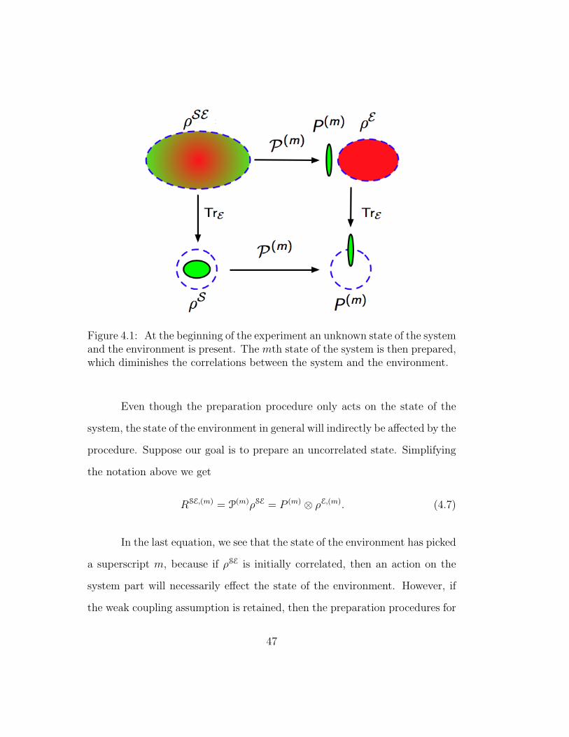
Figure 4.1: At the beginning of the experiment an unknown state of the systemand the environment is present. The mth state of the system is then prepared,which diminishes the correlations between the system and the environment.

Even though the preparation procedure only acts on the state of the

system, the state of the environment in general will indirectly be affected by the

procedure. Suppose our goal is to prepare an uncorrelated state. Simplifying

the notation above we get

RSE,(m) = P(m)ρSE = P (m) ⊗ ρE,(m). (4.7)

In the last equation, we see that the state of the environment has picked

a superscript m, because if ρSE is initially correlated, then an action on the

system part will necessarily effect the state of the environment. However, if

the weak coupling assumption is retained, then the preparation procedures for

47

the closed and the open cases are the same. Let us investigate this through two

specific procedures. See [54] for a similar analysis for quantum measurements.

4.3 Two common preparation procedures

Uncorrelated states are often desired for experiments. Therefore we

will only focus on preparing pure states. We describe two of the most common

preparation procedures to prepare pure states (thus uncorrelated) used today.

We first analyze each preparation procedure for closed quantum systems, and

then analyze them for open quantum systems [5]. In this manner, the dif-

ferences between two will be apparent. More complicated procedures can be

easily studied by writing down the corresponding preparation map.

4.3.1 Stochastic preparation

Many quantum experiments begin by initializing the system to a spe-

cific state. For instance, in the simplest case, the system can be prepared to the

ground state by cooling it to near absolute zero temperature [45–49]. Mathe-

matically, these set of operations can be written as a pin map [55]. Consider

the following map

Θrr′;ss′ = [|Φ〉〈Φ|]rs Ir′s′ . (4.8)

The action of this map on the initial state of the system is

Θρ =∑r′s′

[|Φ〉〈Φ|]rs Ir′s′ρr′s′

= |Φ〉〈Φ|Tr[ρ] = |Φ〉〈Φ| . (4.9)

48

In the procedure above, no matter what the initial state of the system was, it

is “pinned” to the final state |Φ〉〈Φ|. Along with the pin map, a set of unitary

transformations on the system are sufficient to prepare the mth input state.

In that case we can write the preparation as a composition of the stochastic

pin map and a set of local unitary transformations (acting only on the system)

Ω(m) as

P(m)ρ = Ω(m) Θρ = P (m). (4.10)

We call this procedure the stochastic preparation method.

Each preparation map is trace preserving, because the pin map and the

unitary transformations that follow it are all trace preserving transformations.

Also, to prepare m input states, we need m unitary rotations, hence we have

m preparation procedures. However as claimed before, each of these procedure

has the pin map as a common step.

For a closed system, we could just as well use m pin maps to prepare

m input states. The trouble only arises when the system is interacting with

an environment. Let us look at this in detail.

4.3.1.1 For open systems

Let us consider the action of the pin map Θ on a bipartite state of the

system and the environment.

ΘρSE = [|Φ〉〈Φ|]rs Ir′s′ρSEr′α;s′β

= |Φ〉〈Φ| ⊗ TrS[ρSE] = |Φ〉〈Φ| ⊗ ρE. (4.11)

49

As we can see, not much happens differently when a stochastic map is applied

to a bipartite state. The only difference is the presence of the environmental

partner ρE. The pin map fixes the system into a single pure state, which

means that the state of the environment is fixed into a single state as well.

The purpose of the pin map is to decouple the system from the environment,

to eliminate any correlation between the system state and the environment

state.

Once the pin map, Θ, is applied, the system is prepared in the various

different input states by applying local (only on the system part) unitary

transformations as before. The prepared state RSE takes the following form.

RSE(m)= P(m)ρSE = Ω(m) Θ(ρSE)

= Ω(m) (|Φ〉〈Φ|)⊗ ρE = P (m) ⊗ ρE.

Strictly speaking, in a real experiment the pin map is a complicated

set of steps. For instance, cooling the system so it relaxes to the ground state

is very different from optically pumping a system to an excited state. Two

different pin maps would correspond to these two different methods. Then, the

state of the environment in each case can also be different. We have assumed

that an identity map acts on the environment in our mathematical formulation.

This may not be the case; we cannot analyze the state of environment before

or after the pin map is applied. Therefore, to be careful, we should label ρE as

ρEΘ to clarify that the state of the environment may depend on certain steps

involved in applying the pin map.

50

Then, it should be emphasized that the initial pin map is critical. It

may be tempting to simply use a set of pin maps, Θ(m), to prepare the various

input states P (m). The different input states will be

RSE(m)

= P(m)ρSE = Θ(m)ρSE

= P (m) ⊗ ρEΘ(m) . (4.12)

As seen in the last line of the equation above, the state of the environment

has taken the subscript Θ(m) through different pin maps along with the input

state. What this means is that the state of the environment is affected by

the preparation procedure. We show in the next chapter, when the prepara-

tion procedure is not carried out carefully in a quantum process tomography

experiment, the process map can behave non-linear.

4.3.2 Projective preparation

Let us look at another preparation method that is also very common.

Consider an optical experiments, where a beam of photons is sent through

a polarizer [42–44]. Polarizers project the polarization vector of the photons

into a set orthogonal directions. By using a quarter wave plate, all necessary

input states can be prepared.

We can write the action of mth preparation map acting on the initial

state of the system as the following:

P(m)ρ

Tr[P(m)ρ]=

1

r(m)P (m)ρP (m)† = P (m), (4.13)

51

where 1r(m) is the normalization factor with r(m) = Tr[P(m)ρ] = Tr[P (m)ρ]; this

is the probability of obtaining that particular input state from a von-Neumann

measurement [56]. Since projective transformation are not trace preserving,

the preparation map does now preserve trace. The normalization factor, 1r(m) ,

is simply the inverse of the probability that the system will collapse to the

mth state, which can be measured experimentally. In this fashion we can

prepare any pure state as long as we properly normalize them. We call this

method projective preparation. Note that to prepare m input states m different

preparation procedures are necessary.

Though each projective preparation map does not preserve trace, there

is an overall map that preserves trace. Let us write a complete map in the

operator sum representation, where we let the eigenmatrices of the map to be

a set of orthogonal projections. Thus we have

Pρ =∑m

P (m)ρP (m)†, (4.14)

where P (m) form an orthogonal set satisfying P (m)P (n) = δmnP(m) and∑

m P(m)†P (m) =

∑m P

(m) = I. Now we can define each map P(m) for a

single preparation as P (m)P (m)†. Now we see that for a non-trace preserving

preparation there is a complete map that does preserve the trace. In that

sense, the projections are the eigenmatrices of the map P(m).

4.3.2.1 For open systems

A projective preparation is given by a set of orthonormal projections.

If a particular outcome is observed from the measurement, the state of the

52

system collapses to that corresponding projection. Therefore, the input states

can be prepared for an experiment by suitably fixing our measurement basis.

With the knowledge of the basis and the outcomes, the exact input state

becomes known.

Suppose the mth input state is prepared, given by the projection P (m),

by projecting the system into that state. For the open system, the total state

becomes

RSE(m)

=1

r(m)P(m)ρSE =

1

r(m)P (m)ρSEP (m)

= P (m) ⊗ ρE,(m), (4.15)

where once again r(m) = Tr[P(m)ρSE]Tr[P (m)ρSE] is the normalization factor.

Notice that the state of the environment has picked the superscript m. This

is due to the fact that in general ρSE contains correlations between the system

and the environment. We should once again emphasize that the preparation

procedure only acts on the system part and affects the state of the environment

only indirectly.

The dependance that the state of the environment picks up is very

easy to demonstrate. Consider the following one qubit system and one qubit

environment state:

ρSE =1

4(I⊗ I + σ1 ⊗ σ1 − σ2 ⊗ σ2 + σ3 ⊗ σ3).

This is a maximally entangled state of two qubits. It is easy to check that the

projective preparation of this state with different projections P (±j) = 12(I±σj)

53

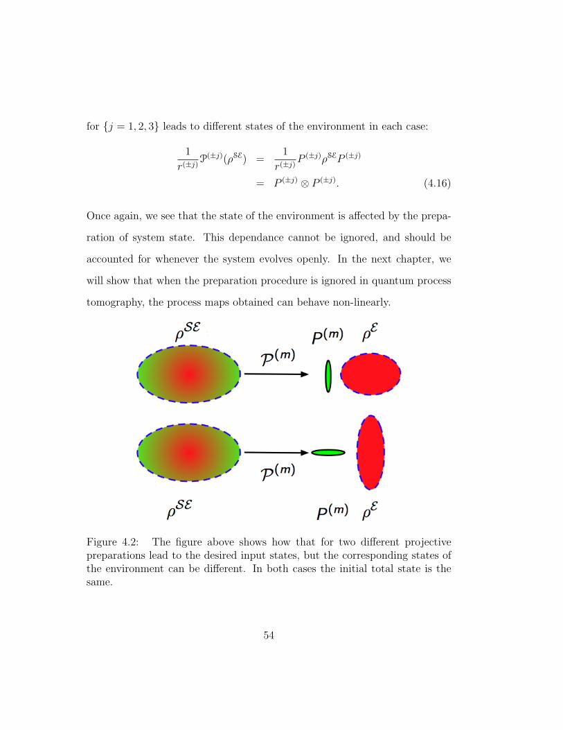
for j = 1, 2, 3 leads to different states of the environment in each case:

1

r(±j) P(±j)(ρSE) =

1

r(±j)P(±j)ρSEP (±j)

= P (±j) ⊗ P (±j). (4.16)

Once again, we see that the state of the environment is affected by the prepa-

ration of system state. This dependance cannot be ignored, and should be

accounted for whenever the system evolves openly. In the next chapter, we

will show that when the preparation procedure is ignored in quantum process

tomography, the process maps obtained can behave non-linearly.

Figure 4.2: The figure above shows how that for two different projectivepreparations lead to the desired input states, but the corresponding states ofthe environment can be different. In both cases the initial total state is thesame.

54

4.4 Discussion

The examples above only aspire to prepare pure states. However, much

more can be obtained from the prescription spelled out above. In principle,

nothing is preventing us from preparing mixed states by using so called gen-

eralized preparations (see [5]). Furthermore, our discussion so far has largely

focused on preparing uncorrelated states; the very same techniques can be

applied in preparing entangled states as well.

We should also add that any time an ancillary system is used in an open

experiment, it is an unreasonable assumption that the ancillary is uncorrelated

with the environment. Furthermore, the ancillary may even interact with the

environment. We will not discuss this topic in this dissertation, but see Sec.

VIII in [5] for a discussion.

Note that, if the system evolves in a closed form then all preparation

procedures are equivalent. Trouble only arises when the preparation procedure

indirectly affects the state of the environment which then interacts with the

system. Additionally, even though we will only use the results here in ana-

lyzing quantum process tomography procedures, they apply to any quantum

experiment that interacts with an environment.

55

Chapter 5

Preparation and quantum process tomography

Each of the quantum process tomography procedure discussed in Chap.

3 assumes the system and the environment are initially uncorrelated. What

if we depart from this assumption? In chapter 2 we showed that initially

correlated states can lead to not-completely positive dynamics for the system.

In many recent experiments, the process maps that characterize the quantum

operations have been plagued with negative eigenvalues and occasional non-

linear behavior (see references in [5]). We now examine the how the two cases

are related.

The quantum process tomography procedures we reviewed require the

input states be uncorrelated with the environment. Just before the experiment

begins, in general the state of the system may be correlated with the environ-

ment. Thus, at the beginning of the experiment it is necessary to prepare

the initially correlated total state into an uncorrelated state. The difference

between the process maps found from a quantum process tomography exper-

iment and the dynamical maps calculated theoretically is precisely the act of

preparation of input states. Let us investigate this issue by analyzing the steps

involved in a quantum process tomography experiment.

56

5.1 Quantum process tomography experiment in steps

The basic steps in a quantum process tomography experiment are bro-

ken down below:

• Just before the experiment begins, the system and environment is in

an unknown state ρSE. The system and the environment in general are

correlated; we are no longer making the weak coupling assumption.

• The system is altered to a known input state by a preparation procedure.

The system and environment state after preparation is therefore given

by

1

r(m)P(m)ρSE.

The input state is given by taking trace with respect to environment

P (m) =1

r(m)TrE

[P(m)ρSE

].

• The system is then sent through a quantum process. We consider the

evolution to be a global unitary transformation in the space of the system

and the environment:

1

r(m)UP(m)ρSEU †.

• Finally the output state is observed. Mathematically it is the trace with

respect to the environment

Q(m) =1

r(m)TrE

[UP(m)ρSEU †

], (5.1)

we will call this the generalized process equation.

57

• Finally using the input and the output states, we construct a map de-

scribing the process is constructed.

The procedure above is identical to the procedure to find a dynamical map,

except for the preparation procedure. In the next two sections we will analyze

quantum process tomography with the two preparation procedures discussed

in last chapter. The differences between what we find here and dynamical

maps will be due to the preparation procedures.

5.2 Stochastic preparation

In this section we analyze quantum process tomography procedures us-

ing the stochastic preparation procedure to generate input states. The stochas-

tic preparation map’s action on a bipartite state is given by 4.11. We plug

that into the generalized process equation 5.1 to get

Q(m) = TrE

[U(Ω(m) Θ

)ρSEU †

]= TrE

[UP (m) ⊗ ρEU †

]. (5.2)

The last equation is the same as the linear process equation (Eq. 3.6) from

Chap. 3. Therefore once the input states are prepared, the procedure for

quantum process tomography is the same as the given in Chap. 3. This is a

generalization of linear quantum process tomography. Here, we have assumed

that only one pin map, Θ, is used. Therefore we have not labeled the state

of the environment with the pin map. We will relax this assumption in the

second example below.

58

5.2.1 An example with stochastic preparation

Consider the following two qubit state as the available state to the

experimenter at t = 0−:

ρSE =1

4(I⊗ I + ajσj ⊗ I + c23σ2 ⊗ σ3) . (5.3)

This is the same state we used in Chap. 2 for the dynamical map example.

Let the pin map, Θ, for our example be

Θ = |φ〉〈φ| ⊗ I, (5.4)

where |φ〉〈φ| is a pure state of the system. The preparation of ρSE with this

pin map leads to

ΘρSE = |φ〉〈φ| ⊗ 1

2I, (5.5)

yielding the initial state |φ〉〈φ| for the system qubit and a completely mixed

state for the environment qubit. The next step is to create the rest of the

input states using maps Ω(m). In this case, the fixed state |φ〉〈φ| can be

locally rotated to get the desired input state P (m) (given in Eq. 3.3)

Ω(m) |φ〉〈φ| ⊗ 1

2I = V (m) |φ〉〈φ|V (m)† ⊗ 1

2I

= P (m) ⊗ 1

2I, (5.6)

where m = (1,−), (1,+), (2,+), (3,+) and V (m) are local unitary operators

acting on the space of the system.

59

Now each input state is sent through the quantum process. The output

states can be calculated using Eq. 5.2. Once again let us choose the same

unitary transformations as in Eq. 2.37. The output states are

Q(1,−) =1

2I− cos2(2ωt)σ1, Q(1,+) =

1

2I + cos2(2ωt)σ1

Q(2,+) =1

2I + cos2(2ωt)σ2, Q(3,+) =

1

2I + cos2(2ωt)σ3. (5.7)

The linear process map is constructed using Eq. 3.7, the duals in Eq.

3.8, and the output states:

Λs =1

2

1 + C2 0 0 2C2

0 1− C2 0 0

0 0 1− C2 0

2C2 0 0 1 + C2

, (5.8)

where C = cos(2ωt). The eigenvalues of the process map are plotted in Fig.

5.1

5.2.2 An example with multiple stochastic preparations

The pin map used in stochastic preparation must be used consistently.

Let us show an example of what happens when two stochastic preparation

procedures are used. Consider a quantum process tomography experiment

where the following linearly independent states are used to span the space of

the system

P I =1

2I, P (1+), P (2+), P (3+). (5.9)

60

2 4 6 8 102Ωt

0.5

1.0

1.5

2.0

Λ1-4

Figure 5.1: The eigenvalues of the process map in Eq. 5.8 are plotted as func-tion of 2ωt. As expected the eigenvalues are always positive. The stochasticpreparation procedure allows the experimentalist to prepare any pure statefor the system. By convexity, then all possible states of the system are in thecompatibility domain of the process map in Eq. 5.8.

These states form the linearly independent set I, σj; which is different from

the set given in Eq. 3.3.

Once again, we take the same initial state and unitary operators as in

the last example. Now suppose the pin map given in Eq. 5.4 is used to prepare

the state |φ〉〈φ|, and then by local transformations P (1,+), P (2,,+), and P (3,+)

are prepared. Finally the mixed state is prepared by letting P (3+) decohere.

This is a different pin map than the one in Eq. 5.4, so we are using two pin

maps to prepare two sets of input states. The unitary operator, we are using,

is often called the swap gate, because it swaps the states of two qubits with

61

the period of t = π4ω

. Then at t = π4ω

, the total state will be

ρSE( π

4ω

)=

1

4I⊗ I + ajI⊗ σj. (5.10)

The state of the system has fully decohered.

The corresponding output states for the input states above are found

using Eq. 5.2. The state of environment in that equation for input P I = 12I

is ρE = 12I + ajσj, while for the other inputs the state of the environment

ρE = 12I. Then the corresponding output states are

Q(I) =1

2I + sin2(2ωt)σ3, Q(1,+) =

1

2I + cos2(2ωt)σ1, (5.11)

Q(2,+) =1

2I + cos2(2ωt)σ2, Q(3,+) =

1

2I + cos2(2ωt)σ3. (5.12)

The last three output states are the same as in the last example, but the fourth

one is different.

Now suppose we calculate the output state corresponding to the input

P (−1). By linearity we have P (−1) = I − P (+1). If the process is linear, then

the output state for this input state is given by

Q(−1) = 2Q(I) −Q(+1) (5.13)

=1

2I + 2 sin2(2ωt)σ3 − cos2(2ωt)σ1. (5.14)

This state is not physical for certain times, and therefore the linearity and the

positivity of the process is violated.

The process has not changed from the last example, only the method

of determining the process has. Thus when the stochastic map is not used

62

consistently, the process map can behave nonlinear. For completeness we find

the process map for this example,

Λms =1

2

1 + C2 −(1 + i)S2 0 2C2

−(1− i)S2 1− C2 + 2S2 0 0

0 0 1− C2 (1 + i)S2

2C2 0 (1− i)S2 1 + C2 − 2S2

, (5.15)

where C = cos(2ωt) and S = sin(2ωt). The eigenvalues of this process map are

negative, as seen in Fig. 5.2. The fact that the state of the environment is not

a constant for all of the input states leads to the negativity and non-linearity

of the process map.

The origin for the negative eigenvalues here is completely different than

the negative eigenvalues found for the dynamical maps in Sec. 2.4.2. The neg-

ative eigenvalues in the dynamical map were due to the initial correlations

between the system and the environment. Since none of the inputs were corre-

lated with the environment here, negativity arises from the inconsistencies in

the preparation procedure. Furthermore, the dynamical map in Sec. 2.4.2 is

linear and has a physical interpretation within the compatibility domain. No

such interpretation is found for the process map in this example.

While this example may not seem realistic, the point regarding inconsis-

tency arising from multiple pin maps still stands. In realistic cases, the trouble

63

2 4 6 8 102Ωt

-0.5

0.5

1.0

1.5

2.0

Λ1-4

Figure 5.2: The eigenvalues of the process map in Eq. 5.15 plotted as functionof 2ωt. One of the eigenvalue is negative for certain values of ωt. The negativityis due to the inconsistency in the preparation procedure, and not due to theinitial correlations with the environment.

may not be seen so easily, due to complicated interactions with the environ-

ment. We will discuss an experiment where multiple stochastic preparation

procedures are implemented in Chap. 8.

5.3 Projective preparation

Let us now consider projective preparation procedure in quantum pro-

cess tomography experiments. Combining the projective preparations given

by Eq. 4.15 with the generalized process equation 5.1, we get the projective

64

process equation for the mth input state

Q(m) =1

r(m)TrE

[UP (m)ρSEP (m)U †

]. (5.16)

Is this process given by a linear map? Dynamically, the evolution of the

total state ρSE is linear, because every operation on ρSE is linear. However, for

the purpose of tomography, the dynamics of the prepared input states P (m)

is of interest. But P (m) appears twice in the process equation, therefore the

output states, Q(m), depend bilinearly on P (m). This bilinearity can also be

seen from the dependence of the environment state on the state of the system.

To see this expand Eq. 5.16 as:

Q(m) = TrB[UP (m) ⊗ ρE,(m)U †

], (5.17)

with (5.18)

ρE,(m) =1

r(m)TrS

[P (m)ρSE

]. (5.19)

The last equation shows the environment state is in effect a function of P (n).

It is well known [17, 57, 58] that if the initial state of the system is related to

the state of the environment by some function f as

ρSE =∑j

ρSj ⊗ f(ρS

j ), (5.20)

then the evolution of the reduced matrices, ρS, cannot be consistently described

by a single linear map. Above f(ρS) are the density matrices of the state of

the environment with dependence on the state of the system. In this case, the

function f is of a specific form that gives us a bilinear dependence.

65

It is instructive to now look at a simple example to demonstrate that

when input states are prepared by projective preparations, the results cannot

be consistently described by a linear map.

5.3.1 An example with projective preparation

Suppose we are unaware of the dependence of the state of the environ-

ment on the state of the system due to projective preparation and assume that

the process is given by a linear map. We would prepare a set of linearly inde-

pendent input states, then construct the linear process map from the output

states and the duals of input states.

We once again start with the total state given by Eq. 2.36 and the

input states given in Eq. 3.3. The state of the system plus the environment

after each projective preparation takes the following form:

P (m)ρSEP (m) → P (m) ⊗ 1

2I (for m = (1,±), (3,+))

P (2,+)ρSEP (2,+) → P (2,+) ⊗ 1

2(I + c′23σ3) , (5.21)

where c′23 = c231+a2

.

Following the same recipe as before, we obtain the output states using

Eq. 5.16. We will use the same global unitary from the last two examples

given by Eq. 2.37. The output states are as follows:

Q(1,−) =1

2

I− cos2(2ωt)σ1

, (5.22)

Q(1,+) =1

2

I + cos2(2ωt)σ1

, (5.23)

66

Q(2,+) =1

2I− c′23 cos(2ωt) sin(2ωt)σ1 (5.24)

+ cos2(2ωt)σ2 + c′23 sin2(2ωt)σ3

,

Q(3,+) =1

2

I + sin2(2ωt)σ3

. (5.25)

The linear process map is constructed using Eq. 3.7, the duals in Eq.

3.8, and the output states:

Λp =1

2

1 + C2 ic′23S

2 0 2C2 − ic′23CS

−ic′23S2 1− C2 ic′23CS 0

0 −ic′23CS 1− C2 −ic′23S2

2C2 + ic′23CS 0 ic′23S2 1 + C2

. (5.26)

Now consider the action of Λp on state P (2,−) = 12(1 − σ2). P (2,−) =

P (1,−) +P (1,+)−P (2,+) is a linear combination of three of the input states used

above. If the action of Λm is linear then the output state corresponding to

P (2,−) should be

Λp

(P (2,−)

)= Λp

(P (1,−) + P (1,+) − P (2,+)

)= Q(1,−) +Q(1,+) −Q(2,+) (5.27)

=1

2(I + c′23 cos(2ωt) sin(2ωt)σ1 (5.28)

− cos2(2ωt)σ2 − c′23 sin2(2ωt)σ3

).

Let us check if this the same as if the system was prepared in the state P (2,−)

by projective preparation. The output state for input P (2,−) can be calculated

67

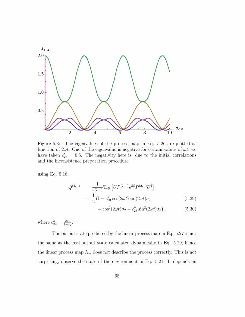
2 4 6 8 102Ωt

0.5

1.0

1.5

2.0

Λ1-4

Figure 5.3: The eigenvalues of the process map in Eq. 5.26 are plotted asfunction of 2ωt. One of the eigenvalue is negative for certain values of ωt; wehave taken c′23 = 0.5. The negativity here is due to the initial correlationsand the inconsistence preparation procedure.

using Eq. 5.16,

Q(2,−) =1

r(2,−)TrB

[UP (2,−)ρSEP (2,−)U †

]=

1

2(I− c′′23 cos(2ωt) sin(2ωt)σ1 (5.29)

− cos2(2ωt)σ2 − c′′23 sin2(2ωt)σ3

), (5.30)

where c′′23 = c231−a2

.

The output state predicted by the linear process map in Eq. 5.27 is not

the same as the real output state calculated dynamically in Eq. 5.29, hence

the linear process map Λm does not describe the process correctly. This is not

surprising; observe the state of the environment in Eq. 5.21. It depends on

68

a2, and subsequently the linear process map depends on a2, thus on the initial

state of the system. The dependence of the environment on the system is the

cause for the non-linear behavior of the process.

5.4 Discussion

The examples with multiple stochastic preparations (in Sec. 5.2.2)

and projective preparations (in Sec. 5.3.1) look very similar. For multiple

stochastic preparations, the state of the environment depends on the stochastic

map. If we think of each projective preparations as an independent stochastic

preparation then the state of the environment, in the example in Sec. 5.3.1,

depends on the preparation map. Then are the two situations the same? Let

us show below that the two situations are fundamentally different.

In the weak coupling limit, the projective preparation procedure does

not play an important role. As we saw in the last chapter, when the sys-

tem and the environment are initially uncorrelated, the projective preparation

procedure will have no affect on the state of the environment. This is be-

cause the state of the environment is affected only indirectly due to the initial

correlations between the system and the environment. Thus the projective

preparations, in the weak coupling limit, yield a linear process map.

This is not the case in the multiple stochastic preparation example.

When multiple stochastic maps are used to prepare different input states, the

inconsistencies do not stem from the initial correlations between the system

and the environment. In fact, in our example all input states are initially

69

uncorrelated from the environment. The inconsistencies arise from the prepa-

ration procedures themselves, leading to different states of the environment

for different input states. These inconsistencies will be absent in the case

where the system develops in a closed form, since the system does not feel the

presence of the environment during the quantum process. Hence in the “weak

interaction limit” multiple stochastic preparations yield a linear process map.

Lastly, note that each of the process map found in this chapter, given by

Eqs. 5.8, 5.15, and 5.27, are different from each other. This clearly shows that

the preparation procedures play a non-trivial role in open quantum system

experiments. The preparation procedure is the only thing that distinguished

each case. For the case where no preparation procedure is applied, i.e. the case

of the dynamical map (Eq. 2.43), the situation is still different. The dynamical

map, which has negative eigenvalues, is linear and has a valid interpretation

within the compatibility domain. The process maps in Eqs. 5.15 and 5.27 do

not have any consistent interpretation.

When negative eigenvalues are found in a process map, they hint to

some problem in the preparation procedure. Although this is a bit premature

to state at this point; we analyze the negative eigenvalues in process map in

more detail in the next chapter. In Chap. 7 we show that a processes can be

correctly described using a general dynamical map, which we call dynamical

M-map. This map is independent of the preparation procedure.

70

Chapter 6

More on stochastic preparations

Dynamical maps [3, 4] are a generalization of the unitary transforma-

tion much like density matrices are a generalization of the pure state rays.

Dynamical maps allow the description of stochastic processes as well as the

evolution of open systems. Dynamical maps used to describe the evolution of

open systems are usually defined with a constant environment state ρE:

BρS = TrE

[UρS ⊗ ρEU †

]. (6.1)

Implicitly, the state of the environment, ρE, is a parameter of the map B.

Therefore, the linear dynamical map B would only consistently describe an

experiment if different input states ρS can be prepared independently of the

environment state ρS. The actual issue of how this can be executed is not

addressed.

It is possible to consider a dynamical map where the environment is not

fixed, such as the reduced dynamical evolution of a initially correlated state

ρSE [27]:

BTrE

[ρSE]

= TrE

[UρSEU †

]. (6.2)

The dynamical map in this problem is applicable only over a compatibility

domain of states, rather than over the complete state space of the system (see

71

Sec. 2.4.2). The compatibility domain is the set of states of the system that

are compatible with the correlations in ρSE. Formally, this problem defines an

embedding map1 that relates the initial state of the system to the tota initial

state, ρSE. The embedding map is linear but not necessarily a completely posi-

tive map [15, 16, 59]. How do we handle the initial correlations experimentally

in the case of stochastic preparation?

The stochastic preparation method provides a way for an experiment

to be performed so that different input states can be prepared with a fixed

environment state. Consider the process equation 5.2 in section 5.2.

Q(m) = TrE

[UΩ(m) ΘρSEU †

]= TrS

[UP (m) ⊗ ρE,ΘU †

].

Then the action of the process map on an arbitrary state of the system is then

given by:

ΛρS = TrE

[UρS ⊗ ρE,ΘU †

].

Therefore, in this context, the dynamical map is equivalent to the process

map. However, for consistency, we have to remember that the environment

state is a constant to the problem, therefore the pin map Θ should also be a

constant to the problem.

1The embedding map is also known as extension map, assignment map, or a preparation(not to be confused with the preparation map from Chap. 4).

72

6.1 Pseudo-pure states

Demanding pure input states in a quantum process tomography exper-

iment guarantees initially uncorrelated state of the system. Though if it is not

possible to prepare pure states, we can still determine the process.

Suppose the initial state is prepared by a pin map leading to

ΘρSE =(pP (3,+) + (1− p)P (3,−)

)⊗ I (6.3)

=1

2I + pσ3 ⊗ I, (6.4)

where 0 << p < 1. The rest of the input states are prepared by rotations.

Then the input states are

P (1,−) =1

2I− pσ1 P (1,+) =

1

2I + pσ1 (6.5)

P (2,+) =1

2I + pσ2 P (3,+) =

1

2I + pσ3. (6.6)

For the unitary operator in Eq. 2.37, the corresponding output states will be

Q(1,−) =1

2I− p cos2(2ωt)σ1, Q(1,+) =

1

2I + p cos2(2ωt)σ1 (6.7)

Q(2,+) =1

2I + p cos2(2ωt)σ2, Q(3,+) =

1

2I + p cos2(2ωt)σ3. (6.8)

The only change that we have to make to find the process map is to

define a dual proper set, in this case

P (1,−) =1

2ppI− σ1 − σ2 − σ3, P (1,+) =

1

2ppI + σ1 − σ2 − σ3,

P (2,+) =1

pσ2, P (3,+) =

1

pσ3. (6.9)

73

We can find the process map using Eq. 3.7. The process map here case turns

out to be the same as in Eq. 5.8. This is to expected; the process map for

stochastic preparation is defined over set of all states, including the input

states above.

The downside of course is that there is no way to distinguish the states

in Eq. 6.3 from the following state

ΘρSE =1

2I⊗ I + pσ3 + c23σ2 ⊗ σ3. (6.10)

Unlike in Eq. 6.5, this is a correlated state. Yet, both total states have the

same reduced state for the system part.

Even in this case we can find the process map properly if we use the

correct dual set given in Eq. 6.9. The process map in that case will be the

same as the dynamical map given in Sec. 2.4.2 by Eq. 2.43. In both of the

examples above, had we assumed that the input states were close enough to

the pure states we desired, and used the dual set give by Eq. 3.8, then the

process map would contain an error of magnitude 1− p.

These two examples illustrate the contrary argument to what some

have suggested, that only the completely positive process maps should be

considered physically valid. We showed in the second example, that one can

obtain a not-completely positive process map in a consistent fashion. The

real issue is that the correlations with environment are not convenient for

experimental purposes. But that does not mean that one should fix a not-

completely positive process map to a completely positive process map with

74

numerical methods [60, 61].

6.2 Negative maps due to control errors

There is one more possibility for non-linearity and negativity in a pro-

cess map. This has to do with poor control in the stochastic preparation

procedure. Suppose the initial state is prepared well using a pin map

ΘρSE = P (3,+) ⊗ I. (6.11)

After obtaining this state, the other input states are prepared by local rota-

tions. Let us consider the case where one of the rotation is not perfect.

V (1,−) |1〉 → 1√2

(√1− ε |1〉 −

√1 + ε |0〉

), (6.12)

where ε is taken to be a small positive real number. We introduced a small

error for the preparation of P (1,−), but we have kept the error simple by not

giving it an additional phase, i.e. keeping ε to be real. For simplicity we have

also assumed that the error of this sort occurs in the preparation of only one

state.

Let us now pretend that we are not aware of this error. Then in reality

we have the following set of input states

P (1,−) =1

2I + εσ3 −

√1− ε2σ1, P (1,+) =

1

2I + σ1, (6.13)

P (2,+) =1

2I + σ2, P (3,+) =

1

2I + σ3. (6.14)

Let us use the same unitary evolution as before given in Eq. 2.37. The output

states corresponding to the last three input states in Eq. 6.13 are the same as

75

before, given by Eq. 5.7. For the input state P (1,−), the corresponding output

state is follows

Q(1,−) =1

2I + (εσ3 −

√1− ε2σ1) cos2(2ωt),

Q(1,+) =1

2I + cos2(2ωt)σ1

Q(2,+) =1

2I + cos2(2ωt)σ2,

Q(3,+) =1

2I + cos2(2ωt)σ3. (6.15)

Using these output states, the duals given by Eq. 3.8, and Eq. 3.7, we can

find the process map.

The process map turns out to be rather complicated, and its eigenvalues

are even more complicated looking. Therefore, we do not write them down,

instead we have plotted the eigenvalues as function of 2ωt. We take the value

for the error to be ε = 0.1 for the plot in Fig 6.1. One of the eigenvalue in Fig.

6.1 is negative for certain times. This shows yet another cause for negative

eigenvalues in a process map. The negative eigenvalues here have nothing

to do with the initial correlations between the system and the environment.

The negative eigenvalues are attributed to poor control in the preparation

procedure.

76

2 4 6 8 102Ωt

0.5

1.0

1.5

2.0Λ1-4

Figure 6.1: The eigenvalues of the process map found using the output statesin Eq. 6.15 and the duals in Eq. 3.8. One of the eigenvalue is negative forcertain times; we have taken ε = 0.1. The negativity is due to the errors inthe unitary operation implemented to prepare one of the input states.

6.3 Discussion

Now we have discussed several scenarios that can lead to negative eigen-

values for a process map. Two comments are in order at this point. When the

prepared input states are not pure and the process map has negative eigenval-

ues, then one should be weary of initial correlations with the environment. To

further check this, the process map should be tested for linearity by sending

several additional input states through the process. If the process map pre-

dicts the output states properly, then one can be confident that the system is

initially correlated with the environment. If the process map does not predict

the output states correctly (non-linear behavior), then there are additional

77

problems with the experiment, including the possibility of poor control in the

preparation procedure. In the case where the input states are pure and the

process map has negative eigenvalues, the negativity can only come from either

inconsistencies in the preparation procedure or poor preparation control.

78

Chapter 7

Dynamical M-map

As we saw in Chap. 5, the additional step of preparation leads to

complications for quantum process tomography experiments. At the same

time, this step cannot be avoided for systems initially correlated with the

environment. Let us try to attack this problem directly. Let us rewrite the

process equation 5.1

Q(m) =1

r(m)TrE[UP(m)ρSEU †]. (7.1)

In terms of matrix indices we have

Q(m)rs =

1

r(m)

∑ε

Urε;r′αP(m)r′r′′;s′s′′ρ

SEr′′α;s′′βU

∗sε;s′β, (7.2)

where the sum over ε denotes the trace with respect to the environment. We

are interested in the reduced dynamics of the system states; not so much in

the details of the preparations. Since the preparation map only acts on the

system, the trace with the environment has no effect on it. Thus, we can just

pull the preparation map out of the trace,

Q(m)rs =

1

r(m)P

(m)r′r′′;s′s′′

∑ε

Urε;r′αρSEr′′α;s′′βU

∗sε;s′β

=1

r(m)M

(rs)r′r′′;s′′s′P

(m)r′r′′;s′s′′ . (7.3)

79

In the last equation, the matrix M is defined as:

M(rs)r′r′′;s′′s′ =

∑ε

Urε,r′αρSEr′′α,s′′βU

∗sε,s′β. (7.4)

Note that in Eq. 7.3 the superscript indices on M match the elements on the

left hand side of the equation, while the subscript indices are summed on the

right hand side of the equation.

The output state, Q(m), is given by the matrix M acting generally on the

preparation of the input state, P(m). Therefore, matrix M fully describes the

process before any preparation is made. M contains both U and ρSE; however

knowing M is not sufficient to determine U and ρSE. As expected, it should not

be possible to determine U and ρSE through measurements and preparations on

the system alone without access to the environment. Conversely, M contains

all information necessary to fully determine the output state for any prepared

state. We will call M the dynamical M-map or just M-map for short. The

M-map is due to Aik-Meng Kuah [62]. Let us look at some basic properties

of M-map.

Trace of M-map:

Let us start with the trace of M. To take the trace, we equate indices

r with s, r′ with s′, and r′′ with s′′ to get:

Tr[M] =∑rr′r′′

δrsδr′s′δr′′s′′M(r,s)r′r′′;s′′s′

=∑ε

∑rr′r′′

Urε,r′αρSEr′′α,r′′βU

∗rε,r′β.

80

Since U †U =∑

rε U∗rε,r′βUrε,r′α = Ir′α,r′β, then

Tr[M] =∑

α,βr′′r′

Ir′α,r′βρSEr′′α,r′′β = d,

where d is the dimension of the system.

Hermiticity of M-map:

As with the case of linear process maps, matrix M is hermitian. This

is easy to see by taking the complex conjugate of matrix M,

(M

(r,s)r′r′′;s′′s′

)∗=

(∑ε


∗sε,s′β

)∗=

∑ε

Usε,s′βρSEs′′β,r′′αU

∗rε,r′α,

= M(s,r)s′s′′;r′′r′ .

The complex conjugate of M is not only the transpose of M, but each element

of M is also transposed. Hence M is a Hermitian matrix.

Positivity of M-map:

The M-map is composed of a unitary matrix operating on a density

matrix. Then we can take the square root of the density matrix to get

M(r,s)r′r′′,s′′s′ =

∑ε

Urε,r′α

[√ρSE]r′′α,σγ

[√ρSE]σγ,s′′β

U∗sε,s′β

=∑ε

(∑α

Urε,r′α

[√ρSE]r′′α,σγ

)(∑β

Usε,s′β

[√ρSE]s′′β,σγ

)∗=

∑µ

M(µ)r;r′r′′M

(µ)s′s′′;s

∗,

81

where M = U√ρSE and µ = σγε. We have written the M-map in operator

sum representation, hence it is completely positive. This means, the M-map

acting on any completely positive preparation procedure will lead to a physical

state.

The action of M-map can now be written as

M(rs)r′r′′;s′′s′Pr′r′′;s′s′′ =

∑µ

M(µ)r;r′r′′Pr′r′′;s′s′′M

(µ)s′s′′;s (7.5)

The advantage of dealing with the M-map is that we no longer need

to worry about the preparation procedure. Once we know the M-map, we

can act with it on any preparation procedure to find the corresponding output

state. Since we took out the preparation part out of the M-map, it contains

all of the dynamical information for the system. In the next section we will

try to extract some of this information from the M-map.

7.1 Uninterrupted dynamics

The M-map contains the dynamics of the system before any preparation

is made on the system. Perhaps we can learn something about that dynamics.

Let us start by looking at the definition of the M-map.

M(rs)r′r′′;s′′s′ =

∑ε


∗sε,s′β. (7.6)

The system is labeled by indices r′′ and s′′. Then by tracing over

everything else we can find the initial state of the system from M-map.∑rr′

δrsδr′s′M(rs)r′r′′;s′′s′ =

∑ε

∑rr′

Urε,r′αρSEr′′α;s′′βU

∗rε,r′β (7.7)

82

=∑r′

(∑rε

U∗rε,r′βUrε,r′α

)ρSEr′′α;s′′β (7.8)

=∑r′

Ir′r′∑αβ

IαβρSEr′′α;s′′β (7.9)

= d ρSr′′s′′ . (7.10)

Furthermore, if we apply an identity preparation, defined as

P(I)r′r′′;s′s′′ = Ir′r′′I∗s′′s′ , (7.11)

on the M-map then we get the final state of the system.

M(rs)r′r′′;s′r′′P

(I)r′r′′;s′s′′ = Ir′r′′M(rs)

r′r′′;s′s′′I∗s′′s′ (7.12)

=∑ε

Urε,r′αIr′r′′ρSEr′′α;s′′βIs′′s′U∗sε,s′β (7.13)

=∑ε

Urε,r′αρSEr′α;s′βU

∗sε,s′β (7.14)

= ρSrs(t). (7.15)

Knowing the initial and the final states of the system (without any

preparations) allows us to find the dynamics uninterrupted. From this infor-

mation we can find the mapping from the initial to the final state. In general

this will not be the same as the dynamical map of Chap. 2. The dynamical

map is defined over a set of initial states of the system. Here we get a mapping

from an initial state to a final state.

7.2 Memory due to correlations

When a system is initially correlated with the environment, the state of

the system in the future will depend on these correlations. This is the memory

83

of a system, and it is a key feature of non-Markovian dynamics [13]. We will

show here that we can find the dynamics of the memory from the M-map.

The memory of the system is obtained from the M-map by tracing over

the system, indices r′′ and s′′.

∑r′′

δr′′s′′M(rs)r′r′′;s′s′′ =

∑ε

Urε,r′αρEαβU

∗sε,s′β. (7.16)

The last equation is the same as Eq. 3.5 for the process map found by stochas-

tic preparations. Thus,

Λs =∑r′′

δr′′s′′M(rs)r′r′′;s′s′′ . (7.17)

This means, even though the M-map contains the correlated total state, we

can find the process for the ideal stochastic preparation from it.

Consider the following matrix composed of the matrices in Eqs. 7.10

and 7.17

L(rs)r′r′′;s′s′′ = Λrr′;ss′ρ

Sr′′s′′ (7.18)

= d

(∑r′′

δr′′s′′M(rs)r′r′′;s′s′′

)(∑rr′

δrsδr′s′M(rr)r′r′′;s′r′′

)(7.19)

=∑ε

Urε,r′αρSr′′s′′ρ

EαβU

∗sε,s′β (7.20)

The last equation similar to the expression for the M-map, except the

state of the system and the state of the environment are uncorrelated. Let us

now write the total correlated state as

ρSE = ρS ⊗ ρE + χ, (7.21)

84

where χ is the correlation matrix [17]. Writing the M-map in terms of the

correlation matrix we get

M(rs)r′r′′;s′s′′ =

∑ε

Urε,r′α(ρSr′′s′′ρ

Eαβ + χr′′α;s′′β)U∗sε,s′β. (7.22)

Now consider the following quantity:

K(rs)r′r′′;s′s′′ = M

(rs)r′r′′;s′s′′ − L

(rs)r′r′′;s′s′′ (7.23)

=∑ε

Urε,r′α(ρSr′′s′′ρ

Eαβ + χr′′α;s′′β − ρS

r′′s′′ρEαβ)U∗sε,s′β (7.24)

=∑ε

Urε,r′αχr′′α;s′′βU∗sε,s′β. (7.25)

The last equation gives us the reduced dynamics of the correlations between

the system and the environment. If the system and the environment were

initially uncorrelated, then K will be zero, i.e. no memory is present. We call

K matrix the memory matrix.

This is an important result for studying non-Markovian systems. It

is important to keep in mind that, the memory matrix will be different for

different preparations. But, if we want to study how the correlations act as

memory in the uninterrupted system then we can just act with the identity

preparation, defined in Eq. 7.11 as,

χS(t) = Krsr′r′′;s′s′′P

(I)r′r′′;s′s′′ (7.26)

=∑ε

Urε,r′αχr′α,s′βU∗sε,s′β, (7.27)

where χS(t) = TrE[UχU †]. The quantity above is the memory for the uninter-

rupted system due to initial correlations with the environment.

85

7.3 An example with M-map and the memory matrix

Now, let us consider an example of the M-map and the memory matrix.

Let us use the same initial states (2.36) and the unitary operator (2.37) as

before. The M-map is given by Eq. 7.4 and the memory matrix is given by

Eq. 7.25.

If we make the identity preparation on the M-map then we get

M P(I) = ρS(t) (7.28)

=1

2I + cos2 (2ωt) ajσj − c23 cos (2ωt) sin (2ωt)σ1, (7.29)

which is the same as the final state of the system in Chap. 2 Eq. 2.40. While

making the identity preparation on memory matrix we get

K P(I) = χS(t) = TrE[UχU †] (7.30)

=1

2−c23 cos (2ωt) sin (2ωt)σ1, (7.31)

where χ is the correlation matrix defined in Eq. 7.21 and χS(t) is the reduced

part of the time evolved correlation matrix. This is precisely the contribution

to ρS due to the correlations with the environment.

86

The

M-m

apan

dth

em

emor

ym

atri

xar

eas

follow

s:

M=

a+ 3C

2 +

20

0a

+ 3C

2−icS

2+a−C

2 +

20

0−cCS

+a−C

2

0a+ 3C

2 −2

00

0ic

+a−

2S

20

0

00

a+ 3C

2 −2

00

0−ic

+a−

2S

20

a+ 3C

20

0a+ 3C

2 +

2cCS

+a−C

20

0icS

2+a−C

2 +

2icS

2+a+C

2 +

20

0cCS

+a

+C

2a− 3C

2 +

20

0a− 3C

2

0−ic

+a+

2S

20

00

a− 3C

2 −2

00

00

ic+a+

2S

20

00

a− 3C

2 −2

0

−cCS

+a

+C

20

−icS

2+a+C

2 +

2a− 3C

20

00

a− 3C

2 +

2

,

K=

1+C

20

02C

2−ic

23S

20

02c

23CS

01−C

20

00

ic23S

20

00

01−C

20

00

−ic

23S

20

2C2

00

1+C

22c

23CS

00

ic23S

2

ic23S

20

02c

23CS

1+C

20

02C

2

0−

1c23S

20

00

1−C

20

00

0ic

23S

20

00

1−C

20

2c23CS

00

−ic

23S

22C

20

01

+C

2

,

wher

eC

=co

s(2ωt)

,S

=si

n(2ωt)

,C

2 ±=

1±C

2,a± 3

=1±a

3,a

+=a

1+ia

2,a−

=a

1−ia

2,

andc

=c 2

3.

87

7.4 Discussion

The M-map and the memory matrix are difficult to obtain in practice.

We have given a recipe to find M-map partially for a qubit in Apps. B and

C. Our recipe is based on projective preparations only. This issue needs to be

further investigated using techniques such as direct characterization of quan-

tum dynamics [38, 39]. Yet, the M-map and memory matrix K are powerful

theoretical tools in their own right. The M-map allows us to determine var-

ious output states for any preparation procedure, while the memory matrix

K provides a quantitative definition for the memory effect due to the initial

correlations for any preparation procedures. This allows us to investigate and

optimize preparation procedures.

88

Chapter 8

Analysis of experiments

In this chapter we analyze two quantum process tomography experi-

ments performed by Myrskog et al.[48] and M. Howard et. al [47, 49]. Our

critiques emphasizes the importance of having a consistent procedure of state

preparation.

8.1 Experiment by Myrskog et al.

In this experiment, quantum process tomography of the motional states

of trapped 85Rb atoms in the potential wells of a one dimensional optical lat-

tice is performed. Only two bound bands are considered, which are labeled

as states |0〉 and |1〉. The states are prepared stochastically. An initial state

of the system is the ground state |g〉〈g|, and from it states |r〉〈r|, |i〉〈i|, and

the fully mixed state 12I are prepared. The states |r〉 and |i〉 stand for the real

and imaginary coherence states, which are prepared by applying appropriate

unitary transformations on the ground state. This is achieved by displacing

the lattice for the real coherence state and for the imaginary coherence state, a

quarter-period delay is added after the displacement. The identity state is pre-

pared by letting a superposition state decohere. The input states are allowed

89

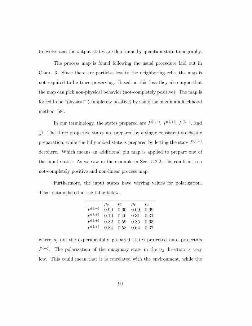
to evolve and the output states are determine by quantum state tomography.

The process map is found following the usual procedure laid out in

Chap. 3. Since there are particles lost to the neighboring cells, the map is

not required to be trace preserving. Based on this loss they also argue that

the map can pick non-physical behavior (not-completely positive). The map is

forced to be “physical” (completely positive) by using the maximum likelihood

method [58].

In our terminology, the states prepared are P (1,+), P (2,+), P (3,−), and

12I. The three projective states are prepared by a single consistent stochastic

preparation, while the fully mixed state is prepared by letting the state P (1,+)

decohere. Which means an additional pin map is applied to prepare one of

the input states. As we saw in the example in Sec. 5.2.2, this can lead to a

not-completely positive and non-linear process map.

Furthermore, the input states have varying values for polarization.

Their data is listed in the table below.

ρg ρI ρr ρiP (3,−) 0.90 0.60 0.69 0.69P (3,+) 0.10 0.40 0.31 0.31P (1,+) 0.82 0.59 0.85 0.63P (2,+) 0.84 0.58 0.64 0.37

where ρj are the experimentally prepared states projected onto projectors

P (m). The polarization of the imaginary state in the σ2 direction is very

low. This could mean that it is correlated with the environment, while the

90

polarization of the ground state along the negative σ3 direction is almost unity,

meaning it is only weakly correlated at best.

Here, we have two potential causes for the process map to have negative

eigenvalues. The first problem is with the experimental procedure; applying

multiple stochastic preparations that may affect the state of the environment

differently. The second problem may be unavoidable; since it is extremely diffi-

cult to prepare pure states in a setup like this. Even if the negative eigenvalues

are due to the initial correlations, we do not have a prescription to obtain a

process map in a consistent fashion. For the second example shown in Chap.

6, we assumed that the initial correlations were constant throughout the pro-

cess. This does not seem to be the case here. Since the ground state is almost

pure, while the imaginary state is clearly not pure. Therefore the correlation

with environment for these two inputs must be different. This concludes our

analysis of this experiment. Let us now consider the second experiment.

8.2 Experiment by Howard et al.

In this experiment, the system that is studied is an electron configura-

tion formed in a nitrogen vacancy defect in a diamond lattice. The quantum

state of the system is given by a spin triplet (S = 1). Again we will write the

initial state of the system and environment as ρSE.

The system is prepared by optical pumping, which results in a strong

spin polarization. The state of the system is said to have a 70% chance of being

in a pure state |φ〉. Or more mathematically, the probability of obtaining |φ〉

91

is Tr[|φ〉〈φ| ρSE] = 0.7.

Since the population probability is high, an assumption was made that

the state of the system can be simply approximated as a pure state |φ〉〈φ|.

From this initial state, different input states can be prepared by suitably ap-

plying microwave pulses resonant with the transition levels. After prepara-

tion, the system is allowed to evolve, and the output states are determined by

quantum state tomography. With the knowledge of the input state and the

measured output states, a linear process map is constructed.

It was found that the linear process map has negative eigenvalues, so

the map was “corrected” using a least squares fit between the experimentally

determined map and a theoretical map based on Hermitian parametrization

[60], while enforcing complete positivity.

However, if we do not regard the negative eigenvalues of the map as

aberrations, then we should consider the assumptions about the preparation

of the system more carefully. The assumption about the initial state of the

system is:

ρSE → |φ〉〈φ| ⊗ τ. (8.1)

This is in effect a pin map. Along with the pin map, the stochastic transfor-

mations are applied on the initial state to prepare the various input states;

this is identical to the stochastic preparation method discussed in Sec. 4.3.1.1.

It is clear that the pure initial state assumption is unreasonable given

our knowledge now of how the process is sensitive to the initial correlations

92

between the system and the environment. In effect the action of the pin map

in this experiment is not perfect, and the pin map can be ignored. Then the

process equation is:

Q(m) = TrB[UΩ(m)ρSEU †] (8.2)

where Ω(m) is the stochastic transformation that prepares the mth input state.

In this experiment, Ω(m) is nothing more than a unitary transformation V (m)

satisfying V (m) |φ〉 = |ψ(m)〉, where |ψ(m)〉 is the desired pure mth input state.

We can write the unitary transformation for a two-level system as:

V (m) = |ψ(m)〉〈φ|+ |ψ(m)⊥ 〉〈φ⊥| (8.3)

where 〈ψ(m)|ψ(m)⊥ 〉 = 〈φ|φ⊥〉 = 0. This defines V (n) as a transformation from

the basis |φ〉 to the basis |ψ(n)i 〉. The equation for the process becomes:

Q(m) = TrE

[U |ψ(m)〉〈φ|ρSE|φ〉〈ψ(m)|U †

]+TrE

[U |ψ(m)

⊥ 〉〈φ⊥|ρSE|φ〉〈ψ(m)|U †

]+TrE

[U |ψ(m)〉〈φ|ρSE|φ⊥〉〈ψ(m)

⊥ |U†]

+TrE

[U |ψ(m)

⊥ 〉〈φ⊥|ρSE|φ⊥〉〈ψ(m)

⊥ |U†].

Therefore, since 〈φ|ρSE|φ〉 = 0.7 to first approximation, the process is a linear

mapping on the states |ψ(m)〉〈ψ(m)|. However, it is clear that if all terms

are included, the process is not truly linear in the states |ψ(m)〉〈ψ(m)|. The

negative eigenvalues are therefore a result of fitting results into a linear map

when the process is not truly represented by a linear map.

93

Chapter 9

Conclusion and future directions

Our study of quantum process tomography started by noting that the

dynamical map acting on a system can have negative eigenvalues. The dy-

namical map has negative eigenvalues when the system is initially correlated

with the environment. In the course of our studies of quantum process tomog-

raphy, we showed that the preparation procedure cannot be neglected for any

quantum system that interacts with an environment. These are the two major

themes discussed in this dissertation. Though, along the way, we presented a

method of quantum process tomography that is independent of the prepara-

tion procedure. The map arising from this procedure lead us to an expression

that quantifies the memory effect on the dynamics of the system due to the

initial correlations with the environment. Determining the memory effect is

an important task in coherence control.

9.1 Future directions

Though this dissertation has come to an end, the work goes unfinished.

There are many open problems that arise from our work. We pointed out sev-

eral causes for errors in quantum process tomography. We have not developed

94

a complete method of distinguishing and correcting these errors. This is an

important problem that has not been fully addressed.

Another problem that needs consideration is fully determining M-map.

This is a challenging task, though there are some possibilities in resolving this

problem by considering a scheme like the direct characterization of quantum

dynamics. In this method a map is found with the aid of an ancillary system,

which allows for direct estimation of the elements of a map without the aid of

quantum state tomography.

Another avenue of research that may prove fruitful is studying various

preparation procedures using M-map. Furthermore, the memory matrix can

aid in better better understanding of the various preparation procedures. This

will especially be the case when the system is multi-partite.

95

Appendix

96

Appendix A

Quantum state tomography

Quantum state tomography [1] is the procedure to experimentally de-

termine the state of a quantum system. Suppose we want to determine the

density matrix Q. To fully determine the state, we need to measure the mag-

nitude of the polarization along the principal directions. For a qubit we need

to make measurements along the σx, σy, and σz directions.

However, a single experiment will not tell us the magnitude along any

direction. Therefore we make many measurements of the magnitude along

each of these direction. In general, the outcome of a set of the experiment

along jth direction is written as

aj = Tr[Qσj],

which is the expectation value for the observable σj. Where σj are the gener-

alized Pauli-Gell-Mann-Tilma [63] matrices. Finally the total density matrix

is given as follows

Q =1

dS

I +

∑j

Tr[Qσj]σj

(A.1)

=1

dS

I +

∑j

ajσj

. (A.2)

97

Appendix B

M-map process tomography

We now develop a tomography procedure to determine the M-map. We

will need to figure out a finite set of input states P (m) and the corresponding

output states Q(m) that will allow us to determine the M-map. After-all, this is

the objective of tomography; by performing measurements on a small number

of select input states a complete description of a process can be obtained

and predict the output state for any input state. The process equation for

projective preparations1 takes the following form

Q(m) =1

r(m)M

(rs)r′r′′;s′s′′P

(m)r′r′′;s′s′′ (B.1)

=1

r(m)P

(m)r′r′′M

(rs)r′r′′;s′s′′P

(m)s′s′′∗. (B.2)

The M-map is a large (d3 × d3) matrix, to make it more manageable,

Eq. 7.3 can be interpreted as:

〈P (m)|M |P (m)〉 = r(m)Q(m), (B.3)

where P (m) is now treated as a vector. In this form, M-map is a d2×d2 matrix,

where each element is a d×d matrix. We will call Eq. B.3 the ‘M-map process

equation’.

1Our procedure here only deals with projective preparations.

98

Since M-map is a Hermitian matrix, it has 12(d4 + d2) independent

elements. Therefore 12(d4 + d2) independent equations in the form of Eq. B.3

are necessary to fully determine M-map. It is clear that neither an orthonormal

set of d nor a linearly independent set of d2 input states would provide sufficient

equations to resolve the elements of the M-map.

B.1 The qubit case

For a qubit system the projections, P (m), can be written in terms of

three real parameter aj and Pauli spin matrices σj:

P (m) =1

2

(I + a

(m)j σj

). (B.4)

Since P (m) is a projection then there is have the additional constrain∑

j(a(m)j )2 =

1. The matrices I and σj together forms a vector basis for this space. There-

fore Eq. B.4 is simply a vector decomposition of the projections in a fixed

basis. Taking this form for P (m) and substituting into Eq. B.3 gives:

4r(m)Q(m) = 4 〈P (m)|M |P (m)〉

= 〈I|M|I〉+ a(m)j 〈I|M|σj〉+ a

(m)k 〈σk|M|I〉

+a(m)j a

(m)k 〈σj|M|σk〉 . (B.5)

Observe that the terms 〈I|M|I〉, 〈I|M|σj〉, 〈σj|M|I〉 and 〈σj|M|σk〉, are simply

the matrix elements of M-map in I, σj basis. We just need to find a set of

projections P (m) that will allow us to solve for these matrix elements.

99

Consider the following specific projections defined as P (j,±) = 12(I±σj)

with j = 1, 2, 3.

4r(j,±)Q(j,±) = 4 〈P (j,±)|M|P (j,±)〉

= 〈I|M|I〉+ 〈σj|M|σj〉 ± 〈σj|M|I〉+ 〈I|M|σj〉 . (B.6)

Simultaneously solving the (+) and the (−) equations above to gives the fol-

lowing unknowns:

〈I|M|I〉+ 〈σj|M|σj〉 = 2(r(j,+)Q(j,+) + r(j,−)Q(j,−)

)〈I|M|σj〉+ 〈σj|M|I〉 = 2

(r(j,+)Q(j,+) − r(j,−)Q(j,−)

).

To obtain the cross terms 〈σj|M|σk〉 consider projections such as P (j+k+1,+) =

12

(I + 1√

2σj + 1√

2σk

)for k > j which give:

r(j+k+1,+)Q(j+k+1,+) = 〈P (j+k+1,+)|M |P (j+k+1,+)〉

=1

8(〈I|M|I〉+ 〈σj|M|σj〉)

+1

8(+ 〈I|M|I〉+ 〈σk|M|σk〉)

+1

4√

2(〈I|M |σj〉+ 〈σj|M|I〉)

+1

4√

2(+ 〈I|M|σk〉+ 〈σk|M|I〉)

+1

8(〈σj|M|σk〉+ 〈σj|M|σk〉) . (B.7)

Substitute the known terms and solve for the desired cross terms,

〈σj|M|σk〉+ 〈σk|M|σj〉 = −2(

1 +√

2)(

r(j,+)Q(j,+) − 2(

1 +√

2)

+ r(k,+)Q(k,+))

−2(

1−√

2)(

r(j,−)Q(j,−) − 2(

1−√

2)

+ r(k,−)Q(k,−))

+8r(j+k+1,+)Q(j+k+1,+).

100

In summary using the following nine projections,

P (j,+) =1

2(I + σj) , P (j,−) =

1

2(I− σj) , P (4,+) =

1

2

(I +

1√2σ1 +

1√2σ2

),

P (5,+) =1

2

(I +

1√2σ1 +

1√2σ3

), P (6,+) =

1

2

(I +

1√2σ2 +

1√2σ3

),

and solving them simultaneously yields all desired matrix elements: 〈I|M|I〉+

〈σj|M|σj〉, 〈I|M|σj〉+ 〈σj|M|I〉, and 〈σj|M|σk〉+ 〈σk|M|σj〉 .

This is not enough to fully determine the M-map, but these elements

are sufficient to determine the output state for any input state. Using the

property∑

j(a(m)j )2 = 1 Eq. B.5 can be rewritten as:

4r(m)Q(m) =∑j

(a

(m)j

)2

(〈I|M|I〉+ 〈σj|M|σj〉)

+∑j

a(m)j (〈I|M|σj〉+ 〈σj|M|I〉) (B.8)

+∑k>j

a(m)j a

(m)k (〈σj|M|σk〉+ 〈σk|M|σj〉) .

Observe that the sums of the cross terms 〈σj|M|σk〉 + 〈σk|M|σj〉 can

appear together because the coefficients a(m)j are real. Also, the element 〈I|M|I〉

can always be paired with a diagonal element 〈σj|M|σj〉 as long as the state

is a projection satisfying∑

j(a(m)j )2 = 1. The diagonal element 〈I|M|I〉 only

has to be known if the system can be prepared directly to a mixed state such

that∑

j(a(m)j )2 < 1. This may be accomplished by a generalized preparations

[54]. If generalized preparations are allowed then just one more input state

is needed, for example 12(I + 1

2σ1), which gives another independent equation

that can be solved to obtain 〈I|M|I〉.

101

Therefore the elements of the M-map found in Eq. B.8 are all that

are needed to describe the process. By measuring the outputs for the nine

specified input states, the matrix M-map can be calculated. We now have a

good quantum process tomography procedure for an open qubit system.

B.2 Beyond one qubit

Note that the choice of these nine states used above is not unique.

The recipe which used to derive these nine states can be used in principle

to derive other choices, and can also be partly generalized to d-level systems

[63, 64]. However, there are some non-trivial obstacles to overcome for the

generalization to d-level systems. In place of the Pauli matrices for two-level

systems, the generalized Pauli-Gell–Mann-Tilma [63] Hermitian traceless d×d

matrices can be used [63, 65] to decompose the d × d density matrix, and

this decomposition will also have only real coefficients. This trick eliminates

certain degrees of freedom in the M-map that is otherwise difficult to deal

with. Unfortunately, for d > 2, these real coefficients no longer satisfy just the

simple constraint∑

j(a(m)j )2 = 1. The additional constraints on the coefficients

complicate the task of constructing the projections needed to simultaneously

span the matrix elements of M-map.

102

Appendix C

Experimental recipe for M-map

Although we have established the M-map process tomography, let us

make the ideas more concrete by developing a complete recipe for an exper-

iment that can be used to determine whether a process is linear or given by

the M-map. We will also show specifically how the M-map or linear map can

be calculated from the measurement results.

For the M-map process tomography nine input states are necessary.

For the nine states derived in App. B the first six states are three pairs of

orthonormal projections, but the last three are not. If we use projections

to prepare the states, we will need use them as given by orthonormal pairs.

Therefore, let us instead use twelve projections, nine from Eq. B.8 and three

orthogonal to the last three in that equation:

P (4,−) =1

2

(I− 1√

2σ1 −

1√2σ2

),

P (5,−) =1

2

(I− 1√

2σ1 −

1√2σ3

), (C.1)

P (6,−) =1

2

(I− 1√

2σ2 −

1√2σ3

).

These twelve projections are neatly grouped into six different sets of

orthonormal pairs. If the states are prepared using projections, these would

103

correspond to measurements in the ±σ1, ±σ2, ±σ3, σ1 ± σ2, σ1 ± σ3 and

σ2 ± σ3 directions. Having twelve states is more than is necessary for the M-

map process tomography, but the extra states and the corresponding output

states can serve as consistency checks.

After recording the corresponding output states for all twelve input

states, we can verify if the process is linear by checking the following eight

linear sum rules (that the input states satisfy) have to be satisfied by the

corresponding output states:

Q(j,+) +Qj,−) = Q(k,+) +Q(k,−) (for j, k = 1, 2, 3)

Q(4,+) =

(1

2− 1√

2

)(Q(1,+) +Q(1,−)

)+

1√2

(Q(1,+) +Q(2,+)

)Q(5,+) =

(1

2− 1√

2

)(Q(1,+) +Q(1,−)

)+

1√2

(Q(1,+) +Q(3,+)

)Q(6,+) =

(1

2− 1√

2

)(Q(1,+) +Q(1,−)

)+

1√2

(Q(2,+) +Q(3,+)

).

If the eight sum rules are satisfied, then the process is not described by

the M-map, and we can be confident the process is described by a linear map.

The linear map Λ can then be computed as follows:

Λ

(1

2(I + pjσj)

)=(Q(1,+) +Q(1,−)

)+ pj

(Q(j,+) −Q(j,−)

)(C.2)

If the eight sum rules are not satisfied, then the process may be given

by the M-map. We will attempt to verify that the process given by the M-map

and calculate it.

104

Note that the probabilities r(m) = Tr[ρSEP (m)] associated with each

preparation should be found experimentally. The probabilities should be com-

plete for an orthonormal set of projections, in other words: r(j,+) + r(j,−) = 1.

Therefore the probabilities can be calculated from the fraction of the (+) states

as compared to the (−) states, for all preparations made in the same direction.

To be certain that the process is given by the M-map, we can check

if the three additional states we included evolve in a way that is consistent

with the M-map derived from the other nine states. The following equations

are derived from this condition. If these equations are satisfied, we can be

confident that the process is given by the M-map:

√2(r(4,+)Q(4,+) − r(4,−)Q(4,−)

)= r(1,+)Q(1,+) − r(1,−)Q(1,−)

+r(2,+)Q(2,+) − r(2,−)Q(2,−)

√2(r(5,+)Q(5,+) − r(5,−)Q(5,−)

)= r(1,+)Q(1,+) − r(1,−)Q(1,−)

+r(3,+)Q(3,+) − r(3,−)Q(3,−)

√2(r(6,+)Q(6,+) − r(6,−)Q(6,−)

)= r(2,+)Q(2,+) − r(2,−)Q(2,−)

+r(3,+)Q(3,+) − r(3,−)Q(3,−).

If the conditions above are satisfied then the process is given by the M-map,

then the M-map can be computed by following the recipe in App. B.

Once the matrix elements of M-map are determined, the evolution of

a generic state X = 12(I +

∑j xjσj) is given by:

4 〈X|M|X〉 = r(X)Q(X) (C.3)

105

=∑j

x2j (〈I|M|I〉+ 〈σj|M|σj〉) (C.4)

+∑j

xj (〈I|M|σi〉+ 〈σj|M|I〉) (C.5)

+∑k>j

xjxk (〈σj|M|σk〉+ 〈σk|M|σj〉) . (C.6)

Note that since Q is a normalized state, the normalization constant r

is the measurement probability r = Tr[XρSE]. Although we had not explicitly

mentioned this before, the M-map contains all information about the mea-

surement probabilities, that is why we needed the measurement probabilities

r(m) to calculate the M-map.

Finally, note that if both the test for linearity and the M-map fail,

then the process cannot be consistently described by either a linear map or

the M-map. The experiment then should be carefully analyzed for problems

such as any non-linear dependence that may have been introduced if the input

states are not accurately prepared or if there is some dependence of ρSE on the

prepared state.

If the process is given by a linear process map, then the nine input states

(Eq. B.8) are over complete; only four input states are needed to determine

a linear process map. This discrepancy is summarized by the following linear

sum rules:

P (1,+) + P (1,−) = P (2,+) + P (2,−) = P (3,+) + P (3,−),

P (4,+) =

(1

2− 1√

2

)(P (1,+) + P (1,−)

)+

1√2

(P (1,+) + P (2,+)

),

106

P (5,+) =

(1

2− 1√

2

)(P (1,+) + P (1,−)

)+

1√2

(P (1,+) + P (4,+)

),

P (6,+) =

(1

2− 1√

2

)(P (1,+) + P (1,−)

)+

1√2

(P (2,+) + P (4,+)

).

If the process is linear, then the output states must satisfy the same

sum rules, which are obtained from the above equations by suitably writing Q

in place of P . If these sum rules are not satisfied, then the process is not linear.

However satisfying the sum rules is necessary but not sufficient to determine

if the process is linear; the M-map can still be constructed from this set of

input and output states without any contradictions. Therefore an additional

input state, distinct from the above nine input states should be tested.

107

Appendix D

Notation

~a : Bloch vector

A : stochastic map

B : dynamical map

cjk : correlation parameters

χ : correlation matrix

H : Hamiltonian

I : indentity matrix

I : identity map

K : memory matrix

Λ : linear process map

M : Kuah’s dynamical M-map

Ω(m) : mth local rotaion

P(m) : mth preparation map

P (m) : mth input states

Q(m) : mth output states

108

ρA : state of the ancillary system

ρE : state of the environment

ρS : state of the system

ρSE : state of the system plus environment

σj : Pauli spin matrices

Θ : pin map

U : unitary operators

X : an arbitrary input state

109

Bibliography

[1] M.A. Nielsen and I.L. Chuang. Quantum Computation and Quantum

Information. Cambridge University Press, 2000.

[2] C E Shannon. A mathematical theory of communication. Bell System

Tech. J., 27:379–423;23–656, 1948.

[3] E.C.G. Sudarshan, P.M. Mathews, and J. Rau. Stochastic dynamics of

quantum-mechanical systems. Phys. Rev., 121:920, 1961.

[4] E. C. G. Sudarshan and T. F. Jordan. Dynamical mappings of density

operators in quantum mechanics. J. Math. Phys., 2(6):772, 1961.

[5] Aik meng Kuah, Kavan Modi, Cesar A. Rodriguez-Rosario, and E. C. G.

Sudarshan. How state preparation can affect a quantum experiment:

Quantum process tomography for open systems. Phys. Rev. A, 76(4):

042113, 2007.

[6] E. B. Davies. Quantum theory of open systems. Academic Press, New

York, 1976.

[7] H. P. Breuer and F. Petruccione. The Theory of Open Quantum Systems.

Oxford university press, New York, 2002.

[8] F. Bloch. Nuclear induction. Phys. Rev., 70(7-8):460–474, Oct 1946.

110

[9] A. Kossakowski. On quantum statistical mechanics of non-Hamiltonian

systems. Rep. Math. Phys., 3:247, 1972.

[10] G. Lindblad. On the generators of quantum dynamical semigroups.

Comm. Math. Phys., 48:119, 1975.

[11] V. Gorini, A. Kossakowski, and E. C. G. Sudarshan. Completely positive

dynamical semigroups of N-level systems. J. Math. Phys., 17:821, 1976.

[12] Herbert Spohn. Kinetic equations from hamiltonian dynamics: Marko-

vian limits. Rev. Mod. Phys., 53(3):569–615, July 1980.

[13] C. A. Rodrıguez-Rosario and E. C. G. Sudarshan. Non-markovian open

quantum systems. arXiv:0803.1183, 2008.

[14] E. B. Davies and J. T. Lewis. An operational approach to quantum

probability. Comm. Math. Phys., 17, 1970.

[15] P. Pechukas. Reduced dynamics need not be completely positive. Phys.

Rev. Lett., 73(8):1060–1062, August 1994.

[16] Robert Alicki. Comment on “Reduced dynamics need not be completely

positive”. Phys. Rev. Lett., 75(16):3020, Oct 1995.

[17] H. Carteret, Daniel R. Terno, and K. Zyckowski. Physical accessibility

of non-completely positive maps. arXiv:quant-ph/0512167, 2005.

111

[18] C. A. Rodrıguez-Rosario, K. Modi, A. Kuah, E. C. G. Sudarshan, and

A. Shaji. Completely positive maps and classical correlations. arXiv:quant-

ph/0703022v3, 2007.

[19] M. D. Choi. Positive linear maps on c∗-algebras. Can. J. Math., 24(3):

520–529, June 1972.

[20] M. D. Choi. Completely positive linear maps on complex matrices. Lin-

ear Algebra and Appl., 10:285, 1975.

[21] E.C.G. Sudarshan. Quantum measurement and dynamical maps. In

E. Gotsman and G. Tauber, editors, From SU(3) to Gravity (Festschrift

in honor of Yuval Ne’eman). Cambridge University Press, 1986.

[22] T F. Jordan, A. Shaji, and E C G. Sudarshan. Mapping the schrodinger

picture of open quantum dynamics. Phys. Rev. A, 73:12106, January

2006.

[23] A. Shaji. Dynamics of initially entangled open quantum. PhD thesis,

The University of Texas at Austin, 2005.

[24] E. C. G. Sudarshan. Evolution and decoherence in finite level systems.

Chaos, Solitons Fractals, 16:369, 2003.

[25] Cesar Rodrıguez-Rosario, Anil Shaji, and E. C. G. Sudarshan. Dynamics

of two qubits: Decoherence and an entanglement optimization protocol.

arXiv:quant-ph/0504051v4, 2006.

112

[26] Thomas F. Jordan. Affine maps of density matrices. Phys. Rev. A, 71

(3):034101, 2005.

[27] Thomas F. Jordan, Anil Shaji, and E. C. G. Sudarshan. Dynamics of

initially entangled open quantum systems. Phys. Rev. A, 70(5):052110,

2004.

[28] C. H. Bennett, P. W. Shor, J. A. Smolin, and A. V. Thapliyal. Entanglement-

assisted capacity of a quantum channel and the reverse Shannon theorem.

IEEE Trans. Information Theory, 48(10):2637–2655, October 2002.

[29] Charles H. Bennett, Peter W. Shor, John A. Smolin, and Ashish V. Thap-

liyal. Entanglement-assisted classical capacity of noisy quantum chan-

nels. Phys. Rev. Lett., 83(15):3081–3084, Oct 1999.

[30] Peter Stelmachovic and Vladimir Buzek. Dynamics of open quantum

systems initially entangled with environment: Beyond the kraus repre-

sentation. Phys. Rev. A, 64:062106, 2001.

[31] A. Shabani and D. A. Lidar. Quantum error correction beyond com-

pletely positive maps. arXiv:quant-ph/0610028, 2006.

[32] Isaac L. Chuang and M. A. Nielsen. Prescription for experimental de-

termination of the dynamics of a quantum black box. J. Mod. Opt., 44:

2455, 1997.

113

[33] J. F. Poyatos, J. I. Cirac, and P. Zoller. Complete characterization of a

quantum process: the two-bit quantum gate. Phys. Rev. Lett., 78(2):

390–393, Jan 1997.

[34] G. M. D’Ariano and P. Lo Presti. Quantum tomography for measuring

experimentally the matrix elements of an arbitrary quantum operation.

Phys. Rev. Lett., 86(19):4195–4198, May 2001.

[35] Francesco De Martini, Andrea Mazzei, Marco Ricci, and Giacomo Mauro

D’Ariano. Exploiting quantum parallelism of entanglement for a com-

plete experimental quantum characterization of a single-qubit device.

Phys. Rev. A, 67(6):062307, Jun 2003.

[36] J. B. Altepeter, D. Branning, E. Jeffrey, T. C. Wei, P. G. Kwiat, R. T.

Thew, J. L. O’Brien, M. A. Nielsen, and A. G. White. Ancilla-assisted

quantum process tomography. Phys. Rev. Lett., 90(19):193601, May

2003.

[37] Giacomo Mauro D’Ariano and Paoloplacido Lo Presti. Imprinting com-

plete information about a quantum channel on its output state. Phys.

Rev. Lett., 91(4):047902, Jul 2003.

[38] M. Mohseni and D. A. Lidar. Direct characterization of quantum dy-

namics. Phys. Rev. Lett., 97(17):170501, 2006.

[39] M. Mohseni and D. A. Lidar. Direct characterization of quantum dy-

namics: General theory. Phys. Rev. A, 75(6):062331, 2007.

114

[40] Ariel Bendersky, Fernando Pastawski, and Juan Pablo Paz. Selective

efficient quantum process tomography. arXiv:0801.0758, 2008.

[41] J. Emerson, M. Silva, O. Moussa, C. Ryan, M. Laforest, J. Baugh, D. G.

Cory, and R. Laflamme. Symmetrised characterisation of noisy quantum

processes. Science, 317:1893, 2007.

[42] M. A. Nielsen, E. Knill, and R. Laflamme. Complete quantum telepor-

tation using nuclear magnetic resonance. Nature, 396(6706):52–55, 1998.

[43] Andrew M. Childs, Isaac L. Chuang, and Debbie W. Leung. Realization

of quantum process tomography in NMR. Phys. Rev. A, 64(1):012314,

Jun 2001.

[44] M. W. Mitchell, C. W. Ellenor, S. Schneider, and A. M. Steinberg. Diag-

nosis, prescription, and prognosis of a Bell-state filter by quantum process

tomography. Phys. Rev. Lett., 91(12):120402, Sep 2003.

[45] Yaakov S. Weinstein, Timothy F. Havel, Joseph Emerson, Nicolas Boulant,

Marcos Saraceno, Seth Lloyd, and David G. Cory. Quantum process to-

mography of the quantum fourier transform. J. Chem. Phys., 121(13):

120402, 2004.

[46] J. L. O’Brien, G. J. Pryde, A. Gilchrist, D. F. V. James, N. K. Langford,

T. C. Ralph, and A. G. White. Quantum process tomography of a

controlled-not gate. Phys. Rev. Lett., 93(8):080502, 2004.

115

[47] M. Howard, J. Twamley, C. Wittmann, T. Gaebel, F. Jelezko, and J. Wrachtrup.

Quantum process tomography and lindblad estimation of a solid-state

qubit. New J. Phys., 8:33, 2006.

[48] S. H. Myrskog, J. K. Fox, M. W. Mitchell, and A. M. Steinberg. Quantum

process tomography on vibrational states of atoms in an optical lattice.

Phys. Rev. A, 72(1):013615, 2005.

[49] M. Howard, J. Twamley, C. Wittmann, T. Gaebel, F. Jelezko, and J. Wrachtrup.

Quantum process tomography of a single solid state qubit. arXiv:quant-

ph/0503153, 2005.

[50] M. Mohseni, A. T. Rezakhani, and D. A. Lidar. Quantum-process to-

mography: Resource analysis of different strategies. Phys. Rev. A, 77

(3):032322, 2008.

[51] Harold Ollivier and Wojciech H. Zurek. Quantum discord: A measure

of the quantumness of correlations. Phys. Rev. Lett., 88(1):017901, Dec

2001.

[52] L. Henderson and V. Vedral. Classical, quantum and total correlations.

J. Phys. A, 34:6899, 2001.

[53] Reinhard F. Werner. Quantum states with Einstein-Podolsky-Rosen cor-

relations admitting a hidden-variablemodel. Phys. Rev. A, 40(8):4277–

4281, Oct 1989.

116

[54] A. Kuah and E. C. G. Sudarshan. Dynamical maps and measurements.

arXiv:quant-ph/0209083v1, 2002.

[55] Vittorio Gorini and E. C. G. Sudarshan. Extreme affine transformations.

Comm. Math. Phys., 46(1):43–52, 1976.

[56] J. von Neumann. Mathematical Foundations of Quantum Mechanics.

Princeton University, Princeton, 1955.

[57] K.M. Fonseka Romero, P. Tolkner, and P. Hanngi. Is the dynamics of

open quantum systems always linear? Phys. Rev. A, 69:052109, 2004.

[58] Mario Ziman. Quantum process tomography: the role of initial correla-

tions. arXiv:quant-ph/0603166, 2006.

[59] K. Modi, C. A. Rodrıguez-Rosario, and E. C. G. Sudarshan. On linear

and not completely positive embading maps. In preparation.

[60] T. F. Havel. Robust procedures for converting among Lindblad, Kraus

and matrix representations of quantum dynamical semigroups. J. Math.

Phys., 44(534), 2003.

[61] Mario Ziman, Martin Plesch, Vladimir Buzek, and Peter Stelmachovic.

Process reconstruction: From unphysical to physical maps via maximum

likelihood. Phys. Rev. A, 72(2):022106, 2005.

[62] A. Kuah. Quantum states, maps, measurements and entanglement. PhD

thesis, The University of Texas at Austin, 2007.

117

[63] T. Tilma and E. C. G. Sudarshan. Generalized Euler angle parametriza-

tion for su(n). J. Phys. A, 35:10467, 2002.

[64] Mark S. Byrd and Navin Khaneja. Characterization of the positivity of

the density matrix in terms of the coherence vector representation. Phys.

Rev. A, 68(6):062322, 2003.

[65] W. Greiner and B. Muller B. Quantum Mechanics: Symmetries. Springer,

Berlin, 1989.

118

Index

C-matrices, 20

M-map, see process map

M-map process tomography, 98

Abstract, x

Acknowledgments, v

Analysis of experiments, 89

ancilla assisted process tomography,

see quantum process tomog-

raphy

Appendix, 96

Bibliography, 118

Bloch sphere, 8

Bloch vector, 8

Choi representation, 19

classical correlations, 39

closed evolution, see unitary evolu-

tion

compatibility domain, 26, 72

complete positivity, 20

Conclusion and future directions, 94

control errors, 75

correlation matrix, 85

Dedication, iv

density matrix, 6

convexity, 7

of one qubit, 7

of two qubits, 23

direct characterization of quantum

dynamics, see quantum pro-

cess tomography

dual set

for a qubit, 36, 73

Dynamical M-map, 79

dynamical map, 13, 71

A-form, 14

B-form, 15

convexity of, 16

from contraction, 20

embedding, 26, 72

entanglement, 38, 39

entanglement assisted process tomog-

raphy, see quantum process

tomography

example of

M-map, 86

dynamical map

initially correlated state, 22

initially product state, 21

memory matrix, 86

process map

multiple stochastic preparations,

60

projective preparation, 66

stochastic preparation, 59

Experimental recipe for M-map, 103

extremal maps, 16

global unitary operator, 36

Hamiltonian evolution, see unitary

evolution

input state, 33

119

for M-map tomography, 101, 103

Introduction, 1

linearly independent set, 34

local unitary operator, 36

memory matrix, 83, 85

More on stochastic preparations, 71

negative maps, 77

control errors, 76

due to correlations, 26, 74

experimental, 89, 93

multiple stochastic preparations,

63



not-completely positive dynamics, see

negative maps

notation, 108

open evolution, 10, 13

open quantum theory, 13

operator sum representation, see Choi

representation

output state, 33

partial trace, 12

Pauli spin matrices, 7

pin map, 50, 92

polarization, 8

positivity classes of maps, 18

positivity domain, 26

preparation, 43

generalized, 55

identity, 86

in open quantum mechanics, 46

in quantum process tomography,

56

multiple stochastic, 60, 90

projective

quantum process tomography,

64

stochastic, 44, 72, 92

quantum process tomography,

58

trace preservation, 45, 52

Preparation and quantum process to-

mography, 56

Preparation of input states, 43

preparation procedure

projective

for close systems, 51

for open systems, 52

stochastic

for close systems, 49

for open systems, 50

process equation

M-map, 80, 98

generalized, 57

linear, 35, 58, 72

projective, 64

process map, 32

M-map, 80

Hermiticity of, 81

matrix representation, 98

positivity of, 81

trace of, 80

uninterrupted dynamics, 82

M−map, 101

linear, 36, 72

multiple stochastic, 63

120

projective, 68

stochastic, 60

product state, 21

projective preparation procedure, see


pseudo-pure state, 73

quantum correlations, 39

quantum discord, 39

quantum process tomography, 57, 89

ancilla assisted, 37

direct characterization of quan-

tum dynamics, 40

entanglement assisted, 37

general description, 33


standard, 35


weak coupling assumption, 41

weak coupling limit, 69

weak interaction limit, 70

Quantum process tomography, 32

Quantum state tomography, 97

Quantum theory of open system, 6

qubit, 7

semi-group property, 16

simply separable, see product state

size of the environment, 29

standard quantum process tomog-

raphy, see quantum process

tomography

stochastic preparation procedure, see


stochastic process, 44, 71

unitary evolution, 9

Vita, 122

von Neumann equation, 8

weak coupling assumption, 41

121

Vita

Kavan was born in Valsad, Gujarat, India on the 21st of October 1978

to Bhagavati and Kishore Modi. He grew up in India till the age of thirteen,

then spent one year in Staten Island, New York. He spent his high school

years in Parsippany, New Jersey, graduating from Parsippany High School in

1997. Upon graduation he enrolled in Embry-Riddle Aeronautical University

in Daytona Beach, Florida. He held summer internships at the Fermi National

Accelerator Laboratory and NASA’s Kennedy Space Center while attending

Embry-Riddle Aeronautical University. In May 2001, he received his Bachelor

of Science in Engineering Physics from Embry-Riddle Aeronautical University.

In the fall of 2001 he joined the University of Texas at Austin as a graduate

student. He received his Master of Arts in physics from there in May 2004. He

has received the 2007 John Bardeen and the 2008 Rolfe Glover awards from

the Forum in History of Physics of the American Physical Society. Beside

physics, he enjoys a diverse social life and traveling.

Permanent address: 4711 Duval St.Austin TX, 78751

This dissertation was typeset with LATEX† by the author.

†LATEX is a document preparation system developed by Leslie Lamport as a specialversion of Donald Knuth’s TEX Program.

122

Copyright by Kavan Kishore Modi 2008 - Monash Quantum ...

Documents

Transcript of Copyright by Kavan Kishore Modi 2008 - Monash Quantum ...