Copyright by Hyung Taek Ahn 2005 - The University of Texas ...
231
Copyright by Hyung Taek Ahn 2005
-
Upload
khangminh22 -
Category
Documents
-
view
3 -
download
0
Transcript of Copyright by Hyung Taek Ahn 2005 - The University of Texas ...

Copyright
by
Hyung Taek Ahn
2005
The Dissertation Committee for Hyung Taek Ahn
certifies that this is the approved version of the following dissertation:
A New Incompressible Navier-Stokes Method with
General Hybrid Meshes and Its Application to
Flow/Structure Interactions
Committee:
Clinton N. Dawson, Supervisor
Yannis Kallinderis, Supervisor
Graham F. Carey
Ronald O. Stearman
Spyridon A. Kinnas
A New Incompressible Navier-Stokes Method with
General Hybrid Meshes and Its Application to
Flow/Structure Interactions
by
Hyung Taek Ahn, B.Eng., M.S.
Dissertation
Presented to the Faculty of the Graduate School of
The University of Texas at Austin
in Partial Fulfillment
of the Requirements
for the Degree of
Doctor of Philosophy
The University of Texas at Austin
May 2005

To my parents, Young Ok Ahn and Tae Hwa Noh
Acknowledgments
I would like to express my profound gratitude to my advisor, Professor Yannis
Kallinderis, for his advices, comments, and encouragement during my dissertation
research. I am also grateful to him for asking questions that helped me consolidating
my ideas and giving me considerable freedom to follow my own paths in research.
His good sense of humor also has been invaluable to me while I was struggling with
research.
I would like to express my sincere appreciation to the members of my dis-
sertation committee. I am extremely indebted to Professor Clinton Dawson, my
co-advisor, for his comments and advices about my work as well as hosting me at
the Institute of Computational Engineering and Sciences (ICES) and providing the
excellent parallel computing resources of the Center for Subsurface Modeling (CSM)
at ICES. My heartfelt gratitude must be expressed to Professor Graham Carey for
his advices both in academics and life. Prof. Carey brought me a perspective view of
my dissertation, and helped me to identify important parts and less important parts.
I wish to thank Professor Spyridon Kinnas for giving me a chance to present my
work at the Offshore Technology Research Center (OTRC) and reading my disserta-
tion. I would like to thank Professor Ronald Stearman for helpful discussions about
aeroelasticity. Also, I wish to thank Professors David Goldstein and Laxminarayan
Raja for serving in my oral qualifying exam committee.
I wish to thank my friends and staffs in ASE/EM department, ICES, and
v

OTRC. My special gratitude has to be expressed to Christos Kavouklis for our
friendship. Our late night discussions (sometimes lasting over the weekend) about
various topics have always been a pleasure to me. I also like to express my appre-
ciation to the Rotary Foundation, the Rotary International, for their scholarships
which actually enabled me to come to the UT for my graduate studies.
I am always thankful to the schools where I studied and the faculty members
who built my academic foundations. Especially, I wish to thank Professors Boung-
Duk Lim and Joung-Youb Sah at Yeungnam University and Professor Hoon Hur at
the Korea Advanced Institute of Science and Technology (KAIST).
Finally, I would like to express my deepest appreciation to my family. I wish
to thank my father, mother, and sister for their endless love and support. I would
like to thank my fiancee, Mikyung Jung, who stood on my side providing me courage
and support.
The present work has been partially supported by the Offshore Technology
Research Center and the Minerals Management Service and its Industry Consor-
tium1, as well as by a Joint Industry Project through the University of Texas at
Austin.
Hyung Taek Ahn
The University of Texas at Austin
May 2005
1Disclaimer: “The views and conclusions contained in this document are those of the authors
and should not be interpreted as representing the opinions or policies of the U.S. Government.
Mention of trade names or commercial products does not constitute their endorsement by the U.S.
Government”.
vi
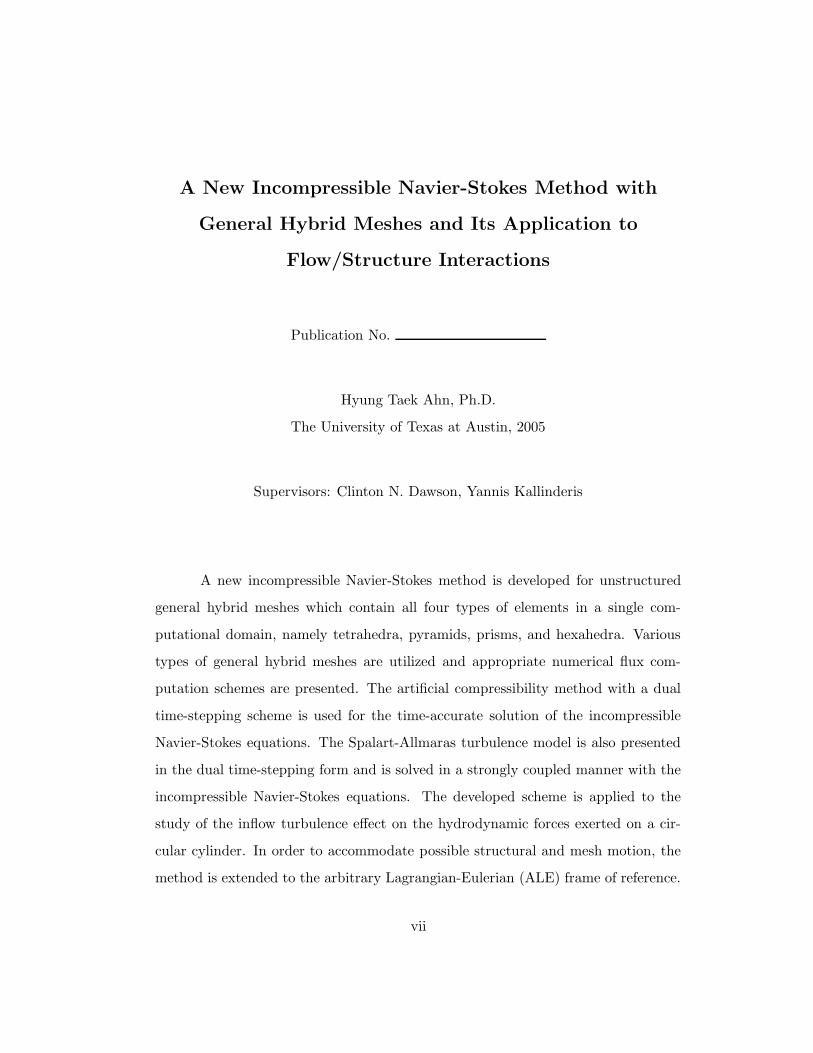
A New Incompressible Navier-Stokes Method with
General Hybrid Meshes and Its Application to
Flow/Structure Interactions
Publication No.
Hyung Taek Ahn, Ph.D.
The University of Texas at Austin, 2005
Supervisors: Clinton N. Dawson, Yannis Kallinderis
A new incompressible Navier-Stokes method is developed for unstructured
general hybrid meshes which contain all four types of elements in a single com-
putational domain, namely tetrahedra, pyramids, prisms, and hexahedra. Various
types of general hybrid meshes are utilized and appropriate numerical flux com-
putation schemes are presented. The artificial compressibility method with a dual
time-stepping scheme is used for the time-accurate solution of the incompressible
Navier-Stokes equations. The Spalart-Allmaras turbulence model is also presented
in the dual time-stepping form and is solved in a strongly coupled manner with the
incompressible Navier-Stokes equations. The developed scheme is applied to the
study of the inflow turbulence effect on the hydrodynamic forces exerted on a cir-
cular cylinder. In order to accommodate possible structural and mesh motion, the
method is extended to the arbitrary Lagrangian-Eulerian (ALE) frame of reference.
vii

The geometric conservation law is satisfied with the proposed ALE scheme in mov-
ing mesh simulations. The developed ALE scheme is applied to the vortex induced
vibration of a cylinder. A strong coupling of fluid and structure interaction based on
the predictor-corrector method is presented. The superior stability property of the
strong coupling is demonstrated by a comparison with the weak coupling. Finally,
the developed methods are parallelized for distributed memory machines using par-
titioned general hybrid meshes and an efficient parallel communication scheme to
minimize CPU time.
viii
Contents
Acknowledgments v
Abstract vii
List of Tables xiii
List of Figures xv
Chapter 1 Introduction 1
1.1 The artificial compressibility method . . . . . . . . . . . . . . . . . . 3
1.2 General hybrid meshes . . . . . . . . . . . . . . . . . . . . . . . . . . 5
1.3 Moving mesh simulations and flow/structure interactions . . . . . . 9
1.4 Motivation of the present research . . . . . . . . . . . . . . . . . . . 11
1.5 Contributions of the current research . . . . . . . . . . . . . . . . . . 13
1.5.1 A new incompressible Navier-Stokes method for general hy-
brid meshes . . . . . . . . . . . . . . . . . . . . . . . . . . . . 13
1.5.2 Geometrically conservative ALE scheme for flow/structure in-
teractions . . . . . . . . . . . . . . . . . . . . . . . . . . . . . 15
1.6 Overview . . . . . . . . . . . . . . . . . . . . . . . . . . . . . . . . . 15
Chapter 2 Governing Equations 17
2.1 Reynolds’ Transport Theorem . . . . . . . . . . . . . . . . . . . . . . 18
ix
2.2 Conservation of Mass . . . . . . . . . . . . . . . . . . . . . . . . . . . 20
2.3 Conservation of Momentum . . . . . . . . . . . . . . . . . . . . . . . 20
2.4 Incompressible Navier-Stokes Equations . . . . . . . . . . . . . . . . 21
2.5 Nondimensionalization . . . . . . . . . . . . . . . . . . . . . . . . . . 23
2.6 Geometric conservation law and the moving mesh source term . . . . 25
2.7 Time-accurate formulation of the artificial compressibility method . 27
2.8 Reynolds Averaged Navier-Stokes Equations . . . . . . . . . . . . . . 30
2.9 Eddy Viscosity Hypothesis . . . . . . . . . . . . . . . . . . . . . . . . 31
2.10 Spalart-Allmaras Turbulence Model . . . . . . . . . . . . . . . . . . 32
Chapter 3 Numerical Integration Scheme 37
3.1 Spatial discretization with general hybrid meshes . . . . . . . . . . . 38
3.2 Convective flux . . . . . . . . . . . . . . . . . . . . . . . . . . . . . . 38
3.2.1 Central difference . . . . . . . . . . . . . . . . . . . . . . . . . 42
3.2.2 Upwind by Roe’s flux-difference splitting . . . . . . . . . . . 42
3.3 Viscous flux . . . . . . . . . . . . . . . . . . . . . . . . . . . . . . . . 46
3.4 Artificial Dissipation . . . . . . . . . . . . . . . . . . . . . . . . . . . 54
3.5 Comparisons of dissipation models on a general hybrid mesh . . . . 56
3.6 Boundary Conditions . . . . . . . . . . . . . . . . . . . . . . . . . . . 59
3.7 Dual time-stepping scheme . . . . . . . . . . . . . . . . . . . . . . . 63
3.8 Time step calculation . . . . . . . . . . . . . . . . . . . . . . . . . . 67
Chapter 4 2D Verification and Validation Study 69
4.1 Computational Meshes . . . . . . . . . . . . . . . . . . . . . . . . . . 70
4.2 Mesh Convergence Study . . . . . . . . . . . . . . . . . . . . . . . . 72
4.2.1 Error analysis about the derivative computations . . . . . . . 72
4.2.2 Analytic field function test . . . . . . . . . . . . . . . . . . . 75
4.2.3 Unsteady flows around a cylinder . . . . . . . . . . . . . . . . 77
x
4.3 Time Step Refinement Study . . . . . . . . . . . . . . . . . . . . . . 79
4.4 High aspect ratio cell effect . . . . . . . . . . . . . . . . . . . . . . . 81
4.5 Small size cell effect . . . . . . . . . . . . . . . . . . . . . . . . . . . 81
4.6 Convergence Criterion . . . . . . . . . . . . . . . . . . . . . . . . . . 86
4.7 Early shedding initiation technique . . . . . . . . . . . . . . . . . . . 88
4.8 Comparison with other results . . . . . . . . . . . . . . . . . . . . . . 90
Chapter 5 Inflow Turbulence Study 96
5.1 Significance of inflow turbulence . . . . . . . . . . . . . . . . . . . . 97
5.2 Unsteady turbulent flow simulations using an eddy viscosity model . 97
5.3 Inlet turbulent velocity profiles . . . . . . . . . . . . . . . . . . . . . 98
5.4 Boundary conditions for inflow turbulence simulations . . . . . . . . 99
5.5 CD and CL responses to inflow turbulence . . . . . . . . . . . . . . . 103
5.6 Local mesh refinement effect . . . . . . . . . . . . . . . . . . . . . . . 104
Chapter 6 3D Verification and Validation Study 113
6.1 Mesh convergence study . . . . . . . . . . . . . . . . . . . . . . . . . 114
6.1.1 Analytic velocity function test . . . . . . . . . . . . . . . . . 115
6.1.2 Flows around a sphere . . . . . . . . . . . . . . . . . . . . . . 117
6.2 High Reynolds number flows around a sphere . . . . . . . . . . . . . 119
6.3 Flows around a cylinder with general hybrid meshes . . . . . . . . . 123
6.4 Effectiveness of local hexahedra . . . . . . . . . . . . . . . . . . . . . 123
6.5 High Reynolds number flows around a cylinder . . . . . . . . . . . . 131
Chapter 7 Strong Coupling of Flow and Structure Interactions 134
7.1 Structural model for the cylinder . . . . . . . . . . . . . . . . . . . . 135
7.2 Equation of motion for the bending vibration . . . . . . . . . . . . . 135
7.3 Nondimensionalization of the equation of motion . . . . . . . . . . . 139
7.4 Coupling strategies . . . . . . . . . . . . . . . . . . . . . . . . . . . . 144
xi
7.5 Strong coupling by using the PC method . . . . . . . . . . . . . . . 146
Chapter 8 Verification of the Solution Algorithm for Fluid and Struc-
ture Interactions 152
8.1 Verification of the proposed ALE scheme by forced excitation . . . . 153
8.1.1 Truncation error analysis of the temporal discretization . . . 153
8.1.2 Effect of the moving mesh source term on the uniform flow
preserving capability . . . . . . . . . . . . . . . . . . . . . . . 160
8.1.3 Temporal accuracy of the ALE scheme . . . . . . . . . . . . . 161
8.2 Vortex induced vibration of the cylinder . . . . . . . . . . . . . . . . 167
8.2.1 Initial imperfection effect on the initiation of VIV . . . . . . 167
8.2.2 Time step refinement study . . . . . . . . . . . . . . . . . . . 167
8.2.3 VIV with different end conditions . . . . . . . . . . . . . . . . 168
8.3 Comparison between structured and unstructured meshes . . . . . . 175
Chapter 9 Parallelization 180
9.1 Partitioning methods . . . . . . . . . . . . . . . . . . . . . . . . . . . 181
9.2 Hybrid mesh data structure for parallel execution . . . . . . . . . . . 184
9.2.1 Inter-processor communication strategy . . . . . . . . . . . . 184
9.2.2 Scalability . . . . . . . . . . . . . . . . . . . . . . . . . . . . . 188
Chapter 10 Conclusions 192
10.1 Contributions . . . . . . . . . . . . . . . . . . . . . . . . . . . . . . . 193
10.2 Conclusions . . . . . . . . . . . . . . . . . . . . . . . . . . . . . . . . 195
10.3 Recommendations for future research . . . . . . . . . . . . . . . . . . 196
Bibliography 197
Vita 208
xii

List of Tables
3.1 Multistage coefficients for central difference and upwind schemes. Co-
efficients for the central difference scheme are designed for the maxi-
mum stability region, and the coefficients for the upwind scheme are
designed for optimal high frequency dampling. . . . . . . . . . . . . 65
4.1 Characteristics of the three O-meshes. . . . . . . . . . . . . . . . . . 72
4.2 Errors of derivative computations by using the prescribed analytic
velocity field. . . . . . . . . . . . . . . . . . . . . . . . . . . . . . . . 76
4.3 Mesh refinement study for Re = 150 . . . . . . . . . . . . . . . . . . 78
4.4 Time step refinement study . . . . . . . . . . . . . . . . . . . . . . . 79
4.5 Comparison with other computational and experimental results. Hy-
brid mesh and polar mesh results are from the current simulations
with ∆t = 0.1. The fine mesh (256x197) is used for the the polar
mesh result. Belov’s result is obtained with a 2D structured polar
mesh, and Lin’s result is obtained with 2D unstructured mesh only
with triangles. Experiment-2 is for Re = 152, and the rest for Re = 150. 91
6.1 Characteristics of the initial (coarse), once (medium) and twice (fine)
refined sphere meshes . . . . . . . . . . . . . . . . . . . . . . . . . . 114
xiii
6.2 Errors of derivitive computations by using prescribed analytic veloc-
ity field. . . . . . . . . . . . . . . . . . . . . . . . . . . . . . . . . . . 116
6.3 Drag coefficients on the initial (coarse), once (medium) and twice
(fine) refined sphere meshes, Re = 100 . . . . . . . . . . . . . . . . . 117
6.4 Characteristics of proposed hybrid meshes . . . . . . . . . . . . . . . 126
6.5 Performance metrics for the hybrid meshes with and without local
hexahedra in the wake region. Maximum memory is measured in
MB, and the CPU time is measured in second when the simulation
reaches T ime = 1.0 on 16 processors. Metrics are then normalized
by the division of total number of nodes (NI). . . . . . . . . . . . . . 127
8.1 VIV periods averaged over the last four cycles. . . . . . . . . . . . . 168
8.2 Comparison of VIV of beam modeled cylinder (current simulation)
and cable modeled cylinder (Newman and Karniadakis [55]) . . . . . 168
8.3 Characteristics of the two levels of structured polar meshes and the
general hybrid mesh. Etotal refers to the total number of elements,
Ntotal to the total number of nodes, Ncircum to the number of nodes on
the cylinder along the circumferential direction, ∆r0 is for the initial
spacing on viscous wall, Rffd is far field distance from the center of
the cylinder. All length units are non-dimensionalized with respect
to the cylinder diameter. . . . . . . . . . . . . . . . . . . . . . . . . . 175
9.1 Communication tables for the node-wise inter-processor communica-
tions. the local is local node numbering and global is global node
numbering. . . . . . . . . . . . . . . . . . . . . . . . . . . . . . . . . 186
xiv
List of Figures
1.1 A typical example of a conventional hybrid mesh around a circular
cylinder. Prisms are located in the viscous region around the cylinder
and tetrahedra are used for the rest of computational domain. . . . . 7
1.2 A typical example of a general hybrid mesh around a circular cylinder.
Hexahedra are located in the frontal half of the viscous region around
the cylinder, prisms are located in the rear half of the viscous region
around the cylinder, pyramids are used at the interfaces between the
hexahedral and tetrahedral region, and tetrahedra are used for the
rest of computational domain including the wake region. . . . . . . . 8
2.1 Deforming control volume . . . . . . . . . . . . . . . . . . . . . . . . 18
3.1 Node-duals in two dimensions . . . . . . . . . . . . . . . . . . . . . . 39
3.2 Node-dual contributions from different types of elements in three di-
mensions . . . . . . . . . . . . . . . . . . . . . . . . . . . . . . . . . . 40
3.3 Fraction of node-dual boundary associated with an edge in two di-
mensions. Always two (left and right) line segments are associated
with an edge, except for edges on the boundary. The two line seg-
ments (on the left and right side of edge i − j) are not necessarily
colinear nor perpendicular to the edge. . . . . . . . . . . . . . . . . . 44
xv
3.4 Fraction of node-dual boundary associated with an edge in three di-
mensions. An arbitrary number of surface segments are associated
with an edge. The surface segments are not necessarily coplanar nor
perpendicular to the edge. . . . . . . . . . . . . . . . . . . . . . . . . 45
3.5 Various formations of edge-duals in two dimensions. An edge-dual is
composed of neighbor cells sharing a common edge (e), indicated by
thick dashed lines. . . . . . . . . . . . . . . . . . . . . . . . . . . . . 47
3.6 Various formations of edge-duals in three dimensions. An edge-dual
is composed of neighbor cells sharing a common edge (e), indicated
by thick dashed lines. . . . . . . . . . . . . . . . . . . . . . . . . . . 48
3.7 Surface integration over the edge-dual boundary with the conven-
tional algorithm; visitting edges and performing surface integration
over the edge-dual boundary. . . . . . . . . . . . . . . . . . . . . . . 49
3.8 Cell-wise surface integrals for velocity gradient computations using
edge-duals . . . . . . . . . . . . . . . . . . . . . . . . . . . . . . . . . 50
3.9 Computationally efficient two-step (face-and-edge) algorithm for the
surface integrals over edge-duals in two dimensions. . . . . . . . . . . 53
3.10 Comparison of pressure contours obtained with different dissipation
models. (a) corresponds to the conventional scalar dissipation model,
(b) to the modified dissipation model of Haselbacher and Blazek,
and (c) to the implicit dissipation by upwind scheme. The pressure
contours on the plane cuts are obtained at the same time within a
shedding cycle. Re = 150. . . . . . . . . . . . . . . . . . . . . . . . . 57
3.11 Two dimensional application of the extrapolation boundary condi-
tion: (a) node-wise direct application on viscous wall and (b) cell-wise
two step application on other types of boundaries such as far fields,
inlet or outlet. . . . . . . . . . . . . . . . . . . . . . . . . . . . . . . 61
xvi
3.12 Three dimensional application of the extrapolation boundary condi-
tion: (a) on viscous wall and (b) other boundaries such as far fields,
symmetric planes, inlet or outlet . . . . . . . . . . . . . . . . . . . . 62
4.1 2D Hybrid mesh composed of quadrilaterals and triangles (13,086
nodes and 13,515 elements) . . . . . . . . . . . . . . . . . . . . . . . 70
4.2 Three subsequently refined meshes for mesh convergence study . . . 71
4.3 Three levels of 1-D meshes. The original level-0 (coarse) mesh is
generated with uniform stretching ratio α. The medium mesh is
obtained by subdividing the coarse mesh and the fine mesh is obtained
by subdividing the medium mesh. . . . . . . . . . . . . . . . . . . . . 73
4.4 Mesh convergence study: Analytic Field Function Test . . . . . . . . 76
4.5 Mesh refinement study, Re = 150 . . . . . . . . . . . . . . . . . . . . 78
4.6 Time step refinement study, 2nd order backward difference . . . . . 80
4.7 Two dimensional hybrid meshes with different aspect ratio cells on
the wall. ∆r0 is the initial mesh spacing on the cylinder surface. . . 82
4.8 Pressure contours on 2D hybrid meshes with different aspect ratios;
moderate aspect ratio cells on the wall (a), and high aspect ratio
cells on the wall (b). Pressure contours are taken approximately at
the same time within a shedding cycle. . . . . . . . . . . . . . . . . . 83
4.9 Two dimensional hybrid meshes with and without small cells in the
wake region. (a) the mesh with regular cells and (b) mesh with small
cells generated by a mesh redistribution technique. . . . . . . . . . . 84
4.10 Small cell effect on the global solution behavior. The comparison of
CD and CL histories for the meshes with and without small cells.
Solid lines are used for the mesh without small cells, and dashed lines
for the mesh with small cells in the wake region. . . . . . . . . . . . 85
4.11 Maximum residual sensitivity on solution accuracy . . . . . . . . . . 87
xvii
4.12 Number of subiteration effect on CD and CL history . . . . . . . . . 88
4.13 Number of subiteration effect on residual decay . . . . . . . . . . . . 89
4.14 Early shedding iniation study . . . . . . . . . . . . . . . . . . . . . . 90
4.15 Stream lines over a shedding cycle. Re = 150 with the 2D hybrid mesh. 92
4.16 Vorticity fields over a shedding cycle. Re = 150 with the 2D hybrid
mesh. . . . . . . . . . . . . . . . . . . . . . . . . . . . . . . . . . . . 93
4.17 Pressure fields over a shedding cycle. Re = 150 with the 2D hybrid
mesh. . . . . . . . . . . . . . . . . . . . . . . . . . . . . . . . . . . . 94
4.18 u-velocity fields over a shedding cycle. Re = 150 with the 2D hybrid
mesh. . . . . . . . . . . . . . . . . . . . . . . . . . . . . . . . . . . . 95
5.1 Turbulent velocity profile at the inlet nodes, Re = 150 . . . . . . . . 101
5.2 CD and CL responses to the turbulent and uniform inflow, Re = 150.
Solid lines are for turbulent inflow, and dash-dotted lines for uniform
inflow. . . . . . . . . . . . . . . . . . . . . . . . . . . . . . . . . . . . 101
5.3 Turbulent velocity profile at the inlet nodes, Re = 1000 . . . . . . . 102
5.4 CD and CL responses to the turbulent and uniform inflow, Re = 1000.
Solid lines are for turbulent inflow, and dash-dotted lines for uniform
inflow. . . . . . . . . . . . . . . . . . . . . . . . . . . . . . . . . . . . 102
5.5 Local mesh refinement in the outer triangular region . . . . . . . . . 106
5.6 Division types for triangular elements without hanging nodes. (a)
original cell, (b) isotropic division, (c) anisotropic division which
is used only at the transitional regions between the triangular and
quadrilateral. . . . . . . . . . . . . . . . . . . . . . . . . . . . . . . . 107
5.7 Mesh adaption effects on CD and CL responses, Re = 150. Solid lines
for original mesh, and dash-dotted lines for refined mesh. . . . . . . 107
5.8 Mesh adaption effects on CD and CL responses, Re = 1000. Solid
lines for original mesh, and dash-dotted lines for refined mesh. . . . 108
xviii

5.9 Vorticity transport with inflow turbulence, Re = 150 . . . . . . . . . 109
5.10 Vorticity transport with inflow turbulence, Re = 1000 . . . . . . . . 110
5.11 FFT spectrums of CL responses for Re = 150. (a) and (b) correspond
to the uniform flow using original mesh; (c) and (d) correspond to
the turbulent flow using original mesh; (e) and (f) correspond to the
turbulent inflow using adapted mesh, which is showing almost idential
result with the original. Same time step ∆t = 0.1 is used for all cases. 111
5.12 FFT spectrums of CL responses for Re = 1000. (a) and (b) correspond
to the uniform flow using original mesh; (c) and (d) correspond to
the turbulent flow using original mesh; (e) and (f) correspond to the
turbulent inflow using adapted mesh, which is showing extra peaks
other than the ones resolved by the original mesh simulation. Same
time step ∆t = 0.1 is used for all cases. . . . . . . . . . . . . . . . . . 112
6.1 Mesh convergence test using analytic velocity fileds . . . . . . . . . . 115
6.2 Three levels of sphere mesh used for the mesh convergence study . . 118
6.3 Stream lines (scaled with u-velocity) are displayed around a sphere,
Re = 100. . . . . . . . . . . . . . . . . . . . . . . . . . . . . . . . . . 120
6.4 CD vs. Re curve for flows around a sphere. Experimental results
from [77, 2] and computational results obtained from the current sim-
ulation using the medium mesh are depicted. . . . . . . . . . . . . . 121
6.5 Delayed separation and narrowed wake region due to the turbulent
boundary layer development. Spalart-Allmaras model is used for all
high Reynolds number flows (Re ≥ 1, 000). . . . . . . . . . . . . . . 122
6.6 General hybrid mesh 1 (GHM 1) containing local hexahedra in the
front half of the viscous region around the cylinder. L/D = 5. . . . . 124
6.7 General hybrid mesh 2 (GHM 2) containing local hexahedra in the
wake region as well as the frontal region of the cylinder. L/D = 5. . 125
xix

6.8 Local hexahedra effect on CD and CL histories. The central difference
scheme is used with modified smoothing of σ4 = 0.1. Solid lines
stand for the GHM 1 containing hexahedra only in the frontal viscous
region, and the dashed lines stand for the GHM 2 which contains
hexahedra in the wake region as well as the frontal viscous region.
Re = 150. . . . . . . . . . . . . . . . . . . . . . . . . . . . . . . . . 129
6.9 Comparison of velocity fileds for Re = 150 on general hybrid mesh 1
(GHM 1) and general hybrid mesh 2 (GHM 2). GHM 1 contains local
hexahedra only in the frontal viscous region and GHM 2 contains local
hexahedra in the wake region as well as the frontal viscous region.
Velocity snap shots are taken at the time step within a shedding cycle.130
6.10 Cd vs. Re curve for cylinder using the general hybrid mesh 1. Com-
putational result is obtained by the current simulation on general
hybrid mesh, and experimental result are from [77, 54, 1, 74]. . . . . 132
6.11 Prediction of delayed separation (accompanied by a smaller wake re-
gion) due to the boundary layer transition from laminar to turbulent.
Velocity fields, colored with u-velocity magnitude, are taken at the
same time step within a shedding cycle. The Spalart-Allmaras tur-
bulence model is used for both cases on the general hybrid mesh 1. . 133
7.1 Structural model in 3D . . . . . . . . . . . . . . . . . . . . . . . . . . 136
7.2 Beam element subjected to (a) an arbitrarily distributed load and (b)
equivalent nodal forces and moments of the uniformly distributed load140
7.3 Weak coupling . . . . . . . . . . . . . . . . . . . . . . . . . . . . . . 144
xx

7.4 Comparison of strong and weak couplings with ∆t = 0.4. Clamped
boundary conditions at both ends of the cylinder (L/D = 5.0, Ured =
5.0). Explicit central difference scheme is used for the weak cou-
pling, and predictor-corrector method, driven by central difference
and trapezodial schemes, is used for the strong coupling. Only one
corrector iteration is performed for the corrector iteration of strong
coupling. . . . . . . . . . . . . . . . . . . . . . . . . . . . . . . . . . . 150
7.5 Strong coupling using Predictor-Corrector scheme in a fixed number
of iteration mode . . . . . . . . . . . . . . . . . . . . . . . . . . . . . 151
8.1 Forced excitation of the cylinder along the cross flow direction, L/D =
4.0 and Re = 150. . . . . . . . . . . . . . . . . . . . . . . . . . . . . 163
8.2 Moving mesh source term effect on the uniform flow preserving ca-
pability. Solid lines are for fixed mesh, and dashed lines are for the
deforming mesh with moving mesh source term, and dotted lines are
for deforming mesh without moving mesh source term. Uniform flow
boundary (no viscous wall) conditions are applied for all three cases. 164
8.3 CL responses to the forced excitation . . . . . . . . . . . . . . . . . . 165
8.4 Temporal accuracy of the backward difference formulas (BDF) for the
proposed ALE scheme. The error is decaying in the order of one for
the first order backward difference formula (BDF1) and two for the
second order backward difference formula (BDF2). . . . . . . . . . . 166
8.5 Initial disturbance effect on the VIV initiation. Solid lines are with
disturbance in the initial cylinder configuration, and the dashed lines
are without disturbance. Pinned boundary conditions are applied at
both ends and L/D = 5.0. . . . . . . . . . . . . . . . . . . . . . . . . 170
xxi

8.6 Timestep refinement study. Pinned boundary condition is used for
both ends of the cylinder, and the same initial disturbance is applied
for all three cases. L/D = 5.0 and Re = 150. . . . . . . . . . . . . . 171
8.7 Development of VIV with different end conditions. z indicates the
spanwise direction of the cylinder, y the amplitude of vibration, and
T ime the nondimensional time. Both cases started with imperfection
in the initial configuration of the cylinder. L/D = 5.0 and Re = 150. 172
8.8 VIV with pinned ends (Ured = 2.5, L/D = 5 and Re = 150). . . . . . 173
8.9 VIV with clamped ends (Ured = 5.0, L/D = 5, and Re = 150). . . . 174
8.10 Three meshes used for mesh convergence study, L/D = 5. . . . . . . 177
8.11 Vortex shedding patterns over vibrating cylinder, Ured = 1.2, L/D =
5, and Re = 150. clamped-sliding end conditions applied for all cases.
Iso-surfaces of span-wise vorticity are displayed over the cylinder at
up-stroke. . . . . . . . . . . . . . . . . . . . . . . . . . . . . . . . . . 178
8.12 Displacement of the cylinder at right end (L/D = 5.0) with different
mesh resolutions. Clamped-sliding end conditions are applied. Ured =
1.2 and Re = 150. . . . . . . . . . . . . . . . . . . . . . . . . . . . . 179
9.1 Partitioning strategies; (a) Graph partitioning (distribution of nodes)
and (b) Mesh partitioning (distribution of elements). . . . . . . . . . 182
9.2 Graph partitioned general hybrid mesh-1 into 16 partitions. Each
color represents a separate partition. . . . . . . . . . . . . . . . . . . 183
9.3 Graph partitioning of a two-dimensional hybrid mesh with overlap-
ping interface cells (cells in gray color). (a) original hybrid mesh with
global node numbering, and (b) partitioned hybrid meshes with local
node numbering. . . . . . . . . . . . . . . . . . . . . . . . . . . . . . 185
9.4 Scalability of the parallel implementation. Measurd on a Linux clus-
ter by using the general hybrid mesh-1 containing 148,719 nodes. . . 189
xxii
9.5 Portion of core nodes with respect to the total number of nodes as-
signed to the part. The ratio is averaged from all parts. The total
number of nodes for each part is the sum of core nodes and ghost
nodes, and the solutions at the ghost nodes are to be received from
other parts having the ghost nodes as core nodes. Measured with a
general hybrid mesh of 148,719 nodes. . . . . . . . . . . . . . . . . . 190
xxiii
Chapter 1
Introduction
Numerical solutions for the incompressible Navier-Stokes equations have been of
great interest because of their wide range of applications. The incompressible
Navier-Stokes equations can be applied to low Mach number aerodynamics, bio-
fluid flows, convective heat transfer problems, or hydrodynamics. Even with the
high interest in incompressible flows, the incompressibility requirement has always
been an obstacle in solving the equations in a straight forward manner. Since there
is no time-evolution term in the continuity equation, the standard time marching
schemes developed for solving the compressible Navier-Stokes equations cannot be
applied directly, and the continuity equation imposes a constraint which the mo-
mentum equations have to satisfy.
The main solution approaches for solving the incompressible Navier-Stokes
equations can be classified into three main categories as follows [26, 25]
1. stream function-vorticity method
2. pressure-correction method
3. artificial compressibility method
1
The first category (stream function-vorticity) calculates the values of the
stream function and vorticity, and determines the velocity and pressure fields after-
wards. The other two categories, pressure correction and artificial compressibility,
both use the primitive variables (pressure and velocity) as unknowns but are com-
pletely different in formulation.
The vorticity based formulation completely decouples the velocity and pres-
sure calculations. In two-dimensional computations, the governing equations are
formulated in terms of a stream function and vorticity [9, 33]. Direct extension of
this method to three dimensions is not possible. However, different formulations
have been used in three dimensions, such as the vorticity-velocity approach [57], the
vector-potential approach [90], and the vector stream function approach [75]. The
selection of boundary conditions is quite challenging for these methods.
The second class of algorithms, called the pressure correction method, uses a
Poisson equation for the pressure field [27, 60]. The usual computational procedure
is to assume an initial pressure field, and then an iterative process is applied until
the continuity equation is satisfied. Even though this method has matured and
been successfully applied to a variety of applications [10, 79], the solution accuracy
and performance is highly dependent on the performance of the pressure Poisson
equation solver, and this can be very expensive for time accurate simulations of
flows over complex geometries.
The last category of methods, artificial compressibility, proposed by Chorin [13],
introduces a pseudo time-derivative of pressure into the continuity equation. This
pseudo term changes the mathematical character of the continuity equation from el-
liptic to hyperbolic, and enables the system of equations to be solved with a variety
of time-marching schemes developed for compressible flow solvers.
2
1.1 The artificial compressibility method
The original form of the artificial compressibility method, introduced by Chorin [13],
was presented in a steady state form. The continuity equation is changed by adding
an artificial time derivative of pressure, and the true time-derivatives in the momen-
tum equations are also changed to the artificial time-serivatives as follows
1
β
∂p
∂t∗+
∂ui
∂xi= 0 (1.1)
∂ui
∂t∗+
∂
∂xj(uiuj) = − ∂p
∂xi+
∂τij
∂xj(1.2)
where t∗ indicates the artificial time, and β is called the artificial compress-
ibility parameter due to the anology that may be drawn between the above equations
and the equations of metion for compressible fluid whose equation of state is given by
p = βρ. The parameter β has the dimensions of a velocity squared so√
β represents
an artificial-speed of sound of the transformed system.
The time accurate formulation of the artificial compressibity method can be
written as follows
1
β
∂p
∂t∗+
∂ui
∂xi= 0 (1.3)
∂ui
∂t∗+
∂ui
∂t+
∂
∂xj(uiuj) = − ∂p
∂xi+
∂τij
∂xj(1.4)
As shown in the above equations, in the momentum equations, there are true
time-evolution terms as well as the added artificial time-derivative terms. This time
accurate formulation was first presented by Peyret [63]. The true time derivatives
were discretized by first order backward difference scheme and the system of equa-
tions was iterated to the steady state in artificial time. Rogers and Kwak [72, 73, 71]
applied the artificial compressibility method to unsteady problems with an implicit
3
line-relaxation procedure using the finite difference method. They first tried a cen-
tral difference scheme with artificial dissipation [76], and later switched to a higher
order upwind scheme based on Roe’s flux-difference splitting [71].
Belov [6] first applied Jameson’s dual time-stepping scheme [31] to a time ac-
curate formulation of the artificial compressibility method. The dual time-stepping
scheme is basically solving a sequence of steady state problems in pseudo-time by
using a well established explicit multi-stage scheme. Hence, even if the formula-
tion is implicit in true-time, the actual time advancement is driven by the explicit
multi-stage scheme in pseudo-time.
The dual time-stepping time accurate formulation can also be used for the
turbulent eddy viscosity transport equation. In a time accurate formulation of
RANS (Reynolds-averaged Navier-Stokes) equations, the turbulent model equation
should also be in a consistent form with the mean flow (Navier-Stokes) equations.
Hence, for the current turbulent flow simulations, the dual time-stepping scheme
is also applied to the eddy viscosity transport equation and is solved concurrently
with the incompressible Navier-Stokes equations.
The application of the artificial compressibility to the unstructured meshes
is relatively recent. Lin [42] applied the dual time-stepping time accurate artificial
compressibility method to adaptive unstructured meshes in two dimensions. An-
derson [4] applied the artificial compressibility method with Roe’s flux-difference
splitting scheme on two-dimensional unstructured meshes.
Even with the successful applications of the artificial compressibility method,
most of the previous simulations are with structured meshes [63, 72, 73, 6], and
applications on unstructured meshes are relatively recent and limited in two dimen-
sions [42, 4]. Furthermore, the applications of the artificial compressibility method
on unstructured meshes are only with simplicial elements (triangles in two dimen-
sions, tetrahedra in three dimensions) and no result has been reported yet about
4
general hybrid meshes containing all four types of elements in three dimensions
(hexahedra, prisms, pyramids, and tetrahedra), which is one of the major topics of
the current research.
1.2 General hybrid meshes
Hybrid meshes refer to unstructured meshes including different types of elements
within a single computational domain. For viscous flow simulations, the superiority
of the hybrid meshes over the structured or conventional unstructured meshes com-
posed of simplexes (tetrahedra in three dimensions and triangles in two dimensions)
only has been advocated by many researchers [34, 36, 35, 89, 64, 80]. This is be-
cause hybrid meshes have the merits of good viscous layer capturing ability owed to
structured meshes and the flexibility of dealing with complex geometries borrowed
from unstructured meshes.
The merits of hybrid meshes can be further enhanced by introducing addi-
tional element types (hexahedra and pyramids) into the conventional hybrid meshes,
which are composed of only prisms and tetrahedra. We call the meshes consisting
of all four types of elements as general hybrid meshes (GHM) as compared to the
conventional hybrid meshes.
By locating local hexahedra in the viscous and wake regions where fine mesh
resolution is required, the connectivity (the number of edges) can be considerably
reduced and this directly leads to saving in overall computational time and memory
storage. In addition to the improvement of computational efficiency, local hexahe-
dra can be used in dealing with more complex geometries and in capturing more
anisotropic flow features. For example, flows around the leading edge of a wing are
pretty much unidirectional, and the gradient of solution is very small in the span-
wise direction compared to the normal and tangential directions. For such cases,
local hexahedra can be used to capture development of the boundary layer with the
5
minimum computational cost compared to prisms or tetrahedra. Typical examples
of conventional and general hybrid meshes used for flow simulation around a circular
cylinder are presented in Figures 1.1 and 1.2.
In summary, the extended capabilities by the introduction of general hybrid
meshes are:
• more flexibility in dealing with complex geometries
• more flexibility in capturing various anisotropic flow features
• less computational cost compared to conventional tetrahedral meshes or pris-
matic/tetrahedral hybrid meshes
• less restriction to adaptive mesh refinement
Furthermore, the solution algorithms for general hybrid meshes, presented
in this research, are general enough to handle all types of meshes, and those are
• general hybrid meshes with all four kinds of element types
• conventional unstructured meshes
• blocked structured meshes
• meshes with locally refined regions where heterogeneous element types are
introduced
The key issue of the general hybrid mesh simulations presented here is how
to evaluate the numerical fluxes through the mixture of different cell topologies,
which may inhibit the correct evaluation of numerical fluxes. When a mesh includes
different types of elements, mesh regularity may be deteriorated more easily. This
is especially happening at the interfaces of different types of elements, such as the
interfaces between the prismatic or hexahedral layers and tetrahedral or pyramidal
6
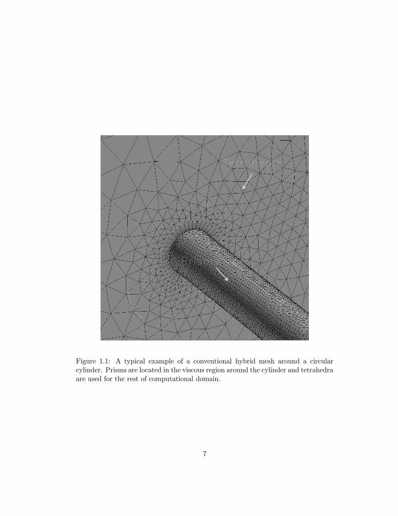
Figure 1.1: A typical example of a conventional hybrid mesh around a circularcylinder. Prisms are located in the viscous region around the cylinder and tetrahedraare used for the rest of computational domain.
7
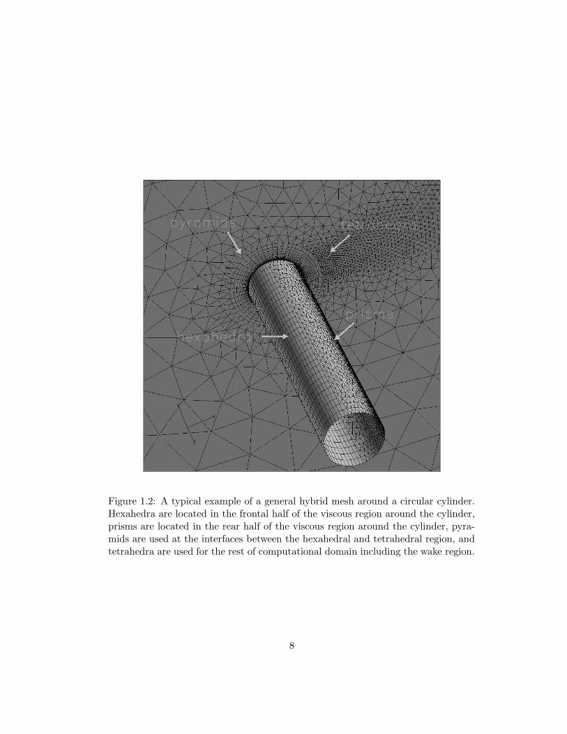
Figure 1.2: A typical example of a general hybrid mesh around a circular cylinder.Hexahedra are located in the frontal half of the viscous region around the cylinder,prisms are located in the rear half of the viscous region around the cylinder, pyra-mids are used at the interfaces between the hexahedral and tetrahedral region, andtetrahedra are used for the rest of computational domain including the wake region.
8
regions. Furthermore, the prismatic/hexahedral cells located in the viscous region
have typically very high aspect and stretching ratios along the direction normal
to the viscous wall. These kinds of mesh irregularity can be further increased by
multiple levels of adaptive mesh refinement or mesh deformation. Comparisons
between high order upwind schemes and central difference schemes with different
artificial dissipation models are presented in terms of solution accuracy as well as
computational efficiency on general hybrid meshes.
When the computational grid includes more types of elements, mesh irreg-
ularity increases and this may prohibit direct extension of a serial algorithm to a
parallel one. A mesh transparent graph partitioning strategy is used as the method
of domain partitioning. A grid-transparent mesh data structure which enables par-
allel inter-processor communications is presented. A single-loop communication
algorithm, which does not require any a priori communication schedule, is pre-
sented for efficient parallel inter-processor communications. The efficiency of the
proposed parallelization algorithm is presented with plots of scalability measured
on a massively-parallel machine with distributed memory architecture.
1.3 Moving mesh simulations and flow/structure inter-
actions
Moving mesh problems in computational fluid dynamics (CFD) have become of great
interest due to their wide area of applications. Blood flow through the arteries or
human heart, airfoil oscillation, wing fluttering, free surface flows, and many kinds
of flow and structure interaction problems can be classified in this category.
In order to simulate the fluid dynamics problem with moving mesh and
boundaries, several approaches have been proposed, such as the arbitrary Lagrangian-
Eulerian (ALE) scheme [29], the space-time approach [86, 87], and the immersed
9
boundary method [62, 61, 99].
The ALE formulation is based on the description of the flow field on an arbi-
trarily moving frame of reference which is typically attached to the moving meshes.
Hence, the mesh velocity appears in the convective flux term of the formulation.
The space-time approach is based on a finite element formulation of the governing
equations which is written over a sequence of space-time slabs. In this formulation,
the finite element interpolation polynomials are functions of both space and time.
Lastly, in the immersed boundary method, a body in the flow field is considered as
a kind of momentum forcing in the Navier-Stokes equations rather than a real body.
In the method, the choice of accurate interpolation schemes satisfying the no-slip
condition on the immersed body is crucial because the mesh does not generally fol-
lows the interface of immersed boundary. Among the aforementioned approaches,
the ALE scheme is the most popular method within the CFD community and has
been chosen for the current study.
For the stable and accurate ALE solution on moving meshes, the time inte-
gration scheme should be developed and verified, such that it preserves the stability
and accuracy of its fixed mesh counterpart. Furthermore, the motion of mesh should
not deteriorate the stability or accuracy, and should be capable of preserving the
uniform flow solution regardless of mesh motion, which the geometric conservation
law (GCL) accounts for.
In the development of stable and accurate ALE schemes and identification
of the role of GCL in terms of accuracy and stability, there have been considerable
research efforts, especially by Farhat’s research group [41, 39, 19, 18]. Essentially,
the ALE time integration schemes developed by Farhat are based on either time-
averaging of fluxes evaluated on different mesh configurations or evaluation of fluxes
on a time-averaged mesh configuration [20]. Such schemes present formal second
order accuracy with GCL obeying property, but time-averaging among multiple
10
mesh configurations can be a demanding computational task.
A more concise approach has been used by others [79, 43, 11], namely the
ALE formulation with a moving mesh source term. Even though such a formulation
has produced reasonable results for moving mesh simulations, there was neither a
clear derivation of the source term nor discussion of its significance. To be certain
about the validity of the ALE formulation with a moving mesh source term, we
have to be able to derive it from the original conservation laws, and address its
significance in moving mesh simulations. One of the main topics of the moving
mesh study is the derivation and validation of the ALE scheme with a moving mesh
source term, and its application to flow and structure interaction problems involving
mesh motion.
Once a stable and accurate ALE scheme is developed for moving mesh simula-
tions, the developed flow solver has to be coupled with a structural solver. Basically
two different coupling methods can be devised, namely weak and strong coupling,
depending on how the information is communicated between the two solvers. In
weak coupling, the two solvers are lagged by one true time step, but in strong cou-
pling the two different solvers are converged simultaneously. Weak coupling can be
a reasonable choice for very small time steps typically employed for explicit time-
stepping schemes. However, since an implicit scheme is used for the current flow
simulations, the time step is relatively large compared to an explicit scheme, hence
the strong coupling method is preferred to the weak coupling. A predictor-corrector
method is used for the strong coupling of flow and structural fields.
1.4 Motivation of the present research
Based on the survey about the previous research efforts in hybrid mesh methods for
flow simulations and fluid/structure interaction problems, the initial motivations of
the current research can be listed as follows.
11

1. generalization of hybrid meshes
2. a new solution algorithm for utilizing general hybrid meshes
3. more stable and accurate simulation of flow/structure interactions
First of all, the generalization of hybrid meshes for flow simulations was
the first goal of this research. The conventional hybrid mesh methods have been
investigated for compressible and incompressible Navier-Stokes equations in prior
studies by Dr. Kallinderis and his students [59, 53, 78]. The first objective of this
research is generalizing the conventional hybrid meshes to general hybrid meshes
which utilizing all four types of elements in a single computational domain. The
utility and effectiveness of general hybrid meshes for flow simulations had not been
reported and was needed to be investigated in the present research.
Second, a new solution algorithm for utilizing general hybrid meshes was
needed to be investigated. By the nature of severe mixing of element types in
general hybrid meshes, the solution algorithm should be more robust and accu-
rate than that of structured or simple unstructured meshes. A pressure-correction
type method has been used for incompressible Navier-Stokes equations [78]. This
method was shown to give reasonable results for incompressible Navier-Stokes so-
lutions. However, the performance of the solution algorithm is highly depends on
the pressure-Poisson solver, which can be expensive for large scale problems with
complex geometries. Therefore, a new solution method (with parallel execution ca-
pability) for incompressible Navier-Stokes equations is needed in order to utilize the
general hybrid meshes.
Third, a more stable and accurate solution algorithm for flow/structure in-
teractions on hybrid meshes was needed. In the past, pressure-correction type in-
compressible Navier-Stokes method was applied to the flow/structure interaction
problems with hybrid meshes [78, 79]. In their work, the structure is modeled with
12

rigid body, and no relative motion in the computational mesh was allowed. The cou-
pling method between the fluidic and structural solver was also in a weak manner
which may be called weak(loose)-coupling. In the weak coupling, the interaction
can be unstable as time step becomes large. Hence, a more stable and accurate
solution algorithm is needed which possibly incorporating flexible structural model
with mesh motion and strong coupling between the structural and fluidic solvers.
1.5 Contributions of the current research
The main research contributions made in this dissertation can be classified into two
parts; first the development of an incompressible Navier-Stokes equations solver for
general hybrid meshes, and second its application to moving mesh simulations of
flow/structure interactions.
1.5.1 A new incompressible Navier-Stokes method for general hy-
brid meshes
In the first part of the development of the incompressible Navier-Stokes method,
the original contributions of the current research can be listed as follows
1. first introduction of general hybrid meshes to incompressible flow simulations
2. first application of the artificial compressibility method with hybrid meshes
3. a computationally efficient face-and-edge algorithm for viscous flux computa-
tions
4. inflow turbulence effect study by using the developed solution algorithm
5. parallelization of the solution algorithm on general hybrid meshes
13

General hybrid meshes are first introduced for simulations of the incompress-
ible Navier-Stokes equations. There have been a few trials of conventional hybrid
meshes (prismatic/tetrahedral) for flow simulations [79, 10], but no general hybrid
meshes have been utilized so far. In this research, the various kinds of general hybrid
meshes are introduced and they are used for the investigation of more accurate and
effective flow solution algorithms. The method of artificial compressibility is used
for solving the incompressible Navier-Stokes equations on general hybrid meshes,
which is also the first application of the method to the hybrid meshes.
A new grid transparent algorithm is presented which is well suited for gen-
eral hybrid meshes. Especially for the viscous flux computations, a computationally
efficient face-and-edge algorithm is presented. This face-and-edge algorithm is com-
posed of a first loop of face-wise operations for the surface integrals over edge-duals,
and a second loop of edge-wise computations of velocity gradients and viscous fluxes.
A dual time-stepping backward difference scheme is used for the time accu-
rate formulation of the artificial compressibility method, and is also applied to the
turbulence equation so that the two sets of equations (incompressible Navier-Stokes
equations and turbulence equation) are solved in a strongly coupled fashion. As
an application study of the developed solution method, the effect of inflow turbu-
lence on the hydrodynamic forces on a cylinder is investigated. A two-dimensional
local mesh refinement study is also performed to identify the effect of local mesh
resolution in capturing the inflow turbulent eddies. Lastly, the proposed algorithm
is parallelized on a distributed memory system by using message passing interface
(MPI) library functions.
14

1.5.2 Geometrically conservative ALE scheme for flow/structure
interactions
In the second part of this research, the developed solution algorithm is further
extended to moving mesh simulations, and the original contributions are as follows
1. derivation of a geometrically conservative finite volume ALE scheme
2. presentation of the temporal accuracy of the proposed ALE scheme
3. presentation of the strong coupling of flow/structure interaction based on a
predictor-corrector method
An ALE finite volume formulation with a moving mesh source term is derived
from the original conservation laws and the geometric conservation law. The signif-
icance of moving mesh source is emphasized by presenting the moving mesh source
effect on moving mesh simulations in terms of the uniform flow preserving capabil-
ity. In order to be sure about the temporal accuracy of the proposed ALE scheme,
a time step refinement study is performed and its order of accuracy is confirmed on
moving mesh configurations by comparisons with a reference solution.
Furthermore, the ALE scheme is applied to the vortex induced vibration
(VIV) of a flexible cylinder. Beam elements are used for modeling the flexural
vibration of the cylinder, and then the equation of motion for the cylinder is nondi-
mensionalized by using the same reference parameters as those of the flow governing
equations. The superior stability of strong coupling as opposed to weak coupling is
emphasized by a comparison between the two coupling methods.
1.6 Overview
The outline of the dissertation is as follows; in chapter 2, the governing equations for
fluid flow are introduced and the turbulent eddy transport equation is also presented.
15
In chapter 3, the discretization and numerical integration schemes are discussed. In
chapter 4, a two-dimensional verification and validation study is presented. A simple
error analysis on a uniformly stretched mesh is investigated in one dimension. In
chapter 5, the inflow turbulence effect is studied by using the developed and validated
flow solution algorithms of the previous chapters. In chapter 6, three-dimensional
verification and validation study is presented. Flows around a sphere and a cylinder
are simulated for various orders of Reynolds number; Re = 10 ∼ 1, 000, 000. The
transition of the boundary layer from laminar to turbulent is predicted by using a
one-equation turbulence model.
In chapter 7, the equation of motion for a vibrating cylinder is presented.
It is nondimensionalized by using the same reference parameters as those for the
flow governing equations. Two different coupling methods are discussed for the
flow/structure interaction simulations; weak coupling and strong coupling. The
improved stability of strong coupling is emphasized by a comparison between the
two methods. In chapter 8, the verification study of the presented ALE scheme is
carried out. Lastly, the presented moving mesh method is applied to the vortex
induced vibration of a cylinder. The result of the current simulation is compared
with other computational results in literature.
In chapter 9, a parallelization of the proposed numerical scheme is introduced.
Different domain partitioning schemes are discussed. A mesh-transparent inter-
processor communication algorithm is presented. Scalability of the implemented
parallel algorithm is also demonstrated.
In chapter 10, the last chapter, results of the current research and their
significance are summarized. Finally, recommendations for future investigations
and research efforts are made.
16
Chapter 2
Governing Equations
In this chapter, the incompressible Navier-Stokes equations in an arbitrary La-
grangian Eulerian (ALE) frame of reference are derived from the conservation laws
for an arbitrarily moving control volume using Reynolds’ transport theorem. A
moving mesh source term is derived from the physical conservation laws and the
geometric conservation law. The significance of the moving mesh source term and
its relation to the geometric conservative property are discussed. The governing
equations are nondimensionalized by using free stream flow qunatities and the char-
acteristic length scale. A time accurate artificial compressibility method is intro-
duced for unsteady simulation of incompressible viscous flow. The Spalart-Allmaras
eddy viscosity transport equation is introduced for turbulence modeling, and its
time-accurate formulation is presented in a consistent form with that of the mean
flow equations.
17
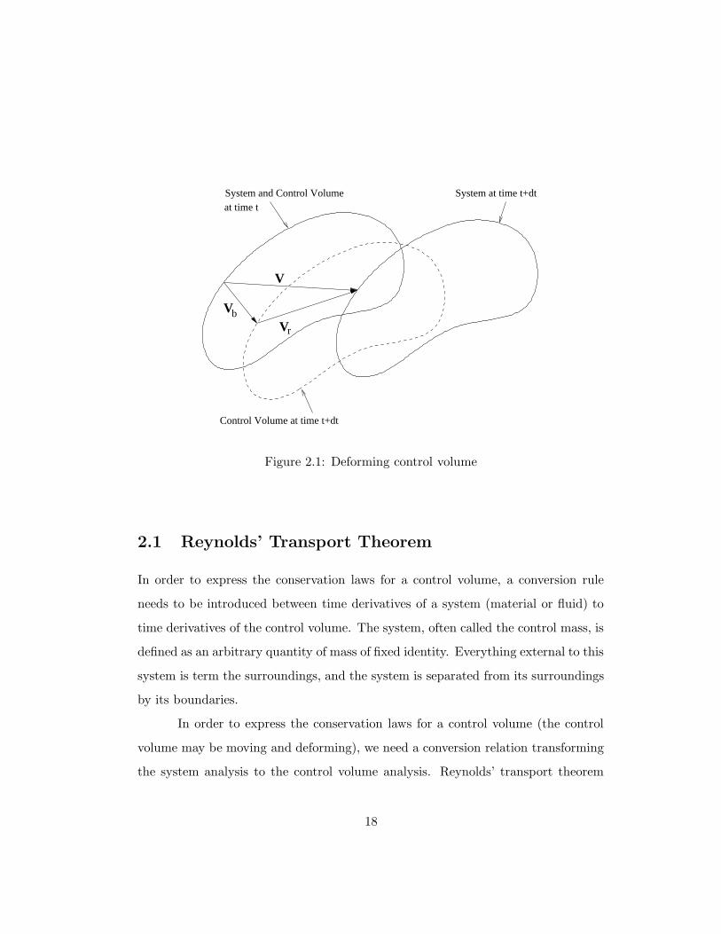
VV
V
System and Control Volumeat time t
System at time t+dt
Control Volume at time t+dt
b
r
Figure 2.1: Deforming control volume
2.1 Reynolds’ Transport Theorem
In order to express the conservation laws for a control volume, a conversion rule
needs to be introduced between time derivatives of a system (material or fluid) to
time derivatives of the control volume. The system, often called the control mass, is
defined as an arbitrary quantity of mass of fixed identity. Everything external to this
system is term the surroundings, and the system is separated from its surroundings
by its boundaries.
In order to express the conservation laws for a control volume (the control
volume may be moving and deforming), we need a conversion relation transforming
the system analysis to the control volume analysis. Reynolds’ transport theorem
18
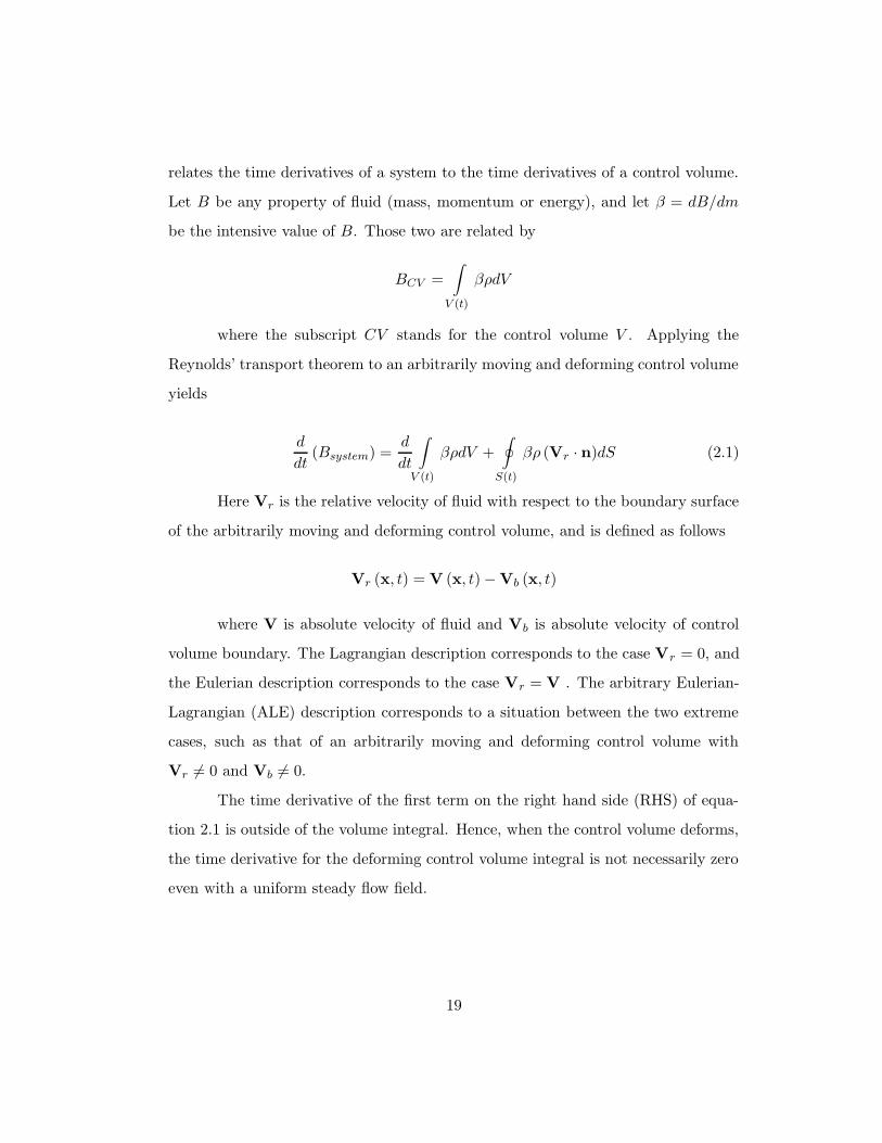
relates the time derivatives of a system to the time derivatives of a control volume.
Let B be any property of fluid (mass, momentum or energy), and let β = dB/dm
be the intensive value of B. Those two are related by
BCV =
∫
V (t)
βρdV
where the subscript CV stands for the control volume V . Applying the
Reynolds’ transport theorem to an arbitrarily moving and deforming control volume
yields
d
dt(Bsystem) =
d
dt
∫
V (t)
βρdV +
∮
S(t)
βρ (Vr · n)dS (2.1)
Here Vr is the relative velocity of fluid with respect to the boundary surface
of the arbitrarily moving and deforming control volume, and is defined as follows
Vr (x, t) = V (x, t) −Vb (x, t)
where V is absolute velocity of fluid and Vb is absolute velocity of control
volume boundary. The Lagrangian description corresponds to the case Vr = 0, and
the Eulerian description corresponds to the case Vr = V . The arbitrary Eulerian-
Lagrangian (ALE) description corresponds to a situation between the two extreme
cases, such as that of an arbitrarily moving and deforming control volume with
Vr 6= 0 and Vb 6= 0.
The time derivative of the first term on the right hand side (RHS) of equa-
tion 2.1 is outside of the volume integral. Hence, when the control volume deforms,
the time derivative for the deforming control volume integral is not necessarily zero
even with a uniform steady flow field.
19
2.2 Conservation of Mass
By using Reynolds’ transport theorem, the law of mass conservation can be derived
as follows. In equation (2.1), the property of interest is mass. Hence B = m and the
intensive property of mass is β = 1. Since mass is neither generated nor destructed,
we have
dmsys
dt= 0
and the final form of the mass conservation law for an arbitrarily moving
control volume can be expressed as follows
d
dt
∫
V (t)
ρdV +
∮
S(t)
ρ (V −Vb) · ndS = 0 (2.2)
where ρ is fluid density, V is fluid velocity and Vb is the velocity of the control
volume boundary. If V is equal to Vb, the flux term vanishes and the formulation
becomes identical with that of the Lagrangian frame of reference.
2.3 Conservation of Momentum
In a similar fashion, the conservation of momentum equations may be derived by an
application of Reynolds’ transport theorem. In this case, the property of interest
is linear momentum B = mV and the intensive property of linear momentum is
β = V. The rate of change of linear momentum is equal to the sum of external
forces
d
dt(mV)sys =
∑
F =
∮
S(t)
σ · ndS +
∫
V (t)
ρfdV
Substituting the above relations in Reynolds’ transport theorem, the law
of momentum conservation for an arbitrarily moving control volume is derived as
follows
20
d
dt
∫
V (t)
ρVdV +
∮
S(t)
ρV (V −Vb) · ndS =
∮
S(t)
σ · ndS +
∫
V (t)
ρfdV (2.3)
The two terms on the RHS of equation (2.3) represent surface and body
forces respectively, which are acting on the material contained within the control
volume V . The stress tensor σ is composed of a normal stress part representing
hydrostatic pressure and a shear stress part, and is defined by
σij = −pδij + τij
where p is the pressure, τij is the shear stress tensor, and δij is the Kronecker
delta. For Newtonian fluids, the shear stress is linearly related to the rate of strain
(deformation) tensor, and is expressed by
τij = λδij∂uk
∂xk
+ µ
(
∂ui
∂xj+
∂uj
∂xi
)
where λ is the coefficient of bulk viscosity and µ is the coefficient of molecular
viscosity. For incompressible flows, density is constant everywhere regardless of the
pressure field. For those kinds of flows, the first term of the shear stress tensor
vanishes because of the continuity equation, and the shear stress tensor reduces to
the following form
τij = µ
(
∂ui
∂xj+
∂uj
∂xi
)
2.4 Incompressible Navier-Stokes Equations
The incompressible Navier-Stokes equations without a body force term are expressed
in integral form. The continuity equation and the three momentum equations are
expressed in conservative form as follows
21
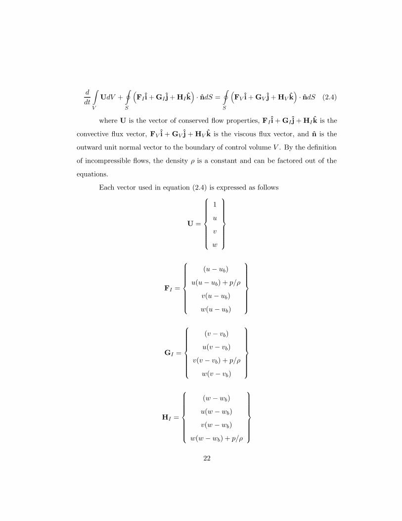
d
dt
∫
V
UdV +
∮
S
(
FI i + GI j + HIk)
· ndS =
∮
S
(
FV i + GV j + HV k)
· ndS (2.4)
where U is the vector of conserved flow properties, FI i + GI j + HI k is the
convective flux vector, FV i + GV j + HV k is the viscous flux vector, and n is the
outward unit normal vector to the boundary of control volume V . By the definition
of incompressible flows, the density ρ is a constant and can be factored out of the
equations.
Each vector used in equation (2.4) is expressed as follows
U =
1
u
v
w
FI =
(u − ub)
u(u − ub) + p/ρ
v(u − ub)
w(u − ub)
GI =
(v − vb)
u(v − vb)
v(v − vb) + p/ρ
w(v − vb)
HI =
(w − wb)
u(w − wb)
v(w − wb)
w(w − wb) + p/ρ
22
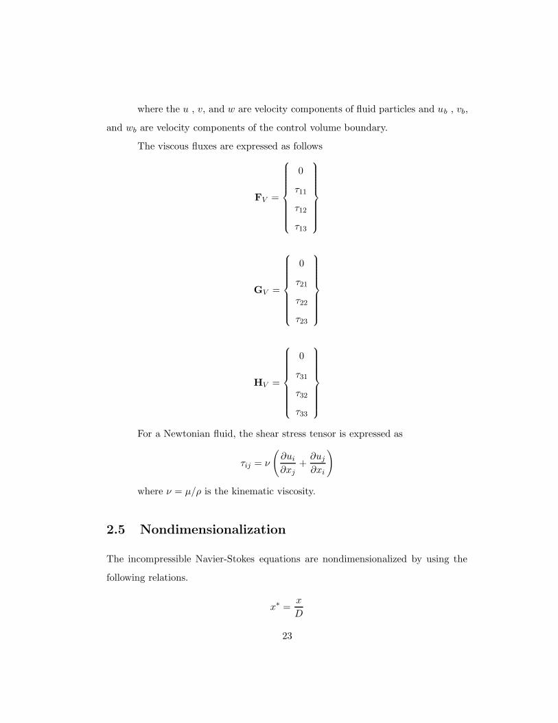
where the u , v, and w are velocity components of fluid particles and ub , vb,
and wb are velocity components of the control volume boundary.
The viscous fluxes are expressed as follows
FV =
0
τ11
τ12
τ13
GV =
0
τ21
τ22
τ23
HV =
0
τ31
τ32
τ33
For a Newtonian fluid, the shear stress tensor is expressed as
τij = ν
(
∂ui
∂xj+
∂uj
∂xi
)
where ν = µ/ρ is the kinematic viscosity.
2.5 Nondimensionalization
The incompressible Navier-Stokes equations are nondimensionalized by using the
following relations.
x∗ =x
D
23

u∗ =u
U∞
t∗ =t
D/U∞
p∗ =p − p∞ρU2
∞
where D is the characteristic length scale which is the diameter of the cylin-
der, U∞ is the free stream velocity, and p∞ is the free stream pressure. Substituting
all of the above relations into equation (2.4), rearranging terms and dropping the
superscript ∗ yields the nondimensional form of the incompressible Navier-Stokes
equations. Each component of vectors in nondimensional form is defined as follows
U =
1
u
v
w
FI =
(u − ub)
u(u − ub) + p
v(u − ub)
w(u − ub)
GI =
(v − vb)
u(v − vb)
v(v − vb) + p
w(v − vb)
24
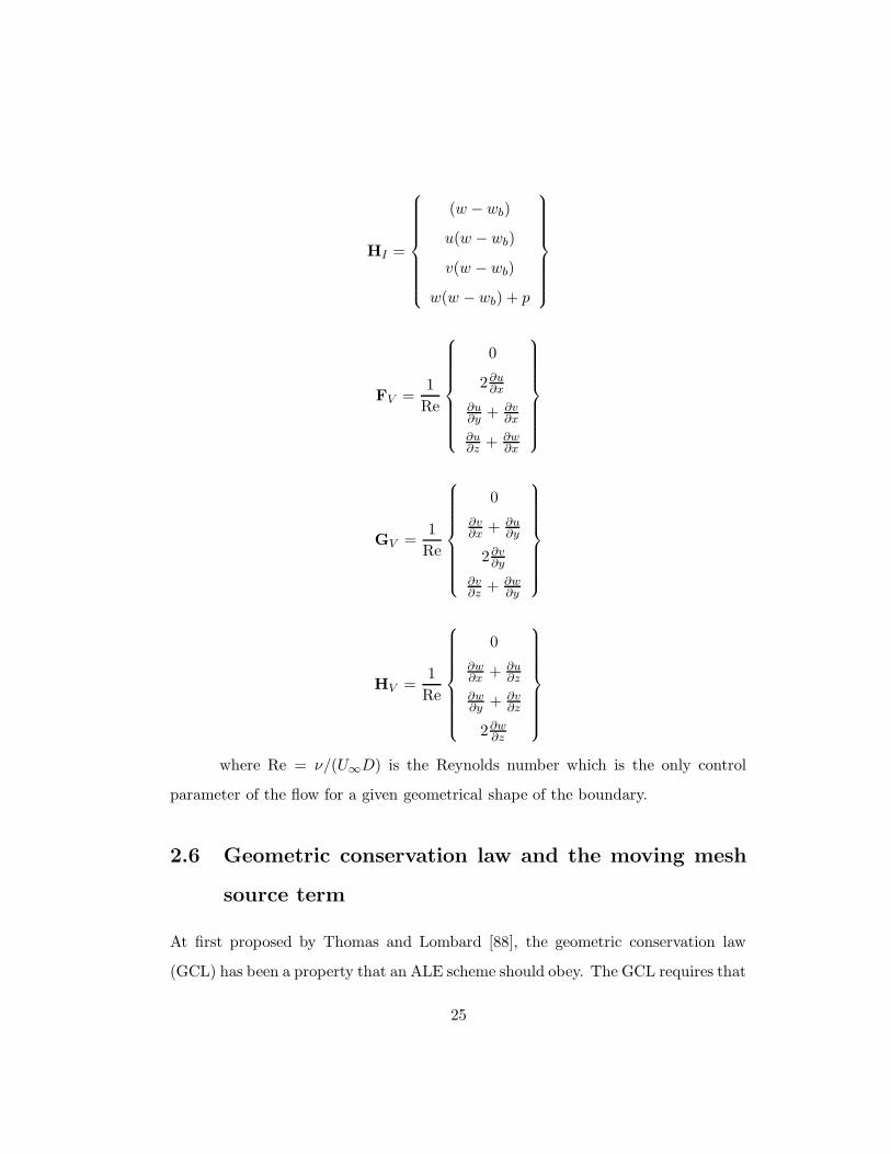
HI =
(w − wb)
u(w − wb)
v(w − wb)
w(w − wb) + p
FV =1
Re
0
2∂u∂x
∂u∂y
+ ∂v∂x
∂u∂z
+ ∂w∂x
GV =1
Re
0
∂v∂x
+ ∂u∂y
2∂v∂y
∂v∂z
+ ∂w∂y
HV =1
Re
0
∂w∂x
+ ∂u∂z
∂w∂y
+ ∂v∂z
2∂w∂z
where Re = ν/(U∞D) is the Reynolds number which is the only control
parameter of the flow for a given geometrical shape of the boundary.
2.6 Geometric conservation law and the moving mesh
source term
At first proposed by Thomas and Lombard [88], the geometric conservation law
(GCL) has been a property that an ALE scheme should obey. The GCL requires that
25

a uniform flow solution should be preserved regardless of mesh motion. The GCL can
be directly derived from the continuity equation, equation (2.2), by considering an
incompressible uniform flow, i.e. a constant density (ρ = ρ∞) and constant velocity
(V = V∞) everywhere. Then the continuity equation reduces to the geometric
conservation law
d
dt
∫
V
dV =
∮
S
Vb · ndS (2.5)
As seen in Eq. (2.5), the GCL states purely kinematic relations, namely the
instantaneous rate of change of control volume is the rate of volume swept by S.
The system of conservation laws in Eq. (2.4) can be rewritten as below
d
dt
∫
V
UdV + R (Q,x, x) = 0 (2.6)
where x and x are time varying position and velocity vectors of the mesh
points. Q is the vector containing primitive variables, which are pressure and ve-
locities, and R(Q,x, x) represents the residual of the system of equations, and is
defined as follows
R(Q,x, x) =∮
S
(
FI i + GI j + HIk)
· ndS
−∮
S
(
FV i + GV j + HV k)
· ndS (2.7)
The system of equations in equation (2.6) may be rewritten as
d
dt
(
UV)
+ R (Q,x, x) = 0 (2.8)
by using the control volume averaged conserved variables defined by
U =1
V
∫
V
UdV
26
Since the control volume V(t) and volume-averaged conserved variables U(t)
are smoothly varying with respect to time, the unsteady term in Eq. (2.8) can be
expanded as
dU
dtV +
dV
dtU + R (Q,x, x) = 0 (2.9)
Finally, the time derivative of the control volume in Eq. (2.9) can be replaced
with a surface integral of control volume boundary velocity by the GCL as shown
in Eq. (2.5) to obtain:
dU
dtV + R (Q,x, x) = −U
∮
S
Vb · ndS (2.10)
We note that since the moving mesh source term is directly derived from the
GCL, the system of conservation laws presented in Eq. (2.10) is inherently equipped
with the GCL. Hence, the uniform flow is preserved regardless of the mesh motion,
and the GCL is always satisfied.
2.7 Time-accurate formulation of the artificial compress-
ibility method
The incompressible Navier-Stokes equations are being solved with the method of
artificial compressibility. The artificial compressibility method is presented as a
time-accurate formulation by using the dual time-stepping scheme of Jameson [31].
The original form of the artificial compressibility method introduced by Chorin [13]
was for steady-state problems where no true time-derivative terms appear the for-
mulation. The time accurate artificial compressibility formulation in the present
work has been presented by Belov [6] by using the dual time-stepping algorithm of
Jameson.
27
In the current time-accurate formulation, a pseudo time-derivative of pres-
sure is added to the continuity equation and pseudo time-derivatives of velocity
components are added to the momentum equations. As a result, the continuity
equation has a pseudo time-derivative and the momentum equations have both true
and pseudo time-derivatives.
The system of conservation laws with the added pseudo-term can be ex-
pressed as
Pd
dt∗
∫
V
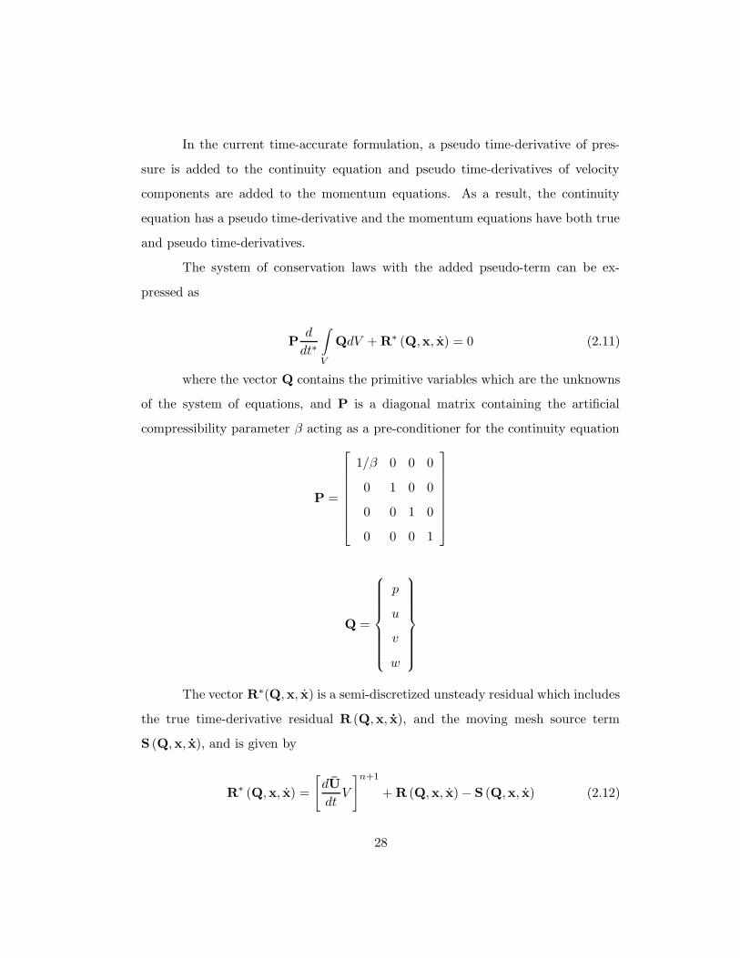
QdV + R∗ (Q,x, x) = 0 (2.11)
where the vector Q contains the primitive variables which are the unknowns
of the system of equations, and P is a diagonal matrix containing the artificial
compressibility parameter β acting as a pre-conditioner for the continuity equation
P =
1/β 0 0 0
0 1 0 0
0 0 1 0
0 0 0 1
Q =
p
u
v
w
The vector R∗(Q,x, x) is a semi-discretized unsteady residual which includes
the true time-derivative residual R (Q,x, x), and the moving mesh source term
S (Q,x, x), and is given by
R∗ (Q,x, x) =
[
dU
dtV
]n+1
+ R (Q,x, x) − S (Q,x, x) (2.12)
28
where the discretized true time-derivative by using the second order backward
difference formula at time step (n + 1) is defined by
[
dU
dtV
]n+1
=
(
3Un+1 − 4Un + Un−1
2∆t
)
V n+1
In a similar way, the velocity of control volume (mesh) can also be approxi-
mated as follows
[x]n+1 =3xn+1 − 4xn + xn−1
2∆t
and the moving mesh source term is defined as follows
S (Q,x, x) = −U
∫
S
Vb · ndS
Since t∗ in equation (2.11) refers to the fictitious time during the pseudo-
transient state and the moving control volume V = V (t) is a function only of the
true time, the pseudo time-derivative can be moved inside of the volume integral.
Once the unsteady residual R∗ is constructed, the following steady-state problem
in pseudo-time
d
dt∗
(
Qn+1,k)
V n+1 + P−1R∗
(
Qn+1,k,xn+1, xn+1)
= 0 (2.13)
is to be solved for the steady state in pseudo-time by using an iterative
scheme. The index k in equation (2.13) refers to the number of interations in
pseudo time. For each true time step, a steady state problem in pseudo time is
solved by an explicit multistage scheme. The iteration in pseudo time is referred to
as the sub-iteration as opposed to the time-stepping in true time. Hence, the time
advancement requires dual time-stepping, which involves the solution of a steady-
state problem in pseudo time for each true time step. A more detailed description
of the dual time-stepping scheme is intoduced later in a separate section.
29
The artificial compressibility parameter β controls the speed of artificial pres-
sure waves and it also affects the overall convergence rate. Depending on the precon-
ditioning method employed, more complicated preconditioning matrices including
the variable β can be used [22, 12, 44, 45, 56, 68, 91, 92, 93, 94]. For the current
study, a simple diagonal preconditioning matrix with a constant β in the order of
O(100) is used.
2.8 Reynolds Averaged Navier-Stokes Equations
In order to express the Reynolds Averaged Navier-Stokes Equations in differential
form, let us rewrite the incompressible Navier-Stokes equations in differential form.
Applying the divergence theorem and letting the control volume shrink to zero yields
the incompressible Navier-Stokes equations in differential form
∂ui
∂xi= 0 (2.14)
ρ∂ui
∂t+ ρ
∂
∂xj(ujui) = − ∂p
∂xi+
∂
∂xj
[
2µ
(
∂ui
∂xj+
∂ui
∂xj
)]
(2.15)
Next, we decompose the instantaneous velocity ui(x, t) into the mean velocity
Ui(x) and the fluctuation u′
i(x, t), that is
ui(x, t) = Ui(x) + u′
i(x, t) (2.16)
where the mean velocity is defined as
Ui(x) = limT→∞
1
T
∫ T
0ui(x, t)dt.
By substituting equation (2.16) in equations (2.14) and (2.15), and time (en-
semble) averaging the incompressible Navier-Stokes equations yields the Reynolds
averaged Navier-Stokes (RANS) equations
30
∂Ui
∂xi= 0
ρ∂Ui
∂t+ ρ
∂
∂xj(UjUi) = − ∂p
∂xi+
∂
∂xj
(
2µSij − ρu′
ju′
i
)
where Sij = (∂Ui/∂xj + ∂Uj/∂xi) is strain rate tensor of mean velocity.
The correlation term of fluctuations ρu′
iu′
j is known as the Reynolds stress
tensor. The Reynolds stresses represent the time-averaged rate of momentum trans-
fer due to turbulence, whereas the viscous stresses 2µSij stem from the momentum
transfer at the molecular level.
2.9 Eddy Viscosity Hypothesis
In the RANS equations, six additional unknowns of Reynolds stresses are intro-
duced in addition to the four unknowns of mean flow variables p , u , v , and
w. The total number of unknowns is ten and the number of equations is only
four, therefore the RANS equations are not closed and cannot be solved unless the
Reynolds stresses are determined by introducing further approximations or addi-
tional equations. The Reynolds stress tensor can be dramatically simplified by using
the turbulent-viscosity hypothesis (also known as the Boussinesq approximation)
−ρu′
iu′
j +2
3ρkδij = 2ρνtSij
where k is turbulent kinetic energy and Sij is strain rate tensor of mean flow
velocities. In the current study of turbulent flow simulations, the Spalart-Allmaras
one-equation model is employed. Compared with a two-equation turbulence model,
the turbulent kinetic energy term is neglected, and the (kinematic) eddy viscosity
νt , the only additional unknown from Reynolds averaging, is being determined by
solving the eddy-viscosity transport equation
31
−ρu′
iu′
j = 2ρνtSij
Substituting the eddy viscosity relation into the RANS equations yields the
momentum equations expressed in the following form
∂Ui
∂t+
∂
∂xj(UjUi) = −1
ρ
∂p
∂xi+
∂
∂xj
[
(ν + νt)
(
∂ui
∂xj+
∂uj
∂xi
)]
The only difference from the original incompressible Navier-Stokes equations
is the appearance of eddy viscosity in the viscous flux term. If the eddy viscosity
νt vanishes, the original incompressible Navier-Stokes equations are recovered. Now
the system of equations is composed of the continuity equation, the three momentum
equations, and the eddy viscosity transport equation. The unknowns are the four
primitive variables (p, u, v, w) and the turbulent eddy viscosity (νt), hence the system
of equations is closed and solvable.
2.10 Spalart-Allmaras Turbulence Model
Spalart and Allmaras [81] introduced a one-equation model originally developed for
aerodynamic flow. A single model transport equation is solved for the turbulent
viscosity (νt) and it has been shown that the model is quite successful especially for
drag prediction in aerodynamic applications [24].
In addition, the model has several attractive features compared to algebraic
(e.g. Baldwin-Lomax) and two-equation (e.g. k − ε) models [5, 24]. First, since the
model is local, it is suitable to implement on unstructured meshes. If a model is
non-local, such as Baldwin-Lomax model, it requires information about the solution
along lines normal to the wall, which is not readily available on unstructured meshes.
Second, probably the most significant in computational aspect, because the working
variable behaves linearly near the wall, it only require wall spacing of y+ ≤ 3.5 which
32
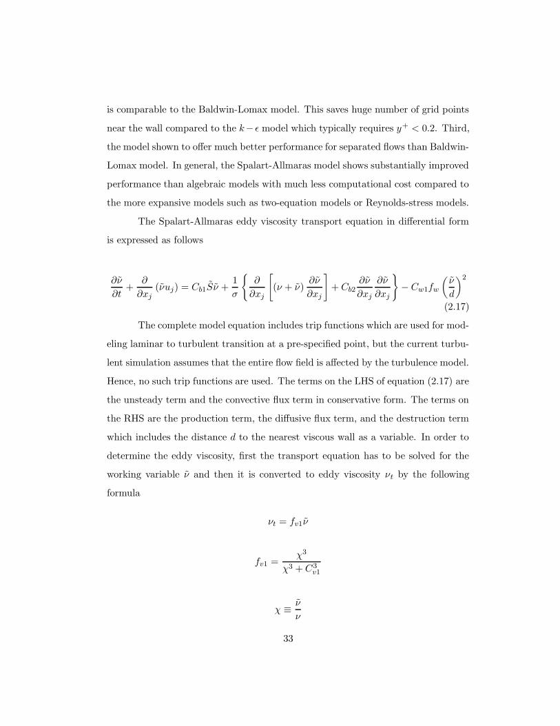
is comparable to the Baldwin-Lomax model. This saves huge number of grid points
near the wall compared to the k− ε model which typically requires y+ < 0.2. Third,
the model shown to offer much better performance for separated flows than Baldwin-
Lomax model. In general, the Spalart-Allmaras model shows substantially improved
performance than algebraic models with much less computational cost compared to
the more expansive models such as two-equation models or Reynolds-stress models.
The Spalart-Allmaras eddy viscosity transport equation in differential form
is expressed as follows
∂ν
∂t+
∂
∂xj(νuj) = Cb1Sν +
1
σ
{
∂
∂xj
[
(ν + ν)∂ν
∂xj
]
+ Cb2∂ν
∂xj
∂ν
∂xj
}
− Cw1fw
(ν
d
)2
(2.17)
The complete model equation includes trip functions which are used for mod-
eling laminar to turbulent transition at a pre-specified point, but the current turbu-
lent simulation assumes that the entire flow field is affected by the turbulence model.
Hence, no such trip functions are used. The terms on the LHS of equation (2.17) are
the unsteady term and the convective flux term in conservative form. The terms on
the RHS are the production term, the diffusive flux term, and the destruction term
which includes the distance d to the nearest viscous wall as a variable. In order to
determine the eddy viscosity, first the transport equation has to be solved for the
working variable ν and then it is converted to eddy viscosity νt by the following
formula
νt = fv1ν
fv1 =χ3
χ3 + C3v1
χ ≡ ν
ν
33
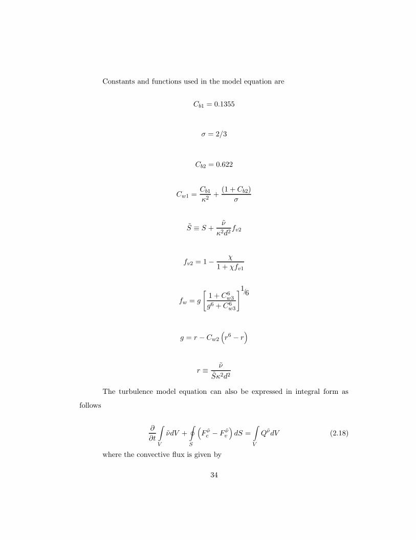
Constants and functions used in the model equation are
Cb1 = 0.1355
σ = 2/3
Cb2 = 0.622
Cw1 =Cb1
κ2+
(1 + Cb2)
σ
S ≡ S +ν
κ2d2fv2
fv2 = 1 − χ
1 + χfv1
fw = g
[
1 + C6w3
g6 + C6w3
]1/6
g = r − Cw2
(
r6 − r)
r ≡ ν
Sκ2d2
The turbulence model equation can also be expressed in integral form as
follows
∂
∂t
∫
V
νdV +
∮
S
(
F νc − F ν
v
)
dS =
∫
V
QνdV (2.18)
where the convective flux is given by
34

F νc = ν (unx + uny + unz)
and the diffusive flux is
F νv = nxτ
νxx + nyτ
νyy + nzτ
νzz
Each component of the diffusive flux is defined as
τ νxx =
1
σ(ν + ν)
∂ν
∂x
τ νyy =
1
σ(ν + ν)
∂ν
∂y
τ νzz =
1
σ(ν + ν)
∂ν
∂z
Lastly, the source term is defined as follows
Qν = Cb1Sν +Cb2
σ
{(∂ν
∂x
)2
+
(∂ν
∂y
)2
+
(∂ν
∂z
)2}
− Cw1fw
(ν
d
)2
In order to couple the turbulence model equation with the mean flow equa-
tions, the time-stepping scheme of the turbulence equation should be in a consistent
form with that of the mean flow equation. A dual time-stepping time-accurate
formulation of the turbulence equation is given by
∂
∂t∗
∫
V
νdV + R∗ (ν) = 0 (2.19)
where t∗ refers to pseudo time and R∗ is the unsteady residual defined by
R∗ (ν) =∂
∂t
∫
V
νdV +
∮
S
(
F νc − F ν
v
)
dS −∫
V
QνdV
35
Once the unsteady residual is constructed by using the temporal and spatial
discretization schemes, the steady state problem in pseudo time is solved for the
eddy viscosity at the next time step. The pseudo transient problems for the turbu-
lence model equation as expressed in equation (2.19) can be coupled with that of
the mean flow equation (2.11). The two sets of equations are coupled and solved
simultaneously, hence the flow field and eddy viscosity are strongly coupled and
converge concurrently.
36
Chapter 3
Numerical Integration Scheme
A conservative finite volume scheme is presented for numerical flux computation
on general hybrid meshes. A node-dual scheme is used for the construction of
non-overlapping finite control volumes. Another conceptual finite volume, called
edge-dual, is introduced for the velocity gradient computation of the viscous flux.
A new computationally efficient two-step (face-and-edge) algorithm is pre-
sented for the velocity gradient computation using the edge-duals. For computation
of the convective numerical flux, two different schemes are introduced, namely a
central difference scheme with artificial dissipation and a high order upwind scheme
based on Roe’s flux-difference splitting. In the present study, the upwind scheme is
first applied to the hybrid meshes, while the central schemes has been employed for
the hybrid meshes in the past. For the central scheme, different artificial dissipation
models are discussed. Special methods for the application of boundary conidtions
are presented for general hybrid meshes.
An implicit dual time-stepping scheme is presented for the time accurate
formulation of the artificial compressibility method. A-stable backward difference
formulas are introduced for the discretization of the true time-evolution term and
an explicit multistage scheme is used for pseudo time-stepping.
37
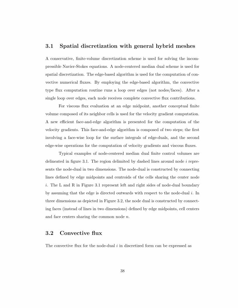
3.1 Spatial discretization with general hybrid meshes
A conservative, finite-volume discretization scheme is used for solving the incom-
pressible Navier-Stokes equations. A node-centered median dual scheme is used for
spatial discretization. The edge-based algorithm is used for the computation of con-
vective numerical fluxes. By employing the edge-based algorithm, the convective
type flux computation routine runs a loop over edges (not nodes/faces). After a
single loop over edges, each node receives complete convective flux contributions.
For viscous flux evaluation at an edge midpoint, another conceptual finite
volume composed of its neighbor cells is used for the velocity gradient computation.
A new efficient face-and-edge algorithm is presented for the computation of the
velocity gradients. This face-and-edge algorithm is composed of two steps; the first
involving a face-wise loop for the surface integrals of edge-duals, and the second
edge-wise operations for the computation of velocity gradients and viscous fluxes.
Typical examples of node-centered median dual finite control volumes are
delineated in figure 3.1. The region delimited by dashed lines around node i repre-
sents the node-dual in two dimensions. The node-dual is constructed by connecting
lines defined by edge midpoints and centroids of the cells sharing the center node
i. The L and R in Figure 3.1 represent left and right sides of node-dual boundary
by assuming that the edge is directed outwards with respect to the node-dual i. In
three dimensions as depicted in Figure 3.2, the node dual is constructed by connect-
ing faces (instead of lines in two dimensions) defined by edge midpoints, cell centers
and face centers sharing the common node n.
3.2 Convective flux
The convective flux for the node-dual i in discretized form can be expressed as
38

i L R
(a) node-dual with mixed cells
iL R
(b) node-dual with triangular cells
Figure 3.1: Node-duals in two dimensions
39

n
n
(a) Hexahedron (b) Prism
n n
(c) Pyramid (d) Tetrahedron
Figure 3.2: Node-dual contributions from different types of elements in three di-mensions
40
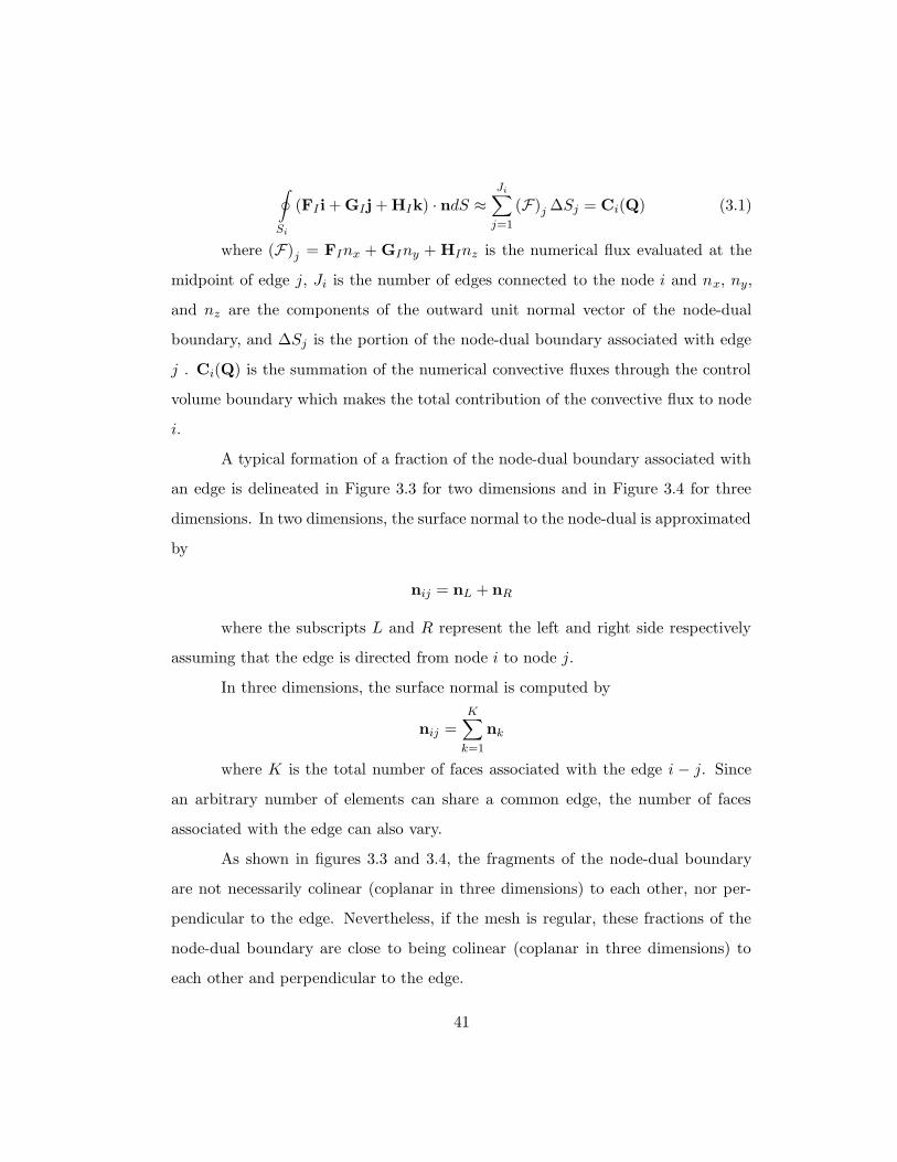
∮
Si
(FI i + GIj + HIk) · ndS ≈Ji∑
j=1
(F)j ∆Sj = Ci(Q) (3.1)
where (F)j = FInx + GIny + HInz is the numerical flux evaluated at the
midpoint of edge j, Ji is the number of edges connected to the node i and nx, ny,
and nz are the components of the outward unit normal vector of the node-dual
boundary, and ∆Sj is the portion of the node-dual boundary associated with edge
j . Ci(Q) is the summation of the numerical convective fluxes through the control
volume boundary which makes the total contribution of the convective flux to node
i.
A typical formation of a fraction of the node-dual boundary associated with
an edge is delineated in Figure 3.3 for two dimensions and in Figure 3.4 for three
dimensions. In two dimensions, the surface normal to the node-dual is approximated
by
nij = nL + nR
where the subscripts L and R represent the left and right side respectively
assuming that the edge is directed from node i to node j.
In three dimensions, the surface normal is computed by
nij =K∑
k=1
nk
where K is the total number of faces associated with the edge i − j. Since
an arbitrary number of elements can share a common edge, the number of faces
associated with the edge can also vary.
As shown in figures 3.3 and 3.4, the fragments of the node-dual boundary
are not necessarily colinear (coplanar in three dimensions) to each other, nor per-
pendicular to the edge. Nevertheless, if the mesh is regular, these fractions of the
node-dual boundary are close to being colinear (coplanar in three dimensions) to
each other and perpendicular to the edge.
41
3.2.1 Central difference
Both the central difference and upwind schemes are used for the convective flux
evaluation. For the central difference scheme, the numerical flux is evaluated at the
node-dual boundary by the arithmetic averaging of the fluxes at the two end nodes
as shown in Eq. (3.2).
(Fcentral)j =1
2(F (Qi) + F (Qj)) (3.2)
Since the central difference scheme is susceptible to the odd-even mode de-
coupling and solution oscillations, an additional artificial dissipation term is needed.
Different artificial dissipation models are tested. A more detailed discussion of the
artificial dissipation models is presented in a later section.
3.2.2 Upwind by Roe’s flux-difference splitting
Instead of the central scheme with the supplementary artificial dissipation term, an
upwind scheme can be used by evaluating the numerical fluxes using Roe’s approx-
imate Riemann solver [69, 70] as follows
Fupwind =1
2(F (QL) + F (QR)) +
1
2
∣∣∣A (QR,QL)
∣∣∣ (QL −QR) (3.3)
where the F (QL) and F (QR) are the convective flux vectors from the so-
lutions reconstructed on the left (QL) and right (QR) sides of the control volume
boundary as delineated in Figure 3.1. These solutions at the edge midpoint are
reconstructed by using Taylor series expansions about the two end nodes, which
requires pre-computation of nodal gradients of the solutions.
Roe’s matrix∣∣∣A∣∣∣ is defined as
∣∣∣A∣∣∣ = R
∣∣∣Λ∣∣∣R−1
42
where R is the right eigenvector matrix of the flux Jacobian, R−1 is its
inverse, and∣∣∣Λ∣∣∣ is a diagonal matrix whose components are absolute values of the
eigenvalues. Roe’s matrix A satisfies the following three properties
1. A (Q,Q) = A (Q) whereA (Q) = ∂F∂Q
is the fluxJacobian
2. A (QR,QL) is diagonalizable and has real eigenvalues
3. For any QR,QL, A (QR,QL) × (QR −QL) = F (QR) − F (QL)
Property 1 is concerned with the consistency condition which guarantees that
the approximate solution converges to the exact solution smoothly as QL and QR
approach each other. Property 2 guarantees that the linearized system is hyperbolic.
Property 3 ensures that the approximate solution is exact if QL and QR can be
connected by a single discontinuity.
As shown by Taylor and Whitfield [85], for the incompressible Euler equations
with artificial compressibility, each component of Roe’s matrix can be constructed
by arithmetic averaging of the left and right states, which results in satisfaction of
all three conditions for Roe’s matrix. A nonsingular eigensystem of Roe’s matrix
was reported by Anderson et al. [4] in two dimensions, and by Kim [38] in three
dimensions.
When the first order upwind scheme is employed, the solutions at the left
and right sides of the control volume boundary can be chosen simply as the solutions
at the two end nodes. However, for high order upwind schemes, the solutions at the
control volume boundary must be reconstructed by using the Taylor series expan-
sions about the two end nodes. The solution reconstruction from the two end nodes
to the edge mid-point which represents the node-dual boundary can be expressed as
QL = Qi +1
2(∇Q)i · ∆rij (3.4)
QR = Qj −1
2(∇Q)j · ∆rij (3.5)
43
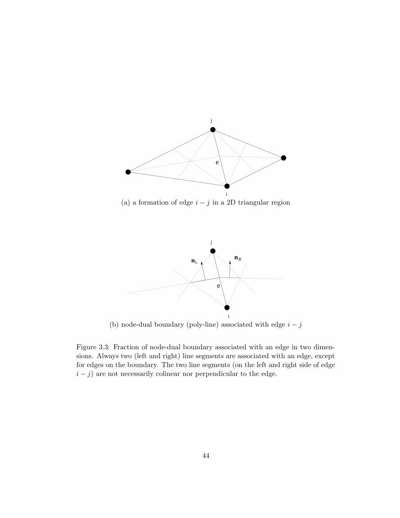
e
i
j
(a) a formation of edge i − j in a 2D triangular region
n n RL
e
i
j
(b) node-dual boundary (poly-line) associated with edge i − j
Figure 3.3: Fraction of node-dual boundary associated with an edge in two dimen-sions. Always two (left and right) line segments are associated with an edge, exceptfor edges on the boundary. The two line segments (on the left and right side of edgei − j) are not necessarily colinear nor perpendicular to the edge.
44
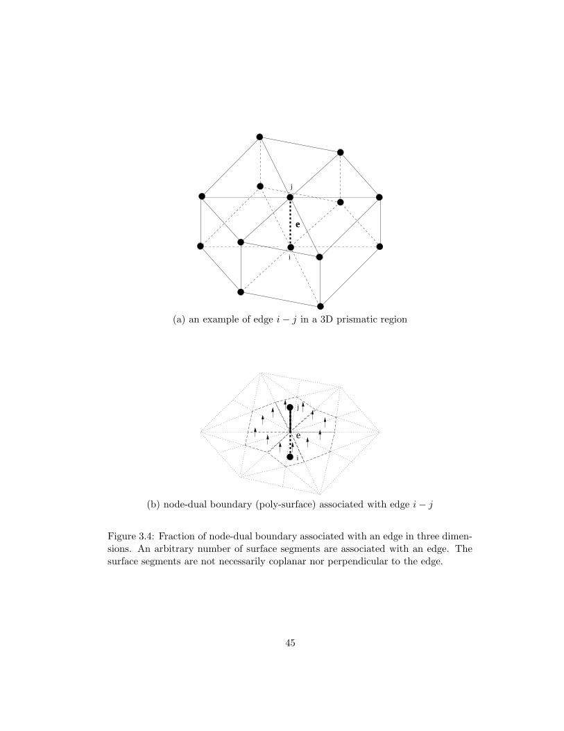
e
i
j
(a) an example of edge i − j in a 3D prismatic region
e
i
j
(b) node-dual boundary (poly-surface) associated with edge i − j
Figure 3.4: Fraction of node-dual boundary associated with an edge in three dimen-sions. An arbitrary number of surface segments are associated with an edge. Thesurface segments are not necessarily coplanar nor perpendicular to the edge.
45
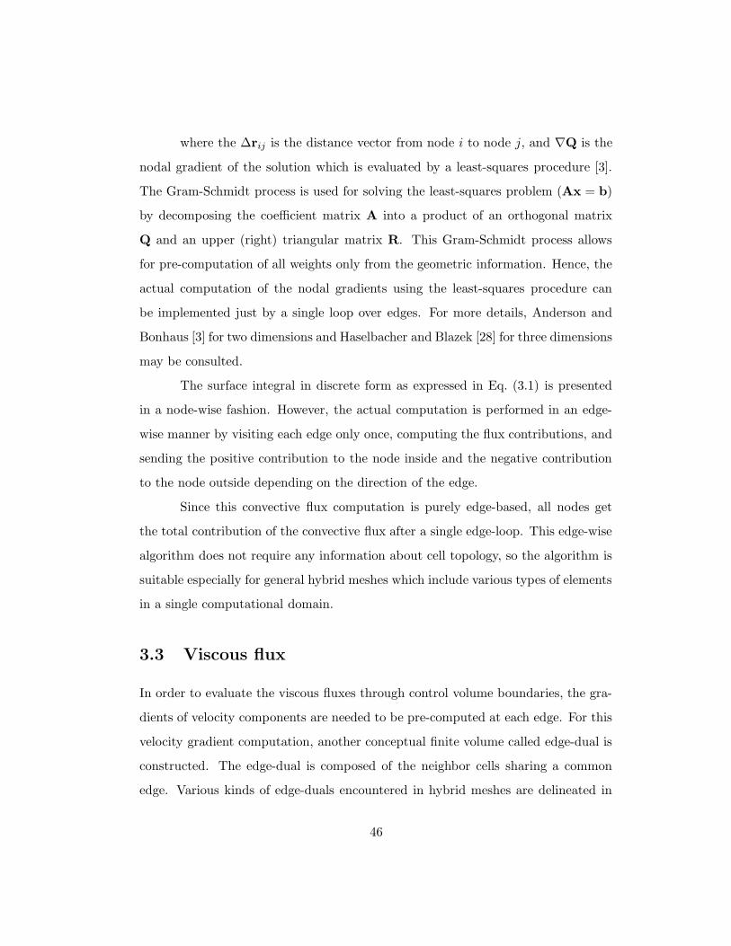
where the ∆rij is the distance vector from node i to node j, and ∇Q is the
nodal gradient of the solution which is evaluated by a least-squares procedure [3].
The Gram-Schmidt process is used for solving the least-squares problem (Ax = b)
by decomposing the coefficient matrix A into a product of an orthogonal matrix
Q and an upper (right) triangular matrix R. This Gram-Schmidt process allows
for pre-computation of all weights only from the geometric information. Hence, the
actual computation of the nodal gradients using the least-squares procedure can
be implemented just by a single loop over edges. For more details, Anderson and
Bonhaus [3] for two dimensions and Haselbacher and Blazek [28] for three dimensions
may be consulted.
The surface integral in discrete form as expressed in Eq. (3.1) is presented
in a node-wise fashion. However, the actual computation is performed in an edge-
wise manner by visiting each edge only once, computing the flux contributions, and
sending the positive contribution to the node inside and the negative contribution
to the node outside depending on the direction of the edge.
Since this convective flux computation is purely edge-based, all nodes get
the total contribution of the convective flux after a single edge-loop. This edge-wise
algorithm does not require any information about cell topology, so the algorithm is
suitable especially for general hybrid meshes which include various types of elements
in a single computational domain.
3.3 Viscous flux
In order to evaluate the viscous fluxes through control volume boundaries, the gra-
dients of velocity components are needed to be pre-computed at each edge. For this
velocity gradient computation, another conceptual finite volume called edge-dual is
constructed. The edge-dual is composed of the neighbor cells sharing a common
edge. Various kinds of edge-duals encountered in hybrid meshes are delineated in
46

e
e
e
(a) (b)
(c)
Figure 3.5: Various formations of edge-duals in two dimensions. An edge-dual iscomposed of neighbor cells sharing a common edge (e), indicated by thick dashedlines.
Fig. 3.5 in two dimensions and Fig. 3.6 in three dimensions.
For the computation of velocity gradients at each edge, the divergence the-
orem is used and the surface integrals along edge-dual boundaries are evaluated.
For example, computing the volume averaged value of ∂u∂x
using an edge-dual can be
expressed as
(∂u
∂x
)
e
=1
Ve
∮
Se
unxdS (3.6)
where Ve is the volume of the edge-dual and Se is its boundary.
This approach has been advocated by other researchers [10, 8] because it is
less susceptible to solution wiggles and can be applied on more compact stencils than
47

e
(a) edge-dual composed of prisms
e
(b) edge-dual composed of tetrahedra
e
(a) edge-dual composed of mixed cells
Figure 3.6: Various formations of edge-duals in three dimensions. An edge-dual iscomposed of neighbor cells sharing a common edge (e), indicated by thick dashedlines.
48
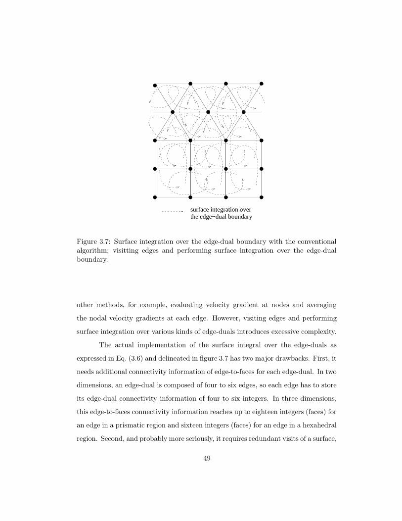
the edge−dual boundarysurface integration over
Figure 3.7: Surface integration over the edge-dual boundary with the conventionalalgorithm; visitting edges and performing surface integration over the edge-dualboundary.
other methods, for example, evaluating velocity gradient at nodes and averaging
the nodal velocity gradients at each edge. However, visiting edges and performing
surface integration over various kinds of edge-duals introduces excessive complexity.
The actual implementation of the surface integral over the edge-duals as
expressed in Eq. (3.6) and delineated in figure 3.7 has two major drawbacks. First, it
needs additional connectivity information of edge-to-faces for each edge-dual. In two
dimensions, an edge-dual is composed of four to six edges, so each edge has to store
its edge-dual connectivity information of four to six integers. In three dimensions,
this edge-to-faces connectivity information reaches up to eighteen integers (faces) for
an edge in a prismatic region and sixteen integers (faces) for an edge in a hexahedral
region. Second, and probably more seriously, it requires redundant visits of a surface,
49
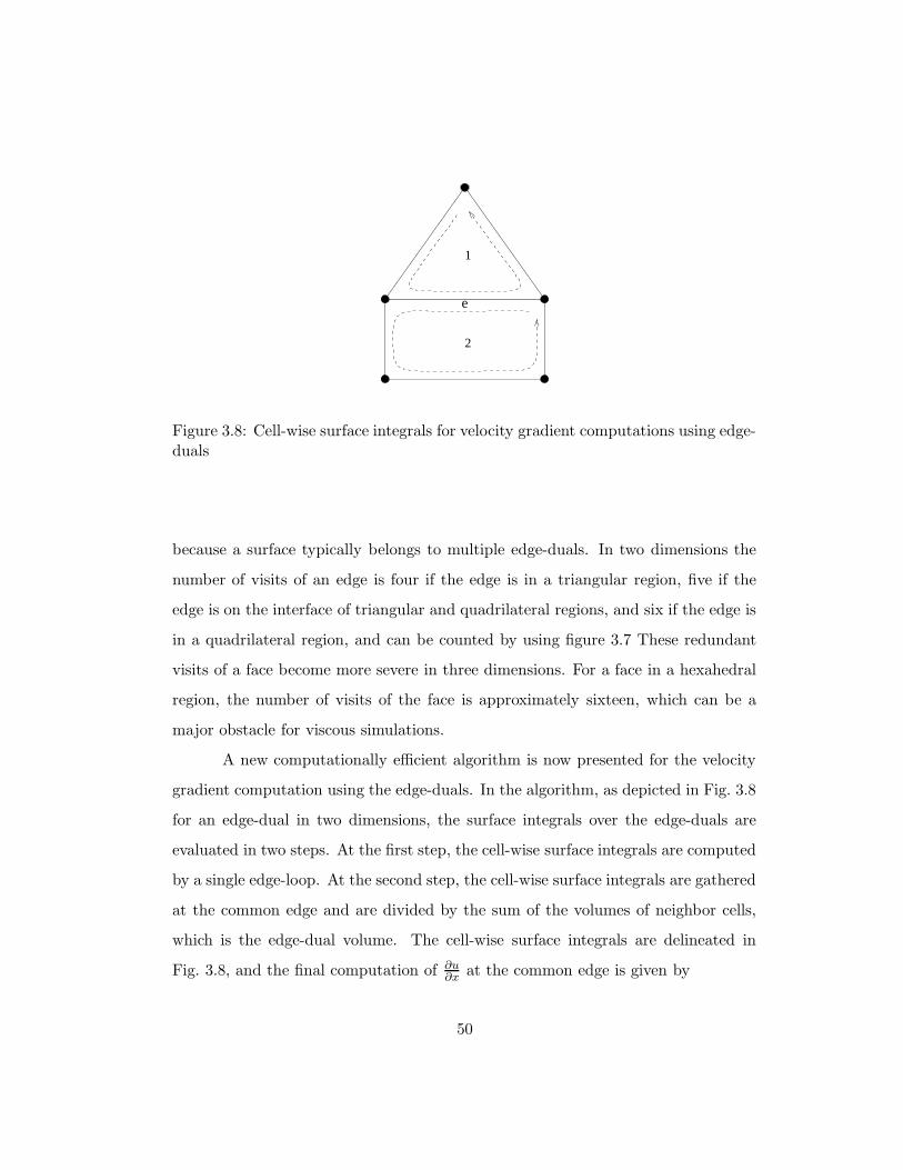
1
2
e
Figure 3.8: Cell-wise surface integrals for velocity gradient computations using edge-duals
because a surface typically belongs to multiple edge-duals. In two dimensions the
number of visits of an edge is four if the edge is in a triangular region, five if the
edge is on the interface of triangular and quadrilateral regions, and six if the edge is
in a quadrilateral region, and can be counted by using figure 3.7 These redundant
visits of a face become more severe in three dimensions. For a face in a hexahedral
region, the number of visits of the face is approximately sixteen, which can be a
major obstacle for viscous simulations.
A new computationally efficient algorithm is now presented for the velocity
gradient computation using the edge-duals. In the algorithm, as depicted in Fig. 3.8
for an edge-dual in two dimensions, the surface integrals over the edge-duals are
evaluated in two steps. At the first step, the cell-wise surface integrals are computed
by a single edge-loop. At the second step, the cell-wise surface integrals are gathered
at the common edge and are divided by the sum of the volumes of neighbor cells,
which is the edge-dual volume. The cell-wise surface integrals are delineated in
Fig. 3.8, and the final computation of ∂u∂x
at the common edge is given by
50
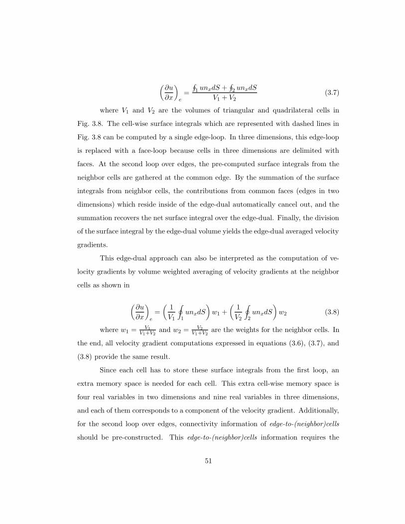
(∂u
∂x
)
e
=
∮
1 unxdS +∮
2 unxdS
V1 + V2(3.7)
where V1 and V2 are the volumes of triangular and quadrilateral cells in
Fig. 3.8. The cell-wise surface integrals which are represented with dashed lines in
Fig. 3.8 can be computed by a single edge-loop. In three dimensions, this edge-loop
is replaced with a face-loop because cells in three dimensions are delimited with
faces. At the second loop over edges, the pre-computed surface integrals from the
neighbor cells are gathered at the common edge. By the summation of the surface
integrals from neighbor cells, the contributions from common faces (edges in two
dimensions) which reside inside of the edge-dual automatically cancel out, and the
summation recovers the net surface integral over the edge-dual. Finally, the division
of the surface integral by the edge-dual volume yields the edge-dual averaged velocity
gradients.
This edge-dual approach can also be interpreted as the computation of ve-
locity gradients by volume weighted averaging of velocity gradients at the neighbor
cells as shown in
(∂u
∂x
)
e
=
(1
V1
∮
1unxdS
)
w1 +
(1
V2
∮
2unxdS
)
w2 (3.8)
where w1 = V1
V1+V2and w2 = V2
V1+V2are the weights for the neighbor cells. In
the end, all velocity gradient computations expressed in equations (3.6), (3.7), and
(3.8) provide the same result.
Since each cell has to store these surface integrals from the first loop, an
extra memory space is needed for each cell. This extra cell-wise memory space is
four real variables in two dimensions and nine real variables in three dimensions,
and each of them corresponds to a component of the velocity gradient. Additionally,
for the second loop over edges, connectivity information of edge-to-(neighbor)cells
should be pre-constructed. This edge-to-(neighbor)cells information requires the
51
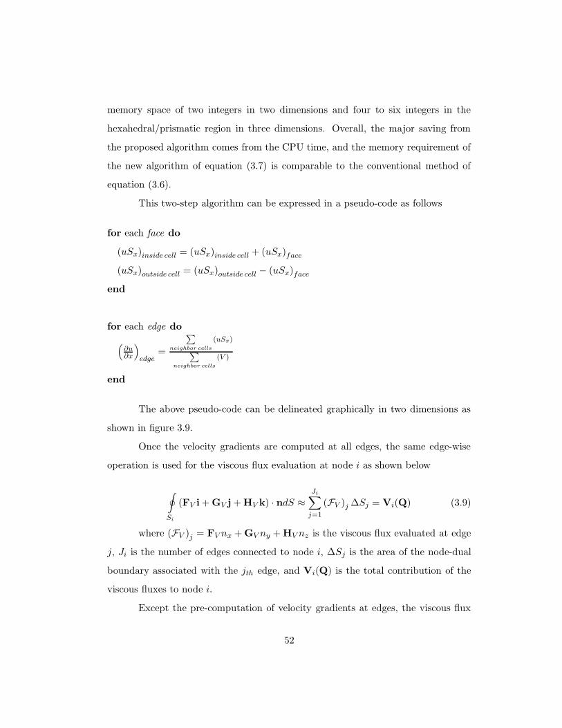
memory space of two integers in two dimensions and four to six integers in the
hexahedral/prismatic region in three dimensions. Overall, the major saving from
the proposed algorithm comes from the CPU time, and the memory requirement of
the new algorithm of equation (3.7) is comparable to the conventional method of
equation (3.6).
This two-step algorithm can be expressed in a pseudo-code as follows
for each face do
(uSx)inside cell = (uSx)inside cell + (uSx)face
(uSx)outside cell = (uSx)outside cell − (uSx)face
end
for each edge do
(∂u∂x
)
edge=
∑
neighbor cells
(uSx)
∑
neighbor cells
(V )
end
The above pseudo-code can be delineated graphically in two dimensions as
shown in figure 3.9.
Once the velocity gradients are computed at all edges, the same edge-wise
operation is used for the viscous flux evaluation at node i as shown below
∮
Si
(FV i + GV j + HV k) · ndS ≈Ji∑
j=1
(FV )j ∆Sj = Vi(Q) (3.9)
where (FV )j = FV nx + GV ny + HV nz is the viscous flux evaluated at edge
j, Ji is the number of edges connected to node i, ∆Sj is the area of the node-dual
boundary associated with the jth edge, and Vi(Q) is the total contribution of the
viscous fluxes to node i.
Except the pre-computation of velocity gradients at edges, the viscous flux
52
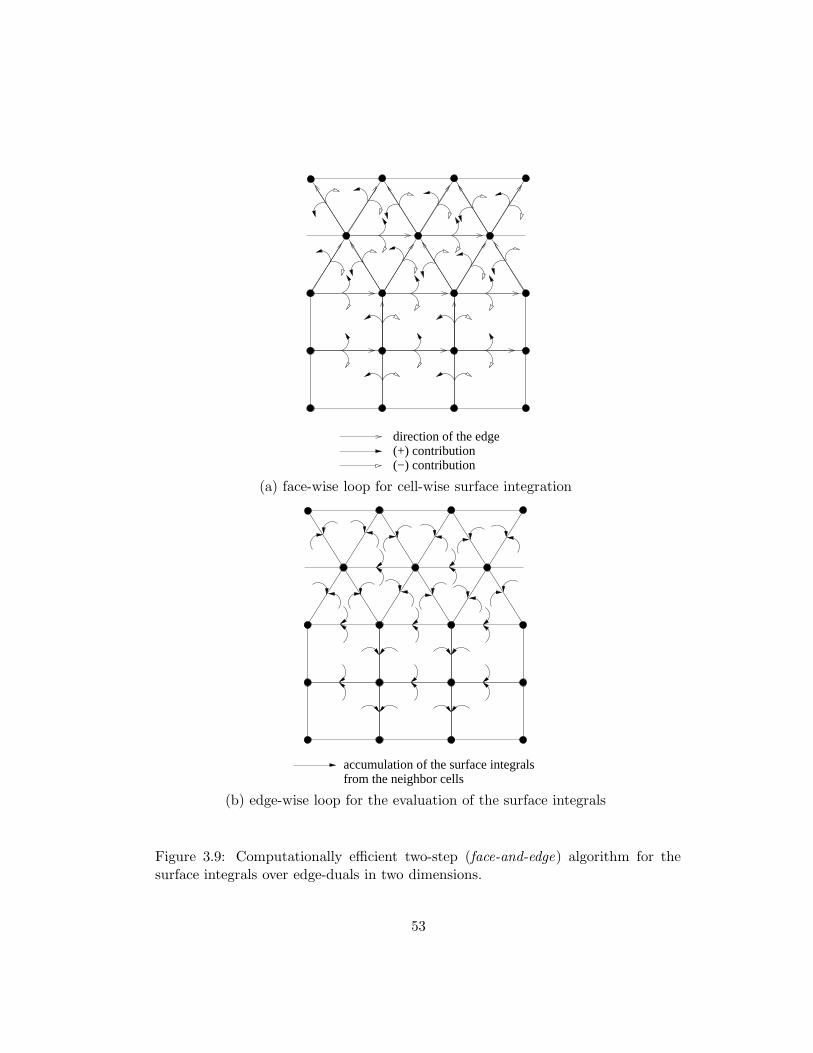
(+) contribution(−) contribution
direction of the edge
(a) face-wise loop for cell-wise surface integration
accumulation of the surface integralsfrom the neighbor cells
(b) edge-wise loop for the evaluation of the surface integrals
Figure 3.9: Computationally efficient two-step (face-and-edge) algorithm for thesurface integrals over edge-duals in two dimensions.
53
computation of Eq. (3.9) can be performed in an edge-wise fashion. This edge-wise
operation for viscous flux evaluation can be combined with the second step of the
face-and-edge algorithm as presented in the pseudo-code, hence the viscous flux
computation can be completed by a pair of face-and-edge loops.
3.4 Artificial Dissipation
Central difference schemes exhibit high frequency spurious oscillations of solutions,
and these oscillations are believed to be triggered by the nonlinear nature of the
governing equations. In order to suppress this high frequency oscillation, an addi-
tional smoothing term is needed. For flows with discontinuities, such as shocks, a
blend of second and fourth order difference artificial dissipation is used [32]. Cur-
rent simulations of incompressible flows, where the speed of sound is always greater
than flow speed, no such discontinuities exist. Hence, only fourth order difference
artificial dissipation is added to suppress the spurious oscillations.
The conventional scalar smoothing for a node i can be expressed as below
Di(Q) = −Ji∑
j=1
σ4ρij (δxxQj − δxxQi) (3.10)
Here, Ji is the number of nodes connected to node i by its neighbor edges,
ρij is an estimate of the spectral radius associated with the jth neighbor edge, and
δxx is an undivided second order difference operator defined as follows
δxxQi =Ji∑
j=1
(Qj −Qi) (3.11)
For nodes on the boundary, the contribution of the undivided Laplacian
is incomplete. Hence, the undivided Laplacian is extrapolated from the adjacent
nodes above the boundary down to the nodes on the boundary. The estimate of the
54
spectral radius scaled by the node-dual boundary associated with edge j is defined
as
ρij = (|un| + c)∆Sj (3.12)
where the velocity normal to the node dual boundary is
un = unx + vny + wnz
and the artificial speed of sound defined as follows
c =√
u2n + β
The spectral radius at each edge is scaled by the area of the node-dual bound-
ary ∆Sj associated with the edge j, and the normal velocity un is associated with
the direction normal to the node-dual boundary associated with the jth edge. This
scaling is often called individual eigenvalue scaling [82] and has been reported that
it is adequate for meshes with aspect ratios up to the order of O(10) [46].
By scaling the spectral radius with the node-dual boundary, the actual contri-
bution of artificial dissipation is dimensionally consistent with the surface integrals
of convective and viscous fluxes. Ideally, on a uniform mesh, the final contribution
of artificial dissipation when divided by the node-dual volume is
1
ViDi (Q) = σ4O
(
∆x3)
∇4Q
Therefore, the added artificial dissipation which is a third-order term should
not affect the spatial accuracy of the central difference scheme which is of second
order. However, on meshes with high aspect ratios, the artificial dissipation may
not be scaled properly [46, 83, 82]. Furthermore, a severe oscillation on hybrid
meshes has been reported by Haselbacher and Blazek [28] when the explicit Runge-
Kutta scheme is used in conjunction with a central scheme. Haselbacher and Blazek
proposed a modified artificial dissipation scheme as expressed below
55
Di(Q) = −Ji∑
j=1
σ4ρij (QL −QR) (3.13)
based on the difference of the reconstructed solutions (QL and QR) on the left
and the right side of the control volume boundary . Taylor series expansions are used
for solution reconstruction at the node-dual boundary as presented in equations (3.4)
and (3.5). Note that the artificial dissipation model expressed in equation (3.13)
results in a second-order accurate dissipation scheme which is equivalent to the
conventional artificial dissipation based on undivided Laplacians as expressed in
equation (3.13). If instead of using the Taylor series expansions, the left and right
states are simply chosen as the nodal states on both sides of the boundary, then the
second-order accurate dissipation scheme reduces to a first-order accurate scheme
as below
Di(Q) = −Ji∑
j=1
σ4ρij (Qi −Qj) (3.14)
3.5 Comparisons of dissipation models on a general hy-
brid mesh
Central differences with the two different artificial dissipation models as well as Roe’s
upwind scheme are tested for the investigation of their applicability to the general
hybrid meshes. The general hybrid mesh used for the current comparison of artificial
dissipation models is displayed in Figures 1.2 and 6.6. It includes local hexahedra
on the frontal viscous region of the cylinder, prisms in its rear half, pyramids at the
interface between the hexahedral and tetrahedral regions, and tetrahedra for the
rest.
The comparison between the central difference schemes with the conventional
artificial dissipation and the modified artificial dissipation based on the solution re-
56
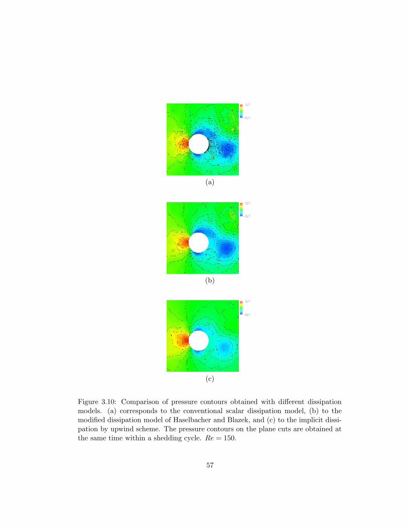
(a)
(b)
(c)
Figure 3.10: Comparison of pressure contours obtained with different dissipationmodels. (a) corresponds to the conventional scalar dissipation model, (b) to themodified dissipation model of Haselbacher and Blazek, and (c) to the implicit dissi-pation by upwind scheme. The pressure contours on the plane cuts are obtained atthe same time within a shedding cycle. Re = 150.
57

constructions are presented. The second order upwind scheme result is also included.
The pressure contours obtained by using the aforementioned schemes are displayed
in Fig. 3.10.
First, the conventional dissipation model shows severe oscillation in the pres-
sure contours, which indicates that the scheme is incapable of suppressing the solu-
tion oscillations on general hybrid meshes. Furthermore, as pointed by Haselbacher
and Blazek [28], this smoothing model shows a severe stability problem on hybrid
meshes when it is driven by the explicit Runge-Kutta time-stepping scheme which
is used in the current study.
The modified smoothing model of Haselbacher and Blazek [28] based on the
differences of the reconstructed solutions (Eq. (3.13)) is tested, and then compared
with the second order upwind scheme by using Roe’s flux-difference splitting. The
Haselbacher and Blazek’s scheme shows superior ability of suppressing the oscilla-
tions to the conventional dissipation scheme. The pressure contours are similar to
the ones yielded by the upwind scheme.
The computational cost of the modified smoothing is slightly higher than
the conventional smoothing due to the solution reconstruction step for each edge.
However, the modified smoothing is still less expensive than the upwind scheme,
because the upwind scheme requires the evaluation of Roe’s matrix at each edge.
In general, in the regions of highly stretched cells and anisotropic support of
the edges (eg. along the interfaces of prisms/hexahedra and tetrahedra/pyramids,
where only a single edge resides inside of the prismatic/hexahedral region), the
Haselbacher and Balzek dissipation model and upwind scheme yield more smooth
pressure contours than the conventional scalar dissipation model. Hence, for general
hybrid meshes, the central difference scheme with the modified dissipation model of
Haselbacher and Blazek or upwind schemes are preferred to the conventional scalar
dissipation model.
58
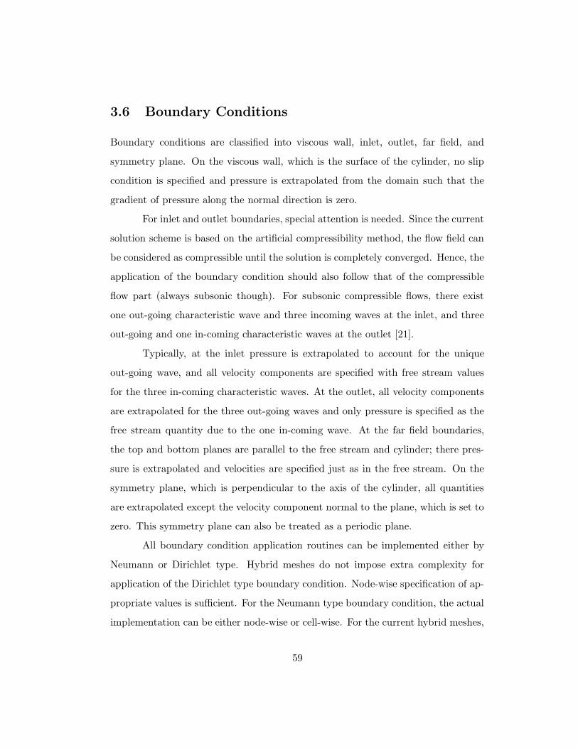
3.6 Boundary Conditions
Boundary conditions are classified into viscous wall, inlet, outlet, far field, and
symmetry plane. On the viscous wall, which is the surface of the cylinder, no slip
condition is specified and pressure is extrapolated from the domain such that the
gradient of pressure along the normal direction is zero.
For inlet and outlet boundaries, special attention is needed. Since the current
solution scheme is based on the artificial compressibility method, the flow field can
be considered as compressible until the solution is completely converged. Hence, the
application of the boundary condition should also follow that of the compressible
flow part (always subsonic though). For subsonic compressible flows, there exist
one out-going characteristic wave and three incoming waves at the inlet, and three
out-going and one in-coming characteristic waves at the outlet [21].
Typically, at the inlet pressure is extrapolated to account for the unique
out-going wave, and all velocity components are specified with free stream values
for the three in-coming characteristic waves. At the outlet, all velocity components
are extrapolated for the three out-going waves and only pressure is specified as the
free stream quantity due to the one in-coming wave. At the far field boundaries,
the top and bottom planes are parallel to the free stream and cylinder; there pres-
sure is extrapolated and velocities are specified just as in the free stream. On the
symmetry plane, which is perpendicular to the axis of the cylinder, all quantities
are extrapolated except the velocity component normal to the plane, which is set to
zero. This symmetry plane can also be treated as a periodic plane.
All boundary condition application routines can be implemented either by
Neumann or Dirichlet type. Hybrid meshes do not impose extra complexity for
application of the Dirichlet type boundary condition. Node-wise specification of ap-
propriate values is sufficient. For the Neumann type boundary condition, the actual
implementation can be either node-wise or cell-wise. For the current hybrid meshes,
59
both of the methods (node-wise and cell-wise) are used in order to take advantage
of the geometric characteristics of hybrid meshes. On the viscous wall, typically
very thin layers of hexahedral or prismatic cells are located with good normality
condition. Hence, on the wall, a node-wise extrapolation scheme is the best. On the
boundaries other than the viscous wall, the good normality condition is no longer
valid. Hence, the cell-wise extrapolation is employed. The cell-wise extrapolation
is composed of two steps. At the first step, a cell-averaged value is computed, and
then at the second step this cell averaged value is projected on the boundary face
and extrapolated to each one of boundary nodes by using inverse-distance weight-
ing. The weights for each one of the boundary nodes are pre-computed, and also
the sum of the weights is checked to be unity for all boundary nodes at which we
get the cell-wise extrapolation. This two extrapolation processes are delineated in
Figure 3.11 for two dimensional hybrid meshes and Figure 3.12 for three dimensional
general hybrid meshes.
60
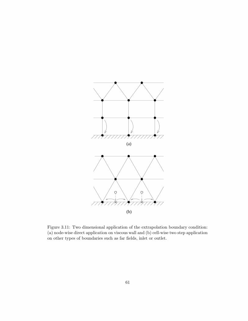
(b)
(a)
Figure 3.11: Two dimensional application of the extrapolation boundary condition:(a) node-wise direct application on viscous wall and (b) cell-wise two step applicationon other types of boundaries such as far fields, inlet or outlet.
61
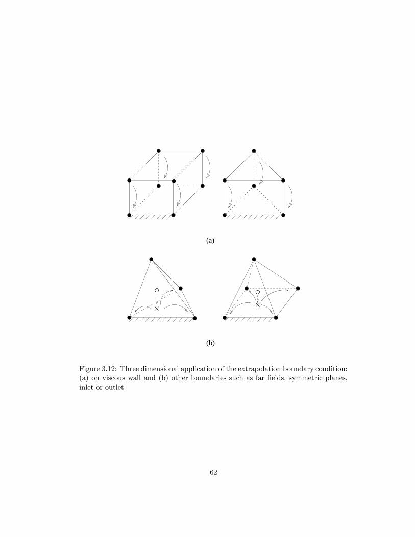
(b)
(a)
Figure 3.12: Three dimensional application of the extrapolation boundary condition:(a) on viscous wall and (b) other boundaries such as far fields, symmetric planes,inlet or outlet
62
3.7 Dual time-stepping scheme
Current time-accurate formulation of the artificial compressibility method includes
two different time evolution terms: one in true (physical) time t and the other
in pseudo time t∗. First, the true time-derivative term is discretized by using the
second order backward difference formula, and then the pseudo time-derivative term
is integrated until it reaches the steady state in pseudo time. Hence, the current
time-accurate simulation is driven by a series of steady state problems in pseudo-
time, and each of the steady state problems corresponds to a single true time-step.
Evaluating all flux contributions to the finite control volume Vi and adding
the supplementary artificial dissipation term, which is necessary for a central differ-
ence scheme, yields the dual time-stepping time accurate formulation
Pd
dt∗(QiVi) +
d
dt(UiVi) + Ci (Q) = Vi (Q) + Di (Q) (3.15)
where Ci (Q) is the convective flux, Vi (Q) is the viscous flux, and Di (Q)
is the added artificial dissipation.
If the upwind scheme is used, there is no need to include such an artificial
dissipation term. This is because the upwind scheme includes dissipation implicitly
in the numerical convective flux. The system of equations can be further simplified
to
Pd
dt∗(QiVi) + R∗
i (Q) = 0 (3.16)
by introducing the unsteady residual R∗
i (Q) defined as follows
R∗
i (Q) =3
2∆t
(
Un+1i V n+1
i
)
− 2
∆t(Un
i V ni ) +
1
2∆t
(
Un−1i V n−1
i
)
+ Ri (Q)
The unsteady residual R∗
i (Q) is the sum of the true time-derivative term
discretized by using the second order backward difference formula, and the steady
residual which includes all flux terms, defined by
63
Ri (Q) = Ci (Q) −Vi (Q) −Di (Q)
In order to advance a time step from the current time tn to the next time
tn+1 , the unsteady residual R∗(Q) is first constructed by discretizing the true time-
derivative with the implicit backward difference formula, and then the steady-state
problem shown in equation (3.16) is being solved in pseudo time. Once the steady-
state in pseudo-time is reached, the pseudo time-derivative vanishes and the solution
has been advanced to the next time step.
The dual time-stepping scheme is driven by the time integration scheme
for the pseudo steady-state problem. Therefore, the overall performance of the dual
time-stepping scheme is highly dependent on the efficiency of the steady-state solver
in pseudo time
d
dt∗
(
Qki Vi
)
+ P−1R∗
i
(
Qk)
= 0 (3.17)
An iterative scheme using a 5-stage scheme is used for solving the steady-state
problem in pseudo time. In the equation (3.17), k is the index for the iteration in
pseudo time. This iteration is referred to as the sub-iteration, because the iteration
loop is inside of the true time-stepping. In pseudo time-stepping there is no need
to preserve the transient temporal accuracy, so the local time-stepping is used for
convergence acceleration in pseudo time. The 5-stage multistage scheme used for
each subiteration is presented below
Q(0) = Qk
...
Q(l) = Q(0) − αl∆t∗i1Vi
P−1R∗
i
(
Q(l−1))
...
Qk+1 = Q(5)
(3.18)
64
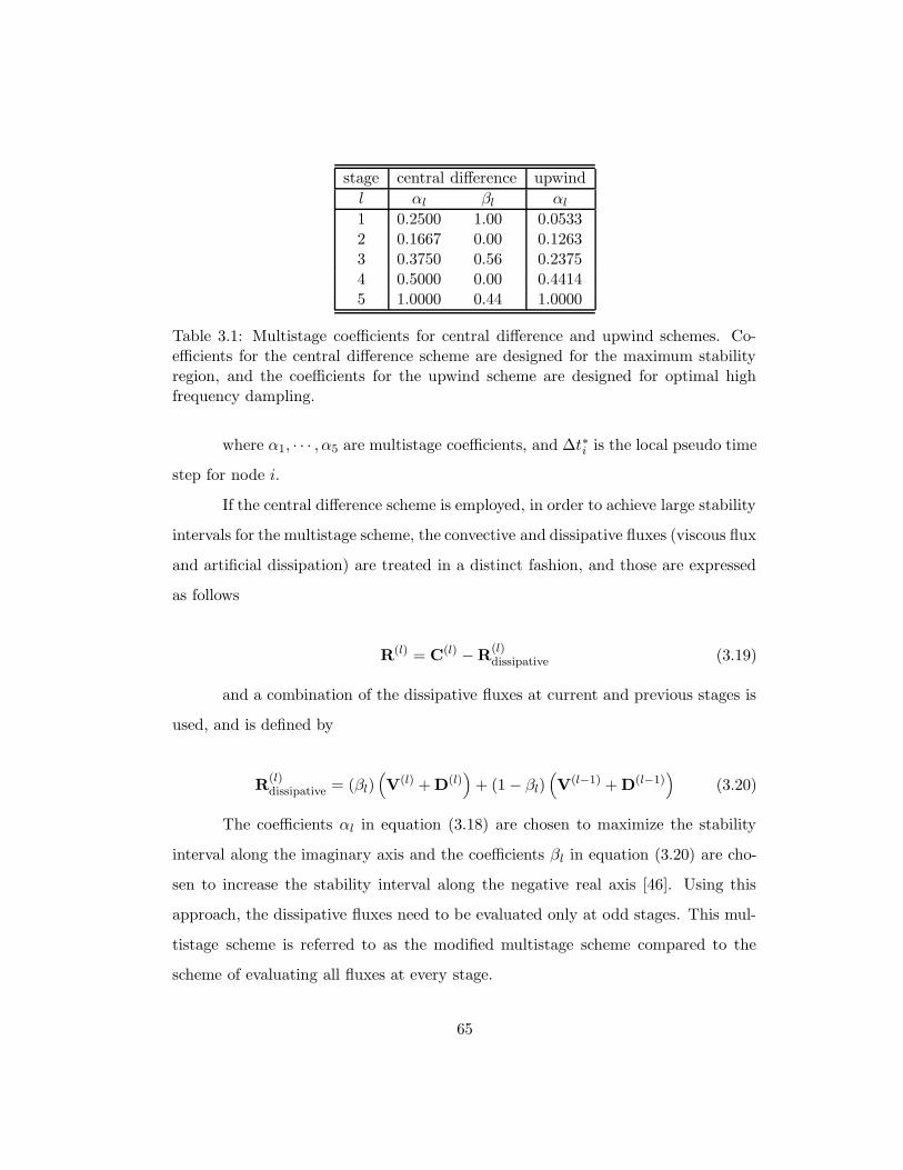
stage central difference upwind
l αl βl αl
1 0.2500 1.00 0.05332 0.1667 0.00 0.12633 0.3750 0.56 0.23754 0.5000 0.00 0.44145 1.0000 0.44 1.0000
Table 3.1: Multistage coefficients for central difference and upwind schemes. Co-efficients for the central difference scheme are designed for the maximum stabilityregion, and the coefficients for the upwind scheme are designed for optimal highfrequency dampling.
where α1, · · · , α5 are multistage coefficients, and ∆t∗i is the local pseudo time
step for node i.
If the central difference scheme is employed, in order to achieve large stability
intervals for the multistage scheme, the convective and dissipative fluxes (viscous flux
and artificial dissipation) are treated in a distinct fashion, and those are expressed
as follows
R(l) = C(l) −R(l)dissipative (3.19)
and a combination of the dissipative fluxes at current and previous stages is
used, and is defined by
R(l)dissipative = (βl)
(
V(l) + D(l))
+ (1 − βl)(
V(l−1) + D(l−1))
(3.20)
The coefficients αl in equation (3.18) are chosen to maximize the stability
interval along the imaginary axis and the coefficients βl in equation (3.20) are cho-
sen to increase the stability interval along the negative real axis [46]. Using this
approach, the dissipative fluxes need to be evaluated only at odd stages. This mul-
tistage scheme is referred to as the modified multistage scheme compared to the
scheme of evaluating all fluxes at every stage.
65
For the upwind scheme, all fluxes are evaluated at every stage. The multi-
stage coefficients α1, · · · , α5 for the upwind scheme are originally presented in [95].
They are designed for optimal high frequency damping. All the coefficients for the
multistage scheme are summarized in Table 3.1.
It was reported that the standard multistage scheme presented in equa-
tion (3.18) suffers from instability [49] if there is a high ratio of pseudo time step
to true time step ∆t∗/∆t . This is especially true when the local-pseudo time step
becomes very large at the cells near far field boundaries. This instability is caused
by the unsteady source term of the backward difference formula, and can be stabi-
lized by treating the term implicitly as proposed by Melson [49]. The modification
of the point-implicit multistage scheme is presented below
Q(0) = Qk
...
Q(l) = 11+αlλ
[
Q(0) − αl∆t∗i1Vi
R∗
i
(
Q(l−1))
+ αlλR∗
i
(
Q(l−1))]
...
Qk+1 = Q(m)
(3.21)
where λ = 32
∆t∗
∆t.
The point implicit treatment affects only the equations with true time-
derivatives. This affects the momentum equations and possibly the turbulent eddy
viscosity transport equation if it is treated in dual time-stepping unsteady form.
The continuity equation which does not have the true time-derivative is not af-
fected. Hence, for simplicity, the diagonal preconditioning matrix P is omitted in
the point implicit multistage formulation shown in Eq. (3.21), since its effect on the
momentum equations is the same as that of an identity matrix.
66
3.8 Time step calculation
The dual-time stepping scheme has two different time steps: the true time step and
the pseudo time step. The true time-stepping is discretized by using the A-stable
second order backward difference formula. This scheme is stable regardless of the
time step size. For the pseudo time-stepping scheme, which is driven by an explicit
multistage scheme, a time step calculation formula is needed. Current local pseudo
time step is calculated by using both convection and diffusion limits which were
originally proposed by Kallinderis [34].
The local pseudo time step for node i is computed by
∆t∗i = ωVi
Ax + Ay + Az + D(3.22)
where
Ax = (|u| + cx)Sx
Ay = (|v| + cy) Sy
Az = (|w| + cz) Sz
D = 21
Re
Vi
Sx + Sy + Sz
The artificial speeds of sound in each coordinate direction are given by
cx =√
u2 + β
cy =√
v2 + β
cz =√
w2 + β
67
and the projected areas of the node-dual volume are defined as follows
Sx =1
2
∑
e
|Sx|e
Sy =1
2
∑
e
|Sy|e
Sz =1
2
∑
e
|Sz|e
where Sx, Sy, and Sz are the components of the area normal vector.
The weighting factor ω may be considered as the local Courant number of
the CFL (Courant, Friedrichs, and Lewy) condition.
68

Chapter 4
2D Verification and Validation
Study
The proposed Navier-Stokes method is verified and validated for two dimensional
applications. Spatial accuracy is verified by a mesh refinement study and temporal
accuracy is demonstrated by a time step refinement study. Robustness of the pro-
posed scheme is tested with high aspect ratio cells and small size cells on 2D hybrid
meshes. The result is validated by the comparisons with available experimental and
computational results.
69
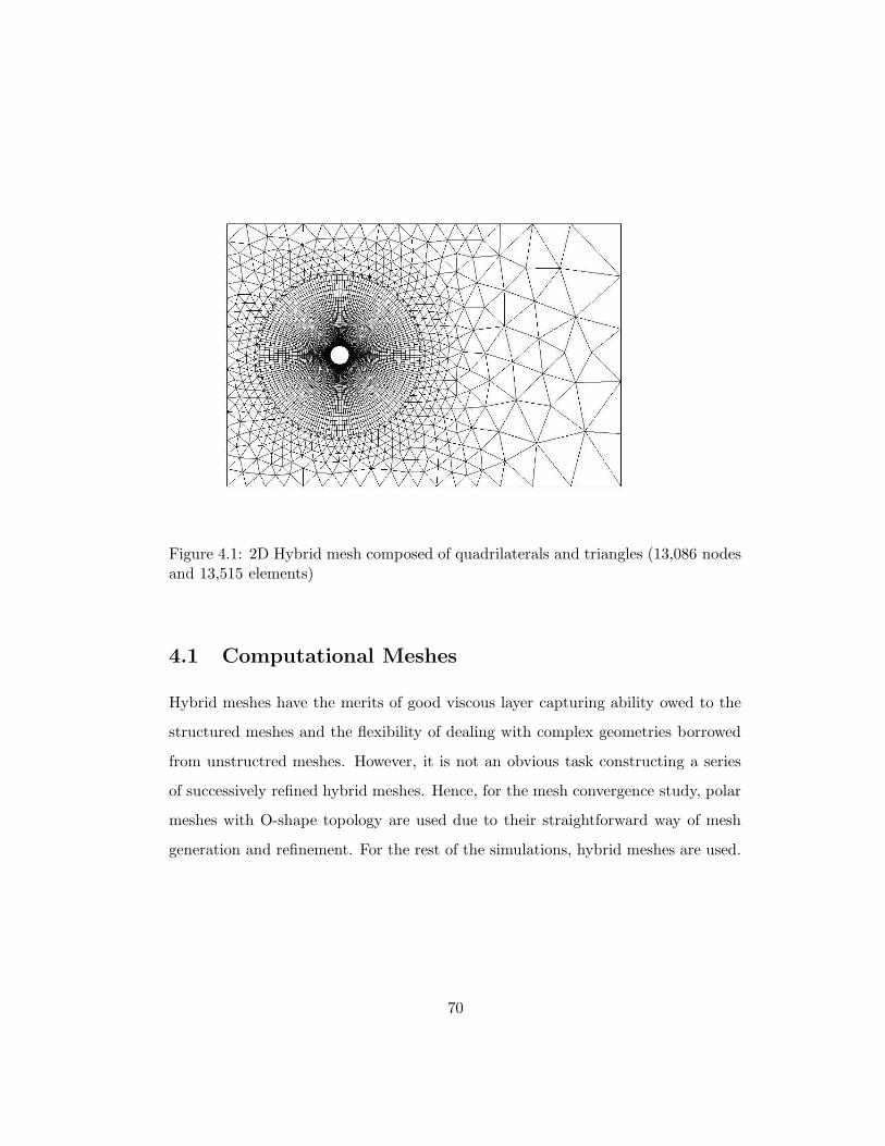
Figure 4.1: 2D Hybrid mesh composed of quadrilaterals and triangles (13,086 nodesand 13,515 elements)
4.1 Computational Meshes
Hybrid meshes have the merits of good viscous layer capturing ability owed to the
structured meshes and the flexibility of dealing with complex geometries borrowed
from unstructred meshes. However, it is not an obvious task constructing a series
of successively refined hybrid meshes. Hence, for the mesh convergence study, polar
meshes with O-shape topology are used due to their straightforward way of mesh
generation and refinement. For the rest of the simulations, hybrid meshes are used.
70
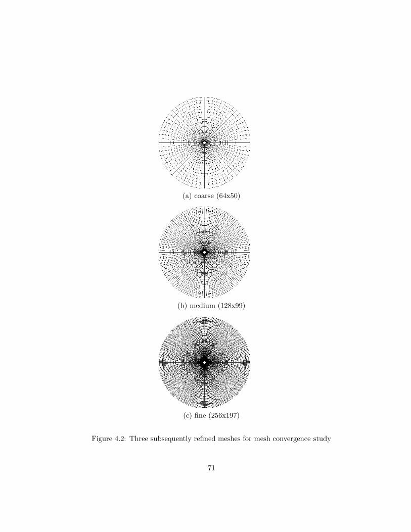
(a) coarse (64x50)
(b) medium (128x99)
(c) fine (256x197)
Figure 4.2: Three subsequently refined meshes for mesh convergence study
71
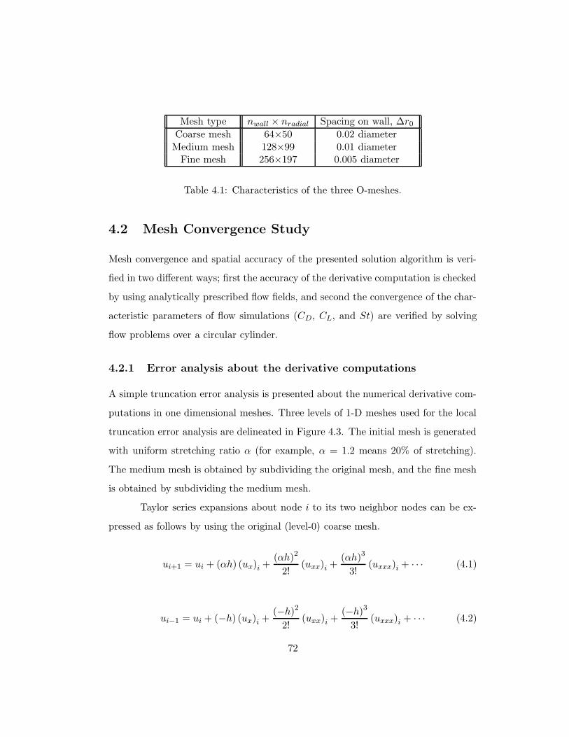
Mesh type nwall × nradial Spacing on wall, ∆r0
Coarse mesh 64×50 0.02 diameterMedium mesh 128×99 0.01 diameter
Fine mesh 256×197 0.005 diameter
Table 4.1: Characteristics of the three O-meshes.
4.2 Mesh Convergence Study
Mesh convergence and spatial accuracy of the presented solution algorithm is veri-
fied in two different ways; first the accuracy of the derivative computation is checked
by using analytically prescribed flow fields, and second the convergence of the char-
acteristic parameters of flow simulations (CD, CL, and St) are verified by solving
flow problems over a circular cylinder.
4.2.1 Error analysis about the derivative computations
A simple truncation error analysis is presented about the numerical derivative com-
putations in one dimensional meshes. Three levels of 1-D meshes used for the local
truncation error analysis are delineated in Figure 4.3. The initial mesh is generated
with uniform stretching ratio α (for example, α = 1.2 means 20% of stretching).
The medium mesh is obtained by subdividing the original mesh, and the fine mesh
is obtained by subdividing the medium mesh.
Taylor series expansions about node i to its two neighbor nodes can be ex-
pressed as follows by using the original (level-0) coarse mesh.
ui+1 = ui + (αh) (ux)i +(αh)2
2!(uxx)i +
(αh)3
3!(uxxx)i + · · · (4.1)
ui−1 = ui + (−h) (ux)i +(−h)2
2!(uxx)i +
(−h)3
3!(uxxx)i + · · · (4.2)
72

uu ui−1 i i+1
x
h α h
h/2 h/2 h/2h/2α α
x
(coarse)
(medium)
(fine)
level−0
level−1
h/4 h/4 h/4 h/4 h/4 h/4 h/4 h/4α α α α
xlevel−2
Figure 4.3: Three levels of 1-D meshes. The original level-0 (coarse) mesh is gener-ated with uniform stretching ratio α. The medium mesh is obtained by subdividingthe coarse mesh and the fine mesh is obtained by subdividing the medium mesh.
Substracting equation 4.1 from equation 4.2 yields
ui+1 − ui−1
αh + h= (ux)i +
(α2h2 − h2
)
2! (αh + h)(uxx)i + H.O.T.
Then the local truncation error at node i for the first order derivative (ux)
computation is
(T.E.)ux=
(
α2h2 − h2)
2! (αh + h)(uxx)i + H.O.T.
and by rearranging the leading order term the local truncation error is
(T.E.)ux= (α − 1)O (h) (uxx)i
73
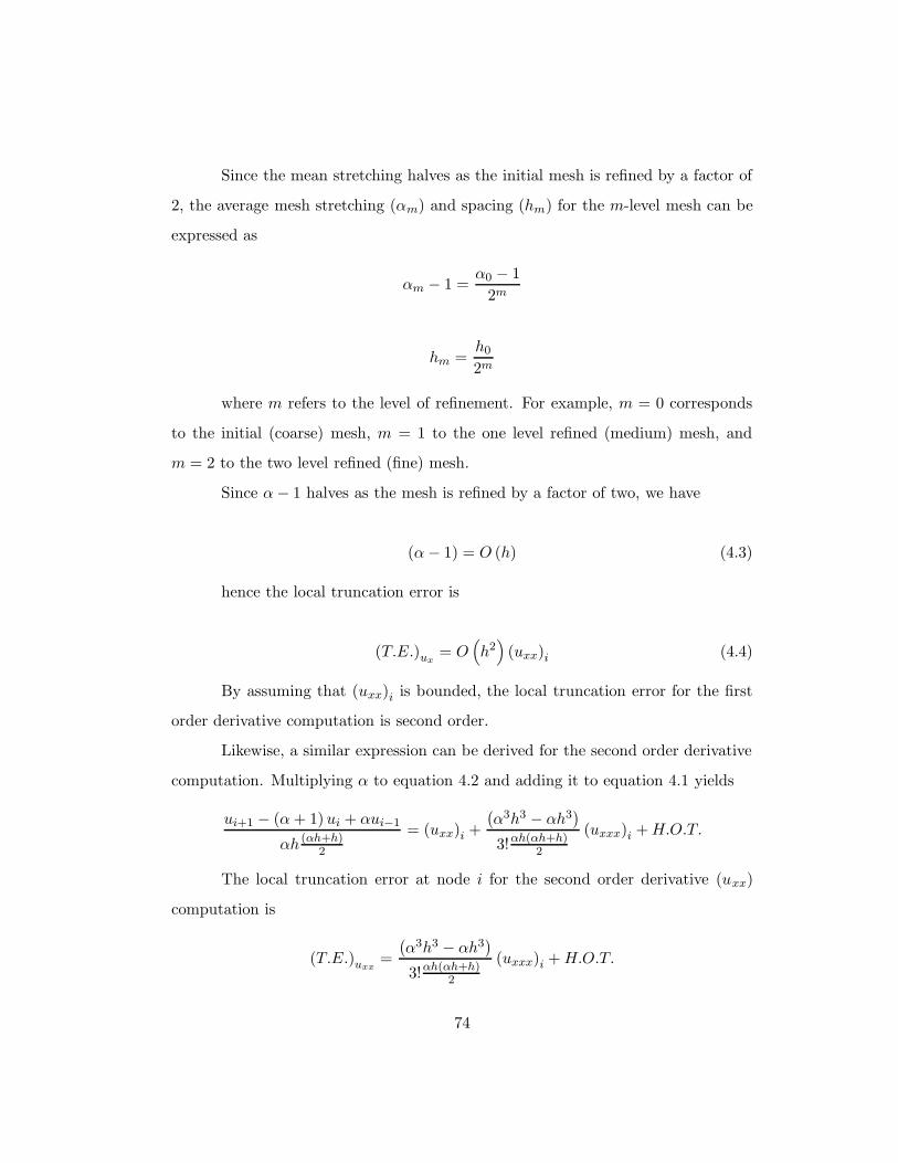
Since the mean stretching halves as the initial mesh is refined by a factor of
2, the average mesh stretching (αm) and spacing (hm) for the m-level mesh can be
expressed as
αm − 1 =α0 − 1
2m
hm =h0
2m
where m refers to the level of refinement. For example, m = 0 corresponds
to the initial (coarse) mesh, m = 1 to the one level refined (medium) mesh, and
m = 2 to the two level refined (fine) mesh.
Since α − 1 halves as the mesh is refined by a factor of two, we have
(α − 1) = O (h) (4.3)
hence the local truncation error is
(T.E.)ux= O
(
h2)
(uxx)i (4.4)
By assuming that (uxx)i is bounded, the local truncation error for the first
order derivative computation is second order.
Likewise, a similar expression can be derived for the second order derivative
computation. Multiplying α to equation 4.2 and adding it to equation 4.1 yields
ui+1 − (α + 1) ui + αui−1
αh (αh+h)2
= (uxx)i +
(
α3h3 − αh3)
3!αh(αh+h)2
(uxxx)i + H.O.T.
The local truncation error at node i for the second order derivative (uxx)
computation is
(T.E.)uxx=
(
α3h3 − αh3)
3!αh(αh+h)2
(uxxx)i + H.O.T.
74

and by rearranging the leading order term, the local truncation error is
(T.E.)uxx= (α − 1) O (h) (uxxx)i
Using equation (4.3), the local truncation error for the uxx computation is
given by
(T.E.)uxx= O
(
h2)
(uxxx)i (4.5)
With bounded (uxxx)i , the local truncation error for the second order deriva-
tive computation is also second order.
4.2.2 Analytic field function test
When the analytic solution exists, the error can be computed directly by comparing
the numerical solution with the exact solution. For current applications where no
exact solution exists, comparison of the results of a few representative differential
operators can be used as a measure of spatial accuracy of the current discretization
scheme. Two differential operators appearing in the Navier-Stokes equations are
chosen to mimic flux computation employed by the flow solver. The divergence
operator is chosen to represent the convective flux computation and the Laplacian
operator is chosen for the viscous flux evaluation.
In order to measure the error of numerical derivatives of a given vector field,
first prescribe an analytical velocity field (hence uh = uexact already), and then
compute numerical derivatives by using the spatial discretization employed, and
finally compare the computed derivatives with the exact derivatives.
An analytic velocity field used for the derivative computations is defined by
U = sin (x) i + cos (y) j
and the error is measured as follows
75
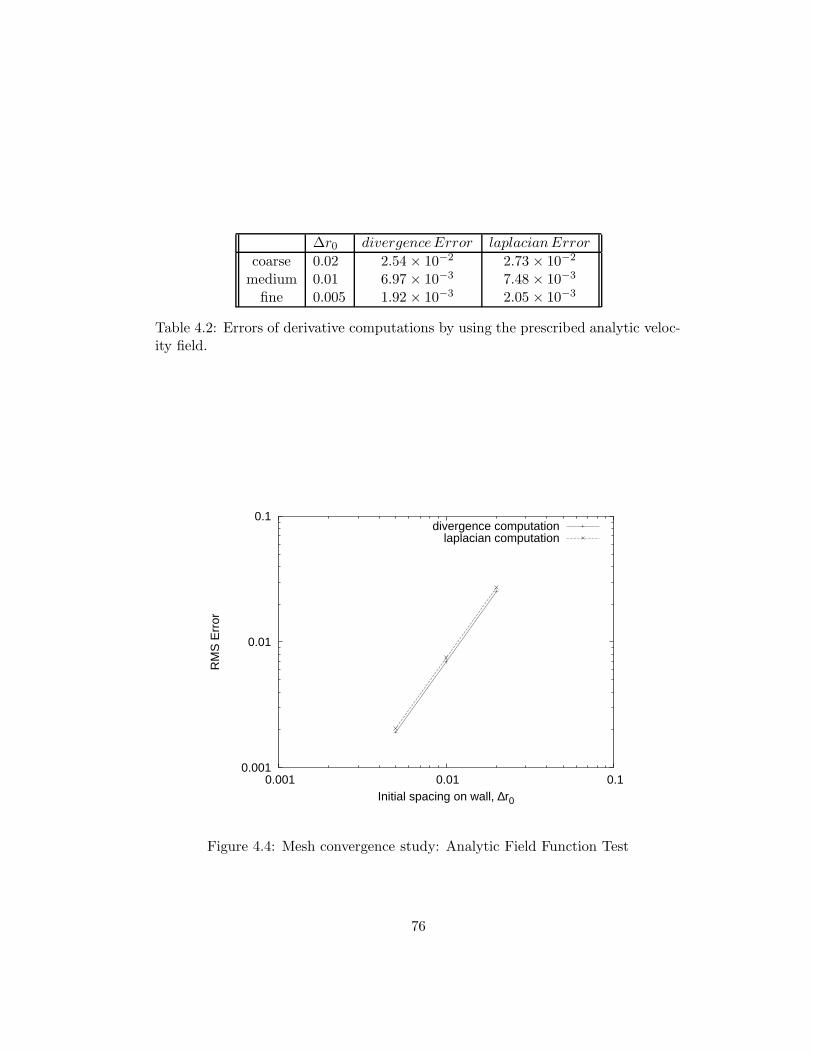
∆r0 divergenceError laplacianError
coarse 0.02 2.54 × 10⁻² 2.73 × 10⁻²
medium 0.01 6.97 × 10⁻³ 7.48 × 10⁻³
fine 0.005 1.92 × 10⁻³ 2.05 × 10⁻³
Table 4.2: Errors of derivative computations by using the prescribed analytic veloc-ity field.
0.001
0.01
0.1
0.001 0.01 0.1
RM
S E
rror
Initial spacing on wall, ∆r0
divergence computationlaplacian computation
Figure 4.4: Mesh convergence study: Analytic Field Function Test
76

divergenceError∆r =
√√√√√
NI∑
i=1|(∇ ·U)∆r − (∇ · U)exact|
2
NI
laplacianError∆r =
√√√√√
NI∑
i=1‖(∇2U)∆r − (∇2U)exact‖
2
NI
where NI is the number of interior nodes. The actual values of error for the
three meshes considered are summarized in Table 4.2 and plotted in Figure 4.4.
The accuracy of derivative computations can be estimated by the technique
of Richardson’s deferred approach to the limit [66, 7] as follows
log2
(divergenceError∆r=0.01
divergenceError∆r=0.005
)
= 1.860
log2
(laplacianError∆r=0.01
laplacianError∆r=0.005
)
= 1.867
Both of the derivative computation is nearly second order accurate and this
agrees well with the 1D analysis as presented in equations (4.4) and (4.5). The slight
discrepancy seems due to the higher spatial dimension.
4.2.3 Unsteady flows around a cylinder
Flow around an impulsively started cylinder is tested for Re = 150. The second
order backward difference scheme is used for discretizing the true time-derivative
and the time step is fixed to ∆t = 0.1 for all three cases.
Figure 4.5 shows the histories of drag and lift coefficients (CD and CL) for
three different simulations, and their convergence as the mesh is refined. A de-
tailed comparison of CD , CL , shedding period T , and Strouhal frequency St are
summarized in Table 4.3.
77
0 10 20 30 40 50 60 70 80 90 1001
1.1
1.2
1.3
1.4
1.5
1.6
CD
Coarse MeshMedium MeshFine Mesh
0 10 20 30 40 50 60 70 80 90 100−1
−0.5
0
0.5
1
Time
CL
Figure 4.5: Mesh refinement study, Re = 150
Mesh type CD CL T St
Coarse mesh 1.3185 ± 0.0195 ± 0.462 5.8 0.172Medium mesh 1.3330 ± 0.0250 ± 0.505 5.5 0.182
Fine mesh 1.3335 ± 0.0265 ± 0.517 5.4 0.185
Table 4.3: Mesh refinement study for Re = 150
78
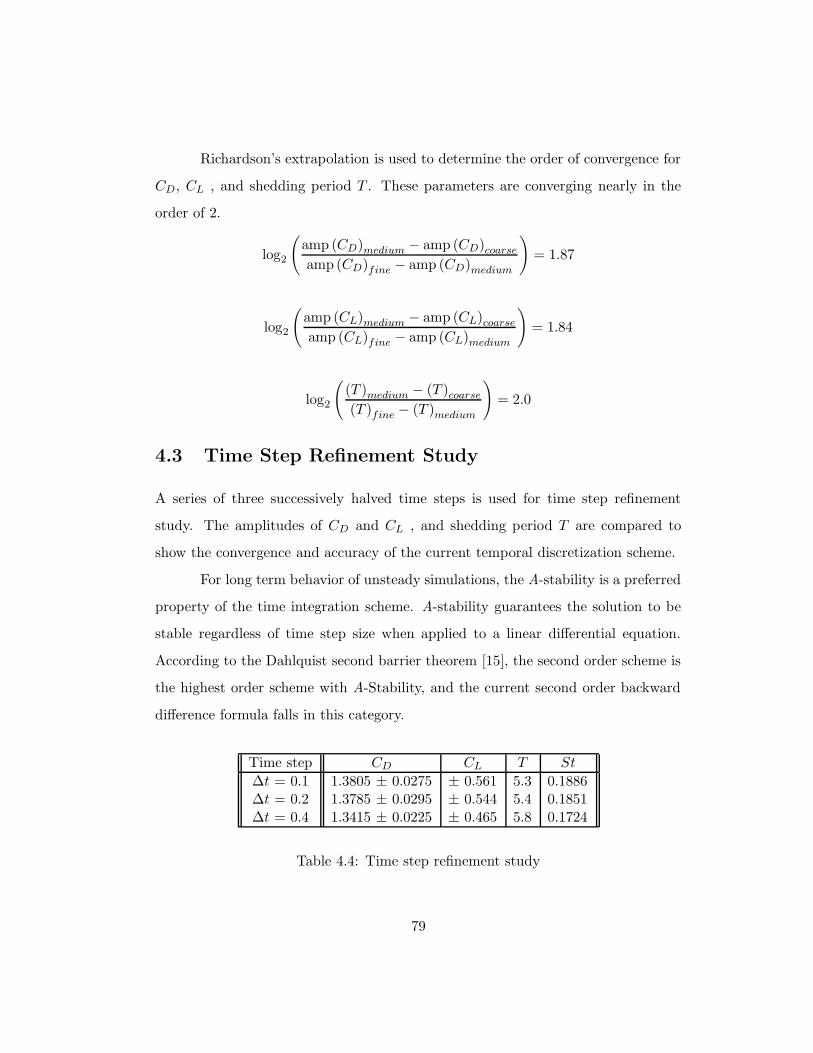
Richardson’s extrapolation is used to determine the order of convergence for
CD, CL , and shedding period T . These parameters are converging nearly in the
order of 2.
log2
(
amp (CD)medium − amp (CD)coarse
amp (CD)fine − amp (CD)medium
)
= 1.87
log2
(
amp (CL)medium − amp (CL)coarse
amp (CL)fine − amp (CL)medium
)
= 1.84
log2
(
(T )medium − (T )coarse
(T )fine − (T )medium
)
= 2.0
4.3 Time Step Refinement Study
A series of three successively halved time steps is used for time step refinement
study. The amplitudes of CD and CL , and shedding period T are compared to
show the convergence and accuracy of the current temporal discretization scheme.
For long term behavior of unsteady simulations, the A-stability is a preferred
property of the time integration scheme. A-stability guarantees the solution to be
stable regardless of time step size when applied to a linear differential equation.
According to the Dahlquist second barrier theorem [15], the second order scheme is
the highest order scheme with A-Stability, and the current second order backward
difference formula falls in this category.
Time step CD CL T St
∆t = 0.1 1.3805 ± 0.0275 ± 0.561 5.3 0.1886∆t = 0.2 1.3785 ± 0.0295 ± 0.544 5.4 0.1851∆t = 0.4 1.3415 ± 0.0225 ± 0.465 5.8 0.1724
Table 4.4: Time step refinement study
79
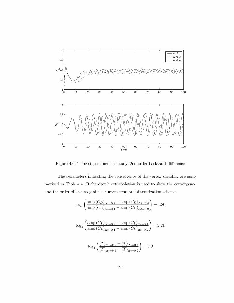
0 10 20 30 40 50 60 70 80 90 1001
1.2
1.4
1.6
1.8
CD
∆t=0.1∆t=0.2∆t=0.4
0 10 20 30 40 50 60 70 80 90 100−1
−0.5
0
0.5
1
Time
CL
Figure 4.6: Time step refinement study, 2nd order backward difference
The parameters indicating the convergence of the vortex shedding are sum-
marized in Table 4.4. Richardson’s extrapolation is used to show the convergence
and the order of accuracy of the current temporal discretization scheme.
log2
(
amp (CD)∆t=0.2 − amp (CD)∆t=0.4
amp (CD)∆t=0.1 − amp (CD)∆t=0.2
)
= 1.80
log2
(
amp (CL)∆t=0.2 − amp (CL)∆t=0.4
amp (CL)∆t=0.1 − amp (CL)∆t=0.2
)
= 2.21
log2
(
(T )∆t=0.2 − (T )∆t=0.4
(T )∆t=0.1 − (T )∆t=0.2
)
= 2.0
80
4.4 High aspect ratio cell effect
For viscous flow simulations, it is typical that high aspect ratio cells are located
near the viscous wall to capture the development of the boundary layer. These high
aspect ratio cells may prevent the proper scaling of the artificial dissipation. In order
to check if the current artificial dissipation model can be used for those high aspect
ratio cells, two dimensional hybrid meshes are tested and compared with different
aspect ratio cells in the viscous region. The close-up views of the two hybrid meshes
with different aspect ratio cells are presented in Figure 4.7. The pressure contours on
the hybrid meshes are compared in Figure 4.8. Both of the two meshes show smooth
and similar patterns of pressure contours around the cylinder, which is supporting
the fact that the current individual eigenvalue scaling as presented in Eq. (3.12) can
be used with cells of high aspect ratio at least up to 50.
4.5 Small size cell effect
Small size cells are encountered not only in the viscous region but also in the region
away from it. These small cells may deteriorate the overall convergence of the
solution if time-accurate explicit scheme is used. In the traditional time-accurate
explicit scheme, the time steps are scaled by the smallest cell size. If the mesh
is successively refined several times, a very small cell can appear even in a region
away from the viscous region. The current time-marching scheme is tested on such
meshes with small cells in the wake region, in order to show the robustness of the
dual time-stepping scheme over the traditional explicit scheme.
Fig. 4.9 shows the comparison of the original and redistributed mesh, where
small cells appear in the wake region. These small size cells may lead to overall
convergence deterioration if the pseudo time steps of the small cells govern the
global convergence rate. This is not the case of the current local pseudo time-
81
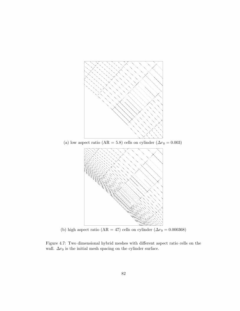
(a) low aspect ratio (AR = 5.8) cells on cylinder (∆r0 = 0.003)
(b) high aspect ratio (AR = 47) cells on cylinder (∆r0 = 0.000368)
Figure 4.7: Two dimensional hybrid meshes with different aspect ratio cells on thewall. ∆r0 is the initial mesh spacing on the cylinder surface.
82

(a) low aspect ratio mesh
(b) high aspect ratio mesh
Figure 4.8: Pressure contours on 2D hybrid meshes with different aspect ratios;moderate aspect ratio cells on the wall (a), and high aspect ratio cells on the wall(b). Pressure contours are taken approximately at the same time within a sheddingcycle.
83
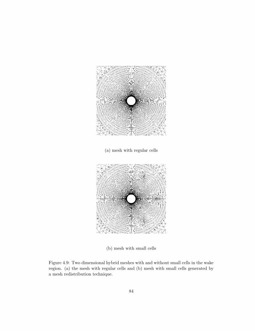
(a) mesh with regular cells
(b) mesh with small cells
Figure 4.9: Two dimensional hybrid meshes with and without small cells in the wakeregion. (a) the mesh with regular cells and (b) mesh with small cells generated bya mesh redistribution technique.
84
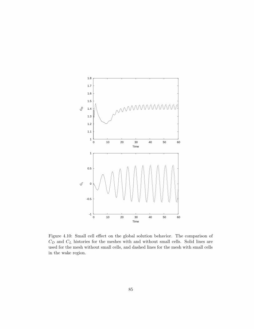
1
1.1
1.2
1.3
1.4
1.5
1.6
1.7
1.8
0 10 20 30 40 50 60
CD
Time
-1
-0.5
0
0.5
1
0 10 20 30 40 50 60
CL
Time
Figure 4.10: Small cell effect on the global solution behavior. The comparison ofCD and CL histories for the meshes with and without small cells. Solid lines areused for the mesh without small cells, and dashed lines for the mesh with small cellsin the wake region.
85
stepping scheme, since solution at every cell is updated with its own local time step,
and this local time step does not affect the time steps of other cells. As shown in
Figure 4.10, these small cells in the wake region do not affect the global solution (CD
and CL) histories. This strengthens the idea that dual time-stepping scheme can be
used with meshes of small cells without great sacrifice of convergence or accuracy.
4.6 Convergence Criterion
For implicit unsteady simulations, there should be appropriate convergence criteri-
ons to determine solution convergence at each time step. Several different criterions
can be used. For example, divergence of the velocity field, maximum or root mean
squared (RMS) residuals, or net mass accumulation over the entire computational
domain may be the parameter indicating overall solution convergence.
Rogers and Kwak [73] reported that driving maximum divergence of velocity
field less than 10−3 gives converged solution and this ensures enough accuracy on
drag and lift coefficients for the cylinder flow on a structured mesh. In order to be
sure about the solution accuracy of the unsteady simulation with hybrid meshes,
two different convergence criteria are tested: one is subiterating until the Residual
gets under a certain level, and the other pre-specifying the number of subiterations.
For the first creterion, the maximum continuity residual is chosen to be
the parameter indicating the overall convergence of solution. Sub-iterations are
performed until the maximum continuity residual gets less than 10−1, 10−2 , and
10−3 . As shown in figure 4.11 the CD and CL history indicate a converged result
when the maximum residual drops below 10−2.
For the second criterion, as presented in Figure 4.12, a series of different
numbers of subiterations (40, 80, and 160) are pre-specified and the results are
compared to show the convergence depending on the number of subiterations. A
fixed number of subiterations more than 80 shows a converged result in CD and
86
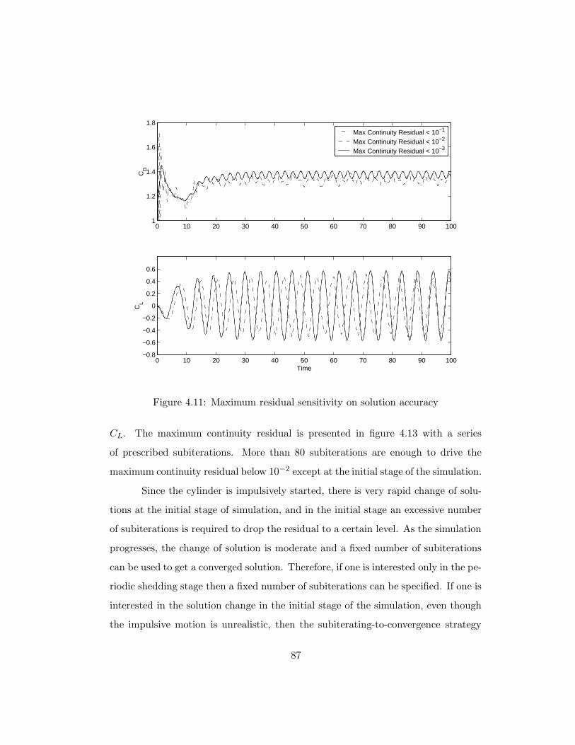
0 10 20 30 40 50 60 70 80 90 1001
1.2
1.4
1.6
1.8
CD
Max Continuity Residual < 10−1
Max Continuity Residual < 10−2
Max Continuity Residual < 10−3
0 10 20 30 40 50 60 70 80 90 100−0.8
−0.6
−0.4
−0.2
0
0.2
0.4
0.6
Time
CL
Figure 4.11: Maximum residual sensitivity on solution accuracy
CL. The maximum continuity residual is presented in figure 4.13 with a series
of prescribed subiterations. More than 80 subiterations are enough to drive the
maximum continuity residual below 10−2 except at the initial stage of the simulation.
Since the cylinder is impulsively started, there is very rapid change of solu-
tions at the initial stage of simulation, and in the initial stage an excessive number
of subiterations is required to drop the residual to a certain level. As the simulation
progresses, the change of solution is moderate and a fixed number of subiterations
can be used to get a converged solution. Therefore, if one is interested only in the pe-
riodic shedding stage then a fixed number of subiterations can be specified. If one is
interested in the solution change in the initial stage of the simulation, even though
the impulsive motion is unrealistic, then the subiterating-to-convergence strategy
87
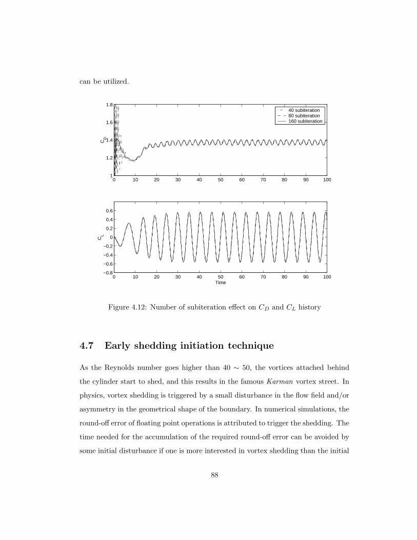
can be utilized.
0 10 20 30 40 50 60 70 80 90 1001
1.2
1.4
1.6
1.8C
D
40 subiteration80 subiteration160 subiteration
0 10 20 30 40 50 60 70 80 90 100−0.8
−0.6
−0.4
−0.2
0
0.2
0.4
0.6
Time
CL
Figure 4.12: Number of subiteration effect on CD and CL history
4.7 Early shedding initiation technique
As the Reynolds number goes higher than 40 ∼ 50, the vortices attached behind
the cylinder start to shed, and this results in the famous Karman vortex street. In
physics, vortex shedding is triggered by a small disturbance in the flow field and/or
asymmetry in the geometrical shape of the boundary. In numerical simulations, the
round-off error of floating point operations is attributed to trigger the shedding. The
time needed for the accumulation of the required round-off error can be avoided by
some initial disturbance if one is more interested in vortex shedding than the initial
88
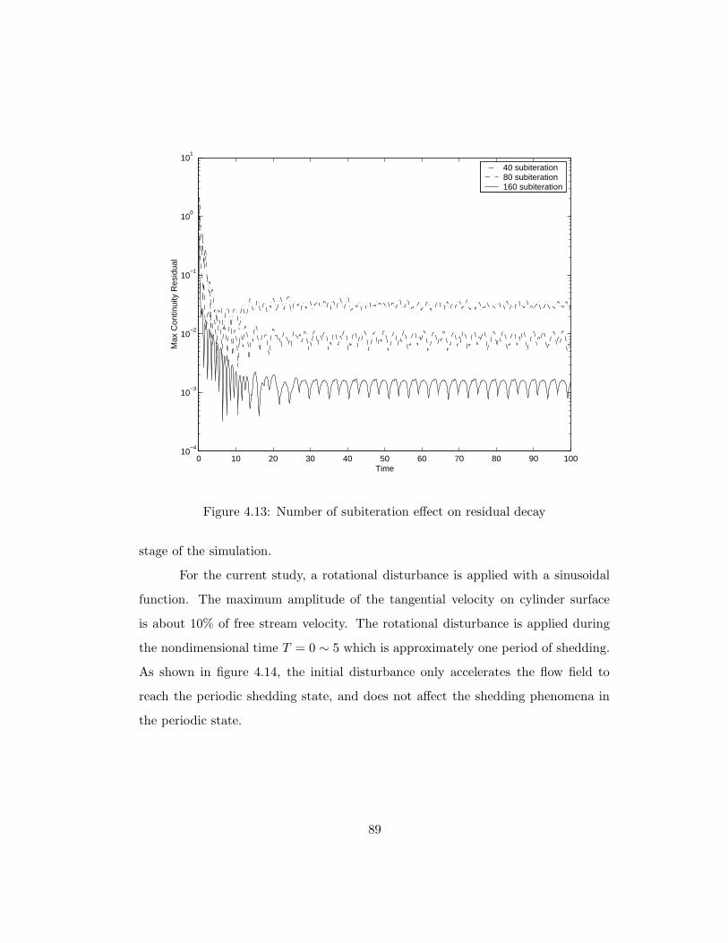
0 10 20 30 40 50 60 70 80 90 10010
−4
10−3
10−2
10−1
100
101
Time
Max
Con
tinui
ty R
esid
ual
40 subiteration80 subiteration160 subiteration
Figure 4.13: Number of subiteration effect on residual decay
stage of the simulation.
For the current study, a rotational disturbance is applied with a sinusoidal
function. The maximum amplitude of the tangential velocity on cylinder surface
is about 10% of free stream velocity. The rotational disturbance is applied during
the nondimensional time T = 0 ∼ 5 which is approximately one period of shedding.
As shown in figure 4.14, the initial disturbance only accelerates the flow field to
reach the periodic shedding state, and does not affect the shedding phenomena in
the periodic state.
89
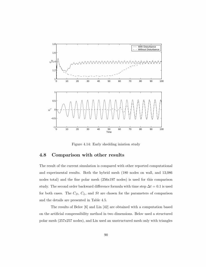
0 10 20 30 40 50 60 70 80 90 1001
1.2
1.4
1.6
1.8
CD
With DisturbanceWithout Disturbance
0 10 20 30 40 50 60 70 80 90 100−1
−0.5
0
0.5
1
Time
CL
Figure 4.14: Early shedding iniation study
4.8 Comparison with other results
The result of the current simulation is compared with other reported computational
and experimental results. Both the hybrid mesh (180 nodes on wall, and 13,086
nodes total) and the fine polar mesh (256x197 nodes) is used for this comparison
study. The second order backward difference formula with time step ∆t = 0.1 is used
for both cases. The CD, CL, and St are chosen for the parameters of comparison
and the details are presented in Table 4.5.
The results of Belov [6] and Lin [42] are obtained with a computation based
on the artificial compressibility method in two dimensions. Belov used a structured
polar mesh (257x257 nodes), and Lin used an unstructured mesh only with triangles
90
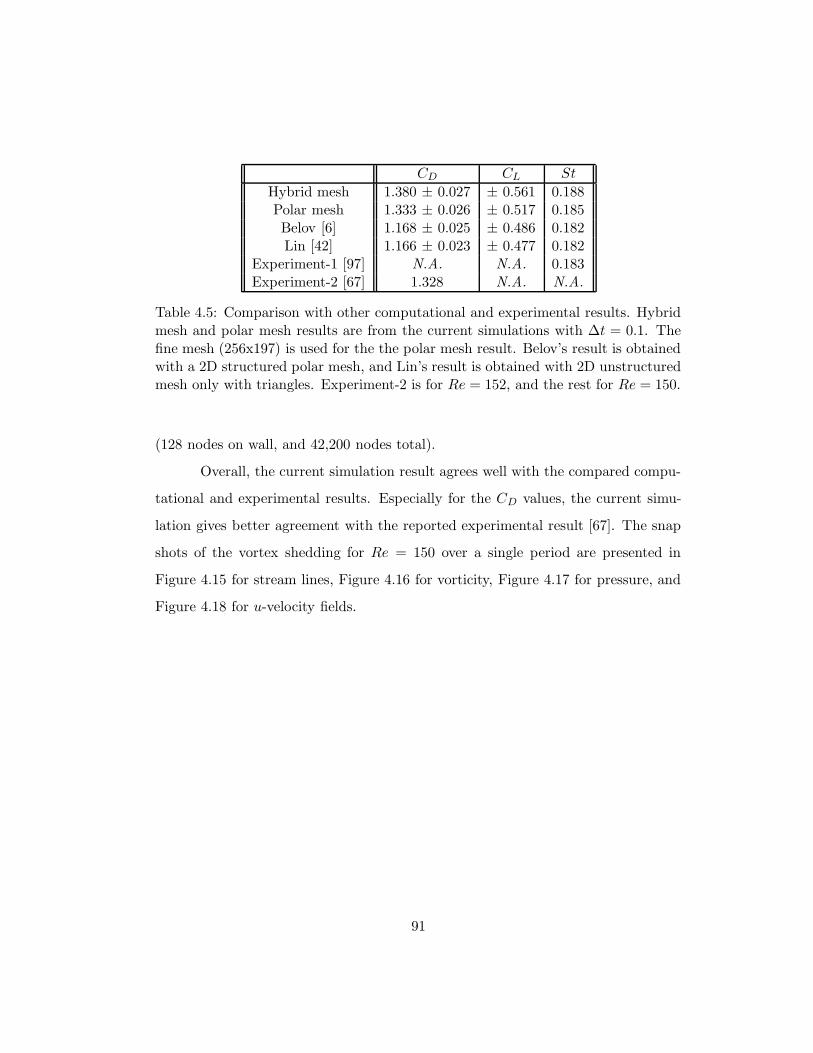
CD CL St
Hybrid mesh 1.380 ± 0.027 ± 0.561 0.188Polar mesh 1.333 ± 0.026 ± 0.517 0.185Belov [6] 1.168 ± 0.025 ± 0.486 0.182Lin [42] 1.166 ± 0.023 ± 0.477 0.182
Experiment-1 [97] N.A. N.A. 0.183Experiment-2 [67] 1.328 N.A. N.A.
Table 4.5: Comparison with other computational and experimental results. Hybridmesh and polar mesh results are from the current simulations with ∆t = 0.1. Thefine mesh (256x197) is used for the the polar mesh result. Belov’s result is obtainedwith a 2D structured polar mesh, and Lin’s result is obtained with 2D unstructuredmesh only with triangles. Experiment-2 is for Re = 152, and the rest for Re = 150.
(128 nodes on wall, and 42,200 nodes total).
Overall, the current simulation result agrees well with the compared compu-
tational and experimental results. Especially for the CD values, the current simu-
lation gives better agreement with the reported experimental result [67]. The snap
shots of the vortex shedding for Re = 150 over a single period are presented in
Figure 4.15 for stream lines, Figure 4.16 for vorticity, Figure 4.17 for pressure, and
Figure 4.18 for u-velocity fields.
91
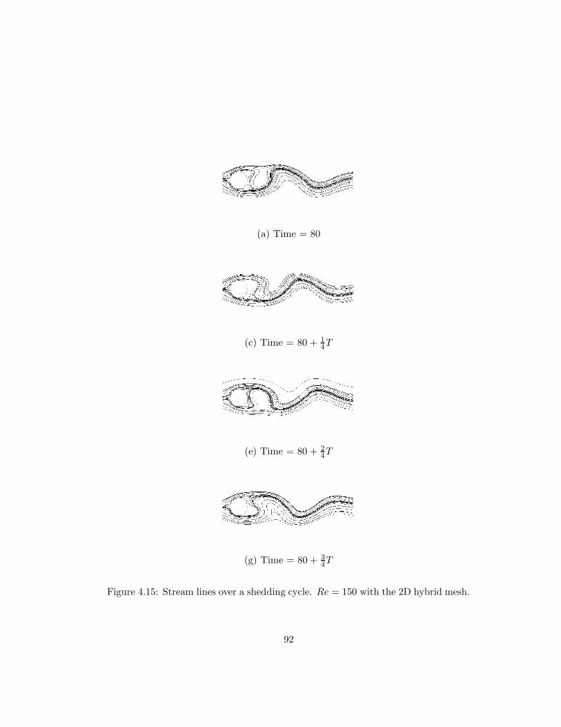
(a) Time = 80
(c) Time = 80 + 14T
(e) Time = 80 + 24T
(g) Time = 80 + 34T
Figure 4.15: Stream lines over a shedding cycle. Re = 150 with the 2D hybrid mesh.
92
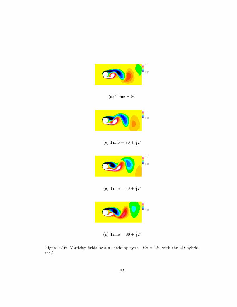
(a) Time = 80
(c) Time = 80 + 14T
(e) Time = 80 + 24T
(g) Time = 80 + 34T
Figure 4.16: Vorticity fields over a shedding cycle. Re = 150 with the 2D hybridmesh.
93

(a) Time = 80
(c) Time = 80 + 14T
(e) Time = 80 + 24T
(g) Time = 80 + 34T
Figure 4.17: Pressure fields over a shedding cycle. Re = 150 with the 2D hybridmesh.
94
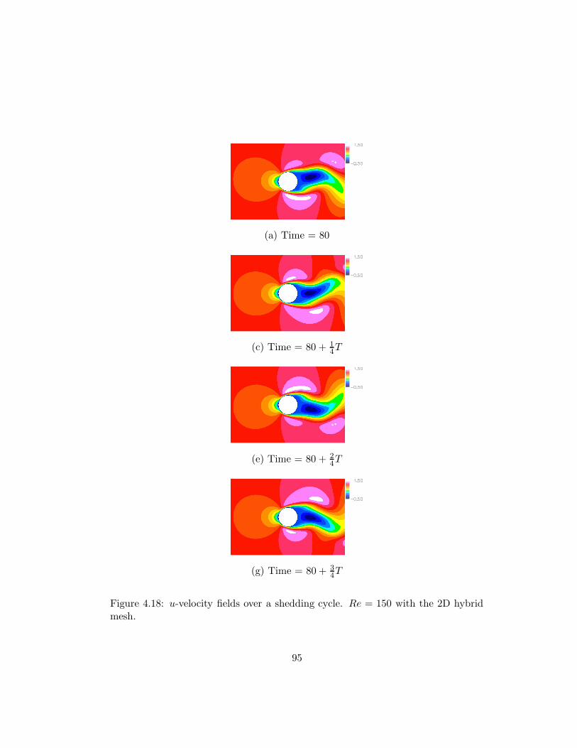
(a) Time = 80
(c) Time = 80 + 14T
(e) Time = 80 + 24T
(g) Time = 80 + 34T
Figure 4.18: u-velocity fields over a shedding cycle. Re = 150 with the 2D hybridmesh.
95
Chapter 5
Inflow Turbulence Study
The purpose of this chapter is to investigate the effect of inflow turbulence on flows
around a circular cylinder in two dimensions using the incompressible Navier-Stokes
method which was developed and validated in previous chapters.
Two different flow conditions are tested: one for low Reynolds number (Re =
150) and the other for moderate Reynolds number (Re = 1, 000). The effect of
inflow turbulence is demonstrated with comparisons to the uniform inflow cases.
A local mesh refinement study is presented to show the effect of mesh resolution
regarding capturing inflow turbulent eddies. The mesh refinement effect on turbulent
vortex shedding is further emphasized by a frequency analysis of the hydrodynamic
responses.
96
5.1 Significance of inflow turbulence
Turbulent flows are present everywhere. Especially, the inflow ocean turbulent ef-
fects on offshore structures are of high interest due to the lack of information about
its role regarding the hydrodynamic forces and fatigue load on structures. If the
inflow condition is changed from uniform to turbulent, the flow condition around
the structure will be completely different from that of uniform inflow. For exam-
ple, an airplane with turbulent inflow typically suffers strong vibration and noise
due to the non-uniform inflow. This is also happening in the offshore structures
exposed to the ocean current which can be turbulent. The difference of the two
cases is the model of flow around the structure: typically flow around airplane is
modeled as compressible flow (except very low Mach number flow), hence it is called
as aero-elasticity problem, but the flow around offshore structure is incompressible,
hence it can be termed as the hydro-elasticity. The structural model in this chapter
is fixed however, in order to first investigate the effect of inflow turbulence on the
hydrodynamic force exerted on the structure, without considering the inertia effect
of the structure.
Two different inflow turbulence profiles (Re=150 and Re=1000) are prepared
by an isotropic geophysical turbulence model [50]. These turbulence profiles are
specified as the inflow condition for the current numerical simulations over a circular
cylinder, our representative offshore structure.
5.2 Unsteady turbulent flow simulations using an eddy
viscosity model
Applying a turbulent eddy viscosity transport model to unsteady turbulent flow
problems may be arguable, however the eddy viscosity model approach is still among
the very few methods which are feasible with the computing power of moderate scale.
97

Since its first introduction in 1992, the Spalart-Allmaras one-equation model, chosen
for the current turbulent flow simulation, has been proven to give reasonable results
with inexpensive computational cost compared to other more computationally ex-
pensive approaches, such as two-equation models, Reynolds stress model, detached
eddy simulations, large eddy simulations, or direct numerical simulations.
5.3 Inlet turbulent velocity profiles
In order to study free stream turbulence effects on the flows around a cylinder, a
turbulent velocity profile is to be prescribed at the inlet instead of the uniform ve-
locity profile. The 2D turbulent velocity profile is obtained by a slice of velocity field
from the 3D velocity field. The 3D velocity field is generated by spatial realizations
of frozen isotropic homogeneous turbulence for a given computational grid [50].
The homogeneous turbulence means its fluctuating velocity u (x, t) is stat-
ically homogeneous (invariant under translations). An approximation of homoge-
neous turbulence can be achieved in wind-tunnel experiments by passing a uniform
stream through a grid with regular spacing. If the flow field is statically invariant
under rotations and reflections of the coordinate system, then it is isotropic. Hun-
dreds of wind-tunnel experiments have been performed on isotropic turbulence, and
much of the turbulence theory is based on it [65].
Time series of inlet turbulent profiles (u = U + u′, v = V + v′) are displayed
in Figure 5.1 for Re = 150 and in Figure 5.3 for Re = 1, 000. Generally, the higher
Reynolds number case shows higher amplitude and frequencies of the fluctuations
and also wider variances of the fluctuations in space (from nodes to nodes) compared
to the lower Reynolds number case.
98
5.4 Boundary conditions for inflow turbulence simula-
tions
In 2D simulations, the boundaries are classified as inlet, outlet, viscous wall, and far
field parallel to the mean flow direction. As the inlet velocity profile changes from
the uniform to the irregular turbulent, boundary conditions (inlet and far field) have
to be modified accordingly for both of the mean flow equations and the turbulence
equation solvers.
For the uniform inflow case, the velocities at the far fields are considered
uniform. This is no longer valid for turbulent inflow case, since the turbulent eddies
are everywhere even at the far fields. Hence, for the turbulence inflow simulations,
the velocities at the far fields are extrapolated from the domain as the pressure is.
Likewise, turbulent eddy viscosity is also extrapolated from the domain along the
far field boundaries. At the inlet, the given turbulent velocity profile is specified
instead of the uniform velocity, while the pressure is extrapolated just as in the
uniform inlet case.
For the turbulent transport equation solver, the inlet boundary requires spe-
cial attention. The instantaneous inlet turbulent velocity profile (ui) is already
equipped with the homogeneous isotropic turbulent fluctuations (u′
i), and those are
defined by
ui (x, t) = Ui (x, t) + u′
i (x, t) (5.1)
where i denotes each coordinate direction. The mean velocity components
are defined as follows
Ui (x) = limT→∞
1
T
∫ t+T
tui (x, t) dt
and this is uniform everywhere and spatially invariant. Hence, the strain
rate tensor of the mean velocity field is equal to zero at the inlet.
99
Sij =1
2
(
∂Ui
∂xj+
∂Ui
∂xj
)
= 0 (5.2)
In order to calculate the eddy viscosity corresponding to a given turbulent
fluctuation, the eddy viscosity hypothesis (Boussinesq approximation) has to be
used. This hypothesis relates the Reynolds stresses ( −u′
iu′
j) with the non-zero
strain rate tensor (Sij), which is defined by
−ρu′
iu′
j = 2ρνtSij (5.3)
Since our mean velocity is uniform, the strain rate tensor Sij of the mean
velocity is also zero, which contradicts the eddy viscosity hypothesis. Hence, the
eddy viscosity of the turbulent fluctuation cannot be determined for uniform mean
flow.
By this contradition a question arises; should the eddy viscosity be non-zero,
even if the mean flow is uniform? The answer is no, because by specifying the
turbulent velocity profiles at the inlet, the turbulent fluctuation is fed to the mean
flow solver. The effect of turbulence is accounted by the mean flow equations, and
no additional eddy viscosity is necessary at the inlet. Hence, eddy viscosity at the
inlet should be ideally zero, otherwise the effect of inflow turbulence will be doubly
counted and contaminated by the non-zero eddy viscosity.
Nevertheless, the hydrodynamic foces exerted on the cylinder are relatively
insensitive to the values of eddy viscosity at the inlet. The reason is that the amount
of eddy viscosity at the upstream is a few orders of magnitude smaller than that in
the near wall region. Hence, we can specify the eddy viscosity at the inlet to be the
same as that of uniform inflow. However, regardless of the values of eddy viscosity
at the inlet, as the flow goes down stream the flow becomes non-uniform even in the
mean-sense, and the Spalart-Allmaras turbulence model detects this and adjusts the
eddy viscosity accordingly.
100

0 20 40 60 80 100 120 140 160 180 2000.4
0.6
0.8
1
1.2
1.4
1.6U+
u’
0 20 40 60 80 100 120 140 160 180 200−0.6
−0.4
−0.2
0
0.2
0.4
0.6
Time
V+v’
Figure 5.1: Turbulent velocity profile at the inlet nodes, Re = 150
0 20 40 60 80 100 120 140 160 180 200−1
0
1
2
3
4
C D
0 20 40 60 80 100 120 140 160 180 200−3
−2
−1
0
1
2
3
Time
C L
Figure 5.2: CD and CL responses to the turbulent and uniform inflow, Re = 150.Solid lines are for turbulent inflow, and dash-dotted lines for uniform inflow.
101
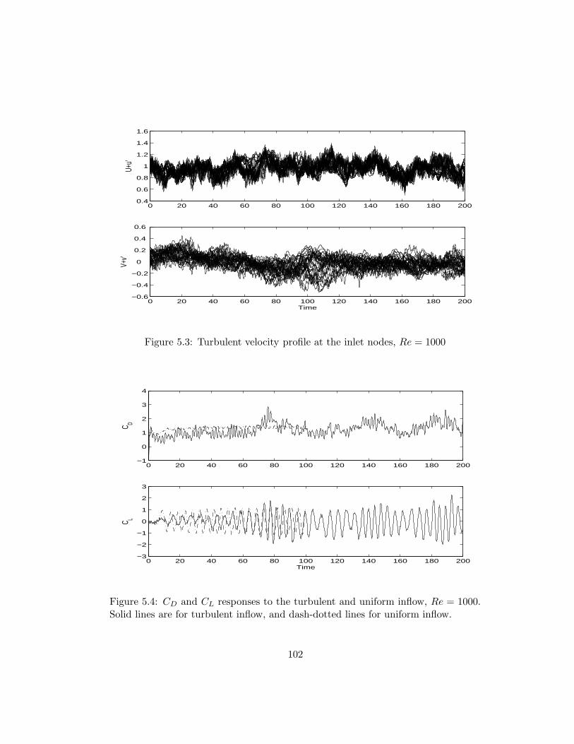
0 20 40 60 80 100 120 140 160 180 2000.4
0.6
0.8
1
1.2
1.4
1.6U+
u’
0 20 40 60 80 100 120 140 160 180 200−0.6
−0.4
−0.2
0
0.2
0.4
0.6
Time
V+v’
Figure 5.3: Turbulent velocity profile at the inlet nodes, Re = 1000
0 20 40 60 80 100 120 140 160 180 200−1
0
1
2
3
4
C D
0 20 40 60 80 100 120 140 160 180 200−3
−2
−1
0
1
2
3
Time
C L
Figure 5.4: CD and CL responses to the turbulent and uniform inflow, Re = 1000.Solid lines are for turbulent inflow, and dash-dotted lines for uniform inflow.
102
5.5 CD and CL responses to inflow turbulence
The effect of inflow turbulence on the hydrodynamic forces exerted on the cylinder
is presented in Figure 5.2 for Re = 150 and Figure 5.4 for Re = 1, 000, and they are
compared with those of the uniform inflow case.
As is evident from Figures 5.1- 5.4, when the inflow turbulence is applied,
the time series of the drag coefficient usually (not always) follows the time series
of the inflow u-velocity. Furthermore, higher values of CD are always accompanied
with higher amplitudes of CL and faster shedding frequencies.
However, there is an exception which does not follow this trend. Especially
in the region of T ime = 100 ∼ 120 for Re = 1, 000, both the CD and the amplitudes
of the CL decrease even though the inflow u-velocity increases. In such region
(T ime = 110 ∼ 120), a wide variances of inflow v-velocity is observed in the inflow
turbulence profile, and their relation (variances of inflow v-velocity and diminishing
of vortex shedding) is uncertain at this time and of interest for further investigation.
The general trends of the drag and lift coefficient to the inflow turbulence
profile can be summarized as below.
1. The stronger inflow u-velocity, the higher CD.
2. The higher CD accompanies the higher amplitudes of CL and St.
3. When shedding diminishes even with increase of inflow u-velocity, a wide vari-
ance of inflow v-velocity is observed.
103
5.6 Local mesh refinement effect
Since the local mesh spacing determines the smallest scale of turbulent eddies which
can be resolved, enough resolution of mesh has to be assured for accurate simulation
of inflow turbulence.
For the Re = 150 case, the cylinder diameter is about 10 times smaller than
the integral length scale of the upstream turbulence, which is a length scale char-
acterizing coherence of the fluctuations. For this case, grid spacing at the inlet
boundary is smaller than the cylinder diameter, so the resolution of the computa-
tional grid is deemed to be fine enough to capture the smallest eddies.
For higher Reynolds number (Re = 1, 000), the scales of the upstream tur-
bulent eddies are getting smaller, so the computational grid near the inlet may need
to be refined in order to resolve these smaller scales of eddies. To see the mesh
resolution effect on inflow turbulence simulations, the large triangular cells which
are located away from the wall are refined. Each triangular cell is divided into four
child triangles. The one-step adapted mesh is compared with the original mesh in
Figure 5.6.
The mesh refinement effect on the CD and CL responses is compared in
Figure 5.7 for Re = 150 and in Figure 5.8 for Re = 1, 000. For Re = 150, the adapted
mesh simulation shows almost identical result to the original mesh simulation. This
tells that the original mesh is fine enough to resolve most of the turbulent eddies
which are significant to the drag and lift response of the structure. But for Re
= 1000, there is a noticeable difference in the drag and lift responses between the
adapted and original mesh results. Especially in the fluctuations of the drag and
lift coefficients, more frequencies are encountered by the adapted meshes than the
original mesh. This extra frequencies in the drag and lift seems to be the direct
effect of the smaller scales of eddies which are resolved by the refined mesh. The
vorticity fields at a series of time steps are presented in Figure 5.9 for Re = 150 and
104
in Figure 5.10 for Re = 1, 000 to show the transport of the turbulent eddies. It is
obvious that the adapted mesh resolves much smaller scales of eddies.
Finally, frequency responses to inflow turbulence are presented. The uniform
inflow case is first examined as a reference. In general, the inflow turbulence intro-
duces more frequencies and the shedding frequencies spread in wider ranges; some
frequencies faster than that of the uniform inflow, and others slower than that.
The details of the frequency analysis are presented in figure 5.11 for Re = 150
and figure 5.12 for Re = 1, 000. For the Re = 150 case, the frequency responses are
almost the same and insensitive to mesh refinement, which means that the original
mesh resolves most of the eddies that are significant to the vortex shedding. How-
ever, for the Re = 1000 case, the frequency analysis of the adapted mesh simulation
reveals more frequencies which were not resolved by the original mesh simulation.
This indicates that the refined mesh is resolving more small scales of turbulent eddies
and these small eddies result directly in the extra frequencies of shedding.
105
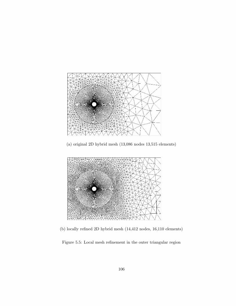
(a) original 2D hybrid mesh (13,086 nodes 13,515 elements)
(b) locally refined 2D hybrid mesh (14,412 nodes, 16,110 elements)
Figure 5.5: Local mesh refinement in the outer triangular region
106
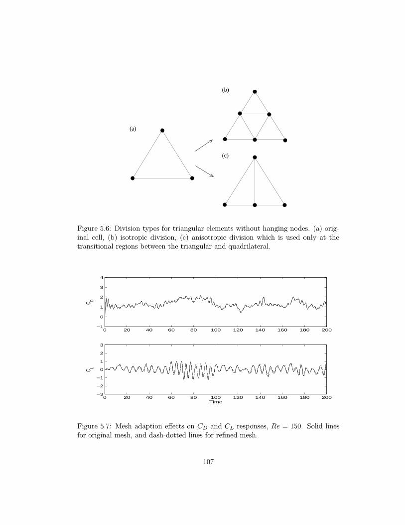
(c)
(b)
(a)
Figure 5.6: Division types for triangular elements without hanging nodes. (a) orig-inal cell, (b) isotropic division, (c) anisotropic division which is used only at thetransitional regions between the triangular and quadrilateral.
0 20 40 60 80 100 120 140 160 180 200−1
0
1
2
3
4
C D
0 20 40 60 80 100 120 140 160 180 200−3
−2
−1
0
1
2
3
Time
C L
Figure 5.7: Mesh adaption effects on CD and CL responses, Re = 150. Solid linesfor original mesh, and dash-dotted lines for refined mesh.
107

0 20 40 60 80 100 120 140 160 180 200−1
0
1
2
3
4
C D
0 20 40 60 80 100 120 140 160 180 200−3
−2
−1
0
1
2
3
Time
C L
Figure 5.8: Mesh adaption effects on CD and CL responses, Re = 1000. Solid linesfor original mesh, and dash-dotted lines for refined mesh.
108
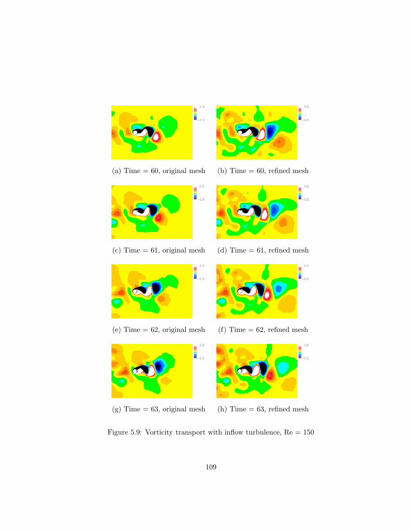
(a) Time = 60, original mesh (b) Time = 60, refined mesh
(c) Time = 61, original mesh (d) Time = 61, refined mesh
(e) Time = 62, original mesh (f) Time = 62, refined mesh
(g) Time = 63, original mesh (h) Time = 63, refined mesh
Figure 5.9: Vorticity transport with inflow turbulence, Re = 150
109
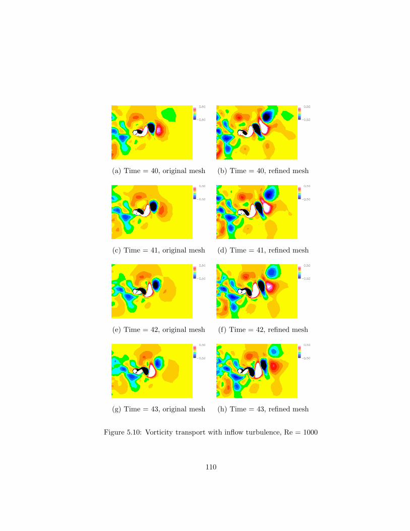
(a) Time = 40, original mesh (b) Time = 40, refined mesh
(c) Time = 41, original mesh (d) Time = 41, refined mesh
(e) Time = 42, original mesh (f) Time = 42, refined mesh
(g) Time = 43, original mesh (h) Time = 43, refined mesh
Figure 5.10: Vorticity transport with inflow turbulence, Re = 1000
110

0 40 80 120 160 200−3
−2
−1
0
1
2
3
Time
CL
0 0.2 0.4 0.6 0.8 10
5
10
15
20
25
30
St
Abs
olut
e va
lue
of F
FT
(a) (b)
0 40 80 120 160 200−3
−2
−1
0
1
2
3
Time
CL
0 0.2 0.4 0.6 0.8 10
5
10
15
20
25
30
St
Abs
olut
e va
lue
of F
FT
(c) (d)
0 40 80 120 160 200−3
−2
−1
0
1
2
3
Time
CL
0 0.2 0.4 0.6 0.8 10
5
10
15
20
25
30
St
Abs
olut
e va
lue
of F
FT
(e) (f)
Figure 5.11: FFT spectrums of CL responses for Re = 150. (a) and (b) correspondto the uniform flow using original mesh; (c) and (d) correspond to the turbulent flowusing original mesh; (e) and (f) correspond to the turbulent inflow using adaptedmesh, which is showing almost idential result with the original. Same time step∆t = 0.1 is used for all cases.
111
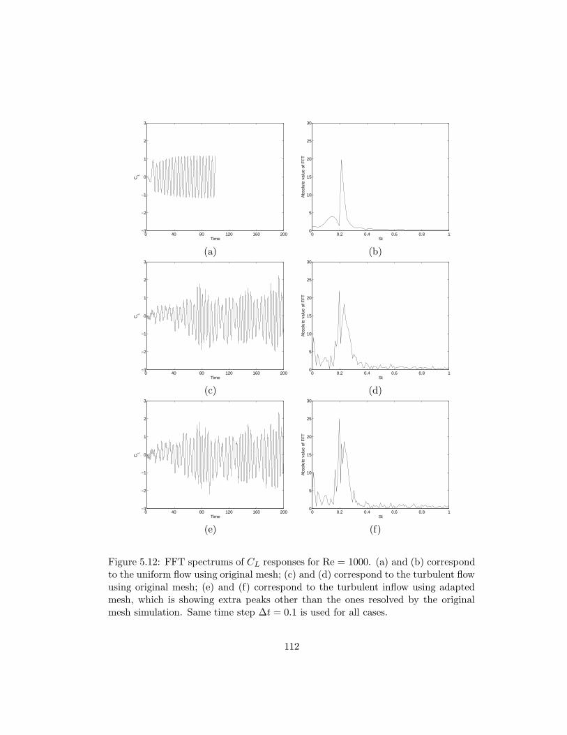
0 40 80 120 160 200−3
−2
−1
0
1
2
3
Time
CL
0 0.2 0.4 0.6 0.8 10
5
10
15
20
25
30
St
Abs
olut
e va
lue
of F
FT
(a) (b)
0 40 80 120 160 200−3
−2
−1
0
1
2
3
Time
CL
0 0.2 0.4 0.6 0.8 10
5
10
15
20
25
30
St
Abs
olut
e va
lue
of F
FT
(c) (d)
0 40 80 120 160 200−3
−2
−1
0
1
2
3
Time
CL
0 0.2 0.4 0.6 0.8 10
5
10
15
20
25
30
St
Abs
olut
e va
lue
of F
FT
(e) (f)
Figure 5.12: FFT spectrums of CL responses for Re = 1000. (a) and (b) correspondto the uniform flow using original mesh; (c) and (d) correspond to the turbulent flowusing original mesh; (e) and (f) correspond to the turbulent inflow using adaptedmesh, which is showing extra peaks other than the ones resolved by the originalmesh simulation. Same time step ∆t = 0.1 is used for all cases.
112
Chapter 6
3D Verification and Validation
Study
Verification and validation of the developed Navier-Stokes method is presented in
three dimensions with general hybrid meshes. Flows around a sphere and a cylinder
are simulated and the results are compared with reported experimental measure-
ments. A mesh convergence study is performed using a series of successively refined
sphere meshes. A wide range of Reynolds numbers (100 ∼ 1, 000, 000) is tested for
validation of the numerical solution using both the sphere and cylinder problems.
Validity and effectiveness of local hexahedra is presented with general hybrid meshes
which contain local hexahedra in various regions of the computational domain.
113
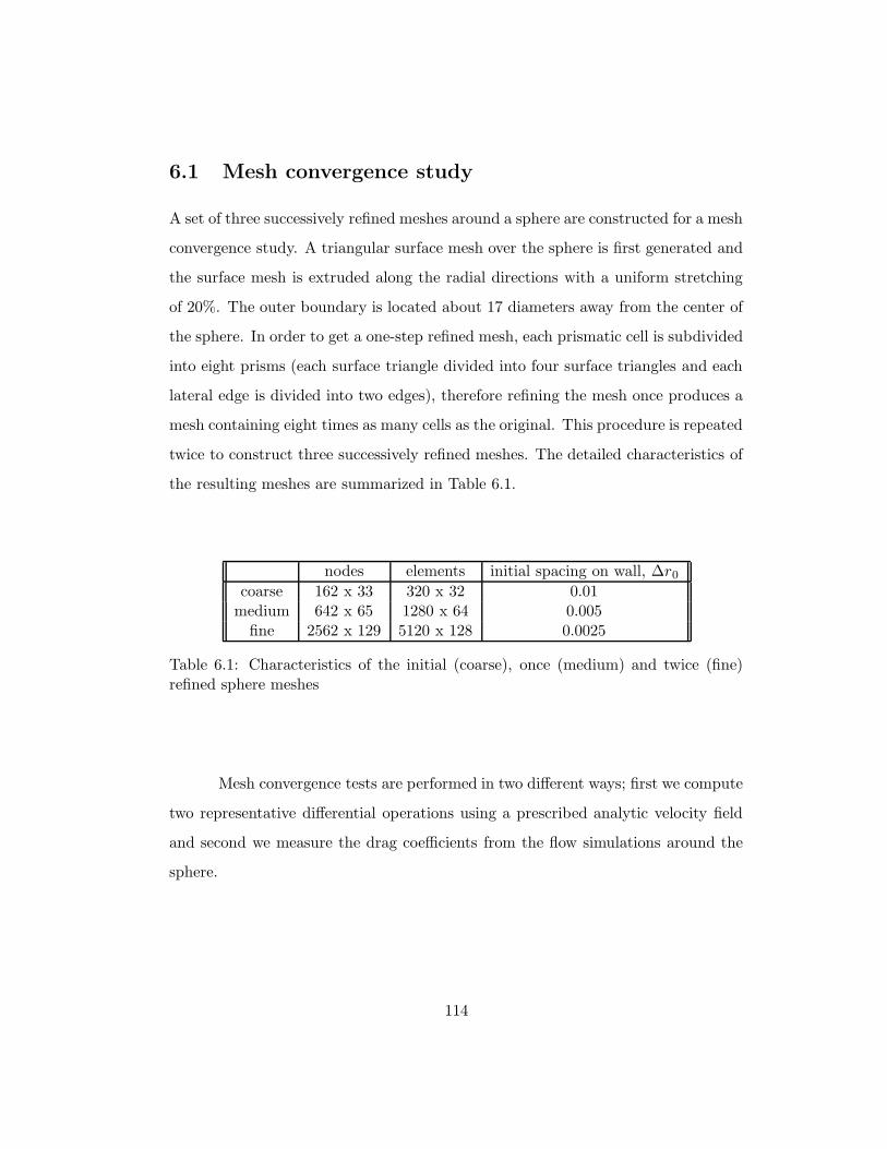
6.1 Mesh convergence study
A set of three successively refined meshes around a sphere are constructed for a mesh
convergence study. A triangular surface mesh over the sphere is first generated and
the surface mesh is extruded along the radial directions with a uniform stretching
of 20%. The outer boundary is located about 17 diameters away from the center of
the sphere. In order to get a one-step refined mesh, each prismatic cell is subdivided
into eight prisms (each surface triangle divided into four surface triangles and each
lateral edge is divided into two edges), therefore refining the mesh once produces a
mesh containing eight times as many cells as the original. This procedure is repeated
twice to construct three successively refined meshes. The detailed characteristics of
the resulting meshes are summarized in Table 6.1.
nodes elements initial spacing on wall, ∆r0
coarse 162 x 33 320 x 32 0.01medium 642 x 65 1280 x 64 0.005
fine 2562 x 129 5120 x 128 0.0025
Table 6.1: Characteristics of the initial (coarse), once (medium) and twice (fine)refined sphere meshes
Mesh convergence tests are performed in two different ways; first we compute
two representative differential operations using a prescribed analytic velocity field
and second we measure the drag coefficients from the flow simulations around the
sphere.
114

0.01
0.1
1
0.001 0.01 0.1
RM
S E
rror
Initial spacing on wall, ∆r0
divergence computationlaplacian computation
Figure 6.1: Mesh convergence test using analytic velocity fileds
6.1.1 Analytic velocity function test
The divergence operator is chosen to mimic the convective flux computation and
the Laplacian operator is chosen for emulating the viscous flux evaluation. The
numerical and exact solutions are compared to show the accuracy of the current
spatial discretization scheme. The analytic velocity field prescribed is
U = sin (x) i + cos (y) j + sin(z)k (6.1)
Since the exact values of the divergence and Laplacian are known for the
analytic velocity field, the error is computed by
115

∆r0 divergenceError laplacianError
coarse 0.01 3.401 × 10⁻¹ 3.285 × 10⁻¹
medium 0.005 1.276 × 10⁻¹ 1.271 × 10⁻¹
fine 0.0025 3.789 × 10⁻² 3.789 × 10⁻²
Table 6.2: Errors of derivitive computations by using prescribed analytic velocityfield.
divergenceError∆r =
√√√√√
NI∑
i=1|(∇ ·U)∆r − (∇ · U)exact|
2
NI
laplacianError∆r =
√√√√√
NI∑
i=1‖(∇2U)∆r − (∇2U)exact‖
2
NI
where NI is the number of interior nodes. The order of convergence can be
approximated by Richardson’s extrapolation [66] as follows
log2
(divergenceError∆r=0.005
divergenceError∆r=0.0025
)
= 1.751
log2
(laplacianError∆r=0.005
laplacianError∆r=0.0025
)
= 1.746
The actual values of error for the three meshes considered are summarized
in Table 6.2 and plotted in Figure 6.1. The small deviation from the second order
accuracy, the theoretical order of accuracy which was derived for simple 1D meshes
in equation (4.4) and (4.5), seems to be due to the higher spatial dimension.
116
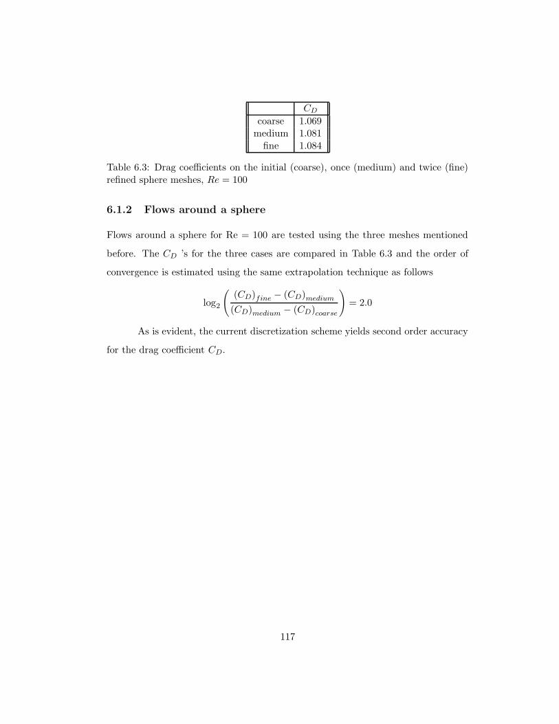
CD
coarse 1.069medium 1.081
fine 1.084
Table 6.3: Drag coefficients on the initial (coarse), once (medium) and twice (fine)refined sphere meshes, Re = 100
6.1.2 Flows around a sphere
Flows around a sphere for Re = 100 are tested using the three meshes mentioned
before. The CD ’s for the three cases are compared in Table 6.3 and the order of
convergence is estimated using the same extrapolation technique as follows
log2
(
(CD)fine − (CD)medium
(CD)medium − (CD)coarse
)
= 2.0
As is evident, the current discretization scheme yields second order accuracy
for the drag coefficient CD.
117

(a) coarse (162x33 nodes, 320x32 elements)
(b) medium (642x65 nodes, 1280x64 elements)
(c) fine (2562x129 nodes, 5120x128 elements)
Figure 6.2: Three levels of sphere mesh used for the mesh convergence study
118
6.2 High Reynolds number flows around a sphere
The current simulation of flows around a sphere is validated by comparison with
experimental results. The medium sphere mesh is used for the flow simulation over
a sphere. Stream lines around the sphere are shown in Figure 6.3 for Re = 100.
A series of simulations are performed for various orders of Reynolds numbers
in the range of 10 ∼ 1, 000, 000. The Spalart-Allmaras turbulence model equation is
solved in conjunction with the mean flow equations (the Reynolds-averaged Naiver-
Stokes equations) for all cases except Re = 10 and Re = 100 which correspond to
laminar flow.
The CD values obtained by the current simulations are compared with ex-
perimental results for various values of surface roughness, and those are presented
in Figure 6.4. Overall, the current simulation follows well the experiments. Drag
reduction induced by boundary layer transition from laminar to turbulent is also
observered for Re ≥ 100, 000. The delayed separation due to the boundary layer
transition is also observed and displayed in Figure 6.5. The narrowed wake re-
gion behind the sphere is evident by the comparison between the two representative
Reynolds numbers, Re = 1, 000 and Re = 100, 000.
One can observe a slight deviation of numerical result from the experiments
for Reynolds numbers in the supercritical regime (Re ≥ 100, 000). This discrepancy
at the supercritical regime may attribute to many factors, such as surface roughness
of the current computation model or mis-prediction of boundary layer transition by
using a relatively simple turbulent model equation. However, it should be noticed
that even the experimental results are very sensitive to surface roughness in the
transcritical regime.
119
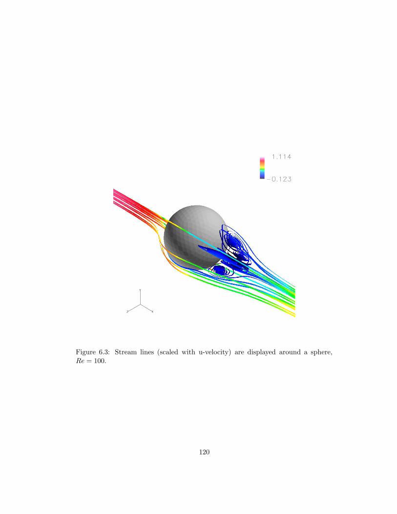
Figure 6.3: Stream lines (scaled with u-velocity) are displayed around a sphere,Re = 100.
120
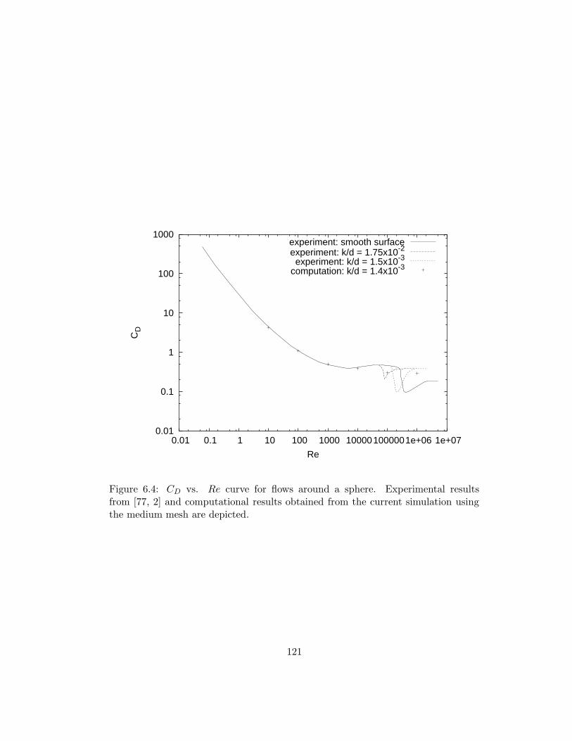
0.01
0.1
1
10
100
1000
0.01 0.1 1 10 100 1000 10000 100000 1e+06 1e+07
CD
Re
experiment: smooth surfaceexperiment: k/d = 1.75x10⁻²
experiment: k/d = 1.5x10⁻³
computation: k/d = 1.4x10⁻³
Figure 6.4: CD vs. Re curve for flows around a sphere. Experimental resultsfrom [77, 2] and computational results obtained from the current simulation usingthe medium mesh are depicted.
121
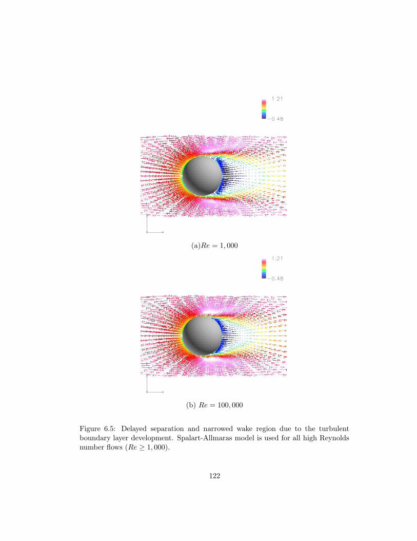
(a)Re = 1, 000
(b) Re = 100, 000
Figure 6.5: Delayed separation and narrowed wake region due to the turbulentboundary layer development. Spalart-Allmaras model is used for all high Reynoldsnumber flows (Re ≥ 1, 000).
122
6.3 Flows around a cylinder with general hybrid meshes
Flow around a circular cylinder is tested to show the validity and effectiveness of
the proposed general hybrid mesh technique. Two different kinds of general hybrid
meshes are used. The objectives of these general hybrid mesh simulations are first
to show the accuracy of the proposed solution algorithm, and second to present the
effectiveness of local hexahedra in general hybrid meshes.
The first general hybrid mesh (GHM 1) displayed in Fig. 6.6 includes lo-
cal hexahedra in the frontal viscous region of the cylinder. The inclusion of local
hexahedra into the GHM 1 is from a priori knowledge of the flow feature. Local
hexahedra in the GHM 1 are intended to capture the unidirectional flow feature
with a less amount of computational cost compared to the prismatic or tetrahedral
elements.
The second general hybrid mesh (GHM 2) is shown in Fig. 6.7. The additional
local hexahedra are introduced in the GHM 2 by replacing the wake region with a
block of local hexahedra. The GHM 2 is intended to capture the wake with local
hexahedra (with less number of edges) instead of tetrahedral elements in the wake
region. Local hexahedra in the wake region and their lower density of edges are
evident by a comparison between Figures of 6.6 and 6.7.
6.4 Effectiveness of local hexahedra
One of the major advantages of using hybrid meshes is their lower connectivity as
compared to meshes with simplexes (triangles in two dimensions and tetrahedra in
three dimensions). In particular, for a given set of nodes, neglecting the boundary
effect, a mesh with tetrahedra contains about seven times as many edges as nodes,
while a mesh with hexahedra contains only three times and a mesh with prisms
contains only four times as many edges as nodes [47].
123
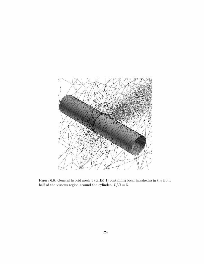
Figure 6.6: General hybrid mesh 1 (GHM 1) containing local hexahedra in the fronthalf of the viscous region around the cylinder. L/D = 5.
124
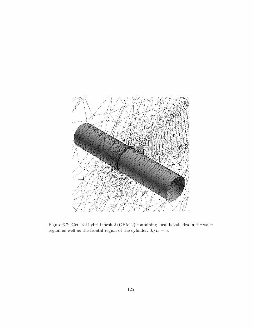
Figure 6.7: General hybrid mesh 2 (GHM 2) containing local hexahedra in the wakeregion as well as the frontal region of the cylinder. L/D = 5.
125
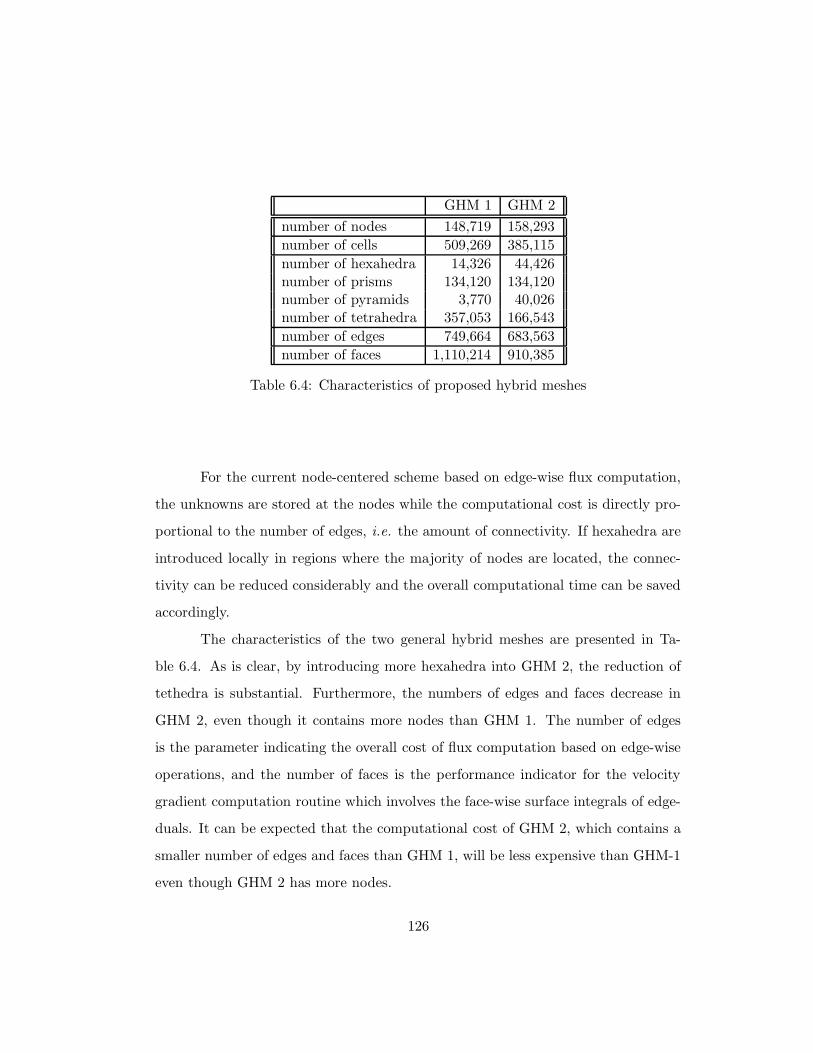
GHM 1 GHM 2
number of nodes 148,719 158,293
number of cells 509,269 385,115
number of hexahedra 14,326 44,426number of prisms 134,120 134,120number of pyramids 3,770 40,026number of tetrahedra 357,053 166,543
number of edges 749,664 683,563
number of faces 1,110,214 910,385
Table 6.4: Characteristics of proposed hybrid meshes
For the current node-centered scheme based on edge-wise flux computation,
the unknowns are stored at the nodes while the computational cost is directly pro-
portional to the number of edges, i.e. the amount of connectivity. If hexahedra are
introduced locally in regions where the majority of nodes are located, the connec-
tivity can be reduced considerably and the overall computational time can be saved
accordingly.
The characteristics of the two general hybrid meshes are presented in Ta-
ble 6.4. As is clear, by introducing more hexahedra into GHM 2, the reduction of
tethedra is substantial. Furthermore, the numbers of edges and faces decrease in
GHM 2, even though it contains more nodes than GHM 1. The number of edges
is the parameter indicating the overall cost of flux computation based on edge-wise
operations, and the number of faces is the performance indicator for the velocity
gradient computation routine which involves the face-wise surface integrals of edge-
duals. It can be expected that the computational cost of GHM 2, which contains a
smaller number of edges and faces than GHM 1, will be less expensive than GHM-1
even though GHM 2 has more nodes.
126
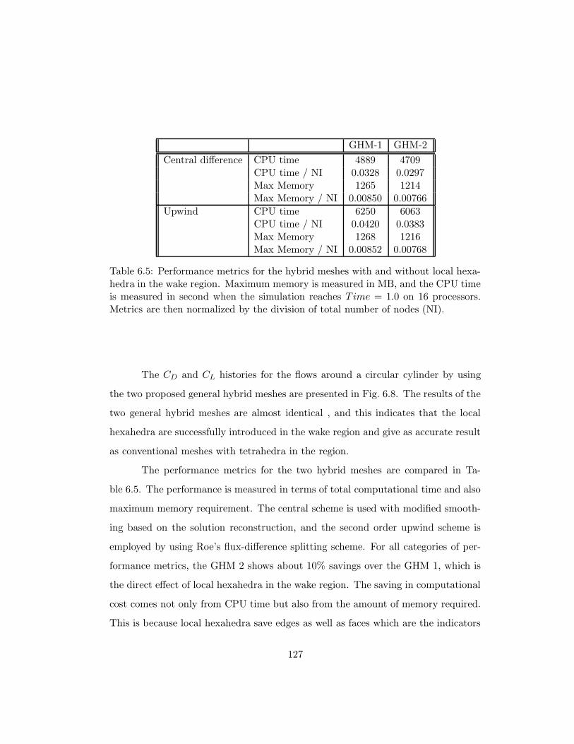
GHM-1 GHM-2
Central difference CPU time 4889 4709CPU time / NI 0.0328 0.0297Max Memory 1265 1214Max Memory / NI 0.00850 0.00766
Upwind CPU time 6250 6063CPU time / NI 0.0420 0.0383Max Memory 1268 1216Max Memory / NI 0.00852 0.00768
Table 6.5: Performance metrics for the hybrid meshes with and without local hexa-hedra in the wake region. Maximum memory is measured in MB, and the CPU timeis measured in second when the simulation reaches T ime = 1.0 on 16 processors.Metrics are then normalized by the division of total number of nodes (NI).
The CD and CL histories for the flows around a circular cylinder by using
the two proposed general hybrid meshes are presented in Fig. 6.8. The results of the
two general hybrid meshes are almost identical , and this indicates that the local
hexahedra are successfully introduced in the wake region and give as accurate result
as conventional meshes with tetrahedra in the region.
The performance metrics for the two hybrid meshes are compared in Ta-
ble 6.5. The performance is measured in terms of total computational time and also
maximum memory requirement. The central scheme is used with modified smooth-
ing based on the solution reconstruction, and the second order upwind scheme is
employed by using Roe’s flux-difference splitting scheme. For all categories of per-
formance metrics, the GHM 2 shows about 10% savings over the GHM 1, which is
the direct effect of local hexahedra in the wake region. The saving in computational
cost comes not only from CPU time but also from the amount of memory required.
This is because local hexahedra save edges as well as faces which are the indicators
127
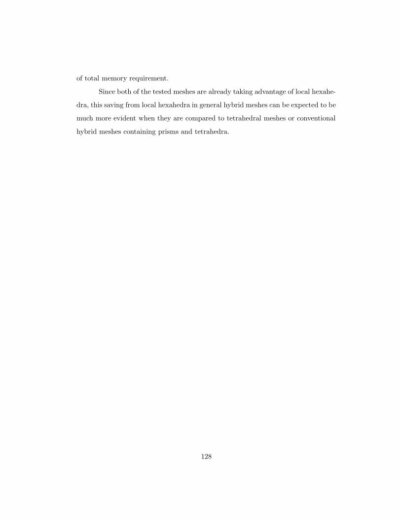
of total memory requirement.
Since both of the tested meshes are already taking advantage of local hexahe-
dra, this saving from local hexahedra in general hybrid meshes can be expected to be
much more evident when they are compared to tetrahedral meshes or conventional
hybrid meshes containing prisms and tetrahedra.
128
1
1.1
1.2
1.3
1.4
1.5
1.6
1.7
1.8
0 10 20 30 40 50 60
CD
Time
1
1.1
1.2
1.3
1.4
1.5
1.6
1.7
1.8
0 10 20 30 40 50 60
CD
Time
(a) Span-averaged CD histories
-1
-0.5
0
0.5
1
0 10 20 30 40 50 60
CL
Time
(b) Span-averaged CL histories
Figure 6.8: Local hexahedra effect on CD and CL histories. The central differencescheme is used with modified smoothing of σ4 = 0.1. Solid lines stand for the GHM 1containing hexahedra only in the frontal viscous region, and the dashed lines standfor the GHM 2 which contains hexahedra in the wake region as well as the frontalviscous region. Re = 150.
129

(a) general hybrid mesh 1
(b) general hybrid mesh 2
Figure 6.9: Comparison of velocity fileds for Re = 150 on general hybrid mesh 1(GHM 1) and general hybrid mesh 2 (GHM 2). GHM 1 contains local hexahedraonly in the frontal viscous region and GHM 2 contains local hexahedra in the wakeregion as well as the frontal viscous region. Velocity snap shots are taken at thetime step within a shedding cycle.
130
6.5 High Reynolds number flows around a cylinder
The validity of the current Navier-Stokes method for general hybrid meshes is further
emphasized by a series of high Reynolds number flow simulations over a circular
cylinder. A wide range of Reynolds numbers are tested; Re = 10 ∼ 1, 000, 000. For
the cases of Re ≤ 100 the flow is considered as laminar, hence no turbulence model is
used. For the rest of the cases, Re ≥ 1, 000, the Spalart-Allmaras turbulence model
is solved in conjunction with the mean flow equation. GHM 1, shown in Figure 6.6,
is used for all of the cases.
For the series of Reynolds number, CD is compared with experimental results.
As shown in Figure 6.10, the current simulation agrees well with the experimental
results. Expecially for the Re = 100, 000 case, a sharp drop of CD is predicted which
is indicating the delayed separation induced by the boundary layer transition from
laminar to turbulent. This delayed separation and narrowed wake region at Re =
100, 000 is compared to the Re = 1000 case and those are displayed in Figure 6.11.
131
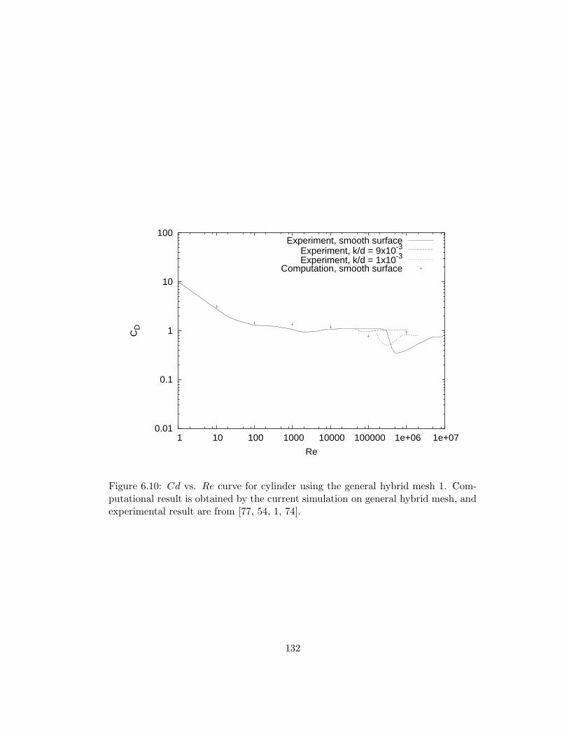
0.01
0.1
1
10
100
1 10 100 1000 10000 100000 1e+06 1e+07
CD
Re
Experiment, smooth surfaceExperiment, k/d = 9x10⁻³
Experiment, k/d = 1x10⁻³
Computation, smooth surface
Figure 6.10: Cd vs. Re curve for cylinder using the general hybrid mesh 1. Com-putational result is obtained by the current simulation on general hybrid mesh, andexperimental result are from [77, 54, 1, 74].
132

(a) Re = 1, 000
(b) Re = 100, 000
Figure 6.11: Prediction of delayed separation (accompanied by a smaller wake re-gion) due to the boundary layer transition from laminar to turbulent. Velocityfields, colored with u-velocity magnitude, are taken at the same time step within ashedding cycle. The Spalart-Allmaras turbulence model is used for both cases onthe general hybrid mesh 1.
133
Chapter 7
Strong Coupling of Flow and
Structure Interactions
In this chapter, the equation of motion for a cylinder subjected to vortex-induced
vibration (VIV) is presented. The cylinder is modeled as a set of beam elements
freely vibrating in the cross-flow direction. The equation of motion is nondimen-
sionalized by using the same reference quantities used for the flow equations. Two
coupling strategies for the fluid and structure interactions are introduced; namely
weak coupling and strong coupling. The weak coupling is implemented by an ex-
plicit central difference scheme, and the strong coupling is constructed by using a
predictor-corrector method driven by the pair of central difference and trapezoidal
schemes. A comparison of the two coupling methods is presented and the superior
stability property of strong coupling is emphasized.
134
7.1 Structural model for the cylinder
Different structural elements can be used for modelling the vibrating cylinder. For
example, strings (cables), beams, or plates can be used. Typically, cables represent
extremely slender structures with tensional rigidity but no bending stiffness. Such
models can be a good choice for tension dominated behavior of structure, which is
characterized by the following criterion [96]
T
EIk2> 30 (7.1)
where T is the tension, EI is the bending stiffness, and k is the wave number
describing the excitation mode. As shown in equation 7.1, if the bending stiffness
becomes significant (i.e. the aspect ratio L/D of the cylinder becomes smaller),
then the cable model cannot be used and bending stiffness should be included.
For cylinder models representing offshore risers (hollow cylinders containing
oil), plate elements can also be considered. However, the deformation of the riser
pipe in the cross sectional plane is negligible compared to the rigid body motion.
As suggested by the elementary beam theory, if the aspect ratio is L/D ∼ 10,
the beam element can be a suitable choice to model the structure [30]. Hence, the
cylinder for the current study, with moderate aspect ratio L/D ≤ O(10) and no
cross sectional deformation, is modeled with beam elements.
7.2 Equation of motion for the bending vibration
The cylinder in Figure 7.1 is modeled with a structural beam element of four degrees
of freedom ( v1, θ1, v2, θ2). The direction of the cross flow displacement (v ) coincides
with the y-axis and the direction of the rotational degree of freedom ( θ) lies in the
negative x-direction in order to be consistent with the sign convention of the beam
element.
135
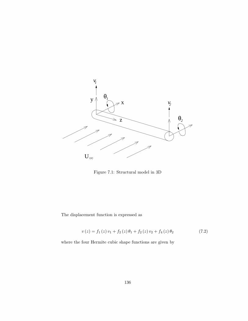
x vθ
θ
1v
2y 1
2z
U
Figure 7.1: Structural model in 3D
The displacement function is expressed as
v (z) = f1 (z) v1 + f2 (z) θ1 + f2 (z) v2 + f4 (z) θ2 (7.2)
where the four Hermite cubic shape functions are given by
136

f1 (z) = 1 − 3(
zL
)2+ 2
(zL
)3
f2 (z) = z − 2(
z2
L
)
+(
z3
L2
)
f3 (z) = 3(
zL
)2 − 2(
zL
)3
f4 (z) = −(
z2
L
)
+(
z3
L2
)
(7.3)
Since these cubic functions ensure that both the displacement and slope (first
derivative) is continuous across the boundary of elements, they form a C 1 basis.
The kinetic energy of the beam element in flexural vibration is given by
T =ρsA
2
∫ L
0v (z)2 dz (7.4)
where ρs is structure density and A is the cross-sectional area of the cylinder.
The strain energy for the beam element in bending is expressed by
U =EI
2
∫ L
0v′′ (z)
2dz (7.5)
Primes denote the derivatives with respect to the axial direction z, while
dots indicate differentiation with respect to time t.
The flexural (bending) stiffness of a beam is defined as EI, where E is
Young’s elastic modulus of the beam and I is the cross-sectional area moment of
inertia about the neutral axis. For a cylinder with a circular cross-section the area
moment of inertia is defined by
I =π
64D4
where D is the cylinder diameter.
Substituting the displacement function into the kinetic energy and strain
energy expressions, and using Lagrange’s equation [98] yields the equation of motion
for the beam element. Lagrange’s equation is given by
137

d
dt
(∂T
∂qi
)
+∂U
∂qi= Fi (7.6)
where qi is i -th degree of freedom, and Fi refers to the external force asso-
ciated with the i -th degree of freedom. Applying Lagrange’s equation with respect
to each one of the four degrees of freedom yields the set of equations of motion
Mq (t) + Kq (t) = f (t) (7.7)
where the components of the mass and stiffness matrices M,K are respec-
tively given by
mij = ρsA
∫ L
0fi (z)fj (z) dz
and
kij = EI
∫ L
0f ′′
i (z)f ′′
j (z) dz.
Finally, expanding equation (7.7) yields the complete set of equations of
motion for a beam element
ρsAL420
156 22L 54 −13L
22L 4L2 13L −3L2
54 13L 156 −22L
−13L −3L2 −22L 4L2
v1
θ1
v2
θ1
+EIL3
12 6L −12 6L
6L 4L2 −6L 2L2
−12 −6L 12 −6L
6L 2L2 −6L 4L2
v1
θ1
v2
θ1
=
Y1
M1
Y2
M2
(7.8)
138
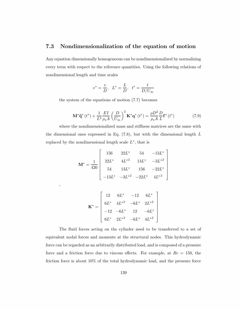
7.3 Nondimensionalization of the equation of motion
Any equation dimensionally homogeneous can be nondimensionalized by normalizing
every term with respect to the reference quantities. Using the following relations of
nondimensional length and time scales
v∗ =v
D, L∗ =
L
D, t∗ =
t
D/U∞
the system of the equations of motion (7.7) becomes
M∗q∗ (t∗) +1
L4
EI
ρsA
(D
U∞
)2
K∗q∗ (t∗) =ρD2
ρsA
D
Lf∗ (t∗) (7.9)
where the nondimensionalized mass and stiffness matrices are the same with
the dimensional ones expressed in Eq. (7.8), but with the dimensional length L
replaced by the nondimensional length scale L∗, that is
M∗ =1
420
156 22L∗ 54 −13L∗
22L∗ 4L∗2 13L∗ −3L∗2
54 13L∗ 156 −22L∗
−13L∗ −3L∗2 −22L∗ 4L∗2
,
K∗ =
12 6L∗ −12 6L∗
6L∗ 4L∗2 −6L∗ 2L∗2
−12 −6L∗ 12 −6L∗
6L∗ 2L∗2 −6L∗ 4L∗2
The fluid forces acting on the cylinder need to be transferred to a set of
equivalent nodal forces and moments at the structural nodes. This hydrodynamic
force can be regarded as an arbitrarily distributed load, and is composed of a pressure
force and a friction force due to viscous effects. For example, at Re = 150, the
friction force is about 10% of the total hydrodynamic load, and the pressure force
139
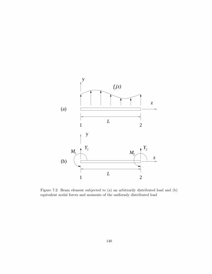
y
z
Y Y1 2
1 2L
M2M1
y
z
1 2L
f (z)y
(a)
(b)
Figure 7.2: Beam element subjected to (a) an arbitrarily distributed load and (b)equivalent nodal forces and moments of the uniformly distributed load
140
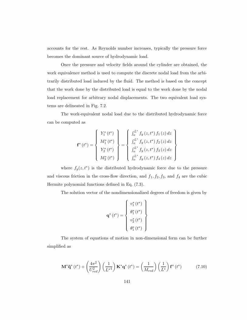
accounts for the rest. As Reynolds number increases, typically the pressure force
becomes the dominant source of hydrodynamic load.
Once the pressure and velocity fields around the cylinder are obtained, the
work equivalence method is used to compute the discrete nodal load from the arbi-
trarily distributed load induced by the fluid. The method is based on the concept
that the work done by the distributed load is equal to the work done by the nodal
load replacement for arbitrary nodal displacements. The two equivalent load sys-
tems are delineated in Fig. 7.2.
The work-equivalent nodal load due to the distributed hydrodynamic force
can be computed as
f∗ (t∗) =
Y ∗
1 (t∗)
M∗
1 (t∗)
Y ∗
2 (t∗)
M∗
2 (t∗)
=
∫ L∗
o fy (z, t∗) f1 (z) dz∫ L∗
o fy (z, t∗) f2 (z) dz∫ L∗
o fy (z, t∗) f3 (z) dz∫ L∗
o fy (z, t∗) f4 (z) dz
where fy(z, t∗) is the distributed hydrodynamic force due to the pressure
and viscous friction in the cross-flow direction, and f1, f2, f3, and f4 are the cubic
Hermite polynomial functions defined in Eq. (7.3).
The solution vector of the nondimensionalized degrees of freedom is given by
q∗ (t∗) =
v∗1 (t∗)
θ∗1 (t∗)
v∗2 (t∗)
θ∗1 (t∗)
The system of equations of motion in non-dimensional form can be further
simplified as
M∗q∗ (t∗) +
(
4π2
U2red
)(1
L∗4
)
K∗q∗ (t∗) =
(1
Mred
)(1
L∗
)
f∗ (t∗) (7.10)
141
by introducing the two non-dimensional parameters Ured and Mred as defined
below. First, the reduced velocity, Ured, is defined as
Ured =U∞
fnD(7.11)
with the effective natural frequency of the structure, ωn, given by
ωn =1
D2
√
EI
ρsA= 2πfn
As shown in the definition of the effective natural frequency, it does not
include the length scale L but represents the natural frequency of a unit length
cylinder. Hence, for a given Ured, if the length of the cylinder changes, the natural
frequency of the cylinder also changes. In order to make a cylinder with a different
length remain in the same resonant state, Ured also has to be changed accordingly.
This is because the reduced velocity affects the bending stiffness of the structure,
and the stiffness of the structure also affects the natural frequency of the bending
vibration.
The main interest of this simulation is in the vortex induced vibration of
the cylinder at its resonant state, namely the lock-in state. Hence Ured of our
structural model is carefully chosen so that its natural frequency of bending vibration
of interest, typically in its first or second mode, is approximately equal to the natural
frequency of vortex shedding over a fixed cylinder. One simple way of checking the
natural frequency of the multiple element beam model is by solving a free vibration
(no forcing term in RHS) problem.
The reduced mass, Mred,which is the ratio of the mass of the structure to
the mass of the fluid displaced by the structure, is defined as,
Mred =ρsA
ρD2. (7.12)
142
This reduced mass represents the inertia of the structural system with respect
to the surrounding fluid. Hence, a smaller mass ratio implies a bigger influence from
the flow with the same scale of hydrodynamic forces. The mass ratio for the VIV
in air is in the order of O(1000). For marine cables in water varies between 1 ∼ 10,
hence we used the representative mass ratio of Mred = 2 [55, 17] for the current
simulations.
143

7.4 Coupling strategies
If the flow and structural solvers are being solved separately, then their interaction
can be implemented using either a strong coupling method or a weak coupling
method depending on how the information between the two solvers is communicated.
n = n + 1
Structural Solver
Mesh deformation
Flow Solver
Figure 7.3: Weak coupling
In the weak coupling strategy, the solution of the flow field at the next time
step is computed from the structural configuration of the previous time step. Once
the solution of the flow field is converged, the new forces acting on the structure
are sent to the structural solver for the new configuration of structure at the next
time step. This simple loop makes both solvers advance one time step. In the weak
coupling method, the external forces to the structural solver come from the solution
of previous mesh configuration, hence this method is also refered as a staggered or
loosely coupled scheme. When the time step is relatively small (especially when an
explicit scheme is used for the flow solver), this weak coupling method can be a
reasonable choice [23].
When an implicit scheme is used for the flow solver, time steps used for the
flow solver is comparable to the time steps restricted by the structural solver. To
144
make the coupling stable even with large time steps of implicit flow solvers, the
structural solver also needs to be solved in an implicit manner which is called strong
coupling. In order to couple the two solvers strongly, iterations between the flow and
structural solvers are necessary for each time step, and this makes their coupling
stable even with large time steps.
The results of two coupling methods are presented in Fig. 7.4 for flow-
structure interactions with time step ∆t = 0.4. For the strong coupling, the flow
and structure interaction is stable, but the weak coupling starts with oscillations and
eventually diverges. This comparison demonstrates the superior stability property
of the strong coupling.
For the implementation of the strong coupling, a predictor-corrector (PC)
method is employed. Any explicit scheme can be used for the predictor, and an
implicit scheme can be used for the corrector.
The correction iteration may be performed until some criterion of conver-
gence, such as∥∥yµ+1 − yµ
∥∥ < ε is achieved, where y is the vector of unknowns for
the structural solver, and ε is the tolerance of the convergence. This strategy is
called iterating to convergence. In this mode, the accuracy and stability properties
are irrespective of the predictor and highly dependent on the corrector alone. What
makes this mode unattractive in practice is that we cannot tell in advance how
many iterations of the corrector (i.e. how many evaluations of the flow field) will be
involved at each time step. In general this is to be avoided, and especially for the
real-time systems [40].
A more acceptable procedure is to fix the number of corrector interations in
advance. The number of corrector iterations (µ ) is small and normally chosen to 1
or 2, with the assumption that the predictor formula is of sufficiently high order q
for p − 1 ≤ q ≤ p, where p is the order of the corrector formula. For current study,
central different scheme is used for the predictor step and trapezodial scheme is used
145
for the corrector iterations. Both of the schemes are second order accurate, and only
one corrector step improves the stability considerably, as shown in Fig. 7.4.
The predictor step is followed by a new evaluation of the flow field and each
corrector step is also followed by a new evaluation of the flow field. This precedure
can be represented as
PE CE · · ·CE︸ ︷︷ ︸
corrector iteration
where P represents the predictor step, C represents the corrector step, and
E represents the evaluation of flow field. When the corrector iteration is fixed to µ,
the predictor-corrector method can be expressed more conveniently as PE (CE)µ.
The evaluation of the flow field following the last corrector step may be omitted,
but finishing the PC method with the last evaluation gives better stability. Hence,
we always solve the flow field whenever a new structural configuration is obtained.
For the PC method with µ corrector iterations, the total number of evaluations of
the flow field is µ + 1. The strong coupling using the PC method is restored to the
weak coupling when the corrector iteration loop is omitted.
7.5 Strong coupling by using the PC method
For the current study, the central difference scheme in time is used for the predictor,
and the trapezoidal scheme is used for the corrector. Both schemes are second order
accurate in time, hence this pair (central-trapezoidal) of the PC method is expected
to be second order accurate. Since the time integration scheme of the flow solver is
also second order (second order backward difference formula), the current choice of
PC pair should not deteriorate the temporal accuracy when it is coupled with the
flow solver.
When the structure is modeled with multiple elements, the complete system
of equations can be assembled by using the equations of motion for a single mas-
146

ter element as shown in Eq. (7.10). Once global mass and stiffness matrices are
assembled and proper boundary conditions are applied, the governing equations of
the bending vibration can be rewritten in a set of coupled second order ordinary
differential equations with a given set of initial conditions as below.
My (t) + Ky (t) = f (t) , t > 0, y (0) = y0 y (0) = y0 (7.13)
where M and K are the global mass and stiffness matrices, y and y are
the vectors containing unknown degrees of freedom and their accleration, y and y
are the initial conditions, and f is external load vector from the flow around the
cylinder. The equation of motion in Eq. (7.13) is in nondimensional form, and all
the ∗’s representing the nondimensional quantities are ommitted for simplicity.
Any explicit/implicit pair can be used for the predictor/corrector method.
For the predictor of the current simulation, the central difference scheme with lagged
approximation of the first derivative is used because of its popularity in structural
dynamics. For the corrector step, the unconditionally stable trapezoidal scheme is
used. This trapezoidal method can be considered a special case of the Newmark
method with average acceleration.
The central difference scheme used for the predictor can be derived by using
the central differenced acceleration
yn =1
∆t2(yn+1 − 2yn + yn−1) (7.14)
and velocity which is lagging half a time step as below.
yn ≈ yn− 1
2
=1
∆t(yn − yn−1) (7.15)
Even with the lagged approximation of the velocity, the central difference
scheme is reported to be second order accurate for the system of small damping [14].
147
Hence, the central difference scheme for the current structural model with no damp-
ing can be expected to be second order accurate.
By using the central differenced accleration and velocity as expressed in
Eq. (7.14) and Eq. (7.15) respectively, and the equation of motion in Eq. (7.10),
the predictor scheme can be expressed as below.
Predictor
y(µ=0)n+1 = ∆t2M−1 (fn −Kyn) + yn + ∆tyn− 1
2
y(µ=0)n+1 ≈ y
(µ=0)
n+ 12
= 1∆t
(
y(µ=0)n+1 − yn
)
By using the trapezoidal rule, the displacement and velocity can be expressed
as.
yn+1 = yn +∆t
2(yn + yn+1)
yn+1 = yn +∆t
2(yn + yn+1)
The velocity and acceleration for the next time step can be derived from the
above relation.
yn+1 =2
∆t(yn+1 − yn) − yn
yn+1 =4
∆t2(yn+1 − yn) − 4
∆tyn − yn
Using the equation of motion Eq. (7.10) and the above relations, the corrector
scheme can be expressed as.
Corrector
for i = 1, · · ·, µmax
148
y(µ)n+1 =
(4
∆t2M + K
)−1 (
f(µ−1)n+1 + M
(4
∆t2yn + 4
∆tyn + yn
))
y(µ)n+1 = 2
∆t
(
y(µ)n+1 − yn
)
− yn
end
The corrector iteration is performed until it meets the maximum number of
iterations ( µmax). For the current study, only one corrector iteration (µmax = 1) is
performed, and this makes the coupling stable for all time steps used in this study.
149
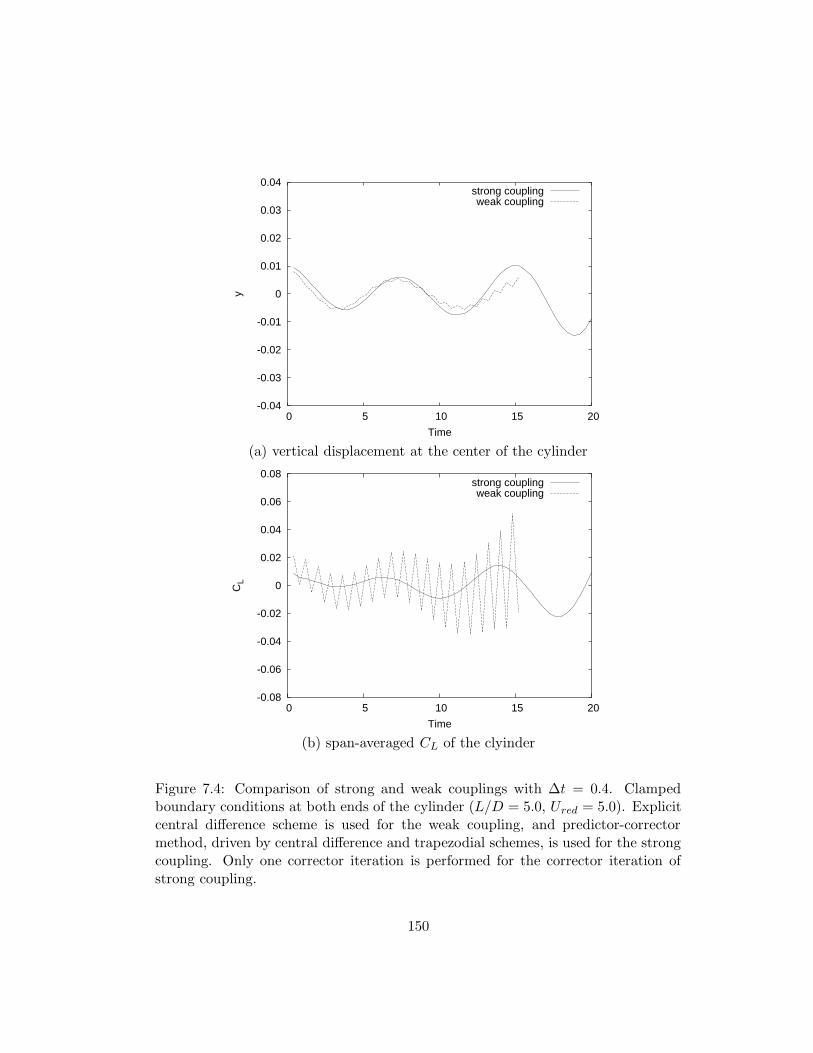
-0.04
-0.03
-0.02
-0.01
0
0.01
0.02
0.03
0.04
0 5 10 15 20
y
Time
strong couplingweak coupling
(a) vertical displacement at the center of the cylinder
-0.08
-0.06
-0.04
-0.02
0
0.02
0.04
0.06
0.08
0 5 10 15 20
CL
Time
strong couplingweak coupling
(b) span-averaged CL of the clyinder
Figure 7.4: Comparison of strong and weak couplings with ∆t = 0.4. Clampedboundary conditions at both ends of the cylinder (L/D = 5.0, Ured = 5.0). Explicitcentral difference scheme is used for the weak coupling, and predictor-correctormethod, driven by central difference and trapezodial schemes, is used for the strongcoupling. Only one corrector iteration is performed for the corrector iteration ofstrong coupling.
150
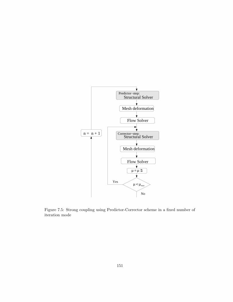
n = n + 1
maxµ < µ Yes
No
Flow Solver
Mesh deformation
Predictor−step:Structural Solver
Structural Solver
Mesh deformation
Flow Solver
µ = µ + 1
Corrector−step:
Figure 7.5: Strong coupling using Predictor-Corrector scheme in a fixed number ofiteration mode
151
Chapter 8
Verification of the Solution
Algorithm for Fluid and
Structure Interactions
In this chapter, a verification study of the ALE scheme is presented, and then
it is applied to fluid and structure interaction problems. In the first part of the
chapter, the proposed ALE scheme with moving mesh source term is verified with
forced excitation of the cylinder. The significance of the moving mesh source term is
demonstrated in terms of the uniform flow preserving capability. Temporal accuracy
of the current time integration scheme is demonstrated by a time step refinement
study. In the second part, the ALE scheme is applied to the vortex-induced vibra-
tion (VIV) of the cylinder. A VIV initiation technique is introduced, and a time
step refinement study is presented. Different end conditions are applied to the vi-
brating cylinder, and finally the current numerical result is compared with others
in literature.
152

8.1 Verification of the proposed ALE scheme by forced
excitation
The proposed finite-volume ALE scheme is validated by simulating flows around a
deforming cylinder. The cylinder is modeled with beam structural elements, and
then excited harmonically at one of its ends in the cross flow direction. The uniform
flow preserving capability of the proposed ALE scheme is demonstrated with the
deforming mesh simulations, and the temporal accuracy of the backward difference
formula is also presented.
8.1.1 Truncation error analysis of the temporal discretization
The proposed ALE formulation with a moving mesh source term can be expressed
as follows
dUi
dtVi + Fi (Q,xf , xf ) = Gi (Q,xg) + Si (Q,xs, xs) (8.1)
where Fi, Gi and Si are the convective, viscous fluxes and moving mesh
source for control volume i, and x and x are the instantaneous mesh configuration
and velocity for the flux or source evaluations.
The temporal discretization of the proposed ALE scheme with second order
backward difference formula can be expressed as follows
(32U
n+1i − 2Un
i + 12U
n−1i
)
V n+1i + ∆t
Kf∑
k=1αkFi
(
Qn+1,x(k)f , x
(k)f
)
= ∆tKg∑
k=1βkGi
(
Qn+1,x(k)g
)
+ ∆tKs∑
k=1γkSi
(
Qn+1,x(k)s , x
(k)s
)(8.2)
The mesh configurations and velocities for the numerical fluxes and moving
mesh source term computation at fictitious time (k) is parameterized as follows
x(k)f = ςn+1
k xn+1 + ςnk xn + ςn−1
k xn−1 (8.3)
153

x(k)f =
θn+1k xn+1 + θn
kxn + θn−1
k xn−1
∆t(8.4)
x(k)g = ηn+1
k xn+1 + ηnkxn + ηn−1
k xn−1 (8.5)
x(k)s = ξn+1
k xn+1 + ξnkxn + ξn−1
k xn−1 (8.6)
x(k)s =
υn+1k xn+1 + υn
kxn + υn−1k xn−1
∆t(8.7)
Proposition 1.
If the parameterization (8.3) to (8.7) satisfies
ςn+1k + ςn
k + ςn−1k = 1 ∀k, (8.8)
θn+1k + θn
k + θn−1k = 0 ∀k, (8.9)
θnk + 2θn−1
k = −1 ∀k, (8.10)
Kf∑
k=1
αk = 1, (8.11)
Kf∑
k=1
αk
(
ςnk + 2ςn−1
k
)
= 0, (8.12)
Kf∑
k=1
αk
(
θnk + 4θn−1
k
)
= 0, (8.13)
154
ηn+1k + ηn
k + ηn−1k = 1 ∀k, (8.14)
Kg∑
k=1
βk = 1, (8.15)
Kg∑
k=1
βk
(
ηnk + 2ηn−1
k
)
= 0, (8.16)
ξn+1k + ξn
k + ξn−1k = 1 ∀k, (8.17)
υn+1k + υn
k + υn−1k = 0 ∀k, (8.18)
υnk + 2υn−1
k = −1 ∀k, (8.19)
Ks∑
k=1
γk = 1, (8.20)
Ks∑
k=1
γk
(
ξnk + 2ξn−1
k
)
= 0, (8.21)
Ks∑
k=1
γk
(
υnk + 4υn−1
k
)
= 0, (8.22)
and the flux and source terms F, G, S are continuous and sufficiently
smooth, then the temporal discretization scheme of the ALE formulation in time is
second order accurate.
155
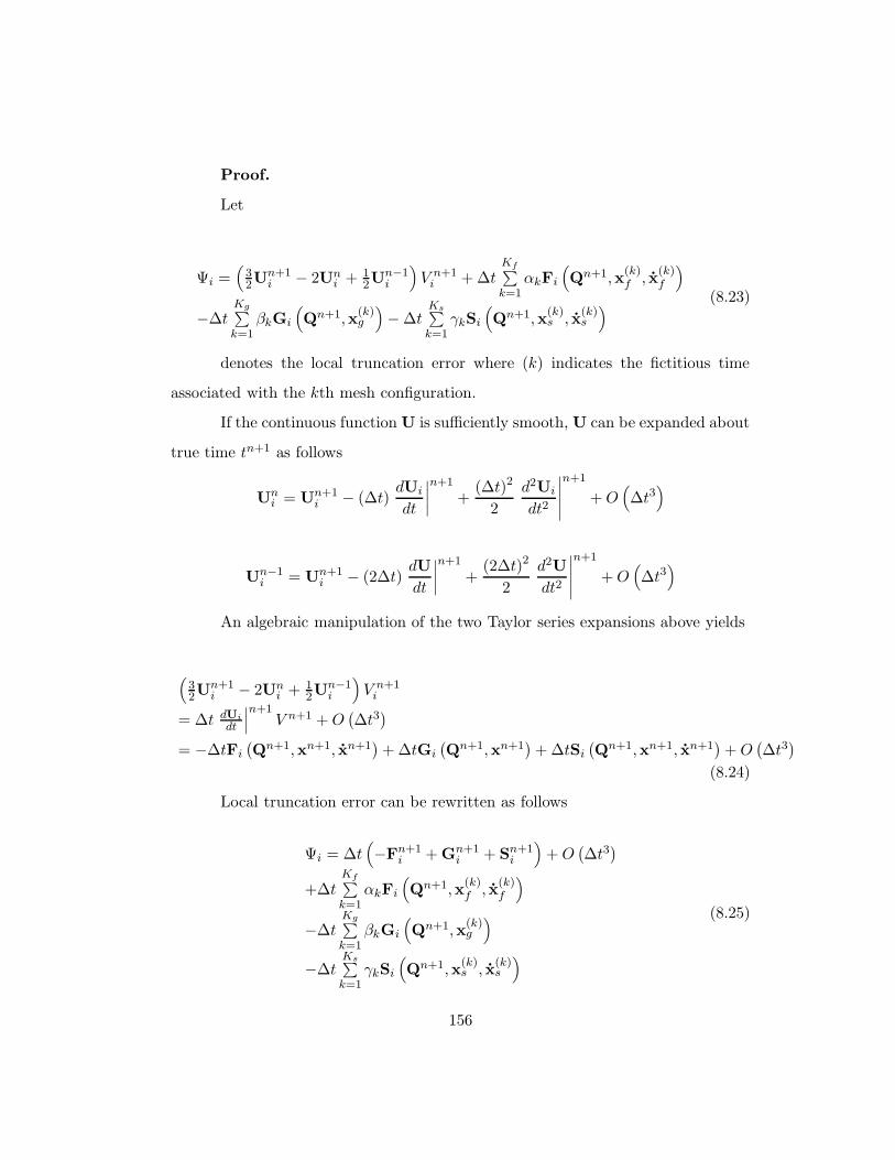
Proof.
Let
Ψi =(
32U
n+1i − 2Un
i + 12U
n−1i
)
V n+1i + ∆t
Kf∑
k=1αkFi
(
Qn+1,x(k)f , x
(k)f
)
−∆tKg∑
k=1βkGi
(
Qn+1,x(k)g
)
− ∆tKs∑
k=1γkSi
(
Qn+1,x(k)s , x
(k)s
)(8.23)
denotes the local truncation error where (k) indicates the fictitious time
associated with the kth mesh configuration.
If the continuous function U is sufficiently smooth, U can be expanded about
true time tn+1 as follows
Uni = Un+1
i − (∆t)dUi
dt
∣∣∣∣
n+1
+(∆t)2
2
d2Ui
dt2
∣∣∣∣∣
n+1
+ O(
∆t3)
Un−1i = Un+1
i − (2∆t)dU
dt
∣∣∣∣
n+1
+(2∆t)2
2
d2U
dt2
∣∣∣∣∣
n+1
+ O(
∆t3)
An algebraic manipulation of the two Taylor series expansions above yields
(32U
n+1i − 2Un
i + 12U
n−1i
)
V n+1i
= ∆t dUi
dt
∣∣∣
n+1V n+1 + O
(∆t3
)
= −∆tFi
(
Qn+1,xn+1, xn+1)
+ ∆tGi
(
Qn+1,xn+1)
+ ∆tSi
(
Qn+1,xn+1, xn+1)
+ O(
∆t3)
(8.24)
Local truncation error can be rewritten as follows
Ψi = ∆t(
−Fn+1i + Gn+1
i + Sn+1i
)
+ O(∆t3
)
+∆tKf∑
k=1αkFi
(
Qn+1,x(k)f , x
(k)f
)
−∆tKg∑
k=1βkGi
(
Qn+1,x(k)g
)
−∆tKs∑
k=1γkSi
(
Qn+1,x(k)s , x
(k)s
)
(8.25)
156
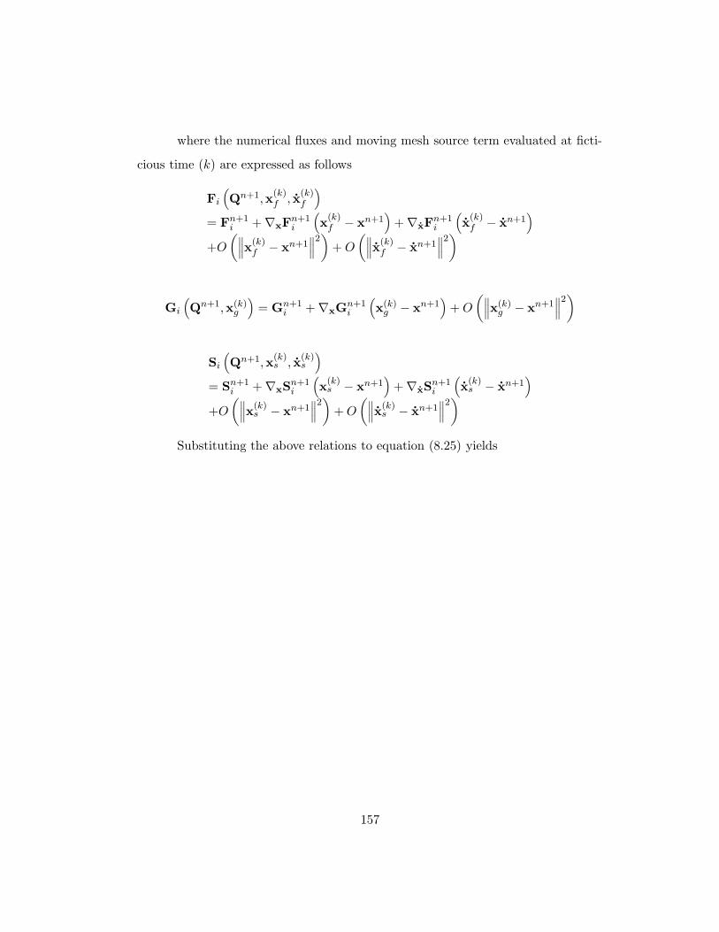
where the numerical fluxes and moving mesh source term evaluated at ficti-
cious time (k) are expressed as follows
Fi
(
Qn+1,x(k)f , x
(k)f
)
= Fn+1i + ∇xF
n+1i
(
x(k)f − xn+1
)
+ ∇xFn+1i
(
x(k)f − xn+1
)
+O
(∥∥∥x
(k)f − xn+1
∥∥∥
2)
+ O
(∥∥∥x
(k)f − xn+1
∥∥∥
2)
Gi
(
Qn+1,x(k)g
)
= Gn+1i + ∇xG
n+1i
(
x(k)g − xn+1
)
+ O
(∥∥∥x(k)
g − xn+1∥∥∥
2)
Si
(
Qn+1,x(k)s , x
(k)s
)
= Sn+1i + ∇xS
n+1i
(
x(k)s − xn+1
)
+ ∇xSn+1i
(
x(k)s − xn+1
)
+O
(∥∥∥x
(k)s − xn+1
∥∥∥
2)
+ O
(∥∥∥x
(k)s − xn+1
∥∥∥
2)
Substituting the above relations to equation (8.25) yields
157

Ψi = ∆t
{(Kf∑
k=1αk
)
− 1
}
Fn+1i
+∆t∇xFn+1i
{Kf∑
k=1αk
(
x(k)f − xn+1
)}
+∆t∇xFn+1i
{Kf∑
k=1αk
(
x(k)f − xn+1
)}
−∆t
{(Kg∑
k=1βk
)
− 1
}
Gn+1i
−∆t∇xGn+1i
{Kg∑
k=1βk
(
x(k)g − xn+1
)}
−∆t
{(Ks∑
k=1γk
)
− 1
}
Sn+1i
−∆t∇xSn+1i
{Ks∑
k=1γk
(
x(k)s − xn+1
)}
−∆t∇xSn+1i
{Ks∑
k=1γk
(
x(k)s − xn+1
)}
+∆t
{Kf∑
k=1αkO
(∥∥∥x
(k)f − xn+1
∥∥∥
2+∥∥∥x
(k)f − xn+1
∥∥∥
2)}
−∆t
{Kg∑
k=1βkO
(∥∥∥x
(k)g − xn+1
∥∥∥
2)}
−∆t
{Kg∑
k=1γkO
(∥∥∥x
(k)s − xn+1
∥∥∥
2+∥∥∥x
(k)s − xn+1
∥∥∥
2)}
+O(∆t3
)
(8.26)
By using Taylor series expansions of the mesh configurations at time n and
n − 1 about time n + 1,
xn = xn+1 − (∆t) xn+1 + O(
∆t2)
xn−1 = xn+1 − (2∆t) xn+1 + O(
∆t2)
The relations of the mesh configurations and velocity between fictitious time
(k) and true time n + 1 can be expressed as
x(k)f − xn+1 =
(
ςn+1k + ςn
k + ςn−1k − 1
)
xn+1 − ∆t(
ςnk − 2ςn−1
k
)
xn+1 + O(
∆t2)
158

x(k)f − xn+1 =
(θn+1
k+θn
k+θn−1
k )∆t
xn+1 −(
θnk + 2θn−1
k + 1)
xn+1
+∆t2
(
θnk + 4θn−1
k
)
xn+1 + O(∆t2
)
x(k)g − xn+1 =
(
ηn+1k + ηn
k + ηn−1k − 1
)
xn+1 − ∆t(
ηnk + 2ηn−1
k
)
xn+1 + O(
∆t2)
x(k)s − xn+1 =
(
ξn+1k + ξn
k + ξn−1k − 1
)
xn+1 − ∆t(
ξnk + 2ξn−1
k
)
xn+1 + O(
∆t2)
x(k)s − xn+1 =
(υn+1
k+υn
k+υn−1
k )∆t
xn+1 −(
υnk + 2υn−1
k − 1)
xn+1
+∆t2
(
υnk + 4υn−1
k
)
xn+1 + O(∆t2
)
Finally the local truncation error can be expressed as follows
Ψi = ∆t
{(Kf∑
k=1αk
)
− 1
}
Fn+1i
+∆t2{
Kf∑
k=1αk
(
ςnk − 2ςn−1
k
)}(
∇xFn+1i
)
xn+1
+∆t2
2
{Kf∑
k=1αk
(
θnk + 4θn−1
k
)}(
∇xFn+1i
)
xn+1
−∆t
{(Kg∑
k=1βk
)
− 1
}
Gn+1i
−∆t2{
Kg∑
k=1βk
(
ηnk + 2ηn−1
k
)}(
∇xGn+1i
)
xn+1
−∆t
{(Ks∑
k=1γk
)
− 1
}
Sn+1i
−∆t2{
Ks∑
k=1γk
(
ξnk + 2ξn−1
k
)}(
∇xSn+1i
)
xn+1
−∆t2
2
{Ks∑
k=1γk
(
υnk + 4υn−1
k
)}(
∇xSn+1i
)
xn+1 + O(∆t3
)
(8.27)
and all terms vanish except the third order term by the Proposition 1. Hence
the any temporal discretization satisfying the Proposition 1 preserves second order
accuracy on moving meshes.
159
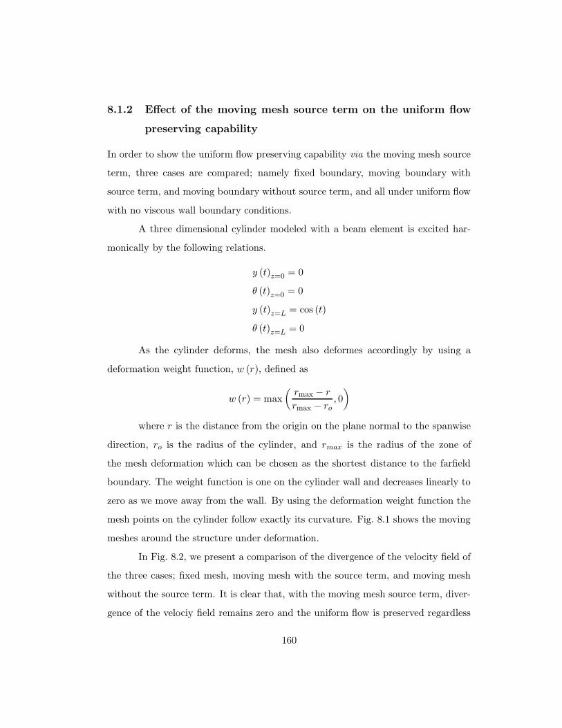
8.1.2 Effect of the moving mesh source term on the uniform flow
preserving capability
In order to show the uniform flow preserving capability via the moving mesh source
term, three cases are compared; namely fixed boundary, moving boundary with
source term, and moving boundary without source term, and all under uniform flow
with no viscous wall boundary conditions.
A three dimensional cylinder modeled with a beam element is excited har-
monically by the following relations.
y (t)z=0 = 0
θ (t)z=0 = 0
y (t)z=L = cos (t)
θ (t)z=L = 0
As the cylinder deforms, the mesh also deformes accordingly by using a
deformation weight function, w (r), defined as
w (r) = max
(rmax − r
rmax − ro, 0
)
where r is the distance from the origin on the plane normal to the spanwise
direction, ro is the radius of the cylinder, and rmax is the radius of the zone of
the mesh deformation which can be chosen as the shortest distance to the farfield
boundary. The weight function is one on the cylinder wall and decreases linearly to
zero as we move away from the wall. By using the deformation weight function the
mesh points on the cylinder follow exactly its curvature. Fig. 8.1 shows the moving
meshes around the structure under deformation.
In Fig. 8.2, we present a comparison of the divergence of the velocity field of
the three cases; fixed mesh, moving mesh with the source term, and moving mesh
without the source term. It is clear that, with the moving mesh source term, diver-
gence of the velociy field remains zero and the uniform flow is preserved regardless
160

of mesh motion. Without the moving mesh source term, divergence of the velocity
field jumps as the mesh deforms, and uniform flow is also not preserved as the mesh
starts to deform. Hence, it can be concluded that the proposed ALE scheme is
geometrically conservative via the moving mesh source term .
8.1.3 Temporal accuracy of the ALE scheme
Temporal accuracy of the presented ALE scheme is verified by using a time step
refinement study. The temporal accuracy of the backward difference formula on
a fixed mesh configuration is verified, but there is no such result reported for the
backward difference formulas applied to the ALE formulation with the moving mesh
source term.
In this section, a time step refinement study is presented for the first and
second order backward difference formulas applied to the current ALE scheme. The
temporal order of accuracy is presented by comparing the solutions with finite time
steps to a reference solution obtained with an extremely small time step in lieu of
the exact solution.
The comparison of the first and second order backward difference formulae
is presented in Fig. 8.3. The CL responses to the harmonically excited cylinder
with uniform inflow is presented with a series of successively refined time steps.
For the first order backward difference formula (BDF1), a relatively wide deviation
of the CL response from the reference solution is observed. For the second order
scheme (BDF2), the CL histories are more clustered to the reference solution, which
indicates better convergence. The overshoots of the second order scheme at the
initial stage of the simulation are attributed to the starting problem of requiring
initial conditions one more time step back.
In order to estimate the order of accuracy of the backward difference for-
mulas of the current ALE scheme, a series of successively refined time-steps (∆t =
161
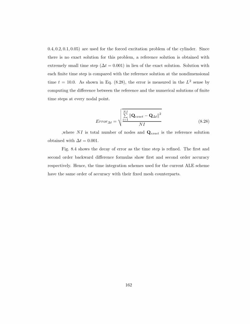
0.4, 0.2, 0.1, 0.05) are used for the forced excitation problem of the cylinder. Since
there is no exact solution for this problem, a reference solution is obtained with
extremely small time step (∆t = 0.001) in lieu of the exact solution. Solution with
each finite time step is compared with the reference solution at the nondimensional
time t = 10.0. As shown in Eq. (8.28), the error is measured in the L2 sense by
computing the difference between the reference and the numerical solutions of finite
time steps at every nodal point.
Error∆t =
√√√√√
NI∑
i=1‖Qexact −Q∆t‖2
NI(8.28)
,where NI is total number of nodes and Qexact is the reference solution
obtained with ∆t = 0.001.
Fig. 8.4 shows the decay of error as the time step is refined. The first and
second order backward difference formulas show first and second order accuracy
respectively. Hence, the time integration schemes used for the current ALE scheme
have the same order of accuracy with their fixed mesh counterparts.
162
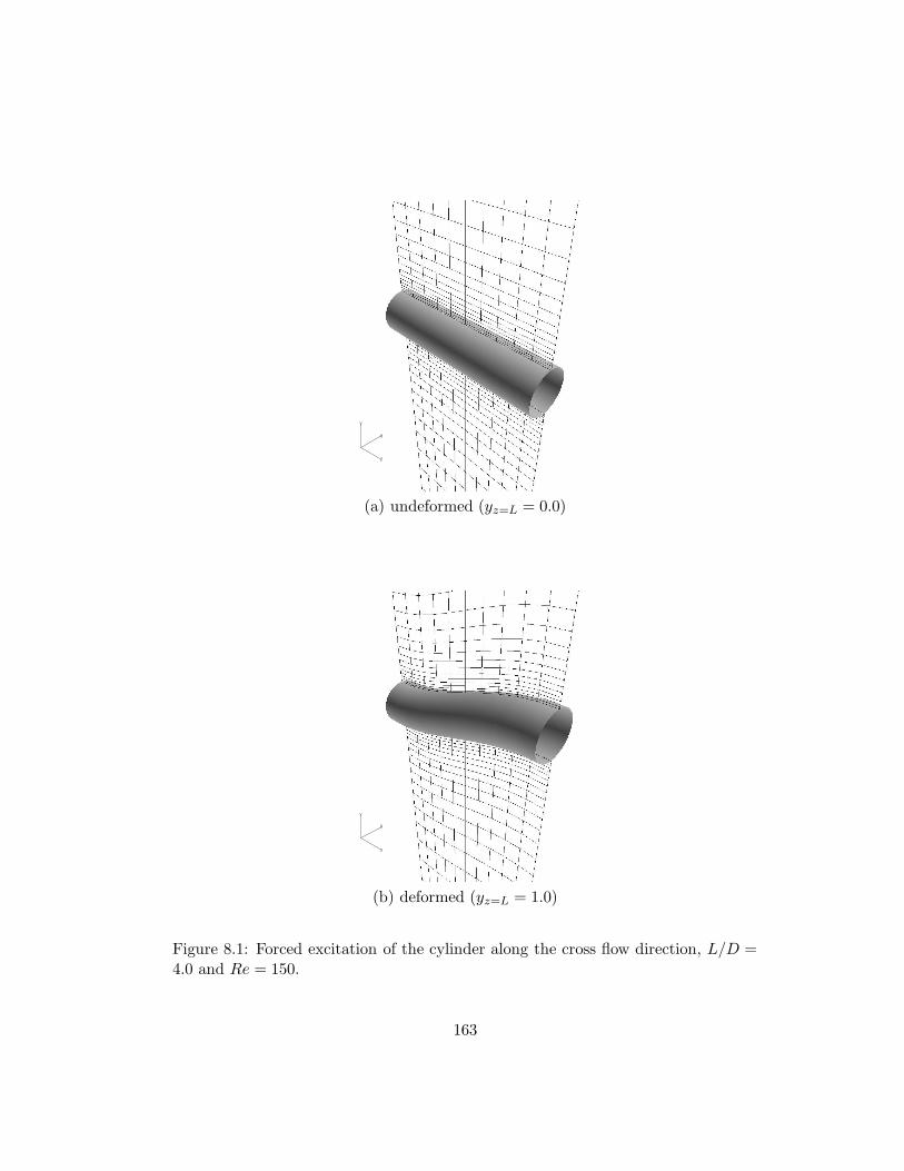
(a) undeformed (yz=L = 0.0)
(b) deformed (yz=L = 1.0)
Figure 8.1: Forced excitation of the cylinder along the cross flow direction, L/D =4.0 and Re = 150.
163
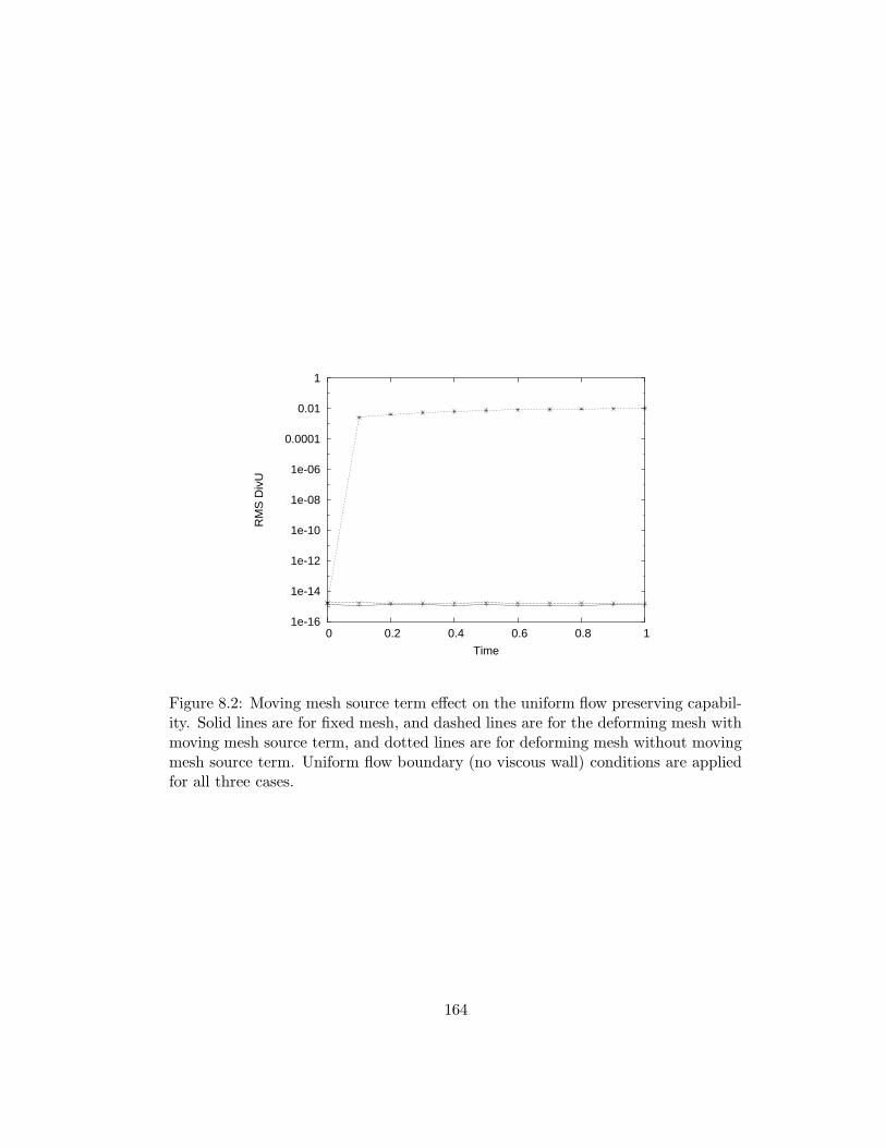
1e-16
1e-14
1e-12
1e-10
1e-08
1e-06
0.0001
0.01
1
0 0.2 0.4 0.6 0.8 1
RM
S D
ivU
Time
Figure 8.2: Moving mesh source term effect on the uniform flow preserving capabil-ity. Solid lines are for fixed mesh, and dashed lines are for the deforming mesh withmoving mesh source term, and dotted lines are for deforming mesh without movingmesh source term. Uniform flow boundary (no viscous wall) conditions are appliedfor all three cases.
164
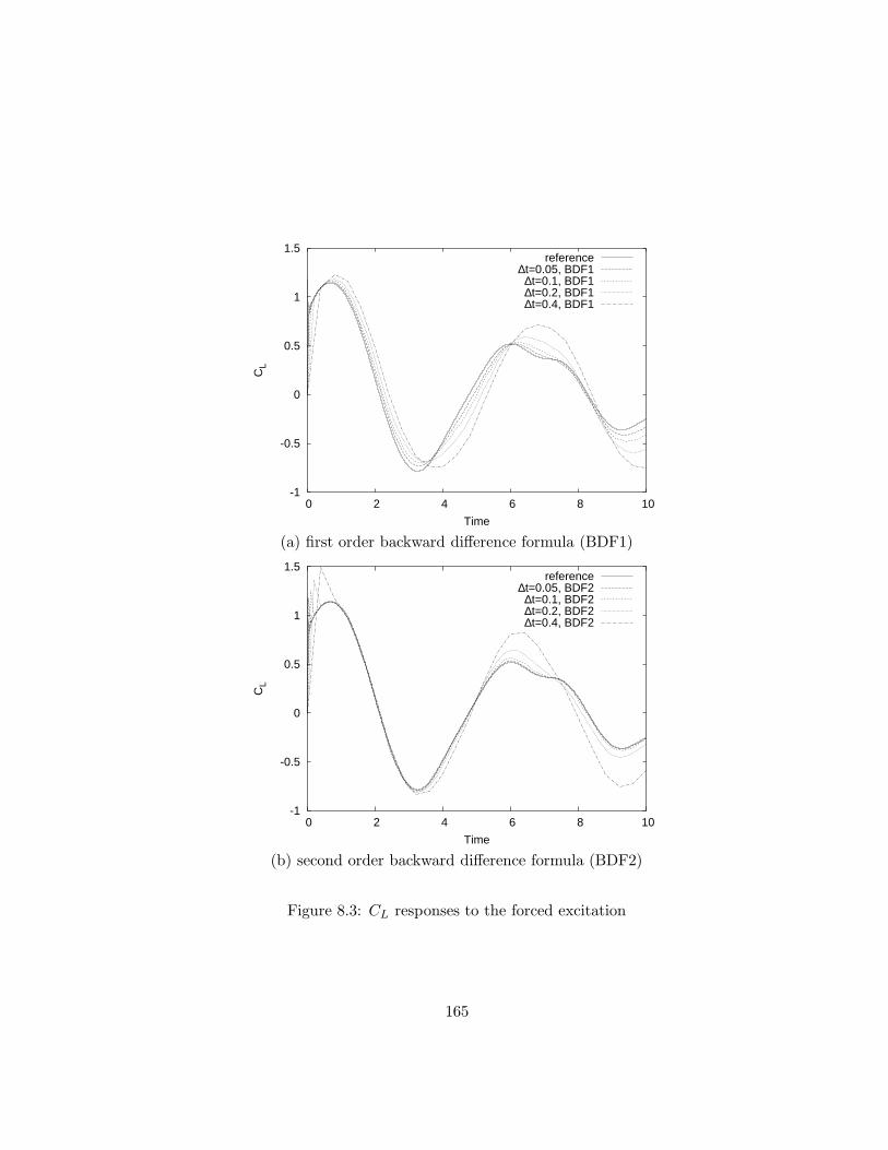
-1
-0.5
0
0.5
1
1.5
0 2 4 6 8 10
CL
Time
reference∆t=0.05, BDF1
∆t=0.1, BDF1∆t=0.2, BDF1∆t=0.4, BDF1
(a) first order backward difference formula (BDF1)
-1
-0.5
0
0.5
1
1.5
0 2 4 6 8 10
CL
Time
reference∆t=0.05, BDF2
∆t=0.1, BDF2∆t=0.2, BDF2∆t=0.4, BDF2
(b) second order backward difference formula (BDF2)
Figure 8.3: CL responses to the forced excitation
165
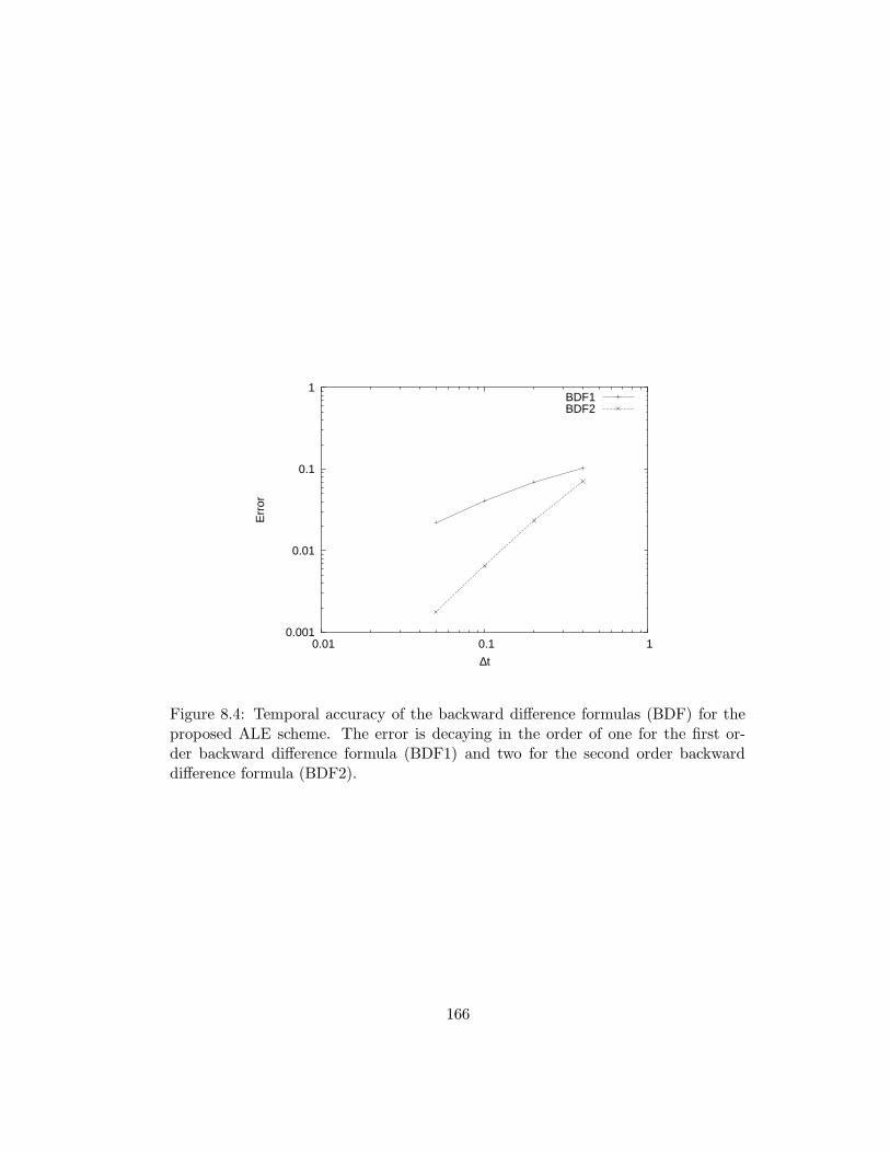
0.001
0.01
0.1
1
0.01 0.1 1
Err
or
∆t
BDF1BDF2
Figure 8.4: Temporal accuracy of the backward difference formulas (BDF) for theproposed ALE scheme. The error is decaying in the order of one for the first or-der backward difference formula (BDF1) and two for the second order backwarddifference formula (BDF2).
166

8.2 Vortex induced vibration of the cylinder
8.2.1 Initial imperfection effect on the initiation of VIV
The development of VIV depends directly on the development of vortex shedding,
and the start of vortex shedding typically requires considerable computation time
until the assymmetry in the flow field develops and initiates shedding. The initiation
of the VIV can be accelerated by applying imperfection on the initial configuration
of the cylinder.
As shown in Fig. 8.5, the initial disturbance only accelerates the VIV and
results in exactly the same periodic state of VIV when it reaches the lock-in resonant
state. As the VIV develops, the displacement at the mid-point of the pinned cylinder
is increasing to the maximum amplitude monotonically, while the span averaged lift
coefficient shows an overshoot and then settles down to the periodic state, which is
attributed to the inertia effect of the cylinder.
8.2.2 Time step refinement study
To be sure about the temporal accuracy of the current VIV simulation, a time step
refinement study is presented with the time steps ∆t = 0.2, 0.1, and 0.05. For each
one of the time steps, shedding period averaged over the last three shedding cycles
are listed in Table 8.1. The order of convergence of the VIV period, T , is estimated
by using Richardson’s extrapolation, as shown below
log2
(
(T )∆t=0.2 − (T )∆t=0.1
(T )∆t=0.1 − (T )∆t=0.05
)
= 2.807 (8.29)
and this agrees well with the formal accuracy of the three point backward
difference formula, which is second order.
The result of the current simulation is compared to other computational
results [55], and is in relatively good agreement although a different approach is
167

∆t VIV period, T
0.2 6.2000.1 6.0250.05 6.000
Table 8.1: VIV periods averaged over the last four cycles.
used. The small difference between the two results seems to be attributed to the
differences in structural models, Reynolds number, and the length of the cylinder.
For modelling of a high aspect ratio cylinder, a cable model with no bending rigidity
can be a reasonable choice, but for a relatively short cylinder, bending rigidity has
to be considered. Since the current cylinder model is relatively short (L/D = 5.0),
the beam elements are chosen in the present study.
structural model Re L/D max y max CL
beam 150 5.0 0.61 0.27cable 100 12.6 0.67 0.35
Table 8.2: Comparison of VIV of beam modeled cylinder (current simulation) andcable modeled cylinder (Newman and Karniadakis [55])
8.2.3 VIV with different end conditions
The strong coupling method introduced in the previous section is applied to the
flow and structure interaction of a vibrating cylinder. The bending stiffness of
the cylinder is modulated such that the natural frequency of the free vibration is
168
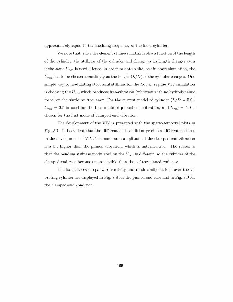
approximately equal to the shedding frequency of the fixed cylinder.
We note that, since the element stiffness matrix is also a function of the length
of the cylinder, the stiffness of the cylinder will change as its length changes even
if the same Ured is used. Hence, in order to obtain the lock-in state simulation, the
Ured has to be chosen accordingly as the length (L/D) of the cylinder changes. One
simple way of modulating structural stiffness for the lock-in regime VIV simulation
is choosing the Ured which produces free-vibration (vibration with no hydrodynamic
force) at the shedding frequency. For the current model of cylinder (L/D = 5.0),
Ured = 2.5 is used for the first mode of pinned-end vibration, and Ured = 5.0 is
chosen for the first mode of clamped-end vibration.
The development of the VIV is presented with the spatio-temporal plots in
Fig. 8.7. It is evident that the different end condition produces different patterns
in the development of VIV. The maximum amplitude of the clamped-end vibration
is a bit higher than the pinned vibration, which is anti-intuitive. The reason is
that the bending stiffness modulated by the Ured is different, so the cylinder of the
clamped-end case becomes more flexible than that of the pinned-end case.
The iso-surfaces of spanwise vorticity and mesh configurations over the vi-
brating cylinder are displayed in Fig. 8.8 for the pinned-end case and in Fig. 8.9 for
the clamped-end condition.
169
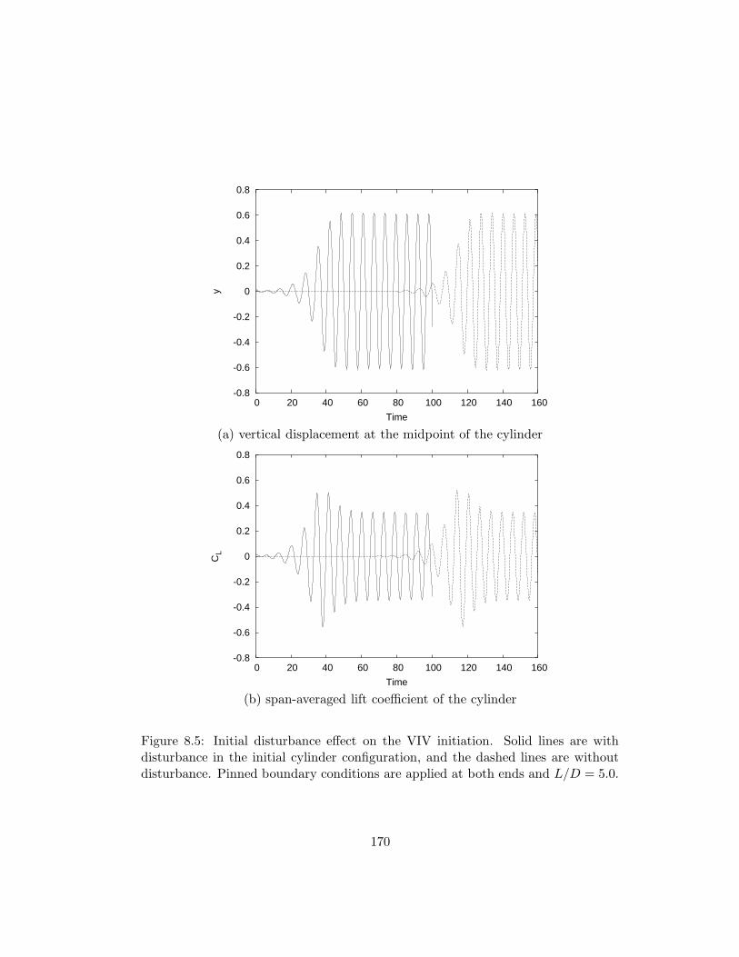
-0.8
-0.6
-0.4
-0.2
0
0.2
0.4
0.6
0.8
0 20 40 60 80 100 120 140 160
y
Time
(a) vertical displacement at the midpoint of the cylinder
-0.8
-0.6
-0.4
-0.2
0
0.2
0.4
0.6
0.8
0 20 40 60 80 100 120 140 160
CL
Time
(b) span-averaged lift coefficient of the cylinder
Figure 8.5: Initial disturbance effect on the VIV initiation. Solid lines are withdisturbance in the initial cylinder configuration, and the dashed lines are withoutdisturbance. Pinned boundary conditions are applied at both ends and L/D = 5.0.
170
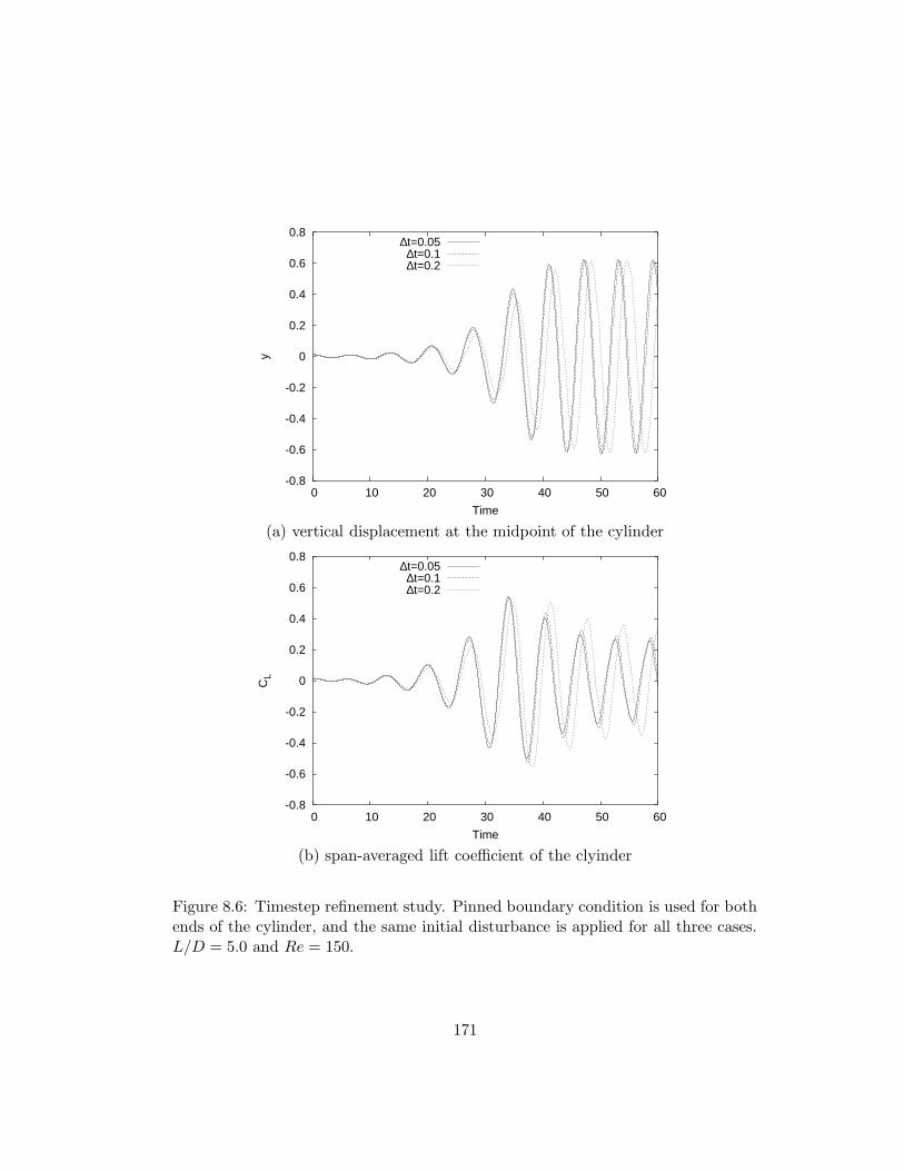
-0.8
-0.6
-0.4
-0.2
0
0.2
0.4
0.6
0.8
0 10 20 30 40 50 60
y
Time
∆t=0.05∆t=0.1∆t=0.2
(a) vertical displacement at the midpoint of the cylinder
-0.8
-0.6
-0.4
-0.2
0
0.2
0.4
0.6
0.8
0 10 20 30 40 50 60
CL
Time
∆t=0.05∆t=0.1∆t=0.2
(b) span-averaged lift coefficient of the clyinder
Figure 8.6: Timestep refinement study. Pinned boundary condition is used for bothends of the cylinder, and the same initial disturbance is applied for all three cases.L/D = 5.0 and Re = 150.
171
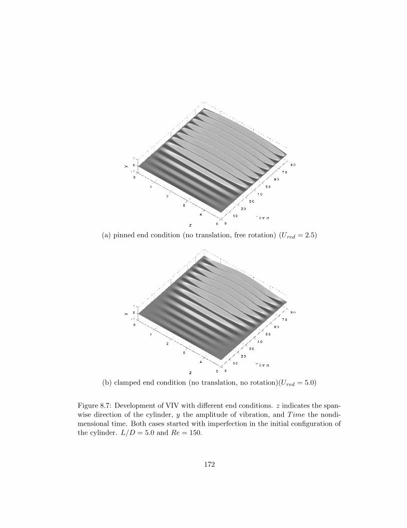
(a) pinned end condition (no translation, free rotation) (Ured = 2.5)
(b) clamped end condition (no translation, no rotation)(Ured = 5.0)
Figure 8.7: Development of VIV with different end conditions. z indicates the span-wise direction of the cylinder, y the amplitude of vibration, and T ime the nondi-mensional time. Both cases started with imperfection in the initial configuration ofthe cylinder. L/D = 5.0 and Re = 150.
172
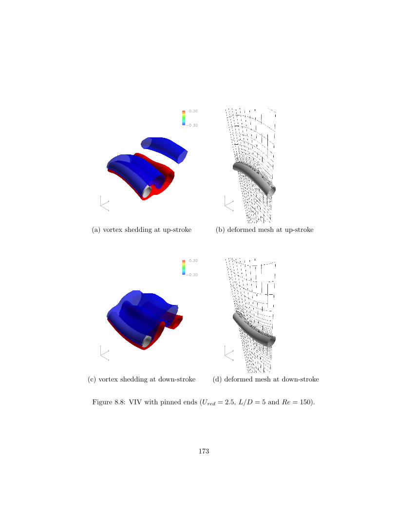
(a) vortex shedding at up-stroke (b) deformed mesh at up-stroke
(c) vortex shedding at down-stroke (d) deformed mesh at down-stroke
Figure 8.8: VIV with pinned ends (Ured = 2.5, L/D = 5 and Re = 150).
173
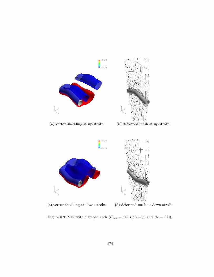
(a) vortex shedding at up-stroke (b) deformed mesh at up-stroke
(c) vortex shedding at down-stroke (d) deformed mesh at down-stroke
Figure 8.9: VIV with clamped ends (Ured = 5.0, L/D = 5, and Re = 150).
174

8.3 Comparison between structured and unstructured
meshes
A mesh comparison study is presented by using two levels of structured polar meshes
and a general hybrid mesh. First, a coarse polar mesh is generated and it is uni-
formly refined in each coordinate direction in order to get the medium polar mesh.
The general hybrid mesh is an unstructured mesh which contains all four types of
elements in three dimensions, namely tetrahedra, pyramids, prisms, and hexahe-
dra. The boundary of the circular cylinder from the three meshes are displayed in
Fig. 8.10 and characteristics of the meshes are listed in Table 8.3.
Vortex induced vibration with clamped-sliding end condition is simulated
with the three meshes, and the results are compared.
structural model coarse polar medium polar hybrid
Etotal 11,520 92,160 509,269Ntotal 13,024 98,112 148,719
Ncircum 32 64 74∆r0 0.004 0.002 0.0009Rffd 15.5 15.5 6.0
Table 8.3: Characteristics of the two levels of structured polar meshes and the gen-eral hybrid mesh. Etotal refers to the total number of elements, Ntotal to the totalnumber of nodes, Ncircum to the number of nodes on the cylinder along the circum-ferential direction, ∆r0 is for the initial spacing on viscous wall, Rffd is far fielddistance from the center of the cylinder. All length units are non-dimensionalizedwith respect to the cylinder diameter.
The vortex shedding over the vibrating cylinder is displayed in Fig. 8.11 for
three meshes. Iso-vorticity surfaces near the vibrating cylinder is similar for all
three meshes. The difference in iso-vorticity surface downstram seems attribute to
175
several factors, for example mesh resolution, domain size and shape, and etc. The
development of VIV is displayed in Fig. 8.12. In generally, as mesh becomes fine,
the amplitude of cylinder displacement converges.
176
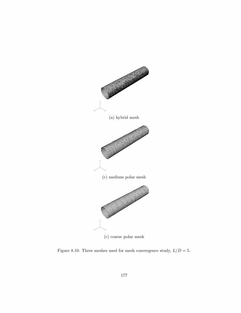
(a) hybrid mesh
(c) medium polar mesh
(c) coarse polar mesh
Figure 8.10: Three meshes used for mesh convergence study, L/D = 5.
177
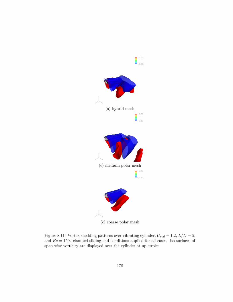
(a) hybrid mesh
(c) medium polar mesh
(c) coarse polar mesh
Figure 8.11: Vortex shedding patterns over vibrating cylinder, Ured = 1.2, L/D = 5,and Re = 150. clamped-sliding end conditions applied for all cases. Iso-surfaces ofspan-wise vorticity are displayed over the cylinder at up-stroke.
178
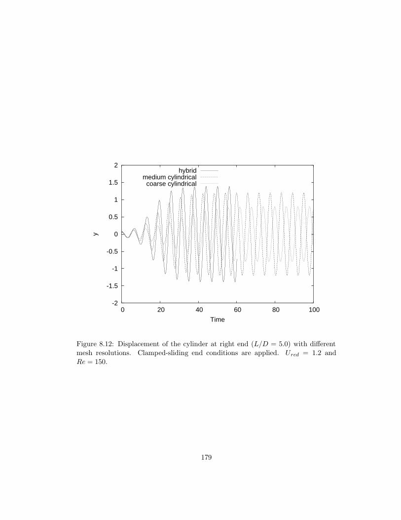
-2
-1.5
-1
-0.5
0
0.5
1
1.5
2
0 20 40 60 80 100
y
Time
hybridmedium cylindricalcoarse cylindrical
Figure 8.12: Displacement of the cylinder at right end (L/D = 5.0) with differentmesh resolutions. Clamped-sliding end conditions are applied. Ured = 1.2 andRe = 150.
179
Chapter 9
Parallelization
A parallel implementation of the presented solution algorithms for general hybrid
meshes is presented for a distributed memory machine by using the message passing
interface (MPI) library. Two different partitioning methods are introduced; namely
graph partitioning and mesh partitioning. An overlapping interface cell strategy is
employed in order to reduce the inter-processor communication phases. A single loop
interprocessor communication algorithm is introduced and the associated pseudo-
code is given. Scalability of the proposed parallel algorithm is presented.
180
9.1 Partitioning methods
Quality of partitioning a computational domain is critical for optimal load balanc-
ing of the parallel computation. Two strategies can be used to partition a given
mesh; graph partitioning and mesh partitioning. Graph partitioning is a partition-
ing method that distributes nodes as evenly as possible (assuming all nodes have the
same weight) with the minimum possible number of edge-cuts. Since graph parti-
tioning is assigning a unique part number to each node, it can also be called as node
partitioning. On the other hand, in mesh partitioning, elements are distributed as
evenly as possible with the minimun number of interface nodes. The two partition-
ing methods are delineated in Figure 9.1. For both methods, the common objective
is equi-distribution of the computational load (nodes,edges,faces, and cells) with the
minimum amount of interface identities (nodes, edges, faces, or cells on interface)
which is the indicator of inter-partition communication load.
If a mesh is composed of only a single type of elements, then mesh partitioning
can be a choice for domain decomposition. However, if a mesh includes multiple
types of elements, mesh partitioning is not an obvious task and no mesh partitioner
is available yet which can handle general hybrid meshes.
In graph partitioning, general hybrid meshes can be handled without extra
complexity. A graph, by definition, is a finite set of vertices (or nodes) connected
by edges [16], and does not include any information about element-wise connectiv-
ity. In the current node-based scheme, all unknowns are stored at nodes and the
conservation laws are solved about the finite control volume around a node. Hence,
graph partitioning (distributing nodes evenly) can be the optimal choice for equi-
distribution of the computational load at least from the memory requirement point
of view. Therefore, graph partitioning is chosen as the partitioning method for gen-
eral hybrid meshes in the present parallel simulations. A graph partitioned general
hybrid mesh is shown in Figure 9.2.
181

1 3
6 7 8
9 10 11
4
5
2
1 2 3
6 7 8
9 10 11
4
5(a)
(b)
Figure 9.1: Partitioning strategies; (a) Graph partitioning (distribution of nodes)and (b) Mesh partitioning (distribution of elements).
182
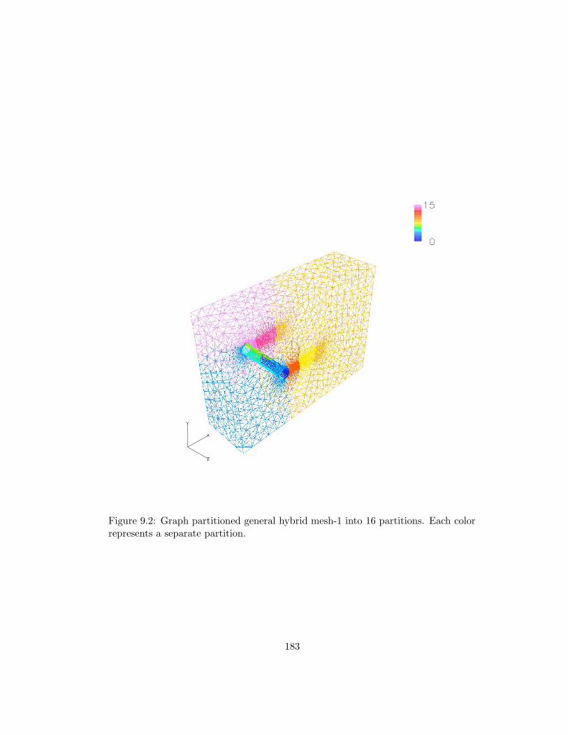
Figure 9.2: Graph partitioned general hybrid mesh-1 into 16 partitions. Each colorrepresents a separate partition.
183
9.2 Hybrid mesh data structure for parallel execution
A parallel implementation of the current solution algorithms for general hybrid
meshes is presented for a distributed memory machine by using MPI (message pass-
ing interface) library functions [58]. The original mesh is partitioned by the METIS
graph partitioning strategy, an open source graph/mesh partitioner [37]. As men-
tioned before, graph partitioning is the strategy of distributing nodes as evenly as
possible with the minimum number of possible edge-cuts. The interface elements,
whose nodes are assigned to multiple parts, are stored redundantly in the neighbor
parts in order to reduce the communication phases. The hybrid mesh data structure
for parallel execution is presented for the inter-processor communication. A pseudo-
code for a single loop inter-processor communication algorithm is presented. Finally,
the scalability of the parallel implementation is measured on a distributed memory
machine. The communication overhead is estimated by counting the number of
nodes participating in the inter-processor communication among all nodes.
9.2.1 Inter-processor communication strategy
The current flow solver is parallelized using the graph partitioning strategy of
METIS [37]. A given mesh can be partitioned either by graph partitioning [48, 84]
or by mesh partitioning [52, 51]. Graph partitioning distributes nodes to each part,
and mesh partitioning distributes elements to each part. Since graph partitioning
distributes nodes to parts, it can be called node partitioning in contrast to mesh
partitioning. In mesh partitioning strategy, equi-distribution of elements is not an
obvious task especially if the mesh includes multiple element types. In graph (node)
partitioning, the algorithm is transparent to cell topologies and node-connectivity is
the only information required by the partitioner. Hence, the graph (node) partition-
ing strategy can be directly applied to general hybrid meshes. Furthermore, since
the current node-based scheme stores unknowns at the nodes, distributing nodes
184

Graph partitioning
1 2 3
6 7 8
9 10 11
21 3
4 5
4
5
6
7 8
1 2 3
4 5 6
7 8
(b)
(a)
Partition−1 Partition−2
Ghost nodeCore node
9
Figure 9.3: Graph partitioning of a two-dimensional hybrid mesh with overlappinginterface cells (cells in gray color). (a) original hybrid mesh with global node num-bering, and (b) partitioned hybrid meshes with local node numbering.
185
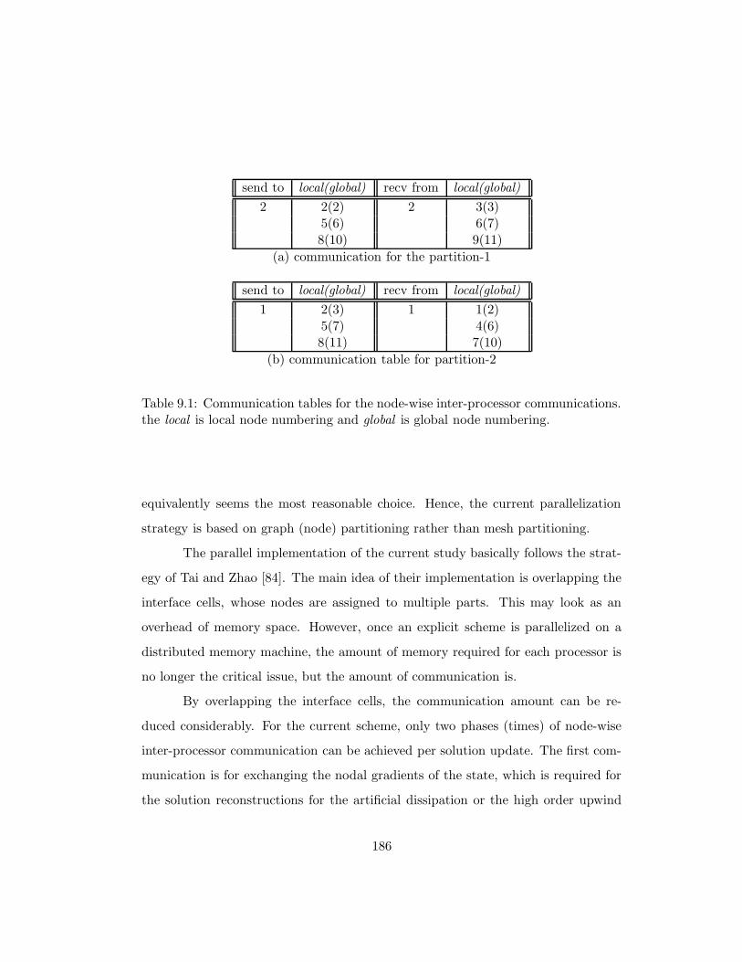
send to local(global) recv from local(global)
2 2(2) 2 3(3)5(6) 6(7)8(10) 9(11)
(a) communication for the partition-1
send to local(global) recv from local(global)
1 2(3) 1 1(2)5(7) 4(6)8(11) 7(10)
(b) communication table for partition-2
Table 9.1: Communication tables for the node-wise inter-processor communications.the local is local node numbering and global is global node numbering.
equivalently seems the most reasonable choice. Hence, the current parallelization
strategy is based on graph (node) partitioning rather than mesh partitioning.
The parallel implementation of the current study basically follows the strat-
egy of Tai and Zhao [84]. The main idea of their implementation is overlapping the
interface cells, whose nodes are assigned to multiple parts. This may look as an
overhead of memory space. However, once an explicit scheme is parallelized on a
distributed memory machine, the amount of memory required for each processor is
no longer the critical issue, but the amount of communication is.
By overlapping the interface cells, the communication amount can be re-
duced considerably. For the current scheme, only two phases (times) of node-wise
inter-processor communication can be achieved per solution update. The first com-
munication is for exchanging the nodal gradients of the state, which is required for
the solution reconstructions for the artificial dissipation or the high order upwind
186
scheme. The second communication phase is at the boundary condition applica-
tion routine which is called after an intra-processor solution update. Once all the
nodal solutions are updated, the solutions at the ghost nodes, which reside at the
inter-processor boundaries, are updated by node-wise inter-processor communica-
tion. This overlapping strategy of general hybrid mesh partitioning is delineated
in Fig. 9.3 in two dimensions. An example of the information required for the
inter-processor communication is listed in Table 9.1.
On the other hand, without overlapping the interface cells, the inter-processor
communication may introduce more phases of communication as well as extra com-
plexity of the communication routines. For example, in the overlapping strategy
no extra communication is needed for the viscous flux computation, while in the
non-overlapping strategy there should be extra communication regarding the com-
putation using edge-duals which lie on the inter-processor boundaries.
According to the partitioning strategy presented in Fig. 9.3, there is no such
assumption that each part has to be contiguous. A completely separate part of the
original mesh can be assigned to the same processor. This is also a big flexibility
for the graph partitioner, which may produce a non-contiguous partitioning, even
though very rarely.
Each part has its own local node numbering, and the translation table of
the local node number to the global node number (and vice versa) is required for
the communications with its neighbors. Once the communication table is built for
all processors (parts), the inter-processor communication can be implemented by
a single loop that runs through the processors. The pseudo-code of the proposed
inter-processor communication is shown below.
for i = 1, · · · , Nprocs
if i is equal to my id
for j = 1, · · ·, Nmy neighbors
187
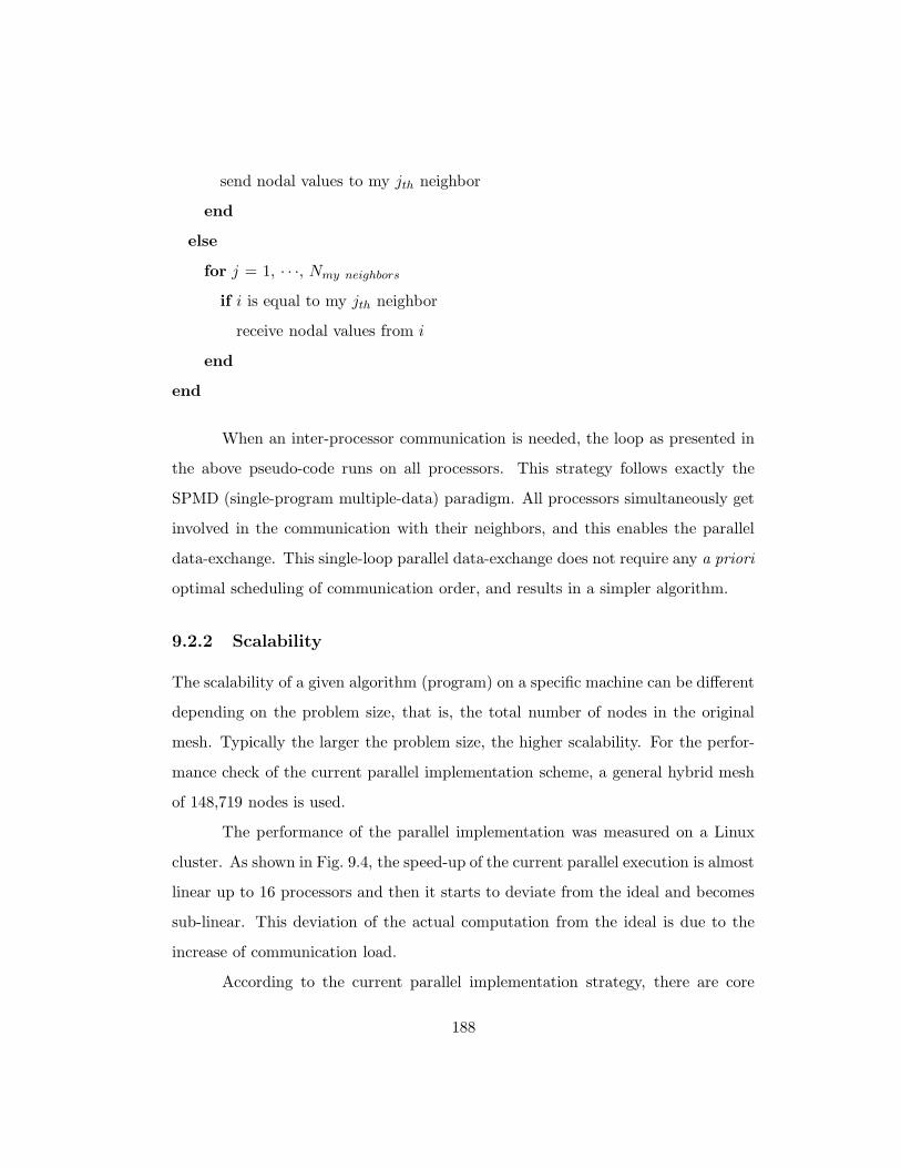
send nodal values to my jth neighbor
end
else
for j = 1, · · ·, Nmy neighbors
if i is equal to my jth neighbor
receive nodal values from i
end
end
When an inter-processor communication is needed, the loop as presented in
the above pseudo-code runs on all processors. This strategy follows exactly the
SPMD (single-program multiple-data) paradigm. All processors simultaneously get
involved in the communication with their neighbors, and this enables the parallel
data-exchange. This single-loop parallel data-exchange does not require any a priori
optimal scheduling of communication order, and results in a simpler algorithm.
9.2.2 Scalability
The scalability of a given algorithm (program) on a specific machine can be different
depending on the problem size, that is, the total number of nodes in the original
mesh. Typically the larger the problem size, the higher scalability. For the perfor-
mance check of the current parallel implementation scheme, a general hybrid mesh
of 148,719 nodes is used.
The performance of the parallel implementation was measured on a Linux
cluster. As shown in Fig. 9.4, the speed-up of the current parallel execution is almost
linear up to 16 processors and then it starts to deviate from the ideal and becomes
sub-linear. This deviation of the actual computation from the ideal is due to the
increase of communication load.
According to the current parallel implementation strategy, there are core
188
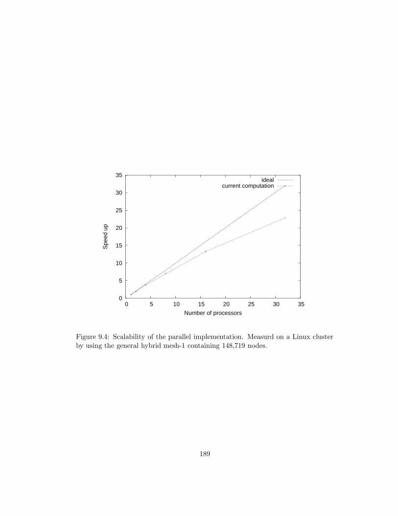
0
5
10
15
20
25
30
35
0 5 10 15 20 25 30 35
Spe
ed u
p
Number of processors
idealcurrent computation
Figure 9.4: Scalability of the parallel implementation. Measurd on a Linux clusterby using the general hybrid mesh-1 containing 148,719 nodes.
189
0.6
0.65
0.7
0.75
0.8
0.85
0.9
0.95
1
0 5 10 15 20 25 30 35
Ave
rage
of N
core
/ N
tota
l
Number of processors
Figure 9.5: Portion of core nodes with respect to the total number of nodes assignedto the part. The ratio is averaged from all parts. The total number of nodes foreach part is the sum of core nodes and ghost nodes, and the solutions at the ghostnodes are to be received from other parts having the ghost nodes as core nodes.Measured with a general hybrid mesh of 148,719 nodes.
190
nodes and ghost nodes at each processor. The total number of nodes at each part
is composed of the core nodes and ghost nodes. Solutions at the core nodes can be
updated without inter-processor communications, but the solution at a ghost node
needs to be received from its neighbor processor which contains the ghost as the
core. Hence, as the number of partitions increases, the number of ghost nodes also
increases as shown in Fig. 9.5. This becomes directly a communication overhead,
and is also one of the major reasons for the deviation of speed-up from the ideal.
Even with the rapid increase of the ghost nodes among the total nodes at each part,
the parallel performance is fairly ideal, and this is because of the smaller number of
communications required by the current parallel algorithm.
191

Chapter 10
Conclusions
In this last chapter, first the major contributions made in this research are summa-
rized, and then conclusions are drawn from the presented results. Finally, recom-
mendations are presented for future research efforts.
192
10.1 Contributions
The contributions made in this research can be categorized as follows
1. development of an incompressible Navier-Stokes method for the general hybrid
meshes
2. application of the method to inflow turbulence study
3. extension of the method to arbitrary Lagrangian-Eulerian (ALE) formulations
4. application of the ALE scheme to the fluid and structure interaction problems
First, a new grid transparent algorithm for the incompressible Navier-Stokes
equations has been presented on the general hybrid meshes with hexahedra, prisms,
pyramids, and tetrahedra. A computationally efficient edge-based algorithm is used
for the numerical flux computations. Especially for the viscous flux evaluations, a
new computationally efficient two-step face-and-edge algorithm has been presented.
The computational efficiency and solution accuracy of the general hybrid meshes
with local hexahedra are investigated. The local hexahedra are introduced into the
viscous layers and also into the wake regions. For both of the cases, the general
hybrid meshes with local hexahedra are shown to be giving as accurate result as the
meshes with prisms/tetrahedra with less computational cost. The proposed scheme
is parallelized for distributed memory machines. Hybrid mesh data structure for
parallel execution was illustrated, and a single-loop inter-processor communication
algorithm was presented. The scalability of the proposed parallelization method is
also presented. The communication overhead is estimated by presenting the growth
of the number of interface nodes among the total nodes as the number of processor
increases.
Second, by using the developed and validated flow solution algorithm, the
effect of inflow turbulence is studies. Local mesh refinement is also performed to
193
identify the effect of mesh resolution capturing the inflow turbulent eddies. The
effect of the inflow turbulence is more emphasized by comparisons with uniform
inflow cases.
Third, a geometrically conservative finite-volume ALE scheme is presented
with moving mesh source term. The moving mesh source term is derived from
the physical conservation laws for an arbitrarily moving control volume and the
geometric conservation law. The significance of the moving mesh source term is
demonstrated by presenting the uniform flow preserving capability on arbitrarily
deforming meshes. The temporal accuracy of the time-integrators, the backward
difference formulas, used for the ALE scheme is verified by time step refinement
study.
Lastly, the presented ALE scheme is applied to the fluid structure interac-
tion problem. The vortex induced vibration of cylinder is simulated by using the
presented ALE scheme. Different coupling strategies, namely weak and strong, are
presented and the superior stability of the strong coupling method is emphasized.
By using beam structural elements for modeling of the cylinder, the applicability of
the proposed scheme for the different types of end-condition are demonstrated.
194

10.2 Conclusions
The following conclusions can be drawn from the present work:
First, general hybrid meshes can be utilized for accurate simulations of incom-
pressible viscous flows with less computational cost compared to conventional meshes.
The general hybrid meshes, containing tetrahedra, pyramids, prisms, and hexahe-
dra in a single computational domain, was successfully applied for incompressible
viscous flow simulations. Local hexahedra are introduced into various regions of
computational domain, and its effectiveness was demonstrated.
Second, the developed incompressible Navier-Stokes method can be applied to
the various types of flow physics study. Through the extensive verification and val-
idation study, the accuracy and robustness of the solution method is presented. By
applying the method successfully to the inflow turbulence effect study, it has been
shown that the method can be utilized for various types of flow physics investiga-
tional study.
Third, moving mesh simulations can be performed accurately by using the
presented ALE scheme. A geometrically conservative property of the proposed finite
volume ALE scheme was presented. The significance of the moving mesh source
term was emphasized (as shown in Figure 8.2) for accurate simulation of moving
mesh simulations. Second order temporal accuracy was also verified (as shown in
Figure 8.4) for the proposed ALE time-integration scheme on moving meshes. By
applying the present ALE scheme, it was shown that moving mesh simulations can
be performed more accurately.
Finally, By using strong coupling method, the developed flow simulation algo-
rithm can be coupled with simulations in different physical regimes. Strong coupling
method of fluid and structure interaction was presented. The improved stability of
the strong coupling is emphasized by comparison with that of weak coupling (shown
in Figure 7.4). By coupling the fluidic and structural fields strongly, a stable and
195
accurate coupling method was presented for multi-physical system simulations.
10.3 Recommendations for future research
The following recommendations can be given for future research based on the cur-
rent work. As the first category, convergence acceleration techniques are suggested
for further developed. Even though the current scheme is accelerated with point-
implicit (diagonal-implicit) local pseudo time stepping scheme, the convergence is
still critical to the convergence rate in pseudo transient state. Hence, more sophis-
ticated convergence acceleration scheme is encouraged to be applied, for examples
multi grid scheme and full matrix preconditioning scheme.
As the second category, the developed method can be applied to multidis-
ciplinary research. For examples, the flow solution method can be applied coupled
with flow control problems, and the moving mesh capability could be used with
shape optimization research.
As the last category, further investigation of moving mesh method is encour-
aged. Since various approaches are in the fields, for examples, space-time method,
fictitious domain method and immersed boundary method, a comparison study also
can be made between those different methods, and further improvement can be
made.
196
Bibliography
[1] E. Achenbach. Influence of surface roughness on the cross-flow around a circular
cylinder. Journal of Fluid Mechanics, 46:321–335, 1971.
[2] E. Achenbach. Experiments on flow past spheres at very high reynolds numbers.
Journal of Fluid Mechanics, 54:565–575, 1972.
[3] W. K. Anderson and D. L. Bonhaus. Algorithm for computing turbulent flows
on unstructured grids. Computers & Fluids, 23:1–21, 1994.
[4] W. K. Anderson, R. D. Rausch, and D. L. Bonhaus. Implicit/multigrid al-
gorithms for incompressible turbulent flows on unstructured grids. Journal of
Computational Physics, 128:391–408, 1996.
[5] G. A. Ashford. An Unstructured Grid Generation and Adaptive Solution Tech-
nique For High-Reynolds-Number Compressible Flows. PhD thesis, University
of Michigan, 1996.
[6] A. Belov, A. Jameson, and L. Martinelli. A new implicit algorithm with multi-
grid for unsteady incompressible flow calculations. AIAA Paper 95-0049, 1995.
[7] Andrey A. Belov. A new implicit multigrid-driven algorithm for unsteady in-
compressible flow calcuations on parallel computers. PhD thesis, Princeton
University, 1997.
197
[8] M. E. Braaten and S. D. Connell. Three-dimensional unstructured adaptive
multigrid scheme for the Navier-Stokes equations. AIAA Journal, 34:281–290,
1996.
[9] K.S. Chang and J.Y. Sa. Patterns of vortex shedding from an oscillating circular
cylinder. AIAA Journal, 30:1331–1336, 1992.
[10] A. J. Chen and Y. Kallinderis. Adaptive hybrid (prismatic-tetrahedral) grids for
incompressible flows. International Journal for Numerical Methods in Fluids,
26:1085–1105, 1998.
[11] X. Chen, G. Zha, and Z. Hu. Numerical simulation of flow induced vibration
based on fully coupled fluid-structural interactions. AIAA Paper 2004-2240,
2004.
[12] Y.H. Choi and C.L. Merkle. The application of preconditioning in viscous flows.
Journal of computational physics, 105:207–223, 1993.
[13] A. J. Chorin. A numerical method for solving incompressible viscous flow
problems. Journal of Computational Physics, 2:12–26, 1967.
[14] Robert D. Cook, David S. Malkus, and Michael E. Plesha. Concepts and Ap-
plications of Finite Element Analysis. John Wiley & Sons, 1989.
[15] G. Dahlquist. Numerical Methods. Prentice-Hall, 1974.
[16] Reinhard Diestel. Graph Theory (Graduate Texts in Mathematics, 173).
Springer-Verlag, 2000.
[17] C. Evangelinos and G.E. Karniadakis. Dynamics and flow structures in the tur-
bulent wake of rigid and flexible cylinders subject to vortex-induced vibrations.
Journal of Fluid Mechanics, 400:91–124, 1999.
198
[18] C. Farhat, P. Geuzaine, and G. Brown. Application of a three-field nonlinear
fluid-structure formulation to the prediction of the aeroelastic parameters of an
f-16 figher. Computer & Fluids, 32:3–29, 2003.
[19] C. Farhat, P. Geuzaine, and C. Grandmont. The discrete geometric conser-
vation law and the nonlinear stability of ale schemes for the solution of flow
problems on moving grids. Journal of computational physics, 174:669–694, 2001.
[20] P. Geuzaine, C. Grandmont, and C. Farhat. Design and analysis of ale schemes
with provable second-order time-accuracy for inviscid and viscous flow simula-
tions. Journal of computational physics, 191:106–227, 2003.
[21] M.B. Giles. Nonreflecting boundary conditions for euler equation calculations.
AIAA Journal, 28:2050–2058, 1990.
[22] M.B. Giles. Preconditioned multigrid methods for compressible flow calcula-
tions on stretched meshes. Journal of Computational Physics, 136:425–445,
1997.
[23] M.B. Giles. Stability and accuracy of numerical boundary conditions in aeroe-
lastic analysis. International Journal for Numerical Methods in Fluids, 24:739–
757, 1997.
[24] P. Godin, D. W. Zingg, and T. E. Nelson. High-lift aerodynamic computations
with one and two- equation turbulence models. AIAA Journal, 35:237–243,
1997.
[25] P. M. Gresho. Incompressible fluid dynamics: Some fundamental formulation
issues. Annual Review of Fluid Mechanics, 23:413–53, 1991.
[26] P. M. Gresho. Some current CFD issues relevant to the incompressible Navier-
Stokes equations. Computer Methods in Applied Mechanics and Engineering,
87:201–252, 1991.
199
[27] F. H. Harlow and J. E. Welch. Numerical calculation of time-dependent viscous
incompressible flow of fluid with free surface. Physics of Fluids, 8:2182, 1965.
[28] A. Haselbacher and J. Blazek. On the accurate and efficient discretization of the
Navier-Stokes equations on mixed grids. AIAA Journal, 38:2094–2102, 2000.
[29] C.W. Hirt, A.A. Amsden, and J. L. Cook. An arbitrary lagrangian-eulerian
computing method for all flow speeds. Journal of Computational Physics,
14:227–253, 1974.
[30] Daniel J. Inman. Engineering Vibrations. Prentice Hall, 2000.
[31] A. Jameson. Time-dependent calculations using with applications to unsteady
flows past airfoils and wings. AIAA Paper 91-1596, 1991.
[32] A. Jameson, W. Schmidt, and E. Turkel. Numerical solution of the euler equa-
tions by finite volume methods using runge-kutta time stepping schemes. AIAA
Paper 81-1259, 1981.
[33] P. Justesen. A numerical study of oscillating flow around a circular cylinder.
Journal of Fluid Mechanics, 222:157–196, 1991.
[34] Y. Kallinderis. A 3-D Finite-Volume method for the Navier-Stokes equations
with adaptive hybrid grids. Applied Numerical Mathematics, 20:387–406, 1996.
[35] Y. Kallinderis, A. Khawaja, and H. McMorris. Hybrid prismatic/tetrahedral
grid generation for viscous flows around complex geometries. AIAA Journal,
34:291–298, 1996.
[36] Y. Kallinderis and S. Ward. Prismatic grid generation for 3-d complex geome-
tries. AIAA Journal, 31:1850–1856, 1993.
200
[37] G. Karypis and V. Kumar. METIS: A software Package for Partitioning Un-
structured Graphs, Partitioning Meshes, and Computing Fill-Reducing Order-
ings of Sparse Matrices, Version 4.0. Department of Computer Science, Uni-
versity of Minnesota, 1998.
[38] S. Kim. Reynolds-Averaged Navier-Stokes Computation of Tip Clearabce Flow
in a Compressor Cascade Using an Unstructured Grid. PhD thesis, Virginia
Polytechnic Institute and State University, 2001.
[39] B. Koobus and C. Farhat. Second-order time-accurate and geometrically conser-
vative implicit schemes for flow computations on unstructured dynamic meshes.
Computer Methods in Applied Mechanics and Engineering, 170:103–129, 1999.
[40] J. D. Lambert. Numerical Methods for Ordinary Differential Systems : The
Initial Value Problem. John Wiley & Sons, 1991.
[41] M. Lesoinne and C. Farhat. Geometric conservation laws for flow problems
with moving boundaries and deformable meshes, and their impact on aeroelas-
tic computations. Computer Methods in Applied Mechanics and Engineering,
134:71–90, 1996.
[42] P.T. Lin. Two-dimensional implicit time dependent calculation for incompres-
silbe flows on adaptive unstructured meshes. PhD thesis, Princeton University,
2001.
[43] Rainald Lohner. Applied CFD Techniques: An Introduction Based on Finite
Element Methods. John Wiley & Sons, 2001.
[44] A. G. Malan, R. W. Lewis, and P. Nithiarasu. An improved unsteady, unstruc-
tured, artificial compressibility, finite volume scheme for viscous incompressbile
flows: Part i. theory and implementation. Internal Journal for Numerical Meth-
ods in Engineering, 54:697–714, 2002.
201
[45] A. G. Malan, R. W. Lewis, and P. Nithiarasu. An improved unsteady, unstruc-
tured, artificial compressibility, finite volume scheme for viscous incompressbile
flows: Part ii. application. Internal Journal for Numerical Methods in Engi-
neering, 54:715–729, 2002.
[46] L. Martinelli. Calculation of Viscous Flows with a Multigrid Method. PhD
thesis, Princeton University, 1987.
[47] D. J. Mavriplis. Unstructured grid techniques. Annual Review of Fluid Me-
chanics, 29:473–514, 1997.
[48] D. J. Mavriplis. Viscous flow analysis using a parallel unstructured multigrid
solver. AIAA Journal, 38:2067–2076, 2000.
[49] N. D. Melson, M. D. Sanetrik, and H. L. Atkins. Time-accurate Navier-Stokes
calculations with multigrid acceleration. In 6th Copper Mountain Conference
on Multigrid Methods, page 423, 1981.
[50] Richard Mercier. Ocean turbulence loads and effects on offshore structures.
Technical report, Offshore Technology Research Center, Texas A&M University
and the University of Texas at Austin, 2004.
[51] T. Minyard and Y. Kallinderis. Octree partitioning of hybrid grids for par-
allel adaptive viscous flow simulations. Internaltional Journal for Numerical
Methods in Fluids, 26:57–78, 1998.
[52] T. Minyard and Y. Kallinderis. Parallel load balancing for dynamic execution
environments. Comput. Methods Appl. Mech. Engrg., 189:1295–1309, 2000.
[53] T. K. Minyard. A parallel adaptive Navier-Stokes method for hybrid grids with
dynamic load balancing. PhD thesis, The University of Texas at Austin, 1999.
202
[54] Y. Nakamura and Y. Tomonari. The effects of surface roughness on the flow
past circular cylinders at high reynolds numbers. Journal of Fluid Mechanics,
123:363–378, 1982.
[55] David J. Newman and George Em Karniadakis. A direct numerical simulation
study of flow past a freely vibrating cable. Journal of Fluid Mechanics, 344:95–
136, 1997.
[56] P. Nithiarasu. An efficient artificial compressibility (ac) scheme based on the
characteristic based split (cbs) method for incompressible flows. Internal Jour-
nal for Numerical Methods in Engineering, 56:1815–1845, 2003.
[57] G.A. Osswald, K.N. Ghia, and U. Ghia. A direct algorithm for solution of in-
compressible three-dimensional unsteady Navier-Stokes equaitons. AIAA Paper
87-1139, 1987.
[58] Peter Pacheco. Parallel Programming with MPI. Morgan Kaufmann, 1996.
[59] V. Parthasarathy. Finite volume, adaptive-multigrid methods for Euler and
Navier-Stokes equations on three-dimensional unstructured grids. PhD thesis,
The University of Texas at Austin, 1999.
[60] S.V. Patankar and D.B. Spalding. A calculation procedure for heat, mass and
momentum transfer in three-dimensional parabolic flows. Internal journal of
heat and mass transfer, 15:1787–1806, 1972.
[61] Charles S. Peskin. The immersed boundary method. Acta Numerica, 11:479–
517, 2002.
[62] C.S. Peskin. Numerical analysis of blood flow in the heart. Journal of Compu-
tational Physics, 25:220–252, 1977.
203
[63] R. Peyret. Unsteady evolution of a horizontal jet in a stratified fluid. Journal
of Fluid Mechanics, 78:49–63, 1976.
[64] S. Pirzadeh. Three-dimensional unstructured viscous grid by the advancing-
layers method. AIAA Journal, 34:43–49, 1996.
[65] Stephen B. Pope. Turbulent Flows. Cambridge University Press, 2000.
[66] William H. Press, Brian P. Flannery, Saul A. Teukolsky, and William T. Vet-
terling. Numerical Recipes in C : The Art of Scientific Computing. Cambridge
University Press, 1992.
[67] E.F. Relf. Discussion of results of measurements of the resistance of wires,with
some additional tests on the resistance of wires of small diameter. Technical
Report 102, The advisory committee for aeronautics, 1915.
[68] A. Rizzi and L.-E. Eriksson. Computation of inviscid incompressible flow with
rotation. Journal of Fluid Mechanics, 153:275–312, 1985.
[69] P. L. Roe. Approximate riemann solvers, parameter vectors and difference
schemes. Journal of Computational Physics, 43:357–372, 1981.
[70] P. L. Roe. Characteristic-based schemes for the euler equations. Annual Review
of Fluid Mechanics, 18:337–365, 1986.
[71] S. E. Rogers and D. Kwak. An upwind differencing scheme for the incom-
pressible Navier-Stokes equations. Applied Numerical Mathematics, 8:43–64,
1988.
[72] S. E. Rogers and D. Kwak. Upwind differencing scheme for the time-accurate
incompressible Navier-Stokes equations. AIAA Journal, 28:253–262, 1990.
[73] S. E. Rogers, D. Kwak, and C. Kiris. Steady and unsteady solutions of the
incompressible Navier-Stokes equations. AIAA Journal, 29:603–610, 1991.
204
[74] A. Roshko. Experiments on the flow past a circular cylinder at very high
reynolds number. Journal of Fluid Mechanics, 10:345–356, 1961.
[75] A. Rubel and G. Volpe. Biharmonic vector stream function formulation and
multigrid solution for a three-dimensional driven-cavity stokes flow. AIAA
Paper 89-1968-CP, 1989.
[76] D. Kwak S. E. Rogers and U. Kaul. On the accuracy of the pseudocompress-
ibility method in solving the incompressible Navier-Stokes equations. Applied
Mathematics and Modelling, 11:35–44, 1991.
[77] Rolf H. Sabersky, Allan J. Acousta, and Edward Hauptman. Fluid Flow: A
First Course in Fluid Mechanics. Prentice Hall, 1998.
[78] K. W. Schulz. Numerical prediction of the hydrodynamic loads and motions of
offshore structures. PhD thesis, The University of Texas at Austin, 1999.
[79] K. W. Schulz and Y. Kallinderis. Unsteady flow structure interaction for in-
compressible flows using deformable hybrid grids. Journal of Computational
Physics, 143:569–597, 1998.
[80] D. Sharov and K. Nakahashi. Hybrid prismatic/tetrahedral grid generation for
viscous flow applications. AIAA Journal, 36:157–162, 1998.
[81] P. R. Spalart and S. R. Allmaras. A one-equation turbulence model for aero-
dynamic flows. AIAA Paper 92-0439, 1992.
[82] R. C. Swanson, R. Radespiel, and E. Turkel. On some numerical dissipation
schemes. Journal of computational physics, 147:518–544, 1998.
[83] R. C. Swanson and E. Turkel. On central-difference and upwind schemes. Jour-
nal of computational physics, 101:292–306, 1992.
205
[84] C. H. Tai and Y. Zhao. Parallel unsteady incompressible viscous flow com-
putations using an unstructured multigrid method. Journal of Computational
Physics, 192:277–311, 2003.
[85] L. K. Taylor and D. L. Whitfield. Unsteady three-dimensional incompressible
euler and Navier-Stokes solver for stationay and dynamic grids. AIAA, 92:–
1650, 1991.
[86] T.E. Tezduyar, M. Behr, and J. Liou. A new strategy for finite element com-
putations involving moving boundaries and interfaces - the deforming-spatial-
domain/space-time procedure: I. the concept and the preliminary numerical
tests. Computer Methods in Applied Mechanics and Engineering, 94:339–351,
1992.
[87] T.E. Tezduyar, M. Behr, S. Mittal, and J. Liou. A new strategy for finite ele-
ment computations involving moving boundaries and interfaces - the deforming-
spatial-domain/space-time procedure: Ii. computation of free-surface flows,
two-liquid flows, and flows with drifiting cylinders. Computer Methods in Ap-
plied Mechanics and Engineering, 94:353–371, 1992.
[88] P.D. Thomas and K. Lombard. Conservation law and its application to flow
computations on moving grids. AIAA Journal, 17:1030–1037, 1979.
[89] Joe F. Thompson, B. K. Soni, and N. P. Weatherill. Handbook of Grid Gener-
ation. CRC Press, Boca Raton, Florida, 1999.
[90] H. Tokunaga, K. Yoyeda, and N. Satofuka. Direct simulations of three di-
mensional flows using generalized vector potentional method. AIAA Paper
91-1610-CP, 1991.
[91] E. Turkel. Preconditioned method for solving the incompressible and low speed
compressible equations. Journal of Computational Physics, 72:277–298, 1987.
206
[92] E. Turkel. A review of preconditioning methods for fluid dynamics. Applied
Numerical Mathematics, 12:257–284, 1993.
[93] E. Turkel. Chapter 13. Preconditioning and the Limit of the Compressible to the
Incompresible Flow Equations for Finite Difference Schemes in the Frontiers
of the Computational Fluid Dynamics 1994. John Wiley & Sons, 1998.
[94] E. Turkel. Preconditioning techniques in computational fluid dynamics. Annual
Review of Fluid Mechanics, 31:385–416, 1999.
[95] B. van Leer, C.-H. Tai, and K. G. Powell. Design of optimally smoothing
multi-stage schemes for the euler equations. AIAA Paper 89-1933, 1989.
[96] J.K. Vandiver. Dimensionless parameters important to the prediction of vortex-
induced vibration of long, flexible cylinders in ocean currents. journal of fluids
and structures. Journal of Fluids and Structures, 7:423–455, 1993.
[97] C. H. K. Williamson. Defining a universal and continuous strouhalreynolds
number relationship for the laminar vortex shedding of a circular cylinder.
Physics of Fluids, 31:2742–2744, 1988.
[98] T.Y. Yang. Finite Element Structural Analysis. Prentice-Hall, 1986.
[99] L. T. Zhang, A. Gerstenberger, X. Wang, and W. K. Liu. Immersed finite ele-
ment method, computer methods in applied mechanics and engineering. Com-
puter Methods in Applied Mechanics and Engineering, 193:2051–2067, 2004.
207
Vita
Hyung Taek Ahn was born on December 28, 1973 in Kyungnam, Korea to Young Ok
Ahn and Tae Hwa Noh. He received Bachelor of Engineering degree in mechanical
engineering from Yeungnam University, Korea in February 1996, and Master of
Science degree in mechanical engineering from Korea Advanced Institute of Science
and Technology (KAIST), Korea in February 1999. He worked for Samsung Display
Instruments in Suwon, Korea as a research engineer from January 1999 to June
1999. He started his doctoral program in aerospace engineering at the University
of Texas at Austin in the fall semester of 1999. He received Rotary Foundation
Ambassadorial Scholarship for the academic years of 1999-2002.
Permanent Address: Narea-maul 812-703
Dowon-dong, Dalso-gu
Daegu, Korea 704-793
This dissertation was typeset with LATEX2ε1 by the author.
1LATEX2ε is an extension of LATEX. LATEX is a collection of macros for TEX. TEX is a trademark of
the American Mathematical Society. The macros used in formatting this dissertation were written
by Dinesh Das, Department of Computer Sciences, The University of Texas at Austin, and extended
by Bert Kay and James A. Bednar.
208