Controlling wave function localization in a multiple quantum well structureAnjana Bagga and Anu Venugopalan Citation: J. Appl. Phys. 113, 054310 (2013); doi: 10.1063/1.4790477 View online: http://dx.doi.org/10.1063/1.4790477 View Table of Contents: http://jap.aip.org/resource/1/JAPIAU/v113/i5 Published by the American Institute of Physics. Related ArticlesShell-thickness-dependent photoinduced electron transfer from CuInS2/ZnS quantum dots to TiO2 films Appl. Phys. Lett. 102, 053119 (2013) Role of photo-assisted tunneling in time-dependent second-harmonic generation from Si surfaces with ultrathinoxides Appl. Phys. Lett. 102, 051602 (2013) Tuning resonant transmission through geometrical configurations of impurity clusters J. Appl. Phys. 113, 044305 (2013) Electron field emission from reduced graphene oxide on polymer film Appl. Phys. Lett. 102, 033102 (2013) Effect of tunneling transfer on thermal redistribution of carriers in hybrid dot-well nanostructures J. Appl. Phys. 113, 034309 (2013) Additional information on J. Appl. Phys.Journal Homepage: http://jap.aip.org/ Journal Information: http://jap.aip.org/about/about_the_journal Top downloads: http://jap.aip.org/features/most_downloaded Information for Authors: http://jap.aip.org/authors

Controlling wave function localization in a multiple quantum well structure

Anjana Bagga and Anu Venugopalana)

University School of Basic and Applied Sciences, GGS Indraprastha University, Sector 16C, Dwarka,New Delhi 110075, India

(Received 1 November 2012; accepted 22 January 2013; published online 6 February 2013)

The dynamics of a wave function describing a particle confined in a multiple quantum well potential

is studied numerically. In particular, the case of four wells and six wells has been studied for the first

time. As a consequence of quantum mechanical tunneling, an initial wavefunction designed to be

localized in one well can localize in the others after a certain time and hop between wells at times

which depends on the height and width of the barriers separating the wells. This control over the

evolution of the wavefunction with time has direct implications in applications based on carrier

dynamics in multiple quantum well nanostructures and can also provide novel mechanisms in solid

state quantum computation for information storage and processing. The ability to include any number

of wells and control the carrier dynamics in them through easily accessible parameters in our study

makes this a particularly attractive system from the point of view of applications. VC 2013 AmericanInstitute of Physics. [http://dx.doi.org/10.1063/1.4790477]

I. INTRODUCTION

Recently, there has been a lot of interest in studying the

dynamics of wavefunctions in simple heterostructures.1–4

Quantum wells are heterostructures that can be easily crafted

in the laboratory by joining thin layers of different semicon-

ductor materials by epitaxial crystal growth techniques. Such

structures are known to show many quantum effects which

are a consequence of quantum confinement. Investigation of

the electronic structure of quantum well structures forms the

basis for exploiting engineered heterostructures for elec-

tronic, optical, and spintronic applications. The dynamics of

wavefunctions and the time scales involved in these systems

can often be controlled externally by physically accessible

parameters. This gives a powerful handle in tuning electronic

and optical properties, setting a path for designing novel

advanced electronic and optoelectronic devices out of them,

e.g., resonant tunneling devices, field-effect transistors, het-

erojunction bipolar transistors, laser diodes, and photodetec-

tors. Artificially engineered two dimensional quantum well

structures forming quantum cascade lasers are known to be

one of the best continuous wave sources of terahertz radia-

tion5—a much sought after source of radiation for many

potential applications. Multiple quantum well structures also

hold great promise for the physical implementation of quan-

tum information processing and solid state quantum computa-

tion.6 The work described in this paper deals with

wavefunction dynamics in a confined system modelled by a

composite potential describing multiple quantum wells. The

possibility of quantum mechanical tunneling across the bar-

riers separating wells allows an initial wavefunction designed

to be localized in one well to localize in the others after a cer-

tain time which depends on the height and width of the bar-

riers separating the wells. This dependence provides a handle

to control the dynamics of the wave function and its localiza-

tion. When coupled with technological advances, this can lead

to the possibility of a gamut of novel applications derived

from controlling carrier dynamics in nanostructures and the

means to implement solid state quantum computation. We

will conclude by discussing the implications of our results in

potentially useful applications.

II. THEORY AND RESULTS

The dynamics of initially localized wavefunctions in

confined systems have often been shown to exhibit

“revivals.” This means that after evolving for a certain time

when the probability distribution of the localized wavefunc-

tion might spread, the wavefunction relocalizes and acquires

its original shape.7–10 This behaviour is a consequence of the

fact that in such systems the initial wavefunction is bound

and its time evolution is governed by a discrete eigenvalue

spectrum.11 The simplest class of systems for which frac-

tional and full revivals can be seen are those for which the

energy spectrum goes as n2, e.g., the infinite square well

potential and the rigid rotator.10–12 A number of studies have

reported quantum revivals in a variety of quantum systems

like that of Rydberg atom wavepackets, molecular wave-

packets, and wave packets in semiconductor quantum wells

and nanostructures15–18 etc. A lot of interest has also been

generated in studying the quantum control of the motion of

wavepackets in quantum well structures.3 Studies show that

such systems can be experimentally designed and the time

scales for wave function dynamics and features like wave

function revivals can be controlled by physically accessible

parameters. The dynamics in a double well structure has also

been studied recently by modelling it with a Dirac d function

potential in the middle of the infinite square well potential.1

On the experimental front, coherent oscillations of an

extended electronic wavepacket in a GaAs/AlGaAS double

quantum well structure have been observed where the wave-

packet had been created by ultrashot pulse excitation. The

sample modeling this potential was a 170A0 GaAs quantum

a)Author to whom correspondence should be addressed. Electronic mail:

anu.venugopalan@gmail.com.

0021-8979/2013/113(5)/054310/6/$30.00 VC 2013 American Institute of Physics113, 054310-1

JOURNAL OF APPLIED PHYSICS 113, 054310 (2013)

well followed by a 17A0 barrier of Al0:35Ga0:65As.2 All these

studies show that such systems can be experimentally

designed and the time scales for wave function dynamics

and features like wave function revivals can be controlled by

physically accessible parameters.

The simplest quantum system to illustrate the feature of

quantum revivals is the one dimensional infinite square well

potential where the time evolution can be beautifully illus-

trated because of the existence of exact analytical expressions

for the energy eigenvalues and eigenstates. This system has

been studied in great detail in the context of wave packet

revivals.10–12 This familiar system has a potential

VðxÞ ¼ 0; 0 < x < L

VðxÞ ¼ 1; x < 0; x > L;(1)

with eigenvalues and eigenfunctions

En ¼�h2p2n2

2mL2; (2)

/nðxÞ ¼ffiffiffi2

L

rsin

npx

L; n ¼ 1; 2; 3:::; (3)

where L is the length of the well and m is the mass of the par-

ticle. The time evolution of a particle in an initial state

wðx; 0Þ can be written as

wðx; tÞ ¼X

n

cn/nðxÞe�iEnt

�h : (4)

Here n is the quantum number and /nðxÞ and En are the

energy eigenstates and corresponding eigenvalues for the

system. The coefficients cns are given in terms of the initial

wavefunction, as cn ¼ h/nðxÞjwðx; 0Þi. The well known fea-

ture in the infinite well potential is that the energy eigenval-

ues are quantized and are exactly quadratic in n. In many

studies it has been shown that the time evolution of a wave

function driven by such a spectrum has an important time

scale called the “revival time” which is contained in the

coefficients of the Taylor series of the energy eigenvalue

spectrum. In an infinite square well potential, this is the time

in which an initial wavefunction regains its initial form. This

“revival time” for an infinite well is given by

Trev ¼4mL2

�hp: (5)

One can see that this time goes as L2, where L is the length

of the well. The dependence on L gives us a physically tuna-

ble parameter to control this time scale. It can be easily seen

from Eq. (4) that in this system such revivals are “exact,”

i.e., wðx; tþ TrevÞ ¼ wðx; tÞ. At intermediate times the wave-

function spreads or shows partial or fractional revivals.10–12

However, not all systems have a purely quadratic energy de-

pendence like the infinite well and would, in general, contain

higher order terms which could lead to more complicated

and qualitatively different dynamics. For example, the more

realistic case of a finite well has been studied where the

energy eigenvalue spectrum is not quadratic. In this system

initial localized wavepackets have been found to undergo

revivals and “superrevivals.”13 Many of these features

have an interesting physical and mathematical analog in the

classical Talbot Effect in waveguides where a field of wave-

length k propagating through a multimode planar waveguide

of width b would regenerate at multiples of a distance

L ¼ 2b2=k.19

In this paper, we numerically study wave function dy-

namics in a composite potential which represents a multiple

quantum well structure. The numerical scheme used to find

out the eigenvalues and eigenfunctions incorporates the tight

binding Hamiltonian model.14 Our analysis allows us to add

in wells, each well separated from the other by a finite barrier

whose height and width can be changed. In particular, we

study how a wavefunction initially designed to be localized

in one well evolves with time to localize in another well.

The time scale for this to happen depends on physically ac-

cessible parameters like the height and width of the barriers

and the dimensions of the system. To illustrate our results,

we look at a simple situation where the dimension of the sys-

tem and the width of the barriers are fixed and the localiza-

tion is studied as a function of the barrier height. For our

study we first illustrate the results for the simple case of two

wells [Fig. 1], and then look at two more scenarios: the

potential profile with four wells and the potential profile with

six wells [Figs. 3 and 6]. Our analysis allows us to generalize

the study to many wells. On solving the chosen system for

its eigenvalues and eigenfunctions, the time evolution of an

initial localized wavefunction is studied. In each case, the

initial wavefunction can be designed by choosing the appro-

priate combination of the eigenstates that localize it in a

chosen well. The time evolution features are revealed by the

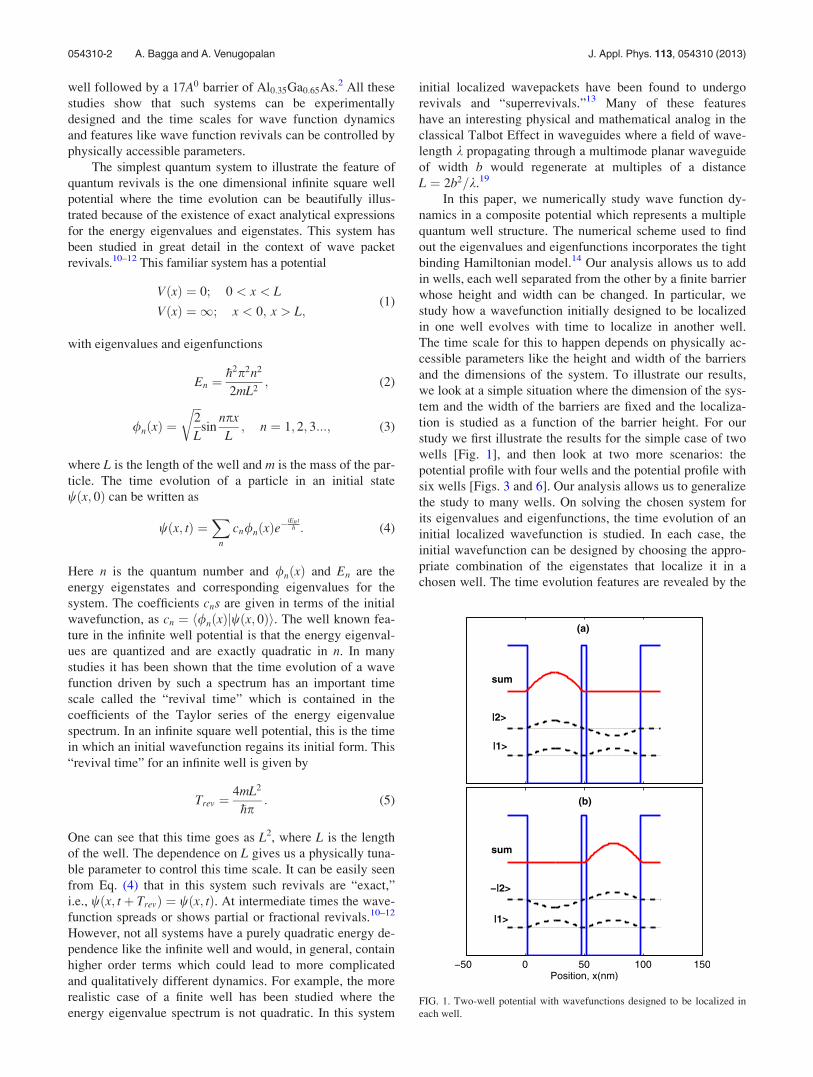
FIG. 1. Two-well potential with wavefunctions designed to be localized in

each well.

054310-2 A. Bagga and A. Venugopalan J. Appl. Phys. 113, 054310 (2013)

probability distributions of the time evolved initial state and

are also reflected in the absolute square of the autocorrelation

functions. The time evolved wave function is according to

Eq. (4). The autocorrelation function is essentially the over-

lap of the time evolved wavefunction with its initial state,

i.e., hwðx; 0Þjwðx; sÞi. For the one dimensional bound system

considered here where the wavefunction is expanded in

terms of the eigenfunctions /n with eigenvalues En, it can be

easily checked that the autocorrelation function is given by

AðsÞ ¼X

n

jcnj2ei �Ens

�h : (6)

In our study s ¼ t=Trev, i.e., the time is scaled in terms of the

revival time, Trev ¼ 4mL2=p, of an infinite well potential of

the same total length L and �En ¼ TrevEn.

Our results reveal that a wavefunction initially localized

in one well hops between wells with time. The time at which

the localization in a particular well happens depends on the

height and width of the barriers separating the wells. This de-

pendence allows a useful handle to control the motion of the

wavefunction by choosing the appropriate height and width

to decide the time scales in which the localization occurs in a

particular well. Consider the simplest case of a symmetric

two-well confining potential (see Fig. 1). For our analysis,

we choose the two-well potential profile with the following

arbitrary parameters: Total length¼ 100 nm and barrier

width �4:2 nm. For our analysis we keep the barrier width

fixed and study the dependence for two values of barrier

height: 0.5 eV, and 0.6 eV. For such a system the time evolu-

tion of an initial wavefunction can be studied as described in

Eq. (4). Since such a system does not have analytical solu-

tions for the eigenvalues and eigenfunctions, we need to

solve the Schrodinger equation numerically. The numerical

solutions for the first two eigenfunctions of this systems are

plotted in Fig. 1. For our analysis, we look at the simplest

possible situation where we just deal with the first two eigen-

functions. We can construct a wavefunction that is localized

in each of the wells by appropriately choosing the values of

the coefficients cns that superpose the two eigenstates. For

example, if the state is to be localized in the first well, it

would be described by the superposition

w1ðx; 0Þ ¼ c11/1ðxÞ þ c1

2/2ðxÞ: (7)

It can be easily verified that the choice of c11 ¼ c1

2 ¼ffiffiffiffiffiffiffi0:5p

gives us the desired localization of the wavefunction in the

first well. Similarly, the wavefunction giving a localization

in the second well is given by the choice of coefficients

c11 ¼ �c1

2 ¼ffiffiffiffiffiffiffi0:5p

. Fig. 1 illustrates these wavefunctions. One

can see that it is possible to design wavefunctions which are

localized in any of the two wells with appropriate choices of

the coefficients and the time evolution shows the “hopping”

of the localized wavefunction between the wells. Once the

initial wavefunction and the eigenvalues and eigenstates are

known, the time evolution according to Eq. (4) gives us the

wavefunctions at various times. The time evolution shows

that the wavefunction periodically hops between the two

wells. In order to ascertain at what time and in which well

the wavefunction has localized, it is convenient to look at the

correlation functions for specific wells. This is done by looking

at the overlaps of the time evolved wavefunction with states

corresponding to the wavefunction being localized in a specific

well, i.e., jhw1ðx; 0Þjwkðx; sÞij2, and jhw2ðx; 0Þjwkðx; sÞij

2

(k¼ 1, or k¼ 2). For example, Fig. 2 looks at the correlation

functions for the time evolved wavefunction w1ðx; sÞ (k¼ 1),

which was initially localized in the first (left) well. Figs. 2(a)

and 2(b) are plots of jhw1ðx; 0Þjw1ðx; sÞij2, and jhw2ðx; 0Þ

jw1ðx; sÞij2, respectively. It is obvious that whenever each of

these functions is peaked, there will be a localization in that

specific well. To illustrate this dependence on the barrier

height, Fig. 2 illustrates this feature for two different barrier

heights, keeping the width fixed. The figure clearly shows, the

periodic hopping between the two wells and illustrates that this

hopping is faster for smaller barrier heights. Note that the time

here is scaled with respect to Trev, the revival time for a single

infinite well of the same length.

Our numerical scheme for solving the Schr€odinger equation

for such a composite potential and incorporating the time evolu-

tion is quite general and can easily incorporate more wells. We

extend this analysis to a four-well potential. Fig. 3 illustrates the

symmetric four-well confining potential with the first four eigen-

functions. We keep all parameters for this the same as those for

the two-well potential. Once again, one can see that it is possible

to design wavefunctions which are localized in any of the four

wells with appropriate choices of the coefficients and the time

evolution shows the “hopping” of the localized wavefunction

between the wells. The respective correlation functions allow us

to determine the exact times at which this would happen. For

example, if the initial state is to be localized in the first well, it

would be described by the superposition

w1ðx; 0Þ ¼ c11/1ðxÞ þ c1

2/2ðxÞ þ c13/3ðxÞ þ c1

4/4ðxÞ; (8)

FIG. 2. Square of the correlation functions for two-well potential with bar-

rier heights¼ 0:5 eV (solid line) and 0:6 eV (dashed line). Peaks indicate

localization in that particular well. (a) A1ðsÞ ¼ hw1ðx; 0Þjw1ðx; sÞi, (b)

A2ðsÞ ¼ hw2ðx; 0Þjw1ðx; sÞi.

054310-3 A. Bagga and A. Venugopalan J. Appl. Phys. 113, 054310 (2013)

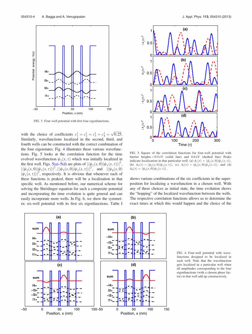
with the choice of coefficients c11 ¼ c1

2 ¼ c13 ¼ c1

4 ¼ffiffiffiffiffiffiffiffiffi0:25p

.

Similarly, wavefunctions localized in the second, third, and

fourth wells can be constructed with the correct combination of

the four eigenstates. Fig. 4 illustrates these various wavefunc-

tions. Fig. 5 looks at the correlation function for the time

evolved wavefunction w1ðx; sÞ which was initially localized in

the first well. Figs. 5(a)–5(d) are plots of jhw1ðx; 0Þjw1ðx; sÞij2;

jhw2ðx; 0Þjw1ðx; sÞij2; jhw3ðx; 0Þjw1ðx; sÞij

2, and jhw4ðx; 0Þ

jw1ðx; sÞij2, respectively. It is obvious that whenever each of

these functions is peaked, there will be a localization in that

specific well. As mentioned before, our numerical scheme for

solving the Shr€odinger equation for such a composite potential

and incorporating the time evolution is quite general and can

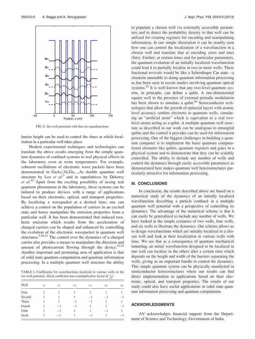
easily incorporate more wells. In Fig. 6, we show the symmet-

ric six-well potential with its first six eigenfunctions. Table I

shows various combinations of the six coefficients in the super-

position for localizing a wavefunction in a chosen well. With

any of these choices as initial state, the time evolution shows

the “hopping” of the localized wavefunction between the wells.

The respective correlation functions allows us to determine the

exact times at which this would happen and the choice of the

FIG. 3. Four-well potential with first four eigenfunctions.

FIG. 4. Four-well potential with wave-

functions designed to be localized in

each well. Note that the wavefunction

gets localized in a particular well when

all amplitudes corresponding to the four

eigenfunctions (with a chosen phase fac-

tor) in that well add up constructively.

FIG. 5. Square of the correlation functions for four-well potential with

barrier heights¼ 0.5 eV (solid line) and 0.6 eV (dashed line) Peaks

indicate localization in that particular well. (a) A1ðsÞ ¼ hw1ðx; 0Þjw1ðx; sÞi,(b) A2ðsÞ ¼ hw2ðx; 0Þjw1ðx; sÞi, (c) A3ðsÞ ¼ hw3ðx; 0Þjw1ðx; sÞi, and (d)

A4ðsÞ ¼ hw4ðx; 0Þjw1ðx; sÞi.

054310-4 A. Bagga and A. Venugopalan J. Appl. Phys. 113, 054310 (2013)

barrier height can be used to control the times at which local-

ization in a particular well takes place.

Modern experimental techniques and technologies can

translate the above results emerging from the simple quan-

tum dynamics of confined systems to real physical effects in

the laboratory even at room temperatures. For example,

coherent oscillations of electronic wave packets have been

demonstrated in GaAs=AlxGa1�xAs double quantum well

structure by Leo et al.2 and in superlattices by Dekorsy

et al.22 Apart from the exciting possibility of seeing real

quantum phenomena in the laboratory, these systems can be

tailored to produce devices with a range of applications

based on their electronic, optical, and transport properties.

By localizing a wavepacket at a desired time, one can

achieve a control on the population of carriers in an excited

state and hence manipulate the emission properties from a

particular well. It has been demonstrated that induced tera-

hertz emission which results from the acceleration of

charged carriers can be shaped and enhanced by controlling

the evolution of the electronic wavepacket in quantum well

structures.3,20,21 The control over the dynamics of a charged

carrier also provides a means to manipulate the direction and

amount of photocurrent flowing through the device.23,24

Another important and promising area of application is that

of solid state quantum computation and quantum information

processing. In a multiple quantum well structure the ability

to populate a chosen well via externally accessible parame-

ters and to detect the probability density in that well can be

utilized for creating registers for encoding and manipulating

information. In our simple illustration it can be readily seen

how one can control the localization of a wavefunction in a

chosen well and translate that as encoding zeros and ones

(bits). Further, at certain times and for particular parameters,

the quantum evolution of an initially localized wavefunction

could lead it to partially localize in two or more wells. These

fractional revivals would be like a Schrodinger Cat state—a

situation amenable to doing quantum information processing

as has been seen in recent studies involving quantum optical

systems.25 It is well known that any two-level quantum sys-

tem, in principle, can define a qubit. A one-dimensional

square well in the presence of external periodic modulation

has been shown to simulate a qubit.26 Semiconductor tech-

nologies that allow the growth of epitaxial layers with atomic

level accuracy confine electrons in quantum wells, simulat-

ing an “artificial atom” which is equivalent to a real two-

level atoms acting as a qubit. A multiple quantum well struc-

ture as described in our work can be analogous to entangled

qubits and the control it provides can be used for information

processing. One of the biggest challenges in building a quan-

tum computer is to implement the basic quantum computa-

tional elements like qubits, quantum registers and gates in a

physical system and to demonstrate that they can be scalably

controlled. The ability to include any number of wells and

control the dynamics through easily accessible parameters as

demonstrated here makes quantum well heterostructures par-

ticularly attractive for information processing.

III. CONCLUSIONS

In conclusion, the results described above are based on a

numerical study of the dynamics of an initially localized

wavefunction describing a particle confined in a multiple

quantum well potential with a perspective of controlling its

dynamics. The advantage of the numerical scheme is that it

can easily be generalized to include any number of wells. We

have looked at the simple scenarios of two wells, four wells,

and six wells to illustrate the dynamics. Our scheme allows us

to design wavefunctions which are initially localized in a cho-

sen well and look at their localization in various wells with

time. We see that as a consequence of quantum mechanical

tunneling, an initial wavefunction designed to be localized in

one well can localize in the others after a certain time which

depends on the height and width of the barriers separating the

wells, giving us an important handle to control the dynamics.

This simple quantum system can be physically manifested in

semiconductor heterostructures where our results can find

direct implementation in applications based on their elec-

tronic, optical, and transport properties. The results of our

study could also have useful applications in solid state quan-

tum information processing and quantum computation.

ACKNOWLEDGMENTS

AV acknowledges financial support from the Depart-

ment of Science and Technology, Government of India.

TABLE I. Coefficients for wavefunctions localized in various wells in the

six-well potential. (Each coefficient has a multiplicative factor of 1ffiffi6p )

Well c1 c2 c3 c4 c5 c6

First 1 1 1 1 1 1

Second 1 1 1 �1 �1 �1

Third 1 1 �1 �1 1 1

Fourth 1 �1 �1 1 1 �1

Fifth 1 �1 1 1 �1 1

Sixth 1 �1 1 �1 1 �1

FIG. 6. Six-well potential with first six eigenfunctions.

054310-5 A. Bagga and A. Venugopalan J. Appl. Phys. 113, 054310 (2013)

1G. A. Vugalter, A. K. Das, and V. A. Sorokin, Phys. Rev. A 66, 012104

(2002).2K. Leo, J. Shah, E. O. Gobel, T. C. Daemen, S. Schmitt-Rink, W. Schafer,

and K. Koehler, Phys. Rev. Lett. 66, 201–204 (1991).3J. L. Krause, D. H. Reitze, G. D.Sanders, A. V. Kuznetsov, and C. J.

Stanton, Phys. Rev. B 57(15), 9024 (1998).4K. L. Shuford and J. L. Krause, J. Appl. Phys. 91(10), 6533 (2002).5B. S. Williams, Nat. Photonics 1, 517 (2007).6D. Loss and D. P. DiVincenzo, Phys. Rev. A 57, 120 (1998).7J. Parker and C. R. Stroud, Phys. Rev. Lett. 56, 716 (1986); Phys. Scr.

T12, 70 (1986).8G. Alber, H. Ritsch, and P. Zoller, Phys. Rev A 34, 1058 (1986).9I. Sh. Averbukh and N. F. Perelman, Phys. Lett. A 139, 449 (1989).

10R. Bluhm, V. A. Kostelecky, and J. A. Porter, Am. J. Phys. 64(7), 944

(1996).11R. W. Robinett, Phys. Rep. 392, 1–119 (2004).12D. L. Aronstein and C. R. Stroud, Jr., Phys. Rev. A 55, 4526 (1997).13A. Venugopalan and G. S. Agarwal, Phys. Rev. A 59, 1413 (1999).14Walter Ashley Harrison, Electronic Structure and the Properties of Solids

(Dover Publications, 1989); A. F. J. Levi, Applied Quantum Mechanics(Cambridge University Press, 2003).

15B. M. Garraway and K.-A. Suominen, Rep. Prog. Phys. 58, 365

(1995).16W. S. Warren, H. Rabitz, and M. Dahleh, Science 259, 1581 (1993).

17Marc. J. J. Vrakking, D. M. Vil-leneuve, and A. Stolow, Phys. Rev. A 54,

37 (1996).18I. Sh. Averbukh, Marc. J. J. Vrakking, D. M. Villeneuve, and A. Stolow,

Phys. Rev Lett. 77, 3518 (1997).19J. Banerji, J. Opt. Soc. Am. B 14, 2378 (1997); J. Banerji, A. R. Davies,

and R. M. Jenkins, Appl. Opt. 36, 1604 (1997).20P. C. M. Planken, I. Brener, M. C. Nuss, M. S. C. Luo, and S. L. Chuang,

Phys. Rev. B 48, 4903 (1993).21M. S. C. Luo, S. L. Chuang, P. C. M. Planken, I. Brener, and M. C. Nuss,

Phys. Rev. B 48, 11043 (1993).22T. Dekorsy, R. Ott, H. Kurz, and K. K€ohler, Phys. Rev. B 51(23), 17275 (1995).23A. V. Kuznetsov, G. D. Sanders, and C. J. Stanton, Phys. Rev. B 52(16),

12045 (1995).24E. Dupont, P. B. Corkum, H. C. Liu, M. Buchanan, and Z. R. Wasilewski,

Phys. Rev. Lett. 74, 3596 (1995).25A. Ourjoumtsev, R. Tualle-Brouri, J. Laurat, and P. Grangier, Science

312(5770), 83–86 (2006); H. Jeong and T. C. Ralph, in Quantum Infor-mation with Continuous Variables of Atoms and Light, edited by N. J.

Cerf, X. Blase, G. Leuchs, and E. S. Polzik (Imperial College Press,

World Scientific Publishing Co. Pte. Ltd., Singapore, 2007), pp 159–177;

A. Gilchrist, K. Nemoto, W. J. Munro, T. C. Ralph, S. Glancy, S. L.

Braunstein, and G. J. Milburn, J. Opt. B: Quantum Semiclassical Opt. 6,

S828 (2004).26S. Iqbal and F. Saif, J. Russ. Laser Res. 29(5), 466–473 (2008).

054310-6 A. Bagga and A. Venugopalan J. Appl. Phys. 113, 054310 (2013)