CONTROL OPTIMIZATION OF A ROBOTIC BIRD

Micael S. Couceiro(1)

, N. M. Fonseca Ferreira(2)

, R. Mendes(3)

,

E. J. Solteiro Pires(4)

, J. A. Tenreiro Machado(5)

1,2Institute of Engineering of Coimbra, e-mail: micaelcouceiro@gmail.com, nunomig@isec.pt, Portugal 3Escola Superior de Educação de Coimbra, e-mail: rmendes@esec.pt, Portugal 4University of Trás-os-Montes and Alto Douro, e-mail: epires@utad.pt, Portugal

5Institute of Engineering of Porto, e-mail: jtm@isep.ipp.pt, Portugal

Abstract: In this paper it is studied the modeling and control of a robotic bird. The results are positive for

the design and construction of flying robots and a new generation of airplanes developed to the similarity

of flying animals. The development of computational simulation based on the dynamic of the robotic bird

should allow testing strategies and different algorithms of control such as integer and fractional

controllers.

Firstly, we provide an overview of the system model; secondly, we compare the behaviour of fractional

and integer order controllers using different algorithm for the controller optimization in order to obtain

the minimum error.

Keywords: robotic, bird, fractional controller, dynamic, position control, flapping flight, PSO.

1. INTRODUCTION

This paper presents the development of a dynamical

model of a bird with several control techniques. We

compare the results of integer and fractional order

control algorithms presenting some real-time

experiments of the closed loop system.

Birds have many similar characteristics to the reptiles

but they are different from all the other animals

because of their feathers (Cianchi, et al. 1988) and

other unique characteristics studied (Kenneth, Randall,

and Terry Dial et al. 2006). In order to simulate and

implement a robotic bird we would need to consider

every single physical aspect.

Having as inspiration the behaviors of the animals,

some works have been developed with the purpose of

implementing similar robotic behaviors. Examples of

some robot-animals already build are spiders (Vallidis

et al. 2001) and snakes (Spranklin et al. 2006). Both of

them require an extended study of the physics and

behavior of the real animals. Other interesting works

focus specific characteristics of animals applying new

technologies such as morphing materials in order to

create wings (Manzo et al. 2006).

The paper is organized as follows. Section two,

presents the state of the art. Section three describes the

bird dynamics implemented in our model. In the

section four we will present the architecture of the

robot control and section five will give an approach to

the optimization methods used to tune the controllers.

In section six we will compare the performance of the

different controllers. Finally, outlines the main

conclusions in section seven.

2. STATE OF THE ART

The first concepts in the area of biological inspired

flying locomotion are quite old. Humans have always

been fascinated with birds and other flapping wing

creatures. The first ideas to implement biological

inspired flying vehicles date from the XV century.

Leonardo da Vinci began to work on a machine,

powered by muscular activity, which would allow a

man to hover in the air by moving its wings like birds

do. There are drawings which show the various kinds

of “ornitotteri”, the flying machines designed by

Leonardo (Fig. 1). The “ornitotteri” was a significant

outgrowth of Leonardo’s studies on the anatomy of

bird’s wings and on the analysis of the function and

distribution of its feathers (Cianchi et al. 1988), but it

took until 1870 for the first successful ornithopter to be

flown 70 meters by its builder Gustave Trouvé

(Chronister et al. 2007).

Our work implements a system that includes a physical

and dynamic model of a bird (Zhu, Muraoka,

Kawabata, Cao, Fujimoto and Chiba et al. 2006) that

use a set of equations to simulate the behavior of a bird,

using a real time animated model taking aerodynamics

into consideration. In this model, a bird flies by the

wing beat motion, using its tail feathers. Besides, the

trajectory is established by determined points in the

space adjusting the bird’s orientation and flapping such

that the bird passes through these points in sequence.

This allows the bird to fly along an arbitrary path.

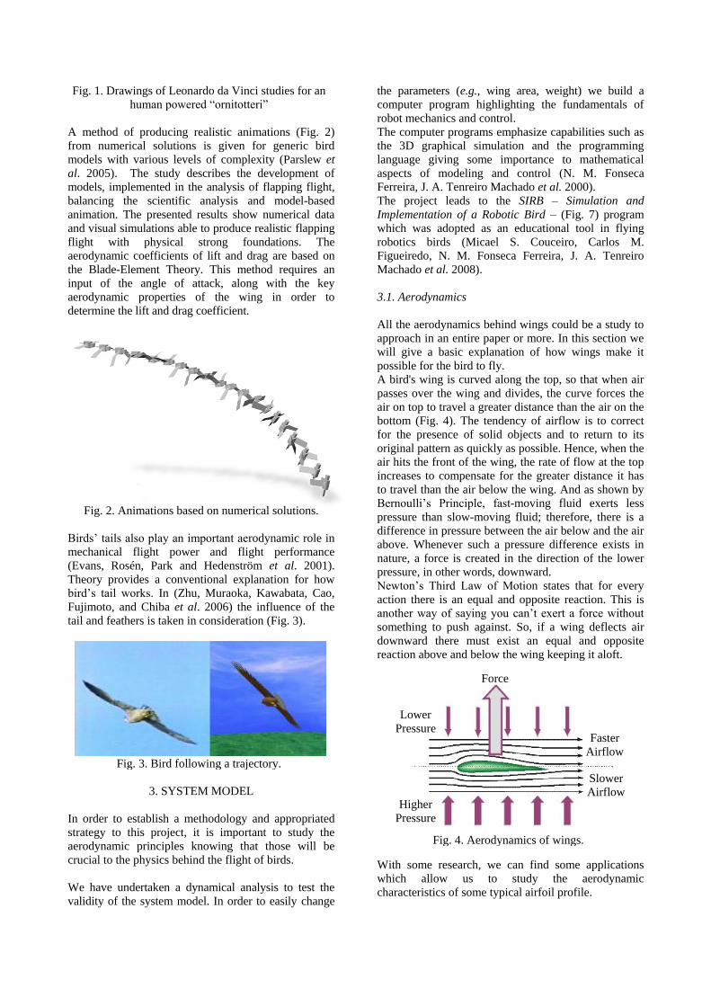
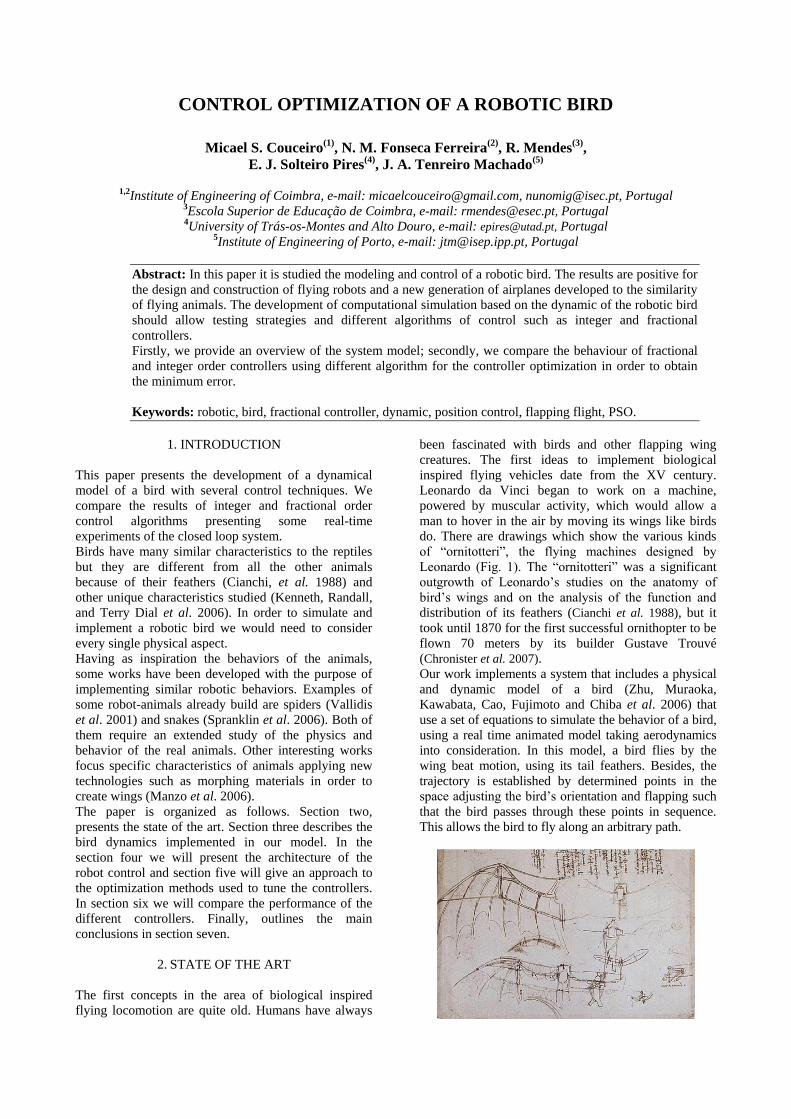
Fig. 1. Drawings of Leonardo da Vinci studies for an

human powered “ornitotteri”

A method of producing realistic animations (Fig. 2)

from numerical solutions is given for generic bird

models with various levels of complexity (Parslew et

al. 2005). The study describes the development of

models, implemented in the analysis of flapping flight,

balancing the scientific analysis and model-based

animation. The presented results show numerical data

and visual simulations able to produce realistic flapping

flight with physical strong foundations. The

aerodynamic coefficients of lift and drag are based on

the Blade-Element Theory. This method requires an

input of the angle of attack, along with the key

aerodynamic properties of the wing in order to

determine the lift and drag coefficient.

Fig. 2. Animations based on numerical solutions.

Birds’ tails also play an important aerodynamic role in

mechanical flight power and flight performance

(Evans, Rosén, Park and Hedenström et al. 2001).

Theory provides a conventional explanation for how

bird’s tail works. In (Zhu, Muraoka, Kawabata, Cao,

Fujimoto, and Chiba et al. 2006) the influence of the

tail and feathers is taken in consideration (Fig. 3).

Fig. 3. Bird following a trajectory.

3. SYSTEM MODEL

In order to establish a methodology and appropriated

strategy to this project, it is important to study the

aerodynamic principles knowing that those will be

crucial to the physics behind the flight of birds.

We have undertaken a dynamical analysis to test the

validity of the system model. In order to easily change

the parameters (e.g., wing area, weight) we build a

computer program highlighting the fundamentals of

robot mechanics and control.

The computer programs emphasize capabilities such as

the 3D graphical simulation and the programming

language giving some importance to mathematical

aspects of modeling and control (N. M. Fonseca

Ferreira, J. A. Tenreiro Machado et al. 2000).

The project leads to the SIRB – Simulation and

Implementation of a Robotic Bird – (Fig. 7) program

which was adopted as an educational tool in flying

robotics birds (Micael S. Couceiro, Carlos M.

Figueiredo, N. M. Fonseca Ferreira, J. A. Tenreiro

Machado et al. 2008).

3.1. Aerodynamics

All the aerodynamics behind wings could be a study to

approach in an entire paper or more. In this section we

will give a basic explanation of how wings make it

possible for the bird to fly.

A bird's wing is curved along the top, so that when air

passes over the wing and divides, the curve forces the

air on top to travel a greater distance than the air on the

bottom (Fig. 4). The tendency of airflow is to correct

for the presence of solid objects and to return to its

original pattern as quickly as possible. Hence, when the

air hits the front of the wing, the rate of flow at the top

increases to compensate for the greater distance it has

to travel than the air below the wing. And as shown by

Bernoulli’s Principle, fast-moving fluid exerts less

pressure than slow-moving fluid; therefore, there is a

difference in pressure between the air below and the air

above. Whenever such a pressure difference exists in

nature, a force is created in the direction of the lower

pressure, in other words, downward.

Newton’s Third Law of Motion states that for every

action there is an equal and opposite reaction. This is

another way of saying you can’t exert a force without

something to push against. So, if a wing deflects air

downward there must exist an equal and opposite

reaction above and below the wing keeping it aloft.

Fig. 4. Aerodynamics of wings.

With some research, we can find some applications

which allow us to study the aerodynamic

characteristics of some typical airfoil profile.

Force

Faster

Airflow

Slower

Airflow Higher

Pressure

Lower

Pressure

One of those free applications is named FoilSim which

is a educational package created by NASA to help and

instruct students with the principles of aerodynamics.

FoilSim can show us charts with the forces and

aerodynamic velocity acting in the airfoil.

Although the majority of avian flight studies have

focused on the wings, the tail also appears to be crucial

to the evolutionary success of birds as flying

organisms.

The precise use of the tail in flying birds has not been

thoroughly documented (Zhu, Muraoka, Kawabata,

Cao, Fujimoto and Chiba et al. 2006). The tail feathers

are instrumental in stabilizing the flight, changing the

direction of the forward movement, compensating for

the lift force, and acting as a brake when the bird lands.

We are using the tail in order to cause a drag force

changing the moment of the bird and, consequently,

producing a rotation around an axis equal to the axis of

rotation of the tail. That is, if the tail is bending up, the

bird will rotate around the same joint bending up too. If

the tail bends up and twists right for example (Fig. 5),

the bird will then rotate around both the joints of the

tail up and right. The angle of rotation of the tail is

always relative to the movement of the bird.

Fig. 5. Action of bird tail.

The influence of the tail has relevance in the

calculation of the moments (Berg and Rayner et al.

1995). The bird will be able to rotate using the tail or

using different angles of attack on each wing (or

different velocities on each wing).

3.2. Gliding Flight

The relative wind acting on a wing produces a certain

amount of force which is called the total aerodynamic

force. This force can be resolved into components,

called Lift and Drag (Fig. 6).

Fig. 6. Force acting on the wing.

The Lift L (2) is the component of aerodynamic force

perpendicular to the relative wind and the Drag D (3)

is the component of aerodynamic force parallel to the

relative wind. Those components can be expressed by

the following formulae:

(2)

(3)

The Lift and Drag on the wing depends on the wing

area S, the density of air ρ, the velocity of the air flow

relative to the wing v∞ and the Lift and Drag

coefficients Cl and Cd respectively, expressed as

functions of the angle of attack α.

The Lift and Drag coefficients depend on the shape of

the airfoil and will alter with changes in the angle of

attack and other wing trimmings. The characteristics of

any particular airfoil section can conveniently be

represented by graphs showing the amount of lift and

drag obtained at various angles of attack, the lift-drag

ratio, and the movement of the center of pressure.

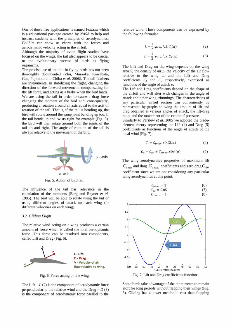
Similarly to Parslew et al. 2005 we adopted the blade-

element theory representing the Lift (4) and Drag (5)

coefficients as functions of the angle of attack of the

local wind (Fig. 7).

(4)

(5)

The wing aerodynamics properties of maximum lift

maxlC and drag maxdC coefficients and zero drag 0dC

coefficient since we are not considering any particular

wing aerodynamics at this point.

(6) (7) (8)

Fig. 7. Lift and Drag coefficients functions.

Some birds take advantage of the air currents to remain

aloft for long periods without flapping their wings (Fig.

8). Gliding has a lower metabolic cost than flapping

L - Lift. D - Drag. V - Velocity of air flow relative to wing.

Cl(α)

Cd(α)

y - axis

z- axis

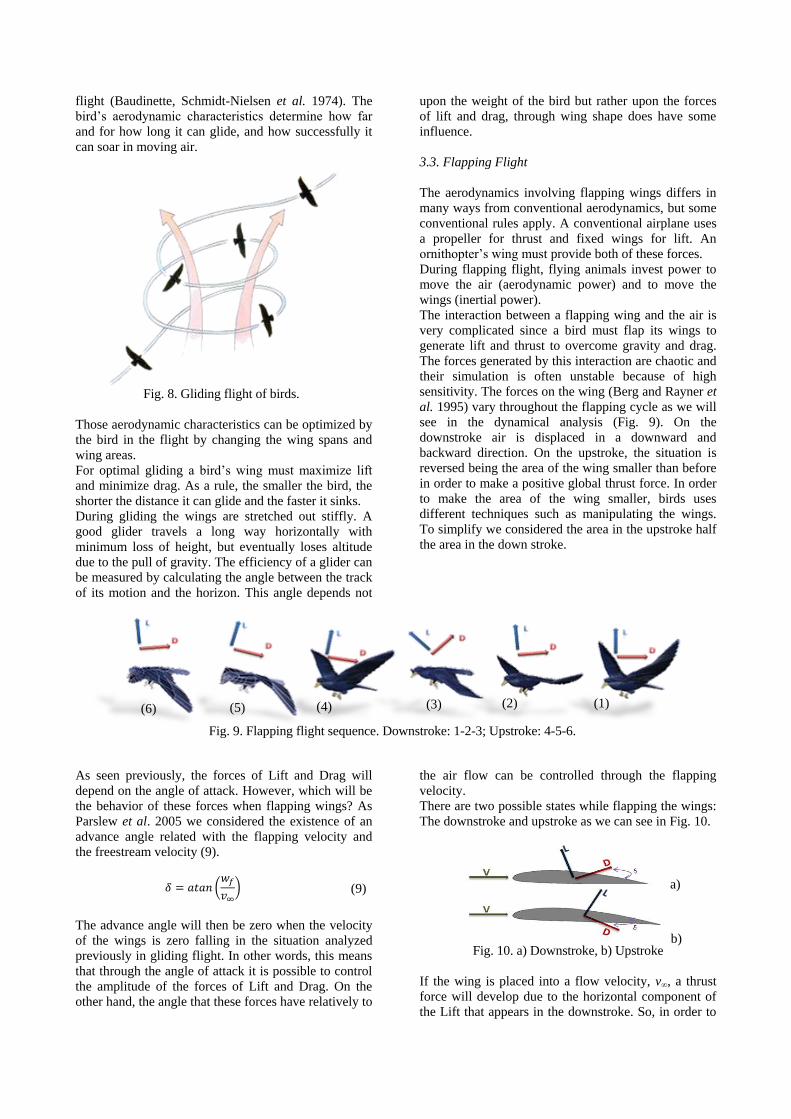
flight (Baudinette, Schmidt-Nielsen et al. 1974). The

bird’s aerodynamic characteristics determine how far

and for how long it can glide, and how successfully it

can soar in moving air.

Fig. 8. Gliding flight of birds.

Those aerodynamic characteristics can be optimized by

the bird in the flight by changing the wing spans and

wing areas.

For optimal gliding a bird’s wing must maximize lift

and minimize drag. As a rule, the smaller the bird, the

shorter the distance it can glide and the faster it sinks.

During gliding the wings are stretched out stiffly. A

good glider travels a long way horizontally with

minimum loss of height, but eventually loses altitude

due to the pull of gravity. The efficiency of a glider can

be measured by calculating the angle between the track

of its motion and the horizon. This angle depends not

upon the weight of the bird but rather upon the forces

of lift and drag, through wing shape does have some

influence.

3.3. Flapping Flight

The aerodynamics involving flapping wings differs in

many ways from conventional aerodynamics, but some

conventional rules apply. A conventional airplane uses

a propeller for thrust and fixed wings for lift. An

ornithopter’s wing must provide both of these forces.

During flapping flight, flying animals invest power to

move the air (aerodynamic power) and to move the

wings (inertial power).

The interaction between a flapping wing and the air is

very complicated since a bird must flap its wings to

generate lift and thrust to overcome gravity and drag.

The forces generated by this interaction are chaotic and

their simulation is often unstable because of high

sensitivity. The forces on the wing (Berg and Rayner et

al. 1995) vary throughout the flapping cycle as we will

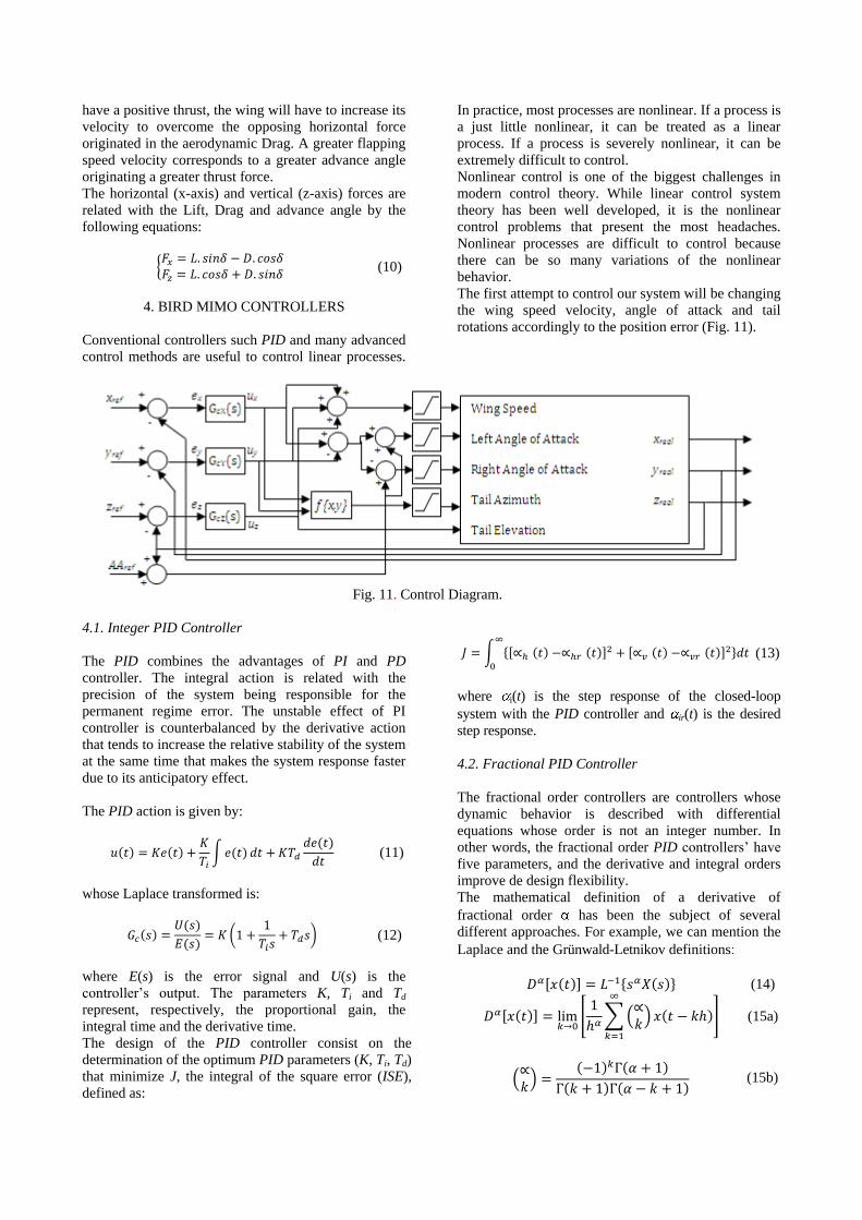
see in the dynamical analysis (Fig. 9). On the

downstroke air is displaced in a downward and

backward direction. On the upstroke, the situation is

reversed being the area of the wing smaller than before

in order to make a positive global thrust force. In order

to make the area of the wing smaller, birds uses

different techniques such as manipulating the wings.

To simplify we considered the area in the upstroke half

the area in the down stroke.

Fig. 9. Flapping flight sequence. Downstroke: 1-2-3; Upstroke: 4-5-6.

As seen previously, the forces of Lift and Drag will

depend on the angle of attack. However, which will be

the behavior of these forces when flapping wings? As

Parslew et al. 2005 we considered the existence of an

advance angle related with the flapping velocity and

the freestream velocity (9).

(9)

The advance angle will then be zero when the velocity

of the wings is zero falling in the situation analyzed

previously in gliding flight. In other words, this means

that through the angle of attack it is possible to control

the amplitude of the forces of Lift and Drag. On the

other hand, the angle that these forces have relatively to

the air flow can be controlled through the flapping

velocity.

There are two possible states while flapping the wings:

The downstroke and upstroke as we can see in Fig. 10.

Fig. 10. a) Downstroke, b) Upstroke

If the wing is placed into a flow velocity, v∞, a thrust

force will develop due to the horizontal component of

the Lift that appears in the downstroke. So, in order to

a)

b)

(1) (2) (3) (4) (5) (6)

have a positive thrust, the wing will have to increase its

velocity to overcome the opposing horizontal force

originated in the aerodynamic Drag. A greater flapping

speed velocity corresponds to a greater advance angle

originating a greater thrust force.

The horizontal (x-axis) and vertical (z-axis) forces are

related with the Lift, Drag and advance angle by the

following equations:

(10)

4. BIRD MIMO CONTROLLERS

Conventional controllers such PID and many advanced

control methods are useful to control linear processes.

In practice, most processes are nonlinear. If a process is

a just little nonlinear, it can be treated as a linear

process. If a process is severely nonlinear, it can be

extremely difficult to control.

Nonlinear control is one of the biggest challenges in

modern control theory. While linear control system

theory has been well developed, it is the nonlinear

control problems that present the most headaches.

Nonlinear processes are difficult to control because

there can be so many variations of the nonlinear

behavior.

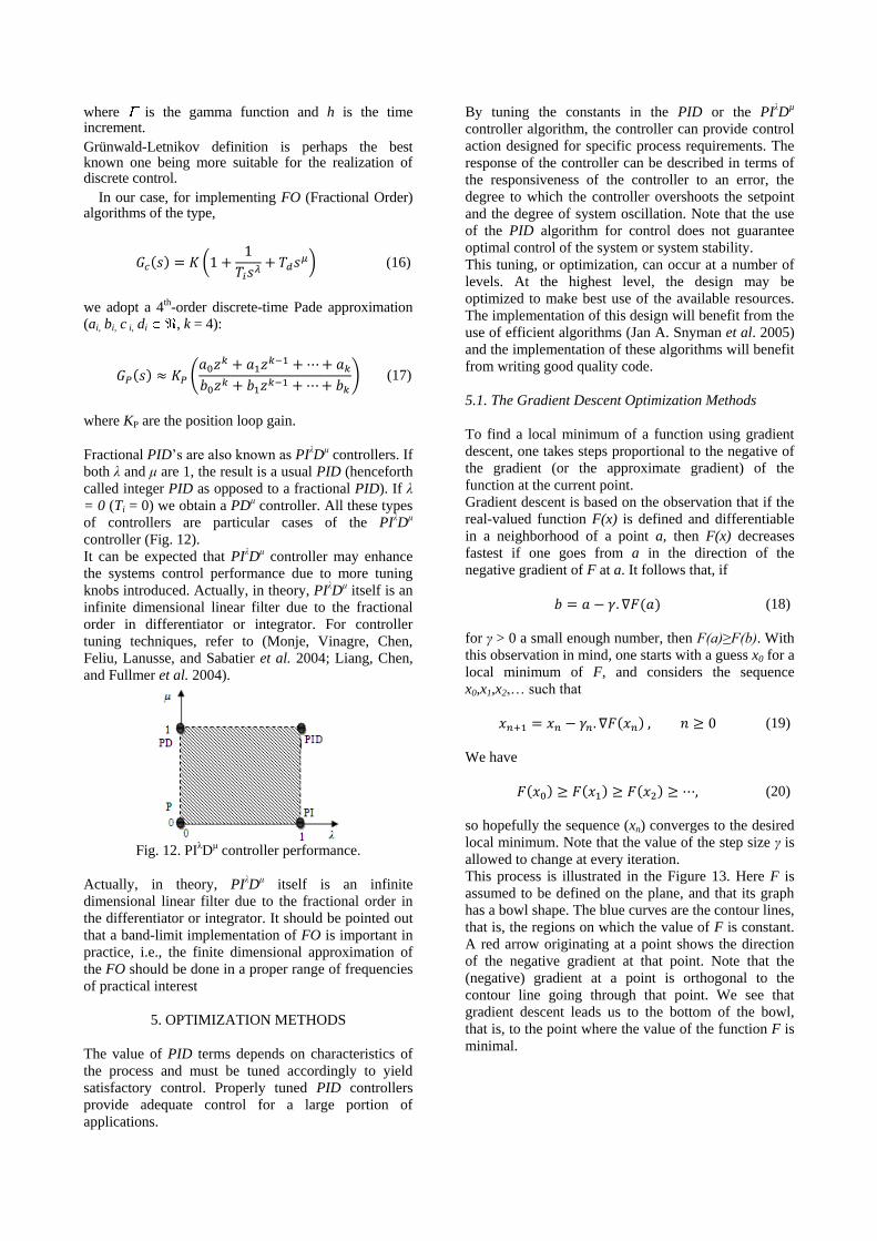
The first attempt to control our system will be changing

the wing speed velocity, angle of attack and tail

rotations accordingly to the position error (Fig. 11).

Fig. 11. Control Diagram.

4.1. Integer PID Controller

The PID combines the advantages of PI and PD

controller. The integral action is related with the

precision of the system being responsible for the

permanent regime error. The unstable effect of PI

controller is counterbalanced by the derivative action

that tends to increase the relative stability of the system

at the same time that makes the system response faster

due to its anticipatory effect.

The PID action is given by:

(11)

whose Laplace transformed is:

(12)

where E(s) is the error signal and U(s) is the

controller’s output. The parameters K, Ti and Td

represent, respectively, the proportional gain, the

integral time and the derivative time.

The design of the PID controller consist on the

determination of the optimum PID parameters (K, Ti, Td)

that minimize J, the integral of the square error (ISE),

defined as:

(13)

where i(t) is the step response of the closed-loop

system with the PID controller and ir(t) is the desired

step response.

4.2. Fractional PID Controller

The fractional order controllers are controllers whose

dynamic behavior is described with differential

equations whose order is not an integer number. In

other words, the fractional order PID controllers’ have

five parameters, and the derivative and integral orders

improve de design flexibility.

The mathematical definition of a derivative of

fractional order has been the subject of several

different approaches. For example, we can mention the

Laplace and the Grünwald-Letnikov definitions

(14)

(15a)

(15b)

where is the gamma function and h is the time increment.

Grünwald-Letnikov definition is perhaps the best known one being more suitable for the realization of discrete control.

In our case, for implementing FO (Fractional Order) algorithms of the type,

(16)

we adopt a 4th-order discrete-time Pade approximation (ai, bi, c i, di , k = 4):

(17)

where KP are the position loop gain.

Fractional PID’s are also known as PIλDμ controllers. If

both λ and μ are 1, the result is a usual PID (henceforth

called integer PID as opposed to a fractional PID). If λ

= 0 (Ti = 0) we obtain a PDμ controller. All these types

of controllers are particular cases of the PIλDμ

controller (Fig. 12).

It can be expected that PIλDμ controller may enhance

the systems control performance due to more tuning

knobs introduced. Actually, in theory, PIλDμ itself is an

infinite dimensional linear filter due to the fractional

order in differentiator or integrator. For controller

tuning techniques, refer to (Monje, Vinagre, Chen,

Feliu, Lanusse, and Sabatier et al. 2004; Liang, Chen,

and Fullmer et al. 2004).

Fig. 12. PIλDμ controller performance.

Actually, in theory, PIλDμ itself is an infinite

dimensional linear filter due to the fractional order in

the differentiator or integrator. It should be pointed out

that a band-limit implementation of FO is important in

practice, i.e., the finite dimensional approximation of

the FO should be done in a proper range of frequencies

of practical interest

5. OPTIMIZATION METHODS

The value of PID terms depends on characteristics of

the process and must be tuned accordingly to yield

satisfactory control. Properly tuned PID controllers

provide adequate control for a large portion of

applications.

By tuning the constants in the PID or the PIλDµ

controller algorithm, the controller can provide control

action designed for specific process requirements. The

response of the controller can be described in terms of

the responsiveness of the controller to an error, the

degree to which the controller overshoots the setpoint

and the degree of system oscillation. Note that the use

of the PID algorithm for control does not guarantee

optimal control of the system or system stability.

This tuning, or optimization, can occur at a number of

levels. At the highest level, the design may be

optimized to make best use of the available resources.

The implementation of this design will benefit from the

use of efficient algorithms (Jan A. Snyman et al. 2005)

and the implementation of these algorithms will benefit

from writing good quality code.

5.1. The Gradient Descent Optimization Methods

To find a local minimum of a function using gradient

descent, one takes steps proportional to the negative of

the gradient (or the approximate gradient) of the

function at the current point.

Gradient descent is based on the observation that if the

real-valued function F(x) is defined and differentiable

in a neighborhood of a point a, then F(x) decreases

fastest if one goes from a in the direction of the

negative gradient of F at a. It follows that, if

(18)

for γ > 0 a small enough number, then F(a)≥F(b). With

this observation in mind, one starts with a guess x0 for a

local minimum of F, and considers the sequence

x0,x1,x2,… such that

(19)

We have

(20)

so hopefully the sequence (xn) converges to the desired

local minimum. Note that the value of the step size γ is

allowed to change at every iteration.

This process is illustrated in the Figure 13. Here F is

assumed to be defined on the plane, and that its graph

has a bowl shape. The blue curves are the contour lines,

that is, the regions on which the value of F is constant.

A red arrow originating at a point shows the direction

of the negative gradient at that point. Note that the

(negative) gradient at a point is orthogonal to the

contour line going through that point. We see that

gradient descent leads us to the bottom of the bowl,

that is, to the point where the value of the function F is

minimal.

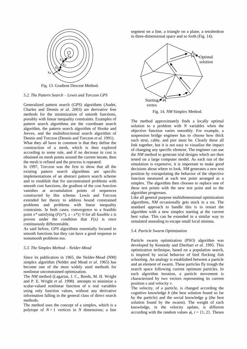
Fig. 13. Gradient Descent Method.

5.2. The Pattern Search – Lewis and Torczon GPS

Generalized pattern search (GPS) algorithms (Audet,

Charles and Dennis et al. 2003) are derivative free

methods for the minimization of smooth functions,

possibly with linear inequality constraints. Examples of

pattern search algorithms are the coordinate search

algorithm, the pattern search algorithm of Hooke and

Jeeves, and the multidirectional search algorithm of

Dennis and Torczon (Dennis and Torczon et al. 1991).

What they all have in common is that they define the

construction of a mesh, which is then explored

according to some rule, and if no decrease in cost is

obtained on mesh points around the current iterate, then

the mesh is refined and the process is repeated.

In 1997, Torczon was the first to show that all the

existing pattern search algorithms are specific

implementations of an abstract pattern search scheme

and to establish that for unconstrained problems with

smooth cost functions, the gradient of the cost function

vanishes at accumulation points of sequences

constructed by this scheme. Lewis and Torczon

extended her theory to address bound constrained

problems and problems with linear inequality

constraints. In both cases, convergence to a feasible

point x* satisfying (F(x*), x - x*)≥ 0 for all feasible x is

proven under the condition that F(x) is once

continuously differentiable.

As said before, GPS algorithms essentially focused to

smooth functions but they can have a good response to

nonsmooth problems too.

5.3. The Simplex Method – Nelder-Mead

Since its publication in 1965, the Nelder-Mead (NM)

simplex algorithm (Nelder and Mead et al. 1965) has

become one of the most widely used methods for

nonlinear unconstrained optimization.

The NM method (Lagarias, J. C., Reeds, M. H. Wright

and P. E. Wright et al. 1998) attempts to minimize a

scalar-valued nonlinear function of n real variables

using only function values, without any derivative

information falling in the general class of direct search

methods.

The method uses the concept of a simplex, which is a

polytope of N + 1 vertices in N dimensions; a line

segment on a line, a triangle on a plane, a tetrahedron

in three-dimensional space and so forth (Fig. 14).

Fig. 14. NM Simplex Method.

The method approximately finds a locally optimal

solution to a problem with N variables when the

objective function varies smoothly. For example, a

suspension bridge engineer has to choose how thick

each strut, cable, and pier must be. Clearly these all

link together, but it is not easy to visualize the impact

of changing any specific element. The engineer can use

the NM method to generate trial designs which are then

tested on a large computer model. As each run of the

simulation is expensive, it is important to make good

decisions about where to look. NM generates a new test

position by extrapolating the behavior of the objective

function measured at each test point arranged as a

simplex. The algorithm then chooses to replace one of

these test points with the new test point and so the

algorithm progresses.

Like all general purpose multidimensional optimization

algorithms, NM occasionally gets stuck in a rut. The

standard approach to handle this is to restart the

algorithm with a new simplex starting at the current

best value. This can be extended in a similar way to

simulated annealing to escape small local minima.

5.4. Particle Swarm Optimization

Particle swarm optimization (PSO) algorithm was

developed by Kennedy and Eberhart et al. 1995. This

optimization technique, based on a population search,

is inspired by social behavior of bird flocking fish

schooling. An analogy is established between a particle

and an element of swarm. These particles fly trough the

search space following current optimum particles. In

each algorithm iteration, a particle movement is

characterized by two vectors representing its current

position x and velocity v.

The velocity, of a particle, is changed according the

cognitive knowledge b (the best solution found so far

by the particle) and the social knowledge g (the best

solution found by the swarm). The weight of each

knowledge, in the velocity update, is different

according with the random values i, i = {1, 2}. Theses

Starting

vertex

Optimal

solution

x0

x3

x1 x2

x4

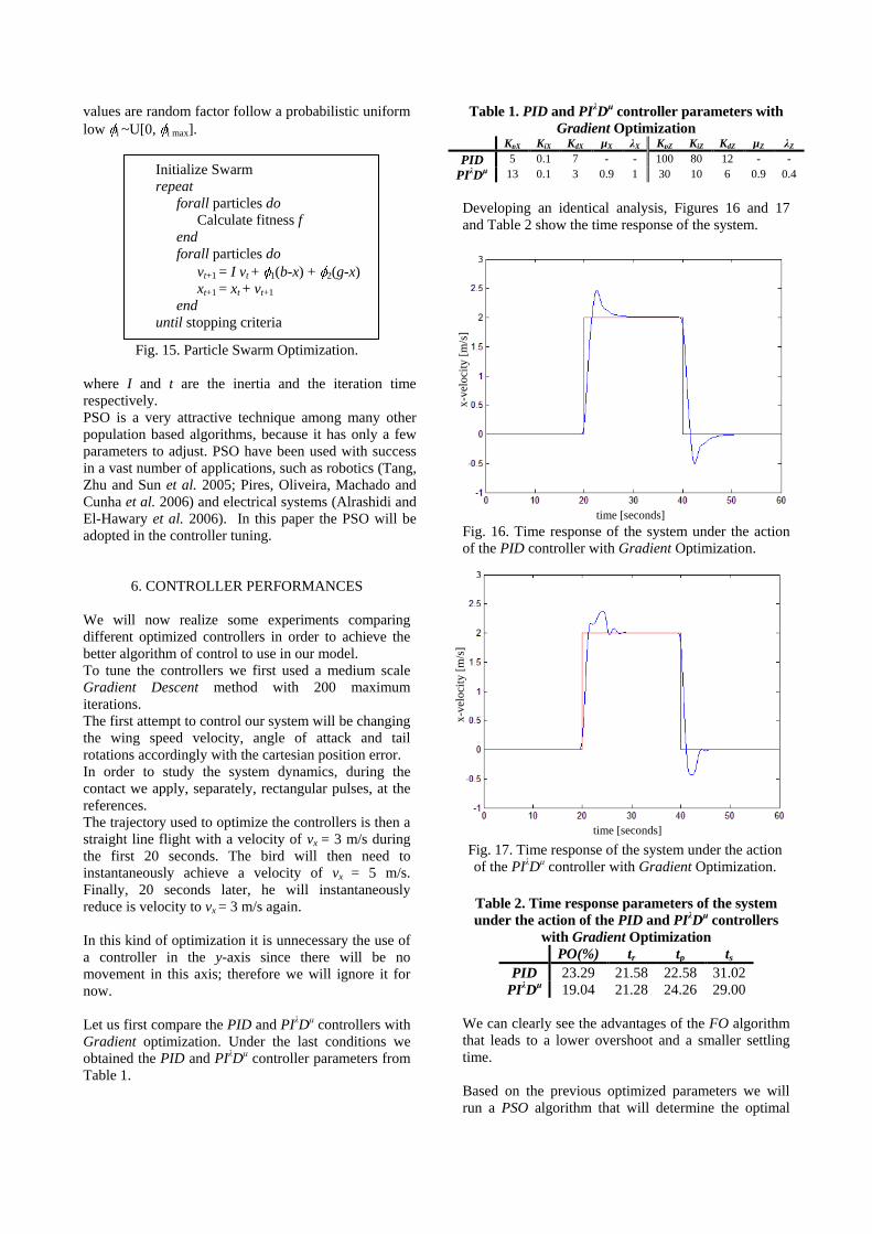
values are random factor follow a probabilistic uniform

low i ~U[0, i max].

Fig. 15. Particle Swarm Optimization.

where I and t are the inertia and the iteration time

respectively.

PSO is a very attractive technique among many other

population based algorithms, because it has only a few

parameters to adjust. PSO have been used with success

in a vast number of applications, such as robotics (Tang,

Zhu and Sun et al. 2005; Pires, Oliveira, Machado and

Cunha et al. 2006) and electrical systems (Alrashidi and

El-Hawary et al. 2006). In this paper the PSO will be

adopted in the controller tuning.

6. CONTROLLER PERFORMANCES

We will now realize some experiments comparing

different optimized controllers in order to achieve the

better algorithm of control to use in our model.

To tune the controllers we first used a medium scale

Gradient Descent method with 200 maximum

iterations.

The first attempt to control our system will be changing

the wing speed velocity, angle of attack and tail

rotations accordingly with the cartesian position error.

In order to study the system dynamics, during the

contact we apply, separately, rectangular pulses, at the

references.

The trajectory used to optimize the controllers is then a

straight line flight with a velocity of vx = 3 m/s during

the first 20 seconds. The bird will then need to

instantaneously achieve a velocity of vx = 5 m/s.

Finally, 20 seconds later, he will instantaneously

reduce is velocity to vx = 3 m/s again.

In this kind of optimization it is unnecessary the use of

a controller in the y-axis since there will be no

movement in this axis; therefore we will ignore it for

now.

Let us first compare the PID and PIλDμ controllers with

Gradient optimization. Under the last conditions we

obtained the PID and PIλDμ controller parameters from

Table 1.

Table 1. PID and PIλD

μ controller parameters with

Gradient Optimization KpX KiX KdX µX λX KpZ KiZ KdZ µZ λZ

PID 5 0.1 7 - - 100 80 12 - -

PIλD

μ 13 0.1 3 0.9 1 30 10 6 0.9 0.4

Developing an identical analysis, Figures 16 and 17

and Table 2 show the time response of the system.

Fig. 16. Time response of the system under the action

of the PID controller with Gradient Optimization.

Fig. 17. Time response of the system under the action

of the PIλDμ controller with Gradient Optimization.

Table 2. Time response parameters of the system

under the action of the PID and PIλD

μ controllers

with Gradient Optimization

PO(%) tr tp ts

PID 23.29 21.58 22.58 31.02

29.00 PIλD

μ 19.04 21.28 24.26

We can clearly see the advantages of the FO algorithm

that leads to a lower overshoot and a smaller settling

time.

Based on the previous optimized parameters we will

run a PSO algorithm that will determine the optimal

Initialize Swarm

repeat

forall particles do

Calculate fitness f

end

forall particles do

vt+1 = I vt + 1(b-x) + 2(g-x)

xt+1 = xt + vt+1

end

until stopping criteria

time [seconds]

x-v

elo

city

[m

/s]

time [seconds]

x-v

elo

city

[m

/s]

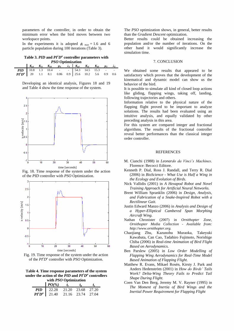
parameters of the controller, in order to obtain the

minimum error when the bird moves between two

workspace points.

In the experiments it is adopted i max = 1.6 and 6

particle population during 100 iterations (Table 3).

Table 3. PID and PIλD

μ controller parameters with

PSO Optimization KpX KiX KdX µX λX KpZ KiZ KdZ µZ λZ

PID 10.8 1.3 10.4 - - 54.3 14.5 15.3 - -

PIλD

μ 20 1.1 8.1 0.86 0.9 25.6 10.2 5.6 0.9 0.6

Developing an identical analysis, Figures 18 and 19

and Table 4 show the time response of the system.

Fig. 18. Time response of the system under the action

of the PID controller with PSO Optimization.

Fig. 19. Time response of the system under the action

of the PIλDμ controller with PSO Optimization.

Table 4. Time response parameters of the system

under the action of the PID and PIλD

μ controllers

with PSO Optimization

PO(%) tr tp ts

PID 22.28 21.20 23.68 27.20

PIλD

μ 21.40 21.16 23.74 27.04

The PSO optimization shows, in general, better results

than the Gradient Descent optimization.

Better results could be obtained increasing the

population and/or the number of iterations. On the

other hand it would significantly increase the

simulation time.

7. CONCLUSION

We obtained some results that appeared to be

satisfactory which proves that the development of the

kinematical and dynamic model can show us the

behavior of the bird.

It is possible to simulate all kind of closed loop actions

like gliding, flapping wings, taking off, landing,

following trajectories and others.

Information relative to the physical nature of the

flapping flight proved to be important to analyze

solutions. The results had been evaluated using an

intuitive analysis, and equally validated by other

preceding analysis in this area.

For this system are compared integer and fractional

algorithms. The results of the fractional controller

reveal better performances than the classical integer

order controller.

REFERENCES

M. Cianchi (1988) in Leonardo da Vinci’s Machines.

Florence: Becocci Editore. Kenneth P. Dial, Ross J. Randall, and Terry R. Dial

(2006) in BioScience - What Use is Half a Wing in

the Ecology and Evolution of Birds.

Nick Vallidis (2001) in A Hexapod Robot and Novel

Training Approach for Artificial Neural Networks. Brent William Spranklin (2006) in Design, Analysis,

and Fabrication of a Snake-Inspired Robot with a

Rectilinear Gait.

Justin Edward Manzo (2006) in Analysis and Design of

a Hyper-Elliptical Cambered Span Morphing

Aircraft Wing. Nathan Chronister (2007) in Ornithopter Zone,

Ornithopter Media Collection - Available from:

http://www.ornithopter.org. Chaojiang Zhu, Kazunobu Muraoka, Takeyuki

Kawabata, Can Cao, Tadahiro Fujimoto, Norishige

Chiba (2006) in Real-time Animation of Bird Flight

Based on Aerodynamics.

Ben Parslew (2005) in Low Order Modelling of

Flapping Wing Aerodynamics for Real-Time Model

Based Animation of Flapping Flight.

Matthew R. Evans, Mikael Rosén, Kirsty J. Park and

Anders Hedenström (2001) in How do Birds’ Tails

Work? Delta-Wing Theory Fails to Predict Tail

Shape During Flight.

Coen Van Den Berg, Jeremy M. V. Rayner (1995) in

The Moment of Inertia of Bird Wings and the

Inertial Power Requirement for Flapping Flight

time [seconds]

x-v

elo

city

[m

/s]

time [seconds]

x-v

elo

city

[m

/s]

R. V. Baudinette, K. Schmidt-Nielsen (1974) in Energy

cost of gliding flight in herring gulls. Nature, Land.

348, 83-84. C. A. Monje, B. M. Vinagre, Y. Q. Chen, V. Feliu, P.

Lanusse, and J. Sabatier (2004) in Proposals for

fractional PIλDμ tuning.

J. Liang, Y. Q. Chen, and R. Fullmer (2004) in

Simulation studies on the boundary stabilization

and disturbance rejection for fractional diffusion-

wave equation.

Jan A. Snyman (2005) in Practical Mathematical

Optimization: An Introduction to Basic

Optimization Theory and Classical and New

Gradient-Based Algorithms.

Audet, Charles and J. E. Dennis Jr (2003) in Analysis

of Generalized Pattern Searches.

J. E. Dennis, Jr. and Virginia Torczon (1991) in Direct

search methods on parallel machines.

J. A. Nelder and R. Mead (1965) in A simplex method

for function minimization, Computer Journal 7,

308-313.

Lagarias, J. C., J. A. Reeds, M. H. Wright, and P. E.

Wright (1998) in Convergence Properties of the

Melder-Mead Simplex Method in Low Dimensions.

J. Kennedy and R. C. Eberhart (1995) in Particle

swarm optimization. In Proceedings of the 1995

IEEE International Conference on Neural

Networks. volume 4. pp. 1942–1948. Perth.

Australia. IEEE Service Center. Piscataway. NJ.

J. Tang, J. Zhu and Z. Sun (2005) in A novel path

panning approach based on appart and particle

swarm optimization. In LNCS. editor.

Proceedings of the 2nd International Symposium

on Neural Networks. volume 3498.

E. J. Solteiro Pires, P. B. de Moura Oliveira, J. A.

Tenreiro Machado and J. Boaventura Cunha

(2006). Particle Swarm Optimization versus

Genetic Algorithm in Manipulator Trajectory

Planning. The 7th Portuguese Conference on

Automatic Control, pp.230. 11-13 September,

Lisbon, Portugal.

M. R. Alrashidi and M. E. El-Hawary (2006) in A

Survey of Particle Swarm Optimization

Applications in Power System Operations.

Electric Power Components and Systems. 34:12.

1349 - 1357 Taylor & Francis.

N. M. Fonseca Ferreira, J. A. Tenreiro Machado,

(2000) in RobLib: An Educational Program for

Robotics, SYROCO’00, IFAC Symposium on

Robot Control, vol.1 pg. 163–168, Vienna, Austria.

Micael S. Couceiro, Carlos M. Figueiredo, N. M.

Fonseca Ferreira, J. A. Tenreiro Machado (2008) in

Simulation of a Robotic Bird, Fractional

Differentiation and its Applications, 05–07

November, Ankara, Turkey.

N. M. Fonseca Ferreira, Fernando B. Duarte, Miguel F.

M. Lima, Maria G. Marcos, J. A. Tenreiro Machado

(2008), Application of Fractional Calculus in the

Dynamical Analysis and Control of Mechanical

Manipulators, Fractional Calculus & Applied

Analysis, vol. 11, number 1, pp. 91–113, ISSN

1311-0454.