
Contextual alignment of biological sequences (Extended abstract)
12
BIOINFORMATICS Vol. 18 Suppl. 2 2002 Pages S116–S127 Contextual alignment of biological sequences (Extended abstract) Anna Gambin, Slawomir Lasota, Radoslaw Szklarczyk, Jerzy Tiuryn and Jerzy Tyszkiewicz Institute of Informatics, Warsaw University, Banacha 2, 02-097, Warsaw, Poland Received on April 8, 2002; accepted on June 15, 2002 ABSTRACT We present a model of contextual alignment of biological sequences. It is an extension of the classical alignment, in which we assume that the cost of a substitution depends on the surrounding symbols. In this model the cost of transforming one sequence into another depends on the order of editing operations. We present efficient algorithms for calculating this cost, as well as reconstructing (the representation of) all the orders of operations which yield this optimal cost. A precise characterization of the families of linear orders which can emerge this way is given. Contact: [email protected] INTRODUCTION A large portion of modern computational biology is concerned with measuring the degree of similarity of biological sequences, the most prominent examples of which are DNA and proteins. Generally, to get such a model of similarity, one assumes a set of operations, which can change sequences, and a score function, assigning a score to each operation performed on a sequence. Then each set of operations transforming a biological sequence V into another such sequence W is assigned a score—typically the sum of the scores of individual operations. The operations correspond to evolutionary changes, higher score reflects that the event is more likely to appear. Several values are then of interest, the crucial ones being the maximal possible score of a transformation of V into W and the maximal score of a transformation of a contiguous fragment of V into a fragment of W (maximized over such fragments, too). The model dominating in the field (the so called alignment model) (Durbin et al., 1998; Gusfield, 1997), used for DNA and proteins, assumes the operation of substitution of one letter for another, as well as an insertion or a deletion of a sequence of letters. The score of a substitution depends only on the two residues exchanged. It is provided by the so-called substitution tables (Dayhoff et al., 1978; Henikoff et al., 1992). The score for insertions and deletions depends solely on the length of the inserted/deleted subsequence (it is quite often an affine function). Of course, the above score model is a great oversim- plification from the biological point of view. However, it is the most commonly used, because it permits very ef- ficient algorithms to compute the key values, called the maximal global and local alignment scores, respectively. Other models, which are biologically more realistic, are computationally very hard (or even provably intractable). For example, a very important property of proteins is their fold (i.e. the 3D shape they assume in the cell), which can decide homology between proteins of quite different se- quences. However, despite very intense efforts, predicting the shape of a protein, based on its sequence, is viewed as an extremely difficult problem. Results In this paper we offer a model, which extends the classical alignment model, with the intention to bring it a step closer to the biological reality without sacrificing its algorithmic properties. The set of operations is the same as that of the alignment model but the score function of a substitution changes. In our model the score of a substitution depends on the surrounding letters in the sequence, too. I.e. the score of substituting b by d in abc can differ from the score of substituting b by d in a bc . The score for insertions and deletions is inherited from the classical model. We call our model the contextual alignment model. The aim of this paper is to present an efficient algorithm for calculating the maximal contextual alignment score, assuming affinity of gap penalty function. The running time of the algorithm is O (||mn), where || is the size of the alphabet (4 in the case of DNA, 20 in the case of proteins) and m, n are the lengths of the sequences. Hence the complexity is, up to a constant factor, the same as that of the algorithms of the classical context-free alignment model. Another topic of our paper is the order in which operations are performed. As it is easy to see, in the contextual alignment model the score of a set of operations S116 c Oxford University Press 2002
Transcript of Contextual alignment of biological sequences (Extended abstract)
BIOINFORMATICS Vol. 18 Suppl. 2 2002Pages S116–S127
Contextual alignment of biological sequences(Extended abstract)
Anna Gambin, Sławomir Lasota, Radosław Szklarczyk, JerzyTiuryn and Jerzy Tyszkiewicz
Institute of Informatics, Warsaw University, Banacha 2, 02-097, Warsaw, Poland
Received on April 8, 2002; accepted on June 15, 2002
ABSTRACTWe present a model of contextual alignment of biologicalsequences. It is an extension of the classical alignment, inwhich we assume that the cost of a substitution dependson the surrounding symbols. In this model the cost oftransforming one sequence into another depends on theorder of editing operations. We present efficient algorithmsfor calculating this cost, as well as reconstructing (therepresentation of) all the orders of operations which yieldthis optimal cost. A precise characterization of the familiesof linear orders which can emerge this way is given.Contact: [email protected]
INTRODUCTIONA large portion of modern computational biology isconcerned with measuring the degree of similarity ofbiological sequences, the most prominent examples ofwhich are DNA and proteins.
Generally, to get such a model of similarity, one assumesa set of operations, which can change sequences, anda score function, assigning a score to each operationperformed on a sequence. Then each set of operationstransforming a biological sequenceV into another suchsequenceW is assigned a score—typically the sum of thescores of individual operations. The operations correspondto evolutionary changes, higher score reflects that theevent is more likely to appear. Several values are then ofinterest, the crucial ones being the maximal possible scoreof a transformation ofV into W and the maximal scoreof a transformation of a contiguous fragment ofV into afragment ofW (maximized over such fragments, too).
The model dominating in the field (the so calledalignment model) (Durbinet al., 1998; Gusfield, 1997),used for DNA and proteins, assumes the operation ofsubstitution of one letter for another, as well as aninsertion or a deletion of a sequence of letters. Thescore of a substitution depends only on the two residuesexchanged. It is provided by the so-called substitutiontables (Dayhoffet al., 1978; Henikoffet al., 1992). Thescore for insertions and deletions depends solely on the
length of the inserted/deleted subsequence (it is quite oftenan affine function).
Of course, the above score model is a great oversim-plification from the biological point of view. However, itis the most commonly used, because it permits very ef-ficient algorithms to compute the key values, called themaximal global and local alignment scores, respectively.Other models, which are biologically more realistic, arecomputationally very hard (or even provably intractable).For example, a very important property of proteins is theirfold (i.e. the 3D shape they assume in the cell), which candecide homology between proteins of quite different se-quences. However, despite very intense efforts, predictingthe shape of a protein, based on its sequence, is viewed asan extremely difficult problem.
ResultsIn this paper we offer a model, which extends the classicalalignment model, with the intention to bring it a step closerto the biological reality without sacrificing its algorithmicproperties. The set of operations is the same as that of thealignment model but the score function of a substitutionchanges. In our model the score of a substitutiondependson the surrounding letters in the sequence, too. I.e. thescore of substitutingb by d in abc can differ from thescore of substitutingb by d in a′bc′. The score forinsertions and deletions is inherited from the classicalmodel. We call our model thecontextual alignment model.
The aim of this paper is to present an efficient algorithmfor calculating the maximal contextual alignment score,assuming affinity of gap penalty function. The runningtime of the algorithm isO(|�|mn), where|�| is the sizeof the alphabet (4 in the case of DNA, 20 in the case ofproteins) andm, n are the lengths of the sequences. Hencethe complexity is, up to a constant factor, the same as thatof the algorithms of the classical context-free alignmentmodel.
Another topic of our paper is the order in whichoperations are performed. As it is easy to see, in thecontextual alignment model the score of a set of operations
S116 c© Oxford University Press 2002
Contextual alignment of biological sequences
depends on the order. Indeed, an operation may change thecontexts of future operations.
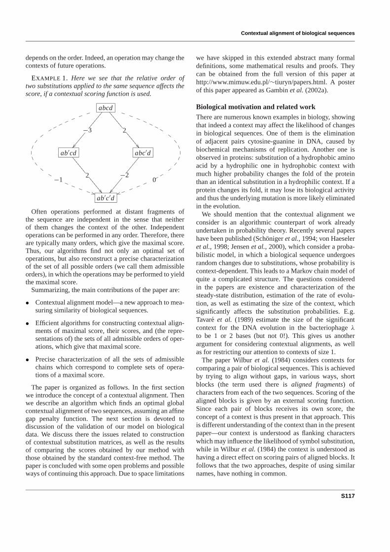
EXAMPLE 1. Here we see that the relative order oftwo substitutions applied to the same sequence affects thescore, if a contextual scoring function is used.
abcd
−3��
����
�
������
��2
����
���
�����
����
−1
������
�� ��
��
��
� � � �
0
� � � � � � ��
��
��
�
��
����
ab′cd
2��
����
�
�����
����
abc′d
−2��
����
������
��
ab′c′d
Often operations performed at distant fragments ofthe sequence are independent in the sense that neitherof them changes the context of the other. Independentoperations can be performed in any order. Therefore, thereare typically many orders, which give the maximal score.Thus, our algorithms find not only an optimal set ofoperations, but also reconstruct a precise characterizationof the set of all possible orders (we call them admissibleorders), in which the operations may be performed to yieldthe maximal score.
Summarizing, the main contributions of the paper are:
• Contextual alignment model—a new approach to mea-suring similarity of biological sequences.
• Efficient algorithms for constructing contextual align-ments of maximal score, their scores, and (the repre-sentations of) the sets of all admissible orders of oper-ations, which give that maximal score.
• Precise characterization of all the sets of admissiblechains which correspond to complete sets of opera-tions of a maximal score.
The paper is organized as follows. In the first sectionwe introduce the concept of a contextual alignment. Thenwe describe an algorithm which finds an optimal globalcontextual alignment of two sequences, assuming an affinegap penalty function. The next section is devoted todiscussion of the validation of our model on biologicaldata. We discuss there the issues related to constructionof contextual substitution matrices, as well as the resultsof comparing the scores obtained by our method withthose obtained by the standard context-free method. Thepaper is concluded with some open problems and possibleways of continuing this approach. Due to space limitations
we have skipped in this extended abstract many formaldefinitions, some mathematical results and proofs. Theycan be obtained from the full version of this paper athttp://www.mimuw.edu.pl/∼tiuryn/papers.html. A posterof this paper appeared as Gambinet al. (2002a).
Biological motivation and related workThere are numerous known examples in biology, showingthat indeed a context may affect the likelihood of changesin biological sequences. One of them is the eliminationof adjacent pairs cytosine-guanine in DNA, caused bybiochemical mechanisms of replication. Another one isobserved in proteins: substitution of a hydrophobic aminoacid by a hydrophilic one in hydrophobic context withmuch higher probability changes the fold of the proteinthan an identical substitution in a hydrophilic context. If aprotein changes its fold, it may lose its biological activityand thus the underlying mutation is more likely eliminatedin the evolution.
We should mention that the contextual alignment weconsider is an algorithmic counterpart of work alreadyundertaken in probability theory. Recently several papershave been published (Schonigeret al., 1994; von Haeseleret al., 1998; Jensenet al., 2000), which consider a proba-bilistic model, in which a biological sequence undergoesrandom changes due to substitutions, whose probability iscontext-dependent. This leads to a Markov chain model ofquite a complicated structure. The questions consideredin the papers are existence and characterization of thesteady-state distribution, estimation of the rate of evolu-tion, as well as estimating the size of the context, whichsignificantly affects the substitution probabilities. E.g.Tavare et al. (1989) estimate the size of the significantcontext for the DNA evolution in the bacteriophageλto be 1 or 2 bases (but not 0!). This gives us anotherargument for considering contextual alignments, as wellas for restricting our attention to contexts of size 1.
The paper Wilburet al. (1984) considers contexts forcomparing a pair of biological sequences. This is achievedby trying to align without gaps, in various ways, shortblocks (the term used there isaligned fragments) ofcharacters from each of the two sequences. Scoring of thealigned blocks is given by an external scoring function.Since each pair of blocks receives its own score, theconcept of a context is thus present in that approach. Thisis different understanding of the context than in the presentpaper—our context is understood as flanking characterswhich may influence the likelihood of symbol substitution,while in Wilbur et al. (1984) the context is understood ashaving a direct effect on scoring pairs of aligned blocks. Itfollows that the two approaches, despite of using similarnames, have nothing in common.
S117
A.Gambin et al.
CONTEXTUAL ALIGNMENTLet V and W be strings over an alphabet�. A gap,denoted−, is asymbol assumed not to belong to�. Letus fix an alignment(V #, W #) of these two sequences. Theconcept of an alignment used in this paper is standard. Weomit it from this presentation for the sake of space. Analignment induces three kinds of blocks, each block hasits uniqueaddress and uniquelength:
• A substitution has an addressi , if V #i , W #
i ∈ �, i.e.if they are not gaps. Substitutions are one elementblocks.
• An insertion has an addressi , if V #i−1 ∈ �, V #
i = −.The length of the insertion block is the leastj > 0such thatV #
i+ j ∈ �.
• A deletion has an addressi , if W #i−1 ∈ �, W #
i = −.The length of the deletion block is the leastj > 0 suchthatW #
i+ j ∈ �.
Following the above classification of blocks we have threekinds ofoperations, each associated with one block.
• (Substitutions) Si,a,b, where 1< i < n is an addressof a substitution block anda, b ∈ �. The charactersa, b are calledcontexts. There are also two outermostsubstitutions:S1 andSn.
• (Insertions) Ii , where i is an address of an insertionblock.
• (Deletions) Di , where i is an address of a deletionblock.
The insertions, deletions and outermost substitutions aretaken without any context.
The cost c(o) of each operationo can be read offfrom the address of the corresponding block and fromthe alignment(V #, W #). It also depends on thegappenalty function g and on thecontextual substitutiontables Ma,b(·, ·), wherea, b ranges over�. The definitionfollows.
c(S1) = c(Sn) = 0.
c(Si,a,b) = Ma,b(V #i , W #
i ), for 1 < i < n.
c(Ii ) = g( j),
where j is the length of the insertion block with addressi .
c(Di ) = g( j),
where j is the length of the deletion block with addressi .
A complete set of operations, CSO, is any set ofoperations which correspond to all blocks, one operationfor each block. Hence each CSO has the same cardinality.
Since the cost of a substitution may depend on thecontext, it follows that when transformingV # into W # the
order in which the operations are performed may influencethe total cost of the transformation. We first define what itmeans to perform an operation on a stringX = x1 . . . xn ∈(� ∪ {−})∗.
• For 1 < i < n, a substitutionSi,a,b is admissible forX , if xi−1 = a and xi+1 = b. The substitutionsS1andSn are always admissible. The result of performingthe substitution (eitherSi,a,b, or S1, or Sn) on X isX ′ = x1 . . . xi−1W #
i xi+1 . . . xn.
• Ii is always admissible forX and the resulting string isX ′ = x1 . . . xi−1W #
i . . . W #i+ j−1xi+ j . . . xn.
• Di is always admissible forX and the resulting stringisX ′ = x1 . . . xi−1 − . . . −︸ ︷︷ ︸
j
xi+ j . . . xn.
Let O = {o1, . . . , ok} be a CSO. A linear ordero1 <
o2 < . . . < ok is said to beadmissible, if starting fromV and performing the operations fromO in the ascendingorder yieldsW without ever performing an inadmissiblesubstitution. More formally, we define a sequence ofstrings X0, . . . , Xk such thatX0 = V , Xk = W andfor every 1 ≤ i ≤ k, the operationoi is admissible forXi−1 and yieldsXi . A CSO is calledadmissible if it hasan admissible linear order. In general, an admissible CSOmay have many admissible linear orders. The aim of thissection is to characterize the structure of admissible linearorders on a given admissible CSO.
Before this, we give the definition of anoptimal con-textual alignment. Given two stringsV, W , we maximizeover all alignments(V #, W #) and over all admissibleCSO’sO the cost
c(O) =∑o∈O
c(o).
Hence the optimal solution consists not only of analignment but also of a family of admissible linear ordersfor this alignment. We will see that in many situations thisfamily of orders can be conveniently represented byoneprincipal partial orderP, all admissible linear orders beingthe linear extensions ofP.
Consider the following example which illustrates theissues we have to deal with.
EXAMPLE 2. Consider the following alignment.
1 2 3 4 5 6e a − − c tf a c d b u
Numbers in the above alignment represent positions.The upper string ea − −ct is a sample V # and the lower
S118

Contextual alignment of biological sequences
string is a sample W #. The operations transform the upperstring into the lower string.
The following set is a CSO
O1 = {S1, S2,e,b, I3, S5,a,u, S6}.There are exactly two admissible linear orders for O1:6 ≤ 5 ≤ 2 ≤ 3 ≤ 1 and 6 ≤ 5 ≤ 2 ≤ 1 ≤ 3. Thesechains can be represented as all linear extensions of thefollowing principal poset.
�
�
�
� �
����
652
1 3
The two admissible linear orders are all (and only) linearextensions of the the above poset. In general the numberof linear orders can be bigger and the structure of theprincipal poset can be more complicated.
Consider now the following CSO:
O2 = {S1, S2,e,b, I3, S5,d,u, S6}.O2 imposes the following constraints: 3 must be per-formed before 5, 5 must be performed before 2 and 2must be performed before 3. Hence there is no admissiblelinear order and O2 is inadmissible.
Finally let us consider the CSO:
O3 = {S1, S2,e,c, I3, S5,a,u, S6}.The constraints generated by O3 are: 6 ≤ 5 ≤ 3 and2 ≤ 1, plus the proviso that if 5 was performed before2, then 3 has to be performed also before 2 (i.e. 2 cannotbe between 5 and 3). It is easy to check that in this casethere is no single principal poset generating all (and only)admissible linear orders. However, two generating posetscan do the job.
� �
� �
�
�
�
�
�
�
������2 6
53
1
65321
Again, the representation works as follows. Every exten-sion to a linear order of any of the above posets is an ad-missible linear order for O3 and every admissible linearorder is obtained in such a way. This example is little de-generated since the second generating poset is already achain, so there is nothing to extend. In general, though, thegenerating posets can be more complicated and the num-ber of such posets can be larger than 2.
Now let us consider a general situation of an insertionsurrounded by two substitutions (we call it aninsertion
block). Constraints for a deletion block are obtained in acompletely dual way.
i j ka − − · · · − ba′ c1 c2 · · · cm b′
Fig. 1. A typical triple of blocks: substitution, insertion, substitution.
The second and third strings in the above Figure areassumed to be parts ofV # and W #, respectively. Thenumbersi, j, k stand for the addresses of the blocks.Clearly we havej = i + 1 andk = i + m + 1 but forthe ease of presentation we choose to work withi, j, k asif they were independent. It is more convenient to examinethe mutual constraints which come from choosing the rightcontext for the left substitutionand the left context for theright substitution.
The substitutioni has three possible right contexts:b, b′andc1. Likewise, the substitutionk has three possible leftcontexts:a, a′ andcm . The case whenm = 0, i.e. whenthere is no insertion betweeni andk will also be coveredby our analysis.
Let us briefly discuss ways of representing families oflinear orders on a three element set{i, j, k}. An explicitway is just to represent a given family by listing all ofits elements. Another, more concise way is to represent afamily by a finite poset whose all linear extensions formexactly the given family. Such a poset will be called aprincipal poset. Not every family of linear orders canbe represented this way. It is easy to show that for afamily of linear orders which has a principal poset, theintersection of all linear orders in that family yields thisposet. We will use the following notation.Cx<y<z standsfor the constraintx < y < z. Cx<y stands for theconstraintx < y. It corresponds to the poset where thethird element is not comparable to the other two.∨y,z
xstands for the constraintx < y, x < z. ∧x
y,z standsfor the dual constrainty < x, z < x . ⊥ stands for thecontradictory constraint, i.e. it generates no linear order. Itdoes not correspond to any poset. Finally� stands for theconstraint which generates all linear orders (on the threeelement set). It corresponds to the discrete order on thethree element set. The constraints are naturally ordered bycomparing the sets of linear orders they generate. In fact,under this order the constraints, viewed as sets of linearorders on the three element set, form a Boolean algebra.If ⊕ stands for the least upper bound and⊗ stands for thegreatest lower bound, then we have the following sample
S119
A.Gambin et al.
identities:
Ci< j ⊗ Ci<k = ∨ j,ki ,
∨ j,ki ⊕ Ck<i< j = Ci< j .
Table 2 (Table 3, resp.) in Appendix lists three basicconstraints for the three possible choices of the rightcontext fori (left context fork, resp.).
If we view constraints as propositions, then⊕ corre-sponds to disjunction,⊗ corresponds to conjunction, and⊥ and� correspond to the truth values ‘false’ and ‘true’,respectively. This observation is useful when we want togenerate from Tables 2 and 3 in Appendix the constraintswhich come from assuming simultaneous contexts: a rightcontext for i and a left context fork. This correspondsto taking a conjunction of the constraints. For example,choosing(b, a) as a pair of contexts yields the constraint∨ j,k
i ⊗ ∨i, jk = ⊥, while choosing(b, a′) yields the con-
straint∨ j,ki ⊗ Ci<k< j = Ci<k< j . The constraints for all
possible pairs of contexts are listed in Chart 1 in Appendix.So far, we have assumed that the symbolsb, b′, c1 are
pairwise different. Likewise for the symbolsa, a′, cm .If, for example, the symbolsb and b′ happen to beequal† in Figure 1, then the constraint associated withchoosingb (which is the same asb′) as the right contextfor i is obtained from Table 2 in Appendix by takingdisjunction of the constraints which correspond toband b′. Thus the constraint becomes∨ j,k
i ⊕ Ck<i< j .This constraint cannot be replaced by a constraint whichdescribes a single poset. The above described situationof collapsing symbolsb, b′ corresponds to taking thepartition {{b, b′}, {c1}} of the set{b, b′, c1}. Clearly thereis a one-to-one correspondence between all possibleequalities among the symbolsb, b′, c1 and partitions ofthe set {b, b′, c1}. There are 5 possible partitions andtherefore there are 25 possible tables, one for each pairof partitions on sets{b, b′, c1} and{a, a′, cm}. Chart 1 inAppendix is just the table which corresponds to the finestpartitions of{b, b′, c1} and {a, a′, cm}. All the 25 tables,each containing all possible pairs of contexts, are listed inAppendix (Charts 1-25).
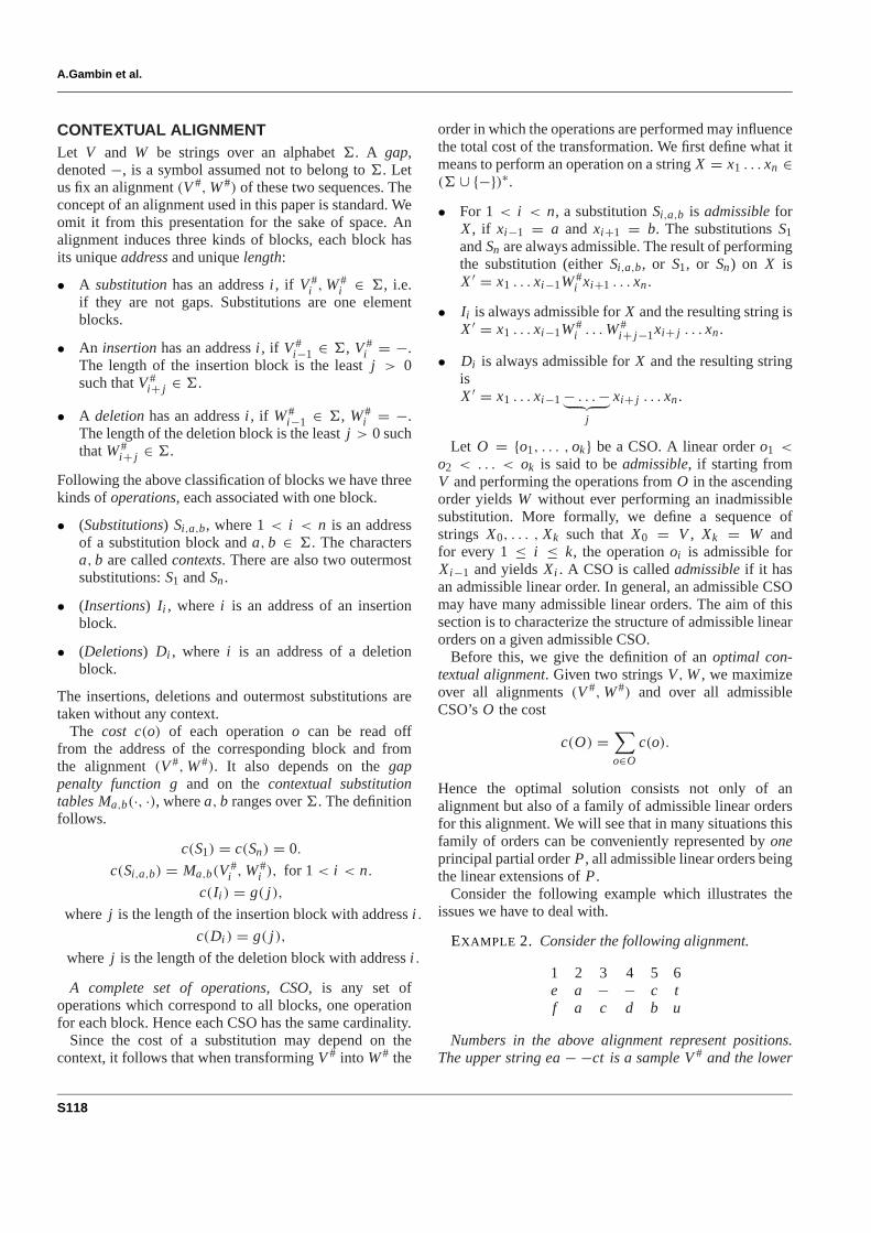
Finally let us discuss briefly a general shape of a posetwhich generates all (and only) admissible linear orders fora given alignment. The crucial notion here is that of ahairyzig-zag. Instead of giving a full definition (the reader mayconsult the full version of this paper) let us consider atypical example of a hairy zig-zag.
† Here we implicitly assume thatc1 is different fromb andb′.
� � � � � �
� � � � �
� � � � �
� � � �
� �
There is a one-to-one correspondance between opera-tions associated with an alignment and the nodes of thehairy zig-zag. Disks in the above picture correspond tosubstitutions and to some insertions and deletions. Theyform a backbone of the zig-zag. Upper circles correspondto the remaining insertion blocks (they form upperhairs);while lower circles correspond to the remaining deletionblocks (they form lower hairs). A hairy zig-zag is just azig-zag if it does not have any hairs.p ≤ q in the aboveposet means that the operation which corresponds top hasto be performed before the operation corresponding toq.Given an alignment(V #, W #) and an admissible completesetO of operations. A posetP is called agenerating posetfor (V #, W #) andO if all linear extensions ofP are admis-sible forO. A principal poset P is a generating poset suchthat every admissible linear order forO is an extension ofP. We have the following characterization of generatingposets.
THEOREM 1. Every generating poset is a disjoint unionof hairy zig-zags.
Moreover every hairy zig-zag can be obtained as aprincipal poset for a certain alignment and a certainCSO O.
For every alignment (V #, W #) without gaps, everyadmissible complete set of operations has a principalposet which is a disjoint union of zig-zags.
CONTEXTUAL ALIGNMENT ALGORITHMSBelow we present aquadratic (precisely, ofO(|�|mn)
time complexity) algorithm for contextual alignment andan affine gap penalty function. The efficiency of thealgorithm is based on the observation that for an affine gappenalty function we can compute the score of an indel, bygradually extending the indel one symbol at a time. Thisway, when extending the alignment, it suffices to considera constant number of cases. LetOpen and Ext be thecosts of opening and extending the gap, respectively.
The main idea of the algorithm is to walk along bothsequences, choosing the optimal extension of the alreadyfound alignment of prefixes. At each step we have thefollowing possible extensions: (i) a single substitution, (ii)an insertion (starting a new one or extending the existingone), (iii) a deletion, analogously.
The algorithm uses the dynamic programming approachand works with 7 three-dimensional arrays indexed by thepositions from the wordV , positions from the wordW and
S120

Contextual alignment of biological sequences
the elements of�. These are 3insertion arrays, 3 deletionarrays and onesubstitution array.
Let us consider a type (ii) extension, i.e. we focus ourattention on a single insertion block:
i j ka − − · · · − ba′ c1 c2 · · · cm xxxα β
For the simplicity of presentation we use, as before,numbersi, j, k as the addresses of the blocks, i.e. positionsin the alignment. The indexα = 1 . . . n is used tonumber the positions in the wordV , and β = 1 . . . mfor the positions in the wordW . The letter xxx in theabove figure stands for an arbitrary letter from�, whichreplacesWk . Considering allxxx ∈ � is necessary to profitfrom the affinity of gap penalty function and to extendan insertion gradually in the course of computation. Infactxxx corresponds to the third dimension in our insertionarrays. Roughly, this third dimension enables us to treatleft substitutioni and right substitutionk separately.
Each insertion array stores at position(α, β, xxx) themaximal score of alignment ofV1 . . . Vα and W1 . . . Wβ
which ends with an insertion, under the assumption thatWβ+1 = xxx and that the insertion is immediately followedby a substitution on the right (substitutionk in the abovefigure). We use three variants of the insertion array, onefor each possible selection of the left context for the rightsubstitutionk (see Table 3 in Appendix).
• I∨i, jk
(α, β, xxx) stores the maximal score as explained
above under the additional condition thata is the leftcontext for the right substitutionk. This selection re-sults in the constraint∨i, j
k , i.e. the rightmost substitu-tion k precedes insertionj and left substitutioni .
• ICi<k< j (α, β, xxx) stores the maximal score as explainedabove under the additional condition thata′ is the leftcontext for the right substitutionk. This selection re-sults in the constraintCi<k< j , i.e. the left substitutionis followed by the insertion which is followed the rightsubstitution.
• IC j<k (α, β, xxx) stores the maximal score as explainedabove under the additional condition thatcm is theleft context for the right substitutionk. This selectionresults in the constraintC j<k , i.e. the rightmostsubstitutionk is performed after the insertionj .
Note that parameterxxx together with the subscript ofI con-tain the information which is necessary and sufficient tocorrectly evaluate an alignment ending with an insertion.The arraysD∧k
i, j, DCk< j , DC j<k<i built for a deletion block
are obtained in a completely dual way.
Table 1. Constrains and scores determined by right context fori .
right context constraint score of extended alignment
b ∨ j,ki S(α, β − 1, b) + Open
xxx Ck<i< j S(α, β − 1, xxx) + Openc1 C j<i S(i, j ′ − 1, c1) + Open
For the case of the extension by a single substitution wehave the following array:
• S(α, β, xxx) stores the maximal score of an alignmentwith gaps of wordsV1 . . . Vα and W1 . . . Wβ whichends with a substitutionVα �→ Wβ whose right contextis xxx .
Since our algorithm requires always left and right contextfor each considered substitution, we need to extendarrays V and W by the new entriesV0, Vn+1 andW0, Wm+1 on the ends. Recall that the leftmost andrightmost substitutions do not contribute to the score of thealignment, they serve only as contexts for the neighboringoperations. Hence the choice of the new entries has anegligible effect on the resulting score—we decided tochoose these values in an ad-hoc manner. In the particularimplementation of our algorithm we choose methionineM = V0 = W0 as the leftmost entry and alanineA =Vn+1 = Wm+1 as the rightmost entry.
In the course of computation there are two possibilitiesto update the insertion arrays: (i) starting a new insertion;(ii) extending an existing insertion. The latter case issimpler: the score of extended alignment is calculated asfollows:
I∗(α, β − 1, xxx) + Ext for ∗ ∈ {∨i, jk , Ci<k< j , C j<k}
When starting a new insertion we have to calculate thescore of the substitution which precedes it. To achievethis aim we consider all possible selections of the rightcontext for this substitution. The corresponding scores andconstraints are summarized in Table 1.
As we are looking for the optimal alignment of prefixesV1 . . . Vα andW1 . . . Wβ , we choose the context pair (i.e.the right context for the left substitution and the leftcontext for the right substitution) which does not generatethe contradiction and which maximizes the score. Theconstraints resulting from all possible pairs of contexts forinsertion arrays are listed in Chart 1 of Appendix (withxxxsubstituted forb′).
E.g. for the left contexta there are two admissiblepairs (xxx, a) and (c1, a) and we should compare thecorresponding scoresS(α, β −1, xxx)+ Open andS(α, β −1, c1) + Open with the score of extended insertion
S121
A.Gambin et al.
I∨i, jk
(α, β − 1, xxx) + Ext and choose the maximal value.
The update rules for three insertion arrays are as follows:
I∨i, jk
(α, β, xxx) := max
I∨i, jk
(α, β − 1, xxx) + Ext
S(α, β − 1, xxx) + Open,
S(α, β − 1, c1) + Open
ICi<k< j (α, β, xxx) := max
{ICi<k< j (α, β − 1, xxx) + Ext,
S(α, β − 1, b) + Open
IC j<k (α, β, xxx) := max
IC j<k (α, β − 1, xxx) + Ext,S(α, β − 1, b) + Open,
S(α, β − 1, c1) + Open
To calculate a new entry in the substitution table, sayS(α, β, xxx), we choose the maximal value among thefollowing 8 possibilities:
• 2 cases for the scenario when the substitutionWα �→ Wβ follows another substitution:
– left substitution precedes the right one:S(α − 1, β − 1, Vα) + MWβ−1,xxx (Vα, Wβ)
– right substitution precedes the left one:S(α − 1, β − 1, Wβ) + MVα−1,xxx (Vα, Wβ)
• 3 cases for the scenario when the substitution followsan insertion.
I∗(α − 1, β − 1, Wβ) + Ml∗,xxx (Vα, Wβ)
for ∗ ∈ {∨i, jk , Ci<k< j , C j<k},
wherel∗ denotes the corresponding left context in eachcase. This context is stored together with the arrayI∗.
• 3 cases for the scenario when the substitution followsadeletion.
D•(α − 1, β − 1, Vα) + Ml•,xxx (Vα, Wβ)
for • ∈ {∧ ji,k, C j<k<i , Ck< j },
wherel• denotes the corresponding left context in eachcase.
The generating posets are reconstructed in the followingway. Starting from the maximal position in substitutionarray, and backtracking in all 7 arrays determines the setof operations performed to achieve the maximal score, andthe corresponding alignment. By comparing the contextswe also determine the set of generating posets. Each stepof the algorithm, in which the substitution is consideredcorresponds to a small (two- or three-element) poset,and by concatenating these posets in reversed order, wereconstruct the generating poset. Each small poset isdetermined (tables from Appendix are used here) by thepartition of the set of symbols which serve as the contextsfor the corresponding pair of substitutions.
Algorithm 1 the overview{ initialization }for xxx ∈ � do S(0, 0, xxx) := 0;for xxx ∈ �, α > 0, β > 0 do S(α, 0, xxx) := −∞;S(0, β, xxx) := −∞;for xxx ∈ �, α = 0 . . . n, ∗ ∈ {∨i, j
k , Ci<k< j , C j<k} doI∗(α, 0, xxx) := −∞;for xxx ∈ �, β = 0 . . . m, • ∈ {∧i
j,k, C j<k<i , Ck< j } doD•(0, β, xxx) := −∞;{ end of initialization }for α = 1 . . . n do
for β := 1 . . . m dofor xxx ∈ � do
calculate the 7 arrays at position(α, β, xxx).end for
end forend for
Score := max
S(n, m, Vn+1), S(n, m, Wm+1),
I∗(n, m, Wm+1), D•(n, m, Vn+1)
∗ ∈ {∨i, jk , Ci<k< j , C j<k}
• ∈ {∧ij,k, C j<k<i , Ck< j }
Algorithms for local alignmentAs with the context-free case (see Smithet al. (1981)),the algorithm for local alignment is in each case a minormodification of the global alignment algorithm. The ideais to add an additional option while filling in the arrays: togive up with the so far constructed alignment and start allover in the middle of the sequences by resetting the scoreto 0. The local versions of the above algorithms inherit thecomplexity of their global counterparts.
EXPERIMENTAL RESULTSWe have performed elementary validation of the contex-tual alignment model. We have found some interestingphenomena, suggesting that further work in this directionis worthwhile.
Substitution tablesThe first, preparatory (but by no means trivial) task hasbeen the construction of appropriate contextual substitu-tion tables. We have developed a procedure to constructsuch tables, which is described in Gambinet al. (2002b).It appears that there is a fundamental difficulty: the amountof data necessary to construct complete contextual substi-tution tables exceeds by an order of magnitude the datapresently available. Indeed, the tables have 204 = 160 000entries, and each entry should be calculated based on asufficient statistical sample. It appears that while for themost common contexts the sample is rich enough, for the
S122
Contextual alignment of biological sequences
GROUP NAME AMINO ACID RESIDUE
Small Aliphatic Alanine, Proline, GlycineAcid amide Glutamine, Aspargine, Glutamic A., Aspartic A.Hydroxyl & Sulfhydryl Serine,Threonine, CysteineAliphatic Valine, Isoleucine, Methionine, LeucineBasic Lysine, Arginine, HistidineAromatic Phenylalanine, Tyrosine, Tryptophan
less common ones it is insufficient and the values are sta-tistically biased, and about one third of the entries remaincompletely undetermined. In order to remedy the situa-tion we have grouped the amino acids into 6 groups, basedon accepted point mutation data (Dayhoffet al., 1978).The molecular sizes and shapes are very similar withineach group. This is a crucial factor in determining whichamino acid interchanges are acceptable to natural selec-tion. Then we have calculated the substitution tables forthe groups rather than individual amino acids, assumingthat all amino acids in one group behave identically ascontexts. The values taken from such group-context tableshave been used to fill in the missing values in the full-context substitution tables.
While interpreting our experimental results, it is impor-tant to remember about the limitations of our tables.
ExperimentsThe experiments reported here are based purely on scorevalues. We decided to assess mainly the influence ofthe context on the score value. We achieved this byproducing four contextual tables, for increasing numberof context groups. We used here the same approach asin the procedure of completing the tables by 6 groupsvalues, described above. The first table assumed all aminoacids to be identical, hence the table is indeed context-free, the second table is based on two context groups (ofhydrophobic and hydrophilic amino acids), the third oneis based on six context groups, and the fourth one used all20 amino acids as contexts (but, as explained above, aboutone third of the entries had to be taken from the six-grouptables). Then we aligned several proteins each with each,using all four tables. To estimate the statistical significanceof our alignments we calculated Z-value (Cometet al.,1999) in the case of global alignment and we adopted themethod of Vingron and Waterman (Vingronet al., 1995)of calculating P-value for local alignments.
In the next phase of model validation we plan tobuild the phylogenetic trees based on contextual similaritydata. Then we will compare two sets of trees (contextualvs. non-contextual) using various agreement methods.The complete experiments illustrating the impact of thecontextual approach for phylogenetic studies will bedescribed in a forthcoming paper.
We decided to use the database of Clusters of Orthol-ogous Groups of proteins (Tatusovet al., 2001) (see alsothe NIH COG page http://www.ncbi.nlm.nih.gov/COG). Itconsists currently of 3307 COGs including 74059 proteinsfrom 43 genomes of bacteria, archaea and the yeastSac-charomyces cerevisiae. COG database represents an at-tempt of a phylogenetic classification of the proteins en-coded in complete genomes. Each COG includes proteinsthat are thought to be orthologous, i.e. connected by verti-cal evolutionary descent.
We restrict our attention to the list of 84 COGs, whichcontain at least one protein from each genome. From thislist 27 COGs (which include as few paralogs as possible)are selected to our analysis. They can be partitionedinto 2 groups; the first one consists of 12 COGs, whichrepresents a wide spectrum of functional categories, andthe second consists of 15t-RNA synthetases families. Thesequences from each COG are pairwise aligned globallyand locally and the statistical significance (Z-value and P-value, respectively) are computed.
This experiment had the following goals.
1. Estimation of the significance of contextual align-ment versus non-contextual one.
2. Observation of the impact the number of con-text groups has on the discriminating power ofcontextual approach.
3. Verification of the accuracy of contextual scoresw.r.t. the classification of proteins inside COGs andevolutionary relationships between proteins.
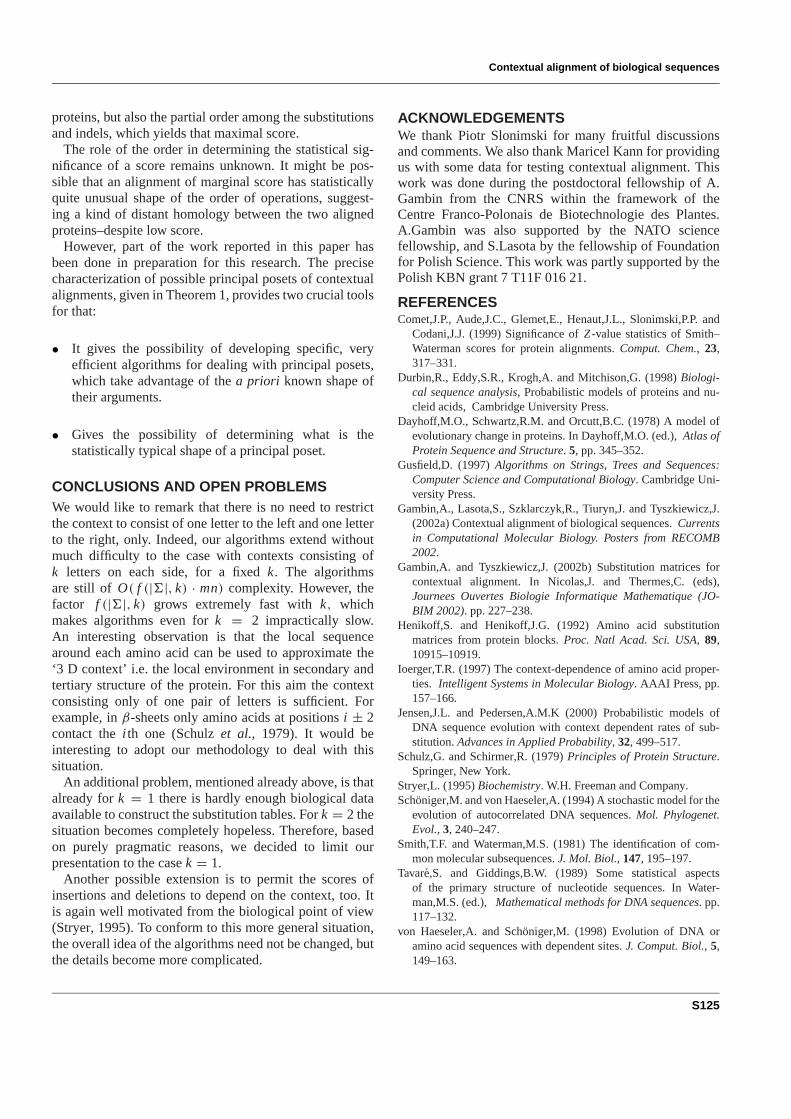
The majority of aligned pairs of proteins gives betterstatistical significance measures for contextual approach.A typical outcome is listed below:+ denotes that thecalculated P-value was 2 orders of magnitude smallerfor contextual alignment when compared with context-free one. The table below contains the results for locallyaligned proteins from COG00030. The names of alignedproteins are listed in the first column.
AF1783 + + + + + + + + + + + + + + + + + + + +
APE0553 + + + + + + + + + +
aq_1816 + + + + + + + + + + + + + + + + + + + + + + + + + + +
BB0590 + + + + + + + + + + + + + + + + + + + + + + + + + + + +
BH0057 + + + + + + + + + + + + + + + + + + + + + + + + + +
BS_ksgA + + + + + + + + + + + + + + + + + + + + + + + + +
BU141 + + + + + + + + + + + + + + + + + + + + + + +
CC1685 + + + + + + + + + + + + + + + + + + + + + + + + + +
Cj1711c + + + + + + + + + + + + + + + + + + + + + + + + +
CPn1059 + + + + + + + + + + + + + + + + + + + + + + + + + + +
CT354 + + + + + + + + + + + + + + + + + + + + + + + + + +
DR1526 + + + + + + + + + + + + + + + + + + + + + + + + + + + +
HI0549 + + + + + + + + + + + + + + + + + + + + +
HP1431 + + + + + + + + + + + + + + + + + + + + + +
jhp1322 + + + + + + + + + + + + + + + + + + + + + +
ksgA + + + + + + + + + + + + + + + + + + + +
L0363 + + + + + + + + + + + + + + + + + + + + + + + + + +
MG463 + + + + + + + + + + + + + + + + + + + + + + + + + + +
MJ1029 + + + + + + + + + + + + + + + + + + + + + + +
ML0241 + + + + + + + + + + + + + + + + + + + + + + + + + + + +
mll7860 + + + + + + + + + + + + + + + + + + + + +
MPN679 + + + + + + + + + + + + + + + + + + + + + + + + +
MTH1326 + + + + + + + + + + + + + + + + + + + + +
NMA0902 + + + + + + + + + + + + + + + + + + + + + + +
NMB0697 + + + + + + + + + + + + + + + + + + + + + + +
PA0592 + + + + + + + + + + + + + + + + + + + + +
PAB0253 + + + + + + + + + + + + + + + + + + + + + + + +
PH1823 + + + + + + + + + + + + + + + + + + + + + + + +
PM1209 + + + + + + + + + + + + + + + + + + + + +
S123
A.Gambin et al.
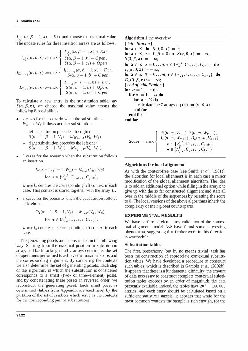
Now, let us observe that the discriminating power indeedincreases with the number of context groups. It is partic-ularly visible in the area of low scores (close to the bot-tom left corner of the plot), where the vertical cut throughthe area occupied by the alignments’ scores is particularlylarge.The plots below have the context-free score as thex-axis, and they-axis is, from left to right, the local align-ment score with 2 and 20 context groups, respectively. Thealigned sequences are all proteins from COG0089 (Ribo-somal proteins—large subunit A). The grid on the plotsmarks multiples of 100.
min_non=0 max_non=228min_ctx=0
max_ctx=256
min_non=0 max_non=228min_ctx=0
max_ctx=285
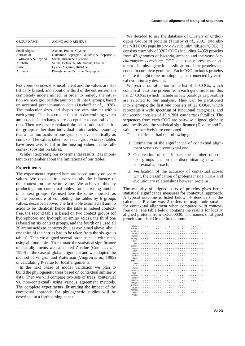
This influence of context should also be verified w.r.t.unrelated sequences. Two plots below illustrate the result:on the left 1176 pairs of distantly related homologouspairs (i.e. having less than 25% sequence identity) arealigned, and on the right plot 1176 pairs of completelyunrelated proteins are aligned. All sequences are selectedfrom COG database. As before plots have the context-free score as thex-axis, and the contextual score asthe y-axis. It is clearly visible that the discriminatingpower of contextual approach decreases, when less similarsequences are investigated.
min_non=0 max_non=200min_ctx=0
max_ctx=300
min_non=0 max_non=200min_ctx=0
max_ctx=300
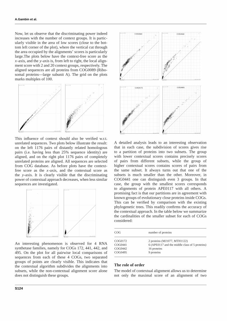
An interesting phenomenon is observed for 4 RNAsynthetase families, namely for COGs 172, 441, 442, and495. On the plot for all pairwise local comparisons ofsequences from each of these 4 COGs, two separatedgroups of points are clearly visible. This indicates thatthe contextual algorithm subdivides the alignments intosubsets, while the non-contextual alignment score alonedoes not distinguish these groups.
COG0441
min_non=0 max_non=1598min_ctx=0
max_ctx=1954COG0442
min_non=0 max_non=1333min_ctx=0
max_ctx=1646
COG0172
min_non=0 max_non=1055min_ctx=0
max_ctx=1288 COG0495
min_non=0 max_non=2222min_ctx=0
max_ctx=2790
A detailed analysis leads to an interesting observationthat in each case, the subdivision of scores gives riseto a partition of proteins into two subsets. The groupwith lower contextual scores contains precisely scoresof pairs from different subsets, while the group ofhigher contextual scores contains scores of pairs fromthe same subset. It always turns out that one of thesubsets is much smaller than the other. Moreover, inCOG0441 one can distinguish even 3 groups. In thatcase, the group with the smallest scores correspondsto alignments of protein APE0117 with all others. Apromising fact is that our partitions are in agreement withknown groups of evolutionary close proteins inside COGs.This can be verified by comparison with the existingphylogenetic trees. This readily confirms the accuracy ofthe contextual approach. In the table below we summarizethe cardinalities of the smaller subset for each of COGsconsidered:
COG number of proteins
COG0172 2 proteins (MJ1077, MTH1122)COG0441 6 (APE0117 and the middle class of 5 proteins)COG0442 16 proteinsCOG0495 9 proteins
The role of orderThe model of contextual alignment allows us to determinenot only the maximal score of an alignment of two
S124
Contextual alignment of biological sequences
proteins, but also the partial order among the substitutionsand indels, which yields that maximal score.
The role of the order in determining the statistical sig-nificance of a score remains unknown. It might be pos-sible that an alignment of marginal score has statisticallyquite unusual shape of the order of operations, suggest-ing a kind of distant homology between the two alignedproteins–despite low score.
However, part of the work reported in this paper hasbeen done in preparation for this research. The precisecharacterization of possible principal posets of contextualalignments, given in Theorem 1, provides two crucial toolsfor that:
• It gives the possibility of developing specific, veryefficient algorithms for dealing with principal posets,which take advantage of thea priori known shape oftheir arguments.
• Gives the possibility of determining what is thestatistically typical shape of a principal poset.
CONCLUSIONS AND OPEN PROBLEMSWe would like to remark that there is no need to restrictthe context to consist of one letter to the left and one letterto the right, only. Indeed, our algorithms extend withoutmuch difficulty to the case with contexts consisting ofk letters on each side, for a fixedk. The algorithmsare still of O( f (|�|, k) · mn) complexity. However, thefactor f (|�|, k) grows extremely fast withk, whichmakes algorithms even fork = 2 impractically slow.An interesting observation is that the local sequencearound each amino acid can be used to approximate the‘3 D context’ i.e. the local environment in secondary andtertiary structure of the protein. For this aim the contextconsisting only of one pair of letters is sufficient. Forexample, inβ-sheets only amino acids at positionsi ± 2contact thei th one (Schulzet al., 1979). It would beinteresting to adopt our methodology to deal with thissituation.
An additional problem, mentioned already above, is thatalready fork = 1 there is hardly enough biological dataavailable to construct the substitution tables. Fork = 2 thesituation becomes completely hopeless. Therefore, basedon purely pragmatic reasons, we decided to limit ourpresentation to the casek = 1.
Another possible extension is to permit the scores ofinsertions and deletions to depend on the context, too. Itis again well motivated from the biological point of view(Stryer, 1995). To conform to this more general situation,the overall idea of the algorithms need not be changed, butthe details become more complicated.
ACKNOWLEDGEMENTSWe thank Piotr Slonimski for many fruitful discussionsand comments. We also thank Maricel Kann for providingus with some data for testing contextual alignment. Thiswork was done during the postdoctoral fellowship of A.Gambin from the CNRS within the framework of theCentre Franco-Polonais de Biotechnologie des Plantes.A.Gambin was also supported by the NATO sciencefellowship, and S.Lasota by the fellowship of Foundationfor Polish Science. This work was partly supported by thePolish KBN grant 7 T11F 016 21.
REFERENCESComet,J.P., Aude,J.C., Glemet,E., Henaut,J.L., Slonimski,P.P. and
Codani,J.J. (1999) Significance ofZ -value statistics of Smith–Waterman scores for protein alignments.Comput. Chem., 23,317–331.
Durbin,R., Eddy,S.R., Krogh,A. and Mitchison,G. (1998)Biologi-cal sequence analysis, Probabilistic models of proteins and nu-cleid acids, Cambridge University Press.
Dayhoff,M.O., Schwartz,R.M. and Orcutt,B.C. (1978) A model ofevolutionary change in proteins. In Dayhoff,M.O. (ed.),Atlas ofProtein Sequence and Structure. 5, pp. 345–352.
Gusfield,D. (1997)Algorithms on Strings, Trees and Sequences:Computer Science and Computational Biology. Cambridge Uni-versity Press.
Gambin,A., Lasota,S., Szklarczyk,R., Tiuryn,J. and Tyszkiewicz,J.(2002a) Contextual alignment of biological sequences.Currentsin Computational Molecular Biology. Posters from RECOMB2002.
Gambin,A. and Tyszkiewicz,J. (2002b) Substitution matrices forcontextual alignment. In Nicolas,J. and Thermes,C. (eds),Journees Ouvertes Biologie Informatique Mathematique (JO-BIM 2002). pp. 227–238.
Henikoff,S. and Henikoff,J.G. (1992) Amino acid substitutionmatrices from protein blocks.Proc. Natl Acad. Sci. USA, 89,10915–10919.
Ioerger,T.R. (1997) The context-dependence of amino acid proper-ties. Intelligent Systems in Molecular Biology. AAAI Press, pp.157–166.
Jensen,J.L. and Pedersen,A.M.K (2000) Probabilistic models ofDNA sequence evolution with context dependent rates of sub-stitution.Advances in Applied Probability, 32, 499–517.
Schulz,G. and Schirmer,R. (1979)Principles of Protein Structure.Springer, New York.
Stryer,L. (1995)Biochemistry. W.H. Freeman and Company.Schoniger,M. and von Haeseler,A. (1994) A stochastic model for the
evolution of autocorrelated DNA sequences.Mol. Phylogenet.Evol., 3, 240–247.
Smith,T.F. and Waterman,M.S. (1981) The identification of com-mon molecular subsequences.J. Mol. Biol., 147, 195–197.
Tavare,S. and Giddings,B.W. (1989) Some statistical aspectsof the primary structure of nucleotide sequences. In Water-man,M.S. (ed.), Mathematical methods for DNA sequences. pp.117–132.
von Haeseler,A. and Schoniger,M. (1998) Evolution of DNA oramino acid sequences with dependent sites.J. Comput. Biol., 5,149–163.
S125
A.Gambin et al.
Tatusov,R.L., Natale,D.A., Garkavtsev,I.V., Tatusova,T.A.,Shankavaram,U.T., Rao,B.S., Kiryutin,B., Galperin,M.Y.,Fedorova,N.D. and Koonin,E.V. (2001) The COG database: newdevelopments in phylogenetic classification of proteins fromcomplete genomes.Nucleic Acids Res., 29, 22–28.
Vingron,M. and Waterman,M.S. (1995) Statistical significance oflocal alignments with gaps.Bioinformatics: from Nucleid Acidsand Proteins to Cell Methabolism. pp. 75–84.
Wilbur,W.J. and Lipman,D.J. (1984) The context dependent com-parison of biological sequences.SIAM J. Appl. Math., 44, 557–567.
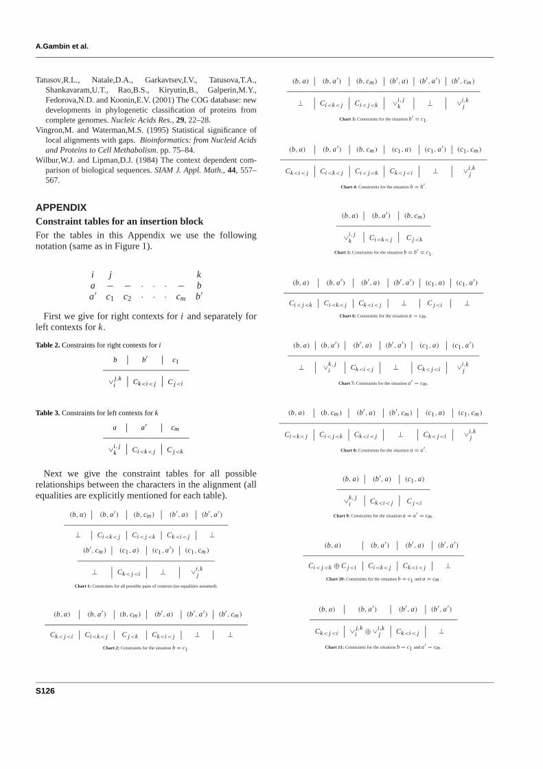
APPENDIXConstraint tables for an insertion blockFor the tables in this Appendix we use the followingnotation (same as in Figure 1).
i j ka − − · · · − ba′ c1 c2 · · · cm b′
First we give for right contexts fori and separately forleft contexts fork.
Table 2. Constraints for right contexts fori
b b′ c1
∨ j,ki Ck<i< j C j<i
Table 3. Constraints for left contexts fork
a a′ cm
∨i, jk Ci<k< j C j<k
Next we give the constraint tables for all possiblerelationships between the characters in the alignment (allequalities are explicitly mentioned for each table).
(b, a) (b, a′) (b, cm ) (b′, a) (b′, a′)
⊥ Ci<k< j Ci< j<k Ck<i< j ⊥(b′, cm ) (c1, a) (c1, a′) (c1, cm )
⊥ Ck< j<i ⊥ ∨i,kj
Chart 1: Constraints for all possible pairs of contexts (no equalities assumed).
(b, a) (b, a′) (b, cm ) (b′, a) (b′, a′) (b′, cm )
Ck< j<i Ci<k< j C j<k Ck<i< j ⊥ ⊥Chart 2: Constraints for the situationb = c1.
(b, a) (b, a′) (b, cm ) (b′, a) (b′, a′) (b′, cm )
⊥ Ci<k< j Ci< j<k ∨i, jk ⊥ ∨i,k
j
Chart 3: Constraints for the situationb′ = c1.
(b, a) (b, a′) (b, cm ) (c1, a) (c1, a′) (c1, cm )
Ck<i< j Ci<k< j Ci< j<k Ck< j<i ⊥ ∨i,kj
Chart 4: Constraints for the situationb = b′ .
(b, a) (b, a′) (b, cm )
∨i, jk Ci<k< j C j<k
Chart 5: Constraints for the situationb = b′ = c1.
(b, a) (b, a′) (b′, a) (b′, a′) (c1, a) (c1, a′)
Ci< j<k Ci<k< j Ck<i< j ⊥ C j<i ⊥Chart 6: Constraints for the situationa = cm .
(b, a) (b, a′) (b′, a) (b′, a′) (c1, a) (c1, a′)
⊥ ∨k, ji Ck<i< j ⊥ Ck< j<i ∨i,k
j
Chart 7: Constraints for the situationa′ = cm .
(b, a) (b, cm ) (b′, a) (b′, cm ) (c1, a) (c1, cm )
Ci<k< j Ci< j<k Ck<i< j ⊥ Ck< j<i ∨i,kj
Chart 8: Constraints for the situationa = a′ .
(b, a) (b′, a) (c1, a)
∨k, ji Ck<i< j C j<i
Chart 9: Constraints for the situationa = a′ = cm .
(b, a) (b, a′) (b′, a) (b′, a′)
Ci< j<k ⊕ C j<i Ci<k< j Ck<i< j ⊥Chart 10: Constraints for the situationb = c1 anda = cm .
(b, a) (b, a′) (b′, a) (b′, a′)
Ck< j<i ∨ j,ki ⊕ ∨i,k
j Ck<i< j ⊥Chart 11: Constraints for the situationb = c1 anda′ = cm .
S126
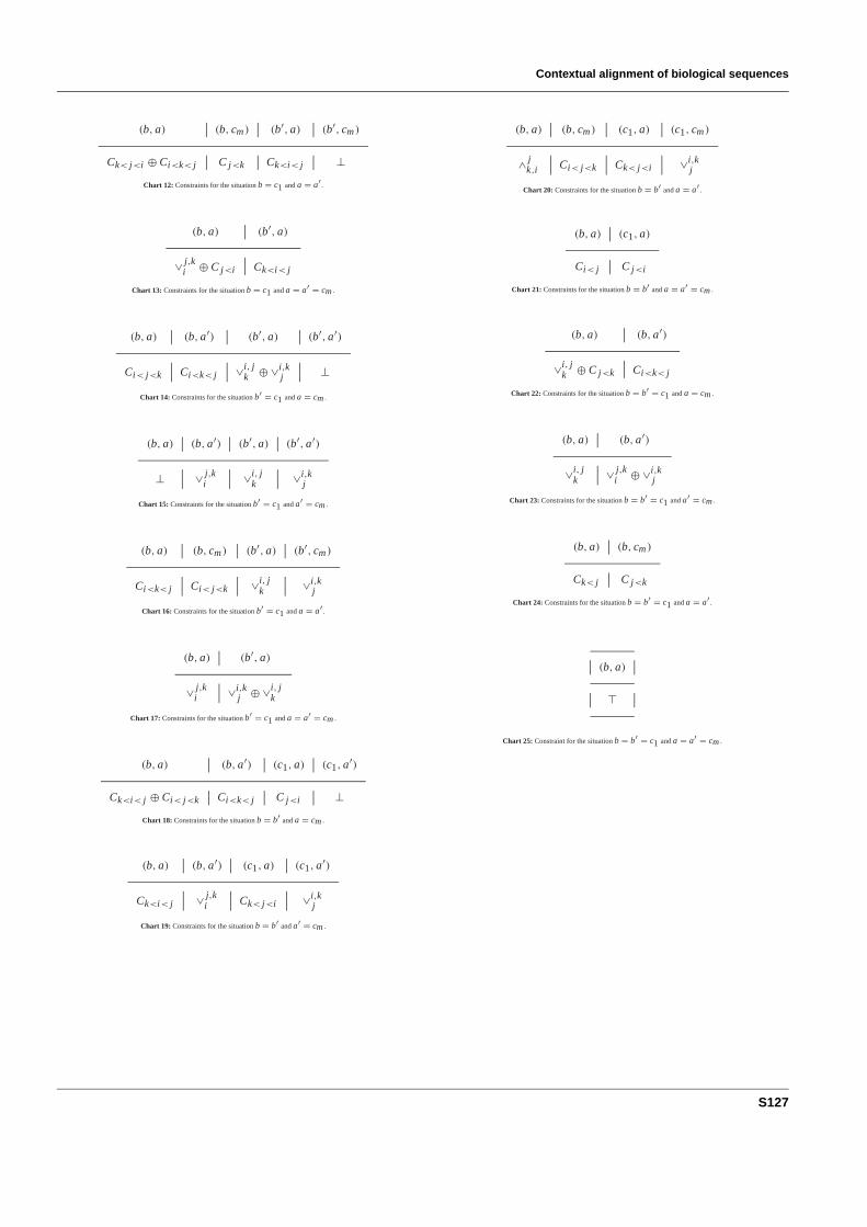
Contextual alignment of biological sequences
(b, a) (b, cm ) (b′, a) (b′, cm )
Ck< j<i ⊕ Ci<k< j C j<k Ck<i< j ⊥Chart 12: Constraints for the situationb = c1 anda = a′ .
(b, a) (b′, a)
∨ j,ki ⊕ C j<i Ck<i< j
Chart 13: Constraints for the situationb = c1 anda = a′ = cm .
(b, a) (b, a′) (b′, a) (b′, a′)
Ci< j<k Ci<k< j ∨i, jk ⊕ ∨i,k
j ⊥Chart 14: Constraints for the situationb′ = c1 anda = cm .
(b, a) (b, a′) (b′, a) (b′, a′)
⊥ ∨ j,ki ∨i, j
k ∨i,kj
Chart 15: Constraints for the situationb′ = c1 anda′ = cm .
(b, a) (b, cm ) (b′, a) (b′, cm )
Ci<k< j Ci< j<k ∨i, jk ∨i,k
j
Chart 16: Constraints for the situationb′ = c1 anda = a′ .
(b, a) (b′, a)
∨ j,ki ∨i,k
j ⊕ ∨i, jk
Chart 17: Constraints for the situationb′ = c1 anda = a′ = cm .
(b, a) (b, a′) (c1, a) (c1, a′)
Ck<i< j ⊕ Ci< j<k Ci<k< j C j<i ⊥Chart 18: Constraints for the situationb = b′ anda = cm .
(b, a) (b, a′) (c1, a) (c1, a′)
Ck<i< j ∨ j,ki Ck< j<i ∨i,k
j
Chart 19: Constraints for the situationb = b′ anda′ = cm .
(b, a) (b, cm ) (c1, a) (c1, cm )
∧ jk,i Ci< j<k Ck< j<i ∨i,k
j
Chart 20: Constraints for the situationb = b′ anda = a′ .
(b, a) (c1, a)
Ci< j C j<i
Chart 21: Constraints for the situationb = b′ anda = a′ = cm .
(b, a) (b, a′)
∨i, jk ⊕ C j<k Ci<k< j
Chart 22: Constraints for the situationb = b′ = c1 anda = cm .
(b, a) (b, a′)
∨i, jk ∨ j,k
i ⊕ ∨i,kj
Chart 23: Constraints for the situationb = b′ = c1 anda′ = cm .
(b, a) (b, cm )
Ck< j C j<k
Chart 24: Constraints for the situationb = b′ = c1 anda = a′ .
(b, a)
�
Chart 25: Constraint for the situationb = b′ = c1 anda = a′ = cm .
S127