Context-Dependent Multi-class Classification with UnknownObservation and Class Distributions with Applications to Bioinformatics

Alexander S. Baras and John S. Baras

Abstract— We consider the multi-class classification problem,based on vector observation sequences, where the conditional(given class observations) probability distributions for each classas well as the unconditional probability distribution of theobservations are unknown. We develop a novel formulationthat combines training with the quality of classification thatcan be obtained using the ’learned’ (via training) models. Theparametric models we use are finite mixture models, where thesame component densities are used in the model for each class,albeit with different mixture weights. Thus we use a modelknown as All-Class-One-Network (ACON) model in the neuralnetwork literature. We argue why this is a more appropriatemodel for context-dependent classification, as is common inbioinformatics. We derive rigorously the solution to this jointoptimization problem. A key step in our approach is to considera tight (provably) bound between the average Bayes error (thetrue minimal classification error) and the average model-basedclassification error. We rigorously show that the parameterestimates maximize the likelihood of the model-based classposterior probability distributions. We illustrate by applicationexamples in the bioinformatics of cancer.

I. INTRODUCTION

The identification of principal structures and featureswithin large sets of high-dimensional data and the generationof simplified models for such data distributions are importanttasks, which arise in many and diverse technical fields in-cluding pattern recognition [22], [15] or the study of complexphysical systems. Various approaches have been proposed[22], [11], [19], [20]. In this paper we consider the multi-class classification problem, based on vector observationsequences, where the conditional (given class observations)probability distributions for each class as well as the un-conditional probability distribution of the observations areunknown. We formulate the problem of training in classifyingobservations, using parametric models for the conditionalpdf for each class, as well as the unconditional pdf ofthe observations. The parametric models we use for thesepdfs are finite mixtures of normal densities [37], [2], [32],[21]. We develop a novel formulation that combines trainingwith the quality of classification that can be obtained usingthe ‘learned’ models. Our approach differs from existingapproaches in the literature in two fundamental ways.

First, the common approach in the literature [22] is to uselabelled observations from each class to obtain a maximumlikelihood estimate of each class conditional pdf, which

Alexander S. Baras is with the School of Medicine, Department ofPathology, University of Virginia Health System, Charlottesville, VA 22901.

John S. Baras is with the Institute for Systems Research, Departmentof Electrical and Computer Engineering, Fischell Department of Bioengi-neering, and the Applied Mathematics, Statistics and Scientific ComputationProgram, University of Maryland, College Park, MD 20742.

is typically obtained via Expectation Maximization (EM)iterations [22], [11]. In the neural network literature thisis known as One-Class-One-Network (OCON) model [22].Then these estimated class conditional pdfs are used forclassifying observations (data) using a variety of criteria (andmethods) for obtaining optimal decisions (classifications). Inour approach we formulate the problem of optimal decisionmaking (i.e. learning the optimal decision rule) and modelparameter estimation as a joint optimization problem. Sec-ond, the parametric models we use are finite mixture models,where the same component densities are used in the modelfor each class, albeit with different mixture weights. Thuswe use a model known as All-Class-One-Network (ACON)model in the neural network literature [22].

We argue that the ACON model is a more appropriatemodel for context-dependent classification, as is common inbioinformatics [13], [1], [28], or in network security [38].The advantages and disadvantages are discussed in [22].In biology as well as in security (intrusion detection andclassification) the patterns and classes are very dependenton the context of the data collection (observations). On theother hand in problems such as face recognition, or speechrecognition, the signal patterns are much less sensitive tocontext, and in these cases the OCON model offers severaladvantages [22].

Discriminative criteria for classification and regressionhave attracted recent attention by the machine learningcommunity. Examples include support vector machines [22],decision directed probabilistic neural networks [23], [25],[20], discriminatively trained HMMs [19], [26], [4], [29],predictively trained neural networks [23], [22]. These newerapproaches optimize models and model parameters drivenby the goal of better performing classifiers; the main taskat hand. This is to be contrasted with more traditionalmethods where models and model parameters are optimallyestimated using maximum likelihood (ML) or maximumaposteriori probability (MAP) so that each density is trainedseparately to escribe observations [22] rather than trained toaid in better classification. Naturally this affects performanceadversely and at the same time increases the complexityof the classification algorithm, which in turn increases thepossibility of overfitting. Some recent papers [22] haveindeed substantiated these adverse effects on performance.

The problem considered here is the classification of Cclasses, using N samples of vector valued data, while usingK component densities. These component densities are alsoknown as ‘features’ in pattern recognition [22]. The numberof components used in these approximations is a design

Joint 48th IEEE Conference on Decision and Control and28th Chinese Control ConferenceShanghai, P.R. China, December 16-18, 2009

FrC15.5

978-1-4244-3872-3/09/$25.00 ©2009 IEEE 8523

variable to be selected as well; we describe our results onthis aspect of the problem elsewhere [5]. In our approach,described in this paper, we derive rigorously the solution tothis joint optimization problem. A key step in our approachis to consider a tight (provably) bound between the averageBayes error (the true minimal classification error) and theaverage model-based classification error. The bound is givenin terms of the average (with respect to observations) ofthe Kullback-Leibler divergence (or relative entropy) of thetrue (but unknown) class a-posteriori distribution given themeasurements and the approximate (model-based) class a-posteriori distribution given the measurements.

We minimize this bound to determine the optimal paramet-ric model for each class that obtains the best approximationto the average Bayes error. We rigorously show that theparameter estimates maximize the likelihood of the model-based class posterior probability distributions. This is differ-ent from the common approach where first the model param-eters are estimated by maximizing the likelihood of the classconditional probability distribution. Our approach is closerto the more recently developed methods for discriminativetraining [20], [26], [2], [14], conditional maximum likelihood[27], [14], [33], [18], or maximum mutual information [27],[12], [7], [4], albeit in a multi-class, multi-component setting.

As discriminative model estimation and conditional like-lihood maximization have attracted more attention recently,the need for developing similar lower bounding and maxi-mization, two step algorithms (i.e. EM-like) has increased.Some developments towards this end have recently appearedin [18], [9], [33]. Using properly constructed upper andlower bounds we have derived [6] an ‘EM-like’ algorithmfor computing these ‘most discriminating’ model parameterestimates.

II. PRELIMINARIES, NOTATION, MODELS

The formulation is as follows. We have N data samples,x1,x2, ...,xt, ...,xN all vectors in RD. These data pointscan come from C distinct classes. These data points togetherwith the class index Yt, t = 1, 2, ..., N , for each, constitutethe training data in our framework. That is Yt is a categorical(discrete) variable with values in {1, 2, ..., c, ..., C} . Thus welet the training set be denoted as

S = {(xt, yt); t = 1, 2, . . . , N}. (1)

When data come from class c , we will denote by pcX(.)

the class-conditional probability distribution of the randomvariable X . We will also use the notation pX|c(.) for thesame pdf. We will give to almost all variables a probabilisticinterpretation, and then we will use the more generic no-tations pXt|Yt

(.|.) and pXt|Yt(xt|yt) . The true probability

distribution functions pX(.) and pX|c(.|.) are unknown. Wewill use approximate models for both from the class of finitenormal mixture models. Thus we will use the model

pX|Y (x|y;θ) = pX|Y (x|c;θ) =K∑

k=1

αc,kG(x;μk,Σk)

where G(x;μk,Sigmak) is a multivariable (D - dimen-sional) normal (Gaussian) probability distribution with meanμk and covariance matrix Σk. These Gaussians constitutethe component distributions (or simply the components) ofthe finite mixture model. In our formalism above there are Kcomponents, the same for all classes, consistent with our useof the ACON model. The weights αc,k represent the ‘mixturecoefficients’ in the model, and satisfy the constraints

0 ≤ αc,k ≤ 1 , andK∑

k=1

αc,k = 1, for all c.

We will also use the notation whereby the coefficients αc,k

for the same class c are collected into a vector αc. We collectthese coefficients into a C × K matrix A; a row-stochasticmatrix.

In this finite mixture model θ represents the vector ofparameters of this parametric class of models

θ =

⎡⎣ μk; k = 1, 2, . . . ,K

Σk; k = 1, 2, . . . ,Kαc,k; k = 1, 2, . . . ,K; c = 1, 2, . . . , C

⎤⎦ . (2)

We let πc, c = 1, 2, ..., C , be the prior probabilities thatdata belong to class c. Then the model we use to approximatethe unknown probability distribution of the data X is

pX(x) =C∑

c=1

pX|c(x;θ)πc =C∑

c=1

K∑k=1

πcαc,kG(x;μk,Σk).

The data vectors {x1,x2, ...,xt, ...,xN} are consideredas independent and identically distributed samples from theunknown probability distribution pX(.) . In the classificationliterature these data are referred to as the incomplete data[22]. On the other hand the set of data vectors together withtheir classes {(x1, y1), (x2, y2), ..., (xt, yt), ..., (xN , yN )}are referred to as the complete data [22].

III. ML AND EM FOR MODELS WITH HIERARCHICAL

STRUCTURE

In this section we formulate and solve the ML estimationproblem of the parameter vector θ when we have a hierar-chical structure, i.e. we have both classes and components.We let xt denote the generic D- vector of measurements, yt

denote the generic categorical value indicating the class ofthe experimental sample, zt denote the generic categoricalvalue indicating the component of the experimental sample.Figure 1 illustrates the hierarchical mixture model with twoclasses and three components.

The training data S are used to “learn” a good classi-fication rule, which will be applied to experimental datafrom similar situations as the training data, but which havenot been used in the training [22], [15]. One way to learna good classification rule is to learn a good set of themodel parameters, for the models we use to represent theclasses, and then use the learned models in constructing agood classification rule. In this section we solve the problemfollowing this approach. The novelty of the results rests

FrC15.5

8524

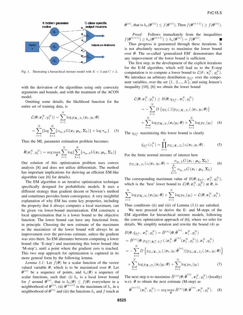
Fig. 1. Illustrating a hierarchical mixture model with K = 3 and C = 2.

with the derivation of the algorithms using only convexityarguments and bounds, and with the treatment of the ACONmodel.

Omitting some details, the likelihood function for theentire set of training data, is

L(θ;xN1 , yN

1 )) =N∑

t=1

log pXt,Yt(xt, yt;θ)

=N∑

t=1

{logK∑

k=1

{αyt,kG(xt;μk,Σk)} + log πyt} (3)

Thus the ML parameter estimation problem becomes:

θ(xN1 , yN

1 ) = arg maxθ

N∑t=1

log{K∑

k=1

{αyt,kG(xt;μk,Σk)}

Our solution of this optimization problem uses convexanalysis [8] and does not utilize differentials. The methodhas important implications for deriving an efficient EM-likealgorithm (see [6] for details).

The EM algorithm is an iterative optimization techniquespecifically designed for probabilistic models. It uses adifferent strategy than gradient decent or Newton’s methodand sometimes provides faster convergence. A very insightfulexplanation of why EM has some key properties, includingthe property that it always computes a local maximum, canbe given via lower-bound maximization. EM constructs alocal approximation that is a lower bound to the objectivefunction. The lower bound can have any functional form,in principle. Choosing the new estimate of the maximumas the maximizer of the lower bound will always be animprovement over the previous estimate, unless the gradientwas zero there. So EM alternates between computing a lowerbound (the ‘E-step’) and maximizing this lower bound (the‘M-step’), until a point where the gradient zero is reached.This two step approach for optimization is captured in itsmore general form by the following lemma.

Lemma 3.1: Let f(θ) be a scalar function of the vectorvalued variable θ, which is to be maximized over θ. Letθ(n) be a sequence of points, and bn(θ) a sequence ofscalar functions, such that: (i) bn is a local lower boundfor f around θ(n), that is bn(θ) ≤ f(θ) everywhere in aneighborhood of θ(n); (ii) θ(n+1) is the maximum of bn in aneighborhood of θ(n) and (iii) the functions bn and f touch at

θ(n), that is bn(θ(n)) ≤ f(θ(n)). Then f(θ(n+1)) ≥ f(θ(n)).

Proof: Follows immediately from the inequalitiesf(θ(n+1)) ≥ bn(θ(n+1)) ≥ bn(θ(n)) = f(θ(n).

Thus progress is guaranteed through these iterations. Itis not absolutely necessary to maximize the lower boundover θ. The so-called ‘generalized EM’ demonstrates thatany improvement of the lower bound is sufficient.

The first step, in the development of the explicit iterationsfor the E-M algorithm, which will lead us to the E-stepcomputation is to compute a lower bound to L(θ ; xN

1 , yN1 ).

We introduce an arbitrary distribution qZN1

over the compo-nent variables, over the set {1 , 2 ,..., K}, and using Jensen’sinequality [10], [6] we obtain the lower bound

L(θ;xN1 , yN

1 ) ≥ B(θ; qZN1

, xN1 , yN

1 )

= −N∑

t=1

D{qZt

(.)||pZt|Xt,Yt(.|xt, yt;θ)

}

+N∑

t=1

log pXt|Yt(xt|yt;θ) +

N∑t=1

log pYt(yt) (4)

The qZN1

maximizing this lower bound is clearly

qZN1

(zN1 ) =

N∏t=1

pZt|Xt,Yt(zt|xt, yt;θ) . (5)

For the finite normal mixture of interest here

pZt|Xt,Yt(zt|xt, yt;θ) =

αyt, kG (xt ; μk,Σk)K∑

k=1

αyt, kG (xt ; μk,Σk)(6)

The corresponding maximum value of B(θ; qZN1

, xN1 , yN

1 ),which is the ‘best’ lower bound to L(θ;xN

1 , yN1 ) at θ, is

N∑t=1

log pXt|Yt(xt|yt;θ) +

N∑t=1

log pYt(yt) = L(θ;xN

1 , yN1 ).

Thus conditions (ii) and (iii) of Lemma (3.1) are satisfied.We next proceed to derive the E- and M-steps of the

EM algorithm for hierarchical mixture models, followingthe convex optimization approach of [6], where we refer fordetails. We simplify notation and rewrite the bound (4) as

B(θ; qZN1

, xN1 , yN

1 ) = B(n)(θ; θ(n)

, xN1 , yN

1 )

= B(n)(θ; pZN1 |XN

1 ,Y N1

(.|xN1 ; θ

(n)(xN

1 , yN1 )),xN

1 , yN1 )

= −N∑

t=1

D{

pZt|Xt,Yt(.|xt, yt; θ

(n))||pZt|Xt,Yt

(.|xt, yt;θ)}

+N∑

t=1

log pXt|Yt(xt|yt;θ) +

N∑t=1

log pYt(yt) (7)

The next step is to maximize B(n)(θ; θ(n)

,xN1 , yN

1 ) (locally)w.r.t. θ to obtain the next estimate (M-step) as

θ(n+1)

(xN1 , yN

1 ) = arg maxθ

B(n)(θ; θ(n)

,xN1 , yN

1 ). (8)

FrC15.5

8525

Applying Lemma 3.1 we obtain the desired increase inthe log-likelihood. We decompose the best lower bound asfollows

B(n)(θ; θ(n)

,xN1 , yN

1 ) = Q(n)(θ) + H(n) + log pY N1

(yN1 ).(9)

where Q(n)(θ)is the expected complete log-likelihood:

Q(n)(θ) =N∑

t=1

K∑zt=1

pZt|Xt,Yt(zt|xt, yt; θ

(n))log pXt, Zt|Yt

(xt, zt|yt;θ),

and H(n) is the entropy of the distribution

pZN1 |XN

1 ,Y N1

(. |xN1 , yN

1 ; θ(n)

(xN1 , yN

1 )).The resulting EM algorithm for the ML estimate of the

model parameter vector θ given (xN1 , yN

1 ) can be summa-rized in the following two steps:

1) E – step: compute pZt|Xt,Yt(.|xt, yt; θ

(n)(xN

1 , yN1 )),

for t = 1, . . . , N and use it to compute theconditional expectation (with respect to the pdf

pZN1 |XN

1 , Y N1

(.|xN1 , yN

1 ; θ(n)

(xN1 , yN

1 ))

Q(n)(θ) = E{log pXN1 , ZN

1 |Y N1

(xN1 , .|yN

1 ;θ)}2) M – step: compute

θ(n+1)

(xN1 ) = arg max

θ{Q(n)(θ)},

.

The E-step, consists of first computing the current con-ditional distribution of the hidden component-indicator cat-

egorical variable pZt|Xt,Yt(. |xt, yt; θ

(n)(xN

1 , yN1 )), for t =

1, . . . , N , given the current estimate of the parameter vector

θ(n)

. Subsequently the E-step uses this conditional prob-ability distribution to compute the conditional expectationQ(n)(θ). From eq. (6) we already have the answer to thefirst step

h(n)k (xt, yt) = pZt|Xt,Yt

(k|xt, yt; θ(n)

)

= pZt|Xt,Yt(zt, k = 1|xt, yt; θ

(n)) = E

{zt, k|xt, yt, θ

(n)}

=α

(n)yt,k

G (xt ; μ(n)k , Σ

(n)

k )K∑

k=1

α(n)yt,k

G (xt ; μ(n)k , Σ

(n)

k ), k = 1, 2, ...,K. (10)

The second computation of the E-step results in

Q(n)(θ)

= −12ND log(2π) +

12

N∑t=1

K∑k=1

{h

(n)k (xt, yt) log |Σ−1

k |}

− 12

N∑t=1

K∑k=1

{h

(n)k (xt, yt)(xt − μk)T Σ−1

k (xt − μk)}

+N∑

t=1

K∑k=1

{h

(n)k (xt, yt) log αyt, k

}(11)

The M – step consists of maximizing Q(n)(θ) w.r.t. θ, i.e.w.r.t. μk, Σk, k = 1, . . . , K and αc, k, c = 1, 2, . . . , C, k =1, 2, . . . ,K. We rewrite the part of Q(n)(θ) that involvescomponents of the model parameters, namely μk and Λk

(where Λk = Σ−1k ≥ 0 and symmetric) as (we left out the

1/2 factor)

F(μ,Λ) =K∑

k=1

Tr[ρk log Λk − ΓkΛk +

1ρk

ξkξTk Λk

− ρk

(μk − 1

ρkξk

)(μk − 1

ρkξk

)T

Λk

]. (12)

In eq. (12) we have introduced scalars (ρk), D-vectors ξk

and matrices (D × D nonnegative and symmetric) Γk):

ρk =N∑

t=1

h(n)k (xt, yt), k = 1, 2, . . . , K,

K∑k=1

ρk = N,

Γk =N∑

t=1

h(n)k (xt, yt)xtx

Tt , k = 1, 2, . . . ,K,

ξk =N∑

t=1

h(n)k (xt, yt)xt, k = 1, 2, . . . ,K.

It is well known [8], [10], that log Det[.] is concaveover the set of symmetric positive definite matrices. It thenfollows, since Tr[BΛ] is linear in Λ for any matrix Band the negative of a positive semidefinite quadratic formis concave, that F(μ,Λ) is concave jointly in all variables.Since it is also continuous in all variables it has a uniquemaximum, achieved at the point (μ∗,Λ∗).

Let

G(Λ ) =K∑

k=1

Tr[ρk log Λk − ΓkΛk + 1

ρkξkξT

k Λk

]=

K∑k=1

ρk log DetΛk − Tr[(

Γk − 1ρk

ξkξTk

)Λk

].

Since G(Λ)is also concave and continuous jointly in allvariables, it also has a unique maximum. Note that thematrix inside the trace, pre-multiplying Λk is symmetric andpositive semidefinite. Now considering the function H(Λ) =α log DetΛ− Tr[BΛ], where α is a positive scalar and Bis a positive definite symmetric matrix, it can be shown [6]that the unique maximum of H(Λ) is at Λ∗ = αB−1. Thenit can be shown [6] that

F(μ,Λ) ≤ F(μ(n+1),Λ) = G(Λ) ≤ G(Λ∗)

= F(μ(n+1), (Σ(n+1)

)−1) , for all μ,Σ. (13)

Therefore the maximization of Q(n)(θ) w.r.t. μ and Σ is

achieved at the μ(n+1)k and Σ

(n+1)

k provided by the iterationsof eq. (17) below.

Third, with respect to the mixture coefficients αc, k, c =1, 2, . . . , C, k = 1, 2, . . . ,K, or equivalently the class-component mixture coefficient C × K matrix A, the partof Q(n)(θ) that depends on these variables is

FrC15.5

8526

I(A) =N∑

t=1

K∑k=1

{h

(n)k (xt, yt) log αyt,k

}

=N∑

t=1

C∑c=1

K∑k=1

h(n)k (xt, yt)δ(c, yt) log αc, k , (14)

where δ(c, yt) is the Kronecker delta.For each c = 1, . . . , C, let Nc = {t ∈ {1, 2, . . . , N}| yt =c}, and Nc = |Nc| be its cardinality. The function I(A)is a convex combination of concave functions of each of itscoordinates, and thus has clearly a unique maximum over themulti-simplex SC in RKC , where S is the set of all vectors

γ in RK with 0 ≤ γk ≤ 1, k = 1, . . . ,K andK∑

k=1

γk = 1.

By re-writing eq. (14) as

I(A) =C∑

c=1

K∑k=1

βc, k log αc, k, (15)

where

βc, k =N∑

t=1

h(n)k (xt, yt)δ(c, yt) =

∑t∈Nc

h(n)k (xt, c).

and using the log-sum inequality [10] we can show that foreach c the maximum is achieved for (see [6] for details)

βc, k

α(n+1)c, k

= γc = const. , k = 1, 2, . . . ,K

K∑k=1

∑t∈Nc

h(n)k (xt, c) = γc

K∑k=1

α(n+1)k , or Nc = γc,

(16)

from which the last iteration, eq. (17), below results.We have therefore established the followingTheorem 3.1: The EM algorithm for the hierarchical

model starts from an initial value of the estimate θ(0)

andcomputes iterative estimates θ

(n)as follows

h(n)k (xt, yt) =

α(n)yt,k

G(xt; μ(n)k , Σ(n)

k )∑Kk=1 α

(n)yt,k

G(xt; μ(n)k , Σ(n)

k ),

k = 1, 2, . . . ,K

μ(n+1)k =

∑Nt=1 h

(n)k (xt, yt)xt∑N

t=1 h(n)k (xt, yt)

,

k = 1, 2, . . . ,K

Σ(n+1)k =

∑Nt=1 h

(n)k (xt, yt)[xt − μ

(n+1)k ][xt − μ

(n+1)k ]T∑N

t=1 h(n)k (xt, yt)

,

k = 1, 2, . . . ,K

α(n+1)c,k =

∑t∈Nc

h(n)k (xt, yt)

Nc, (17)

c = 1, . . . , C, k = 1, . . . ,K

When this algorithm converges, we have, through theparameters, estimates of the class probability distributions,for each class c, which was learned from the training data.These class models can then be used to compute likelihoodratios for new data and assign the data to the class withthe highest value of the likelihood. First, compute for thenew sample xs the posterior probability using the “learned”model

Pr{Y = c|X = xs; θ} =πc

∑Kk=1 αc,kG(xs; μk, Σk)∑C

c=1

∑Kk=1 πcαc,kG(xs; μk, Σk)

for c = 1, . . . , C. Then compute the classification decision

d(xs) = arg maxc

πc

K∑k=1

αc,kG(xs; μk, Σk). (18)

IV. SOLUTION OF THE JOINT OPTIMIZATION PROBLEM

We want to find a decision rule for assigning a class toeach data vector (i.e. a classification strategy) that is optimalin some sense. That is we want to design a function, usuallycalled the classifier,

d : RD → {1, 2, . . . , C},where d(x) is the class estimate for the data vector x .

A. Costs and Approximate Costs

We follow a Bayesian framework [22]. Let Bcc′ denotethe penalty (cost) for deciding that the class of a data vectorx is c′ (d(x) = c′ ) when the true (but unknown) class is c. We consider the simpler cost [22]

Bcc′ ={

0, if c = c′ = d(x)1, if c �= c′ = d(x) = 1−δ(c, c′) = 1−Id(x)=c

where δ(c, c′) denotes the Kronecker delta, as it captures allthe essential ingredients of the problem and of our approach.The expression 1−I{d(x)=c}, with c being the true class ofthe data x, and IH the characteristic function of the set H , iscommonly known as the classification error associated withthe classifier d(.). The probability of correct classificationfor the classifier d(.) is Pr{d(x) = c}.

Following the Bayesian framework we want to find a clas-sifier d∗(.) to minimize the expected cost for a classifier d(.)over the joint distribution of data vectors and their classes,which in this case becomes the expected classification errorfor classifier d(.). As is well known the optimal classifier forthis formulation is the Bayes decision rule

d∗(x) = arg maxc′

{pY |X(c′|x)}, (19)

that is assign to the data vector x the class c for whichpY |X(c|x) ≥ pY |X(c′|x), for all c′ �= c ; i.e. the class withthe maximum posterior probability given x .The corresponding minimum classification error for a datavector x when the Bayes rule d∗ is used, the Bayes error, is

J(d∗;x) = EY |X{1 − δ(y, d∗(x))} = 1 − pY |X(d∗(x)|x)

=C∑

c=1

pY |X(c|x)[1 − δ(c, d∗(x))] (20)

FrC15.5

8527

while the average Bayes error, is

J(d∗) = EX{J(d∗;x)} = mind

J(d) (21)

Proceeding in exactly the same steps we obtain that for aparametric model of all relevant distributions, like the finitemixture models introduced earlier, i.e. pX,Y (x, y;φ) and allmarginals and conditional distributions obtained from thismodel, the optimal classifier is the parametric Bayes rule

d(x;φ) = arg maxc′

{pY |X(c′|x;φ} (22)

The corresponding minimal parametric (or model-based)classification error for a data vector x is then

J(d;x,θ) = EY |X{1 − δ(y, d(x;θ))} = 1 − pY |X(d(x;θ|x)

=C∑

c=1

pY |X(c|x)[1 − δ(c, d(x;θ))] (23)

where we have used the true posterior distribution of theclasses given the data vectors pY |X . Proceeding, we com-pute the optimal expected parametric (model-based) classifi-cation error over the true distribution of the data vectors pX ,for this optimal parametric Bayes rule d(.;θ)

J(d;θ) = EX{J(d;x,θ)} = mind

J(d;θ). (24)

This quantity is also known as the optimal model-basedexpected classification error and as the model-based (orparametric) Bayes error [22]. We are interested to select theparametric models so as to minimize the expected parametricclassification error. This is equivalent to minimizing J(d;θ)with respect to the vector of the model parameters θ. Thisminimization needs to be done based on what we haveavailable - the training data set S = {(xt, yt); t =1, 2, ..., N}. This direct approach is infeasible because ofthe nonlinearities involved in the functional J(d;θ) and mostimportantly because the true distribution pX is unknown.

Instead, in the next subsection, we establish an upperbound for the optimal model-based (parametric) expectedclassification error (24), with the idea being to obtain the‘best’ model parameters by minimizing this upper bound.

B. A Tight Upper Bound for the Model-Based Bayes Error

We derive bounds between the (true) Bayes error and theminimum model-based classification error for a parametrizedclass of models. From (19) and (22) we have the inequality

J(d;x,θ) − J(d∗;x) =

=(1 − pY |X(d(x;θ)|x)

)− (1 − pY |X(d∗(x)|x)

)≤ |pY |X(d∗(x)|x) − pY |X(d∗(x)|x;θ)|

+ |pY |X(d(x;θ)|x) − pY |X(d(x;θ)|x;θ)|. (25)

We can now proceed to obtain, as a direct consequence ofthe inequality (25), the following useful bound

J((d;x,θ) − J(d∗;x) ≤C∑

c=1

|pY |X(c|x) − pY |X(c|x;θ)|.(26)

The usefulness of this bound comes from the fact that as theapproximate model class posterior probability distributionpY |X(.|x;θ) becomes a better approximation to the trueclass posterior probability distribution pY |X(.|x), the opti-mal model-based classification error J(d;x,θ) comes closerto the Bayes error J(d∗;x), for any observed data vectorx ∈ RD. Thus the bound can be considered tight from thisperspective. We next obtain a bound between the expectedBayes error J(d∗) and the optimal model-based expectedclassification error J(d;θ), by taking the expectation, withrespect to the true (but unknown) probability distribution ofthe data pX(.), of both sides of (26).

For two probability distributions p1(.), p2(.) on the finiteset C = {1, 2, ..., C}, a useful and well known measure ofdissimilarity of the two distributions is the Kullback Leibler‘distance’ , relative entropy, or information divergence be-tween p1 and p2 [10]: D(p1||p2) =

∑Cc=1 p1(c) log p1(c)

p2(c)=

Ep1

{log p1(Y )

p2(Y )

}; where log denotes natural logarithms. An-

other well known distance between two probability dis-tributions is the l1 distance or variational distance [10]:V (p1, p2) = ||p1 − p2||1 =

∑Cc=1 |p1(c) − p2(c)|. The

Pinsker inequality [10] establishes a useful relationship be-tween these two important measures

D(p1 ‖ p2) ≥ 12V (p1, p2)2.

Using the Pinsker inequality we obtain the following boundTheorem 4.1:(

J(d;θ) − J(d∗))2

=(∫

V (pY |X(.|x), pY |X(.|x;θ))pX(x)dx

)2

≤ 2∫

D(pY |X(.|x) ‖ pY |X(.|x;θ))pX(x)dx (27)

= 2∫ ( C∑

c=1

pY |X(c|x) logpY |X(c|x)

pY |X(c|x;θ)

)pX(x)dx

This bound between the average Bayes error (the trueminimal classification error) and the average model-basedclassification error, is given in terms of the average (withrespect to observations, or data) of the Kullback-Leiblerdivergence (or relative entropy) of the true (but unknown)class a posteriori distribution given the measurements andthe approximate (model-based) class a posteriori distributiongiven the measurements.

C. Optimal Discriminating Model Parameter Estimate

In this section we use the bound (27) to obtain rigorouslythe “optimal discriminating” model parameter estimate. Thusthe first use of the bound is to determine the optimalparametric model; i.e. the parametric model for a given classthat obtains the best approximation to the average Bayes

FrC15.5

8528

error. For the finite normal mixtures used in our framework,this amounts to finding the estimate θ that minimizes thebound (27) [6]. However, the true probability distribution ofthe data pX(.) is unknown, and what we have to work withis the set of training data S. Using these labelled trainingdata, we approximate, as usual, the unknown probabilitydistribution pX,Y (x, y), by the empirical distribution

pX,Y (x, y) =1N

N∑t=1

δ(x − xt)δ(y, yt). (28)

Thus letting

B(θ) =∫ ( C∑

c=1

pY |X(c|x) logpY |X(c|x)

pY |X(c|x;θ)

)pXdx,

we need to compute

θ = arg minθ

{B(θ)} . (29)

First, we expand B(θ) as follows

B(θ) =∫ C∑

c=1

log pY |X(c|x)pX,Y (x, c)dx

−∫ C∑

c=1

log pY |X(c|x;θ)pX,Y (x, c)dx (30)

Let

M(θ) =∫ C∑

c=1

log pY |X(c|x;θ)pX,Y (x, c)dx. (31)

Since the first component in the expansion (30) of B(θ) doesnot depend on θ, we have

θ = arg minθ

{B(θ)} = arg maxθ

{M(θ)} .

Using the empirical distribution approximation (28) we ob-tain an empirical approximation to M(θ)

M(θ) =1N

N∑t=1

log pY |X(yt|xt;θ). (32)

Thus we have established the followingTheorem 4.2: To get the best approximation to the Bayes

error, by learning from the labelled training data we computethe estimate of the model parameters θ as follows

θ = arg maxθ

{N∑

t=1

log pY |X(yt|xt;θ)

}. (33)

This model parameter estimate maximizes the likelihood ofthe model-based class posterior probability distributionpY |X(y|x;θ). This is different from the common approachwhere first the model parameters are estimated by maxi-mizing the likelihood of the class conditional probabilitydistribution pX|Y (x|y;θ). The criterion and maximizationwe developed here are similar to conditional maximum like-lihood [33], or maximum mutual information [4], [7]. Severalrecent papers on classification comparisons have shown thatthese methods provide better classification performance.

The second important use of the bound (27) that we havedeveloped (see [6]) is to derive an elegant and efficientrecursive (in terms of observed data sequences of increasinglength) algorithm, which is inspired by the EM algorithmfor maximum likelihood estimation of model parameters (seesection III), for the computation of the optimal discriminatingmodel parameter estimate θ.

V. CONTEXT DEPENDENCE IN BIOINFORMATICS AND

ACON

Let us first clarify, that when discussing bioinformaticswe are primarily referring to technologies that assess thelevel of expression for many genes (˜20,000) in cells from agiven sample. Context dependent learning in classificationproblems implies that without knowledge of all classespossible, one cannot construct accurate decision boundaries.In other words, we need the full context of the classificationquestion in order to properly characterize it.

One possible reason for this is the notion of heterogeneousclasses. This concept has received much attention recently incancer biology. The advent of new high-throughput technolo-gies has allowed researchers and clinicians to dramaticallyincrease the number of features they can describe tumorssamples by. Rather straightforward unsupervised clusteringof tumors previously considered rather homogenous, e.g.breast cancer specimens, has shown that a significant levelof unappreciated heterogeneity exists [17], [30], [34], [35].The relevance of this heterogeneity to clinical parameters iscurrently an active area of research. Particularly with regardsto examining if this information can help to better predict ifand with what type of agent a therapeutic response could beachieved [3], [16], [24], [31], [36].

We argue that an ACON learning approach should fairbetter than an OCON in this setting. This intuition basicallystems from the high possibility of overlapping groups giventhe scenario described above. To illustrate this notion wepresent a hypothetical example. Imagine that our task is toclassify instruments of an orchestra composed only of flutes,saxophones, clarinets, and violins into two possibilities: 1)made of wood 2) made of metal. This classification mayseem odd given our complete understanding of how theseinstruments generate their sounds. However, the analogousknowledge in characterizing disease states in biology is notfully characterized. Rather we initially only had a crudeability to observe the “instruments” and have noted thatsome are made of wood and some are made of metal.Additionally, we do not have the luxury of being able toisolate each specific instrument. We can only isolate thegroups of instruments, wood versus metal. A new recordingtechnology now available, allows us to record many morefeatures from a given sample of instruments. From this datawe now observe heterogeneity is the wood instruments andmetal instrument with some overlap though.

Conceptually, we can consider the cell to be a blackbox system with inputs and outputs. This is not far fromreality; we currently only have a marginal understanding ofall the circuits within the cell. The inputs to this system

FrC15.5

8529

could represent various biological states or phenomena andthe outputs represent the expression levels observed for the˜20,000 genes queried. In the most straightforward scenario,a classification task would involve learning the biologicalphenomenon of the cell from the expression data. Contextdependence in these types of scenarios arises primarilybecause of the large degree of indirectness between thephenomena examined and the data used to characterize them.A large amount of processing happens in the cellular blackbox that then may eventually result in changes of expressionpatterns of the genes queried. The various different tissuetypes (i.e. contexts with the body) may initiate differentexpression programs in response to the same stimuli or underthe same biological state; however, some overlap may beexpected. A straightforward example of this concept comesfrom cancer biology. It is now well established that givensamples of a specific tumor type, lung cancer, and its benigncounterpart, normal lung tissue, one will find many geneexpression alterations that can differentiate the two.

In our current research we are applying the methods andalgorithms described here in various lymphomas and lungcancers. After training our ACON Gaussian Mixture Model(GMM) in this feature space, independent test samples arewell characterized. In practice, the feature space, where ourACON GMM will form decision boundaries, are usually of5-10 dimensions [6].

REFERENCES

[1] A. Alizadeh and et al, “Distinct types of diffuse large b-cell lymphomaidentified by gene expression profiling,” Nature 2000, vol. 403, pp.503–511, 2000.

[2] S. Axelrod, V. Goel, R. Gopinath, P. Olsen, and K. Visweswariah,“Discriminative estimation of subspace constrained gaussian mixturemodels for speech recognition,” IEEE Trans. On Audio, Speech andlanguage Processing, vol. 15, no. 1, pp. 172–189, Jan. 2007.

[3] M. Ayers et al., “Gene expression profiles predict complete pathologicresponse to neoadjuvant paclitaxel and fluorouracil, doxorubicin, andcyclophosphamide chemotherapy in breast cancer,” J Clin Oncol,vol. 22, no. 12, pp. 2284–93, 2004.

[4] L. Bahl, P. Brown, P. de Souza, and R. Mercer, “Maximum mutualinformation estimation of hidden markov model parameters for speechrecognition,” in Proc. ICASSP, 1986, p. 4952.

[5] A. Baras and J. Baras, “Joint parameter estimation and feature selec-tion for bioinformatics classification,” submitted for publication, 2009.

[6] ——, “Joint parameter estimation and misclassification error mini-mization and applications,” submitted for publication, 2009.

[7] D. Barber and F. Agakov, “The IM algorithm: A variational approachto information maximization,” Advances in Neural Information Pro-cessing Systems, vol. 16, pp. 201–208, 2004.

[8] S. Boyd and L. Vandenberghe, Convex Optimization. Cambridge,UK: Cambridge University Press, 2004.

[9] W. Buntine, “Variational extensions to EM and multinomial PCA,” inProceedings of the 13th European Conference on Machine Learning,2002, pp. 23–34.

[10] T. Cover and J. Thomas, Elements of Information Theory. Wiley,1991.

[11] A. Dempster, N. Laird, and D. Rubin, “Maximum likelihood fromincomplete data via the EM algorithm,” J. of Royal Statistical Soc.,vol. 39, no. 1, pp. 1–38, 1977.

[12] F. Fleuret, “Fast binary feature selection with conditional mutualinformation,” J. of Machine Learning Research, vol. 5, pp. 1531–1555,2004.

[13] T. Golub and et al, “Molecular classification of cancer class discoveryand class prediction by gene expression monitoring,” Science 1999,vol. 286, pp. 531–537, 1999.

[14] A. Gunawardana and W. Byrne, “Discriminative speaker adaptationwith conditional maximum likelihood linear regression,” in Eur. Conf.Speech Commun. Technol., 2001, pp. 1203–1206.

[15] T. Hastie, R. Tibshirani, and J. Friedman, The Elements of StatisticalLearning. Springer Verlag, 2001.

[16] K. R. Hess et al., “Pharmacogenomic predictor of sensitivity to pre-operative chemotherapy with paclitaxel and fluorouracil, doxorubicin,and cyclophosphamide in breast cancer,” J Clin Oncol, vol. 24, no. 26,pp. 4236–44, 2006.

[17] Z. Hu et al., “The molecular portraits of breast tumors are conservedacross microarray platforms,” BMC Genomics, no. 7, p. 96, 2006.

[18] T. Jebara and A. Pentland, “Maximum conditional likelihood viabound maximization and the CEM algorithm,” Advances in NeuralInformation Processing Systems, vol. 11, pp. 494–500, 1999.

[19] B. Juang and S. Katagiri, “Discriminative learning for minimum errorclassification,” IEEE Trans. On Signal Processing, vol. 40, no. 12, pp.3043–3054, 1992.

[20] S. Katagiri, C. Lee, and B. Juang, “Discriminative multilayer feedfor-ward networks,” in Proc. IEEE Workshop Neural Networks for SignalProcessing, Princeton, NJ, 1991, pp. 11–20.

[21] A. Klautau, N. Jevtic, and A. Orlitsky, “Discriminative gaussian mix-ture models: A comparison with kernel classifiers,” in Proceedings ofthe Twentieth International Conference on Machine Learning (ICML-2003), 2003, pp. 353–360.

[22] S. Kung, M. Mak, and S. Lin, Biometric Authentication, A MachineLearning Approach. Prentice Hall, 2005.

[23] S. Kung and J. Taur, “Decision-based neural networks with sig-nal/image classification applications,” IEEE Trans. On Neural Net-works, vol. 6, no. 1, pp. 170–181, 1995.

[24] J. Lee et al., “A strategy for predicting the chemosensitivity of humancancers and its application to drug discovery,” Proc Natl Acad Sci US A, vol. 104, no. 32, pp. 13 086–91, 2007.

[25] S. Lin and S. Kung, “Probabilistic DBNN via expectation-maximization with multi-sensor classification applications,” in Proc.1995 IEEE International Conference on Image Processing, vol. III,Washington, DC, Oct. 1995, pp. 236–239.

[26] C. Liu, C. Lee, B. Juang, and A. Rosenberg, “Speaker recognitionbased on minimum error discriminative training,” in Proc. ICASSP94,vol. 1, 1994, pp. 325–328.

[27] C. Liu, H. Wang, and C. Lee, “Speaker verification using normalizedlog-likelihood score,” IEEE Trans. On Speech and Audio Processing,vol. 49, no. 1, pp. 56–60, 1996.

[28] H. C. M. Soukup and J. Lee, “Robust classification modeling onmicroarray data using misclassification penalized posterior,” Bioinfor-matics 2005, vol. 21, pp. 423–430, 2005.

[29] Y. Normandin and S. D. Morgera, “An improved MMIE training al-gorithm for speaker-independent, small vocabulary, continuous speechrecognition,” in Proceedings 1991 International Conference on Acous-tics, Speech and Signal Processing (ICASSP 91), 1991, pp. 537–540.

[30] C. Perou et al., “Molecular portraits of human breast tumours,” Nature,vol. 406, no. 6797, pp. 747–52, 2000.

[31] A. Potti et al., “Genomic signatures to guide the use of chemothera-peutics,” Nat Med, vol. 12, no. 11, pp. 1294–300, 2006.

[32] R. Redner and H. Walker, “Mixture densities, maximum likelihoodand the EM algorithm,” SIAM Review, vol. 26, no. 2, pp. 195–239,1984.

[33] J. Salojarvi and K. Puolamaki, “Expectation maximization algorithmsfor conditional likelihoods,” in Proceedings of the 22nd InternationalConference on Machine Learning (ICML-2005). ACM Press, 2005,pp. 753–760.

[34] T. Sorlie et al., “Repeated observation of breast tumor subtypes inindependent gene expression data sets,” Proc Natl Acad Sci U S A,vol. 100, no. 14, pp. 8418–23, 2003.

[35] C. Sotiriou and L. Pusztai, “Gene-expression signatures in breastcancer,” N Engl J Med, vol. 360, no. 8, pp. 790–800, 2009.

[36] J. Staunton et al., “Chemosensitivity prediction by transcriptionalprofiling,” Proc Natl Acad Sci U S A, vol. 98, no. 19, pp. 10 787–92, 2001.

[37] D. Titterington, A. Smith, and U. Makov, Statistical Analysis of FiniteMixture Distributions. New York, Wiley, 1985.

[38] Y. Wang, Statistical Techniques for Network Security: Modern Statis-tically based Intrusion Detection and Protection. IGI Global, 2008.

FrC15.5

8530