Content.pdf - HKU Scholars Hub

Contents lists available at ScienceDirect

Environment International

journal homepage: www.elsevier.com/locate/envint

Air pollution and lung cancer incidence in China: Who are faced with agreater effect?

Huagui Guoa,b, Zheng Changc, Jiansheng Wud,e, Weifeng Lia,b,⁎

a Department of Urban Planning and Design, The University of Hong Kong, Hong Kong, SAR, PR Chinab Shenzhen Institute of Research and Innovation, The University of Hong Kong, Shenzhen 518057, PR Chinac Department of Architecture and Civil Engineering, City University of Hong Kong, Hong Kong, SAR, PR Chinad Key Laboratory for Urban Habitat Environmental Science and Technology, Shenzhen Graduate School, Peking University, Shenzhen 518055, PR Chinae Key Laboratory for Earth Surface Processes, Ministry of Education, College of Urban and Environmental Sciences, Peking University, Beijing 100871, PR China

A R T I C L E I N F O

Handling Editor: Xavier Querol

Keywords:Air pollutionLung cancer incidenceModification effectsChina

A B S T R A C T

Background: Whether socioeconomic indicators modify the relationship between air pollution exposure andhealth outcomes remains uncertain, especially in developing countries.Objective: This work aims to examine modification effects of socioeconomic indicators on the association be-tween PM2.5 and annual incidence rate of lung cancer for males in China.Methods: We performed a nationwide analysis in 295 counties (districts) from 2006 to 2014. Using multivariablelinear regression models controlling for weather conditions and socioeconomic indicators, we examined mod-ification effects in the stratified and combined datasets according to the tertile and binary divisions of socio-economic indicators. We also extensively investigated whether the roles of socioeconomic modifications weresensitive to the further adjustment of demographic factors, health and behaviour covariates, household solid fuelconsumption, the different operationalization of socioeconomic indicators and PM2.5 exposure with single andmoving average lags.Results: We found a stronger relationship between PM2.5 and incidence rate of male lung cancer in urban areas,in the lower economic or lower education counties (districts). If PM2.5 changes by 10 μg/m3, then the shift inincidence rate relative to its mean was significantly higher by 3.97% (95% CI: 2.18%, 4.96%, p=0.000) inurban than in rural areas. With regard to economic status, if PM2.5 changes by 10 μg/m3, then the change inincidence rate relative to its mean was significantly lower by 0.99% (95% CI: −2.18%, 0.20%, p=0.071) and1.39% (95% CI: −2.78%, 0.00%, p=0.037) in the middle and high economic groups than in the low economicgroup, respectively. The change in incidence rate relative to its mean was significantly lower by 1.98% (95% CI:−3.18%, −0.79%, p=0.001) and 2.78% (95% CI: −4.17%, −1.39%, p=0.000) in the middle and higheducation groups compared with the low education group, respectively, if PM2.5 changes by 10 μg/m3. Wefound no robust modification effects of employment rate and urbanisation growth rate.Conclusion: Male residents in urban areas, in the lower economic or lower education counties are faced with agreater effect of PM2.5 on the incidence rate of lung cancer in China. The findings emphasize the need for publichealth intervention and urban planning initiatives targeting the urban–rural, educational or economic disparitiesin health associated with air pollution exposure. Future prediction on air pollution-induced health effects shouldconsider such socioeconomic disparities, especially for the dominant urban–rural disparity in China.

1. Introduction

The increasing severity of air pollution in Chinese cities has becomea global concern. Air pollution exacerbates the health disparity amongstsocioeconomic groups because it causes greater suffering amongst thepoor who are more exposed and may be socioeconomically susceptible

to air pollution (Sacks et al., 2010; Fuller et al., 2017). In addition to theextensive examination of differential exposure (Evans and Kantrowitz,2002; Havard et al., 2009; Bell and Ebisu, 2012; Huang et al., 2019), anin-depth understanding of socioeconomic modifying roles on air pol-lution-induced health effects is also essential in informing policymakingto attenuate health inequality. Consequently, a consensus is growing

https://doi.org/10.1016/j.envint.2019.105077Received 1 February 2019; Received in revised form 29 July 2019; Accepted 31 July 2019

⁎ Corresponding author at: Department of Urban Planning and Design, The University of Hong Kong, Hong Kong, SAR, PR China.E-mail addresses: [email protected] (H. Guo), [email protected] (Z. Chang), [email protected] (J. Wu), [email protected] (W. Li).

Environment International 132 (2019) 105077

Available online 12 August 20190160-4120/ © 2019 The Authors. Published by Elsevier Ltd. This is an open access article under the CC BY license (http://creativecommons.org/licenses/BY/4.0/).

T

http://www.sciencedirect.com/science/journal/01604120

https://www.elsevier.com/locate/envint

https://doi.org/10.1016/j.envint.2019.105077


mailto:[email protected]





http://crossmark.crossref.org/dialog/?doi=10.1016/j.envint.2019.105077&domain=pdf

regarding the need to understand whether socioeconomic factorsmodify the association between air pollution exposure and health out-comes. However, research on this issue is still in its infancy in China.

The relationship between air pollution exposure and health out-comes can be theoretically modified by socioeconomic positionsthrough differences in material resources, biological factors and psy-chological stress. Limited material resources, such as access to medicalcare and fresh food, give rise to the decreased intake of polyunsaturatedfatty acids and vitamins (Romieu et al., 1998; Kan et al., 2008). Bio-logical factors, such as advanced age, are usually associated with in-creasing diseases, such as diabetes, which reduces heart rate variability(Gold et al., 2000) and increases inflammatory symptoms in the blood(Peters et al., 2001). In the psychological aspect, groups in low socio-economic positions usually suffer from high psychological stress(Wright and Steinbach, 2001; Clougherty et al., 2014). Acute stress canexert its single or synergistic effects on the fight-or-flight response,whilst chronic stress can affect the immune function and inflammatoryresponse, which has been summarized in a review paper (Cloughertyand Kubzansky, 2009).

The hypothesis that residents with a low socioeconomic position arefaced with a greater effect of air pollution exposure on health outcomeis debated. Although studies that measure socioeconomic position usingan individually defined unit tend to support this hypothesis, findingsfrom research that gauges socioeconomic position using a spatiallydefined unit are inconsistent. The different findings between these twolevels' examinations could partly be a function of measurement of so-cioeconomic position, model specification, including variable control,and data availability (Pickett and Pearl, 2001; Fuller et al., 2017). Inaddition, the difference in findings might come from the various me-chanisms of the two-level factors' effects. In other words, the me-chanism of the manner by which socioeconomic factors affect the as-sociations between air pollution and health outcomes might differbetween the individual- and area-level measurements (Fuller et al.,2017). The area-level socioeconomic context might exert its effects onhealth through deprivation situation in an area, accessibility of publicgoods and social support (Krieger et al., 1993; Duncan et al., 1998;Morland et al., 2002; O'Neill et al., 2003). Both individual- and area-level factors (including socioeconomic indicators) can exert their effectson individual health and health outcomes' association with environ-mental exposure (Dragano et al., 2009; Bravo et al., 2016). However,these multilevel studies suggested that the findings on the two-level(individual and area) examinations of the same socioeconomic in-dicator are sometimes inconsistent (Hicken et al., 2013; Chi et al., 2016;Hicken et al., 2016; Fuller et al., 2017). Area-level variables, as thesupplement of individual-level studies, might capture unmeasured in-dividual-level variation in health outcome or unobserved mechanismsof socioeconomic effects at the individual level (Geronimus et al., 1996;Pickett and Pearl, 2001). Studies using a spatially defined unit also beartheir strengths on large population sample sizes and broad area cov-erage. The spatially defined unit examination, together with studiesusing an individually defined unit, would contribute to an in-depthunderstanding and the robust examinations of socioeconomic mod-ification roles. Despite the additional examinations of socioeconomicmodification effects at the individual level, such effects at the area levelare obscured.

Here, we mainly review findings that examine socioeconomicmodification effects using spatially defined units. Amongst these stu-dies, socioeconomic position is usually measured in geographical unitswith fine resolution of the census tract/block/neighbourhood (Wonget al., 2008; Chiusolo et al., 2011; McGuinn et al., 2016) and coarseresolution of the city or county (Samet et al., 2000; O'Neill et al., 2004).Several studies found that areas with low socioeconomic position arestatistically associated with large health effects of air pollution ex-posure. Socioeconomic factors with statistical significance mainly in-clude income (Richardson et al., 2013), educational level (Jerrett et al.,2004; Ostro et al., 2005; Chen et al., 2012; Chen et al., 2017),

employment (Jerrett et al., 2004; Yin et al., 2017) and composite so-cioeconomic index (Wong et al., 2008; Chi et al., 2016). In particular, astudy from Hong Kong using time-series analysis suggested that non-accidental, cardiovascular and respiratory mortality was strongly as-sociated with exposure to NO2 and SO2 in communities with a highsocial deprivation index (Wong et al., 2008). A nationwide study inChina extending the analysis unit to the city level indicated the negativeassociation between PM10 exposure and cause-specific mortality andfound that the percentage of workers in the construction industry sta-tistically and negatively modified the dose–response relationship (Yinet al., 2017). In a study using a coarse geographic unit of the subna-tional regions in Europe, the authors suggested that low-income regionswere more susceptible to the health effects of PM10 (Richardson et al.,2013).

Several studies found no socioeconomic modification effects.McGuinn et al. (2016) noted in their study with a total of 5679 parti-cipants that block-level educational attainment and median home valueinsignificantly modify the association between the annual PM2.5 ex-posure and the coronary artery disease index. In a time-series study in20 American cities extending the analysis unit to a large geographicscale, Samet et al. (2000) found that the association between dailycause-specific mortality rate and PM10 exposure was insignificantlyaffected by the city-wide socioeconomic indicators of education andincome. Schwartz (2000) found that the health effect from airborneparticle exposure was unmodified by socioeconomic indicators, such asunemployment rate and percentage of college degrees, measured at thecity level by examining the effect of airborne particles on daily deathsin 10 US cities. A few studies reported results, contrary to the hy-pothesis of socioeconomic modifications. In a study using a time-stra-tified case-crossover analysis in São Paulo, Brazil, Bravo et al. (2016)found that districts with unknown SES characteristics suffer from a highrelative risk of cardiovascular mortality with exposure to SO2, O3, COand NO2 compared with low SES districts. The same authors likewisereported that cardiovascular mortality risk is usually higher in thecommunities at medium and high socioeconomic positions comparedwith those at a low socioeconomic position (Bravo et al., 2016). Despitethe increasing interest in examining socioeconomic modification ef-fects, whether socioeconomic positions modify the relationship be-tween air pollution exposure and health outcome remains uncertain.Studies using large population samples across geographical units arerather limited, especially at the city (or district) level.

To fill the aforementioned gaps, we performed a nationwide studyfor examining the potential modifying roles of socioeconomic indicatorson the association between PM2.5 exposure and annual incidence ratesof male lung cancer using health outcome data collected from 295cancer registries in China from 2006 to 2014. The present study is anextension of our previous work that has indicated the significant effects

Fig. 1. Locations of the 295 Chinese cancer registries.

H. Guo, et al. Environment International 132 (2019) 105077

2

Fig. 2. Spatial distributions of PM2.5 in 2014, incidence rate of male lung cancer in 2014 and socioeconomic modifiers between 2006 and 2014.


3

of PM 2.5 exposure (Guo et al., 2019). We evaluated the modificationeffects in the stratified and combined datasets according to the tertileand binary division of socioeconomic indicators using multivariablelinear regression model controlling for weather conditions and socio-economic indicators. Moreover, we extensively investigated whetherthe socioeconomic modifying roles were sensitive to the further ad-justment of demographic factors, health and behaviour covariates,household solid fuel consumption, the different operationalization ofsocioeconomic indicators and PM2.5 exposure with single and movingaverage lags.

2. Materials and methods

2.1. Study area

The study examined the modification effects in 295 cancer registriesin China. This work included 222 counties (i.e. rural registries) and 73districts (i.e. urban registries). The 295 county-level registries wereselected primarily because of the collection of the most available na-tionwide data on lung cancer incidence for males from 2006 to 2014.These cancer registries are dispersed over 31 of 34 provinces, autono-mous regions and municipalities in China (Fig. 1) and cover a popula-tion of approximately 190.21 million in 2014.

2.2. Data collection

2.2.1. Air pollutionThe variable of air pollution is the annual mean PM2.5 concentra-

tion in each county (or district). Despite the multi-contaminant airpollution in China (Han et al., 2018b), PM2.5 pollution is highly pro-minent, which has received significant scholarly and government at-tention. Meanwhile, Volume 109 of International Agency for Research

on Cancer Monographs on the Evaluation of Carcinogenic Risks toHumans has identified outdoor PM2.5 is as a Group I carcinogenicfactor to lung cancer; biologically, exposure to outdoor air pollution,including PM2.5, increases cancer risks in humans through the eleva-tions in genetic damage, such as cytogenetic abnormalities, altered geneexpression and mutations occurring in somatic and germ cells (Loomiset al., 2013; International Agency for Research on Cancer, 2016c).Empirically, suggestive evidence from China and Western countriesrevealed that PM2.5 has detrimental effects on lung cancer outcomes(Hamra et al., 2014; Guo et al., 2016; Han et al., 2017; Guo et al.,2019). Hence, we select PM2.5 as the variable of air pollution in thepresent study.

PM2.5 data were collected from the dataset of Global Annual PM2.5Grids from MODIS, MISR and SeaWiFS Aerosol Optical Depth (AOD)with GWR, v1 (1998–2016), released by the Socioeconomic Data andApplications Center, NASA (http://beta.sedac.ciesin.columbia.edu/data/set/sdei-global-annual-gwr-pm2-5-modis-misr-seawifs-aod). Inthis dataset, AOD was retrieved on the basis of multiple satellite in-struments of the NASA Moderate Resolution ImagingSpectroradiometer, Multi-angle Imaging Spectroradiometer and Sea-Viewing Wide Field-of-View Sensor. A GEOS-Chem chemical transportmodel was employed to link the retrieved AOD to near-surface PM2.5concentrations, thus producing the data of annual time series of PM2.5concentration with approximately 1 km ∗ 1 km resolution from 1998 to2016 (Van Donkelaar et al., 2016; van Donkelaar et al., 2018). Becauseof the residual PM2.5 bias in the initial satellite-derived values, thegeographically weighted regression model and ground-based measure-ments were further used to adjust for such bias. Van Donkelaar et al.(2016) reported that high consistency is evident between the satellite-derived ground-level PM2.5 data and monitored measurements withR2= 0.81. To date, this dataset has been widely used in PM2.5-relatedresearch (Peng et al., 2016; Lavigne et al., 2017; Han et al., 2018a,

Fig. 3. Descriptive statistics of PM2.5 and the incidence rate of lung cancer for each socioeconomic stratum.


4

http://beta.sedac.ciesin.columbia.edu/data/set/sdei-global-annual-gwr-pm2-5-modis-misr-seawifs-aod

http://beta.sedac.ciesin.columbia.edu/data/set/sdei-global-annual-gwr-pm2-5-modis-misr-seawifs-aod

2018b; Wang et al., 2018; Li et al., 2018; Gui et al., 2019). Fig. 2(A)showed the spatial distribution of PM2.5 concentration in 2014.

2.2.2. Health outcomeThe variable of health outcome is the annual age-standardised in-

cidence rate of male trachea, bronchus and lung cancer (i.e. the in-cidence rate of male lung cancer will be discussed in the followingparts). This variable is defined as the number of incidents of male lungcancer per 100,000 people per year in a given county (district), which isage-standardised using Segi's world population. Hence, the originalhealth outcome data used in present study have excluded the effects ofage and sex on health outcome. The 2017 China Cancer Registry AnnualReport (He and Chen, 2018) indicated that the incidence rate of lungcancer for males is 50.07 per 100,000 people, which is more thantwofold higher than 23.60 per 100,000 people for females, therebyattracting our focus on the vulnerable group of males. Hence, the in-cidence rate of lung cancer for males was selected as the variable ofhealth outcome in our current work.

Data on the incidence rate of male lung cancer (C33–C34) from

2006 to 2014 were extracted from the 2009–2017 China CancerRegistry annual report in terms of the International Classification ofDiseases (ICD) version 10 (ICD-10). These reports were annually re-leased by the Chinese Cancer Registry of the National Cancer Centre,led by the Disease Prevention and Control Bureau, Ministry of Health,China. The Cancer Registry was established to provide timely in-formation on the number and rate of cancer incidence and mortality,which is considerably comprehensive and representative at the nationalscale. The 2017 annual report released the data of specific cancer in-cidence and mortality for 339 cancer registries in 2014; it covered 31 of34 provinces, autonomous regions and municipalities and a populationof> 288 million in China (He and Chen, 2018). Fig. 2(B) presents thespatial distribution of the incidence rate of lung cancer for males in2014.

2.2.3. Socioeconomic indicatorsOur socioeconomic data, including demographic factors, for each

county (or district) from 2006 to 2014 mainly come from five datasources, namely, the China County (City) Economic Statistical

Fig. 4. Stratified analysis of PM2.5 effects in the tertile and binary divisions of socioeconomic factors.


5

Yearbook, China Statistical Yearbook for Regional Economy,Tabulation of the 2010 Population Census of the People's Republic ofChina, Report on the Work of the Government and StatisticalCommunique on National Economic and Social Development.Socioeconomic indicators include finance per capita, education level(i.e. average education years), employment rate, percentage of con-struction workers, percentage of manufacturing workers, populationsize and urban–rural dummy. Demographic factors include maritalstatus (the percentage of males married) and percentage of ethnicminorities. Finance per capita and education level characterise theeconomic and education situation-induced differences, respectively, in

the incidence rate of male lung cancer across counties (or districts).Employment rate, percentage of construction workers, and percentageof manufacturing workers differentiate the situation of occupation.Population size and urban–rural dummy represent the comprehensivemeasures of socioeconomic disparity in health outcome. The spatialdistribution of socioeconomic modifiers was shown in Fig. 2(C–G).

Table 1Modification effects of urban-rural division.

Mean incidence rate= 50.38

β 95% CI

PM2.5 2.58% *** (0.79%, 4.37%)Log 0.10 (−0.10, 0.29)Lat 1.24 *** (0.68, 1.81)Year 2007 3.82 (−5.66, 13.29)Year 2008 6.03 (−3.37, 15.42)Year 2009 5.34 (−2.92, 13.59)Year 2010 6.83 * (−0.81, 14.47)Year 2011 10.31 *** (2.73, 17.90)Year 2012 11.66 *** (4.04, 19.28)Year 2013 10.28 *** (2.91, 17.66)Year 2014 9.99 *** (2.66, 17.32)Precipitation 1.10 *** (0.65, 1.54)Temperature 1.13 *** (0.54, 1.72)Finance 0.00 (0.00, 0.00)Avg_Edu −1.66 ** (−3.36, 0.04)Employment −19.79 ** (−39.06, −0.52)Construction −0.08 (−0.62, 0.45)Manufacture −0.25 *** (−0.42, −0.08)Population 0.04 ** (0.00, 0.07)PM2.5*Urban 3.97% *** (2.18%, 4.96%)

* for p < 0.1, ** for p < 0.05 and *** for p < 0.01. With a 10 μg/m3 changein PM2.5, the change in incidence rate relative to its mean= (10*coefficient forPM2.5 or its interaction terms)/mean incidence rate.

Table 2Modification effects of educational level (i.e. average education years).

Binary division Tertile division

Mean incidence rate= 50.38 Mean incidence rate=50.38

β 95% CI β 95% CI

PM2.5 4.96% *** (3.18%, 6.95%) 5.36% *** (3.37%, 7.34%)Log 0.13 (−0.06, 0.32) 0.14 (−0.06, 0.33)Lat 1.13 *** (0.58, 1.68) 1.12 *** (0.56, 1.68)Year 2007 3.88 (−5.48, 13.25) 4.20 (−5.22, 13.61)Year 2008 6.11 (−3.17, 15.39) 6.16 (−3.17, 15.49)Year 2009 4.88 (−3.27, 13.04) 5.25 (−2.95, 13.45)Year 2010 6.08 (−1.47, 13.63) 6.42 * (−1.17, 14.02)Year 2011 9.44 ** (1.94, 16.95) 9.66 *** (2.11, 17.21)Year 2012 10.74 *** (3.20, 18.28) 11.02 *** (3.44, 18.6)Year 2013 9.38 ** (2.08, 16.67) 9.72 *** (2.39, 17.06)Year 2014 8.92 ** (1.66, 16.18) 9.29 *** (2.00, 16.59)Precipitation 1.09 *** (0.64, 1.53) 1.06 *** (0.61, 1.51)Temperature 1.02 *** (0.44, 1.60) 1.01 *** (0.42, 1.59)Finance 0.00 (0.00, 0.00) 0.00 (0.00, 0.00)Employment −17.09 ** (−33.36, −0.83) −18.48 ** (−35.23, −1.72)Construction −0.13 (−0.66, 0.39) 0.06 (−0.48, 0.60)Manufacturing −0.26 *** (−0.42, −0.09) −0.26 *** (−0.43, −0.10)Population 0.02 (−0.01, 0.06) 0.03 (−0.01, 0.06)Urban-rural 8.71 *** (5.62, 11.81 8.08 *** (4.94, 11.21)PM2.5*Education2 −2.58% *** (−3.57%, −1.59%) −1.98% *** (−3.18%, −0.79%)PM2.5*Education3 −2.78% *** (−4.17%, −1.39%)

* for p < 0.1, ** for p < 0.05 and *** for p < 0.01. With a 10 μg/m3 change in PM2.5, the change in incidence rate relative to its mean= (10*coefficient for PM2.5or its interaction terms)/mean incidence rate.

Table 3Modification effects of economic status (i.e. finance per capita).


Mean incidence rate=50.38 Mean incidence rate=50.38

β 95% CI β 95% CI

PM2.5 4.17% *** (2.38%, 5.95%) 4.37% *** (2.38%, 6.15%)Log 0.16 * (−0.03, 0.36) 0.14 (−0.06, 0.34)Lat 1.25 ** (0.69, 1.81) 1.21 *** (0.65, 1.78)Year 2007 4.20 (−5.21, 13.6) 4.03 (−5.43, 13.49)Year 2008 6.10 (−3.22, 15.42) 6.13 (−3.24, 15.50)Year 2009 5.45 (−2.74, 13.63) 5.54 (−2.69, 13.77)Year 2010 6.91 ** (−0.66, 14.47) 6.89 *** (−0.71, 14.50)Year 2011 10.44 *** (2.98, 17.90) 10.41 *** (2.91, 17.91)Year 2012 11.60 *** (4.16, 19.03) 11.65 *** (4.17, 19.12)Year 2013 10.23 *** (2.96, 17.51) 10.26 *** (2.95, 17.58)Year 2014 9.92 *** (2.70, 17.14) 9.92 *** (2.66, 17.19)Precipitation 1.15 *** (0.71, 1.60) 1.16 *** (0.71, 1.60)Temperature 1.08 *** (0.50, 1.66) 1.05 *** (0.46, 1.64)Edu_avg −1.09 (−2.84, 0.66) −1.29 (−3.08, 0.51)Employment −22.90 ** (−41.95, −3.85) −21.56 ** (−40.76,

−2.37)Construction 0.07 (−0.47, 0.62) −0.04 (−0.58, 0.51)Manufacture −0.16 ** (−0.33, 0.01) −0.20 ** (−0.38, −0.03)Population 0.03 ** (0.00, 0.07) 0.03 * (−0.01, 0.06)Urban-rural 7.39 *** (4.03, 10.74) 7.63 *** (4.22, 11.03)PM2.5*Fin2 −1.98% *** (−3.18%,

−0.99%)−0.99% ** (−2.18%,

0.20%)PM2.5*Fin3 −1.39% ** (−2.78%,

0.00%)



6

2.2.4. Weather condition, location and time covariatesThe variables of annual mean temperature and precipitation were

selected to control weather conditions. We collected the weather datafrom the UDel_AirT_Precip dataset version V4.01, released by the EarthSystem Research Laboratory at National Oceanic and AtmosphericAdministration (NOAA), USA (https://www.esrl.noaa.gov/psd/data/gridded/data.UDel AirT Precip.html). This dataset was mainly drawnfrom the Global Historical Climatology Network (GHCN2) and Legates

and Willmott's station records of monthly and annual mean air tem-perature and total precipitation; it provided the data of monthly timeseries of surface air temperature and precipitation with approximately50 km*50 km resolution from 1990 to 2014 (Willmott and Matsuura,2001). To date, the UDel_AirT_Precip dataset has been widely used tocharacterise climate patterns and estimate climate effects (Gang et al.,2014; Barrett and Hameed, 2017).

Similar to many studies (Almond et al., 2009; Ebenstein et al.,

Table 4Modification effects of employment rate.



β 95% CI β 95% CI

PM2.5 3.18% *** (1.39%, 5.16%) 5.16% *** (2.98%, 7.34%)Log 0.13 (−0.07, 0.32) 0.13 (−0.06, 0.33)Lat 1.27 *** (0.71, 1.84) 1.24 *** (0.68, 1.80)Year 2007 3.85 (−5.65, 13.35) 4.01 (−5.35, 13.38)Year 2008 5.95 (−3.47, 15.36) 6.18 (−3.10, 15.47)Year 2009 5.16 (−3.10, 13.43) 5.34 (−2.81, 13.49)Year 2010 6.65 * (−1.00, 14.31) 6.79 ** (−0.76, 14.33)Year 2011 10.08 *** (2.48, 17.69) 10.20 *** (2.70, 17.69)Year 2012 11.25 *** (3.62, 18.89) 11.63 *** (4.11, 19.16)Year 2013 10.05 *** (2.65, 17.44) 10.31 *** (3.02, 17.60)Year 2014 9.62 *** (2.27, 16.97) 9.92 *** (2.67, 17.16)Precipitation 1.23 *** (0.78, 1.67) 1.16 *** (0.71, 1.60)Temperature 1.09 *** (0.50, 1.67) 1.05 *** (0.47, 1.63)Finance 0.00 (0.00, 0.00) 0.00 (0.00, 0.00)Edu_avg −0.86 (−2.37, 0.66) −1.92 ** (−3.49, −0.35)Construction −0.06 (−0.60, 0.47) 0.18 (−0.36, 0.72)Manufacturing −0.31 *** (−0.48, −0.15) −0.28 *** (−0.44, −0.11)Population 0.03 (−0.01, 0.06) 0.04 ** (0.01, 0.07)Urban-rural 9.16 *** (5.83, 12.48) 8.92 *** (5.61, 12.24)PM2.5*Employment2 0.00% (−0.99%, 0.99%) −3.18% *** (−4.57%, −1.79%)PM2.5*Employment3 −0.99% (−2.58%, 0.40%)


Table 5Modification effects of urbanisation trajectory (i.e. urbanisation growth rate).



β 95% CI β 95% CI

PM2.5 4.57% *** (2.58%, 6.55%) 4.37% *** (1.98%, 6.75%)Log 0.14 (−0.06, 0.33) 0.13 (−0.07, 0.33)Lat 1.24 *** (0.68, 1.81) 1.23 *** (0.67, 1.80)Year 2007 4.03 (−5.43, 13.48) 3.83 (−5.65, 13.31)Year 2008 6.18 (−3.19, 15.55) 6.07 (−3.33, 15.46)Year 2009 5.70 (−2.54, 13.93) 5.35 (−2.91, 13.61)Year 2010 6.92 ** (−0.70, 14.54) 6.68 * (−0.98, 14.33)Year 2011 10.32 *** (2.75, 17.89) 10.11 *** (2.51, 17.71)Year 2012 11.68 *** (4.07, 19.28) 11.45 *** (3.81, 19.1)Year 2013 10.24 *** (2.88, 17.60) 10.08 *** (2.69, 17.47)Year 2014 9.88 *** (2.56, 17.19) 9.74 *** (2.38, 17.09)Precipitation 1.10 *** (0.65, 1.55) 1.14 *** (0.68, 1.59)Temperature 1.10 *** (0.52, 1.69) 1.07 *** (0.48, 1.66)Finance 0.00 (0.00, 0.00) 0.00 (0.00, 0.00)Edu_avg −1.60 ** (−3.34, 0.14) −1.75 ** (−3.50, −0.01)Employment −20.76 ** (−39.88, −1.63) −21.49 ** (−40.72, −2.26)Construction −0.04 (−0.58, 0.50) −0.10 (−0.64, 0.45)Manufacturing −0.22 *** (−0.40, −0.05) −0.25 *** (−0.42, −0.07)Population 0.03 (−0.01, 0.06) 0.03 ** (0.00, 0.07)Urban-rural 9.02 *** (5.63, 12.40) 8.75 *** (5.33, 12.18)PM2.5*Urb-growth2 −1.39% ** (−2.38%, −0.20%) −0.40% (−1.79%, 0.99%)PM2.5*Urb-growth3 −0.99% (−2.58%, 0.79%)



7

https://www.esrl.noaa.gov/psd/data/gridded/data.UDel

https://www.esrl.noaa.gov/psd/data/gridded/data.UDel

2017), we added the degrees of longitude and latitude and a dummyvariable for year to control time and location, respectively.

2.2.5. Health and behaviour covariatesThe health and behaviour data were drawn from the 2015 China

Health and Retirement Longitudinal Study (CHARLS) wave4, publishedby the National School of Development of Peking University (http://charls.pku.edu.cn/en/page/data/2015-charls-wave4). CHARLS is ahigh-quality nationally representative survey of Chinese residents withages 45 or older, which aims to assess the socioeconomic and healthconditions of Chinese residents. CHARLS wave4 included approxi-mately 12,400 households and 23,000 individuals, which covered 28 of34 provinces, autonomous regions and municipalities in China. Weextracted and calculated the health and behaviour covariates ofsmoking, number of cigarettes smoked per day, alcohol consumption,hypertension and diabetes on the basis of the module of health statusand functioning within CHARLS survey.

2.3. Statistical analysis

Data were stratified in terms of the tertile division of socioeconomicfactors. The additional two interaction terms between air pollution andsocioeconomic dummy variable were then constructed and added to the

combined model. We further stratified data into two socioeconomiccategories instead of the commonly used two or three division of so-cioeconomic factors in most studies (Zeka et al., 2006; Dragano et al.,2009; Ostro et al., 2014) to examine the socioeconomic modifying rolesin a robust way. An additional interaction between air pollution andsocioeconomic dummy variable was incorporated into the combinedmodel.

A multivariable linear regression model was employed to performthe analyses in the stratified and combined models. In the stratifiedmodel, we included the annual mean concurrent PM2.5 concentration,time and location factors, weather conditions, including temperatureand precipitation, socioeconomic factors of finance per capita, educa-tion level (i.e. average education years), employment rate, percentageof construction workers, percentage of manufacturing workers, popu-lation size and urban–rural dummy variable. Such model specificationsare used to not only mitigate the effects of unmeasured or unobservedcounty-specific covariates but also address the effects of time and lo-cation. The stratified data were then combined, and the interactionterm(s) were further added to construct our combined model. We ex-cluded the modifier dummy variable to our combined model due to itshigh correlation not only with PM2.5 but also with its interaction term.We examined the modification effects of five socioeconomic factors,namely, urban–rural division, finance per capita, education level,

Fig. 5. Sensitive analysis with further control of demographic factors, health–behaviour covariates or household solid-fuel consumption.


8

http://charls.pku.edu.cn/en/page/data/2015-charls-wave4

http://charls.pku.edu.cn/en/page/data/2015-charls-wave4

employment rate and urbanisation trajectory (i.e. urbanisation growthrate).

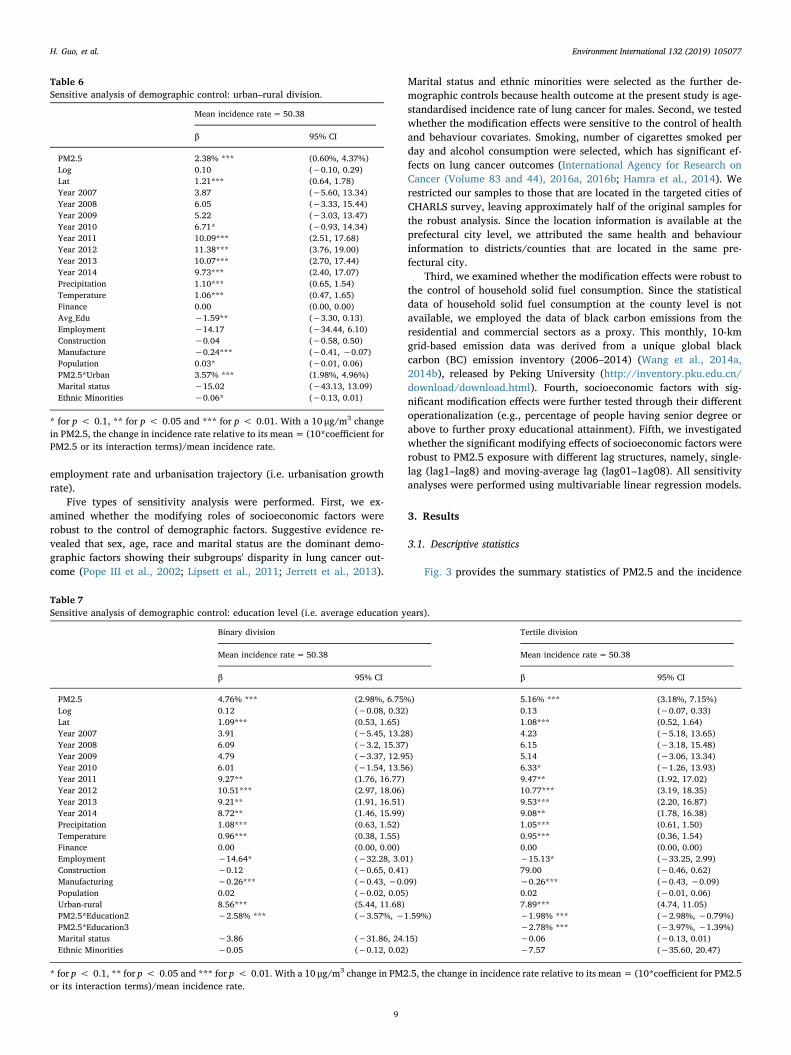
Five types of sensitivity analysis were performed. First, we ex-amined whether the modifying roles of socioeconomic factors wererobust to the control of demographic factors. Suggestive evidence re-vealed that sex, age, race and marital status are the dominant demo-graphic factors showing their subgroups' disparity in lung cancer out-come (Pope III et al., 2002; Lipsett et al., 2011; Jerrett et al., 2013).

Marital status and ethnic minorities were selected as the further de-mographic controls because health outcome at the present study is age-standardised incidence rate of lung cancer for males. Second, we testedwhether the modification effects were sensitive to the control of healthand behaviour covariates. Smoking, number of cigarettes smoked perday and alcohol consumption were selected, which has significant ef-fects on lung cancer outcomes (International Agency for Research onCancer (Volume 83 and 44), 2016a, 2016b; Hamra et al., 2014). Werestricted our samples to those that are located in the targeted cities ofCHARLS survey, leaving approximately half of the original samples forthe robust analysis. Since the location information is available at theprefectural city level, we attributed the same health and behaviourinformation to districts/counties that are located in the same pre-fectural city.

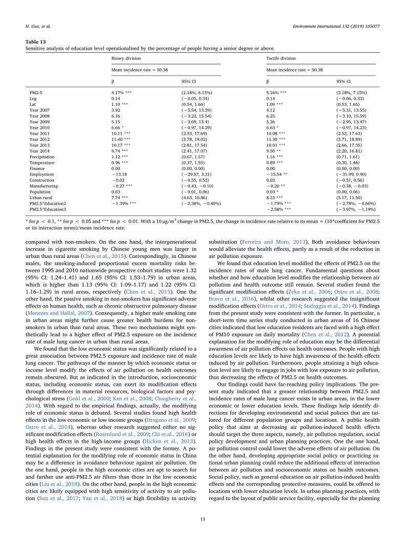
Third, we examined whether the modification effects were robust tothe control of household solid fuel consumption. Since the statisticaldata of household solid fuel consumption at the county level is notavailable, we employed the data of black carbon emissions from theresidential and commercial sectors as a proxy. This monthly, 10-kmgrid-based emission data was derived from a unique global blackcarbon (BC) emission inventory (2006–2014) (Wang et al., 2014a,2014b), released by Peking University (http://inventory.pku.edu.cn/download/download.html). Fourth, socioeconomic factors with sig-nificant modification effects were further tested through their differentoperationalization (e.g., percentage of people having senior degree orabove to further proxy educational attainment). Fifth, we investigatedwhether the significant modifying effects of socioeconomic factors wererobust to PM2.5 exposure with different lag structures, namely, single-lag (lag1–lag8) and moving-average lag (lag01–1ag08). All sensitivityanalyses were performed using multivariable linear regression models.

3. Results

3.1. Descriptive statistics

Fig. 3 provides the summary statistics of PM2.5 and the incidence

Table 6Sensitive analysis of demographic control: urban–rural division.


β 95% CI

PM2.5 2.38% *** (0.60%, 4.37%)Log 0.10 (−0.10, 0.29)Lat 1.21*** (0.64, 1.78)Year 2007 3.87 (−5.60, 13.34)Year 2008 6.05 (−3.33, 15.44)Year 2009 5.22 (−3.03, 13.47)Year 2010 6.71* (−0.93, 14.34)Year 2011 10.09*** (2.51, 17.68)Year 2012 11.38*** (3.76, 19.00)Year 2013 10.07*** (2.70, 17.44)Year 2014 9.73*** (2.40, 17.07)Precipitation 1.10*** (0.65, 1.54)Temperature 1.06*** (0.47, 1.65)Finance 0.00 (0.00, 0.00)Avg_Edu −1.59** (−3.30, 0.13)Employment −14.17 (−34.44, 6.10)Construction −0.04 (−0.58, 0.50)Manufacture −0.24*** (−0.41, −0.07)Population 0.03* (−0.01, 0.06)PM2.5*Urban 3.57% *** (1.98%, 4.96%)Marital status −15.02 (−43.13, 13.09)Ethnic Minorities −0.06* (−0.13, 0.01)


Table 7Sensitive analysis of demographic control: education level (i.e. average education years).



β 95% CI β 95% CI

PM2.5 4.76% *** (2.98%, 6.75%) 5.16% *** (3.18%, 7.15%)Log 0.12 (−0.08, 0.32) 0.13 (−0.07, 0.33)Lat 1.09*** (0.53, 1.65) 1.08*** (0.52, 1.64)Year 2007 3.91 (−5.45, 13.28) 4.23 (−5.18, 13.65)Year 2008 6.09 (−3.2, 15.37) 6.15 (−3.18, 15.48)Year 2009 4.79 (−3.37, 12.95) 5.14 (−3.06, 13.34)Year 2010 6.01 (−1.54, 13.56) 6.33* (−1.26, 13.93)Year 2011 9.27** (1.76, 16.77) 9.47** (1.92, 17.02)Year 2012 10.51*** (2.97, 18.06) 10.77*** (3.19, 18.35)Year 2013 9.21** (1.91, 16.51) 9.53*** (2.20, 16.87)Year 2014 8.72** (1.46, 15.99) 9.08** (1.78, 16.38)Precipitation 1.08*** (0.63, 1.52) 1.05*** (0.61, 1.50)Temperature 0.96*** (0.38, 1.55) 0.95*** (0.36, 1.54)Finance 0.00 (0.00, 0.00) 0.00 (0.00, 0.00)Employment −14.64* (−32.28, 3.01) −15.13* (−33.25, 2.99)Construction −0.12 (−0.65, 0.41) 79.00 (−0.46, 0.62)Manufacturing −0.26*** (−0.43, −0.09) −0.26*** (−0.43, −0.09)Population 0.02 (−0.02, 0.05) 0.02 (−0.01, 0.06)Urban-rural 8.56*** (5.44, 11.68) 7.89*** (4.74, 11.05)PM2.5*Education2 −2.58% *** (−3.57%, −1.59%) −1.98% *** (−2.98%, −0.79%)PM2.5*Education3 −2.78% *** (−3.97%, −1.39%)Marital status −3.86 (−31.86, 24.15) −0.06 (−0.13, 0.01)Ethnic Minorities −0.05 (−0.12, 0.02) −7.57 (−35.60, 20.47)



9

http://inventory.pku.edu.cn/download/download.html

http://inventory.pku.edu.cn/download/download.html

rate of male lung cancer for each socioeconomic stratum. The incidencerate was 55.84 per 100,000 people (95% CI: 53.52, 58.16) in urbanareas, which is considerably higher than 48.90 per 100,000 people(95% CI: 47.71, 50.10) in rural areas. By contrast, the pattern of PM2.5level between these two types of areas reversed, showing the low PM2.5level in urban areas (Fig. 3(A)). With regard to education level, the loweducation group exposed to the lowest PM2.5 concentration exhibitedthe highest incidence rate, whereas the high education group demon-strated higher incidence rate and PM2.5 level compared with themiddle education group (Fig. 3(B)). A decreasing trend of incidencerates across three economic groups was observed with the increase ofthe economic status, declining from 51.76 per 100,000 people (95% CI:49.68, 53.84) in the low economic group to 49.51 per 100,000 people(95% CI, 47.87, 51.14) in the high economic group (Fig. 3(C)). Foremployment, the low employment group was exposed to the lowestPM2.5 level but exhibited the highest incidence rate; compared withthe high employment group, there was a higher PM2.5 level but a lowerincidence rate in the middle employment group (Fig. 3(D)).

3.2. Modification effects

Fig. 4(A–B) and Table 1 present the results of modifying role ofurban-rural division on the association between PM2.5 on the incidencerate of male lung cancer. A significant difference was detected in thePM2.5 effects between urban and rural areas. The stratified datasetplotted in Fig. 4(A) demonstrated that a higher effect of PM2.5 was

detected in urban compared with rural areas in the unadjusted model;the PM2.5 effects were significant in urban and rural groups in the fullyadjusted model, with a higher effect in the former group (Fig. 4(B)). Inthe combined estimation, the change in incidence rate relative to itsmean was significantly higher by 3.97% (95% CI: 2.18%, 4.96%,p=0.000) in urban than in rural areas, with a 10 μg/m3 change inPM2.5 (Table 1).

The modification effect of education level was shown in Fig. 4(C–E)and Table 2. In general, education level significantly and negativelymodifies the effects of PM2.5 on the incidence rate of male lung cancer.Fig. 4(C–D) plotted the incidence rate versus PM2.5 concentration foreach stratum in education's tertile and binary divisions, respectively. Inthe stratified dataset of tertile division, a significant effect of PM2.5 wasdetected in the low and middle education groups but not in the higheducation group (Fig. 2(E)). In the combined dataset, if PM2.5 changesby 10 μg/m3, then the change in incidence rate relative to its mean wassignificantly lower by 1.98% (95% CI: −3.18%, −0.79%, p=0.001)and 2.78% (95% CI: −4.17%, −1.39%, p=0.000) in the middle andhigh education groups compared with the low education group, re-spectively (Table 2). With regard to the binary division, we observedthe significant effects of not only PM2.5 in the low and high educationgroups in the stratified analysis (Fig. 2(E)) but also interaction betweenPM2.5 and education dummy variable in the combined dataset(=− 2.58%, 95% CI: −3.57%, −1.59%, p=0.000).

Fig. 4 and Table 3 present the modification effect of economic status(i.e. finance per capita). Economic status was negatively correlated withthe association between PM2.5 and incidence rate of male lung cancer.We observed a decreased effect of PM2.5 in either the tertile or binarydivision plotted in Fig. 4(F–G), respectively, with the increase of eco-nomic status. With regard to the stratified dataset according to thetertile division, the effect of PM2.5 on the incidence rate of male lungcancer was significant in the middle economic group but not in the lowand high economic groups (Fig. 4(H)). In the combined dataset, ifPM2.5 changed by 10 μg/m3, then the change in incidence rate relativeto its mean was significantly lower by 0.99% (95% CI: −2.18%, 0.20%,p=0.071) and 1.39% (95% CI: −2.78%, 0.00%, p=0.037) in themiddle and high economic groups compared with the low economicgroup, respectively (Table 3). A similar pattern of results was observedfor the situation of binary division (Table 3). Specifically, the interac-tion between PM2.5 and economic dummy variable was significantlyassociated with the incidence rate of male lung cancer (=− 1.98%,95% CI: −3.18%, −0.99%, p=0.000).

The modification effect of employment rate was presented inFig. 4(I–K) and Table 4. No significant difference was detected in PM2.5effects. The incidence rate against PM2.5 concentration for eachstratum in employment rate's tertile and binary divisions was plotted inFig. 4(I–J), respectively. With regard to the tertile division in thecombined dataset, despite the significantly higher PM2.5 effect in themiddle employment group than in the low employment group, no sucha significant higher effect was observed in the high employment group(Table 4). The effect of interaction was also insignificant for the binarydivision situation.

Fig. 4(L–N) and Table 5 show the modification effect of urbanisationtrajectory (i.e. urbanisation growth rate). The urbanisation trajectorywas insignificantly correlated with the association between PM2.5 andincidence rates of male lung cancer. We observed the decreased effectof PM2.5 on incidence rates with the increased urbanisation growthrate, which was plotted in Fig. 4(L–M). With regard to the stratifieddataset according to the tertile division, significant effects of PM2.5were detected in the low and middle growth rate group but not in thehigh growth rate group (Fig. 4(N)). The effect size increasingly de-creased with an increase of growth rate level. A similar pattern of re-sults was observed for the situation of stratified dataset according to thebinary division. However, no significant effects of interaction terms inthe combined dataset were detected in the tertile division, although theinteraction between PM2.5 and the dummy variable was significant in

Table 8Sensitive analysis of demographic control: economic status (i.e. finance percapita).


Mean incidence rate=50.38 Mean incidence rate= 50.38

β 95% CI β 95% CI

PM2.5 3.97% *** (2.18%,5.76%)

3.97% *** (2.18%,5.95%)

Log 0.16 (−0.04, 0.35) 0.14 (−0.06, 0.33)Lat 1.22*** (0.65, 1.78) 1.19*** (0.62, 1.76)Year 2007 4.23 (−5.18, 13.63) 4.06 (−5.40,

13.52)Year 2008 6.10 (−3.22, 15.42) 6.14 (−3.23,

15.52)Year 2009 5.37 (−2.81, 13.56) 5.46 (−2.78,

13.69)Year 2010 6.86** (−0.71, 14.42) 6.84** (−0.77,

14.44)Year 2011 10.32*** (2.86, 17.78) 10.29*** (2.79, 17.8)Year 2012 11.44*** (4.01, 18.88) 11.50*** (4.02, 18.98)Year 2013 10.11*** (2.84, 17.39) 10.15*** (2.83, 17.47)Year 2014 9.78*** (2.55, 17.00) 9.79*** (2.52, 17.05)Precipitation 1.14*** (0.70, 1.59) 1.15*** (0.70, 1.60)Temperature 1.03*** (0.45, 1.62) 1.00*** (0.41, 1.59)Edu_avg −1.00 (−2.77, 0.78) −1.24 (−3.06, 0.58)Employment −19.17** (−39.29, 0.95) −17.56* (−37.83,

2.70)Construction 0.09 (−0.45, 0.64) −0.01 (−0.56, 0.53)Manufacture −0.16** (−0.34, 0.10) −0.20** (−0.39,

−0.02)Population 0.03 (−0.01, 0.06) 0.02 (−0.01, 0.06)Urban-rural 7.15*** (3.78, 10.52) 7.42*** (4.01, 10.84)PM2.5*Fin2 −1.98% *** (−2.98%,

−0.99%)−0.99% * (−2.18%,

0.20%)PM2.5*Fin3 −1.39% ** (−2.78%,

0.00%)Marital status −7.90 (−36.15,

20.35)−10.02 (−39.03,

19.00)Ethnic Minorities −0.05 (−0.12, 0.02) −0.05 (−0.12, 0.02)



10

the binary division (Table 5).

3.3. Sensitivity analysis

Fig. 5(A–C) and Tables 6–8 show the first sensitive analysis with thefurther demographic control. Findings of the significant modificationeffects were still insensitive to this control. With the demographic ad-justment, PM2.5 and its interaction with the dummy of urban–rural

division were still significantly associated with the incidence rate ofmale lung cancer (Fig. 5(A), Table 6). A similar pattern of results wasobserved for the indicators of economic status and education level inthe situation of their binary and tertile divisions (Fig. 5(B–C), Tables7–8).

The significant modifying effect by urban–rural division was robustto the adjustment of health and behaviour covariates. Specifically,significant effects of PM2.5 and its interaction with the urban–ruraldummy were observed for the situation of no adjustment; when ad-justing for the covariates of smoking rate, smoking strength anddrinking, PM2.5 and its interaction with urban–rural dummy still kepttheir significant effects (Fig. 5(D), Table 9).

Fig. 5(E–G) and Tables 10–12 show the sensitive analysis with thefurther household solid-fuel consumption control. Findings of sig-nificant modification effects by urban-rural division, education leveland economic status were still robust to this control. Specifically, withfurther adjustment, the black carbon emission from residential andcommercial sectors (as a proxy of household solid-fuel consumption)was significantly associated with the incidence rate of male lung cancer;PM2.5 and its interaction with the dummy of urban–rural division stillkept their significances. (Fig. 5(E), Table 10). A similar pattern of re-sults was observed for the indicators of economic status and educationlevel in the situation of their binary and tertile divisions (Fig. 5(F–G),Tables 11–12).

Table 13 presents our robust test using the percentage of peoplehaving a senior degree or above to further proxy the education level.The lower educational level was still significantly correlated with astronger association between PM2.5 and incidence rate of male lungcancer. In the combined dataset of tertile division, the change in in-cidence rate relative to its mean per 10 μg/m3 change in PM2.5 wassignificantly lower by 1.79% (95% CI: −2.78%, −0.60%, p=0.005)and 2.58% (95% CI: −3.97%, −1.19%, p=0.000) in the middle andhigh education groups compared with the low education group, re-spectively (Table 13). With regard to the binary division, a significantdifference was observed in PM2.5 effects between the low and higheducation groups (=− 1.39%, 95% CI: −2.38%, −0.40%, p=0.009).

Table 9Sensitive analysis of health and behaviour control: urban–rural division.


Without health-behaviour control Health-behaviour control

β 95% CI β 95% CI

PM2.5 2.98% ** (0.40%, 5.56%) 3.77% *** (1.19%, 6.35%)Log −0.23 (−0.59, 0.13) 0.17 (−0.22, 0.56)Lat 2.20*** (1.31, 3.09) 2.35*** (1.48, 3.22)Year 2007 4.38 (−7.55, 16.31) 4.93 (−6.53, 16.39)Year 2008 5.71 (−6.20, 17.63) 7.12 (−4.33, 18.57)Year 2009 5.81 (−4.95, 16.56) 6.72 (−3.62, 17.06)Year 2010 11.84** (1.89, 21.79) 11.96** (2.40, 21.53)Year 2011 13.78*** (3.93, 23.63) 13.68*** (4.21, 23.14)Year 2012 13.45*** (3.54, 23.35) 13.98*** (4.47, 23.50)Year 2013 13.61*** (4.05, 23.16) 13.38*** (4.20, 22.55)Year 2014 11.82** (2.32, 21.32) 11.74** (2.62, 20.87)Precipitation 1.79*** (1.13, 2.45) 1.59*** (0.94, 2.23)Temperature 1.56*** (0.75, 2.38) 1.84*** (1.04, 2.64)Finance 0.00 (0.00, 0.00) 0.00 (0.00, 0.00)Avg_Edu 1.70 (−0.63, 4.02) 2.24** (−0.02, 4.49)Employment 6.84 (−19.58, 33.25) 20.12 (−5.67, 45.91)Construction −0.02 (−0.76, 0.72) −0.13 (−0.85, 0.60)Manufacture −0.03 (−0.25, 0.20) −0.10 (−0.32, 0.13)Population 0.01 (−0.04, 0.05) 0.00 (−0.04, 0.04)PM2.5*Urban 3.37% *** (1.19%, 5.36%) 2.98% *** (0.99%, 4.96%)Smoking 32.68 *** (20.26, 45.10)Smoking strength 0.33 *** (0.08, 0.59)Drinking 36.24 *** (12.95, 59.53)


Table 10Sensitive analysis of household fuel control: urban–rural division.


β 95% CI

PM2.5 1.98%** (0.00%, 3.77%)Log 0.12 (−0.08, 0.31)Lat 1.22*** (0.66, 1.78)Year 2007 4.12 (−5.28, 13.53)Year 2008 6.45 (−2.87, 15.78)Year 2009 5.81 (−2.38, 14.00)Year 2010 7.26** (−0.33, 14.84)Year 2011 10.67*** (3.14, 18.21)Year 2012 11.87*** (4.30, 19.43)Year 2013 10.81*** (3.49, 18.14)Year 2014 10.17*** (2.89, 17.45)Precipitation 1.26*** (0.81, 1.71)Temperature 1.08*** (0.50, 1.66)Finance 0.00 (0.00, 0.00)Avg_Edu −1.98** (−3.68, −0.28)Employment −17.80*** (−36.96, 1.36)Construction −0.01 (−0.55, 0.52)Manufacture −0.24*** (−0.40, −0.08)Population 0.04** (0.01, 0.07)PM2.5*Urban 3.57%*** (2.18%, 5.16%)Black carbon 0.10*** (0.05, 0.15)



11

The modifying roles of significant socioeconomic factors were ro-bust to PM2.5 exposure with different lag structures. With regard to thePM2.5 single or moving-average lags (i.e. lag 1 to lag 8 and lag 01 to lag08), the PM2.5 effects on the incidence rate of male lung cancer weresignificant and positive. Fig. 6(A) presented that the PM2.5 effects werestill significantly higher in urban than in rural areas. Similarly,Fig. 6(B–G) indicated that the lower education level (operationalised bythe average education years and percentage of people having a seniordegree above) or lower economic status was still associated with astronger relationship between PM2.5 and incidence rate of male lungcancer for the situations of tertile and binary divisions.

4. Discussion

An in-depth understanding of socioeconomic indicators modifyingthe relationship between air pollution and health outcome is essentialto attenuate health inequality. However, whether socioeconomic in-dicators modify the effects of air pollution on health outcomes remainsuncertain. Most studies performed the examination using an in-dividually defined unit, whereas those using large population samplesacross geographical units are rather limited, especially at the city ordistrict level.

To our knowledge, this is the first nationwide county-level studythat systematically examined the socioeconomic modification effects onthe association between air pollution and lung cancer incidence inChina. Our findings contributed to the literature on socioeconomicmodification effects through the examination in a developing settingwhere air pollution is severe. The relationship between PM2.5 and

incidence rate of male lung cancer was stronger in urban areas, in thelower economic or lower educational counties. We found no robustmodification effects of employment rate or urbanisation trajectory.

We found that PM2.5 might exert high effect on the incidence ratesof male lung cancer in urban areas. This result might seem unexpected.However, our findings were consistent with previous studies. A recentnationwide study of 708 counties in US using health data fromMedicare National Claims History files (2002–2006) suggested that therelationship between PM2.5 exposure and cardiovascular hospitalisa-tions was stronger in urban than nonurban counties (Bravo et al.,2016). Similarly, a recent Chinese study also indicated a greater effectof air pollution on lung cancer incidence amongst urban than ruralinhabitants (Zhou et al., 2017). Two health-related mechanisms mightbe responsible for our unexpected findings. One potential explanationmight come from a difference in primary sources of domestic fuel be-tween urban and rural areas in China. Domestic fuel in rural China isdominated by biomass fuel, whilst the primary source of domestic fuelin urban areas is solid fuel. A recent Chinese study published in PNASsuggested that the decrease in household solid-fuel consumption ismostly responsible for the reduced integrated exposure (i.e. ambientand indoor) to PM2.5 pollution in China (Zhao et al., 2018). Hence, thehigh consumption of solid fuel in urban areas might enable urban re-sidents to have a high exposure to PM2.5 pollution, thus leading to ahigh effect in the urban group. Another Chinese study predicted thatsmoking and solid fuel use will be responsible for 75% of death causedby lung cancer in China if they remain unchanged between 2003 and2033 (Lin et al., 2008). Therefore, the difference in solid fuel con-sumption might be responsible for the urban–rural gaps in health ef-fects.

The second explanation for the differential urban–rural effectsmight be due to a difference in smoking status. Several studies (Vena,1982; Wong et al., 2007) indicated that the effects of air pollution onlung cancer and cardio-respiratory diseases are greater in smokers

Table 11Sensitive analysis of household fuel control: education level (i.e. average edu-cation years).


Mean incidence rate=50.38 Mean incidence rate=50.38

β 95% CI β 95% CI

PM2.5 4.37%*** (2.58%,6.35%)

4.57%*** (2.58%,6.75%)

Log 0.15 (−0.04, 0.34) 0.16 (−0.04, 0.35)Lat 1.09*** (0.54, 1.65) 1.08*** (0.53, 1.64)Year 2007 4.16 (−5.15,

13.48)4.50 (−4.87,

13.87)Year 2008 6.50 (−2.74,

15.73)6.56 (−2.73,

15.84)Year 2009 5.34 (−2.78,

13.46)5.64 (−2.52,

13.81)Year 2010 6.58* (−0.94,

14.09)6.87** (−0.69,

14.43)Year 2011 9.88** (2.41, 17.34) 10.05*** (2.54, 17.57)Year 2012 11.04*** (3.54, 18.54) 11.29*** (3.75, 18.83)Year 2013 9.96*** (2.70, 17.22) 10.26*** (2.96, 17.56)Year 2014 9.21*** (1.99, 16.43) 9.56*** (2.30, 16.82)Precipitation 1.22*** (0.77, 1.66) 1.20*** (0.74, 1.65)Temperature 0.97*** (0.39, 1.55) 0.95*** (0.37, 1.54)Finance 0.00 (0.00, 0.00) 0.00 (0.00, 0.00)Employment −0.01** (−0.03, 0.00) −0.02** (−0.03, 0.05)Construction −0.06 (−0.58, 0.47) 0.11 (−0.43, 0.65)Manufacturing −0.25*** (−0.41,

−0.09)−0.26*** (−0.42,

−0.09)Population 0.02 (−0.01, 0.06) 0.03* (0.00, 0.06)Urban-rural 8.23*** (5.14, 11.32) 7.70*** (4.57, 10.83)PM2.5*Education2 −2.58%*** (−3.57%,

−1.59%)−1.79%*** (−2.98%,

−0.60%)PM2.5*Education3 −2.78%*** (−3.97%,

−1.39%)Black carbon 0.09*** (0.04, 0.14) 0.09*** (0.04, 0.14)


Table 12Sensitive analysis of household fuel control: economic status (i.e. finance percapita).


Mean incidence rate= 50.38 Mean incidence rate= 50.38

β 95% CI β 95% CI

PM2.5 3.57%*** (1.59%, 5.36%) 3.57%*** (1.59%, 5.56%)Log 0.17* (−0.02, 0.37) 0.15 (−0.04, 0.35)Lat 1.23*** (0.67, 1.79) 1.19*** (0.63, 1.75)Year 2007 4.42 (−4.95, 13.78) 4.28 (−5.13, 13.69)Year 2008 6.46 (−2.83, 15.74) 6.51 (−2.82, 15.83)Year 2009 5.88 (−2.28, 14.03) 5.98 (−2.21, 14.17)Year 2010 7.36** (−0.18, 14.90) 7.38** (−0.19, 14.95)Year 2011 10.88*** (3.45, 18.31) 10.90*** (3.43, 18.37)Year 2012 11.96*** (4.56, 19.37) 12.05*** (4.60, 19.49)Year 2013 10.80*** (3.54, 18.05) 10.88*** (3.59, 18.17)Year 2014 10.23*** (3.03, 17.43) 10.27*** (3.04, 17.50)Precipitation 1.27*** (0.82, 1.72) 1.29*** (0.84, 1.74)Temperature 1.05*** (0.47, 1.63) 1.01*** (0.43, 1.59)Edu_avg −1.31 (−3.06, 0.44) −1.55* (−3.34, 0.23)Employment −0.02** (−0.04, −0.00) −0.02** (−0.04, −0.00)Construction 0.11 (−0.43, 0.65) 0.01 (−0.53, 0.56)Manufacture −0.16** (−0.33, 0.00) −0.21** (−0.39, −0.03)Population 0.03** (0.00, 0.07) 0.03** (0.00, 0.06)Urban-rural 7.16*** (3.81, 10.50) 7.36*** (3.97, 10.74)PM2.5*Fin2 −1.79%*** (−2.98%,

−0.79%)−0.99%* (−2.18%,

0.20%)PM2.5*Fin3 −1.19%* (−2.58%,

0.20%)Black carbon 0.08*** (0.03, 0.13) 0.09*** (0.04, 0.14)



12

compared with non-smokers. On the one hand, the intergenerationalincrease in cigarette smoking by Chinese young men was larger inurban than rural areas (Chen et al., 2015). Correspondingly, in Chinesemales, the smoking-induced proportional excess mortality risks be-tween 1995 and 2010 nationwide prospective cohort studies were 1.32(95% CI: 1.24–1.41) and 1.65 (95% CI: 1.53–1.79) in urban areas,which is higher than 1.13 (95% CI: 1.09–1.17) and 1.22 (95% CI:1.16–1.29) in rural areas, respectively (Chen et al., 2015). One theother hand, the passive smoking in non-smokers has significant adverseeffects on human health, such as chronic obstructive pulmonary disease(Menezes and Hallal, 2007). Consequently, a higher male smoking ratein urban areas might further cause greater health burdens for non-smokers in urban than rural areas. These two mechanisms might syn-thetically lead to a higher effect of PM2.5 exposure on the incidencerate of male lung cancer in urban than rural areas.

We found that the low economic status was significantly related to agreat association between PM2.5 exposure and incidence rate of malelung cancer. The pathways of the manner by which economic status orincome level modify the effects of air pollution on health outcomesremain obscured. But as indicated in the introduction, socioeconomicstatus, including economic status, can exert its modification effectsthrough differences in material resources, biological factors and psy-chological stress (Gold et al., 2000; Kan et al., 2008; Clougherty et al.,2014). With regard to the empirical findings, actually, the modifyingrole of economic status is debated. Several studies found high healtheffects in the low economic or low income groups (Dragano et al., 2009;Ostro et al., 2014), whereas other research suggested either no sig-nificant modification effects (Rosenlund et al., 2009; Chi et al., 2016) orhigh health effects in the high-income groups (Hicken et al., 2013).Findings in the present study were consistent with the former. A po-tential explanation for the modifying role of economic status in Chinamay be a difference in avoidance behaviour against air pollution. Onthe one hand, people in the high economic cities are apt to search forand further use anti-PM2.5 air filters than those in the low economiccities (Liu et al., 2018). On the other hand, people in the high economiccities are likely equipped with high sensitivity of activity to air pollu-tion (Sun et al., 2017; Yan et al., 2018) or high flexibility in activity

substitution (Ferreira and Moro, 2013). Both avoidance behaviourswould alleviate the health effects, partly as a result of the reduction inair pollution exposure.

We found that education level modified the effects of PM2.5 on theincidence rates of male lung cancer. Fundamental questions aboutwhether and how education level modifies the relationship between airpollution and health outcome still remain. Several studies found thesignificant modification effects (Zeka et al., 2006; Ostro et al., 2008;Bravo et al., 2016), whilst other research suggested the insignificantmodification effects (Ostro et al., 2014; Stafoggia et al., 2014). Findingsfrom the present study were consistent with the former. In particular, ashort-term time series study conducted in urban areas of 16 Chinesecities indicated that low education residents are faced with a high effectof PM10 exposure on daily mortality (Chen et al., 2012). A potentialexplanation for the modifying role of education may be the differentialawareness of air pollution effects on health outcomes. People with higheducation levels are likely to have high awareness of the health effectsinduced by air pollution. Furthermore, people attaining a high educa-tion level are likely to engage in jobs with low exposure to air pollution,thus decreasing the effects of PM2.5 on health outcomes.

Our findings could have far-reaching policy implications. The pre-sent study indicated that a greater relationship between PM2.5 andincidence rates of male lung cancer exists in urban areas, in the lowereconomic or lower education levels. These findings help identify di-rections for developing environmental and social policies that are tai-lored for different population groups and locations. A public healthpolicy that aims at decreasing air pollution-induced health effectsshould target the three aspects, namely, air pollution regulation, socialpolicy development and urban planning practices. One the one hand,air pollution control could lower the adverse effects of air pollution. Onthe other hand, developing appropriate social policy or practicing ra-tional urban planning could reduce the additional effects of interactionbetween air pollution and socioeconomic status on health outcomes.Social policy, such as general education on air pollution-induced healtheffects and the corresponding protective measures, could be offered tolocations with lower education levels. In urban planning practices, withregard to the layout of public service facility, especially for the planning

Table 13Sensitive analysis of education level operationalised by the percentage of people having a senior degree or above.



β 95% CI β 95% CI

PM2.5 4.17% *** (2.18%, 6.15%) 5.16% *** (3.18%, 7.15%)Log 0.14 (−0.05, 0.34) 0.14 (−0.06, 0.33)Lat 1.10 *** (0.54, 1.66) 1.09 *** (0.53, 1.65)Year 2007 3.92 (−5.54, 13.39) 4.12 (−5.31, 13.55)Year 2008 6.16 (−3.22, 15.54) 6.25 (−3.10, 15.59)Year 2009 5.15 (−3.09, 13.4) 5.26 (−2.95, 13.47)Year 2010 6.66 * (−0.97, 14.29) 6.63 * (−0.97, 14.23)Year 2011 10.11 *** (2.53, 17.69) 10.08 *** (2.52, 17.63)Year 2012 11.40 *** (3.78, 19.02) 11.30 *** (3.71, 18.89)Year 2013 10.17 *** (2.81, 17.54) 10.01 *** (2.66, 17.35)Year 2014 9.74 *** (2.41, 17.07) 9.50 ** (2.20, 16.81)Precipitation 1.12 *** (0.67, 1.57) 1.16 *** (0.71, 1.61)Temperature 0.96 *** (0.37, 1.55) 0.89 *** (0.30, 1.48)Finance 0.00 (0.00, 0.00) 0.00 (0.00, 0.00)Employment −13.18 (−29.57, 3.21) −15.54 ** (−31.99, 0.90)Construction −0.02 (−0.55, 0.52) 0.02 (−0.51, 0.56)Manufacturing −0.27 *** (−0.43, −0.10) −0.20 ** (−0.38, −0.03)Population 0.03 (−0.01, 0.06) 0.03 * (0.00, 0.06)Urban-rural 7.74 *** (4.63, 10.86) 8.33 *** (5.17, 11.50)PM2.5*Education2 −1.39% *** (−2.38%, −0.40%) −1.79% *** (−2.78%, −0.60%)PM2.5*Education3 −2.58% *** (−3.97%, −1.19%)



13

Fig. 6. Sensitive analysis of socioeconomic modifications to PM2.5 with both single and moving-average lags.


14

of health services and resources, priority could be given to the loweconomic counties to improve access to emergent medical and healthassistance.

Several limitations and uncertainties regarding our findings shouldbe acknowledged. First, with regard to the sensitive analysis of PM2.5effects adjusted by health and behaviour covariates, we attributed thesame health-related covariates to districts/counties that are located inthe same prefectural city, which might ignore the behaviour variationbetween these districts/counties. Second, similar to ecological studies,inevitable errors in exposure measurement were detected in our studybecause air pollution variation and the pattern of daily human activitycould affect actual human exposure (Yoo et al., 2015; Park and Kwan,2017). Third, the use of several time-invariant socioeconomic factorsthat were extracted from 2010 population census neglected the effectsof socioeconomic mobility, which might bias our examination (Kreineret al., 2018). Certain limitations should be addressed if data is availablein the future.

5. Conclusions

Urban areas or counties with high percentages of low economic orlow educational male residents have high risks of PM2.5-induced lungcancer incidence in China. Policymakers in public health and urbanplanning should develop area-specific strategies, such as alleviating theurban–rural gaps in access to high-quality medical resources in theplanning of health service and resources, to reduce the socioeconomicgaps in health effects. Future prediction on health effects of air pollu-tion exposure should consider socioeconomic disparities in lung cancerrisks, especially for the urban–rural gaps, which is a major phenomenonin China.

Declaration of Competing Interest

All authors declared no conflicts of interests.

Acknowledgement

This work was partially supported by The University of Hong KongSeed Fund for Basic Research (201711159270), Programs of Scienceand Technology of Shenzhen (JCYJ20170412150910443) and NationalScience Foundation of China (Grants numbers 41471370, 41671180).

References

Almond, D., Chen, Y., Greenstone, M., Li, H., 2009. Winter heating or clean air?Unintended impacts of China's Huai river policy. Am. Econ. Rev. 99 (2), 184–190.

Barrett, B.S., Hameed, S., 2017. Seasonal variability in precipitation in central andsouthern Chile: modulation by the South Pacific high. J. Clim. 30 (1), 55–69.

Bell, M.L., Ebisu, K., 2012. Environmental inequality in exposures to airborne particulatematter components in the United States. Environ. Health Perspect. 120 (12),1699–1704.

Bravo, M.A., Ebisu, K., Dominici, F., Wang, Y., Peng, R.D., Bell, M.L., 2016. Airborne fineparticles and risk of hospital admissions for understudied populations: effects byurbanicity and short-term cumulative exposures in 708 US counties. Environ. HealthPerspect. 125 (4), 594–601.

Chen, R., Kan, H., Chen, B., Huang, W., Bai, Z., Song, G., Pan, G., 2012. Association ofparticulate air pollution with daily mortality: the China Air Pollution and HealthEffects Study. Am. J. Epidemiol. 175 (11), 1173–1181.

Chen, Z., Peto, R., Zhou, M., Iona, A., Smith, M., Yang, L., Sherliker, P., 2015. Contrastingmale and female trends in tobacco-attributed mortality in China: evidence fromsuccessive nationwide prospective cohort studies. Lancet 386 (10002), 1447–1456.

Chen, R., Yin, P., Meng, X., Liu, C., Wang, L., Xu, X., Zhou, M., 2017. Fine particulate airpollution and daily mortality. A nationwide analysis in 272 Chinese cities. Am. J.Respir. Crit. Care Med. 196 (1), 73–81.

Chi, G.C., Hajat, A., Bird, C.E., Cullen, M.R., Griffin, B.A., Miller, K.A., Kaufman, J.D.,2016. Individual and neighborhood socioeconomic status and the association be-tween air pollution and cardiovascular disease. Environ. Health Perspect. 124 (12),1840–1847.

Chiusolo, M., Cadum, E., Stafoggia, M., Galassi, C., Berti, G., Faustini, A., Mallone, S.,2011. Short-term effects of nitrogen dioxide on mortality and susceptibility factors in10 Italian cities: the EpiAir study. Environ. Health Perspect. 119 (9), 1233.

Clougherty, J.E., Kubzansky, L.D., 2009. A framework for examining social stress and

susceptibility to air pollution in respiratory health. Environ. Health Perspect. 117 (9),1351.

Clougherty, J.E., Shmool, J.L., Kubzansky, L.D., 2014. The role of non-chemical stressorsin mediating socioeconomic susceptibility to environmental chemicals. Curr.Environ. Health Rep. 1 (4), 302–313.

Dragano, N., Hoffmann, B., Moebus, S., Möhlenkamp, S., Stang, A., Verde, P.E., Siegrist,J., 2009. Traffic exposure and subclinical cardiovascular disease: is the associationmodified by socioeconomic characteristics of individuals and neighbourhoods?Results from a multilevel study in an urban region. Occup. Environ. Med. 66 (9),628–635.

Duncan, C., Jones, K., Moon, G., 1998. Context, composition and heterogeneity: usingmultilevel models in health research. Soc. Sci. Med. 46 (1), 97–117.

Ebenstein, A., Fan, M., Greenstone, M., He, G., Zhou, M., 2017. New evidence on theimpact of sustained exposure to air pollution on life expectancy from China's HuaiRiver Policy. Proc. Natl. Acad. Sci. 114 (39), 10384–10389 201616784.

Evans, G.W., Kantrowitz, E., 2002. Socioeconomic status and health: the potential role ofenvironmental risk exposure. Annu. Rev. Public Health 23 (1), 303–331.

Ferreira, S., Moro, M., 2013. Income and preferences for the environment: evidence fromsubjective well-being data. Environ. Plan. A 45 (3), 650–667.

Fuller, C.H., Feeser, K.R., Sarnat, J.A., O'Neill, M.S., 2017. Air pollution, cardiovascularendpoints and susceptibility by stress and material resources: a systematic review ofthe evidence. Environ. Health 16 (1), 58.

Gang, C., Vodonos, W., Chen, Y., Wang, Z., Sun, Z., Li, J., Odeh, I., 2014. Quantitativeassessment of the contributions of climate change and human activities on globalgrassland degradation. Environ. Earth Sci. 72 (11), 4273–4282.

Geronimus, A.T., Bound, J., Neidert, L.J., 1996. On the validity of using census geocodecharacteristics to proxy individual socioeconomic characteristics. J. Am. Stat. Assoc.91 (434), 529–537.

Gold, D.R., Litonjua, A., Schwartz, J., Lovett, E., Larson, A., Nearing, B., Allen, G., Verrier,M., Cherry, R., Verrier, R., 2000. Ambient pollution and heart rate variability.Circulation 101 (11), 1267–1273.

Gui, K., Che, H., Wang, Y., Wang, H., Zhang, L., Zhao, H., Zhang, X., 2019. Satellite-derived PM2. 5 concentration trends over Eastern China from 1998 to 2016: re-lationships to emissions and meteorological parameters. Environ. Pollut. 247,1125–1133.

Guo, Y., Zeng, H., Zheng, R., Li, S., Barnett, A.G., Zhang, S., Williams, G., 2016. Theassociation between lung cancer incidence and ambient air pollution in China: aspatiotemporal analysis. Environ. Res. 144, 60–65.

Guo, H., Li, W., Wu, J., 2019. Ambient PM2.5 and annual lung cancer incidence: a na-tionwide study in 295 Chinese counties. Environ. Res. Lett (under review).

Hamra, G.B., Guha, N., Cohen, A., Laden, F., Raaschou-Nielsen, O., Samet, J.M., Loomis,D., 2014. Outdoor particulate matter exposure and lung cancer: a systematic reviewand meta-analysis. Environ. Health Perspect. 122 (9), 906–911.

Han, X., Liu, Y., Gao, H., Ma, J., Mao, X., Wang, Y., Ma, X., 2017. Forecasting PM2. 5induced male lung cancer morbidity in China using satellite retrieved PM2. 5 andspatial analysis. Sci. Total Environ. 607, 1009–1017.

Han, L., Zhou, W., Li, W., Qian, Y., 2018a. Urbanization strategy and environmentalchanges: an insight with relationship between population change and fine particulatepollution. Sci. Total Environ. 642, 789–799.

Han, L., Zhou, W., Pickett, S.T., Li, W., Qian, Y., 2018b. Multicontaminant air pollution inChinese cities. Bull. World Health Organ. 96 (4), 233.

Havard, S., Deguen, S., Zmirou-Navier, D., Schillinger, C., Bard, D., 2009. Traffic-relatedair pollution and socioeconomic status: a spatial autocorrelation study to assess en-vironmental equity on a small-area scale. Epidemiology 223–230.

He, J., Chen, W., 2018. 2017 China Cancer Registry Annual Report. People's HealthPublishing House Press, Beijing (in Chinese).

Hicken, M.T., Adar, S.D., Diez Roux, A.V., O'neill, M.S., Magzamen, S., Auchincloss, A.H.,Kaufman, J.D., 2013. Do psychosocial stress and social disadvantage modify the as-sociation between air pollution and blood pressure? The multi-ethnic study ofatherosclerosis. Am. J. Epidemiol. 178 (10), 1550–1562.

Hicken, M.T., Adar, S.D., Hajat, A., Kershaw, K.N., Do, D.P., Barr, R.G., ... Roux, A.V.D.,2016. Air pollution, cardiovascular outcomes, and social disadvantage: the multi-ethnic study of atherosclerosis. Epidemiol. (Cambridge, Mass.) 27 (1), 42.

Huang, G., Zhou, W., Qian, Y., Fisher, B., 2019. Breathing the same air? Socioeconomicdisparities in PM2. 5 exposure and the potential benefits from air filtration. Sci. TotalEnviron. 657, 619–626.

International Agency for Research on Cancer, 2016a. IARC working group on the eva-luation of carcinogenic risks to humans. In: IARC Monographs Volume 44: AlcoholDrinking.

International Agency for Research on Cancer, 2016b. IARC working group on the eva-luation of carcinogenic risks to humans. In: IARC Monographs Volume 83: TobaccoSmoke and Involuntary Smoking.

International Agency for Research on Cancer, 2016c. IARC working group on the eva-luation of carcinogenic risks to humans. In: IARC Monographs Volume 109: OutdoorAir Pollution.

Jerrett, M., Burnett, R.T., Brook, J., Kanaroglou, P., Giovis, C., Finkelstein, N., Hutchison,B., 2004. Do socioeconomic characteristics modify the short term association be-tween air pollution and mortality? Evidence from a zonal time series in Hamilton,Canada. J. Epidemiol. Community Health 58 (1), 31–40.

Jerrett, M., Burnett, R.T., Beckerman, B.S., Turner, M.C., Krewski, D., Thurston, G.,Gapstur, S.M., 2013. Spatial analysis of air pollution and mortality in California. Am.J. Respir. Crit. Care Med. 188 (5), 593–599.

Kan, H., London, S.J., Chen, G., Zhang, Y., Song, G., Zhao, N., Jiang, L., Chen, B., 2008.Season, sex, age, and education as modifiers of the effects of outdoor air pollution ondaily mortality in Shanghai, China: the Public Health and Air Pollution in Asia(PAPA) Study. Environ. Health Perspect. 116 (9), 1183.


15

http://refhub.elsevier.com/S0160-4120(19)30365-4/rf0005


















































































































Kreiner, C.T., Nielsen, T.H., Serena, B.L., 2018. Role of income mobility for the mea-surement of inequality in life expectancy. Proc. Natl. Acad. Sci. 115 (46),11754–11759.

Krieger, N., Rowley, D.L., Herman, A.A., Avery, B., Phillips, M.T., 1993. Racism, sexism,and social class: implications for studies of health, disease, and well-being. Am. J.Prev. Med. 9 (6), 82–122.

Lavigne, É., Bélair, M.A., Do, M.T., Stieb, D.M., Hystad, P., van Donkelaar, A., Brook, J.R.,2017. Maternal exposure to ambient air pollution and risk of early childhood cancers:a population-based study in Ontario, Canada. Environ. Int. 100, 139–147.

Li, T., Zhang, Y., Wang, J., Xu, D., Yin, Z., Chen, H., Kinney, P.L., 2018. All-cause mor-tality risk associated with long-term exposure to ambient PM2· 5 in China: a cohortstudy. Lancet Public Health 3 (10), e470–e477.

Lin, H.H., Murray, M., Cohen, T., Colijn, C., Ezzati, M., 2008. Effects of smoking and solid-fuel use on COPD, lung cancer, and tuberculosis in China: a time-based, multiple riskfactor, modelling study. Lancet 372 (9648), 1473–1483.

Lipsett, M.J., Ostro, B.D., Reynolds, P., Goldberg, D., Hertz, A., Jerrett, M., Bernstein, L.,2011. Long-term exposure to air pollution and cardiorespiratory disease in theCalifornia teachers study cohort. Am. J. Respir. Crit. Care Med. 184 (7), 828–835.

Liu, T., He, G., Lau, A., 2018. Avoidance behavior against air pollution: evidence fromonline search indices for anti-PM 2.5 masks and air filters in Chinese cities. Environ.Econ. Policy Stud. 20 (2), 325–363.

Loomis, D., Grosse, Y., Lauby-Secretan, B., El Ghissassi, F., Bouvard, V., Benbrahim-Tallaa, L., ... Straif, K., 2013. The carcinogenicity of outdoor air pollution. The LancetOncol. 14 (13), 1262–1263.

McGuinn, L.A., Ward-Caviness, C.K., Neas, L.M., Schneider, A., Diaz-Sanchez, D., Cascio,W.E., Chudnovsky, A., 2016. Association between satellite-based estimates of long-term PM 2.5 exposure and coronary artery disease. Environ. Res. 145, 9–17.

Menezes, A.M., Hallal, P.C., 2007. Role of passive smoking on COPD risk in non-smokers.Lancet 370 (9589), 716–717.

Morland, K., Wing, S., Roux, A.D., Poole, C., 2002. Neighborhood characteristics asso-ciated with the location of food stores and food service places. Am. J. Prev. Med. 22(1), 23–29.

O'Neill, M.S., Jerrett, M., Kawachi, I., Levy, J.I., Cohen, A.J., Gouveia, N., ... Workshop onAir Pollution and Socioeconomic Conditions, 2003. Health, wealth, and air pollution:advancing theory and methods. Environ. Health Perspect. 111 (16), 1861–1870.

O'Neill, M.S., Loomis, D., Borja-Aburto, V.H., 2004. Ozone, area social conditions, andmortality in Mexico City. Environ. Res. 94 (3), 234–242.

Ostro, B., Broadwin, R., Green, S., Feng, W.Y., Lipsett, M., 2005. Fine particulate airpollution and mortality in nine California counties: results from CALFINE. Environ.Health Perspect. 114 (1), 29–33.

Ostro, B.D., Feng, W.Y., Broadwin, R., Malig, B.J., Green, R.S., Lipsett, M.J., 2008. Theimpact of components of fine particulate matter on cardiovascular mortality in sus-ceptible subpopulations. Occup. Environ. Med. 65 (11), 750–756.

Ostro, B., Malig, B., Broadwin, R., Basu, R., Gold, E.B., Bromberger, J.T., Kravitz, H.M.,2014. Chronic PM2. 5 exposure and inflammation: determining sensitive subgroupsin mid-life women. Environ. Res. 132, 168–175.

Park, Y.M., Kwan, M.P., 2017. Individual exposure estimates may be erroneous whenspatiotemporal variability of air pollution and human mobility are ignored. HealthPlace 43, 85–94.

Peng, J., Chen, S., Lü, H., Liu, Y., Wu, J., 2016. Spatiotemporal patterns of remotelysensed PM2. 5 concentration in China from 1999 to 2011. Remote Sens. Environ. 174,109–121.

Peters, A., Fröhlich, M., Döring, A., Immervoll, T., Wichmann, H.E., Hutchinson, W.L.,Pepys, M.B., Koenig, W., 2001. Particulate air pollution is associated with an acutephase response in men. Results from the MONICA–Augsburg study. Eur. Heart J. 22(14), 1198–1204.

Pickett, K.E., Pearl, M., 2001. Multilevel analyses of neighbourhood socioeconomiccontext and health outcomes: a critical review. J. Epidemiol. Community Health 55(2), 111–122.

Pope III, C.A., Burnett, R.T., Thun, M.J., Calle, E.E., Krewski, D., Ito, K., Thurston, G.D.,2002. Lung cancer, cardiopulmonary mortality, and long-term exposure to fine par-ticulate air pollution. Jama 287 (9), 1132–1141.

Richardson, E.A., Pearce, J., Tunstall, H., Mitchell, R., Shortt, N.K., 2013. Particulate airpollution and health inequalities: a Europe-wide ecological analysis. Int. J. HealthGeogr. 12 (1), 34.

Romieu, I., Meneses, F., Ramirez, M., Ruiz, S., Padilla, R.P., Sienra, J.J., Brunekreef, B.,1998. Antioxidant supplementation and respiratory functions among workers

exposed to high levels of ozone. Am. J. Respir. Crit. Care Med. 158 (1), 226–232.Rosenlund, M., Bellander, T., Nordquist, T., Alfredsson, L., 2009. Traffic-generated air

pollution and myocardial infarction. Epidemiology 265–271.Sacks, J.D., Stanek, L.W., Luben, T.J., Johns, D.O., Buckley, B.J., Brown, J.S., Ross, M.,

2010. Particulate matter–induced health effects: who is susceptible? Environ. HealthPerspect. 119 (4), 446–454.

Samet, J.M., Dominici, F., Curriero, F.C., Coursac, I., Zeger, S.L., 2000. Fine particulate airpollution and mortality in 20 US cities, 1987–1994. N. Engl. J. Med. 343 (24),1742–1749.

Schwartz, J., 2000. Assessing confounding, effect modification, and thresholds in theassociation between ambient particles and daily deaths. Environ. Health Perspect.108 (6), 563.

Stafoggia, M., Cesaroni, G., Peters, A., Andersen, Z.J., Badaloni, C., Beelen, R., Eriksen,K.T., 2014. Long-term exposure to ambient air pollution and incidence of cere-brovascular events: results from 11 European cohorts within the ESCAPE project.Environ. Health Perspect. 122 (9), 919–925.

Sun, C., Kahn, M.E., Zheng, S., 2017. Self-protection investment exacerbates air pollutionexposure inequality in urban China. Ecol. Econ. 131, 468–474.

Van Donkelaar, A., Martin, R.V., Brauer, M., Hsu, N.C., Kahn, R.A., Levy, R.C., Winker,D.M., 2016. Global estimates of fine particulate matter using a combined geophysical-statistical method with information from satellites, models, and monitors. Environ.Sci. Technol. 50 (7), 3762–3772.

Van Donkelaar, A., R. V. Martin, M. Brauer, N. C. Hsu, R. A. Kahn, R. C. Levy, A.Lyapustin, A. M. Sayer, and D. M. Winker. 2018. Global Annual PM2.5 Grids fromMODIS, MISR and SeaWiFS Aerosol Optical Depth (AOD) with GWR, 1998–2016.Palisades, NY: NASA Socioeconomic Data and Applications Center (SEDAC).doi:https://doi.org/10.7927/H4ZK5DQS. Accessed DAY MONTH YEAR.

Vena, J.E., 1982. Air pollution as a risk factor in lung cancer. Am. J. Epidemiol. 116 (1),42–56.

Wang, R., Tao, S., Balkanski, Y., Ciais, P., Boucher, O., Liu, J., Chen, H., 2014a. Exposureto ambient black carbon derived from a unique inventory and high-resolution model.Proc. Natl. Acad. Sci. 111 (7), 2459–2463.

Wang, R., Tao, S., Shen, H., Huang, Y., Chen, H., Balkanski, Y., Boucher, O., Ciais, O.,Shen, G., Li, W., Zhang, Y., Chen, Y., Lin, N., Su, S., Li, B., Liu, J., Liu, W., 2014b.Trend in global black carbon emissions from 1960 to 2007. Environ. Sci. Technol. 48,6780–6787.

Wang, Q., Wang, J., He, M.Z., Kinney, P.L., Li, T., 2018. A county-level estimate of PM2. 5related chronic mortality risk in China based on multi-model exposure data. Environ.Int. 110, 105–112.

Willmott, C.J., Matsuura, K., 2001. Terrestrial Air Temperature and Precipitation:Monthly and Annual Time Series (1950–1999). http://climate.geog.udel.edu/~climate/html_pages/README.ghcn_ts2.html.

Wong, C.M., Ou, C.Q., Lee, N.W., Chan, K.P., Thach, T.Q., Chau, Y.K., Lam, T.H., 2007.Short-term effects of particulate air pollution on male smokers and never-smokers.Epidemiology 18 (5), 593–598.

Wong, C.M., Ou, C.Q., Chan, K.P., Chau, Y.K., Thach, T.Q., Yang, L., Hedley, A.J., 2008.The effects of air pollution on mortality in socially deprived urban areas in HongKong, China. Environ. Health Perspect. 116 (9), 1189–1194.

Wright, R.J., Steinbach, S.F., 2001. Violence: an unrecognized environmental exposurethat may contribute to greater asthma morbidity in high risk inner-city populations.Environ. Health Perspect. 109 (10), 1085.

Yan, L., Duarte, F., Wang, D., Zheng, S., Ratti, C., 2018. Exploring the effect of air pol-lution on social activity in China using geotagged social media check-in data. Cities125 (11), 117006.

Yin, P., Chen, R., Wang, L., Meng, X., Liu, C., Niu, Y., You, J., 2017. Ambient ozonepollution and daily mortality: a Nationwide study in 272 Chinese cities. Environ.Health Perspect. 125 (11).

Yoo, E., Rudra, C., Glasgow, M., Mu, L., 2015. Geospatial estimation of individual ex-posure to air pollutants: moving from static monitoring to activity-based dynamicexposure assessment. Ann. Assoc. Am. Geogr. 105 (5), 915–926.

Zeka, A., Zanobetti, A., Schwartz, J., 2006. Individual-level modifiers of the effects ofparticulate matter on daily mortality. Am. J. Epidemiol. 163 (9), 849–859.

Zhao, B., Zheng, H., Wang, S., Smith, K.R., Lu, X., Aunan, K., Fu, X., 2018. Change inhousehold fuels dominates the decrease in PM2. 5 exposure and premature mortalityin China in 2005–2015. Proc. Natl. Acad. Sci. 115 (49), 12401–12406.

Zhou, Y., Li, L., Hu, L., 2017. Correlation analysis of PM10 and the incidence of lungcancer in Nanchang, China. Int. J. Environ. Res. Public Health 14 (10), 1253.


16


























































































https://doi.org/10.7927/H4ZK5DQS













http://climate.geog.udel.edu/~climate/html_pages/README.ghcn_ts2.html

http://climate.geog.udel.edu/~climate/html_pages/README.ghcn_ts2.html


























Content.pdf - HKU Scholars Hub

Documents

Transcript of Content.pdf - HKU Scholars Hub