1

Contagion during the subprime crisis: Evidence from bank credit default swap spreads and

abnormal returns.

Suzanne Salloy1

ERUDITE (Research Group on the Use of Panel Data in Economics)

University Paris East Créteil

May 2012

Abstract:

The aim of this paper is to assess what risks occurred during the subprime crisis and led to banks’

abnormal stock performance on stock exchange markets. We also want to study the multivariate

dynamics of banks’ Credit Default Swaps spreads during the crisis. Spillover effects during the crisis

are assessed on the derivative market by analyzing contagion on dynamic conditional cross correlation

between banks (Engle, 2002). The most common distinction between risks is attributed to the

illiquidity risk and insolvency risk (Diamond and Rajan, 2009). As more banks tried to sell out of their

positions from their balance sheets, prices decreased further, and concerns about liquidity shortage

turned to potential insolvency. These two types of risks interfered with credit risk defined as the

capacity of a bank to meet its obligations. Did Lehman Brothers’ bankruptcy on September 15th 2008

trigger off liquidity risk or did other major events have a more significant impact on banks’

performance?

Data on banks’ balance sheets allow us to clarify these views. We formed a panel dataset of banks and

financial institutions belonging to S&P500 and Stoxx 600 market indices over the period 2007-2009.

We applied a panel data and probit regressions to measure on the one hand, the causes of the abnormal

returns and on the other, the probability of a bank having abnormal returns on the ‘event window’

around Lehman Brothers’ bankruptcy (two days before and two days after the bankruptcy). We

measured spillover effects during the subprime crisis through banks’ credit default swaps (CDS)

spreads and we used dynamic conditional correlation analysis. Liquidity risk appears to be a

determinant of banks’ performance during the subprime crisis. Evidence reveals that Lehman

Brothers’ bankruptcy seems to have reinforced the integration between banks.

Key words: Contagion, Liquidity risk, Insolvency risk, Credit Default Swap, Dynamic Conditional

Correlation, Subprime crisis, Abnormal returns.

JEL codes: G01, G15, G21 and G33.

1 PhD Candidate in Financial Economics (under the supervision of D. Rivaud-Danset), University Paris East

Creteil, 61 Avenue du Général de Gaulle, 94010 Créteil Cedex, France.

+33 (6) 24 30 10 75,

suzannesalloy@yahoo.fr

2

1. Introduction

The most traditional common distinction between risks, illiquidity and counterparty risk is

attributed to Bagehot (1873) and it applies to traditional banking, and especially commercial banks.

This typology of risks is important in terms of policy implications because, according to Bagehot

(1873), the intervention of central banks is not the same. Central banks should lend to solvent financial

institutions even if they have had illiquidity problems. However, the distinction between illiquidity

and insolvency is sometimes hard to define and there is strong interaction between illiquidity and

insolvency risks (Frank, Gonzalez-Hermosillo and Hesse, 2008). Bagehot’s distinction, which ignores

market factors that had an impact on illiquidity and insolvency risks, does not seem relevant in the

case of the subprime crisis.

The 2007-2009 financial crisis is not similar to past crises. Traditionally, banking crises due to

a run occurred when depositors queue up to withdraw their money in a panic. These banking crises

appeared with a run on the bank, but they had evolved in time and incorporate different types of risks.

Only Northern Rock in September 2007 went through a ‘bank run’. The ‘traditional’ banking system

with commercial banks used to hold loans until they were repaid, opposed to ‘modern’ banking with

polled loans, tranched loans which are then resold via securitization. This is called the ‘originate and

distribute’ model that is a financial innovation (Brunnermeir, 2009). In the subprime crisis, ‘modern’

runs occurred in financial markets especially in interbank and bond markets because of financial

innovations. Banks stopped giving credit to other banks because of their fears of contamination by

subprime loans. Thus, it is important to take into account the new risks associated with this crisis that

relied on the development of complex financial instruments. Many commercial banks, investment

banks and financial institutions during the crisis such as AIG, Bear Stearns, or Northern Rock were

faced with a sudden lack of funding, not because they ran out of capital but because they ran the risk

of illiquidity. Liquidity risk and insolvency risk appeared to be two intertwined factors of contagion

(Steward, 2011).

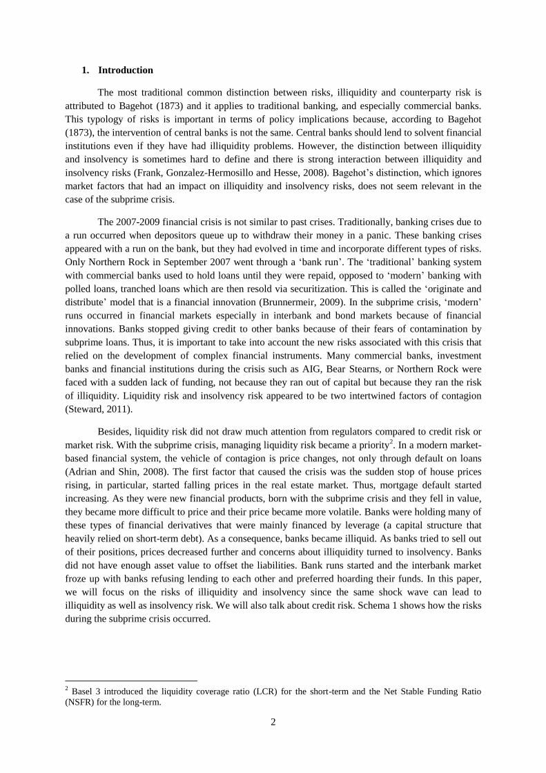
Besides, liquidity risk did not draw much attention from regulators compared to credit risk or

market risk. With the subprime crisis, managing liquidity risk became a priority2. In a modern market-

based financial system, the vehicle of contagion is price changes, not only through default on loans

(Adrian and Shin, 2008). The first factor that caused the crisis was the sudden stop of house prices

rising, in particular, started falling prices in the real estate market. Thus, mortgage default started

increasing. As they were new financial products, born with the subprime crisis and they fell in value,

they became more difficult to price and their price became more volatile. Banks were holding many of

these types of financial derivatives that were mainly financed by leverage (a capital structure that

heavily relied on short-term debt). As a consequence, banks became illiquid. As banks tried to sell out

of their positions, prices decreased further and concerns about illiquidity turned to insolvency. Banks

did not have enough asset value to offset the liabilities. Bank runs started and the interbank market

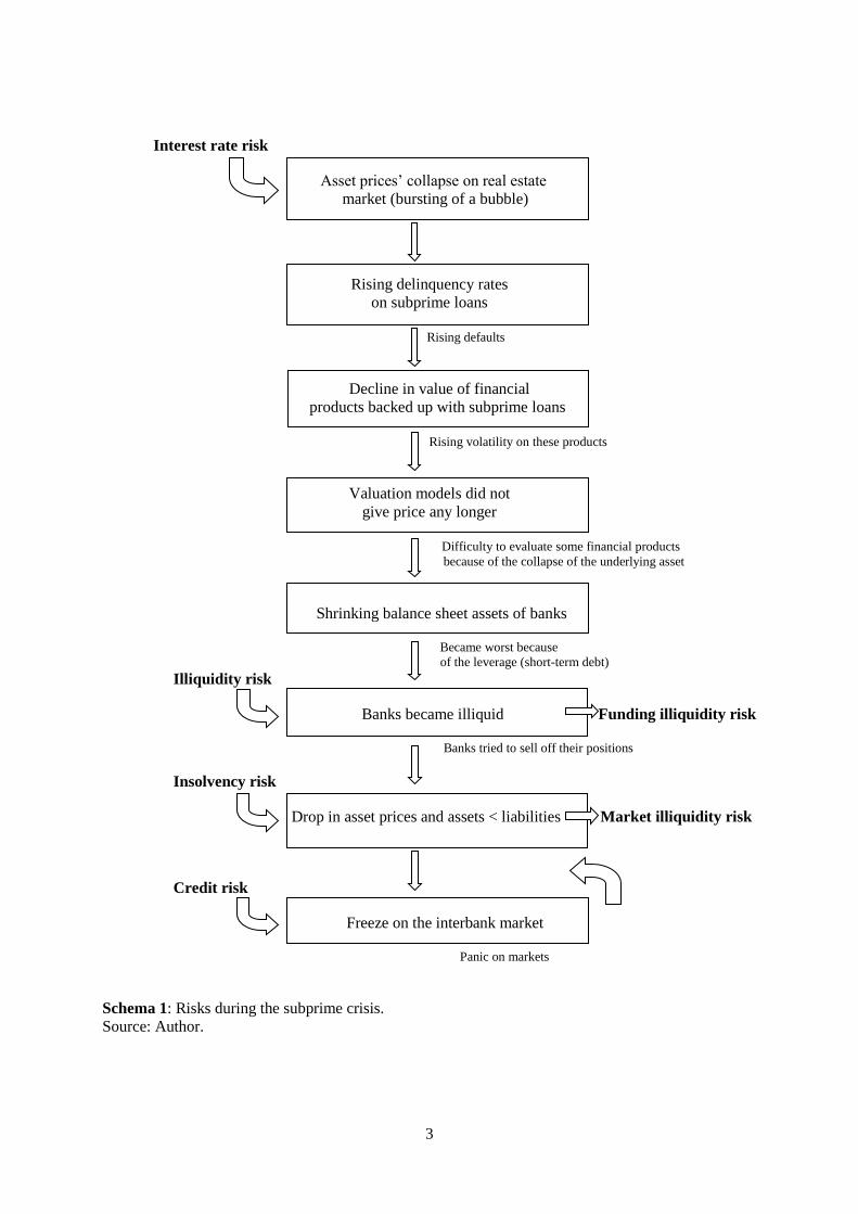
froze up with banks refusing lending to each other and preferred hoarding their funds. In this paper,

we will focus on the risks of illiquidity and insolvency since the same shock wave can lead to

illiquidity as well as insolvency risk. We will also talk about credit risk. Schema 1 shows how the risks

during the subprime crisis occurred.

2 Basel 3 introduced the liquidity coverage ratio (LCR) for the short-term and the Net Stable Funding Ratio

(NSFR) for the long-term.

3

Interest rate risk

Asset prices’ collapse on real estate

market (bursting of a bubble)

Rising delinquency rates

on subprime loans

Rising defaults

Decline in value of financial

products backed up with subprime loans

Rising volatility on these products

Valuation models did not

give price any longer

Difficulty to evaluate some financial products

because of the collapse of the underlying asset

Shrinking balance sheet assets of banks

Became worst because

of the leverage (short-term debt) Illiquidity risk

Banks became illiquid Funding illiquidity risk

Banks tried to sell off their positions

Insolvency risk

Drop in asset prices and assets < liabilities Market illiquidity risk

Credit risk

Freeze on the interbank market

Panic on markets

Schema 1: Risks during the subprime crisis.

Source: Author.

4

Bank contagion is specific to banking and differs from financial contagion as it is global.

Studies on bank and financial contagion use Dynamic Conditional Correlation (DCC) to measure

spillover effects during a crisis. Our approach focusing on bank contagion is innovative in the sense

that many previous studies focused on financial contagion and measured spillover effects through

market indices3. We suppose that correlation is dynamic, which is time-dependant. By accounting for

the time-varying behavior of our data series, we can detect changes in integration over time.

Integration refers to the same dynamics conditional correlation changes between banks. Thus, the

timing of events that occurred during the subprime crisis has been identified endogenously, and there

is no need to identify the events as we have done in our previous paper4. Moreover, DCC specification

allows to take into account possible structural breaks that occurred in the unconditional correlations

amongst the variables over the period of interest. Our methodology focused on individual banks, thus

allowing us to distinguish between the most affected banks instead of taking a global approach to

countries or market indices. Besides, estimating the market assessment of bank credit risk, or default is

relevant to policy implications and more especially to macro prudential policies. By using multivariate

GARCH models instead of the univariate model, we jointly analyze the volatility of two financial

institutions and assessed the links between these two series.

Moreover, we also considered how abnormal returns (either positive or negative) came about

around the ‘event window’ of Lehman Brothers’ bankruptcy. Using panel data and regressions, we

identified a set of explanatory variables that are specific to banks and can explain these abnormal

returns. Liquidity variables appear to be of a great importance to explaining the abnormal returns. The

rest of the paper is organized as follow. First, we review the questions we address in this paper. In the

second section we focus on the risk typology and present a literature review. In the third part, we deal

with the data. In the fourth part, we develop the theoretical model of the dynamic conditional

correlation. In the fifth part, we present the methodology of the DCC analysis. In the sixth part, we

give the result of the DCC analysis. In the seventh part, we give details on the determinants of banks’

abnormal returns. In the last section, we conclude.

Questions

Did Lehman Brothers’ bankruptcy on September 15th 2008 trigger off a liquidity risk or do

other major events have a more significant impact on banks’ performance?

Are there any spillover effects, or common movement of the Credit Default Swaps (CDS)

spread of U.S. banks and Europeans banks?5 If the spreads of different banks move independently,

then it is likely that the risk of bank failure is driven by bank-specific factors. On the contrary if they

move together, they have the same DCC changes, and all banks are perceived by investors as subject

to common risks. In the first case, spillover effects are the results of banks’ specific factors and in the

second case, they refer to a common risk. This typology of contagion was used in our previous paper6.

What are the determinants of banks abnormal returns on the ‘event window’ of Lehman

Brothers’ bankruptcy? What banks’ specific variables were significant?

3 An international Conference was organized on this topic on October, 28

th-29

th 2011 by AEJ

Macro/BDF/CEPR/ECARES/PSE. Spillover effects between countries measured by financial channel were on

purpose. 4 Suzanne Salloy (2011), “Bank Contagion during the subprime crisis: an empirical study on American and

European markets”. 5 Eichengreen (2009) answered to this question with the Principal Component Analysis (PAC).

6 See reference 4.

5

2. Risks typology and literature review

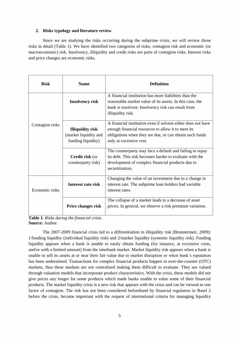
Since we are studying the risks occurring during the subprime crisis, we will review those

risks in detail (Table 1). We have identified two categories of risks; contagion risk and economic (or

macroeconomic) risk. Insolvency, illiquidity and credit risks are parts of contagion risks. Interest risks

and price changes are economic risks.

Risk

Name

Definition

Contagion risks

Insolvency risk

A financial institution has more liabilities than the

reasonable market value of its assets. In this case, the

bank is insolvent. Insolvency risk can result from

illiquidity risk.

Illiquidity risk

(market liquidity and

funding liquidity)

A financial institution even if solvent either does not have

enough financial resources to allow it to meet its

obligations when they are due, or can obtain such funds

only at excessive cost.

Credit risk (or

counterparty risk)

The counterparty may face a default and failing to repay

its debt. This risk becomes harder to evaluate with the

development of complex financial products due to

securitization.

Economic risks

Interest rate risk

Changing the value of an investment due to a change in

interest rate. The subprime loan holders had variable

interest rates.

Price changes risk

The collapse of a market leads to a decrease of asset

prices. In general, we observe a risk premium variation.

Table 1: Risks during the financial crisis.

Source: Author.

The 2007-2009 financial crisis led to a differentiation in illiquidity risk (Brunnermeir, 2009):

1/funding liquidity (individual liquidity risk) and 2/market liquidity (systemic liquidity risk). Funding

liquidity appears when a bank is unable to easily obtain funding (for instance, at excessive costs,

and/or with a limited amount) from the interbank market. Market liquidity risk appears when a bank is

unable to sell its assets at or near their fair value due to market disruption or when bank’s reputation

has been undermined. Transactions for complex financial products happen in over-the-counter (OTC)

markets, thus these markets are not centralized making them difficult to evaluate. They are valued

through valuation models that incorporate product characteristics. With the crisis, these models did not

give prices any longer for some products which made banks unable to value some of their financial

products. The market liquidity crisis is a new risk that appears with the crisis and can be viewed as one

factor of contagion. The risk has not been considered beforehand by financial regulators in Basel 2

before the crisis, became important with the request of international criteria for managing liquidity

6

risk. The importance of an increase in liquidity risk during the crisis entailed many interventions of

central banks to inject funds in order to avoid a freeze on the markets.

Traditional approaches to measuring liquidity risks rely on historical accounting data of bank balance

sheets, such as the ration of loans to deposits. This measure is not adequate for assessing the liquidity

risk of investment banks. Only a few of these ratios incorporate off-balance sheet commitments.

Another major risk factor of contagion is the risk of insolvency. During the financial crisis,

after prices decreased or financial products could not be valued, banks tried to shrink their balance

sheets as they found out that their capital eroded. Funding illiquidity risk then materialized and banks

became concerned about their future access to capital markets and started hoarding funds. As a

consequence, banks tried to sell off some of their positions. This effect was reinforced by the fact that

banks heavily relied on leverage, such as short-term borrowing. Market illiquidity risk was observed

through a sharp drop in asset prices. This illiquidity risk transformed into insolvency risk when the

assets of a bank are not sufficient compared to its liabilities. Insolvency risk is the risk of loss owing to

bankruptcy of an issuer of a financial asset or to the insolvency of the counterparty. Insolvency risk is

likely to be interconnected with illiquidity risk. Even though illiquidity and insolvency risks are

interconnected, liquidity risk does not necessarily imply that the counterparty is insolvent.

Some further risks appeared during the crisis such as credit risk. The nature of credit risk

changed due to securitization. Securitization allows for a system where loans are heterogeneous and

held by a bank to a system with polled loans, tranched loans and then resold to other investors on

financial markets with the intervention of many brokers. By definition, derivative markets are over-

the-counter markets (OTC), and they involve a difficulty to estimate credit risk. Credit risk spread and

moral hazard allow banks to become less prudent when giving credit loans since they can sell then the

credit, and were not obliged to keep them in their balance sheet.

Our paper focuses on the distinction between illiquidity and insolvency risk and also takes into

account the credit risk as it is linked to the development of securitization.

Review of literature

Table 2 synthesizes the principal studies which deal with contagion, either related to finance

or banking. Assessing contagion through the use of correlation is used increasingly. Since

unconditional correlation, to dynamic conditional correlation (DCC) by Engle (2002) to DCC

specification by Cappiello, Engle and Sheppard (2006), techniques to detect contagion through

correlation have improved. The last specification allows to take into account the dynamics of

correlation and structural breaks (Frank, Gonzalez-Hermossillo and Hesse, 2008). They argue that the

first specification by Engle (2002) the autoregressive parameterization implies, that the conditional

correlations are a mean reverting to their constant long-run unconditional average, so that the shock is

transitory. Under the DCC specification by Capiello and al. (2006), the subprime crisis can be

modeled as a structural break in the data generating processes, rather than a transitory shock. Dooley

and Hutchison (2009) through event studies had to specify 15 types of events and assess the market

responses. This event study methodology was also used in our previous paper. Other versions of the

DCC model have been implemented such as DCC-EGARCH (Alraigbat, 2011), G-DCC (Hafner and

Franses, 2009), DCC-GARCH (Wang and Moore, 2012). These studies generally use the log

likelihood estimator which allows for consistent standard errors robust to non normality.

7

Some other studies focus on banks’ performance determinants or bank liquidity risk which in

turn uses a panel database with individual data. Most of the time, the panel is dynamic with the lagged

explanatory variables in the regressors to allow for a dynamics. In such a case, fixed effects and

random effects are implemented with control variables and robustness tests (Rauning and Scheicher

(2009), Omotola, Roya and Safoura (2011), and Shen, Chen, Kao and Yeh (2009)). Generally the

estimator used is General Method of Moments (GMM), Two Stages Least Squares (TSLS) or General

Least Squared (GLS).

When financial contagion is assessed, authors used stock market variables, such as stock

market indices (Naoui, Liouane and Brahim, 2010) and Alrgaibat (2011). Yet, some studies focus on

bank specific variables and look at bank contagion. Risks are identified and proxies for each type of

risks are proposed. Macroeconomic variables allow to control for shocks. These are mainly GDP

growth and inflation variables and are relevant when banks of different countries are assessed.

Concerning the variables, it is interesting to recall that, credit risk is proxied by Credit Default Swap

(CDS), either banks CDS or sovereign bonds CDS. CDS spreads reflect the market’s assessment of

credit market risk (Longstaff and al, 2007). They are an indicator of the depth of the crisis (Wang and

Moore, 2012). Eichengreen and al. (2009) using data on banks’ credit default swaps for 45 banks in

developed economies, investigated the importance of common factors to explain their spreads.

Athanasoglou and al. (2008) implemented a series of bank-variables for Greek banks such as credit

risk, productivity, expense management, size, industry-specific profitability determinants such as

ownership, concentration and macroeconomic profitability determinants such as inflation expectations,

cyclical output to assess the determinants of Greek commercial banks’ profitability.

For the purpose of our paper, we focus on results applying to the 2007-2009 financial crises,

emanating principally from the USA. Frank, Gonzalez-Hermosillo and Hesse (2008) showed that the

interaction between market and funding illiquidity increased sharply during the subprime crisis and

bank solvency became an important issue. Wang and Moore (2012) found out that Lehman Brothers

bankruptcy strengthened the integration between sovereign CDS bonds of developed economies with

the USA. In terms of the driving factors of this correlation, they concluded that CDS bonds markets

were mainly driven by USA interest rates. Wang and Moore (2012) focused on the unconditional

correlations of weekly changes in CDS spreads between the US and others markets and on the

conditional correlation between US and non-US CDS spreads. By using a bivariate DCC-GARCH

model, they found out that the dataset fitted the model specification very well in most cases. By

looking at the DCC series for each country, they found out that the pattern of correlation changed

significantly before and after the Lehman Brothers’ bankruptcy. They concluded that Lehman

Brothers bankruptcy was seen as a major event during the crisis and contributed to the integration of

the CDS markets amongst advanced economies. Rauning and Scheicher (2009) focusing on individual

bank data, found out that after August 2007, investors increased their perception of risk concerning

banks. Finally, Eicheengreen (2009) showed that common factors for banks’ CDS play a major role in

explaining the spillover effects between banks.

8

Authors Problem Data Contagion Sample Period Country RisksVariables to

explainMethodology Estimator Results

Athanasoglou, Brissimis and Delis

(2008)

Examined the effect of bank-specific,

industry-specific and macroeconomic

determinants of bank profitability.

Individual Banking

38

Commercial

banks

1985-2001 Greece Credit riskProfitability (

ROA/ROE)Dynamic panel GMM

Profitability of Greek banks was

shaped by bank-specific factors,

macroeconomic, and control

variables that were not the result of

bank's managerial decision.

Eicheengreen (2009)

Examined how the common factors

influenced the movement of the 45

largest banks' CDS spreads at different

time of the crisis.

Individual Banking

45

developped

banks

July 29, 2002-

November 28,

2008 (weekly)

Developped

Credit

risk/Liquidity

risk/Interest

rate risk

CDS of banks

1/Principal

Component

Analysis. 2/

Dynamic panel

GMMCommon factors played a major role

==> irrational contagion

Rauning and Scheicher (2009)Examined how investors in the

corporate debt market view banks.Individual Banking

41 banks

(largest in

EUR and USA)

and 162 non-

banks

January 2003-

December

2007 (monthly)

US and

EUROPE

Credit

risk/Interest

rate risk

CDS of banks

Fixed effect (FE)

and random effect

(RE) panel

Panel robust

estimates

After August 2007 ==> investors

viewed banks at least at risky as

other firms.

Shen, Chen, Kao and Yeh (2009)

Causes of liquidity risk and the

relationship between bank liquidity

risk and performance.

Individual Banking

12

commercial

banks

1994-2006

(annual)Developped Liquidity risk

Financing gap

ratio/short

term

funding/net

loans to

customers

Panel data

instrumental/FE2SLS

Liquidity risk decreased banks'

profitability.

9

Table 2: Synthesis of the principal studies on contagion.

Source : Author.

Authors Problem Data Contagion Sample Period Country RisksVariables to

explainMethodology Estimator Results

Frank, Gonzalez-Hermosillo and Hesse

(2008)

Estimated the linkages between

market and funding liquidity

pressures, and their interaction with

solvency issues during the 2007

subprime crisis.

Global Financial5 US financial

markets

January 3rd

2003 - January

9th 2008

USA

Liquidity risk

(funding and

market)

Spreads

DCC-GARCH (2006 :

Capiello, Engle

and Sheppard)

1/ Monte carlo.

2/Boostrap

The interaction between market and

funding illiquidity increased sharply

during the subprime crisis and the

bank solvency became important

issue.

Dooley and Hutchison (2009)

Analysis of the spillover effect of the

US subprime crisis on sovereign CDS

spreads of emerging markets.

Global Financial14 emerging

markets

January 1, 2007

- February,

2009 (dally)

Emerging Credit riskCDS sovereign

bonds

1/ Event study on

15 types of news.

2/ VAR model

1/OLS.2/Granger

causality test

Emerging markets were insulated

from the subprime crisis before

Lehman Brothers shock in 2008, but

were infected after the Lehman

crisis by the deteriorating situation

of the US financial system.

Naoui, Liouane and Brahim (2010)

Examined financial contagion

following the American subprime

crisis using Dynamic Conditional

Correlation Model.

Global Financial

6 developped

and 10

emerging

January 3, 2006

- February 26,

2010 (daily)

Developped

/EmergingMarket risk Market indices

DCC-GARCH

(Engle, 2002)Log likelihood

Amplification of dynamic conditional

correlations worldwide during the

crisis period.

Alrgaibat (2011)

Examined the presence of a

symmetric conditional second

moments in major European stock

markets.

Global Financial

3 developped

European

countries

January 1990 -

April 2009

(daily)

DAX

30/CAC40/FT

SE100

Market risk Market indices DCC- EGARCH Log likelihood

The index return series showed a

great asymmetry in conditional

volatility after a shock.

Wang and Moore (2012)

Invistigated the interaction of the CDS

markets of 38 developped and

emerging countries with the US

market during the subprime crisis.

Identification of the driving factors of

this relationship.

Global Financial 38 countries

January 2007 -

December

2009 (weekly)

Developped

/Emerging

Credit

risk/Interest

rate risk

CDS sovereign

bonds

1/DCC-Mutivariate

GARCH (Engle,

2002). 2/Panel

linear model of

DCC

Quasi-maximum

likelyhood

(consistant

standard errors

robust to non

normality)

1/Lehman Brothers shock have

strengthened the integration, in

particular for developped markets.

2/ CDS market driven by the US

interest rates.

10

3. Data for the DCC analysis

We have studied the risks that emerged during the subprime crisis on derivative markets and

we needed the CDS premiums of Financial Institutions (FI) listed on Stoxx 600 and S&P 500 as we

focus on Europe and the U.S. A Credit Default Swap (CDS) is an insurance contract. The buyer of a

CDS makes a payment to the seller called the premium in order to receive a payment if a credit

instrument (a bond or a loan) goes into default or in the event of a specified credit event, such as

bankruptcy (Eichengreen and al., 2009). Brunnermeir (2009) defined CDS as contracts insuring

against the default of a particular bond or tranche. The buyer of these contracts pays a periodic fee in

exchange for a contingent payment in the event of credit default. We will use CDS of banks on a five

year maturity as it is the most traded maturity on the derivative markets. Thus, we collected the CDS

over a five year maturity of our banks and financial institutions.

Our database is built using DataStream. First, we collected CDS spreads from all European

banks and financial institutions. Our sample included 28 banks and 6 financial service institutions

representing 34 European FI. Secondly, we collected CDS spreads from all American banks and

financial institutions. Our sample included 7 banks and 4 financial services institutions representing 11

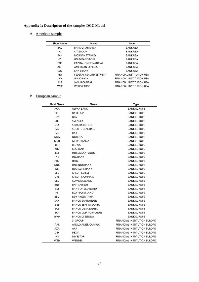
American FI. The European and American samples are shown in Appendix 17.

The dependent variable that we wish to explain is the daily changes in the CDS spreads for

each bank or financial institution in our sample. Because we worked with time series, it is possible that

our series were not stationary. The unit root tests (UR) panel are tests of UR on multiple series that

have been applied to the structure of our panel data. The literature suggests that these tests are more

powerful than tests based on UR time series individually. Two generations of tests exist for the panels.

The first takes into account individual heterogeneity and the second is based on a more general

specification by challenging the assumption of independence between individuals. Assumptions are

made on the regression coefficient itself. In the LLC and Breitung tests, this coefficient is the same for

all individuals in the sample. In tests of IPS ADF and PP, this parameter varies between individuals.

These tests are precisely the combination of individual tests UR. Tests Levin, Lin & Chu and Breitung

do not take into account dependencies between individuals, while the tests Im, Pesaran and Shin ADF

and PP take into account the correlation between individuals.

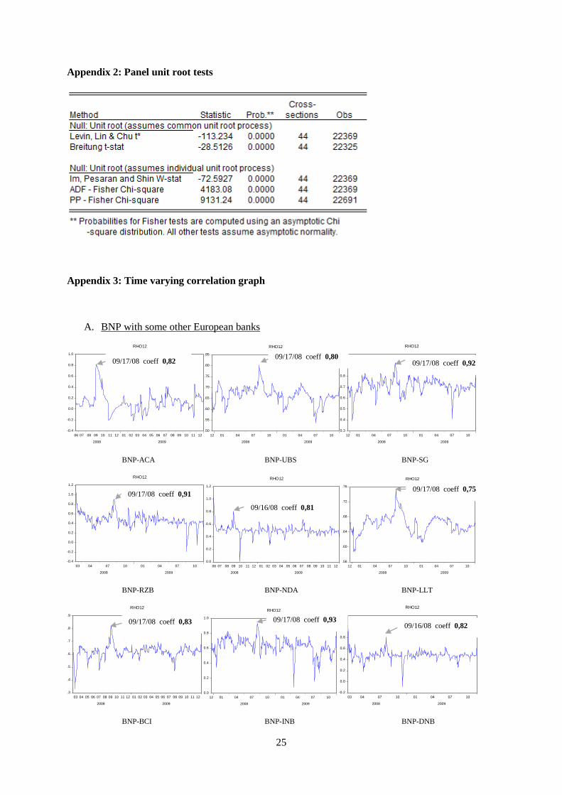
We present in Appendix 2, the results of unit root test in panel data on our samples of

European and American banks and FI. Regardless of the selected test, all lead to the rejection of the

hypothesis of no stationarity. The panel unit root test suggested that changes in the CDS spreads were

stationary variables.

4. Theoretical model: the Dynamic Conditional Correlation

Below, we give details of the theoretical model we used in our study. This model is the

Dynamic Conditional Correlation (DCC) specification used by Engle (2002) and it is part of

multivariate GARCH models. This model is a generalization of the Constant Conditional Correlation

Model (CCC) developed by Bollorsev in 1990. DCC model were used to give a time characteristic to

7 The number of banks and financial institutions in our samples both European and American is smaller than the

number of banks and FI listed on Stoxx 600 and S&P 500. We dropped some banks from our study since the

data on five year CDS were not available on DataStream.

11

the correlation matrix as a time varying correlation matrix. This correlation matrix is obtained

by a combination of standardized residual covariances’(Qt).

The bivariate GARCH model with Dynamic Conditional Correlation (DCC) specification (Engle,

2002) is applied to banks’ CDS spreads in pairs of banks. Let [ ] be a 2 x 1 vector

containing the two CDS in a conditional mean equation as follows:

and | )

Where is a 2 x 1 vector of constant, and [ ] is a vector of innovations conditional on the

information at the time ) The error term is assumed to be conditionally multivariate normal

with mean zero and variance-covariance matrix as,

Where is a 2 x 2 diagonal matrix of the time varying standard deviations from univariate GARCH

models with √ on the ith diagonal. is a 2 x 2 time-varying symmetric conditional correlation

matrix.

The elements in follow the univariate GARCH process of the following:

) (2)

Where is a constant term, captures the ARCH effect (the conditional volatility) and measures

the persistence of volatility.

The evolution of the correlation in the DCC model is given by:

) (3)

Where { } is a 2 x 2 conditional variance covariance matrix of residuals with its time-invariant

variance-covariance matrix )

The correlation matrix is ) )

A typical element of has the form of

√ , i, j = 1,2 and i ≠ j, this represents the

conditional correlation between each pairwise of financial institutions. (5)

Bauwens and al. (2003) give a detailed literature review of the multivariate GARCH model

(MGARCH). Generally, the specification of the matrix is the following:

[

]

Where , i=1,N are the conditional standard deviation of all banks and i=1,N and j=1,N and i ≠

j, the conditional covariance’s.

specification depends on and matrix specifications.

12

[

]

And [

]

[ √ √ √

√ √ √

√ √ √ √

√ √ √ ]

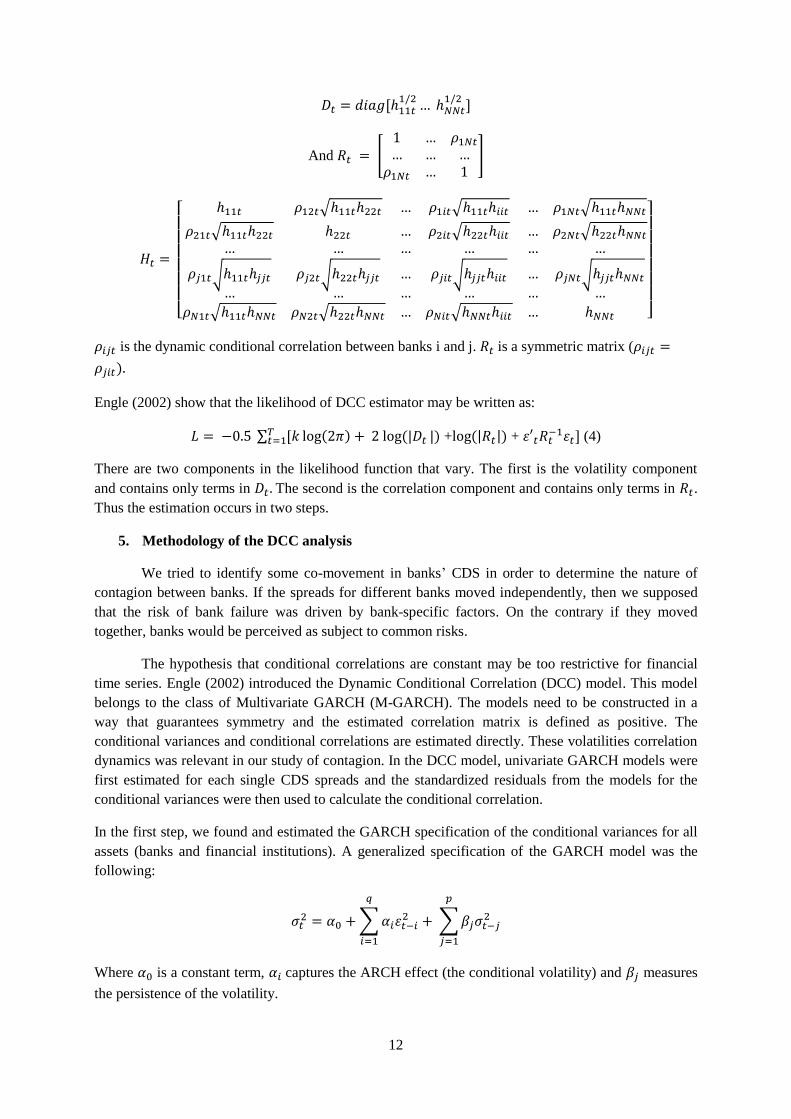
is the dynamic conditional correlation between banks i and j. is a symmetric matrix (

)

Engle (2002) show that the likelihood of DCC estimator may be written as:

∑ [ ) ) + ) +

] (4)

There are two components in the likelihood function that vary. The first is the volatility component

and contains only terms in The second is the correlation component and contains only terms in .

Thus the estimation occurs in two steps.

5. Methodology of the DCC analysis

We tried to identify some co-movement in banks’ CDS in order to determine the nature of

contagion between banks. If the spreads for different banks moved independently, then we supposed

that the risk of bank failure was driven by bank-specific factors. On the contrary if they moved

together, banks would be perceived as subject to common risks.

The hypothesis that conditional correlations are constant may be too restrictive for financial

time series. Engle (2002) introduced the Dynamic Conditional Correlation (DCC) model. This model

belongs to the class of Multivariate GARCH (M-GARCH). The models need to be constructed in a

way that guarantees symmetry and the estimated correlation matrix is defined as positive. The

conditional variances and conditional correlations are estimated directly. These volatilities correlation

dynamics was relevant in our study of contagion. In the DCC model, univariate GARCH models were

first estimated for each single CDS spreads and the standardized residuals from the models for the

conditional variances were then used to calculate the conditional correlation.

In the first step, we found and estimated the GARCH specification of the conditional variances for all

assets (banks and financial institutions). A generalized specification of the GARCH model was the

following:

∑

∑

Where is a constant term, captures the ARCH effect (the conditional volatility) and measures

the persistence of the volatility.

13

In a second step, with the estimates of the univariate GARCH equations, the conditional variance

can be used to derive the standardized GARCH residuals. Those standardized residuals are required to

model the dynamic correlation structure. Specifically, the correlation dynamics are estimated

according to DCC equation:

)

represents the time varying covariance matrix of the standardized residuals, the unconditional

covariance matrix of the standardized residuals, the estimated parameters of the DCC

equation. As in the GARCH equation, the covariance dynamics depends on past shocks and past

covariances. The normalization is the following:

) )

) is a diagonal matrix with the square roots of the diagonal as diagonal elements.

By multiplying by the reverse, the typical element of is the coefficient correlation of two assets and

the diagonal of consists of one as the correlation of one asset with itself is necessarily equal one.

and are parameters that capture the effect of previous shocks and previous dynamic conditional

correlations. In other words, measures the sensitivity due to shocks of correlations. measures

the autoregressive effects of shocks, in other words the volatility persistence.

6. Results of the DCC model for CDS

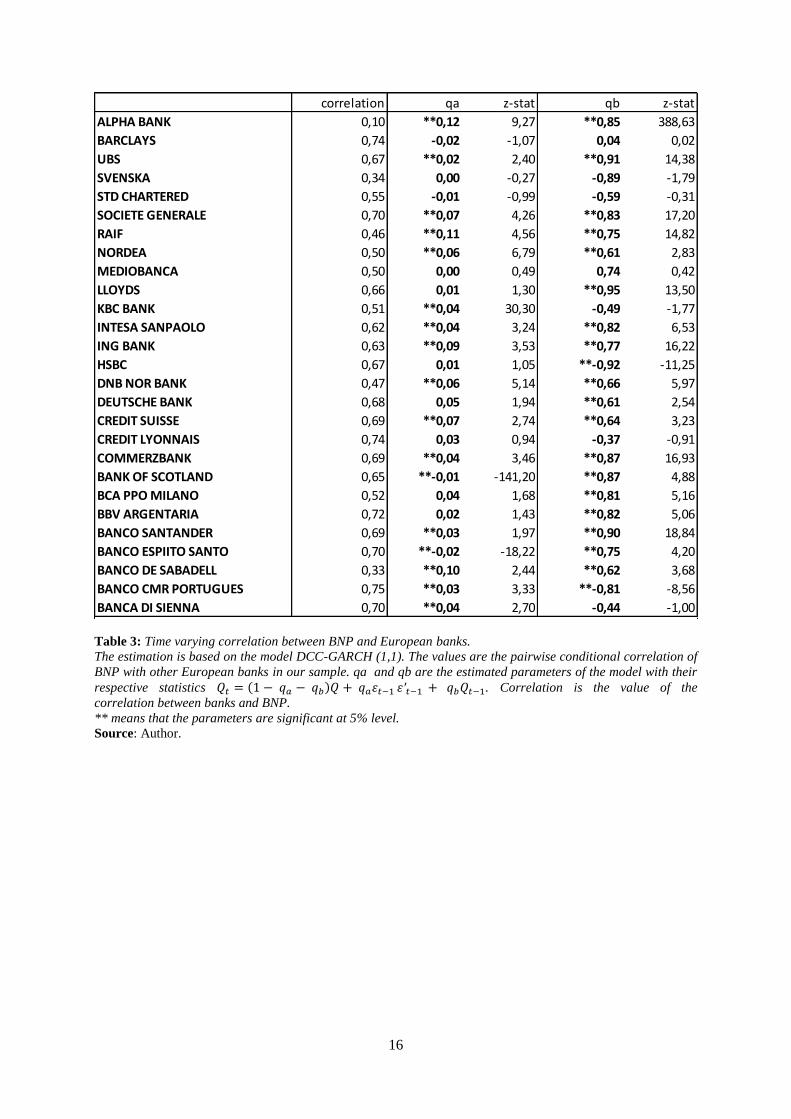
Tables 3, 4, 5 and 6 comprise the estimated results from the bivariate DCC-GARCH model

(see below for the explanation). Table 3 shows the results between European banks, table 4 between

European Financial institutions, table 5 between American banks and table 6 between American

financial institutions. Models are estimated using the quasi-maximum likelihood method to generate

consistent standard errors that are robust to non-normality.

The effect of time-varying correlation is captured by the coefficient qa and qb, which are the

parameters governing the DDC-GARCH process. qa is the sensitivity of correlations due to shocks

and qb is the volatility persistence. First we dealt with BNP time-varying correlation with all other

European banks (Table 3). The coefficients were overwhelmingly significant at the 5% percent level

with 17 out of 27 Europeans banks for qa and 19 out of 27 for qb. The significant coefficients qb are

those which had got the highest value, generally close to 1. This means that the effect of previous

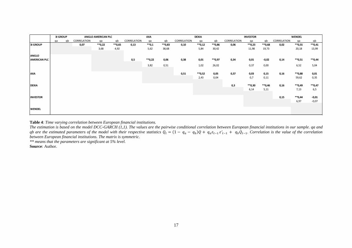
dynamic conditional correlations was high and significant for many European banks. Secondly, we

analyzed the results for the European financial institutions (Table 4). We constructed a dynamic

conditional cross correlation matrix between the financial institutions. In total, we computed 15 cross

conditional dynamic correlations. The parameter qa was significant for 12 correlations and qb for 12

correlations. As for European banks, qb coefficients are significant for financial institutions that had a

high coefficient. The effect of past shock is higher for European financial institutions that for banks.

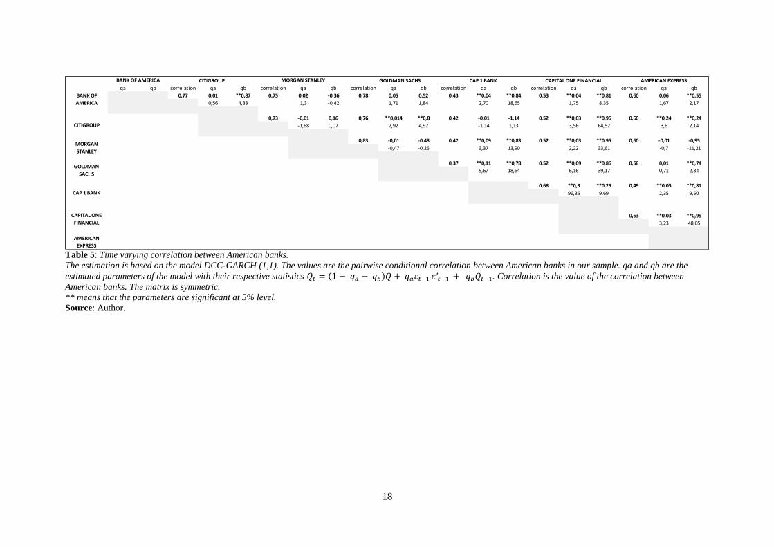
Now, let us turn to the American sample. We have 21 of cross correlation for American banks (Table

5). qa is significant for 12 of them and qb for 15. qb coefficients are significant for financial

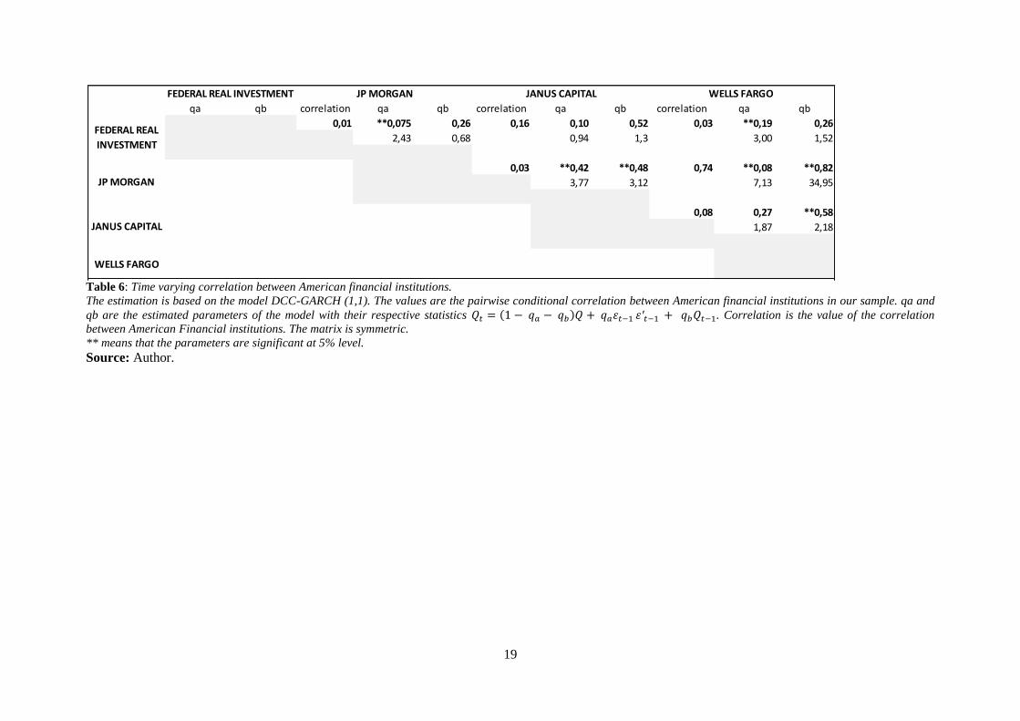
institutions that had high coefficient. Finally concerning the American sample of financial institution,

we have 6 conditional cross correlations (Table 6). qa is significant for 4 of them and qb for 3 of them.

In general the parameter qa is inferior to qb and qa is close to zero and qb to 1.

14

For the purpose of our study, we will focus on the value of the dynamic conditional correlation

between banks i and j at the time t, (Appendix 3). More precisely, we focused on the ‘event

window’ around LB’s bankruptcy. By definition, this correlation is conditional to prior information

(prior shocks) and evolving in time, which means not constant. For each pair of banks i and j, we have

this time varying conditional correlation. These values are represented in graphs to show the changes.

The parameters qa and qb help us to find out if these DCC parameters are significant. For

identification of contagion, a strong temporary increase in volatility correlations coefficients need to

be observed. On the contrary, a permanent increase in correlations which remain stable at the higher

level once the increase is completed is not contagion but interdependence. As a consequence, we

identified contagion effects if correlation measures increased significantly during the ‘event window’

of five days around Lehman Brother’s bankruptcy, but do not remain permanently on the higher level.

Graphs in Appendix 3 concerned banks and financial institutions for which the parameters qa and qb

were significant. These graphs show the evolution of conditional correlations during the subprime

crisis (12/17/2007-12/31/2009) for a sample of banks and FI8. We noted on each graph the ‘event

window’ around LB’s bankruptcy. The graph reports evolutions of dynamic conditional correlations

for each pairwise of banks. The contagion test, based on correlations, defines contagion as the

significant increase of CDS spread co-movements. Contagion is observed for a particular strong

correlation in time, but this change in pattern has to be temporary, otherwise, banks are qualified as

interdependent.

Let us now consider which banks or financial institution were the most affected by the LB’s

bankruptcy. We look at the graph of DCC for banks and FI that had significant parameters qa and qb.

For the others, the model was not significant and we did not focus on their changes in DCC

coefficients.

The panel A. of the Appendix 3 showed the estimated conditional correlations series using

DCC model for BNP with other European banks. We observed an increase in the coefficient

around LB bankruptcy, September 15th 2008 for all banks in our sample, except for Banco Epirito

Santo. The coefficient varied from 0.80 to 0.93 (and 0.33 for Espirito Santo). As this increase in the

correlation coefficients was brief in time and happened for all banks at the same time, we concluded

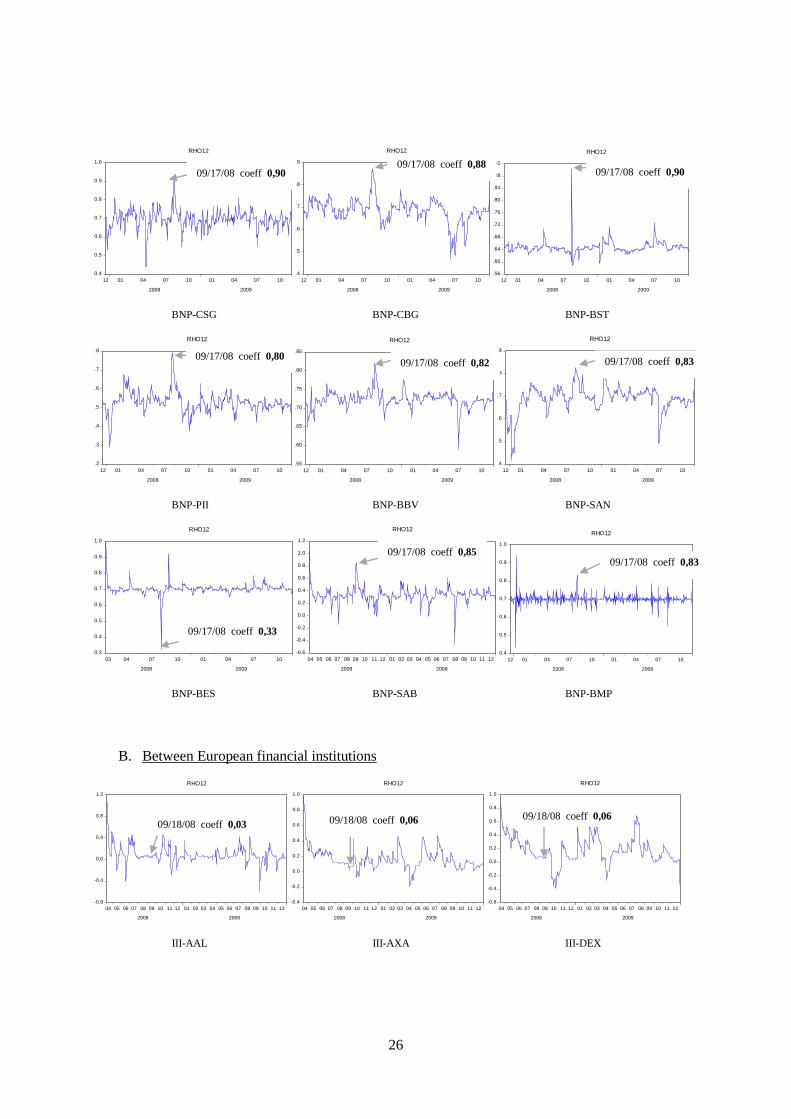
that LB’s bankruptcy was contagious for European banks. The panel B. of the Appendix 3 showed the

estimated conditional correlations series using DCC model for European financial institutions. We

have represented the changes in the correlation between pairs of financial institutions (FI). By looking

at the graphs, it was less clear that LB’s bankruptcy had a contagious impact on European FI. For

many FI, the highest point in correlation was not verified around LB’s bankruptcy, and the series

showed a strong volatility during the whole period in time. 3igroup had very low coefficient of

correlation with other FI on LB’s bankruptcy. Dexia seemed to have a strong volatility in its

correlation coefficient with other FI, even if the coefficient around LB’s bankruptcy increased. From

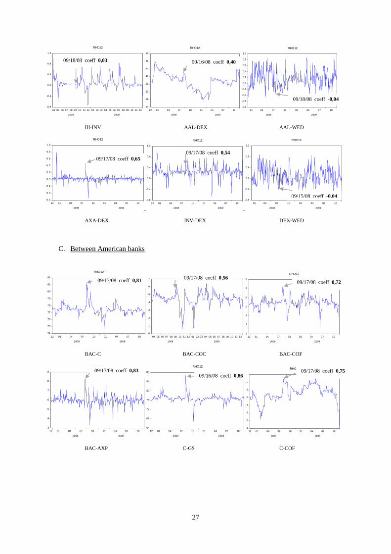
the graphs of European FI, we cannot infer that LB’s bankruptcy was contagious. The panel C. of

Appendix 3 showed the estimated conditional correlations series using DCC model for American

banks. The coefficients varied from 0.56 to 0.95 around LB’s bankruptcy and they were one of the

highest points in time for the banks. Even if some series showed a strong volatility of the correlation

coefficients at some other point in time, it was temporary and the increased around LB’s bankruptcy

was strong but brief in time. From these graphs, we infer that LB’s bankruptcy had negative spillover

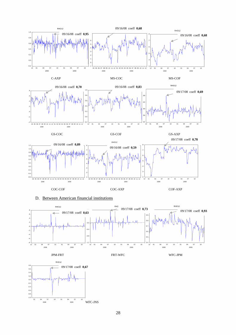
effects on American banks. Last, the panel D. of Appendix 3 showed the estimated conditional

8 Data on CDS spreads were not available at 12/17/2007 for some banks and FI, thus their graphs started later

depending on the availability of data.

15

correlation series using DCC model for American FI. We made the same remarks that for American

banks. The correlation coefficients around LB’s bankruptcy varied from 0.63 to 0.93.

In conclusion, for European and American banks as well as for American FI of the sample, we

observed an increase in the coefficient around LB’s bankruptcy, even if we observed a strong

volatility in the pattern of the DCC. Nevertheless, Lehman Brother’s bankruptcy led to the highest

values in the DCC for many banks and FI. These results show that LB bankruptcy was seen as a

contagious event by banks and FI on credit derivative markets. This is clear for many banks and FI in

the sample since, they had the same DCC around this event with a heightened correlation, a sign of a

spillover effect. Measuring the level of contagion is not permitted with this methodology, it just allows

to assess if there were events that caused spillover effects on other banks.

By looking at the graphs, we see evidence of increased correlations across all banks around September

15th, 2008 which corresponds to Lehman Brothers’ bankruptcy, implying higher interaction between

banks on the derivative market. Conditional correlations between banks considerably increased around

this event with value close to 1. As these dynamic conditional correlations are not stable in time and

seem to show a sharp increase for many banks during the LB’s bankruptcy, we can infer that this event

had a significant impact on bank contagion on the credit derivative market. In conclusion, the

importance of the CDS in explaining spillover effects between banks and FI is clear; credit risk played

a major role in the subprime crisis.

16

Table 3: Time varying correlation between BNP and European banks.

The estimation is based on the model DCC-GARCH (1,1). The values are the pairwise conditional correlation of

BNP with other European banks in our sample. qa and qb are the estimated parameters of the model with their

respective statistics ) . Correlation is the value of the

correlation between banks and BNP.

** means that the parameters are significant at 5% level.

Source: Author.

correlation qa z-stat qb z-stat

ALPHA BANK 0,10 **0,12 9,27 **0,85 388,63

BARCLAYS 0,74 -0,02 -1,07 0,04 0,02

UBS 0,67 **0,02 2,40 **0,91 14,38

SVENSKA 0,34 0,00 -0,27 -0,89 -1,79

STD CHARTERED 0,55 -0,01 -0,99 -0,59 -0,31

SOCIETE GENERALE 0,70 **0,07 4,26 **0,83 17,20

RAIF 0,46 **0,11 4,56 **0,75 14,82

NORDEA 0,50 **0,06 6,79 **0,61 2,83

MEDIOBANCA 0,50 0,00 0,49 0,74 0,42

LLOYDS 0,66 0,01 1,30 **0,95 13,50

KBC BANK 0,51 **0,04 30,30 -0,49 -1,77

INTESA SANPAOLO 0,62 **0,04 3,24 **0,82 6,53

ING BANK 0,63 **0,09 3,53 **0,77 16,22

HSBC 0,67 0,01 1,05 **-0,92 -11,25

DNB NOR BANK 0,47 **0,06 5,14 **0,66 5,97

DEUTSCHE BANK 0,68 0,05 1,94 **0,61 2,54

CREDIT SUISSE 0,69 **0,07 2,74 **0,64 3,23

CREDIT LYONNAIS 0,74 0,03 0,94 -0,37 -0,91

COMMERZBANK 0,69 **0,04 3,46 **0,87 16,93

BANK OF SCOTLAND 0,65 **-0,01 -141,20 **0,87 4,88

BCA PPO MILANO 0,52 0,04 1,68 **0,81 5,16

BBV ARGENTARIA 0,72 0,02 1,43 **0,82 5,06

BANCO SANTANDER 0,69 **0,03 1,97 **0,90 18,84

BANCO ESPIITO SANTO 0,70 **-0,02 -18,22 **0,75 4,20

BANCO DE SABADELL 0,33 **0,10 2,44 **0,62 3,68

BANCO CMR PORTUGUES 0,75 **0,03 3,33 **-0,81 -8,56

BANCA DI SIENNA 0,70 **0,04 2,70 -0,44 -1,00

17

Table 4: Time varying correlation between European financial institutions.

The estimation is based on the model DCC-GARCH (1,1). The values are the pairwise conditional correlation between European financial institutions in our sample. qa and

qb are the estimated parameters of the model with their respective statistics ) . Correlation is the value of the correlation

between European financial institutions. The matrix is symmetric.

** means that the parameters are significant at 5% level.

Source: Author.

INVESTOR WENDEL

qa qb CORRELATION qa qb CORRELATION qa qb CORRELATION qa qb CORRELATION qa qb CORRELATION qa qb

3I GROUP 0,07 **0,22 **0,65 0,13 **0,1 **0,83 0,10 **0,12 **0,86 0,06 **0,23 **0,68 0,02 **0,55 **0,41

3,68 4,92 5,62 38,68 5,84 30,42 11,98 19,73 20,18 13,99

ANGLO

AMERICAN PLC 0,5 **0,22 0,06 0,38 0,01 **0,97 0,34 0,01 -0,02 0,14 **0,51 **0,44

3,82 0,51 1,02 26,02 0,37 0,00 6,52 5,04

AXA 0,51 **0,52 0,05 0,37 0,03 0,15 0,16 **0,88 0,01

2,43 0,04 0,7 0,11 59,62 0,35

DEXIA 0,3 **0,30 **0,46 0,16 **0,49 **0,47

6,14 5,11 7,13 6,5

INVESTOR 0,15 **0,44 -0,01

6,97 -0,07

WENDEL

3I GROUP ANGLO AMERICAN PLC AXA DEXIA

18

Table 5: Time varying correlation between American banks.

The estimation is based on the model DCC-GARCH (1,1). The values are the pairwise conditional correlation between American banks in our sample. qa and qb are the

estimated parameters of the model with their respective statistics ) . Correlation is the value of the correlation between

American banks. The matrix is symmetric.

** means that the parameters are significant at 5% level.

Source: Author.

CITIGROUP GOLDMAN SACHS CAP 1 BANK

qa qb correlation qa qb correlation qa qb correlation qa qb correlation qa qb correlation qa qb correlation qa qb

0,77 0,01 **0,87 0,75 0,02 -0,36 0,78 0,05 0,52 0,43 **0,04 **0,84 0,53 **0,04 **0,81 0,60 0,06 **0,55

0,56 4,33 1,3 -0,42 1,71 1,84 2,70 18,65 1,75 8,35 1,67 2,17

0,73 -0,01 0,16 0,76 **0,014 **0,8 0,42 -0,01 -1,14 0,52 **0,03 **0,96 0,60 **0,24 **0,24

-1,68 0,07 2,92 4,92 -1,14 1,13 3,56 64,52 3,6 2,14

0,83 -0,01 -0,48 0,42 **0,09 **0,83 0,52 **0,03 **0,95 0,60 -0,01 -0,95

-0,47 -0,25 3,37 13,90 2,22 33,61 -0,7 -11,21

0,37 **0,11 **0,78 0,52 **0,09 **0,86 0,58 0,01 **0,74

5,67 18,64 6,16 39,17 0,71 2,34

0,68 **0,3 **0,25 0,49 **0,05 **0,81

96,35 9,69 2,35 9,50

0,63 **0,03 **0,95

3,23 48,05

BANK OF AMERICA CAPITAL ONE FINANCIAL AMERICAN EXPRESSMORGAN STANLEY

BANK OF

AMERICA

CITIGROUP

MORGAN

STANLEY

GOLDMAN

SACHS

CAP 1 BANK

CAPITAL ONE

FINANCIAL

AMERICAN

EXPRESS

19

Table 6: Time varying correlation between American financial institutions.

The estimation is based on the model DCC-GARCH (1,1). The values are the pairwise conditional correlation between American financial institutions in our sample. qa and

qb are the estimated parameters of the model with their respective statistics ) . Correlation is the value of the correlation

between American Financial institutions. The matrix is symmetric.

** means that the parameters are significant at 5% level.

Source: Author.

FEDERAL REAL INVESTMENT

qa qb correlation qa qb correlation qa qb correlation qa qb

0,01 **0,075 0,26 0,16 0,10 0,52 0,03 **0,19 0,26

2,43 0,68 0,94 1,3 3,00 1,52

0,03 **0,42 **0,48 0,74 **0,08 **0,82

3,77 3,12 7,13 34,95

0,08 0,27 **0,58

1,87 2,18

FEDERAL REAL

INVESTMENT

JP MORGAN

JANUS CAPITAL

WELLS FARGO

JP MORGAN JANUS CAPITAL WELLS FARGO

20

7. The determinant of banks’ abnormal returns

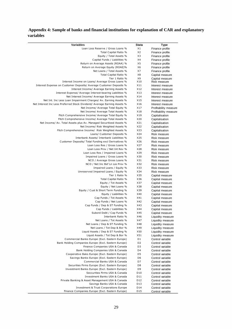
We examined the driving forces behind the abnormal returns9 during the subprime crisis on a linear

framework of a sample of banks (Appendix 4). We implemented three different regressions to explain

AR with a bunch of explanatory variables, such as CDS, leverage, credit rating...We had a panel

database. The explanatory variables were bank specific variables (Appendix 4). All the data were

extracted from Bankscope database from the end of the 2007, the last data available before LB’s

bankruptcy. No interim data were available from mid-2008. The explanatory variables were of

different types and we included dummy variables for the type of the banks. The types of the

explanatory variables were finance profile, capital measure, risk measure, interest measure,

capitalization, and liquidity measure.

The first model is a probit model on panel data. The variable to explain equals one or zero and is the

probability of a bank having AR around the ‘even window’ of LB’ bankruptcy. On the contrary, this

variable is equal to zero if the bank does not have AR on the event day around the bankruptcy. The

model is binary and the explanatory variable equals one if the bank had significant AR on the ‘event

window’ of five days (2 days before and two days after LB’s bankruptcy) and 0 if the bank had no

significant AR on the ‘event window’ ( )). The explanatory variables that are balance sheets

ratios available at the year 2007 are noted We created 15 dummies variables referring to the

type of the bank, noted . The error term of the probit panel regression is noted The constant of

the model is . The model is estimated with the maximum log likelihood estimator.

Model [1] ) ∑ ∑

The second model is a panel regression and the variable to explain is the value of the AR if it is

significant or zero if it is not. The idea of this model is to focus on significant AR.

Model [2] ) ∑ ∑

) is the variable to explain. It takes the value of the AR if they are significant on the ‘event

window’ around LB’s bankruptcy and zero if there are not significant on the ‘event date’. are

the observed explanatory variables of the model. are that explanatory variables that are dummies

variables.

The third model simply focuses on the value of all AR, significant and not significant around the

‘event window’ of LB’s bankruptcy.

Model [3] ) ∑ ∑

Where ) takes the value of the AR, significant as well as not significant.

For each model, we have five variables to explain since the ‘event window’ is five days. Only random

effects were considered in the models [2] and [3], because the explanatory variables are constant for

each bank. No fixed effects were allowed by the specification. We are explaining the AR, not for each

bank, but for the whole sample.

9 The computation of AR is detailed in my previous paper. See reference 4. An abnormal return (AR) at time t is

the difference between an observed return in t and a ‘normal return’ taking into account all the available

information until t. An AR is the difference between an observed return impacted by an event and a ‘normal’

return with no impact of an event. The ‘normal’ return is not observed and need to be implemented with a model

market model. In our study, AR were implemented with the Capital Asset Price Model.

21

The results for the three models are the following. From model [1], we concluded that the type of the

bank was important in explaining the probability of a bank to have AR. Bank holding companies and

saving banks in the USA and Canada were more likely to face AR around LB’s bankruptcy. On the

contrary commercial banks in Europe had a low probability for having AR. The variable customer

deposit/total funding ratio was not significant in this model. Neither were the case for total assets/total

deposit and short term funding.

From model [2], the type of banks was also important and a bank was more subject to have significant

AR if it was a bank holding companies in the USA & Canada. The types of commercial banks in

Europe and savings banks in USA and Canada had a negative impact on the significance of AR.

Moreover, the ratio of liquid asset/total deposit and borrowing had a negative impact on the

significance of AR as opposed to net loans/total assets, interbank ratio, customer deposit/total funding

and equity/total asset ratios which had a positive impact on AR.

From model [3], the type of the bank as Bank holding companies in the USA & Canada also had a

positive impact on AR. This was not the case for commercial banks in Europe and savings banks in

USA and Canada. Meanwhile interbank ratio and equity/liabilities ratio had a positive impact on AR,

liquid assets/total deposit and borrowing had a negative one. The net loans/total assets ratio had a

positive impact on AR. We concluded that the type of a bank is important for understanding AR

especially for bank holding companies in the USA & Canada. The liquidity is a determinant in

explaining AR.

8. Conclusion

In this paper, we explained abnormal returns (AR) and also identified dynamics between

banks in credit market.

We wanted to assess the spillover effect during the Lehman Brothers’ bankruptcy by

analyzing dynamic conditional correlation movements between banks. We focused on banking

contagion, and we had specific data for individual bank (CDS and AR). A multivariate DCC- GARCH

model was estimated in order to test the transmission of spillover effects in derivative markets across

banks. The model showed the interactions between banks and allowed to verify if volatility shocks

persistence on a bank was due to contagion. These DCC coefficients, not stable in time showed a

sharp increase around the LB bankruptcy and were a sign of the spillover effect in credit derivative

market. The subprime crisis, which started with the American risk-based mortgage crisis in 2007

revealed a high interdependence between derivative markets especially on the day of LB’s bankruptcy.

The amplification of the dynamic conditional correlation model seems to point an increase in dynamic

conditional correlation around the LB bankruptcy. For future research, we will try to implement the

DCC-GARCH model developed by Engle, Capiello and Sheppard (2006) which allow taking into

account for possible structural breaks in the unconditional correlations amongst the variables.

Focusing on stock exchange markets allowed us to qualify the AR of banks. The subprime

crisis reveals the liquidity impact of the crisis with many liquidity ratios significant in explaining AR.

USA and Canadian bank holding companies were the most affected by the crisis. The subprime crisis

triggered off by the USA subprime loans proved to be a real epicenter in USA markets, both derivative

and financial. It seems to us that the subprime crisis led to a liquidity crisis with market declines

defaults and bailouts. Financial institutions and banks faced an illiquidity risk, such as funding and

market liquidity risk. Not only was it hard to raise liquidity, but the shrinking balance sheet became

costly with selling assets at depressed prices. Systemic liquidity risk clearly appears as an important

factor in bank contagion during the crisis.

22

Bibliography

Adrian, T. and Shin, H., S. (2009), “Liquidity and Leverage”, Federal Staff Report no.328.

Adrian, T. and Shin, H., S. (2008), “Liquidity and Financial Contagion”, Financial Stability Review –

Special issue on liquidity, Vol.11.

Alrgaibat, G. A. (2011), “Dynamic Conditional Correlation and Asymmetric Volatility Phenomenon:

Case Study in Major European Countries”, European Journal of Economics, Finance and

Administrative Sciences, ISSN 1450-2275, Vol. 33.

Athanasoglou, P., P., Brissimis, S., N. and Delis, M. (2006), “Bank-specific, industry-specific and

macroeconomic determinants of bank profitability”, Journal of International Financial Markets,

Institutions & Money”, Vol.18, 121-136.

Bagehot (1873), “Bagehot’s Lender of Last Resort”, The Independent Review, v. VII, n. 3, Winter

2003.

Bauwens, L., Laurent, S. and Rombouts, T. V. K. (2006), “Multivariate GARCH Models: a Survey”,

Journal of Applied Econometrics, Vol. 21, 79 -109.

Brunnermeier, M., K. (2009), “Deciphering the Liquidity and Credit Crunch 2007-2008”, Journal of

Economic Perspectives, Vol.23, 1, 77-100.

Capiello, L., Engle, R., F. and Sheppard, K. (2006), “Asymmetric Dynamics in the Correlations of

Global Equity and Bond Returns”, Journal of Financial Econometrics, Vol. 4, n°4, 537-572.

Diamond, W., D. and Rajan, R., G. (2009), “The Credit Crisis: Conjectures about Causes and

Remedies”, American Economic Review, Vol.99, 2, 606-610.

Dooley, M. and Hutchison, M. (2009), “Transmission of the U.S. subprime crisis to emerging markets:

Evidence on the decoupling-recoupling hypothesis”, Journal of International Money and Finance, Vol.

28, 1331-1349.

Eichengreen, B., Mody, A., Nedeljkovic, M. and Sarno, L. (2009), “How the subprime crisis went

global: evidence form bank credit default swap spreads”, NBER Working Paper.

Engle, R. (2002), “Dynamic Conditional Correlation: A Simple Class of Multivariate Generalized

Autoregressive Conditional Heteroskedasticity Models”, Journal of Business & Economic Statistics,

Vol. 20, 3. Frank, N., Gonzalez-Hermosillo, B. and Hesse, H. (2008), “Transmission of Liquidity Shocks:

Evidence from the 2007 Subprime Crisis”, Working Paper.

Hafner, C. M. and Franses, P. H. (2009), “A Generalized Dynamic Conditional Correlation Model:

Simulation and Application to many assets”, Econometrics Reviews, Vol. 26, 6, 612-631.

Matz, L. (2008), “Liquidity Risk – New Lessons and Old Lessons”, SunGard Publication.

Missio, S. and Watzka, S. (2011), “Financial Contagion and the European Debt Crisis”, Working

Paper.

23

Naoui, K., Liouane, N., Brahim, S. (2010), « A Dynamic Conditional Correlation Analysis of

Financial Contagion: The Case of the Subprime Crisis”, International Journal of Economics and

Finance, Vol. 2, n°3.

Nikolaou, K. (2009), “Liquidity (risk): concepts, definitions and interactions”, Working Papers series

ECB n°1008.

Rauning, B. and Scheicher, M. (2009), “Are banks different? Evidence from the DCS market”,

Working Paper.

Omotola, A., Roya, A; and Safoura, N. (2011), “Analysing Risk Management in Banks : Evidence of

Bank Efficiency and Macroeconomic Impact”, Munich Personal RePec Archive.

Salloy, S. (2011), “Bank Contagion during the subprime crisis: an empirical study on American and

European markets”, Working Paper.

Stewart, H. (2011), “Liquidity risk: A risk left to be tamed”, Journal of Risk Management in Financial

Institutions, Vol.4, 2, 108-111.

Wang, P. and Moore, T. (2012), “The integration of the credit default swap markets during the US

Subprime crisis: Dynamic correlation analysis”, Journal of International Financial Markets,

Institutions & Money, Vol.22, 1-15.

24

Appendix 1: Description of the samples DCC Model

A. American sample

B. European sample

Short Name Name Type

BAC BANK OF AMERICA BANK USA

C CITIGROUP BANK USA

MS MORGAN STANLEY BANK USA

GS GOLDMAN SACHS BANK USA

COF CAPITAL ONE FINANCIAL BANK USA

AXP AMERICAN EXPRESS BANK USA

COC CAP 1 BANK BANK USA

FRT FEDERAL REAL INVESTMENT FINANCIAL INSTITUTION USA

JPM JP MORGAN FINANCIAL INSTITUTION USA

JNS JANUS CAPITAL FINANCIAL INSTITUTION USA

WFC WELLS FARGO FINANCIAL INSTITUTION USA

Short Name Name Type

ACA ALPHA BANK BANK EUROPE

BCS BARCLAYS BANK EUROPE

UBS UBS BANK EUROPE

SHB SVENSKA BANK EUROPE

STA STD CHARTERED BANK EUROPE

SG SOCIETE GENERALE BANK EUROPE

RZB RAIF BANK EUROPE

NDA NORDEA BANK EUROPE

MDB MEDIOBANCA BANK EUROPE

LLT LLOYDS BANK EUROPE

KBC KBC BANK BANK EUROPE

BCI INTESA SANPAOLO BANK EUROPE

INB ING BANK BANK EUROPE

HBC HSBC BANK EUROPE

DNB DNB NOR BANK BANK EUROPE

DB DEUTSCHE BANK BANK EUROPE

CSG CREDIT SUISSE BANK EUROPE

CRL CREDIT LYONNAIS BANK EUROPE

CBG COMMERZBANK BANK EUROPE

BNP BNP PARIBAS BANK EUROPE

BST BANK OF SCOTLAND BANK EUROPE

PII BCA PPO MILANO BANK EUROPE

BBV BBV ARGENTARIA BANK EUROPE

SAN BANCO SANTANDER BANK EUROPE

BES BANCO ESPIITO SANTO BANK EUROPE

SAB BANCO DE SABADELL BANK EUROPE

BCP BANCO CMR PORTUGUES BANK EUROPE

BMP BANCA DI SIENNA BANK EUROPE

III 3I GROUP FINANCIAL INSTITUTION EUROPE

AAL ANGLO AMERICAN PLC FINANCIAL INSTITUTION EUROPE

AXA AXA FINANCIAL INSTITUTION EUROPE

DEX DEXIA FINANCIAL INSTITUTION EUROPE

INV INVESTOR FINANCIAL INSTITUTION EUROPE

WED WENDEL FINANCIAL INSTITUTION EUROPE

25

Appendix 2: Panel unit root tests

Appendix 3: Time varying correlation graph

A. BNP with some other European banks

BNP-ACA BNP-UBS BNP-SG

BNP-RZB BNP-NDA BNP-LLT

BNP-BCI BNP-INB BNP-DNB

-0.4

-0.2

0.0

0.2

0.4

0.6

0.8

1.0

06 07 08 09 10 11 12 01 02 03 04 05 06 07 08 09 10 11 12

2008 2009

RHO12

.50

.55

.60

.65

.70

.75

.80

.85

12 01 04 07 10 01 04 07 10

2008 2009

RHO12

0.3

0.4

0.5

0.6

0.7

0.8

0.9

1.0

12 01 04 07 10 01 04 07 10

2008 2009

RHO12

-0.4

-0.2

0.0

0.2

0.4

0.6

0.8

1.0

1.2

03 04 07 10 01 04 07 10

2008 2009

RHO12

0.0

0.2

0.4

0.6

0.8

1.0

1.2

06 07 08 09 10 11 12 01 02 03 04 05 06 07 08 09 10 11 12

2008 2009

RHO12

.56

.60

.64

.68

.72

.76

12 01 04 07 10 01 04 07 10

2008 2009

RHO12

.3

.4

.5

.6

.7

.8

.9

03 04 05 06 07 08 09 10 11 12 01 02 03 04 05 06 07 08 09 10 11 12

2008 2009

RHO12

0.0

0.2

0.4

0.6

0.8

1.0

12 01 04 07 10 01 04 07 10

2008 2009

RHO12

-0.2

0.0

0.2

0.4

0.6

0.8

1.0

1.2

03 04 07 10 01 04 07 10

2008 2009

RHO12

09/17/08 coeff 0,82 09/17/08 coeff 0,80

09/17/08 coeff 0,92

09/17/08 coeff 0,91

09/16/08 coeff 0,81

09/17/08 coeff 0,75

09/17/08 coeff 0,83 09/17/08 coeff 0,93 09/16/08 coeff 0,82

26

BNP-CSG BNP-CBG BNP-BST

BNP-PII BNP-BBV BNP-SAN

BNP-BES BNP-SAB BNP-BMP

B. Between European financial institutions

III-AAL III-AXA III-DEX

0.4

0.5

0.6

0.7

0.8

0.9

1.0

12 01 04 07 10 01 04 07 10

2008 2009

RHO12

.4

.5

.6

.7

.8

.9

12 01 04 07 10 01 04 07 10

2008 2009

RHO12

.56

.60

.64

.68

.72

.76

.80

.84

.88

.92

12 01 04 07 10 01 04 07 10

2008 2009

RHO12

.2

.3

.4

.5

.6

.7

.8

12 01 04 07 10 01 04 07 10

2008 2009

RHO12

.55

.60

.65

.70

.75

.80

.85

12 01 04 07 10 01 04 07 10

2008 2009

RHO12

.4

.5

.6

.7

.8

.9

12 01 04 07 10 01 04 07 10

2008 2009

RHO12

0.3

0.4

0.5

0.6

0.7

0.8

0.9

1.0

03 04 07 10 01 04 07 10

2008 2009

RHO12

-0.6

-0.4

-0.2

0.0

0.2

0.4

0.6

0.8

1.0

1.2

04 05 06 07 08 09 10 11 12 01 02 03 04 05 06 07 08 09 10 11 12

2008 2009

RHO12

0.4

0.5

0.6

0.7

0.8

0.9

1.0

12 01 04 07 10 01 04 07 10

2008 2009

RHO12

-0.8

-0.4

0.0

0.4

0.8

1.2

04 05 06 07 08 09 10 11 12 01 02 03 04 05 06 07 08 09 10 11 12

2008 2009

RHO12

-0.4

-0.2

0.0

0.2

0.4

0.6

0.8

1.0

04 05 06 07 08 09 10 11 12 01 02 03 04 05 06 07 08 09 10 11 12

2008 2009

RHO12

-0.6

-0.4

-0.2

0.0

0.2

0.4

0.6

0.8

1.0

04 05 06 07 08 09 10 11 12 01 02 03 04 05 06 07 08 09 10 11 12

2008 2009

RHO12

09/17/08 coeff 0,90 09/17/08 coeff 0,88

09/17/08 coeff 0,90

09/17/08 coeff 0,80 09/17/08 coeff 0,82 09/17/08 coeff 0,83

09/17/08 coeff 0,33

09/17/08 coeff 0,85 09/17/08 coeff 0,83

09/18/08 coeff 0,03

0,03

09/18/08 coeff 0,06 09/18/08 coeff 0,06

27

III-INV AAL-DEX AAL-WED

AXA-DEX INV-DEX DEX-WED

C. Between American banks

BAC-C BAC-COC BAC-COF

BAC-AXP C-GS C-COF

-0.8

-0.4

0.0

0.4

0.8

1.2

04 05 06 07 08 09 10 11 12 01 02 03 04 05 06 07 08 09 10 11 12

2008 2009

RHO12

.24

.28

.32

.36

.40

.44

.48

.52

12 01 04 07 10 01 04 07 10

2008 2009

RHO12

-0.8

-0.6

-0.4

-0.2

0.0

0.2

0.4

0.6

0.8

1.0

01 04 07 10 01 04 07 10

2008 2009

RHO12

0.2

0.3

0.4

0.5

0.6

0.7

0.8

0.9

1.0

12 01 04 07 10 01 04 07 10

2008 2009

RHO12

-0.8

-0.4

0.0

0.4

0.8

1.2

12 01 04 07 10 01 04 07 10

2008 2009

RHO12

-0.8

-0.4

0.0

0.4

0.8

1.2

01 04 07 10 01 04 07 10

2008 2009

RHO12

.74

.75

.76

.77

.78

.79

.80

.81

.82

12 01 04 07 10 01 04 07 10

2008 2009

RHO12

.0

.1

.2

.3

.4

.5

.6

.7

04 05 06 07 08 09 10 11 12 01 02 03 04 05 06 07 08 09 10 11 12

2008 2009

RHO12

.2

.3

.4

.5

.6

.7

.8

12 01 04 07 10 01 04 07 10

2008 2009

RHO12

.3

.4

.5

.6

.7

.8

.9

12 01 04 07 10 01 04 07 10

2008 2009

RHO12

.64

.68

.72

.76

.80

.84

.88

12 01 04 07 10 01 04 07 10

2008 2009

RHO12

.1

.2

.3

.4

.5

.6

.7

.8

12 01 04 07 10 01 04 07 10

2008 2009

RHO12

09/18/08 coeff 0,03 09/16/08 coeff 0,40

09/18/08 coeff -0,04

09/17/08 coeff 0,65

09/17/08 coeff 0,54

09/15/08 coeff -0,04

09/17/08 coeff 0,81 09/17/08 coeff 0,56

09/17/08 coeff 0,72

09/17/08 coeff 0,83 09/16/08 coeff 0,86

09/17/08 coeff 0,75

28

C-AXP MS-COC MS-COF

GS-COC GS-COF GS-AXP

COC-COF COC-AXP COF-AXP

D. Between American financial institutions

JPM-FRT FRT-WFC WFC-JPM

WFC-JNS

-0.2

0.0

0.2

0.4

0.6

0.8

1.0

12 01 04 07 10 01 04 07 10

2008 2009

RHO12

-.1

.0

.1

.2

.3

.4

.5

.6

.7

.8

04 05 06 07 08 09 10 11 12 01 02 03 04 05 06 07 08 09 10 11 12

2008 2009

RHO12

.3

.4

.5

.6

.7

.8

12 01 04 07 10 01 04 07 10

2008 2009

RHO12

-.4

-.2

.0

.2

.4

.6

.8

04 05 06 07 08 09 10 11 12 01 02 03 04 05 06 07 08 09 10 11 12

2008 2009

RHO12

-0.2

0.0

0.2

0.4

0.6

0.8

1.0

12 01 04 07 10 01 04 07 10

2008 2009

RHO12

.52

.56

.60

.64

.68

.72

12 01 04 07 10 01 04 07 10

2008 2009

RHO12

-0.6

-0.4

-0.2

0.0

0.2

0.4

0.6

0.8

1.0

1.2

04 05 06 07 08 09 10 11 12 01 02 03 04 05 06 07 08 09 10 11 12

2008 2009

RHO12

.1

.2

.3

.4

.5

.6

.7

.8

04 05 06 07 08 09 10 11 12 01 02 03 04 05 06 07 08 09 10 11 12

2008 2009

RHO12

.2

.3

.4

.5

.6

.7

.8

12 01 04 07 10 01 04 07 10

2008 2009

RHO12

-.8

-.6

-.4

-.2

.0

.2

.4

.6

.8

12 01 04 07 10 01 04 07 10

2008 2009

RHO12

-1.2

-0.8

-0.4

0.0

0.4

0.8

12 01 04 07 10 01 04 07 10

2008 2009

RHO12

0.4

0.5

0.6

0.7

0.8

0.9

1.0

12 01 04 07 10 01 04 07 10

2008 2009

RHO12

-1.0

-0.8

-0.6

-0.4

-0.2

0.0

0.2

0.4

0.6

0.8

01 04 07 10 01 04 07 10

2008 2009

RHO12

09/16/08 coeff 0,95

09/16/08 coeff 0,68

09/16/08 coeff 0,68

09/16/08 coeff 0,70 09/16/08 coeff 0,83

09/17/08 coeff 0,69

09/16/08 coeff 0,89 09/16/08 coeff 0,59

09/17/08 coeff 0,78

09/17/08 coeff 0,63

09/17/08 coeff 0,73 09/17/08 coeff 0,93

09/17/08 coeff 0,67

29

Appendix 4: Sample of banks and financial institutions for explanation of CAR and explanatory

variables

Variables Stata Type

Loan Loss Reserve / Gross Loans % X1 Finance profile

Total Capital Ratio % X2 Finance profile

Equity / Total Assets % X3 Finance profile

Capital Funds / Liabilities % X4 Finance profile

Return on Average Assets (ROAA) % X5 Finance profile

Return on Average Equity (ROAE)% X6 Finance profile

Net Loans / Total Assets % X7 Finance profile

Total Capital Ratio % X8 Capital measure

Tier 1 Ratio % X9 Capital measureInterest Income on Loans/ Average Gross Loans % X10 Risk measure

Interest Expense on Customer Deposits/ Average Customer Deposits % X11 Interest measure

Interest Income/ Average Earning Assets % X12 Interest measure

Interest Expense/ Average Interest-bearing Liabilities % X13 Interest measure

Net Interest Income/ Average Earning Assets % X14 Interest measure

Net Int. Inc Less Loan Impairment Charges/ Av. Earning Assets % X15 Interest measure

Net Interest Inc Less Preferred Stock Dividend/ Average Earning Assets % X16 Interest measure

Net Income/ Average Total Equity % X17 Profitability measure

Net Income/ Average Total Assets % X18 Profitability measure

Fitch Comprehensive Income/ Average Total Equity % X19 Capitalisation

Fitch Comprehensive Income/ Average Total Assets % X20 Capitalisation

Net Income/ Av. Total Assets plus Av. Managed Securitized Assets % X21 Capitalisation

Net Income/ Risk Weighted Assets % X22 Capitalisation

Fitch Comprehensive Income/ Risk Weighted Assets % X23 Capitalisation

Loans/ Customer Deposits % X24 Risk measure

Interbank Assets/ Interbank Liabilities % X25 Risk measure

Customer Deposits/ Total Funding excl Derivatives % X26 Risk measure

Loan Loss Res / Gross Loans % X27 Risk measure

Loan Loss Prov / Net Int Rev % X28 Risk measure

Loan Loss Res / Impaired Loans % X29 Risk measure

Impaired Loans / Gross Loans % X30 Risk measure

NCO / Average Gross Loans % X31 Risk measure

NCO / Net Inc Bef Ln Lss Prov % X32 Risk measure

Impaired Loans / Equity % X33 Risk measure

Unreserved Impaired Loans / Equity % X34 Risk measure

Tier 1 Ratio % X35 Capital measure

Total Capital Ratio % X36 Capital measure

Equity / Tot Assets % X37 Capital measure

Equity / Net Loans % X38 Capital measure

Equity / Cust & Short Term Funding % X39 Capital measure

Equity / Liabilities % X40 Capital measure

Cap Funds / Tot Assets % X41 Capital measure

Cap Funds / Net Loans % X42 Capital measure

Cap Funds / Dep & ST Funding % X43 Capital measure

Cap Funds / Liabilities % X44 Capital measure

Subord Debt / Cap Funds % X45 Capital measure

Interbank Ratio % X46 Liquidity measure

Net Loans / Tot Assets % X47 Liquidity measure

Net Loans / Dep & ST Funding % X48 Liquidity measure

Net Loans / Tot Dep & Bor % X49 Liquidity measure

Liquid Assets / Dep & ST Funding % X50 Liquidity measure

Liquid Assets / Tot Dep & Bor % X51 Liquidity measure

Commercial Banks Europe (Excl. Eastern Europe) D1 Control variable

Bank Holding Companies Europe (Excl. Eastern Europe) D2 Control variable

Finance Companies USA & Canada D3 Control variable

Bank Holding Companies USA & Canada D4 Control variable

Cooperative Baks Europe (Excl. Eastern Europe) D5 Control variable

Savings Banks Europe (Excl. Eastern Europe) D6 Control variable

Commercial Banks USA & Canada D7 Control variable

Securities Firms Europe (Excl. Eastern Europe) D8 Control variable

Investment Banks Europe (Excl. Eastern Europe) D9 Control variable

Seccurities Firms USA & Canada D10 Control variable

Investment Banks USA & Canada D11 Control variable

Private Banking & Asset Management USA & Canada D12 Control variableSavings Banks USA & Canada D13 Control variable

Investment & Trust Corporations Europe D14 Control variableFinance Companies Europe (Excl. Eastern Europe) D15 Control variable

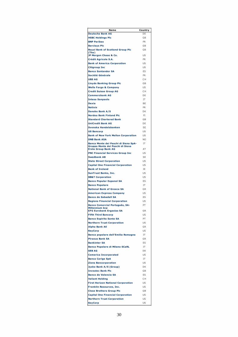
30

Name Country

Deutsche Bank AG DE

HSBC Holdings Plc GB

BNP Paribas FR

Barclays Plc GB

Royal Bank of Scotland Group Plc

(The)

GB

JP Morgan Chase & Co. US

Crédit Agricole S.A. FR

Bank of America Corporation US

Citigroup Inc US

Banco Santander SA ES

Société Générale FR

UBS AG CH

Lloyds Banking Group Plc GB

Wells Fargo & Company US

Credit Suisse Group AG CH

Commerzbank AG DE

Intesa Sanpaolo IT

Dexia BE

Natixis FR

Danske Bank A/S DK

Nordea Bank Finland Plc FI

Standard Chartered Bank GB

UniCredit Bank AG DE

Svenska Handelsbanken SE

US Bancorp US

Bank of New York Mellon Corporation US

DNB Bank ASA NO

Banca Monte dei Paschi di Siena SpA-

Gruppo Monte dei Paschi di Siena

IT

Erste Group Bank AG AT

PNC Financial Services Group Inc US

Swedbank AB SE

State Street Corporation US

Capital One Financial Corporation US

Bank of Ireland IE

SunTrust Banks, Inc. US

BB&T Corporation US

Banco Popular Espanol SA ES

Banco Popolare IT

National Bank of Greece SA GR

American Express Company US

Banco de Sabadell SA ES

Regions Financial Corporation US

Banco Comercial Português, SA-

Millennium bcp

PT

EFG Eurobank Ergasias SA GR

Fifth Third Bancorp US

Banco Espirito Santo SA PT

Northern Trust Corporation US

Alpha Bank AE GR

KeyCorp US

Banca popolare dell'Emilia Romagna IT

Piraeus Bank SA GR

Bankinter SA ES

Banca Popolare di Milano SCaRL IT

SEB AG DE

Comerica Incorporated US

Banca Carige SpA IT

Zions Bancorporation US

Jyske Bank A/S (Group) DK

Investec Bank Plc GB

Banco de Valencia SA ES

Valiant Holding CH

First Horizon National Corporation US

Franklin Resources, Inc. US

Close Brothers Group Plc GB

Capital One Financial Corporation US

Northern Trust Corporation US

KeyCorp US

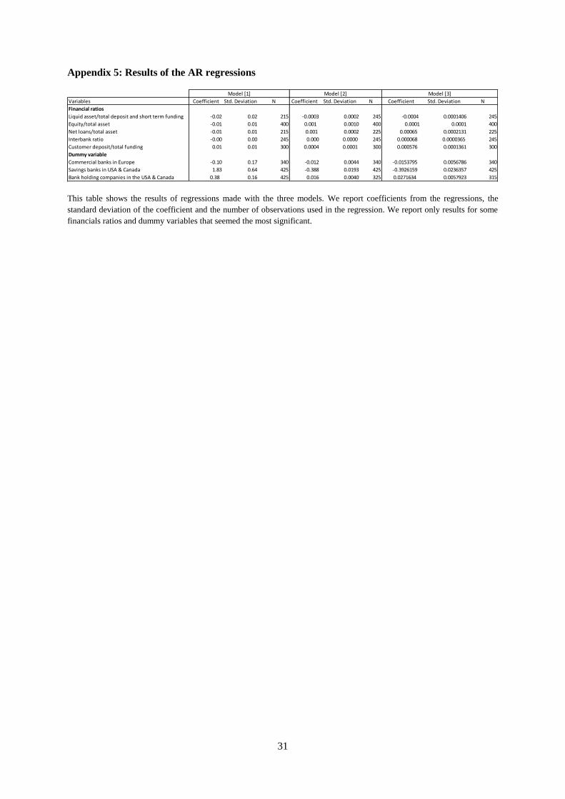
31

Appendix 5: Results of the AR regressions

This table shows the results of regressions made with the three models. We report coefficients from the regressions, the

standard deviation of the coefficient and the number of observations used in the regression. We report only results for some

financials ratios and dummy variables that seemed the most significant.

Variables Coefficient Std. Deviation N Coefficient Std. Deviation N Coefficient Std. Deviation N

Financial ratios

Liquid asset/total deposit and short term funding -0.02 0.02 215 -0.0003 0.0002 245 -0.0004 0.0001406 245

Equity/total asset -0.01 0.01 400 0.001 0.0010 400 0.0001 0.0001 400

Net loans/total asset -0.01 0.01 215 0.001 0.0002 225 0.00065 0.0002131 225

Interbank ratio -0.00 0.00 245 0.000 0.0000 245 0.000068 0.0000365 245

Customer deposit/total funding 0.01 0.01 300 0.0004 0.0001 300 0.000576 0.0001361 300

Dummy variable

Commercial banks in Europe -0.10 0.17 340 -0.012 0.0044 340 -0.0153795 0.0056786 340

Savings banks in USA & Canada 1.83 0.64 425 -0.388 0.0193 425 -0.3926159 0.0236357 425

Bank holding companies in the USA & Canada 0.38 0.16 425 0.016 0.0040 325 0.0271634 0.0057923 315

Model [1] Model [2] Model [3]