Consumption Poverty in Sri Lanka 1985-2002

Consumption Poverty in Sri Lanka 1985-2002

Dileni Gunewardena

November 2007

An updated analysis of household survey data

Working Paper Series No. 14-2007

© Centre for Poverty Analysis 2007

First Published - 2007

ISBN: 978-955-1040-39-0ISSN: 1391-9946

National Library of Sri Lanka - Cataloguing Publication Data

Consumption poverty in Sri Lanka 1985-2002: An updated analysis of household surveydata/Dileni Gunewardena - Colombo: Centre for Poverty Analysis, 2007.

ISBN: 978-955-1040-39-0 Price:

i. 362.5095493 DDC 22 ii. Title

1. Poverty analysis - Sri Lanka

Copyright of this publication belongs to the Centre for Poverty Analysis. Any part of this bookmay be reproduced with due acknowledgement to the author/s and publisher.

The CEPA Publication Series currently includes; Studies, Edited Volumes, Working Papers andBriefing Papers. The interpretations and conclusions expressed in this Working Paper arethose of the individual author and do not necessarily reflect the views or policies of CEPA orthe publication sponsor.

Photographs used in this publication are attributed to CEPA staff.

All enquiries relating to this publication should be directed to:

Centre for Poverty Analysis29 Gregory’s Road, Colombo 7Sri LankaTel: +94 11 2676955-8, 2667967-8Fax: +94 11 2676959Email: [email protected]: www.cepa.lk

Printed by : Karunaratne & Sons Ltd.67, UDA Industrial EstateKatuwana Road, HomagamaSri Lanka

Dileni Gunewardena (B.A. Peradeniya, Ph.D. American) is a Senior Lecturer at theDepartment of Economics and Statistics, University of Peradeniya. Her research interestsinclude the analysis of Poverty, Inequality, and Gender Discrimination. She has over twelveyears of experience in analysing microdata from Household Income and Expenditure Surveys,Demographic and Health Surveys and Labour Force Surveys of the Department of Censusand Statistics. She is the author of two CEPA publications on poverty measurement.

The Centre for Poverty Analysis (CEPA) was established in 2001 as an independentinstitute providing professional services on poverty related development issues. CEPA providesservices in the areas of applied research, advisory services, training and dialogue andexchange to development organisations and professionals. These services are concentratedwithin the core programme areas that currently include: Poverty Impact Monitoring, Povertyand Conflict, and Poverty Assessment & Knowledge Management.

This report is a product of the Poverty Assessment & Knowledge Management Programmeand sponsored by the Asian Development Bank through a technical assistance grantsupporting the programme.

Acknowledgements

The Department of Census and Statistics is gratefully acknowledged for providing the unitrecord (raw) data from the LFSES 1985/86, and HIES 1990/91, 1995/96 and 2002 on whichthe calculations in this study were made. The DCS bears no responsibility for the analysis orinterpretations presented here. Any errors in calculation and interpretation are the soleresponsibility of the author.

Thanks are due to Patricia Alailima, Azra Abdul Cader and Azra Jafferjee who providedguidance at various stages of the study, to Neranjana Gunetilleke and ShivapragasamShivakumaran for helpful comments, to Amalie Ellagala Seneviratne for research assistance,and to Neluka Silva and Fiona Remnant for editing the original version of the document. Theybear no responsibility for any remaining errors and omissions.

v

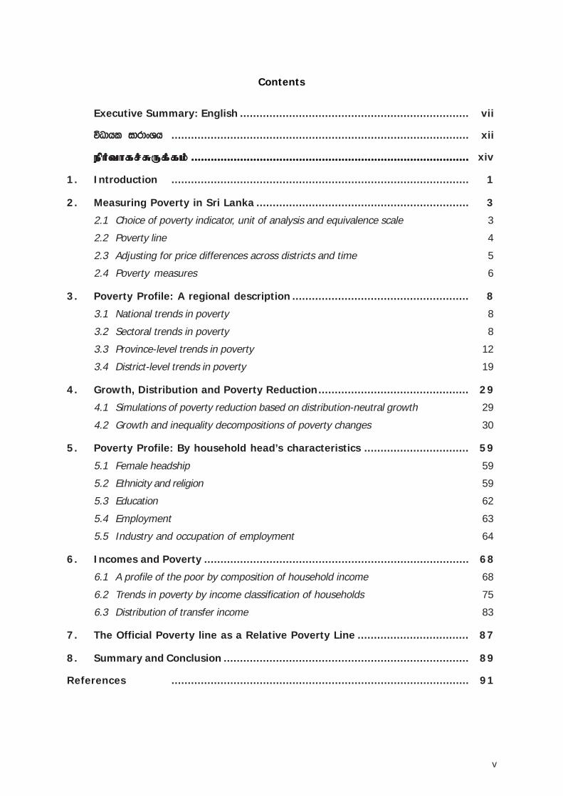
Contents

Executive Summary: English ...................................................................... vii

úOdhl idrdxYh ........................................................................................... xii

epHthfr;RUf;fk;epHthfr;RUf;fk;epHthfr;RUf;fk;epHthfr;RUf;fk;epHthfr;RUf;fk; ......................................................................................................................................................................................................................................................................................................................................................................................................................................... xiv

1. Introduction ........................................................................................... 1

2. Measuring Poverty in Sri Lanka ................................................................. 3

2.1 Choice of poverty indicator, unit of analysis and equivalence scale 3

2.2 Poverty line 4

2.3 Adjusting for price differences across districts and time 5

2.4 Poverty measures 6

3. Poverty Profile: A regional description ...................................................... 8

3.1 National trends in poverty 8

3.2 Sectoral trends in poverty 8

3.3 Province-level trends in poverty 12

3.4 District-level trends in poverty 19

4. Growth, Distribution and Poverty Reduction.............................................. 29

4.1 Simulations of poverty reduction based on distribution-neutral growth 29

4.2 Growth and inequality decompositions of poverty changes 30

5. Poverty Profile: By household head’s characteristics ................................ 59

5.1 Female headship 59

5.2 Ethnicity and religion 59

5.3 Education 62

5.4 Employment 63

5.5 Industry and occupation of employment 64

6. Incomes and Poverty ................................................................................. 68

6.1 A profile of the poor by composition of household income 68

6.2 Trends in poverty by income classification of households 75

6.3 Distribution of transfer income 83

7. The Official Poverty line as a Relative Poverty Line .................................. 87

8. Summary and Conclusion ........................................................................... 89

References ........................................................................................... 91

vi

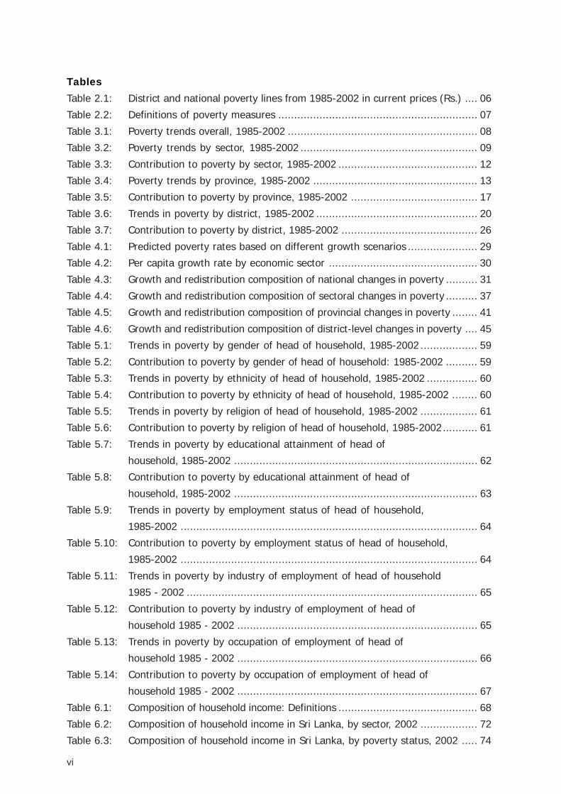
Tables

Table 2.1: District and national poverty lines from 1985-2002 in current prices (Rs.) .... 06

Table 2.2: Definitions of poverty measures ............................................................... 07

Table 3.1: Poverty trends overall, 1985-2002 ............................................................ 08

Table 3.2: Poverty trends by sector, 1985-2002 ........................................................ 09

Table 3.3: Contribution to poverty by sector, 1985-2002 ............................................ 12

Table 3.4: Poverty trends by province, 1985-2002 .................................................... 13

Table 3.5: Contribution to poverty by province, 1985-2002 ........................................ 17

Table 3.6: Trends in poverty by district, 1985-2002 ................................................... 20

Table 3.7: Contribution to poverty by district, 1985-2002 ........................................... 26

Table 4.1: Predicted poverty rates based on different growth scenarios ...................... 29

Table 4.2: Per capita growth rate by economic sector ............................................... 30

Table 4.3: Growth and redistribution composition of national changes in poverty .......... 31

Table 4.4: Growth and redistribution composition of sectoral changes in poverty .......... 37

Table 4.5: Growth and redistribution composition of provincial changes in poverty ........ 41

Table 4.6: Growth and redistribution composition of district-level changes in poverty .... 45

Table 5.1: Trends in poverty by gender of head of household, 1985-2002 .................. 59

Table 5.2: Contribution to poverty by gender of head of household: 1985-2002 .......... 59

Table 5.3: Trends in poverty by ethnicity of head of household, 1985-2002 ................ 60

Table 5.4: Contribution to poverty by ethnicity of head of household, 1985-2002 ........ 60

Table 5.5: Trends in poverty by religion of head of household, 1985-2002 .................. 61

Table 5.6: Contribution to poverty by religion of head of household, 1985-2002........... 61

Table 5.7: Trends in poverty by educational attainment of head of

household, 1985-2002 ............................................................................. 62

Table 5.8: Contribution to poverty by educational attainment of head of

household, 1985-2002 ............................................................................. 63

Table 5.9: Trends in poverty by employment status of head of household,

1985-2002 .............................................................................................. 64

Table 5.10: Contribution to poverty by employment status of head of household,

1985-2002 .............................................................................................. 64

Table 5.11: Trends in poverty by industry of employment of head of household

1985 - 2002 ............................................................................................ 65

Table 5.12: Contribution to poverty by industry of employment of head of

household 1985 - 2002 ............................................................................ 65

Table 5.13: Trends in poverty by occupation of employment of head of

household 1985 - 2002 ............................................................................ 66

Table 5.14: Contribution to poverty by occupation of employment of head of

household 1985 - 2002 ............................................................................ 67

Table 6.1: Composition of household income: Definitions ............................................ 68

Table 6.2: Composition of household income in Sri Lanka, by sector, 2002 .................. 72

Table 6.3: Composition of household income in Sri Lanka, by poverty status, 2002 ..... 74

vii

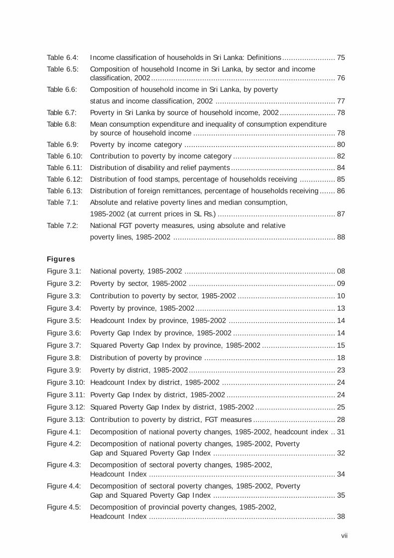
Table 6.4: Income classification of households in Sri Lanka: Definitions ........................ 75

Table 6.5: Composition of household Income in Sri Lanka, by sector and incomeclassification, 2002 ................................................................................... 76

Table 6.6: Composition of household income in Sri Lanka, by poverty

status and income classification, 2002 ...................................................... 77

Table 6.7: Poverty in Sri Lanka by source of household income, 2002 ......................... 78

Table 6.8: Mean consumption expenditure and inequality of consumption expenditureby source of household income ................................................................ 78

Table 6.9: Poverty by income category .................................................................... 80

Table 6.10: Contribution to poverty by income category .............................................. 82

Table 6.11: Distribution of disability and relief payments ............................................... 84

Table 6.12: Distribution of food stamps, percentage of households receiving ................ 85

Table 6.13: Distribution of foreign remittances, percentage of households receiving ....... 86

Table 7.1: Absolute and relative poverty lines and median consumption,

1985-2002 (at current prices in SL Rs.) ..................................................... 87

Table 7.2: National FGT poverty measures, using absolute and relative

poverty lines, 1985-2002 ......................................................................... 88

Figures

Figure 3.1: National poverty, 1985-2002 .................................................................... 08

Figure 3.2: Poverty by sector, 1985-2002 .................................................................. 09

Figure 3.3: Contribution to poverty by sector, 1985-2002 ............................................ 10

Figure 3.4: Poverty by province, 1985-2002 ............................................................... 13

Figure 3.5: Headcount Index by province, 1985-2002 ................................................ 14

Figure 3.6: Poverty Gap Index by province, 1985-2002 .............................................. 14

Figure 3.7: Squared Poverty Gap Index by province, 1985-2002 ................................. 15

Figure 3.8: Distribution of poverty by province ........................................................... 18

Figure 3.9: Poverty by district, 1985-2002 .................................................................. 23

Figure 3.10: Headcount Index by district, 1985-2002 ................................................... 24

Figure 3.11: Poverty Gap Index by district, 1985-2002 ................................................. 24

Figure 3.12: Squared Poverty Gap Index by district, 1985-2002 .................................... 25

Figure 3.13: Contribution to poverty by district, FGT measures ..................................... 28

Figure 4.1: Decomposition of national poverty changes, 1985-2002, headcount index .. 31

Figure 4.2: Decomposition of national poverty changes, 1985-2002, PovertyGap and Squared Poverty Gap Index ....................................................... 32

Figure 4.3: Decomposition of sectoral poverty changes, 1985-2002,Headcount Index .................................................................................... 34

Figure 4.4: Decomposition of sectoral poverty changes, 1985-2002, PovertyGap and Squared Poverty Gap Index ....................................................... 35

Figure 4.5: Decomposition of provincial poverty changes, 1985-2002,Headcount Index .................................................................................... 38

viii

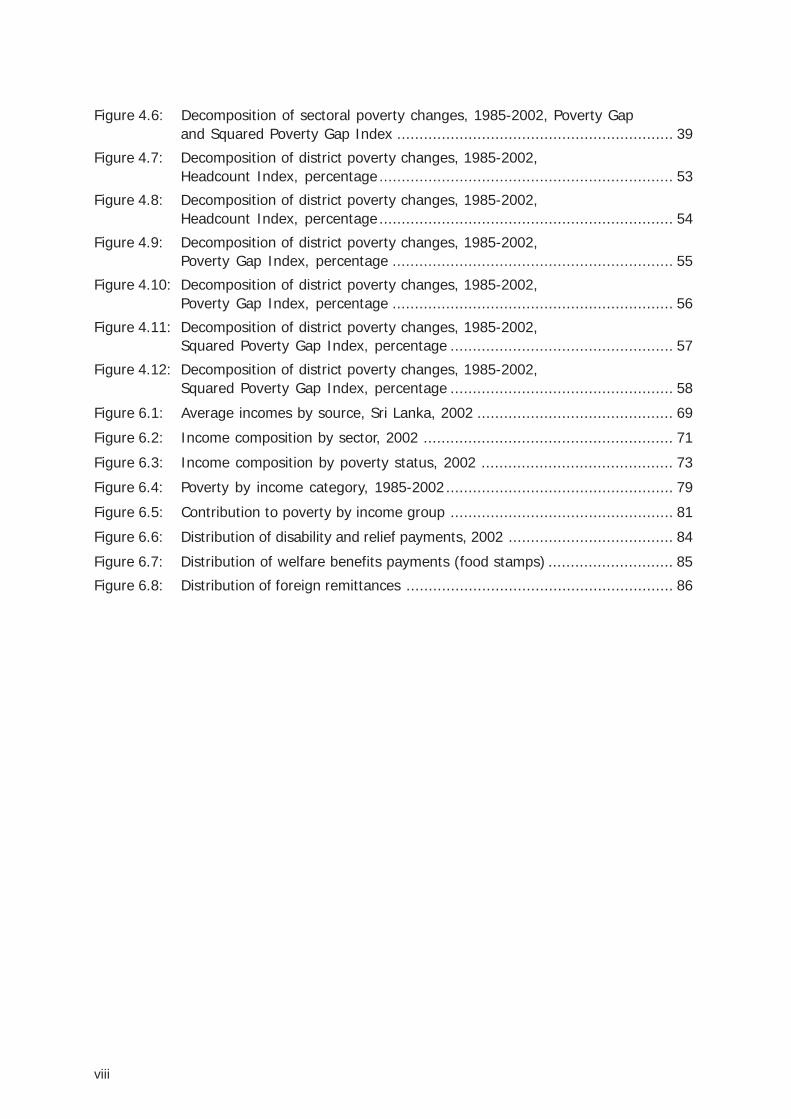
Figure 4.6: Decomposition of sectoral poverty changes, 1985-2002, Poverty Gapand Squared Poverty Gap Index .............................................................. 39

Figure 4.7: Decomposition of district poverty changes, 1985-2002,Headcount Index, percentage .................................................................. 53

Figure 4.8: Decomposition of district poverty changes, 1985-2002,Headcount Index, percentage .................................................................. 54

Figure 4.9: Decomposition of district poverty changes, 1985-2002,Poverty Gap Index, percentage ............................................................... 55

Figure 4.10: Decomposition of district poverty changes, 1985-2002,Poverty Gap Index, percentage ............................................................... 56

Figure 4.11: Decomposition of district poverty changes, 1985-2002,Squared Poverty Gap Index, percentage .................................................. 57

Figure 4.12: Decomposition of district poverty changes, 1985-2002,Squared Poverty Gap Index, percentage .................................................. 58

Figure 6.1: Average incomes by source, Sri Lanka, 2002 ............................................ 69

Figure 6.2: Income composition by sector, 2002 ........................................................ 71

Figure 6.3: Income composition by poverty status, 2002 ........................................... 73

Figure 6.4: Poverty by income category, 1985-2002 ................................................... 79

Figure 6.5: Contribution to poverty by income group .................................................. 81

Figure 6.6: Distribution of disability and relief payments, 2002 ..................................... 84

Figure 6.7: Distribution of welfare benefits payments (food stamps) ............................ 85

Figure 6.8: Distribution of foreign remittances ............................................................ 86

ix

Abbeviations and Accronyms

ADB - Asian Development Bank

CBN - Cost of Basic Needs

CCPI - Colombo Consumer Price Index

CEPA - Centre for Poverty Analysis

DCS - Department of Census and Statistics

FEI - Food Energy Intake

FGT - Foster, Greer, Thorbecke measures of poverty

HCI - Headcount Index

HIES - Household Income and Expenditure Survey

LFSES - Labour Force and Socio-Economic Survey

PG - Poverty Gap Index

PG2 - Squared Poverty Gap Index

SLCPI - Sri Lanka Consumer Price Index

WB - World Bank

x

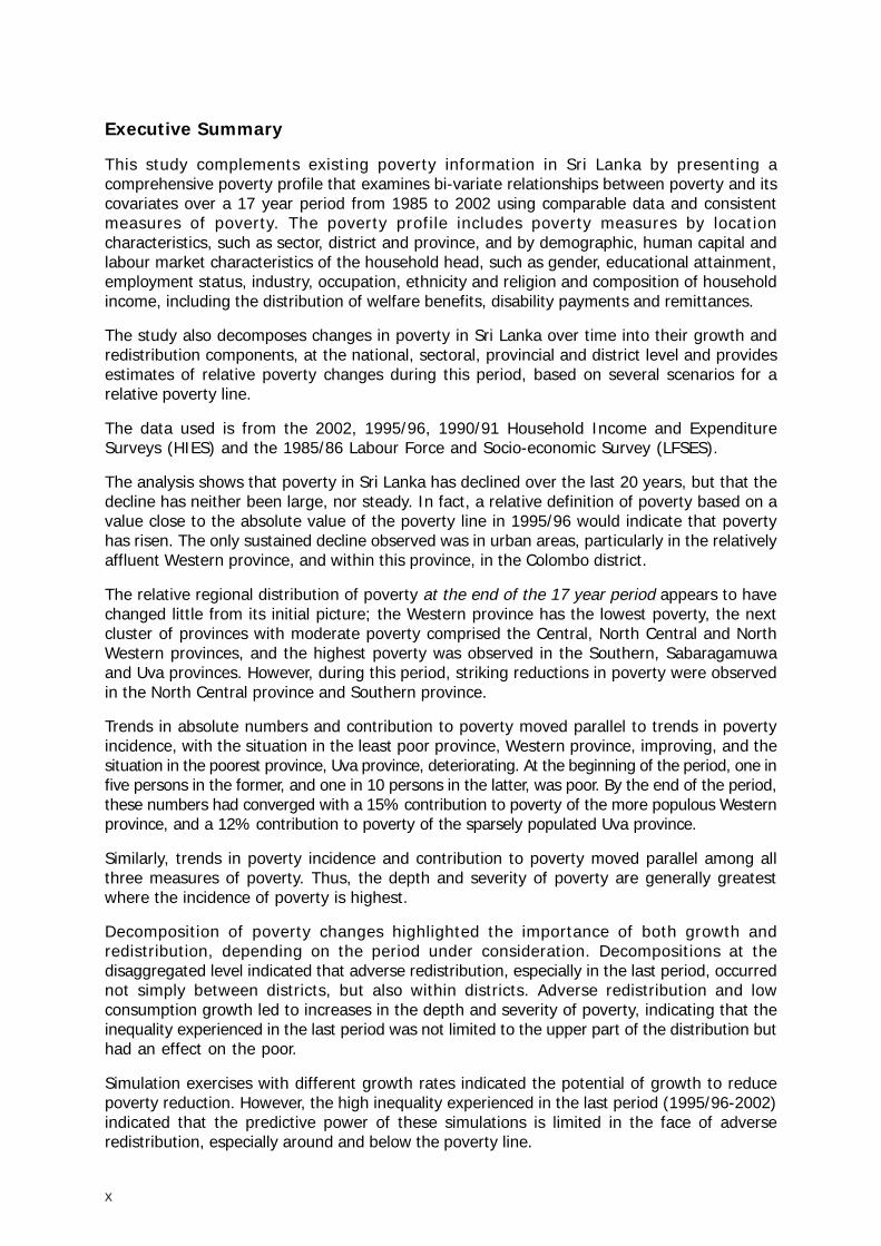
Executive Summary

This study complements existing poverty information in Sri Lanka by presenting acomprehensive poverty profile that examines bi-variate relationships between poverty and itscovariates over a 17 year period from 1985 to 2002 using comparable data and consistentmeasures of poverty. The poverty profile includes poverty measures by locationcharacteristics, such as sector, district and province, and by demographic, human capital andlabour market characteristics of the household head, such as gender, educational attainment,employment status, industry, occupation, ethnicity and religion and composition of householdincome, including the distribution of welfare benefits, disability payments and remittances.

The study also decomposes changes in poverty in Sri Lanka over time into their growth andredistribution components, at the national, sectoral, provincial and district level and providesestimates of relative poverty changes during this period, based on several scenarios for arelative poverty line.

The data used is from the 2002, 1995/96, 1990/91 Household Income and ExpenditureSurveys (HIES) and the 1985/86 Labour Force and Socio-economic Survey (LFSES).

The analysis shows that poverty in Sri Lanka has declined over the last 20 years, but that thedecline has neither been large, nor steady. In fact, a relative definition of poverty based on avalue close to the absolute value of the poverty line in 1995/96 would indicate that povertyhas risen. The only sustained decline observed was in urban areas, particularly in the relativelyaffluent Western province, and within this province, in the Colombo district.

The relative regional distribution of poverty at the end of the 17 year period appears to havechanged little from its initial picture; the Western province has the lowest poverty, the nextcluster of provinces with moderate poverty comprised the Central, North Central and NorthWestern provinces, and the highest poverty was observed in the Southern, Sabaragamuwaand Uva provinces. However, during this period, striking reductions in poverty were observedin the North Central province and Southern province.

Trends in absolute numbers and contribution to poverty moved parallel to trends in povertyincidence, with the situation in the least poor province, Western province, improving, and thesituation in the poorest province, Uva province, deteriorating. At the beginning of the period, one infive persons in the former, and one in 10 persons in the latter, was poor. By the end of the period,these numbers had converged with a 15% contribution to poverty of the more populous Westernprovince, and a 12% contribution to poverty of the sparsely populated Uva province.

Similarly, trends in poverty incidence and contribution to poverty moved parallel among allthree measures of poverty. Thus, the depth and severity of poverty are generally greatestwhere the incidence of poverty is highest.

Decomposition of poverty changes highlighted the importance of both growth andredistribution, depending on the period under consideration. Decompositions at thedisaggregated level indicated that adverse redistribution, especially in the last period, occurrednot simply between districts, but also within districts. Adverse redistribution and lowconsumption growth led to increases in the depth and severity of poverty, indicating that theinequality experienced in the last period was not limited to the upper part of the distribution buthad an effect on the poor.

Simulation exercises with different growth rates indicated the potential of growth to reducepoverty reduction. However, the high inequality experienced in the last period (1995/96-2002)indicated that the predictive power of these simulations is limited in the face of adverseredistribution, especially around and below the poverty line.

xi

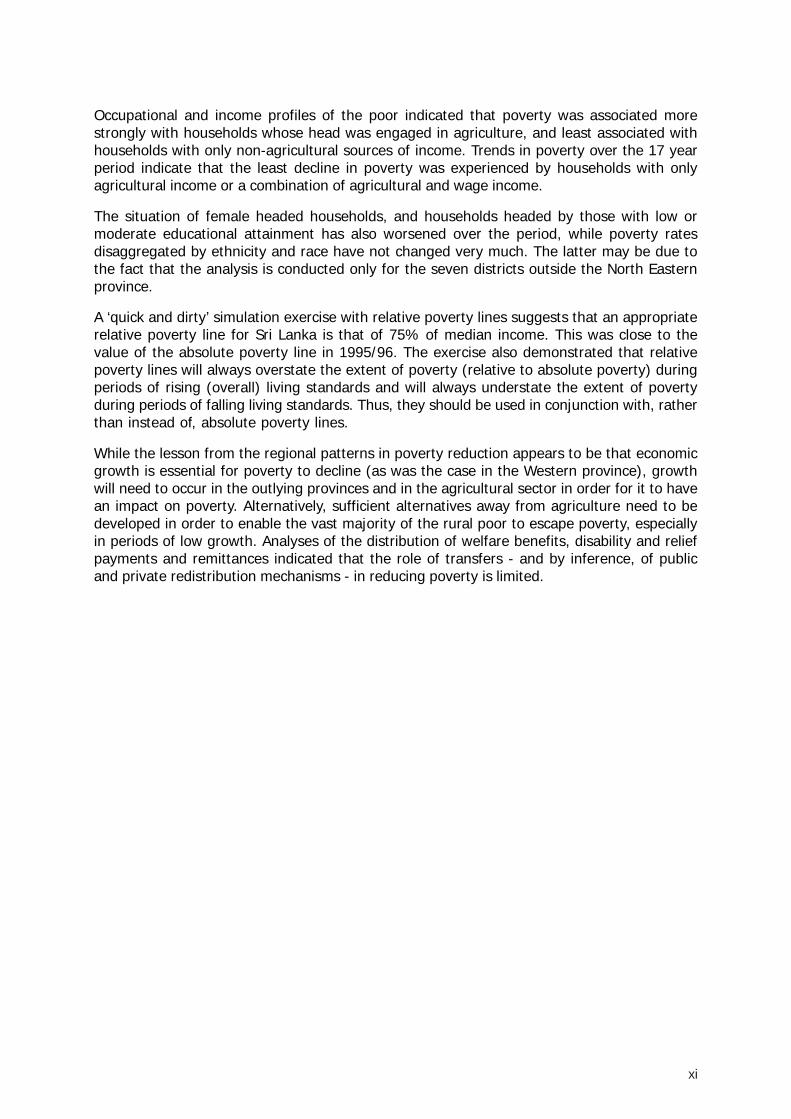
Occupational and income profiles of the poor indicated that poverty was associated morestrongly with households whose head was engaged in agriculture, and least associated withhouseholds with only non-agricultural sources of income. Trends in poverty over the 17 yearperiod indicate that the least decline in poverty was experienced by households with onlyagricultural income or a combination of agricultural and wage income.

The situation of female headed households, and households headed by those with low ormoderate educational attainment has also worsened over the period, while poverty ratesdisaggregated by ethnicity and race have not changed very much. The latter may be due tothe fact that the analysis is conducted only for the seven districts outside the North Easternprovince.

A ‘quick and dirty’ simulation exercise with relative poverty lines suggests that an appropriaterelative poverty line for Sri Lanka is that of 75% of median income. This was close to thevalue of the absolute poverty line in 1995/96. The exercise also demonstrated that relativepoverty lines will always overstate the extent of poverty (relative to absolute poverty) duringperiods of rising (overall) living standards and will always understate the extent of povertyduring periods of falling living standards. Thus, they should be used in conjunction with, ratherthan instead of, absolute poverty lines.

While the lesson from the regional patterns in poverty reduction appears to be that economicgrowth is essential for poverty to decline (as was the case in the Western province), growthwill need to occur in the outlying provinces and in the agricultural sector in order for it to havean impact on poverty. Alternatively, sufficient alternatives away from agriculture need to bedeveloped in order to enable the vast majority of the rural poor to escape poverty, especiallyin periods of low growth. Analyses of the distribution of welfare benefits, disability and reliefpayments and remittances indicated that the role of transfers - and by inference, of publicand private redistribution mechanisms - in reducing poverty is limited.

xii

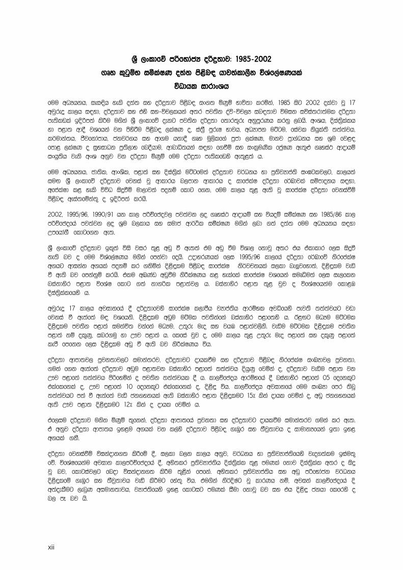
YS% ,xldfõ mßfNdacH oßø;dj( 1985-2002

.Dy l=gqïN iólaIK o;a; ms<sn| hdj;ald,Sk úYaf,aIKhla

úOdhl idrdxYh

fuu wOHhkh” iei¢h yels o;a; iy oßø;dj ms<sn| ix.; ñKqï Ndú;d lrñka” 1985 isg 2002 olajd jQ 17wjqreÿ ld,h i|yd” oßø;dj iy tys iy-úp,lhka w;r mj;sk oaú-úp,H in|;dj úuik iúia;rd;aul oßø;dme;slvla bÈßm;a lsÍu u.ska Y%S ,xldfõ oekg mj;sk oßø;d f;dr;=re wkqmQrKh lrkq ,nhs’ wxYh” Èia;%slalhyd m<d; wd§ jYfhka jk msysàu ms<sn| ,laIK o” ia;%S mqreI Ndjh” wOHdmk uÜgu” fiajl kshqla;s ;;a;ajh”l¾udka;h” Ôjfkdamdh” ckj¾.h iy wd.u hkd§ .Dy uQ,slf.a m%cd ,laIK” udkj m%d.aOkh iy Y%u fj<|fmd< ,laIK o iqNidOk m%;s,dN fn§hdu” wdndê;hka i|yd f.ùï iy ixl%uKsl fma%IK we;=¿ .Dyia: wdodhïixhq;sh jeks wxY wkqj jk oßø;d ñKqï fuu oßø;d me;slfvys we;=<;a h’

fuu wOHhkh” cd;sl” wdxYsl” m<d;a iy Èia;s%la uÜgfu;a oßø;dj j¾Okh yd m%;sjHdma;s ix>glj,g” ld,h;aiuÕ Y%S ,xldfõ oßø;dj fjkia jQ wdldrh n,mdk wdldrh o idfmalaI oßø;d f¾Ldjla iïmdokh i|yd”wfmalaId l< yels úúO isÿùï ud,dj;a mokï fldg f.k” fuu ld,h ;=< we;s jQ idfmalaI oßø;d fjkiaùïms<sn| weia;fïka;= o bÈßm;a lrhs’

2002” 1995$96” 1990$91 hk ld, mßÉfþoj, mj;ajk ,o .Dyia: wdodhï iy úhoï iólaIK iy 1985$86 ld,mßÉfþofha mj;ajk ,o Y%u n,ldh iy iudc wd¾Ól iólaIK u.ska ,nd .;a o;a; fuu wOHhkh i|ydWmfhda.S fldgf.k we;’

Y%S ,xldfõ oßø;dj bl=;a úis jir ;=< wvq ù we;;a tu wvq ùu úYd, fkdjQ w;r th taldldr f,i isÿùke;s nj o fuu úYaf,aIKh u.ska fmkajd fohs’ WodyrKhla f,i 1995$96 ld,fha oßø;d f¾Ldfõ ksrfmalaIw.hg wdikak w.hla mokï lr .ksñka È<s÷lu ms<sn| idfmalaI ks¾jpkhla i,ld ne¨jfyd;a” È<s÷lu jeäù we;s nj fmkakqï lrhs’ tlu wLKav wvqùu ksÍlaIKh l< yelafla idfmalaI jYfhka iuDêu;a f,i ie,flkniakdysr m<d; úfYaI fldg .;a kd.ßl m<d;aj, h’ niakdysr m<d; ;=< jqj o úfYaIfhkau fld<UÈia;%slalfhys h’

wjqreÿ 17 ld,h wjidkfha § oßø;dfjys idfmalaI l,dmSh jHdma;sh wdrïNl wjêfhys mej;s ;;a;ajhg jvdfjkia ù we;af;a u| jYfhks’ È<s÷lu wvqu uÜul mj;skafka niakdysr m<df;ys h’ B<Õg uOHu uÜgulÈ<s÷lu mj;sk m<d;a iukaú; jkafka uOHu” W;=re ueo iy jhU m<d;aj,sks’ jeäu uÜgul È<s÷lu mj;skm<d;a kï ol=Kq” inr.uq yd W!j m<d;a h’ flfia jqj o” fuu ld,h ;=< W;=re ueo m<df;a iy ol=Kq m<df;alemS fmfkk f,i È<s÷lu wvq ù we;s nj ksÍlaIKh úh’

oßø;d wdmd;j, m%jk;dj,g iudka;rj” oßø;djg odhlùu iy oßø;dj ms<sn| ksrfmalaI ixLHdj, m%jk;d”.uka f.k we;af;a oßø;dj wvqu m<d;jk niakdysr m<df;a ;;a;ajh ÈhqKq fjñka o” oßø;dj jeäu m<d; jkW!j m<df;a ;;a;ajh msßfyñka o mj;sk ;;a;ajhl § h’ ld,Éfþoh wdrïNfha § niakdysr m<df;a 05 fofkl=gtlaflfkla o” W!j m<df;a 10 fofkl=g tlaflfkla o” È<s÷ úh’ ld,Éfþoh wjidkfha fuu ixLHd fmr ;snQ;;a;ajhg m;a ù we;af;a jeä ck.ykhla we;s niakdysr m<d; È<s÷lug 15] lska odhl fjñka o” wvq ck.ykhlawe;s W!j m<d; È<s÷lug 12] lska o odhl fjñka h’

tf,iu oßø;dj uksk ñKqï ;=fkka” oßø;d wdmd;fha m%jk;d iy oßø;djg odhlùu iudka;rj .uka lr we;’ta wkqj oßø;d wdmd;h by<u w.hla jk l,ays oßø;dj ms<sn| .eUqr iy ;Sj%;djh o idudkHfhka b;d by<w.hla .kS’

oßø;d fjkiaùï úikaodk.; lsÍfï §” i,ld n,k ld,h wkqj” j¾Okh yd m%;sjHdma;sfhys jeo.;alu biau;=fõ’ úfYaIfhkau wjidk ld,mßÉfþofha §” wys;lr m%;sjHdma;sh Èia;%slal ;=< muKla fkdj Èia;s%lal w;r o isÿjQ nj” fldgiaj,g fnod úikaodk.; lsÍu ;=<ska fmfka’ wys;lr m%;sjHdma;sh iy wvq mßfNdack j¾OkhÈ<s÷lfï .eUqr iy ;Sj%;djh jeä lsÍug fya;= úh’ tu.ska ks¾ÈIag jQ ldrKh kï” wjika ld,Éfþofha Èw;aoelSug ,enqK wiudk;djh” jHdma;sfhys by< fldgig muKla iSud fkdjQ nj iy th È<s÷ ckhd flfrys on, mE nj hs’

xiii

úúO j¾Ok wkqmd; Wmfhda.S fldg f.k l< iudkdlD;s iE§fï wNHdi” È<s÷lu wvq lsÍfï fõ.h wvq lsÍugwd¾Ól j¾Okh i;= úNjH;djh fmkajd ÿks’ úfYaIfhkau” È<s÷ f¾Ldj wjg iy Bg my< uÜgïj, §” fuuiudkdlD;sj, mqfrdal:k n,h wys;lr m%;sjHdma;sh wìhi iSudjk nj” wjika ld,fha § ^1995$96 - 2002&olskakg ,enqK by< uÜufï wiudk;d fmkajd ÿkafka h’

lDIsl¾ufhys kshq;= m%OdkSka isák .Dyia; wdYs%;j jeä jYfhka È<s÷lu mj;sk nj o” lDIsl¾uh fkdjk wdodhïm%Njhka muKla i;= jk .Dyia: wdY%s;j wvqu uÜgul È<s÷lu mj;sk nj o” È<s÷ ck;djf.a Ôjfkdamdh iywdodhï me;slv oelaùh’ lDIsl¾u wdodhu muKla fyda lDIsl¾uh iy fõ;k tl;=jlska wdodhu ,nd .kakd.Dyia:j, È<s÷lu wvq ùu wvqu uÜgfuys mej;s nj bl=;a 17 jir ;=< È<s÷lu ms<sn| m%jk;d fmkajd fohs’

ckjd¾.sl;ajh iy cd;sh wkqj fldgiaj,g fnÿ oßø;d wkqmd; ie,lsh hq;= fjkila fkdolajk w;r ldka;djkakdhl;ajh ork .Dyia: iy wvq yd uOHia: wOHdmkh ,o wh kdhl;ajh ork .Dyia:j, ;;a;ajh fuu ld,h;=< krl w;g yeÍ we;’ ckjd¾.sl;ajh iy cd;sh wkqj fldgiaj,g fn¥ oßø;d wkqmd;h ie,lsh hq;= fjkilafkdolajkafka W;=re-kef.kysr m<d;a yer wfkla Èia;s%lal y; ;=< muKla iólaIKh mj;ajd ;sîu ksid úh yel’

wdodhï uOHia:fhka ishhg 75 Y%S ,xldjg fhda.H idfmalaI oßø;d f¾Ldj yeáhg ie,lsh yels nj idfmalaIoßø;d f¾Ld fhdod f.k isÿ l< zlaIKsl yd ls,sÜZ ^quick and dirty& iudkdlD;s iE§fï wNHdih fmkajd fohs’fuh 1995$96 ld,fha § mej;s ksrfmalaI oßø;d f¾Ldfjys w.hg wdikak h’ Ôjk ;;a;ajh ^iuia;& jYfhkaj¾Okh jk ld,j,” idfmalaI oßø;d f¾Ld iEu úgu” oßø;djfha uÜgu mj;sk i;H ;;a;ajhg jvd jeä f,iolajk w;r” Ôjk ;;a;ajh my; jefgk ld,j,§” tu f¾Ldj;a iEu úgu” oßø;djfha uÜgu mj;sk i;H;;a;ajhg jvd jeä f,i olajk w;r” Ôjk ;;a;ajh my; jefgk ld,j,§” tu f¾Ldj;a iEu úgu” oßø;djfhauÜgu mj;sk i;H ;;a;ajhg jvd wvqfjka olajk nj” wNHdih meyeÈ,s lf<a h’ tneúka tajd ksrfmalaI oßø;df¾Ld fjkqjg fkdj” ksrfmalaI oßø;d f¾Ld iuÕ Ndú;d l< hq;=h’

oßø;djh wvq lsÍug wd¾Ól j¾Okh ^niakdysr m<df;a olakg ,efnk mßÈ& wjYH nj oßø;d wvq lsÍfï l,dmShrgdjkaf.ka W.; hq;= mdvu jk w;r” oßø;dj flfrys n,mEula we;s lsÍug” hdno Èia;s%lalj, iy lDIsl¾uwxYfha j¾Okhla isÿ úh hq;= fõ’ tfia ke;fyd;a” úfYaIfhkau wvq j¾Okhla we;s ld,j,§” .%dóh È<s÷ ck;djw;=ßka w;s nyq;rhlg È<s÷lfuka ñ§ug lDIsl¾ufhka ndysrj m%udKj;a úl,amh;a j¾Okh l< hq;= h’ Y=NidOk m%;s,dN fn§u o” wdndê; wh i|yd f.ùï” iyk f.ùï iy fm%aIK úYaf,aIKh meyeÈ,s lf<a oßø;djwvq lsÍfuys,d wdodhu tla wxYhlska ;j;a wxYhlg ,efnkakg ie,eiaùfuys” tkï fm!oa.,sl yd fmdÿm%;sjHdma;sfhys ld¾hNdrh iSñ; nj h’

xiv

epiwNtw;Wr; rhuhk;rk;

tWikapd; xg;gplf;$ba juTfisAk;> Kuz;glhj eltbf;iffisAk; gad;gLj;jp 1985

Kjy; 2002 tiuapyhd 17 tUl fhyj;jpd; NghJ tWikf;Fk;> mjd; xj;j

khwpypfSf;Fk; ,ilapyhd ,ul;il khwpyp cwTfisg; ghprPypf;fpd;w tphpthdnjhU

tWikg; Gwtiuia Kd;itg;gjd; %yk;> ,yq;ifapy; eilKiwap;y; cs;s tWikj;

jftiy ,t;tha;T �h;j;jp nra;fpd;wJ. Jiw> khtl;lk; kw;Wk; khfhzk; Nghd;w

miktpl Fztpay;GfspdhYk;> ghy;epiy> fy;tprhh; NgW> njhopy;epiy> ifj;njhopy;>

njhopy;> ,dj;Jtk; kw;Wk; rkak; Nghd;w Fbj;jdj; jiythpd; Fbj;njhifapay;> kdpj

%yjd kw;Wk; njhopy; re;ij Fztpay;Gfs; Mfpadtw;wpdhYk;> Nrkeyd; ed;ikfspd;

gq;fPL> mq;ftPdf; nfhLg;gdTfs; kw;Wk; mDg;gPLfs; Mfpatw;wpd; gq;fPL cl;gl

Fbj;jd tUkhdj;jpd; mlf;fk; Mfpatw;wpdhYk; tWik eltbf;iffis tWikg;

Gwtiu cs;slf;Ffpd;wJ.

Njrpa> Jiwfs;> khfhz kw;Wk; khtl;l kl;lq;fspy; jkJ tsh;r;rp kw;Wk; kPs;gq;fPL

mk;rq ;fspDs; fhyg ;Nghf ;f py ; ,yq;ifapy ; tWikapy ; khw ;wq ;fis Ma;T

g ph pj ;Jg ;ghh ;g ;gJld ; > rhh ;Gh Pj pa pyhd tWikf ; Nfhl ;nlhd ;Wf ;fhd ngUksT

fhl;rpj;Njhw;wq;fs; kPjhd mbg;gilapy;> ,f; fhyj;jpd; NghJ rhh;GhPjpapyhd tWik

khw;wq;fspd; kjpg;gPLfisAk; toq;Ffpd;wJ.

2002> 1995-96> 1990-91 Fbj;jd tUkhd> nrytpd mstPLfs; kw;Wk; 1985-86 ciog;ghsh;

gil> r%f-nghUshjhu mstPL Mfpatw;wpypUe;J juTfs; gad;gLj;jg;gl;Ls;sd.

fle;j 20 tUlq;fspd; NghJ ,yq;ifapy; tWik tPo;r;rpaile;Js;sjhfTk;> Mdhy;>

me;j tPo;;r;rp xd;wpy; ghhpajhf> my;yJ cWjpahf ,Uf;ftpy;iy vd gFg;gha;T

fhl;Lfpd;wJ. cz;ikapy;> 1975-96,y; tWikf; Nfhl;bd; �uzkhd ngWkjpf;F fpl;ba

ngWkjpnahd;wpd; kPjhd mbg;gilapy; tWikapd; rhh;GhPjpapyhd tiutpyf;fzkhdJ

tWik mjpfhpj;Js;sijNa fhl;Lfpd;wJ. efug; gFjpfspy;> Fwpg;ghf rhh;GhPjpapy; nropg;G

epiyapyhd Nky; khfhzj;jpy ; > ,k; khfhzj;jpDs; nfhOk;G khtl;lj ;j py ; >

epiyj;jpUf;fj;jf;f tPo;;r;rp kl;LNk mtjhdpf;fg;gl;lJ.

17 tUl fhyj;jpd; ,Wjpapy; tWikapy; rhh;GhPjpapyhd gpuhe;jpa gq;fPL mjd;

Muk;gj;jpypUe;J rpwpjsT khw;wkile;Js;sjhfj; Njhd;Wfpd;wJ. Nky; khfhzk;

Mff;Fiwe;j tWikiaf; nfhz;Ls;sJ. mLj;j kpjkhd tWikAldhd khfhzq;fshf

kj;jpa> tl kj;jpa kw;Wk; tl Nky; khfhzq;fs; tpsq;FtJld;> Mff;$Ljyhd tWik

njd;> rg;ufKt kw;Wk; Cth khfhzq;fspy; mtjhdpf;fg;gl;lJ. vdpDk;> ,f; fhyj;jpd;

NghJ> tl kj;jpa khfhzj;jpYk;> njd; khfhzj;jpYk; tWikapd; kdjpy; gjpaj;jf;f

Fiwg;Gf;fs; mtjhdpf;fg;gl;ld.

Mff ;Fiwe ; j tWika pyhd khfhzkhd Nky ; khfhzj ;j py ; #o ; e piy

Kd;Ndw;wkile;Js;sJ. Mdhy;> kpfTk; tWikg;gl;l khfhzkhd Cth khfhzj;jpy;

#o;epiy rPh;Nflile;Js;sJld;> tWik epfo;tpy; cs;s Nghf;FfSf;Fr; rkhe;jukhf

tWikf;fhf �uzkhd vz;zpf;ifapy; Nghf;FfSk;> tWikf;fhd gq;fspg;Gk; efh;e;jd.

fhyj;jpd; Muk;gj;jpy; Nky; khfhzj;jpy; Ie;J egh;fspy; xUtUk;> Cth khfhzj;jpy;

10 egh;fspy; xUtUk; Viofshf tpsq;fpdhh;fs;. fhyj;jpd; Kbtpd; NghJ> mjpf

rdj;njhifiaf; nfhz;l Nky; khfhzj;jpd; tWikf;F 15% gq;fspg ;GlDk;>

mlh ; j ; j paw ; w rdj ;njhifiaf ; nfhz ;l tWikf ;F 12% gq ;fs pg ; GlDk ;

,t;ntz;zpf;iffs; Fiwtile;jpUe;jd.

,Nj Nghy> tWik epfo;tpy; Nghf;FfSk;> tWikf;fhd gq;fspg;Gk; tWikapd; rfy

%d;W eltbf;iffs; kj;jpapy; rkhe;jukhf efh;e;jd. Mjypdhy;> nghJthfNt

tWikapd; MoKk;> jPtpuj;jd;ikAk; ghhpait vd;gJld;> tWikapd; epfo;T

Mff;$LjyhdJ.

xv

fhpridapd; fPOs;s fhyj;jpidg; nghWj;J> tsh;r;;rp kw;Wk; kPs;gq;fPL Mfpa ,uz;bdJk;

Kf;fpaj;Jtj;ij tWik khw;wq;fspd; rpijTfs; KidTgLj;jpd. kWjiyapyhd

gpsTfs;> tpNrlkhf filrp fhyj;jpy; ntWkNd khtl;lq;fSf;F ,ilapy; kl;Lkd;wp>

Mdhy; khtl;lq;fspDs;Sk; ,lk;ngw;wpUg;gjhf xd;W Nrh;f;fg;glhj kl;lj;jpy; rpijTfs;

vLj;Jf; fhl;bd. kWjiyahd kPs;gq;fPLk;> Fiwe;j ghtid tsh;r;rpAk; tWikapd;

Moj;jpYk;> jPtpuj;jd;ikapYk; mjpfhpg;Gf;F ,l;Lr; nrd;wJ. ,J fle;j fhyj;jpy;

mDkjpf ;fg ;gl ;l rkj ;Jtkpd ;ikahdJ gq ;f Pl ;bd ; cauj ;j pYs;s ghfj ;j pw ;F

kl;Lg;gl;bUf;ftpy;iy> Mdhy; Viofs; kPJ jhf;fnkhd;iwf; nfhz;bUg;gij vLj;Jf;

fhl;Lfpd;wJ.

NtWgl;l tsh;r;rp tPjq;fSldhd ghrhq;F mg;gpahrq;fs; tWikiaf; Fiwg;gjw;F

tsh;r;rpapd; Mw;wysit vLj;Jf; fhl;bd. vdpDk;> kWjiyahd kPs;gq;fPl;bd; fhuzkhf>

tpNrlkhf tWikf;Nfhl;ilr; Rw;wpAk;> fPNoAk; ,g;ghrhq;Ffspd; vjph;T$wj;jf;f rf;jp

kl;Lg;gLj;jg;gl;Ls;sJ vd;gij fle;j fhyj;jpy; (1995-96 - 2002) mDgtpf;fg;gl;l

cah;thd rkj;Jtkpd;ik vLj;Jf; fhl;Lfpd;wJ.

tptrhaj;jpy; <Lgl;Ls;s jiytiuf; nfhz;Ls;s Fbj;jdq;fSld; tWikahdJ

mjpfsT tYTld; ,ize;Js;sjhfTk;> tptrhak; rhuhj tUkhd %yq;fis kl;LNk

nfhz;l Fbj ;jdq;fSld; Mff;Fiwe ;jsT ,ize;Js;sjhfTk; Viofspd ;

njhopy;epiy kw;Wk; tUkhdg; Gwtiufs; vLj;Jf; fhl;bd. fle;j 17 tUl fhyj;jpd;

NghJ tWikapd; Nghf;Ffs; tWikapy; Mff;Fiwe;j tPo ;r ;r pahdJ tptrha

tUkhdj;Jld; kl;Lk; nfhz;Ls;s> my;yJ tptrha kw;Wk; Ntjd tUkhdk; Mfpa

,uz;ilAk; nfhz;Ls;s Fbj;jdq;fspdhy; mDgtpf;fg;gl;ld.

,f; fhyj;jpd; NghJ ngz; jiyikapyhd Fbj;jdq;fspdJk;> Fiwe;j my;yJ kpjkhd

fy;tprhh; Ngw;Wld; cs;sth;fspd; jiyikapyhd Fbj;jdq;fspdJk; #o;epiy

Nkhrkile;Js;s mNj Ntis> ,dj;Jtj;jpdhYk;> ,dj;jpdhYk; xUq;fpizf;fg;glhj

tWik tPjq;fs; kpfTk; mjpfsT khw;wkilatpy;iy.

rhh;GhPjpapyhd tWikf; NfhLfSld; ~tpiuthdJk;> fz;zpakw;wJkhd| mg;gpahrkhdJ

,yq;iff;fhd nghUj;jkhd rhh;GhPjpapyhd tWikf; Nfhnlhd;W 75% nfhz;l eLepiy

tUkhdnkhd;iwf; Rl;br;nrhy;fpd;wJ. ,J 1995-96,y; �uzkhd tWikf; Nfhl;bd;

ngWkjpf; Nfhl;Lf;F fpl;bajhf cs;sJ. cah;fpd;w (KOikahd) tho;f;ifj; juq;fspd;

fhyq;fspd; NghJ> tWikapd; msit (�uzkhd tWikf;Fj; rhh ;Gh Pjpahd)

rhh;GhPjpapyhd tWikf; NfhLfs; vg;nghOJNk $l;bf; $Wfpd;wJ vd;gijAk;>

tho;f;ifj; juq;fspd; tPo;r;rpAWk; fhyq;fspd; NghJ tWikapd; msit vg;nghOJNk

Fiwj;Jf; $Wfpd;wJ vd;gijAk; vLj;Jf; fhl;baJ. Mjypdhy;> �uzkhd tWikf;

NfhLfSf;F gjpyhf> xd;W Nru mit gad;gLj;jg;gl Ntz;Lk;.

tWik tPo;r;rpailtjw;F (Nky; khfhzj;jpy; tpsq;FtJ Nghd;W) nghUshjhu tsh;r;rp

mtrpakhf ,Uf;f Ntz;Lk; vd tWikf; Fiwg;gpy; gpuhe;jpa tbtj;jd;ikfspy; ,Ue;J

vOk; ghlk ; Njhd;Wfpd ;w mNj Ntis> tWik kPJ mJ jhf ;fnkhd;iwf ;

nfhz;bUf;FKfkhf mLj;Js;s khfhzq;fspYk;> tptrhaj;jpYk; tsh;r;rp ,lk;ngWtJ

mtrpakhdjhFk;. khw;Wtopahf> tpNrlkhf Fiwe;j tsh;r;rpf; fhyj;jpy; tWikapypUe;J

jg;Gtjw;F> fpuhkpa Viofspd; mjpf ngUk;ghd;ikapdiu ,ayr; nra;tjw;fhf

tptrhaj;jpypUe;J tpyfp NghjpasT khw;Wtopfis tpUj;jp nra;tJ mtrpakhdjhFk;.

tWikiaf; Fiwg;gjpy; murhq;f kw;Wk; jdpahh; kPs;gq;fPL nghwp Kiwfspd;

,lkhw;wq;fspd; tfpgq;Fk;> mtw;wpd; mDkhdKk; kl;Lg;gLj;jg;gl;Ls;sd vd;gijNa

Nrkeyd; ed;ikfspd; gq;fPL> mq;ftPdk; kw;Wk; epthuzf; nfhLg;gdTfs; kw;Wk;

mDg;gPLfs; Mfpad gw;wpa gFg;gha;T vLj;Jf; fhl;Lfpd;wJ.

1

1. Introduction

Measurement of consumption poverty in Sri Lanka has made great strides forward in recentyears, including the introduction of an official poverty line, derived according to best practiceprinciples, by the Department of Census and Statistics (DCS) in June 2004 (DCS 2004a).

Following the computation of the official poverty line, the DCS has published several povertystatistics for a variety of disaggregated categories.1 These include:

National, sector-, district- and province-level estimates of the Headcount Index ofpoverty for the 1990-2002 period (DCS 2004a).

Sector-level estimates of other indices of poverty (Poverty Gap and Squared PovertyGap) for the 1990-2002 period (DCS 2004b).

Estimates of the Head count Index and Poverty Gap ratio of poverty for male- andfemale-headed households, national, by sector, and district for 1990/91 and 2002(DCS 2004b, DCS 2005a).

Estimates of the percentage of households below the poverty line by province, districtand ethnicity for 2002 (DCS 2004b).

Estimates of the percentage of households below the poverty line by employment/livelihood status of the household head, by industry of the principal income earner, and byeducational attainment of the head of household for all three sectors for 2002 (DCS2004b).

Estimates of poverty (percentage of population, and number of poor people)estimated using small area data techniques (poverty maps) at the District SecretariatDivision (DSD) (DCS 2005b).

In addition, the most recent World Bank Poverty Assessment (World Bank 2007) conducted acomprehensive analysis of poverty and generated many poverty and inequality statistics,including among them growth and redistribution decompositions of poverty changes at thenational level, and multivariate determinants of poverty.

The purpose of this study on disaggregated poverty measures is to complement existingpoverty data and analysis, specifically:

to supplement existing poverty statistics with a comprehensive poverty profile thatexamines bi-variate relationships between poverty and its covariates for Sri Lanka forthe 17 year period from 1985 to 2002 using comparable data and consistent measuresof poverty2.

to provide an analysis of the relative contributions of growth and redistribution inreducing poverty in Sri Lanka over time, nationally, and at the sectoral, provincial anddistrict level.

to conduct simulations of poverty reduction for several scenarios of distribution-neutralgrowth.

to examine several possibilities for a relative poverty line for Sri Lanka, based on therelative position of the value of the (absolute) official poverty line in 2002.

The new information generated and reported here includes:

A poverty line for 1985/86, derived by using the method recommended by DCS (2004a).

1 A summary of these statistics is available in DCS (2006).2 The analysis excludes the Northern and Eastern provinces as the HIES data do not contain data from

these regions. They have also been excluded from the 1985/86 data for purposes of comparability.

2

A complete poverty profile for 1985/86 based on LFSES 1985/86 data using the newlyderived poverty line (which is based on the official poverty line).

Complete poverty profiles for 1990/91, 1995/96 and 2002 using HIES 2002, 1995/96,1990/91 which include poverty measures by location characteristics, such as sector,district and province, and by demographic, human capital and labour marketcharacteristics of the household head, such as gender, educational attainment,employment status, industry, occupation, ethnicity and religion for all three Foster-Greer-Thorbecke (FGT) measures of poverty.

Simulations of poverty reduction for several (distribution-neutral) growth scenarios.

Growth and inequality decompositions of poverty changes for the entire 1985-2002period and for sub-periods within this time, at the national, sectoral, provincial anddistrict level.

A complete profile of the poor by the composition of household income, including thedistribution of welfare benefits, disability payments and remittances.

Relative poverty line simulations.

The analysis has a major limitation in that the analysis of poverty in Sri Lanka is restricted tothe seven provinces outside the North and the East. Given the conflict situation in thesedistricts, poverty changes between 1985-2002 are likely to have been adverse. While severalrecent studies have attempted to get a picture of the poverty situation in these areas withsmaller surveys and other available information on a few districts in this region (World Bank2007, Central Bank 2005), this study is unable to do so as it relies entirely on HIES data.3

The study is organised as follows. The next section describes the poverty measurementmethodology used in this study which is also the official methodology adopted by theDepartment of Census and Statistics. This method is then applied in the sections that follow.In section 3, a spatial-sectoral profile of poverty for 2002 is constructed and compared todata from 1985-6, 1990-1 and 1995-6. Section 4 first simulates poverty reduction possibilitiesbased on several distribution-neutral growth scenarios at the national level. Actual changes arethen decomposed over the 1985-2002 period into their growth and redistribution components,at the national and regionally disaggregated level. Section 5 presents a poverty profile bydemographic and labour market characteristics of the household head, while section 6presents a profile of the poor by composition of household income. Section 7 provides anestimate of relative poverty changes during this period, based on several scenarios for arelative poverty line. The last section summarises the findings and suggests avenues forfuture work.4

3 See footnote 2.4 Stata version 9 was used to conduct the data analysis throughout the study.

3

5 If the information generated by this approach is considered inadequate, it can always be supplementedwith other indicators that influence wellbeing, such as access to education and health, disabilities thatmake it difficult to translate a given bundle of consumption into capabilities, etc.

6 The data is from the Household Income and Expenditure Surveys (HIES) for 2002, 1995/96 and 1990/91, and Labour Force and Socioeconomic survey for 1985/86 (LFSES). Food consumption is reportedcalendar-style, for a week, while non-food consumption is reported for the past month, six months ortwelve months. Consumption on all items is then converted to monthly consumption. Reported valuesare of the amount consumed, which includes purchased goods and services, as well as home-producedgoods and services. The household is defined as “one or more persons living together and havingcommon arrangements for food and other essentials of living” (LFSES 1985/86 Final Report). Boarders’and domestic workers’ non-food consumption is not included, although their food consumption may beincluded if they are present for meals.

7 Deaton (1997:150) points out that the equivalent scale literature is still far from providing satisfactoryanswers to the theoretical and methodological problems involved, and that “the use of household [percapita expenditure] PCE assigned to individuals is still best practice.” Another problem with using percapita expenditure is that it ignores economies of scale. Studies have shown that the effect of ignoringeconomies of scale is not negligible (Lanjouw and Ravallion 1995, Deaton and Paxson 1996). However,there are similar problems with measuring economies of scale (Deaton 1997:262-270). DCS (2004a)reports that “analysis on equivalence scales and economies of scale showed that there is no markeddifference between (1) per capita and (2) per adult equivalent, in terms of Head Count Index.”

2. Measuring Poverty in Sri Lanka

2.1 Choice of poverty indicator, unit of analysis and equivalence scale

Absolute poverty exists when one or more persons fall short of a level of wellbeing deemed toconstitute a reasonable minimum, in some absolute sense (Lipton and Ravallion 1995).Wellbeing can be defined in terms of access to basic needs, or enjoying a certain quality oflife, or in being well, that is, having the capability to function within a society.

While the limitations of unidimensional measures of poverty are well known, it is neverthelessconvenient and simple to define poverty in terms of a single indicator of economic resources.5

If we consider poverty as a measure of disadvantage in living standards or lack of access tobasic needs, the most appropriate choice of poverty indicator is current real total consumption,i.e. expenditure on consumption plus home produced goods and services (Atkinson 1991,Ravallion 1994, Lipton and Ravallion 1995). Thus, we use data on (per capita) total householdconsumption as measured by the household surveys of the Department of Census andStatistics, which includes over 400 items of household consumption.6

The equivalent scale we use is per capita consumption, which is a special case of the generaldefinition:

equivalent consumption = total consumption /ns

where n is the household size and s is equal to one. 7

Note that in terms of indicator, unit of analysis and equivalence scale, this profile is in line withcurrent DCS measures of poverty and poverty profiles used in World Bank PovertyAssessments (World Bank 2007, World Bank 2002, Gunewardena 2000, World Bank 1995,Datt and Gunewardena 1997).

4

2.2 Poverty line

The poverty line used is the official poverty line of Rs.1,423 in 2002.8 This poverty line isconstructed following the cost of basic needs (CBN) method (Ravallion 1994).9

In this method, a food poverty line is first derived using the cost of a food bundle that satisfiesthe food-energy requirement, at given tastes. The food energy requirement that providesthe nutritional anchor for the official poverty line is 2030kcal per person per day (DCS 2004a).

The food poverty line is derived as the cost per calorie multiplied by the monthly nutritionalrequirement (cost per calorie × 2030 × 30kcal). This is done by obtaining aggregate foodexpenditures and calorie intakes of the households in the second to fourth deciles of the populationranked by real per capita total consumption expenditure. The value of the food poverty line thusobtained from unit data from HIES 2002 is Rs.973 per person per month (DCS 2004a).

Typically, a lower-bound estimate and upper-bound estimate of the poverty line are thenderived. The definition of the lower bound estimate of the poverty line is that it is equal to thefood poverty line plus the average non-food consumption of those who can afford to meettheir food energy needs. The latter component can alternatively be specifically defined as theaverage per capita non-food expenditure of households whose per capita total consumptionexpenditure is close to the food poverty line. Intuitively, any non-food expenditure of ahousehold whose total consumption is close to the food poverty line has to occur by cuttingdown on essential food expenditure – one can reasonably interpret the value of any non-foodconsumption of such households as being ‘essential’. DCS calculates the lower bound of the totalpoverty line at Rs.1,1267 based on the addition to the food poverty line of the median per-capita non-food expenditure of households whose real per-capita total consumption expenditureis within an interval of plus or minus 10% around the food poverty line (DCS 2004a:4-5).

The upper bound estimate is defined as the poverty line at which a person typically attainstheir food requirement (Ravallion 1994:122-3). The non-food component of the upper boundestimate is then the average non-food expenditure of households whose food expenditure isclose to the food poverty line. DCS calculates the upper bound of the total poverty line atRs.1,579 based on the addition to food poverty line of the median non-food expenditure ofhouseholds whose real per-capita food expenditure is within an interval of plus or minus 10%around the food poverty line (ibid:4-5).

The official poverty line is then calculated as the simple arithmetic mean of the two estimates,Rs.1,423. This does away with the need for using two poverty lines, while grounding thepoverty line firmly between the lower and upper bound estimates.

8 DCS (2004a) provides a detailed description of how the official poverty line was derived. This section drawson that description.

9 The cost of basic needs (CBN) method used here in deriving the poverty line is superior to thealternatives, the direct calorie intake (DCI) method and the food energy intake (FEI) methods. The DCImethod has an advantage in that it is a ‘real’ measure of consumption. If one uses this method, onedoes not have to calculate price indices to make comparisons over time and space. Its main disadvantageis that it ignores the fact that food consumption is only one aspect of wellbeing, that poverty denotes alack of access to basic needs other than food, such as clothing, housing, education and health. The FEImethod is superior to the DCI method because it includes consumption on all items, not merely food.However, it is inferior to the CBN method in the manner in which it translates food energy requirementsinto consumption expenditure. The problem with the FEI method is that while it allows poverty lines todiffer according to activity levels and relative prices, it also allows them to differ according to other factorswhich may not be relevant to poverty comparisons (Ravallion and Bidani 1994).

5

10 Official poverty lines for years after 2002 are obtained by updating with the Sri Lanka Consumer PriceIndex (SLCPI).

11 E.g. The spatial price index for Colombo is the poverty line for Colombo district divided by the nationalpoverty line. Nominal consumption figures are then converted to real (i.e. spatially comparable) consumptionby dividing by the relevant spatial price index.

12 This follows the recommendation in DCS 2004a.

Both the official poverty line and previously estimated poverty lines used in World BankAssessments (World Bank 2007, World Bank 2002, Gunewardena 2000, World Bank 1995,Datt and Gunewardena 1997) are based on the cost of basic needs method (CBN). Thedifference between the official estimates of the national poverty line and previous estimatesof the national poverty line lie in, a) the caloric norm used (other measures use 2500kcalper adult equivalent per day), and b) the non-food component of the lower bound povertyline in previous studies was obtained parametrically as the food share at the poverty line,with the regression based on the reference group of the lowest 4 deciles and the upperbound was calculated as simply being 20% higher (Datt and Gunewardena 1997,Gunewardena 2000).

2.3 Adjusting for price differences across districts and time

2.3.1 Adjusting the poverty line across time

The official national poverty line is derived by DCS (2004a) for 2002 using HIES householdexpenditure data from January to December 2002. The DCS recommends that in order toobtain official poverty lines at current prices for previous years this line is deflated using theColombo Consumer Price Index (CCPI) (DCS 2004a).10 We use the poverty lines provided byDCS for 1990/1 and 1995/6 which are derived by using the CCPI.

2.3.2 Adjusting the poverty line across districts

Spatial price indices are computed by the DCS using the Laspeyres Method, using implicitprices (unit values) from the survey data (DCS 2004a). These were obtained from a sub-sample of the data - the second to fourth deciles ranked by nominal per capita consumption.They are constructed at the district level (as opposed to a combination of regions and sectorsused by Datt and Gunewardena (1997) and Gunewardena (2000) in previous estimates).The DCS regional poverty lines derived following this method are used in this study to constructspatial price indices to standardise consumption across the country.11

2.3.3 A poverty line for 1985/86

This report uses the poverty lines provided by DCS (2004a) for 2002, 1990/91 and 1995/96.However, DCS does not provide a poverty line for 1985/86. Thus the poverty line for 2002was deflated using the CCPI to obtain a figure of Rs.261.45 as the poverty line for 1985/86 incurrent prices.12 This is 8% higher than the lower bound estimate of Rs.242.06 (and 12%lower than the corresponding upper bound estimate) used in previous profiles (World Bank2002, Gunewardena 2000, World Bank 1995, Datt and Gunewardena 1997).

6

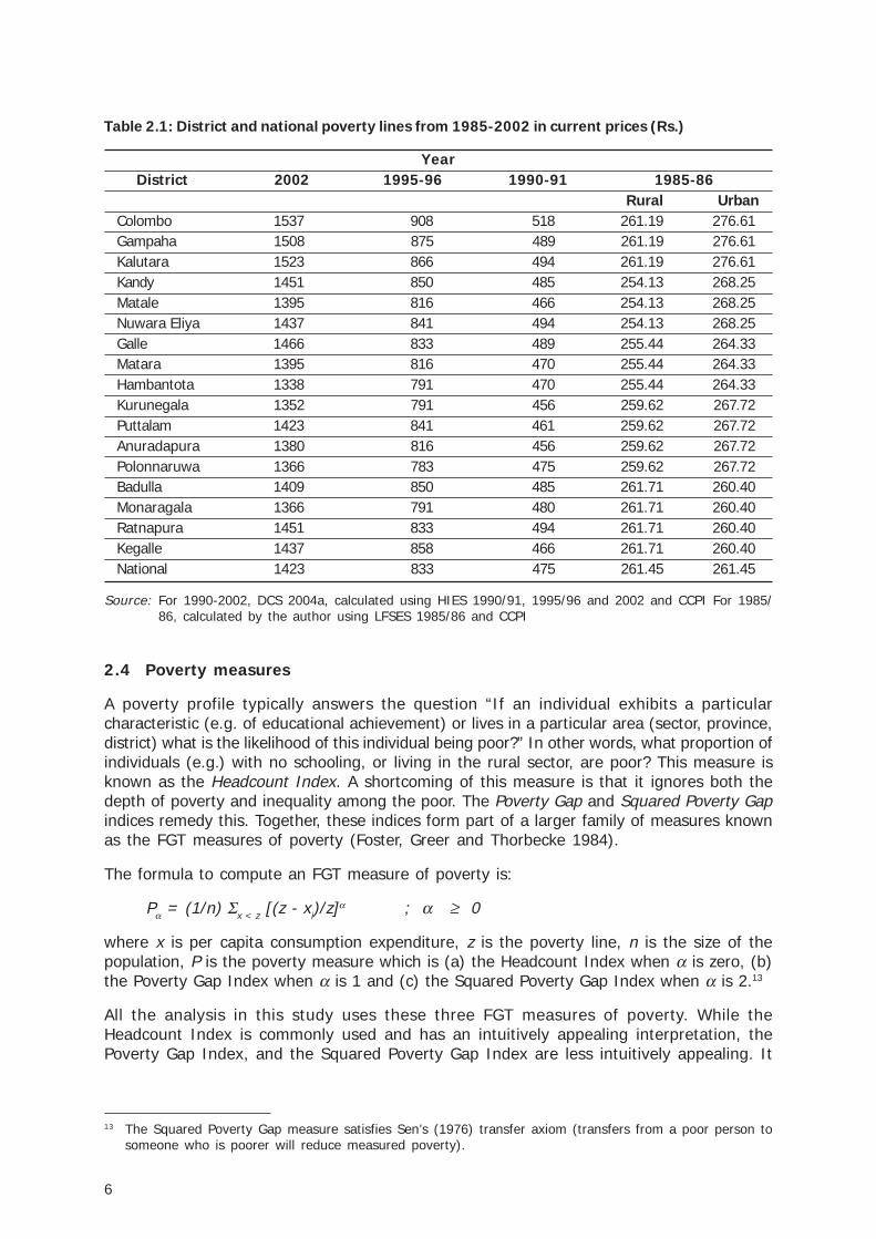
2.4 Poverty measures

A poverty profile typically answers the question “If an individual exhibits a particularcharacteristic (e.g. of educational achievement) or lives in a particular area (sector, province,district) what is the likelihood of this individual being poor?” In other words, what proportion ofindividuals (e.g.) with no schooling, or living in the rural sector, are poor? This measure isknown as the Headcount Index. A shortcoming of this measure is that it ignores both thedepth of poverty and inequality among the poor. The Poverty Gap and Squared Poverty Gapindices remedy this. Together, these indices form part of a larger family of measures knownas the FGT measures of poverty (Foster, Greer and Thorbecke 1984).

The formula to compute an FGT measure of poverty is:

Pα = (1/n) Σx < z [(z - xi)/z]α ; α ≥ 0

where x is per capita consumption expenditure, z is the poverty line, n is the size of thepopulation, P is the poverty measure which is (a) the Headcount Index when α is zero, (b)the Poverty Gap Index when α is 1 and (c) the Squared Poverty Gap Index when α is 2.13

All the analysis in this study uses these three FGT measures of poverty. While theHeadcount Index is commonly used and has an intuitively appealing interpretation, thePoverty Gap Index, and the Squared Poverty Gap Index are less intuitively appealing. It

Table 2.1: District and national poverty lines from 1985-2002 in current prices (Rs.)

YearDistrict 2002 1995-96 1990-91 1985-86

Rural UrbanColombo 1537 908 518 261.19 276.61Gampaha 1508 875 489 261.19 276.61Kalutara 1523 866 494 261.19 276.61Kandy 1451 850 485 254.13 268.25Matale 1395 816 466 254.13 268.25Nuwara Eliya 1437 841 494 254.13 268.25Galle 1466 833 489 255.44 264.33Matara 1395 816 470 255.44 264.33Hambantota 1338 791 470 255.44 264.33Kurunegala 1352 791 456 259.62 267.72Puttalam 1423 841 461 259.62 267.72Anuradapura 1380 816 456 259.62 267.72Polonnaruwa 1366 783 475 259.62 267.72Badulla 1409 850 485 261.71 260.40Monaragala 1366 791 480 261.71 260.40Ratnapura 1451 833 494 261.71 260.40Kegalle 1437 858 466 261.71 260.40National 1423 833 475 261.45 261.45

Source: For 1990-2002, DCS 2004a, calculated using HIES 1990/91, 1995/96 and 2002 and CCPI For 1985/86, calculated by the author using LFSES 1985/86 and CCPI

13 The Squared Poverty Gap measure satisfies Sen’s (1976) transfer axiom (transfers from a poor person tosomeone who is poorer will reduce measured poverty).

7

Table 2.2: Definitions of poverty measures

P0Headcount Index (H) The percentage of individuals in a given population whose standardThe incidence of poverty of living lies below the poverty line

P1Poverty Gap index (PG) The average shortfall between an individual’s level of consumptionThe depth of poverty and the poverty line, where the shortfall for all individuals whose

consumption falls above the poverty line is zero.

P2Squared Poverty Gap index (PG2) As for the poverty gap, but by squaring the shortfall between anThe severity of poverty individual’s level of consumption and the poverty line, it places

greater weight on poorer individuals.

may help to think of the poverty gap in terms of its cousin, the Income Gap Ratio, which isinterpreted as the gap in consumption (distance between own consumption and the povertyline) of the average poor person. The difference between the Income Gap Ratio and thePoverty Gap Index is simply in the denominator, and the PG index can be interpreted as anaverage consumption shortfall, where shortfalls in consumption for the non-poor areconsidered to be zero (Table 2.2)14 Similarly, the Squared Poverty Gap can be interpreted asa weighted average of the consumption shortfall, where weights for poorer people (largershortfalls) are larger.

14 It can be easily shown that the Poverty Gap (PG) Index is the multiple of the Headcount (H) Index andthe Income Gap (I) ratio (PG=H x I) and the latter can be derived by dividing PG by H.

8

3. Poverty Profile: A regional description

3.1 National trends in poverty

National trends show that poverty was highest in 1985/86, dropping steeply in 1990/91,increasing in 1995/96, and then declining again in 2002. (Table 3.1 and Figure 3.1) Povertylevels in 2002 were in general lower than in 1995/96, but higher than levels in 1990/91.

Table 3.1: Poverty trends overall, 1985-2002

Year Headcount Index Poverty Gap Squared Poverty Gap1985 36.31 9.55 3.59

1990 21.27 4.48 1.43

1995 29.46 6.70 2.26

2002 22.80 5.07 1.65

Source: Author’s calculations from LFSES and HIES data

3.2 Sectoral trends in poverty

Trends in poverty by sector15 indicate a continuous decline in the incidence, depth and severityof urban poverty, but fluctuating poverty levels in the rural and estate sectors (Figure 3.2).While poverty (by all three FGT measures) in the rural sector in 2002 was marginally higherthan its 1990 levels, estate sector poverty doubled over the same period.

15 Note that the comparison of sector is not consistent as the definition used changed during this period.

Figure 3.1: National poverty, 1985-2002


9

Figure 3.2: Poverty by sector, 1985-2002


The bulk of the estate population has a household per capita consumption that is very close to thepoverty line (World Bank 2007, Gunewardena 2005). This implies a high degree of vulnerability, aswell as sensitivity of poverty measure to the location of the poverty line (Gunewardena 2005). At anygiven poverty line, slight shifts in consumption of estate sector households - caused by idiosyncraticshocks such as a health shock to the breadwinner, or covariate shocks such as the loss ofemployment or days of work due to restructuring in the plantations, or rising cost of living with nowage indexation - can lead to very large increases in poverty in this sector (World Bank 2007).16

16 World Bank 2007 shows that a shock equivalent to 10% of the poverty line could increase poverty inthe estate sector by 10%, while the comparable figure for the entire country is 6%. Chapter 8 of WorldBank 2007 examines causes of poverty in the estate sector in great detail.

Table 3.2: Poverty trends by sector, 1985-2002

Sector Poverty Measure 1985 1990 1995 2002Headcount Index 22.13 15.38 14.84 8.05

Urban Poverty Gap 5.58 3.49 2.99 1.68Squared Poverty Gap 2.08 1.20 0.93 0.53

Headcount Index 41.54 23.59 31.5 24.72Rural Poverty Gap 11.10 4.95 7.28 5.56

Squared Poverty Gap 4.21 1.57 2.48 1.83

Headcount Index 24.56 14.85 38.81 30.09Estate Poverty Gap 5.28 2.49 7.87 6.01



10

If the Headcount Index (incidence of) poverty answers the question “If an individual lives in aparticular area (sector, province, district) what is the likelihood of that individual being poor?”,the question “What is the likelihood of a poor person living in a particular area (sector, province,district)?” is answered by the percentage contribution to poverty.17 Table 3.2 and Figure 3.3provide these statistics for the urban, rural and estate sectors for the 1985-2002 period andshow quite clearly that by all poverty measures, the chances of a poor person being in therural or estate sector increased while the chances of a poor person being in the urban sectordecreased.18 The chances of a poor person being in the rural sector are 11 times higher thanthe possibility they will be in the estate sector, and almost 20 times higher than the possibilitythat they will be in the urban sector.

17 This is simply the relevant poverty measure for the sector/province/district divided by the same povertymeasure at the national level and multiplied by the population share of that sector/province/district andconverted to a percentage.

18 These figures are not consistent as the definition of sector changed over the period.

Figure 3.3: Contribution to poverty by sector, 1985-2002


Headcount Index

(a)

11

Poverty Gap

(b)Source: Author’s calculations from LFSES and HIES data

Squared Poverty Gap


Figure 3.3: Contribution to poverty by sector, 1985-2002 (Contd.)

12

Table 3.3: Contribution to poverty by sector, 1985-2002

Sector Poverty Measure 1985 1990 1995 2002Headcount Index 12.73 15.12 7.01 4.74

Urban Poverty Gap 12.22 16.32 6.19 4.43Squared Poverty Gap 12.09 17.47 5.71 4.32

Headcount Index 82.58 80.08 88.09 87.41Rural Poverty Gap 83.94 79.86 89.43 88.51


Headcount Index 4.69 4.80 4.91 7.85Estate Poverty Gap 3.84 3.82 4.37 7.05



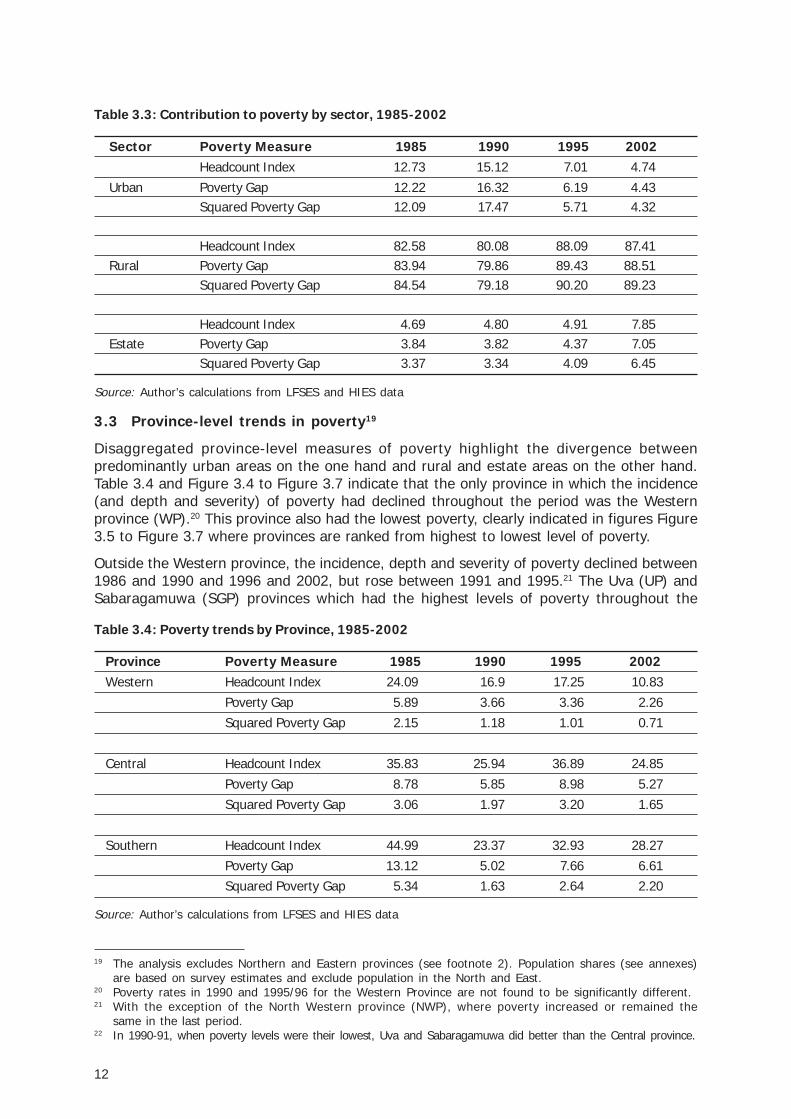
3.3 Province-level trends in poverty19

Disaggregated province-level measures of poverty highlight the divergence betweenpredominantly urban areas on the one hand and rural and estate areas on the other hand.Table 3.4 and Figure 3.4 to Figure 3.7 indicate that the only province in which the incidence(and depth and severity) of poverty had declined throughout the period was the Westernprovince (WP).20 This province also had the lowest poverty, clearly indicated in figures Figure3.5 to Figure 3.7 where provinces are ranked from highest to lowest level of poverty.

Outside the Western province, the incidence, depth and severity of poverty declined between1986 and 1990 and 1996 and 2002, but rose between 1991 and 1995.21 The Uva (UP) andSabaragamuwa (SGP) provinces which had the highest levels of poverty throughout the

Table 3.4: Poverty trends by Province, 1985-2002

Province Poverty Measure 1985 1990 1995 2002Western Headcount Index 24.09 16.9 17.25 10.83

Poverty Gap 5.89 3.66 3.36 2.26Squared Poverty Gap 2.15 1.18 1.01 0.71

Central Headcount Index 35.83 25.94 36.89 24.85Poverty Gap 8.78 5.85 8.98 5.27Squared Poverty Gap 3.06 1.97 3.20 1.65

Southern Headcount Index 44.99 23.37 32.93 28.27Poverty Gap 13.12 5.02 7.66 6.61Squared Poverty Gap 5.34 1.63 2.64 2.20

19 The analysis excludes Northern and Eastern provinces (see footnote 2). Population shares (see annexes)are based on survey estimates and exclude population in the North and East.

20 Poverty rates in 1990 and 1995/96 for the Western Province are not found to be significantly different.21 With the exception of the North Western province (NWP), where poverty increased or remained the

same in the last period.22 In 1990-91, when poverty levels were their lowest, Uva and Sabaragamuwa did better than the Central province.


13

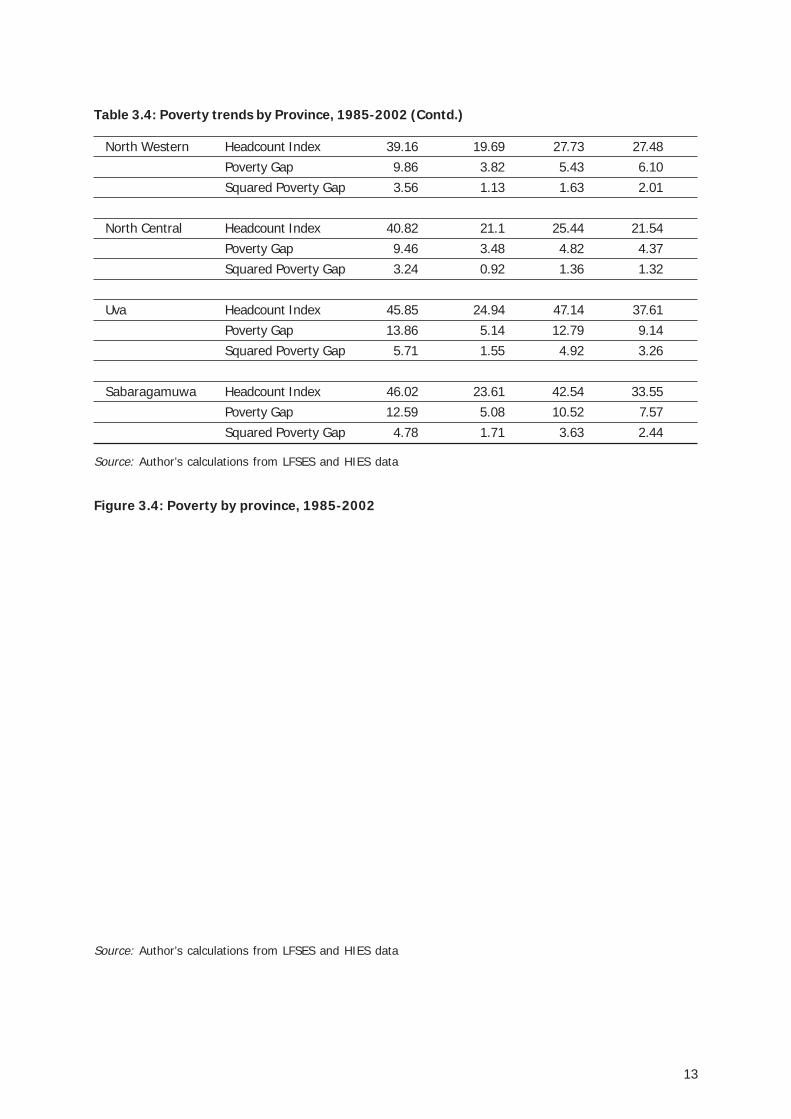
North Western Headcount Index 39.16 19.69 27.73 27.48Poverty Gap 9.86 3.82 5.43 6.10Squared Poverty Gap 3.56 1.13 1.63 2.01

North Central Headcount Index 40.82 21.1 25.44 21.54Poverty Gap 9.46 3.48 4.82 4.37Squared Poverty Gap 3.24 0.92 1.36 1.32

Uva Headcount Index 45.85 24.94 47.14 37.61Poverty Gap 13.86 5.14 12.79 9.14Squared Poverty Gap 5.71 1.55 4.92 3.26

Sabaragamuwa Headcount Index 46.02 23.61 42.54 33.55Poverty Gap 12.59 5.08 10.52 7.57Squared Poverty Gap 4.78 1.71 3.63 2.44


Figure 3.4: Poverty by province, 1985-2002


Table 3.4: Poverty trends by Province, 1985-2002 (Contd.)

14

Figure 3.5: Headcount Index by province, 1985-2002


Figure 3.6: Poverty Gap Index by province, 1985-2002


15

Figure 3.7: Squared Poverty Gap Index by province, 1985-2002


Figure 3.5 to Figure 3.7 help to track changes in poverty over the period. Initial poverty ratesin 1985-86 show a clear clustering of provinces. The Western province with lowest poverty liesclearly apart from all other provinces, while the next three provinces are Central province,North Western province and North Central province, with the Southern province, Uva provinceand Sabaragamuwa province clearly having the highest poverty. Rankings appear to remainsomewhat stable over the period, except for the Central province. This had the lowestpoverty in 1990-1 (admittedly a year when the dispersion of poverty across provinces wasfairly narrow), rose to third lowest position in 1995-6 and was third highest in 2002. This highdegree of fluctuation in poverty rates in the Central province may be due to the dominance ofthe estate sector, which, as we have seen, has a large percentage of the population close tothe poverty line, making it open to considerable vulnerability.

The fortunes of the North Central province and North Western province remained similar until2002. In the North Central province, poverty levels since 1990 have remained relativelystable, at a level approximately half that of 1985 levels of poverty. The drastic decline inpoverty in 1990 in this region (with the depth and severity of poverty falling to below Westernprovince levels) was attributed to the large infrastructure investments in these regions in the1980s.23 In the North Western province, although poverty fell considerably in 1990-1, and therise in 1995-6 was only slightly higher than that in the North Central province, in 2002, thesetwo provinces diverge. Despite relatively low levels of economic activity and growth in theNorth Central province, the incidence of poverty fell to 1/5 of the population, and the depth

23 These were primarily in irrigation, with supporting road and energy investments.

16

and severity of poverty were only slightly higher than 1990 levels. On the other hand, in theNorth Western province, headcount poverty remained close to 1995-6 levels, and the depthand severity of poverty increased.

In the last cluster of provinces - Southern province, Uva province and Sabaragamuwa province- poverty changes have followed the overall trend over the period. Gains in 1990-1 wereroughly similar for all three provinces, but increases in 1995-96 left SGP and Uva province farbelow Southern province. While all three provinces managed to reduce poverty in 2002, (by1/4 in Sabaragamuwa province and Uva province, compared to 1/8 in Southern province)poverty levels in Sabaragamuwa province and Uva province remained considerably higherthan in Southern province.

Thus, in 2002, the clustering of provinces returned to that of 1985-86: lowest poverty inWestern province, moderate poverty in the Central province, North Central province andNorth Western province and highest poverty in Southern province, Sabaragamuwa provinceand Uva province. Changes in ranking within clusters were primarily due to the reduction inpoverty in the North Central province and Southern province.

Comparing Figure 3.5 with Figure 3.6 and Figure 3.7 shows that ranking reversals can beobserved across poverty measures in the first two periods. In 1985-86, the depth andseverity of poverty were much greater in Uva province and Southern province than they werein Sabaragamuwa province, which had a similar or higher proportion of people in poverty.Similarly, in 1990-91, the year of lowest poverty in the entire period, the depth and severity ofpoverty in the North Cental province and the severity of poverty in the North Westernprovince were even lower than in the Western province which had the lowest incidence ofpoverty.

Relative rankings across provinces are constant across measures in the last two periods. Thisimplies that that the depth and severity of poverty are highest where the magnitude ofpoverty is highest, and vice-versa. However, distances between provinces, vary as illustratedquite clearly in Figure 3.5 to Figure 3.7. For example, in 2002, while headcount poverty outsidethe Western province had a wide variation, ranging from 22%-38%, with most provincesequidistant from each other, the squared poverty gap measure is much less dispersed, with fiveprovinces in the narrow band from 1.3% to 2.4%, but with Uva province lagging behind at 3.2%

Table 3.5 and Figure 3.8 provide calculations of the contribution to poverty by province, andindicate that although approximately one in ten people in the Western province are poor(Table 3.4), the chances of a poor person being from Western province are higher, at 15%.This figure too has steadily declined from 1990 onward. On the other hand, while more thanone in three persons in Uva province and Sabaragamuwa province were poor, the chances ofa poor person being from Uva province is 12% and from Sabaragamuwa province is 16%,reflecting the distribution of population in these provinces.

In 2002, the poor people in the Western, Central and Southern provinces made up half thenumber of poor people in the country. This was a decline from previous years, primarily dueto the steady decline in the share of the Western province, and to a lesser extent due to thedecline in the share of the Central province. The increase in the share of Uva andSabaragamuwa provinces in the last 10 years is also evident, as is the increase in the NorthWestern province in the last 5 years, returning to 1985 proportions of the relative share inpoverty.

Relative shares in the Poverty Gap and Squared Poverty Gap indices do not diverge greatlyacross provinces, but three distinct patterns are evident. In some provinces (North Westernprovince, Sabaragamuwa province) the contribution to overall poverty in these provinces aresimilar across all three measures. In other provinces (Western province, Central province,

17

North Central province) the contribution of higher order measures of poverty (reflectingcontribution to the depth and severity of poverty) is lower. These are also provinces where (in2002) headcount poverty incidence is lower. In the third category (Southern province and Uvaprovince), the contribution to the overall depth and severity of poverty is higher than thecontribution to the incidence of poverty. These results confirm the evidence from measuresof incidence that the poorest provinces also have the highest depth and severity of poverty.

Figure 3.8 underscores that the share of the Western province has declined over the years,while the share of Uva province has increased, for all three measures of poverty.

Table 3.5: Contribution to poverty by province, 1985-2002

Province Poverty Measure 1985 1990 1995 2002Western Headcount Index 20.28 24.07 18.79 15.44


Central Headcount Index 14.98 18.35 18.97 16.22Poverty Gap 13.97 19.67 20.29 15.48Squared Poverty Gap 12.92 20.67 21.43 14.82

Southern Headcount Index 18.66 16.69 16.58 17.58Poverty Gap 20.7 17.03 16.94 18.49Squared Poverty Gap 22.4 17.34 17.27 18.89

North Western Headcount Index 14.72 12.74 12.35 16.05Poverty Gap 14.11 11.75 10.62 16.02Squared Poverty Gap 13.53 10.88 9.46 16.22

North Central Headcount Index 7.76 6.94 5.39 6.37Poverty Gap 6.84 5.43 4.49 5.81Squared Poverty Gap 6.23 4.49 3.74 5.37

Uva Headcount Index 9.01 8.47 11.55 12.02Poverty Gap 10.36 8.3 13.77 13.14Squared Poverty Gap 11.33 7.85 15.68 14.35

Sabaragamuwa Headcount Index 14.58 12.74 16.36 16.32Poverty Gap 15.17 13.04 17.78 16.56Squared Poverty Gap 15.31 13.74 18.16 16.37


18

Figure 3.8: Distribution of poverty by province

Headcount Index

Poverty Gap

(a)

(b)

19

Squared Poverty Gap


3.4 District-level trends in poverty

Disaggregated measures of poverty at the district level are given in Table 3.6 and Figure3.9.24 The latter illustrates quite clearly that poverty is high, and has remained high in thedistricts of Moneragala, Ratnapura, Badulla and Kegalle.25 Within Uva province andSabaragamuwa province, one sees convergence between districts between 1995-6 and 2002,with the incidence of poverty in Moneragala and Ratnapura declining to the levels of Badullaand Kegalle, respectively. Section 4.2 indicates that adverse redistribution in the Uva provinceand Sabaragamuwa province contributed to the rise in poverty in this period and confirms thatthis occurred within districts rather than between districts.

24 Note that poverty rates for 1990-91 reported here differ from those published by DCS. It is not clear whythis should be given that the same data and poverty line were used. Stata do-files used by the author areavailable upon request.

25 Badulla and Moneragala districts together comprise the Uva province, while Ratnapura and Kegallecomprise Sabaragamuwa province.

(c)

Figure 3.8: Distribution of poverty by province (Contd.)

20

Table 3.6: Trends in poverty by district, 1985-2002

Poverty indices 1985 1990 1995 2002Colombo Headcount Index 15.33 14.55 13.07 6.34


Gampaha Headcount Index 32.15 13.57 15.11 10.69Poverty Gap 8.01 2.46 2.62 2.22Squared Poverty Gap 2.96 0.70 0.72 0.68

Kalutara Headcount Index 28.88 27.21 30.08 20.11Poverty Gap 7.08 6.03 7.09 4.42Squared Poverty Gap 2.55 1.96 2.38 1.41

Kandy Headcount Index 40.88 31.5 37.5 24.46Poverty Gap 10.51 7.1 10.12 5.53Squared Poverty Gap 3.78 2.36 3.80 1.80

Matale Headcount Index 40.1 23.41 41.84 29.64Poverty Gap 9.27 5.57 10.81 6.25Squared Poverty Gap 3.04 1.87 4.04 1.79

Nuwara Eliya Headcount Index 20.89 14.96 33.08 22.58Poverty Gap 4.42 3.16 6.09 4.21Squared Poverty Gap 1.42 1.11 1.76 1.28

Galle Headcount Index 45.7 23.86 31.92 26.3Poverty Gap 13.01 5.3 7.8 5.85Squared Poverty Gap 5.12 1.78 2.84 1.96

Matara Headcount Index 37.73 22.34 35.54 27.65Poverty Gap 10.04 4.73 8.06 6.63Squared Poverty Gap 3.98 1.47 2.73 2.19

Hambantota Headcount Index 54.61 24.01 30.92 32.85Poverty Gap 17.97 4.92 6.80 8.00Squared Poverty Gap 7.82 1.61 2.14 2.68

Kurunegala Headcount Index 40.62 19.31 26.29 25.05Poverty Gap 10.44 3.58 5.1 5.47Squared Poverty Gap 3.86 1.02 1.51 1.79

Puttalam Headcount Index 35.6 20.58 31.09 32.43Poverty Gap 8.45 4.41 6.19 7.36Squared Poverty Gap 2.84 1.41 1.93 2.47

21

Anuradhapura Headcount Index 45.9 22.07 27.79 20.37Poverty Gap 10.86 3.55 4.90 4.04Squared Poverty Gap 3.75 0.90 1.29 1.15

Polonnaruwa Headcount Index 29.49 18.92 20.64 23.94Poverty Gap 6.33 3.31 4.68 5.05Squared Poverty Gap 2.12 0.96 1.49 1.66

Badulla Headcount Index 43.64 24.59 41.69 37.46Poverty Gap 13.22 4.88 10.24 8.76Squared Poverty Gap 5.48 1.44 3.55 2.96

Moneragala Headcount Index 50.47 25.67 56.17 37.89Poverty Gap 15.21 5.66 17.02 9.87Squared Poverty Gap 6.19 1.78 7.19 3.84

Ratnapura Headcount Index 51.16 22.05 46.61 34.39Poverty Gap 14.59 4.28 12.03 7.81Squared Poverty Gap 5.77 1.33 4.20 2.56

Kegalle Headcount Index 39.88 25.56 37.84 32.46Poverty Gap 10.19 6.09 8.78 7.25Squared Poverty Gap 3.60 2.19 2.97 2.29


At the other extreme, disaggregation of poverty in the Western province indicates that acontinuous decline occurred only in the Colombo district. In both Gampaha and Kalutara,poverty rose marginally between 1990-1 and 1995-6. While Gampaha district experiencedthe greatest decline in poverty over the entire 22-year period, poverty levels in Kalutararemained considerably higher than in the other two districts in 2002. District level changesdo not appear to be related to patterns of redistribution, indicating that distributional changeswithin the province were dominated by distributional changes within districts rather thanbetween districts.

The pattern of rank reversals indicated in the previous section in relation to the Centralprovince are somewhat illuminated by district-level disaggregation. For e.g. in 1990-1, theCentral province had the highest incidence of poverty. This was when poverty felldrastically in most provinces (Figure 3.4) including in the Central province, but to a lesserextent. Figure 3.9 shows that while Matale experienced this large decline in poverty (whichwas also experienced in districts where non-plantation agriculture is an importantlivelihood), this was much less the case in Kandy and Nuwara Eliya where urban andestate livelihoods are more dominant. The improvement in the relative position of theCentral province in 1995-6 is due to the fact that poverty increases were smaller in thesedistricts, especially in Kandy. Between 1995 and 2002, the fall in poverty was much largerthan in other districts, and this appears to be true for Matale and Nuwara Eliya as well.

Table 3.6: Trends in poverty by district, 1985-2002 (Contd.)

22

In the Southern province, levels of poverty by district converged in 1990-91, with drasticdeclines in poverty in all three districts of Galle, Matara and Hambantota, but divergedthereafter, with poverty rising continuously in Hambantota from 1990-1 onward. Part ofthe favourable redistribution experienced in the Southern province in the 1986-1990 period(Section 4.2) may have been due to the convergence in districts (especially the large declinein poverty in Hambantota) during this period.

The gradual worsening of the relative position of the North Western province since 1990appears to be largely driven by the increase in poverty in Puttalam since 1995-6. This isconsistent with the influx into this district of large numbers of people displaced by the civilconflict. However, the increase in depth and severity of poverty between 1995/96 and 2002in the North Western province is due to sharp increases in these measures in both Puttalamand Kurunegala districts.

In the North Central province, sharp declines in poverty between 1986 and 1990 occurred inboth Anuradhapura and Polonnaruwa. North Central province continued to improve itsrelative ranking in 1995-6 as the province with the second lowest incidence of poverty andmaintained this position in 2002 despite poverty increasing in both districts in 1995-6, and inthe latter in 2002. This is because the size of the increase in poverty in both these yearswas relatively small.

23

Figu

re 3

.9: P

over

ty b

y di

stri

ct, 1

985-

2002

Sour

ce:

Auth

or’s

cal

cula

tions

fro

m L

FSES

and

HIE

S da

ta

24

Figure 3.11: Poverty Gap Index by district, 1985-2002


Figure 3.10: Headcount Index by district, 1985-2002


25

Figure 3.12: Squared Poverty Gap Index by district, 1985-2002

Table 3.7 and Figure 3.13 indicate the probability of a poor person being from a particulardistrict. The chances of a poor person being in Kurunegala district, which has a largepopulation, are highest, at close to 10%, while they are lowest in Polonnaruwa, for both thebeginning and end of this period. When regional disparities in poverty are low, as in 1990-1,relative population shares play a large role in determining the location of the highest numbersof people in poverty. Thus, in 1990-1, the probability of a poor person being in Colombo wasthree times the probability of a person being in Moneragala. When there is greater divergencein poverty measures across districts, this is not the case, and in 2002, it was just as likely thata poor person would be in Moneragala as it was that they were in Colombo. When a district’srelative contribution to the depth and severity of poverty is greater than its contribution to theincidence of poverty, as in the case of Moneragala in 1995-6 and 2002 and Kandy, Ratnapuraand Matale in 1995-6, this is indicative that the depth and severity of poverty in these districtsis considerable.


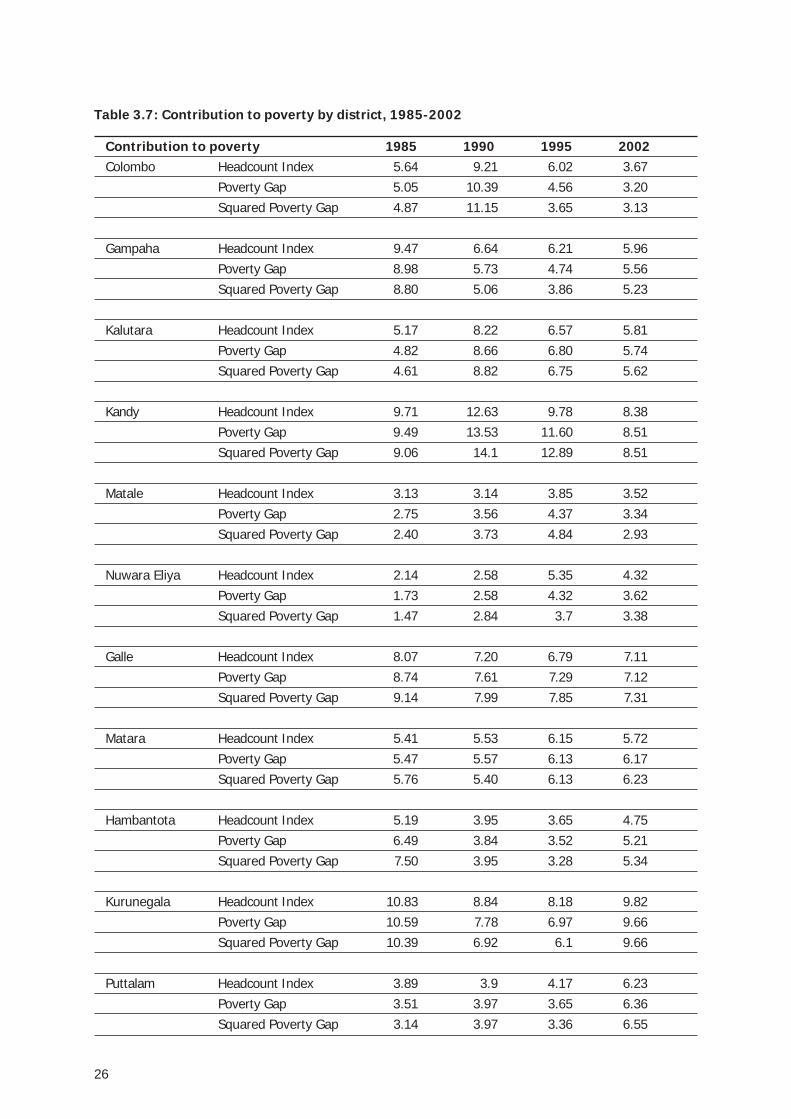
26

Table 3.7: Contribution to poverty by district, 1985-2002

Contribution to poverty 1985 1990 1995 2002Colombo Headcount Index 5.64 9.21 6.02 3.67


Gampaha Headcount Index 9.47 6.64 6.21 5.96Poverty Gap 8.98 5.73 4.74 5.56Squared Poverty Gap 8.80 5.06 3.86 5.23

Kalutara Headcount Index 5.17 8.22 6.57 5.81Poverty Gap 4.82 8.66 6.80 5.74Squared Poverty Gap 4.61 8.82 6.75 5.62

Kandy Headcount Index 9.71 12.63 9.78 8.38Poverty Gap 9.49 13.53 11.60 8.51Squared Poverty Gap 9.06 14.1 12.89 8.51

Matale Headcount Index 3.13 3.14 3.85 3.52Poverty Gap 2.75 3.56 4.37 3.34Squared Poverty Gap 2.40 3.73 4.84 2.93

Nuwara Eliya Headcount Index 2.14 2.58 5.35 4.32Poverty Gap 1.73 2.58 4.32 3.62Squared Poverty Gap 1.47 2.84 3.7 3.38

Galle Headcount Index 8.07 7.20 6.79 7.11Poverty Gap 8.74 7.61 7.29 7.12Squared Poverty Gap 9.14 7.99 7.85 7.31

Matara Headcount Index 5.41 5.53 6.15 5.72Poverty Gap 5.47 5.57 6.13 6.17Squared Poverty Gap 5.76 5.40 6.13 6.23

Hambantota Headcount Index 5.19 3.95 3.65 4.75Poverty Gap 6.49 3.84 3.52 5.21Squared Poverty Gap 7.50 3.95 3.28 5.34

Kurunegala Headcount Index 10.83 8.84 8.18 9.82Poverty Gap 10.59 7.78 6.97 9.66Squared Poverty Gap 10.39 6.92 6.1 9.66

Puttalam Headcount Index 3.89 3.9 4.17 6.23Poverty Gap 3.51 3.97 3.65 6.36Squared Poverty Gap 3.14 3.97 3.36 6.55

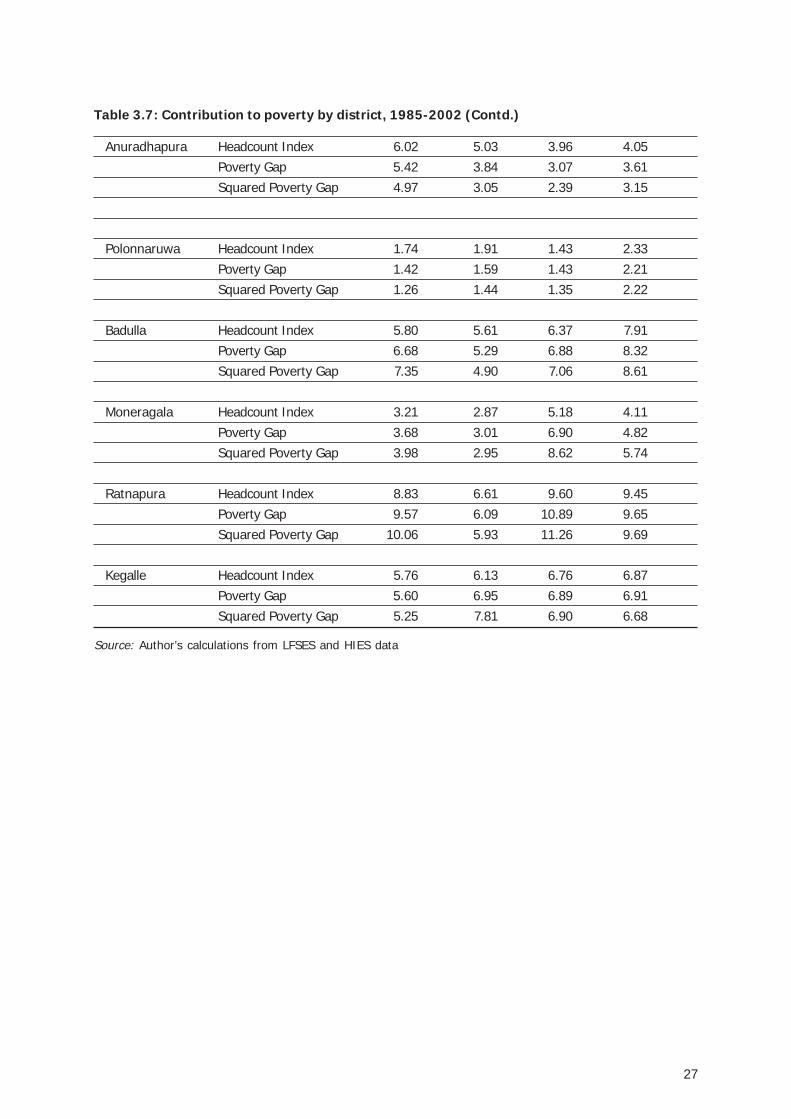
27

Anuradhapura Headcount Index 6.02 5.03 3.96 4.05Poverty Gap 5.42 3.84 3.07 3.61Squared Poverty Gap 4.97 3.05 2.39 3.15

Polonnaruwa Headcount Index 1.74 1.91 1.43 2.33Poverty Gap 1.42 1.59 1.43 2.21Squared Poverty Gap 1.26 1.44 1.35 2.22

Badulla Headcount Index 5.80 5.61 6.37 7.91Poverty Gap 6.68 5.29 6.88 8.32Squared Poverty Gap 7.35 4.90 7.06 8.61

Moneragala Headcount Index 3.21 2.87 5.18 4.11Poverty Gap 3.68 3.01 6.90 4.82Squared Poverty Gap 3.98 2.95 8.62 5.74

Ratnapura Headcount Index 8.83 6.61 9.60 9.45Poverty Gap 9.57 6.09 10.89 9.65Squared Poverty Gap 10.06 5.93 11.26 9.69

Kegalle Headcount Index 5.76 6.13 6.76 6.87Poverty Gap 5.60 6.95 6.89 6.91Squared Poverty Gap 5.25 7.81 6.90 6.68


Table 3.7: Contribution to poverty by district, 1985-2002 (Contd.)

28

Figure 3.13: Contribution to poverty by district, FGT measures


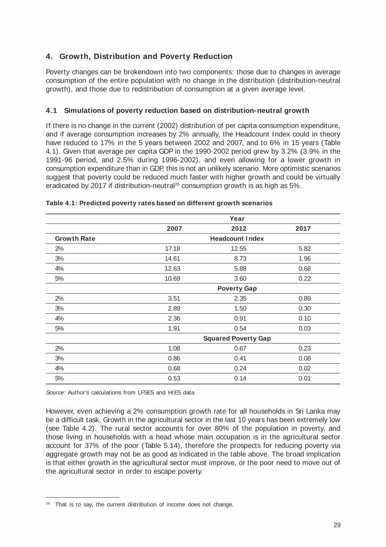
29

4. Growth, Distribution and Poverty Reduction

Poverty changes can be brokendown into two components: those due to changes in averageconsumption of the entire population with no change in the distribution (distribution-neutralgrowth), and those due to redistribution of consumption at a given average level.

4.1 Simulations of poverty reduction based on distribution-neutral growth

If there is no change in the current (2002) distribution of per capita consumption expenditure,and if average consumption increases by 2% annually, the Headcount Index could in theoryhave reduced to 17% in the 5 years between 2002 and 2007, and to 6% in 15 years (Table4.1). Given that average per capita GDP in the 1990-2002 period grew by 3.2% (3.9% in the1991-96 period, and 2.5% during 1996-2002), and even allowing for a lower growth inconsumption expenditure than in GDP, this is not an unlikely scenario. More optimistic scenariossuggest that poverty could be reduced much faster with higher growth and could be virtuallyeradicated by 2017 if distribution-neutral26 consumption growth is as high as 5%.

26 That is to say, the current distribution of income does not change.

Table 4.1: Predicted poverty rates based on different growth scenarios

Year2007 2012 2017

Growth Rate Headcount Index2% 17.18 12.55 5.823% 14.61 8.73 1.964% 12.63 5.88 0.685% 10.69 3.60 0.22

Poverty Gap2% 3.51 2.35 0.893% 2.89 1.50 0.304% 2.36 0.91 0.105% 1.91 0.54 0.03

Squared Poverty Gap2% 1.08 0.67 0.233% 0.86 0.41 0.084% 0.68 0.24 0.025% 0.53 0.14 0.01


However, even achieving a 2% consumption growth rate for all households in Sri Lanka maybe a difficult task. Growth in the agricultural sector in the last 10 years has been extremely low(see Table 4.2). The rural sector accounts for over 80% of the population in poverty, andthose living in households with a head whose main occupation is in the agricultural sectoraccount for 37% of the poor (Table 5.14), therefore the prospects for reducing poverty viaaggregate growth may not be as good as indicated in the table above. The broad implicationis that either growth in the agricultural sector must improve, or the poor need to move out ofthe agricultural sector in order to escape poverty.

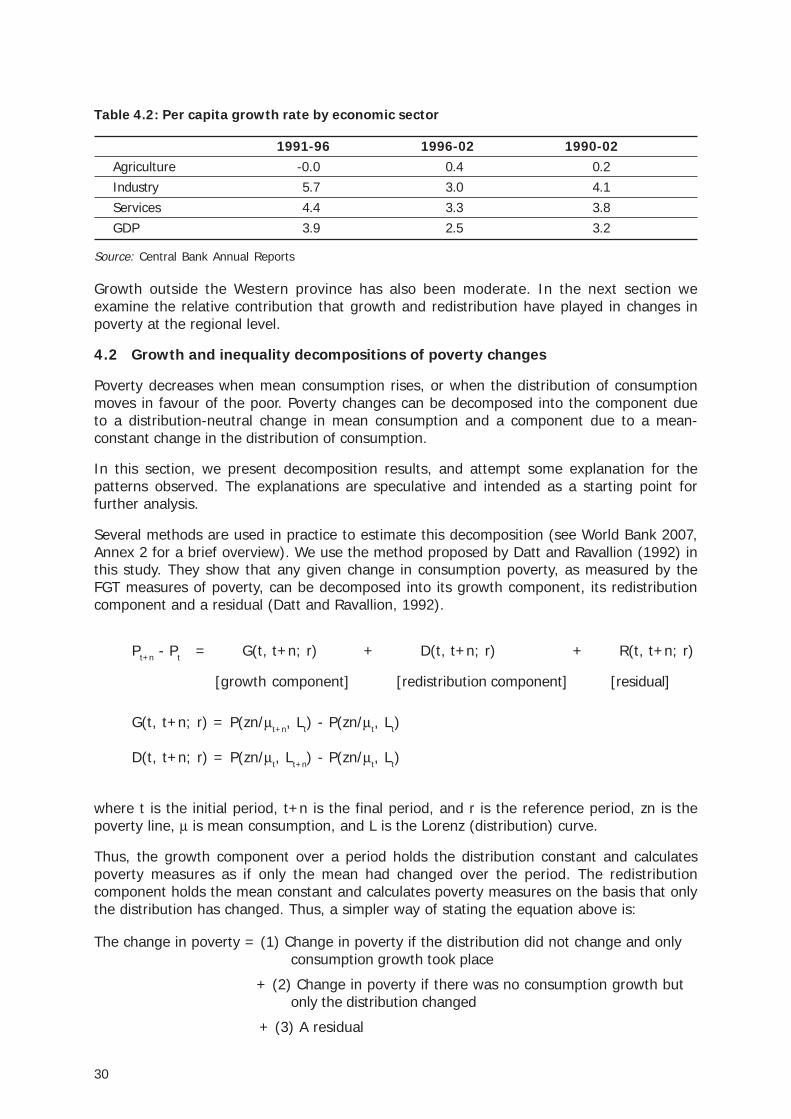
30

Table 4.2: Per capita growth rate by economic sector

1991-96 1996-02 1990-02Agriculture -0.0 0.4 0.2Industry 5.7 3.0 4.1Services 4.4 3.3 3.8GDP 3.9 2.5 3.2

Source: Central Bank Annual Reports

Growth outside the Western province has also been moderate. In the next section weexamine the relative contribution that growth and redistribution have played in changes inpoverty at the regional level.

4.2 Growth and inequality decompositions of poverty changes

Poverty decreases when mean consumption rises, or when the distribution of consumptionmoves in favour of the poor. Poverty changes can be decomposed into the component dueto a distribution-neutral change in mean consumption and a component due to a mean-constant change in the distribution of consumption.

In this section, we present decomposition results, and attempt some explanation for thepatterns observed. The explanations are speculative and intended as a starting point forfurther analysis.

Several methods are used in practice to estimate this decomposition (see World Bank 2007,Annex 2 for a brief overview). We use the method proposed by Datt and Ravallion (1992) inthis study. They show that any given change in consumption poverty, as measured by theFGT measures of poverty, can be decomposed into its growth component, its redistributioncomponent and a residual (Datt and Ravallion, 1992).

Pt+n - Pt = G(t, t+n; r) + D(t, t+n; r) + R(t, t+n; r)

[growth component] [redistribution component] [residual]

G(t, t+n; r) = P(zn/μt+n, Lt) - P(zn/μt, Lt)

D(t, t+n; r) = P(zn/μt, Lt+n) - P(zn/μt, Lt)

where t is the initial period, t+n is the final period, and r is the reference period, zn is thepoverty line, μ is mean consumption, and L is the Lorenz (distribution) curve.

Thus, the growth component over a period holds the distribution constant and calculatespoverty measures as if only the mean had changed over the period. The redistributioncomponent holds the mean constant and calculates poverty measures on the basis that onlythe distribution has changed. Thus, a simpler way of stating the equation above is:

The change in poverty = (1) Change in poverty if the distribution did not change and onlyconsumption growth took place

+ (2) Change in poverty if there was no consumption growth butonly the distribution changed

+ (3) A residual

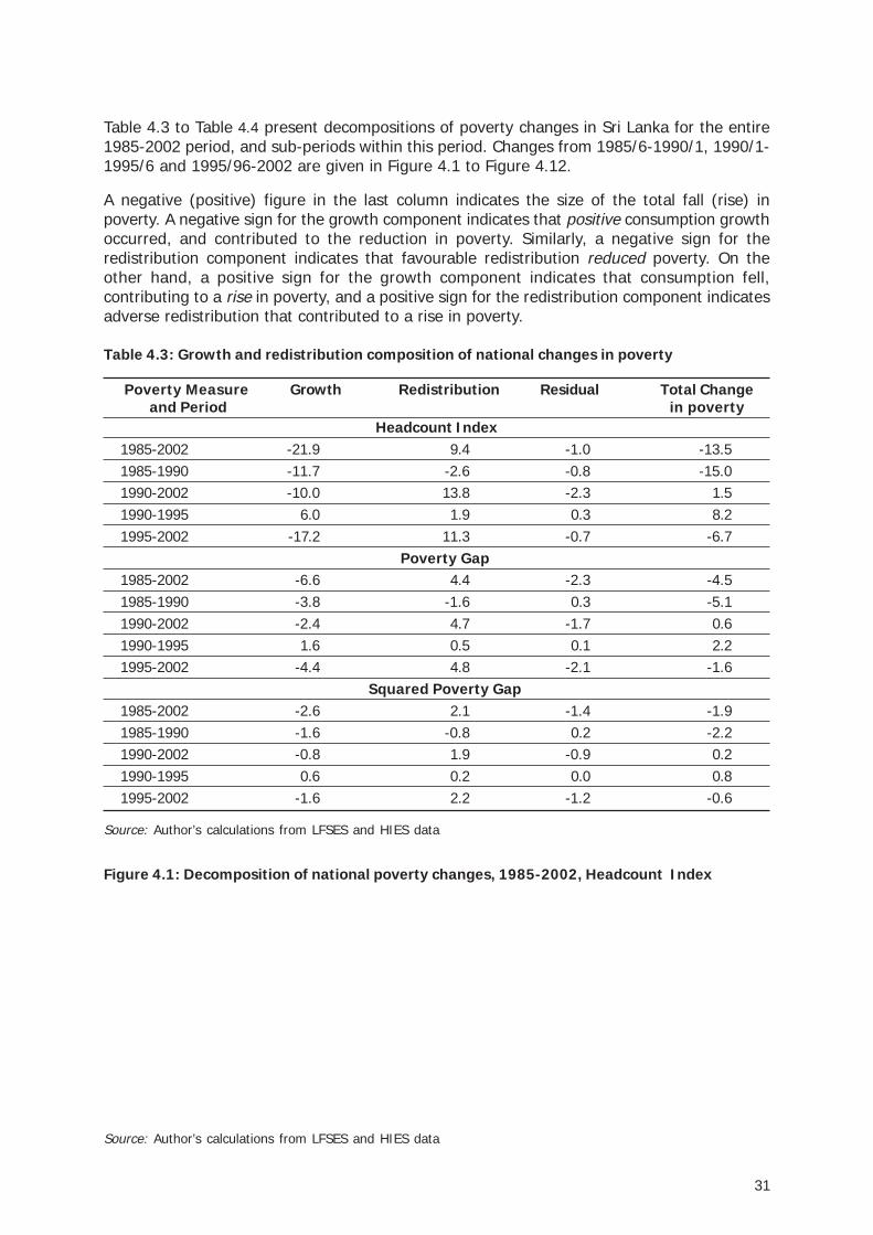
31

Table 4.3 to Table 4.4 present decompositions of poverty changes in Sri Lanka for the entire1985-2002 period, and sub-periods within this period. Changes from 1985/6-1990/1, 1990/1-1995/6 and 1995/96-2002 are given in Figure 4.1 to Figure 4.12.

A negative (positive) figure in the last column indicates the size of the total fall (rise) inpoverty. A negative sign for the growth component indicates that positive consumption growthoccurred, and contributed to the reduction in poverty. Similarly, a negative sign for theredistribution component indicates that favourable redistribution reduced poverty. On theother hand, a positive sign for the growth component indicates that consumption fell,contributing to a rise in poverty, and a positive sign for the redistribution component indicatesadverse redistribution that contributed to a rise in poverty.

Table 4.3: Growth and redistribution composition of national changes in poverty

Poverty Measure Growth Redistribution Residual Total Change and Period in poverty

Headcount Index1985-2002 -21.9 9.4 -1.0 -13.51985-1990 -11.7 -2.6 -0.8 -15.01990-2002 -10.0 13.8 -2.3 1.51990-1995 6.0 1.9 0.3 8.21995-2002 -17.2 11.3 -0.7 -6.7

Poverty Gap1985-2002 -6.6 4.4 -2.3 -4.51985-1990 -3.8 -1.6 0.3 -5.11990-2002 -2.4 4.7 -1.7 0.61990-1995 1.6 0.5 0.1 2.21995-2002 -4.4 4.8 -2.1 -1.6

Squared Poverty Gap1985-2002 -2.6 2.1 -1.4 -1.91985-1990 -1.6 -0.8 0.2 -2.21990-2002 -0.8 1.9 -0.9 0.21990-1995 0.6 0.2 0.0 0.81995-2002 -1.6 2.2 -1.2 -0.6


Figure 4.1: Decomposition of national poverty changes, 1985-2002, Headcount Index


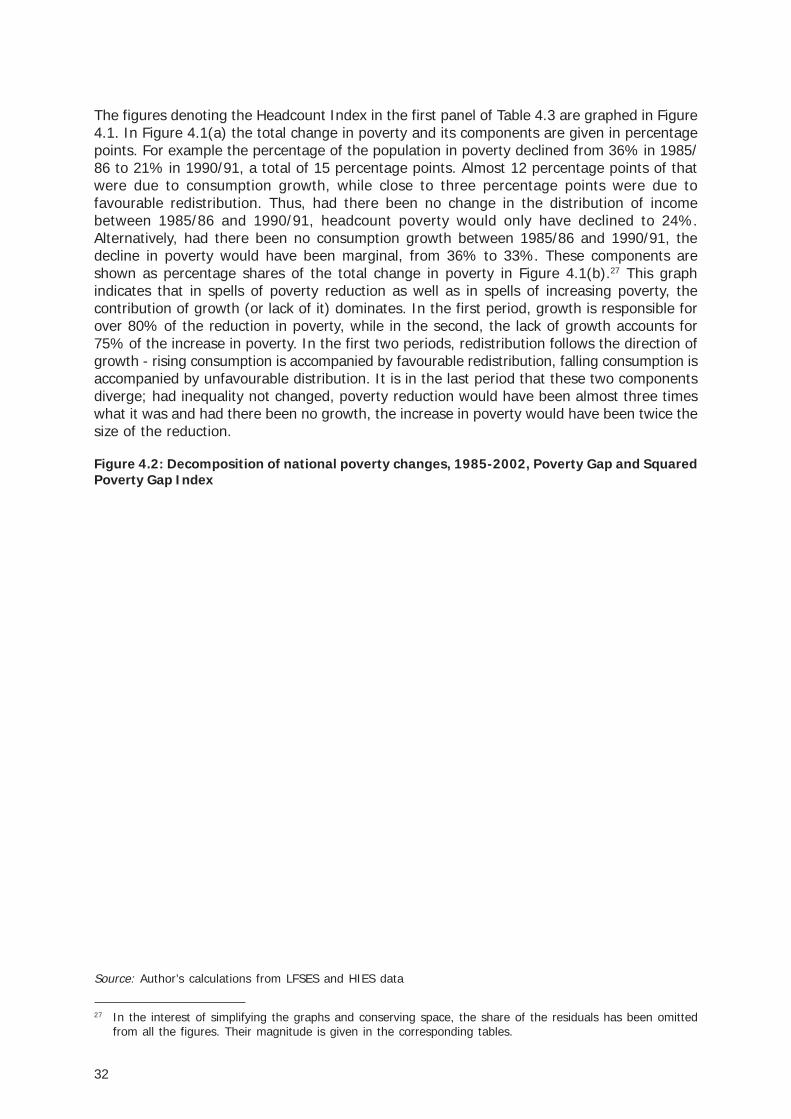
32

The figures denoting the Headcount Index in the first panel of Table 4.3 are graphed in Figure4.1. In Figure 4.1(a) the total change in poverty and its components are given in percentagepoints. For example the percentage of the population in poverty declined from 36% in 1985/86 to 21% in 1990/91, a total of 15 percentage points. Almost 12 percentage points of thatwere due to consumption growth, while close to three percentage points were due tofavourable redistribution. Thus, had there been no change in the distribution of incomebetween 1985/86 and 1990/91, headcount poverty would only have declined to 24%.Alternatively, had there been no consumption growth between 1985/86 and 1990/91, thedecline in poverty would have been marginal, from 36% to 33%. These components areshown as percentage shares of the total change in poverty in Figure 4.1(b).27 This graphindicates that in spells of poverty reduction as well as in spells of increasing poverty, thecontribution of growth (or lack of it) dominates. In the first period, growth is responsible forover 80% of the reduction in poverty, while in the second, the lack of growth accounts for75% of the increase in poverty. In the first two periods, redistribution follows the direction ofgrowth - rising consumption is accompanied by favourable redistribution, falling consumption isaccompanied by unfavourable distribution. It is in the last period that these two componentsdiverge; had inequality not changed, poverty reduction would have been almost three timeswhat it was and had there been no growth, the increase in poverty would have been twice thesize of the reduction.

27 In the interest of simplifying the graphs and conserving space, the share of the residuals has been omittedfrom all the figures. Their magnitude is given in the corresponding tables.

Figure 4.2: Decomposition of national poverty changes, 1985-2002, Poverty Gap and SquaredPoverty Gap Index


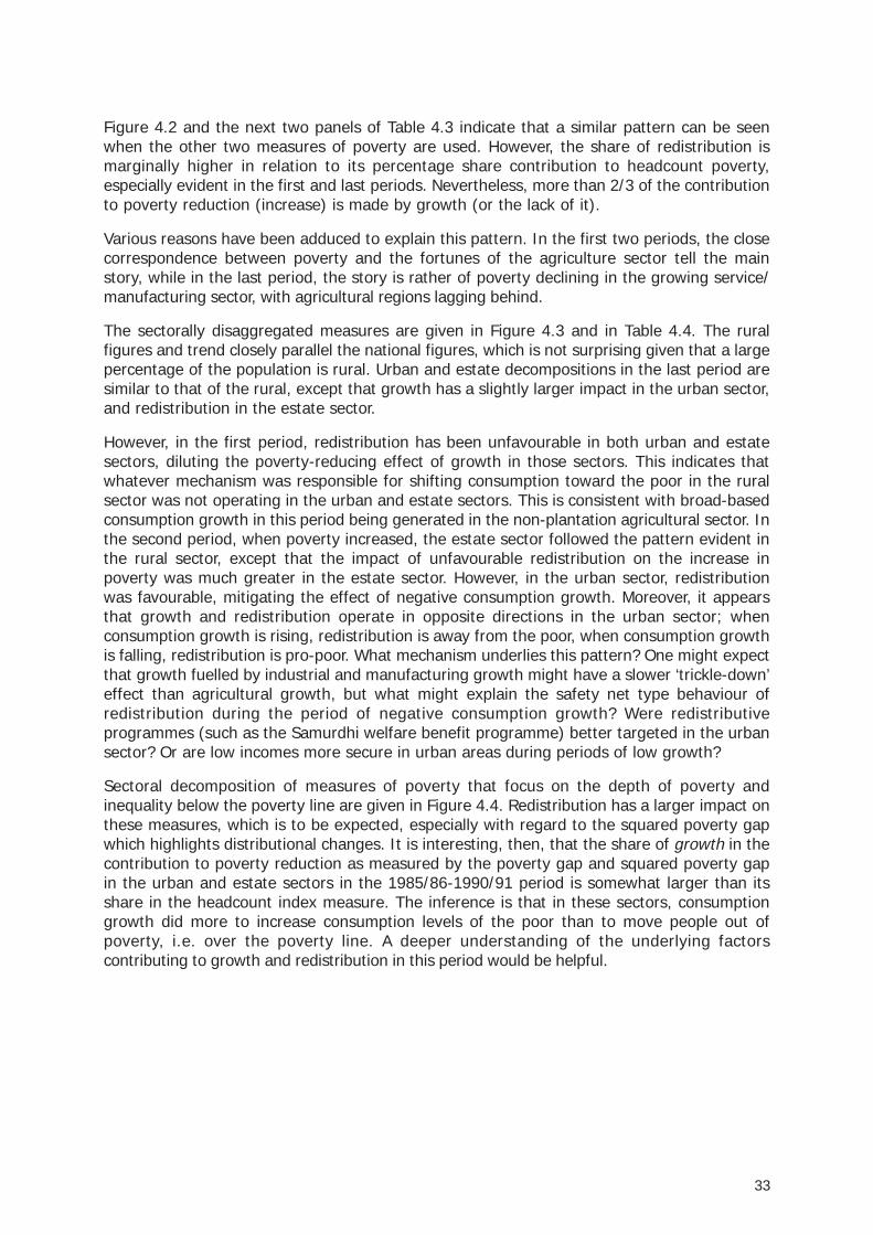
33

Figure 4.2 and the next two panels of Table 4.3 indicate that a similar pattern can be seenwhen the other two measures of poverty are used. However, the share of redistribution ismarginally higher in relation to its percentage share contribution to headcount poverty,especially evident in the first and last periods. Nevertheless, more than 2/3 of the contributionto poverty reduction (increase) is made by growth (or the lack of it).

Various reasons have been adduced to explain this pattern. In the first two periods, the closecorrespondence between poverty and the fortunes of the agriculture sector tell the mainstory, while in the last period, the story is rather of poverty declining in the growing service/manufacturing sector, with agricultural regions lagging behind.

The sectorally disaggregated measures are given in Figure 4.3 and in Table 4.4. The ruralfigures and trend closely parallel the national figures, which is not surprising given that a largepercentage of the population is rural. Urban and estate decompositions in the last period aresimilar to that of the rural, except that growth has a slightly larger impact in the urban sector,and redistribution in the estate sector.

However, in the first period, redistribution has been unfavourable in both urban and estatesectors, diluting the poverty-reducing effect of growth in those sectors. This indicates thatwhatever mechanism was responsible for shifting consumption toward the poor in the ruralsector was not operating in the urban and estate sectors. This is consistent with broad-basedconsumption growth in this period being generated in the non-plantation agricultural sector. Inthe second period, when poverty increased, the estate sector followed the pattern evident inthe rural sector, except that the impact of unfavourable redistribution on the increase inpoverty was much greater in the estate sector. However, in the urban sector, redistributionwas favourable, mitigating the effect of negative consumption growth. Moreover, it appearsthat growth and redistribution operate in opposite directions in the urban sector; whenconsumption growth is rising, redistribution is away from the poor, when consumption growthis falling, redistribution is pro-poor. What mechanism underlies this pattern? One might expectthat growth fuelled by industrial and manufacturing growth might have a slower ‘trickle-down’effect than agricultural growth, but what might explain the safety net type behaviour ofredistribution during the period of negative consumption growth? Were redistributiveprogrammes (such as the Samurdhi welfare benefit programme) better targeted in the urbansector? Or are low incomes more secure in urban areas during periods of low growth?

Sectoral decomposition of measures of poverty that focus on the depth of poverty andinequality below the poverty line are given in Figure 4.4. Redistribution has a larger impact onthese measures, which is to be expected, especially with regard to the squared poverty gapwhich highlights distributional changes. It is interesting, then, that the share of growth in thecontribution to poverty reduction as measured by the poverty gap and squared poverty gapin the urban and estate sectors in the 1985/86-1990/91 period is somewhat larger than itsshare in the headcount index measure. The inference is that in these sectors, consumptiongrowth did more to increase consumption levels of the poor than to move people out ofpoverty, i.e. over the poverty line. A deeper understanding of the underlying factorscontributing to growth and redistribution in this period would be helpful.

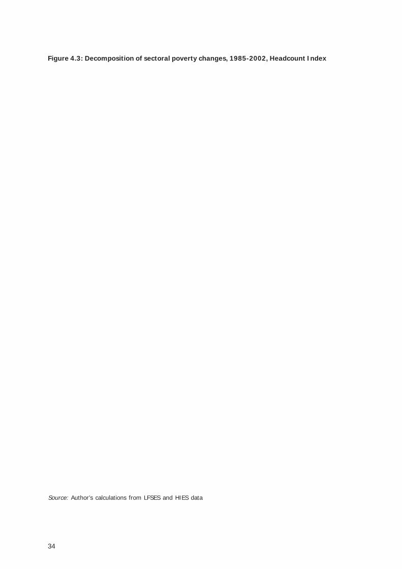
34

Figure 4.3: Decomposition of sectoral poverty changes, 1985-2002, Headcount Index


35

Figure 4.4: Decomposition of sectoral poverty changes, 1985-2002, Poverty Gap and SquaredPoverty Gap Index

36


Figure 4.4: Decomposition of sectoral poverty changes, 1985-2002, Poverty Gap and SquaredPoverty Gap Index (Contd.)

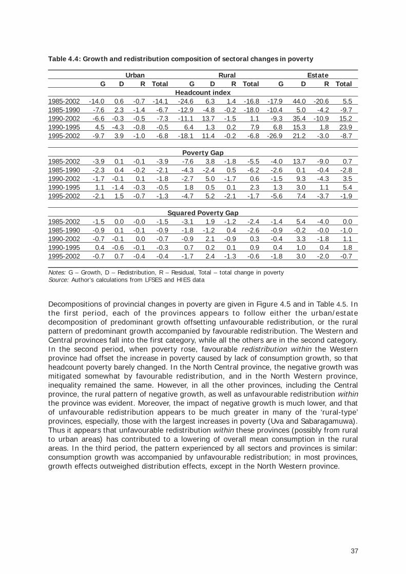
37

Table 4.4: Growth and redistribution composition of sectoral changes in poverty

Urban Rural EstateG D R Total G D R Total G D R Total

Headcount index1985-2002 -14.0 0.6 -0.7 -14.1 -24.6 6.3 1.4 -16.8 -17.9 44.0 -20.6 5.51985-1990 -7.6 2.3 -1.4 -6.7 -12.9 -4.8 -0.2 -18.0 -10.4 5.0 -4.2 -9.71990-2002 -6.6 -0.3 -0.5 -7.3 -11.1 13.7 -1.5 1.1 -9.3 35.4 -10.9 15.21990-1995 4.5 -4.3 -0.8 -0.5 6.4 1.3 0.2 7.9 6.8 15.3 1.8 23.91995-2002 -9.7 3.9 -1.0 -6.8 -18.1 11.4 -0.2 -6.8 -26.9 21.2 -3.0 -8.7

Poverty Gap1985-2002 -3.9 0.1 -0.1 -3.9 -7.6 3.8 -1.8 -5.5 -4.0 13.7 -9.0 0.71985-1990 -2.3 0.4 -0.2 -2.1 -4.3 -2.4 0.5 -6.2 -2.6 0.1 -0.4 -2.81990-2002 -1.7 -0.1 0.1 -1.8 -2.7 5.0 -1.7 0.6 -1.5 9.3 -4.3 3.51990-1995 1.1 -1.4 -0.3 -0.5 1.8 0.5 0.1 2.3 1.3 3.0 1.1 5.41995-2002 -2.1 1.5 -0.7 -1.3 -4.7 5.2 -2.1 -1.7 -5.6 7.4 -3.7 -1.9

Squared Poverty Gap1985-2002 -1.5 0.0 -0.0 -1.5 -3.1 1.9 -1.2 -2.4 -1.4 5.4 -4.0 0.01985-1990 -0.9 0.1 -0.1 -0.9 -1.8 -1.2 0.4 -2.6 -0.9 -0.2 -0.0 -1.01990-2002 -0.7 -0.1 0.0 -0.7 -0.9 2.1 -0.9 0.3 -0.4 3.3 -1.8 1.11990-1995 0.4 -0.6 -0.1 -0.3 0.7 0.2 0.1 0.9 0.4 1.0 0.4 1.81995-2002 -0.7 0.7 -0.4 -0.4 -1.7 2.4 -1.3 -0.6 -1.8 3.0 -2.0 -0.7

Notes: G – Growth, D – Redistribution, R – Residual, Total – total change in povertySource: Author’s calculations from LFSES and HIES data

Decompositions of provincial changes in poverty are given in Figure 4.5 and in Table 4.5. Inthe first period, each of the provinces appears to follow either the urban/estatedecomposition of predominant growth offsetting unfavourable redistribution, or the ruralpattern of predominant growth accompanied by favourable redistribution. The Western andCentral provinces fall into the first category, while all the others are in the second category.In the second period, when poverty rose, favourable redistribution within the Westernprovince had offset the increase in poverty caused by lack of consumption growth, so thatheadcount poverty barely changed. In the North Central province, the negative growth wasmitigated somewhat by favourable redistribution, and in the North Western province,inequality remained the same. However, in all the other provinces, including the Centralprovince, the rural pattern of negative growth, as well as unfavourable redistribution withinthe province was evident. Moreover, the impact of negative growth is much lower, and thatof unfavourable redistribution appears to be much greater in many of the ‘rural-type’provinces, especially, those with the largest increases in poverty (Uva and Sabaragamuwa).Thus it appears that unfavourable redistribution within these provinces (possibly from ruralto urban areas) has contributed to a lowering of overall mean consumption in the ruralareas. In the third period, the pattern experienced by all sectors and provinces is similar:consumption growth was accompanied by unfavourable redistribution; in most provinces,growth effects outweighed distribution effects, except in the North Western province.

38


Figure 4.5: Decomposition of provincial poverty changes, 1985-2002, Headcount Index

39

Poverty gap and squared poverty gap results are shown in Figure 4.6 below, and correspondto the results for the Headcount Index.

Figure 4.6: Decomposition of sectoral poverty changes, 1985-2002, Poverty Gap and SquaredPoverty Gap Index


40

Figure 4.6: Decomposition of sectoral poverty changes, 1985-2002, Poverty Gap and SquaredPoverty Gap Index (Contd.)


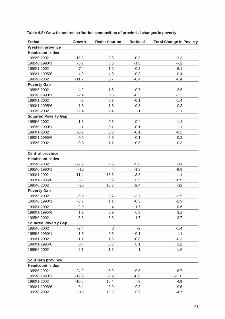
41

Table 4.5: Growth and redistribution composition of provincial changes in poverty

Period Growth Redistribution Residual Total Change in PovertyWestern provinceHeadcount Index1985/6-2002 -15.5 2.8 -0.5 -13.31985/6-1990/1 -8.7 3.3 -1.8 -7.21990/1-2002 -7.4 1.6 -0.3 -6.11990/1-1995/6 4.9 -4.3 -0.3 0.41995/6-2002 -11.7 5.7 -0.4 -6.4Poverty Gap1985/6-2002 -4.2 1.3 -0.7 -3.61985/6-1990/1 -2.4 0.5 -0.3 -2.21990/1-2002 -2 0.7 -0.1 -1.41990/1-1995/6 1.3 -1.3 -0.3 -0.31995/6-2002 -2.4 2.4 -1 -1.1Squared Poverty Gap1985/6-2002 -1.6 0.5 -0.4 -1.41985/6-1990/1 -1 0.1 -0.1 -11990/1-2002 -0.7 0.3 -0.1 -0.51990/1-1995/6 0.5 -0.5 -0.1 -0.21995/6-2002 -0.8 1.1 -0.6 -0.3

Central provinceHeadcount Index1985/6-2002 -22.9 17.5 -5.6 -111985/6-1990/1 -12 4 -1.9 -9.91990/1-2002 -11.4 13.6 -3.3 -1.11990/1-1995/6 6.6 3.9 0.5 10.91995/6-2002 -20 10.3 -2.4 -12Poverty Gap1985/6-2002 -6.5 6.7 -3.7 -3.51985/6-1990/1 -3.7 1.1 -0.3 -2.91990/1-2002 -2.9 4 -1.7 -0.61990/1-1995/6 1.9 0.9 0.3 3.11995/6-2002 -5.6 3.6 -1.7 -3.7Squared Poverty Gap1985/6-2002 -2.4 3 -2 -1.41985/6-1990/1 -1.5 0.5 -0.1 -1.11990/1-2002 -1.1 1.5 -0.8 -0.31990/1-1995/6 0.8 0.3 0.1 1.21995/6-2002 -2.1 1.5 -1 -1.6

Southern provinceHeadcount Index1985/6-2002 -24.2 6.9 0.6 -16.71985/6-1990/1 -12.9 -7.9 -0.8 -21.61990/1-2002 -10.5 18.4 -3 4.91990/1-1995/6 6.4 2.9 0.3 9.61995/6-2002 -19 13.6 0.7 -4.7

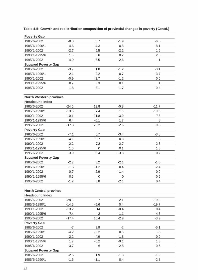
42

Poverty Gap1985/6-2002 -8.3 3.7 -1.9 -6.51985/6-1990/1 -4.6 -4.3 0.8 -8.11990/1-2002 -2.7 6.5 -2.2 1.61990/1-1995/6 1.8 0.6 0.2 2.61995/6-2002 -4.9 6.5 -2.6 -1Squared Poverty Gap1985/6-2002 -3.7 1.8 -1.2 -3.11985/6-1990/1 -2.1 -2.2 0.7 -3.71990/1-2002 -0.9 2.7 -1.2 0.61990/1-1995/6 0.7 0.3 0.1 11995/6-2002 -1.8 3.1 -1.7 -0.4

North Western provinceHeadcount Index1985/6-2002 -24.6 13.8 -0.8 -11.71985/6-1990/1 -13.5 -7.4 1.5 -19.51990/1-2002 -10.1 21.8 -3.9 7.81990/1-1995/6 6.4 -0.1 1.7 81995/6-2002 -17.8 20.2 -2.6 -0.3Poverty Gap1985/6-2002 -7.1 6.7 -3.4 -3.81985/6-1990/1 -4.1 -2.7 0.8 -61990/1-2002 -2.2 7.2 -2.7 2.31990/1-1995/6 1.6 0 0.1 1.61995/6-2002 -3.9 8.4 -3.8 0.7Squared Poverty Gap1985/6-2002 -2.7 3.2 -2.1 -1.51985/6-1990/1 -1.6 -1.2 0.4 -2.41990/1-2002 -0.7 2.9 -1.4 0.91990/1-1995/6 0.5 0 0 0.51995/6-2002 -1.2 3.8 -2.1 0.4

North Central provinceHeadcount Index1985/6-2002 -28.3 7 2.1 -19.31985/6-1990/1 -14.5 -5.6 0.4 -19.71990/1-2002 -13.2 14 -0.4 0.41990/1-1995/6 7.4 -2 -1.1 4.31995/6-2002 -17.4 16.4 -2.9 -3.9Poverty Gap1985/6-2002 -7 3.9 -2 -5.11985/6-1990/1 -4.2 -2.2 0.5 -61990/1-2002 -2.2 4.9 -1.8 0.91990/1-1995/6 1.7 -0.2 -0.1 1.31995/6-2002 -3.7 6 -2.8 -0.5Squared Poverty Gap1985/6-2002 -2.5 1.9 -1.3 -1.91985/6-1990/1 -1.6 -1.1 0.4 -2.3

Table 4.5: Growth and redistribution composition of provincial changes in poverty (Contd.)

43

1990/1-2002 -0.6 2 -1 0.41990/1-1995/6 0.5 -0.1 0 0.41995/6-2002 -1.1 2.6 -1.6 0

Uva provinceHeadcount Index1985/6-2002 -23.6 18.5 -3.1 -8.21985/6-1990/1 -11.3 -6.3 -3.4 -20.91990/1-2002 -11.8 28.5 -4.1 12.71990/1-1995/6 7.4 14.4 0.4 22.21995/6-2002 -22.5 12.1 0.9 -9.5Poverty Gap1985/6-2002 -8.7 8.3 -4.3 -4.71985/6-1990/1 -4.7 -4.6 0.6 -8.71990/1-2002 -2.9 10.4 -3.5 41990/1-1995/6 1.9 4.9 0.8 7.71995/6-2002 -7.3 6.1 -2.4 -3.6Squared Poverty Gap1985/6-2002 -4 4 -2.5 -2.51985/6-1990/1 -2.3 -2.6 0.7 -4.21990/1-2002 -0.9 4.6 -1.9 1.71990/1-1995/6 0.7 2.2 0.5 3.41995/6-2002 -3.1 3 -1.5 -1.7

Sabaragamuwa provinceHeadcount Index1985/6-2002 -26.5 14.7 -0.6 -12.51985/6-1990/1 -13.7 -10.6 1.9 -22.41990/1-2002 -11.7 26 -4.4 9.91990/1-1995/6 5.6 12.4 0.9 18.91995/6-2002 -22.8 12.7 1.1 -9Poverty Gap1985/6-2002 -8.5 7.2 -3.7 -51985/6-1990/1 -4.9 -3.8 1.2 -7.51990/1-2002 -2.6 8.4 -3.3 2.51990/1-1995/6 1.8 2.9 0.8 5.41995/6-2002 -6.7 6.1 -2.4 -3Squared Poverty Gap1985/6-2002 -3.5 3.5 -2.3 -2.31985/6-1990/1 -2.1 -1.6 0.6 -3.11990/1-2002 -0.9 3.3 -1.6 0.71990/1-1995/6 0.7 0.9 0.4 1.91995/6-2002 -2.5 2.9 -1.6 -1.2

Table 4.5: Growth and redistribution composition of provincial changes in poverty (Contd.)


44

District level changes in poverty are decomposed and results shown in Figure 4.7, Figure 4.8 andTable 4.6. In the figures, districts are given in order of the largest overall decline in poverty over theentire period 1985/86-2002. This ranges from a reduction of 25.5 percentage points in Anuradhapurato a 1.7 percentage point increase in Nuwara Eliya. Although there was much fluctuation withinthis period, in all districts, poverty in 2002 was lower than the initial levels in 1985/86.

In the first period, most districts exhibited the ‘rural-type’ pattern of growth and favourableredistribution combining to reduce poverty. The exceptions were Colombo, Kalutura, Kandy andNuwara Eliya, where the poverty-reducing impact of growth was reduced by unfavourableredistribution. Even in districts with a substantial estate sector, such as Badulla, Matale, Kegalleand Ratnapura, redistribution was favourable during this period. A possible reason for this is thatfavourable agricultural yields in the 1990-91 period had a poverty reducing effect. In Hambantota,Ratnapura and Moneragala, the impact of favourable redistribution was larger than that ofgrowth during this period, while in all other districts, the growth impact predominated.

In the second period, when poverty increased, Gampaha, Kurunegala and the North Centralprovince districts of Anuradhapura and Polonnaruwa, in addition to Colombo and Kalutara,exhibited ‘urban-type’ favourable redistribution, that mitigated the poverty-increasing impactof negative consumption growth in these districts.

Among the districts that experienced both negative consumption growth and unfavourable redistributionduring this period, three distinct groups are evident. In the first group, Hambantota, Galle, Puttalam andKandy, negative growth, rather than adverse redistribution was for the most part responsible for theincrease in poverty. Three of these four are coastal districts, and all four are somewhat more urbanisedthan the remaining districts. In the second group, i.e. Matara and Kegalle, negative growth and adverseredistribution are about equally responsible for the rise in poverty, whereas in the last group, i.e. Ratnapura,Moneragala, Matale, Nuwara Eliya and Badulla, adverse redistribution is the main contributor to therise in poverty.

In the last period, the pattern in all districts is of positive consumption growth and adverseredistribution. Districts vary according to the relative importance of these two components.Surprisingly, the district with the lowest poverty and that with the highest poverty both indicategrowth to have been key in reducing poverty, with adverse redistribution having a very smallimpact. It is not clear whether this is coincidental, or whether these districts shared somecommon phenomenon during this period. Some of the surprises in terms of adverseredistribution are Polonnaruwa, Kurunegala and Hambantota, where redistribution effectsdominated the low growth in these districts. This points to the need to investigate patterns ofgrowth and redistribution more closely in these districts in this period. Puttalam and Badulladistricts were among the high-poverty districts where adverse redistribution kept poverty at highlevels, while in Kegalle, Ratnapura, Nuwara Eliya, Anuradhapura, Galle and, surprisingly,Gampaha, adverse redistribution also kept improvements in poverty very low.

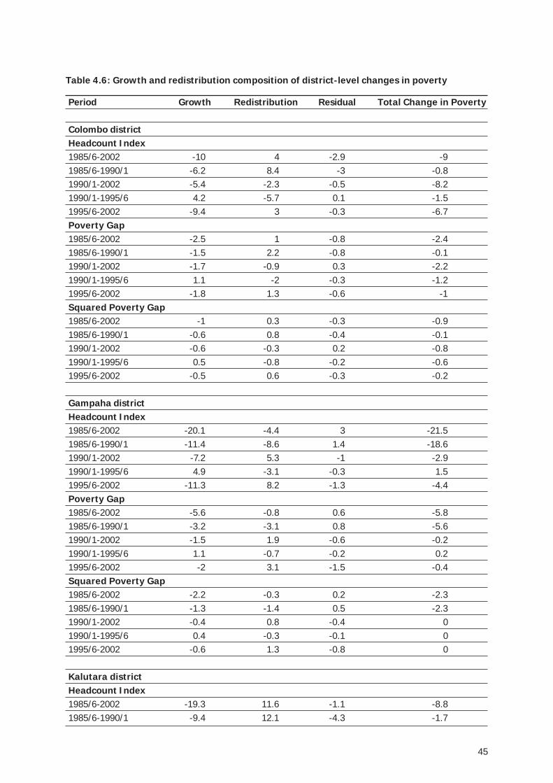
45

Table 4.6: Growth and redistribution composition of district-level changes in poverty

Period Growth Redistribution Residual Total Change in Poverty

Colombo districtHeadcount Index1985/6-2002 -10 4 -2.9 -91985/6-1990/1 -6.2 8.4 -3 -0.81990/1-2002 -5.4 -2.3 -0.5 -8.21990/1-1995/6 4.2 -5.7 0.1 -1.51995/6-2002 -9.4 3 -0.3 -6.7Poverty Gap1985/6-2002 -2.5 1 -0.8 -2.41985/6-1990/1 -1.5 2.2 -0.8 -0.11990/1-2002 -1.7 -0.9 0.3 -2.21990/1-1995/6 1.1 -2 -0.3 -1.21995/6-2002 -1.8 1.3 -0.6 -1Squared Poverty Gap1985/6-2002 -1 0.3 -0.3 -0.91985/6-1990/1 -0.6 0.8 -0.4 -0.11990/1-2002 -0.6 -0.3 0.2 -0.81990/1-1995/6 0.5 -0.8 -0.2 -0.61995/6-2002 -0.5 0.6 -0.3 -0.2

Gampaha districtHeadcount Index1985/6-2002 -20.1 -4.4 3 -21.51985/6-1990/1 -11.4 -8.6 1.4 -18.61990/1-2002 -7.2 5.3 -1 -2.91990/1-1995/6 4.9 -3.1 -0.3 1.51995/6-2002 -11.3 8.2 -1.3 -4.4Poverty Gap1985/6-2002 -5.6 -0.8 0.6 -5.81985/6-1990/1 -3.2 -3.1 0.8 -5.61990/1-2002 -1.5 1.9 -0.6 -0.21990/1-1995/6 1.1 -0.7 -0.2 0.21995/6-2002 -2 3.1 -1.5 -0.4Squared Poverty Gap1985/6-2002 -2.2 -0.3 0.2 -2.31985/6-1990/1 -1.3 -1.4 0.5 -2.31990/1-2002 -0.4 0.8 -0.4 01990/1-1995/6 0.4 -0.3 -0.1 01995/6-2002 -0.6 1.3 -0.8 0

Kalutara districtHeadcount Index1985/6-2002 -19.3 11.6 -1.1 -8.81985/6-1990/1 -9.4 12.1 -4.3 -1.7

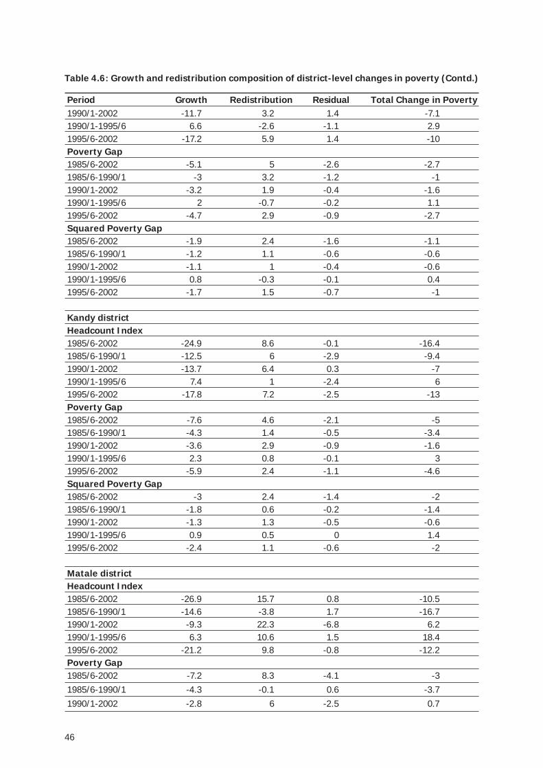
46

Period Growth Redistribution Residual Total Change in Poverty1990/1-2002 -11.7 3.2 1.4 -7.11990/1-1995/6 6.6 -2.6 -1.1 2.91995/6-2002 -17.2 5.9 1.4 -10Poverty Gap1985/6-2002 -5.1 5 -2.6 -2.71985/6-1990/1 -3 3.2 -1.2 -11990/1-2002 -3.2 1.9 -0.4 -1.61990/1-1995/6 2 -0.7 -0.2 1.11995/6-2002 -4.7 2.9 -0.9 -2.7Squared Poverty Gap1985/6-2002 -1.9 2.4 -1.6 -1.11985/6-1990/1 -1.2 1.1 -0.6 -0.61990/1-2002 -1.1 1 -0.4 -0.61990/1-1995/6 0.8 -0.3 -0.1 0.41995/6-2002 -1.7 1.5 -0.7 -1

Kandy districtHeadcount Index1985/6-2002 -24.9 8.6 -0.1 -16.41985/6-1990/1 -12.5 6 -2.9 -9.41990/1-2002 -13.7 6.4 0.3 -71990/1-1995/6 7.4 1 -2.4 61995/6-2002 -17.8 7.2 -2.5 -13Poverty Gap1985/6-2002 -7.6 4.6 -2.1 -51985/6-1990/1 -4.3 1.4 -0.5 -3.41990/1-2002 -3.6 2.9 -0.9 -1.61990/1-1995/6 2.3 0.8 -0.1 31995/6-2002 -5.9 2.4 -1.1 -4.6Squared Poverty Gap1985/6-2002 -3 2.4 -1.4 -21985/6-1990/1 -1.8 0.6 -0.2 -1.41990/1-2002 -1.3 1.3 -0.5 -0.61990/1-1995/6 0.9 0.5 0 1.41995/6-2002 -2.4 1.1 -0.6 -2

Matale districtHeadcount Index1985/6-2002 -26.9 15.7 0.8 -10.51985/6-1990/1 -14.6 -3.8 1.7 -16.71990/1-2002 -9.3 22.3 -6.8 6.21990/1-1995/6 6.3 10.6 1.5 18.41995/6-2002 -21.2 9.8 -0.8 -12.2Poverty Gap1985/6-2002 -7.2 8.3 -4.1 -31985/6-1990/1 -4.3 -0.1 0.6 -3.71990/1-2002 -2.8 6 -2.5 0.7

Table 4.6: Growth and redistribution composition of district-level changes in poverty (Contd.)

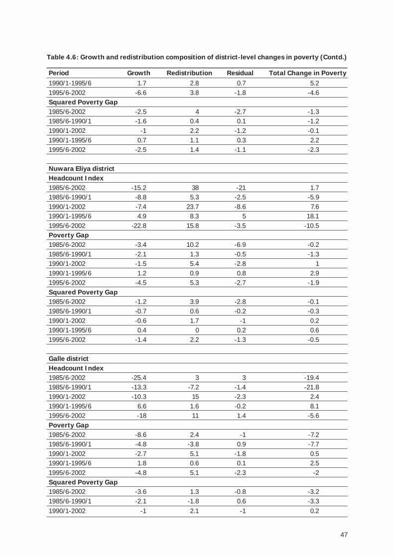
47

Period Growth Redistribution Residual Total Change in Poverty1990/1-1995/6 1.7 2.8 0.7 5.21995/6-2002 -6.6 3.8 -1.8 -4.6Squared Poverty Gap1985/6-2002 -2.5 4 -2.7 -1.31985/6-1990/1 -1.6 0.4 0.1 -1.21990/1-2002 -1 2.2 -1.2 -0.11990/1-1995/6 0.7 1.1 0.3 2.21995/6-2002 -2.5 1.4 -1.1 -2.3

Nuwara Eliya districtHeadcount Index1985/6-2002 -15.2 38 -21 1.71985/6-1990/1 -8.8 5.3 -2.5 -5.91990/1-2002 -7.4 23.7 -8.6 7.61990/1-1995/6 4.9 8.3 5 18.11995/6-2002 -22.8 15.8 -3.5 -10.5Poverty Gap1985/6-2002 -3.4 10.2 -6.9 -0.21985/6-1990/1 -2.1 1.3 -0.5 -1.31990/1-2002 -1.5 5.4 -2.8 11990/1-1995/6 1.2 0.9 0.8 2.91995/6-2002 -4.5 5.3 -2.7 -1.9Squared Poverty Gap1985/6-2002 -1.2 3.9 -2.8 -0.11985/6-1990/1 -0.7 0.6 -0.2 -0.31990/1-2002 -0.6 1.7 -1 0.21990/1-1995/6 0.4 0 0.2 0.61995/6-2002 -1.4 2.2 -1.3 -0.5

Galle districtHeadcount Index1985/6-2002 -25.4 3 3 -19.41985/6-1990/1 -13.3 -7.2 -1.4 -21.81990/1-2002 -10.3 15 -2.3 2.41990/1-1995/6 6.6 1.6 -0.2 8.11995/6-2002 -18 11 1.4 -5.6Poverty Gap1985/6-2002 -8.6 2.4 -1 -7.21985/6-1990/1 -4.8 -3.8 0.9 -7.71990/1-2002 -2.7 5.1 -1.8 0.51990/1-1995/6 1.8 0.6 0.1 2.51995/6-2002 -4.8 5.1 -2.3 -2Squared Poverty Gap1985/6-2002 -3.6 1.3 -0.8 -3.21985/6-1990/1 -2.1 -1.8 0.6 -3.31990/1-2002 -1 2.1 -1 0.2


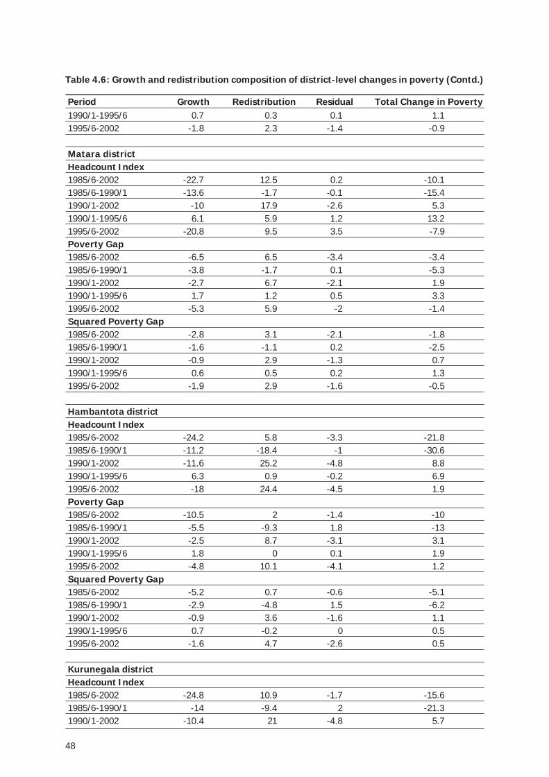
48

Period Growth Redistribution Residual Total Change in Poverty1990/1-1995/6 0.7 0.3 0.1 1.11995/6-2002 -1.8 2.3 -1.4 -0.9

Matara districtHeadcount Index1985/6-2002 -22.7 12.5 0.2 -10.11985/6-1990/1 -13.6 -1.7 -0.1 -15.41990/1-2002 -10 17.9 -2.6 5.31990/1-1995/6 6.1 5.9 1.2 13.21995/6-2002 -20.8 9.5 3.5 -7.9Poverty Gap1985/6-2002 -6.5 6.5 -3.4 -3.41985/6-1990/1 -3.8 -1.7 0.1 -5.31990/1-2002 -2.7 6.7 -2.1 1.91990/1-1995/6 1.7 1.2 0.5 3.31995/6-2002 -5.3 5.9 -2 -1.4Squared Poverty Gap1985/6-2002 -2.8 3.1 -2.1 -1.81985/6-1990/1 -1.6 -1.1 0.2 -2.51990/1-2002 -0.9 2.9 -1.3 0.71990/1-1995/6 0.6 0.5 0.2 1.31995/6-2002 -1.9 2.9 -1.6 -0.5

Hambantota districtHeadcount Index1985/6-2002 -24.2 5.8 -3.3 -21.81985/6-1990/1 -11.2 -18.4 -1 -30.61990/1-2002 -11.6 25.2 -4.8 8.81990/1-1995/6 6.3 0.9 -0.2 6.91995/6-2002 -18 24.4 -4.5 1.9Poverty Gap1985/6-2002 -10.5 2 -1.4 -101985/6-1990/1 -5.5 -9.3 1.8 -131990/1-2002 -2.5 8.7 -3.1 3.11990/1-1995/6 1.8 0 0.1 1.91995/6-2002 -4.8 10.1 -4.1 1.2Squared Poverty Gap1985/6-2002 -5.2 0.7 -0.6 -5.11985/6-1990/1 -2.9 -4.8 1.5 -6.21990/1-2002 -0.9 3.6 -1.6 1.11990/1-1995/6 0.7 -0.2 0 0.51995/6-2002 -1.6 4.7 -2.6 0.5

Kurunegala districtHeadcount Index1985/6-2002 -24.8 10.9 -1.7 -15.61985/6-1990/1 -14 -9.4 2 -21.31990/1-2002 -10.4 21 -4.8 5.7


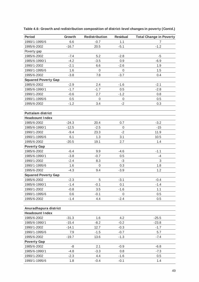
49

Period Growth Redistribution Residual Total Change in Poverty1990/1-1995/6 6.6 -0.7 1.1 71995/6-2002 -16.7 20.5 -5.1 -1.2Poverty gap1985/6-2002 -7.4 5.2 -2.8 -51985/6-1990/1 -4.2 -3.5 0.9 -6.91990/1-2002 -2.1 6.6 -2.6 1.91990/1-1995/6 1.6 0 0 1.51995/6-2002 -3.8 7.8 -3.7 0.4Squared Poverty Gap1985/6-2002 -2.9 2.4 -1.6 -2.11985/6-1990/1 -1.7 -1.7 0.5 -2.81990/1-2002 -0.6 2.7 -1.2 0.81990/1-1995/6 0.5 0 0 0.51995/6-2002 -1.2 3.4 -2 0.3

Puttalam districtHeadcount Index1985/6-2002 -24.3 20.4 0.7 -3.21985/6-1990/1 -12.5 -2.5 0 -151990/1-2002 -9.4 23.3 -2 11.91990/1-1995/6 6.1 1.3 3.1 10.51995/6-2002 -20.5 19.1 2.7 1.4Poverty Gap1985/6-2002 -6.4 9.9 -4.6 -1.11985/6-1990/1 -3.8 -0.7 0.5 -41990/1-2002 -2.4 8.3 -3 31990/1-1995/6 1.6 0 0.3 1.81995/6-2002 -4.3 9.4 -3.9 1.2Squared Poverty Gap1985/6-2002 -2.3 5 -3.1 -0.41985/6-1990/1 -1.4 -0.1 0.1 -1.41990/1-2002 -0.8 3.5 -1.6 1.11990/1-1995/6 0.6 -0.1 0 0.51995/6-2002 -1.4 4.4 -2.4 0.5

Anuradhapura districtHeadcount Index1985/6-2002 -31.3 1.6 4.2 -25.51985/6-1990/1 -15.4 -8.2 -0.2 -23.81990/1-2002 -14.1 12.7 -0.3 -1.71990/1-1995/6 7.9 -1.5 -0.7 5.71995/6-2002 -19.7 13.6 -1.3 -7.4Poverty Gap1985/6-2002 -8 2.1 -0.9 -6.81985/6-1990/1 -4.8 -3.3 0.8 -7.31990/1-2002 -2.3 4.4 -1.6 0.51990/1-1995/6 1.8 -0.4 -0.1 1.4


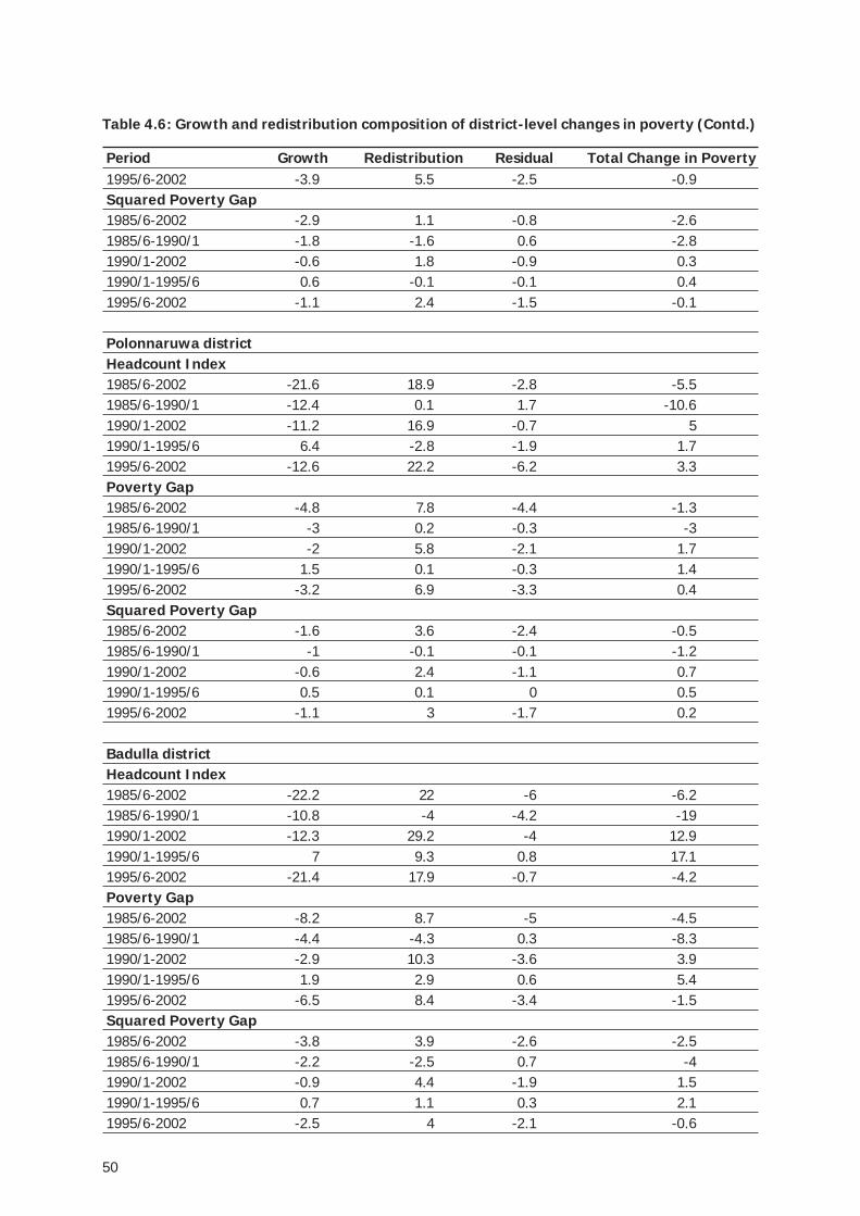
50

Period Growth Redistribution Residual Total Change in Poverty1995/6-2002 -3.9 5.5 -2.5 -0.9Squared Poverty Gap1985/6-2002 -2.9 1.1 -0.8 -2.61985/6-1990/1 -1.8 -1.6 0.6 -2.81990/1-2002 -0.6 1.8 -0.9 0.31990/1-1995/6 0.6 -0.1 -0.1 0.41995/6-2002 -1.1 2.4 -1.5 -0.1

Polonnaruwa districtHeadcount Index1985/6-2002 -21.6 18.9 -2.8 -5.51985/6-1990/1 -12.4 0.1 1.7 -10.61990/1-2002 -11.2 16.9 -0.7 51990/1-1995/6 6.4 -2.8 -1.9 1.71995/6-2002 -12.6 22.2 -6.2 3.3Poverty Gap1985/6-2002 -4.8 7.8 -4.4 -1.31985/6-1990/1 -3 0.2 -0.3 -31990/1-2002 -2 5.8 -2.1 1.71990/1-1995/6 1.5 0.1 -0.3 1.41995/6-2002 -3.2 6.9 -3.3 0.4Squared Poverty Gap1985/6-2002 -1.6 3.6 -2.4 -0.51985/6-1990/1 -1 -0.1 -0.1 -1.21990/1-2002 -0.6 2.4 -1.1 0.71990/1-1995/6 0.5 0.1 0 0.51995/6-2002 -1.1 3 -1.7 0.2

Badulla districtHeadcount Index1985/6-2002 -22.2 22 -6 -6.21985/6-1990/1 -10.8 -4 -4.2 -191990/1-2002 -12.3 29.2 -4 12.91990/1-1995/6 7 9.3 0.8 17.11995/6-2002 -21.4 17.9 -0.7 -4.2Poverty Gap1985/6-2002 -8.2 8.7 -5 -4.51985/6-1990/1 -4.4 -4.3 0.3 -8.31990/1-2002 -2.9 10.3 -3.6 3.91990/1-1995/6 1.9 2.9 0.6 5.41995/6-2002 -6.5 8.4 -3.4 -1.5Squared Poverty Gap1985/6-2002 -3.8 3.9 -2.6 -2.51985/6-1990/1 -2.2 -2.5 0.7 -41990/1-2002 -0.9 4.4 -1.9 1.51990/1-1995/6 0.7 1.1 0.3 2.11995/6-2002 -2.5 4 -2.1 -0.6


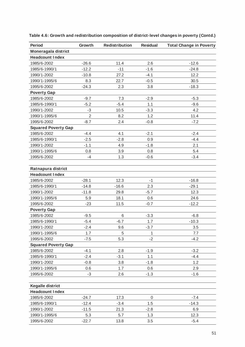
51

Period Growth Redistribution Residual Total Change in PovertyMoneragala districtHeadcount Index1985/6-2002 -26.6 11.4 2.6 -12.61985/6-1990/1 -12.2 -11 -1.6 -24.81990/1-2002 -10.8 27.2 -4.1 12.21990/1-1995/6 8.3 22.7 -0.5 30.51995/6-2002 -24.3 2.3 3.8 -18.3Poverty Gap1985/6-2002 -9.7 7.3 -2.9 -5.31985/6-1990/1 -5.2 -5.4 1.1 -9.61990/1-2002 -3 10.5 -3.3 4.21990/1-1995/6 2 8.2 1.2 11.41995/6-2002 -8.7 2.4 -0.8 -7.2Squared Poverty Gap1985/6-2002 -4.4 4.1 -2.1 -2.41985/6-1990/1 -2.5 -2.8 0.9 -4.41990/1-2002 -1.1 4.9 -1.8 2.11990/1-1995/6 0.8 3.9 0.8 5.41995/6-2002 -4 1.3 -0.6 -3.4

Ratnapura districtHeadcount Index1985/6-2002 -28.1 12.3 -1 -16.81985/6-1990/1 -14.8 -16.6 2.3 -29.11990/1-2002 -11.8 29.8 -5.7 12.31990/1-1995/6 5.9 18.1 0.6 24.61995/6-2002 -23 11.5 -0.7 -12.2Poverty Gap1985/6-2002 -9.5 6 -3.3 -6.81985/6-1990/1 -5.4 -6.7 1.7 -10.31990/1-2002 -2.4 9.6 -3.7 3.51990/1-1995/6 1.7 5 1 7.71995/6-2002 -7.5 5.3 -2 -4.2Squared Poverty Gap1985/6-2002 -4.1 2.8 -1.9 -3.21985/6-1990/1 -2.4 -3.1 1.1 -4.41990/1-2002 -0.8 3.8 -1.8 1.21990/1-1995/6 0.6 1.7 0.6 2.91995/6-2002 -3 2.6 -1.3 -1.6

Kegalle districtHeadcount Index1985/6-2002 -24.7 17.3 0 -7.41985/6-1990/1 -12.4 -3.4 1.5 -14.31990/1-2002 -11.5 21.3 -2.8 6.91990/1-1995/6 5.3 5.7 1.3 12.31995/6-2002 -22.7 13.8 3.5 -5.4


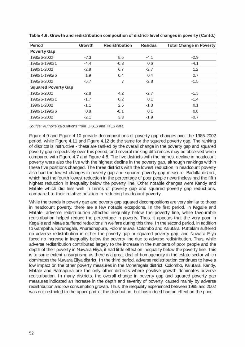
52

Period Growth Redistribution Residual Total Change in PovertyPoverty Gap1985/6-2002 -7.3 8.5 -4.1 -2.91985/6-1990/1 -4.4 -0.3 0.6 -4.11990/1-2002 -2.9 6.7 -2.7 1.21990/1-1995/6 1.9 0.4 0.4 2.71995/6-2002 -5.7 7 -2.8 -1.5Squared Poverty Gap1985/6-2002 -2.8 4.2 -2.7 -1.31985/6-1990/1 -1.7 0.2 0.1 -1.41990/1-2002 -1.1 2.5 -1.3 0.11990/1-1995/6 0.8 -0.1 0.1 0.81995/6-2002 -2.1 3.3 -1.9 -0.7


Figure 4.9 and Figure 4.10 provide decompositions of poverty gap changes over the 1985-2002period, while Figure 4.11 and Figure 4.12 do the same for the squared poverty gap. The rankingof districts is instructive - these are ranked by the overall change in the poverty gap and squaredpoverty gap respectively over this period, and several ranking differences may be observed whencompared with Figure 4.7 and Figure 4.8. The five districts with the highest decline in headcountpoverty were also the five with the highest decline in the poverty gap, although rankings withinthese five positions changed. The three districts with the lowest reduction in headcount povertyalso had the lowest changes in poverty gap and squared poverty gap measure. Badulla district,which had the fourth lowest reduction in the percentage of poor people nevertheless had the fifthhighest reduction in inequality below the poverty line. Other notable changes were Kandy andMatale which did less well in terms of poverty gap and squared poverty gap reductions,compared to their relative position in reducing headcount poverty.

While the trends in poverty gap and poverty gap squared decompositions are very similar to thosein headcount poverty, there are a few notable exceptions. In the first period, in Kegalle andMatale, adverse redistribution affected inequality below the poverty line, while favourableredistribution helped reduce the percentage in poverty. Thus, it appears that the very poor inKegalle and Matale suffered reductions in welfare during this time. In the second period, in additionto Gampaha, Kurunegala, Anuradhapura, Polonnaruwa, Colombo and Kalutara, Puttalam sufferedno adverse redistribution in either the poverty gap or squared poverty gap, and Nuwara Eliyafaced no increase in inequality below the poverty line due to adverse redistribution. Thus, whileadverse redistribution contributed largely to the increase in the numbers of poor people and thedepth of their poverty in Nuwara Eliya, it had little effect on inequality below the poverty line. Thisis to some extent unsurprising as there is a great deal of homogeneity in the estate sector whichdominates the Nuwara Eliya district. In the third period, adverse redistribution continues to have alow impact on the other poverty measures in the Moneragala district. Colombo, Kalutara, Kandy,Matale and Ratnapura are the only other districts where positive growth dominates adverseredistribution. In many districts, the overall change in poverty gap and squared poverty gapmeasures indicated an increase in the depth and severity of poverty, caused mainly by adverseredistribution and low consumption growth. Thus, the inequality experienced between 1995 and 2002was not restricted to the upper part of the distribution, but has indeed had an effect on the poor.


53

Figure 4.7: Decomposition of district poverty changes, 1985-2002, Headcount Index,percentage points


54

Figure 4.8: Decomposition of district poverty changes, 1985-2002, Headcount Index,percentage share


55

Figure 4.9: Decomposition of district poverty changes, 1985-2002, Poverty Gap Index,percentage points


56

Figure 4.10: Decomposition of district poverty changes, 1985-2002, Poverty Gap Index,percentage share


57

Figure 4.11: Decomposition of district poverty changes, 1985-2002, Squared Poverty GapIndex, percentage points


58

Figure 4.12: Decomposition of district poverty changes, 1985-2002, Squared Poverty GapIndex, percentage share


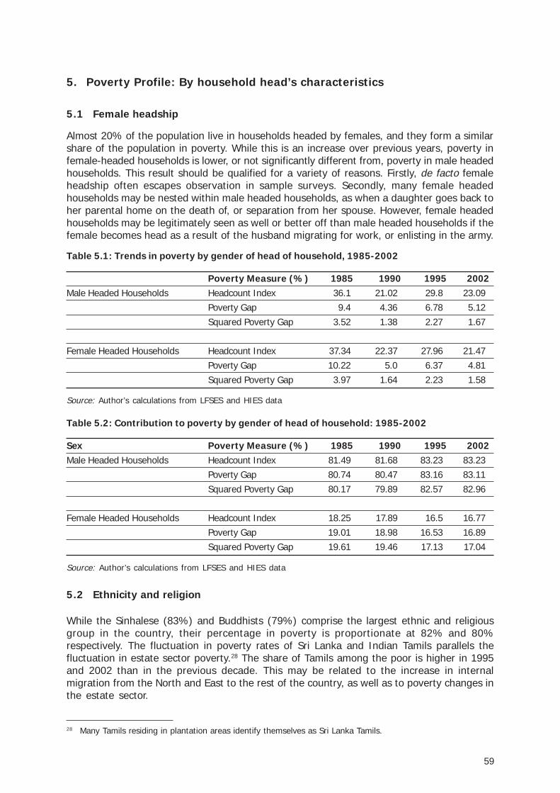
59

5. Poverty Profile: By household head’s characteristics

5.1 Female headship

Almost 20% of the population live in households headed by females, and they form a similarshare of the population in poverty. While this is an increase over previous years, poverty infemale-headed households is lower, or not significantly different from, poverty in male headedhouseholds. This result should be qualified for a variety of reasons. Firstly, de facto femaleheadship often escapes observation in sample surveys. Secondly, many female headedhouseholds may be nested within male headed households, as when a daughter goes back toher parental home on the death of, or separation from her spouse. However, female headedhouseholds may be legitimately seen as well or better off than male headed households if thefemale becomes head as a result of the husband migrating for work, or enlisting in the army.

Table 5.1: Trends in poverty by gender of head of household, 1985-2002

Poverty Measure (%) 1985 1990 1995 2002Male Headed Households Headcount Index 36.1 21.02 29.8 23.09


Female Headed Households Headcount Index 37.34 22.37 27.96 21.47Poverty Gap 10.22 5.0 6.37 4.81Squared Poverty Gap 3.97 1.64 2.23 1.58


Table 5.2: Contribution to poverty by gender of head of household: 1985-2002

Sex Poverty Measure (%) 1985 1990 1995 2002Male Headed Households Headcount Index 81.49 81.68 83.23 83.23


Female Headed Households Headcount Index 18.25 17.89 16.5 16.77Poverty Gap 19.01 18.98 16.53 16.89Squared Poverty Gap 19.61 19.46 17.13 17.04


5.2 Ethnicity and religion

While the Sinhalese (83%) and Buddhists (79%) comprise the largest ethnic and religiousgroup in the country, their percentage in poverty is proportionate at 82% and 80%respectively. The fluctuation in poverty rates of Sri Lanka and Indian Tamils parallels thefluctuation in estate sector poverty.28 The share of Tamils among the poor is higher in 1995and 2002 than in the previous decade. This may be related to the increase in internalmigration from the North and East to the rest of the country, as well as to poverty changes inthe estate sector.

28 Many Tamils residing in plantation areas identify themselves as Sri Lanka Tamils.

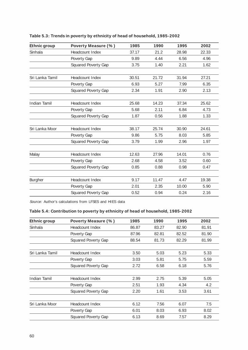
60

Table 5.3: Trends in poverty by ethnicity of head of household, 1985-2002

Ethnic group Poverty Measure (%) 1985 1990 1995 2002Sinhala Headcount Index 37.17 21.2 28.98 22.33


Sri Lanka Tamil Headcount Index 30.51 21.72 31.94 27.21Poverty Gap 6.93 5.27 7.99 6.35Squared Poverty Gap 2.34 1.91 2.90 2.13

Indian Tamil Headcount Index 25.68 14.23 37.34 25.62Poverty Gap 5.68 2.11 6.84 4.73Squared Poverty Gap 1.87 0.56 1.88 1.33

Sri Lanka Moor Headcount Index 38.17 25.74 30.90 24.61Poverty Gap 9.86 5.75 8.03 5.85Squared Poverty Gap 3.79 1.99 2.96 1.97

Malay Headcount Index 12.63 27.96 14.01 0.76Poverty Gap 2.68 4.58 3.52 0.60Squared Poverty Gap 0.85 0.88 0.98 0.47

Burgher Headcount Index 9.17 11.47 4.47 19.38Poverty Gap 2.01 2.35 10.00 5.90Squared Poverty Gap 0.52 0.94 0.24 2.16


Table 5.4: Contribution to poverty by ethnicity of head of household, 1985-2002

Ethnic group Poverty Measure (%) 1985 1990 1995 2002Sinhala Headcount Index 86.87 83.27 82.90 81.91


Sri Lanka Tamil Headcount Index 3.50 5.03 5.23 5.33Poverty Gap 3.03 5.81 5.75 5.59Squared Poverty Gap 2.72 6.58 6.18 5.76

Indian Tamil Headcount Index 2.99 2.75 5.39 5.05Poverty Gap 2.51 1.93 4.34 4.2Squared Poverty Gap 2.20 1.61 3.53 3.61

Sri Lanka Moor Headcount Index 6.12 7.56 6.07 7.5Poverty Gap 6.01 8.03 6.93 8.02Squared Poverty Gap 6.13 8.69 7.57 8.29

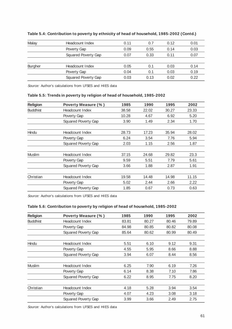
61

Malay Headcount Index 0.11 0.7 0.12 0.01Poverty Gap 0.09 0.55 0.14 0.03Squared Poverty Gap 0.07 0.33 0.11 0.07

Burgher Headcount Index 0.05 0.1 0.03 0.14Poverty Gap 0.04 0.1 0.03 0.19Squared Poverty Gap 0.03 0.13 0.02 0.22


Table 5.5: Trends in poverty by religion of head of household, 1985-2002

Religion Poverty Measure (%) 1985 1990 1995 2002Buddhist Headcount Index 38.58 22.02 30.27 23.33


Hindu Headcount Index 28.73 17.23 35.94 28.02Poverty Gap 6.24 3.54 7.76 5.94Squared Poverty Gap 2.03 1.15 2.56 1.87

Muslim Headcount Index 37.15 24.68 29.82 23.3Poverty Gap 9.59 5.51 7.79 5.61Squared Poverty Gap 3.66 1.88 2.87 1.91

Christian Headcount Index 19.58 14.48 14.98 11.15Poverty Gap 5.02 2.44 2.66 2.22Squared Poverty Gap 1.85 0.67 0.73 0.63


Table 5.6: Contribution to poverty by religion of head of household, 1985-2002

Religion Poverty Measure (%) 1985 1990 1995 2002Buddhist Headcount Index 83.81 80.27 80.46 79.89


Hindu Headcount Index 5.51 6.10 9.12 9.31Poverty Gap 4.55 5.95 8.66 8.88Squared Poverty Gap 3.94 6.07 8.44 8.56

Muslim Headcount Index 6.25 7.90 6.19 7.26Poverty Gap 6.14 8.38 7.10 7.86Squared Poverty Gap 6.22 8.95 7.75 8.20

Christian Headcount Index 4.18 5.28 3.94 3.54Poverty Gap 4.07 4.23 3.08 3.18Squared Poverty Gap 3.99 3.66 2.49 2.75


Table 5.4: Contribution to poverty by ethnicity of head of household, 1985-2002 (Contd.)

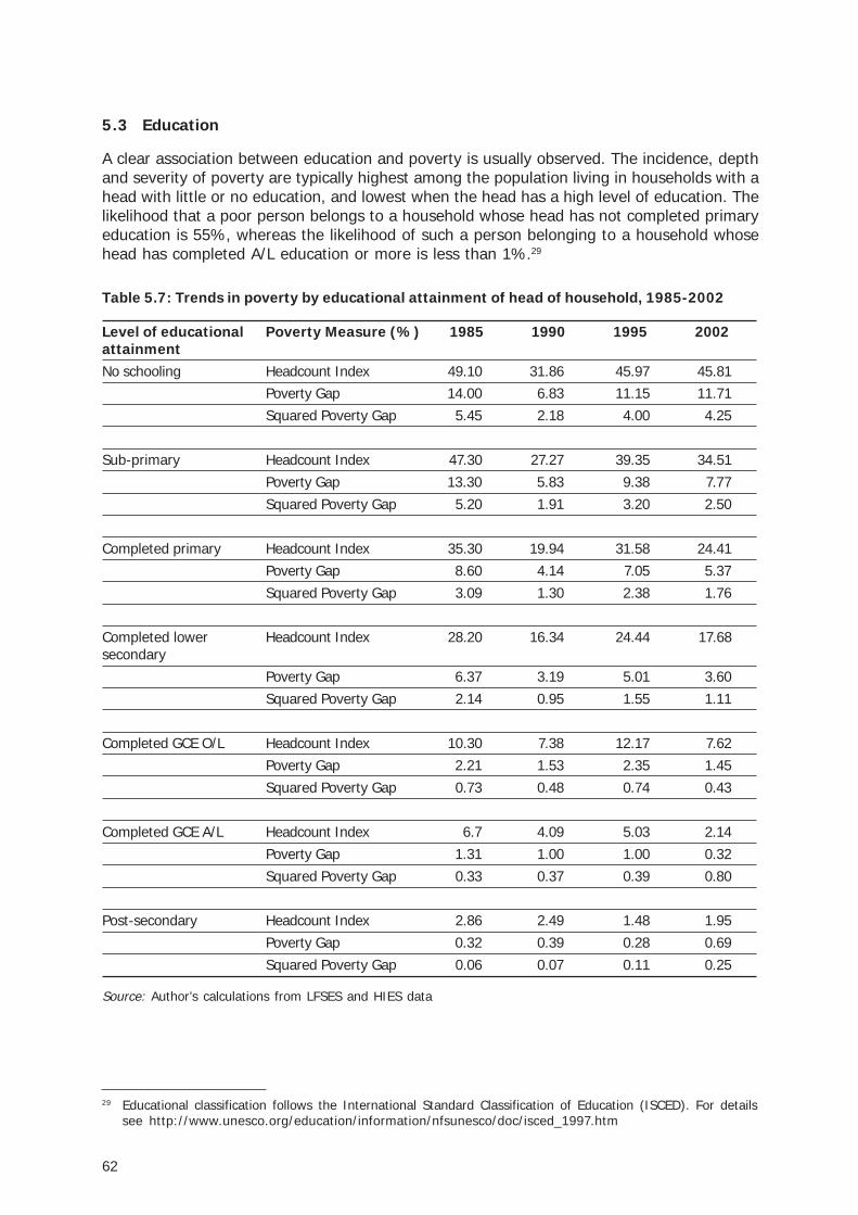
62

5.3 Education

A clear association between education and poverty is usually observed. The incidence, depthand severity of poverty are typically highest among the population living in households with ahead with little or no education, and lowest when the head has a high level of education. Thelikelihood that a poor person belongs to a household whose head has not completed primaryeducation is 55%, whereas the likelihood of such a person belonging to a household whosehead has completed A/L education or more is less than 1%.29

29 Educational classification follows the International Standard Classification of Education (ISCED). For detailssee http://www.unesco.org/education/information/nfsunesco/doc/isced_1997.htm

Table 5.7: Trends in poverty by educational attainment of head of household, 1985-2002

Level of educational Poverty Measure (%) 1985 1990 1995 2002attainmentNo schooling Headcount Index 49.10 31.86 45.97 45.81


Sub-primary Headcount Index 47.30 27.27 39.35 34.51Poverty Gap 13.30 5.83 9.38 7.77Squared Poverty Gap 5.20 1.91 3.20 2.50

Completed primary Headcount Index 35.30 19.94 31.58 24.41Poverty Gap 8.60 4.14 7.05 5.37Squared Poverty Gap 3.09 1.30 2.38 1.76

Completed lower Headcount Index 28.20 16.34 24.44 17.68secondary


Completed GCE O/L Headcount Index 10.30 7.38 12.17 7.62Poverty Gap 2.21 1.53 2.35 1.45Squared Poverty Gap 0.73 0.48 0.74 0.43

Completed GCE A/L Headcount Index 6.7 4.09 5.03 2.14Poverty Gap 1.31 1.00 1.00 0.32Squared Poverty Gap 0.33 0.37 0.39 0.80

Post-secondary Headcount Index 2.86 2.49 1.48 1.95Poverty Gap 0.32 0.39 0.28 0.69Squared Poverty Gap 0.06 0.07 0.11 0.25


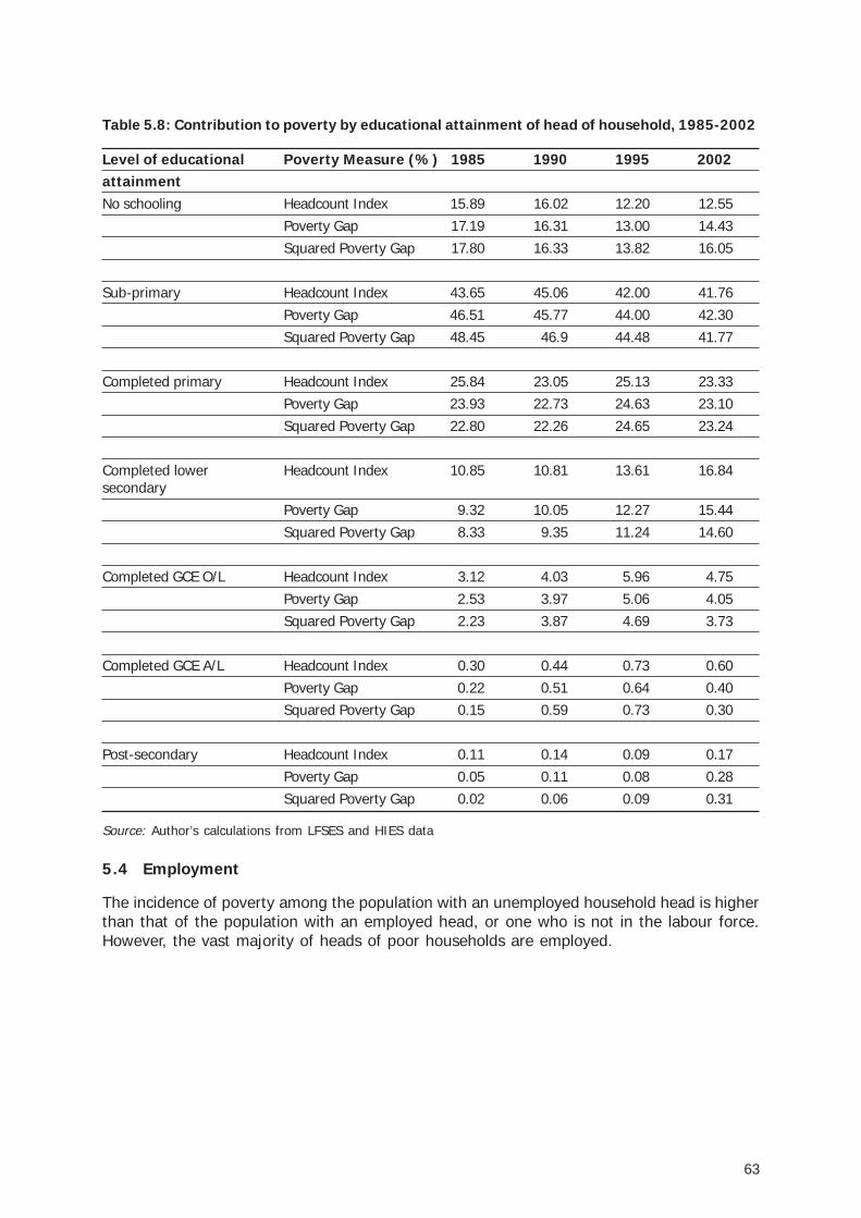
63

Table 5.8: Contribution to poverty by educational attainment of head of household, 1985-2002

Level of educational Poverty Measure (%) 1985 1990 1995 2002attainmentNo schooling Headcount Index 15.89 16.02 12.20 12.55


Sub-primary Headcount Index 43.65 45.06 42.00 41.76Poverty Gap 46.51 45.77 44.00 42.30Squared Poverty Gap 48.45 46.9 44.48 41.77

Completed primary Headcount Index 25.84 23.05 25.13 23.33Poverty Gap 23.93 22.73 24.63 23.10Squared Poverty Gap 22.80 22.26 24.65 23.24

Completed lower Headcount Index 10.85 10.81 13.61 16.84secondary


Completed GCE O/L Headcount Index 3.12 4.03 5.96 4.75Poverty Gap 2.53 3.97 5.06 4.05Squared Poverty Gap 2.23 3.87 4.69 3.73

Completed GCE A/L Headcount Index 0.30 0.44 0.73 0.60Poverty Gap 0.22 0.51 0.64 0.40Squared Poverty Gap 0.15 0.59 0.73 0.30

Post-secondary Headcount Index 0.11 0.14 0.09 0.17Poverty Gap 0.05 0.11 0.08 0.28Squared Poverty Gap 0.02 0.06 0.09 0.31


5.4 Employment

The incidence of poverty among the population with an unemployed household head is higherthan that of the population with an employed head, or one who is not in the labour force.However, the vast majority of heads of poor households are employed.

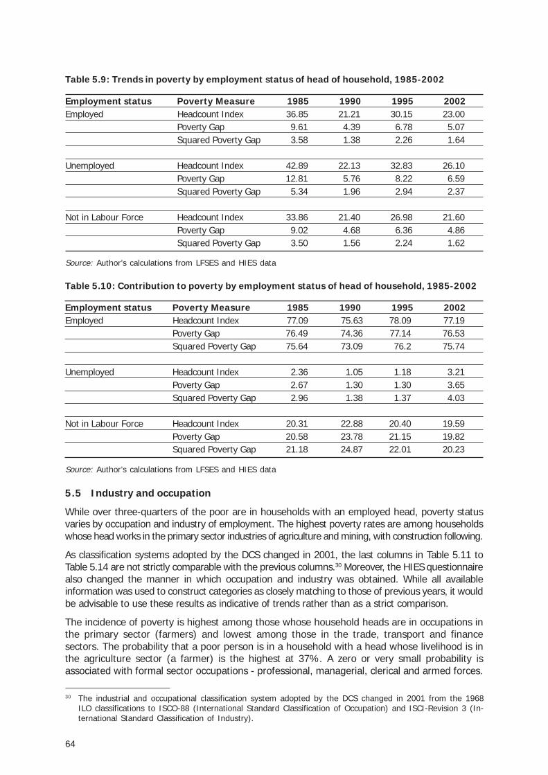
64

Table 5.9: Trends in poverty by employment status of head of household, 1985-2002

Employment status Poverty Measure 1985 1990 1995 2002Employed Headcount Index 36.85 21.21 30.15 23.00


Unemployed Headcount Index 42.89 22.13 32.83 26.10Poverty Gap 12.81 5.76 8.22 6.59Squared Poverty Gap 5.34 1.96 2.94 2.37

Not in Labour Force Headcount Index 33.86 21.40 26.98 21.60Poverty Gap 9.02 4.68 6.36 4.86Squared Poverty Gap 3.50 1.56 2.24 1.62


Table 5.10: Contribution to poverty by employment status of head of household, 1985-2002

Employment status Poverty Measure 1985 1990 1995 2002Employed Headcount Index 77.09 75.63 78.09 77.19


Unemployed Headcount Index 2.36 1.05 1.18 3.21Poverty Gap 2.67 1.30 1.30 3.65Squared Poverty Gap 2.96 1.38 1.37 4.03

Not in Labour Force Headcount Index 20.31 22.88 20.40 19.59Poverty Gap 20.58 23.78 21.15 19.82Squared Poverty Gap 21.18 24.87 22.01 20.23


5.5 Industry and occupation

While over three-quarters of the poor are in households with an employed head, poverty statusvaries by occupation and industry of employment. The highest poverty rates are among householdswhose head works in the primary sector industries of agriculture and mining, with construction following.

As classification systems adopted by the DCS changed in 2001, the last columns in Table 5.11 toTable 5.14 are not strictly comparable with the previous columns.30 Moreover, the HIES questionnairealso changed the manner in which occupation and industry was obtained. While all availableinformation was used to construct categories as closely matching to those of previous years, it wouldbe advisable to use these results as indicative of trends rather than as a strict comparison.

The incidence of poverty is highest among those whose household heads are in occupations inthe primary sector (farmers) and lowest among those in the trade, transport and financesectors. The probability that a poor person is in a household with a head whose livelihood is inthe agriculture sector (a farmer) is the highest at 37%. A zero or very small probability isassociated with formal sector occupations - professional, managerial, clerical and armed forces.

30 The industrial and occupational classification system adopted by the DCS changed in 2001 from the 1968ILO classifications to ISCO-88 (International Standard Classification of Occupation) and ISCI-Revision 3 (In-ternational Standard Classification of Industry).

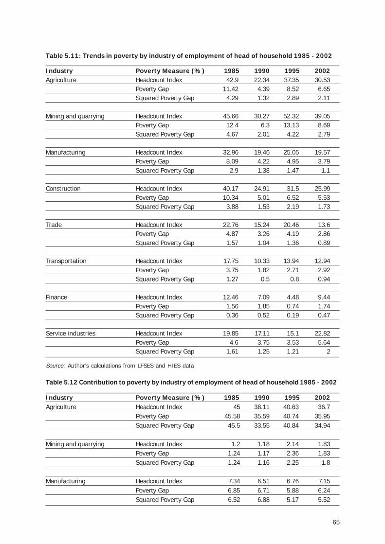
65

Table 5.11: Trends in poverty by industry of employment of head of household 1985 - 2002

Industry Poverty Measure (%) 1985 1990 1995 2002Agriculture Headcount Index 42.9 22.34 37.35 30.53


Mining and quarrying Headcount Index 45.66 30.27 52.32 39.05Poverty Gap 12.4 6.3 13.13 8.69Squared Poverty Gap 4.67 2.01 4.22 2.79

Manufacturing Headcount Index 32.96 19.46 25.05 19.57Poverty Gap 8.09 4.22 4.95 3.79Squared Poverty Gap 2.9 1.38 1.47 1.1

Construction Headcount Index 40.17 24.91 31.5 25.99Poverty Gap 10.34 5.01 6.52 5.53Squared Poverty Gap 3.88 1.53 2.19 1.73

Trade Headcount Index 22.76 15.24 20.46 13.6Poverty Gap 4.87 3.26 4.19 2.86Squared Poverty Gap 1.57 1.04 1.36 0.89

Transportation Headcount Index 17.75 10.33 13.94 12.94Poverty Gap 3.75 1.82 2.71 2.92Squared Poverty Gap 1.27 0.5 0.8 0.94

Finance Headcount Index 12.46 7.09 4.48 9.44Poverty Gap 1.56 1.85 0.74 1.74Squared Poverty Gap 0.36 0.52 0.19 0.47

Service industries Headcount Index 19.85 17.11 15.1 22.82Poverty Gap 4.6 3.75 3.53 5.64Squared Poverty Gap 1.61 1.25 1.21 2


Table 5.12 Contribution to poverty by industry of employment of head of household 1985 - 2002

Industry Poverty Measure (%) 1985 1990 1995 2002Agriculture Headcount Index 45 38.11 40.63 36.7


Mining and quarrying Headcount Index 1.2 1.18 2.14 1.83Poverty Gap 1.24 1.17 2.36 1.83Squared Poverty Gap 1.24 1.16 2.25 1.8

Manufacturing Headcount Index 7.34 6.51 6.76 7.15Poverty Gap 6.85 6.71 5.88 6.24Squared Poverty Gap 6.52 6.88 5.17 5.52

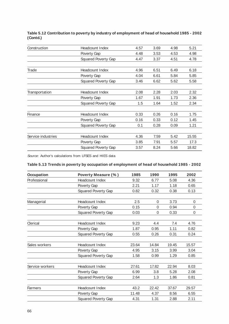
66

Construction Headcount Index 4.57 3.69 4.98 5.21Poverty Gap 4.48 3.53 4.53 4.98Squared Poverty Gap 4.47 3.37 4.51 4.78

Trade Headcount Index 4.96 6.51 6.49 6.18Poverty Gap 4.04 6.61 5.84 5.85Squared Poverty Gap 3.46 6.62 5.62 5.58

Transportation Headcount Index 2.08 2.28 2.03 2.32Poverty Gap 1.67 1.91 1.73 2.36Squared Poverty Gap 1.5 1.64 1.52 2.34

Finance Headcount Index 0.33 0.26 0.16 1.75Poverty Gap 0.16 0.33 0.12 1.45Squared Poverty Gap 0.1 0.28 0.09 1.21

Service industries Headcount Index 4.36 7.59 5.42 15.55Poverty Gap 3.85 7.91 5.57 17.3Squared Poverty Gap 3.57 8.24 5.66 18.82


Table 5.13 Trends in poverty by occupation of employment of head of household 1985 - 2002

Occupation Poverty Measure (%) 1985 1990 1995 2002Professional Headcount Index 9.32 6.77 5.08 4.36


Managerial Headcount Index 2.5 0 3.73 0Poverty Gap 0.15 0 0.94 0Squared Poverty Gap 0.03 0 0.33 0

Clerical Headcount Index 9.23 4.4 7.4 4.76Poverty Gap 1.87 0.95 1.11 0.82Squared Poverty Gap 0.55 0.26 0.31 0.24

Sales workers Headcount Index 23.64 14.84 19.45 15.57Poverty Gap 4.95 3.15 3.99 3.04Squared Poverty Gap 1.58 0.99 1.29 0.85

Service workers Headcount Index 27.61 17.82 22.94 8.03Poverty Gap 6.99 3.8 5.28 2.08Squared Poverty Gap 2.64 1.3 1.86 0.81

Farmers Headcount Index 43.2 22.42 37.67 29.57Poverty Gap 11.48 4.37 8.56 6.55Squared Poverty Gap 4.31 1.31 2.88 2.11

Table 5.12 Contribution to poverty by industry of employment of head of household 1985 - 2002(Contd.)

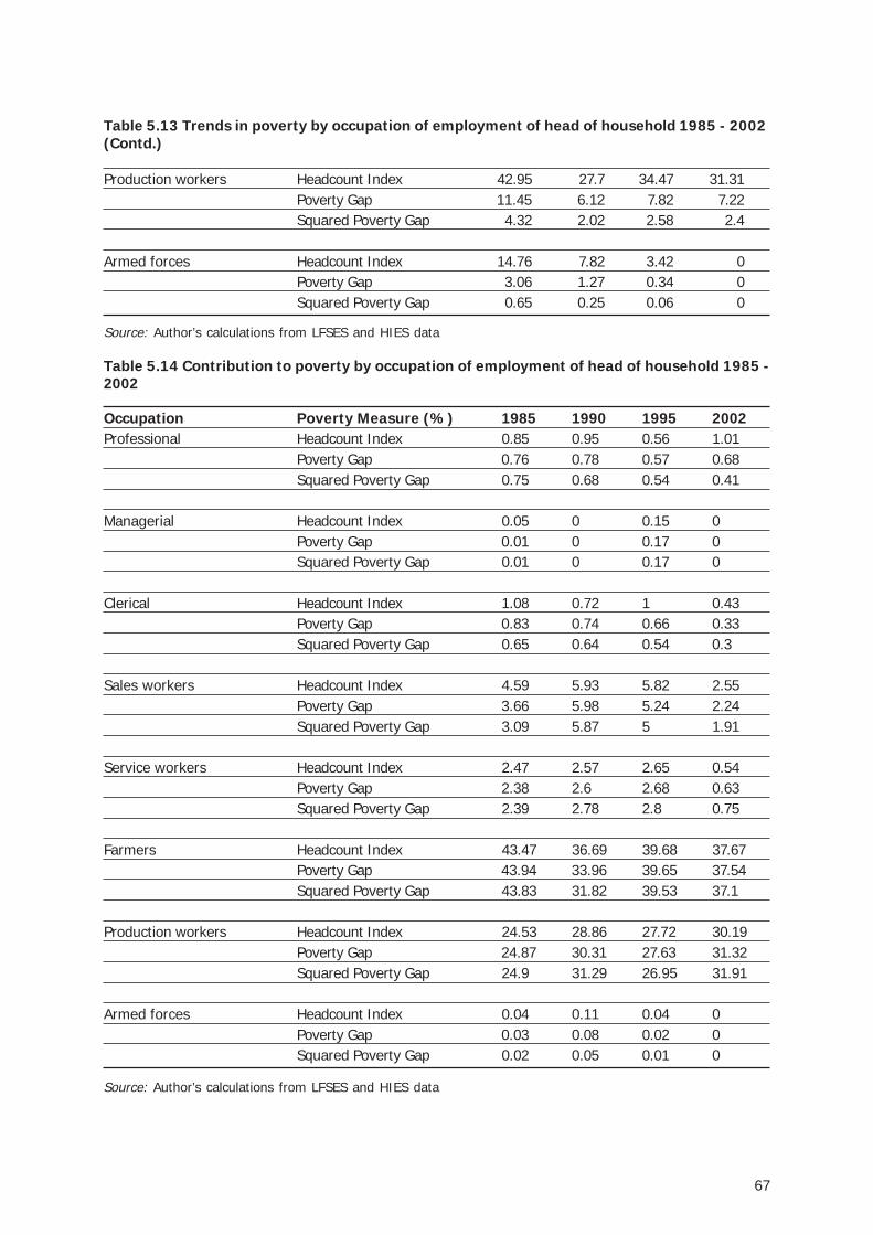
67



Table 5.14 Contribution to poverty by occupation of employment of head of household 1985 -2002

Occupation Poverty Measure (%) 1985 1990 1995 2002Professional Headcount Index 0.85 0.95 0.56 1.01


Managerial Headcount Index 0.05 0 0.15 0Poverty Gap 0.01 0 0.17 0Squared Poverty Gap 0.01 0 0.17 0

Clerical Headcount Index 1.08 0.72 1 0.43Poverty Gap 0.83 0.74 0.66 0.33Squared Poverty Gap 0.65 0.64 0.54 0.3

Sales workers Headcount Index 4.59 5.93 5.82 2.55Poverty Gap 3.66 5.98 5.24 2.24Squared Poverty Gap 3.09 5.87 5 1.91

Service workers Headcount Index 2.47 2.57 2.65 0.54Poverty Gap 2.38 2.6 2.68 0.63Squared Poverty Gap 2.39 2.78 2.8 0.75

Farmers Headcount Index 43.47 36.69 39.68 37.67Poverty Gap 43.94 33.96 39.65 37.54Squared Poverty Gap 43.83 31.82 39.53 37.1

Production workers Headcount Index 24.53 28.86 27.72 30.19Poverty Gap 24.87 30.31 27.63 31.32Squared Poverty Gap 24.9 31.29 26.95 31.91

Armed forces Headcount Index 0.04 0.11 0.04 0Poverty Gap 0.03 0.08 0.02 0Squared Poverty Gap 0.02 0.05 0.01 0

Production workers Headcount Index 42.95 27.7 34.47 31.31Poverty Gap 11.45 6.12 7.82 7.22Squared Poverty Gap 4.32 2.02 2.58 2.4

Armed forces Headcount Index 14.76 7.82 3.42 0Poverty Gap 3.06 1.27 0.34 0Squared Poverty Gap 0.65 0.25 0.06 0

Table 5.13 Trends in poverty by occupation of employment of head of household 1985 - 2002(Contd.)

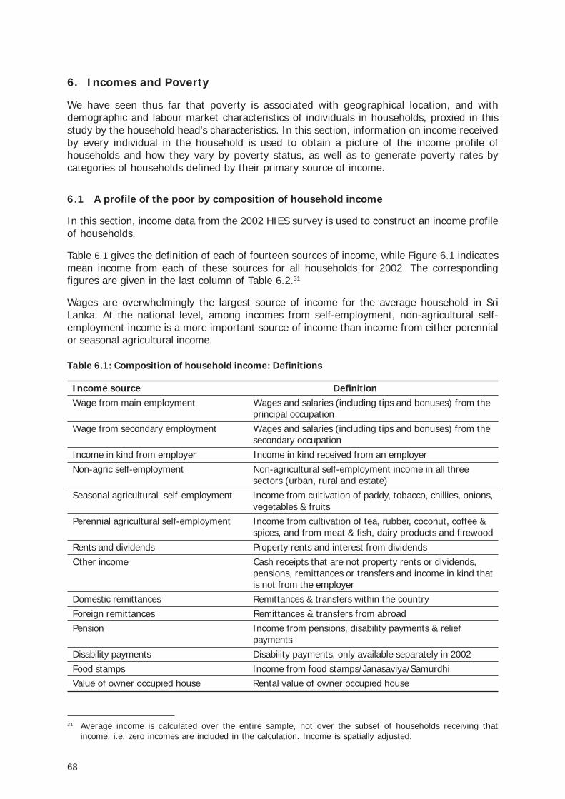
68

6. Incomes and Poverty

We have seen thus far that poverty is associated with geographical location, and withdemographic and labour market characteristics of individuals in households, proxied in thisstudy by the household head’s characteristics. In this section, information on income receivedby every individual in the household is used to obtain a picture of the income profile ofhouseholds and how they vary by poverty status, as well as to generate poverty rates bycategories of households defined by their primary source of income.

6.1 A profile of the poor by composition of household income

In this section, income data from the 2002 HIES survey is used to construct an income profileof households.

Table 6.1 gives the definition of each of fourteen sources of income, while Figure 6.1 indicatesmean income from each of these sources for all households for 2002. The correspondingfigures are given in the last column of Table 6.2.31

Wages are overwhelmingly the largest source of income for the average household in SriLanka. At the national level, among incomes from self-employment, non-agricultural self-employment income is a more important source of income than income from either perennialor seasonal agricultural income.

Table 6.1: Composition of household income: Definitions

Income source DefinitionWage from main employment Wages and salaries (including tips and bonuses) from the

principal occupationWage from secondary employment Wages and salaries (including tips and bonuses) from the

secondary occupationIncome in kind from employer Income in kind received from an employerNon-agric self-employment Non-agricultural self-employment income in all three

sectors (urban, rural and estate)Seasonal agricultural self-employment Income from cultivation of paddy, tobacco, chillies, onions,

vegetables & fruitsPerennial agricultural self-employment Income from cultivation of tea, rubber, coconut, coffee &

spices, and from meat & fish, dairy products and firewoodRents and dividends Property rents and interest from dividendsOther income Cash receipts that are not property rents or dividends,

pensions, remittances or transfers and income in kind thatis not from the employer

Domestic remittances Remittances & transfers within the countryForeign remittances Remittances & transfers from abroadPension Income from pensions, disability payments & relief

paymentsDisability payments Disability payments, only available separately in 2002Food stamps Income from food stamps/Janasaviya/SamurdhiValue of owner occupied house Rental value of owner occupied house

31 Average income is calculated over the entire sample, not over the subset of households receiving thatincome, i.e. zero incomes are included in the calculation. Income is spatially adjusted.

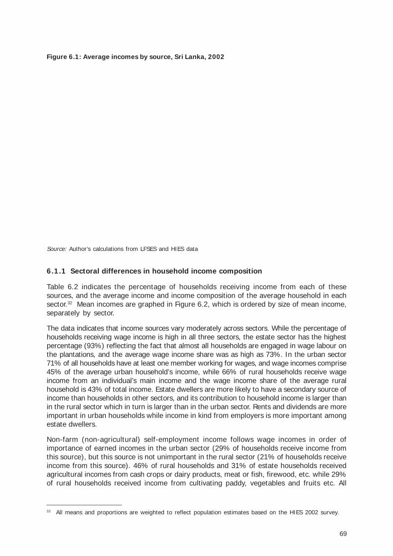
69

Figure 6.1: Average incomes by source, Sri Lanka, 2002


6.1.1 Sectoral differences in household income composition

Table 6.2 indicates the percentage of households receiving income from each of thesesources, and the average income and income composition of the average household in eachsector.32 Mean incomes are graphed in Figure 6.2, which is ordered by size of mean income,separately by sector.

The data indicates that income sources vary moderately across sectors. While the percentage ofhouseholds receiving wage income is high in all three sectors, the estate sector has the highestpercentage (93%) reflecting the fact that almost all households are engaged in wage labour onthe plantations, and the average wage income share was as high as 73%. In the urban sector71% of all households have at least one member working for wages, and wage incomes comprise45% of the average urban household’s income, while 66% of rural households receive wageincome from an individual’s main income and the wage income share of the average ruralhousehold is 43% of total income. Estate dwellers are more likely to have a secondary source ofincome than households in other sectors, and its contribution to household income is larger thanin the rural sector which in turn is larger than in the urban sector. Rents and dividends are moreimportant in urban households while income in kind from employers is more important amongestate dwellers.

Non-farm (non-agricultural) self-employment income follows wage incomes in order ofimportance of earned incomes in the urban sector (29% of households receive income fromthis source), but this source is not unimportant in the rural sector (21% of households receiveincome from this source). 46% of rural households and 31% of estate households receivedagricultural incomes from cash crops or dairy products, meat or fish, firewood, etc. while 29%of rural households received income from cultivating paddy, vegetables and fruits etc. All

32 All means and proportions are weighted to reflect population estimates based on the HIES 2002 survey.

70

agricultural (non-wage) income comprised about 12% of the average rural household’s incomeand 5% of the average estate household’s income.

As many as 81% of urban households and 94% of rural households indicated a positive valueof imputed rents. This signifies that they own the houses they live in. Receipts in kind andother cash receipts were also moderately important in all three sectors.

7% of urban and 5% of rural households received foreign remittances, while 5% and 4% ofrural and estate households respectively received domestic remittances. This indicates thatforeign employment is slightly more accessible to urban dwellers than rural dwellers, and ruraldwellers than estate dwellers. Domestic remittances appear to have some significance,although their share in total income is low (approximately 1% in rural and estate sectors).While more urban households (13%) receive pensions than rural households (6%), 2% ofurban and 3% of rural households receive disability and relief payments.

6.1.2 Household income composition by poverty status

Table 6.3 and Figure 6.3 reveal differences in the composition of household income by povertystatus. A larger proportion of poor households received wage income than non-poorhouseholds, indicating a greater reliance of the poor on wage employment. Moreover, agreater percentage of poor households received wage income from a secondary wage-earning occupation, supporting the supposition that the poor engage in a variety of activities inorder to make ends meet.

71

Figure 6.2: Income composition by sector, 2002


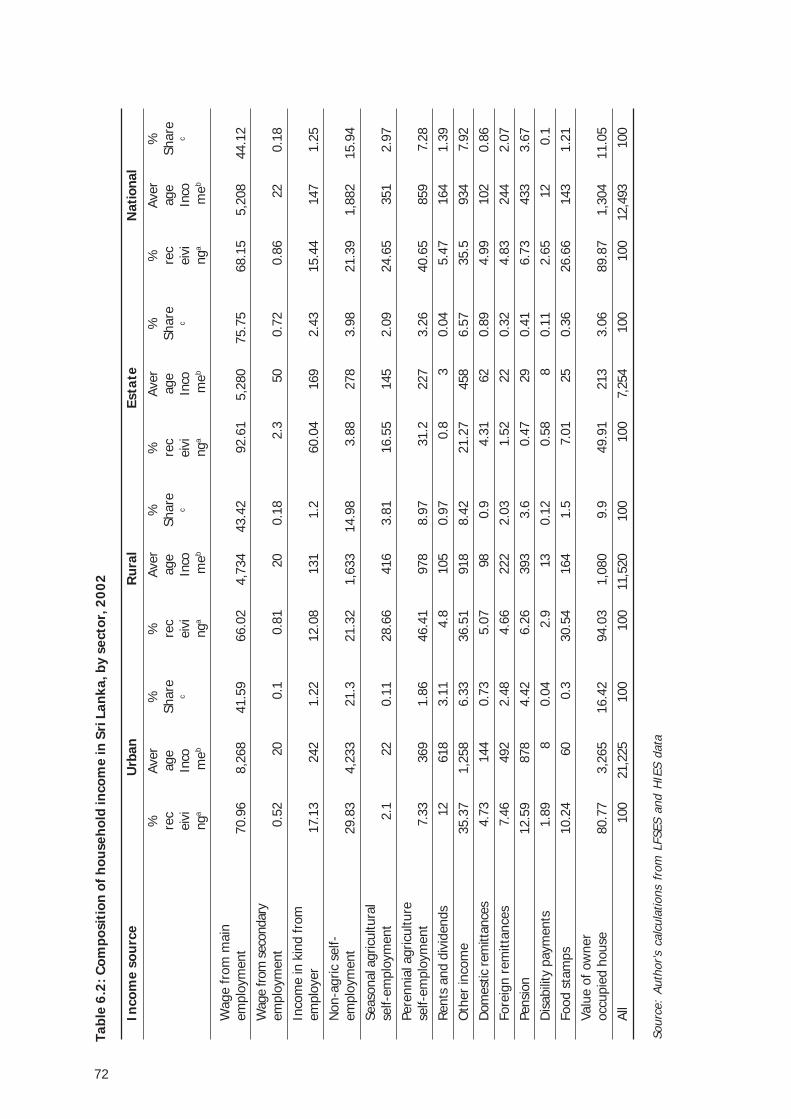
72

Tabl

e 6.

2: C

ompo

siti

on o

f hou

seho

ld in

com

e in

Sri

Lan

ka, b

y se

ctor

, 200

2

Sour

ce:

Auth

or’s

cal

cula

tions

fro

m L

FSES

and

HIE

S da

ta

Wag

e fr

om m

ain

empl

oym

ent

70.9

68,

268

41.5

966

.02

4,73

443

.42

92.6

15,

280

75.7

568

.15

5,20

844

.12

Wag

e fro

m s

econ

dary

empl

oym

ent

0.52

200.

10.

8120

0.18

2.3

500.

720.

8622

0.18

Inco

me

in k

ind

from

empl

oyer

17.1

324

21.

2212

.08

131

1.2

60.0

416

92.

4315

.44

147

1.25

Non

-agr

ic s

elf-

empl

oym

ent

29.8

34,

233

21.3

21.3

21,

633

14.9

83.

8827

83.

9821

.39

1,88

215

.94

Seas

onal

agr

icul

tura

lse

lf-em

ploy

men

t2.

122

0.11

28.6

641

63.

8116

.55

145

2.09

24.6

535

12.

97Pe

renn

ial a

gric

ultu

rese

lf-em

ploy

men

t7.

3336

91.

8646

.41

978

8.97

31.2

227

3.26

40.6

585

97.

28Re

nts

and

divi

dend

s12

618

3.11

4.8

105

0.97

0.8

30.

045.

4716

41.

39O

ther

inco

me

35.3

71,

258

6.33

36.5

191

88.

4221

.27

458

6.57

35.5

934

7.92

Dom

estic

rem

ittan

ces

4.73

144

0.73

5.07

980.

94.

3162

0.89

4.99

102

0.86

Fore

ign

rem

ittan

ces

7.46

492

2.48

4.66

222

2.03

1.52

220.

324.

8324

42.

07Pe

nsio

n12

.59

878

4.42

6.26

393

3.6

0.47

290.

416.

7343

33.

67D

isab

ility

pay

men

ts1.

898

0.04

2.9

130.

120.

588

0.11

2.65

120.

1Fo

od s

tam

ps10

.24

600.

330

.54

164

1.5

7.01

250.

3626

.66

143

1.21

Valu

e of

ow

ner

occu

pied

hou

se80

.77

3,26

516

.42

94.0

31,

080

9.9

49.9

121

33.

0689

.87

1,30

411

.05

All

100

21,2

2510

010

011

,520

100

100

7,25

410

010

012

,493

100

%Av

er%

%Av

er%

%Av

er%

%Av

er%

rec

age

Shar

ere

cag

eSh

are

rec

age

Shar

ere

cag

eSh

are

eivi

Inco

cei

viIn

coc

eivi

Inco

cei

viIn

coc

nga

meb

nga

meb

nga

meb

nga

meb

Inco

me

sour

ceU

rban

Rur

alEs

tate

Nat

iona

l

73

Figure 6.3: Income composition by poverty status, 2002


The importance of self-employment incomes to the poor depends on the type of income.Agricultural self-employment income of both categories is more important to the poor than tothe non-poor in terms of percentage of households receiving this income. 29% of poorhouseholds receive income from paddy, vegetables, etc. compared to 24% of the non-poor,and 47% of the poor receive income from cash crops, dairy products, meat, fish, firewood,etc. compared to 39% of the non-poor. On the other hand, non-farm self-employmentincome is more important to non-poor households (23% of non-poor households receiveincome from this source compared to 13% of poor households).

While 2% of poor households received foreign remittances which are 0.5% of their incomes,the non-poor receive greater benefit from foreign employment with 6% of householdsreceiving foreign remittances and an income share of almost 2%. While a larger proportion ofnon-poor households received pensions, a slightly higher proportion of poor households receivedisability and relief payments.

Similar percentages of poor and non-poor households (90-91%) live in their own houses, whileimputed rents account for about 8% of incomes for the poor and 12% of incomes for the non-poor.

As is expected, food stamps are a more importance source of income for the poor than for thenon-poor, but it appears that close to half of poor households do not receive food stamps (46%),while about a quarter of the non-poor receive food stamps. This is explored further in section 6.3.

a Percentage of households receiving any income from this source.b Average income (spatially deflated rupees and cents) received from each source by the average household.c Income composition (% share of each source in total income) of the average household.

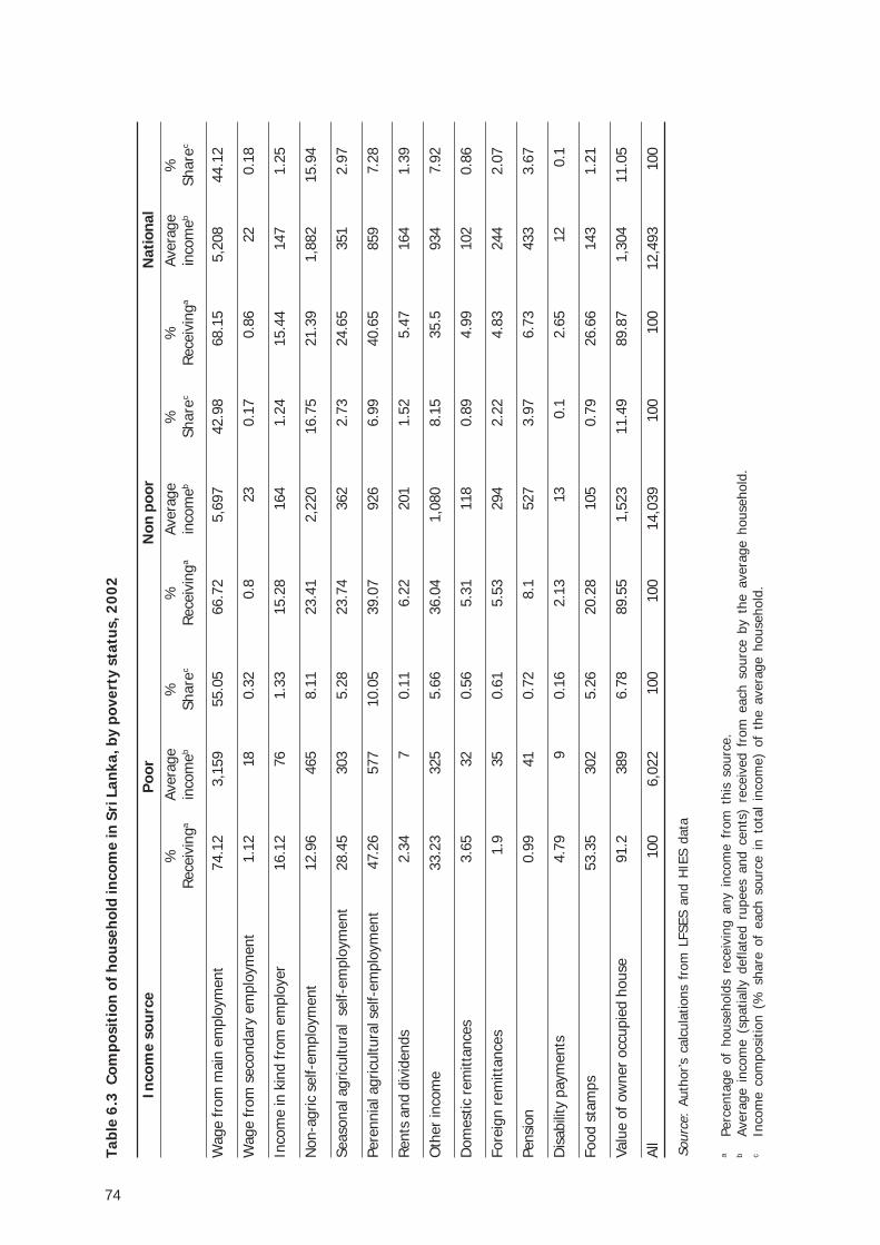
74

Sour

ce:

Auth

or’s

cal

cula

tions

fro

m L

FSES

and

HIE

S da

ta

Tabl

e 6.

3 C

ompo

siti

on o

f hou

seho

ld in

com

e in

Sri

Lan

ka, b

y po

vert

y st

atus

, 200

2

aPe

rcen

tage

of

hous

ehol

ds r

ecei

ving

any

inc

ome

from

thi

s so

urce

.b

Aver

age

inco

me

(spa

tially

def

late

d ru

pees

and

cen

ts)

rece

ived

fro

m e

ach

sour

ce b

y th

e av

erag

e ho

useh

old.

cIn

com

e co

mpo

sitio

n (%

sha

re o

f ea

ch s

ourc

e in

tot

al i

ncom

e) o

f th

e av

erag

e ho

useh

old.

%Av

erag

e%

%Av

erag

e%

%Av

erag

e%

Rece

ivin

gain

com

ebSh

arec

Rece

ivin

gain

com

ebSh

arec

Rece

ivin

gain

com

ebSh

arec

Wag

e fr

om m

ain

empl

oym

ent

74.1

23,

159

55.0

566

.72

5,69

742

.98

68.1

55,

208

44.1

2

Wag

e fr

om s

econ

dary

em

ploy

men

t1.

1218

0.32

0.8

230.

170.

8622

0.18

Inco

me

in k

ind

from

em

ploy

er16

.12

761.

3315

.28

164

1.24

15.4

414

71.

25

Non

-agr

ic s

elf-

empl

oym

ent

12.9

646

58.

1123

.41

2,22

016

.75

21.3

91,

882

15.9

4

Seas

onal

agr

icul

tura

l se

lf-em

ploy

men

t28

.45

303

5.28

23.7

436

22.

7324

.65

351

2.97

Pere

nnia

l agr

icul

tura

l sel

f-em

ploy

men

t47

.26

577

10.0

539

.07

926

6.99

40.6

585

97.

28

Rent

s an

d di

vide

nds

2.34

70.

116.

2220

11.

525.

4716

41.

39

Oth

er in

com

e33

.23

325

5.66

36.0

41,

080

8.15

35.5

934

7.92

Dom

estic

rem

ittan

ces

3.65

320.

565.

3111

80.

894.

9910

20.

86

Fore

ign

rem

ittan

ces

1.9

350.

615.

5329

42.

224.

8324

42.

07

Pens

ion

0.99

410.

728.

152

73.

976.

7343

33.

67

Dis

abili

ty p

aym

ents

4.79

90.

162.

1313

0.1

2.65

120.

1

Food

sta

mps

53.3

530

25.

2620

.28

105

0.79

26.6

614

31.

21

Valu

e of

ow

ner

occu

pied

hou

se91

.238

96.

7889

.55

1,52

311

.49

89.8

71,

304

11.0

5

All

100

6,02

210

010

014

,039

100

100

12,4

9310

0

Inco

me

sour

cePo

orN

on p

oor

Nat

iona

l

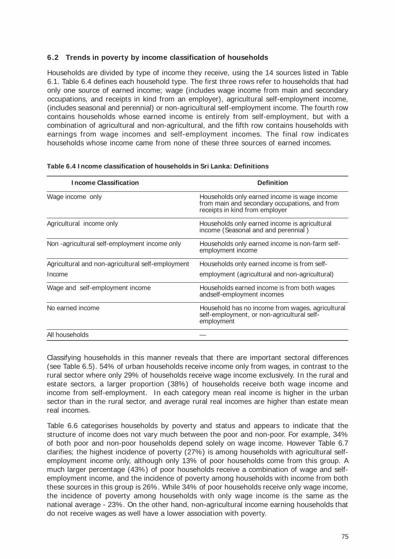
75

6.2 Trends in poverty by income classification of households

Households are divided by type of income they receive, using the 14 sources listed in Table6.1. Table 6.4 defines each household type. The first three rows refer to households that hadonly one source of earned income; wage (includes wage income from main and secondaryoccupations, and receipts in kind from an employer), agricultural self-employment income,(includes seasonal and perennial) or non-agricultural self-employment income. The fourth rowcontains households whose earned income is entirely from self-employment, but with acombination of agricultural and non-agricultural, and the fifth row contains households withearnings from wage incomes and self-employment incomes. The final row indicateshouseholds whose income came from none of these three sources of earned incomes.

Table 6.4 Income classification of households in Sri Lanka: Definitions

Income Classification Definition

Wage income only Households only earned income is wage incomefrom main and secondary occupations, and fromreceipts in kind from employer

Agricultural income only Households only earned income is agriculturalincome (Seasonal and and perennial )

Non -agricultural self-employment income only Households only earned income is non-farm self-employment income

Agricultural and non-agricultural self-employment Households only earned income is from self-

Income employment (agricultural and non-agricultural)

Wage and self-employment income Households earned income is from both wagesandself-employment incomes

No earned income Household has no income from wages, agriculturalself-employment, or non-agricultural self-employment

All households —

Classifying households in this manner reveals that there are important sectoral differences(see Table 6.5). 54% of urban households receive income only from wages, in contrast to therural sector where only 29% of households receive wage income exclusively. In the rural andestate sectors, a larger proportion (38%) of households receive both wage income andincome from self-employment. In each category mean real income is higher in the urbansector than in the rural sector, and average rural real incomes are higher than estate meanreal incomes.

Table 6.6 categorises households by poverty and status and appears to indicate that thestructure of income does not vary much between the poor and non-poor. For example, 34%of both poor and non-poor households depend solely on wage income. However Table 6.7clarifies; the highest incidence of poverty (27%) is among households with agricultural self-employment income only, although only 13% of poor households come from this group. Amuch larger percentage (43%) of poor households receive a combination of wage and self-employment income, and the incidence of poverty among households with income from boththese sources in this group is 26%. While 34% of poor households receive only wage income,the incidence of poverty among households with only wage income is the same as thenational average - 23%. On the other hand, non-agricultural income earning households thatdo not receive wages as well have a lower association with poverty.

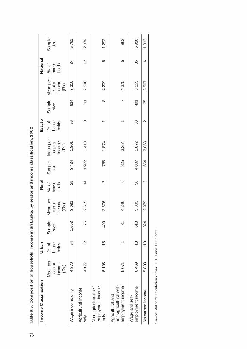
76

Sour

ce:

Auth

or’s

cal

cula

tions

fro

m L

FSES

and

HIE

S da

ta

Tabl

e 6.

5: C

ompo

siti

on o

f hou

seho

ld I

ncom

e in

Sri

Lan

ka, b

y se

ctor

and

inco

me

clas

sifi

cati

on, 2

002

Wag

e in

com

e on

ly4,

870

541,

693

3,08

129

3,43

41,

801

5663

43,

319

345,

761

Agric

ultu

ral i

ncom

eon

ly4,

177

276

2,51

514

1,97

21,

410

331

2,53

012

2,07

9

Non

-agr

icul

tura

l sel

f-em

ploy

men

t inc

ome

onl

y6,

105

1549

93,

576

778

51,

874

18

4,20

98

1,29

2

Agric

ultu

ral a

ndno

n-ag

ricul

tura

l sel

f-em

ploy

men

t inc

ome

6,07

11

314,

346

682

53,

354

17

4,37

55

863

Wag

e an

d se

lf-em

ploy

men

t inc

ome

6,46

918

618

3,00

338

4,80

71,

872

3849

13,

155

355,

916

No

earn

ed in

com

e5,

803

1032

42,

979

566

42,

068

225

3,56

76

1,01

3

Inco

me

Cla

ssifi

cati

onU

rban

Rur

alEs

tate

Nat

iona

l

Mea

n pe

r%

of

Sam

ple

Mea

n pe

r%

of

Sam

ple

Mea

n pe

r%

of

Sam

ple

Mea

n pe

r%

of

Sam

ple

cap

itaho

use

size

capi

taho

use

size

capi

taho

use

size

capi

taho

use

size

inco

me

hold

sin

com

eho

lds

inco

me

hold

sin

com

eho

lds

(Rs.

)(R

s.)

(Rs.

)(R

s.)

77

Tabl

e 6.

6 C

ompo

siti

on o

f hou

seho

ld in

com

e in

Sri

Lan

ka, b

y po

vert

y st

atus

and

inco

me

clas

sifi

cati

on, 2

002

Inco

me

Cla

ssifi

cati

onPo

orN

on-p

oor

All

Mea

n pe

r%

of

Sam

ple

Mea

n pe

r%

of

Sam

ple

Mea

n pe

r%

of

Sam

ple

capi

taho

use

size

capi

taho

use

size

capi

taho

use

size

inco

me

(Rs.

)ho

lds

inco

me

(Rs.

)ho

lds

inco

me

(Rs.

)ho

lds

Wag

e in

com

e on

ly12

6134

1086

3808

3446

7533

1934

5761

Agric

ultu

ral i

ncom

e on

ly10

1514

471

2956

1216

0825

3012

2079

Non

-agr

icul

tura

l sel

f-em

ploy

men

t

inco

me

only

1351

310

944

799

1183

4209

812

92

Agric

ultu

ral a

nd n

on-a

gric

ultu

ral

self-

empl

oym

ent i

ncom

e13

154

122

4871

674

143

755

863

Wag

e an

d se

lf em

ploy

men

t inc

ome

1344

4113

6636

8534

4550

3155

3559

16

No

earn

ed in

com

e90

84

122

3955

689

135

676

1013

Sour

ce:

Auth

or’s

cal

cula

tions

fro

m L

FSES

and

HIE

S da

ta

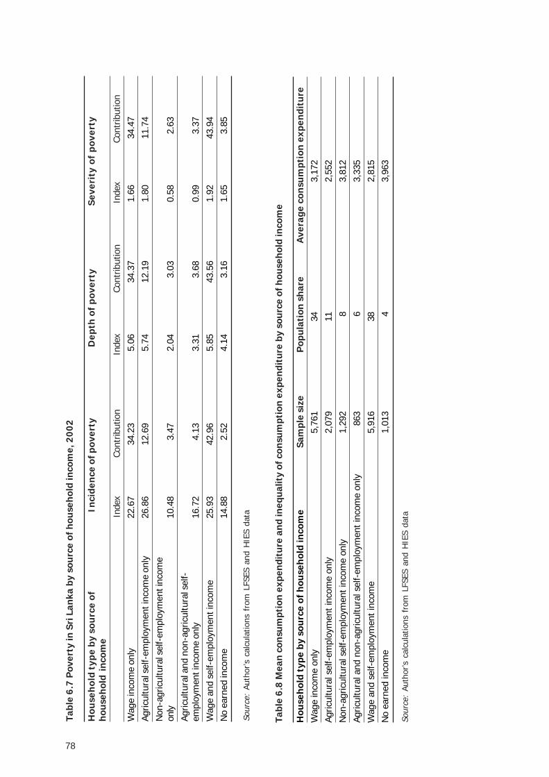
78

Tabl

e 6.

8 M

ean

cons

umpt

ion

expe

ndit

ure

and

ineq

ualit

y of

con

sum

ptio

n ex

pend

itur

e by

sou

rce

of h

ouse

hold

inco

me

Sour

ce:

Auth

or’s

cal

cula

tions

fro

m L

FSES

and

HIE

S da

ta

Hou

seho

ld t

ype

by s

ourc

e of

hou

seho

ld in

com

eSa

mpl

e si

zeP

opul

atio

n sh

are

Ave

rage

con

sum

ptio

n ex

pend

itur

eW

age

inco

me

only

5,76

134

3,17

2Ag

ricul

tura

l sel

f-em

ploy

men

t inc

ome

only

2,07

911

2,55

2N

on-a

gric

ultu

ral s

elf-

empl

oym

ent i

ncom

e on

ly1,

292

83,

812

Agric

ultu

ral a

nd n

on-a

gric

ultu

ral s

elf-

empl

oym

ent i

ncom

e on

ly86

36

3,33

5W

age

and

self-

empl

oym

ent i

ncom

e5,

916

382,

815

No

earn

ed in

com

e1,

013

43,

963

Tabl

e 6.

7 P

over

ty in

Sri

Lan

ka b

y so

urce

of h

ouse

hold

inco

me,

200

2

Hou

seh

old

type

by

sou

rce

ofIn

cide

nce

of p

over

tyD

epth

of

pove

rty

Sev

erit

y of

pov

erty

hous

ehol

d in

com

eIn

dex

Cont

ribut

ion

Inde

xCo

ntrib

utio

nIn

dex

Cont

ribut

ion

Wag

e in

com

e on

ly22

.67

34.2

35.

0634

.37

1.66

34.4

7Ag

ricul

tura

l sel

f-em

ploy

men

t inc

ome

only

26.8

612

.69

5.74

12.1

91.

8011

.74

Non

-agr

icul

tura

l sel

f-em

ploy

men

t inc

ome

only

10.4

83.

472.

043.

030.

582.

63Ag

ricul

tura

l and

non

-agr

icul

tura

l sel

f-em

ploy

men

t inc

ome

only

16.7

24.

133.

313.

680.

993.

37W

age

and

self-

empl

oym

ent i

ncom

e25

.93

42.9

65.

8543

.56

1.92

43.9

4N

o ea

rned

inco

me

14.8

82.

524.

143.

161.

653.

85

Sour

ce:

Auth

or’s

cal

cula

tions

fro

m L

FSES

and

HIE

S da

ta

79

Figu

re 6

.4: P

over

ty b

y in

com

e ca

tego

ry, 1

985-

2002

Sour

ce:

Auth

or’s

cal

cula

tions

fro

m L

FSES

and

HIE

S da

ta

80

Table 6.9: Poverty by income category

Income Category Poverty measure 1985 1990 1995 2002

Wages only Headcount Index 35.36 22.31 29.27 22.67Poverty Gap 9.66 5.04 6.68 5.06Squared Poverty Gap 3.7 1.71 2.27 1.66

Agricultural self-employment only Headcount Index 33.9 18.03 29.53 26.86Poverty Gap 8.4 3.52 6.71 5.74Squared Poverty Gap 3.14 1.05 2.17 1.8

Non agricultural self-employment only Headcount Index 24.84 16.99 16.99 10.48Poverty Gap 6 3.68 3.83 2.04Squared Poverty Gap 2.28 1.22 1.34 0.58

Both agric and non-agric self-employment Headcount Index 32.74 14.94 25.8 16.72Poverty Gap 8.33 2.68 5.26 3.31Squared Poverty Gap 3.12 0.78 1.61 0.99

Wages and self-employment Headcount Index 39.11 23.44 32.41 25.93Poverty Gap 10.33 4.83 7.39 5.85Squared Poverty Gap 3.87 1.49 2.51 1.92

Non-labour income Headcount Index 28 17.28 20.66 14.88Poverty Gap 7.39 4.25 5.5 4.14Squared Poverty Gap 2.85 1.68 2.11 1.65


Poverty incidence by income category for all four periods is shown in Figure 6.4 which illustratesthe numbers in Table 6.9. In each year, the incidence of poverty has been highest amonghouseholds whose income is a combination of wage and self-employment income. The secondhighest incidence of poverty in the first two periods is among households with only wageincome, but in the third and last periods it is among households with only agricultural self-employment. Households engaged only in non-agricultural self-employment had the lowestincidence of poverty (except in 1990-1, when the incidence among households with bothagricultural and non-agricultural self-employment income was lowest) which has been decliningsteadily over time. The smallest decline in poverty incidence in 2002 from 1995-6 levels wasalso observed among households with only agricultural self-employment incomes.

Table 6.10 and Figure 6.5 illustrate the contribution to poverty by income group. That theshare of households with only wage income has steadily risen over the period while the shareof households with wage and self-employment income has steadily declined is clearly illustratedin Figure 6.5. These trends are similar for the contribution to poverty of the poverty gap andthe squared poverty gap as well.

81

Figure 6.5: Contribution to poverty by income group

Headcount

(a)

Poverty Gap

(b)

82

Table 6.10: Contribution to Poverty by Income Category

Income Category Poverty measure 1985 1990 1995 2002

Wages only Headcount Index 21.93 28.58 29.41 34.23Poverty Gap 22.79 30.71 29.51 34.37Squared Poverty Gap 23.2 32.5 29.68 34.47

Agricultural self-employment only Headcount Index 12.07 11.35 12.04 12.69Poverty Gap 11.38 10.53 12.02 12.19Squared Poverty Gap 11.29 9.85 11.53 11.74

Non agricultural self-employment only Headcount Index 2.79 4.23 3.38 3.47Poverty Gap 2.56 4.36 3.34 3.03Squared Poverty Gap 2.58 4.52 3.47 2.63

Both agric and non-agric self-employment Headcount Index 6.22 5.19 5.08 4.13Poverty Gap 6.03 4.42 4.55 3.68Squared Poverty Gap 5.98 4.02 4.13 3.37

Wages and self-employment Headcount Index 55.17 48.47 47.77 42.96Poverty Gap 55.42 47.42 47.86 43.56Squared Poverty Gap 55.09 45.96 48.12 43.94

Figure 6.5: Contribution to poverty by income group (Contd.)

Squared Poverty Gap

(c)Source: Author’s calculations from LFSES and HIES data

83


6.3 Distribution of transfer income

In this section, the distribution of particular types of public and private transfers amonghouseholds ranked into deciles by per capita consumption is examined in greater detail. Thefirst two income sources are public transfers - welfare benefit payments and disability andrelief payments - while the third, a form of private transfers, is overseas remittances.

6.3.1 Distribution of disability and relief payments

In household surveys prior to 2002, disability and relief payments were nested in a largercategory together with pensions, making a separate analysis of these payments impossible.However, in HIES 2002 information started to be recorded separately on the amount receivedas disability or relief payment. Thus, it is not possible to compare changes in disabilitypayments with previous years for this reason. Nevertheless, the information from HIES 2002proves to be instructive and worth presenting.

A large percentage (91%) of transfer payments to households made by the Social WelfareMinistry (SWM) in 2002 were disability payments to disabled soldiers or social security tofamilies of soldiers who lost their lives while in service. The latter payments continue until theyear of retirement of the soldier who lost his/her life (CEPA 2004). Flood and drought reliefpayments in 2002 were approximately 7% of SWM transfers to households.33

Whether the ‘disability and relief payments’ referred to in the HIES questionnaire schedulereflect only relief payments or whether they include payments to disabled soldiers and/orsocial security to families of soldiers who have lost their lives is not known. Table 6.2 indicatesthat 2.65% of all households outside the North and East received these payments.

What is evident from Figure 6.6 is that the distribution of disability and relief payments is ingeneral progressive, with the average of 3% of households being distributed from 6% ofhouseholds in the lowest decile to less than 2% among the top four deciles.

If these payments were mainly (disaster) relief payments, and if the distribution of paymentswere an indication of the distribution of households affected by disasters, this would indicatethat poorer households were more vulnerable than richer households.34

On the other hand, if the distribution of disability and relief payments were more a reflection of thedistribution of payments to soldiers or their families, Figure 6.6 could be taken as evidence thatemployment in the armed forces is greater among poorer households. This would provide somesupport for the argument that recruitment into the armed forces has a poverty reducing effect.

33 Data from CEPA 2004.34 Note that this conclusion is at best indicative, depending as it does on two conditions about which there

is no information available.

Table 6.10: Contribution to Poverty by Income Category (Contd.)

Non-labour income Headcount Index 1.81 2.18 2.31 2.52Poverty Gap 1.82 2.55 2.7 3.16Squared Poverty Gap 1.86 3.15 3.07 3.85

84

Figure 6.6: Distribution of disability and relief payments, 2002


Table 6.11 Distribution of disability and relief payments

Decile Lowest 2 3 4 5 6 7 8 9 HighestPercentage 5.97 4.17 3.83 4.12 2.59 3.07 1.56 1.23 1.00 0.76


6.3.2 Distribution of welfare benefits

In this section, the distribution of welfare benefits is examined over the 1985 to 2002 period.The benefit is mainly in terms of the value of food stamps, while the related programme haschanged over the period, from Janasaviya in 1985-6 and 1990-91 to Samurdhi after 1995.

In 2002, the percentage of households that receive welfare benefit (food stamps) paymentsis highest (31 percent) in the rural sector, reflecting the high proportion of rural poor, followedby the urban (10 percent) and estate (7 percent) sectors (Table 6.2). As noted already,Table 6.3 indicates that only 53% of poor households receive welfare benefits, implying that47% of them do not, while 21% of non-poor households do receive these benefits, indicatinga problem of mis-targeting of both type I and type II errors.

Figure 6.7 graphs the percentage of households receiving benefits, and the income share ofbenefits, against deciles of population (ranked by per capita consumption). The graphs clearlyindicate that the distribution of welfare benefits is progressive, with a higher coverage ofbenefits to the lower part of the distribution and a lower coverage of the upper part of thedistribution.35

35 Government spending in 1995 on Janasaviya and Samurdhi were Rs.2.8 billion and Rs.2.33 billion respec-tively. Government spending on food stamps was a little over a billion rupees, and on kerosene, Rs.437million, and Rs.34 million on infant milk food subsidy (Gunatilaka et al. 1997). The estimated allocation forSamurdhi relief and infant milk subsidy was Rs.12 billion (CEPA 2004).

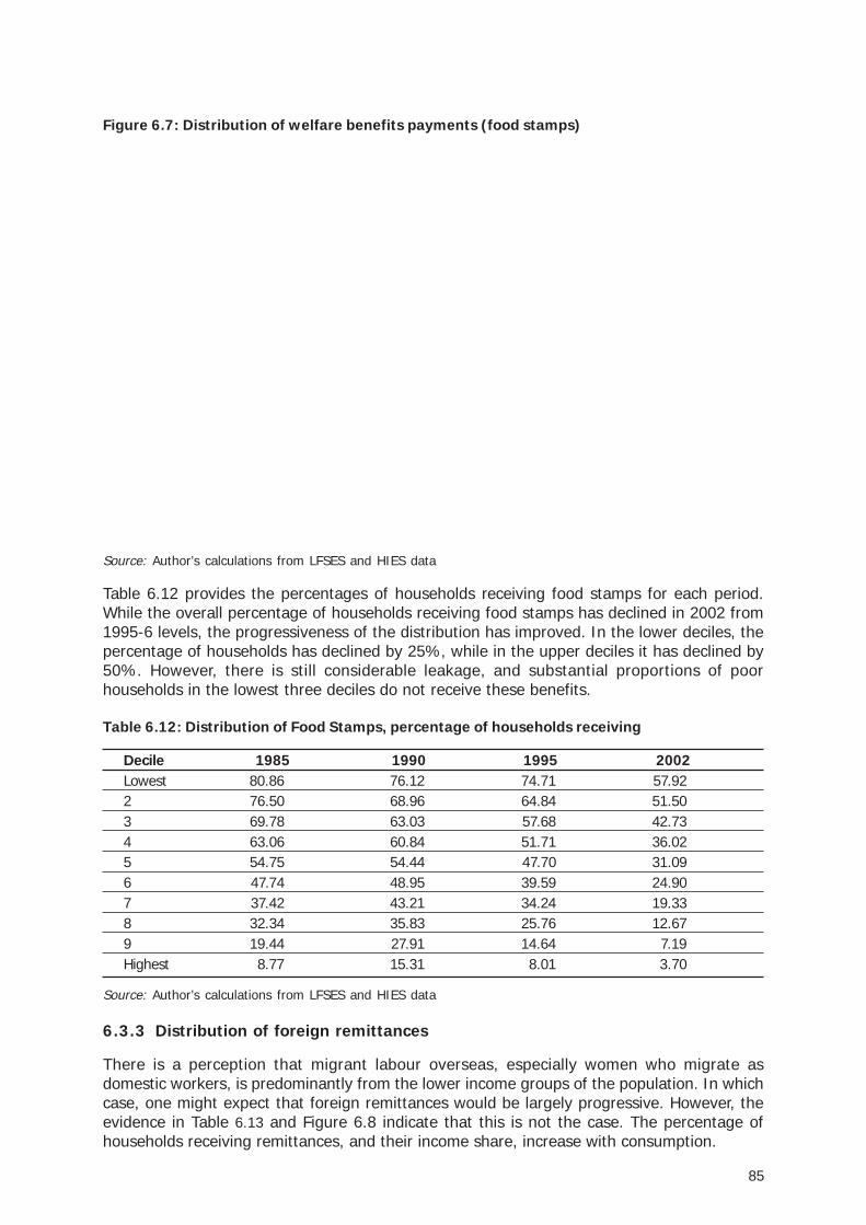
85

Table 6.12: Distribution of Food Stamps, percentage of households receiving

Decile 1985 1990 1995 2002Lowest 80.86 76.12 74.71 57.922 76.50 68.96 64.84 51.503 69.78 63.03 57.68 42.734 63.06 60.84 51.71 36.025 54.75 54.44 47.70 31.096 47.74 48.95 39.59 24.907 37.42 43.21 34.24 19.338 32.34 35.83 25.76 12.679 19.44 27.91 14.64 7.19Highest 8.77 15.31 8.01 3.70

6.3.3 Distribution of foreign remittances

There is a perception that migrant labour overseas, especially women who migrate asdomestic workers, is predominantly from the lower income groups of the population. In whichcase, one might expect that foreign remittances would be largely progressive. However, theevidence in Table 6.13 and Figure 6.8 indicate that this is not the case. The percentage ofhouseholds receiving remittances, and their income share, increase with consumption.

Figure 6.7: Distribution of welfare benefits payments (food stamps)


Table 6.12 provides the percentages of households receiving food stamps for each period.While the overall percentage of households receiving food stamps has declined in 2002 from1995-6 levels, the progressiveness of the distribution has improved. In the lower deciles, thepercentage of households has declined by 25%, while in the upper deciles it has declined by50%. However, there is still considerable leakage, and substantial proportions of poorhouseholds in the lowest three deciles do not receive these benefits.


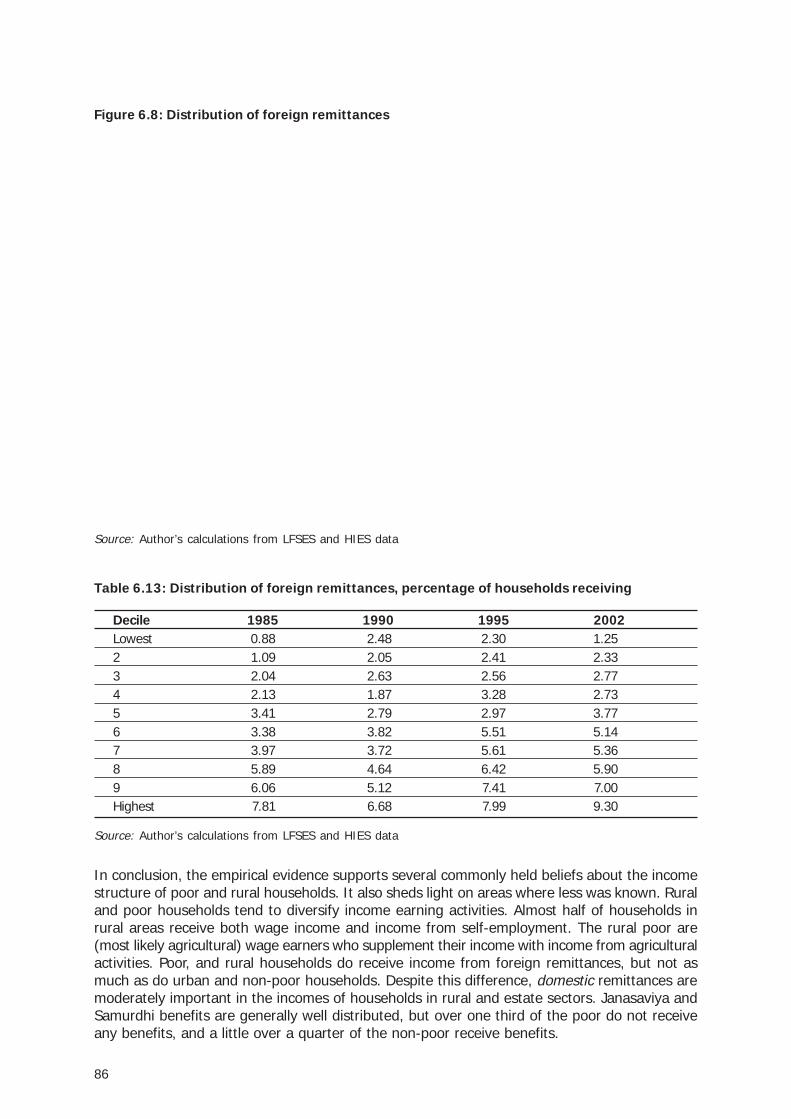
86

Figure 6.8: Distribution of foreign remittances


Table 6.13: Distribution of foreign remittances, percentage of households receiving

Decile 1985 1990 1995 2002Lowest 0.88 2.48 2.30 1.252 1.09 2.05 2.41 2.333 2.04 2.63 2.56 2.774 2.13 1.87 3.28 2.735 3.41 2.79 2.97 3.776 3.38 3.82 5.51 5.147 3.97 3.72 5.61 5.368 5.89 4.64 6.42 5.909 6.06 5.12 7.41 7.00Highest 7.81 6.68 7.99 9.30


In conclusion, the empirical evidence supports several commonly held beliefs about the incomestructure of poor and rural households. It also sheds light on areas where less was known. Ruraland poor households tend to diversify income earning activities. Almost half of households inrural areas receive both wage income and income from self-employment. The rural poor are(most likely agricultural) wage earners who supplement their income with income from agriculturalactivities. Poor, and rural households do receive income from foreign remittances, but not asmuch as do urban and non-poor households. Despite this difference, domestic remittances aremoderately important in the incomes of households in rural and estate sectors. Janasaviya andSamurdhi benefits are generally well distributed, but over one third of the poor do not receiveany benefits, and a little over a quarter of the non-poor receive benefits.

87

Table 7.1 Absolute and relative poverty lines and median consumption, 1985-2002 (atcurrent prices in SL Rs.)

Poverty lines/consumption 1985-86 1990-91 1995-96 2002Absolute 261 475 833 1423Median consumption 313 682 1081 2155Absolute as a% of median 83.4 69.6 77.0 66.0RELATIVE1 (66%) 207 451 714 1423RELATIVE2 (75%) 450 512 811 1616Ratio of A/R1 1.26 1.05 1.17 1


7. The Official Poverty Line as a Relative Poverty Line

The official poverty line derived for Sri Lanka is an absolute poverty line, derived using the costof basic needs method. However, it has recently been suggested that a relative notion ofpoverty is also important in Sri Lanka (Abeyratne and Tabor 2001). It is in this context thatthis study undertakes the following exercise to ’locate’ a relative poverty line for Sri Lanka.

Arguments in favour of a relative poverty line focus on the advantage that it automaticallyupdates for improvements in living standards in situations where living standards rise slowlyand steadily over time. Whether the latter situation exists in Sri Lanka is debatable.Nevertheless, an examination of consumption poverty using ’simulations’ of relative povertylines is likely to be instructive.

In practice, a ’good’ relative poverty line is not simply a fixed proportion of the population (i.e.the cut-off at the poorest 40%), rather it is a fixed proportion of a measure of centraltendency, such as the mean or median. Two examples are those formerly and currently usedby the European Union. The previous poverty line used half of mean adjusted income, butthis was abandoned in favour of 60% of median adjusted income in 2002.36

A good place to start determining a relative poverty line for Sri Lanka is the official (absolute)poverty line. This is converted to a ’relative’ poverty line, by calculating, for example, themedian consumption level (50% of the population consume below this amount) for thepopulation in 2002 using the HIES data and calculating what fraction of this is the officialpoverty line.37 Median consumption expenditure for 2002 was Rs.2,154.71. The officialpoverty line at Rs.1,423 is 66% of the median.38 Relative poverty lines that are 66% of themedian in each respective year are then constructed for the years 1985/86-1990/91 (seeRELATIVE1, 4th row in Table 7.1 below).

36 The reason for this was that the median is less sensitive to changes in consumption, especially that of veryrich people. However, the problem with using a relative poverty line that is some fraction (<1) of themedian, in developing countries, where absolute poverty levels can and do fluctuate is that the upper limitof relative poverty by definition will never exceed 50%.

37 The measure that is used is population weighted consumption expenditure adjusted for differences inprices between districts.

38 1423/2154.71=0.66. Coincidentally, this is the same definition used by the World Bank to measure relativepoverty in Ghana (World Bank 1995b), the only instance that this author could find of a relative povertyline defined in this manner (as % of median) for a developing country.

88

These relative poverty lines (RELATIVE1) are lower than the absolute poverty lines for all 3years before 2002. This is not by design, but reflects the fact that living standards in 2002were an improvement over the previous years. In those years, the absolute poverty line (thelevel at which minimum basic needs are met) was higher than 66% of median income. Thesmallest difference between the two is observed in 1990/91 when absolute poverty levelswere the lowest (at 27%) and the largest difference in 1985/86 when they were highest (at36%). Thus, had a relative poverty line fixed at 66% of median consumption (the level of theofficial poverty line in 2002) been used to measure poverty prior to 2002, this would haveunderestimated poverty, as is shown below. Table 7.2 shows that every measure of povertyestimated using RELATIVE1 is lower than those based on the absolute poverty line.

Table 7.2: National FGT poverty measures, using absolute and relative poverty lines, 1985-2002

Poverty measures 1985-86 1990-91 1995-96 2002H PG PG2 H PG PG2 H PG PG2 H PG PG2

Absolute 36 10 4 21 4 1 29 7 2 23 5 2RELATIVE1 (66%) 20 5 1 18 4 1 19 4 1 23 5 2RELATIVE2 (75%) 29 7 2 26 6 2 27 6 2 31 8 3

Source: Author’s calculations from LFSES and HIES dataNote: H - Headcount Index, PG – Poverty Gap Index, PG2 – Squared Poverty Gap Index

Clearly, a poverty line higher than 66% of median income is needed, unless one can safelyassume that living standards are going to improve steadily beyond 2002 levels. An appropriatestep at this point would be to use a higher fraction of the median, say the average of thefractions indicated in the third row of Table 7.1 (Absolute as a % of the median). This is 74%.The definition of 75% of median consumption is used instead for convenience. Current valuesof poverty lines under this definition are given in the 5th row of Table 7.1 and results are givenin the last row of Table 7.2.

If we compare results for 1995/96, where the values of absolute and relative definitions of thepoverty lines are quite close, with the results for 2002, we see that with an absolute definitionof poverty, the measures of poverty have improved, but if one uses the relative definition,taking into account the overall improvement in living standards between these years, relativepoverty has increased.

These results are helpful in understanding the benefits and limitations of a relative definition ofpoverty. The benefit is that the relative poverty line, which by definition is not kept constant orabsolute, but is allowed to improve with rising living standards (and fall with falling livingstandards), prevents a country from getting too complacent about small improvements in itspoverty situation. In Sri Lanka, absolute poverty levels have declined between 1996 and2002, but using a relative poverty line close to the absolute value of the poverty line in 1996shows that relative poverty has actually increased. However, the limitations or disadvantagesof the relative poverty line are also immediately apparent when one considers that the relativedefinition of poverty underestimated poverty significantly in 1985/86.39 This underscores thenotion that for countries where absolute poverty is still largely prevalent, a relative poverty lineshould be used in conjunction with, and not instead of, an absolute poverty line.

39 See also footnote 36

89

8. Summary and Conclusion

This analysis of the most recent Household Survey data shows that poverty in Sri Lanka hasdeclined over the last 20 years, but the decline has neither been large, nor steady. In fact, arelative definition of poverty based on a value close to the absolute value of the poverty line in1995/96 would indicate that poverty has risen. The sustained decline in poverty was largely inurban areas, particularly in the relatively affluent Western province. Within this province too, acontinuous decline in poverty was observed only in the Colombo district.

Poverty in rural and estate areas fluctuated over this period, with 1990-91 showing the mostconvergence among poverty levels in provinces and districts. Despite some fluctuation overthe period, the relative regional distribution of poverty at the end of the 17 year periodappears to have changed little from its initial picture; the Western province has the lowest levelof poverty, the next cluster of provinces with moderate poverty comprises the Central, NorthCentral and North Western provinces, and the highest poverty was observed in the Southern,Sabaragamuwa and Uva provinces. However, during this period, striking reductions in povertywere observed in the North Central province and Southern province.

The study showed that trends in absolute numbers or contribution to poverty moved parallelto trends in incidence, with the situation in the least poor province (Western) improving, andthe situation in the poorest province (Uva), deteriorating. At the beginning of the period, onein five persons in the former, and one in ten persons in the latter, was poor. By the end of theperiod, these numbers had converged with a 15% contribution to poverty by the morepopulous Western province, and a 12% contribution to poverty by the sparsely populatedUva province.

Similarly, trends in poverty and contribution to poverty moved parallel among all threemeasures of poverty, except in the estate areas where there is less inequality below thepoverty line. Thus, the depth and severity of poverty are generally greatest where theincidence of poverty is highest.

Decompositions of poverty changes highlighted the importance of both growth andredistribution, depending on the period under consideration. Decompositions at thedisaggregated level indicated that adverse redistribution, especially in the last period, was notsimply between districts, but also occurred within districts. Adverse redistribution and lowconsumption growth led to increases in the depth and severity of poverty, indicating that theinequality experienced in the last period was not limited to the upper part of the distribution buthad an effect on the poor.

Simulation exercises with different growth rates indicated the potential of growth to reducepoverty reduction. However, the high inequality experienced in the last period (1995/96-2002)indicated that the predictive power of these simulations is limited in the face of changingdistribution, especially around and below the poverty line.

Occupational and income profiles of the poor indicated that poverty was associated morestrongly with households whose head was engaged in agriculture, and least associated withhouseholds with only non-agricultural sources of income. Trends in poverty over the 17 yearperiod indicate that the least decline in poverty was experienced by households with onlyagricultural income or a combination of agricultural and wage income.

The situation of female headed households, and households headed by those with low ormoderate educational attainment has also worsened over the period, while poverty ratesdisaggregated by ethnicity and race have not changed very much. The latter may be due tothe fact that the analysis is restricted to the seven districts outside the North Easternprovince.

90

A ‘quick and dirty’ simulation exercise with relative poverty lines suggests that an appropriaterelative poverty line for Sri Lanka is that of 75% of median income. This is close to the valueof the absolute poverty line in 1995/96. The exercise also demonstrated that relative povertylines will always overstate the extent of poverty (relative to absolute poverty) during periodsof rising (overall) living standards and will always understate the extent of poverty duringperiods of falling living standards. Thus, they should be used in conjunction with, rather thaninstead of, absolute poverty lines.

While the lesson from the regional patterns in poverty reduction appears to be that economicgrowth is essential for poverty to decline (as in the Western province), this growth will need tooccur in the outlying provinces and in the agricultural sector in order for it to have an impact onpoverty. Alternatively, sufficient alternatives away from agriculture need to be developed inorder to enable the vast majority of the rural poor to escape poverty, especially in periods oflow growth. Analysis of the distribution of welfare benefits, disability and relief payments andremittances indicated that the role of transfers - and by inference, of public and privateredistribution mechanisms - in reducing poverty is limited.

91

References

ABEYRATNE, S., TABOR, S., 2001. Poverty Reduction in Sri Lanka: Maximising the AsianDevelopment Bank’s Contribution, Colombo. March.

CENTRAL BANK OF SRI LANKA, 2005. Consumer Finances and Socio-Economic Survey 2003/04. Colombo. July.

CEPA, 2004. Sri Lanka Public Expenditure Review: Social welfare sector policy note. Unpublishedmimeograph. World Bank Group, Sri Lanka: Colombo.

DATT, G., GUNEWARDENA, D.,1997. Some Aspects of Poverty in Sri Lanka, WashingtonD.C.: World Bank. (Policy Research Working Paper No. 1790)

DEATON, A., 1997. The Analysis of Household Surveys. Baltimore: Johns Hopkins UniversityPress.

DEATON, A. and PAXSON, C., 1998. Economies of scale, household size and the demand forfood. Journal of Political Economy, vol. 106 (October), pages 897-930.

DEPARTMENT OF CENSUS AND STATISTICS, 2004a. Announcement of the Official PovertyLine [online]. Department of Census and Statistics: Colombo. June. Available from:www.statistics.gov.lk.

DEPARTMENT OF CENSUS AND STATISTICS, 2004b. Poverty Statistics [online]. Departmentof Census and Statistics: Colombo. Available from: www.statistics.gov.lk

DEPARTMENT OF CENSUS AND STATISTICS, 2005a. Selected Millenium Development Goals(MDGs) Indicators [online]. Department of Census and Statistics. Colombo. Available from:www.statistics.gov.lk

DEPARTMENT OF CENSUS AND STATISTICS, 2005A. Poverty Maps [online]. Department ofCensus and Statistics. Colombo. Available from: www.statistics.gov.lk

DEPARTMENT OF CENSUS AND STATISTICS, 2006. Poverty in Sri Lanka: Issues and Options[online]. Department of Census and Statistics. Colombo. Available from: www.statistics.gov.lk

GUNATILAKA, R., et.al. 1997. The Samurdhi Programme: A Preliminary Evaluation, Instituteof Policy Studies, Colombo, Sri Lanka

GUNEWARDENA, D. 2000. Consumption poverty in Sri Lanka, 1985-1996. Paper written forthe Policy Framework for Poverty Alleviation in Sri Lanka, Colombo.

GUNEWARDENA, D. 2005. Improving Poverty Measurement in Sri Lanka. Centre for PovertyAnalysis Working Paper Series 9-2005. Centre for Poverty Analysis. Colombo.

LANJOUW, P., RAVALLION, M.,1995. Poverty and household size. Economic Journal, 105(November), pp. 1415-1434.

RAVALLION, M.,1994. Poverty Comparisons. Fundamentals of pure and applied economics,(56). Chur, Switzerland: Harwood Academic Press.

RAVALLION, M., BIDANI, B., 1994. How robust is a poverty profile. World Bank EconomicReview, 8(1), pp. 75-102.

WORLD BANK, 1995. Sri Lanka Poverty Assessment. Washington, D.C.: World Bank.

WORLD BANK, 2002. Sri Lanka Poverty Assessment. Washington, D.C.: World Bank.

WORLD BANK, 2007. Sri Lanka Poverty Assessment. Colombo: World Bank.

https://www.researchgate.net/publication/5217794_How_Robust_Is_a_Poverty_Profile?el=1_x_8&enrichId=rgreq-bbc322498cc0814de57b3d8eecb9967a-XXX&enrichSource=Y292ZXJQYWdlOzI1NzAyODc1NjtBUzoxMDUwNDk0MDEzMzE3MTRAMTQwMjA1NzEzNzY5OQ==

https://www.researchgate.net/publication/5217794_How_Robust_Is_a_Poverty_Profile?el=1_x_8&enrichId=rgreq-bbc322498cc0814de57b3d8eecb9967a-XXX&enrichSource=Y292ZXJQYWdlOzI1NzAyODc1NjtBUzoxMDUwNDk0MDEzMzE3MTRAMTQwMjA1NzEzNzY5OQ==

Consumption Poverty in Sri Lanka 1985-2002

Documents

Transcript of Consumption Poverty in Sri Lanka 1985-2002