Construction of Physical Maps FromOligonucleotide Fingerprints Data�Guy Mayraz y Ron Shamir zAugust 10, 1998AbstractA new algorithm for the construction of physical maps from hy-bridization �ngerprints of short oligonucleotide probes has been de-veloped. Extensive simulations in high-noise scenarios show that thealgorithm produces an essentially completely correct map in over 95%of trials. Tests for the in uence of speci�c experimental parametersdemonstrate that the algorithm is robust to both false positive andfalse negative experimental errors. The algorithm was also tested insimulations using real DNA sequences of C. Elegans, E. Coli, S. Cere-visiae and H. Sapiens. To overcome the non-randomness of probefrequencies in these sequences, probes were preselected based on se-quence statistics and a screening process of the hybridization data wasdeveloped. With these modi�cations, the algorithm produced very en-couraging results.�This research was supported in part by grants from the G.I.F., the German-IsraeliFoundation for Scienti�c Research and Development, and from the Ministry of Scienceand Technology, Israel.yDepartment of Computer Science, Sackler Faculty of Exact Sciences, Tel-Aviv Uni-versity, Tel-Aviv 69978 ISRAEL. gmz@math.tau.ac.ilzDepartment of Computer Science, Sackler Faculty of Exact Sciences,Tel-Aviv University, Tel-Aviv 69978 ISRAEL. shamir@math.tau.ac.il URL:http://www.math.tau.ac.il/�shamir Parts of this work were performed while thisauthor was on sabbatical at the Department of Computer Science and Engineering,University of Washington, Seattle.

1 IntroductionPhysical mapping is the process of determining the relative position of land-marks along a genome section. The resulting maps are used as a basisfor DNA sequencing, and for the isolation and characterization of individ-ual genes or other DNA regions of interest (e.g., transcripts and regulatorysequences)[11]. The construction of a high-resolution sequence-ready physi-cal maps for human and other organisms is still one of the top priorities ofthe Human Genome Project. The mapping process involves the productionof clones, i.e., cloned pieces of DNA, each representing a chromosomal seg-ment. The mapping itself is the reconstruction of the order of and physicaldistance between the clones. Refer to Figure 1 for an illustration of thephysical mapping problem, and for de�nitions of some basic terminology.Physical mapping using hybridization �ngerprints of short oligonucleo-tides was �rst suggested by Poustka et al. [13] in 1986. In this techniqueshort labeled DNA sequences, or probes, attach, or hybridize, to positionsalong the target DNA matching their own DNA sequence. The probes arenon-unique, i.e., they occur at many points along the genome, and typicallyhybridize with 10%-50% of the clones. Overlapping clones can be identi�edby their similar �ngerprints. Refer to Figure 2 for an illustration of thishybridization scenario. Poustka et al. suggested this method in order toeliminate the need to process individual clones in the restriction digestiontechnique. They reported on preliminary computer simulations demonstrat-ing feasibility, and suggested the use of Bayesian statistics in data analysis.More detailed strategies were o�ered by Michiels et al. [10]. A likelihoodratio based on a detailed statistical model was used to make overlap deci-sions, and a discussion of experimental errors was also included. Craig etal. [3] used short oligonucleotides in the ordering of cosmid clones coveringthe Herpes Simplex Virus (HSV-I) genome. The clones were ordered manu-ally. As each probe occurred only once or twice along the short (140K basepairs) genome, this experiment is not representative of the general problem.Lehrach et al. [8] described an integrated approach to physical mapping,suggesting the advantages of using non-unique probes. Fu et al. [5] providedan analysis of the number of clones required to avoid gaps and the numberof probes needed with a simple construction method. Hoheisel et al. [6] usedshort probes as a check for the order of unique probes in a map of the �ssionyeast S. pombe. Cuticchia et al. [4] provided an ordering program, usingthe Hamming distance between consecutive clones as an objective functionfor simulated annealing. Its performance was demonstrated on the data ofthe HSV-I virus[3] (see note above). The problem received a detailed formal1

0100 0 100clone # inconstructed map clone position in genomeFigure 1: An example of a physical map. The short horizontal lines are theclones x coordinates corresponding to the position on the target genome.The y coordinates correspond to the clone order in the constructed map.Note that most points on the target genome are covered by many clones.The total length of the clones divided by the length of the genome is calledthe clone coverage (10 in this example). The location of the clones alongthe target genome is not directly known to the experimenters. Mappingdata (such as hybridization data) produced by the experiment is used toreconstruct the map. A list giving for every clone its estimated position onthe genome is a solution to the mapping problem. A list of clones coveringa continuous section of the genome together with their physical distances iscalled a contig. With su�cient coverage the whole map is usually one contig.Such a plot of clone order in the constructed map vs. real clone positionprovides a visual map quality measure. If the order of the clones in theconstructed map is completely correct then the left endpoints of clones in-crease as y increases. (or decreases, if the orders in the true and constructedmaps happen to be reversed, as in this example). Minor ordering errorsare seen as small deviations from the monotonicity, as in this �gure, andthe construction is still essentially correct. Very small errors, which do notchange the clone order, cannot be seen in the plot. A completely randomsolution will correspond to randomly placed clones, whereas a non-randomsolution containing several large errors will translate into several randomlyplaced broken contigs with an approximately correct intra-contig order. InSection 5.2 we de�ne a quantitative map quality characterization.2

Position along the target genome

Clo

ne o

rder

(to

be

reco

nstr

ucte

d)

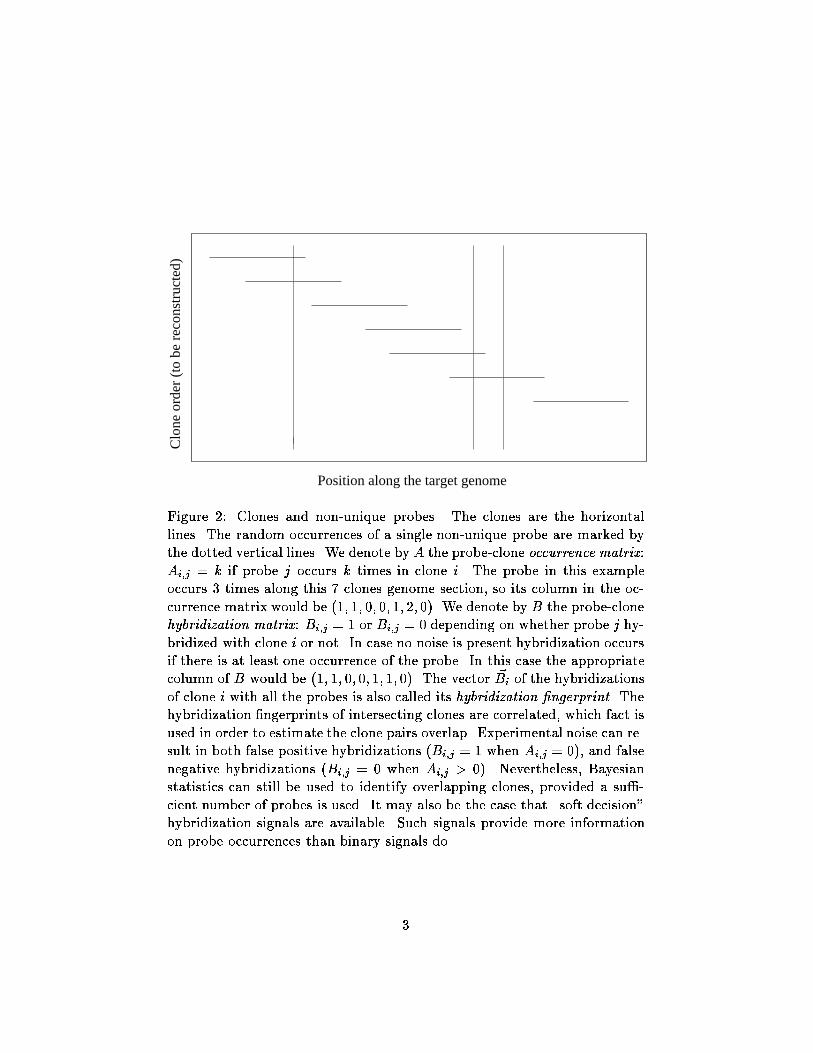
Figure 2: Clones and non-unique probes. The clones are the horizontallines. The random occurrences of a single non-unique probe are marked bythe dotted vertical lines. We denote by A the probe-clone occurrence matrix:Ai;j = k if probe j occurs k times in clone i. The probe in this exampleoccurs 3 times along this 7 clones genome section, so its column in the oc-currence matrix would be (1; 1; 0; 0; 1; 2; 0). We denote by B the probe-clonehybridization matrix: Bi;j = 1 or Bi;j = 0 depending on whether probe j hy-bridized with clone i or not. In case no noise is present hybridization occursif there is at least one occurrence of the probe. In this case the appropriatecolumn of B would be (1; 1; 0; 0; 1; 1; 0). The vector ~Bi of the hybridizationsof clone i with all the probes is also called its hybridization �ngerprint. Thehybridization �ngerprints of intersecting clones are correlated, which fact isused in order to estimate the clone pairs overlap. Experimental noise can re-sult in both false positive hybridizations (Bi;j = 1 when Ai;j = 0), and falsenegative hybridizations (Bi;j = 0 when Ai;j > 0). Nevertheless, Bayesianstatistics can still be used to identify overlapping clones, provided a su�-cient number of probes is used. It may also be the case that \soft decision"hybridization signals are available. Such signals provide more informationon probe occurrences than binary signals do.3

analysis by Alizadeh et al. [1]. Local improvement methods were used tosolve the problem in a noise free scenario.Physical mapping using non-unique probes shares with the popular map-ping techniques that use unique probes the much simpler handling require-ments, as well as the ability to analyze many clones in parallel. It alsoenjoys the insensitivity to repeat sequences of restriction digestion. Advan-tages over mapping with unique probes include: (1) Probe generation isstraightforward and much cheaper, (2) The number of required probes is in-dependent of the genome size[6], and (3) The information theoretic contentof each experiment is much higher: The overwhelming majority of uniqueprobe hybridizations to clones in a map are negative. (RH mapping [2] is analternative recent approach that set out to overcome the latter drawback.)This makes possible a very natural and e�cient probabilistic interpretationof the hybridization data, resulting in strong robustness to experimentalerrors.In this paper we suggest a practical algorithm for this problem. InSection 2 we suggest a statistical model for the problem. Perhaps the singlemost important idea in the paper is the Bayesian analysis of the overlaplength between contigs, based on the analysis of the overlap length betweentwo clones. Both are presented in Section 3. These overlap scores enable usto make much more e�cient use of the hybridization data than was possiblewith a binary yes/no overlap decision used before [13, 1, 10]. In Section 4we present the actual construction algorithm. Section 5 includes the resultsof simulations in a variety of experimental scenarios, including results onreal DNA sequences. To the best of our knowledge, this study gives the�rst quantitative performance analysis in noisy experimental scenarios. Wewere therefore unable to include direct comparison with other papers. In thediscussion section we take a close look at the inevitable simpli�cations madefor the purpose of the general simulations, and discuss what remains to bedone for a successful performance on real experimental data. An appendixgives the mathematical details of the overlap score.2 The statistical modelWe �rst describe the statistical model that underlies our algorithm and oursimulations. In the basic simulations we make the following assumptions:(1) Clones are uniformly and independently distributed along the targetgenome, (2) Clones are of equal length, (3) Probe occurrences along thegenome are modeled by a Poisson process with the same rate for all probes.4

The rate � is related to the probes' length plen by the formula � = 1=4plen.Probe occurrences on clones are then determined by the clone position.These assumptions originate in [10], where they are also discussed in depth.The same assumptions were later adopted by other researchers [1, 12]. As-sumptions (1) and (2) were also used in [7] in a general analysis of mappingscenarios, and were shown to produce clone distributions that mimic quiteaccurately real genomic clones.Noise is introduced into the model via false positive and false negativeerrors. False positives are modeled by an independent Poisson process withthe same rate on each clone. Each probe occurrence results in a hybridizationwith probability 1�� independently of other occurrences of the same probe.The parameter � is a measure of false negatives errors.We believe the �rst assumption and the noise modeling are in good agree-ment with real experiments. The second assumption is a reasonable approx-imation for cosmid clones, which are the most likely clones to be used inphysical mapping with oligonucleotides. There are nevertheless other inter-esting scenarios where larger clone length variability occurs. In Section 5.5we examine the e�ect of variable clone lengths. The third assumption is themost problematic. In Section 6 we focus on mapping simulated data based onreal genomic sequences of several organisms. We show that while the Poissonapproximation appears to be valid, the assumption that all probes appearwith the same Poisson rate does not hold for randomly chosen probes. Wepresent a solution to this problem based on judicious preselection of probes.With this improvement, our mapping algorithm obtains very good resultson real sequence data.Like any probabilistic model, ours is only a model, and as such does notfully re ect reality. In spite of the above caveats these assumptions havethe advantage of simplicity allowing both analytical and simulation aidedinvestigation. The insights gained from such an investigation shed invaluablelight on the more complicated experimental conditions of a real lab.3 The Bayesian overlap scoreContigs are ordered, contiguous clone sets. The aim of physical mappingis to create one correct contig out of all the input clones. We begin ouranalysis with a Bayesian score for the overlap length between clone pairs(Section 3.1), and then describe how we use it to estimate the overlap be-tween two contigs (Section 3.2). The construction algorithm which usesthese overlap scores to build the map is described in Section 4. A Bayesian5

overlap score for clones was suggested in several previous papers [1, 10, 13].Such a score lends itself to local improvement methods based on the clonespermutation. In these studies the score was only used to determine if twoclones do or do not overlap. In contrast, we compute a more detailed overlaplength estimate and contigs score, which make a better use of the �ngerprintinformation. An alternative approach suggested in [1] starts with a formaldiscussion of a global Bayesian score for complete maps, and proceeds withvarious ways of approximating it.3.1 Clone pairs overlap scoreThe next two subsections give the outline and key ideas of the overlap scores.A full description is given in the Appendix.Consider a pair of clones with an overlap section of length l . With asmall l it is quite likely for a probe to hybridize with one clone, but notwith the other. With a larger l the probe is more likely to hybridize withboth clones, or with neither. This observation can be made precise, givingfor every possible value of l its likelihood given the data. Combined witha priori overlap probabilities, Bayes Theorem makes it possible to calcu-late the probability that two clones overlap by a certain length given their�ngerprinting data.Because of e�ciency considerations, we make the simplifying assumptionthat l can only take few quantized values, in steps of 1=d of a clone'slength. With the aid of simple tables the complexity of calculating theoverlap probabilities vector for a pair of clones is O(n + d), where n is thenumber of probes. Typically, d � n (d = 10 was used in our simulations),and so the total complexity is linear in the number of probes.We �nally note that in the calculation of the overlap length likelihoodwe assume that only a yes/no hybridization signal is available to the con-struction algorithm. Finer hybridization strength distinctions can be usedto provide improved overlap probabilities estimates.3.2 Contig pairs overlap scoreExtending the exact overlap probability calculation to more than a fewclones is impractical due to the exponential growth in complexity as a func-tion of the number of clones. We seek instead to use the information fromclone pairs to �nd the relative placement between two contigs. This is doneby taking all clone pairs from the two contigs (one clone from each contig)as independent sources of information on the contigs' relative placement.6

This approach runs the risk of counting the same evidence multiple timesresulting in over sharp estimates. This problem is not severe, since the algo-rithm depends on a correct identi�cation of the maximum likelihood overlap,rather than on the precise shape of the distribution of likely overlap lengths.In practice, the approximation was found to produce good results.4 The construction algorithmSection 4.1 describes the basic algorithm. Several changes described in Sec-tion 4.2 were found to improve performance.4.1 The basic algorithm1. Initialize a contig set, so that for each clone there is a correspondingcontig consisting of that clone.2. Calculate for all the initial contig pairs and for the two possible relativeorientations their relative placement probabilities vector. The resultsare stored in a table.3. Find for all contig pairs and for their two possible relative orientationstheir best relative placement, and its probability.4. While more than one contig remains:(a) Find two contigs which have relative orientation and placementthat attain the highest probability.(b) Merge the two contigs.(c) Change the table calculated in step 2 to re ect the last merger.Suppose contig b was merged into contig a, then the table entriesfor all contig pairs (a; x) need to be changed. The required changeis a simple combination of the previous entries for (a; x) and for(b; x).(d) Find for contig pairs a�ected by the merger their new best relativeplacement.Assume that there are n probes andm clones of length d, and the genome haslength Ld. The bottleneck steps in the computation are steps 2 that takesO(m2(n+Ld)) time and Steps 4(c) and 4(d) that take O(mLd) time. Step 4is repeatedm�1 times, giving a total time complexity of O(m2(m+Ld+n)).7

4.2 Improvements to the basic algorithmWe brie y describe below several ideas that were found to improve the per-formance of the basic algorithm. These ideas were incorporated into the�nal version of the algorithm used in the simulations.4.2.1 Initial partition into groupsThe clone pairs score is used to divide the initial clone set into groups ofclones, such that in each group there is a clone that overlaps all the otherclones in its group with a near certain probability. Construction is done atthe group level before the ordered groups are combined. This process makesfor a signi�cant improvement in the average running time. More impor-tantly, the weighted information of many clone pairs is available when theordered groups are combined, thus helping avoid wrong mergers of distantclones with similar �ngerprints.4.2.2 Choosing the best overlapping relative placementIn every step of the basic algorithm the contig pair to be merged is theone with the highest a posteriori relative placement probability, thus mini-mizing the probability of making an error. In practice, however, errors areunavoidable, and some are far more costly than others. We therefore seek toavoid wrong mergers of non-overlapping contigs and other particularly largeerrors. One idea was to �rst identify the contig pairs that have the lowestprobability of no overlap, and among those to pick the pair that has thehighest relative overlap probability. Another idea was to apply a Gaussian�lter on the probabilities vector, with the result that unimodal distributionsare preferred over multi-peaked distributions, thereby decreasing the proba-bility of large errors. Both processes decrease the probability of large errorsat the cost of increasing that of smaller ones.4.2.3 Weak points detectionFor any clone pair (Ci; Cj) with an overlap oi;j and hybridization �ngerprints( ~Bi; ~Bj) de�ne its clone pair \energy" as Ei;j = � logPr( ~Bi; ~Bj joi;j). Thecontig energy E is de�ned as E =Pi<j Ei;j . In analogy to the breaking-upof a chemical molecule, the separation of a contig into two non-overlappingparts should increase the energy substantially. However, if the two partsdo not overlap in the real map, the separation energy should be quite smallor even negative. We de�ne weak points as points along the contig having8

separation energy below a threshold (determined experimentally). Such in-formation can be used by the laboratory in order to pinpoint areas whereadditional hybridizations should be performed. We also make use of theweak points in our algorithm to break-up a contig and to reassemble itagain. In case an error was made at an early stage, this process enablesthe algorithm to correct its previous error with the bene�t of the additionalinformation from other clones added at a later stage. A similar processwas reported in [12] to be slightly favorable, when only the clone order wassought.4.2.4 Simulated annealingSimulated annealing on the clones order was used before [4, 12] where itsperformance was validated on small data sets. The basic problem withthis approach is that the natural neighborhood relation must allow a moveand reversal of a contiguous group of clones. Thus, when there are manyclones, the number of neighbors becomes prohibitively large. In addition,this method ignores the signi�cant overlap between non consecutive clones.In order to overcome these problems we tried instead simulated annealingon the contig order after the intra-contig clone relative positioning is known.This method enjoys the fact that there are typically 10 clones in one contig(reducing the number of neighbors by a factor of 1000), and also, that thereis usually no overlap between non consecutive contigs. We implemented thismethod, but have found it to perform no better than the basic algorithm ofSection 4.1.5 Simulation resultsThis section describes the simulations we have performed with the algorithmwhen clone positions, �ngerprint data and errors were generated accordingto the statistical model described in Section 2.5.1 Simulation setupm clones of length lc were positioned randomly with a uniform distribu-tion along a genome of length L. The Poisson rate for probe occurrenceswas calculated from the probe length plen using the formula � = 1=4plen.Probe occurrences determined the probe-clone occurrence vector ~Ai for eachclone Ci (Ai;j = k i� probe j occurs k times on Ci). The probe hybridiza-tion probability was de�ned by p(hybi;j) = p(false positive) + (1 � p(false9

positive))(1� �Ai;j ), giving the expression p(hybi;j) = 1� e��lc�Ai;j . A bi-nary hybridization pattern ~Bi was therefore chosen randomly according tothe hybridization probabilities p(hybi;j).The simulation program receives the following as instance generationparameters: L, lc, n, �, plen, f:p:prob and the clone coverage. The numberof clones is m = coverage � L=lc. The false positives probability parameterf:p:prob is the probability of a false positive in a clone, and is related to �by the formula f:p:prob = 1� e��lc .The following combination of parameters was used as a base scenario:clone length lc = 40960 bp (base pairs), genome length L = 25 clone lengths(approximately 1M bp), coverage of 10, false negative probability � = 0:2,false positive probability f:p:prob = 0:05, probe length plen = 8, numberof probes n = 500. These parameters correspond to an experiment withcosmid clones, many probes and a realistic high noise. Other scenarios wereconstructed by changing one of the parameters from its value in the basescenario.5.2 Map accuracy measuresWe developed several measures for quantifying the accuracy of maps pro-duced by the algorithm. We report here on one measure that we have foundmost informative. It detects signi�cant errors between the constructed andthe correct map and ignores small di�erences that can be corrected by smallshifts or local reordering. Sub-contigs of the constructed map between signif-icant errors are essentially correct, but the relative order and orientation ofthese sub-contigs are incorrectly determined. We call such errors big errors.For example, the map in Figure 3(c) contains one big error. A descriptionof the calculation of big errors is included in the appendix. When no bigerrors are found the map is essentially correct. A variable any big is de�nedto be 1 or 0 depending on whether there are any big errors. Its average isused to estimate the probability of having at least one big error.5.3 Test examplesRefer to Figure 3 for a graphical illustration of the algorithm's results. Intypical runs in the standard scenario there are only only insigni�cant order-ing errors between nearby clones. Increasing the genome length does nothave a signi�cant e�ect on performance (See also Section 5.5.) The last twosub�gures illustrate what happens under very adverse conditions. The weakpoints detected by the algorithm (Section 4.2.3) enable the experimenter to10

0250 0 250(a) std. scenariopppppppppppppppppppppppppppppppppppppppppppppppppppppppppppppppppppppppppppppppppppppppppppppppppppppppppppppppppppppppppppppppppppppppppppppppppppppppppppppppppppppppppppppppppppppppppppppppppppppppppppppppppppppppppppppppppppppppppppppppppppppppppp 0500 0 500(b) 2MB genome lengthpppppppppppppppppppppppppppppppppppppppppppppppppppppppppppppppppppppppppppppppppppppppppppppppppppppppppppppppppppppppppppppppppppppppppppppppppppppppppppppppppppppppppppppppppppppppppppppppppppppppppppppppppppppppppppppppppppppppppppppppppppppppppppppppppppppppppppppppppppppppppppppppppppppppppppppppppppppppppppppppppppppppppppppppppppppppppppppppppppppppppppppppppppppppppppppppppppppppppppppppppppppppppppppppppppppppppppppppppppppppppppppppppppppppppppppppppppppppppppppppppppppppppppppppppppp0125 0 125(c) coverage = 5ppppppppppppppppppppppppppppppppppppppppppppppppppppppppppppppppppppppppppppppppppppppppppppppppppppppppppppppppppppppppppppp 0125 0 125(d) coverage = 5, high noisepppppppppppppppppppppppppppppppppppppppppppppppppppppppppppppppppppppppppppppppppppppppppppppppppppppppppppppppppppppppppppppFigure 3: True clone order (y axis) vs. constructed order (x axis) in fourscenarios. When applicable, weak points shown as vertical dotted lines. Theresults are taken from the following scenarios: (a) base scenario, (b) a long2M bp genome, (c) a simulation with very low coverage (5), (d) a simulationwith very low coverage (5) and very high noise (� = 0:3 and f:p:prob = 0:25).Note that all big errors were detected as weak points, though some weakpoints incorrectly predicted additional big errors.pinpoint possible errors. This information can be used for a judicious choiceof additional hybridization experiments, minimizing cost and human e�ort.5.4 Performance in the base scenario1000 separate experiments were performed in the base scenario (Section 5.1)in order to obtain accurate expectation and standard deviation values. In0:961 � 0:006 of the cases the algorithm made no big errors. Recall (Sec-tion 5.2) that the absence of big errors is a guarantee that the map is essen-tially correct, as every two clones that are consecutive in reality are placedby the algorithm within a clone length from each other.11

5.5 The e�ect of separate parametersThe e�ect of separate parameters was tested by altering one parameter,while keeping the other parameters at their value in the base scenario. 1000separate experiments were performed for each value, and the probability ofhaving big errors was estimated by the average of any big.The tested parameters (Section 5.1) were: 5 � L � 50 (in clone lengths)in steps of �L = 5, 7 � plen � 10 in steps of �plen = 1, 50 � n � 1000in steps of �n = 50 up to n = 200 and �n = 100 between 200 and 1000,0 � � � 0:8 in steps of �� = 0:1, 0 � f:p:prob � 0:5 in steps of �f:p:prob =0:05.The results in Figure 4 demonstrate robustness to experimental noise.Even with � = 0:6 the algorithm makes no big errors in the majority ofthe runs. The algorithm also copes well with relatively low coverage, butperformance deteriorates rapidly below coverage 7. The algorithm is mostsensitive to the frequency of probe occurrences, as it is mirrored in the probeslength. Sensitivity to the number of probes becomes pronounced with lessthan 200 probes. The results for large map sizes indicate that the algorithmis still robust in a genome of about 50 clone lengths (2M bp). We expectacceptable performance even with larger map sizes. In the discussion sectionwe comment on the implication of these results on the design of hybridizationexperiments.We also tested the in uence of variable clone lengths. Clones length werechosen from a uniform distribution, and the construction program estimatedthe lengths by the maximum likelihood length as a function of the totalnumber of hybridizations with the clone. The results in Figure 5 show arobustness to about 37% variability. Better performance can be expectedwith a Normal distribution of clone lengths, which is probably more realistic.5.6 Physical resourcesA PC with a 100Mhz Pentium Microprocessor and 32MB of memory (256Kcache) was used. The implementation was written using GNU C++, andrun under the LINUX Unix type operating system. An average run of theconstruction algorithm (excluding instance generation) took 10 seconds inthe base scenario and required 3MB of memory (memory requirements varysomewhat between runs, as the clones are divided into groups di�erently).12

00.050.10.15 10 20 30 40 50Genome Length (in clone lengths)r r r r r r r r r r 00.20.40.60.81 5 10 15 20Clone Coverager r r r r r r r r r r r r r r r r r r r00.20.40.60.81 0 0.2 0.4 0.6 0.8�r r r r r r r r r 00.10.20.30.40.50.6 0 0.1 0.2 0.3 0.4 0.5false positives prob.r r r r r r r r r r r00.20.40.60.81 250 500 750 1000probe num.r r r r r r r r r r r r 00.20.40.60.8 7 8 9 10probe lengthr r r rFigure 4: The in uence of the various simulation parameters on the proba-bility of having big errors (as estimated from the average of any big). Thevertical dotted line indicates the value of the parameter in the base scenario.Note that the e�ect of a decrease in the number of probes is very similar tothat of an increase in the experimental noise. This is because noise decreasesthe informational content of each probe, an e�ect that can be countered byan increase in the number of probes. It is also notable that the probe sizehas a very signi�cant e�ect, resulting from its direct in uence on the fre-quency of probe occurrences, and therefore on the informational content ofthe experiment. By contrast, the genome size has only a moderate e�ect onperformance. 13

00.10.20.3 0 10000 20000anybig r r r r r 200022002400260028003000 0 10000 20000avg.error 3 3 3 3 3Figure 5: The in uence of clone length variability. The x axis represents themaximal variability from the average clone sized length. Clone lengths wereuniformly distributed in this range. The graphs show good performancewith a variability of up to about 15000 bp, or 37.5%.6 Results on real DNA sequencesOur next step was to test the algorithm in simulations involving real DNAsequences. These sequences were taken from a variety of representativeorganisms: the nematode C. Elegans 1, bacterium (E. Coli)2, yeast3, andhuman4. The lengths of the sequences ranged from about 1.7MB to over4MB. Non overlapping sections of length 1MB from each genome were usedfor the tests (1MB and 730MB for Homo Sapiens). An additional randomDNA sequence was used for comparison.With the exception of probes �tting repetitive sequences, the occurrences1The C. Elegans data is from a Sanger Centre sequencing project. The �le we haveused is ftp://ftp.sanger.ac.uk/pub/databases/C.elegans sequences/FINISHED SEQUE-NCES/large C. elegans contig.2The E. Coli DNA was taken from the E. Coli Genome Project, University of Wis-consin Madison. The �le we have used is ftp://ftp.genetics.wisc.edu/pub/sequence/eco-lim52.fas.gz.3The yeast DNA we have used is chromosomes iv,vii, and xv taken from the Mu-nich Information Centre for Protein Sequences (MIPS) accessed through the web site athttp://www.mips.biochem.mpg.de/mips/programs/get fragment.html.4The human DNA was taken from two separate sources. Chromosome 7data was taken from the University of Washington Genome Center (UWGC) athttp://chimera.biotech.washington.edu/UWGC. The sequence itself, of length 1050106 bpis available through a link in the above web site into GenBank. Chromosome 17 data wastaken from the Whitehead Institute/MIT Genome Sequencing Project at http://www-seq.wi.mit.edu/sequencing/public release/human17.html. We have used the following�les: L106,L107,L108,L117,L118,L127. The chromosome 7 data was used as the mainsequence �le. The chromosome 17 DNA contigs were concatenated into one sequence andused as an additional DNA �le. 14

of most probes on the target genome appear to be uniformly distributed, thusgiving support to the Poisson model. However, the same rate assumptionalso predicts a Poisson distribution of the number of probe occurrences. AsFigure 6 demonstrates, this stronger assumption cannot be sustained.The obvious solution of �tting a separate Poisson model for each probewill not do, because most probes occur very infrequently, and will there-fore provide very little information. However, Figure 6 have led us to anencouraging observation: In all the distributions, a signi�cant fraction fallsunder the graph of the randomDNA, thereby demonstrating that there fairlymany \good" probes. Because probe hybridizations are e�ort and cost in-tensive it is impractical to make very many experiments and then choosea small subset of \good" probes. However, if probes can be chosen beforethe actual experiment based on prior knowledge of the organism's typicalsequences (e.g. from other sequenced parts of its genome), better results canbe achieved. We call this process probe pre-selection. Figure 7 demonstratesthat a fairly good �t with the same-rate model can be achieved.One important problem that cannot be seen clearly in Figure 7 is thatthe resulting distributions still have very long tails. These tails representprobes that either occur very rarely or very frequently, and thus hinder theperformance of the algorithm. To overcome this problem we implemented aprocedure that we call probe post-screening. It uses the hybridization datato screen out certain probes that deviate signi�cantly from the same-ratemodel. Only those probes which �t well the same-rate model are subse-quently used by the mapping algorithm. As hybridization data is obtainedafter probe pre-selection, most probes already conform with the model, andso there is little loss of usable hybridization information. The post-screeningprocess uses the number of actual probe occurrences in the hybridizationdata and the noise parameters. This technique works well when the noiseestimate is good. If no good noise estimates are available, one would prob-ably do better by computing a histogram of the number of hybridizations,and keeping only the probes in the central part of the histogram.One important problem that cannot be seen clearly in Figure 7 is thatthe resulting distributions still have very long tails. These tails representprobes, which either occur very rarely or else almost in all clones. In order toprevent such probes from hindering the algorithm's performance we success-fuly experimented with probe post-screening, namely maintaining only thoseprobes which �t well the same-rate model. Because of probe pre-screeningmost probes can be maintained with only a small loss of usable hybridizationinformation. The process is based on the number of probe occurrences andon the noise parameters. Of course, we only have the hybridization data to15

organism test type % maps with errorsRandom no post-screening 2:8� 0:7Random PS - 500 probes before 2:2� 0:7Random PS - 500 probes after 0:0� 0:0Bacterium no post-screening 60:6� 2:2Bacterium PS - 500 probes before 20:6� 1:8Bacterium PS - 500 probes after 10:8� 1:4Yeast no post-screening 20:4� 1:8Yeast PS - 500 probes before 4:0� 0:9Yeast PS - 500 probes after 1:2� 0:5C. Elegans no post-screening 34:6� 2:1C. Elegans PS - 500 probes before 7:4� 1:2C. Elegans PS - 500 probes after 0:0� 0:0Human no post-screening 88:2� 1:4Human PS - 500 probes before 12:6� 1:5Human PS - 500 probes after 0:0� 0:0Table 1: Results of the mapping algorithm with probe pre-selection on realsequence data. The three lines for each organism correspond to: (1) Nopost-screening, (2) Post-screening on the 500 original probes (leaving about300 screened probes), and (3) 500 post-screened probes (requiring more tobegin with). The screened probes were chosen out of a pre-selected sample ofprobes occurring within �10% of the mean on a di�erent genome section ofthe same organism. The post-screened probes are estimated to occur within10% of the mean frequency on the target genome section too. Averages andstandard deviations are based on 1000 simulations in each scenario. PS:post-screening.use, and so we compute the expected number of clone hybridizations as afunction of the number of occurrences along the genome, and use that whenscreening probes. The disadvantage of this technique is that it works onlywhen the noise estimate is good. If this is not the case, one would probablydo better by computing a histogram of the number of hybridizations, andthen maintain only the probes in the central part of the histogram.Table 1 shows the mapping results with probe pre-selection and withand without post-screening. The results clearly demonstrate the e�cacyof using probe post-screening. In fact, the algorithm works better withscreened probes even when the probes were Poisson distributed in the �rstplace. 16

0250050007500

0 10 20 30 40 50# of probes

# of probe occurrences"Bacterium""C.Elegans""Yeast""Human""Random"

Figure 6: Histogram of the number of 8-mer probe occurrences along agenome section of length 1MB. The number of occurrences for each possible8-mers was recorded, and the resulting histogram is displayed. Additionalsamples available in the Bacterium, Yeast and C. Elegans data produceessentially the same histograms as in this graph. Probe occurrences on realorganisms clearly deviates widely from the Poisson distribution exhibitedby the random DNA. An additional salient feature is the di�erence betweenthe human genome and that of other organisms.17

02500500075000 10 20 30

(a) Bacterium02500500075000 10 20 30

(b) Yeast02500500075000 10 20 30

(c) C.Elegans02500500075000 10 20 30

(d) HumanFigure 7: Histograms of the number of probe occurrences on a genome sec-tion of length 1MB, when using only probes with an average number ofoccurrences (between 0.9 and 1.1 of average) as estimated from a di�erentgenome section of length 1MB (730KB for human) of the same organism.The x-axis is the number of occurrences, and the y-axis is the number ofprobes with that many occurrences. Each �gure contains 8-mers sampleddirectly (heavily dotted line), and 8-mers chosen according to the distribu-tion of 4-mers (lightly dotted line). The latter is useful since the distributionof 4-mers can be assessed with greater precision. The �gures also containthe random distribution for reference (continuous line). The graphs demon-strate that this type of pre-selection process can improve substantially thedistribution of probe occurrences, but that further post-screening may benecessary to achieve a better �t with the same rate model. In particular thepre-selection leaves some probes which occur many times more often thanthe model predicts. There is only a small di�erence between assessing thedistribution of 8-mers directly and using the 4-mers distribution.18

7 Concluding remarksThe basic simulations demonstrate a robust performance in scenarios con-taining a large genome and highly noisy hybridizations. The algorithm isalso robust to considerably more clone length variability than is the case withcosmid clones. With clones of widely variable lengths some length screeningis likely to contribute signi�cantly to performance. The basic simulationsalso show the importance of using many probes. The manufacturing of manyprobes involves high initial costs, but the same probes can later be used forthe entire genome. The per-experiment costs are then much smaller thanan experiment using unique probes.A key issue emerging from the simulations is probe selection. The basicsimulations demonstrate how crucial it is to choose probes with approxi-mately 50% hybridizations. The simulations on real DNA show that ran-dom probes are a very poor choice with real DNA, but also show that byusing pre-selection based on known sequence statistics speci�c to the organ-ism, the algorithm could then apply post-screening and still have a su�cientnumber of probes to work well.Short hybridization techniques are challenged by the di�culty to predictthe strength of hybridization (and hence of the signal) between an oligo anda particular sequence: Factors such as GC content, mismatches and localfold structure in uence the actual signal. A very important observationis that accurate prediction is not really necessary for the success of thealgorithm. All that is required is that the hybridization strength betweenany probe and any point (a sequence segment) in the target will be consistentin all the clones that contain that point. The actual level of match betweenthe sequence of the oligo and the sequence at that point in the target isimmaterial. Any relation whatsoever can exist between the two sequences,provided that consistency is maintained. For example, a probe and a targetsometimes hybridize well even when only a partial complementary matchexists between them, but this is not a problem for the algorithm. This typeof consistent deviation from a simple hybridization model has to be clearlydi�erentiated from uncorrelated deviations of individual clone and probepairs. The latter deviations are the false positive and the false negativeerrors.The statistical inference approach to analyzing oligonucleotide hybridiza-tion data is not limited to physical mapping. In cDNA clustering, clone pairscan either fully overlap (one is contained in the other), or else come fromdi�erent genes and have zero overlap. A likelihood ratio of these two possi-bilities can be used as input to the clustering algorithm. Initial experiments19

that we have done [9] show that it may give substantially better results thanthe currently used Euclidean norm or Hamming distance.Another particularly promising �eld for applications is preselection ofclones for shotgun sequencing. The problem is to select as small a subset aspossible of clones covering the target genome, sequence only those �rst andthereby avoid re-sequencing the same target parts unnecessarily and savetime and cost in sequencing [14]. Relatively inexpensive oligonucleotides�ngerprinting is performed, and the resulting hybridization data can be usedto produce a physical map, from which a near optimal clone subset can bechosen. In this problem the clone lengths are typically of the order of 1200bp,and so 8mers are suboptimal as probes, as their occurrence probability is low.However, it has been suggested (Uwe Radelof - personal communication)that oligo pooling can be used, with a pool of several 8mers serving as oneprobe, thus making it possible to achieve around 50% hybridization.A �nal possible application is to restriction digest mapping. In thisproblem each clone is completely digested by a restriction enzyme and theinput data for mapping is a list of fragment lengths for each clone. Ouralgorithm can be applied also to this seemingly very di�erent type of data:On an abstract level, all the algorithm needs in order to work is features orlandmarks along the DNA, where the appearance or absence of each featureis consistent in all the clones containing the corresponding DNA segment.If restriction fragment lengths serve as the features, the algorithm can beapplied to restriction mapping too.20

References[1] F. Alizadeh, R. M. Karp, L. A. Newberg, and D. K. Weisser. Physi-cal mapping of chromosomes: A combinatorical problem in molecularbiology. Algorithmica, 13:52{76, 1995.[2] D.R. Cox, M. Burmeister, R. Price, S. Kim, and R.M. Myers. Radiationhybrid mapping: a somatic cell genetic method for reconstructing high-resolution maps of mammalian chromosomes. Science, 250:245{250,1990.[3] A. G. Craig, D. Nizetic, D. Hoheisel, G. Zehetner, and H. Lehrach. Or-dering of cosmid clones covering the herpes simplex virus type I (HSV-I)genome: A test case for �ngerprinting by hybridization. Nucleic AcidsResearch, 18:2653{2660, 1990.[4] A. Cutticchia, J. Arnold, and W. Timberlake. ODS: ordering DNAsequences - a physical mapping algorithmbased on simulated annealing.CABIOS, 9:215{219, 1993.[5] Y.-X. Fu, W. E. Timberlake, and J. Arnold. On the design of genomemapping experiments using short synthetic oligonucleotides. Biomet-rics, 48:337{359, 1992.[6] J.D. Hoheisel, E. Maier, R. Mott, L. McCarthy, A.V. Grigoriev, L.C.Schalkwyk, D. Nizetic, F. Francis, and H. Lehrach. High resolutioncosmid and P1 maps spanning the 14 Mb genome of the �ssion yeastS. pombe. Cell, 73:109{120, 1993.[7] E. S. Lander and M. S. Waterman. Genomic mapping by �ngerprintingrandom clones: A mathematical analysis. Genomics, 2:231{239, 1988.[8] H. Lehrach, R. Drmanac, J. Hoheisel, Z. Larin, G. Lennon, A. P.Monaco, D. Nizetic, G. Zehetner, and A. Poustka. Hybridization �n-gerprinting in genome mapping and sequencing. In K. E. Davies andS. Tilghman, editors, Genome analysis: genetic and physical mapping,pages 39{81. Cold Spring Harbor, New York, 1990.[9] G. Mayraz and R. Shamir. A bayesian score for cdna clustering. Techni-cal report, School of Mathematics, Tel-Aviv University, Tel-Aviv, Israel,1997. 21

[10] F. Michiels, A. G. Craig, G. Zehetner, G. P. Smith, and H. Lehrach.Molecular approaches to genome analysis: a strategy for the construc-tion of ordered overlapping clone libraries. CABIOS, 3(3):203{210,1987.[11] R.F. Mott, A.V. Grigoriev, E. Maier, J.D. Hoheisel, and H. Lehrach.Algorithms and software tools for ordering clone libraries: appplicationto the mapping of the genome of Schizosaccharomyces pombe. NucleicAcids Research, 21:1965{1974, 1993.[12] Darren M. Platt and Trevor I. Dix. Comparison of clone-ordering algo-rithms used in physical mapping. Genomics, 40:490{492, 1997.[13] A. Poustka, T. Pohl, D.P. Barlow, G. Zehetner, A. Craig, F. Michiels,E. Ehrich, A.M. Frischauf, and H. Lehrach. Molecular approaches tomammalian genetics. Cold Spring Harb Symp Quant Biol, 51:131{139,1986.[14] U. Radelof, S. Hennig, P. Seranski, F. Francis, A. Schmitt, J. Ramser,C. Ste�ens, A. Poustka, and H. Lehrach. Preselection of shotgun clonesfor sequencing by oligo�ngerprinting. In Proceedings of the HumanGenome Meeting (HGM '98), Turin, Italy, March 1998, page 52. Na-ture Genetics, 1998.22

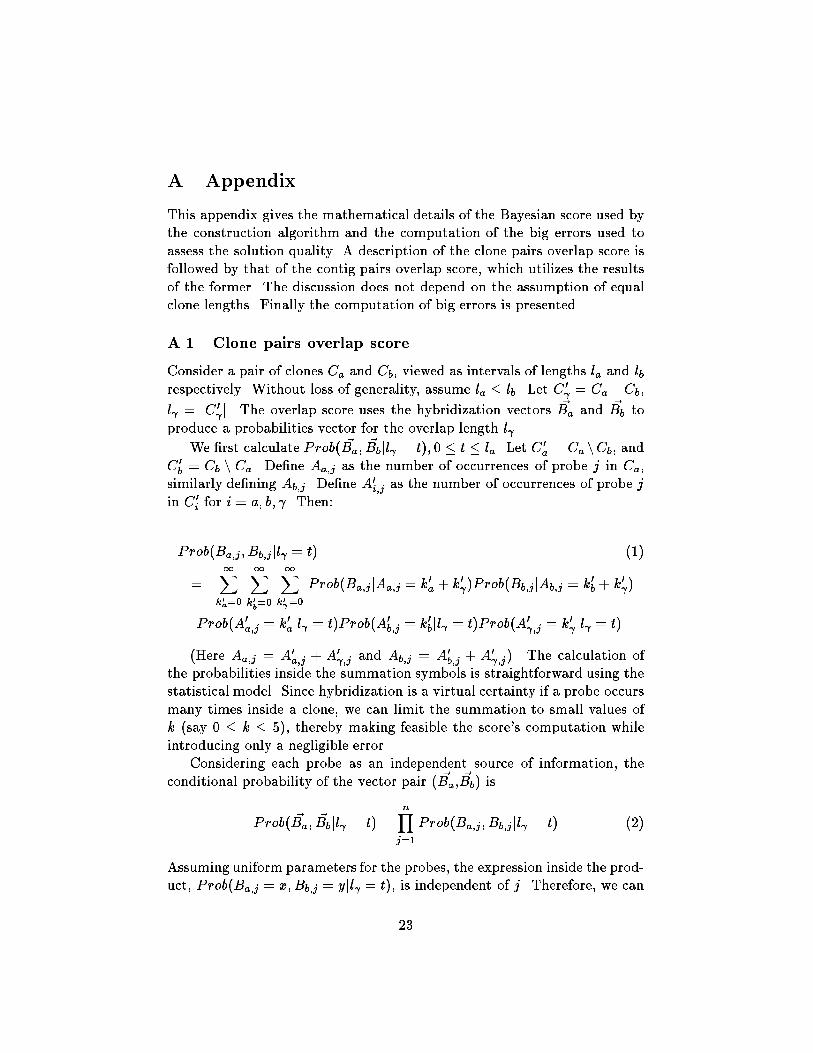
A AppendixThis appendix gives the mathematical details of the Bayesian score used bythe construction algorithm and the computation of the big errors used toassess the solution quality. A description of the clone pairs overlap score isfollowed by that of the contig pairs overlap score, which utilizes the resultsof the former. The discussion does not depend on the assumption of equalclone lengths. Finally the computation of big errors is presented.A.1 Clone pairs overlap scoreConsider a pair of clones Ca and Cb, viewed as intervals of lengths la and lbrespectively. Without loss of generality, assume la � lb. Let C 0 = Ca \ Cb,l = jC 0 j. The overlap score uses the hybridization vectors ~Ba and ~Bb toproduce a probabilities vector for the overlap length l .We �rst calculate Prob( ~Ba; ~Bbjl = t); 0 � t � la. Let C 0a = Ca nCb, andC0b = Cb n Ca. De�ne Aa;j as the number of occurrences of probe j in Ca,similarly de�ning Ab;j . De�ne A0i;j as the number of occurrences of probe jin C 0i for i = a; b; . Then:Prob(Ba;j ; Bb;j jl = t) (1)= 1Xk0a=0 1Xk0b=0 1Xk0 =0 Prob(Ba;j jAa;j = k0a + k0 )Prob(Bb;j jAb;j = k0b + k0 )Prob(A0a;j = k0ajl = t)Prob(A0b;j = k0bjl = t)Prob(A0 ;j = k0 jl = t)(Here Aa;j = A0a;j + A0 ;j and Ab;j = A0b;j + A0 ;j). The calculation ofthe probabilities inside the summation symbols is straightforward using thestatistical model. Since hybridization is a virtual certainty if a probe occursmany times inside a clone, we can limit the summation to small values ofk (say 0 � k � 5), thereby making feasible the score's computation whileintroducing only a negligible error.Considering each probe as an independent source of information, theconditional probability of the vector pair ( ~Ba, ~Bb) isProb( ~Ba; ~Bbjl = t) = nYj=1Prob(Ba;j ; Bb;j jl = t) (2)Assuming uniform parameters for the probes, the expression inside the prod-uct, Prob(Ba;j = x;Bb;j = yjl = t), is independent of j. Therefore, we can23

de�ne P tx;y for 0 � x; y � 1 by P tx;y = Prob(Ba;j = x;Bb;j = yjt). Denotingby Sx;y the set of probes 1 � j � n , such that Ba;j = x and Bb;j = y, wecan write: Prob( ~Ba; ~Bbjt) = 1Yx=0 1Yy=0 P tx;y jSx;y j (3)Having computed Prob( ~Ba; ~Bbjl = t) we can use Bayes Theorem:Prob(l = t0j ~Ba; ~Bb) = Prob( ~Ba; ~Bbjl = t0)Prob(l = t0)laXt=0 Prob( ~Ba; ~Bbjl = t)Prob(l = t) (4)The actual computation uses logarithms to avoid accuracy and under- ow problems. We also use only quantized values for l , so that l =0; lad ; 2lad ; : : : ; la. Because the probability of each of the four possible hy-bridization combinations is either increasing with l or else decreasing withl , the maximal error introduced by the quantization is less than the quanti-zation unit length d. The experiments in this paper use a quantization unitsize of one tenth of a clone length.A.1.1 ComplexityWith the aid of simple tables, the calculation of the Bayesian score for apair of clones consists of the following steps:1. Counting the number of probes with each of the four possible hy-bridization combinations in the pair (Ba;x; Bb;y) (jSx;yj in equation 3.This calculation requires O(n) steps.2. Calculating logProb( ~Ba; ~Bbjl = t) using quantized values of t. Theprobabilities P tx;y are calculated in advance and stored in a table. Sucha table can be used for variable sized clones as well as for �xed sizeclones. Using this table the calculation takes O(d) steps.3. Normalization (Bayes Theorem), taking O(d) steps.The overall complexity is, thus, is O(n + d), where n is the number ofprobes, and d is the number of possible quantized values for l . Typically,d� n, so the total complexity is proportional to the number of probes.24

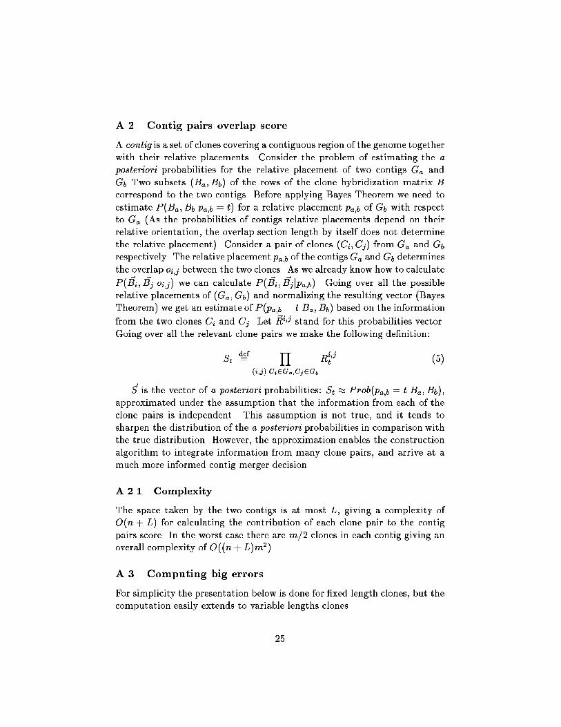
A.2 Contig pairs overlap scoreA contig is a set of clones covering a contiguous region of the genome togetherwith their relative placements. Consider the problem of estimating the aposteriori probabilities for the relative placement of two contigs Ga andGb Two subsets (Ba; Bb) of the rows of the clone hybridization matrix Bcorrespond to the two contigs. Before applying Bayes Theorem we need toestimate P (Ba; Bbjpa;b = t) for a relative placement pa;b of Gb with respectto Ga (As the probabilities of contigs relative placements depend on theirrelative orientation, the overlap section length by itself does not determinethe relative placement). Consider a pair of clones (Ci; Cj) from Ga and Gbrespectively. The relative placement pa;b of the contigsGa and Gb determinesthe overlap oi;j between the two clones. As we already know how to calculateP ( ~Bi; ~Bj joi;j) we can calculate P ( ~Bi; ~Bj jpa;b). Going over all the possiblerelative placements of (Ga; Gb) and normalizing the resulting vector (BayesTheorem) we get an estimate of P (pa;b = tjBa; Bb) based on the informationfrom the two clones Ci and Cj. Let ~Ri;j stand for this probabilities vector.Going over all the relevant clone pairs we make the following de�nition:St def= Y(i;j)jCi2Ga;Cj2GbRi;jt (5)~S is the vector of a posteriori probabilities: St � Prob(pa;b = tjBa; Bb),approximated under the assumption that the information from each of theclone pairs is independent. This assumption is not true, and it tends tosharpen the distribution of the a posteriori probabilities in comparison withthe true distribution. However, the approximation enables the constructionalgorithm to integrate information from many clone pairs, and arrive at amuch more informed contig merger decision.A.2.1 ComplexityThe space taken by the two contigs is at most L, giving a complexity ofO(n + L) for calculating the contribution of each clone pair to the contigpairs score. In the worst case there are m=2 clones in each contig giving anoverall complexity of O((n+ L)m2).A.3 Computing big errorsFor simplicity the presentation below is done for �xed length clones, but thecomputation easily extends to variable lengths clones.25

clone no. 1 2 3 4 5 6 7 8 9 10location in A 0 6 6 13 13 18 19 21 24 32location in P 6 13 13 18 -3 -10 -9 -9 23 30location in P 24 17 17 12 33 40 39 39 7 0errors w.r.t P - - - + + - - + -errors w.r.t P + - + + - - - + +big errors - - - + - - - + -Table 2: Example of the computation of big errors. The locations of the 10clones in the algorithmic solution A is presented together with their locationin the correct solution in both orientations P and P . Clone locations in Pwere de�ned by P i = 30 � Pi, with 30 being an arbitrary constant. Thevalue L is set to 10, the clones length. Errors with respect to P and Pare marked with + signs. The last line in the table marks big errors, asdetermined from the previous two lines.By a location of a clone we mean the coordinate of its left endpoint. Wenumber of clones in non-decreasing order of the locations in the algorithmicsolution. The solution is thus an ordered sequence A = A1 � A2 � : : :� An.Let P be the correct solution, with Pi the location of clone i, indexed usingthe same indices as in A. Let P be the reverse of solution P . That is,Pi = S � Pi for some constant S.We say that an error with respect to P occurred at position i of A ifj(Ai+1 � Ai)� (Pi+1 � Pi)j � L, where L is some constant (in practice weused the average clone length). We similarly de�ne an error with respect toP . The determination of big errors is done as follows: We �rst check foreach 1 � i � n whether an error occurred at position i w.r.t. P . A similarcheck is done for errors w.r.t. P. Then, starting from position 1 we computethe position of the next error w.r.t. P and P, and pick the larger positioni as the place of the next big error. The process is then repeated startingfrom position i+ 1. Table 2 and Figure 8 demonstrate the computation ona small example.26

010 0 10 20 30 40(a) locations in A 010 -10 0 10 20 30 40 50(b) locations in PFigure 8: Physical maps for the data in Table 2. In both parts of the �gurethe y-axis corresponds to the clone indices in the algorithmic solution. Inpart (a) the x-axis denotes clone locations in algorithmic solution. In part(b) the x-axis denotes clone locations in the correct solution. Note thatregardless of the correctness of the algorithmic solution, the clone locationsin A form a non-decreasing series. It is in a graph such as (b), that thequality of the solution can be assessed. In this case, a division into threesection is apparent, corresponding to the two big errors. Note also that inthe �rst and third regions the orientation appears to be correct, whereas inthe second region a reversed orientation �ts A better.

27