Journal of Marine Systems 145 (2015) 1–14

Contents lists available at ScienceDirect

Journal of Marine Systems

j ourna l homepage: www.e lsev ie r .com/ locate / jmarsys

Construction of a trophically complex near-shore Antarctic food webmodel using the Conservative Normal framework withstructural coexistence

Michael L. Bates a,⁎, Susan M. Bengtson Nash a, Darryl W. Hawker a, John Norbury b,Jonny S. Stark c, Roger A. Cropp a

a Griffith School of Environment, Griffith University, 170 Kessels Rd., Nathan, QLD 4111, Australiab Mathematical Institute, University of Oxford, Andrew Wiles Building, ROQ, Woodstock Road, Oxford OX2 6GG, UKc Australian Antarctic Division, 203 Channel Highway, Kingston, TAS 7050, Australia

⁎ Corresponding author.E-mail address: m.bates@griffith.edu.au (M.L. Bates).

http://dx.doi.org/10.1016/j.jmarsys.2014.12.0020924-7963/© 2014 Elsevier B.V. All rights reserved.

a b s t r a c t

a r t i c l e i n f o

Article history:Received 8 October 2014Received in revised form 24 December 2014Accepted 25 December 2014Available online 3 January 2015

Keywords:Ecosystem modellingKolmogorov ecological systemsConservative normalOptimisationAntarctic ecosystem

The analysis of trophically complex mathematical ecosystem models is typically carried out using numericaltechniques because it is considered that the number and nonlinear nature of the equations involved makesprogress using analytic techniques virtually impossible. Exploiting the properties of systems that are written inKolmogorov form, the conservative normal (CN) framework articulates a number of ecological axioms that gov-ern ecosystems. Previous work has shown that trophically simple models developed within the CN frameworkaremathematically tractable, simplifying analysis. By exploiting the properties of Kolmogorov ecological systemsit is possible to design particular properties, such as the property that all populations remain extant, into an eco-logical model. Herewe demonstrate the usefulness of these results to construct a trophically complex ecosystemmodel.We also show that the properties of Kolmogorov ecological systems can be exploited to provide a compu-tationally efficientmethod for the refinement ofmodel parameters which can be used to precondition parametervalues used in standard optimisation techniques, such as genetic algorithms, to significantly improve conver-gence towards a target equilibrium state.

© 2014 Elsevier B.V. All rights reserved.

1. Introduction

The resolution of trophic complexity is an important factor in deter-mining the solutions of ecosystemmodels. Over-simplification results inimportant dynamics being omitted whilst a very fine trophic resolutionsignificantly increases the data requirements to parameterise trophicrelationships between different populations, as well as computationaland storage requirements of the model. The highly non-linear natureof trophic interactions, the paucity of data and the lack of clearly articu-lated and widely accepted governing laws (analogous to those found infields like thermodynamics) makes the development of such ecosystemmodels challenging. In particular, building trophically complex ecosys-tem models is a notoriously difficult task; many ecosystem modelscollapse (i.e. havemultiple spurious extinctions)with increasing trophiccomplexity (Fulton et al., 2003). This is a realisation in silico of Gause'sPrinciple of Competitive Exclusion (Gause, 1932; Gause, 1934) that stip-ulates that only asmany competing populations can coexist as there areresources to support them. This led Hutchinson (1961) to propose the

Paradoxof the Plankton,which observed thatmanypopulations of plank-ton coexisted in the ocean in apparent contradiction of Gause's Principleand predictions of the simple theoretical models of the day.Whilst manysolutions to the Paradox of the Plankton of varying robustness (for exam-ple, Huisman andWeissing, 1999; Schippers et al., 2001) have been pro-posed, the solution of Cropp and Norbury (2012b) provides a practicalsolution that works for models with any number of populations or tro-phic levels and any complexity of trophic interactions. This solution pro-poses particular function forms to represent gain and loss processes thatprovide the equations describing the population interactions with thestructural property that populations cannot go extinct. It also facilitatesthe analysis of the properties of the ecosystem model by consideringthe properties of boundary equilibrium points, rather than the usual ap-proach of considering internal equilibrium points.

Much of the analysis of model ecosystems is concerned with findingequilibrium points and determining their stability. In the context ofecological modelling an equilibrium point is a point in the ecospacewhere all derivatives with respect to time are zero. The ecospace, E, isa subset of state space that contains ecologically valid solutions to themodel equations (e.g. a negative population may be part of the mathe-matical state space but is exterior to the ecospace). An internal equilib-rium point is a point where the system does not change in time and all

2 M.L. Bates et al. / Journal of Marine Systems 145 (2015) 1–14

populations are greater than zero, whilst a boundary equilibrium pointis an equilibrium point on a face or vertex (boundary) of the ecospace(i.e. where one or more populations are extinct). The stability ofequilibrium points is typically assessed by finding the eigenvalues ofthe Jacobian (J, sometimes called the community matrix) at theequilibrium point. The Jacobian gives a linear approximation to thenon-linear equations that govern the ecosystem. Finding the character-istic values (i.e. the eigenvalues, λ) of the Jacobian at equilibrium pointsgives us information about the local stability of those equilibrium points.

Formanymodels, the parameter values that provide stable solutionswhere all populations remain extant are only a very small subset of allpossible values (e.g. Cropp and Norbury, 2012b). It is often assumedthat realistic models, which are often trophically complex, are too com-plicated for any tractable mathematical analysis.

In the 1930s the eminent Soviet mathematician Andrey Kolmogorovwrote down a form of equation that he considered to be ecologicallynatural (Kolmogorov, 1936). These equations, generalised to n popula-tions, are

dx1dt

¼ x1 f 1 x1; x2;…; xnð Þdx2dt

¼ x2 f 2 x1; x2;…; xnð Þ⋮

dxndt

¼ xn f n x1; x2;…; xnð Þ ;

ð1Þ

where xi is the nutrient biomass of the ith populations, with l b i b n. Werefer to fi as the life function, which contains information on the trophicinteractions of that population. Some eigenvalues of boundary equilibri-um points are obtained trivially in Kolmogorov systems since they arethe life function evaluated at the extinction point:

λ j ¼ f jjx�j¼0 : ð2Þ

We shall refer to these eigenvalues as “competition eigenvalues”, so-called because they are the eigenvalue of an invading population that iscompeting for resources with existing populations, and determinewhether a population can invade. Here the superscripted asterisk de-notes the value of xj at an equilibrium point, which are the points in

the ecospace where dxidt ¼ 0 ∀ i ¼ 1;2;…;n.

The classical approach to building ecosystem models begins at thespecies level, where priority is given to reproducing observed speciespopulation trajectories. A community level approach, on the otherhand, attempts to reproduce community level patterns (e.g. rank-abundance curves; Record et al., 2014a; Record et al., 2014b; CroppandNorbury, 2014).We haveused a community level approach byplac-ing the emphasis of our parameter refinement efforts on reproducing acommunity trophic pyramid structure.

Trophically complexmodels of realistic systems have a large numberof parameters and oftenmany are poorly constrained due to the paucityof observations. Therefore parameters are chosen to fit amodel to, for in-stance, observed population biomass. A common tool that is used for pa-rameter optimisation in non-linear systems is a genetic algorithm (GA).As their name suggests GAs optimise a solution by breeding and mutat-ing parameter sets. Using the properties of the competition eigenvalueswe have devised a methodology to efficiently pre-condition parametersets andbetter constrain theparameter space that a GA searches, leadingto more rapid convergence of the model solution to the target solution.

The model we have developed to demonstrate themethodology hastwenty-one functional groups, from primary producers to apex preda-tors and therefore encompasses all trophic levels. The rationale forchoosing our particular ecosystem is that the model we develop willbe used in a future study coupled to a fugacity basedmodel of persistentorganic pollutants (POPs). The intended application of the POP model-ling is to examine the annual and inter-annual cycle of POPs and theirpartitioning in a near-shore Antarctic marine environment. POPs are

lipophilic and the energy (and therefore biomass) pathways throughthe food-web are important to capturing the bioaccumulation andbiomagnification of POPs. As such, we require a model that is able tocapture the major pathways of POP movement from the abiotic envi-ronment through the food web to apex predators, necessitating a largenumber of functional groups to model realistic food web dynamics.

Our overarching aim in this study is to build a trophically complexmodel with known properties (i.e. all populations coexist) and for theequilibrium solution of themodel to have a particular community struc-ture. To impart the coexistence property, we developed our model inthe conservative normal (CN) framework and used particular mathe-matical forms for trophic interactions that guarantee coexistence. To ob-tain a particular community structure requires an appropriate set ofparameters to be chosen. We devised a new, computationally efficient,method for parameter refinement that exploits the properties of thecompetition eigenvalues.

The manuscript is set out as follows: Section 2 summarises the prop-erties of CN systems that form themathematical framework used to con-struct our ecosystem model and summarises the relevant equations ofour model ecosystem; Section 3 outlines our methodology for using thecompetition eigenvalues to efficiently refine the parameters tooptimise the model solution towards a target community structure;Section 4 describes the example ecosystem that we are modellingand rationalises our choice of functional groups; Section 5 comparesour new parameter refinement techniques with that of a standard GAandfinally, Section 6 is a summary of the results and concluding remarks.

2. Mathematical framework

Themodel is constructed so that it satisfiesmost of the rules for a CNsystem (Cropp and Norbury, 2009a; Cropp and Norbury, 2009b; Croppand Norbury, 2012a); Cropp and Norbury, 2012b; Cropp and Norbury,2013). The CN framework is a set of ecological axioms that definebasic properties that characterise ecological systems, and from whichall properties of the system can be derived. This is in analogy with, forexample, the laws of thermodynamics. These rules formalise basic eco-logical concepts, principally that all organisms have to consume re-sources to survive, and that these resources are finite.

2.1. The CN framework

Rule 0 System measurement: we assume each interacting popula-tion is sufficiently large in number that we can ignore the typical in-dividual and instead define a measure of the population mass in theisolated physical volume that the ecosystem occupies. Macro- andmega-fauna may be validly treated in this manner so long as thephysical volume is large and it contains a significant population. Attime zero (t = 0) we measure the amount of the limiting nutrientin each living population, xi, and the total mass of abiotic limitingnutrient, N:

ex1 þ ex2 þ…þ exn þ eN ¼ eNT : ð3Þ

That is, the CN framework respects the fundamental principle ofconservation of mass of a limiting nutrient which is used as themodel currency to measure all populations. We scale the measure-ments ofexi and Ñ by the total amount of nutrient ÑT, so that all pop-ulations and inorganic nutrient are expressed as fractions of the totalnutrient in the system:

x1 0ð Þ þ x2 0ð Þ þ…þ xn 0ð Þ þ N 0ð Þ ¼ 1 ; ð4Þ

with 0 b xi(0), N(0) b 1, and NT = 1.

3M.L. Bates et al. / Journal of Marine Systems 145 (2015) 1–14

Rule 1 Change of living populations: The per capita populationgrowth rates are independent of the way in which we measure theliving populations, and satisfy:

1xi

dxidt

¼ f i x1; x2;…; xn;Nð Þ for tN0 ; ð5Þ

where i= 1,…, n and each life function, f i is continuously differen-tiable in xi, N≥ 0. The life histories ( f i) in Eq. (5) describe how eachpopulation grows and dies, and capture each population's interac-tions with all the other populations and with abiotic nutrient. Thelife function of each population includes parameters that implicitlyquantify rates of environmental and ecological interactions thatwill be considered in detail later. These parameters can be depen-dent upon various environmental factors (e.g. incoming solar radia-tion) to modulate the life function.Rule 2 Conservation of nutrientmass:Wemake the assumption thatthere is no net population migration or nutrient flow into or out ofthemodel domain and require that the total mass of (recycling) nu-trient in themodel domain remains constant for all time (we discussthe appropriateness of this to an Antarctic ecosystem in Section 4).Conservation of total nutrient implies that N = 1 − ∑j = 1

n xjwhich allows us to algebraically eliminate N from Eq. (5) so thatthe life function may be written as:

1xi

dxidt

¼ f i x1; x2;…; xnð Þ for tN0: ð6Þ

A corollary of conservation of mass is that populations cannot havegrowth beyond the resources available to them. This necessitatesthe definition of a lid for the ecospace, which is given by a positivesimplex

E ¼ x1; x2;…; xn : 0≤xi≤1;0≤x1 þ x2 þ…þ xn≤1f g: ð7Þ

Rule 3 Resources and Normal ecosystems: All living populations xjrequire food to survive and grow. This food may be abiotic nutrientfor autotrophs and detritivors, or prey (i.e. other living organisms)in the cases of grazers and predators. These resources, Rj (for popu-lation j), are finite and limit the growth of population xj when theybecome depleted; hence resources should be explicitly representedfor every population in ecosystemmodels, as otherwise a populationcould have unlimited growth (Cropp and Norbury, 2012b). Wedefine two basic criteria that a living population (measured by thebiomass of limiting nutrient xj; recall Rule 0) must satisfy:(a) when its resources are maximal (Rj = 1, a feast), the popula-

tion xj must be able to grow (i.e. f jjR j¼1N0)(b) when there is no resource available (Rj = 0, a famine), the

population xj must die (i.e. f jjR j¼0b0).This means that each life function fj must satisfy the naturalresource constraints:

f jjR j¼1N0N f jjR j¼0: ð8Þ

Conventionally the populations are numbered from thelowest trophic level to the highest such that grazer/predatorpopulations, xj, feed on another population, xi, where i b j. Inthe case of autotrophs, which feed on inorganic nutrient N,their resource is Rj = x0 = N. Note that mixotrophs, omni-vores and other populations with multiple resources willhave their resources identified by multiple subscriptslower than their own.

Rule 4 Feeding behaviour:we assume “normal” feeding behaviour ofthe population, that is, that each life function fj increases monotoni-cally along every ray drawn from every point of zero resource toevery point of maximum resource:

δ f iδx1

cosγ1 þδ f iδx2

cosγ2 þ…þ δ f iδxn

cosγnN0 ; ð9Þ

where γi is the angle of the raywith the ith axis. This precludes com-plex co-operative behaviour where an optimal population size mayprovide certain feeding benefits which are reduced for larger popu-lation sizes. To ensure that conservation of mass is respected a lidcondition is defined in Rule 2 which specifies the bounds of theecospace, thus ensuring thatN(t)≥ 0 for t N 0. To enforce the lid con-dition we require that

dNdt

≥0 when N tð Þ ¼ 1−Xnj¼1

xj tð Þ ¼ 0 : ð10Þ

This is sometimes referred to as the “consistency condition”.Rule 1 and Rule 2 ensure that xi(t) N 0 for all t N 0 if xi(0) N 0, whilstRule 3 and the lid condition constrain the solutions to lie in or on theecospace E, thereby ensuring that conservation of mass is never vio-lated. The lid condition ensures that the conservation of mass crite-rion has physical consistency by ensuring that negative nutrientconcentrations cannot occur.CN systems are endowed with several properties that improve theiranalytic tractability. It is some of these properties that we use to ef-ficiently refine our parameter estimates (see Section 3). In the fol-lowing section, we describe some of the properties of CN systems.

2.2. Some properties of CN systems

All n-population CN ecologies have 2n sets of equations that describeits equilibrium points. Of these, 2n − 1 sets of equations describe“extinction” equilibrium points where one or more populations arezero, that is {xi⁎=0}, where i∈ 1,…, n. One of these equilibrium pointsmust be the origin of the ecospace, defined by {xi⁎ = 0} ∀ i = 1, …, n.Some boundary equilibrium points lie outside the ecospace and donot materially affect solutions inside E, whilst some are degenerate(i.e. two or more collapse to a single point). For instance, there cannotbe a boundary equilibrium point where all primary producers are ex-tinct whilst some or all consumers remain extant; all such boundaryequilibrium points are located at the origin where all populations areextinct. There is also one set of equations that describe the coexistenceequilibrium point(s) defined by {xi⁎≠ 0 = fi} ∀ i= 1,…, n (i.e. equilib-rium points where all populations coexist). The number, location, andstability of equilibrium points depends on the mathematical form andparameter values of fi. Note that a CN ecology does not guarantee thatany or all coexistence equilibrium points lie within the ecospace. How-ever, numerical investigations suggest that structural coexistencemodels have the general property that a stable internal coexistenceequilibrium point exists for all reasonable parameter sets.

Analysis of a model ecosystem usually involves looking for the loca-tion of equilibrium points within the ecospace and the stability of thosepoints. The Lyapunov stability (i.e. the linear stability) of the equilibri-um points is determined by the eigenvalues, λ, of the Jacobian, J. TheJacobian is a linear approximation of the full nonlinear equations at apoint in the ecospace and the eigenvalues are the characteristic valuesat that point. If the real part of λ is positive the equilibrium point is un-stable whilst if it is negative the equilibrium point is stable (amixture ofpositive and negative indicates saddle nodes; under certain other cir-cumstances the points can have stable or unstable limit cycles). One ofthe convenient properties of CN ecologies is that analytic expressionscan easily be found for the eigenvalue λj for any population xj evaluated

4 M.L. Bates et al. / Journal of Marine Systems 145 (2015) 1–14

at its extinction equilibrium point xj⁎ = 0. We refer to these points asboundary equilibrium points since they reside on the boundary of theecospace. The eigenvalues of these boundary equilibrium points, calledcompetition eigenvalues, are given by Eq. (2), and restated here forcompleteness:

λ j ¼ f jjx�j¼0 ;

where the eigenvalue λj is given by the life function fj evaluated at theboundary equilibrium point xj⁎ = 0 (Cropp and Norbury, 2013).

2.3. Ensuring coexistence in CN systems

The application of the example model we developed will be toexamine the partitioning of POPs in Antarctic near-shore ecosystemson interannual timescales. A detailed description of the ecosystem isgiven in Section 4. The short term simulation requirements of thePOPs study (interannual timescales) means that we seek a model thatis not susceptible to the inadvertent extinction of populations due tocompetitive exclusion; a feature of many complex ecosystem models(Cropp and Norbury, 2009a). Coexistence of all populations in an eco-system model, irrespective of the number of populations, the numberof trophic levels, or the interactions between populations can be guar-anteed by ensuring that the competition eigenvalues at the boundaryequilibrium points of all populations are non-negative, that is:

λi ¼ f ijx�i ¼0≥0: ð11Þ

We can ensure coexistence in two ways: either find a parameter setforwhich Eq. (11) holds for all populations (parameterised coexistence;PC); or choose appropriate functional forms for the growth and lossterms in the life function so that Eq. (11) holds for all sensible parametervalues for all populations (structural coexistence; SC).

The SC approach makes it relatively straightforward to construct amodel where all populations remain extant (Cropp and Norbury,2012b) and allows us to design community level and other desirableproperties into a model (Cropp and Norbury, 2014). However, to usethis approach, we must modify the CN framework by relaxing the strictinequality of Eq. (8) to allow the life function to be zero at points of zeroresource. This relaxation recognises that it is in general unrealistic for anecosystem model to have the property that no population can go ex-tinct. Whilst inappropriate for many ecosystem models, these relaxa-tions are consistent with the development and heuristic application ofa model to simulate the distribution of POPs in Antarctica. These relax-ations reconcile the inconsistency between Eqs. (8) and (11) thatwouldotherwise occur when both xi=0 and Ri=0. This leads to themodifiedconditions on fi:

f ijRi¼1N0≥ f ijRi¼0; ð12Þ

where specifically

f ijxi¼0;Ri≠0N0 ; f ijxi≠0;Ri¼0b0 ; f ijxi¼0;Ri¼0 ¼ 0: ð13Þ

This allows us to use life functions that have the structural prop-erty that they are non-negative in all cases when the population iszero (i.e. f ijxi¼0≥0). The relaxation changes the nature of the zerolife function isosurface that must, by CN Rule 3, exist in E. This hasa profound implication for the way in which the zero isosurfaces in-tersect within the ecospace andmeans that these systems have a sta-ble internal coexistence point for every reasonable parameter set.Here we define a reasonable parameter set to be one where the pa-rameter values are positive and those parameters that representfractions or efficiencies lie between zero and one.

Generally, imposition of the ray gradient condition (see Rule 4 inSection 2.1) to ensure a normal ecology would place constraints on

themagnitude of someparameters in a SCmodel. However, in thisman-uscript we will relax this rule and allow the possibility of non-normalpopulation behaviour. This removes the need to place additional con-straints on the model's parameter space to ensure this property.

The reader will observe that the relaxation of CN Rule 4 defined inEqs. (12) and (13) means that populations can exist without resources.This is ecologically unrealistic, and we note that it is only within the CNframework that such ecological silliness can be identified mathemati-cally. We note that this means that all SC models are by definition eco-logically unrealistic, and this is totally consistent with their propertythat no population can ever go extinct. However, for many applicationsthis is not an unreasonable property: for example, the application of themodel described in this manuscript is to model the movement of POPsthrough the ecosystem in a typical annual cycle, and in this context, ex-tinction processes are not relevant. We also note that the DynamicGreen Ocean Models currently being developed to simulate biogeo-chemical processes in the upper ocean also (at this stage of their devel-opment) require models in which populations do not go extinct.

2.4. An example trophically complex model

As discussed in the previous section, a key characteristic that en-dows SC models with their robust coexistence property is that thecompetition eigenvalue(s) at the boundary equilibrium point(s) arepositive [c.f. Eq. (11)] for all populations. To guarantee that the condi-tion described by Eq. (11) is always satisfied, each population in themodel should have non-vanishing growth processes and vanishingloss processes. Here “vanishing” describes a process that tends tozero as the population of interest tends to zero, whilst “non-vanishing” terms do not tend to zero as the population tends tozero. Non-vanishing growth processes cannot have the population(xj) factored out when they appear in the life function (fj) and thus in-clude the usual Droop, Michaelis–Menten, Holling (Types I, II and III)and Lotka–Volterra functional forms. Vanishing loss processes canhave the population factored out when they appear in the life functionand thus include Holling Type III grazing/predation and nonlinearmortality. Given that predator–prey interactions in SC models requirethe prey to have a vanishing loss term and the predator to have a non-vanishing growth term, only Holling Type III (or higher order) grazingterms may be used. Choosing these functional forms leads to SCmodels which satisfy Eq. (11) for all realistic parameter values, whilstchoosing other functional forms leads to PC models. To construct ourtrophically complex SC model we exclusively used Michaelis–Mentengrowth, Holling Type III grazing/predation and quadratic mortality,thereby guaranteeing all populations remain extant for all realistic pa-rameter values.

We write the life function as the sum of several terms which de-scribe growth and loss of the population:

f j ¼Xl

sl j−mjl

h i−Xk

p jk þXi

gi j ð14Þ

where slj is growth due to nutrient uptake,mjl is loss due to mortality orexudation, pjk is loss due to grazing/predation by other functionalgroups, and gij is growth due to feeding (i.e. grazing/predation of otherpopulations). Note that only mixotrophs (i.e. organisms that can bothphotosynthesise and prey/graze on other organisms) will have non-zero terms for both slj and gij. We also relax the standard subscriptingnotation described in Section 2.1 because in trophically complexmodels, such as the one described in Section 4, the definition of trophiclevels is somewhat nebulous. We now discuss each term in Eq. (14) inturn.

In many ecosystem models it is necessary to have several forms oflimiting inorganic nutrient available (e.g. nitrate, ammonia, etc.; seeSection 4.1). Fractionating the inorganic nutrient and dead organicmatter within one model compartment allows different organisms

5M.L. Bates et al. / Journal of Marine Systems 145 (2015) 1–14

to feed on the same nutrient pool. We partition the abiotic nutrientassuming that the ratio between the different forms of nutrient isconstant:

N ¼Xl

Nl ¼ NXl

αl ; ð15Þ

where Nl is the nutrient content of each nutrient form, αl is the frac-tion of the total abiotic nutrient that corresponds to the subscriptednutrient form and has the property that ∑lαl = 1.

Populations that take up nutrient (organic or inorganic) were givennon-vanishing Michaelis–Menten functional forms for growth:

sl j ¼μ l jαlN

αlN þ Kl j; ð16Þ

where subscript j indicates the functional group taking up the nutrient(N) and the subscript l is the nutrient type. Here μlj is the maximumgrowth rate of the functional group and Klj is the half-saturation con-stant (which is the nutrient level at which the growth rate is half ofμ lj). We define a functional group as a group of organisms that occupya similar trophic niche.

Mortality is describedwith a vanishing quadraticmortality loss termin the life function:

mjl ¼ σ jlx j ; ð17Þ

where σjl is the rate at which nutrient is passed from the jth functionalgroup to the lth nutrient type. We also use a quadratic loss term forother loss processes, such as the exudation of transparent exopolymerparticles (TEPs; see Section 4.3).

For grazers and predators the Holling Type III functional form hasthe desirable property that when it functions as a loss term (for prey/autotrophs) it is vanishing whilst when it functions as a growth term(for predators/grazers), it is non-vanishing. The Holling Type III func-tional form has many variations; including basic distinctions betweenspecialists and generalists. The specialist form assumes that a predatoronly hunts one kind of prey at a time, whilst the generalist assumesthat a predator can hunt multiple types of prey at a time (e.g. Koen-Alonso, 2007). It is conceivable for both specialist and generalist strate-gies to be included in the one model, and indeed for a predator to havedifferent strategies for different prey. For simplicity we assume that allgrazers and predators are generalists, yielding the loss term frompredation/grazing as

pjk ¼φ jkx jxkX

rx2r þ κk ;

ð18Þ

where xj is the prey/autotroph, xk indicates the predator/grazer, xr indi-cates the prey/autotrophs consumed by xk (noting that xj must be amember of xr, i.e. j ∈ r), κk is the half saturation constant, and φjk isthe maximum rate of predation of xk on xj. The corresponding non-vanishing growth term in the predator/grazer life function is:

gi j ¼φi j 1−ψi j

� �x2iX

qx2q þ κ j :

ð19Þ

where 1− ψij is the assimilation efficiency for the consumption of xi byxj. By definitionψijmust be between zero and one.We again note that xqindicates the prey/autotrophs consumed by xj and thus xi must be amember of xq (i.e. i ∈ q).

Substituting these terms into Eq. (6), which describes the evolutionof the population, we have the general model equations:

1xj

dxj

dt¼ f j x1; x2;…; xnð Þ

¼Xl

μ l jαlNαlN þ Kl j

−σ jlx j

" #−Xk

φ jkx jxkXrx2r þ κk

þXi

φi j 1−ψi j

� �x2iX

qx2q þ κ j:

ð20Þ

The equation is written for xj which is the jth functional group, l indi-cates the nutrient form, subscript k indicates a predator/grazer of j, sub-script r is other organisms consumed by k, subscript i indicates prey of jand subscript q is other organisms (including i) consumed by j. We notethat for functional groups where a trophic link does not exist then weset μ or φ to zero.

Mathematical analysis of the model requires us to substitute Eq. (4)into Eq. (20) to eliminate an equation describing the dynamics of N.However, when numerically solving the model, we include this equa-tion, check that the integration routine is conserving mass, and use Nin Eq. (20). The general form for the diagnostic nutrient equation isgiven by

dNdt

¼Xj

φi jψi jx2i x jX

qx2q þ κ j

þXl

σ jlx2j−

xjμ l jαlNαlN þ κ l j

" #8>><>>:9>>=>>; ; ð21Þ

where all of the subscripts have the same meaning as in Eq. (20). Theterms on the right hand side represent, respectively, waste from thepredation/grazing of xj on xi, mortality or exudation of xj to nutrienttype l, and uptake of nutrient l by xj.

Note that our ecosystemmodel equations are designed to satisfy CNRules 0–2, and our relaxed Rule 3, for all reasonable parameter values.After relaxing Rule 4, allowing SC systems to have “exotic” ecologies, itremains only to check the lid condition to ensure ecological veracityfor all model solutions. Inspection of Eq. (21) reveals that setting N =0 removes all negative terms from the equation, and hence the lid con-dition is satisfied for all reasonable parameter values.

3. A new method for estimating parameter values

Once the mathematical form for the various trophic interactionshave been chosen the particular solutions of the model are depen-dent on the choice of parameter values. It is often difficult to derivevalues for these parameters from observations or laboratory experi-ments and thus the parameters are often very poorly constrained.The parameters are thus usually found by optimisation techniquesto fit the model solutions to quantities that are easier to derivefrom observations (e.g. biomass).

To fit themodel requires some sort of optimisation routine, such as aGA, for the parameterswhich, in turn, requiresmanymodel evaluations.Here we describe a new method which exploits the properties ofKolmogorov systems to significantly improve the convergence to aspecific model solution and, therefore, reduce the computational timerequired to optimise the parameter set. Section 5 demonstrates thatthis method is applicable to the trophically complex ecosystemdescribed in Section 4.

The newmethod involves adjusting parameter values to change themagnitude of the competition eigenvalues, which in turn changes theposition of the interior equilibrium point within the ecospace. Asdiscussed in Section 2.2, finding the eigenvalue at the boundary equilib-rium point (i.e. the competition eigenvalue) in a Kolmogorov system isstraightforward. The competition eigenvalues are a linearised measureof the stability at the extinction point.We can use this property to adjustthe parameters in the life functions to refine the solution. Adjusting the

a) boundary eigenvalue nudging

(BEN)

initial

parameters

initial

integration

evaluate

fitness

select

worst

population

select pa-

rameter(s)

to adjust

adjust pa-

rameter(s)

integrate

model

more

nudges?

stop or

start GA

yes

no

b) boundary eigenvalue nudg-ing with a genetical gorithm(BENGA)

BEN

routine

initialise

GA

population

integrate

evaluate

fitness

breed

population

integrate

model

assess

fitness

more gen-

erations?

stop

yes

no

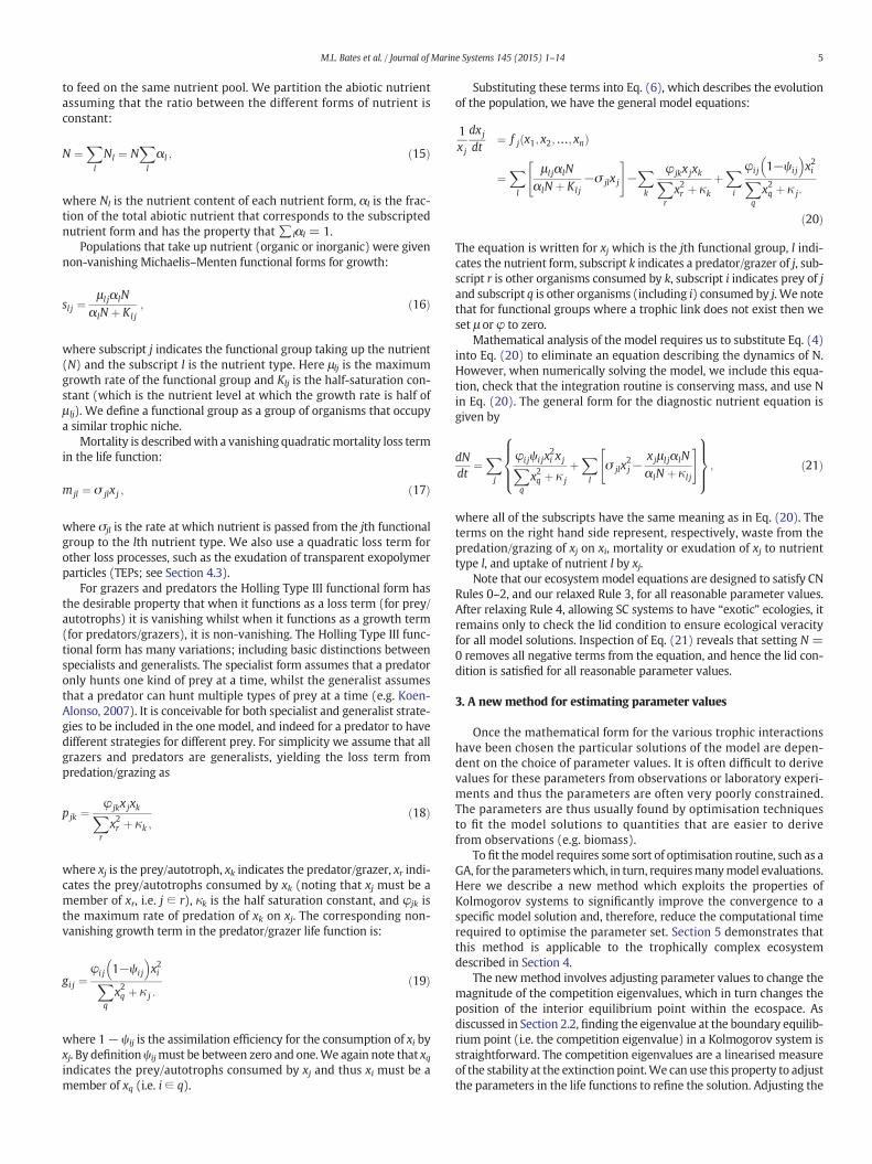
Fig. 1. The procedures, based on the nudging of boundary eigenvalues, used to refine theparameter values of the model.

6 M.L. Bates et al. / Journal of Marine Systems 145 (2015) 1–14

magnitude of a population's competition eigenvalues also affects the in-terior point. By conducting a series of adjustments to the competition ei-genvalues of the systemwe can nudge the interior equilibrium point toa target equilibriumpoint. A caveat is that the eigenvalues are only a lin-ear approximation. Thus, the further away from the boundary equilibri-um point the interior equilibrium point sits, the more imprecise theadjustments to the interior equilibrium point will be.

The ecosystemoutlined in Section 4,which has 21 functional groups,has 221 − 1 = 2, 097, 151 sets of equations that describe the boundaryequilibrium points where one or more populations are zero. This is avery large number of competition eigenvalues to choose from. Weonly use 21 of these eigenvalues: the eigenvalues that correspond toboundary equilibrium points where only one population is zero. In SCsystems these eigenvalues contain only the production terms for eachpopulation, of whichwe only refinemaximal growth rates (μ) andmax-imal grazing/predation rates (φ). Note that adjusting the φ of a grazer/predator also affects its prey, so for each grazer/predator we adjust theφ relating to its worst performing prey. We do not adjust ψ, Κ or κ inthis example, but they could also be adjusted using this method.

3.1. The boundary eigenvalue nudging (BEN) method

We denote themethod of adjusting the eigenvalues of the boundaryequilibrium points to refine the values of μ and φ BEN. The procedure issummarised in Fig. 1a. Inmore detail, the procedure includes the follow-ing steps:

1. A parameter set is randomly generated1 from an initial parameterspace bounded by our best knowledge of parameter values.

2. The model is run to equilibrium. In our model runs, we took equilib-rium to be 1

xidxidt b10

−4 ∀ i.3. The fitness of the solution is evaluated. Here, we used a sum of

squared error as our measure of fitness. That is, we used the equilib-riumnutrient biomass fraction and compared it to the target nutrientbiomass fraction, ∑i(Δxi)2, where Δx = xtarget − xmodel. The targetnutrient biomass fraction is shown in Table 1.

4. The populationwith the poorest fitness (i.e.max{(Δxi)2}) is identified.5. The competition eigenvalue of the worst fitting group contains only

growth terms but may contain several parameters describing growthon different resources. If the population has multiple resources, theterm that describes the interaction with the worst fitting resourcepopulation is selected for nudging (i.e. the worst fitting group (s),the resource group (r) that is most under its desired level is chosen).

6. The growth parameter (μrs or φrs) selected in step 5 with the magni-tude of the adjustment being proportional to the poorness of the fitand is done according to the saturation function Eq. (22).

7. The model is integrated to equilibrium with the adjusted parameterset and its fitness reassessed.

8. The above procedure is repeated for a predeterminednumber of steps.

Taking an example from the model described in Section 4, if themodel is run and benthic macroalgae (BM) nutrient biomass has thelargest error, its competition eigenvalue is identified

λBM ¼ μBMαIN�

αIN� þ KBM

;

where αI corresponds to the fraction of the nutrient form that is dis-solved inorganic nutrient and N⁎ is the equilibrium amount of abiotic

1 In our model the parameter space that the initial parameters are sampled from is auniform distribution between zero and one for μ, φ, ψ, and σ whilst it is a uniform distri-bution between zero and 0.5 for κ, and K. Once a parameter set is chosen the parametersare allowed to vary above the upper bound of these ranges (except for ψwhich, by defini-tion, must not be greater than one).

nutrient for that parameter set. This contains a maximum growthterm, which is then adjusted using the sigmoidal function

μnew ¼ μold 1þ ΔxijΔxij þ ε

� �ð22Þ

where ε is a tunable parameter that controls the strength of the nudg-ing. The larger the value of ε the smaller the nudges. Here, we set ε =1/∑jxj⁎=1/(1−N*). In our implementationwe have not preferentiallyoptimised the parameters associated with any particular population.

Another example is for algavores (Al), who graze on both ice algae(IA) and BM. The eigenvalue for the boundary equilibrium point foralgavores is

λAl ¼φBM Al 1−ψBM Alð Þx�2BM

x�2BM þ x�2IA þ κAlþ φIA Al 1−ψIA Alð Þx�2IA

x�2BM þ x�2IA þ κAl:

Table 1Table of scaled target (xtarget) and equilibriummodel (xmodel) nutrient values for each functional group from the fittest parameter set. In addition the ratio between the model and targetvalues as well as a reference (where relevant) fromwhere the target value was estimated is listed. The parameter set used to arrive at thesemodel results was obtained without any pref-erence given to refining the parameters of particular populations.

Functional group Percentage of total mass Ratio Reference

Target Model xmodel/xtarget

Nutrient 42.1292 45.1313 1.07 Smith et al. (2000)Benthic macroalgae (BM) 0.7813 0.4431 0.57 Quartino et al. (2001)Ice algae (IA) 0.0277 0.0195 0.70 McMinn (1996)Algavores (Al) 0.0405 0.0176 0.44Benthic filter feeders (BFF) 20.3971 18.7844 0.92 Jazdzeski et al. (1986)Benthic predators omnivores (BPO) 0.5390 0.1771 0.33Deposit feeders (DF) 0.3419 0.8778 2.57 Jazdzeski et al. (1986)Demersal fish (DFi) 0.6992 0.2374 0.34Small phytoplankton (SP) 17.1185 15.7245 0.92 Swadling et al. (1997)Large phytoplankton (LP) 17.1185 17.8669 1.04 Swadling et al. (1997)Salps (Sal) 0.0037 0.0035 0.95 Pakhomov et al. (2006)Mesozooplankton (Mzp) 0.1932 0.3160 1.64 Swadling et al. (1997)Other macrozooplankton (OMz) 0.1932 0.2765 1.43 Swadling et al. (1997)Krill (Kr) 0.2926 0.0344 0.12 Pakhomov et al. (1998)Baleen whales (BW) 0.0293 0.0170 0.58Small fish (SF) 0.0163 0.0135 0.82Squid (Sq) 0.0154 0.0105 0.68Large fish (LF) 0.0244 0.0149 0.61Penguins (Pe) 0.0108 0.0105 0.97Aerial seabirds (ASb) 0.0107 0.0089 0.84Seals (Se) 0.0153 0.0128 0.83Toothed whales (TW) 0.0020 0.0020 1.00Total 100.0000 100.0000

7M.L. Bates et al. / Journal of Marine Systems 145 (2015) 1–14

In this instance, we have two parameters (that we could adjust thatalso affect the prey populations), namely, φBM Al and φIA Al. One param-eter is selected to be adjusted on the basis of which corresponding pop-ulation (i.e.φBM Al for benthicmacroalgae andφIA Al for ice algae) has thelargest Δx of opposite sign. The adjustment for φ is a sigmoidal functionof the same form used for μ in Eq. (22). In the event that all the popula-tions have the same sign for Δx then all the μ and φ are adjusted.

3.2. The boundary eigenvalue nudging with a genetic algorithm (BENGA)method

Not all parameters in SC models can be refined using BEN becausethe competition eigenvalues contain only growth parameters. For SCmodels we use the BEN methodology to “precondition” the parametersthat can then be used by other optimisation routines such as a GA. Theprocedure, which we have called the BENGA method (summarised inFig. 1b) is as follows:

1. Run the BEN for a predetermined number of nudges for an initial pa-rameter set (randomly chosen from a given parameter space; seeSection 3.1).

2. Use the refined parameter set to generate a population of genomesfor the GA. If the GA population has m members then we makem− 1 copies of the parameter set and run each of the copies throughthe mutation algorithm. This gives us the initial population of ge-nomes for the GA to operate upon. In addition, we use informationfrom the BEN to refine the strength of the mutation GA (see later inthis section).

3. Integrate the model for each genome.4. Evaluate the fitness of each genome.5. Select the genomes to breed based on their fitness. Conduct cross-

over and mutations. Nudging is conducted on individuals who aremutated, so nudging is superimposed on the mutations.

6. Integrate the model with the new genomes.7. Assess the fitness of each genome.8. Repeat for a given number of generations.

For this study we used a GA with a population of 14. The standaloneGA and the GA portion in the BENGAwere identical, with the exceptionthat nudging was also used on mutated individuals in the BENGA (see

below). Individuals selected to breed were done via a series of three-way tournaments. In a three-way tournament three members are ran-domly selected and the individual with the best fitness is chosen forbreeding. We ensured, however, that the fittest individual from eachgenerationwas carried over into the next generationwithout alteration.

Each new generation in the GA is bred from the winners of the fit-ness tournament of the previous generation. Breeding involves cross-over and mutation of “genomes” (where each model parameter makesup an allele of the genome).We adopted a one point crossover strategy,where the two parent genomes are split at a single point andrecombined. The probability of crossover for any given gene is 1/2.Themutation strategy adopted randomly chose a newvalue for each pa-rameter from a normal distribution with a mean of the current param-eter value. Using this strategy the strength of the mutation iscontrolled by the variance of the distribution. Having a large variancegives strong mutation, which allows for rapid convergence when faraway from the optimum and can avoid having the GA converge tolocal optima. However, when in the near vicinity of the optimum theGA loses evolvability and convergence can become very slow. Ratherthan having a fixed mutation strength we implement a self-evolvingGA which mutates the mutation strength to maximise evolvabilityand, thus, convergence (Beyer and Schwefel, 2002). The mutation ofthe mutation strength is controlled by a learning parameter, which re-quires a constant, c, to be defined a priori. A value that has been foundempirically to maximise convergence for benchmark problems is c =1, however, our testing found that c=10 gave more rapid convergencefor this problem and as such we used c = 10. The probability that agiven genome is mutated is 3/4 and the probability that an allele fromthat genome is mutated is 1/5.

The BENpreconditioning refines the parameter set so that themodelcommunity structure is, on average, closer to the target communitystructure than a randomly generated parameter set. A corollary is thatthe parameter space that we need the GA to span in order to find the“optimum” solution ismuch narrower.We therefore reduced themuta-tion strength of the BENGA by using a smaller initial variance for themutation. The initial variance for the mutation of the standalone GA is1/5 the size of the distribution that the initial parameter is drawnfrom (e.g. for μ the initial parameter is chosen from a uniform distribu-tion between zero and one, thus the variance of normal distribution

8 M.L. Bates et al. / Journal of Marine Systems 145 (2015) 1–14

controlling themutation strength is 0.2). For the BENGA the variance forthe normal distribution is 1/20 of the size of the initial parameter space(e.g. for μ it is 0.05). Nudging is superimposed onto the mutation pro-cess in the BENGA, with the parameter selection and magnitude of thenudge being the same as described in Section 3.1.

4. Model ecosystem

The ecosystem model identifies important functional groups in anAntarctic near-shore ecosystem and represents the relationships be-tween those functional groups in order to study POPs in that environ-ment. A consideration in our study is that POPs biomagnify as theymove up trophic levels and we have therefore included a variety ofupper-trophic functional groups to study how POPs partition in thefood web.

We identified one or more canonical species for each functionalgroup and based the trophic relationships of that group on the canonicalspecies (see Table 2). The choice of “canonical species” is inherentlysubjective, but, factors taken into account were the observed biomassof the species and its perceived importance in the ecosystem'strophodynamics.

Our hypothetical “study site” is an area nominally located in eastAntarctica and is predominantly within the neritic zone. In the remain-der of this section we describe the functional groups that make up ourecosystem and their trophic relationships, which are summarisedgraphically in Fig. 2.

Rule 2 stated that we assume that there is no net population migra-tion. Whilst none of our “canonical species” are migratory, Antarcticecosystems contain migratory species and whilst it is a simplificationto assume that total nutrient mass remains constant, the nutrient bio-mass of these migratory species is small relative to the total nutrientmass of the system. Furthermore, it is reasonable to assume that thenet export/import of nutrient by migratory species is close to zero.Thus, the error introduced by migratory species to the assumption ofconservation of system nutrient is insignificant.

4.1. Nutrient

The CN framework uses limiting nutrient as themodel currency (seeSection 2). In Antarctic near-shore environments, the limiting nutrientis typically nitrogen, so, we assume that in our study site the totalamount of nitrogen is conserved. For brevity we shall refer to abiotic

Table 2A list of functional groups used in themodel, their abbreviations, the canonical species that werenear-shore eastern Antarctic environments.

Functional Group Abbreviation

Benthic macroalgae BMDeposit feeders DFAlgavores AlBenthic filter feeders BFFBenthic predators & omnivores BPOIce algae IASmall phytoplankton SPLarge phytoplankton LPMesozooplankton MzpSalps SalKrill KrOther macrozooplankton OMzBaleen whales BWDemersal fish DFiSmall pelagic fish SPFLarge pelagic fish LPFSquid SqPenguins PeAerial seabirds ASbSeals SeToothed whales TW

nutrient as nutrient (N) unless otherwise stated. Herewe divide the nu-trient into four types:

1. dissolved inorganice nitrogen (DIN),2. dissolved organic nitrogen (DON),3. suspended detritus (SuDet), and4. settled detritus (SeDet).

All non-living organicmatter lost from each of the functional groups be-comes either settled or suspended detritus. Settling and turbation pro-cesses mean that nutrient can transfer between SuDet and SeDet.Somedetritus breaks down and becomes DON. Someplankton also con-tribute to the production of DON through the exudation of TEPs (seeSection 4.3). Eventually all organic matter is mineralised and becomesDIN via bacterial processes. As discussed in Section 2.4, we assume aconstant partitioning of the nutrient pool, with the nutrient beingequally partitioned between the four types of nutrient.

4.2. Benthos

Our choice of functional groups for the benthic community is largelybased upon the results of Gillies et al. (2012) who described a trophicstructure for a benthic community in the Windmill Islands (nearCasey Station in East Antarctica) using stable isotope analysis. Basedon their trophic analysiswe have divided the benthos into six functionalgroups

1. benthic macroalgae,2. deposit feeders,3. algavores,4. benthic filter feeders,5. predators–scavengers, omnivores, and necrophagous feeders, and6. demersal fish.

Benthic macroalgae are a central component of the Antarctic benthicfoodweb (Quartino and Boraso de Zaixso, 2008) and an important foodsource for fauna in near-shore ecosystems being grazed upon by bothalgavores and omnivores. Indirectly, macroalgae are a source of foodfor filter feeders and deposit feeders when consumed as detritus(Gillies et al., 2012). Deposit feeders predominantly feed upon SeDetand filter feeders predominantly feed upon SuDet. The functional groupof predators, predator-scavengers, omnivores and necrophagousfeeders is very diverse and has a large diversity of food sources. Demer-salfish are thefinal functional group andhave a varied diet. Indeed, they

used to estimate parameter values and the reference identifying it as a common species in

Canonical species Reference

Himantothallus grandifolius Gillies et al. (2012)Orchomenella franklini Gillies et al. (2012)Paramoera walkeri Gillies et al. (2012)Laturnula elliptica Gillies et al. (2012)Sterechinus neumayeri Gillies et al. (2012)Thalassiosira australis McMinn (1996)Thalassiosira dichotomica Gibson et al. (1997)Phaeocystis antarctica Gibson et al. (1997)Oncaea curvata Swadling et al. (1997)Ihlea racovitzai Atkinson et al. (2012)Euphausia crystallorophias Hosie and Cochran (1994)Calanoides acutus Swadling et al. (1997)Balaenoptera bonaerensis Tamura and Konishi (1998)Trematomus bernacchii Gillies et al. (2012)Pleuragramma antarcticum La Mesa and Eastman (2012)Dissostichus mawsoni Agnew et al. (2009)Psychroteuthis glacialis Emslie and Woehler (2005)Pygoscelis adeliae Wienecke et al. (2000)Pagodroma nivea Woehler et al. (2003)Leptonychotes weddellii Lake et al. (2003)Orcinus orca Pitman and Ensor (2003)

Nutrient

Small Phytoplankton

Large Phytoplankton

Ice Algae

Benthic Filter

Feeders

Deposit Feeders

Benthic Macroalgae

Krill

Salps

Macrozooplankton

MesozooplanktonAlgavores

Small Pelagic Fish

Squid

Baleen Whales

Penguins

Aerial Seabirds

Large Pelagic Fish

Seals

Toothed Whales

Demersal Fish

Predator- Scavengers, etc.

Fig. 2. A diagram showing the interrelationships of the functional groups that make up the near-shore Antarctic ecosystem model.

9M.L. Bates et al. / Journal of Marine Systems 145 (2015) 1–14

could be included as an omnivore, however, we have separated theminto their own group since they are an important trophic link betweenthe benthos and the rest of the food web.

There are several species of benthic macroalgae that are abundant inAntarctic waters; here we have used the endemic Antarctic speciesHimantothallus grandifolius as the canonical species as it is relativelywell studied and is widespread in east Antarctica. Similarly we haveused the ubiquitous and relatively well studied benthic amphipodOrchomenella franklini as the canonical species for deposit feeders.O. frankliniwas foundbyGillies et al. (2012) to have closely grouped iso-topic signatures (implying similar feeding strategies) to larger surfacedeposit feeders and other infaunal deposit feeders. The amphipodParamoera walkeri feeds on macroalgae and in winter feeds on icealgae, and was shown by Gillies et al. (2012) to have similar feedingstrategies to other grazer/herbivores and was selected as the canonicalalgavore. Benthic filter feeders (also referred to as suspension feeders)form one of the largest components of Antarctic shallow water benthiccommunities. This group predominantly feeds on suspended particulateorganicmatter, however, some species obtain a significant proportion oftheir diet from macroalgal detritus. The bivalve mollusc Laturnulaelliptica is a member of this group (Gillies et al., 2012) and we use it asour canonical species. The functional group of benthic predators, preda-tor–scavengers, omnivores and necrophagous feeders is, by definition, avery diverse groupwith an equally diverse range of food sources (Gillieset al., 2012). To best capture this diversitywe have used a relativelywellstudied omnivore, the Antarctic Sea Urchin (Sterechinus neumayeri), asour canonical species. The final functional group is demersal fish,which are typically generalist feeders. Demersal fishes are an importantlink between benthic species and upper trophic levels (see Section 4.4).Trematomus bernacchii is one of the most common demersal fishesfound in the Vestfold Hills region of east Antarctica (Gillies et al.,2012) and as such, we use it as our canonical species.

4.3. Plankton

Plankton communities form the basis for much of the Antarctic foodweb and containmany species (e.g. Scott andMarchant, 2005). Hereweseparate plankton into seven functional groupswith primary producersseparated into three functional groups viz.

1. small phytoplankton (length b53 μm),2. large phytoplankton (length N53 μm),3. ice algae,

and zooplankton separated into four, viz.

1. mesozooplankton (biomass dominated by copepods and othermainly suspension-feeding taxa)

2. salps,3. krill, and4. other macrozooplankton (mostly carnivorous taxa),

following the suggestion of Atkinson et al. (2012).Considerable intra- and inter-annual variabilities in phytoplankton

biomass has been observed in near-shore environments in EastAntarctica (Skerratt et al., 1995; Gibson et al., 1997) whichmakes iden-tifying a canonical species in this group a subjective choice. We choseThalassiosira dichotomica and Phaeocystis antarctica as the small andlarge pelagic phytoplankton species respectively based on their ubiqui-tous presence observed during the study of Swadling et al. (1997). Thehaptophyte P. antarctica is one of the most abundant species of phyto-plankton in Antarctica. It is one of the first algae to bloom in coastalAntarctica where it frequently dominates the phytoplankton in the iceand ice-edgewaters during spring (e.g. Marchant et al., 2005, and refer-ences therein). Phaeocystis species are known in the Northern Hemi-sphere for their production of TEPs which are a source of DON.Experiments in the Ross Sea conducted by Smith et al. (1998) indicate

10 M.L. Bates et al. / Journal of Marine Systems 145 (2015) 1–14

that P. antarctica is not a significant source of DON compared to otherspecies in other regions. Exudation from TEPs is included in our modeland is combinedwith themortality term for large phytoplankton. In ad-dition, it is becoming evident that mixotrophy is much more prevalentin marine planktonic ecosystems than has traditionally been thought(Flynn et al., 2013), therefore we include a link for large phytoplanktonto consume small phytoplankton, although we acknowledge that thereare many other mixotrophic interactions that are possible as well.

The resting spores of Thalassiosira australis have been commonlyfound in and around sea-ice indicating it is an ice associated diatom spe-cies. T. australis has been found to form dense populations in mats onthe underside of fast ice in Ellis Fjord (near Davis Station, EastAntarctica; McMinn, 1996) and was used as the canonical ice algaespecies.

Oncaea curvata is a copepod that is endemic to Antarctica and is thedominant species of the genus Oncaea. It is very abundant and oftendominates zooplankton numerically and sometimes in termsof biomass(Metz, 1998). O. curvata was amongst the dominant species of zoo-plankton in the study of Swadling et al. (1997) near Davis Station, andwe use it as the canonical mesozooplankton species.

There are two species of salps that are commonly found inAntarctica, Salpa thompsoni and Ihlea racovitzai, both with circumpolardistributions. S. thompsoni is more abundant but I. racovitzai is charac-teristic of higher latitudes (Atkinson et al., 2012, and references there-in), thus we chose I. racovitzai as our canonical species.

The krill species Euphausia crystallorophias is an important compo-nent of high-latitude shelf ecosystems. It is smaller than the betterknown and commercially exploited Euphausia superbawhich is typical-ly found in much deeper waters. In a large scale survey of the Prydz Bayregion Hosie and Cochran(1994) found that E. crystallorophias persis-tently appeared in high abundance in neritic communities. In anotherstudy in the shelf region of the Lazarev Sea region (in the Atlantic sectorof Antarctica) Pakhomov et al.(1998) found that E. crystallorophias hadan omnivorous diet which included phytoplankton (including diatomsbut not Phaeocystis), microzooplankton and mesozooplankton (includ-ing copepods). Therefore we use E. crystallorophias as our canonicalkrill species and have krill grazing on small phytoplankton and icealgae whilst also eating mesozooplankton.

The macrozooplankton, including large copepods, tend to be associ-ated with oceanic conditions. Some species, such as Calanoides acutus,can be found closer to shore but tend to be less abundant in terms of bio-mass than smaller zooplankton. Swadling et al. (1997) studied primaryproductivity and grazing by copepods at a coastal station near Davis Sta-tion; C. acutuswas consistently present in their study but typically hadmuch lower biomass than mesozooplankton such as O. curvata. Wetherefore use C. acutus as our canonical mesozooplankton. Metz andSchnack-Schiel (1995) also conducted a study on the carnivorousfeeding habits of calanoid copepods in the Bellingshausen Sea. Theyfound that C. acutus does not appear to have carnivorous feeding habits(i.e. they predominantly feed on phytoplankton), however, other cope-pods of similar size do feed on species such as O. curvata. We thereforeinclude trophic links from the two phytoplankton groups, as well asmesozooplankton to other macrozooplankton.

4.4. Megafauna

Antarctic waters are known for their iconic megafauna, which wedivide into eight functional groups:

1. small pelagic fish,2. large pelagic fish,3. squid,4. baleen whales,5. penguins,6. aerial seabirds,

7. seals, and8. toothed whales.

The Antarctic silverfish (Pleuragramma antarcticum) is our canonicalspecies for small pelagic fish. It is a common circumpolar pelagic fishthat is usually found in near-shore environments and is a key speciesin high-latitude Antarctic ecosystems. P. antarcticum reaches a bodylength of up to 25 cm and feeds predominantly on krill but is alsoknown to feed on copepods and salps (La Mesa and Eastman, 2012,and references therein). Our canonical species for large pelagic fish isthe Antarctic toothfish (Dissostichus mawsoni), which is one of the larg-est fish inhabiting the Southern Ocean and can grow to more than200 cm (see La Mesa et al., 2004, and references therein). D. mawsoniis commercially exploited in the Ross Sea but is known to occur inPrydz Bay and other areas of East Antarctica (Agnew et al., 2009).

Squid form an important food source for marine birds and seals. Astudy examining the diet of Adélie penguins in the Windmill Islandsof East Antarctica found the most common species of cephalopod tobe Psychroteuthis glacialis (Emslie and Woehler, 2005), which we takeas our canonical species. Squid are known as voracious predators(Rodhouse andNigmatullin, 1996) however in Antarctica their diet like-ly mostly consists of krill with some fish (Kear, 1992).

Minke whales (Balaenoptera bonaerensis) are found throughout EastAntarctica andwe take them as our canonical species for baleenwhales.They predominantly feed upon two krill species, E. superba andE. crystallorophiaswith the latter dominating the diet of whales in shal-low areas. There is evidence of whales consuming amphipods and fish,however, these species only make up less than one percent of the dietof B. bonaerensis (Tamura and Konishi, 1998).

Adélie penguins (Pygoscelis adeliae) are abundant in Antarctic wa-ters and are our canonical penguin species. The composition of thediet of P. adeliea is known to vary geographically and includes krill,fish and cephalopods. A survey of the foraging behaviour of Adélie pen-guins in east Antarctica showed that penguins from Shirley Island nearthe Australian Casey Station fed predominantly on E. crystallorophias(Wienecke et al., 2000). Of the aerial seabirds, petrels were found tobe the most numerically abundant in surveys of Prydz Bay, with themost common being the snow petrel (Pagodroma nivea; Woehleret al., 2003). A study of the feeding of summer breeding seabirds inAdélie Land by Ridoux and Offredo (1989) showed that P. nivea pre-dominantly consumed fish (95%). Other aerial seabirds, such as thesouthern fulmar (Fulmarus glacialoides), relied much more on krill andcarrion with only 16% of their diet made up of fish. It is also knownthat skuas prey on penguins whilst breeding (e.g. Young, 2005). Onthis basis, even thoughwe take the snowpetrel as our canonical species,which relies predominantly on small pelagic fish, we included trophicinteractions with krill and penguins.

Weddell seals, our canonical seal species, have a unique ice holebreathing behaviour that allows them to live under continuous sea-ice, thus they are the only air breathing predator to forage in both ben-thic and pelagic coastal habitats year round. Analysis of scat from theMawson Coast, Commonwealth Bay, Larsemann Hills and VestfoldHills (Lake et al., 2003) showed that their dietary composition is diverseand includes pelagic fish (predominantly P. antarcticum), benthic fish(including T. bernacchii), cephalapods (regionally P. glacialis is an impor-tant component of seal diet in spring) and crustacea (includingE. crystallorophias). In the Ross Sea it is known that D. mawsoni are animportant component of the diet of Wedell seals (La Mesa et al., 2004)and thus, a link between large pelagic fish and seals is included inFig. 2. A study by Hall-Aspland and Rogers (2004) of Leopard seals(Hydrurga leptonyx) in Prydz Bay showed that they eat penguins,other seals, benthic and pelagic fish, amphipods and krill; therefore atrophic link from penguins to seals is also shown in Fig. 2.

Killer whales (Orcinus orca) are at the top of the trophic pyramid inAntarctic waters and are our canonical toothed whale species. O. orcahas a global distribution, however, there are three distinct forms in

11M.L. Bates et al. / Journal of Marine Systems 145 (2015) 1–14

Antarctica that display different feeding habits (Pitman and Ensor,2003). All three types have circumpolar distributions, but, appear toprefer different habitat types and have different food preferences.Type A feeds mainly on B. bonaerensis, type B predominantly feeds onseals and penguins whilst type C feeds mainly on fish but may supple-ment its diet with seals and penguins. We do not differentiate betweenthe three types in our ecosystem model and include all three trophiclinks.

4.5. Community structure

As discussed in Section 2, decisions fundamental to the communitystructure are made when choosing the mathematical form of the equa-tions to describe inter-population relations. This section is concernedwith describing how we specified the desired community structure ofour ecosystem. In Section 2.4 we chose particular mathematical formsto ensure that all populations remain extant. In this section we specifythe community structure (i.e. the nutrient biomass of each functionalgroup) that we want our model to have when in equilibrium.

The dimensions of our hypothetical study site were 10000 km2 withan average depth of 200 m. Assuming a mixed layer depth of 100 m, anaverage ice cover fraction of 30%, and a benthos cover fraction of 40%wehave obtained estimates of nutrient mass using density surveys fromthe literature for particulate organic matter, primary producers, zoo-plankton, deposit feeders and benthic filter feeders. For other functionalgroupswe used an objectivemethod for determining their nutrient bio-mass, namely a functional group is 10% of the mass of the average of allof the functional groups that it itself feeds upon Pauly and Christensen(1995). As mentioned previously, the currency of our model is themass of nitrogen. Where the nitrogen content of a functional grouphas not been reported in the literature we have taken the carbon con-tent and used the Redfield ratio of C:N = 106:16 to convert to mass ofnitrogen. Below we describe our specific methodology for obtaining ni-trogen biomass estimates from the literature, which is summarised(including references) in Table 1.

The density of suspended particular organic nitrogen in for the RossSea, Antarctica was reported by Smith et al. (2000). We multiplied thisby the dimensions of our hypothetical study site to obtain the totalmass of suspended particular organic nitrogen. We assumed that themass of the entire abiotic nutrient to be four times that of the suspendedparticular organic nitrogen, with each class of nutrient (SuDet, SeDet,DON, and DIN) having a quarter of the total abiotic nutrient.

Tofind themass of benthicmacroalgaewe used an average of valuesfrom the survey sites for Potter Cove (KingGeorge Island, Antarctica) re-ported by Quartino et al. (2001).We converted their dry weight densityto nitrogen using a mass fraction of 0.031 g/g (Peters et al., 2005). Tofind the biomass of benthic filter feeders we used the survey results ofJazdzeski et al. (1986) for bivalva from Admiralty Bay, King GeorgeIsland (in the South Shetland Islands) and converted tomass of nitrogenusing amass fraction of 0.085 g/g (from Pearse and Giese, 1966), for thebivalve Limatula hodgsoni from near McMurdo Station). The mass ofdeposit feeders was also taken from the survey of Jazdzeski et al.(1986) using the mass of amphipods and converted to carbon using amass fraction of 0.45 g/g.

McMinn (1996) reported the density (based on carbon) of ice algaein Ellis Fjord, eastern Antarctica. In a study near Davis Station, easternAntarctica (Swadling et al., 1997) reported thedensity of phytoplanktonin terms of chlorophyll a content and assumed a 75:1 ratio of carbon tochlorophyll a in order to convert it to carbon. Here we have assumed anequipartitioning of biomass between small and large phytoplankton.Pakhomov et al. (2006) reported the nitrogen biomass of salps in theEastern Bellingshausen Sea whilst the density of krill individualswas estimated by Pakhomov et al. (1998) in the Lazarev Sea and con-verted tomass using 0.027 g/individual and a carbonmass fraction of0.45 g/g. The mass fraction of carbon in mesozooplankton and othermacrozooplankton were estimated by Swadling et al. (1997), where

we took themass of C. acutus to be themass of othermacrozooplanktonand that of all other zooplankton to be the mass of mesozooplankton.The values of nitrogen in each functional group derived using theabove procedure are summarised in Table 1.

5. Results and discussion

We ran an ensemble of simulations to examine the convergence oftheparameter refinement techniques (Section3) to the chosen commu-nity structure (Section 4.5). These results show that, in the majority ofcases, the BEN technique (Section 3.1) provides a computationally effi-cient means to refine parameter values. However, as discussed inSection 3.2, the BEN is not able, by itself, to refine all parameter values.So, we use the BEN to precondition the parameter values used in a GA aswell as to “weaken” the mutation strength (see Section 3.2); a proce-dure we refer to as the BENGA. Benchmarking against a standard GAwe have shown that, on average, the BENGA gives more rapid conver-gence to the desired community structure.

Evaluating model skill in reproducing observed data is a comple-mentary tool to understanding the implications of functional forms onmodel properties when developing models in Earth System science.Multivariate approaches such as we have used here typically identifythat some variables are estimated better than others (see for example,Allen and Somerfield, 2009), as is apparent in Table 1. In practice, vari-ables would be ranked according to the importance of “getting themright” according to the question being investigated with the model,and the goal function used for the model calibration would reflect thisrelative importance. Here we present the results of the BENGA solelyto demonstrate the accelerated convergence of the method, but havenot weighted the goal function to optimise the fit to any particularpopulation.

5.1. BEN

Using an ensemble of 20 randomly generated parameter sets wenudged each parameter set 14 times (resulting in a total of 15 modelevaluations for each ensemble member) using the BEN method (seeSection 3.1 for details). Fig. 3 shows the fitness of each ensemble mem-ber after each nudge-integrate-evaluate cycle. The BEN method, for themajority of parameter sets, yields a significant improvement in fitnessfor relatively few simulations.

The rapid convergence to a target community structure, using theBEN methodology, arises from exploiting the stability properties of theboundary equilibrium points. Recall that for Kolmogorov systems,which all CN systems are, determining the boundary equilibriumpoints,and thus their stability, is trivial (see Section 2.2). Aside from providinga method to efficiently refine parameter values towards a desired com-munity structure this illustrates the utility, even for trophically complexmodels, of understanding the mathematical properties of a modelecosystem.

5.2. BENGA

To assess the convergence of the BENGA (Section 3.2) to the desiredcommunity structure, we ran two ensembles: onewith a standalone GAand the other using the BENGA. Using the BEN results from Section 5.1we spawned a population of 14 genomes from each parameter set andused them in the GA phase of the BENGA.

Fig. 4 shows the evolution of fitness of the best individual in each en-semble member for the GA and the GA phase of the BENGA. Due to thepreconditioning by the BEN (see Fig. 3) the initial fitness of the GA por-tion of the BENGA is clearlymuchbetter than the standaloneGA. TheGAportion of the BENGA continues to improve the fitness of the ensemblemembers and after 100 simulations, the ensemble mean fitness (blacksolid line in Fig. 4b) of the BENGA is only slightly higher than the ensem-ble minimum for the standalone GA (the dashed black line in Fig. 4a).

1 3 5 7 9 11 13 15Number of simulations

0.0

0.2

0.4

0.6

0.8

1.0F

itne

ss

Fig. 3.The evolution offitness of 20 randomly generatedparameter sets that have their pa-rameters adjusted using the BEN method (described in Section 3.1). The parameters arenudged 14 times, leading to 15 model evaluations. These results were then used as thepreconditioned parameter sets for the GA phase of the BENGA. The thin grey lines areeach of the 20 ensemble members, the solid black line is the ensemble mean and thedashed black line is the ensemble minimum.

12 M.L. Bates et al. / Journal of Marine Systems 145 (2015) 1–14

The majority of BENGA cases have a fitness that is much better than thebest fitness using the standalone GA.

When the genomes of a GA is near the optimal solution weak muta-tion improves the evolvability. Conversely, when the genomes are farfrom the optimal solution, having strong mutation improves theevolvability. Mutating the mutation strength, such as we did in our GA(see Section 3.2), helps to improve the evolvability of a GA as it movescloser to anoptimal solution (e.g. Beyer and Schwefel, 2002). Inmost in-stances the BEN improves the fitness of a parameter set and is thus rel-atively close to the optimal solution. It is therefore, in the majority ofcases, advantageous to have weaker mutation in the BENGA than inthe standalone GA, which is initialised with random parameter sets.We hypothesise that this allows the GA phase of the BENGA to have im-proved evolvability and therefore relatively good convergence evenonce the BENphase is complete. In addition the continuation of nudgingsuperimposed on the randommutation of the GA portion of the BENGAaids continued convergence. The community structure of the fittestmember from Fig. 4 is shown in Table 1 alongwith the target communi-ty structure and the ratio of the two, showing that the BENGA has found

15 30 45 60 75 90Number of simulations Number of simulations

0.00

0.05

0.10

0.15

0.20

0.25

Fit

ness

a) GA only

15 30 45 60 75 90

b) BENGA

Fig. 4. The evolution of fitnesswith the number of simulations. The best fitness of each en-semblemember is the thin grey lines, the black solid line is themean ensemble fitness andthe dashed black line is the minimum ensemble fitness.

a parameter set whose equilibrium point is largely comparable to thedesired community structure.

Fig. 3 shows three parameter sets for which the BEN has little effect;because these ensemble members have a significantly poorer fitness tothe rest of the BENGA ensemble, they have a significant effect on the en-semble mean. It is our experience that in our model ~10% of parametersets do not see very much improvement from the BEN. These ensemblemembers also tend to have relatively slow convergence in the GA phasebecause, we suspect, they sit in a poorly fitting part of the parameterspace and, because the BENGA has a narrow mutation variance, theyhave poor evolvability. As discussed in Section 3, the competition eigen-values are a linear approximation to the full non-linear equations. Wehypothesise that, in these instances, the poor preconditioning resultsfrom the competition eigenvalues having very limited influence on theinternal equilibrium point due to the non-linearity of the full equations.A simple and relatively computationally inexpensive means to over-come this problem would be to discard a parameter set if it has notreached a threshold fitness after a given number of nudges and startthe process again with a new randomly generated parameter set.

6. Summary and conclusion

We constructed a zero (spatial) dimension, trophically complex,end-to-end model ecosystem for a near-shore Antarctic marine envi-ronment. The model encompassed 21 functional groups from primaryproducers to apex predators including benthic organisms, pelagicplankton, fishes, cephalapods, marine mammals and marine birds. Themodel represents the interconnectedness of these different componentsof the ecosystem and describes, mathematically, their trophic interac-tions. Themodel has 141 parameters that control nutrient uptake, graz-ing, predation, excretion, exudation and mortality. The currency of themodel is limiting nutrient, namely, nitrogen. The model is intended tobe coupled to a fugacity model of POP and in future work we will usethis ecosystem model to examine the partitioning of POP in Antarcticnear-shore environments.

In formulating the mathematical basis of our ecosystem model, wehave taken the community level approach (Record et al., 2014b;Cropp and Norbury, 2014; Record et al., 2014a), in which we defined aparticular community structure and used appropriate mathematicalforms to obtain that community structure. We used functional formsthat comply with the CN framework (Cropp and Norbury, 2009a;Cropp and Norbury, 2009b; Cropp and Norbury, 2012a; Cropp andNorbury, 2013). Simply using Michalis–Menten growth, Holling TypeIII predation and quadratic mortality for each population leads to SC,in which all populations remain extant for any reasonable parameterset (Cropp and Norbury, 2012b). Consequently, no numerical simula-tion conducted resulted in any extinction event overcoming Gause'sPrinciple of Competitive Exclusion, the bane of numerical ecosystemmodelling. This result gives credence to the claim that the resultshown for trophically simple models by Cropp and Norbury (2012b) isgeneralisable to trophically complex models, such as the presentmodel. This is an important property as a significant problem formany trophically complex models is that populations often becomeextinct (Fulton et al., 2003).

We have also highlighted that SC models violate fundamental eco-logical principles. The CN framework, and the analytical approach it fa-cilitates, allows us to explicitly describe how each population isecologically unrealistic. This does notmean that themodels are not use-ful, but that their uses are restricted to modelling scenarios such as an-nual cycles where populations are not expected to go extinct. At thecurrent stage of the application of complex ecosystemmodels in climateand natural resource management, models in which all populations re-main extant for all time are necessary. Whilst SC models may be strictlyunrealistic, it is less unrealistic than the numerical fudges (such as arbi-trary minimum populations or changing mortality terms to growth

13M.L. Bates et al. / Journal of Marine Systems 145 (2015) 1–14

terms; Cropp and Norbury, 2012b) that are otherwise employed toenforce coexistence.

We have further exploited the properties of models that complywith the CN framework to develop a novel methodology for parameterrefinement that we have dubbed BEN. It uses the eigenvalues at bound-ary equilibrium points (i.e. extinction points), which are obtained trivi-ally in the CN framework, to “nudge” parameter values. By focusing onthe worst performing populations and adjusting the parameters thatare used in calculating the eigenvalues, we increase or decrease themagnitude of the parameters depending on whether their populationsare too small or too large, thereby improving the model fit to data.

The parameter nudging method does, however, have some limita-tions. For example, in models that have SC, not all parameters appearin the competition eigenvalues (e.g. mortality) of the boundary equilib-rium points. To obtain refinements of parameters that are absent fromthe competition eigenvalues other methods must also be used. Weshowed that the BEN can be used to precondition parameter sets thatmay then be used by standard optimisation strategies, such as a GA.We implemented a BENGA, where the BEN is used to precondition pa-rameters before being used by a GA. We showed that, on average, theBENGA reached a better fit with fewer simulations than a standaloneGA.

This study demonstrates that insights from the study of the mathe-matical properties of a model can be exploited even in trophically com-plex systems. In this case, we used the knowledge of the eigenvalues ofthe boundary equilibrium points to reduce the computational burdenrequired to refine the parameter values. In future work, we will intro-duce a seasonal cycle and couple this ecosystem model to a fugacitymodel to examine the partitioning of POPs in near-shore Antarcticecosystems.

Acknowledgements

The authors would like to thank Maurice Levasseur for the helpfuldiscussions on formulating the ecosystem. We would also like tothank two anonymous reviewers whose comments improved the man-uscript. This project was made possible through funding fromAustralian Antarctic Science grant number 4121. The numerical solu-tions to the ecosystem were solved using the ODE module of SciPy(Oliphant, 2007) and plotting was done using matplotlib (Hunter,2007). The genetic algorithm was developed using Distributed Evolu-tionary Algorithms in Python (DEAP; Fortin et al., 2012) and parallelisedusing Scalable Concurrent Operations in Python (SCOOP; Hold-Geoffroyet al., 2014).

References

Agnew, D., Edwards, C., Hillary, R., Mitchell, R., Abellán, L.L., 2009. Status of the coastalstocks of Dissostichus spp. in East Antarctica (Divisions 58.4.1 and 58.4.2). CCAMLRSci. 16, 71–100.

Allen, J., Somerfield, P., Feb. 2009. A multivariate approach to model skill assessment.J. Mar. Syst. 76 (1–2), 83–94.

Atkinson, A., Ward, P., Hunt, B., Pakhomov, E.A., Hosie, G., Jun. 2012. An overview ofSouthern Ocean zooplankton data: abundance, biomass, feeding and functional rela-tionships. CCAMLR Sci. 19, 171–218.

Beyer, H.-G., Schwefel, H.-P., Mar. 2002. Evolution strategies: a comprehensive introduc-tion. Nat. Comput. 1 (1), 3–52.

Cropp, R.A., Norbury, J., Jun. 2009a. Parameterizing plankton functional type models: in-sights from a dynamical systems perspective. J. Plankton Res. 31 (9), 939–963.

Cropp, R.A., Norbury, J., Jul. 2009b. Simple predator–prey interactions control dynamics ina plankton food web model. Ecol Modell 220 (13–14), 1552–1565.

Cropp, R.A., Norbury, J., 2012a. Constructing ecologies. J. Theor. Biol. 294, 1–8.Cropp, R.A., Norbury, J., Nov. 2012b. The mechanisms of coexistence and competitive ex-

clusion in complex plankton ecosystem models. Ecosystems 15 (2), 200–212.Cropp, R.A., Norbury, J., 2013. Modelling plankton ecosystems and the Library of Lotka.

J. Mar. Syst. 125, 3–13.Cropp, R.A., Norbury, J., Jan. 2014. Comment on ‘The paradox of the “paradox of the plank-

ton”’ by Record et al. ICES J. Mar. Sci. 71 (2), 293–295.Emslie, S.D., Woehler, E.J., Mar. 2005. A 9000-year record of Adélie penguin occupation

and diet in the Windmill Islands, East Antarctica. Antarct. Sci. 17 (1), 57–66.

Flynn, K.J., Stoecker, D.K., Mitra, A., Raven, J.A., Glibert, P.M., Hansen, P.J., Graneli, E.,Burkholder, J.M., Sep. 2013. Misuse of the phytoplankton–zooplankton dichotomy:the need to assign organisms as mixotrophs within plankton functional types.J. Plankton Res. 35 (1), 3–11.

Fortin, F.-A., Rainville, F.-M.D., Gardner, M.-A., Parizeau, M., Gagné, C., 2012. DEAP: evolu-tionary algorithms made easy. J. Mach. Learn. Res. 13, 2171–2175.

Fulton, E.A., Smith, A.D.M., Johnson, C.R., 2003. Effect of complexity on marine ecosystemmodels. Mar. Ecol. Prog. Ser. 253, 1–16.

Gause, G., 1932. Experimental studies on the struggle for existence: I. Mixed population oftwo species of yeast. J. Exp. Biol. 9, 389–402.

Gause, G., 1934. The struggle for existence. Williams & Wilkins Co., Baltimore.Gibson, J.A.E., Swadling, K.M., Burton, H.R., 1997. Interannual variation in dominant phy-

toplankton species and biomass near Davis Station, East Antarctica. Proc. NIPR Symp.Polar Biol. 10, 77–89.

Gillies, C.L., Stark, J., Johnstone, G.J., Smith, S.D.A., Jan. 2012. Carbon flow and trophic struc-ture of an Antarctic coastal benthic community as determined by δ13C and δ15N.Estuar. Coast. Shelf Sci. 97, 44–57.

Hall-Aspland, S.A., Rogers, T.L., Aug. 2004. Summer diet of leopard seals (Hydrurgaleptonyx) in Prydz Bay, Eastern Antarctica. Polar Biol. 27 (12), 729–734.

Hold-Geoffroy, Y., Gagnon, O., Parizeau, M., 2014. Once you SCOOP, no need to fork. Proc.2014 Annu. Conf. Extrem. Sci. Eng. Discov. Environ. ACM, p. 60.

Hosie, G.W., Cochran, T.G., 1994. Mesoscale distribution patterns of macrozooplankton com-munities in Prydz Bay, Antarctica January to February 1991. Mar. Ecol. Prog. Ser. 106,21–39.

Huisman, J., Weissing, F.J., Nov. 1999. Biodiversity of plankton by species oscillations andchaos. Nature 402 (6760), 407–410.

Hunter, J.D., May 2007. Matplotlib: a 2D graphics environment. Comput. Sci. Eng. 9 (3),90–95.

Hutchinson, G.E., 1961. The paradox of the plankton. Am. Nat. 95 (882), 137–145.Jazdzeski, K., Jurasz,W., Kittel, W., Presler, E., Presler, P., SiciÅ ski, J., Aug. 1986. Abundance

and biomass estimates of the benthic fauna in Admiralty Bay, King George Island,South Shetland Islands. Polar Biol. 6 (1), 5–16.

Kear, A.J., Apr. 1992. The diet of antarctic squid: comparison of conventional and serolog-ical gut contents analyses. J. Exp. Mar. Bio. Ecol. 156 (2), 161–178.

Koen-Alonso, M., 2007. A process-oriented approach to the multispecies functional re-sponse. In: Rooney, N., McCann, K., Noakes, D. (Eds.), Energ. to Ecosyst. Dyn. Struct.Ecol. Syst. 1. Springer, Dordrecht, Ch, pp. 1–36

Kolmogorov, A., 1936. Sulla Teoria di Volterra della Lotta per l'Esistenza. G. Inst. Ital.Attuari 7, 74–80.

La Mesa, M., Eastman, J.T., Sep. 2012. Antarctic silverfish: life strategies of a key species inthe high-Antarctic ecosystem. Fish Fish. 13 (3), 241–266.

La Mesa, M., Eastman, J.T., Vacchi, M., May 2004. The role of notothenioid fish in the foodweb of the Ross Sea shelf waters: a review. Polar Biol. 27 (6), 321–338.

Lake, S., Burton, H., van den Hoff, J., 2003. Regional, temporal and fine-scale spatial varia-tion in Weddell seal diet at four coastal locations in east Antarctica. Mar. Ecol. Prog.Ser. 254, 293–305.

Marchant, H.J., Scott, F.J., Davidson, A.T., 2005. Haptophytes: order Prymnesiales. In: Scott,F.J., Marchant, H.J. (Eds.), Antarct. Mar. Protists 5. Australian Biological ResourcesStudy, Canberra, Ch, pp. 255–275.

McMinn, A., Apr. 1996. Preliminary investigation of the contribution of fast-ice algae to thespring phytoplankton bloom in Ellis Fjord, easternAntarctica. Polar Biol. 16 (4), 301–307.

Metz, C., 1998. Feeding of Oncaea curvata (Poecilostomatoida, Copepoda). Mar. Ecol. Prog.Ser. 169, 229–235.

Metz, C., Schnack-Schiel, S.B., 1995. Observations on carnivorous feeding in Antarcticcalanoid copepods. Mar. Ecol. Prog. Ser. 129, 71–75.

Oliphant, T.E., May 2007. Python for scientific computing. Comput. Sci. Eng. 9 (3), 10–20.Pakhomov, E.A., Perissinotto, R., Froneman, P., Nov. 1998. Abundance and

trophodynamics of Euphausia crystallorophias in the shelf region of the Lazarev Seaduring austral spring and summer. J. Mar. Syst. 17 (1–4), 313–324.

Pakhomov, E.A., Dubischar, C.D., Strass, V., Brichta, M., Bathmann, U.V., Jan. 2006. Thetunicate Salpa thompsoni ecology in the Southern Ocean. I. Distribution, biomass, de-mography and feeding ecophysiology. Mar. Biol. 149 (3), 609–623.

Pauly, D., Christensen, V., Mar. 1995. Primary production required to sustain globalfisheries. Nature 374 (6519), 255–257.

Pearse, J., Giese, A., May 1966. The organic constitution of several benthonic invertebratesfrom McMurdo sound, Antarctica. Comp. Biochem. Physiol. 18 (1), 47–57.

Peters, K.J., Amsler, C.D., Amsler, M.O., McClintock, J.B., Dunbar, R.B., Baker, B.J., 2005. Acomparative analysis of the nutritional and elemental composition of macroalgaefrom the western Antarctic Peninsula. Phycologia 44 (4), 453–463.

Pitman, R.L., Ensor, P., 2003. Three forms of killer whales (Orcinus orca) in Antarctic wa-ters. J. Cetac. Res. Manage. 5 (2), 131–139.

Quartino, M.L., Boraso de Zaixso, A.L., Sep. 2008. Summer macroalgal biomass in PotterCove, South Shetland Islands, Antarctica: its production and flux to the ecosystem.Polar Biol. 31 (3), 281–294.

Quartino, M.L., Kloser, H., Wiencke, C., Schloss, I., Apr. 2001. Biomass and associations ofbenthic marine macroalgae from the inner Potter Cove (King George Island,Antarctica) related to depth and substrate. Polar Biol. 24 (5), 349–355.

Record, N.R., Pershing, A.J., Maps, F., Jan. 2014a. Plankton post-paradox: reply to commenton ‘The paradox of the “paradox of the plankton”’ by Record et al. ICES J. Mar. Sci. 71(2), 296–298.

Record, N.R., Pershing, A.J., Maps, F., Jun. 2014b. The paradox of the “paradox of the plank-ton”. ICES J. Mar. Sci. 71 (2), 236–240.

Ridoux, V., Offredo, C., Jan. 1989. The diets of five summer breeding seabirds in AdelieLand, Antarctica. Polar Biol. 9 (3), 137–145.

Rodhouse, P.G., Nigmatullin, C.M., Aug. 1996. Role as consumers. Philos. Trans. R. Soc. BBiol. Sci. 351 (1343), 1003–1022.

14 M.L. Bates et al. / Journal of Marine Systems 145 (2015) 1–14

Schippers, P., Verschoor, A.M., Vos, M., Mooij, W.M., Sep. 2001. Does “supersaturated co-existence” resolve the “paradox of the plankton”? Ecol. Lett. 4 (5), 404–407.

Scott, F.J., Marchant, H.J. (Eds.), 2005. Antarctic Marine Protists. Australian Biological Re-sources Study, Canberra.

Skerratt, J., Nichols, P., McMeekin, T., Burton, H., Oct. 1995. Seasonal and inter-annualchanges in planktonic biomass and community structure in eastern Antarcticausing signature lipids. Mar. Chem. 51 (2), 93–113.

Smith, W.O., Carlson, C.A., Ducklow, H.W., Hansell, D.A., 1998. Growth dynamics ofPhaeocystis antarctica-dominated plankton assemblages from the Ross Sea. Mar.Ecol. Prog. Ser. 168, 229–244.

Smith, W.O., Marra, J., Hiscock, M.R., Barber, R.T., Jan. 2000. The seasonal cycle of phyto-plankton biomass and primary productivity in the Ross Sea, Antarctica. Deep SeaRes. Part II Top. Stud. Oceanogr. 47 (15–16), 3119–3140.

Swadling, K.M., Gibson, J.A.E., Ritz, D.A., Nichols, P.D., Hughes, D.E., Apr. 1997. Grazing ofphytoplankton by copepods in eastern Antarctic coastal waters. Mar. Biol. 128 (1),39–48.

Tamura, T., Konishi, K., 1998. Feeding habits and prey consumption of antarctic minkewhale (Balaenoptera bonaerensis) in the Southern Ocean. J. Northwest Atl. Fish. Sci.42, 13–25.

Wienecke, B., Lawless, R., Rodary, D., Bost, C.-A., Thomson, R., Pauly, T., Robertson, G.,Kerry, K., LeMaho, Y., Aug. 2000. Adélie penguin foraging behaviour and krill abun-dance along the Wilkes and Adélie land coasts, Antarctica. Deep Sea Res. Part IITop. Stud. Oceanogr. 47 (12–13), 2573–2587.

Woehler, E.J., Raymond, B., Watts, D.J., 2003. Decadal-scale seabird assemblages in PrydzBay, East Antarctica. Mar. Ecol. Prog. Ser. 251, 299–310.

Young, E., 2005. Skua and penguin: predator and prey. Cambridge University Press.