Consistency Conditions for Regulatory Analysis of Financial Institutions:A Comparison of Frontier Efficiency Methods

Pad W. BauerFederal Reserve Bank of Cleveland

Cleveland,OH 41101-1387

Allen N. BergerBoard of Governors of the Federal Reserve System

Washington, DC 20551and

Whtion Financial InstitutionsCenterPhiladelphia,PA 19104 U.S.A.

Gary D. FerrierUniversity of Arkansas

Fayetteville,AR 72701-1201

David B. HumphreyFlorida State UniversityTallahassee, FL 32306

Forthcoming,JournalofEconomicsandBusiness,1998

Abstract

We propose a set of consistencyconditions that frontier efficiencymeasures should meet to be mostusefd for re@atory analysis or other purposes. The efficiency estimates shotid be consistent in theirefficiency levels, rankings, and identification of best and worst fus, consistent over time and withcompetitiveconditions in the market, and consistentwith standard nonfrontiermeasures of performance. Weprovide evidence on these conditions by evaluating and comparing efficiency estimates on U.S. bankefficiency from variants of all four of the major approaches -- DEA, SFA, TFA, and DFA -- and fmd mixedresults.

JEL Classification:G21, G28, E58Keywords:Financial Institutions,Efficiency,Re@ation

The opinions expressed do not necessarily reflect those of the Board of Governors, the Federal Reserve Bankof Cleveland, or their staffs. The authors thank Bob DeYoung for helpti suggestions, and Seth Bonirne,Maria Filson, A.J. Matteo, and Linda Pitts for valuable research assistance.

Please address correspondence to Allen N. Berger, Mail Stop 153, Federal Reserve Board, 20th and C Sts.NW, Washington, DC 20551, call 202-452-2903, fax 202-452-5295, or email aberger@fib.gov.

I. Introduction

To make informed policy decisions regarding financial institutions, re~ators need to have fairly

accurate information about the likely effects of their decisions on the performance of the institutions they

re~ate/supervise.l Specifically, the regulators of commercial banks, thrifts, credit unions, and insurance

companies shodd have some expert knowledge based on rigorous empirical research regarding whether the

mergers and acquisitions they are petitioned to approve will restit in higher or lower costs, and whether the “--

increases in equity capital ratios they may require will raise costs significantly and reduce the supply of

intermediation services. Similarly, re@atoW authorities shotid be aware whether the observed managerial

inefficiencythey may observe could raise the probability of financial institution failure substantially, and so

codd be used to reallocate scarce supervisory resources to where they are most needed. In addition,

re~ators shotid have quantitative evidence on the performance effects of redatory restrictions on the

interest rates and insurance premiums these institutions are allowed to pay and receive, the prudential

restrictions on the risks these fms are allowed to bear, the geographic areas they are allowed to serve, and

the types of financial services they are allowed to offer. If regulatory authorities do not have the benefit of

quality information based upon quantitative research regarding the performance effects of their actions, then

their decisions may have the unintended consequencesof raising the costs of providing financial services to

the public, reducing the quantity or quality of these services,or increasing systemicrisk.

In recent years, the academic research on the performance of financial institutions has increasingly

focused on frontier efficiencyor X-efficiency,which measures deviations in performance from that of “best-

practice” firms on the efficient frontier, holding constant a number of exogenous market factors such as the

prices faced in local markets. That is. the frontier efficiencyof an institution measures how well it performs

relative to the predicted performance of the “best” fms in the industry if these best fms were facing its

samemarket conditions. Frontier efficiencyis superior for most regulato~ and other purposes to the standard

financial ratios from accountingstatements -- such as return on assets (ROA) or the cost/revenueratio -- that

are commonly employed by regulators, financial institution managers, and indus~ constitants to assess

performance. This is because frontier efficiencymeasures use prograrnming or statistical techniques to try

to remove the effects of differences in input prices and other exogenousmarket factors affecting the standard

IFor convenience,we simply use the term “regulators” to refer to all lawmakers, superviso~ agencies,antitrust authorities,etc. that exercise any re~atory or supervisoryauthorityover financial institutions.

2

performanceratios in order to obtain better estimates of the underlyingperformance of the managers.

The financial institution efficiency literature is both large and recent -- a review of 130 studies of

financial institution frontier efficiency across 21 countries found that fully 116 were written or published

during 1992-1997 (Berger and Humphrey 1997). Frontier inefficiency or X-inefficiency of financial

institutions has generally been found to consume a considerable portion of costs on average, to be a much ‘-”

greater source of performance problems than either scale or product mix inefficiencies,and to have a strong

empirical association with higher probabilities of financial institution failures over several years following

the observation of substantial inefficiency.

Frontier efficiencyhas been used extensivelyin re~atory analysis to measure the effects of mergers

and acquisitions, capital regulations, dere~ation of deposit rates, removal of geographic restrictions on

branching and holding company acquisitions, etc. on financial institution performance. The main advmtage

of fi-ontierefficiency over other indicators of performance is that it is an objectivelydetermined quantitative

measure that removes the effects of market prices and other exogenous factors that Muence observed

performance. This allows the researcher to focus on the quantitative effects on costs, input use, etc. that

changes in re~atory policy are likelyto engender.

Despite intense research effoti, there is no consensus on the best method or set of methods for

measuring frontier efficiency,and the choice of method may affect the policy conclusionsthat are drawn from

the analyses. In the past twenty years, at least four main frontier approaches have been developed to assess

firm performance relative to some empiricallydefined “best-practice” standard. These are the nonparametric

linear programming approach, often referred to as data envelopment analysis (DEA), and three parametric

econometric approaches -- the stochastic frontier approach (SFA), thick frontier approach (TFA), and

distribution-freeapproach (DFA). These approaches differ in the assumptionsthey make regarding the shape

of the efficient frontier, the existence of random error, and (if random error is allowed) the distributional

assumptions imposed on the inefficienciesand random error in order to disentangle one from the other. As

discussed below, these approaches also often differ in whether the underlying concept analyzed is

technologicalefficiencyversus economicefficiency,althoughthis differenceneed not occur in practice.

In this paper, we argue that it is not necessary to have a consensuson which is the singlebest fi-ontier

approach for measuring efficiency for the efficiencies to be usefil for regulatory analysis. Instead, we

3

propose a set of consistencyconditionsthat efficiencymeasures derived from tie various approaches shodd

meet to be most usefil for re@ators or other decision makers. The efficiency estimates derived from the

different approaches shotid be consistent in their efficiency levels, rankings, and identification of best and

worst fins, consistent over time and with competitiveconditionsin the market, and consistent with standmd

nofiontier measures of performance. Specifically,the consistencyconditionsare:

(i)

(ii)

(iii)

(iv)

(v)

(vi)

the efficiency scores generated by the different approaches should have comparable means,standard deviations, and other distributionalproperties;

tie different approaches shotid rank the institutionsin the approximatelythe same order;

the different approaches shodd identi~ mostly the same institutions as “best practice” and as“worst practice;”

all of tie useti approaches shodd demonstrate reasonable stability over time, i.e., tend toconsistently identi~ the same institutions as relatively efficient or inefficient in different years,ratier than varying mmkedly from one year to the next;

tie efficiencyscores generated by the different approaches shotid be reasonably consistentwithcompetitiveconditionsin the mmket; and

the measured efficienciesfrom all of the useful approaches shodd be reasonably consistentwithstandard notiontier performance measures, such as return on assets or the cost/revenue ratio.

Consistency conditions (i), (ii), and (iii) may be thought of as measuring the degree to which the

Werent approaches are mutuallyconsistent, and conditions(iv), (v), and (vi) maybe thought of as measuring

the degree to which the efficiencies generated by tie different approaches are consistent with reality or are

believable. The former are more helpful in determiningg whether the different approaches will give the same

answers to re@ato~ policy questionsor other queries, and the latter are more helpfi in determiningg whether

these answers are likely to be correct.

Specifically for the mutual-consistency conditions, if tie approaches generate similar distributions

of efficiency as in condition (i), then tie projected quantitativeeffects of regulato~ policies on performance

wodd be more likelyto be similar across the approaches. If the methods all rank tie institutionsin about the

same order as in (ii), then regulatory authorities would generally get the same answer when evaluating

whether institutions that had undergone mergers and other regulatory-influencedevents had became more

or less efficient as a result. As a weaker condition than (ii), if the approaches at least found mostly the same

institutions to be in the highest and lowest efficiencygroups, as in condition (iii), then re~atory authorities

4

could draw reasonable conclusions about which operating policies and procedures or managerial control

structures were “best-practice” and “worst-practice,” and design their policies accordingly. For example, if

it were determined that branch banking or universal banking were best practices that consistentlymaximized

measured efficiency across all the approaches, then re@ators might be less inclined to put restrictions on

branch expansion or circumscribe banking powers. Importantly, all of the efficiency approaches could be ‘--

mutually consistent as in conditions (i), (ii), and (iii), but still not be very usefil if they are not realistic or

believableas in conditions(iv), (v), and (vi).

For the consistent-with-realityor believabilityconditions, if the efficiencyscores are stable over time

as in condition (iv) instead of the efficiencies bouncing up and down dramatically from year to year, this

would be consistent with the likely pattern of true managerial efficiencies over time. Management usually

does not turn over ofien, and even when this occurs, it is difficult to implementnew policies and procedures

quickly. Similarly, some of efficiency differences may arise from differences in technology that are

embodied in durable plant and equipment that maybe difficult and costly to replace in the short term. Thus,

only in exceptional cases wotid it be likely that efficiencieswodd fluctuate markedly over short periods of

time. If condition (iv) were met, then authorities could also be more confident that their policies targeted

toward either very inefficientor very efficient firms would still generally identify them correctly after normal

policy and implementationlags for re@ato~ actions. In addition, competitiveconditionsmay help limit the

range of believable efficiencies in the market, as in condition (v). For instance, if the entry barriers to the

industry or local market are not too steep and the market is reasonably unconcentrated, then condition (v)

suggeststhat most fms that remain in business for a long period of time shodd be reasonably efficient, since

competition should drive most of the very inefficient fms out of the industry. Finally, if the efficiencies

generated by the different approaches all were positively related to standard financial ratio measures of

performance as in condition (vi), then authoritiescould be more cotildent that the measured efficiencieswere

accurate indicators of actual accomplishment, and not just artifacts of the assumptions of the efficiency

approaches. It is expected that accurate efficiencymeasures wotid have positive rank-order correlationswith

the standard nonfrontier performance measures, but the correlations shotid be far from 1.00 because the

standard measures embody not only the efficiencies, but also the effects of differences in input prices md

other exogenousvariables over which financial institutionmanagers have no little or no control.

5

There is some prior evidence on these points, but there has never been a comprehensive study of

financial institutions that has examined all six of these consistency conditions for re~ato~ use~ess and

applied them to all four of the major frontier approaches. The prior evidence suggests that the efficiency

scoreshorn the different approaches often yield quite different distributionsof measured efficiencies,contrary

to condition (i). For example, a comparison of 118 average annual efficiencyvalues from 66 studies of U.S. “--

banks indicated that nonparametricmethods such as DEA yielded a lower mean and higher standard deviation

than did the parametric methods such as SFA, TFA, and DFA (Berger and Humphrey 1997, Table 2).2

However, these studies differed in their choice of efficiency concept (technological efficiency versus

economic efficiency),samples of banks, time periods chosen, specificationsof inputs and outputs, functional

forms, and employment of different techniques within each approach, and so do not provide a good

experimental design for evaluating whether the efficiency approaches are consistent. For evaluating

consistency, it is necessary to hold these other factors constant and apply mtitiple efficiencymethods to the

same data set.

There are a few such studies that applied two or more methods to the same data set, and these are

reviewed in Section III below. As will be shown, this evidence is very limited at present, and the resdts are

quite mixed across studies. The studies sometimes fmd the average efficienciesto be similar and sometimes

dissimilar across the approaches, and sometimes consistent and sometimes inconsistent with market

competitive conditions, yielding ambiguous evidence regarding conditions (i) and (v). These studies have

also yielded mixed evidence on the issues of whether the different efficiency approaches rank the best and

worst institutions similarly, as in conditions (ii) and (iii). There is also very little evidence on the stability

of efficiency, and whether measured efficiencies rank firms in the same order as standard notiontier

measures of performance, as in conditions(iv) and (vi).

The main purpose of the current study is to add to this limited information set by providing specific

evidence on all of the six conditions for re@atory usefukess by evaluating and comparing new efficiency

estimates from all four of the major approaches. To be complete,we employ multiple techniqueswithin each

of the four approaches, using single-period and panel methods, for a total of nine efficiency techniques

‘The mean and standard deviationof the nonparametricefficiencyscores were 72Y0and 17V0,respectively,as opposed to 84°Aand 60/.,respectively,for the parametric estimates.

6

evaluated. To be sure that the applications are comparable, all nine techniques use the same efficiency

concept (economic efficiency), the same sample of banks, the same time period, the same specifications of

inputs and outputs, and (for the parametric methods) the same functional form. To be sure that the results

do not depend upon any one particdar economic environment of the banking industry or any peculiarities

of any one small group of bds, we estimate the average efficiency over time of a panel of 683 banks over ‘--

a 12-year period during which there were significant changes in the banking industry. This experimental

design helps assure that the observed differences in efficiency scores reflect the effects of the differences in

the measurementtechniques,rather than any of these otier factors.

Our examination of the consistency conditions is in the spirit of Charnes, Cooper, and Sueyoshi

(1988), who advocated the “methodological cross-checking” of resdts that have policy importance. Our

application is also in concordance with Learner and Leonard (1983) and Learner (1994), who emphasized

assessing the “fragili~” of one’s results by reporting the resdts of diverse or “extreme” models to better

understand the implicationsof one’s analysis. We believe that our estimation of nine different models using

12 years of data, and applying all six consistencyrequirementsto the nine models qualifies as “extreme,” and

if there is “fi-agility”in the findings across efficiency approaches, we are likely to fmd it. As well, if there

are dimensions of consistency in the frontier efficiency approaches, we shotid also be able to fmd some

evidenceof these consistencies.

The remainder of this paper is organized as follows. Section II outlines the four frontier efficiency

approaches, and Section III reviews earlier studies that compared two or more approaches. Section IV

describes the data set and model specifications, and SectionV applies the consistencyconditions to the nine

efficiency techniques. Section VI pulls all of this information together and draws some conclusions about

the consistency of the various frontier efficiency approaches for use in re@ato~ analysis, and discusses

some avenues for fiture research.

II. TheFourFrontierEfficiencyA~~roachw

As noted above, the four frontier approaches differ in the assumptions made about the shape of the

frontier, the treatment of random error, and the distributions assumed for inefficiency and random error.

These methods also often differ in whether the underlyingconcept of efficiencyis technologicalor economic,

with the nonparametric DEA studies usually measuring technological efficiency and the parametric SFA,

7

TFA, and DFA studies usually measuring economic efficiency. In this section, we briefly review the

methods, focusing on the underlying concepts and assumptions, rather than the technical details of the

estimationmethods which have already been well-explainedin several comprehensivesurveys.3

We begin by discussing the efficiency concepts, and then assess the four frontier approaches.

Technologicalefficiency,or technical efficiencyas it is sometimescalled, focuses on levels of inputs relative ‘--

to levels of outputs. To be technologicallyefficient, a firm must either minimize its inputs given outputs or

maximize its outputs given inputs. Economic efficiency is a broader concept than technological efficiency,

in that economic efficiency also involves optimally choosing the levels and mixes of inputs and/or outputs

based on reactions to market prices. To be economicallyefficient, a firm has to choose its input and/or output

levels and mixes so as to optimize an economic goal, usually cost minimization or profit mtization.

Economic efficiencyrequires technologicalefficiencyas well as allocativeefficiency-- i.e, the optimal inputs

and/or outputs are chosen based on both the production technology and the relative prices in the market. It

is quite plausible that some firms that are relatively technologically efficient are relatively economically

inefficient and vice versa, depending upon the relationship between managers’ abilities to use the best

technologyand their abilities to respond to market signals. Therefore, the use of the two different efficiency

concepts may give significantlydifferent rankings of firms, even for a given frontier approach. Technological

efficiency scores will also tend to be higher than economic efficiency scores on average, all else equal,

because economicefficiencysets a higher standard that includesallocativeefficiency.

Technological efficiency requires only input and output data, but economic efficiency also requires

price data. Most of the early nonparametric frontiermodels (e.g., Charnes, Cooper, and Rhodes 1978) as well

as some of the early parametric frontier models (e.g., Aigner, Lovell, and Schmidt 1977) focused on

technological efficiency. In fact, DEA was developed specifically for measuring technological efficiency in

the public and not-for-profit sectors, where prices may not be availableor reliable, and the assumption of cost

minimizingor profit maximizingbehavior may not be appropriate (Charnes, Cooper, and Rhodes 1978).

However, in recent efficiency analyses, there is usually a difference in the efficiency concept

3 See, for example, the surveys by Banker, Charnes, Cooper, Swarts, and Thomas (1989), Bauer (1990),Seiford and Thrall (1990), Ali and Seiford (1993), Greene (1993), Grosskopf (1993), Lovell (1993), orCharnes, Cooper, Lewin, and Seiford (1994).

8

employedbetween the nonparametric and parametric approaches. Most nonparametic DEA studies continue

to apply technologicalefficiency to inputs and outputs, although a few studies do use cost-breed DEA (e.g.,

Ferrier and Lovell 1990, Ferrier, Grosskopf, Hayes, and Yaisawarng 1993, Curnrnins and Zi 1998). In

contrast, virtually all recent parametric SFA, TFA, and DFA studies employ prices and examine economic

efficiency.4 This means that in most cases, efficiency scores generated by DEA are not filly comparable to ‘--

tiose of SFA, TFA, and DFA.

We argue here for the appropriateness of economic efficiency for use in the re@ato~ analysis of

financial institutions. Price data do exist for financial institutions, and cost minimization and profit

maximization are likely important behavioral objectives. Moreover, the economic inefficienciesof financial

institutions are better measures for re@ators to use in evaluating the costs and benefits to society of various

policies than are the technological inefficiencies, which do not put value weights on the inputs wasted or

outputs not produced. Using technological efficiency in place of economic efficiency, thus neglecting

allocative efficiency, would likely increase the level of average efficiency (condition i), affect the overall

rankings of financial institutions and the identificationof best practice and worst practice fms (conditions

ii and iii), and may reduce the consistency of measured efficiency with the state of competition in banking

markets and with standard nonfrontier measures of performance (conditions v and vi), which generally

depend on economic reactions to market prices. Therefore, in all the empirical applications in this paper

(includingDEA), we incorporateprice data and employ tie concept of economicoptimization.

We choose cost minimizationover profit maximization because it is a more commonly specified and

accepted efficiency concept in the literature, and because there are problems measuring output prices from

the bank Call Reports during the first part of our sample @rior to 1984). Ideally, both cost and profit

specifications wotid be employed and compared, but examining our six consistency conditions over nine

different efficiency techniques already seem to strain the very limits of space and time. We recommend that

future investigationsfollowthis path.

4 The move to economic efficiencyby the parametric studies may have been motivated in large part byanother concern -- the need to account for multiple outputs. Unlike with DEA, this cannot be accomplishedin a single parametric production function, but can be handled in cost or profit functions, which wouldnormally include prices as arguments. However, with recent advances in distance fiction estimation,mdtiple outputs can now be handled in production settings.

9

1Data Enve opment Analvtis (DEA). Nonparametric approaches to measuring efficiency,

represented here by DEA (but also including the Free Disposal Hull or FDH), use linear programming

techniques. In the usual radial forms of DEA that are based on technologicalefficiency,efficient fms are

those for which no other fm or linear combinationof firms produces as much or more of every output (given

inputs)or uses as little or less of every input (given outputs). The DEA efficient frontier is composed of these “

undominated fms and the piecewise linear segments that connect tie set of input/output combinations of

these fins, yielding a convex production possibilities set.5 In the version of DEA we apply here which is

based on economic efficiency,efficient firms are those which minimize the cost of producing their observed

outputs given the best-practice technology and input prices.GAn obvious benefit of DEA is that it does not

require the explicit specificationof a functional form and so imposes very little structure on the shape of the

efficient frontier.

A potential problem of “self-identifiers” and “near-self-identifiers”may arise when DEA is applied.

Under the usual radial forms of DEA, each fm can only be compared to fms on the frontier or their linear

combinationswith the same or more of every output (given inputs) or the same or fewer of every input (given

outputs). In addition,other constraints are often imposed on DEA problems which require comparabilitywith

linear combinations of other fins. Other constraints specified in financial institutions research include

quality controls, such as the number of branches or average bank account size, or environmentalvariables,

such as controls for state regulatory environment. These other constraints potentiallyapply to ~ the radial

and cost-based forms of DEA. Having to match other firms in so many dimensionscan result in fms being

measured as highly efficient solely because no other firms or few otier fms (and their linear combinations)

have comparable values of inputs, outputs, or other constrained variables.7 That is, some firms maybe self-

identified as 100°/0efficient not because they dominate any other fins, but simply because no other fms

or linear combination of fms are comparable in so many dimensions. Similarly, other fms may be

5DEA presumes that linear substitution is possible between observed input combinationson a piecewiselinear frontier while FDH presumes that no substitution is possible.

GIn applying DEA, we followed procedures outlined in F&e, Grosskopf, and Lovell (1994). Variablereturns to scale were permitted through use of a side summationrestriction in the linear program.

7 While new procedures have been devised to test for and limit extraneous specification of inputs andoutputs or other constraints (e.g., Lovell and Pastor 1997), their applicationis not yet common.

10

measured as 100°/0efficient or nearly 100°/0efficient because there are only a few other observations with

which they are comparable. The problem of self-identifiersand near-self-identifiersmost often arises when

there are a small number of observations relative to the number of inputs, outputs, and other constraints, so

that a large proportion of the observations are difficult to match in all dimensions. Some empirical evidence

from the literature on this point is presented below.

Our DEA application tries to minimizethe self-identifierproblem in three ways. First, we use input

prices in a cost-based DEA methodology. In the usual radial input-based (output-based) DEA applications,

input mix (output mix) is held constant, so fms with unusual input (output) mixes may be found to be self-

identifiers or near-self-identifiers. We can compare any input mix in our application by combining input

prices and quantities andcomparing total costs, rather than having to compare fms in every input dimension.

Second, we do not impose any extra constraints on our DEA problem, so fms only have to minimize costs

relative to other fms or linear combinationsof fms producing the same output bundle. By speci~g costs

and by imposing no extra constraints, we can only have self-identifiersor near-self-identifiers to the extent

that the output bundles of some banks cannot be easily replicated by linear combinations of other banks.s

Third,we use a relatively large number of observationsrelative to the small number of constraints in our DEA

problems, so that most fms will have quite a few linear combinations of other fms that are comparable.

Specifically,we solve cost minimizing linear programming problems with data on 683 observations for each

singleyear (DEA-S), specifying4 outputs and no other constraints. We also combine all 12 years of data into

a panel (DEA-P), where the reference set is constant over the entire period, for a total of 8196 observations.9

One potential problem with DEA that we do not try to solve is that DEA usually does not allow for

random error due to measurement problems associated with using accounting data, good or bad luck that

temporarily raises or lowers inputs or outputs, or specificationerror such as excluded inputs and outputs and

imposing the piecewise linear shape on the frontier. Any random errors that do exist may be counted as

differences in efficiency by DEA. Presumably, this would result in lower average efficiency, as there will

‘The comparability problems for both inputs and outputs could be solved by using a profit-based DEAapproach (e.g., Ftie and Whittaker 1996).

91nour empirical application of cost-based DEA, none of the banks that were identifiedas technologicallyefficient were found to be cost efficient. This suggests that including prices ad accounting for allocativeinefficiencyhelps amelioratethe potential self-identifierproblem.

11

be more dispersion in the data, unless there is some unusual statistical association between random error and

“true” efficiency. This effect may be quite large, since the random error in a single observation on the

efficient frontier will affect the measured efficiency of all of the firms that are compared to any linear

combinationon the frontier involvingthis fm. ’”

S~proach (SFA}i . The parametric methods -- SFA, TFA, and DFA -- have a “-”

disadvantage relative to the nonparametric metiods of having to impose more structure on the shape of the

frontier by speci~ing a fictional form for it. As noted above, we choose a cost function specificationhere.

However, an advantage of the parametric methods is that they allow for random error, so these methods are

less likely to misidenti~ measurement error, transito~ differences in cost, or specification error as

inefficiency. The primary challenge in implementing the parametric methods is determiningg how best to

separate random error from inefficiency,since neither of them are observed. The parametric methods SFA,

TFA, and DFA differ in the distributionalassumptions imposed to accomplishthis disentanglement.

SFA employs a composed error model in which inefficienciesare assumed to follow an asymmetric

distribution, usually the half-normal, while random errors are assumed to follow a symmetic distribution,

usually the standard normal (Aigner, Lovell, and Schmidt 1977). That is, the error term horn the cost

function is given by ~ = v + u, where v > 0 represents inefficiency and follows a half-normal distribution,

md u represents random error and behaves according to a normal distribution. The reasoning is that

inefficienciescannot subtract from costs, and so must be drawn horn a truncated distribution,whereas random

error can both add and subtract costs, and so may be drawn from a symmetric distribution. Boti the

inefficiencies p and the random errors u are assumed to be orthogonal to the input prices, output quantities,

and my other cost function regressors specified. The efficiencyof each firm is based on the conditionalmean

(or mode) of inefficiencyterm p, given the residual which is an estimate of the composed error ~.

Greene (1990) and others have argued that alternative distributions for inefficiency may be more

appropriate than the half-normal, and the application of different distributions sometimes do matter to the

average efficienciesfound for financial institutions (e.g., Yuengert 1993, Mester 1996, Berger and DeYoung

●

10There are some efforts to deal with random error in DEA using bootstrapping to gain statistical inference(e.g., Simar and Wilson 1995, Ferrier and Hirschberg 1997) and chance-constrainedprogrammingg to reducethe effects of noise (e.g., Land, Lovell. and There 1993). See Grosskopf (1996) for a survey of theseapproaches.

12

1997). We argue here fiat ~ distributional assumptions simply imposed witiout basis in fact are quite

arbitrary and cotid lead to significant error in estimating individualfm efficiencies. For example, the half-

normal assumption on tie inefficiencies p imposes that most of the firms are clustered near fl.dlefficiency,

but there is no theoretical reason why inefficienciescould not be more evenly distributed, or distributed close

to symmetrically like the assumed distribution of the random error. In fact, prior studies using the DFA “-”

approach (described below) -- which imposes no shape on the distribution of inefficiencies-- suggested that

the inefficienciesbehaved more like symmetric normal distributions than half-normals (Bauer and Hancock

1993, Berger 1993).11

Despite these potential problems with measuring tie - of efficiency,one positive aspect of tie

SFA approach is that it will always m the efficienciesof the fms in the same order as their cost function

residuals, no matter which specific distributional assumptions are imposed. That is, fms with lower costs

for a given set of input prices, output quantities, and any other cost function regressors will always be ranked

as more efficient, since the conditionalmean or mode of p (given the estimate of the residual ~) is always

increasing in the size of the residual. This property of SFA has intuitiveappeal for a measure of performance

for regulatory purposes -- a firm is measured as high in the efficiencyrankings if it keeps costs relatively low

for its given exogenous conditions. This is likely to prove helpful in meeting our consistency conditions,

which are primarily based on rank orderings.

In our empirical application of SFA, we use the half-normal - normal assumptions on the

inefficiencies and random error, since these are the most common assumptions in the literature, and leave

examination of our consistencyconditionsfor other distributionsfor future research efforts. Similarto DEA-

S and DEA-P, we apply SFA to both each single year of data separately (SFA-S) and to the 12-year panel

as a whole (SFA-P). SFA-S allows the coefficientsof the translog cost function to vary over time, while the

SFA-P holds the slope coefficients fixed over time and allows the cost function intercepts to vary over time

with changes in technology,re~ato~ environment,and the macroeconomy.

1lToinvestigate tis issue further, we tested the distributionsof efficiencyscores fi-omall nine techniquesemployed here for symmetryusing the nonparametric test proposed by D’Agostino,Balanger and D’Agostino(1990). In all cases, the null hypothesis ofsymmetrywas rejected. This is not surprising for the SFAresults,since an asymmetricdistribution was imposed on these scores, but the other seven rejections suggest that theunderlyingefficienciesmay not be distributed close to symmetricallyas was found in the prior studies.

13

Thick Frontier ADnroac h (TFA]. TFA uses the same functional form for the fi-ontiercost fiction

as SFA, but is based on a regression that is estimated using only the ostensibly best performers in the data

set -- those in the lowest average cost quartile for their size class.12Parameter estimates from this estimation

arethenused to obtain estimates of best-practice cost for all of the firms in the data set (Berger and Humphrey

1991). Banks in the lowest average cost quartile are assumed to have above-average efficiency and to form ‘--

a “thick frontier.”

As it is usually implemented,TFA assumes that deviationsfrom predicted petiorrnance values within

the highest and lowest performance quartiles of fms represent ordy random error, while deviations in

predicted performance between the highest and lowest average-cost quartiles represent only inefficiencies

(a special case of composed error) plus exogenousdifferences in the regressors. Measured inefficienciesthus

are embedded in the difference in predicted costs between the lowest and highest cost quartiles. This

differencemay occur in either the intercepts or in the slope parameters.

In most applications, TFA gives an estimate of efficiency differences between the best and worst

quartile to indicate the general level of overall efficiency,but does not provide point estimates of efficiency

for all individualfins. In our application,we need to obtain efficiencyestimates for each bank in each time

period so that we can compare these estimates to our other frontier efficiency methods. This requires an

adjustment. The thick frontier is estimated from data limitedto only the lowest cost quartile of banks for each

size class (as is standard). A separate efficiency term for every bank (including banks not in the thick

frontier) is calculated using a method very similar to tie DFA estimates described below. The estimated

residuals for the entire sample are calculated and it is assumed tiat the inefficiency disturbances are

ttncorrelatedwith tie regressors, so that a separate intercept for each bank can be recovered as the mean of

its residuals. The most efficient 1°/0of the sample (7 banks) are assumed to be ftdly efficient and their

average residuals are truncated to be at the 1°/0point of the sample distribution, and the efficiency of each

bank is determined from the difference from the frontier in these average residuals. The TFA efficiency

12Banks are fwst stratified into 8 asset size classes and their average cost over the entire time period(measuredhere as total cost per dollar of assets) is computed. Those banks in each size class with the lowestaverage cost form the subset of the data used to estimate the thick frontier for each year separately or for allyears together. This ensures that an equal number of banks of all size classes are included in the estimation.

14

estimates from the panel data set (TFA-P) are based on one set of parameter estimates over the entire time

period (corrected for fwst-order serial correlation), and the TFA efficiency estimates for each year (TFA-S)

estimate the cost tiction parameters separately for each year.

As was the case for SFA, the levels of efficiencygeneratedby TFA are potentially suspect, since they

are based on rather arbitrary assumptions -- that the lowest average cost quartile within each size class is an ‘--

adequate “thick frontier” of efficient firms, etc. Nevertheless, there are again reasons for optimism regarding

the rank orde rin u generated by TFA. Since the efficiency orderings are determined by cost function

residuals after controlling for input prices, output quantities, and possibly other factors, they have intuitive

appeal, and are likely to be very consistentwith the SFA estimates and other measures of performance.

Distribution-Free AI)Droach (DFA). DFA specifies a functional form for the cost function as does

SFA and TFA, but DFA separates inefficienciesfrom random error in a different way. It does not impose

a specific shape on the distribution of efficiency(as does SFA), nor does it impose that deviationswithin one

group of firms are all random error and deviations between groups are all inefficiencies (as does TFA).

Instead, DFA assumes that there is a “core” efficiencyor averageefficiencyfor each fm that is constant over

time, while random error tends to average out over time (Schmidt and Sickles 1984, Berger 1993). Unlike

the other approaches, a panel data set is required, and therefore ordy panel estimates of efficiency over the

entire time interval are available (DFA-P). These estimates may be derived using three different techniques.

Thefist DFA technique,DFA-P WITHIN, is a fixed-effectsmodel which estimates inefficiencyfrom

the value of a fro-specific dummy variable (derived by estimating with all the cost function variables

measured as deviations from fro-specific means). Efficiency is estimated using the deviation from the most

efficient firm’s intercept term. A single set of parameters are obtained so inefficiency is fixed over time.

However, since inefficiencyis no longer a separately specified element in a composed error term, we do not

needan assumption that inefficiencyis uncorrelatedwith the regressors (as in SFA) and we adjust for possible

fwst-orderserial correlation.

The second DFA technique, DFA-P GLS, applies generalized least squares to pmel data, obtains a

single set of parameters, assumes that bank inefficiencies are fixed over time,13and that inefficiency is

13This assumption is not strictly necessary. Cornwell, Schmidt, and Sickles (1990), Kumbhakar (1990),and Battese and Coelli (1992) generalized the approach to allow inefficiencies to vary over time, but in a

15

uncorrelatedwith the regressors. In our cost function,which is also corrected for fwst-orderserial correlation,

a separate intercept for each fm is recovered fi-omthe panel estimates as the average residual for that fm

over the time period. The fm with the smallest average residual is presumed to be the most efficient firm

and the inefficiencyof all the other fms is measured relative to this benchmark.

Thethird DFAtechnique, DFA-P TRUNCATED, estimates the cost function separately for each year. ‘--

The efficiency estimates are based on the average residuals for each bank. Since some noise might also be

persistent over time, we follow Berger (1993) and truncate the residuals at both the upper and lower IYoof

the distribution,thus limiting the effects of extreme averageresiduals at both ends.

As with the other efficiency approaches, there is concern that the levels of the DFA efficiency

estimates may be influenced by the somewhat arbitrary assumptions. The measurement of the “core”

efficiency means that efficiencyvariations over time for an individualfm tend to be averaged out with the

random error. DFA also implicitly assumes that inefficiencyis the only time-invariant fixed effect. If tiere

are other factors that are persistently affecting a fnm’s costs that are not included in tie regression model,

such as being in a high-crime location, this maybe counted as inefficiency(although this wotid affect all the

other frontier approaches as well).

Nonetheless, similar to SFA and TFA approaches, DFA is intuitively appealing as a measure of

economic performance because it is based on keeping costs low for a given set of outputs and input prices

over a long period of time and over many changes in economic conditions. We therefore expect the DFA

efficiencyranks to be highly correlated with SFA and TFA ranks and other measures of bank performance.

III. Results f om Er arlierEfficiencv Comparisons

Although there is a large literature on financial institution efficiency,there is not much information

available on our consistency conditionsbecause most studies applied a single efficiency approach and these

conditions are best malyzed by comparing the applicationof multiple approaches to a single data set. A few

studies did compare multiple techniques, usually applying two efficiencymethods to the same data set. The

comparisons of bank efficiencies using more than one approach include Ferrier and Lovell (1990), Bauer,

Berger, and Humphrey (1993), Hasan and Hunter (1996), Berger and Mester (1997), Eisenbeis, Ferner, and

structuredmanner.

16

Kwan (1997), Resti (1997), and Berger and Hannan (forthcoming).” We briefly extie some of the

evidencefrom these studieshere.15

The studies by Bauer, Berger, and Humphrey (1993), Hasan and Hunter (1996), Berger and Mester

(1997), and Berger and Hannan (forthcoming) compared estimates using two or more of the parametric

approaches. In most cases, these studies found that average efficiencies were comparable and reasonably ‘--

consistent with competitive conditions in the banking industry -- supporting consistency conditions (i) and

(v) above -- but there were exceptions. Hasan and Hunter (1996) found SFA average efficiencyvalues to be

much higher than TFA, .81 versus .67, respectively, and Berger and Hannan (forthcoming) found SFA

average efficienciesof .92 to be quite a bit higher than the .70 average for DFA. All of these studies found

that the parametric approaches tended to rti the banks similarly and identi~ the same ones as highly

efficient and inefficient -- supporting consistency conditions (ii) and (iii) -- but again there were differences

of degree. For example, Berger and Mester (1997) found a rank-order correlation of .988 between SFA and

DFA efficiencies,but Bauer, Berger, and Humphrey (1993) found that the two methods identified the same

banks in the most and least efficient 25Y0of the banks 38Y0of the time and 46Y0of the time, respectively,not

all that much higher than the 25°A correspondence that wotid be expected by chance alone. When

consistency conditions (iv) and (vi) were looked at in these and other studies, the limited evidence suggested

that tie parametric approaches appeared to be yield efficienciesthat persisted over several years (e.g., Berger

and Humphrey 1991,1992, Eisenbeis, Ferner, and Kwan 1997, DeYoung 1997), and these efficiencieswere

related in the expected way (although not always strongly) with standard, nofiontier measures of

performance such as return on assets (e.g., Berger and Humphrey 1991, Berger and Mester 1997, Eisenbeis,

Ferrier, and Kwm 1997).

Perhaps more interesting are the comparisons of bank efficiencies between nonparametric and

parametricapproaches,which are really much more dissimilarfrom each other than the parametric approaches

are from one another. DEA and SFA were compared by Ferner and Lovell (1990), Eisenbeis, Ferrier, and

14A few frontier model comparisons have also been made using data for other financial institutions, suchas bti branches (Giokas 1991), insurance fu-ms(Fecher, Kessler, Perelman, and Pestieau 1993, Yuengert1993, C s and Zi 1998), mutual funds (Ferrier and Philpot 1994), and Federal Reserve offices (Bauerand Hancock 1993).

‘5Some additionalsummary details maybe found in Berger and Humphrey (1997),

17

Kwan (1997), and Resti (1997). These studies reported fairly close average efficienciesgenerated by the two

approaches. However, this belies the potential problem that the levels of efficiency under DEA may be

sensitive to “self-identifiers” or “near-self-identifiers” when there are too few observations relative to the

number of constraints in DEA. There is some empirical evidence that this problem may have occurred. For

example, Ferner and Lovell (1990) found that the average efficiency level rose from 54°/0to 83°/0when ‘--

constraints on number of branches and average account sizes were added to the model, keeping the same

number of observations. Since the average efficiencyfor SFA was 79°/0and the average efficiencyfor DEA

is somewhere between very low (540A)and relatively high (83Yo),the question of whether DEA and SFA

yield similar distributions of efficiencythat are consistentwith competitiveconditionsin the banking industry

-- as in consistency conditions (i) and (v) -- remains open.]c With regard to consistent rankings -- as in

conditions (ii) and (iii) -- the restits from the literature are contradictory. Resti (1997) fomd very high rank-

order correlationsbetween DEA and SFA of .73 to .89, and Eisenbeis, Ferrier, and Kwan (1997) found fairly

high rank correlations ranging between .44 and .59, but Ferrier and Lovell (1990) found rank-order

correlation of only .02, which was not significantly different from zero. With respect to consistency

conditions (iv) and (vi), the very small amount of evidence suggested consistency over time, and very low,

but positive correlationwith nonfrontiermeasures of performance (Eisenbeis,Ferrier, and Kwan 1997).17

‘cAdditional empirical evidence on this question comes fi-omstudies of bank branches, where there areoften small numbers of observations employed in DEA analyses. For example, several DEA studies of bankbranches used 35 or fewer observations and large numbers of inputs and outputs and usually found mostbranches to be either 100% efficient or ve~ close to it (Sherman and Gold 1985, Parkan 1987, Oral andYolahuI1990,Vassiglou and Giokas 1990, Giokas 1991, and Pastor 1993),whereas a DFA study found muchlower average efficiencies(Berger, Leusner, and Mingo 1997).

17There is also some mixed evidence regarding the consistency of estimates within the same techniqueapplied to the same data set, where some of the assumptions or methods are altered. Some of these studiesfound strong consistency. For example, Berger and Mester (1997) found the DFA efficiencyestimates to berobust to most changes in specification, Maudos (1996) found very high rank-order correlations ofefficiencies generated using different distributional assumptionson the inefficienciesunder SFA (.86 to .99),and Ferrier, Kerstens, and Vanden Eeckaut (1994) obtained correlations between .87 and .99 when applyingfour different radial and nonradial DEA procedures. However, other studies found less consistency. Forexample, Berger and DeYoung (1997) found the average efficiencies to differ significantly when thespecifications of the inefficiencydistribution and the functional form for the cost tiction under SFA werealtered, DeBorger, Ferrier, and Kerstens (forthcoming) compared radial and nonradial technical efficiencyusing input-based and output-based FDH and found rank correlations to vary substantially between .32 and.96, and DeYoung (1998) found very different identificationof the best and worst performance groups underTFA, depending upon whether average costs versus superviso~ ratings of management (the M in CAMEL)

18

Thus, the evidenceis quite limited and sometimescontradictoryon the extent to which tie efficiency

approaches pass our consistencyconditionsfor use in re~atory analysis, or which subset of them may pass

and which may fail. We therefore proceed with our empirical analysis of the four major methods using nine

techniques applied to a large data set of banks over an extended period of time in order add to the evidence.

IV. Data and SDecificationISSW

Consistentwith the spirit of Charnes, Cooper, and Sueyoshi(1988), Learner and Leonard (1983), and

Learner (1994) -- who argued for using diverse or extreme conditions for evaluating models -- we choose a

long and turbulent time period with many regulato~ changes and many changes in market conditions for

evaluatingour consistencyconditions. Our data set is composed of 683 U.S. banks over the 12-period 1977-

88. All banks have over $100 million in assets, come from branch-banking states, and were in continuous

operation over the entire period. As a group, the banks account for over two-thirds of all assets in the U.S.

banking system. In addition, since all states now allow branch banking, our resdts may be taken as fairly

representative of the banking system as a whole.18

This time period is one of many changes in the U.S. banking industry. During the late 1970s, rapid

inflation and financial market innovation in the areas of cash management and money market mutual funds

expanded competition in bank corporate and consumer markets from less-regulated financial intermediaries,

who were not subject to restrictions on deposit rates. In the early 1980s, deposit interest rates and account

types at banks and savings and loans were substantially dere~ated and bank charters became more freely

issued, leading to higher costs and ftier competition among financial institutions. As well, 20 of the 51

states (District of Columbia counted as a state) either relaxed or eliminatedremaining geographic restrictions

on branching within the state, and 43 of the 51 removed barriers to interstate banking through holding

company acquisitions during this period (Berger, Kashyap, and Scalise 1995, Table B6). In addition, the

entry of foreign banks into the market for nonfarm, nofilnancial corporate debt during this period

was used to determinethe groups.

18If failed banks had been included in the data set, it is likely that our efficiencieswould have been loweron average. Failing banks and thrifts typically have lower than average efficiency levels than other banks,although it is a matter of some controversythe extent to which the inefficienciescause the failures versus highcosts created by dealing with problem loans just before failure cause measured efficiency to be downwardlybiased (e.g., Berger and Humphrey 1992, Cebenoyan,Coopeman, and Register 1993, Hermalin and Wallace1994, Barr, Seiford, md Siems 1994, Berger and DeYoung 1997).

19

dramatically reduced the market share of U.S. banks and likely reduced margins on the loans that domestic

banks continued to make. This time interval also witnessed a substantial amount of technological and

financial innovation, starting with the substitution of ATMs for human tellers in the late 1970s, and the

development and refinement of derivative contracts and other products of financial engineering during the

1980s. As a restit of all of these changes, many banks performed well, mmy performed poorly, md a total ‘--

of over 800 banks failed over this period.

Thus, the period 1977-88 for U.S. banks is almost an ideal interval to determine how the different

frontier models identifi and measure bank efficiency over a variety of extreme conditions. As well, it is

under such extreme conditionsthat it is most important for regulators to be able to evaluate the effects of their

policies

Table 1 shows the main variables employed in the various frontier efficiencyestimations. We speci~

the same four banking outputs md same four inputs in all of our frontier models, whether estimated for a

series of single years or pooled within a panel data set. The outputs are demand deposits, real estate loans,

commercial and industrial loans, and installment loans, all measured in real dollar terms. Production of

services in these account categories is associated with the vast majority of banking costs. The four banking

inputs specified are labor, physical capital, small denomination time and savings deposits, and purchased

funds. The parametric approaches use only the input prices, whereas our cost-based DEA techniques speci~

both input quantities and prices.19 In all cases, total costs -- operating expenses from the physical inputs of

labor and capital, plus interest costs from the financial inputs of time and savings deposits and purchased

finds -- are includedto measure total cost efficiency

The outputs and inputs chosen are fairly basic and standard, although there is considerablevariation

within the literature, and many studies add other bank outputs (e.g., off-balance sheet activities), other inputs

(e.g., financial equity capital), other bank characteristics (e.g., nonperforming loans), and environmental

factors (e.g., state income growth) to the models. The specification of the cost function for the parametric

19Theinput prices are not directly observed, and so must be constructed from the available informationby dividing flows of expenditures by stocks. The price of labor equals salaries and benefits divided by thenumber of Ml time equivalent workers. The price of physical capital is expenditures on equipment andpremises divided by the book value of physical assets, and the prices of time deposits and purchased fundsare the interest expenses on these categoriesdividedby the dollars in these accounts. These procedures createdata errors and likely account some of the substantial variation in prices shown in Table 1.

20

modelsis alsofairlybasicandstandard,a translogcostmodelwithpartially-restrictedshareequations.20As

above,we choosethe most standardspecificationsfromthe literature,ad are preventedby spaceand time

constraintsfrom trying all of the interestingvariationson our nine separatemodelsin evaluatingour six

separateconsistencyconditions.21We recommendthat futureresearchtry to veri~ or overturnour restits

with robustnesschecksusingmore and perhapsbetter specificationsof the outputs,inputs,and functional “-”

forms.

V. ~on of the Cons stencv Co -. .

i n

The data presented in Tables 2-6 and Figures 1 and 2 provide direct evidence on our consistency

conditionsfor the nine efficiencytechniques, arranged in order of the conditions.

Cons stencv Condl~ (I). . .

i Comparisons -encv Dlstrlbutlons with Each Oti. . . .-- . A

number of distributional chwacteristics of the efficiency scores generated by the nme efficiency techniques

are reported in Table 2. The mean efficiency from the seven SFA, TFA, and DFA parametric models

averaged .83 (with a mode of .84), while mean efficiency averaged only .30 (mode of .21) across the two

nonparametric DEA models. The average standard deviation of efficiency estimates from the parametric

models (.06) was less than one-half that for the nonparametricmodels (.14).

The level and time pattern of mean efficiency for each frontier method over our 12-year period are

displayed in Figure 1. By assumption, the three DFA-P panel methods estimate ordy a single “core

efficiency” over time, and so yield flat lines by construction,but their levels can still be compared with the

other methods. As shown, the parametric methods generallyyield relativelyhigh mean efficiencies,between

about 80°/0and 90°/0,that are reasonably close to one another in terms of level, and do not vary much over

time even when data for separate years (S) are used. The ordy significant exception is TFA-S, which has

20The total cost function was jointly estimatedwith n-1 of the cost share equations with the standard cross-equation Shephard’s Lemma restrictions on the slope parameters imposed. The intercepts of the shareequations were allowed to vary to incorporate allocative inefficiencies. Berger (1993) found that efficiencyestimates using no share equations, share equations like this with the intercepts free to vary, and Wlyrestricted share equations gave very similar efficiencyresults.

21Some recent frontier efficiencystudies use more globally flexible fmctional forms, such as the Fourier-flexible specification (e.g., Spong, Sullivan, and DeYoung 1995, Berger, Cumm”ms, and Weiss 1997, Bergerand DeYoung 1997, Berger, Leusner, and Mingo 1997, Berger and Mester 1997, DeYoung, Hasan, andKirchhoff 1998).

21

mean efficiency of 67.4°Aand varies quite a bit over time. It appears that using only 25°Aof the data from

a singleyear to estimate the cost functions adds significantnoise to the model,but that this problem is solved

by using information from the other years, as indicatedby the TFA-P restdts,

The most striking resuk from Table 2 and Figure 1 is how much lower the efficienciesfrom the DEA

approaches are. The mean efficienciesfrom DEA-S and DEA-P are substantiallybelow the efficienciesfrom ..-

all the parametric methods. This inconsistency between the distributions of the DEA and the parametric

distributions of efficiency is ftier illustrated in Figure 2, which shows the cumtiative distribution functions

for the efficiencies from one panel parametric technique (DFA-P GLS) and one panel nonpararnetric

technique (DEA-P).22 This shows that the relatively low mean efficiencyfor the DEA methods is manifested

in low efficiencies for the great majority of the bds. The nonpararnetricmethod identifies about 90°/0of

the banks as having less than 30Y0 efficiency, while the parametric method suggests a much closer

correspondenceof efficiencyacross observations,with almost all of the fms near 900/0efficiency.23

These data suggest tiat the parametric methods are generally consistent with one another in terms

of the distributions of the efficienciesgenerated, yielding relatively high efficiencies for the vast majority of

fms and the nonparametric methods are generally mutually consistent, yielding relatively low efficiencies

for most fins. The determination of which set of methods maybe more usefi for regtdatory analysis or

other uses must wait for evaluation of the other consistency conditions,partictiarly which approaches yield

more realistic or believableefficiencyestimates,

-- Rank-OrderCorr&ons oftheEfficencvDi istr*. Although

estimates of the levels of cost efficiency for the parametric and nonparametric frontier methods are quite

different across banks, it is still possible that these methods will generate similar ~ of banks by their

efficiency scores across frontier methods. As discussed above, identi@ing the rough ordering of which

**Themaximum value for DEA-P efficiencyshown in Figure 2 is less than 1.00 because it is the averageefficiencyover time for each bank, and no bank was on the DEA panel frontier in every period.

231tis also notable that the efficiency scores are generally not very strongly affected by the choice of asingle-year versus panel method or other differences in technique within each approach, with the possibleexception of TFA. The nonpararnetricChi-square and Kolmogorov-Smimovtests can be used to test whethera pair of samples share a common distribution. Both test procedures failed to reject the ntdl hypotheses thateach of the pairs DEA-S and DEA-P, SFA-S and SFA-P, TFA-S and TFA-P, and DFA-P WITHIN andDFA-P GLS belong to the same population.

22

financial institutions are more efficient than others is usually more important for re~ato~ policy decisions

than measuring the level of efficiency,so that re~ators can determinewhether re~atory-influenced events

like mergers resdt in improved or worsened financial institution firm efficiency. If the methods do not rank

institutions similarly, then policy conclusions may be “fragile” and depend on which frontier efficiency

approach is employed.

Table 3 contains Spearman rank-order correlation coefficients showing how close the rankings of

banks are among each of the nine frontier methods using the full sample of banks. The ranking for each

method is based on the average efficiency value for each bank over the entire 12-year period. It would be

expected hat the rankings among all seven of tie parametric methods wodd be relatively high, since all of

these methods essentially rank the banks by teasing efficiencies from random error in the residuals from

similarly specified cost fictions. Indeed, the average rank-order correlation among these seven methods is

.756, and all of these correlations are statistically significant at the IYolevel. We wodd also expect a

relatively high rank correlation among the two nonparametric methods, since they also generate efficiencies

from essentially the same model. Again, this expectation is justified, as the rank-order correlation between

them is a statistically significant .895.

However, the data suggests that the DEA and the parametric techniques give only very weakly

consistent rankings with each other. The average rank-order correlations between the parametric and

nonpararnetricmethods is only .098. Ten of the fourteen correlationsare positive and statistically significant,

two are negative and statistically significant, and two are not statistically significantlydifferent from zero.24

Thus, the DEA and tie parametric models cannot be relied upon to generally rank the banks in the same

order, and so may give conflictingresults when evaluating important re~atory questions.

co nsistencv co ndition (iii) -- Identificat ion of Best-Practice and Worst-Pract ice Firms. As

discussed above, even if the methods do not always rank the financial institutions similarly, they may still

be useful for some regulatory purposes if they are consistent in identi~g which are most efficient md least

efficient institutions. The upper triangle of the matrix shown in Table 4 reports for each pair of fi-ontier

24Thenonparametric Kruskal-Wallis test can be used to test whetier mdtiple samples are drawn from thesame population. Given the lack of consistency between the parametric and nonparametric techniques, it isnot surprising that a Kruskal-Wallis test rejected the null hypothesis that the nine sets of efficiency scores allwere drawn from the same distribution.

23

efficiencytechniques, the proportion of banks that are identifiedby one technique as having efficiencyscores

in the top 25Y0that are also identified in the top quarter by the other technique. For example, of the banks

identified as in the best-practice 25°Aby DEA-S, 35.70/0of tiese same banks were also identified as being

in the top quarter by SFA-S. This number also describes the proportion of the best qutier of fms as

identified by SFA-S that are also in the top 25°/0by DEA-S, since the number of banks in the top 25°/0is ..-

always the same (171 of 683 banks). Random chance alone would yield an expected value of a 25.0°A

correspondence,and the value of .357 shown in the table is not statistically significantlydifferent fi-om.250.

The same analysis with respect to the lowest efficiency 25Y0of banks -- the “worst-practice” -- is shown in

the lower triangle of the table.

Table 4 tells essentially the same story as the rank-order correlations above -- there is very good

consistency among the seven parametric techniques, very good consistency between the two nonparametric

techniques, but poor consistencybetween the parametric and nonparametric methods. Within the parametric

techniques, the correspondence of the best practice 25Y0of banks ranges from 49.lYo to 93.OYO,is always

statistically significantlyhigher than .250 at the 1°Alevel, md averages a 69.3°Acorrespondence. Similarly,

among the SFA, TFA, and DFA methods, the joint identificationof the worst practice 25°/0of banks ranges

from 49. IYoto 89.5Y0,is always statistically significantlydifferent from random chance, and gives an average

correspondenceof 69.20A. The two DEA methods identifi the best- and worst-practice quarter of the banks

identically 76.0°Aand 74.9°Aof the time. respectively, and both are statistically significantly greater than

.250.

In contrast, the correspondencesof the best-practice and worst-practice banks between the two DEA

methods and the seven parametric methods goes only as high as 37.40A,and is below the random expectation

of 25°/0in several cases. For best-practice, the average correspondenceis 31.1°/0,and for worst-practice, it

is 32.8°/0,and in no cases are the correspondences statistically significmtly different from .250. Thus,

although the parametric methods tend to identi~ the same firms as efficient and inefficient and the

nonparametic methods are also internally consistent in this regard, the two types of approaches are not

consistent in their identificationof the best-practice and worst-practice fins. As a restit, re~atory policies

targeted at either efficient or inefficientfirms would hit different targets, dependingupon which set of frontier

efficiencyapproacheswere used to frame the policy.

24

co nsistencv Condition (iv) -- The Stabilitv of Measured Efficiency Over Time, As discussed

above, to be usefil for re~ato~ policy purposes, it is important that the efficiency measures demonstrate

reasonable stability over time, and do not vary markedly from one year to the next. Although some banks

may marginally improve or worsen their performance over short periods of time, it is unlikely that a very

efficient bank in one yem wodd become very inefficient the next, ordy to return to high efficiency in the

following year. Consequently,measured efficiencyby acceptable approaches shotid yield efficiencieswhich

are fairly stable over time, and regulatory policies targeted specifically at either very efficient or very

inefficientfirms should still hit their marks after normal policy md implementationlags.

We now determine the year-to-year stability of the DEA, SFA, and TFA efficiency estimates over

time. The three DFA efficiency measures are excluded from this part of the analysis because they measure

only “core” efficiency that persists over the entire time period, and so we perfectly stable by cons~ction.

We calculated the Spearman rank-order correlations for each of the six time-varying efficiency measures

between each pair of years. That is, we computed the rank-order correlation between DEA-S efficiency in

each year i, i=1977,...,1987, and DEA-S efficiency in each year j, j=1978,...,1988, with j>i to avoid

redundancy,and then repeated this process for the five other techniques. These 396 correlationswere positive

and statistically significant in all cases. To summarize this large amount of information in the most useful

way, Table 5 presents the average correlations by the number of years apart. Each figure in the One-Year-

Apart first column reports for a single efficiency method, the average of the correlations of efficiencies in

1977 with 1978, 1978 with 1979, ..., 1987 with 1988, an average of 11 correlations in all. Each figure in the

next column reports the average of 10 two-year-apart correlations, 1977 with 1979, 1978 with 1980, ..., 1986

with 1988. In general, the n-year-apart figures are averages of the 12 - n correlations between efficiencies

that men years away from each other. It is these averages that would seem to be most useful for regulatory

analysis that must forecast the effects of their policieson fms in the future. For example, if it is thought that

the policy and implementation lags are likely to take 3 years to work, then the three-year-apart average

correlationsmay give the best indicator as to whether the policy will hit the intendedtarget banks.

The correlation coefficients decline over time, but remain surprisingly high ad statistically

significant over all the available lags for all of the methods examined. Afier three yems, the correlations are

between 54.7Y0and 75.97., suggestingthat all the methods are stable. After elevenyears, all the efficiencies

25

still have statistically significantcorrelations between 16.2°Aand 31.5°4. This suggests that manyof the

“worstpractice” and “best practice” banks tend to remain inefficient or eficient, respectively, over time.25

All of the DEA, SFA, and TFA methods shown seemto indicate this stabili~. This also lends somesupport

to the basic assumption of stability that underlies the DFA approach. Importantly, there is little difference

in the stability of efficiencybetween the parametric and nonpararnetricmethods. The only notable difference “-

among the techniques is that the DEA methods generally show slightlymore stability than the SFA and TFA

methods.

co nsismcv Condition (v) -- Consistencv of Efficiencies with Market Co . .m~etitive Condltlons.

As shown above in Table 2 and Figures 1 and 2, the parametric methods generally yield mean efficiencies

between about SOY.and 90Y0,with the vast majorityof firms having relatively high efficiency,whereas the

nonparametric methods yield meanefficienciesbetween about 20°Ato 400A,with the vast majori~ of fms

having relatively low efficiency. It seems fairly clear that the parametric approaches are generally more

consistent with what are generally believed to be the competitive conditions in the banking industry. The

relatively high efficiencies for the vast majorityof banks seemsconsistentwiti a reasonablycompetitive

industryin localmarketsthat allowedentryby branchbanking(recallthat all the banksin our samplecome

frombrmch-bankingstates). Moreover,allof thesefms survivedbranchingcompetitionoverat leasta 12-

year period of economicturbulencein the industry,which would be difficultto achievefor fms that

consumedmanymoreinputsthanthebestpracticebanks.

In contrast,the DEAresultthat thevastmajorityof fms havemeasuredefficiencyof lessthan30Y0

does not seemto be consistentwithcompetitiveconditionsin this industry.Onepotentialexplanationof this

finding is that DEA does not take accountof random error as the parametric approaches do. As discussed

above, the dispersion fromrandom errorwotid likely result in lower average efficiency. If there are a few

firms with very “lucky” outcomes,the fms that are comparedto them may have very low measured

efficiencyby DEA,andthismayhaveoccurredhere,sincetheDEAefficienciesaresomuchlowerthanthose

25The stability shown in Table 5 is much longer than was reported by Eisenbeis, Ferrier, and Kwan (1997)for a sample of large multibank holding companies overthe period 1986-91, where stability was statisticallysignificantfor about three and a half years. DeYoung (1997) found effectivelyan “optimal” stability of about6 years for use in DFA malysis that struck a balance between the benefits and costs of the extrainformationfromaddinga marginalyearof data.

26

generated by the parametric models and so much lower than are likely to be allowed by market forces. Note

that this problem likely is not as serious as a general concern as it appears here, since most prior

nonparametricstudiesof U.S. banks fmd muchhigherefficiencies,on average12 percentagepoints lower

thantheparametricstudies,as opposedto theaveragedifferentialof about53 percentagepointshere. Inpart,

the DEA efficiencyscoreshere may be lower than most of those found in the bd efficiencyliterature, “--

becauseour cost-basedDEAmethodsarebasedon economicefficiency,ratherthantechnologicalefficiency

as most of tie priorDEAstudiesare. As notedabove,technologicalefficiencyscoreswilltendto be higher

than economicefficiencyscoresbecauseeconomicefficiencysets a higherstandardthat includesallocative

efficiency. In addition,our DEA efficiencyscoresmay be lowerthan those in most other DEA financial

institutionstudiesbecauseof the steps we take to reducethe self-identifierproblem(using input prices,

speci~ingnoextraconstraints,andhavinga largenumberof observationsrelativeto constraints).

ConsistencvUltlon (vI). . . .- Consi@cy with S@dard No-r Performance Measurw.

As indicated above, efficiency measures should be positively correlated with nofiontier measures of

performance generally used by re@ators, financialinstitutionmmagers,and industryconsdtmts. Positive

rank-ordercorrelationswith thesemeasureswouldgiveassurancethat the fi-ontiermeasuresare not simply

artificialproductsof the assumptionsmade regardingthe underlyingoptimizationconcept(technological

efficiencyversuseconomicefficiency),the shapeof the efficientfrontier,the existenceof randomerror,and

anydistributionalassumptionsimposedon the inefficienciesandrandomerror. As alsoindicatedabove,the

correlationsbetweenaccurateefficiencymeasuresandthe accountingratiosof performancearenot expected

be close to 1.00, since the accountingratios embodynot only the efficiencies,but also the effects of

differencesin inputpricesandotherexogenousvariablesovermanagershaveno littleorno control.

Table 6 showsthe correlationsbetweenthe efficienciesgeneratedby the nine techniquesand four

notiontier measuresof performance.Both the efficienciesandthe morestandardratios are averagedover

timeto reducethe effectsof noise. Thestandardperformancemeasuresare the returnon assets(ROA),the

negativeof the total operatingand interestcost per dollarof assets (-TC/TA),the negativeof total costper

dollarof revenue(-TC/TR),and the negativeof laboremployedper bankingoffice(-Labor/Branch).The

negativesigns areplacedon the last threeratios to simplythe discussion-- all four measuresare positive

indicators of performance which should be positively correlated with fi-ontierefficiency. These four

27

performanceratiosand other similarmeasuresarewhat b~ managers and constitantsuseto generallyassess

their performanceand rank themselvesagainst their peers within the industry. The first three standard

performancemeasuresare indicatorsof economicoptimizationin termsof bankcostsandrevenues,whereas

-Labor/Branchis a measureof technologicaloptimization.2G

Theresultsin Table6 suggestthat theparametric-basedef~cienciesaregenerallyconsistentwiththe ‘--

standardperformancemeasures,but the DEA-basedefficienciesaremuchless so. Lookingfirst at the DEA

columns,only four of the eight correlationsbetweenthe DEA measuresand the standardmeasuresare

positiveand statisticallysignificantat eitherthe 5Y0or IYosignificancelevel,whiletwo othersarenegative

andstatisticallysignificantat the 5°/0level. Thepositivecorrelationsaremostlyfatilylow,about10°/0or less,

with onlyone correlationapproaching20°/0.The two negative,statisticallysignificantcorrelationssuggest

that fms measuredas efficientby DEAgenerallyuse morelaborper branch,whichis generallyconsidered

to be a signalofpoorproductivityat thebranchlevelbybankersandconstants. Overall,the simpleaverage

of theseeightrank-ordercorrelationsof .053 suggeststhat DEAefficiencyis at best weaklyrelatedto our

bting industryindicatorsof firmperformance.

For the sevenparametrictechniques,all 28 correlationsare positive(althoughsomeare btiely so),

21 are statisticallysignificantlydifferentfromzeroat the IYolevel and another is significantat tie 5Y0level.

The TFA frontierefficiencyestimatesare the most consistentwiththe standardperformanceratios,with all

eight correlationsstatisticallysignificant,and averaging.218. The results for SFA are similar,with an

averagerank-ordercorrelationwiththe performancemeasuresof .205,butthecorrelationsfor -Labor/Branch

ratio me onlystatisticallysignificantat the 10°/0significancelevel(10°/0levelnot shownin table). For the

three DFA techniques,the averagecorrelationis similar,.199,but there is less consistencythan the other

parametricmeasures,with4 of the 12correlationsbelow10Yoandnotstatisticallysignificant.

Overall,the parametricapproaches,SFA, TFA, and DFA, are fairlyconsistentwith the standard

2bTheremaybe difficdties withusing the quantity of labor in this last ratio. It has beenshownthat theratio of laborto costshas changedconsiderablyovertime (Bergerand Humphrey1992). It has also beensuggestedthat bankholdingcompanieshavemovedmanyof theiroperationsinto affiliatesoutsidethe b~itself, so that the labor input is consumed,but it is not countedbecauseit is employedelsewherein theholdingcompany(Berger,Kashyap,and Scalise1995). This is likelymoreof a problemwithmeasuresofproductivitygrowththan efficiency,becauseit is a changeover time,but it does introducenoise into ourmeasure.Weincludeit to haveat leastonemeasureof technologicalefficiency.

28

nonfrontiermeasuresof performance and are statistically significantand positivelycorrelatedwith these

measuresin the vast majorityof cases. Thisgivesconfidencethat the generalmethodof teasingefficiencies

fromrandomerror in the residualsfromcost functionsdoesnot do excessiveharmto the data. In contrast,

there is a much weaker relationshipbetween the DEA nonparametricmethods and these same fm

performancemeasures. Evenwhenthe correlationsare statisticallysignificant,the magnitudesaregenerally “-

muchsmaller. Thismightoccurinpti becausethesemethodsmayinadvertentlycounta substantialamount

of therandomerroras differencesin efficiency.

VI. Conclusions

This paper specifies a set of six consistency conditionsthat frontier efficiencyapproachesto

measuringthe performanceof financialinstitutionsshouldmeetto be most useti for re@ato~ purposes.

The f~st threeconditions-- that the efficienciesgeneratedby theseapproachesbe consistentwitheachother

in termsof theirefficiencylevels,rankings,and identificationof best andworst fms -- help determinethe

degreeto whichthe differentapproachesare consistentwith eachother. The latterthreeconditions-- that

the efficienciesareconsistentovertime,consistentwithcompetitiveconditionsin the market,ad consistent

with standardnonfiontiermeasuresof performance-- help determinethe degreeto whichthe efficiencies

generatedby the differentapproachesare consistentwith realityand are believable,whichis necessaryfor

the efficiencyestimatesto be useful. Theseconsistencyconditionswouldlikelybe helpti for evaluating

efficiencyapproachesfor otherpurposesand for firmsoutsideof the financialinstitutionsindus@ as well,

andweencourageothersto try applyingtheseconditionselsewhere.

We evaluatethe extentto whichall four of the mainapproachesto estimatingfi-ontierefficiencyor

X-efficiencymeet these consistencyconditions. We employmultipletechniqueswithin each of the four

approaches,using single-periodandpanelmethods,for a total of nineefficiencytechniquesevaluated. To

be sure that the applicationsare comparable,all nine techniquesuse the same efficiencyconcept (cost

efficiency),tie samesampleof banks,sametimeinterval,samespecificationsof inputsandoutputs,and(for

the parametricmethods)the samefunctionalform. Ourdata set consistsof a panelof 683 largeU.S. banks

(assetsover$100million)that werein operationoverthe entire12-yearperiodfrom 1977-88,andoperated

in statesthat allowedbranchbanking. Thiswas a periodof manyregulato~changesandmanychangesin

market conditions,making it an ahnost ideal period to determinehow the differentfrontier approaches

29

identi~ and measurebank efficiency over a varietyof extreme conditions. It is also under such extreme

conditions that it is most important for regulators to be able to determine the effects of their actionson

efficiency.

Our findingsyield somemixedevidenceregardingthe consistencyof the four main approaches--

nonparametricdataenvelopmentanalysis(DEA),andtheparametic stochasticfrontierapproach(SFA),thick

frontierapproach(TFA),and distribution-freeapproach(DFA). With regmdto the f~st three consistency

conditions,thesedata suggestthat the parametricmethodsaregenerallyconsistentwithoneanotier, andthe

nonparametricmethodsare generallyconsistentwith one another,but the parametricand nonpmametic

methodsarenot generallymutuallyconsistent.TheSFA,TFA,andDFAparametricapproachestendto yield

aboutthe samedistributionsof efficiency(conditioni), rankbanksin roughlythe sameorder(conditionii),

andidentifimostlythe samebanksas “bestpractice”and“worstpractice”(conditioniii). Whilethereis also

consistencywithin the nonparametricDEA methods,the parametricand nonparametricmethodsare not

consistentwith eachother in these dimensions. The DEA methodsyieldmuchloweraverageefficiencies,

rank the banksdifferently,andidenti~ the best andworstbanksdifferentlyfromparametricmethods.These

restits suggest that there may be “fragility”in drawing regulato~ policy conclusionsthat may differ

accordingto whetherDEAversustheparametricapproachesarespecified.

Possible“tie-breakers”-- or conditionswhichmay help choosewhetherthe nonparametricversus

parametricmethodsmightbe “better”-- arewhetherthe efficienciesdrawnfromthedifferentapproachesare

consistentwithrealityandarebelievable.All of the methodsare foundto be consistentovertime(condition

iv), but the parametricmethodsappearto be more consistentwith what are generallybelievedto be the

competitiveconditionsin bankingmarkets(conditionv), andalsomoreconsistentwithnonfrontiermeasures

of bank performancesuch as return on assets or variouscost ratios that are often used by regulators,

managers,andconsultants(conditionvi). SFA,TFA,andDFAyieldrelativelyhighefficienciesfor the vast

majorityof firms,consistentwiththe stateof competitionin bankingmarkets,whereasDEAyieldsrelatively

low efficienciesfor most fins, perhapsreflectingthe confoundingof randomerror and inefficiencyin this

approachthat usuallydoesnot accountfor randomerror. In addition,the parametricmeasuresare generally

highlypositivelycorrelatedwiththe standardnonfrontierperformancemeasures,whereasDEAmeasuresme

muchlessstronglyrelatedto theseotherindicatorsof fm performance.

30

The data also show a high degree of consistency within the parametricmethodsmd withinthe

nonparametricmethods. Thistendsto suggestthat re@atoV policyconclusionsmaynotbe greatlyaffected

by the choiceof SFA versusTFA versusDFA, or by the choicebetweenpaneland single-yeartechniques

(withthe possibleexceptionof single-yearTFA). Rather,the onlychoicethat appearsto mattergreatlyfor

regulato~ policyconsiderationsis the choicebetweenthe parametricand nonparametricmethods,at least -

for thisdataset andthesetechniques.

We hastento add that these are the resdts of a singlestudy,andno policyconclusionsshodd be

drawnfroma singleevaluationof theseconsistencyconditions.Ourresdts aregenerallysupportedby past

research,but there is still relativelylittle evidenceon the consistencyconditions,md it is unknownhow

robust theseresults are. For example,our findingsof very low efficiencyfor the DEAmodelis not very

typicalandmay reflectour inclusionof allocativeinefficiencyor somethingelse aboutour specificationor

sample,so morerobustnesschecksareneededusingalternativespecificationsmd datasources.

As a finalpolicyconclusion,ourresdts suggestthatwhenperformingre~ato~ analysis--or really

any other analysisthat dependson frontierefficiencymeasurement-- the use of mtitiple techniquesand

specificationsis likelyto be helpti. If the six consistencyconditionsaremet for two or more approaches,

thenone canbe morecotildent in the conclusionsdrawn.

REFERENCES

Aigner, D., Lovell C.A.K., and Schmidt P. 1977. Formulation and estimation of stochastic frontier productionfunction models.JournalofEconometrics6:21-37.

Ali, A.I. and Seiford L.M. (1993.) The mathematical programming approach to efficiency analysis. in H.O.Fried, C.A.K. Lovell, and S.S. Schmidt, eds., The Measurementof ProductiveEf@ciency:TechniquesandApplications,Oxford University Press, U.K.: 120-59.

Banker, R.D., Charnes, A., Cooper W.W., Swarts J., and Thomas D.A. (1989.) An introductionto data -.envelopmentanalysis with some of its models and their uses. In Research in GovernmentalandNonprofitAccounting,5, (J.L. Chan and J.M. Patton eds.) JAI Press, Greenwich,CN: 125-63.

Barr, R. S., Seiford L.M., and Siems T.F. 1993. An envelopment-analysisapproach to measuring the managerialefficiencyof banks, Annalsof OperationsResearch45: 1-19.

Battese, G. E., and Coelli T.J. 1992. Frontier production functions, technical efficiency and panel data: withapplication to paddy farmers in Indian agriculture.JournalofProductivityAnalysis3: 153-169.

Bauer, P.W. Oct./Nov. 1990. Recent developments in the econometric estimation of frontiers, Journal ofEconometrics46 :39-56.

Bauer, P.W., Berger A.N., and Humphrey D.B. 1993. Efficiency and productivity growth in U.S. banking, pp.386-413, in H.O. Fried, C.A.K. Lovell, and S.S. Schmidt, eds., me measurementof productiveefjciency: Techniquesand applications.New York: Oxford University Press.

Bauer, P.W., and Hancock D., April 1993. The efficiencyof the Federal Reserve in providing check processingservices,JournalofBank”ngandFinance17:287-311.

Berger, Allen N., 1993. ‘Distribution-free’estimates of efficiency in the U.S. banking industry and tesk of thestandard distributionalassumptions,Journalof ProductivityAnalysis4,61-92.

Berger, A.N., Cumrnins, D. and Weiss, M. Oct. 1997. The coexistenceof mdtiple distribution systems forfinancial services:The case of property-liabilityinsurance, JournalofBusiness, 70.

Berger, A.N. and DeYoung, R. June 1997. Problem loans and cost efficiency in commercialbanks, JournalofBankingandFinance21:849-70.

Berger, A.N., and T.H. Hannan, forthcoming, The efficiency cost of market power in the banking indus~: Atest of the quiet life’and related hypotheses,ReviewofEconomicsandStatistics.

Berger, A.N. and Humphrey D.B. 1991. The Dominanceof inefficienciesover scale andproduct mix economiesin banking,JournalofMonetaryEconomics28, 117-148.

Berger, A.N. and Humphrey D.B. 1992. Measurement and efficiencyissues in commercialbanking, pp. 245-79,in Zvi Griliches,cd., Outputmeasurementin theservicesectors,National Bureau of EconomicResearchStudies in Incomeand Wealth, vol. 56. Chicago:University of ChicagoPress.

Berger, A.N. and Humphrey, D.B. April 1997. Efficiency of financial institutions:Internationalsurvey anddirectionsfor futureresearch,EuropeanJournalof OperationalResearch,98, 175-212.

Berger, A.N., Kashyap, A.K and Scalise, J.M. 1995. The transformation of the U.S. banking industry: What along, strange trip it’sbeen, BrookingsPapersonEconomicActivity,55-201.

R-2

Berger, A.N., Leusner, J. ad Mingo, J. Sept. 1997. The Efficiency of Bank Branches, JournalojMonetaryEconomics40: 141-162.

Berger, A.N., and Mester, L.J. July 1997. Beyond the black box: Whatexplains differences in the efficienciesof financial institutions?,JournalofBanking andFinance21: 895-947.

Cebenoyan, A.S., Cooperman, L.J. and Register, C.A. 1993. Firm inefficiency and the regulato~ closure ofS&Ls: An empirical investigation,ReviewofEconomicsandStatistics,75:540-5.

Charnes, A., Cooper, C.A., Lewin, A., md Seiford,L. 1994.DataEnvelopmentAnalysis:~eory, MethodologyandApplications,KluwerAcademic Publishers,Boston, U.S.A.

Charnes,A., Cooper,W.W.andRhodes,E., 1978.Measuringthe efficiencyof decisionmakingunits,EuropeanJournalof OperationalResearch,2;429-44.

Charnes, A., Cooper, W.W., Sueyoshi, T. 1988. A goal progr~ “rig/constrainedregression review of the BellSystembreakup,ManagementScience34, 1-26.

Cornwell, C., Schmidt, P. and Sickles, R.C. 1990. Production frontierswith cross-sectionaland time-seriesvariationin efficiencylevels,JournalofEconometrics46, 185-200.

curnmins, D., and Zi, H. 1998. Comparison of frontier efficiency metiods: An application to the U.S. LifeInsurance Industry,JournalofProductivityAnalysis,10.

D’Agostino,R.B., Balmger, A., and D’Agostino,R.B. Jr. 1990.A suggestionfor using powefl and informativetests of normality, me AmericanStatistician,44,no. 4,316-321.

DeBorger, B., Ferrier, G., and Kerstens, K., forthcoming, The choice of a technical efficiency measure on thefi-eedisposal hull reference technology:A Comparison using U.S. Btig Data, EuropeanJournalofOperationalResearch.

DeYoung, R., 1997. A Diagnostic test for the distribution-free efficiency estimator:An exampleusing U.S.CommercialBankData,EuropeanJournalof OperationalResearch98,243-249.

DeYoung, R., Feb.1998. Management Quality and X-Efficiency in National Banks, Journal of FinancialServicesResearch,13

DeYoung, R., Hasan, I., and Kirchhoff, B. 1998. The impact of out-of-state entry on the efficiency of localbanks, JournalofEconomicsandBusiness.

Eisenbeis,R.A., Ferrier, G.D. and Kwan S. 1997. The MormativenessofLinearProgrammingandEconometricEfficiencyScores: An AnalysisUsingUS BankingData,Bureauof BusinessandEconomicResearch.Universityof Arkansasworkingpaper.

Fare, R., Grosskopf, S. and Lovell, C.A.K. 1994, ProductionFrontiers. Cambridge: Cambridge UniversityPress.

F&e, R., and Whittaker, G. 1996. Dynamic Measurement of Efficiency: An Application to Western PublicGrazing, pp. 168-185, in IntertemporalProductionFrontiers: WithDynamicDEA,by Rolf F&e andShawna Grosskopf. Boston: KluwerAcademic Publishers.

Fecher,

Ferrier,

Ferrier,

Ferrier,

Ferrier,

Ferrier,

Giokas,

R-3

F., Kessler, D., Perelman, S. and Pestieau, P. Productivepetiormace of the French insurance industry,JournalofProductivityAnalysis,4 1993:77-93.

G., Grosskopf, S., Hayes, K., and Yaisawarng, S. 1993. Economies of diversification in the bankingindustry:A frontierapproach,JournalofMonetaryEconomics,31:229-49.

G.D., and Hirschberg, J.D. March 1997. Bootstrapping Cotildence Intervals for Linew ProgrammingEfficiency Scores: With an Illustration Using Italian Banking Data, Journalof ProductivityAnalysis, .8, 19-33.

G., Kerstens, K., Vanden Eeckaut, P. 1994. Radial and Nonradial Technical Efficiency Measures on aDEA RefmenceTechnology:A ComparisonUsing Banking Data, RecherchesEconomiquesdeLouvain,60:449-79.

G. D. and Lovell, C.A.K. 1990. Measuring cost efficiency in banking: Econometric and linearprograrnmingevidence,JournalofEconometrics46, 229-245.

G. D. and Philpot, J. 1994. The Relative Efficiency of Mutual Funds: A Frontier Analysis of TheirPerformance,Universi@of Arkansas working paper.

D., 1991. Bank Branch Operating Efficiency: A Comparative Application of DEA and the LoglinearModel, OWGA InternationalJournalofManagementScience,19:549-57.

Greene, W.H., 1993. The EconometricApproach to EfficiencyAnalysis, in H.O. Fried, C.A.K. Lovell, and S.S.Schmidt, eds., The Measurementof ProductiveE@ciency:Techniquesand Applications,OxfordUniversity Press, U.K. 68-119.

Grosskopf, S., 1993. Efficiency and Productivity, in H.O. Fried, C.A.K. Lovell, and S.S. Schmidt, eds., TheMeasurementof ProductiveEficiency: Techniquesand Applications,Oxford University Press, U.K.160-94.

Grosskopf, S., Jdy 1996. Statistical Inference and Nonparametric Efficiency: A Selective Survey, JournalofProductivityAnalysis,7:61-76.

Hasan, I., and Hunter, W.C. 1996. Efficiency of Japanese MultinationalBanks in the U.S., in A.H. Chen, cd.,ResearchinFinance,Volume14,JAI Press, Greenwich,CT 157-73.

Herrnalin, B.E., and Wallace N.E. Autumn 1994. The determinants of efficiency and solvency in savings andloans, RandJournalofEconomics,25:361-81.

Kumbhakar, S. C., Oct./Nov. 1990. Production frontiers,paneldata, and time-varyingtechnicalinefficiency,JournalofEconometrics,46:201-212.

Land, K., Lovell, C.A.K., and There, S. Nov/Dec 1993. Chance-Constrained Data Envelopment Analysis,Managerialand DecisionEconomics,14:541-54.

Learner,E. E., 1994.Sturdyeconometrics.Aldershot,U.K.: Edward Elgar.

Learner, E.E. and Leonard, H.B. 1983. Reporting the Fragility of Regression Estimates, ReviewofEconomicsandStatistics65, 306-317.

R-4

Lovell, C.A.K., 1993. Production Frontiers and Productive Efficiency, in H.O. Fried,C.A.K.Lovell,and S.S.Schmidt,eds., The Measurementof ProductiveEfjciency: Techniquesand Applications,OxfordUniversity Press, U.K. 3-67

Lovell, C.A.K., and Pastor, J. 1997. Target setting: An application to a bankbranch network,EuropeanJournalof OperationalResearch,98,290-299.

Maudos, J., June 1996. A Comparison of Different Stochastic Frontier Techniques with Pmel Data: An .Application for Efficiency of Spanish Banks, working paper, University of Valencia, Valencia, Spain.

Mester, L. J., 1996. A study of bank efficiency taking into accountrisk-preferences, Journal of Banh”ngandFinance20, 1025-1045.

Oral, M., and Yolalan, R., 1990. An Empirical Study on Measuring Operating Efficiency and Profitability ofBank Branches,EuropeanJournalof OperationalResearch46:282-94.

Parkan, C. 1987. Measuring the Efficiency of Service Operations: An Application to Bank Branches,EngineeringCostsandProductionEconomics12:237-42.

Pastor, J.T., July 1993. Efficiency of Bank Branches Through DEA: The Attracting of Liabilities, WorkingPaper, Universidad de Alicante, Alicante, Spain.

Resti, A. Feb. 1997. Evaluating the cost-efficiencyof the Italian banking system:What can be learned from thejoint applicationof parametric and nonparametrictechniques, JournalofBanfing andFinance20:221-50.

Schmidt,P. md Sickles,R.C. 1984., Production Frontiers and Panel Data, Journalof Businessand EconomicStatistics2,367-374.

Seiford,L.M., andThrall,R.M.Oct./Nov.1990.RecentDevelopmentsinDEA:TheMathematicalProgrammingApproachto FrontierAnalysis,JournalofEconometrics46:7-38.

Sherman, H.D., and F. Gold, Bank Branch Operating Efficiency:Evaluation with Data Envelopment Analysis,

S

Spong,

JournalofBanking andFinance,9 1985:279-315.

L., and Wilson, P.W. 1995. Sensitivi@ Analysis of Efficiency Scores: How to Bootstrap inNonparametricFrontier Models, workingpaper, Institute of Statistics,UniversityCatholiquede Louvain,Belgium.

K., Sullivan R., and DeYoung, R. December 1995. Whatmakesa bank efficient? A look at financialcharacteristics and bank management and ownership structure, Financial Industry Perspectives, FederalReserve Bank of Kansas City, pp. 1-19.

Vassiglou, M., and Giokas, D. 1990. A study of the relative efficiency of bank branches: An Application ofData EnvelopmentAnalysis,Journalof the OperationalResearchSociety41:91-97.

Yuengert, A., 1993. The Measurement of Efficiency in Life Insurance: Estimates of a Mixed Normal-GammaError Model, JournalqfBanking andFinance,17:483-96.

i

1.000

0.900

0.800

0.700

O.m

0.500

0.400

o.3m

0.200

0.100

0.000

Figure 1: AverageEfficiencyoverTimefor theNineTechniques

“ “

x “ . xm . . .

~ S

- S

~~FA-S*TFA-P-DEA-S--.- DEA-P+DFA-P WITHIN— DFA-PGLS‘DFP-P TRUNCATED

1976 1978 1980 1982 1984 1986 1988

1.0000

0.9000

0.8000

0.7000

0.6000

%o

.g 0.5000

.-=

0.4000

0.3000

0.2000

0.1000

0.0000

Figure 2: T C D it D G a D E S

t

, , , # m , , a I

0.000 0.100 0.200 0.300 0.400 0.500 0.600 0.700 0.800 0.900 1.000

Proportion of Observations

Table 1: DescriptiveStatisticsoftheAggregateData(683bankso 12years:1977-88)1

TotalCost

OutDutQuantities:

DemandDeposits

RealEstateL

InstallmentLoans

CommercialLoans

bgl.ltOu-:

LaboP

PhysicalCapital

TimeDeposits

PurchasedFunds

buut prices:

Labor

PhysicalCapital

TimeDeposits3

PurchasedFunds’

Standard_m

MaximumMean Deviation Value Value

2

6785700.65

323196.21

214890.11

755611.30

1

3

6

1

24.07

76.71

0.05

0.08

9

3400066.25

1215954.37

637394.20

3780350.97

3

1

1

6

5.30

9.96

0.02

0.04

8

1

0

0

1

12.00

495.32

605.65

2727.43

8

4

0

0

2

..

1

3

1

6

7

6

3

1

1

1

0

1

‘A financialdataareannualrealvaluesin 1000’sof 1988dollars,urdessotherwiseindicated.

zN f ie qe

3Prices I ii a i r

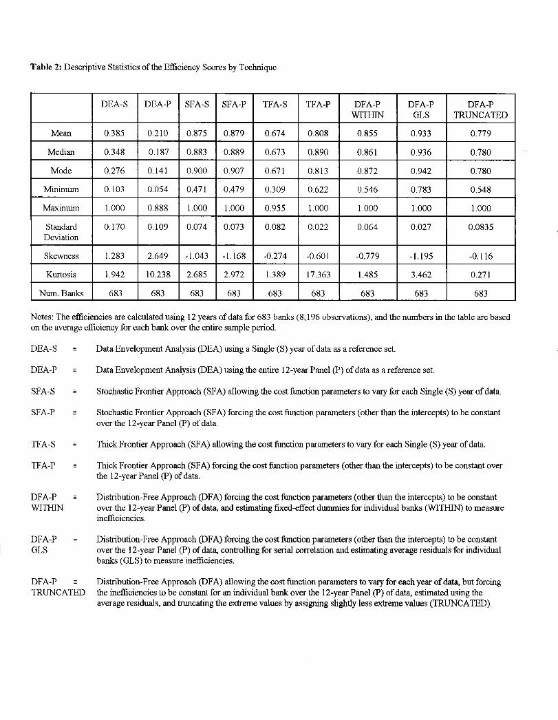
Table 2: DescriptiveStatisticsoftie EfficiencyS T

I Median I 0.348

HI Maximum I I.000

D S S T T D D DW G T

0 0 0 0 0 0 0 0

0,187 I 0.883 I 0.889 I 0.673 I 0,890 I 0.861 I 0.936 I 0.780

0 0 0 0 0 0 0 0

0 0 0 0 0 0 0 0

0.888 ] 1.000 I 1.000 I 0.955 I 1,000 I 1.000 I 1.000 I 1

0 I 0 I 0 I 0 I 0 I 0 I 0 I 0

1 1 I 1 1 I 1

2 - - - - - - -

1 2 2 1 1 1 3 0

6 6 6 6 6 6 6 6

N T e fa c au y d f 6 b ( o a t n t t a bt a e ff e b o t e s p

D

D

S

S

T

T

DW

DIG

DT R

———

———

—

——

———

———

—

———

D E nA @ u a S ( y d a r s

D E nA @ u t e 1 P ( d a r s

S tF A ( a t c f p v f e S ( y d

S tF A ( f t c t p ( t t i co t 1 P ( d

T F A ( a t c f p v f e S ( y d

T F A ( f t c f p ( t t i c ot 1 P d

D i sA @ f t c f p ( t t i co t 1 P ( d a e f d f i b ( mi n

D i sA @ f t c f p ( t t i co t 1 P d c f s c a e a r f ib ( m i n

D i sA ( a t c f p v f e y d b ft i nc f i b o t 1 P ( d e u ta r ea t t e v a s l e v (

Table 3: S Rank-OrderCorrelationsA t E S C V T

D D S S T T D D DW G T

D 1 0 0 O O 0 - - 0

D 1 0 0 0 0 0 0 0

S 1 0 0 0 ( 0 0

S 1 0 0 0 o 0

T 1 0 0 0 0

T 1 0 0 0

D 1 0 0W

D 1 0G

D 1

T R

N r t e n t r c ot averaveefficiencies t i b o t ar ea t c ou t e e f t s y a q s

* C os ts id f z t 5°/0level,@o-sided.**Conflationis statisticallysi@lcantly dtierent f z t 1°Alevel,two-sided.

Table4: Correspondence“ P a “ P B a T@ t s “ p a l t s “ p

D

ED

0D

0

S0

TD 0

WD 0

GD 0

I T RI

DEA-P SFA-S

0.760** 0.357

0.351

0.368

0.316 0.877**

0.374 0.725**

0.368 0.778**

0.374 0.491**

0.345 0.532**

0.357 0.895**

S T T D D DW G T

0 0 0 0 0 0, , ,

0 0 0 0 0 0.368 ---1 1 I I I

0 0 0 0 0 0

0 0 0 0 0

0 0 0 0 0

0.790** 0.854** 0.591** 0.632** 0.813**

0 0 0 0 0

0 0 0 0 0

0 0 0 0 0

N E n t u t a t p b t a i o t h e s t-. .-M e f2 b t a a i t ~ e 2 t o t

E n t l t t p b t a i o t h e s t ~e f2 b t a a i dt ~ e 2 t o t

* C os ts id f 0 t 5 l tC os ts id f 0 t 1 l t

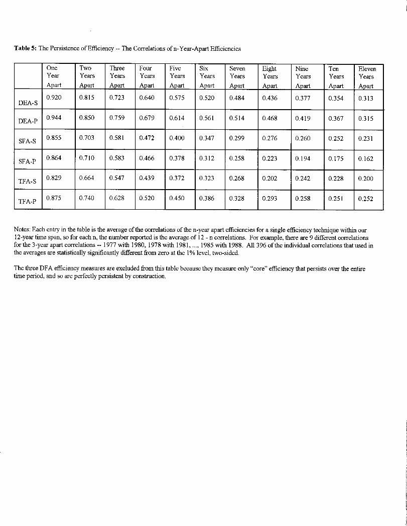
Table5: T P eE fT C on E

O T T F F S S E N T EY Y Y Y Y Y Y Y Y Y YA A A A A A A A A A A

0 0 0D

0 0 0 0 0 0 0 0

D 0 0 0 0 0 0 0 0 0 0 0

S0 0 0 0 0 0 0 0 0 0 0

S0 0 0 0 0 0 0 0 0 0 0

T 0 0 0 0 0 0 0 0 0 0 0

T0 0 0 0 0 0 0 0 0 0 0

N E e t t t a t c ot n a e f a s e t w o1 t s f e t n r t a 1 n c F e t a 9 d cf t 3 a c o- w 1 1 w 1 . 1 w 1 A 3 t i c t ut a va s ts id f z t I l t

T t D e fm a e h t t b t m o “ e t p o t et p a a p ep ec o

Table6:E fC ow S N oP M

D D S S T T D D DW G T

O 0 0 0 0 0 0 0 0R

O 0 0 0 0 0 0 0 0- -

0 1 0 0 0 0 0 0 0 0-

- - 0 0 0 0 0 0 1 0-B

N r t e n t r c ot avera~eefficienciesand~ standardnofiontierperformance——m et i nb o t a r a t c u t e e f t s y aq s i

* C os ts id f z t 5 l tC os ts d h z t 1 l t

ROA =—

-TCITA z- ——

- L❑

r an t c oan t c orn n e p b o