IPTEK, The Journal for Technology and Science, Vol. 21, No. 1, February 2010 1

AbstractIn this paper, a micromechanical model based on the Mori-Tanaka method and the spring-layer model is developed to study the stress-strain behavior of concrete. The concrete is modeled as a two-phase composite. And the failure of concrete is categorized as mortar failure and interface failure. The research presents a method for esti-mating the modulus of concrete under its whole loading process. The proposed micromechanical model owns the good capabilities for predicting the entire response of con-crete under uniaxial compression. It is suitable that tensile strain is as the criterion of concrete failure and the prediction of crack direction also fits with experimental phenomenon.

KeywordsMori-Tanaka method, interface, mortar, Weibull distribution

I. INTRODUCTION

ecently some researchers studied the elastic properties of concrete using the micromechanical

model [1]. The interface zone is usually considered as a new elastic phase. However, concrete contains many microcracks, especially in the interface zone, even before any loading is applied (Fig. 1). Some experiments have shown that the matrix just surrounding the aggregate is found to have quite different stiffness properties than that away from the aggregate[2]. Here concrete is considered as a kind of two-phase composite (the mortar and coarse aggregates). They are bonded together by the interface zone. Softening of concrete is considered as the appear-ance and development of microcracks.

II. BASIC FORMULATION

In the Mori-Tanaka method, consider an infinitely ex-tended mortar medium D containing many spherical in-clusions (coarse aggregates) with an imperfectly bonded interface (Fig. 2). The elastic stiffness of the mortar and coarse aggregate are L0 and L1. Homogeneous boundary condition in the external surface S of D is employed:n(S) = 0.n (1)where 0 is constant stress tensor, and n denotes the ex-ternal normal to the external surface S. If the solid did not contain any inhomogeneity, the strain field would be0 = L0

-1.0 (2)The stress and strain in mortar differ from 0 and 0 by

~ and~ . ~ is the perturbed strain due to the presence of all the coarse aggregates. The average stress is

~~ 00

00 L (3)

1Endah Wahyuni is with Department of Civil Engineering, FTSP,

Institut Teknologi Sepuluh Nopember, Surabaya, 60111, Indonesia. E-mail: endah@ce.its.ac.id.

The stress and strain of the coarse aggregates expe-rience further perturbations from those of the surround-

ing mortar by pt and pt . The average stress in aggre-gate is

*0

0

01

01

~

~

~

pt

pt

pt

L

L(4)

here * is the equivalent transformation strain. There is an assumption that the two sides of interface

always are connected with each other so there is only the displacement jump. The interfacial traction remains con-tinous, while both the normal and the tangential dis-placements might experience a jump across the interface [3]. The interface conditions is[ij]nj = 0 (5)[ui] (ik-nink) = T.Tk (6)[ui]nink = N.Nk (7)

In which T and N denote the compliance in the tangential and the normal directions. [.] =(out)-(in), ni is the outward unit normal on the interface, and Ti=kj.nj(ik-nink) and Ni=kj.nk.nj.ni represent the shear and the normal tractions. ij is the Kronecker . T and N

should be positive.For the coarse aggregates with imperfect interface, we

have the relationship between the eigenstrain and pertur-bation strain in coarse aggregates isij

pt = Sijkl.kl* (8)

whereSijkl

Eijklijkl SSS (9)

Here EijklS is Eshelby's solution for uniform eigenstrain

problem of inclusion with perfectly bonded interface. For the spherical inclusion, it gives

klijEE

jkiljlikEE

ijklS 3

1

2

1 (10)

with

0

0

115

57333322221111

EEE SSS ,

0

01122 115

1533222211113333112233

EEEEEE SSSSSS ,

0

0

115

54313123231212

EEE SSS .

where

0

0

0

0

115

542,

13

1

EE (11)

Here 0 is Poisson's ratio of cement paste. If there is an infinite medium D containing a uniform eigenstrain ij

*

in a spherical inclusion with an imperfectly bonded

Concrete Failure Modeling Based on Micromechanical Approach Subjected

to Static LoadingEndah Wahyuni 11

R

2 IPTEK, The Journal for Technology and Science, Vol. 21, No. 1, February 2010

(a)

(b)

Fig. 1. The microstructure of transition zone in concrete by use of SEM(a) Normal concrete; (b) High performance concrete [14]

Fig. 2. Three-Phase model with imperfect interface

Equivalent homogeneous medium

Mortar

Interface (Non-thickness spring layer)

Coarse aggregate

Spring Layer Model

n

t

Spring Layer Model

IPTEK, The Journal for Technology and Science, Vol. 21, No. 1, February 2010 3

interface , which is modeled by an equivalent Somigliana dislocation field [4], we define S

ijklS is*kl

Sijkl

Sij S (12)

where

Sij

Sji

Sij uu ,,2

1 (13)

Here siu is the displacement field caused by the inter-

facial sliding and normal separation. Sij is the body

average of Sij inside the spherical inclusion:

drrddR

dVV

R SijV

Sij

Sij

0

2

0

2

03sin

4

31

(14)

If we separate Sij into its hydrostatic and deviatoric

components, we can write (12) as

*

*

''ij

SS

iji

kkSS

kk

(15)

Furthermore, for spherical inclusion, we have

*

*

''ij

SEpt

ij

kkSEpt

kk

(16)

The perturbation stress can also be divided into two parts

SEpt (17)

In this case, Eshelby's solution for spherical inclusion with perfect interface gives

*

0*

00

0 '573110145

2ijijll

Eij

(18)

where 0 is the shear modulus of cement paste phase, 0

Poisson's ratio of cement paste phase, and ij’* is the

deviatoric part of ij*.

The stress S inside the inclusion [4] is

*

002

*

00

2

*

002

*

002

2*

000

0

*

00

200

*

00

00*0

0

00

'53

7'1072

'12'12'472135

4

'15

24'115

572

13

14

ijijlk

kl

iljl

jlilij

ijlkklijijllSij

Ba

xxB

a

xxB

a

xxB

a

xB

xxBa

A

where a is the radius of the spherical inclusion (aggregate) defined by xi.xi < a2 for which ni=xi/a. According to Zhong and Meguid's derivation, it is

10

100 13 k

k

(20)

4320040320

43200200 1 kkkkkk

kkkkA

(21)

4320040320

2000 1 kkkkkk

kB

(22)

with

aaNT

00

00 ,

0

04

0

03

0

02

0

01

1105

11354,

1105

1974

115

572,

13

14

kk

kk

We solve the body average of S, as

ijllSij

Sij dV

V

*0

0

00

13

141

*

0

0000 '175

25572ij

BA

(23)

According to Equation (16), we have*

*' '

pt

pt

(24)

whereSESE , (25)

0

0000

0

0

175

2557,

1

212

BASS (26)

If denotes the overall average stress tensor and ci (i= 0, 1) represent the volume fractions of cement paste and aggregate, separately, we have

11

00 cc (27)

If there is not special statements below, hydrostatic and deviatoric components of the stress and strain tensors will be written as and ’, , and ’.

When the geometry of coarse aggregates is considered as sphere, the average stresses in the mortar and the coarse aggregates then follow Eqs. (3), (4), (24), and (27), as

01010

0100

cc

(28)

''

01010

0100

cc

(29)

01010

11

cc(30)

''

01010

11

cc(31)

where i (i = 0, 1) are the bulk moduli of mortar and

coarse aggregates and i (i = 0, 1) are the shear moduli of mortar and coarse aggregates. The strains are their forms by

0

01010

0100

cc(32)

0

01010

0100 ''

cc(33)

0

01010

01

cc(34)

0

01010

01 ''

cc

(35)

The body average of the strain can be defined as

S ijjiijijij dSnunuV

cc2

111

00 (36)

in which V is the volume of whole body [5].According to Zhong and Meguid's solution, [ui] can be

written as :

ilkkljijilli xxxBa

xAxu*'

02

*'0

*0

1 (37)

Substituting Eqs. (32), (33), (34), (35), and (37) into Eqs. (36), we have

0

01010

010100

cc

cc (38)

0

01010

010010 ''

cc

cAc (39)

(19)

4 IPTEK, The Journal for Technology and Science, Vol. 21, No. 1, February 2010

Thus we further leads to the effective bulk and shear moduli of the concrete as

010010

01010

0

cc

cc (40)

010010

01010

0

cAc

cc (41)

Due to the isotropy of concrete here, and known, the Young's modulus E is

3

9E (42)

III. RESULT AND DISCUSSION

Weibull statistical distribution function has been applied broadly in the field of damage mechanics and concrete failure analysis [5-8]. Lambrigger pointed out Weibull function could correctly characterize the strength and failure of macroscopically homogeneous specimens [9]. Here it is applied to evaluate the failure volume of mortar and interfaces.

In the framework of Mori-Tanaka method, the modulus of concrete is calculated by the procedure in Fig. 3 if on-ly the effect of interfaces is considered.

We assume the volume ratio of aggregates, whose in-terfaces have been destroyed, conform to a Weibull dis-tribution function. Its form is

m

theci

1 (43)

where ci is the volume ratio of interface failure, is the effective strain of concrete. In the state of the pure com-pressive stress, is equal to 3. The '3' means the com-pressive stress direction. The th is the strain threshold, in the state of pure compressive stress, it should be equal to the peak strain of concrete, which is corresponding to the strain value when the concrete reaches the ultimate com-pressive stress (about th 0.002). If we consider that ci

should be equal to 1 when is equal to th, we normalize Equation (43) and have

11

1

e

ec

m

th

i

(44)

The Weibull distribution can model the distribution of microscopic flaws in the material. The following equation is used to decide the failure volume ratio under the current principal tensile strain.

11

1

11

e

ec

mm

tensileu

tensile

m

(45)

where 1 is the first principal tensile strain in mortar, tensile is a strain threshold value (when 1 reach the value, the cracks appear in mortar), u is the maximum tensile value (when 1 reach the value, the mortar is completely destroyed), mm is a shape index.

Here the main failure reason of concrete is considered as the development of microcracks in mortar and interface microcracks. Microcracks in mortar are considered as a series of aligned microcracks. Interface microcracks are considered as a kind of non-thickness spring layer.

In order to calculate the modulus of concrete, firstly, the modulus of mortar is computed. The principal tension causes the initial aligned microcracks arising if

the principal tension strain reaches the critical value. These aligned microcracks should be perpendicular to the direction of the principal tension strain. These a-ligned microcracks are considered as a kind of materials whose modulus is zero.

For the two-phase composite, we have Equation (46) to follow to solve the overall modulus of composite accord-ing to Mori-Tanaka method [10].L = L0 + c1 [(L1 – L0) T] [c0.I + c1 [T]]-1 (46)withT = [I+(c0.S + c1.I)L0

-1(L1-L0)]-1

Here subscript 0 represents matrix and subscript 1 is inclusion.

Microcracks in mortar are considered as a kind of aligned crack. They can be modeled as a sort of special constituent in composite: void. So we have

100000 1 TcIcTLcLL mmm

(47)

with

1

01

000 1 LLIcScIT mm

Here cm is the volume ratio of cracks in mortar and 0 represents the material properties of mortar. If there is a series of aligned inclusion in a certain composite (Fig. 4), the corresponding Eshelby's tensor can be given as the following Equation (11):

4

100000

04

10000

0018

43000

00018

45

18

14

212

00018

14

18

45

212

000000

0

0

0

0

0

0

0

0

0

0

0

0

0

0

0

S

(48)

For the plane stress problem (Fig. 5), Equation (49) can be expressed like below.

21

00

018

45

12

000

0

0

0

00

S

(49)

When the principal tension reaches the critical value for cracking, we can calculate the current modulus for concrete. Using Equation (45) to get the current volume ratio of aligned microcracks for mortar, we can get the current modulus of mortar.

When the principal tension reaches the critical value for cracking, we can calculate the current modulus for concrete. Using Equation (45) to get the current volume ratio of aligned microcracks for mortar, we can get the current modulus of mortar.

After the modulus of mortar is calculated, the modulus of concrete can be solved. The volume ratio of interface failure for concrete is calculated by Equation (44). The modulus of concrete is shown as follows.

1100110

TcIcTLLcLL (50)

with

1

011

010

LLLIcScIT

IPTEK, The Journal for Technology and Science, Vol. 21, No. 1, February 2010 5

Fig. 3. Outline for calculation of concrete modulus

For the plane stress problem, the Eshelby tensor S can be expressed as the following equation.

200

03

2

3

033

2

S(51)

For perfect interfaces, we can get the modulus of con-crete for perfect interfaces: Lp. And we can get the mo-dulus of concrete for interfaces destroyed: Ld.

For a certain load stage, the overall modulus of con-crete is

dipi LcLcL 1 (52)

IV. MODEL PARAMETER

Here the main parameters are the shape index: m, mm,and the threshold value of strain: εu, εth. These para-meters usually can not be measured directly. Based on si-mulation for concrete, m and εth, related to the interface failure and compression of concrete, are set to 3 and 0.008. mm and εu are related to the mortar failure and ten-sion of concrete and the basic assumption of concrete failure is tensile strain. Here εu is defined as follows [12, 13].

mt

Fu lf

G2 (53)

where ft is tensile strength for concrete, GF is fracture

energy of concrete and lm is eigen-length for mortar. According to CEB-FIP Code (1993), we have the simple empirical formula relating GF (J/m2 = N/m) to the con-ventional quality control parameter–namely the mean compressive strength of concrete fc’ (MPa) [7] as GF = αF (f’c)

0.7. The empirical coefficient αF depends on the maximum aggregate size g (Table 1). Normally, the compressive strength of concrete is given in the common experiment. If the proposed model is used, the tensile strength should be calculated by some empirical equations. There is an empirical formula, which has been suggested by ACI Committee 209 for computing the direct tensile strength of different weight concrete.

'

3

1ct wff psi; w in pcf; and f’c in psi

If we change all of the units to SI units, we have the following equation:

'2187.0 ct wff kPa w in kg/m3 and f’c in kPa (54)

For normal weight concrete, f’c, ft are expressed in MPa by the following equation:ft = 1.5909 f’c

1/2 (55)Then the parameter lm should be defined. According to

Bazant's random particle model, there is lm = βF.g and roughly βF is considered to be equal to 1/2. The expression of εu can be written like the following equa-tion.

gf F

cu

2.0'5143.2 (56)

Major unknown parameter0 Tangential parameter of interfaces0 Normal parameter of interfaces

Condition 1When interfaces are perfect

0 = 00 = 0

Condition 2When interfaces are imperfect

0 0

Using Eqs. (20), (21), and (22) get the parameter 0, A0, and B0

Using Eqs. (11), (25), and (26) get and

Using Eqs. (40), (41), and (42), calculate the modulus of concrete

Step 1:Decide the value of the two important parameters

Step 2:Compute the corresponding parameters further

Step 3:Get the modulus of concrete

6 IPTEK, The Journal for Technology and Science, Vol. 21, No. 1, February 2010

TABLE 1.COEFFICIENT αF WITH MAXIMUM AGGREGATE SIZE g

(KARIHALOO, 1995)

Maximum Aggregate Size g(mm) αF

8 4

16 6

32 10

TABLE 2.SPECIFIC WEIGHT RATIO FOR MORTAR AND CONCRETE

Grade Cement Sand Water Coarse Aggregate

G40 Mortar 1 2.8 0.35 None

GC40 Concrete 1 2.8 0.35 2.8

GC50 Concrete 1 2.8 0.35 1.4

TABLE 3.ELASTIC PROPERTIES OF G40 MORTAR

Initial Modulus (GPa)

Compressive Strength (MPa)

εu mm

25.3 37.74 0.0016 1.51

If these parameter values of the certain concrete are given in experiments, the proposed model can predict the stress-strain behavior very well. Studies in this research show the mm is related to the strength of mortar. The stronger the strength of mortar, the larger the value of mm

is εu is related to the ductile properties of concrete. The smaller the strength of mortar/concrete, the better the ductile properties of concrete or mortar is so εu is larger. When we do not know the exact value of mm and εu, we should use Equations (57) and (58) to calculate them. Here εu is revised as εr. For the different strength level, the following equations are recommended to calculate the ultimate tensile strain and mm.

48.205101.359.134.3 uer

(57)57.31.055.74.8 emm

(58)

where

r

u

V. DAMAGE EFFECT

Here it is worth nothing that the lateral deformation in-creases significantly at higher stress level after the peak loading point. And the large cracks appear and crack growth becomes unstable. Therefore, the change from volume decrease to sudden volume increases leads to find a proper way for the description of lateral strain du-ring the descending branch. Here the following equation

is assumed to modify the behavior of lateral strain after the peak loading point under uniaxial compression.

laterale

lateral

l

e 5667.1

200

whereλ1 = 1 - compression /f’c

Fig. 4. Mortar with aligned microcracks (3D)

Fig. 5. Mortar with aligned micro cracks

There are some suitable experimental data available [14]. The concrete and mortar are tested. The mortar and concrete were pan-mixed in the laboratory and were cast in steel moulds (100 mm in diameter and 200 mm in height). The mix design is shown in Table 2. The pro-perties of mortar are shown in Table 3.

In Fig. 6, it is shown that the proposed model can pre-dict the mortar behavior very well, especially for the as-cending part and the peak point. It is also shown that the aligned microcrack model can properly evaluate the failure of mortar.

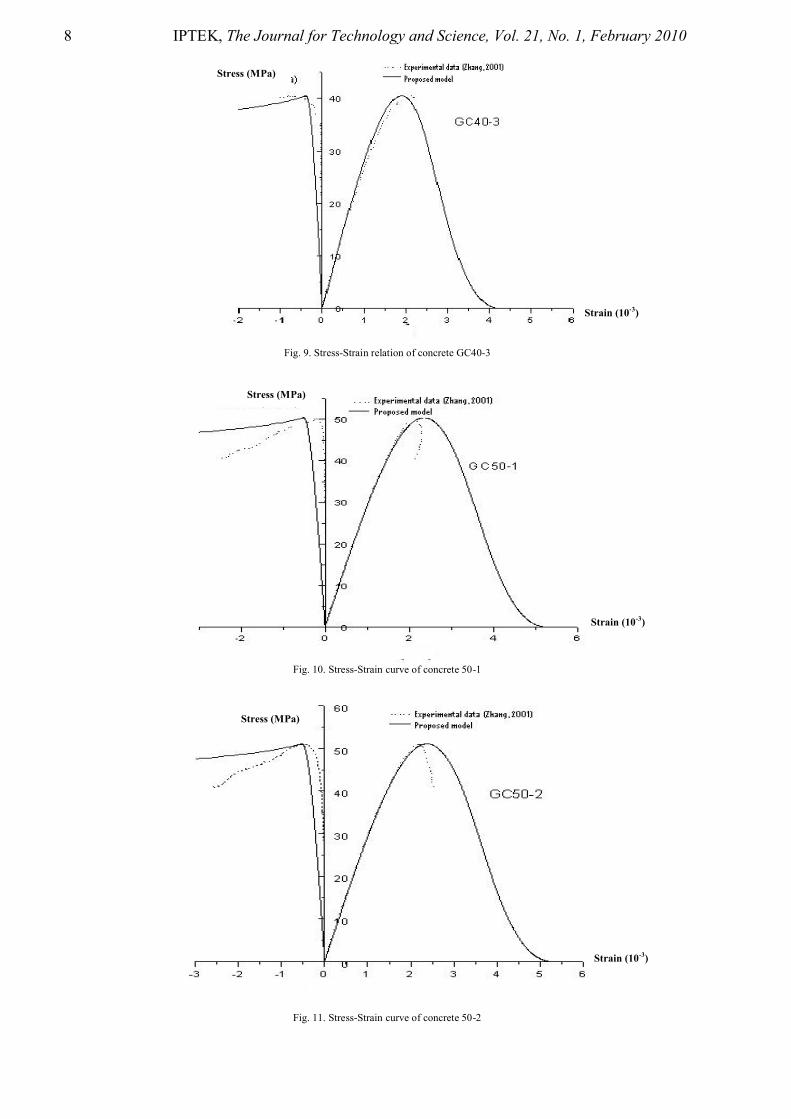
The proposed model is further used to predict the com-pressive behavior of concrete. The volume ratio of mor-tar and coarse aggregates (Table 4) can be calculated if their densities are known. Here they are assumed. All related data are shown in Table 4. These responses of the predicted compressive behavior are shown in Fig. 7- Fig. 12. These results also show that the comparison for late-ral strain does not agree very well. The main reason is that the behavior of concrete in the tensile direction is considered in the model to be that of a continuum mate-rial no matter how serious the cracks are.

In order to explore the model capabilities of predicting the transition in behavior from low to high strength con-crete, the experimental data for different strength level of concrete are collected in Tables 5 and 6. In comparison with that obtained experimentally, these predictions are very accurate shown in Fig. 13 and Fig. 14.

x1

x2

x3

AlignedCrack

---- Aligned Crack

---- Aligned Crack

IPTEK, The Journal for Technology and Science, Vol. 21, No. 1, February 2010 7

Fig. 6. Stress-Strain curve for mortar

Fig. 7. Stress-Strain relation of concrete GC40-1

Fig. 8. Stress-Strain relation of concrete GC40-2

Stress (MPa)

Strain (10-3)

Stress (MPa)

Strain (10-3)

Stress (MPa)

Strain (10-3)

8 IPTEK, The Journal for Technology and Science, Vol. 21, No. 1, February 2010

Fig. 9. Stress-Strain relation of concrete GC40-3

Fig. 10. Stress-Strain curve of concrete 50-1

Fig. 11. Stress-Strain curve of concrete 50-2

Stress (MPa)

Strain (10-3)

Stress (MPa)

Strain (10-3)

Stress (MPa)

Strain (10-3)

IPTEK, The Journal for Technology and Science, Vol. 21, No. 1, February 2010 9

Fig. 12. Stress-Strain curve of concrete 50-3

Fig. 13. Stress-Strain curves of different strength for concrete

Fig. 14. Stress-Strain curves of different strength for concrete [15]

Stress (MPa)

Strain (10-3)

Stress (MPa)

Strain

Stress (MPa)

Strain

10 IPTEK, The Journal for Technology and Science, Vol. 21, No. 1, February 2010

TABLE 4.PROPERTIES OF CONCRETE

GradeDensity of Mortar (assumed) (kg/m3)

Density of Coarse Aggregates (assumed)

(kg/m3)

Volume Ratio of Mortar

Elastic Modulus of Concrete

(GPa)

Elastic Modulus of Coarse Aggregates (GPa)

GC40-1 2400 2640 0.6198 32.69 50.69

GC40-2 2400 2640 0.6198 30.78 42.7

GC40-3 2400 2640 0.6198 30.25 40.69

GC50-1 2400 2640 0.7653 31.02 63.41

GC50-2 2400 2640 0.7653 31.06 63.83

GC50-3 2400 2640 0.7653 31.31 66.57

TABLE 5.MATERIAL PROPERTIES AND COEFFICIENTS FOR THE PROPOSED MODEL (NEVILLE, 1996)

f'c(MPa) Ec (GPa) E0 (GPa) mm εu (10-3) εr (10-3)

20.8329 20.23 12.6347 0.9 1.7307 3.3

28.6999 24.66 16.6408 1 1.8452 2.9

35.7387 28.28 20.3116 1.25 1.9279 2.3

42.3858 30.34 21.2075 1.6 1.9948 2

55.8684 34.13 27.0243 1.8 2.1081 1.9

69.7838 37.53 31.3671 2.1 2.204 1.8

83.6917 38.98 33.3155 2.5 2.2856 1.8

TABLE 6.MATERIAL PROPERTIES AND COEFFICIENTS FOR THE PROPOSED MODEL (DAHL, 1992)

American Society of Mechanical Engineers, Applied Mechanics Division, AMD, Vol. 205, pp. 21-34

VI. CONCLUSION

The proposed micromechanical model owns the good capabilities for predicting the entire response of concrete under uniaxial compression. It is suitable that tensile strain is as the criterion of concrete failure and the pre-diction of crack direction also fits with experimental phenomenon. And Weibull distribution function can describe the behavior of crack development for mortar and interface.

REFERENCES

[1] G. Ramesh, E. D. Sotelino, and W. F. Chen, 1996, "Effect of transition zone on elastic moduli of concrete materials", Cement and Concrete Research, Vol. 26, No. 4, pp. 611-622.

[2] A. U. Nilsen and P. J. M. Monteiro, 1993, "Concrete: A three phase material", Cement and Concrete Research, Vol. 23, pp. 147-151.

[3] J. Qu, 1993, "The effect of slightly weakened interfaces on the overall elastic properties of composite materials”, Mechanics of Materials, Vol. 12, pp. 269-281.

[4] Z. Zhong and S. A. Meguid, 1996, "On the Eigenstrain problem of a spherical inclusion with an imperfectly bonded interface”,Journal of Applied Mechanics, Vol. 63, pp. 877-883.

[5] E. P. Chen, 1995, "Dynamic brittle material response based on a continuum damage model”, Impact, Waves, and Fracture.

[6] W. Weibull, 1951, "A statistical distribution function of wide applicability”, Journal of Applied Mechanics, Vol. 18, pp. 293-297.

[7] B. L. Karihaloo, 1995, Fracture Mechanics and Structural Con-crete, Longman Scientific and Technical.

[8] W. K. Yip, et al., 1995, "A statistical model of microcracking of concrete under uniaxial compression”, Theoretical and Applied Fracture Mechanics, Vol. 22, pp. 17-27.

[9] M. Lambrigger, 1997, "Alternative scaling of cumulative Weibull failure probability distribution functions”, Journal of Material Science Letter, Vol. 16, No. 19, pp. 1537-1539.

[10] Y. Benvensite, 1987, "A new approach to the application of Mori-Tanaka's theory in composite materials”, Mechanics of Ma-terials, Vol. 6, pp. 147-157.

[11] T. Mura, 1987, Micromechanics of Defects in Solids, Martinus Nijhoff Publishers.

[12] Z. P. Bazant, M. R. Tabbara, M. T. Kazemi, and G. Pijaudier-Cabot, 1990, "Random particle model for fracture of aggregate or fiber composite”, Journal of Engineering Mechanics, Vol. 116, No. 8, pp. 1686-1704.

[13] A. R. Mohamed and W. Hansen, 1999, "Micromechanical modeling of concrete response under static loading – Part 1: Mo-del development and validation”, ACI Materials Journal, Vol. 96, No. 2, pp. 196-203.

[14] J. G. Zhang, 2001, “Triaxial behaviour of cement mortar under monotonic loading”, Master Thesis, Nanyang Technological University.

[15] K. K. B. Dahl, 1992, A constitutive model for normal and high-strength concrete, ABK Report No. R 287, Department of Structural Engineering, TU Denmark, Lyngby.

f'c (MPa) Ec (GPa) E0 (GPa) mm εu (10-3) εr (10-3)

105.8 42.85 38.786 2.815 2.395 1.758

94.17 40 34.72 2.663 2.34 1.763

67.4 33.3 26.013 2.219 2.189 1.802

50.3 30 22.195 1.772 2.064 1.917

31.7 26.6 18.563 1.092 1.882 2.578

22 20 12.441 0.93 1.75 3.28