Computing our way to electric commuting in Africa: The data roadblock

A.J. Rix a, C.J. Abraham a, M.J. Booysen a,∗

aDepartment of E&E Engineering, Stellenbosch University, South Africa

Abstract

In the information age, the value of good data can hardly be overstated. Unsurprisingly, a severe lack

thereof is seen as a pothole on the road to the decarbonisation of Africa’s paratransit – the mainstay of the

region’s transport. Data acquisition in transport used to be concerned with the temporal flow rates and

volumes of passengers and vehicles on sections of roads. This was done with surveys and vehicle counting.

Separately, vehicle mobility data has been used for vehicle health monitoring, driver behaviour monitoring and

vehicle recovery. For paratransit in Africa, where passenger counts and routes are unknown (and fluid), and

where data acquisition is tedious, standardised passengers with tracking applications on phones are extensively

used for this purpose. This brings the meaning of “good data” in this region of low and lower-middle-income

countries into focus. Given the long ranges and fast refilling times of combustion engine vehicles, manufacturers

and fuel outlets had hitherto existed in a symbiotic relationship without the bondage of mobility pattern

information. However, in the era of electrification, battery-powered vehicles and their specifications and

limitations have become inextricably coupled to road-side infrastructure through their mobility patterns due

to their lower range and slower charge times. The infrastructure energy supply side can be modelled with

dated passenger-based or roadside-based gathered data, assuming unchanged patterns. But, the charging

potential calculations requires stationary rather than moving times. Moreover, energy demand per point is

effectively that of an individual vehicle, which depends on spatio-temporal mobility patterns and battery

capacity. Intermittent renewable energy generation further complicates this time variant challenge. In this

paper we use a public passenger-based data set that is normally used to characterise routes, which has over

300 000 trips, to establish the energy requirements of seven cities in Africa - Abidjan, Accra, Cairo, Freetown,

Harare, Kampala and Nairobi. The results show that the peak demand per city varies wildly, apparently with

the reliability of the city’s data, with realistic peaks of 100 MW to 300 MW. Although the results give an

indication of the supply side requirements, it highlights the problem with using incomplete and/or unreliable

data to estimate a city’s peak load, which points to a need for vehicle-based data acquisition to adequately

answer the question, or at least validate, the results.

∗Corresponding authorEmail address: mjbooysen@sun.ac.za (M.J. Booysen )

March 1, 2022

Keywords: Electric vehicle; Paratransit; Minibus taxi; Demand management; Renewable energy; Transport

data.

1. Introduction

“In light of the climate crisis, transport systems globally need to be decarbonised. This is particularly

challenging in Sub-Saharan Africa (SSA) where transport systems are poorly characterised due to a lack of

data, which contributes to hindering investment. We call for a more systematic approach to data collection to

support the sustainable transition to electric vehicles in SSA.”—Collett and Hirmer [1] in Nature Sustainability.

Over the years, paratransit has become one of the most dominant forms of transport in Africa, providing

countless jobs and cheap transport for millions of people every day. Paratransit is a mode of informal public

transport, owned by small operators, and which does not follow fixed schedules or routes, but rather adapts

to passenger demand. Paratransit is characteristic of African cities, and accounts for over 70% of the modal

share (excluding non-motorized modes of transport) [2].

Although paratransit in the region takes various forms, such as minibus taxis, motorcycle taxis and

tuk-tuks [3], minibus taxis in particular have become ubiquitous throughout Africa. They are able to carry

many passengers and, moreover, they are available at low-cost, as second-hand imports from developed

countries. [4, p. 348] Unfortunately, this has led to the system being fraught with old, under-maintained

vehicles, causing a serious environmental concern. One study done on 12 African cities found that the average

age of minibus taxis was 15 years [5]. Powered by internal combustion engines, these vehicles contribute

greatly to the emission of greenhouse gases and a general decline of air quality in African cities [1].

Part of the reason that Africa’s public transport is in this state is that there has been very little regulation

on the paratransit industry. The paratransit industry originated from the collapse of state-owned public

transport throughout the continent, during the restructuring of World Bank policies in the 1990s [5–7]. As

a result, paratransit grew organically to fill this vacuum. By the time governments sought to control the

transition, the system had already grown to a size that made it resistant to change [2, 8].

Although there is a lack of regulation, it does create the advantage that the system has low barriers to

entry, encouraging small-business to enter the market. However, taxi operators also misuse this freedom to

cut-costs in taxi-maintenance in order to squeeze profits from this relatively flooded market. At the same

time, the urban poor have resigned to the poor standards of transport due to the fact that they cannot afford

any better.

Some countries have made various interventions to try to improve the quality, safety and environmental

footprint of these vehicles. While some of these countries have attempted to establish control through

2

regulation, this has often resulted in pushback by the paratransit sector. In other cases, countries have tried

to financially subsidise the sector to upgrade their fleets. This has been successful in economically advanced

countries such as South Africa, which incentivised taxi owners with around USD 7500when they scrapped

their old taxis [2]. However, in most African countries, paratransit subsidies do not exist and would be

unaffordable by the government [5].

Some countries have also tried to override the paratransit industry by competing against it with more

formal modes of mass transit, such as metro rail, bus rapid transit, etc. However, these have been fraught

with poor government spending, poor integration with existing paratransit, and general incompatibility with

the dynamic transport needs of the urban poor. All this has led to formal mass transit being a burden on the

tax-payer. [9]

In order to improve the state of transport in the future, a different approach needs to be taken. Sustainable

mobility needs to be achieved hand-in-hand with paratransit, using computer optimisation. One paradigm

through which to achieve sustainable mobility is the three-pronged “Avoid-Shift-Improve” approach [10, 11].

This paradigm follows three steps. The first is to avoid redundancy. For example, this can be done by reducing

redundant taxi trips through computer optimisation. The second step is to shift to alternative technologies

(e.g. electric vehicles). The software presented in this paper can be used to investigate the energy demands of

various technologies to select the best alternative. Finally, the last step is to continuously improve the new

technology through various efficiency upgrades. For example, an electric paratransit system can be enhanced

with more/faster charging stations, integration of solar energy charging, and more efficient vehicles. All three

of these steps require adequate data in order to drive the process.

Unfortunately, attempts at capturing paratransit data is surprisingly scarce, leading to poor decision

making [1]. A few known attempts conducted in Africa are summarised in Table 1, and is outlined in more

detail in the following paragraphs.

The paratransit data capturing approaches can be grouped into four categories: vehicle-based tracking,

passenger-based tracking, roadside-based counting and household travel surveys.

We have found that, out of these various paratransit data collection methods, the passenger-based tracking

method has become the most prevalent. A list of many such datasets can be found in [15] in addition to

the seven datasets used in this article (listed in Table 2). In order to compile this data into a consumable

digital format, several standards could be considered. Most of the datasets made use of the General Transit

Feed Specification (GTFS), which is an open format used for digitally specifying public transport routes and

schedules. Additional datasets were collected by a company called GoMetro [15] who use their own custom

specification. However documentation of their specification could not be found, and the GTFS standard is

3

Table 1: Paratransit data-capturing methods

Methods Strengths Weaknesses

Vehicle-based Track-ing: A selected number ofminibus taxis are installedwith GPS tracking devices.The tracking devices logthe position and speed ofthe taxi at various points intime. (Examples: [12, 13])

• Data is collected on a per-taxibasis. This allows one to analysethe net energy that a taxi uses onany day of operation.

• The times that the taxi makesstops between routes is known,allowing one to analyse how longthe taxi has to charge on any dayof operation.

• The data is extremely robust sinceit is collected continuously and thetaxi’s day plan is recorded repeat-edly. Hence, the data is updatedcontinuously.

• GPS traces do not inform whereand when a particular route stopsand ends. Neither does it informwhen a taxi stopped to deliverpassengers (as opposed to stoppingat a traffic light). Further dataanalysis needs to be done on thecollected data to make it useful.

• Capital cost can be extremelyexpensive.

• Tracking devices are liable to theft.

• High technical expertise requiredfor installation and maintenance.

Passenger-based Track-ing: Hired personnel aredeployed into the paratransitsystem with mobile trackingdevices. They travel in eachof the routes that exist inthe paratransit system, log-ging data regarding the stoplocations and times alongthe route. (Examples: referTable 2, [14, 15])

• Requires very little consultationwith paratransit operators.

• Minimal technical expertise re-quired.

• Can be cost-effective in countrieswhere uneducated labour is rel-atively cheap, if updating thedataset is not planned.

• Takes very long to obtain sufficientdata quality. Certain routes maytake very long to traverse, andneed to be taken multiple times inorder to obtain confidence in thedata.

• Data is collected on a per-routebasis rather than per-vehicle.Therefore, no information willbe available regarding the exactitinerary of each of the taxis.

• Data needs to be manually up-dated periodically.

Roadside-based Count-ing: Hired personnel arehired to stand at a partic-ular location (e.g. a para-transit terminal) and countthe number of paratransitvehicles passing or stoppingat that location. (Examples:[16–18])

• Requires very little consultationwith paratransit operators.

• Minimal technical expertise re-quired.

• Can be cost-effective in countrieswhere uneducated labour is rel-atively cheap, if updating thedataset is not planned.

• No information on the exactitinerary of each of the taxis.

• Data needs to be manually up-dated periodically.

Household Travel Sur-vey: Hired personnel aredeployed to households inthe region of study. House-holds then answer a ques-tionnaire regarding theirtravel patterns. (Examples:[19])

• Can be cost-effective in coun-tries where uneducated labour isrelatively cheap.

• Requires very little consultationwith paratransit operators.

• Minimal technical expertise re-quired.

• Data is presented at a very highlevel. Data is presented in anorigin-destination based format.No vehicle-based or route-baseddata.

• Data capture takes a lot of time,and might be difficult if sufficientrespondents can not be obtainedfor the study.

• Data needs to be manually up-dated periodically.

4

more widespread globally. This paper therefore makes use of the available GTFS data to:

• Forecast electric paratransit energy demands in the various paratransit systems.

• Evaluate the GTFS method’s suitability for electric paratransit forecasting.

• Validate if the quality of currently available GTFS paratransit data is acceptable.

This paper specifically focuses on minibus taxis, since that particular mode of paratransit is the most

prevalent across Africa [2]. While the various GTFS datasets contained various modes of paratransit, the

minibus taxi was the only mode present in all the available GTFS datasets.

GTFS was originally developed for formal public transport systems, which have predetermined timetables

and routes. In the case of paratransit, schedules and routes are fluid and based on the demand. Hence, it

becomes necessary to collect sufficient data in order to synthesise “typical” routes and schedules within a

boundary of confidence. The GTFS standard has provisions to capture (1) The shapes of the various routes,

(2) location, arrival time, and duration of stops along each route, and (3) what times of the day a taxi departs

on each route.

The popular approach for capturing this data for paratransit systems is the one pioneered by The Digital

Matatu Project [20]. This approach employs data collectors equipped with mobile phones who ride on the

taxis to collect data. As the data collector makes a trip on a particular route, the mobile phone records the

path taken, and the data collector will make a record when the taxi stops to drop off or pick up passengers.

The process is very manual. The advantage of this is that very little permission is required from the taxi

association to collect data, as nothing is installed on the vehicles. As a result, the capital cost of the data

capture is minimised.

However, there are some major disadvantages with this approach. First of all, the data is only valid

for as long as the paratransit system continues to follow the same movement patterns. However, in reality,

paratransit movement patterns often adapt to the evolving demand of its customers. Therefore, data will need

to be re-captured at regular intervals in order to keep the dataset up to date. Although unskilled labour is

often cheap in Africa’s developing countries, the cost can quickly compound due to the number of man-hours

required to collect the data. This could be the reason that none of the datasets we analysed have been updated

since their initial release.

DigitalTransport4Africa (DT4A) [14] is a recent concerted effort to collect GTFS data for paratransit

systems in African cities. The collection of datasets are hosted online, and can be used by the public for free.

Furthermore, the collection can easily be contributed to by the public, allowing for the public to add their

own GTFS data and request corrections to existing datasets. This has facilitated rapid growth to the size

5

of the collection. Currently, the site hosts GTFS data for the paratransit systems of 12 African cities. The

quality of this data will be evaluated in this paper, and the data will be used to estimate Africa’s readiness

for EV taxis, while at the same time highlighting how the state of the art in paratransit data collection can

be improved for future EV evaluations.

In sum, this paper will use the DT4A paratransit datasets to project the amount of energy that would be

required for electric paratransit in various African cities. The paper seeks to answer a few questions from this

data. Firstly, from the perspective of the grid: how much additional energy would the system require, and

what would the peak load be on the grid? Secondly, from the perspective of the vehicle: what battery size

would be required, and what are ideal times for the taxi to stop and charge? Finally, the paper will discuss

the suitability and reliability of using this data to answer these questions. If it is found that GTFS data is not

descriptive enough to answer some of our research questions, the paper will suggest alternative data schemes

or suggest how the current data scheme can be improved.

Our custom-built software, which we call EV-Fleet-Sim, was used to obtain the results in this paper. This

software and its source code can be downloaded from the following website: https://gitlab.com/eputs/

ev-fleet-sim. We publish the software for free use and modification, subject to the terms of the GPLv3

license. The data [14] is also publicly available, allowing for easy reproduction of the results.

2. Method

GTFS datasets were obtained for ten African cities from DigitalTransport4Africa [14]. These datasets

described the schedules, routes, and stop locations of minibus paratransit. Although the methods described in

this paper should be extendable to any other form of public transport that can be described in the GTFS

specification, minibus paratransit is quite unique in that it is highly unregulated. Because of this, the compilers

of these GTFS datasets were required to do their own data collection in order compile their GTFS datasets.

This meant that varying approaches were used in this process, each with varying degrees of scientific rigour

and reliability.

2.1. Data Reliability Analysis

Therefore, the first step was to inspect the datasets and the methods used to compile them, in order to

evaluate their reliability. This was done in a systematic way. As discussed in the introduction, a few methods

of paratransit data-collection exist. By reading through the literature surrounding each dataset and contacting

the various dataset compilers, it was possible to obtain the details of the methods used to collect the data

behind seven of the ten datasets.

6

In the case of this study, all the datasets were compiled using the approach of deploying human data-

collectors into the field. We selected a couple of metrics that could be used to give an idea of how the data

was collected and how much effort was put into collecting the data and keeping it up to date. The chosen

metrics include:

• Whether data-collection was passenger-based or roadside-based :

– Passenger-based data collection means that the collectors boarded the minibuses as passengers,

and recorded data by travelling the various routes.

– Roadside-based data collection means that the collectors stood at the various terminals, recording

the frequency at which taxis arrive and depart.

• Months since last update: Indicates whether the dataset is being kept up to date.

• Number of human data collectors: More data collectors would indicate more effort put into collecting

the data.

• Number of weeks of data collection: A longer data collection period would indicate more effort put into

collecting the data.

We tabulated these metrics for each of the seven cities in order to compare the rigour with which their

data was captured. Furthermore, we classified the effort behind each dataset into three categories: high,

medium and low.*1

However, in order to make a fair comparison of the reliability of the datasets, it was also necessary to

capture metrics that would illustrate the size of each dataset. A larger dataset would naturally require more

effort to capture. Hence, another table was generated with the following metrics to get a context of the size of

each dataset.

• Number of routes: The data capturers would need to make at least one trip on each route of the

paratransit system. Hence, more routes there are, the more effort required to complete the data

capturing project.

• Number of trips per day: Each day, multiple trips are taken on a particular route. This metric summarises

how many trips are taken per day across all the routes of the transport system.

*1We classified datasets with less than 50 man-weeks as low effort, less than 100 man-weeks as medium effort, and above 100man-weeks as high-effort.

7

• Geographic spread of the transport system: This is the area in km2 of the transport system, as derived

from the dataset. This is calculated by creating a bounding box from the minimum and maximum

coordinates that are recorded in the transport system’s route definitions, and calculating the area of

that bounding box. A larger geographical spread would indicate that the routes are longer. A longer

route, would probably require more time to capture than a shorter route.

We therefore classified the size of each dataset as small, medium or large. For example, a dataset with

many routes and a large geographic area, would be classified as “large”.*2

From these classifications, it was possible to evaluate the reliability of each of the datasets. This was

done by comparing the effort to the dataset size. If the level of effort was less than the dataset size, then the

dataset’s reliability was classified as “low”. If the effort was equivalent to the level of the dataset size, then it’s

reliability was classified as “medium”. If the effort exceeded the level of the dataset size, then it’s reliability

was classified as “high”. For example, a dataset with with of a medium size would have its reliability classified

as “low” if the effort was low, “medium” if the effort was medium, and “high” if the effort was high.

2.2. Minibus taxi mobility modelling from data

For each of the cities, the following method was used to create a simulation-ready model from the data:

The first step was to obtain geographical data that would describe the road network and terrain that

the paratransit system operates in. We were able to utilise a free dataset developed by OpenStreetMap [21].

The download server stores the data as one file per country. Therefore, we were forced to download the

data for the whole country in which the city lies [22]. For each of the routes defined in the GTFS file, we

searched for the coordinates of the smallest possible rectangular bounding box which would enclose all the

routes of that city. We then cropped the geographical data to the bounding box, using the OSMConvert

program [23]. This would extract only the appropriate section of the data for our study, greatly reducing

simulation overhead. This geographical data was then converted to a simulation-ready road network using the

Netconvert program [24].

The software searched this road network to find the exact path (sequence of roads) that the simulated

taxi must follow to go from one stop to the next. The location of these stops were extracted from the GTFS

file [25]. The times and sequences of the stops were also extracted and combined with the paths generated in

order to create route plans, files which direct the movement of the electric vehicle model during the simulation.

*2We multiplied the routes with the area (in km2) for each of the datasets. If the resulting value was below 200 thousand, itwas classified as small. Values below 400 thousand were classified as medium, and values above 400 thousand were classified aslarge.

8

The Dijkstra algorithm was used for solving the paths [24]. This algorithm chooses between various

optimisation objectives when solving for a path: time, distance, energy-usage, etc. We chose to use distance,

as it is the computationally cheapest optimisation [26]. However, for more realistic paths, the time objective

should be used instead. With the distance objective, the algorithm might choose short paths that go along

roads with low speed limits and possible congestion. For example, it might choose a path through the city

rather than along the highway. With the time objective, the algorithm might choose the highway option,

which is longer in distance but shorter in time. This would be more realistic, because the taxi driver would

prefer the quicker option.

For each route, the route plan was generated by traversing through the route’s sequence of stops. For

each stop, the nearest road on the road network from the stop’s coordinates was found, and the shortest path

from the road of the previous stop to the current road is calculated. This path is appended to the route plan

being built. The route plan also specifies that the simulated vehicle should stop on the current road until the

departure time of the current stop. This process is illustrated in Algorithm 1.

foreach city doforeach route do

Initialise the route plan as an empty list;foreach stop do

current road := Find the nearest road to the stop’s coordinates;if previous road was found then

Calculate the shortest path from previous road to current road;Append this path to the route plan;Append stop’s timestamp to the route. It will be the departure time from the current stop;

end/* Store the current road for the next iteration. */

previous road := current road;

endSave the route plan;

end

end

Algorithm 1: Route plan algorithm.

2.3. The Taxi EV model

With the route plans established, the next step was to define an electric vehicle model that can follow

the route plans. The model would need to be configurable and use the route’s distance, road inclination and

curvature to evaluate the electric vehicle’s energy usage.

The SUMO software [24] was used for this purpose. The electric vehicle model built into SUMO allows

the user to set various parameters. Since the focus of this study is minibus taxis, a common minibus taxi,

namely the Toyota Quantum, was used as a basis for the EV parameters. The following model parameters

were chosen from the Quantum’s geometry:

Height: 2.3m, width: 1.9m, front-facing surface area: 4m2, weight: 2900 kg.

9

We approximated the rest of the parameters according to the recommendations by Fridlund and Wilen

[27]. These include:

Constant power intake: 100W, propulsion efficiency: 0.8, recuperation efficiency: 0.5, roll drag coefficient:

0.01 and radial drag coefficient: 0.5.

The software initialised the EV model for each route that was defined in the GTFS file. The EVs followed

the route plans, obeying all speed limits, traffic signals, etc. as defined in the road network. For every second

of simulation time, the simulator outputted the energy consumption and speed of the EV as it progressed

along its route.

The simulation resulted in energy and power usage profiles of each of the routes. The GTFS file defines a

frequencies.txt file. This file indicates the frequency at which new trips commence on each route, for various

periods of the day. For example, a new trip may commence on a particular route every 30 minutes from 6

AM to 8 AM, and every 10 minutes from 8 AM to 9 AM. Based on this frequency data, the results were

replicated for the trips on each of the routes.

With an average of 45,000 daily minibus taxi trips per city, the volume of output data from the simulation

was substantial. Our goal was to obtain useful metrics that would summarise this data. The first metric we

considered was the total power usage profile of the whole electric minibus paratransit system. Such a profile

would indicate how much power the system would require at various times of the day. This profile would be

indispensable, for example, for identifying the peak strain that the electric fleet would have on the grid. It

could also indicate what times this strain would occur.

We calculated this profile as follows: First we retrieved the power-vs-time results of each trip, to generate

power profiles of each trip. For each route, we aggregated power profiles of the trips done on that route, to

get the total power profile of the route. Finally, we aggregated the power profiles of all the routes in the taxi

system, to get the total power profile of the city’s taxis. The profile was plotted with respect to time.

In addition to the power usage characteristics, the energy usage of the minibus taxi system was also of

interest. The power profiles obtained in the previous step were integrated with respect to time, in order to

obtain energy-vs-time profiles. The net energy profile of the minibus taxi system of each city would give an

estimate of the total daily energy usage, how much energy was saved due to regenerative braking, and how

much energy would be used between times of relative inactivity.

Finally, for each city, box plots were created to show the median energy usage of the routes, as well as the

spread of energy usage across the various routes of the city.

In order to verify the results, we generated a table of the characteristics of paratransit in the various

cities. The simulation results were compared to these characteristics to see if they corresponded. We chose

10

characteristics about the city that would indicate the magnitude of its transport needs. The following metrics

were chosen for this purpose:

• Number of taxis: A higher number of taxis would indicate that there are probably more trips to be

serviced, and hence more energy would be required.

• Number of inhabitants: A city with more inhabitants would have higher transport needs, and, hence,

more energy usage could be expected.

• Modal split of minibus paratransit: If a higher percentage of trips are taken via minibus taxis, as

opposed to other modes, the energy usage would be higher.

After further investigation, we found that some of the cities did not have reliable, up-to-date statistics on

the number of taxis. We therefore used the remaining two metrics to classify the expected energy demand as

high, medium or low.*3

3. Results and discussion

This section will discuss the results obtained from the various steps of the methodology. It will first

attempt to investigate the reliability of the data. After this, it will use the data reliability investigations

to discuss what can be expected from the simulation. The simulation results will then be presented, and

correspondence with the data reliability investigation will be highlighted. Finally, the simulation results will

be verified with the verification metrics discussed in the methodology. Throughout this section, we will suggest

reasons for data reliability issues and the consequences thereof.

3.1. Data Reliability Analysis

Since the various datasets were collected by different independent entities, the effort taken varied for each

set. Table 2 captures a few metrics that indicate the method, recency, and rigour with which each dataset was

collected. For each city, we evaluated the effort made to capture the data based on these metrics. Many data

collectors and many weeks of data collection would imply that more effort was taken in the data collection

process.

Due to the fact that four of the seven datasets were missing sufficient documentation, we were unable to

populate some of the cells. Unfortunately, this reduced our ability to interpret the reliability of the data.

*3If the product of the population size and the modal split was below a threshold of 1.5 million, we classified the expectedenergy demand as low. If it was below 2.5 million it was classified as medium, and if was above 2.5 million it was classified ashigh.

11

Table 2: Data collection method, recency, and rigour

City Approach Months sincelast update

Number ofCollectors

Numberof Weeks

Reference Effort

Abidjan Onboard + Static 2 7 ∼ 24 [16] High

Accra Onboard + Static 36 6 ∼ 5 [17] Low

Cairo Onboard 42 19 – [28] Low

Freetown – 27 – – [29] Low

Harare Onboard 29 – 2 [30] Low

Kampala Onboard 15 – 10 [31] Medium

Nairobi Onboard 27 5 ∼ 24 [20] High

The table shows that the Abidjan dataset has a high effort rating. This was due to the fact that they did

more man-weeks of work (7 × 24 = 168 man-weeks) than any other dataset. We considered datasets with

limited documentation also deficient in reliability. For each missing metric we assigned the worst value found

in the other populated rows. As a result, Freetown and Harare were classified as low effort.

Furthermore, all the datasets provided paratransit data only for a “typical weekday”. In other words, the

dataset did not express variation between days of the week, nor did it express the variation between seasons

of the year. If the data was more descriptive, perhaps we could quantify how much less active taxis are on the

weekend, when compared to the midweek, and how much later taxis start operating during Winter, when

compared to Summer.

Although the datasets had these various issues, they were all relatively up to date. Only 1 dataset (Cairo)

had not been updated in last three years.

However, effort alone is insufficient as a proxy for taken is not enough to evaluate the reliability of a

dataset. This is because a large dataset requires proportionally more effort in the data collection. Therefore,

we needed to have an idea of the size of each dataset. We computed various metrics which indicated the size

of the datasets. Based on these metrics we classified the datasets as small, medium and large. This is shown

in Table 3.

12

Table 3: Size and scope of the datasets.

City Number

of routes

Daily number

of trips

Geographic

spread (km2)*4

Dataset Size

/ Required Effort

Reliability

Abidjan 73 8890 1850 Small High

Accra 277 49 214 1356 Medium Low

Cairo 94 29 000 4150 Medium Low

Freetown 69 16 954 530 Small Medium

Harare 486 86 733 4639 Large Low

Kampala 369 92 262 2478 Large Low

Nairobi 136 35 640 3097 Large Medium

Finally, we were able to classify the reliability of each of the datasets. For example, the Abidjan data

collectors took a lot of effort in producing their dataset, although the measured paratransit size was small,

instilling high confidence in the reliability of the dataset. On the other hand, with Harare, although the

dataset was large, little effort was put in, resulting in an apparent low reliability. These classifications are

shown in the last column of Table 3.

We can expect datasets with a high reliability to produce results that are more verifiable.

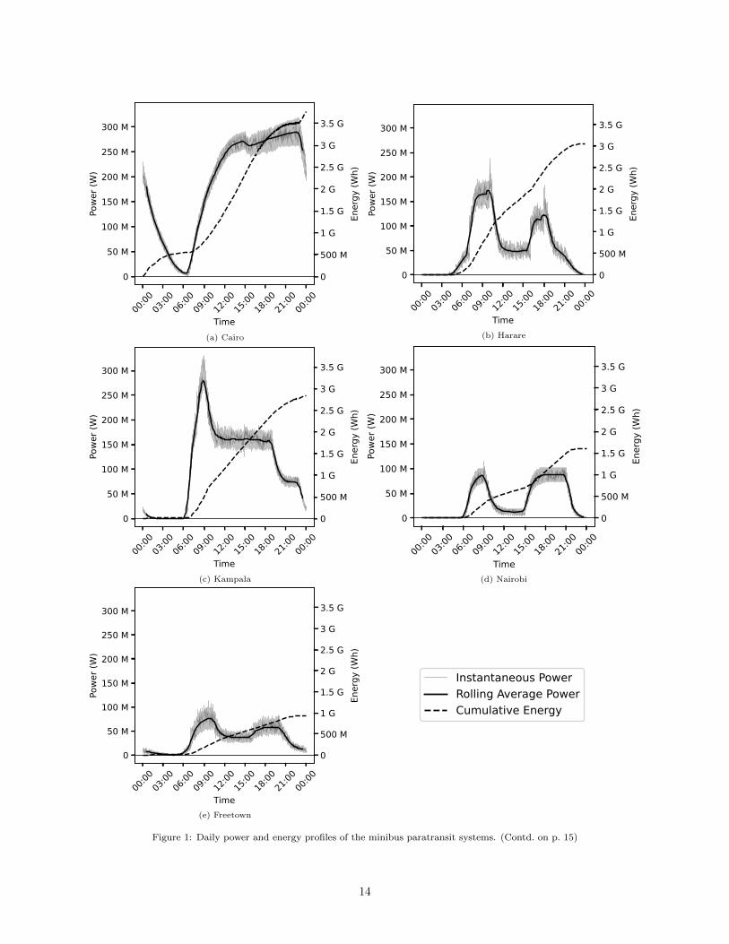
3.2. EV Simulation Results

We took the seven datasets and ran it through our custom EV-Fleet-Sim simulation program. This yielded

the power and energy profiles shown in Figure 1.

Four of the cities (Harare, Kampala, Nairobi and Freetown) have a peak in their power profile in the

mid-morning hours (around 9 am). All of these except one (Kampala) also have an evening peak of power

usage (at around 6 pm).

Cairo on the other hand displays a different power usage profile. Unlike the other cities, Cairo is North of

the Sahara dessert. It is possible that its geographical differences have different living/mobility patterns.

The remaining two cities (Abidjan and Accra), do not have any peaks in their power profiles. Rather,

they appear flat with low power consumption profiles. This corresponds with the fact that the geographical

spread of the cities are small as indicated by Table 3. It could also indicate that the cities make use of other

*4Simulation size was determined by creating a rectangular box that bounded all the routes defined in the dataset, and then

computing the box’s size.

13

00:00

03:00

06:00

09:00

12:00

15:00

18:00

21:00

00:00

Time

0

50 M

100 M

150 M

200 M

250 M

300 M

Powe

r (W

)

00:00

03:00

06:00

09:00

12:00

15:00

18:00

21:00

00:00

Time

0

2.5

5

7.5

10

12.5

15

17.5

20

Spee

d (k

m/h

)

00:00

03:00

06:00

09:00

12:00

15:00

18:00

21:00

00:00

Time

0

500 M

1 G

1.5 G

2 G

2.5 G

3 G

3.5 G

Ener

gy (W

h)

0 2 4 6Distance (km) 1e6

0

500 M

1 G

1.5 G

2 G

2.5 G

3 G

3.5 GEn

ergy

(Wh)

0 2 4 6Distance (km) 1e6

0.0

0.5

1.0

1.5

2.0

2.5

3.0

Inst

anta

neou

s Pow

er (W

)

1e8

0 2 4 6Distance (km) 1e6

0

50 k

100 k

150 k

200 k

250 k

300 k

350 k

Spee

d(k

mh

1 )

0

500 M

1 G

1.5 G

2 G

2.5 G

3 G

3.5 G

Ener

gy (W

h)

Simulation Output of experiment: Fleet > Total Plot

(a) Cairo

00:00

03:00

06:00

09:00

12:00

15:00

18:00

21:00

00:00

Time

0

50 M

100 M

150 M

200 M

250 M

300 M

Powe

r (W

)

00:00

03:00

06:00

09:00

12:00

15:00

18:00

21:00

00:00

Time

0

2.5

5

7.5

10

12.5

15

17.5

20

Spee

d (k

m/h

)

00:00

03:00

06:00

09:00

12:00

15:00

18:00

21:00

00:00

Time

0

500 M

1 G

1.5 G

2 G

2.5 G

3 GEn

ergy

(Wh)

0.00 0.25 0.50 0.75 1.00 1.25Distance (km) 1e6

0

500 M

1 G

1.5 G

2 G

2.5 G

3 G

Ener

gy (W

h)

0.00

0.25

0.50

0.75

1.00

1.25

Distance (km) 1e6

0.0

0.5

1.0

1.5

2.0

Inst

anta

neou

s Pow

er (W

)

1e8

0.00 0.25 0.50 0.75 1.00 1.25Distance (km) 1e6

0

50 k

100 k

150 k

200 k

250 k

Spee

d(k

mh

1 )

0

500 M

1 G

1.5 G

2 G

2.5 G

3 G

3.5 G

Ener

gy (W

h)

Simulation Output of experiment: Fleet > Total Plot

(b) Harare

00:00

03:00

06:00

09:00

12:00

15:00

18:00

21:00

00:00

Time

0

50 M

100 M

150 M

200 M

250 M

300 M

Powe

r (W

)

00:00

03:00

06:00

09:00

12:00

15:00

18:00

21:00

00:00

Time

0

2.5

5

7.5

10

12.5

15

17.5

20

Spee

d (k

m/h

)

00:00

03:00

06:00

09:00

12:00

15:00

18:00

21:00

00:00

Time

0

500 M

1 G

1.5 G

2 G

2.5 G

Ener

gy (W

h)

0.0 0.5 1.0 1.5 2.0Distance (km) 1e6

0

500 M

1 G

1.5 G

2 G

2.5 G

Ener

gy (W

h)

0.0 0.5 1.0 1.5 2.0Distance (km) 1e6

0.0

0.5

1.0

1.5

2.0

2.5

3.0

Inst

anta

neou

s Pow

er (W

)

1e8

0.0 0.5 1.0 1.5 2.0Distance (km) 1e6

0

50 k

100 k

150 k

200 k

250 k

300 k

Spee

d(k

mh

1 )

0

500 M

1 G

1.5 G

2 G

2.5 G

3 G

3.5 GEn

ergy

(Wh)

Simulation Output of experiment: Fleet > Total Plot

(c) Kampala

00:00

03:00

06:00

09:00

12:00

15:00

18:00

21:00

00:00

Time

0

50 M

100 M

150 M

200 M

250 M

300 MPo

wer (

W)

00:00

03:00

06:00

09:00

12:00

15:00

18:00

21:00

00:00

Time

0

2.5

5

7.5

10

12.5

15

17.5

20

Spee

d (k

m/h

)

00:00

03:00

06:00

09:00

12:00

15:00

18:00

21:00

00:00

Time

0

200 M

400 M

600 M

800 M

1 G

1.2 G

1.4 G

1.6 G

Ener

gy (W

h)

0 200000 400000 600000 800000Distance (km)

0

200 M

400 M

600 M

800 M

1 G

1.2 G

1.4 G

1.6 G

Ener

gy (W

h)

0

2000

00

4000

00

6000

00

8000

00

Distance (km)

0.0

0.2

0.4

0.6

0.8

1.0

Inst

anta

neou

s Pow

er (W

)

1e8

0 200000 400000 600000 800000Distance (km)

0

20 k

40 k

60 k

80 k

100 k

Spee

d(k

mh

1 )

0

500 M

1 G

1.5 G

2 G

2.5 G

3 G

3.5 G

Ener

gy (W

h)

Simulation Output of experiment: Fleet > Total Plot

(d) Nairobi

00:00

03:00

06:00

09:00

12:00

15:00

18:00

21:00

00:00

Time

0

50 M

100 M

150 M

200 M

250 M

300 M

Powe

r (W

)

00:00

03:00

06:00

09:00

12:00

15:00

18:00

21:00

00:00

Time

0

2.5

5

7.5

10

12.5

15

17.5

20

Spee

d (k

m/h

)

00:00

03:00

06:00

09:00

12:00

15:00

18:00

21:00

00:00

Time

0

200 M

400 M

600 M

800 M

Ener

gy (W

h)

0 200000 400000 600000Distance (km)

0

200 M

400 M

600 M

800 M

Ener

gy (W

h)

0

2000

00

4000

00

6000

00

Distance (km)

0.0

0.2

0.4

0.6

0.8

1.0

Inst

anta

neou

s Pow

er (W

)

1e8

0 200000 400000 600000Distance (km)

0

10 k

20 k

30 k

40 k

50 k

60 k

70 k

Spee

d(k

mh

1 )

0

500 M

1 G

1.5 G

2 G

2.5 G

3 G

3.5 G

Ener

gy (W

h)

Simulation Output of experiment: Fleet > Total Plot

(e) Freetown

Figure 1: Daily power and energy profiles of the minibus paratransit systems. (Contd. on p. 15)

14

00:00

03:00

06:00

09:00

12:00

15:00

18:00

21:00

00:00

Time

0

50 M

100 M

150 M

200 M

250 M

300 MPo

wer (

W)

00:00

03:00

06:00

09:00

12:00

15:00

18:00

21:00

00:00

Time

0

2.5

5

7.5

10

12.5

15

17.5

20

Spee

d (k

m/h

)

00:00

03:00

06:00

09:00

12:00

15:00

18:00

21:00

00:00

Time

0

200 M

400 M

600 M

800 M

1 G

1.2 G

1.4 G

Ener

gy (W

h)

0 100000 200000 300000Distance (km)

0

200 M

400 M

600 M

800 M

1 G

1.2 G

1.4 G

Ener

gy (W

h)

0

1000

00

2000

00

3000

00

Distance (km)

0

1

2

3

4

5

6

Inst

anta

neou

s Pow

er (W

)

1e7

0 100000 200000 300000Distance (km)

0

5 k

10 k

15 k

20 k

25 k

Spee

d(k

mh

1 )

0

500 M

1 G

1.5 G

2 G

2.5 G

3 G

3.5 G

Ener

gy (W

h)

Simulation Output of experiment: Fleet > Total Plot

(f) Accra

06:00

08:00

10:00

12:00

14:00

16:00

18:00

20:00

22:00

00:00

Time

0

50 M

100 M

150 M

200 M

250 M

300 M

Powe

r (W

)

06:00

08:00

10:00

12:00

14:00

16:00

18:00

20:00

22:00

00:00

Time

0

2.5

5

7.5

10

12.5

15

17.5

20

Spee

d (k

m/h

)

06:00

08:00

10:00

12:00

14:00

16:00

18:00

20:00

22:00

00:00

Time

0

50 M

100 M

150 M

200 M

250 M

Ener

gy (W

h)

0 20000 40000 60000 80000Distance (km)

0

50 M

100 M

150 M

200 M

250 M

Ener

gy (W

h)

020

000

4000

060

000

8000

0

Distance (km)

0.0

0.5

1.0

1.5

2.0

Inst

anta

neou

s Pow

er (W

)

1e7

0 20000 40000 60000 80000Distance (km)

0

2 k

4 k

6 k

8 k

10 k

12 k

Spee

d(k

mh

1 )

0

500 M

1 G

1.5 G

2 G

2.5 G

3 G

3.5 G

Ener

gy (W

h)

Simulation Output of experiment: Fleet > Total Plot

(g) Abidjan

Figure 1: (Contd. from p. 14) Daily power and energy profiles of the minibus paratransit systems.

modes of transport to satisfy the bulk of their mobility demands. Both these cities are situated close to one

another geographically, in North-West Africa. Freetown, the remaining city from North-West Africa, also has

a low overall energy usage like Abidjan and Accra.

The total energy demand of each of the simulation scenarios is summarised in Table 4. These values will

be used in order to perform verification. We will use data from an alternative source to approximate the

energy requirements of each of the cities, and compare them to the results found in Table 4.

Table 4: Summary of simulation results.

City Daily EnergyUsage (MWh/day)

Cairo 3778

Harare 3053

Kampala 2835

Nairobi 1612

Accra 1405

Freetown 943

Abidjan 250

We also generated box-plots (Figure 2) which indicate the per-route energy usage of each paratransit

system. If each route was apportioned a dedicated fleet of vehicles to service that route, the box plots show

how much energy the fleets would use. Consequently, if each route was apportioned a dedicated charging

station for its fleet, the box plots indicate how much energy the charging stations would require from the grid.

Of course, such a scenario would be sub-optimal, but it was the only scenario we could conjure up that would

allow the GTFS data to be useful on a disaggregated level.

15

AbidjanAccra Cairo

FreetownHarare

KampalaNairobi

City

0

100

200

300

400

Daily

ene

rgy

usag

e (k

Wh)

Figure 2: Daily energy usage of the routes of each city

3.3. Results Verification

In order to verify the results and see if they corresponded to what could be expected in reality, the taxi

energy demands were categorised as high, medium or low based on the city’s population size and the taxi

modal split, as gathered from independent data sources. These are shown in Table 4. As shown in the table,

Cairo is expected to have a high energy demand due to the fact that it has an extremely large population

that relies on taxis. Conversely, Freetown is expected to have a low energy demand due to the fact that it has

a relatively small population, and they don’t rely on taxis much, as indicated by the low modal split.

Table 5: Paratransit characteristics of the cities.

City Number of

taxis*5

Number of inhabitants

(Mil.) [32, 33]

Modal split

(%)*6

Reference Expected Energy

Demand

Abidjan 5000 4.7 23 [34, 35] Low

Accra 15 000 4.8 33 [36, 37] Medium

Cairo 15 000 21.3 20 [28, 38] High

Freetown 5000 1.2 23 [39] Low

Harare 100 000 2.9 60 [40, 41] Medium

Kampala 25 000 4.0 63 [42, 43] High

Nairobi 15 000 4.7 43 [44, 45] Medium

*5Refers to the total number of operational minibus taxis. Approximate values.*6Refers to the number of trips that are taken by taxi, as a fraction of the total motorised trips.

16

We see that, for the most part, the energy usage from the simulations (in Table 4) correspond with the

expected energy demands (in Table 5). For example, we see that Cairo has the highest simulated energy

usage, and it also has a high expected energy demand. Abidjan has the lowest simulated energy usage, and it

also has a low expected energy demand. The only results that did not correspond perfectly were Harare and

Kampala. Harare had a higher simulated energy usage than expected, while Kampala had a lower simulated

energy usage than expected. This can be attributed to the fact that both of those datasets had a low reliability

rating in Table 3.

We can therefore say that GTFS data can be used to give a rough estimate of the order of magnitude of a

paratransit system’s energy demands. However, due to the current state of data quality, they are likely to be

unreliable for quantifying the exact energy demands.

Our original intention was to approximate the expected energy demand using the number of taxis in each

paratransit system. However, this proved to be difficult due to unreliable figures we found for this metric. In

most of the countries, the transport authorities did not publish a figure on this metric. We therefore relied on

independent sources, who’s figures did not agree. For example, Harare’s transport authority did not publish

any figure on the number of taxis, and the figure of 100 000which we found from an independent source seems

extremely disproportionate when one takes into account the city’s population size. In addition, that figure

was the most recent we could find, although it is from 2002. This highlights, once again, the need for some

level of systematic data collection.

Reliable statistics on the number of taxis would have also been useful for downscaling the power/energy

profiles in Figure 1, in order to get the average taxi’s energy demand. In the following paragraphs, we will

nevertheless downscale the Kampala profile by the number of taxis in order to compare its power profile to

one we computed from independently gathered, reliable, vehicle-based paratransit data. [46]

3.4. Discussion: Passenger-based data shortcomings

Transport engineers typically obtain information by employing people in two outdated ways, either to

stand next to the road to record inflows and outflows or to get into vehicles to act as human carriers of

tracking devices. These methods are particularly attractive in developing countries where operational traffic

monitoring infrastructure is sparse and cheap labour is abundant. But, as mentioned in Table 1, this shortcut

has many pitfalls.

Developments in vehicle tracking technology have changed the game. Although the setup cost is more,

tracking devices have the substantial advantage that they are not susceptible to human behavioural problems.

For example, they don’t wake up late, get tired and need eating breaks, and they do not sleep.

To illustrate the difference, in Figure 3 we show Kampala’s energy profile from the two vantage points.

17

The overlay shows two plots. One is the passenger-based power profile from Figure 1c, which was downscaled

by the number of taxis in Kampala (25 000, as shown in Table 5 [42]). The second plot is a vehicle-based

power profile of Kampala obtained from Booysen et al. [46]. The differences are stark. First, it is clear that

the taxis started moving between 4 am and 5 am, before the fieldworkers managed to get on board. Second,

the passenger-based profile grinds to a halt just before supper time. But we see in the vehicle-based profile

that the minibus taxis samples happily chug away until after 9 pm.

Clearly, if we make assumptions about the power profile and energy requirements of electric minibus taxis

from passenger-based data, we will miss the mark by a substantial margin. This adds weight to the statement

by Collett and Hirmer that we quoted earlier, stressing the need for a more systematic approach to data

collection for the purpose of planning decarbonisation of paratransit [1].

Passenger-based

Vehicle-based

Figure 3: Comparison of Kampala per-vehicle power profiles derived from passenger-based and vehicle-based data.

4. Conclusion

Climate change is forcing the world to adapt to new, cleaner technologies, especially in the transport

sector, which contributes a large share of carbon emissions. Developed countries have committed to ambitious

plans to reduce their emissions in the short term, and are turning away from fossil fuel vehicles. Eventually,

developed countries will be compelled to do the same, and must be prepared for such big changes.

This paper prepares for this eventual migration by providing a method for modelling and simulating

electric paratransit, Africa’s most used mode of motorised transport [2]. Using this method, this paper has

attempted to establish the energy requirements that paratransit would have on the electric utilities of several

cities across Africa. Publicly available GTFS data was used for the simulations, in order to evaluate how

the state of the art can be improved for future evaluations, and whether the approach of paratransit data

18

collection should be changed.

The first objective was to the establish the net energy demand that the paratransit systems would have on

each of the cities. This was plotted in Figure 1 and summarised in Table 4. Although, the presented method

was able to obtain the net energy demands of the paratransit systems, our evaluation of the data collection

processes revealed a few quality issues that have hurt our confidence in the data. Therefore, we demand

for more rigour in future paratransit data collection projects. Despite this, the results can still serve as an

indication of what the future energy demand would look like.

The profiles give a rough idea of what the taxis’ movement profiles would look like. Four of the cities

(Harare, Kampala, Nairobi and Freetown) indicate that the highest energy demand of the taxis are at around

9AM. This would indicate that taxis have a period of high activity in the so-called “morning rush”. It is

clear therefore that taxis need to be adequately charged overnight in order to sustain this high-activity period.

Three of these cities also indicate a high-activity period in the evening. This would mean that the taxis may

also need to charge around midday when there is a period of relative inactivity.

Although we know the periods of relative inactivity, we don’t know exactly how long the typical taxi stops.

This is because the data does not capture the individual taxis’ itineraries. Rather, it gives the perspective

from an infrastructure, passenger demand, and traffic modelling point of view. Specifically, it captures the

itinerary and frequency of each route and assumes that taxis will be available to service the route. Therefore,

since we do not know when the taxis stop, it is not possible to know exactly when and how much the peak

strain on the electric grid would be due to the charging of the vehicles. In order to do this, tracking data of

the individual taxis will be required. At best, with this data, we have an indication that the peak charging

strain on the grid would be approximately the peak power usage from the electric vehicles, but offset a few

hours earlier to the hours of inactivity.

If there was tracking data of the individual taxis, we would know exactly which routes they service during

the day, and how long their breaks are between routes. We would then be able to profile the individual taxis’

daily energy requirements which would be useful for calculating the battery size required for the taxis. This

would have also been possible to find this metric through the GTFS data, if we knew the number of taxis

operating the paratransit systems. However, statistics on the number of taxis operating in the cities are

unreliable.

Finding the battery size would be important, since a mass roll-out of electric taxis would provide the

electric network with a distributed energy resource. Essentially, the grid can use the batteries of vehicles

connected to the grid as a buffer in which to store excess energy that is generated and draw energy when

needed. A tariff scheme could help taxi owners to make a profit when they provide this service to the electric

grid. To know exactly how much of a benefit this service would have on the grid, again we would need to

19

know the battery size of the taxis and the times that the taxis stop to connect to the electrical network. At

best, the results which could be generated from the GTFS data could give only a rough indication of the size

of the total distributed energy resource at the grid’s disposal. Assuming that each taxi’s battery size is the

approximately the same as its energy demand, then the total paratransit system would provide the grid with

a distributed energy buffer equivalent to its energy demand (as found in Table 4).

Similarly, to evaluate the renewable energy generation capacity that is needed to supplement the grid

to charge the taxis, we would need to know the stopping times of the taxis. Since most renewable energy

resources are time variant, the exact stopping times are important. From the GTFS data, we have identified

that, in some of the cities, the taxis have a dip in activity at midday, which presents and opportunity for

charging from solar energy. However to quantify exactly how much solar resource is required, the stopping

times need to be known.

In conclusion, the GTFS data that seems to be the state of the art in paratransit data capture is useful

in giving us an idea of the total energy requirements of a paratransit system, in giving indications of the

supply-side energy requirements, in estimating the distributed battery resource available to the electric

network, and in identifying opportunities for charging the taxis through renewable energy generation. However,

the data quality needs to be improved in order to establish enough confidence in the data to quantify these

energy requirements and opportunities with a scientific level of accuracy. More rigour needs to be applied

when collecting the data, possibly by increasing the number of field workers and the number of times data

is collected on each route. The results clearly show that it is not possible to identify the per-vehicle energy

requirements from GTFS data. Although an attempt was made to scale down the power profile by the number

of taxis, we found that the result did not correspond satisfactorily with independently gathered GPS tracking

data. This has highlighted the issues of human data collection, calling for a more systematic, autonomous

approach in data capture. With all this in mind, the authors recommend that future data collection efforts

employ the vehicle-based strategy (e.g. through GPS trackers). Through higher quality data driving the

process of decision making, we can finally compute our way towards sustainable mobility in Africa.

References

[1] K. A. Collett and S. A. Hirmer. Data needed to decarbonize paratransit in Sub-Saharan Africa.

Nature Sustainability, 4(7):562–564, 2021. ISSN 2398-9629. doi: 10.1038/s41893-021-00721-7. URL

https://rdcu.be/ckzez.

[2] R Behrens, D McCormick, and D Mfinanga. Paratransit in African cities: Operations, regulation and

reform. Routledge, London, 1 edition, 2016. ISBN 9781315849515. doi: 10.4324/9781315849515.

20

[3] Daniel Ehebrecht, Dirk Heinrichs, and Barbara Lenz. Motorcycle-taxis in sub-Saharan Africa: Current

knowledge, implications for the debate on “informal” transport and research needs. Journal of Transport

Geography, 69:242–256, 2018. ISSN 0966-6923. doi: https://doi.org/10.1016/j.jtrangeo.2018.05.006.

[4] Raffaello Cervigni, John Allen Rogers, and Irina Dvorak. Assessing Low-Carbon Development in Nigeria

: An Analysis of Four Sectors. World Bank, Washington, DC, 2013. URL https://openknowledge.

worldbank.org/handle/10986/15797.

[5] Ajay Mahaputra Kumar, Vivien Foster, and Fanny Barrett. Stuck in traffic : urban transport in

Africa. Technical report, Washington, DC: World Bank, 2008. URL http://documents1.worldbank.

org/curated/en/671081468008449140/pdf/0Urban1Trans1FINAL1with0cover.pdf.

[6] Ajay Mahaputra Kumar. Understanding the emerging role of motorcycles in African cities : a political

economy perspective. Technical Report 13, Washington, DC: World Bank, Washington, DC, 2011.

[7] Robert Cervero and Aaron Golub. Informal transport: A global perspective. Transport Policy, 14(6):

445–457, 11 2007. ISSN 0967-070X. doi: 10.1016/J.TRANPOL.2007.04.011.

[8] Gail Jennings and Roger Behrens. The case for investing in paratransit: Strategies for regulation and

reform. 1 2017. URL https://trid.trb.org/view/1660898.

[9] Dominic Stead and Dorina Pojani. The Urban Transport Crisis in Emerging Economies: A Comparative

Overview. In Dorina Pojani and Dominic Stead, editors, The Urban Transport Crisis in Emerging

Economies, pages 283–295. Springer International Publishing, Cham, 2017. ISBN 978-3-319-43851-1. doi:

10.1007/978-3-319-43851-1 14.

[10] Transformative Urban Mobility Initiative. Sustainable Urban Transport: Avoid-Shift-Improve (A-S-

I), 2022. URL https://www.transformative-mobility.org/assets/publications/ASI_TUMI_SUTP_

iNUA_No-9_April-2019.pdf. [Online; accessed 15. Feb. 2022].

[11] Jakub Galuszka, Emilie Martin, Alphonse Nkurunziza, Judith Achieng’ Oginga, Jacqueline Senyagwa,

Edmund Teko, and Oliver Lah. East Africa’s Policy and Stakeholder Integration of Informal Operators

in Electric Mobility Transitions—Kigali, Nairobi, Kisumu and Dar es Salaam. Sustainability, 13(4), 2021.

ISSN 2071-1050. doi: 10.3390/su13041703.

[12] Innocent Ndibatya and M J Booysen. Characterizing the movement patterns of minibus taxis in

Kampala’s paratransit system. Journal of Transport Geography, 92:103001, 2021. ISSN 0966-6923. doi:

10.1016/j.jtrangeo.2021.103001.

21

[13] C.J. Abraham, A.J. Rix, I. Ndibatya, and M.J. Booysen. Ray of hope for sub-Saharan Africa’s paratransit:

Solar charging of urban electric minibus taxis in South Africa. Energy for Sustainable Development,

64:118–127, 2021. ISSN 0973-0826. doi: https://doi.org/10.1016/j.esd.2021.08.003. URL https://www.

sciencedirect.com/science/article/pii/S0973082621000946.

[14] DigitalTransport4Africa. Data, 2021. URL https://git.digitaltransport4africa.org/data. [Online;

accessed 17. Oct. 2021].

[15] Dirk du Preez, Mark Zuidgeest, and Roger Behrens. A quantitative clustering analysis of para-

transit route typology and operating attributes in Cape Town. Journal of Transport Geography,

80(C), 1 2019. doi: 10.1016/j.jtrangeo.2019.1. URL https://ideas.repec.org/a/eee/jotrge/

v80y2019ics096669231830807x.html.

[16] Abidjantransport, 2021. URL http://doc.digitaltransport.io/abidjantransport. [Online; accessed

7. Nov. 2021].

[17] Transitec. Recording, Mapping and Analyzing the Performance of Paratransit Services.

Feb 2018. URL https://git.digitaltransport4africa.org/data/africa/accra/-/blob/

f04f2f1209f4235a832c7008463bd6eb019e32a2/papers/0844_170-gui-ssd-2-AM3_guide.pdf.

[18] Jacobus Petrus Snyman. Establishing and applying road classification and access management techniques

on Bird street in Stellenbosch, South Africa. PhD thesis, Stellenbosch: Stellenbosch University, 2020.

[19] StatsSA. P0320 - National Household Travel Survey, 2020, Mar 2021. URL http://www.statssa.gov.

za/?page_id=1854&PPN=P0320&SCH=72769.

[20] Sarah Williams, Adam White, Peter Waiganjo, Daniel Orwa, and Jacqueline Klopp. The digital matatu

project: Using cell phones to create an open source data for Nairobi’s semi-formal bus system. Journal

of Transport Geography, 49:39–51, 2015. ISSN 09666923. doi: 10.1016/j.jtrangeo.2015.10.005.

[21] OpenStreetMap Contributors. OpenStretMap Data, Feb 2022. URL https://www.openstreetmap.org.

[22] Geofabrik. OpenStreetMap Data Extracts, Jan 2022. URL https://download.geofabrik.de. [Online;

accessed 7. Jan. 2022].

[23] marqqs. osmctools, Jan 2022. URL https://gitlab.com/osm-c-tools/osmctools. [Online; accessed

7. Jan. 2022].

[24] Pablo Alvarez Lopez, Michael Behrisch, Laura Bieker-Walz, Jakob Erdmann, Yun-Pang Flotterod, Robert

Hilbrich, Leonhard Lucken, Johannes Rummel, Peter Wagner, and Evamarie Wießner. Microscopic

22

Traffic Simulation using SUMO. In 2019 IEEE Intelligent Transportation Systems Conference (ITSC),

pages 2575–2582. IEEE, 11 2018. URL https://elib.dlr.de/127994/.

[25] Pedro R. Andrade, Rafael H M Pereira, Joao Pedro Bazzo Vieira, dhersz, and Marcus Saraiva.

ipeagit/gtfs2gps: v1.5-4, September 2021. URL https://doi.org/10.5281/zenodo.5501855.

[26] Rhyd Lewis. Algorithms for Finding Shortest Paths in Networks with Vertex Transfer Penalties.

Algorithms, 13(11), 2020. ISSN 1999-4893. doi: 10.3390/a13110269.

[27] Joakim Fridlund and Oliver Wilen. Parameter Guidelines for Electric Vehicle Route Planning, 2020.

[28] TICD and TfC. How can Transit Mapping contribute to achieving Adequate Urban Mobility? The

Case of Cairo, Egypt. 2017. URL https://git.digitaltransport4africa.org/data/africa/cairo/

-/blob/ae279a3097e0c1aa1f99003acf0724f0da947778/Research%20&%20Policy%20Papers/TfC_

TICD_How%20can%20Transit%20Mapping%20Contribute%20to%20achieving%20AUM%20(28-11-2017)

%20Resource%20Center.pdf.

[29] Dunstan Matekenya, Xavier Espinet Alegre, Fatima Arroyo Arroyo, and Marta Gonza-

lez. Using Mobile Data to Understand Urban Mobility Patterns in Freetown, Sierra

Leone. 2021. URL https://openknowledge.worldbank.org/bitstream/handle/10986/35033/

Using-Mobile-Data-to-Understand-Urban-Mobility-Patterns-in-Freetown-Sierra-Leone.pdf.

Policy research working paper 9519.

[30] Travis Fried. Readme, 2019. URL https://git.digitaltransport4africa.org/data/africa/

harare/-/blob/178fa08537240b8a3faf8f2d172186b600fa1244/README.md.

[31] Transport for Cairo. Kampala and Parantransit street usage study, Sep 2020. URL https:

//transportforcairo.com/2020/09/01/kampala. [Online; accessed 7. Nov. 2021].

[32] G. Falchetta, M. Noussan, and A.T. Hammad. Comparing paratransit in seven major african cities: An

accessibility and network analysis. Journal of Transport Geography, 94:103131, 2021. ISSN 0966-6923.

doi: https://doi.org/10.1016/j.jtrangeo.2021.103131. URL https://www.sciencedirect.com/science/

article/pii/S0966692321001848.

[33] United Nations, Department of Economic and Social Affairs, Population Division. World Population

Prospects 2019, custom data acquired via website, 2019. URL https://population.un.org/wpp/

DataQuery. [Online; accessed 10. Aug. 2021].

23

[34] Leonard Johnstone and Vatanavongs Ratanavaraha. Public transport initiatives in west africa, a case

study of abidjan. Int J Geomate, 19:197–204, 2020. URL https://www.geomatejournal.com/user/

download/1929/197-204-5529-Leonard-Aug-2020-72.pdf.

[35] Amakoe Adolehoume and Alain Bonnafous. Urban transport microenterprises in abid-

jan. 2001. URL https://openknowledge.worldbank.org/bitstream/handle/10986/9805/

28537findeng186.pdf?sequence=1.

[36] Albert M Abane. Travel behaviour in ghana: empirical observations from four metropoli-

tan areas. Journal of Transport Geography, 19(2):313–322, 2011. URL https://www.

sciencedirect.com/science/article/pii/S0966692310000347?casa_token=83Ql-exFglMAAAAA:

4DPySIPY3i2OGVA1f1vciAJ_EockuCqouKLMLbroyc03H4kqQaaFB3r7MQk90LB0g_cxeF09ol0.

[37] A Kumar, EA Kwakye, and Z Girma. What works in private provision of

bus transport services—case study of accra and addis ababa. In 11th Con-

ference of CODATU, 2004. URL http://www.codatu.org/wp-content/uploads/

What-works-in-private-provision-of-bus-transport-services-case-study-of-Accra-and-Addis-Ababa-A.

-KUMAR-E.A.-KWAKYE-Z.-GIRMA.pdf.

[38] Mohamed El Esawey and Ahmed Ghareib. Analysis of mode choice behavior in greater cairo

region. Technical report, 2009. URL https://www.researchgate.net/profile/Mohamed-Elesawey/

publication/282134483_Analysis_of_Mode_Choice_Behavior_in_Greater_Cairo_Region/links/

594e304a0f7e9be7b2da7963/Analysis-of-Mode-Choice-Behavior-in-Greater-Cairo-Region.

pdf.

[39] B Koroma, D Oviedo, Y Yusuf, J Macarthy, C Cavoli, P Jones, L Caren, and S Sellu. City profile:

Freetown: Base conditions of mobility, accessibility and land use. 2021. URL https://discovery.ucl.

ac.uk/id/eprint/10122487/1/TSUM_CityProfile_Freetown.pdf.

[40] Tatenda C Mbara. Activity patterns, transport and policies for the urban

poor in harare, zimbabwe. Final country report.[En ligne.] www. transport-links.

org/transport links/filearea/documentstore/305 Zimbabwe% 20Final% 20Report, 2002. URL

http://citeseerx.ist.psu.edu/viewdoc/download?doi=10.1.1.1003.6243&rep=rep1&type=pdf.

[41] Abraham R. Matamanda, Innocent Chirisa, Munyaradzi A. Dzvimbo, and Queen L. Chinozvina. The

political economy of zimbabwean urban informality since 2000 – a contemporary governance dilemma.

Development Southern Africa, 37(4):694–707, 2020. doi: 10.1080/0376835X.2019.1698410. URL https:

//doi.org/10.1080/0376835X.2019.1698410.

24

[42] Dave Spooner, John Mark Mwanika, Shadrack Natamba, and Erick Oluoch Manga. Kampala bus rapid

transit: Understanding kampala’s paratransit market structure, 2020. URL https://www.researchgate.

net/profile/Dave-Spooner/publication/342233740_Kampala_Bus_Rapid_Transit_

Understanding_Kampala’s_Paratransit_Market_Structure/links/5ee9f250a6fdcc73be82f860/

Kampala-Bus-Rapid-Transit-Understanding-Kampalas-Paratransit-Market-Structure.pdf.

[43] Susan Watundu. Urban household road travel demand and transport mode choice: the case of kampala,

uganda. 2015. URL http://publication.aercafricalibrary.org/handle/123456789/2077.

[44] Jennifer Graeff. The organization and future of the matatu industry in nairobi, kenya. Paper prepared

by Center for Sustainable Urban development, earth Institute, Columbia University, New York, pages

1–3, 2009. URL http://www.vref.se/download/18.53e8780912f2dbbe3a580002295/1377188299857/

Organization+and+Future+of+the+Matatu+Industry.pdf.

[45] Eric Bruun, Romano Del Mistro, Yolandi Venter, and David Mfinanga. The state of public transport

systems in three Sub-Saharan African cities. In Roger Behrens, Dorothy McCormick, and David Mfinanga,

editors, Paratransit in African Cities: Operations, Regulation and Reform, chapter 2. Routledge, New

York, 1 edition, 2016. ISBN 9781315849515. doi: 10.4324/9781315849515.

[46] M. J. Booysen, C. J. Abraham, A. J. Rix, and I. Ndibatya. Walking on sunshine: Pairing electric vehicles

with solar energy for sustainable informal public transport in Uganda, in press. Energy Research and

Social Science, 2022. doi: 10.1016/j.erss.2021.102403.

25