A commuting generation model requiring onlyaggregated data

Maxime Lenormand1, Sylvie Huet1 and Floriana Gargiulo2

1 Cemagref, LISC, 24 avenue des Landais, 63172 AUBIERE, France(maxime.lenormand, sylvie.huet)@cemagref.fr

2 INED, 133 boulevard Davout, 75020 PARIS, Francefloriana.gargiulo@gmail.com

Abstract. We recently proposed, in (Gargiulo et al., 2011), an innova-tive stochastic model with only one parameter to calibrate. It reproducesthe complete network by an iterative process stochastically choosing, foreach commuter living in the municipality of a region, a workplace in theregion. The choice is done considering the job offer in each municipalityof the region and the distance to all the possible destinations. The modelis quite effective if the region is sufficiently autonomous in terms of joboffers. However, calibrating or being sure of this autonomy require dataor expertise which are not necessarily available. Moreover the region canbe not autonomous. In the present, we overcome these limitations, ex-tending the job search geographical base of the commuters to the outsideof the region, and changing the deterrence function form. We also founda law to calibrate the improvement model which does not require data.

1 Introduction

For two decades, not only the number of commuters, but also the average dis-tance travelled by workers has been increasing in most European countries. Thismakes commuting a fundamental phenomenon to understand. A precise descrip-tion of the commuting patterns has a central role in many applied questions:from the studies on traffic and the planning of infrastructures (Ortuzar andWillumsen, 2011) to the diffusion of epidemics (Balcan et al., 2009) or largedemographic simulations (Huet and Deffuant, 2011). The literature on this ar-gument is abundant, both from the point of view of the analysis of the structuresand from the point of view of the models, see (Ortuzar and Willumsen, 2011;Barthelemy, 2010) for reviews.

Many recent papers have adopted an approach based on network theory. Aninteresting and complete analysis of the commuting structures from this pointof view has been introduced for example in (De Montis et al., 2007, 2010). Inthis framework, most importantly concerning the modelling issues, the questionabout the commuting networks is set in a larger conceptual category: spatiallyconstrained network structures. This kind of analysis concerns not only com-muting, but all the situations where the geography has a significant role: fromthe reconstruction of migrant patterns (Lemercier and Rosental, 2008) to the

arX

iv:1

109.

6759

v1 [

mat

h.ST

] 3

0 Se

p 20

11

analysis of the internet at autonomous system (AS) level (Pastor-Satorras andVespignani, 2004), to the airline network structure (Barrat et al., 2004). A par-ticularly important study in this context is, for example, (Barrat et al., 2005)where the concept of ”preferential attachment” (Barabasi and Albert, 1999) isadapted in order to take into account not only the strength of a node given by itscurrent in-degree, but also the spatial constraint included in the journey-to-worknetwork.

A more traditional approach to the commuting structures is based on the so-called gravity law models (Haynes and Fotheringham, 1984). The term gravitylaw is a metaphor from classical physics. We can imagine that, as it happens ingravitation, the interaction between two municipalities depends proportionallyon a parameter, for example the size of the municipality (equivalent to massin the gravitational law), and in inverse proportion with some power law of thedistance. Many versions of this law were studied to better fit detailed data. Some-times the inverse proportion with the distance dij is replaced by an exponentialdecay. In general, we can speak of a deterrence function f(dij). The literaturegenerally agrees that an exponential specification appears better for modellingcommuting. However, in some applications, a power law decay often seems to bea better fit (De Montis et al., 2007, 2010).

In the framework of the European project PRIMA1 we need an effective algo-rithm generating commuting network from only aggregated data of commutingat the municipal level. We inspire from the gravity law approach recently pro-pose in (Gargiulo et al., 2011) which is an innovative stochastic model with onlyone parameter to calibrate. It reproduces the complete network by an iterativeprocess stochastically choosing, for each commuter living in the municipality of aregion, a workplace in the region. The choice is done considering the job offer ineach municipality of the region and the distance to all the possible destinations.This model has been tested and evaluated with inputs based on data extractedfrom the origin-destination table of each case study regions. This model is astochastic discrete choice model. It differs from the review of such a model pre-sented in (Ortuzar and Willumsen, 2011) since the individual decision functionis inspired from the gravity law. Moreover, the choice of the place of work isconstrained by the municipality job offer assimilated to the total number ofcommuters of the municipality. This model is stochastic and allows replicationsgiving an idea of the various spatial configurations which can be obtained verylocally where the commuting flows are small. Indeed, the small flows betweencouple of municipalities make an optiming deterministic approach irrelevant.The model can be applied to a region for which only the aggregated data at themunicipal level is available: the total number of commuters coming to work intothe municipality (called in-commuters in this paper) and the total number ofcommuters living in the municipality and going working elsewhere. However, itis necessary to collect data or expertise to be sure that the region is sufficiently

1 PRototypical policy Impacts on Multifunctional Activities in rural municipalities -EU 7th Framework Research Programme; 2008-2011; https://prima.cemagref.fr/the-project

autonomous in terms of job offers. That means that the larger part of people liv-ing in the region also works there and the part of people living in the region andworking outside is negligible. If such information does’nt exist or if the region isnot autonomous enough, the algorithm can’t be used in a relevant and effectivemanner. The second difficulty to apply this model to a region where disaggre-gated data is not available is linked to the calibration. Only an approximationof the value of the parameter can be done if no detailed data is available.

We have to keep in mind that, in many cases, statistical offices do not providethe full origin-destination table to reconstruct exactly the network structure butjust the total number of out-commuters and in-commuters in a location. Thus,to overcome the difficulties of the actual model, we propose to improve it in twoways. We first change the job search geographical base to take into account theeffects of the neighbouring regions and of the functional form of the distancefunction. It allows us to use aggregated data as input since it is no longer usefulto isolate the part of commuters living in the region and working outside. We alsochange the form of the deterrence function to ensure the quality of the results.Finally using a large number of case study regions we show that an universalway to calibrate the model parameter can be found. This is the very strongpoint of this model, since, it allow to rebuild with an incredibly high accuracythe commuting networks for every region where the origin-destination tables arenot provided from the statistical offices.

In the first part, we summarize the basic model. The second part describesimprovement of the basic model, namely the introduction of the neighbourhoodand the exponential deterrence function. The last section shows how it is possibleto bypass the direct calibration of the model. The model and its improvementsare validated on at least 23 French regions or districts. All the data used inthe paper are measured for the 1999 French Census by the French StatisticalInstitute, INSEE. They were kindly made available by the Maurice HalbwachsCenter. This measured data is called observed data in the following.

2 The basic model

That is the model proposed by (Gargiulo et al., 2011). Consider a region com-posed by n municipalities. We can model the real commuting network startingfrom the matrix: R1 ∈ Mn×n(N) where R1ij is the number of commuters fromthe municipality i (in the region) to the municipality j (in the region).

We describe it from its algorithmic formulation to make it easily understand-able. The inputs are:

– D = (dij)1≤i,j≤n the Euclidean distance matrix between municipalities– Ij the number of in-commuters of the municipality j in the region, 1 ≤ j ≤ n.– Oi the number of out-commuters in the region of the municipality i in the

region, 1 ≤ i ≤ n.

Ij and Oj can be respectively assimilated to the job offers and the job demandof the municipality j, 1 ≤ j ≤ n. The algorithm starts with:

Ij =

n∑i=1

R1ij (1)

and

Oi =

n∑j=1

R1ij (2)

These offers and demand decrease each time an individual living somewherefinds a working place. Thus, the complete algorithm is:

For each remaining commuter who has not already found its place of work

(while Oi > 0 ∀ 1 ≤ i ≤ n), do:

– Select a living municipality i at random among the municipalities

where at least one out-commuter remains (such as Oi 6= 0)– Select the working destination j randomly following the probability

distribution given by:

Pi→j =Ij(dij)

−β∑nk=1 Ik(dik)−β

, β > 0. (3)

– Update the number of in-commuters of j: Ij = Ij − 1– Update the number of out-commuters of i: Oi = Oi − 1– Compute again the distribution of Pi→j

We obtain a matrix (only dedicated to the region) SA ∈ Mn×n(N) where SAijis the number of commuters from the municipality i to the municipality j. Onecan notice that at the end of the algorithm Oi = 0 and Ij = 0 ∀ 1 ≤ i ≤ n sinceat the beginning we have the same number of out-commuters as in-commuters.

Classically, the deterrence function f(dij , β) can assume two main possibleshapes: a power law or an exponential law.The power law is used in Gargiulo et al. (2011):

f(dij , β) = d−βij 1 ≤ i, j ≤ n . (4)

3 How to cope with not autonomous regions or lack ofdetailed data

A commuting network is defined by an origin-destination table (light grey tablein Table 1). At the regional level, it means that we need to know, for eachmunicipality of residence of the region and for each municipality of employmentof the region, the value of the flow of commuters going from one to another.This kind of data is not always provided by the statistical offices and usually thedatasets are aggregated. That means only the total number of out-commuters

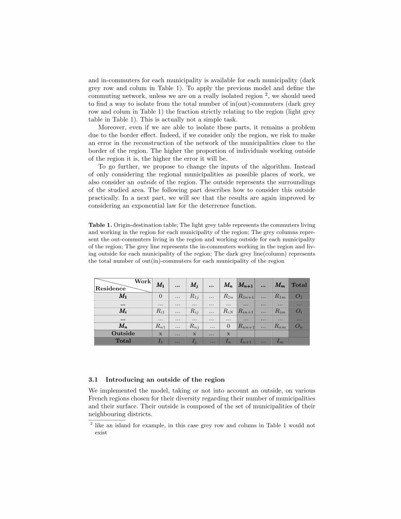
and in-commuters for each municipality is available for each municipality (darkgrey row and colum in Table 1). To apply the previous model and define thecommuting network, unless we are on a really isolated region 2, we should needto find a way to isolate from the total number of in(out)-commuters (dark greyrow and colum in Table 1) the fraction strictly relating to the region (light greytable in Table 1). This is actually not a simple task.

Moreover, even if we are able to isolate these parts, it remains a problemdue to the border effect. Indeed, if we consider only the region, we risk to makean error in the reconstruction of the network of the municipalities close to theborder of the region. The higher the proportion of individuals working outsideof the region it is, the higher the error it will be.

To go further, we propose to change the inputs of the algorithm. Insteadof only considering the regional municipalities as possible places of work, wealso consider an outside of the region. The outside represents the surroundingsof the studied area. The following part describes how to consider this outsidepractically. In a next part, we will see that the results are again improved byconsidering an exponential law for the deterrence function.

Table 1. Origin-destination table; The light grey table represents the commuters livingand working in the region for each municipality of the region; The grey columns repre-sent the out-commuters living in the region and working outside for each municipalityof the region; The grey line represents the in-commuters working in the region and liv-ing outside for each municipality of the region; The dark grey line(column) representsthe total number of out(in)-commuters for each municipality of the region

XXXXXXXXXResidenceWork

M1M1M1 ......... MjMjMj ......... MnMnMn Mn+1Mn+1Mn+1 ......... MmMmMm Total

M1M1M1 0 ... R1j ... R1n R1n+1 ... R1m O1

......... ... ... ... ... ... ... ... ... ...

MiMiMi Ri1 ... Rij ... RiN Rin+1 ... Rim Oi

......... ... ... ... ... ... ... ... ... ...

MnMnMn Rn1 ... Rnj ... 0 Rnn+1 ... Rnm On

Outside x ... x ... x

Total I1 ... Ij ... In In+1 ... Im

3.1 Introducing an outside of the region

We implemented the model, taking or not into account an outside, on variousFrench regions chosen for their diversity regarding their number of municipalitiesand their surface. Their outside is composed of the set of municipalities of theirneighbouring districts.

2 like an island for example, in this case grey row and colums in Table 1 would notexist

A new job search base. We consider the outside of the region composed bym−n municipalities, where n is the number of municipalities of the region. Theinputs are the directly available aggregated data at the municipal level:

– D = (dij) 1≤i≤n1≤j≤m

the Euclidean distance matrix between the municipalities

both in the same region and in the outside– (Ij)1≤j≤m the number of in-commuters of the municipality j of the region

and outside of it– (Oi)1≤i≤n the number of out-commuters of the municipality i of the region

only, as previously

The principle remains the same: Ij and Oi are respectively assimilated to thejob offers and the job demands of a municipality, 1 ≤ j ≤ m and 1 ≤ i ≤ n.These offers and demands decrease each time an individual living somewherefinds a working place. Only the computation of the probability of an individualliving in a municipality i to choose a municipality j changes slightly to considerall the offers, the ones of the outside included. It becomes:

Pi→j =Ijf(dij , β)∑mk=1 Ikf(dik, β)

, β > 0. (5)

Differently from before, at the end of the algorithm we have Oi = 0 andIj ≥ 0 ∀ 1 ≤ i ≤ n and ∀ 1 ≤ j ≤ m. Indeed, a part of the offer has not beentaken. This part corresponds, on the one hand, to the inside region offer nottaken by people living outside, and on the other hand, to the outside job offersnormally taken by people living outside the region. One can notice that it iswhat we have to isolate when the outside is not considered in the job searchbase.

We obtain two simulated matrices. The first matrix is only dedicated tothe region: SB1 ∈ Mn×n(N) where SB1ij is the number of commuters from themunicipality i (in the region) to the municipality j (in the region). The secondmatrix is dedicated to the region and its outside: SB2 ∈ M(n+1)×(n+1)(N). Threedifferent types of commuters can be identified in this matrix:

– if i, j 6= n + 1 SB2ij is the number of commuters from the municipality i (inthe region) to the municipality j (in the region);

– if i = n+ 1 and j 6= n+ 1, SB2ij is the number of commuters from the outsideto the municipality j (in the region);

– if i 6= n + 1 and j = n + 1, SB2ij is the number of commuters from themunicipality i to the outside.

The matrix composed by the n first columns and the n first rows of thegenerated matrix SB2ij is the matrix of commuters in the region. The matrixcomposed by the n + 1 first columns and the n first rows of the generatedmatrix SB2ij is the matrix of out-commuters (commuters in the region and theout-commuters from the region to the outside). The matrix composed by the nfirst columns and the n+ 1 first rows of the generated matrix SB2ij is the matrixof in-commuters in the region (commuters in the region and the in-commutersfrom the outside to the region).

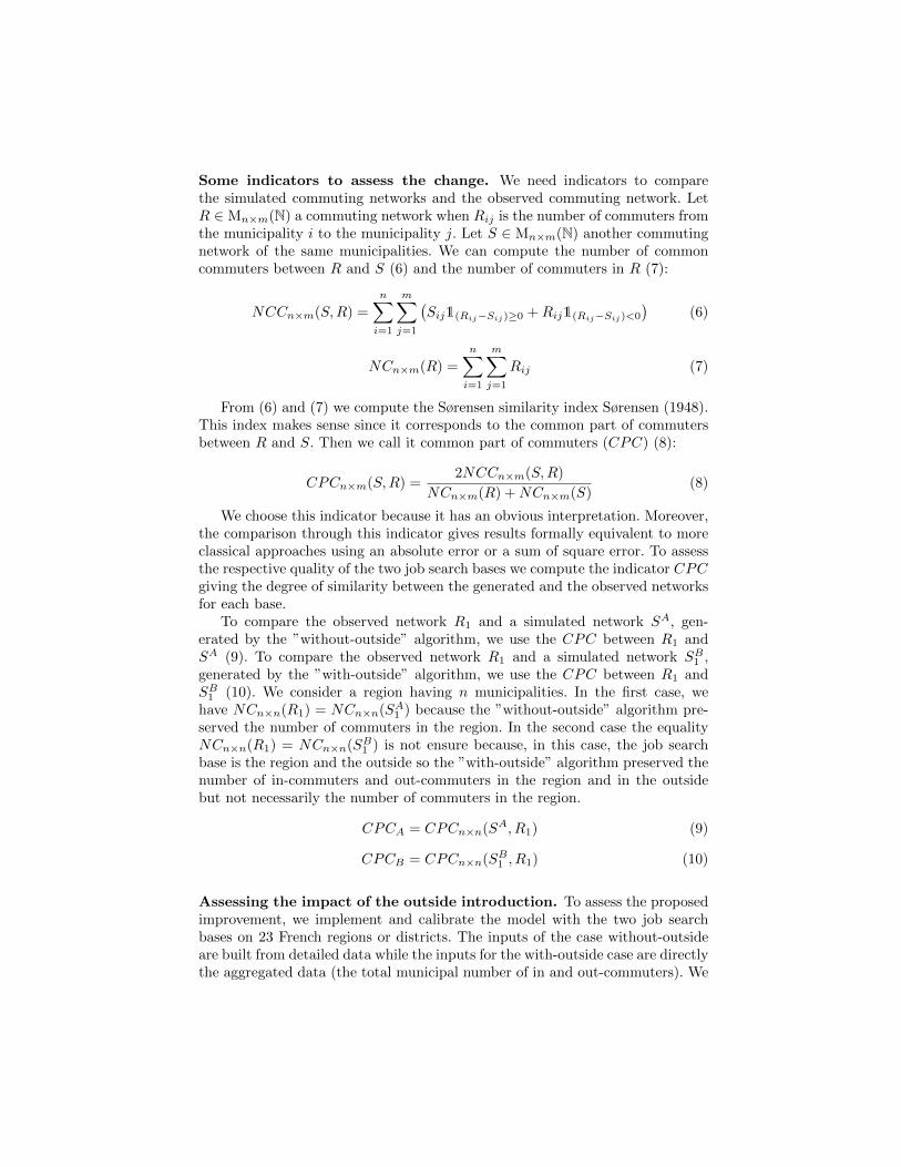
Some indicators to assess the change. We need indicators to comparethe simulated commuting networks and the observed commuting network. LetR ∈ Mn×m(N) a commuting network when Rij is the number of commuters fromthe municipality i to the municipality j. Let S ∈ Mn×m(N) another commutingnetwork of the same municipalities. We can compute the number of commoncommuters between R and S (6) and the number of commuters in R (7):

NCCn×m(S,R) =

n∑i=1

m∑j=1

(Sij1(Rij−Sij)≥0 +Rij1(Rij−Sij)<0

)(6)

NCn×m(R) =

n∑i=1

m∑j=1

Rij (7)

From (6) and (7) we compute the Sørensen similarity index Sørensen (1948).This index makes sense since it corresponds to the common part of commutersbetween R and S. Then we call it common part of commuters (CPC) (8):

CPCn×m(S,R) =2NCCn×m(S,R)

NCn×m(R) +NCn×m(S)(8)

We choose this indicator because it has an obvious interpretation. Moreover,the comparison through this indicator gives results formally equivalent to moreclassical approaches using an absolute error or a sum of square error. To assessthe respective quality of the two job search bases we compute the indicator CPCgiving the degree of similarity between the generated and the observed networksfor each base.

To compare the observed network R1 and a simulated network SA, gen-erated by the ”without-outside” algorithm, we use the CPC between R1 andSA (9). To compare the observed network R1 and a simulated network SB1 ,generated by the ”with-outside” algorithm, we use the CPC between R1 andSB1 (10). We consider a region having n municipalities. In the first case, wehave NCn×n(R1) = NCn×n(SA1 ) because the ”without-outside” algorithm pre-served the number of commuters in the region. In the second case the equalityNCn×n(R1) = NCn×n(SB1 ) is not ensure because, in this case, the job searchbase is the region and the outside so the ”with-outside” algorithm preserved thenumber of in-commuters and out-commuters in the region and in the outsidebut not necessarily the number of commuters in the region.

CPCA = CPCn×n(SA, R1) (9)

CPCB = CPCn×n(SB1 , R1) (10)

Assessing the impact of the outside introduction. To assess the proposedimprovement, we implement and calibrate the model with the two job searchbases on 23 French regions or districts. The inputs of the case without-outsideare built from detailed data while the inputs for the with-outside case are directlythe aggregated data (the total municipal number of in and out-commuters). We

calibrate the model with the regional base with a β value with one digit afterdecimal point while the model with a regional plus the outside base considers aninteger precision for the β value. We replicate ten times the generation for eachregion and compute our indicators on each replicate. In all the presented figures,the indicator is averaging on 10 replications. The variation of the indicator overthe replications is very low, 1.89% of the average at most. Consequently, it isnot represented on the figures. The Fig. 1 presents the CPCA obtained with theregional job search base (square) and the CPCB (triangle) obtained with a jobsearch base comprising the region and its outside.

0.5

0.6

0.7

0.8

0.9

Au

verg

ne

Bre

tag

ne

Als

ace

Aq

uita

ine

May

en

ne

Lo

zère

Po

itou

Ain

Ce

ntr

e

Mid

i−P

yré

né

e

Lim

ou

sin

Fra

nch

e−

Co

mté

Ha

ute

−N

orm

an

die

Ha

ute

−M

arn

e

Vo

sge

s

Lo

rra

ine

Cre

use

Ha

ut−

de

−S

ein

e

Yve

line

s

Va

l d'O

ise

Va

l de

Ma

rne

La

ng

ue

do

c

Ch

are

nte

CPCA

CPCB

Fig. 1. Average CPCA and CPCB for 23 regions.

Fig. 1 shows that the two job search bases give results which are not re-ally different. However the CPCB qualifying the with-outside case is upper theCPCA relative to the regional case in two thirds of cases. Moreover we have tokeep in mind that the inputs of the with-outside case does not require to havedetailed data on the contrary to the without outside case. Then we can say thatthe with-outside case is better than the regional case. Thus, adding the outsideis an improvement and allow to apply the algorithm even if the region is notautonomous.

This is not present on the graph but in each cases the model (with-outsidecase) tends to underestimate the number of commuters going to work insidethe region, NCn×n(R1) ≥ NCn×n(SB1 ). This underestimation of the number ofcommuters inside the region can be partly linked to the form of the deterrencefunction. Indeed, we use a power law deterrence function which never reaches azero value. That means that the very distant job offers of the outside we add

to the job search base are going to be considered as possible places of work.At the same time, the larger the job search base is, the larger the most distantoffers is since the diameter of the job search base increases relatively. We knowthat a large part of the job offers of the outside is not for people living insidethe region. Then the introduction of these false offers into the job search base,coupled to the power law deterrence function, allows people to choose a placeof work further away than in reality. This leads to an overestimation of peopleliving inside the region and working outside. We assume than using a deterrencefunction able to reach zero, as the classical exponential function, will at leastpartly correct this bias. That is the subject of the next section.

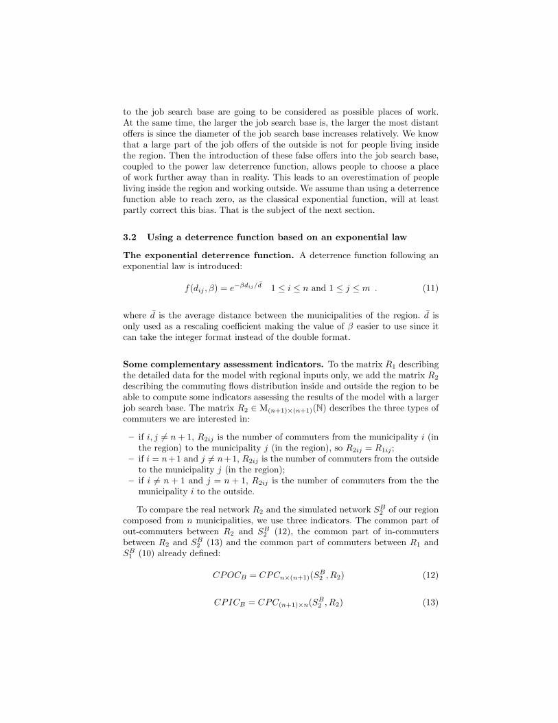
3.2 Using a deterrence function based on an exponential law

The exponential deterrence function. A deterrence function following anexponential law is introduced:

f(dij , β) = e−βdij/d 1 ≤ i ≤ n and 1 ≤ j ≤ m . (11)

where d is the average distance between the municipalities of the region. d isonly used as a rescaling coefficient making the value of β easier to use since itcan take the integer format instead of the double format.

Some complementary assessment indicators. To the matrix R1 describingthe detailed data for the model with regional inputs only, we add the matrix R2

describing the commuting flows distribution inside and outside the region to beable to compute some indicators assessing the results of the model with a largerjob search base. The matrix R2 ∈ M(n+1)×(n+1)(N) describes the three types ofcommuters we are interested in:

– if i, j 6= n+ 1, R2ij is the number of commuters from the municipality i (inthe region) to the municipality j (in the region), so R2ij = R1ij ;

– if i = n+1 and j 6= n+1, R2ij is the number of commuters from the outsideto the municipality j (in the region);

– if i 6= n + 1 and j = n + 1, R2ij is the number of commuters from the themunicipality i to the outside.

To compare the real network R2 and the simulated network SB2 of our regioncomposed from n municipalities, we use three indicators. The common part ofout-commuters between R2 and SB2 (12), the common part of in-commutersbetween R2 and SB2 (13) and the common part of commuters between R1 andSB1 (10) already defined:

CPOCB = CPCn×(n+1)(SB2 , R2) (12)

CPICB = CPC(n+1)×n(SB2 , R2) (13)

Note that :NCn×(n+1)(R2) = NCn×(n+1)(S

B2 ) and NC(n+1)×n(R2) = NC(n+1)×n(SB2 ). We

have these two equalities because the job search base is the region and the outsideso the ”with-outside” algorithm preserved the number of in-commuters and out-commuters in the region and in the outside. These indicators are computed foreach replication.

The impact of the exponential law coupled to the job search baseincluding the outside. To compare the two deterrence functions, we havesimulated and calibrated 34 French regions replicating ten times for each region.The Fig. 2 shows, as an example for the Auvergne region, we obtained a betterestimation of the commuting distance distribution with the exponential law.

0 10 20 30 40 50 60

0.00

0.02

0.04

0.06

0.08

Commuting distance (Km)

Den

sity

Real dataPowerExponential

Fig. 2. Density of the Auvergne com-muting distance distribution; the solidline represents the observed commutingdistance distribution; the dotted linerepresents the commuting distance dis-tribution obtained with the calibratedmodel with a job search base compris-ing the outside and the exponential law(β = 17) for one replication; the dashedline represents the commuting distancedistribution obtained with a job searchbase comprising the outside and thepower law (β = 2.7)

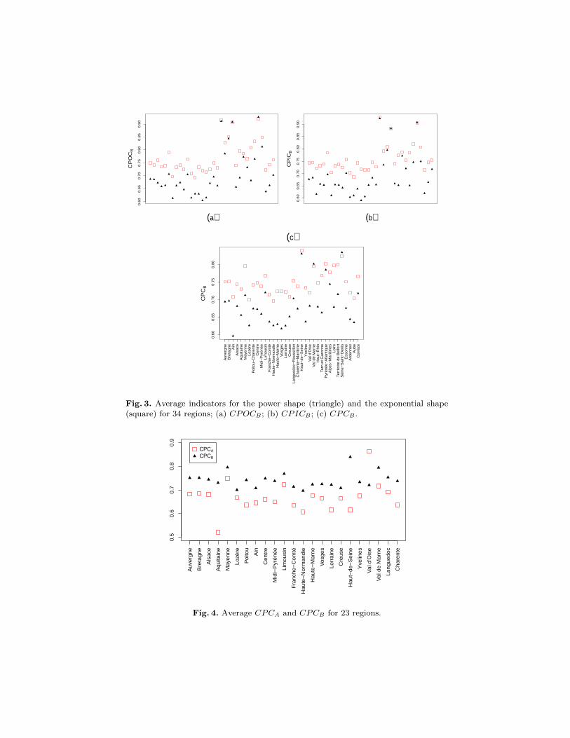
More systematically, we plot for the two different deterrence functions, ex-ponential and power law, applied to the with-outside case, the average on thereplications of our three indicators in the Fig. 3. It shows that the average propor-tion of common commuters is always better with the exponential law representedby the squares.

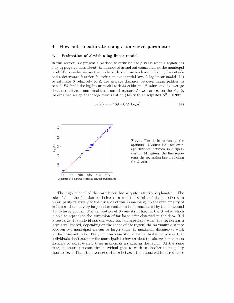
The Fig. 4 presents the CPCA for the without-outside case and a power lawdeterrence function (that is the initial model) against the CPCB for the with-outside case coupled to an exponential deterrence function. It shows that ourimprovements requiring less detailed inputs almost always have better resultsthan the one based on the power law. There is only one region, the Hauts-de-Seine, for which it is not true.

The last difficulty to solve is about the calibration process which requiresuntil now to have detailed data to be accurate.

0.6

00

.65

0.7

00

.75

0.8

00

.85

0.9

0

CP

OC

B

(a)

0.6

00

.65

0.7

00

.75

0.8

00

.85

0.9

0

CP

ICB

(b)0.

600.

650.

700.

750.

80

(c)

C

PC

B

Auv

ergn

eB

reta

gne

Ain

Als

ace

Aqu

itain

eM

ayen

neLo

zère

Poi

tou−

Cha

rent

eC

entr

eM

idi−

Pyr

énée

Lim

ousi

nF

ranc

he−

Com

téH

aute

−N

orm

andi

eH

aute

−M

arne

Vos

ges

Lorr

aine

Cre

use

Lang

uedo

c−R

ouss

illon

Cha

rent

e−M

ariti

me

Hau

t−de

−S

eine

Yve

line

Val

d'O

ise

Val

de

Mar

neH

aut−

Rhi

nTa

rn e

t Gar

onne

Pyr

énée

−A

tlant

ique

Alp

es−

Mar

itim

esLo

ireTe

rrito

ire d

e B

elfo

rtS

eine

−S

aint

−D

enis

Ess

onne

Ard

enne

sA

ube

Cor

rèze

Fig. 3. Average indicators for the power shape (triangle) and the exponential shape(square) for 34 regions; (a) CPOCB ; (b) CPICB ; (c) CPCB .

0.5

0.6

0.7

0.8

0.9

Au

verg

ne

Bre

tag

ne

Als

ace

Aq

uita

ine

May

en

ne

Lo

zère

Po

itou

Ain

Ce

ntr

e

Mid

i−P

yré

né

e

Lim

ou

sin

Fra

nch

e−

Co

mté

Ha

ute

−N

orm

an

die

Ha

ute

−M

arn

e

Vo

sge

s

Lo

rra

ine

Cre

use

Ha

ut−

de

−S

ein

e

Yve

line

s

Va

l d'O

ise

Va

l de

Ma

rne

La

ng

ue

do

c

Ch

are

nte

CPCA

CPCB

Fig. 4. Average CPCA and CPCB for 23 regions.

4 How not to calibrate using a universal parameter

4.1 Estimation of β with a log-linear model

In this section, we present a method to estimate the β value when a region hasonly aggregated data about the number of in and out commuters at the municipallevel. We consider we use the model with a job search base including the outsideand a deterrence function following an exponential law. A log-linear model (14)to estimate β relatively to d, the average distance between municipalities, istested. We build the log-linear model with 34 calibrated β values and 34 averagedistances between municipalities from 34 regions. As we can see on the Fig. 5,we obtained a significant log-linear relation (14) with an adjusted R2 = 0.992.

log(β) = −7.69 + 0.92 log(d) (14)

●●

●

●

●

●

●

●

●●

●

●

●

●●

●

●

●

●

●

●●

●

● ●

●

●

●

●

●

●

●

●●

9.0 9.5 10.0 10.5 11.0 11.5

1.0

1.5

2.0

2.5

3.0

Logarithm of the average distance between municipalies

log(

β)

Fig. 5. The circle represents theoptimum β values for each aver-age distance between municipali-ties for 34 regions; the line repre-sents the regression line predictingthe β value

The high quality of the correlation has a quite intuitive explanation. Therole of β in the function of choice is to rule the weight of the job offer of amunicipality relatively to the distance of this municipality to the municipality ofresidence. Then, a very far job offer continues to be considered by the individualif it is large enough. The calibration of β consists in finding the β value whichis able to reproduce the attraction of far large offer observed in the data. If βis too large, the individuals can work too far, especially when the region has alarge area. Indeed, depending on the shape of the region, the maximum distancebetween two municipalities can be larger than the maximum distance to workin the observed data. The β in this case should be calibrated in a way thatindividuals don’t consider the municipalities further than the observed maximumdistance to work, even if these municipalities exist in the region. At the sametime, commuting means the individual goes to work in another municipalitythan its own. Then, the average distance between the municipality of residence

and the next ones has to be somehow known by the algorithm. Indeed, thisdistance should be considered as negligible by the decision function. β should becalibrated in a way the individual decides about the very close municipalities asplace of work only considering the amount of job offers. d gives at the same timesome implicit indications of the maximum and the minimum distances betweentwo municipalities in the region. That is the reason why it is highly correlatedto the β value.

4.2 Validation of the log-linear model

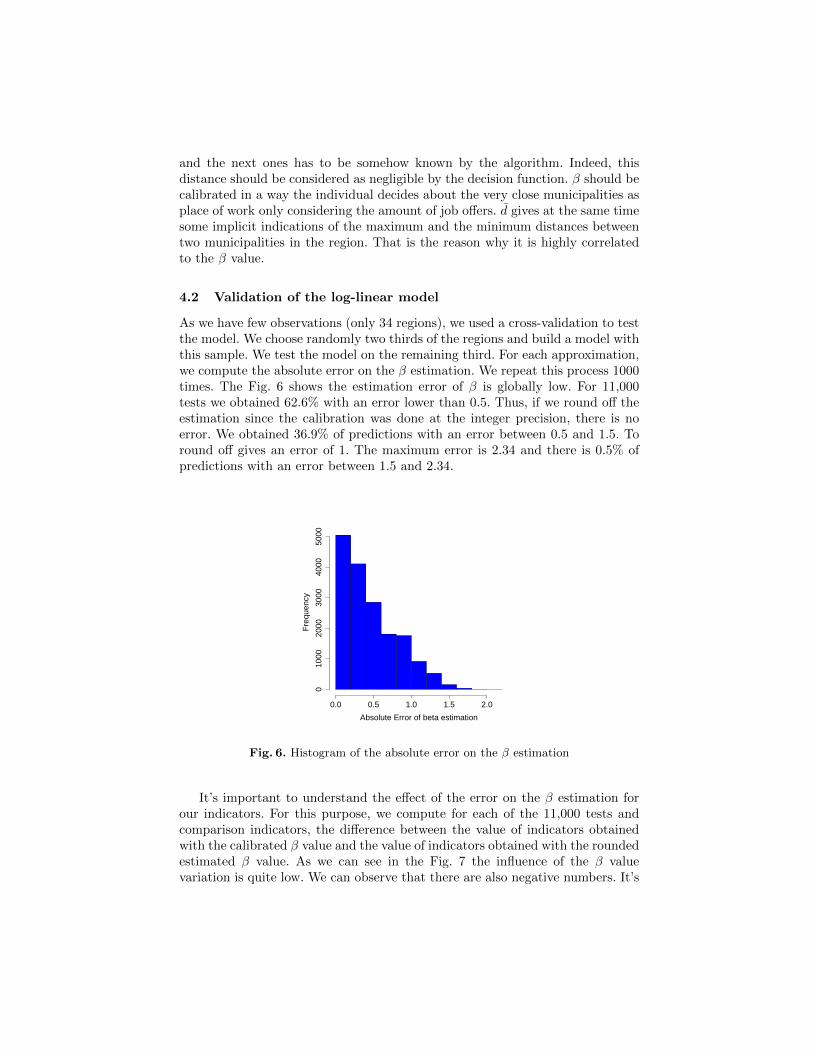
As we have few observations (only 34 regions), we used a cross-validation to testthe model. We choose randomly two thirds of the regions and build a model withthis sample. We test the model on the remaining third. For each approximation,we compute the absolute error on the β estimation. We repeat this process 1000times. The Fig. 6 shows the estimation error of β is globally low. For 11,000tests we obtained 62.6% with an error lower than 0.5. Thus, if we round off theestimation since the calibration was done at the integer precision, there is noerror. We obtained 36.9% of predictions with an error between 0.5 and 1.5. Toround off gives an error of 1. The maximum error is 2.34 and there is 0.5% ofpredictions with an error between 1.5 and 2.34.

Absolute Error of beta estimation

Fre

quen

cy

0.0 0.5 1.0 1.5 2.0

010

0020

0030

0040

0050

00

Fig. 6. Histogram of the absolute error on the β estimation

It’s important to understand the effect of the error on the β estimation forour indicators. For this purpose, we compute for each of the 11,000 tests andcomparison indicators, the difference between the value of indicators obtainedwith the calibrated β value and the value of indicators obtained with the roundedestimated β value. As we can see in the Fig. 7 the influence of the β valuevariation is quite low. We can observe that there are also negative numbers. It’s

(a)

Fre

quen

cy

−0.010 0.000 0.010

020

0040

0060

00

(b)

Fre

quen

cy

−0.005 0.000 0.005 0.010

020

0040

0060

00

(c)

Fre

quen

cy

−0.05 0.00 0.05 0.10

020

0040

0060

0080

00

Fig. 7. Histograms of the difference between the value obtained with the calibratedβ value and the rounded estimated β value; (a) The difference for CPOCB ; (b) Thedifference for CPICB ; (c) The difference for CPCB .

possible that the different values of the common part of commuters are betterwith another β value because it’s not the calibration criterion. Generally, the βvalue maximizing the different indicators is at more or less 1 (β is an integer) ofthe calibrated β. For the 34 regions studied β varies between 2 and 22.

For the CPOC we have 75.57% of test with a negative difference, 24.43% witha positive difference and a maximum difference of 0.012. For the CPIC we have75.57% of prevision with a negative difference, 24.43% with a positive differenceand a maximum difference of 0.009. The percentages of prevision with a negativeand positive difference are equal because it’s the same β value maximizing thecommon part of out-commuters and the common part of in-commuters. For theCPC we have 80.29% of prevision with a negative difference, 19.71% with apositive difference from which 95.02% with a difference less than 0.01 and amaximum difference of 0.107.

4.3 How to use the universal parameter?

Let a region Rtest composed by n municipalities and an outside of m−n munic-ipalities. For this region we have: the Euclidean distance matrix between the nmunicipalities of the region and the m municipalities of the region and its out-side; the number of out-commuters for each municipality of the region; the num-ber of in-commuters for each municipality of the region and the outside. Withthe Euclidean distance matrix, we compute dtest the average distance betweenthe municipalities of the region. It’s possible to estimate βtest, the calibratedparameter, at least for a French region, by a function of dtest (15).

βtest = e−7.69d 0.92test (15)

Then, to simulate the network Rtest, it is possible to directly use the modelwith the deterrence function (16):

f(dij) = e−e−7.69d 0.92

test dij/dtest = e−e−7.69d−0.08

test dij (16)

Let us remind that it’s sheer coincidence if the most explanatory variableof β is the value used to normalize the distance in the deterrence exponentialfunction originally chosen (namely d).

5 Discussion and conclusion

Starting from the simple and efficient stochastic model proposed in (Gargiuloet al., 2011), we propose an improvement allowing the generation of commut-ing network for regions where the detailed data on the value of the origin todestination flows are not available. It is sufficient to have the aggregated totalnumber of in and out commuters at the municipal level to be able to generatethe commuting network. Moreover we can reproduce the commuting networkof a region even if that one is quite dependent of its outside to satisfy its ownjob demand. Our improvements consist in enlarging the job search geographicalbase by considering the number of in-commuters not only of the municipality ofthe region but also of the neighbouring municipalities. Using this extension ofthe job search base coupling to an exponential deterrence function allows us togenerate a statistically relevant commuting network for the region of interest.Moreover, the model coupled to our improvements no longer requires to be cal-ibrated since a very accurate calibration law has been found depending on theaverage distance between the municipalities.

The model and the proposed improvements have been tested on at most 34French set of municipalities, which are French regions or districts. It has shown itsaccuracy. However, the sample has to be enlarged to double check the results.It would be especially relevant to test our proposals on regions from variouscountries having different geographical and socio-economical characteristics fromthe French ones. Moreover, even if the exponential deterrence function allowsus not to overestimate too much the probability of the commuters going towork outside the region, the size and the number of the outside neighbouringmunicipalities adding to the job search base has certainly an impact on theweight of the overestimation. This question has not really being studied in thispaper, and neither has the one consisting in understanding better why the foundcalibration law gives such an accurate prevision of the parameter.

Bibliography

Balcan, D., Colizza, V., Goncalves, B., Hud, H., and Ramasco, J.J.and Vespig-nani, A. (2009). Multiscale mobility networks and the spatial spreading ofinfectious diseases. Proceedings of the National Academy of Sciences of theUnited States of America, 106(51):21484–21489.

Barabasi, A. and Albert, R. (1999). Emergence of scaling in random networks.Science, 286(5439):509–512.

Barrat, A., Barthelemy, M., Pastor-Satorras, R., and Vespignani, A. (2004).The architecture of complex weighted networks. Proceedings of the NationalAcademy of Sciences of the United States of America, 101(11):3747–3752.

Barrat, A., Barthelemy, M., and Vespignani, A. (2005). The effects of spatialconstraints on the evolution of weighted complex networks. Journal of Statis-tical Mechanics: Theory and Experiment, (5):49–68.

Barthelemy, M. (2010). Spatial networks.De Montis, A., Barthelemy, M., Chessa, A., and Vespignani, A. (2007). The

structure of interurban traffic: A weighted network analysis. Environmentand Planning B: Planning and Design, 34(5):905–924.

De Montis, A., Chessa, A., Campagna, M., Caschili, S., and Deplano, G. (2010).Modeling commuting systems through a complex network analysis: A study ofthe italian islands of sardinia and sicily. The Journal of Transport and LandUse, 2(3):39–55.

Gargiulo, F., Lenormand, M., Huet, S., and Baqueiro Espinosa, O. (2011). Com-muting network: going to the bulk. Submitted to the Journal of ArtificialSocieties and Social Simulation, page 13 pages.

Gitlesen, J. P., Kleppe, G., Thorsen, I., and Ube, J. (2010). An empirically basedimplementation and evaluation of a hierarchical model for commuting flows.Geographical Analysis, 42(3).

Haynes, K. E. and Fotheringham, A. S. (1984). Gravity and spatial interactionmodels. Sage Publications, Beverly Hills.

Hensen, M. and Bongaerts, D. (2009). Delimitation and coherence of functionaland administrative regions. Regional Studies, 1:19–31.

Huet, S. and Deffuant, G. (2011). Common framework for the microsimulationmodel in prima project. Technical report, Cemagref LISC.

Konjar, M., Lisec, A., and Drobne, S. (2010). Method for delineation of func-tional regions using data on commuters. Guimares, Portugal. 13th AGILEInternational Conference on Geographic Information Science.

Lemercier, C. and Rosental, P.-A. (2008). Les migrations dans le nord de la franceau XIXe siecle. In Nouvelles approches, nouvelles techniques en analyse desreseaux sociaux, Lille France.

Ortuzar, J. and Willumsen, L. (2011). Modeling Transport. John Wiley andSons Ltd, New York.

Pastor-Satorras, R. and Vespignani, A. (2004). Evolution and Structure of theInternet: A Statistical Physics Approach. Cambridge University Press, NewYork, NY, USA.

Sørensen, T. (1948). A method of establishing groups of equal amplitude inplant sociology based on similarity of species and its application to analysesof the vegetation on danish commons. Biol. Skr., 5:1–34.

Stillwell, J. and Duke-Williams, O. (2007). Understanding the 2001 UK censusmigration and commuting data: The effect of small cell adjustment and prob-lems of comparison with 1991. Journal of the Royal Statistical Society.SeriesA: Statistics in Society, 170(2):425–445.