Computer Vision and Deep Learning for Retail Store ...
180
ALMA MATER STUDIORUM – UNIVERSITÀ DI BOLOGNA D ottorato di R icerca in COMPUTER SCIENCE AND ENGINEERING C iclo 31 ° S ettore C oncorsuale di afferenza : 09 /H 1 S ettore S cientifico -D isciplinare : ING-INF/ 05 COMPUTER VISION AND DEEP LEARNING FOR RETAIL STORE MANAGEMENT P resentata da :A lessio Tonioni C oordinatore dottorato R elatore C hiar . mo P rof .I ng . C hiar . mo P rof .I ng . Paolo C iaccia L uigi D i S tefano E same finale anno 2019
-
Upload
khangminh22 -
Category
Documents
-
view
0 -
download
0
Transcript of Computer Vision and Deep Learning for Retail Store ...
ALMA MATER STUDIORUM – UNIVERSITÀ DI BOLOGNA
Dottorato di R icerca in
COMPUTER SCIENCE AND ENGINEERING
C iclo 31°
Settore Concorsuale di afferenza : 09/H1
Settore Scientifico -D isciplinare : ING-INF/05
C O M P U T E R V I S I O N A N D D E E PL E A R N I N G F O R R E TA I L S T O R E
M A N A G E M E N T
Presentata da : Alessio Tonioni
Coordinatore dottorato Relatore
Chiar .mo Prof . Ing . Chiar .mo Prof . Ing .
Paolo C iaccia Luigi D i Stefano
Esame finale anno 2019

Alessio Tonioni: Computer Vision and Deep Learning for Retail Store Management,Dottorato di ricerca in Computer Science and Engineering, © 2018
supervisor:Luigi Di Stefano
location:Bologna, Italy
A B S T R A C T
The management of a supermarket or retail store is a quite complex pro-cess that requires the coordinated execution of many different tasks (e.g.,shelves management, inventory, surveillance, customer support. . . ). Cur-rently, the vast majority of those tasks still rely on human personnel thatfor this reason spend most of their working hours on repetitive and boringjobs. More often than not this will cause below expectancy efficiency that isobviously undesirable from the management perspective. Thank to recentadvancements of technology, however, many of those repetitive tasks canbe completely or partially automated easing and speeding up the job forsales clerks, improving the overall efficiency of the store, providing real-timeanalytics and resulting in potential additional services for the customers (e.g.,customized shopping experience). One of the key technology requirementshared between most of the aforementioned tasks is the ability to understandsomething specific about a scene based only on information acquired bya camera, for this reason, we will focus on how to deploy state of the artcomputer vision techniques to solve some management problems insidea grocery retail store. In particular, we will address two main problems:(a) how to detect and recognize automatically products exposed on storeshelves and (b) how to obtain a reliable 3D reconstruction of an environmentusing only information coming from a camera. A good solution to (a) willbe crucial to automate management tasks like visual aisle inspection or auto-matic inventory. At the same time it could drastically improve the customerexperience with visual aid during the shopping, improved interaction viaaugmented reality or automatic assistance for visually impaired. We willtackle (a) both in a constrained version where the objective is to verify thecompliance of observed items to a planned disposition, as well as an uncon-strained one where no assumption on the observed scenes are considered.For both cases, we will show how to overcome some shortcoming resultingfrom naively applying state of the art computer vision techniques in thisdomain. As for (b), a good solution represents one of the first crucial stepsfor the development and deployment of low-cost autonomous agents ableto safely navigate inside the store either to carry out management jobs orto help customers (e.g., autonomous cart or shopping assistant). We believe
iii
that algorithms for depth prediction from stereo or mono camera are goodcandidates for the solution of this problem thanks to the low price of therequired sensors, the great deployment flexibility and the achievable preci-sion. However, the current state of the art algorithms for depth estimationfrom mono or stereo rely heavily on machine learning by deploying hugeconvolutional neural networks that take RGB images as input and output anestimation of the distance of each pixel from the camera. Those techniquesmight be hardly applied in the retail environment due to problems arisingfrom the domain shift between data used to train them (usually syntheticimages) and the deployment scenario (real indoor images). To overcomethose limitations we will introduce techniques to adapt those algorithmsto unseen environments without the need of acquiring costly ground truthdata and, potentially, in real time as soon as the algorithm starts to operateon unseen scenes.
iv

A C K N O W L E D G E M E N T S
I would like to thank Centro Studi srl1 for financing my Ph.D. and providingsupport for the development of some of the projects discussed in this work.I would like to thank my supervisor Prof. Luigi Di Stefano for all the timeand effort spent mentoring me during the three years of my Ph.D.My thanksextend to Prof. Philip Torr for offering me the possibility to spend six monthsin the Torr Vision Group at the University of Oxford, a period that I considerfundamental for my growth as a researcher. Moreover, I would like to thankall the people with whom I have worked together during these years: MatteoPoggi, Fabio Tosi, Stefano Mattoccia, Pierluigi Zama Ramirez, Daniele DeGregorio, Riccardo Spezialetti, Samuele Salti, Federico Tombari, EugenioSerra, Alioscia Petrelli, Tommaso Cavallari, Gianluca Berardi, Paolo Galeone,Oscar Rahnama, Tom Joy and Ajanthan Thalaiyasingam. Nevertheless, Iwould also like to thank all the other people that have worked at CVLabin Bologna and Torr Vision Group in Oxford for the insightful talks anddiscussions inside and outside the office. Finally, I would like to thank myfamily and friends for always supporting me during all my university andPh.D. years. Last but not least, my greatest thanks goes to my girlfriendArianna for helping me during my Ph.D. and always being there when Ineeded support during particularly stressful periods.
1 https://www.orizzontiholding.it/centro-studi/
v

C O N T E N T S
1 introduction 1
1 .1 Automatic Detection and Recognition of items on store shelves . 3
1 .2 Reliable 3D reconstruction of unseen environments . . . . . . . . 5
i recognition of products on store shelves
2 initial remarks 11
2 .1 Related Work . . . . . . . . . . . . . . . . . . . . . . . . . . . . . . 12
3 planogram compliance check 15
3 .1 Related Works . . . . . . . . . . . . . . . . . . . . . . . . . . . . . . 15
3 .2 Proposed Pipeline . . . . . . . . . . . . . . . . . . . . . . . . . . . . 16
3 .2 .1 Unconstrained Product Recognition . . . . . . . . . . . . . . . . 18
3 .2 .2 Graph-based Consistency Check . . . . . . . . . . . . . . . . . . 19
3 .2 .3 Product Verification . . . . . . . . . . . . . . . . . . . . . . . . . 22
3 .3 Experimental Results . . . . . . . . . . . . . . . . . . . . . . . . . . 24
4 unconstrained product detection 29
4 .1 Related Works . . . . . . . . . . . . . . . . . . . . . . . . . . . . . . 30
4 .2 Proposed Approach . . . . . . . . . . . . . . . . . . . . . . . . . . . 31
4 .2 .1 Detection . . . . . . . . . . . . . . . . . . . . . . . . . . . . . . . . 32
4 .2 .2 Recognition . . . . . . . . . . . . . . . . . . . . . . . . . . . . . . 32
4 .2 .3 Refinement . . . . . . . . . . . . . . . . . . . . . . . . . . . . . . . 34
4 .3 Experimental Results . . . . . . . . . . . . . . . . . . . . . . . . . . 35
4 .3 .1 Datasets and Evaluation Metrics . . . . . . . . . . . . . . . . . . 35
4 .3 .2 Implementation Details . . . . . . . . . . . . . . . . . . . . . . . 36
4 .3 .3 Customer Use Case . . . . . . . . . . . . . . . . . . . . . . . . . . 37
4 .3 .4 Qualitative Results . . . . . . . . . . . . . . . . . . . . . . . . . . 43
5 domain invariant hierarchical embedding for gro-cery products recognition 45
5 .1 Related Work . . . . . . . . . . . . . . . . . . . . . . . . . . . . . . 46
5 .2 Domain invariant hierarchical embedding . . . . . . . . . . . . . . 48
5 .2 .1 Hierarchical Embedding . . . . . . . . . . . . . . . . . . . . . . . 49
5 .2 .2 Domain Invariance . . . . . . . . . . . . . . . . . . . . . . . . . . 49
5 .3 Implementation details . . . . . . . . . . . . . . . . . . . . . . . . . 51
5 .4 Experimental Results . . . . . . . . . . . . . . . . . . . . . . . . . . 53
5 .4 .1 Ablation Study . . . . . . . . . . . . . . . . . . . . . . . . . . . . 56
vii
5 .4 .2 Product Recognition . . . . . . . . . . . . . . . . . . . . . . . . . 58
5 .4 .3 Beyond product recognition . . . . . . . . . . . . . . . . . . . . . 63
5 .4 .4 Qualitative Results . . . . . . . . . . . . . . . . . . . . . . . . . . 64
5 .4 .5 DIHE for product detection . . . . . . . . . . . . . . . . . . . . . 65
6 conclusions 69
ii unsupervised adaptation for deep depth
7 initial remarks 73
7 .1 Related Work . . . . . . . . . . . . . . . . . . . . . . . . . . . . . . 77
8 unsupervised domain adaptation for learned depth
estimation 79
8 .1 Related work . . . . . . . . . . . . . . . . . . . . . . . . . . . . . . . 81
8 .2 Domain adaptation for depth sensing . . . . . . . . . . . . . . . . 81
8 .2 .1 Confidence Guided Loss . . . . . . . . . . . . . . . . . . . . . . . 83
8 .2 .2 Smoothing Term . . . . . . . . . . . . . . . . . . . . . . . . . . . 85
8 .2 .3 Image Reconstruction Loss . . . . . . . . . . . . . . . . . . . . . 85
8 .3 Experimental results . . . . . . . . . . . . . . . . . . . . . . . . . . 86
8 .3 .1 Effectiveness of Confidence Estimation . . . . . . . . . . . . . . 87
8 .3 .2 Deep Stereo . . . . . . . . . . . . . . . . . . . . . . . . . . . . . . 90
8 .3 .3 Depth-from-Mono . . . . . . . . . . . . . . . . . . . . . . . . . . 94
8 .3 .4 Qualitative Results . . . . . . . . . . . . . . . . . . . . . . . . . . 99
8 .3 .5 Qualitative evaluation on Supermarket Environment . . . . . . 102
9 online unsupervised domain adaptation for deep stereo103
9 .1 Related Work . . . . . . . . . . . . . . . . . . . . . . . . . . . . . . 104
9 .2 Online Domain Adaptation . . . . . . . . . . . . . . . . . . . . . . 105
9 .2 .1 MADNet - Modularly ADdaptive Network . . . . . . . . . . . . 105
9 .2 .2 MAD - Modular ADaptation . . . . . . . . . . . . . . . . . . . . 107
9 .3 Experimental Results . . . . . . . . . . . . . . . . . . . . . . . . . . 109
9 .3 .1 MADNet performance . . . . . . . . . . . . . . . . . . . . . . . . 111
9 .3 .2 Online Adaptation . . . . . . . . . . . . . . . . . . . . . . . . . . 111
9 .3 .3 Different online adaptation strategies . . . . . . . . . . . . . . . 114
9 .3 .4 Deployment on embedded platforms . . . . . . . . . . . . . . . 116
10 learning to adapt for stereo 117
10 .1 Related Works . . . . . . . . . . . . . . . . . . . . . . . . . . . . . . 118
10 .2 Problem Setup and Preliminaries . . . . . . . . . . . . . . . . . . . 118
10 .2 .1Online Adaptation for Stereo . . . . . . . . . . . . . . . . . . . . 118
10 .2 .2Model Agnostic Meta Learning . . . . . . . . . . . . . . . . . . . 120
10 .3 Learning to Adapt for Stereo . . . . . . . . . . . . . . . . . . . . . 121
viii

10 .3 .1Meta Learning for Stereo Adaptation . . . . . . . . . . . . . . . 121
10 .3 .2Confidence Weighted Adaptation . . . . . . . . . . . . . . . . . 123
10 .4 Experiments . . . . . . . . . . . . . . . . . . . . . . . . . . . . . . . 126
10 .4 .1Experimental Setup . . . . . . . . . . . . . . . . . . . . . . . . . . 126
10 .4 .2Results . . . . . . . . . . . . . . . . . . . . . . . . . . . . . . . . . 127
10 .4 .3Confidence Weighted Loss Function . . . . . . . . . . . . . . . . 131
11 conclusions 133
iii final remarks
12 conclusions 137
ix

AU T H O R ’ S P U B L I C AT I O N S
During the PhD period, the author contributed to the following publications.Research conducted during the development of some of them is integralpart of this thesis.
[1] Alessio Tonioni and Luigi Di Stefano. ‘Product recognition in storeshelves as a sub-graph isomorphism problem’. In: InternationalConference on Image Analysis and Processing. Springer. 2017, pp. 682–693.
[2] Alessio Tonioni, Matteo Poggi, Stefano Mattoccia and Luigi DiStefano. ‘Unsupervised adaptation for deep stereo’. In: The IEEEInternational Conference on Computer Vision (ICCV). Vol. 2. 7. 2017,p. 8.
[3] Pierluigi Zama Ramirez, Alessio Tonioni and Luigi Di Stefano. ‘Ex-ploiting Semantics in Adversarial Training for Image-Level DomainAdaptation’. In: International Conference on Image Processing, Applica-tions and Systems. 2018.
[4] Alessio Tonioni, Samuele Salti, Federico Tombari, Riccardo Spezialettiand Luigi Di Stefano. ‘Learning to Detect Good 3D Keypoints’. In:International Journal of Computer Vision 126.1 (2018), pp. 1–20.
[5] Alessio Tonioni, Eugenio Serra and Luigi Di Stefano. ‘A deep learningpipeline for fine-grained products recognition on store shelves’. In:International Conference on Image Processing, Applications and Systems.2018.
[6] Oscar Rahnama, Tommaso Cavallari, Stuart Golodetz, Alessio To-nioni, Tom Joy, Luigi Di Stefano, Simon Walker and Philip H.S. Torr.‘Real-Time Highly Accurate Dense Depth on a Power Budget usingan FPGA-CPU Hybrid SoC’. In: Procedings of the IEEE InternationalSymposium on Circuits and Systems. 2019.
[7] Daniele De Gregorio, Alessio Tonioni, Gianluca Palli and Luigi DiStefano. ‘Semi-Automatic Labeling for Deep Learning in Robotics’.In: Machine Vision and Applications. under review.
xi
[8] Alessio Tonioni and Luigi Di Stefano. ‘Domain invariant hierarchicalembedding for grocery products recognition’. In: Computer Visionand Image Understanding (under review).
[9] Alessio Tonioni, Matteo Poggi, Stefano Mattoccia and Luigi DiStefano. ‘Unsupervised Domain Adaptation for Depth Predictionfrom Images’. In: IEEE Transactions on Pattern Analysis and MachineIntelligence. under review.
[10] Alessio Tonioni, Oscar Rahnama, Tom Joy, Luigi Di Stefano, AjanthanThalaiyasingam and Philip Torr. ‘Learning to adapt for stereo’. In:Conference on Computer Vision and Pattern Recognition. under review.
[11] Alessio Tonioni, Fabio Tosi, Matteo Poggi, Stefano Mattocia and LuigiDi Stefano. ‘Real-time self-adaptive deep stereo’. In: Conference onComputer Vision and Pattern Recognition. under review.
xii

1I N T R O D U C T I O N
The management of grocery stores or supermarkets is a challenging task thatrequires many people constantly busy with the supervision of shelves and ofthe whole shop. Technology advances may help by providing more reliableinformation in real time to the store manager, so that he may coordinate ina more targeted way the human resources at his disposal. New technologiesmay not only lead to better and more effective management of the store, butalso to improvements for the customers by giving to store owners the abilityto provide better services without additional fixed costs like new employees.Since understanding an observed scene is one of the crucial premises formost tasks, in this work we are going to study how to develop, deployand tune state of the art computer vision techniques to ease and partiallyautomate some management tasks for stores. Some examples of such tasksare automatic inventory, store surveillance, aided shopping for visuallyimpaired people, customer tracking and analytics. . . . In the following, weare going to address some of these tasks by developing computer visionsystems based on state of the art techniques. We will spend quite some timediscussing in details how we overcome some of the several problems arisingfrom a naive deployment of general solutions in real applications. All theworks featured in this thesis will share some common traits that we aregoing to briefly discuss here.
Firstly we work under the assumption of modifying existing stores andcommercial practices as little as possible. By assuming this constraint wehope to achieve solutions viable from an economic perspective even for small-medium operators, that don’t modify dramatically the current customerexperience and that are more interesting from a research perspective. Thisassumption is, however, in direct contrast with the way industrial practicesare currently evolving: the most successful proposals so far try to easethe management of a store by completely changing the way we build andorganize them. Some practical examples of these solutions have alreadyreached the commercial phase and are available across stores all aroundthe world. For example, commercial outlets belonging to the Decathlonretail chain already includes on almost all the products on sale a disposable
1

RFID tag both to protect items from being stolen as well as to performautomatic recognition for inventory and fast checkout. This solution isvery effective and fail-safe but can hardly be applied to grocery stores thatmay feature goods for which the selling price would be lower than the costof the disposable RFID tag itself. Another famous example of disruptivetechnology in retails is the Amazon Go project1, the first, and currently only,implementation of an almost completely autonomous grocery store. Inside,customers can benefit from a checkout free experience with no queue orcashier. By taking an item from a shelve and walking out of the store thecustomer agrees to purchase the item and automatically charge the cost on itsbill. While potentially disruptive and intriguing, technological solutions likethese require huge investments that are often not viable for the vast majorityof retail chains. Moreover covering the whole store with camera and sensorsto track the customers, as in the Amazon Go project, can be perceived as aquite invasive technology that can lead to potential loss of customers due toserious concerns regarding the user privacy during shopping. In contrast,all our proposals will not require ad-hoc stores or packaging nor additionalsensors besides a camera. We believe that our proposals could be easilyintegrated with the current job of sales clerk blending unnoticed and withoutthreatening the customer experience. Besides these extremes, in recent yearssome research and industrial solutions which rely on assumption closer toours have started to emerge to solve some of the aforementioned problems,however, to the best of our knowledge, established scientific approacheshave not emerged yet while the few commercial solutions seems either at aprototype stage or in the very early part of their life cycle.
The second common feature among all the researches presented in thisthesis will be to solve problems arising in the retail scenario with the hopeof proposing solutions to more general problems. For example one of therecurrent topics across this work will be the loss in performance due todomain shift between training and testing data for machine learning basedalgorithms. We faced this kind of issue when applying state of the art deeplearning based algorithms to the solution of retail problems, however, thesame problem arises across countless other applications and research fields.As such for most of the works we have tried to keep the presentation and theproposed solutions as general as possible, using the retail environment onlyas an exemplary test case rather than developing more ad-hoc and specific
1 https://www.amazon.com/b?ie=UTF8&node=16008589011
2
solutions. We believe that most of our proposals can be interesting from amore broad research audience rather than only for practitioners searchingfor a solution to specific retail related problems.
Among all the possible in-store problems addressable through computervision techniques, we are going to focus mainly on two: automatic recog-nition of items on store shelves and obtaining a reliable 3D reconstructionof an environment for navigation purpose. We will now briefly introducethe two problems that will be more carefully analyzed in Part i and Part iirespectively.
1 .1 automatic detection and recognition of items on store
shelves
The first task that we are going to analyze concerns the detection andrecognition of all visible products on an image of a store shelf. To perform therecognition we assume the availability beforehand of one or more referenceimages depicting each one of the possible items on sale. We addressedthe solution of this problem as it can be crucial to automate a series oflow-level repetitive management tasks, like visual shelves inspections todetect out or low in stock products, while laying the foundations for acompletely automatic inventory. At the same time, automate the recognitionof products can be quite beneficial to offer new services to customers visitingthe store, for example, allowing assisted shopping for visually impaired andbeing one of the building blocks for checkout free technologies. From aresearch point of view the recognition of products on shelves can be tracedback to the more general case of object recognition, where we have one ormore reference images of the sought object and a scene image where theobjects may appear in different poses, such as rotated, translated, scaled,or even partially covered by other objects and under diverse illuminationconditions. Analysis of products on shelves, though, may be regarded asa quite challenging case of the general visual object recognition problem.Firstly, it requires the simultaneous detection and recognition of the manydifferent instances typically exposed on a store shelf; moreover, recognitionmust be carried out choosing among the thousands of possible items onsale on a store at any given times and at a quite fine instance classificationlevel (e.g., two different types of pasta, even from the same brand, must berecognized as different items). Finally, the reference images for each product
3
are usually produced for marketing purpose and, therefore, exhibit ideal,but quite unrealistic, lighting and acquisition conditions. In store images fedto the recognition engine, instead, are usually acquired with lower qualityequipment (e.g., smartphone cameras) and in conditions far from ideal. Assuch a viable solution for the problem must somehow address this huge shiftbetween the image available offline (i.e., the high-quality reference ones) andthe low-quality one acquired in stores where recognition should be carriedout. The problem became even more prominent when relying on state ofthe art object detectors based on machine learning that will obviously faceproblems coming from the domain shift between train and test data.
In Chap. 3 we will first address a constrained version of this problemwhere we assume to know in advance the expected product dispositionon store shelves, which is usually called planogram. This arrangement iscarefully planned to maximize sales and keep customers happy, currently,however, verifying compliance of real shelves to the ideal layout is still mostlyperformed by store personnel. We try to automate this step by deployingan object recognition pipeline to verify if the observed portion of a shelveis compliant with the planned disposition or if there are missing and/ormisplaced products, a task we will reefer as planogram compliance check.For the solution of this task, we deploy local invariant features togetherwith a novel formulation of the product recognition problem as a sub-graphisomorphism between the items appearing in the given image and the ideallayout. This allows for auto-localizing the given image within the aisle orstore and improving recognition dramatically.
In Chap. 4 we will address the more general problem of detecting itemson store shelves without any assumption. To this end, we will deploy stateof the art object detectors based on deep learning to obtain an initial product-agnostic items detection. Then, we pursue product recognition through asimilarity search between global descriptors computed on reference productimages and cropped (query) images extracted from the shelf picture. Tomaximize performance, we learn an ad-hoc global descriptor by a CNN2
trained on reference images through an image embedding loss. Our systemis computationally expensive at training time but can perform recognitionrapidly and accurately at test time. We will also advocate why direct deploy-ment of state of the art object recognition system based on classification isimpractical, if not completely infeasible, for this specific task.
2 Convolutional Neural Network
4
Finally, in Chap. 5 we will focus on the recognition phase of the pipelineintroduced above and explicitly address problems arising from the domainshift between reference images for products available beforehand and queryimages acquired in store. Inspired by recent advances in image retrieval,one-shot learning and semi-supervised domain adaptation, we propose anend-to-end architecture comprising a GAN3 to address the domain shift attraining time and a deep CNN trained on the samples generated by the GANto learn an embedding for product images that enforces a hierarchy betweenproduct categories. At test time, we perform recognition by means of K-NN4
search against a database consisting of one reference image per product.We will also show experimentally how our proposed solution generalizesfairly well to domains different than the retail one where might be useful toexplicitly address the distribution shift between training and testing data.
1 .2 reliable 3d reconstruction of unseen environments
While not immediately related to problems typically addressed in retailenvironments, the ability to correctly sense the 3D structure of an environ-ment is one of the crucial building blocks for any applications that wantto rely on autonomous agents moving inside an environment. Example ofsuch agents inside a store could be automatic shopping carts, personalizedrobotic shopping assistants or autonomous platform for aisle inspection andmanagement. All these systems should be able to correctly sense the 3Dstructure of the environment that surrounds them to navigate safely insidethe store and to ease the interaction with customers or items exposed on theshelves. More in general, the availability of reliable 3D information could behelpful for other retail-oriented tasks such as the detection of out of stocksproducts on shelves or to allow virtual shopping and tour in a realistic 3Dreconstruction of stores.
Among the available technologies for 3D sensing, we have mostly invest-igated the use of algorithms which relies only on one or two passive RGBcameras and ignored all the active alternatives. We have made this choiceboth due to the well-known shortcoming of active sensors when dealingwith dark or highly reflective surfaces, being both quite common among thepattern on product packages, and for the cheapest cost and higher flexibility
3 Generative Adversarial Network4 K Nearest Neighbour
5
offered by passive sensors. State-of-the-art to obtain accurate and densedepth measurements out of RGB images currently consists of training deepCNN models in end-to-end fashion on large amounts of data. Despite theoutstanding performance achievable, these frameworks suffer from drasticdrops in accuracy when running on unseen imagery different from thoseobserved during training either in terms of appearance (synthetic vs real) orcontext (indoor vs outdoor). The effect due to this domain shift is usuallysoftened by fine-tuning on smaller sets of images with depth labels, but inpractice, it is not always possible, or it is extremely costly, to acquire suchkind of data required to supervise the network. For example, one possibleway to acquire reliable 3D labels mandate the use of costly Lidar5 sensors, acareful calibration between sensors and, finally, a noise removal step fromthe sensor raw output. Unfortunately, as we will see, only a few selectedenvironments and applications offer publicly available annotated datasetsuitable for supervised fine-tuning, and none of these concerns a supermar-ket like environments. To overcome these shortcomings, we have mainlyworked on methods to perform these adaptation steps effectively withoutrequiring ground truth information. We have mostly tested our solutions onautonomous driving environments due to the public availability of datasetswith precise ground-truth data for evaluation, but all the proposed solutioncan be generalized to any environments without changes.
In Chap. 8 we will introduce an effective off-line and unsupervised do-main adaptation technique enabling to overcome the domain shift problemwithout requiring any ground-truth label. Relying on easier to obtain stereopairs we deploy traditional non-learned stereo algorithms to produce dispar-ity/depth labels and confidence measures to assess their degree of reliability.With these cues, we can fine-tune deep models by means of a confidence-guided loss function, neglecting the effect of possible outliers outcome of thestereo algorithms. Experimental results prove that our technique is effectiveto adapt models for both stereo and monocular depth estimations.
In Chap. 9 we address the domain shift problem by performing a con-tinuous and unsupervised on-line adaptation of a deep stereo network topreserve good performance in challenging environments. Performing con-tinuous training of a network can be extremely demanding on computationalresources, however, we mitigate the requirements by introducing a new light-
5 Laser Imaging Detection and Ranging, active sensors that measures distance to a target byilluminating the target with pulsed laser light and measuring the reflected pulses with asensor.
6

weight yet effective deep stereo architecture and by developing an algorithmto train independently only sub-portions of the network. We will show howusing both our new architecture and our fast adaptation schema we are ableto continuously fine-tune a network to unseen environments at ∼ 25FPS ona GPU, opening the way to widespread applications.
Finally in Chap. 10 we will present some ongoing work on how to deploymeta-learning techniques to speed up and make more efficient the adaptationprocess for depth prediction models. We will introduce a novel trainingschema to condition the initial weight configuration of a network to be moresuitable to be adapted once exposed to unseen environments, i.e. it willrequire fewer adaptation steps to get optimal performance in an unseenenvironment. This will obviously help in the deployment of the onlineadaptation schema described before.
7


Part I
R E C O G N I T I O N O F P R O D U C T S O N S T O R E
S H E LV E S


2I N I T I A L R E M A R K S
The arrangement of products in supermarket shelves is planned very care-fully in order to maximize sales and keep customers happy. Shelves void,low in stock or misplaced products renders it difficult for the customer tobuy what she/he needs, which, in turn, not only leads to unhappy shoppersbut also to a significant loss of sales. As pointed out in [5], 31% of customersfacing a void shelf purchase the item elsewhere and 11% do not buy itat all. The planned layout of products within shelves is called planogram:it specifies where each product should be placed within shelves and howmany facings it should cover, that is how many packages of the same productshould be visible in the front row of the shelf. Keeping shelves full as well ascompliant to the planogram is a fundamental task for all types of stores. Thekey step to verify the compliance between the planned and observed layoutis the recognition of products displayed on store shelves. If properly solvedthis task could be used for many different applications ranging from faststore management to improved customer experience inside the store. Forthese reasons, in this chapter we are going to address the problem of visualshelf monitoring through computer vision techniques and in particular theautomatic detection and recognition of packaged products exposed on storeshelves. A visual representation of the task we are trying to solve is depictedin Fig. 2.1
The seminal work on product recognition dates back to [13], where Merleret al. highlights the particular issues to be addressed in order to achieve aviable approach. First of all, the number of different items to be recognizedis huge, in the order of several thousand for small to medium shops, wellbeyond the usual target for current state-of-the-art object detector based onimage classifier. Moreover, product recognition can be better described asa hard instance recognition problem, rather than a classification one, as itdeals with lots of objects looking remarkably similar but for small details(e.g., different flavors of the same brand of cereals). Then, any practicalmethodology should rely only on the information available within existingcommercial product databases, i.e. at most just one high-quality image foreach side of the package, either acquired in studio settings or rendered (see
11
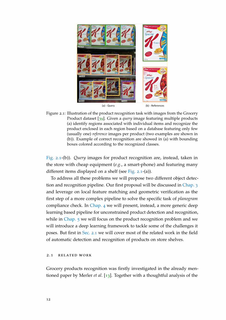
(a) - Query (b) - References
Figure 2.1: Illustration of the product recognition task with images from the GroceryProduct dataset [39]. Given a query image featuring multiple products(a) identify regions associated with individual items and recognize theproduct enclosed in each region based on a database featuring only few(usually one) reference images per product (two examples are shown in(b)). Example of correct recognition are showed in (a) with boundingboxes colored according to the recognized classes.
Fig. 2.1-(b)). Query images for product recognition are, instead, taken inthe store with cheap equipment (e.g., a smart-phone) and featuring manydifferent items displayed on a shelf (see Fig. 2.1-(a)).
To address all these problems we will propose two different object detec-tion and recognition pipeline. Our first proposal will be discussed in Chap. 3
and leverage on local feature matching and geometric verification as thefirst step of a more complex pipeline to solve the specific task of planogramcompliance check. In Chap. 4 we will present, instead, a more generic deeplearning based pipeline for unconstrained product detection and recognition,while in Chap. 5 we will focus on the product recognition problem and wewill introduce a deep learning framework to tackle some of the challenges itposes. But first in Sec. 2.1 we will cover most of the related work in the fieldof automatic detection and recognition of products on store shelves.
2 .1 related work
Grocery products recognition was firstly investigated in the already men-tioned paper by Merler et al. [13]. Together with a thoughtful analysis of the
12
problem, the authors propose a dataset and a system based on local invariantfeatures to realize an assistive tool for visually impaired customers. Theyassume that no information concerning product layout may be deployed toease detection. Given these settings, the performance of the proposed sys-tems turned out quite unsatisfactory in terms of both precision and efficiency.Further research has then been undertaken to ameliorate the performance ofautomatic visual recognition of grocery products [21], [64], [36]. In particular,Cotter et al. [36] report significant performance improvements by leveragingon machine learning techniques, such as HMAX and ESVM, together withHOG-like features. Yet, their proposal requires many training images foreach product, which is unlikely feasible in real settings and deploys a largeensemble of example-specific detectors, which makes the pipeline ratherslow at test time. Moreover, adding a new type of sought product is rathercumbersome as it involves training a specific detector for each exemplaryimage, thereby also further slowing down the whole system at test time. Theapproach proposed in [36] was then extended in [48] through a contextualcorrelation graph between products. Such a structure can be queried attest time to predict the products more likely to be seen given the last kdetections, thereby reducing the number of ESVM computed at test timeand speeding up the whole system. A similar idea of deploying contextualinformation to ease the recognition phase was also deployed by [66]. Morerecently, Franco et al. [91] proposed a hierarchical multi-stage recognitionpipeline that seems to be able to obtain remarkably good performance buthas only been tested on small-scale problems regarding the detections offew tens of different items. Yet, all these recent papers focus on a relativelysmall-scale problem, i.e. recognition of a few hundred different items atmost, whilst usually, several thousand products are on sale in a real shopGeorge et al. [39] address more realistic settings and propose a multi-stagesystem capable of recognizing ∼ 3400 different products based on a singlemodel image per product. First, they carry out an initial classification toinfer the macro categories of the observed items to reduce the recognitionsearch space. Then, following detection, they run an optimization step basedon a genetic algorithm to detect the most likely combination of productsfrom a series of proposals. Despite the quite complex pipeline, when relyingon only one model image per product the overall precision of the system isbelow 30%. The paper proposes also a publicly available dataset, referredto as Grocery Products, comprising 8350 product images classified into 80
hierarchical categories together with 680 high-resolution images of shelves.
13

The same large-scale realistic problem has been subsequently tackled by[86] using a standard local feature based recognition pipeline and an op-timized Hough Transform to detect multiple object instances and filter outinconsistent matches, which brings in a slight performance improvement.More recently, [98] have shown how it is possible to improve detectionand recognition performance on the same dataset relying on a probabilisticmodel based on local feature matching and refinement by a deep network.
14
3P L A N O G R A M C O M P L I A N C E C H E C K
In this section, we will describe a computer vision pipeline that, given anexpected product disposition (referred herein as planogram) and an imagedepicting supermarket shelves, can correctly localize each product, checkwhether the real arrangement is compliant to the planned one and detectmissing or misplaced items. Key to our approach is a novel formulation ofthe problem as a sub-graph isomorphism between the product detected inthe given image and those that should ideally be found therein given theplanogram. Accordingly, our pipeline relies on a standard feature-basedobject recognition step, followed by a novel graph-based consistency checkand a final refinement step to improve the overall product recognition rate.
3 .1 related works
Beside works related to unconstrained product recognition already discussedin Sec. 2.1, it is worth mentioning the closely related work by Marder etal. [56] since it addresses the very same problem of checking planogramcompliance through computer vision. Their approach relies on detecting andmatching SURF features [11] followed by visual and logical disambiguationbetween similar products. To improve product recognition the authorsdeploy information dealing with the known product arrangement throughspecific hand-crafted rules, such as ‘conditioners are placed on the right ofshampoos‘. Differently, we propose to deploy automatically these kinds ofconstraints by modeling the problem as a sub-graph isomorphism betweenthe items detected in the given image and the planogram. Unlike ours, theirmethod mandates a-priori categorization of the sought products into subsetsof visually similar items. Systems to tackle the planogram compliance problemare described also in [38], [52] and [29]. These papers delineate solutionsrelying either on large sensor/camera networks or mobile robots monitoringshelves while patrolling aisles. In contrast, our proposal would require justan off-the-shelf device, such as a smartphone, tablet or hand-held computer.
15
InputsUnconstrained Product
RecognitionGraph-based Consistency Check Product Verification Output
Observed Planogram
Reference Planogram
Missing detection
False Detections
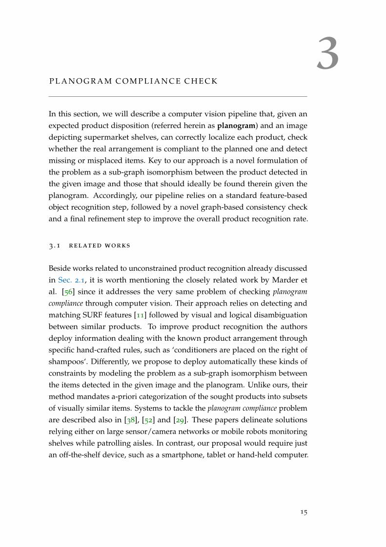
Figure 3.1: Overview of our pipeline. For each step we highlight the inputs andoutputs through red and yellow boxes, respectively. Product detectionsthroughout stages are highlighted by green boxes, while blue lines showthe edges between nodes on the graphs enconding both the Referenceand the Observed planograms.
3 .2 proposed pipeline
We address the typical industrial settings in which at least one model imageper product together with a general schema of the correct disposition ofitems (the planogram) are available. At test time, given one image featuringproducts on shelves, the system would detect and localize each item andcheck if the observed product layout is compliant to the given planogram.As depicted in Fig. 3.1, we propose to accomplish the above tasks by a visualanalysis pipeline consisting of three steps. We provide here an overview ofthe functions performed by the three steps, which are described in moredetail in the following.
The first step operates only on model images and the given shelves image.Indeed, to pursue seamless integration with existing procedures, we assumethat the information concerning which portion of the aisle is observed isnot available together with the input image. Accordingly, the first stepcannot deploy any constraint dealing with the expected product dispositionand is thus referred to as Unconstrained Product Recognition. As mostproduct packages consist of richly textured piecewise planar surfaces, weobtained promising result through a standard object recognition pipelinebased on local invariant features (as described, e.g., in [7]). Yet, the previ-
16
ously highlighted nuisances cause both missing product items as well asfalse detections due to similar products. Nonetheless, the first step cangather enough correct detections to allow the successive steps to identify theobserved portion of the aisle in order to deploy constraints on the expectedproduct layout and improve product recognition dramatically. The output ofthe first step consists of a set of bounding boxes corresponding to detectedproduct instances (see Fig. 3.1).
From the second step, dubbed Graph-based Consistency Check, we startleveraging on the information about products and their relative dispositioncontained in planograms. We choose to represent a planogram as a grid-likefully connected graph where each node corresponds to a product facing andis linked to at most 8 neighbors at 1-edge distance, i.e. the closest facingsalong the cardinal directions. We rely on a graph instead of a rigid grid toallow for a more flexible representation; an edge between two nodes doesnot represent a perfect alignment between them but just proximity alongthat direction.
This abstract representation, referred to as Reference Planogram, encodes in-formation about the number of facings related to each product and the itemsplaced close together in shelves. An example of Reference Planogram is shownin Fig. 3.1. The detections provided by the first step are used in the secondto automatically build another grid-like graph having the same structure asthe Reference Planogram and referred to as Observed Planogram. Then, we findthe sub-graph isomorphism between the Observed and Reference planograms,so as to identify local clusters of self-consistent detected products, e.g., setsof products placed in the same relative position in both the Observed andReference planograms. As a result, the second step ablates away inconsistentnodes from the Observed Planogram, which typically correspond to falsedetections yielded by the first step. It is worth pointing out that, as theObserved Planogram concerns the shelves seen in the current image while theReference Planogram models the whole aisle, matching the former into thelatter implies localizing the observed scene within the aisle1.
After the second step the Observed Planogram should contain true detec-tions only. Hence, those nodes that are missing compared to the ReferencePlanogram highlight items that appear to be missing w.r.t. the plannedproduct layout. The task of the third step, referred to as Product Verific-ation, is to verify whether these product items are really missing in the
1 More generally, matching the Observed to a set of Reference planograms does localizeseamlessly the scene within a set of aisles or, even, the whole store.
17
scene or not. More precisely, we start considering the missing node showingthe highest number of already assigned neighbors, for which we can mostreliably determine a good approximation of the expected position in theimage. Accordingly, a simpler computer vision problem than in the first stepneeds to be tackled, i.e. verify whether or not a known object is visible in awell-defined ROI (Region of Interest) within the image. Should the verifica-tion process highlight the presence of the product, the corresponding nodewould be added to the Observed Planogram, so to provide new constraintsbetween found items; otherwise, a planogram compliance issue related tothe checked node is reported (i.e., missing/misplaced item). The process isiterated till all the facings in the observed shelves are either associated withdetected instances or flagged as compliance issues.
3 .2 .1 Unconstrained Product Recognition
For the initial detection step, we rely on the classical multi-object and multi-instance object recognition pipeline based on local invariant features presen-ted in [7], which is effective with planar textured surfaces and scales wellto database comprising several hundreds or a few thousands models, i.e.comparable to the number of different products typically sold in grocerystores and supermarkets. Accordingly, we proceed through feature detection,description, and matching, then cast votes into a pose space by a GeneralizedHough Transform that can handle multiple peaks associated with differentinstances of the same model in order to cluster correspondences and filterout outliers. In our settings, it turns out reasonable to assume the inputimage to represent an approximately frontal view of shelves, so that bothin-plane and out-of-plane image rotations are small. Therefore, we estimatea 3 DOF pose (image translation and scale change).
Since the introduction of SIFT [7], a plethora of other feature detectors anddescriptors have been proposed in the literature. Interestingly, the objectrecognition pipeline we implemented may be deployed seamlessly withmost such newer proposals. Moreover, it turns out just as straightforwardto rely on multiple types of features jointly to pursue higher sensitivityby detecting diverse image structures. Purposely, our implementation ofthe standard object recognition pipeline can run in parallel several detec-tion/description/matching processes based on different features and havethem eventually cast vote altogether within the same Hough pose space. In
18
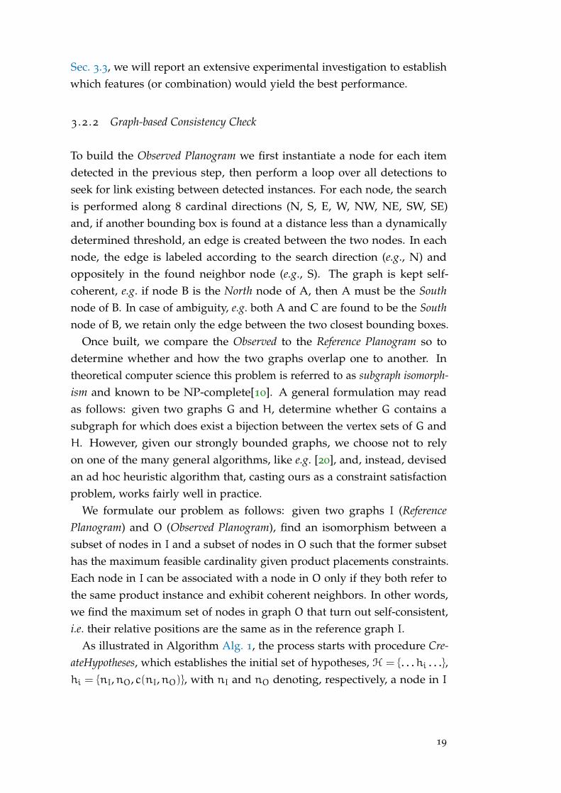
Sec. 3.3, we will report an extensive experimental investigation to establishwhich features (or combination) would yield the best performance.
3 .2 .2 Graph-based Consistency Check
To build the Observed Planogram we first instantiate a node for each itemdetected in the previous step, then perform a loop over all detections toseek for link existing between detected instances. For each node, the searchis performed along 8 cardinal directions (N, S, E, W, NW, NE, SW, SE)and, if another bounding box is found at a distance less than a dynamicallydetermined threshold, an edge is created between the two nodes. In eachnode, the edge is labeled according to the search direction (e.g., N) andoppositely in the found neighbor node (e.g., S). The graph is kept self-coherent, e.g. if node B is the North node of A, then A must be the Southnode of B. In case of ambiguity, e.g. both A and C are found to be the Southnode of B, we retain only the edge between the two closest bounding boxes.
Once built, we compare the Observed to the Reference Planogram so todetermine whether and how the two graphs overlap one to another. Intheoretical computer science this problem is referred to as subgraph isomorph-ism and known to be NP-complete[10]. A general formulation may readas follows: given two graphs G and H, determine whether G contains asubgraph for which does exist a bijection between the vertex sets of G andH. However, given our strongly bounded graphs, we choose not to relyon one of the many general algorithms, like e.g. [20], and, instead, devisedan ad hoc heuristic algorithm that, casting ours as a constraint satisfactionproblem, works fairly well in practice.
We formulate our problem as follows: given two graphs I (ReferencePlanogram) and O (Observed Planogram), find an isomorphism between asubset of nodes in I and a subset of nodes in O such that the former subsethas the maximum feasible cardinality given product placements constraints.Each node in I can be associated with a node in O only if they both refer tothe same product instance and exhibit coherent neighbors. In other words,we find the maximum set of nodes in graph O that turn out self-consistent,i.e. their relative positions are the same as in the reference graph I.
As illustrated in Algorithm Alg. 1, the process starts with procedure Cre-ateHypotheses, which establishes the initial set of hypotheses, H = {. . . hi . . .},hi = {nI,nO, c(nI,nO)}, with nI and nO denoting, respectively, a node in I
19
1 2
43
Ideal Planogram (I)
I II
III IV
Observed Planogram (O)
𝐻 = { [𝑛𝐼1, 𝑛𝑂
𝐼 , Τ2 8], [𝑛𝐼3, 𝑛𝑂
𝐼𝐼𝐼, Τ2 8],[𝑛𝐼
4, 𝑛𝑂𝐼𝑉, Τ2 8 ], [𝑛𝐼
1, 𝑛𝑂𝐼𝐼, Τ1 8],
[𝑛𝐼3, 𝑛𝑂
𝐼𝑉, Τ1 8], [𝑛𝐼4, 𝑛𝑂
𝐼𝐼𝐼, Τ0 8] }
a) Pick the best hypothesis and add it to the solution. In case more hypotheses have equal score randomly pick one.
𝑆 = {[𝑛𝐼1, 𝑛𝑂
𝐼 , Τ2 8]}
b) Remove hypotheses and increase scores.
𝐻 = { [𝑛𝐼3, 𝑛𝑂
𝐼𝐼𝐼, Τ108 ], [𝑛𝐼
4, 𝑛𝑂𝐼𝑉, Τ10
8 ],[𝑛𝐼3, 𝑛𝑂
𝐼𝑉, Τ1 8], [𝑛𝐼4, 𝑛𝑂
𝐼𝐼𝐼, Τ0 8] }
𝐻 = { [𝑛𝐼1, 𝑛𝑂
𝐼 , Τ2 8], [𝑛𝐼3, 𝑛𝑂
𝐼𝐼𝐼,1 + Τ2 8], [𝑛𝐼4, 𝑛𝑂
𝐼𝑉, 1 + Τ2 8 ], [𝑛𝐼1, 𝑛𝑂
𝐼𝐼, Τ1 8], [𝑛𝐼3, 𝑛𝑂
𝐼𝑉, Τ1 8], [𝑛𝐼
4, 𝑛𝑂𝐼𝐼𝐼, Τ0 8] }
1 2
43
I II
III IV
𝑆 = { [𝑛𝐼1, 𝑛𝑂
𝐼 , Τ2 8]}
c) Compute 𝐵𝐶 . If 𝐵𝑐 < 𝐶𝑚𝑎𝑥 return C = 𝐵𝑐.
1 2
43
I 2
III IV
𝑆 = { [𝑛𝐼1, 𝑛𝑂
𝐼 , Τ2 8], [𝑛𝐼3, 𝑛𝑂
𝐼𝐼𝐼, Τ108],
[𝑛𝐼4, 𝑛𝑂
𝐼𝑉, Τ188 ]}
d) Restart from step (a) until 𝐻 = ∅ or 𝑐 𝑛𝐼 , 𝑛𝑂 < 𝜏 for all remaining hypotheses.
𝐵𝑐 = B (S, H ) = 3
C = C ( S ) = 3
ℎ0 = [𝑛𝐼1, 𝑛𝑂
𝐼 , Τ2 8]
e) Compute C and return.
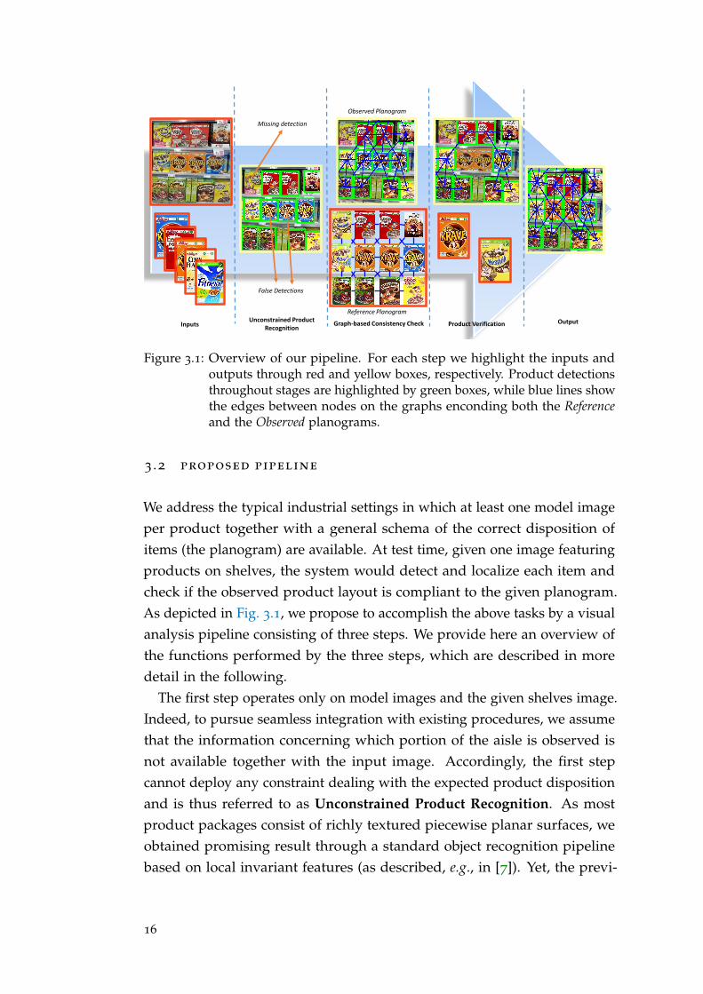
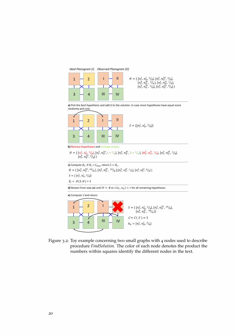
Figure 3.2: Toy example concerning two small graphs with 4 nodes used to describeprocedure FindSolution. The color of each node denotes the product thenumbers within squares identify the different nodes in the text.
20
Algorithm 1 Find sub-graph isomorphism between I and O
Cmax ← 0
Sbest ← ∅H← CreateHypotheses(I,O)while H 6= ∅ doC, S,h0 ← FindSolution(H,Cmax, τ)if C > Cmax thenSbest,Cmax ← S,C
H← H− h0return Sbest,Cmax
and O related to the same product and c(nI,nO) = nncnnt
with nnc numberof coherent neighbors (e.g., refering to the same product both in O and I)and nnt number of neighbors for that node in I. CreateHypotheses iteratesover all nI ∈ I so to instantiate all possible hypotheses. An example of thehypotheses set determined by CreateHypotheses given I and O is shown inthe first row of Fig. 3.2. Then, procedure FindSolution finds a solution, S, byiteratively picking the hypothesis featuring the highest score. The first hypo-thesis picked in the considered example is shown in Fig. 3.2-a). Successively,H is updated by removing the hypotheses containing either of the two nodesin the best hypothesis and increasing the scores of hypotheses associatedwith coherent neighbors (Fig. 3.2-b)). Procedure FindSolution returns also aconfidence score for the current solution, C, which takes into account thecardinality of S, together with a factor which penalizes the presence in O ofdisconnected sub-graphs that exhibit relative distances different than thoseexpected given the structure of I2 which instead is always fully connected.FindSolution takes as input the score of the current best solution, Cmax, andrelies on a branch-and-bound scheme to accelerate the computation. In par-ticular, as illustrated in Fig. 3.2-c), after updating H (Fig. 3.2-b)), FindSolutioncalculates an upper-bound for the score, BC, by adding to the cardinality ofS the number of hypotheses in H that are not mutually exclusive, so as toearly terminate the computation when the current solution can not improveCmax. The iterative process continues with picking the new best hypothesisuntil H is found empty or containing only hypotheses with confidence lowerthan a certain threshold (τ) (Fig. 3.2-d). The found solution, S, contains allthe hypotheses that are self-consistent and such that each node nI is eitherassociated with a node nO or to none, as shown in the last row of Fig. 3.2.In the last step ((Fig. 3.2-e)), the procedure computes C and returns also the
2 In the toy example in Fig. 3.2, O does not contain disconnected sub-graphs.
21
ROI Estimation Detections
Proposals
Chosen Detection
Figure 3.3: One iteration of our proposed Product Verification step. The estimatedROI is drawn in yellow. The correct proposal is highlighted in greenwhile others are in red.
first hypothesis, h0, that was added into S, i.e. the one with the highest scorec(nI,nO) (Fig. 3.2.-a)). Upon returning from FindSolution, the algorithmchecks whether or not the new solution S improves the best one found sofar and removes h0 from H (see Algorithm Alg. 1) to allow evaluation ofanother solution based on a different initial hypotheses.
As a result, Algorithm Alg. 1 finds self-consistent nodes in O given I,thereby removing inconsistent (i.e. likely false) detections and localizing theobserved image wrt to the planogram. Accordingly, the output of the secondsteps contains information about which items appear to be missing giventhe planned product layout and where they ought to be located within theimage.
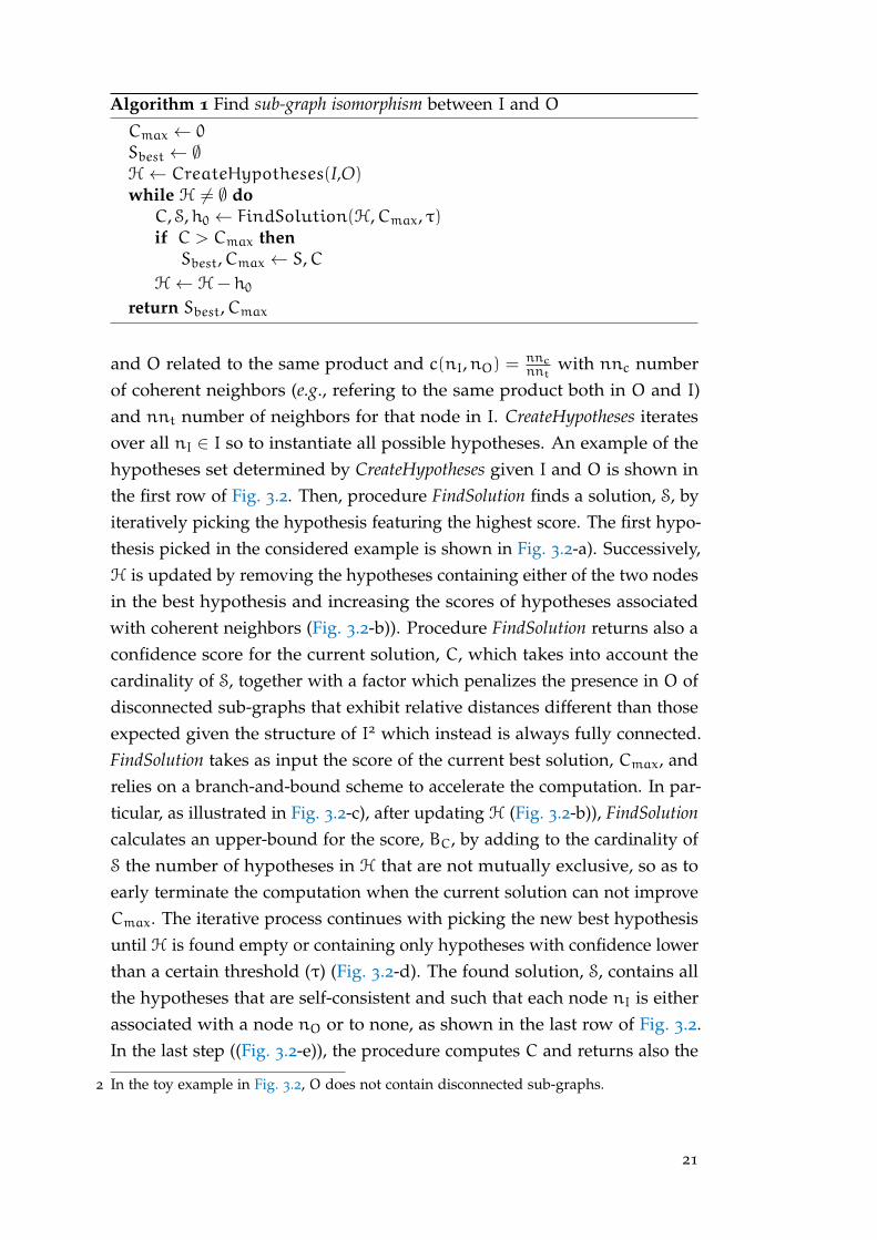
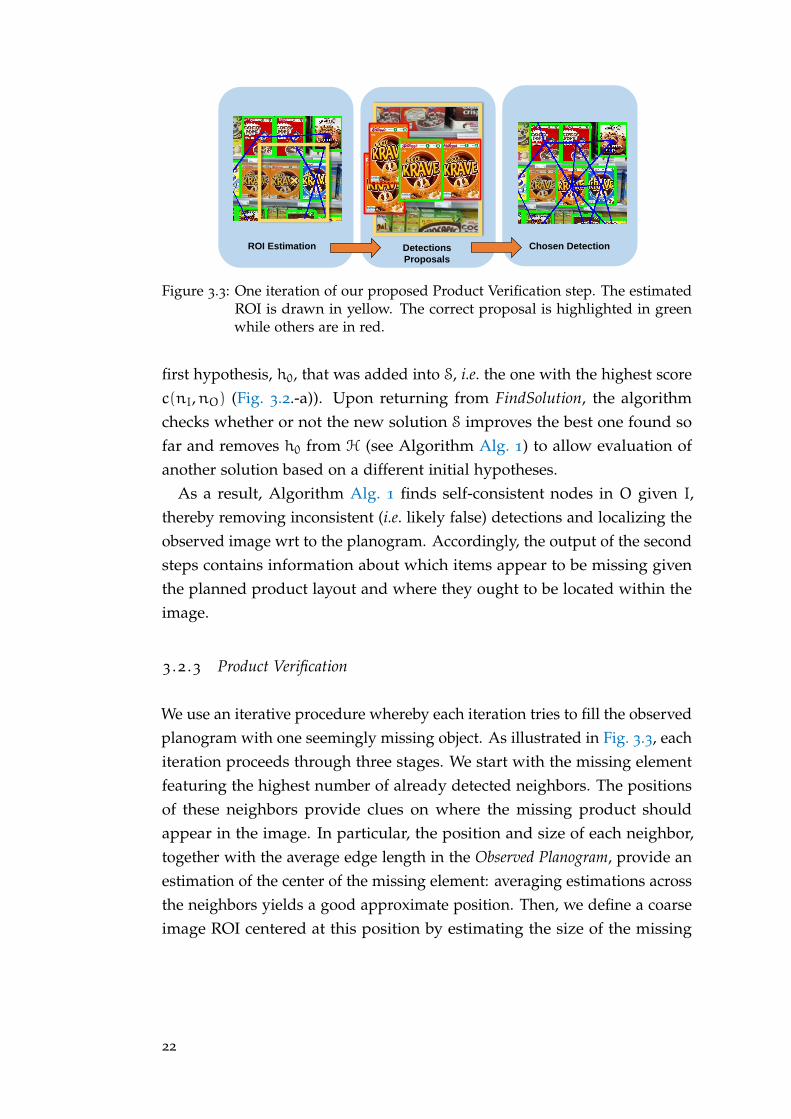
3 .2 .3 Product Verification
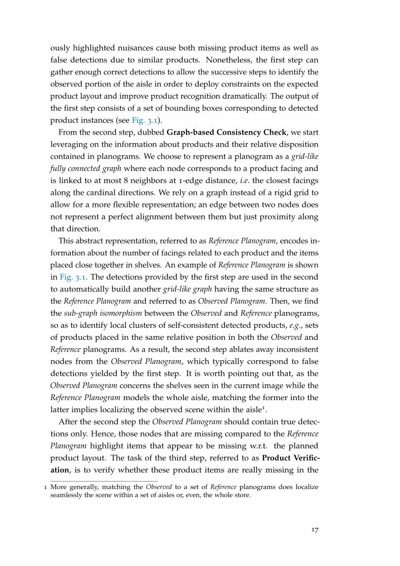
We use an iterative procedure whereby each iteration tries to fill the observedplanogram with one seemingly missing object. As illustrated in Fig. 3.3, eachiteration proceeds through three stages. We start with the missing elementfeaturing the highest number of already detected neighbors. The positionsof these neighbors provide clues on where the missing product shouldappear in the image. In particular, the position and size of each neighbor,together with the average edge length in the Observed Planogram, provide anestimation of the center of the missing element: averaging estimations acrossthe neighbors yields a good approximate position. Then, we define a coarseimage ROI centered at this position by estimating the size of the missing
22
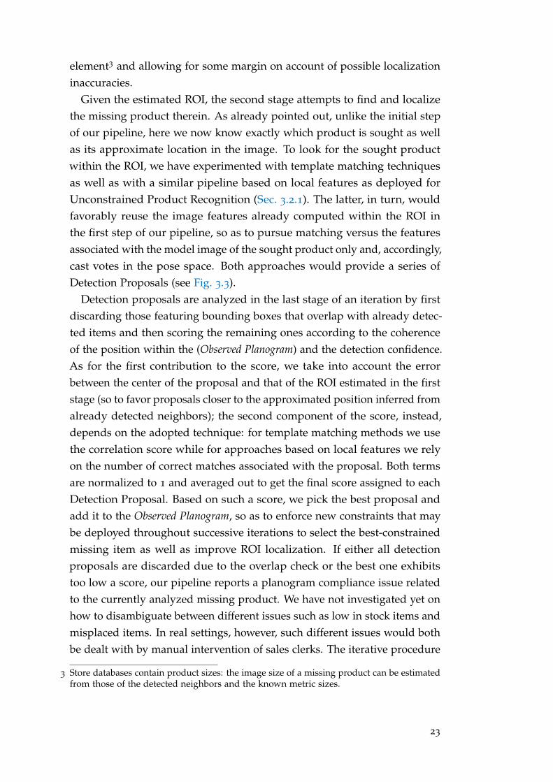
element3 and allowing for some margin on account of possible localizationinaccuracies.
Given the estimated ROI, the second stage attempts to find and localizethe missing product therein. As already pointed out, unlike the initial stepof our pipeline, here we now know exactly which product is sought as wellas its approximate location in the image. To look for the sought productwithin the ROI, we have experimented with template matching techniquesas well as with a similar pipeline based on local features as deployed forUnconstrained Product Recognition (Sec. 3.2.1). The latter, in turn, wouldfavorably reuse the image features already computed within the ROI inthe first step of our pipeline, so as to pursue matching versus the featuresassociated with the model image of the sought product only and, accordingly,cast votes in the pose space. Both approaches would provide a series ofDetection Proposals (see Fig. 3.3).
Detection proposals are analyzed in the last stage of an iteration by firstdiscarding those featuring bounding boxes that overlap with already detec-ted items and then scoring the remaining ones according to the coherenceof the position within the (Observed Planogram) and the detection confidence.As for the first contribution to the score, we take into account the errorbetween the center of the proposal and that of the ROI estimated in the firststage (so to favor proposals closer to the approximated position inferred fromalready detected neighbors); the second component of the score, instead,depends on the adopted technique: for template matching methods we usethe correlation score while for approaches based on local features we relyon the number of correct matches associated with the proposal. Both termsare normalized to 1 and averaged out to get the final score assigned to eachDetection Proposal. Based on such a score, we pick the best proposal andadd it to the Observed Planogram, so as to enforce new constraints that maybe deployed throughout successive iterations to select the best-constrainedmissing item as well as improve ROI localization. If either all detectionproposals are discarded due to the overlap check or the best one exhibitstoo low a score, our pipeline reports a planogram compliance issue relatedto the currently analyzed missing product. We have not investigated yet onhow to disambiguate between different issues such as low in stock items andmisplaced items. In real settings, however, such different issues would bothbe dealt with by manual intervention of sales clerks. The iterative procedure
3 Store databases contain product sizes: the image size of a missing product can be estimatedfrom those of the detected neighbors and the known metric sizes.
23
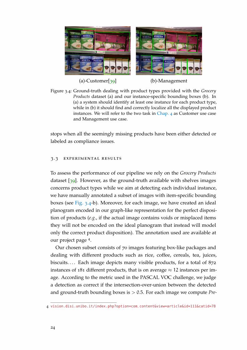
(a)-Customer[39] (b)-Management
Figure 3.4: Ground-truth dealing with product types provided with the GroceryProducts dataset (a) and our instance-specific bounding boxes (b). In(a) a system should identify at least one instance for each product type,while in (b) it should find and correctly localize all the displayed productinstances. We will refer to the two task in Chap. 4 as Customer use caseand Management use case.
stops when all the seemingly missing products have been either detected orlabeled as compliance issues.
3 .3 experimental results
To assess the performance of our pipeline we rely on the Grocery Productsdataset [39]. However, as the ground-truth available with shelves imagesconcerns product types while we aim at detecting each individual instance,we have manually annotated a subset of images with item-specific boundingboxes (see Fig. 3.4-b). Moreover, for each image, we have created an idealplanogram encoded in our graph-like representation for the perfect disposi-tion of products (e.g., if the actual image contains voids or misplaced itemsthey will not be encoded on the ideal planogram that instead will modelonly the correct product disposition). The annotation used are available atour project page 4.
Our chosen subset consists of 70 images featuring box-like packages anddealing with different products such as rice, coffee, cereals, tea, juices,biscuits. . . . Each image depicts many visible products, for a total of 872
instances of 181 different products, that is on average ≈ 12 instances per im-age. According to the metric used in the PASCAL VOC challenge, we judgea detection as correct if the intersection-over-union between the detectedand ground-truth bounding boxes is > 0.5. For each image we compute Pre-
4 vision.disi.unibo.it/index.php?option=com_content&view=article&id=111&catid=78
24
0,543444794
0,546391278
0,585297931
0,653671185
0,697201406
0,70248215
0,708543372
0,72462017
0,728284908
0,739289332
0,764505117
0,503033349
0,510239968
0,50120875
0,613688125
0,790300502
0,721576748
0,672802246
0,806630091
0,753502071
0,697562891
0,752929081
0,590916366
0,588055975
0,703291013
0,6992273
0,623725233
0,684372075
0,748294876
0,657747148
0,704700953
0,786325316
0,776442667
0 0,1 0,2 0,3 0,4 0,5 0,6 0,7 0,8 0,9 1
BOLD
KAZE
MSD/FREAK
AKAZE
ORB
SIFT
OPPONENT SURF
BRISK+SURF
SURF
BRISK/FREAK
BRISK
Precision Recall F-Measure
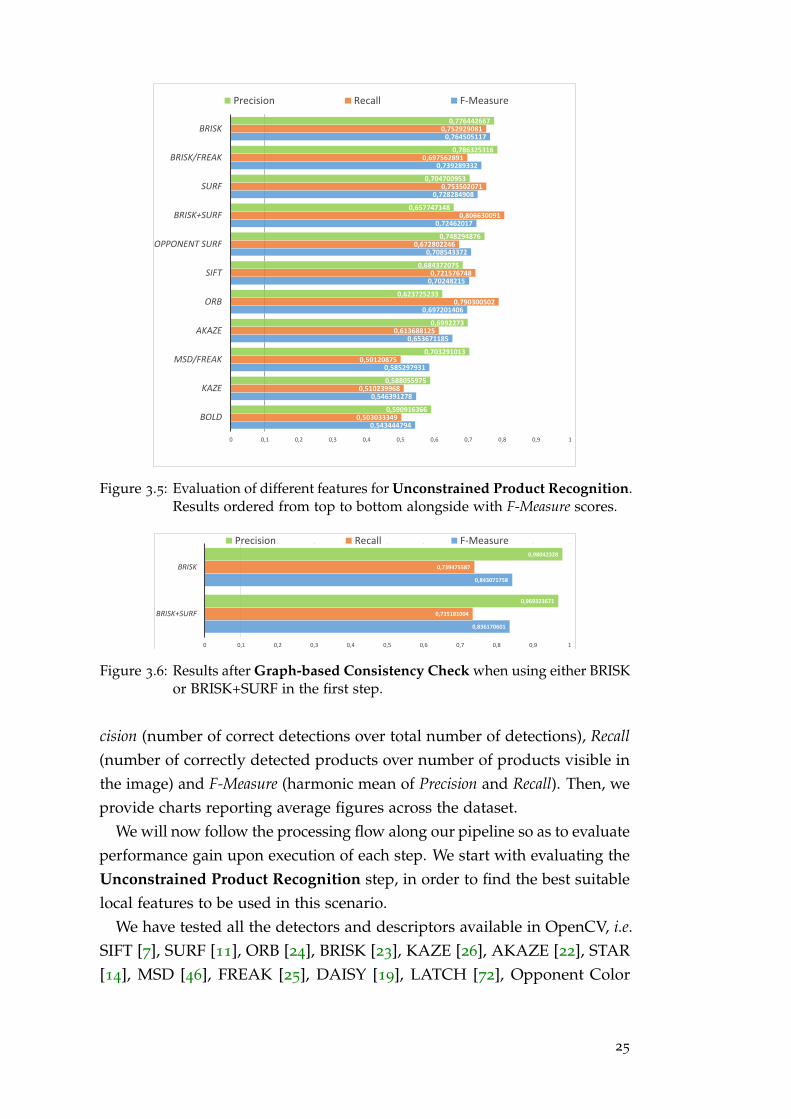
Figure 3.5: Evaluation of different features for Unconstrained Product Recognition.Results ordered from top to bottom alongside with F-Measure scores.
0,836170601
0,843071758
0,735181004
0,739475587
0,969323671
0,98042328
0 0,1 0,2 0,3 0,4 0,5 0,6 0,7 0,8 0,9 1
BRISK+SURF
BRISK
Precision Recall F-Measure
Figure 3.6: Results after Graph-based Consistency Check when using either BRISKor BRISK+SURF in the first step.
cision (number of correct detections over total number of detections), Recall(number of correctly detected products over number of products visible inthe image) and F-Measure (harmonic mean of Precision and Recall). Then, weprovide charts reporting average figures across the dataset.
We will now follow the processing flow along our pipeline so as to evaluateperformance gain upon execution of each step. We start with evaluating theUnconstrained Product Recognition step, in order to find the best suitablelocal features to be used in this scenario.
We have tested all the detectors and descriptors available in OpenCV, i.e.SIFT [7], SURF [11], ORB [24], BRISK [23], KAZE [26], AKAZE [22], STAR[14], MSD [46], FREAK [25], DAISY [19], LATCH [72], Opponent Color
25
0,837077873
0,842530284
0,903683273
0,835598284
0,840220009
0,902630484
0,838562711
0,844853298
0,904738521
0 0,1 0,2 0,3 0,4 0,5 0,6 0,7 0,8 0,9 1
BRISK + BB
BRISK + ZNCC
BRISK + BRISK
Precision Recall F-Measure
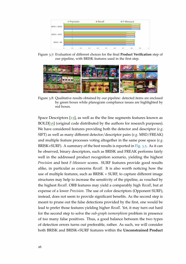
Figure 3.7: Evaluation of different choices for the final Product Verification step ofour pipeline, with BRISK features used in the first step.
Figure 3.8: Qualitative results obtained by our pipeline: detected items are enclosedby green boxes while planogram compliance issues are highlighted byred boxes.
Space Descriptors [15], as well as the the line segments features known asBOLD[35] (original code distributed by the authors for research purposes).We have considered features providing both the detector and descriptor (e.g.SIFT) as well as many different detector/descriptor pairs (e.g. MSD/FREAK)and multiple feature processes voting altogether in the same pose space (e.g.BRISK+SURF). A summary of the best results is reported in Fig. 3.5. As it canbe observed, binary descriptors, such as BRISK and FREAK performs fairlywell in the addressed product recognition scenario, yielding the highestPrecision and best F-Measure scores. SURF features provide good resultsalike, in particular as concerns Recall. It is also worth noticing how theuse of multiple features, such as BRISK + SURF, to capture different imagestructures may help to increase the sensitivity of the pipeline, as vouched bythe highest Recall. ORB features may yield a comparably high Recall, but atexpense of a lower Precision. The use of color descriptors (Opponent SURF),instead, does not seem to provide significant benefits. As the second step ismeant to prune out the false detections provided by the first, one would belead to prefer those features yielding higher Recall. Yet, it may turn out hardfor the second step to solve the sub-graph isomorphism problem in presenceof too many false positives. Thus, a good balance between the two typesof detection errors turns out preferable, rather. As such, we will considerboth BRISK and BRISK+SURF features within the Unconstrained Product
26
Recognition step in order to further evaluate the results provided by ourpipeline after the Graph-based Consistency Check step.
For the second step we fixed τ = 0.25 and deployed the algorithm pro-posed in Sec. 3.2.2, the results are displayed in Fig. 3.6. First, the boostin Precision attained with both types of features compared to the outputprovided by the first step (Fig. 3.5) proves that the proposed sub-graph iso-morphism formulation described in Sec. 3.2.2 is very effective to improveproduct recognition by removing false detections arising in unconstrainedsettings. In particular, when using BRISK features, Precision raises from ≈78% to ≈ 98% and with BRISK+SURF from ≈ 66% to ≈ 97%. Alongside,though, we observe a decrease in Recall, such as from ≈ 75% to ≈ 74% withBRISK and from ≈ 81% to ≈ 74% with BRISK+SURF. This is mostly dueto items that, although detected correctly in the first step, cannot rely onenough self-coherent neighbors to be validated (i.e. c(nI,nO) < τ). Overall,the Graph-based Consistency Check does improves performance signific-antly, as the F-Measure increases from ≈ 76% to ≈ 84% and from ≈ 72% to≈ 84% with BRISK and BRISK+SURF, respectively.
Given that in Fig. 3.6 BRISK slightly outperforms BRISK+SURF accordingto all the performance indexes and requires less computation, we pickthe former features for the first step and evaluate different design choicesas regards the final Product Verification. In particular, as mentioned inSec. 3.2.3, we considered different template matching and feature-basedapproaches. The best results, summarized in Fig. 3.7, concern templatematching by the ZNCC (Zero-mean Normalized Cross Correlation) in theHSV color space, the recent Best-buddies Similarity method [51] in the RGBcolor space and a feature-based approach deploying the same features usedfor the first step, that is BRISK. As shown in Fig. 3.7, using BRISK featuresin both the first and last step does provide the best results, all the threeperformance indexes getting now as high as ≈ 90%.
Eventually, in Fig. 3.8 we present some qualitative results obtained by ourpipeline both in case of compliance between the observed scene and theplanogram as well as in the case of missing products.
27

4U N C O N S T R A I N E D P R O D U C T D E T E C T I O N
After having addressed the problem of verifying planogram compliance, inthis section, we are going to focus on the more general task of unconstrainedproduct detection and recognition on store shelves. Due to the already dis-cussed peculiarities of this scenario, unfortunately, the deployment of stateof the art multi-class object detectors based on deep learning [59, 96, 111]cannot offers a trivial solution since all of them will require a large corpus ofannotated images as similar as possible to the deployment scenario in orderto provide good performance. Even acquiring and manually annotatingwith product labels a huge dataset of in-store images is not a viable solutiondue to the products on sale in stores, as well as their appearance, changingfrequently over time, which would mandate continuous gathering of annot-ated in-store images and retraining of the system. Conversely, a practicalapproach should be trained once and then be able to handle seamlesslynew stores, new products and/or new packages of existing products (e.g.,seasonal packages).
We propose to address product recognition by a pipeline consisting ofthree stages. Given a shelf image, we perform first a class-agnostic objectdetection to extract region proposals enclosing the individual product items.This stage relies on a deep learning based object detector trained to localizeproduct items within images taken in the store; we will refer to this networkas to the Detector. In the second stage, we perform product recognitionseparately on each of the region proposal provided by the Detector. Purposely,we carry out K-NN (K-Nearest Neighbours) similarity search between aglobal descriptor computed on the extracted region proposal and a databaseof similar descriptors computed on the reference images available in theproduct database. Rather than deploying a general-purpose global descriptor(e.g., Fisher Vectors [17]), we train a CNN using the reference images to learnan image embedding function that maps RGB inputs to n-dimensional globaldescriptors amenable for product recognition; this second network will bereferred to as to the Embedder. Eventually, to help prune out false detectionsand improve disambiguation between similarly looking products, in the
29
third stage of our pipeline we refine the recognition output by re-rankingthe first K proposals delivered by the similarity search.
It is worth pointing out how our approach needs samples of annotatedin-store images only to train the product-agnostic Detector, which, however,does not require product-specific labels but just bounding boxes drawnaround items. In Sec. 4.3 we will show how the product-agnostic Detectorcan be trained once and for all so to achieve remarkable performance acrossdifferent stores despite changes in shelves disposition and product appear-ance. Therefore, new items/packages are handled seamlessly by our systemsimply by adding their global descriptors (computed through the Embedder)in the reference database. Besides, our system scales easily to the recognitionof thousands of different items, as we use just one (or few) reference imagesper product, each encoded into a global descriptor in the order of a thousandfloat numbers.
Finally, while computationally expensive at training time, our systemturns out light (i.e., memory efficient) and fast at deployment time, therebyenabling near real-time operation. Speed and memory efficiency do notcome at a price in performance, as our system compares favorably withrespect to previous work on the standard benchmark dataset for productrecognition.
4 .1 related works
CNN-based systems are widely recognized as state-of-the-art across manyobject detection benchmarks. The different proposals can be broadly sub-divided into two main families of algorithms based on the number of stagesrequired to perform detection. On one hand, we have the slower but moreaccurate two stage detectors [59], which decompose object detection into aregion proposal followed by an independent classification for each region.On the other hand, fast one stage approaches [96, 111] can perform detectionand classification jointly. A very recent work has also addressed the specificdomain of grocery products, so as to propose an ad hoc detector [107] thatanalyzes the image at multiple scales to produce more meaningful regionproposals.
Besides, deploying CNNs to obtain rich image representations is an es-tablished approach to pursue image search, both as a strong off-the-shelfbaseline [43] and as a key component within more complex pipelines [69].
30
Detector
Embedder
CropRefinement
Search
Query Image Region Proposals
Reference images
Reference Database Final Output
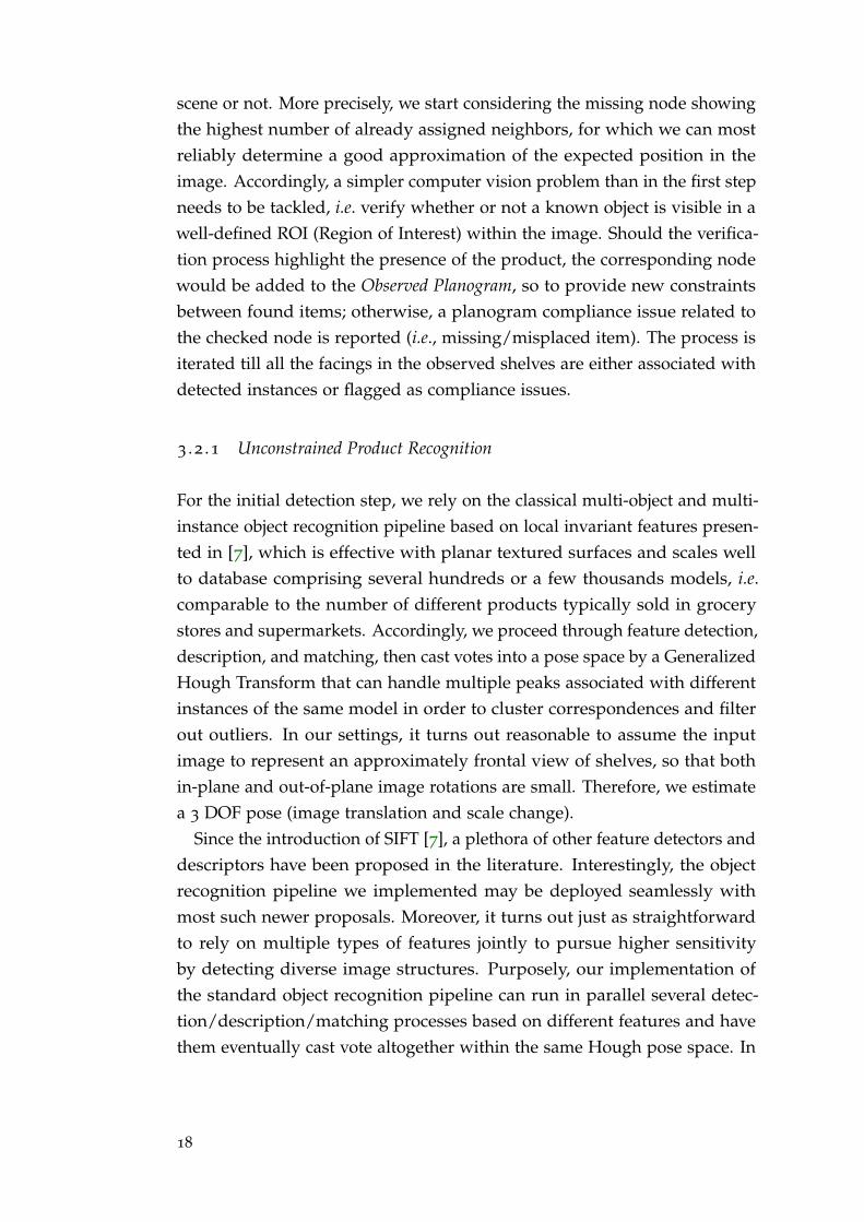
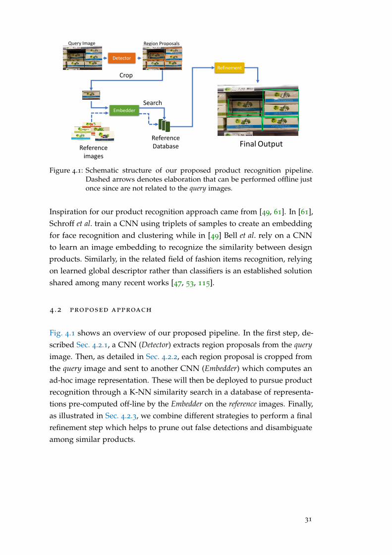
Figure 4.1: Schematic structure of our proposed product recognition pipeline.Dashed arrows denotes elaboration that can be performed offline justonce since are not related to the query images.
Inspiration for our product recognition approach came from [49, 61]. In [61],Schroff et al. train a CNN using triplets of samples to create an embeddingfor face recognition and clustering while in [49] Bell et al. rely on a CNNto learn an image embedding to recognize the similarity between designproducts. Similarly, in the related field of fashion items recognition, relyingon learned global descriptor rather than classifiers is an established solutionshared among many recent works [47, 53, 115].
4 .2 proposed approach
Fig. 4.1 shows an overview of our proposed pipeline. In the first step, de-scribed Sec. 4.2.1, a CNN (Detector) extracts region proposals from the queryimage. Then, as detailed in Sec. 4.2.2, each region proposal is cropped fromthe query image and sent to another CNN (Embedder) which computes anad-hoc image representation. These will then be deployed to pursue productrecognition through a K-NN similarity search in a database of representa-tions pre-computed off-line by the Embedder on the reference images. Finally,as illustrated in Sec. 4.2.3, we combine different strategies to perform a finalrefinement step which helps to prune out false detections and disambiguateamong similar products.
31
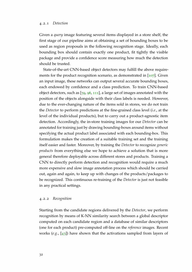
4 .2 .1 Detection
Given a query image featuring several items displayed in a store shelf, thefirst stage of our pipeline aims at obtaining a set of bounding boxes to beused as region proposals in the following recognition stage. Ideally, eachbounding box should contain exactly one product, fit tightly the visiblepackage and provide a confidence score measuring how much the detectionshould be trusted.
State-of-the-art CNN-based object detectors may fulfill the above require-ments for the product recognition scenario, as demonstrated in [107]. Givenan input image, these networks can output several accurate bounding boxes,each endowed by confidence and a class prediction. To train CNN-basedobject detectors, such as [59, 96, 111], a large set of images annotated with theposition of the objects alongside with their class labels is needed. However,due to the ever-changing nature of the items sold in stores, we do not trainthe Detector to perform predictions at the fine-grained class level (i.e., at thelevel of the individual products), but to carry out a product-agnostic itemdetection. Accordingly, the in-store training images for our Detector can beannotated for training just by drawing bounding-boxes around items withoutspecifying the actual product label associated with each bounding-box. Thisformulation makes the creation of a suitable training set and the trainingitself easier and faster. Moreover, by training the Detector to recognize genericproducts from everything else we hope to achieve a solution that is moregeneral therefore deployable across different stores and products. Training aCNN to directly perform detection and recognition would require a muchmore expensive and slow image annotation process which should be carriedout, again and again, to keep up with changes of the products/packages tobe recognized. This continuous re-training of the Detector is just not feasiblein any practical settings.
4 .2 .2 Recognition
Starting from the candidate regions delivered by the Detector, we performrecognition by means of K-NN similarity search between a global descriptorcomputed on each candidate region and a database of similar descriptors(one for each product) pre-computed off-line on the reference images. Recentworks (e.g., [43]) have shown that the activations sampled from layers of
32
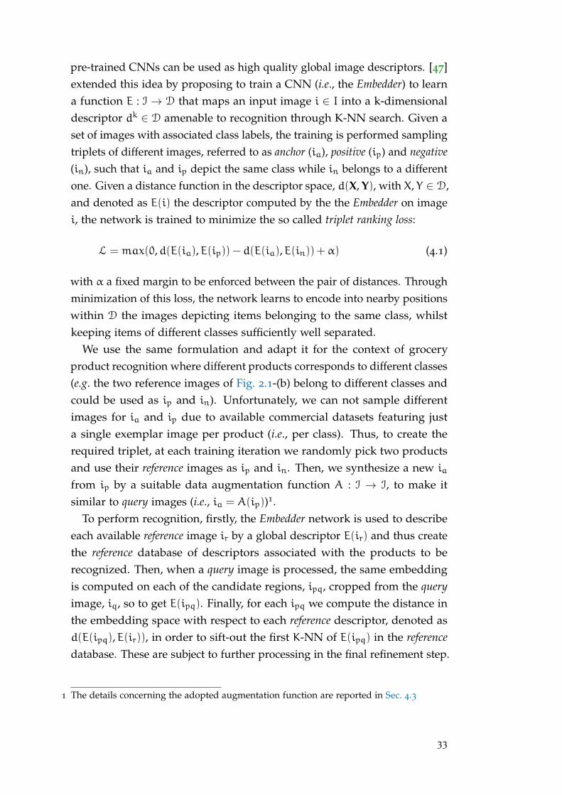
pre-trained CNNs can be used as high quality global image descriptors. [47]extended this idea by proposing to train a CNN (i.e., the Embedder) to learna function E : I → D that maps an input image i ∈ I into a k-dimensionaldescriptor dk ∈ D amenable to recognition through K-NN search. Given aset of images with associated class labels, the training is performed samplingtriplets of different images, referred to as anchor (ia), positive (ip) and negative(in), such that ia and ip depict the same class while in belongs to a differentone. Given a distance function in the descriptor space, d(X, Y), with X, Y ∈ D,and denoted as E(i) the descriptor computed by the the Embedder on imagei, the network is trained to minimize the so called triplet ranking loss:
L = max(0,d(E(ia),E(ip)) − d(E(ia),E(in)) +α) (4.1)
with α a fixed margin to be enforced between the pair of distances. Throughminimization of this loss, the network learns to encode into nearby positionswithin D the images depicting items belonging to the same class, whilstkeeping items of different classes sufficiently well separated.
We use the same formulation and adapt it for the context of groceryproduct recognition where different products corresponds to different classes(e.g. the two reference images of Fig. 2.1-(b) belong to different classes andcould be used as ip and in). Unfortunately, we can not sample differentimages for ia and ip due to available commercial datasets featuring justa single exemplar image per product (i.e., per class). Thus, to create therequired triplet, at each training iteration we randomly pick two productsand use their reference images as ip and in. Then, we synthesize a new ia
from ip by a suitable data augmentation function A : I → I, to make itsimilar to query images (i.e., ia = A(ip))1.
To perform recognition, firstly, the Embedder network is used to describeeach available reference image ir by a global descriptor E(ir) and thus createthe reference database of descriptors associated with the products to berecognized. Then, when a query image is processed, the same embeddingis computed on each of the candidate regions, ipq, cropped from the queryimage, iq, so to get E(ipq). Finally, for each ipq we compute the distance inthe embedding space with respect to each reference descriptor, denoted asd(E(ipq),E(ir)), in order to sift-out the first K-NN of E(ipq) in the referencedatabase. These are subject to further processing in the final refinement step.
1 The details concerning the adopted augmentation function are reported in Sec. 4.3
33
4 .2 .3 Refinement
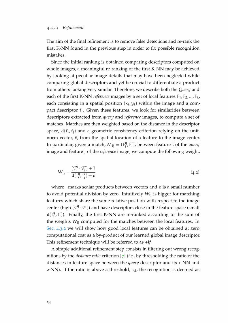
The aim of the final refinement is to remove false detections and re-rank thefirst K-NN found in the previous step in order to fix possible recognitionmistakes.
Since the initial ranking is obtained comparing descriptors computed onwhole images, a meaningful re-ranking of the first K-NN may be achievedby looking at peculiar image details that may have been neglected whilecomparing global descriptors and yet be crucial to differentiate a productfrom others looking very similar. Therefore, we describe both the Query andeach of the first K-NN reference images by a set of local features F1, F2, ..., Fk,each consisting in a spatial position (xi,yi) within the image and a com-pact descriptor fi. Given these features, we look for similarities betweendescriptors extracted from query and reference images, to compute a set ofmatches. Matches are then weighted based on the distance in the descriptorspace, d(fi, fj) and a geometric consistency criterion relying on the unit-norm vector, ~v, from the spatial location of a feature to the image center.In particular, given a match, Mij = (Fqi , Frj ), between feature i of the queryimage and feature j of the reference image, we compute the following weight:
Wij =(~vqi ·~v
rj ) + 1
d(fqi , frj ) + ε(4.2)
where · marks scalar products between vectors and ε is a small numberto avoid potential division by zero. Intuitively Wij is bigger for matchingfeatures which share the same relative position with respect to the imagecenter (high (~vqi ·~v
rj )) and have descriptors close in the feature space (small
d(fqi , frj )). Finally, the first K-NN are re-ranked according to the sum ofthe weights Wij computed for the matches between the local features. InSec. 4.3.2 we will show how good local features can be obtained at zerocomputational cost as a by-product of our learned global image descriptor.This refinement technique will be referred to as +lf .
A simple additional refinement step consists in filtering out wrong recog-nitions by the distance ratio criterion [7] (i.e., by thresholding the ratio of thedistances in feature space between the query descriptor and its 1-NN and2-NN). If the ratio is above a threshold, τd, the recognition is deemed as
34

ambiguous and discarded. In the following, we will denote this refinementtechnique as +th.
Finally, as commercial product databases typically provide a multilevelclassification of the items (e.g., at least instance, and category level), wepropose a re-ranking and filtering method specific to the grocery domainwhere, as pointed out by [39], products belonging to the same macro categoryare typically displayed close one to another on the shelf. Given the candidateregions extracted from the query image and their corresponding sets of K-NN,we consider the 1-NN of the region proposals extracted with high confidence(> 0.1) by the Detector in order to find the main macro category of the image.Then, in case the majority of detections votes for the same macro category, itis safe to assume that the pictured shelf contains almost exclusively items ofthat category thus filter the K-NN for all candidate regions accordingly.It isworth observing how this strategy implicitly leverages on those productseasier to identify (i.e., the high-confidence detections) to increase the chanceto correctly recognize the harder ones. We will refer to this refinementstrategy as to +mc.
4 .3 experimental results
To validate the performance of our product recognition pipeline we takeinto account two possible use cases dealing with different final users:
• Customer: the system should be deployed for a guided or partiallyautomated shopping experience (e.g., product localization inside theshop, augmented reality overlays or support to visually impaired). Asproposed in [39] the goal is to detect at least one instance of each visibletype of product displayed in a shelf picture.
• Management: the system will be used to partially automate the man-agement of a shop (e.g., automatic inventory, and restocking). Here,the goal is to recognize each product instance displayed on the shelve.
4 .3 .1 Datasets and Evaluation Metrics
For our experimental evaluation, we rely on the publicly available GroceryProducts dataset [39], which features more than 8400 grocery products or-ganized in hierarchical classes and with each product described by exactly
35
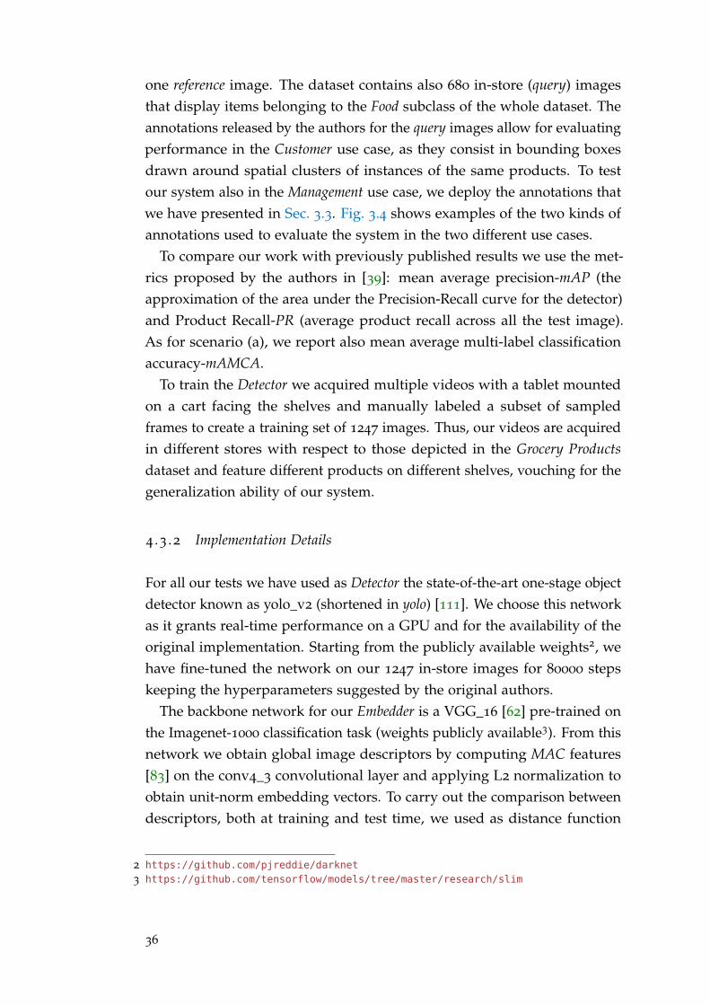
one reference image. The dataset contains also 680 in-store (query) imagesthat display items belonging to the Food subclass of the whole dataset. Theannotations released by the authors for the query images allow for evaluatingperformance in the Customer use case, as they consist in bounding boxesdrawn around spatial clusters of instances of the same products. To testour system also in the Management use case, we deploy the annotations thatwe have presented in Sec. 3.3. Fig. 3.4 shows examples of the two kinds ofannotations used to evaluate the system in the two different use cases.
To compare our work with previously published results we use the met-rics proposed by the authors in [39]: mean average precision-mAP (theapproximation of the area under the Precision-Recall curve for the detector)and Product Recall-PR (average product recall across all the test image).As for scenario (a), we report also mean average multi-label classificationaccuracy-mAMCA.
To train the Detector we acquired multiple videos with a tablet mountedon a cart facing the shelves and manually labeled a subset of sampledframes to create a training set of 1247 images. Thus, our videos are acquiredin different stores with respect to those depicted in the Grocery Productsdataset and feature different products on different shelves, vouching for thegeneralization ability of our system.
4 .3 .2 Implementation Details
For all our tests we have used as Detector the state-of-the-art one-stage objectdetector known as yolo_v2 (shortened in yolo) [111]. We choose this networkas it grants real-time performance on a GPU and for the availability of theoriginal implementation. Starting from the publicly available weights2, wehave fine-tuned the network on our 1247 in-store images for 80000 stepskeeping the hyperparameters suggested by the original authors.
The backbone network for our Embedder is a VGG_16 [62] pre-trained onthe Imagenet-1000 classification task (weights publicly available3). From thisnetwork we obtain global image descriptors by computing MAC features[83] on the conv4_3 convolutional layer and applying L2 normalization toobtain unit-norm embedding vectors. To carry out the comparison betweendescriptors, both at training and test time, we used as distance function
2 https://github.com/pjreddie/darknet3 https://github.com/tensorflow/models/tree/master/research/slim
36
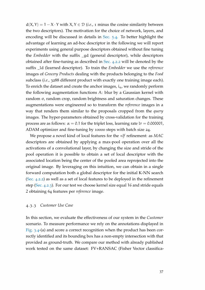
d(X, Y) = 1−X · Y with X, Y ∈ D (i.e., 1 minus the cosine similarity betweenthe two descriptors). The motivation for the choice of network, layers, andencoding will be discussed in details in Sec. 5.4. To better highlight theadvantage of learning an ad-hoc descriptor in the following we will reportexperiments using general purpose descriptors obtained without fine tuningthe Embedder with the suffix _gd (general descriptor), while descriptorsobtained after fine-tuning as described in Sec. 4.2.2 will be denoted by thesuffix _ld (learned descriptor). To train the Embedder we use the referenceimages of Grocery Products dealing with the products belonging to the Foodsubclass (i.e., 3288 different product with exactly one training image each).To enrich the dataset and create the anchor images, ia, we randomly performthe following augmentation functions A: blur by a Gaussian kernel withrandom σ, random crop, random brightness and saturation changes. Theseaugmentations were engineered so to transform the reference images in away that renders them similar to the proposals cropped from the queryimages. The hyper-parameters obtained by cross-validation for the trainingprocess are as follows: α = 0.1 for the triplet loss, learning rate lr = 0.000001,ADAM optimizer and fine-tuning by 10000 steps with batch size 24.
We propose a novel kind of local features for the +lf refinement: as MACdescriptors are obtained by applying a max-pool operation over all theactivations of a convolutional layer, by changing the size and stride of thepool operation it is possible to obtain a set of local descriptor with theassociated location being the center of the pooled area reprojected into theoriginal image. By leveraging on this intuition, we can obtain in a singleforward computation both a global descriptor for the initial K-NN search(Sec. 4.2.2) as well as a set of local features to be deployed in the refinementstep (Sec. 4.2.3). For our test we choose kernel size equal 16 and stride equals2 obtaining 64 features per reference image.
4 .3 .3 Customer Use Case
In this section, we evaluate the effectiveness of our system in the Customerscenario. To measure performance we rely on the annotations displayed inFig. 3.4-(a) and score a correct recognition when the product has been cor-rectly identified and its bounding box has a non-empty intersection with thatprovided as ground-truth. We compare our method with already publishedwork tested on the same dataset: FV+RANSAC (Fisher Vector classifica-
37
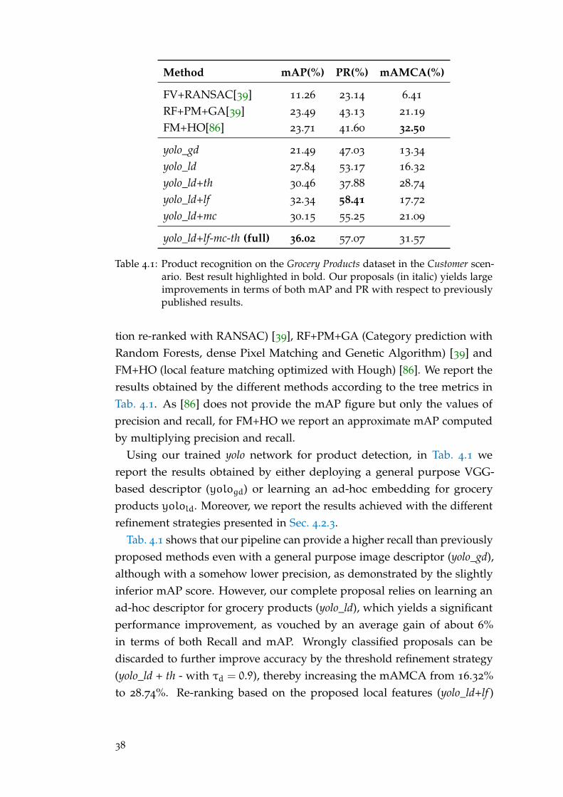
Method mAP(%) PR(%) mAMCA(%)
FV+RANSAC[39] 11.26 23.14 6.41
RF+PM+GA[39] 23.49 43.13 21.19
FM+HO[86] 23.71 41.60 32.50
yolo_gd 21.49 47.03 13.34
yolo_ld 27.84 53.17 16.32
yolo_ld+th 30.46 37.88 28.74
yolo_ld+lf 32.34 58.41 17.72
yolo_ld+mc 30.15 55.25 21.09
yolo_ld+lf-mc-th (full) 36.02 57.07 31.57
Table 4.1: Product recognition on the Grocery Products dataset in the Customer scen-ario. Best result highlighted in bold. Our proposals (in italic) yields largeimprovements in terms of both mAP and PR with respect to previouslypublished results.
tion re-ranked with RANSAC) [39], RF+PM+GA (Category prediction withRandom Forests, dense Pixel Matching and Genetic Algorithm) [39] andFM+HO (local feature matching optimized with Hough) [86]. We report theresults obtained by the different methods according to the tree metrics inTab. 4.1. As [86] does not provide the mAP figure but only the values ofprecision and recall, for FM+HO we report an approximate mAP computedby multiplying precision and recall.
Using our trained yolo network for product detection, in Tab. 4.1 wereport the results obtained by either deploying a general purpose VGG-based descriptor (yologd) or learning an ad-hoc embedding for groceryproducts yolold. Moreover, we report the results achieved with the differentrefinement strategies presented in Sec. 4.2.3.
Tab. 4.1 shows that our pipeline can provide a higher recall than previouslyproposed methods even with a general purpose image descriptor (yolo_gd),although with a somehow lower precision, as demonstrated by the slightlyinferior mAP score. However, our complete proposal relies on learning anad-hoc descriptor for grocery products (yolo_ld), which yields a significantperformance improvement, as vouched by an average gain of about 6%in terms of both Recall and mAP. Wrongly classified proposals can bediscarded to further improve accuracy by the threshold refinement strategy(yolo_ld + th - with τd = 0.9), thereby increasing the mAMCA from 16.32%to 28.74%. Re-ranking based on the proposed local features (yolo_ld+lf )
38
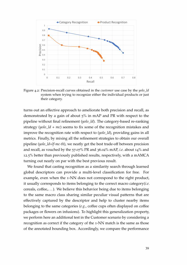
0
0.1
0.2
0.3
0.4
0.5
0.6
0.7
0.8
0.9
1
0 0.1 0.2 0.3 0.4 0.5 0.6 0.7 0.8
Pre
cisi
on
Recall
Category Recognition Product Recognition
Figure 4.2: Precision-recall curves obtained in the customer use case by the yolo_ldsystem when trying to recognize either the individual products or justtheir category.
turns out an effective approach to ameliorate both precision and recall, asdemonstrated by a gain of about 5% in mAP and PR with respect to thepipeline without final refinement (yolo_ld). The category-based re-rankingstrategy (yolo_ld + mc) seems to fix some of the recognition mistakes andimprove the recognition rate with respect to (yolo_ld), providing gains in allmetrics. Finally, by mixing all the refinement strategies to obtain our overallpipeline (yolo_ld+lf-mc-th), we neatly get the best trade-off between precisionand recall, as vouched by the 57.07% PR and 36.02% mAP, i.e. about 14% and12.5% better than previously published results, respectively, with a mAMCAturning out nearly on par with the best previous result.
We found that casting recognition as a similarity search through learnedglobal descriptors can provide a multi-level classification for free. Forexample, even when the 1-NN does not correspond to the right product,it usually corresponds to items belonging to the correct macro category(i.e.cereals, coffee,. . . ). We believe this behavior being due to items belongingto the same macro class sharing similar peculiar visual patterns that areeffectively captured by the descriptor and help to cluster nearby itemsbelonging to the same categories (e.g., coffee cups often displayed on coffeepackages or flowers on infusions). To highlight this generalization property,we perform here an additional test in the Customer scenario by considering arecognition as correct if the category of the 1-NN match is the same as thoseof the annotated bounding box. Accordingly, we compare the performance
39
Method mAP(%) PR(%)
FS 66.37 75.0
yolo_gd 66.95 78.89
yolo_ld 74.32 84.75
yolo_ld+th 75.62 81.55
yolo_ld+lf 76.37 86.56yolo_ld+mc 74.80 85.28
yolo_ld+lf-mc-th (full) 76.93 85.71
Table 4.2: Product recognition for Management use case. Our proposal highlighted(in italic), best results in bold.
Method mAP(%) PR(%)
FS 47.32 57.0
yolo_gd 60.17 73.66
yolo_ld 67.88 80.27
yolo_ld+th 69.70 76.01
yolo_ld+lf 70.69 82.83yolo_ld+mc 69.01 81.55
yolo_ld+lf-mc-th (full) 73.50 82.66
Table 4.3: Results in the Management use case performing recognition against allthe items belonging to the Food subclass of the Grocery Products dataset(∼ 3200). Our proposals highlighted (in italic), best results in bold.
of yolo_ld when trying to recognize either the individual products or theircategory. The results of this experiment are reported as Precision-Recallcurves in Fig. 4.2. The large difference between the two curves provesthat very often the system mistakes items at the product level but correctlyrecognizing their category. Eventually, it is worth pointing out that ourmethod not only provides a significant performance improvement withrespect to previously published results but turns out remarkably fast. Indeed,our whole pipeline can be run on a GPU in less than one second per image.
Management Use Case
The experiments presented in this Section concern the Management use casewhere we are required to correctly detect and recognize all the individual
40
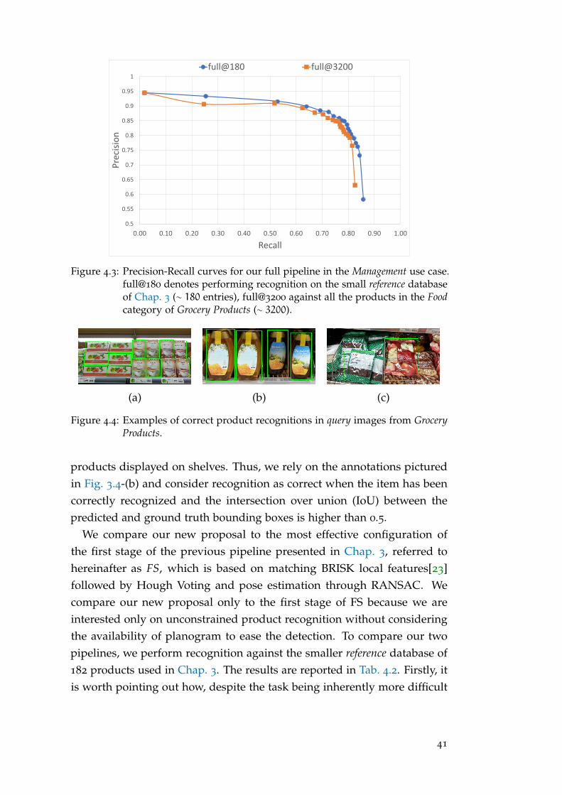
0.5
0.55
0.6
0.65
0.7
0.75
0.8
0.85
0.9
0.95
1
0.00 0.10 0.20 0.30 0.40 0.50 0.60 0.70 0.80 0.90 1.00
Precision
Recall
full@180 full@3200
Figure 4.3: Precision-Recall curves for our full pipeline in the Management use case.full@180 denotes performing recognition on the small reference databaseof Chap. 3 (∼ 180 entries), full@3200 against all the products in the Foodcategory of Grocery Products (∼ 3200).
(a) (b) (c)
Figure 4.4: Examples of correct product recognitions in query images from GroceryProducts.
products displayed on shelves. Thus, we rely on the annotations picturedin Fig. 3.4-(b) and consider recognition as correct when the item has beencorrectly recognized and the intersection over union (IoU) between thepredicted and ground truth bounding boxes is higher than 0.5.
We compare our new proposal to the most effective configuration ofthe first stage of the previous pipeline presented in Chap. 3, referred tohereinafter as FS, which is based on matching BRISK local features[23]followed by Hough Voting and pose estimation through RANSAC. Wecompare our new proposal only to the first stage of FS because we areinterested only on unconstrained product recognition without consideringthe availability of planogram to ease the detection. To compare our twopipelines, we perform recognition against the smaller reference database of182 products used in Chap. 3. The results are reported in Tab. 4.2. Firstly, itis worth pointing out how, despite the task being inherently more difficult
41
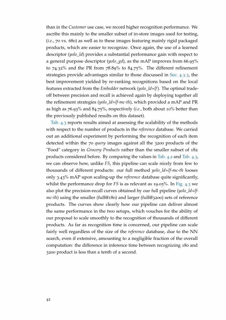
than in the Customer use case, we record higher recognition performance. Weascribe this mainly to the smaller subset of in-store images used for testing,(i.e., 70 vs. 680) as well as to these images featuring mainly rigid packagedproducts, which are easier to recognize. Once again, the use of a learneddescriptor (yolo_ld) provides a substantial performance gain with respect toa general purpose descriptor (yolo_gd), as the mAP improves from 66.95%to 74.32% and the PR from 78.89% to 84.75%. The different refinementstrategies provide advantages similar to those discussed in Sec. 4.3.3, thebest improvement yielded by re-ranking recognitions based on the localfeatures extracted from the Embedder network (yolo_ld+lf ). The optimal trade-off between precision and recall is achieved again by deploying together allthe refinement strategies (yolo_ld+lf-mc-th), which provided a mAP and PRas high as 76.93% and 84.75%, respectively (i.e., both about 10% better thanthe previously published results on this dataset).
Tab. 4.3 reports results aimed at assessing the scalability of the methodswith respect to the number of products in the reference database. We carriedout an additional experiment by performing the recognition of each itemdetected within the 70 query images against all the 3200 products of the"Food" category in Grocery Products rather than the smaller subset of 182
products considered before. By comparing the values in Tab. 4.2 and Tab. 4.3,we can observe how, unlike FS, this pipeline can scale nicely from few tothousands of different products: our full method yolo_ld+lf-mc-th loosesonly 3.43% mAP upon scaling-up the reference database quite significantly,whilst the performance drop for FS is as relevant as 19.05%. In Fig. 4.3 wealso plot the precision-recall curves obtained by our full pipeline (yolo_ld+lf-mc-th) using the smaller (full@180) and larger (full@3200) sets of referenceproducts. The curves show clearly how our pipeline can deliver almostthe same performance in the two setups, which vouches for the ability ofour proposal to scale smoothly to the recognition of thousands of differentproducts. As far as recognition time is concerned, our pipeline can scalefairly well regardless of the size of the reference database, due to the NNsearch, even if extensive, amounting to a negligible fraction of the overallcomputation: the difference in inference time between recognizing 180 and3200 product is less than a tenth of a second.
42
4 .3 .4 Qualitative Results
Fig. 4.4 reports some qualitative results obtained by our pipeline. Picture (a)shows the recognition results on an image taken quite far from the shelf andfeaturing a lot of different items; (b) deal with some successful recognition ina close-up query image, where only a few items are visible at once. Finally, (c)refers to recognition of products featuring deformable and highly reflectivepackages, which are quite challenging to recognize due to the appearance ofthe items within the query images turning out significantly different than inthe available reference images. Yet, in (c) our system was able to find at leastone item for each product type (i.e., as required in the Customer use case).
43

5D O M A I N I N VA R I A N T H I E R A R C H I C A L E M B E D D I N G F O RG R O C E RY P R O D U C T S R E C O G N I T I O N
After describing in Chap. 4 a complete computer vision pipeline to solvethe problem of unconstrained product recognition on store shelves, in thissection we will explore more in detail how to properly address the recognitionphase. As in Chap. 4 we still rely on a global image descriptor learned todisentangle grocery products and to pursue recognition through K-NNsearch within a database featuring one reference image per sought product.We rely on learned image embeddings as this approach allows seamlesslyto perform recognition both on products seen or unseen at training time.For example, should a new product be put on sale in the store, our systemwould just require to add its image into the reference database withoutthe need to perform new costly training. Moreover, K-NN search is quiteamenable to product recognition from a computational standpoint alike.Indeed, compared to typical image retrieval settings, the database is verysmall, i.e. in the order of several thousand images rather than millions oreven billions of images. Thus, a global image descriptor of about a fewhundred entries turns out viable in terms of time and memory efficiency.
In Chap. 4 we have already show how a standard triplet loss can bedeployed to learn an embedding suitable for product recognition. Here,instead, we wish to go one step further and directly address some criticalityof the product recognition task: the domain shift between data acquired in-store and those available during training (e.g., see Fig. 5.1) and the similaritybetween products belonging to the same category. We propose to learn animage embedding through a deep CNN trained by a loss function that forcesboth similar looking items as well as items belonging to the same high-levelcategory to map close one to another in the descriptor space. Moreover,to tackle the domain shift between images available at training time andthose acquired in stores, and to increase the training set size we propose todeploy an image-to-image translation GAN together with the embeddingCNN and to optimize the whole architecture end-to-end. In particular,some of the training samples for the embedding network are generated by aGAN that learns without supervision to transform images taken in studio
45
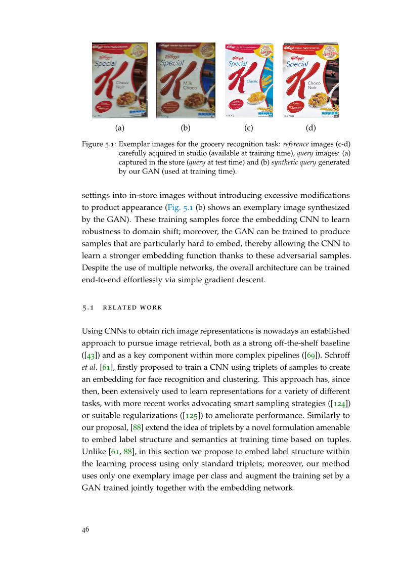
(a) (b) (c) (d)
Figure 5.1: Exemplar images for the grocery recognition task: reference images (c-d)carefully acquired in studio (available at training time), query images: (a)captured in the store (query at test time) and (b) synthetic query generatedby our GAN (used at training time).
settings into in-store images without introducing excessive modificationsto product appearance (Fig. 5.1 (b) shows an exemplary image synthesizedby the GAN). These training samples force the embedding CNN to learnrobustness to domain shift; moreover, the GAN can be trained to producesamples that are particularly hard to embed, thereby allowing the CNN tolearn a stronger embedding function thanks to these adversarial samples.Despite the use of multiple networks, the overall architecture can be trainedend-to-end effortlessly via simple gradient descent.
5 .1 related work
Using CNNs to obtain rich image representations is nowadays an establishedapproach to pursue image retrieval, both as a strong off-the-shelf baseline([43]) and as a key component within more complex pipelines ([69]). Schroffet al. [61], firstly proposed to train a CNN using triplets of samples to createan embedding for face recognition and clustering. This approach has, sincethen, been extensively used to learn representations for a variety of differenttasks, with more recent works advocating smart sampling strategies ([124])or suitable regularizations ([125]) to ameliorate performance. Similarly toour proposal, [88] extend the idea of triplets by a novel formulation amenableto embed label structure and semantics at training time based on tuples.Unlike [61, 88], in this section we propose to embed label structure withinthe learning process using only standard triplets; moreover, our methoduses only one exemplary image per class and augment the training set by aGAN trained jointly together with the embedding network.
46
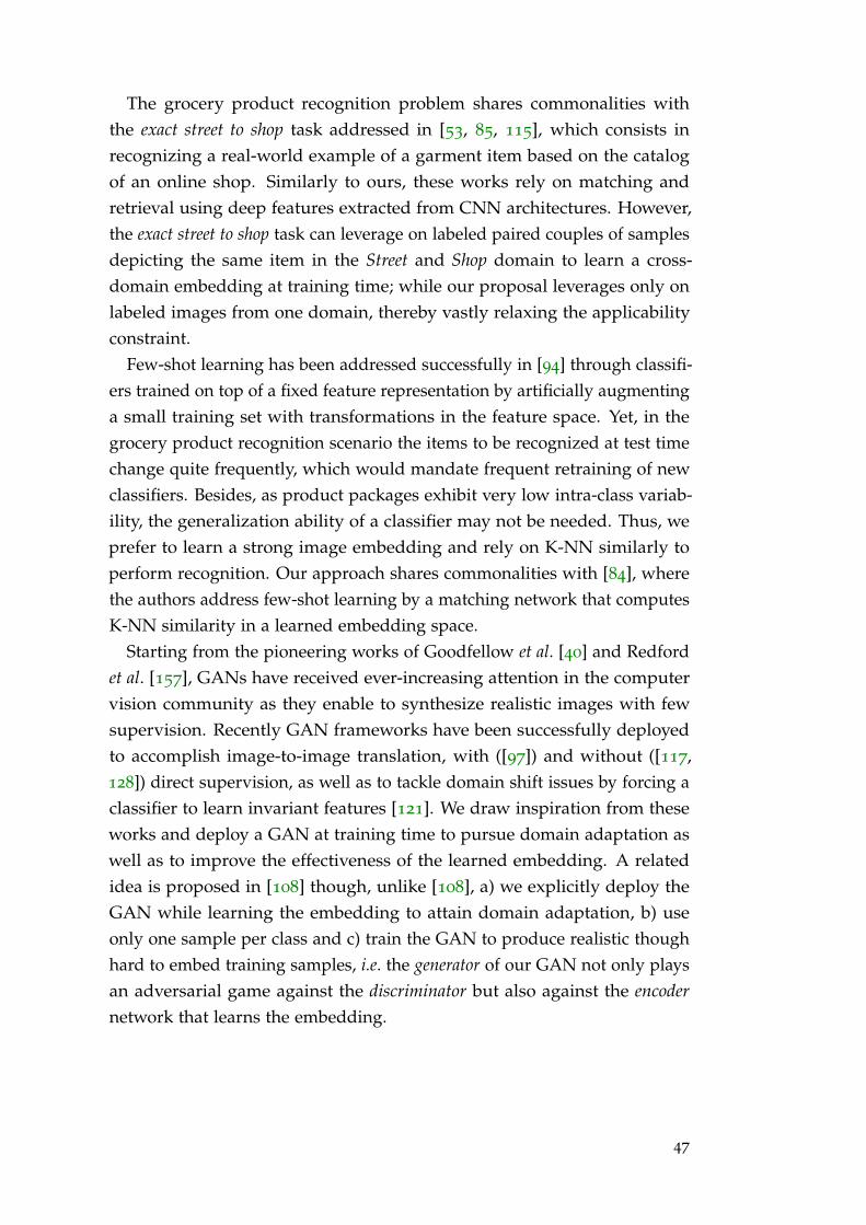
The grocery product recognition problem shares commonalities withthe exact street to shop task addressed in [53, 85, 115], which consists inrecognizing a real-world example of a garment item based on the catalogof an online shop. Similarly to ours, these works rely on matching andretrieval using deep features extracted from CNN architectures. However,the exact street to shop task can leverage on labeled paired couples of samplesdepicting the same item in the Street and Shop domain to learn a cross-domain embedding at training time; while our proposal leverages only onlabeled images from one domain, thereby vastly relaxing the applicabilityconstraint.
Few-shot learning has been addressed successfully in [94] through classifi-ers trained on top of a fixed feature representation by artificially augmentinga small training set with transformations in the feature space. Yet, in thegrocery product recognition scenario the items to be recognized at test timechange quite frequently, which would mandate frequent retraining of newclassifiers. Besides, as product packages exhibit very low intra-class variab-ility, the generalization ability of a classifier may not be needed. Thus, weprefer to learn a strong image embedding and rely on K-NN similarly toperform recognition. Our approach shares commonalities with [84], wherethe authors address few-shot learning by a matching network that computesK-NN similarity in a learned embedding space.
Starting from the pioneering works of Goodfellow et al. [40] and Redfordet al. [157], GANs have received ever-increasing attention in the computervision community as they enable to synthesize realistic images with fewsupervision. Recently GAN frameworks have been successfully deployedto accomplish image-to-image translation, with ([97]) and without ([117,128]) direct supervision, as well as to tackle domain shift issues by forcing aclassifier to learn invariant features [121]. We draw inspiration from theseworks and deploy a GAN at training time to pursue domain adaptation aswell as to improve the effectiveness of the learned embedding. A relatedidea is proposed in [108] though, unlike [108], a) we explicitly deploy theGAN while learning the embedding to attain domain adaptation, b) useonly one sample per class and c) train the GAN to produce realistic thoughhard to embed training samples, i.e. the generator of our GAN not only playsan adversarial game against the discriminator but also against the encodernetwork that learns the embedding.
47
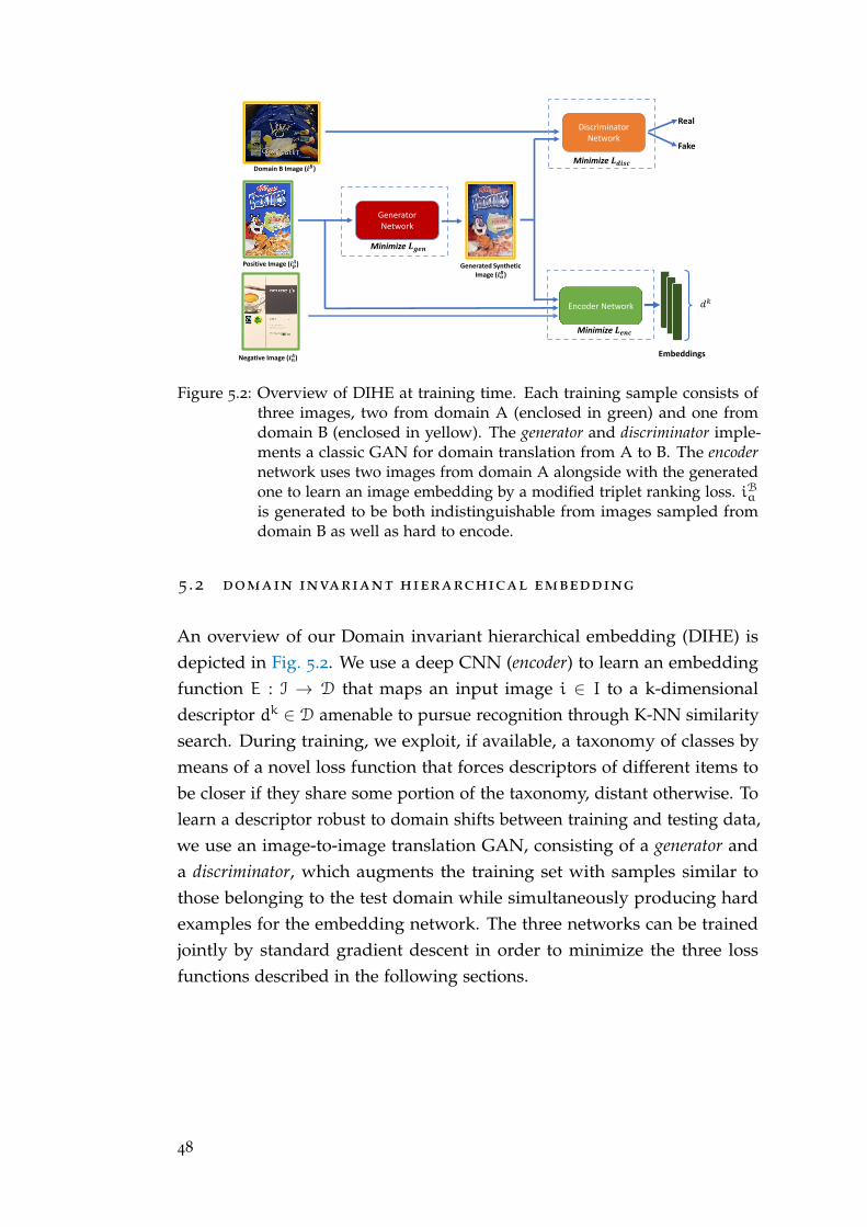
Positive Image (𝒊𝒑𝑨)
Negative Image (𝒊𝒏𝑨)
Domain B Image (𝒊𝑩)
Generated SyntheticImage (𝒊𝒂
𝑩)
Generator Network
Minimize 𝑳𝒈𝒆𝒏
Discriminator Network
Real
Minimize 𝑳𝒅𝒊𝒔𝒄
Fake
Encoder Network
Embeddings
Minimize 𝑳𝒆𝒏𝒄
𝑑𝑘
Figure 5.2: Overview of DIHE at training time. Each training sample consists ofthree images, two from domain A (enclosed in green) and one fromdomain B (enclosed in yellow). The generator and discriminator imple-ments a classic GAN for domain translation from A to B. The encodernetwork uses two images from domain A alongside with the generatedone to learn an image embedding by a modified triplet ranking loss. iBais generated to be both indistinguishable from images sampled fromdomain B as well as hard to encode.
5 .2 domain invariant hierarchical embedding
An overview of our Domain invariant hierarchical embedding (DIHE) isdepicted in Fig. 5.2. We use a deep CNN (encoder) to learn an embeddingfunction E : I → D that maps an input image i ∈ I to a k-dimensionaldescriptor dk ∈ D amenable to pursue recognition through K-NN similaritysearch. During training, we exploit, if available, a taxonomy of classes bymeans of a novel loss function that forces descriptors of different items tobe closer if they share some portion of the taxonomy, distant otherwise. Tolearn a descriptor robust to domain shifts between training and testing data,we use an image-to-image translation GAN, consisting of a generator anda discriminator, which augments the training set with samples similar tothose belonging to the test domain while simultaneously producing hardexamples for the embedding network. The three networks can be trainedjointly by standard gradient descent in order to minimize the three lossfunctions described in the following sections.
48
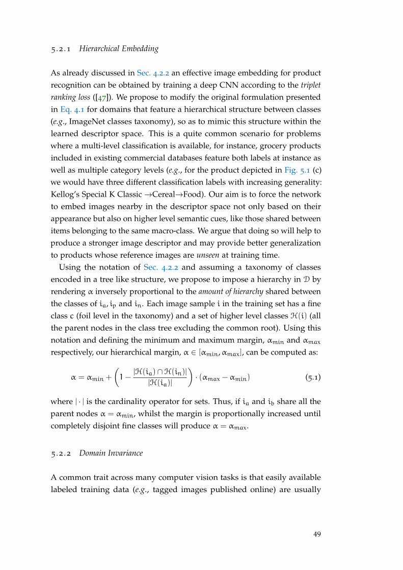
5 .2 .1 Hierarchical Embedding
As already discussed in Sec. 4.2.2 an effective image embedding for productrecognition can be obtained by training a deep CNN according to the tripletranking loss ([47]). We propose to modify the original formulation presentedin Eq. 4.1 for domains that feature a hierarchical structure between classes(e.g., ImageNet classes taxonomy), so as to mimic this structure within thelearned descriptor space. This is a quite common scenario for problemswhere a multi-level classification is available, for instance, grocery productsincluded in existing commercial databases feature both labels at instance aswell as multiple category levels (e.g., for the product depicted in Fig. 5.1 (c)we would have three different classification labels with increasing generality:Kellog’s Special K Classic→Cereal→Food). Our aim is to force the networkto embed images nearby in the descriptor space not only based on theirappearance but also on higher level semantic cues, like those shared betweenitems belonging to the same macro-class. We argue that doing so will help toproduce a stronger image descriptor and may provide better generalizationto products whose reference images are unseen at training time.
Using the notation of Sec. 4.2.2 and assuming a taxonomy of classesencoded in a tree like structure, we propose to impose a hierarchy in D byrendering α inversely proportional to the amount of hierarchy shared betweenthe classes of ia, ip and in. Each image sample i in the training set has a fineclass c (foil level in the taxonomy) and a set of higher level classes H(i) (allthe parent nodes in the class tree excluding the common root). Using thisnotation and defining the minimum and maximum margin, αmin and αmaxrespectively, our hierarchical margin, α ∈ [αmin,αmax], can be computed as:
α = αmin +
(1−
|H(ia)∩H(in)|
|H(ia)|
)· (αmax −αmin) (5.1)
where | · | is the cardinality operator for sets. Thus, if ia and ib share all theparent nodes α = αmin, whilst the margin is proportionally increased untilcompletely disjoint fine classes will produce α = αmax.
5 .2 .2 Domain Invariance
A common trait across many computer vision tasks is that easily availablelabeled training data (e.g., tagged images published online) are usually
49
sampled from a different distribution than the actual test images. Thus,machine learning models straightly trained with such samples, such asembedding networks, will typically perform poorly at test time due todomain shift issues. However, annotating samples from the test distribution,even if possible, is usually very expensive and time-consuming. We proposeto address this problem by dynamically transforming the appearance ofthe available labeled training images to make them look similar to samplesfrom the unlabeled test images. This transformation is carried out by twoCNNs, referred to in Fig. 5.2 as generator and discriminator, realizing animage-to-image translation GAN which is trained end-to-end together withthe embedding network (encoder).
Given two image domains A,B ⊂ I consisting of iAk ∈ A and iBk ∈ B, thestandard image-to-image GAN framework can be summarized as a generatornetwork that tries to learns a generative function G : A → B by playing atwo player min-max game against a discriminator network D : I → R thattries to classify examples either as real images from B or fake ones producedby G. In the following we will denote with G(iAk ) ∈ I the output of thegenerator network given the input image iAk and with D(i) ∈ R the outputof the discriminator network for image i. To generate samples similar tothe images from domain B without drastically changing the appearance ofthe input image iAk , we introduce an additional term in the generator lossfunction (Lreg) that, similarly to the self regularization term deployed in[117], forces G(iAk ) to be visually consistent with iAk . In our architecture, Ais the training set while B is a set of unlabeled images from the test datadistribution. Thus, in the grocery product recognition scenario, A will be thetraining images, either rendered or studio quality, while B a set of unlabeledproduct images acquired in the store.
During each training iteration of the whole architecture we sample oneimage iB ∈ B to train the discriminator and two from the other domainiAp , iAn ∈ A to train the encoder and generator. As mentioned in Sec. 5.2.1, theencoder needs triplets of samples to compute its loss, so we synthesize themissing image using the generator iBa = G(iAp ). With this architecture thetriplet used to calculate Eq. 4.1 consists of two images from domain A andone from the simulated domain B, thereby mimicking the test conditionswhere the query images to be recognized will came from B and the referenceimages to perform K-NN similarity from A.
50

The encoder is trained to minimize Eq. 4.1 with the margin defined inEq. 5.1. The discriminator tries to minimize a standard cross entropy loss:
Ldisc = log(D(iB)) + log(1−D(G(iAp ))) (5.2)
while the generator minimizes a loss consisting of three terms:
Lgen = Ladv + λreg · Lreg + λemb · LembLadv = −log(D(G(iAp )))
Lreg = φ(iAp , iBa )
Lemb = −d(E(iAp ),E(G(iAp )))
(5.3)
with φ(x,y), x,y ∈ I a similarity measure between the appearance of imagex and y, either at pixel level (e.g., mean absolute difference. . . ) or at imagelevel (e.g., SAD, ZNCC. . . ), and λreg, λemb two hyper parameters that weighthe different terms of the loss function. The contribution of the three termscan be summarized as follows. Ladv is the standard adversarial loss for thegenerator network that forces the synthesized images to be indistinguishablefrom those sampled from domain B; Lreg is aimed at synthesizing imagesthat preserve the overall structure of the input ones (avoiding thereby themode collapse issue often occurring in unconstrained GAN generators);Lemb forces an additional adversarial behaviour against the encoder, so as tocreate hard to embed samples.
At training time, given a minibatch of M different triplets of samples(iAp , iAn , iB), the three networks are trained jointly to minimize their averageloss on the M samples.
5 .3 implementation details
For the implementation of DIHE we have used tensorflow1 as our deeplearning framework. For the initialization of the encoder network on the finetuning tests we have used the weights publicly available in the tensorflow/-models repository2. The three networks that compose DIHE can easily fit ina single GPU, so training our system, once implemented, in a deep learningframework is straightforward. For all our test we used as generator U-Net([60]) and as discriminator PatchGAN ([97]), the latter producing a dense grid
1 https://www.tensorflow.org/2 https://github.com/tensorflow/models/tree/master/research/slim
51
of predictions for each input image. For the encoder we tested different avail-able CNN model with or without pre-trained weights on the ImageNet-1000
classification task. We will show how for the grocery product recognitionscenario, the best performance can be obtained using as embedding themaximum activation of convolution features (MAC [83]) extracted fromdifferent layers, which are concatenated and L2-normalized to get a finalrepresentation laying on the unit hypersphere. For all our tests, we usedas distance function d(X, Y) = 1− X · Y with X, Y ∈ D (i.e., one minus thecosine similarity between the two descriptors). As for φ in Lreg, we tried thepixel-wise L1 or L2 norms, the Structured Similarity Index (SSIM) ([8]) andthe Zero Mean Normalized Cross Correlation (ZNCC) and found out thelast to work best in all our tests, in the following φ(x,y) = ZNCC(x,y). Theweights of each network are trained to minimize their specific loss functionsas introduced in Sec. 5.2. We use Adam ([54]) as optimizer at differentlearning rates across the different tests. Concerning data preprocessing, weuse as input color images with a fixed size of 256X256X3 and intensitiesrescaled between [−1, 1]. To obtain the input dimension the original imagesare rescaled to the target resolution preserving the aspect ratio and fillingthe extra pixels with 0s. The only additional data augmentation is a randomcrop with size at least 80% of the original image to attain the input of thegenerator network performed before rescaling the images to input resolution.
At test time the encoder network is extracted from the whole DIHE andused as a stand-alone global image descriptor. Our implementation is quiteefficient and can easily encode, on GPU, more than 200 images per secondtaking into account also the time needed to load the images from diskand rescale them to the 256x256 input size. Finally, given that usually ourreference database only provide a single image per product and the descriptordimension is relatively low (between 256 and 1024 floats across differenttests), we perform the K-NN similarity search extensively without any kindof approximation. The biggest descriptor database considered in our tests isthe one obtained from Product8600 using a 1024 float dimensional embeddingvector (i.e., the reference database is a matrix of float with 8600 rows and1024 column). Even on this kind of database given a query descriptor thewhole similarity search can be solved in a tenth of a second using bruteforce search, nevertheless, the search could potentially be speeded up usingKD-Tree or approximate search technique.
52

Food
Figure 5.3: Visualization of the hierarchy of categories of the Grocery_Food datasetused as training set throughout our experiments. Each outermost cat-egory contains several different fine classes (products) not depicted forclarity.
5 .4 experimental results
To evaluate the effectiveness of DIHE in recognizing grocery products werely on two products datasets comprising thousands of items: the publiclyavailable Grocery Products dataset ([39]) and a standard commercial database,referred to here as Product8600. Both datasets include more than 8500 groceryproducts, each described by exactly one studio-quality (reference) image ofthe frontal face of the package, and feature a multi-level class hierarchyin the categorization of products. As already discussed, at test time wepursue recognition from a different set of images (query). To create this set,for Grocery Products we automatically cropped individual items from theavailable shelf images according to the annotation used in Chap. 3, therebyobtaining a total of 938 query images. As for Product8600, we cropped andannotated individual items from shelf videos that we acquired in a grocerystore by a tablet camera, for a total number of 273 query images. As theshelf images available in Grocery Products concern only items belonging tothe Food macro class, which accounts for 3288 products, we consider alsothis smaller subset of products, which will be referred to as Grocery_Food,whilst Grocery_Full will denote all the products of the Grocery Product dataset.We depict in Fig. 5.3 the taxonomy of macro categories that compose theGrocery_Food dataset which we are going to use as the training set, eachcategory features several fine-grained classes (one for each product) not
53
depicted in the figure. As for the samples from domain B needed to train thediscriminator and generator of our architecture (see Sec. 5.2.2), we have used547 additional images cropped from the shelf images available in GroceryProducts, picked as to have no overlap with the previously mentioned 938
query images used at test time. We wish to point out how our formulationrequires images from domain B only for the discriminator of the GANsystem. Therefore, few samples without any kind of annotation are sufficientto learn the appearance of products on the shelf. Moreover, we can useimages from domain B that depict any kind of product, even items not in A.
network architectures For the implementation of DIHE we haveused tensorflow3 as our deep learning framework. For all our test weused as generator U-Net ([60]) and as discriminator PatchGAN ([97]), thelatter producing a dense grid of predictions for each input image. For theencoder we tested different available CNN model with or without pretrainedweight on the ImageNet-1000 classification task. For the initialization of theencoder network on the fine tuning tests we have used the weights publiclyavailable in the tensorflow/models repository4. The three networks thatcompose DIHE can easily fit in a single GPU, so training our system, onceimplemented, in a deep learning framework is straightforward.
descriptor computation We will show how for the grocery productrecognition scenario, the best performance can be obtained using as embed-ding the maximum activation of convolution features (MAC [83]). We extractthese descriptors from different layers, concatenate them and finally performL2-normalization to get a final representation laying on the unit hypersphere.For all our tests, we used as distance function d(X, Y) = 1 − X · Y withX, Y ∈ D (i.e., one minus the cosine similarity between the two descriptors).
training details As for φ in Lreg, we tried the pixel-wise L1 or L2norms, the Structured Similarity Index (SSIM) ([8]) and the Zero MeanNormalized Cross Correlation (ZNCC) and found out the last to work bestin all our tests, in the following φ(x,y) = ZNCC(x,y). The weights of eachnetwork are trained to minimize their specific loss functions as introducedin Sec. 5.2. We use Adam ([54]) as optimizer with different learning ratesfor the different tests. Concerning data preprocessing, we use as input color
3 https://www.tensorflow.org/4 https://github.com/tensorflow/models/tree/master/research/slim
54
images with a fixed size of 256× 256 and intensities rescaled between [−1, 1].To obtain the input dimension the original images are rescaled to the targetresolution preserving the aspect ratio and filling the extra pixels with 0s.The only additional data augmentation is a preliminary random crop withsize at least 80% of the original image to attain the input of the generatornetwork.
evaluation protocol To test our embedding network we encode allthe reference images of the considered dataset to create a reference database,then compute the same encoding for the query images. For each queryvector we perform similarity search against all the reference vectors andretain the K most similar database entries; if the reference image for theproduct depicted in the query does belong to this set of nearest neighborswe consider recognition to be successful. As a measure of the effectivenessof the embedding, we report the accuracy (number of successful recognitionsover the number of queries) for different K values.
Based on these premises, we train once and for all our architecture usingonly the reference images belonging to Grocery_Food, (i.e., one referenceimage for each of 3288 different products organized in a multi-level hierarchyof products categories). We then use the trained embedding model to addressthree different test scenarios:
(a) Grocery_Food: we recognize the 938 query images from Grocery Productsbased on the 3288 reference images from Grocery_Food. Thus, all thereference images were deployed at training time.
(b) Grocery_Full: we recognize the 938 query images from Grocery Productsbased on the 8403 reference images from Grocery_Full. Thus, only 40%of the reference images were deployed at training time.
(c) Product8600: we recognize the 273 query images cropped from ourvideos based on the 8597 reference images from Product8600. Thus,none of the reference images was deployed at training time.
Among the three, (b) is the most likely to happen in practical settingsas product appearance changes frequently over time and it is infeasible toconstantly retrain the embedding network, although perhaps a portion ofthe reference images dealing with the items actually on sale in the store hadbeen used at training time
55
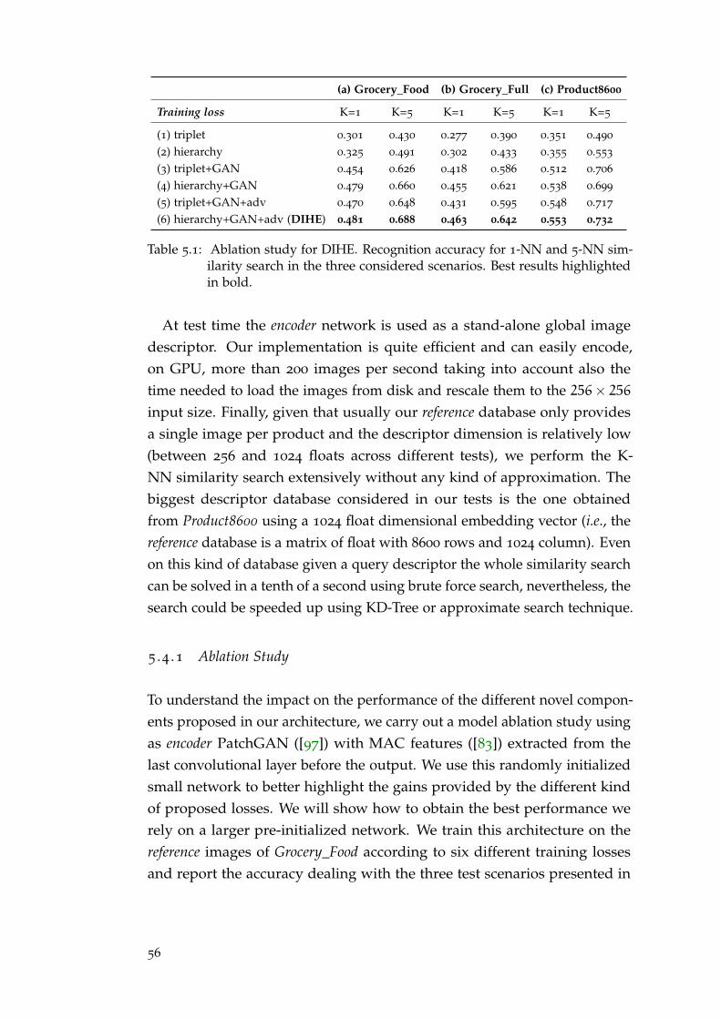
(a) Grocery_Food (b) Grocery_Full (c) Product8600
Training loss K=1 K=5 K=1 K=5 K=1 K=5
(1) triplet 0.301 0.430 0.277 0.390 0.351 0.490
(2) hierarchy 0.325 0.491 0.302 0.433 0.355 0.553
(3) triplet+GAN 0.454 0.626 0.418 0.586 0.512 0.706
(4) hierarchy+GAN 0.479 0.660 0.455 0.621 0.538 0.699
(5) triplet+GAN+adv 0.470 0.648 0.431 0.595 0.548 0.717
(6) hierarchy+GAN+adv (DIHE) 0.481 0.688 0.463 0.642 0.553 0.732
Table 5.1: Ablation study for DIHE. Recognition accuracy for 1-NN and 5-NN sim-ilarity search in the three considered scenarios. Best results highlightedin bold.
At test time the encoder network is used as a stand-alone global imagedescriptor. Our implementation is quite efficient and can easily encode,on GPU, more than 200 images per second taking into account also thetime needed to load the images from disk and rescale them to the 256× 256input size. Finally, given that usually our reference database only providesa single image per product and the descriptor dimension is relatively low(between 256 and 1024 floats across different tests), we perform the K-NN similarity search extensively without any kind of approximation. Thebiggest descriptor database considered in our tests is the one obtainedfrom Product8600 using a 1024 float dimensional embedding vector (i.e., thereference database is a matrix of float with 8600 rows and 1024 column). Evenon this kind of database given a query descriptor the whole similarity searchcan be solved in a tenth of a second using brute force search, nevertheless, thesearch could be speeded up using KD-Tree or approximate search technique.
5 .4 .1 Ablation Study
To understand the impact on the performance of the different novel compon-ents proposed in our architecture, we carry out a model ablation study usingas encoder PatchGAN ([97]) with MAC features ([83]) extracted from thelast convolutional layer before the output. We use this randomly initializedsmall network to better highlight the gains provided by the different kindof proposed losses. We will show how to obtain the best performance werely on a larger pre-initialized network. We train this architecture on thereference images of Grocery_Food according to six different training lossesand report the accuracy dealing with the three test scenarios presented in
56
Sec. 5.4 in Tab. 5.1. In particular, with reference to the first column, tripletdenotes training by triplet loss with fixed margin (α = 0.3 obtained bycross-validation); hierarchy denotes training by our triplet loss with variablemargin introduced in Sec. 5.2.1 (αmin = 0.1,αmax = 0.5); entries with +GANdenote deploying the image translation GAN to generate the anchor imageiBa (Eq. 5.3: λreg = 1, λemb = 0); finally, entries with +GAN+adv concernsintroducing also the adversarial term in the loss of the GAN generator(Eq. 5.3: λreg = 1, λemb = 0.1). For all the models that do not use GANs, werely on standard data augmentation techniques (e.g., crop, gaussian blur,color transformation. . . ) to obtain the anchor image given the positive one.In all the tests the networks are randomly initialized and trained for thesame number of steps and identical learning rates.
The results reported in Tab. 5.1 show how each individual novel compon-ent proposed in our DIHE architecture provides a significant performanceimprovement with respect to the standard triplet ranking loss. Indeed, bycomparing rows (2),(4) and (6) to (1),(3) and (5), respectively, it can be ob-served that modifying the fixed margin of the standard triplet loss into ourproposed hierarchically adaptive margin can improve accuracy with all mod-els and in all scenarios, with a much larger gain in (c)(i.e., completely unseenreference images). This proves that embedding a hierarchy into the descriptorspace is an effective strategy to help to learn an embedding amenable togeneralize to unseen data. The main improvements are clearly achieved bymethods featuring a GAN network to pursue domain adaptation by gener-ating training samples similar to the images coming from the test domain.Indeed, comparison of (3) and (4) to (1) and (2), respectively, highlightshow performance nearly double across all models and scenarios, testifyingthat the domain shift between test and train data and the lack of multipletraining samples are indeed the key issues in this task that the proposedimage-to-image translation GAN can help to address very effectively. Finally,comparing (5) and (6) to (3) and (4), respectively, vouches that training thegenerator to produce anchor images not only realistic but also hard to embedturns out always beneficial to performance. Indeed, the adversarial gameplayed by the generator and encoder may be thought of as an online andadaptive hard-mining capable of dynamically synthesize hard to embedsamples that help training a more robust embedding. Performance of ouroverall DIHE architecture are reported in the row (6) and show a dramaticimprovement with respect to the standard triplet loss, row (1).
57
5 .4 .2 Product Recognition
model and descriptor selection To ameliorate product recogni-tion performance we can rely on larger networks pre-trained on the Im-ageNet classification benchmark. To chose the best CNN model as ourencoder network we downloaded the public available weights of differentmodels trained on ImageNet-1000 classification and test them as generalpurpose off-the-shelf feature extractors on our datasets without any kind offine-tuning. We considered three different popular CNN models (VGG_16
[62], resnet_[50/101/152] [70] and inception_v4 [119]) and compute threekind of different descriptors from activations extracted at various layers:
• Direct: directly use the vectorized activation of a given layer. Thedimension of the descriptor is the number of elements in the featuremaps for that layer.
• AVG: perform average pooling on the feature map with a kernelwith width and height equals those of the map. Therefore, we use asdescriptor the average activation of each convolutional filter for a givenlayer. The dimension of the descriptor is the number of convolutionalfilters in the selected layer.
• MAC [[83]]: perform max pooling on the feature map with a ker-nel with width and height equals those of the map. Therefore, weuse as descriptor the maximum activation of each convolutional filterfor a given layer. The dimension of the descriptor is the number ofconvolutional filters in the selected layer.
We applied the three different descriptors above at different layers ofthe three networks and report in Tab. 5.2 the 1-NN accuracy using the testprotocol described in Sec. 5.4.1. For all our tests the descriptors were L2
normalized to the unit norm and the similarity search is performed usingcosine similarity. In Tab. 5.2 we report only some of the best performinglayers for each network and additional tests where the descriptors are ob-tained by concatenation of representations extracted at different depths inthe CNN (e.g., conv4_3+conv5_3 is the concatenation of representations ex-tracted at layers conv4_3 and conv5_3) with L2 normalization performedafter concatenation.
Looking at the results in Tab. 5.2 we can observe how, in our settings,newer and more powerful CNN, like inception_v4 or resnet_152, fail to
58

CNN Layer Type Grocery_Food Grocery_Full Product8600
VGG_16
conv4_3MAC 0.789 0.785 0.717
AVG 0.515 0.510 0.538
conv5_3MAC 0.724 0.720 0.611
AVG 0.406 0.398 0.395
conv4_3+conv5_3MAC 0.792 0.787 0.725AVG 0.501 0.493 0.523
fc6 Direct 0.560 0.549 0.549
fc7 Direct 0.444 0.433 0.432
inception_v4
Mixed_7a MAC 0.610 0.603 0.509
AVG 0.673 0.670 0.560
Mixed_7b MAC 0.652 0.641 0.512
AVG 0.675 0.668 0.5091
Mixed_7a+Mixed_7b MAC 0.655 0.646 0.534
AVG 0.690 0.685 0.542
resnet_50
Block3MAC 0.731 0.729 0.703
AVG 0.441 0.433 0.432
Block4MAC 0.654 0.646 0.509
AVG 0.571 0.558 0.465
Block3+Block4MAC 0.723 0.720 0.644
AVG 0.547 0.538 0.545
resnet_101
Block3MAC 0.737 0.735 0.695
AVG 0.389 0.388 0.432
Block4MAC 0.636 0.662 0.490
AVG 0.570 0.556 0.417
Block3+Block4MAC 0.714 0.708 0.626
AVG 0.535 0.524 0.520
resnet_152
Block3MAC 0.708 0.703 0.655
AVG 0.345 0.337 0.446
Block4MAC 0.571 0.561 0.435
AVG 0.571 0.561 0.435
Block3+Block4MAC 0.678 0.671 0.542
AVG 0.506 0.500 0.504
Table 5.2: 1-NN accuracy for different descriptors obtained from layers of networkpre-trained on the ImageNet-1000 classification dataset without any kindof additional fine-tuning. Best results are higlighted in bold.
59
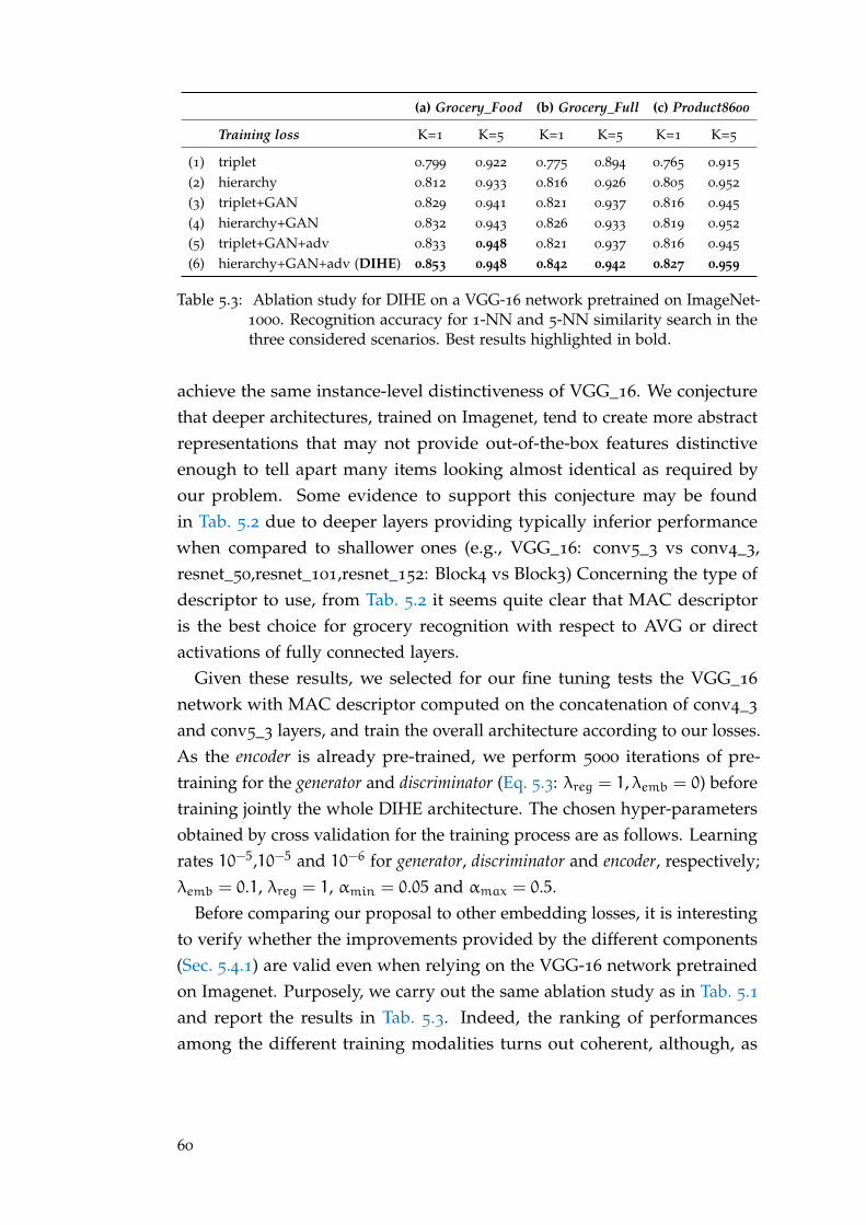
(a) Grocery_Food (b) Grocery_Full (c) Product8600
Training loss K=1 K=5 K=1 K=5 K=1 K=5
(1) triplet 0.799 0.922 0.775 0.894 0.765 0.915
(2) hierarchy 0.812 0.933 0.816 0.926 0.805 0.952
(3) triplet+GAN 0.829 0.941 0.821 0.937 0.816 0.945
(4) hierarchy+GAN 0.832 0.943 0.826 0.933 0.819 0.952
(5) triplet+GAN+adv 0.833 0.948 0.821 0.937 0.816 0.945
(6) hierarchy+GAN+adv (DIHE) 0.853 0.948 0.842 0.942 0.827 0.959
Table 5.3: Ablation study for DIHE on a VGG-16 network pretrained on ImageNet-1000. Recognition accuracy for 1-NN and 5-NN similarity search in thethree considered scenarios. Best results highlighted in bold.
achieve the same instance-level distinctiveness of VGG_16. We conjecturethat deeper architectures, trained on Imagenet, tend to create more abstractrepresentations that may not provide out-of-the-box features distinctiveenough to tell apart many items looking almost identical as required byour problem. Some evidence to support this conjecture may be foundin Tab. 5.2 due to deeper layers providing typically inferior performancewhen compared to shallower ones (e.g., VGG_16: conv5_3 vs conv4_3,resnet_50,resnet_101,resnet_152: Block4 vs Block3) Concerning the type ofdescriptor to use, from Tab. 5.2 it seems quite clear that MAC descriptoris the best choice for grocery recognition with respect to AVG or directactivations of fully connected layers.
Given these results, we selected for our fine tuning tests the VGG_16
network with MAC descriptor computed on the concatenation of conv4_3
and conv5_3 layers, and train the overall architecture according to our losses.As the encoder is already pre-trained, we perform 5000 iterations of pre-training for the generator and discriminator (Eq. 5.3: λreg = 1, λemb = 0) beforetraining jointly the whole DIHE architecture. The chosen hyper-parametersobtained by cross validation for the training process are as follows. Learningrates 10−5,10−5 and 10−6 for generator, discriminator and encoder, respectively;λemb = 0.1, λreg = 1, αmin = 0.05 and αmax = 0.5.
Before comparing our proposal to other embedding losses, it is interestingto verify whether the improvements provided by the different components(Sec. 5.4.1) are valid even when relying on the VGG-16 network pretrainedon Imagenet. Purposely, we carry out the same ablation study as in Tab. 5.1and report the results in Tab. 5.3. Indeed, the ranking of performancesamong the different training modalities turns out coherent, although, as
60
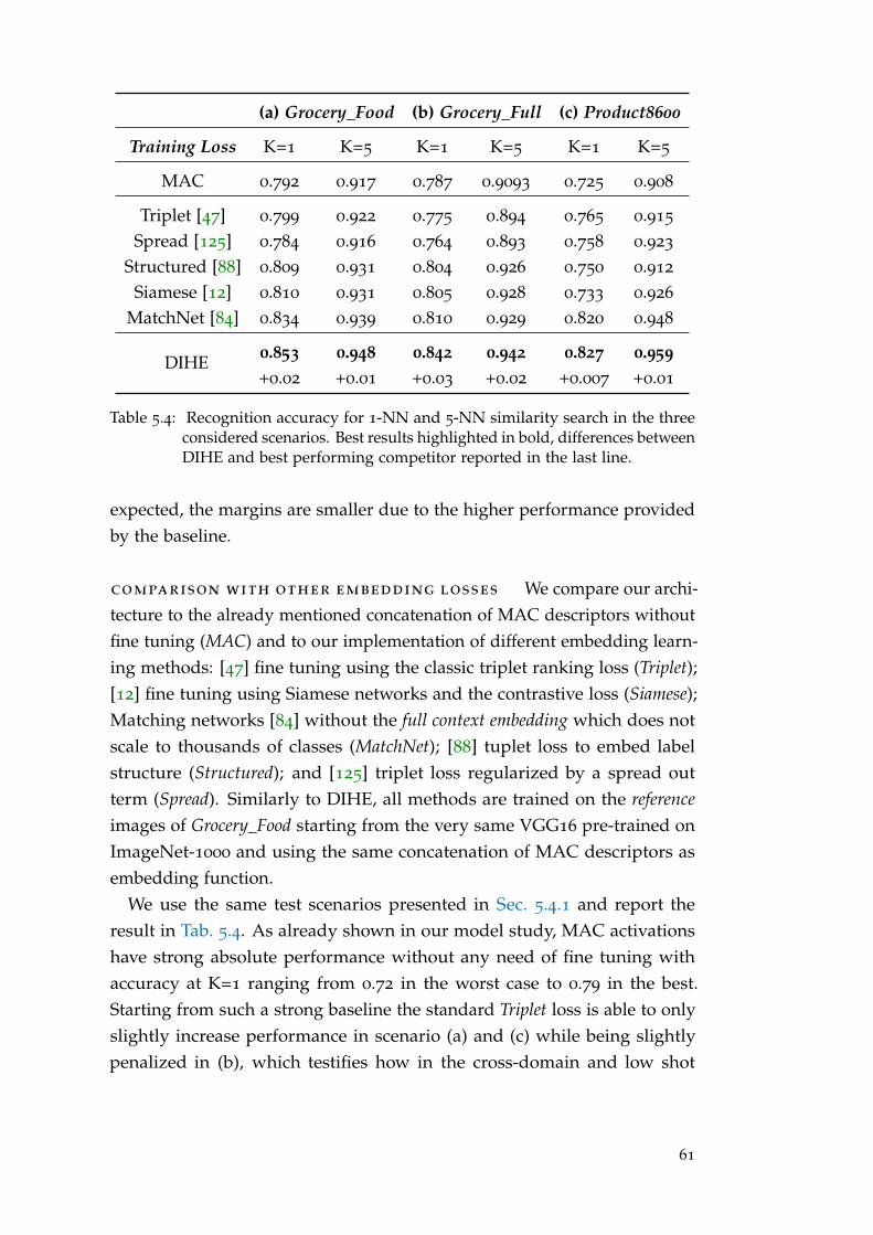
(a) Grocery_Food (b) Grocery_Full (c) Product8600
Training Loss K=1 K=5 K=1 K=5 K=1 K=5
MAC 0.792 0.917 0.787 0.9093 0.725 0.908
Triplet [47] 0.799 0.922 0.775 0.894 0.765 0.915
Spread [125] 0.784 0.916 0.764 0.893 0.758 0.923
Structured [88] 0.809 0.931 0.804 0.926 0.750 0.912
Siamese [12] 0.810 0.931 0.805 0.928 0.733 0.926
MatchNet [84] 0.834 0.939 0.810 0.929 0.820 0.948
DIHE 0.853 0.948 0.842 0.942 0.827 0.959+0.02 +0.01 +0.03 +0.02 +0.007 +0.01
Table 5.4: Recognition accuracy for 1-NN and 5-NN similarity search in the threeconsidered scenarios. Best results highlighted in bold, differences betweenDIHE and best performing competitor reported in the last line.
expected, the margins are smaller due to the higher performance providedby the baseline.
comparison with other embedding losses We compare our archi-tecture to the already mentioned concatenation of MAC descriptors withoutfine tuning (MAC) and to our implementation of different embedding learn-ing methods: [47] fine tuning using the classic triplet ranking loss (Triplet);[12] fine tuning using Siamese networks and the contrastive loss (Siamese);Matching networks [84] without the full context embedding which does notscale to thousands of classes (MatchNet); [88] tuplet loss to embed labelstructure (Structured); and [125] triplet loss regularized by a spread outterm (Spread). Similarly to DIHE, all methods are trained on the referenceimages of Grocery_Food starting from the very same VGG16 pre-trained onImageNet-1000 and using the same concatenation of MAC descriptors asembedding function.
We use the same test scenarios presented in Sec. 5.4.1 and report theresult in Tab. 5.4. As already shown in our model study, MAC activationshave strong absolute performance without any need of fine tuning withaccuracy at K=1 ranging from 0.72 in the worst case to 0.79 in the best.Starting from such a strong baseline the standard Triplet loss is able to onlyslightly increase performance in scenario (a) and (c) while being slightlypenalized in (b), which testifies how in the cross-domain and low shot
61
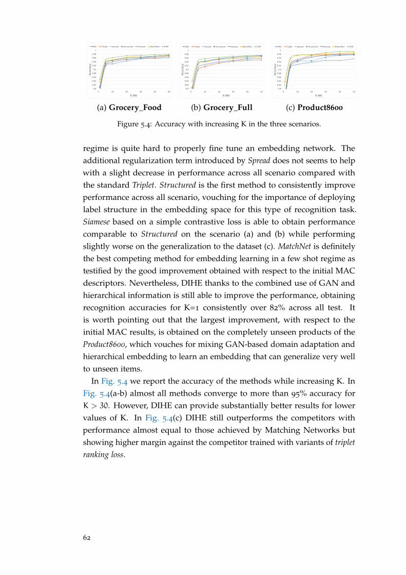
0.8
0.82
0.84
0.86
0.88
0.9
0.92
0.94
0.96
0.98
1
0 10 20 30 40 50Accuracy
K-NN
MAC Triplet Spread Structured Siamese MatchNet DIHE
0.8
0.82
0.84
0.86
0.88
0.9
0.92
0.94
0.96
0.98
1
0 10 20 30 40 50
Accuracy
K-NN
MAC Triplet Spread Structured Siamese MatchNet DIHE
0.8
0.82
0.84
0.86
0.88
0.9
0.92
0.94
0.96
0.98
1
0 10 20 30 40 50
Accuracy
K-NN
MAC Triplet Spread Structured Siamese MatchNet DIHE
(a) Grocery_Food (b) Grocery_Full (c) Product8600
Figure 5.4: Accuracy with increasing K in the three scenarios.
regime is quite hard to properly fine tune an embedding network. Theadditional regularization term introduced by Spread does not seems to helpwith a slight decrease in performance across all scenario compared withthe standard Triplet. Structured is the first method to consistently improveperformance across all scenario, vouching for the importance of deployinglabel structure in the embedding space for this type of recognition task.Siamese based on a simple contrastive loss is able to obtain performancecomparable to Structured on the scenario (a) and (b) while performingslightly worse on the generalization to the dataset (c). MatchNet is definitelythe best competing method for embedding learning in a few shot regime astestified by the good improvement obtained with respect to the initial MACdescriptors. Nevertheless, DIHE thanks to the combined use of GAN andhierarchical information is still able to improve the performance, obtainingrecognition accuracies for K=1 consistently over 82% across all test. Itis worth pointing out that the largest improvement, with respect to theinitial MAC results, is obtained on the completely unseen products of theProduct8600, which vouches for mixing GAN-based domain adaptation andhierarchical embedding to learn an embedding that can generalize very wellto unseen items.
In Fig. 5.4 we report the accuracy of the methods while increasing K. InFig. 5.4(a-b) almost all methods converge to more than 95% accuracy forK > 30. However, DIHE can provide substantially better results for lowervalues of K. In Fig. 5.4(c) DIHE still outperforms the competitors withperformance almost equal to those achieved by Matching Networks butshowing higher margin against the competitor trained with variants of tripletranking loss.
62
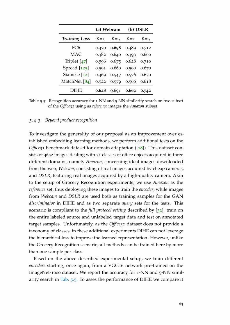
(a) Webcam (b) DSLR
Training Loss K=1 K=5 K=1 K=5
FC6 0.470 0.698 0.489 0.712
MAC 0.382 0.640 0.393 0.660
Triplet [47] 0.596 0.675 0.628 0.710
Spread [125] 0.591 0.660 0.590 0.670
Siamese [12] 0.469 0.547 0.576 0.630
MatchNet [84] 0.522 0.579 0.566 0.618
DIHE 0.628 0.691 0.662 0.742
Table 5.5: Recognition accuracy for 1-NN and 5-NN similarity search on two subsetof the Office31 using as reference images the Amazon subset.
5 .4 .3 Beyond product recognition
To investigate the generality of our proposal as an improvement over es-tablished embedding learning methods, we perform additional tests on theOffice31 benchmark dataset for domain adaptation ([18]). This dataset con-sists of 4652 images dealing with 31 classes of office objects acquired in threedifferent domains, namely Amazon, concerning ideal images downloadedfrom the web, Webcam, consisting of real images acquired by cheap cameras,and DSLR, featuring real images acquired by a high-quality camera. Akinto the setup of Grocery Recognition experiments, we use Amazon as thereference set, thus deploying these images to train the encoder, while imagesfrom Webcam and DSLR are used both as training samples for the GANdiscriminator in DIHE and as two separate query sets for the tests. Thisscenario is compliant to the full protocol setting described by [32]: train onthe entire labeled source and unlabeled target data and test on annotatedtarget samples. Unfortunately, as the Office31 dataset does not provide ataxonomy of classes, in these additional experiments DIHE can not leveragethe hierarchical loss to improve the learned representation. However, unlikethe Grocery Recognition scenario, all methods can be trained here by morethan one sample per class.
Based on the above described experimental setup, we train differentencoders starting, once again, from a VGG16 network pre-trained on theImageNet-1000 dataset. We report the accuracy for 1-NN and 5-NN simil-arity search in Tab. 5.5. To asses the performance of DIHE we compare it
63
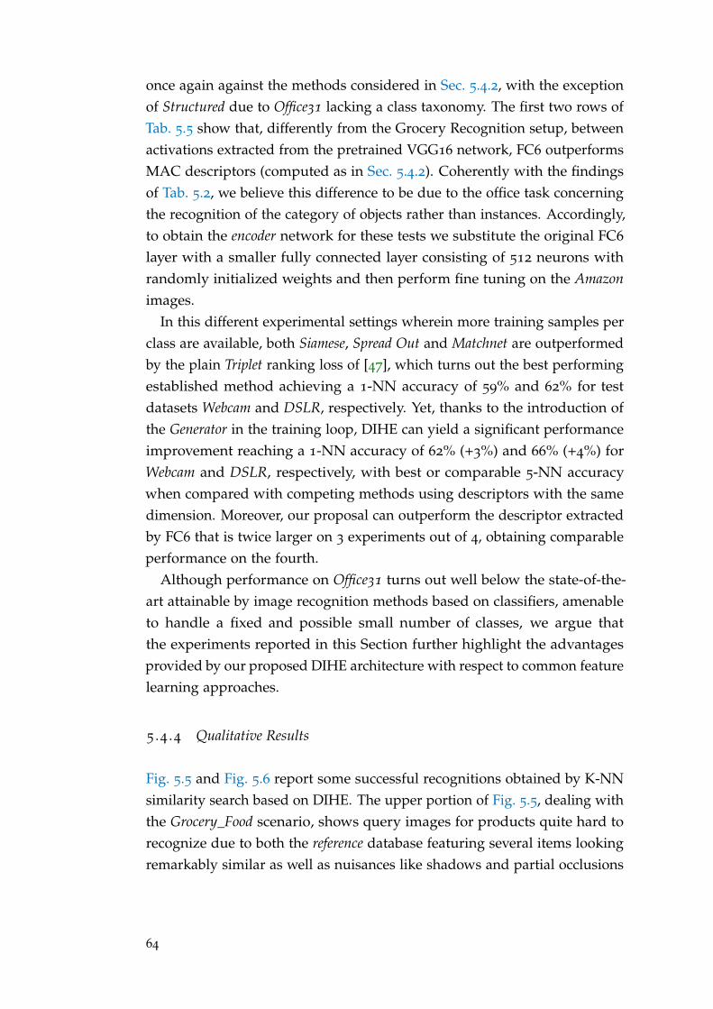
once again against the methods considered in Sec. 5.4.2, with the exceptionof Structured due to Office31 lacking a class taxonomy. The first two rows ofTab. 5.5 show that, differently from the Grocery Recognition setup, betweenactivations extracted from the pretrained VGG16 network, FC6 outperformsMAC descriptors (computed as in Sec. 5.4.2). Coherently with the findingsof Tab. 5.2, we believe this difference to be due to the office task concerningthe recognition of the category of objects rather than instances. Accordingly,to obtain the encoder network for these tests we substitute the original FC6
layer with a smaller fully connected layer consisting of 512 neurons withrandomly initialized weights and then perform fine tuning on the Amazonimages.
In this different experimental settings wherein more training samples perclass are available, both Siamese, Spread Out and Matchnet are outperformedby the plain Triplet ranking loss of [47], which turns out the best performingestablished method achieving a 1-NN accuracy of 59% and 62% for testdatasets Webcam and DSLR, respectively. Yet, thanks to the introduction ofthe Generator in the training loop, DIHE can yield a significant performanceimprovement reaching a 1-NN accuracy of 62% (+3%) and 66% (+4%) forWebcam and DSLR, respectively, with best or comparable 5-NN accuracywhen compared with competing methods using descriptors with the samedimension. Moreover, our proposal can outperform the descriptor extractedby FC6 that is twice larger on 3 experiments out of 4, obtaining comparableperformance on the fourth.
Although performance on Office31 turns out well below the state-of-the-art attainable by image recognition methods based on classifiers, amenableto handle a fixed and possible small number of classes, we argue thatthe experiments reported in this Section further highlight the advantagesprovided by our proposed DIHE architecture with respect to common featurelearning approaches.
5 .4 .4 Qualitative Results
Fig. 5.5 and Fig. 5.6 report some successful recognitions obtained by K-NNsimilarity search based on DIHE. The upper portion of Fig. 5.5, dealing withthe Grocery_Food scenario, shows query images for products quite hard torecognize due to both the reference database featuring several items lookingremarkably similar as well as nuisances like shadows and partial occlusions
64
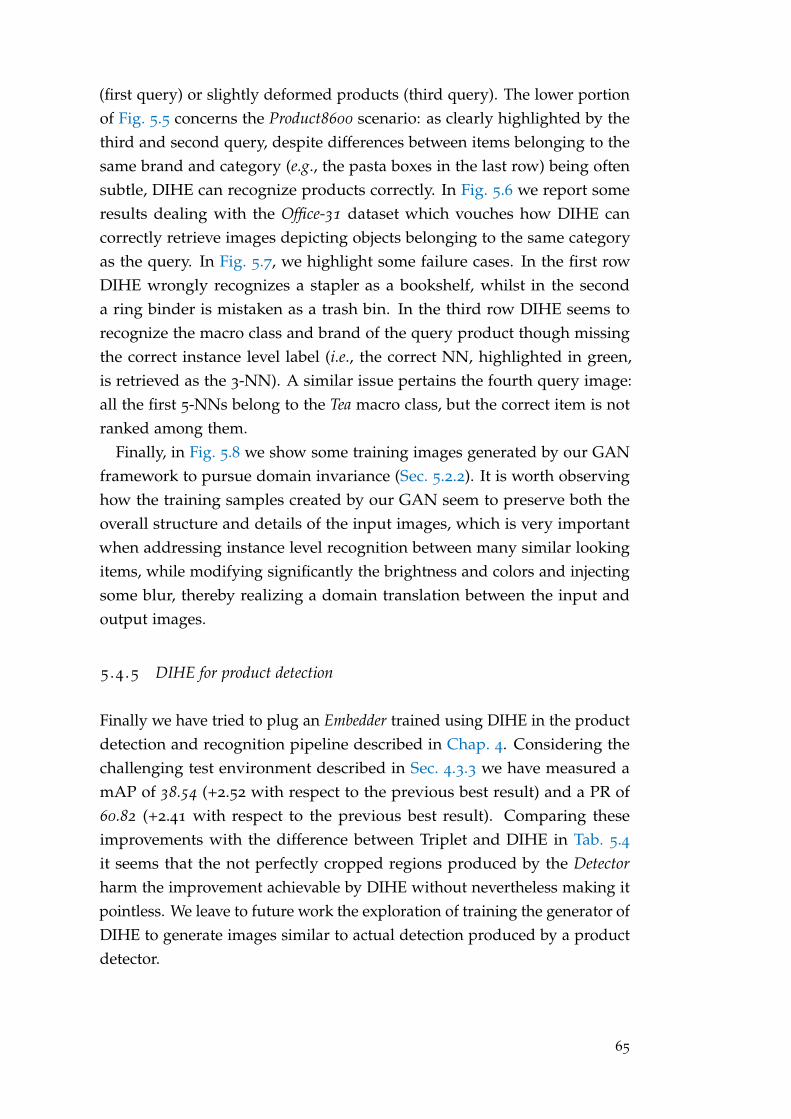
(first query) or slightly deformed products (third query). The lower portionof Fig. 5.5 concerns the Product8600 scenario: as clearly highlighted by thethird and second query, despite differences between items belonging to thesame brand and category (e.g., the pasta boxes in the last row) being oftensubtle, DIHE can recognize products correctly. In Fig. 5.6 we report someresults dealing with the Office-31 dataset which vouches how DIHE cancorrectly retrieve images depicting objects belonging to the same categoryas the query. In Fig. 5.7, we highlight some failure cases. In the first rowDIHE wrongly recognizes a stapler as a bookshelf, whilst in the seconda ring binder is mistaken as a trash bin. In the third row DIHE seems torecognize the macro class and brand of the query product though missingthe correct instance level label (i.e., the correct NN, highlighted in green,is retrieved as the 3-NN). A similar issue pertains the fourth query image:all the first 5-NNs belong to the Tea macro class, but the correct item is notranked among them.
Finally, in Fig. 5.8 we show some training images generated by our GANframework to pursue domain invariance (Sec. 5.2.2). It is worth observinghow the training samples created by our GAN seem to preserve both theoverall structure and details of the input images, which is very importantwhen addressing instance level recognition between many similar lookingitems, while modifying significantly the brightness and colors and injectingsome blur, thereby realizing a domain translation between the input andoutput images.
5 .4 .5 DIHE for product detection
Finally we have tried to plug an Embedder trained using DIHE in the productdetection and recognition pipeline described in Chap. 4. Considering thechallenging test environment described in Sec. 4.3.3 we have measured amAP of 38.54 (+2.52 with respect to the previous best result) and a PR of60.82 (+2.41 with respect to the previous best result). Comparing theseimprovements with the difference between Triplet and DIHE in Tab. 5.4it seems that the not perfectly cropped regions produced by the Detectorharm the improvement achievable by DIHE without nevertheless making itpointless. We leave to future work the exploration of training the generator ofDIHE to generate images similar to actual detection produced by a productdetector.
65
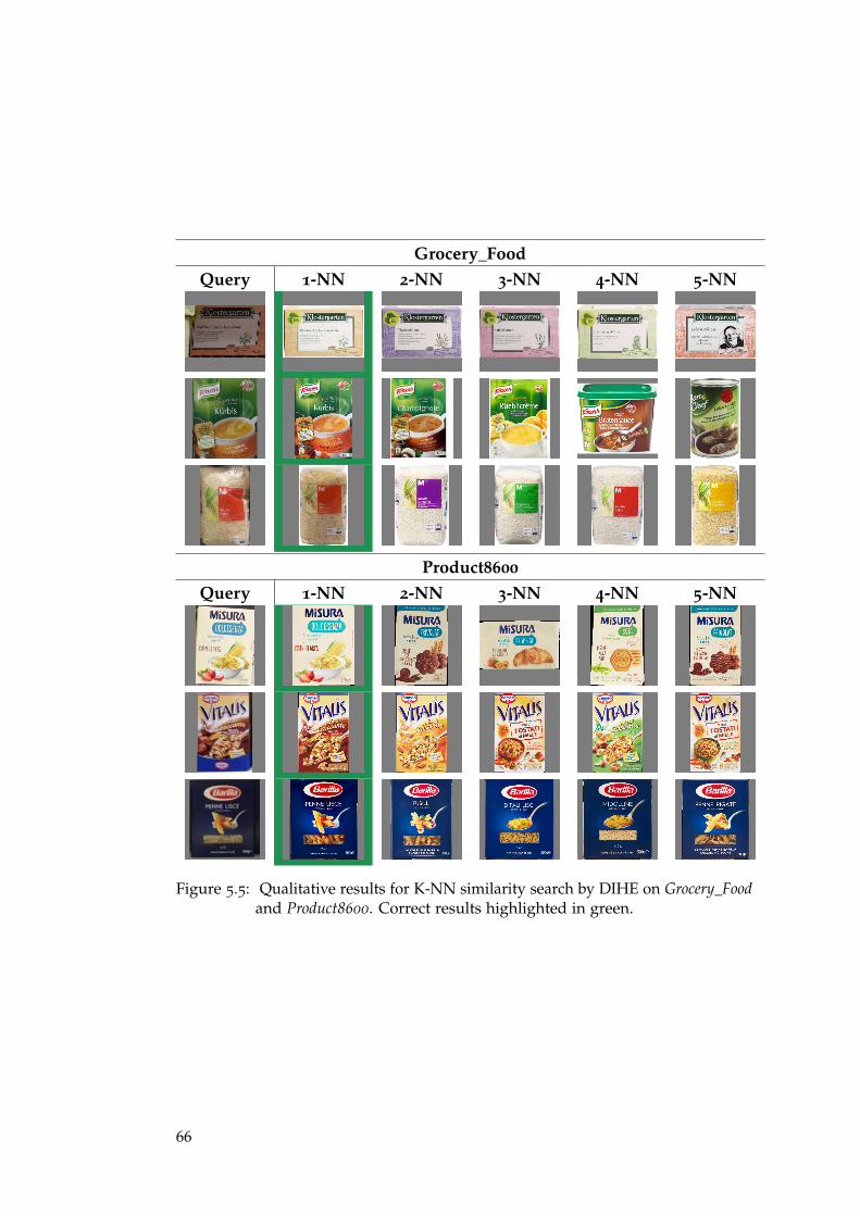
Grocery_FoodQuery 1-NN 2-NN 3-NN 4-NN 5-NN
Product8600Query 1-NN 2-NN 3-NN 4-NN 5-NN
Figure 5.5: Qualitative results for K-NN similarity search by DIHE on Grocery_Foodand Product8600. Correct results highlighted in green.
66
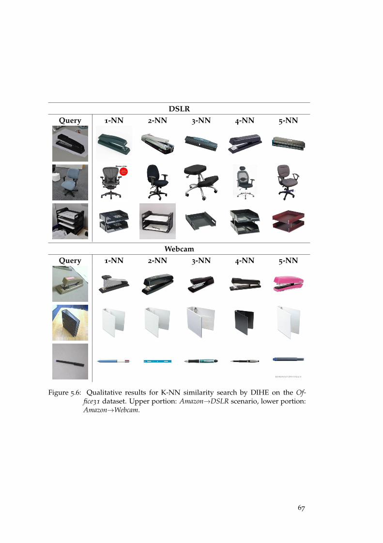
DSLRQuery 1-NN 2-NN 3-NN 4-NN 5-NN
WebcamQuery 1-NN 2-NN 3-NN 4-NN 5-NN
Figure 5.6: Qualitative results for K-NN similarity search by DIHE on the Of-fice31 dataset. Upper portion: Amazon→DSLR scenario, lower portion:Amazon→Webcam.
67
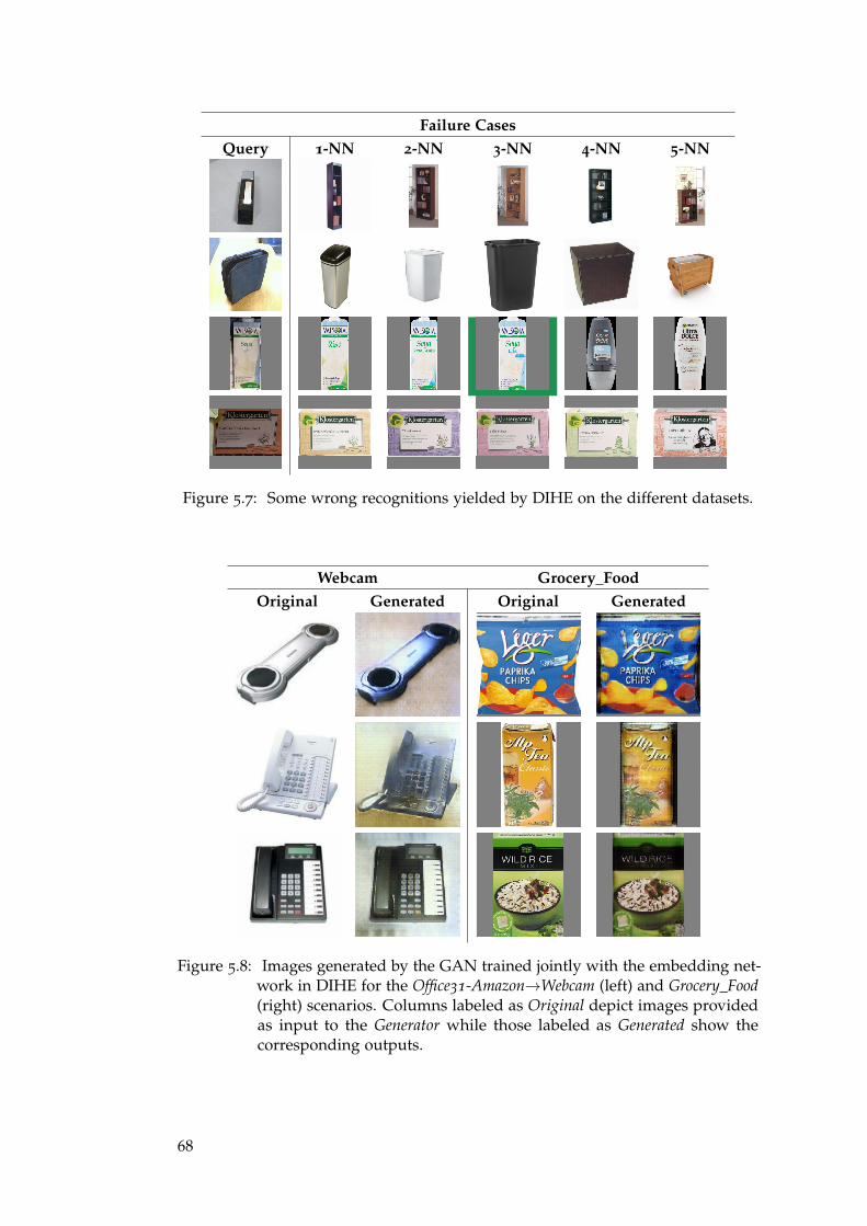
Failure CasesQuery 1-NN 2-NN 3-NN 4-NN 5-NN
Figure 5.7: Some wrong recognitions yielded by DIHE on the different datasets.
Webcam Grocery_FoodOriginal Generated Original Generated
Figure 5.8: Images generated by the GAN trained jointly with the embedding net-work in DIHE for the Office31-Amazon→Webcam (left) and Grocery_Food(right) scenarios. Columns labeled as Original depict images providedas input to the Generator while those labeled as Generated show thecorresponding outputs.
68
6C O N C L U S I O N S
In this part, we have extensively addressed the recognition of products instore shelves either assuming the availability beforehand of the expectedproduct layout (Chap. 3) or in a completely unconstrained setup (Chap. 4).For the solution of the first task, we relied on classic algorithms based on localfeatures to achieve detection and recognition, while for the second we haveshown how modern machine learning based methods can be successfullydeployed. We have put a lot of effort into designing a system that doesnot require expensive manually annotated dataset, nor constantly retrainingand relies only on information available in commercial databases. By self-imposing such limitations, we hope to produce an appealing solution forreal stores. By comparing the results obtained by our two pipelines it is clearhow machine learning based approaches can outperform feature based onesboth in terms of accuracy and scalability. While features work remarkablywell on textured packaged products, they tend to fail in presence of reflectivesurface or deformable packages, machine learning based method insteadseems to be able to handle seamlessly even those situations (if properlytrained). Finally in Chap. 5 we have shown how a CNN can be trained todirectly address some of the criticality of the product recognition processsuch as the difference between images available during training and thoseto be recognized at test time.
Our system is still composed of multiple independent parts and featuresa lot of hyperparameters that need to be carefully tuned to achieve goodperformances. For the future we would like to investigate the possibility todeploy a unified CNN architecture acting as both Detector and Embedder forour machine learning based pipeline. Fusing the multiple stages in a singlenetwork will hopefully result in a lighter system that will be easier to deployon mobile or resource-constrained platforms. However, the development ofan all in one system for detection and image embeddings is non-trivial. Typ-ically the solution of the former task involves a certain degree of invariancein learned image representation, while for the latter we wish to represent ina compact way peculiar image details. One possible solution that we wish toexplore is to split the model into two parts, an initial feature extractor shared
69

across the different problems and two separate final portions specialized forthe solution of detection and image embedding respectively.
70
Part II
U N S U P E RV I S E D A D A P TAT I O N F O R D E E P
D E P T H

7I N I T I A L R E M A R K S
The focus of this part of the thesis will be on the problem of acquiring inform-ation about the 3D structure of an observed scene. This problem is one ofthe key steps to enable the solution of more complex tasks, like autonomousnavigation, reconstruction and augmented reality and as such has alwaysattracted huge research efforts. This technology has also wide applicationsin the supermarket environment where it could pave the way to augmentedshopping experience for customers as well as be a fundamental buildingblock for the development of autonomous agents moving inside the shop tomonitor shelves or serve as personal shopping assistants. A more straight-forward application concern the use of depth information to ease other tasks,for example, the planogram compliance check pipeline described in Chap. 3
would more easily detect missing product if depth information could be de-ployed by detecting discontinuities in the 3D structure of the items exposedon shelves. Moreover, even the object detection pipeline described in Chap. 4
could leverage on 3D information to improve the accuracy when detectingdeformable objects or items with characteristic shapes. Other applications inthe retail environment concern the 3D mapping and virtual reconstructionof real stores by using SLAM techniques. A 3D map of the shop wouldalso be useful both for planning tasks as well as for interactive customerexperiences like virtual tours or navigation aid to reach specific items. Bycombining the product detection capabilities shown in the previous chapterwith the 3D sensing technologies that we are going to introduce here wecan also think of reconstructing the shelves of a whole salespoint with thereal product disposition in near real time, completely revolutionizing theway store are currently managed. For example, the concept of planogramcould be completely redefined by allowing the head office to provide storeswith a precise rendering of how the product should be arranged inside theirspecific shelves rather than a generic abstract representation.
The more commonly used technologies for depth sensing can be broadlycategorized in active and passive sensors. The first family concerns devicesthat emits some signals (e.g., lasers or infra-red light) and measure how theyget perturbed by the environment to estimate the underlining 3D geometry
73
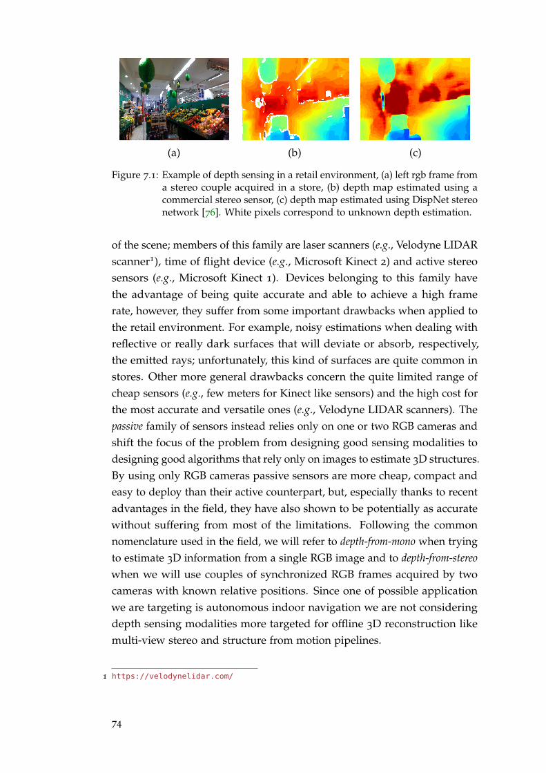
(a) (b) (c)
Figure 7.1: Example of depth sensing in a retail environment, (a) left rgb frame froma stereo couple acquired in a store, (b) depth map estimated using acommercial stereo sensor, (c) depth map estimated using DispNet stereonetwork [76]. White pixels correspond to unknown depth estimation.
of the scene; members of this family are laser scanners (e.g., Velodyne LIDARscanner1), time of flight device (e.g., Microsoft Kinect 2) and active stereosensors (e.g., Microsoft Kinect 1). Devices belonging to this family havethe advantage of being quite accurate and able to achieve a high framerate, however, they suffer from some important drawbacks when applied tothe retail environment. For example, noisy estimations when dealing withreflective or really dark surfaces that will deviate or absorb, respectively,the emitted rays; unfortunately, this kind of surfaces are quite common instores. Other more general drawbacks concern the quite limited range ofcheap sensors (e.g., few meters for Kinect like sensors) and the high cost forthe most accurate and versatile ones (e.g., Velodyne LIDAR scanners). Thepassive family of sensors instead relies only on one or two RGB cameras andshift the focus of the problem from designing good sensing modalities todesigning good algorithms that rely only on images to estimate 3D structures.By using only RGB cameras passive sensors are more cheap, compact andeasy to deploy than their active counterpart, but, especially thanks to recentadvantages in the field, they have also shown to be potentially as accuratewithout suffering from most of the limitations. Following the commonnomenclature used in the field, we will refer to depth-from-mono when tryingto estimate 3D information from a single RGB image and to depth-from-stereowhen we will use couples of synchronized RGB frames acquired by twocameras with known relative positions. Since one of possible applicationwe are targeting is autonomous indoor navigation we are not consideringdepth sensing modalities more targeted for offline 3D reconstruction likemulti-view stereo and structure from motion pipelines.
1 https://velodynelidar.com/
74
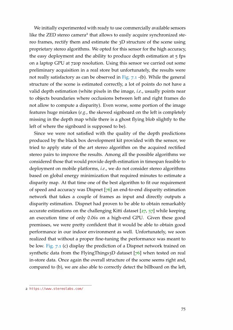
We initially experimented with ready to use commercially available sensorslike the ZED stereo camera2 that allows to easily acquire synchronized ste-reo frames, rectify them and estimate the 3D structure of the scene usingproprietary stereo algorithms. We opted for this sensor for the high accuracy,the easy deployment and the ability to produce depth estimation at 5 fpson a laptop GPU at 720p resolution. Using this sensor we carried out somepreliminary acquisition in a real store but unfortunately, the results werenot really satisfactory as can be observed in Fig. 7.1 -(b). While the generalstructure of the scene is estimated correctly, a lot of points do not have avalid depth estimation (white pixels in the image, i.e., usually points nearto objects boundaries where occlusions between left and right frames donot allow to compute a disparity). Even worse, some portion of the imagefeatures huge mistakes (e.g., the skewed signboard on the left is completelymissing in the depth map while there is a ghost flying blob slightly to theleft of where the signboard is supposed to be).
Since we were not satisfied with the quality of the depth predictionsproduced by the black box development kit provided with the sensor, wetried to apply state of the art stereo algorithm on the acquired rectifiedstereo pairs to improve the results. Among all the possible algorithms weconsidered those that would provide depth estimation in timespan feasible todeployment on mobile platforms, i.e., we do not consider stereo algorithmsbased on global energy minimization that required minutes to estimate adisparity map. At that time one of the best algorithm to fit our requirementof speed and accuracy was Dispnet [76] an end-to-end disparity estimationnetwork that takes a couple of frames as input and directly outputs adisparity estimation. Dispnet had proven to be able to obtain remarkablyaccurate estimations on the challenging Kitti dataset [27, 57] while keepingan execution time of only 0.06s on a high-end GPU. Given these goodpremisses, we were pretty confident that it would be able to obtain goodperformance in our indoor environment as well. Unfortunately, we soonrealized that without a proper fine-tuning the performance was meant tobe low. Fig. 7.1 (c) display the prediction of a Dispnet network trained onsynthetic data from the FlyingThings3D dataset [76] when tested on realin-store data. Once again the overall structure of the scene seems right and,compared to (b), we are also able to correctly detect the billboard on the left,
2 https://www.stereolabs.com/
75
however, the disparity map still features huge mistakes in the backgroundarea (that seems to cut off after a certain distance) and on the ceiling.
We ascribe those unsatisfactory result to the domain shift between trainingdata (i.e., rendered abstract synthetic images) and real ones (i.e., our in-store acquisition). The usual practice to address domain shift is to finetune the deep network on the target environment, however, in the depthestimation case, this procedure became quite challenging since it requiresthe acquisition of multiple frames from the new scenarios and a carefulannotation of each pixel with its distance or disparity from the camera. Theonly way to generate such annotations, unfortunately, is to rely on costlyhigh precision sensors like LIDAR laser scanners that, however, requirecareful calibration, can sense depth information only for a sparse subset ofpoints in the image and still have to deal with possible mistakes comingfrom moving objects and reflective surfaces. Since the deployment of suchsensors in our scenario was completely unrealistic we focused our researcheffort on possible way to adapt a deep depth estimation network to unseenenvironments without relying on ground truth data, i.e., we wish to realizea self-supervised adaptation. Having ground truth information is, however,crucial to measure quantitatively if an algorithm is performing well or not.For this reason, and to compare our results with those achieved by otherresearch groups, we are going to introduce and test our proposal in thecontext of autonomous driving where the KITTI datasets [27, 31, 57] offerrectified stereo frames coupled with sparse ground truth data coming froma LIDAR scanner that act as ground truth annotations.
In Chap. 8 we are going to describe a procedure to produce pseudoground-truth labels by filtering noisy estimation using state of the art con-fidence measures and test it for offline fine tuning of a stereo network tounseen environments. In Chap. 9 we are going to introduce a new disparityestimation network and a procedure to adapt it online without the need ofground truth data to a new environment as soon as new frames are sensed.Finally in Chap. 10 we are going to present some ongoing work on how touse meta-learning techniques to make a depth estimation network able toadapt to unseen environments better and faster. But first, in Sec. 7.1 we aregoing to revise some of the recent literature on depth estimation from monoand stereo images.
76
7 .1 related work
We briefly review the literature for deep stereo matching and depth-from-mono.
Deep stereo matching. Since early works on stereo [6], traditional al-gorithms are thought as a number of subsequential steps, involving initialmatching cost computation, local aggregation, disparity optimization andrefinement. The firsts attempt to plug deep learning into stereo algorithmsaimed at replacing single steps of the established pipeline, such as matchingcost computation [50, 65, 74] and more recently optimization [82, 113] orrefinement [92]. While these works substantially proved the superiority oflearning based methods with respect to their non-learned counterparts onthe single subtasks, in most cases they still required traditional optimizationstrategies, such as Semi Global Matching (SGM) [9], to reach top accuracy.The shift to end-to-end models started with Dispnet [76]. While previousworks [50, 65, 74] processed small image patches to compute similarityscores, Dispnet works on a much larger receptive field and jointly extractfeatures from two input frames, compute correlations between them andpredict final disparities. Because of the large inputs processed, the fewhundreds of images available from KITTI [27, 57] are not enough to trainsuch model. To this aim a large synthetic dataset [76] is used for training,while KITTI images are used to address the domain shift when running onreal imagery. Despite Dispnet did not reach the top of KITTI, it inspiredmany other end-to-end models [102, 139] able to assess this approach asstate-of-the-art. Kendall et al. introduced the use of 3D convolutions [99]to explicitly exploit geometry and context, followed by [131, 152]. Despitethe different architectural details, all of these techniques follow the samesynthetic-to-real completely supervised training schedule. Only recently,this training paradigm has been questioned by proposing an unsupervisedtraining schema. Pang et al. [143] propose a novel way of fine-tuning a deepnetwork for stereo estimation by exploiting the output of the network at mul-tiple resolutions combined within an iterative optimization problem withgraph Laplacian regularization. Zhou et al. [126] use an iterative procedurebased on the left-right check to train a network from scratch. Finally, Zhanget al. [155] propose a novel loss formulation based on image reprojection fordepth estimation using an active stereo acquisition system.
Depth-from-mono. Deep learning dramatically boosted the quality ofresults obtained through depth-from-mono techniques. While most works
77
addressed it as a supervised learning problem [16, 37, 41, 55, 71, 73, 123,135, 150], an exciting trend concerns the possibility of self-supervisingCNNs during training by solving an image reconstruction problem. Thesesolutions earned a lot of attention from researchers thanks to the possibilityof training them without requiring hard to source depth labels. They canbe broadly classified into two main categories according to the cues usedto replace ground-truth labels, that are respectively monocular [127] andstereo [93] self-supervision. In the first case, images are acquired by anunconstrained moving camera [127, 140, 149, 151]. Estimated depth is usedto reconstruct views across the different frames by means of camera-to-worldprojection and vice-versa. To do so, the network also needs to estimate therelative camera pose between the different images, which is unknown. Theseapproaches are weak in presence of dynamic objects, making reprojectionsin non-static regions of the frames not matching the real image content.The second category requires calibrated stereo pairs to be used as trainingdataset [68, 93, 129, 144, 153]. In this case, the relative pose is known thanksto stereo geometry, making the network only in charge of learning depth(actually, disparity) to minimize the reprojection between the two views. Thissolves the problem of moving objects, being images synchronized, but addsconstraints for collecting data. Networks trained with this second approachusually results to be more accurate. This approach can be extended totrinocular setup [145] to compensate for occlusions inherited by the binocularstereo. Finally, we mention the semi-supervised frameworks proposed in[101, 134] and the joint use of these two supervisions [153].
78
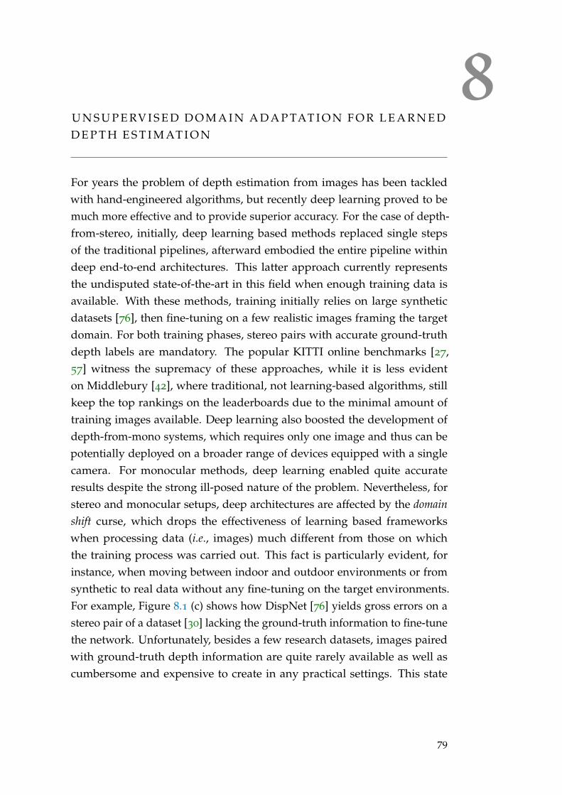
8U N S U P E RV I S E D D O M A I N A D A P TAT I O N F O R L E A R N E DD E P T H E S T I M AT I O N
For years the problem of depth estimation from images has been tackledwith hand-engineered algorithms, but recently deep learning proved to bemuch more effective and to provide superior accuracy. For the case of depth-from-stereo, initially, deep learning based methods replaced single stepsof the traditional pipelines, afterward embodied the entire pipeline withindeep end-to-end architectures. This latter approach currently representsthe undisputed state-of-the-art in this field when enough training data isavailable. With these methods, training initially relies on large syntheticdatasets [76], then fine-tuning on a few realistic images framing the targetdomain. For both training phases, stereo pairs with accurate ground-truthdepth labels are mandatory. The popular KITTI online benchmarks [27,57] witness the supremacy of these approaches, while it is less evidenton Middlebury [42], where traditional, not learning-based algorithms, stillkeep the top rankings on the leaderboards due to the minimal amount oftraining images available. Deep learning also boosted the development ofdepth-from-mono systems, which requires only one image and thus can bepotentially deployed on a broader range of devices equipped with a singlecamera. For monocular methods, deep learning enabled quite accurateresults despite the strong ill-posed nature of the problem. Nevertheless, forstereo and monocular setups, deep architectures are affected by the domainshift curse, which drops the effectiveness of learning based frameworkswhen processing data (i.e., images) much different from those on whichthe training process was carried out. This fact is particularly evident, forinstance, when moving between indoor and outdoor environments or fromsynthetic to real data without any fine-tuning on the target environments.For example, Figure 8.1 (c) shows how DispNet [76] yields gross errors on astereo pair of a dataset [30] lacking the ground-truth information to fine-tunethe network. Unfortunately, besides a few research datasets, images pairedwith ground-truth depth information are quite rarely available as well ascumbersome and expensive to create in any practical settings. This state
79
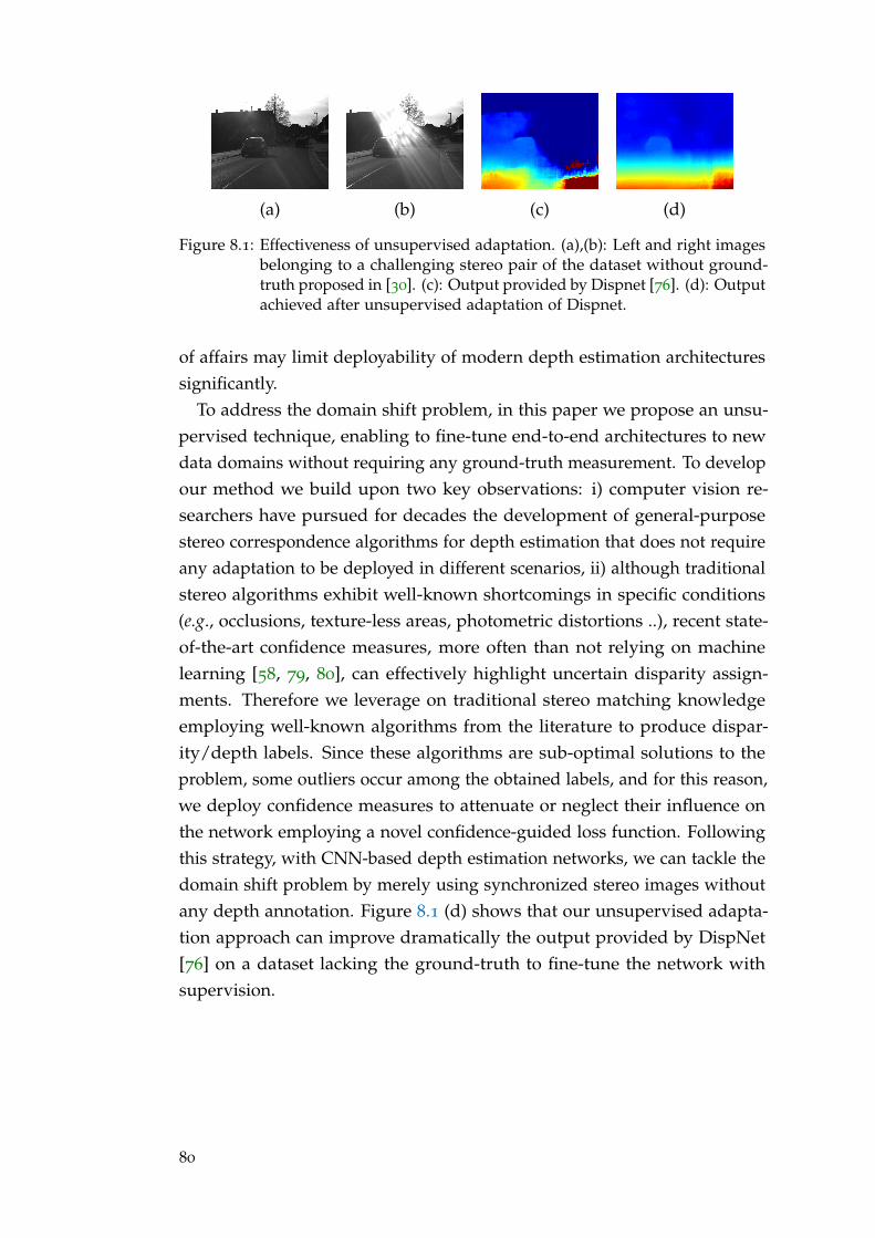
(a) (b) (c) (d)
Figure 8.1: Effectiveness of unsupervised adaptation. (a),(b): Left and right imagesbelonging to a challenging stereo pair of the dataset without ground-truth proposed in [30]. (c): Output provided by Dispnet [76]. (d): Outputachieved after unsupervised adaptation of Dispnet.
of affairs may limit deployability of modern depth estimation architecturessignificantly.
To address the domain shift problem, in this paper we propose an unsu-pervised technique, enabling to fine-tune end-to-end architectures to newdata domains without requiring any ground-truth measurement. To developour method we build upon two key observations: i) computer vision re-searchers have pursued for decades the development of general-purposestereo correspondence algorithms for depth estimation that does not requireany adaptation to be deployed in different scenarios, ii) although traditionalstereo algorithms exhibit well-known shortcomings in specific conditions(e.g., occlusions, texture-less areas, photometric distortions ..), recent state-of-the-art confidence measures, more often than not relying on machinelearning [58, 79, 80], can effectively highlight uncertain disparity assign-ments. Therefore we leverage on traditional stereo matching knowledgeemploying well-known algorithms from the literature to produce dispar-ity/depth labels. Since these algorithms are sub-optimal solutions to theproblem, some outliers occur among the obtained labels, and for this reason,we deploy confidence measures to attenuate or neglect their influence onthe network employing a novel confidence-guided loss function. Followingthis strategy, with CNN-based depth estimation networks, we can tackle thedomain shift problem by merely using synchronized stereo images withoutany depth annotation. Figure 8.1 (d) shows that our unsupervised adapta-tion approach can improve dramatically the output provided by DispNet[76] on a dataset lacking the ground-truth to fine-tune the network withsupervision.
80
8 .1 related work
Confidence measures have been extensively reviewed by Hu and Mordohai[28] and by Poggi et al. [106] more recently including methods based onmachine-learning. These latter methods can be broadly categorized intorandom-forest based [33, 45, 58, 79] and CNN based [80, 82, 136, 148]. Whilethe first category, except [79], usually combines different cues available fromthe intermediate cost volume processed by traditional stereo algorithms [3, 9,87], CNN based approaches only process disparity map and image contentcues, making them better suited to work on custom systems or frameworksnot explicitly providing a cost volume (i.e., end-to-end CNNs). In general,this second category vouches for better outliers detection properties. Par-allel works proposed an effective strategy to improve confidence measuresby exploiting local consistency [103] and a method [105] to improve ran-dom forest-based approaches for confidence fusion [45, 58, 79] by using aCNN. Shaked and Wolf [114] embedded confidence estimation inside a deepmodel stereo matching, while Poggi et al. [104] propose an evaluation ofconventional confidence measures and their simplifications when targetingembedded systems. Some works looked deeper into the learning process ofconfidence measures, by studying features augmentation [100] or by design-ing self-supervised techniques to train them on static video sequences [77]or stereo pairs [120]. In addition to otuliers detection and the unsuperviseddomain adaptation technique proposed in this paper, other applications ofconfidence measures aim at improving stereo accuracy [45, 58, 79, 82, 113],combine multiple algorithms [63, 78] and sensor fusion [75].
8 .2 domain adaptation for depth sensing
This section describes our domain adaptation framework, which is suited toboth deep stereo as well as monocular depth estimation networks. To adapta pre-trained model to face a new environment, we first acquire stereo pairsfrom the target domain. Then, we deploy a classical (i.e., not learning-based)stereo algorithm to generate dense depth measurements together with astate-of-the-art confidence measure to estimate the reliability of the depthvalues calculated by the stereo algorithm. A key observation behind ourmethod is that classical stereo algorithms, although affected by well-knownshortcomings such as occlusions, poorly-textured regions and repetitive
81

patterns, are substantially agnostic to the specific target environment andthus behave similarly across different scenarios. More importantly, theyfail in the same predictable way, thereby enabling confidence measures toachieve remarkably good accuracy in detecting mistakes regardless of thesensed environment [106]. Based on the above observations, we advocatedeploying the depths delivered by a classical stereo algorithm as noisy labelsendowed with reliability estimations in order to fine-tune a network aimedat depth prediction. This is achieved through a novel per-pixel regressionloss wherein the error between each model prediction and the correspondingdepth measurement provided by the stereo algorithm is weighted accordingto the reliability estimated by the confidence measure, with higher weightsassociated to more reliable depth measurements. Thereby, the learning pro-cess is guided by the high-confidence depth measurements, i.e. those labelsthat appear to be more reliable, while the errors due to the shortcomings ofthe stereo algorithm have a negligible impact.
Thus, given a pre-trained depth estimation network, either stereo ormonocular, and a set of stereo pairs, (Il, Ir) ∈ I, acquired from the targetdomain, for each pair we compute a dense disparity map, D ∈ D, by meansof a classical stereo algorithm, f : (I, I) → D, such as, e.g., SGM [9] or AD-CENSUS[3]. Moreover, for each disparity map, D, we estimate a pixel-wisedegree of reliability according to a confidence measure, c : D → C. Theresulting confidence map, C ∈ C, encodes the reliability of the disparitycalculated at each pixel as a score ranging from 0 (not reliable) to 1 (reliable).
We run f and c on each stereo pair available from the target domainso as to produce the training set deployed to perform fine-tuning of thepre-trained depth estimation network. Therefore, each sample, (Si), in thetraining set is a tuple of four elements:
Si = (Ili, Iri ,Di,Ci) = (Ili, I
ri , f(I
li, Iri), c(f(I
li, Iri))) (8.1)
Given the depth estimation network (either stereo or monocular), whichtakes input images and outputs per pixel disparities, we fine tune it towardthe target domain by minimizing a loss function, L, consisting of three terms:
82
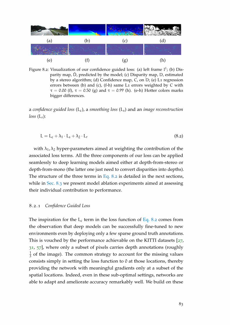
(a) (b) (c) (d)
(e) (f) (g) (h)
Figure 8.2: Visualization of our confidence guided loss: (a) left frame Il; (b) Dis-parity map, D, predicted by the model; (c) Disparity map, D, estimatedby a stereo algorithm; (d) Confidence map, C, on D; (e) L1 regressionerrors between (b) and (c), (f-h) same L1 errors weighted by C withτ = 0.00 (f), τ = 0.50 (g) and τ = 0.99 (h). (e-h) Hotter colors marksbigger differences.
a confidence guided loss (Lc), a smoothing loss (Ls) and an image reconstructionloss (Lr):
L = Lc + λ1 · Ls + λ2 · Lr (8.2)
with λ1, λ2 hyper-parameters aimed at weighting the contribution of theassociated loss terms. All the three components of our loss can be appliedseamlessly to deep learning models aimed either at depth-from-stereo ordepth-from-mono (the latter one just need to convert disparities into depths).The structure of the three terms in Eq. 8.2 is detailed in the next sections,while in Sec. 8.3 we present model ablation experiments aimed at assessingtheir individual contribution to performance.
8 .2 .1 Confidence Guided Loss
The inspiration for the Lc term in the loss function of Eq. 8.2 comes fromthe observation that deep models can be successfully fine-tuned to newenvironments even by deploying only a few sparse ground truth annotations.This is vouched by the performance achievable on the KITTI datasets [27,31, 57], where only a subset of pixels carries depth annotations (roughly13 of the image). The common strategy to account for the missing valuesconsists simply in setting the loss function to 0 at those locations, therebyproviding the network with meaningful gradients only at a subset of thespatial locations. Indeed, even in these sub-optimal settings, networks areable to adapt and ameliorate accuracy remarkably well. We build on these
83
observations and leverage on the confidence measure, c, to obtain sparseand reliable depth labels from the noisy output D of the stereo algorithm.With reference to 8.1, denoting as D the output predicted by the model atthe current training iteration, we compute Lc as
Lc =1
|Pv|
∑p∈Pv
E(p) (8.3)
E(p) = C(p) · |D(p) −D(p)| (8.4)
Pv = {p ∈ P : C(p) > τ} (8.5)
where P is the set of all spatial locations on the image and τ ∈ [0, 1] ahyper-parameter that controls the sparseness and reliability of the disparitymeasurements provided by f that are actually deployed to update the model.A higher value of τ will mask out more mistakes in D though permittingless spatial locations to contribute to model update. Hence, points belongingto Pv define a set of sparse labels that, assuming the availability of a perfectconfidence measure, may be used as if they were groundtruth annotations,e.g. akin to the LiDAR measurements deployed in the KITTI dataset. Yet,confidence measures are not perfect and often show some degree of uncer-tainty in the score assigned to disparity measurements. Thus, we weightthe contribution at location p by C(p) ∈ [0, 1], i.e. as much as the depthmeasurement, D(p), can be trusted according to the confidence estimation,C(p). We point out that, re-weighting the loss function in presence of noisylabels has been successfully exploited in supervised classification [137, 146].Our formulation deploys a similar idea for a dense regression problem. Yet,we leverage on an external and highly accurate strategy to detect noise inthe labels (i.e., the confidence measure) and mask out those labels which,according to the adopted strategy, are very likely wrong, i.e., {D(p) : p /∈ Pv}.In Sec. 8.3.2 we will show how both masking and re-weighting are crucialcomponents to maximize performance in presence of noisy depth labels.
A graphical visualization of the errors that our Lc loss term tries to min-imize can be observed in the bottom row of Fig. 8.2. On (e) we report theerrors that will be minimized trying to directly regress the noisy depth
84
labels of (c) given the model prediction on (b); on (f-g-h) we report, instead,the errors minimized by applying Lc with different τ values (0, 0.5 and 0.99respectively). By tuning τ we can control the number of pixels, and thereforelabels, taking part in the network adaptation process. Clearly, leveraging onmore labels comes at the cost of injecting more noise in the process, which,in turn, may harm adaptation, even if their contribution will be attenuatedby C, e.g. compare (f) to (e) where the only difference is the scaling of errorsby C(p) in (f). In (h) we can appreciate how even with τ = 0.99 the amountof pixels considered during the optimization process is still quite high.
8 .2 .2 Smoothing Term
As Lc produces error signals to improve disparity prediction only at thesubset of sparse image locations Pv, similarly to [34] we use an additionalloss term, Ls, to propagate model update signals across neighbouring spatiallocations. In particular, Ls tends to penalize large gradients in the predicteddisparity map (∂D) taking into acocunt the presence of gradients in pixelintensities (∂I):
Ls =1
|P|
∑p∈P
∂xD(p) · e−||∂xI(p)|| + ∂yD(p) · e−||∂yI(p)|| (8.6)
Thus, based on the consideration that depth discontinuities occur incorrespondence of edge, Ls constrains the predicted disparity map, D, to besmooth everywhere but at image edges. To efficiently compute gradientsalong x and y we use convolution with 3× 3 Sobel filter.
8 .2 .3 Image Reconstruction Loss
To further compensate for the sparse model update information yielded byLc, we include in the loss function a pixel-wise image reconstruction term,denoted as Lr in Eq. 8.2. Inclusion of this term in our loss has been inspiredby [93], which has shown how deploying image re-projection betweenstereo frames can deliver a form of self-supervision to train a depth-from-mono network. Hence, given a stereo pair, Il can be reconstructed fromIr according to the current disparity prediction D by employing a bilinearsampler in order to render the process locally differentiable. Denoted as Il
85
the re-projection of Ir according to D, we define the image reconstructionloss, Lr, as a weighted combination of the L1 norm and the single scale SSIM[8]:
Lr =1
|P|
∑p∈P
α1− SSIM(Il(p), Il(p))
2+ (1−α)|Il(p) − Il(p)| (8.7)
Similarly to [93], we use a simplified SSIM based on a 3× 3 block filterand set α = 0.85 throughout all our experiments.
8 .3 experimental results
In this section, we report exhaustive experiments showing the effectivenessof the proposed unsupervised domain adaptation technique. We run twomain experiments i) adaptation of a stereo network and ii) adaptation of adepth-from-mono network. For the first case, we run extensive experimentson the entire KITTI raw dataset [31], counting about 40k images, thanksto a large amount of ground truth labels made recently available [122] inthe official website. Concerning the second evaluation, we follow commonprotocols from the literature of self-supervised monocular depth estimation[93], splitting the KITTI raw data into train and test portions according toEigen et al. [37].
To deploy the confidence guided loss described in Sec. 8.2.1, in ourevaluation we consider two classical stereo algorithms (f): AD-CENSUS(shortened AD) [3] and Semi-Global Matching (shortened SGM) [9] andleverage the implementations of [44]. We have selected these two popularalgorithms because they show quite different behaviors. While AD tendsto generate prediction errors in the form of small spikes in the disparitymaps, the errors generated by SGM can often cause over-smoothing. Theeffectiveness of our proposal with both types of error patterns may helptestify its general validity. Besides, while SGM may turn out remarkablyaccurate, AD is notoriously significantly more prone to errors, which, in ourframework, leads to fewer disparity measurements used at training time tocompute Lc due to fewer pixels belonging to Pv. To measure the confidenceof the disparity measurements coming from the stereo algorithms, we relyon CCNN [80] as it can yield state-of-the-art performance and does requireas input just the disparity map to be analyzed. Thanks to the latter trait,
86
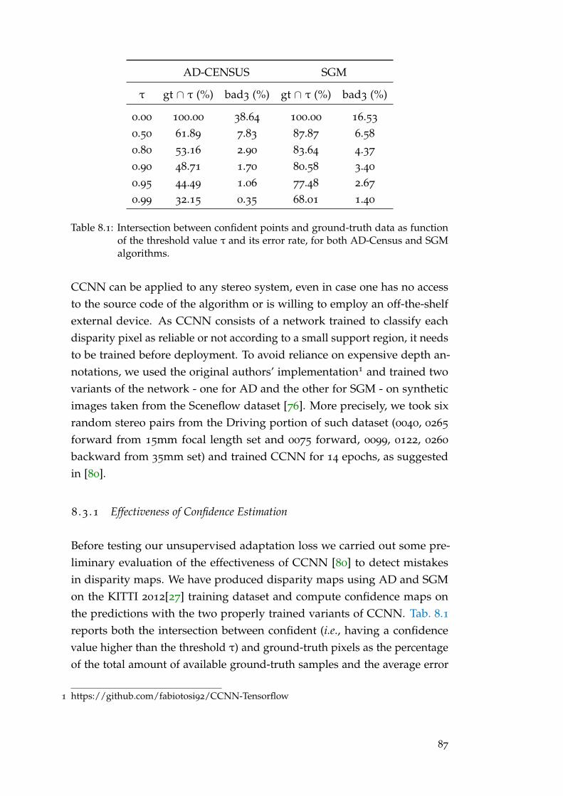
AD-CENSUS SGM
τ gt ∩ τ (%) bad3 (%) gt ∩ τ (%) bad3 (%)
0.00 100.00 38.64 100.00 16.53
0.50 61.89 7.83 87.87 6.58
0.80 53.16 2.90 83.64 4.37
0.90 48.71 1.70 80.58 3.40
0.95 44.49 1.06 77.48 2.67
0.99 32.15 0.35 68.01 1.40
Table 8.1: Intersection between confident points and ground-truth data as functionof the threshold value τ and its error rate, for both AD-Census and SGMalgorithms.
CCNN can be applied to any stereo system, even in case one has no accessto the source code of the algorithm or is willing to employ an off-the-shelfexternal device. As CCNN consists of a network trained to classify eachdisparity pixel as reliable or not according to a small support region, it needsto be trained before deployment. To avoid reliance on expensive depth an-notations, we used the original authors’ implementation1 and trained twovariants of the network - one for AD and the other for SGM - on syntheticimages taken from the Sceneflow dataset [76]. More precisely, we took sixrandom stereo pairs from the Driving portion of such dataset (0040, 0265
forward from 15mm focal length set and 0075 forward, 0099, 0122, 0260
backward from 35mm set) and trained CCNN for 14 epochs, as suggestedin [80].
8 .3 .1 Effectiveness of Confidence Estimation
Before testing our unsupervised adaptation loss we carried out some pre-liminary evaluation of the effectiveness of CCNN [80] to detect mistakesin disparity maps. We have produced disparity maps using AD and SGMon the KITTI 2012[27] training dataset and compute confidence maps onthe predictions with the two properly trained variants of CCNN. Tab. 8.1reports both the intersection between confident (i.e., having a confidencevalue higher than the threshold τ) and ground-truth pixels as the percentageof the total amount of available ground-truth samples and the average error
1 https://github.com/fabiotosi92/CCNN-Tensorflow
87
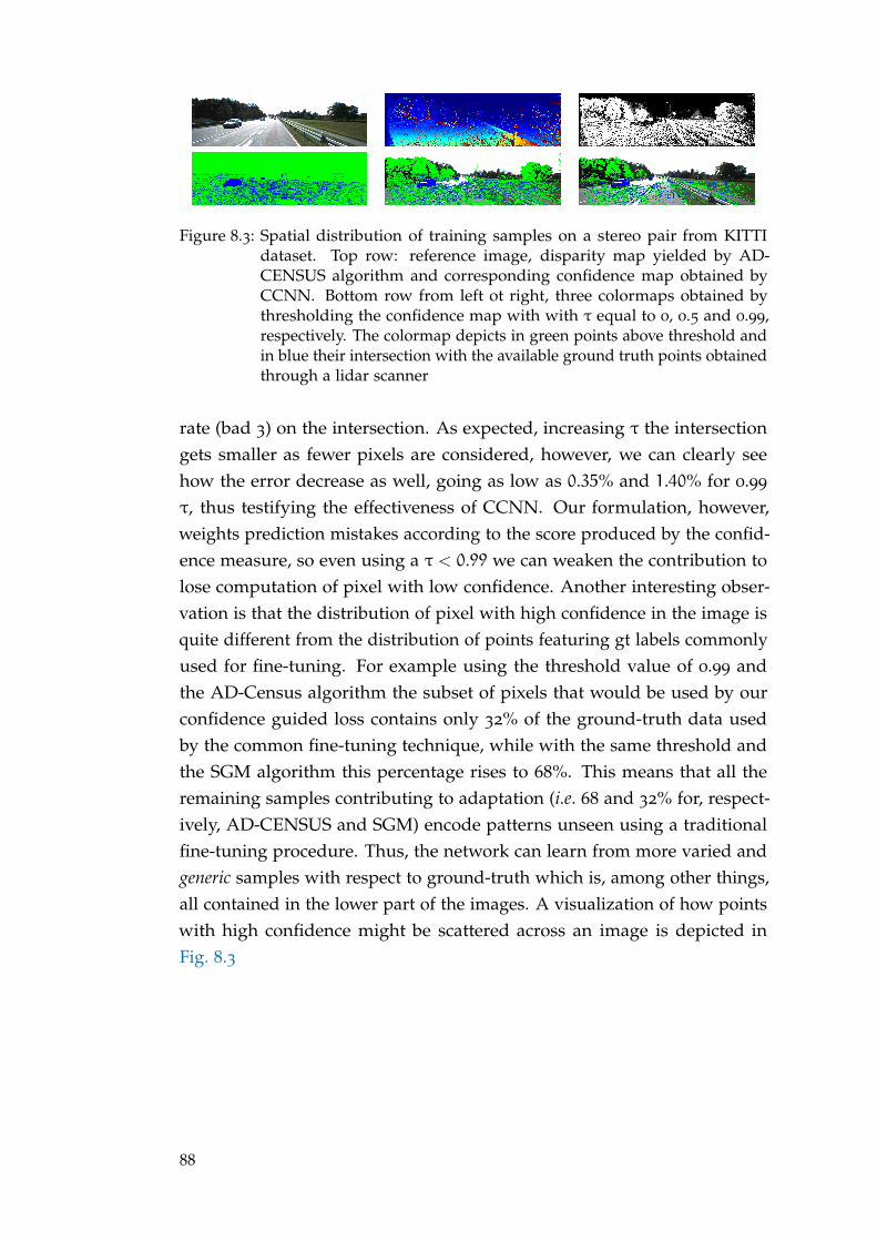
Figure 8.3: Spatial distribution of training samples on a stereo pair from KITTIdataset. Top row: reference image, disparity map yielded by AD-CENSUS algorithm and corresponding confidence map obtained byCCNN. Bottom row from left ot right, three colormaps obtained bythresholding the confidence map with with τ equal to 0, 0.5 and 0.99,respectively. The colormap depicts in green points above threshold andin blue their intersection with the available ground truth points obtainedthrough a lidar scanner
rate (bad 3) on the intersection. As expected, increasing τ the intersectiongets smaller as fewer pixels are considered, however, we can clearly seehow the error decrease as well, going as low as 0.35% and 1.40% for 0.99
τ, thus testifying the effectiveness of CCNN. Our formulation, however,weights prediction mistakes according to the score produced by the confid-ence measure, so even using a τ < 0.99 we can weaken the contribution tolose computation of pixel with low confidence. Another interesting obser-vation is that the distribution of pixel with high confidence in the image isquite different from the distribution of points featuring gt labels commonlyused for fine-tuning. For example using the threshold value of 0.99 andthe AD-Census algorithm the subset of pixels that would be used by ourconfidence guided loss contains only 32% of the ground-truth data usedby the common fine-tuning technique, while with the same threshold andthe SGM algorithm this percentage rises to 68%. This means that all theremaining samples contributing to adaptation (i.e. 68 and 32% for, respect-ively, AD-CENSUS and SGM) encode patterns unseen using a traditionalfine-tuning procedure. Thus, the network can learn from more varied andgeneric samples with respect to ground-truth which is, among other things,all contained in the lower part of the images. A visualization of how pointswith high confidence might be scattered across an image is depicted inFig. 8.3
88
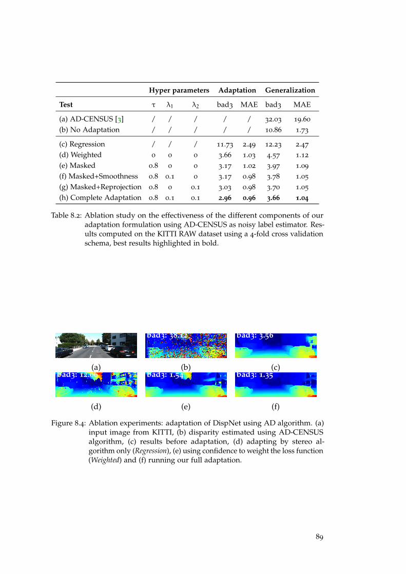
Hyper parameters Adaptation Generalization
Test τ λ1 λ2 bad3 MAE bad3 MAE
(a) AD-CENSUS [3] / / / / / 32.03 19.60
(b) No Adaptation / / / / / 10.86 1.73
(c) Regression / / / 11.73 2.49 12.23 2.47
(d) Weighted 0 0 0 3.66 1.03 4.57 1.12
(e) Masked 0.8 0 0 3.17 1.02 3.97 1.09
(f) Masked+Smoothness 0.8 0.1 0 3.17 0.98 3.78 1.05
(g) Masked+Reprojection 0.8 0 0.1 3.03 0.98 3.70 1.05
(h) Complete Adaptation 0.8 0.1 0.1 2.96 0.96 3.66 1.04
Table 8.2: Ablation study on the effectiveness of the different components of ouradaptation formulation using AD-CENSUS as noisy label estimator. Res-ults computed on the KITTI RAW dataset using a 4-fold cross validationschema, best results highlighted in bold.
bad3: 38.12 bad3: 3.56
(a) (b) (c)bad3: 12.06 bad3: 1.54 bad3: 1.35
(d) (e) (f)
Figure 8.4: Ablation experiments: adaptation of DispNet using AD algorithm. (a)input image from KITTI, (b) disparity estimated using AD-CENSUSalgorithm, (c) results before adaptation, (d) adapting by stereo al-gorithm only (Regression), (e) using confidence to weight the loss function(Weighted) and (f) running our full adaptation.
89
8 .3 .2 Deep Stereo
Our first experimental scenario is about the adaptation of a depth-from-stereo network to a new environment. The common training procedurefor this kind of models consists of first training on the large syntheticFlyingThings3D dataset [76] and then fine-tuning on the target environment.In these settings, our proposal brings in the advantage of enabling fine-tuning without reliance on depth annotations from the target environment,which would be costly or prohibitive to collect. For all our tests we have usedthe DispNet-Corr1D [76] architecture, from now on shortened as DispNet.Following the authors’ guidelines [76], we have trained a re-implementationof DispNet on FlyingThings3D by the standard and supervised L1 regressionloss. Then, we have used these pre-trained weights as initialization for allthe tests discussed hereinafter.
For our experiments we rely on the KITTI RAW [31] dataset, whichfeatures ∼ 43K images with depth labels [122] converted into disparities byknown camera parameters. Images are taken from stereo video sequencesconcerning four diverse environments, namely Road, Residential, Campus andCity, containing 5674, 28067, 1149 and 8027 frames, respectively. Althoughall images come from driving scenarios, each environment shows peculiartraits that would lead a deep stereo model to gross errors without suitablefine-tuning. For example, City and Residential often depict road surroundedby buildings, while Road mostly concerns highways and country roads wherethe most common objects are cars and vegetation. Using this data we wishto measure both target domain performance, i.e., how the network performson the target domain upon unsupervised adaptation without access to anyground-truth information, as well as similar domains performance, i.e., howthe network adapted without supervision generalizes to unseen images fromsimilar domains. To analyze both behaviors, we have alternatively used oneof the environments as the training set to perform fine-tuning, then testedthe resulting model on all the four environments. In fact, this allows forassessing target domain performance by testing on the environment used forunsupervised fine-tuning and similar domains performance by testing on theother three. Since the environments amenable to perform fine-tuning arefour, we can carry out 4-fold cross-validation in order to average performancefigures. Hence, for each fold we average performance figures within anenvironment (i.e., across all of its frames), obtaining, thereby, four sets ofmeasurements. Then, we compute target domain performance by averaging
90
the scores dealing with the four training sets in the corresponding four foldsand similar domains performance by averaging across the other twelve scores.
As for the per-frame performance figures, we compute both the MeanAverage Error (MAE) and the percentage of pixels with disparity error largerthan 3 (bad3) as suggested in [27, 57]. Due to image formats being differentacross the KITTI RAW dataset, we extract a central crop of size 320× 1216from each frame, which matches to the downsampling factor of DispNet andallows for validating almost all pixels with respect to the available groundtruth disparities.
Ablation
i) Can we simply use D as noisy ground truth without deploying C? ii) Ismasking by τ really needed or could we just use C as a per-pixel weightingin Lc? iii) How important is the contribution of the additional loss terms Ls,Lr?
To answer the above questions, we set AD as the stereo algorithm, CCNNas confidence measure and run a set of experiments according to the cross-validation protocol described in Sec. 8.3.2. The resulting performance figuresare reported in Tab. 8.2 as follows. Starting from the top row: (a) AD, i.e.the stereo algorithm providing us with the noisy labels, (b) DispNet trainedonly on synthetic data (i.e. the initial weights used for all the subsequent finetunings), (c) DispNet fine-tuned to directly regress AD without deployinga confidence measure, (d) DispNet fine-tuned to minimize Lc with τ = 0
(thereby weighting all disparities yielded by AD without masking out likelymistakes), (e-g) training to minimize different combinations of Lc,Ls and Lrusing a fixed τ = 0.8. The values for τ, λ1 and λ2 are obtained by preliminarycross-validation and will be kept fixed across all experiments. Since rows (a)and (b) do not need any kind of fine-tuning on KITTI we report the sameperformances for both target and similar domains.
To answer question i), we can compare results between rows (c) and (b). Asexpected. fine-tuning the network to directly regress the noisy measurementsproduced by AD is not a valid optimization strategy as it worsens the initialnetwork performance both in the target domain as well as in similar domains.Interestingly, the network structure seems to behave as a regularizer anddoes not overfeat too much to the noise in the labels as testified by the hugeperformance gap between rows (c) and (a). To answer question ii), we cancompare line (e) and (d), where the only difference is the value of τ. The
91
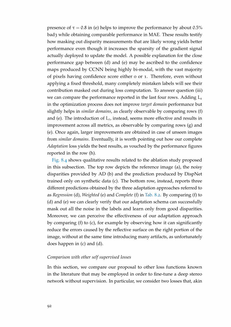
presence of τ = 0.8 in (e) helps to improve the performance by about 0.5%bad3 while obtaining comparable performance in MAE. These results testifyhow masking out disparity measurements that are likely wrong yields betterperformance even though it increases the sparsity of the gradient signalactually deployed to update the model. A possible explanation for the closeperformance gap between (d) and (e) may be ascribed to the confidencemaps produced by CCNN being highly bi-modal, with the vast majorityof pixels having confidence score either 0 or 1. Therefore, even withoutapplying a fixed threshold, many completely mistaken labels will see theircontribution masked out during loss computation. To answer question (iii)we can compare the performance reported in the last four rows. Adding Lsin the optimization process does not improve target domain performance butslightly helps in similar domains, as clearly observable by comparing rows (f)and (e). The introduction of Lr, instead, seems more effective and results inimprovement across all metrics, as observable by comparing rows (g) and(e). Once again, larger improvements are obtained in case of unseen imagesfrom similar domains. Eventually, it is worth pointing out how our completeAdaptation loss yields the best results, as vouched by the performance figuresreported in the row (h).
Fig. 8.4 shows qualitative results related to the ablation study proposedin this subsection. The top row depicts the reference image (a), the noisydisparities provided by AD (b) and the prediction produced by DispNettrained only on synthetic data (c). The bottom row, instead, reports threedifferent predictions obtained by the three adaptation approaches referred toas Regression (d), Weighted (e) and Complete (f) in Tab. 8.2. By comparing (f) to(d) and (e) we can clearly verify that our adaptation schema can successfullymask out all the noise in the labels and learn only from good disparities.Moreover, we can perceive the effectiveness of our adaptation approachby comparing (f) to (c), for example by observing how it can significantlyreduce the errors caused by the reflective surface on the right portion of theimage, without at the same time introducing many artifacts, as unfortunatelydoes happen in (c) and (d).
Comparison with other self supervised losses
In this section, we compare our proposal to other loss functions knownin the literature that may be employed in order to fine-tune a deep stereonetwork without supervision. In particular, we consider two losses that, akin
92
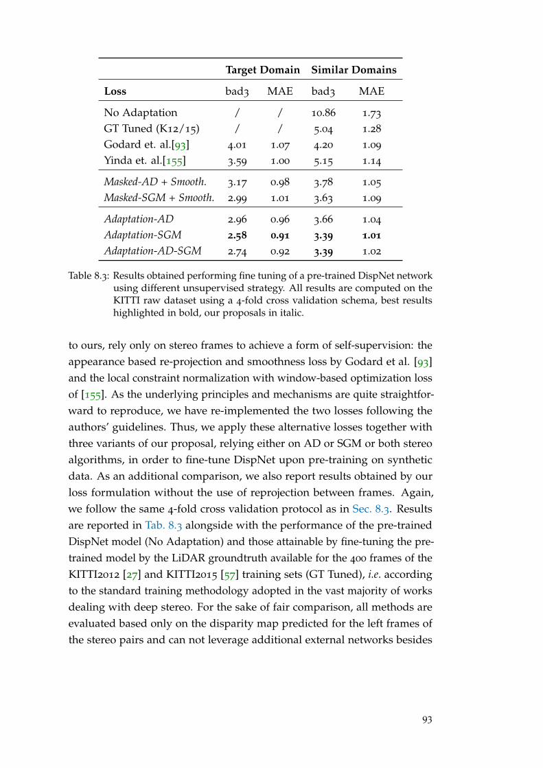
Target Domain Similar Domains
Loss bad3 MAE bad3 MAE
No Adaptation / / 10.86 1.73
GT Tuned (K12/15) / / 5.04 1.28
Godard et. al.[93] 4.01 1.07 4.20 1.09
Yinda et. al.[155] 3.59 1.00 5.15 1.14
Masked-AD + Smooth. 3.17 0.98 3.78 1.05
Masked-SGM + Smooth. 2.99 1.01 3.63 1.09
Adaptation-AD 2.96 0.96 3.66 1.04
Adaptation-SGM 2.58 0.91 3.39 1.01Adaptation-AD-SGM 2.74 0.92 3.39 1.02
Table 8.3: Results obtained performing fine tuning of a pre-trained DispNet networkusing different unsupervised strategy. All results are computed on theKITTI raw dataset using a 4-fold cross validation schema, best resultshighlighted in bold, our proposals in italic.
to ours, rely only on stereo frames to achieve a form of self-supervision: theappearance based re-projection and smoothness loss by Godard et al. [93]and the local constraint normalization with window-based optimization lossof [155]. As the underlying principles and mechanisms are quite straightfor-ward to reproduce, we have re-implemented the two losses following theauthors’ guidelines. Thus, we apply these alternative losses together withthree variants of our proposal, relying either on AD or SGM or both stereoalgorithms, in order to fine-tune DispNet upon pre-training on syntheticdata. As an additional comparison, we also report results obtained by ourloss formulation without the use of reprojection between frames. Again,we follow the same 4-fold cross validation protocol as in Sec. 8.3. Resultsare reported in Tab. 8.3 alongside with the performance of the pre-trainedDispNet model (No Adaptation) and those attainable by fine-tuning the pre-trained model by the LiDAR groundtruth available for the 400 frames of theKITTI2012 [27] and KITTI2015 [57] training sets (GT Tuned), i.e. accordingto the standard training methodology adopted in the vast majority of worksdealing with deep stereo. For the sake of fair comparison, all methods areevaluated based only on the disparity map predicted for the left frames ofthe stereo pairs and can not leverage additional external networks besides
93
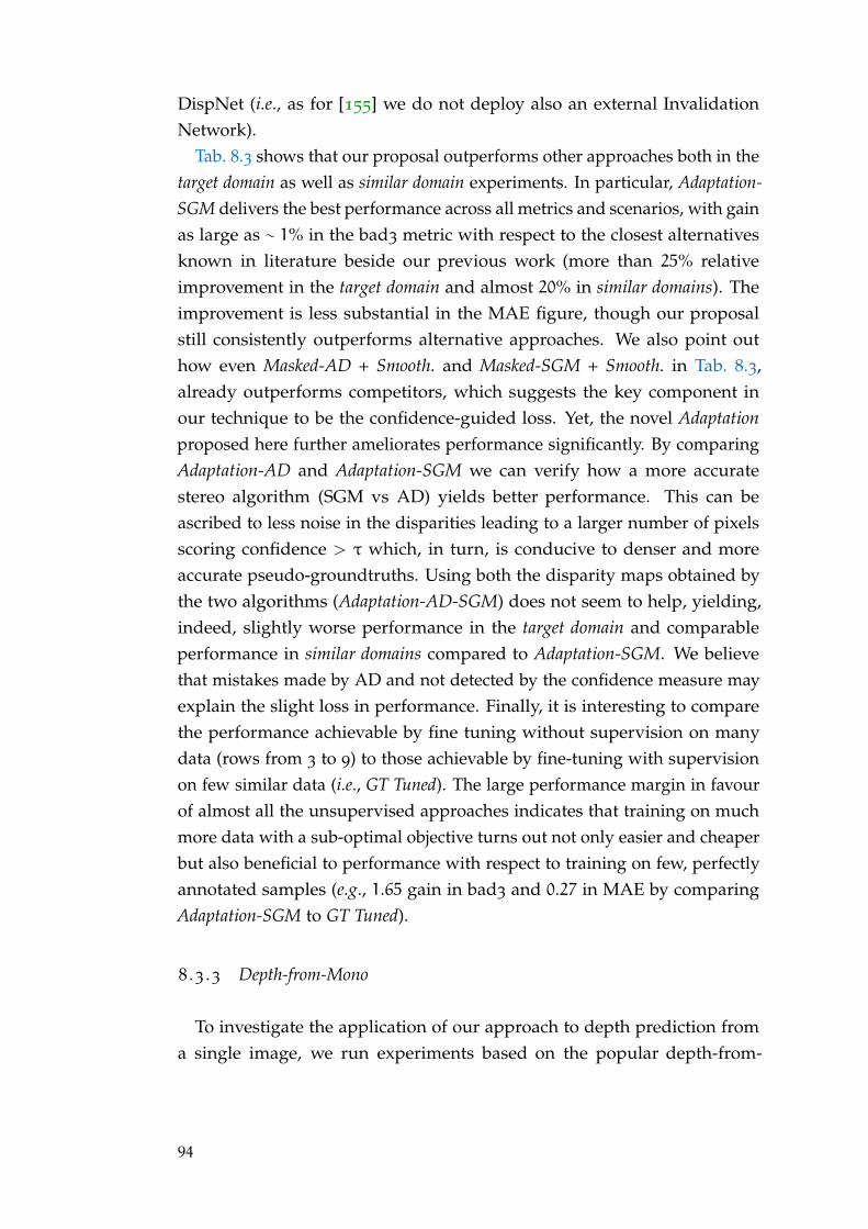
DispNet (i.e., as for [155] we do not deploy also an external InvalidationNetwork).
Tab. 8.3 shows that our proposal outperforms other approaches both in thetarget domain as well as similar domain experiments. In particular, Adaptation-SGM delivers the best performance across all metrics and scenarios, with gainas large as ∼ 1% in the bad3 metric with respect to the closest alternativesknown in literature beside our previous work (more than 25% relativeimprovement in the target domain and almost 20% in similar domains). Theimprovement is less substantial in the MAE figure, though our proposalstill consistently outperforms alternative approaches. We also point outhow even Masked-AD + Smooth. and Masked-SGM + Smooth. in Tab. 8.3,already outperforms competitors, which suggests the key component inour technique to be the confidence-guided loss. Yet, the novel Adaptationproposed here further ameliorates performance significantly. By comparingAdaptation-AD and Adaptation-SGM we can verify how a more accuratestereo algorithm (SGM vs AD) yields better performance. This can beascribed to less noise in the disparities leading to a larger number of pixelsscoring confidence > τ which, in turn, is conducive to denser and moreaccurate pseudo-groundtruths. Using both the disparity maps obtained bythe two algorithms (Adaptation-AD-SGM) does not seem to help, yielding,indeed, slightly worse performance in the target domain and comparableperformance in similar domains compared to Adaptation-SGM. We believethat mistakes made by AD and not detected by the confidence measure mayexplain the slight loss in performance. Finally, it is interesting to comparethe performance achievable by fine tuning without supervision on manydata (rows from 3 to 9) to those achievable by fine-tuning with supervisionon few similar data (i.e., GT Tuned). The large performance margin in favourof almost all the unsupervised approaches indicates that training on muchmore data with a sub-optimal objective turns out not only easier and cheaperbut also beneficial to performance with respect to training on few, perfectlyannotated samples (e.g., 1.65 gain in bad3 and 0.27 in MAE by comparingAdaptation-SGM to GT Tuned).
8 .3 .3 Depth-from-Mono
To investigate the application of our approach to depth prediction froma single image, we run experiments based on the popular depth-from-
94
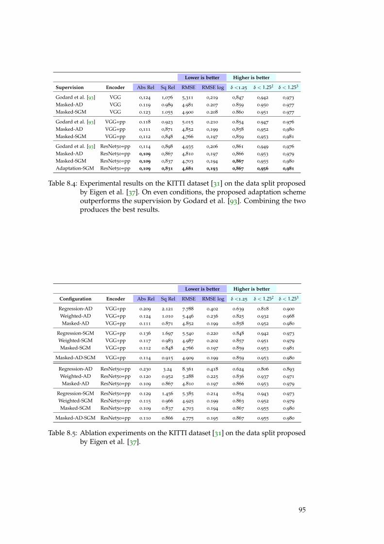
Lower is better Higher is better
Supervision Encoder Abs Rel Sq Rel RMSE RMSE log δ <1.25 δ < 1.252 δ < 1.253
Godard et al. [93] VGG 0,124 1,076 5,311 0,219 0,847 0,942 0,973
Masked-AD VGG 0.119 0.989 4.981 0.207 0.859 0.950 0.977
Masked-SGM VGG 0.123 1.055 4.900 0.208 0.860 0.951 0.977
Godard et al. [93] VGG+pp 0.118 0.923 5.015 0.210 0.854 0.947 0.976
Masked-AD VGG+pp 0,111 0,871 4,852 0,199 0,858 0,952 0,980
Masked-SGM VGG+pp 0,112 0,848 4,766 0,197 0,859 0,953 0,981
Godard et al. [93] ResNet50+pp 0,114 0,898 4,935 0,206 0,861 0,949 0,976
Masked-AD ResNet50+pp 0,109 0,867 4,810 0,197 0,866 0,953 0,979
Masked-SGM ResNet50+pp 0,109 0,837 4,703 0,194 0,867 0,955 0,980
Adaptation-SGM ResNet50+pp 0,109 0,831 4,681 0,193 0,867 0,956 0,981
Table 8.4: Experimental results on the KITTI dataset [31] on the data split proposedby Eigen et al. [37]. On even conditions, the proposed adaptation schemeoutperforms the supervision by Godard et al. [93]. Combining the twoproduces the best results.
Lower is better Higher is better
Configuration Encoder Abs Rel Sq Rel RMSE RMSE log δ <1.25 δ < 1.252 δ < 1.253
Regression-AD VGG+pp 0.209 2.121 7.788 0.402 0.639 0.818 0.900
Weighted-AD VGG+pp 0.124 1.010 5.446 0.236 0.825 0.932 0.968
Masked-AD VGG+pp 0.111 0.871 4.852 0.199 0.858 0.952 0.980
Regression-SGM VGG+pp 0.136 1.697 5.540 0.220 0.848 0.942 0.973
Weighted-SGM VGG+pp 0.117 0.983 4.987 0.202 0.857 0.951 0.979
Masked-SGM VGG+pp 0.112 0.848 4.766 0.197 0.859 0.953 0.981
Masked-AD-SGM VGG+pp 0.114 0.915 4.909 0.199 0.859 0.953 0.980
Regression-AD ResNet50+pp 0.230 3.24 8.361 0.418 0.624 0.806 0.893
Weighted-AD ResNet50+pp 0.120 0.952 5.288 0.225 0.836 0.937 0.971
Masked-AD ResNet50+pp 0.109 0.867 4.810 0.197 0.866 0.953 0.979
Regression-SGM ResNet50+pp 0.129 1.456 5.385 0.214 0.854 0.943 0.973
Weighted-SGM ResNet50+pp 0.115 0.966 4.925 0.199 0.863 0.952 0.979
Masked-SGM ResNet50+pp 0.109 0.837 4.703 0.194 0.867 0.955 0.980
Masked-AD-SGM ResNet50+pp 0.110 0.866 4.775 0.195 0.867 0.955 0.980
Table 8.5: Ablation experiments on the KITTI dataset [31] on the data split proposedby Eigen et al. [37].
95
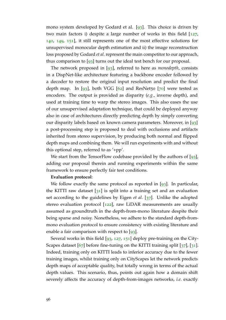
mono system developed by Godard et al. [93]. This choice is driven bytwo main factors i) despite a large number of works in this field [127,140, 149, 151], it still represents one of the most effective solutions forunsupervised monocular depth estimation and ii) the image reconstructionloss proposed by Godard et al. represent the main competitor to our approach,thus comparison to [93] turns out the ideal test bench for our proposal.
The network proposed in [93], referred to here as monodepth, consistsin a DispNet-like architecture featuring a backbone encoder followed bya decoder to restore the original input resolution and predict the finaldepth map. In [93], both VGG [62] and ResNet50 [70] were tested asencoders. The output is provided as disparity (e.g., inverse depth), andused at training time to warp the stereo images. This also eases the useof our unsupervised adaptation technique, that could be deployed anywayalso in case of architectures directly predicting depth by simply convertingour disparity labels based on known camera parameters. Moreover, in [93]a post-processing step is proposed to deal with occlusions and artifactsinherited from stereo supervision, by producing both normal and flippeddepth maps and combining them. We will run experiments with and withoutthis optional step, referred to as ’+pp’.
We start from the TensorFlow codebase provided by the authors of [93],adding our proposal therein and running experiments within the sameframework to ensure perfectly fair test conditions.
Evaluation protocol:We follow exactly the same protocol as reported in [93]. In particular,
the KITTI raw dataset [31] is split into a training set and an evaluationset according to the guidelines by Eigen et al. [37]. Unlike the adoptedstereo evaluation protocol [122], raw LiDAR measurements are usuallyassumed as groundtruth in the depth-from-mono literature despite theirbeing sparse and noisy. Nonetheless, we adhere to the standard depth-from-mono evaluation protocol to ensure consistency with existing literature andenable a fair comparison with respect to [93].
Several works in this field [93, 127, 151] deploy pre-training on the City-Scapes dataset [67] before fine-tuning on the KITTI training split [37], [31].Indeed, training only on KITTI leads to inferior accuracy due to the fewertraining images, whilst training only on CityScapes let the network predictsdepth maps of acceptable quality, but totally wrong in terms of the actualdepth values. This scenario, thus, points out again how a domain shiftseverely affects the accuracy of depth-from-images networks, i.e. exactly
96
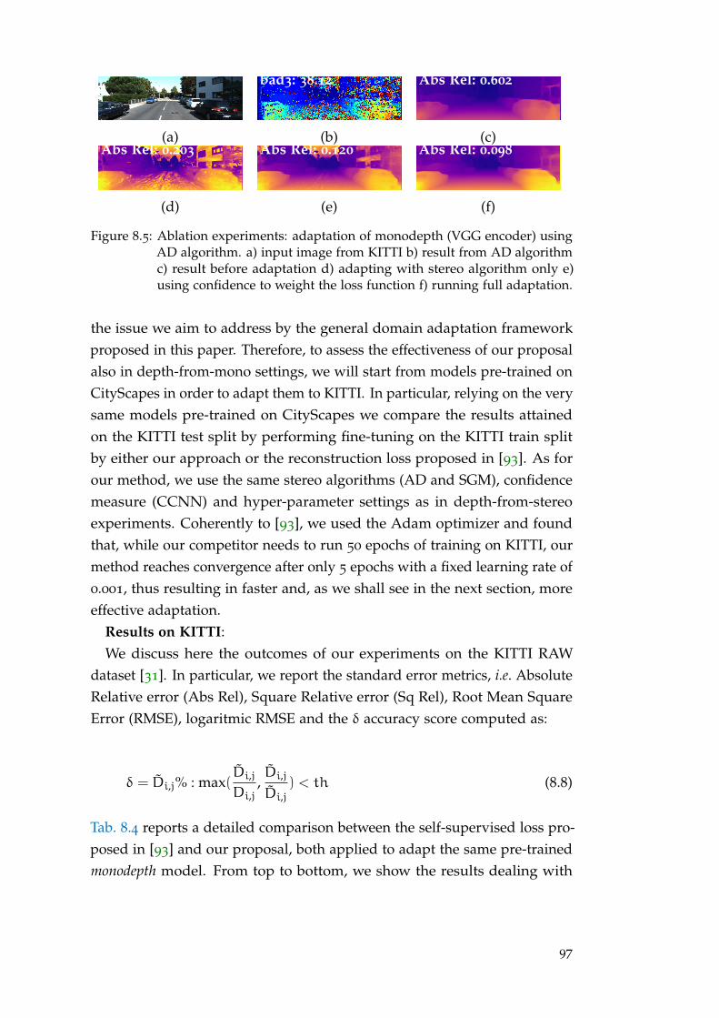
bad3: 38.12 Abs Rel: 0.602
(a) (b) (c)Abs Rel: 0.203 Abs Rel: 0.120 Abs Rel: 0.098
(d) (e) (f)
Figure 8.5: Ablation experiments: adaptation of monodepth (VGG encoder) usingAD algorithm. a) input image from KITTI b) result from AD algorithmc) result before adaptation d) adapting with stereo algorithm only e)using confidence to weight the loss function f) running full adaptation.
the issue we aim to address by the general domain adaptation frameworkproposed in this paper. Therefore, to assess the effectiveness of our proposalalso in depth-from-mono settings, we will start from models pre-trained onCityScapes in order to adapt them to KITTI. In particular, relying on the verysame models pre-trained on CityScapes we compare the results attainedon the KITTI test split by performing fine-tuning on the KITTI train splitby either our approach or the reconstruction loss proposed in [93]. As forour method, we use the same stereo algorithms (AD and SGM), confidencemeasure (CCNN) and hyper-parameter settings as in depth-from-stereoexperiments. Coherently to [93], we used the Adam optimizer and foundthat, while our competitor needs to run 50 epochs of training on KITTI, ourmethod reaches convergence after only 5 epochs with a fixed learning rate of0.001, thus resulting in faster and, as we shall see in the next section, moreeffective adaptation.
Results on KITTI:We discuss here the outcomes of our experiments on the KITTI RAW
dataset [31]. In particular, we report the standard error metrics, i.e. AbsoluteRelative error (Abs Rel), Square Relative error (Sq Rel), Root Mean SquareError (RMSE), logaritmic RMSE and the δ accuracy score computed as:
δ = Di,j% : max(Di,j
Di,j,Di,j
Di,j) < th (8.8)
Tab. 8.4 reports a detailed comparison between the self-supervised loss pro-posed in [93] and our proposal, both applied to adapt the same pre-trainedmonodepth model. From top to bottom, we show the results dealing with
97
a monodepth with a VGG encoder, a VGG encoder and the post-processingstep (+pp) and finally a ResNet50 encoder with the post-processing step.Starting from the basic VGG-based model, we can observe that adaptingby either AD or SGM with the masked configuration alone leads to betterperformance with respect to using the image reconstruction loss proposedin [93]. In general, adapting by SGM yields superior results, outperformingthe model based on AD on nearly all metrics. This finding is confirmedwhen applying the post-processing step (i.e., VGG+pp), as our adaptationapproach outperforms [93] under all evaluation metrics. Moreover, VGG+ppnetworks optimized by our technique can deliver better results than using aResNet+pp network trained according to the image reconstruction loss of[93] despite the large difference in complexity between the two networks(VGG features about 31 millions learnable parameters, ResNet50 about57 millions). By applying the considered adaptation approaches to theResNet50-based monodepth, the margin turns out even higher. Finally, inthe last row of Table 8.4, we report the results obtained by our approachwhen using SGM together with the complete adaptation loss of Eq. 8.2, theperformance metrics scoring slightly better than those achieved by Masked-SGM. This, again, highlights how in Eq. 8.2 the confidence-guided lossterm provides a more relevant contribution to performance than the imagere-projection term inspired by [93].
Ablation experiments: Similarly to the previously addressed stereo set-tings, we report here an ablation study aimed at establishing upon therelative importance of the key ingredients deployed in our framework. Table8.5 collects the results obtained in this evaluation. We comment about fourmain experiments, dealing with running our method with both AD andSGM in order to adapt VGG and ResNet50. The post-processing step isenabled in all tests, thereby solving most issues near occlusions and leftborder and highlighting how the full confidence-guided loss amelioratesresults in many regions of the images where post-processing cannot operate.Three setups are considered in descending order in the Table for each of thefour experiments: i) adaptation by minimization of the L1 loss with respectto the disparity maps estimated by the stereo algorithm (AD or SGM) "as is"(Regression) ii) adaptation by weighting the L1 loss with per-pixel confidencescores (Weighted) iii) full confidence-guided loss using threshold τ (Masked).We turn off additional terms to focus on the different key factors of theconfidence-guided loss. In all experiments, we can notice how using thedisparity labels alone leads to poor results, in particular when adapting the
98
model by the AD algorithm, which is much more prone to outliers. Thisfurther highlights how, in our framework, deploying the confidence measureis crucial to avoid the impact of the wrong disparities possibly computed bythe stereo algorithms. Formulating the confidence-guided loss as a simpleweighting between confidence scores and loss signals reduces the impact ofthe outliers, but does not completely removes it as they can still contribute tothe entire loss function with a lower weight and thus may lead, as reported,to worse performance. To better perceive this effect, Fig. 8.5 shows somequalitative results obtained by the three ablated configurations reportedin the Table. In particular, we point out how on (c) the results from theoriginal model trained on different environments look good qualitatively,but the range of the predicted depth values is totally wrong (Abs Rel of0.620). We can observe how ablated configurations of our technique (d-e) doyield gradual improvements, whereas the full adaptation scheme (f) greatlyameliorates the quality of the estimated depth maps, i.e. so as to bring theerror down to 0.098 Abs Rel.
As an additional experiment, and similarly to the stereo experiments, wetried to adapt the model using labels from both AD and SGM by simplycomputing the loss function according to both disparity hypotheses. Thisleads to slightly worse results, possibly because some outliers not correctlymasked out from the one algorithm may interfere with the correct assign-ments suggested by the other.8 .3 .4 Qualitative Results
Finally we show some qualitative results, concerning both stereo and depth-from-mono networks, on the Middlebury v3 [42] and ETH3D [112] datasets.Fig. 8.6 shows examples of depth maps obtained by monodepth pre-trainedon CityScapes [67] before and after adaptation by our technique. The overallquality of the maps is greatly improved by the adaptation step, which isalso vouched by the drastic drop of the absolute error reported in the Figure.We show similar results for DispNet on Fig. 8.7: the column labeled asNo Adaptation concerns predictions obtained by the model pre-trained onFlyingThings3D while the Adaptation column deals with the results obtainedafter fine-tuning by our unsupervised adaptation approach. Results indicateclearly how our proposal can successfully correct the prediction range anddrastically reduce the percentage of wrong pixels.
99
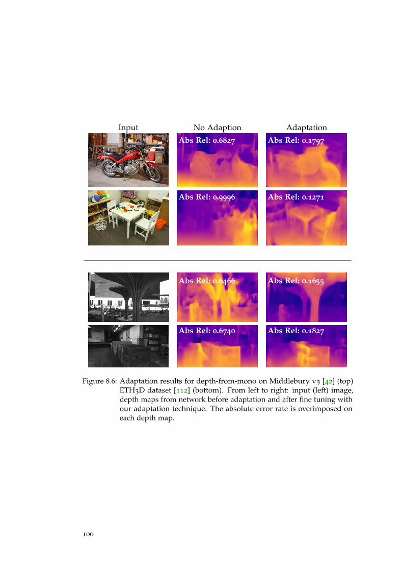
Input No Adaption Adaptation
Abs Rel: 0.6827 Abs Rel: 0.1797
Abs Rel: 0.9996 Abs Rel: 0.1271
Abs Rel: 0.6466 Abs Rel: 0.1655
Abs Rel: 0.6740 Abs Rel: 0.1827
Figure 8.6: Adaptation results for depth-from-mono on Middlebury v3 [42] (top)ETH3D dataset [112] (bottom). From left to right: input (left) image,depth maps from network before adaptation and after fine tuning withour adaptation technique. The absolute error rate is overimposed oneach depth map.
100
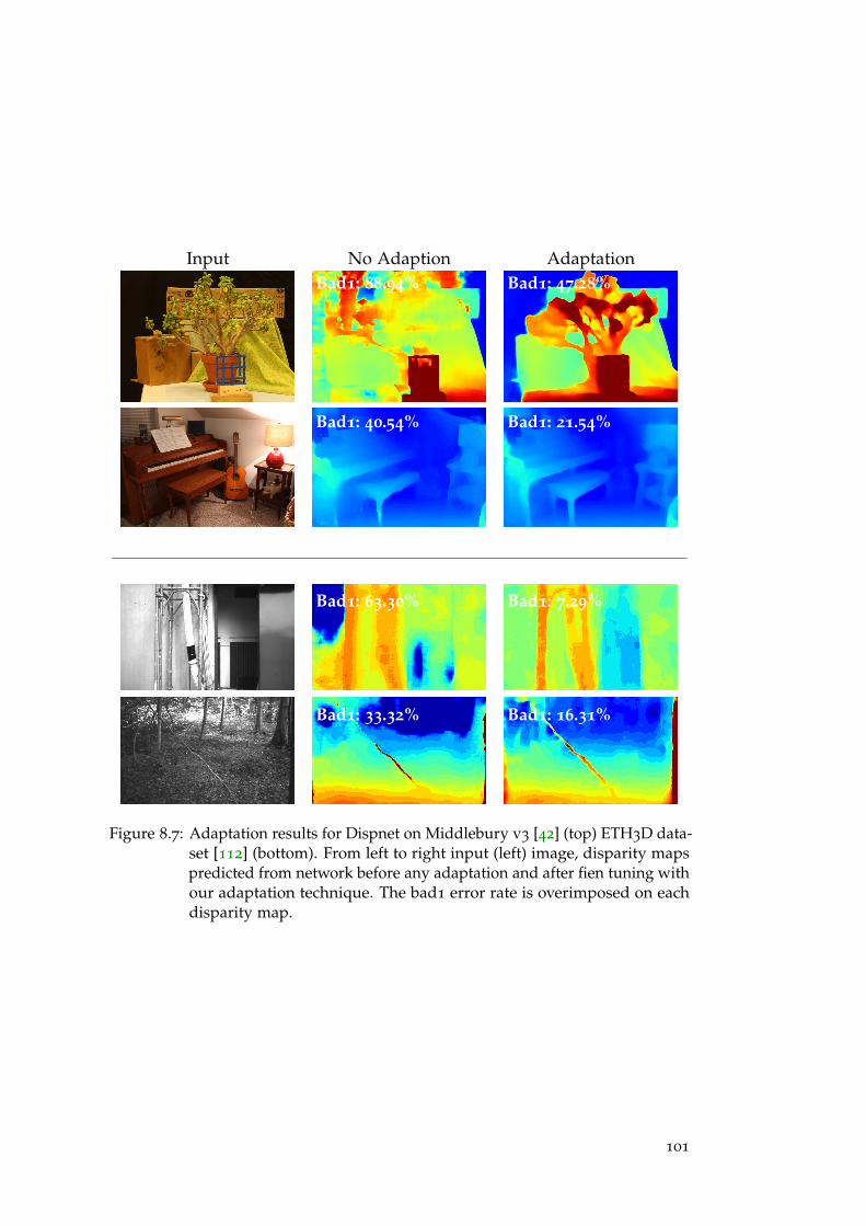
Input No Adaption AdaptationBad1: 88.94% Bad1: 47.28%
Bad1: 40.54% Bad1: 21.54%
Bad1: 63.30% Bad1: 7.29%
Bad1: 33.32% Bad1: 16.31%
Figure 8.7: Adaptation results for Dispnet on Middlebury v3 [42] (top) ETH3D data-set [112] (bottom). From left to right input (left) image, disparity mapspredicted from network before any adaptation and after fien tuning withour adaptation technique. The bad1 error rate is overimposed on eachdisparity map.
101
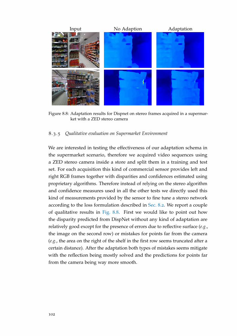
Input No Adaption Adaptation
Figure 8.8: Adaptation results for Dispnet on stereo frames acquired in a supermar-ket with a ZED stereo camera
8 .3 .5 Qualitative evaluation on Supermarket Environment
We are interested in testing the effectiveness of our adaptation schema inthe supermarket scenario, therefore we acquired video sequences usinga ZED stereo camera inside a store and split them in a training and testset. For each acquisition this kind of commercial sensor provides left andright RGB frames together with disparities and confidences estimated usingproprietary algorithms. Therefore instead of relying on the stereo algorithmand confidence measures used in all the other tests we directly used thiskind of measurements provided by the sensor to fine tune a stereo networkaccording to the loss formulation described in Sec. 8.2. We report a coupleof qualitative results in Fig. 8.8. First we would like to point out howthe disparity predicted from DispNet without any kind of adaptation arerelatively good except for the presence of errors due to reflective surface (e.g.,the image on the second row) or mistakes for points far from the camera(e.g., the area on the right of the shelf in the first row seems truncated after acertain distance). After the adaptation both types of mistakes seems mitigatewith the reflection being mostly solved and the predictions for points farfrom the camera being way more smooth.
102
9O N L I N E U N S U P E RV I S E D D O M A I N A D A P TAT I O N F O RD E E P S T E R E O
In Chap. 8 we have proposed a novel loss function to address the domainshift issue for depth estimation networks by means of unsupervised offlinefine tuning. In this section, instead, we want to go one step further andcast adaptation as a continuous unsupervised learning process whereby a depthestimation network evolves online based on the images gathered by a cameraduring its real deployment. We believe that the ability to constantly adaptitself in real-time is key to any deep learning machinery meant to workin relevant practical scenarios, like autonomous driving, where gatheringtraining samples to be deployed offline from all possible surroundings turnsout definitely unfeasible.
We will show how continuous online adaptation can be achieved byleveraging on one of the unsupervised losses proposed in the literature tocompute the loss on the current frames, update the whole network by back-propagation (from now on shortened back-prop) and move to the next coupleof input frames. Adapting, however, comes with the side effect of reducinginference speed to ∼ 1
3 at best, as we will show experimentally, a price fartoo high to pay for most modern state of the art deep stereo systems whichare relatively slow. To keep a high enough frame rate we have developed anovel Modularly ADdaptive Network (MADNet) designed to be lightweight,fast and modular. Our architecture exhibits accuracy comparable to DispNetyet use 1
10 of the parameters, runs at ∼ 40FPS for disparity inference andperforms online adaptation of the whole network at ∼ 15FPS. Moreover, toallow a higher frame rate during the adaptation at the cost of slightly worseaccuracy, we have developed Modular ADaptation (MAD) an algorithm thatleverage on the modular architecture of MADNet and train independentlysub-portion of the whole network. Using MADNet together with MAD weare able to adapt our system without supervision to unseen environment at∼ 25FPS.
Fig. 9.1 shows the disparity maps predicted by MADNet on three success-ive frames of a video from the KITTI dataset [31] either without undergoingany adaptation (b) or by adapting online the whole network (c) or by our
103
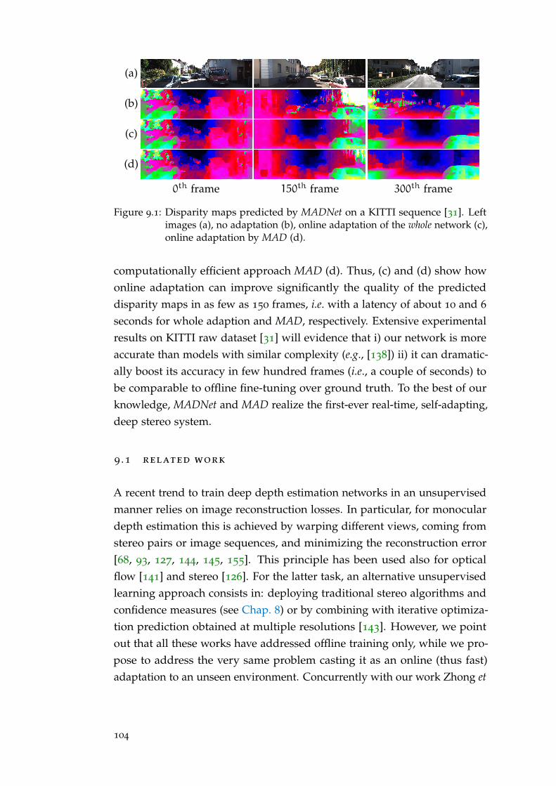
(a)
(b)
(c)
(d)
0th frame 150th frame 300th frame
Figure 9.1: Disparity maps predicted by MADNet on a KITTI sequence [31]. Leftimages (a), no adaptation (b), online adaptation of the whole network (c),online adaptation by MAD (d).
computationally efficient approach MAD (d). Thus, (c) and (d) show howonline adaptation can improve significantly the quality of the predicteddisparity maps in as few as 150 frames, i.e. with a latency of about 10 and 6
seconds for whole adaption and MAD, respectively. Extensive experimentalresults on KITTI raw dataset [31] will evidence that i) our network is moreaccurate than models with similar complexity (e.g., [138]) ii) it can dramatic-ally boost its accuracy in few hundred frames (i.e., a couple of seconds) tobe comparable to offline fine-tuning over ground truth. To the best of ourknowledge, MADNet and MAD realize the first-ever real-time, self-adapting,deep stereo system.
9 .1 related work
A recent trend to train deep depth estimation networks in an unsupervisedmanner relies on image reconstruction losses. In particular, for monoculardepth estimation this is achieved by warping different views, coming fromstereo pairs or image sequences, and minimizing the reconstruction error[68, 93, 127, 144, 145, 155]. This principle has been used also for opticalflow [141] and stereo [126]. For the latter task, an alternative unsupervisedlearning approach consists in: deploying traditional stereo algorithms andconfidence measures (see Chap. 8) or by combining with iterative optimiza-tion prediction obtained at multiple resolutions [143]. However, we pointout that all these works have addressed offline training only, while we pro-pose to address the very same problem casting it as an online (thus fast)adaptation to an unseen environment. Concurrently with our work Zhong et
104
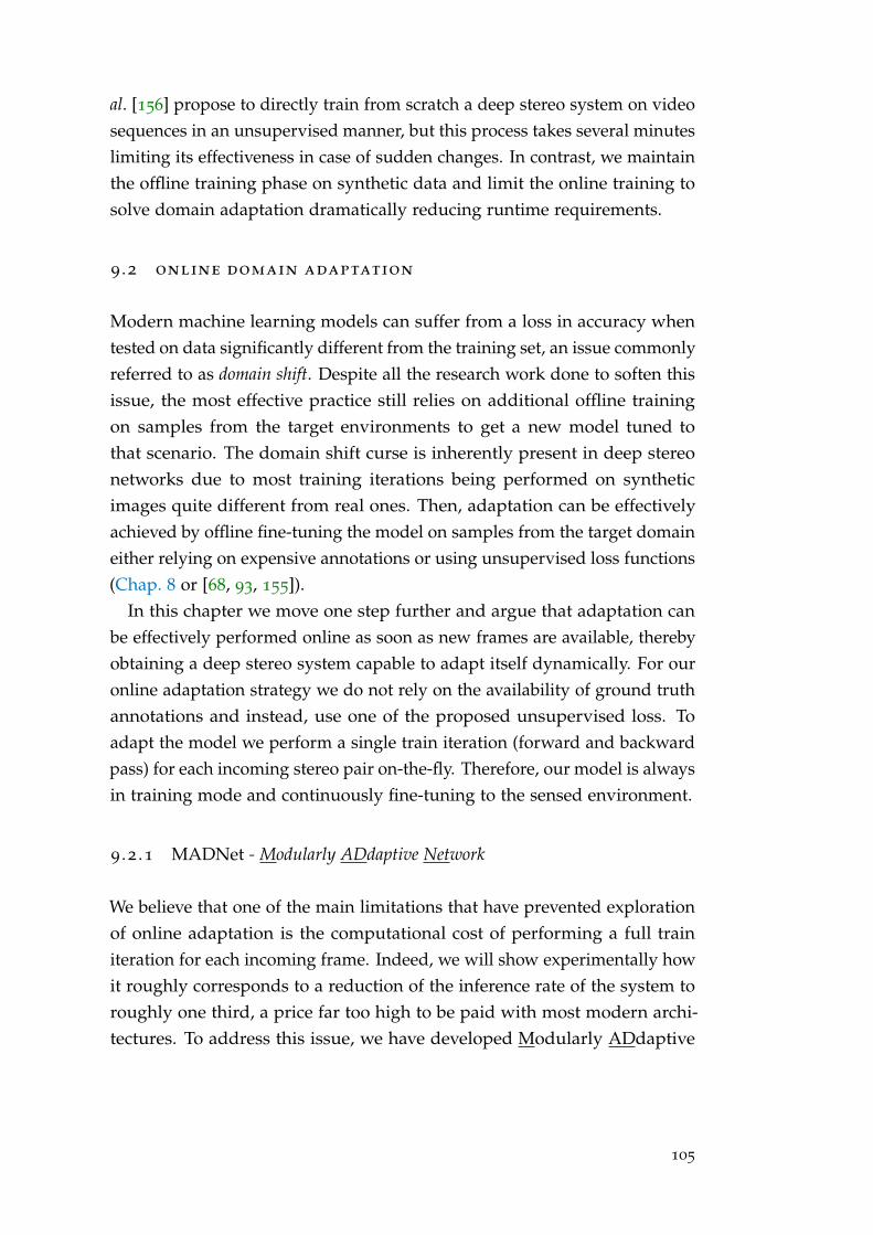
al. [156] propose to directly train from scratch a deep stereo system on videosequences in an unsupervised manner, but this process takes several minuteslimiting its effectiveness in case of sudden changes. In contrast, we maintainthe offline training phase on synthetic data and limit the online training tosolve domain adaptation dramatically reducing runtime requirements.
9 .2 online domain adaptation
Modern machine learning models can suffer from a loss in accuracy whentested on data significantly different from the training set, an issue commonlyreferred to as domain shift. Despite all the research work done to soften thisissue, the most effective practice still relies on additional offline trainingon samples from the target environments to get a new model tuned tothat scenario. The domain shift curse is inherently present in deep stereonetworks due to most training iterations being performed on syntheticimages quite different from real ones. Then, adaptation can be effectivelyachieved by offline fine-tuning the model on samples from the target domaineither relying on expensive annotations or using unsupervised loss functions(Chap. 8 or [68, 93, 155]).
In this chapter we move one step further and argue that adaptation canbe effectively performed online as soon as new frames are available, therebyobtaining a deep stereo system capable to adapt itself dynamically. For ouronline adaptation strategy we do not rely on the availability of ground truthannotations and instead, use one of the proposed unsupervised loss. Toadapt the model we perform a single train iteration (forward and backwardpass) for each incoming stereo pair on-the-fly. Therefore, our model is alwaysin training mode and continuously fine-tuning to the sensed environment.
9 .2 .1 MADNet - Modularly ADdaptive Network
We believe that one of the main limitations that have prevented explorationof online adaptation is the computational cost of performing a full trainiteration for each incoming frame. Indeed, we will show experimentally howit roughly corresponds to a reduction of the inference rate of the system toroughly one third, a price far too high to be paid with most modern archi-tectures. To address this issue, we have developed Modularly ADdaptive
105
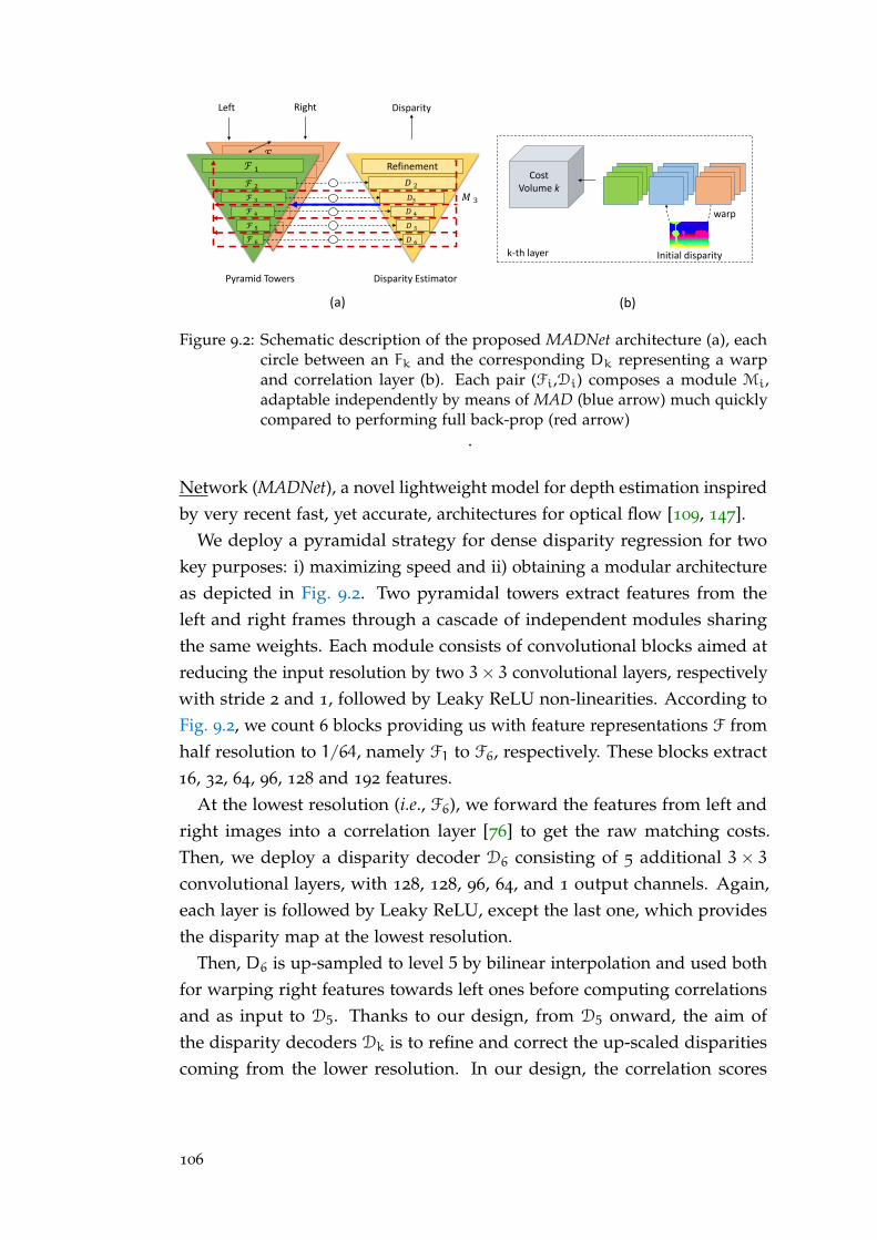
ℱ 1
ℱ 2
ℱ 3
ℱ 4
ℱ 5
ℱ 6
ℱ 1
ℱ 2
ℱ 4
ℱ 5
ℱ 6
Initial disparity
Cost Volume k
Pyramid Towers
Left Right
k-th layer
warp
Refinement
𝐷 2
𝐷 4
𝐷 5
𝐷 6
Disparity Estimator
(a) (b)
Disparity
𝐷3ℱ 3 𝑀 3
Figure 9.2: Schematic description of the proposed MADNet architecture (a), eachcircle between an Fk and the corresponding Dk representing a warpand correlation layer (b). Each pair (Fi,Di) composes a module Mi,adaptable independently by means of MAD (blue arrow) much quicklycompared to performing full back-prop (red arrow)
.
Network (MADNet), a novel lightweight model for depth estimation inspiredby very recent fast, yet accurate, architectures for optical flow [109, 147].
We deploy a pyramidal strategy for dense disparity regression for twokey purposes: i) maximizing speed and ii) obtaining a modular architectureas depicted in Fig. 9.2. Two pyramidal towers extract features from theleft and right frames through a cascade of independent modules sharingthe same weights. Each module consists of convolutional blocks aimed atreducing the input resolution by two 3× 3 convolutional layers, respectivelywith stride 2 and 1, followed by Leaky ReLU non-linearities. According toFig. 9.2, we count 6 blocks providing us with feature representations F fromhalf resolution to 1/64, namely F1 to F6, respectively. These blocks extract16, 32, 64, 96, 128 and 192 features.
At the lowest resolution (i.e., F6), we forward the features from left andright images into a correlation layer [76] to get the raw matching costs.Then, we deploy a disparity decoder D6 consisting of 5 additional 3× 3convolutional layers, with 128, 128, 96, 64, and 1 output channels. Again,each layer is followed by Leaky ReLU, except the last one, which providesthe disparity map at the lowest resolution.
Then, D6 is up-sampled to level 5 by bilinear interpolation and used bothfor warping right features towards left ones before computing correlationsand as input to D5. Thanks to our design, from D5 onward, the aim ofthe disparity decoders Dk is to refine and correct the up-scaled disparitiescoming from the lower resolution. In our design, the correlation scores
106
computed between the original left and right features aligned according tothe lower resolution disparity prediction should provide the network withguidance for the refinement process. We compute all correlations inside ournetwork along a [-2,2] range of possible shifts.
This process is repeated up to quarter resolution (i.e., D2), where we adda further refinement module consisting of 3× 3 dilated convolutions [147],with, respectively 128, 128, 128, 96, 64, 32, 1 output channels and 1, 2, 4, 8,16, 1, 1 dilation factors, before bilinearly upsampling to full resolution.
MADNet has a smaller memory footprint and delivers disparity mapsmuch more rapidly than other more complex networks such as [liang2018learning,99, 132] with a small loss in accuracy. Concerning efficiency, working atdecimated resolutions allows for computing correlations on a small ho-rizontal window [147], while warping features and forwarding disparitypredictions across the different resolutions enables to maintain a smallsearch range and look for residual displacements only. With a 1080Ti GPU,MADNet runs at about 40 FPS at KITTI resolution and can performs onlineadaptation with full back-prop at 15 FPS.
9 .2 .2 MAD - Modular ADaptation
As we will show, MADNet is remarkably accurate while performing theonline adaptation of the whole network at 15 FPS. However, for someapplications, it might be desirable to have a higher frame rate without losingthe ability to tune the network to unseen environments automatically. Mostof the time needed to perform online adaptation is effectively spent executingback-prop and weights update across the whole network layers. A naive wayto speed up the process will be to freeze the initial part of the network andfine tune only a subset of k final layers, thus realizing a shorter back-propthat would yield a higher frame rate. However, there is no guarantee thatthese last k layers are indeed those that would benefit most from onlinefine-tuning. One might reasonably guess that other portions of the networkshould be adapted as well, in particular, the initial layers, which directlyinteracts with the images from a new, unseen, domain. Indeed, we will showin Sec. 9.3.3 that training only the final layers is not enough for handlingdrastic domain changes that typically occur in practical applications.
Thus, following the key intuition that to keep up with fast inferencewe should pursue a partial, though effective, online adaptation, we de-
107

veloped Modular ADaptation (MAD) an approximate online adaptationalgorithm tailored for MADNet, but extensible to any multi-scale inferencenetwork. The key intuition for our method is to take a network N andsubdivide it into p non-overlapping portions, each referred to as n, suchthat N = [n1,n2, ..np]. Each portion ni consists of k connected layers withthe last one (the deeper) able to output a disparity estimation of yi. Givenas input a couple of stereo frames x, N will output p+ 1 disparity estima-tion [y,y1, . . . ,yp] = forward(N, x), with y being the final prediction of themodel at full resolution. Due to its modular structure, MADNet naturallyallows such subdivision by assigning to the same ni layers working at thesame resolution both in the convolutional towers and among the disparityestimators (e.g., referring to Fig. 9.2 ni = [Fi,Di]). Each ni can be independ-ently trained by computing a loss directly on the disparity yi and back-proponly across the layers belonging to ni, thereby skipping the costly backwardpass through lower resolution layers in between. This process can be figuredout as an approximation of the standard full back-prop. In fact, by altern-ating the portion ni of the network that is trained, it sequentially allowsupdating all layers. Such a strategy drastically reduces the time neededto compute and apply gradients without sacrificing too much accuracy asconfirmed by experimental results.
Offline, we statically subdivide the network into different portions, thatwith MADNet correspond to different layers of the pyramids. Online, foreach incoming stereo pair, first we perform a forward pass to obtain allthe disparity predictions at multiple scales [y,y1, . . . ,yp], then, we choose aportion θ ∈ [1, . . . ,p] of the network to train according to some heuristic andupdate the weights of layers belonging to nθ according to a loss computedon yθ. We consider a valid heuristic any function that outputs a probabilitydistribution among the p trainable portions of N from whom we couldperform sampling.
Among different functions, we obtained effective results using a simplereward/punishment mechanism detailed in Algorithm Alg. 2. We start bycreating a histogram H with p bins all initialized at 0. For each stereo pair weperform a forward pass to get the disparity predictions (line 5) and measurethe performance of the model by computing the loss Lt using the fullresolution disparity y and potentially the input frames x, e.g., reprojectionerror between left and right frames [93] (line 6). Then, we sample theportion to train θ ∈ [1, . . . ,p] according to the distribution softmax(H)
(line 7) and compute one optimization step for layers of nθ with respect
108
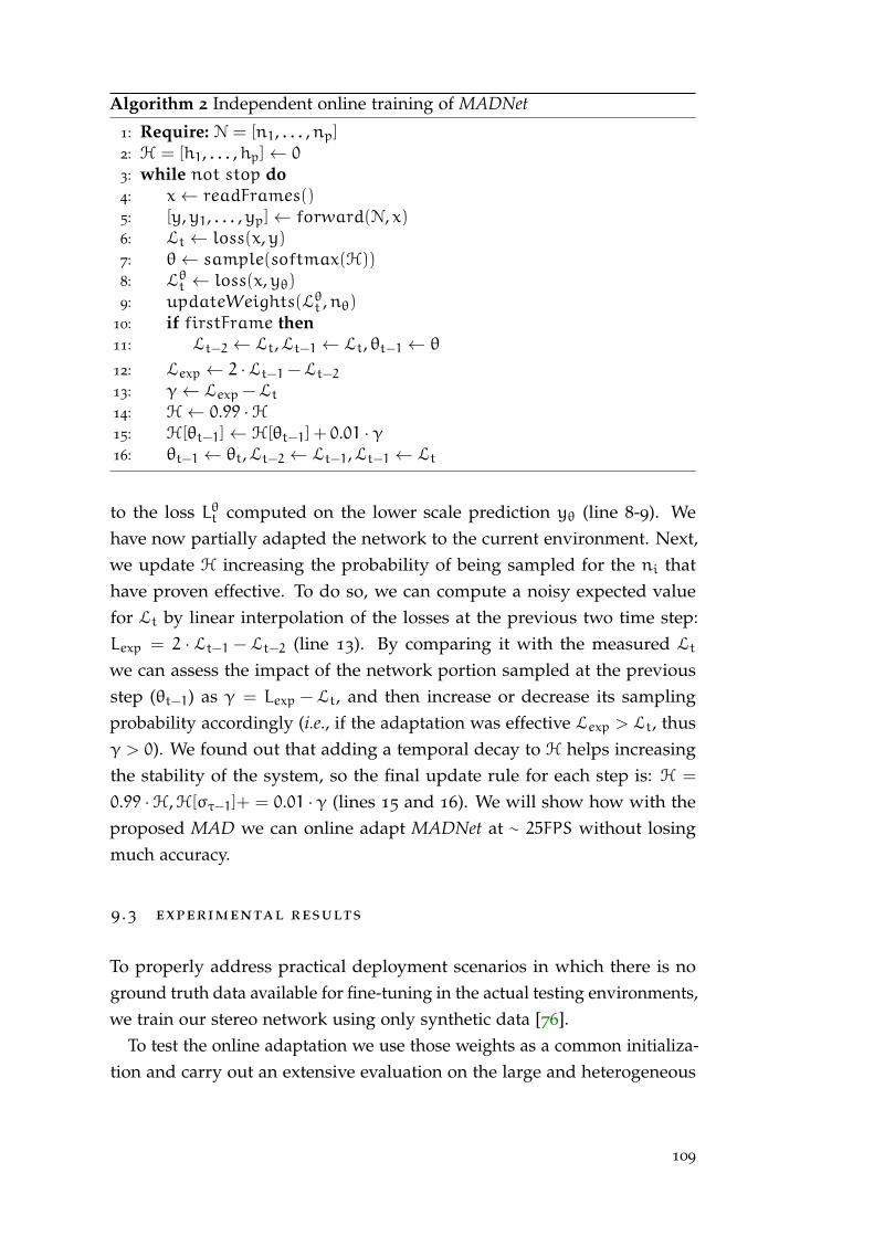
Algorithm 2 Independent online training of MADNet
1: Require: N = [n1, . . . ,np]2: H = [h1, . . . ,hp]← 0
3: while not stop do4: x← readFrames()5: [y,y1, . . . ,yp]← forward(N, x)6: Lt ← loss(x,y)7: θ← sample(softmax(H))8: Lθt ← loss(x,yθ)9: updateWeights(Lθt ,nθ)
10: if firstFrame then11: Lt−2 ← Lt,Lt−1 ← Lt, θt−1 ← θ
12: Lexp ← 2 ·Lt−1 −Lt−213: γ← Lexp −Lt14: H← 0.99 ·H15: H[θt−1]← H[θt−1] + 0.01 · γ16: θt−1 ← θt,Lt−2 ← Lt−1,Lt−1 ← Lt
to the loss Lθt computed on the lower scale prediction yθ (line 8-9). Wehave now partially adapted the network to the current environment. Next,we update H increasing the probability of being sampled for the ni thathave proven effective. To do so, we can compute a noisy expected valuefor Lt by linear interpolation of the losses at the previous two time step:Lexp = 2 · Lt−1 − Lt−2 (line 13). By comparing it with the measured Lt
we can assess the impact of the network portion sampled at the previousstep (θt−1) as γ = Lexp − Lt, and then increase or decrease its samplingprobability accordingly (i.e., if the adaptation was effective Lexp > Lt, thusγ > 0). We found out that adding a temporal decay to H helps increasingthe stability of the system, so the final update rule for each step is: H =
0.99 ·H,H[στ−1]+ = 0.01 · γ (lines 15 and 16). We will show how with theproposed MAD we can online adapt MADNet at ∼ 25FPS without losingmuch accuracy.
9 .3 experimental results
To properly address practical deployment scenarios in which there is noground truth data available for fine-tuning in the actual testing environments,we train our stereo network using only synthetic data [76].
To test the online adaptation we use those weights as a common initializa-tion and carry out an extensive evaluation on the large and heterogeneous
109
KITTI raw dataset [31] with depth labels [122] converted into disparitiesby knowing the camera parameters. Overall, we assess the effectivenessof our proposal on 43k images. Specifically, according to the KITTI classi-fication, we evaluate our framework in four heterogeneous environments,namely Road, Residential, Campus and City, obtained by concatenation ofthe available video sequences and resulting in 5674, 28067, 1149 and 8027
frames respectively. Although these sequences are all concerned with driv-ing scenarios, each has peculiar traits that would lead a deep stereo modelto gross errors without a suitable fine-tuning in the target domain. Forexample, City and Residential often depict road surrounded by buildings,while Road mostly concern highways and country roads where the mostcommon objects depicted are cars and vegetation.
By processing stereo pairs within sequences, we can measure how wellthe network adapts, either with full back-prop or MAD, to the target domaincompared to an offline trained model. For all experiments, we analyze bothaverage End Point Error (EPE) and the percentage of pixels with disparityerror larger than 3 (D1-all). Due to image format being different for eachsequence, we extract a central crop of size 320 × 1216 from each frame,which suits to the downsampling factor of our architecture and allows forvalidating almost all pixels with available ground-truth disparities.
Finally, we highlight that for both full back-prop and MAD, we computethe error rate on each frame before applying the model adaptation step.That is, we measure performances achieved by the current model on thestereo frame at time t and then adapt it according to the current prediction.Therefore, the model update carried out at time t will affect the predictiononly from frame t+ 1 and so on. As unsupervised loss for online adaptation,we rely on the photometric consistency between the left frame and the rightone reprojected according to the predicted disparity. Following [93], tocompute the reprojection error between the two images we combine theStructural Similarity Measure (SSIM) and the L1 distance, weighted by 0.85
and 0.15, respectively. We selected this unsupervised loss function as it isthe fastest to compute among those proposed in literature (Chap. 8 and [126,143] and does not require additional information besides a couple of stereopairs.
110
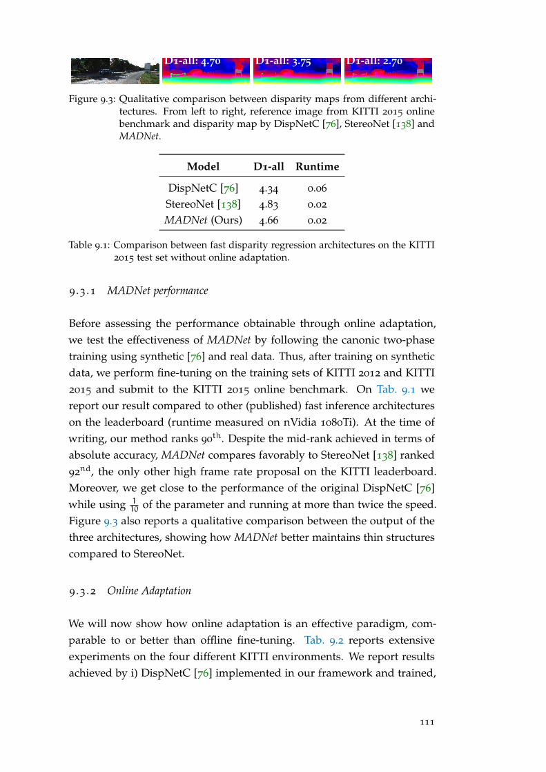
D1-all: 4.70 D1-all: 3.75 D1-all: 2.70
Figure 9.3: Qualitative comparison between disparity maps from different archi-tectures. From left to right, reference image from KITTI 2015 onlinebenchmark and disparity map by DispNetC [76], StereoNet [138] andMADNet.
Model D1-all Runtime
DispNetC [76] 4.34 0.06
StereoNet [138] 4.83 0.02
MADNet (Ours) 4.66 0.02
Table 9.1: Comparison between fast disparity regression architectures on the KITTI2015 test set without online adaptation.
9 .3 .1 MADNet performance
Before assessing the performance obtainable through online adaptation,we test the effectiveness of MADNet by following the canonic two-phasetraining using synthetic [76] and real data. Thus, after training on syntheticdata, we perform fine-tuning on the training sets of KITTI 2012 and KITTI2015 and submit to the KITTI 2015 online benchmark. On Tab. 9.1 wereport our result compared to other (published) fast inference architectureson the leaderboard (runtime measured on nVidia 1080Ti). At the time ofwriting, our method ranks 90
th. Despite the mid-rank achieved in terms ofabsolute accuracy, MADNet compares favorably to StereoNet [138] ranked92nd, the only other high frame rate proposal on the KITTI leaderboard.
Moreover, we get close to the performance of the original DispNetC [76]while using 1
10 of the parameter and running at more than twice the speed.Figure 9.3 also reports a qualitative comparison between the output of thethree architectures, showing how MADNet better maintains thin structurescompared to StereoNet.
9 .3 .2 Online Adaptation
We will now show how online adaptation is an effective paradigm, com-parable to or better than offline fine-tuning. Tab. 9.2 reports extensiveexperiments on the four different KITTI environments. We report resultsachieved by i) DispNetC [76] implemented in our framework and trained,
111

City Residential Campus Road
Model Adapt. D1-all(%) EPE D1-all(%) EPE D1-all(%) EPE D1-all(%) EPE FPS
DispNetC No 8.31 1.49 8.72 1.55 15.63 2.14 10.76 1.75 15.85
DispNetC Full 4.34 1.16 3.60 1.04 8.66 1.53 3.83 1.08 5.22
DispNetC-GT No 3.78 1.19 4.71 1.23 8.42 1.62 3.25 1.07 15.85
MADNet No 37.42 9.96 37.41 11.34 51.98 11.94 47.45 15.71 39.48
MADNet Full 2.63 1.03 2.44 0.96 8.91 1.76 2.33 1.03 14.26
MADNet MAD 5.82 1.51 3.96 1.31 23.40 4.89 7.02 2.03 25.43
MADNet-GT No 2.21 0.80 2.80 0.91 6.77 1.32 1.75 0.83 39.48
Table 9.2: Performance on the City, Residential, Campus and Road sequences fromKITTI [31]. Experiments with DispNetC [76] (top) and MADNet (bottom)with and without online adaptations.
from top to bottom, on synthetic data following authors’ guidelines, usingonline adaptation or fine-tuned on ground-truth and ii) MADNet trainedwith the same modalities and, in addition, using MAD. These experiments,together to Sec. 9.3.1, support the three-fold claim of this work.
DispNetC: Full adaptation. On top of Tab. 9.2, focusing on the D1-allmetric, we can notice how running full back-prop online to adapt DispNetC[76] decimates the number of outliers on all scenarios compared to themodel trained on the synthetic dataset only. In particular, this approachcan consistently halve D1-all on Campus, Residential and City and nearlyreduce it to one third on Road. Alike, the average EPE drops significantlyacross the four considered environments, with improvement as high as anearly 40% relative improvement on the Road sequences. These massivegains in accuracy, though, come at the price of slowing the network downsignificantly to about one-third of the original inference rate, i.e. from nearly16 to 5.22 FPS. As mentioned above, the Table also reports the performanceof the models fine-tuned offline on the 400 stereo pairs with ground-truthdisparities from the KITTI 2012 and 2015 training dataset [27, 57]. It is worthpointing out how online adaptation by full back-prop turns out competitivewith respect to fine-tuning offline by ground-truth, even more accurate in theResidential environment. This fact may hint at training without supervisionby a more considerable amount of data possibly delivering better modelsthan supervision by fewer data.
MADNet: Full adaptation. On bottom of Tab. 9.2 we repeat the aforemen-tioned experiments for MADNet. Due to the much higher errors yieldedby the model trained on synthetic data only, full online adaptation turnsout even more beneficial with MADNet, leading to a model which is moreaccurate than DispNetC with Full adaptation in all sequences but Campus
112
and can run nearly three times faster (i.e. at 14.26 FPS compared to the 5.22
FPS of DispNetC-Full). These results also highlight the inherent effectivenessof the proposed MADNet. Indeed, as vouched by the rows dealing withMADNet-GT and DispNetC-GT, using for both our implementations andtraining them following the same standard procedure in the field, MADNetyields better accuracy than DispNetC while running about 2.5 times faster.
MADNet: MAD. Having proven that online adaptation is feasible andbeneficial, we show that MADNet employing MAD for adaptation (markedas MAD in column Adapt.) allows for effectively and efficient adaptation.Since the proposed heuristic has a non-deterministic sampling step, wehave run the tests regarding MAD five times each and reported here theaverage performance. We refer the reader to Sec. 9.3.3 for analysis on thestandard deviation across different runs. Indeed, MAD provides a significantimprovement in all the performance figures reported in the table comparedto the corresponding models trained by synthetic data only. Using MAD,MADNet can be adapted paying a relatively small computational overheadwhich results in a remarkably fast inference rate of about 25 FPS. Overall,these results highlight how, whenever one has no access to training data fromthe target domain beforehand, online adaptation is feasible and definitelyworth. Moreover, if speed is a concern MADNet combined with MADprovides a favorable trade-off between accuracy and efficiency.
Short-term Adaptation. Tab. 9.2 shows also how all adapted modelsperform significantly worse on Campus with respect to the other sequences.We ascribe this mainly to Campus featuring fewer frames (1149) compared theother sequences (5674, 28067, 8027), which implies a correspondingly lowernumber of adaptation steps being executed online. Indeed, a key trait ofonline adaptation is the capability to improve performance as more and moreframes are sensed from the environment. This favourable behaviour, notcaptured by the average error metrics reported in Tab. 9.2, is highlighted inFig. 9.4, which plots the D1-all error rate over time for MADNet models in thefour modalities. While without adaptation the error keeps being always large,models adapted online clearly improve over time such that, after a certaindelay, they become as accurate as the model that could have been obtained byoffline fine-tuning had ground-truth disparities been available. In particular,full online adaptation achieves performance comparable to fine-tuning bythe ground-truth after 900 frames (i.e., about 1 minute) while for MAD ittakes about 1600 frames (i.e., 64 seconds) to reach an almost equivalent
113
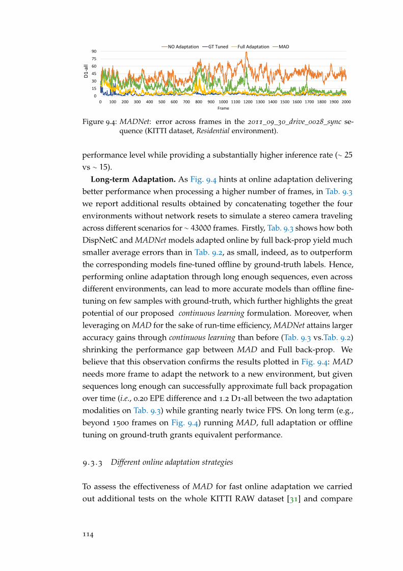
0
15
30
45
60
75
90
0 100 200 300 400 500 600 700 800 900 1000 1100 1200 1300 1400 1500 1600 1700 1800 1900 2000
D1
-all
Frame
NO Adaptation GT Tuned Full Adaptation MAD
Figure 9.4: MADNet: error across frames in the 2011_09_30_drive_0028_sync se-quence (KITTI dataset, Residential environment).
performance level while providing a substantially higher inference rate (∼ 25vs ∼ 15).
Long-term Adaptation. As Fig. 9.4 hints at online adaptation deliveringbetter performance when processing a higher number of frames, in Tab. 9.3we report additional results obtained by concatenating together the fourenvironments without network resets to simulate a stereo camera travelingacross different scenarios for ∼ 43000 frames. Firstly, Tab. 9.3 shows how bothDispNetC and MADNet models adapted online by full back-prop yield muchsmaller average errors than in Tab. 9.2, as small, indeed, as to outperformthe corresponding models fine-tuned offline by ground-truth labels. Hence,performing online adaptation through long enough sequences, even acrossdifferent environments, can lead to more accurate models than offline fine-tuning on few samples with ground-truth, which further highlights the greatpotential of our proposed continuous learning formulation. Moreover, whenleveraging on MAD for the sake of run-time efficiency, MADNet attains largeraccuracy gains through continuous learning than before (Tab. 9.3 vs.Tab. 9.2)shrinking the performance gap between MAD and Full back-prop. Webelieve that this observation confirms the results plotted in Fig. 9.4: MADneeds more frame to adapt the network to a new environment, but givensequences long enough can successfully approximate full back propagationover time (i.e., 0.20 EPE difference and 1.2 D1-all between the two adaptationmodalities on Tab. 9.3) while granting nearly twice FPS. On long term (e.g.,beyond 1500 frames on Fig. 9.4) running MAD, full adaptation or offlinetuning on ground-truth grants equivalent performance.
9 .3 .3 Different online adaptation strategies
To assess the effectiveness of MAD for fast online adaptation we carriedout additional tests on the whole KITTI RAW dataset [31] and compare
114
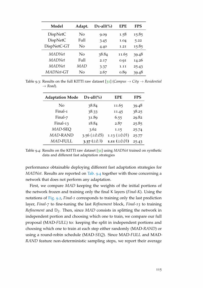
Model Adapt. D1-all(%) EPE FPS
DispNetC No 9.09 1.58 15.85
DispNetC Full 3.45 1.04 5.22
DispNetC-GT No 4.40 1.21 15.85
MADNet No 38.84 11.65 39.48
MADNet Full 2.17 0.91 14.26
MADNet MAD 3.37 1.11 25.43
MADNet-GT No 2.67 0.89 39.48
Table 9.3: Results on the full KITTI raw dataset [31] (Campus→ City→ Residential→ Road).
Adaptation Mode D1-all(%) EPE FPS
No 38.84 11.65 39.48
Final-1 38.33 11.45 38.25
Final-7 31.89 6.55 29.82
Final-13 18.84 2.87 25.85
MAD-SEQ 3.62 1.15 25.74
MAD-RAND 3.56 (±0.05) 1.13 (±0.01) 25.77
MAD-FULL 3.37 (±0.1) 1.11 (±0.01) 25.43
Table 9.4: Results on the KITTI raw dataset [31] using MADNet trained on syntheticdata and different fast adaptation strategies
performance obtainable deploying different fast adaptation strategies forMADNet. Results are reported on Tab. 9.4 together with those concerning anetwork that does not perform any adaptation.
First, we compare MAD keeping the weights of the initial portions ofthe network frozen and training only the final K layers (Final-K). Using thenotations of Fig. 9.2, Final-1 corresponds to training only the last predictionlayer, Final-7 to fine-tuning the last Refinement block, Final-13 to trainingRefinement and D2. Then, since MAD consists in splitting the network inindependent portion and choosing which one to train, we compare our fullproposal (MAD-FULL) to: keeping the split in independent portions andchoosing which one to train at each step either randomly (MAD-RAND) orusing a round-robin schedule (MAD-SEQ). Since MAD-FULL and MAD-RAND feature non-deterministic sampling steps, we report their average
115
performance obtained across 5 independent runs on the whole dataset withthe corresponding standard deviations between brackets.
By comparing the Final entries with the ones featuring MAD we can clearlysee how training only the final layers is not enough to successfully performonline adaptation. Even training as many as 13 last layers (at a comparablecomputational cost with our proposed MAD) we are at most able to halvethe initial error rate, with performance still far from optimal. The threevariants of MAD by training the whole network can successfully reducethe D1-all to 1
10 of the original. Among the three options, our proposedlayer selection heuristic provides the best overall performance even takinginto account the slightly higher standard deviation caused by our samplingstrategy. Moreover, the computational cost to pay to deploy our heuristic isnegligible losing only 0.3 FPS compared to the other two options.
9 .3 .4 Deployment on embedded platforms
All the tests reported so far have been executed on a desktop PC equippedwith a Nvidia 1080 Ti GPU. Unfortunately for many application like roboticsor autonomous vehicles, it is unrealistic to rely on such high end and power-hungry hardware. One of the key benefits of MADNet, however, is itslightweight architecture conducive to easy deployment on lower-powerembedded platforms. Thus, we evaluated MADNet on a Nvidia Jetson TX2
while processing stereo pairs at the full KITTI resolution and comparedit to StereoNet [138] implemented using the same framework (i.e., samelevel of optimization). We measured 0.26s for a single forward of MADNetversus 0.76-0.96s required by StereoNet, respectively with 1 or 3 refinementmodules. Thus, MADNet runs faster and more accurately than existing fastarchitectures [138], making it an appealing alternative also for embeddedapplications.
116
10L E A R N I N G T O A D A P T F O R S T E R E O
In Chap. 9 we have shown how online adaptation can be deployed to adapt adeep stereo model to an unseen environment, in this chapter we are going toexpand on the topic and propose a way of improving the effectiveness of theadaptation process. In detail, we propose to investigate the use of syntheticdata to learn a model offline, which, when deployed, can quickly adapt toany unseen target domain online in an unsupervised manner, eliminatingthe need for expensive data collection.
We formulate this learning-to-adapt problem using a model agnostic meta-learning framework [90]. Specifically, we devise a meta-learning scheme forcontinuous adaptation. Our goal is to learn a model offline using syntheticdata, which can continuously adapt to unseen real video sequences in an un-supervised manner at test time. This means our model is always in trainingmode and its parameters are automatically tuned to the current environmentonline without the need for supervision. Such an online adaptation scenariohas been considered previously in the literature Chap. 9 and [156]. However,in this work, we explicitly learn-to-adapt which allows us to achieve superiorperformance.
Our meta-learning approach directly incorporates the online adaptationstep into the learning objective, thus allowing us to obtain a base set ofweights that are better suited for unsupervised online adaptation. However,since the adaptation is performed in an unsupervised manner (e.g., basedon re-projection loss [68, 93]), it is inherently noisy, causing an adverse effecton the overall algorithm. To alleviate this deficiency, we learn a confidencemeasure on the unsupervised loss and use the confidence weighted lossto update the network parameters. This effectively masks the noise inthe adaptation step, preventing detrimental parameter updates. In ourcase, the confidence measures are predicted using a small CNN which isincorporated into the meta-learning framework, allowing the network to betrained end-to-end with no additional supervision.
In our experiments, we make use of a synthetic stereo dataset (Syn-thia [81]), a real-world dataset (KITTI-raw [122]), and generate a newsynthetic dataset containing multiple sequences of varying weather and
117
lighting conditions using the Carla simulator [89]. We evaluate our al-gorithm between two pairs of dataset domains: 1) Carla to Synthia; and 2)Carla or Synthia to KITTI-raw. In all experiments, our learning-to-adaptmethod consistently outperforms the previous unsupervised adaptationmethod (Chap. 9), validating our hypothesis that learning-to-adapt providesan effective framework for stereo.
10 .1 related works
Meta-learning is a long-standing problem in machine learning [1, 2, 4] thattries to exploit structures in data to learn more effective learning rules oralgorithms. Most of the recent development in meta-learning algorithmshave been focused on the few shot classification task [84, 110, 118], with fewexceptions like [90, 142] extending their models for simple function regres-sion and reinforcement learning. In [90] the authors propose to constrainthe learning rule for the model to be stochastic gradient descent and updatethe initial weight configuration of a network to make it more suited to learnnew tasks. This simple formulation has been recently extended to addressonline adaptation in reinforcement learning using meta-learning to adaptto changing agents [133] or non-stationary and competitive environments[116]. Our work builds on [90] by modifying it to use structured regression,unsupervised loss functions and temporal consistency during the updateprocess.
10 .2 problem setup and preliminaries
In this section, first we formalize online adaptation and discuss its advant-ages. We then briefly review a meta-learning algorithm which we willtranspose into our continuous adaptation scenario.
10 .2 .1 Online Adaptation for Stereo
Let us denote two datasets of stereo video sequences: Ds (supervised), withavailable ground truth, and Du (unsupervised), without ground truth. Wewould like to learn network parameters offline using Ds, and use Du asthe target (or test) domain. However, in contrast to the standard evaluation
118

(a) Left frame (b) Equalized (c) KITTI tuned (d) Ours
Figure 10.1: We demonstrate the effectiveness of continuous adaptation on a chal-lenging video sequence from [30]. (a) Left input frame, (b) histogramequalized frame for visualization purpose, (c) disparity map producedby a Dispnet-Corr1D [76] trained on annotated real data from KITTI, (d)disparity map produced by a Dispnet-Corr1D [76] trained on syntheticdata using our learning-to-adapt framework and continuously adaptedon this video sequence. As shown, the prediction of our method doesnot suffer from the same artifacts as (c) (highlighted in white), thusillustrating the advantage of continuous unsupervised adaptation.
setting and following the evaluation protocol of Chap. 9 and [156], the modelis allowed to adapt to the target domain in an unsupervised manner.
Formally, let the parameters of the base model trained on Ds be θ. Givenan unseen target video sequence V ∈ Du, the adaptation is iterativelyperformed for each pair of frames in the sequence, using gradient descenton a predefined unsupervised loss function (Lu). At iteration t, the onlineadaptation can be written as:
θt ← θt−1 −α∇θLu(θt−1, it) , (10.1)
where θ0 = θ, α > 0 is the learning rate and it denotes the stereo pair of tth
frame of the sequence V. Note that the network parameters are continuouslyupdated for the entire video in a sequential manner. This process is repeatedfor each video sequence starting from the learned parameters θ.
motivating example . To show that deep CNN based stereo networksare highly sensitive to domain-shift and that online adaptation is indeednecessary, we give a motivating example below. We select a video sequencefrom [30] as a test domain, where the environment is similar to that ofKITTI but features extreme weather conditions (e.g., night, snow, etc.). Wecompare the predicted disparities of a Dispnet-Corr1D network [76] for twotraining regimes. The first is fine-tuned on the KITTI training sets [27, 57],and the second is trained on synthetic data using our learning-to-adapt
119
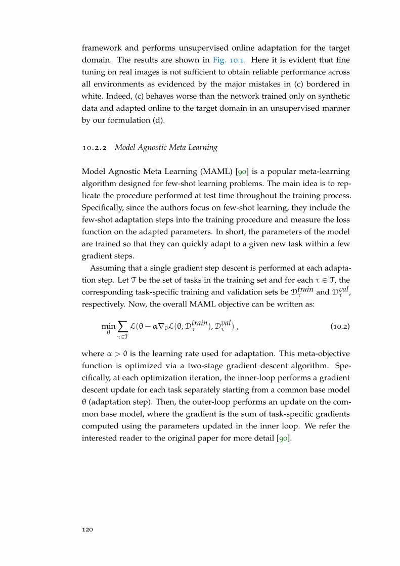
framework and performs unsupervised online adaptation for the targetdomain. The results are shown in Fig. 10.1. Here it is evident that finetuning on real images is not sufficient to obtain reliable performance acrossall environments as evidenced by the major mistakes in (c) bordered inwhite. Indeed, (c) behaves worse than the network trained only on syntheticdata and adapted online to the target domain in an unsupervised mannerby our formulation (d).
10 .2 .2 Model Agnostic Meta Learning
Model Agnostic Meta Learning (MAML) [90] is a popular meta-learningalgorithm designed for few-shot learning problems. The main idea is to rep-licate the procedure performed at test time throughout the training process.Specifically, since the authors focus on few-shot learning, they include thefew-shot adaptation steps into the training procedure and measure the lossfunction on the adapted parameters. In short, the parameters of the modelare trained so that they can quickly adapt to a given new task within a fewgradient steps.
Assuming that a single gradient step descent is performed at each adapta-tion step. Let T be the set of tasks in the training set and for each τ ∈ T, thecorresponding task-specific training and validation sets be Dtrain
τ and Dvalτ ,
respectively. Now, the overall MAML objective can be written as:
minθ
∑τ∈T
L(θ−α∇θL(θ,Dtrainτ ),Dval
τ ) , (10.2)
where α > 0 is the learning rate used for adaptation. This meta-objectivefunction is optimized via a two-stage gradient descent algorithm. Spe-cifically, at each optimization iteration, the inner-loop performs a gradientdescent update for each task separately starting from a common base modelθ (adaptation step). Then, the outer-loop performs an update on the com-mon base model, where the gradient is the sum of task-specific gradientscomputed using the parameters updated in the inner loop. We refer theinterested reader to the original paper for more detail [90].
120
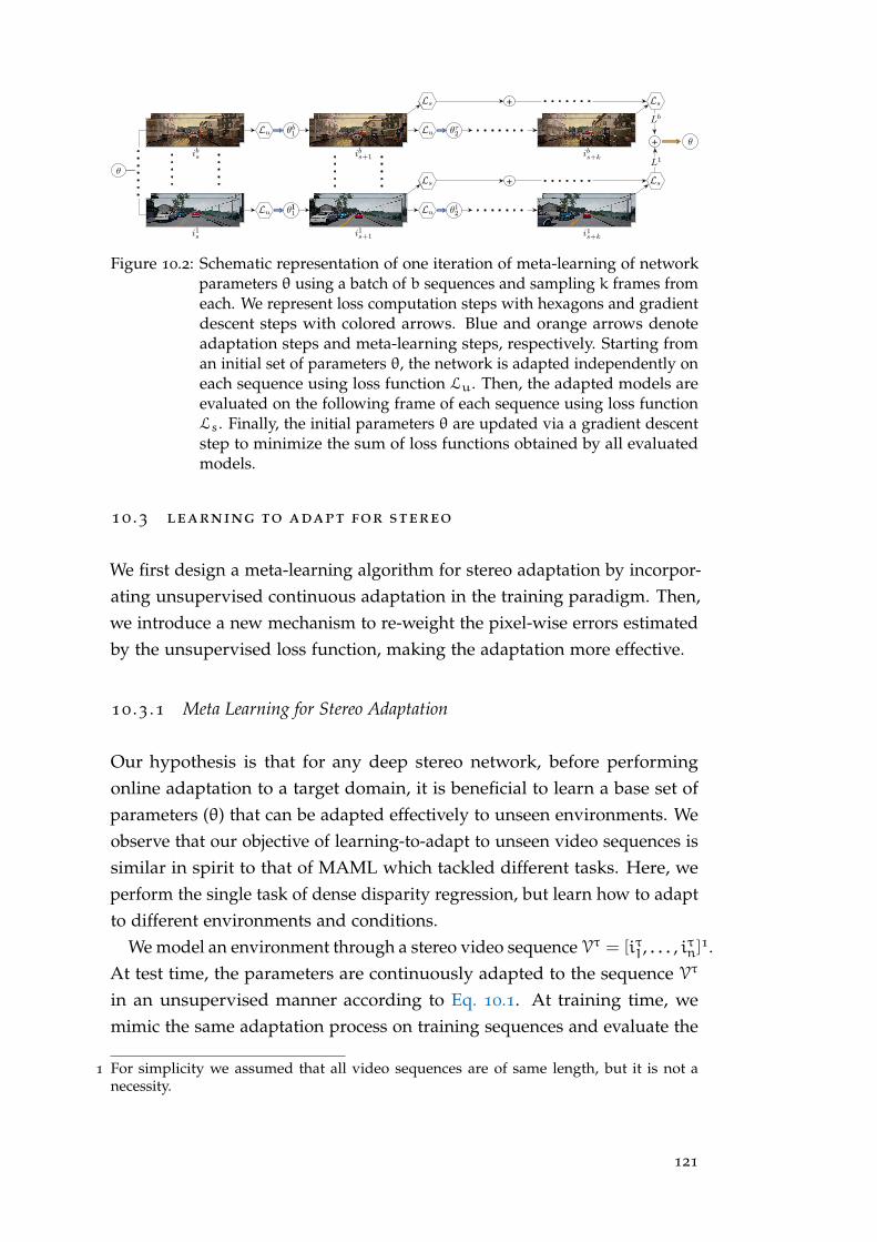
+
+
+
Figure 10.2: Schematic representation of one iteration of meta-learning of networkparameters θ using a batch of b sequences and sampling k frames fromeach. We represent loss computation steps with hexagons and gradientdescent steps with colored arrows. Blue and orange arrows denoteadaptation steps and meta-learning steps, respectively. Starting froman initial set of parameters θ, the network is adapted independently oneach sequence using loss function Lu. Then, the adapted models areevaluated on the following frame of each sequence using loss functionLs. Finally, the initial parameters θ are updated via a gradient descentstep to minimize the sum of loss functions obtained by all evaluatedmodels.
10 .3 learning to adapt for stereo
We first design a meta-learning algorithm for stereo adaptation by incorpor-ating unsupervised continuous adaptation in the training paradigm. Then,we introduce a new mechanism to re-weight the pixel-wise errors estimatedby the unsupervised loss function, making the adaptation more effective.
10 .3 .1 Meta Learning for Stereo Adaptation
Our hypothesis is that for any deep stereo network, before performingonline adaptation to a target domain, it is beneficial to learn a base set ofparameters (θ) that can be adapted effectively to unseen environments. Weobserve that our objective of learning-to-adapt to unseen video sequences issimilar in spirit to that of MAML which tackled different tasks. Here, weperform the single task of dense disparity regression, but learn how to adaptto different environments and conditions.
We model an environment through a stereo video sequence Vτ = [iτ1, . . . , iτn]
1.At test time, the parameters are continuously adapted to the sequence Vτ
in an unsupervised manner according to Eq. 10.1. At training time, wemimic the same adaptation process on training sequences and evaluate the
1 For simplicity we assumed that all video sequences are of same length, but it is not anecessity.
121
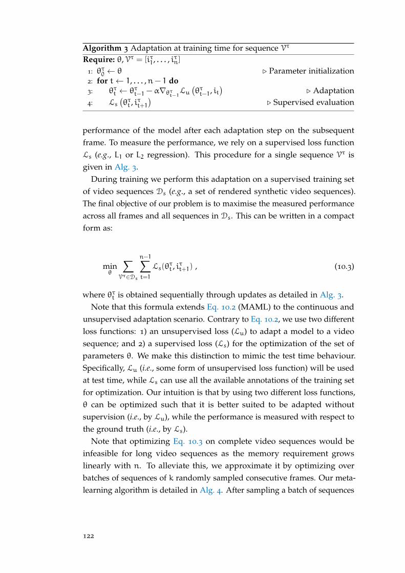
Algorithm 3 Adaptation at training time for sequence Vτ
Require: θ,Vτ = [iτ1, . . . , iτn]
1: θτ0 ← θ . Parameter initialization2: for t← 1, . . . ,n− 1 do3: θτt ← θτt−1 −α∇θτt−1Lu
(θτt−1, it
). Adaptation
4: Ls(θτt , i
τt+1
). Supervised evaluation
performance of the model after each adaptation step on the subsequentframe. To measure the performance, we rely on a supervised loss functionLs (e.g., L1 or L2 regression). This procedure for a single sequence Vτ isgiven in Alg. 3.
During training we perform this adaptation on a supervised training setof video sequences Ds (e.g., a set of rendered synthetic video sequences).The final objective of our problem is to maximise the measured performanceacross all frames and all sequences in Ds. This can be written in a compactform as:
minθ
∑Vτ∈Ds
n−1∑t=1
Ls(θτt , i
τt+1) , (10.3)
where θτt is obtained sequentially through updates as detailed in Alg. 3.Note that this formula extends Eq. 10.2 (MAML) to the continuous and
unsupervised adaptation scenario. Contrary to Eq. 10.2, we use two differentloss functions: 1) an unsupervised loss (Lu) to adapt a model to a videosequence; and 2) a supervised loss (Ls) for the optimization of the set ofparameters θ. We make this distinction to mimic the test time behaviour.Specifically, Lu (i.e., some form of unsupervised loss function) will be usedat test time, while Ls can use all the available annotations of the training setfor optimization. Our intuition is that by using two different loss functions,θ can be optimized such that it is better suited to be adapted withoutsupervision (i.e., by Lu), while the performance is measured with respect tothe ground truth (i.e., by Ls).
Note that optimizing Eq. 10.3 on complete video sequences would beinfeasible for long video sequences as the memory requirement growslinearly with n. To alleviate this, we approximate it by optimizing overbatches of sequences of k randomly sampled consecutive frames. Our meta-learning algorithm is detailed in Alg. 4. After sampling a batch of sequences
122
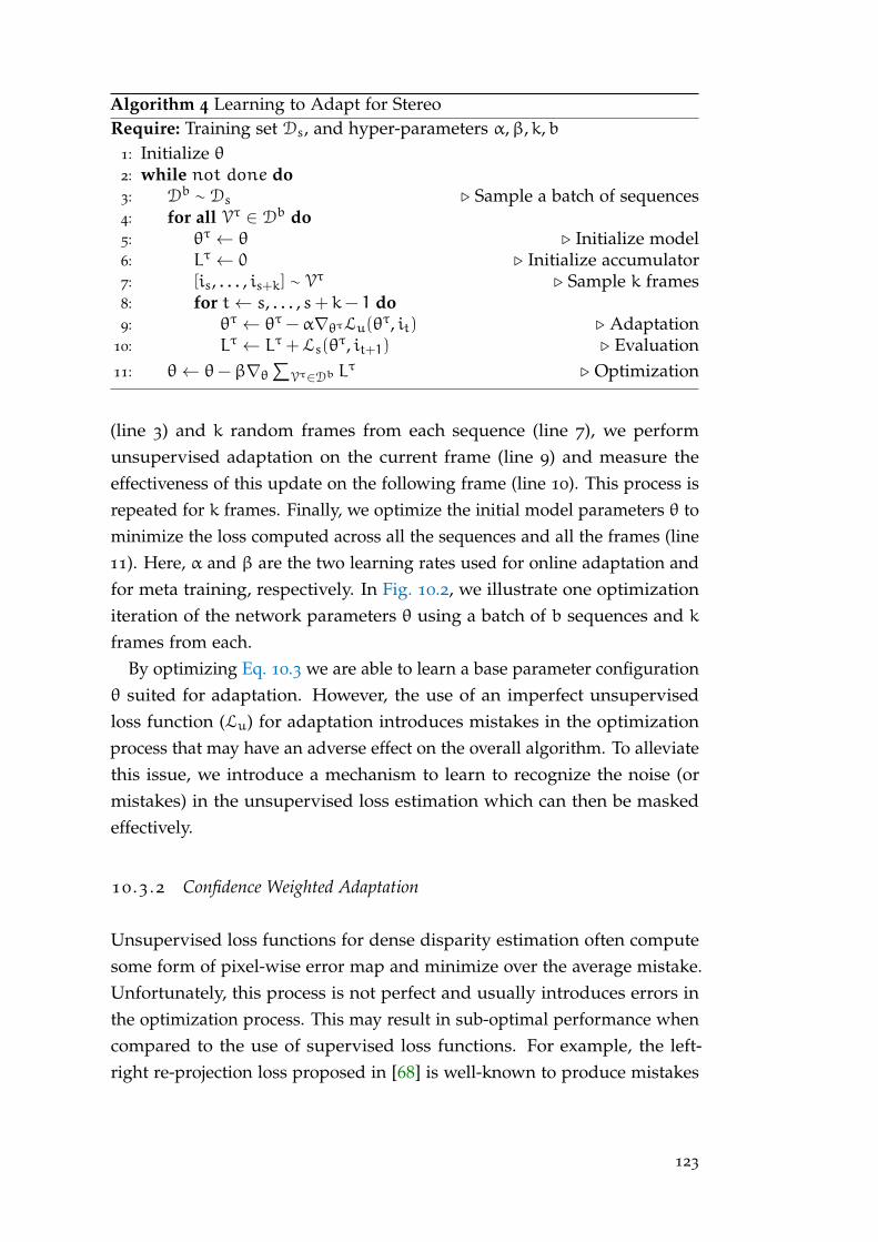
Algorithm 4 Learning to Adapt for StereoRequire: Training set Ds, and hyper-parameters α,β,k,b
1: Initialize θ2: while not done do3: Db ∼ Ds . Sample a batch of sequences4: for all Vτ ∈ Db do5: θτ ← θ . Initialize model6: Lτ ← 0 . Initialize accumulator7: [is, . . . , is+k] ∼ Vτ . Sample k frames8: for t← s, . . . , s+ k− 1 do9: θτ ← θτ −α∇θτLu(θτ, it) . Adaptation
10: Lτ ← Lτ +Ls(θτ, it+1) . Evaluation
11: θ← θ−β∇θ∑
Vτ∈Db Lτ . Optimization
(line 3) and k random frames from each sequence (line 7), we performunsupervised adaptation on the current frame (line 9) and measure theeffectiveness of this update on the following frame (line 10). This process isrepeated for k frames. Finally, we optimize the initial model parameters θ tominimize the loss computed across all the sequences and all the frames (line11). Here, α and β are the two learning rates used for online adaptation andfor meta training, respectively. In Fig. 10.2, we illustrate one optimizationiteration of the network parameters θ using a batch of b sequences and kframes from each.
By optimizing Eq. 10.3 we are able to learn a base parameter configurationθ suited for adaptation. However, the use of an imperfect unsupervisedloss function (Lu) for adaptation introduces mistakes in the optimizationprocess that may have an adverse effect on the overall algorithm. To alleviatethis issue, we introduce a mechanism to learn to recognize the noise (ormistakes) in the unsupervised loss estimation which can then be maskedeffectively.
10 .3 .2 Confidence Weighted Adaptation
Unsupervised loss functions for dense disparity estimation often computesome form of pixel-wise error map and minimize over the average mistake.Unfortunately, this process is not perfect and usually introduces errors inthe optimization process. This may result in sub-optimal performance whencompared to the use of supervised loss functions. For example, the left-right re-projection loss proposed in [68] is well-known to produce mistakes
123

Weighting Network
Reprojection Loss
Network
Figure 10.3: Schematic representation of our weighted adaptation for a single stereoframe using an unsupervised re-projection based loss function Lu(bright colors indicate higher values). The system takes a stereo-pair(it) and computes a disparity map as well as a re-projection loss (εt).This loss is then weighted according to Wt effectively masking themistakes.
in occluded areas and reflective surfaces. These mistakes are not due tobad predictions by the disparity estimation model, but instead are due todifferences between the left and right frames. Ideally, we would like to havea confidence function to detect erroneous estimations of this loss such thatthey can be effectively masked. However, training such a confidence functionmight be difficult since there is no easy procedure to produce ground-truthannotations for this task. We propose to avoid explicit supervised training,and instead, automatically learn to detect noise in the loss estimations byincorporating this new objective into our meta-learning formulation.
In particular, we propose to learn a small CNN that takes a pixel-wiseerror map estimated by Lu as an input and produces a tensor W as anoutput, which has the same shape as the input and its elements are between0 and 1. This output can be interpreted as a per pixel confidence on thereliability of the loss estimation with 1 corresponding to high reliability. Wecan now mask out potentially erroneous estimations by multiplying the lossvalues by their corresponding confidence values. The result is a cleanermeasurement of the loss function that would reduce detrimental weightupdates due to incorrect loss values. The idea of masking or weighting thecontribution of single examples in the presence of noise or class imbalancein the labels has been previously studied for supervised classification in [137,
124
146]. In our case, we transpose the similar idea to pixel-wise loss, estimatedfor a dense regression task and directly predict a dense confidence map.
Let W = F(η, ε) be the mask produced by the re-weighting networkparametrized by η and ε = Lu(θ, i) be the estimated pixel-wise error mapcomputed on the prediction of the disparity model with parameter θ onstereo frame i. We normalize the elements of W by dividing each one ofthem by the number of elements in W. Now, by modifying Eq. 10.1, the finalweighted adaptation formula can be written as:
θt ← θt−1 −α∇θ(Wt �Lu(θt−1, it)
),
Wt = F(η,Lu(θt−1, it)) ,(10.4)
where θ0 = θ and � indicating the element-wise product between thematrices. We denote θ as the network parameters which are updated accord-ing to the unsupervised loss weighted by W.
In Fig. 10.3, we show a schematic representation of our proposed weightedadaptation computed from a single stereo input frame it. On the bottomright corner we give a visualization of the error map produced by an unsu-pervised re-projection loss Lu, while the top right corner shows a possibleconfidence mask Wt. In this example the weighting network is maskingerrors due to occlusions (e.g., on the left side of the car) and due to reflections(e.g., the puddles on the road).
Since supervision is not available for W, we indirectly train η by incorpor-ating Eq. 10.4 inside the meta-learning objective described in Eq. 10.3. Thefinal objective of our complete system becomes:
minθ,η
∑Vτ∈Ds
n−1∑t=1
Ls(θτt , i
τt) . (10.5)
Here, θτt are the parameter of the model updated according to the weightedunsupervised loss function on sequence Vτ. As such it depends on η and θat the same time. The whole network can be trained end-to-end with theonly supervision coming from the depth annotations used to compute Ls.Both θ and η are tuned to maximize the network performances after fewsteps of optimization as measured by Ls. By optimizing a single objectivefunction we are able to learn the parameter (η) of the weighting network,and a set of base weights for the disparity estimation model (θ) which allowfor fast adaptation.
125
10 .4 experiments
This section presents an evaluation of the quality of our proposed adaptationmethod. Firstly, we lay out our evaluation setup in Sec. 10.4.1. Secondly,in Sec. 10.4.2, we provide qualitative and quantitative results for two pairsof domains: 1) synthetic to real (i.e., training on synthetic data and testingon real data from KITTI); and 2) synthetic to synthetic (i.e., training on onesynthetic dataset and testing on a different synthetic domain). Finally, inSec. 10.4.3 we report qualitative results illustrating our confidence weightedloss.
10 .4 .1 Experimental Setup
datasets . In our experimental evaluation we simulate realistic test con-ditions, in which no data from the target domain is available. We thereforeuse training and testing data sampled from two completely disjoint datasets.For the real dataset, we use the 71 different sequences of the KITTI-rawdataset [31] (denoted as KITTI) accounting for ∼43K images with sparsedepth annotations provided by [122].
For the synthetic dataset, we have used the FlyingThings3D dataset [76](shortened F3D) to perform an initial training of the networks from randominitialization. Then, we use the Synthia dataset [81] as a synthetic datasetcontaining scenarios similar to KITTI. The dataset is composed of 50 differentvideo sequences rendered in different seasons and weather conditions for atotal of ∼45K images. For this dataset we scaled the image to half resolutionto bring the disparity into the same range as KITTI.
Finally, using the Carla simulator[89], we have rendered a new dataset(referenced as Carla) composed of 25 different video sequences, each beinga thousand frames long, with accurate ground truth data for each frame.Each video sequence is rendered in 15 different weather conditions to addvariance to the dataset. Resulting in a total of 375K frames. During therendering we set up the virtual cameras to match the geometry of the realKITTI dataset (i.e., same baseline, field of view and similar image resolution).
network architectures . For the experiments we have selected theDispnet-Corr1D [76] architecture (shortened to Dispnet). For all the evalu-ation tests, we pretrain the networks on F3D to obtain a set of weights that
126
will be used as an initialization across all the other tests. We implementthe confidence function introduced in Sec. 10.3.2 as a small three layer fullyconvolutional CNN with batch normalization. The network takes the re-projection error scaled to quarter resolution as an input and produces anoutput at the same resolution. The prediction is then scaled to full resolutionusing bilinear upsampling.
evaluation protocol . After an initial offline training, we performonline adaptation and evaluate models on sequences of stereo frames. To testindependent adaptations for each sequence, we reset the disparity networkto its trained weight configuration at the beginning of each test sequence.Then, for each frame, first, we measure the performance of the current modeland then we adapt it by a single step of back-propagation and weight updateaccording to Eq. 10.1 before moving to the next frame. We do not measurethe performance on frames already used for adaptation.
metrics . We measure performance according to both average End PointError (EPE) and percentage of pixels with disparity error larger than 3
(D1-all). Firstly, we measure both metrics independently for each frameto plot performance as a function of the number of frames processed foradaptation. Secondly, we can average both metrics over each sequence andfinally average over all the dataset.
offline training . After the initial pretraining on F3D we fine tunethe networks on a training set with our learning-to-adapt framework, weuse k = 3 consecutive frames for each sample and set the learning ratesα = 0.00001 and β = 0.0001
online adaptation. We use the left-right re-projected unsupervisedloss [93] for the adaptation. Optimization is performed with SGD withmomentum, where the momentum value is set to 0.9 and a learning rate setto 0.0001.
10 .4 .2 Results
We evaluate our learning-to-learn method between pairs of datasets, onefor training, and one for evaluation. We consider two scenarios: 1) synthetic
127

Method Training set D1-all (%) EPE ∆D1 ∆EPE
(a) SL - 9.43 1.62 - -(b) SL+Ad - 7.81 1.44 -1.62 -0.18
(c) SL Carla 7.46 1.48 - -(d) SL+Ad Carla 5.26 1.20 -2.20 -0.28
(e) SL Synthia 8.55 1.51 - -(f) SL+Ad Synthia 5.33 1.19 -3.22 -0.32
Our
s
(g) L2A Carla 8.41 1.51 - -(h) L2A+WAd Carla 4.49 1.12 -3.92 -0.39(i) L2A Synthia 8.22 1.50 - -(j) L2A+WAd Synthia 4.65 1.14 -3.57 -0.36
(k) SL (ideal) KITTI 4.26 1.12 - -
Table 10.1: Performance on KITTI for the Dispnet network trained according todifferent methods after initialization from F3D. It can clearly be seenthat online adaptation (+Ad/+WAd) provides a significant improvementcompared to when it is left out. The best results are obtained when thetraining is achieved using the L2A+WAd framework. Line (k) indicatesan upper bound on how well Dispnet can perform when fine tunedon a subset of samples from the target domain. The last two columnsindicate the performance improvement with adaptation, and as it isevident in the table, our L2A+WAd method obtains the largest increasein performance with adaptation.
to real and 2) synthetic to synthetic. We compare the results of our learning-to-adapt framework (L2A), and the method trained using a supervised L1regression loss (SL). Methods performing unsupervised online adaptationat test time are indicated by appending +Ad to the training method, andconfidence weighted adaptation by +WAd.
Synthetic to Real
The most interesting scenario is the one where training on a syntheticdomain is followed by testing on a real-life domain. Specifically, we train onSynthia or Carla and then evaluate on the KITTI dataset.
The results for the Dispnet architecture are provided in Tab. 10.1. Lines(a) to (f) report the performance when the network weights are obtainedin a standard way (using a supervised L1 loss function). As expected, thenetwork performs poorly when tested on a different domain with respect to
128
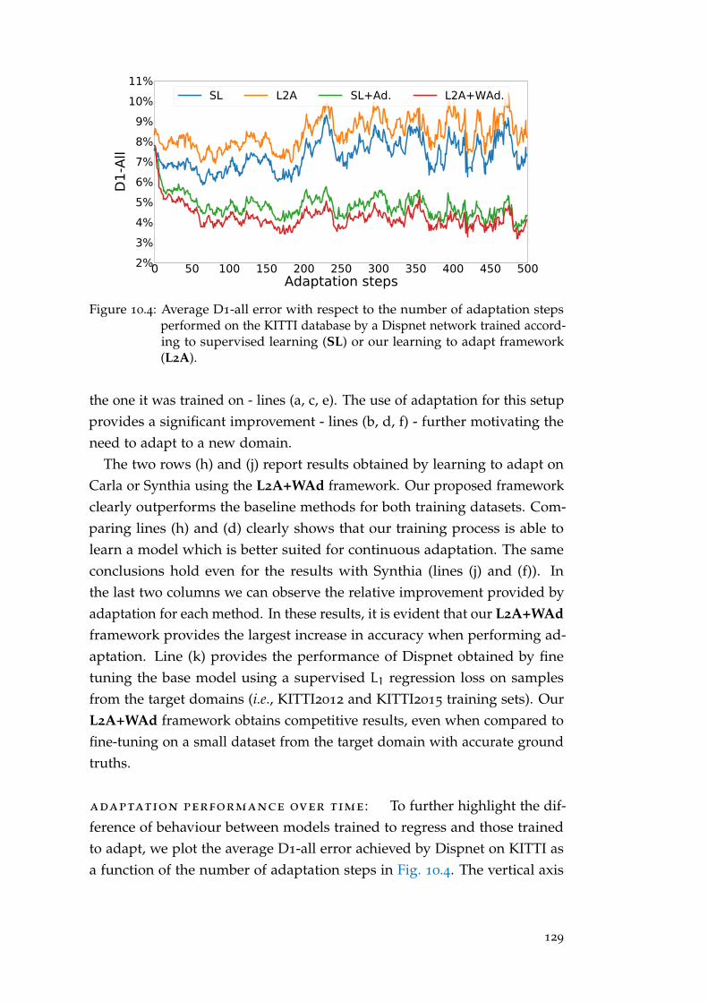
0 50 100 150 200 250 300 350 400 450 500Adaptation steps
2%3%4%5%6%7%8%9%
10%11%
D1-A
llSL L2A SL+Ad. L2A+WAd.
Figure 10.4: Average D1-all error with respect to the number of adaptation stepsperformed on the KITTI database by a Dispnet network trained accord-ing to supervised learning (SL) or our learning to adapt framework(L2A).
the one it was trained on - lines (a, c, e). The use of adaptation for this setupprovides a significant improvement - lines (b, d, f) - further motivating theneed to adapt to a new domain.
The two rows (h) and (j) report results obtained by learning to adapt onCarla or Synthia using the L2A+WAd framework. Our proposed frameworkclearly outperforms the baseline methods for both training datasets. Com-paring lines (h) and (d) clearly shows that our training process is able tolearn a model which is better suited for continuous adaptation. The sameconclusions hold even for the results with Synthia (lines (j) and (f)). Inthe last two columns we can observe the relative improvement provided byadaptation for each method. In these results, it is evident that our L2A+WAdframework provides the largest increase in accuracy when performing ad-aptation. Line (k) provides the performance of Dispnet obtained by finetuning the base model using a supervised L1 regression loss on samplesfrom the target domains (i.e., KITTI2012 and KITTI2015 training sets). OurL2A+WAd framework obtains competitive results, even when compared tofine-tuning on a small dataset from the target domain with accurate groundtruths.
adaptation performance over time : To further highlight the dif-ference of behaviour between models trained to regress and those trainedto adapt, we plot the average D1-all error achieved by Dispnet on KITTI asa function of the number of adaptation steps in Fig. 10.4. The vertical axis
129
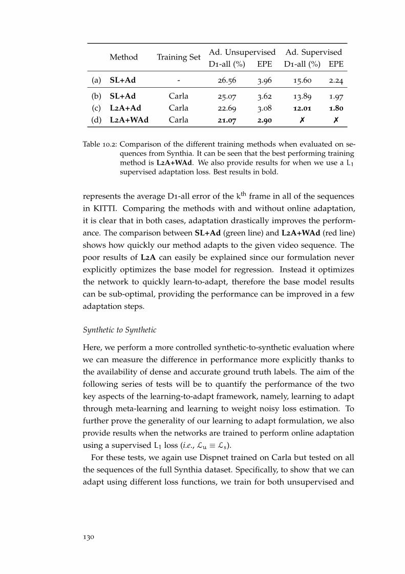
Method Training Set Ad. Unsupervised Ad. SupervisedD1-all (%) EPE D1-all (%) EPE
(a) SL+Ad - 26.56 3.96 15.60 2.24
(b) SL+Ad Carla 25.07 3.62 13.89 1.97
(c) L2A+Ad Carla 22.69 3.08 12.01 1.80(d) L2A+WAd Carla 21.07 2.90 7 7
Table 10.2: Comparison of the different training methods when evaluated on se-quences from Synthia. It can be seen that the best performing trainingmethod is L2A+WAd. We also provide results for when we use a L1supervised adaptation loss. Best results in bold.
represents the average D1-all error of the kth frame in all of the sequencesin KITTI. Comparing the methods with and without online adaptation,it is clear that in both cases, adaptation drastically improves the perform-ance. The comparison between SL+Ad (green line) and L2A+WAd (red line)shows how quickly our method adapts to the given video sequence. Thepoor results of L2A can easily be explained since our formulation neverexplicitly optimizes the base model for regression. Instead it optimizesthe network to quickly learn-to-adapt, therefore the base model resultscan be sub-optimal, providing the performance can be improved in a fewadaptation steps.
Synthetic to Synthetic
Here, we perform a more controlled synthetic-to-synthetic evaluation wherewe can measure the difference in performance more explicitly thanks tothe availability of dense and accurate ground truth labels. The aim of thefollowing series of tests will be to quantify the performance of the twokey aspects of the learning-to-adapt framework, namely, learning to adaptthrough meta-learning and learning to weight noisy loss estimation. Tofurther prove the generality of our learning to adapt formulation, we alsoprovide results when the networks are trained to perform online adaptationusing a supervised L1 loss (i.e., Lu ≡ Ls).
For these tests, we again use Dispnet trained on Carla but tested on allthe sequences of the full Synthia dataset. Specifically, to show that we canadapt using different loss functions, we train for both unsupervised and
130
supervised adaptation2, and evaluate the performance of the following train-ing scenarios: (a) Using the initial model trained using F3D; (b) Trainingon Carla using a supervised L1 loss; (c) Using the learning-to-adapt frame-work without confidence weighted loss; (d) Using the learning-to-adaptframework with confidence weighted loss.
We report the results in Tab. 10.2, where it can be seen that explicitlytraining Dispnet to adapt using our learning-to-learn formulation (c), al-lows the network to exploit the online adaptation and greatly improve theperformance both in the unsupervised and supervised adaptation setups.Finally, it can also be seen that weighting the unsupervised loss valuesresults in superior performance (d). For this test set up, the results clearlydemonstrate how our formulation is able to learn a weight configurationthat is more inclined to be adapted to a new environment.
10 .4 .3 Confidence Weighted Loss Function
In Fig. 10.5, we show a visualization of the confidence masks and weightederrors optimized by our confidence guided adaptation loss described inSec. 10.3.2. The predicted confidence maps effectively mask out occludedregions in the image while keeping the useful error signals in the rest of theimage (low confidence areas are encoded as dark pixels). Errors on occludedregions, e.g., to the left of the traffic sign in the left column or to the left of thecar in the right column, are effectively masked out, producing a cleaner errorestimation that will improve adaptation performances. We wish to highlightthat the confidence network has been trained without any direct supervisionand only on Carla, nevertheless, it seems to be able to generalize well toKITTI. We believe this ability to generalize is mainly due to the avoidanceof working directly with RGB inputs, which inevitably change drasticallybetween datasets. Instead, the confidence network relies on the estimatedre-projection error, which is more consistent across different environments.
2 In online adaptation we use the L1 loss between the predicted disparity and the groundtruth annotations for each stereo pair.
131
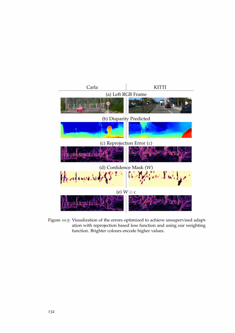
Carla KITTI(a) Left RGB Frame
(b) Disparity Predicted
(c) Reprojection Error (ε)
(d) Confidence Mask (W)
(e) W � ε
Figure 10.5: Visualization of the errors optimized to achieve unsupervised adapt-ation with reprojection based loss function and using our weightingfunction. Brighter colours encode higher values.
132
11C O N C L U S I O N S
In this part, we have proposed different procedures to adapt depth estima-tion networks to unseen environments without the need for ground truthdata. In Chap. 8 we have shown how classic stereo algorithms can be used toproduce noisy label estimation and how confidence measure can be deployedto identify such mistakes. By combining the two source of information wewere able to design a novel confidence guided loss able to outperform allthe other self-supervised proposal in our extensive experimentation. Whilethe focus of Chap. 8 was more on the achievable precision disregarding thetraining time and amount of data needed to achieve it, in Chap. 9 we tacklethe adaptation problem from an online and continuous learning perspectiveand focus on the best trade-off between speed and accuracy. To do so wehave introduced a new fast depth estimation architecture for stereo cameras(MADNet) and a novel way to adapt it online to unseen environments whilekeeping a high throughput (MAD). In terms of absolute performance, ouronline proposal is still worse than the offline procedure proposed in Chap. 8,but we believe this to be a key contribution for real-world applicationswhere the deployment environment is unknown beforehand and dynamic-ally changing (e.g., weather conditions in an autonomous driving scenario).To furthermore boost the performance of our online formulation in Chap. 10
we have shown how it is possible to train a depth prediction model that ismore amenable to be adapted effectively to new and unseen environmentsby changing the training paradigm and deploying meta-learning techniques.We believe this to be an exciting new direction to explore as for many applic-ations having a reactive system able to compensate for sudden unexpectedchanges is key to success. We have mainly reported quantitative results onlyon an autonomous driving scenario due to the lack of properly annotateddataset in different environments. However, the qualitative results shownon our target supermarket environment seems to imply the effectiveness ofour solutions even in this completely different setup.
All the test proposed in this work concern adaptation of a pre-traineddeep neural network to new environments, however, we believe that bothour unsupervised loss formulations could also be effective in training from
133
scratch a deep neural network without any kind of supervision, we leavethis to future research. Moreover, in Chap. 8 we have shown how combiningnaively noisy labels obtained from two very different stereo algorithmsdoes not result in an improvement in performance. Recent works like[130], however, have shown how combining different disparity estimationstaking into account their confidence maps can result in reliable disparitypredictions. We plan to include in our work a similar procedure to obtainmore reliable noisy labels that might be used as pseudo ground truth foroff-line adaptation. We wish also to investigate a fast way to implementthe loss function we introduced in Chap. 8 as to deploy it inside the onlineadaptation pipeline presented in Chap. 9 since in our experiments ourconfidence guided loss always outperformed the competing reprojectionbased methods. Regarding our online formulation, we plan to test andeventually extend MAD to be applicable to any end-to-end stereo system. Wewould also like to investigate more effective methods to select the portion ofthe network to be updated online at each step. In particular, we might deploya small network trained by reinforcement learning in order to contextuallychoose which training action to perform based on the current frame and/orcurrent network state. Finally, even with our lightweight MADNet, thecomputational cost to deploy the system on embedded low power device isstill too high for most practical application as shown in Sec. 9.3.4, for thisreason, we would like to focus some research efforts on ways to make ournetwork even faster and lighter. Inspirations for this extension can come fromworks regarding the deployment of neural networks on mobile low powerdevice such as [95, 154] where different paradigms for the implementation ofefficient convolutional layers are deployed. Finally we believe that the use ofmore complex training paradigm, for example the meta-learning proceduredescribed in Chap. 10, represent a still quite fresh research field that has notyet been properly addressed, for this reason in the future we plan to betterexplore the deployment of the learning to learn paradigm in the context ofadaptation to unseen environments.
134

Part III
F I N A L R E M A R K S

12C O N C L U S I O N S
The works presented in this thesis have concerned how to effectively deploystate of the art computer vision techniques to ease and automate man-agement tasks in retail shops or supermarket. We have mainly discussedtwo macro problems: the detection and recognition of products on storeshelves (discussed in Part i) and the estimation of reliable 3D informationon unknown environments (discussed in Part ii). For both sections, wehave explained some of the peculiar shortcomings emerging from naivelyapplying state of the art computer vision techniques and how to effectivelyovercome them.
For example, referring to Part i, we have shown how classic local featurebased object detection pipeline provide satisfying results when dealingwhit rigid boxed products but fails in presence of deformable packages androtated or skewed products (see Chap. 3). We then moved on to more moderndeep learning based object detectors and verified that they can indeed betrained to effectively detect and recognize products with remarkable accuracy.Such good performance comes at the cost of requiring huge annotateddataset at training time to tune the network behavior. Since in a commonretail environment is unfeasible to think of keeping an up to date annotateddataset concerning all possible types of products exposed on shelves andconstantly retraining an inference engine to keep up with changes, wepropose in Chap. 4 to split the detection and recognition phases into twoseparate steps solved by two different algorithms. First, we carry out aclass agnostic detection phase where the task is only to recognize individualinstances of products on store shelves, then we perform recognition throughsimilarity search in a learned embedding space for product images. Weproved that our solution is able to outperform other competing methods inthe commonly used public Grocery product dataset in terms of accuracywhile keeping runtime efficiency. Finally in Chap. 5 we examined in depththe task of performing product recognition through similarity search andpropose a novel metric learning network to directly address one of themain problems in the retail scenario: the huge domain gap between imagesacquired in-store and those available for training.
137
Moving on to Part ii, we have shown how the modern state of the artalgorithms for depth estimation suffers from huge performance drops whenexposed to environments different from those used at training time. To mitig-ate the negative effects of this domain shift we have introduced in Chap. 8 anovel way to adapt depth estimation networks to new environments withoutthe need of annotated data that are usually too costly to acquire for dense3D estimation. We have proven the effectiveness of our proposal both inindoor and outdoor environments, with stereo and mono depth estimationnetworks, and only assuming the availability of stereo images from thetarget domain at training time. In Chap. 9 we tackle the same problem butpropose to solve the domain shift online performing continuous domainadaptation to new environments as soon as new frames are sensed. In ourproposal we keep the deep network always in training mode, thus slowingit down considerably, for this reason we have introduced a novel lightweightdepth estimation network (MADNet) and a modular update process (MAD)to improve network efficiency. Finally in Chap. 10 we have explored the ideaof designing the training process of a network from the beginning to makeit more suitable to be adapted quickly to new environments, we achieve soby deploying training techniques taken from the meta-learning literature.
In this thesis, we have analyzed how to apply state of the art computervision techniques in real environments to solve two very different tasks.Even if the two applications, at first sight, do not seems closely related,most of the problems that we had to face to solve them are shared. Forexample, since almost all our proposed solutions are based on deep learningtechniques, one of the main limitations that we had to overcome was howto effectively train them without relying on a huge annotated dataset thatare often too costly to produce for many real applications. We tackled thisproblem in the product recognition scenario by deploying GANs to easilyperform data augmentation and relying on embedding rather than classifierto perform product recognition, while in the dense depth estimation scenariowe designed an ad hoc unsupervised loss function. Another commonobstacle that we had to overcome across the two tasks was how to close thedomain gap between train and test data. To address this problem in theproduct scenario we deployed GANs to solve the domain shift at trainingtime by transforming images from one domain to the other, while for thedense depth estimation we have designed systems and loss functions toallow efficient continuous training and adaptation of deep learning basedmethods. We believe these problems to be more general than the single
138
examples presented in this thesis and we are excited to test some of ourproposed solutions in contexts different from those considered so far. Forexample, our online adaptation formulation could be extended to differenttasks like semantic segmentation or optical flow as long as it is possible todefine some kind of unsupervised loss function. At the same time, we havealready shown some preliminary results obtained by applying our metriclearning technique (Chap. 5) to scenario different than the retail ones. Finally,the preliminary results in Chap. 10 seems to suggest that it is possible todesign more efficient learning algorithms able to converge to good solutionsusing only a few examples. Besides applications to dense depth regression,we would like to apply the same concept to object detection algorithm soas to obtain a flexible system able to learn how to recognize new categoriesbased only on few annotated samples.
139

L I S T O F F I G U R E S
Figure 2.1 Illustration of the product recognition task with im-ages from the Grocery Product dataset [39]. Given aquery image featuring multiple products (a) identifyregions associated with individual items and recog-nize the product enclosed in each region based ona database featuring only few (usually one) referenceimages per product (two examples are shown in (b)).Example of correct recognition are showed in (a) withbounding boxes colored according to the recognizedclasses. . . . . . . . . . . . . . . . . . . . . . . . . . . . 12
Figure 3.1 Overview of our pipeline. For each step we highlightthe inputs and outputs through red and yellow boxes,respectively. Product detections throughout stages arehighlighted by green boxes, while blue lines show theedges between nodes on the graphs enconding boththe Reference and the Observed planograms. . . . . . . 16
Figure 3.2 Toy example concerning two small graphs with 4
nodes used to describe procedure FindSolution. Thecolor of each node denotes the product the numberswithin squares identify the different nodes in the text. 20
Figure 3.3 One iteration of our proposed Product Verificationstep. The estimated ROI is drawn in yellow. Thecorrect proposal is highlighted in green while othersare in red. . . . . . . . . . . . . . . . . . . . . . . . . . . 22
Figure 3.4 Ground-truth dealing with product types providedwith the Grocery Products dataset (a) and our instance-specific bounding boxes (b). In (a) a system shouldidentify at least one instance for each product type,while in (b) it should find and correctly localize allthe displayed product instances. We will refer tothe two task in Chap. 4 as Customer use case andManagement use case. . . . . . . . . . . . . . . . . . . 24
141
Figure 3.5 Evaluation of different features for UnconstrainedProduct Recognition. Results ordered from top tobottom alongside with F-Measure scores. . . . . . . . . 25
Figure 3.6 Results after Graph-based Consistency Check whenusing either BRISK or BRISK+SURF in the first step. 25
Figure 3.7 Evaluation of different choices for the final ProductVerification step of our pipeline, with BRISK featuresused in the first step. . . . . . . . . . . . . . . . . . . . 26
Figure 3.8 Qualitative results obtained by our pipeline: detecteditems are enclosed by green boxes while planogramcompliance issues are highlighted by red boxes. . . . 26
Figure 4.1 Schematic structure of our proposed product recog-nition pipeline. Dashed arrows denotes elaborationthat can be performed offline just once since are notrelated to the query images. . . . . . . . . . . . . . . . 31
Figure 4.2 Precision-recall curves obtained in the customer usecase by the yolo_ld system when trying to recognizeeither the individual products or just their category. . 39
Figure 4.3 Precision-Recall curves for our full pipeline in theManagement use case. full@180 denotes performingrecognition on the small reference database of Chap. 3
(∼ 180 entries), full@3200 against all the products inthe Food category of Grocery Products (∼ 3200). . . . . . 41
Figure 4.4 Examples of correct product recognitions in queryimages from Grocery Products. . . . . . . . . . . . . . . 41
Figure 5.1 Exemplar images for the grocery recognition task: ref-erence images (c-d) carefully acquired in studio (avail-able at training time), query images: (a) captured inthe store (query at test time) and (b) synthetic querygenerated by our GAN (used at training time). . . . . 46
142
Figure 5.2 Overview of DIHE at training time. Each trainingsample consists of three images, two from domain A(enclosed in green) and one from domain B (enclosedin yellow). The generator and discriminator implementsa classic GAN for domain translation from A to B.The encoder network uses two images from domain Aalongside with the generated one to learn an imageembedding by a modified triplet ranking loss. iBa isgenerated to be both indistinguishable from imagessampled from domain B as well as hard to encode. . . 48
Figure 5.3 Visualization of the hierarchy of categories of the Gro-cery_Food dataset used as training set throughout ourexperiments. Each outermost category contains sev-eral different fine classes (products) not depicted forclarity. . . . . . . . . . . . . . . . . . . . . . . . . . . . . 53
Figure 5.4 Accuracy with increasing K in the three scenarios. . . 62
Figure 5.5 Qualitative results for K-NN similarity search by DIHEon Grocery_Food and Product8600. Correct resultshighlighted in green. . . . . . . . . . . . . . . . . . . . 66
Figure 5.6 Qualitative results for K-NN similarity search by DIHEon the Office31 dataset. Upper portion: Amazon→DSLRscenario, lower portion: Amazon→Webcam. . . . . . . . 67
Figure 5.7 Some wrong recognitions yielded by DIHE on thedifferent datasets. . . . . . . . . . . . . . . . . . . . . . 68
Figure 5.8 Images generated by the GAN trained jointly withthe embedding network in DIHE for the Office31-Amazon→Webcam (left) and Grocery_Food (right) scen-arios. Columns labeled as Original depict imagesprovided as input to the Generator while those labeledas Generated show the corresponding outputs. . . . . 68
Figure 7.1 Example of depth sensing in a retail environment, (a)left rgb frame from a stereo couple acquired in a store,(b) depth map estimated using a commercial stereosensor, (c) depth map estimated using DispNet stereonetwork [76]. White pixels correspond to unknowndepth estimation. . . . . . . . . . . . . . . . . . . . . . 74
143
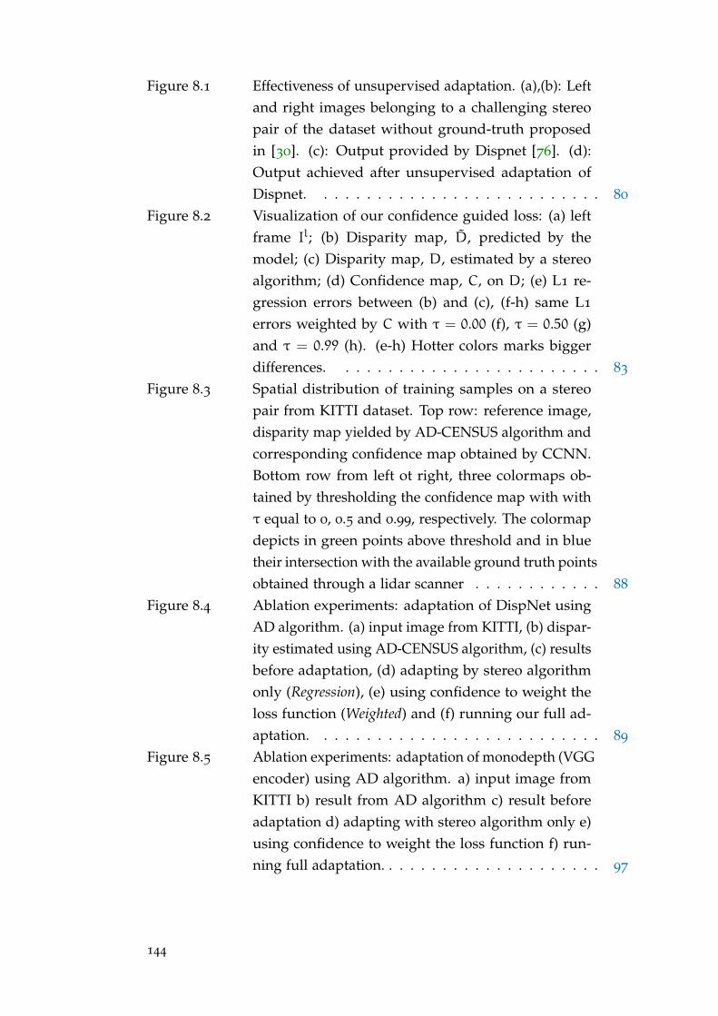
Figure 8.1 Effectiveness of unsupervised adaptation. (a),(b): Leftand right images belonging to a challenging stereopair of the dataset without ground-truth proposedin [30]. (c): Output provided by Dispnet [76]. (d):Output achieved after unsupervised adaptation ofDispnet. . . . . . . . . . . . . . . . . . . . . . . . . . . 80
Figure 8.2 Visualization of our confidence guided loss: (a) leftframe Il; (b) Disparity map, D, predicted by themodel; (c) Disparity map, D, estimated by a stereoalgorithm; (d) Confidence map, C, on D; (e) L1 re-gression errors between (b) and (c), (f-h) same L1
errors weighted by C with τ = 0.00 (f), τ = 0.50 (g)and τ = 0.99 (h). (e-h) Hotter colors marks biggerdifferences. . . . . . . . . . . . . . . . . . . . . . . . . 83
Figure 8.3 Spatial distribution of training samples on a stereopair from KITTI dataset. Top row: reference image,disparity map yielded by AD-CENSUS algorithm andcorresponding confidence map obtained by CCNN.Bottom row from left ot right, three colormaps ob-tained by thresholding the confidence map with withτ equal to 0, 0.5 and 0.99, respectively. The colormapdepicts in green points above threshold and in bluetheir intersection with the available ground truth pointsobtained through a lidar scanner . . . . . . . . . . . . 88
Figure 8.4 Ablation experiments: adaptation of DispNet usingAD algorithm. (a) input image from KITTI, (b) dispar-ity estimated using AD-CENSUS algorithm, (c) resultsbefore adaptation, (d) adapting by stereo algorithmonly (Regression), (e) using confidence to weight theloss function (Weighted) and (f) running our full ad-aptation. . . . . . . . . . . . . . . . . . . . . . . . . . . 89
Figure 8.5 Ablation experiments: adaptation of monodepth (VGGencoder) using AD algorithm. a) input image fromKITTI b) result from AD algorithm c) result beforeadaptation d) adapting with stereo algorithm only e)using confidence to weight the loss function f) run-ning full adaptation. . . . . . . . . . . . . . . . . . . . . 97
144
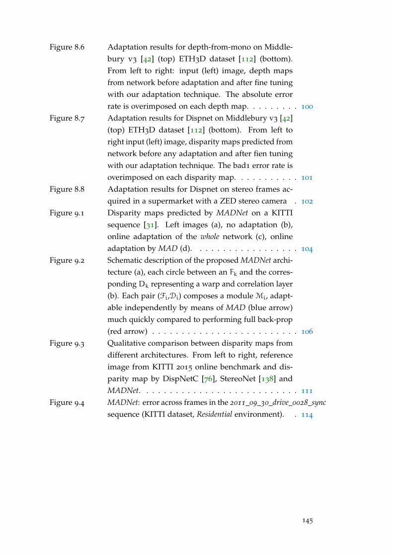
Figure 8.6 Adaptation results for depth-from-mono on Middle-bury v3 [42] (top) ETH3D dataset [112] (bottom).From left to right: input (left) image, depth mapsfrom network before adaptation and after fine tuningwith our adaptation technique. The absolute errorrate is overimposed on each depth map. . . . . . . . . 100
Figure 8.7 Adaptation results for Dispnet on Middlebury v3 [42](top) ETH3D dataset [112] (bottom). From left toright input (left) image, disparity maps predicted fromnetwork before any adaptation and after fien tuningwith our adaptation technique. The bad1 error rate isoverimposed on each disparity map. . . . . . . . . . . 101
Figure 8.8 Adaptation results for Dispnet on stereo frames ac-quired in a supermarket with a ZED stereo camera . 102
Figure 9.1 Disparity maps predicted by MADNet on a KITTIsequence [31]. Left images (a), no adaptation (b),online adaptation of the whole network (c), onlineadaptation by MAD (d). . . . . . . . . . . . . . . . . . 104
Figure 9.2 Schematic description of the proposed MADNet archi-tecture (a), each circle between an Fk and the corres-ponding Dk representing a warp and correlation layer(b). Each pair (Fi,Di) composes a module Mi, adapt-able independently by means of MAD (blue arrow)much quickly compared to performing full back-prop(red arrow) . . . . . . . . . . . . . . . . . . . . . . . . . 106
Figure 9.3 Qualitative comparison between disparity maps fromdifferent architectures. From left to right, referenceimage from KITTI 2015 online benchmark and dis-parity map by DispNetC [76], StereoNet [138] andMADNet. . . . . . . . . . . . . . . . . . . . . . . . . . . 111
Figure 9.4 MADNet: error across frames in the 2011_09_30_drive_0028_syncsequence (KITTI dataset, Residential environment). . 114
145
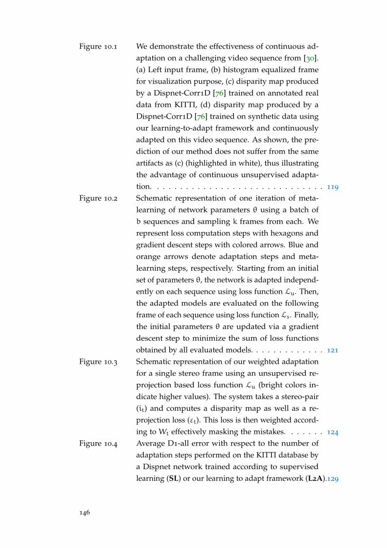
Figure 10.1 We demonstrate the effectiveness of continuous ad-aptation on a challenging video sequence from [30].(a) Left input frame, (b) histogram equalized framefor visualization purpose, (c) disparity map producedby a Dispnet-Corr1D [76] trained on annotated realdata from KITTI, (d) disparity map produced by aDispnet-Corr1D [76] trained on synthetic data usingour learning-to-adapt framework and continuouslyadapted on this video sequence. As shown, the pre-diction of our method does not suffer from the sameartifacts as (c) (highlighted in white), thus illustratingthe advantage of continuous unsupervised adapta-tion. . . . . . . . . . . . . . . . . . . . . . . . . . . . . . 119
Figure 10.2 Schematic representation of one iteration of meta-learning of network parameters θ using a batch ofb sequences and sampling k frames from each. Werepresent loss computation steps with hexagons andgradient descent steps with colored arrows. Blue andorange arrows denote adaptation steps and meta-learning steps, respectively. Starting from an initialset of parameters θ, the network is adapted independ-ently on each sequence using loss function Lu. Then,the adapted models are evaluated on the followingframe of each sequence using loss function Ls. Finally,the initial parameters θ are updated via a gradientdescent step to minimize the sum of loss functionsobtained by all evaluated models. . . . . . . . . . . . . 121
Figure 10.3 Schematic representation of our weighted adaptationfor a single stereo frame using an unsupervised re-projection based loss function Lu (bright colors in-dicate higher values). The system takes a stereo-pair(it) and computes a disparity map as well as a re-projection loss (εt). This loss is then weighted accord-ing to Wt effectively masking the mistakes. . . . . . . 124
Figure 10.4 Average D1-all error with respect to the number ofadaptation steps performed on the KITTI database bya Dispnet network trained according to supervisedlearning (SL) or our learning to adapt framework (L2A).129
146

Figure 10.5 Visualization of the errors optimized to achieve un-supervised adaptation with reprojection based lossfunction and using our weighting function. Brightercolours encode higher values. . . . . . . . . . . . . . . 132
147

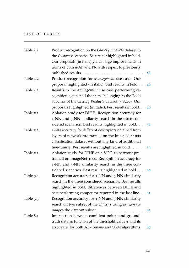
L I S T O F TA B L E S
Table 4.1 Product recognition on the Grocery Products dataset inthe Customer scenario. Best result highlighted in bold.Our proposals (in italic) yields large improvements interms of both mAP and PR with respect to previouslypublished results. . . . . . . . . . . . . . . . . . . . . . 38
Table 4.2 Product recognition for Management use case. Ourproposal highlighted (in italic), best results in bold. . 40
Table 4.3 Results in the Management use case performing re-cognition against all the items belonging to the Foodsubclass of the Grocery Products dataset (∼ 3200). Ourproposals highlighted (in italic), best results in bold. . 40
Table 5.1 Ablation study for DIHE. Recognition accuracy for1-NN and 5-NN similarity search in the three con-sidered scenarios. Best results highlighted in bold. . . 56
Table 5.2 1-NN accuracy for different descriptors obtained fromlayers of network pre-trained on the ImageNet-1000
classification dataset without any kind of additionalfine-tuning. Best results are higlighted in bold. . . . . 59
Table 5.3 Ablation study for DIHE on a VGG-16 network pre-trained on ImageNet-1000. Recognition accuracy for1-NN and 5-NN similarity search in the three con-sidered scenarios. Best results highlighted in bold. . . 60
Table 5.4 Recognition accuracy for 1-NN and 5-NN similaritysearch in the three considered scenarios. Best resultshighlighted in bold, differences between DIHE andbest performing competitor reported in the last line. . 61
Table 5.5 Recognition accuracy for 1-NN and 5-NN similaritysearch on two subset of the Office31 using as referenceimages the Amazon subset. . . . . . . . . . . . . . . . . 63
Table 8.1 Intersection between confident points and ground-truth data as function of the threshold value τ and itserror rate, for both AD-Census and SGM algorithms. 87
149
Table 8.2 Ablation study on the effectiveness of the differentcomponents of our adaptation formulation using AD-CENSUS as noisy label estimator. Results computedon the KITTI RAW dataset using a 4-fold cross valid-ation schema, best results highlighted in bold. . . . . 89
Table 8.3 Results obtained performing fine tuning of a pre-trained DispNet network using different unsuper-vised strategy. All results are computed on the KITTIraw dataset using a 4-fold cross validation schema,best results highlighted in bold, our proposals in italic. 93
Table 8.4 Experimental results on the KITTI dataset [31] on thedata split proposed by Eigen et al. [37]. On even con-ditions, the proposed adaptation scheme outperformsthe supervision by Godard et al. [93]. Combining thetwo produces the best results. . . . . . . . . . . . . . . 95
Table 8.5 Ablation experiments on the KITTI dataset [31] on thedata split proposed by Eigen et al. [37]. . . . . . . . . 95
Table 9.1 Comparison between fast disparity regression archi-tectures on the KITTI 2015 test set without onlineadaptation. . . . . . . . . . . . . . . . . . . . . . . . . . 111
Table 9.2 Performance on the City, Residential, Campus andRoad sequences from KITTI [31]. Experiments withDispNetC [76] (top) and MADNet (bottom) with andwithout online adaptations. . . . . . . . . . . . . . . . 112
Table 9.3 Results on the full KITTI raw dataset [31] (Campus→City→ Residential→ Road). . . . . . . . . . . . . . . . . 115
Table 9.4 Results on the KITTI raw dataset [31] using MADNettrained on synthetic data and different fast adaptationstrategies . . . . . . . . . . . . . . . . . . . . . . . . . . 115
150

Table 10.1 Performance on KITTI for the Dispnet network trainedaccording to different methods after initialization fromF3D. It can clearly be seen that online adaptation(+Ad/+WAd) provides a significant improvement com-pared to when it is left out. The best results areobtained when the training is achieved using theL2A+WAd framework. Line (k) indicates an upperbound on how well Dispnet can perform when finetuned on a subset of samples from the target domain.The last two columns indicate the performance im-provement with adaptation, and as it is evident inthe table, our L2A+WAd method obtains the largestincrease in performance with adaptation. . . . . . . . 128
Table 10.2 Comparison of the different training methods whenevaluated on sequences from Synthia. It can be seenthat the best performing training method is L2A+WAd.We also provide results for when we use a L1 super-vised adaptation loss. Best results in bold. . . . . . . . 130
151

B I B L I O G R A P H Y
[1] Jürgen Schmidhuber. ‘Evolutionary principles in self-referential learning, or
on learning how to learn: the meta-meta-... hook’. PhD thesis. Technische
Universität München, 1987 (cit. on p. 118).
[2] Devang K Naik and RJ Mammone. ‘Meta-neural networks that learn by
learning’. In: Neural Networks, 1992. IJCNN., International Joint Conference on.
Vol. 1. IEEE. 1992, pp. 437–442 (cit. on p. 118).
[3] Ramin Zabih and John Woodfill. ‘Non-parametric Local Transforms for
Computing Visual Correspondence’. In: Proceedings of the Third EuropeanConference on Computer Vision (Vol. II). ECCV ’94. Stockholm, Sweden:
Springer-Verlag New York, Inc., 1994, pp. 151–158 (cit. on pp. 81, 82, 86, 89).
[4] Sebastian Thrun and Lorien Pratt. ‘Learning to learn: Introduction and
overview’. In: Learning to learn. Springer, 1998, pp. 3–17 (cit. on p. 118).
[5] Thomas W Gruen, Daniel Corsten and Sundrr Bharadwaj. ‘Retail out of
stocks: A worldwide examination of causes, rates, and consumer responses’.
In: Grocery Manufacturers of America, Washington, DC (2002) (cit. on p. 11).
[6] Daniel Scharstein and Richard Szeliski. ‘A taxonomy and evaluation of
dense two-frame stereo correspondence algorithms’. In: International journalof computer vision 47.1-3 (2002), pp. 7–42 (cit. on p. 77).
[7] David G Lowe. ‘Distinctive image features from scale-invariant keypoints’.
In: International journal of computer vision 60.2 (2004), pp. 91–110 (cit. on
pp. 16, 18, 25, 34).
[8] Zhou Wang, Alan C Bovik, Hamid R Sheikh and Eero P Simoncelli. ‘Image
quality assessment: from error visibility to structural similarity’. In: IEEEtransactions on image processing 13.4 (2004), pp. 600–612 (cit. on pp. 52, 54,
86).
[9] Heiko Hirschmuller. ‘Accurate and efficient stereo processing by semi-
global matching and mutual information’. In: Computer Vision and PatternRecognition. Vol. 2. IEEE. 2005, pp. 807–814 (cit. on pp. 77, 81, 82, 86).
[10] Ingo Wegener. Complexity theory: exploring the limits of efficient algorithms.
Springer Science & Business Media, 2005 (cit. on p. 19).
[11] Herbert Bay, Tinne Tuytelaars and Luc Van Gool. ‘Surf: Speeded up robust
features’. In: European conference on computer vision. Springer. 2006, pp. 404–
417 (cit. on pp. 15, 25).
153
[12] Raia Hadsell, Sumit Chopra and Yann LeCun. ‘Dimensionality reduction by
learning an invariant mapping’. In: Computer vision and pattern recognition,2006 IEEE computer society conference on. Vol. 2. IEEE. 2006, pp. 1735–1742
(cit. on pp. 61, 63).
[13] Michele Merler, Carolina Galleguillos and Serge Belongie. ‘Recognizing
groceries in situ using in vitro training data’. In: Computer Vision and PatternRecognition, 2007. CVPR’07. IEEE Conference on. IEEE. 2007, pp. 1–8 (cit. on
pp. 11, 12).
[14] Motilal Agrawal, Kurt Konolige and Morten Rufus Blas. ‘Censure: Cen-
ter surround extremas for realtime feature detection and matching’. In:
Computer Vision–ECCV 2008. Springer, 2008, pp. 102–115 (cit. on p. 25).
[15] Koen EA van de Sande, Theo Gevers and Cees GM Snoek. ‘Color descriptors
for object category recognition’. In: Conference on Colour in Graphics, Imaging,and Vision. Vol. 2008. 1. Society for Imaging Science and Technology. 2008,
pp. 378–381 (cit. on p. 26).
[16] Ashutosh Saxena, Min Sun and Andrew Y Ng. ‘Make3d: Learning 3d scene
structure from a single still image’. In: IEEE transactions on pattern analysisand machine intelligence 31.5 (2009), pp. 824–840 (cit. on p. 78).
[17] Florent Perronnin, Yan Liu, Jorge Sánchez and Hervé Poirier. ‘Large-scale
image retrieval with compressed fisher vectors’. In: Computer Vision andPattern Recognition (CVPR), 2010 IEEE Conference on. IEEE. 2010, pp. 3384–
3391 (cit. on p. 29).
[18] Kate Saenko, Brian Kulis, Mario Fritz and Trevor Darrell. ‘Adapting visual
category models to new domains’. In: European conference on computer vision.
Springer. 2010, pp. 213–226 (cit. on p. 63).
[19] Engin Tola, Vincent Lepetit and Pascal Fua. ‘Daisy: An efficient dense
descriptor applied to wide-baseline stereo’. In: Pattern Analysis and MachineIntelligence, IEEE Transactions on 32.5 (2010), pp. 815–830 (cit. on p. 25).
[20] Julian R Ullmann. ‘Bit-vector algorithms for binary constraint satisfaction
and subgraph isomorphism’. In: Journal of Experimental Algorithmics (JEA)15 (2010), pp. 1–6 (cit. on p. 19).
[21] Tess Winlock, Eric Christiansen and Serge Belongie. ‘Toward real-time
grocery detection for the visually impaired’. In: Computer Vision and PatternRecognition Workshops (CVPRW), 2010 IEEE Computer Society Conference on.
IEEE. 2010, pp. 49–56 (cit. on p. 13).
[22] Pablo F Alcantarilla and TrueVision Solutions. ‘Fast explicit diffusion for
accelerated features in nonlinear scale spaces’. In: IEEE Trans. Patt. Anal.Mach. Intell 34.7 (2011), pp. 1281–1298 (cit. on p. 25).
154
[23] Stefan Leutenegger, Margarita Chli and Roland Y Siegwart. ‘BRISK: Binary
robust invariant scalable keypoints’. In: Computer Vision (ICCV), 2011 IEEEInternational Conference on. IEEE. 2011, pp. 2548–2555 (cit. on pp. 25, 41).
[24] Ethan Rublee, Vincent Rabaud, Kurt Konolige and Gary Bradski. ‘ORB: an
efficient alternative to SIFT or SURF’. In: Computer Vision (ICCV), 2011 IEEEInternational Conference on. IEEE. 2011, pp. 2564–2571 (cit. on p. 25).
[25] Alexandre Alahi, Raphael Ortiz and Pierre Vandergheynst. ‘Freak: Fast
retina keypoint’. In: Computer Vision and Pattern Recognition (CVPR), 2012IEEE Conference on. Ieee. 2012, pp. 510–517 (cit. on p. 25).
[26] Pablo Fernández Alcantarilla, Adrien Bartoli and Andrew J Davison. ‘KAZE
features’. In: Computer Vision–ECCV 2012. Springer, 2012, pp. 214–227 (cit.
on p. 25).
[27] Andreas Geiger, Philip Lenz and Raquel Urtasun. ‘Are we ready for
autonomous driving? the kitti vision benchmark suite’. In: ComputerVision and Pattern Recognition (CVPR), 2012 IEEE Conference on. IEEE. 2012,
pp. 3354–3361 (cit. on pp. 75–77, 79, 83, 87, 91, 93, 112, 119).
[28] Xiaoyan Hu and Philippos Mordohai. ‘A quantitative evaluation of confid-
ence measures for stereo vision’. In: IEEE Transactions on Pattern Analysisand Machine Intelligence (PAMI) (2012), pp. 2121–2133 (cit. on p. 81).
[29] Kunal Mankodiya, Rajeev Gandhi and Priya Narasimhan. ‘Challenges and
opportunities for embedded computing in retail environments’. In: SensorSystems and Software. Springer, 2012, pp. 121–136 (cit. on p. 15).
[30] Stephan Meister, Bernd Jähne and Daniel Kondermann. ‘Outdoor stereo
camera system for the generation of real-world benchmark data sets’. In:
Optical Engineering 51.2 (2012), p. 021107 (cit. on pp. 79, 80, 119).
[31] Andreas Geiger, Philip Lenz, Christoph Stiller and Raquel Urtasun. ‘Vision
meets Robotics: The KITTI Dataset’. In: International Journal of RoboticsResearch (IJRR) (2013) (cit. on pp. 76, 83, 86, 90, 95–97, 103, 104, 110, 112, 114,
115, 126).
[32] Boqing Gong, Kristen Grauman and Fei Sha. ‘Connecting the dots with
landmarks: Discriminatively learning domain-invariant features for un-
supervised domain adaptation’. In: International Conference on MachineLearning. 2013, pp. 222–230 (cit. on p. 63).
[33] R. Haeusler, R. Nair and D. Kondermann. ‘Ensemble Learning for Confid-
ence Measures in Stereo Vision’. In: CVPR. Proceedings. 1. 2013, pp. 305–312
(cit. on p. 81).
155
[34] Philipp Heise, Sebastian Klose, Brian Jensen and Alois Knoll. ‘Pm-huber:
Patchmatch with huber regularization for stereo matching’. In: Proceedingsof the IEEE International Conference on Computer Vision. 2013, pp. 2360–2367
(cit. on p. 85).
[35] Federico Tombari, Alessandro Franchi and Luigi Stefano. ‘BOLD features to
detect texture-less objects’. In: Proceedings of the IEEE International Conferenceon Computer Vision. 2013, pp. 1265–1272 (cit. on p. 26).
[36] Matthew Cotter, Siddharth Advani, Jack Sampson, Kevin Irick and Vi-
jaykrishnan Narayanan. ‘A hardware accelerated multilevel visual classifier
for embedded visual-assist systems’. In: Proceedings of the 2014 IEEE/ACMInternational Conference on Computer-Aided Design. IEEE Press. 2014, pp. 96–
100 (cit. on p. 13).
[37] David Eigen, Christian Puhrsch and Rob Fergus. ‘Depth map prediction
from a single image using a multi-scale deep network’. In: Advances inneural information processing systems. 2014, pp. 2366–2374 (cit. on pp. 78, 86,
95, 96).
[38] Emanuele Frontoni, Adriano Mancini, Primo Zingaretti and Valerio Pla-
cidi. ‘Information management for intelligent retail environment: The Shelf
Detector system’. In: Information 5.2 (2014), pp. 255–271 (cit. on p. 15).
[39] Marian George and Christian Floerkemeier. ‘Recognizing products: A per-
exemplar multi-label image classification approach’. In: Computer Vision–ECCV 2014. Springer, 2014, pp. 440–455 (cit. on pp. 12, 13, 24, 35, 36, 38,
53).
[40] Ian Goodfellow, Jean Pouget-Abadie, Mehdi Mirza, Bing Xu, David Warde-
Farley, Sherjil Ozair, Aaron Courville and Yoshua Bengio. ‘Generative
adversarial nets’. In: Advances in neural information processing systems. 2014,
pp. 2672–2680 (cit. on p. 47).
[41] Lubor Ladicky, Jianbo Shi and Marc Pollefeys. ‘Pulling things out of
perspective’. In: Proceedings of the IEEE Conference on Computer Vision andPattern Recognition. 2014, pp. 89–96 (cit. on p. 78).
[42] Daniel Scharstein, Heiko Hirschmüller, York Kitajima, Greg Krathwohl,
Nera Nesic, Xi Wang and Porter Westling. ‘High-Resolution Stereo Datasets
with Subpixel-Accurate Ground Truth.’ In: GCPR. Ed. by Xiaoyi Jiang,
Joachim Hornegger and Reinhard Koch. Vol. 8753. Lecture Notes in Com-
puter Science. Springer, 2014, pp. 31–42. isbn: 978-3-319-11751-5 (cit. on
pp. 79, 99–101).
156
[43] Ali Sharif Razavian, Hossein Azizpour, Josephine Sullivan and Stefan Carls-
son. ‘CNN features off-the-shelf: an astounding baseline for recognition’. In:
Proceedings of the IEEE Conference on Computer Vision and Pattern RecognitionWorkshops. 2014, pp. 806–813 (cit. on pp. 30, 32, 46).
[44] Robert Spangenberg, Tobias Langner, Sven Adfeldt and Raúl Rojas. ‘Large
scale semi-global matching on the cpu’. In: Intelligent Vehicles SymposiumProceedings, 2014 IEEE. IEEE. 2014, pp. 195–201 (cit. on p. 86).
[45] Aristotle Spyropoulos, Nikos Komodakis and Philippos Mordohai. ‘Learn-
ing to Detect Ground Control Points for Improving the Accuracy of Stereo
Matching.’ In: The IEEE Conference on Computer Vision and Pattern Recognition(CVPR). IEEE, 2014, pp. 1621–1628 (cit. on p. 81).
[46] Federico Tombari and Luigi Di Stefano. ‘Interest Points via Maximal Self-
Dissimilarities’. In: Computer Vision–ACCV 2014. Springer, 2014, pp. 586–
600 (cit. on p. 25).
[47] Jiang Wang, Yang Song, Thomas Leung, Chuck Rosenberg, Jingbin Wang,
James Philbin, Bo Chen and Ying Wu. ‘Learning fine-grained image similar-
ity with deep ranking’. In: Proceedings of the IEEE Conference on ComputerVision and Pattern Recognition. 2014, pp. 1386–1393 (cit. on pp. 31, 33, 49, 61,
63, 64).
[48] Siddharth Advani, Brigid Smith, Yasuki Tanabe, Kevin Irick, Matthew
Cotter, Jack Sampson and Vijaykrishnan Narayanan. ‘Visual co-occurrence
network: using context for large-scale object recognition in retail’. In:
Embedded Systems For Real-time Multimedia (ESTIMedia), 2015 13th IEEESymposium on. IEEE. 2015, pp. 1–10 (cit. on p. 13).
[49] Sean Bell and Kavita Bala. ‘Learning visual similarity for product design
with convolutional neural networks’. In: ACM Transactions on Graphics(TOG) 34.4 (2015), p. 98 (cit. on p. 31).
[50] Zhuoyuan Chen, Xun Sun, Liang Wang, Yinan Yu and Chang Huang. ‘A
Deep Visual Correspondence Embedding Model for Stereo Matching Costs’.
In: The IEEE International Conference on Computer Vision (ICCV). 2015 (cit. on
p. 77).
[51] Tali Dekel, Shaul Oron, Michael Rubinstein, Shai Avidan and William
T Freeman. ‘Best-Buddies Similarity for robust template matching’. In:
Computer Vision and Pattern Recognition (CVPR), 2015 IEEE Conference on.
IEEE. 2015, pp. 2021–2029 (cit. on p. 27).
[52] Emanuele Frontoni, Adriano Mancini and Primo Zingaretti. ‘Embedded
Vision Sensor Network for Planogram Maintenance in Retail Environments’.
In: Sensors 15.9 (2015), pp. 21114–21133 (cit. on p. 15).
157
[53] M Hadi Kiapour, Xufeng Han, Svetlana Lazebnik, Alexander C Berg and
Tamara L Berg. ‘Where to buy it: Matching street clothing photos in online
shops’. In: Proceedings of the IEEE International Conference on Computer Vision.
2015, pp. 3343–3351 (cit. on pp. 31, 47).
[54] Diederik Kingma and Jimmy Ba. ‘Adam: A method for stochastic op-
timization’. In: Proceedings of the 3rd International Conference for LearningRepresentations. 2015 (cit. on pp. 52, 54).
[55] Bo Li, Chunhua Shen, Yuchao Dai, Anton van den Hengel and Mingyi
He. ‘Depth and surface normal estimation from monocular images using
regression on deep features and hierarchical CRFs’. In: Proceedings of theIEEE Conference on Computer Vision and Pattern Recognition. 2015, pp. 1119–
1127 (cit. on p. 78).
[56] M Marder, S Harary, A Ribak, Y Tzur, S Alpert and A Tzadok. ‘Using
image analytics to monitor retail store shelves’. In: IBM Journal of Researchand Development 59.2/3 (2015), pp. 3–1 (cit. on p. 15).
[57] Moritz Menze and Andreas Geiger. ‘Object Scene Flow for Autonomous
Vehicles’. In: Conference on Computer Vision and Pattern Recognition (CVPR).2015 (cit. on pp. 75–77, 79, 83, 91, 93, 112, 119).
[58] Min Gyu Park and Kuk Jin Yoon. ‘Leveraging Stereo Matching With
Learning-Based Confidence Measures’. In: The IEEE Conference on Com-puter Vision and Pattern Recognition (CVPR). 2015 (cit. on pp. 80, 81).
[59] Shaoqing Ren, Kaiming He, Ross Girshick and Jian Sun. ‘Faster R-CNN:
Towards real-time object detection with region proposal networks’. In:
Advances in neural information processing systems. 2015, pp. 91–99 (cit. on
pp. 29, 30, 32).
[60] Olaf Ronneberger, Philipp Fischer and Thomas Brox. ‘U-net: Convolutional
networks for biomedical image segmentation’. In: International Conference onMedical Image Computing and Computer-Assisted Intervention. Springer. 2015,
pp. 234–241 (cit. on pp. 51, 54).
[61] Florian Schroff, Dmitry Kalenichenko and James Philbin. ‘Facenet: A
unified embedding for face recognition and clustering’. In: Proceedings of theIEEE Conference on Computer Vision and Pattern Recognition. 2015, pp. 815–823
(cit. on pp. 31, 46).
[62] Karen Simonyan and Andrew Zisserman. ‘Very deep convolutional net-
works for large-scale image recognition’. In: (2015) (cit. on pp. 36, 58,
96).
158
[63] A. Spyropoulos and P. Mordohai. ‘Ensemble Classifier for Combining Stereo
Matching Algorithms’. In: 2015 International Conference on 3D Vision. 2015
(cit. on p. 81).
[64] Gül Varol and Rıdvan S Kuzu. ‘Toward retail product recognition on
grocery shelves’. In: Sixth International Conference on Graphic and ImageProcessing (ICGIP 2014). International Society for Optics and Photonics.
2015, pp. 944309–944309 (cit. on p. 13).
[65] Jure Zbontar and Yann LeCun. ‘Computing the stereo matching cost with
a convolutional neural network’. In: Proceedings of the IEEE conference oncomputer vision and pattern recognition. 2015, pp. 1592–1599 (cit. on p. 77).
[66] Ipek Baz, Erdem Yoruk and Mujdat Cetin. ‘Context-aware hybrid classifica-
tion system for fine-grained retail product recognition’. In: Image, Video, andMultidimensional Signal Processing Workshop (IVMSP), 2016 IEEE 12th. IEEE.
2016, pp. 1–5 (cit. on p. 13).
[67] Marius Cordts, Mohamed Omran, Sebastian Ramos, Timo Rehfeld, Markus
Enzweiler, Rodrigo Benenson, Uwe Franke, Stefan Roth and Bernt Schiele.
‘The cityscapes dataset for semantic urban scene understanding’. In: Pro-ceedings of the IEEE conference on computer vision and pattern recognition. 2016,
pp. 3213–3223 (cit. on pp. 96, 99).
[68] Ravi Garg, Vijay Kumar BG, Gustavo Carneiro and Ian Reid. ‘Unsupervised
cnn for single view depth estimation: Geometry to the rescue’. In: EuropeanConference on Computer Vision. Springer. 2016, pp. 740–756 (cit. on pp. 78,
104, 105, 117, 123).
[69] Albert Gordo, Jon Almazán, Jerome Revaud and Diane Larlus. ‘Deep image
retrieval: Learning global representations for image search’. In: EuropeanConference on Computer Vision. Springer. 2016, pp. 241–257 (cit. on pp. 30,
46).
[70] Kaiming He, Xiangyu Zhang, Shaoqing Ren and Jian Sun. ‘Deep residual
learning for image recognition’. In: Proceedings of the IEEE conference oncomputer vision and pattern recognition. 2016, pp. 770–778 (cit. on pp. 58, 96).
[71] Iro Laina, Christian Rupprecht, Vasileios Belagiannis, Federico Tombari and
Nassir Navab. ‘Deeper depth prediction with fully convolutional residual
networks’. In: 3D Vision (3DV), 2016 Fourth International Conference on. IEEE.
2016, pp. 239–248 (cit. on p. 78).
[72] Gil Levi and Tal Hassner. ‘LATCH: learned arrangements of three patch
codes’. In: 2016 IEEE winter conference on applications of computer vision(WACV). IEEE. 2016, pp. 1–9 (cit. on p. 25).
159
[73] Fayao Liu, Chunhua Shen, Guosheng Lin and Ian Reid. ‘Learning depth
from single monocular images using deep convolutional neural fields’. In:
IEEE transactions on pattern analysis and machine intelligence 38.10 (2016),
pp. 2024–2039 (cit. on p. 78).
[74] Wenjie Luo, Alexander G Schwing and Raquel Urtasun. ‘Efficient deep
learning for stereo matching’. In: Proceedings of the IEEE Conference onComputer Vision and Pattern Recognition. 2016, pp. 5695–5703 (cit. on p. 77).
[75] Giulio Marin, Pietro Zanuttigh and Stefano Mattoccia. ‘Reliable Fusion of
ToF and Stereo Depth Driven by Confidence Measures’. In: 14th EuropeanConference on Computer Vision (ECCV 2016). 2016, pp. 386–401 (cit. on p. 81).
[76] Nikolaus Mayer, Eddy Ilg, Philip Hausser, Philipp Fischer, Daniel Cremers,
Alexey Dosovitskiy and Thomas Brox. ‘A Large Dataset to Train Convolu-
tional Networks for Disparity, Optical Flow, and Scene Flow Estimation’. In:
The IEEE Conference on Computer Vision and Pattern Recognition (CVPR). 2016
(cit. on pp. 74, 75, 77, 79, 80, 87, 90, 106, 109, 111, 112, 119, 126).
[77] Christian Mostegel, Markus Rumpler, Friedrich Fraundorfer and Horst
Bischof. ‘Using Self-Contradiction to Learn Confidence Measures in Stereo
Vision’. In: 2016 IEEE Conference on Computer Vision and Pattern Recognition,CVPR 2016, Las Vegas, NV, USA, June 27-30, 2016. 2016, pp. 4067–4076 (cit. on
p. 81).
[78] Matteo Poggi and Stefano Mattoccia. ‘Deep Stereo Fusion: combining
multiple disparity hypotheses with deep-learning’. In: Proceedings of the 4thInternational Conference on 3D Vision, 3DV. 2016 (cit. on p. 81).
[79] Matteo Poggi and Stefano Mattoccia. ‘Learning a general-purpose confid-
ence measure based on O(1) features and a smarter aggregation strategy for
semi global matching’. In: Proceedings of the 4th International Conference on3D Vision, 3DV. 2016 (cit. on pp. 80, 81).
[80] Matteo Poggi and Stefano Mattoccia. ‘Learning from scratch a confidence
measure’. In: Proceedings of the 27th British Conference on Machine Vision,BMVC. 2016 (cit. on pp. 80, 81, 86, 87).
[81] German Ros, Laura Sellart, Joanna Materzynska, David Vazquez and Ant-
onio M. Lopez. ‘The SYNTHIA Dataset: A Large Collection of Synthetic
Images for Semantic Segmentation of Urban Scenes’. In: The IEEE Conferenceon Computer Vision and Pattern Recognition (CVPR). June 2016 (cit. on pp. 117,
126).
[82] Akihito Seki and Marc Pollefeys. ‘Patch Based Confidence Prediction for
Dense Disparity Map’. In: British Machine Vision Conference (BMVC). 2016
(cit. on pp. 77, 81).
160
[83] Giorgos Tolias, Ronan Sicre and Hervé Jégou. ‘Particular object retrieval
with integral max-pooling of CNN activations’. In: (2016) (cit. on pp. 36, 52,
54, 56, 58).
[84] Oriol Vinyals, Charles Blundell, Tim Lillicrap, Daan Wierstra et al. ‘Match-
ing networks for one shot learning’. In: Advances in Neural InformationProcessing Systems. 2016, pp. 3630–3638 (cit. on pp. 47, 61, 63, 118).
[85] Xi Wang, Zhenfeng Sun, Wenqiang Zhang, Yu Zhou and Yu-Gang Jiang.
‘Matching user photos to online products with robust deep features’. In:
Proceedings of the 2016 ACM on International Conference on Multimedia Retrieval.ACM. 2016, pp. 7–14 (cit. on p. 47).
[86] Erdem Yörük, Kaan Taha Öner and Ceyhun Burak Akgül. ‘An efficient
Hough transform for multi-instance object recognition and pose estimation’.
In: Pattern Recognition (ICPR), 2016 23rd International Conference on. IEEE.
2016, pp. 1352–1357 (cit. on pp. 14, 38).
[87] Jure Zbontar and Yann LeCun. ‘Stereo matching by training a convolutional
neural network to compare image patches’. In: Journal of Machine LearningResearch 17.1-32 (2016), p. 2 (cit. on p. 81).
[88] Xiaofan Zhang, Feng Zhou, Yuanqing Lin and Shaoting Zhang. ‘Embedding
label structures for fine-grained feature representation’. In: Proceedings of theIEEE Conference on Computer Vision and Pattern Recognition. 2016, pp. 1114–
1123 (cit. on pp. 46, 61).
[89] Alexey Dosovitskiy, German Ros, Felipe Codevilla, Antonio Lopez and
Vladlen Koltun. ‘CARLA: An Open Urban Driving Simulator’. In: Proceed-ings of the 1st Annual Conference on Robot Learning. 2017, pp. 1–16 (cit. on
pp. 118, 126).
[90] Chelsea Finn, Pieter Abbeel and Sergey Levine. ‘Model-Agnostic Meta-
Learning for Fast Adaptation of Deep Networks’. In: Proceedings of the34th International Conference on Machine Learning. Ed. by Doina Precup
and Yee Whye Teh. Vol. 70. Proceedings of Machine Learning Research.
International Convention Centre, Sydney, Australia: PMLR, Aug. 2017,
pp. 1126–1135 (cit. on pp. 117, 118, 120).
[91] Annalisa Franco, Davide Maltoni and Serena Papi. ‘Grocery product de-
tection and recognition’. In: Expert Systems with Applications (2017) (cit. on
p. 13).
[92] Spyros Gidaris and Nikos Komodakis. ‘Detect, Replace, Refine: Deep
Structured Prediction for Pixel Wise Labeling’. In: The IEEE Conference onComputer Vision and Pattern Recognition (CVPR). 2017 (cit. on p. 77).
161
[93] Clément Godard, Oisin Mac Aodha and Gabriel J Brostow. ‘Unsupervised
monocular depth estimation with left-right consistency’. In: CVPR. Vol. 2.
6. 2017, p. 7 (cit. on pp. 78, 85, 86, 93, 95–98, 104, 105, 108, 110, 117, 127).
[94] Bharath Hariharan and Ross Girshick. ‘Low-shot visual recognition by
shrinking and hallucinating features’. In: Proc. of IEEE Int. Conf. onComputer Vision (ICCV), Venice, Italy. 2017 (cit. on p. 47).
[95] Andrew G Howard, Menglong Zhu, Bo Chen, Dmitry Kalenichenko, Weijun
Wang, Tobias Weyand, Marco Andreetto and Hartwig Adam. ‘Mobilenets:
Efficient convolutional neural networks for mobile vision applications’. In:
arXiv preprint arXiv:1704.04861 (2017) (cit. on p. 134).
[96] Jonathan Huang, Vivek Rathod, Chen Sun, Menglong Zhu, Anoop Kor-
attikara, Alireza Fathi, Ian Fischer, Zbigniew Wojna, Yang Song, Sergio
Guadarrama and Kevin Murphy. ‘Speed/Accuracy Trade-Offs for Modern
Convolutional Object Detectors’. In: 2017 IEEE Conference on Computer Visionand Pattern Recognition, CVPR 2017, Honolulu, HI, USA, July 21-26, 2017. 2017,
pp. 3296–3297. doi: 10.1109/CVPR.2017.351 (cit. on pp. 29, 30, 32).
[97] Phillip Isola, Jun-Yan Zhu, Tinghui Zhou and Alexei A Efros. ‘Image-to-
Image Translation with Conditional Adversarial Networks’. In: ComputerVision and Pattern Recognition, CVPR 2017. 2017 (cit. on pp. 47, 51, 54, 56).
[98] Leonid Karlinsky, Joseph Shtok, Yochay Tzur and Asaf Tzadok. ‘Fine-
grained recognition of thousands of object categories with single-example
training’. In: Proceedings of the IEEE Conference on Computer Vision and PatternRecognition. 2017, pp. 4113–4122 (cit. on p. 14).
[99] Alex Kendall, Hayk Martirosyan, Saumitro Dasgupta, Peter Henry, Ryan
Kennedy, Abraham Bachrach and Adam Bry. ‘End-To-End Learning of Geo-
metry and Context for Deep Stereo Regression’. In: The IEEE InternationalConference on Computer Vision (ICCV). 2017 (cit. on pp. 77, 107).
[100] Sunok Kim, Dongbo Min, Seungryong Kim and Kwanghoon Sohn. ‘Feature
Augmentation for Learning Confidence Measure in Stereo Matching’. In:
IEEE Transactions on Image Processing 26.12 (2017), pp. 6019–6033 (cit. on
p. 81).
[101] Yevhen Kuznietsov, Jorg Stuckler and Bastian Leibe. ‘Semi-Supervised Deep
Learning for Monocular Depth Map Prediction’. In: The IEEE Conference onComputer Vision and Pattern Recognition (CVPR). 2017 (cit. on p. 78).
[102] Jiahao Pang, Wenxiu Sun, Jimmy SJ. Ren, Chengxi Yang and Qiong Yan.
‘Cascade Residual Learning: A Two-Stage Convolutional Neural Network
for Stereo Matching’. In: The IEEE International Conference on Computer Vision(ICCV) Workshops. 2017 (cit. on p. 77).
162
[103] Matteo Poggi and Stefano Mattoccia. ‘Learning to Predict Stereo Reliability
Enforcing Local Consistency of Confidence Maps’. In: The IEEE Conferenceon Computer Vision and Pattern Recognition (CVPR). 2017 (cit. on p. 81).
[104] Matteo Poggi, Fabio Tosi and Stefano Mattoccia. ‘Efficient confidence
measures for embedded stereo’. In: 19th International Conference on ImageAnalysis and Processing (ICIAP 2017). 2017 (cit. on p. 81).
[105] Matteo Poggi, Fabio Tosi and Stefano Mattoccia. ‘Even More Confident
predictions with deep machine-learning’. In: 12th IEEE Embedded VisionWorkshop (EVW2017) held in conjunction with IEEE Conference on ComputerVision and Pattern Recognition (CVPR). 2017 (cit. on p. 81).
[106] Matteo Poggi, Fabio Tosi and Stefano Mattoccia. ‘Quantitative Evaluation
of Confidence Measures in a Machine Learning World’. In: The IEEEInternational Conference on Computer Vision (ICCV). 2017 (cit. on pp. 81, 82).
[107] Siyuan Qiao, Wei Shen, Weichao Qiu, Chenxi Liu and Alan Yuille. ‘Scalenet:
Guiding object proposal generation in supermarkets and beyond’. In: 2017IEEE International Conference on Computer Vision, ICCV. 2017, pp. 22–29
(cit. on pp. 30, 32).
[108] Zhaofan Qiu, Yingwei Pan, Ting Yao and Tao Mei. ‘Deep Semantic Hashing
with Generative Adversarial Networks’. In: Proceedings of the 40th Inter-national ACM SIGIR Conference on Research and Development in InformationRetrieval. ACM. 2017, pp. 225–234 (cit. on p. 47).
[109] Anurag Ranjan and Michael J. Black. ‘Optical Flow Estimation Using a
Spatial Pyramid Network’. In: The IEEE Conference on Computer Vision andPattern Recognition (CVPR). 2017 (cit. on p. 106).
[110] Sachin Ravi and Hugo Larochelle. ‘Optimization as a model for few-shot
learning’. In: In International Conference on Learning Representations (ICLR).2017 (cit. on p. 118).
[111] Joseph Redmon and Ali Farhadi. ‘YOLO9000: Better, Faster, Stronger’. In:
2017 IEEE Conference on Computer Vision and Pattern Recognition,CVPR 2017,Honolulu, HI, USA, July 21-26, 2017. 2017, pp. 6517–6525. doi: 10.1109/
CVPR.2017.690 (cit. on pp. 29, 30, 32, 36).
[112] Thomas Schöps, Johannes L. Schönberger, Silvano Galliani, Torsten Sattler,
Konrad Schindler, Marc Pollefeys and Andreas Geiger. ‘A Multi-View
Stereo Benchmark with High-Resolution Images and Multi-Camera Videos’.
In: Conference on Computer Vision and Pattern Recognition (CVPR). 2017 (cit.
on pp. 99–101).
163
[113] Akihito Seki and Marc Pollefeys. ‘SGM-Nets: Semi-Global Matching With
Neural Networks’. In: The IEEE Conference on Computer Vision and PatternRecognition (CVPR). 2017 (cit. on pp. 77, 81).
[114] Amit Shaked and Lior Wolf. ‘Improved Stereo Matching With Constant
Highway Networks and Reflective Confidence Learning’. In: The IEEEConference on Computer Vision and Pattern Recognition (CVPR). 2017 (cit. on
p. 81).
[115] Devashish Shankar, Sujay Narumanchi, HA Ananya, Pramod Kompalli and
Krishnendu Chaudhury. ‘Deep learning based large scale visual recom-
mendation and search for E-Commerce’. In: arXiv preprint arXiv:1703.02344(2017) (cit. on pp. 31, 47).
[116] Maruan Al-Shedivat, Trapit Bansal, Yuri Burda, Ilya Sutskever, Igor
Mordatch and Pieter Abbeel. ‘Continuous adaptation via meta-learning
in nonstationary and competitive environments’. In: arXiv preprintarXiv:1710.03641 (2017) (cit. on p. 118).
[117] Ashish Shrivastava, Tomas Pfister, Oncel Tuzel, Josh Susskind, Wenda
Wang and Russ Webb. ‘Learning from Simulated and Unsupervised Images
through Adversarial Training’. In: Computer Vision and Pattern Recognition,CVPR 2017. 2017 (cit. on pp. 47, 50).
[118] Jake Snell, Kevin Swersky and Richard Zemel. ‘Prototypical networks for
few-shot learning’. In: Advances in Neural Information Processing Systems.
2017, pp. 4077–4087 (cit. on p. 118).
[119] Christian Szegedy, Sergey Ioffe, Vincent Vanhoucke and Alexander A Alemi.
‘Inception-v4, Inception-ResNet and the Impact of Residual Connections on
Learning.’ In: AAAI. 2017, pp. 4278–4284 (cit. on p. 58).
[120] Fabio Tosi, Matteo Poggi, Alessio Tonioni, Luigi Di Stefano and Stefano
Mattoccia. ‘Learning confidence measures in the wild’. In: Proceedings ofthe 28th British Machine Vision Conference (BMVC 2017), London, UK. 2017,
pp. 4–7 (cit. on p. 81).
[121] Eric Tzeng, Judy Hoffman, Kate Saenko and Trevor Darrell. ‘Adversarial dis-
criminative domain adaptation’. In: Computer Vision and Pattern Recognition(CVPR). Vol. 1. 2. 2017, p. 4 (cit. on p. 47).
[122] Jonas Uhrig, Nick Schneider, Lukas Schneider, Uwe Franke, Thomas Brox
and Andreas Geiger. ‘Sparsity Invariant CNNs’. In: International Conferenceon 3D Vision (3DV). 2017 (cit. on pp. 86, 90, 96, 110, 117, 126).
164

[123] Benjamin Ummenhofer, Huizhong Zhou, Jonas Uhrig, Nikolaus Mayer,
Eddy Ilg, Alexey Dosovitskiy and Thomas Brox. ‘Demon: Depth and
motion network for learning monocular stereo’. In: IEEE Conference onComputer Vision and Pattern Recognition (CVPR). Vol. 5. 2017 (cit. on p. 78).
[124] Chao-Yuan Wu, R Manmatha, Alexander J Smola and Philipp Krähenbühl.
‘Sampling matters in deep embedding learning’. In: The IEEE InternationalConference on Computer Vision (ICCV). 2017 (cit. on p. 46).
[125] Xu Zhang, Felix X Yu, Sanjiv Kumar and Shih-Fu Chang. ‘Learning Spread-
out Local Feature Descriptors’. In: The IEEE International Conference onComputer Vision (ICCV). 2017 (cit. on pp. 46, 61, 63).
[126] Chao Zhou, Hong Zhang, Xiaoyong Shen and Jiaya Jia. ‘Unsupervised learn-
ing of stereo matching’. In: The IEEE International Conference on ComputerVision (ICCV). Vol. 2. 8. 2017 (cit. on pp. 77, 104, 110).
[127] Tinghui Zhou, Matthew Brown, Noah Snavely and David G Lowe. ‘Unsu-
pervised learning of depth and ego-motion from video’. In: CVPR. Vol. 2.
6. 2017, p. 7 (cit. on pp. 78, 96, 104).
[128] Jun-Yan Zhu, Taesung Park, Phillip Isola and Alexei A Efros. ‘Unpaired
image-to-image translation using cycle-consistent adversarial networks’. In:
International Computer Vision Conference, ICCV 2017. 2017 (cit. on p. 47).
[129] Filippo Aleotti, Fabio Tosi, Matteo Poggi and Stefano Mattoccia. ‘Generative
Adversarial Networks for unsupervised monocular depth prediction’. In:
15th European Conference on Computer Vision (ECCV) Workshops. 2018 (cit. on
p. 78).
[130] Konstantinos Batsos, Changjiang Cai and Philippos Mordohai. ‘CBMV: A
Coalesced Bidirectional Matching Volume for Disparity Estimation’. In: TheIEEE Conference on Computer Vision and Pattern Recognition (CVPR). 2018
(cit. on p. 134).
[131] Jia-Ren Chang and Yong-Sheng Chen. ‘Pyramid Stereo Matching Network’.
In: The IEEE Conference on Computer Vision and Pattern Recognition (CVPR).2018 (cit. on p. 77).
[132] Jia-Ren Chang and Yong-Sheng Chen. ‘Pyramid Stereo Matching Network’.
In: Proceedings of the IEEE Conference on Computer Vision and Pattern Recogni-tion. 2018, pp. 5410–5418 (cit. on p. 107).
[133] Ignasi Clavera, Anusha Nagabandi, Ronald S Fearing, Pieter Abbeel, Sergey
Levine and Chelsea Finn. ‘Learning to Adapt: Meta-Learning for Model-
Based Control’. In: arXiv preprint arXiv:1803.11347 (2018) (cit. on p. 118).
165
[134] Arun CS Kumar, Suchendra M. Bhandarkar and Prasad Mukta. ‘Monocular
Depth Prediction using Generative Adversarial Networks’. In: 1st Inter-national Workshop on Deep Learning for Visual SLAM, (CVPR). 2018 (cit. on
p. 78).
[135] Huan Fu, Mingming Gong, Chaohui Wang, Kayhan Batmanghelich and
Dacheng Tao. ‘Deep Ordinal Regression Network for Monocular Depth Es-
timation’. In: The IEEE Conference on Computer Vision and Pattern Recognition(CVPR). 2018 (cit. on p. 78).
[136] Zehua Fu and Mohsen Ardabilian. ‘Learning Confidence Measures by Multi-
modal Convolutional Neural Networks.’ In: The IEEE Winter Conference onApplications of Computer Vision (WACV). IEEE, 2018 (cit. on p. 81).
[137] Lu Jiang, Zhengyuan Zhou, Thomas Leung, Li-Jia Li and Li Fei-Fei. ‘Ment-
orNet: Regularizing very deep neural networks on corrupted labels’. In:
Procedings of the International Conference on Machine Learning (ICML). 2018
(cit. on pp. 84, 124).
[138] Sameh Khamis, Sean Fanello, Christoph Rhemann, Adarsh Kowdle, Julien
Valentin and Shahram Izadi. ‘StereoNet: Guided Hierarchical Refinement
for Real-Time Edge-Aware Depth Prediction’. In: 15th European Conferenceon Computer Vision (ECCV 2018). 2018 (cit. on pp. 104, 111, 116).
[139] Zhengfa Liang, Yiliu Feng, Yulan Guo, Hengzhu Liu, Wei Chen, Linbo Qiao,
Li Zhou and Jianfeng Zhang. ‘Learning for Disparity Estimation Through
Feature Constancy’. In: The IEEE Conference on Computer Vision and PatternRecognition (CVPR). 2018 (cit. on p. 77).
[140] Reza Mahjourian, Martin Wicke and Anelia Angelova. ‘Unsupervised
Learning of Depth and Ego-Motion from Monocular Video Using 3D Geo-
metric Constraints’. In: The IEEE Conference on Computer Vision and PatternRecognition (CVPR). 2018 (cit. on pp. 78, 96).
[141] Simon Meister, Junhwa Hur and Stefan Roth. ‘UnFlow: Unsupervised
Learning of Optical Flow with a Bidirectional Census Loss’. In: AAAI. New
Orleans, Louisiana, 2018 (cit. on p. 104).
[142] Nikhil Mishra, Mostafa Rohaninejad, Xi Chen and Pieter Abbeel. ‘A simple
neural attentive meta-learner’. In: In International Conference on LearningRepresentations (ICLR). 2018 (cit. on p. 118).
[143] Jiahao Pang, Wenxiu Sun, Chengxi Yang, Jimmy Ren, Ruichao Xiao, Jin
Zeng and Liang Lin. ‘Zoom and Learn: Generalizing Deep Stereo Matching
to Novel Domains’. In: The IEEE Conference on Computer Vision and PatternRecognition (CVPR). 2018 (cit. on pp. 77, 104, 110).
166
[144] Matteo Poggi, Filippo Aleotti, Fabio Tosi and Stefano Mattoccia. ‘Towards
real-time unsupervised monocular depth estimation on CPU’. In: IEEE/JRSConference on Intelligent Robots and Systems (IROS). 2018 (cit. on pp. 78, 104).
[145] Matteo Poggi, Fabio Tosi and Stefano Mattoccia. ‘Learning monocular depth
estimation with unsupervised trinocular assumptions’. In: 6th InternationalConference on 3D Vision (3DV). 2018 (cit. on pp. 78, 104).
[146] Mengye Ren, Wenyuan Zeng, Bin Yang and Raquel Urtasun. ‘Learning to re-
weight examples for robust deep learning’. In: Procedings of the InternationalConference on Machine Learning (ICML). 2018 (cit. on pp. 84, 124).
[147] Deqing Sun, Xiaodong Yang, Ming-Yu Liu and Jan Kautz. ‘PWC-Net: CNNs
for Optical Flow Using Pyramid, Warping, and Cost Volume’. In: The IEEEConference on Computer Vision and Pattern Recognition (CVPR). 2018 (cit. on
pp. 106, 107).
[148] Fabio Tosi, Matteo Poggi, Antonio Benincasa and Stefano Mattoccia. ‘Bey-
ond local reasoning for stereo confidence estimation with deep learning’.
In: 15th European Conference on Computer Vision (ECCV). 2018 (cit. on p. 81).
[149] Chaoyang Wang, Jose Miguel Buenaposada, Rui Zhu and Simon Lucey.
‘Learning Depth from Monocular Videos using Direct Methods’. In: TheIEEE Conference on Computer Vision and Pattern Recognition (CVPR). 2018
(cit. on pp. 78, 96).
[150] Dan Xu, Wei Wang, Hao Tang, Hong Liu, Nicu Sebe and Elisa Ricci. ‘Struc-
tured Attention Guided Convolutional Neural Fields for Monocular Depth
Estimation’. In: The IEEE Conference on Computer Vision and Pattern Recogni-tion (CVPR). 2018 (cit. on p. 78).
[151] Zhichao Yin and Jianping Shi. ‘GeoNet: Unsupervised Learning of Dense
Depth, Optical Flow and Camera Pose’. In: The IEEE Conference on ComputerVision and Pattern Recognition (CVPR). 2018 (cit. on pp. 78, 96).
[152] Lidong Yu, Yucheng Wang, Yuwei Wu and Yunde Jia. ‘Deep Stereo Matching
With Explicit Cost Aggregation Sub-Architecture’. In: AAAI Conference onArtificial Intelligence. 2018 (cit. on p. 77).
[153] Huangying Zhan, Ravi Garg, Chamara Saroj Weerasekera, Kejie Li, Harsh
Agarwal and Ian Reid. ‘Unsupervised Learning of Monocular Depth Es-
timation and Visual Odometry with Deep Feature Reconstruction’. In: TheIEEE Conference on Computer Vision and Pattern Recognition (CVPR). 2018
(cit. on p. 78).
167
[154] Xiangyu Zhang, Xinyu Zhou, Mengxiao Lin and Jian Sun. ‘ShuffleNet: An
Extremely Efficient Convolutional Neural Network for Mobile Devices’. In:
The IEEE Conference on Computer Vision and Pattern Recognition (CVPR). 2018
(cit. on p. 134).
[155] Yinda Zhang, Sameh Khamis, Christoph Rhemann, Julien Valentin,
Adarsh Kowdle, Vladimir Tankovich, Michael Schoenberg, Shahram Izadi,
Thomas Funkhouser and Sean Fanello. ‘ActiveStereoNet: End-to-End
Self-Supervised Learning for Active Stereo Systems’. In: 15th EuropeanConference on Computer Vision (ECCV). 2018 (cit. on pp. 77, 93, 94, 104, 105).
[156] Yiran Zhong, Hongdong Li and Yuchao Dai. ‘Open-World Stereo Video
Matching with Deep RNN’. In: 15th European Conference on Computer Vision(ECCV 2018). 2018 (cit. on pp. 105, 117, 119).
[157] Alec Radford, Luke Metz and Soumith Chintala. ‘Unsupervised Represent-
ation Learning with Deep Convolutional Generative Adversarial Networks’.
In: International Conference on Learning Representation, ICLR 2016 () (cit. on
p. 47).
168