Computer Sound Transformations Guided by Perceptually ...
131
Faculdade de Engenharia da Universidade do Porto Computer Sound Transformations Guided by Perceptually Motivated Features Nuno Figueiredo Pires Master in Electrical and Computers Engineering Supervisor: Professor Rui Luis Nogueira Penha Second Supervisor: Dr. Gilberto Bernardes de Almeida January 2018
-
Upload
khangminh22 -
Category
Documents
-
view
0 -
download
0
Transcript of Computer Sound Transformations Guided by Perceptually ...
Faculdade de Engenharia da Universidade do Porto
Computer Sound Transformations
Guided by Perceptually Motivated
Features
Nuno Figueiredo Pires
Master in Electrical and Computers Engineering
Supervisor: Professor Rui Luis Nogueira Penha
Second Supervisor: Dr. Gilberto Bernardes de Almeida
January 2018

c© Nuno Figueiredo Pires, 2018
Resumo
Nesta dissertacao, apresentamos uma revalidacao de estudos feitos sobre descritores desom quente. A partir de um modelo existente, implementamos um algoritmo que define owarmth de um som harmonico monofonico. O algoritmo permite a produtores e a musicos,manipular o warmth de um audio musical em tempo real (ou seja, performance ao vivo).
O termo warmth cai numa categoria de conceitos de atributos musicais, tais como”brilho”, ”aborrecido”, ”monotono”, os quais musicos e produtores musicais adoptam quandose referem a atributos tımbricos do som. Esta lexico musical e bastante relevante para acomunidade de peritos musicais. Porem, devido a sua natureza subjetiva, e dificıl definirum modelo matematico que nos permita manipular sons usando tecnicas de processamentode sinal digital. Portanto, ao estarmos cientes da importancia desta ferramenta de proces-samento, procuramos compreender os timbres que afetam tal atributo sonico informal e emsegundo, codifica-la como um modelo matematico que possa ser utilizado para manipularo warmth the audio musical em tempo real.
O descritor proposto manipula uma area de warmth calculada, que e baseada no tra-balho de D. Williams [1], onde o warmth e uma relacao entre a energia dos tres primeirosharmonicos e a energia do resto do espectro do sinal. Para este fim, nos regulamos as am-plitudes das componentes espectrais do audio musical para molda-los de acordo nıvel rel-ativo de warmth controlado pelo utilizador. Por outras palavras, permitimos ao utilizadorreduzir ou aumentar a percentagem de warmthness dinamicamente do audio musical deentrada mantendo a relativas variacoes, em tempo real.
Para primeiro tentarmos perceber de que forma e que o warmth num som instrumentale percepcionado, realizamos uma avaliacao perceptual que foi enviada para 128 pessoascom diferentes nıveis de proficiencia musical.
Por forma a validar e avaliar a eficacia da nossa aplicacao, realizamos um segundo testede escuta que contou com a participacao de 51 indivıduos.
Concluimos que, apesar de termos conseguido correlacionar o warmth com a centroidespectral, o algoritmo tem de ser melhorado pois a diminuacao do nıvel de warmth nao epercetıvel.
i

ii
Abstract
We present a revalidation of previous research done on description of warm sound. Withan existing model, we elaborate an algorithm that defines the “warmth” of a monophonicharmonic sound. A twofold approach to the algorithm allows producers and musiciansto not only measure this sound attribute but also manipulate it in real-time (i.e. a liveperformance).
The term warmth falls in a category of music audio attributes, such as bright, dull, flat,which expert musicians and music producers widely adopt to address timbral attributesof sound. This (semantic) musical jargon is highly relevant to the community of musicalexperts. Yet, due to its subjective nature, it’s hard to define mathematically, whichwould enable us to manipulate sounds using digital signal processing techniques. By beingaware of the importance of such a processing tool, we strive here to first understand thetimbral attributes which impact such an informal sonic attribute and second encode it asa mathematical model which can be used to manipulate the warmth of musical audio inreal-time.
Based on the work of D. William and T. Brookes [1], the proposed warmth descriptormanipulates a certain ”Warmth Region”, where this ”warmth” is a relation between theenergy of the first three harmonics and the energy of the remainder magnitude of thespectrum. To this end, we regulate the amplitudes of the spectral components of a musicalaudio, to shape them according to a relative user-controlled level of warmth. In otherwords, we allow the user to dynamically reduce or increase the percentage of warmthnessin the musical audio input, while retaining the relative variability over time.
To first understand how warmth in instrumental sounds is perceived, we performed aperceptual evaluation, that was submitted to over 128 people of different levels of musicalproficiency.
To validate and evaluate the effectiveness of the application we designed a secondlistening test that counted with the participation of 51 individuals.
We conclude that despite having a correlation between the warmth and the spectralcentroid, the algorithm has to be improved as the decrease of warmth was not perceived.
iii

iv
Acknowledgment
I start by thanking my supervisor Professor Rui Penha for giving me the opportunity towork on this dissertation. I thank you for all the support and feedback given throughoutthis work. Ever since I discovered the class of Advanced Synthesis of Sound I decidedthat I would like to do my thesis with Professor Rui Penha, where I could join electricalan computer engineering and audio. I’d also like to thank my INESC-TEC supervisorGilberto Bernardes for his tireless support, for always being available to teach me andcorrect my wrong doings and whose orientation was crucial for the completion of thisthesis.
I thank all the elements of the Sound and Music Computing group for the meetingswhere we shared knowledge and brainstormed.
I’d also like to thank all my colleagues who accompanied me in this long journey,in particular to: Diogo “Souma” Sebe for his companionship and for all the delicaciesyou cooked at @Cisco’s; to the “owners” of the @Cisco’s Francisco “Cisco” Alpoim forall the moments during this endeavor and for helping reviewing this document; Diogo“Paqueton” Dias for his friendship and support; Joni “7kratos” Gonacalves for keeping usin check whenever we got together at @Cisco’s and for making me realize that FEUPreally affects a person :). I’d also like to thank Alexandre “Russo” Pires, Joaquim “Quim”Ribeiro, Pedro “kun” Dinis and Fabio “Beer Guy” Vasconcelos for this final years and alllaughable moments.
I’d like to give a special thanks to all my family that supported me all this years,specially to my godmother.
A very special and heartfelt thank you to my sister Ana for putting up with me allthese years and for being my partner and friend. To my dear parents for always goingfurther and beyond and doing the impossible for my well being and personal growth.Thank you mother for being my guardian angel and, despite the difficult moments,beingthere to guide me and help me overcome incoming obstacles. Thank you father for beingmy Superman and for supporting me and helping me all my life and for being my strengthand guiding me during this past few months. Thank you both for allowing and helpingme close this important chapter of my life and I hope to count on your advice and supportfrom now on too.
Once again, thank you all!
Nuno Figueiredo Pires
v

vi
“Failures, repeated failures,are finger posts on the road
to achievement. One failsforward toward success.”
C. S. Lewis
vii

viii
Contents
1 Introduction 1
1.1 Context . . . . . . . . . . . . . . . . . . . . . . . . . . . . . . . . . . . . . . 1
1.2 Motivation . . . . . . . . . . . . . . . . . . . . . . . . . . . . . . . . . . . . 1
1.3 Goals . . . . . . . . . . . . . . . . . . . . . . . . . . . . . . . . . . . . . . . 2
1.4 Document Structure . . . . . . . . . . . . . . . . . . . . . . . . . . . . . . . 2
2 Overview of Digital Audio Processing 3
2.1 Digital Signal Processing . . . . . . . . . . . . . . . . . . . . . . . . . . . . . 3
2.2 Music Information Retrieval . . . . . . . . . . . . . . . . . . . . . . . . . . . 5
2.3 Content-based audio description . . . . . . . . . . . . . . . . . . . . . . . . 6
2.3.1 Low-Level Descriptors . . . . . . . . . . . . . . . . . . . . . . . . . . 6
2.3.2 Mid-Level Descriptors . . . . . . . . . . . . . . . . . . . . . . . . . . 6
2.3.3 High-Level Descriptors . . . . . . . . . . . . . . . . . . . . . . . . . . 7
2.3.4 From Low-Level to Mid-Level to High-Level Descriptors . . . . . . . 7
2.4 Taxonomy of low-level audio descriptors . . . . . . . . . . . . . . . . . . . . 8
2.4.1 Temporal Energy Envelope . . . . . . . . . . . . . . . . . . . . . . . 8
2.4.2 Spectral Features . . . . . . . . . . . . . . . . . . . . . . . . . . . . . 9
2.4.3 Sinusoidal Harmonic Partials . . . . . . . . . . . . . . . . . . . . . . 11
2.5 Description of Sound Warmth . . . . . . . . . . . . . . . . . . . . . . . . . . 12
2.5.1 Williams and Brookes’ Metric . . . . . . . . . . . . . . . . . . . . . . 12
2.5.1.1 Warmth Region . . . . . . . . . . . . . . . . . . . . . . . . 12
2.5.2 Aurelian’s Metric . . . . . . . . . . . . . . . . . . . . . . . . . . . . . 13
3 Accessing the perceptual manifestation of sound warmth 15
3.1 Perceptual Evaluation . . . . . . . . . . . . . . . . . . . . . . . . . . . . . . 15
3.1.1 Listening Test . . . . . . . . . . . . . . . . . . . . . . . . . . . . . . 15
3.1.2 Results . . . . . . . . . . . . . . . . . . . . . . . . . . . . . . . . . . 16
3.2 Analysis of the instrumental sounds . . . . . . . . . . . . . . . . . . . . . . 17
4 Development of the system 25
4.1 System Overview . . . . . . . . . . . . . . . . . . . . . . . . . . . . . . . . . 25
4.2 Definition of the Warmth Region . . . . . . . . . . . . . . . . . . . . . . . . 25
4.3 Resynthesis . . . . . . . . . . . . . . . . . . . . . . . . . . . . . . . . . . . . 27
4.3.1 Crossfade . . . . . . . . . . . . . . . . . . . . . . . . . . . . . . . . . 28
5 Evaluation of the system 29
5.1 Listening Test . . . . . . . . . . . . . . . . . . . . . . . . . . . . . . . . . . . 29
5.2 Results . . . . . . . . . . . . . . . . . . . . . . . . . . . . . . . . . . . . . . . 30
ix
x CONTENTS
5.3 Analysis of the manipulated instrumental sounds . . . . . . . . . . . . . . . 33
6 Conclusion and Future Work 376.1 Summary . . . . . . . . . . . . . . . . . . . . . . . . . . . . . . . . . . . . . 376.2 Conclusion and Future work . . . . . . . . . . . . . . . . . . . . . . . . . . . 37
A Appendix 39A.1 Pure Data Code . . . . . . . . . . . . . . . . . . . . . . . . . . . . . . . . . 39A.2 Print screens and charts of the 1st listening test . . . . . . . . . . . . . . . . 44A.3 Matlab plots of the results of the first listening test . . . . . . . . . . . . . . 51A.4 Print screens charts and plots relative to the second listening test . . . . . . 64A.5 Matlab plots of the results of the second listening test . . . . . . . . . . . . 71
References 105
List of Figures
2.1 Digital Audio Processing [9] . . . . . . . . . . . . . . . . . . . . . . . . . . . 4
2.2 Analog-to-Digital Conversion [10] . . . . . . . . . . . . . . . . . . . . . . . . 5
2.3 Layers of audio analysis based on[16] . . . . . . . . . . . . . . . . . . . . . . 7
2.4 Table of descriptor by G. Peeters [25] . . . . . . . . . . . . . . . . . . . . . . 9
2.5 Architecture of Williams and Brookes’ sound warmth descriptor . . . . . . . 13
2.6 Definition of the Warmth Region . . . . . . . . . . . . . . . . . . . . . . . . 13
3.1 Responses of the first listening test with a graphical color code representation 17
3.2 Values of the spectral centroid of the violoncello C3 and oboe C6 sounds . . 20
3.3 Values of warmth of the violoncello C3 and oboe C6 sounds . . . . . . . . . 20
3.4 Linear regression between the weighted arithmetic mean evaluation and thespectral centroid of all instrumental sounds . . . . . . . . . . . . . . . . . . 21
3.5 Linear regression between the weighted arithmetic mean evaluation and thewarmth of all instrumental sounds . . . . . . . . . . . . . . . . . . . . . . . 21
3.6 Linear regression between the warmth and the spectral centroid of all in-strumental sounds . . . . . . . . . . . . . . . . . . . . . . . . . . . . . . . . 23
4.1 System Architecture . . . . . . . . . . . . . . . . . . . . . . . . . . . . . . . 26
4.2 First three harmonics of a Viola C4 sound . . . . . . . . . . . . . . . . . . . 27
4.3 Example of a window with overlap of four blocks . . . . . . . . . . . . . . . 27
4.4 Band-pass filter where only the values within the warmth region are allowed,and the rest is attenuated . . . . . . . . . . . . . . . . . . . . . . . . . . . . 28
4.5 Reject-band filter where the amplitudes within the warmth region are at-tenuated . . . . . . . . . . . . . . . . . . . . . . . . . . . . . . . . . . . . . . 28
5.1 Responses of the second listening test with a graphical color code represen-tation . . . . . . . . . . . . . . . . . . . . . . . . . . . . . . . . . . . . . . . 30
5.2 Values of the Spectral Centroid of the oboe C5 with 0%,+25% and +50%warmth . . . . . . . . . . . . . . . . . . . . . . . . . . . . . . . . . . . . . . 34
5.3 Values of the Spectral Centroid of the oboe C5 with 0%, -25% and -50%warmth . . . . . . . . . . . . . . . . . . . . . . . . . . . . . . . . . . . . . . 35
5.4 Values of the Spectral Centroid of the oboe C5 with 0%,+25% and +50%warmth . . . . . . . . . . . . . . . . . . . . . . . . . . . . . . . . . . . . . . 36
5.5 Values of the Spectral Centroid of the oboe C5 with 0%, -25% and -50%warmth . . . . . . . . . . . . . . . . . . . . . . . . . . . . . . . . . . . . . . 36
A.1 Pure Data patch that receives the values of the Warmth Region and SpectralCentroid of all frames and calculates the mean, media, and standard deviation 39
A.2 Pure Data patch that calculates the Warmth Region and the Spectral Centroid 40
xi
xii LIST OF FIGURES
A.3 Pure Data patch relative to the manipulation of the Warmth Region inreal-time . . . . . . . . . . . . . . . . . . . . . . . . . . . . . . . . . . . . . . 41
A.4 Pure Data patch that performs the FFT of the signal, applies a band-passfilter and reject-band filter in order to get part of the signal related to theWarmth Region and the Remainder Magnitude, respectively, and allow themanipulation of the Warmth Region . . . . . . . . . . . . . . . . . . . . . . 42
A.5 Pure Data patch that performs the manipulation of the warmth region basedon a user input . . . . . . . . . . . . . . . . . . . . . . . . . . . . . . . . . . 43
A.6 Pure Data patch relative to the creation of an array with the first threeharmonics of the signal . . . . . . . . . . . . . . . . . . . . . . . . . . . . . 43
A.7 Listening Test 1 - instructions, in portuguese, of how to answer the firstlistening . . . . . . . . . . . . . . . . . . . . . . . . . . . . . . . . . . . . . . 44
A.8 Listening Test 1 - instructions, in English, of how to answer the first listening 45
A.9 Listening Test 1 - characterization of the participant . . . . . . . . . . . . . 46
A.10 Listening Test 1 - example of question where the participant has to evaluatethe sound according to the categories. This same type of question was donefor all the sample chosen in Table 3.1. . . . . . . . . . . . . . . . . . . . . . 47
A.11 Response chart for all three tuba examples . . . . . . . . . . . . . . . . . . 47
A.12 Response chart for all three horn examples . . . . . . . . . . . . . . . . . . 48
A.13 Response chart for all three clarinet examples . . . . . . . . . . . . . . . . . 48
A.14 Response chart for all three oboe examples . . . . . . . . . . . . . . . . . . 49
A.15 Response chart for all three viola examples . . . . . . . . . . . . . . . . . . 49
A.16 Response chart for all three violoncello examples . . . . . . . . . . . . . . . 50
A.17 Variation of the value of warmth in each audio file . . . . . . . . . . . . . . 51
A.18 Mean median and standard deviation of warmth in the three tuba soundexamples. The leftmost (at ’0’) values belong to the sound of tuba C2. Thevalues at ’1’ belongs to the sound of tuba C3 and the rightmost (at ’2’)values belong to the sound of tuba C4 . . . . . . . . . . . . . . . . . . . . . 52
A.19 Variation of the value of the spectral centroid in each audio file . . . . . . . 52
A.20 Mean median and standard deviation of the spectral centroid in the threetuba sound examples. The leftmost (at ’0’) values belong to the of soundtuba C2. The values at ’1’ belongs to the sound of tuba C3 and the rightmost(at ’2’) values belong to the sound of tuba C4 . . . . . . . . . . . . . . . . . 53
A.21 Variation of the value of warmth in each audio file . . . . . . . . . . . . . . 53
A.22 Mean median and standard deviation of warmth in the three horn soundexamples. The leftmost (at ’0’) values belong to the sound of horn C2. Thevalues at ’1’ belongs to the sound of horn C3 and the rightmost (at ’2’)values belong to the sound of horn C4 . . . . . . . . . . . . . . . . . . . . . 54
A.23 Variation of the value of the spectral centroid in each audio file. . . . . . . . 54
A.24 Mean median and standard deviation of the spectral centroid in the threehorn sound examples. The leftmost (at ’0’) values belong to the of soundhorn C2. The values at ’1’ belongs to the sound of horn C3 and the right-most (at ’2’) values belong to the of sound horn C4 . . . . . . . . . . . . . . 55
A.25 Variation of the value of warmth in each audio file . . . . . . . . . . . . . . 55
A.26 Mean median and standard deviation of warmth in the three clarinet soundexamples. The leftmost (at ’0’) values belong to the sound of clarinet C4.The values at ’1’ belongs to the sound of clarinet C5 and the rightmost (at’2’) values belong to the sound of clarinet C6 . . . . . . . . . . . . . . . . . 56
LIST OF FIGURES xiii
A.27 Variation of the value of the spectral centroid in each audio file . . . . . . . 56
A.28 Mean median and standard deviation of the spectral centroid in the threeclarinet sound examples. The leftmost (at ’0’) values belong to the soundof clarinet C4. The values at ’1’ belongs to the sound of clarinet C5 andthe rightmost (at ’2’) values belong to the sound of clarinet C6 . . . . . . . 57
A.29 Variation of the value of warmth in each audio file . . . . . . . . . . . . . . 57
A.30 Mean median and standard deviation of warmth in the three oboe soundexamples. The leftmost (at ’0’) values belong to the sound of oboe C4. Thevalues at ’1’ belongs to the sound of oboe C5 and the rightmost (at ’2’)values belong to the sound of oboe C6 . . . . . . . . . . . . . . . . . . . . . 58
A.31 Variation of the value of the spectral centroid in each audio file . . . . . . . 58
A.32 Mean median and standard deviation of the spectral centroid in the threeoboe sound examples. The leftmost (at ’0’) values belong to the soundof oboe C4. The values at ’1’ belongs to the sound of oboe C5 and therightmost (at ’2’) values belong to the sound of oboe C6 . . . . . . . . . . . 59
A.33 Variation of the value of warmth in each audio file . . . . . . . . . . . . . . 59
A.34 Mean median and standard deviation of warmth in the three viola soundexamples. The leftmost (at ’0’) values belong to the sound of viola C3. Thevalues at ’1’ belongs to the sound of viola C4 and the rightmost (at ’2’)values belong to the sound of viola C5 . . . . . . . . . . . . . . . . . . . . . 60
A.35 Variation of the value of the spectral centroid in each audio file . . . . . . . 60
A.36 Mean median and standard deviation of the spectral centroid in the threeviola sound examples. The leftmost (at ’0’) values belong to the soundof viola C3. The values at ’1’ belongs to the sound of viola C4 and therightmost (at ’2’) values belong to the sound of viola C5 . . . . . . . . . . . 61
A.37 Variation of the value of warmth in each audio file . . . . . . . . . . . . . . 61
A.38 Mean median and standard deviation of warmth in the three violoncellosound examples. The leftmost (at ’0’) values belong to the sound of violon-cello C3. The values at ’1’ belongs to the sound of violoncello C4 and therightmost (at ’2’) values belong to the sound of violoncello C5 . . . . . . . . 62
A.39 Variation of the value of the spectral centroid in each audio file . . . . . . . 62
A.40 Mean median and standard deviation of the spectral centroid in the threevioloncello sound examples. The leftmost (at ’0’) values belong to the soundof violoncello C3. The values at ’1’ belongs to the sound of violoncello C4and the rightmost (at ’2’) values belong to the sound of violoncello C5 . . . 63
A.41 Listening Test 2 - instructions, in portuguese, of how to answer the firstlistening . . . . . . . . . . . . . . . . . . . . . . . . . . . . . . . . . . . . . . 64
A.42 Listening Test 2 - instructions, in english, of how to answer the first listening 65
A.43 Listening Test 2 - characterization of the individual . . . . . . . . . . . . . . 66
A.44 Listening Test 2 - example of question where the individual has to evaluatethe modified sound taking into account the original audio file. Each modifiedsound could be equal to the original audio file, or with +-25% or +-50%warmth. This same type of question was done for all the audio file explainedin Section 5.1. . . . . . . . . . . . . . . . . . . . . . . . . . . . . . . . . . . . 67
A.45 Chart of the responses for all four transformation of horn C4 . . . . . . . . 68
A.46 Chart of the responses for all four transformation of clarinet C5 . . . . . . . 68
A.47 Chart of the responses for all four transformation of oboe C5 . . . . . . . . 69
A.48 Chart of the responses for all four transformation of viola C5 . . . . . . . . 69

xiv LIST OF FIGURES
A.49 Chart of the responses for all four transformation of violoncello C5 . . . . . 70
A.50 Variation of the value of the spectral centroid of horn C4, when increasedthe level of warmth by 25% and 50%, in each analysis audio file . . . . . . . 71
A.51 Variation of the value of the spectral centroid of horn C4, when decreasedthe level of warmth by 25% and 50%, in each analysis audio file . . . . . . . 72
A.52 Mean, median and standard deviation of the spectral centroid of horn C4,when increased the level of warmth by 25% and 50%, in each analysis audiofile. The leftmost (at ’0’) values belong to the sound of horn C4 with notransformation. The values at ’1’ belongs to the sound of horn C4 with+25% warmth and the rightmost (at ’2’) values belong to the sound of hornC4 with +50% warmth . . . . . . . . . . . . . . . . . . . . . . . . . . . . . . 73
A.53 Mean, median and standard deviation of horn C4 when decreased the levelof warmth by 25% and 50%. The leftmost (at ’0’) values belong to the soundof horn C4 with no transformation. The values at ’1’ belongs to the soundof horn C4 with -25% warmth and the rightmost (at ’2’) values belong tothe sound of horn C4 with -50% warmth . . . . . . . . . . . . . . . . . . . . 74
A.54 Variation of the value of warmth of horn C4, when increased the level ofwarmth by 25% and 50%, in each analysis audio file . . . . . . . . . . . . . 75
A.55 Variation of the value of warmth of horn C4, when decreased the level ofwarmth by 25% and 50%, in each analysis audio file . . . . . . . . . . . . . 75
A.56 Mean, median and standard deviation of the warmth of horn C4 whenincreased the level of warmth by 25% and 50%. The leftmost (at ’0’) valuesbelong to the sound of horn C4 with no transformation. The values at ’1’belongs to the sound of horn C4 with +25% warmth and the rightmost (at’2’) values belong to the sound of horn C4 with +50% warmth . . . . . . . 76
A.57 Mean, median and standard deviation of horn C4 when decreased the levelof warmth by 25% and 50%. The leftmost (at ’0’) values belong to the soundof horn C4 with no transformation. The values at ’1’ belongs to the soundof horn C4 with -25% warmth and the rightmost (at ’2’) values belong tothe sound of horn C4 with -50% warmth . . . . . . . . . . . . . . . . . . . . 77
A.58 Variation of the value of the spectral centroid of clarinet C5, when increasedthe level of warmth by 25% and 50%, in each analysis audio file . . . . . . . 78
A.59 Variation of the value of the spectral centroid of clarinet C5, when decreasedthe level of warmth by 25% and 50%, in each analysis audio file . . . . . . . 78
A.60 Mean, median and standard deviation of the spectral centroid of clarinetC5, when increased the level of warmth by 25% and 50%, in each analysisaudio file. The leftmost (at ’0’) values belong to the sound of clarinet C5with no transformation. The values at ’1’ belongs to the sound of clarinetC5 with +25% warmth and the rightmost (at ’2’) values belong to the soundof clarinet C5 with +50% warmth . . . . . . . . . . . . . . . . . . . . . . . 79
A.61 Mean, median and standard deviation of clarinet C5 when decreased thelevel of warmth by 25% and 50%. The leftmost (at ’0’) values belong tothe sound of clarinet C5 with no transformation. The values at ’1’ belongsto the sound of clarinet C5 with -25% warmth and the rightmost (at ’2’)values belong to the sound of clarinet C5 with -50% warmth . . . . . . . . . 80
A.62 Variation of the value of warmth of clarinet C5, when increased the level ofwarmth by 25% and 50%, in each analysis audio file . . . . . . . . . . . . . 81
LIST OF FIGURES xv
A.63 Variation of the value of warmth of clarinet C5, when decreased the levelof warmth by 25% and 50%, in each analysis audio file . . . . . . . . . . . . 81
A.64 Mean, median and standard deviation of the warmth of clarinet C5 whenincreased the level of warmth by 25% and 50%. The leftmost (at ’0’) valuesbelong to the sound of clarinet C5 with no transformation. The values at ’1’belongs to the sound of clarinet C5 with +25% warmth and the rightmost(at ’2’) values belong to the sound of clarinet C5 with +50% warmth . . . . 82
A.65 Mean, median and standard deviation of clarinet C5 when decreased thelevel of warmth by 25% and 50%. The leftmost (at ’0’) values belong tothe sound of clarinet C5 with no transformation. The values at ’1’ belongsto the sound of clarinet C5 with -25% warmth and the rightmost (at ’2’)values belong to the sound of clarinet C5 with -50% warmth . . . . . . . . . 83
A.66 Variation of the value of the spectral centroid of oboe C5, when increasedthe level of warmth by 25% and 50%, in each analysis audio file . . . . . . . 84
A.67 Variation of the value of the spectral centroid of oboe C5, when decreasedthe level of warmth by 25% and 50%, in each analysis audio file . . . . . . . 84
A.68 Mean, median and standard deviation of the spectral centroid of oboe C5,when increased the level of warmth by 25% and 50%, in each analysis audiofile. The leftmost (at ’0’) values belong to the sound of oboe C5 with notransformation. The values at ’1’ belongs to the sound of oboe C5 with+25% warmth and the rightmost (at ’2’) values belong to the sound ofoboe C5 with +50% warmth . . . . . . . . . . . . . . . . . . . . . . . . . . . 85
A.69 Mean, median and standard deviation of oboe C5 when decreased the levelof warmth by 25% and 50%. The leftmost (at ’0’) values belong to thesound of oboe C5 with no transformation. The values at ’1’ belongs tothe sound of oboe C5 with -25% warmth and the rightmost (at ’2’) valuesbelong to the sound of oboe C5 with -50% warmth . . . . . . . . . . . . . . 86
A.70 Variation of the value of warmth of oboe C5, when increased the level ofwarmth by 25% and 50%, in each analysis audio file . . . . . . . . . . . . . 87
A.71 Variation of the value of warmth of oboe C5, when decreased the level ofwarmth by 25% and 50%, in each analysis audio file . . . . . . . . . . . . . 87
A.72 Mean, median and standard deviation of the warmth of oboe C5 whenincreased the level of warmth by 25% and 50%. The leftmost (at ’0’) valuesbelong to the sound of oboe C5 with no transformation. The values at ’1’belongs to the sound of oboe C5 with +25% warmth and the rightmost (at’2’) values belong to the sound of oboe C5 with +50% warmth . . . . . . . 88
A.73 Mean, median and standard deviation of oboe C5 when decreased the levelof warmth by 25% and 50%. The leftmost (at ’0’) values belong to thesound of oboe C5 with no transformation. The values at ’1’ belongs tothe sound of oboe C5 with -25% warmth and the rightmost (at ’2’) valuesbelong to the sound of oboe C5 with -50% warmth . . . . . . . . . . . . . . 89
A.74 Variation of the value of the spectral centroid of viola C5, when increasedthe level of warmth by 25% and 50%, in each analysis audio file . . . . . . . 90
A.75 Variation of the value of the spectral centroid of viola C5, when decreasedthe level of warmth by 25% and 50%, in each analysis audio file . . . . . . . 90
xvi LIST OF FIGURES
A.76 Mean, median and standard deviation of the spectral centroid of viola C5,when increased the level of warmth by 25% and 50%, in each analysis audiofile. The leftmost (at ’0’) values belong to the sound of viola C5 with notransformation. The values at ’1’ belongs to the sound of viola C5 with+25% warmth and the rightmost (at ’2’) values belong to the sound ofviola C5 with +50% warmth . . . . . . . . . . . . . . . . . . . . . . . . . . 91
A.77 Mean, median and standard deviation of viola C5 when decreased the levelof warmth by 25% and 50%. The leftmost (at ’0’) values belong to thesound of viola C5 with no transformation. The values at ’1’ belongs tothe sound of viola C5 with -25% warmth and the rightmost (at ’2’) valuesbelong to the sound of viola C5 with -50% warmth . . . . . . . . . . . . . . 92
A.78 Variation of the value of warmth of viola C5, when increased the level ofwarmth by 25% and 50%, in each analysis audio file . . . . . . . . . . . . . 93
A.79 Variation of the value of warmth of viola C5, when decreased the level ofwarmth by 25% and 50%, in each analysis audio file . . . . . . . . . . . . . 93
A.80 Mean, median and standard deviation of the warmth of viola C5 whenincreased the level of warmth by 25% and 50%. The leftmost (at ’0’) valuesbelong to the sound of viola C5 with no transformation. The values at ’1’belongs to the sound of viola C5 with +25% warmth and the rightmost (at’2’) values belong to the sound of viola C5 with +50% warmth . . . . . . . 94
A.81 Mean, median and standard deviation of viola C5 when decreased the levelof warmth by 25% and 50%. The leftmost (at ’0’) values belong to thesound of viola C5 with no transformation. The values at ’1’ belongs tothe sound of viola C5 with -25% warmth and the rightmost (at ’2’) valuesbelong to the sound of viola C5 with -50% warmth . . . . . . . . . . . . . . 95
A.82 Variation of the value of the spectral centroid of violoncello C5, when in-creased the level of warmth by 25% and 50%, in each analysis audio file . . 96
A.83 Variation of the value of the spectral centroid of violoncello C5, when de-creased the level of warmth by 25% and 50%, in each analysis audio file . . 96
A.84 Mean, median and standard deviation of the spectral centroid of violoncelloC5, when increased the level of warmth by 25% and 50%, in each analysisaudio file. The leftmost (at ’0’) values belong to the sound of violoncello C5with no transformation. The values at ’1’ belongs to the sound of violoncelloC5 with +25% warmth and the rightmost (at ’2’) values belong to the soundof violoncello C5 with +50% warmth . . . . . . . . . . . . . . . . . . . . . . 97
A.85 Mean, median and standard deviation of violoncello C5 when decreased thelevel of warmth by 25% and 50%. The leftmost (at ’0’) values belong to thesound of violoncello C5 with no transformation. The values at ’1’ belongsto the sound of violoncello C5 with -25% warmth and the rightmost (at ’2’)values belong to the sound of violoncello C5 with -50% warmth . . . . . . . 98
A.86 Variation of the value of warmth of violoncello C5, when increased the levelof warmth by 25% and 50%, in each analysis audio file . . . . . . . . . . . . 99
A.87 Variation of the value of warmth of violoncello C5, when decreased the levelof warmth by 25% and 50%, in each analysis audio file . . . . . . . . . . . . 99
LIST OF FIGURES xvii
A.88 Mean, median and standard deviation of the warmth of violoncello C5 whenincreased the level of warmth by 25% and 50%. The leftmost (at ’0’) valuesbelong to the sound of violoncello C5 with no transformation. The valuesat ’1’ belongs to the sound of violoncello C5 with +25% warmth and therightmost (at ’2’) values belong to the sound of violoncello C5 with +50%warmth . . . . . . . . . . . . . . . . . . . . . . . . . . . . . . . . . . . . . . 100
A.89 Mean, median and standard deviation of violoncello C5 when decreased thelevel of warmth by 25% and 50%. The leftmost (at ’0’) values belong to thesound of violoncello C5 with no transformation. The values at ’1’ belongsto the sound of violoncello C5 with -25% warmth and the rightmost (at ’2’)values belong to the sound of violoncello C5 with -50% warmth . . . . . . . 101
A.90 Linear regression between the weighted arithmetic mean evaluation and thespectral centroid of the sounds with increased level of warmth . . . . . . . . 101
A.91 Linear regression between the weighted arithmetic mean evaluation and thespectral centroid of the sounds with decreased level of warmth . . . . . . . 102
A.92 Linear regression between the weighted arithmetic mean evaluation and thewarmth of the sounds with increased level of warmth . . . . . . . . . . . . . 102
A.93 Linear regression between the weighted arithmetic mean evaluation and thewarmth of the sounds with decreased level of warmth . . . . . . . . . . . . . 103
A.94 Linear regression between the warmth and the spectral centroid of all trans-formed sounds . . . . . . . . . . . . . . . . . . . . . . . . . . . . . . . . . . 103

xviii LIST OF FIGURES

List of Tables
3.1 Chosen octaves for each instruments for the first listening test . . . . . . . . 163.2 Results of the first listening test that aimed to evaluate how warmth in the
different instrumental sounds is perceived . . . . . . . . . . . . . . . . . . . 183.3 Weighted arithmetic mean, variance and standard deviation of the results
of the first listening test. The present Pearson correlation values result froma correlation between the values of warmth and the weighted mean valuesand also from a correlation between the values of the spectral centroid andthe weighted mean values. . . . . . . . . . . . . . . . . . . . . . . . . . . . . 19
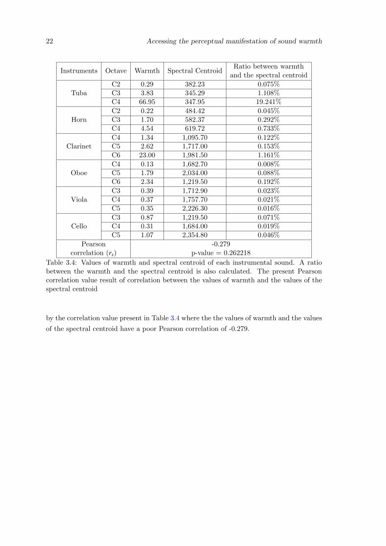
3.4 Values of warmth and spectral centroid of each instrumental sound. Aratio between the warmth and the spectral centroid is also calculated. Thepresent Pearson correlation value result of correlation between the values ofwarmth and the values of the spectral centroid . . . . . . . . . . . . . . . . 22
4.1 Lowest Detectable Frequency according to the FFT window size, consider-ing 44100Hz the sampling rate . . . . . . . . . . . . . . . . . . . . . . . . . 26
5.1 Responses of the second listening test that aimed to evaluate the system . . 315.2 Weighted arithmetic mean, variance and standard deviation of the results of
the second listening test. The present Pearson correlation values result froma correlation between the values of warmth and the weighted mean valuesand also from a correlation between the values of the spectral centroid andthe weighted mean values. . . . . . . . . . . . . . . . . . . . . . . . . . . . . 32
5.3 Calculation of the Warmth and Spectral Centroid of each instrumentalsounds that were modified according to a certain degree of warmth. It wasalso calculated the ratio between warmth and the centroid. The presentPearson correlation value result of the correlation between the values ofwarmth and the values of the spectral centroid. . . . . . . . . . . . . . . . . 33
xix

xx LIST OF TABLES
Abbreviations and symbols
ADC Analog-to-Digital-ConversionDAC Digital-to-Analog-ConversionDSP Digital Signal ProcessingFFT Fast Fourier TransformHz Hertz - The unit of frequency of the International SystemMIR Music Information RetrievalPCM Pulse-Code ModulationRM Remainder MagnitudeSTFT Short-time Fourier TransformWR Warmth Region
xxi

xxii Abbreviations and symbols
Chapter 1
Introduction
1.1 Context
Today, audio processing enables composers and musicians to freely manipulate the char-
acteristics of sound.
Traditionally, music experts refer to sound warmth according to two levels of granular-
ity. The first one is rather broad and categorizes the timbre of different musical instruments
from ‘cold’ to ‘warm’. For example, the low register of the clarinet tends to have a much
warmer sound than the piccolo. Similarly, the horn has a much warmer sound than the
trumpet. The second exists at a smaller scale and consists on the manipulations that
expert musicians perform, shaping their instrument timbre according to different shades
of warmth (e.g. in manipulating the point at which the bow hits the strings, a violinist
can change drastically the sound warmth of the instrument - these techniques are referred
to as sul tasto and sul ponticello). Music performers, composers and audio engineers have
been wanting to manipulate qualities of timbre[2]. However, the last two decades marked
a new scientific era in sound processing, having developed descriptors to extract attribute
from the sound spectrum[3].
Music information retrieval(MIR)[4] is a growing field of research concerned with the
extraction and inference of meaningful features from music (from the audio signal, symbolic
representation), indexing of music using these features, and the development of different
search and retrieval systems (for instance, content-based search, music recommendation
systems, or user interfaces for browsing large music collections), as explained by Downie[5].
1.2 Motivation
Up to this day, the term warmth falls in a category of music audio attributes, such as
bright, dull, flat, which expert musicians and music producers widely adopted to address
timbral attributes of sound. This musical jargon is highly relevant to the community of
musical experts.
1
2 Introduction
Being still hard to define mathematically, creates an opportunity to further investi-
gate and try to define an algorithm, a system, which would enable us to manipulate this
subjective attribute of sound using digital signal processing techniques.
To a lesser extent, this dissertation aims to contribute to music perception by answering
questions such as “Is this sound warm? How is warmth perceived? What is warmth?”. By
the end of the dissertation it is hoped to get some clarifications on the matter.
1.3 Goals
The purpose of this dissertation is to expand upon previously published results and create
a software to manipulate the warmth of sound that could be used worldwide in music
production, in audio effects, music composition in general.
Towards this goal, we will start by reviewing the existing proposal of Williams et.al[1]
and Antoine[6] and understand how the concept of warmth is perceived.
After this study, we design a listening test where the participants evaluate the level of
warmth in several monophonic instrumental sounds.
Then, we develop, in a controlled environment, a descriptor based on additive synthesis.
Accordingly, the definition of the descriptor will be redefined mainly regarding the output.
Ultimately, we generate a second listening test in order to evaluate the descriptor.
1.4 Document Structure
In Chapter 2 we review the state of the art of digital audio processing, introducing an
overview of digital audio processing, music information and content-based description of
musical audio signals. Later we review the existing work on warmth description in musical
audio.
In Chapter 3 we present a perceptual evaluation of sound warmth , and results, which
aims to evaluate how people perceive sound warmth.
In Chapter 4 we propose a system for manipulating the warmth in an audio file. We
start by presenting an overview of our system, followed by a detailed explanation of its
implementation.
In Chapter 5 we present the evaluation of our system. We detail and analyze the results
of the listening test designed to evaluate the sounds that were transformed according to
different levels of warmth.
In Chapter 6 we present conclusion of this work and point direction for future work.
Chapter 2
Overview of Digital Audio
Processing
In this chapter, we start with an overview of techniques and applications of Digital Signal
Processing (DSP). After, we introduce the field of Music Information Retrieval, and its
relevant techniques used to extract features from audio signals. Next, we present and
detail the different levels of abstraction of audio description. The chapter concludes with
the taxonomy of low-level layer of audio descriptors.
2.1 Digital Signal Processing
Digital Signal Processing[7] is the process of analysis and manipulation - applying mathe-
matical and computational algorithms - of data from analog signals (such as sound, light
or heat) that have been digitized or digitally generated signals. This includes a wide va-
riety of technical tools such as: filtering; speech recognition; image enhancement; data
compression; neural networks and more.
The use of DSP started around the ’70s, when digital computers first appeared and
became one of the most powerful technologies that would shape science and engineering
in the XXth century, across a large range of applications[8]:
• Communication Systems - modulation/demodulation, channel equalization, echo
cancellation;
• Consumer electronics - perceptual coding of audio and video on DVDs, speech syn-
thesis, speech recognition;
• Music - synthesized instruments, audio effects, noise cancellation;
• Medical Diagnostics - magnetic resonance and ultrasonic, imaging, computed to-
mography, electroencephalography (EEG), electrocardiography (ECG), magnetoen-
cephalography (MEG), automatic external defibrillator (AED), audiology;
3
4 Overview of Digital Audio Processing
• Geophysics - seismology, oil exploration;
• Astronomy - Very-long-baseline interferometry (VLBI), speckle interferometry;
• Experimental Physics - sensor-data evaluation;
• Aviation - radar, radio navigation;
• Security - steganography, digital watermarking, biometric identification, surveillance
systems, signals intelligence, electronic warfare;
Sound and light are good examples of analog signals, which machines cannot compute.
Therefore, a system is needed to convert analog signals to digital signals - a microphone
regarding sound, and a digital camera if the signal is light.
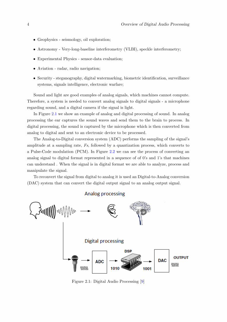
In Figure 2.1 we show an example of analog and digital processing of sound. In analog
processing the ear captures the sound waves and send them to the brain to process. In
digital processing, the sound is captured by the microphone which is then converted from
analog to digital and sent to an electronic device to be processed.
The Analog-to-Digital conversion system (ADC) performs the sampling of the signal’s
amplitude at a sampling rate, Fs, followed by a quantization process, which converts to
a Pulse-Code modulation (PCM). In Figure 2.2 we can see the process of converting an
analog signal to digital format represented in a sequence of of 0’s and 1’s that machines
can understand . When the signal is in digital format we are able to analyze, process and
manipulate the signal.
To reconvert the signal from digital to analog it is used an Digital-to-Analog conversion
(DAC) system that can convert the digital output signal to an analog output signal.
Figure 2.1: Digital Audio Processing [9]

2.2 Music Information Retrieval 5
Figure 2.2: Analog-to-Digital Conversion [10]
2.2 Music Information Retrieval
At a time where technology tends towards ubiquitous computing, music is mainly accessed
in digital format. We used to listen to music using the Walkman, Discman or even in a
stereo system at home. Today music streaming is the trend, and there are a number of
known services like Spotify1, Pandora2 and Deezer3 that have an enormous database from
where the user can choose what to listen.
But this vast amount of digital audio available requires a deeper understanding of how
to process audio signals, in particular how retrieving algorithms are formulated, to be able
to extract information from the audio file to enhance user centered retrieval methods from
these large archives.
1https://www.spotify.com/2https://www.pandora.com/3https://www.deezer.com/

6 Overview of Digital Audio Processing
The field of research in MIR[11] gathers people with background on computer science
and information retrieval, musicology and music theory, audio engineering and digital sig-
nal processing, machine learning and psychology, working together to create and enhance
toolboxes to better describe and extract relevant information from audio data[12].
MIR has several application domains[4] such as music retrieval, music recommendation,
music playlist generation and music browsing interfaces. All these applications demand
methods for retrieving information, for example audio identification or fingerprinting,
where the goal is to retrieve or identify the same fragment of a given music recording
with some robustness requirements. Another is query by humming and query by tapping,
where the goal is to retrieve music from a given melodic or rhythmic input (in audio or
symbolic format) which is described in terms of features and is compared to the documents
in a music collection (i.e Shazam4)[13].
2.3 Content-based audio description
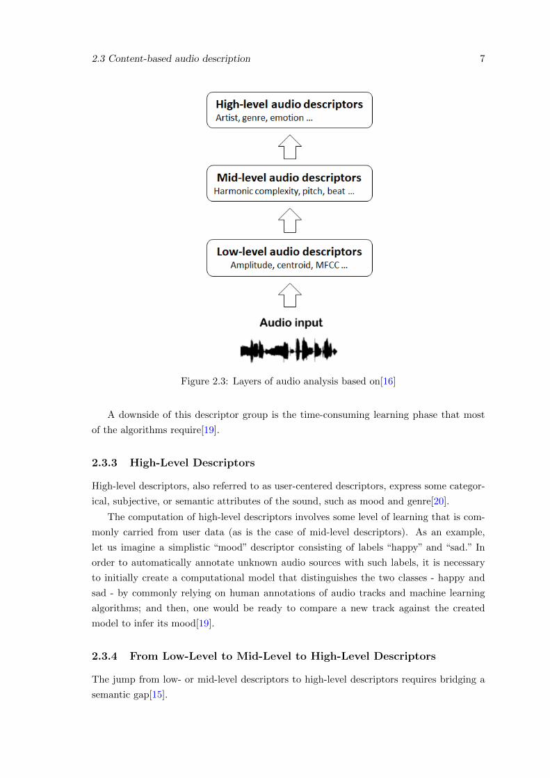
A lot of MIR research is based on human perception since the top-level ground-truth data
mostly consists of human annotations[14]. The description of audio can be presented in
an hierarchical structure, as shown by Herrera[15], from low-level to perceptual features
(mid-level) and finally to a semantic description (high-level).
Descriptors are resources of digital audio processing that, from the temporal and spec-
tral variation of the frequencies, represent the characteristics of the signal, which are useful
for the creation of a taxonomy of the properties of the signal content.
2.3.1 Low-Level Descriptors
The literature in signal processing and speech processing documents a large amount of
low-level audio features, either in the time domain (e.g. amplitude, zero-crossing rate, and
autocorrelation coefficients) or in the frequency domain (e.g. spectral centroid, spectral
skewness, and spectral flatness)[17]. They are computed from the digitized audio data by
simple means and with very little computational effort in a straight or derivative fashion.
Most low-level descriptors make little sense to humans, especially if one does not mas-
ter statistical analysis and signal processing techniques, because the terminology used to
designate them denotes the mathematical operations on the signal representation.
2.3.2 Mid-Level Descriptors
As stated by Gutierrez[18], mid-level descriptors are used when it is necessary to carry-out
operations which allow, after an analysis of the audio signal, to perform some generaliza-
tion. This generalization can be a description of the data according to music theory, such
as pitch, keys, meter, onsets, beats, harmonic complexity.
4https://www.shazam.com/
2.3 Content-based audio description 7
Figure 2.3: Layers of audio analysis based on[16]
A downside of this descriptor group is the time-consuming learning phase that most
of the algorithms require[19].
2.3.3 High-Level Descriptors
High-level descriptors, also referred to as user-centered descriptors, express some categor-
ical, subjective, or semantic attributes of the sound, such as mood and genre[20].
The computation of high-level descriptors involves some level of learning that is com-
monly carried from user data (as is the case of mid-level descriptors). As an example,
let us imagine a simplistic “mood” descriptor consisting of labels “happy” and “sad.” In
order to automatically annotate unknown audio sources with such labels, it is necessary
to initially create a computational model that distinguishes the two classes - happy and
sad - by commonly relying on human annotations of audio tracks and machine learning
algorithms; and then, one would be ready to compare a new track against the created
model to infer its mood[19].
2.3.4 From Low-Level to Mid-Level to High-Level Descriptors
The jump from low- or mid-level descriptors to high-level descriptors requires bridging a
semantic gap[15].
8 Overview of Digital Audio Processing
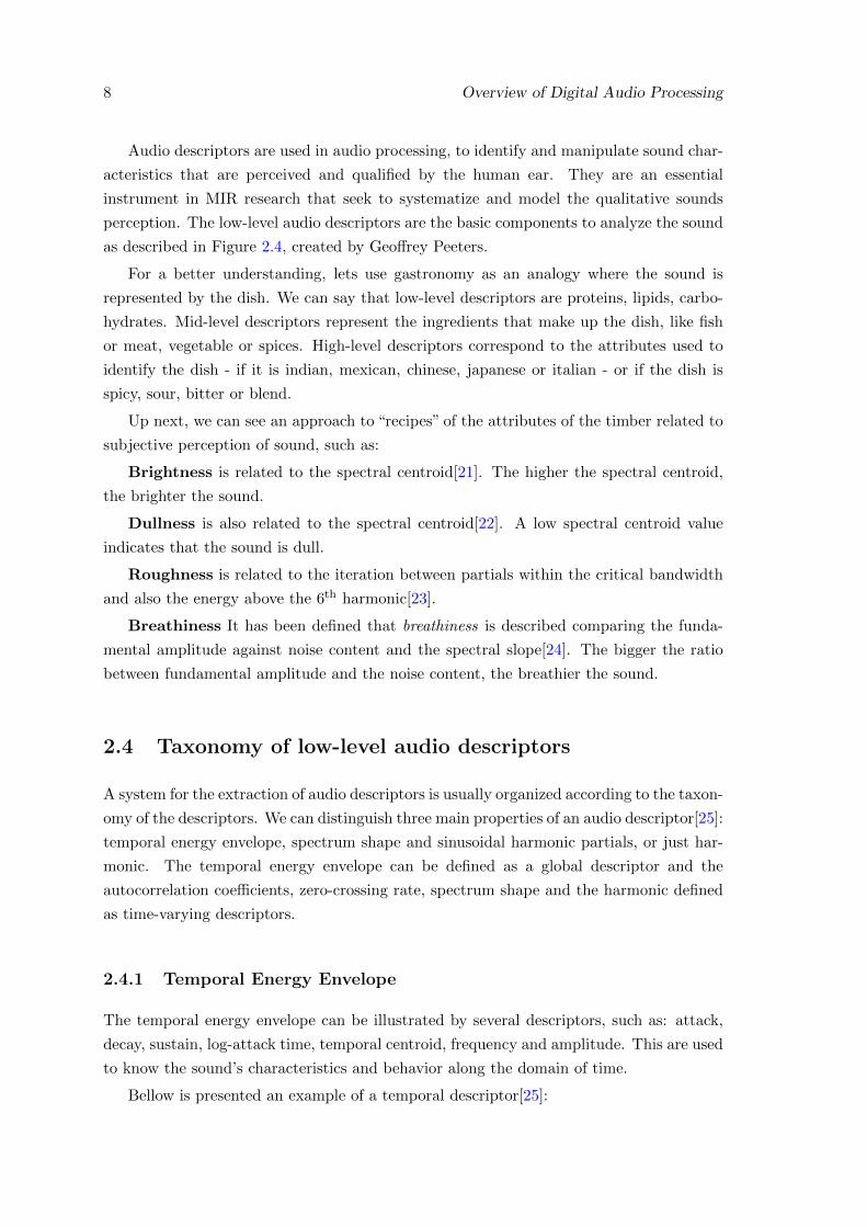
Audio descriptors are used in audio processing, to identify and manipulate sound char-
acteristics that are perceived and qualified by the human ear. They are an essential
instrument in MIR research that seek to systematize and model the qualitative sounds
perception. The low-level audio descriptors are the basic components to analyze the sound
as described in Figure 2.4, created by Geoffrey Peeters.
For a better understanding, lets use gastronomy as an analogy where the sound is
represented by the dish. We can say that low-level descriptors are proteins, lipids, carbo-
hydrates. Mid-level descriptors represent the ingredients that make up the dish, like fish
or meat, vegetable or spices. High-level descriptors correspond to the attributes used to
identify the dish - if it is indian, mexican, chinese, japanese or italian - or if the dish is
spicy, sour, bitter or blend.
Up next, we can see an approach to “recipes” of the attributes of the timber related to
subjective perception of sound, such as:
Brightness is related to the spectral centroid[21]. The higher the spectral centroid,
the brighter the sound.
Dullness is also related to the spectral centroid[22]. A low spectral centroid value
indicates that the sound is dull.
Roughness is related to the iteration between partials within the critical bandwidth
and also the energy above the 6th harmonic[23].
Breathiness It has been defined that breathiness is described comparing the funda-
mental amplitude against noise content and the spectral slope[24]. The bigger the ratio
between fundamental amplitude and the noise content, the breathier the sound.
2.4 Taxonomy of low-level audio descriptors
A system for the extraction of audio descriptors is usually organized according to the taxon-
omy of the descriptors. We can distinguish three main properties of an audio descriptor[25]:
temporal energy envelope, spectrum shape and sinusoidal harmonic partials, or just har-
monic. The temporal energy envelope can be defined as a global descriptor and the
autocorrelation coefficients, zero-crossing rate, spectrum shape and the harmonic defined
as time-varying descriptors.
2.4.1 Temporal Energy Envelope
The temporal energy envelope can be illustrated by several descriptors, such as: attack,
decay, sustain, log-attack time, temporal centroid, frequency and amplitude. This are used
to know the sound’s characteristics and behavior along the domain of time.
Bellow is presented an example of a temporal descriptor[25]:
2.4 Taxonomy of low-level audio descriptors 9
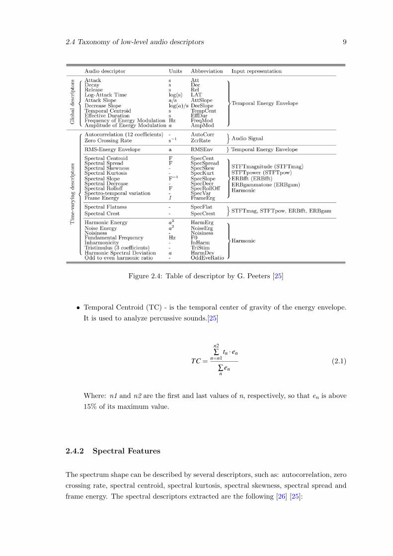
Figure 2.4: Table of descriptor by G. Peeters [25]
• Temporal Centroid (TC) - is the temporal center of gravity of the energy envelope.
It is used to analyze percussive sounds.[25]
TC =
n2∑
n=n1tn · en
∑n
en(2.1)
Where: n1 and n2 are the first and last values of n, respectively, so that en is above
15% of its maximum value.
2.4.2 Spectral Features
The spectrum shape can be described by several descriptors, such as: autocorrelation, zero
crossing rate, spectral centroid, spectral kurtosis, spectral skewness, spectral spread and
frame energy. The spectral descriptors extracted are the following [26] [25]:
10 Overview of Digital Audio Processing
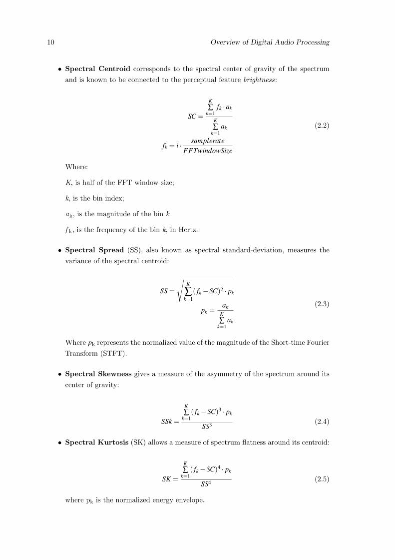
• Spectral Centroid corresponds to the spectral center of gravity of the spectrum
and is known to be connected to the perceptual feature brightness:
SC =
K∑
k=1fk ·ak
K∑
k=1ak
fk = i · samplerateFFTwindowSize
(2.2)
Where:
K, is half of the FFT window size;
k, is the bin index;
ak, is the magnitude of the bin k
f k, is the frequency of the bin k, in Hertz.
• Spectral Spread (SS), also known as spectral standard-deviation, measures the
variance of the spectral centroid:
SS =
√K
∑k=1
( fk−SC)2 · pk
pk =ak
K∑
k=1ak
(2.3)
Where pk represents the normalized value of the magnitude of the Short-time Fourier
Transform (STFT).
• Spectral Skewness gives a measure of the asymmetry of the spectrum around its
center of gravity:
SSk =
K∑
k=1( fk−SC)3 · pk
SS3 (2.4)
• Spectral Kurtosis (SK) allows a measure of spectrum flatness around its centroid:
SK =
K∑
k=1( fk−SC)4 · pk
SS4 (2.5)
where pk is the normalized energy envelope.
2.4 Taxonomy of low-level audio descriptors 11
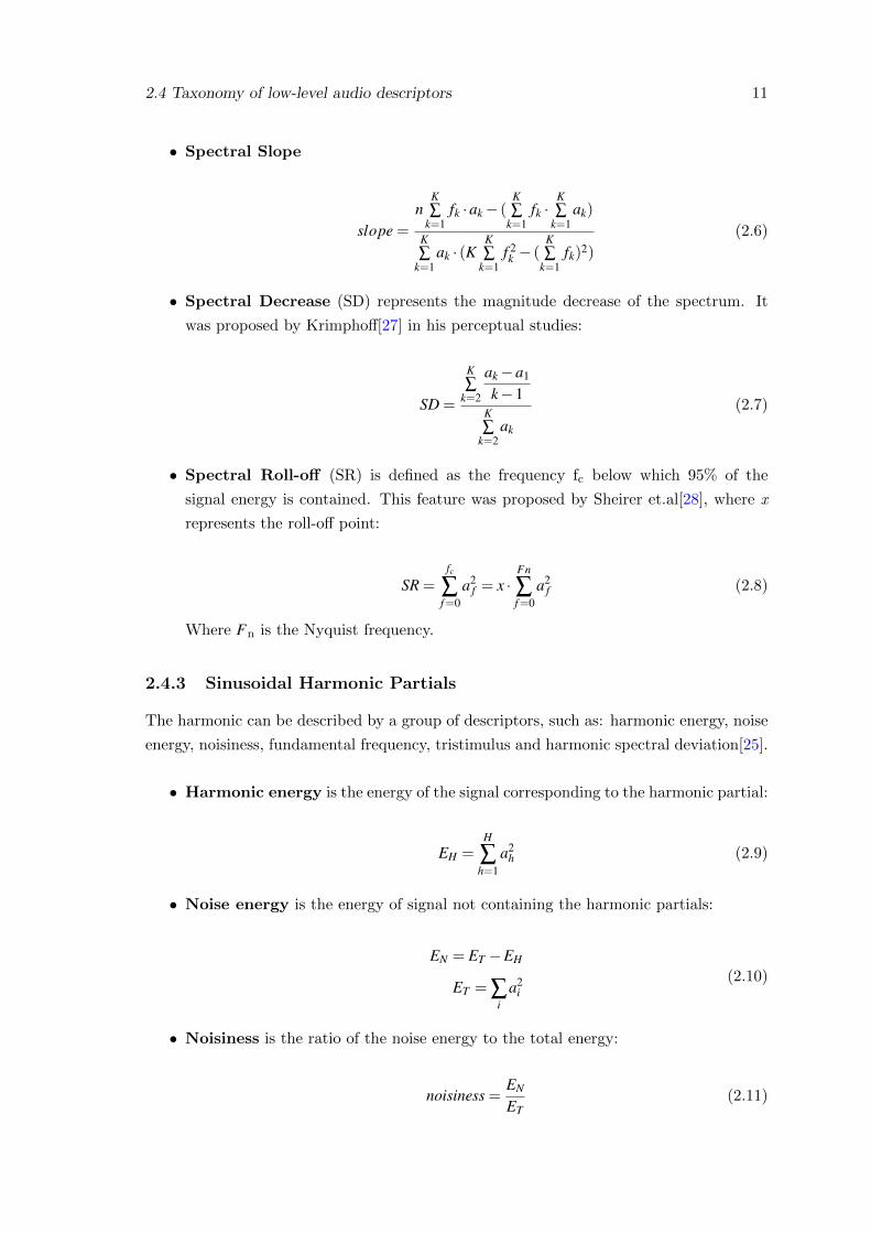
• Spectral Slope
slope =
nK∑
k=1fk ·ak− (
K∑
k=1fk ·
K∑
k=1ak)
K∑
k=1ak · (K
K∑
k=1f 2k − (
K∑
k=1fk)2)
(2.6)
• Spectral Decrease (SD) represents the magnitude decrease of the spectrum. It
was proposed by Krimphoff[27] in his perceptual studies:
SD =
K∑
k=2
ak−a1
k−1K∑
k=2ak
(2.7)
• Spectral Roll-off (SR) is defined as the frequency fc below which 95% of the
signal energy is contained. This feature was proposed by Sheirer et.al[28], where x
represents the roll-off point:
SR =fc
∑f =0
a2f = x ·
Fn
∑f =0
a2f (2.8)
Where Fn is the Nyquist frequency.
2.4.3 Sinusoidal Harmonic Partials
The harmonic can be described by a group of descriptors, such as: harmonic energy, noise
energy, noisiness, fundamental frequency, tristimulus and harmonic spectral deviation[25].
• Harmonic energy is the energy of the signal corresponding to the harmonic partial:
EH =H
∑h=1
a2h (2.9)
• Noise energy is the energy of signal not containing the harmonic partials:
EN = ET −EH
ET = ∑i
a2i
(2.10)
• Noisiness is the ratio of the noise energy to the total energy:
noisiness =EN
ET(2.11)
12 Overview of Digital Audio Processing
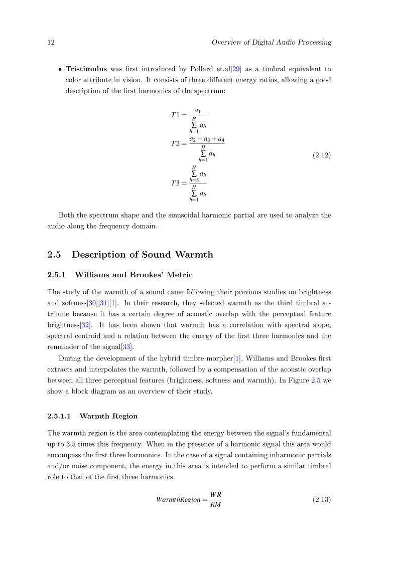
• Tristimulus was first introduced by Pollard et.al[29] as a timbral equivalent to
color attribute in vision. It consists of three different energy ratios, allowing a good
description of the first harmonics of the spectrum:
T 1 =a1
H∑
h=1ah
T 2 =a2 + a3 + a4
H∑
h=1ah
T 3 =
H∑
h=5ah
H∑
h=1ah
(2.12)
Both the spectrum shape and the sinusoidal harmonic partial are used to analyze the
audio along the frequency domain.
2.5 Description of Sound Warmth
2.5.1 Williams and Brookes’ Metric
The study of the warmth of a sound came following their previous studies on brightness
and softness[30][31][1]. In their research, they selected warmth as the third timbral at-
tribute because it has a certain degree of acoustic overlap with the perceptual feature
brightness[32]. It has been shown that warmth has a correlation with spectral slope,
spectral centroid and a relation between the energy of the first three harmonics and the
remainder of the signal[33].
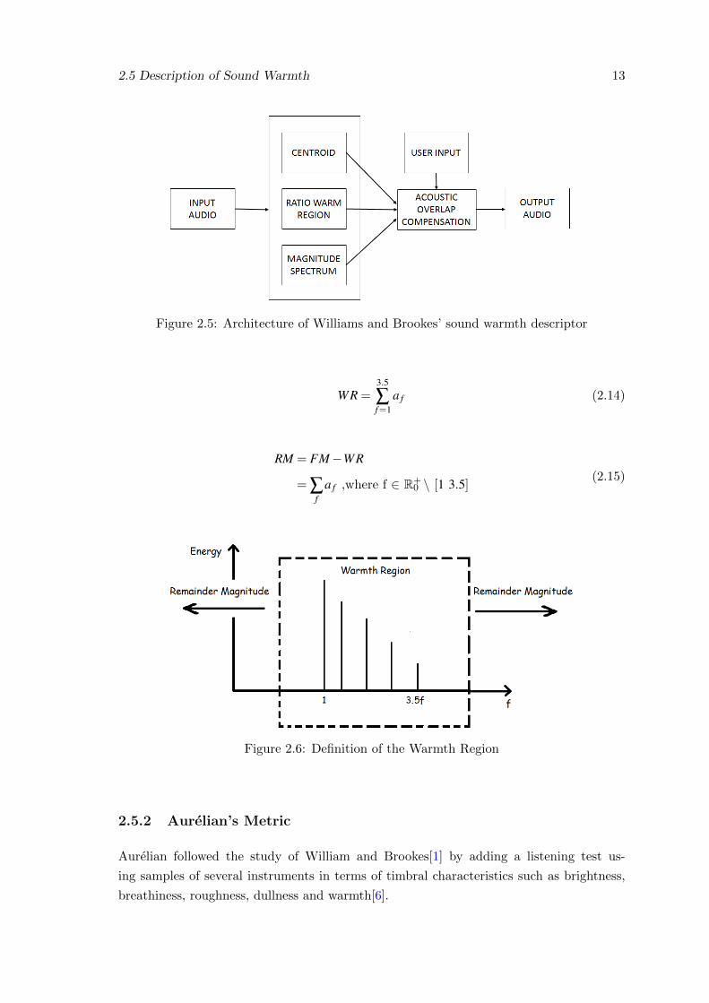
During the development of the hybrid timbre morpher[1], Williams and Brookes first
extracts and interpolates the warmth, followed by a compensation of the acoustic overlap
between all three perceptual features (brightness, softness and warmth). In Figure 2.5 we
show a block diagram as an overview of their study.
2.5.1.1 Warmth Region
The warmth region is the area contemplating the energy between the signal’s fundamental
up to 3.5 times this frequency. When in the presence of a harmonic signal this area would
encompass the first three harmonics. In the case of a signal containing inharmonic partials
and/or noise component, the energy in this area is intended to perform a similar timbral
role to that of the first three harmonics.
WarmthRegion =WRRM
(2.13)
2.5 Description of Sound Warmth 13
Figure 2.5: Architecture of Williams and Brookes’ sound warmth descriptor
WR =3.5
∑f =1
a f (2.14)
RM = FM−WR
= ∑f
a f ,where f ∈ R+0 \ [1 3.5]
(2.15)
Figure 2.6: Definition of the Warmth Region
2.5.2 Aurelian’s Metric
Aurelian followed the study of William and Brookes[1] by adding a listening test us-
ing samples of several instruments in terms of timbral characteristics such as brightness,
breathiness, roughness, dullness and warmth[6].

14 Overview of Digital Audio Processing
The results for the first four perceptual features showed strong correlation between the
participant’s responses and the classification system ratings[6]. However, the same cannot
be said for warmth, as the results felt short and inconclusive.
Given the lack of results and more in-depth information regarding his approach for
the analysis of warmth in sound, we designed an experiment which aims at evaluating the
perceptual basis of the attributes considered in both metrics, which we detail at length in
the following Chapter.
Chapter 3
Accessing the perceptual
manifestation of sound warmth
Previously, we reviewed the metrics that have been proposed in related literature to gauge
the warmth of a sound. Given the limitations, we compare the perception of warmth in
sound with the existing metrics, we conducted an online listening experiment of a set of
instrumental sounds.
This chapter details an experiment design followed by exposure of the results and ends
with the analysis of the instrumental sounds. In other words, we present and comment
on the values of warmth and spectral centroid of the instrumental sounds used on the
listening test.
3.1 Perceptual Evaluation
3.1.1 Listening Test
In order to design this listening test1, we used the IRCAM’s SOL database of acoustic
instruments. In this database we can find audio samples from almost all families of in-
struments (with the exception of percussion) which cover a wide spectral range, roughly
from the lowest octave (e.g A123) to the highest octave (e.g A8).
Due to the vast number of samples, with their unique timbral richness, and taking
into account the extension of the listening test[34], we created a data set consisting of 18
acoustic instrumental sounds - two instruments for each family of instruments and three
octaves for each instrument - with variable duration, ranging from 2 to 8 seconds. The
criteria for selecting these samples was that all instruments had to have the central C (Do)
1The listening test is available at http://npires91.polldaddy.com/s/listening-test-12Music notation using the alphabet to represent musical notes, from A (La) to G(Sol)3Music notation, using numbers, to represent the octave of the musical note (commonly present in a
piano keyboard), where 1 represents 1st (lowest) octave and 8 represents the 8th (highest) octave
15
16 Accessing the perceptual manifestation of sound warmth
sound as a common audio sample, which can be seen in Table 3.1. The test can be found
in Appendix A.2.
Participants were asked to rate on a 7-point Likert scale (1-7) the level of warmth of
the instrumental sounds, where 1 corresponds to not warm at all and 7 to completely
warm. They were asked to listen - using high quality headphones - to the entire duration
of the sound before rating it. To prevent response bias introduced by order effects, the
musical examples were presented in a random order. To submit their ratings and complete
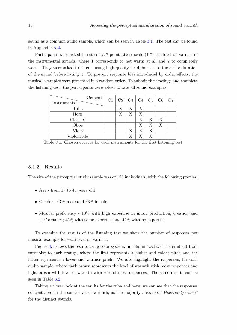
the listening test, the participants were asked to rate all sound examples.
`````````````InstrumentsOctaves
C1 C2 C3 C4 C5 C6 C7
Tuba X X X
Horn X X X
Clarinet X X X
Oboe X X X
Viola X X X
Violoncello X X X
Table 3.1: Chosen octaves for each instruments for the first listening test
3.1.2 Results
The size of the perceptual study sample was of 128 individuals, with the following profiles:
• Age - from 17 to 45 years old
• Gender - 67% male and 33% female
• Musical proficiency - 13% with high expertise in music production, creation and
performance; 45% with some expertise and 42% with no expertise;
To examine the results of the listening test we show the number of responses per
musical example for each level of warmth.
Figure 3.1 shows the results using color system, in column “Octave” the gradient from
turquoise to dark orange, where the first represents a higher and colder pitch and the
latter represents a lower and warmer pitch. We also highlight the responses, for each
audio sample, where dark brown represents the level of warmth with most responses and
light brown with level of warmth with second most responses. The same results can be
seen in Table 3.2.
Taking a closer look at the results for the tuba and horn, we can see that the responses
concentrated in the same level of warmth, as the majority answered “Moderately warm”
for the distinct sounds.

3.2 Analysis of the instrumental sounds 17
Figure 3.1: Responses of the first listening test with a graphical color code representation
On the other hand, the string family instruments (viola and violoncello) were evaluated
as expected as we can see a step-like distribution in their responses. For lower octaves,
they were evaluated with a higher level of warmth.
In the responses for the clarinet we can see a step-like distribution, similar to the
strings family responses. For the oboe, the results of the sounds example C5 and C6
were evaluated as expected, but for the C4 participants were divided which resulted in
evaluation both slightly, very slightly and moderately warm.
In order to know which sound was evaluated as the warmest, and least warm, we
calculated the weighted arithmetic mean of the results, where each evaluation had a weight
from 1 to 7 (the same as the Likert scale). After examining Table 3.3 we conclude that
the sound of the violoncello C3 was the warmest sound and, on the other hand, the sound
of the oboe C6 was the least warm of the data set.
3.2 Analysis of the instrumental sounds
For the purpose of knowing if there is a correlation between the warmth and spectral
centroid of the musical examples and the results from the listening test, we created a pure
data patch (Figure A.2 an A.1) that calculates the warmth and spectral centroid of each
analysis window for each instrumental sound. It also calculates the mean and standard
deviation of the values of warmth and spectral centroid and also a ratio between warmth
and the centroid, which are presented in Table 3.4. All the results were gathered and
analyzed using a Matlab script.
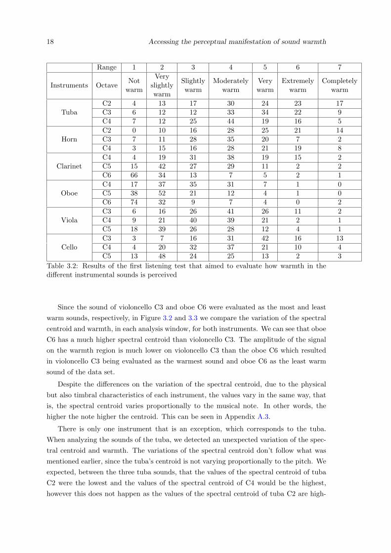
18 Accessing the perceptual manifestation of sound warmth
Range 1 2 3 4 5 6 7
Instruments OctaveNot
warm
Veryslightlywarm
Slightlywarm
Moderatelywarm
Verywarm
Extremelywarm
Completelywarm
TubaC2 4 13 17 30 24 23 17C3 6 12 12 33 34 22 9C4 7 12 25 44 19 16 5
HornC2 0 10 16 28 25 21 14C3 7 11 28 35 20 7 2C4 3 15 16 28 21 19 8
ClarinetC4 4 19 31 38 19 15 2C5 15 42 27 29 11 2 2C6 66 34 13 7 5 2 1
OboeC4 17 37 35 31 7 1 0C5 38 52 21 12 4 1 0C6 74 32 9 7 4 0 2
ViolaC3 6 16 26 41 26 11 2C4 9 21 40 39 21 2 1C5 18 39 26 28 12 4 1
CelloC3 3 7 16 31 42 16 13C4 4 20 32 37 21 10 4C5 13 48 24 25 13 2 3
Table 3.2: Results of the first listening test that aimed to evaluate how warmth in thedifferent instrumental sounds is perceived
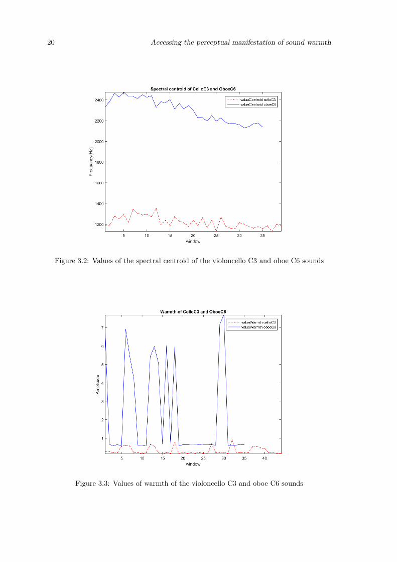
Since the sound of violoncello C3 and oboe C6 were evaluated as the most and least
warm sounds, respectively, in Figure 3.2 and 3.3 we compare the variation of the spectral
centroid and warmth, in each analysis window, for both instruments. We can see that oboe
C6 has a much higher spectral centroid than violoncello C3. The amplitude of the signal
on the warmth region is much lower on violoncello C3 than the oboe C6 which resulted
in violoncello C3 being evaluated as the warmest sound and oboe C6 as the least warm
sound of the data set.
Despite the differences on the variation of the spectral centroid, due to the physical
but also timbral characteristics of each instrument, the values vary in the same way, that
is, the spectral centroid varies proportionally to the musical note. In other words, the
higher the note higher the centroid. This can be seen in Appendix A.3.
There is only one instrument that is an exception, which corresponds to the tuba.
When analyzing the sounds of the tuba, we detected an unexpected variation of the spec-
tral centroid and warmth. The variations of the spectral centroid don’t follow what was
mentioned earlier, since the tuba’s centroid is not varying proportionally to the pitch. We
expected, between the three tuba sounds, that the values of the spectral centroid of tuba
C2 were the lowest and the values of the spectral centroid of C4 would be the highest,
however this does not happen as the values of the spectral centroid of tuba C2 are high-
3.2 Analysis of the instrumental sounds 19
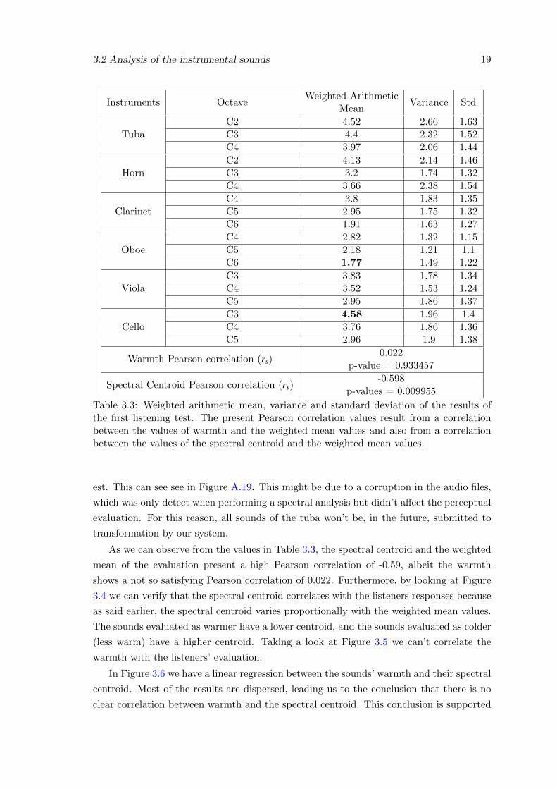
Instruments OctaveWeighted Arithmetic
MeanVariance Std
TubaC2 4.52 2.66 1.63C3 4.4 2.32 1.52C4 3.97 2.06 1.44
HornC2 4.13 2.14 1.46C3 3.2 1.74 1.32C4 3.66 2.38 1.54
ClarinetC4 3.8 1.83 1.35C5 2.95 1.75 1.32C6 1.91 1.63 1.27
OboeC4 2.82 1.32 1.15C5 2.18 1.21 1.1C6 1.77 1.49 1.22
ViolaC3 3.83 1.78 1.34C4 3.52 1.53 1.24C5 2.95 1.86 1.37
CelloC3 4.58 1.96 1.4C4 3.76 1.86 1.36C5 2.96 1.9 1.38
Warmth Pearson correlation (rs)0.022
p-value = 0.933457
Spectral Centroid Pearson correlation (rs)-0.598
p-values = 0.009955
Table 3.3: Weighted arithmetic mean, variance and standard deviation of the results ofthe first listening test. The present Pearson correlation values result from a correlationbetween the values of warmth and the weighted mean values and also from a correlationbetween the values of the spectral centroid and the weighted mean values.
est. This can see see in Figure A.19. This might be due to a corruption in the audio files,
which was only detect when performing a spectral analysis but didn’t affect the perceptual
evaluation. For this reason, all sounds of the tuba won’t be, in the future, submitted to
transformation by our system.
As we can observe from the values in Table 3.3, the spectral centroid and the weighted
mean of the evaluation present a high Pearson correlation of -0.59, albeit the warmth
shows a not so satisfying Pearson correlation of 0.022. Furthermore, by looking at Figure
3.4 we can verify that the spectral centroid correlates with the listeners responses because
as said earlier, the spectral centroid varies proportionally with the weighted mean values.
The sounds evaluated as warmer have a lower centroid, and the sounds evaluated as colder
(less warm) have a higher centroid. Taking a look at Figure 3.5 we can’t correlate the
warmth with the listeners’ evaluation.
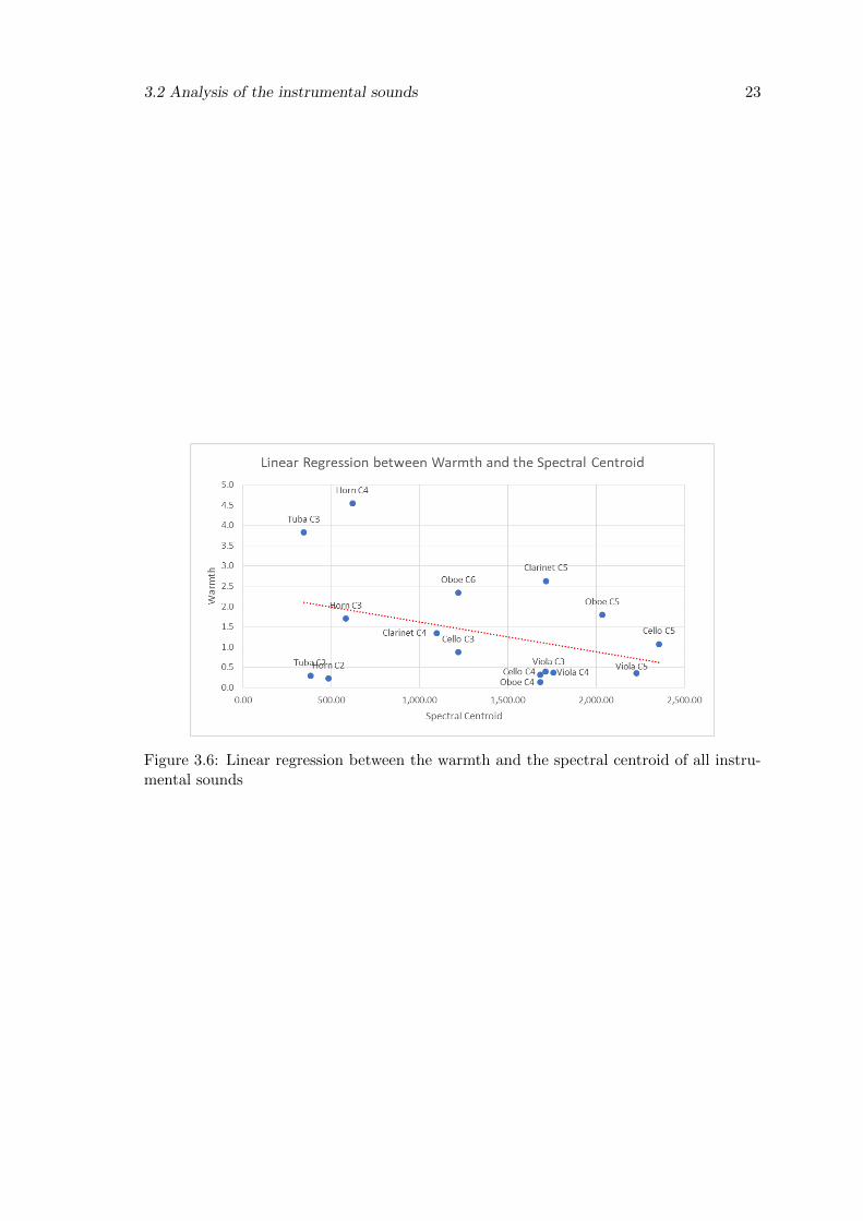
In Figure 3.6 we have a linear regression between the sounds’ warmth and their spectral
centroid. Most of the results are dispersed, leading us to the conclusion that there is no
clear correlation between warmth and the spectral centroid. This conclusion is supported
20 Accessing the perceptual manifestation of sound warmth
Figure 3.2: Values of the spectral centroid of the violoncello C3 and oboe C6 sounds
Figure 3.3: Values of warmth of the violoncello C3 and oboe C6 sounds
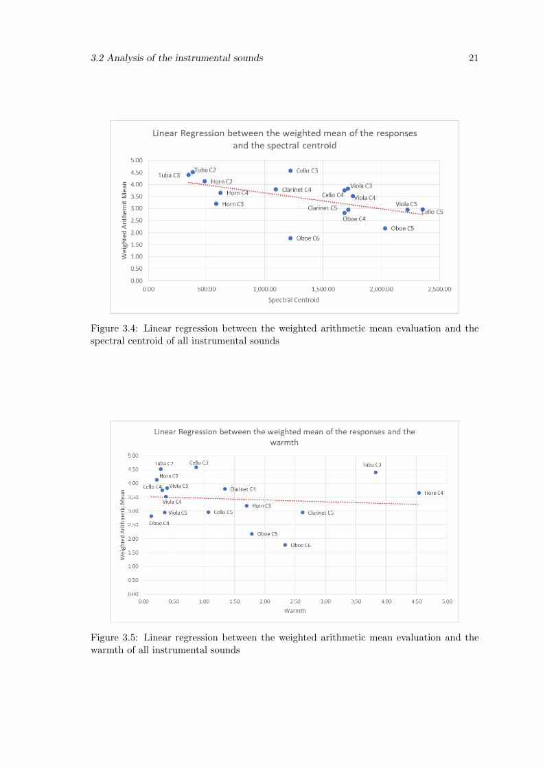
3.2 Analysis of the instrumental sounds 21
Figure 3.4: Linear regression between the weighted arithmetic mean evaluation and thespectral centroid of all instrumental sounds
Figure 3.5: Linear regression between the weighted arithmetic mean evaluation and thewarmth of all instrumental sounds
22 Accessing the perceptual manifestation of sound warmth
Instruments Octave Warmth Spectral CentroidRatio between warmth
and the spectral centroid
TubaC2 0.29 382.23 0.075%C3 3.83 345.29 1.108%C4 66.95 347.95 19.241%
HornC2 0.22 484.42 0.045%C3 1.70 582.37 0.292%C4 4.54 619.72 0.733%
ClarinetC4 1.34 1,095.70 0.122%C5 2.62 1,717.00 0.153%C6 23.00 1,981.50 1.161%
OboeC4 0.13 1,682.70 0.008%C5 1.79 2,034.00 0.088%C6 2.34 1,219.50 0.192%
ViolaC3 0.39 1,712.90 0.023%C4 0.37 1,757.70 0.021%C5 0.35 2,226.30 0.016%
CelloC3 0.87 1,219.50 0.071%C4 0.31 1,684.00 0.019%C5 1.07 2,354.80 0.046%
Pearsoncorrelation (rs)
-0.279p-value = 0.262218
Table 3.4: Values of warmth and spectral centroid of each instrumental sound. A ratiobetween the warmth and the spectral centroid is also calculated. The present Pearsoncorrelation value result of correlation between the values of warmth and the values of thespectral centroid
by the correlation value present in Table 3.4 where the the values of warmth and the values
of the spectral centroid have a poor Pearson correlation of -0.279.
3.2 Analysis of the instrumental sounds 23
Figure 3.6: Linear regression between the warmth and the spectral centroid of all instru-mental sounds

24 Accessing the perceptual manifestation of sound warmth
Chapter 4
Development of the system
In this chapter we describe, in detail, the development of the system, created in Pure
Data[35], that allows producers and musicians to manipulate the warmth of monophonic
harmonic audio in real-time (e.g., of a live performance).
4.1 System Overview
Based on the new linear combination resulting from our listening test, we developed a
(one-knob) audio effect which allows users to transform the warmth of a sound in real-
time. To this end, we regulate the amplitudes of the spectral components of a musical
audio, to shape them according to a relative user-controlled level of warmth. In other
words, we allow user to dynamically reduce or increase the percentage of warmness in the
musical audio input while retaining the relative variability over time.
Yet, due to its subjective nature, it’s hard to define it with a mathematical model,
which would enable us to manipulate sounds using digital signal processing techniques.
Therefore, by being aware of the importance of such a processing tool, we strive here to
first understand the timbral attributes which impact such an informal sonic attribute and
secondly encode it as a mathematical model which can be used to manipulate the warmth
of musical audio in real-time.
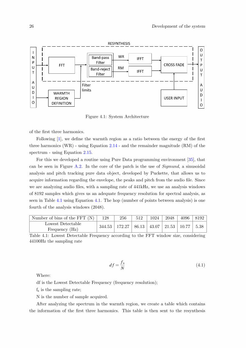
The architecture of our system is shown in Figure 4.1. After receiving the input audio
file, the system first calculates the warmth region (WR) and the remainder magnitude
(RM) as outputs. These outputs are then processed by a resynthesis algorithm. This
algorithm takes the user input, which will control the level of warmth that he wants in the
output audio file.
4.2 Definition of the Warmth Region
In order to define the warmth region, we use Williams and Brookes’ metric, explained in
Section 2.5.1.1. They defend that the warmth region is the area encompassing the energy
25
26 Development of the system
Figure 4.1: System Architecture
of the first three harmonics.
Following [1], we define the warmth region as a ratio between the energy of the first
three harmonics (WR) - using Equation 2.14 - and the remainder magnitude (RM) of the
spectrum - using Equation 2.15.
For this we developed a routine using Pure Data programming environment [35], that
can be seen in Figure A.2. In the core of the patch is the use of Sigmund, a sinusoidal
analysis and pitch tracking pure data object, developed by Puckette, that allows us to
acquire information regarding the envelope, the peaks and pitch from the audio file. Since
we are analyzing audio files, with a sampling rate of 441kHz, we use an analysis windows
of 8192 samples which gives us an adequate frequency resolution for spectral analysis, as
seen in Table 4.1 using Equation 4.1. The hop (number of points between analysis) is one
fourth of the analysis windows (2048).
Number of bins of the FFT (N) 128 256 512 1024 2048 4096 8192
Lowest DetectableFrequency (Hz)
344.53 172.27 86.13 43.07 21.53 10.77 5.38
Table 4.1: Lowest Detectable Frequency according to the FFT window size, considering44100Hz the sampling rate
d f =f sN
(4.1)
Where:
df is the Lowest Detectable Frequency (frequency resolution);
fs is the sampling rate;
N is the number of sample acquired.
After analyzing the spectrum in the warmth region, we create a table which contains
the information of the first three harmonics. This table is then sent to the resynthesis
4.3 Resynthesis 27
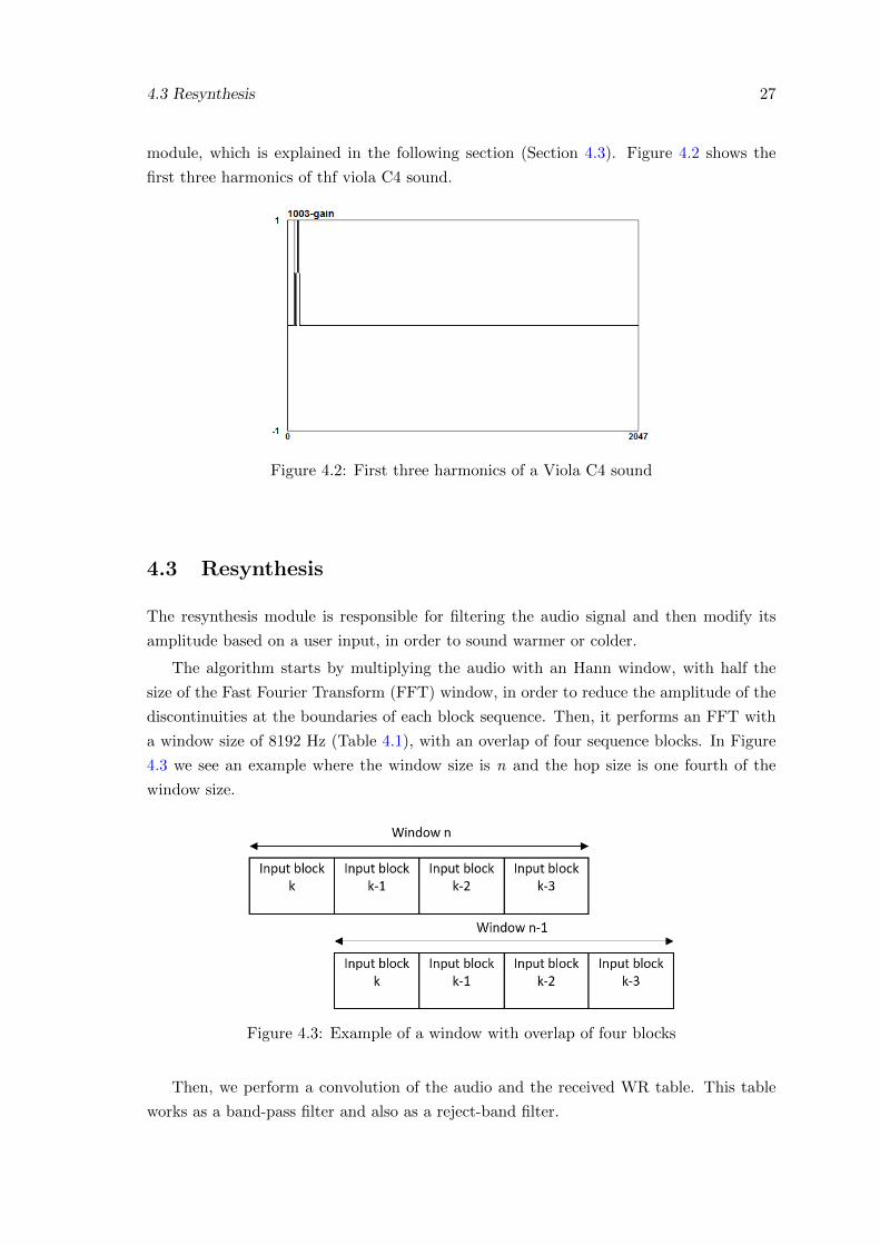
module, which is explained in the following section (Section 4.3). Figure 4.2 shows the
first three harmonics of thf viola C4 sound.
Figure 4.2: First three harmonics of a Viola C4 sound
4.3 Resynthesis
The resynthesis module is responsible for filtering the audio signal and then modify its
amplitude based on a user input, in order to sound warmer or colder.
The algorithm starts by multiplying the audio with an Hann window, with half the
size of the Fast Fourier Transform (FFT) window, in order to reduce the amplitude of the
discontinuities at the boundaries of each block sequence. Then, it performs an FFT with
a window size of 8192 Hz (Table 4.1), with an overlap of four sequence blocks. In Figure
4.3 we see an example where the window size is n and the hop size is one fourth of the
window size.
Figure 4.3: Example of a window with overlap of four blocks
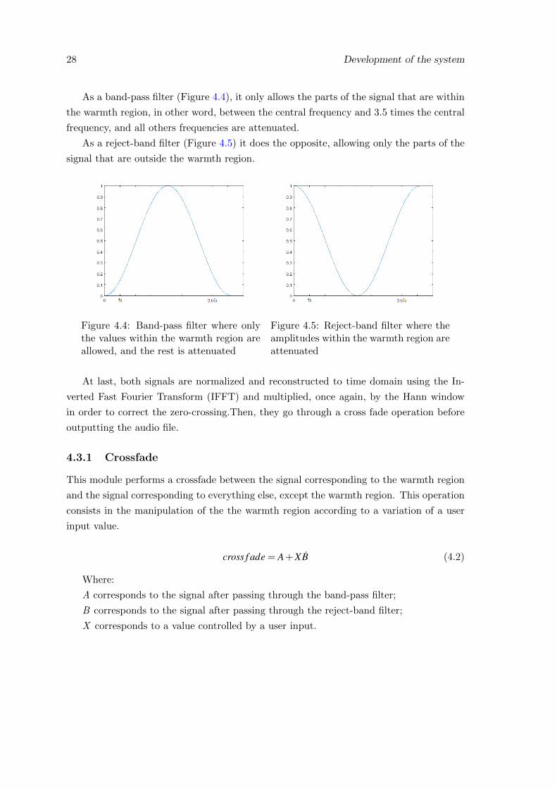
Then, we perform a convolution of the audio and the received WR table. This table
works as a band-pass filter and also as a reject-band filter.
28 Development of the system
As a band-pass filter (Figure 4.4), it only allows the parts of the signal that are within
the warmth region, in other word, between the central frequency and 3.5 times the central
frequency, and all others frequencies are attenuated.
As a reject-band filter (Figure 4.5) it does the opposite, allowing only the parts of the
signal that are outside the warmth region.
Figure 4.4: Band-pass filter where onlythe values within the warmth region areallowed, and the rest is attenuated
Figure 4.5: Reject-band filter where theamplitudes within the warmth region areattenuated
At last, both signals are normalized and reconstructed to time domain using the In-
verted Fast Fourier Transform (IFFT) and multiplied, once again, by the Hann window
in order to correct the zero-crossing.Then, they go through a cross fade operation before
outputting the audio file.
4.3.1 Crossfade
This module performs a crossfade between the signal corresponding to the warmth region
and the signal corresponding to everything else, except the warmth region. This operation
consists in the manipulation of the the warmth region according to a variation of a user
input value.
cross f ade = A + XB (4.2)
Where:
A corresponds to the signal after passing through the band-pass filter;
B corresponds to the signal after passing through the reject-band filter;
X corresponds to a value controlled by a user input.
Chapter 5
Evaluation of the system
This chapter starts by explaining the listening experiment used to evaluate the effectiveness
of the system. Then we present and comment on the results from the listening test.
Lastly, we analyze the new values of warmth and spectral centroid of the transformed
sounds and compare them to their original sound.
5.1 Listening Test
In order to evaluate the performance of our system, we conducted a second online listening
experiment1 of a set of instrumental sounds.
Based on the responses of the first listening test, the violoncello was the instrument
with a warmer evaluation overall. In this regard, we selected the highest octave (C5) in
order to evaluate if the variation of its warmth would be perceived. This same octave was
selected for all the others instruments, except for the horn where we used the octave C4,
which is the highest octave available.
To perform an objective evaluation of the system, we modified each instrument ac-
cording to different degrees of warmth. Specifically, we increased the warmth by 25% and
50% and decreased the warmth by 25% and 50%. The test can be found in Appendix A.4.
In the survey, participants were asked to rate on a 5-point Likert scale (1-5) the dif-
ference in warmth between the two available audio, where 1 corresponds to the modified
sound being much warmer than the original sound, 3 corresponds to no prominent differ-
ence between the two sounds, and 5 corresponds to evaluating the modified sound as much
colder than the original sound.
Before rating, the participants were asked to find a quiet place and listen to the full
extent of both audio examples using high quality headphones.
In order to submit their ratings and complete the listening test, the participants were
obliged to rate all sound examples. To prevent responses bias introduced by order effects,
the musical examples were presented in a random order at each experiment trial.
1The listening test is available at http://npires91.polldaddy.com/s/listening-test-2
29
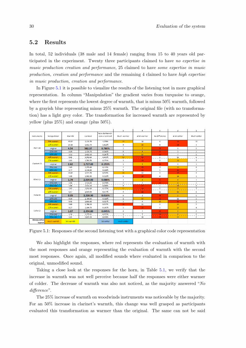
30 Evaluation of the system
5.2 Results
In total, 52 individuals (38 male and 14 female) ranging from 15 to 40 years old par-
ticipated in the experiment. Twenty three participants claimed to have no expertise in
music production creation and performance, 25 claimed to have some expertise in music
production, creation and performance and the remaining 4 claimed to have high expertise
in music production, creation and performance.
In Figure 5.1 it is possible to visualize the results of the listening test in more graphical
representation. In column “Manipulation” the gradient varies from turquoise to orange,
where the first represents the lowest degree of warmth, that is minus 50% warmth, followed
by a grayish blue representing minus 25% warmth. The original file (with no transforma-
tion) has a light grey color. The transformation for increased warmth are represented by
yellow (plus 25%) and orange (plus 50%).
Figure 5.1: Responses of the second listening test with a graphical color code representation
We also highlight the responses, where red represents the evaluation of warmth with
the most responses and orange representing the evaluation of warmth with the second
most responses. Once again, all modified sounds where evaluated in comparison to the
original, unmodified sound.
Taking a close look at the responses for the horn, in Table 5.1, we verify that the
increase in warmth was not well perceive because half the responses were either warmer
of colder. The decrease of warmth was also not noticed, as the majority answered “No
difference”.
The 25% increase of warmth on woodwinds instruments was noticeable by the majority.
For an 50% increase in clarinet’s warmth, this change was well grasped as participants
evaluated this transformation as warmer than the original. The same can not be said
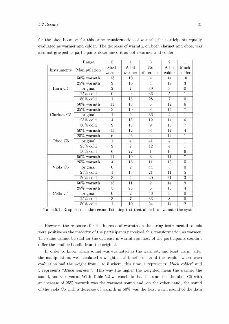
5.2 Results 31
for the oboe because; for this same transformation of warmth, the participants equally
evaluated as warmer and colder. The decrease of warmth, on both clarinet and oboe, was
also not grasped as participants determined it as both warmer and colder.
Range 5 4 3 2 1
Instruments ManipulationMuch
warmerA bit
warmerNo
differenceA bitcolder
Muchcolder
Horn C4
50% warmth 13 10 4 14 1025% warmth 9 16 4 19 3
original 2 7 39 3 025% cold 0 9 36 5 150% cold 1 15 28 7 0
Clarinet C5
50% warmth 13 15 5 12 625% warmth 3 19 8 14 7
original 1 9 36 4 125% cold 4 15 12 14 650% cold 9 13 9 13 7
Oboe C5
50% warmth 15 12 3 17 425% warmth 6 26 4 14 1
original 1 4 41 4 125% cold 2 2 42 4 150% cold 6 22 1 16 6
Viola C5
50% warmth 11 19 3 11 725% warmth 4 18 11 13 5
original 0 2 44 5 025% cold 1 13 21 11 550% cold 3 4 20 21 3
Cello C5
50% warmth 15 11 2 14 925% warmth 5 23 6 13 4
original 0 2 46 3 025% cold 3 7 33 8 050% cold 1 10 24 14 2
Table 5.1: Responses of the second listening test that aimed to evaluate the system
However, the responses for the increase of warmth on the string instrumental sounds
were positive as the majority of the participants perceived this transformation as warmer.
The same cannot be said for the decrease in warmth as most of the participants couldn’t
differ the modified audio from the original.
In order to know which sound was evaluated as the warmest, and least warm, after
the manipulation, we calculated a weighted arithmetic mean of the results, where each
evaluation had the weight from 1 to 5 where, this time, 1 represents“ Much colder” and
5 represents “Much warmer”. This way the higher the weighted mean the warmer the
sound, and vice versa. With Table 5.2 we conclude that the sound of the oboe C5 with
an increase of 25% warmth was the warmest sound and, on the other hand, the sound
of the viola C5 with a decrease of warmth in 50% was the least warm sound of the data
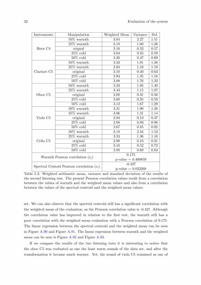
32 Evaluation of the system
Instruments Manipulation Weighted Mean Variance Std
Horn C4
50% warmth 3.04 2.27 1.5125% warmth 3.18 1.60 1.26
orignal 3.16 0.33 0.5725% cold 3.04 0.35 0.5950% cold 3.20 0.47 0.69
Clarinet C5
50% warmth 3.33 1.91 1.3825% warmth 2.94 1.43 1.19
original 3.10 0.40 0.6325% cold 2.94 1.35 1.1650% cold 3.08 1.76 1.33
Oboe C5
50% warmth 3.33 1.95 1.4025% warmth 3.43 1.15 1.07
original 3.00 0.31 0.5625% cold 3.00 0.35 0.5950% cold 3.12 1.67 1.29
Viola C5
50% warmth 3.31 1.90 1.3825% warmth 3.06 1.31 1.14
original 2.94 0.13 0.3725% cold 2.88 0.93 0.9650% cold 2.67 0.85 0.92
Cello C5
50% warmth 3.18 2.34 1.5325% warmth 3.24 1.36 1.16
original 2.98 0.10 0.3125% cold 3.10 0.52 0.7250% cold 2.88 0.69 0.83
Warmth Pearson correlation (rs)0.175
p-value = 0.400859
Spectral Centoid Pearson correlation (rs)-0.427
p-value = 0.033268
Table 5.2: Weighted arithmetic mean, variance and standard deviation of the results ofthe second listening test. The present Pearson correlation values result from a correlationbetween the values of warmth and the weighted mean values and also from a correlationbetween the values of the spectral centroid and the weighted mean values.
set. We can also observe that the spectral centroid still has a significant correlation with
the weighted mean of the evaluation, as the Pearson correlation value is -0.427. Although
the correlation value has improved in relation to the first test, the warmth still has a
poor correlation with the weighted mean evaluation with a Pearson correlation of 0.175.
The linear regression between the spectral centroid and the weighted mean can be seen
in Figure A.90 and Figure A.91. The linear regression between warmth and the weighted
mean can be seen is Figure A.92 and Figure A.93.
If we compare the results of the two listening tests it is interesting to notice that
the oboe C5 was evaluated as one the least warm sounds of the data set, and after the
transformation it became much warmer. Yet, the sound of viola C5 remained as one of
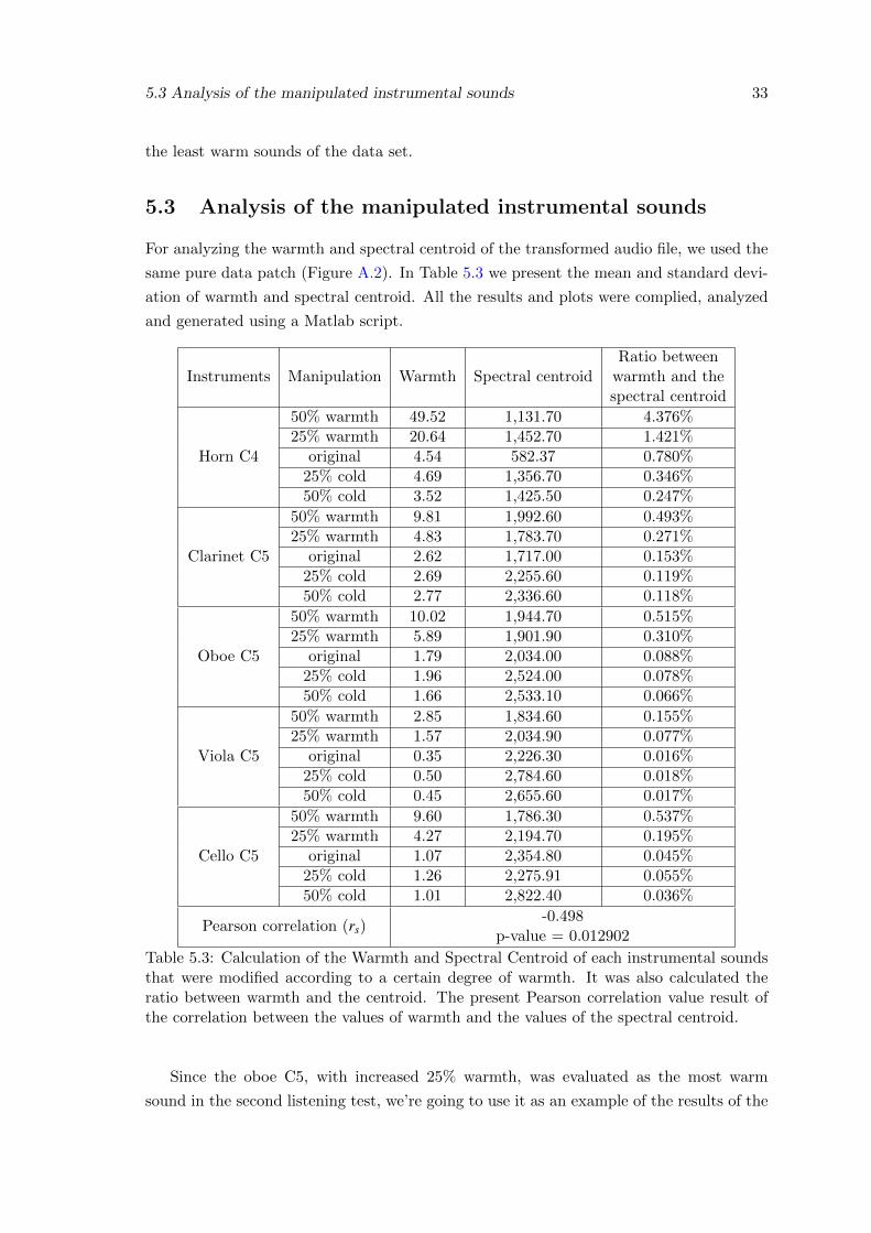
5.3 Analysis of the manipulated instrumental sounds 33
the least warm sounds of the data set.
5.3 Analysis of the manipulated instrumental sounds
For analyzing the warmth and spectral centroid of the transformed audio file, we used the
same pure data patch (Figure A.2). In Table 5.3 we present the mean and standard devi-
ation of warmth and spectral centroid. All the results and plots were complied, analyzed
and generated using a Matlab script.
Instruments Manipulation Warmth Spectral centroidRatio between
warmth and thespectral centroid
Horn C4
50% warmth 49.52 1,131.70 4.376%25% warmth 20.64 1,452.70 1.421%
original 4.54 582.37 0.780%25% cold 4.69 1,356.70 0.346%50% cold 3.52 1,425.50 0.247%
Clarinet C5
50% warmth 9.81 1,992.60 0.493%25% warmth 4.83 1,783.70 0.271%
original 2.62 1,717.00 0.153%25% cold 2.69 2,255.60 0.119%50% cold 2.77 2,336.60 0.118%
Oboe C5
50% warmth 10.02 1,944.70 0.515%25% warmth 5.89 1,901.90 0.310%
original 1.79 2,034.00 0.088%25% cold 1.96 2,524.00 0.078%50% cold 1.66 2,533.10 0.066%
Viola C5
50% warmth 2.85 1,834.60 0.155%25% warmth 1.57 2,034.90 0.077%
original 0.35 2,226.30 0.016%25% cold 0.50 2,784.60 0.018%50% cold 0.45 2,655.60 0.017%
Cello C5
50% warmth 9.60 1,786.30 0.537%25% warmth 4.27 2,194.70 0.195%
original 1.07 2,354.80 0.045%25% cold 1.26 2,275.91 0.055%50% cold 1.01 2,822.40 0.036%
Pearson correlation (rs)-0.498
p-value = 0.012902
Table 5.3: Calculation of the Warmth and Spectral Centroid of each instrumental soundsthat were modified according to a certain degree of warmth. It was also calculated theratio between warmth and the centroid. The present Pearson correlation value result ofthe correlation between the values of warmth and the values of the spectral centroid.
Since the oboe C5, with increased 25% warmth, was evaluated as the most warm
sound in the second listening test, we’re going to use it as an example of the results of the
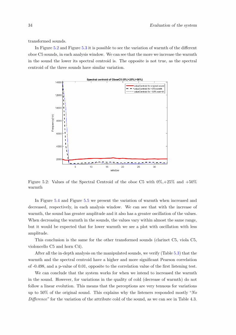
34 Evaluation of the system
transformed sounds.
In Figure 5.2 and Figure 5.3 it is possible to see the variation of warmth of the different
oboe C5 sounds, in each analysis window. We can see that the more we increase the warmth
in the sound the lower its spectral centroid is. The opposite is not true, as the spectral
centroid of the three sounds have similar variation.
Figure 5.2: Values of the Spectral Centroid of the oboe C5 with 0%,+25% and +50%warmth
In Figure 5.4 and Figure 5.5 we present the variation of warmth when increased and
decreased, respectively, in each analysis window. We can see that with the increase of
warmth, the sound has greater amplitude and it also has a greater oscillation of the values.
When decreasing the warmth in the sounds, the values vary within almost the same range,
but it would be expected that for lower warmth we see a plot with oscillation with less
amplitude.
This conclusion is the same for the other transformed sounds (clarinet C5, viola C5,
violoncello C5 and horn C4).
After all the in-depth analysis on the manipulated sounds, we verify (Table 5.3) that the
warmth and the spectral centroid have a higher and more significant Pearson correlation
of -0.498, and a p-value of 0.01, opposite to the correlation value of the first listening test.
We can conclude that the system works for when we intend to increased the warmth
in the sound. However, for variations in the quality of cold (decrease of warmth) do not
follow a linear evolution. This means that the perceptions are very tenuous for variations
up to 50% of the original sound. This explains why the listeners responded mostly “No
Difference” for the variation of the attribute cold of the sound, as we can see in Table 4.3.
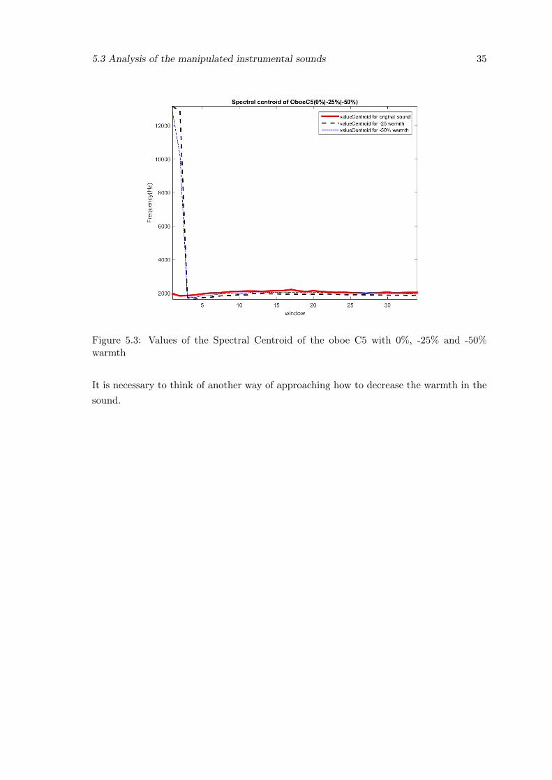
5.3 Analysis of the manipulated instrumental sounds 35
Figure 5.3: Values of the Spectral Centroid of the oboe C5 with 0%, -25% and -50%warmth
It is necessary to think of another way of approaching how to decrease the warmth in the
sound.
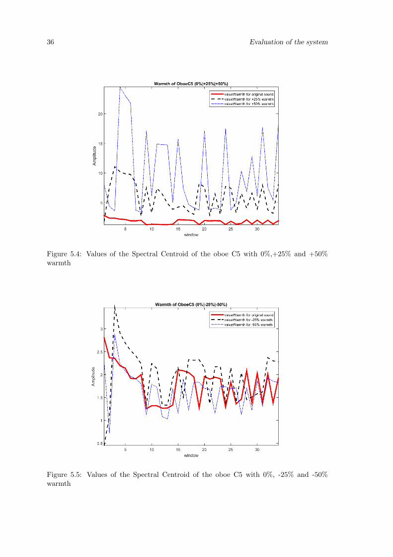
36 Evaluation of the system
Figure 5.4: Values of the Spectral Centroid of the oboe C5 with 0%,+25% and +50%warmth
Figure 5.5: Values of the Spectral Centroid of the oboe C5 with 0%, -25% and -50%warmth
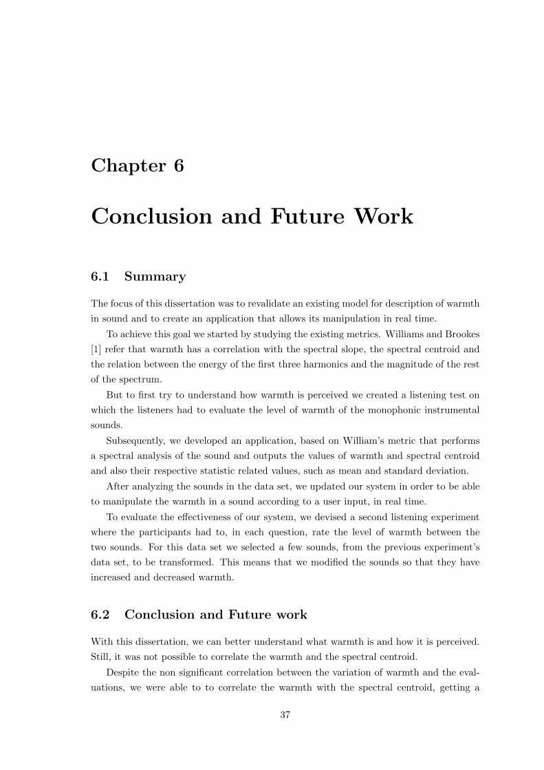
Chapter 6
Conclusion and Future Work
6.1 Summary
The focus of this dissertation was to revalidate an existing model for description of warmth
in sound and to create an application that allows its manipulation in real time.
To achieve this goal we started by studying the existing metrics. Williams and Brookes
[1] refer that warmth has a correlation with the spectral slope, the spectral centroid and
the relation between the energy of the first three harmonics and the magnitude of the rest
of the spectrum.
But to first try to understand how warmth is perceived we created a listening test on
which the listeners had to evaluate the level of warmth of the monophonic instrumental
sounds.
Subsequently, we developed an application, based on William’s metric that performs
a spectral analysis of the sound and outputs the values of warmth and spectral centroid
and also their respective statistic related values, such as mean and standard deviation.
After analyzing the sounds in the data set, we updated our system in order to be able
to manipulate the warmth in a sound according to a user input, in real time.
To evaluate the effectiveness of our system, we devised a second listening experiment
where the participants had to, in each question, rate the level of warmth between the
two sounds. For this data set we selected a few sounds, from the previous experiment’s
data set, to be transformed. This means that we modified the sounds so that they have
increased and decreased warmth.
6.2 Conclusion and Future work
With this dissertation, we can better understand what warmth is and how it is perceived.
Still, it was not possible to correlate the warmth and the spectral centroid.
Despite the non significant correlation between the variation of warmth and the eval-
uations, we were able to to correlate the warmth with the spectral centroid, getting a
37
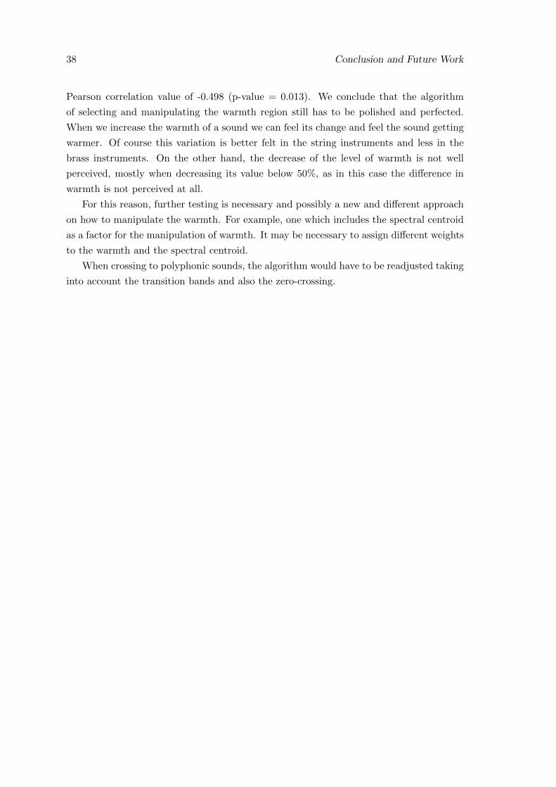
38 Conclusion and Future Work
Pearson correlation value of -0.498 (p-value = 0.013). We conclude that the algorithm
of selecting and manipulating the warmth region still has to be polished and perfected.
When we increase the warmth of a sound we can feel its change and feel the sound getting
warmer. Of course this variation is better felt in the string instruments and less in the
brass instruments. On the other hand, the decrease of the level of warmth is not well
perceived, mostly when decreasing its value below 50%, as in this case the difference in
warmth is not perceived at all.
For this reason, further testing is necessary and possibly a new and different approach
on how to manipulate the warmth. For example, one which includes the spectral centroid
as a factor for the manipulation of warmth. It may be necessary to assign different weights
to the warmth and the spectral centroid.
When crossing to polyphonic sounds, the algorithm would have to be readjusted taking
into account the transition bands and also the zero-crossing.
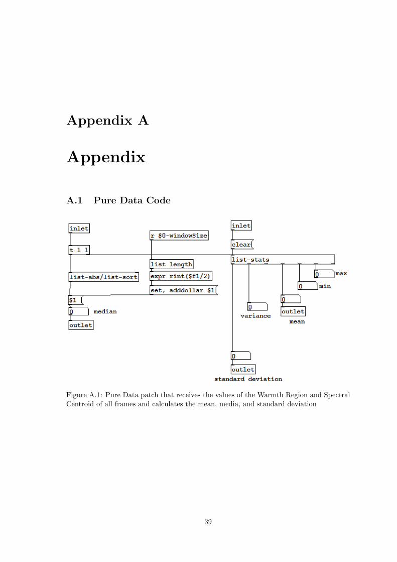
Appendix A
Appendix
A.1 Pure Data Code
Figure A.1: Pure Data patch that receives the values of the Warmth Region and SpectralCentroid of all frames and calculates the mean, media, and standard deviation
39
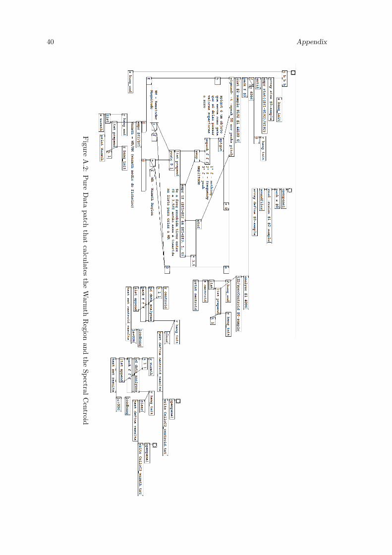
40 Appendix
Figu
reA
.2:
Pu
reD
ata
patch
that
calculates
the
Warm
thR
egionan
dth
eSp
ectralC
entroid
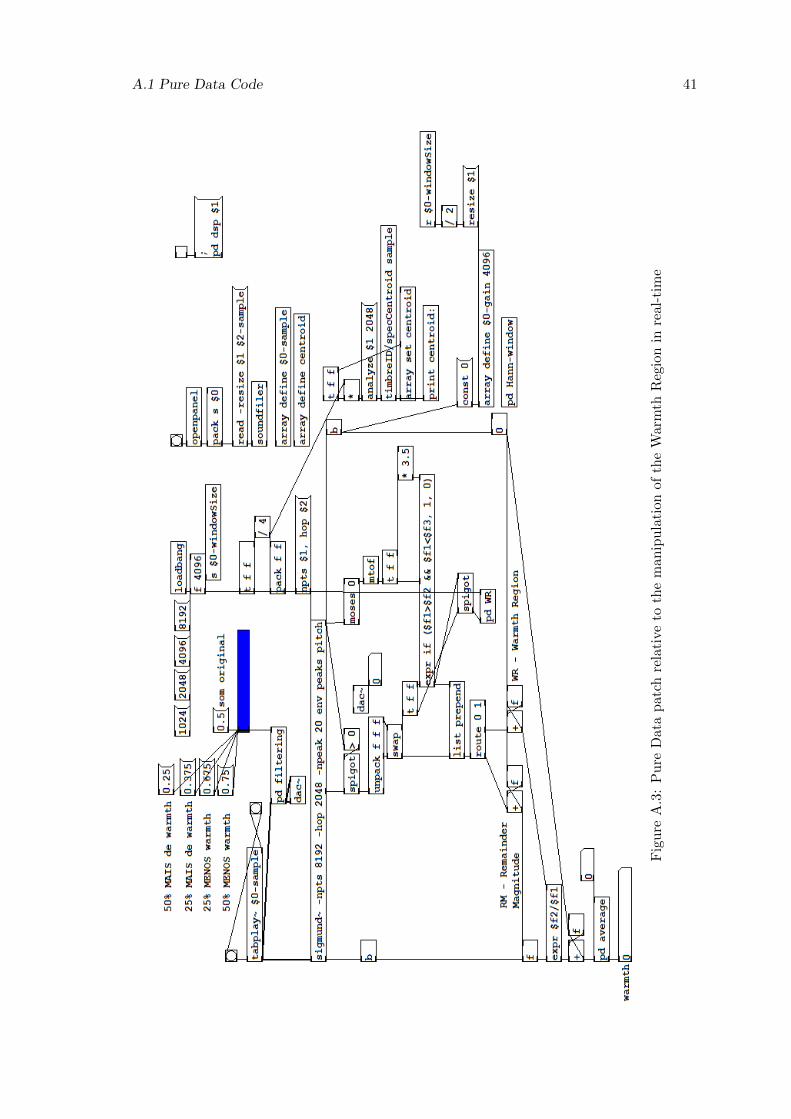
A.1 Pure Data Code 41
Fig
ure
A.3
:P
ure
Data
patc
hre
lati
veto
the
man
ipu
lati
onof
the
Warm
thR
egio
nin
real
-tim
e
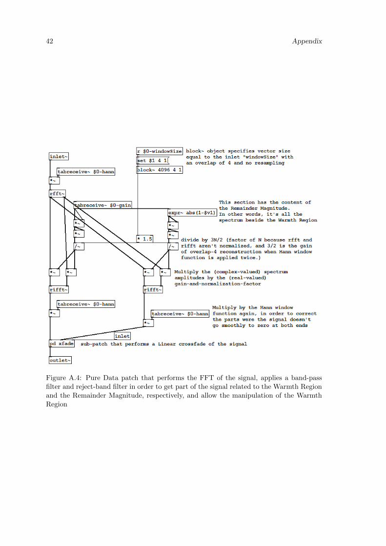
42 Appendix
Figure A.4: Pure Data patch that performs the FFT of the signal, applies a band-passfilter and reject-band filter in order to get part of the signal related to the Warmth Regionand the Remainder Magnitude, respectively, and allow the manipulation of the WarmthRegion
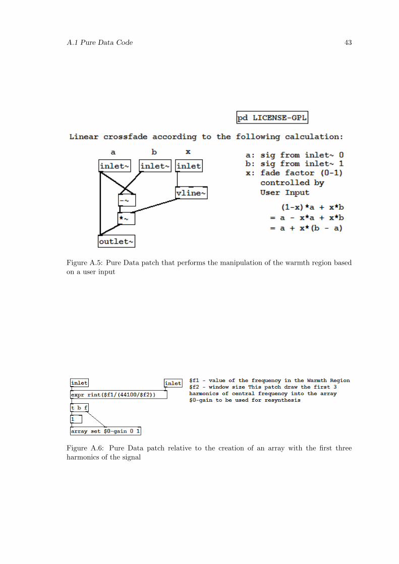
A.1 Pure Data Code 43
Figure A.5: Pure Data patch that performs the manipulation of the warmth region basedon a user input
Figure A.6: Pure Data patch relative to the creation of an array with the first threeharmonics of the signal
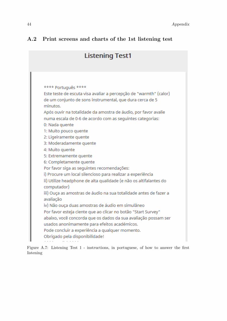
44 Appendix
A.2 Print screens and charts of the 1st listening test
Figure A.7: Listening Test 1 - instructions, in portuguese, of how to answer the firstlistening
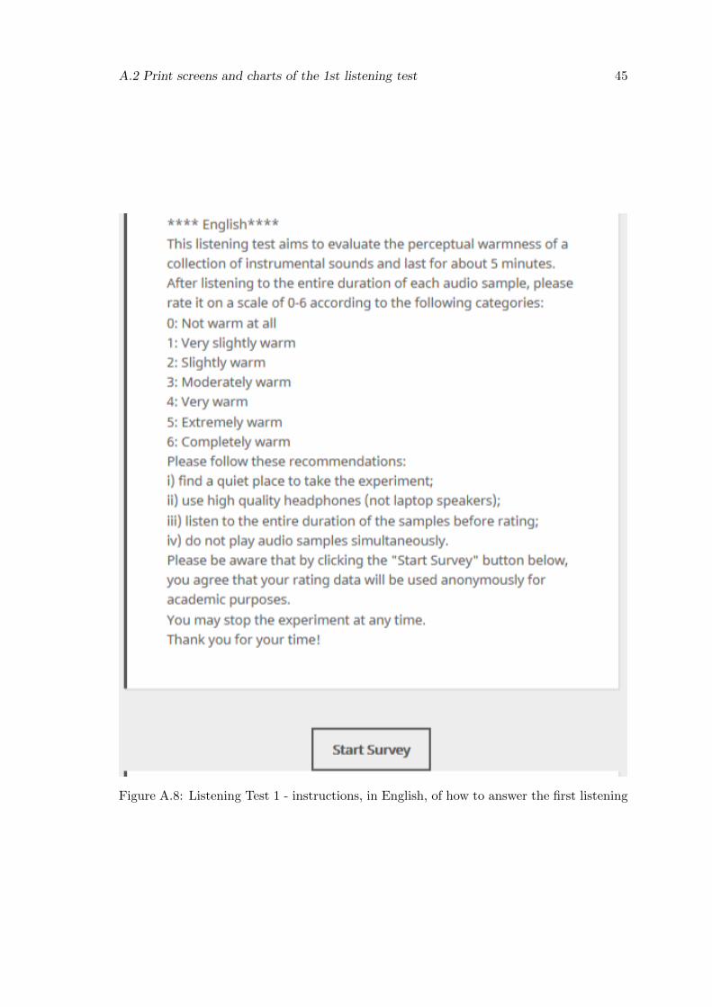
A.2 Print screens and charts of the 1st listening test 45
Figure A.8: Listening Test 1 - instructions, in English, of how to answer the first listening
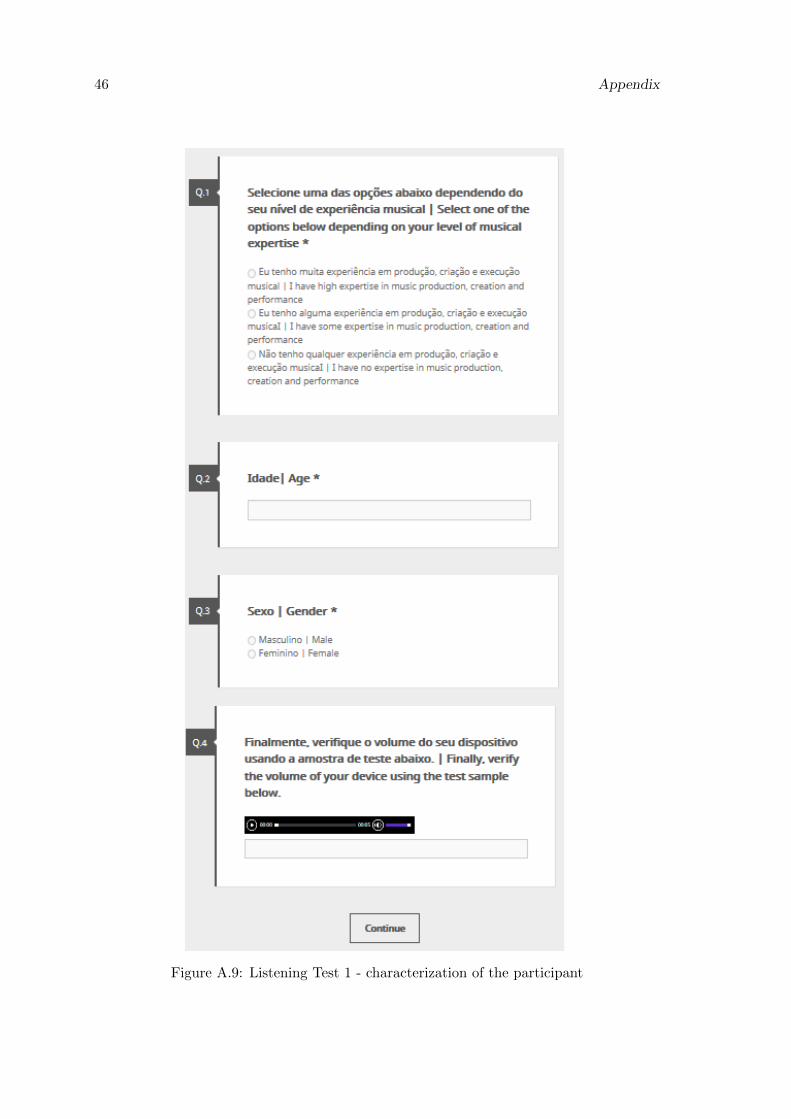
46 Appendix
Figure A.9: Listening Test 1 - characterization of the participant
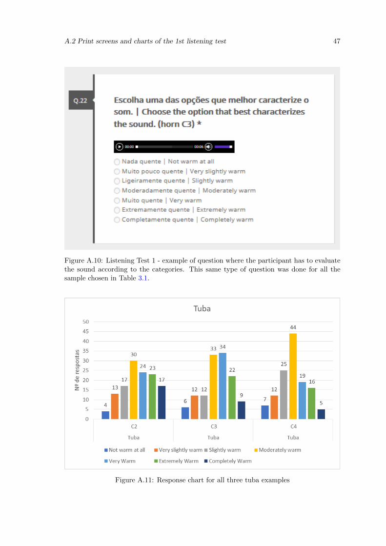
A.2 Print screens and charts of the 1st listening test 47
Figure A.10: Listening Test 1 - example of question where the participant has to evaluatethe sound according to the categories. This same type of question was done for all thesample chosen in Table 3.1.
Figure A.11: Response chart for all three tuba examples
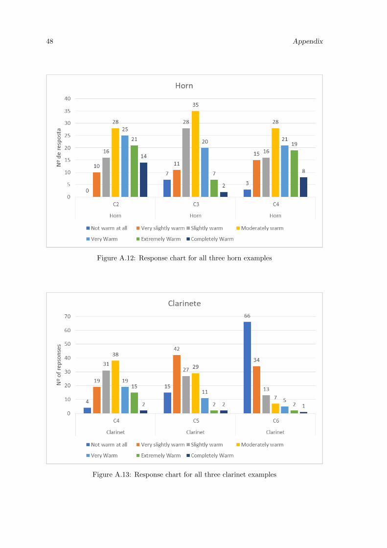
48 Appendix
Figure A.12: Response chart for all three horn examples
Figure A.13: Response chart for all three clarinet examples
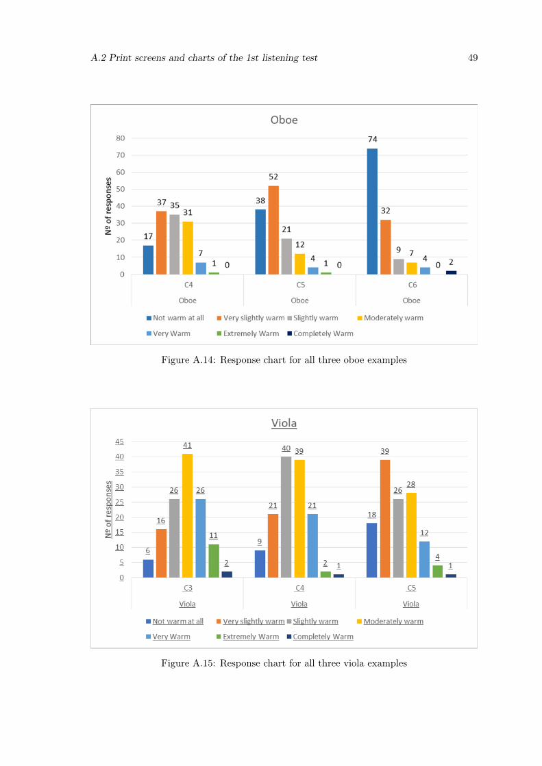
A.2 Print screens and charts of the 1st listening test 49
Figure A.14: Response chart for all three oboe examples
Figure A.15: Response chart for all three viola examples
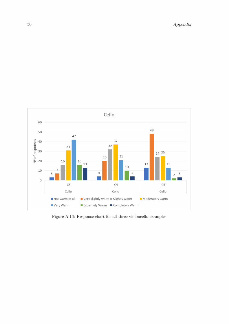
50 Appendix
Figure A.16: Response chart for all three violoncello examples
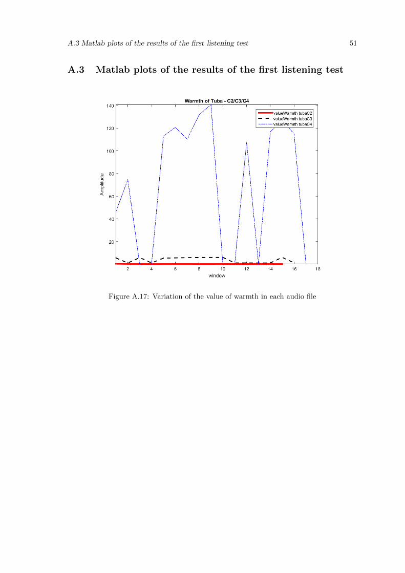
A.3 Matlab plots of the results of the first listening test 51
A.3 Matlab plots of the results of the first listening test
Figure A.17: Variation of the value of warmth in each audio file
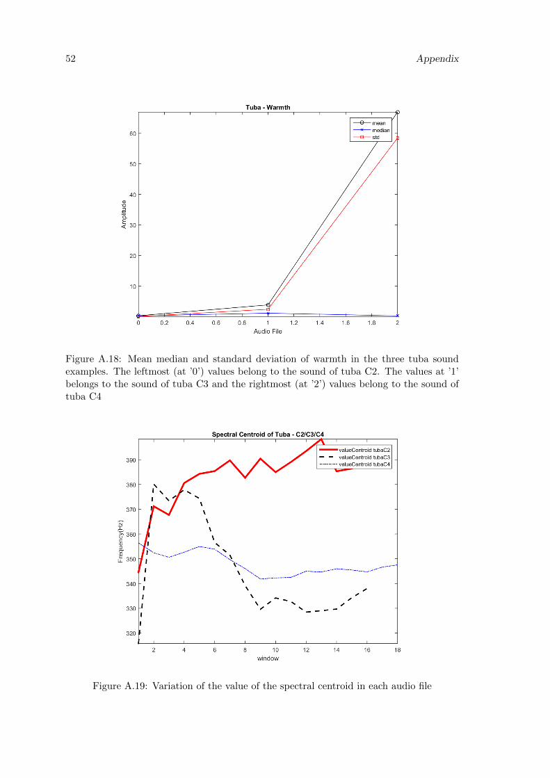
52 Appendix
Figure A.18: Mean median and standard deviation of warmth in the three tuba soundexamples. The leftmost (at ’0’) values belong to the sound of tuba C2. The values at ’1’belongs to the sound of tuba C3 and the rightmost (at ’2’) values belong to the sound oftuba C4
Figure A.19: Variation of the value of the spectral centroid in each audio file
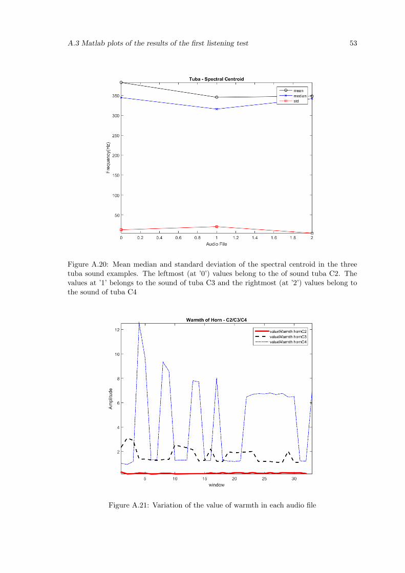
A.3 Matlab plots of the results of the first listening test 53
Figure A.20: Mean median and standard deviation of the spectral centroid in the threetuba sound examples. The leftmost (at ’0’) values belong to the of sound tuba C2. Thevalues at ’1’ belongs to the sound of tuba C3 and the rightmost (at ’2’) values belong tothe sound of tuba C4
Figure A.21: Variation of the value of warmth in each audio file
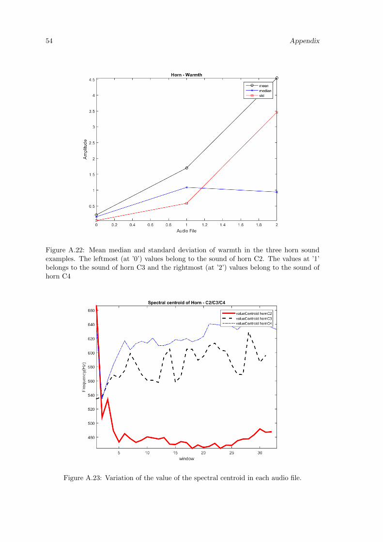
54 Appendix
Figure A.22: Mean median and standard deviation of warmth in the three horn soundexamples. The leftmost (at ’0’) values belong to the sound of horn C2. The values at ’1’belongs to the sound of horn C3 and the rightmost (at ’2’) values belong to the sound ofhorn C4
Figure A.23: Variation of the value of the spectral centroid in each audio file.
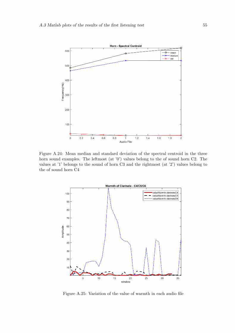
A.3 Matlab plots of the results of the first listening test 55
Figure A.24: Mean median and standard deviation of the spectral centroid in the threehorn sound examples. The leftmost (at ’0’) values belong to the of sound horn C2. Thevalues at ’1’ belongs to the sound of horn C3 and the rightmost (at ’2’) values belong tothe of sound horn C4
Figure A.25: Variation of the value of warmth in each audio file
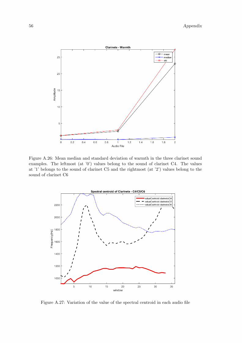
56 Appendix
Figure A.26: Mean median and standard deviation of warmth in the three clarinet soundexamples. The leftmost (at ’0’) values belong to the sound of clarinet C4. The valuesat ’1’ belongs to the sound of clarinet C5 and the rightmost (at ’2’) values belong to thesound of clarinet C6
Figure A.27: Variation of the value of the spectral centroid in each audio file
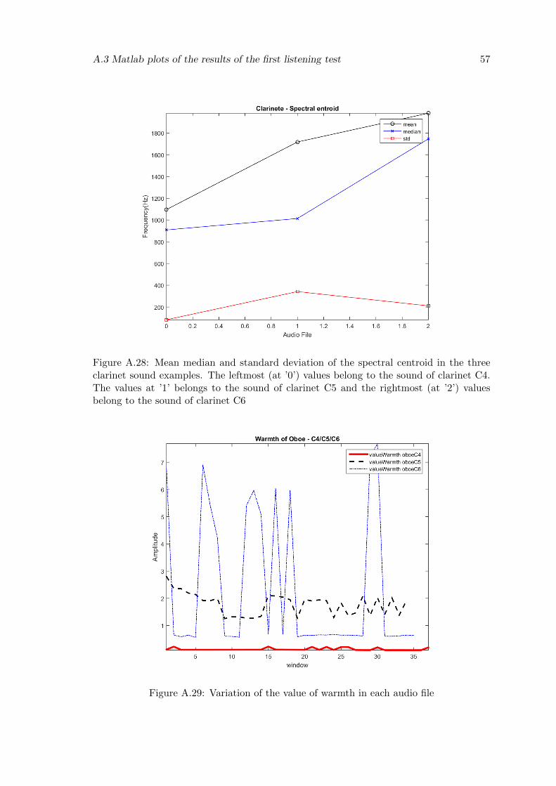
A.3 Matlab plots of the results of the first listening test 57
Figure A.28: Mean median and standard deviation of the spectral centroid in the threeclarinet sound examples. The leftmost (at ’0’) values belong to the sound of clarinet C4.The values at ’1’ belongs to the sound of clarinet C5 and the rightmost (at ’2’) valuesbelong to the sound of clarinet C6
Figure A.29: Variation of the value of warmth in each audio file
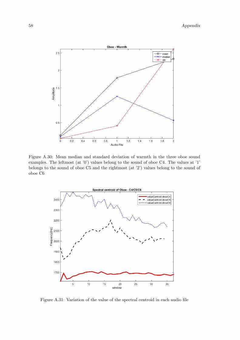
58 Appendix
Figure A.30: Mean median and standard deviation of warmth in the three oboe soundexamples. The leftmost (at ’0’) values belong to the sound of oboe C4. The values at ’1’belongs to the sound of oboe C5 and the rightmost (at ’2’) values belong to the sound ofoboe C6
Figure A.31: Variation of the value of the spectral centroid in each audio file
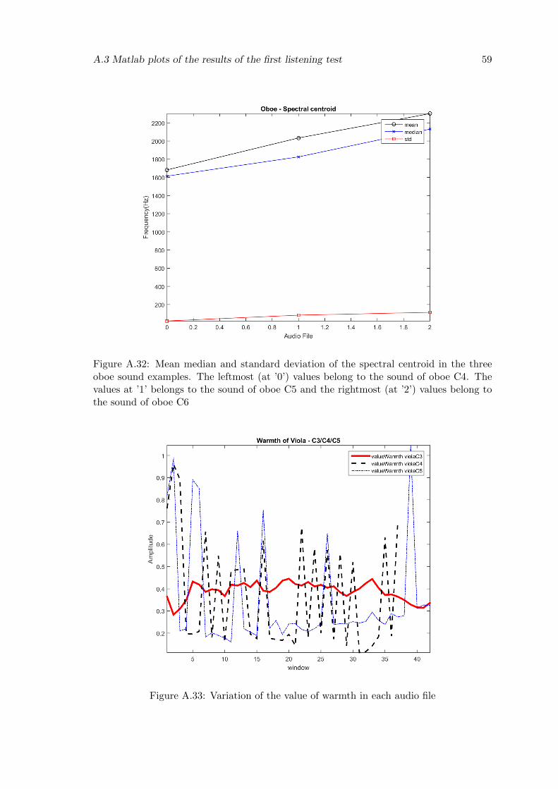
A.3 Matlab plots of the results of the first listening test 59
Figure A.32: Mean median and standard deviation of the spectral centroid in the threeoboe sound examples. The leftmost (at ’0’) values belong to the sound of oboe C4. Thevalues at ’1’ belongs to the sound of oboe C5 and the rightmost (at ’2’) values belong tothe sound of oboe C6
Figure A.33: Variation of the value of warmth in each audio file
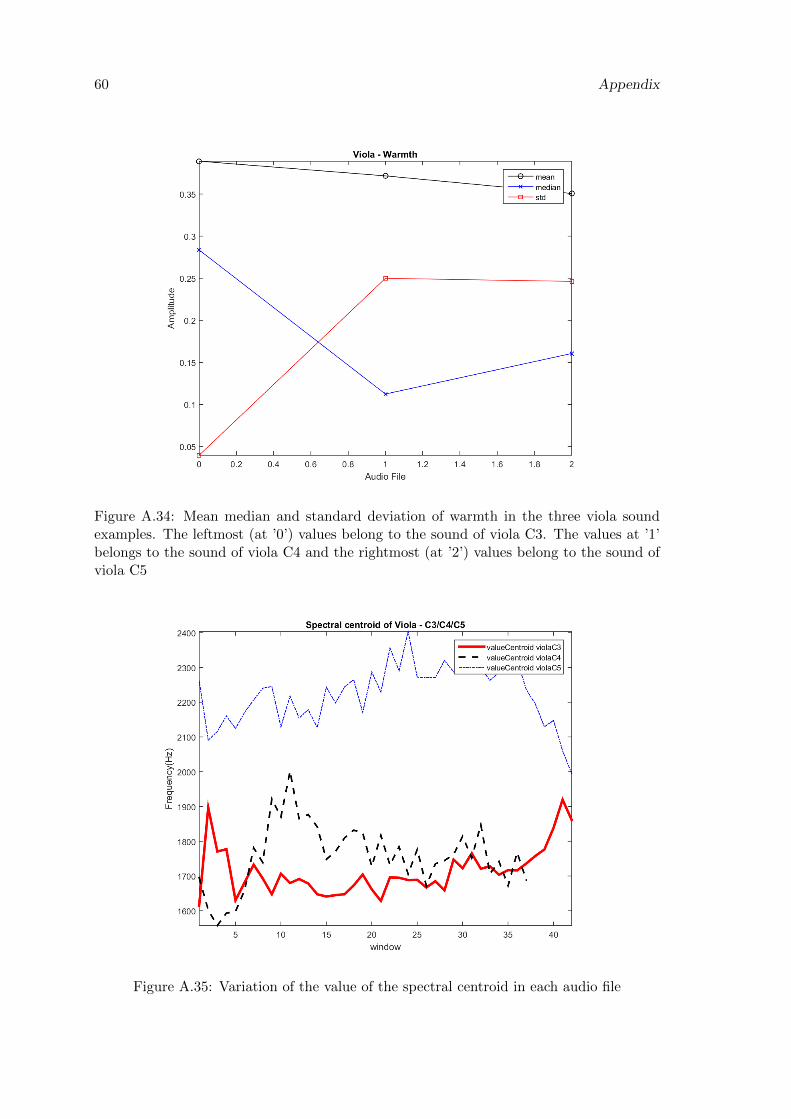
60 Appendix
Figure A.34: Mean median and standard deviation of warmth in the three viola soundexamples. The leftmost (at ’0’) values belong to the sound of viola C3. The values at ’1’belongs to the sound of viola C4 and the rightmost (at ’2’) values belong to the sound ofviola C5
Figure A.35: Variation of the value of the spectral centroid in each audio file
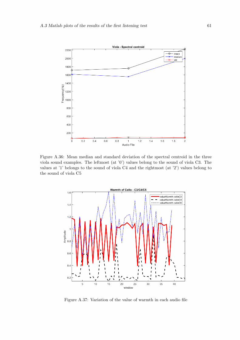
A.3 Matlab plots of the results of the first listening test 61
Figure A.36: Mean median and standard deviation of the spectral centroid in the threeviola sound examples. The leftmost (at ’0’) values belong to the sound of viola C3. Thevalues at ’1’ belongs to the sound of viola C4 and the rightmost (at ’2’) values belong tothe sound of viola C5
Figure A.37: Variation of the value of warmth in each audio file
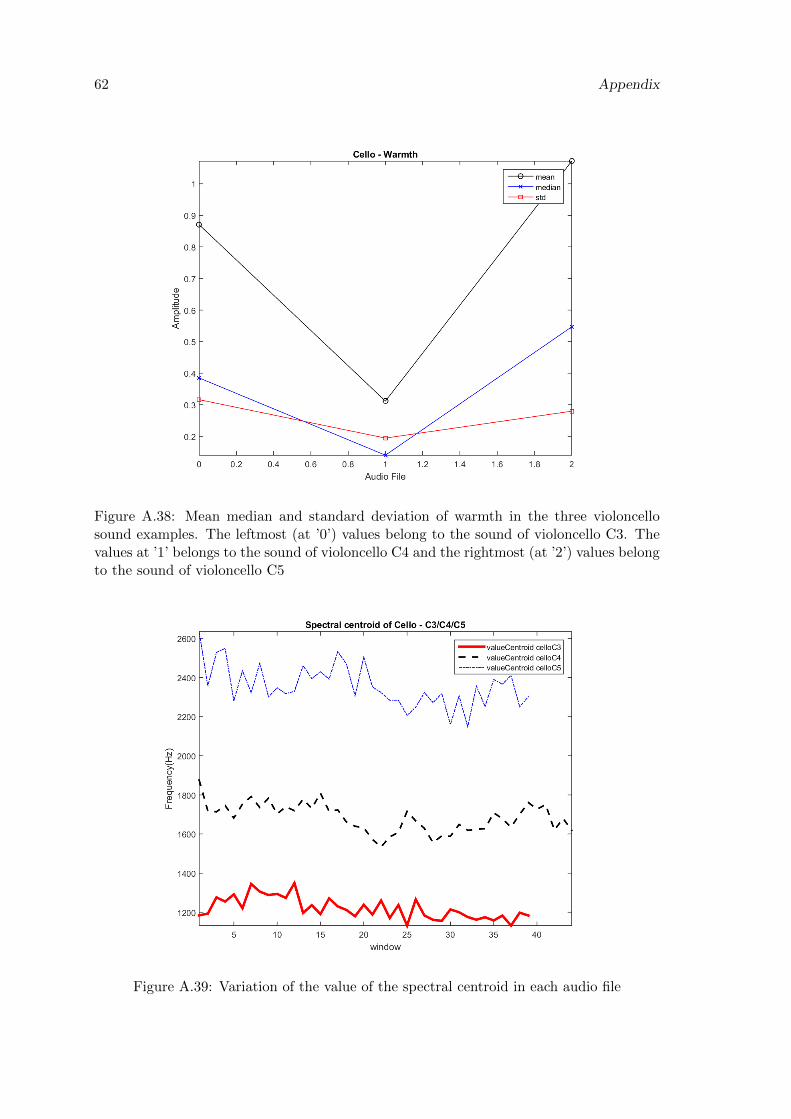
62 Appendix
Figure A.38: Mean median and standard deviation of warmth in the three violoncellosound examples. The leftmost (at ’0’) values belong to the sound of violoncello C3. Thevalues at ’1’ belongs to the sound of violoncello C4 and the rightmost (at ’2’) values belongto the sound of violoncello C5
Figure A.39: Variation of the value of the spectral centroid in each audio file
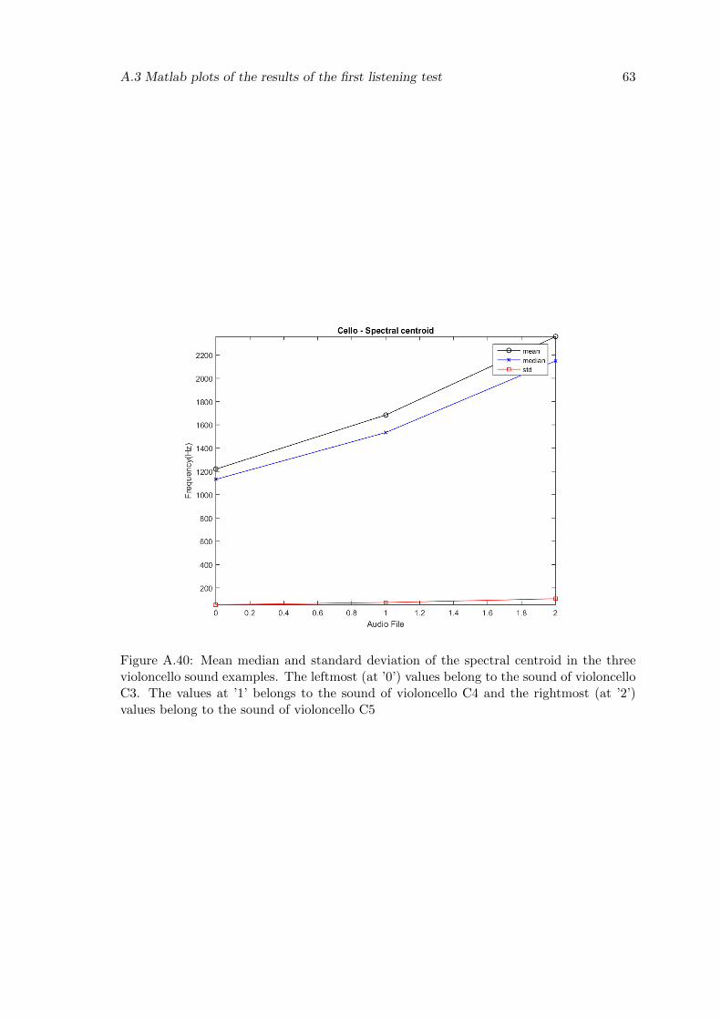
A.3 Matlab plots of the results of the first listening test 63
Figure A.40: Mean median and standard deviation of the spectral centroid in the threevioloncello sound examples. The leftmost (at ’0’) values belong to the sound of violoncelloC3. The values at ’1’ belongs to the sound of violoncello C4 and the rightmost (at ’2’)values belong to the sound of violoncello C5
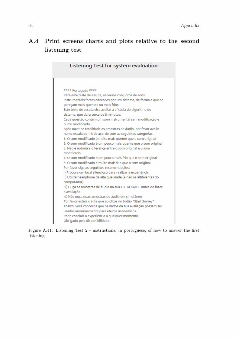
64 Appendix
A.4 Print screens charts and plots relative to the second
listening test
Figure A.41: Listening Test 2 - instructions, in portuguese, of how to answer the firstlistening
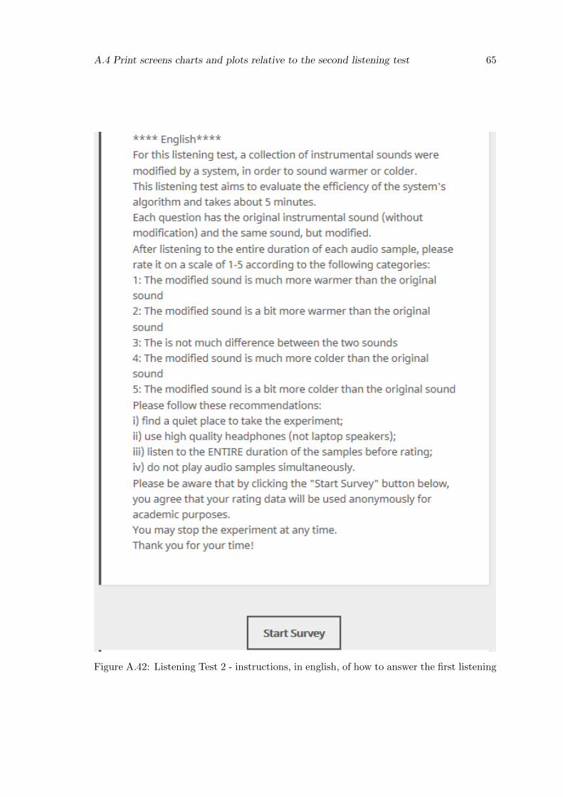
A.4 Print screens charts and plots relative to the second listening test 65
Figure A.42: Listening Test 2 - instructions, in english, of how to answer the first listening
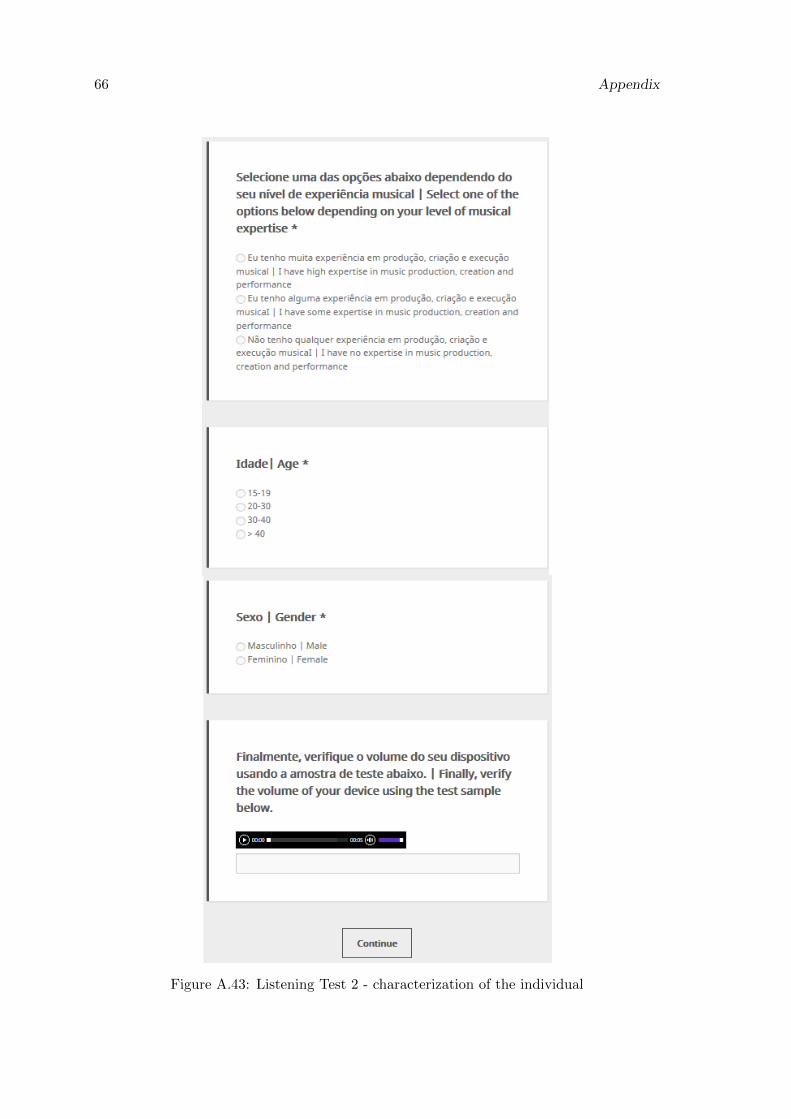
66 Appendix
Figure A.43: Listening Test 2 - characterization of the individual
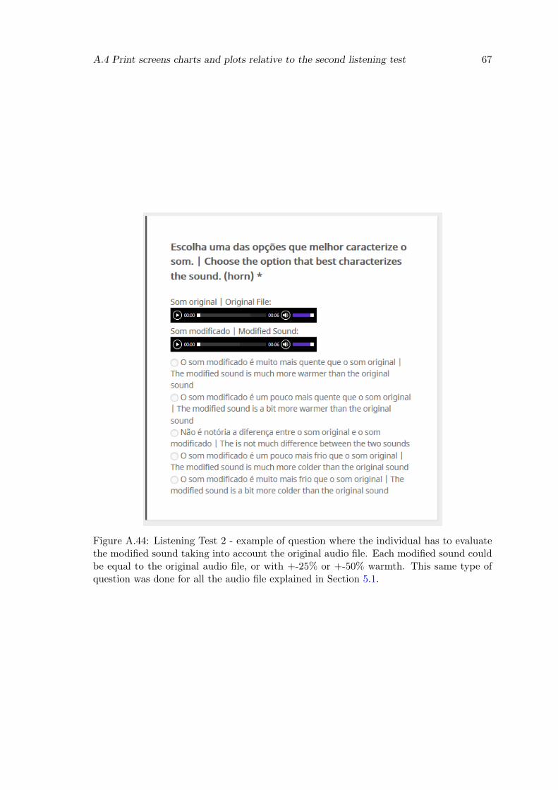
A.4 Print screens charts and plots relative to the second listening test 67
Figure A.44: Listening Test 2 - example of question where the individual has to evaluatethe modified sound taking into account the original audio file. Each modified sound couldbe equal to the original audio file, or with +-25% or +-50% warmth. This same type ofquestion was done for all the audio file explained in Section 5.1.
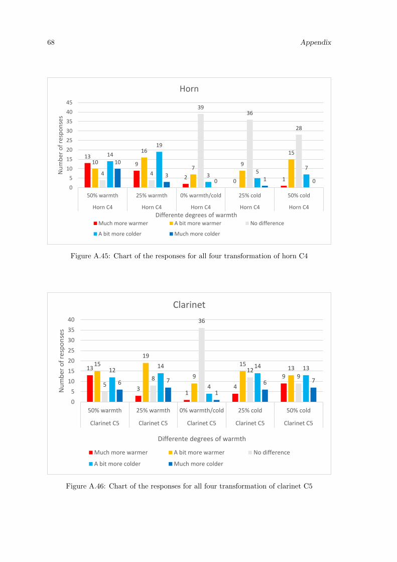
68 Appendix
13
9
20 1
10
16
79
15
4 4
3936
28
14
19
35
710
30 1 0
0
5
10
15
20
25
30
35
40
45
50% warmth 25% warmth 0% warmth/cold 25% cold 50% cold
Horn C4 Horn C4 Horn C4 Horn C4 Horn C4
Nu
mb
er
of
resp
on
ses
Differente degrees of warmth
Horn
Much more warmer A bit more warmer No difference
A bit more colder Much more colder
Figure A.45: Chart of the responses for all four transformation of horn C4
13
31
4
9
15
19
9
1513
58
36
129
1214
4
14 13
6 7
1
6 7
0
5
10
15
20
25
30
35
40
50% warmth 25% warmth 0% warmth/cold 25% cold 50% cold
Clarinet C5 Clarinet C5 Clarinet C5 Clarinet C5 Clarinet C5
Nu
mb
er
of
resp
on
ses
Differente degrees of warmth
Clarinet
Much more warmer A bit more warmer No difference
A bit more colder Much more colder
Figure A.46: Chart of the responses for all four transformation of clarinet C5
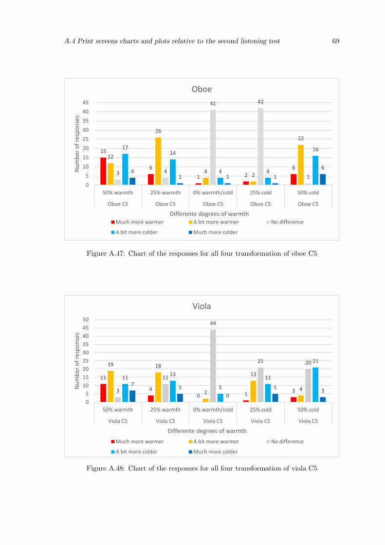
A.4 Print screens charts and plots relative to the second listening test 69
15
6
1 2
6
12
26
42
22
3 4
41 42
1
1714
4 4
16
41 1 1
6
0
5
10
15
20
25
30
35
40
45
50% warmth 25% warmth 0% warmth/cold 25% cold 50% cold
Oboe C5 Oboe C5 Oboe C5 Oboe C5 Oboe C5
Nu
mb
er
of
resp
on
ses
Differente degrees of warmth
Oboe
Much more warmer A bit more warmer No difference
A bit more colder Much more colder
Figure A.47: Chart of the responses for all four transformation of oboe C5
11
40 1
3
19 18
2
13
43
11
44
21 20
1113
5
11
21
75
0
53
0
5
10
15
20
25
30
35
40
45
50
50% warmth 25% warmth 0% warmth/cold 25% cold 50% cold
Viola C5 Viola C5 Viola C5 Viola C5 Viola C5
Nu
mb
er
of
resp
on
ses
Differente degrees of warmth
Viola
Much more warmer A bit more warmer No difference
A bit more colder Much more colder
Figure A.48: Chart of the responses for all four transformation of viola C5

70 Appendix
15
5
03
1
11
23
2
710
2
6
46
33
24
14 13
3
8
14
9
40 0
2
0
5
10
15
20
25
30
35
40
45
50
50% warmth 25% warmth 0% warmth/cold 25% cold 50% cold
Cello C5 Cello C5 Cello C5 Cello C5 Cello C5
Nu
mb
er
of
resp
on
ses
Differente degrees of warmth
Viloncello
Much more warmer A bit more warmer No difference
A bit more colder Much more colder
Figure A.49: Chart of the responses for all four transformation of violoncello C5
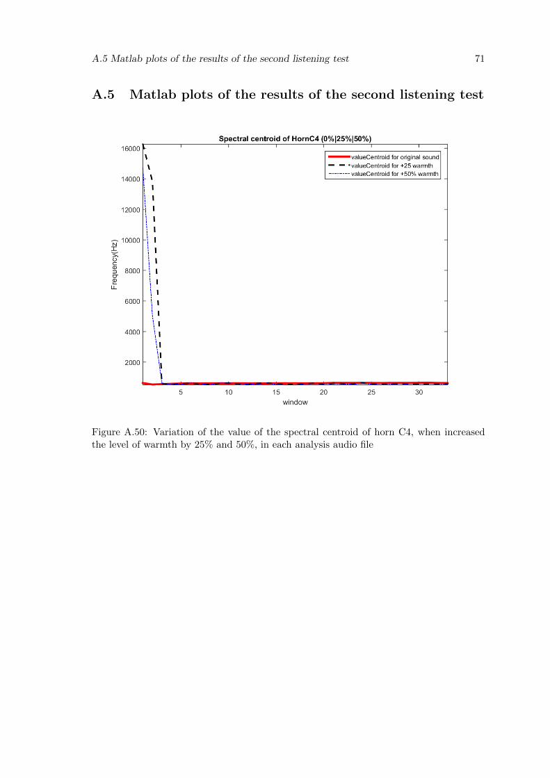
A.5 Matlab plots of the results of the second listening test 71
A.5 Matlab plots of the results of the second listening test
Figure A.50: Variation of the value of the spectral centroid of horn C4, when increasedthe level of warmth by 25% and 50%, in each analysis audio file

72 Appendix
Figure A.51: Variation of the value of the spectral centroid of horn C4, when decreasedthe level of warmth by 25% and 50%, in each analysis audio file
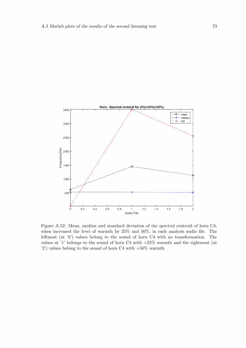
A.5 Matlab plots of the results of the second listening test 73
Figure A.52: Mean, median and standard deviation of the spectral centroid of horn C4,when increased the level of warmth by 25% and 50%, in each analysis audio file. Theleftmost (at ’0’) values belong to the sound of horn C4 with no transformation. Thevalues at ’1’ belongs to the sound of horn C4 with +25% warmth and the rightmost (at’2’) values belong to the sound of horn C4 with +50% warmth
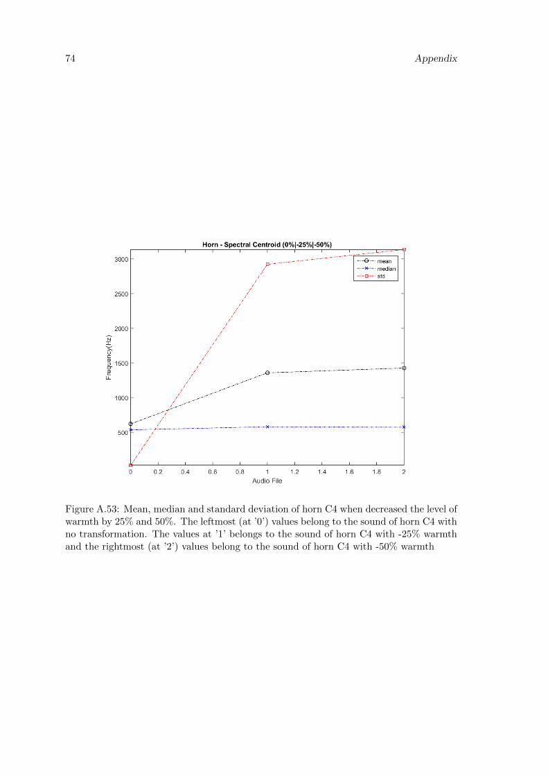
74 Appendix
Figure A.53: Mean, median and standard deviation of horn C4 when decreased the level ofwarmth by 25% and 50%. The leftmost (at ’0’) values belong to the sound of horn C4 withno transformation. The values at ’1’ belongs to the sound of horn C4 with -25% warmthand the rightmost (at ’2’) values belong to the sound of horn C4 with -50% warmth
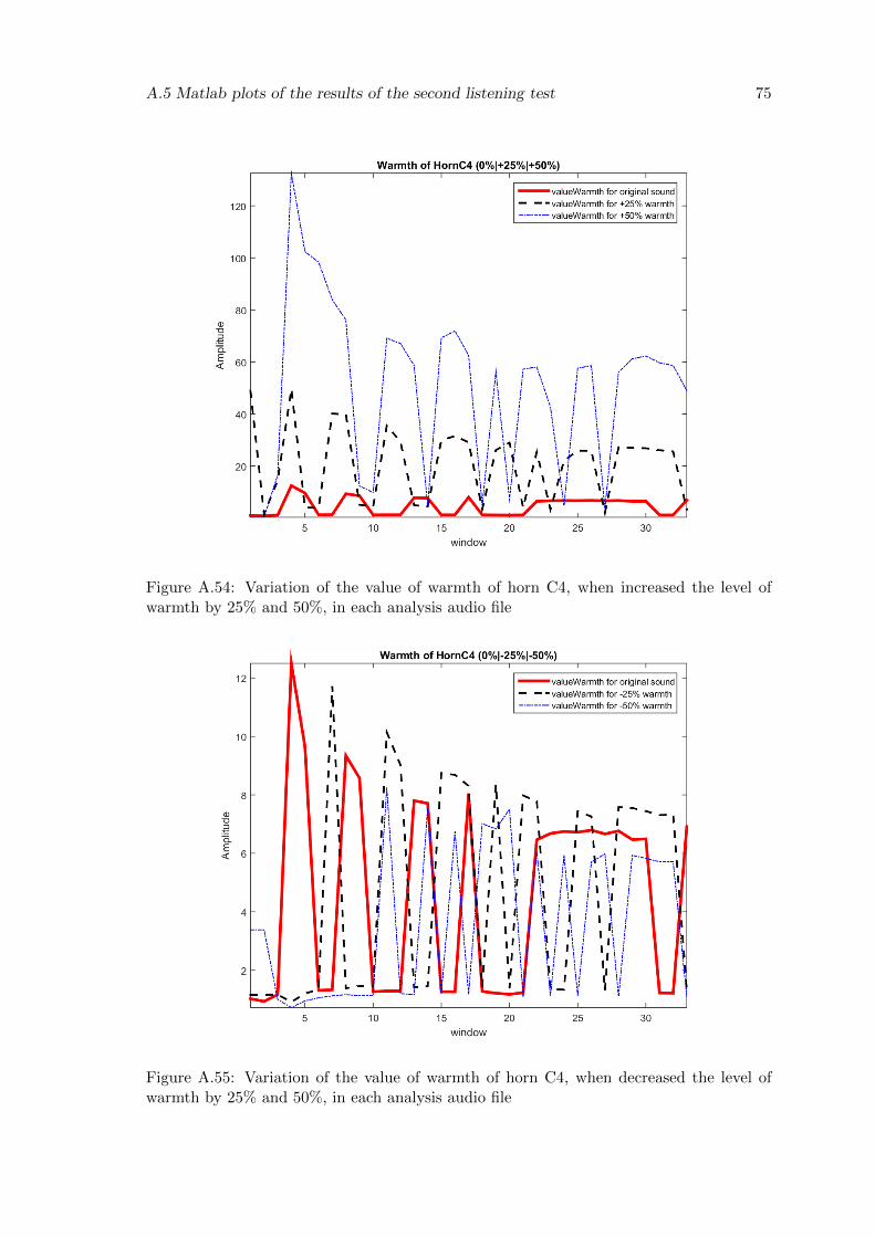
A.5 Matlab plots of the results of the second listening test 75
Figure A.54: Variation of the value of warmth of horn C4, when increased the level ofwarmth by 25% and 50%, in each analysis audio file
Figure A.55: Variation of the value of warmth of horn C4, when decreased the level ofwarmth by 25% and 50%, in each analysis audio file
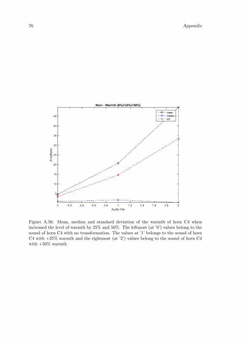
76 Appendix
Figure A.56: Mean, median and standard deviation of the warmth of horn C4 whenincreased the level of warmth by 25% and 50%. The leftmost (at ’0’) values belong to thesound of horn C4 with no transformation. The values at ’1’ belongs to the sound of hornC4 with +25% warmth and the rightmost (at ’2’) values belong to the sound of horn C4with +50% warmth
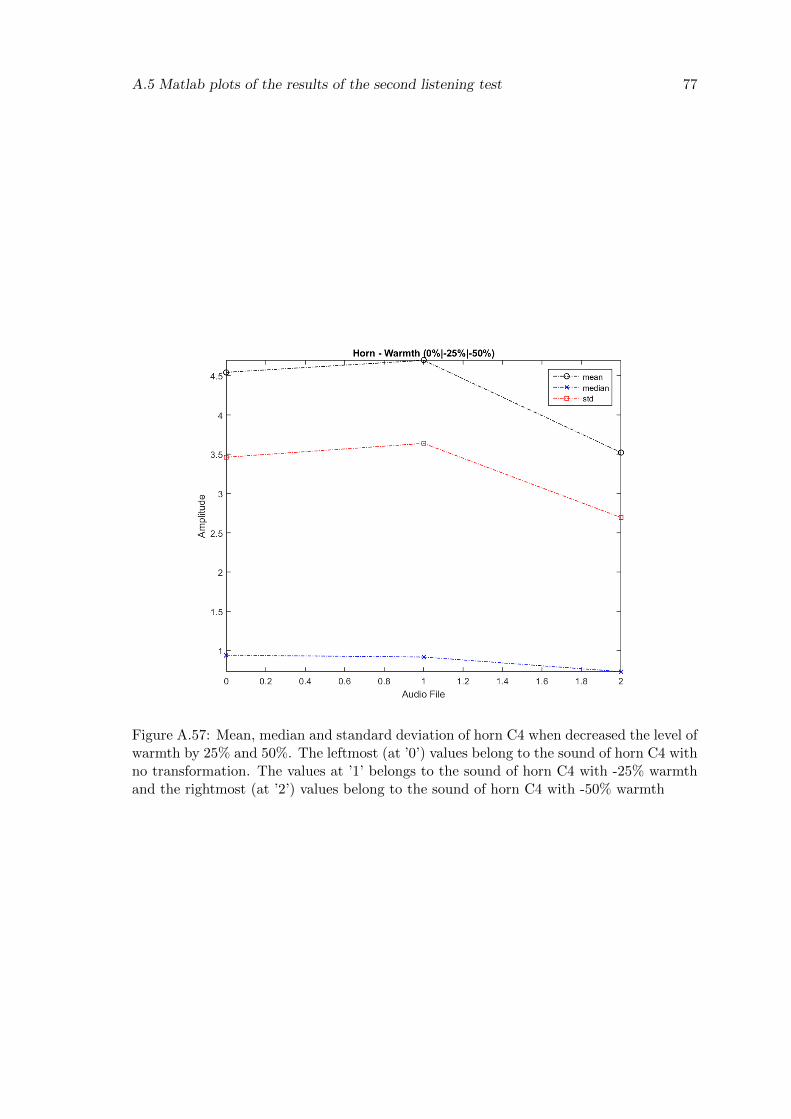
A.5 Matlab plots of the results of the second listening test 77
Figure A.57: Mean, median and standard deviation of horn C4 when decreased the level ofwarmth by 25% and 50%. The leftmost (at ’0’) values belong to the sound of horn C4 withno transformation. The values at ’1’ belongs to the sound of horn C4 with -25% warmthand the rightmost (at ’2’) values belong to the sound of horn C4 with -50% warmth
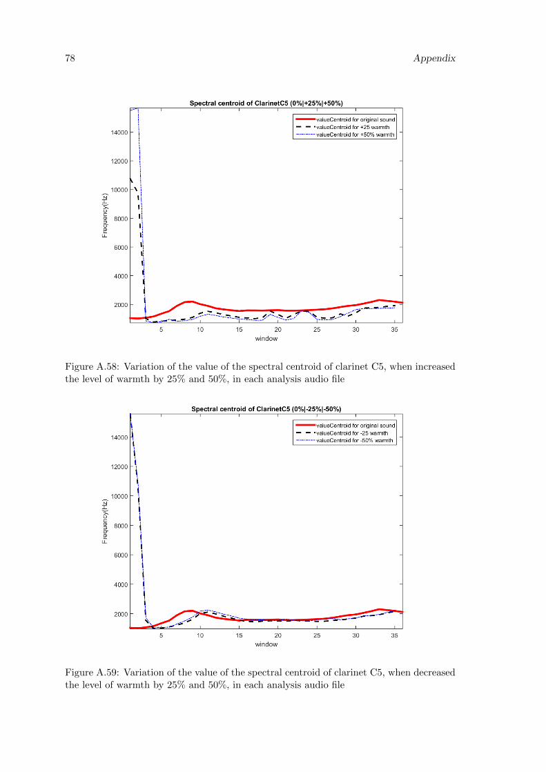
78 Appendix
Figure A.58: Variation of the value of the spectral centroid of clarinet C5, when increasedthe level of warmth by 25% and 50%, in each analysis audio file
Figure A.59: Variation of the value of the spectral centroid of clarinet C5, when decreasedthe level of warmth by 25% and 50%, in each analysis audio file

A.5 Matlab plots of the results of the second listening test 79
Figure A.60: Mean, median and standard deviation of the spectral centroid of clarinetC5, when increased the level of warmth by 25% and 50%, in each analysis audio file. Theleftmost (at ’0’) values belong to the sound of clarinet C5 with no transformation. Thevalues at ’1’ belongs to the sound of clarinet C5 with +25% warmth and the rightmost(at ’2’) values belong to the sound of clarinet C5 with +50% warmth
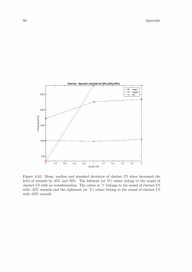
80 Appendix
Figure A.61: Mean, median and standard deviation of clarinet C5 when decreased thelevel of warmth by 25% and 50%. The leftmost (at ’0’) values belong to the sound ofclarinet C5 with no transformation. The values at ’1’ belongs to the sound of clarinet C5with -25% warmth and the rightmost (at ’2’) values belong to the sound of clarinet C5with -50% warmth
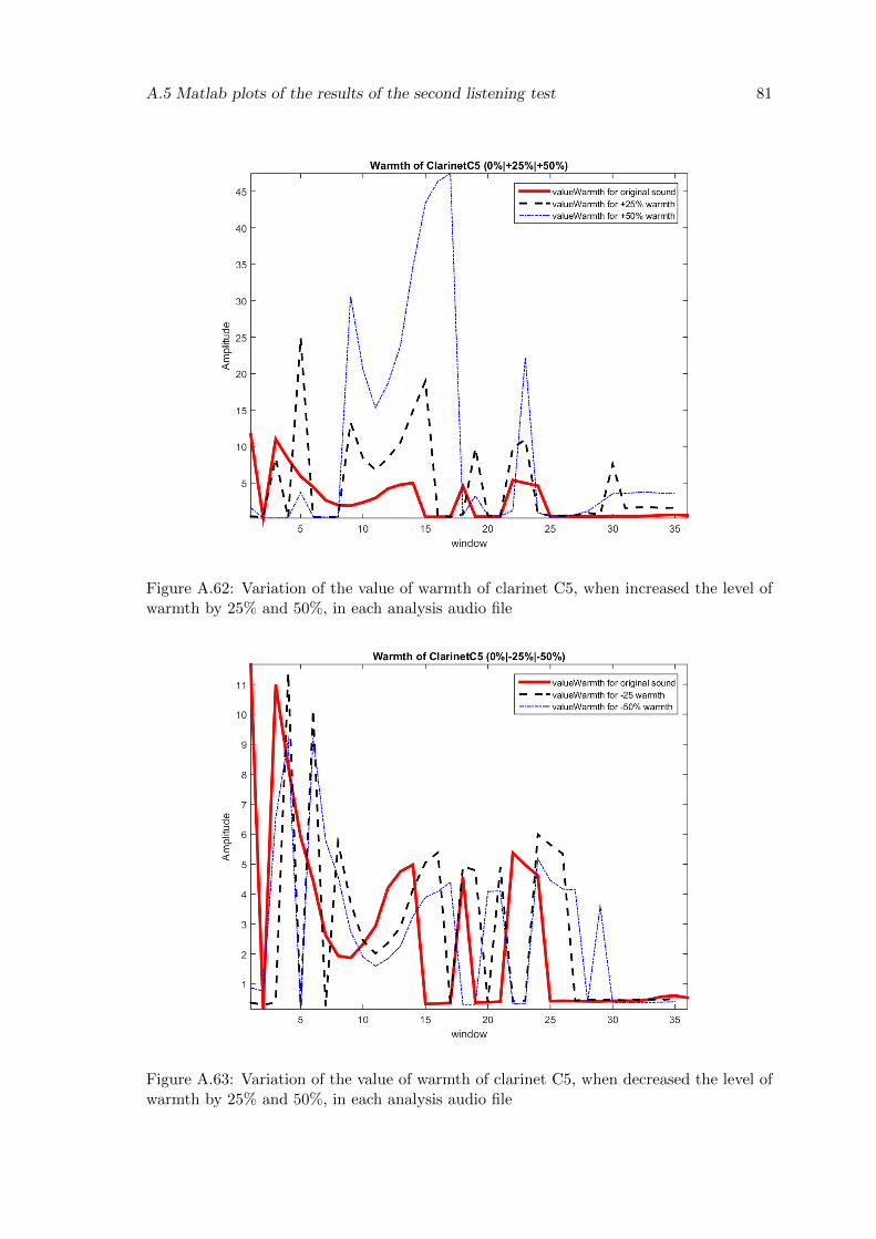
A.5 Matlab plots of the results of the second listening test 81
Figure A.62: Variation of the value of warmth of clarinet C5, when increased the level ofwarmth by 25% and 50%, in each analysis audio file
Figure A.63: Variation of the value of warmth of clarinet C5, when decreased the level ofwarmth by 25% and 50%, in each analysis audio file
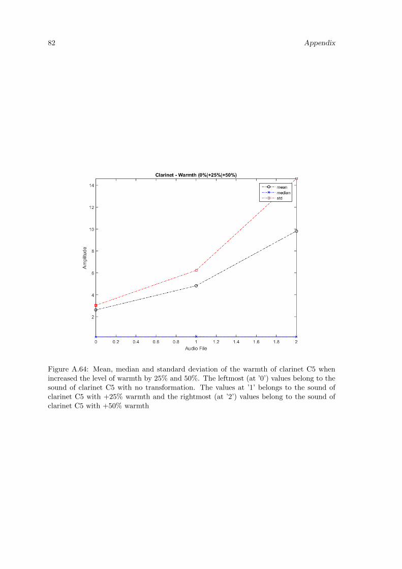
82 Appendix
Figure A.64: Mean, median and standard deviation of the warmth of clarinet C5 whenincreased the level of warmth by 25% and 50%. The leftmost (at ’0’) values belong to thesound of clarinet C5 with no transformation. The values at ’1’ belongs to the sound ofclarinet C5 with +25% warmth and the rightmost (at ’2’) values belong to the sound ofclarinet C5 with +50% warmth
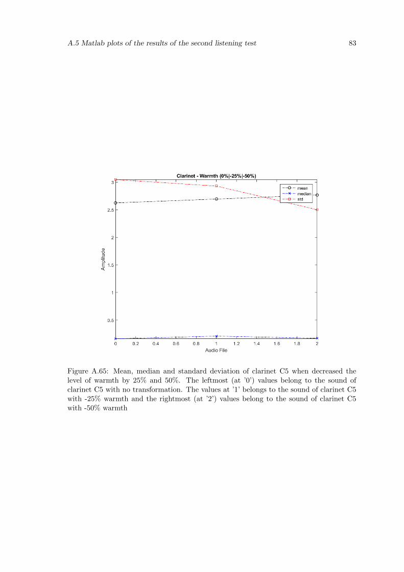
A.5 Matlab plots of the results of the second listening test 83
Figure A.65: Mean, median and standard deviation of clarinet C5 when decreased thelevel of warmth by 25% and 50%. The leftmost (at ’0’) values belong to the sound ofclarinet C5 with no transformation. The values at ’1’ belongs to the sound of clarinet C5with -25% warmth and the rightmost (at ’2’) values belong to the sound of clarinet C5with -50% warmth
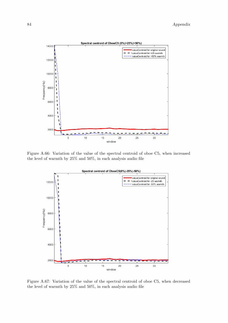
84 Appendix
Figure A.66: Variation of the value of the spectral centroid of oboe C5, when increasedthe level of warmth by 25% and 50%, in each analysis audio file
Figure A.67: Variation of the value of the spectral centroid of oboe C5, when decreasedthe level of warmth by 25% and 50%, in each analysis audio file
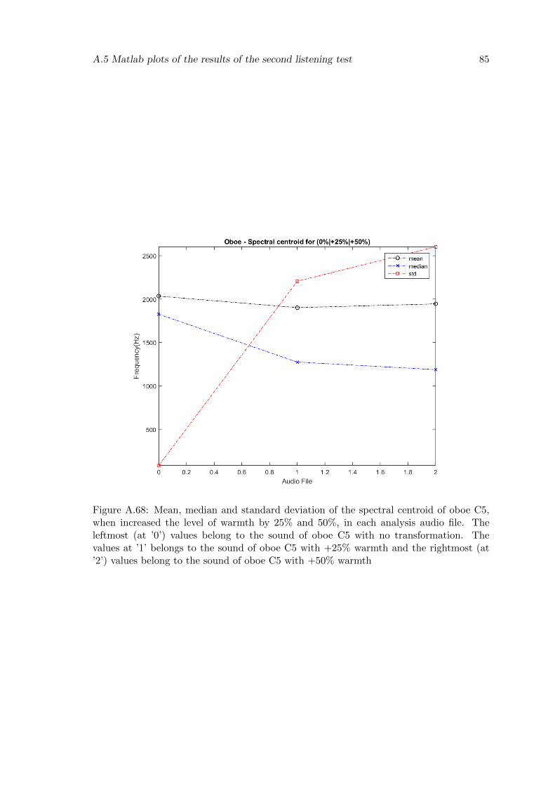
A.5 Matlab plots of the results of the second listening test 85
Figure A.68: Mean, median and standard deviation of the spectral centroid of oboe C5,when increased the level of warmth by 25% and 50%, in each analysis audio file. Theleftmost (at ’0’) values belong to the sound of oboe C5 with no transformation. Thevalues at ’1’ belongs to the sound of oboe C5 with +25% warmth and the rightmost (at’2’) values belong to the sound of oboe C5 with +50% warmth
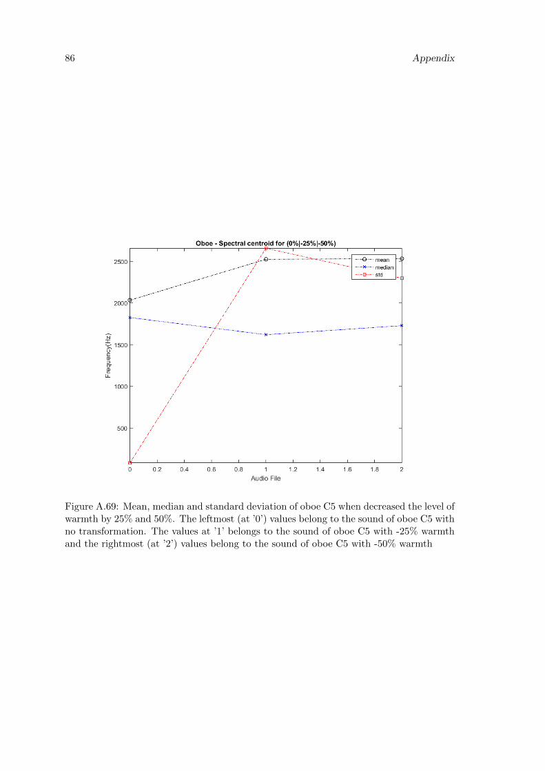
86 Appendix
Figure A.69: Mean, median and standard deviation of oboe C5 when decreased the level ofwarmth by 25% and 50%. The leftmost (at ’0’) values belong to the sound of oboe C5 withno transformation. The values at ’1’ belongs to the sound of oboe C5 with -25% warmthand the rightmost (at ’2’) values belong to the sound of oboe C5 with -50% warmth
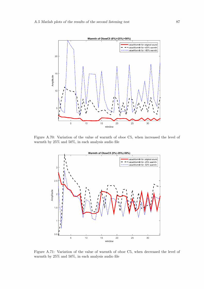
A.5 Matlab plots of the results of the second listening test 87
Figure A.70: Variation of the value of warmth of oboe C5, when increased the level ofwarmth by 25% and 50%, in each analysis audio file
Figure A.71: Variation of the value of warmth of oboe C5, when decreased the level ofwarmth by 25% and 50%, in each analysis audio file
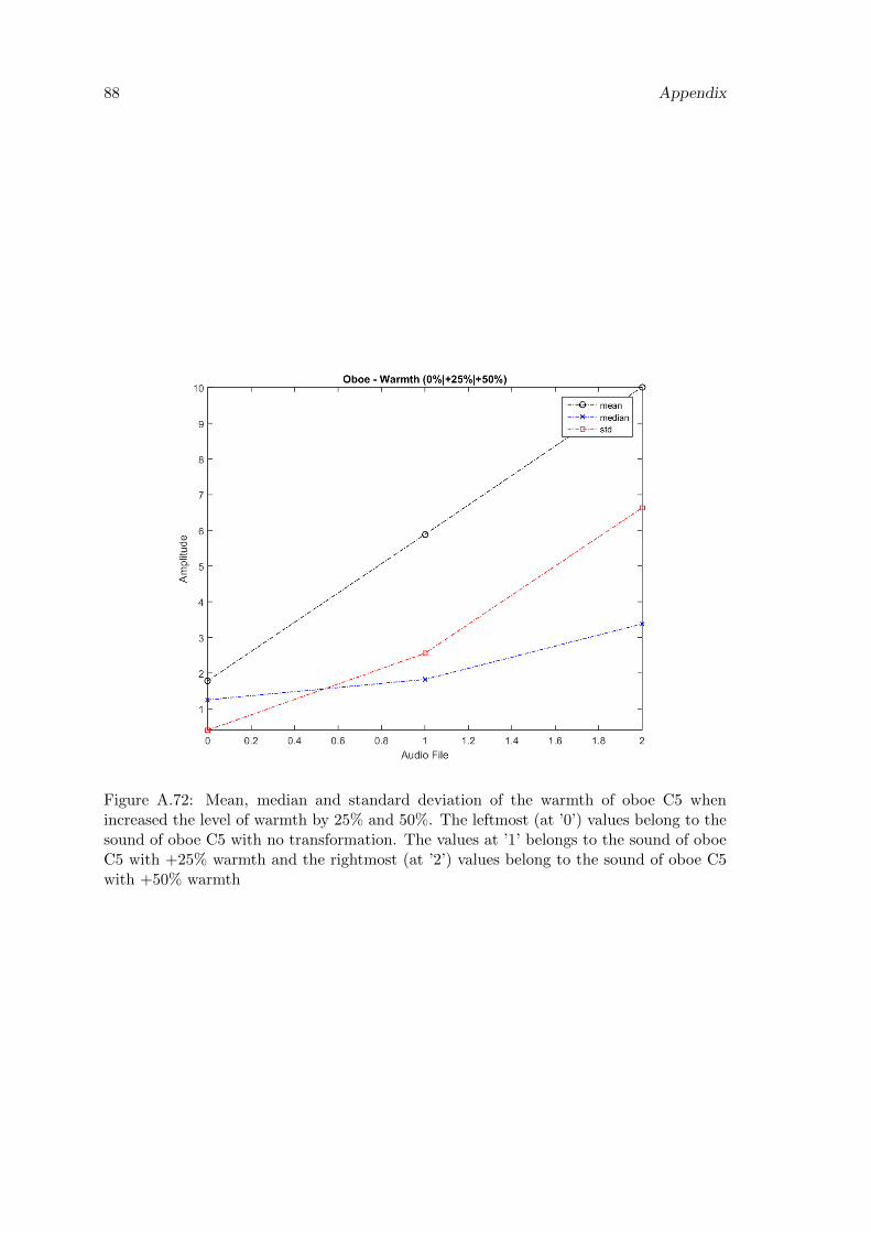
88 Appendix
Figure A.72: Mean, median and standard deviation of the warmth of oboe C5 whenincreased the level of warmth by 25% and 50%. The leftmost (at ’0’) values belong to thesound of oboe C5 with no transformation. The values at ’1’ belongs to the sound of oboeC5 with +25% warmth and the rightmost (at ’2’) values belong to the sound of oboe C5with +50% warmth
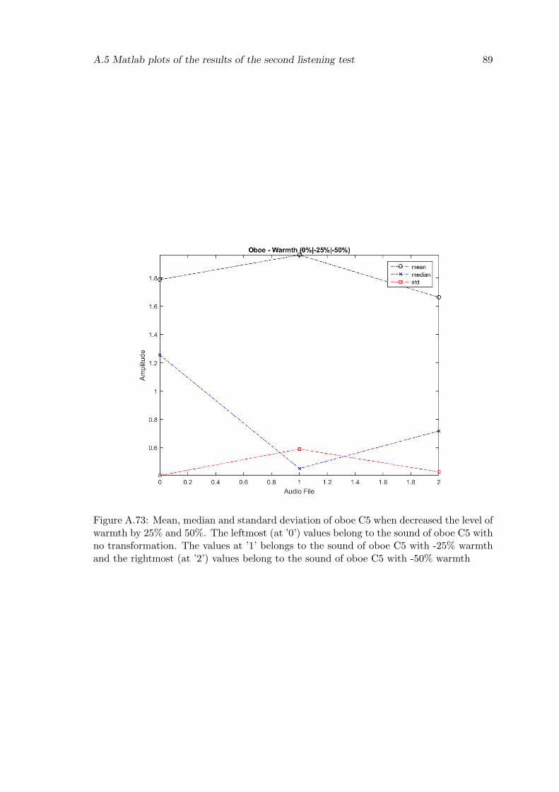
A.5 Matlab plots of the results of the second listening test 89
Figure A.73: Mean, median and standard deviation of oboe C5 when decreased the level ofwarmth by 25% and 50%. The leftmost (at ’0’) values belong to the sound of oboe C5 withno transformation. The values at ’1’ belongs to the sound of oboe C5 with -25% warmthand the rightmost (at ’2’) values belong to the sound of oboe C5 with -50% warmth
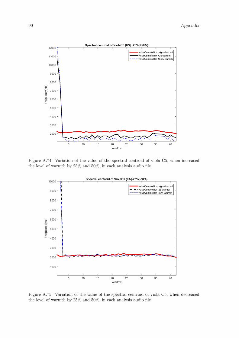
90 Appendix
Figure A.74: Variation of the value of the spectral centroid of viola C5, when increasedthe level of warmth by 25% and 50%, in each analysis audio file
Figure A.75: Variation of the value of the spectral centroid of viola C5, when decreasedthe level of warmth by 25% and 50%, in each analysis audio file
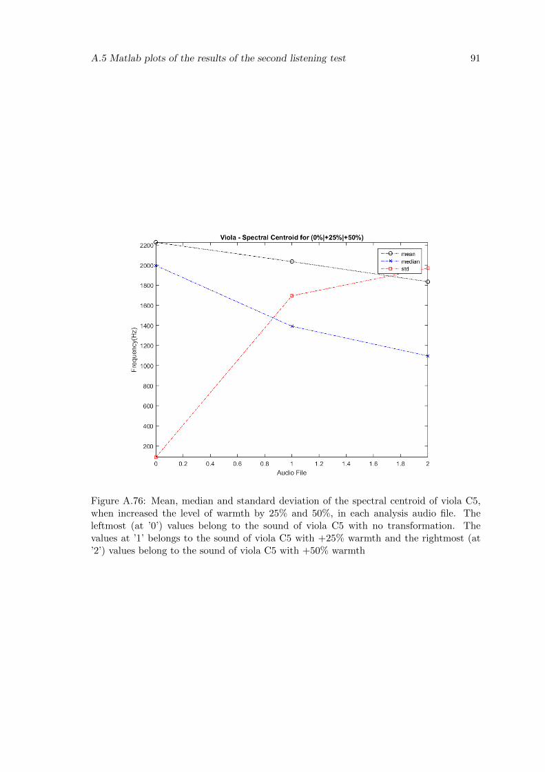
A.5 Matlab plots of the results of the second listening test 91
Figure A.76: Mean, median and standard deviation of the spectral centroid of viola C5,when increased the level of warmth by 25% and 50%, in each analysis audio file. Theleftmost (at ’0’) values belong to the sound of viola C5 with no transformation. Thevalues at ’1’ belongs to the sound of viola C5 with +25% warmth and the rightmost (at’2’) values belong to the sound of viola C5 with +50% warmth

92 Appendix
Figure A.77: Mean, median and standard deviation of viola C5 when decreased the level ofwarmth by 25% and 50%. The leftmost (at ’0’) values belong to the sound of viola C5 withno transformation. The values at ’1’ belongs to the sound of viola C5 with -25% warmthand the rightmost (at ’2’) values belong to the sound of viola C5 with -50% warmth
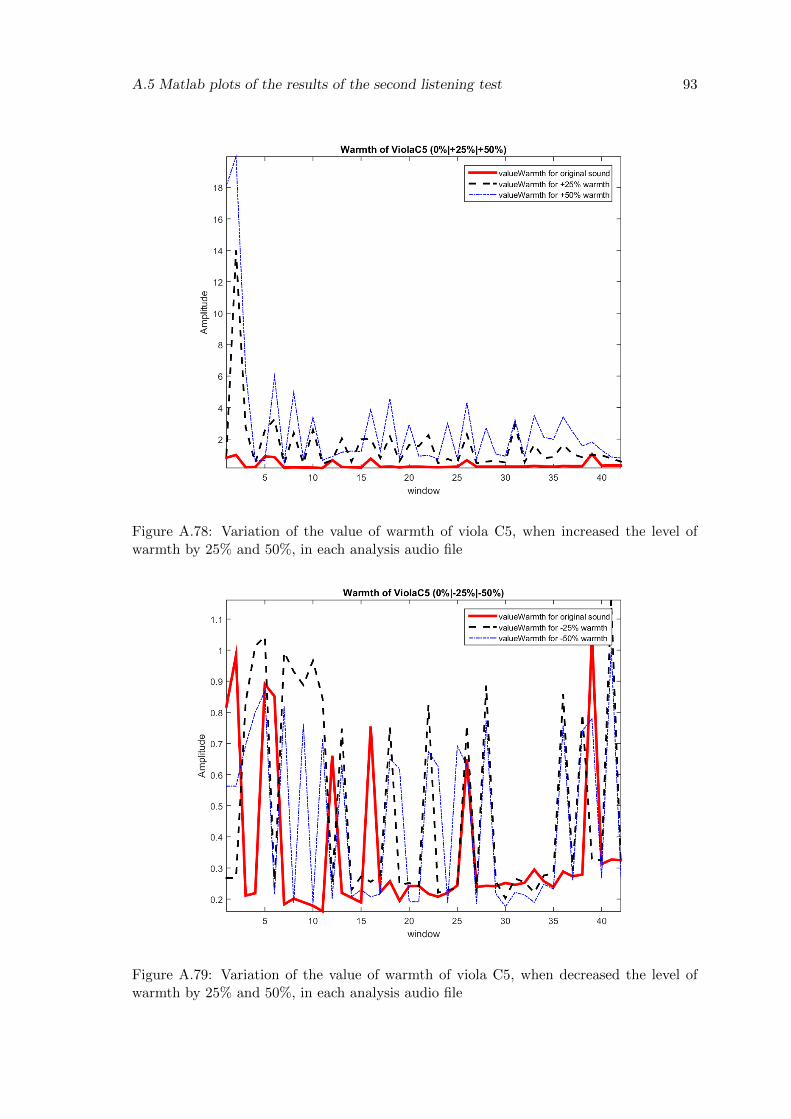
A.5 Matlab plots of the results of the second listening test 93
Figure A.78: Variation of the value of warmth of viola C5, when increased the level ofwarmth by 25% and 50%, in each analysis audio file
Figure A.79: Variation of the value of warmth of viola C5, when decreased the level ofwarmth by 25% and 50%, in each analysis audio file

94 Appendix
Figure A.80: Mean, median and standard deviation of the warmth of viola C5 whenincreased the level of warmth by 25% and 50%. The leftmost (at ’0’) values belong to thesound of viola C5 with no transformation. The values at ’1’ belongs to the sound of violaC5 with +25% warmth and the rightmost (at ’2’) values belong to the sound of viola C5with +50% warmth
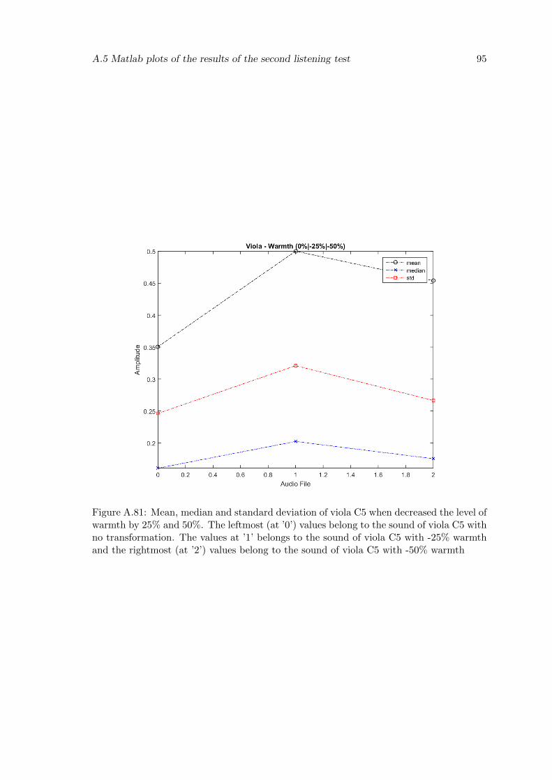
A.5 Matlab plots of the results of the second listening test 95
Figure A.81: Mean, median and standard deviation of viola C5 when decreased the level ofwarmth by 25% and 50%. The leftmost (at ’0’) values belong to the sound of viola C5 withno transformation. The values at ’1’ belongs to the sound of viola C5 with -25% warmthand the rightmost (at ’2’) values belong to the sound of viola C5 with -50% warmth
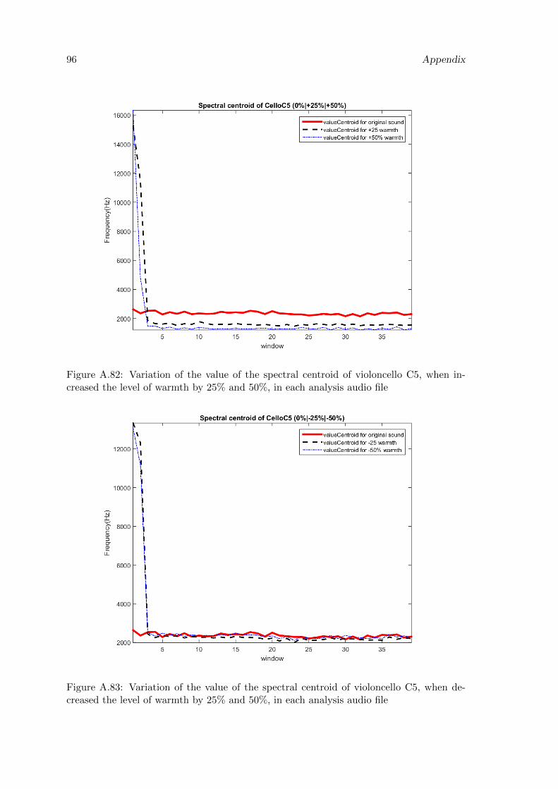
96 Appendix
Figure A.82: Variation of the value of the spectral centroid of violoncello C5, when in-creased the level of warmth by 25% and 50%, in each analysis audio file
Figure A.83: Variation of the value of the spectral centroid of violoncello C5, when de-creased the level of warmth by 25% and 50%, in each analysis audio file

A.5 Matlab plots of the results of the second listening test 97
Figure A.84: Mean, median and standard deviation of the spectral centroid of violoncelloC5, when increased the level of warmth by 25% and 50%, in each analysis audio file. Theleftmost (at ’0’) values belong to the sound of violoncello C5 with no transformation. Thevalues at ’1’ belongs to the sound of violoncello C5 with +25% warmth and the rightmost(at ’2’) values belong to the sound of violoncello C5 with +50% warmth
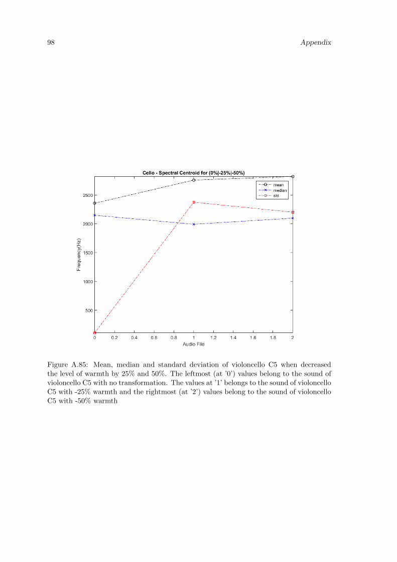
98 Appendix
Figure A.85: Mean, median and standard deviation of violoncello C5 when decreasedthe level of warmth by 25% and 50%. The leftmost (at ’0’) values belong to the sound ofvioloncello C5 with no transformation. The values at ’1’ belongs to the sound of violoncelloC5 with -25% warmth and the rightmost (at ’2’) values belong to the sound of violoncelloC5 with -50% warmth
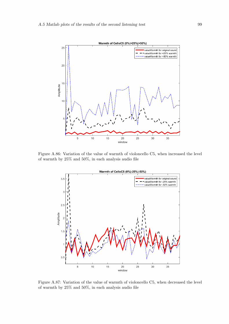
A.5 Matlab plots of the results of the second listening test 99
Figure A.86: Variation of the value of warmth of violoncello C5, when increased the levelof warmth by 25% and 50%, in each analysis audio file
Figure A.87: Variation of the value of warmth of violoncello C5, when decreased the levelof warmth by 25% and 50%, in each analysis audio file
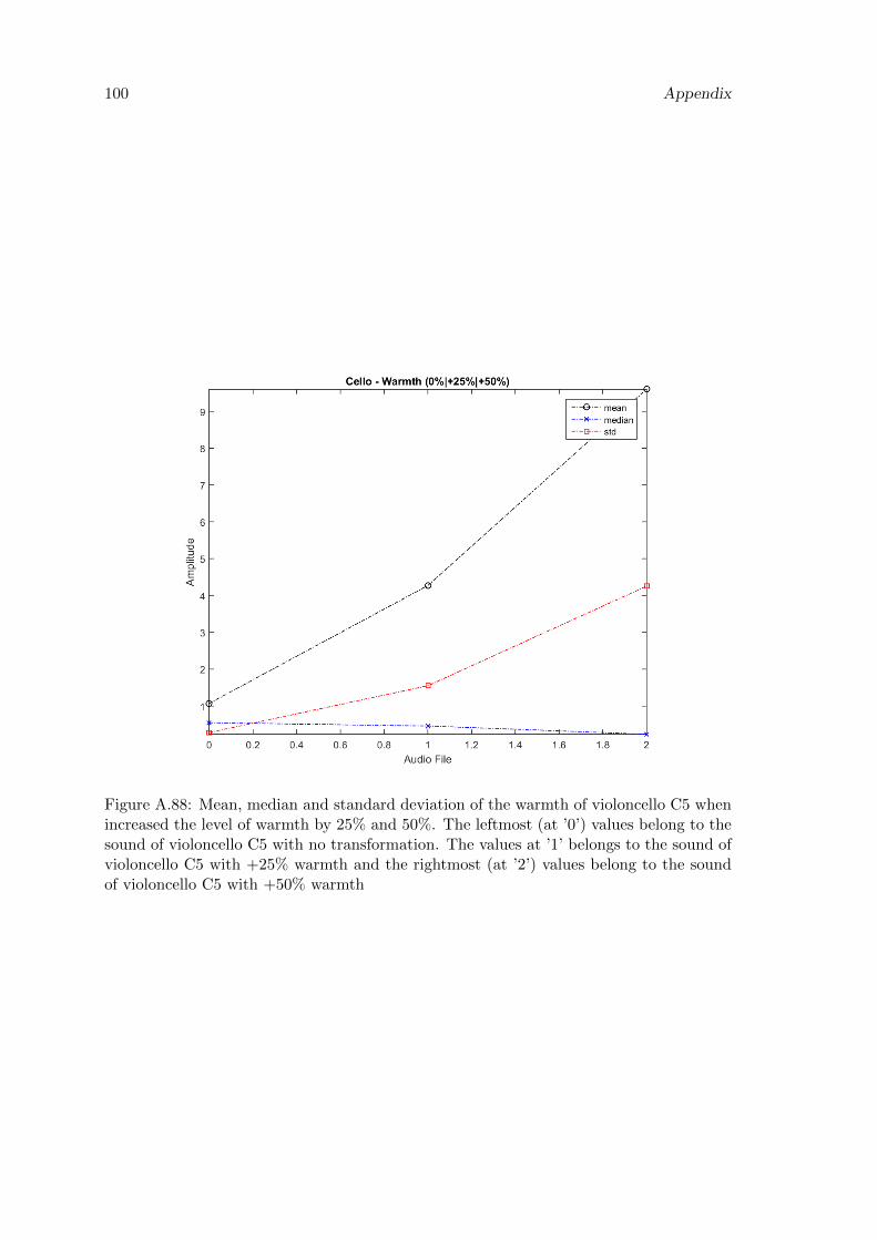
100 Appendix
Figure A.88: Mean, median and standard deviation of the warmth of violoncello C5 whenincreased the level of warmth by 25% and 50%. The leftmost (at ’0’) values belong to thesound of violoncello C5 with no transformation. The values at ’1’ belongs to the sound ofvioloncello C5 with +25% warmth and the rightmost (at ’2’) values belong to the soundof violoncello C5 with +50% warmth
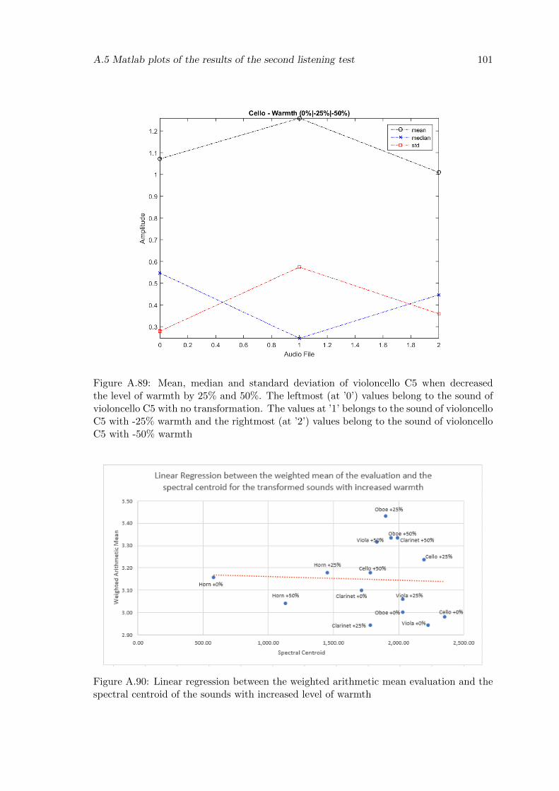
A.5 Matlab plots of the results of the second listening test 101
Figure A.89: Mean, median and standard deviation of violoncello C5 when decreasedthe level of warmth by 25% and 50%. The leftmost (at ’0’) values belong to the sound ofvioloncello C5 with no transformation. The values at ’1’ belongs to the sound of violoncelloC5 with -25% warmth and the rightmost (at ’2’) values belong to the sound of violoncelloC5 with -50% warmth
Figure A.90: Linear regression between the weighted arithmetic mean evaluation and thespectral centroid of the sounds with increased level of warmth
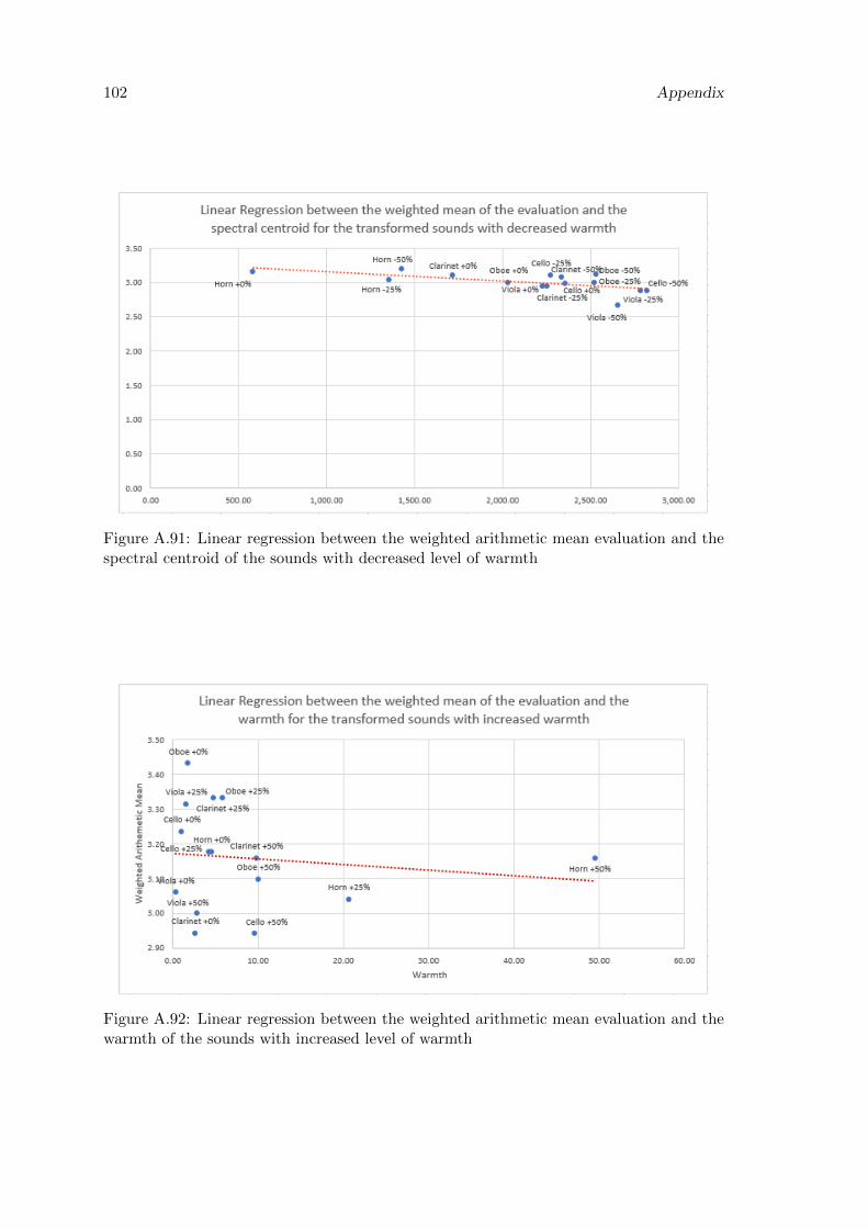
102 Appendix
Figure A.91: Linear regression between the weighted arithmetic mean evaluation and thespectral centroid of the sounds with decreased level of warmth
Figure A.92: Linear regression between the weighted arithmetic mean evaluation and thewarmth of the sounds with increased level of warmth
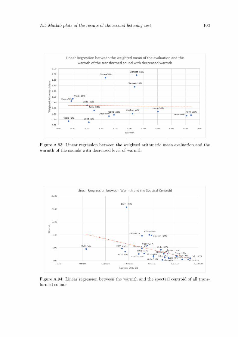
A.5 Matlab plots of the results of the second listening test 103
Figure A.93: Linear regression between the weighted arithmetic mean evaluation and thewarmth of the sounds with decreased level of warmth
Figure A.94: Linear regression between the warmth and the spectral centroid of all trans-formed sounds

104 Appendix
References
[1] D. Williams and T. Brookes, “Perceptually-motivated audio morphing: warmth,” in
128th Convention, London, UK, 2010.
[2] I. E. Y. Simurra et al., “A utilizacao descritores de audio a analise e composicao
musical assistidas por computador: um estudo de caso na obra Labori Ruinae,” XXV
Congresso da Associacao Nacional de Pesquisa e Pos-Graduacao em Musica, Vitoia,
2015.
[3] I. E. Y. Simurra,“Contribuicao ao problema da orquestracao assistida por computador
com suporte de descritores de audio,” Ph.D. dissertation, Univeridade Estadual de
Campinas, 2016.
[4] M. Schedl, E. Gomez, J. Urbano et al., “Music information retrieval: Recent develop-
ments and applications,” Foundations and Trends R© in Information Retrieval, vol. 8,
no. 2-3, pp. 127–261, 2014.
[5] J. S. Downie, D. Byrd, and T. Crawford, “Ten years of ismir: Reflections on challenges
and opportunities.” in ISMIR, 2009, pp. 13–18.
[6] A. Antoine, D. Williams, and E. Miranda, “Towards a timbre classification system
for orchestral excerpts,” in 2nd AES Workshop on Intelligent Music Production,
September 2016. [Online]. Available: http://goo.gl/YkdOA6
[7] U. Zolzer, Digital audio signal processing. John Wiley & Sons, 2008.
[8] M. Kuhn, “Digital signal processing,” 2009. [Online]. Available: http://www.cl.cam.
ac.uk/teaching/0809/DSP/slides.pdf
[9] M. Rizk and A. Wassal, “Asic implementation of tms320c2x dsp as a second phase of
cordoba dsp,” 2014.
[10] J. Macedo Fechine Regis de Araujo, “Processamento digital de sinais: Conceitos e
aplicacoes,” 2012. [Online]. Available: https://goo.gl/i9hEAw
[11] J. Futrelle and J. S. Downie, “Interdisciplinary communities and research issues in
music information retrieval.” in ISMIR, vol. 2, 2002, pp. 215–221.
105

106 REFERENCES
[12] D. Moffat, D. Ronan, J. D. Reiss et al., “An evaluation of audio feature extraction
toolboxes,” 2015.
[13] A. Wang et al., “An industrial strength audio search algorithm.” in Ismir, vol. 2003.
Washington, DC, 2003, pp. 7–13.
[14] M. S. Lew, N. Sebe, C. Djeraba, and R. Jain, “Content-based multimedia
information retrieval: State of the art and challenges,” ACM Trans. Multimedia
Comput. Commun. Appl., vol. 2, no. 1, pp. 1–19, Feb. 2006. [Online]. Available:
http://doi.acm.org/10.1145/1126004.1126005
[15] P. Herrera, X. Serra, and G. Peeters, “Audio descriptors and descriptor schemes in
the context of mpeg-7.” in ICMC, 1999.
[16] A. Friberg, E. Schoonderwaldt, A. Hedblad, M. Fabiani, and A. Elowsson, “Using
listener-based perceptual features as intermediate representations in music informa-
tion retrieval,” The Journal of the Acoustical Society of America, vol. 136, no. 4, pp.
1951–1963, 2014.
[17] D. Schwarz, “A system for data-driven concatenative sound synthesis,” in Digital
Audio Effects (DAFx), 2000, pp. 97–102.
[18] E. G. Gutierrez, “Tonal description of music audio signals,” Ph.D. dissertation, Uni-
versitat Pompeu Fabra, 2006.
[19] F. Gouyon, P. Herrera, E. Gomez, P. Cano, J. Bonada, A. Loscos, X. Amatriain, and
X. Serra, Content Processing of Music Audio Signals. Berlin: Logos Verlag Berlin
GmbH, 2008.
[20] G. Bernardes, “Composing music by selection: Content-based algorithmic-assisted
audio composition,” Ph.D. dissertation, PhD dissertation, University of Porto, 2014.
[21] E. Schubert, J. Wolfe, and A. Tarnopolsky, “Spectral centroid and timbre in complex,
multiple instrumental textures,” in Proceedings of the international conference on
music perception and cognition, North Western University, Illinois. Citeseer, 2004,
pp. 112–116.
[22] D. Bolger and N. Griffith, “Multidimensional timbre analysis of shakuhachi
honkyoku,” in Proceedings of the Conference on International Musicology, 2005.
[23] H. Fastl and E. Zwicker, Psychoacoustics: facts and models. Springer Science &
Business Media, 2006, vol. 22.
[24] M. A. Landera and R. Shrivastav, “Effects of spectral slope on perceived breathiness
in vowels,” The Journal of the Acoustical Society of America, vol. 119, no. 5, pp.
3339–3340, 2006.
REFERENCES 107
[25] G. Peeters, B. L. Giordano, P. Susini, N. Misdariis, and S. McAdams, “The tim-
bre toolbox: Extracting audio descriptors from musical signals,” The Journal of the
Acoustical Society of America, vol. 130, no. 5, pp. 2902–2916, 2011.
[26] M. Malt and E. Jourdan, “Zsa. descriptors: a library for real-time descriptors analy-
sis,” Sound and Music Computing, Berlin, Germany, 2008.
[27] J. Krimphoff, “Analyse acoustique et perception du timbre [acoustic analysis and
perception of timbre] unpublished master’s thesis,” Universite du Maine, Le Mans,
France, 1993.
[28] E. Scheirer and M. Slaney, “Construction and evaluation of a robust multifeature
speech/music discriminator,” in Acoustics, Speech, and Signal Processing, 1997.
ICASSP-97., 1997 IEEE International Conference on, vol. 2. IEEE, 1997, pp. 1331–
1334.
[29] H. F. Pollard and E. V. Jansson,“A tristimulus method for the specification of musical
timbre,” Acta Acustica united with Acustica, vol. 51, no. 3, pp. 162–171, 1982.
[30] T. Brookes and D. Williams, “Perceptually-motivated audio morphing: Brightness,”
in Audio Engineering Society Convention 122. Audio Engineering Society, 2007.
[31] D. Williams and T. Brookes, “Perceptually-motivated audio morphing: softness,” in
Audio Engineering Society Convention 126. Audio Engineering Society, 2009.
[32] J.-M. Jot and O. Warusfel, “Spat: A spatial processor for musicians and sound en-
gineers,” in CIARM: International Conference on Acoustics and Musical Research,
1995.
[33] R. Ethington and B. Punch, “Seawave: A system for musical timbre description,”
Computer Music Journal, vol. 18, no. 1, pp. 30–39, 1994.
[34] D. Schwarz, G. Lemaitre, M. Aramaki, and R. Kronland-Martinet, “Effects of test
duration in subjective listening tests,” in International Computer Music Conference
(ICMC). HKU University of the Arts Utrecht, HKU Music and Technology, 2016,
pp. 515–519.
[35] M. Puckette et al., “Pure data: another integrated computer music environment,”
Proceedings of the second intercollege computer music concerts, pp. 37–41, 1996.