arX

iv:0

705.

3295

v1 [

cond

-mat

.dis

-nn]

23

May

200

7

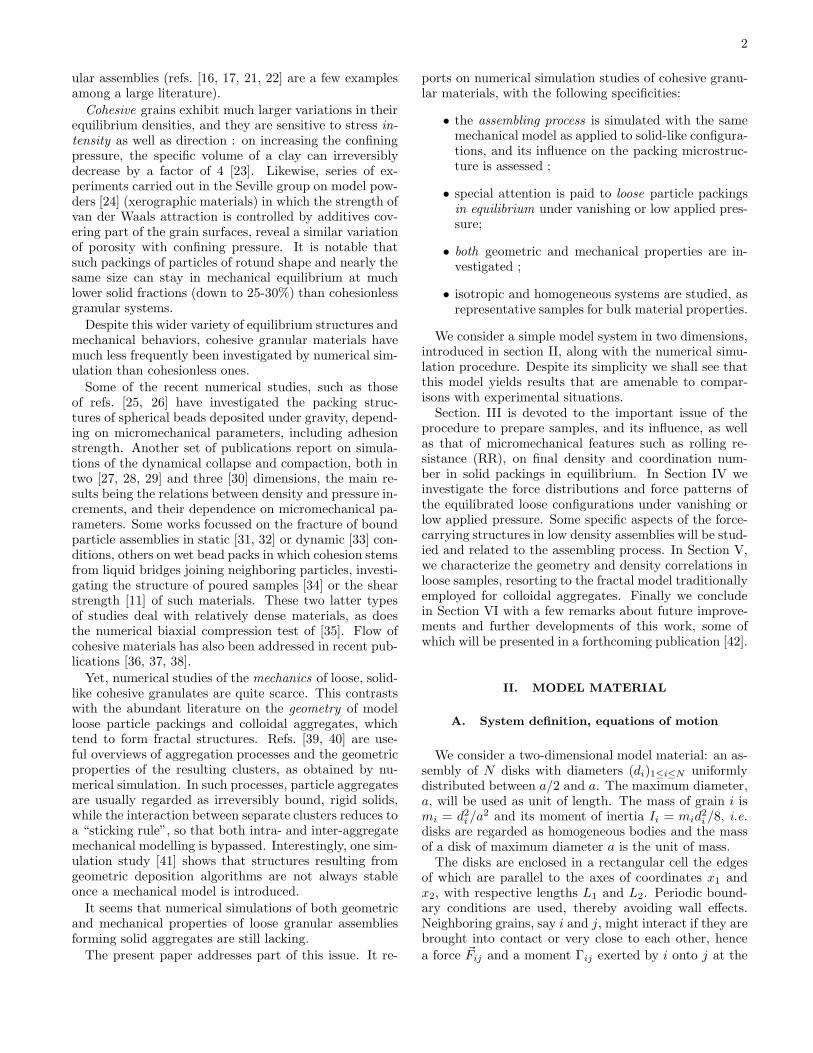
Computer simulation of model cohesive powders:

influence of assembling procedure and contact laws on low consolidation states.

F. A. Gilabert,1, ∗ J.-N. Roux,2 and A. Castellanos1

1Faculty of Physics, University of Seville, Avda. Reina Mercedes s/n, 41012 Seville, Spain.2Laboratoire des Materiaux et des Structures du Genie Civil†, Institut Navier,

2 Allee Kepler, Cite Descartes, 77420 Champs-sur-Marne, France.(Dated: October, 2006)

Molecular dynamics simulations are used to investigate the structure and mechanical properties ofa simple two-dimensional model of a cohesive granular material. Intergranular forces involve elastic-ity, Coulomb friction and a short range attraction akin to the van der Waals force in powders. Theeffects of rolling resistance (RR) at intergranular contacts are also studied. The microstructure ofthe cohesive packing under low pressure is shown to depend sensitively on the assembling procedurewhich is applied to the initially isolated particles of a granular gas. While a direct compressionproduces a final equilibrated configuration with a similar density to that of cohesionless systems,the formation of large aggregates prior to the application of an external pressure results in muchlooser stable packings. A crucial state variable is the ratio P ∗ = Pa/F0 of applied pressure P ,acting on grains of diameter a, to maximum tensile contact force F0. At low P ∗ the force-carryingstructure and force distribution are sensitive to the level of velocity fluctuations in the early stagesof cluster aggregation. The coordination number of packings with RR approaches 2 in the limit oflow initial velocities or large rolling friction. In general the force network is composed of hyper-static clusters, typically comprising 4 to a few tens of grains, in which forces reach values of theorder of F0, joined by barely rigid arms, where contact forces are very small. Under growing P ∗, itquickly rearranges into force chain-like patterns that are more familiar in dense systems. Densitycorrelations are interpreted in terms of a fractal structure, up to a characteristic correlation lengthξ of the order of ten particle diameters for the studied solid fractions. The fractal dimension insystems with RR coincides, within measurement uncertainties, with the ballistic aggregation result,in spite of a possibly different connectivity, but is apparently higher without RR. Possible effects ofmicromechanical and assembling process parameters on mechanical strength of packings are evoked.

PACS numbers:81.05.Rm: Porous materials, granular materials,83.10.Rs: Computer simulation of molecular and particle dynamics,61.43.Hv: Fractals, macroscopic aggregates,47.57.J-: Colloidal systems

I. INTRODUCTION

Granular materials are currently being studied bymany research groups [1, 2, 3, 4], motivated by funda-mental issues (such as the relations between microstruc-ture and global properties) as well as by practical needsin civil engineering and in the food and drug industries.The relation of their mechanical behavior in quasistaticconditions to the packing geometry, which depends itselfon the assembling procedure, tends to escape intuitionand familiar modelling schemes.

The configuration of the contact networks is hardlyaccessible to experiments, even though particle positionsare sometimes measured [5, 6, 7, 8], and some experi-mental quantitative studies on intergranular contacts car-ried out in favorable cases (such as millimeter-sized beadsjoined by capillary menisci [6, 9, 10, 11]). Intergranular

†LMSGC is a joint laboratory depending on Laboratoire Centraldes Ponts et Chaussees, Ecole Nationale des Ponts et Chausseesand Centre National de la Recherche Scientifique.∗Electronic address: gilav@us.es

forces are also, most often, inaccessible to measurements.Consequently, computer simulation methods of the “dis-crete element” type, as introduced 30 years ago [12], haveproved a valuable tool to investigate the internal statesof granular systems. Simulation methods like moleculardynamics [13] or “contact dynamics” [14, 15] have beengaining an increasingly large constituency of users and awide range of applications, as witnessed e.g., by recentconference proceedings [4].

Dry assemblies of grains interacting via contact elas-ticity and friction, such as sands or glass beads, mightform stable packings of varying solid fraction (typicallybetween 58% and 64% for monosized spheres if they donot crystallize), which deform plastically in response tochanges in stress direction, rather than stress intensity.Their elastic or elastoplastic properties have been stud-ied by discrete simulation (see, e.g., [16, 17]), and, inagreement with laboratory experiments and macroscopicmodelling [18], found to depend sensitively on the initialdensity. Numerical simulation also stressed the impor-tance of additional variables such as coordination num-ber [19] and fabric [20, 21], and it has often been appliedto the study of quasi-static stress-strain behavior of gran-

2

ular assemblies (refs. [16, 17, 21, 22] are a few examplesamong a large literature).

Cohesive grains exhibit much larger variations in theirequilibrium densities, and they are sensitive to stress in-

tensity as well as direction : on increasing the confiningpressure, the specific volume of a clay can irreversiblydecrease by a factor of 4 [23]. Likewise, series of ex-periments carried out in the Seville group on model pow-ders [24] (xerographic materials) in which the strength ofvan der Waals attraction is controlled by additives cov-ering part of the grain surfaces, reveal a similar variationof porosity with confining pressure. It is notable thatsuch packings of particles of rotund shape and nearly thesame size can stay in mechanical equilibrium at muchlower solid fractions (down to 25-30%) than cohesionlessgranular systems.

Despite this wider variety of equilibrium structures andmechanical behaviors, cohesive granular materials havemuch less frequently been investigated by numerical sim-ulation than cohesionless ones.

Some of the recent numerical studies, such as thoseof refs. [25, 26] have investigated the packing struc-tures of spherical beads deposited under gravity, depend-ing on micromechanical parameters, including adhesionstrength. Another set of publications report on simula-tions of the dynamical collapse and compaction, both intwo [27, 28, 29] and three [30] dimensions, the main re-sults being the relations between density and pressure in-crements, and their dependence on micromechanical pa-rameters. Some works focussed on the fracture of boundparticle assemblies in static [31, 32] or dynamic [33] con-ditions, others on wet bead packs in which cohesion stemsfrom liquid bridges joining neighboring particles, investi-gating the structure of poured samples [34] or the shearstrength [11] of such materials. These two latter typesof studies deal with relatively dense materials, as doesthe numerical biaxial compression test of [35]. Flow ofcohesive materials has also been addressed in recent pub-lications [36, 37, 38].

Yet, numerical studies of the mechanics of loose, solid-like cohesive granulates are quite scarce. This contrastswith the abundant literature on the geometry of modelloose particle packings and colloidal aggregates, whichtend to form fractal structures. Refs. [39, 40] are use-ful overviews of aggregation processes and the geometricproperties of the resulting clusters, as obtained by nu-merical simulation. In such processes, particle aggregatesare usually regarded as irreversibly bound, rigid solids,while the interaction between separate clusters reduces toa “sticking rule”, so that both intra- and inter-aggregatemechanical modelling is bypassed. Interestingly, one sim-ulation study [41] shows that structures resulting fromgeometric deposition algorithms are not always stableonce a mechanical model is introduced.

It seems that numerical simulations of both geometricand mechanical properties of loose granular assembliesforming solid aggregates are still lacking.

The present paper addresses part of this issue. It re-

ports on numerical simulation studies of cohesive granu-lar materials, with the following specificities:

• the assembling process is simulated with the samemechanical model as applied to solid-like configura-tions, and its influence on the packing microstruc-ture is assessed ;

• special attention is paid to loose particle packingsin equilibrium under vanishing or low applied pres-sure;

• both geometric and mechanical properties are in-vestigated ;

• isotropic and homogeneous systems are studied, asrepresentative samples for bulk material properties.

We consider a simple model system in two dimensions,introduced in section II, along with the numerical simu-lation procedure. Despite its simplicity we shall see thatthis model yields results that are amenable to compar-isons with experimental situations.

Section. III is devoted to the important issue of theprocedure to prepare samples, and its influence, as wellas that of micromechanical features such as rolling re-sistance (RR), on final density and coordination num-ber in solid packings in equilibrium. In Section IV weinvestigate the force distributions and force patterns ofthe equilibrated loose configurations under vanishing orlow applied pressure. Some specific aspects of the force-carrying structures in low density assemblies will be stud-ied and related to the assembling process. In Section V,we characterize the geometry and density correlations inloose samples, resorting to the fractal model traditionallyemployed for colloidal aggregates. Finally we concludein Section VI with a few remarks about future improve-ments and further developments of this work, some ofwhich will be presented in a forthcoming publication [42].

II. MODEL MATERIAL

A. System definition, equations of motion

We consider a two-dimensional model material: an as-sembly of N disks with diameters (di)1≤i≤N uniformlydistributed between a/2 and a. The maximum diameter,a, will be used as unit of length. The mass of grain i ismi = d2

i /a2 and its moment of inertia Ii = mid2i /8, i.e.

disks are regarded as homogeneous bodies and the massof a disk of maximum diameter a is the unit of mass.

The disks are enclosed in a rectangular cell the edgesof which are parallel to the axes of coordinates x1 andx2, with respective lengths L1 and L2. Periodic bound-ary conditions are used, thereby avoiding wall effects.Neighboring grains, say i and j, might interact if they arebrought into contact or very close to each other, hence

a force ~Fij and a moment Γij exerted by i onto j at the

3

contact point. Simulations do not model material defor-mation in a contact region, but consider overlapping par-ticles, and the contact point is defined as the center of theintersecting surface of the two disks. In the case of an in-teraction without contact, the force will be normal to thesurfaces at the points of nearest approach, and thereforecarried by the line of centers. Let ~ri denote the positionof the center of disk i. ~rij = ~rj − ~ri is the vector joiningthe centers of i and j, and hij = |~rij | − (di + dj)/2 theiroverlap distance. The degrees of freedom, in addition tothe positions ~ri, are the angles of rotation θi, velocities~vi, angular velocities ωi = θi of the grains (1 ≤ i ≤ N),the dimensions (Lα)α=1,2 of the cell containing the grainsand their time derivatives, through the strain rates:

ǫα = −Lα/L0α,

in which L0α denotes the initial size for the corresponding

compression process. The time evolution of those degreesof freedom is governed by the following equations.

mid2~ri

dt2=

N∑

j=1

~Fij (1)

Iidωi

dt=

N∑

j=1

Γij (2)

Md2ǫα

dt2= σI

αα − σMαα

σMαα =

1

A

N∑

i=1

miv2i,α +

∑

j 6=i

F(α)ij r

(α)ij

(3)

In Eqns. (1) and (2), only those disks j interacting with i,i. e. in contact or very close, will contribute to the sumson the right-hand side. In Eqn. (3), σI

αα is the externallyimposed stress component, σM

αα is the measured stresscomponent, resulting from ballistic momentum transport

and from the set of intergranular forces ~Fij , A = L1L2

denotes the cell surface area, and M is a generalized in-ertia parameter.

Stresses σ11 and σ22, rather than strains or cell dimen-sions, are controlled in our simulation procedure. Notethat compressions are counted positively for both stressesand strains. Eqn. (3) entails that the sample will expand(respectively, shrink) along direction α if the correspond-ing stress σM

αα is larger (resp., smaller) than the requestedvalue σI

αα, which should be reached once the system equi-librates. This barostatic method is adapted from the onesinitially proposed by Parrinello and Rahman [43, 44, 45]for Hamiltonian, molecular systems.

The choice of the “generalized mass” M is rather arbi-trary, yet innocuous provided calculations are restrictedto small strain rates. In practice we strive to approachmechanical equilibrium states with good accuracy, andchoose M in order to achieve this goal within affordable

computation times. We usually attribute to M a valueequal to a fraction of the sum of grain masses (3/10 inmost calculations), divided by a linear size L of the cell.This choice is dimensionally correct and corresponds tothe appropriate time scale for strain fluctuations in thecase of a thermodynamic system.

B. Interaction law

The contact law in a granular material is the relation-ship between the relative motion of two contacting grainsand the contact force. As we deal with particles that mayattract one another at short distance without touching,the law governing intergranular forces and moments isbest referred to simply as the interaction law.

Although the interaction we adopted is based on theclassical linear “spring-dashpot” model with Coulombfriction for contact elasticity, viscous dissipation and slid-ing, as used in many discrete simulations of granular me-dia [13, 37, 38, 46], some of its features (short-range at-traction and rolling resistance) are less common ; more-over, one can think of different implementations of theCoulomb condition, depending on which parts of normaland tangential force components are taken into account.Therefore, for the sake of clarity and completeness, wegive a full, self-contained presentation of the interactionlaw below.

We express intergranular forces in a mobile systemof coordinates with axes oriented along the normal unitvector nij (along ~rij) and the tangential unit vector tij(nij , tij is a direct base in the plane), and use the con-vention that repulsive forces are positive.

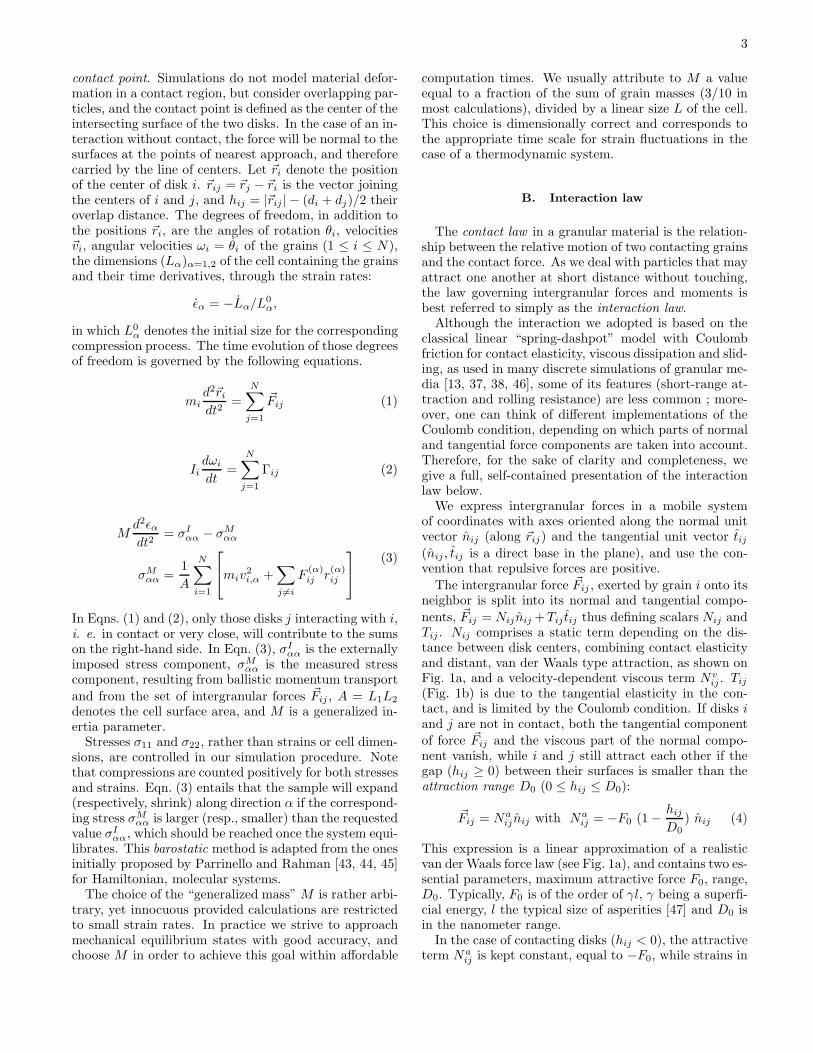
The intergranular force ~Fij , exerted by grain i onto itsneighbor is split into its normal and tangential compo-

nents, ~Fij = Nij nij +Tij tij thus defining scalars Nij andTij . Nij comprises a static term depending on the dis-tance between disk centers, combining contact elasticityand distant, van der Waals type attraction, as shown onFig. 1a, and a velocity-dependent viscous term Nv

ij . Tij

(Fig. 1b) is due to the tangential elasticity in the con-tact, and is limited by the Coulomb condition. If disks iand j are not in contact, both the tangential component

of force ~Fij and the viscous part of the normal compo-nent vanish, while i and j still attract each other if thegap (hij ≥ 0) between their surfaces is smaller than theattraction range D0 (0 ≤ hij ≤ D0):

~Fij = Naij nij with Na

ij = −F0 (1 − hij

D0) nij (4)

This expression is a linear approximation of a realisticvan der Waals force law (see Fig. 1a), and contains two es-sential parameters, maximum attractive force F0, range,D0. Typically, F0 is of the order of γl, γ being a superfi-cial energy, l the typical size of asperities [47] and D0 isin the nanometer range.

In the case of contacting disks (hij < 0), the attractiveterm Na

ij is kept constant, equal to −F0, while strains in

4

KN

(a)

h ij

Nij

e+Nij

a

D0

-F0

-F0

- F0

(b)

F0

Tij

Nij

e+Nij

a

FIG. 1: Graphical representation of the model for the adhesive elastic contact force as a function of the distance betweenthe surfaces of particles i and j, hij . (a) The elastic normal force consists of a repulsive Hookean part Ne

ij plus a linearizedattractive part Na

ij . (b) The elastic tangential force is limited by the Coulomb cone (adhesion shifting its tip to −F0 on thenormal force axis).

the contact region result in normal (Neij) and tangential

(Tij) elastic forces. It is also assumed that a viscousnormal term Nv

ij opposes relative normal displacements.One thus writes:

~Fij = (Neij + Nv

ij − F0) nij + Tij tij (5)

The different terms introduced in Eqn. (5) are definedaccording to the following models. First,

Neij = −KNhij

is the linear elastic unilateral repulsion, due to the normaldeflection −hij in the contact as the disks are pressedagainst each other. KN is the normal stiffness coefficient,related to the elastic moduli of the material the grainsare made of.

The viscous normal force opposes the normal relativereceding velocity δvN

ij = nij · (~vj − ~vi) as long as thecontact persists. The relative normal motion of two disksi and j in contact is that of an oscillator with viscousdamping, and ηij is the damping coefficient. We chooseits value as a constant fraction ζ of the critical dampingcoefficient,

ηij = ζ

√

4KNmimj

mi + mj. (6)

This is equivalent to the choice of a constant restitutioncoefficient in normal collisions if F0 = 0. In the presenceof attractive forces the apparent restitution coefficient ina collision will depend on the initial relative velocity, andwill be equal to zero for small values, when the recedingvelocity after the collision will not be able to overcomethe attraction and separate the particles. The minimumreceding velocity for two particles of unit mass (i.e., of

maximum diameter a) to separate is V ∗√

2, with

V ∗ =√

F0D0. (7)

The elastic tangential force in contact i, j is linearlyrelated to the elastic part δuT

ij of the total relative tan-

gential displacement ∆uTij , as

Tij = KT δuTij ,

and is subject to the Coulomb inequality. KT is thetangential stiffness coefficient. ∆uT

ij can be updated forall closed contacts according to

d∆uTij

dt= (~vij · tij)

and vanishes as soon as the contact opens. Its elasticpart satisfies

dδuTij

dt= H

(

µNeij

KT− |δuT

ij |)

(~vij · tij)

in which H denotes the Heaviside function. This lastequation introduces the friction coefficient µ. It is im-portant to note that the Coulomb inequality,

|Tij | ≤ µNeij , (8)

applies to the sole repulsive elastic component of the nor-mal force (see Fig. 1b). We chose not to implement anytangential viscous force.

The moment that disk i exerts onto its contactingneighbor j, of radius Rj , in its center, is denoted by Γij

in Eqn. (2). It is first due to the tangential contact force,then to a possible moment Γ r

ij of the force density dis-tribution within the contact region. One thus writes:

Γij = −TijRj + Γ rij . (9)

Γ rij is most often neglected on dealing with smooth, con-

vex particle shapes, because the contact region is verysmall on the scale of the particle radius.

5

To model rolling resistance (RR), like in [48], we intro-duce a rotational stiffness parameter Kr and a rotationalfriction parameter µr in contacts, so that rolling elas-ticity and rolling friction are modelled just like slidingelasticity and friction. One thus writes

Γ rij = Kr δθij ,

while enforcing the inequality

Kr|δθij | ≤ µrNeij . (10)

This involves the definition of δθij as the elastic partof the total relative rotation ∆θij . The total relativerotation angle satisfies

d∆θij

dt= ωj − ωi,

while the equation for δθij is

dδθij

dt= H

(

µrNeij

Kr− |δθij |

)

(ωj − ωi).

Parameters Kr and µr are often related to the size of acontact region [27]. Kr is dimensionally the product of astiffness by the square of a length, which is of the order ofthe contact size. In the following we set Kr to 10−4a2KN ,while µr, which has the dimension of a length, is chosenequal to 10−2µa. The motivation for the introduction ofRR into our model is twofold. First, cohesive particlesare usually small (typically less than 30µm in size) andirregular in shape. Contacts between grains are likelyto involve several asperities, and hence some lateral ex-tension, of the order of the distance between asperities,however small the normal deflection −h. Then, it willbe observed that even quite a small rotational frictionhas a notable influence on the microstructure of cohesivepackings.

C. Control parameters and dimensional analysis

In this section we present the dimensionless param-eters which express the relative importance of differentphysical phenomena. Such parameters enable qualitativecomparisons with real materials, bearing in mind that thepresent model is admittedly an idealization of real pow-ders and that our simulations do not aim at quantitativeaccuracy.

Dimensionless numbers related to contact behavior arethe reduced interaction range D0/a, the friction coeffi-cient µ, the viscous damping parameter ζ, and the stiff-ness parameter κ.

Under the attractive force −F0, the elastic deflectionof one contact is

h0 = F0/KN (11)

The stiffness parameter κdef

= aKN/F0 characterizes theamount of elastic deflection h0 under contact force F0,

relative to grain size a (h0/a = κ−1). A suitable analo-gous definition for Hertzian spheres in three dimensionswould be κ = (Ea2/F0)

2/3.The dimensionless number h0/D0 is the ratio of

elastic to adhesive stiffnesses, and its physical mean-ing is similar to that of the Tabor parameter λ =(1/D0)(γ

2a/E2)1/3 [49] for a Hertzian contact betweenspheres of diameter a when the material Young modu-lus is E and the interfacial energy is γ (more precisely,the equilibrium normal deflection h0, due to adhesion, inthe contact between an isolated pair of grains, satisfiesλ ∼ (h0/D0)

1/3 in this case).The viscous damping parameter, ζ, corresponds to a

normal restitution coefficient eN = exp[−πζ/√

1 − ζ2] inthe absence of cohesion (F0 = 0).

In our calculations we set ζ = 0.8, corresponding toa high viscous dissipation in collisions, or a very lowrestitution coefficient in binary collisions. Models witha constant ζ were adopted in other published simulationworks [46, 50], although little is known about dissipationin collisions. ζ is known to influence the packing struc-tures obtained in the initial assembling stage [46, 51],but we did not investigate its effects in the present study.The simulations reported in [25, 26] use the viscous forcemodel introduced in ref. [52], with a choice of param-eters corresponding to strongly overdamped dynamics(i.e., analogous to ζ ≫ 1 in our case).

In addition to those control parameters determined bythe contact behavior, other dimensionless numbers areintroduced by the loading or the process being appliedto the material. The effect of the external pressure, com-pared to the adhesion strength, is characterized by a di-mensionless reduced pressure P ∗:

P ∗ def= Pa/F0. (12)

In the present paper, we focus on the assembling processand the low P ∗ range. As we shall see below (Sec. III)low density, tenuous structures are then stabilized by ad-hesion, and the relevant force scale is F0. However, asbriefly reported in [53], such structures tend to collapseupon increasing P ∗. These phenomena will be the sub-ject of another paper [42]. Wolf et al. [29] introduced adimensionless stress proportional to P ∗, and observed, innumerical simulations, stepwise increases in pressure toproduce large dynamical collapse effects around P ∗ = 1.The importance of P ∗ was also stressed in simulations ofcohesive granular flow, in which the effects of cohesionon rheological laws were expressed in terms of a cohesionnumber defined as 1/P ∗ [37]. In three dimensions, P ∗

should be defined as a2P/F0.For large reduced pressures, externally imposed forces

dominate the adhesion strength, and one should observebehaviors similar to those of confined cohesionless gran-ular materials. For P ∗ > 1, the relevant force scale isaP . The influence of κ, which should then be defined as

κdef= KN/P , so that the typical contact deflection h satis-

fies h/a ∝ κ−1, was studied in simulations of grains with-out adhesion [54]. Whatever the reference force used to

6

define it, the limit of rigid grains is κ → +∞. With rela-tively soft grains (say, κ below 103), a significant numberof additional contacts appear in dense configurations, dueto the closing of gaps between near neighbors. Such a κparameter defined with reference to pressure, in the caseof contacts ruled by Hertz’s law between spherical grainsmade of a material with Young modulus E, should bechosen as κ = (E/P )2/3, in order to maintain h/a ∼ κ−1.

In order to stay within the limit of rigid grains bothfor small and large P ∗, we choose quite a large value ofκ = KNa/F0: κ = 104 or κ = 105.

Table I summarizes the values (or the range of val-ues) of dimensionless parameters in the simulations pre-sented below. In addition to those values of the param-

µ ζ κKT

KN

D0

a

Kr

KNa2

µr

aP ∗

0.15, 0.5 0.8 105, 104 1 10−3 10−4 0, 10−2µ 0, 0.01

TABLE I: Values of dimensionless model parameters used in

most simulations. Note that h0/D0 is fixed by κ =KNa

F0and

D0/a to 10−2 or 10−1. In the absence of cohesion, or forvalues of P ≥ F0/a, κ is defined as KN/P

eters, adopted as a plausible choice for realistic ordersof magnitudes, some calculations were also performedwith deliberately extreme choices, such as very large RR(µr = 0.5a) or absence of friction (µ = 0 and µr = 0), inorder to better explore some connections between mi-cromechanics and macroscopic properties. The corre-sponding results will be described in Section IV.

The definition of dimensionless parameters, suitablygeneralized to three-dimensional situations as P ∗ =a2P/F0 and κ ≃ (Ea2/F0)

2/3 for spherical particles of di-ameter a, enables one to discuss qualitative features andorders of magnitude in the model system defined with theparameters of Table I with comparisons to some cohesivepackings studied in the laboratory.

When adhesive forces are due to liquid menisci joiningneighboring particles, we should take F0 ∼ γa, where γ isthe surface tension. P ∗ = 1 corresponds then to confiningpressure P in the range of 10-100 Pa for millimeter-sizedparticles, taking standard values for γ. Those are ratherlow pressures in practice, which are comparable, e.g., tothe ones caused by the weight of a typical laboratorysand sample. Thus wet granular materials are commonlyunder reduced pressures P ∗ of order 1 or larger, and arenot observed with much lower solid fractions than dryones [6, 9, 10, 11].

The cohesive powders studied in refs. [24, 55, 56, 57]are xerographic toners with typical particle diametera ∼ 10 µm. F0, the van der Waals attractive force, isa few tens of nN, and the range D0 is several nanome-ters [58]. Therefore, a reduced pressure P ∗ = 0.01 wouldcorrespond to about 1 Pa in the experimental situation[59]. This is an initial state of very low consolidationstress, which is present in a powder under gravity, pro-

vided a controlled gas flow, going upwards through thepowder, counterbalances part of its weight [59]. As tocontact stiffnesses, our values of h0/a would correspondto E ∼ 0.1 GPa (for KN = 104F0/a) or 3.2 GPa (forKN = 105F0/a), while the ratio D0/a would imply an in-teraction range of 10 nm. This gives us the correct ordersof magnitudes for the toner particles, those being made ofa relatively soft solid (polymer, such as polystyrene) withE ∼ 3−6 GPa. Xerographic toner particles appear to un-dergo plastic deformation in the contacts [56, 60, 61, 62].Plastic deflections of contacts are accounted for in themodel of ref. [35], applied to the simulation of a biaxialcompression of a dense powder. In our study, for simplic-ity’s sake, and because we expect macroscopic plasticityof loose samples to be essentially related to the collapseof tenuous structures, we ignored this feature.

D. Equilibrated states

Although numerical simulations of the quasistaticresponse of granular materials requires by definitionthat configurations of mechanical equilibrium should bereached, equilibrium criteria are sometimes left unspec-ified, or quite vaguely stated in the literature. Yet, inorder to report results on important, often studied quan-tities like the coordination number or the force distribu-tion, it is essential to know which pairs of grains are incontact and which are not. Due to the frequent occur-rence of small contact force values, this requires forcesto balance with sufficient accuracy. We found that thefollowing criteria allowed us to identify the force-carryingstructure clearly enough. We use the typical intergran-ular force value F1 = max(F0, Pa) to set the tolerancelevels. A configuration is deemed equilibrated when thefollowing conditions are fulfilled:

• the net force on each disk is less than 10−4F1, andthe total moment is lower than 10−4F1a;

• the difference between imposed and measured pres-sure is less than 10−4F1/a;

• the kinetic energy per grain is less than 5 ·10−8F1a.

We observed that once samples were equilibrated accord-ing to those criteria, then the Coulomb criterion (8), aswell as the rolling friction condition (10) were satisfied asstrict inequalities in all contacts. No contact is ready toyield in sliding, and with RR no contact is ready to yieldin rolling either.

III. ASSEMBLING PROCEDURE

It has been noted in experiments [23] and simula-tions [16, 19, 46] that the internal structure and resultingbehavior of solid-like granular materials is sensitive to thesample preparation procedure, even in the cohesionlesscase.

7

In the case of powders, it has been observed that thesedimentation in dry nitrogen (to minimize the capillaryeffects of the humidity on the interparticle adhesion) ofa previously fluidized bed produced reproducible statesof low solid fractions (down to 10 − 15%) [63, 64]. Thisinitial state under such a low consolidation, as we com-mented in II C, plays a decisive role on the evolution ofthe dynamics of powder packing. That is, appreciabledifferences in initial states will lead to considerable onesin final packings [57]. This is mainly due to the role ofaggregation, which we shall analyze in the second part ofthis section.

The motivation of this section is to investigate the de-pendence on packing procedure in a cohesive granularsystem, the first step being to obtain stable equilibratedconfigurations with low densities. For comparison, somesimulation results are presented for the same model ma-terial with no cohesion.

Specimens were prepared in two different ways, respec-tively denoted as method 1 and method 2, and the result-ing states are classified as type 1 or type 2 configurationsaccordingly.

Due to our choice of boundary conditions, our sam-ples will be completely homogeneous, under a uniform(isotropic) state of stress. This choice is justified bythe complexity of seemingly more “realistic” processes,such as gravity deposition, due to the influence of manymaterial (such as viscous dissipation, as recalled in Sec-tion II C) and process parameters. Both pouring rate andheight of free fall should be kept constant during sucha pluviation process in order to obtain a homogeneouspacking [51, 65] with cohesionless grains. Cohesive ones,because of the irreversible compaction they undergo onincreasing the pressure, would end up with a density in-creasing with depth. Hence our choice to ignore gravityin our simulations. Our final configurations should beregarded as representative of the local state of a largersystem, corresponding to a local value of the confiningstress.

A. Method 1

In simulations of cohesionless granular materials, acommon procedure [16, 17, 66] to prepare solid samplesconsists in compressing an initially loose configuration (a“granular gas”), without intergranular contacts, until astate of mechanical equilibrium is reached in which in-terparticle forces balance the external pressure (furthercompaction being prevented by the jamming of the parti-cle assembly). We first adopted this traditional method,hereafter referred to as method 1, to assemble cohesiveparticles.

In this procedure, disks are initially placed in randomnon-overlapping positions in the cell, with zero velocity.We denote such an initial situation as the I-state. Thenthe external pressure is applied, causing the cell to shrinkhomogeneously. Thus contacts gradually appear and the

configuration rearranges until the system equilibrates ata higher density.

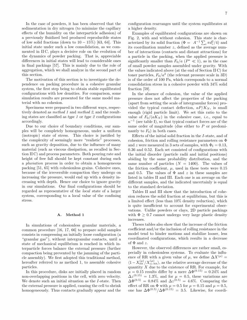
Examples of equilibrated configurations are shown onFig. 2, with and without cohesion. This state is char-acterized by its solid fraction (Φ = A−1

∑

i πd2i /4) and

its coordination number z, defined as the average num-ber of interactions (contacts and distant attractions) fora particle in the packing, when the applied pressure issignificantly smaller than F0/a (P ∗ ≪ 1), as in the caseof small powder samples assembled under gravity. Withthe values indicated above (at the end of Section II C) fortoner particles, F0/a2 (the relevant pressure scale in 3D)is of the order of 100 Pa, which corresponds to a normalconsolidation stress in a cohesive powder with 34% solidfraction [59].

In the absence of cohesion, the value of the appliedpressure does not affect the properties of the packing(apart from setting the scale of intergranular forces) pro-vided the typical contact deflection, aP/KN , is smallenough (rigid particle limit). We set this ratio to thevalue of F0/(aKN) in the cohesive case, i.e., equal toκ−1 (see table I), so that typical contact forces are of thesame order of magnitude (due either to P or predomi-nantly to F0) in both cases.

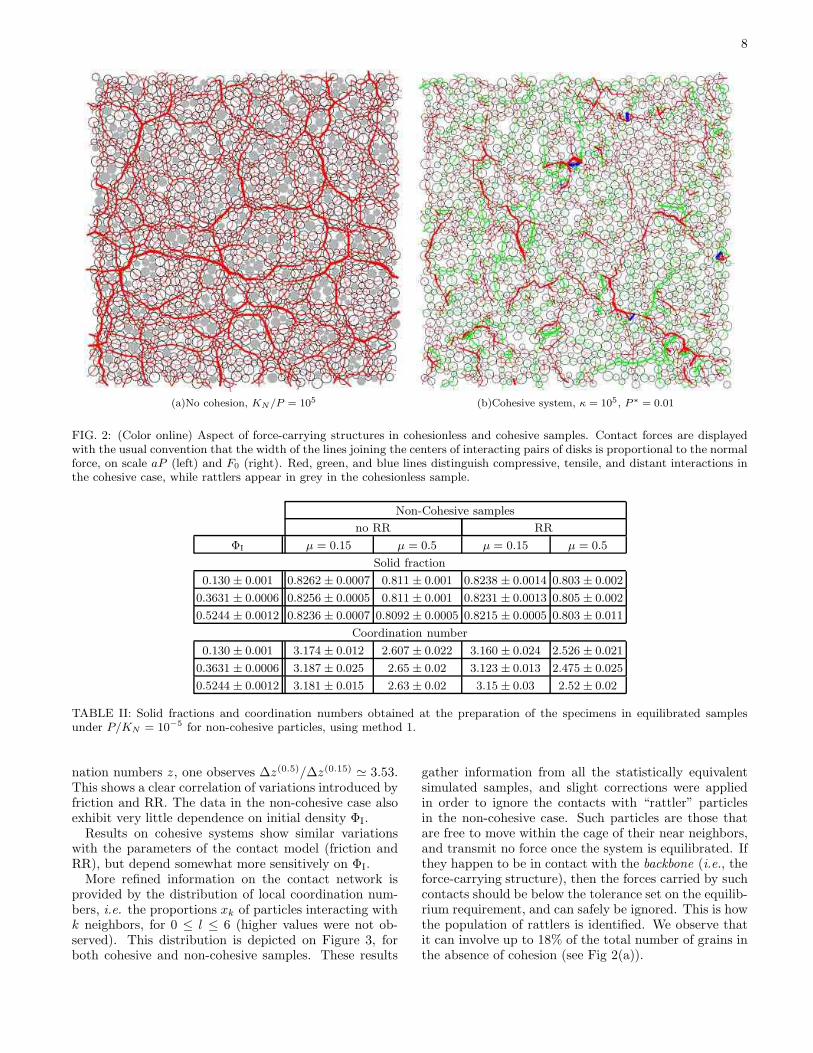
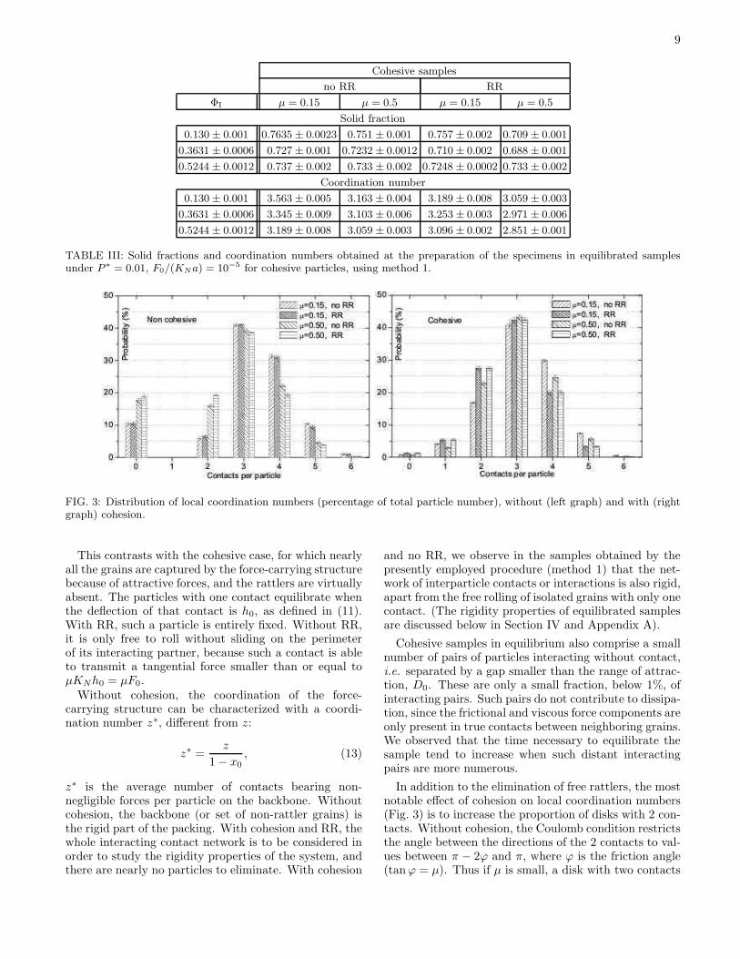
Effects of the initial solid fraction in the I-state, and ofcohesion, friction and rolling resistance parameters on Φand z were measured in 3 sets of samples, with ΦI = 0.13,0.36 and 0.52. Each set consisted of configurations withthe initial disorder (particle radii and initial positions)abiding by the same probability distribution, and thesame number of particles (N = 1400). The values ofthe friction coefficient, µ, used in these tests were 0.15and 0.5. The values of Φ and z in these samples arelisted in tables II and III. Each one is an average on thedifferent samples, and the indicated uncertainly is equalto the standard deviation.

Tables II and III show that the introduction of cohe-sion reduces the solid fraction at equilibrium, but this isa limited effect (less than 10% density reduction), whichis quite insufficient to account for experimental obser-vations. Unlike powders or clays, 2D particle packingswith Φ ≥ 0.7 cannot undergo very large plastic densityincreases.

Theses tables also show that the increase of the frictioncoefficient and/or the inclusion of rolling resistance in themodel tend to hinder motions and stabilize looser, lesscoordinated configurations, which results in a decreaseof Φ and z.

However, the observed differences are rather small, es-pecially in cohesionless systems. To evaluate the influ-ence of RR with a given value of µ, we define ∆X(µ) =

〈1−X(µ)RR /X

(µ)no RR〉, as the relative average decrease of the

quantity X due to the existence of RR. For example, forµ = 0.15 results differ by a mere ∆Φ(0.15) = 0.24% and∆z(0.15) = 1.3%, and for µ = 0.5, these variations are∆Φ(0.5) = 0.84% and ∆z(0.5) = 4.6%. Comparing theeffect of RR on Φ with µ = 0.5 for µ = 0.15 and µ = 0.5,one has ∆Φ(0.5)/∆Φ(0.15) = 3.5. Likewise, for coordi-

8

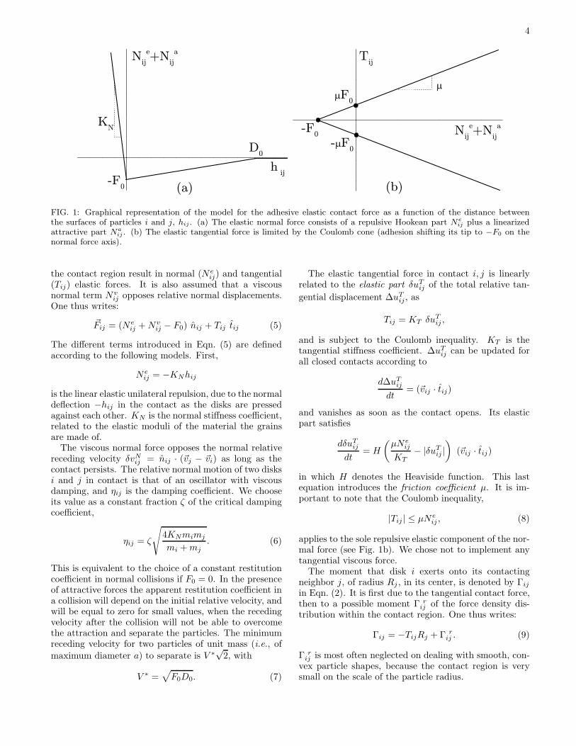
(a)No cohesion, KN/P = 105 (b)Cohesive system, κ = 105, P ∗ = 0.01

FIG. 2: (Color online) Aspect of force-carrying structures in cohesionless and cohesive samples. Contact forces are displayedwith the usual convention that the width of the lines joining the centers of interacting pairs of disks is proportional to the normalforce, on scale aP (left) and F0 (right). Red, green, and blue lines distinguish compressive, tensile, and distant interactions inthe cohesive case, while rattlers appear in grey in the cohesionless sample.

Non-Cohesive samples

no RR RR

ΦI µ = 0.15 µ = 0.5 µ = 0.15 µ = 0.5

Solid fraction

0.130 ± 0.001 0.8262 ± 0.0007 0.811 ± 0.001 0.8238 ± 0.0014 0.803 ± 0.002

0.3631 ± 0.0006 0.8256 ± 0.0005 0.811 ± 0.001 0.8231 ± 0.0013 0.805 ± 0.002

0.5244 ± 0.0012 0.8236 ± 0.0007 0.8092 ± 0.0005 0.8215 ± 0.0005 0.803 ± 0.011

Coordination number

0.130 ± 0.001 3.174 ± 0.012 2.607 ± 0.022 3.160 ± 0.024 2.526 ± 0.021

0.3631 ± 0.0006 3.187 ± 0.025 2.65 ± 0.02 3.123 ± 0.013 2.475 ± 0.025

0.5244 ± 0.0012 3.181 ± 0.015 2.63 ± 0.02 3.15 ± 0.03 2.52 ± 0.02

TABLE II: Solid fractions and coordination numbers obtained at the preparation of the specimens in equilibrated samplesunder P/KN = 10−5 for non-cohesive particles, using method 1.

nation numbers z, one observes ∆z(0.5)/∆z(0.15) ≃ 3.53.This shows a clear correlation of variations introduced byfriction and RR. The data in the non-cohesive case alsoexhibit very little dependence on initial density ΦI.

Results on cohesive systems show similar variationswith the parameters of the contact model (friction andRR), but depend somewhat more sensitively on ΦI.

More refined information on the contact network isprovided by the distribution of local coordination num-bers, i.e. the proportions xk of particles interacting withk neighbors, for 0 ≤ l ≤ 6 (higher values were not ob-served). This distribution is depicted on Figure 3, forboth cohesive and non-cohesive samples. These results

gather information from all the statistically equivalentsimulated samples, and slight corrections were appliedin order to ignore the contacts with “rattler” particlesin the non-cohesive case. Such particles are those thatare free to move within the cage of their near neighbors,and transmit no force once the system is equilibrated. Ifthey happen to be in contact with the backbone (i.e., theforce-carrying structure), then the forces carried by suchcontacts should be below the tolerance set on the equilib-rium requirement, and can safely be ignored. This is howthe population of rattlers is identified. We observe thatit can involve up to 18% of the total number of grains inthe absence of cohesion (see Fig 2(a)).

9

Cohesive samples

no RR RR

ΦI µ = 0.15 µ = 0.5 µ = 0.15 µ = 0.5

Solid fraction

0.130 ± 0.001 0.7635 ± 0.0023 0.751 ± 0.001 0.757 ± 0.002 0.709 ± 0.001

0.3631 ± 0.0006 0.727 ± 0.001 0.7232 ± 0.0012 0.710 ± 0.002 0.688 ± 0.001

0.5244 ± 0.0012 0.737 ± 0.002 0.733 ± 0.002 0.7248 ± 0.0002 0.733 ± 0.002

Coordination number

0.130 ± 0.001 3.563 ± 0.005 3.163 ± 0.004 3.189 ± 0.008 3.059 ± 0.003

0.3631 ± 0.0006 3.345 ± 0.009 3.103 ± 0.006 3.253 ± 0.003 2.971 ± 0.006

0.5244 ± 0.0012 3.189 ± 0.008 3.059 ± 0.003 3.096 ± 0.002 2.851 ± 0.001

TABLE III: Solid fractions and coordination numbers obtained at the preparation of the specimens in equilibrated samplesunder P ∗ = 0.01, F0/(KNa) = 10−5 for cohesive particles, using method 1.

FIG. 3: Distribution of local coordination numbers (percentage of total particle number), without (left graph) and with (rightgraph) cohesion.

This contrasts with the cohesive case, for which nearlyall the grains are captured by the force-carrying structurebecause of attractive forces, and the rattlers are virtuallyabsent. The particles with one contact equilibrate whenthe deflection of that contact is h0, as defined in (11).With RR, such a particle is entirely fixed. Without RR,it is only free to roll without sliding on the perimeterof its interacting partner, because such a contact is ableto transmit a tangential force smaller than or equal toµKNh0 = µF0.

Without cohesion, the coordination of the force-carrying structure can be characterized with a coordi-nation number z∗, different from z:

z∗ =z

1 − x0, (13)

z∗ is the average number of contacts bearing non-negligible forces per particle on the backbone. Withoutcohesion, the backbone (or set of non-rattler grains) isthe rigid part of the packing. With cohesion and RR, thewhole interacting contact network is to be considered inorder to study the rigidity properties of the system, andthere are nearly no particles to eliminate. With cohesion

and no RR, we observe in the samples obtained by thepresently employed procedure (method 1) that the net-work of interparticle contacts or interactions is also rigid,apart from the free rolling of isolated grains with only onecontact. (The rigidity properties of equilibrated samplesare discussed below in Section IV and Appendix A).

Cohesive samples in equilibrium also comprise a smallnumber of pairs of particles interacting without contact,i.e. separated by a gap smaller than the range of attrac-tion, D0. These are only a small fraction, below 1%, ofinteracting pairs. Such pairs do not contribute to dissipa-tion, since the frictional and viscous force components areonly present in true contacts between neighboring grains.We observed that the time necessary to equilibrate thesample tend to increase when such distant interactingpairs are more numerous.

In addition to the elimination of free rattlers, the mostnotable effect of cohesion on local coordination numbers(Fig. 3) is to increase the proportion of disks with 2 con-tacts. Without cohesion, the Coulomb condition restrictsthe angle between the directions of the 2 contacts to val-ues between π − 2ϕ and π, where ϕ is the friction angle(tanϕ = µ). Thus if µ is small, a disk with two contacts

10

should have its center close to the line of centers of its twopartners. The increase of the population of 2-coordinateddisks as µ is raised from 0.15 to 0.5 (see Fig. 3) in co-hesionless systems corresponds to a less severe geometricrestriction on contact angles. With cohesion, contactsmay transmit a tangential force reaching µF0 while thenormal force is equal to zero. Consequently, a disk mightbe in equilibrium with two contact points in arbitrarypositions on its perimeter. As there is no geometric con-straint on the angle between the two contact directions,2-coordinated disks are easier to stabilize, and their pro-portion raises from about 5% without cohesion to above15% with cohesion in the case µ = 0.15. A populationof disks with one contact (therefore carrying a vanishingnormal force, with deflection −h = h0) is also present.Those particles are fixed by a small rolling resistance,but are free to roll on their interacting neighbor withoutRR. Such a rolling motion is not damped in our model.Therefore, on waiting long enough, they should eventu-ally stop after a collision, in a stable position with 2 con-tacts. Such a collision is bound to happen because thecontact network is completely connected. However, westop our calculations when the kinetic energy is below aset tolerance (see Section II D), and we do not wait untilall freely rolling disks reach their final position. Hencethe remaining population of disks with one contact insamples without RR.

The final configuration, with this preparation method,depends somewhat on the rate of compaction in the as-sembling stage. The latter is related to the choice ofthe dynamical parameter M , the “mass” with which thechanges in cell dimensions are computed with Eqn. (3).The slight influence of the initial solid fraction, ΦI, alsorelates to such dynamical effects: a lower value of ΦI en-tails larger colliding velocities, which favors larger finalsolid fractions.

Although some of the aspects of the model (in par-ticular the homogeneous shrinking imposed through theperiodic cell dimensions in a dynamical regime) do notcorrespond to experimental conditions, configurations oftype 1 should be regarded as typical results of fast as-sembling processes, in which the particles are requestedto balance the external pressure before stable loose struc-tures can be built. When the toner particles mentionedat the end of Section II C are first fluidized, and thensettle under their own weight, a rough estimate of thesettling time, assuming particles are settling individuallyin air, and fall over distances of order 1 cm, is ∼ 1 s.Fig. 4, with the value T0 ∼ 10−5 s corresponding to suchparticles, shows that the duration of the “method 1” com-pression process is a few milliseconds. In practice, dueto the presence of the surrounding fluid, the packing ofa powder in a loose state by settling and compaction ofan initially fluidized state is therefore considerably slowerthan this numerical process.

In the next section, we consequently turn to the oppo-site limit, in which the external confining pressure is feltonly after large, tenuous contact networks are formed.

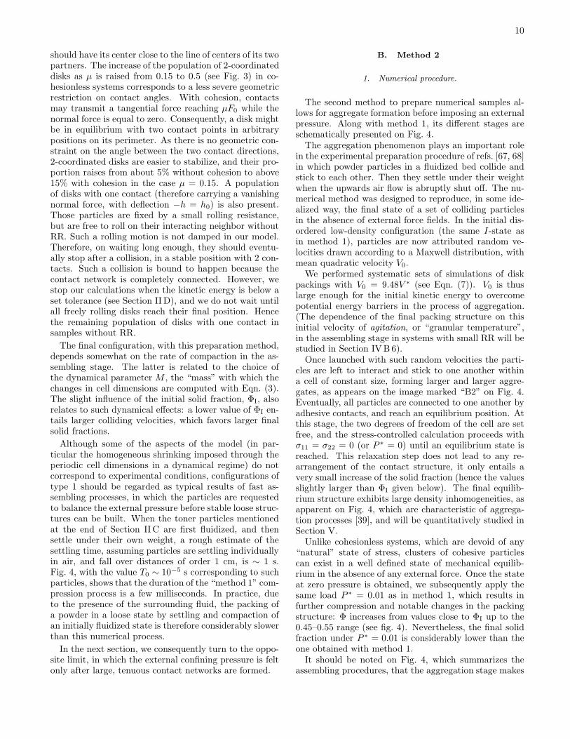
B. Method 2

1. Numerical procedure.

The second method to prepare numerical samples al-lows for aggregate formation before imposing an externalpressure. Along with method 1, its different stages areschematically presented on Fig. 4.

The aggregation phenomenon plays an important rolein the experimental preparation procedure of refs. [67, 68]in which powder particles in a fluidized bed collide andstick to each other. Then they settle under their weightwhen the upwards air flow is abruptly shut off. The nu-merical method was designed to reproduce, in some ide-alized way, the final state of a set of colliding particlesin the absence of external force fields. In the initial dis-ordered low-density configuration (the same I-state asin method 1), particles are now attributed random ve-locities drawn according to a Maxwell distribution, withmean quadratic velocity V0.

We performed systematic sets of simulations of diskpackings with V0 = 9.48V ∗ (see Eqn. (7)). V0 is thuslarge enough for the initial kinetic energy to overcomepotential energy barriers in the process of aggregation.(The dependence of the final packing structure on thisinitial velocity of agitation, or “granular temperature”,in the assembling stage in systems with small RR will bestudied in Section IVB 6).

Once launched with such random velocities the parti-cles are left to interact and stick to one another withina cell of constant size, forming larger and larger aggre-gates, as appears on the image marked “B2” on Fig. 4.Eventually, all particles are connected to one another byadhesive contacts, and reach an equilibrium position. Atthis stage, the two degrees of freedom of the cell are setfree, and the stress-controlled calculation proceeds withσ11 = σ22 = 0 (or P ∗ = 0) until an equilibrium state isreached. This relaxation step does not lead to any re-arrangement of the contact structure, it only entails avery small increase of the solid fraction (hence the valuesslightly larger than ΦI given below). The final equilib-rium structure exhibits large density inhomogeneities, asapparent on Fig. 4, which are characteristic of aggrega-tion processes [39], and will be quantitatively studied inSection V.

Unlike cohesionless systems, which are devoid of any“natural” state of stress, clusters of cohesive particlescan exist in a well defined state of mechanical equilib-rium in the absence of any external force. Once the stateat zero pressure is obtained, we subsequently apply thesame load P ∗ = 0.01 as in method 1, which results infurther compression and notable changes in the packingstructure: Φ increases from values close to ΦI up to the0.45–0.55 range (see fig. 4). Nevertheless, the final solidfraction under P ∗ = 0.01 is considerably lower than theone obtained with method 1.

It should be noted on Fig. 4, which summarizes theassembling procedures, that the aggregation stage makes

11

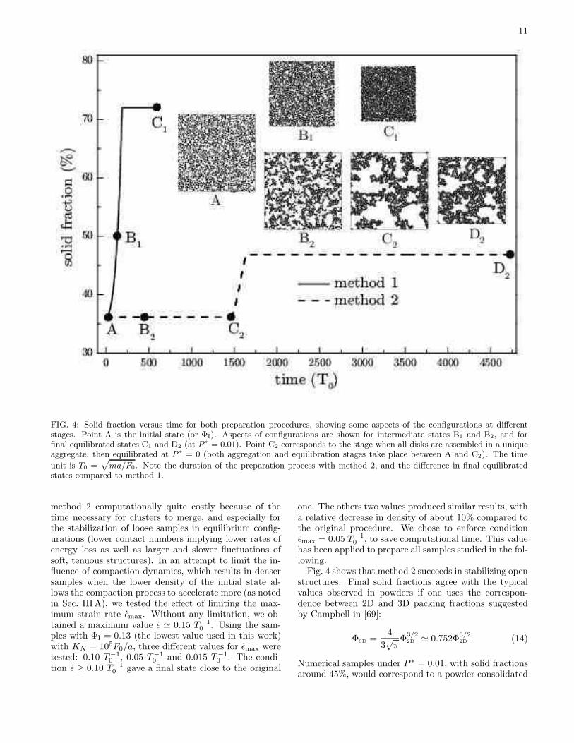
FIG. 4: Solid fraction versus time for both preparation procedures, showing some aspects of the configurations at differentstages. Point A is the initial state (or ΦI). Aspects of configurations are shown for intermediate states B1 and B2, and forfinal equilibrated states C1 and D2 (at P ∗ = 0.01). Point C2 corresponds to the stage when all disks are assembled in a uniqueaggregate, then equilibrated at P ∗ = 0 (both aggregation and equilibration stages take place between A and C2). The time

unit is T0 =p

ma/F0. Note the duration of the preparation process with method 2, and the difference in final equilibratedstates compared to method 1.

method 2 computationally quite costly because of thetime necessary for clusters to merge, and especially forthe stabilization of loose samples in equilibrium config-urations (lower contact numbers implying lower rates ofenergy loss as well as larger and slower fluctuations ofsoft, tenuous structures). In an attempt to limit the in-fluence of compaction dynamics, which results in densersamples when the lower density of the initial state al-lows the compaction process to accelerate more (as notedin Sec. III A), we tested the effect of limiting the max-imum strain rate ǫmax. Without any limitation, we ob-tained a maximum value ǫ ≃ 0.15 T−1

0 . Using the sam-ples with ΦI = 0.13 (the lowest value used in this work)with KN = 105F0/a, three different values for ǫmax weretested: 0.10 T−1

0 , 0.05 T−10 and 0.015 T−1

0 . The condi-tion ǫ ≥ 0.10 T−1

0 gave a final state close to the original

one. The others two values produced similar results, witha relative decrease in density of about 10% compared tothe original procedure. We chose to enforce conditionǫmax = 0.05 T−1

0 , to save computational time. This valuehas been applied to prepare all samples studied in the fol-lowing.

Fig. 4 shows that method 2 succeeds in stabilizing openstructures. Final solid fractions agree with the typicalvalues observed in powders if one uses the correspon-dence between 2D and 3D packing fractions suggestedby Campbell in [69]:

Φ3D =4

3√

πΦ

3/22D ≃ 0.752Φ

3/22D . (14)

Numerical samples under P ∗ = 0.01, with solid fractionsaround 45%, would correspond to a powder consolidated

12

in the laboratory under 1 Pa with a solid fraction of about23%. This is in satisfactory agreement with the experi-mental results of Ref. [59].

We therefore regard method 2 as an appropriate wayto reach an essential objective of this work, since stableloose structures are obtained.

Although we perform simulations of a mechanical

model, the final configurations exhibit at first sight(Fig. 4) similar features as those obtained with geomet-

ric algorithms implemented in numerical studies of col-loid aggregation models [28, 40]. We are not aware ofsimilar results in the literature, at least with equilibriumrequirements comparable to those of Sec. II D.

Tenuous, fractal-like contact networks contain denserregions and large cavities. Such heterogeneities producelong range density correlations, to be analyzed in Sec. V.Without tensile contact forces, the walls of the cavities,comprising particles that are pushed towards the holeby the resultant of contact normal forces, would tend tobuckle in.

We regard method 2 as yielding typical results for as-

sembling processes in which particles form tenuous aggre-

gates before they are packed in a structure that is able to

sustain a confining stress. In the sequel, we focus on thetenuous structures obtained with method 2.

2. Global characterization of loose packings at P ∗ = 0 andP ∗ = 0.01.

We simulated four samples with 1400 disks and threeof 5600 for ΦI = 0.36, rather than lower initial densities,in order to achieve statistical significance at affordablecomputational costs, and to check for possible size effects.This set of samples will be denoted as series A.

Samples with Φ = 0.13 (series A0), which require theinitial cell to shrink more before a stable network canresist the pressure, request longer calculations. Althoughsome samples were prepared at P ∗ = 0, we do not usethem any more in the following, except for the valuesshowed in Table IV.

To accelerate the numerical assembling procedure, wealso created samples with KN = 104F0/a, using an in-termediate value of ΦI = 0.26, and softer contacts, suchthat κ = 102 in the initial aggregation stage (recall thetime step is proportional to A/

√KN ). Once equilibrium

was reached with P ∗ = 0, we slowly changed the stiff-ness parameter from κ = 102 to κ = 104, and recordedthe final equilibrated configuration. This procedure isabout ten times as fast as the normal one, and generatessimilar structures and coordination numbers as series Aprepared with the same I-state density. We shall refer tothis set as series B.

In table IV we list the corresponding results for solidfractions and coordination numbers. In such data we didnot find a significant difference between the two differ-ent sample sizes, and therefore we did not distinguishbetween sizes in the presentation of statistical results.

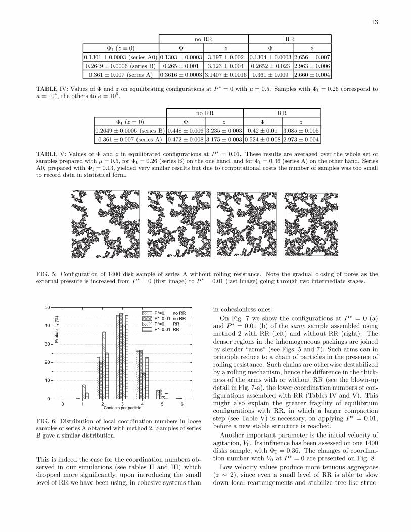
The tenuous networks obtained with method 2 collapseon changing the pressure: Table V gives the new valuesof Φ and z after the compaction caused by the pressureincrease from P ∗ = 0 to P ∗ = 0.01.

Structural changes between P ∗ = 0 and P ∗ = 0.01 areshown on Fig. 5, which illustrates by means of four se-lected snapshots the mechanism of the closing of poresin a 1400 disks sample of series A. The first image cor-responds to equilibrium at P ∗ = 0, and the fourth oneto equilibrium under P ∗ = 0.01. The two others showintermediate, out of equilibrium configurations duringthe collapse. One may appreciate how the denser re-gions grow and merge while pores shrink. Fig. 5 alsomakes it quite evident that the size of 1400 disk sam-ples is not very much larger than the scale ξ of densityheterogeneities (typical diameter of large pores or denseregions, which will be studied in Sec. V). These sys-tems will exhibit large fluctuations in their mechanicalproperties: the rectangular shape of the final configura-tion displayed on Fig. 5 shows that the disorder is largeenough for the mechanical response of the system to be-come anisotropic. Isotropy should be recovered in thelimit of large sample sizes, L ≫ ξ.

Finally, Fig. 6 displays the histogram of local coordi-nation numbers (percentage of particles interacting withk others, 0 ≤ k ≤ 6), for the same samples as those ofTables IV and V (µ = 0.5, ΦI = 0.36). It is remark-able that this distribution, in spite of the large differ-ence in sample geometries, remains rather close to theone observed in the denser packings made with method1 (compare P ∗ = 0.01, µ = 0.5 case), just like global co-ordination numbers take very similar values in samplesprepared with both methods (see Tables III and V), inspite of the very different solid fractions.

An essential conclusion of the present study is there-fore, for one given material, the absence of a general rela-

tion between the density of a cohesive packing and its co-

ordination number, in spite of previous claims [26]. Bothquantities are determined, rather, by the conjunction ofmicromechanical laws and sample preparation history.

3. Effects of micromechanical parameters

Adhesion should enhance the role of sliding friction androlling friction, because the limiting values for tangentialcontact forces and rolling moments are both proportionalto the elastic repulsive part of the normal force, Ne (

|Tij | < µNeij , |~Γ r

ij | < µrNeij). Consequently, contacts

with the equilibrium value h0 of the elastic deflection foran isolated pair of grains transmit no normal force, butare able to sustain tangential force components as largeas µF0 and rolling moments as large as µrF0. Thosevalues might turn out to be large in comparison to thetypical level of intergranular forces under low externalpressure (P ∗ ≪ 1). Therefore, even very low values ofµ and µr should affect the final structure of equilibratedpackings considerably more than in the cohesionless case.

13

no RR RR

ΦI (z = 0) Φ z Φ z

0.1301 ± 0.0003 (series A0) 0.1303 ± 0.0003 3.197 ± 0.002 0.1304 ± 0.0003 2.656 ± 0.007

0.2649 ± 0.0006 (series B) 0.265 ± 0.001 3.123 ± 0.004 0.2652 ± 0.023 2.963 ± 0.006

0.361 ± 0.007 (series A) 0.3616 ± 0.0003 3.1407 ± 0.0016 0.361 ± 0.009 2.660 ± 0.004

TABLE IV: Values of Φ and z on equilibrating configurations at P ∗ = 0 with µ = 0.5. Samples with ΦI = 0.26 correspond toκ = 104, the others to κ = 105.

no RR RR

ΦI (z = 0) Φ z Φ z

0.2649 ± 0.0006 (series B) 0.448 ± 0.006 3.235 ± 0.003 0.42 ± 0.01 3.085 ± 0.005

0.361 ± 0.007 (series A) 0.472 ± 0.008 3.175 ± 0.003 0.524 ± 0.008 2.973 ± 0.004

TABLE V: Values of Φ and z in equilibrated configurations at P ∗ = 0.01. These results are averaged over the whole set ofsamples prepared with µ = 0.5, for ΦI = 0.26 (series B) on the one hand, and for ΦI = 0.36 (series A) on the other hand. SeriesA0, prepared with ΦI = 0.13, yielded very similar results but due to computational costs the number of samples was too smallto record data in statistical form.

FIG. 5: Configuration of 1400 disk sample of series A without rolling resistance. Note the gradual closing of pores as theexternal pressure is increased from P ∗ = 0 (first image) to P ∗ = 0.01 (last image) going through two intermediate stages.

0 1 2 3 4 5 60

10

20

30

40

50

Pro

babi

lity

(%)

Contacts per particle

P*=0. no RR P*=0.01 no RR P*=0. RR P*=0.01 RR

FIG. 6: Distribution of local coordination numbers in loosesamples of series A obtained with method 2. Samples of seriesB gave a similar distribution.

This is indeed the case for the coordination numbers ob-served in our simulations (see tables II and III) whichdropped more significantly, upon introducing the smalllevel of RR we have been using, in cohesive systems than

in cohesionless ones.

On Fig. 7 we show the configurations at P ∗ = 0 (a)and P ∗ = 0.01 (b) of the same sample assembled usingmethod 2 with RR (left) and without RR (right). Thedenser regions in the inhomogeneous packings are joinedby slender “arms” (see Figs. 5 and 7). Such arms can inprinciple reduce to a chain of particles in the presence ofrolling resistance. Such chains are otherwise destabilizedby a rolling mechanism, hence the difference in the thick-ness of the arms with or without RR (see the blown-updetail in Fig. 7-a), the lower coordination numbers of con-figurations assembled with RR (Tables IV and V). Thismight also explain the greater fragility of equilibriumconfigurations with RR, in which a larger compactionstep (see Table V) is necessary, on applying P ∗ = 0.01,before a new stable structure is reached.

Another important parameter is the initial velocity ofagitation, V0. Its influence has been assessed on one 1400disks sample, with ΦI = 0.36. The changes of coordina-tion number with V0 at P ∗ = 0 are presented on Fig. 8.

Low velocity values produce more tenuous aggregates(z ∼ 2), since even a small level of RR is able to slowdown local rearrangements and stabilize tree-like struc-

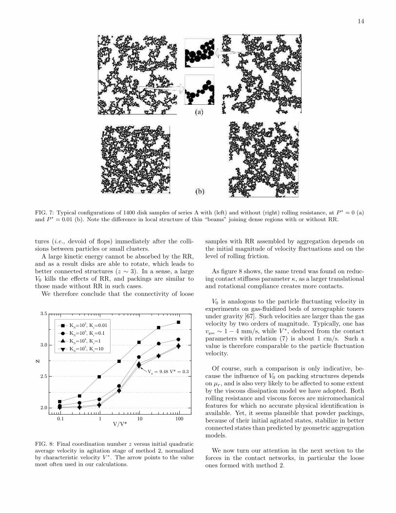
14

FIG. 7: Typical configurations of 1400 disk samples of series A with (left) and without (right) rolling resistance, at P ∗ = 0 (a)and P ∗ = 0.01 (b). Note the difference in local structure of thin “beams” joining dense regions with or without RR.

tures (i.e., devoid of flops) immediately after the colli-sions between particles or small clusters.

A large kinetic energy cannot be absorbed by the RR,and as a result disks are able to rotate, which leads tobetter connected structures (z ∼ 3). In a sense, a largeV0 kills the effects of RR, and packings are similar tothose made without RR in such cases.

We therefore conclude that the connectivity of loose

0.1 1 10 100

2.0

2.5

3.0

3.5

z

V/V*

KN=102, K

r=0.01

KN=103, K

r=0.1

KN=104, K

r=1

KN=105, K

r=10

V0 = 9.48 V* = 0.3

FIG. 8: Final coordination number z versus initial quadraticaverage velocity in agitation stage of method 2, normalizedby characteristic velocity V ∗. The arrow points to the valuemost often used in our calculations.

samples with RR assembled by aggregation depends onthe initial magnitude of velocity fluctuations and on thelevel of rolling friction.

As figure 8 shows, the same trend was found on reduc-ing contact stiffness parameter κ, as a larger translationaland rotational compliance creates more contacts.

V0 is analogous to the particle fluctuating velocity inexperiments on gas-fluidized beds of xerographic tonersunder gravity [67]. Such velocities are larger than the gasvelocity by two orders of magnitude. Typically, one hasvgas ∼ 1 − 4 mm/s, while V ∗, deduced from the contactparameters with relation (7) is about 1 cm/s. Such avalue is therefore comparable to the particle fluctuationvelocity.

Of course, such a comparison is only indicative, be-cause the influence of V0 on packing structures dependson µr, and is also very likely to be affected to some extentby the viscous dissipation model we have adopted. Bothrolling resistance and viscous forces are micromechanicalfeatures for which no accurate physical identification isavailable. Yet, it seems plausible that powder packings,because of their initial agitated states, stabilize in betterconnected states than predicted by geometric aggregationmodels.

We now turn our attention in the next section to theforces in the contact networks, in particular the looseones formed with method 2.

15

IV. MECHANICAL CHARACTERIZATION OF

CONTACT NETWORKS

Many numerical studies, in the past 15 years, haveaddressed the issue of contact network geometry andforce distribution in cohesionless systems [70]. The im-age of force chains, i.e. a pattern in which larger inter-granular forces tend to line up on the scale of severalgrains, was evidenced in experiments [71, 72] and sim-ulations [73, 74], and the p.d.f of contact force valueshas often been measured and studied. An interpretationof the mechanical role of “force chains” [75] is that theycarry the essential part of deviatoric stress, while the con-tacts carrying the lower forces are less sensitive to stressorientation and laterally stabilize the strong force chainsagainst buckling.

The main features of the distribution of forces andtheir spatial correlations have been reproduced by ap-proximate models [76] based on local equilibrium ruleson each grain, supplemented by inequality constraints.One important such constraint is released in cohesive sys-tems, in which normal force components can have eithersign. It is therefore worth investigating how the usualfeatures of force-carrying structures in equilibrated gran-ular packings are affected by the presence of negativenormal forces. One may also wonder to what extent theconsiderable difference in the density fields will affect theforce patterns, given that the coordination of the forcenetworks, as observed previously, does not seem to bevery sensitive to density levels and density fluctuations.

A. Force scale and force distribution

The first obvious distinction between cohesive and non-cohesive systems is the appearance of a new force scaleF0, in addition to the one provided by the confiningpressure, i.e., aP , the ratio of those characteristic forcesdefining the reduced pressure, P ∗. It is especially inter-esting to investigate the values and spatial organizationof forces in systems with P ∗ ≪ 1, as little informationis to be found in the literature on this issue: numeri-cal studies of loose cohesive systems [29] tend to focus ondensity and geometry of packings as a function of appliedstresses. Some information on force networks is providedin a recent publication [11] on bead assemblies with cap-illary cohesion, but the confining stress is considerablyhigher is that study (P ∗ of order 1) than in the presentone.

In the absence of cohesion, the distribution of force val-ues is usually presented in a form normalized by its av-erage, which itself scales with the applied pressure. Thisscaling can be made more quantitative on using a gen-eral relation between pressure P and the average normal

contact force FNdef= 〈Nij〉 and particle diameter d, which

is known in the literature on powders as the Rumpf for-mula. We write it here in a form involving the spatial

dimension D, which is valid both for D = 2 and D = 3:

P =1

π

zΦ

dD−1FN . (15)

In (15), d stands for the typical grain diameter. This rela-tion can be made more accurate if one notes that it stemsfrom the standard formula for stresses in an equilibriumconfiguration (see the r.h.s. term in Eqn. 3). To de-

rive the formula, defining P = 1D

∑Dα=1 σαα, the average

pressure, one assumes hij ≪ Ri + Rj and then neglectscorrelations between particle radii and forces, assuming

〈Nij(Ri + Rj)〉 ≃ FN 〈d〉. (16)

Then, with a simple transformation of the sum, one ob-tains

P =1

π

〈d〉〈dD〉zΦFN . (17)

With D = 2 and our diameter distribution (for which〈d〉 = 3a/4 and 〈d2〉 = 7a2/12) this yields

FN =7πa

9

P

zΦ. (18)

We found relation (18) to be remarkably accurate in allour simulations, with or without cohesion, with configu-rations obtained by either method 1 or method 2, therebychecking that the correlations between particle sizes andcontact forces could safely be neglected on writing (16).

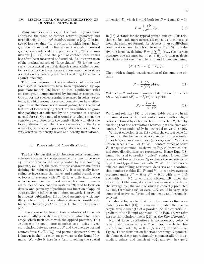
Without cohesion, Eqn. (18) yields the correct scale forforces, i.e. the frequency of occurrence of intergranularforces larger than a few times FN is very small. With co-hesion, when P ∗ = 0 or P ∗ ≪ 1, contact forces of orderF0 are quite common, as shown on Fig. 9, on which nor-mal force distributions are represented. Hence Eqn. (18)cannot be used to predict “typical” contact forces. Thepresence of forces of order F0 explains the sensitivity oftype 1 and type 2 samples with P ∗ ≪ 1 to friction co-efficient and rolling resistance: densities and coordina-tion numbers (tables III, IV and V), in cohesive systemsprepared under P ∗ = 0 or P ∗ = 0.01 with µ = 0.15and with µ = 0.5, or with and without RR, differ sig-nificantly. Otherwise, if contact forces were of order ofthe average FN , the value of which is correctly predictedby (18), thresholds µF0 or even µrF0 would be very largecompared to typical forces and moments, and become ir-relevant.

(It should be recalled that Rumpf’s name is often asso-ciated (as in Ref. [11]) to a means to predict the macro-scopic tensile strength of a powder. As the essential in-gredient of the Rumpf approach [77] is Eqn. 15, we referhere to that relation (like in [24]), as the Rumpf formula).

Normal force distributions in cohesionless, cohesivetype 1 and cohesive type 2 samples, the latter be-ing obtained with ΦI = 0.36 (series A), are shown onFig. 9. Those distribution functions are roughly symmet-ric about 0, decay approximately exponentially at inter-mediate values, and vanish at −F0, and F0. In type 2

16

0 1 2 3 4 5

10-3

10-2

10-1

100

P(N

) no RR =0.15 no RR =0.50 RR =0.15 RR =0.50

N/ N

(a)No cohesion, KN/P = 105

-1.0 -0.5 0.0 0.5 1.010-3

10-2

10-1

100

101

no RR =0.15 no RR =0.50 RR =0.15 RR =0.50

P(N

)

N/F0

(b)With cohesion, method 1, P ∗ = 0.01, µ = 0.15 andµ = 0.5

-1.0 -0.5 0.0 0.5 1.010-3

10-2

10-1

100

101

no RR P*=0 no RR P*=0.01 RR P*=0 RR P*=0.01

P(N

)

N/F0

(c)With cohesion, method 2, P ∗ = 0 and P ∗ = 0.01, µ = 0.5

FIG. 9: Distribution of normal forces for series A samples.The non-cohesive case (9(a)) is normalized by the averagerepulsive elastic part. The cohesive cases (9(b) and 9(c)) arenormalized by F0 (note that the average of the elastic part ofN is 〈Ne〉 ≃ F0 in cohesive cases with P ∗ ≪ 1).

samples without RR, for P ∗ = 0, there is a finite pro-portion of contacts carrying vanishing forces, about onefourth in the A series (Φ = 0.36). In addition to thisDirac mass, there might be a power-law divergence near0, with an exponent our level of statistics is not sufficientto resolve accurately (about 0.6 to 0.8 in the range offorces between 10−3F0 and 10−2F0). This proportion ofzero forces is smaller, down to 9%, with RR, and drops asP ∗ reaches 0.01, to 7% and 3%, respectively, without andwith RR. It is worth pointing out that the correspond-ing contacts carry zero total forces, i.e. vanishing normalcomponents (−h = h0, see (11)) and no tangential elasticdisplacement either. In principle we cannot distinguishthem from forces below the numerical tolerance definedin Sec. II D. However, as we shall argue below in Sec-tion IVB, under P ∗ = 0 one could expect all contactforces to vanish, and non-zero forces are related to thesmall, but finite degree of force indeterminacy.

Before turning our attention to such features and tothe spatial organization of forces, let us briefly discussthe differences between sets of (type 2) samples A andB. B samples, which are obtained with the “accelerated”procedure and ΦI = 0.26 (see Sec. III), exhibit, due totheir specific history, larger forces at P ∗ = 0, with asmany as 10% of the contacts transmitting normal forcesN such that |N | > F0/10, while this proportion lies below2% in A samples. On the other hand, B samples arelooser, with more open contact networks under P = 0and a larger proportion of contacts (about one third inconfigurations without RR) carrying vanishing forces. Inthe following we shall use them to illustrate qualitativetendencies in very loose samples.

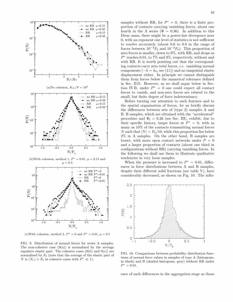
When the pressure is increased to P ∗ = 0.01, differ-ences in force distributions between A and B samples,despite their different solid fractions (see table V), haveconsiderably decreased, as shown on Fig. 10. The influ-

FIG. 10: Comparisons between probability distribution func-tions of normal force values in samples of type A (histogram,in black) and B (shaded histogram, grey) without RR underP ∗ = 0.01.

ence of such differences in the aggregation stage as those

17

between our samples A and B are therefore expected tofade out after the systems are compressed to higher pres-sures and densities.

B. Packing structure and force patterns

The spatial organization of forces in type 2 samples,which we now discuss, is related to the distribution offorce values, and should determine the ability of givenconfigurations and contact networks to support stress in-crements. We first discuss systems without RR, thenwith the small RR values we adopted in most cases (seeTable I). We emphasize the role of force indeterminacy

and assembling history (the collisions by which cohesiveclusters were built) in the final force patterns in equi-librium under vanishing or low applied stress. Extremecases of systems with large RR on the one hand, or with-out friction on the other hand, are useful reference situ-ations, which we briefly examine and discuss. We con-clude this part with a discussion of the main physicalimplications of the relationships between force patterns,assembling process, geometry and micromechanical pa-rameters

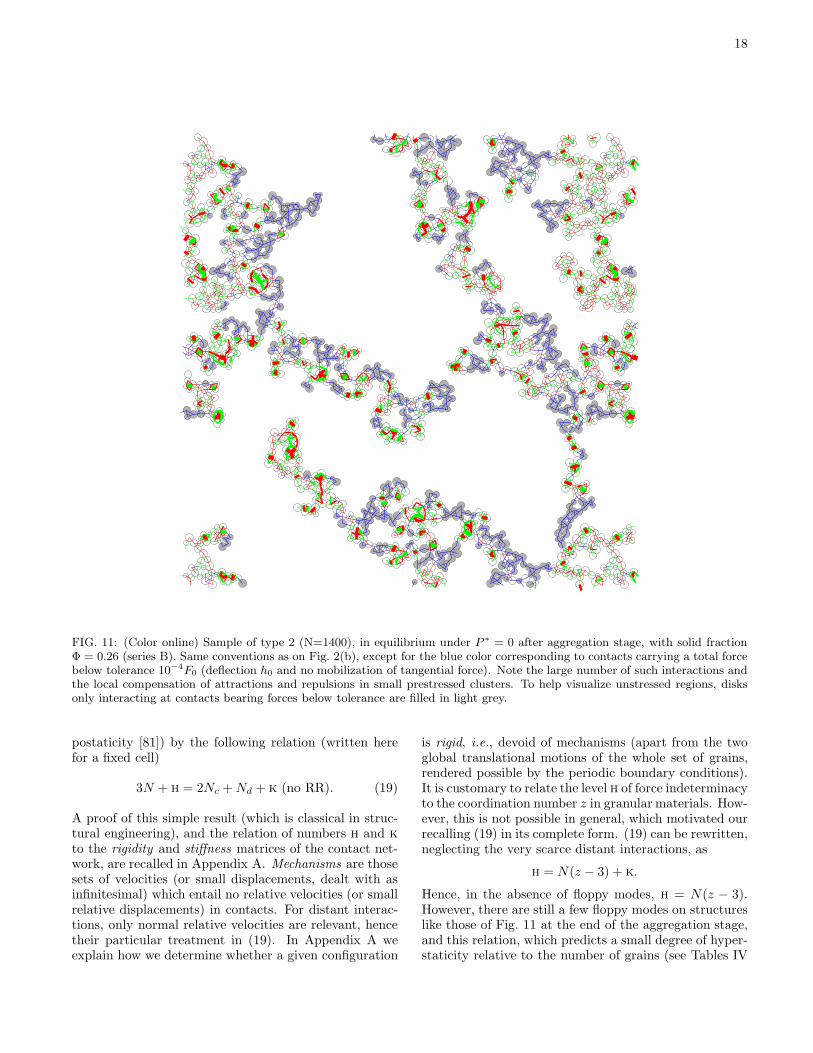
1. Qualitative aspects of force networks with no RR

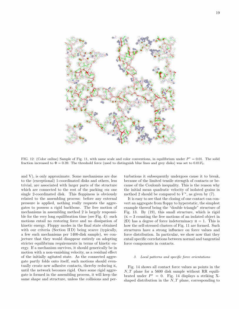
It is instructive to represent the forces carried by thecontact network with a visualization of positive (repul-sive) and negative (attractive) normal forces, as wasdone on Fig. 2(b), showing the force network in onetype 1 sample. Figs 11 and 12 respectively correspondto equilibrated samples prepared with method 2 underP ∗ = 0 (immediately after the aggregation stage) andunder P ∗ = 0.01, without RR. They are represented herewith (approximately) the same scale. Both belong to the(ΦI = 0.26) B series. Line widths, which are propor-tional to the intensity of the total interaction force, i.e.

to ||F|| =∣

∣

∣

∣Nn + T t∣

∣

∣

∣, witness the presence, in spite ofthe low pressure, of many forces of order F0 (which cor-respond on the figures to line thicknesses comparable toparticle radii). Stressed clusters, in loose type 2 samplesunder P ∗ = 0, are separated by large parts of the inter-acting network in which contacts carry vanishing forces:the corresponding normal deflection is h0 (Eqn. (11)) andthere has been no elastic relative tangential displacement.Attractions (green) and compressions (red) have to com-pensate for Eqn. (18) to hold true. This compensationappears to operate on a smaller scale in type 2 samples,because internal forces were previously balanced withinisolated particle clusters. Such a local balance of forces isquite conspicuous at P ∗ = 0 (Fig. 11), in which internalstresses in small clusters often take the form of a periph-eral tension compensating a radial compression, or theother way round. This contrasts with samples preparedwith method 1 (Fig. 2(b)), in which the spatial distribu-tion of forces is more similar to the familiar “force chain”

pattern of cohesionless systems, although there are ofcourse compressive and tensile “chains”. Unstressed re-gions are rather scarce in type 1 samples, although someareas with smaller forces are still present. The structureof type 2 samples under P ∗ = 0.01 (Fig. 12) is somewhatintermediate: isolated stressed clusters are still present,but elongated, force-chain-like structures emerge.

To characterize such force patterns in a slightly morequantitative way, one can evaluate a threshold force Fperc

such that contacts carrying a force F with ||F|| ≥ Fperc

percolate through the sample. Such a criterion was usedto identify a “strong” subnetwork of force chains in [75].One observes Fperc of the order of the tolerance 10−4F0

in ΦI = 0.26 samples with no RR and P ∗ = 0, whichshows that stressed regions are isolated “islands” withinthe network. Fperc raises to slightly less than 0.1F0 underP ∗ = 0.01.

Configurations of series A, assembled with Φ = 0.36,possess the same qualitative features, although quantita-tively slightly weaker, due to their higher density. Forinstance, local stressed regions are somewhat less iso-lated, with a threshold force Fperc between 10−3F0 and8 × 10−3F0 at P ∗ = 0.

2. Force indeterminacy (without RR)

The presence of large interaction forces of order F0 inequilibrated samples is not obviously necessary, and is re-lated to the assembling process. Let us imagine particlesare brought very slowly, one by one, within interactionrange of the previous network, thus gradually building aunique cluster in equilibrium in the absence of externalstress. One could expect, rather, each new contact tostabilize with N = T = 0 and h = −h0. The existenceof non-zero interaction forces in equilibrium is related tothe hyperstaticity or force indeterminacy of the contactnetwork. On writing all equilibrium equations for grainsand collective degrees of freedom (i.e., setting accelera-tion terms to zero in Eqns. 1, 2 and 3) and regarding allcontact forces as unknowns, the degree of force indetermi-nacy h (or degree of hyperstaticity) is the number of re-maining independent unknowns, which cannot be deter-mined by the equilibrium requirement. If h = 0, knowingthat some equilibrium forces exist (since an equilibriumstate has been found), then one would necessarily have allinteraction forces equal to zero under P ∗ = 0 (since thisis one obvious possible solution). The notion of forceindeterminacy has been recently discussed by differentgroups in the context of granular materials, essentiallybecause of the special case of rigid frictionless grains, forwhich the contact network is generically such that forcesare uniquely determined [73, 78, 79, 80, 81]. The degreeof force indeterminacy is linked to the number of degreesof freedom, equal to 3N (or 3N + 2 if the cell sizes canchange), to the number of contacts Nc, the number ofdistant interactions Nd and the number of independentmechanisms or floppy modes k (also called degree of hy-

18

FIG. 11: (Color online) Sample of type 2 (N=1400), in equilibrium under P ∗ = 0 after aggregation stage, with solid fractionΦ = 0.26 (series B). Same conventions as on Fig. 2(b), except for the blue color corresponding to contacts carrying a total forcebelow tolerance 10−4F0 (deflection h0 and no mobilization of tangential force). Note the large number of such interactions andthe local compensation of attractions and repulsions in small prestressed clusters. To help visualize unstressed regions, disksonly interacting at contacts bearing forces below tolerance are filled in light grey.

postaticity [81]) by the following relation (written herefor a fixed cell)

3N + h = 2Nc + Nd + k (no RR). (19)

A proof of this simple result (which is classical in struc-tural engineering), and the relation of numbers h and k

to the rigidity and stiffness matrices of the contact net-work, are recalled in Appendix A. Mechanisms are thosesets of velocities (or small displacements, dealt with asinfinitesimal) which entail no relative velocities (or smallrelative displacements) in contacts. For distant interac-tions, only normal relative velocities are relevant, hencetheir particular treatment in (19). In Appendix A weexplain how we determine whether a given configuration

is rigid, i.e., devoid of mechanisms (apart from the twoglobal translational motions of the whole set of grains,rendered possible by the periodic boundary conditions).It is customary to relate the level h of force indeterminacyto the coordination number z in granular materials. How-ever, this is not possible in general, which motivated ourrecalling (19) in its complete form. (19) can be rewritten,neglecting the very scarce distant interactions, as

h = N(z − 3) + k.

Hence, in the absence of floppy modes, h = N(z − 3).However, there are still a few floppy modes on structureslike those of Fig. 11 at the end of the aggregation stage,and this relation, which predicts a small degree of hyper-staticity relative to the number of grains (see Tables IV

19

FIG. 12: (Color online) Sample of Fig. 11, with same scale and color conventions, in equilibrium under P ∗ = 0.01. The solidfraction increased to Φ = 0.39. The threshold force (used to distinguish blue lines and grey disks) was set to 0.01F0 .

and V), is only approximate. Some mechanisms are dueto the (exceptional) 1-coordinated disks and others, lesstrivial, are associated with larger parts of the structurewhich are connected to the rest of the packing via onesingle 2-coordinated disk. This floppiness is obviouslyrelated to the assembling process: before any externalpressure is applied, nothing really requests the aggre-gates to possess a rigid backbone. The free motion ofmechanisms in assembling method 2 is largely responsi-ble for the very long equilibration time (see Fig. 4): suchmotions entail no restoring force and no dissipation ofkinetic energy. Floppy modes in the final state obtainedwith our criteria (Section II D) being scarce (typically,a few such mechanisms per 1400-disk sample), we con-jecture that they would disappear entirely on adoptingstricter equilibrium requirements in terms of kinetic en-ergy. If a mechanism survives, it should generically be inmotion with a non-vanishing velocity, as a residual effectof the initially agitated state. As the connected aggre-gate partly folds onto itself, such motions should even-tually create new adhesive contacts, thereby reducing k,until the network becomes rigid. Once some rigid aggre-gate is formed in the assembling process, it will keep thesame shape and structure, unless the collisions and per-

turbations it subsequently undergoes cause it to break,because of the limited tensile strength of contacts or be-cause of the Coulomb inequality. This is the reason whythe initial mean quadratic velocity of isolated grains inmethod 2 should be compared to V ∗, as given by (7).

It is easy to see that the closing of one contact can con-vert an aggregate from floppy to hyperstatic, the simplestexample thereof being the “double triangle” structure ofFig. 13. By (19), this small structure, which is rigid(k = 3 counting the free motions of an isolated object in2D) has a degree of force indeterminacy h = 1. This ishow the self-stressed clusters of Fig. 11 are formed. Suchstructures have a strong influence on force values andforce distribution. In particular, we show now that theyentail specific correlations between normal and tangentialforce components in contacts.

3. Local patterns and specific force orientations

Fig. 14 shows all contact force values as points in theN, T plane for a 5600 disk sample without RR equili-brated under P ∗ = 0. Fig. 14 displays a striking X-shaped distribution in the N, T plane, corresponding to

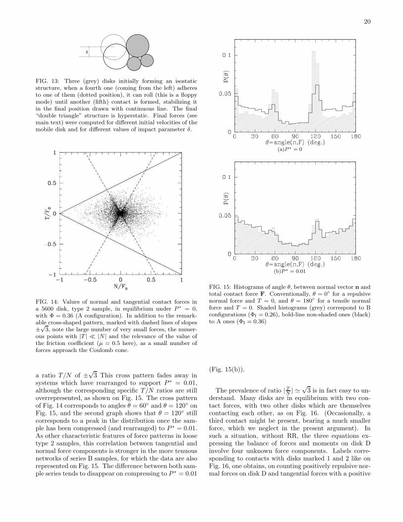
20

δ

FIG. 13: Three (grey) disks initially forming an isostaticstructure, when a fourth one (coming from the left) adheresto one of them (dotted position), it can roll (this is a floppymode) until another (fifth) contact is formed, stabilizing itin the final position drawn with continuous line. The final“double triangle” structure is hyperstatic. Final forces (seemain text) were computed for different initial velocities of themobile disk and for different values of impact parameter δ.

FIG. 14: Values of normal and tangential contact forces ina 5600 disk, type 2 sample, in equilibrium under P ∗ = 0,with Φ = 0.36 (A configuration). In addition to the remark-able cross-shaped pattern, marked with dashed lines of slopes±√

3, note the large number of very small forces, the numer-ous points with |T | ≪ |N | and the relevance of the value ofthe friction coefficient (µ = 0.5 here), as a small number offorces approach the Coulomb cone.

a ratio T/N of ±√

3 This cross pattern fades away insystems which have rearranged to support P ∗ = 0.01,although the corresponding specific T/N ratios are stilloverrepresented, as shown on Fig. 15. The cross patternof Fig. 14 corresponds to angles θ = 60◦ and θ = 120◦ onFig. 15, and the second graph shows that θ = 120◦ stillcorresponds to a peak in the distribution once the sam-ple has been compressed (and rearranged) to P ∗ = 0.01.As other characteristic features of force patterns in loosetype 2 samples, this correlation between tangential andnormal force components is stronger in the more tenuousnetworks of series B samples, for which the data are alsorepresented on Fig. 15. The difference between both sam-ple series tends to disappear on compressing to P ∗ = 0.01

(a)P ∗ = 0

(b)P ∗ = 0.01

FIG. 15: Histograms of angle θ, between normal vector n andtotal contact force F. Conventionally, θ = 0◦ for a repulsivenormal force and T = 0, and θ = 180◦ for a tensile normalforce and T = 0. Shaded histograms (grey) correspond to Bconfigurations (ΦI = 0.26), bold-line non-shaded ones (black)to A ones (ΦI = 0.36)

(Fig. 15(b)).

The prevalence of ratio | TN | ≃

√3 is in fact easy to un-

derstand. Many disks are in equilibrium with two con-tact forces, with two other disks which are themselvescontacting each other, as on Fig. 16. (Occasionally, athird contact might be present, bearing a much smallerforce, which we neglect in the present argument). Insuch a situation, without RR, the three equations ex-pressing the balance of forces and moments on disk Dinvolve four unknown force components. Labels corre-sponding to contacts with disks marked 1 and 2 like onFig. 16, one obtains, on counting positively repulsive nor-mal forces on disk D and tangential forces with a positive

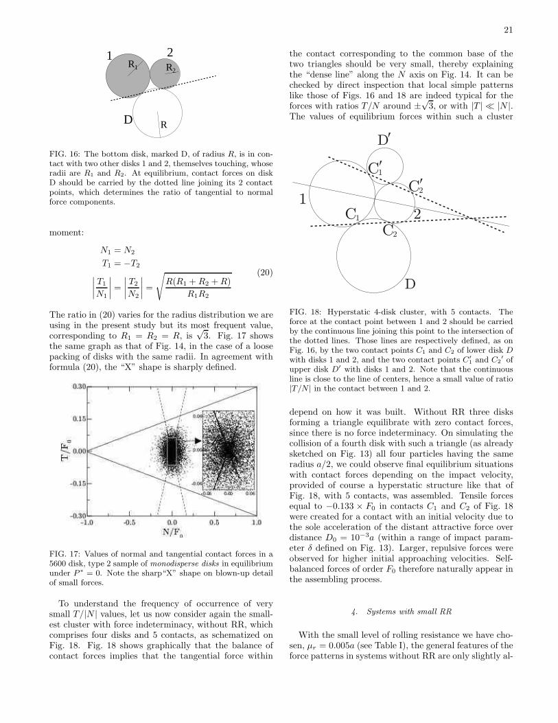
21

R1 R2

R

21

D

FIG. 16: The bottom disk, marked D, of radius R, is in con-tact with two other disks 1 and 2, themselves touching, whoseradii are R1 and R2. At equilibrium, contact forces on diskD should be carried by the dotted line joining its 2 contactpoints, which determines the ratio of tangential to normalforce components.

moment:

N1 = N2

T1 = −T2

∣

∣

∣

∣

T1

N1

∣

∣

∣

∣

=

∣

∣

∣

∣

T2

N2

∣

∣

∣

∣

=

√

R(R1 + R2 + R)

R1R2

(20)

The ratio in (20) varies for the radius distribution we areusing in the present study but its most frequent value,corresponding to R1 = R2 = R, is

√3. Fig. 17 shows

the same graph as that of Fig. 14, in the case of a loosepacking of disks with the same radii. In agreement withformula (20), the “X” shape is sharply defined.

FIG. 17: Values of normal and tangential contact forces in a5600 disk, type 2 sample of monodisperse disks in equilibriumunder P ∗ = 0. Note the sharp“X” shape on blown-up detailof small forces.

To understand the frequency of occurrence of verysmall T/|N | values, let us now consider again the small-est cluster with force indeterminacy, without RR, whichcomprises four disks and 5 contacts, as schematized onFig. 18. Fig. 18 shows graphically that the balance ofcontact forces implies that the tangential force within

the contact corresponding to the common base of thetwo triangles should be very small, thereby explainingthe “dense line” along the N axis on Fig. 14. It can bechecked by direct inspection that local simple patternslike those of Figs. 16 and 18 are indeed typical for theforces with ratios T/N around ±

√3, or with |T | ≪ |N |.

The values of equilibrium forces within such a cluster

D

D

C1

C2

C1

C2

1

2

FIG. 18: Hyperstatic 4-disk cluster, with 5 contacts. Theforce at the contact point between 1 and 2 should be carriedby the continuous line joining this point to the intersection ofthe dotted lines. Those lines are respectively defined, as onFig. 16, by the two contact points C1 and C2 of lower disk Dwith disks 1 and 2, and the two contact points C′

1 and C2′ of

upper disk D′ with disks 1 and 2. Note that the continuousline is close to the line of centers, hence a small value of ratio|T/N | in the contact between 1 and 2.

depend on how it was built. Without RR three disksforming a triangle equilibrate with zero contact forces,since there is no force indeterminacy. On simulating thecollision of a fourth disk with such a triangle (as alreadysketched on Fig. 13) all four particles having the sameradius a/2, we could observe final equilibrium situationswith contact forces depending on the impact velocity,provided of course a hyperstatic structure like that ofFig. 18, with 5 contacts, was assembled. Tensile forcesequal to −0.133 × F0 in contacts C1 and C2 of Fig. 18were created for a contact with an initial velocity due tothe sole acceleration of the distant attractive force overdistance D0 = 10−3a (within a range of impact param-eter δ defined on Fig. 13). Larger, repulsive forces wereobserved for higher initial approaching velocities. Self-balanced forces of order F0 therefore naturally appear inthe assembling process.

4. Systems with small RR

With the small level of rolling resistance we have cho-sen, µr = 0.005a (see Table I), the general features of theforce patterns in systems without RR are only slightly al-

22

tered, as apparent on Fig. 19, which shows the interactionforces in an equilibrated sample of series B with RR un-der P ∗ = 0. Like in type 2 systems devoid of RR underP ∗ = 0, forces of order F0 only exist in isolated regions.Note, however, that the small forces outside these regionswith self-balanced stresses do not vanish, but are of orderµrF0/a, a feature which is further commented below.

In principle, the discussion of force indeterminacy andrigidity is quite different with RR. Contacts now carryinga moment, the analog of relation 19 becomes

3N + h = 3Nc + Nd + k ( RR) (21)

With RR (and as we could check with the method of Ap-pendix A), all connected clusters are rigid. One maytherefore use directly k = 0 (ignoring the two globaltranslations) in (21). All independent loops contribute2 to the degree of force indeterminacy, and the coordina-tion number corresponding to isostaticity (no floppiness,no hyperstaticity) is equal to 2. To find self-balancedforces in a loop, note that each one of the two contacts ofany particle in the loop will carry opposite forces (whencetwo independent force components); the resulting torquesare then to be compensated by the rolling moments atthe contacts, to be determined with a number of equa-tions (one per particle in the loop) equal to the numberof unknowns (one per contact in the loop). However,those moments are severely limited by inequality (10).The constant force F transmitted around the loop shouldthen be of the same order of magnitude as µrF0/a , hencesmall. If we had used the same threshold for blue con-tacts on Fig. 19 than on Fig. 11, then all contacts within aloop, because they carry forces above the tolerance level10−4F0, would have appeared as red (compressive) orgreen (tensile). Resetting the threshold to 10−2F0, ofthe order of µrF0/a, thus enabled us to distinguish thehyperstatic clusters analogous to the previous case with-out RR from the new source of hyperstaticity, the effectsof which are limited by the smallness of the RR param-eter µr. We could check that the force threshold Nperc

for percolation, as defined above in paragraph IVB 1, isclose to 0.01F0 in that case. If clusters made with RR,which are (infinitesimally) rigid could not be broken, noloop should appear because two independent clusters donot generically collide simultaneously in several points.The existence of loops in the final structure thereforewitnesses the fragility of tenuous structures which formwith a small level of RR (which is further confirmed bythe large scale changes observed between P ∗ = 0 andP ∗ = 0.01).

Other features of force distributions and force pat-terns in systems without RR, such as the correlations be-tween normal and tangential contact force components,can still be observed with the small rolling friction levelµr = 5.10−3a. The graphs of Figs. 14 and 15, if drawnfor configurations prepared in the same way with a smallRR, are very similar. The small RR level used in simu-lations therefore only introduces small quantitative dif-ferences in that respect, at least for the parameters of

the assembling procedure defined in Section III B. In thenext paragraphs, we investigate, first, as an instructivelimiting case, the effects of large RR, and then the situ-ations in samples with low RR assembled with differentinitial random velocities (as on Fig. 8).

5. Effect of a large rolling resistance.

Fig 20 shows the analog of Figs. 11 and 19, obtainedwith a large rolling resistance: µr = 0.5a in a 5600 disksample. The resulting structure has very few, large loops,hence an extremely small degree of hyperstaticity, andmost contacts carry but very small forces. The charac-teristic prestressed clusters of Figs. 11, 12 and 19 havedisappeared. Such packings with large RR therefore ap-proach the limit in which a simple geometrical rule isadopted to aggregate particles: in the present case onerecovers the results of the ballistic aggregation algorithm,stipulating that particles or clusters move on straight-linetrajectories and join to form larger, rigid objects as soonas they touch. This results in isostatic, loop-free struc-tures with coordination number 2. The resulting contactnetwork has no force indeterminacy, and is consequentlynot prestressed. Our introduction, in the previous sim-ulations, of a finite rolling resistance (and a finite fric-tion coefficient) changes those structures in two respects:first, they form better connected structures, with loops ;second, they carry significant self-balanced forces, of theorder of the maximum tensile force in a contact. Thoseeffects are however dependent on the initial conditionsfor aggregation, as we now report.

6. Effects of initial velocities in aggregation process

As shown on Fig. 8, the initial mean quadratic ve-locity V0 in the aggregation stage of assembling method2 determines the final coordination number of systemswith RR. Isostatic, loop-free networks are formed withthe small RR level (µr/a = 0.005) used in our systematicsimulation series provided V0 is small enough. The re-sulting force network, as displayed as an inset on Fig. 20,approaches a tree-like, loop-free structure, in which allcontact forces vanish under P = 0.

Table VI shows the dependence of coordination num-bers and force values on initial velocity parameter V0/V ∗.One distinguishes three populations of contacts or inter-actions: those with repulsive, negative and vanishing nor-mal forces (i.e., below tolerance level 10−4F0), and, like-wise, between the average number of contacts per grainsof each kind, respectively contributing z+, z− and z0 tothe coordination number z. N+ (respectively, N−) isthe average value of repulsive (attractive) normal forces,

N(2)+ (resp., N

(2)− ) the quadratic average. These results

illustrate the dependence of the force distribution on theinitial velocity parameter. Force indeterminacy and sig-nificant non-vanishing forces appear as V0/V ∗ reaches

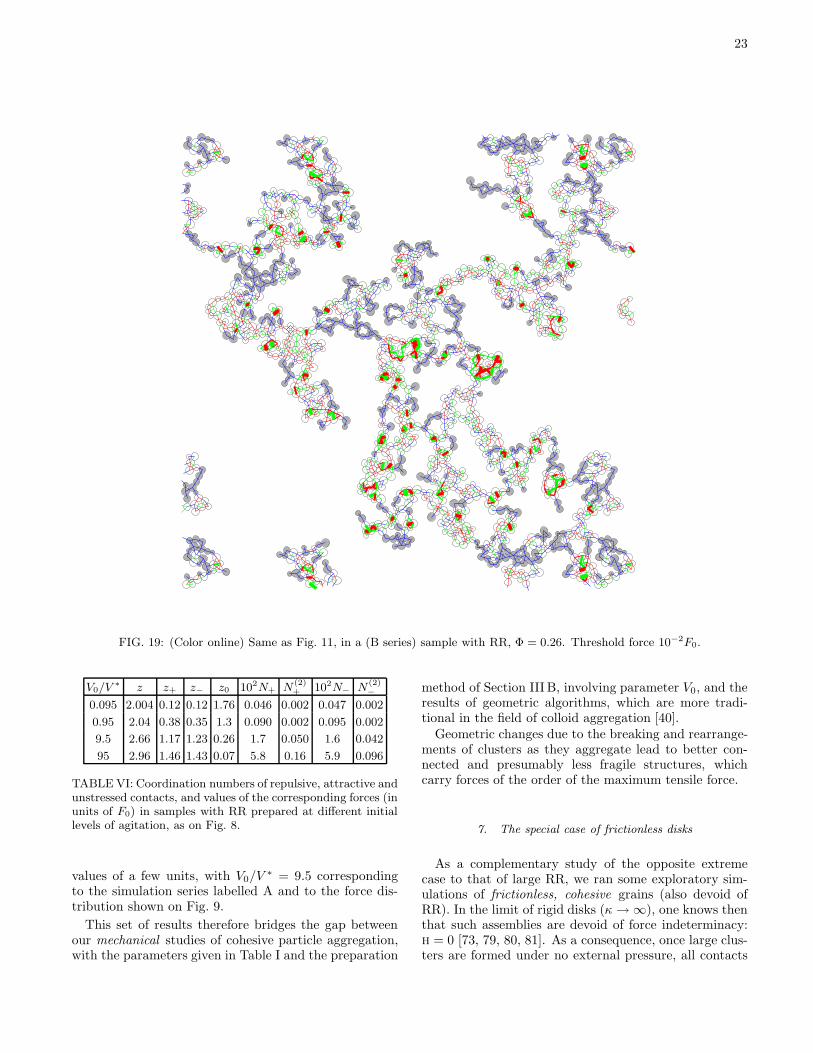
23

FIG. 19: (Color online) Same as Fig. 11, in a (B series) sample with RR, Φ = 0.26. Threshold force 10−2F0.

V0/V ∗ z z+ z− z0 102N+ N(2)+ 102N− N

(2)−

0.095 2.004 0.12 0.12 1.76 0.046 0.002 0.047 0.002

0.95 2.04 0.38 0.35 1.3 0.090 0.002 0.095 0.002

9.5 2.66 1.17 1.23 0.26 1.7 0.050 1.6 0.042

95 2.96 1.46 1.43 0.07 5.8 0.16 5.9 0.096

TABLE VI: Coordination numbers of repulsive, attractive andunstressed contacts, and values of the corresponding forces (inunits of F0) in samples with RR prepared at different initiallevels of agitation, as on Fig. 8.

values of a few units, with V0/V ∗ = 9.5 correspondingto the simulation series labelled A and to the force dis-tribution shown on Fig. 9.

This set of results therefore bridges the gap betweenour mechanical studies of cohesive particle aggregation,with the parameters given in Table I and the preparation

method of Section III B, involving parameter V0, and theresults of geometric algorithms, which are more tradi-tional in the field of colloid aggregation [40].

Geometric changes due to the breaking and rearrange-ments of clusters as they aggregate lead to better con-nected and presumably less fragile structures, whichcarry forces of the order of the maximum tensile force.

7. The special case of frictionless disks

As a complementary study of the opposite extremecase to that of large RR, we ran some exploratory sim-ulations of frictionless, cohesive grains (also devoid ofRR). In the limit of rigid disks (κ → ∞), one knows thenthat such assemblies are devoid of force indeterminacy:h = 0 [73, 79, 80, 81]. As a consequence, once large clus-ters are formed under no external pressure, all contacts

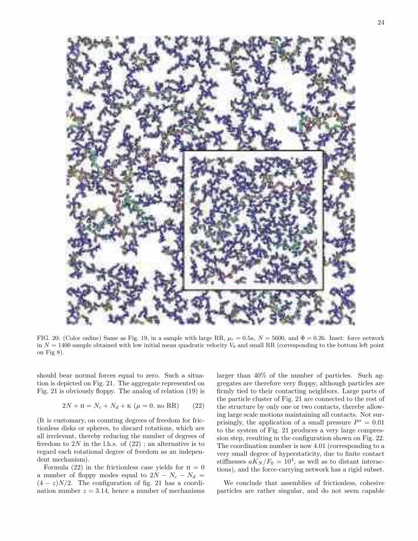
24

FIG. 20: (Color online) Same as Fig. 19, in a sample with large RR, µr = 0.5a, N = 5600, and Φ = 0.26. Inset: force networkin N = 1400 sample obtained with low initial mean quadratic velocity V0 and small RR (corresponding to the bottom left pointon Fig 8).

should bear normal forces equal to zero. Such a situa-tion is depicted on Fig. 21. The aggregate represented onFig. 21 is obviously floppy. The analog of relation (19) is

2N + h = Nc + Nd + k (µ = 0, no RR) (22)

(It is customary, on counting degrees of freedom for fric-tionless disks or spheres, to discard rotations, which areall irrelevant, thereby reducing the number of degrees offreedom to 2N in the l.h.s. of (22) ; an alternative is toregard each rotational degree of freedom as an indepen-dent mechanism).

Formula (22) in the frictionless case yields for h = 0a number of floppy modes equal to 2N − Nc − Nd =(4 − z)N/2. The configuration of fig. 21 has a coordi-nation number z = 3.14, hence a number of mechanisms

larger than 40% of the number of particles. Such ag-gregates are therefore very floppy, although particles arefirmly tied to their contacting neighbors. Large parts ofthe particle cluster of Fig. 21 are connected to the rest ofthe structure by only one or two contacts, thereby allow-ing large scale motions maintaining all contacts. Not sur-prisingly, the application of a small pressure P ∗ = 0.01to the system of Fig. 21 produces a very large compres-sion step, resulting in the configuration shown on Fig. 22.The coordination number is now 4.01 (corresponding to avery small degree of hyperstaticity, due to finite contactstiffnesses aKN/F0 = 104, as well as to distant interac-tions), and the force-carrying network has a rigid subset.

We conclude that assemblies of frictionless, cohesiveparticles are rather singular, and do not seem capable

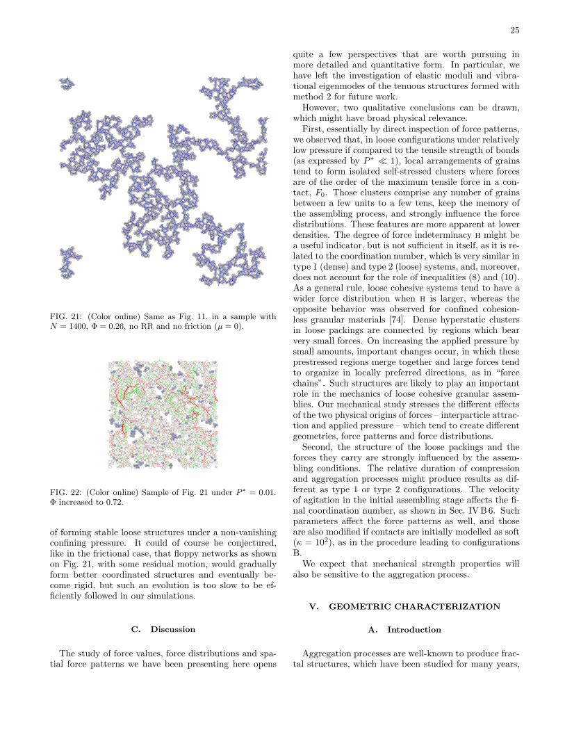
25

FIG. 21: (Color online) Same as Fig. 11, in a sample withN = 1400, Φ = 0.26, no RR and no friction (µ = 0).

FIG. 22: (Color online) Sample of Fig. 21 under P ∗ = 0.01.Φ increased to 0.72.

of forming stable loose structures under a non-vanishingconfining pressure. It could of course be conjectured,like in the frictional case, that floppy networks as shownon Fig. 21, with some residual motion, would graduallyform better coordinated structures and eventually be-come rigid, but such an evolution is too slow to be ef-ficiently followed in our simulations.

C. Discussion

The study of force values, force distributions and spa-tial force patterns we have been presenting here opens

quite a few perspectives that are worth pursuing inmore detailed and quantitative form. In particular, wehave left the investigation of elastic moduli and vibra-tional eigenmodes of the tenuous structures formed withmethod 2 for future work.

However, two qualitative conclusions can be drawn,which might have broad physical relevance.

First, essentially by direct inspection of force patterns,we observed that, in loose configurations under relativelylow pressure if compared to the tensile strength of bonds(as expressed by P ∗ ≪ 1), local arrangements of grainstend to form isolated self-stressed clusters where forcesare of the order of the maximum tensile force in a con-tact, F0. Those clusters comprise any number of grainsbetween a few units to a few tens, keep the memory ofthe assembling process, and strongly influence the forcedistributions. These features are more apparent at lowerdensities. The degree of force indeterminacy h might bea useful indicator, but is not sufficient in itself, as it is re-lated to the coordination number, which is very similar intype 1 (dense) and type 2 (loose) systems, and, moreover,does not account for the role of inequalities (8) and (10).As a general rule, loose cohesive systems tend to have awider force distribution when h is larger, whereas theopposite behavior was observed for confined cohesion-less granular materials [74]. Dense hyperstatic clustersin loose packings are connected by regions which bearvery small forces. On increasing the applied pressure bysmall amounts, important changes occur, in which theseprestressed regions merge together and large forces tendto organize in locally preferred directions, as in “forcechains”. Such structures are likely to play an importantrole in the mechanics of loose cohesive granular assem-blies. Our mechanical study stresses the different effectsof the two physical origins of forces – interparticle attrac-tion and applied pressure – which tend to create differentgeometries, force patterns and force distributions.

Second, the structure of the loose packings and theforces they carry are strongly influenced by the assem-bling conditions. The relative duration of compressionand aggregation processes might produce results as dif-ferent as type 1 or type 2 configurations. The velocityof agitation in the initial assembling stage affects the fi-nal coordination number, as shown in Sec. IVB6. Suchparameters affect the force patterns as well, and thoseare also modified if contacts are initially modelled as soft(κ = 102), as in the procedure leading to configurationsB.

We expect that mechanical strength properties willalso be sensitive to the aggregation process.

V. GEOMETRIC CHARACTERIZATION

A. Introduction

Aggregation processes are well-known to produce frac-tal structures, which have been studied for many years,

26

in particular with numerical simulations (see ref. [40]for a review). Universal fractal regimes due to vari-ous types of aggregation processes (ballistic, diffusion-limited, reaction-limited) are most conveniently observedin very low density samples. Indeed, an object of frac-tal dimension dF extending over distance L in d dimen-sions (d > dF ) will have an apparent volume fractionΦ ∼ LdF −d, which vanishes as L → ∞. Starting from Nisolated particles in a finite volume with periodic bound-ary conditions, an aggregation process cannot producea fractal geometry over arbitrarily large length scales.In practice, for low enough values of Φ, the aggregationprocess will begin just like in the Φ → 0 limit, when cor-relations between particles can be neglected. Later on,the crowding and interpenetration of clusters will pre-vent the fractal behavior to extend to larger scales [82],and a classical geometric model to describe this situationis a dense packing of fractal domains (sometimes called“blobs”) of typical diameter ξ. ξ is the upper limit of thefractal regime, and is related to Φ (see the discussion ofeqn. 1 in [40]) as

ξ ∼ Φ− 1

d−dF , (23)

a relation which should be independent of the total sam-ple diameter L, provided L ≫ ξ. This “fractal blob”model is reminiscent of semi-dilute polymer solutions [83]and has been employed in many different physical situ-ations, e.g., silica aerogels [84]. It has been shown todescribe experimental results on the packing of cohesivepowders [24, 59]. If such a geometric description appliesto our loose systems, then ξ should be of the order ofthe typical size of large density inhomogeneities (denseregions or holes) in the samples depicted on Fig. 5.

B. Definitions

Self-similarity is conveniently detected on studying thedensity autocorrelation function (DACF), as follows. Letχ(r) denote the indicator function of solid particles, tak-ing values 1 if point r is within a solid disk, and zerootherwise. Then we define the DACF as:

C(r) = 〈χ(R)χ(R + r)〉R =1

A

∫

χ(R)χ(R + r))dR,

(24)with an average over the origin position R over the wholesample surface, of area A. On computing C(r) periodicboundary conditions should be accounted for, so that po-sition R + r stays within the simulation cell. Isotropyensures that C(r) is only dependent on distance r = ||r||in the large sample limit (or on taking its ensemble aver-age). C(r), by construction, takes the value Φ (the solidfraction) for r = 0, and tends to Φ2 as r → ∞.

In practice it is convenient to calculate, rather thanC(r) − Φ2, its Fourier transform, a function of the mag-nitude k = ||k|| of wavevector k by isotropy, which we

denote as I(k). I(k) is simply related to the Fouriertransform χ of the field χ(r) by:

I(k) =|χ(k)|2

A. (25)

The notation I(k) is of course reminiscent of the scatter-ing intensity per unit volume for wavevector k (as usedin e.g. small-angle X-ray or neutron scattering experi-ments), which is equal to I(k), up to a “contrast factor”,replaced by 1 in (25).

A fractal structure with dimension dF in 2D shouldhave a power-law decreasing scattering intensity oversome range of k:

I(k) ∝ k−dF (2π

ξ≪ k ≪ 2π

a). (26)

An exponential cut-off of the decreasing power law be-havior of C(r) around r ∼ ξ is sometimes used [85, 86]:

C(r) − Φ2 = Φ(r

ℓ

)dF −2

e−r/ξ (27)

where the length ℓ, introduced to make C(r) appropri-ately dimensionless, is a constant of the order of the av-erage particle radius. Then the corresponding form ofI(k), is given in terms of Gauss’s hypergeometric func-tion 2F1[a, b; c; x] [87]:

I(k) = Cst+Φ2πℓ2Γ(dF )ξdF

ℓdF2F1

[

1 + dF

2,dF

2; 1;−ξ2k2

]

(28)In 2D, as soon as the particles form one continuous ag-

gregate, the empty space is split into a set of disconnectedholes or pores. The distribution of sizes and shapes ofsuch holes is another way to characterize the system ge-ometry.

C. Procedure

To compute I(k) from the configurations obtained insimulations, we first discretized the density field χ(r),i.e., we considered its values on the points of a regularmesh, with spacings ∆x and ∆y along the edges of therectangular cell of the order of a/100. χ(k) was thenevaluated using a two-dimensional FFT algorithm, fromwhich I(k) was deduced by formula (25) and orientation-ally averaged on binning values of wavevectors k accord-ing to k = ||k||.

The field χ(r) = 0 defines a set of holes. We charac-terize a hole labelled as H by the value of its equivalent

radius RH . RH is defined as the radius of a disk withthe same radius of gyration as the hole. Specifically, ifNH is the number of mesh nodes in the hole, which arelabelled as i, 1 ≤ i ≤ NH , and have coordinates xi, yi, ondenoting as (xc

H ,ycH) the coordinates of the mass center

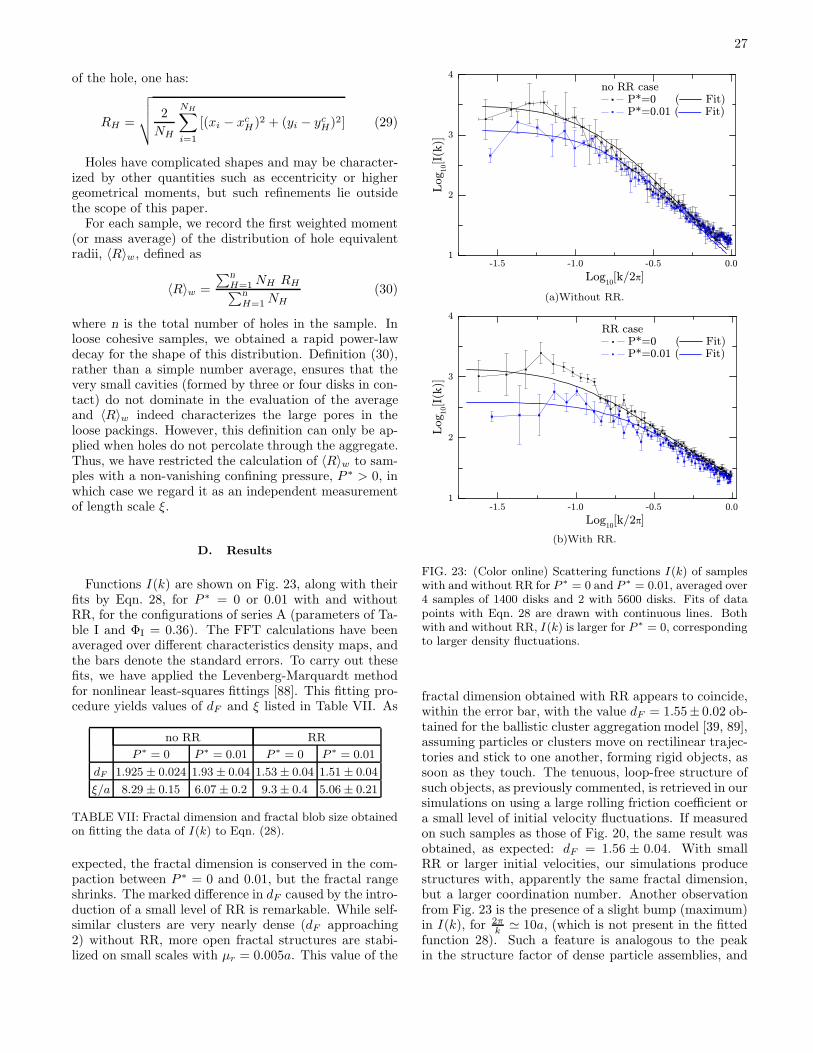
27

of the hole, one has:

RH =

√

√

√

√

2

NH

NH∑

i=1

[(xi − xcH)2 + (yi − yc

H)2] (29)

Holes have complicated shapes and may be character-ized by other quantities such as eccentricity or highergeometrical moments, but such refinements lie outsidethe scope of this paper.

For each sample, we record the first weighted moment(or mass average) of the distribution of hole equivalentradii, 〈R〉w, defined as

〈R〉w =

∑

n

H=1 NH RH∑

n

H=1 NH(30)

where n is the total number of holes in the sample. Inloose cohesive samples, we obtained a rapid power-lawdecay for the shape of this distribution. Definition (30),rather than a simple number average, ensures that thevery small cavities (formed by three or four disks in con-tact) do not dominate in the evaluation of the averageand 〈R〉w indeed characterizes the large pores in theloose packings. However, this definition can only be ap-plied when holes do not percolate through the aggregate.Thus, we have restricted the calculation of 〈R〉w to sam-ples with a non-vanishing confining pressure, P ∗ > 0, inwhich case we regard it as an independent measurementof length scale ξ.

D. Results

Functions I(k) are shown on Fig. 23, along with theirfits by Eqn. 28, for P ∗ = 0 or 0.01 with and withoutRR, for the configurations of series A (parameters of Ta-ble I and ΦI = 0.36). The FFT calculations have beenaveraged over different characteristics density maps, andthe bars denote the standard errors. To carry out thesefits, we have applied the Levenberg-Marquardt methodfor nonlinear least-squares fittings [88]. This fitting pro-cedure yields values of dF and ξ listed in Table VII. As

no RR RR

P ∗ = 0 P ∗ = 0.01 P ∗ = 0 P ∗ = 0.01

dF 1.925 ± 0.024 1.93 ± 0.04 1.53 ± 0.04 1.51 ± 0.04

ξ/a 8.29 ± 0.15 6.07 ± 0.2 9.3 ± 0.4 5.06 ± 0.21

TABLE VII: Fractal dimension and fractal blob size obtainedon fitting the data of I(k) to Eqn. (28).

expected, the fractal dimension is conserved in the com-paction between P ∗ = 0 and 0.01, but the fractal rangeshrinks. The marked difference in dF caused by the intro-duction of a small level of RR is remarkable. While self-similar clusters are very nearly dense (dF approaching2) without RR, more open fractal structures are stabi-lized on small scales with µr = 0.005a. This value of the

-1.5 -1.0 -0.5 0.01

2

3

4

Log10[I(k

)]

Log10[k/2 ]

no RR case P*=0 ( Fit) P*=0.01 ( Fit)

(a)Without RR.

-1.5 -1.0 -0.5 0.01

2

3

4

RR case P*=0 ( Fit) P*=0.01 ( Fit)

Log10[I(k

)]

Log10[k/2 ]

(b)With RR.

FIG. 23: (Color online) Scattering functions I(k) of sampleswith and without RR for P ∗ = 0 and P ∗ = 0.01, averaged over4 samples of 1400 disks and 2 with 5600 disks. Fits of datapoints with Eqn. 28 are drawn with continuous lines. Bothwith and without RR, I(k) is larger for P ∗ = 0, correspondingto larger density fluctuations.

fractal dimension obtained with RR appears to coincide,within the error bar, with the value dF = 1.55± 0.02 ob-tained for the ballistic cluster aggregation model [39, 89],assuming particles or clusters move on rectilinear trajec-tories and stick to one another, forming rigid objects, assoon as they touch. The tenuous, loop-free structure ofsuch objects, as previously commented, is retrieved in oursimulations on using a large rolling friction coefficient ora small level of initial velocity fluctuations. If measuredon such samples as those of Fig. 20, the same result wasobtained, as expected: dF = 1.56 ± 0.04. With smallRR or larger initial velocities, our simulations producestructures with, apparently the same fractal dimension,but a larger coordination number. Another observationfrom Fig. 23 is the presence of a slight bump (maximum)in I(k), for 2π

k ≃ 10a, (which is not present in the fittedfunction 28). Such a feature is analogous to the peakin the structure factor of dense particle assemblies, and

28

is likely related to the packing of aggregates. As theaggregates are requested to be mechanically rigid theytend to be multiply connected and, at least in 2D, nearlyimpenetrable: the maximum in the structure factor is asignature of steric exclusion.

The evaluation of the first weighted moment 〈R〉w ofthe distribution of hole equivalent radii, for P ∗ = 0.01yields 〈R〉w/a = 6.6 ± 0.2, and 〈R〉w/a = 5.47 ± 0.14with RR. As expected, these results are similar to thevalues of ξ given in Table VII.

VI. CONCLUSIONS AND FINAL REMARKS

Cohesive packings can form equilibrium structures atvery small solid fractions in qualitative agreements withexperiments in fine and ultrafine powders. Equilibratedconfigurations are sensitive to the level of applied pres-sure, relative to contact tensile strength F0, as expressedby the dimensionless number P ∗. They crucially de-pend on the assembling procedure, as even a low pres-sure (P ∗ ≪ 1) can lead to rather compact states if ap-plied to a initial “cold” (i.e., with vanishing or low ve-locities) granular gas of isolated particles, as in method1. If, on the other hand, particles are given some ran-dom motion and have time to stick to one another beforehaving to sustain some stress, as in method 2, tenuousparticle networks and open structures are obtained. Theinitial random motion, which is ballistic in our simula-tions, could be diffusive in practical situations in whichfine particles are dispersed in a fluid. Some random rel-

ative motion of different particles is also present, due tovelocity fluctuations, in situations of global flow or sus-pension sedimentation.

Under low pressure, such loose packings carry self-balanced forces of the order of the maximum tensile forceF0 in hyperstatic, well-connected lumps joined by thin-ner arms where many contacts carry vanishing or verysmall forces. Such structures are sensitive to the magni-tude of initial velocities with which particles collide onforming aggregates. In general force networks differ fromthe usual “force chain” patterns of cohesionless systems,and are associated with different force distributions. Theforce balance is strongly influenced by the structure ofsmall aggregates that are first created on assembling thesystem. They evolve very fast as the system rearrangeswhen P ∗ grows even by small amounts (from P ∗ = 0 toP ∗ = 0.01).

Due to the limited strength of contacts with respectto tangential relative displacement and rolling, force-carrying structures therefore differ from the ones ob-tained with geometry-based algorithms in which any par-ticles or clusters that join form one unique rigid, unbreak-able object. The result of such algorithms is howeverretrieved, in the presence of rolling resistance, if largestrength properties are attributed to contacts (to the RRparameter µr in particular) or if initial velocities of col-liding grains are kept low enough. In such limits isostatic,

loop-free clusters are formed with coordination number2.

Micromechanical parameters do otherwise influencethe structure of packings and the initial (self-balanced)forces they carry, especially those without rolling resis-tance.

The study of density correlations show that loose con-figurations can be regarded as dense packings of self-similar blobs of typical size ξ (about 10 times as large asthe average diameter in our case), as in fractal clustersproduced by colloid aggregation models. The estimatedvalue of the fractal dimension, with RR, is compatiblewith the 2D result for ballistic aggregation, even whenthe connectivity (coordination number) is different. Wethus expect different structures of the same density andfractal dimension to possess, due to the difference in loopnumbers and self-stresses, different mechanical proper-ties.

The fractal dimension appears to be larger in sys-tems without RR. Thus systems without RR seem toexhibit systematic qualitative peculiarities, and since asmall level of rolling resistance is likely to exist in all re-alistic models, this feature should preferably be includedin numerical studies.

The effect of a growing pressure, as well as pressurecycles, on the packing density and internal state will beinvestigated in a forthcoming publication [42]. Other im-mediately related perspectives are the study of macro-scopic tensile and shear strength in relation to geometriccharacterizations and self-balanced forces.

APPENDIX A: RIGIDITY AND STIFFNESS

MATRICES

Degrees of force indeterminacy h, of velocity indeter-minacy k and their relations are properties of the rigidity

matrix G, which is defined as follows. First, let us denoteas U a displacement vector for all degrees of freedom inthe system,

U = ((ui, ∆θi)1≤i≤n, (ǫα)1≤α≤2) . (A1)

in which one conveniently separates out in the displace-ment ui of grain i the part due to the global strain, thuswriting ui = −ǫ · ri + ui. U has dimension 3N + 2 for Ndisks and 2 strain increments. Then for each one of theNc contacts, say between i and j, the relative displace-ment of the contact point (with notations Ri,j for the

radii, and tij for unit tangential vectors as in Sec. II B)

δuij = ui +∆θi×Ritij − uj +∆θj ×Rj tij + ǫ ·rij , (A2)

can be regarded as providing 2 coordinates to one 2Nc-dimensional vector of relative displacements, δu. As (A2)expresses a linear dependence of δu on U, one has defineda 2Nc × (3N +2) matrix, which is the rigidity matrix G:

δu = G · U (A3)

29

All coordinates of u and δu are to be thought of as small(infinitesimal) increments, for which the system geome-try is fixed. The degree of displacement (or velocity) in-determinacy k is by definition the dimension of the nullspace of G. The relevant definition of relative displace-ments includes all relative motions that are associated toforces or moments. In the presence of RR, one shouldinclude all relative rotations δθi − δθj into the compo-nents of δu, the dimension of which thus raises to 3Nc.On the other hand, in the absence of friction the tangen-tial relative displacement of the contact point becomesirrelevant, and δu should only include normal relativedisplacements. In general all distant attractions betweenclose neighbors should be dealt with similarly, becauseonly normal forces are transmitted between such pairs.For future use we just denote as M the appropriate di-mension of the relative displacement vector.

On writing δu it is most convenient to use a local basisfor each contact, with normal and tangential directions ascoordinate axes. Increments of contact forces, and possi-bly moments (with RR), are related via the contact lawto δu. Together they define a contact force vector f , thedimension of which is equal to that of δu. f , in a systemwith RR, also includes rolling moments at contacts.

Externally applied forces and torques onto the grains,as well as stresses, define together a vector of externalforces Fext:

Fext = ((Fi, Γi)1≤i≤N , (Aσαα)1≤α≤2) . (A4)

A denotes the surface area of the sample, so that thework of the load for small displacements is just Fext ·U.The equilibrium relations, stating that contact forces f

balance the load Fext, just read (as one easily checks):

Fext = TG · f , (A5)

with the transposed rigidity matrix, TG. That matricesappearing in relations (A3) and (A5) are transposed toeach other is just a statement of the theorem of virtual

work : the work of external forces in any displacementvector is Fext · U = f · δu, provided Fext is related to f

by (A5) and δu is related to U by (A3). By definition,the degree of force indeterminacy h is the dimension ofthe null space of TG.

The rank of matrix G is r = Nf −k, with Nf the num-ber of degrees of freedom (the dimension of displacementor external load vectors). This rank r is also the dimen-sion of the range of the matrix, which is the orthogonalsubspace, within the M -dimensional space of relative dis-placements, to the null space of its transpose TG in thedual space of contact forces. Hence r = M −h. We haveobtained

Nf + h = M + k,

which yields, according to the appropriate definition ofrelevant relative motions, relations (19), (21), and (22).

Assuming elastic behavior in the contact (i.e., strict in-equalities in (8) and (10), which, as noted in Section II D,is the general case at equilibrium), in a quasistatic ex-periment contact force increments ∆f relate to relativedisplacement increments ∆δu with a contact stiffness ma-trix K:

∆f = K · ∆δu.

K is a square, diagonal matrix, containing coefficientsKN , KT and (with RR) Kr for each contact. Thus K onlycontains positive elements, except for the (very scarce)distant interactions, which contribute the negative nor-mal stiffness −F0/D0 in our model. If ∆f balances someload increment ∆Fext, while δu corresponds to the Nf -dimensional displacement vector U, one then has:

∆Fext = K ·U,

where one has introduced the stiffness matrix K:

K = TG · K ·G. (A6)

(K is traditionally called dynamical matrix in the con-text of solid-state physics and interactions of atoms orions in a crystal [90]). Unlike G and TG, K is always asquare, symmetric matrix. It has to be positive definitein order for the equilibrium state to be stable, becauseit expresses the elastic energy associated with small dis-placements. (In fact, the full stiffness matrix also con-tains a small non-symmetric correction to (A6) [91] dueto the effect of contact forces prior to the application ofthe load increment, which we ignore here.)

By construction, the null space of G is contained in thenull space of K, and coincides with it in the absence ofdistant attractions, because K is then a positive matrix.In practice, the positiveness of K can be investigated withthe Cholesky algorithm. We applied this method (in aform suitable for sparse matrices, stored in a “skyline”form) to the stiffness matrix of the contact networks ofthe simulated equilibrium configurations. This is how, onfinding that K was positive definite, we could concludethat the contact structure was devoid of mechanisms (orfloppy modes, eigenmodes of K with eigenvalue zero) inall cases with P ∗ = 0.01. On the contrary, stiffness ma-trices associated with contact structures without RR atP ∗ = 0 usually possess some mechanisms, although weargued that their number k must be small.

Aknowledgements: This work has been supportedby the Ministerio de Educacion y Ciencia of the SpanishGovernment under contract number BFM2003-1739.J.-N. Roux wishes to thank Dietrich Wolf for useful con-tacts and discussions.

[1] H. J. Herrmann, J.-P. Hovi, and S. Luding, eds., Physicsof Dry Granular Media (Balkema, Dordrecht, 1998).

[2] Y. Kishino, ed., Powders and Grains 2001 (Swets &

30

Zeitlinger, Lisse, 2001).[3] H. Hinrichsen and D. E. Wolf, eds., The Physics of Gran-

ular Media (Wiley-VCH, Berlin, 2004).[4] R. Garcıa Rojo, H. J. Herrmann, and S. McNamara, eds.,

Powders and Grains 2005 (Balkema, Leiden, 2005).[5] P. Richard, P. Philippe, F. Barbe, S. Bourles,

X. Thibault, and D. Bideau, PRE 68, 020301(R) (2003).[6] J. Q. Xu, R. P. Zou, and A. B. Yu, Physical Review E

69, 032301(4) (2004).[7] T. Aste, M. Saadatfar, A. Sakellariou, and T. J. Senden,

Physica A 339, 16 (2004).[8] T. Aste, M. Saadatfar, and T. J. Senden, Physical Review

E 71, 061302 (2005).[9] M. M. Kohonen, D. Geromichalos, M. Scheel, C. Schier,

and S. Herminghaus, Physica A 39, 7 (2004).[10] Z. Fournier, D. Geromichalos, S. Herminhaus, M. M. Ko-

honen, F. Mugele, M. Scheel, B. Schulz, C. Schier, R. See-mann, and A. Skudelny, Journal of Physics CondensedMatter 17, 5477 (2005).

[11] V. Richefeu, M. S. El Youssoufi, and F. Radjai, PRE 73

(2006).[12] P. A. Cundall and O. D. L. Strack, Geotechnique 29, 47

(1979).[13] H. J. Herrmann and S. Luding, Continuum Mech. Ther-

modyn. 10, 189 (1998).[14] M. Jean, Computational Methods in Applied Engineer-

ing 177, 235 (1999).[15] M. Jean, V. Acary, and Y. Monerie, Philosophical Trans-

actions of the Royal Society of London A359, 2497(2001).

[16] C. Thornton, Geotechnique 50, 43 (2000).[17] A. S. J. Suiker and N. A. Fleck, ASME Journal of Applied

Mechanics 71, 350 (2004).[18] D. M. Wood, Soil Behaviour and Critical State Soil Me-

chanics (Cambridge University Press, 1990).[19] I. Agnolin and J.-N. Roux, in [4], pp. 87–91.[20] R. J. Bathurst and L. Rothenburg, Mechanics of Materi-

als 9, 65 (1990).[21] F. Radjai and S. Roux, in [3], pp. 165–187.[22] J.-N. Roux and G. Combe, C. R. Academie des Sciences

(Physique) 3, 131 (2002).[23] J. K. Mitchell, Fundamentals of soil behavior (Wiley,

New York, 1993).[24] A. Castellanos, Advances in Physics 54, 263 (2005).[25] R. Y. Yang, R. P. Zou, and A. B. Yu, Physical Review E

62, 3900 (2000).[26] R. Y. Yang, R. P. Zou, and A. B. Yu, J. Appl. Phys. 94,

3025 (2003).[27] D. Kadau, G. Bartels, L. Brendel, and D. E. Wolf, Com-

putational Physics Communications 147, 190 (2002).[28] D. Kadau, G. Bartels, L. Brendel, and D. E. Wolf, Phase

Trans. 76, 315 (2003).[29] D. E. Wolf, T. Unger, D. Kadau, and L. Brendel, in [4],

pp. 525–533.[30] G. Bartels, T. Unger, D. Kadau, W. D. E., and

J. Kertesz, Granular Matter 7, 139 (2005).[31] J.-Y. Delenne, M. S. el Youssoufi, and J.-C. Benet,

Comptes-Rendus Academie des Sciences, Mecanique330, 475 (2002).

[32] J.-Y. Delenne, M. S. el Youssoufi, F. Cherblanc, and J.-C. Benet, Int. J. Numer. Anal. Meth. Geomech. 28, 1577(2004).

[33] C. Thornton and L. Liu, Powder Technoology 143–144,110 (2004).

[34] R. Y. Yang, R. P. Zou, and A. B. Yu, AIChE Journal 49,1656 (2003).

[35] S. Luding, Powder Technology 158, 45 (2005).[36] P. G. Rognon, J.-N. Roux, and F. Chevoir, in [4], pp.

565–568.[37] P. Rognon, J.-N. Roux, D. Wolf, M. Naaım, and

F. Chevoir, Europhysics Letters 74, 644 (2006).[38] R. Brewster, G. S. Grest, J. W. Landry, and A. J. Levine,

Physical Review E 72, 061301 (2005).[39] B. Smirnov, Physics Reports 188, 1 (1990).[40] P. Meakin, Journal of Sol-Gel Science and Technology

15, 97 (1999).[41] I. Bratberg, F. Radjai, and A. Hansen, Physical Review

E 66, 031303 (2002).[42] F. A. Gilabert, J.-N. Roux, and A. Castellanos, Com-

puter simulation of model cohesive powders: plasticcompaction under isotropic loads, to be submitted toPhys. Rev. E.

[43] M. Parrinello and A. Rahman, Physical Review Letters45, 1196 (1980).

[44] M. Parrinello and A. Rahman, Journal of AppliedPhysics 52, 7182 (1981).

[45] M. Parrinello and A. Rahman, Journal of ChemicalPhysics 76, 2662 (1982).

[46] L. E. Silbert, D. Ertas, G. S. Grest, T. C. Halsey, andD. Levine, Physical Review E 65, 031304 (2002).

[47] A. J. Forsyth and M. J. Rhodes, J. Coll. Inter. Sci. pp.133–138 (2000).

[48] A. Tordesillas and D. C. Stuart, Powder Technology 124,106 (2002).

[49] D. Maugis, Contact, adhesion and rupture of elasticsolids (Springer, Berlin, 2000).

[50] E. Somfai, J.-N. Roux, J. Snoeijer, M. van Hecke, andW. van Saarloos, PRE 72, 021301 (2005).

[51] Z. P. Zhang, L. F. Liu, Y. D. Yuan, and A. B. Yu, PowderTech. 116, 23 (2001).

[52] N. V. Brilliantov, F. Spahn, J. M. Hertzsch, andT. Poschel, Physical Review E 53, 5382 (1996).

[53] F. A. Gilabert, J.-N. Roux, and A. Castellanos, in [4],pp. 541–544.

[54] G. Combe and J.-N. Roux, in Deformation characteris-tics of geomaterials, edited by H. di Benedetto, T. Doanh,H. Geoffroy, and C. Sauzeat (Swets and Zeitlinger, Lisse,2003), pp. 1071–1078.

[55] P. Watson, J. M. Valverde, and A. Castellanos, PowderTechnology 115, 45 (2001).

[56] M. A. Sanchez Quintanilla, Ph.D. thesis, Universidad deSevilla (2003).

[57] A. Castellanos, J. M. Valverde, and M. A. S. Quintanilla,Physical Review Letters 94, 075501 (2005).

[58] H. Krupp, Advances in Colloid and Interface Science 1,111 (1967).

[59] J. M. Valverde, M. A. S. Quintanilla, and A. Castellanos,Physical Review Letters 92, 258303 (2004).

[60] D. Maugis and H. M. Pollock, Acta Metallica p. 1323(1984).

[61] M. A. S. Quintanilla, A. Castellanos, and J. M. Valverde,Physical Review E 64, 031301 (2001).

[62] F. A. Gilabert, A. M. Krivtsov, and A. Castellanos, Mec-canica 41, 341 (2006).

[63] J. M. Valverde, A. Castellanos, A. Ramos, A. T. Perez,M. A. Morgan, and P. Watson, Review of Scientific In-struments 71, 2791 (2000).

[64] A. Castellanos, J. M. Valverde, and M. A. S. Quintanilla,

31

Physical Review E 64, 041304 (2001).[65] S. Emam, J.-N. Roux, J. Canou, A. Corfdir, and J.-C.

Dupla, in [4], pp. 49–52.[66] H. A. Makse, N. Gland, D. L. Johnson, and L. Schwartz,

Physical Review E 70, 061302 (2004).[67] J. M. Valverde, A. Castellanos, and P. Watson, Powder

Technology 118, 236 (2001).[68] J. M. Valverde, A. Castellanos, and M. A. S. Quintanilla,

Physical Review Letters 86, 3020 (2001).[69] C. S. Campbell and C. E. Brennen, J. Fluid Mech. 151,

167 (1985).[70] F. Radjai, M. Jean, J.-J. Moreau, and S. Roux, Phys.

Rev. Lett. 27, 274 (1996).[71] D. M. Mueth, H. M. Jaeger, and S. R. Nagel, Phys. Rev.

E 57, 3164 (1998).[72] D. L. Blair, N. W. Mueggenburg, A. H. Marshall,

H. Jaeger, and S. R. Nagel, Physical Review E 63, 041304(2001).

[73] S. Ouaguenouni and J.-N. Roux, Europhysics Letters,39, 117 (1997).

[74] H. Makse, D. Johnson, and L. Schwartz, Physical ReviewLetters 84, 4160 (2000).

[75] F. Radjai, D. E. Wolf, M. Jean, and J.-J. Moreau, Phys-ical Review Letters 80, 61 (1998).

[76] S. N. Coppersmith, C. H. Liu, S. Majumdar, O. Narayan,and T. A. Witten, Physical Review E 53, 4673 (1996).

[77] H. Rumpf, Chem. Eng. Tech. 30, 144 (1958).[78] J.-N. Roux, in Proceedings of the Saint-Venant Sym-

posium on Multiple Scale Analysis and Coupled Physi-cal Systems (Presses de l’Ecole Nationale des Ponts et

Chaussees, Paris, 1997), pp. 577–584.[79] C. F. Moukarzel, Physical Review Letters 81, 1634

(1998).[80] A. Tkachenko and T. A. Witten, Physical Review E 60,

627 (1999).[81] J.-N. Roux, Physical Review E 61, 6802 (2000).[82] A. M. Puertas, A. Fernandez-Barbero, F. J. De las

Nieves, and L. F. Rull, Langmuir 20, 9861 (2004).[83] P.-G. de Gennes, Scaling Concepts in Polymer Physics

(Cornell University Press, Ithaca, 1979).[84] A. Hasmy, E. Anglaret, M. Foret, J. Pelous, and R. Jul-

lien, Physical Review B 50, 6006 (1994).[85] T. Freltoft, K. Kjems, and S. Sihna, Physical Review B

33, 269 (1986).[86] J. Teixeira, Journal of Applied Crystallography 21, 781

(1988).[87] M. Abramowitz and I. A. Stegun, Handbook of Mathe-

matical Functions (Dover Publications, Inc., New York,1972).

[88] J. J. More, in Lecture Notes in Mathematics, edited byG. A. Watson (Springer-Verlag, Berlin, 1977), vol. 630 ofNumerical Analysis, pp. 104–116.

[89] P. Meakin, Phys. Rev. A 29, 997 (1984).[90] N. W. Ashcroft and D. N. Mermin, Solid State

Physics (Harcourt College Publishers. ISBN 0-03-083993-9, 1976).

[91] K. Bagi, On the Concept of Jammed Configurations froma Structural Mechanics Perspective, to be published inGranular Matter (2006).