Article

Computational simulation of PT6A gas turbine engineoperating with different blends of biodiesel: Atransient-response analysis

Camilo Bayona-Roa 1,2, J.S. Solís-Chaves 1∗ Javier Bonilla1 and Diego Castellanos 1

1 Laboratorio de Simulación Computacional - Universidad ECCI; jsolisc@ecci.edu.co2 Centro de Ingeniería Avanzada, Investigación y Desarrollo – CIAID, Bogotá (Colombia); cbayonar@unal.edu.co* Correspondence: jsolisc@ecci.edu.co‡ These authors contributed equally to this work.

1

2

3

4

5

6

7

8

Abstract: A computational simulation of a PT6A gas turbine engine operating at off-design conditions is described in the present article. The model consists of a 0-dimensional thermo-fluidic description of the engine by applying the mass, linear momentum, angular momentum, and energy balances in each engine’s component. The transient behavior of the engine is simulated for different blends of the original JET-A1 fuel with bio-diesel. Simulated thermodynamic variables of the air at each engine’s component, as well as some performance parameters correspond to the reported experimental measurements. The numerical results also demonstrate the ability of the computational simulation to predict acceptable fuel blends, such that the efficiency of the engine is maximized and its structural integrity is maintained.

Keywords: Gas turbine engine; Thermo-fluidic model; System dynamics; Bio-diesel; Thermal efficiency.9

1. Introduction10

The necessary thrust that is required for an aircraft to provide lift is commonly supplied by a heat engine. In11

particular, a gas turbine engine has the ability to convert heat energy into mechanical energy by involving the flow12

of air passing through several thermo-fluidic processes within its components. The most important feature of gas13

turbine engines is that, contrary to reciprocating engines, separate sections of the engine are devoted to the intake,14

compression, combustion, power conversion, and exhaust processes. This also means that all processes are performed15

simultaneously and are strongly coupled between them.16

Various levels of modeling of operational gas turbine engines, ranging from the systematic engine simulation17

in [1–6], to the detailed component manufacturing of engine parts in [7–9] rely on the thermo-fluidic modeling of18

each engine’s component. In this sense, as the engine’s model increase in detail it may lack maturity and robustness:19

detailed models are based on Computational Fluid Dynamics (CFD), which describes numerically the air flow through20

the components of the engine, including the combustion phenomena inside the burner. But fully three-dimensional21

CFD models resolve separately the thermo-fluidic phenomena occurring at each engine’s component [10,11]. Those22

models are mostly devoted to the design of the turbo-machinery components of the engine (e.g. compressor’s and23

turbine’s blades), rather than providing the full operational response. Indeed, the aerodynamic matching of stages24

within the turbo-machinery, and even worst, it’s coupling with other physical descriptions such as the combustion or25

the blade dynamics, greatly impedes the utility of these models.26

This article aims to computationally simulate a gas turbine engine when operational parameters like the fuel27

type are modified. We develop a computational simulation -in the sense of the System Dynamics (SD) analysis-28

which is capable of giving the transient response of the gas turbine engine’s performance when a change in the29

operation parameters occurs. Specifically, when the Jet-A1 fuel that is typically used is replaced by a blend with30

bio-diesel. We rely on the wide range of thermo-fluidic models that have been proposed in the literature: from31

Preprints (www.preprints.org) | NOT PEER-REVIEWED | Posted: 19 June 2019 doi:10.20944/preprints201906.0181.v1

© 2019 by the author(s). Distributed under a Creative Commons CC BY license.

2 of 17

systematic models in [12–14], to detailed mathematical descriptions in [15–17]. But the conceptual description of the32

gas turbine engine’s response is complex; it involves the approximation from very different engineering disciplines:33

Aerodynamics, Thermodynamics, Heat Transfer, Structural Analysis, Materials Science and Mechanical Design, among34

others. As the main objective of this work is to provide predictive information about the engine operation at off-design35

conditions, including the computational simulation of test bench analyses and the complete monitoring of the engine,36

we implement a model that gives a systematic response of the gas turbine engine. This model is aimed to give the37

indication of the various sensors -Avionics- in the engine. For example, the pressure and temperature of the air stream38

and the rotating power of the shafts occurring at the different stages of the engine’s components.39

We restrict our survey to computational codes that give the avionics response of the engine: applications can40

be found in the literature ranging from preliminary analysis of the new system’s designs, like the ones described41

in [18–20], to detailed responses of each component’s settings in [21–23]. These fast computational-based engine42

simulations are the milestone to prevent in-flight operational failures on-live, when engine’s parameters are modified.43

Our model focus on describing the primary flow-path components such that on-live calculations can be achieved,44

and avoids the description of the structural behavior of the solid parts of the engine, which are not essential in the45

engine’s operation. Since some other non-flow-path components affect the ability to maintain the operation conditions,46

accounting for them can be significant to obtain accurate simulations. This is the case of the combustion control47

system or the external loads related to the propeller. In any case, the excluded relationships from the model are48

the engine-inlet or engine-outlet integration (to reproduce the inlet and outlet flows), the engine-aircraft integration49

(to reproduce structural analysis), the engine-environment integration (for adverse weather and pollution), and the50

control systems.51

The remaining parts of this article are organized in the following order. In Section 2 the real operational gas52

turbine engine is described: we reproduce a generic version of the Pratt-Whitney PT6A engine. Simultaneously,53

we present the theoretical description of the thermodynamic processes occurring inside each engine’s components54

and the SD approach. The simulation of different operation scenarios are given in Section 3. The scenarios include55

a benchmark problem of the engine’s steady operation using Jet-A1 fuel, the subsequent operation with blends of56

bio-diesel, and the transient engine response at the start-up procedure. Finally, in Section 4 some conclusions close the57

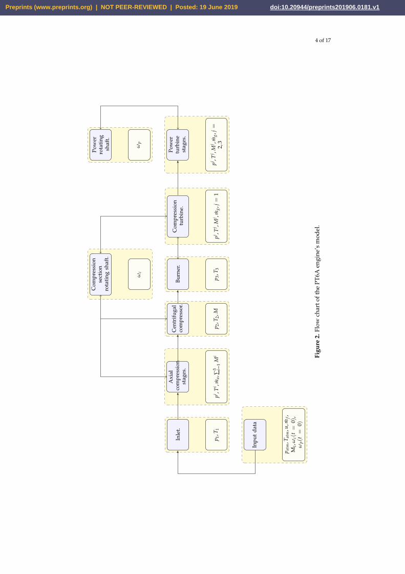
article.58

2. The PT6A engine model59

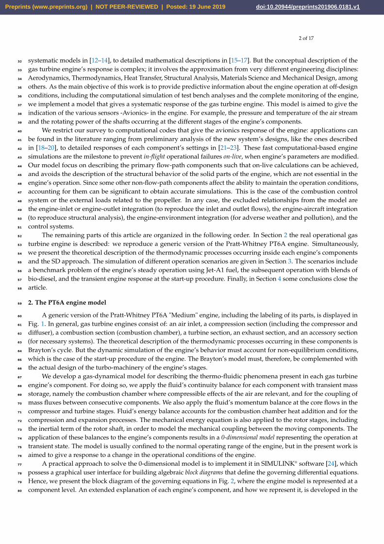
A generic version of the Pratt-Whitney PT6A "Medium" engine, including the labeling of its parts, is displayed in60

Fig. 1. In general, gas turbine engines consist of: an air inlet, a compression section (including the compressor and61

diffuser), a combustion section (combustion chamber), a turbine section, an exhaust section, and an accessory section62

(for necessary systems). The theoretical description of the thermodynamic processes occurring in these components is63

Brayton’s cycle. But the dynamic simulation of the engine’s behavior must account for non-equilibrium conditions,64

which is the case of the start-up procedure of the engine. The Brayton’s model must, therefore, be complemented with65

the actual design of the turbo-machinery of the engine’s stages.66

We develop a gas-dynamical model for describing the thermo-fluidic phenomena present in each gas turbine67

engine’s component. For doing so, we apply the fluid’s continuity balance for each component with transient mass68

storage, namely the combustion chamber where compressible effects of the air are relevant, and for the coupling of69

mass fluxes between consecutive components. We also apply the fluid’s momentum balance at the core flows in the70

compressor and turbine stages. Fluid’s energy balance accounts for the combustion chamber heat addition and for the71

compression and expansion processes. The mechanical energy equation is also applied to the rotor stages, including72

the inertial term of the rotor shaft, in order to model the mechanical coupling between the moving components. The73

application of these balances to the engine’s components results in a 0-dimensional model representing the operation at74

transient state. The model is usually confined to the normal operating range of the engine, but in the present work is75

aimed to give a response to a change in the operational conditions of the engine.76

A practical approach to solve the 0-dimensional model is to implement it in SIMULINK® software [24], which77

possess a graphical user interface for building algebraic block diagrams that define the governing differential equations.78

Hence, we present the block diagram of the governing equations in Fig. 2, where the engine model is represented at a79

component level. An extended explanation of each engine’s component, and how we represent it, is developed in the80

Preprints (www.preprints.org) | NOT PEER-REVIEWED | Posted: 19 June 2019 doi:10.20944/preprints201906.0181.v1

3 of 17

following paragraphs. Moreover, each component’s block diagram will be presented through the detailed explanation81

of each sub-system. We list inputs, parameters, variables, and outputs for each block diagram.82

Figure 1. Cross section of the Pratt-Whitney PT6A engine.

2.1. Air inlet83

One of the main characteristics of this gas turbine engine is that in most aircraft installations it is mounted84

backward in the nacelle. This feature makes that the airflow inside the components of the engine is directed in the85

same direction as the aircraft’s displacement. Another consequence is that the intake is located at the rear part of86

the engine, and therefore, the air passes through the exterior of the aircraft (and the engine itself) before entering to87

the intake. The PT6A design cares for guiding the intake air to the engine using ducts that avoid facing the exhaust88

gases: since the typical requirement is to provide laminar air into the compressor -so that, it can operate at maximum89

efficiency-, the inlet duct changes smoothly from opposing the direction of the airflow to the axially forward direction90

of the aircraft’s speed.91

We define the inlet component as to be the intake air conditioner: even though our model is restricted to an92

on-ground operation, with no rarefying processes of the atmospheric air entering into the engine, we extend the93

possibility of the operation of the model during in-flight operation conditions. This effect is modeled using the relations94

for the pressure and temperature of the air which are presented in the block diagram of Figure 3. In the model, patm,95

and Tatm are the atmospheric pressure and temperature, M = u/c is the flight Mach number that relates the aircraft96

speed u with the speed of sound c =√

γpatm/ρ, γ is the quotient between specific heats of the air, and η is the97

isentropic efficiency. We use the subscript 1 to label the thermodynamic variables of air at the inlet. Note that when the98

engine is supposed to operate in the test bench, the model equates the inlet conditions to the atmospheric conditions99

p1 = patm, and T1 = Tatm.100

2.2. Compression section101

In the PT6A gas turbine engine (used for aviation), the compression section consists of three axial stages and102

a single centrifugal stage, each considered to be a rise in the air’s pressure: the air flows from the inlet duct to the103

low-pressure compressor, and then to the next two axial flow stages before passing to the centrifugal stage. The axial104

stages are composed by rotating blades called rotors, and static blades called stators. Those rotating stages move at105

around 40000 Revolutions Per Minute (RPM) increasing the air’s pressure more than eight times the inlet’s pressure.106

The last stage of the compressor section is composed of a single centrifugal-flow compressor that accelerates the air107

outwardly. This centrifugal section has a high-pressure rise, but since there can be several losses between centrifugal108

Preprints (www.preprints.org) | NOT PEER-REVIEWED | Posted: 19 June 2019 doi:10.20944/preprints201906.0181.v1

4 of 17

Inp

ut

dat

a

Inle

t.A

xial

com

pres

sion

stag

es.

Cen

trif

ugal

com

pres

sor.

Bu

rner

.C

omp

ress

ion

turb

ine.

Pow

ertu

rbin

est

ages

.

Com

pre

ssio

nse

ctio

nro

tati

ngsh

aft.

Pow

erro

tati

ngsh

aft.

p atm

,Tat

m,u

,mf,

Ml,

ωc(

t=

0),

ωp(

t=

0)

p 1,T

1pi ,

Ti ,

ma,

∑3 i=

1M

ip 2

,T2,

Mp 3

,T3

pj ,T

j ,M

j ,m

g,j=

1pj ,

Tj ,

Mj ,

mg,

j=

2,3

ωc

ωp

Figu

re2.

Flow

char

toft

hePT

6Aen

gine

’sm

odel

.

Preprints (www.preprints.org) | NOT PEER-REVIEWED | Posted: 19 June 2019 doi:10.20944/preprints201906.0181.v1

5 of 17

Calculations:ρ, c, M.

Parameters:η, γ.

p1 = patm

[1 + η γ−1

2 M2] γ

γ−1

T1 = Tatm

[1 + γ−1

2 M2]

Inlet modelu Velocity

patmPressure

Tatm

Temperature

Pressure p1

TemperatureT1

Figure 3. Inlet model.

stages, it is restricted to a single stage before discharging the airflow. The air stream then leaves the centrifugal109

compressor section via the diffuser, which is a section of the engine just before the combustion chamber that has the110

function of preparing the air for the burning area so that it can burn uniformly and continuously. We neglect the111

diffuser in our representation of the compression section of the engine.112

A work previous to the modeling of the compressor has to do with the estimation of its geometry. In this sense,113

we determine the compressor’s geometry by extracting most of the information from technical reports, as well as114

from the engine’s manual Whitney [25]. Since the axial compression section geometry has been reported in [26] for a115

four-axial stages PT6A engine, we transcript the geometrical parameters for the first and last stages, but calculate the116

mean values of the second and third stages of that compressor, and set those values as the second axial stage of our117

PT6A axial compressor model. The geometric parameters that we have processed for each axial stage geometry are118

presented in Table 1. In the case of the inner and external radius of the rotor blades, we determine those parameters119

from cross-checking the engine’s manual schemes and the measured values from a disassembled engine. The geometry120

of the centrifugal compressor is described the rotor’s blade geometry and the inlet’s and outlet’s cross-sectional121

dimensions, where the inner r1 and outer r2 radii of the rotor are determined from the engine’s technical report, being122

92 mm and 117 mm, respectively.123

Blade Symbol 1st-stage rotor 2nd-stage rotor 3th-stage rotorInlet air angle, deg. αl 61.5 59.8 58.0Exit air angle, deg. αt 54.4 48.9 42.0Inlet metal angle, deg βl 56.8 57.85 57.1Exit metal angle, deg. βt 50.5 43.5 36.2Inner radius, mm. r0 72 76 80Outter radius, mm. r 100 96 92

Table 1. Processed values of aerodynamic and geometric parameters for the axial compressor stages.

The overall compression stage is defined from the compressor intake (p1, T1) to state 2, at the diffuser outlet124

(p2, T2). Therefore, it covers the three axial stages, the centrifugal stage, and the diffuser of the PT6A engine.125

Knowledge of the inlet (upwind) conditions of the air, such as temperature and pressure, as well as the rotational126

speed of the engine’s rotating shaft, is required. Also, the knowledge of the geometry of the compressor at each stage127

is mandatory to apply the continuity, momentum and energy balances on which the enthalpy raise and the mass flow128

depend. Since each compression section is composed of successive stages of rotating blades (rotors) and stationary129

guide vanes (stators), we analyze at each rotor-stator stage the transmission of the shaft’s mechanical energy into the130

air’s fluid energy and compose the complete compressor performance by adding the multiple successive compression131

stages.132

For simplicity, we assume that the compressor’s blades are thin, rather than having the complete airfoil cross-shape133

geometry. This supposition is acceptable since in the PT6A engine those are constructed of sheet metal. In the case of134

the axial compressor, we analyze a single i−th stage, where a rotor precedes a stator, and consider the same hub radius135

for the rotor as for the stator. We also make this supposition for the shaft radius at each axial stage. Nevertheless,136

we consider different cross areas between consecutive compression stages, such that the axial component of velocity137

can be calculated to conserve mass: in the case of the multistage axial-flow compressor, the blades of each successive138

stage of the compressor get smaller as the air gets further compressed. In each rotor-stator stage, we consider the139

cross section of only one stator and rotor blade as it moves vertically, knowing that the next rotor blade passes shortly140

Preprints (www.preprints.org) | NOT PEER-REVIEWED | Posted: 19 June 2019 doi:10.20944/preprints201906.0181.v1

6 of 17

thereafter. This is the well-known cascade two-dimensional approximation of turbomachinery analysis, and which141

configures our control volume.142

We aim to calculate the variation in the air’s velocity originated by the rotor’s torque. To do this, we apply a143

simplified analysis of the fluid’s dynamics of the air occurring through the blade: the velocity triangle. The axial speed144

of the airflow via can be measured at the inlet section, such that the volume flow rate can be calculated in terms of the145

cross-sectional area. Another possibility is to know the inlet air angle (presented in table 1), such that the axial velocity146

is calculated from the velocity triangle. To evaluate the torque on the rotating shaft, we use the angular momentum147

balance that states that the total momentum in the shaft M is equal to the change between the angular momentum of148

the flow that crosses the surfaces of the control volume. This change is only related to the tangential velocities of the149

air given by the velocity triangle analysis.150

In our model, we consider reversible losses in the compression stages, and therefore, full mechanical efficiency.151

This implies that the shaft power is the same as the power delivered to the air. We suppose a quasi-static process in152

which the difference between the amount of energy in the air is given by the increment in power and calculate the153

temperature rise inside the axial compression stage by applying the energy balance in the control volume. We suppose154

then, that the net pressure head induced by the compressor is modeled as a polytropic process, where the pressure155

ratio Π is related with the temperature variation of the air and the polytropic constant of the gas n. The previous156

exposition is concisely presented in the block diagrams of Figures 4 and 5.157

In the case of the centrifugal compressor, we consider that the circumferential cross-sectional area can be defined158

by the radius and the width of the blade b. For completeness, we suppose that the flow is defined completely in159

the normal direction (v1)n, and therefore, the normal velocity at the outlet of the blade can be calculated with the160

conservation of mass.161

Calculations:ρ, vi

aParameters:

cp, Πi

Geometry(αi , βi , ri)

ma = ρviaπ[(ri)2 − (ri

0)2]

pi = pi−1Πi

Ti = ωC(M)i

macp+ Ti−1

(M)i = rima(via)(tan βi

l − tan βit)

i−th axial-stage compressor model

ωCRotor speed

pi−1 Pressure

Ti−1

Temperature

Mass fluxma

Pressurepi

TemperatureTi

TorqueMi

Figure 4. Axial stages compressor model.

Calculations:ρ,

(v1)n,(v2)n.Parameters:

cp, ΠGeometry(α, β, r, b)

ma = ma

p2 = piΠ

T2 = ωC Mmacp

+ Ti

M = r2ma(v2)t − r1ma(v1)t

Centrifugal compressor modelmaMass flux

ωC Rotor speed

pi Pressure

Ti

Temperature

Mass fluxma

Pressure p2

TemperatureT2

TorqueM

Figure 5. Centrifugal compressor model.

Preprints (www.preprints.org) | NOT PEER-REVIEWED | Posted: 19 June 2019 doi:10.20944/preprints201906.0181.v1

7 of 17

2.3. Burner162

The PT6A burner is mainly characterized by the split in the amount of compressed air that is used for maintaining163

the combustion: only a fraction of the air entering in the burner reacts with the fuel, while most of the compressed164

air is used for cooling purposes. The geometrical shape of the burner chamber is an annulus. In this sense, the165

overall volume is hard to be determined and we have approximated its value from measurements of the disassembled166

engine’s burner to be around 0.028 m3.167

Inside the burner, the fuel and the air are separated apart before the flame: combustion with the liquid fuel168

is performed by the injection of the fuel inside the air stream. Scattering of the fluid into fine droplets leads to the169

convection and final evaporation of the liquid inside the compressed air-stream. This mixture is a steady non-premixed170

stream of air-fuel before the full combustion reaction takes place inside the burner. Buoyant mechanisms, but mostly171

forced convection and turbulence mechanisms of inlet air (due to its high pressure and temperature at the exit of172

the compression section) maintain the combustion process in the flame. The reaction rate and the products of the173

combustion (exhaust gases) depend on the quality of the air-fuel mixture occurring before the flame.174

The combustion quality is automatically controlled by the combustion control system that fixes the amount of175

injection of fuel; this control is set by default for the Jet-A1 fuel. We neglect the combustion control in our present176

approach since we aim to investigate the response of the engine to different blends with biodiesel. The change in the177

physical properties of the fuel affects its spraying as it passes through the fuel injectors in the combustion chamber.178

This has effects on the maximum temperature inside the fuel chamber at the start-up of the engine. In this sense, the179

starting procedure has to be designed to be rigorous and must be established for each new operating fuel. For all the180

above, computational simulation of the particular gas turbine engine’s performance is proposed as a predictive tool181

for the engine operation, which allows determining the operation variables when the change in the composition of the182

fuel occurs. This, with a low cost, and without risking the operation of test engines.183

Our approach to model the burner’s combustion phenomena is simple. The net power of the gas turbine engine184

is related to the amount of fuel that is burned inside the burner: the heat added to the air-stream is calculated from185

the energy balance inside the burning chamber, where LHV is the Low Heating Value of the fuel that represents the186

amount of energy that is delivered in the combustion process (accounting for the steam boiling in the liquid fuel). This187

is depicted in the block diagram of Figure 6.188

Note that the amount of chemical energy that is transferred to the air (which is later transformed to mechanical189

energy in the turbine) depends on the type of fuel used, and this is completely characterized by the fuel flow rate190

and its lower heating value. The burner also works as an accumulator of mass, where the temporal change of the191

thermodynamic conditions of the air inside the burner is related to the amount of fuel m f , the incoming air flow rate192

ma, the exhausting rate flow of gasses mg, and the volume of the chamber VB. Nevertheless, we describe the temporal193

variation of the pressure inside the burner to be solely represented by a loss of pressure (with coefficient Cb ≤ 1).194

Calculations:ρ.

Parameters:Cb, cp, LHV.

GeometryVB.

p3 = Cb p2

ρVbcpdT3dt = macp(T2 − T3) + m f (LHV − cpT3)

Burner model

ma, m f , mg Mass fluxes

p2Pressure

T2

Temperature

Pressure p3

TemperatureT3

Figure 6. Burner model.

2.4. Turbine section195

The air stream leaves the burner with the addition of heat from the combustion and flows through several turbine196

stages. The first turbine stage is a single-stage axial turbine that powers the compression section synchronously197

rotating at 40000 RPM via the engine spool, or common shaft. We determine from measurements of the disassembled198

engine spool an overall mass moment of inertia of the engine spool of about 0.12 Kg m2.199

Preprints (www.preprints.org) | NOT PEER-REVIEWED | Posted: 19 June 2019 doi:10.20944/preprints201906.0181.v1

8 of 17

In the PT6A, the hot air flows then into the power turbines, which are composed by two axial stages that turn at200

about 30000 RPM, and that are connected to the main shaft that drives the propeller (or load). We also determine that201

the mass moment of inertia of the main shaft is 0.06 Kg m2. The air is discharged next to the exhaust, and then to the202

atmosphere, where the air recovers its original free-stream conditions.203

The turbine process is defined from the state 3 at the combustion chamber outlet (p3, T3) to state 4, at the engine204

outlet (p4, T4). This means that the expansion ratio of the gas is known for the turbine section. Indeed, knowing the205

expansion ratio of the j−th stage Πj, one can model each turbine stage as a polytropic expansion process where the206

pressure and temperature of the air at the discharge can be calculated straightforward.207

The temperature drop is used then to calculate the retrieved mechanical power inside the turbine. Again, we208

suppose a complete transformation efficiency between the fluidic and the mechanical power, such that the extracted209

torque at each axial stage of the turbine is equal to the change in the angular momentum of the air inside the turbine.210

Similarly to the axial flow compressor analysis, an accurate model of the turbine performance can be derived from a211

detailed computation of the aerodynamics of the flow over the individual blade elements. The distinctive feature of212

the turbine is that the mass flow rate of gases through the turbine section depends on the expansion work: we use the213

angular momentum balance in order to obtain the mass flow of gases through the turbine stage, and therefore, the214

axial term of the air velocity. The turbine relations are presented in the block diagrams of Figures 7 and 8.215

Calculations:ρ, vj

a.Parameters:

cp, Πj

Geometry(βj, rj)

mg = vjaρπ

((rj)2 − r2

0)

pj = p3/Πj

T j = T3

(Πj)

((n−1)

n

)

Mj = rjmg(vja)(tan β

jl − tan β

jt)

Compression section turbine model

ωcRotor speed

p3Pressure

T3

Temperature

Mass flux mg

Pressurepj

TemperatureT j

TorqueMj

Figure 7. Compression section turbine model.

Calculations:ρ, vj

a.Parameters:

cp, Πj

Geometry(βj, rj)

mg = vjaρπ

((rj)2 − r2

0)

pj = pj−1/Πj

T j = T j−1

(Πj)

((n−1)

n

)

Mj = rjmg(vja)(tan β

jl − tan β

jt)

Power turbine modelmgMass flux

ωp Rotor speed

pj−1 Pressure

T j−1

Temperature

Mass flux mg

Pressurepj

TemperatureT j

TorqueMj

Figure 8. Power turbine model.

2.5. Rotating Shafts216

The rotating shafts are modeled by applying the balance of angular momentum. We use the rigid body assumption,217

and apply the momentum balance in the rotational motion, such that the acceleration power of the shaft must equal218

the balance between turbine power, compression (or load) power, and parasitic powers. The angular momentum219

balance applied to the engine spool, as well as the power rotating shaft is presented in the block diagrams of Figures 9220

and 10. We define IR to be the mass moment of inertia of the rotating shaft about its rotating axis, M is each one of the221

torques applied to the shaft, and ω is the angular velocity of the shaft which can be calculated in terms of ω = Nπ/60,222

Preprints (www.preprints.org) | NOT PEER-REVIEWED | Posted: 19 June 2019 doi:10.20944/preprints201906.0181.v1

9 of 17

being N the revolutions per minute. We assume a parasitic power from the friction of the rotating shaft. The parasitic223

torque M f can be modeled as a bearing friction coefficient b that multiplies the rotational speed, with its effect acting224

in the contrary-rotation sense.225

Parameters:IRc, bc,

ωc(t = 0).IRc

dωcdt = ∑3

i=1 (M)i + M + (M)j=1 − M f c

Engine spool model(M)i , M Compressor’s torque

Mj=1

Turbine’s torque

Angular speedωc

Figure 9. Compression section rotor shaft model.

Parameters:IRp, bp,

ωp(t = 0).IRp

dωpdt = ∑3

j=2 (M)j + Ml −M f p

Power rotor model

MlLoad’s torque

(M)jTurbine’s torque

Angular speedωp

Figure 10. Power turbines rotor model.

2.6. Compatibility conditions226

Besides the physical description of each engine’s component, one must close the engine’s model coupling the227

different components to what is referred to the compatibility conditions.228

The mass compatibility conditions are related to the conservation of the air mass flow rate. The inlet’s air mass229

flow rate ma is calculated by knowing the inlet air angle at the first axial stage, such that the axial velocity can be230

calculated knowing the rotational speed and the geometric parameters of the rotor blades. It has been explained231

that ma is conserved among the stages of the compression section. Nevertheless, the mass compatibility condition232

differs substantially when the air enters the burner: the exhaust gasses mass flow rate mg is not only related to the233

compressed air flow ma reacting with the mass flow of fuel m f , but the exhaust gasses depend on the flow through the234

turbine section and the engine’s exhaust. Here the compatibility condition is related to the mass flow rate resulting235

from each turbine stage. Some further explanation about this compatibility condition will be taken in the next section.236

On the other hand, the angular momentum compatibility condition is the balance of the torques applied for each237

rotating shaft. Its readily understood that the rotation speed of the axial and centrifugal compressor stages matches238

with the compressor’s turbine via the engine spool. In the same line, the velocity of the power turbines rotating shaft239

matches the propeller’s shaft velocity through the reduction gear.240

Finally, the energetic compatibility conditions are associated with the thermodynamic variables of the air at each241

one of the stages of the engine. It has been readily mentioned that the air enters each consecutive stage with the242

pressure and temperature conditions that it obtains at the stage immediately before. This is clear from the overall243

system’s block diagram depicted in Figure 2.244

3. Numerical Results245

In this section, we present the numerical results for several different simulation scenarios. The first scenario is the246

steady response of the engine which is intended to validate the computational model. Then, we solve the steady-state247

operation by using the blends with biodiesel. Finally, we address the transient operation of the engine using the fuel248

blends, specifically at the start-up of the engine, when the maximum temperatures can be reached. We suppose an249

on-ground operation in all scenarios so that the inlet velocity is set to zero.250

Preprints (www.preprints.org) | NOT PEER-REVIEWED | Posted: 19 June 2019 doi:10.20944/preprints201906.0181.v1

10 of 17

Table 2. On-ground steady operation conditions using Jet-A1 fuel. Extracted from [25].

Standard conditions ValueAtmospheric temperature 288 K

Atmospheric pressure 101352.9 paLHV of Jet-A1 fuel 42.8 MJ/Kg

Jet-A1 fuel mass flow 0.062 Kg/sPropeller’s load (at propeller’s shaft) 2684.51 N.m

3.1. Validation of the computational model251

We first validate the computational model by considering a standard operation of the PT6A engine reported in the252

operation manual [25]. The geometrical parameters of the PT6A motor are implemented in the computational model253

correspondingly to Section 2. The operation parameters are presented in Table 2, where the International Standard254

Atmosphere (ISA) conditions are set as the environmental conditions. We also assume a constant flow of Jet-A1 fuel,255

with a calorific power of 42.8 MJ/Kg, and a constant propeller’s load of 2684.51 N.m. We evaluate the stationary256

response of some tracked variables (invariant in time): for the sake of validation, we track the stationary pressure,257

temperature and air flow at the stations of the engine. We also set the polytropic constant of the air to n = 1.4, and258

fit some remaining geometric parameters of the model so that we obtain the closest numerical results to the ones259

reported in the operation manual. In Table 3 we list the experimental results that have been previously reported in the260

operation manual for several stations of the engine, and that we use for the sake of comparisons.261

We first determine the compression and expansion ratios based on the experimental measurements. The overall262

compression ratio at the axial stages can be calculated from the data in Table 3 to be 3.14 : 1 atm, while for the263

centrifugal compressor the compression ratio is around 2.56 : 1 atm. In this sense, we fit the centrifugal compressor’s264

angles β1 and β2 to 40 and 38 degrees, respectively, such that the centrifugal compressor gives rise to the pressure265

change. On the other hand, the expansion ratio for the compression and power turbines are calculated to be 1 : 3.03266

atm and 1 : 2.18 atm, respectively. We suppose an expansion ratio of 1 : 1.47 atm for each stage of the power turbines267

section, and fit the blade’s angles in order to fulfill the mass flow rate compatibility (conservation) condition between268

the different turbine stages. Table 4 presents the fitted aerodynamic and geometric parameters for all the turbine269

stages of the PT6A engine that have been processed. These parameters have been determined following the previously270

exposed ideas, from cross-checking the engine’s manual schemes and the measured values from a disassembled271

engine, but mostly from the fulfillment of the mass conservation requirement. The rotor blade airfoils, which are metal272

profiles followed and preceded by stator vanes, are completely defined by these geometric parameters. Finally, the273

parasitic power that is lost due to friction can be modeled by setting the bearing coefficients bc and bp to 0.04 Kg.m2/s274

and 0.05 Kg.m2/s, respectively, for the engine spool and power rotor shaft. We also model the pressure loss coefficient275

in the burner to be Cb = 0.95.276

The simulated steady engine response is presented in Table 5. In that table, we list the temperature and277

pressure along the stations of the PT6A engine, together with the calculated relative error against the experimental278

measurements. We confirm a consistent physical behavior of those thermodynamic variables. Distinctively, the279

observed pressure at the discharge of the axial compressor stages is higher than the reported one. This inaccuracy is280

countered by the centrifugal compression section, where the blade’s geometrical parameters are fitted to give accurate281

results of the overall compression ratio. In this regard, fitting the compressor’s parameters affects negatively the282

accuracy of the temperature at the discharge of the compression stage, but the energy balance inside the combustion283

chamber counteracts this effect, and matches the stipulated temperature in the manual, with an error of only 1.57%.284

Temperature and pressure variables at the expansion stages correspond well to the experimental counterparts, mainly285

due to the possibility of fixing the expansion relation and the geometrical parameters of the turbines. Given the286

previous exposition, we believe that the error is restricted to a low range such that it validates the usage of the287

proposed model for predicting the engine response when new operating conditions are evaluated.288

3.2. Stationary operation of the PT6A using fuel blends289

Once the computational model has been validated, the following simulation scenarios are considered: we evaluate290

the stationary operation of the PT6A-42 engine at both 100% of the fuel mass flow and 60% of the fuel flow, meaning291

Preprints (www.preprints.org) | NOT PEER-REVIEWED | Posted: 19 June 2019 doi:10.20944/preprints201906.0181.v1

11 of 17

Table 3. Temperatures and pressures for PT6A-42 engine at 850 shp and ISA standard conditions. Extracted from [25].

Station Location Temperature (K) Pressure (pa)0 Ambient 288 101352.91 Compressor Inlet 288.2 102042.4

1.5 Interstage Compressor 415.4 307506.22 Compressor Discharge 610.4 787381.283 Turbine 1212.1 770144.39

3.5 Inter Turbine 967.1 246142.84 Turbine Exit 811.5 1130745 Exhaust 811.5 106179.3

Table 4. Fitted aerodynamic and geometric parameters of the turbine stages.

Blade 1st-stage rotor 2nd-stage rotor 3th-stage rotorInlet metal angle, deg -20 -20 -20Exit metal angle, deg. 80 43 43Inner radius, mm. 92 90 88Outter radius, mm. 117 125 142

two different engine operation throttles. Since we aim to predict the engine’s response to the usage of new hypothetical292

fuels, we vary the parameters that represent the fuel and perform the simulation. In this sense, the standard Jet-A1293

fuel is mainly composed of n−heptane and isooctane, which are hydrocarbons that possess between 8 and 16 carbon294

atoms per molecule, giving a LHV of around 42.8 MJ/Kg (measured in experimental tests [27]). On the other hand,295

the chemical composition of a biodiesel sample results in an approximated LHV value of 36.29 MJ/Kg [28]. Hence,296

the pure biodiesel retains a smaller amount of energy than conventional Jet-A1 fuel. We simulate the operation with297

biodiesel fuel, as well as other hypothetical blends of Jet-A1 with biodiesel. In this sense, we establish a discrete range298

of mass concentrations of biodiesel in Jet-A1 which are 3 in total: 10% of biodiesel (B10), 20% of biodiesel (B20), and299

30% of biodiesel (B30). These concentrations give a LHV of 40.84 MJ/Kg, 41.49 MJ/Kg, and 42.14 MJ/Kg, respectively.300

In the successive, we plot the simulation results for the different types of fuel, so that they are easy to compare visually.301

We adopt the following notation in the plots for each type of fuel: we use a � to denote the pure biodiesel fuel, a302

? to denote the B10 fuel, a4 to denote the B20 fuel, a ∗ to denote the B30 fuel, and a© to denote the Jet-A1 fuel.303

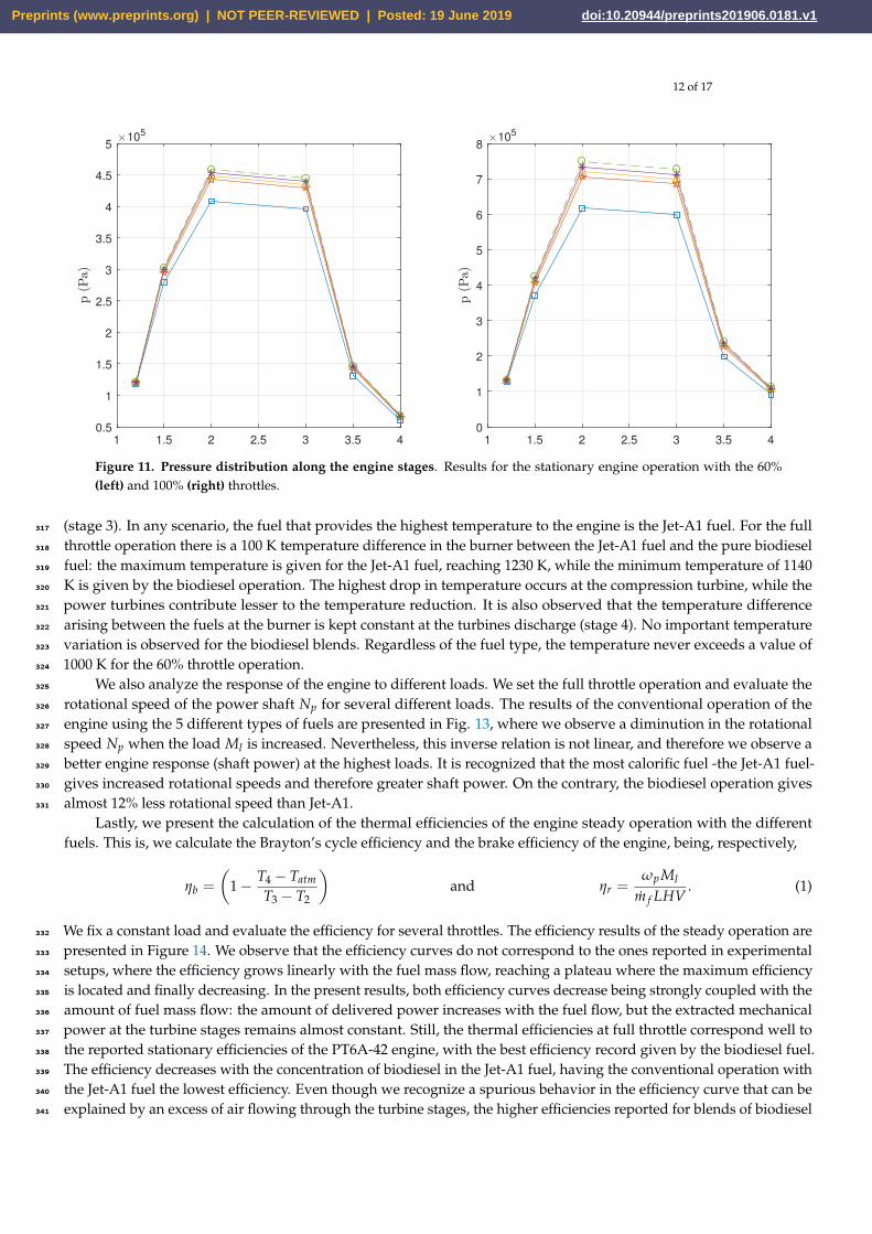
Figure 11 shows the air pressure through the engine stages for the two different throttle ranges. We clearly observe304

a pressure rise at the compression section, as well as an expansion process at the turbine stages. It is evident for both305

operations ranges that the maximum pressure is located at the centrifugal compressor’s discharge (stage 2) and that306

there is a slight loss in this pressure at the burner (stage 3). In the full throttle case (right side of the figure), it can be307

observed that the pressure gap inside the burner between the Jet-A1 fuel and the pure biodiesel fuel is considerable,308

with an observable maximum pressure of 750 kPa and a lower pressure of 610 kPa. In the case of the 60% throttle,309

there is a difference of 60 kPa between those fuels, with a maximum pressure of 460 kPa and a minimum pressure of310

approximately 400 kPa. The fuel blends give results that lay below some 5% of the Jet-A1 pressure range. In any case,311

the maximum values of pressure are related to the use of the Jet-A1 fuel. This can be explained since it delivers the312

highest amount of power, which in turn is extracted by the turbine stage and transferred to the compression section313

via the engine spool.314

Figure 12 displays the air temperature through the engine stages for the two different throttles. The temperature315

results agree well with those reported in the manual: the maximum air temperature is observed at the burner discharge316

Table 5. Simulation results. Stationary temperatures and pressures at different stations of the PT6A-42 engine. Therelative error is calculated against the reported results in Table 3.

Station T (K) Error (%) p (pa) Error (%)1.5 433.63 4.39 423635.89 37.762 510.44 16.38 749710.57 4.783 1231.15 1.57 727219.25 5.57

3.5 896.92 7.26 240006.35 2.494 719.69 11.31 1111067.77 1.77

Preprints (www.preprints.org) | NOT PEER-REVIEWED | Posted: 19 June 2019 doi:10.20944/preprints201906.0181.v1

12 of 17

1 1.5 2 2.5 3 3.5 4

0.5

1

1.5

2

2.5

3

3.5

4

4.5

510

5

1 1.5 2 2.5 3 3.5 4

0

1

2

3

4

5

6

7

810

5

Figure 11. Pressure distribution along the engine stages. Results for the stationary engine operation with the 60%(left) and 100% (right) throttles.

(stage 3). In any scenario, the fuel that provides the highest temperature to the engine is the Jet-A1 fuel. For the full317

throttle operation there is a 100 K temperature difference in the burner between the Jet-A1 fuel and the pure biodiesel318

fuel: the maximum temperature is given for the Jet-A1 fuel, reaching 1230 K, while the minimum temperature of 1140319

K is given by the biodiesel operation. The highest drop in temperature occurs at the compression turbine, while the320

power turbines contribute lesser to the temperature reduction. It is also observed that the temperature difference321

arising between the fuels at the burner is kept constant at the turbines discharge (stage 4). No important temperature322

variation is observed for the biodiesel blends. Regardless of the fuel type, the temperature never exceeds a value of323

1000 K for the 60% throttle operation.324

We also analyze the response of the engine to different loads. We set the full throttle operation and evaluate the325

rotational speed of the power shaft Np for several different loads. The results of the conventional operation of the326

engine using the 5 different types of fuels are presented in Fig. 13, where we observe a diminution in the rotational327

speed Np when the load Ml is increased. Nevertheless, this inverse relation is not linear, and therefore we observe a328

better engine response (shaft power) at the highest loads. It is recognized that the most calorific fuel -the Jet-A1 fuel-329

gives increased rotational speeds and therefore greater shaft power. On the contrary, the biodiesel operation gives330

almost 12% less rotational speed than Jet-A1.331

Lastly, we present the calculation of the thermal efficiencies of the engine steady operation with the differentfuels. This is, we calculate the Brayton’s cycle efficiency and the brake efficiency of the engine, being, respectively,

ηb =

(1− T4 − Tatm

T3 − T2

)and ηr =

ωp Ml

m f LHV. (1)

We fix a constant load and evaluate the efficiency for several throttles. The efficiency results of the steady operation are332

presented in Figure 14. We observe that the efficiency curves do not correspond to the ones reported in experimental333

setups, where the efficiency grows linearly with the fuel mass flow, reaching a plateau where the maximum efficiency334

is located and finally decreasing. In the present results, both efficiency curves decrease being strongly coupled with the335

amount of fuel mass flow: the amount of delivered power increases with the fuel flow, but the extracted mechanical336

power at the turbine stages remains almost constant. Still, the thermal efficiencies at full throttle correspond well to337

the reported stationary efficiencies of the PT6A-42 engine, with the best efficiency record given by the biodiesel fuel.338

The efficiency decreases with the concentration of biodiesel in the Jet-A1 fuel, having the conventional operation with339

the Jet-A1 fuel the lowest efficiency. Even though we recognize a spurious behavior in the efficiency curve that can be340

explained by an excess of air flowing through the turbine stages, the higher efficiencies reported for blends of biodiesel341

Preprints (www.preprints.org) | NOT PEER-REVIEWED | Posted: 19 June 2019 doi:10.20944/preprints201906.0181.v1

13 of 17

1 1.5 2 2.5 3 3.5 4

300

400

500

600

700

800

900

1000

1 1.5 2 2.5 3 3.5 4

300

400

500

600

700

800

900

1000

1100

1200

1300

Figure 12. Temperature distribution along the engine stages. Results for the stationary engine operation with the 60%(left) and 100% (right) throttles.

1000 1500 2000 2500 3000

2.6

2.8

3

3.2

3.4

3.6

3.8

4

4.2

4.410

4

Figure 13. Rotational speed of the power shaft. Results for different loads.

Preprints (www.preprints.org) | NOT PEER-REVIEWED | Posted: 19 June 2019 doi:10.20944/preprints201906.0181.v1

14 of 17

20 40 60 80 100

0.4

0.45

0.5

0.55

0.6

0.65

0.7

0.75

20 40 60 80 100

0.2

0.25

0.3

0.35

0.4

0.45

0.5

0.55

0.6

Figure 14. Efficiency results. Thermal efficiency (left) and brake efficiency (right) for the engine operation with differentthrottles.

are promissory. Also, the combustion control -which has been neglected in the present model- may help to explain the342

difference between the present results and the experimental ones, since it reduces the amount of fuel entering the343

engine when the air flowing through the engine stages is not sufficient to perform stoichiometric combustion.344

3.3. Transient operation of the PT6A motor using fuel blends345

Finally, we evaluate the start-up procedure of the engine with the fuel types that have been tested in previous346

scenarios. The main goal is to identify problematic conditions during the engine start-up, which is the transient347

procedure that can actually affect the engine’s integrity. For reproducing the start-up scenario, we initialize the engine348

spool to an angular velocity of Nc(t = 0) = 12000 RPM, that is the rotational speed that is provided by the starter.349

From this point, there is a positive increment of the air pressure (given by the rotation of the compression system)350

until the desired mass flow of air into the burner is granted. During the initial compression operation, no fuel mass351

flow is injected into the burner. We consider that at a later instant (t = 10) s, when the compressed air into the burner352

stabilizes, the fuel is injected into the burner and ignited. The mass fuel flow is then gradually increased until the353

desired throttle is reached at (t = t f ). All the start-up procedure is considered to undergo with a constant load.354

We aim to evaluate the start-up procedure of the PT6A-42 engine with both 100% and 60% of throttle. The results355

for the operation with fuel blends are displayed similarly as for the stationary operation. We present comparisons of356

some important variables, such as the air pressure at the compressor discharge and the air temperature inside the357

burner. It is noticeable that the start-up procedure converges to the steady-state operation.358

Figure 15 shows the transient pressure results at the compression stage for the two different throttles. It can be359

observed that the pressure in the compressor’s discharge undergoes an initial equilibrium when the engine spool is360

started, reaching a compression ratio below of 1.5 : 1 atm. At (t = 10) s, when the fuel is ignited, a sudden increment361

of the compression ratio of around 2 : 1 atm is noticed for all fuels and throttles. In the case of the 60% throttle, the362

pressure stabilizes from this instantaneous peak, but the pressure keeps increasing for the full throttle case reaching363

the reported 8 : 1 atm compression ratio. There is not a significant pressure fluctuation related to the fuel blends: it can364

only be appreciated a moderate increment for the full throttle and the biodiesel fuel than for the blends and Jet-A1 fuel.365

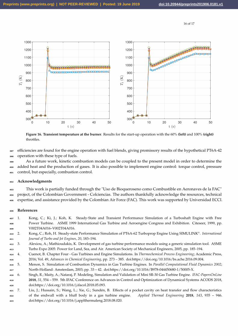
The transient temperature inside the burner is presented in Figure 16 for the two different throttles. We observe a366

slight increment in the temperature at the initial compression operation. Then, the fuel intake generates a temperature367

peak in the combustion chamber, which in all scenarios is the maximum temperature that is reached throughout the368

operation of the engine. Since the initial fuel flow is the same for both throttle scenarios, the maximum temperature in369

Preprints (www.preprints.org) | NOT PEER-REVIEWED | Posted: 19 June 2019 doi:10.20944/preprints201906.0181.v1

15 of 17

0 10 20 30 40 50

1

1.5

2

2.5

3

3.5

4

4.510

5

0 10 20 30 40 50

1

2

3

4

5

6

7

810

5

Figure 15. Transient pressure at the compressor’s discharge. Results for the start-up operation with the 60% (left) and100% (right) throttles.

the engine does not vary. Instead, it only depends on the fuel blend, where the maximum temperature of 1220 K inside370

the burner is obtained with the Jet-A1 fuel, and the minimum of 1100 K, approximately, is obtained with the pure371

biodiesel. After this critical instant, the temperature stabilizes at around 1000 K for the 60% case, with a fluctuation372

of less than 100 K between the blends and the biodiesel fuel. On the other hand, the temperature in the full throttle373

scenario increases gradually until the steady state of 1200K is reached at about 40 s.374

4. Conclusions375

In this article, we have simulated the PT6A engine operating at off-design conditions. For this, we have simplified376

the PT6A engine in a process that extracted the essential components of the engine and eliminated the auxiliary ones.377

The mass, linear momentum, angular momentum, and energy balances have been applied into these components, by378

which together with the compatibility conditions compose a 0-dimensional thermo-fluidic model of the engine. We379

have implemented the numerical solution of the model in the SIMULINK software and different simulation scenarios380

have granted the predictive capacity of our computational model in relation to the systemic response of the engine.381

Firstly, we have performed a comparison of some thermodynamic variables against the ones reported in the PT6A-42382

manual. The distribution of temperatures and pressures through each of the engine stages shows similar behavior to383

that predicted in the thermodynamic theory, as well as in the previously reported experimental measurements of the384

engine. The relative error between the present results and those reported in the manual is below 10% for most of the385

stages.386

The evaluation of the engine response against the change in the composition of the fuel has been achieved next:387

on one side, to test the hypothetical operation of the engine with blends of biodiesel, but also to predict the start-up388

response of the engine, which is a complex and transient phenomenon that depends greatly on the type of fuel. In389

the transient engine starting procedure, the air inside the chamber reaches a temperature peak at the moment of fuel390

ignition, and the ratio of this temperature to the fuel type is crucial. The simulation results allow us to conclude that391

the use of blends of biodiesel that are less energetic than the conventional Jet-A1 fuel would not generate a burner392

overheating since the standard temperature of 1220 K inside the chamber is never exceeded. It is also clear that fuel393

blends would not generate a pressure excess in the compressor’s discharge, and consequently, these can not generate394

internal damage to the motor structure. We have also observed that the thermodynamic efficiencies are closely related395

to the amount of air flowing through the power turbines, as well as to the hypothetical fuel heating value: higher396

Preprints (www.preprints.org) | NOT PEER-REVIEWED | Posted: 19 June 2019 doi:10.20944/preprints201906.0181.v1

16 of 17

0 10 20 30 40 50

300

400

500

600

700

800

900

1000

1100

1200

1300

0 10 20 30 40 50

300

400

500

600

700

800

900

1000

1100

1200

1300

Figure 16. Transient temperature at the burner. Results for the start-up operation with the 60% (left) and 100% (right)throttles.

efficiencies are found for the engine operation with fuel blends, giving promissory results of the hypothetical PT6A-42397

operation with these type of fuels.398

As a future work, kinetic combustion models can be coupled to the present model in order to determine the399

added heat and the production of gases. It is also possible to implement engine control: torque control, pressure400

control, but especially, combustion control.401

Acknowledgments402

This work is partially funded through the "Uso de Bioqueroseno como Combustible en Aeronaves de la FAC"403

project, of the Colombian Government - Colciencias. The authors thankfully acknowledge the resources, technical404

expertise, and assistance provided by the Colombian Air Force (FAC). This work was supported by Universidad ECCI.405

References406

1. Kong, C.; Ki, J.; Koh, K. Steady-State and Transient Performance Simulation of a Turboshaft Engine with Free407

Power Turbine. ASME 1999 International Gas Turbine and Aeroengine Congress and Exhibition. Citeseer, 1999, pp.408

V002T04A016–V002T04A016.409

2. Kong, C.; Roh, H. Steady-state Performance Simulation of PT6A-62 Turboprop Engine Using SIMULINK®. International410

Journal of Turbo and Jet Engines, 20, 183–194.411

3. Alexiou, A.; Mathioudakis, K. Development of gas turbine performance models using a generic simulation tool. ASME412

Turbo Expo 2005: Power for Land, Sea, and Air. American Society of Mechanical Engineers, 2005, pp. 185–194.413

4. Cuenot, B. Chapter Four - Gas Turbines and Engine Simulations. In Thermochemical Process Engineering; Academic Press,414

2016; Vol. 49, Advances in Chemical Engineering, pp. 273 – 385. doi:https://doi.org/10.1016/bs.ache.2016.09.004.415

5. Menon, S. Simulation of Combustion Dynamics in Gas Turbine Engines. In Parallel Computational Fluid Dynamics 2002;416

North-Holland: Amsterdam, 2003; pp. 33 – 42. doi:https://doi.org/10.1016/B978-044450680-1/50005-X.417

6. Singh, R.; Maity, A.; Nataraj, P. Modeling, Simulation and Validation of Mini SR-30 Gas Turbine Engine. IFAC-PapersOnLine418

2018, 51, 554 – 559. 5th IFAC Conference on Advances in Control and Optimization of Dynamical Systems ACODS 2018,419

doi:https://doi.org/10.1016/j.ifacol.2018.05.093.420

7. Liu, J.; Hussain, S.; Wang, L.; Xie, G.; Sundén, B. Effects of a pocket cavity on heat transfer and flow characteristics421

of the endwall with a bluff body in a gas turbine engine. Applied Thermal Engineering 2018, 143, 935 – 946.422

doi:https://doi.org/10.1016/j.applthermaleng.2018.08.020.423

Preprints (www.preprints.org) | NOT PEER-REVIEWED | Posted: 19 June 2019 doi:10.20944/preprints201906.0181.v1

17 of 17

8. Sousa, J.; Paniagua, G.; Collado-Morata, E. Thermodynamic analysis of a gas turbine engine with a rotating detonation424

combustor. Applied Energy 2017, 195, 247 – 256. doi:https://doi.org/10.1016/j.apenergy.2017.03.045.425

9. Wang, M.; Chen, Y.; Liu, Q. Experimental study on the gas engine speed control and heating performance of a gas426

Engine-driven heat pump. Energy and Buildings 2018, 178, 84 – 93. doi:https://doi.org/10.1016/j.enbuild.2018.08.041.427

10. Xia, Z.; Tang, X.; Luan, M.; Zhang, S.; Ma, Z.; Wang, J. Numerical investigation of two-wave collision and wave428

structure evolution of rotating detonation engine with hollow combustor. International Journal of Hydrogen Energy 2018.429

doi:https://doi.org/10.1016/j.ijhydene.2018.09.165.430

11. Smirnov, N.; Nikitin, V.; Stamov, L.; Mikhalchenko, E.; Tyurenkova, V. Rotating detonation in a431

ramjet engine three-dimensional modeling. Aerospace Science and Technology 2018, 81, 213 – 224.432

doi:https://doi.org/10.1016/j.ast.2018.08.003.433

12. Dagaut, P.; Cathonnet, M. The ignition, oxidation, and combustion of kerosene: A review of experimental and kinetic434

modeling. Progress in Energy and Combustion Science 2006, 32, 48 – 92. doi:https://doi.org/10.1016/j.pecs.2005.10.003.435

13. Nascimento, M.; Lora, E.; Corrêa, P.; Andrade, R.; Rendon, M.; Venturini, O.; Ramirez, G. Biodiesel fuel436

in diesel micro-turbine engines: Modelling and experimental evaluation. Energy 2008, 33, 233 – 240. 19th437

International Conference on Efficiency, Cost, Optimization, Simulation and Environmental Impactof Energy Systems,438

doi:https://doi.org/10.1016/j.energy.2007.07.014.439

14. Azami, M.; Savill, M. Comparative study of alternative biofuels on aircraft engine performance. Proceedings440

of the Institution of Mechanical Engineers, Part G: Journal of Aerospace Engineering 2017, 231, 1509–1521,441

[https://doi.org/10.1177/0954410016654506]. doi:10.1177/0954410016654506.442

15. Gatto, E.; Li, Y.; Pilidis, P. Gas turbine off-design performance adaptation using a genetic algorithm. ASME Turbo Expo443

2006: Power for Land, Sea, and Air. American Society of Mechanical Engineers, 2006, pp. 551–560.444

16. Li, Y.; Ghafir, M.; Wang, L.; Singh, R.; Huang, K.; Feng, X.; Zhang, W. Improved multiple point nonlinear genetic algorithm445

based performance adaptation using least square method. Journal of Engineering for Gas Turbines and Power 2012, 134, 031701.446

17. Li, Y.; Ghafir, M.; Wang, L.; Singh, R.; Huang, K.; Feng, X. Nonlinear multiple points gas turbine off-design performance447

adaptation using a genetic algorithm. Journal of Engineering for Gas Turbines and Power 2011, 133, 071701.448

18. Pan, M.; Cao, L.; Zhou, W.; Huang, J.and Chen, Y. Robust decentralized control design for aircraft engines: A fractional type.449

Chinese Journal of Aeronautics 2018. doi:https://doi.org/10.1016/j.cja.2018.08.004.450

19. Zhang, T.; Wu, H.; Fang, Q.; Huang, T.; Gong, Z.; Peng, Y. UHP-SFRC panels subjected to aircraft engine451

impact: Experiment and numerical simulation. International Journal of Impact Engineering 2017, 109, 276 – 292.452

doi:https://doi.org/10.1016/j.ijimpeng.2017.07.012.453

20. Balli, O. Advanced exergy analyses of an aircraft turboprop engine (TPE). Energy 2017, 124, 599 – 612.454

doi:https://doi.org/10.1016/j.energy.2017.02.121.455

21. Sirignano, W.; Liu, F. Performance increases for gas-turbine engines through combustion inside the turbine. Journal of456

propulsion and power 1999, 15, 111–118.457

22. Liu, F.; Sirignano, W. Turbojet and turbofan engine performance increases through turbine burners. Journal of propulsion and458

power 2001, 17, 695–705.459

23. Ghoreyshi, S.; Schobeiri, M. Numerical simulation of the multistage ultra-high efficiency gas turbine engine, UHEGT. ASME460

Turbo Expo 2017: Turbomachinery Technical Conference and Exposition. American Society of Mechanical Engineers, 2017,461

pp. V003T06A034–V003T06A034.462

24. MATLAB Simulink Toolbox, Release 2016a.463

25. Whitney, P.. PT6 TRAINING MANUAL; Canada, 2001.464

26. Yoshinaka, T.; Thue, K. A Cost-Effective Performance Development of the PT6A-65 Turboprop Compressor. ASME 1985465

Beijing International Gas Turbine Symposium and Exposition. Citeseer, 1985, pp. V001T02A015–V001T02A015.466

27. Cheng, T.; Simone, H. Measurements of laminar flame speeds of liquid fuels: Jet-A1, diesel, palm methyl esters467

and blends using particle imaging velocimetry (PIV). Proceedings of the Combustion Institute 2011, 33, 979 – 986.468

doi:https://doi.org/10.1016/j.proci.2010.05.106.469

28. Llamas-Lois, A. Biodiesel and biokerosenes: Production, characterization, soot & pah emissions. PhD thesis, ETSI_Energia,470

2015.471

Preprints (www.preprints.org) | NOT PEER-REVIEWED | Posted: 19 June 2019 doi:10.20944/preprints201906.0181.v1