arX

iv:1

004.

4255

v1 [

mat

h.D

G]

24

Apr

201

0

ON CERTAIN SURFACES IN THE EUCLIDEAN SPACE E3

MARIAN IOAN MUNTEANU AND ANA-IRINA NISTOR

Abstract. In the present paper we classify all surfaces in E3 with a canonical principaldirection. Examples of these type of surfaces are constructed. We prove that the only minimalsurface with a canonical principal direction in the Euclidean space E3 is the catenoid.

1. Preliminaries

Due to recent research work in the field of classical differential geometry, the theory of surfacesand submanifolds knew a rapid development. Next to the classical problems of minimality andflatness for different types of surfaces, another topic is represented by the study of constantangle surfaces. Even though in the Euclidean space the constant angle surfaces are knownin literature, in [6] is given a new approach of this problem regarding the ambient space E3

as the product space R2 × R. By definition, a constant angle surface is defined as a surfacefor which its unit normal makes a constant angle with a fixed direction given by the realline R. Projecting the fixed direction on the tangent plane to the surface and denoting byU its tangent part we get that U is a principal direction with null corresponding principalcurvature. Assuming that U remains a principal direction but the corresponding principalcurvature is different from zero - the angle function is no longer constant - we denominateU a canonical principal direction. First result on this topic was given in [3] for the ambientspace S2 × R and the study in H2 × R was done in [4].

In the present paper we classify all surfaces with a canonical principal direction in E3. Inour study we make use of canonical coordinates on the surface, obtaining also classificationtheorems under the extra assumptions of minimality or flatness. For example, we prove thatthe only minimal surface with a canonical principal direction in the Euclidean space E3 isthe catenoid and we give its parametrization in canonical coordinates. Moreover, illustrativeexamples of angle functions are constructed for known surfaces in E3 under harmonicityrestrictions.

Let us consider a surface M isometrically immersed in E3 endowed with the scalar product

〈 , 〉 and with the flat connection ∇̃. Denote by g the metric on M which is the restriction ofthe scalar product on M and by ∇ its corresponding Levi-Civita connection. We consider an

orientation of E3 and we denote by−→k the fixed direction. If N represents the unit normal to

the surface, then θ(p) := ∠(N,−→k ), with θ(p) ∈ (0, π), represents the angle function between

the unit normal and the fixed direction in any point of the surface p ∈M .

2000 Mathematics Subject Classification. 53B25.Key words and phrases. canonical coordinates, minimal surface, Euclidean 3-space.The first author was supported by Grant PN-II ID 398/2007-2010 (Romania).

1

2 M. I. MUNTEANU AND A. I. NISTOR

Classically we have the Gauss and Weingarten formulas for the surface M isometrically im-mersed in E3:

(G) ∇̃XY = ∇XY + h(X,Y )

(W) ∇̃XN = −AXfor every X,Y tangent to M . Moreover h is a symmetric (1, 2)-tensor field called the secondfundamental form of the surface and A is a symmetric (1, 1)-tensor field denoting the shapeoperator associated to N which satisfies 〈h(X,Y ), N〉 = g(X,AY ) for any vector fields X,Ytangent to M .

Denoting by R the curvature tensor on M and using the previous notations, the equations ofGauss and Codazzi are given by

(E.G.) R(X,Y ) = AX ∧AY(E.C.) (∇XA)Y − (∇YA)X = 0

where X ∧ Y ∈ T 11 (M),

(X ∧ Y

)Z = g(X,Z)Y − g(Y,Z)X, for all X,Y tangent to M .

One can decompose the fixed direction−→k as

(1)−→k = U(p) + cos θ(p)N(p),

where U(p) is a tangent vector to M in a point p of the surface.

It follows that cos θ(p) = 〈−→k ,N(p)〉. From now on we drop the explicit writing of the argumentp being obvious that the relations involving the angle function are local and take place in aneighborhood of any point of the surface. All objects we use in this paper are supposed tobe smooth, at least locally. Moreover, θ 6= 0 and θ 6= π

2 because these situations were alreadystudied as particular cases of constant angle surfaces [6].

Taking into account the decomposition (1), from the equation (E.G.) the Gaussian curvaturecan be computed as

(2) K = detA.

Proposition 1. For any X tangent to M the following statements hold

∇XU = cos θAX(3)

X[cos θ] = −g(AU, X), which can be equivalently written as(4)

AU = sin θ grad θ.(5)

Here grad is thought with respect to the metric g.

Proof. Let us compute ∇̃X−→k = ∇XU + h(X, U) + X[cos θ]N − cos θAX. Identifying the

tangent parts and taking into account that ∇̃X−→k = 0 we get (3). Next, identifying the

normal parts and using the fact that h(X, U) = g(AX, U)N one has (4). In order to retrieve

(5) we can write X[cos θ] = − sin θ dθ(X) and together with (4) yields AU = sin θ dθ♯,where ♯ denotes the rising indices operation with respect to the metric g. We conclude withg(dθ♯, X) = X(θ) = g(grad θ, X).

�

3

In the sequel we propose a way to deal with orthogonal coordinates on M .

Proposition 2. For any angle function θ /∈ {0, π2 } one can choose local coordinates (x, y)

on the surface M , isometrically immersed in E3, with ∂x in direction of U and such that themetric has the form

(6) g =1

sin2 θdx2 + β2(x, y)dy2.

The shape operator in the basis {∂x, ∂y} can be expressed as

(7) A =

(θx sin θ θy sin θ

θysin θβ2

sin2 θβxcos θβ

)

and the functions β and θ are related by the PDE

(8)sin2 θ

cos θ

βxxβ

+sin θθxcos2 θ

βxβ

+θysin θ

βyβ3

+

(2cos θθ2y

sin2 θ− θyy

sin θ

)1

β2= 0.

Proof. Choosing an arbitrary point p ∈ M such that the angle function θ 6= 0, π2 we canconsider locally the orthogonal coordinates (x, y) such that ∂x is in direction of U and themetric is given by

(9) g = α2(x, y)dx2 + β2(x, y)dy2

with α and β functions on M . The Levi-Civita connection for this metric can be expressed interms of (x, y) coordinates as follows:

∇∂x∂x =αxα∂x −

ααyβ2

∂y(10.a)

∇∂x∂y = ∇∂y∂x =αyα∂x +

βxβ∂y(10.b)

∇∂y∂y = −ββxα2

∂x +βyβ∂y(10.c)

One may compute the shape operator A in this way. Since ∂x is in the direction of U , then

U =sin θ

α∂x. Combining now the expression grad θ =

θxα2∂x +

θyβ2∂y with (5) we get

(11) A∂x =θxα∂x +

θyα

β2∂y.

On the other hand, computing A∂x using formulas (3) for X = ∂x and (10.a) we have

(12) A∂x =θxα∂x − tan θ

αyβ2∂y.

Comparing (11) and (12) it follows that θ and α are related by

(13) tan θαy + αθy = 0.

Moreover, in order to determine A∂y, we use formulas (3) for X = ∂y and (10.b) getting

(14) A∂y =θyα∂x + tan θ

βxαβ

∂y.

4 M. I. MUNTEANU AND A. I. NISTOR

Hence, the shape operator is given by

(15) A =

θxα

θyα

θyα

β2

tan θβxαβ

.

The expression (13) is equivalent with ∂y(α sin θ) = 0 and it yields α =φ(x)

sin θ, where φ is a

function on M depending on x. Changing the x-coordinate we can assume that α =1

sin θand

substituting it in the general expression of the metric (9) we get (6). Moreover, replacing thevalue of α in expression (15) of A we obtain the shape operator given exactly by formula (7).

Furthermore, (E.C.) is equivalent with ∇∂xA∂y − ∇∂yA∂x = 0. By straightforward compu-tations the PDE (8) is obtained, concluding the proof.

�

Remark 1. Any two functions θ and β defined on a smooth simply connected surface Mrelated by (8) give a surface isometrically immersed in E3 with the metric in the form (6) andthe shape operator (7).

Sketch of Proof. Knowing θ and β one could write the metric of the surface in form (6) andone could determine the coefficients of the second fundamental form such that the associatedmatrix in the {∂x, ∂y} basis is given by (7). The existence of the immersion easily followsapplying the Fundamental Theorem for the local theory of surfaces and Proposition 2.

2

As we would like to find some explicit parameterizations, we should be able to solve (8) inorder determine the metric. A first step to solve it is to impose some extra conditions gettingsome results involving harmonic maps and illustrative examples.

Proposition 3. Let M be a minimal isometric immersion in E3. We can choose local coordi-nates (x, y) on M such that ∂x is in direction of U , the metric of the surface can be expressedas

(16) g =1

sin2 θ(dx2 + dy2)

and the shape operator A in the basis {∂x, ∂y} has the following expression

(17) A = sin θ

(θx θyθy −θx

).

Moreover, the function log

(tan

θ

2

)is harmonic.

Proof. Using the results from Proposition 2, the minimality condition traceA = 0 in (7) yieldsthe PDE cos θθxβ + sin θβx = 0, or equivalently (β sin θ)x = 0. Integrating once w.r.t x andafter a change of y-coordinate, one finds β = 1

sin θ . Hence, combining it with (6) we get themetric (16), which corresponds to isothermal coordinates (x, y) on M . The expression of theshape operator (17) follows after straightforward computations.

5

Now, condition (8) together with the expression of β yields

(18) cos θ(θ2x + θ2y)− sin θ(θxx + θyy) = 0.

The Laplacian of the surface M is ∆ = sin2 θ(∂2xx + ∂2yy), and therefore the above equation isequivalent to

(19) ∆ log

(tan

θ

2

)= 0.

Hence, the considered function is harmonic and this concludes the proof.

�

Corollary 1. There are no minimal, compact and orientable surfaces isometrically immersedin E3.

Sketch of proof. We proceed by contradiction. If M is such a surface (minimal, compact andorientable) and we denote by θ the angle function then we could apply the previous propositionobtaining that log

(tan θ

2

)is harmonic. By compactness of M it follows that θ is constant (see

e.g. [5]). Accordingly to the classification given in [6] we get the contradiction. (All constantangle surfaces in E3 are ruled surfaces, hence they cannot be compact.)

2

Remark 2. Any smooth function θ defined on a smooth simply connected surface M satis-fying (19) gives a minimal surfaceM in E3 such that the metric on the surface can be writtenin the form (6) and the shape operator is given by (7).

At this point we are interested to give some examples of angle functions θ for which thecorresponding surface is minimal in E3. So, we have to solve (18).

In order to do this, let us look for θ such that there exists a real constant a satisfying θx = aθy.

Computing θxx = aθxy and θyy =θxya, equation (18) becomes cos θθ2y−sin θ

θxya

= 0. This yields

∂x

(θysin θ

)= 0 and ∂y

(θysin θ

)= 0, which means

θysin θ

= b, b ∈ R. Integrating now with respect

to y it follows ln

∣∣∣∣tanθ

2

∣∣∣∣ = by + m(x), where m is a function depending on x which must

be determined. Taking the derivative with respect to x in the previous expression, we findm(x) = abx+ d, with d ∈ R. After simple computations one concludes that

(20) θ = 2arctan(c eb(ax+y)

), where b, c ∈ R .

Hence, there exists a minimal surface M isometrically immersed in E3 for which the normal

to surface forms with the fixed direction−→k the angle θ given by (20).

Remark 3. Notice that b(ax+y)+d is a harmonic function. We ask now if for any harmonicfunction generically denoted f the angle function

(21) θ = 2arctan(ef)

still gives a minimal surface ?

6 M. I. MUNTEANU AND A. I. NISTOR

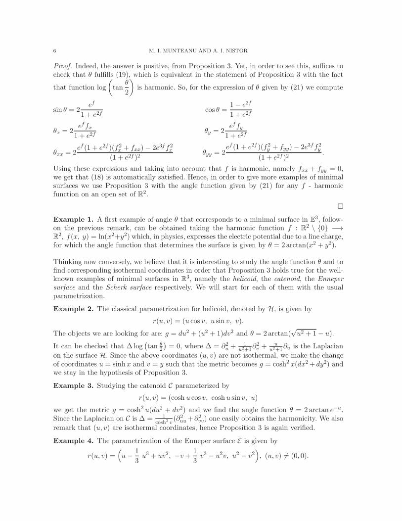
Proof. Indeed, the answer is positive, from Proposition 3. Yet, in order to see this, suffices tocheck that θ fulfills (19), which is equivalent in the statement of Proposition 3 with the fact

that function log

(tan

θ

2

)is harmonic. So, for the expression of θ given by (21) we compute

sin θ = 2ef

1 + e2fcos θ =

1− e2f

1 + e2f

θx = 2effx

1 + e2fθy = 2

effy1 + e2f

θxx = 2ef (1 + e2f )(f2x + fxx)− 2e3ff2x

(1 + e2f )2θyy = 2

ef (1 + e2f )(f2y + fyy)− 2e3ff2y(1 + e2f )2

.

Using these expressions and taking into account that f is harmonic, namely fxx + fyy = 0,we get that (18) is automatically satisfied. Hence, in order to give more examples of minimalsurfaces we use Proposition 3 with the angle function given by (21) for any f - harmonicfunction on an open set of R2.

�

Example 1. A first example of angle θ that corresponds to a minimal surface in E3, follow-on the previous remark, can be obtained taking the harmonic function f : R2 \ {0} −→R2, f(x, y) = ln(x2+y2) which, in physics, expresses the electric potential due to a line charge,for which the angle function that determines the surface is given by θ = 2arctan(x2 + y2).

Thinking now conversely, we believe that it is interesting to study the angle function θ and tofind corresponding isothermal coordinates in order that Proposition 3 holds true for the well-known examples of minimal surfaces in R3, namely the helicoid, the catenoid, the Ennepersurface and the Scherk surface respectively. We will start for each of them with the usualparametrization.

Example 2. The classical parametrization for helicoid, denoted by H, is given by

r(u, v) = (u cos v, u sin v, v).

The objects we are looking for are: g = du2 + (u2 + 1)dv2 and θ = 2arctan(√u2 + 1− u).

It can be checked that ∆ log(tan θ

2

)= 0, where ∆ = ∂2u +

1u2+1∂

2v +

uu2+1∂u is the Laplacian

on the surface H. Since the above coordinates (u, v) are not isothermal, we make the changeof coordinates u = sinhx and v = y such that the metric becomes g = cosh2 x(dx2+ dy2) andwe stay in the hypothesis of Proposition 3.

Example 3. Studying the catenoid C parameterized by

r(u, v) = (cosh u cos v, cosh u sin v, u)

we get the metric g = cosh2 u(du2 + dv2) and we find the angle function θ = 2arctan e−u.Since the Laplacian on C is ∆ = 1

cosh2 v(∂2uu+∂

2vv) one easily obtains the harmonicity. We also

remark that (u, v) are isothermal coordinates, hence Proposition 3 is again verified.

Example 4. The parametrization of the Enneper surface E is given by

r(u, v) =(u− 1

3u3 + uv2, −v + 1

3v3 − u2v, u2 − v2

), (u, v) 6= (0, 0).

7

The metric has the form g = (1 + u2 + v2)2(du2 + dv2) and the angle function isθ = 2arctan 1√

u2+v2. Again, using the expression of the Laplacian ∆ = 1

(1+u2+v2)2(∂uu2 +

∂2vv) on the surface E one obtains that the function log(tan θ

2

)is harmonic. Moreover, the

coordinates (u, v) are isothermal as in Proposition 3.

Example 5. The parametrization of the Scherk surface S over the square (see [7]) can bewritten as

r(u, v) =(u, v, log

cos u

cos v

).

The angle function θ satisfies cos θ =(

1cos2 u

+ 1cos2 v

− 1)− 1

2

. Notice that in this case the

coordinates are no longer orthogonal, since the metric has the following form g = 1cos2 u

du2 −2 sinu sin vcos u cos vdudv + 1

cos2 vdv2. Looking for an isothermal parametrization in (x, y) coordinates,

one has to find u = u(x, y) and v = v(x, y) such that the following system is fulfilled:{

(u2x − u2y)1

cos2 u+ 2(−uxvx + uyvy) tan u tan v + (v2x − v2y)

1cos2 v

= 0

uxuy1

cos2 u− (uxvy + uyvx) tan u tan v + vxvy

1cos2 v

= 0.

The isothermal parametrization of S is the given by r(x, y) =(u(x, y), v(x, y), log cosu(x,y)

cos v(x,y)

)

with u(x, y) = arctan 2x1−x2−y2 and v(x, y) = arctan −2y

1−x2−y2 .

We conclude this section with a non existence result

Remark 4. There are no minimal and flat surfaces isometrically immersed in E3 with a nonconstant angle function.

Proof. Computing the Gaussian curvature K for a minimal surface given as in Proposition 3we get that K = 0 is equivalent with θ2x + θ2y = 0. Consequently, it follows that θ is constant.

�

2. Surfaces with a Canonical Principal Direction

The study of constant angle surfaces in E3 can be generalized for surfaces whose angle func-tion is no longer constant, but certain properties are preserved. More precisely, this is thecase in which U remains a principal direction, whereas the corresponding principal curva-ture is different from 0. They will be called surfaces with a canonical principal direction. Wecharacterize these surfaces in the following

Theorem 1. Let M be an isometrically immersed surface in E3. Let (x, y) be orthogonalcoordinates on M such that U is collinear to ∂x. Then, U is a principal direction on Meverywhere if and only if θy = 0.

Proof. We know that such coordinates exist as in the proof of Proposition 2. We have

U = sin2 θ∂x.

Moreover, from the expression (7) of the shape operator it follows that

AU = sin3 θθx∂x + sin θθyβ2∂y.

8 M. I. MUNTEANU AND A. I. NISTOR

We find that U is a principal direction implies θy = 0.

Conversely, from (4) it follows g(AU, ∂y) = 0 which means that AU is parallel to ∂x, hence Uis a principal direction for M .

�

The following statement is essential for the rest of the paper.

Proposition 4. Let M be a surface immersed in E3 and a point p ∈ M such that θ(p) /∈{0, π2 }. If U is a principal direction of M , we can choose coordinates (x, y) in a neighborhoodof p such that ∂x is in the direction of U , the metric has the form

(22) g = dx2 + β2(x, y)dy2

and the shape operator is given by

(23) A =

(θx 0

0 tan θ βxβ

).

Moreover, θ and β are related by the PDE

(24) βxx + tan θθxβx = 0

and θy = 0.

Proof. The results are obtained using similar techniques as in Proposition 2 by straightforwardcomputations.

�

Remark 5. Accordingly to [4], we say that (x, y) are canonical coordinates on M if U isa principal direction collinear to ∂x and the metric g has the form (22). Notice that suchcoordinates are not unique and two pairs (x, y) and (x, y) of canonical coordinates are relatedby x = ± x+ c, c ∈ R and y = y(y).

An illustration of canonical coordinates is given by Example 2, the classical parametrizationof the helicoid. In this case the metric is written in form (22) with β =

√u2 + 1 and together

with θ = 2arctan(√u2 + 1− u) fulfill (24) identically.

In order to determine explicitly all surfaces in E3 with a canonical principal direction we haveto solve (24) in order to find the unknown function β from the expression (22) of the metric.They are described in the following classification theorem:

Theorem 2. A surfaceM isometrically immersed in E3 with U a canonical principal directionis given (up to isometries of E3) by one of the following cases:

• Case 1.

(25) r :M → E3, r(x, y) =

(φ(x)(cos y, sin y) + γ(y),

∫ x

0sin θ(τ)dτ

)

where

γ(y) =

(−∫ y

0ψ(τ) sin τdτ,

∫ y

0ψ(τ) cos τdτ

)

9

• Case 2.

(26) r :M → E3, r(x, y) =

(φ(x) cos y0, φ(x) sin y0,

∫ x

0sin θ(τ)dτ

)+ yv0

where v0 = (− sin y0, cos y0, 0), y0 ∈ R. Notice that these surfaces are cylinders.

In both cases φ(x) denotes a primitive of cos θ.

Proof. Let us denote the isometric immersion of the surface M in E3 by

r :M → E3, r(x, y) =(r1(x, y), r2(x, y), r3(x, y)

)=(rj(x, y), r3(x, y)

), j = 1, 2.

Since the statements of Proposition 4 hold true, we are able to choose canonical coordinates(x, y) such that the metric is given by (22). At this point we have to determine the function

β which satisfies the PDE (24), or equivalently, ∂x

(βxcos θ

)= 0. Integrating twice one gets:

• either β = k(y)(φ(x) + ψ(y)), where φ′(x) = cos θ, ψ(y) and k(y) are defined on M• or β = β(y).

We may immediately obtain the 3rd component of the immersion r. Since from Proposition 4U = sin θ∂x, the decomposition (1) becomes

(27)−→k = sin θrx + cos θN.

Computing now (r3)x = 〈rx,−→k 〉 = sin θ and (r3)y = 〈ry,

−→k 〉 = 0 we conclude that

(28) r3(x, y) =

∫ x

sin θ(τ)dτ.

From (27) and (28) one can express the normal to the surface as

(29) N =(− tan θ(rj)x, cos θ

), j = 1, 2.

Let us distinguish two cases for β.

Case 1. β = k(y)(φ(x) + ψ(y))After a change of the y−coordinate we may assume that β = φ(x) +ψ(y) and substituting itin (16) we get the metric

(30) g = dx2 + (φ(x) + ψ(y))2dy2.

By using Koszul formula one obtains the corresponding Levi-Civita connection

∇∂x∂x = 0, ∇∂x∂y = ∇∂y∂x =cos θ

φ(x) + ψ(y)∂y

∇∂y∂y = −(φ(x) + ψ(y)) cos θ∂x +ψ′(y)

φ(x) + ψ(y)∂y.

Taking into account the expression of the shape operator (23) and the metric (30) we get

A =

(θx 0

0 sin θφ(x)+ψ(y)

).

10 M. I. MUNTEANU AND A. I. NISTOR

Moreover, from the Weingarten formula (W) we have

Nx = −θx rx(31.a)

Ny = − sin θ

φ(x) + ψ(y)ry.(31.b)

Computing the derivative with respect to x in (29),

Nx =

(− θxcos2 θ

(rj)x − tan θ(rj)xx,− sin θθx

)

and combining it with (31.a) it follows that r must fulfil cos θ(rj)xx + sin θθx(rj)x = 0 which

can be equivalently written ∂x

((rj)xcos θ

)= 0, j = 1, 2. One gets

(32)(r1, r2

)x= cos θf(y)

where f(y) = (cosϕ(y), sinϕ(y)) represents a parametrization of the unit circle S1. Thisis a consequence of the fact that ‖rx‖2 = 1 which, combined with (28) and (32), leads to‖f(y)‖ = 1. Here and all over this paper ‖ · ‖ denotes the Euclidean norm.

Integrating with respect to x in (32) and taking into account (28) we get the following ex-pression for the immersion r

(33) r(x, y) =

(φ(x)f(y) + γ(y),

∫ x

0sin θ(τ)dτ

)

where γ(y) = (γ1(y), γ2(y)) is a smooth R2−valued map.

Since r is an isometric immersion we get

(i) 〈γ′(y), f(y)〉 = 0

(ii) φ(x)2‖f ′(y)‖2 + ‖γ′(y)‖2 + 2φ(x)〈f ′(y), γ′(y)〉 = β2.

From (i) we deduce that γ′(y) and f ′(y) are parallel vectors, so, there exists a C∞-functionη(y) such that γ′(y) = η(y)f ′(y). Replacing it in (ii) and taking into account the expressionof β we get equivalently

(φ(x) + η(y)

)|ϕ′(y)| = φ(x) + ψ(y). Since φ(x) is not a constant, it

follows |ϕ′(y)| = 1 and consequently η(y) = ψ(y). By fixing an orientation on the y-axis andafter a translation along it, we may choose ϕ(y) = y and hence

(34) γ(y) =

(−∫ y

0ψ(τ) sin τdτ,

∫ y

0ψ(τ) cos τdτ

).

Combining now (28), (33) and (34) we get exactly the parametrization (25).

Case 2. β = β(y)After a change of the y-coordinate in this case, β = 1 and the metric becomes g = dx2 + dy2.

The shape operator is given by A =

(θx 00 0

). From the Weingarten formula (W) we get

Nx = −θxrx(35.a)

Ny = 0.(35.b)

11

Firstly, taking the derivative with respect to y in (29) and combining it with (35.b) one gets

(36) (rj)xy = 0, j = 1, 2.

Secondly, taking the derivative with respect to x in (29) and combining it with (35.a) oneobtains

(rj)xx + tan θθx(rj)x = 0, j = 1, 2.

It follows

(rj)x = cos θfj(y), where fj ∈ C∞(M), j = 1, 2 with f1(y)2 + f2(y)

2 = 1.

Combining the above equation with (36) one obtains

(r1(x, y), r2(x, y)) = f0φ(x) + γ(y)

where f0 = (cos y0, sin y0) and γ(y) = (−(sin y0)y+ c1, (cos y0)y+ c2), with c1, c2 ∈ R since ris an isometric immersion. After a translation in E3, the constants c1 and c2 may be assumedto be zero. So, the expression (26) is proven.

Conversely, we will give the proof only in Case 1 because the idea of the proof is the samealso in the second case. Suppose that we have a surface given by (25) and we prove that ithas U as a canonical principal direction. The tangent plane of the surface is generated by thefollowing vectors

rx = (cos θ cos y, cos θ sin y, sin θ)

ry = (−(φ(x) + ψ(y)) sin y, (φ(x) + ψ(y)) cos y, 0) .

Hence, the metric is given by g = dx2 + (φ(x) + ψ(y))2dy2, which corresponds to (22). Bystraightforward computations we get that the shape operator has the form as in (23) andfrom its symmetry we have θy = 0. One easily proves that 〈rx, U〉 = sin θ and 〈ry, U〉 = 0concluding that U is a principal direction of the surface M parameterized by (25). At thispoint the theorem is completely proved.

�

An alternative proof of this result, but in a different manner, can be found in [8]. The authorclassifies hypersurfaces f : Mn → Qn

ǫ × R with a principal direction, where Qnǫ denotes

either the n-sphere Sn, the Euclidean n-space Rn or the hyperbolic n-space Hn according toǫ = 1, ǫ = 0, or ǫ = −1.

The study of minimal surfaces is another classical problem in differential geometry. Below weclassify all minimal surfaces with a canonical principal direction given by U in E3.

Theorem 3. Let M be a surface isometrically immersed in E3. M is a minimal surface withU a principal direction if and only if the immersion is, up to isometries of the ambient space,given by

(37) r :M → E3, r(x, y) =(√

x2 + c2 cos y,√x2 + c2 sin y, c ln

(x+

√x2 + c2

)), c ∈ R.

Proof. The result is local, hence Proposition 4 can be used. From the proof of the previoustheorem we already know the solutions of (24), namely β = φ(x) + ψ(y), respectively β = 1after a change of the y-coordinate.

12 M. I. MUNTEANU AND A. I. NISTOR

Let us consider the first solution for β. Under the minimality assumption we get, after atranslation along the x-coordinate, that

(38) θ = arctanc

x, c ∈ R.

Writing β in two ways, once β = csin θ from the minimality condition and second in the general

form β = φ(x) + ψ(y), we immediately find that ψ(y) is constant and it may be added toφ(x). Therefore ψ(y) could be considered zero.

Going back to Theorem 2 we know the parametrization (25). Substituting the value of θ from(38), by straightforward computations we find

φ(x) =√x2 + c2 , γ(y) = 0

and the 3rd component of the parametrization becomes∫ x

sin θ(τ)dτ = c ln(x+√x2 + c2).

Combining these expressions in (25), we find that a minimal surface which has U a principaldirection everywhere is parameterized by (37).

In the second case of the classification theorem, corresponding to β = 1, under the assumptionof minimality we get that θx = 0 which contradicts our initial hypothesis that θ is neverconstant. So, this situation cannot occur.

The converse results immediately by direct computations.

�

Remark 6. We notice that this surface can be obtained by rotating the catenary around theOz-axis. Hence, the only minimal surface in the Euclidean 3-space with a canonical principaldirection is the catenoid. See for details [1, 2]. This result can be retrieved in a differentmanner also from [8].

Theorem 4. Let M be a surface isometrically immersed in E3. M is a flat surface with Ua principal direction if and only if the immersion is, up to isometries of the ambient space,given by

r :M → E3, r(x, y) =

(φ(x) cos y0, φ(x) sin y0,

∫ x

0sin θ(τ)dτ

)+ yv0

where v0 =(− sin y0, cos y0, 0

), y0 ∈ R and φ(x) represents a primitive of cos θ.

Proof. Using the canonical coordinates furnished by Proposition 4, under the flatness assump-tion, from (2) one gets θx tan θβx = 0. As the angle function θ cannot be constant, it yieldsβx = 0 which implies β = β(y). This corresponds precisely to Case 2 from the classificationtheorem. Hence, the second case of the classification coincides with the class of all flat surfacesM with a canonical principal direction U .

�

Remark 7. Starting from Proposition 4 and using the expression of the shape operatorA together with the expression (24) relating θ and β we could find the expressions of theangle function θ in the case of equal principal curvatures or constant mean curvature (CMC).

13

Studying surfaces with equal principal curvatures, we solve (24) and after a change of y-co-ordinate, we get the following solutions for β:

case 1. β = φ(x) +ψ(y) and replacing this expression in (23), if the principal curvatures areequal, then θ must satisfy θx =

sin θφ(x)+ψ(y) . By direct computations and by taking into account

that the angle function depends only of x we get that

θ = ax+ b, a, b ∈ R.

Note that in the case when the principal curvatures are constant, they must be equal withthe same constant and hence in this case we obtain a piece of the 2-sphere S2 in Euclidean3-space. Conversely, writing the sphere in canonical coordinates (which coincide with thespherical coordinates) the angle function θ is an affine function.

case 2. β = 1 implies θx = 0, hence θ is constant, situation excluded all over this paper.

Regarding the constant mean curvature surfaces, we discuss again the two solutions for β.case 1. β = φ(x) + ψ(y), then under the CMC−condition we get that θ must satisfy thefollowing differential equation:

θx +sin θ

φ(x) + ψ0= 2H, where H denotes the constant mean curvature and ψ0 ∈ R.

case 2. β = 1 implies that the angle function which gives a CMC surface is an affine functionθ = 2Hx+ d, with H, d ∈ R.For the general case of CMC hypersurfaces in Qn

ǫ × R see [8, Thm. 3].

References

[1] D.E. Blair, On a generalization of the catenoid, Canad. J. Math. 27 (1975), 231-236.[2] M. do Carmo, M. Dajczer, Rotation hypersurfaces in spaces of constant curvature, Trans. Amer. Math.

Soc. 277 (2) (1983), 685-709.[3] F. Dillen, J. Fastenakels, J. Van der Veken, Surfaces in S2

× R with a canonical principal direction, Ann.Glob. Anal. Geom. 35 (4) (2009), 381–396.

[4] F. Dillen, M.I. Munteanu, A.I. Nistor, Canonical Coordinates and Principal Directions for surfaces in

H2× R, arXiv:0910.2135v1[math.DG], 2010.

[5] S. Morita, Geometry of Differential Forms, Translations of Mathematical Monographs, Vol. 201, AMS,2001.

[6] M.I. Munteanu, A.I. Nistor, A new approach on constant angle surfaces in E3, Turk. J. Math. 33 (2)(2009), 169–178.

[7] B. O’Neill, Elementary Differential Geometry, (revised second edition) Academic Press, 2006.[8] R. Tojeiro, On a class of hypersurfaces in Sn

× R and Hn× R, arXiv:0909.2265v1[math.DG], 2009.

E-mail address: marian.ioan.munteanu (at) gmail.com

E-mail address: ana.irina.nistor (at) gmail.com