Citation: Orovic, J.; Valcic, M.;

Kneževic, V.; Pavin, Z. Comparison

of the on Board Measured and

Simulated Exhaust Gas Emissions on

the Ro-Pax Vessels. Atmosphere 2022,

13, 794. https://doi.org/10.3390/

atmos13050794

Academic Editor: Kenichi Tonokura

Received: 12 April 2022

Accepted: 10 May 2022

Published: 13 May 2022

Publisher’s Note: MDPI stays neutral

with regard to jurisdictional claims in

published maps and institutional affil-

iations.

Copyright: © 2022 by the authors.

Licensee MDPI, Basel, Switzerland.

This article is an open access article

distributed under the terms and

conditions of the Creative Commons

Attribution (CC BY) license (https://

creativecommons.org/licenses/by/

4.0/).

atmosphere

Article

Comparison of the on Board Measured and Simulated ExhaustGas Emissions on the Ro-Pax VesselsJosip Orovic * , Marko Valcic , Vlatko Kneževic and Zoran Pavin

Maritime Department, University of Zadar, Mihovila Pavlinovica 1, 23000 Zadar, Croatia;mvalcic@unizd.hr (M.V.); vknezevi1@unizd.hr (V.K.); zpavin@unizd.hr (Z.P.)* Correspondence: jorovic@unizd.hr

Abstract: Increasingly stringent environmental requirements for marine engines imposed by theInternational Maritime Organisation and the European Union require that marine engines have thelowest possible emissions of greenhouse and harmful exhaust gases into the atmosphere. In thisresearch, exhaust gas emissions were measured on three Ro-Pax vessels sailing in the Adriatic Sea.Testo 350 Maritime exhaust gas analyser was used for monitoring the dry exhaust gas concentrationsof CO2 and O2 in percentage, concentrations of CO and NOx in ppm and exhaust gas temperaturein ◦C after the turbocharger at different engine loads. In order to compare and validate measuredvalues, exhaust gas measurement data were also obtained from a Wartsila-Transas simulator modelof a similar Ro-Pax vessel during the joint operation of the engine room and navigational simulators.All analysed main engines on three vessels had complete combustion processes in the cylinderswith small differences which should be further investigated. Comparison of on board measuredparameters with simulated parameters showed that significant fuel oil reduction per voyage could beaccomplished by voyage and/or engine operation optimization procedures. Results of this analysiscould be used for creating additional emission database and data-driven models for further analysisand improved estimation of exhaust gasses under various marine engine conditions. Additionally,the results could be useful to all interested parties in reducing the fuel oil consumption and emissionsof greenhouse and harmful exhaust gases from vessels into the atmosphere.

Keywords: exhaust gas emission; Ro-Pax vessel; on board measurement; engine room and nauticalsimulator

1. Introduction

International and domestic shipping is a growing source of exhaust gas pollutantsand greenhouse gas emissions. This problem was recognized by the European Union (EU)and they approved Regulation 2015/757 of the European Parliament and of the Council onthe monitoring, reporting and verification of CO2 emissions from maritime transport [1].The goal of the EU Commission is to limit the greenhouse gases on board by 2% in 2025and up to 6% in 2030 compared with 2020 levels. This regulation includes monitoring andreporting CO2 emissions in the European Economic Area (EEA) from ships larger than5000 gross tonnage (GT). According to the European Maritime Safety Agency (EMSA),companies should submit their emission report through the THETIS-MRV web platform [2].This database was used to analyse CO2 emissions in 2018 from Ro-Pax vessels calling atEuropean ports [3]. International Maritime Organization (IMO) followed this example withthe IMO Data Collection System module which requires ships larger than 5000 GT to reportand record fuel oil consumption [4]. The mentioned regulations and amendments are thefirst steps to develop the strategy for the decarbonizing maritime sector.

To evaluate the amount of emissions in one shipping area or from a specific type ofship is not an easy task. The most accurate method for estimating ship exhaust emissionsis by on board measuring in real conditions with adequate measuring equipment. Thus

Atmosphere 2022, 13, 794. https://doi.org/10.3390/atmos13050794 https://www.mdpi.com/journal/atmosphere

Atmosphere 2022, 13, 794 2 of 19

far, research studies on the on board emissions measurement, especially in the Ro-Paxsegment, are very limited. This problem presents a need for a more relevant onboardemission database that will offer the possibility to enhance the estimation of emissions andcomparison with the current emission database and current estimation models.

Cooper D.A. measured exhaust emissions on high-speed passenger ferries with differ-ent propulsion types (conventional diesel engine, gas turbine, diesel engine with selectivecatalytic reduction) and at three most frequent engine loads [5]. The proposed methodto quantify exhaust emissions without direct measurement of fuel consumption duringmanoeuvring is presented in [6]. An improved emission inventory method is suggestedin [7] considering experimental on board measurement on two ocean going vessels withslow speed diesel engines using the heavy fuel oil (HFO). Another on board measurementresearch [8] was carried out on a slow speed, two stroke main engine running on HFO(3.13% sulphur content) with the goal to predict primary emissions while cruising, ma-noeuvring and at berth operating mode. Similar studies [9–12] have used equipment tomeasure the concentration of NOX, CO2, CO, SO2 and particulate matter (PM) pollutants inburned HFO, with respect to engine power output and vessel speed at different operatingconditions. In [13], the comparison of fuel-based emission factors (NOX, PM, HC, CO) fordifferent engine loads is presented with a conclusion that emission factors are increasingdue to higher engine loads. Most of the vessel types in the previously mentioned literatureare bulk carriers, container ships or general cargo ships with slow speed two stroke enginesusing the HFO. However, all researchers share the same opinion and conclusion that thereshould be more experimental measured data acquired under real seagoing conditions toprovide development and validation of more relevant emission factors.

The aim of this paper is to compare and validate exhaust gas emissions data fromonboard measurements with simulated data. The measurement campaign was performedon three similar Ro-Pax vessels, and simulation was performed in a joint operation of theWartsila-Transas engine room and navigational simulators with Ro-Pax vessel models.

2. An Overview of Combustion Process and Exhaust Gases

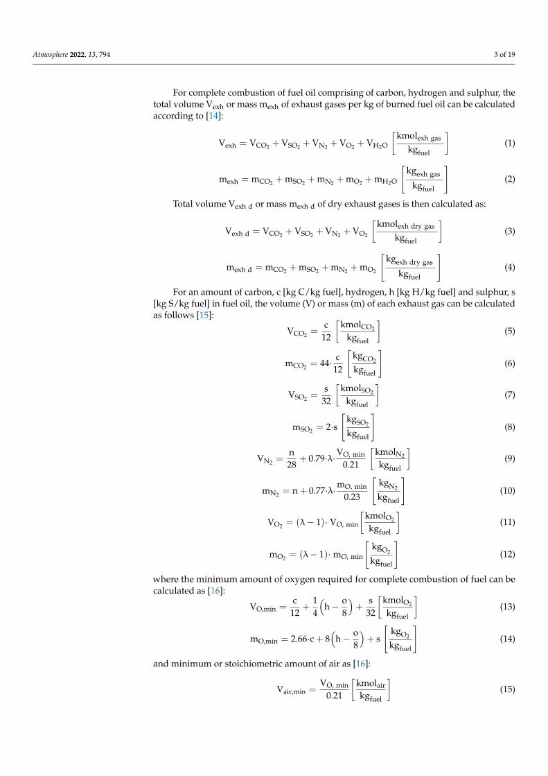
Fuel oil for marine diesel engines mainly consists of carbon, hydrogen and sulphur(C, H, and S). Fuel oil is mixed with air and burned inside the cylinders. The products ofthe combustion process are exhaust gases (Figure 1), which are led to the atmosphere aftertheir heat energy is used for power generation in the marine engines.

Figure 1. Combustion process in engines.

Atmosphere 2022, 13, 794 3 of 19

For complete combustion of fuel oil comprising of carbon, hydrogen and sulphur, thetotal volume Vexh or mass mexh of exhaust gases per kg of burned fuel oil can be calculatedaccording to [14]:

Vexh = VCO2 + VSO2 + VN2 + VO2 + VH2O

[kmolexh gas

kgfuel

](1)

mexh = mCO2 + mSO2 + mN2 + mO2 + mH2O

[kgexh gas

kgfuel

](2)

Total volume Vexh d or mass mexh d of dry exhaust gases is then calculated as:

Vexh d = VCO2 + VSO2 + VN2 + VO2

[kmolexh dry gas

kgfuel

](3)

mexh d = mCO2 + mSO2 + mN2 + mO2

[kgexh dry gas

kgfuel

](4)

For an amount of carbon, c [kg C/kg fuel], hydrogen, h [kg H/kg fuel] and sulphur, s[kg S/kg fuel] in fuel oil, the volume (V) or mass (m) of each exhaust gas can be calculatedas follows [15]:

VCO2 =c

12

[kmolCO2

kgfuel

](5)

mCO2 = 44· c12

[kgCO2

kgfuel

](6)

VSO2 =s

32

[kmolSO2

kgfuel

](7)

mSO2 = 2·s[

kgSO2

kgfuel

](8)

VN2 =n28

+ 0.79·λ·VO, min

0.21

[kmolN2

kgfuel

](9)

mN2 = n + 0.77·λ·mO, min

0.23

[kgN2

kgfuel

](10)

VO2 = (λ− 1)· VO, min

[kmolO2

kgfuel

](11)

mO2 = (λ− 1)·mO, min

[kgO2

kgfuel

](12)

where the minimum amount of oxygen required for complete combustion of fuel can becalculated as [16]:

VO,min =c

12+

14

(h− o

8

)+

s32

[kmolO2

kgfuel

](13)

mO,min = 2.66·c + 8(

h− o8

)+ s

[kgO2

kgfuel

](14)

and minimum or stoichiometric amount of air as [16]:

Vair,min =VO, min

0.21

[kmolair

kgfuel

](15)

Atmosphere 2022, 13, 794 4 of 19

mair,min =mO, min

0.23

[kgairkgfuel

]. (16)

Usually, in the actual combustion process, more air than the stoichiometric amount isused in order to increase the chances of complete combustion. The amount of excess airexpressed as a ratio λ between the actual amount of air and the minimum or stoichiometricamount of air is obtained with the equation [17,18]:

λ =Vair

Vair,min=

mair

mair,min. (17)

Additionally, in the actual combustion process, there could be gases present in partsper million (ppm) like NOx, CO and other. The emission factor of each gas is convertedinto g/kWh units, which represent mass per kWh of engine work. For gases measured inppm, the emission factors EF are obtained with the following equation [19]:

EFi = Cj·10−6· Mi

Mexh··

m exhPeng

[ gkWh

](18)

where Mi and Mexh are relative molecular weight of particular gas and exhaust gas mixturein kmol/kg, respectively, Cj is gaseous concentration in ppm in dry or wet gases,

·m exh is

dry or wet exhaust gas flow in kg/h and Peng is the engine power.To calculate the precise amount of exhaust gas (or exhaust flow) it is necessary to know

the exact chemical properties of used fuel oil. The fuel oil properties used in this researchare in correspondence with ISO 8217 2017 fuel standards for marine distillate fuels [20].The amount of sulphur content in fuel must not exceed 0.10% by mass in all EU ports andinland waters, which is defined by EU directive 2016/802 [21].

3. On Board Measurement and Simulation Process

On board exhaust gas measurements were carried out on three Ro-Pax vessels withfour stroke main engines connected through reduction gearboxes to controllable pitchpropellers (CPP) during multiple voyages in the Adriatic Sea between ports of Croatia, Italyand Montenegro. In order to compare the on board measurement values of the exhaustprocess with the simulated ones and in addition to perform the validation of the engineroom simulator with the measured on board values under a series of different engineoperating regimes, the simulated exhaust gas data were also obtained using a Wartsila-Transas simulator model of similar Ro-Pax vessel. The simulated vessel was operated in ajoint operation of the engine room and navigational simulators during different weatherand engine operating conditions. The basic vessels’ and simulator’s particulars/parametersare shown in Table 1.

The equipment used for measuring and analysing the exhaust gases on board vesselswas Testo 350 Maritime flue gas analyser [22]. This flue gas analyser is used for monitoringexhaust gas temperature and concentrations of CO2 and O2 as a percentage in volumeof dry exhaust gas, as well as CO, NOx, SOx in ppm in dry exhaust gas. It is working inaccordance with ISO 8178-4:2020, Marpol Annex VI and NOx Technical Code 2008. Themeasurement range and accuracy of the exhaust gas analyser can be found in [23]. Themeasured raw data files are saved into the analyser internal memory with an option totransfer it to the computer and then use for the analysis. On all three vessels diesel fuelEurodiesel BS with a maximum of 10 mg/kg of sulphur content was used, which is also inconformity with Regulation 14(1) or 4(a) and Regulation 18(1) of Annex VI [24].

Atmosphere 2022, 13, 794 5 of 19

Table 1. Vessel and engine particulars/parameters.

Particulars/Parameters Vessel I Vessel II Vessel III Simulated Vessel

LOA/Breath/Draft (m) 128.13/19.62/5.73 116.0/18.9/5.2 122.06/18.82/4.83 125.0/23.4/5.3Service speed (knots) 19.5 17.5 20.0 19.0Year of build 1973 1993 1979 N/A

Engine type Stork Werkspoor Diesel8TM410

Bazan MAN B&W8L40/54 A MaK Diesel 8M551AK MAN B&W 8L32/40

No. of Engines/Propellers 4/2 2/2 4/2 2/2Engine Power MCR (kW) 3750 3500 3310 4000Number of cylinders 8 8 8 8

Engine speed(min−1)/propeller speed(min−1)

550/250 428/225 425/245 750/175

Bore/stroke (mm) 410/470 400/540 450/550 320/400Mean effect. pressure (bar) 16.82 18.45 13.3 24.9Average voyage length (Nm) 136.7 102.6 115.0 N/AAverage vessel speed (kt) 13.4 11.6 12.1 N/A

Average vessel heading: Leg1 (◦)/Leg 2 (◦) 260/99 245/65 210/61 N/A

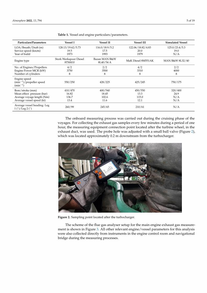
The onboard measuring process was carried out during the cruising phase of thevoyages. For collecting the exhaust gas samples every few minutes during a period of onehour, the measuring equipment connection point located after the turbine wheel, in theexhaust duct, was used. The probe hole was adjusted with a small ball valve (Figure 2),which was located approximately 0.2 m downstream from the turbocharger.

Figure 2. Sampling point located after the turbocharger.

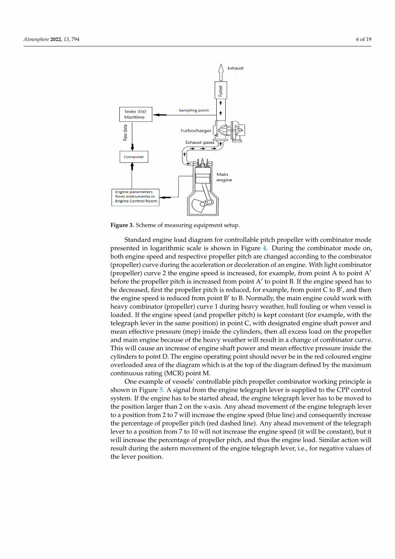
The scheme of the flue gas analyser setup for the main engine exhaust gas measure-ment is shown in Figure 3. All other relevant engine/vessel parameters for this analysiswere also collected directly from instruments in the engine control room and navigationalbridge during the measuring processes.

Atmosphere 2022, 13, 794 6 of 19

Figure 3. Scheme of measuring equipment setup.

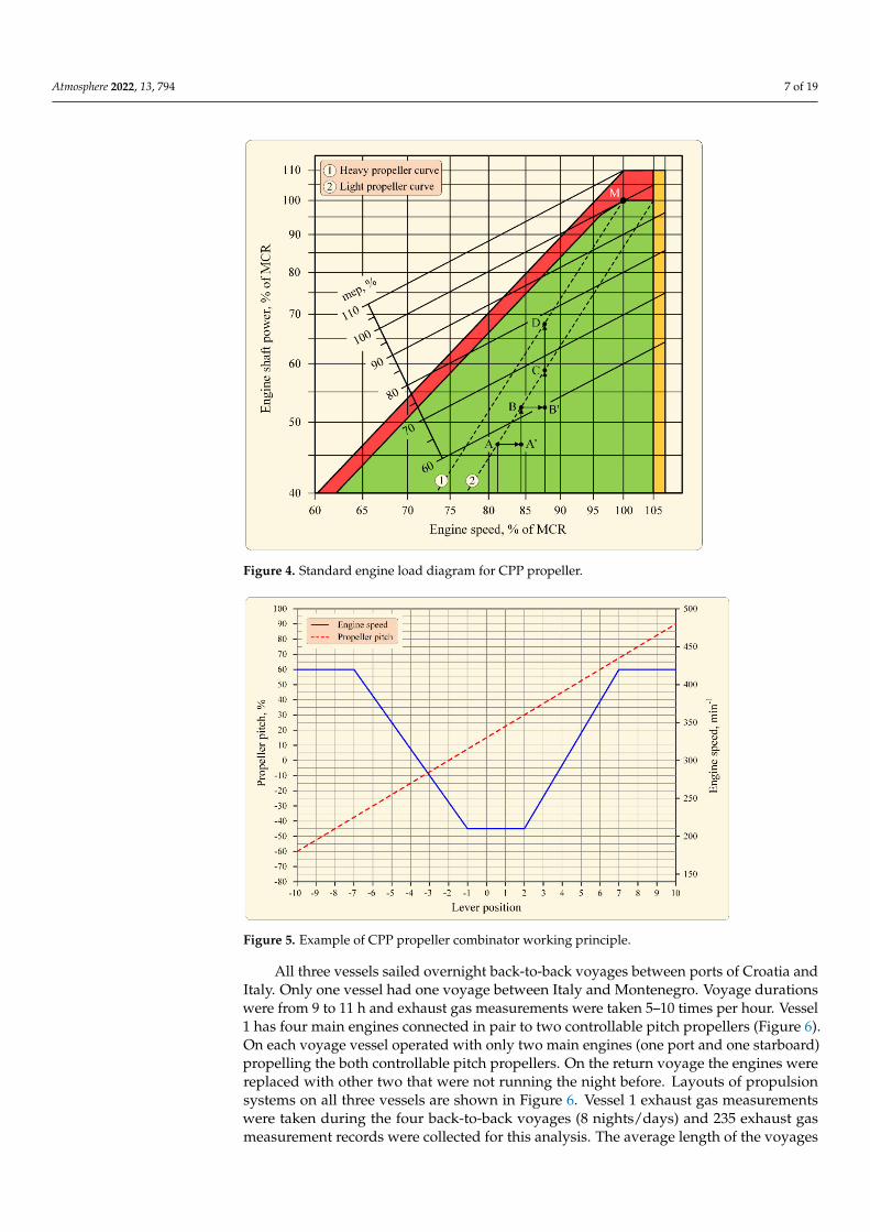
Standard engine load diagram for controllable pitch propeller with combinator modepresented in logarithmic scale is shown in Figure 4. During the combinator mode on,both engine speed and respective propeller pitch are changed according to the combinator(propeller) curve during the acceleration or deceleration of an engine. With light combinator(propeller) curve 2 the engine speed is increased, for example, from point A to point A′

before the propeller pitch is increased from point A′ to point B. If the engine speed has tobe decreased, first the propeller pitch is reduced, for example, from point C to B′, and thenthe engine speed is reduced from point B′ to B. Normally, the main engine could work withheavy combinator (propeller) curve 1 during heavy weather, hull fouling or when vessel isloaded. If the engine speed (and propeller pitch) is kept constant (for example, with thetelegraph lever in the same position) in point C, with designated engine shaft power andmean effective pressure (mep) inside the cylinders, then all excess load on the propellerand main engine because of the heavy weather will result in a change of combinator curve.This will cause an increase of engine shaft power and mean effective pressure inside thecylinders to point D. The engine operating point should never be in the red coloured engineoverloaded area of the diagram which is at the top of the diagram defined by the maximumcontinuous rating (MCR) point M.

One example of vessels’ controllable pitch propeller combinator working principle isshown in Figure 5. A signal from the engine telegraph lever is supplied to the CPP controlsystem. If the engine has to be started ahead, the engine telegraph lever has to be moved tothe position larger than 2 on the x-axis. Any ahead movement of the engine telegraph leverto a position from 2 to 7 will increase the engine speed (blue line) and consequently increasethe percentage of propeller pitch (red dashed line). Any ahead movement of the telegraphlever to a position from 7 to 10 will not increase the engine speed (it will be constant), but itwill increase the percentage of propeller pitch, and thus the engine load. Similar action willresult during the astern movement of the engine telegraph lever, i.e., for negative values ofthe lever position.

Atmosphere 2022, 13, 794 7 of 19

Figure 4. Standard engine load diagram for CPP propeller.

Figure 5. Example of CPP propeller combinator working principle.

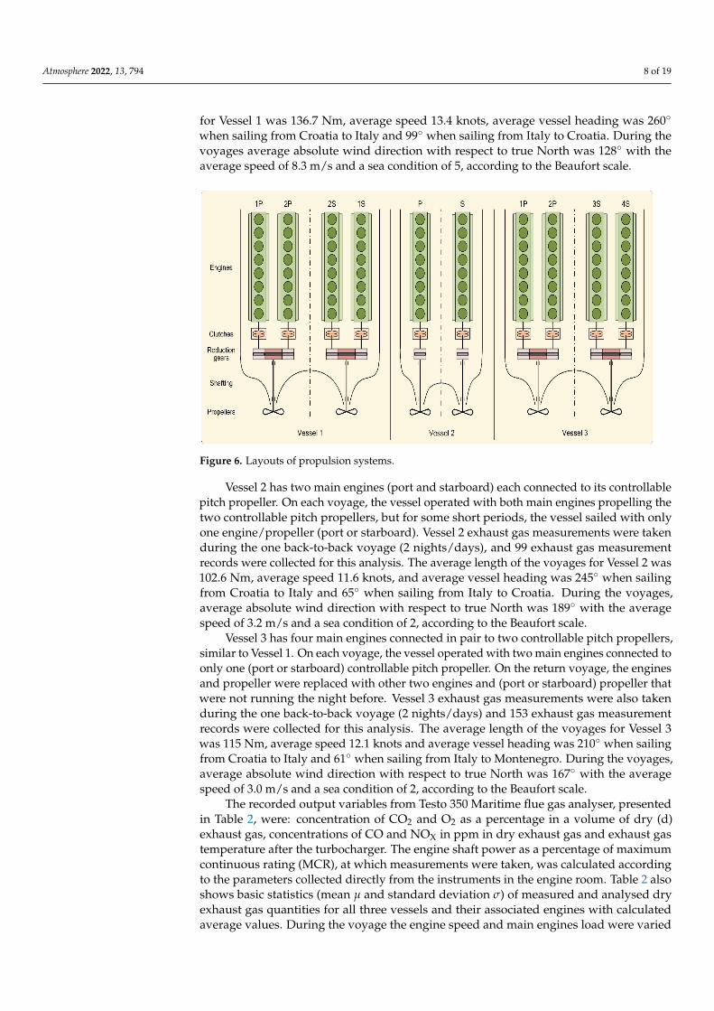
All three vessels sailed overnight back-to-back voyages between ports of Croatia andItaly. Only one vessel had one voyage between Italy and Montenegro. Voyage durationswere from 9 to 11 h and exhaust gas measurements were taken 5–10 times per hour. Vessel1 has four main engines connected in pair to two controllable pitch propellers (Figure 6).On each voyage vessel operated with only two main engines (one port and one starboard)propelling the both controllable pitch propellers. On the return voyage the engines werereplaced with other two that were not running the night before. Layouts of propulsionsystems on all three vessels are shown in Figure 6. Vessel 1 exhaust gas measurementswere taken during the four back-to-back voyages (8 nights/days) and 235 exhaust gasmeasurement records were collected for this analysis. The average length of the voyages

Atmosphere 2022, 13, 794 8 of 19

for Vessel 1 was 136.7 Nm, average speed 13.4 knots, average vessel heading was 260◦

when sailing from Croatia to Italy and 99◦ when sailing from Italy to Croatia. During thevoyages average absolute wind direction with respect to true North was 128◦ with theaverage speed of 8.3 m/s and a sea condition of 5, according to the Beaufort scale.

Figure 6. Layouts of propulsion systems.

Vessel 2 has two main engines (port and starboard) each connected to its controllablepitch propeller. On each voyage, the vessel operated with both main engines propelling thetwo controllable pitch propellers, but for some short periods, the vessel sailed with onlyone engine/propeller (port or starboard). Vessel 2 exhaust gas measurements were takenduring the one back-to-back voyage (2 nights/days), and 99 exhaust gas measurementrecords were collected for this analysis. The average length of the voyages for Vessel 2 was102.6 Nm, average speed 11.6 knots, and average vessel heading was 245◦ when sailingfrom Croatia to Italy and 65◦ when sailing from Italy to Croatia. During the voyages,average absolute wind direction with respect to true North was 189◦ with the averagespeed of 3.2 m/s and a sea condition of 2, according to the Beaufort scale.

Vessel 3 has four main engines connected in pair to two controllable pitch propellers,similar to Vessel 1. On each voyage, the vessel operated with two main engines connected toonly one (port or starboard) controllable pitch propeller. On the return voyage, the enginesand propeller were replaced with other two engines and (port or starboard) propeller thatwere not running the night before. Vessel 3 exhaust gas measurements were also takenduring the one back-to-back voyage (2 nights/days) and 153 exhaust gas measurementrecords were collected for this analysis. The average length of the voyages for Vessel 3was 115 Nm, average speed 12.1 knots and average vessel heading was 210◦ when sailingfrom Croatia to Italy and 61◦ when sailing from Italy to Montenegro. During the voyages,average absolute wind direction with respect to true North was 167◦ with the averagespeed of 3.0 m/s and a sea condition of 2, according to the Beaufort scale.

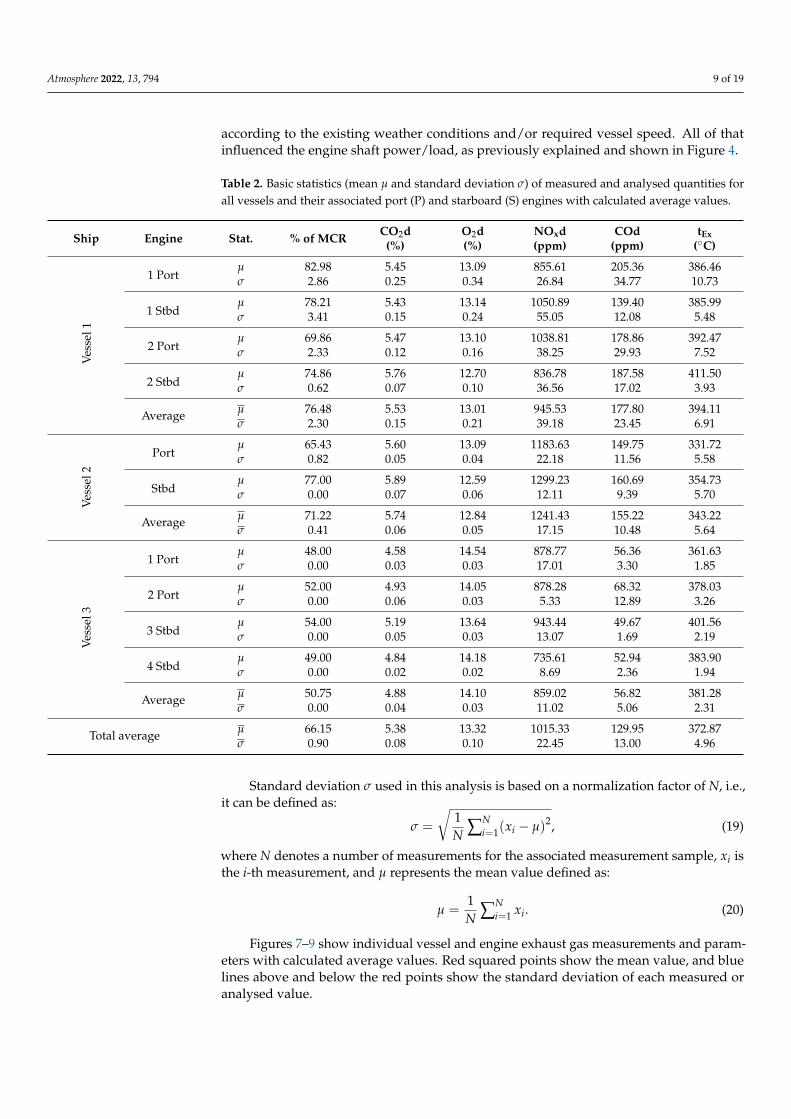
The recorded output variables from Testo 350 Maritime flue gas analyser, presentedin Table 2, were: concentration of CO2 and O2 as a percentage in a volume of dry (d)exhaust gas, concentrations of CO and NOX in ppm in dry exhaust gas and exhaust gastemperature after the turbocharger. The engine shaft power as a percentage of maximumcontinuous rating (MCR), at which measurements were taken, was calculated accordingto the parameters collected directly from the instruments in the engine room. Table 2 alsoshows basic statistics (mean µ and standard deviation σ) of measured and analysed dryexhaust gas quantities for all three vessels and their associated engines with calculatedaverage values. During the voyage the engine speed and main engines load were varied

Atmosphere 2022, 13, 794 9 of 19

according to the existing weather conditions and/or required vessel speed. All of thatinfluenced the engine shaft power/load, as previously explained and shown in Figure 4.

Table 2. Basic statistics (mean µ and standard deviation σ) of measured and analysed quantities forall vessels and their associated port (P) and starboard (S) engines with calculated average values.

Ship Engine Stat. % of MCR CO2d(%)

O2d(%)

NOxd(ppm)

COd(ppm)

tEx(◦C)

Vess

el1

1 Portµ 82.98 5.45 13.09 855.61 205.36 386.46σ 2.86 0.25 0.34 26.84 34.77 10.73

1 Stbdµ 78.21 5.43 13.14 1050.89 139.40 385.99σ 3.41 0.15 0.24 55.05 12.08 5.48

2 Portµ 69.86 5.47 13.10 1038.81 178.86 392.47σ 2.33 0.12 0.16 38.25 29.93 7.52

2 Stbdµ 74.86 5.76 12.70 836.78 187.58 411.50σ 0.62 0.07 0.10 36.56 17.02 3.93

Average µ 76.48 5.53 13.01 945.53 177.80 394.11σ 2.30 0.15 0.21 39.18 23.45 6.91

Vess

el2

Portµ 65.43 5.60 13.09 1183.63 149.75 331.72σ 0.82 0.05 0.04 22.18 11.56 5.58

Stbdµ 77.00 5.89 12.59 1299.23 160.69 354.73σ 0.00 0.07 0.06 12.11 9.39 5.70

Average µ 71.22 5.74 12.84 1241.43 155.22 343.22σ 0.41 0.06 0.05 17.15 10.48 5.64

Vess

el3

1 Portµ 48.00 4.58 14.54 878.77 56.36 361.63σ 0.00 0.03 0.03 17.01 3.30 1.85

2 Portµ 52.00 4.93 14.05 878.28 68.32 378.03σ 0.00 0.06 0.03 5.33 12.89 3.26

3 Stbdµ 54.00 5.19 13.64 943.44 49.67 401.56σ 0.00 0.05 0.03 13.07 1.69 2.19

4 Stbdµ 49.00 4.84 14.18 735.61 52.94 383.90σ 0.00 0.02 0.02 8.69 2.36 1.94

Average µ 50.75 4.88 14.10 859.02 56.82 381.28σ 0.00 0.04 0.03 11.02 5.06 2.31

Total average µ 66.15 5.38 13.32 1015.33 129.95 372.87σ 0.90 0.08 0.10 22.45 13.00 4.96

Standard deviation σ used in this analysis is based on a normalization factor of N, i.e.,it can be defined as:

σ =

√1N ∑N

i=1(xi − µ)2, (19)

where N denotes a number of measurements for the associated measurement sample, xi isthe i-th measurement, and µ represents the mean value defined as:

µ =1N ∑N

i=1 xi. (20)

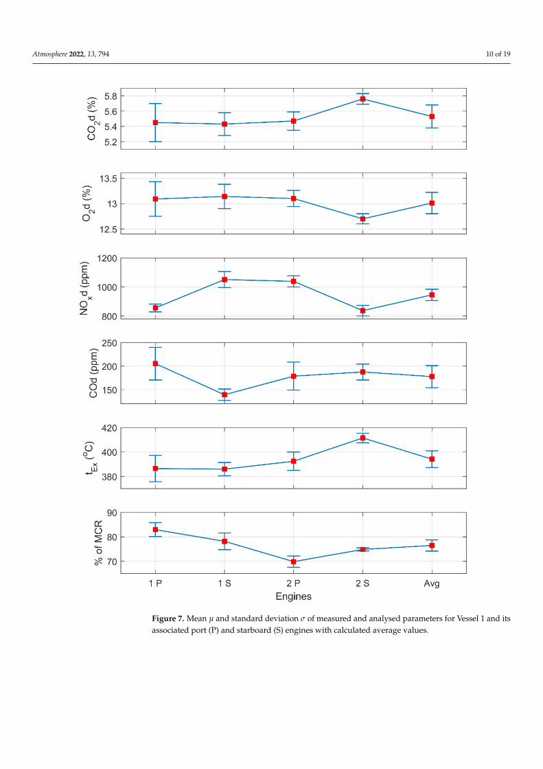
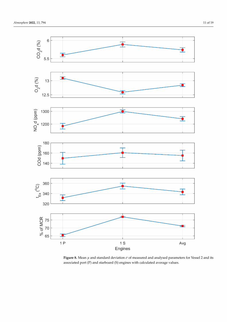
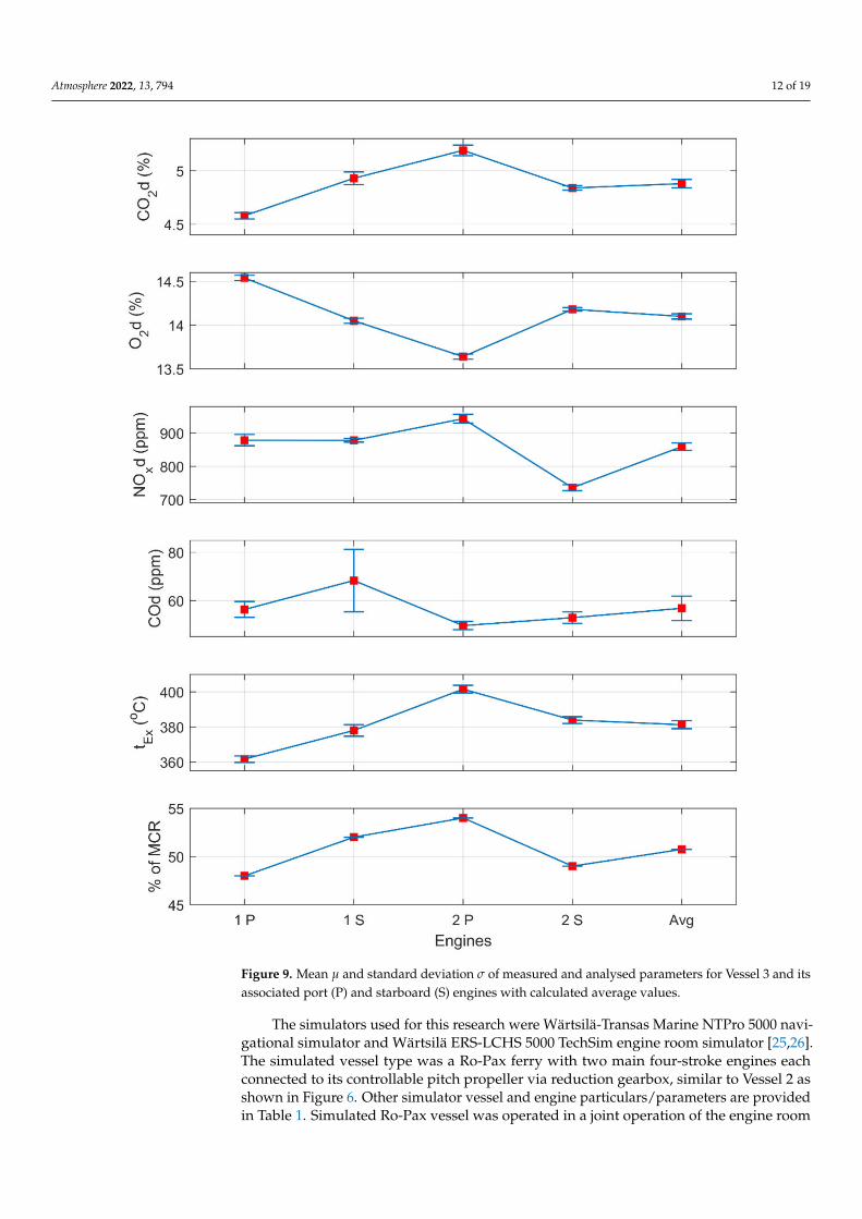
Figures 7–9 show individual vessel and engine exhaust gas measurements and param-eters with calculated average values. Red squared points show the mean value, and bluelines above and below the red points show the standard deviation of each measured oranalysed value.

Atmosphere 2022, 13, 794 10 of 19

Figure 7. Mean µ and standard deviation σ of measured and analysed parameters for Vessel 1 and itsassociated port (P) and starboard (S) engines with calculated average values.

Atmosphere 2022, 13, 794 11 of 19

Figure 8. Mean µ and standard deviation σ of measured and analysed parameters for Vessel 2 and itsassociated port (P) and starboard (S) engines with calculated average values.

Atmosphere 2022, 13, 794 12 of 19

Figure 9. Mean µ and standard deviation σ of measured and analysed parameters for Vessel 3 and itsassociated port (P) and starboard (S) engines with calculated average values.

The simulators used for this research were Wärtsilä-Transas Marine NTPro 5000 navi-gational simulator and Wärtsilä ERS-LCHS 5000 TechSim engine room simulator [25,26].The simulated vessel type was a Ro-Pax ferry with two main four-stroke engines eachconnected to its controllable pitch propeller via reduction gearbox, similar to Vessel 2 asshown in Figure 6. Other simulator vessel and engine particulars/parameters are providedin Table 1. Simulated Ro-Pax vessel was operated in a joint operation of the engine room

Atmosphere 2022, 13, 794 13 of 19

and navigational simulators. This means that simulators are synchronously connectedand operated as one vessel, which enables simultaneous recordings and later analysis ofsimulated vessel parameters, i.e., both from navigational and marine engine room point ofview. The simulator was operated with various simulation scenarios of different weatherand engine operating conditions typical for the Adriatic Sea [27] in order to record vesseland engine parameters. The simulator data obtained from these scenarios were partiallyused for the research published by Mannarini et al. [28] and were also used for this analysisin order to compare exhaust emissions from onboard measurements with simulated values.

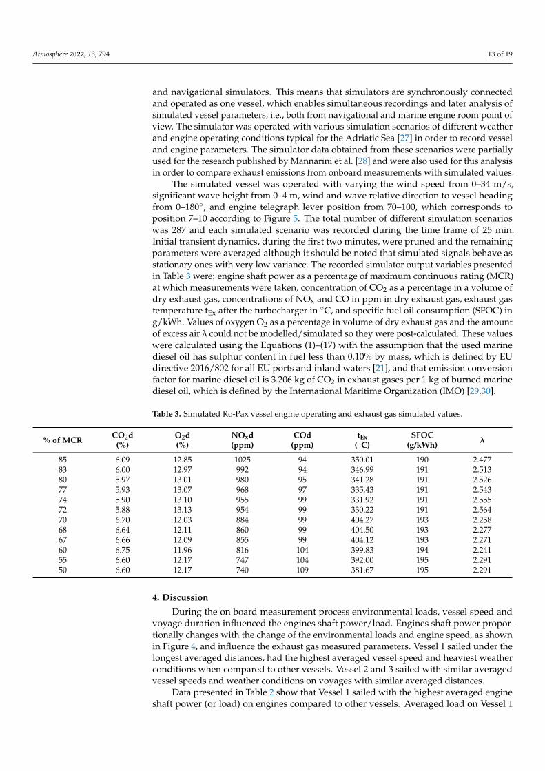
The simulated vessel was operated with varying the wind speed from 0–34 m/s,significant wave height from 0–4 m, wind and wave relative direction to vessel headingfrom 0–180◦, and engine telegraph lever position from 70–100, which corresponds toposition 7–10 according to Figure 5. The total number of different simulation scenarioswas 287 and each simulated scenario was recorded during the time frame of 25 min.Initial transient dynamics, during the first two minutes, were pruned and the remainingparameters were averaged although it should be noted that simulated signals behave asstationary ones with very low variance. The recorded simulator output variables presentedin Table 3 were: engine shaft power as a percentage of maximum continuous rating (MCR)at which measurements were taken, concentration of CO2 as a percentage in a volume ofdry exhaust gas, concentrations of NOx and CO in ppm in dry exhaust gas, exhaust gastemperature tEx after the turbocharger in ◦C, and specific fuel oil consumption (SFOC) ing/kWh. Values of oxygen O2 as a percentage in volume of dry exhaust gas and the amountof excess air λ could not be modelled/simulated so they were post-calculated. These valueswere calculated using the Equations (1)–(17) with the assumption that the used marinediesel oil has sulphur content in fuel less than 0.10% by mass, which is defined by EUdirective 2016/802 for all EU ports and inland waters [21], and that emission conversionfactor for marine diesel oil is 3.206 kg of CO2 in exhaust gases per 1 kg of burned marinediesel oil, which is defined by the International Maritime Organization (IMO) [29,30].

Table 3. Simulated Ro-Pax vessel engine operating and exhaust gas simulated values.

% of MCR CO2d(%)

O2d(%)

NOxd(ppm)

COd(ppm)

tEx(◦C)

SFOC(g/kWh) λ

85 6.09 12.85 1025 94 350.01 190 2.47783 6.00 12.97 992 94 346.99 191 2.51380 5.97 13.01 980 95 341.28 191 2.52677 5.93 13.07 968 97 335.43 191 2.54374 5.90 13.10 955 99 331.92 191 2.55572 5.88 13.13 954 99 330.22 191 2.56470 6.70 12.03 884 99 404.27 193 2.25868 6.64 12.11 860 99 404.50 193 2.27767 6.66 12.09 855 99 404.12 193 2.27160 6.75 11.96 816 104 399.83 194 2.24155 6.60 12.17 747 104 392.00 195 2.29150 6.60 12.17 740 109 381.67 195 2.291

4. Discussion

During the on board measurement process environmental loads, vessel speed andvoyage duration influenced the engines shaft power/load. Engines shaft power propor-tionally changes with the change of the environmental loads and engine speed, as shownin Figure 4, and influence the exhaust gas measured parameters. Vessel 1 sailed under thelongest averaged distances, had the highest averaged vessel speed and heaviest weatherconditions when compared to other vessels. Vessel 2 and 3 sailed with similar averagedvessel speeds and weather conditions on voyages with similar averaged distances.

Data presented in Table 2 show that Vessel 1 sailed with the highest averaged engineshaft power (or load) on engines compared to other vessels. Averaged load on Vessel 1

Atmosphere 2022, 13, 794 14 of 19

engines was 76.48% and the lowest averaged engine load was 50.75% on Vessel 3. Thishigher load on Vessel 1 was caused due to the heavier weather and higher vessel speeddue to the longer distances of the voyages. Averaged concentrations of CO2 and O2 in dryexhaust gases were similar on Vessel 1 and Vessel 2 which is normal due to almost similarengine loads. These engines were working with sufficient excess air quantity in order toenable complete combustion process in the cylinders and have a certain concentration ofO2 in exhaust gases. Vessel 3 operated with lower CO2 and higher O2 concentrations inthe dry exhaust gas, compared to the other vessels, which is typical for lower engine loads.The standard deviation for all averaged concentrations of CO2 and O2 in dry exhaust gaseson all three vessels was very small. Highest averaged concentrations of CO in dry exhaustgases were on Vessel 1 because of the higher engine loads and engine speed, and the loweston Vessel 3 for the opposite reasons. Highest averaged NOx concentrations were recordedon Vessel 2, and the lowest on Vessel 3. The formation of NOx concentration in exhaustgases is influenced with high combustion temperatures, pressures and the duration of thecombustion process [31]. Engines on all three vessels were built before 1 January 2000(Pre-2000 Engines), so the IMO emission standards, commonly referred to as Tier I, II andIII standards, do not apply to these engines [32].

Figure 7 shows measured data and differences on all four main engines on Vessel1. The standard deviation of all measured values is higher compared to other vesselsbecause of the influence of heavier weather on main engines during the voyages. For Portengines (1 P and 2 P) and 1 Starboard (1 S) engine the averaged concentrations of CO2and O2 in dry exhaust gases were similar except for the engine 2 Starboard (2 S) whereconcentrations of CO2 were higher and O2 lower. Additionally, for engine 2 S, averagedconcentrations of NOx were the lowest, the exhaust gas temperatures after the turbochargerthe highest and concentrations of CO the second highest. All of this can indicate theretarded injection timing or prolonged duration of the combustion process. Engine 1 S hadthe lowest averaged concentrations of CO, lowest exhaust gas temperatures and highestaveraged concentrations of NOx, which can indicate the best combustion process among allengines. Higher NOx concentration, which results from higher combustion temperatures,should satisfy Tier I, II or III emission levels for engines built after the 1 January 2000.

Figure 8 shows measured data and differences on port and starboard main engineson Vessel 2. Starboard main engine had a higher averaged load than the port main engineand consequently higher exhaust gas temperatures after the turbocharger, higher averagedvalues of CO2 and NOx and slightly higher values of CO. Averaged concentrations of O2 indry exhaust gases were lower on the port main engine compared to starboard engine. Thisdata difference is normal for engines working at such different engine loads. Averagedconcentrations of NOx on Vessel 2 are the highest when compared to other vessels whichshould be investigated further.

Figure 9 shows measured data and differences on all four main engines on Vessel3. Main engine 2 Port (2 P) had the highest percentage of averaged load compared toother engines. That resulted with the highest averaged values of exhaust gas temperatures,concentrations of CO2, NOx and lowest values of averaged data for concentrations ofO2 and CO in dry exhaust gases. All four engine data presented in Figure 8 follow thesame line pattern as previously explained. As the averaged load increases the exhaust gastemperatures, averaged concentrations of CO2 and NOx increase (except for CO data forengine 2 P) and averaged data for concentrations of O2 and CO decrease (and vice versa).

Data presented in Table 3 show averaged simulator engine parameters during theengine shaft power/load change in percentage of MCR. Other values that are not providedby the simulator were post-calculated, as explained in the previous section. Engine loads,during simulation process, varied from 50–85%, which are usual loads on board vesselsduring the voyages and were also during the measurement processes. The data in the tablecan be divided in two parts, engine parameters lower and higher than 70% of MCR. Thedata in the table follow the previously mentioned pattern (with the minor exception at lowerloads, at 60% and 67%). When the engine load increases, the exhaust gas temperatures,

Atmosphere 2022, 13, 794 15 of 19

concentrations of CO2 and NOx increase and concentrations of O2 and CO decrease. Atengine loads higher than 70% of MCR the turbocharger operates more efficiently and theexhaust gas temperature after the turbocharger decreases from 404 ◦C to 330 ◦C. Thiscauses suction of more combustion air quantity into the cylinder (excess air λ is higher). Asthe engine load again increases (more than 72% of MCR), the simulated data follow thepreviously mentioned pattern.

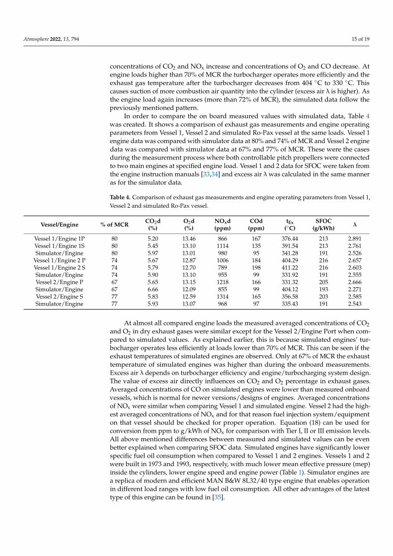
In order to compare the on board measured values with simulated data, Table 4was created. It shows a comparison of exhaust gas measurements and engine operatingparameters from Vessel 1, Vessel 2 and simulated Ro-Pax vessel at the same loads. Vessel 1engine data was compared with simulator data at 80% and 74% of MCR and Vessel 2 enginedata was compared with simulator data at 67% and 77% of MCR. These were the casesduring the measurement process where both controllable pitch propellers were connectedto two main engines at specified engine load. Vessel 1 and 2 data for SFOC were taken fromthe engine instruction manuals [33,34] and excess air λ was calculated in the same manneras for the simulator data.

Table 4. Comparison of exhaust gas measurements and engine operating parameters from Vessel 1,Vessel 2 and simulated Ro-Pax vessel.

Vessel/Engine % of MCR CO2d(%)

O2d(%)

NOxd(ppm)

COd(ppm)

tEx(◦C)

SFOC(g/kWh) λ

Vessel 1/Engine 1P 80 5.20 13.46 866 167 376.44 213 2.891Vessel 1/Engine 1S 80 5.45 13.10 1114 135 391.54 213 2.761Simulator/Engine 80 5.97 13.01 980 95 341.28 191 2.526

Vessel 1/Engine 2 P 74 5.67 12.87 1006 184 404.29 216 2.657Vessel 1/Engine 2 S 74 5.79 12.70 789 198 411.22 216 2.603Simulator/Engine 74 5.90 13.10 955 99 331.92 191 2.555Vessel 2/Engine P 67 5.65 13.15 1218 166 331.32 205 2.666Simulator/Engine 67 6.66 12.09 855 99 404.12 193 2.271Vessel 2/Engine S 77 5.83 12.59 1314 165 356.58 203 2.585Simulator/Engine 77 5.93 13.07 968 97 335.43 191 2.543

At almost all compared engine loads the measured averaged concentrations of CO2and O2 in dry exhaust gases were similar except for the Vessel 2/Engine Port when com-pared to simulated values. As explained earlier, this is because simulated engines’ tur-bocharger operates less efficiently at loads lower than 70% of MCR. This can be seen if theexhaust temperatures of simulated engines are observed. Only at 67% of MCR the exhausttemperature of simulated engines was higher than during the onboard measurements.Excess air λ depends on turbocharger efficiency and engine/turbocharging system design.The value of excess air directly influences on CO2 and O2 percentage in exhaust gases.Averaged concentrations of CO on simulated engines were lower than measured onboardvessels, which is normal for newer versions/designs of engines. Averaged concentrationsof NOx were similar when comparing Vessel 1 and simulated engine. Vessel 2 had the high-est averaged concentrations of NOx and for that reason fuel injection system/equipmenton that vessel should be checked for proper operation. Equation (18) can be used forconversion from ppm to g/kWh of NOx for comparison with Tier I, II or III emission levels.All above mentioned differences between measured and simulated values can be evenbetter explained when comparing SFOC data. Simulated engines have significantly lowerspecific fuel oil consumption when compared to Vessel 1 and 2 engines. Vessels 1 and 2were built in 1973 and 1993, respectively, with much lower mean effective pressure (mep)inside the cylinders, lower engine speed and engine power (Table 1). Simulator engines area replica of modern and efficient MAN B&W 8L32/40 type engine that enables operationin different load ranges with low fuel oil consumption. All other advantages of the latesttype of this engine can be found in [35].

Atmosphere 2022, 13, 794 16 of 19

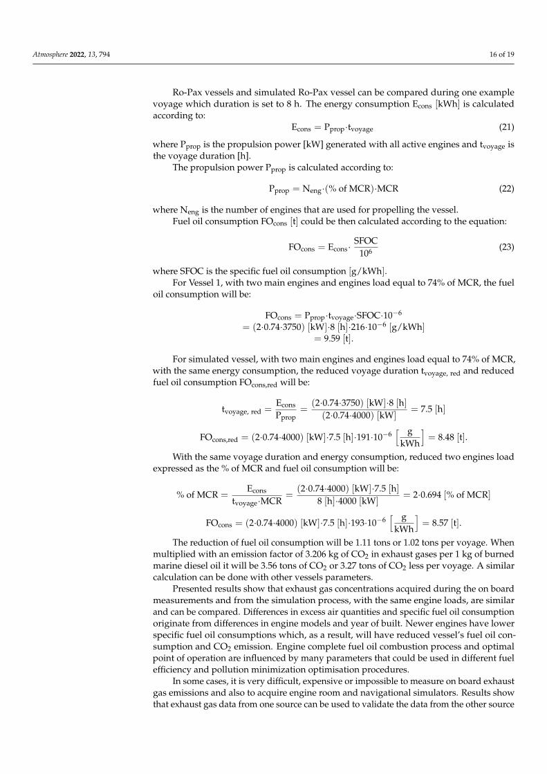
Ro-Pax vessels and simulated Ro-Pax vessel can be compared during one examplevoyage which duration is set to 8 h. The energy consumption Econs [kWh] is calculatedaccording to:

Econs = Pprop·tvoyage (21)

where Pprop is the propulsion power [kW] generated with all active engines and tvoyage isthe voyage duration [h].

The propulsion power Pprop is calculated according to:

Pprop = Neng·(% of MCR)·MCR (22)

where Neng is the number of engines that are used for propelling the vessel.Fuel oil consumption FOcons [t] could be then calculated according to the equation:

FOcons = Econs·SFOC

106 (23)

where SFOC is the specific fuel oil consumption [g/kWh].For Vessel 1, with two main engines and engines load equal to 74% of MCR, the fuel

oil consumption will be:

FOcons = Pprop·tvoyage·SFOC·10−6

= (2·0.74·3750) [kW]·8 [h]·216·10−6 [g/kWh]= 9.59 [t].

For simulated vessel, with two main engines and engines load equal to 74% of MCR,with the same energy consumption, the reduced voyage duration tvoyage, red and reducedfuel oil consumption FOcons,red will be:

tvoyage, red =Econs

Pprop=

(2·0.74·3750) [kW]·8 [h](2·0.74·4000) [kW]

= 7.5 [h]

FOcons,red = (2·0.74·4000) [kW]·7.5 [h]·191·10−6[ g

kWh

]= 8.48 [t].

With the same voyage duration and energy consumption, reduced two engines loadexpressed as the % of MCR and fuel oil consumption will be:

% of MCR =Econs

tvoyage·MCR=

(2·0.74·4000) [kW]·7.5 [h]8 [h]·4000 [kW]

= 2·0.694 [% of MCR]

FOcons = (2·0.74·4000) [kW]·7.5 [h]·193·10−6[ g

kWh

]= 8.57 [t].

The reduction of fuel oil consumption will be 1.11 tons or 1.02 tons per voyage. Whenmultiplied with an emission factor of 3.206 kg of CO2 in exhaust gases per 1 kg of burnedmarine diesel oil it will be 3.56 tons of CO2 or 3.27 tons of CO2 less per voyage. A similarcalculation can be done with other vessels parameters.

Presented results show that exhaust gas concentrations acquired during the on boardmeasurements and from the simulation process, with the same engine loads, are similarand can be compared. Differences in excess air quantities and specific fuel oil consumptionoriginate from differences in engine models and year of built. Newer engines have lowerspecific fuel oil consumptions which, as a result, will have reduced vessel’s fuel oil con-sumption and CO2 emission. Engine complete fuel oil combustion process and optimalpoint of operation are influenced by many parameters that could be used in different fuelefficiency and pollution minimization optimisation procedures.

In some cases, it is very difficult, expensive or impossible to measure on board exhaustgas emissions and also to acquire engine room and navigational simulators. Results showthat exhaust gas data from one source can be used to validate the data from the other source

Atmosphere 2022, 13, 794 17 of 19

in order to reduce the research expenses and help creating relevant emission database.Acquired data can be also used for creating exhaust gas emissions models, engine andvessel optimization models, ship routing models [36] and similar.

5. Conclusions

In this research, exhaust gas emissions were measured on three Ro-Pax vessels sailingin the Adriatic Sea. Testo 350 Maritime flue gas analyser was used for monitoring the con-centrations of CO2 and O2 as a percentage in volume of dry exhaust gas, concentrations ofCO and NOx in ppm in dry exhaust gas and exhaust gas temperature after the turbocharger.During the measurement of exhaust gases main engines on Ro-Pax vessels were operatedat different averaged loads, from 48% to 83% of MCR. As the averaged load increases theexhaust gas temperatures, averaged concentrations of CO2 and NOx increase and averageddata for concentrations of O2 and CO decrease (and vice versa). Analysis and comparisonof main engines concentrations of exhaust gases from the same vessel and other vessels canindicate possible inefficiencies/faults that are caused by incomplete combustion processwhich will increase fuel oil consumption. All 10 analysed main engines on three vessels hadvery good combustion process in the cylinders. On Vessel 1, one main engine had differentexhaust gas values than other engines which can indicate small retarded injection timing orprolonged duration of the combustion process and both engines on Vessel 2 had higherNOx emissions, which should be further investigated. Averaged values from all 10 engineson three vessels were: 5.38% of CO2, 13.32% of O2, 1115 ppm of NOx and 130 ppm of COin dry exhaust gas with the averaged exhaust gas temperature after the turbocharger of373 ◦C at 66% of MCR.

For this research, Wartsila-Transas engine room and navigational simulators werealso used for creating the additional database of the exhaust gases and engine operatingparameters in different weather conditions typical for the Adriatic Sea. The recordedsimulator output variables, which were similar to the on board measured parameters, werecompared to the exhaust gas emissions and engine operating parameters of Vessels 1, 2 and3 engines. Comparison of data measured on board vessels with simulated data showed thatconcentrations of exhaust gas components were similar for all engine loads and measuredaveraged concentrations. The difference in results was due to the difference in engine designparameters and year of built of analysed engines. Specific fuel oil consumption of simulatedengines at analysed loads was 191–193 g/kWh, for Vessel 1 SFOC was 213–216 g/kWhand for Vessel 2 SFOC was 203–205 g/kWh. When comparing the simulated vessel withVessel 1, for one voyage of 8 h, at engines load of 74% of MCR and with the same energyconsumption, simulated vessel will arrive 30 min faster and consume 1.11 tons of fueloil or will produce 3.56 tons of CO2 less per voyage. If the voyage is set for an equalduration of 8 h and with the same energy consumption, the simulated vessel engines loadwill be reduced to 69% of MCR and still consume 1.02 tons of fuel oil, i.e., it will produce3.27 tons of CO2 less per voyage. Presented analysis shows that significant fuel oil andCO2 emission reduction per voyage could be accomplished by voyage and/or engineoperation optimization. Finally, it should be noted that the values presented in Table 3 canbe further used for any kind of future data-driven modelling with the purpose of exhaustgases estimation with respect to different engine operating conditions.

Research studies on exhaust gases on board Ro-Pax vessels are very limited so mea-sured data presented in this research will help creating more relevant on board emissiondatabase and offer the possibility to enhance the estimation of emissions and comparisonwith the current emission database. Measured and simulated data can be used for rootcause analysis, creating engine optimization and exhaust emissions models, ship routingmodels and similar. Results of this analysis could be of interest to shipowners, ship opera-tors, environmentalists and all other in reducing the fuel oil consumption and emissions ofgreenhouse and harmful exhaust gases into the atmosphere.

The main limitations of the presented analysis and obtained results are naturallyconnected with a limited number of performed measurements and very bounded initial

Atmosphere 2022, 13, 794 18 of 19

conditions, particularly in terms of a relatively small sample of various environmentalconditions and sea states during the measurement campaign, as well as the selected vesselswhich are far away from being the state-of-the-art. However, these vessels still representthe majority of passenger ships in Adriatic and therefore the obtained results are alsorepresentative having that in mind. Nevertheless, the research results could be improvedby enhancing the measurement procedures at different weather conditions and distanceswith the same vessels and on even more vessels, particularly the newer ones.

Author Contributions: Conceptualization, J.O., M.V. and V.K.; methodology, J.O. and M.V.; softwareJ.O. and Z.P.; validation, J.O. and M.V.; formal analysis, J.O., M.V. and Z.P.; investigation, J.O., M.V.,V.K. and Z.P.; resources, J.O. and M.V.; data curation, J.O., M.V. and Z.P.; writing—original draftpreparation, J.O, M.V. and V.K.; writing—review and editing, J.O., M.V., V.K. and Z.P.; visualization,M.V., J.O. and V.K.; supervision, J.O. and M.V.; project administration, J.O.; funding acquisition, J.O.All authors have read and agreed to the published version of the manuscript.

Funding: This research was funded by the European Regional Development Fund through theItaly-Croatia Interreg programme, project GUTTA, grant number 10043587.

Institutional Review Board Statement: Not applicable.

Informed Consent Statement: Not applicable.

Data Availability Statement: The data presented in this study are available on request from thecorresponding author.

Acknowledgments: This work was also supported by the Croatian Science Foundation under theproject IP-2018-01-3739. The authors would like to extend their appreciations to the ship-owner officefor all the help during the exploitation measurements.

Conflicts of Interest: The authors declare no conflict of interest. The funders had no role in the designof the study; in the collection, analyses, or interpretation of data; in the writing of the manuscript, orin the decision to publish the results.

References1. Regulation (EU) 2015/757 of the European Parliament and of the Council of 29 April 2015 on the Monitoring, Reporting

and Verification of Carbon Dioxide Emissions from Maritime Transport, and Amending Directive 2009/16/EC (Text withEEA Relevance)—EUR-Lex. Available online: https://eur-lex.europa.eu/legal-content/EN/LSU/?uri=CELEX%3A32015R0757(accessed on 16 March 2022).

2. Reducing Emissions from the Shipping Sector. Available online: https://ec.europa.eu/clima/eu-action/transport-emissions/reducing-emissions-shipping-sector_en (accessed on 16 March 2022).

3. Mannarini, G.; Carelli, L.; Salhi, A. EU-MRV: An Analysis of 2018’s Ro-Pax CO2 Data. In Proceedings of the 2020 21st IEEEInternational Conference on Mobile Data Management (MDM), Versailles, France, 30 June–3 July 2020; IEEE: Piscataway, NJ,USA, 2020; pp. 287–292.

4. Data Collection System for Fuel Oil Consumption of Ships. Available online: https://www.imo.org/en/OurWork/Environment/Pages/Data-Collection-System.aspx (accessed on 16 March 2022).

5. Cooper, D.A. Exhaust Emissions from High Speed Passenger Ferries. Atmos. Environ. 2001, 35, 4189–4200. [CrossRef]6. Bogdanowicz, A.; Kniaziewicz, T. Marine Diesel Engine Exhaust Emissions Measured in Ship’s Dynamic Operating Conditions.

Sensors 2020, 20, 6589. [CrossRef]7. Jahangiri, S.; Nikolova, N.; Tenekedjiev, K. An Improved Emission Inventory Method for Estimating Engine Exhaust Emissions

from Ships. Sustain. Environ. Res. 2018, 28, 374–381. [CrossRef]8. Jahangiri, S.; Nikolova, N.; Tenekedjiev, K. Empirical Testing of Inventories Applying On-Board Measurements of Exhaust

Emissions at Port and at Sea. J. Sustain. Dev. Transp. Logist. 2018, 3, 6–33. [CrossRef]9. Khan, M.Y.; Ranganathan, S.; Agrawal, H.; Welch, W.A.; Laroo, C.; Miller, J.W.; Cocker, D.R. Measuring In-Use Ship Emissions

with International and U.S. Federal Methods. J. Air Waste Manag. Assoc. 2013, 63, 284–291. [CrossRef] [PubMed]10. Agrawal, H.; Welch, W.A.; Henningsen, S.; Miller, J.W.; Cocker, D.R. Emissions from Main Propulsion Engine on Container Ship

at Sea. J. Geophys. Res. 2010, 115, D23205. [CrossRef]11. Chu-Van, T.; Ristovski, Z.; Pourkhesalian, A.M.; Rainey, T.; Garaniya, V.; Abbassi, R.; Jahangiri, S.; Enshaei, H.; Kam, U.-S.;

Kimball, R.; et al. On-Board Measurements of Particle and Gaseous Emissions from a Large Cargo Vessel at Different OperatingConditions. Environ. Pollut. 2018, 237, 832–841. [CrossRef] [PubMed]

12. Agrawal, H.; Welch, W.A.; Miller, J.W.; Cocker, D.R. Emission Measurements from a Crude Oil Tanker at Sea. Environ. Sci. Technol.2008, 42, 7098–7103. [CrossRef] [PubMed]

Atmosphere 2022, 13, 794 19 of 19

13. Fu, M. Real-World Emissions of Inland Ships on the Grand Canal, China. Atmos. Environ. 2013, 81, 222–229. [CrossRef]14. Introduction to Fuel and Energy. Available online: http://eyrie.shef.ac.uk/eee/cpe630/comfun1.html (accessed on 17 March

2022).15. Trisha, S. How Much Air Is Required for Complete Combustion? In Thermodynamics; Engineering Notes India, 2018. Avail-

able online: https://www.engineeringenotes.com/thermal-engineering/fuels-and-combustion/how-much-air-is-required-for-complete-combustion-thermodynamics/51415 (accessed on 16 March 2022).

16. Smith, C.B. (Ed.) 9—Management of Process Energy. In Energy, Management, Principles; Elsevier: Amsterdam, The Netherlands,1981; pp. 236–279, ISBN 978-0-08-028036-3.

17. Sarkar, D.K. (Ed.) Chapter 3—Fuels and Combustion. In Thermal Power Plant; Elsevier: Amsterdam, The Netherlands, 2015;pp. 91–137, ISBN 978-0-12-801575-9.

18. Çengel, Y.A.; Boles, M.A. Thermodynamics: An Engineering Approach, 5th ed.; Tata McGraw-Hill: New York, NY, USA, 2006.19. Kosky, P.; Balmer, R.; Keat, W.; Wise, G. (Eds.) Chapter 7—Chemical Engineering. In Exploring Engineering, 5th ed.; Academic

Press: Cambridge, MA, USA, 2021; pp. 129–145, ISBN 978-0-12-815073-3.20. ISO 8217 2017; Fuel Standard for Marine Distillate Fuels. ISO: Geneva, Switzerland, 2017.21. Directive (EU) 2016/802 of the European Parliament and of the Council of 11 May 2016 Relating to a Reduction in the Sulphur Content of

Certain Liquid Fuels; 2016; Volume 132. Available online: https://eur-lex.europa.eu/legal-content/EN/TXT/PDF/?uri=CELEX:32016L0802&rid=5 (accessed on 17 March 2022).

22. Available online: https://www.testo.com/hr-HR/testo-350-maritime/p/0563-3503 (accessed on 17 March 2022).23. Testo-350-Maritime-Instruction-Manual.pdf. Available online: https://static-int.testo.com/media/30/a7/476842882400/testo-

350-maritime-Instruction-manual.pdf (accessed on 17 March 2022).24. Internal Company Document: Bunker Delivery Note; Croatiainspect: Zagreb, Croatia, 2019.25. Available online: https://www.wartsila.com/voyage/simulation-and-training/technological-simulators (accessed on 17

March 2022).26. Available online: https://www.wartsila.com/voyage/simulation-and-training/navigational-simulators (accessed on 17

March 2022).27. Farkas, A.; Parunov, J.; Katalinic, M. Wave statistics for the middle Adriatic Sea. Pomor. Zb. 2016, 52, 33–47. [CrossRef]28. Mannarini, G.; Carelli, L.; Orovic, J.; Martinkus, C.P.; Coppini, G. Towards Least-CO2 Ferry Routes in the Adriatic Sea. J. Mar. Sci.

Eng. 2021, 9, 115. [CrossRef]29. IMO. MEPC.1/Circ.684 Guidelines for Voluntary Use of the Ship Energy Efficiency Operational Indicator (EEOI); Technical Report;

International Maritime Organization: London, UK, 2009.30. IMO: Fourth Greenhouse Gas Study. 2020. Available online: https://wwwcdn.imo.org/localresources/en/OurWork/

Environment/Documents/Fourth%20IMO%20GHG%20Study%202020%20-%20Full%20report%20and%20annexes.pdf (accessedon 30 March 2022).

31. European Maritime Safety Agency (EMSA): Possible Technical Modifications on Pre-2000 Marine Diesel Engines for NOx Reduc-tions. 2008. Available online: http://www.emsa.europa.eu/tags/download/1017/604/23.html (accessed on 30 March 2022).

32. US Environmental Protection Agency. Regulatory update—Overview of EPA’s Emission Standards for Marine Engines, August 2004; USEnvironmental Protection Agency: Washington, DC, USA, 2004.

33. Internal Company Document: Instruction Manual for Stork Werkspoor Diesel 8TM410 Engine; Stork Werkspoor Diesel: Amsterdam,The Netherlands, 1972.

34. Internal Company Document: Instruction Manual for Bazan MAN B&W 8L40/54 a Engine; Bazan Motores: Cartagena, Columbia, 1992.35. MAN B&W: L+V32/40 Project Guide—Marine Four-Stroke Diesel Engines Compliant with IMO Tier II. Available online: https:

//man-es.com/applications/projectguides/4stroke/manualcontent/L32-40_GenSet_TierII.pdf (accessed on 30 March 2022).36. Available online: https://www.gutta-visir.eu (accessed on 30 March 2022).