COMPARISON OF PROCESS-BASED AND ARTIFICIAL NEURAL NETWORK APPROACHES FOR STREAMFLOW MODELING IN AN...

ABSTRACT: The performance of the Soil and Water AssessmentTool (SWAT) and artificial neural network (ANN) models in sim-ulating hydrologic response was assessed in an agriculturalwatershed in southeastern Pennsylvania. All of the performanceevaluation measures including Nash-Sutcliffe coefficient of effi-ciency (E) and coefficient of determination (R2) suggest thatthe ANN monthly predictions were closer to the observed flowsthan the monthly predictions from the SWAT model. Morespecifically, monthly streamflow E and R2 were 0.54 and 0.57,respectively, for the SWAT model calibration period, and 0.71and 0.75, respectively, for the ANN model training period. Forthe validation period, these values were -0.17 and 0.34 for theSWAT and 0.43 and 0.45 for the ANN model. SWAT model per-formance was affected by snowmelt events during wintermonths and by the model’s inability to adequately simulatebase flows. Even though this and other studies using ANNmodels suggest that these models provide a viable alternativeapproach for hydrologic and water quality modeling, ANN mod-els in their current form are not spatially distributed watershedmodeling systems. However, considering the promising perfor-mance of the simple ANN model, this study suggests that theANN approach warrants further development to explicitlyaddress the spatial distribution of hydrologic/water quality pro-cesses within watersheds.(KEY TERMS: surface water hydrology; models; Soil and WaterAssessment Tool (SWAT); streamflow; runoff; base flow.)

Srivastava, Puneet, James N. McNair, and Thomas E. Johnson,2006. Comparison of Process-Based and Artificial Neural Net-work Approaches for Streamflow Modeling in an AgriculturalWatershed. Journal of the American Water Resources Associa-tion (JAWRA) 42(2):545-563.

INTRODUCTION

Watershed hydrology is of central importance tothe structure and function of stream ecosystems.Stochastic by nature, streamflow varies over time inresponse to precipitation and is inherently subject toepisodic extremes of high and low flows. Streamflowalso varies among watersheds due to complex physio-graphic, landscape, and disturbance characteristics.Stream organisms are generally well adapted to arange of streamflow conditions but can be stronglyaffected by extreme flow events. Extreme high flowevents can reduce benthic algae abundance (Biggsand Close, 1989) and disrupt benthic macroinverte-brate communities through scouring and bed instabil-ity. Low flows can severely stress fish communitiesand, in extreme cases, may cause changes in localcommunity composition and density. Given the greatimportance of hydrology to stream ecosystems, it fol-lows that any understanding of ecosystem structureand function in these systems must explicitly accountfor the effects of flow variability (Poff et al., 1997;Richter et al., 1997). Further, together with sedimentloadings from watersheds, streamflow is also a keyvariable influencing the morphology of stream chan-nels, which in turn determines the physical habitat –the foundation of any stream ecosystem (Leopold etal., 1964).

Given the great importance of hydrology to streamecosystems, accurate prediction of streamflow is ofutmost importance. However, accurate predictions ofrainfall-runoff and consequent streamflows from aregional scale watershed are extremely difficult

1Paper No. 04021 of the Journal of the American Water Resources Association (JAWRA) (Copyright © 2006). Discussions are open untilDecember 1, 2006.

2Respectively, Assistant Professor, Biosystems Engineering, Auburn University, 206 Tom E. Corley Building, Auburn, Alabama 36849-5417; and Senior Scientists, Patrick Center for Environmental Research, The Academy of Natural Sciences of Philadelphia, 1900 BenjaminFranklin Parkway, Philadelphia, Pennsylvania 19103 (E-Mail/Srivastava: [email protected]).

JOURNAL OF THE AMERICAN WATER RESOURCES ASSOCIATION 545 JAWRA

JOURNAL OF THE AMERICAN WATER RESOURCES ASSOCIATIONJUNE AMERICAN WATER RESOURCES ASSOCIATION 2006

COMPARISON OF PROCESS-BASED AND ARTIFICIAL NEURALNETWORK APPROACHES FOR STREAMFLOW MODELING

IN AN AGRICULTURAL WATERSHED1

Puneet Srivastava, James N. McNair, and Thomas E. Johnson2

because of tremendous spatial and temporal variabili-ty of watershed characteristics and weather patternsand an incomplete understanding of complex underly-ing physical processes. The traditional approach tohydrologic modeling is to link several detailed mecha-nistic, quasi-mechanistic, or empirical submodels ofsystem processes (e.g., evapotranspiration, infiltra-tion, percolation, flow routing) in an effort to build aprocess-based model of the complete hydrologic system such as Hydrologic Simulation Program-FORTRAN (HSPF) (Bicknell et al., 2001) and SWAT(Neitsch et al., 2001a). Because of the enormous spa-tial scale of the system and the complex, poorlyunderstood processes and their interactions, alterna-tives to traditional process-based modeling approach-es must be developed. Further, process-based modelsare usually difficult to implement because of theirhigh complexity and massive input data require-ments, much of which are unavailable for significantportions of any regional scale watershed. Such modelsalso require considerable technical expertise to imple-ment and use and therefore are not suitable for mostwatershed managers. Moreover, inadequate scientificunderstanding of underlying processes implies thatstructural (or knowledge) uncertainty will be substan-tial in such models, imposing severe constraints onefforts to reduce prediction uncertainty.

In response to these concerns and the demonstrat-ed success of ANNs applied to complex problems in avariety of disciplines (e.g., physics, biomedical engi-neering, electrical engineering, computer science,robotics, and image processing), several researchersin the hydrologic community are attempting to useANN as an alternative modeling tool for streamflowpredictions. Maier and Dandy (2000) provide a reviewof neural network models for predicting and forecast-ing various water resources variables. For example,Karunanithi et al. (1994), Minns and Hall (1996),Braddock et al. (1998), Dawson and Wilby (1998),Anmala et al. (2000), Gupta et al. (2000), Salas et al.(2000), and Zhang and Govindaraju (2000, 2003) usedvarious forms of ANNs for rainfall-runoff modeling. Anumber of researchers also compared performance ofANNs with other empirical approaches. Anmala etal. (2000) compared the performance of various ANNarchitectures with empirical approaches such as com-plex time series and multivariate time series in threeKansas watersheds and found ANNs and recurrentneural networks (RNNs) to perform as well or better.Hsu et al. (1995) found ANN performance to be betterthan a conceptual Sacramento Soil Moisture Account-ing (SAC-SMA) model and an autoregressive movingaverage with exogenous variables (ARMAX) timeseries approach in a subbasin of the Mississippi Riverbasin for daily streamflow predictions. Fernando and Jayawardena (1998) found a radial basis function

network (a type of ANN) to work better than theARMAX approach. Tokar and Johnson (1999) foundANNs to be superior to simple conceptual models inthe Little Patuxent River basin, Maryland.

Braddock et al. (1998) suggested that ANNs shouldbe rigorously compared with established methods forthem to become a tool for hydrologic forecasting.These methods can be broadly classified into two cate-gories – statistical/stochastically based and conceptu-al/physically based (Salas et al., 2000). As listedabove, a few studies have compared the performanceof various ANN architectures to statistical/stochasticapproaches. However, studies are scarce that havecompared the performance of ANNs with a spatiallyexplicit, physically based, continuous simulationmodel such as SWAT, HSPF, or AnnAGNPS (Annual-ized Agricultural Non-Point Source) (USDA-ARS,2001).

This study compares the performance of an ANNhydrologic model with the SWAT model in a smallagricultural watershed in southeastern Pennsylvania.The main objectives of this study were to evaluate theperformance of the SWAT model for simulatingstreamflows from a small agricultural watershed andto compare the performance of the SWAT model withthat of an ANN hydrologic model.

THEORETICAL CONSIDERATIONS

Artificial Neural Networks

Artificial neural networks (ANNs) are dynamic sys-tem models originally designed to mimic the way sim-ple biological nervous systems were thought tooperate (Rumelhart and McClelland, 1986). They arebased on simulated nerve cells, or neurons, which arejoined together in various ways to form networks. Intheir modern form, these networks have the capacityto learn, memorize, and extract relationships amongdata. Unlike in physically based models, the set ofprocesses influencing the system are not knownbeforehand. Nevertheless, ANNs should not be con-sidered black boxes, since a firm understanding of thehydrologic system being modeled is important fortheir successful application (Govindaraju, 2000).

Artificial neural networks have been successfullyapplied to numerous real world problems in suchwidely varying disciplines as hydrology (Poff et al.,1996; Braddock et al., 1998; Campolo et al., 1999;Tokar and Johnson, 1999; Deo and Thirumalaiah,2000; Gupta et al., 2000; Salas et al., 2000; Zhang andGovindaraju, 2000; Beven, 2001), statistics (Bishop,1995; Ripley, 1996; Venables and Ripley, 1999),

JAWRA 546 JOURNAL OF THE AMERICAN WATER RESOURCES ASSOCIATION

SRIVASTAVA, MCNAIR, AND JOHNSON

medicine (Guez and Nevo, 1996), music (Mozer, 1994),and robotics and control (Guez et al.,, 1998). Theyhave been particularly useful in real world applica-tions involving complex, poorly understood systemswith noisy observational data, where traditionalmechanistic methods often perform poorly. An impor-tant property of ANNs is that they are universal func-tion approximators (Hornik et al., 1990). That is, theycan approximate arbitrary continuous, nonlinearfunctions with any prescribed precision uniformly oncompact domains. Thus, they can represent evenhighly complicated, multidimensional, nonlinear rela-tionships quite well – a highly desirable property formodeling complex ecosystems.

There are many different kinds of ANNs (e.g., Guezet al., 1988; Eberhart and Dobbins, 1990; Hinton,1992; Kohonen, 1997). The most widely used type isknown as the feed forward ANN with back propaga-tion. This type of ANN performs very well in predic-tion and classification tasks. A feed forward ANNconsists of a number of nodes, or processing elements,typically organized in layers (Figure 1a). Each nodereceives inputs, which it weights differentially, sums,and then passes through a nonlinear activation func-tion (Figure 1b) to produce an output. Nodes in onelayer are connected to nodes in the neighboringlayer(s) via inputs received or outputs generated.Typically, each node in one layer is connected to everynode in the neighboring layer(s), though other archi-tectures can be used. Patterns (data) are presented tothe network via the input layer, which communicatesto nodes in one or more hidden layers where most ofthe actual processing is done. The hidden layer thenlinks to an output layer where the ANN's responsecorresponding to each input pattern is produced by

generating a weighted sum of inputs received fromthe hidden layer and passing it through a nonlinearactivation function.

An important issue with ANNs is how to adjust theweights of the links to achieve the desired systemresponse for each input pattern. This procedure iscalled training and corresponds roughly to calibrationof traditional models. Training requires a set of pairsof input patterns and corresponding desired, or tar-get, responses. The basic procedure is to start with apossibly random choice of weights for every process-ing element, present the ANN with a set of traininginput patterns, allow the ANN to compute a response,and then use the difference between computed anddesired response (i.e., the error) to determine themeans of adjusting the weights (e.g., by gradientdescent toward a minimum on the error surface). Thisprocedure is repeated iteratively until a stopping cri-terion is satisfied.

Once a neural network is trained to a satisfactorylevel, it may be used as an analytical tool on otherinput data of the same type. To do this, new inputsare presented to the input layer, where they filter intoand are processed by the middle layers as duringtraining, but the output is now retained withoutadjusting the weights. The output is the model predic-tion for the input data, which can then be used forfurther analysis and interpretation.

In ANNs with multiple inputs, the various inputvariables typically have different characteristic mag-nitudes and degrees of variability that are unrelatedto their relative values as predictors of the target out-puts. Since these differences tend to interfere withtraining, it is desirable to preprocess (normalize) theinputs so that all have the same mean and variance.


COMPARISON OF PROCESS-BASED AND ARTIFICIAL NEURAL NETWORK APPROACHES FOR STREAMFLOW MODELING IN AN AGRICULTURAL WATERSHED

Figure 1. (a) Flow Diagram of an ANN, Illustrating the Input, Hidden, and Output Layers, Nodes, or ProcessingElements, Most Common Pattern of Connections, and Use of Input Preprocessing and Output Postprocessing.

(b) Signal Flow Through a Processing Element, Showing Formation of a Weighted Sum of Inputs,Which is Then Passed Through a Nonlinear Activation Function to Produce the Output.

In addition, whenever the output node's activationfunction is logistic, predicted outputs will be restrict-ed to the interval (0, 1), and target outputs shouldtherefore be preprocessed (scaled) to lie within thissame interval. When used in prediction mode, ANNoutput must then be postprocessed by applying theinverse of the preprocessing transformation to recoverthe original, physically meaningful dimensions.

One of the major advantages of ANNs is their abili-ty to generalize. This means that a trained net cansuccessfully predict from or classify data that are ofthe same type as the learning data but have neverbeen seen before. In real world applications, one nor-mally has only a small fraction of all possible patternsfor training a neural net. To achieve the best general-ization, a technique called cross validation isemployed. The dataset is split into three parts (1) thetraining set is used to train the ANN and the error forthis dataset is systematically reduced during train-ing; (2) the validation set is accessed periodically dur-ing training (but without adjusting weights) to assessgeneralization performance of the ANN; and (3) aftertraining is complete, a test set is employed for finalassessment of the ANN's overall performance.

Typically, error on the training dataset willdecrease continually during training. As training pro-ceeds, error on the validation set will initiallydecrease but then will begin to increase. Trainingshould be stopped when error on the validation setreaches its minimum. This is the recommended stop-ping criterion for most real-world problems, since thenet generalizes best at this point. If learning isallowed to proceed further, overtraining occurs andthe ANN's performance on nontraining data degrades.After stopping the training phase, the net should bechecked with the third dataset, the test set, to assessperformance. Details about various ANN architec-tures and their mathematical aspects have been pro-vided by a number of authors (e.g., Govindaraju,2000; Gupta et al., 2000; Salas et al., 2000; Zhang andGovindaraju, 2000).

SWAT Model

The SWAT model, developed by Dr. Jeffrey Arnoldfor the U.S. Department of Agriculture, AgriculturalResearch Service (USDA-ARS), is a watershed scale,distributed parameter, physically based, continuoussimulation model for predicting the impact of landmanagement practices on water, sediment, nutrients,and pesticides for large, complex watersheds (Neitschet al., 2001b). SWAT is an extended and improved ver-sion of the Simulator for Water Resources in Rural

Basins (SWRRB) (Arnold et al., 1990) and RoutingOutputs to Outlets (ROTO) (Arnold et al., 1995) mod-els and incorporates features from other USDA-ARSmodels, including Chemicals, Runoff, and Erosionfrom Agricultural Management Systems (CREAMS)(Knisel, 1980), Groundwater Loading Effects on Agri-cultural Management Systems (GLEAMS) (Leonardet al., 1987), and Erosion-Productivity Impact Calcu-lator (EPIC) (Williams et al., 1984). To allow for spa-tial representation of a watershed to reflect landscapespatial heterogeneity, SWAT allows partitioning of awatershed into a number of subwatersheds or sub-basins. Inputs from each subwatershed are groupedinto climate, hydrologic response units (HRUs),ponds/wetlands, ground water, and reach categories.Hydrologic response units are lumped areas within asubwatershed that are comprised of unique landcover, soil, and management combinations. The SWATmodel components include weather, surface runoff,return flow, percolation, evapotranspiration, trans-mission losses, pond and reservoir storage, cropgrowth and irrigation, ground water flow, reach rout-ing, nutrient and pesticide loading, and water trans-fer. The model operates on a daily time step.

Accurate simulation of hydrology is the backbone ofSWAT model. In SWAT, simulation of hydrology of awatershed is done in two separate components: theland phase of the hydrologic cycle that controls theamount of water, sediment, nutrient, and pesticideloadings to the reach in each subwatershed; and therouting phase of the hydrologic cycle that moves thewater, sediment, nutrients, and pesticides through thestream network to the watershed outlet.

The land phase of the hydrologic cycle is based on awater balance equation that keeps track of daily soilwater content, precipitation, surface runoff, evapo-transpiration, water entering the vadose zone, andreturn flow. All of the major hydrologic processes, i.e.,canopy storage, infiltration, redistribution, evapotran-spiration, lateral subsurface flow, surface runoff, andreturn flows, are simulated in SWAT. In addition, forthe land phase of hydrologic cycle, the model also sim-ulates ponds within a subbasin that intercepts sur-face runoff and tributary channels within subbasinsto determine the time of concentrations. The routingphase of the hydrologic cycle is based on either thevariable storage coefficient method developed byWilliams (1969) or the Muskingum routing method.The routing phase simulates evaporation and trans-mission losses in the channel, water diversions, andaddition of water from point source discharges.



METHODOLOGY

Watershed Description

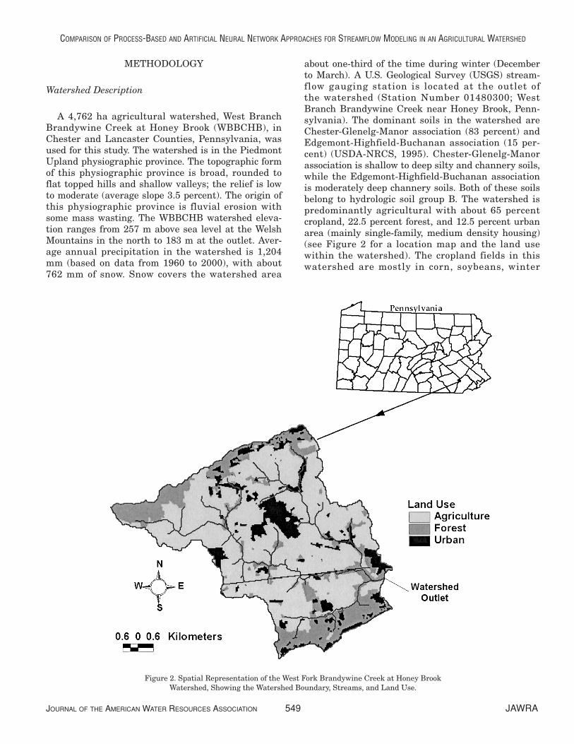
A 4,762 ha agricultural watershed, West BranchBrandywine Creek at Honey Brook (WBBCHB), inChester and Lancaster Counties, Pennsylvania, wasused for this study. The watershed is in the PiedmontUpland physiographic province. The topographic formof this physiographic province is broad, rounded toflat topped hills and shallow valleys; the relief is lowto moderate (average slope 3.5 percent). The origin ofthis physiographic province is fluvial erosion withsome mass wasting. The WBBCHB watershed eleva-tion ranges from 257 m above sea level at the WelshMountains in the north to 183 m at the outlet. Aver-age annual precipitation in the watershed is 1,204mm (based on data from 1960 to 2000), with about762 mm of snow. Snow covers the watershed area

about one-third of the time during winter (Decemberto March). A U.S. Geological Survey (USGS) stream-flow gauging station is located at the outlet of the watershed (Station Number 01480300; WestBranch Brandywine Creek near Honey Brook, Penn-sylvania). The dominant soils in the watershed areChester-Glenelg-Manor association (83 percent) andEdgemont-Highfield-Buchanan association (15 per-cent) (USDA-NRCS, 1995). Chester-Glenelg-Manorassociation is shallow to deep silty and channery soils,while the Edgemont-Highfield-Buchanan associationis moderately deep channery soils. Both of these soilsbelong to hydrologic soil group B. The watershed ispredominantly agricultural with about 65 percentcropland, 22.5 percent forest, and 12.5 percent urbanarea (mainly single-family, medium density housing)(see Figure 2 for a location map and the land usewithin the watershed). The cropland fields in thiswatershed are mostly in corn, soybeans, winter



Figure 2. Spatial Representation of the West Fork Brandywine Creek at Honey BrookWatershed, Showing the Watershed Boundary, Streams, and Land Use.

wheat, alfalfa, and oats rotation. The forest type ismostly oak and hickory.

Available Data

A USGS streamflow gauging station is located atthe outlet of the watershed. Daily streamflow datawere obtained from this gauging station for a periodfrom January 1994 to May 2001 (USGS, 2002). Dailyrainfall, snow, and maximum and minimum tempera-ture data were acquired from the only weather stationwithin the watershed (Pennsylvania State Climatolo-gist, 2002). Since all other weather stations were toofar away to accurately represent within watershedconditions, true spatial variability of rainfall could notbe captured. Spatial variability of rainfall is clearlyimportant, and where appropriate data are available,simulation results can be improved by consideringspatial variability of rainfall in modeling exercises.However, especially for small watersheds, lack of mul-tiple weather stations is a common problem, andtherefore this study represents a real world scenarioin which SWAT and other similar models are applied.Only the daily rainfall, snow, and minimum tempera-ture data were used for ANN modeling. Other weath-er data required as inputs by the SWAT model (solarradiation, wind speed, and relative humidity) weresimulated by the WXGEN weather generator model(Sharpley and Williams, 1990) available with theSWAT model. However, since Hargreaves’ method wasused for estimating potential evapotranspiration, theWXGEN generated solar radiation, wind speed, andrelative humidity data were not actually used inSWAT simulations. The main inputs of Hargreaves’method are maximum and minimum air temperatureand extraterrestrial solar radiation (not net solarradiation provided by the WXGEN weather genera-tor).

Detailed land use/land cover data for 1995 wereobtained from Delaware Valley Regional PlanningCommission (Delaware Valley Regional PlanningCommission, unpublished data). Digital elevationmodel (DEM) data at the horizontal resolution of 30 m (USGS, 2001) and STATSGO (State Soil Geo-graphic Database) soils data (USDA-NRCS, 2002)were obtained. Stream network data were generatedby the SWAT model and were checked against hand-digitized stream network data. For streamflow model-ing using SWAT, based on the current practices usedin Pennsylvania, five different crop rotations andrelated management practices (ranging from continu-ous corn to permanent alfalfa and conventional tillageto no-till tillage practice) were assumed. The croprotations used were Corn-Corn-Alfalfa-Alfalfa-Alfalfa,Corn-Corn-Oats-Alfalfa-Alfalfa, Corn-Corn-Winter

Wheat-Alfalfa-Alfalfa-Alfalfa, Corn-Soybeans-WinterWheat-Corn, and Corn-Soybeans. The tillage prac-tices used were conventional, conservation, and no-till.

The ANN Modeling Approach

A typical ANN modeling approach requires threedifferent datasets – training, validation, and testing.Therefore, the dataset was divided into a training set(1994 to 1997), a validation dataset (1998), and a test-ing dataset (January 1999 to May 2001). Only thetraining set was used to train (calibrate) ANN, andthe training was stopped when the error on the vali-dation dataset was near minimum. Once an ANN wastrained, its ability to predict streamflow was assessedby feeding it the test data with all network weightsand biases fixed.

As is typical of hydrographs, observed streamflowsshowed both high frequency variation (which wasclosely related to recent precipitation events) and lowfrequency variation (which was related to longer termhydrologic processes). Because these components ofvariation respond to precipitation events over sub-stantially different periods of time, the hydrographwas separated into a high frequency component(HFC) and a low frequency component (LFC) usingthe sliding interval method of the USGS’s Hydro-graph Separation Program (HYSEP) (USGS, 2003).These components can be viewed as rough estimatesof surface flow and base flow, respectively. Two ANNswere then developed: one to predict LFC and theother to predict HFC.

Both ANNs had a single output node (whose outputpredicted the scaled LFC or HFC) and a single hiddenlayer consisting of 25 nodes. Different types and num-bers of inputs were employed in the two ANNs (seebelow). As a result, the LFC ANN had three inputnodes and the HFC ANN had eight input nodes. Inboth the training data and test data, HFC and LFC(i.e., the surface flows and base flows) were scaled(linearly transformed) so that they ranged between0.1 and 0.9. The reason for this step is related to thefact that a logistic activation function was used in theoutput node and in all nodes of the hidden layer. Thestandard logistic activation function generates out-puts in the interval (0, 1), so the output node cannotapproximate values greater than 1. In addition, thelogistic function is relatively unresponsive to itsinputs when its activation level is outside 0.1 to 0.9.Restricting the target HFC and LFC values to thissmaller interval therefore improves training. Sudheeret al. (2003) have demonstrated the importance ofappropriate data transformation for better perfor-mance of ANNs.



Inputs used to predict LFC in the first ANN were:the 50-day moving average of total daily precipitation(rainfall and snow); the 100-day moving average oftotal daily precipitation; and the smoothed minimumdaily temperature curve (constructed using theNadaraya-Watson kernel smoother with bandwidth40) (e.g., Wand and Jones, 1995). The 50-day movingaverage of total precipitation for day i was estimatedby averaging the precipitation that occurred in last 50days including day i. Similarly, the 100-day movingaverage of total precipitation for day i was estimatedby averaging the precipitation that occurred in thelast 100 days including day i. The two precipitationinputs were intended to provide information aboutinputs due to ground water accumulations over peri-ods of many days, while the smoothed temperatureinput provided information about warm versus coolweather.

Inputs used to predict HFC in the second ANNwere: rainfall for the current day; rainfall for one dayprior; rainfall for two days prior; snowmelt for thecurrent day; snowmelt for one day prior; snowmelt fortwo days prior; the smoothed minimum daily temper-ature curve; and the slope of the smoothed minimumdaily temperature curve. The precipitation inputs(rainfall and snowmelt) provided information aboutrecent precipitation, while the smoothed temperaturecurve and its derivative together provided informa-tion about season (not just warm versus cool weath-er). Snowmelt was computed using the procedureoutlined in SWAT Theoretical Documentation(Neitsch et al., 2001a).

Each “raw” input was preprocessed before being fedto the appropriate ANN. Specifically, each input wasnormalized to have zero mean and unit standard devi-ation by subtracting the raw mean from each valueand dividing by the raw standard deviation. The pur-pose of this step was to avoid biasing the inputs bytheir different magnitudes (which may have little todo with their different values as predictors of LFC orHFC) and thereby improve training. The raw outputs(linearly transformed surface and base flows) of thetwo ANNs were predicted scaled LFC and HFC, eachranging between 0.1 and 0.9. During each step of thetraining process, the computer program comparedthese values with the scaled observed values and com-puted the relative mean squared error. Back propaga-tion was used to adjust the network weights andbiases (via a quasi-Newton algorithm) in order toreduce the error. New sets of predicted scaled LFCand HFC values were then computed; each set wasagain compared with the scaled observed values; andthe network weights and biases were readjusted.This iterative process continued until the Nash-Sutcliffe coefficient of efficiency (described later) wassufficiently large on the validation dataset, at which

point training was stopped. More details on the work-ing of various ANN architectures have been providedby a number of authors (e.g., Govindaraju, 2000;Gupta et al., 2000; Salas et al., 2000; Zhang andGovindaraju, 2000).

To test the trained ANNs, all network weights andbiases were fixed, the appropriate test data were fedinto each ANN, and sequences of predicted scaledLFC and HFC were computed. These sequences werepostprocessed by applying the inverse of the lineartransformation used earlier to scale the target LFCand HFC values. Postprocessing yielded sequences ofpredicted LFC and HFC in units of mm, which wereadded pair wise to obtain the sequence of predictedstreamflows. Observed and predicted LFC, HFC, andtotal streamflows were then compared in variousways to assess prediction error (see below). As men-tioned earlier, LFC and HFC correspond roughly tobase flow and surface flow. To avoid confusion whilecomparing the performance of SWAT model with theperformance of ANN hydrologic model, LFC isreferred as base flow and HFC as surface flow.

SWAT Modeling Approach

For this study, SWAT was selected as a process-based model because it is currently one of the mostadvanced models for simulating flows and water qual-ity from an agricultural watershed. In addition,SWAT is currently supported and heavily used by theU.S. Environmental Protection Agency’s (USEPA’s)Total Maximum Daily Load (TMDL) program. SWATwas set up using the data described earlier and theArcView‚ (ESRI, 1998) geographic information system(GIS) interface (AVSWAT) available with the SWATmodel.

Model Calibration and Testing. Four years(January 1994 through December 1997) of data wereused for model calibration, and about three and a halfyears (January 1998 through May 2001) of data wereused for model testing. During calibration and testing,the first six months of data (January through June1994 for the calibration period and January throughJune 1998 for the testing period) were used for modelinitialization. When the model is run, base flow is ini-tially zero for the first few weeks. Once the model isallowed to run for a few months (which is called theinitialization period), predicted base flows becomesimilar to observed base flows. The data from the ini-tialization period were not used for model calibrationor testing. In addition, for the testing period, an addi-tional six months of data (July through December1998) were not used because the ANN model used allthe 1998 data for cross validation. The model was



calibrated at both annual and monthly time scales.Further, the model was separately calibrated for sur-face and base flows (separated using USGS’ HYSEPprogram, as noted in the ANN Modeling Approachsection).

First, an effort was made to minimize the differ-ence in simulated and observed average annual sur-face and base flows by adjusting various modelparameters (listed in the next paragraph). Once thesedifferences were minimized (average annual flowswithin 5 percent), the model parameters were furtheradjusted to improve the Nash-Sutcliffe coefficient ofefficiency (described later) on monthly streamflowpredictions. Peterson and Hamlett (1998) stated thata successful calibration requires achieving a Nash-Sutcliffe coefficient of 0.75 or greater on observed andsimulated daily flow rates. However, despite the besteffort, a Nash-Sutcliffe coefficient of 0.75 on dailyflows was not achieved. Even though Peterson andHamlett (1998) suggested this criterion, they them-selves were unsuccessful in meeting it with the SWATmodel. As discussed in Results and Discussion, thiswas mainly due to poor performance of SWAT duringwinter months. A revised calibration goal was set toachieve a Nash-Sutcliffe coefficient of 0.50 or higheron monthly streamflows.

The procedure described in the SWAT user’s manu-al (Neitsch et al., 2001b) was used to adjust modelparameters during the calibration process. In particu-lar, surface flows were calibrated by adjusting curve number (CN), soil-available water capacity(SOL_AWC), and soil evapotranspiration compensa-tion factor (ESCO). The base flows were calibrated by adjusting ground water “revap” coefficient(GW_REVAP), threshold depth of water in the shal-low aquifer for “revap” or percolation to the deepaquifer to occur (REVAPMN), and threshold depth ofwater in the shallow aquifer required for return flowto occur (GWQMN). In addition, temporal flow cali-brations were performed by adjusting base flow alphafactor (ALPHA_BF), maximum and minimum meltrates for snow (SMFMX and SMFMN), and tempera-ture lapse rate (TLAPS).

After SWAT model calibration, testing data (Jan-uary 1998 through May 2001) were used for modeltesting. As mentioned earlier, 1998 data were not fac-tored into the evaluation of model performance.

Model Performance Evaluation and Error MeasuresUsed

For adequate protection of aquatic ecosystems,accurate prediction of daily flow rates is importantbecause storm events contribute significant pollutant

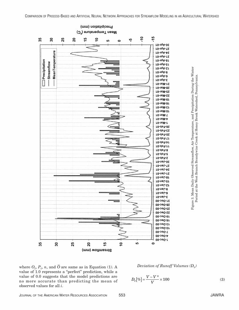
loads, and aquatic organisms respond to daily fluctua-tions in flow rates. However, since SWAT is intendedas a long term yield model, observed and simulatedmonthly and yearly surface flow, base flow, and totalstreamflow volumes were used for performance evalu-ations. In addition, model performances were sepa-rately evaluated for the entire simulation period,winter periods, and nonwinter periods. Even thoughwinter periods varied from year to year, on averagethe winter period ranged approximately from Decem-ber 15 until March 15 (Figure 3); the rest of the yearwas considered the nonwinter period. During thisthree-month period streamflows are dominated bysnowmelt events. The temperatures usually remainabove freezing rest of the year.

Two different types (relative and absolute) of goodness-of-fit statistics were used for performanceevaluations.

Relative Goodness-of-Fit Statistics. Relativegoodness-of-fit statistics are nondimensional indicesthat provide a relative comparison of the performanceof one model against another or against observed data (Kneale et al., 2001). Three different relativegoodness-of-fit statistics, Coefficient of Determination,Nash-Sutcliffe Coefficient of Efficiency, and Deviationof Runoff Volumes (a measure of a model’s ability tosimulate measured volume) were used.

Coefficient of Determination (R2)

where Oi is the observed value at time i, Pi is the pre-dicted value at time i, n is the total number of obser-vations, and O

–and P

–are the means of observed and

predicted values, respectively. R2 ranges between 0and 1 with a higher value indicating higher degree ofcollinearity.

Nash-Sutcliffe Coefficient of Efficiency (E)



R

O O P P

O O P P

i ii

n

ii

n

ii

n

2 1

2

1

0 52

1

0 5=−( ) −( )

−( )⎡

⎣⎢⎢

⎤

⎦⎥⎥

−( )⎡

⎣⎢⎢

⎤

⎦⎥⎥

⎧

⎨

⎪⎪⎪

⎩

⎪⎪⎪

⎫

⎬

⎪⎪⎪

⎭

⎪⎪⎪

=

=

−

=

−

∑

∑ ∑. .

E

O P

O O

i ii

n

i ii

n= −−( )

−( )=

=

∑

∑1

2

12

1

(1)

(2)

where Oi, Pi, n, and O–

are same as in Equation (1). Avalue of 1.0 represents a “perfect” prediction, while avalue of 0.0 suggests that the model predictions areno more accurate than predicting the mean ofobserved values for all i.

Deviation of Runoff Volumes (Dv)



Fig

ure

3. M

ean

Dai

ly O

bser

ved

Str

eam

flow

, Air

Tem

pera

ture

, an

d P

reci

pita

tion

Du

rin

g th

e W

inte

rP

erio

d at

th

e W

est

Bra

nch

Bra

ndy

win

e C

reek

at

Hon

ey B

rook

Wat

ersh

ed, P

enn

sylv

ania

.

DV V

Vv %*[ ] = − × 100 (3)

where V is the measured yearly or seasonal runoffvolume (mm) and V* is the simulated yearly or sea-sonal runoff volume (mm).

Absolute Goodness-of-Fit Statistics. Absolutegoodness-of-fit statistics are measured in the units offlow measurements (mm) (Kneale et al., 2001).

Root Mean Squared Error (RMSE)

where Oi, Pi, and n are same as in Equation (1).

Mean Absolute Error (MAE)

Again, Oi, Pi, and n are same as in Equation (1).

RESULTS AND DISCUSSION

As noted in the Introduction, the purpose of thisstudy was twofold: to evaluate the performance of thephysically based, distributed parameter SWAT modelfor simulating streamflows from a small agriculturalwatershed in Pennsylvania and to compare SWATmodel’s performance with the performance of an ANNhydrologic model that required a significantly smallernumber of inputs and fewer resources to implement.

Model Calibration and Training

Data from 1994 through 1997 were used for SWATmodel calibration and ANN training. However, thefirst six months of data for 1994 were used to initial-ize SWAT model and were therefore not used for cali-bration. Similarly, the first six months of 1994 datawere not used for training of the ANN hydrologicmodel. As mentioned earlier, the mean annual precip-itation in this watershed is about 1,204 mm. Theannual precipitation during 1995 was close to the nor-mal, whereas annual precipitation for 1996 was wellabove normal and annual precipitation during 1997was below normal (Table 1). Hence, even though only

three years (1995 through 1997) of data were used for calibration, they encompassed a wide range of weath-er conditions.

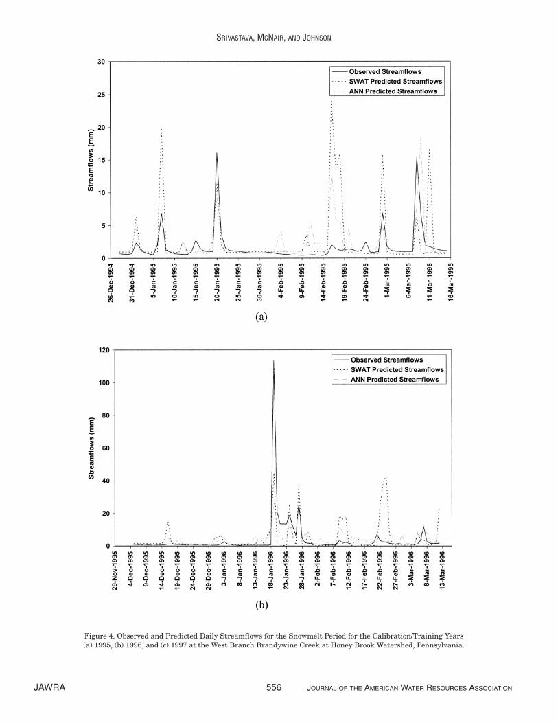
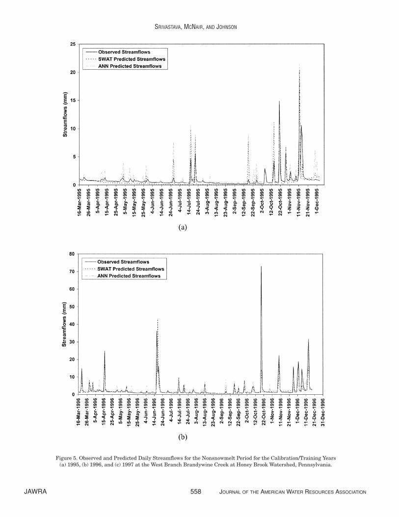
Time series of observed, SWAT predicted, and ANNpredicted daily flows for the winter period and non-winter period for the years 1995, 1996, and 1997 areprovided in Figures 4 and 5, respectively. These fig-ures suggest that, except for the winter months, theSWAT model seems to adequately simulate stream-flows. Artificial neural network predicted flows for thenonwinter months were also adequate for 1995 and1996; ANN overpredicted nonwinter flows for 1997.However, ANN predicted peaks occurred when thepeaks were observed in the observed streamflows.SWAT predicted daily flows during winter months donot seem to exhibit any trend (such as low flows thatare too low and high flows too high or low flows thatare too high and high flows too low). However, ANNpredicted daily flows during winter months seem tobe in slightly better agreement with the observeddata as compared to the SWAT predicted daily flows.Monthly flow statistics (described later) tend to sup-port this finding. SWAT calibration efforts to furtherimprove the model’s performance during wintermonths were unsuccessful because snowmelt eventswere not adequately simulated by the SWAT model.This finding is consistent with that of Peterson andHamlett (1998), who studied a northeastern Pennsyl-vania watershed. This can be better understood bylooking at Figure 3, which shows precipitation, meantemperature, and streamflow during winter 2001. Ascan be seen in this figure, the mean temperature inwinter months often remained well below zero. Themean temperature went above zero only once in awhile, and if there was snow on the ground (which isoften difficult to determine), snowmelt eventsoccurred. The snowmelt is often a very complex pro-cess, and it is often difficult to determine how muchsnow actually melted and how much remained on theground to melt later. Also, often the snowmelt eventsoccur over a period of a few days to a month or more.Because of this complexity, it is difficult to show whensnowmelt events occurred. Therefore, the entire win-ter period was lumped as the snowmelt period.

Even though accurate simulation of daily flows isimportant because peak runoff events contribute sig-nificant pollutant loads (Peterson and Hamlett, 1998)and daily high and low flows affect stream biota (out-lined in the introduction), most of the model perfor-mance evaluation was done on monthly and yearlyflows. This was done mainly because SWAT is intend-ed as a long term yield model and is incapable ofdetailed, single-event flooding (Arnold and Allen,1996, as referenced by Peterson and Hamlett, 1998).



RMSE

O P

n

i ii

n

=−( )

=∑ 2

1 (4)

MAE

O P

n

i ii

n

=−

=∑

1 (5)

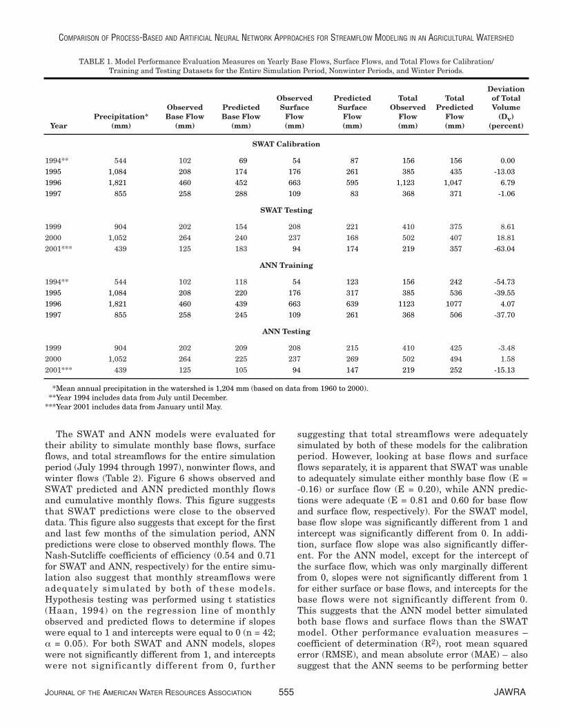
The SWAT and ANN models were evaluated fortheir ability to simulate monthly base flows, surfaceflows, and total streamflows for the entire simulationperiod (July 1994 through 1997), nonwinter flows, andwinter flows (Table 2). Figure 6 shows observed andSWAT predicted and ANN predicted monthly flowsand cumulative monthly flows. This figure suggeststhat SWAT predictions were close to the observeddata. This figure also suggests that except for the firstand last few months of the simulation period, ANNpredictions were close to observed monthly flows. TheNash-Sutcliffe coefficients of efficiency (0.54 and 0.71for SWAT and ANN, respectively) for the entire simu-lation also suggest that monthly streamflows wereadequately simulated by both of these models.Hypothesis testing was performed using t statistics(Haan, 1994) on the regression line of monthlyobserved and predicted flows to determine if slopeswere equal to 1 and intercepts were equal to 0 (n = 42;α = 0.05). For both SWAT and ANN models, slopeswere not significantly different from 1, and interceptswere not significantly different from 0, further

suggesting that total streamflows were adequatelysimulated by both of these models for the calibrationperiod. However, looking at base flows and surfaceflows separately, it is apparent that SWAT was unableto adequately simulate either monthly base flow (E =-0.16) or surface flow (E = 0.20), while ANN predic-tions were adequate (E = 0.81 and 0.60 for base flowand surface flow, respectively). For the SWAT model,base flow slope was significantly different from 1 andintercept was significantly different from 0. In addi-tion, surface flow slope was also significantly differ-ent. For the ANN model, except for the intercept ofthe surface flow, which was only marginally differentfrom 0, slopes were not significantly different from 1for either surface or base flows, and intercepts for thebase flows were not significantly different from 0.This suggests that the ANN model better simulatedboth base flows and surface flows than the SWATmodel. Other performance evaluation measures –coefficient of determination (R2), root mean squarederror (RMSE), and mean absolute error (MAE) – alsosuggest that the ANN seems to be performing better



TABLE 1. Model Performance Evaluation Measures on Yearly Base Flows, Surface Flows, and Total Flows for Calibration/Training and Testing Datasets for the Entire Simulation Period, Nonwinter Periods, and Winter Periods.

DeviationObserved Predicted Total Total of Total

Observed Predicted Surface Surface Observed Predicted VolumePrecipitation* Base Flow Base Flow Flow Flow Flow Flow (Dv)

Year (mm) (mm) (mm) (mm) (mm) (mm) (mm) (percent)

SWAT Calibration

1994** 544 102 069 054 087 156 156 0.001995 1,084 208 174 176 261 385 435 -13.031996 1,821 460 452 663 595 1,123 1,047 6.791997 855 258 288 109 083 368 371 -1.06

SWAT Testing

1999 904 202 154 208 221 410 375 8.612000 1,052 264 240 237 168 502 407 18.812001*** 439 125 183 094 174 219 357 -63.04

ANN Training

1994** 544 102 118 054 123 156 242 -54.731995 1,084 208 220 176 317 385 536 -39.551996 1,821 460 439 663 639 1123 1077 4.071997 855 258 245 109 261 368 506 -37.70

ANN Testing

1999 904 202 209 208 215 410 425 -3.482000 1,052 264 225 237 269 502 494 1.582001*** 439 125 105 094 147 219 252 -15.13

***Mean annual precipitation in the watershed is 1,204 mm (based on data from 1960 to 2000).***Year 1994 includes data from July until December.***Year 2001 includes data from January until May.



Figure 4. Observed and Predicted Daily Streamflows for the Snowmelt Period for the Calibration/Training Years(a) 1995, (b) 1996, and (c) 1997 at the West Branch Brandywine Creek at Honey Brook Watershed, Pennsylvania.

(higher R2 and lower RMSE and MAE) than SWATfor the entire simulation period.

Time series of daily observed and predicted flowssuggested that SWAT did not adequately simulatewinter flows. Therefore, winter and nonwinter flowswere separated, and the performance of these modelswas determined in simulating monthly flows for thesetwo periods separately. The Nash-Sutcliffe coefficientof efficiency (E) and slopes and intercepts of regres-sion lines suggest that, except for SWAT predictedbase flows, both SWAT and ANN models adequatelysimulated nonwinter monthly surface and totalstreamflows (the slope of the regression line for SWATpredicted flows was only marginally different from 1);ANN predicted base flows were also adequate (E =0.76, a slope not significantly different from 1 andintercept not significantly different from 0). Otherperformance measures (high R2 and low RMSE andMAE) also suggest that nonwinter monthly flowswere adequately simulated by both models. For thewinter flows, even though slopes were not significant-ly different from 1 and intercepts were not signifi-cantly different from 0 (except for SWAT predictedbase flows), other performance evaluation measures(E, R2, RMSE, and MAE) suggest that SWAT did not adequately simulate winter flows. Except for high RMSE and MAE errors for surface flows, ANN

predictions during winter periods seem to be ade-quate. Yearly flow volume data (Table 1) suggest thatdeviation in base flow volumes were similar for bothSWAT and ANN models. However, deviations in sur-face flow volumes and, as a consequence, deviations intotal flow volumes were slightly higher for the ANNmodel. This is not surprising, considering that SWATwas first calibrated to match average annual baseflow and surface flow.

Model Testing

Data from January 1998 through May 2001 wereused for SWAT and ANN testing. Again, first-year(1998) data were used to initialize the SWAT modeland cross validation of the ANN model and thereforewere not used for testing. Precipitation in 1999 wasbelow the annual mean, whereas precipitation in2000 and 2001 was close to the annual mean (Table1). The model performance evaluation was done forthe entire simulation period, nonwinter months, andwinter months.

Figure 7 graphically presents observed and SWATpredicted and ANN predicted monthly streamflowsand cumulative monthly streamflows for the entiretesting period. Based on this figure, both SWAT and



Figure 4 (cont’d). Observed and Predicted Daily Streamflows for the Snowmelt Period for the Calibration/Training Years(a) 1995, (b) 1996, and (c) 1997 at the West Branch Brandywine Creek at Honey Brook Watershed, Pennsylvania.



Figure 5. Observed and Predicted Daily Streamflows for the Nonsnowmelt Period for the Calibration/Training Years(a) 1995, (b) 1996, and (c) 1997 at the West Branch Brandywine Creek at Honey Brook Watershed, Pennsylvania.

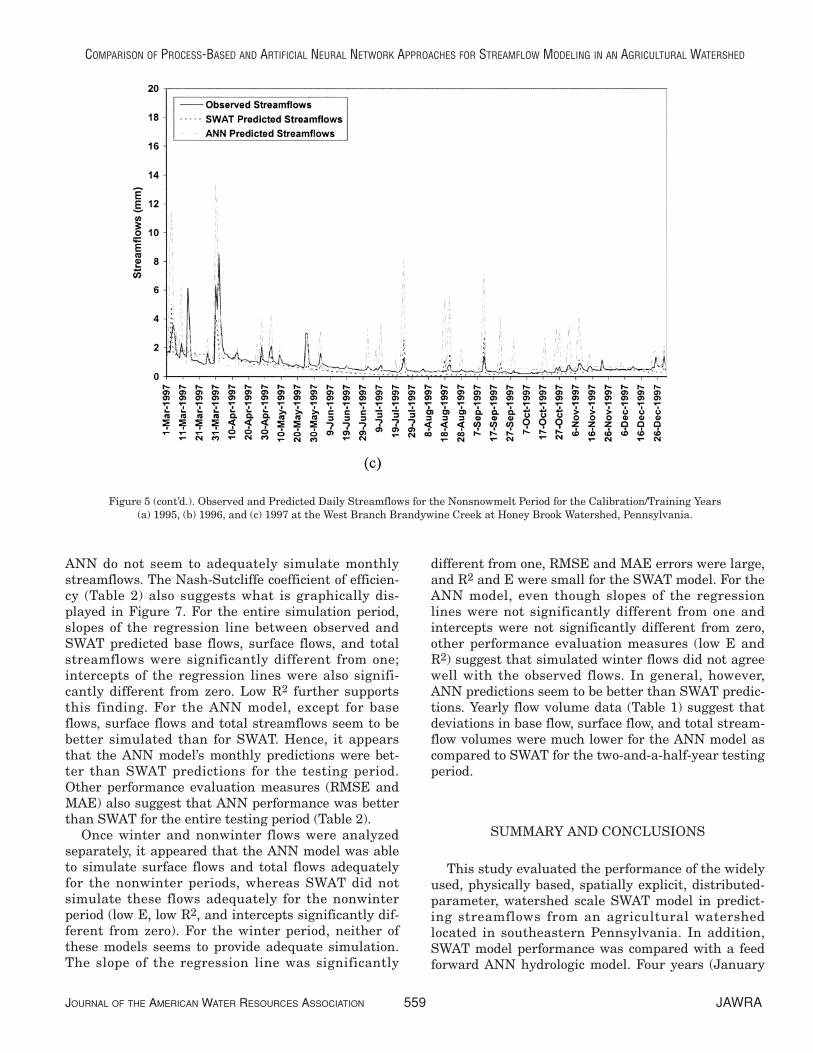
ANN do not seem to adequately simulate monthlystreamflows. The Nash-Sutcliffe coefficient of efficien-cy (Table 2) also suggests what is graphically dis-played in Figure 7. For the entire simulation period,slopes of the regression line between observed andSWAT predicted base flows, surface flows, and totalstreamflows were significantly different from one;intercepts of the regression lines were also signifi-cantly different from zero. Low R2 further supportsthis finding. For the ANN model, except for baseflows, surface flows and total streamflows seem to bebetter simulated than for SWAT. Hence, it appearsthat the ANN model’s monthly predictions were bet-ter than SWAT predictions for the testing period.Other performance evaluation measures (RMSE andMAE) also suggest that ANN performance was betterthan SWAT for the entire testing period (Table 2).

Once winter and nonwinter flows were analyzedseparately, it appeared that the ANN model was ableto simulate surface flows and total flows adequatelyfor the nonwinter periods, whereas SWAT did notsimulate these flows adequately for the nonwinterperiod (low E, low R2, and intercepts significantly dif-ferent from zero). For the winter period, neither ofthese models seems to provide adequate simulation.The slope of the regression line was significantly

different from one, RMSE and MAE errors were large,and R2 and E were small for the SWAT model. For theANN model, even though slopes of the regressionlines were not significantly different from one andintercepts were not significantly different from zero,other performance evaluation measures (low E andR2) suggest that simulated winter flows did not agreewell with the observed flows. In general, however,ANN predictions seem to be better than SWAT predic-tions. Yearly flow volume data (Table 1) suggest thatdeviations in base flow, surface flow, and total stream-flow volumes were much lower for the ANN model ascompared to SWAT for the two-and-a-half-year testingperiod.

SUMMARY AND CONCLUSIONS

This study evaluated the performance of the widelyused, physically based, spatially explicit, distributed-parameter, watershed scale SWAT model in predict-ing streamflows from an agricultural watershedlocated in southeastern Pennsylvania. In addition,SWAT model performance was compared with a feedforward ANN hydrologic model. Four years (January



Figure 5 (cont’d.). Observed and Predicted Daily Streamflows for the Nonsnowmelt Period for the Calibration/Training Years(a) 1995, (b) 1996, and (c) 1997 at the West Branch Brandywine Creek at Honey Brook Watershed, Pennsylvania.



TA

BL

E 2

. Mod

el P

erfo

rman

ce E

valu

atio

n M

easu

res

on M

onth

ly B

ase

Flo

ws

(BF

), S

urf

ace

Flo

ws

(SF

), a

nd

Tot

al F

low

s (T

F)

for

Cal

ibra

tion

/Tra

inin

g an

d T

esti

ng

Dat

aset

s fo

r th

e E

nti

re S

imu

lati

on P

erio

d, N

onw

inte

r P

erio

ds, a

nd

Win

ter

Per

iods

.

Cal

ibra

tion

/Tra

inin

g D

atas

etT

esti

ng

Dat

aset

(Ju

ly 1

994

- D

ecem

ber

199

7)(J

anu

ary

1999

- M

ay 2

001)

SW

AT

AN

NS

WA

TA

NN

Per

form

ance

Eva

luat

ion

Mea

sure

BF

SF

TF

BF

SF

TF

BF

SF

TF

BF

SF

TF

En

tire

Sim

ula

tion

Per

iod

(n

= 4

2 ca

lib

rati

on/t

rain

ing

dat

aset

; n =

29

test

ing

dat

aset

)

Nas

h-S

utc

liff

e C

oeff

. of

Eff

icie

ncy

, E0-

0.16

0-0.

20-0

0.54

-0.8

10-

0.60

-00.

710-

1.18

0-0.

350-

0.17

-0.0

80-

0.43

-00.

43

Coe

ffic

ien

t of

Det

erm

inat

ion

, R2

-00.

510-

0.38

-00.

57-0

.81

0-0.

67-0

0.75

0-0.

290-

0.39

-00.

34-0

.31

0-0.

48-0

0.45

Slo

pe, a

-00.

47*

0-0.

60*

-00.

80-1

.03

0-1.

18-0

1.16

0-0.

31*

0-0.

42*

-00.

45*

-0.5

7*0-

0.83

-00.

83

Inte

rcep

t, b

(m

m)

-13.

56**

0-9.

30-0

9.90

-0.6

3-1

3.88

**-1

7.05

**-1

4.31

**-1

0.42

**-2

1.32

**-9

.78*

*0-

0.60

-05.

43

Roo

t M

ean

Sq.

Err

or, R

MS

E (

mm

)-1

6.76

-33.

35-3

4.55

-6.7

5-2

3.73

-27.

39-1

1.02

-21.

33-2

3.44

-7.1

6-1

3.85

-16.

39

Mea

n A

bsol

ute

Err

or, M

AE

(pe

rcen

t)-1

1.36

-17.

55-1

9.45

-5.5

1-1

9.28

-21.

54-8

.46

-14.

65-1

7.70

-5.9

90-

9.79

-11.

96

Non

win

ter

Per

iod

(n

= 3

6 ca

lib

rati

on/t

rain

ing

dat

aset

; n =

24

test

ing

dat

aset

)

Nas

h-S

utc

liff

e C

oeff

. of

Eff

icie

ncy

, E-0

0.50

0-0.

49-0

0.77

-0.7

60-

0.58

-00.

710-

0.18

0-0.

32-0

0.30

-0.2

00-

0.61

-00.

58

Coe

ffic

ien

t of

Det

erm

inat

ion

, R2

-00.

860-

0.58

-00.

86-0

.78

0-0.

66-0

0.77

0-0.

460-

0.51

-00.

43-0

.39

0-0.

63-0

0.58

Slo

pe, a

-00.

62*

0-1.

30-0

1.23

*-1

.20

0-1.

11-0

1.19

0-0.

46*

0-0.

68**

-00.

68-0

.60*

0-0.

99-0

0.97

Inte

rcep

t, b

(m

m)

-08.

92**

0-1.

990-

0.98

-3.4

30-

9.31

**-1

4.66

**0-

9.00

**0-

8.23

**-1

3.08

**-7

.74*

*0-

2.35

0-0.

29

Roo

t M

ean

Sq.

Err

or, R

MS

E (

mm

)-0

8.17

-18.

96-1

6.89

-5.7

5-1

7.24

-19.

020-

8.60

-15.

11-1

8.34

-7.0

8-1

1.47

-14.

28

Mea

n A

bsol

ute

Err

or, M

AE

(pe

rcen

t)-0

7.03

-11.

40-1

0.53

-5.0

9-1

4.90

-16.

610-

6.85

0-9.

91-1

2.64

-5.6

1-7

.01

-09.

85

Win

ter

Per

iod

(n

= 1

0 ca

lib

rati

on/t

rain

ing

dat

aset

; n =

9 t

esti

ng

dat

aset

)

Nas

h-S

utc

liff

e C

oeff

. of

Eff

icie

ncy

, E0-

0.98

0-0.

03-0

0.26

-0.7

70-

0.53

-00.

620-

1.60

0-2.

600-

1.21

-0.4

60-

0.20

-00.

12

Coe

ffic

ien

t of

Det

erm

inat

ion

, R2

0-0.

050-

0.36

-00.

38-0

.78

0-0.

66-0

0.71

0-0.

000-

0.25

-00.

22-0

.64

0-0.

13-0

0.22

Slo

pe, a

-00.

15*

0-0.

55-0

0.79

-1.0

30-

1.34

-01.

310-

0.02

*0-

0.27

*-0

0.31

*-1

.31

0-0.

41-0

0.60

Inte

rcep

t, b

(m

m)

-25.

08**

0-2.

390-

6.95

-1.5

4-2

5.27

-33.

97-1

8.80

**-1

0.52

-23.

47-2

.10

-10.

67-1

4.94

Roo

t M

ean

Sq.

Err

or, R

MS

E (

mm

)-2

6.19

-51.

02-5

7.55

-7.7

3-3

2.36

-37.

84-1

1.58

-30.

56-3

1.20

-5.2

8-1

7.60

-19.

64

Mea

n A

bsol

ute

Err

or, M

AE

(pe

rcen

t)-1

7.79

-28.

03-4

0.59

-4.8

7-2

3.82

-26.

360-

8.98

-22.

70-2

6.65

-4.3

5-1

5.11

-16.

33

**S

lope

sig

nif

ican

tly

diff

eren

t fr

om 1

at α

= 0.

05.

**In

terc

ept

sign

ific

antl

y di

ffer

ent

from

0 a

t α

= 0.

05.

Not

e:T

he

sum

of

n f

or w

inte

r an

d n

onw

inte

r m

onth

s do

es n

ot a

dd u

p to

n in

th

e en

tire

sim

ula

tion

per

iod

beca

use

win

ter

and

non

win

ter

mon

ths

are

not

alw

ays

com

plet

e m

onth

s. F

or

exam

ple,

th

e fi

rst

hal

f of

Mar

ch m

igh

t h

ave

been

con

side

red

a w

inte

r pe

riod

an

d se

con

d h

alf

as a

non

win

ter

peri

od.

1994 through December 1997) of daily streamflowdata were used for SWAT model calibration and train-ing of ANN hydrologic model, and about three and a half years (January 1998 through May 2001) of data were used for model testing. Various model performance measures were used to determine the

suitability of these models in predicting base flows,surface flows, and total streamflows. In addition,models were separately evaluated using the data forthe entire simulation period, nonwinter periods, andwinter periods.



Figure 6. Observed and Predicted Monthly Streamflows for the Calibration/Training Periodat the West Branch Brandywine Creek at Honey Brook Watershed, Pennsylvania.

Figure 7. Observed and Predicted Monthly Streamflows for the Testing/Validation Periodat the West Branch Brandywine Creek at Honey Brook Watershed, Pennsylvania.

Results suggest that SWAT adequately simulatedmonthly surface flows and total streamflows for thenonwinter and entire simulation periods for the cali-bration period. SWAT simulated monthly flows wereinadequate for the winter months for the calibrationperiod. Further, SWAT inadequately simulated flowsfor the whole duration of test period. ANN simulatedflows were adequate for the entire simulation, non-winter months, and winter months for the calibrationperiod. In addition, ANN simulated monthly surfaceand total streamflows were adequate for the entiresimulation and nonwinter months for the testing peri-od. Overall, results suggest that ANN simulatedmonthly flows were closer to the observed values thanSWAT simulated monthly flows. Hence, this studydemonstrates that ANN is a promising modelingalternative to a traditional, process-based approachfor watershed flow simulations. The ANN approach isalso more efficient because it requires very few inputvariables and minimal resources to implement. How-ever, most studies to date have used simple ANNapproaches that predict streamflows at a single out-let. They do not spatially represent a watershed sys-tem and hence are incapable of predicting flows atvarious points along a stream network. In addition,the current implementation of ANN models is inade-quate because the models will have to be retrained ifrainfall network and land use types are changed. Fur-ther, the ANN models cannot be used to predict futureconditions if the land use in the watershed changes.The results of this study, however, suggest that theANN approach is sufficiently promising to warrantfurther development of the approach to explicitlyaddress the spatial distribution of hydrologic andwater quality processes and land use in watersheds.

ACKNOWLEDGMENTS

The authors gratefully acknowledge the Environmental Associ-ates at the Academy of Natural Sciences for providing funding forthis research.

LITERATURE CITED

Anmala, J., B. Zhang, and R.S. Govindaraju, 2000. Comparison ofANNs and Empirical Approaches for Predicting WatershedRunoff. J. Water Resources Planning and Management126(3):156-166.

Arnold, J.G. and P.M. Allen, 1996. Estimating Hydrologic Budgetsfor Three Illinois Watersheds. J. Hydrology 176:57-77.

Arnold, J.G., J.R. Williams, and D.R. Maidment, 1995. Continuous-Time Water and Sediment-Routing Model for Large Basins. J. Hydraulic Engineering 121(2):171-183.

Arnold, J.G., J.R. Williams, A.D. Nicks, and N.B. Sammons, 1990.SWRRB: A Basin Scale Simulation Model for Soil and WaterResources Management. Texas A&M Univ. Press, College Sta-tion, Texas.

Beven, K.J., 2001. Rainfall-Runoff Modeling. John Wiley, New York,New York.

Bicknell, B.R., J.C. Imhoff, J.L. Kittle, Jr., T.H. Jobes, and A.S.Donigian, Jr., 2001. Hydrologic Simulation Program-FORTRAN– User’s Manual. National Exposure Research Laboratory,Office of Research and Development, U.S. Environmental Pro-tection Agency, Athens, Georgia.

Biggs, B.J.F. and M.E. Close, 1989. Periphyton Biomass Dynamicsin Gravel Bed Rivers: The Relative Effect of Flows and Nutri-ents. Freshwater Biology 22:209-231.

Bishop, C.M., 1995. Neural Networks for Pattern Recognition.Oxford University Press, New York, New York.

Braddock, R.D., M.L. Kremmer, and L. Sanzogni, 1998. Feed-Forward Artificial Neural Network Model for Forecasting Rain-fall Run-Off. Environmetrics 9:419-432.

Campolo, M., P. Andreussi, and A. Soldati, 1999. River Flood Fore-casting With a Neural Network Model. Water Resour. Res.35:1191-1197.

Dawson, C.W. and R. Wilby, 1998. An Artificial Neural NetworkApproach to Rainfall-Runoff Modeling. J. Hydrological Sciences43(1):47-66.

Deo, M.C. and K. Thirumalaiah, 2000. Real-Time Forecasting UsingNeural Networks. In: Artificial Neural Networks in Hydrology,R.S. Govindaraju and A. Ramachandra (Editors). Springer-Verlag, New York, New York, pp. 53-71.

Eberhart, R.C. and R.W. Dobbins, 1990. Early Neural NetworkDevelopment History: The Age of Camelot. IEEE Engineering inMedicine and Biology 9:15-18.

ESRI (Environmental Systems Research Institute), 1998. ArcView3.1. Environmental Systems Research Institute, Inc., Redlands,California.

Fernando, D.A.K. and A.W. Jayawardena, 1998. Runoff ForecastingUsing RBF Networks With OLS Algorithm. ASAE, J. Hydr.Engrg. 3(3):203-209.

Govindaraju, R.S., 2000. Artificial Neural Networks in Hydrology. I:Preliminary Concepts. ASAE, J. Hydr. Engrg. 5(2):115-123.

Guez, A. and I. Nevo, 1996. Neural Networks and Fuzzy Logic inClinical Laboratory Computing With Applications to IntegratedMonitoring. Clinica Chemica Acta 248:73-90.

Guez, A., V. Protopopesu, and J. Barhen, 1988. On the Stability,Storage Capacity, and Design of Nonlinear Continuous NeuralNetworks. IEEE Trans. on System Man and Cybernetics18(1):80-87.

Guez, A., E. Tabatabei, and C. Hyantai, 1998. Adaptive SigmoidalMolten Metal Pouring Control. IEEE Trans. on Control SystemsTechnology 6(2):270-280.

Gupta, H.V., K. Hsu, and S. Sorooshian, 2000. Effective and Effi-cient Modeling for Streamflow Forecasting. In: Artificial NeuralNetworks in Hydrology, R.S. Govindaraju and A. Ramachandra(Editors). Springer-Verlag, New York, New York, pp. 7-22.

Haan, C.T., 1994. Statistical Methods in Hydrology. Iowa State Uni-versity Press, Ames, Iowa.

Hinton, G.E., 1992. How Neural Networks Learn From Experience.Scientific American 267:144-151.

Hornik, K., M. Stinchcombe, and H. White, 1990. UniversalApproximation of an Unknown Mapping and its DerivativesUsing Multilayer Feed-Forward Networks. Neural Networks3(5):551-560.

Hsu, K., H.V. Gupta, and S. Sorooshian, 1995. Artificial NeuralNetwork Modeling of the Rainfall-Runoff Process. Water Resour.Res. 31(10):2517-2530.



Karunanithi, N., W.J. Grenney, D. Whitley, and K. Bovee, 1994.Neural Networks for River Flow Prediction. J. Computing inCivil Engineering 8(2):201-220.

Kneale, P., L. See, and A. Smith, 2001. Towards Defining Evalua-tion Measures for Neural Network Forecasting Models. In: Pro-ceedings of the 6th International Conference onGeoComputation, University of Queensland, Brisbane, Aus-tralia. GeoComputation, Leeds, United Kingdom, CD-ROM.

Knisel, W.G., 1980. CREAMS, A Field Scale Model for Chemicals,Runoff and Erosion From Agricultural Management Systems.U.S. Department of Agriculture Conservation Research ReportNo. 26. Washington, D.C.

Kohonen, T., 1997. Self-Organizing Maps. Springer-Verlag. Berlin,Germany.

Leonard, R.A., W.G. Knisel, and D.A. Still, 1987. GLEAMS:Groundwater Loading Effects on Agricultural Management Sys-tems. Trans. ASAE 30(5):1403-1428.

Leopold, L.B., M.G. Wolman, and J.P. Miller, 1964. Fluvial Process-es in Geomorphology. Dover Publications, Inc., New York, NewYork.

Maier, H.R. and G.C. Dandy, 2000. Neural Networks for the Predic-tion and Forecasting of Water Resources Variables: A Review ofModeling Issues and Applications. Environ. Modelling and Soft-ware 15:101-124.

Minns, A.W. and M.J. Hall, 1996. Artificial Neural Networks asRainfall-Runoff Models. J. Hydrological Sciences 41(3):399-417.

Mozer, M.C., 1994. Neural Network Music Composition by Predic-tion: Exploring the Benefits of Psychophysical Constraints andMultiscale Processing. Connection Science 6:247-280.

Neitsch, S.L., J.G. Arnold, J.R. Kiniry, and J.R. Williams, 2001a.Soil and Water Assessment Tool (SWAT) Theoretical Documen-tation: Version 2000. U.S. Department of Agriculture, Agricul-tural Research Service, Grassland, Soil, and Water ResearchLaboratory, Temple, Texas.

Neitsch, S.L., J.C. Arnold, J.R. Kiniry, and J.R. Williams, 2001b.Soil and Water Assessment Tool (SWAT) User’s Manual: Version2000. U.S. Department of Agriculture, Agricultural ResearchService, Grassland, Soil, and Water Research Laboratory, Tem-ple, Texas.

Pennsylvania State Climatologist, 2002. Climate Data for Pennsyl-vania. Available at http://pasc.met.psu.edu/PA_Climatologist/index.php. Accessed in December 2002.

Peterson, J.R. and J.M. Hamlett, 1998. Hydrologic Calibration ofthe SWAT Model in a Watershed Containing Fragipan Soils. J. American Water Resources Association (JAWRA) 34(3):531-544.

Poff, N.L., J.D. Allan, M.B. Bain, J.R. Karr, K.L. Prestegaard, B.D.Richter, R.E. Sparks, and J.C. Stromberg, 1997. The NaturalFlow Regime: A Paradigm for River Conservation and Restora-tion. BioScience 47:769-784.

Poff, N.L., S. Tokar, and P.A. Johnson, 1996. Stream Hydrologicaland Ecological Responses to Climate Change Assessed With anArtificial Neural Network. Limnol. Oceanogr. 41(5):857-863.

Richter, B.D., J.V. Baumgartner, R. Wigington, and D.P. Braun,1997. How Much Water Does a River Need? Freshwater Biology37:231- 249.

Ripley, B.D., 1996. Pattern Recognition and Neural Networks. Cam-bridge University Press, New York, New York.

Rumelhart, D.E. and J.L. McClelland, 1986. Parallel DistributedProcessing: Explorations in the Microstructure of Cognition.Vols. I and II, MIT Press, Cambridge, Massachusetts.

Salas, J.D., M. Markus, and A.S. Tokar, 2000. Streamflow Forecast-ing Based on Artificial Neural Networks. In: Artificial NeuralNetworks in Hydrology, R.S. Govindaraju and A. Ramachandra(Editors). Springer-Verlag, New York, New York, pp. 23-51.

Sharpley, A.N. and J.R. Williams (Editors), 1990. EPIC – ErosionProductivity Impact Calculator, 1. Model Documentation. U.S.Department of Agriculture, Agricultural Research Service, Tech.Bull. 1768, Washington, D.C.

Sudheer, K.P., P.C. Nayak, and K.S. Ramasastri, 2003. ImprovingPeak Flow Estimates in Artificial Neural Network River FlowModels. Hydrol. Process 17:677-686.

Tokar, A.S. and P.A. Johnson, 1999. Rainfall-Runoff Modeling UsingArtificial Neural Networks. ASAE, J. Hydr. Engrg. 4(3):231-239.

USDA-ARS (U. S. Department of Agriculture-Agricultural ResearchService), 2001. AnnAGNPS Version 2: User Documentation.Available at http://www.ars.usda.gov/SP2UserFiles/Place/64080510/AGNPS/PLModel/Document/User_Doc.PDF. Accessedin February 2006.

USDA-NRCS (U. S. Department of Agriculture-Natural ResourcesConservation Service), 1995. State Soils Geographic (STATSGO)Data Base. National Soil Survey Center. Misc. Publication Number 1492. Available at ftp://ftp-fc.sc.egov.usda.gov/NCGC/products/statsgo/statsgo-user-guide.pdf. Accessed in February2006.

USDA-NRCS (U. S. Department of Agriculture-Natural ResourcesConservation Service), 2002. Pennsylvania STATSGO Database.Available at http://www.ncgc.nrcs.usda.gov/products/datasets/statsgo/data/pa.html. Accessed in December 2002.

USGS (U.S. Geological Survey), 2001. 7.5 minute Digital ElevationModel (DEM) for Honey Brook Quadrangle Quadrangle(o40075a8). Available at http://www.pasda.psu.edu/summary.cgi/dem24k/honey_brook_pa.xml. Accessed in December 2002.

USGS (U.S. Geological Survey), 2002. USGS 01480300 West BranchBrandywine Creek Near Honey Brook, Pennsylvania. Availableat http://waterdata.usgs.gov/pa/nwis/dv/?site_no=01480300&PARAmeter_cd=00060. Accessed in December 2002.

USGS (U.S. Geological Survey), 2003. HYSEP: Hydrograph Separa-tion Program. Available at http://water.usgs.gov/software/hysep.html. Accessed on January 25, 2003.

Venables, W.N. and B.D. Ripley, 1999. Modern Applied StatisticsWith S-Plus. Springer-Verlag, New York, New York.

Wand, M.P. and M.C. Jones, 1995. Kernel Smoothing. Chapmanand Hall, London, United Kingdom.

Williams, J.R., 1969. Flood Routing With Variable Travel Time orVariable Storage Coefficients. Trans ASAE 12(1):100-103.

Williams, J.R., C.A. Jones, and P.T. Dyke, 1984. A ModelingApproach to Determining the Relationship Between Erosion andSoil Productivity. Trans. ASAE 27(1):129-144.

Zhang, B. and R.S. Govindaraju, 2000. Prediction of WatershedRunoff Using Bayesian Concepts and Modular Neural Network.Water. Resour. Res. 36(3):753-762.

Zhang, B. and R.S. Govindaraju, 2003. Geomorphology-Based Arti-ficial Neural Networks (GANNs) for Estimation of Direct RunoffOver Watersheds. J. Hydrology 273:18-34.



COMPARISON OF PROCESS-BASED AND ARTIFICIAL NEURAL NETWORK APPROACHES FOR STREAMFLOW MODELING IN AN...

Documents

Transcript of COMPARISON OF PROCESS-BASED AND ARTIFICIAL NEURAL NETWORK APPROACHES FOR STREAMFLOW MODELING IN AN...