
Comparison of ELF/VLF generation modes in the ionosphere by the HIPAS heater array
16
Radio Science, Volume 31, Number 1, Pages 211-226, January-February 1996 Comparison of ELF/VLF generation modes in the ionosphere by the HIPAS heater array J. Villascfior, • A. Y. Wong, B. Song, J. Pau, • and M. McCatrick Department of Physics, University of California, Los Angeles D. Sentman Geophysical Institute, University of Alaska, Fairbanks Abstract. The characteristics of three different modes of ELF and VLF excitation using the high-power auroral simulation (HIPAS) HF heater array are compared under different ionospheric conditions. For each of these three methods, amplitude modulation (AM), phase demodulation (DM), and the double-frequencyexcitation (DF), we observed signalson the order of a few picoteslasat two widely separated receiver sites for both X and O mode heater polarizations. Strong electrojet activity is essential for ELF generation at frequencies close to the Schumann range, whereas at higher frequencies, such as in the VLF range (greater than 1 kHz), signalscould be observed under a wider range of ionosopheric conditions. The AM method generally produced the largest signal at both frequency ranges, while the DM mode was approximately half of this signal amplitude. The DF generated signalsare comparable in strength with the AM signalsat VLF frequencies and are more stable than either method as a function of time. The X mode polarization also produces a stronger signal than the O mode for these three methods of excitation by a factor of two. The polarization of the received signals follow the same variation at VLF frequencies for all three modes, indicating a common height of origin. 1. Introduction Exciting EM waves in the ELF (30-3000 Hz) and VLF (3-30 kHz) range of frequencies using a ground-based, phased array of transmitting ele- ments has been routinely demonstratedat this Fair- banks, Alaska, site and at the facility in Ramfjord- moen near Troms0, Norway [Stubbe et al., 1982a, b, 1985; Reitveld, 1985]. These arrays use high- power HF waves to heat a localized region in the ionosphere and thereby change the conductivity of the medium. In the presenceof steady state electric fields normally present in the ionosphericD and E regions, the modulation of the conductivity in turn creates a modulated current, producing a virtual antenna embedded in the electrojet currents. This antenna radiates into the earth-ionosphere waveguide, and for low frequencies in the ELF range, the low attenuation coefficient(1 dB/Mm) of these EM waves allows them to propagate long 1Nowat HIPAS Observatory, Fairbanks, Alaska. Copyfight 1996 by the American GeophysicalUnion. Paper number 95RS01993. 0048-6604/96/95RS-01993508.00 distances in the Earth-ionosphere waveguide. This is suitable for some forms of radio communications, which normally require large antenna structures to radiate long wavelengths efficiently. Furthermore, working in polar regions, where the electrojet cur- rents are much greater than those at lower latitudes, increases the effectiveness of such an antennna. Tapping into these strong natural currents reduces the power requirements for equivalent ground- based HF sources. Electrojet modification is readily achieved by modulating the amplitude of the radiated HF wave (amplitude modulation, or AM). Square wave mod- ulation is easily implemented at the low-power, local oscillator which feeds the HF signal into the high-power tubes; the local oscillator is gated on for half a cycle and then off for the other half. This method has long been used in different experiments. In particular, Stubbe et al. [1985] have demon- strated the generation of VLF waves up to 23 kHz. At the lower Schummanrange of ELF frequencies, however, AM modulation is not viable because of potentially damaging system resonances inherent with high-power systems. In our particular case at 211
Transcript of Comparison of ELF/VLF generation modes in the ionosphere by the HIPAS heater array
Radio Science, Volume 31, Number 1, Pages 211-226, January-February 1996
Comparison of ELF/VLF generation modes in the ionosphere by the HIPAS heater array
J. Villascfior, • A. Y. Wong, B. Song, J. Pau, • and M. McCatrick Department of Physics, University of California, Los Angeles
D. Sentman
Geophysical Institute, University of Alaska, Fairbanks
Abstract. The characteristics of three different modes of ELF and VLF excitation
using the high-power auroral simulation (HIPAS) HF heater array are compared under different ionospheric conditions. For each of these three methods, amplitude modulation (AM), phase demodulation (DM), and the double-frequency excitation (DF), we observed signals on the order of a few picoteslas at two widely separated receiver sites for both X and O mode heater polarizations. Strong electrojet activity is essential for ELF generation at frequencies close to the Schumann range, whereas at higher frequencies, such as in the VLF range (greater than 1 kHz), signals could be observed under a wider range of ionosopheric conditions. The AM method generally produced the largest signal at both frequency ranges, while the DM mode was approximately half of this signal amplitude. The DF generated signals are comparable in strength with the AM signals at VLF frequencies and are more stable than either method as a function of time. The X mode polarization also produces a stronger signal than the O mode for these three methods of excitation by a factor of two. The polarization of the received signals follow the same variation at VLF frequencies for all three modes, indicating a common height of origin.
1. Introduction
Exciting EM waves in the ELF (30-3000 Hz) and VLF (3-30 kHz) range of frequencies using a ground-based, phased array of transmitting ele- ments has been routinely demonstrated at this Fair- banks, Alaska, site and at the facility in Ramfjord- moen near Troms0, Norway [Stubbe et al., 1982a, b, 1985; Reitveld, 1985]. These arrays use high- power HF waves to heat a localized region in the ionosphere and thereby change the conductivity of the medium. In the presence of steady state electric fields normally present in the ionospheric D and E regions, the modulation of the conductivity in turn creates a modulated current, producing a virtual antenna embedded in the electrojet currents. This antenna radiates into the earth-ionosphere waveguide, and for low frequencies in the ELF range, the low attenuation coefficient (1 dB/Mm) of these EM waves allows them to propagate long
1 Now at HIPAS Observatory, Fairbanks, Alaska.
Copyfight 1996 by the American Geophysical Union.
Paper number 95RS01993. 0048-6604/96/95RS-01993508.00
distances in the Earth-ionosphere waveguide. This is suitable for some forms of radio communications, which normally require large antenna structures to radiate long wavelengths efficiently. Furthermore, working in polar regions, where the electrojet cur- rents are much greater than those at lower latitudes, increases the effectiveness of such an antennna.
Tapping into these strong natural currents reduces the power requirements for equivalent ground- based HF sources.
Electrojet modification is readily achieved by modulating the amplitude of the radiated HF wave (amplitude modulation, or AM). Square wave mod- ulation is easily implemented at the low-power, local oscillator which feeds the HF signal into the high-power tubes; the local oscillator is gated on for half a cycle and then off for the other half. This method has long been used in different experiments. In particular, Stubbe et al. [1985] have demon- strated the generation of VLF waves up to 23 kHz. At the lower Schumman range of ELF frequencies, however, AM modulation is not viable because of potentially damaging system resonances inherent with high-power systems. In our particular case at
211

212 VILLASE•OR ET AL.' COMPARISON OF ELF/VLF GENERATION MODES
HIPAS, we avoid operating in the AM mode at frequencies between 10 and 100 Hz.
A variation of AM modulation which avoids the
on-off duty cycle is to direct the beam energy away from the intended heating region by phasing the appropriate elements of the transmitting array. In the HIPAS demodulation mode (DM), all eight transmitting elements are excited in phase to focus on a small region directly overhead for half a cycle, and then phased to maximally spread the power away from the zenith for the next half cycle. This is accomplished by subdividing the array into two subarrays and shifting the phase of one set by 180 ø. This method has also been used successfully to excite waves in the Schumann resonance range of frequencies [McCarrick et al., 1990].
The third method compared in this study involves simultaneously applying two heating frequencies in CW (double frequency, hence DF). The heater array is subdivided in the same manner as the DM mode, but instead of forcing a change of phase in one subset, we transmit at a frequency to o + to, to being the difference frequency of the two subarrays. The phase of that subarray varies smoothly from maximum to minimum coherence with the first
subarray, the variation repeating with a period T = 2•r/to. Fewer harmonics are generated in this fash- ion, and our modulation is sinusoidal. We show that under certain conditions, this method may be more efficient in producing stable, large-amplitude VLF signals. These three modes are schematically pre- sented in Figure 1.
This study aims to quantify the differences be- tween these modes of excitation under varying ionospheric conditions and over a frequency range extending from the low ELF to the middle VLF range. The bulk of the data presented here compare the signal strengths and polarization parameters obtained by ground-based detectors simultaneously recorded at two different locations (Figure 2).
2. Experimental Setup The experiments were performed at the Univer-
sity of California, Los Angeles, HIPAS heating facility located 25 miles (40 km) east of Fairbanks, Alaska. An array of eight crossed dipoles arranged in a circular fashion (R = 103.6 m) with a crossed dipole placed in the center allows us to focus an RF beam along any azimuth and elevation. The half- power beamwidth for transmission at vertical ele-
1st Half Cycle : 2nd Half Cycle
AM
HIPAS
DM
DF
Figure 1. Schematic of the different modes of excitation. In the DF mode, the array is subdivided into two subar- rays each radiating a different frequency in CW.
vations and 2.85 MHz is approximately 22.5 ø (Fig- ure 3). At low beam elevations large sidelobes are formed, carrying a significant fraction of the power away from the intended direction and defocusing the radiated power more isotropically. In normal operations, each dipole radiates 100 kW, which leads to a total of 800 kW radiated power for the whole array. The effective radiated power (ERP) of the array when all elements are in phase is 50 MW [Wong et al., 1990].
Each dipole is resonantly tuned to frequencies of 2.85 and 4.53 MHz, although most of our experi- ments were carried out at the lower frequency. The bandwidth of these antennas is sufficiently large for us to vary the frequency by 13 kHz from the center frequency without the need to retune. The polariza- tion of the transmitted wave can be programmed to

VILLASENOR ET AL.' COMPARISON OF ELF/VLF GENERATION MODES 213
switch from X mode (left circularly polarized with respect to the k vector and antiparallel to the magnetic field) and O mode (right circularly polar- ized). The phase for each dipole element can be altered during transmissions via a set of computer- controlled phase shifters, which forms the heart of the beam-steering and defocusing capability of the heater array. The control computers are synchro- nized with a Global Positioning System (GPS) clock, which also allows us to synchronize our diagnostics with our transmissions.
In the DM mode, four of the dipoles are phased 180 ø from the rest of the dipoles, forming the beam pattern shown in Figure 4. The two frequency experiments were carried out using the same con- figuration, but with each subset radiating the ELF or VLF frequency of interest. We should note that there are four isomorphically different ways of subdividing the array into two equal groups, taking rotational symmetry into account. The most fre- quently used method (and the one we used in these experiments) is where the elements are maximally spread out, as depicted in the inset of Figure 4.
To avoid potentially damaging system reso- nances, the AM mode was operated only for fre- quencies above 150 Hz. Only the DF and DM modes were employed to transmit at frequencies
NORTI•I• .oo.I I
I / /,
150
$4
149 ø 148 ø 147 ø 146 ø 145 ø 144 ø
Figure 2. Area map of the HIPAS facility. ELF/VLF receivers are located at the Gilmore Creek NOAA facility and at Delta Junction. The U.S. Geological Survey Col- lege magnetometer station is located close to Fairbanks.
-20 -15 -10 -5 0
Figure 3, Map of the power flux as a function of the solid angle, showing the beam spread of the radiation from the array. The relative phasing is 0 ø between transmitter elements, and the frequency is 2.85 MHz.
below this level. At the Schumann range of frequen- cies, the heater was operated at frequencies of 29, 44, 52, 55, 75, and 154 Hz. These were chosen to avoid the noise presented by the Schumann reso- nances.
The signals were detected at two receiver sites, accessed via modem connections. The first site is
located at the NOAA Tracking Facility at Gilmore Creek, 33 km E-NE from the HIPAS heater. The site has both VLF and ELF receivers intercon-
nected to two sets of orthogonal magnetic coils oriented along the geographic NS and EW. One set of coils has a frequency response from a few millihertz to 300 Hz, while the other set covers the range 2-30 kHz. A similar ELF system was used at Delta Junction, 133 km S-SE from HIPAS, with a set of coils covering 2-30 kHz. In this paper, only ELF signals will be presented from this site, al- though the system has since been upgraded to include VLF capability.
The signal electronics on both ELF systems reduce the bandwidth to 2-200 Hz, and the data acquisition systems continuously digitize data at a rate of 1000 Hz. Digital postprocessing is then employed to extract the desired signal [McCarrick et al., 1990]. The VLF detector at Gilmore Creek

214 VILLASENOR ET AL.' COMPARISON OF ELF/VLF GENERATION MODES
Figure 4. DM pattern for maximum out of phase trans- mission. The small diagram at bottom right shows which of the four antenna elements are 180 ø out of phase with the rest of the array.
also operates in the same manner, but digitization and post processing are carried out by a BB-71 data acquisition and Tiger-30 DSP board. The VLF receiver has an overall system receptivity from 200 Hz to 13 kHz, which is the limiting upper bound of our modulation experiments. The system noise level is at least 10 dB smaller than the atmospheric noise. The signal-to-noise ratio for most of the acquired signals is approximately 10-12 dB for a 1-pT signal over the specified range. These signals are time stamped using a GPS satellite monitor, ensuring the accuracy of the timing of our experi- ments.
We checked for the possibility of sky wave de- modulation at the Gilmore Creek site. Twin dipoles were erected over the detection coils and made to
radiate HF power, simulating AM and DF sky wave signals. No signals were detected by the coils, even with the HF power raised beyond the amplitude at which HIPAS-generated sky waves were expected to return. The possibility of demodulation at the Delta Junction site poses less of a problem com- pared to the Gilmore Creek site because the sky wave return signal power is smaller by approxi- mately 12 dB.
An ionosonde also located at the NOAA facility provides us with ionograms every 10 min during each run. In experimental runs concurrent with strong magnetic activity, absorptive conditions oc- casionally return blank ionograms. Successive soundings often show a few scattered returns, and taken as a whole the set of soundings can be used to gauge the absorption of the ELF signals. In addi- tion, sky wave HF signals were monitored at the Gilmore Creek site using a coaxial-collinear array circularly polarized in the right-hand direction. A Racal RA6790/GM receiver with a bandwidth of 8
kHz, centered at the heater frequency of 2.85 MHz, was then used to detect the signal [Song et al., 1995].
Supporting data from the Space Environment Laboratory Data Acquisition and Display System (SELDADS) database include the magnetometer traces from the U.S. Geological Survey College station and several other stations in the Alaskan
Meridian Chain. A particularly useful diagnostic is the high-latitude monitoring station auroral radar based in Anchorage, which measures coherently backscattered waves traveling perpendicular to the magnetic field lines. This diagnostic qualitatively in- dicates the presence of electrojets over the college (or HIPAS) region and shows diurnal variations of the electrojet region, which further allows us to schedule our runs for optimum conditions. The amplitude re- turns are recorded every minute, for 40 range bins which correspond to a span of 200-1000 km from the station.
In comparing the AM, DM, and DF modes, our typical method of heater operation is to succes- sively alternate between the modes and/or polariza- tions. We apply the heater for each mode and polarization for a receiver integration time sufficient to reduce the background noise and detect the signal. For the ELF frequencies in the Schumman range, this integration time is on the order of half a minute to a few minutes, and is partly due to the larger noise levels. This leads to data collection times of $-10 min per mode and polarization. As a check for repeatability, each mode is repeated at least three times over the course of the run to
account for temporal variations in the ionosphere. In comparison, VLF frequencies need integration times of only 5-10 s, which allows us to monitor temporal variations for each mode on a much faster timescale.
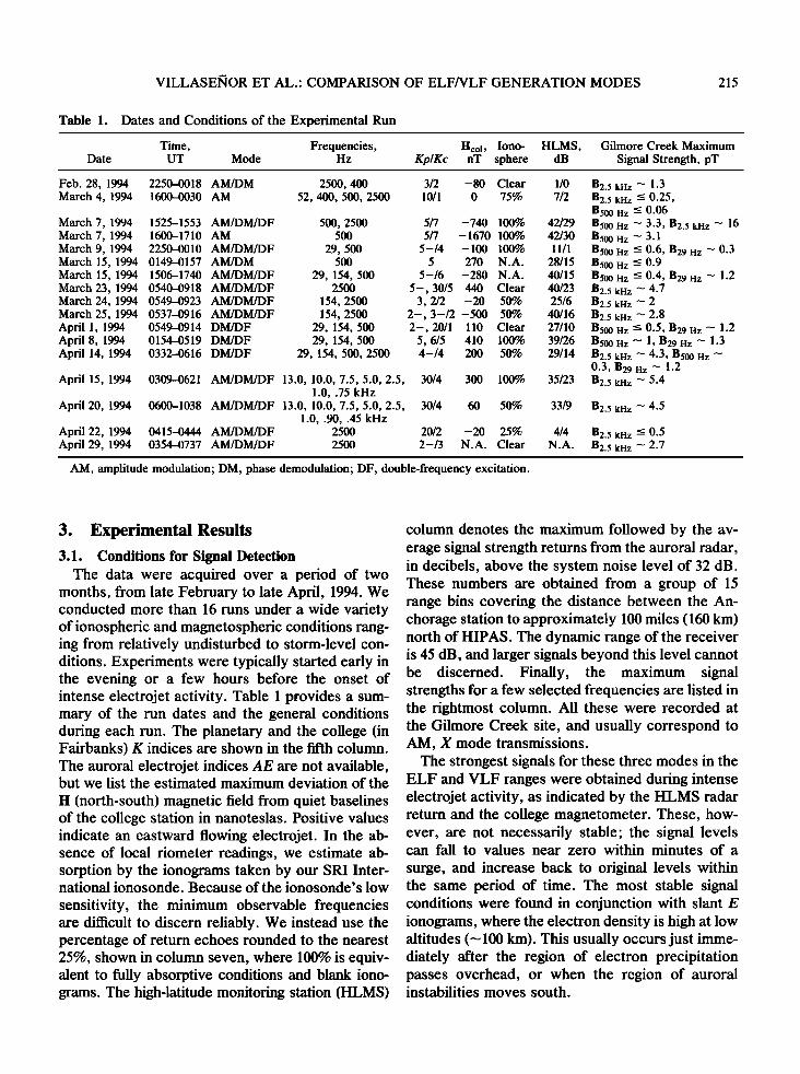
VILLASENOR ET AL.' COMPARISON OF ELF/VLF GENERATION MODES 215
Table 1. Dates and Conditions of the Experimental Run
Time, Frequencies, Hcol, Iono- HLMS, Gilmore Creek Maximum Date UT Mode Hz Kp/Kc nT sphere dB Signal Strength, pT
Feb. 28, 1994 2250-0018 AM/DM March 4, 1994 1600-0030 AM
2500, 400 3/2 -80 Clear 1/0 52,400, 500, 2500 10/1 0 75% 7/2
500, 2500 5/7 -740 100% 42/29 500 5/7 - 1670 100% 42/30
29, 500 5-/4 - 100 100% 11/1 500 5 270 N.A. 28/15
29, 154, 500 5-/6 -280 N.A. 40/15 2500 5-, 30/5 440 Clear 40/23
154, 2500 3, 2/2 -20 50% 25/6 154, 2500 2-, 3-/2 - 500 50% 40/16
29, 154, 500 2-, 20/1 110 Clear 27/10 29, 154, 500 5, 6/5 410 100% 39/26
29, 154, 500, 2500 4-/4 200 50% 29/14
30/4 300 100% 35/23
March 7, 1994 1525-1553 AM/DM/DF March 7, 1994 1600-1710 AM March 9, 1994 2250-0010 AM/DM/DF March 15, 1994 0149-0157 AM/DM March 15, 1994 1506-1740 AM/DM/DF March 23, 1994 0540-0918 AM/DM/DF March24, 1994 0549-0923 AM/DM/DF March 25, 1994 0537-0916 AM/DM/DF April 1, 1994 0549-0914 DM/DF April 8, 1994 0154-0519 DM/DF April 14, 1994 0332-0616 DM/DF
April 15, 1994 0309-0621 AM/DM/DF 13.0, 10.0, 7.5, 5.0, 2.5, 1.0, .75 kHz
April 20, 1994 0600-1038 AM/DM/DF 13.0, 10.0, 7.5, 5.0, 2.5, 30/4 60 50% 33/9 1.0, .90, .45 kHz
0415-0444 AM/DM/DF 2500 0354-0737 AM/DM/DF 2500
April 22, 1994 April 29, 1994
20/2 -20 25% 4/4 2-/3 N.A. Clear N.A.
B2.5 kHz '• 1.3 B2.5 kHz •< 0.25, B500 Hz •< 0.06 B500 Hz "' 3.3, B2.5 kHz "' 16 B5oo Hz "' 3.1 B5oo Hz --< 0.6, B29 Hz "' 0.3 B5oo Hz •< 0.9 B500 az < 0.4, B29 az "• 1.2 B2.5 kaz "• 4.7 B2.5 kaz • 2 B2.5 kaz "' 2.8 B5oo Hz --< 0.5, B29 Hz "' 1.2 B5oo Hz "' 1, B29 Hz "' 1.3 B2.5 kHz "' 4.3, B5oo Hz •' 0.3, B29 Hz "' 1.2 B2.5 kHz "' 5.4
B2.5 kHz "' 4.5
B2.5 kHz • 0.5 B2.5 kHz "' 2.7
AM, amplitude modulation; DM, phase demodulation; DF, double-frequency excitation.
3. Experimental Results
3.1. Conditions for Signal Detection The data were acquired over a period of two
months, from late February to late April, 1994. We conducted more than 16 runs under a wide variety of ionospheric and magnetospheric conditions rang- ing from relatively undisturbed to storm-level con- ditions. Experiments were typically started early in the evening or a few hours before the onset of intense electrojet activity. Table 1 provides a sum- mary of the run dates and the general conditions during each run. The planetary and the college (in Fairbanks) K indices are shown in the fifth column. The auroral electrojet indices AE are not available, but we list the estimated maximum deviation of the
H (north-south) magnetic field from quiet baselines of the college station in nanoteslas. Positive values indicate an eastward flowing electrojet. In the ab- sence of local riometer readings, we estimate ab- sorption by the ionograms taken by our SRI Inter- national ionosonde. Because of the ionosonde's low
sensitivity, the minimum observable frequencies are difficult to discern reliably. We instead use the percentage of return echoes rounded to the nearest 25%, shown in column seven, where 100% is equiv- alent to fully absorptive conditions and blank iono- grams. The high-latitude monitoring station (HLMS)
column denotes the maximum followed by the av- erage signal strength returns from the auroral radar, in decibels, above the system noise level of 32 dB. These numbers are obtained from a group of 15 range bins covering the distance between the An- chorage station to approximately 100 miles (160 km) north of HIPAS. The dynamic range of the receiver is 45 dB, and larger signals beyond this level cannot be discerned. Finally, the maximum signal strengths for a few selected frequencies are listed in the rightmost column. All these were recorded at the Gilmore Creek site, and usually correspond to AM, X mode transmissions.
The strongest signals for these three modes in the ELF and VLF ranges were obtained during intense electrojet activity, as indicated by the HLMS radar return and the college magnetometer. These, how- ever, are not necessarily stable; the signal levels can fall to values near zero within minutes of a
surge, and increase back to original levels within the same period of time. The most stable signal conditions were found in conjunction with slant E ionograms, where the electron density is high at low altitudes (--• 100 km). This usually occurs just imme- diately after the region of electron precipitation passes overhead, or when the region of auroral instabilities moves south.

216 VILLASENOR ET AL.' COMPARISON OF ELF/VLF GENERATION MODES
1 5 9 1:3 17 21 25 29 33 :37 41
::".-":-'-':':-' '
!-".:'"' '"::" ' '"' '"":•... •":•:•i "-:?." ' "'" "::' ':'"•' """'•-••••-•i i ......... ' '"" '":':"••:'"•••'••••ii i!• -"•- •'""•'"' •'""::''" '" ' ''' ' "•4••:••••••4
03:00 o4:0o o5:0o o•.oo o7:o0 o8:0000:OO lO:OO 11:oo
Time (UT) ß , , ß . , , . ,
i i i i I . . i
03:00 04:00 05:00 06:00 0?:00 08:00 09:00 10:00 11:00
0.8
0.6
0.4
0.2
o .,......l, L•u. J•.,l,l.• L 06:00 07:00 08:00 09:00
Time (UT)
UT. The ionograms evolved from clear F to slant E traces, with the region of polar electrojet activity moving south and increasing in intensity near the end of the run. The signal strength likewise increased as the edge of the region passed over the college and decreased as the electrojets receded north. The radar dependence of the signal strength holds true for other frequencies, as shown in Figure 6, where the aver- aged radar strength is plotted versus the maximum signal strength for 2.5 kHz and 500 Hz.
During periods of very intense electrojet activity, the ionospheric D region is very absorptive and obscures the reception of ELF signals. As a useful gauge, successful detection of ELF signals could only be achieved when the magnetosphere is quies- cent, or the deviation at the college magnetometer did not exceed +50 nT from the baseline several
hours prior to the onset of strong electrojet condi- tions. Prolonged periods of electrojet activity lead to successive blank ionograms (i.e., no return pulses' could be discriminated from the noise), and low-frequency ELF signals could not be detected from the higher-noise background. The electrojet instabilities are often north of the facility, but when these move directly overhead (visible aurora can be observed), signal reception is clear even in Delta Junction. VLF frequencies greater than 1.5 kHz, on the other hand, are less dependent on the absorp- tivity and previous activity for good reception.
10
Figure 5. Time evolution of the signals as a function of conditions. (a) The HLMS radar return showing the presence of electrojet instabilities. The region of instabil- ity is moving south from 0700 to 0900. (b) The trace is a weighted average of the five range bins roughly centered over the U.S. Geological Survey College station. (c) Signals recording DM/DF excitation for a segment of the plots in (a) and (b). The cycle of DM/DF excitation was on from 0530 UT up to 0915 UT, April 1, 1994.
Comparison of HLMS auroral radar intensities as a function of time shows that for both X and O mode
polarizations, the signal strength is proportional to the presence of electrojets, as illustrated by Figure 5. In this particular example, a continuous cycle of DM/DF modulation at 29 Hz was applied from 0530 to 0915
I I ' ! I I I I
o ß
o 6 o
ß 5OOHz
o 2.5 kHz
i I I I I I
0 5 10 15 :3:) 25 30
Average radar return signal (dB)
Figure 6. Relation between the maximum signal strengths at 500 Hz and 2.5 kHz and the averaged HLMS radar return strength. The radar average is carried out over a bin range corresponding to the distance from Anchorage to approximately 100 miles north of HIPAS.

VILLASENOR ET AL.' COMPARISON OF ELF/VLF GENERATION MODES 217
1.25 --
1.00
0.75
0.50
0.25 --
0.00
01:30 02:00 02:30 03:00 03:30 04:00 04:30 05:00
0.10 __[I ' I ' I ' I ' I ' I ' I ' I ' _ ß
0.08 0.06
0.04
0.02
0.00
01:30 02:00 02:30 03:00 03:30 04:00 04:30 05:00 UT (hours)
Figure 7. Comparison of ELF signals received at the (a) Gilmore Creek and (b) Delta Junction sites for f = 29 Hz. The east-west coils at each site are shown. (c) The timing sequence showing the combinations of DM/DF modes and O/X polarizations. The total power radiated for this sequence was held constant at 800 kW. (Data were taken April 8, 1994.)
3.2. Comparison of Signals at Different Locations In most of these runs, signals of a few pT were
observed in both the Gilmore Creek and Delta
Junction receivers in the ELF range of frequencies (Figures 7a and 7b). The ratio of the signal ampli- tudes between the two sites is approximately 10. The scaling provided by Bannister et al. [1993] shows that for a horizontal magnetic dipole (HMD) or horizontal electric dipole (HED) generated di- rectly overhead, the signal amplitude ratio should be approximately -10 dB, or 0.32. Distance scaling at VLF frequencies is currently under study.
The north-south signal is generally slightly stron- ger than the east-west component, indicating a greater east-west direction of flow of the electrojets. At each site, X mode heater polarizations produce larger sig- nals than O mode heater polarization, as expected. These results also apply to VLF frequencies, a typical example of which is shown in Figures 8a and 8b.
Polarization ellipses of received signals from both sites are shown in Figure 9 at 29 Hz. The degree of ellipticity is indicated by the shape of the figure, and the ellipse angle is depicted as the angle which the
ellipse makes with the horizontal. The magnitude of the arrow shows the strength of the signal; for clarity, the Delta Junction signals are multiplied by a factor of 10. The ellipticity • is positive if the sense of rotation is right-hand circularly polarized (RHCP; arrow pointing up on the diagram) with respect to the Earth's magnetic field (pointing downward with (b = 77.2ø). The signals are gener- ally elliptically polarized, but the right and left components are sufficiently close in magnitude that no wave mode strongly dominates. Thus, the range of e falls between 14 -< .5. For frequencies in the Schumman range, we typically find that e > 0 (RHCP) at the Gilmore Creek site, and e < 0 (left-hand circularly polarized, or LHCP) at the Delta Junction receiver. At higher frequencies, e < 0 (LHCP) for most of the data collected by the Gilmore Creek VLF receiver.
3.3. HF Spectra of the Modes
In Figures 10a-10c we compare the HF spectra between the three modes for 2500 Hz during moder- ately active magnetospheric conditions. The ampli-

218 VILLASE•OR ET AL.' COMPARISON OF ELF/VLF GENERATION MODES
.
•- 3
x 2
1
0 I I
07:35 07:37 07:40 07:43 07:46
4-- ' I ' I ' I ' i ' I-
•'3
>-2
1
0 • •
07:35 07:37 07:40 07:43 07:46 UT (hours)
< • X-mode > <, O-mode •.>
Figure 8. An example of AM/DM/DF generated signals detected by the east-west coils at X and O mode polarized transmissions for the VLF frequency of 2500 Hz. The integration time is 5 s. (a) NS component; (b) EW component; (c) timing sequence. (Data were taken April 20, 1994.)
tude fluctuations in the sidebands can reach up to 5-10 dB, but generally the DF mode shows the carrier peaks 10-13 dB from the amplitudes of the AM and DM signals. Since half of the array is radiating, the 10-dB difference from the expected peak is due to defocusing. For the AM and DM modes, sidebands corresponding to the modulation frequency appear above and below the pump frequency, with the higher odd harmonics cutoff due to the bandwidth of the
receiver. The signal amplitudes for the harmonics of the AM and DM modes are 10-dB higher than those of the carrier frequencies of the DF mode, because of the larger number of radiators and larger focusing power of the array. Figures 10d-10g show the spectra for DM/DF and X/O polarization at 154 Hz. At these lower frequencies, the odd harmonics corresponding to square wave modulation are detectable by the Racal receiver.
We should note that the HF spectra is highly dependent on the background conditions. During quiescent periods when the absorption is low, mul- tiple sidebands, as shown in Figure 10b, were observed for AM and DM transmission. However,
when there are strong electrojets present, the higher harmonics are suppressed, and only the upper and lower sidebands are observed. Furthermore, the presence of multiple harmonics of the modulation frequency in the HF spectra does not ensure the detection of ELF signals. For quiet conditions where the absorption is low and the ionograms are clear (the polar electrojet is absent), the measured ELF/VLF signal tends to be reduced or nonexist- ent. Thus there is an anticorrelation between the
detection of the ground based ELF signal and the HF sky wave return.
3.4. Frequency Variation Frequency scans were performed on two sepa-
rate dates to compare the differences between the AM, DM, and DF modes of excitation. For each frequency, the three modes were cycled through four times within 10 min before the polarization was switched and the cycling repeated. The averaged results are shown in Figures 1 l a and 1 lb. Strong signals on the order of a few picoteslas were ob- served from 13 kHz all the way down to 750 Hz.

VILLASE•OR ET AL.' COMPARISON OF ELF/VLF GENERATION MODES 219
DIVVO DF/O DM/X DF/X DM/O DF,O DM/X DF/X D M/O DF,O 01:55 02.05 02:15 0225 02:36 02:46 0256 03.06 03:17 0327
Gilmore Creek,
Delta Junction' Hz •(• • ! • DM/X DF/X DM/O DF/O • DM/X DF/X 03:37 03:47 03:58 04.1:)8 04.'18 0428
DM/O DFA3 DM/X DF/X
04:39 04:4 9 04:59 05.139
Figure 9. Polarization ellipses of ELF signals at 29 Hz for the Gilmore Creek and Delta Junction sites. RHCP waves point upward, and LHCP downward. The length of the arrow depicts the relative amplitude of the signal; the Delta Junction signals are multiplied by a factor of 10. The ellipticities of the signals detected at the two sites are generally opposite in sign.
The maximum signal observed for each frequency for AM excitation is at a constant level of 2.5-3 pT for both the X and O modes. The DF mode for this
run generated signals with comparable or even greater magnitude with the AM mode, except at frequencies below 2 kHz. The large values obtained may be due to the short sampling periods and the inherent stability of the DF mode (see the next section below). The DM signal is the weakest of the three modes. The results of this scan compare favorably with the AM scan obtained at the Tromso facility [Stubbe et al., 1982b]. At frequencies below 1.5 kHz where the transverse electric (TE) cutoff exists, the generation of EM waves decreases con- siderably. The decrease is due to the corresponding decrease in the excitation efficiency of a horizontal dipole in the ionosphere [Barr and Stubbe, 1984].
The ellipticity e as a function of frequency is displayed in Figures 12a and 12b. The variation with frequency for all modes is nearly identical, even for the X and O mode polarizations. This similarity suggests that the signals originated from a common height.
3.5. Temporal Variations
We conducted a run over an extended period to investigate the time dependence of the signals. Figure 13 shows the amplitude as a function of time showing fluctuations in the AM and DM generated signals, while the DF generated signal remains relatively steady. One important observation is that the DF signal varies on a relatively longer timescale than either AM or DM. The DF signal monitored over time was fairly constant, while the AM and DM signals fluctuate approximately in step, main- taining a ratio of around 0.6. At certain periods, the DF signal was actually larger than the AM signal, but on average was usually around 0.6 times the AM signal. The X mode DF signals were the most stable under electrojet conditions.
Comparing the corresponding ellipticity e for the same graph, as in Figure 14, as a function of time, we note that e < 0 (LHCP) for most of the X mode polarized waves. In the period where e increases to values > 0 (RHCP), we see that a corresponding decrease in the signal amplitude occurs for all three

220 VILLASENOR ET AL.' COMPARISON OF ELF/VLF GENERATION MODES
center frequency = 2.85 MHz
,_•
ß . ß . ß
-6000 -4O00 -2000 0 20O0 4OO0 •000
offset frequency (Hz)
- . - . - . - , - . -
-4O
:
offset frequency (Hi}
- ß - ß - ! - ß - ß -
-50
. , . , , ß
-6OOO -4O0O -2000 0 2OOO 4OOO 6OOO
offset frequency (Hi}
ß , ß ß ß ß , ß ,
• •o
-70
offset frequency (Hi) offset frequency (Hi) offset frequency (Hi) offset frequency (Hi)
Figure 10. Comparison of the HF spectra for the DF, DM, and AM transmissions. Here, &f = 2500 Hz, for AM, DM, and DF, at X mode polarization (upper panels). For &f = 154 Hz, the spectra for DF/DM at O and X mode polarizations are shown in the lower panels. Note the absence of strong sidebands in the DF mode.
modes. For O mode polarization, we see that e < 0 for AM, while e > 0 for the DF and DM modes.
We also show the results of sending signals with mixed polarization in Figure 15, where half of the array was polarized at X mode and the other half with O mode. In the figure, a set of AM, DM, and DF mode transmissions polarized with X mode preceded the mixed mode transmissions, ending with an O mode set. The AM mode is relatively unaffected by the mixed polarity, but the DM and the DF are reduced to values which are much lower
than the signals observed for O mode polarization. For AM modulation, the overall transmitted power at the zenith is linearly polarized and elliptically polarized in the surrounding region. For the DM and DF cases, the half which is changed in phase from 0 ø to 180 ø is kept at a different polarity. In the first half cycle, the net polarization at the zenith is linear with the E field pointing north; in the second, changing the phasing of the second set also results in a linearly polarized wave, but with the E field rotated 90 ø to the east. Since the electric field
intensity does not vary to Oth order, this should result in little or no heater modulation.
4. Analysis
4.1. Signal Strengths for AM, DM, and DF Excitation
We turn to the question of AM, DM, and DF ratios by calculating the sky map intensities for the three configurations, under the assumption that the heated region is more or less confined to a 45 ø cone over the zenith. We should note that the cone angle can be larger, depending on the extent to which the electrojets overlap the heated region. For example, for eight antennas radiating in phase, the fraction of power contained in the cone as a function of the cone angle is presented in Figure 16. In this case, about 73% of the total flux is contained within 20 ø
from the zenith (total cone angle equals 40ø). Since we completely turn off the power in the second half of the cycle, the power is 100% modulated at the ground level; this is to be compared with DM

VILLASE•OR ET AL.' COMPARISON OF ELF/VLF GENERATION MODES 221
4.0
3.5
3.0
2.5 2.0 1.5
1.0
0.5
0.0
ß ! ' I ' ! ' I ' I ' I '
X-mode --e--Did 2.0
1.0
0.5
I I I I I I
2000 4000 6000 8000 10000 12000 14000 0
ß ß I ' ! ' ! ' I ' I '
,--d,.--DF
ß I ' I ' I " I ' I ' I '
2000 4000 6000 8000 10000 12000 14000
frequency (Hz) frequency (Hz)
Figure 11. Frequency comparison of the AM/DM/DF modes. (a) X mode heater polarization; (b) O mode heater polarization. The data were taken April 15, 1994.
transmission, where we still send ---12% of the power in the dephased cycle into a 45 ø cone. In the region of interest, •oq' T • 1, SO We can expect the electron temperature in the heated region to approach equilibrium in each half cycle. Since the conductivity modulation at the interaction region is proportional to the difference Te0 (Pmax) - Teo (Pmin), where Pmax and P rnin are the maximum and minimum power
levels for each mode, we must look at the dependence of the temperature to the applied heater power.
Strong electric fields can modify the characteris- tics of the medium in which they propagates, hence the temperature rise produced by the heater is classified according to ratio of the electric field E to the characteristic plasma field E•, = [3T(rn/e:)&o(OO •
v2 •] 1/2 + •o• , where •o is the average fraction of the
0.1
0.0
-0.1
.• -0.2 -0.3
-0.4
-0.5
ß I ' I ' I ' I ' I ' I ' ' I ' I ' I ' I ' I ' I ' 4 X-mode --o---AM 0.1 O-mode --a,--.DF
............................ 0.0 t I• ................................. i '
i
I I I I I I
2000 4000 6000 8000 10000 12000 14000 0 2000 4000 6000 8000 10000 12000 14000
frequency (Hz) frequency (Hz)
Figure 12. Corresponding ellipticity plots for the plots in Figure 10. (a) X mode; (b) O mode.

222 VILLASENOR ET AL.: COMPARISON OF ELF/VLF GENERATION MODES
1.6 X-mode, 2500 Hz • AM O-mode 2500 Hz .--o-- AM • DM 0.5 ' ---•-- DM
1.4 •DF
1.2 0.4
1.0
0.6 .
0.4
0.0 .
0400 04:10 04:20 04:30 04:40 0450 05:00 05:10 0520 0530 0540 05:50 06:00 06:10 06:20 06:30 06:40 06:50
UT (hours) UT (hours)
Figure 13. Comparison of the time evolution of the AM/DM/DF excitation modes for (a) X mode and (b) O mode polarizations. Note the fast time variation of the AM/DM modes.
energy transferred in one collision [Gurevich, 1978]. For E/Ep < 1, AT c• E 2 c• p, whereas for E/Ep > 1 and to - %0, AT--• E c• p 1/2. The electron temper- ature variation during the on-off cycle is given by the relation
1 (1 + ito•-T 1 ATe(Pmax, Pmin)= •[Teo(Pmax) - Teo(Pmin)] 1 •
where Teo(P) is the electron temperature corre- sponding to the power level P, to is the heater frequency, and vr is the characteristic time for thermal equilibrium [Stubbe, 1982b]. The ratio ATeDM/ATeAM DM DM AM AM • (Pmax - Pmin )/(Pmax - Pmin ) • 0.85 for the weak field (E/Ev (1) case, and ATeI)•/ATe •
AM AM • (X/•m • -- X/•min)/(X/Pma x - X/Pmin) • 0.61 for the strong field (E/E v y 1). Neglecting changes in the
0.6
0.4
0.2
o 0.0
-0.2
ß I ' I ' I ' I ' I ' I ' I ' I • I
--o--AM
X-mode, 2500 Hz ---era DM '- DF
...
' I ' ' I ' I ' ' ' I ' ' '
05:00
UT (hours)
0.6
0.4
• 0.2 =>, _9.o 0.0
-0.2
-0.4
-0.6
' i ' I ' i ' I ' I ' I ' I ' I ' I '
---o• AM O-mode, 2500 Hz
•m DM
ß --a•-- DF
o ß o ß
0530 05:40 05:50 06:00 06 10 06:20 0630 0640 06:50
UT (hours)
Figure 14. Comparison of the ellipticity of the AM/DM/DF excitation modes for (a) X mode and (b) O mode polarization. For X mode polarization, the signal strength markedly decreases as the ellipticity e becomes right handed (positive).

VILLASE•OR ET AL.' COMPARISON OF ELF/VLF GENERATION MODES 223
3.0
2.5
2.0
1.0
0.5
0.0 ,
I ß I ' I ' I ' I ß I ß I
mixed-mode .--e• DM
07:00 07 05 07:10 07 15 07 20 07:25 07:30
ß I ' I ' I ß I ' I ' I
0.2 .--e--- DM •DF
mixed-mode
0.1 X-mode O-mode
-0.1
-0.2
07:00 07 05 07:10 07:15 07:20 07:25 0 30
UT (hours) UT (hours)
Figure 15. Mixed mode results. The initial set of AM/DM/DF modulations was X mode, followed by the mixed mode polarization where half of the four transmitters are X, and the other half O, and, finally, the last set is O mode polarization. The onset of electron precipitation (strong D layer, formation of auroral electrojets) coincided with the beginning of the O mode cycle.
recombination rate which leads to density perturba- tions, the change in the conductivity A•r = (0o/OT)AT. The ratio of the signal strengths • AO'DM/AO'AM • 0.61-0.85, which is consistent with the experimental data. Estimates by Papadopoulos et al. [1990] yield similar results. The ratio of the magnetic field pertur- bation as measured on the ground BDM/B^M --- A•rDM/ AO'^M, where A•r--- [PHF/L2] a, PHF is the heating power, a --- 1, and L is the spot size at the appropriate
---• 100 c
(I) c o 80 (,3
,,, ,•,
•: e0
o (,3
o
• 0
ß I ' I ' I ' i ' I ' I ß I ' I
,i
inphase
0 10 210 30 40 50 60 70 80
cone angle (degrees)
Figure 16. Fraction of power contained as a function of cone angle for the in-phase and out of phase mode.
dipole height. This scaling yields a value of BDM/BAM --• 50-88%.
Since the method of excitation is fundamentally similar to the DM mode, the same analysis should hold to give a ratio BDF/BAM '-• 50-88%.
4.2. X Mode and O Mode Comparison
The other issue is how absorption varies from X mode to O mode. The attenuation factor due to
absorption by electron-neutral collisions is given by
n (fo +-fc cos 0) 2 + (Ve/2•r) 2
where f•,, f0, and fc are the plasma, carrier, and electron cyclotron frequency, respectively, n is the index of refraction of the wave, Ve is the electron neutral collision frequency, and the plus and minus correspond to the O mode and the X mode, respec- tively. If we define the wave absorption scale as a = •odc, then the electric field attenuates as
E(h) •-•-n exp - adz As an estimate, we can integrate up to a height h and assume that the power dissipated goes into modulating the electrojets. We use typical profiles

224 VILLASENOR ET AL.' COMPARISON OF ELF/VLF GENERATION MODES
10o
Figure 17.
I ß I ß I . I . I ß I ß I i
height (km)
Ratio of the absorbed power in the X and O modes as a function of height. The corresponding ratio of the received signal for the X and O modes must be roughly equivalent to this ratio.
of the electron density, electron-neutral collision frequencies, and magnetic field for this location and time of the year and integrate up to an altitude of 75 km. We obtain the values of Ex/E0 • 0.75 and Eo/E 0 -• 0.93. This indicates a ratio of power absorption in the D region for the O versus X to be --•65% (Figure 17). For h = 85 km, this ratio decreases to •40%. Thus for modulation of the
electrojets in the D region we can expect the ratio of the X to O signals to be roughly a factor of two. These numbers are consistent with our experimen- tal data.
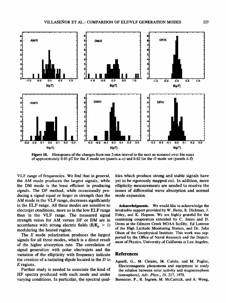
4.3. Signal Stability and Phase Considerations In Figure 18 we quantify the stability of the signal
by using histogram plots of the change in the magnetic field at averaged 2-min intervals from the data shown in Figure 13. Note that the ratio of the spread between the O mode and X mode returns is also roughly a factor of two, or the same factor as the ratio of the signal strengths.
The stability of the DF mode over the DM mode and the HF spectra suggest the effects of harmon- ics, and the possible nonlinear interactions between them. Nonlinear interaction between the carrier and
sideband waves can produce a signal due to the detection effect arising from a ponderomotive force, which can occur if V(E 2) does not vanish [Stubbe, 1982b; Agnelli, 1970]. Here, E is the sum of the electric fields of both carrier and sidebands. The
low-frequency signal is generated by the sum of
pairwise interactions between the carrier and the first harmonics; if their phases are rotated due to turbulence, signal cancellation may occur. The DF mode is less susceptible to this, since the major interaction occurs between the two frequencies and no further vector addition or cancellation in the
ionosphere occurs. The issue of stability, however, is still open to
interpretation subject to additional data we are in the process of gathering.
4.4. Ellipticity The excited wave traveling to each receiver site is
generally elliptically polarized with some combina- tion of right-hand and left-hand waves. The partic- ular instance shown in Figure 14 where the elliptic- ity changes sign when the total amplitude of the received signal goes to zero is most probably due to differential absorption, where the left-hand compo- nent was more strongly absorbed than the right- hand component. The background noise spectra at this frequency are usually close to linearly polar- ized. Comparing the ellipticities at two sites, the longer distance to Delta Junction can lead to a larger differential absorption between the RHCP and the LHCP waves, and thus the Gilmore Creek site should receive signals more "handed" than at Delta Junction; that is, IGCI > I•DJI.
Another explanation for the opposite signs of ellipticity is through normal mode expansion of the excited field for a spherical cavity [Sentman, 1987]. Gilmore Creek is nearly magnetic west of the HIPAS site, while Delta Junction is magnetic E-SE. The excited magnetic field can be decomposed into a sum of eigenmodes which are proportional to the derivatives of spherical harmonics Y/re. In our case, the dominant or lowest mode has three multiplets with rn = 1 being a "westward" RHCP and rn - - 1 an "eastward" LHCP wave. Thus each site is
receptive to one of these modes, depending on the direction of the electrojet current flow.
At present, more data is needed to distinguish between the effects of differential absorption and normal mode expansion. Ellipticity measurements at different locations are particularly useful in re- solving the normal mode structure of the radiation pattern.
5. Summary and Conclusions In this paper we have presented three different
modes of generating waves in both the ELF and
VILLASENOR ET AL.' COMPARISON OF ELF/VLF GENERATION MODES 225
-1.0
AM/X
-0.5 0.0
B(pT)
DM/X DF/X
0.5 1.0 -1.0 -0.5 0.0 0.5 1.0 -1.0 -0.5 0.0
B(pT) B(pT)
0.5 1.0
AM/O DM/O DF/O
-0.3 -0.2 -0.1 0.0 0.1 0.2 0.3 -0.3 -0.2 -0.1 0.0 0.1 0.2 0.3 -0.3 -0.2 -0.1 0.0 0.1 0.2
B(pT) B(pT) B(pT)
Figure ]8. Histograms of the changes from one 2-min intcval to the next as summed over Din sizes of approximately 0.05 pT for the J mode set (panels a-c) and 0.02 for the O mode set (panels d-f).
0.3
VLF range of frequencies. We find that in general, the AM mode produces the largest signals, while the DM mode is the least efficient in producing signals. The DF method, while occasionally pro- ducing a signal equal or larger in strength than the AM mode in the VLF range, decreases significantly in the ELF range. All these modes are sensitive to electrojet c•nditions, more so in the low ELF range than in the VLF range. The measured signal strength ratios for AM versus DF or DM are in accordance with strong electric fields (E/Ep > 1) modulating the heated region.
The X mode polarization produces the largest signals for all three modes, which is a direct result of the higher absorption rate. The correlation of signal generation with polar electrojets and the variation of the ellipticity with frequency indicate the creation of a radiating dipole located in the D to E regions.
Further study is needed to associate the kind of HF spectra produced with each mode and under varying conditions. In particular, the spectral qual-
ities which produce strong and stable signals have yet to be rigorously mapped out. In addition, more ellipticity measurements are needed to resolve the issues of differential wave absorption and normal mode expansion.
Acknowledgments. We would like to acknowledge the invaluable support provided by W. Huhn, R. Dickman, J. Foley, and K. Hopson. We are highly grateful for the continuing cooperation extended by C. Jones and D. Ooms at the Gilmore Creek NOAA facility, Ed Luteran of the High Latitude Monitoring Station, and Dr. John Olson of the Geophysical Institute. This work was sup- ported by the Office of Naval Research and the Depart- ment of Physics, University of California at Los Angeles.
References
Agnelli, G., M. Cimino, M. Cutolo, and M. Puglisi, Electromagnetic phenomena and equipment to study the relation between solar activity and magnetosphere (ionosphere), Adv. Phys., 19, 217, 1970.
Bannister, P., R. Ingram, M. McCarrick, and A. Wong,

226 VILLASE•OR ET AL.: COMPARISON OF ELF/VLF GENERATION MODES
Results of the joint HIPAS/NUWC campaigns to inves- tigate ELF generated by auroral electrojet modulation, AGARD Conf. Proc., 529, 18-1-18-12, 1993.
Barr, R., and P. Stubbe, The "Polar Electrojet Antenna" as a source of ELF radiation in the Earth-ionosphere waveguide, J. Atmos. Terr. Phys., 46(4), 315-320, 1984.
Gurevich, A., Non-Linear Phenomena in the Ionosphere, translated from Russian by J. Adashko, Springer-Ver- lag, New York, 1978.
McCarrick, M., D. Sentman, A. Wong, R. Weurker, and B. Chouinard, Excitation of ELF waves in the Schu- mann resonance range by modulated HF heating of the polar electrojet, Radio Sci., 25(6), 1291-1298, 1990.
Papadopoulos, K., C. Chang, P. Vitello, and A. Drobot, On the efiSciency of ionospheric ELF generation, Radio Sci., 25, 1311-1320, 1990.
Reitveld, M., Ground and in situ excitation of waves in the ionospheric plasma, J. Atmos. Terr. Phys., 47, 1283-1296, 1985.
Sentman, D., Magnetic elliptical polarization of Schu- mann resonances, Radio Sci., 22, 595-606, 1987.
Song, B., Experimental study of the double resonance parametric excitation in the ionosphere, Radio Sci., 30(6), 1875-1883, 1995.
Stubbe, P., H. Kopka, M. Reitveld, and R. Dowden,
Ionospheric modulation experiments in northern Scan- dinavia, J. Atmos. Terr. Phys., 44, 1025-1041, 1982a.
Stubbe, P., H. Kopka, M. Reitveld, and R. Dowden, ELF and VLF wave generation by modulated HF heating of the current carrying lower ionosphere, J. Atmos. Terr. Phys., 44, 1123-1135, 1982b.
Stubbe, P., et al., Ionospheric modification experiments with the Troms0 Heating Facility, J. Atmos. Terr. Phys., 47, 1151-1163, 1985.
Wong, A. Y., et al., High-power radiating facility at the HIPAS Observatory, Radio Sci., 25(6), 1269-1282, 1990.
M. McCarrick, B. Song, and A. Y. Wong, Department of Physics, University of California, Los Angeles, CA 90024.
J. Pau and J. Villasefior, HIPAS Observatory, 7795 Chena Hot Springs Rd., Fairbanks, AK 99712. (e-mail: jsvilla @physics.ucla.edu)
D. Sentman, Geophysical Institute, University of Alaska, Fairbanks, AK 99712.
(Received December 8, 1994; revised June 28, 1995; accepted June 28, 1995.)