Reliability and efficiency analysis of distributed source coding in wireless sensor networks
Upload
khangminh22Category
view
0download
0
Comparison of Distributed OptimizationAlgorithms in Sensor Networks
Simulations and results
CESARE MARIA CARRETTI
Masters’ Degree ProjectStockholm, Sweden January 2008
XR-EE-RT 2008:001


Abstract
We consider a peer-to-peer approach to wireless sensor networks us-ing the IEEE 802.15.4 standard, with sensors not synchronized, andwithout any routing protocol. Only communications between neigh-bors are allowed. In this scenario we do a comparison between fourdistributed algorithms that solve a special class of optimization prob-lems, which are of great interest in networking applications. We wantto retrieve, without a central node, the average of a scalar measure-ment from all sensors in the network. In the final state, each sensorshould have the global average of the considered measurement. Toevaluate performances of the algorithms, we build an application forthe network simulator ns2, and we do several simulations to evaluateconvergence delay, and final error, respect to time and to number ofpackets sent. In this thesis we present the algorithms from theoreticaland practical point of views, we describe our application for ns2, and weshow the results obtained, which show that this types of algorithms, iftuned properly, work well and are ready to be practically implementedin a real sensor network.
Contents
Contents 4
1 Introduction 71.1 General description . . . . . . . . . . . . . . . . . . . . . . . . 81.2 Distributed vs Centralized . . . . . . . . . . . . . . . . . . . . 91.3 Originality of the work . . . . . . . . . . . . . . . . . . . . . . 91.4 Thesis’ overview . . . . . . . . . . . . . . . . . . . . . . . . . . 101.5 Previous Work . . . . . . . . . . . . . . . . . . . . . . . . . . 11
2 Background 132.1 Wireless Sensor Networks . . . . . . . . . . . . . . . . . . . . 14
2.1.1 Hardware and Software . . . . . . . . . . . . . . . . . . 142.1.2 Application of Wireless Sensor Networks . . . . . . . . 16
3

4 Contents
2.2 IEEE 802.15.4 and ZigBee . . . . . . . . . . . . . . . . . . . . 182.2.1 Physical layer (PHY) . . . . . . . . . . . . . . . . . . . 192.2.2 MAC sublayer . . . . . . . . . . . . . . . . . . . . . . . 202.2.3 Devices for IEEE 802.15.4 . . . . . . . . . . . . . . . . 222.2.4 Power saving . . . . . . . . . . . . . . . . . . . . . . . 22
3 Optimization Theory 233.1 Convex Optimization Problem . . . . . . . . . . . . . . . . . . 24
3.1.1 Convex Optimization overview . . . . . . . . . . . . . . 243.1.2 Dual approach . . . . . . . . . . . . . . . . . . . . . . . 253.1.3 Solve the problem: descent methods . . . . . . . . . . . 27
3.2 Distributed algorithms . . . . . . . . . . . . . . . . . . . . . . 293.2.1 Distributed optimization problem . . . . . . . . . . . . 293.2.2 Average: least squares solution . . . . . . . . . . . . . 303.2.3 Topology . . . . . . . . . . . . . . . . . . . . . . . . . . 30
3.3 Algorithms and naming . . . . . . . . . . . . . . . . . . . . . . 313.3.1 Unicast . . . . . . . . . . . . . . . . . . . . . . . . . . 313.3.2 Broadcast . . . . . . . . . . . . . . . . . . . . . . . . . 333.3.3 Unreliable broadcast . . . . . . . . . . . . . . . . . . . 363.3.4 Dual . . . . . . . . . . . . . . . . . . . . . . . . . . . . 37
3.4 Robust Optimization . . . . . . . . . . . . . . . . . . . . . . . 39
4 Implementation 414.1 ns2 . . . . . . . . . . . . . . . . . . . . . . . . . . . . . . . . . 42
4.1.1 Structure and functioning of ns2 . . . . . . . . . . . . . 424.1.2 802.15.4 in ns2 . . . . . . . . . . . . . . . . . . . . . . 464.1.3 New agent for ns2 . . . . . . . . . . . . . . . . . . . . . 494.1.4 OTcl script and simulation run . . . . . . . . . . . . . 53
4.2 Our Application: CCsensorApp . . . . . . . . . . . . . . . . . 574.2.1 CCsensorApp’s general structure . . . . . . . . . . . . 574.2.2 Implementation of the algorithms . . . . . . . . . . . . 594.2.3 Neighbors’ discovery . . . . . . . . . . . . . . . . . . . 66
5 Results and Comments 675.1 Types of comparison . . . . . . . . . . . . . . . . . . . . . . . 68
5.1.1 Tools . . . . . . . . . . . . . . . . . . . . . . . . . . . . 685.2 Algorithms . . . . . . . . . . . . . . . . . . . . . . . . . . . . . 70
5.2.1 Parameter setting and tuning . . . . . . . . . . . . . . 705.2.2 General comparison . . . . . . . . . . . . . . . . . . . . 715.2.3 Broadcast Algorithm . . . . . . . . . . . . . . . . . . . 755.2.4 Broadcast Unreliable Algorithm . . . . . . . . . . . . . 80

Contents 5
5.2.5 Dual Optimization Algorithm . . . . . . . . . . . . . . 845.2.6 Unicast Algorithm . . . . . . . . . . . . . . . . . . . . 86
6 Conclusions 91
7 Future work 95
Bibliography 97


Chapter 1
Introduction
7
8 CHAPTER 1. INTRODUCTION
1.1 General description
During the last years, the diffusion of wireless sensor networks is making theresearch concentrate a lot on this field. Also, the continuous improvementsin sensors’ technology give unlimited possibility of application: environmentmonitoring, home automation, traffic control, assistance, without mentioningmilitary application, are all very actual and useful fields of application forsensor networks, and there is in each of these fields a big effort in researchingways to improve the performances of the networks, to find better ways to dothe same things, to discover new applications. The use of sensors could, forexample, go from avoid the use of wires in simple applications like remotecontrol (e.g., a light switcher), to built a large complex sensor network tomonitor the pollution in the atmosphere.
The request of a wireless sensor network are very different from those ofa computer wireless network, and from those of mobile phones: sensors donot need high data rate transfer, while need data reliability, power savingand network self-configuring. In particular the problem of preserving power isvery important, because of the difficulty and, often, impossibility, in changingthe battery pack. For all these reasons, there was the need to develop a newprotocol especially thought for low data rate networks. The answer was theIEEE 802.15.4 standard. The aim of this standard is indeed to provide acommunication protocol for networks that not need an high bit rate and thathave power consumption constraints.
When a new technology is introduced, to exploit it at best, there is theneed of doing a lot of research upon the different aspects and the differentpossibilities this technology can offer. This is what is happening for IEEE802.15.4 and for sensor networks in general. The scientific world is showing abig interest on these issues, thinking that in the next future, there will be anexponential growth of wireless sensor networks in a lot of different fields.
This Master Thesis Project aims at giving a contribute to the research,simulating on the network simulator ns2 a wireless sensor network (which usethe standard IEEE 802.15.4) and implementing over it four distributed opti-mization algorithms, to calculate the average of sensors’ scalar measurementusing only peer-to-peer connections, without any routing protocolo and with-out synchronization. This approach is very useful to have high reliability inthe system, and to preserve as much as possible battery power inside devices.A project for future work is to implement the algorithms in a real sensor net-work, using t-mote sky sensors, but it is important to test in a simulationwhat kind of performances to expect and the possible problems.

1.2. DISTRIBUTED VS CENTRALIZED 9
1.2 Distributed vs Centralized
The first thing people who want to calculate the average of scalar measure-ments in a sensor network think, is to send the values from each sensor toa central node who does the sum of all values and then divides for the totalnumber of sensors in the network. This approach has two main disadvantages:
• Reliability, because if there is a failure in the central node, then allnetwork would be out of order
• With the assumption that the central node is not in range of all othernodes, there is the problem of multi-hop passages, with the nodes closerto the central one that have to transmit their data and data from farnodes, in this way consuming more energy
For these reasons, the approach in this work is to utilize only peer-to-peercommunications, without any multi-hop passages, and without any centralnode. In this way there are the advantages of power saving, of better reliabil-ity of the network, because in case a node has a failure the network is able toreconfigure itself, and also that each node, after some iterations of the algo-rithms, should have the global value of convergence, so it would be possibleto retrieve data regarding all the network from anyone of the nodes. It ispossible to think to applications as environmental control, where the sensorsare spread, e.g., in a forest for fire control, or for general parameter control.Another interesting field for the kind of networks we take into considerationin this work could be road monitoring, e.g, in highways, cars could have at thesame time local and global informations, connecting with sensors lying on theroad side. These sensors could be divided into interconnected clusters, withoptimization algorithms inside each cluster and between all clusters. We talkmore about possible applications in section 2.1.2.
1.3 Originality of the work
There are a lot of works in literature about wireless sensor networks (seesection 1.5), but usually the approach is only theoretical or with Matlab simu-lations. This work shows a comparison between different distributed optimiza-tion algorithms using the network simulator ns2, a more realistic environmentthan Matlab. The simulator ns2, as deeply explained in section 4.1, takes inaccount a lot of physical variables like power in transmission, height of antennafrom the ground, propagation model, retransmissions, propagation upon thechannel. Of course the best way to try these algorithms would be to imple-ment them on real sensors (see future work section at the end of this thesis),

10 CHAPTER 1. INTRODUCTION
but before trying to spend a lot of time and resources on real networks, thereis the need of doing some simulations, to see whether the research is worthyto be done. We think it is in our case.
1.4 Thesis’ overview
After this introduction and a description about previous works in the samefield of this work (in the next section), in the second chapter we provide abackground for wireless sensor networks (WSN): what is a WSN, what typesof hardware exist in the industry, what are the main fields of application,and also a description of the standard communication protocol used in WSN,the IEEE 802.15.4. In the third chapter, we present the theory behind thefour algorithms: it is given a general introduction about convex optimization,and then a description of distributed optimization, with details about eachalgorithm from a mathematical point of view. In the forth chapter, we describethe implementation: what is and how to use in general the network simulatorns2, how to build an application for it, how to change the source code, how ourapplication work and problems in the implementation of the algorithms. Inthe fifth chapter, we present our results, with tables, graphs and comments.We describe the metrics and the tools used to evaluate the performances.First is showed a general comparison, and then a particular list of results foreach algorithms, varying also different parameters. Finally, in the chapterssixth and seventh respectively, we give some conclusions and description aboutsomething we would like to do in the future to expand this work.

1.5. PREVIOUS WORK 11
1.5 Previous Work
Our work touches different fields, all quite present in the literature. Regardingoptimization in general, the literature is huge. For us was very useful the booksof S.Boyd [8], and the book from M. Fischetti [13] (in Italian). In particularabout subgradients methods, are very important the works of A. Nedic withD. P. Bertsekas, [22, 21], used as basis in many other works (e.g., [17, 25]).
Regarding distributed optimization, particularly important for our work,there are the works of M. Rabbat with R. Nowak, [27, 26, 25], where, inparticular, [25] forms the basis for distributed optimization in sensor networks.They investigate a general class of distributed algorithms for ”in-network”data processing, eliminating the need to transmit raw data to a central point.This is the basis for several followings works, such as the ones cited below (inparticular [17, 31, 37, 18]).
In [17], B. Johansson, M. Rabi and M. Johansson propose a distributedalgorithm for sensor networks (it is one of the algorithms implemented in ourwork, we describe it in details in section 3.3.1). As basis for our implemen-tation, we used also the paper from Xiao and Boyd [36], to implement, withsome differences (see for details section 3.3.2), their algorithm, and the paperfrom Rabbat, Nowak, and Bucklew, [26], whose algorithm is implemented al-most exactly in our simulations (see section 3.3.4 for details). We can find anapproach similar to [25] in the work of S. H. Son et others, [31], but here theyhave an in cluster approach, to be able to have a trade off between accuracyof the estimation and power constraints, using the subgradient method withineach cluster. Each cluster, then, can send the convergence value to a centralstation. It is possible to choose how many clusters to form in the network(more clusters mean less power consume but also less estimation accuracy).In [9], Intanagonwiwat, Govindan, and Estrin study a data-centric paradigm,called ”Directed diffusion”. It is something different from what we do, but itis very interesting: all nodes in a directed diffusion-based network are appli-cation aware. They apply this model to a simple remote-surveillance sensornetwork.
Another important field of application for distributed algorithm in sensornetworks is robust estimation: it is beyond the scope of our work but it isvery correlated, and there are several paper about it, e.g., the already cited[31] and [37]: Xiao, Boyd, and Lall propose here a simple distributed iterativescheme, based on distributed average consensus in the network, to computethe maximum-likelihood estimate of the parameters, diffusing informationsacross the network by updating each node’s data with a weighted average ofits neighbors’ data. At each step, every node can compute a local weightedleast-sqares estimate, which converges to the global maximum-likelihood so-

12 CHAPTER 1. INTRODUCTION
lution. This scheme is robust to unreliable communication links. Also aboutrobustness, Kar and Moura, in [18], study the impact of the topology of a sen-sor network on distributed average consensus algorithms when the networklinks fail at random, deriving convergence results.
Even if it is not directly aimed at sensor networks, there is an interestingapproach in [19]: they introduce a reliable neighborcast protocol (RNP), fortransferring data reliably in networks with nodes that change their positionsand availability in a dynamic way. That protocol is at application layer in theOSI model, so it is possible to use it virtually over any different physic andMAC layer (so also with IEEE 802.15.4 ). The problems with RNP applied tosensors could concern power constraints of sensors (in fact RNP needs severalcommunications between nodes) and sensors’ CPU too small computationalcapability.
All these work, more or less, describe the problem from a theoretical pointof view. What we want to do in this thesis is to try to do a more realistic sim-ulation of distributed optimization in sensor networks, using the ns2 networksimulator.

Chapter 2
Background
13

14 CHAPTER 2. BACKGROUND
2.1 Wireless Sensor Networks
A Wireless Sensor Network (WSN) is a network consisting of a large numberof heterogeneous sensor devices spread over a large field. Sensors can monitorphysical or environmental conditions, such as temperature, sound, vibration,pressure, motion or pollutants, at different locations. Each node in a sensornetwork, is usually equipped with a radio transceiver or other wireless com-munications device, a small microcontroller, and an energy source, usually abattery. Size of sensor node can vary from the size of a small box to the sizeof a grain of dust. In this latter case, it is used the name smart dust : sensorsso small to result almost invisible, but with interconnection and measuringcapabilities. They are mainly useful in military applications but also in othercontrol applications. In general, it is possible to find some common, uniquecharacteristics that a WSN should have:
• Small-scale sensor nodes
• Limited power they can harvest or store
• Harsh environmental conditions
• Node failures
• Mobility of nodes
• Dynamic network topology
• Communication failures
• Heterogeneity of nodes
• Large scale of deployment
• Unattended operation
2.1.1 Hardware and Software
In general, sensor nodes can be imagined as small computers, extremely basicin terms of their interfaces and their component. There are a cpu, a memoryslot, a communications chipset, and a power source, usually a battery. Infigure 2.1 it is shown an example of sensor device: the tmote sky from moteiv(now sentilla, [30]). For deep details, refer to the tmote sky data-sheet [23],but here we provide some key features of this very diffuse type of sensor, fromits data-sheet, also to give a general idea on what type of hardware capabilitiesa sensor needs:

2.1. WIRELESS SENSOR NETWORKS 15
Figure 2.1: An example of sensor device: the tmote sky.
• 250kbps 2.4GHz IEEE 802.15.4 Chipcon Wireless Transceiver
• Interoperability with other IEEE 802.15.4 devices
• 8MHz Texas Instruments MSP430 microcontroller (10k RAM, 48k Flash)
• Integrated ADC, DAC, Supply Voltage Supervisor, and DMA (DirectMemory Access) Controller
• Integrated onboard antenna with 50m range indoors / 125m range out-doors
• Integrated Humidity, Temperature, and Light sensors
• Ultra low current consumption
• Fast wakeup from sleep (< 6µs)
• Hardware link-layer encryption and authentication
• Programming and data collection via USB
• 16-pin expansion support and optional SMA (SubMiniature version A)antenna connector
• TinyOS support : mesh networking and communication implementation
• Complies with FCC (Federal Communication Commission) Part 15 andIndustry Canada regulations
Every sensor, in general, has a transceiver, a microcontroller, memory, anda power source. We describe the communication standard IEEE 802.15.4 insection 2.2.

16 CHAPTER 2. BACKGROUND
The problem in writing software for sensors is in severe limitations withrespect to memory, power consumption, and computations capabilities. Themost diffused operating system for sensors is TinyOs, [5], an open-source op-erating system designed for wireless embedded sensor networks. Other possi-bilities are in the Contiki operative system, [10]. This is an OS developed notspecifically for sensors, but constrained systems or ‘deeply embedded’ systemsin general. These two (TinyOs and Contiki), are the most diffused OperativeSystem used on sensors such as the tmote sky in figure2.1, but there are also alot of other solutions in property software for embedded system. The marketseems to go towards an easier way to develop applications for sensors, e.g.,using a programming language as java instead of C or similar (e.g., nesC onTinyOs).
2.1.2 Application of Wireless Sensor Networks
Figure 2.2: Examples of possible applications for a Wireless Sensor Networks.
In figure 2.2, we provide some examples of typical possible applications fora WSN such as the one we consider in this thesis. In the picture, we wantto stress the fact that a WSN should interact with a lot of different othernetworks and devices, such as smart phones and gateways to control remotelythe sensors and to retrieve data from them. Applications are not limited:

2.1. WIRELESS SENSOR NETWORKS 17
from military battlefield surveillance, to environmental monitoring (e.g., ina forest or in a vulcan, or in the atmosphere), from traffic control and roadmonitoring, to smart factories, to improve and monitor in a way not possibleuntil now production processes. Other very useful applications could regardpeople assistance and home automation. With the decrease of the devices’size and increase of battery duration, there will be an exponential growth offields which could take advantages by the use of WSNs.

18 CHAPTER 2. BACKGROUND
2.2 IEEE 802.15.4 and ZigBee
A sensor network is a type of Low Rate Wireless Personal Area Network (LR-WPAN ), a simple, low-cost communication network that allows wireless con-nectivity in applications with limited power and low throughput requirements.IEEE 802.15.4 is the standard which specifies the physical layer and MediumAccess Control, (MAC ) for devices belonging to a LR-WPAN, while ZigBee isthe name of a specification for a suite of high level communication protocols(mainly network and application layers) in the WPAN (see figure 2.3).
Our work was to simulate, using the network simulator ns2 (see section4.1.1), four distributed optimization algorithms over the IEEE 802.15.4 pro-tocol. We did not use ZigBee, because for our work we did not need a routingprotocol like AODV (Ad-hoc On-demand Distance Vector), one of the maincomponent of ZigBee standard. We was interested in only peer-to-peer com-munications, without any routing protocol, synchronization, and beacons, totest the behavior of the algorithms in this situation.
The standard IEEE 802.15.4 defines two topologies: the star topology andthe peer-to-peer topology. In the star topology the communication is estab-lished between devices and a single central controller, called PAN coordinator.In the peer-to-peer topology there is also a PAN coordinator, but, differentlyfrom the star topology, any device may communicate with any other device aslong as they are in range of one another. While in the star topology the PANcoordinator is already decided, in the peer-to-peer case one device is nomi-nated as the PAN coordinator, for instance, by virtue of being the first deviceto communicate on the channel. In order to have communication in the peerto peer mode, the devices wishing to communicate will need to either receiveconstantly (and transmit its data using unslotted CSMA/CA, described insection 2.2.2), or synchronize with each other (see also [15, section 5.3.2 and5.5.2.3]). For the kind of work we did, we needed to use only the peer-to-peer topology without synchronization, which allows more complex networkformations to be implemented respect to the star topology.
A we said above in this section, IEEE 802.15.4 specifies only the physicallayer and the MAC sublayer (following the layout of the OSI model). Eachlayer is responsible for one part of the standard and offers services to the higherlayers. An IEEE 802.2 Type 1 logical link control (LLC), the standard highersublayer of the data link layer, can access the MAC sublayer through theservice-specific convergence sublayer (SSCS, see figure 2.3), a direct interfaceto the primitive of the MAC. Here we describe, respectively in section 2.2.1and 2.2.2, the two components of the standard, Physical layer and MediumAccess Control sublayer.

2.2. IEEE 802.15.4 AND ZIGBEE 19
SSCS
MAC
PHY
802.2 LLC
Network Layer
IEEE 802.15.4
ZigBeespecification
Application Layer
PLME-SAPPD-SAP
MLME-SAPMCPS-SAP
Interface to MAC primitives
Standard Logical Link Control
Figure 2.3: OSI model for a WPAN
2.2.1 Physical layer (PHY)
The PHY, provides two services (see the IEEE 802.15.4 standard definition[15, section 5.4.1 and 6] and also the works of J. Zheng with M. Lee, [40, 39]):the PHY data service and the PHY management service interfacing to thephysical layer management entity (PLME) service access point (SAP). ThePHY data service enables the transmission and reception of PHY protocoldata units (PPDUs) across the physical radio channel.
The feature of the PHY are (for details, see [15, chapter 6]):
• activation and deactivation of the radio transceiver

20 CHAPTER 2. BACKGROUND
• energy detection within the current channel (part of channel selectionalgorithm)
• link quality indicator (LQI) for received packets (a characterization ofthe strength and/or quality of a received packet)
• channel frequency selection
• clear channel assessment (CCA) for carrier sense multiple access withcollision avoidance (CSMA/CA, see section 2.2.2)
• transmitting as well as receiving packets across the physical medium
The radio operates at one or more of the following unlicensed ISM (Indus-trial Scientific Medical) bands:
• 868-868.6 MHz (e.g. Europe) - 1 channel with a data rate of 20 kb/s (3channels in the newest version of the standard)
• 902-928 MHz (e.g. North America) - 10 channels with a data rate of 40kb/s (30 channels in the newest version of the standard)
• 2400-2483.5 MHz (worldwide) - 16 channels with a data rate of 250 kb/s
for a total of 27 channels (59 channels in the newest version of the standard).An IEEE 802.15.4 network can choose to work in one of the channels dependingon the availability, congestion state, and data rate of each channel. Differentdata rates offer better choices for different applications in terms of energy andcost efficiency, because if there is no need to have the highest data rate, thenetwork can choose to work in a lower channel, saving power (because of thelower rate and for the lower frequency).
2.2.2 MAC sublayer
The MAC sublayer provides two services (see the IEEE 802.15.4 standarddefinition [15, section 5.4.2 and 7] and also, again, the works of J. Zheng withM. Lee, [40, 39]): the MAC data service and the MAC management serviceinterfacing to the MAC sublayer management entity (MLME) service accesspoint (SAP). The MAC data service enables the transmission and receptionof MAC protocol data units (MPDUs) across the PHY data service.
The features of the MAC sublayer are (for details, see [15, chapter 7]):
• beacon1 management, if the device is a coordinator
1Is called beacon a periodical signal, provided by the network coordinator, which givessynchronization to all devices in the network.
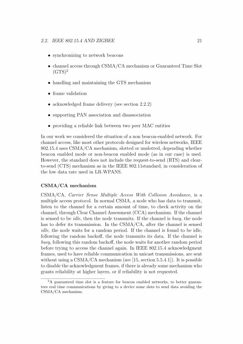
2.2. IEEE 802.15.4 AND ZIGBEE 21
• synchronizing to network beacons
• channel access through CSMA/CA mechanism or Guaranteed Time Slot(GTS)2
• handling and maintaining the GTS mechanism
• frame validation
• acknowledged frame delivery (see section 2.2.2)
• supporting PAN association and disassociation
• providing a reliable link between two peer MAC entities
In our work we considered the situation of a non beacon-enabled network. Forchannel access, like most other protocols designed for wireless networks, IEEE802.15.4 uses CSMA/CA mechanism, slotted or unslotted, depending whetherbeacon enabled mode or non-beacon enabled mode (as in our case) is used.However, the standard does not include the request-to-send (RTS) and clear-to-send (CTS) mechanism as in the IEEE 802.11standard, in consideration ofthe low data rate used in LR-WPANS.
CSMA/CA mechanism
CSMA/CA, Carrier Sense Multiple Access With Collision Avoidance, is amultiple access protocol. In normal CSMA, a node who has data to transmit,listen to the channel for a certain amount of time, to check activity on thechannel, through Clear Channel Assessment (CCA) mechanism. If the channelis sensed to be idle, then the node transmits. If the channel is busy, the nodehas to defer its transmission. In the CSMA/CA, after the channel is sensedidle, the node waits for a random period. If the channel is found to be idle,following the random backoff, the node transmits its data. If the channel isbusy, following this random backoff, the node waits for another random periodbefore trying to access the channel again. In IEEE 802.15.4 acknowledgmentframes, used to have reliable communication in unicast transmissions, are sentwithout using a CSMA/CA mechanism (see [15, section 5.5.4.1]). It is possibleto disable the acknowledgment frames, if there is already some mechanism whogrants reliability at higher layers, or if reliability is not requested.
2A guaranteed time slot is a feature for beacon enabled networks, to better guaran-tees real time communications by giving to a device some slots to send data avoiding theCSMA/CA mechanism.
22 CHAPTER 2. BACKGROUND
2.2.3 Devices for IEEE 802.15.4
Two different types of devices are defined in a IEEE 802.15.4 network, a fullfunction device (FFD) and a reduced function device (RFD). A FFD can talkto RFDs and other FFDs, and operate in three modes serving either as a PANcoordinator, a coordinator, or a device. An RFD can only talk to an FFD andis intended for applications that are extremely simple. They do not have theneed to send large amounts of data and may only associate with a single FFDat time. The association process is the service used to establish membershipfor a device in a WPAN, in this case to let the FFD know about the presenceof the RFD. In our work we considered all nodes as FFDs.
2.2.4 Power saving
One of the most important issues for WSN is the power saving: as we said inthe introduction, it is very difficult, often impossible, to change the batterypacks to sensors spread in an environment. To save power, each sensor isable to put itself in a sleep mode, and therefore have a duty-cycle, listeningto the channel not always, but at precise time, or only when requested. Inthis thesis, to be more general, we take in consideration the worst case, withsensor listening all the time and without any beacon and synchronization.The IEEE 802.15.4 standard (see [15]) provides for duty-cycles and beacons.There are several studies on how to improve MAC to save power. This issuesis beyond the scope of this thesis, but we remind to [14] for details: theycompare CSMA/CA mechanism with others to find a better way to respectpower constraints.

Chapter 3
Optimization Theory
23

24 CHAPTER 3. OPTIMIZATION THEORY
3.1 Convex Optimization Problem
Our work was for the most part a practical one, but it is important to un-derstand the theoretical basis for the algorithms we implemented. The math-ematical basis is convex optimization theory, in fact we will approach theproblem from this point of view. Indeed we want to solve the problem
minimizeθ
∑Ni=1 fi(θ)
subject to θ ∈ Θ,(3.1)
where θ is the variable to optimize, Θ is the feasible set for θ, and fi(θ) is thecost function associated with node i, function assumed to be a convex one,so that the local minimum is the global minimum (see [8] for references aboutconvex optimization).
3.1.1 Convex Optimization overview
We here give a general overview about convex optimization and solution al-gorithms. For this introduction, we will follow almost exactly chapters four,five, and nine of Boyd’s Convex Optimization book [8]. For the subgradientpart we follow [21] and [11].
In general, an optimization problem, not necessarily convex, can be writtenas
minimize f0(x)
subject to fi(x) ≤ 0, i = 1, . . . ,mhi(x) = 0, i = 1, . . . , p
(3.2)
where the problem is finding an x ∈ Rn (optimization variable) that min-imizes f0(x) among all x that satisfy the conditions fi(x) ≤ 0, i = 1, . . . ,mand hi(x) = 0, i = 1, . . . , p.
f0 : Rn → R is the objective function or cost function. The inequalitiesfi(x) ≤ 0 are called the inequality constraints, and the corresponding functionsfi : Rn → R are called the inequality constraint functions. The equationshi(x) = 0 are called the equality constraints, and the functions hi : Rn → Rare the equality constraint functions. The domain of the optimization problem(3.2) is the set of points for which the objective and all constraint functionsare defined,
D =m⋂i=0
dom fi ∩p⋂i=1
dom hi
A point x ∈ D is feasible if it satisfies the constraints fi(x) ≤ 0, i =1, . . . ,m, and hi(x) = 0, i = 1, . . . , p. The problem (3.2) is said to be feasible
3.1. CONVEX OPTIMIZATION PROBLEM 25
if there exists at least one feasible point, and infeasible otherwise. The set ofall feasible points is called the feasible set or the constraint set. The optimalvalue p∗ of the problem (3.2) is defined as
p∗ = inf{f0(x)|fi(x) ≤ 0, i = 1, . . . ,m, hi(x) = 0, i = 1, . . . , p}.
A convex optimization problem is one of the form (as we can find in section4.2 of [8])
minimize f0(x)
subject to fi(x) ≤ 0, i = 1, . . . ,maTi (x) = bi, i = 1, . . . , p,
(3.3)
where f0, . . . , fm are convex functions1.The equation (3.3) differs from the (3.2) on three additional requirements:
• the objective function must be convex,
• the inequality constraint functions must be convex,
• the equality constraint functions hi(x) = aTi x− bi must be affine2.
The feasible set of a convex optimization problem is convex, since it is theintersection of the domain of the problem
D =m⋂i=0
dom fi,
which is a convex set, with m(convex) sublevel sets {x|fi(x) ≤ 0} and p hyper-planes {x|aTi x = bi}. Thus, in a convex optimization problem, we minimize aconvex objective function over a convex set.
3.1.2 Dual approach
If we have an optimization problem like in the equation (3.2), we could thinkabout relaxing some constraints, considering them ’inside’ the objective func-tion (see also [11] (in Italian) and [8, chap. 5]). In practice we take the con-straints into account by augmenting the objective function with a weighted
1a function is convex if satisfies f(αx + βy) ≤ αf(x) + βf(y) for all x, y ∈ Rn and allα, β ∈ R with α+ β = 1, α ≥ 0, β ≥ 0.
2a function f : Rn → Rm is affine if it is a sum of a linear function and a constant,i.e., if it has the form f(x) = Ax+ b, where A ∈ Rm×n and b ∈ Rm.

26 CHAPTER 3. OPTIMIZATION THEORY
sum of the constraint functions. As in [8, sections 5.1.1-5.2.2], we define theLagrangian L : Rn ×Rm ×Rp → R associated with the problem (3.2) as
L(x, λ, ν) = f0(x) +m∑i=1
λifi(x) +
p∑i=1
νihi(x), (3.4)
with dom L = D × Rm × Rp. We refer to λi as the Lagrange multiplierassociated with the ith inequality constraint fi(x) ≤ 0; similarly we referto νi as the Lagrange multiplier associated with the ith equality constrainthi(x) = 0. The vectors λ and ν are called the dual variables or Lagrangemultiplier vectors associated with the problem (3.2).
We define the Lagrange dual function g : Rm ×Rp → R as the minimumvalue of the Lagrangian over x for λ ∈ Rm, ν ∈ Rp,
g(λ, ν) = infx∈D
L(x, λ, ν) = infx∈D
(f0(x) +
m∑i=1
λifi(x) +
p∑i=1
νihi(x)
).
When the Lagrangian is unbounded below in x, the dual function takes onthe value −∞. Since the dual function is the pointwise infimum of a familyof affine functions of (λ, ν), it is concave3, even when the problem (3.2) is notconvex.
It can easily verified (see [8, section 5.1.3] and [11]) that the Lagrange dualfunction yields lower bounds on the optimal value p∗ of the problem (3.2):For any λ � 0 and any ν we have
g(λ, ν) ≤ p∗. (3.5)
The best lower bound that can be obtained from the Lagrange dual func-tion is the Lagrange dual problem associated with the problem (3.2):
maximize g(λ, ν)subject to λ � 0.
(3.6)
The original problem (3.2) is sometimes called the primal problem. Werefer to (λ∗, ν∗) as dual optimal or optimal Lagrange multipliers if they areoptimal for the problem (3.6). The Lagrange dual problem (3.6) is a convexoptimization problem, since the objective to be maximized is concave and theconstraint is convex. This is the case whether or not the primal problem (3.2)is convex.
3a function f is concave if −f is convex.

3.1. CONVEX OPTIMIZATION PROBLEM 27
3.1.3 Solve the problem: descent methods
A problem like (3.3), usually has to be solved by an iterative algorithm, i.e.an algorithm that computes a sequence of points x(0), x(1), . . . ∈ dom f withf(xk) → p∗ as k → ∞. Such a sequence of points is called a minimizingsequence for our problem. The algorithm is terminated when f(x(k))−p∗ ≤ ε,where ε > 0 is some specified tolerance (see [8, section 9.1 and 9.2]). In generalthe upgrade step is similar to
x(k+1) = x(k) + t(k)∆x(k)
with t(k) > 0 (except when x(k) is optimal). The concatenated symbols ∆ andx that form ∆x mean a vector in Rn called the step or search direction(eventhough it needs not have unit norm), and k = 0, 1, . . . denotes the iterationnumber. The scalar t(k) ≥ 0 is called the step size or step length at iterationk (even though it is not equal to ‖x(k+1) − x(k)‖ unless ‖∆x(k) = 1‖). In adescent method,
f(x(k+1)) < f(x(k)),
except when x(k) is optimal. This implies that for all k we have x(k) ∈ S, theinitial sublevel set4, and in particular we have x(k) ∈ dom f . From convexitywe know that ∇f(x(k))T (y − x(k)) ≥ 0 implies f(y) ≥ f(x(k))), so the searchdirection in a descent method must satisfy
∇f(x(k))T∆x(k) < 0,
i.e., it must make an acute angle with the negative gradient. We call such adirection a descent direction (for f , at x(k)).
The outline of a general descent method is as follows. It alternates betweentwo steps: determining a descent direction ∆x, and the selection of a step sizet(k).
4The α-sublevel set of a function f : Rn → R is defined as
Cα = {x ∈ dom f |f(x) ≤ α}.
Sublevel sets of a convex function are convex, for any value of α. The proof is immediatefrom the definition of convexity: if x, y ∈ Cα, then f(x) ≤ α and f(y) ≤ α, and sof(θx+ (1− θ)y) ≤ α for 0 ≤ θ ≤ 1, and hence θx+ (1− θ)y ∈ Cα (see [8, section 3.1.6]).

28 CHAPTER 3. OPTIMIZATION THEORY
Algorithm 1 General descent method.
Require: a starting point x ∈ dom f .
1: repeat2: Determine a descent direction ∆x3: Line search. Choose a step size t > 0.4: Update. x := x+ t∆x.5: until stopping criterion is satisfied.
The third step is called the line search since selection of the step size tdetermines where along the line {x+ t∆x|t ∈ R+} the next iterate will be.
Gradient descent method
We first consider the problem minimize f(x). This is the case of an uncon-
strained optimization problem , where f : Rn → R is convex and twicecontinuously differentiable, which implies that dom f is open (see [8, section9.1]).Since f is differentiable and convex, a necessary and sufficient condition for apoint x∗ to be optimal (if the problem is solvable) is
∇f(x∗) = 0 (3.7)
We denote the optimal value, infx f(x) = f(x∗), as p∗.Knowing that, a natural choice for the search direction in algorithms like
the General descent method is the negative gradient ∆x = −∇f(x). We canrewrite the algorithm in this way:
Algorithm 2 Gradient descent method.
Require: a starting point x ∈ dom f .
1: repeat2: ∆x := −∇f(x).3: Line search. Choose a step size t > 0.4: Update. x := x+ t∆x.5: until stopping criterion is satisfied.
Subgradient
If f(x) is convex but not differentiable, we cannot calculate the ∇f(x) andtherefore we do not have a suitable search direction. Here it is useful tointroduce the concept of subgradient.

3.2. DISTRIBUTED ALGORITHMS 29
First we recall an important property of the gradient of a convex differen-tiable function (see [25, section 2], [22], and [11]). For a convex differentiablefunction, f : Rn → R , the following inequality for the gradient of f at apoint x0 holds for all x ∈ dom f :
f(x) ≥ f(x0) + (x− x0)T∇f(x0).
In general, for a convex function f , a subgradient of f at x0 (observing that fmay not be differentiable at x0) is any direction g such that
f(x) ≥ f(x0) + (x− x0)Tg, (3.8)
and the subdifferential of f at x0, denoted ∂f(x0), is the set of all subgradientsof f at x0. Note that if f is differentiable at x0 then ∂f(x0) ≡ {∇f(x0)}, i.e.,the gradient of f at x0 is the only direction satisfying (3.8).
3.2 Distributed algorithms
Our problem is to find a way to have reliable communications to make opti-mization algorithms converge in networks composed of several sensors spreadover an environment (for example a forest or a building), while preservingas much power as possible. Preserving power is difficult using a centralizedapproach, because of multi-hop passages, so it is important to find a way forreaching convergence (hopefully with a low latency and quickly) in distributedsensor networks, that better can answer to power constraints. If we use adistributed algorithms, we also are more covered in case of node failures (inparticular in the case of failure of the central node) and we can retrieve thevalues from every node of the network.
3.2.1 Distributed optimization problem
Many estimation criteria possess the following important form (see [25]):
f(θ) =1
n
n∑i=1
fi(θ),
where θ is the parameter of function to be estimated, and f(θ) is the costfunction which can be expressed as a sum of n ”local” functions {fi(θ)}ni=1
in which fi(θ) only depends on the data measured at sensor i. So we canspecialize our problem in the form (3.1) that we rewrite here for convenience:
minimizeθ
∑Ni fi(θ)
subject to θ ∈ Θ,(3.9)

30 CHAPTER 3. OPTIMIZATION THEORY
where fi(θ) is the node i associated cost function, that we assume to be aconvex function.
So we can spread the computation of the algorithms over a network, finallyhaving in each node the same value, hopefully the optimum. The purposeof this thesis is to check through the network simulator ns2 (see section 4.1)several algorithms to diffuse data over a sensor network and to have a compar-ison between them. We would like to discover advantages and disadvantagesof different solutions presented in the literature, more close to reality thanonly Matlab simulations. Of course the best would be to simulate with realsensors, but this approach is more expensive and less immediate, so it is betterin our opinion to begin to work with real sensor only after several simulationsthat indicate the best ways in which focus the research, in a way as close aspossible to reality.
3.2.2 Average: least squares solution
We concentrate our work on calculating the average because this is a problemof particular interest in literature (see for example [25, 18, 26, 20, 37] ): ifwe have a network with several sensors spread in an environment, it is verynatural to want to know the average of the values of each sensor, e.g., if wehave temperature sensors spread in an environment, it would be very usefulto retrieve, first of all, the average temperature in that environment.
From a convex optimization point of view, if we have a network of Nsensors, the average is the minimization of the sum of squares 1
n
∑Ni=1(xi−θ)2,
where xi is the local value of each sensor, and θ is the real average that wewant to estimate. It is a least squares solution. The local function that everysensor has to calculate is fi(θ) = (xi − θ)2 and our problem is
minimizeθ
∑Ni (xi − θ)2
subject to θ ∈ Θ,
We assume that θ is scalar for simplicity, but the algorithms are readilyextended to the vector case.
3.2.3 Topology
For the problem (3.9), we need to have a communication topology represented(see [17]) by a graph G = (V , E) with vertex set V = {1, . . . , N} and edgeset E ⊆ V × V . The presence of an edge (i, j) in E means that node i cancommunicate directly with node j, and vice versa. The graph G has N nodes(vertices). For all the algorithms, we made the assumption that the commu-nication topology is connected.

3.3. ALGORITHMS AND NAMING 31
3.3 Algorithms and naming
The most part of our work was to implement in practice through the net-work simulator ns2 (section 4.1) several distributed optimization algorithmsto compute the average value of sensor networks with different topologies anddifferent number of nodes. We did simulations and comparison for:
• Unicast subgradient distributed algorithm (called unicast in this thesis)
• Broadcast algorithm with acknowledgments (called broadcast in this the-sis)
• Broadcast algorithm without acknowledgments (called unreliable broad-cast in this thesis)
• Broadcast dual optimization algorithm without acknowledgments (calleddual in this thesis)
To refer to the algorithms, our choice in this thesis is to simplify in the nameof each algorithms describing the main feature of each algorithm in the name,in a way as easy as possible to understand and to remember, in particular inthe section 5.2 in which we provide results.
Here we provide a mathematical background and general description forall this algorithms. For the implementation details of each one, see section4.2.2 of this work. All algorithms converge to a value more or less close to theoptimum one, depending from the algorithm and from parameters (see section5.2).
3.3.1 Unicast
We implemented this algorithm in ns2 following almost literally the work ofB. Johansson, M. Rabi, and M. Johansson in [17]. This algorithm extendsthe randomized incremental subgradient method with fixed stepsize due toNedic and Bertsekas [22, 21]. Nodes maintain individual estimates and needto exchange information only with their neighbors. In a randomized versionof the estimate passing scheme, a node sends the value to a random neighborover the whole network, in a way that needs a routing protocol and that canproduce multi-hop passages. In [17] they show that it is sufficient to send toa random neighbor, avoiding multi-hop passages. The transition probabilities,which determine how the parameter estimate is passed around in the network,can be computed using local network topology characteristics.

32 CHAPTER 3. OPTIMIZATION THEORY
In [17] the optimization problem is defined as
minimizeθ,x1,...,xN
∑Ni=1 fi(xi, θ)
subject to xi ∈ χi, i = 1, . . . , Nθ ∈ Θ,
(3.10)
where fi(xi, θ) is a cost function associated with node i, xi is a vector ofvariables local to node i, and χi is the feasible set for the local variables. Theset Θ is the feasible set of a global (network-wide) decision variable θ. Theyassume also that fi are convex functions and that χi and Θ are convex setswith non-empty interior.
The problem (3.10) is then rewritten as
minimizeθ
∑Ni=1 qi(θ)
subject to θ ∈ Θ,(3.11)
where qi(θ) = minxi∈χifi(xi, θ), defining then q∗ as the optimal value of (3.11)
and q(θ) =∑N
i=1 qi(θ). In [17], then, they assume that each (convex) compo-nent qi(·) has a subgradient gi(θ) at θ and that each of these subgradients arebounded as follows
gi(θ) ≤ C for all θ ∈ Θ and all i = 1, . . . , N.
The update equation of the estimate, θk, of the optimizer is
θk+1 = PΘ{θk − αgwk(θk)}, (3.12)
where PΘ{·} denotes projection on the set Θ and α > 0 is a fixed stepsize.Instead of setting wk, variables which indicates the node who does the upgradeat step k, as an IID taking values from the set {1, . . . , N} with equal proba-bility, in [17] they let wk be the state of a Markov chain5corresponding to thecommunication structure. In addition they assume that the Markov chain isirreducible, acyclic, and have the uniform distribution as its stationary distri-bution. This assumption means that the underlying communication structureis connected; after a sufficient amount of time the chain can be in any state;and that all state in the chain will be visited the same number of times in thelong run. The way used in [17] (and that we use in 4.2.2) to construct thetransition matrix using only local information was the Metropolis-Hastings
5a Markov chain, named after Andrey Markov, is a discrete-time stochastic process withthe Markov property. Having the Markov property means the next state solely depends onthe present state and does not directly depend on the previous states.

3.3. ALGORITHMS AND NAMING 33
scheme [36]. If the underlying communication topology is connected, then allassumptions on the transition matrix is fulfilled if the elements are set to
Pij =
min{ 1
di, 1dj} if (i, j) ∈ E and i 6= j∑
(i,k)∈E max{0, 1dj− 1
dk} if i = j
0 otherwise,
(3.13)
where di is node i’s number of edges.
Algorithm 3 Peer to peer unicast optimization algorithm
1: Initialize θ0 and α. set k := 0 and wk := 1.2: repeat3: At node wk, compute a subgradient, gwk , for qwk(θk).4: θk+1 := PΘ{θk − αgwk}5: Send θk+1 to a random neighbor, wk+1, with transition probability ac-
cording to P .6: k := k + 17: until convergence.
In our case of calculating the average, the update function at node i is
θk+1i = θki − α(θki − xi), (3.14)
where xi is the local measurement of node i.For the proof of the convergence we refer to [17]. In our implementation,
we have a convergence between a bound, with an oscillatory behavior, and thebest estimate is close to the optimal point.
3.3.2 Broadcast
For this algorithm, we had as basis the work of Xiao and Boyd [36]. There, theauthors want to find optimal weights to have the fastest possible convergencein solving the problem of finding the average of the values of different nodesin a network, using distributed linear iterations, which have the form
xk+1i = Wiix
ki +
∑j∈Ni
Wijxkj , i = 1, . . . , n, (3.15)
where k = 0, 1, 2, . . . is the iteration index, and Wij is the weight on xj atnode i. In [36], they prove that a necessary and sufficient condition for the(3.15) to converge, is
limk→∞
W k =11T
n. (3.16)
34 CHAPTER 3. OPTIMIZATION THEORY
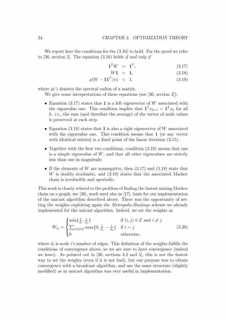
We report here the conditions for the (3.16) to hold. For the proof we referto [36, section 2]. The equation (3.16) holds if and only if
1TW = 1T , (3.17)
W1 = 1, (3.18)
ρ(W − 11T/n) < 1, (3.19)
where ρ(·) denotes the spectral radius of a matrix.We give some interpretations of these equations (see [36, section 2]):
• Equation (3.17) states that 1 is a left eigenvector of W associated withthe eigenvalue one. This condition implies that 1Txk+1 = 1Txk for allk, i.e., the sum (and therefore the average) of the vector of node valuesis preserved at each step.
• Equation (3.18) states that 1 is also a right eigenvector of W associatedwith the eigenvalue one. This condition means that 1 (or any vectorwith identical entries) is a fixed point of the linear iteration (3.15).
• Together with the first two conditions, condition (3.19) means that oneis a simple eigenvalue of W , and that all other eigenvalues are strictlyless than one in magnitude.
• If the elements of W are nonnegative, then (3.17) and (3.18) state thatW is doubly stochastic, and (3.19) states that the associated Markovchain is irreducible and aperiodic.
This work is closely related to the problem of finding the fastest mixing Markovchain on a graph, see [36], work used also in [17], basis for our implementationof the unicast algorithm described above. There was the opportunity of set-ting the weights exploiting again the Metropolis-Hastings scheme we alreadyimplemented for the unicast algorithm. Indeed, we set the weights as
Wij =
min{ 1
di, 1dj} if (i, j) ∈ E and i 6= j∑
(i,k)∈E max{0, 1dj− 1
dk} if i = j
0 otherwise,
(3.20)
where di is node i’s number of edges. This definition of the weights fulfills theconditions of convergence above, so we are sure to have convergence (indeedwe have). As pointed out in [36, sections 4.2 and 5], this is not the fastestway to set the weights (even if it is not bad), but our purpose was to obtainconvergence with a broadcast algorithm, and use the same structure (slightlymodified) as in unicast algorithm was very useful in implementation.
3.3. ALGORITHMS AND NAMING 35
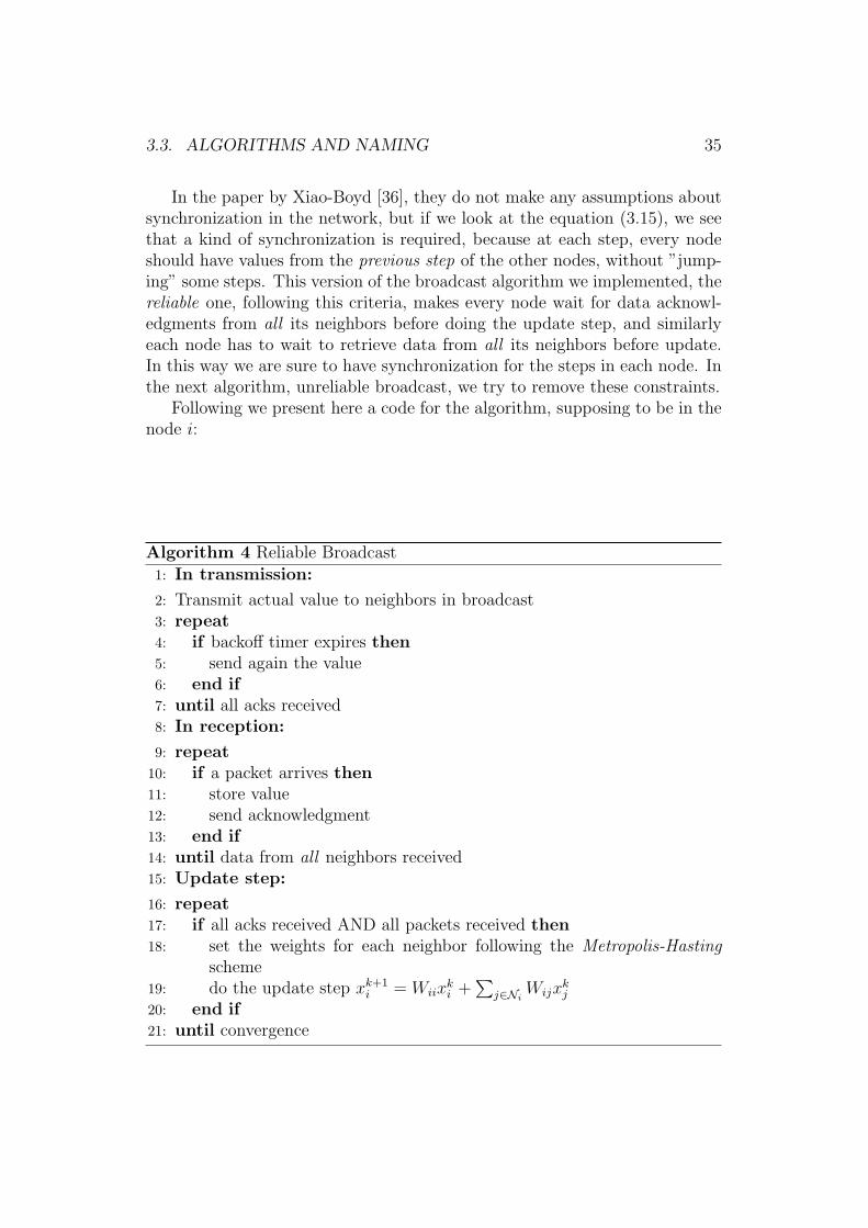
In the paper by Xiao-Boyd [36], they do not make any assumptions aboutsynchronization in the network, but if we look at the equation (3.15), we seethat a kind of synchronization is required, because at each step, every nodeshould have values from the previous step of the other nodes, without ”jump-ing” some steps. This version of the broadcast algorithm we implemented, thereliable one, following this criteria, makes every node wait for data acknowl-edgments from all its neighbors before doing the update step, and similarlyeach node has to wait to retrieve data from all its neighbors before update.In this way we are sure to have synchronization for the steps in each node. Inthe next algorithm, unreliable broadcast, we try to remove these constraints.
Following we present here a code for the algorithm, supposing to be in thenode i:
Algorithm 4 Reliable Broadcast
1: In transmission:
2: Transmit actual value to neighbors in broadcast3: repeat4: if backoff timer expires then5: send again the value6: end if7: until all acks received8: In reception:
9: repeat10: if a packet arrives then11: store value12: send acknowledgment13: end if14: until data from all neighbors received15: Update step:
16: repeat17: if all acks received AND all packets received then18: set the weights for each neighbor following the Metropolis-Hasting
scheme19: do the update step xk+1
i = Wiixki +
∑j∈Ni
Wijxkj
20: end if21: until convergence

36 CHAPTER 3. OPTIMIZATION THEORY
3.3.3 Unreliable broadcast
This algorithm is a modification of the previous algorithm. We wanted toinvesigate if it was possible to reach convergence, using the same update stepas the reliable broadcast algorithm, but without any acknowledgments andsynchronization. The problem was mainly to investigate whether it was possi-ble to change the weights in the equation (3.15) in a way to take into accountmissing values, still having convergence. Finally, we found that simply settingto 0 the weights for neighbors with no new values, and therefore increasing theweight assigned to the local data of the node in which we are doing computa-tion, we have convergence. So we can rewrite the Metropolis-Hasting schemein this way:
Wij =
min{ 1
di, 1dj} if (i, j) ∈ E , i 6= j, j has sent a packet to i∑
(i,k)∈E max{0, 1dj− 1
dk} if i = j
0 otherwise
(3.21)Here is the pseudocode of the algorithm:
Algorithm 5 Unreliable Broadcast
In transmission:
if transmission timer expire thensend actual value to neighbors, without waiting for response
end ifIn reception:
if a new packet arrives thenstore value
end ifUpdate step:
repeatif Update timer expire then
set weights to neighbors whose there is a new packet, following theMetropolis-Hasting scheme and setting to 0 the value from neighborswhose packet is missingdo the update step xk+1
i = Wiixki +
∑j∈Ni
Wijxkj
end ifuntil convergence
A problem of both reliable and unreliable broadcast algorithms, could bethat we use the local sensor value only the first time each node send broadcast
3.3. ALGORITHMS AND NAMING 37
data, so, if this value is changing, it is difficult to recognize. A way to correctthis problem could be to take in parallel an old value and begin again theiterations to see whether measurements are significantly changed.
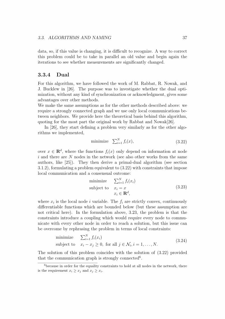
3.3.4 Dual
For this algorithm, we have followed the work of M. Rabbat, R. Nowak, andJ. Bucklew in [26]. The purpose was to investigate whether the dual opti-mization, without any kind of synchronization or acknowledgment, gives someadvantages over other methods.We make the same assumptions as for the other methods described above: werequire a strongly connected graph and we use only local communications be-tween neighbors. We provide here the theoretical basis behind this algorithm,quoting for the most part the original work by Rabbat and Nowak[26].
In [26], they start defining a problem very similarly as for the other algo-rithms we implemented,
minimize∑N
i=1 fi(x), (3.22)
over x ∈ Rd, where the functions fi(x) only depend on information at nodei and there are N nodes in the network (see also other works from the sameauthors, like [25]). They then derive a primal-dual algorithm (see section3.1.2), formulating a problem equivalent to (3.22) with constraints that imposelocal communication and a consensual outcome:
minimize∑N
i=1 fi(xi)
subject to xi = xxi ∈ Rd,
(3.23)
where xi is the local node i variable. The fi are strictly convex, continuouslydifferentiable functions which are bounded below (but these assumption arenot critical here). In the formulation above, 3.23, the problem is that theconstraints introduce a coupling which would require every node to commu-nicate with every other node in order to reach a solution, but this issue canbe overcome by rephrasing the problem in terms of local constraints:
minimize∑N
i=1 fi(xi)
subject to xi − xj ≥ 0, for all j ∈ Ni, i = 1, . . . , N.(3.24)
The solution of this problem coincides with the solution of (3.22) providedthat the communication graph is strongly connected6.
6because in order for the equality constraints to hold at all nodes in the network, thereis the requirement xi ≥ xj and xj ≥ xi.
38 CHAPTER 3. OPTIMIZATION THEORY
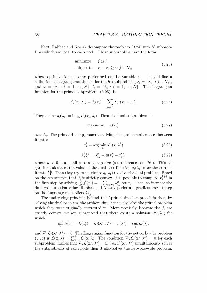
Next, Rabbat and Nowak decompose the problem (3.24) into N subprob-lems which are local to each node. These subproblem have the form
minimize fi(xi)
subject to xi − xj ≥ 0, j ∈ Ni,(3.25)
where optimization is being performed on the variable xi. They define acollection of Lagrange multipliers for the ith subproblem, λi = {λi,j : j ∈ Ni},and x = {xi : i = 1, . . . , N}, λ = {λi : i = 1, . . . , N}. The Lagrangianfunction for the primal subproblem, (3.25), is
Li(xi, λi) = fi(xi) +∑j∈Ni
λi,j(xi − xj). (3.26)
They define qi(λi) = infxiLi(xi, λi). Then the dual subproblem is
maximize qi(λi), (3.27)
over λi. The primal-dual approach to solving this problem alternates betweeniterates
xki = arg minxi
Li(x, λk) (3.28)
λk+1i,j = λki,j + µ(xki − xkj ), (3.29)
where µ > 0 is a small constant step size (see references on [26]). This al-gorithm calculates the value of the dual cost function qi(λi) near the currentiterate λk
i . Then they try to maximize qi(λi) to solve the dual problem. Basedon the assumption that fi is strictly convex, it is possible to compute xk+1
i inthe first step by solving ∂
∂xifi(xi) = −
∑j∈Ni
λki,j for xi. Then, to increase thedual cost function value, Rabbat and Nowak perform a gradient ascent stepon the Lagrange multipliers λki,j.
The underlying principle behind this ”primal-dual” approach is that, bysolving the dual problem, the authors simultaneously solve the primal problemwhich they were originally interested in. More precisely, because the fi arestrictly convex, we are guaranteed that there exists a solution (x∗, λ∗) forwhich
infxfi(x) = fi(x
∗i ) = Li(x∗, λ∗) = qi(λ
∗) = supλqi(λ),
and ∇xLi(x∗, λ∗) = 0. The Lagrangian function for the network-wide problem(3.24) is L(x, λ) =
∑Ni=1 Li(x, λ). The condition ∇xLi(x∗, λ∗) = 0 for each
subproblem implies that∇xL(x∗, λ∗) = 0; i.e., if (x∗, λ∗) simultaneously solvesthe subproblems at each node then it also solves the network-wide problem.

3.4. ROBUST OPTIMIZATION 39
For the implementation details, see section 4.2.2. For the proof of convergence,we refer to [26].
In our case, see section 4.2.2, we have a network of sensors that are notsynchronized. Each sensor upgrades its own value according to the equationsabove (in particular (3.28) and (3.29)) every ζ seconds, where ζ is a parameter,not correlated with the arrivals of new packet from other nodes. In reception,when a new packet arrives, the receiving node upgrades the value of λi,j relativeto the sender. We can present a pseudocode of the algorithm in this way,supposing to be in the node i and supposing to have a timer that expiresevery ζ seconds:
Algorithm 6 Dual broadcast distributed optimization algorithm
1: In transmission:2: repeat3: if Timer expire then4: xki = arg min
xi
Li(x, λk)5: end if6: until convergence
7: In reception:8: if a new packet arrives from node j then9: compute λk+1
i,j = λki,j + µ(xki − xkj )10: end if
In the case of the average, the upgrade equation is
xki = ui −∑j∈Ni
λki,j,
where ui is the scalar measurement of each sensor.
3.4 Robust Optimization
Another field of interest is about robust optimization, i.e., if some node, asoften happens, has some problem or has not feasible data, it would be goodto have less sensitivity to large measurement errors respect to least squaresmeasures. A way to reduce sensitivity to outliers, could be to use the HuberNorm. This is a very interesting field, even if outside the scope of this work.We refer to the work and the references in [37] for details.


Chapter 4
Implementation
41

42 CHAPTER 4. IMPLEMENTATION
This implementation chapter wants to illustrate the tools used for thiswork in practical and wants to be a practical help to people who want to dosimilar things. We describe here also some code.
4.1 ns2
The most important tool for our work was the Network simulator 2 ns2, [24].It is a discrete event driven simulator developed at UC Berkeley as a part ofthe VINT project. It is open source and versions are available for FreeBSD,Solaris, Windows, Linux, and Os X (the platform we used), and it is widelyused, maintained and developed as a collaborative environment by a lot ofinstitutes and people.
As showed in the manual [32, chapter 3], ns is an object oriented simulatorwritten in C++, with an OTcl (Object Tool Command language) interpreteras interface 1. This duality gives big advantages to the user, because it is pos-sible to exploit the powerful, fast execution time and efficiency of the C++language to write the cpu-intensive ”core” of the code (e.g protocols), andin the same time it is possible to have the simplicity of the OTcl scriptinglanguage, for quickly change different parameters without the need of recom-piling. So, two code hierarchies are supported, the C++ one (compiled) andthe OTcl one (interpreted), with one to one correspondence between them(see[6]).
4.1.1 Structure and functioning of ns2
Ns2 has a very modular structure (see figure 4.1 for an overview of the directorystructure of ns2). All the objects are derived from the class TclObject and arefirst instantiated in the OTcl interface. The OTcl can make use of the objectscompiled in C++ through an OTcl linkage that creates a matching of OTclobject for each of the C++. Ns2 is in practice a glue between Tcl and C++.It is a discrete event simulator, where the advance of time depends in thetiming of events which are maintained by a scheduler. An event is an objectin the C++ hierarchy with an unique ID, a scheduled time and the pointerto an object that handles the event. The scheduler keeps an oredered datastructure with the events to be execute and fires them one by one, invokingthe handler of the event (see [6, section 1.1]).
1Tcl is a language with simple syntax and easy integration with other languages, createdby John Ousterhout. For further information see [1].

4.1. NS2 43
An ns2 simulation consists of communications between objects. Everylink, node, channel model, propagation model, application and the simulatorinstance itself is an object and the powerful thing is that it is possible to com-bine all that objects in almost any way, following our needs [32, 24, 6]. Atthe beginning we have to define a topology, i.e., where our nodes are in theenvironment. In wireless simulations it is also possible to define node move-ment. After defining the topology we have to define the features that eachnode should use in our simulation, like the physical layer, the MAC layer, thelink layer, the routing layer, the type of interface priority queue (IFQ) (i.e.,the buffer at the entrance of the node) and its maximum length, the type ofantenna and the propagation model (for wireless). See [32, chap 5 and 16] forthe list of all the possibilities. Then, we configure the agents we want to usein our simulation, i.e., the transport layer and application layer objects. Wedo all these things, and more, from the Tcl interface, so if we do not need tomodify C++ code and we want only to do tests on already implemented pro-tocols, we can do it very quickly, without recompiling ns2 and writing merelysome simple (more or less) Tcl script.When, as in this thesis work, we have to simulate something not already im-plemented, we can write C++ code and add our code to the general structureof ns2, recompile all, and use our object in simulations. Of course it is alsopossible to modify existing code, as ns2 is an open-source project. The beststarting point to learn how the simulator work is indeed to try to modify ex-isting code to change protocols behavior.
Installing
Installation of single packages of ns2 is quite tricky, in particular on Windows,where it needs the Cygwin package to work (www.cygwin.com), but the in-stallation process is a lot easier on all platforms using the all-in-one package[24].On OsX we installed ns2 without problems, just executing the ’install’ scriptand setting the right environment paths as suggested by the installation’sscript. For using NAM, the network animator (see next section), we need theX11 package that is present in the MacOsX’s dvd or can be easily downloadedfrom the apple website.For recompiling ns2, we need gcc in our system. With MacOsX it is veryeasy: the only thing to do is to install the Apple’s Xcode package that wecan find in the MacOsX’s dvd. Also in almost all Linux distributions gcc isalready present or it can be installed easily. In cygwin we have to select thegcc package during cygwin’s installation process.

44 CHAPTER 4. IMPLEMENTATION
Figure 4.1: The ns2 directory structure
We need to recompile ns2 if we change something in the C++ code or if wewrite new code. If we already have gcc installed, to recompile ns2 (inde-pendently from which platform we are working in) we just need to type thecommands ’make depend’ and ’make’ in the main ns2 directory. This pro-cess usually is not so long, because every time only the modified parts will berecompiled.
Output and tools
We can define three types of outputs for ns2:
• Trace output
• Nam output
• Log output
The trace output is the main ns2 output, there it is possible to find all thepackets sent, received and dropped in the simulation, with informations aboutaddress of the sender and recipient, energetic informations and different infor-mations for each protocols and for different types of packets. If we write, as wedid in our work, some new code, it is possible to put our particular output inthe trace file, modifying (for wireless simulations) the files trace/cmu-trace.htrace/cmu-trace.cc .

4.1. NS2 45
Figure 4.2: A five-nodes wireless configuration in the nam window exchangingbroadcast and unicast data
Nam, the network animator, is, as we can find on the introduction of chapter45 in [32],
a Tcl/TK based animation tool for viewing network simulationtraces and real world packet tracedata. The design theory behindnam was to create an animator that is able to read large anima-tion data sets and be extensible enough so that it could be usedindifferent network visualization situations. (. . . ) When the namtrace file is generated from ns2 or others applications, it is readyto be animated by nam. Upon startup, nam will read the tracefile,create topology, pop up a window, do layout if necessary, and thenpause at time 0. (. . . ) Through its user interface, nam providescontrol over many aspects of animation.
The nam animations are very useful to give a general idea of how the networkworks. There are (see figure 4.2) commands for play, play in reverse, forwardand rewind the animation and for setting the animation’s speed. Broadcastpackets are represented as circle, while unicast packets are represented by dots.It is possible to have info about each packet, link or node, just clicking on it.
The log output is the output we have from our C++ code (it could bedone in several ways, e.g with fprintf(stdout,”Message we want to print”);)

46 CHAPTER 4. IMPLEMENTATION
Figure 4.3: ns2 simulator for IEEE 802.15.4. Picture taken from the work ofJ. Zheng and M. J. Lee, [40].
and from the Tcl script (with the puts command). In this way it is possibleto print useful information that is not possible to put in trace files. The des-tination of these informations is the standard output but we can redirect to afile with the ’>’ operator.For parsing the different outputs it is better to use external applications, likeawk or perl (see introduction to results section for details).For create and editing the code under MacOs X we used the application Ko-modo edit, [3].
4.1.2 802.15.4 in ns2
The 802.15.4 protocol is implemented in ns2 thanks to J. Zheng and M. J. Lee,[38, 40]. In figure 4.3 we present the function modules in the simulator and theservices implemented in the PHY and MAC modules (see also section 2.2.1 and2.2.2). Unfortunately no real documentation exists on the implementation, butit seems that, even if there is some minor bug, the behavior of the simulatorrespect faithfully the standard IEEE 802.15.4, in the version P802.15.4/D18Draft. In figure 4.3 we show the general structure of the module and theservice implemented in the PHY and MAC layers.

4.1. NS2 47
Flow of packets inside ns2
Here we show the path that each packet go through inside the ns2 structure inour case, in particular inside the module 802 15 4, developed by J. Zheng andM. J. Lee (see section 4.1.2). The module 802 15 4 is not so well documented,so we deduced the following informations from the code and from the work ofIyappan Ramachandran, [28].
Outgoing:
• The application we developed, ccsensorApp, sends a request to send(broadcast or unicast) to the agent ccsensorAgent, throughCcsensorApp::sendSensorData() or CcsensorApp::sendDataUnicast().
• ccsensorAgent sends through Agent::send(packet ∗p, Handler ∗h)
the packet to the classifier that, based on the field of the header, send itto the right module (to the routing protocol in the case of an outgoingpacket)
• so classifier sends the packet to dump agent, a basic routing protocol(we do not use a routing protocol, but ns2 structure needs something atnetwork layer, so there is this dump agent)
• the routing protocol sends the packet to the LLC sublayer of the datalink layer, whose is part also the MAC sublayer. The function of LLCsublayer here is only to deliver the packet to the arp and to the quequeit
• In the arp we translate the ip address into MAC address. We deactivatedthe arp module because without the routing protocol, we did not needaddress resolution, and we did not want to take in consideration arppackets.
• queue is in this case the typical Drop Tail, a FIFO scheduling and drop-on-overflow buffer management.
Now we describe in a bit deeper detail what happen inside the 802.14.4 module:
• The upper layer (queue) hands down a packet to MAC by callingMAC802 15 4::recv(Packet ∗P, Handler ∗h).
• recv() then calls Mac802 15 4::mcps data request(), which works giv-ing control to other functions, selected basing upon a variable called step,initialized to 0 and incremented before passing control to other functions.
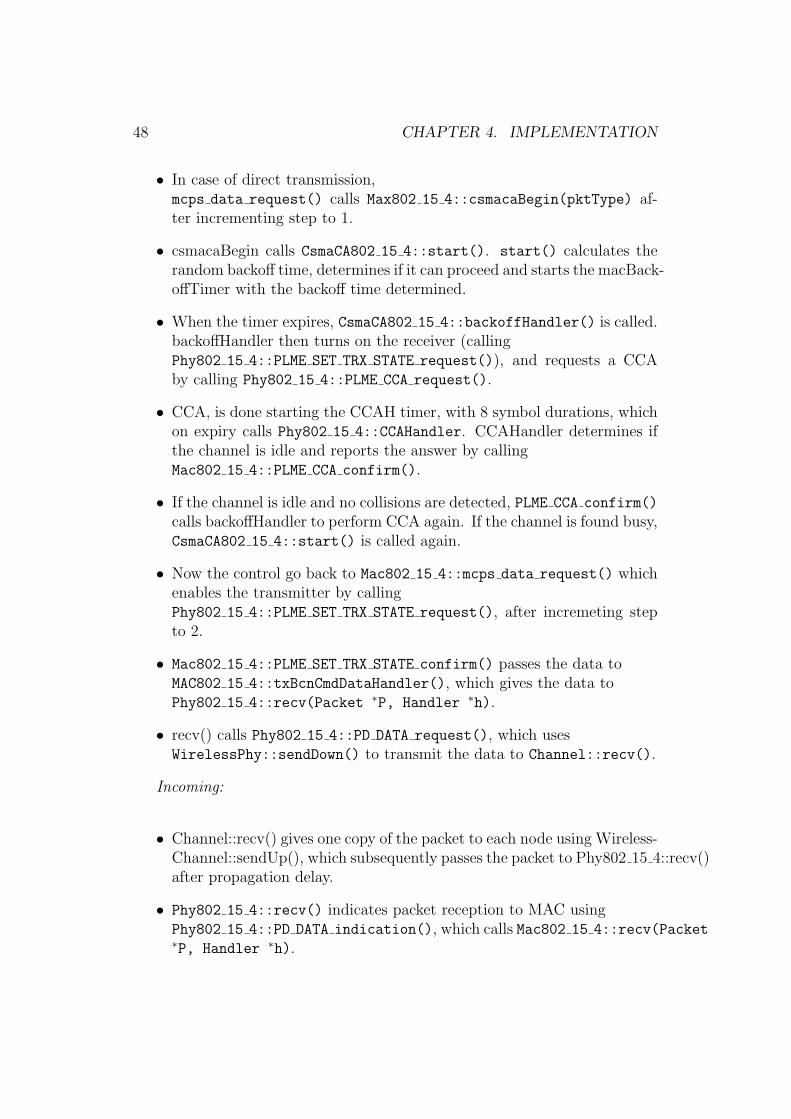
48 CHAPTER 4. IMPLEMENTATION
• In case of direct transmission,mcps data request() calls Max802 15 4::csmacaBegin(pktType) af-ter incrementing step to 1.
• csmacaBegin calls CsmaCA802 15 4::start(). start() calculates therandom backoff time, determines if it can proceed and starts the macBack-offTimer with the backoff time determined.
• When the timer expires, CsmaCA802 15 4::backoffHandler() is called.backoffHandler then turns on the receiver (callingPhy802 15 4::PLME SET TRX STATE request()), and requests a CCAby calling Phy802 15 4::PLME CCA request().
• CCA, is done starting the CCAH timer, with 8 symbol durations, whichon expiry calls Phy802 15 4::CCAHandler. CCAHandler determines ifthe channel is idle and reports the answer by callingMac802 15 4::PLME CCA confirm().
• If the channel is idle and no collisions are detected, PLME CCA confirm()
calls backoffHandler to perform CCA again. If the channel is found busy,CsmaCA802 15 4::start() is called again.
• Now the control go back to Mac802 15 4::mcps data request() whichenables the transmitter by callingPhy802 15 4::PLME SET TRX STATE request(), after incremeting stepto 2.
• Mac802 15 4::PLME SET TRX STATE confirm() passes the data toMAC802 15 4::txBcnCmdDataHandler(), which gives the data toPhy802 15 4::recv(Packet ∗P, Handler ∗h).
• recv() calls Phy802 15 4::PD DATA request(), which usesWirelessPhy::sendDown() to transmit the data to Channel::recv().
Incoming:
• Channel::recv() gives one copy of the packet to each node using Wireless-Channel::sendUp(), which subsequently passes the packet to Phy802 15 4::recv()after propagation delay.
• Phy802 15 4::recv() indicates packet reception to MAC usingPhy802 15 4::PD DATA indication(), which calls Mac802 15 4::recv(Packet∗P, Handler ∗h).
4.1. NS2 49
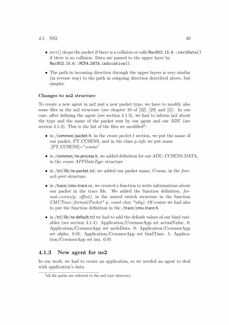
• recv() drops the packet if there is a collision or calls Mac802 15 4::recvData()
if there is no collision. Data are passed to the upper layer byMac802 15 4::MCPA DATA indication().
• The path in incoming direction through the upper layers is very similar(in reverse way) to the path in outgoing direction described above, butsimpler.
Changes to ns2 structure
To create a new agent in ns2 and a new packet type, we have to modify alsosome files in the ns2 structure (see chapter 10 of [32], [29] and [2]). In ourcase, after defining the agent (see section 4.1.3), we had to inform ns2 aboutthe type and the name of the packet sent by our agent and our ADU (seesection 4.1.3). This is the list of the files we modified2:
• in /common/packet.h, in the enum packet t section, we put the name ofour packet, PT CCSENS, and in the class p info we put name[PT CCSENS]=”ccsens”
• in /common/ns-process.h, we added definition for our ADU, CCSENS DATA,in the enum APPDataType structure
• in /tcl/lib/ns-packet.tcl, we added our packet name, Ccsens, in the fore-ach prot structure.
• in /trace/cmu-trace.cc, we created a function to write informations aboutour packet in the trace file. We added the function definition, for-mat ccsens(p, offset), in the nested switch structure in the functionCMUTrace::format(Packet* p, const char *why). Of course we had alsoto put the function definition in the /trace/cmu-trace.h.
• in /tcl/lib/ns-default.tcl we had to add the default values of our bind vari-ables (see section 4.1.4): Application/CcsensorApp set actualValue 0;Application/CcsensorApp set nodeData 0; Application/CcsensorAppset alpha 0.01; Application/CcsensorApp set bindTime 1; Applica-tion/CcsensorApp set mu 0.01
4.1.3 New agent for ns2
In our work, we had to create an application, so we needed an agent to dealwith application’s data.
2all file paths are referred to the ns2 root directory.

50 CHAPTER 4. IMPLEMENTATION
Problems and reason for a new agent
What we wanted to do in our work was to implement in ns2 different algo-rithms for distributed optimization in sensor networks, using only communi-cations between neighbors (i.e without multi-hop passages), see 3.1For doing our purposes, it was essential to exchange scalar values betweenneighbors. In ns2 there are some already implemented applications, like tel-net and FTP (see chapters 38-39 of [32]), but they are ’virtual’, the all theytransmit is only size and time when data are transferred. For sending realapplication data, ns2 provides a packet-like structure, called ADU (chapter39.1.1 [32]), to pack user data into an array, which is then included in theuser data area of an ns2 packet by an Agent, but there is not support yet inthe class agent to transmit user data, so there were two possibilities: use thetcpApp application (a kind of wrapper application for sending user data) orbuild a new agent and send data through it.We tried both ways, and finally the best solution was to write a new agent tohave more flexibility. With TcpApp it was indeed difficult to send broadcastpackets, even if at the beginning it is easier to modify already existent codethan write new one. After writing our agent, ccsensorAgent, it was possibleto built our application, ccsensorApp, to implement the algorithms. A goodstart point for writing new protocols and agents is [29] and chapter 10 of [32]We did not use a routing protocol because we need to send data only to neigh-bors, and for the same reason we disabled also the arp protocol (for neighborswe can use the MAC address, we do not need arp translation).
Adu definition
First, in the file ccsensor-packet.h, we defined our ADU, derived from theabstract base class of all ADU, AppData:
file: ccsens/ ccsens-packet.h
class CCSensData : public AppData {
private:
unsigned char code_;
unsigned char iterNumber_;
double data_;
public:
CCSensData();
CCSensData(char * b);
4.1. NS2 51
unsigned char& code() { return (code_); }
unsigned char& iterNumber() {return (iterNumber_);}
double& data() { return (data_); }
void setHeader(hdr_ccsens *ih);
virtual int size() const { return sizeof(CCSensData); }
virtual AppData* copy() { return (new CCSensData(*this)); }
void pack(char* buf) const;
void print();
};
Each ADU contain:
• a code for differentiate the type of message we want to send
• an iteration number to recognize new packets
• data we want to send
Then are defined the functions to access directly data and to pack in an array.In an ADU should be always provided at least the constructor, to extract datafrom an array and the pack function, to pack data into an array.We have to provide also an header for accessing our ADU from the agent andfrom the application:
file: /ccsens/ccsens-packet.h
struct hdr_ccsens{
unsigned char code_;
unsigned char iterNumber_;
double data_;
unsigned char& code() { return (code_); }
unsigned char& iterNumber() {return (iterNumber_); }
double& data() { return (data_); }
static int offset_;
inline static int& offset() { return offset_; }
inline static hdr_ccsens* access(const Packet* p) {
return (hdr_ccsens*) p->access(offset_);

52 CHAPTER 4. IMPLEMENTATION
}
};
Function of the agent
The functions of the agent are:
• Prepare the packet for broadcast message
• Prepare the packet for unicast message
• Receive new packets and give them to the application
The first two functions consist in setting the right values on the commonheader and on the ip header, and to send down the packet to the next step inthe ns2 chain, in this case the logical link layer.for our application’s details see section 4.2.
To compile our files, we had also to modify the makefile, adding our filesto compile under the line OBJECT CC.

4.1. NS2 53
Figure 4.4: Instructions for executing our script
4.1.4 OTcl script and simulation run
The simulation itself and the main application where the algorithms are im-plemented (see section 4.2) are controlled by an OTcl script (figure 4.4) thatdefines which feature to use, and which part of the ns2 structure utilize. As wesaid in section 4.1.1, one of the most powerful features of ns2 is the completecorrespondence and parallelism between OTcl and C++, to exploit advan-tages from both languages. In the OTcl script, we define, in the wireless case,characteristics like the topology we want to use, the number of nodes, thetype of channel, the type of antenna, the network interface, the mac type, thepropagation model and others (for a detailed list in general see [32, chapter16], for a detailed list of the ones we used, see later in this section). Here weprovide a detailed description of the OTcl script we wrote for our simulation.For reference about OTcl we found very useful the tutorial at [35].
Script description
At the beginning of the script, it is necessary to list and initialize all thevariables we will use in the script, so to have a general view of the configurationwe want and so to be able to quickly change parameters.
#==========================================================
#Define options
#==========================================================
set val(chan) Channel/WirelessChannel ;#channel type
set val(prop) Propagation/TwoRayGround ;#radio-propagation model
54 CHAPTER 4. IMPLEMENTATION
set val(netif) Phy/WirelessPhy/802_15_4;#network interface type
set val(mac) Mac/802_15_4; #MAC type
set val(ifq) Queue/DropTail/PriQueue; #interface queue type
set val(ll) LL; #link layer type
set val(ant) Antenna/OmniAntenna; #antenna model
set val(ifqlen) 25000; #max packet ifq
set val(nn) 5 ;#number of mobile nodes
set val(rp) DumbAgent; #routing protocol
set val(x) 100; #horizontal size of topology
set val(y) 100; #vertical size of topology
set val(stop) 100; #duration of simulation
set val(cp) "wpanBasic3.scn"; #default scenario file
set val(tr) "simple.tr"; #default trace file
set val(nam) "simple.nam"; #default nam file
set val(errConv) "errConv.conv"; #default time/error output file
set val(errNode) "errNode.ncon"; #default node/error output file
set val(timePacket) "timePacket.out"
set val(energymodel) EnergyModel; #definition of energy model
set val(initialenergy) 100; #Initial energy in Joules
set val(brdcst) yes; #set which algorithm to use
set val(autoDiscovery) no;#automatic neighbor discovery
set val(reliable) yes; #choose reliable or unreliable broadcast
set val(dual) yes; #for setting dual or primal algorithm
set val(bindTime_) 1;#time for upgrade window in dual algorithm
set val(mu_) 0.1;#constant stepsize for dual broadcast algorithm
set val(alpha_) 0.01;#constant step size for unicast algorithm
set val(step) 0.01;#could be mu or alpha
set val(macAck) off ;#set mac acknowledgment
set val(algorithm) "broadcast";#only for naming output files
It is possible to change from command line several of this parameters,since the OTcl stores command line arguments in the variables argc (numberof arguments) and argv (list of arguments). We do not provide here the simpleOTcl function to do this because it is not strictly correlated with our thesisbut only with OTcl programming. For that a very good tutorial could befound at [35]. We use some of the parameters defined above to define thefeatures that each node should have:
$ns_ node-config -adhocRouting $val(rp) \
-llType $val(ll) \
-macType $val(mac) \

4.1. NS2 55
-ifqType $val(ifq) \
-ifqLen $val(ifqlen) \
-antType $val(ant) \
-propType $val(prop) \
-phyType $val(netif) \
-topoInstance $topo \
-agentTrace ON \
-routerTrace OFF \
-macTrace ON \
-movementTrace OFF \
-channel $chan_1_ \
-energyModel $val(energymodel) \
-rxPower 0.3 \
-txPower 0.6 \
-initialEnergy $val(initialenergy)
and finally we create the nodes:
for {set i 0} {$i < $val(nn) } {incr i} {
global rng sum
set node_($i) [$ns_ node]
$node_($i) random-motion 0 ;#disable random motion
$god_ new_node $node_($i);#inform god (for neighborDiscovery)
set nodeData($i) [$rng uniform 0 4]
set b_($i) [new Agent/Ccsensor]
$node_($i) attach $b_($i) 250
Application/CcsensorApp set nodeData_ $nodeData($i);#sensor value
Application/CcsensorApp set bindTime_ $val(bindTime_)
Application/CcsensorApp set mu_ $val(mu_)
puts "local data node $i: $nodeData($i)"
set app_($i) [new Application/CcsensorApp]
$app_($i) attach-agent $b_($i)
$app_($i) broadcast $val(brdcst)
$app_($i) neighDiscovery $val(autoDiscovery);#automatic neighbors discovery
$app_($i) reliable $val(reliable);#use reliable broadacast or not
56 CHAPTER 4. IMPLEMENTATION
$app_($i) dual $val(dual) ;#dual or primal optimization
set sum [expr $sum+$nodeData($i)]
$ns_ at 0.1 "$app_($i) start"
}
We can see that we also can give instructions directly to our application (seesection 4.2) through the command function and through variable bindingsbetween OTcl and C++. Then we start the simulation with the command$ns_ run. The script is more complex but here we wanted to show only themain aspects that should have a OTcl script for an ns simulation. We refer toOTcl tutorial [35] and to the ns manual [32] for further details.
Variable connection between OTcl and C++
OTcl and C++ can access and modify the same variables, and it is possiblealso to share results between the two structure (the OTcl hierarchy and theC++ hierarchy) and to give commands to C++ from OTcl and vice-versa.For a complete discussion about this very important and useful feature, thatwe used a lot in our work, see chapter 3 of [32]. Variables accessible fromboth structures are called bind variables, e.g in our case bindTime, nodeData,mu , and alpha are bind variables in our application. It is better to put adefault value for each bind variables in the file ns-default, as suggested by awarning (if the bind variable is not properly initialized) each time we executeour simulation.To give direct command to an application, we have to implement the commandin the command function in the C++ code (see section 4.2).The way for execute OTcl command from C++ is trickier: we have first toaccess to the Tcl instance, Tcl& tcl =Tcl::instance();, then evaluate ourcommand (a string) with tcl.eval(command);, and finally access to the resultof the command, through const char* ref =tcl.result(). Now we havethe result in the const char variable ref, and we can use it for our purposes.

4.2. OUR APPLICATION: CCSENSORAPP 57
4.2 Our Application: CCsensorApp
Most part of our work was focused on programming the application CCsensorApp.Here are implemented in practice the algorithms we have worked on.What we wanted to do was a flexible structure to simulate different distributedoptimization algorithms that use broadcast and unicast communications onlybetween neighbors.We use the same general structure to simulate different algorithms, having thepossibility to choose which algorithm to use from the OTcl interface.
4.2.1 CCsensorApp’s general structure
In the file ccsensor/ccsensorapp.h, other than several timers, we defined twomain classes, the class dataAddress, a container for data originated from eachneighbor, and the application’s main class, ccsensorApp.The informations that we need from our neighbors, defined in the dataAddressclass, are:
• address of the neighbor
• a buffer to store two different data values
• the number of neighbors of our neighbor
• the probability of send a packet to that node in the unicast optimizationalgorithm
• iteration number value, to identify if the packet that is arriving is a newone
• a flag to know if the value from that neighbors is a new one
• a flag to know if we have acknowledgment for our last iteration fromthat neighbor
• a value to know the number of the last iteration received from thatneighbor
• the lambda value for our neighbor
Not all algorithms implemented use all fields of the dataAddress class, e.g thelambda value is used only in the dual broadcast optimization algorithm (seesection 3.3.4). In the main class, ccsensorApp, we have a vector of dataAd-dress objects big enough to store information about all neighbors for each
58 CHAPTER 4. IMPLEMENTATION
node.The main class is the one who implements the algorithms. It provides functionsto send sensor data in broadcast (sendSensorData) and in unicast (sendDataU-nicast); to process (process data) packets arrived from neighbors through theunderline structure; to do the upgrade step, different for each algorithm (up-gradeValue). It is also implemented a function to do automatic discovery ofneighbors (see section 4.2.3), but it can be deactivated from Otcl interfacefor statistical purposes (we are not interested in packets sent for discoveringthe network, only in packets inherent in the algorithms’ data transfer). Ifthe automatic discovery of neighbors is deactivated, each node knows who itsneighbors are through god (General Operation Director), an ns object that hasa global view of the current simulation and can easily calculate each node’sneighbors 3. The god object has to know the range of radio communicationto work properly. We had to modify the file mobile/god.cc to make possibleto set the radio range from OTcl interface.
Here we provide the complete list of functions in the CcsensorApp class,from the file ccsensorApp.h:
file ccsensorApp.h
public:
CcsensorApp();
void process_data(char *d, hdr_ip* ih);
protected:
int command(int argc, const char*const* argv);
void start(); // Start sending data packets
void stop(); // Stop sending data packets
private:
void sendSensorData();
void sendDataUnicast();
void upgradeValue();
void neighborsDiscovery();
int getEdge(int neigh);
void reset_sens_timer();
ns_addr_t markov();
inline bool wait(){return neighWaiting;}
3see chapter 16 of [32], but the role of god is not so well discussed there. For moreinformation, very good websites are [12] and [33].
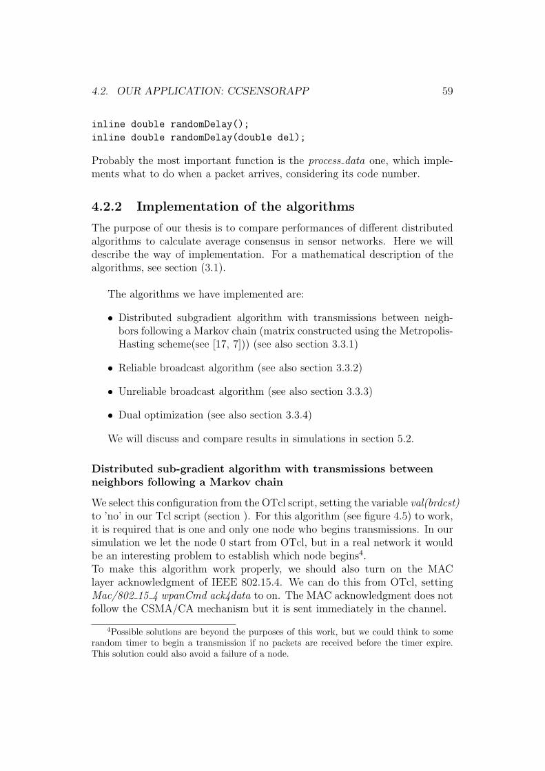
4.2. OUR APPLICATION: CCSENSORAPP 59
inline double randomDelay();
inline double randomDelay(double del);
Probably the most important function is the process data one, which imple-ments what to do when a packet arrives, considering its code number.
4.2.2 Implementation of the algorithms
The purpose of our thesis is to compare performances of different distributedalgorithms to calculate average consensus in sensor networks. Here we willdescribe the way of implementation. For a mathematical description of thealgorithms, see section (3.1).
The algorithms we have implemented are:
• Distributed subgradient algorithm with transmissions between neigh-bors following a Markov chain (matrix constructed using the Metropolis-Hasting scheme(see [17, 7])) (see also section 3.3.1)
• Reliable broadcast algorithm (see also section 3.3.2)
• Unreliable broadcast algorithm (see also section 3.3.3)
• Dual optimization (see also section 3.3.4)
We will discuss and compare results in simulations in section 5.2.
Distributed sub-gradient algorithm with transmissions betweenneighbors following a Markov chain
We select this configuration from the OTcl script, setting the variable val(brdcst)to ’no’ in our Tcl script (section ). For this algorithm (see figure 4.5) to work,it is required that is one and only one node who begins transmissions. In oursimulation we let the node 0 start from OTcl, but in a real network it wouldbe an interesting problem to establish which node begins4.To make this algorithm work properly, we should also turn on the MAClayer acknowledgment of IEEE 802.15.4. We can do this from OTcl, settingMac/802 15 4 wpanCmd ack4data to on. The MAC acknowledgment does notfollow the CSMA/CA mechanism but it is sent immediately in the channel.
4Possible solutions are beyond the purposes of this work, but we could think to somerandom timer to begin a transmission if no packets are received before the timer expire.This solution could also avoid a failure of a node.
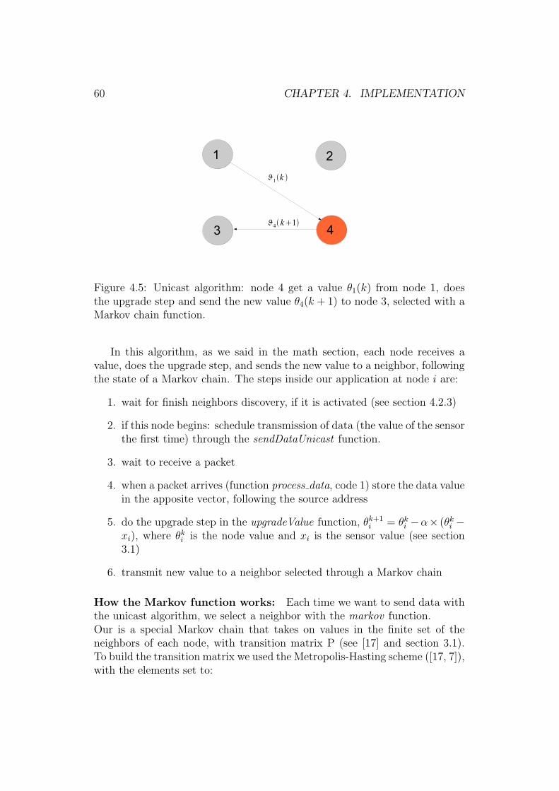
60 CHAPTER 4. IMPLEMENTATION
1
43
2
1k
4k1
Figure 4.5: Unicast algorithm: node 4 get a value θ1(k) from node 1, doesthe upgrade step and send the new value θ4(k + 1) to node 3, selected with aMarkov chain function.
In this algorithm, as we said in the math section, each node receives avalue, does the upgrade step, and sends the new value to a neighbor, followingthe state of a Markov chain. The steps inside our application at node i are:
1. wait for finish neighbors discovery, if it is activated (see section 4.2.3)
2. if this node begins: schedule transmission of data (the value of the sensorthe first time) through the sendDataUnicast function.
3. wait to receive a packet
4. when a packet arrives (function process data, code 1) store the data valuein the apposite vector, following the source address
5. do the upgrade step in the upgradeValue function, θk+1i = θki −α× (θki −
xi), where θki is the node value and xi is the sensor value (see section3.1)
6. transmit new value to a neighbor selected through a Markov chain
How the Markov function works: Each time we want to send data withthe unicast algorithm, we select a neighbor with the markov function.Our is a special Markov chain that takes on values in the finite set of theneighbors of each node, with transition matrix P (see [17] and section 3.1).To build the transition matrix we used the Metropolis-Hasting scheme ([17, 7]),with the elements set to:

4.2. OUR APPLICATION: CCSENSORAPP 61
Pij =
min( 1
di, 1dj
) if(i, j) ∈ ε and i 6= j∑(i,k)∈ε max{0, 1
di− 1
dk} if i = j
0 otherwise
where di and dj are the number of neighbors of the node i and j.When we execute the markov function, we are in a particular node, so we haveknowledge only about the i row of the matrix, therefore the probability totransmit to our neighbor j is the minimum between our number of neighborsand the number of neighbors of node j, that we have in the dataAddressstructure (see section 4.2.1).For selecting a node using its transition probability, we ordered our list ofneighbors in increasing order and we select one of them with the help of arandom value (see chap 25 of [32] for random number generation in ns2). Themarkov function return finally the address of the selected neighbor. If noneighbors are selected we do another upgrade step in the same node (withprobability 1−
∑j Pij).
For convergence statistics and results see the section 5.2.
Reliable broadcast algorithm
We select this configuration from the OTcl script, setting the variable val(brdcst)to ’yes’ in our Tcl script (section 4.1.4). We can turn off the MAC acknowl-edgment because we already send acknowledgments at application level. Thiswill give us more realistic simulations and let us avoid too many useless colli-sions. In this algorithm, each node send a broadcast message to its neighborswith its local value, and wait for acknowledgment from all of its neighbors.It also waits to have all data from all its neighbors. If both conditions arefullfilled, the node has received all acks for its message and it has all valuefrom its neighbors, it does the upgrade step. So here we have a kind of syn-chronization between the nodes, because each one has to wait for the othersto be ready.For this purpose, it is also important to keep track of the sequence number ofeach packet, so it is possible to recognize if the packet arrived is a new one oran old one. It could happen that a node do the upgrade step while some ofits neighbors are still waiting for others, so they receive a new value withouthave used the old one. For this purpose we have a buffer to temporarily storenew data to use in the next iteration. For each packet arrived, even if it is anold packet, each node send an acknowledgment.Here the upgrade step for the node i is (see also section 3.1): newV alue =(∑
j∈NiWij×data(j))+Wii×data(i) where the weight for each neighbor (ma-

62 CHAPTER 4. IMPLEMENTATION
trix W) is given again using the Metropolis-Hasting scheme (see also [36]):
Wij =
min( 1
di, 1dj
) if(i, j) ∈ E and i 6= j∑(i,k)∈E max{0, 1
di− 1
dk} if i = j
0 otherwise
In detail, the steps inside our application are:In transmission:
1. wait for finish neighbors discovery, if it is activated (see section 4.2.3)
2. wait for a random delay5 and send data in broadcast (function sendSen-sorData)
3. wait for acknowledgments from all neighbors and eventually send dataagain a MAXATTEMPTS number of time. The time to wait was em-pirically established.
4. when all acks are received, put to true the flag okUpgrade and cancelbackoff timer for send data again
In reception:
1. when a packet arrives, it is processed by the function process data (code3 for a reliable broadcast packet).
2. if it is a new packet (looking at the iteration number), store data in thedata field of the dataAddress structure for the appropriate neighbor
3. if it is a new packet, but the previous one was not yet used in the upgradestep, store the new data in the data buffer field of the dataAddressstructure for the appropriate neighbor
4. send a reply for the packet received (no waiting at application level, butCSMA/CA at MAC layer (see [15])
5. check whether there are new data packets from all neighbors. If thereare, check if the okUpgrade flag is true (all acks received for the lastpacket sent) and if it is, to the upgrade step
6. if the okUpgrade flag is false, schedule the Upgrade Timer to wait andtry again when the timer expires (interval set empirically)
5it is possible to avoid this because there is already a random delay at mac layer withCSMA/CA(see [15] for detailed explanations about csma/ca in 802.15.4).

4.2. OUR APPLICATION: CCSENSORAPP 63
For the upgrade step:
1. execute the markov function to assign the appropriate weight to eachneighbor
2. assign to the current node a weight equal to 1−∑
j∈NiWij
3. do the upgrade step (see above) newV alue = (∑
j∈NiWij × data(j)) +
Wii × data(i)
4. update the iteration number
5. check the buffer if there are already new packets
6. send a broadcast message with new data (through the function sendSen-sorData)
This algorithm has a very fast convergence to the optimum value. Problemsare about the number of packets and the thing that we use the local sensorvalue only for the first packet sent, so it is more difficult to recognize if thesensor data changes (see section 5.2)
Unreliable broadcast algorithm
This algorithm is quite similar to the reliable broadcast one, but it does nothave any type of acknowledgment and synchronization. The update functionis the same of the reliable broadcast case, but is assigned a weight only to thenodes whose is present a new data packet. To the others we assign a weightof zero. In practice if we are doing the upgrade step in the node i, followingthe formula Wii =
∑jWij for i = j, we assign a bigger weight to the value
of the node i itself. The steps inside our application are:
1. wait for finish neighbors discovery, if it is activated (see section 4.2.3)
2. wait a random delay5 and send data in broadcast (function sendSensor-Data)
3. if the backoff time is not stopped, continue sending again the data whenthe backoff timer expires
In reception:
1. when a packet arrives, if it is a new packet, store data as in reliablebroadcast and set the flag validate for the node who sent the packet

64 CHAPTER 4. IMPLEMENTATION
1
43
2
4k
3k 2k 1k
(a) Node 4 has already values from other nodesand sends its value
1
43
24k
3k 2k 1k
4k
4k ack
ack
ack
(b) Other nodes send acks to node 4 for valueθ4(k)
1
43
2
4 k1
(c) Node 4 does the upgrade step and sends newvalue θ4(k + 1)
Figure 4.6: Reliable broadcast algorithm

4.2. OUR APPLICATION: CCSENSORAPP 65
2. if it is not started, start the timer to do the upgrade step (intervalsettable through OTcl script)
3. when the timer expires, do the update step as in reliable broadcast butcounting only the neighbors from who sent a new packet
4. set the timer for the next upgrade step
The only parameter is the interval for upgrading. The problem is still thatwe use the sensor value only at the beginning.
Dual optimization
We select this configuration from the OTcl script, setting the variable val(dual)to yes in our Tcl script (section...) It does not matter whether the mac ac-knowledgment is set on or off, because we only send broadcast packets here,and there are never acknowledgments for broadcast packets at mac layer (see[15] for details about acks in 802.15.4). The aim of this algorithm (see mathsection and [26]) is to have a reliable and sharp enough final value in all nodes(the average in our case), without any kind of synchronization and withoutany acknowledgments. Here each node do the update step every interval oftime (settable from OTcl and not synchronized with other nodes), based onthe values of the λi,j, a collection of Lagrange multipliers for the ith subprob-lem (λi = {λi,j : j ∈ Ni}). If we are in the node i and a packet arrives from thenode j, we only upgrade the λi,j value, not the local value of i. We upgradethe local value of i after the upgrade interval, in a way not correlated with thearrive of packets or to what other nodes do (for mathematical details, see therelative section in this Thesis and [26]).The steps inside our application are:
In transmission:
1. wait for finish neighbors discovery, if it is activated (see section 4.2.3)
2. wait a random delay and send local value in broadcast
3. schedule the upgrade step after the interval set from OTcl
4. when the timer for the upgrade expires, do the upgrade step. For nodei: newV alue = localsensorData−
∑j λi,j
5. send the new value in broadcast. We decide to send the value severaltimes before the next update, to have more possibilities to reach a greaternumber of neighbors
In reception:
66 CHAPTER 4. IMPLEMENTATION
1. when a dual broadcast packet arrives (code 2), process in the pro-cess data function
2. if it is a new packet (looking at the iteration number), store data in thedata field of the dataAddress structure for the appropriate neighbor
3. if we are in the node i and the source is the node j, we upgrade the λi,jvalue following the formula λk+1
i,j = λki,j +µ× (xi−xj), where µ is a fixedstep size (settable from OTcl interface), and xi and xj are the local datarespectively of the node i and of the node j
In practice we are able to have convergence without any acks or synchro-nizations, even if convergence is usually slower than in the other algorithms(see section 5.2). We have a very good behavior changing the parameters ofthe upgrade interval and µ. For results, considerations and comparison withthe other algorithms, see the section 5.2 on this thesis.
4.2.3 Neighbors’ discovery
Beyond the scope of this thesis but very interesting problem for future work.In the application shown in this thesis there is already a function for auto-matic neighbors discovery: each node at the beginning of the simulation andafter a fixable period (to recognize whether the topology is changed), sendsin broadcast an hello packet. All nodes who reply, are considered neighbors.This approach seems to work well with a small number of nodes, but thereare some problems with many nodes (depending from the topology of thenetwork), because there are too many packets in the network with a lot ofcollisions, and therefore it takes a long time to discover all neighbors. how-ever this approach seems good but needs to be improved. In the simulationsthe automatic neighbors discovery is disabled: each node knows how manyneighbors it has by the already cited structure god.

Chapter 5
Results and Comments
67
68 CHAPTER 5. RESULTS AND COMMENTS
5.1 Types of comparison
To compare different algorithms, we had to choose some common metrics. Foreach algorithm (Broadcast, Broadcast Unreliable, Broadcast dual, and Unicast)we present:
• graphs of error versus time
• graphs of error versus number of packets
• graphs of error versus time for each node
We will present these graphs in section 5.2 for different number of nodesand for different scenarios, starting with the extreme case of a fully connectedrandom network, and considering then other topologies like a ring network anda random network (connected). For each algorithm we present also some othergraphs to see the behavior in function of different parameters, like stepsize,upgrade interval, number of nodes, topology and robustness to packet losses.
5.1.1 Tools
For doing statistics, it is necessary to parse the NS2 output (see section 4.1.1).At this purpose, there are some tools, all open source. Also in general it isuseful to have all procedures as much automated as possible, so to do a bignumber of iterations and to plot graphs without the need of too much humancontrol.
The different outputs are prepared through the main tcl script describedin section 4.1.4, to have, in addiction to the trace file and the nam file, also atime-error and an time-error for node file. From the time-error file, combinedwith the trace file, it is possible to derive for each iteration also the packets-error file, to take then the average and variance over a big number of iterations.Results are shown for each number of node and for different parameters. Thetools we used for parsing are:
• OTcl scripting
• bash scripting
• awk scripting
• gnuplot plotting tool
all these tools are normally present in every linux distributions and they can beinstalled without problems in Mac OsX (they are almost all already installed)and also on WindowsXP and Windows Vista, through the cygwin package.

5.1. TYPES OF COMPARISON 69
Otcl scripting
We used the OTcl language inside NS2, as we describe in section 4.1.4. OTclis not only the interface for NS2, but also a very powerful scripting language,suitable for many applications and for different using. Still for some scriptingwork our choice was bash scripting, for the big popularity and simplicity.
Bash scripting
Bash (http://www.gnu.org/software/bash/bash.html), acronym for Bourne-againshell, is the default shell on most Linux systems as well as on Mac OSX. It isvery useful to automate also quite complex processes. We used a bash scriptfor the complete automatism in our work. The script calls NS2 the desirednumber of time for all algorithms for different parameters, and it calls also theother tools for parsing, doing statistics and plotting graphs.
Awk
Awk is a program that runs other programs written in the AWK (pronounce’auk ’) programming language. AWK (see [4]) is a general purpose program-ming language that is designed for processing text-based data, either in filesor data streams. For several aspects is similar to Perl, but simpler. A versionof the AWK language is a standard feature of nearly every modern Unix-likeoperating system available today.
We wrote many AWK scripts for our work: to put data in a suitableway to plot, to take average values and variance from many iterations of thesimulation, and to combine different outputs, e.g., time-error and time-packetsto obtain packets-error. Awk was the main parsing tool we used.
Gnuplot
Gnuplot, [34], is a command line program that can generate two- and three-dimensional plots of function and data. We used this tool to plot all ourgraphs, exploiting the possibility of scripting that gnuplot offers. In an unix-like environment there are no free alternatives to using gnuplot. It wouldbe possible to plot data in Matlab, but we preferred to use this free plot-specialized tool, that offers a lot of possibilities, even if it is not always easyto configure and to use.

70 CHAPTER 5. RESULTS AND COMMENTS
Other tools
In our scripts we used also other open-source tools, mostly coming from theunix world and default installed in all unix-like environment and also on cyg-win, like, e.g., the sort program to order our data, or bc to calculate automat-ically some parameters into the bash scripts.
5.2 Algorithms
In this section we present our result graphs for all algorithms. In figure 5.1,a and b, we see an example respectively of a ring scenario and of a randomscenario we used for our simulations. To obtain a connected topology, weset properly the radio range. For all connected simulations, we set the radiorange to a value bigger than the size of the topology, to be sure that allnodes are in the range of each other. For the ring topology, each node canestablish communications only with two nodes (one right, one left). In therandom scenario, it is all random (position of the node and radio range): wasonly checked the strong connection constraint. All graphs are product of theaverage of 100 monte carlo simulations (when there is parameters changing,100 iterations for each value of the parameter taken in consideration). Wepresent also the standard deviation in the time/error graphs. For naming ofthe algorithms, see also section 3.3.
5.2.1 Parameter setting and tuning
The performances of the different algorithms depend from several parameters.The broadcast algorithm is the one that does need less tuning, we only needto set the time-out window length to wait for acknowledgments after sendingvalues. In our simulations, it seemed reasonable to let this parameter dependon the number of neighbors of each node, 1 + Ni
20, where Ni is the number of
neighbors of node i.For the broadcast unreliable algorithm, the most important parameter to
tune is the time-out window length between each upgrade, and the number ofretransmissions of the same values during this window, to have bigger prob-ability of reception. In the simulations, the time-out window was set to 0.4seconds, and the number of retransmissions to 3.
Also for the dual algorithm are very important the same parameters usedfor unreliable broadcast, length of the time-out window between each upgradeand number of retransmissions. In addition, here there is also the length of thestepsize µ. In the simulations (except when differently specified) the time-out
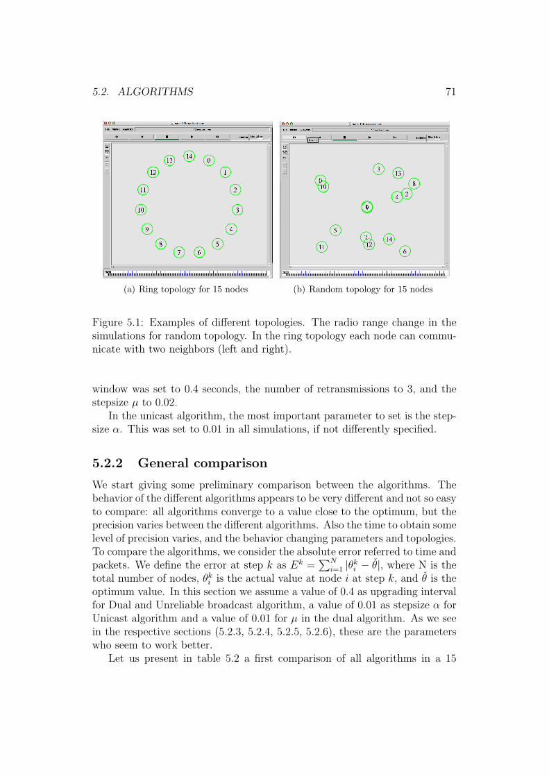
5.2. ALGORITHMS 71
(a) Ring topology for 15 nodes (b) Random topology for 15 nodes
Figure 5.1: Examples of different topologies. The radio range change in thesimulations for random topology. In the ring topology each node can commu-nicate with two neighbors (left and right).
window was set to 0.4 seconds, the number of retransmissions to 3, and thestepsize µ to 0.02.
In the unicast algorithm, the most important parameter to set is the step-size α. This was set to 0.01 in all simulations, if not differently specified.
5.2.2 General comparison
We start giving some preliminary comparison between the algorithms. Thebehavior of the different algorithms appears to be very different and not so easyto compare: all algorithms converge to a value close to the optimum, but theprecision varies between the different algorithms. Also the time to obtain somelevel of precision varies, and the behavior changing parameters and topologies.To compare the algorithms, we consider the absolute error referred to time andpackets. We define the error at step k as Ek =
∑Ni=1 |θki − θ|, where N is the
total number of nodes, θki is the actual value at node i at step k, and θ is theoptimum value. In this section we assume a value of 0.4 as upgrading intervalfor Dual and Unreliable broadcast algorithm, a value of 0.01 as stepsize α forUnicast algorithm and a value of 0.01 for µ in the dual algorithm. As we seein the respective sections (5.2.3, 5.2.4, 5.2.5, 5.2.6), these are the parameterswho seem to work better.
Let us present in table 5.2 a first comparison of all algorithms in a 15

72 CHAPTER 5. RESULTS AND COMMENTS
node completely connected random scenario like the one in figure 5.1(b) witha radio range bigger of the diagonal size of the topology (in this case a radiorange of 150 m with a topology of 100 m2 in area) to be sure to have thecomplete connection (all node can communicate with all other nodes). Weshow the error value and the number of packet sent after 20 seconds.
Table 5.2: Error and packets (average over 100 simulations) after 20 seconds(completely connected scenario). Error defined as Ek =
∑Ni=1 |θki − θ|, step k,
node i
ALGORITHM TIME PACKETS ERROR ERROR NORMALIZEDBroadcast 20 6334.41 1.24694 0.08312933Broadcast Unr 20 4855.13 0.2361977 0.015746513Dual 20 4869.31 0.448073 0.029871533Unicast 20 12999.9 1.68033 0.112022
If we analyze table 5.2, we immediately note two things:
• In the same amount of time, the unicast algorithm sends a significantlylarger number of packets with respect to the other algorithms. This isbecause in the broadcast algorithm we do not have any waiting time,and each node sends immediately the packet after the upgrade step.
• As expected, the number of packets sent in the same amount of time inthe Broadcast Unreliable algorithm and in the Dual Algorithm is similar.However in the reliable broadcast there are also the acknowledgmentpackets, and the number of packets sent is larger.
We note also that the error after 20 seconds for Broadcast and Unicast algo-rithms is larger respect to the others, but here we have different explanationsfor this evidence. Before explaining, let us analyze the table 5.3. Comparedto the previous table, 5.2, we see that for all algorithms the number of packetssent is, as expected, a lot larger, but the error tells us that the three algo-rithms Broadcast Unreliable, Dual, and Unicast already had a convergenceat 20 seconds, while the broadcast algorithm is improving the precision alot, getting closer to the optimum value. So, for how it is implemented, theBroadcast algorithm is slower than the others, because it has to wait for allacknowledgments, but its precision is a lot better than the others.
About the big error of the unicast algorithm, we have to say that in thisalgorithm, unlike the others, we have in each node a value fluctuating aroundthe optimum, but different at the same time for each node, so the error seemsbigger than it is in reality, because of the way itself we defined the error,

5.2. ALGORITHMS 73
Ek =∑N
i=1 |θki − θ| (for comparing the behavior with different number of
nodes, we used the normalized error Ek
N, with N total number of nodes, to
plot the graphs). We present in table 5.4 a comparison based on the minimumerror, obtained taking the minimum error at each node, no matter at whattime or for which number of packets, and summing. This is only a lowerbound, because we are not sure that the minimum value will be reached atthe end of the simulation, maybe it is only a transient value, however we seethat the unicast algorithm is comparable to the others for precision (with theexception of the reliable broadcast, which is a lot more precise).
Table 5.3: Error and packets after 50 seconds (completely connected scenariowith 15 nodes). Error defined as Ek =
∑Ni=1 |θki − θ|, step k, node i
ALGORITHM TIME PACKETS ERROR ERROR NORMALIZEDBroadcast 50 10449.1 0.0995448 0.00663632Broadcast Unr 50 11440.7 0.2361995 0.015746Dual 50 11397.8 0.447761 0.0298507Unicast 50 32908.3 1.70994 0.113996
Table 5.4: Minimum error (completely connected scenario with 15 nodes). Minerror defined as Emin =
∑Ni=1 |min
kθi − θ|, k step, node i
ALGORITHM MIN ERROR ERROR NORMALIZEDBroadcast 1.71405e-08 0.1e-9Broadcast Unr 0.00521683 0.000347788Dual 0.142558 0.0095038Unicast 0.0709973 0.004733153
It is very useful to do a comparison also at the same number of packets:we show in table 5.5 values after 5000 and 20000 packets sent. We can seethat unicast and broadcast unreliable have already reached convergence after5000 packets, while broadcast and dual not yet. If, we look at values after20000 packets, we see as expected that the broadcast algorithm has improveda lot the precision, the dual is improved and the others have more or less thesame values. We have to notice also the difference in timing for the samenumber of packets. We note that the broadcast, despite the presence of theacknowledgments, sent less packets in the same amount of time respect to theother algorithms.
Graphically, in figure 5.6 is showed the same data of the previous tables.We can note the strange time packets behaviour (fig. 5.6(c)) of the reliable

74 CHAPTER 5. RESULTS AND COMMENTS
Table 5.5: Error and packets after 5000 and 20000 packets sent (completelyconnected scenario with 15 nodes). Error defined as Ek =
∑Ni=1 |θki − θ|, step
k, node i
ALGORITHM TIME PACKETS ERROR ERROR NORMALIZEDBroadcast 13.3 4991.58 3.14384 0.20956Broadcast Unr 20.7 5007.17 0.2361978 0.01574652Dual 20.5 4990.67 2.36547 0.157698Unicast 7.7 5000.65 1.59591 0.106394
Broadcast 120.7 19998.3 0.00143186 0.000095457Broadcast Unr 89 19989.5 0.2361994 0.15746626Dual 89.1 19986.8 0.447762 0.0298508Unicast 30.5 19979.3 1.73451 0.115634
broadcast algorithm, which diminish the inclination of the time-packets curve.We note also that the fastest convergence is from the unreliable broadcastalgorithm. As we told above, the unicast algorithm seems so much worse thanthe others for precision, but in reality it is comparable, as it is showed in table5.4. In figure 5.7, we see the same plots for the 5 nodes scenario, completelyconnected. We see that, also with a minor number of nodes, things does notchange a lot, we have the fastest convergence from the broadcast unreliablealgorithm, but we can see how much the reliable broadcast suffers by the biggernumber of nodes in the 15 scenario completely connected. It is clear that itwould be impossible to apply the reliable broadcast algorithm in a scenarioin which every node has a big number of neighbors. The reliable broadcastwould be too slow. The dual algorithm suffers more than the others in termsof precision and speed of convergence. In the table 5.8 we see the minimumerror in the 5 nodes completely connected scenario and we notice the betterprecision reached by all algorithms. Comparing fig. 5.6(c) and 5.7(c) we alsosee that the number of packets sent by the unicast algorithm does not dependby the number of nodes. In fact, the unicast algorithm just sends packets asfast as possible, with only one node that does the upgrade step at every time.
We show the same graphs for different scenarios and for different numberof nodes in figures from 5.9 to 5.12. We can see that the algorithm thatseems suffer more the changes in topology seems to be the dual one. Inparticular in the ring topology, like in figure 5.1(a), seems to be the mostdifficult one, also with a smaller number of nodes. However in general allalgorithms seems to have a bigger delay in convergence with the ring topology.Also the precision suffers, not only in the dual case but also with unreliable

5.2. ALGORITHMS 75
(a) Time error (b) Packet error
(c) Time packets
Figure 5.6: Comparison of the algorithms in a 15 node completely connectedscenario
broadcast and unicast. The best configuration seems to be the one with allconnected nodes, so we could think to a network with small clusters, withnode all connected inside each cluster.
Here we begin to describe results specifically for each algorithm.
5.2.3 Broadcast Algorithm
The broadcast algorithm has the value of convergence closest to the optimumvalue respect to the other algorithms in all scenarios. We expected this result,because it is the only algorithm between the ones we analyzed which is syn-chronized. There is not an explicit synchronization, but for doing the upgradestep, each node has to wait to receive new values from all its neighbor andalso to receive all acknowledgments for its last sent value. So we are sure that

76 CHAPTER 5. RESULTS AND COMMENTS
(a) Time error (b) Packet error
(c) Time packets
Figure 5.7: Comparison of the algorithms in a 5 node completely connectedscenario
Table 5.8: Minimum error (completely connected scenario with 5 nodes). Minerror defined as Emin =
∑Ni=1 |min
kθi − θ|, k step, node i
ALGORITHM MIN ERROR ERROR NORMALIZEDBroadcast 2.58076e-07 5.16151e-08Broadcast Unr 0.000370062 7.40123e-05Dual 0.00365258 0.000730517Unicast 0.0166802 0.00333604

5.2. ALGORITHMS 77
(a) Time error (b) Packet error
Figure 5.9: Comparison of the algorithms in a 15 node Ring scenario
(a) Time error (b) Packet error
Figure 5.10: Comparison of the algorithms in a 5 node Ring scenario

78 CHAPTER 5. RESULTS AND COMMENTS
(a) Time error (b) Packet error
Figure 5.11: Comparison of the algorithms in a 15 node Random scenario
(a) Time error (b) Packet error
Figure 5.12: Comparison of the algorithms in a 5 node Random scenario

5.2. ALGORITHMS 79
when a node does the upgrade step, it is using the correct values, so the finalprecision is extremely high, as we see in tables from 5.2 to 5.8, and is alwaysimproving with the time, limited only by the numerical precision we used inour simulations (10−6).The problem of the broadcast algorithm seems to bethe speed of convergence, not always fast respect to the others (see section5.2.2).
In figure 5.13, we show the behavior of broadcast algorithm varying thenumber of nodes. We present in the graphs also the standard deviation over1000 iterations on a completely connected random topology. We see that thenumber of packets sent increasing the number of total nodes in scenario is notlinear (see fig. 5.13(a)), probably because of the need of more retransmissionswith a bigger number of nodes. In 5.13(b), we present the average delayfor iteration, where with the word iteration we mean the delay between thefirst transmission of a new packet, and the arrive of the last acknowledgmentfrom the neighbors. This type of statistic is possible only with the reliablebroadcast algorithm, because in the other cases we do not have iterations withthe meaning we have just explained.
While considering the very good results of this algorithm, we have to re-member that it is specially tailored for the average consensus problem, and itis not general like dual optimization and unicast.
Reliable broadcast: All connected Scenario
As it is shown in figures from 5.6 to 5.12, the behavior of the broadcastalgorithm (in red in the figures cited) is affected by topology, not so muchfor final precision of the value, but mainly for the convergence delay. In thecompletely connected scenario, we have the best behavior for this algorithm interms of convergence delay. We show in figure 5.14 the behavior of each nodein this scenario. We maintained a long time scale in the graph for comparisonwith other topologies and algorithms.
Reliable broadcast: Random Scenario
Maybe the random scenario is the most ’realistic’ one, because we have arandom topology which has the only constraint of connection, so for everytopology generated, we can not know how many neighbors each node willhave. If we look at the behavior for nodes in picture 5.15, we can confirm thatwith a random scenario the convergence delay is bigger.

80 CHAPTER 5. RESULTS AND COMMENTS
(a) Packets sent in function of number ofnodes
(b) Average delay for iteration in functionof number of nodes
(c) Convergence delay in function of num-ber of nodes
Figure 5.13: RELIABLE BROADCAST: behavior varying the number ofnodes
Reliable broadcast: Ring Scenario
The ring scenario seems the most difficult one for every algorithm. We showgraphs of error for node with this topology in figure 5.16. For the reliablebroadcast algorithm, differently from the others, this is not the worst topology,even if the convergence delay seems longer respect to the completely connectedcase.
5.2.4 Broadcast Unreliable Algorithm
The broadcast unreliable algorithm, has the fastest convergence in all situa-tions. This algorithm, as said in the theory section, 3.1, and in implemen-

5.2. ALGORITHMS 81
(a) 15 nodes (b) 5 nodes
Figure 5.14: RELIABLE BROADCAST: behavior for each node in a com-pletely connected scenario
(a) 15 nodes (b) 5 nodes
Figure 5.15: RELIABLE BROADCAST: behavior for each node in a randomtopology scenario
tation section, 4.2.2, is directly derived from the reliable broadcast one, andits behavior is not completely theoretically explored. However, the results aresurprisingly good. We have to remember that, as a derived of the reliablebroadcast algorithm, also the unreliable case is tailored on the average con-sensus problem, while the dual and unicast algorithms are more general. Infigure 5.17 it is shown the behavior varying waiting interval parameter. It ispossible to note an improvement in precision increasing the value of waitingtime, but after a value of about 0.1, it not seems possible to note further

82 CHAPTER 5. RESULTS AND COMMENTS
(a) 15 nodes (b) 5 nodes
Figure 5.16: RELIABLE BROADCAST: behavior for each node in a ringtopology scenario
improvements. Anyway, with bigger values of waiting time, the algorithm ismore ’robust’ in case of channel problem. It would be important in this casealso to set properly the number of retransmissions during each waiting interval(set to 3 in our simulations). It is also important to note how the behaviorof the algorithm seems stable also with very small (0.0005 seconds) waitinginterval time. This is not true for example in the dual algorithm case.
Figure 5.17: UNRELIABLE BROADCAST: behavior varying waiting intervalparameter

5.2. ALGORITHMS 83
Unreliable broadcast: All connected Scenario
In the all connected scenario, we have a very fast convergence, as we show infigure 5.18. As for the other algorithms, this is the most favorable scenario.The final bias is also very small.
(a) 15 nodes (b) 5 nodes
Figure 5.18: UNRELIABLE BROADCAST: behavior for each node in a com-pletely connected scenario
Unreliable broadcast: Random Scenario
Respect to all connected scenario, here we see (figure 5.19) that the conver-gence delay is increased. Also the precision suffers more. It is strange inparticular the differences in convergences between different nodes. It is pos-sible to note in figure 5.19 the strange behavior of node 2. This confirm thesometimes unpredictable performances of unreliable broadcast, that is just anexperiment derived from reliable broadcast.
Unreliable broadcast: Ring Scenario
For the ring scenario in unreliable broadcast (figure 5.20), we see that therate is similar to the random case, with more uniformity between the differentnodes. However, even if small, the convergence time is longer than in the allconnected case.

84 CHAPTER 5. RESULTS AND COMMENTS
(a) 15 nodes (b) 5 nodes
Figure 5.19: UNRELIABLE BROADCAST: behavior for each node in a ran-dom scenario
(a) 15 nodes (b) 5 nodes
Figure 5.20: UNRELIABLE BROADCAST: behavior for each node in a ringscenario
5.2.5 Dual Optimization Algorithm
The dual algorithm has the worst behavior for convergence delay and forprecision. The problem with this algorithm is to find a trade-off betweenprecision and convergence delay, because the algorithm is very dependent onthe parameters, mainly the upgrade interval window and the µ (stepsize). Weshow here graphs varying these two parameters. We have to say that, even ifthe performance of this algorithm compared to the others are not so good, thisapproach is very general and permits to compute different objective functions.

5.2. ALGORITHMS 85
In Figure 5.21 it is showed the behavior of the algorithm varying the stepsizeµ and the waiting interval. Increasing the stepsize, the convergence delay isshorter but the bias is higher. Instead diminishing the waiting interval, theconvergence is faster but the bias is higher, because at each upgrade step thealgorithm has less new packets from other nodes. With a waiting time of 0.01seconds the algorithm seems to be not stable (an example trajectory withwaiting time 0.01 is showed in figure 5.21(c)). From a time point of view, ifwe decrease the waiting time interval, the amount of packets sent in the sametime is of course bigger, so the convergence is faster.
(a) Packet Error (logscale) varying µ step-size (fixed waiting interval = 0.4 seconds)
(b) Packets Error (logscale) varying waitinginterval time from 0.01 to 0.08 (fixed µ =0.02)
(c) Example of trajectory of one node withwaiting interval set to 0.01 (fixed µ = 0.02)
Figure 5.21: DUAL: algorithm’s behavior varying parameters (15 nodes Com-pletely connected)

86 CHAPTER 5. RESULTS AND COMMENTS
Dual: All connected Scenario
In figure 5.22 it is showed the error for node of the dual algorithm with stepsizeµ = 0.01 in an all connected scenario. The dual algorithm is in general theslowest one between the algorithms proposed, but its behavior is not so bad,considering also that the algorithm can be easily adapted to other objectivefunctions. Comparing figures 5.22, 5.23, 5.24 it is possible to see how muchthe dual algorithm depends on topology.
(a) 15 nodes (b) 5 nodes
Figure 5.22: DUAL: behavior for each node in a completely connected scenario(waiting interval = 0.4 seconds, µ = 0.01)
Dual: Random Scenario
The error for node results for the random scenario is showed in figure 5.23.Respect to the completely connected scenario, the convergence delay is a lotlonger respect to completely connected topology.
Dual: Ring Scenario
In the ring scenario, also for the dual algorithm, we have the worst perfor-mance. We present the error for node graphs in figure 5.24. The convergencedelay is the longest one.
5.2.6 Unicast Algorithm
The unicast algorithm has a behavior surprisingly good in all scenarios. Weused a fixed step size instead of a diminishing one (see section 3.1), so we do not

5.2. ALGORITHMS 87
(a) 15 nodes (b) 5 nodes
Figure 5.23: DUAL: behavior for each node in a random scenario (waitinginterval = 0.4 seconds, µ = 0.01)
(a) 15 nodes (b) 5 nodes
Figure 5.24: DUAL: behavior for each node in a ring scenario(waiting interval= 0.4 seconds, µ = 0.01)
have a perfect convergence but an oscillatory bound. The parameter to tuneis α, the stepsize. In figure 5.25 it is showed the behavior of the algorithm in acompletely connected scenario varying the stepsize α. Diminishing the valueof α, the error decreases and the convergence delay increases, even if not somuch. With α < 0.01, not reported here, there are no significant improvementin precision, but the oscillations diminish. With less nodes (figure 5.25(b)),the convergence delay does not improve a lot, but the precision seems better.The error seems bigger respect to the other algorithms because of oscillatory

88 CHAPTER 5. RESULTS AND COMMENTS
behavior, but looking at the single values, the precision is comparable to dualand unreliable broadcast. Maybe the performance of the algorithm could beimproved by low-pass filtering the values at each node, taking, e.g., the averageover several values.
(a) 15 nodes (b) 5 nodes
Figure 5.25: UNICAST: behavior at changing of parameter α
Unicast: All connected Scenario
The behavior of the unicast algorithm with different topologies does notchange a lot, however in figure 5.26 it is shown the behavior of each nodein a completely connected scenario. It is possible to note the very fast con-vergence, and the differences in precision between different nodes.
Unicast: Random Scenario
In figure 5.27 it is shown the error for node of unicast algorithm in a randomscenario. Differently from the other algorithms, we do not note a significantchange in performance for this algorithm when the topology changes.
Unicast: Ring Scenario
In figure 5.28 it is shown the error for node of unicast algorithm in a ringscenario. Also here, respect to the other algorithms, it is not possible to notesignificant differences in performances even for the ring topology.
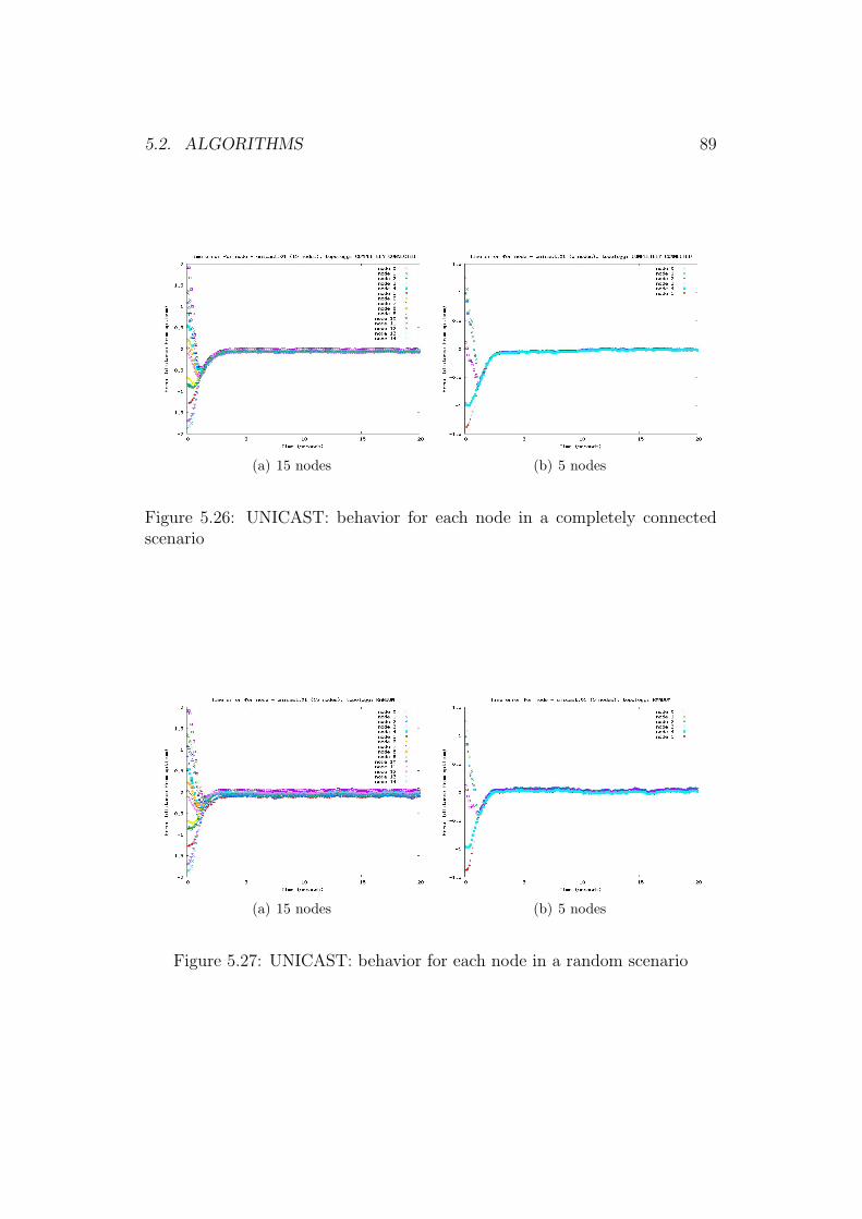
5.2. ALGORITHMS 89
(a) 15 nodes (b) 5 nodes
Figure 5.26: UNICAST: behavior for each node in a completely connectedscenario
(a) 15 nodes (b) 5 nodes
Figure 5.27: UNICAST: behavior for each node in a random scenario

90 CHAPTER 5. RESULTS AND COMMENTS
(a) 15 nodes (b) 5 nodes
Figure 5.28: UNICAST: behavior for each node in a ring scenario

Chapter 6
Conclusions
91

92 CHAPTER 6. CONCLUSIONS
The aim of this work was to compare different distributed optimizationalgorithms in a sensor network compatible with the standard IEEE 802.15.4.We developed a new application for the network simulator ns2, implementingfour distributed optimization algorithms (called, following the notation usedin the whole thesis, broadcast, unreliable broadcast, dual, unicast). Two of thealgorithms, broadcast and unreliable broadcast are tailored upon the problemof calculating the average of a value over a sensor network; the other two,dual and unicast, are more general, and allow the optimization not only ofthe average, but also of other objectives function, beyond the scope in thiswork. Several simulations was done to test in different situations and withdifferent parameters the behavior of the algorithms, and to compare them indifferent way: convergence delay in function of packets sent and time, andbias in convergence value respect to the optimum.
The results obtained do not indicate an algorithm, among the ones pre-sented, which is the best in all situations, but instead our data show that allthe algorithms have a quite good behavior in general, and that, for differentapplication, is preferable to chose an algorithm instead of another. For exam-ple, for an application which needs high precision in calculating the averageamong scalar values in a sensor network (e.g., temperature), the best algo-rithm would be the reliable broadcast, which, thanks to the synchronizationbetween nodes, has no final bias in convergence value respect to the optimum.If instead the problem is the speed of convergence, also for a battery savingpurpose, the unicast algorithm fits better. For the unreliable broadcast algo-rithm, we have to say that we derived it from the reliable broadcast one, totry to avoid acknowledgments, but theoretical proof of convergence is not yetdone. We included this algorithm because its behavior is surprisingly good,because the convergence is fast and enough accurate for most applicationswhich need to calculate averages.
In general we can say that if there are too many nodes, the performancesof all algorithms (maybe with the exception of the unicast one) suffer, inparticular in same extreme topology as the ring one. The best results arereached in a small all-connected network, so we could think to a networksplit in clusters, where each cluster is composed of a small number of nodes,all-connected one with another.
Another important thing that emerges from results is that who implementsa sensor network using a distributed optimization algorithm like the ones pro-posed in this work, in particular with the dual one, should spend some timeto tune the parameters, because the performances could improve a lot tailor-ing in base of topology and application request parameters such as stepsize,waiting interval window, number of retransmissions.
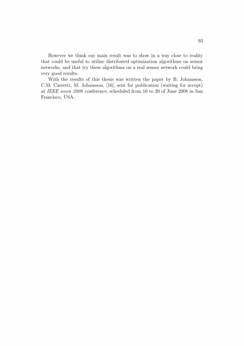
93
However we think our main result was to show in a way close to realitythat could be useful to utilize distributed optimization algorithms on sensornetworks, and that try these algorithms on a real sensor network could bringvery good results.
With the results of this thesis was written the paper by B. Johansson,C.M. Carretti, M. Johansson, [16], sent for publication (waiting for accept)at IEEE secon 2008 conference, scheduled from 16 to 20 of June 2008 in SanFrancisco, USA.


Chapter 7
Future work
95

96 CHAPTER 7. FUTURE WORK
In this thesis we did a simulation and comparison of distributed optimiza-tion algorithms in sensor networks. It would be very good to try to implementthis work on real sensors. Also we would like to investigate more deeply theproblem of energy consumption in real sensors.
It would be very interesting to expand the research on other different algo-rithms, comparing them with the ones implemented in this thesis. To improveeven more the work, we are planning to try to change objective function fromleast square, to see whether the results are good as well with different convexfunctions. It would be interesting also to try to use and to investigate moreabout robust optimization.
In the results of this thesis, we have found some problems in the speed ofconvergence if there are too many nodes. This could suggest that the bestsolution is to divide a sensor network into clusters, all interconnected. Wewould like to go deeply in this issue, to find the best way to automaticallydivide the network into clusters, and the best way to interconnect clusters.

Bibliography
[1] Tcl wiki pages. URL http://wiki.tcl.tk.
[2] Ns by example, november 2007. URL http://nile.wpi.edu/NS/.
[3] Activestate. Web page of komodo edit for macos x. URL http://www.
activestate.com/Products/komodo_edit/.
[4] Alfred V. Aho, Brian W. Kernighan, , Peter J. Weinberger, and Addison-Wesley. The AWK Programming Language. Addison-Wesley, 1988.
[5] TinyOS alliance. TinyOS website. tinyOS alliance. URL www.tinyos.
net.
[6] Eitan Altman and Tania Jimenez. Ns Simulator for beginners. Univ.de Los Andes, Merida, Venezuela and ESSI, Sophia-Antipolis, France,lecture notes, 2003-2004 edition, December 2003.
[7] S. Boyd, P.Diaconis, and L. Xiao. Fastest mixing markov chain on agraph. SIAM Review, (46):667–689, 2004.
[8] Stephen Boyd and Lieven Vandenberghe. Convex Optimization. Cam-bridge University Press, first edition, 2004.
[9] Ramesh Govindan Chalermek Intanagonwiwat and Deborah Estrin. Di-rected diffusion: A scalable and robust communication paradigm for sen-sor networks. In In Proceedings of the Sixth Annual International Con-ference on Mobile Computing and Networking (MobiCOM ’00), August2000, Boston, Massachussetts.
[10] contiki. contiki os website. URL http://www.sics.se/contiki/.
[11] Paolo Detti. Il rilassamento lagrangiano nella soluzione di problemi diottimizzazione combinatoria. dual lagrangian theory, University of Siena,October 26 2006.
97
98 BIBLIOGRAPHY
[12] Pedro Vale Estrela. Pedro vale estrela- ns2 page. URL http://tagus.
inesc-id.pt/~pestrela/ns2.
[13] Matteo Fischetti. Lezioni di Ricerca Operativa. Edizioni libreria progettoPadova, ii edition, 1999.
[14] G. P. Halkes, T. van Dam, and K. G. Langendoen. Comparing energy-saving mac protocols for wireless sensor networks. Mob. Netw. Appl., 10(5):783–791, 2005. ISSN 1383-469X.
[15] IEEE. Part 15.4: Wireless Medium Access Control (MAC) and PhysicalLayer (PHY) Specifications for Low-Rate Wireless Personal Area Net-works (WPANs). IEEE Computer Society, IEEE 3 Park Avenue NewYork, NY 10016-5997, USA, 2006 edition, september 2006.
[16] Bjorn Johansson, Cesare Maria Carretti, and Mikael Johansson. Ondistributed optimization using peer-to-peer communications in 802.15.4wireless networks. Sent for publication at IEEE secon 2008 conference.Waiting for response, January 2008.
[17] Bjorn Johansson, Maben Rabi, and Mikael Johansson. A simple peer-to-peer algorithm for distributed optimization in sensor networks. Basis forunicast algorithm implemented in this thesis.
[18] Soummya Kar and Jose M.F. Moura. Distributed average consensus insensor networks with random link failures. In The 32nd InternationalConference on Acoustics, Speech, and Signal Processing (ICASSP), Hon-olulu, Hawaii., April 2007.
[19] N.F. Maxemchuk, P. Tientrakool, and T.L. Willke. Reliable neighbor-cast. Vehicular Technology, IEEE Transactions on, 56(6):3278–3288,Nov. 2007. ISSN 0018-9545.
[20] Mortada Mehyar, Demetri Spanos, John Pongsajapan, Steven H. Low,and Richard M. Murray. Asynchronous distributed averaging on commu-nication networks. Networking, IEEE/ACM Transactions, pages 512–520,2007.
[21] Angelia Nedic. Subgradient Methods for Convex Minimization. PhD the-sis, Massachusets Institute of Technology, 2002.
[22] Angelia Nedic and Dimitri P. Bertsekas. Incremental subgradient meth-ods1 for nondifferentiable optimization. SIAM J. on Optimization, 1999.
99
[23] Moteiv (now Sentilla). tmote sky datasheet. Moteiv (now sentilla). URLwww.sentilla.com.
[24] ns-users group. ns2 website (wiki). URL http://nsnam.isi.edu/nsnam/
index.php/User_Information.
[25] Michael Rabbat and Robert Nowak. Distributed optimization in sensornetworks. In IPSN ’04: Proceedings of the third international symposiumon Information processing in sensor networks, pages 20–27, New York,NY, USA, 2004. ACM. ISBN 1-58113-846-6.
[26] Michael G. Rabbat, Robert D. Nowak, and James A. Bucklew. Gener-alized consensus computation in networked systems with erasure links.Signal Processing Advances in Wireless Communications, 2005 IEEE 6thWorkshop on, pages 1088– 1092, june 2005.
[27] R.D. Rabbat, M.G.; Nowak. Quantized incremental algorithms for dis-tributed optimization. Selected Areas in Communications, IEEE Journalon, 23(4):798–808, April 2005. ISSN 0733-8716.
[28] Iyappan Ramachandran. Packets flow in ns2. It is a description whohelped us to give some more details on ns2 packet’s flow. It was notpossible to find again the source.
[29] Francisco J. Ros and Pedro M. Ruiz. Implementing a New Manet Uni-cast Routing Implementing a New Manet Unicast Routing Protocol inNS2. Dept. of Information and Communications Engineering, Univer-sity of Murcia, December 2004. URL http://masimum.dif.um.es/
nsrt-howto/.
[30] Sentilla. Sentilla website (producer of tmote-sky).
[31] Sung-Hyun Son, Mung Chiang, Sanjeev R. Kulkarni, and Stuart C.Schwartz. Clustering in distributed incremental estimation in wirelesssensor networks. unknown, 2005.
[32] The VINT Project, a Collaboration between researchers at UC Berkeley,LBL,USC/ISI, and Xerox PARC. ns Notes and Documentation. URLhttp://www.isi.edu/nsnam/ns/ns-documentation.html.
[33] Bo Wang. Network simulator (ns2). URL www.cse.msu.edu/~wangbo1/
ns2.
[34] Thomas Williams and Colin Kelley. Gnuplot website. URL www.gnuplot.
info.

100 BIBLIOGRAPHY
[35] www.tcl.tk. Tcl tutorial. URL http://www.tcl.tk/man/tutorial/
tcltutorial.html.
[36] Lin Xiao and Stephen Boyd. Fast linear iterations for distributed averag-ing. Decision and Control, 2003. Proceedings. 42nd IEEE Conference on,5(4997-5002), Rev 2004. URL citeseer.ist.psu.edu/boyd03fastest.
html.
[37] Lin Xiao, Stephen Boyd, and Sanjay Lall. A scheme for robust distributedsensor fusion based on average consensus. Information Processing in Sen-sor Networks, 2005. IPSN 2005. Fourth International Symposium, pages63–70, April 2005.
[38] Jianliang Zheng. J. zheng home page. URL http://www-ee.ccny.cuny.
edu/zheng/.
[39] Jianliang Zheng and Myung J. Lee. Will ieee 802.15.4 make ubiquitousnetworking a reality?: A discussion on a potential low power, low bit ratestandard. Communications Magazine, IEEE, 42(6):140– 146, June 2004.
[40] Jianliang Zheng and Myung J. Lee. A comprehensive performance studyof ieee 802.15.4. Sensor Network Operations, IEEE press, Wiley Inter-science, chapter 4:218–237, 2006. URL http://www-ee.ccny.cuny.edu/
zheng/pub/.
This thesis was written using LATEX on Mac OS X.
Acknowledgments
There are a lot of websites on internet, in which a lot of people suggest tonot put any dedication and acknowledgments (a word so used with a differentmeaning during this work!) on a master thesis. I really think they are wrong,at least in my case. My experience in doing this thesis abroad was so goodthanks to a lot of people that I cannot forget here. My parents was always soclose to me through skype, with our very useful discussions every day. Also,my girlfriend Claudia was always so present for me, and it was wonderful toremain so close despite our ’double erasmus’ situation, and it is wonderful!
A special thanks also to people who followed my work in Stockholm, inparticular to prof. Mikael Johansson and to Bjorn, who helped me in doingthis thesis. I want to remember here also all people who stayed with me in thedepartment and in general during my experience abroad: my friends-of-a-lifeLapo and Marco, who shared this and many others experiences with me, Pan,

101
Pigi, then Pablo, who suggested us to come in Stockholm, and all people thatI have met in this period (the list would be too long!). A special thanks tomy corridor neighbors, in particular Sebastien, Violaine, and Heidi. Even ifprobably you will never read this paper, I have to say that it was great tospend this time with you and I really hope to see you again!
Thanks also to all people who came to visit e in Stockholm, in particular,again, Claudia, my brother Pier Paolo and my cousin Alberto. It was reallynice to have you with me in Sweden!
I have to say thank you also to the Guitar: it (I would like to say she) isalways with me and is a very important part of my life, and gives me a lot ofideas also in engineering!
La laurea e anche la fine di un ciclo, e, senza discorsi troppo lunghi e tropporetorici, vorrei ringraziare Feriae Matricularum per tutte le esperienze irripeti-bili e uniche che mi ha fatto vivere, e per tutte le esperienze extra-universitarieche tanto mi hanno insegnato. La favola no non finisce qui...Grazie a tutti.
Copyright © 2022 FDOKUMEN